Reconnection of Stable/Unstable Manifolds of the Harper Map

arX

iv:n

lin/0

5010

42v1

[nl

in.C

D]

24

Jan

2005

Reconnection of Stable/Unstable Manifolds of the

Harper Map

− Asymptotics-Beyond-All-Orders Approach −

Shigeru Ajisaka† § and Shuichi Tasaki†

† Advanced Institute for Complex Systems and Department of Applied Physics,

School of Science and Engineerings, Waseda University,

3-4-1 Okubo, Shinjuku-ku, Tokyo 169-8555, Japan

Abstract. The Harper map is one of the simplest chaotic systems exhibiting recon-

nection of invariant manifolds. The method of asymptotics beyond all orders (ABAO)

is used to construct stable/unstable manifolds of the Harper map. By enlarging the

neighborhood of a singularity, the perturbative solution of the unstable manifold is

expressed as a Borel summable asymptotic expansion in a sector including t = −∞and is analytically continued to the other sector, where the solution acquires new

terms describing heteroclinic tangles. When the parameter changes to the reconnec-

tion threshold, the stable/unstable manifolds are shown to acquire new oscillatory

portion corresponding to the heteroclinic tangle after the reconnection.

Mathmatics Subject Classification: 34C37, 37C29, 37E99, 40G10, 70K44

§ To whom correspondence should be addressed ([email protected])

http://arxiv.org/abs/nlin/0501042v1

Reconnection of Stable/Unstable Manifolds of the Harper Map 2

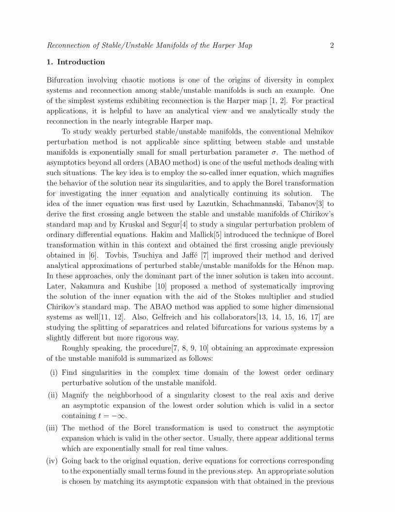
1. Introduction

Bifurcation involving chaotic motions is one of the origins of diversity in complex

systems and reconnection among stable/unstable manifolds is such an example. One

of the simplest systems exhibiting reconnection is the Harper map [1, 2]. For practical

applications, it is helpful to have an analytical view and we analytically study the

reconnection in the nearly integrable Harper map.

To study weakly perturbed stable/unstable manifolds, the conventional Melnikov

perturbation method is not applicable since splitting between stable and unstable

manifolds is exponentially small for small perturbation parameter σ. The method of

asymptotics beyond all orders (ABAO method) is one of the useful methods dealing with

such situations. The key idea is to employ the so-called inner equation, which magnifies

the behavior of the solution near its singularities, and to apply the Borel transformation

for investigating the inner equation and analytically continuing its solution. The

idea of the inner equation was first used by Lazutkin, Schachmannski, Tabanov[3] to

derive the first crossing angle between the stable and unstable manifolds of Chirikov’s

standard map and by Kruskal and Segur[4] to study a singular perturbation problem of

ordinary differential equations. Hakim and Mallick[5] introduced the technique of Borel

transformation within in this context and obtained the first crossing angle previously

obtained in [6]. Tovbis, Tsuchiya and Jaffe [7] improved their method and derived

analytical approximations of perturbed stable/unstable manifolds for the Henon map.

In these approaches, only the dominant part of the inner solution is taken into account.

Later, Nakamura and Kushibe [10] proposed a method of systematically improving

the solution of the inner equation with the aid of the Stokes multiplier and studied

Chirikov’s standard map. The ABAO method was applied to some higher dimensional

systems as well[11, 12]. Also, Gelfreich and his collaborators[13, 14, 15, 16, 17] are

studying the splitting of separatrices and related bifurcations for various systems by a

slightly different but more rigorous way.

Roughly speaking, the procedure[7, 8, 9, 10] obtaining an approximate expression

of the unstable manifold is summarized as follows:

(i) Find singularities in the complex time domain of the lowest order ordinary

perturbative solution of the unstable manifold.

(ii) Magnify the neighborhood of a singularity closest to the real axis and derive

an asymptotic expansion of the lowest order solution which is valid in a sector

containing t = −∞.

(iii) The method of the Borel transformation is used to construct the asymptotic

expansion which is valid in the other sector. Usually, there appear additional terms

which are exponentially small for real time values.

(iv) Going back to the original equation, derive equations for corrections corresponding

to the exponentially small terms found in the previous step. An appropriate solution

is chosen by matching its asymptotic expansion with that obtained in the previous


step.

The additional terms are determined by the singularities of the Borel-transformed

solutions and, so far, only contributions from poles were considered. In this paper, with

the aid of ABAO method, the reconnection of the unstable manifold is studied for the

Harper map. Our analysis mainly follows the method by Nakamura and Kushibe [10],

but contributions from the branch cuts of the Borel-transformed solution are also taken

into account.

The Harper map depends on a real parameter k and is defined on (v, u) ∈ [−π, π]2:

v(t + σ) − v(t) = − σ sin u(t)

u(t + σ) − u(t) = kσ sin v(t + σ) (1)

where σ(> 0) is the time step and plays a role of the small parameter. Since the case

of k < 0 is conjugate to that of k > 0, it is sufficient to consider the latter [2]. In the

continuous time limit, where σ → 0, the map reduces to a set of integrable differential

equations:

v′(t) = − sin u(t)

u′(t) = k sin v(t) . (2)

Throughout this paper, The prime is used to indicate the differentiation with respect

to time t such as u′(t) ≡ du(t)dt

. Eq.(2) admits topologically different separatrices

depending on the parameter k (cf. Fig. 1) and the separatrix changes its shape when

k → 1. Since the solution for k > 1 can be obtained from that for k < 1 by a simple

symmetry argument (cf. Appendix A), we restrict ourselves to the case of 0 < k < 1

and consider the change of the stable/unstable manifolds for k → 1. In the text,

an approximation of the unstable manifold is constructed and only the result of the

approximate stable manifold is given.

The rest of this paper is arranged as follows: In the next section, the lowest order

solution of the Melnikov perturbation method is constructed and the inner equation is

derived. In Sec. 3, the Borel resummation method is used to solve the inner equation and

Figure 1. Separatrix of the Harper map in the continuous limit


derive the additional exponentially small terms. In Sec. 4, the solution of the original

equation with the corresponding corrections is obtained and compared with numerical

calculations. The reconnection of the unstable manifolds is discussed in Sec. 5. Sec. 6

is devoted to the summary.

2. Melnikov Perturbation and Inner Equation

Let v0, u0 be the solutions obtained by Melnikov perturbation, i.e.,

v0(t) ≡∞∑

n=0

σnv0n(t) , u0(t) ≡∞∑

n=0

σnu0n(t)

The lowest order terms satisfy (2) and the first and second order terms obey

v′01(t) + u01(t) cos u00(t) = −1

2v′′00(t)

u′01(t) − kv01(t) cos v00(t) =

1

2u′′

00(t) (3)

v′02(t) + u02(t) cos u00(t) = −1

2v′′01(t) −

1

6v′′′00(t) +

u201(t)

2sin u00(t)

u′02(t) − kv02(t) cos v00(t) =

1

2u′′

01(t) −1

6u′′′

00(t) − kv201(t)

2sin v00(t) (4)

The lowest order solution of the unstable manifold with v0(0) = 0 is given by

v00(t) = − 2 tan−1[√

1 − k sinh√

kt]

u00(t) = 2 tan−1

[√k

1 − k

1

cosh√

kt

](5)

Because of the boundary conditions v0n(t) → 0, u0n(t) → 0 for t → −∞ and v0n(0) = 0,

the first and the second order solutions are

v01(t) = 0 , u01(t) =1

2y1(t) (6)

v02(t) = − 1

24

[x′

1(t) + x1(t)

(kt − 2(1 − k)

√k tanh

√kt

1 − k tanh2√

kt

)]

u02(t) =1

24

[2y′

1(t) − y1(t)

(kt − 2(1 − k)

√k tanh

√kt

1 − k tanh2√

kt

)](7)

where auxiliary functions are given by

x1(t) = − 2√

k(1 − k)cosh

√kt

1 + (1 − k) sinh2√

kt

y1(t) = − 2k√

1 − ksinh

√kt

1 + (1 − k) sinh2√

kt(8)


Figure 2. Singular points (crosses) of the lowest order solution v00, u00 in the complex

time domain.

We observe that the lowest order solution (5) has two sequences of singular points

in the complex t-plane (see Fig. 2).

t =1√k

{ln

1 ±√

k√1 − k

+

(n +

1

2

)πi

}(9)

Now we examine the behavior of perturbative solutions near two singular points

in the upper half plane closest to the real axis: t1 ≡ 1√k

{ln 1−

√k√

1−k+ 1

2πi}

, t2 ≡1√k

{ln 1+

√k√

1−k+ 1

2πi}

. From now on, tc stands for t1 or t2, and the upper sign corresponds

to t1 and the lower one corresponds to t2.

As easily seen, the perturbative solution admits an expansion like

v0(t, σ) − v00(t) =

∞∑

n=1

∞∑

l=0

a(n)l+1

(t − tc)n−lσn (10)

This indicates that the higher order terms with respect to σ has higher order poles at

t = tc and that the behavior near the singularities should be carefully investigated. For

this purpose, it is convenient to introduce a rescaled variable z ≡ t−tcσ

[5, 7, 8, 9, 10].

Then, one finds that Φ0(z, σ) ≡ v0(tc + σz, σ) − v00(tc + σz) and Ψ0(z, σ) ≡ u0(tc +

σz, σ) − u00(tc + σz) can be expanded into power series with respect to σ:

Φ0(z, σ) =

∞∑

l=0

Φ0l(z)σl , Ψ0(z, σ) =

∞∑

l=0

Ψ0l(z)σl , (11)

where (Φ00, Ψ00), (Φ01, Ψ01) . . . correspond to the most divergent terms, the next

divergent terms . . ..

We remark that, in terms of Φ(z, σ) ≡ v(tc + σz, σ) − v00(tc + σz) and Ψ(z, σ) ≡u(tc + σz, σ) − u00(tc + σz), the Harper map (1) reads as

∆Φ(z, σ) = − σ sin Ψ(z, σ) cos u00(tc + σz)

− σ cos Ψ(z, σ) sin u00(tc + σz) − ∆v00(tc + σz)


∆Ψ(z − 1, σ) = kσ sin Φ(z, σ) cos v00(tc + σz) (12)

+ kσ cos Φ(z, σ) sin v00(tc + σz) − ∆u00(tc + σ(z − 1))

where ∆ stands for the difference operator: ∆f(z) = f(z + 1) − f(z), and that

Φ0(z, σ), Ψ0(z, σ) are its perturbative solutions with respect to σ. This equation will

be referred to as an inner equation.

Substituting (11) into (12), one can easily obtain the equations for Φ0l, Ψ0l. The

first two sets are as follows

∆Φ00(z) = ie∓iΨ00(z)

z− i ln

(1 +

1

z

)

∆Ψ00(z) = ∓ ieiΦ00(z+1)

z + 1± i ln

(1 +

1

z

)(13)

∆Φ01(z) = ±[ik − 1

2+

Ψ01(z)

z

]e∓iΨ00(z) ∓ i

2(k − 1)

∆Ψ01(z) =

[±Φ01(z + 1)

z + 1− i

1 − k

2

]eiΦ00(z+1) +

i

2(1 − k) (14)

By matching the residues at z = 0:

Res

(Φ0k(z)

Ψ0k(z)

)∣∣∣∣z=0

= Res

(v0 k+1(t)

u0 k+1(t)

)∣∣∣∣t=tc

, (15)

one obtains the solution corresponding to the expansion (10)

Φ00(z) =i

12z2− 107i

4320z4+ O

(1

z5

)

Ψ00(z) = ∓(

i

2z− i

24z2− i

24z3+

191i

8640z4

)+ O

(1

z5

)(16)

Φ01(z) = ∓ i

24

±ktc + 1

z+ O

(1

z3

)

Ψ01(z) =i(k − 1)

4+

i

24

k(±tc + 1)

z− i

48

k(±tc + 1)

z2+ O

(1

z3

)(17)

This is the asymptotic solution of the inner equation which is valid in the sector

involving Re z = −∞. It is necessary to analytically continue it to another sector

involving Re z = +∞ in order to construct an approximation of the unstable manifold

in the time domain Re t > Re tc. This will be carried out in the next section.

3. Borel Transformation and Solution of Inner Equation

3.1. Borel Transformation and Analytic Continuation

As mentioned in the previous section, in order to construct an approximation of the

unstable manifold in the time domain Re t > Re tc, the solution of the inner equation

in the sector involving Re[z] = −∞ should be analytically continued to the sector

involving Re[z] = +∞. The analytic continuation is carried out with the aid of the

Borel transformation. Let us begin with Φ00(z), Ψ00(z).


Figure 3. Integral path in p-plane

Since we are interested in the unstable manifold, we define the Borel transforms

V0(p), U0(p) of Φ00(z), Ψ00(z), respectively, as

Φ00(z) ≡ L[V0(p)](z) ≡∫ −∞

0

dp e−pz V0(p)

Ψ00(z) ≡ L[U0(p)](z) ≡∫ −∞

0

dp e−pz U0(p) (18)

The analytic continuations of Φ00(z) and Ψ00(z) from Re[z] < 0, Im[z] < 0 to Re[z] > 0

are obtained by rotating the integral path in the p-plane from C to C′ (cf. Fig. 3).

Other possible singularities and branch cuts of V0, U0 are also shown in Fig. 3. Note

that the integral path should be rotated over π2

[rad] in a clockwise way so that the

convergence domain rotates counterclockwise. Thus, the analytic continuation from

Re[z] < 0, Im[z] < 0 to π + ǫ < arg[z] < 2π + ǫ is given by∫ −∞

0

dp e−pz V0(p) →∫ −∞ei(π/2+ǫ)

0

dp e−pz V0(p) −∫

γ

dp e−pz V0(p) (19)

where ǫ is a small positive real number.

If one can write down the Borel-transformed inner solution explicitly, one has only

to change the integral path. But it is difficult and we have to deal with the inner

equation and the Borel-transformed inner equation simultaneously. The procedure can

be summarized as follows

(a) Write down the equation for V0, U0:

− i(e−p − 1)V0(p) = 1 +

∫ p

0

dp

{ ∞∑

n=1

(∓i)nU(∗n)0 (p)

n!− 1 − e−p

p

}

±i(1 − ep)U0(p) = 1 +

∫ p

0

dp

{ ∞∑

n=1

inV(∗n)0 (p)

n!− ep − 1

p

}(20)

where V(∗n)0 denote the nth convolution defined by

V(∗n)0 (p) =

∫ p

0

dxV0(p − x)V(∗(n−1))0 (x) (21)


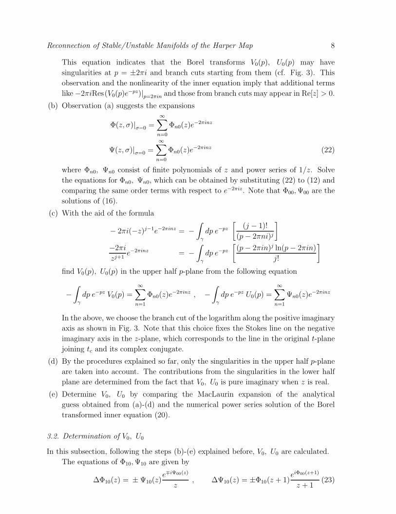
This equation indicates that the Borel transforms V0(p), U0(p) may have

singularities at p = ±2πi and branch cuts starting from them (cf. Fig. 3). This

observation and the nonlinearity of the inner equation imply that additional terms

like −2πiRes(V0(p)e−pz)|p=2πin and those from branch cuts may appear in Re[z] > 0.

(b) Observation (a) suggests the expansions

Φ(z, σ)|σ=0 =

∞∑

n=0

Φn0(z)e−2πinz

Ψ(z, σ)|σ=0 =

∞∑

n=0

Φn0(z)e−2πinz (22)

where Φn0, Ψn0 consist of finite polynomials of z and power series of 1/z. Solve

the equations for Φn0, Ψn0, which can be obtained by substituting (22) to (12) and

comparing the same order terms with respect to e−2πiz. Note that Φ00, Ψ00 are the

solutions of (16).

(c) With the aid of the formula

− 2πi(−z)j−1e−2πinz = −∫

γ

dp e−pz

[(j − 1)!

(p − 2πni)j

]

−2πi

zj+1e−2πinz = −

∫

γ

dp e−pz

[(p − 2πin)j ln(p − 2πin)

j!

]

find V0(p), U0(p) in the upper half p-plane from the following equation

−∫

γ

dp e−pz V0(p) =

∞∑

n=1

Φn0(z)e−2πinz , −∫

γ

dp e−pz U0(p) =

∞∑

n=1

Ψn0(z)e−2πinz

In the above, we choose the branch cut of the logarithm along the positive imaginary

axis as shown in Fig. 3. Note that this choice fixes the Stokes line on the negative

imaginary axis in the z-plane, which corresponds to the line in the original t-plane

joining tc and its complex conjugate.

(d) By the procedures explained so far, only the singularities in the upper half p-plane

are taken into account. The contributions from the singularities in the lower half

plane are determined from the fact that V0, U0 is pure imaginary when z is real.

(e) Determine V0, U0 by comparing the MacLaurin expansion of the analytical

guess obtained from (a)-(d) and the numerical power series solution of the Borel

transformed inner equation (20).

3.2. Determination of V0, U0

In this subsection, following the steps (b)-(e) explained before, V0, U0 are calculated.

The equations of Φ10, Ψ10 are given by

∆Φ10(z) = ± Ψ10(z)e∓iΨ00(z)

z, ∆Ψ10(z) = ±Φ10(z + 1)

eiΦ00(z+1)

z + 1(23)


which have two independent solutions:

Φ(A)10 = − 1

z+

23

48z3+ · · · , Ψ

(A)10 = ±

(1

z− 1

2z2− 1

48z3

)+ · · ·

Φ(B)10 = z +

1

12z− 17

1080z3+ · · · , Ψ

(B)10 = ±

(z +

1

2− 1

540z3

)+ · · ·

and Φ10, Ψ10 are their linear combinations.[

Φ10

Ψ10

]= cA

[Φ

(A)10

Ψ(A)10

]+ cB

[Φ

(B)10

Ψ(B)10

](24)

From (24), V0(p) is given by

−∫

γ

dp e−pz V0(p) =

∞∑

n=1

Φn0e−2πinz

= Φ10e−2πiz + Φ20e

−4πiz + · · ·

≈[cB

(z +

1

12z

)− cA

z+ O

(1

z3

)]e−2πiz (25)

and U0 can be represented in a similar way. As easily seen from (20), the coefficients cA

and cB are imaginary number.

In order to determine the Borel transforms V0, U0 from the expansion (25) by taking

into account the singularities in the lower half plane, we introduce auxiliary functions

f(R)lj (p), f

(I)lj (p) satisfying the following two conditions:

• −∫

γ

dp e−pz f(R)lj (p) = zje−2πliz

−∫

γ

dp e−pz f(I)lj (p) = izje−2πliz

• f(R)lj (p), f

(I)lj (p) is pure imaginary when p is real.

Especially, for non-negative j, f(R)1j (p) f

(I)1j (p) are given by

f(R)1j (p) =

j!

2πi

(1

(p − 2πi)j+1+

(−1)j+1

(p + 2πi)j+1

)(26)

f(I)1j (p) = i

j!

2πi

(1

(p − 2πi)j+1− (−1)j+1

(p + 2πi)j+1

)(27)

And f(I)1,−1 is

f(I)1,−1(p) = − 1

2π[ln(p − 2πi) − ln(p + 2πi)] (28)

In terms of these functions V0 is given by

V0(p) =cB

if

(I)11 (p) +

1

i(cB

12− cA)f

(I)1,−1(p)

= M +1

4π3

∞∑

n=0

(cB(2n + 2) − 4π2( cB

12− cA)

2n + 1

)(−1)n

( p

2π

)2n+1

(29)


where the constant M depends on the choice of the Riemann surface of the logarithm.

In a similar way, one finds

± U0(p) =1

i

(cBf

(I)11 (p) + cAf

(I)1,−1(p) +

cB

2f

(I)10 (p)

)

= M ′ +1

4π3

∞∑

n=0

(cB(2n + 2) − 4π2cA

2n + 1

)(−1)n

( p

2π

)2n+1

− cB

4π2

∞∑

n=0

(−1)n( p

2π

)2n

(30)

where M ′ depends on the choice of the Riemann surface.

In order to check the validity of analytical guess (29) and (30) about singularities

and to evaluate cA, cB, we derive power series solutions of (20) numerically and compare

them with the power series expansions of the R.H.S. of (29) and (30). By substituting

the power series expansions:

V0(p) ≡∞∑

n=0

anpn, U0(p) ≡

∞∑

n=0

bnpn; a0 = 0, b0 = ∓i1

2

into (20) and comparing term by term, one can determine the coefficients an, bn

recursively. They have the following asymptotic forms.

− ia2n+1(−1)n(2π)2n+1 → 0.27893(2n + 2) − 0.417

(2n + 1), as n → ∞

≡ A1(2n + 2) − A2

(2n + 1)

±ib2n+1(−1)n(2π)2n+1 → − 0.27893(2n + 2) +0.417

(2n + 1), as n → ∞

−ia2n = 0, ∀n

±ib2n(−1)n(2π)2n → 0.87628 ≡ A3 (31)

The numerical evaluations of A1, A3 are quite robust. On the other hand, A2 is sensitive

to an error of A1 since the coefficients of 1/(2n+1) are fitted after subtracting the leading

terms. However, we observe that the coefficients of 1/(2n+1) in a2n+1(−1)n(2π)2n+1 and

b2n+1(−1)n(2π)2n+1 are always the same. This observation suggests that the coefficients

of 1/z in Φ10, Ψ10 are identical, which implies

A2 =cA

iπ=

cB

24iπ=

A1π2

6(32)

The present numerical estimation gives a consistent value of 0.417 with this relation.

According to (29), (30) and (31), the asymptotic expansions of a2n+1(−1)n(2π)2n+1

and b2n+1(−1)n(2π)2n+1 with respect to n should have the same leading terms. This

is indeed the case. Moreover, A3/A1 should be equal to π and we have an excellent

agreement: A3/A1 = 3.14158 · · ·. Therefore, we can conclude that our guess about the

poles and branch cuts in the p-domain is valid. Then the constants cA, cB are given by

cA = iπA2 and cB = i4π3A1.


So far, we have considered the first three dominant terms in V0, U0.

From the asymptotic expansions of (25), one finds that V0, U0 involve f(I)1j (p)

(j ≤ −2) and f(I)lj (p) (l ≥ 2). As easily seen, one has the following rough estimations:

f(λ)lj (p) ∼

∞∑

n=0

1

n2(2πl)npn (j ≤ −2) , f

(λ)lj (p) ∼

∞∑

n=0

nj

(2πl)npn (j ≥ −1)

Therefore, if [f(λ)lj ]n denotes the absolute value of the coefficient of pn, one has the

following relation for large n:

[f(λ)11 ]n ≫ [f

(λ)10 ]n ≫ [f

(λ)1,−1]n ≫ [f

(λ)20 ]n · · · . (33)

As a result, neglected terms are expected to be sufficiently small in the present numerical

estimation.

In short, in this subsection, we have constructed the Borel transforms of Φ0, Ψ0

following the procedure discussed in the previous subsection. The result is summarized

as

V0(p) = 4π3A1f(I)11 (p) + πA2f

(I)1,−1(p)

U0(p) = ±(4π3A1f

(I)11 (p) + 2π3A1f

(I)10 (p) + πA2f

(I)1,−1(p)

)(34)

3.3. Borel Transforms of Φ01 and Ψ01

Let Φ−0j(z), Ψ−

0j(z) be the sum of negative powers of z in the asymptotic expansion of

Φ0j(z), Ψ0j(z) and Vj(p), Uj(p) be the Borel transform of Φ−0j , Ψ−

0j in the sector including

z = −∞, then Vj(p) provides the following terms in another sector including z = +∞

−∫

γ

dp e−pz Vj(p) =

∞∑

n=1

Φnj(z)e−2πinz (35)

In addition, we define Φn(z) =∑∞

j=0 σjΦnj(z) for later use. Similar quantities Ψnj and

Ψn are introduced for Ψ.

As the construction of V0, U0 from Φ10, Ψ10, V1, U1 can be obtained from the

solutions Φ11, Ψ11 of the following equations:

∆Φ11(z) = ± Ψ11(z) ± k−12

zΨ10(z)

ze∓iΨ00(z) − i

Ψ10(z)Ψ01(z)

ze∓iΨ00(z)

∆Ψ11(z − 1) = ± Φ11(z) ± 1−k2

zΦ10(z)

zeiΦ00(z) ± i

Φ10(z)Φ01(z)

zeiΦ00(z)(36)

Indeed, from this equation, asymptotic expansions of Φ11, Ψ11 in z are obtained and,

by exactly the same procedure as in the previous subsection, V1, U1 are determined as

(for more detail, see Appendix B)

V1(p) = ±(8π4B2(k − 1)f

(I)12 (p) + 4π3(B3(k + 1) ∓ B1ktc)f

(R)11 (p)

)

U1(p) = − 8π4B2(k − 1)f(I)12 (p) + 4π3(B3(k + 1) ∓ B1ktc)f

(R)11 (p)

− 4π3B4(k − 1)f(I)11 (p) (37)

And B1, B2, B3 and B4 can be numerically evaluated as A1, A2 and A3:

B1 = 0.7303, B2 = 0.007399, B3 = 0.03651, B4 = 0.04649 . (38)


3.4. General Structure of Inner Solution and Stokes Multiplier

In this subsection, we study the general structure of the inner solution Φ1(z) ≡∑∞j=0 σjΦ1j(z) Ψ1(z) ≡∑∞

j=0 σjΨ1j(z), which satisfies the following equation:

∆Φ1(z) = − σΨ1(z) cos (Ψ0(z) + u00(tc + σz))

∆Ψ1(z − 1) = kσΦ1(z) cos (Φ0(z) + v00(tc + σz)) (39)

For this purpose, it is convenient to introduce two solutions of the above equation

admitting the expansions:[

Φ(A)10 (z)

Ψ(A)10 (z)

]+

∞∑

j=1

σj

[Φ

(A)1j (z)

Ψ(A)1j (z)

],

[Φ

(B)10 (z)

Ψ(B)10 (z)

]+

∞∑

j=1

σj

[Φ

(B)1j (z)

Ψ(B)1j (z)

](40)

where Φ(A)1j (z) and Φ

(B)1j (z) are uniquely determined by posing

{coefficient of

1

zin Φ

(A)1j (z)

}={

coefficient of z in Φ(B)1j (z)

}= 0 .

Then, because of the linearity of (39), one has the following expressions

Φ10 = Λ0Φ(A)10 + Λ0Φ

(B)10

Φ11 = Λ0Φ(A)11 + Λ0Φ

(B)11 + Λ1Φ

(A)10 + Λ1Φ

(B)10

· · · · · · · · ·

Φ1n =

n∑

j=0

ΛkΦ(A)1,n−k +

n∑

j=0

ΛkΦ(B)1,n−k (41)

which leads to

Φ1(z) = (Λ0 + σΛ1 + · · ·)(Φ

(A)10 + σΦ

(A)11 + · · ·

)

+ (Λ0 + σΛ1 + · · ·)(Φ

(B)10 + σΦ

(B)11 + · · ·

). (42)

The coefficient Λ =

∞∑

n=0

σnΛn is referred to as the Stokes multiplier in [10]. Let

Λ =

∞∑

n=0

σnΛn, then one finally has

[Φ1

Ψ1

]= Λ

[Φ

(A)10 + σΦ

(A)11 + · · ·

Ψ(A)10 + σΨ

(A)11 + · · ·

]+ Λ

[Φ

(B)10 + σΦ

(B)11 + · · ·

Ψ(B)10 + σΨ

(B)11 + · · ·

].

The first two terms of the Stokes multiplier can be estimated as follows:

−∫

γ

dp e−pz {V0(p) + σV1(p)}

−∫

γ

dp e−pz {U0(p) + σU1(p)}

=

(Λ

[(Φ

(B)10 + Φ

(B)11 σ + · · ·)

(Ψ(B)10 + Ψ

(B)11 σ + · · ·)

]+ Λ

[(Φ

(A)10 + Φ

(A)11 σ + · · ·)

(Ψ(A)10 + Ψ

(A)11 σ + · · ·)

])e−2πiz

=

[±Λ0z + σ(±Λ1z ± k−1

6Λ0z

2)

Λ0z + σ(Λ1z − k−1

6Λ0(z

2 + z))]

e−2πiz (43)


where the contour integral is evaluated with the aid of (34) and (37). This leads to the

following relations

Λ0 = i4π3A1 = i48π4B2 = i24π3B4

Λ1 = 4π3(B3(k + 1) ∓ B1ktc) (44)

Eq.(44) implies two linear relations among A1, B2 and B4, which are satisfied by the

present numerical estimations rather well:

A1

12πB2= 0.99998 ≃ 1

A1

6πB4= 0.99997 ≃ 1 .

4. Matching of Inner and Outer Solutions

4.1. Matching at a Singular Point

In this section, solutions of the outer equations are constructed and are matched

with the inner solutions. We first consider the contribution from the singularity

t1. Corresponding to the expansion of the analytically continued inner solutions:

Φ =∑∞

n=0 Φne−2πinz, Ψ =∑∞

n=0 Ψne−2πinz, the original solutions v and u acquire new

terms in a sector Re t ≥ Re t1 of the t1-neighborhood:

v(t) = v0(t, σ) + v1(t, σ)e−2πiσ

t + v2(t, σ)e−4πiσ

t + · · ·u(t) = u0(t, σ) + u1(t, σ)e−

2πiσ

t + u2(t, σ)e−4πiσ

t + · · · (45)

Because of e−2πinz ∝ ǫne−2πin

σt with ǫ ≡ e

− π2

σ√

k , vn and un are of order of ǫn. By

substituting (45) into (1) and comparing term by term, we obtain the equations for v1

and u1:

v1(t + σ) − v1(t) = − σu1(t) cos u0(t)

u1(t + σ) − u1(t) = kσv1(t + σ) cos v0(t + σ) (46)

Its solution is uniquely determined by the matching condition:

e−2πit

σ

[v1(t, σ)

u1(t, σ)

]∣∣∣∣t=t1+σz

= e−2πiz{

Λ

[Φ

(A)10 (z) + σΦ

(A)11 (z) + · · ·

Ψ(A)10 (z) + σΨ

(A)11 (z) + · · ·

]

+ Λ

[Φ

(B)10 (z) + σΦ

(B)11 (z) + · · ·

Ψ(B)10 (z) + σΨ

(B)11 (z) + · · ·

]},(47)

or equivalently[

v1(t1 + σz, σ)

u1(t1 + σz, σ)

]= e

2πit1σ

{Λ

[Φ

(A)10 (z) + σΦ

(A)11 (z) + · · ·

Ψ(A)10 (z) + σΨ

(A)11 (z) + · · ·

]

+ Λ

[Φ

(B)10 (z) + σΦ

(B)11 (z) + · · ·

Ψ(B)10 (z) + σΨ

(B)11 (z) + · · ·

]}. (48)

The matching condition suggests the following expansions:

v1(t, σ) = σje2πit1

σ

∞∑

n=0

v1n(t)σn , u1(t, σ) = σje2πit1

σ

∞∑

n=0

u1n(t)σn (49)


where j is an integer. Then equations for v10, u10 · · · are given by

v′10(t) = −u10(t) cos u00(t)

u′10(t) = kv10(t) cos v00(t) (50)

v′11(t) +

1

2v′′10(t) = −u11(t) cosu00(t) + u10(t)u01(t) sin u00(t)

u′11(t) −

1

2u′′

10(t) = k (v11(t) cos v00(t) − v10(t)v01(t) sin v00(t)) (51)

First, we solve (50). Since it admits two linearly independent solutions:

[x1

y1

]of

(8) and the following

[x2

y2

]:

x2(t) =−x1(t)

4k(1 − k)

[(1 − k)2

2√

k

(sinh

√kt cosh

√kt +

√kt)− k3/2 tanh

√kt

]

y2(t) =y1(t)

4k(1 − k)

[(1 − k)2

2√

k

(sinh

√kt cosh

√kt −

√kt)

+1√k

coth√

kt

],

(52)

one has [v10(t)

u10(t)

]= a

[x1(t)

y1(t)

]+ b

[x2(t)

y2(t)

](53)

with the matching condition

σj

[v10(σz + t1)

u10(σz + t1)

]∣∣∣∣σ0

= σj

{a

[x1(σz + t1)

y1(σz + t1)

]+ b

[x2(σz + t1)

y2(σz + t1)

]}∣∣∣∣σ0

= Λ0

[Φ

(A)10 (z)

Ψ(A)10 (z)

]+ Λ0

[Φ

(B)10 (z)

Ψ(B)10 (z)

]∣∣∣∣dom.

= Λ0

[z

z

](54)

where the subscript σ0 indicates to take the terms of order σ0 and dom. stands for the

largest part for z → ∞.

Because L.H.S. of (54) starts from z, one should have j = −1. Then, the coefficients

a and b are determined by the requirement that (54) admits well defined σ → 0 limit:

a = Λ0t1(k − 1)2 + (1 + k)

4ik(k − 1), b = −2Λ0

i.

Therefore, up to the 0th order in σ, we have[v1(t)

u1(t)

]≈ 2Λ0

iσe

2πit1σ

{t1(k − 1)2 + (1 + k)

8k(k − 1)

[x1(t)

y1(t)

]−[

x2(t)

y2(t)

]}(55)

Similarly, up to the first order in σ, one obtains[v1(t)

u1(t)

]≈ 2Λ(1)

iσe

2πit1σ

{t1(k − 1)2 + (1 + k)

8k(k − 1)

[x1(t)

y1(t) + σy′1(t)/2

]

−[

x2(t)

y2(t) + σy′2(t)/2

]}(56)


where Λ(1) ≡ Λ0 + σΛ1 is the first order Stokes multiplier.

In the t2-neighborhood, the unperturbed solutions v0, u0 acquire the following terms

in a sector Re t ≥ Re t2:[v1(t)

u1(t)

]≈ 2Λ(2)

iσe

2πit2σ

{t2(k − 1)2 − (1 + k)

8k(k − 1)

[x1(t)

y1(t) + σy′1(t)/2

]

−[

x2(t)

y2(t) + σy′2(t)/2

]}(57)

where Λ(2) is the first order Stokes multiplier arising from the singularity t2.

4.2. Contributions from Other Singular Points

So far, contributions from t1 and t2 have been considered. Here, we study contributions

from other singular points.

Let t(n) denote the singular points satisfying, |Im[t(n)]| = (2n+1)π2

2√

k. Then terms

arising from t(n) are of order ǫ2n+1, where ǫ = e− π2

√

kσ . Since (v0(t), u0(t)) is bounded and

(vn(t), un(t)) ≈ e√

kt, (n ≥ 1) for sufficiently large t, one can neglect the terms arising

from t(n) (n ≥ 1) even for sufficiently large t.

On the other hand, terms arising from t1 may produce new terms when t passes

through t2-neighborhood, but they are negligible as they are higher order with respect

to ǫ. Therefore, the overall contribution of the singular points is a simple sum of the

contributions from t1, t2, t∗1, t∗2 and one has the following solution of the unstable

manifold in the whole time domain:

vu(t) = v00(t) + σ2v02(t)

+ S−(t)Re

[4Λ(1)

iσe

2πit1σ

(t1(k − 1)2 + (1 + k)

8k(k − 1)x1(t) − x2(t)

)e−

2πitσ

]

+ S+(t)Re

[4Λ(2)

iσe

2πit2σ

(t2(k − 1)2 − (1 + k)

8k(k − 1)x1(t) − x2(t)

)e−

2πitσ

]

uu(t) = u00(t) + σy1(t)

2+ σ2u02(t) + σ3

(1

2u′

02(t) −1

24y′′

1(t)

)

+ S−(t)Re[4Λ(1)

iσe

2πit1σ

{t1(k − 1)2 + (1 + k)

8k(k − 1)

(y1(t) + σ

y′1(t)

2

)

−(

y2(t) + σy′

2(t)

2

)}e−

2πitσ

]

+ S+(t)Re[4Λ(2)

iσe

2πit2σ

{t2(k − 1)2 − (1 + k)

8k(k − 1)

(y1(t) + σ

y′1(t)

2

)

−(

y2(t) + σy′

2(t)

2

)}e−

2πitσ

]

(58)


where S±(t) = S(t± tR1 ) and S(t) stands for the step function, and Λ(1), Λ(2) denote the

first order Stokes multipliers from the analysis of t1, t2, respectively.

4.3. Comparison with Numerical Calculation

Here we compare the analytical solution (58) obtained in the previous subsection with

the numerical calculation. For this purpose, it is convenient to rewrite the solution as

vu(t) = v0(t) + 2S(t)

[a11(t) cos

2πt

σ+ b11(t) sin

2πt

σ

]

+ 2S(t + 2tR1 )

[a12(t) cos

2π(t + 2tR1 )

σ+ b12(t) sin

2π(t + 2tR1 )

σ

]

uu(t) = u0(t) + 2S(t)

[a21(t) cos

2πt

σ+ b21(t) sin

2πt

σ

]

+ 2S(t + 2tR1 )

[a22(t) cos

2π(t + 2tR1 )

σ+ b22(t) sin

2π(t + 2tR1 )

σ

]

(59)

where the auxiliary functions are given by

a11(t) = (K + K1)(αx1(t) − x2(t)

)− K ′

1βx1(t)

b11(t) = K ′1

(αx1(t) − x2(t)

)+ (K + K1)βx1(t)

a12(t) = (K1 − K)(αx1(t) + x2(t)

)− K ′

1βx1(t)

b12(t) = − K ′1

(αx1(t) + x2(t)

)+ (K − K1)βx1(t)

a21(t) = (K + K1){α(y1(t) +

σ

2y′

1(t))−(y2(t) +

σ

2y′

2(t))}

− K ′1β(y1(t) +

σ

2y′

1(t))

b21(t) = K ′1

{α(y1(t) +

σ

2y′

1(t))−(y2(t) +

σ

2y′

2(t))}

+ (K + K1)β(y1(t) +

σ

2y′

1(t))

a22(t) = (K1 − K){α(y1(t) +

σ

2y′

1(t))−(y2(t) +

σ

2y′

2(t))}

− K ′1β(y1(t) +

σ

2y′

1(t))

b22(t) = − K ′1

{α(y1(t) +

σ

2y′

1(t))

+(y2(t) +

σ

2y′

2(t))}

+ (K − K1)β(y1(t) +

σ

2y′

1(t))

(60)

The functions with tilde are defined as f(t) ≡ f(t+tR1 ) and the constants α, β, K1, K ′1

are given by

K =8π3A1

σe− π2

σ√

k , K1 = −8π3B1tI1e

− π2

σ√

k


K ′1 = 8π3(B1ktR1 − B3(k + 1))e

− π2

σ√

k

α =tR1 (k − 1)2 + (1 + k)

8k(k − 1), β =

tI1(k − 1)

8k(61)

where tR1 and tI1 are the real and imaginary parts of t1, respectively. Eq.(59) indicates

that, when t exceeds t = 0, exponentially growing oscillatory term appears and, when

t exceeds t = −2tR1 (> 0), another exponentially growing term is added. These terms

should describe heteroclinic tangles.

This is indeed the case. Fig. 4, Fig. 5 shows an analytical solution of the unstable

manifold from (π, 0). One can see a large-amplitude oscillation near (−π, 0). As shown

in Fig. 4, Fig. 5, the analytical solution (59) (solid curve) well reproduces the oscillation

in the numerically calculated orbit (dots). The dots show the time evolution of an

ensemble consisting of 500 points. One can see the stretching of the ensemble is also

well reproduced by the approximate unstable manifold. When only the leading order

terms of the inner equation are retained, the agreement between the analytical and

numerical results is not so good (cf. Fig. 6) and, thus, the terms in the inner solution

of order σ are important.

Before closing this section, we give an approximate stable manifold (vs(t), us(t)). By

the similar approach to construct the unstable manifold, we have the similar expressions:

vs(t) = v0(t) − 2S(−t)

[a11(t) cos

2πt

σ+ b11(t) sin

2πt

σ

]

− 2S(−t + 2tR1 )

[a12(t) cos

2π(t + 2tR1 )

σ+ b12(t) sin

2π(t + 2tR1 )

σ

]

us(t) = u0(t) − 2S(−t)

[a21(t) cos

2πt

σ+ b21(t) sin

2πt

σ

]

− 2S(−t + 2tR1 )

[a22(t) cos

2π(t + 2tR1 )

σ+ b22(t) sin

2π(t + 2tR1 )

σ

]

(62)

5. Reconnection of Unstable Manifold

We remind that the separatrix of the continuous-limit equation is the unperturbed

stable/unstable manifold. As mentioned in Introduction (cf.Fig. 1), the separatrix

changes its topology depending on the parameter k (reconnection). When 0 < k < 1,

there appears a separatrix connecting (π, 0) and (−π, 0). As k → 1, it approaches

the union of two segments: the one connecting (π, 0) with (0, π) and the other (0, π)

with (−π, 0). Both segments are separatrices at the parameter value k = 1. The

corresponding topological change occurs for stable/unstable manifolds, which will be

discussed in this section. As shown in the previous section, since the approximate

stable and unstable manifolds are related with each other by simple symmetry, it is

enough to discuss the topological change of the unstable manifold.


Figure 4. The analytically constructed unstable manifold (solid line) near (−π, 0) and

time evolution of the ensemble (dots). Inset shows the overall view of the analytically

construced unstbale manifold. σ = 0.35, k = 0.85

Figure 5. The analytically constructed unstable manifold (solid line) near (−π, 0)

and time evolution of the ensemble (dots). σ = 0.35, k = 0.85

Fig. 7, Fig. 8, Fig. 9, Fig. 10 show the unstable manifolds when σ = 0.35 and

k = 0.2, 0.5, 0.85, 1.0 − 10−9, respectively. The overall structure of the unstable

manifold except near the fixed point (−π, 0) is very close to that of the separatrix.

Near (−π, 0), the unstable manifold acquires an oscillatory portion and the slope of this

portion becomes steeper as k → 1. The behavior of the slope can be understood from

the asymptotic ratio between the additional terms:

limt→+∞

u1(t)

v1(t) + π= −

√k − k

2σ .

It is interesting to see that, when k is very close to unity (i.e., k = 1.0−10−9), there

appears an additional oscillatory portion in the unstable manifold near (0, π) (cf. Fig. 5).


Figure 6. The analytically constructed unstable manifold (solid line) near (−π, 0)

and time evolution of the ensemble (dots). Only the leading term of the inner equation

is taken into consideration. k = 0.85, σ = 0.35

Figure 7. The analytically constructed unstable manifold. σ = 0.35, k = 0.2

As mentioned before, at k = 1, two segments from (π, 0) to (0, π) and from (0, π) to

(−π, 0) are separatrices of the continuous-limit equation. Thus, the perturbed unstable

manifold at k = 1 starting from (π, 0) should have an oscillatory portion near (0, π).

The oscillation near (0, π) of the unstable manifold shown in Fig. 5 can be considered

as the precursor of the oscillation in the unstable manifold at k = 1.

The origin of these behaviors are summarized as follows. When k is not very close

to 1, splitting term is exponentially small compared to the unperturbed solution and

can be negligible for not too large t . But this term becomes dominant for sufficiently

large t because x2, y2 → ∞ as t → ∞. Thus, a large-amplitude oscillation appears

near (−π, 0). This is not the case when k is very close to 1 because exponentially small

terms with respect to σ are proportional to 11−k

. Therefore, the additional terms are


Figure 8. The analytically constructed unstable manifold. σ = 0.35, k = 0.5

Figure 9. Analytically constructed unstable manifold. σ = 0.35, k = 0.85

Figure 10. The analytically constructed unstable manifold. σ = 0.35, k = 1.0−10−9


Figure 11. The analytically constructed unstable manifold and the oscillation near

(0, π). σ = 0.35, k = 1.0 − 10−9

not too small compared to the unperturbed solution near (0, π) and we can observe the

oscillation near (0, π). We further remark that two oscillatory portions in the unstable

manifold for k ≃ 1 come from two singularities t1 and t2 in the complex time plane. In

other words, the two sequences of singularities are necessary to exhibit the reconnection

of stable/unstable manifolds.

6. Conclusions

With the aid of ABAO (the asymptotics beyond all orders) method, we have derived

analytical approximations of the stable/unstable manifolds, which agree rather well

with those obtained by the numerical iteration. When k is not close to 1, the perturbed

unstable manifold starting from (π, 0) exhibits highly oscillatory behavior near the fixed

point (−π, 0) and its overall structure far from (−π, 0) is almost the same as that of the

unperturbed unstable manifold. However, when k is very close to 1, we can observe a

oscillation near (0, π), which is considered to be the precursor of the heteroclinic tangle

in the unstable manifold at k = 1. In this way, even when the heteroclinic tangle exists,

the unstable manifold smoothly changes its topology as the change of the parameter k.

Contrary to the systems studied so far by ABAO method, the unperturbed solution

of the Harper map have two sequences of singular points in the complex time plane and

the interference of the contributions from them might be expected. In this paper, the

approximate stable/unstable manifolds are constructed just adding the contributions

from the two sequences, but they agree quite well with the numerically constructed

unstable manifold. In a higher order approximation, we need to take into account this


interference. This aspect will be discussed elsewhere.

Acknowledgments

The authors thank Hidekazu Tanaka and Satoshi Nakayama for their contributions to

the early stage of this work. Also, they are grateful to Prof. K. Nakamura, Prof. A.

Shudo, Dr.S. Shinohara, T. Miyaguchi and Dr. G. Kimura for fruitful discussions and

useful comments. Particularly, they thank Prof. Nakamura for turning their attention

to Ref.[10]. This work is partially supported by a Grant-in-Aid for Scientific Research of

Priority Areas “Control of Molecules in Intense Laser Fields” and the 21st Century COE

Program at Waseda University “Holistic Research and Education Center for Physics

of Self-organization Systems” both from Ministry of Education, Culture, Sports and

Technology of Japan, as well as by Waseda University Grant for Special Research

Projects, Individual Research (2004A-161).

Appendix A. Case of k > 1

In this section, we consider the case of k > 1. Put

τ ≡ kt, σ ≡ kσ, u(τ) ≡ v(−τ

k+ σ)

, v(τ) ≡ u(−τ

k+ σ)

(A.1)

then v, u are the solution of the Harper map with parameter 1/k:

v(τ + σ) − v(τ) = − σ sin u(τ)

u(τ + σ) − u(τ) =σ

ksin v(τ + σ) (A.2)

Appendix B. Borel-transformed first order solution of inner equation

The aim of this appendix is to calculate the Borel transforms of the solutions Φ−01, Ψ−

01.

In order to investigate the behavior near t = t1 and t = t2 in a unified way, we introduce

Φ01(z) and Ψ01(z) by

± iΦ01 ≡ Φ−01 , iΨ01 ≡ Ψ−

01 , (B.1)

The Borel transforms V1, U1 of Φ01, Ψ01 satisfy

(e−p − 1)V1 =k − 1

2(g′(p) +

1

2) +

k − 1

4(g(p) − 1) + U1 ∗ g(p)

(1 − ep)U1 =k − 1

2f ′(p) + V1 ∗ f(p) (B.2)

where

B

[eiΦ00

z

]= f(p), B

[e∓iΨ00

z

]= g(p)

The power series expansions of V1, U1 is defined by

V1 = −±ktc + 1

24+

∞∑

n=1

cnpn , U1 =k(±tc + 1)

24+

∞∑

n=1

dnpn (B.3)


(B.2) and (B.3) gives the following form:

cn = ±ktcc(1)n + kc(2)

n + c(3)n , dn = ±ktcd

(1)n + kd(2)

n + d(3)n (B.4)

where c(i)n , d

(i)n are independent of k. By substituting (B.4) into (B.2), we numerically

get the following estimation. cn, dn as follows:

c2n = B2(k − 1)(2n + 2)(2n + 1)

(2π)2n(−1)n− (±B1ktc − B3(k + 1))

2n + 1

(2π)2n(−1)n

d2n = B2(1 − k)(2n + 2)(2n + 1)

(2π)2n(−1)n− (±B1ktc − B3(k + 1))

2n + 1

(2π)2n(−1)n

d2n+1 = − B4(k − 1)(2n + 2)

(2π)2n+1(−1)n

This estimation gives (37).

References

[1] Saito S, Nomura Y, Hirose K and Ichikawa Y H 1997 Separatrix reconnection and periodic orbit

annihilation in the Harper map Chaos 7 245-253 and references therein.

[2] Shinohara S 2002 The threshold for global diffusion in the kicked Harper map Phys. Lett. A 298

330-334 and references therein. See also S.Shinohara 1999 PhD thesis, Waseda University.

[3] Lazutkin V F, Schachmannski I G and Tabanov M B 1989 Splitting of separatrices for standard

and semistandard mappings Physica D 40 235-248

[4] Kruskal M D and Segur H 1991 Asymptotics beyond all orders in a model of crystal growth

Stud.Appl.Math 85 129-181

[5] Hakim V and Mallick K 1993 Exponentially small splitting of separatrices, matching in the complex

plane and Borel summation Nonlinearity 6 57-70

[6] Lazutkin V F 1984 “Splitting of separatrices for the Chirikov’s standard map” VINITI 6372/84

preprint [Russian]

[7] Tovbis A, Tsuchiya M and Jaffe C 1998 Exponential asymptotic expansions and approximations

of the unstable and stable manifolds of singularly perturbed systems with the Henon map as

an example Chaos 8 665-681; “Exponential asymptotic expansions and approximations of the

unstable and stable manifolds of the Henon map”, preprint (1994).

[8] Nakamura K and Hamada M 1996 Asymptotic expansion of homoclinic structures in a symplectic

mapping J. Phys. A 29 7315-7327

[9] Nakamura K 1997 Quantum versus Chaos: Questions Emerging from Mesoscopic Cosmos (Kluwer,

Boston)

[10] Nakamura K and Kushibe H 2000 Beyond-All-Orders Asymptotics and Heteroclinic Structures

Prog.Theor.Phys. Supplement 139 178-190

[11] Hirata Y, Nozaki K and Konishi T 1999 Exponentially Small Oscillation of 2-Dimensional Stable

and Unstable Manifolds in 4-Dimensional Symplectic Mappings Prog. Theor. Phys. 101 No.5

1181-1185

[12] Hirata Y, Nozaki K and Konishi T 1999 The Intersection Angles between N-Dimensional Stable

and Unstable Manifolds in 2N-Dimensional Symplectic Mappings Prog. Theor. Phys. 102 No.3

701-706

[13] Gelfreich V and Lerman L 2003 Long-periodic orbits and invariant tori in a singularly perturbed

Hamiltonian system Physica D 176 125-146 and references therein.

[14] Gelfreich V 2002 Near strongly resonant periodic orbits in a Hamiltonian system Proc. Nat. Acad.

Sci. USA 99 13975-13979


[15] Gelfreich V and Lazutkin V 2001 “Splitting of Separatrices: perturbation theory and exponential

smallness” Russ. Math. Surv. 56 499-558 [Russian]

[16] Gelfreich V and Sauzin D 2001 Borel summation and splitting of separatrices for the Henon map

Annal. Instit. Fourier,51,513-567 and references therein.

[17] Gelfreich V G, Lazutkin V F and Tabanov M B 1991 Exponentially small splittings in Hamiltonian

systems Chaos,1,137-142 and references therein.

Reconnection of Stable/Unstable Manifolds of the Harper Map

Documents

Transcript of Reconnection of Stable/Unstable Manifolds of the Harper Map