1

Magnetic Bubbles and Kinetic Alfven Waves in the High-Latitude

Magnetopause Boundary

K. Stasiewicz1,2, C. E. Seyler3, F. S. Mozer4, G. Gustafsson1, J. Pickett5 and B. Popielawska2

1Swedish Institute of Space Physics, Uppsala

2Space Research Centre, Polish Academy of Sciences, Warsaw

3Cornell University, Ithaca

4University of Berkeley, California

5Iowa University, Iowa

submitted to Journal of Geophysical Research, 7 July 2000, revised December, 2000.

Short title: MAGNETIC BUBBLES AND KAW

2

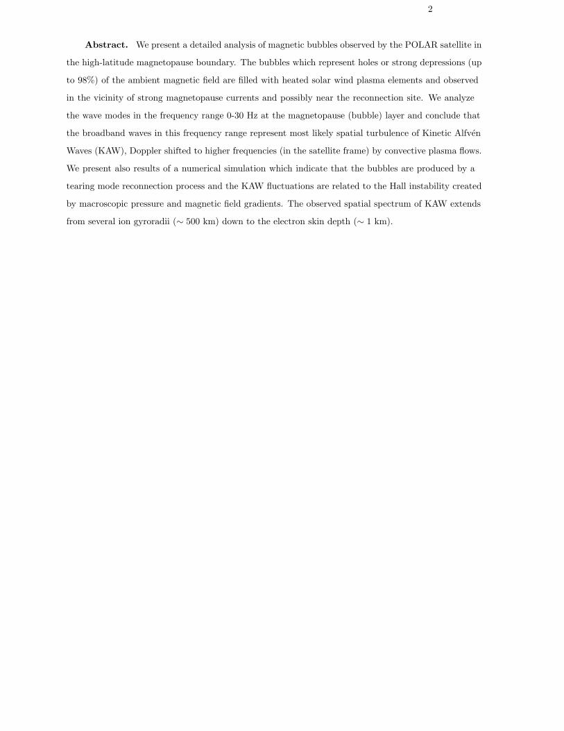
Abstract. We present a detailed analysis of magnetic bubbles observed by the POLAR satellite in

the high-latitude magnetopause boundary. The bubbles which represent holes or strong depressions (up

to 98%) of the ambient magnetic field are filled with heated solar wind plasma elements and observed

in the vicinity of strong magnetopause currents and possibly near the reconnection site. We analyze

the wave modes in the frequency range 0-30 Hz at the magnetopause (bubble) layer and conclude that

the broadband waves in this frequency range represent most likely spatial turbulence of Kinetic Alfven

Waves (KAW), Doppler shifted to higher frequencies (in the satellite frame) by convective plasma flows.

We present also results of a numerical simulation which indicate that the bubbles are produced by a

tearing mode reconnection process and the KAW fluctuations are related to the Hall instability created

by macroscopic pressure and magnetic field gradients. The observed spatial spectrum of KAW extends

from several ion gyroradii (∼ 500 km) down to the electron skin depth (∼ 1 km).

3

Introduction

Satellites traversing the magnetopause boundary layer, the outer magnetospheric cusp, or the

magnetosheath observe frequently regions with strong depressions of the magnetic field, δB/B0 ∼ 90%

[Kaufmann et al., 1970; Tsurutani et al., 1982; Treumann et al., 1990; Luhr and Klocker, 1987; Savin

et al., 1998]. Similar non-periodic phenomena have been observed in the solar wind [Turner et al.,

1977; Winterhalter et al., 1994] and in the magnetospheres of Jupiter [Tsurutani et al., 1993; Erdos

and Balogh, 1996]. The nature and origin of these structures is not well understood. Although many

researchers associate them with mirror-mode instability there are some doubts in the validity of this

mechanism [Tsurutani et al., 1999] and explanations in terms of MHD solitary waves have been also

suggested [Baumgartel, 1999].

In this paper we present a detailed analysis of magnetic bubbles observed by the POLAR satellite.

We find that it is unlikely that the magnetic holes observed at the magnetopause boundary layer are

related to mirror mode waves. We present results of a numerical simulation which indicate that the

bubbles may be related to tearing mode instability driven by strong magnetopause currents and the

smaller scale fluctuations represent kinetic Alfven waves driven by macroscopic pressure and magnetic

field gradients via Hall instability. The results suggest also presence of a turbulent cascade where the

energy of KAW cascades through wide range of spatial scales: from a few ion gyroradi ρi ∼ 500 km

down to the electron inertial scale λe ∼ 1 km.

Observations

Overview of the event April 11, 1997

During periods of high solar wind pressure (5-10 nPa) the orbit of the POLAR spacecraft with

the apogee of 9 RE occasionally crosses the magnetopause current layer and enters the magnetosheath

region. In 1996 and 1997 during spring/summer season, when POLAR apogee was on the dayside,

the magnetopause crossings were most common in region poleward of the cusp at high-latitudes. One

such an event occurred on April 11, 1997, 13:30-15:30 UT when POLAR was in the dusk sector of the

high-latitude dayside lobe, GSM (x, y, z)=(2.8, 1.5, 8.0) RE at 14:30 UT. The ISTP WIND spacecraft

was located 230 RE in front of the Earth and registered solar wind at a steady speed of 450 km/s with

the pressure increasing from 5 to 10 nPa, due to the increase of the solar wind number density. During

this time interval the IMF was relatively steady with BGSM=(3, -2, 20) nT at WIND position, delayed

to POLAR by 56 min. A general configuration of the POLAR orbit during this case can be found in

Russell et al. [2000].

4

We shall now focus on the magnetometer data (courtesy of C. Russell) which are shown in Figure

1. The spacecraft was in the high-latitude compressed lobe field of the magnitude of 110 nT until 14:28 Fig 1

UT, when it encountered three Magnetic Bubbles Layers (MBL) seen best in panel B as dropouts

of the total magnetic field, marked with solid bars. The bubble layers are located adjacent to the

magnetopause current layer best seen as reversals of Bz. The minimum field measured during this event

was 1.4 nT which corresponds to 98 % depression of the ambient field of ∼ 100 nT. The first bubble

layer was followed by a prominent crossing of the magnetopause layer at 14:34 UT and entering into

the magnetosheath with nearly oppositely directed magnetic field of similar strength. A sudden change

of the Bz and Bx to opposite values at 14:35 UT, accompanied by a decrease of |By|, is consistent witha high-latitude magnetopause crossing, as the change is toward IMF-like configuration of Bz, a strongly

dominating component in the solar wind.

The spacecraft re-entered the MBL during 14:43-14:46, returned to the magnetosheath and

after another crossing of the MBL and the magnetopause at 14:52 it continued its journey inside the

magnetosphere. From the electric field measured by the EFI instrument we compute the vE = E×B/B2

velocity for the time interval in Figure 1. The modulus of velocity vE is shown in the lowest panel.

As can be seen in Figure 1 the vE flows are highly variable (50-300 km/s) and significantly higher

(∼ 200 km/s) in the bubble layers compared to ∼ 80 km/s in the magnetosheath and inside the

magnetosphere. The general direction of the convective vE and the bulk plasma flow V (not shown

here) are consistent with the expected geometry of flows associated with magnetopause crossing. The

GSM vEx component is positive (sunward) inside the magnetosphere and consistently negative (albeit

small) in the magnetosheath ”proper” (i.e., in the MS region ouside of the outer part of the MBL, from

14:35:30 to 14:42:00 UT and from 14:47:00 to 14:51:00 UT). Correspondingly, the GSM vEz component

is negative in the magnetosphere and consistently positive in the MS proper. The GSM vEy component

is positive throughout all regions, consistent with the expected flow duskward in the post-afternoon

sector of the magnetopause. The bulk plasma flow in the MS proper is sub-Alfvenic, V < 170 km/s,

antisunward, duskward and poleward, with all 3 components of equal magnitude of about 100km/s

(C. Kletzing, private communication). The three bubble layers are characterized by enhanced vE flows

with increased kinetic energy coming presumably from the redistribution of the ambient magnetic field

energy, which can be deduced from high correlation between B and vE panels in Figure 1.

The characteristics of the electron and ion distributions measured during this event and shown

in Figure 2 corroborate the presented above interpretation of the magnetopause crossings. It is seen Fig 2

that the magnetic depressions in Figure 1 are filled with ions and electrons with energy higher than

5

in the adjacent magnetosheath region. The particle energization is accompanied by strong depressions

(annihilation) of the magnetic field. The maximum depression of the magnetic field is ∆B ≈ 100 nT

which corresponds to the magnetic energy density ∆B2/2µ0 = 4 × 10−9 J/m3. This magnetic energy

is equivalent to particle energy of 800 eV per ion-electron pair at the number density of 30 cm−3. It

should be noted here that contrary to our conclusions, some other authors [Fuselier et al., 2000; Russell

et al., 2000; Le et al., 2000] do not interpret this case as a magnetopause crossing.

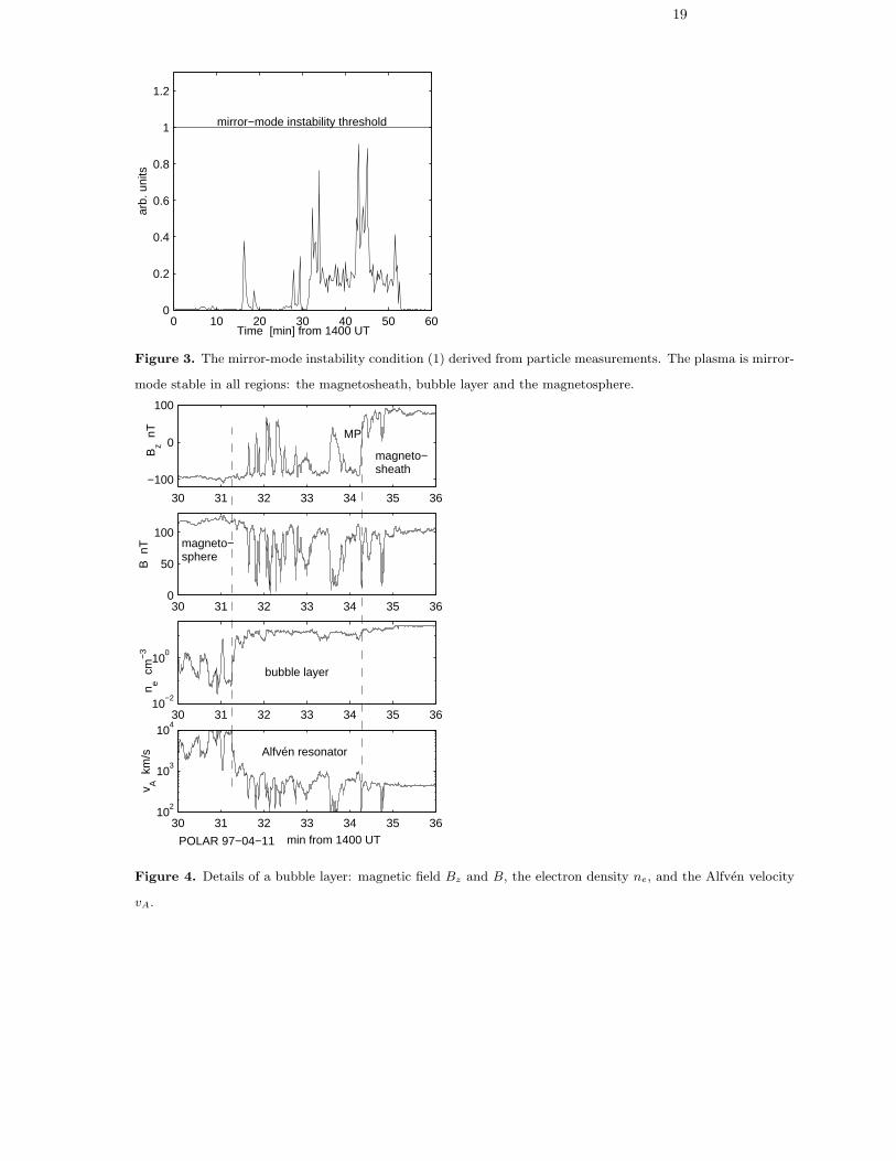
The particle moments show that in the bubble layer the parallel ion and electron pressure exceeds

the perpendicular components. This indicates that the condition for the mirror instability [Southwood

and Kivelsen, 1993]T⊥/T‖1 + β−1

⊥> 1 (1)

is not fulfilled. In Figure 3 we show the plot of the mirror instability condition (1) derived from particle

measurements. The plasma is found to be mirror-mode stable in all regions. In Table I we show Fig.3

characteristic plasma parameters in the three main regions of Figure 1: the magnetosheath, bubble

layer, and the magnetosphere. Tab I

We now focus on the first bubble layer from Figure 1 which we show in Figure 4. The picture

shows that the strong depressions of the magnetic field B are associated with some density variations

(on logarithmic scale they do not show very well, see Figure 5 for details), but the very strong density

gradient at 1431:15 (first vertical line) is not related to appreciable magnetic perturbations. This density

gradient separates obviously the inner magnetosphere from the magnetopause boundary (bubble) layer.

On the other hand the magnetic signatures of the magnetopause seen as reversals of Bz at 1434:10

(second vertical line) is not associated with strong density variation. It is, however, associated with

strong particle heating leading to a large decrease of total B. In the bottom panel we show the Alfven

velocity Fig 4

vA =B0

(µ0ρ)1/2, (2)

where ρ = nimi is the ion mass density. The ion species is assumed to be hydrogen, and the number

density is derived from the “satellite potential“ measured by the electric field experiment. We have

used an empirical formula derived by [Escoubet et al., 1997], calibrated here with the moments of the

particle distributions measured by the HYDRA instrument.

Magnetic bubbles and KAWs

The nature of the observed magnetic bubbles is revealed if we inspect higher resolution plot of

two orthogonal components of the magnetic and electric fields shown in Figure 5. High degree of

6

correlation between Bz and Ey components is characteristic for Alfven waves. Indeed, for amplitudes

δE ≈ 30 mV/m and δB ≈ 150 nT, the ratio δE/δB ≈ 200 km/s, which is close to the value for Alfven

velocity vA inside the bubble layer. The bottom panel shows the electron density derived from the

satellite potential (solid line) with superimposed values obtained as moments from the electron and ion

measurements (asterisks). One can see good agreement between these two techniques. Fig 5

Let us recall basic properties of Alfven waves. The original low frequency MHD wave [Alfven,

1942] is dispersionless

ω = kzvA, (3)

where kz is the wave vector parallel to the ambient magnetic field. Significant modifications are

introduced when the wavelength perpendicular to the background magnetic field becomes comparable

either to the ion gyroradius at electron temperature, ρs = (Te/mi)1/2/ωci, the ion thermal gyroradius,

ρi = (Ti/mi)1/2/ωci [Hasegawa, 1976], or to the collisionless electron skin depth λe = c/ωpe [Goertz

and Boswell, 1979], where ωci is ion cyclotron frequency and ωpe is electron plasma frequency.

Recent review by [Stasiewicz et al., 2000a] provides a comprehensive discussion on dispersive Alfven

waves in the ionospheric and in laboratory plasmas. In standard terminology, the Inertial Alfven Waves

(IAW) are ω < ωci Alfven waves in a medium where the electron thermal velocity, vte = (2Te/me)1/2,

is less than vA. In such a case, the parallel electric field is supported by the electron inertia. Kinetic

Alfven Waves (KAW) are waves in a medium where vte > vA. In this case, the parallel electric force is

balanced by the parallel electron pressure gradient. The term Dispersive Alfven Waves (DAW) would

cover these two cases. Clearly, the IAW arises in a low-beta plasma with β = 2µ0nT/B20 < me/mi,

whereas the KAW appear in an intermediate beta plasma with me/mi < β < 1. Here, T = (Te + Ti)/2

is the plasma temperature. The low-beta conditions and IAW occur in the topside ionosphere below

approximately 1 RE , whereas at higher altitudes the Alfven waves have kinetic properties (KAW).

For ω < ωci kinetic Alfven waves, the well know dispersion equation reads

ω = kzvA

√1 + k2

⊥(ρ2s + ρ2

i ), (4)

whereas the E/B ratio for plane, obliquely propagating waves can be expressed as [Stasiewicz et al.,

2000a] ∣∣∣∣ δEy

δBx

∣∣∣∣ = vA(1 + k2⊥ρ

2i )

[1 + k2⊥(ρ2

s + ρ2i )]1/2

≈ vA

√1 + k2

⊥ρ2i . (5)

In the above approximation we have used the experimental condition Ti/Te ≈ 8 which implies ρi ρs.

An analysis of the E/B ratio performed for IAW measured by Freja at lower altitudes [Stasiewicz

et al., 2000b] has demonstrated that broadband ELF waves (BB-ELF) observed in the frequency range

7

0-500 Hz represent in fact spatial turbulence of dispersive Alfven waves. Simply, waves ω ωci with a

spectrum of spatial scales ∆k (such that k = 2π/λ) are recorded on a moving spacecraft as waves in

the frequency domain

∆ωd = v ·∆k, (6)

where v is velocity of the plasma structure with respect to the satellite. Distinction between true

time-domain waves ∆ω and Doppler shifted spatial waves ∆k can be done directly with multiple probe

measurements, or indirectly with the help of the dispersion relation (5) as has been done by [Stasiewicz

et al., 2000b] for waves measured by Freja. The dispersion relation for IAW is similar to (5) with

collisionless electron skin depth λe instead of ion gyroradius ρi. Additional difference between the Freja

and POLAR cases is that the convective flows at Freja altitudes (∼1500 km) are much smaller than

the satellite velocity so v ≈ vs ≈ 7 km/s in equation (6). On the other hand at POLAR apogee, the

satellite speed vs ≈ 3 km/s is much smaller than convective flows, and v ≈ vE ≈ 100 km/s. DAW

spectrum ∆k described by equation (5) should be observed on a spacecraft as a frequency spectrum

∣∣∣∣ δEy

δBx

∣∣∣∣ ≈ 〈vA〉√1 +

⟨2πρi

v cos θ

⟩2

f2, (7)

where f(= k · v/2π) is an apparent Doppler frequency in the satellite frame, θ is the angle between the

k-vector and the velocity v, and brackets 〈〉 represent a spatial average. Fig 6

In Figure 6 we show average power spectrum of the electric field fluctuations measured in the

frequency range 0-104 Hz and the ratio δE/δB as a function of frequency. To make these plots we took

continuous dc field and snapshot measurements at higher frequencies within the bubble layers marked

in Figure 1. The frequency spectrum is covered by three instruments. The dc magnetic field is sampled

continuously at the rate 8.3 s−1, the low-frequency waveform receiver (LFWR) and high-frequency

waveform receiver (HFWR) provide snapshots sampled at the rate 100 s−1, and 50,000 s−1, respectively.

The plots of dc and LFWR channels overlap completely indicating good inter-calibration. However,

because of the wave instrument filter characteristics the plots in Figure 6 at the transition frequency of

∼ 50 Hz between LFWR and HFWR are not reliable. Anyway, the power spectrum and the waveforms

show that the dominant mode represent broadband ELF waves 0-30 Hz with a significant power drop

above ∼30 Hz, which is near the lower hybrid range.

The asterisk curve shows equation (7) computed for vA = 150 km/s and ρi/v = 0.4 s, which is

satisfied for e.g. ρi = 60 km and v = 150 km/s, 〈cos θ〉 ∼ 1. A good agreement between approximation

(7) and the measurements provides indirect evidence that in the frequency range 0-30 Hz the waves

represent spatial turbulence of DAW. Transition from equation (5) to (7) requires knowledge of the

8

angle between the convection velocity vE and the wavevector k. Because both these vectors are

expected to vary significantly in time (space) we use here statistical average of spectra which would

result in an average value for 〈cos θ〉 and other parameters in equation (7).

Translation from frequency to spatial scale λ = v/f requires the knowledge of the convective

velocity v. For v ≈100 km/s, the frequency of 1 Hz corresponds to λ =100 km which is on the order

of ion gyroradius, while 100 Hz corresponds to λ ≈ 1 km, which is about the electron inertial length.

It appears from Figure 6 that for scales larger than ρi waves have δE/δB ≈ vA, while the dispersive

KAW spectrum (7) extends from ρi down to λe. Above 30 Hz, or close to the inertial electron scale,

dissipative processes related presumably to electron acceleration lead to the dropout of the electric field

power seen in Figure 6. The bubble structures correspond roughly to ∼ 0.2 Hz. It is interesting to note

that the ordering of scales ρi and λe is reversed at low altitudes and DAW waves measured on Freja

extends from λe ∼ 300 m down to ρi ∼ 20 m, where they are strongly dissipated due to stochastic

acceleration of ions [Stasiewicz et al., 2000b; Stasiewicz et al., 2000c].

Theory and simulation

The discussion on linear spectra for KAW in the previous section could not address the origin

of the observed large amplitude structures. Since the kinetic Alfven wave carry a parallel and

perpendicular electric field they can accelerate ions and electrons along as well as perpendicular to the

magnetic field. The nonlinear interaction with quasi-stationary density and compressional magnetic

field perturbations can gives rise to modulational instability. Even the linear small amplitude DAW

become compressional for sufficiently large k⊥. Indeed, the density fluctuations depend on the k⊥λi,

where λi = vA/ωci = c/ωpi is the inertial ion length, as [Hollweg, 1999]

δni

n0= k⊥λi

vE

vA. (8)

The above result applies both to KAW and IAW and shows that the Alfven wave becomes compressible

when perpendicular size of the structures becomes comparable to the inertial ion length. In our case, it

is seen from Table I that the wave induced convective flows are comparable to the Alfven velocity and

the density perturbations implied by (8) may be quite large, as seen in Figure 5.

The density fluctuations imply pressure fluctuations that drive a magnetization current, which

in turn produces a compressive magnetic field δBz. In the linear approximation the density and

compressional magnetic field fluctuations are related as [Hollweg, 1999]

δBz/B0

δni/n0= − c2s

v2A

, (9)

9

where cs is the ion sound speed. The observed values for cs can be obtained from Table I as

vs = vi

√Te/Ti, i.e., they are 2-3 times smaller than vi.

The parallel electric field of KAW will affect particles which are in Landau resonance with the wave

kzvz = ω. (10)

Table I shows that both ion thermal and bulk flow is on the order of the Alfven speed. Thus, one

expects efficient ion heating via Landau resonance which can account for ion energization seen in Figure

2.

The linear theory has a limited application to the strongly nonlinear structures seen in the

measurements. We present here results from the solution of the resistive Hall MHD equations which are

intended to model a tearing mode reconnection process leading to magnetic bubble or island formation

which are associated with kinetic Alfven wave fluctuations. We present the general resistive Hall MHD

equations then specialize to the two-dimensional geometry that we use in the simulations. The Hall

instability which is related to drift Alfven waves is discussed in the context of the two-dimensional

model for which it is shown that instability exists at scales smaller than the tearing mode scale. A

sample simulation of high spatial resolution is presented which exhibits the formation of magnetic

islands through the tearing mode and kinetic Alfven wave fluctuations through the Hall instability.

Hall MHD Model

The Hall MHD equations are:

∂tn+∇ · (nu) = 0 (11)

(∂t + u · ∇)u = −1ρ∇p+

1µ0ρ

(∇×B)×B (12)

(∂t + u · ∇) p+ γp∇ · u = 0 (13)

∂tB = −∇×E (14)

E+ u×B =1

µ0ne(∇×B)×B+ ηJ (15)

∇×B = µ0J (16)

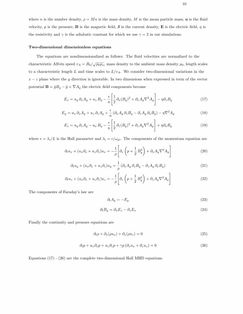
10

where n is the number density, ρ = Mn is the mass density, M is the mean particle mass, u is the fluid

velocity, p is the pressure, B is the magnetic field, J is the current density, E is the electric field, η is

the resistivity and γ is the adiabatic constant for which we use γ = 2 in our simulations.

Two-dimensional dimensionless equations

The equations are nondimensionalized as follows: The fluid velocities are normalized to the

characteristic Alfven speed vA = B0/√ρ0µo, mass density to the ambient mass density ρ0, length scales

to a characteristic length L and time scales to L/vA. We consider two-dimensional variations in the

x− z plane where the y direction is ignorable. In two dimensions when expressed in term of the vector

potential B = yBy − y ×∇Ay the electric field components become

Ex = uy ∂xAy + uz By − ε

n

[12∂x(By)2 + ∂xAy∇2Ay

]− η∂zBy (17)

Ey = ux ∂xAy + uz ∂zAy +ε

n(∂xAy ∂zBy − ∂zAy ∂xBy)− η∇2Ay (18)

Ez = uy ∂zAy − ux By − ε

n

[12∂z(By)2 + ∂zAy∇2Ay

]+ η∂xBy (19)

where ε = λi/L is the Hall parameter and λi = c/ωpi. The components of the momentum equation are

∂tux + (ux∂x + uz∂z)ux = −1ρ

[∂x

(p+

12B2

y

)+ ∂xAy∇2Ay

](20)

∂tuy + (ux∂x + uz∂z)uy =1ρ(∂xAy ∂zBy − ∂zAy ∂xBy) (21)

∂tuz + (ux∂x + uz∂z)uz = −1ρ

[∂z

(p+

12B2

y

)+ ∂zAy∇2Ay

](22)

The components of Faraday’s law are

∂tAy = −Ey (23)

∂tBy = ∂xEz − ∂zEx (24)

Finally the continuity and pressure equations are

∂tρ+ ∂x(ρux) + ∂z(ρuz) = 0 (25)

∂tp+ ux∂xp+ uz∂zp+ γp (∂xux + ∂zuz) = 0 (26)

Equations (17) - (26) are the complete two-dimensional Hall MHD equations.

11

Hall instability

The Hall equations can exhibit instability in the presence of equilibrium electric field created by

equilibrium pressure and magnetic field gradients. We perform a local analysis of (17) - (26) assuming

perturbations of the form exp[ikzz − iωt]. After considerable algebra we find

(ω2 − k2zv

2A)(ω − kzvE) + ω(ω2 − k2

zc2s)kzλ

2i = 0 (27)

where vE = E0xB0y/B20 and c2s = γp0/ρ0. Equation (27) has unstable roots for vE > cs and within a

band limited range of wavenumbers. When vE = 0 the dispersion relation becomes

ω2 =k2

zv2A(1 + k2

zρ2s)

1 + k2zλ

2i

(28)

where ρs = cs/Ωi. Equation (28) is the dispersion relation for Alfven-ion cyclotron waves. For kzλi 1

it reduces to pure kinetic Alfven waves. The local approximation does not allow us to consider kx = 0

since the equilibrium varies in the x direction although the simulation does of course allow nonzero

kx. For the homogeneous case we can allow kx = 0 and we find for kzλi 1, the dispersion relation

ω2 = k2zv

2A(1 + k2ρ2

s), where k2 = k2x + k2

z , which is more typically considered to be the kinetic

Alfven wave dispersion relation. For vE > cs there is a band of wavenumbers that are unstable. This

instability has been discussed in the context of cold laboratory plasma by Gordeev et. al [1994] and

warm laboratory plasma by Maggs and Morales [1996]. The instability given by (27) is due to the

interaction between the drift mode ω = kzvE and the Alfven-ion cyclotron mode given in (28). The

acoustic speed is stabilizing and the threshold condition is vE > cs. A local analysis can be misleading

in a sheared magnetic field such as we consider here. This is because the shear limits the x extent of the

mode thereby significantly altering the stability properties. A nonlocal analysis is required to obtain

quantitative estimates of the growth rate. That analysis is beyond the scope of the present paper and

will be deferred to a future publication.

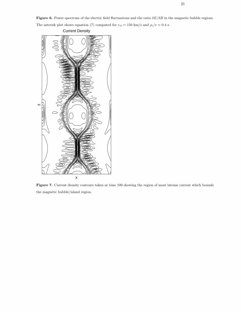
Simulation results

We present the results of one simulation to show the magnetic bubble structure and the fluctuations

associated with the Hall instability. The simulation is not intended to reproduce the observations in

any detail but only to show that with reasonable initial conditions spontaneous reconnection in the

form of a tearing mode will result and that instability associated with the large gradients of the bubble

boundary will arise from the Hall instability. This should be considered in comparing the simulation

12

results to the data.

The simulation code is based upon the Fourier spectral method and is similar to that described

in Seyler [1990]. The equations are solved in dimensionless form with the following non-dimensional

tilded variables: t = tL/vA, x = x/L, u = u/vA, B = B/B0, P = P/P0, and ρ = ρ/ρ0, where L is the

characteristic scale of the equilibrium. From these one can revert from simulation to physical units.

The simulation dimensions are −π < x ≤ π and −2π < z ≤ 2π. The Hall parameter is ε = 0.026.

The number of grid points used are 128 in x and 256 in z. The time step is ∆t = 0.0025. The initial

equilibrium is of the form Jy(x) = J0 sech(−ax2), where J0 = 8 and a = 4π. The dimensionless

resistivity is η = 0.002. The dimensionless current layer width a was chosen to produce an tearing

mode unstable current layer that grows to form fully developed bubbles in a time comparable to the

Hall instability growth time. Fig 7

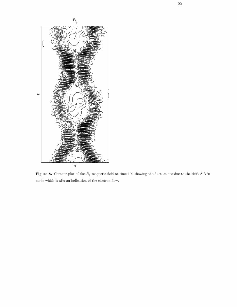
The current density is shown in Figure 7. The magnetic bubbles are the two magnetic islands

formed by the tearing mode. The kinetic Alfven wave fluctuations are readily apparent. The contour

plot of By(x, z) is shown in Figure 8. This plot clearly shows the vortices associated with the flow

due to the Hall instability. The fluctuations due to the Hall instability are concentrated on the

bubble boundaries since that is where the magnetic field gradient is largest. Figures 1 and 4 also

show that magnetic fluctuations are enhanced near the bubble boundaries. This is consistent with the

interpretation that the fluctuations are the result of the Hall instability which is driven by the magnetic

gradient. Fig 8

The plots shown in Figures 9 and 10 are taken along z at 4 grid points to the right of the centerline

of the simulation region. They show the relative level of variation of the magnetic field, pressure and

density. Fig 9

Figure 9 shows the magnetic bubble from the perspective of a one-point satellite measurement and

can be compared to Figure 4 (of the observational section). The best comparison is obtained when the

simulation Bx is compared to the observed By and when the simulation z coordinate has a significant

component in the data x direction. Given the POLAR GSM coordinates, (x, y, z) = (2.8, 1.5, 8.0)RE ,

this correspondence is reasonable, since the simulation uses coordinates appropriate to the magnetopause

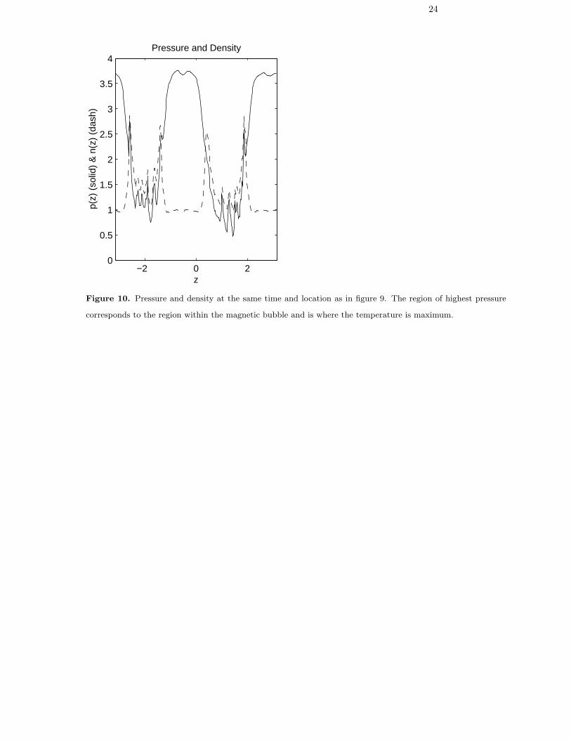
located approximately at (x, y, z) = (10, 0, 0)RE . Fig 10

Figure 10 shows that the region inside the magnetic bubble or island is significantly hotter than

the outside region. This is due to the fact that the initial pressure at x = 0 must be larger to create

pressure balance with the equilibrium magnetic field. Since we chose the initial density to be constant,

this implies the temperature is hottest initially at x = 0. The evolution of the pressure is such that

13

the temperature is hottest in the center of the magnetic island. This is not surprising since the tearing

mode evolves quasi-statically in that the growth time is much less that the Alfven time. Therefore

quasi-static pressure balance requires that the pressure has a maximum where the magnetic field

magnitude is a minimum. Thus the increase of the plasma pressure is due to the compensation the

magnetic field depression, so that the total pressure is approximately constant.

The tearing mode instability has been discussed by numerous authors the list of which is too

extensive to give here. Much of the relevant literature is referenced in the review article by [White,

1986]. The tearing mode is spontaneous reconnection that lowers the magnetic energy of the initial

equilibrium state. The formation of magnetic islands is characteristic of the tearing mode. A magnetic

island is a region of closed contours of the vector potential which typically has a lower field at the

center of the island. Magnetic islands form as the result of the reconnection flow in which the plasma is

advected towards the separatrix by the inflow and exhausted into the region inside the separatrix by

the outflow jets thereby filling the region inside the separatrix with plasma and forming a magnetic

bubble. The magnetic energy is lowered and converted into kinetic energy in this process. The amount

the initial magnetic energy is lowered depends considerably upon the plasma parameters and the initial

conditions, but about 10% is typical [Steinholfson and Van Hoven, 1984]. The redistribution of the

magnetic energy density can vary greatly between the outside and inside regions of the island. The

POLAR observation of more than 90% is not unreasonable and is close to what was found in the

simulation.

Discussion and Conclusions

A detailed analysis of electromagnetic and plasma properties of magnetic holes observed in the

vicinity of the magnetopause layer supplemented by a numerical simulation show that these are most

likely related to tearing mode instability which develops strongly nonlinear structures on the scale of

the current layer width.

We have demonstrated that the δE/δB ratio for large scale features is close to the Alfven velocity,

indicating that these can be regarded as nonlinear Alfven wave structures. For smaller scale structures

this ratio gradually increases and it is well represented by the dispersion relation for KAWs (see Figure

6). Thus, the measurements suggest that broadband waves observed at the magnetopause layer in the

frequency range 0.1-30 Hz represent most likely spatial turbulence of nonlinear and dispersive Alfven

waves (λ⊥ ≈ 1500 − 5 km and ω 1 Hz), which are Doppler shifted to the observed frequencies by

convective plasma flows vE ∼ 150 km/s.

14

The numerical simulation indicates that the small scale KAW may be generated through the Hall

instability on the macroscopic pressure and magnetic field gradients produced by the tearing mode

driven by strong magnetopause currents. The presented particle measurements indicate that both

ions and electron are energized to about twice their initial energy inside the magnetopause bubble

layer. The particle energization could be related to kinetic Alfven waves which cover the spatial scales

ranging from λi, ρi down to λe and thus can interact and energize both with ions and electrons. The

magnetic fluctuation are likely due to a drift-Alfven type instability. We have only presented a limited

analysis and more work is necessary to have complete understanding of the fluctuations. The simulation

model is limited to two-dimensions. This in itself restricts the possible types of instabilities. Since the

current due to reconnection is in the ignorable direction of the simulation, these instabilities would not

accounted for in the model. To include these would require a three dimensional model. The solution of

a three-dimensional model at the required resolution is beyond our capabilities at this point in time. A

linear stability analysis, however is tractable and will be reported upon in a future paper.

The processes discussed in this paper involve transformations of considerable amount of energy

between the magnetic, electric fields and particles (thermal and translational). For example we observe

a reduction of 98% of the magnetic energy inside some bubbles. Consequently, full understanding of

the processes discussed in this paper is of fundamental importance for the energetics of the solar wind -

magnetosphere coupling.

Acknowledgments. The authors would like to thank C. Kletzing for providing the HYDRA data and

principal investigators: D. Gurnett, C. T. Russell and J. Scudder for making available the field and plasma

measurements. Work of F.S. Mozer was partly supported by NASA grant FDNAG5-8078 and B.Popielawska

was supported by KBN grant 2.P03C.004.13.

15

References

Alfven, H., Existence of electromagnetic-hydromagnetic waves, Nature, 150, 405–406, 1942.

Baumgartel, K., Soliton approach to magnetic holes, J. Geophys. Res., 104, 28295, 1999.

Erdos, G., and A. Balogh, Statistical properties of mirror mode structures observed by Ulysses in the

magnetosheath of Jupiter, J. Geophys. Res., 101, 1–12, 1996.

Escoubet, C. P., A. Pedersen, R. Schmidt, and P. A. Lindqvist, Density in the magnetosphere inferred from

ISEE 1 spacecraft potential, J. Geophys. Res., 102, 17,595, 1997.

Fuselier, S. A., K. J. Trattner, and S. M. Petrinec, Cusp observations of high- and low-latitude reconnection for

northward IMF, J. Geophys. Res., 105, 253-266, 2000.

Goertz, C. K., and R. W. Boswell, Magnetosphere-ionosphere coupling, J. Geophys. Res., 84, 7239–7246, 1979.

Gordeev, A. V., A. S. Kinsep, and L. I. Rudakov, Electron magnetohydrodynamics, Phys. Rep., 243, 215–315,

1994.

Hasegawa, A., Particle acceleration by MHD surface wave and formation of aurora, J. Geophys. Res., 81,

5083–5090, 1976.

Hollweg, J. V., Kinetic Alfven wave revisited, J. Geophys. Res., 104, 14,811, 1999.

Kaufmann, R., J. T. Horng, and A. Wolfe, Large amplitude hydromagnetic waves in the inner magnetosheath,

J. Geophys. Res., 75, 4666, 1970.

Le, G., J. Raeder, C. T. Russell, G. Lu, S. M. Petrinec, and F. S. Mozer, Polar cusp and vicinity under strongly

northward IMF on April 11, 1997: Observations and MHD simulations, J. Geophys. Res., xx, in press,

2000.

Luhr, H., and N. Klocker, AMPTE IRM observations of magnetic cavities near the magnetopause, Geophys.

Res. Lett., 14, 186, 1987.

Maggs, J. E., and G. J. Morales, Magnetic fluctuations associated with field-aligned striations, Geophys. Res.

Lett., 23, 633, 1996.

Russell, C. T., G. Le, and S. M. Petrinec, Cusp observations of high- and low-latitude reconnection for

northward IMF: An alternate view, J. Geophys. Res., 105, 5489-5495, 2000.

Savin, S. P., et al., The cusp/magnetosheath interface on May 29, 1996: Interball-1 and Polar observations,

Geophys. Res. Lett., 25, 2963, 1998.

Seyler, C. E., A mathematical model of the structure and evolution of small-scale discrete auroral arcs, J.

Geophys. Res., 95, 17199, 1990.

Southwood, D. J., and M. G. Kivelsen, Mirror instability 1, the physical mechanism of linear instability, J.

Geophys. Res., 98, 9181, 1993.

Stasiewicz, K., P. Bellan, C. Chaston, C. Kletzing, R. Lysak, J. Maggs, O. Pokhotelov, C. Seyler, P. Shukla,

16

L. Stenflo, A. Streltsov, and J.-E. Wahlund, Small scale Alfvenic structure in the aurora, Space Sci.

Rev., 92, 423-533, 2000a.

Stasiewicz, K., Y. Khotyaintsev, M. Berthomier, and J.-E. Wahlund, Identification of widespread turbulence of

dispersive Alfven waves, Geophys. Res. Lett., 27, 173, 2000b.

Stasiewicz, K., R. Lundin, and G. Marklund, Stochastic ion heating by orbit chaotization on electrostatic waves

and nonlinear structures, Phys. Scripta, T84, 60, 2000c.

Steinholfson R. S. and G. V. Van Hoven, Nonlinear Evolution of the Resistive Tearing Mode, Phys. Fluids, 27,

1207, 1984.

Treumann, R., L. Brostrom, J. LaBelle, and N. Scopke, The plasma waave signature of a magnetic hole in the

vicinity of the magnetopause, J. Geophys. Res., 95, 19,099, 1990.

Tsurutani, B. T., E. J. Smith, R. R. Anderson, K. W. Ogilvie, J. D. Scudder, D. N. Baker, and S. J. Bame,

Lion roars and nonoscillatory drift mirror waves in the magnetosheath, J. Geophys. Res., 87, 6060, 1982.

Tsurutani, B. T., J. Arballo, E. J. Smith, D. Southwood, and A. Balogh, Large amplitude magnetic pulses

downstream of the jovian bow shock, Planet. Space Sci., 41, 851, 1993.

Tsurutani, B. T., G. S. Lakhina, D. Winterhalter, J. Arballo, G. Galvan, and R. Sukurai, Energetic particle

cross-field diffusion: Interactions with magnetic decreases, Nonlinear Proc. in Geophys., 6, 235, 1999.

Turner, J. M., L. F. Burlaga, N. F. Ness, and J. F. Lemaire, Magnetic holes in the solar wind, J. Geophys.

Res., 82, 1921, 1977.

White, R. B., Resistive Reconnection, Rev. Mod. Phys., 58, 183, 1986.

Winterhalter, D., M. Neugebauer, B. E. Goldstein, E. J. Smith, S. J. Bame, and A. Balogh, Ulysses field and

plasma observations of magnetic holes in the solar wind and their relation to mirror-mode structures, J.

Geophys. Res., 99, 23,371, 1994.

Received

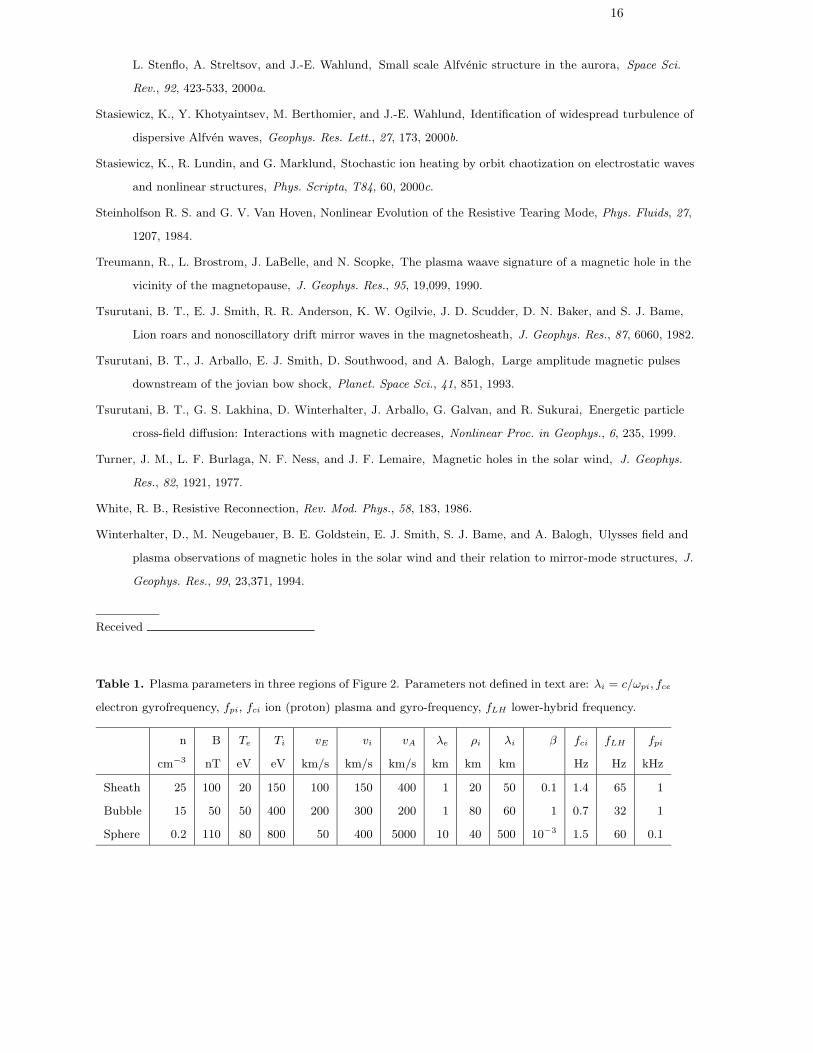
Table 1. Plasma parameters in three regions of Figure 2. Parameters not defined in text are: λi = c/ωpi, fce

electron gyrofrequency, fpi, fci ion (proton) plasma and gyro-frequency, fLH lower-hybrid frequency.

n B Te Ti vE vi vA λe ρi λi β fci fLH fpi

cm−3 nT eV eV km/s km/s km/s km km km Hz Hz kHz

Sheath 25 100 20 150 100 150 400 1 20 50 0.1 1.4 65 1

Bubble 15 50 50 400 200 300 200 1 80 60 1 0.7 32 1

Sphere 0.2 110 80 800 50 400 5000 10 40 500 10−3 1.5 60 0.1

17

0 10 20 30 40 50 60

−50

0

50

Bx

nT

0 10 20 30 40 50 60−80

−40

0

40B

y n

T

0 10 20 30 40 50 60−100

0

100

Bz

nT

0 10 20 30 40 50 600

50

100

150

B n

T

0 10 20 30 40 50 600

100

200

300

VE k

m/s

MS MS

POLAR 97−04−11 Time [min] from 1400 UT

Figure 1. Magnetopause crossings on 11 April 1997. Three component magnetic field Bx, By, Bz in GSM

coordinates, |B| and the convection speed vE .

Figure 2. Particle distributions measured during the analyzed event. Three electron and three ion panels show

particle fluxes along the magnetic field, perpendicular, and antiparallel to B. The magnetosheath and bubble

layers are marked with MS and B, respectively.

19

0 10 20 30 40 50 600

0.2

0.4

0.6

0.8

1

1.2

Time [min] from 1400 UT

arb.

uni

ts

mirror−mode instability threshold

Figure 3. The mirror-mode instability condition (1) derived from particle measurements. The plasma is mirror-

mode stable in all regions: the magnetosheath, bubble layer and the magnetosphere.

30 31 32 33 34 35 36

−100

0

100

Bz n

T

30 31 32 33 34 35 360

50

100

B n

T

30 31 32 33 34 35 3610

−2

100

n e cm

−3

30 31 32 33 34 35 3610

2

103

104

v A k

m/s

magneto−sphere

bubble layer

magneto−sheath

MP

Alfvén resonator

POLAR 97−04−11 min from 1400 UT

Figure 4. Details of a bubble layer: magnetic field Bz and B, the electron density ne, and the Alfven velocity

vA.

20

31.5 32 32.5 33−100

−50

0

50

Bz

nT

31.5 32 32.5 33−20

0

20

Ey

mV

/m

31.5 32 32.5 330

50

100

B n

T

31.5 32 32.5 330

5

10

15

ne c

m−

3

POLAR 97−04−11 [min] from 1400 UT

Figure 5. High degree of correlation between perpendicular components of Bz and Ey with δEy/δBz ≈ 200

km/s ≈ vA indicates Alfvenic structures. The bottom panel shows the electron density derived from the satellite

potential (solid line) and from particle measurements (asterisk)

10−2

100

102

104

10−5

100

POLAR 97−04−11 (1430−1453)

PE

(m

V/m

)2 /Hz

10−2

100

102

104

102

104

106

δ E

/δ B

km

/s

Frequency Hz

fce

100 1 km

ρi λ

e

bubbles

21

Figure 6. Power spectrum of the electric field fluctuations and the ratio δE/δB in the magnetic bubble regions.

The asterisk plot shows equation (7) computed for vA = 150 km/s and ρi/v = 0.4 s.

Current Density

x

z

Figure 7. Current density contours taken at time 100 showing the region of most intense current which bounds

the magnetic bubble/island region.

22

By

x

z

Figure 8. Contour plot of the By magnetic field at time 100 showing the fluctuations due to the drift-Alfven

mode which is also an indication of the electron flow.

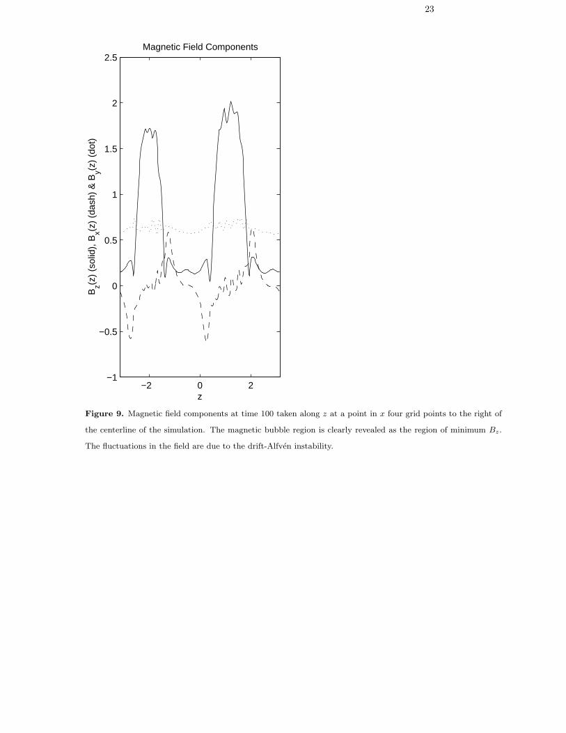
23

−2 0 2−1

−0.5

0

0.5

1

1.5

2

2.5

z

Bz(z

) (s

olid

), B

x(z)

(das

h) &

By(z

) (d

ot)

Magnetic Field Components

Figure 9. Magnetic field components at time 100 taken along z at a point in x four grid points to the right of

the centerline of the simulation. The magnetic bubble region is clearly revealed as the region of minimum Bz.

The fluctuations in the field are due to the drift-Alfven instability.

24

−2 0 20

0.5

1

1.5

2

2.5

3

3.5

4

z

p(z)

(so

lid)

& n

(z)

(das

h)

Pressure and Density

Figure 10. Pressure and density at the same time and location as in figure 9. The region of highest pressure

corresponds to the region within the magnetic bubble and is where the temperature is maximum.