UNCORRECTED PROOF

CNM 954pp: 1–16 (col.fig.: Nil)

PROD. TYPE: COMED: Senthil

PAGN: PR -- SCAN: NitShree

COMMUNICATIONS IN NUMERICAL METHODS IN ENGINEERINGCommun. Numer. Meth. Engng (in press)

Published online in Wiley InterScience (www.interscience.wiley.com). DOI: 10.1002/cnm.954

1

Extension of weakly compressible approximationsto incompressible thermal flows3

Mofdi El-Amrani1,∗,† and Mohammed Seaıd2

1Departamento Matematicas ESCET, Universitat Rey Juan Carlos, C/Tulipan, s/n, Mostoles-Madrid 28933, Spain52AG Technomathematik, FB Mathematik, Universitat Kaiserslautern, Kaiserslautern 67663, Germany

SUMMARY7

Weakly compressible and advection approximations of incompressible isothermal flows were developedand tested in (Commun. Numer. Methods Eng. 2006; 22:831–847). In this paper, we extend the method to9solve equations governing incompressible thermal flows. The emphasis is again on the reconstruction ofunconditionally stable numerical scheme such that, restriction on time steps, projection procedures, solution11of linear system of algebraic equations and staggered grids are completely avoided in its implementation.These features are achieved by combining a low-Mach asymptotic in compressible flow equations with13a semi-Lagrangian method for the weakly compressible approach. The time integration is carried outusing an explicit Runge–Kutta with variable stages. The method is applied to the natural convection flows15in a squared cavity for both steady and transient computations. The numerical results demonstrate highresolution of the proposed method and confirm its capability to provide accurate and efficient simulations17for thermal flow problems. Copyright q 2006 John Wiley & Sons, Ltd.

Received 12 May 2006; Revised 15 September 2006; Accepted 29 September 2006

KEY WORDS: weakly compressible flows; low-Mach asymptotic; semi-Lagrangian method; incom-19pressible Navier–Stokes equations; natural convection

21

1. INTRODUCTION

Many thermal incompressible flows use the incompressible Navier–Stokes/Boussinesq equations in23

their mathematical modelling. For flow problems in two space dimensions, the governing equations

can be formulated in dimensionless form as25

∇ ·u = 0 (1a)

∗Correspondence to: Mofdi El-Amrani, Departamento Matematicas ESCET, Universitat Rey Juan Carlos, C/Tulipan,s/n, Mostoles-Madrid 28933, Spain.

†E-mail: mofdi.elamrani@urjc.es

Copyright q 2006 John Wiley & Sons, Ltd.

UNCORRECTED PROOF

2

CNM 954

M. EL-AMRANI AND M. SEAID

�u

�t+ u · ∇u + ∇ p −

1

Re∇2u=

Gr

Re2�j (1b)

��

�t+ u · ∇� −

1

Pr Re∇2

� = 0 (1c)

where u= (u, v)T is the velocity field, p the pressure, � the temperature, Pr the Prandlt number,1

Gr the Grashof number, and j the unit vector in direction of gravity. The Rayleigh number Ra,

which is a parameter of interest, is the product of Pr and Gr. Equations (1) have to be solved in an3

open bounded domain � ⊂ R2 with smooth boundary � and a time interval [0, T ]. We assume that

appropriate initial and boundary conditions are given in such a way the problem is well defined5

and has a unique solution.

Most of the numerical methods for solving (1) suffer from two major computational prob-7

lems namely, the velocity–pressure coupling and the zero divergence restriction. Furthermore,

when convection dominates, spurious spatial oscillations may occur if standard Eulerian-based9

discretizations are used. These numerical difficulties have been treated by combining a low-Mach

number asymptotically in compressible flows with a semi-Lagrangian discretization for advection.11

The low-Mach analysis replaces Equations (1) by a weakly compressible flow problem which,

for small Mach numbers, asymptotically approximates the solution of (1). This approach does not13

need staggered grids and avoids Poisson or Stokes solvers for its numerical solution. On the other

hand, the semi-Lagrangian procedure is not limited by a stability-based CFL condition. This is15

due to the fact that each gridpoint is treated in Lagrangian manner. Since high-order difference

schemes have the potential to reduce numerical diffusion, the spatial discretization is performed17

using a fourth-order centred scheme.

The time integration is carried out using the modified Runge–Kutta Chebyshev method imple-19

mented in [1] for the weakly compressible approximation of the incompressible Navier–Stokes

equations for isothermal flows. The idea of this scheme is to stabilize the Runge–Kutta method21

by using extended number of stages in its formulation. The proposed method is efficient, easy

to implement and uniformly accurate such that the selection of time steps in the computational23

process is independent of the Mach number and is based only on the required numerical accuracy.

We demonstrate these claims by presenting results on two benchmarks for steady and transient25

natural convection problems.

This work is an extension of Reference [1] to incompressible thermal flows. Therefore, the dif-27

ferent formulations will be simply described and then the numerical results presented. In Section 2,

we formulate the weakly compressible approximation of incompressible thermal flows. A brief29

description of the solution procedure is presented in Section 3. Section 4 is devoted to numerical

results for natural convection flows. Conclusions are drawn in Section 5.31

2. WEAKLY COMPRESSIBLE MODEL FOR INCOMPRESSIBLE THERMAL FLOWS

Following the same formalism as in [1], the weakly compressible problem we consider in this33

paper to approximate Equations (1) reads

�p

�t+ u · ∇ p + p∇ ·u = 0 (2a)35

Copyright q 2006 John Wiley & Sons, Ltd. Commun. Numer. Meth. Engng (in press)

DOI: 10.1002/cnm

UNCORRECTED PROOF

CNM 954

EXTENSION OF WEAKLY COMPRESSIBLE APPROXIMATIONS 3

�u

�t+ u · ∇u +

1

M2∇ p −

1

Re∇2u=

Gr

Re2�j (2b)

��

�t+ u · ∇� −

1

Pr Re∇2

� = 0 (2c)

where M is the Mach number, namely the ratio of a characteristic velocity in the flow with the1

sound speed in the fluid. Integrating (1a) over the space domain, we obtain the incompressibility

condition as follows:3

∮

�

u ·n ds = 0 (3)

where n denotes the unit outward normal vector on boundary �. This condition has to be satisfied by5

Equations (2) also. Formally, for small Mach number M , the solution of the weakly compressible

model (2) asymptotically converges to the solution of incompressible equations (1) with an error7

of O(M2), we refer to [2–4] for more details and further references are cited therein. Thus, for

small Mach number and appropriate numerical methods, the solution of thermal incompressible9

Navier–Stokes equations (1) can be recovered by solving the weakly compressible problem (2).

Assume M�1, the asymptotic equations are obtained by expanding the pressure, temperature11

and velocity variables in terms of the Mach number

u= u(0) + M2u(2) + · · ·

p = p(0) + M2 p(2) + · · ·

� = �(0) + M2

�(2) + · · ·

(4)

13

where the terms u(0) and u(2) satisfy the incompressibility condition (3). The variables p(0) and

p(2) can be interpreted as a thermodynamic pressure and a hydrodynamic pressure, respectively.15

Introducing expansions (4) into Equations (2) and balancing all terms of the same power of M ,

the asymptotic equations of leading, first and second order are obtained, see [2–4] among others.17

Thus, the leading order equations of (2) are

�p(0)

�t+ u(0) · ∇ p(0) + p(0)∇ ·u(0) = 0 (5a)

∇ p(0) = 0 (5b)

�u(0)

�t+ u(0) · ∇u(0) + ∇ p(2) −

1

Re∇2u(0) =

Gr

Re2�

(0)j (5c)

��(0)

�t+ u(0) · ∇�

(0) −1

Pr Re∇2

�(0) = 0 (5d)

From (5b), it follows that p(0) depends on time only, i.e.19

p(0) = p(0)(t) (6)

Copyright q 2006 John Wiley & Sons, Ltd. Commun. Numer. Meth. Engng (in press)

DOI: 10.1002/cnm

UNCORRECTED PROOF

4

CNM 954

M. EL-AMRANI AND M. SEAID

Consequently, the term ∇ p(0) cancels out in (5a). Integrating Equation (5a) over the spatial domain1

� and applying the Gauss theorem we obtain the following:

�p(0)(t)

�t

∫

�

d� + p(0)(t)

∮

�

u(0) ·n ds = 0 (7)3

Since the velocity u(0) satisfies (3), Equation (7) gives that p(0) is constant in time, i.e.

p(0)(t) = p0 (8)5

with p0 is a constant. Back-substituting (8) in Equation (5a) implies that the velocity field

is divergence free. All together lead to the following thermal incompressible Navier–Stokes7

equations:

∇ ·u(0) = 0 (9a)

�u(0)

�t+ u · ∇u(0) + ∇ p(2) −

1

Re∇2u(0) =

Gr

Re2�

(0)j (9b)

��(0)

�t+ u(0) · ∇�

(0) −1

Pr Re∇2

�(0) = 0 (9c)

The role of the pressure in the above asymptotic analysis can be understood as follows. At small9

Mach number limit, two pressure terms p(0) and p(2) appear in the asymptotic equations. The

leading order pressure, p(0), becomes constant in both space and time. Whereas, the second pressure11

term, p(2), is used to establish the divergence-free condition for the velocity field. This can be

formally obtained from the fact that13

1

M2∇ p −→ ∇ p(2) for M −→ 0 (10)

In order to show the connection between a compressible fluid dynamics problem and the weakly15

compressible model (2), we consider the compressible Navier–Stokes equations written in conser-

vative form as17

��

�t+ ∇ · (�u) = 0 (11a)

�(�u)

�t+ ∇ · (�u ⊗ u) + ∇ p = ∇ · � + �g (11b)

�E

�t+ ∇ · (u(E + p)) = ∇ · (�u) + ∇ · (k∇�) (11c)

where �, E and � denote, respectively, the density, total energy and viscous stress; whereas k is

the thermal conduction coefficient and g is the gravitational force. The stress tensor � is given by19

the following:

� = 2�D − 23�∇u with D= 1

2(∇u + (∇u)T)21

Copyright q 2006 John Wiley & Sons, Ltd. Commun. Numer. Meth. Engng (in press)

DOI: 10.1002/cnm

UNCORRECTED PROOF

CNM 954

EXTENSION OF WEAKLY COMPRESSIBLE APPROXIMATIONS 5

An equation of state is required to close system (11). For simplicity, we consider perfect gases1

such that

p= R��, E = cv� (12)3

with cv and cp are, respectively, the specific heat at constant volume and pressure; R = cp − cv

is the universal gas constant, and � = cp/cv is the ratio of specific heat. We assume that fluid5

properties are constant, viscous dissipation and fluid density variations are neglected except in the

buoyancy term, i.e. the Boussinesq approximation holds. Using these assumptions the governing7

equations (11) can be reformulated in primitive variables (p,u, �) instead of the conservative

variables (�, �u, E) as9

�p

�t+ u · ∇ p + p∇ · u= k∇2

� (13a)

�

(

�u

�t+ u · ∇u

)

+ ∇ p = �∇2u + �(1 − �(� − �ref))g (13b)

�cv

(

��

�t+ u · ∇�

)

+ p∇ ·u= k∇2� (13c)

where �ref is a reference temperature and � is the thermal expansion coefficient. To rewrite

Equations (13) in non-dimensional form we introduce the following scales:11

x∗ =x

xref, y∗ =

y

xref, t∗ =

ureft

xref, u∗ =

u

uref, v∗ =

v

vref, p∗ =

p − �ref

�refu2ref

g∗ =xrefg

u2ref

, �∗ =

� − �ref

��, �∗ = ���

with the subscript ‘ref’ presents the reference quantities, and�� denotes the temperature difference.

We also define the following non-dimensional numbers:13

� =�

�ref, M =

uref√

�R�ref

, Pr =�

k, Gr =

|g|�x3ref��

�2, Re=

urefxref

�(14)

Hence, in dimensionless form Equations (13) become15

�p

�t+ u · ∇ p + �p∇ ·u= (� − 1)∇2

� (15a)

�u

�t+ u · ∇u +

1

M2∇ p =

1

Re∇2u +

Gr

Re2�j (15b)

��

�t+ u · ∇� + p∇ ·u=

1

Pr Re∇2

� (15c)

where we have dropped the asterisk of the dimensionless variables for ease of notation. The formal

asymptotic analysis reported in [2] shows that, for small values of Mach number, the divergence-17

free condition (1a) is almost satisfied. Thus, by neglecting the effect of heat flux in (15a) and setting

Copyright q 2006 John Wiley & Sons, Ltd. Commun. Numer. Meth. Engng (in press)

DOI: 10.1002/cnm

UNCORRECTED PROOF

6

CNM 954

M. EL-AMRANI AND M. SEAID

∇ ·u= 0, Equations (13) can be rearranged as those in the weakly compressible equations (2). We1

should mention that the pressure p in Equations (2) plays the same role as the one appears in the

compressible equations (13).3

3. SOLUTION PROCEDURE

In this paper, we adapt the same solution procedure as the one used in [1] for the isothermal flow5

problems. The key idea is to rewrite Equations (2) in transport form as

Dp

Dt+ p∇ · u= 0 (16a)

Du

Dt+

1

M2∇ p −

1

Re∇2u=

Gr

Re2�j (16b)

D�

Dt−

1

Pr Re∇2

� = 0 (16c)

where Dw/Dt measures the rate of change of a generic function w following trajectories of the7

flow particles with the velocity u

Dw

Dt=

�w

�t+ u · ∇w (17)9

Next, we consider a semi-Lagrangian method for the numerical solution of (16). The semi-

Lagrangian method imposes a regular grid at the new time level, and backtracks the flow trajectories11

to the previous time level. At the old time level, the quantities that are needed are evaluated by

interpolation from their known values on a regular grid.13

Let us discretize the time interval into subintervals [tn, tn+1] of length �t with tn := n�t . For the

spatial discretization, we assume without loss of generality a rectangular domain�=[a, b]× [c, d],15

covered with a uniform numerical mesh defined as

�h ={xi, j := (xi , y j )T, xi = a + i�x, y j = c + j�y, i = 0, 1 . . . , I, j = 0, 1 . . . , J }17

where �x = (b−a)/I ,�y = (d−c)/J and h denotes the maximum cell size, h := max(�x,�y). We

use the notations wi, j (t) :=w(xi , y j , t) and wni, j :=w(xi , y j , tn). Hence, the characteristic curves19

Xi, j := (X i, j , Yi, j )T associated with the material derivative (17) are solutions of the following

initial value problem:21

dXi, j (t)

dt= u(t,Xi, j (t)), t ∈ [tn, tn+1]

Xi, j (tn+1) = xi, j

(18)

The solution of the ordinary differential equation (18) is a continuous curve Xi, j (t), known as23

departure point at time t of a fluid particle passing through the gridpoint xi, j at time t = tn+1. The

semi-Lagrangian method does not follow the flow particles forward in time, as the Lagrangian25

schemes do, instead it traces backwards the position at time tn of particles that will reach the

points of a fixed mesh at time tn+1. By so doing, the semi-Lagrangian method avoids the grid27

Copyright q 2006 John Wiley & Sons, Ltd. Commun. Numer. Meth. Engng (in press)

DOI: 10.1002/cnm

UNCORRECTED PROOF

CNM 954

EXTENSION OF WEAKLY COMPRESSIBLE APPROXIMATIONS 7

distortion difficulties that the conventional Lagrangian schemes have. In the current work, we solve1

Equations (18) using a Runge–Kutta scheme along with an extrapolation method and an iterative

procedure to decouple the equations. Details on these techniques are given in [1, 5] and are not3

repeated here.

Let the departure points Xi, j (tn) be accurately calculated and let the mesh elements where5

Xi, j (tn) reside is correctly identified. Then, the material derivative (17) is approximated by

Dwi, j

Dt=

wn+1i, j − wn

i, j

�twith wn

i, j := w(tn,Xi, j (tn)) (19)7

The solutions wni, j are computed by bicubic Lagrangian interpolation from gridpoints of the

mesh element where Xi, j (tn) belong. Hence, a spatial discretization of Equations (16) can be9

formulated as

Dpi, j

Dt+ pi, j (Dxui, j + Dyvi, j ) = 0 (20a)

Dui, j

Dt+

1

M2Dx pi, j −

1

Re�hui, j = 0 (20b)

Dvi, j

Dt+

1

M2Dy pi, j −

1

Re�hvi, j =

Gr

Re2�i, j (20c)

D�i, j

Dt−

1

Pr Re�h�i, j = 0 (20d)

whereDx ,Dy and �h =D2x +D

2y are difference approximations of �/�x , �/�y and ∇2 = �

2/�x2+11

�2/�y2. A second-order centred finite difference discretization of these operators has been used

in [1]. In the present work, we consider the following fourth-order approximation13

Dxwi, j =wi−2, j − 8wi−1, j + 8wi+1, j − wi+2, j

12�x, 1�i�I − 1, 1� j�J − 1

D2xwi, j =

−wi−2, j + 16wi−1, j − 30wi, j + 16wi+1, j − wi+2, j

12(�x)2

(21)

The operators Dy and D2y are approximated in similar manner. At boundary points we use the15

notion of ‘ghost points’. For example, at the left boundary (x = a) and the right boundary (x = b),

the values w−1, j and wI+1, j are respectively needed for Dx and D2x in (21). To calculate these17

values we use a fourth-order interpolation formula obtained by Taylor expansion as follows:

1. For Dirichlet boundary conditions w(a, y)=wa(y); w(b, y)=wb(y), we use19

w0, j = wa(y j )

w−1, j = 5w0, j − 10w1, j + 10w2, j − 5w3, j + w4, j

wI, j = wb(y j )

wI+1, j = 5wI, j − 10wI−1, j + 10wI−2, j − 5wI−3, j + wI−4, j

Copyright q 2006 John Wiley & Sons, Ltd. Commun. Numer. Meth. Engng (in press)

DOI: 10.1002/cnm

UNCORRECTED PROOF

8

CNM 954

M. EL-AMRANI AND M. SEAID

2. For Neumann boundary conditions (�w/�x)(a, y)= ga(y), (�w/�x)(b, y)= gb(y), we use1

w0, j = −12�x

25ga(y j ) +

48

25w1, j −

36

25w2, j +

16

25w3, j −

3

25w4, j

w−1, j = −12�x

3ga(y j ) −

10

3w0, j +

18

3w1, j −

6

3w2, j +

1

3w3, j

wI, j = −12�x

25gb(y j ) +

48

25wI−1, j −

36

25wI−2, j +

16

25wI−3, j −

3

25wI−4, j

wI+1, j = −12�x

3gb(y j ) −

10

3wI, j +

18

3wI−1, j −

6

3wI−2, j +

1

3wI−3, j

Similar work has to be done for other boundary values wi,−1 and wi,J+1 for the boundary

reconstruction of D2y and Dy .3

The time integration of (20) can be carried out using any robust ordinary differential equa-

tions solver. However, the presence of the term 1/M2 in the pressure variable makes the ex-5

plicit schemes unstable. A way to stabilize explicit schemes without solving linear systems

is to treat the pressure term in (20) implicitly. In our computations presented in Section 4,7

we have used a modified Runge–Kutta Chebyshev scheme. This method offers an uncondi-

tionally stable explicit time stepping where stability is maintained by extending the number9

of stages in the Runge–Kutta scheme. Its implementation for Equations (20) is carried out as

follows:

11

1. Compute

P(0)i, j = pni, j , U

(0)i, j = uni, j , V

(0)i, j = vni, j , T

(0)i, j = �

ni, j13

2. Solve

P(1)i, j =P

(0)i, j − �1�tP

(1)i, j (Dx u

ni, j + Dy v

ni, j )15

3. Compute

T(1)i, j =T

(0)i, j + �1

�t

Pr Re�

ni, j

U(1)i, j =U

(0)i, j − �1�t

(

1

M2DxP

(1)i, j −

1

Re�h u

ni, j

)

(22a)

V(1)i, j =V

(0)i, j − �1�t

(

1

M2DyP

(1)i, j −

1

Re�h v

ni, j −

Gr

Re2T

(1)i, j

)

(22b)17

Copyright q 2006 John Wiley & Sons, Ltd. Commun. Numer. Meth. Engng (in press)

DOI: 10.1002/cnm

UNCORRECTED PROOF

CNM 954

EXTENSION OF WEAKLY COMPRESSIBLE APPROXIMATIONS 9

4. For k = 2, 3, . . . , s:1

(i) Solve

P(k)i, j = (1 − �k − �k)P

(0)i, j + �kP

(k−1)i, j + �kP

(k−2)i, j

− �k�tP(k)i, j (DxU

(k−1)i, j + DyV

(k−1)i, j )

− �k�tP(0)i, j (DxU

(0)i, j + DyV

(0)i, j )

(ii) Compute3

T(k)i, j = (1 − �k − �k)T

(0)i, j + �kT

(k−1)i, j + �kT

(k−2)i, j

+ �k�t

Pr Re�hT

(k−1)i, j + �k

�t

Pr Re�hT

(0)i, j

U(k)i, j = (1 − �k − �k)U

(0)i, j + �kU

(k−1)i, j + �kU

(k−2)i, j

− �k�t

(

1

M2DxP

(k)i, j −

1

Re�hU

(k−1)i, j

)

− �k�t

(

1

M2DxP

(1)i, j −

1

Re�hU

(0)i, j

)

(22c)

V(k)i, j = (1 − �k − �k)V

(0)i, j + �kV

(k−1)i, j + �kV

(k−2)i, j

− �k�t

(

1

M2DyP

(k)i, j −

1

Re�hV

(k−1)i, j −

Gr

Re2T

(k)i, j

)

− �k�t

(

1

M2DyP

(1)i, j −

1

Re�hV

(0)i, j −

Gr

Re2T

(1)i, j

)

(22d)

6. Update the new solution

pn+1i, j =P

(s)i, j , un+1

i, j =U(s)i, j , vn+1

i, j =V(s)i, j , �

n+1i, j =T

(s)i, j5

All the coefficients �k , �k , �k and �k , appearing in the above equations, are given in the analytical

form for k = 1, 2, . . . , s with arbitrary s>0. Their expressions are the same as for conventional7

Runge–Kutta Chebyshev scheme, compare [6] among others. The starting point is the Chebyshev

polynomial of the first kind of degree k9

Tk(z) = cos(k arcos z), −1�z�1

Copyright q 2006 John Wiley & Sons, Ltd. Commun. Numer. Meth. Engng (in press)

DOI: 10.1002/cnm

UNCORRECTED PROOF

10

CNM 954

M. EL-AMRANI AND M. SEAID

Then, the parameters used by the Runge–Kutta Chebyshev scheme are defined as1

� =2

13, q0 = 1 +

�

s2, q1 =

T ′s (q0)

T ′′s (q0)

b0 = b2, b1 = b2, bk =T ′′k (q0)

(T ′k(q0))

2(2�k�s)

�1 = b1q1, �k =2bkq0

bk−1, �k =

−bk

bk−2(2�k�s)

�k =2bkq1

bk−1, �k = − (1 − bk−1Tk−1(q0))�k (2�k�s)

Note that the pressure and temperature terms in Equations (22) are treated implicitly. This comes

from the fact that the semi-Lagrangian method decouples the energy equation in (20d) from the3

momentum equations (20b) and (20c), which can be solved separately once the advective step is

performed.5

4. NUMERICAL RESULTS

To demonstrate the performance of the weakly compressible approximation we consider two7

test examples on thermal incompressible flows. Both examples were used in the literature as

benchmarks to verify and validate numerical methods. Therefore, our results will be compared9

with those available from the literature for the considered test examples. In all the computations

we used a Mach number M = 0.1. Other smaller values of M have also been tested and from11

our comparisons we have observed that M = 0.1 produces reasonable results. The time step is

fixed to �t = 0.01 and the number of stages required for this time-step selection in the modified13

Runge–Kutta Chebyshev scheme is adjusted as in [1].

4.1. Steady natural convection in a squared cavity15

As a first example we consider the well-established problem of natural convection in a squared

cavity. The flow domain is a squared cavity with dimension L as shown in Figure 1 (left plot).17

The left and right vertical walls are maintained at dimensionless hot temperature �H = 1 and

cold temperature �c = 0, respectively. The bottom and top horizontal walls are insulated, whereas19

no-slip boundary conditions are imposed on all cavity walls. The literature is abundant for this

flow configuration which shows many flow features depending on the Rayleigh number. Authors21

in [7–10] presented numerical solutions up to Ra = 108 using standard Eulerian-based methods.

Their works represent a comprehensive study of natural convection in squared cavity and therefore,23

our results will be compared with those reported therein.

We present results for Prandtl number Pr = 0.71 with Ra ranging from 103 to 108 and the25

number of gridpoints is set to 128× 128. In Figure 2, we present the isotherms, velocity vectors

and streamlines for different Rayleigh numbers at time t = 200. At this time, the flow has all the27

characteristic features of the steady state. As can be seen, the flow is symmetric with respect to the

Copyright q 2006 John Wiley & Sons, Ltd. Commun. Numer. Meth. Engng (in press)

DOI: 10.1002/cnm

UNCORRECTED PROOF

CNM 954

EXTENSION OF WEAKLY COMPRESSIBLE APPROXIMATIONS 11

L

L /43L /8

L /4

LL

L

L /4

Figure 1. Flow domain for the steady natural convection (left) and for transient buoyancy flow (right).

Figure 2. Isotherms (first row), velocity fields (second row), streamlines (third row) for Rayleigh numbers

(from left to right) Ra = 103, 104, 105, 106, 107 and 108.

cavity centre for all the Rayleigh numbers. At low Ra numbers, the flow exhibits a central vortex,1

and the heat transfer is dominated by conduction regime. At Ra = 105, the vortex breaks into two

vortices moving towards the vertical walls. At high Rayleigh numbers, the flow becomes fully3

convection dominated, the cold fluid is entrained right to the hot wall where high-temperature

gradients are created. There is excellent agreement between these results and those published5

in [7–10]. Note that the performance of our approach is very attractive since the computed

solutions remain stable and highly accurate without solving linear systems of algebraic equations7

or requiring special projection methods or relying on pressure correction procedures.

Copyright q 2006 John Wiley & Sons, Ltd. Commun. Numer. Meth. Engng (in press)

DOI: 10.1002/cnm

UNCORRECTED PROOF

12

CNM 954

M. EL-AMRANI AND M. SEAID

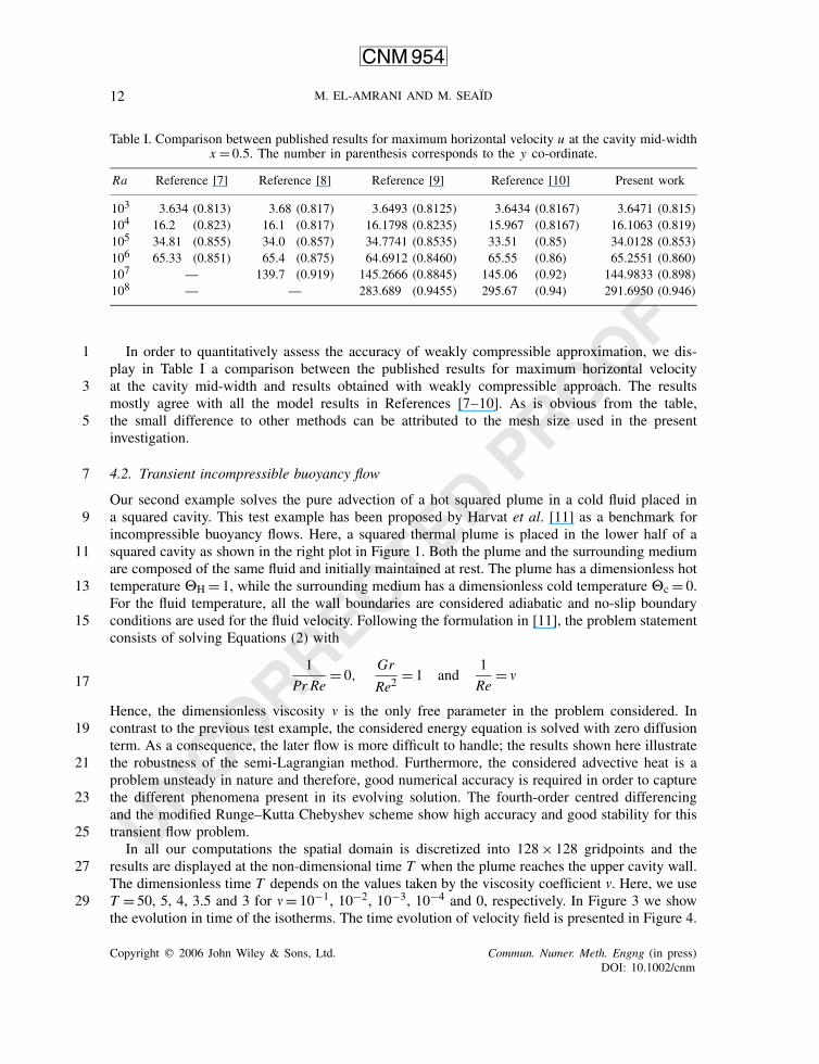
Table I. Comparison between published results for maximum horizontal velocity u at the cavity mid-widthx = 0.5. The number in parenthesis corresponds to the y co-ordinate.

Ra Reference [7] Reference [8] Reference [9] Reference [10] Present work

103 3.634 (0.813) 3.68 (0.817) 3.6493 (0.8125) 3.6434 (0.8167) 3.6471 (0.815)

104 16.2 (0.823) 16.1 (0.817) 16.1798 (0.8235) 15.967 (0.8167) 16.1063 (0.819)

105 34.81 (0.855) 34.0 (0.857) 34.7741 (0.8535) 33.51 (0.85) 34.0128 (0.853)

106 65.33 (0.851) 65.4 (0.875) 64.6912 (0.8460) 65.55 (0.86) 65.2551 (0.860)

107 — 139.7 (0.919) 145.2666 (0.8845) 145.06 (0.92) 144.9833 (0.898)

108 — — 283.689 (0.9455) 295.67 (0.94) 291.6950 (0.946)

In order to quantitatively assess the accuracy of weakly compressible approximation, we dis-1

play in Table I a comparison between the published results for maximum horizontal velocity

at the cavity mid-width and results obtained with weakly compressible approach. The results3

mostly agree with all the model results in References [7–10]. As is obvious from the table,

the small difference to other methods can be attributed to the mesh size used in the present5

investigation.

4.2. Transient incompressible buoyancy flow7

Our second example solves the pure advection of a hot squared plume in a cold fluid placed in

a squared cavity. This test example has been proposed by Harvat et al. [11] as a benchmark for9

incompressible buoyancy flows. Here, a squared thermal plume is placed in the lower half of a

squared cavity as shown in the right plot in Figure 1. Both the plume and the surrounding medium11

are composed of the same fluid and initially maintained at rest. The plume has a dimensionless hot

temperature �H = 1, while the surrounding medium has a dimensionless cold temperature �c = 0.13

For the fluid temperature, all the wall boundaries are considered adiabatic and no-slip boundary

conditions are used for the fluid velocity. Following the formulation in [11], the problem statement15

consists of solving Equations (2) with

1

Pr Re= 0,

Gr

Re2= 1 and

1

Re= �17

Hence, the dimensionless viscosity � is the only free parameter in the problem considered. In

contrast to the previous test example, the considered energy equation is solved with zero diffusion19

term. As a consequence, the later flow is more difficult to handle; the results shown here illustrate

the robustness of the semi-Lagrangian method. Furthermore, the considered advective heat is a21

problem unsteady in nature and therefore, good numerical accuracy is required in order to capture

the different phenomena present in its evolving solution. The fourth-order centred differencing23

and the modified Runge–Kutta Chebyshev scheme show high accuracy and good stability for this

transient flow problem.25

In all our computations the spatial domain is discretized into 128× 128 gridpoints and the

results are displayed at the non-dimensional time T when the plume reaches the upper cavity wall.27

The dimensionless time T depends on the values taken by the viscosity coefficient �. Here, we use

T = 50, 5, 4, 3.5 and 3 for �= 10−1, 10−2, 10−3, 10−4 and 0, respectively. In Figure 3 we show29

the evolution in time of the isotherms. The time evolution of velocity field is presented in Figure 4.

Copyright q 2006 John Wiley & Sons, Ltd. Commun. Numer. Meth. Engng (in press)

DOI: 10.1002/cnm

UNCORRECTED PROOF

CNM 954

EXTENSION OF WEAKLY COMPRESSIBLE APPROXIMATIONS 13

0

0

Figure 3. Isotherms at times from bottom to top: T/4 (first row), T/2 (second row), 3T/4 (third row), T

(fourth row) for viscosity coefficients from left to right: �= 10−1, 10−2, 10−3, 10−4 and 0.

In these figures, we plot the results at four non-dimensional instants t = T/4, T/2, 3T/4 and T1

for each viscosity coefficient. As expected, for small values of viscosity the thermal plume travels

faster towards the upper cavity wall. For � = 0, the flow is purely convection such that no physical3

diffusion is present in the equations. This last case presents a challenge for many Eulerian-based

methods for which numerical diffusion is consequence of their stabilization. For our approach, no5

excessive numerical diffusion has been detected for the case with � = 0.

The plume temperature and the fluid velocity in Figures 3 and 4 demonstrate the effect of7

buoyancy force on the fluid dynamics. For large viscosity values the buoyancy force strongly

increases the shear stresses on the cavity walls. These wall effects slow the advection of the9

thermal plume towards the upper cavity wall allowing the plume to preserve its compact shape

during the whole simulation period. Small viscosity values decrease the wall shear stresses leading11

to an increase in the velocity field. The thermal plume also exhibits Rayleigh–Taylor instabilities

which cause its deformation and rolling up along the advection process. At zero viscosity, the13

wall stresses disappear and the fluid motion is purely driven by convection. The presented results

Copyright q 2006 John Wiley & Sons, Ltd. Commun. Numer. Meth. Engng (in press)

DOI: 10.1002/cnm

UNCORRECTED PROOF

14

CNM 954

M. EL-AMRANI AND M. SEAID

00

Figure 4. Velocity vectors at times from bottom to top: T/4 (first row), T/2 (second row), 3T/4 (third

row), T (fourth row) for viscosity coefficients from left to right: � = 10−1, 10−2, 10−3, 10−4 and 0.

also indicate that as the viscosity decreases, the size of the recirculation zones increases with the1

flow exhibiting eddies with different magnitudes and separating shear layers. We can see the small

complex patterns of the flow being captured by the weakly compressible approximation.3

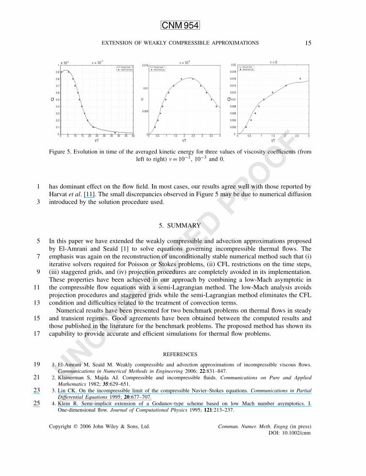
A quantitative comparison between our results and those presented in [11] is also performed in

the present example. To do so, we compute the averaged kinetic energy Q(t) at each time step as5

Q(t) =1

2

∑

i, j

(u2i, j + v2i, j )�x�y (23)

In Figure 5, we plot the averaged kinetic energy Q(t) versus the time t for the selected viscosity7

coefficients � = 10−1, 10−3 and 0. We also plot the results from [11] for comparison. It is clear that

the viscosity has direct influence on the kinetic energy of the fluid. For instance, decreasing the9

viscosity coefficients leads to an increase in the averaged kinetic energy within the simulation time.

This influence is more pronounced for zero viscosity test which indicates that the buoyancy force11

Copyright q 2006 John Wiley & Sons, Ltd. Commun. Numer. Meth. Engng (in press)

DOI: 10.1002/cnm

UNCORRECTED PROOF

CNM 954

EXTENSION OF WEAKLY COMPRESSIBLE APPROXIMATIONS 15

Figure 5. Evolution in time of the averaged kinetic energy for three values of viscosity coefficients (from

left to right) � = 10−1, 10−3 and 0.

has dominant effect on the flow field. In most cases, our results agree well with those reported by1

Harvat et al. [11]. The small discrepancies observed in Figure 5 may be due to numerical diffusion

introduced by the solution procedure used.3

5. SUMMARY

In this paper we have extended the weakly compressible and advection approximations proposed5

by El-Amrani and Seaıd [1] to solve equations governing incompressible thermal flows. The

emphasis was again on the reconstruction of unconditionally stable numerical method such that (i)7

iterative solvers required for Poisson or Stokes problems, (ii) CFL restrictions on the time steps,

(iii) staggered grids, and (iv) projection procedures are completely avoided in its implementation.9

These properties have been achieved in our approach by combining a low-Mach asymptotic in

the compressible flow equations with a semi-Lagrangian method. The low-Mach analysis avoids11

projection procedures and staggered grids while the semi-Lagrangian method eliminates the CFL

condition and difficulties related to the treatment of convection terms.13

Numerical results have been presented for two benchmark problems on thermal flows in steady

and transient regimes. Good agreements have been obtained between the computed results and15

those published in the literature for the benchmark problems. The proposed method has shown its

capability to provide accurate and efficient simulations for thermal flow problems.17

REFERENCES

1. El-Amrani M, Seaıd M. Weakly compressible and advection approximations of incompressible viscous flows.19Communications in Numerical Methods in Engineering 2006; 22:831–847.

2. Klainerman S, Majda AJ. Compressible and incompressible fluids. Communications on Pure and Applied21Mathematics 1982; 35:629–651.

3. Lin CK. On the incompressible limit of the compressible Navier–Stokes equations. Communications in Partial23Differential Equations 1995; 20:677–707.

4. Klein R. Semi-implicit extension of a Godunov-type scheme based on low Mach number asymptotics. I.25One-dimensional flow. Journal of Computational Physics 1995; 121:213–237.

Copyright q 2006 John Wiley & Sons, Ltd. Commun. Numer. Meth. Engng (in press)

DOI: 10.1002/cnm

UNCORRECTED PROOF

16

CNM 954

M. EL-AMRANI AND M. SEAID

5. Staniforth A, Cote J. Semi-Lagrangian integration schemes for the atmospheric models: a review. Weather Review11991; 119:2206–2223.

6. Verwer JG, Hundsdorfer WH, Sommeijer BP. Convergence properties of the Runge–Kutta–Chebychev method.3Numerical Mathematics 1990; 57:157–178.

7. De Valhl Davis D. Natural convection of air in a square cavity: a Benchmark solution. International Journal for5Numerical Methods in Fluids 1983; 3:249–264.

8. Manzari MT. An explicit finite element algorithm for convective heat transfer problems. International Journal7of Numerical Methods for Heat and Fluid Flow 1999; 9:860–877.

9. Mayne DA, Usmani AS, Carpper M. h-adaptive finite element solution of high Rayleigh number thermally driven9cavity problem. International Journal of Numerical Methods for Heat and Fluid Flow 2000; 10:598–615.

10. Wan DC, Patnaik SV, Wei GW. A new Benchmark quality solution for the Buoyancy-driven cavity by discrete11singular convolution. Numerical Heat Transfer, Part B 2001; 40:199–228.

11. Horvat A, Kljenak I, Marn J. On incompressible Buoyancy flow Benchmarking. Numerical Heat Transfer,13Part B 2001; 39:61–78.

Copyright q 2006 John Wiley & Sons, Ltd. Commun. Numer. Meth. Engng (in press)

DOI: 10.1002/cnm