A compressible Lagrangian

Framework for the Simulation of Underwater Implosion Problems

K. Kamran E. Oñate

S. R. Idelsohn R. Rossi

Monograph CIMNE Nº-150, January 2013

A compressible Lagrangian

Framework for the Simulation of Underwater Implosion Problems

K. Kamran E. Oñate

S. R. Idelsohn R. Rossi

Monograph CIMNE Nº-150, January 2013

International Center for Numerical Methods in Engineering Gran Capitán s/n, 08034 Barcelona, Spain

INTERNATIONAL CENTER FOR NUMERICAL METHODS IN ENGINEERING Edificio C1, Campus Norte UPC Gran Capitán s/n 08034 Barcelona, Spain www.cimne.com First edition: October 2014 A COMPRESSIBLE LAGRANGIAN FRAMEWORK FOR THE SIMULATION OF UNDERWATER IMPLOSION PROBLEMS Monograph CIMNE M150 Los autores ISBN: 978-84-943307-2-8 Depósito legal: B-23558-2014

To my parents.

A B S T R A C T

The development of efficient algorithms to understand implosion dynamics presentsa number of challenges. The foremost challenge is to efficiently represent the cou-pled compressible fluid dynamics of internal air and surrounding water. Secondly,the method must allow one to accurately detect or follow the interface between thephases. Finally, it must be capable of resolving any shock waves which may be createdin air or water during the final stage of the collapse. We present a fully Lagrangiancompressible numerical framework for the simulation of underwater implosion. Bothair and water are considered compressible and the equations for the Lagrangian shockhydrodynamics are stabilized via a variationally consistent multiscale method [109].A nodally perfect matched definition of the interface is used [57, 25] and then the ki-netic variables, pressure and density, are duplicated at the interface level. An adaptivemesh generation procedure, which respects the interface connectivities, is applied toprovide enough refinement at the interface level. This framework is then used to simu-late the underwater implosion of a large cylindrical bubble, with a size in the order ofcm. Rapid collapse and growth of the bubble occurred on very small spatial (0.3mm),and time (0.1ms) scales followed by Rayleigh-Taylor instabilities at the interface, inaddition to the shock waves traveling in the fluid domains are among the phenom-ena that are observed in the simulation. We then extend our framework to model theunderwater implosion of a cylindrical aluminum container considering a monolithicfluid-structure interaction (FSI). The aluminum cylinder, which separates the internalatmospheric-pressure air from the external high-pressure water, is modeled by a threenode rotation-free shell element. The cylinder undergoes fast transient deformations,large enough to produce self-contact along it. A novel elastic frictionless contact modelis used to detect contact and compute the non-penetrating forces in the discretizeddomain between the mid-planes of the shell. Two schemes are tested, implicit usingthe predictor/multi-corrector Bossak scheme, and explicit, using the forward Eulerscheme. The results of the two simulations are compared with experimental data.

R E S U M E N

El desarrollo de métodos eficientes para modelar la dinámica de implosión presentavarios desafíos. El primero es una representación eficaz de la dinámica del sistemaacoplado de aire-agua. El segundo es que el método tiene que permitir una detecciónexacta o un seguimiento adecuado de la interfase entre ambas fases. Por último elmétodo tiene que ser capaz de resolver cualquier choque que podría generar en elaire o en el agua, sobre todo en la última fase del colapso.

Nosotros presentamos un método numérico compresible y totalmente Lagrangianopara simular la implosión bajo el agua. Tanto el aire como el agua se consideran com-presibles y las ecuaciones Lagrangianos para la hidrodinámica del choque se estabi-lizan mediante un método multiescala que es variacionalmente consistente [109]. Se

v

utiliza una definición de interfase que coincide perfectamente con los nodos [57, 25].Ésta, nos facilita duplicar eficazmente las variables cinéticas como la presión y la den-sidad en los nodos de la interfase. Con el fin de obtener suficiente resolución alrededorde la interfase, la malla se genera de forma adaptativa y respetando la posición de lainterfase. A continuación el método desarrollado se utiliza para simular la implosiónbajo el agua de una burbuja cilíndrica del tamaño de un centímetro. Varios fenómenosse han capturado durante el colapso: un ciclo inmediato de colapso-crecimiento de laburbuja que ocurre en un espacio (0.3mm) y tiempo (0.1ms) bastante limitado, apari-ción de inestabilidades de tipo Rayleigh-Taylor en la interfase y formaron de variasondas de choque que viajan tanto en el agua como en el aire. Después, seguimosel desarrollo del método para modelar la implosión bajo el agua de un contenedormetálico considerando una interacción monolítica de fluido y estructura. El cilindrode aluminio, que a su vez contiene aire a presión atmosférica y está rodeada de aguaen alta presión, se modelando con elementos de lámina de tres nodos y sin gradosde libertad de rotación. El cilindro se somete a deformaciones transitorias suficiente-mente rápidos y enormes hasta llegar a colapsar. Un nuevo modelo elástico de con-tacto sin considerar la fricción se ha desarrollado para detectar el contacto y calcularlas fuerzas en el dominio discretizado entre las superficies medianas de las laminas.Dos esquemas temporales están considerados, uno es implícito utilizando el métodode Bossak y otro es explícito utilizando Forward Euler. Al final los resultados deambos casos se comparan con los resultados experimentales.

vi

P U B L I C AT I O N S

I A Compressible Lagrangian framework for the simulation of the underwater im-plosion of large air bubbles. K. Kamran, R. Rossi, E. Oñate and S.R. Idelsohn.Computer Methods in Applied Mechanics and Engineering, 225(1): 210-225, March2013. http://dx.doi.org/10.1016/j.cma.2012.11.018

II A Compressible Lagrangian framework for modeling the fluid-structure interac-tion in the underwater implosion of an aluminum cylinder. K. Kamran, R. Rossi,E. Oñate and S.R. Idelsohn. Mathematical Models and Methods in Applied Sciences,23(2), February 2013. 10.1142/S021820251340006X

III A contact algorithm for shell problems via Delaunay-based meshing of the contactdomain. K. Kamran, R. Rossi and E. Oñate, Computational Mechanics, September2012. 10.1007/s00466-012-0791-x

vii

A C K N O W L E D G M E N T S

I am so grateful to my supervisors, Prof. Eugenio Oñate, Prof. Sergio Rodolfo Idelsohnand Dr. Riccardo Rossi for their constant support and guidance during my research.Studying and working in CIMNE is a unique opportunity that has enriched my lifeand has extended my vision and I would like to deeply thank Prof. Eugenio Oñatefor that.

My special thanks to Riccardo Rossi for insightful discussions on different topicsand his endless patient in instructing me with programming skills. I am also so grate-ful to Pooyan Dadvand for his many friendly supports during these years in Barcelonaand also to step by step introducing me to programming in KRATOS. Without theirhelp this research couldn’t reach to its end.

I would like to thank my colleagues that I have had very enjoyable moments withthem and have always helped me in these years, viz. Pavel, Roberto, Antonia, Julio,Jordi, Miguel Angel, Salva, Prashant, Mohamamd, Behrooz, Enrique, Abel and Temo.

Last but not least I express my many sincere gratitude to my parents that have al-ways unconditionally supported me. This thesis is dedicated to them.

This work was partially supported by the Office of Naval Research (ONR) undercontract N00014-09-1-0969. Support for this research was also granted by projectsREALTIME and SAFECON of the European Research Council (ERC) of the EuropeanCommission.

ix

C O N T E N T S

1 introduction 1

1.1 Cavitation damage 1

1.2 Sonoluminescence (SL) 2

1.3 Bio-medical applications 3

1.4 Underwater implosion and submarine design 5

1.5 Current work motivation and thesis outline 6

2 bubble dynamics 9

2.1 Rayleigh-Plesset equation 9

2.2 Growth 11

2.3 Collapse 13

2.4 About the bubble collapse 15

2.5 Essentials of the bubble dynamics 17

2.6 Lagrangian framework 18

3 governing equations 23

3.1 Introduction 23

3.2 Governing equations 25

3.2.1 Euler equations 25

3.2.2 Lagrangian hydrodynamic equations 27

3.2.3 Stabilization of the linearized form 29

3.2.4 Stabilization of the nonlinear form 32

3.2.5 Discontinuity-Capturing (DC) operator 36

3.2.6 Explicit predictor-multi corrector time scheme 37

3.3 Two-phase treatment 41

3.3.1 Nodally matched interface 41

3.3.2 Mesh construction 43

3.3.3 Discontinuous kinetic field 46

3.4 Numerical examples 46

3.4.1 Noh test 47

3.4.2 Sedov test 49

3.4.3 Air-water system with big density jump 50

3.4.4 Underwater implosion of cylindrical bubble 52

3.5 Discussion 59

3.6 Conclusion 63

4 contact algorithm for shell problems 65

4.1 Introduction 65

4.2 Contact criteria and contact forces 67

4.3 Distance and normal 69

4.3.1 Canonical elements 70

4.3.2 Non-canonical elements 71

4.3.3 Region attributes and multi-object contacts 73

xi

xii contents

4.4 Summary of the contact algorithm 74

4.5 Rotation-free shell triangle 75

4.6 Numerical examples 77

4.6.1 Contact patch test 77

4.6.2 An example on mesh refinement 79

4.6.3 Collapse of a compressed spherical shell 81

4.6.4 Contact-impact between two tubes 82

4.6.5 Ball impacting a clamped plate 83

4.6.6 Buckling of cylindrical tube 84

4.7 Conclusions 85

5 fluid-structure interaction 89

5.1 Introduction 89

5.2 Governing equations 91

5.2.1 Lagrangian hydrodynamic equations 91

5.2.2 Rotation-free shell triangle 92

5.2.3 Contact model 93

5.3 Time discretization 95

5.3.1 Implicit time discretization 95

5.3.2 Explicit time discretization scheme 101

5.4 Solution strategy 104

5.5 Equation of state 106

5.6 Underwater implosion of cylindrical container 108

5.7 Conclusions 113

6 conclusions and future work 115

bibliography 117

L I S T O F F I G U R E S

Figure 1.1 Cavitation damage in a propeller. 2

Figure 1.2 Bubble sonoluminescence. Bubbles are driven by sound wavesto emit light. a) At low sound-wave pressure, a gas bubble ex-pands until (b) an increase in pressure triggers its collapse. Dur-ing collapse, temperatures can soar to 15,000 K, as it is observedfrom spectra of light [33] emitted from the bubble (c).Analysisof the emission spectra also provides direct evidence for theexistence of a plasma inside the collapsing bubbles. [73] 3

Figure 1.3 Schematic of the set-up for SWL using an electrohydraulic lithotripter [96]. 4

Figure 1.4 Pressure profile in the focal region of a lithotripter [63]. 5

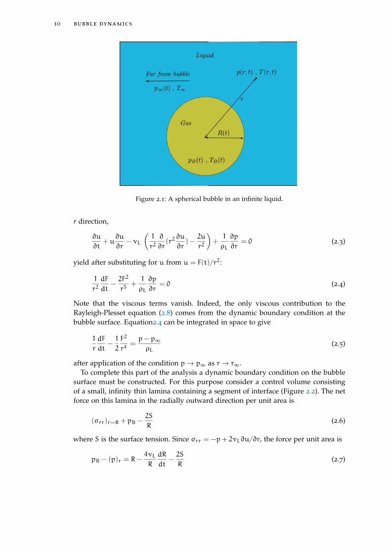
Figure 2.1 A spherical bubble in an infinite liquid. 10

Figure 2.2 Portion of the bubble surface 11

Figure 2.3 Typical solution of the Rayleigh-Plesset equation for spheri-cal bubble size/ initial size, R/R0. The nucleus enters a low-pressure region at a dimensionless time of 0 and is convectedback to the original pressure at a dimensionless time of 500.The low-pressure region is sinusoidal and symmetric about250 [9]. 13

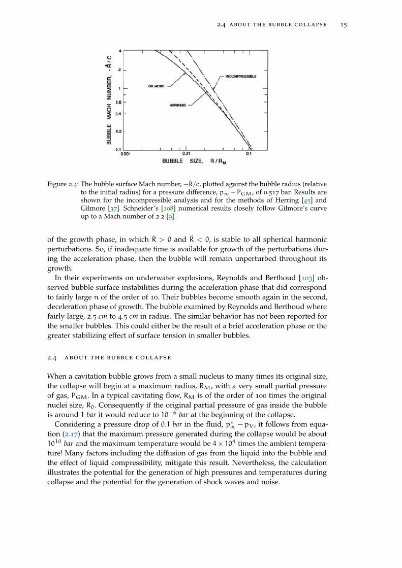
Figure 2.4 The bubble surface Mach number, −R/c, plotted against thebubble radius (relative to the initial radius) for a pressure dif-ference, p∞ − PGM, of 0.517 bar. Results are shown for the in-compressible analysis and for the methods of Herring [45] andGilmore [37]. Schneider’s [108] numerical results closely followGilmore’s curve up to a Mach number of 2.2 [9]. 15

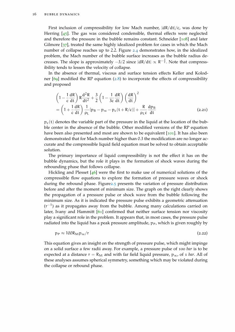
Figure 2.5 Typical results of Hickling and Plesset [46] for the pressure dis-tributions in the liquid before collapse (left) and after collapse(right) (without viscosity or surface tension). The parametersare p∞ = 1 bar, γ = 1.4, and the initial pressure in the bubblewas 10−3 bar. The values attached to each curve are propor-tional to the time before or after the minimum size [9]. 17

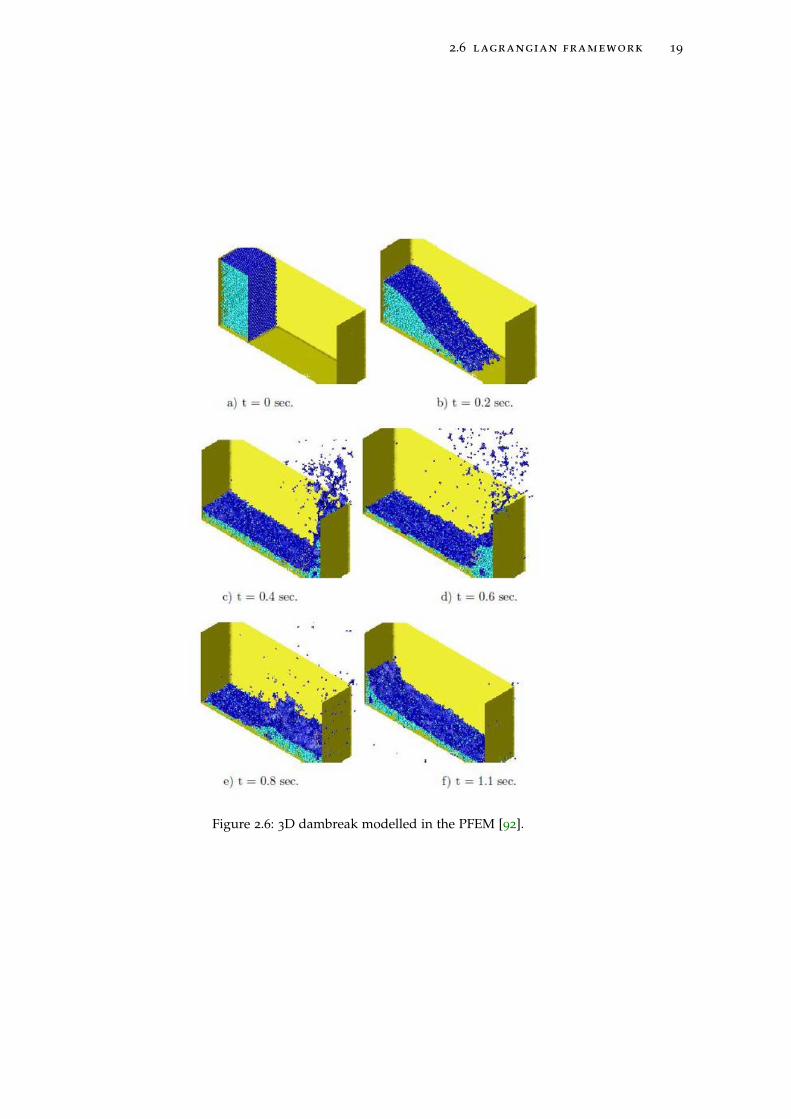
Figure 2.6 3D dambreak modelled in the PFEM [92]. 19

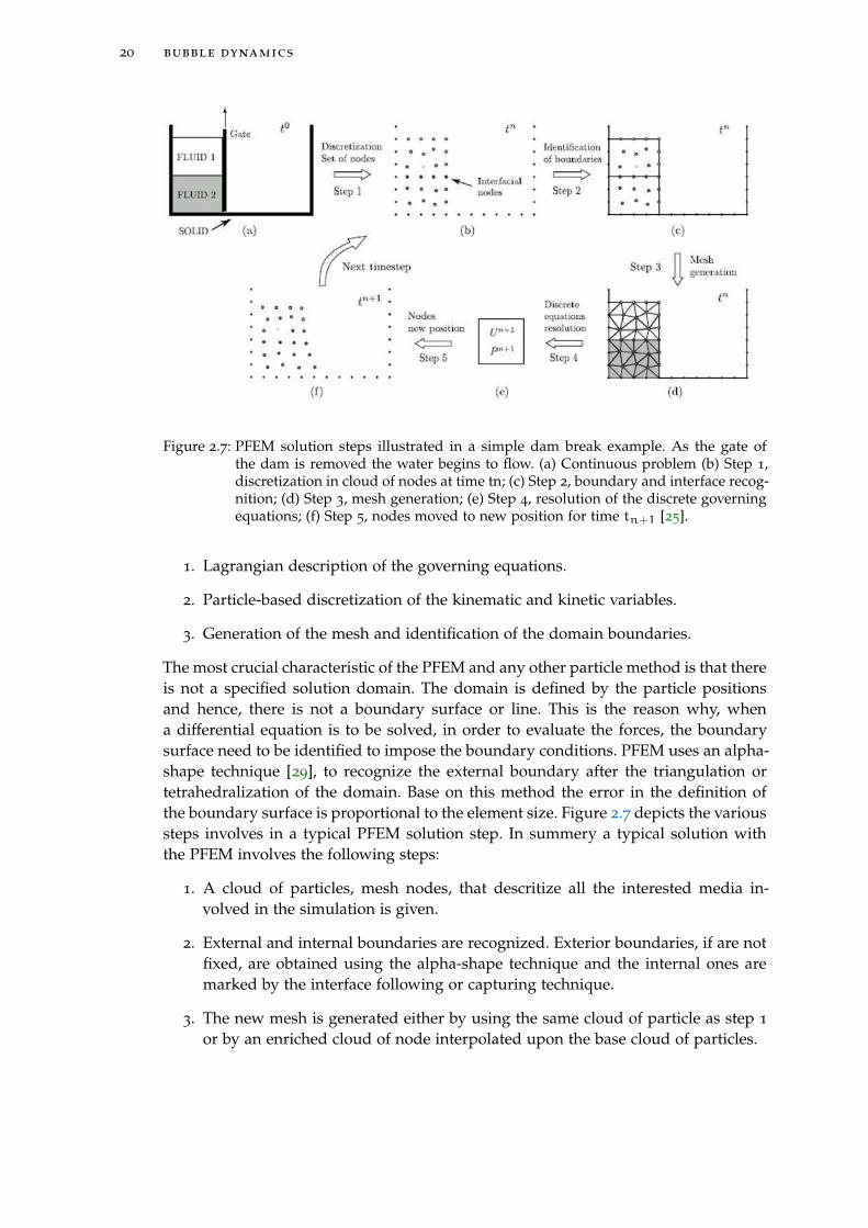
Figure 2.7 PFEM solution steps illustrated in a simple dam break example.As the gate of the dam is removed the water begins to flow. (a)Continuous problem (b) Step 1, discretization in cloud of nodesat time tn; (c) Step 2, boundary and interface recognition; (d)Step 3, mesh generation; (e) Step 4, resolution of the discretegoverning equations; (f) Step 5, nodes moved to new positionfor time tn+1 [25]. 20

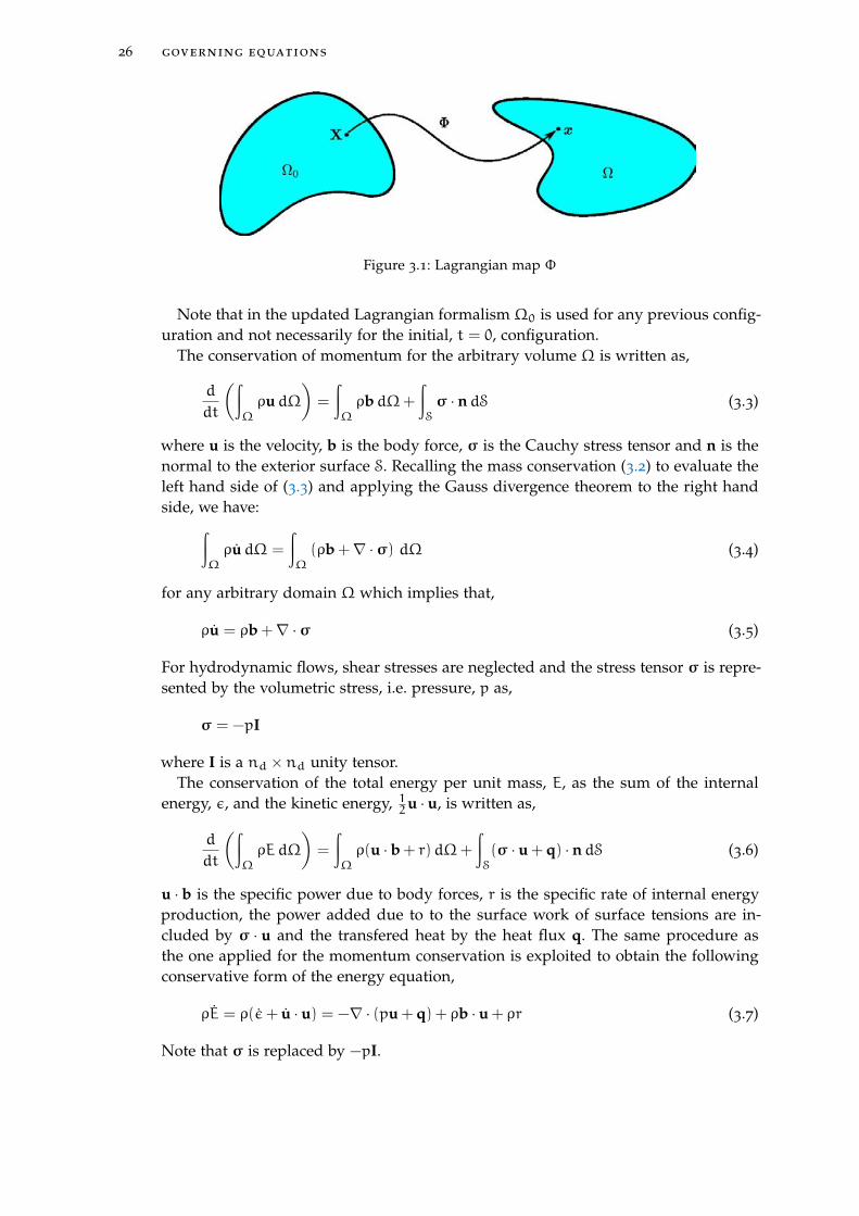
Figure 3.1 Lagrangian map Φ 26

Figure 3.2 Solution, U, is devided to two parts: coarse scale, Uh, capturedby the FEM and fine scale U ′. 30

xiii

xiv List of Figures

Figure 3.3 A schematic view of a two-fluid system with different materialproperties and the internal interface. 41

Figure 3.4 Density and pressure representations for the different interfacedefinitions: a) Elemental definition of the interface. , b) Nodallymatched interface. Note the exact representation of pressure forthe nodally matched interface. 42

Figure 3.5 Nodally matched interface 43

Figure 3.6 Edge swapping occurs when four nodes line on the same cir-cle. 44

Figure 3.7 Change of connectivities causes change of interface position44

Figure 3.8 1D Noh test shock tube 47

Figure 3.9 1D Noh test. Results for 50, “2”, and 100, “•”, element meshes.Figures a to d show the exact solution in solid line for pressure,density, internal energy and velocity in comparison with thenumerical ones. Artificial viscosities are shown in figures e andf . 48

Figure 3.10 2D Noh test. Mesh configuration and pressure field at timet = 0.6 s. 49

Figure 3.11 2D Noh test. Results for 50×50,“2”, and 100×100, “•”, elementmeshes. Figures a to d show the exact solution in solid line forpressure, density, internal energy and velocity in comparisonwith the numerical ones. Artificial viscosities are shown in fig-ures e and f . 50

Figure 3.12 1D Sedov test. a) constant initial density, b) initial mesh config-uration, c) mesh configuration for t = 1.0s 51

Figure 3.13 1D Sedov test. Results for 60, “2”, and 120, “•”, element meshes.Figures a to d show the exact solution in solid line for pressure,density, internal energy and velocity in comparison with thenumerical ones. Artificial viscosities are shown in figures e andf . 52

Figure 3.14 2D Sedov test. Pressure field and mesh configuration at timet = 1.0 s. 53

Figure 3.15 2D Sedov test. Results for 60× 60, “2” , and 120× 120, “•”, ele-ment meshes. Figures a to d show the exact solution in solid linefor pressure, density, internal energy and velocity in compari-son with the numerical ones. Artificial viscosities are shown infigures e and f . 54

Figure 3.16 Air-Water tube 55

Figure 3.17 Air-water tube. Results for pressure, density and velocity areshown in figures a to c and are compared with the exact onesdepicted in solid lines. Artificial viscosities are shown in figuresd and e. 55

Figure 3.18 Underwater implosion setup 56

Figure 3.19 Time histories of a) “X”, “Y” measures of bubble radius andpressure at the center of the bubble, b) Length parameter, H.

57

List of Figures xv

Figure 3.20 Adaptive mesh refinement, a) initial mesh near the interface,b) mesh at the moment of maximum contraction. Solid lineindicates the position of the interface. 58

Figure 3.21 Formation of the shock at the center of the bubble 59

Figure 3.22 Bubble implosion. Velocity distributions a)X direction b)Y di-rection 60

Figure 3.23 Bubble implosion. Appearance of the RT instabilities. 61

Figure 3.24 Expansion of the bubble and violent collapse 61

Figure 3.25 Time history of pressure at 10.16 cm from the center of thebubble 62

Figure 3.26 1D analysis. Variation of distortion amplitude, b/b0, as a func-tion of R/R0 63

Figure 4.1 a) Shell thicknesses t1 and t2 and actual distance between mid-planes, h. b) Element A and its neighbors B and C 68

Figure 4.2 a) Potential contact elements, b) Active contact elements 70

Figure 4.3 “Canonical” contact elements 70

Figure 4.4 Vertex-edge combinations 71

Figure 4.5 a) Sliver b) corner element c) boundary element d) two by twoelement, in which segment AB belongs to the one contact sur-face and segment CD to the other one 73

Figure 4.6 a) Initial geometry with bounding box b) Region attributes shownin a mid-plane. 74

Figure 4.7 Patch test a) setup of the test b) discretization in x-direction c)active contact elements d) contact forces. 76

Figure 4.8 Unstructured discretization in x-direction and the distributionof the computed consistent nodal forces. 76

Figure 4.9 The discretization of a) bottom shell and b) top shell with theobtained displacement field (c) for the top shell under the con-stant load. 78

Figure 4.10 Hemispherical shell and plate,front view. The contact is trig-gered by the vertical movement of the plate. 78

Figure 4.11 Normal stress at the apex and the radius of the contact zoneversus the, n, number of refinement levels. A top view of theactive contact elements related to the refinements n = 1 andn = 8 are shown. 79

Figure 4.12 Collapse of spherical shell compressed a to f Mid-plane evolu-tion, g) H4 specimen [39] h) final configuration 80

Figure 4.13 Collapse of compressed spherical shell. Appearance of lobes 80

Figure 4.14 Collapse of compressed spherical shell. Midplane, 3D view andactive contact elements at two instants 82

Figure 4.15 Contact-impact of two tubes. Geometries at time t = 1ms 83

Figure 4.16 Ball impacting a clamped plate a) our method b) Cardoso etal. [15] 84

Figure 4.17 Buckling of cylindrical tube under external pressure. Mid-planeview for the second mode collapse 85

Figure 4.18 Third mode buckling of cylindrical tube. Active contact ele-ments a) mid-plane view b) 3D view 86

Figure 4.19 Experimental results for third buckling mode [3] 86

Figure 5.1 EBST rotation-free shell triangle “A” and element patch usedto compute the curvatures and membrane strains at points G1,G2, G3 93

Figure 5.2 Shell thicknesses t1 and t2 and actual distance between mid-planes, h. Light gray zone is the potential contact domain dis-cretized by triangular elements. Element “A” in dark gray is anactive element that satisfies the contact criteria. 94

Figure 5.3 Two fluids that are separated by the shell structure. Interfacenodes are common between fluids and structure and have du-plicated pressure and density. 96

Figure 5.4 Coupled mass matrix. MS represents the contribution of theshell element to the coupled system. Note that each domain hasits own pressure variables that are duplicated at the interfacenodes (Figure 5.3). 99

Figure 5.5 Aluminum cylinder filled with air and submerged into the wa-ter tank. Sensors are put in 10.16 cm from the center of thecylinder. 104

Figure 5.6 Schematic view of the model geometry (a) and mesh configu-ration at time t = 0 (b). 108

Figure 5.7 Final configuration of cylinder a) experiment, b) simulation 109

Figure 5.8 Time history of pressure in one of the sensors compared withimplicit and explicit results. Zero pressure corresponds to theinitial pressure of 6.99 MPA. 109

Figure 5.9 Mesh configuration of cylinder (a), potential contact elements (b)and active contact elements (c). 110

Figure 5.10 Mesh configuration inside and near the cylinder at the begin-ning of the simulation. 111

Figure 5.11 Collapse of the cylinder visualized through the evolution of thecut planes. 112

Figure 5.12 A view of the refined mesh near the cylinder at the final stageof the collapse. 114

L I S T O F TA B L E S

Table 3.1 Mid-point explicit predictor/multi-corrector algorithm 39

Table 3.2 Constrained mesh generation process 45

Table 4.1 Contact algorithm 75

Table 5.1 Residual-based implicit predictor/multi-corrector algorithm 101

Table 5.2 One step of the explicit scheme 103

xvi

List of Tables xvii

Table 5.3 One step of the FSI scheme 105

1I N T R O D U C T I O N

Cavitation is normally defined as the formation of bubbles filled with vapour/ gasor their mixture and subsequent activities (such as growth, collapse and rebound) inliquids. According to the content of bubbles, cavitation can be classified as vaporouscavitation and gaseous cavitation. It is a phenomenon directly related to the pressurereduction below a certain critical value. In this way the formation of bubbles is notconsidered cavitation.

Usually there are two ways by which the pressure reduction is caused. One is byreduction of pressure in some zones of a fluid flow which is often referred to as hy-drodynamic cavitation. The other is by an acoustic field, which is often referred to asacoustic cavitation. However, there are also other cavitations generated either by pho-tons of laser light or by other elementary particles (e.g. protons in a bubble chamber).These cavitations are achieved in nature by local energy deposit rather than by tensionin liquid. Therefore, they are often referred to as optical cavitation and particle cativation,respectively.

If pressure inside the bubble is less than the external pressure, the inrush of themomentum of the external liquid can cause considerable condensation of mater andenergy, something that is referred to as implosion. Furthermore, it may happen that theinside low pressure gas is separated from the outside high pressure flow by meansof a separating structure. The general expression of underwater implosion is used forthese cases to distinguish them in the cavitation study.

In the following some applications of this phenomenon in science and engineeringis presented. Although, the first studies on this field were motivated by the damagesproduced by the cavitation, recently some desirable applications of cavitation damagehave arisen.

1.1 cavitation damage

Cavitaion erosion is observed over a wide range of scales and in different engineeringapplications. One of the most spectacular examples is the cavitation erosion sustainedby the passage of a large flood through a spillway or the outlet of a dam. Turboma-chines, on the other hand, constitute another field where cavitation plays a deleteriousrole (Figure 1.1). In certain flows of liquid through rotating machines such as pumpsand turbines cavitation can not be avoided [72]. The operation of valves and nozzlesmay also be affected by cavitation, due to changes in the velocity of the liquid passingthrough them. Thus, care must be taken in the design of such instruments in order tominimize the destructive action of cavitation [9].

1

2 introduction

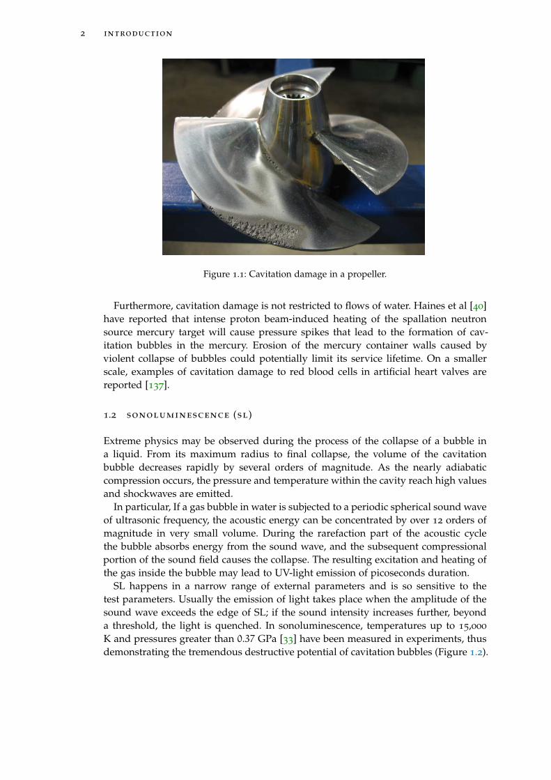
Figure 1.1: Cavitation damage in a propeller.

Furthermore, cavitation damage is not restricted to flows of water. Haines et al [40]have reported that intense proton beam-induced heating of the spallation neutronsource mercury target will cause pressure spikes that lead to the formation of cav-itation bubbles in the mercury. Erosion of the mercury container walls caused byviolent collapse of bubbles could potentially limit its service lifetime. On a smallerscale, examples of cavitation damage to red blood cells in artificial heart valves arereported [137].

1.2 sonoluminescence (sl)

Extreme physics may be observed during the process of the collapse of a bubble ina liquid. From its maximum radius to final collapse, the volume of the cavitationbubble decreases rapidly by several orders of magnitude. As the nearly adiabaticcompression occurs, the pressure and temperature within the cavity reach high valuesand shockwaves are emitted.

In particular, If a gas bubble in water is subjected to a periodic spherical sound waveof ultrasonic frequency, the acoustic energy can be concentrated by over 12 orders ofmagnitude in very small volume. During the rarefaction part of the acoustic cyclethe bubble absorbs energy from the sound wave, and the subsequent compressionalportion of the sound field causes the collapse. The resulting excitation and heating ofthe gas inside the bubble may lead to UV-light emission of picoseconds duration.

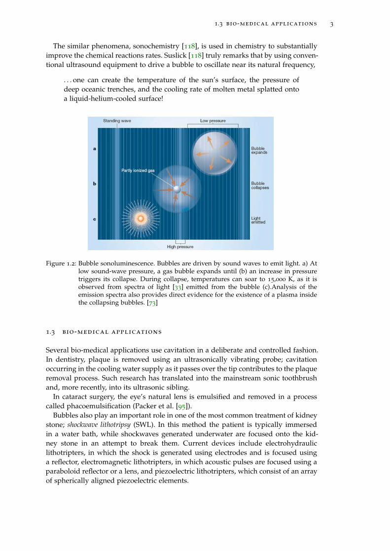
SL happens in a narrow range of external parameters and is so sensitive to thetest parameters. Usually the emission of light takes place when the amplitude of thesound wave exceeds the edge of SL; if the sound intensity increases further, beyonda threshold, the light is quenched. In sonoluminescence, temperatures up to 15,000

K and pressures greater than 0.37 GPa [33] have been measured in experiments, thusdemonstrating the tremendous destructive potential of cavitation bubbles (Figure 1.2).

1.3 bio-medical applications 3

The similar phenomena, sonochemistry [118], is used in chemistry to substantiallyimprove the chemical reactions rates. Suslick [118] truly remarks that by using conven-tional ultrasound equipment to drive a bubble to oscillate near its natural frequency,

. . . one can create the temperature of the sun’s surface, the pressure ofdeep oceanic trenches, and the cooling rate of molten metal splatted ontoa liquid-helium-cooled surface!

Figure 1.2: Bubble sonoluminescence. Bubbles are driven by sound waves to emit light. a) Atlow sound-wave pressure, a gas bubble expands until (b) an increase in pressuretriggers its collapse. During collapse, temperatures can soar to 15,000 K, as it isobserved from spectra of light [33] emitted from the bubble (c).Analysis of theemission spectra also provides direct evidence for the existence of a plasma insidethe collapsing bubbles. [73]

1.3 bio-medical applications

Several bio-medical applications use cavitation in a deliberate and controlled fashion.In dentistry, plaque is removed using an ultrasonically vibrating probe; cavitationoccurring in the cooling water supply as it passes over the tip contributes to the plaqueremoval process. Such research has translated into the mainstream sonic toothbrushand, more recently, into its ultrasonic sibling.

In cataract surgery, the eye’s natural lens is emulsified and removed in a processcalled phacoemulsification (Packer et al. [95]).

Bubbles also play an important role in one of the most common treatment of kidneystone; shockwave lithotripsy (SWL). In this method the patient is typically immersedin a water bath, while shockwaves generated underwater are focused onto the kid-ney stone in an attempt to break them. Current devices include electrohydrauliclithotripters, in which the shock is generated using electrodes and is focused usinga reflector, electromagnetic lithotripters, in which acoustic pulses are focused using aparaboloid reflector or a lens, and piezoelectric lithotripters, which consist of an arrayof spherically aligned piezoelectric elements.

4 introduction

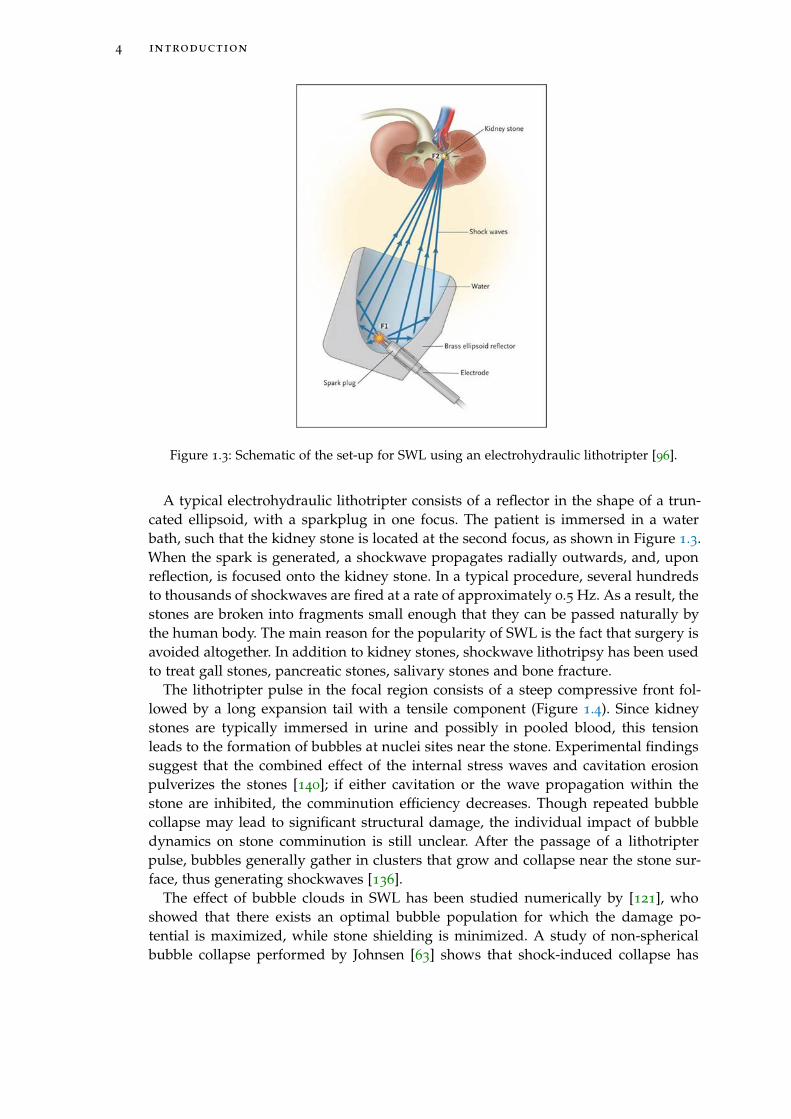
Figure 1.3: Schematic of the set-up for SWL using an electrohydraulic lithotripter [96].

A typical electrohydraulic lithotripter consists of a reflector in the shape of a trun-cated ellipsoid, with a sparkplug in one focus. The patient is immersed in a waterbath, such that the kidney stone is located at the second focus, as shown in Figure 1.3.When the spark is generated, a shockwave propagates radially outwards, and, uponreflection, is focused onto the kidney stone. In a typical procedure, several hundredsto thousands of shockwaves are fired at a rate of approximately 0.5 Hz. As a result, thestones are broken into fragments small enough that they can be passed naturally bythe human body. The main reason for the popularity of SWL is the fact that surgery isavoided altogether. In addition to kidney stones, shockwave lithotripsy has been usedto treat gall stones, pancreatic stones, salivary stones and bone fracture.

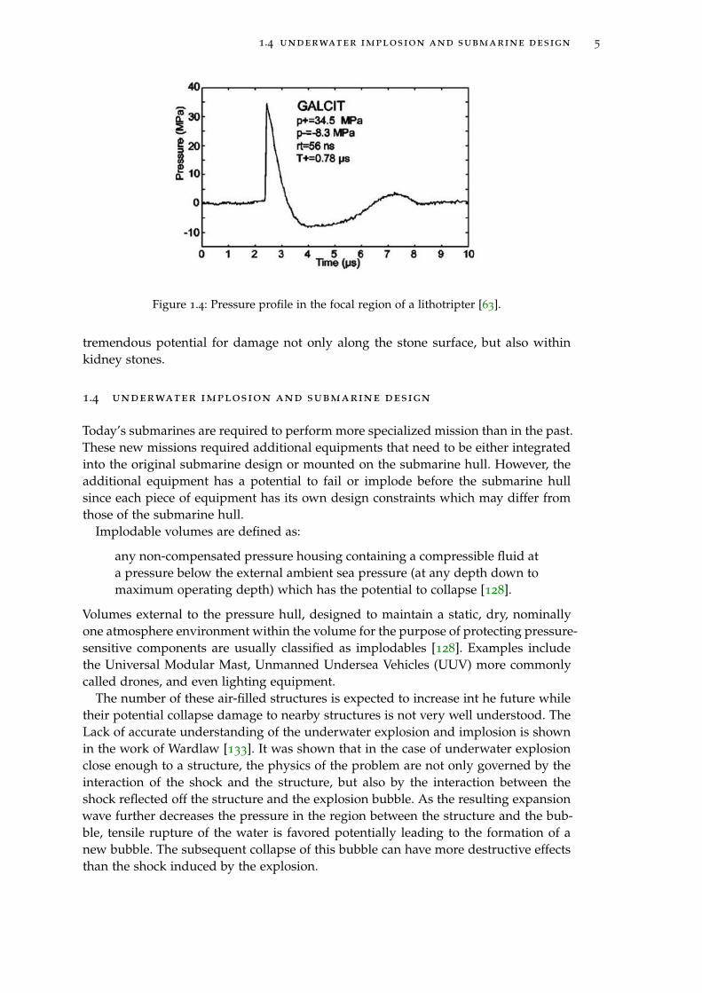
The lithotripter pulse in the focal region consists of a steep compressive front fol-lowed by a long expansion tail with a tensile component (Figure 1.4). Since kidneystones are typically immersed in urine and possibly in pooled blood, this tensionleads to the formation of bubbles at nuclei sites near the stone. Experimental findingssuggest that the combined effect of the internal stress waves and cavitation erosionpulverizes the stones [140]; if either cavitation or the wave propagation within thestone are inhibited, the comminution efficiency decreases. Though repeated bubblecollapse may lead to significant structural damage, the individual impact of bubbledynamics on stone comminution is still unclear. After the passage of a lithotripterpulse, bubbles generally gather in clusters that grow and collapse near the stone sur-face, thus generating shockwaves [136].

The effect of bubble clouds in SWL has been studied numerically by [121], whoshowed that there exists an optimal bubble population for which the damage po-tential is maximized, while stone shielding is minimized. A study of non-sphericalbubble collapse performed by Johnsen [63] shows that shock-induced collapse has

1.4 underwater implosion and submarine design 5

Figure 1.4: Pressure profile in the focal region of a lithotripter [63].

tremendous potential for damage not only along the stone surface, but also withinkidney stones.

1.4 underwater implosion and submarine design

Today’s submarines are required to perform more specialized mission than in the past.These new missions required additional equipments that need to be either integratedinto the original submarine design or mounted on the submarine hull. However, theadditional equipment has a potential to fail or implode before the submarine hullsince each piece of equipment has its own design constraints which may differ fromthose of the submarine hull.

Implodable volumes are defined as:

any non-compensated pressure housing containing a compressible fluid ata pressure below the external ambient sea pressure (at any depth down tomaximum operating depth) which has the potential to collapse [128].

Volumes external to the pressure hull, designed to maintain a static, dry, nominallyone atmosphere environment within the volume for the purpose of protecting pressure-sensitive components are usually classified as implodables [128]. Examples includethe Universal Modular Mast, Unmanned Undersea Vehicles (UUV) more commonlycalled drones, and even lighting equipment.

The number of these air-filled structures is expected to increase int he future whiletheir potential collapse damage to nearby structures is not very well understood. TheLack of accurate understanding of the underwater explosion and implosion is shownin the work of Wardlaw [133]. It was shown that in the case of underwater explosionclose enough to a structure, the physics of the problem are not only governed by theinteraction of the shock and the structure, but also by the interaction between theshock reflected off the structure and the explosion bubble. As the resulting expansionwave further decreases the pressure in the region between the structure and the bub-ble, tensile rupture of the water is favored potentially leading to the formation of anew bubble. The subsequent collapse of this bubble can have more destructive effectsthan the shock induced by the explosion.

6 introduction

Because the collapse of implodable volumes can have devastating consequences,it is essential to improve the understanding of the underlying physics of implosionproblems in order to better define design constraints for both submarine hulls andimplodable volumes.

The structural failure of an implodable volume leads to the compression of theair inside. The pressure then rapidly increases to the thousand times of the initialpressure and even much greater than the hydrostatic pressure. The differential ofpressures between the air and the water forces the air bubble to expand, generatinga shock wave that travels throughout the water. Since the implodable volumes areusually mounted to the submarine hull, the shock waves’ emission point is very closeto the submarine and its strength is only slightly decreased before it reaches thesubmarine hull. Thus, it may be the effect of the implosion that lead to the failure ofthe submarine hull rather than the initial shock wave induced by the explosion.

The main characteristics of these implosion problems are first the violent nature ofthe phenomenon and second the strong interactions between the different mechani-cal systems i.e. the structures and the fluids. Furthermore, the air, water and gaseousproducts of explosives, interact not only with each other but also with one or morestructures. Strong pressure waves travel through all media leading to large deforma-tions of structures, in very small time scales, that may lead to failure in the form ofcracks or collapse.

These violent motions of the flow occurs at the vicinity of the structure. At the sametime, other regions of the flow are unperturbed. Hence, implosions form a complexsystem to study as they involve the strong interactions of systems with very differentbehaviors and in a vast range of regimes.

1.5 current work motivation and thesis outline

The main motivation of this work is to develop a compressible Lagrangian frameworkfor the simulation of underwater implosion. In particular two problems are studied;First the collapse and growth of cm size cylindrical bubbles and second the underwa-ter implosion of an aluminum cylinder.

The development of efficient algorithms to understand rapid bubble dynamicspresents a number of challenges. The foremost challenge is to efficiently representthe coupled compressible fluid dynamics of internal air and surrounding water. Sec-ondly, the method must allow one to accurately detect or follow the interface betweenthe phases. Finally, it must be capable of resolving any shock waves which may becreated in air or water during the final stage of the collapse. Chapter three, essentially,explains our suggestion “a la PFEM” for modeling of the bubble collapse.

Concerning the underwater implosion of an aluminum cylinder, the main chal-lenges are; appropriate coupling of the fluid and structure subdomains, providingenough resolution at the zones where large deformations appear and last but notleast treat the self-contact at the final stage of the collapse.

In the next chapter the dynamics of the simple bubble is reviewed. In particular, thefast dynamics of the collapse and rebound and the appearance of instabilities at thefinal stage of the collapse that makes the symmetric analysis invalid are highlighted.The PFEM as a powerful tool to model different physical phenomenon are presented

1.5 current work motivation and thesis outline 7

at the end of this chapter.

In chapter three the Euler equations that governs the fast dynamics of the inviscidflows is studied. A stabilized variational multi-scaled method developed by Scov-azzi [109] is taken as the core of the compressible solver. Our main contribution inthis section is to extend this solver for the two-phase flows. This is done first by in-troducing an interface following technique presented by Idelsohn et al [57, 25] to bestfollow the position of the interface distortions and second by enriching the pressure atthe interface level. Large deformation of the mesh at some specific zones of the fluidnecessitates the regeneration of the mesh. An adaptive mesh generation that respectsthe interface connectivities completed our Lagrangian compressible framework. Latervarious examples are solved and then the implosion of the large, cm size, cylindricalbubble is modeled. The appearance of the RT instabilities at the final stage of the col-lapse and the rupture of the bubble after a cycle of expansion and contraction are theoutcomes of this study.

Chapter four is dedicated to a new contact algorithm that is developed for theshell-to-shell frictionless contact. The final stage in the implosion of closed containersusually consists of the total collapse of the containers. It is, therefor, inevitable to in-troduce a self-contact scheme to model the collapse. Our proposed method belongsto the contact domain methods in which the volume between the contacting bodiesis discretized by a finite element mesh. A simple contact criteria is verified for eachcontact element to determine the active contact elements and then the contact forcesare calculated. We finish this chapter by a set of examples to verify different aspectsof the method.

Chapter five is dedicated to present a fully Lagrangian monolithic fluid-structureinteraction scheme to solve the underwater implosion of an aluminum cylinder. Themain features of this framework are the monolithic coupling of the fluid and structuresubsystems, the discontinuous treatment of the pressure and density at the interfaceand the possibility of providing the desired mesh resolution when large displace-ments occur. The monolithic FSI system is solved using an implicit predictor/multi-corrector Bossak scheme at each step. An explicit forward Euler solution of this systemis also provided and both results are then compared with experimental data.

All simulations are provided using the free source parallel multi-physics platformof KRATOS [24, 23] developed at CIMNE. The pre and post processing of data wasprovided by the GID [36] software.

2B U B B L E D Y N A M I C S

We devote this chapter to the fundamental dynamics of a growing or collapsing bub-ble in an infinite domain of liquid that is at rest far from the bubble . While theassumption of spherical symmetry is violated in several important processes, it isnecessary to first develop this baseline.

2.1 rayleigh-plesset equation

Consider a spherical bubble of radius, R(t) (where t is time), in an infinite domainof liquid whose temperature and pressure far from the bubble T∞ and p∞(t), respec-tively. The temperature, T∞, is considered constant since temperature gradients arenot considered. On the other hand, the pressure, p∞(t), is assumed to be a knowninput that regulates the collapse or growth of the bubble.

Though compressibility of the liquid can be important in the context of bubble col-lapse, it will, for the present, be assumed that the liquid density, ρL, is a constant. Fur-thermore the dynamic viscosity, νL, is assumed constant and uniform. It will also beassumed that the contents of the bubble are homogeneous and that the temperature,TB(t), and pressure, pB(T), within the bubble are always uniform. These assumptionsmay not be justified in circumstances that will be identified as the analysis proceeds.

The radius of the bubble, R(t), will be one of the primary results of the analysis.As indicated in Figure 2.1, radial position within the liquid will be denoted by thedistance, r, from the center of the bubble; the pressure, p(r, t), radial outward velocity,u(r, t), and temperature, T(r, t), within the liquid will be so designated. Conservationof mass requires that [9]

u(r, t) =F(t)

r2(2.1)

where F(t) is related to R(t) by a kinematic boundary condition at the bubble surface.In the idealized case of zero mass transport across the interface, it is clear that u(r, t) =dR/dt and hence

F(t) = R2dR

dt(2.2)

This is often a good approximation even when evaporation or condensation is oc-curring at the interface provided the vapor density is much smaller than the liquiddensity. Assuming a Newtonian liquid, the Navier-Stokes equation for motion in the

9

10 bubble dynamics

Figure 2.1: A spherical bubble in an infinite liquid.

r direction,

∂u

∂t+ u

∂u

∂r− νL

(1

r2∂

∂r(r2∂u

∂r) −

2u

r2

)+1

ρL

∂p

∂r= 0 (2.3)

yield after substituting for u from u = F(t)/r2:

1

r2dF

dt−2F2

r5+1

ρL

∂p

∂r= 0 (2.4)

Note that the viscous terms vanish. Indeed, the only viscous contribution to theRayleigh-Plesset equation (2.8) comes from the dynamic boundary condition at thebubble surface. Equation2.4 can be integrated in space to give

1

r

dF

dt−1

2

F2

r4=p− p∞ρL

(2.5)

after application of the condition p→ p∞ as r→ r∞.To complete this part of the analysis a dynamic boundary condition on the bubble

surface must be constructed. For this purpose consider a control volume consistingof a small, infinity thin lamina containing a segment of interface (Figure 2.2). The netforce on this lamina in the radially outward direction per unit area is

(σrr)r=R + pB −2S

R(2.6)

where S is the surface tension. Since σrr = −p+ 2νL∂u/∂r, the force per unit area is

pB − (p)r = R−4νLR

dR

dt−2S

R(2.7)

2.2 growth 11

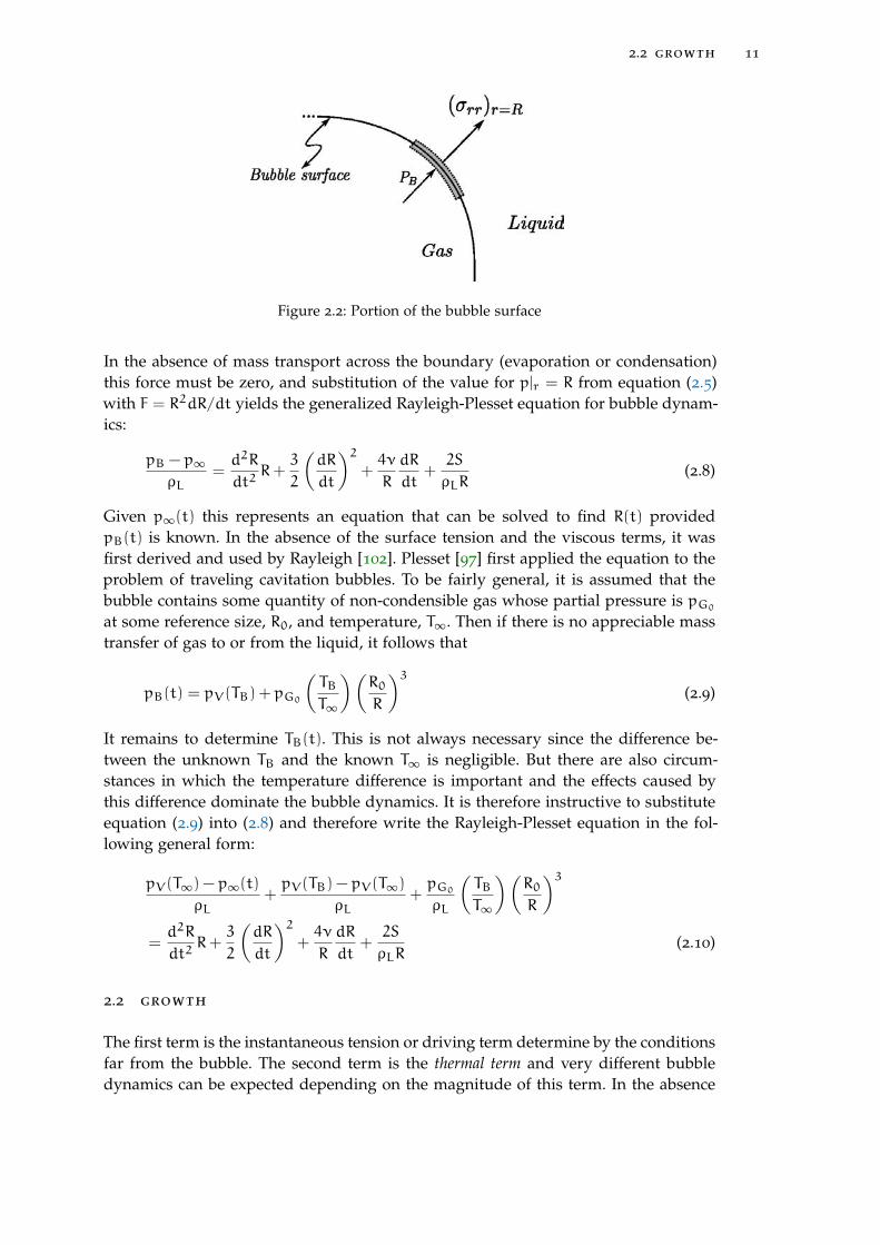
Figure 2.2: Portion of the bubble surface

In the absence of mass transport across the boundary (evaporation or condensation)this force must be zero, and substitution of the value for p|r = R from equation (2.5)with F = R2dR/dt yields the generalized Rayleigh-Plesset equation for bubble dynam-ics:

pB − p∞ρL

=d2R

dt2R+

3

2

(dR

dt

)2+4ν

R

dR

dt+2S

ρLR(2.8)

Given p∞(t) this represents an equation that can be solved to find R(t) providedpB(t) is known. In the absence of the surface tension and the viscous terms, it wasfirst derived and used by Rayleigh [102]. Plesset [97] first applied the equation to theproblem of traveling cavitation bubbles. To be fairly general, it is assumed that thebubble contains some quantity of non-condensible gas whose partial pressure is pG0at some reference size, R0, and temperature, T∞. Then if there is no appreciable masstransfer of gas to or from the liquid, it follows that

pB(t) = pV(TB) + pG0

(TBT∞)(

R0R

)3(2.9)

It remains to determine TB(t). This is not always necessary since the difference be-tween the unknown TB and the known T∞ is negligible. But there are also circum-stances in which the temperature difference is important and the effects caused bythis difference dominate the bubble dynamics. It is therefore instructive to substituteequation (2.9) into (2.8) and therefore write the Rayleigh-Plesset equation in the fol-lowing general form:

pV(T∞) − p∞(t)ρL

+pV(TB) − pV(T∞)

ρL+pG0ρL

(TBT∞)(

R0R

)3=d2R

dt2R+

3

2

(dR

dt

)2+4ν

R

dR

dt+2S

ρLR(2.10)

2.2 growth

The first term is the instantaneous tension or driving term determine by the conditionsfar from the bubble. The second term is the thermal term and very different bubbledynamics can be expected depending on the magnitude of this term. In the absence

12 bubble dynamics

of any significant thermal effect, the bubble dynamics behavior is termed inertiallycontrolled to distinguish it from thermally controlled. In the latter case, the temperaturein the liquid is assumed uniform and therefor the second term in the Rayleigh-Plessetequation (2.10) is zero. For simplicity, it will be assumed that the behavior of the gasin the bubble is polytropic so that

pG = pG0

(R0R

)3k(2.11)

where k is approximately constant. Clearly k = 1 implies a constant bubble tempera-ture and k = γwould model adiabatic behavior. It should be understood that accurateevaluation of the behavior of the gas in the bubble requires the solution of the mass,momentum and energy equations for the bubble contents combined with appropriateboundary conditions that will include a thermal boundary condition at the bubblewall.

With these assumptions the Rayleigh-Plesset equation becomes

pV(T∞) − p∞(t)ρL

+pG0ρL

(R0R

)3k=d2R

dt2R+

3

2

(dR

dt

)2+4ν

R

dR

dt+2S

ρLR(2.12)

Equation (2.12) without the viscous term was first derived and used by Noltingk andNeppiras [82]; the viscous term was investigated first by Poritsky [100]. Equation (2.12)can be readily integrated numerically to find R(t) given the input p∞(t), the tempera-ture T∞, and the other constants. In the context of cavitating flows, it is appropriate toassume that the bubble begins as a micro-bubble of radius R0 in equilibrium at t = 0at a pressure p∞(0) so that

pG0 = p∞(0) − pV(T∞) + 2S

R0(2.13)

and the bubble is consider at rest at t = 0; dR/dt = 0. A typical solution for equa-tion (2.12) under these conditions is shown in figure 2.3. The bubble in this case expe-riences a a pressure, p∞(t), that first decreases below p∞(0) and then recovers to itsoriginal value. The general features of this solution are characteristic of the responseof a bubble as it passes through any low pressure region; they also reflect the strongnonlinearity of equation (2.12). The growth is fairly smooth and the maximum sizeoccurs after the minimum pressure. The collapse process is quite different. The bubblecollapses catastrophically, and this is followed by successive rebounds and collapses.In the absence of dissipation mechanisms such as viscosity these rebounds wouldcontinue indefinitely without attenuation. Analytical solution to the equation (2.12)are limited to the case of a step function change in p∞. Nevertheless, these solutionsreveal some of the characteristics of more general pressure histories. Considering in-viscid flow, isothermal gas behavioral and with k = 1 the behavior for bubble growthphase can be easily obtained. This study [9], reveals that for a constant drop of pres-sure in the growing phase, p∞(t > 0) = p∗∞ and p∗∞ < p∞(0), equation (2.12) showsthat the asymptotic growth rate for R R0 is given by

R→[2

3

pV − p∗∞ρL

] 12

(2.14)

2.3 collapse 13

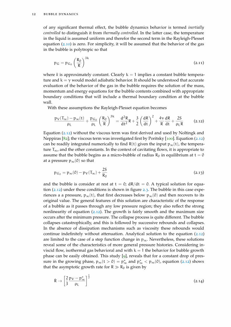
Figure 2.3: Typical solution of the Rayleigh-Plesset equation for spherical bubble size/ initialsize, R/R0. The nucleus enters a low-pressure region at a dimensionless time of 0

and is convected back to the original pressure at a dimensionless time of 500. Thelow-pressure region is sinusoidal and symmetric about 250 [9].

Thus, following an initial period of acceleration, the velocity of the interface is rela-tively constant. It should be emphasized that equation (2.14) implies explosive growthof the bubble, in which the volume displacement is increasing like t3.

2.3 collapse

In case that R R0, equation (2.12) yields

R→ −

(R0R

)3/2 [2(p∗∞ − pV)

3ρL+

2S

ρLR0−

2pG03(k− 1)ρL

(R0R

)3(k−1)]1/2(2.15)

in contrary to the growth phase, p∗∞ indicates a constant jump in the pressure. In thecase of k = 1 the gas term can be simplified, however, most bubble collapse motionbecomes so rapid that the gas behavior is much closer to adiabatic than isothermaland we therefore assume k 6= 1.

For a bubble with a substantial gas content the asymptotic collapse velocity givenby equation (2.16) will not be reached and the bubble will simply oscillate about anew, but smaller, equilibrium radius. On the other hand, when the bubble containsvery little gas, the inward velocity will continually increase (as R−3/2) until the lastterm within the curly brackets reaches a magnitude comparable to the other terms.The collapse velocity then decreases and a minimum size given by

Rmin = R0

[1

(k− 1)

pG0p∗∞ − pV − pG0 + 3S/R0

] 13(k−1)

(2.16)

14 bubble dynamics

will be reached, following which the bubble will rebound. Note that if pG0 is smallRmin could be very small indeed. The pressure and temperature in the bubble at theminimum radius are then given by pm and Tm where

pm = pG0 [(k− 1)(p∗∞ − pV + 3S/R0)/pG0 ]

k/(k−1) (2.17)

Tm = T0[(k− 1)(p∗∞ − pV + 3S/R0)/pG0 ] (2.18)

The case of zero gas content presents a special albeit somewhat a hypothetical prob-lem, since the bubble will reach zero size and at that time will have an infinite inwardvelocity. In the absence of both surface tension and gas content, Rayleigh (1917) wasable to integrate equation (2.12) to obtain the time, ttc, required for total collapse fromR = R0 to R = 0:

ttc = 0.915(

ρLR20

p∗∞ − pV

) 12

(2.19)

It is important at this point to emphasize that while the results for bubble growth arequite practical, the results for bubble collapse may be quite misleading. Apart fromthe neglect of thermal effects, the analysis was based on two other assumptions thatmay be violated during the collapse:

1. The final stages of collapse may involve such high velocities (and pressures) thatthe assumption of liquid incompressibility is no longer appropriate.

2. It transpires that a collapsing bubble loses its spherical symmetry in ways thatcan have important engineering consequences.

The stability to non-spherical disturbances has been investigated from a purely hy-drodynamic point of view by Birkhoff [6] and Plesset and Mitchell [98], among others.These analysis essentially examine the spherical equivalent of the Rayleigh-Taylor in-stability; they do not include thermal effects.

Neglecting the inertia of the gas in the bubble, then the amplitude, a(t), of a spher-ical harmonic distortion of order n (n > 1) will be governed by the equation:

d2a

dt2+3

R

dR

dt

da

dt−

[(n− 1)

R

d2R

dt2− (n− 1)(n+ 1)(n+ 2)

S

ρLR3

]a = 0 (2.20)

It is clear from this equation that the most unstable circumstances occur when R < 0and R >= 0. These conditions will be met just prior to the rebound of a collapsingcavity. On the other hand the most stable circumstances occur when R > 0 and R < 0,which is the case for growing bubble as they approach their maximum size. As thebubble grows the wavelength on the surface increases, and hence the growth of theamplitude is lessened. The reverse occurs during collapse. In any real scenario ofthe bubble growth, the initial acceleration phase for which R >= 0 and thereforevulnerable to instability, is of limited duration, so the issue will be whether or not theinstability has sufficient time during the acceleration phase for significant growth tooccur.

Plesset and Mitchell performed hand calculations of equation (2.20) for small n andfound only minor amplification during growth. However, as can be anticipated fromthis equation, the amplitude may be much larger for large n. In any case, the last phase

2.4 about the bubble collapse 15

Figure 2.4: The bubble surface Mach number, −R/c, plotted against the bubble radius (relativeto the initial radius) for a pressure difference, p∞ − PGM, of 0.517 bar. Results areshown for the incompressible analysis and for the methods of Herring [45] andGilmore [37]. Schneider’s [108] numerical results closely follow Gilmore’s curveup to a Mach number of 2.2 [9].

of the growth phase, in which R > 0 and R < 0, is stable to all spherical harmonicperturbations. So, if inadequate time is available for growth of the perturbations dur-ing the acceleration phase, then the bubble will remain unperturbed throughout itsgrowth.

In their experiments on underwater explosions, Reynolds and Berthoud [103] ob-served bubble surface instabilities during the acceleration phase that did correspondto fairly large n of the order of 10. Their bubbles become smooth again in the second,deceleration phase of growth. The bubble examined by Reynolds and Berthoud wherefairly large, 2.5 cm to 4.5 cm in radius. The similar behavior has not been reported forthe smaller bubbles. This could either be the result of a brief acceleration phase or thegreater stabilizing effect of surface tension in smaller bubbles.

2.4 about the bubble collapse

When a cavitation bubble grows from a small nucleus to many times its original size,the collapse will begin at a maximum radius, RM, with a very small partial pressureof gas, PGM. In a typical cavitating flow, RM is of the order of 100 times the originalnuclei size, R0. Consequently if the original partial pressure of gas inside the bubbleis around 1 bar it would reduce to 10−6 bar at the beginning of the collapse.

Considering a pressure drop of 0.1 bar in the fluid, p∗∞ − pV , it follows from equa-tion (2.17) that the maximum pressure generated during the collapse would be about1010 bar and the maximum temperature would be 4× 104 times the ambient tempera-ture! Many factors including the diffusion of gas from the liquid into the bubble andthe effect of liquid compressibility, mitigate this result. Nevertheless, the calculationillustrates the potential for the generation of high pressures and temperatures duringcollapse and the potential for the generation of shock waves and noise.

16 bubble dynamics

First inclusion of compressibility for low Mach number, |dR/dt|/c, was done byHerring [45]. The gas was considered condensible, thermal effects were neglectedand therefore the pressure in the bubble remains constant. Schneider [108] and laterGilmore [37], treated the same highly idealized problem for cases in which the Machnumber of collapse reaches up to 2.2. Figure 2.4 demonstrates how, in the idealizedproblem, the Mach number of the bubble surface increases as the bubble radius de-creases. The slope is approximately −3/2 since |dR/dt| ∝ R− 3

2 . Note that compress-ibility tends to lessen the velocity of collapse.

In the absence of thermal, viscous and surface tension effects Keller and Kolod-ner [69] modified the RP equation (2.8) to incorporate the effects of compressibilityand proposed(

1−1

c

dR

dt

)Rd2R

dt2+3

2

(1−

1

3c

dR

dt

)(dR

dt

)2=

(1+

1

c

dR

dt

)1

ρL[pB − p∞ − pc(t+ R/c)] +

R

ρLc

dpBdt

(2.21)

pc(t) denotes the variable part of the pressure in the liquid at the location of the bub-ble center in the absence of the bubble. Other modified versions of the RP equationhave been also presented and most are shown to be equivalent [101]. It has also beendemonstrated that for Mach number higher than 0.3 the modification are no longer ac-curate and the compressible liquid field equation must be solved to obtain acceptablesolution.

The primary importance of liquid compressibility is not the effect it has on thebubble dynamics, but the role it plays in the formation of shock waves during therebounding phase that follows collapse.

Hickling and Plesset [46] were the first to make use of numerical solutions of thecompressible flow equations to explore the formation of pressure waves or shockduring the rebound phase. Figure2.5 presents the variation of pressure distributionbefore and after the moment of minimum size. The graph on the right clearly showsthe propagation of a pressure pulse or shock wave from the bubble following theminimum size. As it is indicated the pressure pulse exhibits a geometric attenuation(r−1) as it propagates away from the bubble. Among many calculations carried onlater, Ivany and Hammitt [61] confirmed that neither surface tension nor viscosityplay a significant role in the problem. It appears that, in most cases, the pressure pulseradiated into the liquid has a peak pressure amplitude, pP, which is given roughly by

pP ≈ 100RMp∞/r (2.22)

This equation gives an insight on the strength of pressure pulse, which might impingeon a solid surface a few radii away. For example, a pressure pulse of 100 bar is to beexpected at a distance r = RM and with far field liquid pressure, p∞, of 1 bar. All ofthese analyses assumes spherical symmetry, something which may be violated duringthe collapse or rebound phase.

2.5 essentials of the bubble dynamics 17

Figure 2.5: Typical results of Hickling and Plesset [46] for the pressure distributions in theliquid before collapse (left) and after collapse (right) (without viscosity or surfacetension). The parameters are p∞ = 1 bar, γ = 1.4, and the initial pressure in thebubble was 10−3 bar. The values attached to each curve are proportional to thetime before or after the minimum size [9].

2.5 essentials of the bubble dynamics

Studies on the 1D bubble dynamics, as presented up to now, suggest that for a realisticmodeling of the bubble behavior following considerations are crucial:

1. Both internal air and external water have to be modeled as compressible to cor-rectly represent the damped radial oscillation of the pressure wave.

2. At the final stage of the collapse instabilities, of both shape and surface types,appear and therefore the symmetry assumption is no more valid. Althoughthese instabilities may appear for a very short period, they severly affect theintensity of the emitted shock waves.

3. Lack of symmetry and the possibility of the shock presence necessitate the solu-tion of the full hydrodynamics set of equations. Challenges appear in this caseare:

- Efficiently represent the coupled compressible fluid dynamics of both phases(liquidand gas).

- Accurately track the interface between the phases. This is important tostudy the instabilities that may appear.

- Appropriately resolve any shock waves which may be created in one orboth phases during the final stage of bubble implosion.

4. The initial size of the bubble and the initial external and internal pressures havecrucial effects both on the bubble oscillation modes and on the shape/surfaceinstabilities.

18 bubble dynamics

In this work we choose the Lagrangian description of the hydrodynamic equationsfor the simulation of underwater implosion. Numerical schemes in Lagrangian coor-dinates, by construction, are capable of precisely capturing and tracking contact dis-continuities without adding any numerical dissipation. Furthermore, recent develop-ments in Lagrangian shock hydrodynamics algorithms, hydrocodes, have improved therobustness of simulation with respect to mesh distortion, while maintaining second-order accuracy in smooth regions of the flow.

We close this section by referencing the Lagrangian frameworks and in particularthe Particle Finite Element Method (PFEM) as one of the most renown one.

2.6 lagrangian framework

PFEM belongs to the family of particle methods in which all kinetic and kinematicinformations are carried by fluid particles. Gingold [38] pioneered the first attemptsin this approach to treat astrophysical hydrodynamic problems which lead to the so-called Smooth Particle Hydrodynamics Method (SPH) that later was generalized to fluidmechanics problem [8, 26]. Kernel approximation are used in the SPH method tointerpolate the unknowns. It must be noted that the particle methods may be usedwith either mesh-base or meshless shape functions.

In the field of meshless methods various formulation have been developed forthe fluid and structure problems. All these methods use the idea of a polynomialinterpolant that fits a number of points minimizing the distance between the inter-polated function and the value of the unknown point. These ideas were proposedfirst by Nayroles et al [79] which were later used by Belytschko et al [2] for struc-tural problems. Oñate et al [90, 58] proposed the Finite Point Method (FPM) [90] forconvection-diffusion in fluid flow problems and then generalized it by Idelsohn et alto the Meshless Finite Element Method (MFEM) [58]. MFEM uses the extended Delau-nay tessellation to build a mesh combining elements of different polygonal shapes ina computing time which is linear with the number of nodal points.

PFEM treats the mesh nodes in either fluid or solid domains as particles which canfreely move an even separate from the main fluid domain representing, for instance,the effect of drops (Figure 2.6). A finite element mesh connects the nodes defining thediscretized domain where the governing equations are solved in the standard FEMfashion. The same elements and shape function as of the MFEM are used in the firstversions of the PFEM but later standard simple elements (triangles or tetrahedra) withstandard shape functions were used.

An obvious advantage of the Lagrangian formulation is that the convective termsdisappear from the fluid equations, however, the difficulty is transfered to the prob-lem of particles final positions. Indeed for large mesh motions, re-meshing may be afrequent necessity along the time solution.

In the opinion of the author, this is one of the main drawbacks of the method as itbecomes quite time consuming, comparing to the solve and build, especially by theraise of massive parallel solvers. To this end and also to be able to perform real timesimulation, Idelsohn et al [55] have recently proposed a new PFEM that liberates theneed to mesh generation and indeed improve particle motion by integrating along thestreamlines.

As an overview, the main properties of the PFEM can be summarized as :

2.6 lagrangian framework 19

Figure 2.6: 3D dambreak modelled in the PFEM [92].

20 bubble dynamics

Figure 2.7: PFEM solution steps illustrated in a simple dam break example. As the gate ofthe dam is removed the water begins to flow. (a) Continuous problem (b) Step 1,discretization in cloud of nodes at time tn; (c) Step 2, boundary and interface recog-nition; (d) Step 3, mesh generation; (e) Step 4, resolution of the discrete governingequations; (f) Step 5, nodes moved to new position for time tn+1 [25].

1. Lagrangian description of the governing equations.

2. Particle-based discretization of the kinematic and kinetic variables.

3. Generation of the mesh and identification of the domain boundaries.

The most crucial characteristic of the PFEM and any other particle method is that thereis not a specified solution domain. The domain is defined by the particle positionsand hence, there is not a boundary surface or line. This is the reason why, whena differential equation is to be solved, in order to evaluate the forces, the boundarysurface need to be identified to impose the boundary conditions. PFEM uses an alpha-shape technique [29], to recognize the external boundary after the triangulation ortetrahedralization of the domain. Base on this method the error in the definition ofthe boundary surface is proportional to the element size. Figure 2.7 depicts the varioussteps involves in a typical PFEM solution step. In summery a typical solution withthe PFEM involves the following steps:

1. A cloud of particles, mesh nodes, that descritize all the interested media in-volved in the simulation is given.

2. External and internal boundaries are recognized. Exterior boundaries, if are notfixed, are obtained using the alpha-shape technique and the internal ones aremarked by the interface following or capturing technique.

3. The new mesh is generated either by using the same cloud of particle as step 1

or by an enriched cloud of node interpolated upon the base cloud of particles.

2.6 lagrangian framework 21

4. Solution of the Lagrangian governing set of equations together with the bound-ary and interface conditions. It results in the updated set of nodal variables thatare stored in the particles.

5. Moving the mesh nodes, particles, to the new position obtained from the solu-tion step.

6. Go back to step 1 and repeat the solution. Note that in case of small deforma-tions the same mesh can be used for the new step.

One of our goals in this work is to improve the current state of the art in hyrdrocodesfor flows with large deformations. As it is already mentioned, current Lagrangianshock hydrodynamics algorithms are capable of treat cases with large distortions ofthe mesh but few works are able to solve highly deformed flows where the initialFEM mesh is no more suitable. The approach followed in this thesis is simply equipthe hydrocodes with the adaptive mesh generating module of the PFEM and thenimprove it for the case of two-fluid flows by precisely following the interface andduplicating the kinetic variables at the interface level. Next chapter is devoted to thestep-by-step build up of this approach.

3G O V E R N I N G E Q U AT I O N S

The material of this section is taken from our paper A Compressible Lagrangian frame-work for the simulation of the underwater implosion of large air bubbles [68]. we present afully Lagrangian shock hydrodynamics framework to solve two-phase flow problemswith large distortions at the interface and big pressure and density jumps. To solvethe hydrodynamic set of equations in each phase the stabilized variational multiscalemethod presented by Scovazzi et al [109] is adopted. Later we improve the interfacedetecting technique proposed by Idelsohn et al [57, 56], by conserving the interfaceconnectivities. This method is then extended to compressible multi-fluid flows byconsidering a discontinuous representation of the kinetic variables, i.e. pressure anddensity, at the interface level. The simulation of the large-bubble implosion using theproposed framework allows to identify, to our best knowledge for the first time, theappearance of the RT instabilities in these bubbles, at the final stage of the collapse.The possibility of the appearance of such instabilities has been reported by manyauthors [46, 48, 7, 77, 9]. We continue the simulation during the rebounce phase tillinstabilities disappear and the second collapse occurs. The second collapse ends upwith the rupture of the air bubble.

3.1 introduction

As explained in the previous chapter, the underwater implosion of air-filled bubbleshas been studied by many authors in the last century due to its main role in a numberof phenomena in science, like sonoluminescence, sonochemistry and sonofusion anda series of applications in engineering like cavitation damages, seabed detection andstructure safety in the vicinity of the imploded volumes.

Historically, the first work on the cavitation and bubble dynamic was done byRayleigh [102], who considered the collapse of both empty and gas filled cavitiesin an inviscid incompressible liquid. Plesset extended his work by adding surfacetension and viscous effects that resulted in the famous Rayleigh-Plesset equation [46].The presence of high pressures in liquid near the interface in addition to the dampingoscillations of the bubble lead many authors to take into account for the compressibil-ity of the surrounding liquid in their analysis [69, 45, 101]. Depending on the initialradius of the bubble and external driving pressure two types of behavior are observedin the bubble motion, namely weakly oscillating and strongly collapsing.

In physics, violent collapse of µm size bubbles excited by the sound waves maylead to UV-light emission of picoseconds duration that is known as sonoluminescence,SL [48]. Super compression of the internal air and high velocities obtained during thefinal stage of the violent collapse put in doubt the stability of the bubble. Later stud-

23

24 governing equations

ies on the shape stability of the bubble [99, 7] revealed that the spherical symmetryassumption can not be rigorously correct especially in the final stage of the violentcollapse. Bogoyavlenskiy [7] demonstrated that time derivatives of shape perturba-tions grow significantly as the bubble radius vanishes. In general two different typesof instabilities are prone to be excited during this stage, (i) interfacial instabilities, i.e.Rayleigh-Taylor (RT) instabilities, which occur when a gas is strongly accelerated intothe liquid, and (ii) shape instabilities due the excitation of non-spherical modes caus-ing the bubble to take on a non spherical shape. The shape instability is well shownin the DNS results provided by Nagrat et al [77] for a micron-size bubble implosion.Although they predict the RT instabilities during the very short time interval thatthe bubble radius is near its minimum, no numerical evidence is presented in theirresults.

In engineering applications, on the other hand, larger size bubbles, in the order ofcm, are of interest. Acoustic waves emanated from broken glass spheres are used toindicate the contact of the equipment with the seabed. Orr et al [94] have reportedthe pressure signatures and energy-density spectra for a series of preweakend hollowglass spheres imploded at ocean depths of approximately 3 km. The signature ofall implosions have many features in common. Basically each consists of a low flatnegative-pulse followed by a sharp positive-pressure spike of roughly 0.2 ms duration.Different pressure signature is reported for shallow depth implosion, less than 300 m.Here linear oscillation, resembling a strongly damped sinusoid with damping factorof e per oscillation cycle occurs. McDonald et al [75] propose turbulent instabilitiesexcited by the shape oscillation of the bubble as the decay mechanism in shallowdepth. Recently, Turner [129] studied the influence of the structure failure on thepressure pulse. Four glass spheres of diameter 7.62 cm were imploded in a pressurevessel at a hydrostatic pressure of 6.996 MPa and the pressure-time histories werecompared with numerical results obtained from different failure rates. He reportedan error of 44% for models that do not account for structure failure.

The development of efficient algorithms to understand rapid bubble dynamicspresents a number of challenges. The foremost challenge is to efficiently representthe coupled compressible fluid dynamics of internal air and surrounding water. Sec-ondly, the method must allow one to accurately detect or follow the interface betweenthe phases. Finally, it must be capable of resolving any shock waves which may becreated in air or water during the final stage of the collapse. Regarding the Eulerianapproach and for small bubbles, µm-size, Nagrat et al [77] proposed a DNS solutionof the full hydrodynamics set of equations stabilized by the SUPG method. The inter-face is tracked by a modified level-set method and a DC operator is added to providesmooth transition in shock zones. Surface tension is also included to see its influenceon the final shape of the bubble. Concerning large bubbles, in the order of cm, Farhatet al [31] solved the Euler equation for the multi-fluid problem using a ghost fluidmethod for the poor (GFMP) generalized for an arbitrary equation of state (EOS). Vis-cous effect and surface tension are neglected due to the size of the bubbles and anexact Riemann solver is used to resolve the shock at the interface.

Lagrangian frameworks to solve the Euler equations in the presence of the shockwaves and with large mesh movement have been developed by different authors. Ef-forts have been dedicated to improve the robustness of the simulation with respect tomesh distortion, while maintaining second order accuracy in smooth regions of the

3.2 governing equations 25

flow [109, 1, 13]. Scovazzi et al [109] developed a robust second-order FEM methodwith continuous linear approximation of kinematic and kinetic variables that is sta-bilized by operators driven from the variational multiscale paradigm. In moving La-grangian curvilinear coordinates, traditional staggered grid hydro (SGH) methods,that use continuous linear representation for kinematic variables and discontinuousconstant field for thermodynamic variables, have been extended for higher order ele-ments [27].

All of the above mentioned Lagrangian methods are able to treat air or water phaseas well as to represent shock waves in them. None of them, however, is designed tocapture possible distortions of the interface that appear in multi-fluid flow. The recentdevelopments in the Particle Finite Element Method (PFEM) [59, 92, 57, 56] to dealwith multi-fluid flows provide a good basis to capture interface instabilities in thefinal stage of the collapse. In particular, Idelsohn et al [57, 56] successfully track theinterface in an incompressible heterogeneous flows in the presence of large densityand viscosity jumps. Interface is forced to match the nodes and due to the jump inpressure gradient across the interface, a discontinuous pressure gradient projection isnecessary to stabilize the flow near the interface.

In the next section a review of the stabilized variational multiscale method devel-oped by Scovazzi et al [109] to solve the Euler hydrodynamic set of equations ispresented. Then, the interface-following technique proposed by Idelsohn et al [57, 56]is presented and extended for compressible flow, emphasizing on the use of a discon-tinuous pressure along the interface. In the final section we present some numericalexamples that verify the method and show its potential for simulating the implosionof a large size cylindrical bubble.

3.2 governing equations

3.2.1 Euler equations

Let us define the admissible transformation Φ, figure 3.1, from a reference configura-tion, X, to the current configuration, x, as,

Φ : Rnd → Rnd

X 7→ x = Φ(X, t)

where nd is the spatial dimension, the deformation gradient, F, is defined as, FiA =∂xi∂XA

, and the determinant of F defines the Jacobian determinant of the transformation.Conservation of mass M is expressed as,

0 =dM

dt=d

dt

(∫Ωt

ρdΩ

)=d

dt

(∫Ω0

ρJ dΩ0

)=d

dt

(∫Ω0

ρ0 dΩ0

)(3.1)

In the third equality we made use that for any infinitesimal volume dΩ we have,dΩ = J dΩ0. As the domain Ω0 is arbitrary and in the Lagrangian coordinate is not afunction of time we have the following expression for the mass conservation,

ρJ = ρ0 (3.2)

26 governing equations

Figure 3.1: Lagrangian map Φ

Note that in the updated Lagrangian formalism Ω0 is used for any previous config-uration and not necessarily for the initial, t = 0, configuration.

The conservation of momentum for the arbitrary volume Ω is written as,

d

dt

(∫Ω

ρudΩ)

=

∫Ω

ρbdΩ+

∫S

σ · ndS (3.3)

where u is the velocity, b is the body force, σ is the Cauchy stress tensor and n is thenormal to the exterior surface S. Recalling the mass conservation (3.2) to evaluate theleft hand side of (3.3) and applying the Gauss divergence theorem to the right handside, we have:∫

Ω

ρudΩ =

∫Ω

(ρb +∇ ·σ) dΩ (3.4)

for any arbitrary domain Ω which implies that,

ρu = ρb +∇ ·σ (3.5)

For hydrodynamic flows, shear stresses are neglected and the stress tensor σ is repre-sented by the volumetric stress, i.e. pressure, p as,

σ = −pI

where I is a nd ×nd unity tensor.The conservation of the total energy per unit mass, E, as the sum of the internal

energy, ε, and the kinetic energy, 12u · u, is written as,

d

dt

(∫Ω

ρEdΩ

)=

∫Ω

ρ(u · b + r)dΩ+

∫S

(σ · u + q) · ndS (3.6)

u · b is the specific power due to body forces, r is the specific rate of internal energyproduction, the power added due to to the surface work of surface tensions are in-cluded by σ · u and the transfered heat by the heat flux q. The same procedure asthe one applied for the momentum conservation is exploited to obtain the followingconservative form of the energy equation,

ρE = ρ(ε+ u · u) = −∇ · (pu + q) + ρb · u + ρr (3.7)

Note that σ is replaced by −pI.

3.2 governing equations 27

A non-conservative form of the energy equation can be obtained by multiplying themomentum equation (3.5) by u and use to simplify the conservative form (3.7) toobtain,

ρε+ p∇ · u = ∇ · q + ρr (3.8)

3.2.2 Lagrangian hydrodynamic equations

Underwater implosions result in bubbles whose characteristic size is considerablylarger than that of bubbles obtained in liquid suspensions. Hence such bubbles areless affected by surface tension and viscous forces and therefore their dynamics canbe modeled by the Euler equations:

ρJ = ρ0

ρu +∇xp = b inΩ, t ∈]0, T [ (3.9)

ρε+ p∇x · u = ∇x · q + ρr inΩ, t ∈]0, T [

The gradient derivatives,∇x, are calculated in the current configuration and () refersto the material time derivative. J is the deformation Jacobian determinant, ρ0 is thereference density, ρ is the current density, u is the velocity vector, b is the body force, pis the thermodynamic pressure, r is the energy source term, q is the heat flux and ε isthe internal energy per unit mass. Although the energy equation is not written in theconservative form it can still be used to develop a globally conservative variationalformulation [109].

For the sake of simplicity and without loss of generality, a homogeneous Dirichletboundary condition is considered. These equations and the boundary conditions, inaddition to an equation of state for the pressure p and a constitutive law for the heatflux, q, together with the appropriate initial conditions define the evolution of thesystem.

We use the Mie-Grüneisen equation of state (EOS) that is widely used in today’shydro-codes to model real materials such as compressible ideal gases, co-volumegases, high explosives, elasto-plastic solids with negligible shear strength etc [111,113, 132, 76]. The hydrostatic pressure, p, is then related to the density, ρ, and internalenergy, ε, as the following,

p = p(ρ, ε) = f1(ρ) + f2(ρ)ε. (3.10)

where f1 and f2 are known from the reference thermodynamic state of the system.Ideal gases, as an example, can be expressed using equation of state (3.10) if f1 = 0.0and f2 = (γ−1)ρ. Note that another equivalent of (3.10) can be written for the internalenergy, ε, as, ε = ε(ρ,p). In this case the differentiation of ε is computed as,

dε =∂ε

∂ρ

∣∣∣pdρ+

∂ε

∂p

∣∣∣ρdp (3.11)

28 governing equations

By considering (3.11) and recalling the differential form of the conservation of mass,ρ+ ρ∇ · u = 0, the energy equation (3.8) can be rewritten as,

0 = ρε+ p∇ · u

= ρ∂ε

∂ρ

∣∣∣pρ+ ρ

∂ε

∂p

∣∣∣ρp+ p∇ · u

= ρ∂ε

∂p

∣∣∣ρ

p+ pρ − ρ∂ε∂ρ

∣∣∣p

∂ε∂p

∣∣∣ρ

∇ · u

(3.12)

For a general compressible flow ρ ∂p ε|ρ 6= 0. It is possible to further simplify theprevious equations. First note that, by standard calculus derivations,(

∂ε

∂p

∣∣∣ρ

)−1

=∂p

∂ε

∣∣∣ρ

. (3.13)

Second, by the combination of the first and second law of thermodynamics, i.e. Gibbsidentity, we have, dε− p/ρ2dρ = Tdη. Where T is temperature and η is the entropyper unit mass. For a constant entropy we have,

p

ρ= ρ

∂ε

∂ρ

∣∣∣η

(3.14)

The multiplying factor in the last term of equation (3.12), can be rewritten using (3.13)and (3.14) as,

pρ − ρ∂ε∂ρ

∣∣∣p

∂ε∂p

∣∣∣ρ

= ρ∂p

∂ε

∣∣∣ρ

(∂ε

∂ρ

∣∣∣η−∂ε

∂ρ

∣∣∣p

). (3.15)

Recalling the EOS of the form p = p(ρ, ε), we have:

dp =∂p

∂ρ

∣∣∣εdρ+

∂p

∂ε

∣∣∣ρdε (3.16)

that for the the constant pressure leads to,

0 =∂p

∂ρ

∣∣∣p=∂p

∂ρ

∣∣∣ε+∂p

∂ε

∣∣∣ρ

∂ε

∂ρ

∣∣∣p

. (3.17)

3.2 governing equations 29

Substituting (3.17) into (3.15) yields

pρ − ρ∂ε∂ρ

∣∣∣p

∂ε∂p

∣∣∣ρ

= ρ

(∂p

∂ε

∣∣∣ρ

∂ε

∂ρ

∣∣∣η−∂p

∂ε

∣∣∣ρ

∂ε

∂ρ

∣∣∣p

)

= ρ

(∂p

∂ε

∣∣∣ρ

∂ε

∂ρ

∣∣∣η+∂p

∂ρ

∣∣∣ε

)= ρ

∂p

∂ρ

∣∣∣η

= ρc2s , (3.18)

where cs is the isentropic speed of sound in the medium. Hence (3.12) reduces to,

0 = ρ∂ε

∂p

∣∣∣ρ

(p+ ρc2s∇x · u

). (3.19)

The term ρ∂pε|ρ 6= 0 can be simplified in (3.19), and the momentum and energyequations can be combined into the mixed, first order system form of a nonlinearwave equation in u and p as,

ρu +∇xp = 0

p+ ρc2s∇x · u = 0. (3.20)

We recognize here the relation between ∂pε|ρ and the Grüneisen parameter [76], de-fined as

Γ =1

ρ ∂ε∂p |ρ=1

ρ

∂p

∂ε

∣∣∣ρ

. (3.21)

The thermodynamic parameter Γ varies only mildly with the thermodynamic state ofa fluid system, unless phase transition occur [76]. In the case of an ideal gas satisfyinga γ-law EOS, it is easy to drive Γ = 1− γ = cte.

As the hydrodynamic equations (5.1) are quite nonlinear, we first develop the sta-bilized variational multiscale form of the linearized version of these equations, (3.20).Such linearized problem is presented in the next section.

3.2.3 Stabilization of the linearized form

The linearization is done considering a small-strain approximation in which the deriva-tives in the reference and current configurations coincide and the solution of the ther-modynamic variables, density, pressure and internal energy, is considered as a smallperturbation to the constant reference state;

ρ = ρ+ ρ, ρ = const., ρ 1, (3.22)

p = p+ p, p = const., p 1, (3.23)

cs = cs + cs, cs = const., cs 1. (3.24)

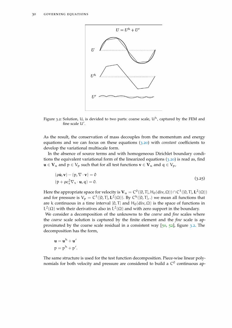
30 governing equations

Figure 3.2: Solution, U, is devided to two parts: coarse scale, Uh, captured by the FEM andfine scale U ′.

As the result, the conservation of mass decouples from the momentum and energyequations and we can focus on these equations (3.20) with constant coefficients todevelop the variational multiscale form.

In the absence of source terms and with homogeneous Dirichlet boundary condi-tions the equivalent variational form of the linearized equations (3.20) is read as, findu ∈ Vu and p ∈ Vp such that for all test functions v ∈ Vu and q ∈ Vp,

(ρu, v) − (p,∇ · v) = 0(p+ ρc2s∇x · u,q) = 0.

(3.25)

Here the appropriate space for velocity is Vu = C0([0, T ],H0(div,Ω))∩C1([0, T ], L2(Ω))

and for pressure is Vp = C1([0, T ], L2(Ω)). By Ck([0, T ], .) we mean all functions thatare k continuous in a time interval [0, T ] and H0(div,Ω) is the space of functions inL2(Ω) with their derivatives also in L2(Ω) and with zero support in the boundary.We consider a decomposition of the unknowns to the coarse and fine scales where

the coarse scale solution is captured by the finite element and the fine scale is ap-proximated by the coarse scale residual in a consistent way [50, 52], figure 3.2. Thedecomposition has the form,

u = uh + u ′

p = ph + p ′.

The same structure is used for the test function decomposition. Piece-wise linear poly-nomials for both velocity and pressure are considered to build a C0 continuous ap-

3.2 governing equations 31

proximation of the test and trial functions over the domain. Equations (3.25) tested bythe coarse scale test functions reduce to

(ρ(uh + u ′), vh) − (ph + p ′,∇ · vh) = 0(ph + p ′ + ρc2s∇x · uh,qh) + (ρc2s∇x · u ′,qh) = 0.

(3.26)

Some well known simplifications in the context of the variational multiscale approach [50,52] are considered as follows,

1. Fine scales are considered quasi-static and as a consequence their time deriva-tives are neglected in comparison to the time derivatives of the coarse scales.This implies that the fine scales adjust instantaneously to complement the coarsescales.

2. For smooth flows or at least smooth regions of the flow one expect continuoussolutions. Therefore the fine scales, similarly as the coarse ones, are consideredat least continuous in the entire domain. As a result inter-element fluxes areautomatically canceled.

3. No contribution of the fine scales is considered on the exterior boundaries.

Integrating by part the last term of equations (3.26) and considering the previousassumptions, the coarse scale equations (3.26) reduce to,

(ρuh, vh) − (ph + p ′,∇ · vh) = 0(ph + ρc2s∇x · uh,qh) − (ρc2su ′,∇xqh) = 0.

(3.27)

Fine scales u ′,p ′ in the coarse scale equations (3.27) are obtained by testing equa-tions (3.25) this time by the fine scale test functions, that is,

(ρu ′, v ′) − (p ′,∇ · v ′) = − < Rhu, v ′ >

(p ′ + ρc2s∇x · u ′,q ′) = − < Rhp,q ′ > .

(3.28)

Rhu and Rh

p are residuals of the momentum and energy equations, respectively andare obtained considering the same assumptions mentioned above. They have the fol-lowing forms

Rhu := ρuh +∇xph

Rhp := ph + ρc2s∇x · uh.

(3.29)

Fixing v ′ and q ′, the left sides of the equations (3.28) can be seen as complicatedoperators of the fine scales acting on v ′ and q ′. In this case and by means of the RieszRepresentation theorem [83], residuals introduced in equation (3.29) can be identifiedas the Riesz candidates for these operators and therefore it is guaranteed that Rh

u andRhp belong to the space of v ′ and q ′, respectively.

32 governing equations

As the exact solution of the fine scale equations (3.28) is expensive and even unnec-essary, one simple way to approximate subscales would be through residuals (3.29) as(see [18, 42] and references therein for the similar approach),

u ′ = −τ1

ρRh

u

p ′ = −τRhp

(3.30)

where τ has dimension of time.This seems to be the simplest approach because subscale approximations are com-

pletely decoupled one from another. Consequently, the time derivative terms in equa-tions (3.28) are dominant and so only their discrete inverse τ1ρ and τ are used to scalethe residuals Rh

u, Rhp respectively.

Inserting the preceding approximations (3.30) into the coarse scale equations (3.27)the final stabilized form of the linearized acoustic problem is:

(ρuh, vh) − (ph,∇x · vh) + (ph + ρc2s∇x · uh,∇x · vh)τ = 0

(3.31)

(ph + ρc2s∇x · uh,qh) + (c2s(ρuh +∇xph),∇xqh)τ = 0.

The main stabilization effect comes from an incomplete Laplacian of the velocity,

(∇x · uh,∇x · vh)τc2s ,

in the momentum equation and a full Laplacian of the pressure,

(∇xph,∇xqh)τc2s ,

in the energy equation. In addition, the presence of the full residual avoids reductionin accuracy order, which is quite common in residually inconsistent stabilizations.

A similar set of stabilized equations can be obtained using the Finite Calculus (FIC)approach [85, 86].

In the following section we present the full stabilization for the nonlinear case, in-spired in the linearized one previously mentioned.

3.2.4 Stabilization of the nonlinear form

The variational multiscale stabilization of the linearized case reveals the overall struc-ture of the stabilization method. To elaborate the variational multiscale stabilization ofthe nonlinear form, first the variational equivalence of the hydrodynamic set of equa-tions (5.1) is presented. We consider homogeneous Dirichlet boundary conditions and

3.2 governing equations 33

r, q and b are set to zero. We are interested in finding u ∈ Vu and p, ρ, ε ∈ Vp suchthat, ∀v ∈ Vu and ∀q ∈ Vp∫

Ω0

q (ρ0 − ρJ)dΩ0 = 0 (3.32a)∫Ω

v · (ρ u)dΩ+

∫Ω

σ : ∇sxvdΩ = 0 (3.32b)∫Ω

q (ρ ε−σ : ∇sxu)dΩ = 0. (3.32c)

Here ∇sx is the symmetric part of the gradient operator and σ = −p I. Piece-wiselinear continuous approximation of both kinematic,u, and thermodynamic, p, ρ andε, variables are considered. We consider the same decomposition as is performed forthe velocity and pressure in section 3.2.3, but this time the decomposition of the ε isalso added. This gives,

u = uh + u ′

p = ph + p ′ (3.33)

ε = εh + ε ′.

Scovazzi [109] consider also the decomposition of ρ to develop the multiscale method.However, as it has no apparent contribution to the final stabilized form, the densitydecomposition is omitted here. Furthermore, due to the intrinsic ability of the La-grangian description to exactly track contact discontinuities without adding numeri-cal dissipation, and as the mass conservation is associated with one of these disconti-nuities in the form of standing entropy wave, we only focus on the momentum andenergy equations to construct the stabilized form.

Inserting the decomposition (3.33) into the variational form (3.32b)-(3.32c), the coarsescale equations are formulated as,∫

Ω

vh · ρ (uh + u ′)dΩ−

∫Ω

(ph + p ′) (∇x · vh)dΩ = 0 (3.34)∫Ω

qh ρ (εh + ε ′)dΩ

+

∫Ω

qh (ph + p ′) ∇x · (uh + u ′)dΩ = 0. (3.35)

Using integration by parts, the energy equation (3.35) can be reformulated as,∫Ω

qh ρ (εh + ε ′)dΩ+

∫Ω

qh (ph + p ′) ∇x · uh dΩ−∫Ω

∇xqh · ((ph + p ′)u ′)dΩ−

∫Ω

qh (∇(ph + p ′)) · u ′ dΩ

+

nel∑e=1

∫∂Ωe

qh (ph + p ′)u ′ · ne d(∂Ωe) = 0. (3.36)

The last term in (3.36), which is a boundary integral, has two terms; one inter-elementboundary term and one domain boundary term.

34 governing equations

Similar to the linearized case, some simplifications are considered.

1. The fine scale solution, u ′, is considered to be zero on the domain boundary.

2. Assuming a continuous solution for p, u and a continuous approximation for uh,the fine scale solution turns out to be continuous in the inter-element boundarytoo i.e. u ′ = u − uh. As the result, the last term in (3.36) is zero.

3. To preserve the global conservation [109], the internal work done by the fine-scale velocity, u ′, is assumed to be zero in a weak sense:∫

Ω

qh (∇(ph + p ′)) · u ′ dΩ = 0.

4. The quasi-static tracking of the subscales is considered.

5. The product of the fine-scale terms is neglected.

The simplified form of the exact coarse scale equations (3.34) and (3.35) can be writtennow as,∫

Ω

vh · ρ (uh)dΩ−

∫Ω

(ph + p ′) (∇x · vh)dΩ = 0∫Ω

qh (ρεh + ph∇x · uh)dΩ+

∫Ω

qh p ′ ∇x · uh dΩ

−

∫Ω

∇xqh · (ph u ′)dΩ = 0. (3.37)

Certain similarities are observed comparing the nonlinear coarse-scale equations (3.37)and their linear counterpart (3.27). In particular the momentum equations are practi-cally the same and also recalling (3.19),

ρhεh + ph∇x · uh = ρ∂ε

∂p

∣∣∣ρ(p+ ρc2s∇x · u), (3.38)

we observe similarities in the linear and nonlinear energy equations. These similaritiesgive clue to design approximation for the subscales u ′ and p ′. Note that in comparisonto the linearized case (3.27) a new stabilization term of the form,∫

Ω

qh p ′ ∇x · uh dΩ

appears. This term has a fundamental role in the global conservation of total en-ergy [109].

We complete our multiscale stabilization by writing the counterpart of equations (3.34)and (3.35), this time tested by the fine scales and rearranged as,∫

Ω

v ′ · ρu ′dΩ−

∫Ω

p ′(∇x · v ′)dΩ = − < Rhu , v ′ > (3.39)∫Ω

q ′ρε ′dΩ+

∫Ω

q ′p ′∇x · (uh + u ′)dΩ = − < Rhε ,q ′ >

3.2 governing equations 35

where < Rhu , . > and < Rhε , . > belong to the dual space of v ′ and q ′ respectively.They are calculated by doing integration by parts and neglecting the boundary terms,i.e.

< Rhu , v ′ >:=∫Ω

v ′ · (ρhuh +∇xph)dΩ

< Rhε ,q ′ >:=∫Ω

q ′ (ρhεh + ph∇x · uh)dΩ.

Similar to the linearized case and by means of the Riesz representation theorem, thecoarse scale residuals, ρhuh +∇xph and ρhεh + ph∇x · uh, can be identified as themembers of (L2(Ω))nd and L2(Ω) respectively.

We need to approximate subscales from the fine scale equations (3.39) and plugthem into the coarse scale equations (3.37). Note that the only fine scales that appearin (3.37) are u ′ and p ′. Recalling equation (3.38), there is a one by one relationshipbetween Rhε and Rhp, defined in (3.29), so we come out with the same expression asthe linear case to approximate p ′, i.e.

p ′ = −τRhp. (3.40)

Although u ′ can be approximated invoking the same rationalism applied in the lin-earized case, i.e. u ′ = −τ1ρR

hu, and it is still dimensionally consistent, a more delicate

structure could be obtained considering the construction of the term∫Ω∇xq

h · (ph u ′)that appears in the coarse scale equations (3.37). The alternative form we propose forthe velocity subscales to be substituted into the coarse scale equations (3.37) is,

phu ′ = −τ(c2s)Rhu (3.41)

where τ has the dimension of time[53, 71, 126, 127, 122, 109, 68, 18] and is taken as∆t, which was one of the options used in,[53, 71] and was the transient limit of thedefinitions given in[126, 127, 122]. An intuitive interpretation of this choice is to notethat u ′ ∝ ∆t

ρ Rhu and p ∝ ρ c2s .

Introducing the fine scales approximation (3.40) and (3.41) into (3.37), the stabilizedvariational form of the nonlinear hydrodynamic equations is summarized as,∫

Ω

vh · ρ (uh)dΩ−

∫Ω

(∇x · vh)ph dΩ

+

∫Ω

∇x · vh τ (p+ ρc2s∇x · u)dΩ = 0 (3.42)∫Ω

qh (ρεh + ph∇x · uh)dΩ

+

∫Ω

τ(c2s)∇xqh · (ρuh +∇xph)dΩ (3.43)

−

∫Ω

qh∇x · uh τ (p+ ρc2s∇x · u)dΩ = 0

Note that the first integral in energy equation (5.8) can be replaced by means of equa-tion (3.38) to get a u,p form similar to the linearized case (3.31). Also by means of(3.41), all stabilization terms are scaled by the acoustic type kinematic viscosity τ(c2s)

36 governing equations

as mentioned in [109]. Finally the presence of a full residual provides a variationallyconsistent stabilization that does not reduce the order of accuracy.

The formulation presented above does not apply to the regions where strong dis-continuities or shocks appear. In this case a discontinuity capturing operator in theform of artificial viscosities is introduced.

3.2.5 Discontinuity-Capturing (DC) operator

In practice we compute an artificial symmetric stress tensor, νart;u∇sxu, and an ar-tificial flux vector, νart;p∇xp, that will be activated in the compression zones. Thediscontinuity capturing operator is then given by,

σa =

ρνart;u∇sxu ∇x · u < 0

0 else

λa =

νart;p∇xp ∇x · u < 0

0 else(3.44)

where σa is similar to the quadratic viscosity of von Neumann-Richtmyer [131] typeand λa provides stabilization on the pressure in the energy equation.

One would be tempted to think about λa as an artificial heat flux, but this inter-pretation would be incorrect. In fact, the term λa involves only pressure gradients,and not temperature (i.e., internal energy) gradients. Most importantly, the term λa isnot active at contact discontinuities, where the pressure is continuous and typicallyconstant. λa is only active where shocks are present, and because the correspondingartificial viscosity does not scale with the speed of sound, this term is expected to benegligible also in compression regions characterized by small pressure gradients.

The artificial viscosities are,

νart;u = c1|∇x · u| h2a νart;p = c2

√|∇xp|ρ

h3/2a (3.45)

νart;p is zero when the pressure is constant and so it does not affect the solution at thecontact discontinuities and ha is a measure of the element length along the normalto the shock front. The same definition as [109] is chosen here to define the normaldirection, that is a weighted average of the direction of the acceleration vector and thedensity gradient, as follows,

n =

0.75u‖u‖

+ 0.25∇xρ‖∇xρ‖

‖0.75 u‖u‖

+ 0.25∇xρ‖∇xρ‖

‖(3.46)

and subsequently ha is defined as,

ha =2√

nT (FFT )nF =

∂x∂ξ

(3.47)

3.2 governing equations 37

where F is the Jacobian of the gradient deformation from the parent domain of theelement to the current one and the denominator in (3.47) is a measure of the stretchalong the direction of the normal n.

In the next section we present an explicit iterative time integrator for the stabilizednonlinear hydrodynamics equations (5.7)-(5.8). A study of the conservation propertiesof this scheme can be found in [109].

3.2.6 Explicit predictor-multi corrector time scheme

Considering the stabilized form (5.7)-(5.8), the subscales equations (3.40)-(3.41) andthe DC operator (3.44), the final form of the hydrodynamic equations (3.32) can bewritten as,∫

Ω0

q (ρ0 − ρJ)dΩ0 = 0 (3.48a)∫Ω

vh · ρ (uh)dΩ+

∫Ω

(σ+σa) : ∇sxvh dΩ = 0 (3.48b)∫Ω

qh (ρεh)dΩ−

∫Ω

qh (σ : ∇sxuh)dΩ

−

∫Ω

∇xqh · (λ+ λa)dΩ = 0 (3.48c)

Where σ = (ph + p ′) I, λ = ph u ′ and λa is the artificial, shock-capturing vector fluxintroduced in (3.44).

The system of equations (3.48) is now discretized in time. An explicit predictor/multi-corrector strategy applied to the mid-point scheme is used. In this way the conserva-tion of mass, momentum and energy are enforced not only at the end of step butalso at each nonlinear iteration [109]. Let us introduce the following notation for themid-point value of a quantity f,

fn+1/2 =fn + fn+1

2,

where fn = f (tn). The discretized equivalence of the mass conservation equation is,∫Ω0

qhρ0 dΩ0 =

∫Ω0

qhρJ dΩ0 =

∫Ω

qhρ dΩ,

and therefore the nodal densities at time step n+ 1, ρn+1, are computed as

Vn+1ρn+1 = M0

M0 is the vector of nodal mass and its i th component, mi, is defined as

mi =

∫Ω0

Niρ0 dΩ0. (3.49)

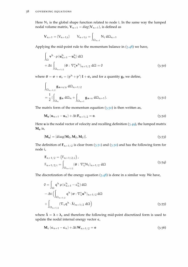
38 governing equations

Here Ni is the global shape function related to node i. In the same way the lumpednodal volume matrix, Vn+1 = diag(Vn+1), is defined as

Vn+1 = Vn+1;i Vn+1;i =

∫Ωn+1

Ni dΩn+1

Applying the mid-point rule to the momentum balance in (3.48) we have,∫Ω

vh · ρ (uhn+1 − uhn)dΩ

+∆t

∫Ωn+1/2

(σ : ∇sxvh)n+1/2 dΩ = 0 (3.50)

where σ = σ+σa = (ph + p ′) I+σa and for a quantity g t we define,∫Ωn+1/2

g n+1/2 dΩn+1/2

=1

2(

∫Ωn

g n dΩn +

∫Ωn+1

g n+1 dΩn+1). (3.51)

The matrix form of the momentum equation (3.50) is then written as,

Mu (un+1 − un) +∆tFn+1/2 = 0. (3.52)

Here u is the nodal vector of velocity and recalling definition (3.49), the lumped matrixMu is,

[Mu] = [diag(M0, M0, M0)]. (3.53)

The definition of Fn+1/2 is clear from (3.51) and (3.50) and has the following form fornode i,

Fn+1/2 =Fn+1/2; i

,

Fn+1/2; i =

∫Ωn+1/2

(σ : ∇sxNi)n+1/2 dΩ(3.54)

The discretization of the energy equation (3.48) is done in a similar way. We have,

0 =

∫Ω

qh ρ (εhn+1 − εhn)dΩ

−∆t(∫Ωn+1/2

qh (σ : ∇sxuh)n+1/2 dΩ

+

∫Ωn+1/2

(∇xqh · λ)n+1/2 dΩ)

(3.55)

where λ = λ+ λa and therefore the following mid-point discretized form is used toupdate the nodal internal energy vector ε,

Mε (εn+1 − εn) +∆tWn+1/2 = 0 (3.56)

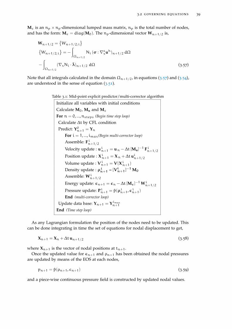
3.2 governing equations 39

Mε is an np ×np-dimensional lumped mass matrix, np is the total number of nodes,and has the form: Mε = diag(M0). The np-dimensional vector Wn+1/2 is,

Wn+1/2 =Wn+1/2; i

Wn+1/2; i

= −

∫Ωn+1/2

Ni (σ : ∇sxuh)n+1/2 dΩ

−

∫Ωn+1/2

(∇xNi · λ)n+1/2 dΩ (3.57)

Note that all integrals calculated in the domain Ωn+1/2, in equations (3.57) and (3.54),are understood in the sense of equation (3.51).

Table 3.1: Mid-point explicit predictor/multi-corrector algorithm

Initialize all variables with initial conditionsCalculate M0, Mu and Mε

For n = 0, ...,nsteps (Begin time step loop)

Calculate ∆t by CFL conditionPredict: Y0n+1 = Yn

For i = 1, ..., imax(Begin multi-corrector loop)

Assemble: F in+1/2Velocity update : u in+1 = un −∆t [Mu]

−1 F in+1/2Position update : X in+1 = Xn +∆tuin+1/2Volume update : V in+1 = V(X in+1)Density update : ρ in+1 = [Vin+1]

−1M0

Assemble: W in+1/2

Energy update: εn+1 = εn −∆t [Mε]−1W i

n+1/2

Pressure update: P in+1 = p(ρin+1,ε in+1)

End (multi-corrector loop)

Update data base: Yn+1 = Y imaxn+1

End (Time step loop)

As any Lagrangian formulation the position of the nodes need to be updated. Thiscan be done integrating in time the set of equations for nodal displacement to get,

Xn+1 = Xn +∆tun+1/2 (3.58)

where Xn+1 is the vector of nodal positions at tn+1.Once the updated value for εn+1 and ρn+1 has been obtained the nodal pressures

are updated by means of the EOS at each nodes,

pn+1 = p(ρn+1, εn+1) (3.59)

and a piece-wise continuous pressure field is constructed by updated nodal values.

40 governing equations

The update of velocity and internal energy from (3.52) and (3.56) needs the knowl-edge of step n+ 1. A fully explicit predictor/multi-corrector strategy is adopted toavoid the inverse of systems and also to best handle the nonlinearities in the calcula-tion of the force and work terms.

Table 4.1 shows the predictor/multi-corrector algorithm. In this table Yt:

Yt =[ρTt , uTt ,εTt , PTt , XTt

]Tis the state of the system at time t where P is the vector of nodal pressures.

The mid-point values at each iteration are calculated form the previous step andthe current iteration data.

The subscales are included in F in+1/2 and W in+1/2. As the residuals are evaluated

at the mid-points, the residual-based definition of the subscales implies that the sub-scales are also calculated at the mid time intervals. Therefore, by recalling the hy-pothesis of quasi-static subscales, we consider that they are constant during a timeinterval.

Recalling (3.40) and (3.41) we have

p ′n+1/2; i = −τ (Rhp)in+1/2

(phu ′)n+1/2; i = −τ (c2sRhu )in+1/2

where residuals are defined as,

(Rhp)in+1/2 =

ph; in+1 − p

hn

∆t+ (ρc2s∇x · u)

h; in+1/2

(Rhu )in+1/2 = ρ

in+1/2

uh; in+1 − uhn∆t

+ (∇xp)h; in+1/2

Considering that the subscales are constant during each time interval the force termrelated to the subscales in (3.54) is calculated as,∫

Ωn+1/2

(p ′n+1/2; i∇x · u)n+1/2 dΩ

=1

2

(∫Ωn+1

p ′n+1/2; i(∇x · u)n+1 dΩ

+

∫Ωn

p ′n+1/2; i(∇x · u)n dΩ)

The fine scale work term in (3.57) is calculated in a similar way by assuming that thesubscales are constant in the time interval.

The Lagrangian description of the motion, considered in this work, implies move-ment of the particles with their convective velocities that may cause large deforma-tions of the finite element mesh. In the next section we extend and improve an in-terface detecting technique, that was originally proposed for incompressible multi-flows [57, 56], to the air-water compressible system. In essence, pressure and densityare duplicated at the interface and the interface shape is conserved at each generationof the mesh.

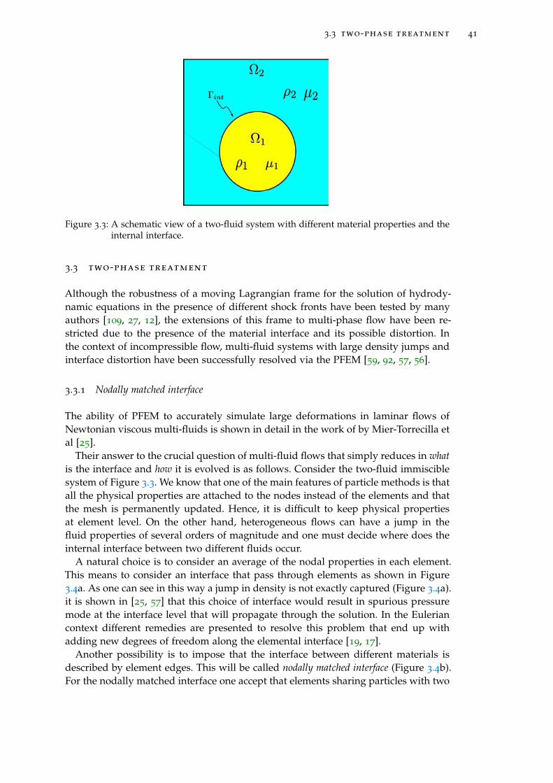
3.3 two-phase treatment 41

Figure 3.3: A schematic view of a two-fluid system with different material properties and theinternal interface.

3.3 two-phase treatment

Although the robustness of a moving Lagrangian frame for the solution of hydrody-namic equations in the presence of different shock fronts have been tested by manyauthors [109, 27, 12], the extensions of this frame to multi-phase flow have been re-stricted due to the presence of the material interface and its possible distortion. Inthe context of incompressible flow, multi-fluid systems with large density jumps andinterface distortion have been successfully resolved via the PFEM [59, 92, 57, 56].

3.3.1 Nodally matched interface

The ability of PFEM to accurately simulate large deformations in laminar flows ofNewtonian viscous multi-fluids is shown in detail in the work of by Mier-Torrecilla etal [25].

Their answer to the crucial question of multi-fluid flows that simply reduces in whatis the interface and how it is evolved is as follows. Consider the two-fluid immisciblesystem of Figure 3.3. We know that one of the main features of particle methods is thatall the physical properties are attached to the nodes instead of the elements and thatthe mesh is permanently updated. Hence, it is difficult to keep physical propertiesat element level. On the other hand, heterogeneous flows can have a jump in thefluid properties of several orders of magnitude and one must decide where does theinternal interface between two different fluids occur.

A natural choice is to consider an average of the nodal properties in each element.This means to consider an interface that pass through elements as shown in Figure3.4a. As one can see in this way a jump in density is not exactly captured (Figure 3.4a).it is shown in [25, 57] that this choice of interface would result in spurious pressuremode at the interface level that will propagate through the solution. In the Euleriancontext different remedies are presented to resolve this problem that end up withadding new degrees of freedom along the elemental interface [19, 17].

Another possibility is to impose that the interface between different materials isdescribed by element edges. This will be called nodally matched interface (Figure 3.4b).For the nodally matched interface one accept that elements sharing particles with two

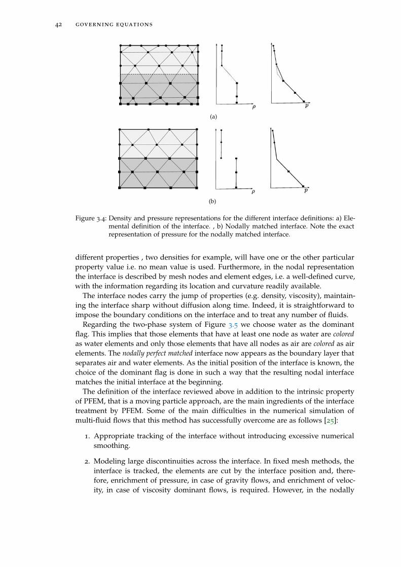
42 governing equations

(a)

(b)

Figure 3.4: Density and pressure representations for the different interface definitions: a) Ele-mental definition of the interface. , b) Nodally matched interface. Note the exactrepresentation of pressure for the nodally matched interface.

different properties , two densities for example, will have one or the other particularproperty value i.e. no mean value is used. Furthermore, in the nodal representationthe interface is described by mesh nodes and element edges, i.e. a well-defined curve,with the information regarding its location and curvature readily available.

The interface nodes carry the jump of properties (e.g. density, viscosity), maintain-ing the interface sharp without diffusion along time. Indeed, it is straightforward toimpose the boundary conditions on the interface and to treat any number of fluids.

Regarding the two-phase system of Figure 3.5 we choose water as the dominantflag. This implies that those elements that have at least one node as water are coloredas water elements and only those elements that have all nodes as air are colored as airelements. The nodally perfect matched interface now appears as the boundary layer thatseparates air and water elements. As the initial position of the interface is known, thechoice of the dominant flag is done in such a way that the resulting nodal interfacematches the initial interface at the beginning.

The definition of the interface reviewed above in addition to the intrinsic propertyof PFEM, that is a moving particle approach, are the main ingredients of the interfacetreatment by PFEM. Some of the main difficulties in the numerical simulation ofmulti-fluid flows that this method has successfully overcome are as follows [25]:

1. Appropriate tracking of the interface without introducing excessive numericalsmoothing.

2. Modeling large discontinuities across the interface. In fixed mesh methods, theinterface is tracked, the elements are cut by the interface position and, there-fore, enrichment of pressure, in case of gravity flows, and enrichment of veloc-ity, in case of viscosity dominant flows, is required. However, in the nodally

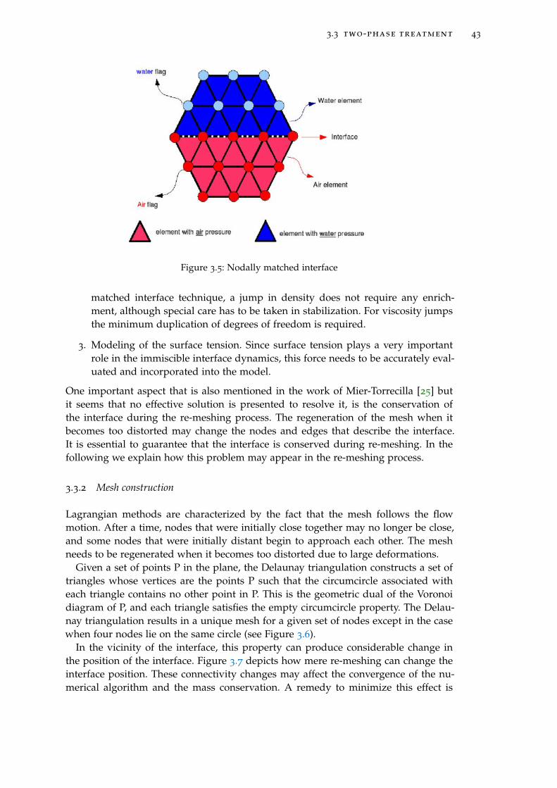
3.3 two-phase treatment 43

Figure 3.5: Nodally matched interface

matched interface technique, a jump in density does not require any enrich-ment, although special care has to be taken in stabilization. For viscosity jumpsthe minimum duplication of degrees of freedom is required.

3. Modeling of the surface tension. Since surface tension plays a very importantrole in the immiscible interface dynamics, this force needs to be accurately eval-uated and incorporated into the model.

One important aspect that is also mentioned in the work of Mier-Torrecilla [25] butit seems that no effective solution is presented to resolve it, is the conservation ofthe interface during the re-meshing process. The regeneration of the mesh when itbecomes too distorted may change the nodes and edges that describe the interface.It is essential to guarantee that the interface is conserved during re-meshing. In thefollowing we explain how this problem may appear in the re-meshing process.

3.3.2 Mesh construction

Lagrangian methods are characterized by the fact that the mesh follows the flowmotion. After a time, nodes that were initially close together may no longer be close,and some nodes that were initially distant begin to approach each other. The meshneeds to be regenerated when it becomes too distorted due to large deformations.

Given a set of points P in the plane, the Delaunay triangulation constructs a set oftriangles whose vertices are the points P such that the circumcircle associated witheach triangle contains no other point in P. This is the geometric dual of the Voronoidiagram of P, and each triangle satisfies the empty circumcircle property. The Delau-nay triangulation results in a unique mesh for a given set of nodes except in the casewhen four nodes lie on the same circle (see Figure 3.6).

In the vicinity of the interface, this property can produce considerable change inthe position of the interface. Figure 3.7 depicts how mere re-meshing can change theinterface position. These connectivity changes may affect the convergence of the nu-merical algorithm and the mass conservation. A remedy to minimize this effect is

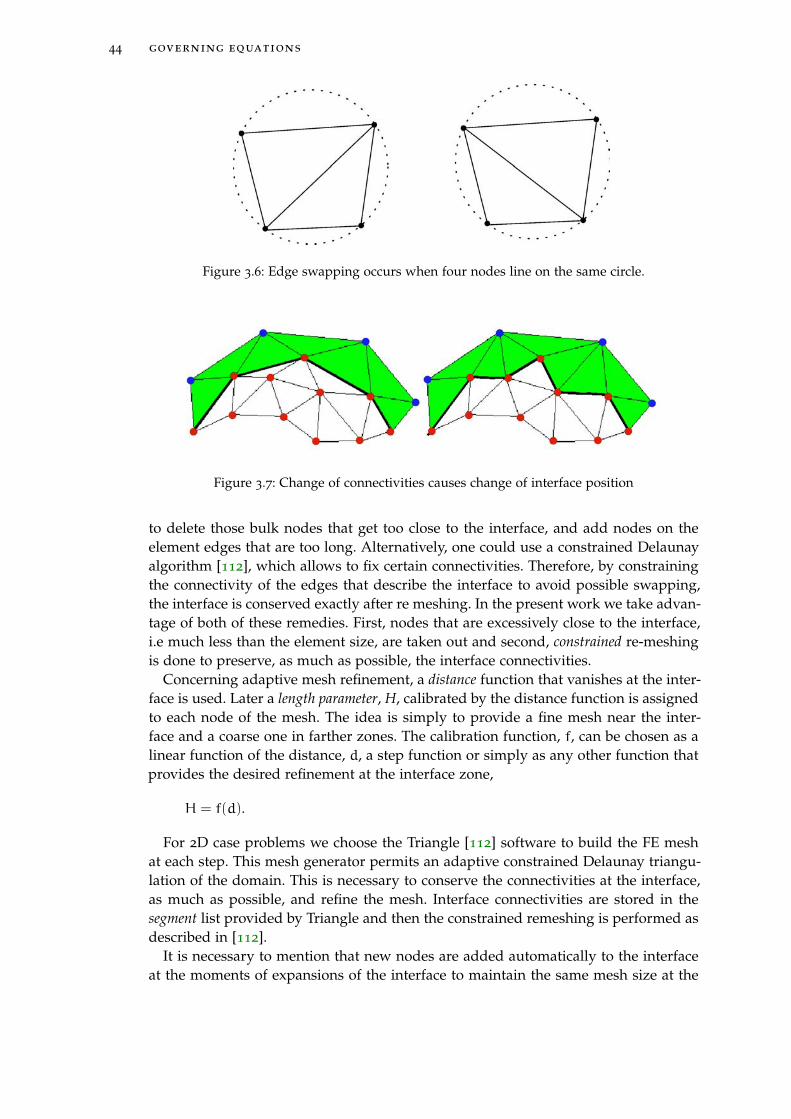
44 governing equations

Figure 3.6: Edge swapping occurs when four nodes line on the same circle.

Figure 3.7: Change of connectivities causes change of interface position

to delete those bulk nodes that get too close to the interface, and add nodes on theelement edges that are too long. Alternatively, one could use a constrained Delaunayalgorithm [112], which allows to fix certain connectivities. Therefore, by constrainingthe connectivity of the edges that describe the interface to avoid possible swapping,the interface is conserved exactly after re meshing. In the present work we take advan-tage of both of these remedies. First, nodes that are excessively close to the interface,i.e much less than the element size, are taken out and second, constrained re-meshingis done to preserve, as much as possible, the interface connectivities.

Concerning adaptive mesh refinement, a distance function that vanishes at the inter-face is used. Later a length parameter, H, calibrated by the distance function is assignedto each node of the mesh. The idea is simply to provide a fine mesh near the inter-face and a coarse one in farther zones. The calibration function, f, can be chosen as alinear function of the distance, d, a step function or simply as any other function thatprovides the desired refinement at the interface zone,

H = f(d).

For 2D case problems we choose the Triangle [112] software to build the FE meshat each step. This mesh generator permits an adaptive constrained Delaunay triangu-lation of the domain. This is necessary to conserve the connectivities at the interface,as much as possible, and refine the mesh. Interface connectivities are stored in thesegment list provided by Triangle and then the constrained remeshing is performed asdescribed in [112].

It is necessary to mention that new nodes are added automatically to the interfaceat the moments of expansions of the interface to maintain the same mesh size at the

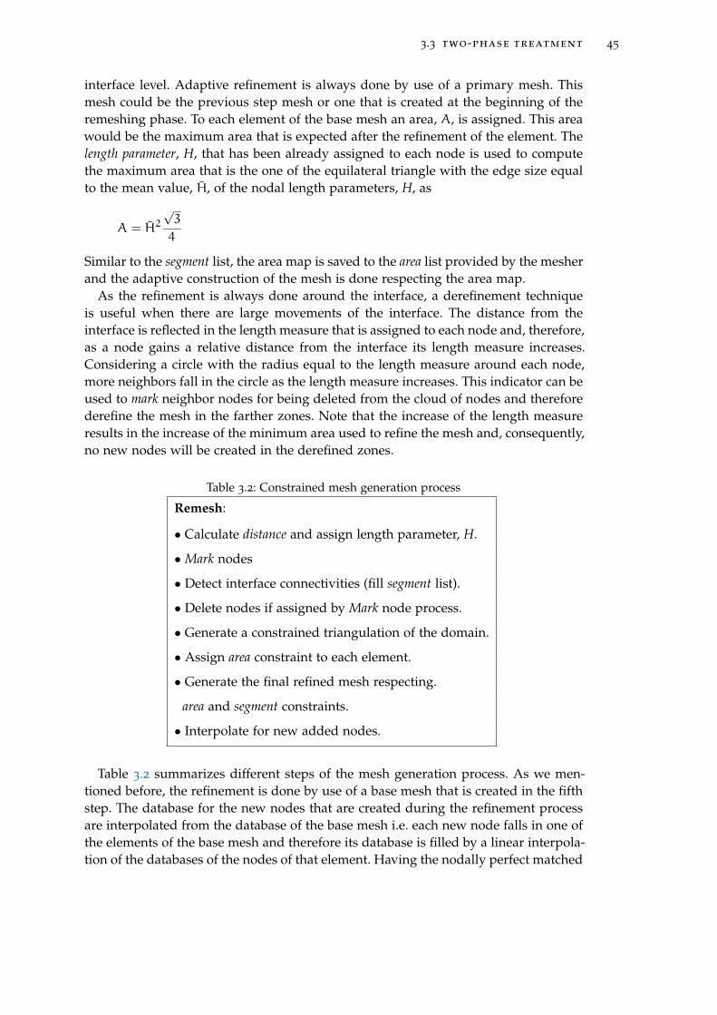
3.3 two-phase treatment 45

interface level. Adaptive refinement is always done by use of a primary mesh. Thismesh could be the previous step mesh or one that is created at the beginning of theremeshing phase. To each element of the base mesh an area, A, is assigned. This areawould be the maximum area that is expected after the refinement of the element. Thelength parameter, H, that has been already assigned to each node is used to computethe maximum area that is the one of the equilateral triangle with the edge size equalto the mean value, H, of the nodal length parameters, H, as

A = H2√3

4

Similar to the segment list, the area map is saved to the area list provided by the mesherand the adaptive construction of the mesh is done respecting the area map.

As the refinement is always done around the interface, a derefinement techniqueis useful when there are large movements of the interface. The distance from theinterface is reflected in the length measure that is assigned to each node and, therefore,as a node gains a relative distance from the interface its length measure increases.Considering a circle with the radius equal to the length measure around each node,more neighbors fall in the circle as the length measure increases. This indicator can beused to mark neighbor nodes for being deleted from the cloud of nodes and thereforederefine the mesh in the farther zones. Note that the increase of the length measureresults in the increase of the minimum area used to refine the mesh and, consequently,no new nodes will be created in the derefined zones.

Table 3.2: Constrained mesh generation process

Remesh:

• Calculate distance and assign length parameter, H.

• Mark nodes

• Detect interface connectivities (fill segment list).

• Delete nodes if assigned by Mark node process.

• Generate a constrained triangulation of the domain.

• Assign area constraint to each element.

• Generate the final refined mesh respecting.

area and segment constraints.

• Interpolate for new added nodes.

Table 3.2 summarizes different steps of the mesh generation process. As we men-tioned before, the refinement is done by use of a base mesh that is created in the fifthstep. The database for the new nodes that are created during the refinement processare interpolated from the database of the base mesh i.e. each new node falls in one ofthe elements of the base mesh and therefore its database is filled by a linear interpola-tion of the databases of the nodes of that element. Having the nodally perfect matched

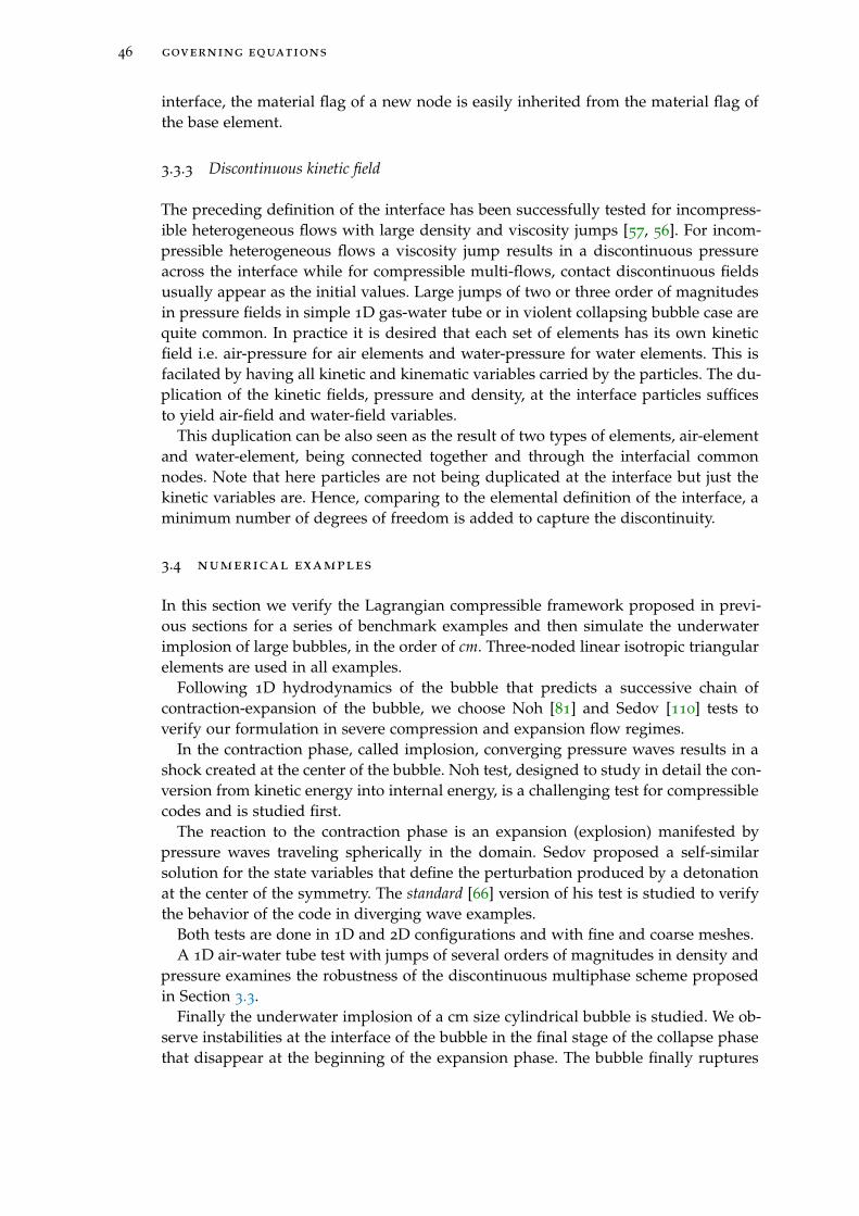
46 governing equations

interface, the material flag of a new node is easily inherited from the material flag ofthe base element.

3.3.3 Discontinuous kinetic field

The preceding definition of the interface has been successfully tested for incompress-ible heterogeneous flows with large density and viscosity jumps [57, 56]. For incom-pressible heterogeneous flows a viscosity jump results in a discontinuous pressureacross the interface while for compressible multi-flows, contact discontinuous fieldsusually appear as the initial values. Large jumps of two or three order of magnitudesin pressure fields in simple 1D gas-water tube or in violent collapsing bubble case arequite common. In practice it is desired that each set of elements has its own kineticfield i.e. air-pressure for air elements and water-pressure for water elements. This isfacilated by having all kinetic and kinematic variables carried by the particles. The du-plication of the kinetic fields, pressure and density, at the interface particles sufficesto yield air-field and water-field variables.

This duplication can be also seen as the result of two types of elements, air-elementand water-element, being connected together and through the interfacial commonnodes. Note that here particles are not being duplicated at the interface but just thekinetic variables are. Hence, comparing to the elemental definition of the interface, aminimum number of degrees of freedom is added to capture the discontinuity.

3.4 numerical examples

In this section we verify the Lagrangian compressible framework proposed in previ-ous sections for a series of benchmark examples and then simulate the underwaterimplosion of large bubbles, in the order of cm. Three-noded linear isotropic triangularelements are used in all examples.

Following 1D hydrodynamics of the bubble that predicts a successive chain ofcontraction-expansion of the bubble, we choose Noh [81] and Sedov [110] tests toverify our formulation in severe compression and expansion flow regimes.

In the contraction phase, called implosion, converging pressure waves results in ashock created at the center of the bubble. Noh test, designed to study in detail the con-version from kinetic energy into internal energy, is a challenging test for compressiblecodes and is studied first.

The reaction to the contraction phase is an expansion (explosion) manifested bypressure waves traveling spherically in the domain. Sedov proposed a self-similarsolution for the state variables that define the perturbation produced by a detonationat the center of the symmetry. The standard [66] version of his test is studied to verifythe behavior of the code in diverging wave examples.

Both tests are done in 1D and 2D configurations and with fine and coarse meshes.A 1D air-water tube test with jumps of several orders of magnitudes in density and

pressure examines the robustness of the discontinuous multiphase scheme proposedin Section 3.3.

Finally the underwater implosion of a cm size cylindrical bubble is studied. We ob-serve instabilities at the interface of the bubble in the final stage of the collapse phasethat disappear at the beginning of the expansion phase. The bubble finally ruptures

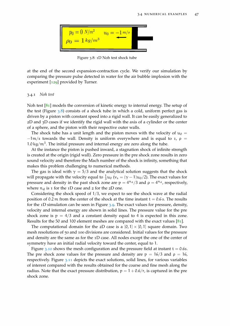
3.4 numerical examples 47

Figure 3.8: 1D Noh test shock tube

at the end of the second expansion-contraction cycle. We verify our simulation bycomparing the pressure pulse detected in water for the air bubble implosion with theexperiment [129] provided by Turner.

3.4.1 Noh test

Noh test [81] models the conversion of kinetic energy to internal energy. The setup ofthe test (Figure 3.8) consists of a shock tube in which a cold, uniform perfect gas isdriven by a piston with constant speed into a rigid wall. It can be easily generalized to2D and 3D cases if we identify the rigid wall with the axis of a cylinder or the centerof a sphere, and the piston with their respective outer walls.

The shock tube has a unit length and the piston moves with the velocity of u0 =

−1m/s towards the wall. Density is uniform everywhere and is equal to 1, ρ =

1.0 kg/m3. The initial pressure and internal energy are zero along the tube.At the instance the piston is pushed inward, a stagnation shock of infinite strength

is created at the origin (rigid wall). Zero pressure in the pre shock zone results in zerosound velocity and therefore the Mach number of the shock is infinity, something thatmakes this problem challenging to numerical methods.

The gas is ideal with γ = 5/3 and the analytical solution suggests that the shockwill propagate with the velocity equal to 1

3u0 (vs = (γ− 1)u0/2). The exact values forpressure and density in the past shock zone are p = 4nd/3 and ρ = 4nd , respectively,where nd is 1 for the 1D case and 2 for the 2D one.

Considering the shock speed of 1/3, we expect to see the shock wave at the radialposition of 0.2m from the center of the shock at the time instant t = 0.6 s. The resultsfor the 1D simulation can be seen in Figure 3.9. The exact values for pressure, density,velocity and internal energy are shown in solid lines. The pressure value for the preshock zone is p = 4/3 and a constant density equal to 4 is expected in this zone.Results for the 50 and 100 element meshes are compared with the exact values [81].

The computational domain for the 2D case is a [0, 1]× [0, 1] square domain. Twomesh resolutions of 50 and 100 divisions are considered. Initial values for the pressureand density are the same as for the 1D case. All nodes except the one of the center ofsymmetry have an initial radial velocity toward the center, equal to 1.

Figure 3.10 shows the mesh configuration and the pressure field at instant t = 0.6s.The pre shock zone values for the pressure and density are p = 16/3 and ρ = 16,respectively. Figure 3.11 depicts the exact solutions, solid lines, for various variablesof interest compared with the results obtained for the coarse and fine mesh along theradius. Note that the exact pressure distribution, p = 1+ 0.6/r, is captured in the preshock zone.

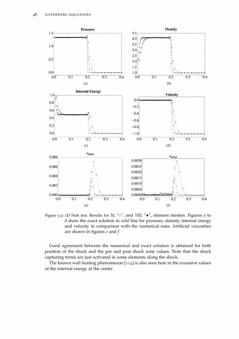
48 governing equations

(a) (b)

(c) (d)

(e) (f)

Figure 3.9: 1D Noh test. Results for 50, “2”, and 100, “•”, element meshes. Figures a tod show the exact solution in solid line for pressure, density, internal energyand velocity in comparison with the numerical ones. Artificial viscositiesare shown in figures e and f .

Good agreement between the numerical and exact solution is obtained for bothposition of the shock and the pre and post shock zone values. Note that the shockcapturing terms are just activated in some elements along the shock.

The known wall heating phenomenon [104] is also seen here in the excessive valuesof the internal energy at the center.

3.4 numerical examples 49

Figure 3.10: 2D Noh test. Mesh configuration and pressure field at time t = 0.6 s.

3.4.2 Sedov test

Sedov [110] provided analytical solution for the motion of a gas initially at rest andbeing disturbed by a detonation at the center of symmetry (Figure 3.12a).

We choose here the constant initial density case among the Sedov setting tests forwhich the initial density, ρ0 = 1g/cm3, is uniform and constant everywhere, the gasis ideal with γ = 7/5 and the internal energy, e, is zero everywhere except in a smallzone at the center of symmetry.

Planar and cylindrical tests are considered for which e = 0.0673185 for the planarcase, and e = 0.311357 for the cylindrical one, in some elements near the center. Thesevalue are chosen in accordance with [66] to be able to reproduce the exact self-similarSedov solutions.

For the 1D case a 1m long tube as shown in Figure 3.12b is discretized with trian-gular elements. Two mesh sizes of 0.01 and 0.02 are considered. The left wall has afixed velocity and the rest of the domain has zero initial velocity. The shock, instanta-neously created at the left wall, reaches the middle of the tube at time t = 1.0s. Themesh configuration at this instant is shown in Figure 3.12c.

In Figure 3.13 the self similar exact solutions for the state variables (solid lines) arecompared with the numerical ones at t = 1.0s.

The extension to the cylindrical case is obtained by considering a square domainof [0, 1.2]× [0, 1.2]. Two Cartesian meshes, with the same element sizes as the 1D case,are considered. The initial internal energy is zero everywhere except at the center ofsymmetry where an initial value of e = 0.311357 is assigned to few elements nearthe center. Zero velocity is considered everywhere and the initial density is equal to1. After 1s the circular detonation shock wave reaches to the radial position of 0.75.This pressure wave and the current mesh configuration can be seen in Figure 3.14. Noremeshing is applied to the Sedov and Noh tests. Figure 3.15 compares the exact [66]and numerical solutions obtained for the two mesh resolutions.

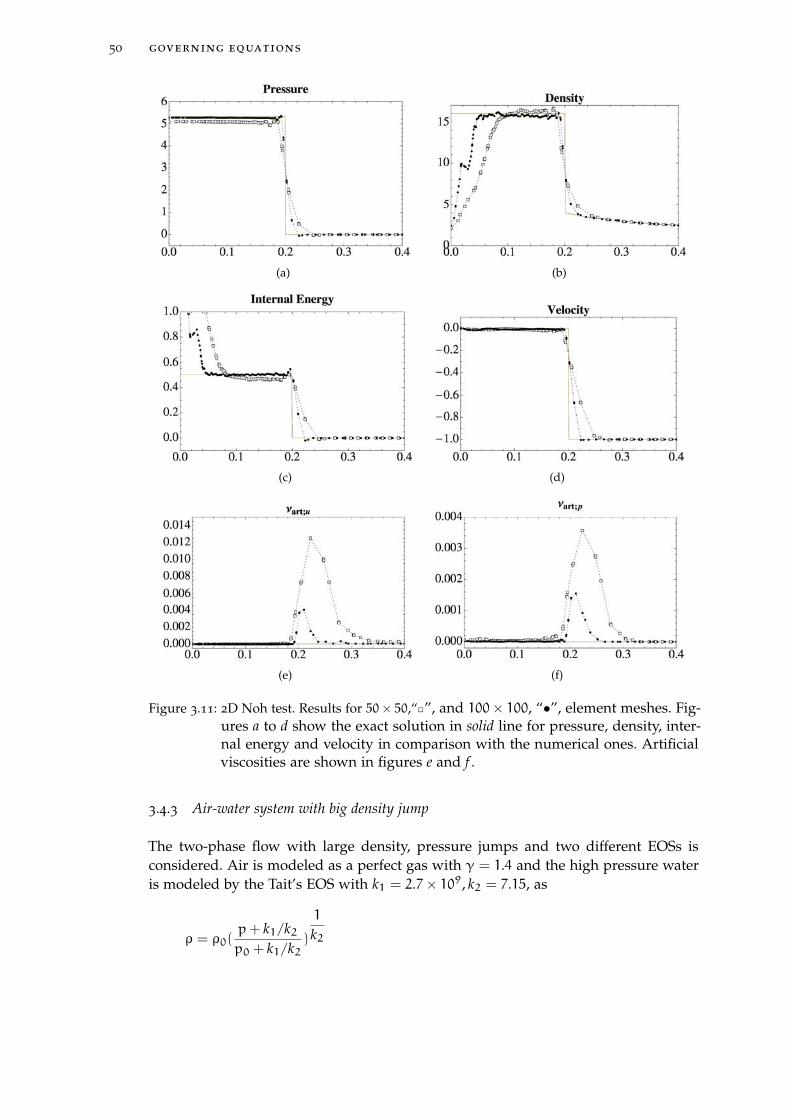
50 governing equations

(a) (b)

(c) (d)

(e) (f)

Figure 3.11: 2D Noh test. Results for 50× 50,“2”, and 100× 100, “•”, element meshes. Fig-ures a to d show the exact solution in solid line for pressure, density, inter-nal energy and velocity in comparison with the numerical ones. Artificialviscosities are shown in figures e and f .

3.4.3 Air-water system with big density jump

The two-phase flow with large density, pressure jumps and two different EOSs isconsidered. Air is modeled as a perfect gas with γ = 1.4 and the high pressure wateris modeled by the Tait’s EOS with k1 = 2.7× 109, k2 = 7.15, as

ρ = ρ0(p+ k1/k2p0 + k1/k2

)

1

k2

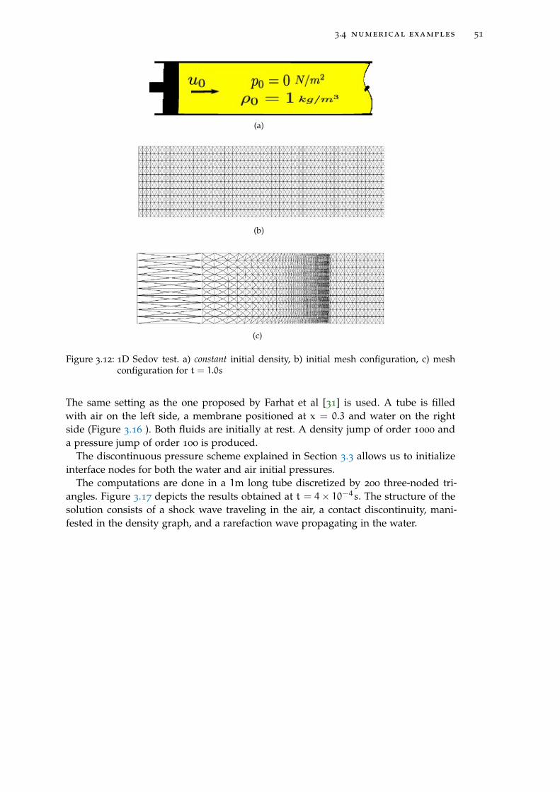
3.4 numerical examples 51

(a)

(b)

(c)

Figure 3.12: 1D Sedov test. a) constant initial density, b) initial mesh configuration, c) meshconfiguration for t = 1.0s

The same setting as the one proposed by Farhat et al [31] is used. A tube is filledwith air on the left side, a membrane positioned at x = 0.3 and water on the rightside (Figure 3.16 ). Both fluids are initially at rest. A density jump of order 1000 anda pressure jump of order 100 is produced.

The discontinuous pressure scheme explained in Section 3.3 allows us to initializeinterface nodes for both the water and air initial pressures.

The computations are done in a 1m long tube discretized by 200 three-noded tri-angles. Figure 3.17 depicts the results obtained at t = 4× 10−4s. The structure of thesolution consists of a shock wave traveling in the air, a contact discontinuity, mani-fested in the density graph, and a rarefaction wave propagating in the water.

52 governing equations

(a) (b)

(c) (d)

(e) (f)

Figure 3.13: 1D Sedov test. Results for 60, “2”, and 120, “•”, element meshes. Figures a tod show the exact solution in solid line for pressure, density, internal energyand velocity in comparison with the numerical ones. Artificial viscositiesare shown in figures e and f .

3.4.4 Underwater implosion of cylindrical bubble

In this section we study the implosion of an infinitely long cm size cylindrical bubblewhich is initially at atmospheric pressure and is being compressed by the surroundingpressurized water at 70 atmospheres. The initial radius of the bubble is 3.81 cm andthe numerical domain is a 1× 1m square (Figure 3.18).

As we are interested to study the possible instabilities that may occur during thecollapse, a full model is considered. The inside air is modeled as a perfect gas withγ = 1.4. Water is modeled by Tait’s equation of state presented in Section 3.4.3.

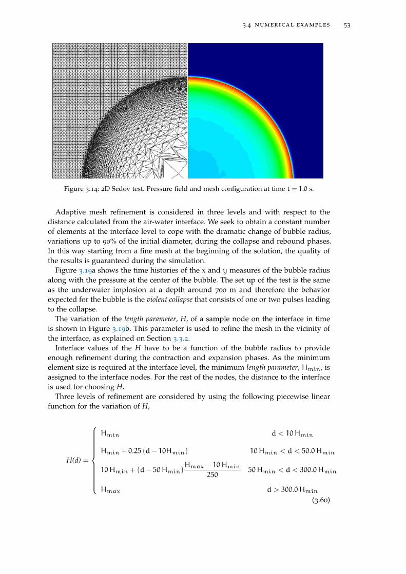
3.4 numerical examples 53

Figure 3.14: 2D Sedov test. Pressure field and mesh configuration at time t = 1.0 s.

Adaptive mesh refinement is considered in three levels and with respect to thedistance calculated from the air-water interface. We seek to obtain a constant numberof elements at the interface level to cope with the dramatic change of bubble radius,variations up to 90% of the initial diameter, during the collapse and rebound phases.In this way starting from a fine mesh at the beginning of the solution, the quality ofthe results is guaranteed during the simulation.

Figure 3.19a shows the time histories of the x and y measures of the bubble radiusalong with the pressure at the center of the bubble. The set up of the test is the sameas the underwater implosion at a depth around 700 m and therefore the behaviorexpected for the bubble is the violent collapse that consists of one or two pulses leadingto the collapse.

The variation of the length parameter, H, of a sample node on the interface in timeis shown in Figure 3.19b. This parameter is used to refine the mesh in the vicinity ofthe interface, as explained on Section 3.3.2.

Interface values of the H have to be a function of the bubble radius to provideenough refinement during the contraction and expansion phases. As the minimumelement size is required at the interface level, the minimum length parameter, Hmin, isassigned to the interface nodes. For the rest of the nodes, the distance to the interfaceis used for choosing H.

Three levels of refinement are considered by using the following piecewise linearfunction for the variation of H,

H(d) =

Hmin d < 10Hmin

Hmin + 0.25 (d− 10Hmin) 10Hmin < d < 50.0Hmin

10Hmin + (d− 50Hmin)Hmax − 10Hmin

25050Hmin < d < 300.0Hmin

Hmax d > 300.0Hmin(3.60)

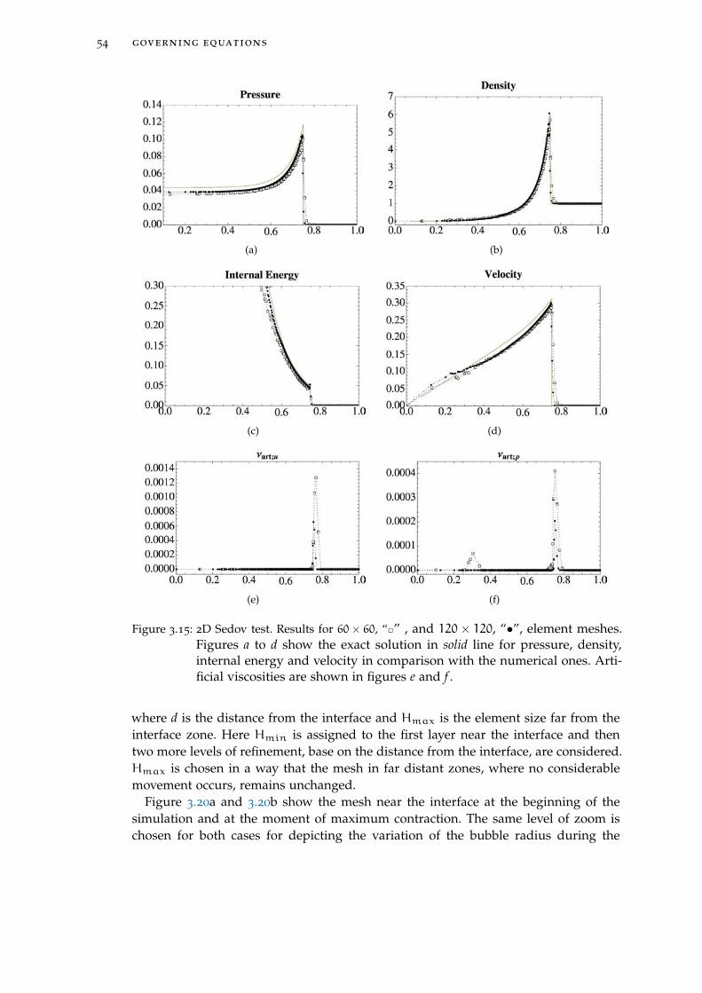
54 governing equations

(a) (b)

(c) (d)

(e) (f)

Figure 3.15: 2D Sedov test. Results for 60× 60, “2” , and 120× 120, “•”, element meshes.Figures a to d show the exact solution in solid line for pressure, density,internal energy and velocity in comparison with the numerical ones. Arti-ficial viscosities are shown in figures e and f .

where d is the distance from the interface and Hmax is the element size far from theinterface zone. Here Hmin is assigned to the first layer near the interface and thentwo more levels of refinement, base on the distance from the interface, are considered.Hmax is chosen in a way that the mesh in far distant zones, where no considerablemovement occurs, remains unchanged.

Figure 3.20a and 3.20b show the mesh near the interface at the beginning of thesimulation and at the moment of maximum contraction. The same level of zoom ischosen for both cases for depicting the variation of the bubble radius during the

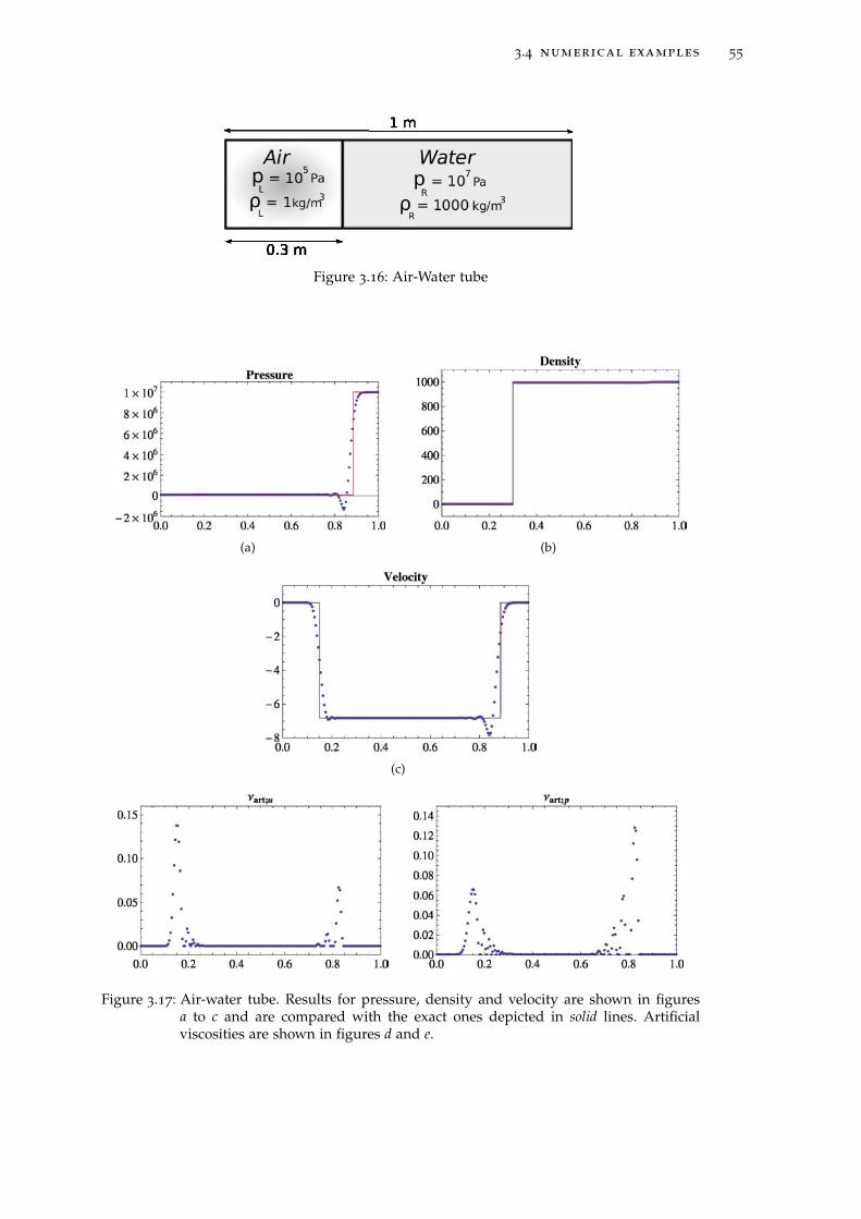
3.4 numerical examples 55

Figure 3.16: Air-Water tube

(a) (b)

(c)

Figure 3.17: Air-water tube. Results for pressure, density and velocity are shown in figuresa to c and are compared with the exact ones depicted in solid lines. Artificialviscosities are shown in figures d and e.

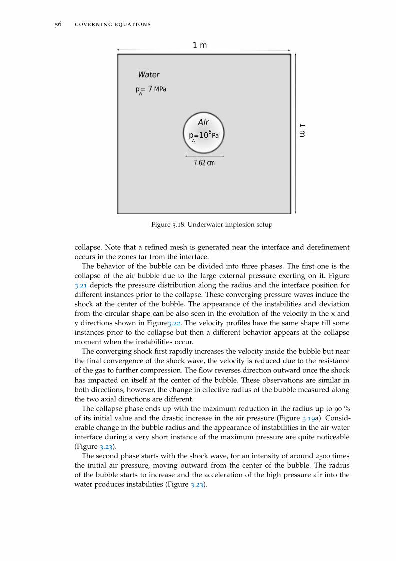
56 governing equations

Figure 3.18: Underwater implosion setup

collapse. Note that a refined mesh is generated near the interface and derefinementoccurs in the zones far from the interface.

The behavior of the bubble can be divided into three phases. The first one is thecollapse of the air bubble due to the large external pressure exerting on it. Figure3.21 depicts the pressure distribution along the radius and the interface position fordifferent instances prior to the collapse. These converging pressure waves induce theshock at the center of the bubble. The appearance of the instabilities and deviationfrom the circular shape can be also seen in the evolution of the velocity in the x andy directions shown in Figure3.22. The velocity profiles have the same shape till someinstances prior to the collapse but then a different behavior appears at the collapsemoment when the instabilities occur.

The converging shock first rapidly increases the velocity inside the bubble but nearthe final convergence of the shock wave, the velocity is reduced due to the resistanceof the gas to further compression. The flow reverses direction outward once the shockhas impacted on itself at the center of the bubble. These observations are similar inboth directions, however, the change in effective radius of the bubble measured alongthe two axial directions are different.

The collapse phase ends up with the maximum reduction in the radius up to 90 %of its initial value and the drastic increase in the air pressure (Figure 3.19a). Consid-erable change in the bubble radius and the appearance of instabilities in the air-waterinterface during a very short instance of the maximum pressure are quite noticeable(Figure 3.23).

The second phase starts with the shock wave, for an intensity of around 2500 timesthe initial air pressure, moving outward from the center of the bubble. The radiusof the bubble starts to increase and the acceleration of the high pressure air into thewater produces instabilities (Figure 3.23).

3.4 numerical examples 57

(a)

(b)

Figure 3.19: Time histories of a) “X”, “Y” measures of bubble radius and pressure at the centerof the bubble, b) Length parameter, H.

Surface instabilities appear in a very short period, less than 0.1 ms, and then thebubble recovers its circular shape with some oscillations remaining in its interface.The next expansion of the bubble starts at the final part of the second stage, as theresult of the reduction in water pressure at the post shock zone. At the end of thisstage the bubble has recovered 50% of its initial radius (Figure 3.19a), and air pressurehas been reduced due to the rapid expansion of the bubble volume (Figure 3.24).

Last phase of the simulation is again an implosion similar to the first phase, butthis time ends up with the rupture of the bubble as the result of the shape instabilitiesexcited at this stage, (Figure 3.24). Note that the bubble almost recovers a circularshape at the end of the second stage.

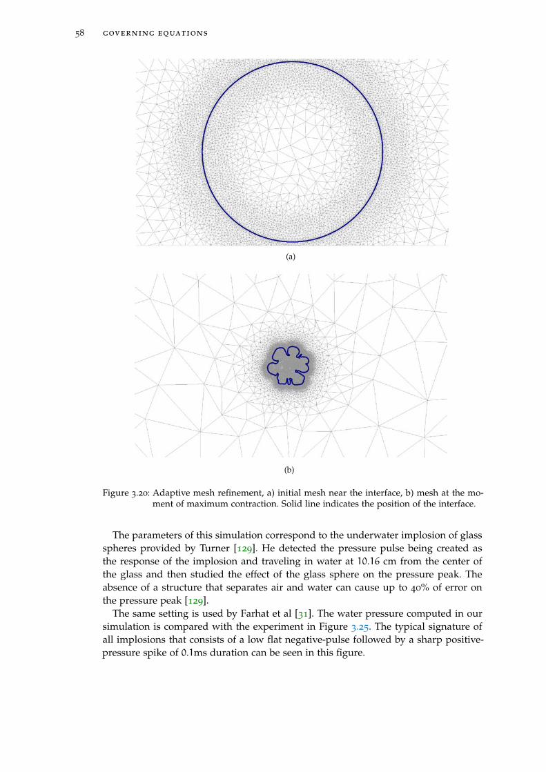
58 governing equations

(a)

(b)

Figure 3.20: Adaptive mesh refinement, a) initial mesh near the interface, b) mesh at the mo-ment of maximum contraction. Solid line indicates the position of the interface.

The parameters of this simulation correspond to the underwater implosion of glassspheres provided by Turner [129]. He detected the pressure pulse being created asthe response of the implosion and traveling in water at 10.16 cm from the center ofthe glass and then studied the effect of the glass sphere on the pressure peak. Theabsence of a structure that separates air and water can cause up to 40% of error onthe pressure peak [129].

The same setting is used by Farhat et al [31]. The water pressure computed in oursimulation is compared with the experiment in Figure 3.25. The typical signature ofall implosions that consists of a low flat negative-pulse followed by a sharp positive-pressure spike of 0.1ms duration can be seen in this figure.

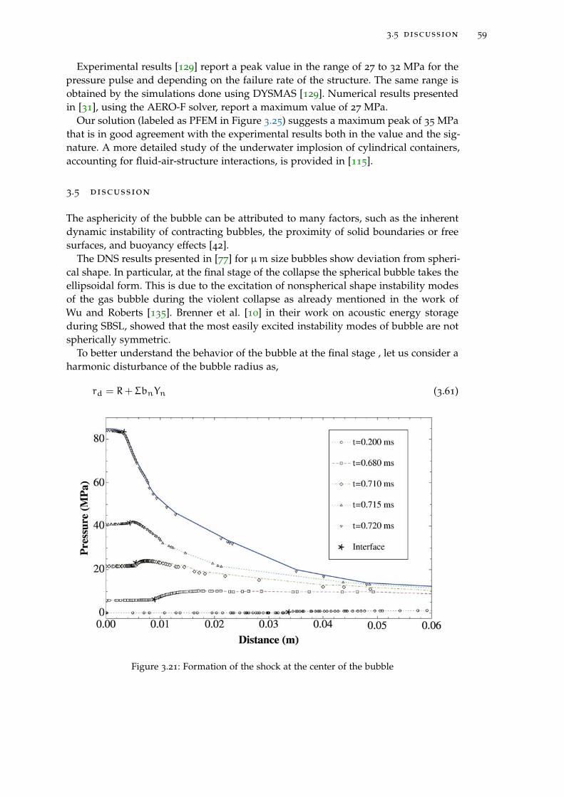
3.5 discussion 59

Experimental results [129] report a peak value in the range of 27 to 32 MPa for thepressure pulse and depending on the failure rate of the structure. The same range isobtained by the simulations done using DYSMAS [129]. Numerical results presentedin [31], using the AERO-F solver, report a maximum value of 27 MPa.

Our solution (labeled as PFEM in Figure 3.25) suggests a maximum peak of 35 MPathat is in good agreement with the experimental results both in the value and the sig-nature. A more detailed study of the underwater implosion of cylindrical containers,accounting for fluid-air-structure interactions, is provided in [115].

3.5 discussion

The asphericity of the bubble can be attributed to many factors, such as the inherentdynamic instability of contracting bubbles, the proximity of solid boundaries or freesurfaces, and buoyancy effects [42].

The DNS results presented in [77] for µm size bubbles show deviation from spheri-cal shape. In particular, at the final stage of the collapse the spherical bubble takes theellipsoidal form. This is due to the excitation of nonspherical shape instability modesof the gas bubble during the violent collapse as already mentioned in the work ofWu and Roberts [135]. Brenner et al. [10] in their work on acoustic energy storageduring SBSL, showed that the most easily excited instability modes of bubble are notspherically symmetric.

To better understand the behavior of the bubble at the final stage , let us consider aharmonic disturbance of the bubble radius as,

rd = R+ ΣbnYn (3.61)

Figure 3.21: Formation of the shock at the center of the bubble

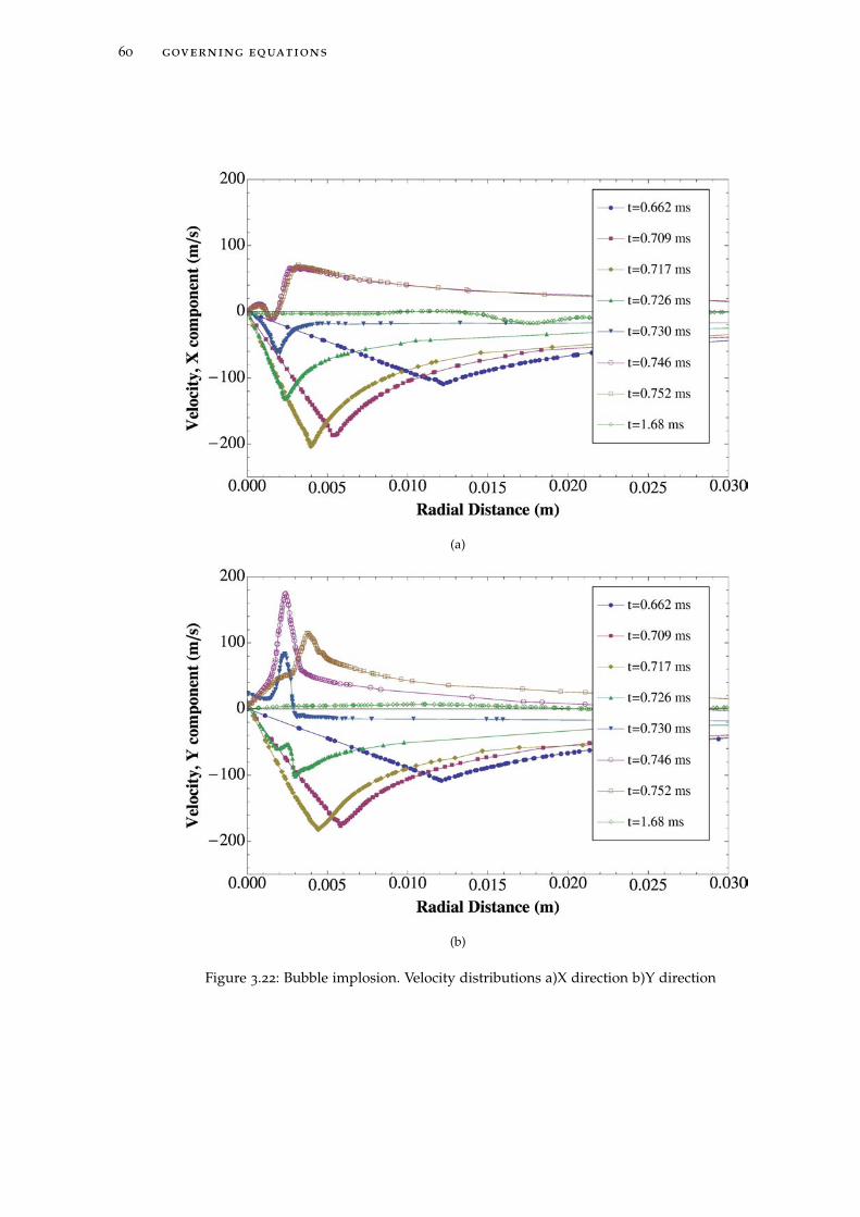
60 governing equations

(a)

(b)

Figure 3.22: Bubble implosion. Velocity distributions a)X direction b)Y direction

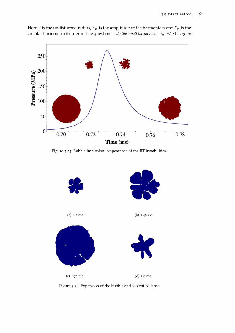
3.5 discussion 61

Here R is the undisturbed radius, bn is the amplitude of the harmonic n and Yn is thecircular harmonics of order n. The question is: do the small harmonics, |bn| R(t), grow,

Figure 3.23: Bubble implosion. Appearance of the RT instabilities.

(a) 1.2 ms (b) 1.48 ms

(c) 1.75 ms (d) 2.0 ms

Figure 3.24: Expansion of the bubble and violent collapse

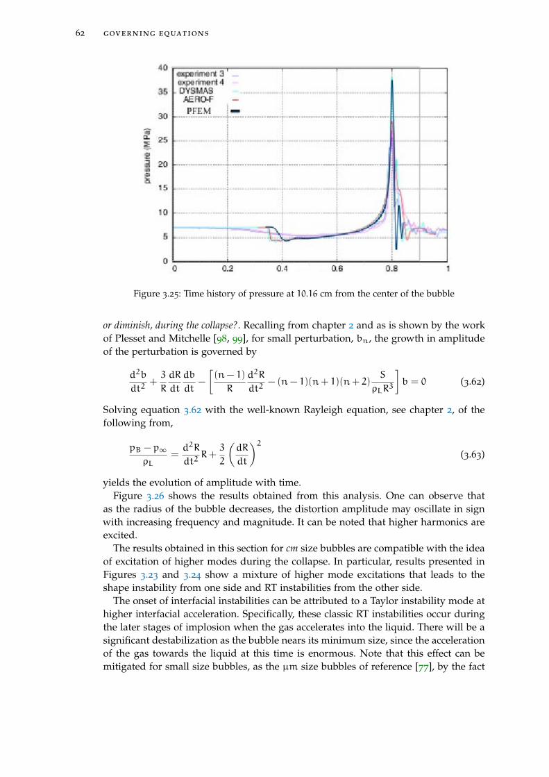
62 governing equations

Figure 3.25: Time history of pressure at 10.16 cm from the center of the bubble

or diminish, during the collapse?. Recalling from chapter 2 and as is shown by the workof Plesset and Mitchelle [98, 99], for small perturbation, bn, the growth in amplitudeof the perturbation is governed by

d2b

dt2+3

R

dR

dt

db

dt−

[(n− 1)

R

d2R

dt2− (n− 1)(n+ 1)(n+ 2)

S

ρLR3

]b = 0 (3.62)

Solving equation 3.62 with the well-known Rayleigh equation, see chapter 2, of thefollowing from,

pB − p∞ρL

=d2R

dt2R+

3

2

(dR

dt

)2(3.63)

yields the evolution of amplitude with time.Figure 3.26 shows the results obtained from this analysis. One can observe that

as the radius of the bubble decreases, the distortion amplitude may oscillate in signwith increasing frequency and magnitude. It can be noted that higher harmonics areexcited.

The results obtained in this section for cm size bubbles are compatible with the ideaof excitation of higher modes during the collapse. In particular, results presented inFigures 3.23 and 3.24 show a mixture of higher mode excitations that leads to theshape instability from one side and RT instabilities from the other side.

The onset of interfacial instabilities can be attributed to a Taylor instability mode athigher interfacial acceleration. Specifically, these classic RT instabilities occur duringthe later stages of implosion when the gas accelerates into the liquid. There will be asignificant destabilization as the bubble nears its minimum size, since the accelerationof the gas towards the liquid at this time is enormous. Note that this effect can bemitigated for small size bubbles, as the µm size bubbles of reference [77], by the fact

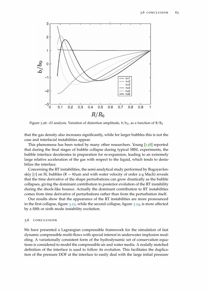
3.6 conclusion 63

Figure 3.26: 1D analysis. Variation of distortion amplitude, b/b0, as a function of R/R0

that the gas density also increases significantly, while for larger bubbles this is not thecase and interfacial instabilities appear.

This phenomena has been noted by many other researchers. Young [138] reportedthat during the final stages of bubble collapse during typical SBSL experiments, thebubble interface decelerates in preparation for re-expansion, leading to an extremelylarge relative acceleration of the gas with respect to the liquid, which tends to desta-bilize the interface.

Concerning the RT instabilities, the semi-analytical study performed by Bogoyavlen-skiy [7] on SL bubbles (R = 40µm and with water velocity of order 2-4 Mach) revealsthat the time derivative of the shape perturbations can grow drastically as the bubblecollapses, giving the dominant contribution to posterior evolution of the RT instabilityduring the shock-like bounce. Actually the dominant contribution to RT instabilitiescomes from time derivative of perturbations rather than from the perturbation itself.

Our results show that the appearance of the RT instabilities are more pronouncedin the first collapse, figure 3.23, while the second collapse, figure 3.24, is more affectedby a fifth or sixth mode instability excitation.

3.6 conclusion

We have presented a Lagrangian compressible framework for the simulation of fastdynamic compressible multi-flows with special interest in underwater implosion mod-eling. A variationally consistent form of the hydrodynamic set of conservation equa-tions is considered to model the compressible air and water media. A nodally matcheddefinition of the interface is used to follow its evolution. This facilitates the duplica-tion of the pressure DOF at the interface to easily deal with the large initial pressure

64 governing equations

jumps typical of implosion problems. The severe deformation of the interface, in addi-tion to the large local motion of the fluids, require an adaptive mesh generation thatrespects the interface connectivities at each time step.

The formulation has been successfully tested for several benchmark problems andthen has been applied to model the underwater implosion of cm size cylindrical bub-bles. Numerical results show that the hydrodynamics of the bubble has three differentstages. The first one is the collapse of the bubble that results in the reduction up to90% in the bubble radius and an increase in the internal pressure up to 2500 times theinitial pressure. At this point a shock wave is created at the center of the bubble andRT instabilities appear at the air-water interface. The pressure wave traveling in wateris detected at 10.16 cm from the center of the bubble. Results for this phase have beensuccessfully compared with experimental and numerical data. The second stage thenstarts by the expansion of the bubble, due to the high internal pressure, and the van-ishing of the RT instabilities till the bubble recovers 50% of its initial radius and gainsan almost circular shape. The third stage is again a collapse of the bubble volume thatends up with the rupture of the bubble initiated from a fifth mode instability thatappears at the air-water interface.

4C O N TA C T A L G O R I T H M F O R S H E L L P R O B L E M S

The final stage in the implosion of closed containers usually consists of the totalcollapse of the containers. It is, therefor inevitable to introduce a self-contact schemein the finite element structural model used for simulating the container collapse. Inthis chapter we present a contact algorithm developed for modeling shell-to-shellfrictionless contact. The material for this chapter is taken from our paper A contactalgorithm for shell problems via Delaunay-based meshing of the contact domain [67].

4.1 introduction

One of the major issues in contact problems is the definition and discretization of thecontact surfaces. Many contact algorithms enforce the non penetration constraint onsome collocation points. Hallquist et al. [4] proposed the simple idea that a specificslave node must not penetrate an opposing master segment. This node-to-segment ap-proach is applied through a single pass algorithm that just checks for slave nodes, andso is prone to master node penetration, and also does not satisfy the patch test [30]. Tocure this deficiency, a number of two-pass algorithms have been proposed. Althoughsome of these algorithms satisfy the patch test, they may cause locking for certainconfigurations of the master and slave nodes.

Based on the so called mortar method [5] some segment-to-segment discretizationstrategies of the contact interface have been proposed [47, 49]. Segment-to-segmentstrategies are well suited for non-conforming interface grids and opposite to the node-to-segment approach enforce the constraint condition not at discrete nodes but alongthe entire coupling boundary and in a weak integral sense. Concerning the frictionalcontact, Heintz and Hansbo [44] proposed a method based on Nitsche’s approach [80]that combines Lagrange multipliers and stabilization terms to reach a condensed ma-trix. This approach was first used by Wriggers and Zavarise [134] to solve frictionlesssmall deformation.

In the context of the so-called Particle Finite Element Method (PFEM), Oñate etal. [92, 59] proposed a simple technique to define a contact domain where the contactconstraints are imposed on the interacting interfaces. This Contact Domain (CD) tech-nique has been applied for modeling fluid-solid and solid-solid contact situations ina variety of engineering problems [91, 28, 87, 14]. In this method the elements createdduring the mesh generation step are used to calculate the distance between the solidobjects and determine the contact domain on an arbitrary minimum distance. Thenan approximate contact force which is sufficient to avoid the penetration betweenthe contacting bodies is activated. Because of such approximation only a rough esti-mation of the real contact forces can be provided. Oliver et al. [84, 41] refined such

65

66 contact algorithm for shell problems

simple contact model by using a constrained meshing technique and by allowing thecontact domain to have zero thickness. Their formulation can be considered as a gen-eralization of the method proposed by Heintz and Hansbo [44] for large deformationfrictional contact problems.

The contact domain has the same dimension as the contacting bodies and providesa complete, continuous and non-overlapping pairing of the contact surfaces. It alsoovercomes some deficiencies of the node-to-segment pairings like dependence on thechoice of master or slave faces and over constraining of some specific parings. Thedisplacement field on the contact domain is naturally taken from the interface of thecontacting bodies and the definition of the strain measures are straightforward.

The essence of the CD method is to discretize the domain within the contacting bod-ies by a finite element mesh, so to allow the accurate definition of the gap within theactive contact area. The contact boundary condition is then enforced in the continuumby the use of Nitsche’s technique and the discretized problem is solved following theUzawa approach.

The resulting method was proved to be robust and efficient for a variety of demand-ing problems in computational mechanics. It was shown that the method succesfullypasses the patch test and that much smaller penalty parameters (presented as stabi-lization in the reference works) are sufficient to prevent unwanted penetrations whileguaranteeing locking-free behaviour. The resulting method was hence proved to besuperior to penalty-based approaches for body-to-body contact problems.

Despite the attractiveness and the elegance of the approach, the CD method hasstill some disadvantages, related in particular to the need to performing a “shrink-ing“ of the contacting domains to allow the correct definition of the contact volume.Even though such ”shrinking“ is only used in the meshing phase, and the nodes arebrought back to their original position prior to the calculation of the contact forces,this represents a sensitive operation which should be performed with great care. Asecond, technical, disadvantage is the need for modifying the element formulationused in the discretization of the domain. The element formulation needs in fact to bemodified so to be able to compute ”consistent“ contact forces depending on the gapintensity at the contact boundary. This implies that existing library of elements needto be modified to include such additional capabilities.

While such drawbacks are fully justified when dealing with body-to-body contactproblems, since in such a context it is vital to enforce strictly the no-penetration con-straint while avoiding the use of high penalty values, they may represent an unec-essary burden in dealing with problems of different nature. Namely, if we focus onshell-to-shell contact, the use of Oliver’s approach would require treating the shellsas physical bodies and estimating the contact forces as they appear on the shell’ssurfaces. While this approach is possible, it leads to technical difficulties since thecontacting surfaces are typically not discretized (only the mid-surface is representedin the FEM), and hence not easily available for meshing purposes. Furthermore, sinceshell formulations typically neglect the elastic deformation of the shell thickness as-sociated to the normal forces, the computation of the contact forces by the Nitsche’smethod would imply a rather extensive reformulation of the shell element.

In the current work we will focus exclusively on the shell-to-shell frictionless con-tact, and define an algorithm designed to take advantage of the specific features ofsuch setting, in the effort of defining a simple algorithm, but still appropriate for the

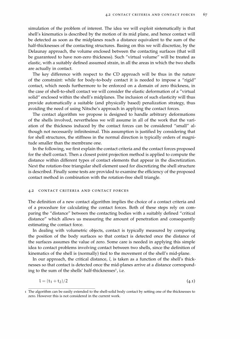
4.2 contact criteria and contact forces 67

simulation of the problem of interest. The idea we will exploit sistematically is thatshell’s kinematics is described by the motion of its mid plane, and hence contact willbe detected as soon as the midplanes reach a distance equivalent to the sum of thehalf-thicknesses of the contacting structures. Basing on this we will discretize, by theDelaunay approach, the volume enclosed between the contacting surfaces (that willbe guaranteed to have non-zero thickness). Such ”virtual volume” will be treated aselastic, with a suitably defined assumed strain, in all the areas in which the two shellsare actually in contact.

The key difference with respect to the CD approach will be thus in the natureof the constraint: while for body-to-body contact it is needed to impose a “rigid“contact, which needs furthermore to be enforced on a domain of zero thickness, inthe case of shell-to-shell contact we will consider the elastic deformation of a ”virtualsolid“ enclosed within the shell’s midplanes. The inclusion of such elasticity will thusprovide automatically a suitable (and physically based) penalization strategy, thusavoiding the need of using Nitsche’s approach in applying the contact forces.

The contact algorithm we propose is designed to handle arbitrary deformationsof the shells involved, nevertheless we will assume in all of the work that the vari-ation of the thickness induced by the contact forces can be considered “small” al-though not necessarily infinitesimal. This assumption is justified by considering thatfor shell structures, the stiffness in the normal direction is typically orders of magni-tude smaller than the membrane one.

In the following, we first explain the contact criteria and the contact forces proposedfor the shell contact. Then a closest point projection method is applied to compute thedistance within different types of contact elements that appear in the discretization.Next the rotation-free triangular shell element used for discretizing the shell structureis described. Finally some tests are provided to examine the efficiency of the proposedcontact method in combination with the rotation-free shell triangle.

4.2 contact criteria and contact forces

The definition of a new contact algorithm implies the choice of a contact criteria andof a procedure for calculating the contact forces. Both of these steps rely on com-paring the “distance” between the contacting bodies with a suitably defined “criticaldistance” which allows us measuring the amount of penetration and consequentlyestimating the contact force.

In dealing with volumetric objects, contact is typically measured by comparingthe position of the body surfaces so that contact is detected once the distance ofthe surfaces assumes the value of zero. Some care is needed in applying this simpleidea to contact problems involving contact between two shells, since the definition ofkinematics of the shell is (normally) tied to the movement of the shell’s mid-plane.

In our approach, the critical distance, l, is taken as a function of the shell’s thick-nesses so that contact is detected once the mid-planes arrive at a distance correspond-ing to the sum of the shells’ half-thicknesses1, i.e.

l = (t1 + t2)/2 (4.1)

1 The algorithm can be easily extended to the shell-solid body contact by setting one of the thicknesses tozero. However this is not considered in the current work.

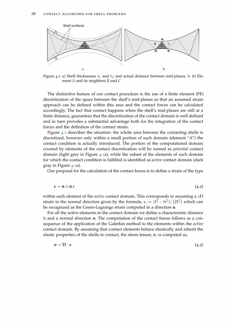
68 contact algorithm for shell problems

Figure 4.1: a) Shell thicknesses t1 and t2 and actual distance between mid-planes, h. b) Ele-ment A and its neighbors B and C

The distinctive feature of our contact procedure is the use of a finite element (FE)discretization of the space between the shell’s mid-planes so that an assumed strainapproach can be defined within this area and the contact forces can be calculatedaccordingly. The fact that contact happens when the shell’s mid-planes are still at afinite distance, guarantees that the discretization of the contact domain is well definedand in turn provides a substantial advantage both for the integration of the contactforces and the definition of the contact strain.

Figure 4.1 describes the situation: the whole area between the contacting shells isdiscretized, however only within a small portion of such domain (element “A”) thecontact condition is actually introduced. The portion of the computational domaincovered by elements of the contact discretization will be named as potential contactdomain (light grey in Figure 4.1a), while the subset of the elements of such domainfor which the contact condition is fulfilled is identified as active contact domain (darkgray in Figure 4.1a).

Our proposal for the calculation of the contact forces is to define a strain of the type

ε = n⊗ n ε (4.2)

within each element of the active contact domain. This corresponds to assuming a 1Dstrain in the normal direction given by the formula, ε := (l2 − h2)/

(2l2)

which canbe recognized as the Green-Lagrange strain computed in a direction n.

For all the active elements in the contact domain we define a characteristic distanceh and a normal direction n. The computation of the contact forces follows as a con-sequence of the application of the Galerkin method to the elements within the activecontact domain. By assuming that contact elements behave elastically and inherit theelastic properties of the shells in contact, the stress tensor, σ, is computed as,

σ = D : ε (4.3)

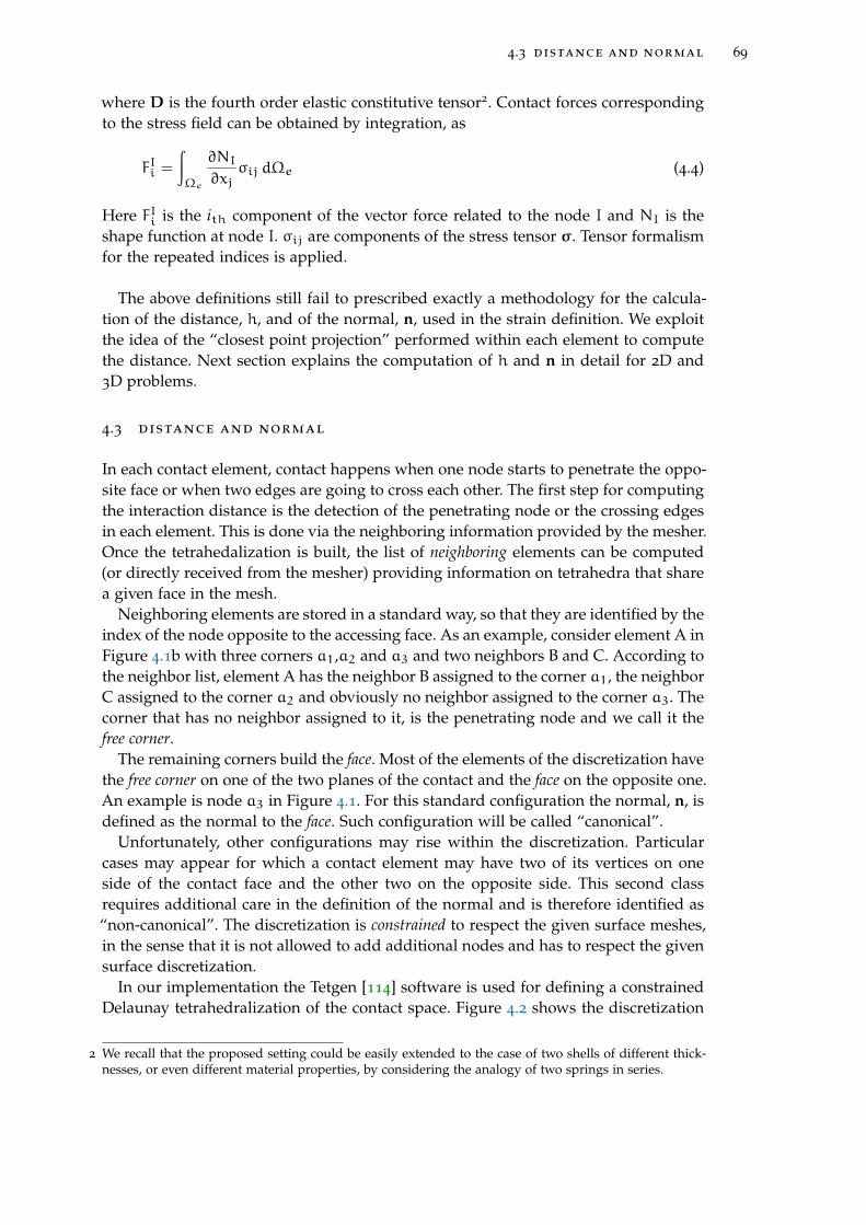
4.3 distance and normal 69

where D is the fourth order elastic constitutive tensor2. Contact forces correspondingto the stress field can be obtained by integration, as

FIi =

∫Ωe

∂NI∂xj

σij dΩe (4.4)

Here FIi is the ith component of the vector force related to the node I and NI is theshape function at node I. σij are components of the stress tensor σ. Tensor formalismfor the repeated indices is applied.

The above definitions still fail to prescribed exactly a methodology for the calcula-tion of the distance, h, and of the normal, n, used in the strain definition. We exploitthe idea of the “closest point projection” performed within each element to computethe distance. Next section explains the computation of h and n in detail for 2D and3D problems.

4.3 distance and normal

In each contact element, contact happens when one node starts to penetrate the oppo-site face or when two edges are going to cross each other. The first step for computingthe interaction distance is the detection of the penetrating node or the crossing edgesin each element. This is done via the neighboring information provided by the mesher.Once the tetrahedalization is built, the list of neighboring elements can be computed(or directly received from the mesher) providing information on tetrahedra that sharea given face in the mesh.

Neighboring elements are stored in a standard way, so that they are identified by theindex of the node opposite to the accessing face. As an example, consider element A inFigure 4.1b with three corners a1,a2 and a3 and two neighbors B and C. According tothe neighbor list, element A has the neighbor B assigned to the corner a1, the neighborC assigned to the corner a2 and obviously no neighbor assigned to the corner a3. Thecorner that has no neighbor assigned to it, is the penetrating node and we call it thefree corner.

The remaining corners build the face. Most of the elements of the discretization havethe free corner on one of the two planes of the contact and the face on the opposite one.An example is node a3 in Figure 4.1. For this standard configuration the normal, n, isdefined as the normal to the face. Such configuration will be called “canonical”.

Unfortunately, other configurations may rise within the discretization. Particularcases may appear for which a contact element may have two of its vertices on oneside of the contact face and the other two on the opposite side. This second classrequires additional care in the definition of the normal and is therefore identified as“non-canonical”. The discretization is constrained to respect the given surface meshes,in the sense that it is not allowed to add additional nodes and has to respect the givensurface discretization.

In our implementation the Tetgen [114] software is used for defining a constrainedDelaunay tetrahedralization of the contact space. Figure 4.2 shows the discretization

2 We recall that the proposed setting could be easily extended to the case of two shells of different thick-nesses, or even different material properties, by considering the analogy of two springs in series.

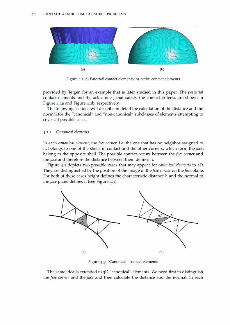
70 contact algorithm for shell problems

(a) (b)

Figure 4.2: a) Potential contact elements, b) Active contact elements

provided by Tetgen for an example that is later studied in this paper. The potentialcontact elements and the active ones, that satisfy the contact criteria, are shown inFigure 4.2a and Figure 4.2b, respectively.

The following sections will describe in detail the calculation of the distance and thenormal for the “canonical” and “non-canonical” subclasses of elements attempting tocover all possible cases.

4.3.1 Canonical elements

In each canonical element, the free corner, i.e. the one that has no neighbor assigned toit, belongs to one of the shells in contact and the other corners, which form the face,belong to the opposite shell. The possible contact occurs between the free corner andthe face and therefore the distance between them defines h.

Figure 4.3 depicts two possible cases that may appear for canonical elements in 2D.They are distinguished by the position of the image of the free corner on the face plane.For both of these cases height defines the characteristic distance h and the normal tothe face plane defines n (see Figure 4.3).

(a) (b)

Figure 4.3: “Canonical” contact elements

The same idea is extended to 3D “canonical” elements. We need first to distinguishthe free corner and the face and then calculate the distance and the normal. In each

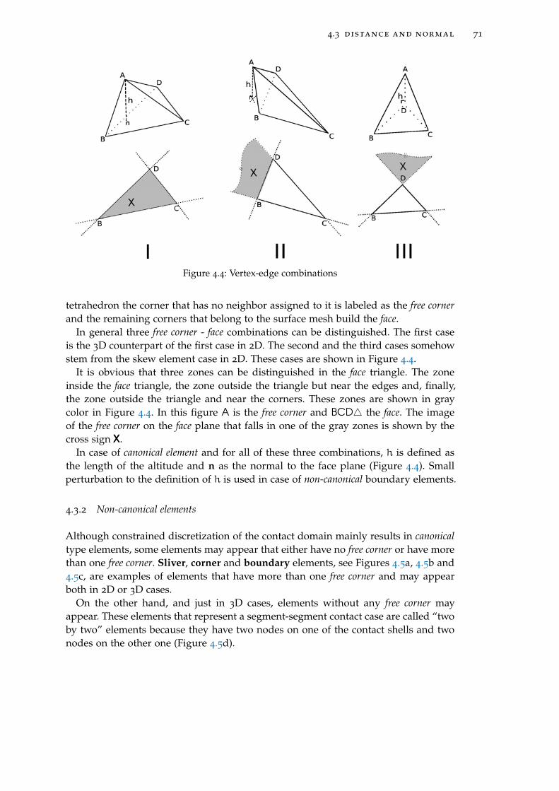
4.3 distance and normal 71

Figure 4.4: Vertex-edge combinations

tetrahedron the corner that has no neighbor assigned to it is labeled as the free cornerand the remaining corners that belong to the surface mesh build the face.

In general three free corner - face combinations can be distinguished. The first caseis the 3D counterpart of the first case in 2D. The second and the third cases somehowstem from the skew element case in 2D. These cases are shown in Figure 4.4.

It is obvious that three zones can be distinguished in the face triangle. The zoneinside the face triangle, the zone outside the triangle but near the edges and, finally,the zone outside the triangle and near the corners. These zones are shown in graycolor in Figure 4.4. In this figure A is the free corner and BCD4 the face. The imageof the free corner on the face plane that falls in one of the gray zones is shown by thecross sign XXX.

In case of canonical element and for all of these three combinations, h is defined asthe length of the altitude and n as the normal to the face plane (Figure 4.4). Smallperturbation to the definition of h is used in case of non-canonical boundary elements.

4.3.2 Non-canonical elements

Although constrained discretization of the contact domain mainly results in canonicaltype elements, some elements may appear that either have no free corner or have morethan one free corner. Sliver, corner and boundary elements, see Figures 4.5a, 4.5b and4.5c, are examples of elements that have more than one free corner and may appearboth in 2D or 3D cases.

On the other hand, and just in 3D cases, elements without any free corner mayappear. These elements that represent a segment-segment contact case are called “twoby two” elements because they have two nodes on one of the contact shells and twonodes on the other one (Figure 4.5d).

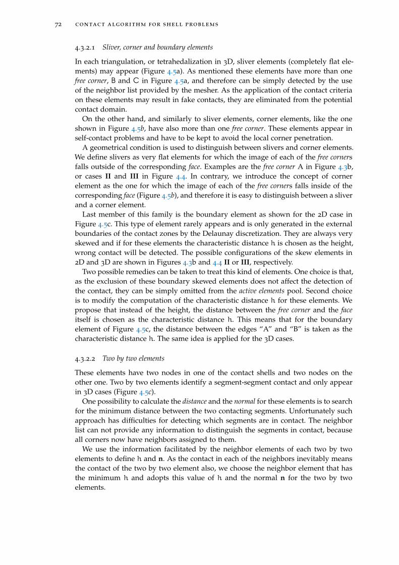
72 contact algorithm for shell problems

4.3.2.1 Sliver, corner and boundary elements

In each triangulation, or tetrahedalization in 3D, sliver elements (completely flat ele-ments) may appear (Figure 4.5a). As mentioned these elements have more than onefree corner, B and C in Figure 4.5a, and therefore can be simply detected by the useof the neighbor list provided by the mesher. As the application of the contact criteriaon these elements may result in fake contacts, they are eliminated from the potentialcontact domain.

On the other hand, and similarly to sliver elements, corner elements, like the oneshown in Figure 4.5b, have also more than one free corner. These elements appear inself-contact problems and have to be kept to avoid the local corner penetration.

A geometrical condition is used to distinguish between slivers and corner elements.We define slivers as very flat elements for which the image of each of the free cornersfalls outside of the corresponding face. Examples are the free corner A in Figure 4.3b,or cases II and III in Figure 4.4. In contrary, we introduce the concept of cornerelement as the one for which the image of each of the free corners falls inside of thecorresponding face (Figure 4.5b), and therefore it is easy to distinguish between a sliverand a corner element.

Last member of this family is the boundary element as shown for the 2D case inFigure 4.5c. This type of element rarely appears and is only generated in the externalboundaries of the contact zones by the Delaunay discretization. They are always veryskewed and if for these elements the characteristic distance h is chosen as the height,wrong contact will be detected. The possible configurations of the skew elements in2D and 3D are shown in Figures 4.3b and 4.4 II or III, respectively.

Two possible remedies can be taken to treat this kind of elements. One choice is that,as the exclusion of these boundary skewed elements does not affect the detection ofthe contact, they can be simply omitted from the active elements pool. Second choiceis to modify the computation of the characteristic distance h for these elements. Wepropose that instead of the height, the distance between the free corner and the faceitself is chosen as the characteristic distance h. This means that for the boundaryelement of Figure 4.5c, the distance between the edges “A” and “B” is taken as thecharacteristic distance h. The same idea is applied for the 3D cases.

4.3.2.2 Two by two elements

These elements have two nodes in one of the contact shells and two nodes on theother one. Two by two elements identify a segment-segment contact and only appearin 3D cases (Figure 4.5c).

One possibility to calculate the distance and the normal for these elements is to searchfor the minimum distance between the two contacting segments. Unfortunately suchapproach has difficulties for detecting which segments are in contact. The neighborlist can not provide any information to distinguish the segments in contact, becauseall corners now have neighbors assigned to them.

We use the information facilitated by the neighbor elements of each two by twoelements to define h and n. As the contact in each of the neighbors inevitably meansthe contact of the two by two element also, we choose the neighbor element that hasthe minimum h and adopts this value of h and the normal n for the two by twoelements.

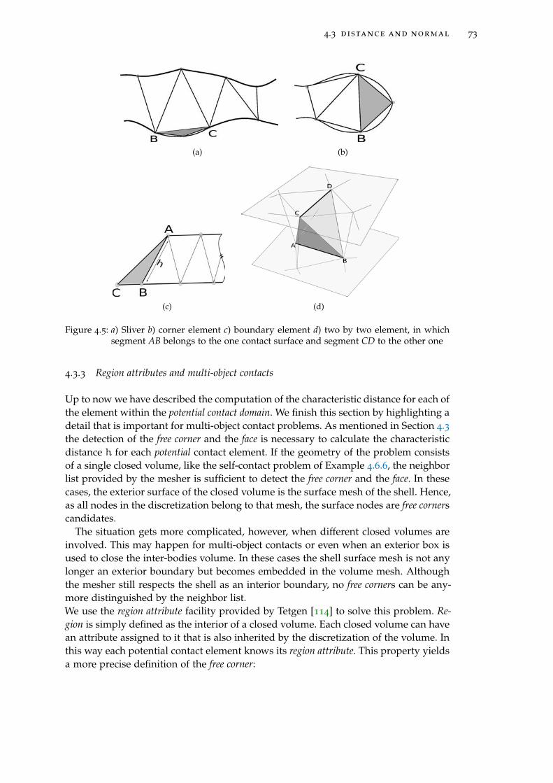
4.3 distance and normal 73

(a) (b)

(c) (d)

Figure 4.5: a) Sliver b) corner element c) boundary element d) two by two element, in whichsegment AB belongs to the one contact surface and segment CD to the other one

4.3.3 Region attributes and multi-object contacts

Up to now we have described the computation of the characteristic distance for each ofthe element within the potential contact domain. We finish this section by highlighting adetail that is important for multi-object contact problems. As mentioned in Section 4.3the detection of the free corner and the face is necessary to calculate the characteristicdistance h for each potential contact element. If the geometry of the problem consistsof a single closed volume, like the self-contact problem of Example 4.6.6, the neighborlist provided by the mesher is sufficient to detect the free corner and the face. In thesecases, the exterior surface of the closed volume is the surface mesh of the shell. Hence,as all nodes in the discretization belong to that mesh, the surface nodes are free cornerscandidates.

The situation gets more complicated, however, when different closed volumes areinvolved. This may happen for multi-object contacts or even when an exterior box isused to close the inter-bodies volume. In these cases the shell surface mesh is not anylonger an exterior boundary but becomes embedded in the volume mesh. Althoughthe mesher still respects the shell as an interior boundary, no free corners can be any-more distinguished by the neighbor list.We use the region attribute facility provided by Tetgen [114] to solve this problem. Re-gion is simply defined as the interior of a closed volume. Each closed volume can havean attribute assigned to it that is also inherited by the discretization of the volume. Inthis way each potential contact element knows its region attribute. This property yieldsa more precise definition of the free corner:

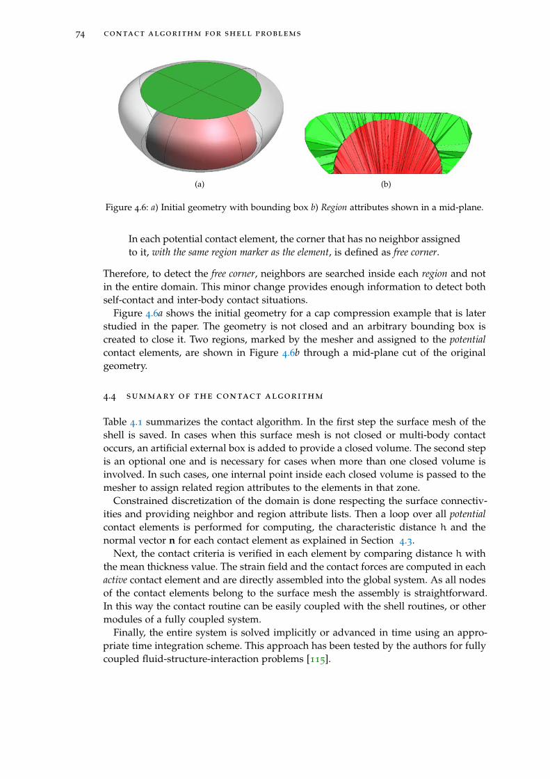
74 contact algorithm for shell problems

(a) (b)

Figure 4.6: a) Initial geometry with bounding box b) Region attributes shown in a mid-plane.

In each potential contact element, the corner that has no neighbor assignedto it, with the same region marker as the element, is defined as free corner.

Therefore, to detect the free corner, neighbors are searched inside each region and notin the entire domain. This minor change provides enough information to detect bothself-contact and inter-body contact situations.

Figure 4.6a shows the initial geometry for a cap compression example that is laterstudied in the paper. The geometry is not closed and an arbitrary bounding box iscreated to close it. Two regions, marked by the mesher and assigned to the potentialcontact elements, are shown in Figure 4.6b through a mid-plane cut of the originalgeometry.

4.4 summary of the contact algorithm

Table 4.1 summarizes the contact algorithm. In the first step the surface mesh of theshell is saved. In cases when this surface mesh is not closed or multi-body contactoccurs, an artificial external box is added to provide a closed volume. The second stepis an optional one and is necessary for cases when more than one closed volume isinvolved. In such cases, one internal point inside each closed volume is passed to themesher to assign related region attributes to the elements in that zone.

Constrained discretization of the domain is done respecting the surface connectiv-ities and providing neighbor and region attribute lists. Then a loop over all potentialcontact elements is performed for computing, the characteristic distance h and thenormal vector n for each contact element as explained in Section 4.3.

Next, the contact criteria is verified in each element by comparing distance h withthe mean thickness value. The strain field and the contact forces are computed in eachactive contact element and are directly assembled into the global system. As all nodesof the contact elements belong to the surface mesh the assembly is straightforward.In this way the contact routine can be easily coupled with the shell routines, or othermodules of a fully coupled system.

Finally, the entire system is solved implicitly or advanced in time using an appro-priate time integration scheme. This approach has been tested by the authors for fullycoupled fluid-structure-interaction problems [115].

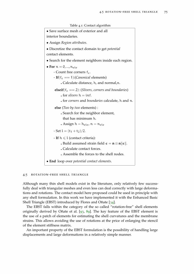
4.5 rotation-free shell triangle 75

Table 4.1: Contact algorithm

• Save surface mesh of exterior and allinterior boundaries.

• Assign Region attributes.

• Discretize the contact domain to get potentialcontact elements.

• Search for the element neighbors inside each region.

• For n = 0, ...,nele- Count free corners fc.- If(fc == 1):(Canonical elements) Calculate distance, h, and normal,n.

elseif(fc == 2): (Slivers, corners and boundaries) for slivers h = inf. for corners and boundaries calculate, h and n.

else (Two by two elements) : Search for the neighbor element,

that has minimum h. Assign h = hele, n = nele

- Set l = (t1 + t2)/2.

- If h 6 l (contact criteria): Build assumed strain field ε = n⊗ n‖ε‖. Calculate contact forces. Assemble the forces to the shell nodes.

• End loop over potential contact elements.

4.5 rotation-free shell triangle

Although many thin shell models exist in the literature, only relatively few success-fully deal with triangular meshes and even less can deal correctly with large deforma-tions and rotations. The contact model here proposed could be used in principle withany shell formulation. In this work we have implemented it with the Enhanced BasicShell Triangle (EBST) introduced by Flores and Oñate [34].

The EBST falls within the category of the so called “rotation-free” shell elementsoriginally derived by Oñate et al. [93, 89]. The key feature of the EBST element isthe use of a patch of elements for estimating the shell curvatures and the membranestrains. This allows avoiding the use of rotations at the price of enlarging the stencilof the element stiffness matrix.

An important property of the EBST formulation is the possibility of handling largedisplacements and large deformations in a relatively simple manner.

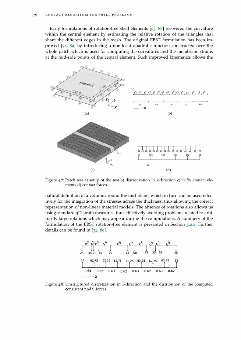
76 contact algorithm for shell problems

Early formulations of rotation-free shell elements [93, 88] recovered the curvaturewithin the central element by estimating the relative rotation of the triangles thatshare the different edges in the mesh. The original EBST formulation has been im-proved [34, 89] by introducing a non-local quadratic function constructed over thewhole patch which is used for computing the curvatures and the membrane strainsat the mid-side points of the central element. Such improved kinematics allows the

(a) (b)

(c) (d)

Figure 4.7: Patch test a) setup of the test b) discretization in x-direction c) active contact ele-ments d) contact forces.

natural definition of a volume around the mid-plane, which in turn can be used effec-tively for the integration of the stresses across the thickness, thus allowing the correctrepresentation of non-linear material models. The absence of rotations also allows ususing standard 3D strain measures, thus effectively avoiding problems related to arbi-trarily large rotations which may appear during the computations. A summery of theformulation of the EBST rotation-free element is presented in Section 5.2.2. Furtherdetails can be found in [34, 89].

Figure 4.8: Unstructured discretization in x-direction and the distribution of the computedconsistent nodal forces.

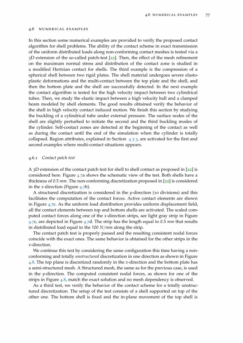
4.6 numerical examples 77

4.6 numerical examples

In this section some numerical examples are provided to verify the proposed contactalgorithm for shell problems. The ability of the contact scheme in exact transmissionof the uniform distributed loads along non-conforming contact meshes is tested via a3D extension of the so-called patch-test [22]. Then, the effect of the mesh refinementon the maximum normal stress and distribution of the contact zone is studied ina modified Hertzian contact for shells. The third example is the compression of aspherical shell between two rigid plates. The shell material undergoes severe elasto-plastic deformations and the multi-contact between the top plate and the shell, andthen the bottom plate and the shell are successfully detected. In the next examplethe contact algorithm is tested for the high velocity impact between two cylindricaltubes. Then, we study the elastic impact between a high velocity ball and a clampedbeam modeled by shell elements. The good results obtained verify the behavior ofthe shell in high velocity contact induced motion. We finish this section by studyingthe buckling of a cylindrical tube under external pressure. The surface nodes of theshell are slightly perturbed to initiate the second and the third buckling modes ofthe cylinder. Self-contact zones are detected at the beginning of the contact as wellas during the contact until the end of the simulation when the cylinder is totallycollapsed. Region attributes, explained in Section 4.3.3, are activated for the first andsecond examples where multi-contact situations appears.

4.6.1 Contact patch test

A 3D extension of the contact patch test for shell to shell contact as proposed in [22] isconsidered here. Figure 4.7a shows the schematic view of the test. Both shells have athickness of 0.5 mm. The non-conforming discretization proposed in [22] is consideredin the x-direction (Figure 4.7b).

A structured discretization is considered in the y-direction (10 divisions) and thisfacilitates the computation of the contact forces. Active contact elements are shownin Figure 4.7c. As the uniform load distribution provides uniform displacement field,all the contact elements between top and bottom shells are activated. The scaled com-puted contact forces along one of the x-direction strips, see light gray strip in Figure4.7c, are depicted in Figure 4.7d. The strip has the length equal to 0.5 mm that resultsin distributed load equal to the 100 N/mm along the strip.

The contact patch test is properly passed and the resulting consistent nodal forcescoincide with the exact ones. The same behavior is obtained for the other strips in thex-direction.

We continue this test by considering the same configuration this time having a non-conforming and totally unstructured discretization in one direction as shown in Figure4.8. The top plane is discretized randomly in the x-direction and the bottom plate hasa semi-structured mesh. A Structured mesh, the same as for the previous case, is usedin the y-direction. The computed consistent nodal forces, as shown for one of thestrips in Figure 4.8, match the exact solution and no mesh dependency is observed.

As a third test, we verify the behavior of the contact scheme for a totally unstruc-tured discretization. The setup of the test consists of a shell supported on top of theother one. The bottom shell is fixed and the in-plane movement of the top shell is

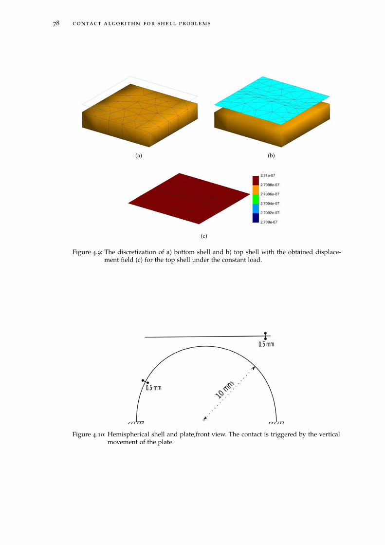
78 contact algorithm for shell problems

(a) (b)

(c)

Figure 4.9: The discretization of a) bottom shell and b) top shell with the obtained displace-ment field (c) for the top shell under the constant load.

Figure 4.10: Hemispherical shell and plate,front view. The contact is triggered by the verticalmovement of the plate.

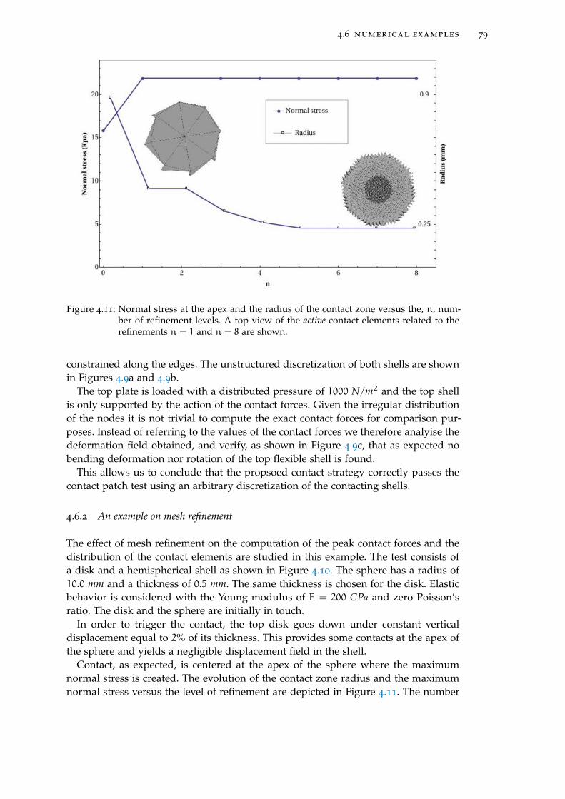
4.6 numerical examples 79

Figure 4.11: Normal stress at the apex and the radius of the contact zone versus the, n, num-ber of refinement levels. A top view of the active contact elements related to therefinements n = 1 and n = 8 are shown.

constrained along the edges. The unstructured discretization of both shells are shownin Figures 4.9a and 4.9b.

The top plate is loaded with a distributed pressure of 1000 N/m2 and the top shellis only supported by the action of the contact forces. Given the irregular distributionof the nodes it is not trivial to compute the exact contact forces for comparison pur-poses. Instead of referring to the values of the contact forces we therefore analyise thedeformation field obtained, and verify, as shown in Figure 4.9c, that as expected nobending deformation nor rotation of the top flexible shell is found.

This allows us to conclude that the propsoed contact strategy correctly passes thecontact patch test using an arbitrary discretization of the contacting shells.

4.6.2 An example on mesh refinement

The effect of mesh refinement on the computation of the peak contact forces and thedistribution of the contact elements are studied in this example. The test consists ofa disk and a hemispherical shell as shown in Figure 4.10. The sphere has a radius of10.0 mm and a thickness of 0.5 mm. The same thickness is chosen for the disk. Elasticbehavior is considered with the Young modulus of E = 200 GPa and zero Poisson’sratio. The disk and the sphere are initially in touch.

In order to trigger the contact, the top disk goes down under constant verticaldisplacement equal to 2% of its thickness. This provides some contacts at the apex ofthe sphere and yields a negligible displacement field in the shell.

Contact, as expected, is centered at the apex of the sphere where the maximumnormal stress is created. The evolution of the contact zone radius and the maximumnormal stress versus the level of refinement are depicted in Figure 4.11. The number

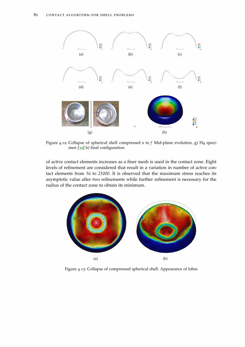
80 contact algorithm for shell problems

(a) (b) (c)

(d) (e) (f)

(g) (h)

Figure 4.12: Collapse of spherical shell compressed a to f Mid-plane evolution, g) H4 speci-men [39] h) final configuration

of active contact elements increases as a finer mesh is used in the contact zone. Eightlevels of refinement are considered that result in a variation in number of active con-tact elements from 16 to 21000. It is observed that the maximum stress reaches itsasymptotic value after two refinements while further refinement is necessary for theradius of the contact zone to obtain its minimum.

(a) (b)

Figure 4.13: Collapse of compressed spherical shell. Appearance of lobes

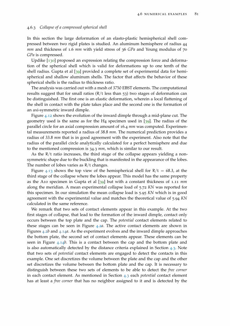
4.6 numerical examples 81

4.6.3 Collapse of a compressed spherical shell

In this section the large deformation of an elasto-plastic hemispherical shell com-pressed between two rigid plates is studied. An aluminum hemisphere of radius 44

mm and thickness of 1.6 mm with yield stress of 36 GPa and Young modulus of 70

GPa is compressed.Updike [130] proposed an expression relating the compression force and deforma-

tion of the spherical shell which is valid for deformations up to one tenth of theshell radius. Gupta et al [39] provided a complete set of experimental data for hemi-spherical and shallow aluminum shells. The factor that affects the behavior of thesespherical shells is the radius to thickness ratio.

The analysis was carried out with a mesh of 3750 EBST elements. The computationalresults suggest that for small ratios (R/t less than 53) two stages of deformation canbe distinguished. The first one is an elastic deformation, wherein a local flattening ofthe shell in contact with the plate takes place and the second one is the formation ofan axi-symmetric inward dimple.

Figure 4.12 shows the evolution of the inward dimple through a mid-plane cut. Thegeometry used is the same as for the H4 specimen used in [39]. The radius of theparallel circle for an axial compression amount of 16.4 mm was computed. Experimen-tal measurements reported a radius of 38.8 mm. The numerical prediction provides aradius of 33.8 mm that is in good agreement with the experiment. Also note that theradius of the parallel circle analytically calculated for a perfect hemisphere and dueto the mentioned compression is 34.3 mm, which is similar to our result.

As the R/t ratio increases, the third stage of the collapse appears yielding a non-symmetric shape due to the buckling that is manifested in the appearance of the lobes.The number of lobes varies as R/t changes.

Figure 4.13 shows the top view of the hemispherical shell for R/t = 68.3, at thethird stage of the collapse where the lobes appear. This model has the same propertyas the A10 specimen in Gupta et al [39] but with a constant thickness of 1.11 mmalong the meridian. A mean experimental collapse load of 5.72 KN was reported forthis specimen. In our simulation the mean collapse load is 5.95 KN which is in goodagreement with the experimental value and matches the theoretical value of 5.94 KNcalculated in the same reference.

We remark that two sets of contact elements appear in this example. At the twofirst stages of collapse, that lead to the formation of the inward dimple, contact onlyoccurs between the top plate and the cap. The potential contact elements related tothese stages can be seen in Figure 4.2a. The active contact elements are shown inFigures 4.2b and 4.14a. As the experiment evolves and the inward dimple approachesthe bottom plate, the second set of contact elements appear. These elements can beseen in Figure 4.14b. This is a contact between the cap and the bottom plate andis also automatically detected by the distance criteria explained in Section 4.3. Notethat two sets of potential contact elements are engaged to detect the contacts in thisexample. One set discretizes the volume between the plate and the cap and the otherset discretizes the volume between the bottom plate and the cap. It is necessary todistinguish between these two sets of elements to be able to detect the free cornerin each contact element. As mentioned in Section 4.3 each potential contact elementhas at least a free corner that has no neighbor assigned to it and is detected by the

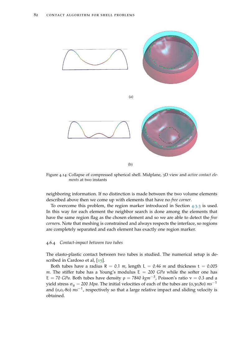
82 contact algorithm for shell problems

(a)

(b)

Figure 4.14: Collapse of compressed spherical shell. Midplane, 3D view and active contact ele-ments at two instants

neighboring information. If no distinction is made between the two volume elementsdescribed above then we come up with elements that have no free corner.

To overcome this problem, the region marker introduced in Section 4.3.3 is used.In this way for each element the neighbor search is done among the elements thathave the same region flag as the chosen element and so we are able to detect the freecorners. Note that meshing is constrained and always respects the interface, so regionsare completely separated and each element has exactly one region marker.

4.6.4 Contact-impact between two tubes

The elasto-plastic contact between two tubes is studied. The numerical setup is de-scribed in Cardoso et al, [15].

Both tubes have a radius R = 0.1 m, length L = 0.46 m and thickness t = 0.005m. The stiffer tube has a Young’s modulus E = 200 GPa while the softer one hasE = 70 GPa. Both tubes have density ρ = 7840 kgm−3, Poisson’s ratio ν = 0.3 and ayield stress σy = 200 Mpa. The initial velocities of each of the tubes are (0,30,80) ms−1

and (0,0,-80) ms−1, respectively so that a large relative impact and sliding velocity isobtained.

4.6 numerical examples 83

Figure 4.15: Contact-impact of two tubes. Geometries at time t = 1ms

7000 EBST elements were used for discretizing each tube. Figure 4.15 shows thedeformed geometry after the impact. A similar set of results obtained by Cardoso etal. [15]. This example clearly shows the behavior of the shell for large deformationsand severe contact conditions. Note that the surface meshes are unstructured andno restriction is imposed on them. As in the previous example, different regions areconsidered to detect the contact elements. Tubes are made closed by putting top andbottom caps and both of them are place in a closed box. Consequently three regionsappear, one in each tube to mark elements for the self-contacts and one inter-tuberegion to mark the contact between tubes.

4.6.5 Ball impacting a clamped plate

In this example we study a ball impacting a clamped rectangular plate. The data forthis test was provided by Zhong [139]. Both the ball and the plate are assumed to beelastic with Young’s modulus E = 200 GPa and Poisson’s ratio ν = 0.3. The ball hasa radius R = 0.1 m and the beam has a length L = 1.0 m, width W = 0.24 m andthickness t = 0.0015 m. An initial velocity of (0,0,-30.0) ms−1 is assigned to the ball.Figure 4.16 shows the results obtained by our method using a mesh of 4800 EBSTelements and those obtained by Cardoso et al [15]. Good agreement is again obtainedbetween both set of results.

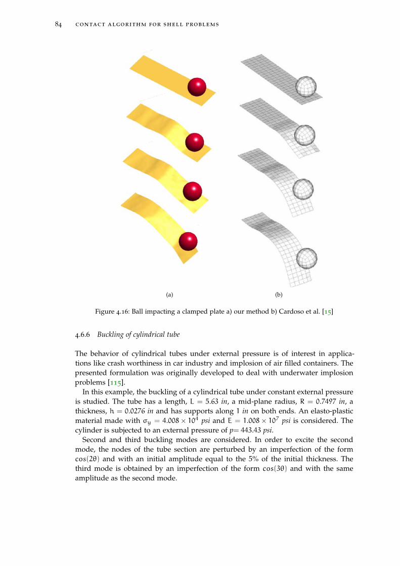
84 contact algorithm for shell problems

(a) (b)

Figure 4.16: Ball impacting a clamped plate a) our method b) Cardoso et al. [15]

4.6.6 Buckling of cylindrical tube

The behavior of cylindrical tubes under external pressure is of interest in applica-tions like crash worthiness in car industry and implosion of air filled containers. Thepresented formulation was originally developed to deal with underwater implosionproblems [115].

In this example, the buckling of a cylindrical tube under constant external pressureis studied. The tube has a length, L = 5.63 in, a mid-plane radius, R = 0.7497 in, athickness, h = 0.0276 in and has supports along 1 in on both ends. An elasto-plasticmaterial made with σy = 4.008× 104 psi and E = 1.008× 107 psi is considered. Thecylinder is subjected to an external pressure of p= 443.43 psi.

Second and third buckling modes are considered. In order to excite the secondmode, the nodes of the tube section are perturbed by an imperfection of the formcos(2θ) and with an initial amplitude equal to the 5% of the initial thickness. Thethird mode is obtained by an imperfection of the form cos(3θ) and with the sameamplitude as the second mode.

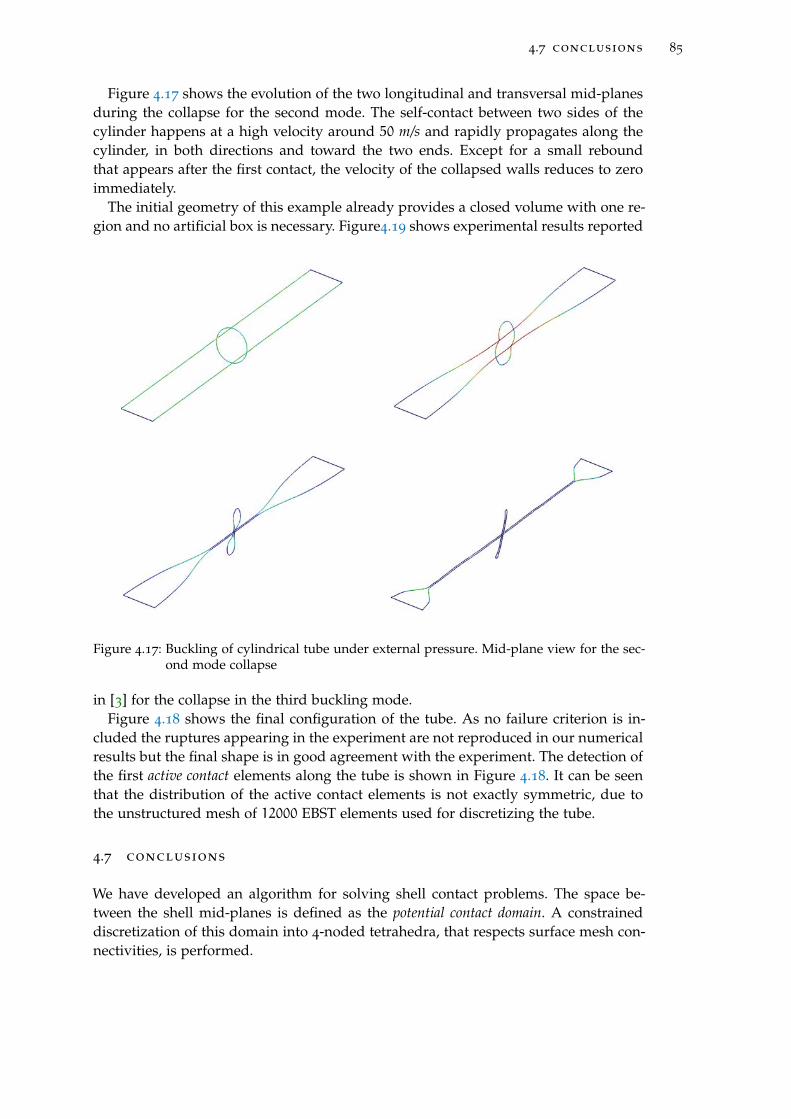
4.7 conclusions 85

Figure 4.17 shows the evolution of the two longitudinal and transversal mid-planesduring the collapse for the second mode. The self-contact between two sides of thecylinder happens at a high velocity around 50 m/s and rapidly propagates along thecylinder, in both directions and toward the two ends. Except for a small reboundthat appears after the first contact, the velocity of the collapsed walls reduces to zeroimmediately.

The initial geometry of this example already provides a closed volume with one re-gion and no artificial box is necessary. Figure4.19 shows experimental results reported

Figure 4.17: Buckling of cylindrical tube under external pressure. Mid-plane view for the sec-ond mode collapse

in [3] for the collapse in the third buckling mode.Figure 4.18 shows the final configuration of the tube. As no failure criterion is in-

cluded the ruptures appearing in the experiment are not reproduced in our numericalresults but the final shape is in good agreement with the experiment. The detection ofthe first active contact elements along the tube is shown in Figure 4.18. It can be seenthat the distribution of the active contact elements is not exactly symmetric, due tothe unstructured mesh of 12000 EBST elements used for discretizing the tube.

4.7 conclusions

We have developed an algorithm for solving shell contact problems. The space be-tween the shell mid-planes is defined as the potential contact domain. A constraineddiscretization of this domain into 4-noded tetrahedra, that respects surface mesh con-nectivities, is performed.

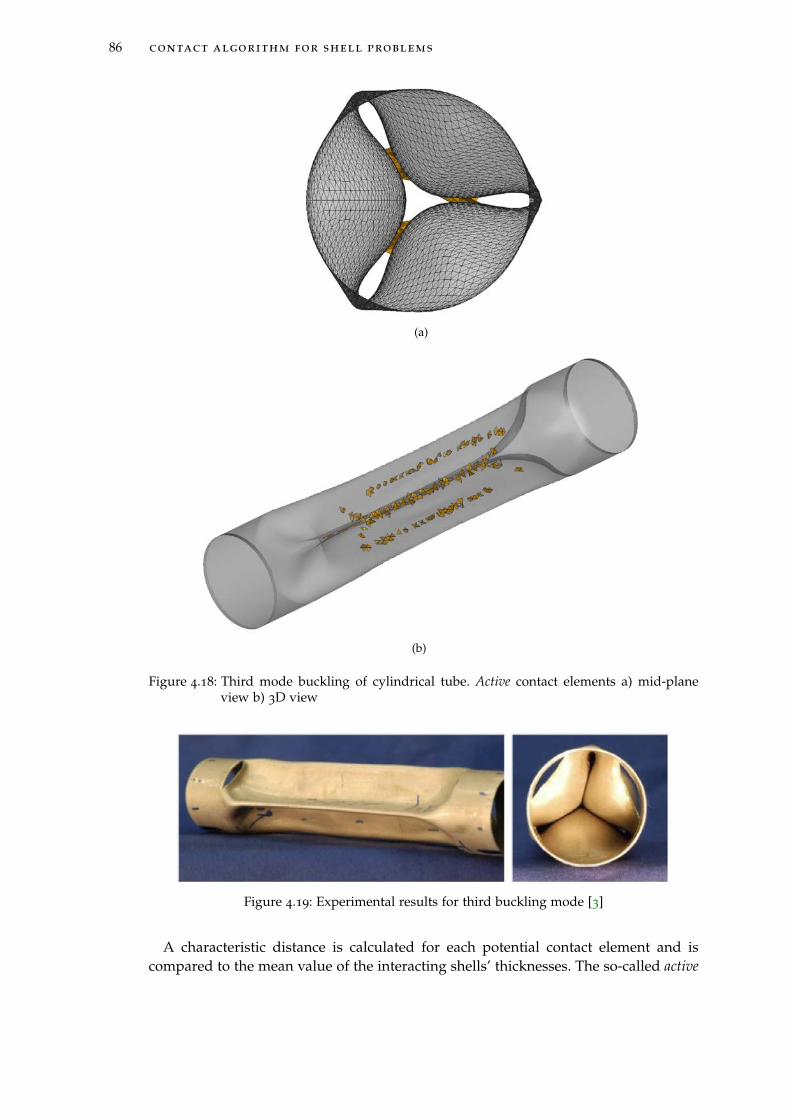
86 contact algorithm for shell problems

(a)

(b)

Figure 4.18: Third mode buckling of cylindrical tube. Active contact elements a) mid-planeview b) 3D view

Figure 4.19: Experimental results for third buckling mode [3]

A characteristic distance is calculated for each potential contact element and iscompared to the mean value of the interacting shells’ thicknesses. The so-called active

4.7 conclusions 87

contact domain consist of those elements that satisfy this contact criteria. We constructa Green strain field by means of element normals in each active contact element andthen calculate elastic contact forces. As the contact elements share all nodes withshell surface meshes, these forces are directly assembled to the shell nodes. This con-tact algorithm has been tested for various self-contact and multi-body contact prob-lems in shells using the rotation-free EBST shell triangle. The algorithm can be easilyintegrated in coupled problems involving shells, solids and fluids. Unlike penaltymethods, no arbitrary contact factor to enforce the contact conditions is required andregularity is not needed for the meshes discretizing the shell surface. Very good re-sults have been obtained in the application of the new contact algorithm to differentshell-contact problems.

5F L U I D - S T R U C T U R E I N T E R A C T I O N

We propose a fully Lagrangian monolithic framework to simulate the underwater im-plosion of closed containers “a la PFEM” [59, 92]. To our knowledge, it is the only fullyLagrangian compressible FSI framework available. The main features of this frameworkare the monolithic coupling of the fluid and structure subsystems, the discontinuoustreatment of the pressure and density at the interface and the possibility of providingthe desired mesh resolution when large displacements occur. This framework is anextension of the multi-fluid compressible formulation, presented in chapter 3, to FSIproblems.

We first recall the stabilized variational multiscale method developed in chapter3

for solving the Euler hydrodynamic set of equations. Then the coupling of the EBSTshell element and the contact algorithm presented in previous section is explained.The implicit and explicit time integration schemes for the coupled system are detailedand the matrices of the coupled system are extracted. A Section is devoted to explainthe Lagrangian framework that includes the adaptive constrained mesh generation,and the construction and solution of the coupled system. Finally the underwater im-plosion of an aluminum cylinder is simulated and compared with the experimentalresults.

The material of this chapter are taken from our paper, A compressible Lagrangianframework for modeling the fluid-structure interaction in the underwater implosion of analuminum cylinder [115].

5.1 introduction

The goal of the present work is to accurately predict the underwater implosion of analuminum cylinder. An implodable volume, by definition, is any pressure housingcontaining a non-compensated compressible volume at a pressure below the externalpressure which has the potential to collapse [74].

From the pioneer studies of Rayleigh [102] on the dynamics of bubble and cavitationto the latest works on the violent collapse of µm size bubbles excited by the soundwaves [48, 77], different aspects of the underwater implosion have been investigated.

The main signature of this phenomenon is a low flat negative-pulse that is fol-lowed by a sharp positive-pressure spike. The strength and duration of the pressurepeak depend on the dimension of the implodable volume and the depth in which theimplosion occurs[94, 75]. Although, the 1D theoretical studies predict an oscillatingbehavior of the bubble, with the same amplitude and strength, the compressibilityof the high pressure surrounding water [99, 101] and the appearance of the instabili-ties [7, 77, 9] on the air-water interface explain the strongly damped sinusoidal pulse

89

90 fluid-structure interaction

detected in the experiments. In many of such experiments [94, 129, 43] the implodablevolume is simply a light bulb preweakend in some zones or being attached to a crackinitiator device.

In practice, the acoustic wave emanating from these glass spheres can be used to de-tect the contact of the equipment with the seabed. On the other hand, there is concernthat under the wrong circumstances, the pressure pulses produced by the collapsingvolume, which in this case are metallic containers filled with fluid at atmospheric-pressure, can damage nearby submersibles or other objects [21, 78].

Although the first predictions on the dynamics of the implosion can be done using1D models and neglecting the surrounding structure, a full 3D model that considersthe realistic, fast dynamic, fluid-structure interaction (FSI) of the problem seems in-evitable. It is also necessary to model the structure that separates air and water. Notonly the physics of the problem changes by considering a separating structure at theair-water interface, obviously no Rayleigh-Taylor interfacial instabilities appear, butthe errors in the pressure peak value neglecting this structure can reach 44% [129] ofits maximum value.

The major challenges during the underwater implosion process are: fast dynamicsof the FSI, all the process occurs in less than 1 ms; resolution of the possible shockwaves that appear in both air and water, and, last but not least, the large deformationsof the structure that in some cases end up with cracks and self-contact in the shellstructure.

As high pressures are involved, the external fluid (water) as much as the internalone (air) are modeled as compressible media. Respecting the structural part, the ge-ometric and material nonlinearities of the shell structure need to be considered toobtain a realistic solution.

Various studies considering the FSI in related applications are performed. Amongthem, Kalumuk [16] studied bubble interactions with nearby bodies using the bound-ary element technique. Some authors [141, 70] investigated the interaction of a bubble,caused by an underwater implosion, with free-surface structures. Iakovlev[54] investi-gated the interaction of an external explosion with a deformable inner structure. Coret al [21] evaluated the effect of internal structure on the behavior of spherical andcylindrical implodable volumes.

Among the relatively few works that fully model the FSI system is the one proposedby Farhat et al [31, 32]. They designed a three-field formulation for the non-linearfluid-structure problem based on the Arbitrary Lagrangian Eulerian (ALE) formula-tion of the fluid equations. Furthermore, a second-order loosely coupled staggeredscheme is designed to treat the FSI and few elements have been used for discretizingthe internal air due to the restrictions of the ALE mesh motion algorithms.

In the following we recall the stabilized hydrodynamic set of equations presentedin chapter 3. The main difference comparing the presenetd two-fluid system isthepresence of a shell structure that separates the internal air from the external water.This shell is modeled with the three node rotation-free EBST shell element [35].

Linear tetrahedra are used to discretize the air and water domain and both fluidsare modeled as compressible continua. A nodally perfect matched definition of theinterface, proposed by Idelsohn et al [57], allows us to duplicate the pressure anddensity at the interface level. The contact method described in chapter 4 is used todetect the contact and compute the non-penetrating forces. As large deformations

5.2 governing equations 91

occur during the solution, a constrained adaptive mesh is generated, whenever nec-essary, to ensure the quality of the mesh. The monolithic FSI system is solved usingan implicit predictor/multi-corrector Bossak scheme at each step. An explicit forwardEuler solution of this system is also provided and both results are then comparedwith experimental data.

5.2 governing equations

5.2.1 Lagrangian hydrodynamic equations

We recall from chapter 3 that the Lagrangian compressible hydrodynamic governingthe conservation of mass, momentum and energy are, respectively,

ρJ = ρ0 (5.1a)

ρu +∇xp = b inΩ, t ∈]0, T [ (5.1b)

ρε+ p∇x · u = ∇x · h + ρr inΩ, t ∈]0, T [ (5.1c)

We then complete this set of equations by an equation of state of the form p =

p(ρ, ε). Applying the multisclae paradigm with the decomposition of the unknownsas,

u = uh + u ′

p = ph + p ′ (5.2)

ε = εh + ε ′.

and considering some simplifications typical of the multiscale method, we end upwith the stabilized form of the Eqs. (5.1), i.e.:∫

Ω

vh · ρ (uh)dΩ−

∫Ω

(∇x · vh)ph dΩ

+

∫Ω

∇x · vh τ (p+ ρc2s∇x · u)dΩ = 0 (5.3)∫Ω

qh (ρεh + ph∇x · uh)dΩ

+

∫Ω

τ(c2s)∇xqh · (ρuh +∇xph)dΩ (5.4)

−

∫Ω

qh∇x · uh τ (p+ ρc2s∇x · u)dΩ = 0

These equations are best suited for the mid-point explicit time descritization as pre-sented in chapter 3, while a more suitbe form for the implicit scheme can be obtainedby introdcing a full u − p equivalence of this stabilized form. We have already shownin chapter3 that considering the Mie-Grüneisen equation of state (EOS) that has thefollowing general form:

p = p(ρ, ε) = f1(ρ) + f2(ρ)ε. (5.5)

92 fluid-structure interaction

and by applying Gibbs identity, an equivalent for the energy equation can be obtainedas,

ρhεh + ph∇x · uh = ρ∂ε

∂p

∣∣∣ρ(p+ ρc2s∇x · u), (5.6)

In this way, and by applying equation (5.6) to the stabilzied form of the enery equa-tion (5.8), the u − p stabilized form can be obtained as,∫

Ω

vh · ρ (uh)dΩ−

∫Ω

(∇x · vh)ph dΩ

+

∫Ω

∇x · vh τ (p+ ρc2s∇x · u)dΩ = 0 (5.7)∫Ω

ρh∂ε

∂p

∣∣∣ρ(qh (p+ ρc2s∇x · u))dΩ

+

∫Ω

ρh∂ε

∂p

∣∣∣ρ(τ(c2s)∇xqh · (ρuh +∇xph))dΩ (5.8)

−

∫Ω

qh∇x · uh τ (p+ ρc2s∇x · u)dΩ = 0

We remind that for an ideal gas the term ρh ∂ε∂p

∣∣∣ρ

is constant and equal to 1/(γ− 1).

Eqs. (5.7) and (5.8) are used in Section 5.3.1 for obtaining the matrices of the im-plicit monolithic scheme. We remind that at the presence of the shock waves, shock-capturing operators in the form of artificial viscosities are introduced to smear thediscontinuity over a few cells of the computational grid.

In the following, the variational model used for the structure is briefly presented.

5.2.2 Rotation-free shell triangle

A rotation-free shell triangular element is used to model the behavior of the cylinderunder the high external water pressure. The Enhanced Basic Shell Triangle (EBST),is derived using an assumed linear field for the membrane strains and an assumedconstant curvature field [35, 34]. Both assumed fields are obtained from a quadraticinterpolation of the displacement field of a patch. For each element the patch is de-fined as the element itself and three neighboring elements, as shown in Figure 5.1.

The virtual work principle is written as,∫ [δεTmσm + δκTσb

]dA =

∫δyT t dA (5.9)

Where δεm is the virtual Green-Lagrange membrane strain vector, δκ is the virtualcurvatures vector and δy is the virtual displacement vector. σm and σb are the re-sultant membrane and bending stresses computed from the integration of the sec-ond Piola-Kirchhoff stresses along the shell thickness. A detailed descriptions of theelement matrices can be found in [35, 34]. The original EBST formulation was im-proved [34, 89] by introducing a non-local quadratic function constructed over thewhole patch which is used for computing the curvatures and the membrane strainsat the mid-side points of the central element. Such improved kinematics allows the

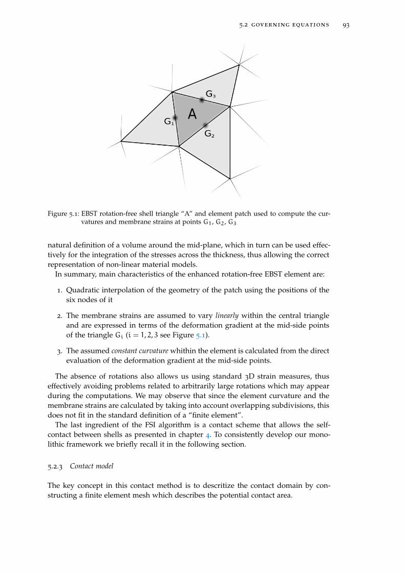
5.2 governing equations 93

Figure 5.1: EBST rotation-free shell triangle “A” and element patch used to compute the cur-vatures and membrane strains at points G1, G2, G3

natural definition of a volume around the mid-plane, which in turn can be used effec-tively for the integration of the stresses across the thickness, thus allowing the correctrepresentation of non-linear material models.

In summary, main characteristics of the enhanced rotation-free EBST element are:

1. Quadratic interpolation of the geometry of the patch using the positions of thesix nodes of it

2. The membrane strains are assumed to vary linearly within the central triangleand are expressed in terms of the deformation gradient at the mid-side pointsof the triangle Gi (i = 1, 2, 3 see Figure 5.1).

3. The assumed constant curvature whithin the element is calculated from the directevaluation of the deformation gradient at the mid-side points.

The absence of rotations also allows us using standard 3D strain measures, thuseffectively avoiding problems related to arbitrarily large rotations which may appearduring the computations. We may observe that since the element curvature and themembrane strains are calculated by taking into account overlapping subdivisions, thisdoes not fit in the standard definition of a “finite element”.

The last ingredient of the FSI algorithm is a contact scheme that allows the self-contact between shells as presented in chapter 4. To consistently develop our mono-lithic framework we briefly recall it in the following section.

5.2.3 Contact model

The key concept in this contact method is to descritize the contact domain by con-structing a finite element mesh which describes the potential contact area.

94 fluid-structure interaction

Figure 5.2 depicts two shell surfaces and the potential contact area between themdiscretized by a finite element mesh. As we model the mid-planes of the shells, acritical distance, l, is defined as a function of the shells half-thicknesses as,

l = (t1 + t2)/2 (5.10)

For each element of the potential contact domain a distance h is computed, repre-senting the distance between the shells in contact (Figure 5.2). The contact criterion,

h 6 l

is then checked for each element and those elements that satisfy this criteria build theactive contact domain (element “A” in Figure 5.2).

Having known the active contact elements, a strain field of the type,

ε = n⊗ n ε (5.11)

is defined in each of these elements. Here n is the normal direction defined in eachelement and ε is the 1D Green-Lagrange strain defined in that direction, namely:

ε := (l2 − h2)/l2. (5.12)

We assume a small deformation frictionless contact. The contact algorithm is designedto handle arbitrary deformations of the shells involved, nevertheless we assume thatthe variation of the thickness induced by the contact forces can be considered “small”although not necessarily infinitesimal.

The stress tensor inside each active element is then computed as,

σ = D : ε (5.13)

where D is the fourth order elastic constitutive tensor for the shell material.Note that in this contact scheme the strain field is computed directly from the

displacement of the shell. As the nodes of the contact elements coincide with those ofthe shell, the contact forces are directly assembled on the nodes of the shell.

Figure 5.2: Shell thicknesses t1 and t2 and actual distance between mid-planes, h. Light grayzone is the potential contact domain discretized by triangular elements. Element“A” in dark gray is an active element that satisfies the contact criteria.

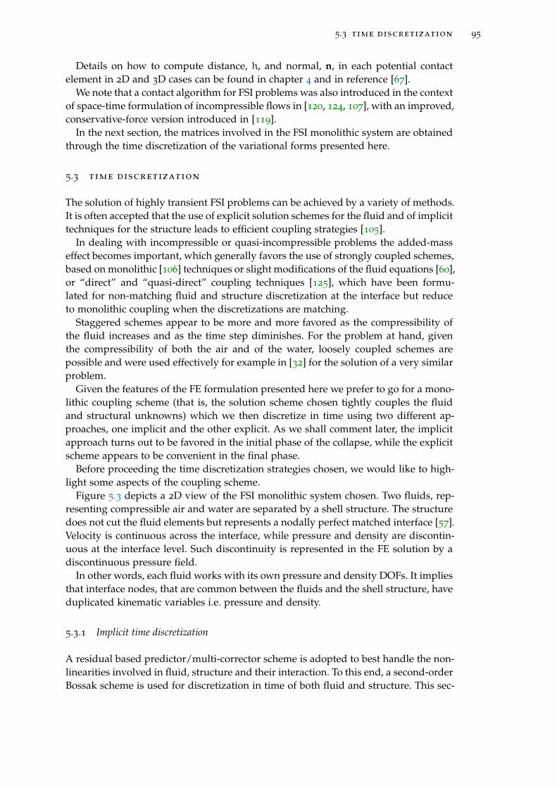
5.3 time discretization 95

Details on how to compute distance, h, and normal, n, in each potential contactelement in 2D and 3D cases can be found in chapter 4 and in reference [67].

We note that a contact algorithm for FSI problems was also introduced in the contextof space-time formulation of incompressible flows in [120, 124, 107], with an improved,conservative-force version introduced in [119].

In the next section, the matrices involved in the FSI monolithic system are obtainedthrough the time discretization of the variational forms presented here.

5.3 time discretization

The solution of highly transient FSI problems can be achieved by a variety of methods.It is often accepted that the use of explicit solution schemes for the fluid and of implicittechniques for the structure leads to efficient coupling strategies [105].

In dealing with incompressible or quasi-incompressible problems the added-masseffect becomes important, which generally favors the use of strongly coupled schemes,based on monolithic [106] techniques or slight modifications of the fluid equations [60],or “direct” and “quasi-direct” coupling techniques [125], which have been formu-lated for non-matching fluid and structure discretization at the interface but reduceto monolithic coupling when the discretizations are matching.

Staggered schemes appear to be more and more favored as the compressibility ofthe fluid increases and as the time step diminishes. For the problem at hand, giventhe compressibility of both the air and of the water, loosely coupled schemes arepossible and were used effectively for example in [32] for the solution of a very similarproblem.

Given the features of the FE formulation presented here we prefer to go for a mono-lithic coupling scheme (that is, the solution scheme chosen tightly couples the fluidand structural unknowns) which we then discretize in time using two different ap-proaches, one implicit and the other explicit. As we shall comment later, the implicitapproach turns out to be favored in the initial phase of the collapse, while the explicitscheme appears to be convenient in the final phase.

Before proceeding the time discretization strategies chosen, we would like to high-light some aspects of the coupling scheme.

Figure 5.3 depicts a 2D view of the FSI monolithic system chosen. Two fluids, rep-resenting compressible air and water are separated by a shell structure. The structuredoes not cut the fluid elements but represents a nodally perfect matched interface [57].Velocity is continuous across the interface, while pressure and density are discontin-uous at the interface level. Such discontinuity is represented in the FE solution by adiscontinuous pressure field.

In other words, each fluid works with its own pressure and density DOFs. It impliesthat interface nodes, that are common between the fluids and the shell structure, haveduplicated kinematic variables i.e. pressure and density.

5.3.1 Implicit time discretization

A residual based predictor/multi-corrector scheme is adopted to best handle the non-linearities involved in fluid, structure and their interaction. To this end, a second-orderBossak scheme is used for discretization in time of both fluid and structure. This sec-

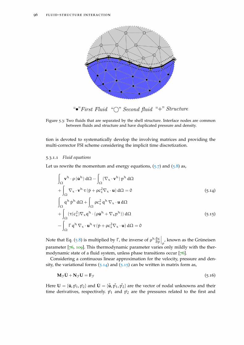
96 fluid-structure interaction

Figure 5.3: Two fluids that are separated by the shell structure. Interface nodes are commonbetween fluids and structure and have duplicated pressure and density.

tion is devoted to systematically develop the involving matrices and providing themulti-corrector FSI scheme considering the implicit time discretization.

5.3.1.1 Fluid equations

Let us rewrite the momentum and energy equations, (5.7) and (5.8) as,∫Ω

vh · ρ (uh)dΩ−

∫Ω

(∇x · vh)ph dΩ

+

∫Ω

∇x · vh τ (p+ ρc2s∇x · u)dΩ = 0 (5.14)∫Ω

qh ph dΩ+

∫Ω

ρc2s qh∇x · udΩ

+

∫Ω

(τ(c2s)∇xqh · (ρuh +∇xph))dΩ (5.15)

−

∫Ω

Γ qh∇x · uh τ (p+ ρc2s∇x · u)dΩ = 0

Note that Eq. (5.8) is multiplied by Γ , the inverse of ρh ∂ε∂p∣∣∣ρ

, known as the Grüneisen

parameter [76, 109]. This thermodynamic parameter varies only mildly with the ther-modynamic state of a fluid system, unless phase transitions occur [76].

Considering a continuous linear approximation for the velocity, pressure and den-sity, the variational forms (5.14) and (5.15) can be written in matrix form as,

MFU + NFU = FF (5.16)

Here U = u, p1, p2 and U = ˜u, ˜p1, ˜p2 are the vector of nodal unknowns and theirtime derivatives, respectively. p1 and p2 are the pressures related to the first and

5.3 time discretization 97

second fluid as shown in Figure 5.3. Subscript F in Eq. (5.16) refers to the matricescalculated for the fluid medium. Matrix MF has the form,

MF =

Mu τD1 τD2

τG1 Mp1 0

τG2 0 Mp2

(5.17)

Mu, Mp1 and Mp2 are diagonal lumped mass matrices related to the inertia and pres-sure rate terms respectively. Note that the terms related to air and water pressures arenot directly coupled with each other. If we denote the node indexes with superscriptsa and b the components of the arrays involved in (5.17) are,

Dab1 = Dab2 =

∫Ω

∇x ·NaNb dΩ

Gab1 = Gab2 =

∫Ω

ρc2s∇xNaNb dΩ.

NF contains terms related to the nodal values of velocity and pressure and has theform,

NF =

τC D1 D2

DTρ1c

21τL1 0

DTρ2c

22

0 τL2

(5.18)

where,

Cab =

∫Ω

ρc2 ∇x ·Na ∇x ·Nb dΩ

Dabρic

2i=

∫Ω

ρic2i ∇x ·NaNb dΩ (5.19)

Labi =

∫Ω

c2i ∇xNa ∇xNb dΩ.

Subscript i refers to the corresponding fluid domain. Note that all integrals related tothe stabilization terms are understood as the sum over all elements. In this sense thesound velocity, c, takes its value at each element in the computation of C in (5.19).

The last term in Eq. (5.15) is a nonlinear term and as we are going to introduce apredictor/multi-corrector scheme to deal with nonlinearities, the last iteration values,are used to evaluate explicitly this term. Finally we have,

FF =

0

τ f1

τ f2

. (5.20)

98 fluid-structure interaction

Here the terms for node a are computed as,

fai =

∫Ω

Na(Γ ∇x · uh (pi + ρic2i∇x · u)

)jdΩ (5.21)

where j refers to the values obtained from the last iteration of the predictor/multi-corrector scheme.

5.3.1.2 Structure

Matrices for the shell element can be obtained by recalling Eq. (5.9) as,∫A

[BTmσm + BTbσb

]dA =

∫A

N tdA (5.22)

here, Bm and Bb, are membrane and bending strain matrices, respectively. N is thematrix of linear shape functions for a triangle element.

To be consistent with the matrix form (5.16) presented for the fluid, the followingform is introduced for the shell by considering the inertia term,

MSU + KSY = fS (5.23)

where MS , is the lumped mass matrix for the shell element, Y is the vector of nodaldisplacements and fS represents external forces. Note that, with an abuse of notation,U in (5.23) contains time derivatives of the displacements (i.e. the velocities) only.

For the elastic behavior , KS, takes the form

KS =

∫A

BTmCeBm dA+

∫A

BTbCeBb dA (5.24)

Here, Ce, is the constitutive elastic matrix assuming plane stress behavior for the shell,as usual. If plastic behavior of the shell is considered, the internal forces are calculateddirectly by evaluating the plastic stresses in Eq. (5.22). In this case, KS represents thetangent matrix, with material and geometric components, and KSY represents theinternal forces.

5.3.1.3 Contact

The contribution of the contact scheme, presented in chapter 4 and Section 5.2.3, tothe monolithic FSI scheme is a vector of non-penetrating nodal forces, FC.

This vector is the assembly of contact forces, fC, computed at each active contactelement. Once the stress field, σ in Eq. (5.13), is known inside each active contactelement the corresponding internal nodal forces are computed as,

fC =

∫Ωe

BTeσdΩe (5.25)

where Be is the generalized strain matrix for the element. Note that once the configu-ration of the shell is known, the generalized strain field can be calculated inside eachcontact element.

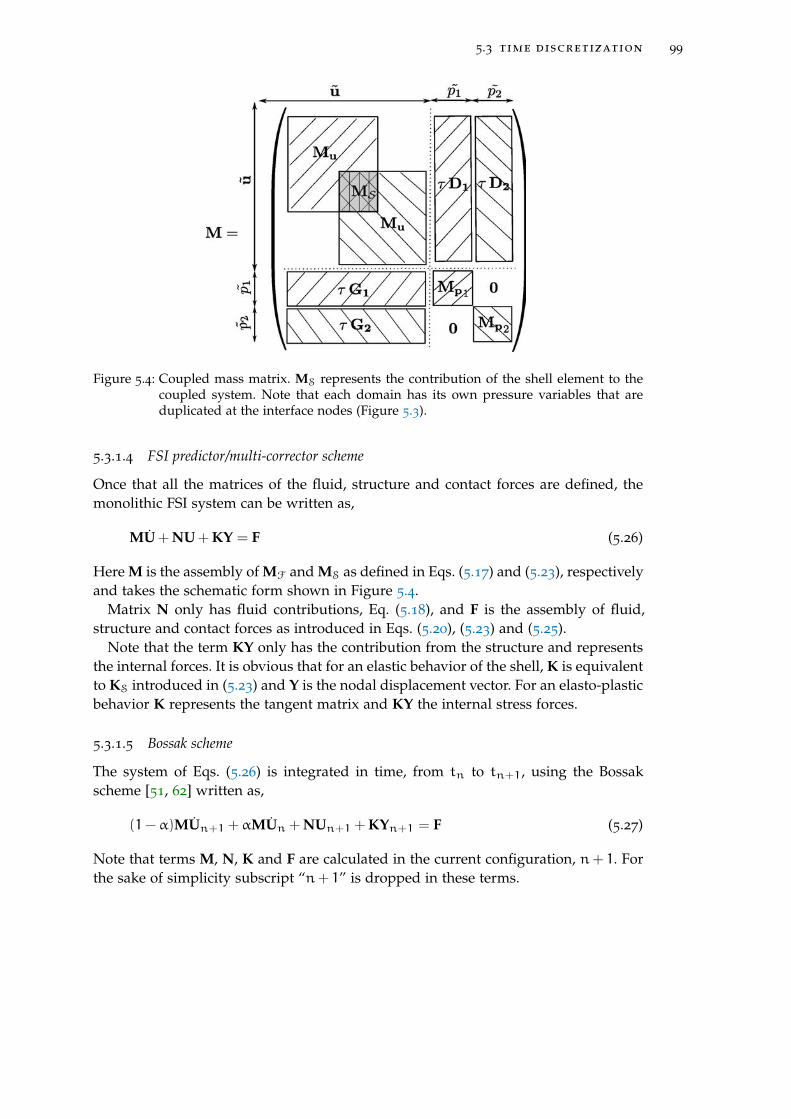
5.3 time discretization 99

Figure 5.4: Coupled mass matrix. MS represents the contribution of the shell element to thecoupled system. Note that each domain has its own pressure variables that areduplicated at the interface nodes (Figure 5.3).

5.3.1.4 FSI predictor/multi-corrector scheme

Once that all the matrices of the fluid, structure and contact forces are defined, themonolithic FSI system can be written as,

MU + NU + KY = F (5.26)

Here M is the assembly of MF and MS as defined in Eqs. (5.17) and (5.23), respectivelyand takes the schematic form shown in Figure 5.4.

Matrix N only has fluid contributions, Eq. (5.18), and F is the assembly of fluid,structure and contact forces as introduced in Eqs. (5.20), (5.23) and (5.25).

Note that the term KY only has the contribution from the structure and representsthe internal forces. It is obvious that for an elastic behavior of the shell, K is equivalentto KS introduced in (5.23) and Y is the nodal displacement vector. For an elasto-plasticbehavior K represents the tangent matrix and KY the internal stress forces.

5.3.1.5 Bossak scheme

The system of Eqs. (5.26) is integrated in time, from tn to tn+1, using the Bossakscheme [51, 62] written as,

(1−α)MUn+1 +αMUn + NUn+1 + KYn+1 = F (5.27)

Note that terms M, N, K and F are calculated in the current configuration, n+ 1. Forthe sake of simplicity subscript “n+ 1” is dropped in these terms.

100 fluid-structure interaction

The following updates are considered for the accelerations and displacements, as

Un+1 =1

γ∆t(Un+1 − Un) −

1− γ

γUn

Yn+1 = Yn +∆tUn +∆t2[1− 2β

2Un +βUn+1] (5.28)

Stability analysis [51] reveals that unconditional stability, second order accuracy andmaximal high-frequency dissipation are obtained by choosing the algorithmic param-eter α less than or equal to zero (α 6 0). γ and β are then computed as,

γ =1

2−α β =

1

4(1−α) (5.29)

We choose a residual based predictor/multi-corrector, similar to those proposed in [11]for incompressible flows and in [53] for compressible flows, to handle the nonlineari-ties embedded in the system of Eqs. (5.27).

The residual, R, at each iteration, i, and in the current step, n+ 1, is defined as,

Rin+1 := MUin+α + NUin+1 + KYin+1 − Fi (5.30)

The Taylor expansion of the residual, R, around the solution Uin+1 results in thefollowing incremental system,

R(Uin+α, Uin+1, Yin+1) +∂R(Uin+α, Uin+1, Yin+1)

∂Uin+1∆Uin+1 = 0 (5.31)

The increments, ∆Uin+1, are computed at each iteration from (5.31) and the solutionis updated;

Ui+1n+1 = Un +∆Uin+1. (5.32)

The tangent matrix is evaluated recalling the Bossak update equations for displace-ments and accelerations, (5.28), and applying the chain rule as,

Ain+1 :=∂Rin+1∂Uin+1

= M∂ Uin+α∂Uin+1

+ N + K∂Yin+1∂Uin+1

=1−α

γ∆tM + N +

∆tβ

γK (5.33)

Note that matrix K represents now the tangent matrix for the shell element. It reducesto KS, introduced in (5.23), for the elastic behavior of the shell. The tangent matrixincludes material and geometric components for the elasto-plastic behavior. The de-tailed calculation of K is presented in [34].

Table 5.1 summarizes one step of the residual-based predictor/multi-corrector schemedeveloped herein. Note that densities are updated at the beginning of each iteration

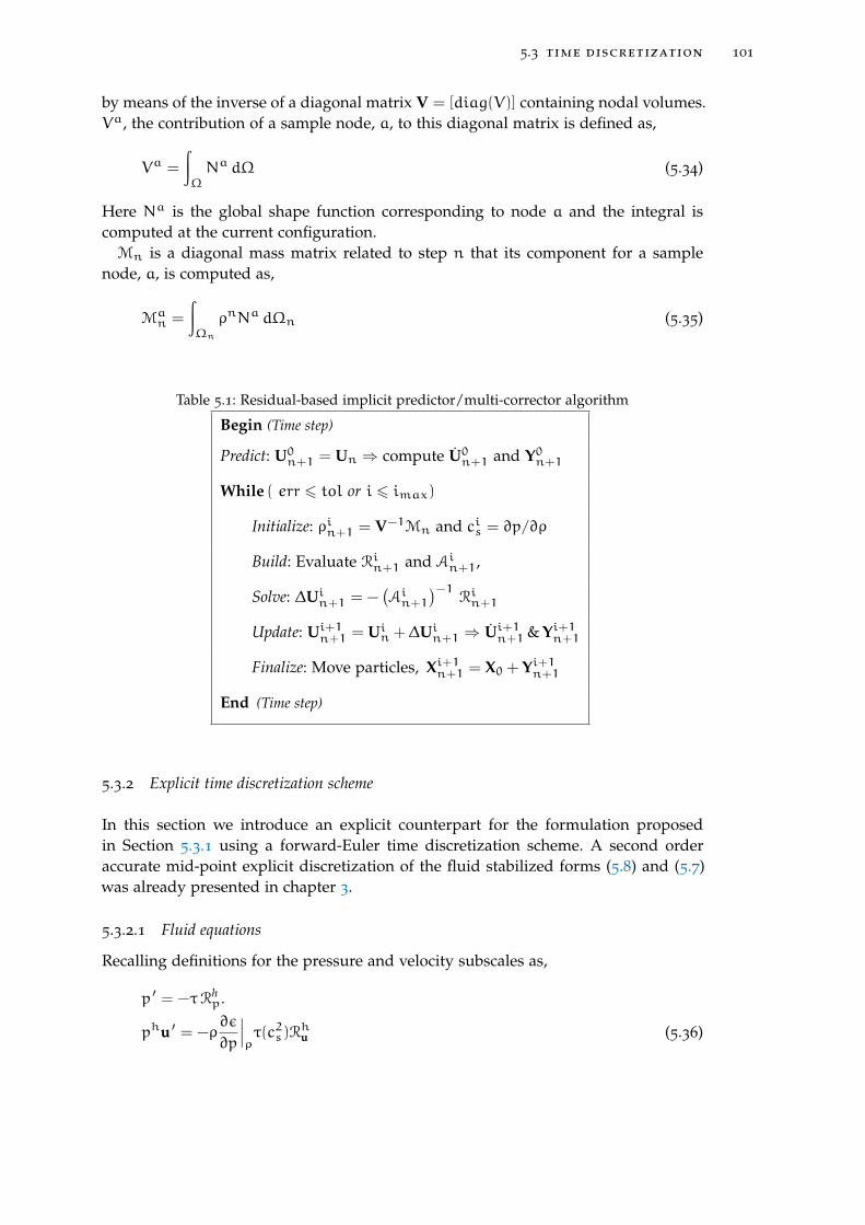
5.3 time discretization 101

by means of the inverse of a diagonal matrix V = [diag(V)] containing nodal volumes.Va, the contribution of a sample node, a, to this diagonal matrix is defined as,

Va =

∫Ω

Na dΩ (5.34)

Here Na is the global shape function corresponding to node a and the integral iscomputed at the current configuration.Mn is a diagonal mass matrix related to step n that its component for a sample

node, a, is computed as,

Man =

∫Ωn

ρnNa dΩn (5.35)

Table 5.1: Residual-based implicit predictor/multi-corrector algorithm

Begin (Time step)

Predict: U0n+1 = Un ⇒ compute U0n+1 and Y0n+1

While ( err 6 tol or i 6 imax)

Initialize: ρin+1 = V−1Mn and cis = ∂p/∂ρ

Build: Evaluate Rin+1 and Ain+1,

Solve: ∆Uin+1 = −(Ain+1

)−1Rin+1

Update: Ui+1n+1 = Uin +∆Uin+1 ⇒ Ui+1n+1& Yi+1n+1

Finalize: Move particles, Xi+1n+1 = X0 + Yi+1n+1

End (Time step)

5.3.2 Explicit time discretization scheme

In this section we introduce an explicit counterpart for the formulation proposedin Section 5.3.1 using a forward-Euler time discretization scheme. A second orderaccurate mid-point explicit discretization of the fluid stabilized forms (5.8) and (5.7)was already presented in chapter 3.

5.3.2.1 Fluid equations

Recalling definitions for the pressure and velocity subscales as,

p ′ = −τRhp.

phu ′ = −ρ∂ε

∂p

∣∣∣ρτ(c2s)R

hu (5.36)

102 fluid-structure interaction

the stabilized form of the conservation of momentum and energy, Eqs. (5.14) and(5.15), can be rewritten as,∫

Ω

vh · ρ (uh)dΩ−

∫Ω

∇x · vh (ph + p ′)dΩ = 0 (5.37)∫Ω

qh ph dΩ+

∫Ω

qh (ρc2s + Γ p′)∇x · udΩ

+

∫Ω

Γ ∇xqh (pu ′)dΩ = 0 (5.38)

Applying the forward-Euler scheme to the momentum Eq. (5.37) we have,∫Ω

vh · ρ (uhn+1 − uhn)dΩ

= ∆t

∫Ωn

∇x · vh (ph + p ′)n dΩ (5.39)

The matrix form of Eq. (5.39) is written as,

Mu (un+1 − un) = ∆t (gF)n. (5.40)

where Mu is the same lumped mass matrix introduced in Section 5.3.1.1. The compo-nent of vector (gF)n for node a has the form,

(gF)an =

∫Ωn

∇x ·Na (ph + p ′)n dΩ (5.41)

where Na is the global shape function corresponding to node a and subscript n refersto the time tn.

Note that for the interface nodes, (gF)an has two contributions due to the discontin-

uous pressure at the interface that are summed up. Discretizing the energy Eq. (5.38)in time we have,∫

Ω

qh (phn+1 − phn)dΩ = −∆t

∫Ω

Γ ∇xqh (p u ′)n dΩ

− ∆t

∫Ω

qh[(ρc2s + Γ p

′)∇x · u]ndΩ (5.42)

this results in the matrix equations,

Mp (pn+1 − pn) = ∆t (wF)n. (5.43)

where Mp is an nd×nd, nd is the number of nodes, lumped mass matrix introducedin Section 5.3.1.1. The component related to the node a of the vector (wF)n has theform,

(wF)an =−

∫Ω

Na[(ρc2s + Γ p

′)∇x · u]ndΩ

−

∫Ω

∇xNa Γ (p u ′)n dΩ (5.44)

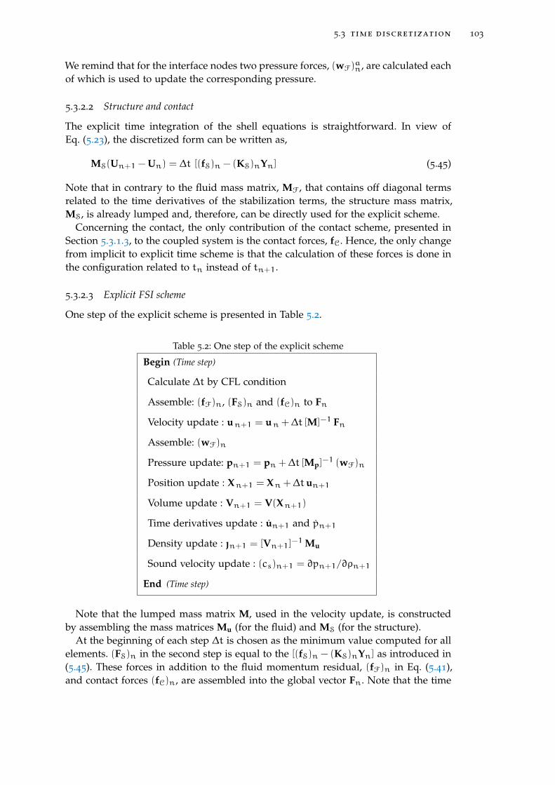
5.3 time discretization 103

We remind that for the interface nodes two pressure forces, (wF)an, are calculated each

of which is used to update the corresponding pressure.

5.3.2.2 Structure and contact

The explicit time integration of the shell equations is straightforward. In view ofEq. (5.23), the discretized form can be written as,

MS(Un+1 − Un) = ∆t [(fS)n − (KS)nYn] (5.45)

Note that in contrary to the fluid mass matrix, MF, that contains off diagonal termsrelated to the time derivatives of the stabilization terms, the structure mass matrix,MS, is already lumped and, therefore, can be directly used for the explicit scheme.

Concerning the contact, the only contribution of the contact scheme, presented inSection 5.3.1.3, to the coupled system is the contact forces, fC. Hence, the only changefrom implicit to explicit time scheme is that the calculation of these forces is done inthe configuration related to tn instead of tn+1.

5.3.2.3 Explicit FSI scheme

One step of the explicit scheme is presented in Table 5.2.

Table 5.2: One step of the explicit scheme

Begin (Time step)

Calculate ∆t by CFL condition

Assemble: (fF)n, (FS)n and (fC)n to Fn

Velocity update : un+1 = un +∆t [M]−1 Fn

Assemble: (wF)n

Pressure update: pn+1 = pn +∆t [Mp]−1 (wF)n

Position update : Xn+1 = Xn +∆tun+1

Volume update : Vn+1 = V(Xn+1)

Time derivatives update : un+1 and pn+1

Density update : n+1 = [Vn+1]−1Mu

Sound velocity update : (cs)n+1 = ∂pn+1/∂ρn+1

End (Time step)

Note that the lumped mass matrix M, used in the velocity update, is constructedby assembling the mass matrices Mu (for the fluid) and MS (for the structure).

At the beginning of each step ∆t is chosen as the minimum value computed for allelements. (FS)n in the second step is equal to the [(fS)n − (KS)nYn] as introduced in(5.45). These forces in addition to the fluid momentum residual, (fF)n in Eq. (5.41),and contact forces (fC)n, are assembled into the global vector Fn. Note that the time

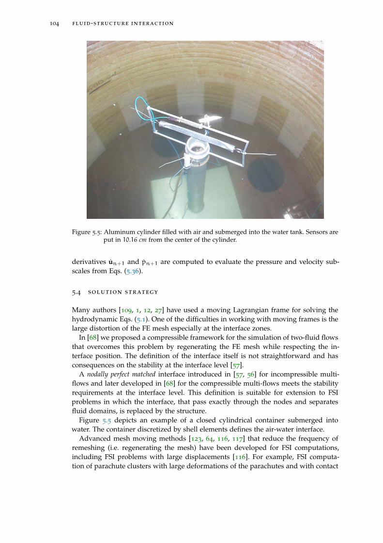
104 fluid-structure interaction

Figure 5.5: Aluminum cylinder filled with air and submerged into the water tank. Sensors areput in 10.16 cm from the center of the cylinder.

derivatives un+1 and pn+1 are computed to evaluate the pressure and velocity sub-scales from Eqs. (5.36).

5.4 solution strategy

Many authors [109, 1, 12, 27] have used a moving Lagrangian frame for solving thehydrodynamic Eqs. (5.1). One of the difficulties in working with moving frames is thelarge distortion of the FE mesh especially at the interface zones.

In [68] we proposed a compressible framework for the simulation of two-fluid flowsthat overcomes this problem by regenerating the FE mesh while respecting the in-terface position. The definition of the interface itself is not straightforward and hasconsequences on the stability at the interface level [57].

A nodally perfect matched interface introduced in [57, 56] for incompressible multi-flows and later developed in [68] for the compressible multi-flows meets the stabilityrequirements at the interface level. This definition is suitable for extension to FSIproblems in which the interface, that pass exactly through the nodes and separatesfluid domains, is replaced by the structure.

Figure 5.5 depicts an example of a closed cylindrical container submerged intowater. The container discretized by shell elements defines the air-water interface.

Advanced mesh moving methods [123, 64, 116, 117] that reduce the frequency ofremeshing (i.e. regenerating the mesh) have been developed for FSI computations,including FSI problems with large displacements [116]. For example, FSI computa-tion of parachute clusters with large deformations of the parachutes and with contact

5.4 solution strategy 105

Table 5.3: One step of the FSI scheme

• Regenerate Mesh

Compute distance and volume constrains

Mark and delete nodes

Generate the constrained adaptive mesh

Merge fluid and shell elements

• Search for possible contacts

Descritize the potential contact volume

Check the contact criteria

Save active contact elements

Merge contact elements into fluid and shell ones

• Solve FSI system

One step of implicit (Table 5.1) or explicit (Table 5.2) solver

between them can be carried out with very few remeshings during the entire compu-tation (see [119]).

In our computations here, due to the extensive nature of the contact we face, weneed remeshing, at least in the vicinity of the interface. This is done via utilizing theTetgen software [114].

In case that a fine mesh near the interface is needed, adaptive mesh generation canbe done by assigning volume constrains in the desired zones [114]. As the positionof the interface (i.e. structure) is known, a distance function that has its zero on theinterface is used to compute the volume constrains at each zone. This technique istested for 2D multi-flows in [68] to generate a fine mesh near the interface.

The importance of having layers of refined mesh near the fluid-solid interface andmaintaining that mesh resolution as the interface moves was recognized as early asin 3D fluid-particle interaction computations reported in [65]. This also motivated thedevelopment of the Solid-Extension Mesh Moving Technique [117] for FSI problemsin general, where the layers of refined mesh go through minimal deformation as theinterface deforms.

In case that large deformations of the shell structure lead to the contact, the contactscheme proposed in Section 5.2.3 is used to compute the contact forces.

Table 5.3 summarizes one step of the FSI scheme. Note that before regeneratingthe new mesh, nodes in air and water domains that are too close to the interface aremarked and deleted to avoid unnecessary local refinement of the mesh.

The new mesh is generated with two constrains: the first one is the volume con-straint that provides a fine mesh near the structure and the second one is a ConstrainedDelaunay Triangulation to preserve connectivities at the shell surface. Each shell ele-ment uses the neighbor elements data to compute the curvature. Therefore, it is moreconvenient to preserve the connectivities of the shell elements.

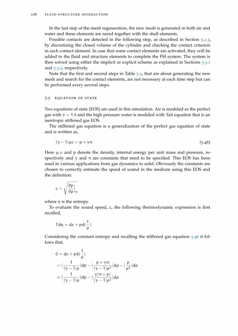
106 fluid-structure interaction

In the last step of the mesh regeneration, the new mesh is generated in both air andwater and these elements are saved together with the shell elements.

Possible contacts are detected in the following step, as described in Section 5.2.3,by discretizing the closed volume of the cylinder and checking the contact criterionin each contact element. In case that some contact elements are activated, they will beadded to the fluid and structure elements to complete the FSI system. The system isthen solved using either the implicit or explicit scheme as explained in Sections 5.3.1and 5.3.2, respectively.

Note that the first and second steps in Table 5.3, that are about generating the newmesh and search for the contact elements, are not necessary at each time step but canbe performed every several steps.

5.5 equation of state

Two equations of state (EOS) are used in this simulation. Air is modeled as the perfectgas with γ = 1.4 and the high pressure water is modeled with Tait equation that is anisentropic stiffened gas EOS.

The stiffened gas equation is a generalization of the perfect gas equation of stateand is written as,

(γ− 1)ρε = p+ γπ (5.46)

Here ρ, ε and p denote the density, internal energy per unit mass and pressure, re-spectively and γ and π are constants that need to be specified. This EOS has beenused in various applications from gas dynamics to solid. Obviously the constants arechosen to correctly estimate the speed of sound in the medium using this EOS andthe definition:

c =

öp

∂ρ

∣∣∣η

where η is the entropy.To evaluate the sound speed, c, the following thermodynamic expression is first

recalled,

Tdη = dε+ pd(1

ρ).

Considering the constant entropy and recalling the stiffened gas equation 5.46 it fol-lows that,

0 = dε+ pd(1

ρ)

= (1

(γ− 1)ρ)dp− (

p+ γπ

(γ− 1)ρ2)dρ− (

p

ρ2)dρ

= (1

(γ− 1)ρ)dp− (

γ(π+ p)

(γ− 1)ρ2)dρ

5.5 equation of state 107

and the speed of sound in a stiffened gas is given by,

c =

öp

∂ρ

∣∣∣η=

√γ(π+ p)

ρ.

In case of water the following values for the constant are found,

π = 6.0× 108 Pa γ ∈ 4.4, 5.5, 7.0

Note that for π = 0 the stiffened gas equation simplifies to the perfect gas equation.The Tait equation of state,

p = η+αρβ

models water as a compressible barotropic medium. In contrary to the perfect gasEOS, here, pressure is just a function of density. η,α and β are three constants thatcan be determined from the initial state of the material and by the fact that the bulkmodulus of a fluid, K, is an affine function of pressure determined by two constantsk1 and k2. Hence,

k1 + k2p = K = ρdp

dρ= βαρβ = β(p− η),

which gives

η = −k1k2

β = k2.

Furthermore, writing p0 = p(ρ0) gives,

α =p0 +

k1k2

ρk20

In the literature, the following values are found for water,

k1 = 2.07× 109kg

m3s2k2 = 7.15

In this case the speed of sound is computed as,

c =

öp

∂ρ

∣∣∣η=

√(k2p0 + k1)

ρ0(ρ

ρ0)k2−1.

For the initial values of our implosion model, ρ = 1000 and p0 = 106 Pa, the predictedspeed of sound is,

c0 = c(ρ0) =

√(k2p0 + k1)

ρ0= 1441.23

m

s

It can be easily shown that Tait EOS corresponds to the particular case of an isen-tropic stiffened gas. It differs from the ideal gas EOS in one important aspect. Since

108 fluid-structure interaction

(a) (b)

Figure 5.6: Schematic view of the model geometry (a) and mesh configuration at time t = 0(b).

it involves only pressure and density but not energy, the Tait EOS is barotropic. Thiscloses the Euler equations but decouples the energy equation from the mass and mo-mentum equations, so that simulations may be carried out with only the mass andmomentum equations. However there is no harm in also solving the energy equation,which is done in this work.

5.6 underwater implosion of cylindrical container

The underwater implosion of a cylindrical tube is considered in this section. The tubeis made of aluminum and has a diameter,D = 2.4 cm, length, L = 27 cm, and thickness,t = 8.89× 10−2 cm. It is filled with air at the atmospheric pressure, pa = 101.3 KPa, isclosed at both ends and then submerged in a water tank.

The tank is rigid and has a diameter, D = 1.5 m, and length, L = 3.65 m. Figures 5.5and 5.6a show the experiment setup and the schematic view of the test, respectively.Pressure sensors are placed at a radial distance, d = 10.16 cm, from the center of thetube (Figure 5.5 ). The aluminum cylinder is maintained at the center of the tank bya set of rigid bars attached to the tank. Water pressure inside the tank is atmosphericat the beginning and the initial velocity is zero everywhere.

Hydrostatic loading is accomplished by activating a water pump to slowly raise thewater pressure. Following the experiment the aluminum cylinder collapses flat, butdoes not crack open, when the external pressure reaches pw = 6.99 Mpa.

Figure 5.7a and Figure 5.7b show the collapsed view of the cylinder at the end ofthe experiment and the simulation, respectively.

The time histories of pressure captured by the sensors reveal a drop of roughly 1.2MPa in water pressure after 0.6 ms from the beginning of the experiment. This dropreaches its maximum just before contact occurs and is followed by an instant pressure

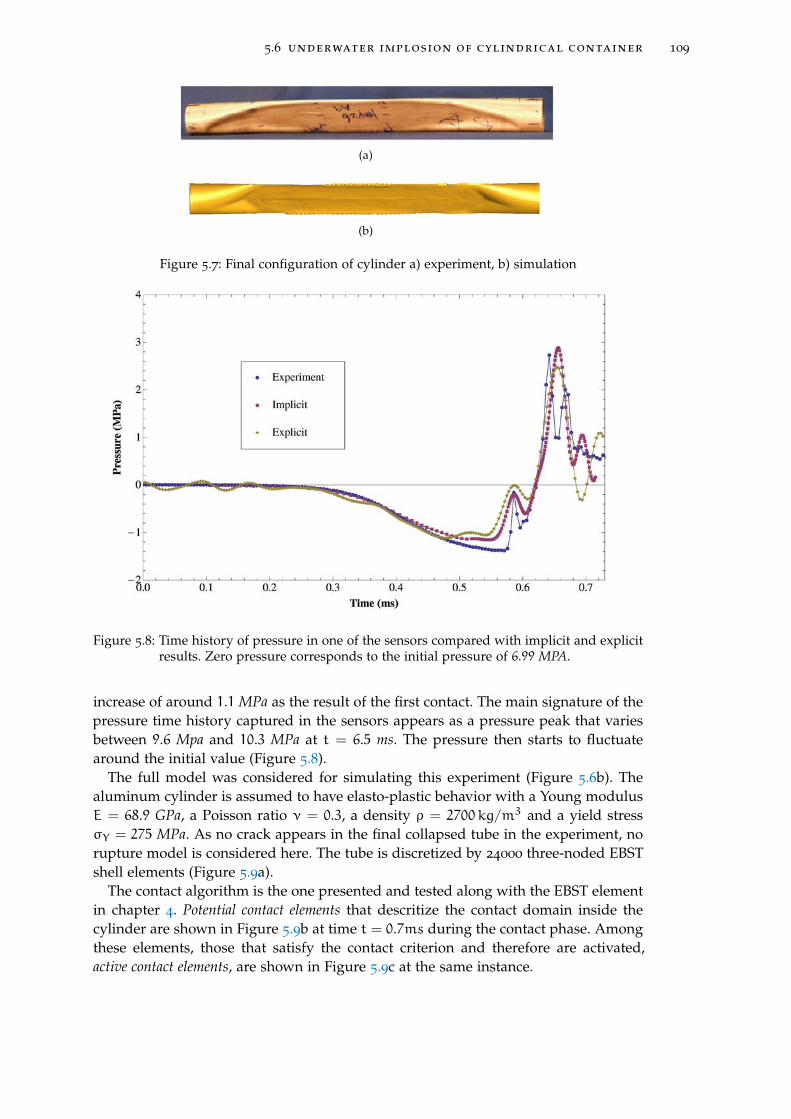
5.6 underwater implosion of cylindrical container 109

(a)

(b)

Figure 5.7: Final configuration of cylinder a) experiment, b) simulation

Figure 5.8: Time history of pressure in one of the sensors compared with implicit and explicitresults. Zero pressure corresponds to the initial pressure of 6.99 MPA.

increase of around 1.1 MPa as the result of the first contact. The main signature of thepressure time history captured in the sensors appears as a pressure peak that variesbetween 9.6 Mpa and 10.3 MPa at t = 6.5 ms. The pressure then starts to fluctuatearound the initial value (Figure 5.8).

The full model was considered for simulating this experiment (Figure 5.6b). Thealuminum cylinder is assumed to have elasto-plastic behavior with a Young modulusE = 68.9 GPa, a Poisson ratio ν = 0.3, a density ρ = 2700 kg/m3 and a yield stressσY = 275 MPa. As no crack appears in the final collapsed tube in the experiment, norupture model is considered here. The tube is discretized by 24000 three-noded EBSTshell elements (Figure 5.9a).

The contact algorithm is the one presented and tested along with the EBST elementin chapter 4. Potential contact elements that descritize the contact domain inside thecylinder are shown in Figure 5.9b at time t = 0.7ms during the contact phase. Amongthese elements, those that satisfy the contact criterion and therefore are activated,active contact elements, are shown in Figure 5.9c at the same instance.

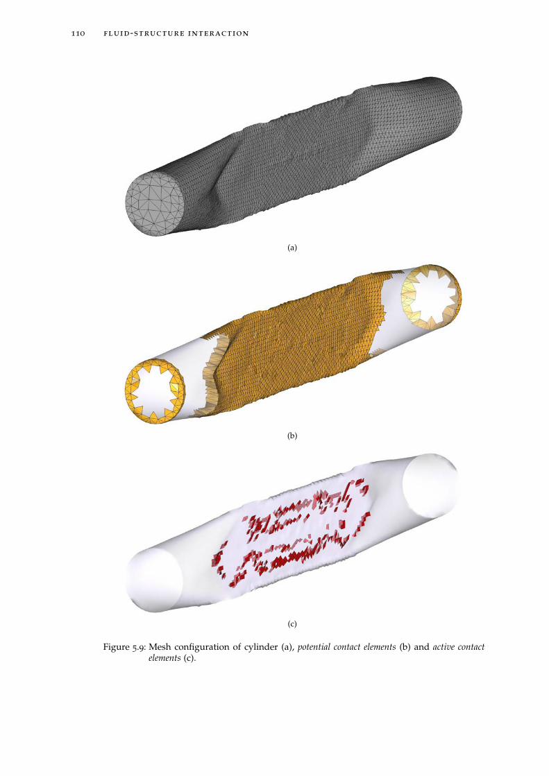
110 fluid-structure interaction

(a)

(b)

(c)

Figure 5.9: Mesh configuration of cylinder (a), potential contact elements (b) and active contactelements (c).

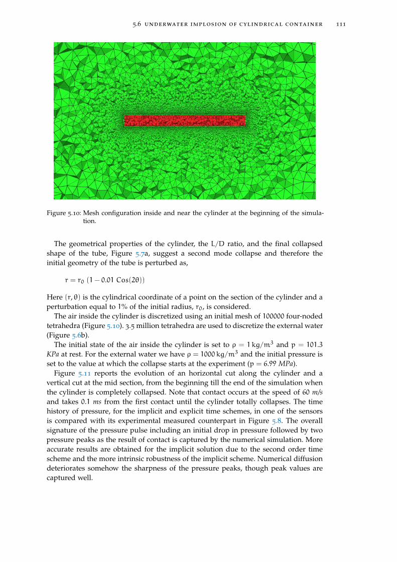
5.6 underwater implosion of cylindrical container 111

Figure 5.10: Mesh configuration inside and near the cylinder at the beginning of the simula-tion.

The geometrical properties of the cylinder, the L/D ratio, and the final collapsedshape of the tube, Figure 5.7a, suggest a second mode collapse and therefore theinitial geometry of the tube is perturbed as,

r = r0 (1− 0.01 Cos(2θ))

Here (r, θ) is the cylindrical coordinate of a point on the section of the cylinder and aperturbation equal to 1% of the initial radius, r0, is considered.

The air inside the cylinder is discretized using an initial mesh of 100000 four-nodedtetrahedra (Figure 5.10). 3.5 million tetrahedra are used to discretize the external water(Figure 5.6b).

The initial state of the air inside the cylinder is set to ρ = 1 kg/m3 and p = 101.3KPa at rest. For the external water we have ρ = 1000 kg/m3 and the initial pressure isset to the value at which the collapse starts at the experiment (p = 6.99 MPa).

Figure 5.11 reports the evolution of an horizontal cut along the cylinder and avertical cut at the mid section, from the beginning till the end of the simulation whenthe cylinder is completely collapsed. Note that contact occurs at the speed of 60 m/sand takes 0.1 ms from the first contact until the cylinder totally collapses. The timehistory of pressure, for the implicit and explicit time schemes, in one of the sensorsis compared with its experimental measured counterpart in Figure 5.8. The overallsignature of the pressure pulse including an initial drop in pressure followed by twopressure peaks as the result of contact is captured by the numerical simulation. Moreaccurate results are obtained for the implicit solution due to the second order timescheme and the more intrinsic robustness of the implicit scheme. Numerical diffusiondeteriorates somehow the sharpness of the pressure peaks, though peak values arecaptured well.

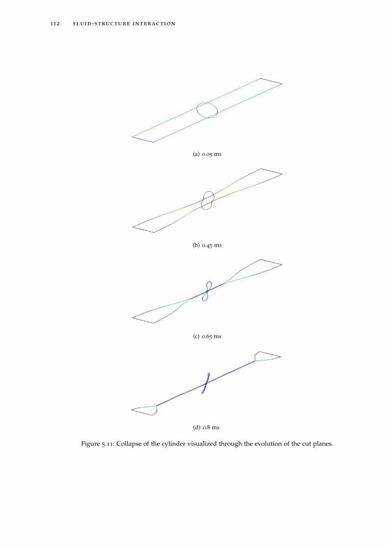
112 fluid-structure interaction

(a) 0.05 ms

(b) 0.45 ms

(c) 0.65 ms

(d) 0.8 ms

Figure 5.11: Collapse of the cylinder visualized through the evolution of the cut planes.

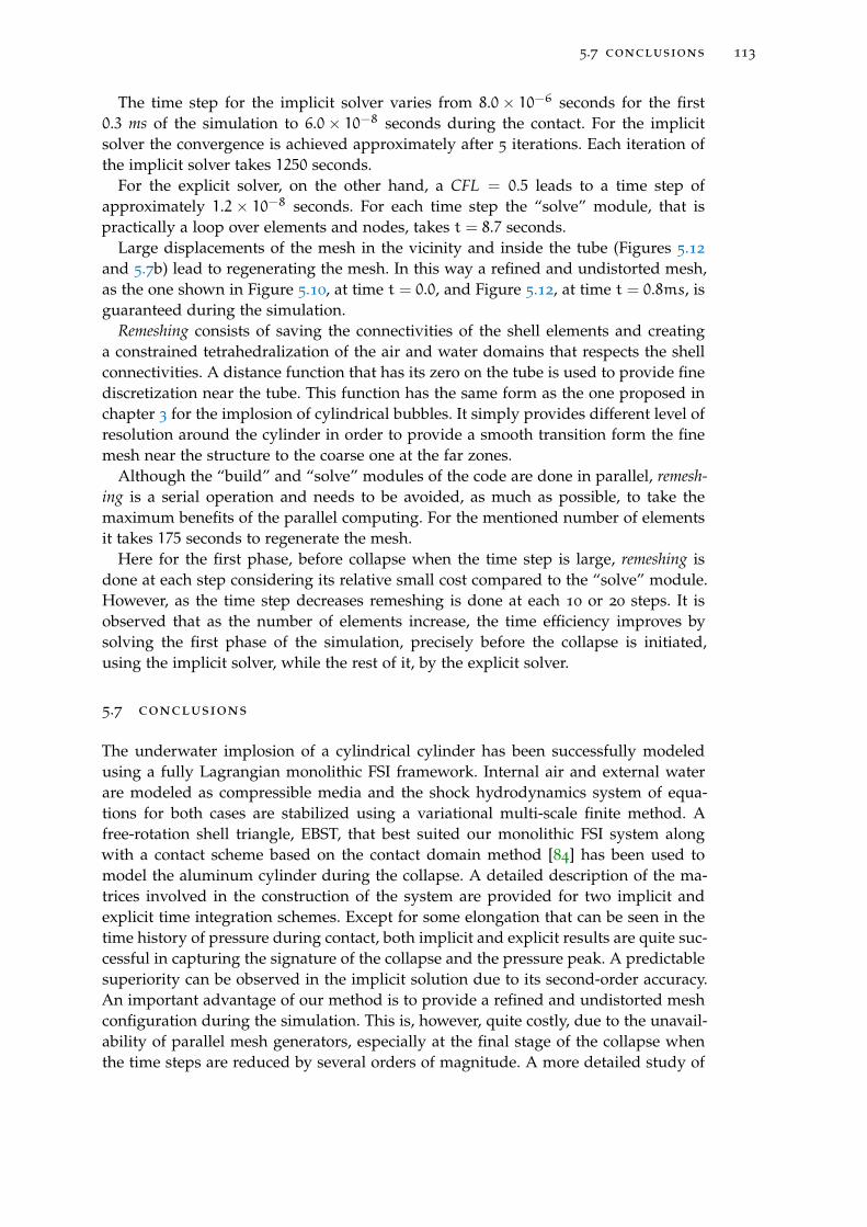
5.7 conclusions 113

The time step for the implicit solver varies from 8.0 × 10−6 seconds for the first0.3 ms of the simulation to 6.0× 10−8 seconds during the contact. For the implicitsolver the convergence is achieved approximately after 5 iterations. Each iteration ofthe implicit solver takes 1250 seconds.

For the explicit solver, on the other hand, a CFL = 0.5 leads to a time step ofapproximately 1.2 × 10−8 seconds. For each time step the “solve” module, that ispractically a loop over elements and nodes, takes t = 8.7 seconds.

Large displacements of the mesh in the vicinity and inside the tube (Figures 5.12

and 5.7b) lead to regenerating the mesh. In this way a refined and undistorted mesh,as the one shown in Figure 5.10, at time t = 0.0, and Figure 5.12, at time t = 0.8ms, isguaranteed during the simulation.

Remeshing consists of saving the connectivities of the shell elements and creatinga constrained tetrahedralization of the air and water domains that respects the shellconnectivities. A distance function that has its zero on the tube is used to provide finediscretization near the tube. This function has the same form as the one proposed inchapter 3 for the implosion of cylindrical bubbles. It simply provides different level ofresolution around the cylinder in order to provide a smooth transition form the finemesh near the structure to the coarse one at the far zones.

Although the “build” and “solve” modules of the code are done in parallel, remesh-ing is a serial operation and needs to be avoided, as much as possible, to take themaximum benefits of the parallel computing. For the mentioned number of elementsit takes 175 seconds to regenerate the mesh.

Here for the first phase, before collapse when the time step is large, remeshing isdone at each step considering its relative small cost compared to the “solve” module.However, as the time step decreases remeshing is done at each 10 or 20 steps. It isobserved that as the number of elements increase, the time efficiency improves bysolving the first phase of the simulation, precisely before the collapse is initiated,using the implicit solver, while the rest of it, by the explicit solver.

5.7 conclusions

The underwater implosion of a cylindrical cylinder has been successfully modeledusing a fully Lagrangian monolithic FSI framework. Internal air and external waterare modeled as compressible media and the shock hydrodynamics system of equa-tions for both cases are stabilized using a variational multi-scale finite method. Afree-rotation shell triangle, EBST, that best suited our monolithic FSI system alongwith a contact scheme based on the contact domain method [84] has been used tomodel the aluminum cylinder during the collapse. A detailed description of the ma-trices involved in the construction of the system are provided for two implicit andexplicit time integration schemes. Except for some elongation that can be seen in thetime history of pressure during contact, both implicit and explicit results are quite suc-cessful in capturing the signature of the collapse and the pressure peak. A predictablesuperiority can be observed in the implicit solution due to its second-order accuracy.An important advantage of our method is to provide a refined and undistorted meshconfiguration during the simulation. This is, however, quite costly, due to the unavail-ability of parallel mesh generators, especially at the final stage of the collapse whenthe time steps are reduced by several orders of magnitude. A more detailed study of

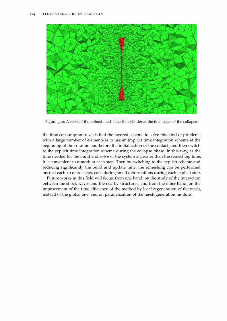
114 fluid-structure interaction

Figure 5.12: A view of the refined mesh near the cylinder at the final stage of the collapse.

the time consumption reveals that the favored scheme to solve this kind of problemswith a large number of elements is to use an implicit time integration scheme at thebeginning of the solution and before the initialization of the contact, and then switchto the explicit time integration scheme during the collapse phase. In this way, as thetime needed for the build and solve of the system is greater than the remeshing time,it is convenient to remesh at each step. Then by switching to the explicit scheme andreducing significantly the build and update time, the remeshing can be performedonce at each 10 or 20 steps, considering small deformations during each explicit step.

Future works in this field will focus, from one hand, on the study of the interactionbetween the shock waves and the nearby structures, and from the other hand, on theimprovement of the time efficiency of the method by local regeneration of the mesh,instead of the global one, and on parallelization of the mesh generation module.

6C O N C L U S I O N S A N D F U T U R E W O R K

In this section we provide a summary of the achievements of this work and an outlookof the future work.

ConclusionsConcerning the main motivation of this work that is the simulation of underwater im-plosion of cylindrical cylinder, we first developped a compressible Lagrangian frame-work “ a la PFEM” to simulate the multi-fluid compressible problems. To this end,we have taken advantage of a variationally stabilized form of the Euler equationsproposed by Scovazzi and an interface tracking method proposed by Idelsohn. Theextension to the multi-fluid modeling was then obtained by discontinuous treatment ofthe kinetic variables i.e. pressure, density at the interface , from one side, and interface-connectivity-preserving remeshing, from the other side. A geometrical adaptive meshgeneration was added to our framework in order to provide enough resolution at theinterface level.

At this point we tested our framework to simulate the underwater implosion oflarge, cm size, cylindrical bubble. Beside obtaining the essential signatures of the bub-ble dynamics, we have captured for the first time, up to our knowledge, the detailedgeneration of shape and surface instabilities for this size bubbles.

To later expand the mentioned framework for FSI problems, a new shell-to-shellcontact method has been developed. This method belongs to the category of the con-tact domain methods and exploits the fact that shell’s kinematics is described by themotion of its mid plane. Therefore, contact is detected as soon as the mid-planes reacha distance equivalent to the sum of the half-thicknesses of the contacting structures.Basing on this we discretize, by the Delaunay approach, the volume enclosed betweenthe contacting surfaces (that will be guaranteed to have non-zero thickness). Such “vir-tual volume” is treated as elastic, with a suitably defined assumed strain, in all theareas in which the two shells are actually in contact.

A monolithic coupling between the shell structure, cylinder, the compressible air in-side the cylinder and the compressible water outside it, has been considered to modelthe underwater implosion of an aluminum cylinder. The coupled system has beensolved by an implicit second-order predictor multi-corrector scheme. Mesh quality isguaranteed during the simulaion by regenerating the mesh. An explicit forward Eulersolution of this system is also provided. Both results, explicit and implicit ones, havebeen compared to experimental data and good agreement has been obtained.

A more detailed study of the time consumption reveals that the favored strategy tosolve this kind of problems, with a large number of elements, is to use an implicit timeintegration scheme at the beginning of the simulation and before the initialization of

115

116 conclusions and future work

the contact, and then switch to the explicit one for the collapse phase.

Future workOne of the main advantages of the Lagrangian framework proposed, compared to theEulerian ones [31] is its intrinsic property of regenerating the mesh at the presence oflarge deformations. This benefit is obtained at the cost of the serial process of remesh-ing that is quite time consuming compared to the rest of the code modules that areimplemented for parallel computing. Therefore, for this specific class of applicationsfor which the deformations are restricted to specific zones, a local remeshing processin which just the mesh in the vicinity of the large movement zones are regenerated,is suitable. Of course, a parallel remeshing technique, if available, is always a recom-mended alternative.

In view of above comments, the following developments can be performed for eachof the sections of this thesis.

1. The compressible hydrocode can be improved by considering higher order el-ements instead of the actual simple elements in case that more resolution isneeded at the shock zones.

2. The interface following technique for multi-fluids [57, 25] is just developed for2D cases. The extension of this method to 3D is inevitable for real simulationsof multi-fluid problems.

3. The structure is considered uncracked during the simulation, while in some im-plosion experiments cracks are initiated during the collapse phase. Apart fromthe crack simulation, the instantaneous mixture of high pressure air and waterrequires a more delicate treatment.

Considering the applications of the analysis framework proposed in this thesis, twodifferent lines of research can be considered for future research work.

1. The interaction between the shock wave, produced by implosion of a singlebubble or multiple bubbles, and the nearby objects can be of interest in variousapplications [20, 72, 96].

2. It is known that the high pressures produced at the final stage of collapse, spe-cially for smaller bubbles of µm size, leads to excessively high temperatures i.e.some thousands of Kelvin [77]. Modeling of this effect requires more complexEOS’s and also to consider the possible phase change effect. In this way, theanalysis framework proposed in this thesis can be improved for the real mod-eling of acoustic cavitation and phenomena like SL (sonoluminescence) [138] orsonochemistry [118].

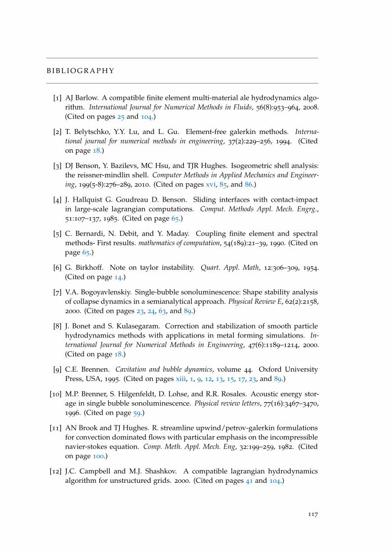
B I B L I O G R A P H Y

[1] AJ Barlow. A compatible finite element multi-material ale hydrodynamics algo-rithm. International Journal for Numerical Methods in Fluids, 56(8):953–964, 2008.(Cited on pages 25 and 104.)

[2] T. Belytschko, Y.Y. Lu, and L. Gu. Element-free galerkin methods. Interna-tional journal for numerical methods in engineering, 37(2):229–256, 1994. (Citedon page 18.)

[3] DJ Benson, Y. Bazilevs, MC Hsu, and TJR Hughes. Isogeometric shell analysis:the reissner-mindlin shell. Computer Methods in Applied Mechanics and Engineer-ing, 199(5-8):276–289, 2010. (Cited on pages xvi, 85, and 86.)

[4] J. Hallquist G. Goudreau D. Benson. Sliding interfaces with contact-impactin large-scale lagrangian computations. Comput. Methods Appl. Mech. Engrg.,51:107–137, 1985. (Cited on page 65.)

[5] C. Bernardi, N. Debit, and Y. Maday. Coupling finite element and spectralmethods- First results. mathematics of computation, 54(189):21–39, 1990. (Cited onpage 65.)

[6] G. Birkhoff. Note on taylor instability. Quart. Appl. Math, 12:306–309, 1954.(Cited on page 14.)

[7] V.A. Bogoyavlenskiy. Single-bubble sonoluminescence: Shape stability analysisof collapse dynamics in a semianalytical approach. Physical Review E, 62(2):2158,2000. (Cited on pages 23, 24, 63, and 89.)

[8] J. Bonet and S. Kulasegaram. Correction and stabilization of smooth particlehydrodynamics methods with applications in metal forming simulations. In-ternational Journal for Numerical Methods in Engineering, 47(6):1189–1214, 2000.(Cited on page 18.)

[9] C.E. Brennen. Cavitation and bubble dynamics, volume 44. Oxford UniversityPress, USA, 1995. (Cited on pages xiii, 1, 9, 12, 13, 15, 17, 23, and 89.)

[10] M.P. Brenner, S. Hilgenfeldt, D. Lohse, and R.R. Rosales. Acoustic energy stor-age in single bubble sonoluminescence. Physical review letters, 77(16):3467–3470,1996. (Cited on page 59.)

[11] AN Brook and TJ Hughes. R. streamline upwind/petrov-galerkin formulationsfor convection dominated flows with particular emphasis on the incompressiblenavier-stokes equation. Comp. Meth. Appl. Mech. Eng, 32:199–259, 1982. (Citedon page 100.)

[12] J.C. Campbell and M.J. Shashkov. A compatible lagrangian hydrodynamicsalgorithm for unstructured grids. 2000. (Cited on pages 41 and 104.)

117

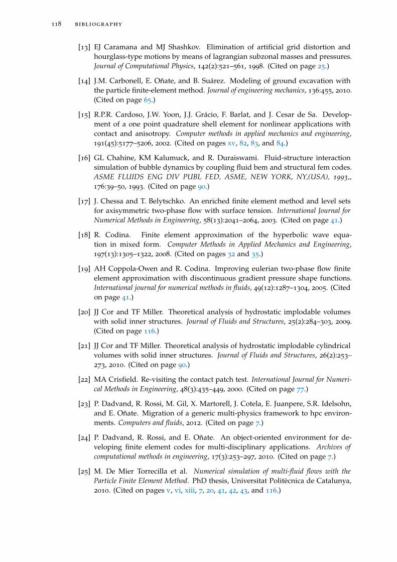
118 bibliography

[13] EJ Caramana and MJ Shashkov. Elimination of artificial grid distortion andhourglass-type motions by means of lagrangian subzonal masses and pressures.Journal of Computational Physics, 142(2):521–561, 1998. (Cited on page 25.)

[14] J.M. Carbonell, E. Oñate, and B. Suárez. Modeling of ground excavation withthe particle finite-element method. Journal of engineering mechanics, 136:455, 2010.(Cited on page 65.)

[15] R.P.R. Cardoso, J.W. Yoon, J.J. Grácio, F. Barlat, and J. Cesar de Sa. Develop-ment of a one point quadrature shell element for nonlinear applications withcontact and anisotropy. Computer methods in applied mechanics and engineering,191(45):5177–5206, 2002. (Cited on pages xv, 82, 83, and 84.)

[16] GL Chahine, KM Kalumuck, and R. Duraiswami. Fluid-structure interactionsimulation of bubble dynamics by coupling fluid bem and structural fem codes.ASME FLUIDS ENG DIV PUBL FED, ASME, NEW YORK, NY,(USA), 1993,,176:39–50, 1993. (Cited on page 90.)

[17] J. Chessa and T. Belytschko. An enriched finite element method and level setsfor axisymmetric two-phase flow with surface tension. International Journal forNumerical Methods in Engineering, 58(13):2041–2064, 2003. (Cited on page 41.)

[18] R. Codina. Finite element approximation of the hyperbolic wave equa-tion in mixed form. Computer Methods in Applied Mechanics and Engineering,197(13):1305–1322, 2008. (Cited on pages 32 and 35.)

[19] AH Coppola-Owen and R. Codina. Improving eulerian two-phase flow finiteelement approximation with discontinuous gradient pressure shape functions.International journal for numerical methods in fluids, 49(12):1287–1304, 2005. (Citedon page 41.)

[20] JJ Cor and TF Miller. Theoretical analysis of hydrostatic implodable volumeswith solid inner structures. Journal of Fluids and Structures, 25(2):284–303, 2009.(Cited on page 116.)

[21] JJ Cor and TF Miller. Theoretical analysis of hydrostatic implodable cylindricalvolumes with solid inner structures. Journal of Fluids and Structures, 26(2):253–273, 2010. (Cited on page 90.)

[22] MA Crisfield. Re-visiting the contact patch test. International Journal for Numeri-cal Methods in Engineering, 48(3):435–449, 2000. (Cited on page 77.)

[23] P. Dadvand, R. Rossi, M. Gil, X. Martorell, J. Cotela, E. Juanpere, S.R. Idelsohn,and E. Oñate. Migration of a generic multi-physics framework to hpc environ-ments. Computers and fluids, 2012. (Cited on page 7.)

[24] P. Dadvand, R. Rossi, and E. Oñate. An object-oriented environment for de-veloping finite element codes for multi-disciplinary applications. Archives ofcomputational methods in engineering, 17(3):253–297, 2010. (Cited on page 7.)

[25] M. De Mier Torrecilla et al. Numerical simulation of multi-fluid flows with theParticle Finite Element Method. PhD thesis, Universitat Politècnica de Catalunya,2010. (Cited on pages v, vi, xiii, 7, 20, 41, 42, 43, and 116.)

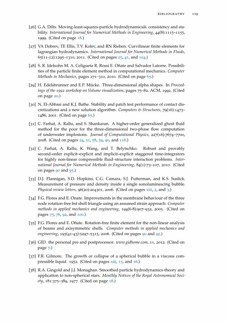
bibliography 119

[26] G.A. Dilts. Moving-least-squares-particle hydrodynamicsâi. consistency and sta-bility. International Journal for Numerical Methods in Engineering, 44(8):1115–1155,1999. (Cited on page 18.)

[27] VA Dobrev, TE Ellis, T.V. Kolev, and RN Rieben. Curvilinear finite elements forlagrangian hydrodynamics. International Journal for Numerical Methods in Fluids,65(11-12):1295–1310, 2011. (Cited on pages 25, 41, and 104.)

[28] S. R. Idelsohn M. A. Celigueta R. Rossi E. Oñate and Salvador Latorre. Possibili-ties of the particle finite element method in computational mechanics. ComputerMethods in Mechanics, pages 271–310, 2010. (Cited on page 65.)

[29] H. Edelsbrunner and E.P. Mücke. Three-dimensional alpha shapes. In Proceed-ings of the 1992 workshop on Volume visualization, pages 75–82. ACM, 1992. (Citedon page 20.)

[30] N. El-Abbasi and K.J. Bathe. Stability and patch test performance of contact dis-cretizations and a new solution algorithm. Computers & Structures, 79(16):1473–1486, 2001. (Cited on page 65.)

[31] C. Farhat, A. Rallu, and S. Shankaran. A higher-order generalized ghost fluidmethod for the poor for the three-dimensional two-phase flow computationof underwater implosions. Journal of Computational Physics, 227(16):7674–7700,2008. (Cited on pages 24, 51, 58, 59, 90, and 116.)

[32] C. Farhat, A. Rallu, K. Wang, and T. Belytschko. Robust and provablysecond-order explicit–explicit and implicit–explicit staggered time-integratorsfor highly non-linear compressible fluid–structure interaction problems. Inter-national Journal for Numerical Methods in Engineering, 84(1):73–107, 2010. (Citedon pages 90 and 95.)

[33] D.J. Flannigan, S.D. Hopkins, C.G. Camara, S.J. Putterman, and K.S. Suslick.Measurement of pressure and density inside a single sonoluminescing bubble.Physical review letters, 96(20):204301, 2006. (Cited on pages xiii, 2, and 3.)

[34] F.G. Flores and E. Onate. Improvements in the membrane behaviour of the threenode rotation-free bst shell triangle using an assumed strain approach. Computermethods in applied mechanics and engineering, 194(6-8):907–932, 2005. (Cited onpages 75, 76, 92, and 100.)

[35] F.G. Flores and E. Oñate. Rotation-free finite element for the non-linear analysisof beams and axisymmetric shells. Computer methods in applied mechanics andengineering, 195(41-43):5297–5315, 2006. (Cited on pages 90 and 92.)

[36] GID. the personal pre and postprocessor. www.gidhome.com, 11, 2012. (Cited onpage 7.)

[37] F.R. Gilmore. The growth or collapse of a spherical bubble in a viscous com-pressible liquid. 1952. (Cited on pages xiii, 15, and 16.)

[38] R.A. Gingold and J.J. Monaghan. Smoothed particle hydrodynamics-theory andapplication to non-spherical stars. Monthly Notices of the Royal Astronomical Soci-ety, 181:375–389, 1977. (Cited on page 18.)

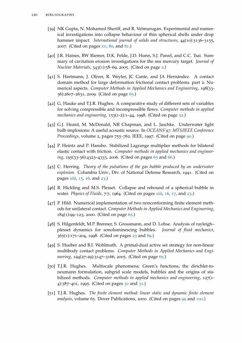
120 bibliography

[39] NK Gupta, N. Mohamed Sheriff, and R. Velmurugan. Experimental and numer-ical investigations into collapse behaviour of thin spherical shells under drophammer impact. International journal of solids and structures, 44(10):3136–3155,2007. (Cited on pages xv, 80, and 81.)

[40] J.R. Haines, BW Riemer, D.K. Felde, J.D. Hunn, S.J. Pawel, and C.C. Tsai. Sum-mary of cavitation erosion investigations for the sns mercury target. Journal ofNuclear Materials, 343(1):58–69, 2005. (Cited on page 2.)

[41] S. Hartmann, J. Oliver, R. Weyler, JC Cante, and JA Hernández. A contactdomain method for large deformation frictional contact problems. part 2: Nu-merical aspects. Computer Methods in Applied Mechanics and Engineering, 198(33-36):2607–2631, 2009. (Cited on page 65.)

[42] G. Hauke and T.J.R. Hughes. A comparative study of different sets of variablesfor solving compressible and incompressible flows. Computer methods in appliedmechanics and engineering, 153(1-2):1–44, 1998. (Cited on page 32.)

[43] G.J. Heard, M. McDonald, NR Chapman, and L. Jaschke. Underwater lightbulb implosions: A useful acoustic source. In OCEANS’97. MTS/IEEE ConferenceProceedings, volume 2, pages 755–762. IEEE, 1997. (Cited on page 90.)

[44] P. Heintz and P. Hansbo. Stabilized Lagrange multiplier methods for bilateralelastic contact with friction. Computer methods in applied mechanics and engineer-ing, 195(33-36):4323–4333, 2006. (Cited on pages 65 and 66.)

[45] C. Herring. Theory of the pulsations of the gas bubble produced by an underwaterexplosion. Columbia Univ., Div. of National Defense Research, 1941. (Cited onpages xiii, 15, 16, and 23.)

[46] R. Hickling and M.S. Plesset. Collapse and rebound of a spherical bubble inwater. Physics of Fluids, 7:7, 1964. (Cited on pages xiii, 16, 17, and 23.)

[47] P. Hild. Numerical implementation of two nonconforming finite element meth-ods for unilateral contact. Computer Methods in Applied Mechanics and Engineering,184(1):99–123, 2000. (Cited on page 65.)

[48] S. Hilgenfeldt, M.P. Brenner, S. Grossmann, and D. Lohse. Analysis of rayleigh–plesset dynamics for sonoluminescing bubbles. Journal of fluid mechanics,365(1):171–204, 1998. (Cited on pages 23 and 89.)

[49] S. Hueber and B.I. Wohlmuth. A primal-dual active set strategy for non-linearmultibody contact problems. Computer Methods in Applied Mechanics and Engi-neering, 194(27-29):3147–3166, 2005. (Cited on page 65.)

[50] T.J.R. Hughes. Multiscale phenomena: Green’s functions, the dirichlet-to-neumann formulation, subgrid scale models, bubbles and the origins of sta-bilized methods. Computer methods in applied mechanics and engineering, 127(1-4):387–401, 1995. (Cited on pages 30 and 31.)

[51] T.J.R. Hughes. The finite element method: linear static and dynamic finite elementanalysis, volume 65. Dover Publications, 2000. (Cited on pages 99 and 100.)

bibliography 121

[52] T.J.R. Hughes, G.R. Feijóo, L. Mazzei, and J.B. Quincy. The variational multiscalemethod–a paradigm for computational mechanics. Computer methods in appliedmechanics and engineering, 166(1-2):3–24, 1998. (Cited on pages 30 and 31.)

[53] T.J.R. Hughes and TE Tezduyar. Finite element methods for first-order hyper-bolic systems with particular emphasis on the compressible euler equations.Computer Methods in Applied Mechanics and Engineering, 45(1-3):217–284, 1984.(Cited on pages 35 and 100.)

[54] S. Iakovlev. Submerged fluid-filled cylindrical shell subjected to a shock wave:fluid–structure interaction effects. Journal of fluids and structures, 23(1):117–142,2007. (Cited on page 90.)

[55] S. Idelsohn, N. Nigro, A. Limache, and E. Oñate. Large time-step explicit in-tegration method for solving problems with dominant convection. ComputerMethods in Applied Mechanics and Engineering, 2012. (Cited on page 18.)

[56] S.R. Idelsohn, M. Mier-Torrecilla, N. Nigro, and E. Oñate. On the analysis ofheterogeneous fluids with jumps in the viscosity using a discontinuous pressurefield. Computational Mechanics, 46(1):115–124, 2010. (Cited on pages 23, 25, 40,41, 46, and 104.)

[57] S.R. Idelsohn, M. Mier-Torrecilla, and E. Oñate. Multi-fluid flows with the par-ticle finite element method. Computer Methods in Applied Mechanics and Engineer-ing, 198(33-36):2750–2767, 2009. (Cited on pages v, vi, 7, 23, 25, 40, 41, 46, 90, 95,104, and 116.)

[58] S.R. Idelsohn, E. Onate, N. Calvo, and F. Del Pin. The meshless finite elementmethod. International Journal for Numerical Methods in Engineering, 58(6):893–912,2003. (Cited on page 18.)

[59] S.R. Idelsohn, E. Oñate, and F.D. Pin. The particle finite element method: apowerful tool to solve incompressible flows with free-surfaces and breakingwaves. International Journal for Numerical Methods in Engineering, 61(7):964–989,2004. (Cited on pages 25, 41, 65, and 89.)

[60] Idelsohn, SR and Del Pin, F. and Rossi, R. and Oñate, E. Fluid–structure interac-tion problems with strong added-mass effect. International journal for numericalmethods in engineering, 80(10):1261–1294, 2009. (Cited on page 95.)

[61] RD Ivany and F.G. Hammitt. Cavitation bubble collapse in viscous, compress-ible liquidsânumerical analysis. Journal of Basic Engineering, 87:977, 1965. (Citedon page 16.)

[62] K.E. Jansen, C.H. Whiting, and G.M. Hulbert. A generalized α method forintegrating the filtered navier–stokes equations with a stabilized finite elementmethod. Computer Methods in Applied Mechanics and Engineering, 190(3):305–319,2000. (Cited on page 99.)

[63] E. Johnsen and T. Colonius. Numerical simulations of non-spherical bubblecollapse. Journal of fluid mechanics, 629(1):231–262, 2009. (Cited on pages xiii, 4,and 5.)

122 bibliography

[64] A.A. Johnson and T.E. Tezduyar. Mesh update strategies in parallel finite ele-ment computations of flow problems with moving boundaries and interfaces.Computer Methods in Applied Mechanics and Engineering, 119(1-2):73–94, 1994.(Cited on page 104.)

[65] AA Johnson and TE Tezduyar. 3d simulation of fluid-particle interactions withthe number of particles reaching 100. Computer Methods in Applied Mechanics andEngineering, 145(3):301–321, 1997. (Cited on page 105.)

[66] J.R. Kamm. Evaluation of the sedov-von neumann-taylor blast wave solution.Astrophys. J. Suppl.(submitted), 2000. (Cited on pages 46 and 49.)

[67] K. Kamran, R. Rossi, and E. Oñate. A contact algorithm for shell prob-lems via the particle finite element method (pfem). Computational Mechanics,10.1007/s00466-012-0791-x, 2012. (Cited on pages 65 and 95.)

[68] K. Kamran, R. Rossi, E. Oñate, and S.R. Idelsohn. A compressible lagrangianframework for the simulation of the underwater implosion of large air bubbles.Computer Methods in Applied Mechanics and Engineering, 225:210–225, 2013. (Citedon pages 23, 35, 104, and 105.)

[69] J.B. Keller and I.I. Kolodner. Damping of underwater explosion bubble oscil-lations. Journal of applied physics, 27(10):1152–1161, 1956. (Cited on pages 16

and 23.)

[70] E. Klaseboer, BC Khoo, and KC Hung. Dynamics of an oscillating bubble neara floating structure. Journal of Fluids and Structures, 21(4):395–412, 2005. (Citedon page 90.)

[71] G.J. Le Beau, SE Ray, SK Aliabadi, and TE Tezduyar. Supg finite element compu-tation of compressible flows with the entropy and conservation variables formu-lations. Computer Methods in Applied Mechanics and Engineering, 104(3):397–422,1993. (Cited on page 35.)

[72] SC Li. Cavitation of hydraulic machinery, volume 277. Imperial College Press,2000. (Cited on pages 1 and 116.)

[73] D. Lohse. Cavitation hots up. Nature, 434(7029):33–34, 2005. (Cited on pages xiiiand 3.)

[74] J.F.M. Manual. Vol. 5, partiii. Quality Maintenance, Submarine Maintenance Engi-neering, US Navy, Portsmouth, NH, 2006. (Cited on page 89.)

[75] B.E. McDonald and C. Holland. Decay of large underwater bubble oscillations.The Journal of the Acoustical Society of America, 107:3084, 2000. (Cited on pages 24

and 89.)

[76] R. Menikoff and B.J. Plohr. The riemann problem for fluid flow of real materials.Reviews of modern physics, 61(1):75, 1989. (Cited on pages 27, 29, and 96.)

[77] S. Nagrath, K. Jansen, R.T. Lahey, et al. Hydrodynamic simulation of air bubbleimplosion using a level set approach. Journal of Computational Physics, 215(1):98–132, 2006. (Cited on pages 23, 24, 59, 62, 89, and 116.)

bibliography 123

[78] US Navy. The navy unmanned undersea vehicle (uuv) master plan. US Navy,November, 9, 2004. (Cited on page 90.)

[79] B. Nayroles, G. Touzot, and P. Villon. Generalizing the finite element method:diffuse approximation and diffuse elements. Computational mechanics, 10(5):307–318, 1992. (Cited on page 18.)

[80] J. Nitsche. Uber ein variationsprinzip zur losung von dirichlet-problemen beiverwendung von teilraumen, die keinen randbedingungen unterworfen sind.In Abhandlungen aus dem Mathematischen Seminar der Universitat Hamburg, vol-ume 36, pages 9–15. Springer, 1971. (Cited on page 65.)

[81] WF Noh. Errors for calculations of strong shocks using an artificial viscosityand an artificial heat flux. Journal of Computational Physics, 72(1):78–120, 1987.(Cited on pages 46 and 47.)

[82] B.E. Noltingk and E.A. Neppiras. Cavitation produced by ultrasonics. Proceed-ings of the Physical Society. Section B, 63:674, 1950. (Cited on page 12.)

[83] J.T. Oden and L. Demkowicz. Applied functional analysis. Chapman & Hall/CRC,2009. (Cited on page 31.)

[84] J. Oliver, S. Hartmann, JC Cante, R. Weyler, and JA Hernández. A contact do-main method for large deformation frictional contact problems. Part 1: The-oretical basis. Computer Methods in Applied Mechanics and Engineering, 198(33-36):2591–2606, 2009. (Cited on pages 65 and 113.)

[85] E. Oñate. Derivation of stabilized equations for numerical solution of advective-diffusive transport and fluid flow problems. Computer Methods in Applied Me-chanics and Engineering, 151(1-2):233–265, 1998. (Cited on page 32.)

[86] E. Oñate. Possibilities of finite calculus in computational mechanics. Interna-tional journal for numerical methods in engineering, 60(1):255–281, 2004. (Cited onpage 32.)

[87] E. Oñate, M.A. Celigueta, S.R. Idelsohn, F. Salazar, and B. Suárez. Possibilities ofthe particle finite element method for fluid–soil–structure interaction problems.Computational Mechanics, pages 1–12, 2011. (Cited on page 65.)

[88] E. Onate and M. Cervera. Derivation of thin plate bending elements with onedegree of freedom per node: a simple three node triangle. Engineering Com-putations: Int J for Computer-Aided Engineering, 10(6):543–561, 1993. (Cited onpage 76.)

[89] E. Onate and F.G. Flores. Advances in the formulation of the rotation-free ba-sic shell triangle. Computer methods in applied mechanics and engineering, 194(21-24):2406–2443, 2005. (Cited on pages 75, 76, and 92.)

[90] E. Onate, S. Idelsohn, OC Zienkiewicz, and RL Taylor. A finite point methodin computational mechanics. applications to convective transport and fluid flow.International Journal for Numerical Methods in Engineering, 39(22):3839–3866, 1996.(Cited on page 18.)

124 bibliography

[91] E. Oñate, S.R. Idelsohn, M.A. Celigueta, and R. Rossi. Advances in the parti-cle finite element method for the analysis of fluid–multibody interaction andbed erosion in free surface flows. Computer Methods in Applied Mechanics andEngineering, 197(19):1777–1800, 2008. (Cited on page 65.)

[92] E. Oñate, S.R. Idelsohn, F. Del Pin, and R. Aubry. The particle finite elementmethod. an overview. International Journal of Computational Methods, 1(2):267–307, 2004. (Cited on pages xiii, 19, 25, 41, 65, and 89.)

[93] E. Onate and F. Zarate. Rotation-free triangular plate and shell elements. Interna-tional Journal for Numerical Methods in Engineering, 47(1-3):557–603, 2000. (Citedon pages 75 and 76.)

[94] M. Orr and M. Schoenberg. Acoustic signatures from deep water implosions ofspherical cavities. The Journal of the Acoustical Society of America, 59:1155, 1976.(Cited on pages 24, 89, and 90.)

[95] M. Packer, W.J. Fishkind, I.H. Fine, B.S. Seibel, and R.S. Hoffman. The physicsof phaco: a review. Journal of Cataract & Refractive Surgery, 31(2):424–431, 2005.(Cited on page 3.)

[96] M.S. Pearle. Shock-wave lithotripsy for renal calculi. New England Journal ofMedicine, 367(1):50–57, 2012. (Cited on pages xiii, 4, and 116.)

[97] M.S. Plesset. The dynamics of cavitation bubbles. ASME J. Appl.Mech., 16:228–231, 1949. (Cited on page 11.)

[98] MS Plesset and TP Mitchell. On the stability of the spherical shape of a vaporcavity in a liquid. Technical report, DTIC Document, 1954. (Cited on pages 14

and 62.)

[99] M.S. Plesset and A. Prosperetti. Bubble dynamics and cavitation. Annual Reviewof Fluid Mechanics, 9(1):145–185, 1977. (Cited on pages 24, 62, and 89.)

[100] H. Poritsky. The collapse or growth of a spherical bubble or cavity in a vis-cous fluid. Proc. First Nat. Cong. in Appl. Math, pages 813–821, 1952. (Cited onpage 12.)

[101] A. Prosperetti and A. Lezzi. Bubble dynamics in a compressible liquid. part 1.first-order theory. J. FLUID MECH., 1986, 168:457–478, 1986. (Cited on pages 16,23, and 89.)

[102] L. Rayleigh. On the pressure developed in a liquid during the collapse of aspherical cavity. Phil. Mag, 34(200):94–98, 1917. (Cited on pages 11, 23, and 89.)

[103] AB Reynolds and G. Berthoud. Analysis of excobulle two-phase expansion tests.Nuclear Engineering and Design, 67(1):83–100, 1981. (Cited on page 15.)

[104] W.J. Rider. Revisiting wall heating. Journal of Computational Physics, 162(2):395–410, 2000. (Cited on page 48.)

[105] Rossi, R. and Oñate, E. Analysis of some partitioned algorithms for fluid-structure interaction. Engineering Computations: Int J for Computer-Aided Engi-neering, 27(1):20–56, 2010. (Cited on page 95.)

bibliography 125

[106] Ryzhakov, PB and Rossi, R. and Idelsohn, SR and Oñate, E. A monolithic La-grangian approach for fluid–structure interaction problems. Computational Me-chanics, 46(6):883–899, 2010. (Cited on page 95.)

[107] S. Sathe and T.E. Tezduyar. Modeling of fluid–structure interactions with thespace–time finite elements: contact problems. Computational Mechanics, 43(1):51–60, 2008. (Cited on page 95.)

[108] A.J.R. Schneider. Some compressibility effects in cavitation bubble dynamics. PhDthesis, California Institute of Technology, 1949. (Cited on pages xiii, 15, and 16.)

[109] G. Scovazzi, JN Shadid, E. Love, and WJ Rider. A conservative nodal variationalmultiscale method for lagrangian shock hydrodynamics. Computer Methods inApplied Mechanics and Engineering, 2010. (Cited on pages v, 7, 23, 25, 27, 33, 34,35, 36, 37, 41, 96, and 104.)

[110] L.I. Sedov. Similarity and dimensional methods in mechanics. CRC, 1993. (Cited onpages 46 and 49.)

[111] S.B. Segletes. Thermodynamic stability of the mie–grüneisen equation ofstate, and its relevance to hydrocode computations. Journal of applied physics,70(5):2489–2499, 1991. (Cited on page 27.)

[112] J.R. Shewchuk. Delaunay refinement algorithms for triangular mesh generation.Computational geometry, 22(1):21–74, 2002. (Cited on page 44.)

[113] K.M. Shyue. A fluid-mixture type algorithm for compressible multicomponentflow with mie–grüneisen equation of state. Journal of Computational Physics,171(2):678–707, 2001. (Cited on page 27.)

[114] H. Si. Tetgen: A quality tetrahedral mesh generator and a 3d delaunay trian-gulator. Weierstrass Institute for Applied Analysis and Stochastics, available fromhttp://tetgen. berlios. de Haber, E., Ascher, UM, Aruliah, DM, & Oldenberg, D, pages150–171, 2000. (Cited on pages 69, 73, and 105.)

[115] K.Kamran R.Rossi S.Idelsohn and E.Oñate. Underwater implosion using theparticle finite element method. CIMNE research report, PI-371, 2012. (Cited onpages 59, 74, 84, and 89.)

[116] K. Stein, T. Tezduyar, and R. Benney. Mesh moving techniques for fluid-structure interactions with large displacements. Journal of Applied Mechanics,70:58, 2003. (Cited on page 104.)

[117] K. Stein, T.E. Tezduyar, and R. Benney. Automatic mesh update with the solid-extension mesh moving technique. Computer Methods in Applied Mechanics andEngineering, 193(21):2019–2032, 2004. (Cited on pages 104 and 105.)

[118] K.S. Suslick. Sonochemistry. Science, 247(4949):1439–1445, 1990. (Cited onpages 3 and 116.)

[119] K. Takizawa, T. Spielman, and T.E. Tezduyar. Space–time fsi modeling and dy-namical analysis of spacecraft parachutes and parachute clusters. ComputationalMechanics, pages 1–20, 2011. (Cited on pages 95 and 105.)

126 bibliography

[120] K. Takizawa and T.E. Tezduyar. Computational methods for parachute fluid–structure interactions. Archives of computational methods in engineering, 19(1):125–169, 2012. (Cited on page 95.)

[121] M. Tanguay. Computation of bubbly cavitating flow in shock wave lithotripsy. Cali-fornia Institute of Technology, 2005. (Cited on page 4.)

[122] M. Senga T.E. Tezduyar and D. Vicker. Computation of inviscid supersonicflows around cylinders and spheres with the supg formulation and yzβ shock-capturing. Computational Mechanics, 38:469–481, 2006. (Cited on page 35.)

[123] T. Tezduyar, S. Aliabadi, M. Behr, A. Johnson, and S. Mittal. Parallel finite-element computation of 3d flows. Computer, 26(10):27–36, 1993. (Cited onpage 104.)

[124] T.E. Tezduyar, S. Sathe, T. Cragin, B. Nanna, B.S. Conklin, J. Pausewang, andM. Schwaab. Modelling of fluid–structure interactions with the space–time fi-nite elements: Arterial fluid mechanics. International Journal for Numerical Meth-ods in Fluids, 54(6-8):901–922, 2007. (Cited on page 95.)

[125] T.E. Tezduyar, S. Sathe, R. Keedy, and K. Stein. Space–time finite element tech-niques for computation of fluid–structure interactions. Computer Methods inApplied Mechanics and Engineering, 195(17):2002–2027, 2006. (Cited on page 95.)

[126] T.E. Tezduyar and M. Senga. Stabilization and shock-capturing parameters insupg formulation of compressible flows. Computer methods in applied mechanicsand engineering, 195(13):1621–1632, 2006. (Cited on page 35.)

[127] T.E. Tezduyar and M. Senga. Supg finite element computation of inviscid super-sonic flows with yzβ shock-capturing. Computers & fluids, 36(1):147–159, 2007.(Cited on page 35.)

[128] N. TS500-AU-SPN. Us navy general specification for the design, construction,and repair of diving and hyperbaric equipment revision 1 august 23, 2006. 2006.(Cited on page 5.)

[129] S.E. Turner. Underwater implosion of glass spheres. The Journal of the AcousticalSociety of America, 121:844, 2007. (Cited on pages 24, 47, 58, 59, and 90.)

[130] DP Updike. On the large deformation of a rigid plastic spherical shell com-pressed by a rigid plate. Journal of Engineering for Industry, 94(3):949–955, 1972.(Cited on page 81.)

[131] J. VonNeumann and RD Richtmyer. A method for the numerical calculation ofhydrodynamic shocks. Journal of Applied Physics, 21(3):232–237, 1950. (Cited onpage 36.)

[132] GM Ward and DI Pullin. A study of planar richtmyer-meshkov instability influids with mie-grüneisen equations of state. Physics of Fluids, 23:076101, 2011.(Cited on page 27.)

[133] A.B. Wardlaw Jr and J.A. Luton. Fluid-structure interaction mechanisms forclose-in explosions. Shock and Vibration, 7(5):265–275, 2000. (Cited on page 5.)

bibliography 127

[134] P. Wriggers and G. Zavarise. Computational contact mechanics. Wiley OnlineLibrary, 2004. (Cited on page 65.)

[135] CC Wu and P.H. Roberts. Shock-wave propagation in a sonoluminescing gasbubble. Physical review letters, 70(22):3424–3427, 1993. (Cited on page 59.)

[136] X. Xi and P. Zhong. Dynamic photoelastic study of the transient stress fieldin solids during shock wave lithotripsy. The Journal of the Acoustical Society ofAmerica, 109:1226, 2001. (Cited on page 4.)

[137] A.P. Yoganathan, Z. He, and S. Casey Jones. Fluid mechanics of heart valves.Annu. Rev. Biomed. Eng., 6:331–362, 2004. (Cited on page 2.)

[138] F.R. Young. Sonoluminescence. CRC press, 2004. (Cited on pages 63 and 116.)

[139] Z.H. Zhong. Finite element procedures for contact-impact problems, volume 7. Ox-ford University Press, 1993. (Cited on page 83.)

[140] S. Zhu, F.H. Cocks, G.M. Preminger, and P. Zhong. The role of stress wavesand cavitation in stone comminution in shock wave lithotripsy. Ultrasound inmedicine & biology, 28(5):661–671, 2002. (Cited on page 4.)

[141] Z. Zong. A hydroplastic analysis of a free–free beam floating on water subjectedto an underwater bubble. Journal of fluids and structures, 20(3):359–372, 2005.(Cited on page 90.)

colophon

This document was typeset using the typographical look-and-feel classicthesis de-veloped by André Miede. The style was inspired by Robert Bringhurst’s seminal bookon typography “The Elements of Typographic Style”. classicthesis is available for bothLATEX and LYX: