Robust observation and identification ofnDOF Lagrangian systems

INTERNATIONAL JOURNAL OF ROBUST AND NONLINEAR CONTROLInt. J. Robust Nonlinear Control 2007; 17:842–861Published online 21 December 2006 in Wiley InterScience (www.interscience.wiley.com). DOI: 10.1002/rnc.1156

Robust observation and identification of nDOFLagrangian systems

David I. Rosas Almeida1,*,y, Joaquın Alvarez1 and Leonid Fridman2

1Electronics and Telecommunications Department, Scientific Research and Advanced Studies Centerof Ensenada, Mexico

2Department of Postgraduate Study, Engineering Faculty, National Autonomous University of Mexico,Mexico D.F., Mexico

SUMMARY

A procedure to design a global exponentially stable, second-order, sliding-mode observer for nDOFLagrangian systems is presented. The observer converges to the system state in spite of the existence ofbounded disturbances or parameter uncertainties affecting the system dynamics. The generation of slidingmodes permits the identification of disturbances using the equivalent output injection which, under somecircumstances, can also be used to identify the system parameters via a continuous version of the last-square method. The proposed methodology is illustrated with some numerical examples and experiments.Copyright # 2006 John Wiley & Sons, Ltd.

Received 22 November 2005; Revised 11 August 2006; Accepted 6 October 2006

KEY WORDS: robust observers; variable structure systems; sliding modes; identification; Lagrangiansystems

1. INTRODUCTION

Antecedents and motivation. The problem of observation of systems with unknown inputs hasbeen one of the most important problems in control theory during the last two decades [1]. In[2, 3], sufficient and necessary conditions for observer robustness with respect to unknowninputs are established. These conditions require that the unknown inputs must be matched byknown outputs, which turn out to be restrictive because they do not include the simplest class of

*Correspondence to: David I. Rosas Almeida, CICESE, Km. 107 Carr. Tijuana-Ensenada, Ensenada, B.C. Mexico C.P.22860, Mexico.yE-mail: [email protected], [email protected]

Contract/grant sponsor: CONACyT; contract/grant number: 43807-YContract/grant sponsor: PROMEPContract/grant sponsor: Autonomous University of Baja CaliforniaContract/grant sponsor: POPIIT; contract/grant number: 11703

Copyright # 2006 John Wiley & Sons, Ltd.

mechanical systems with unknown inputs, where only the position is available. In [4], to coverthis situation, an adaptive observer, ensuring an exponential convergence of the estimation errorto a small neighbourhood of zero, was suggested.

The observation of systems with unknown inputs has been actively developed within variablestructure theory using the sliding-mode approach. Sliding-mode observers are widely used due totheir attractive features: (a) insensitivity with respect to unknown inputs; (b) possibility to use theequivalent output injection to identify unknown inputs; (c) finite time convergence to exactvalues of the state vectors (see, for example, the corresponding chapters in the textbooks [5, 6],and the recent tutorials [7–9]). In [10] a step-by-step design of sliding-mode observers wasproposed. Such design is based on the transformation of a given system to a block observableform and the sequential estimation of each state by using the equivalent output injection. Fromthe one hand, this scheme allows to formulate extended observability conditions for systems withunknown inputs, covering the observation of mechanical systems with measured positions. Suchconditions were formulated in [10, 11] for the scalar case. On the other hand, realization of thisscheme caused obligatory filtration due to the non-idealities during sliding-mode generation.

In [12, 13] a robust, exact, arbitrary-order differentiator ensuring finite time convergence to thevalues of the corresponding derivatives is proposed, and applications of higher-order sliding-modealgorithms were considered. A new generation of observers based on second-order sliding-modealgorithms has been recently designed and applied to some practical problems [14–19]. The maindisadvantage of those observers is that they are semiglobal. Some new ideas of usage of equivalentoutput injections for parameter and disturbance identifications are suggested in [20, 21].

Main contribution. In this paper we present a robust, globally exponentially stable second-order sliding-mode observer for Lagrangian systems. Some specific contributions areenumerated below:

1. A robust globally asymptotically stable second-order sliding-mode observer forLagrangian systems is proposed, ensuring convergence to the exact system state evenunder the presence of unknown inputs.

2. An algorithm for unknown input identification is proposed.3. A modification of the least-square method allowing to identify the system parameters is

presented.4. Some simulations and experimental examples illustrating the main results are given.

Paper structure. The problem statement is given in the second section. In the third section atheorem establishing the stability properties of a class of discontinuous, second-order systems isdiscussed. This result is essential to prove the exponential convergence of the observer for nDOFsystems. In the fourth section the observer design is presented, and in the next section thealgorithms for perturbation and parameter identifications are described. Finally, in Section 6 thedesign technique is numerically and experimentally illustrated via the design and implementa-tion of an observer for a simple pendulum.

2. PROBLEM STATEMENT

Consider a nDOF Lagrangian system described by

MðqÞ.qþ Cðq; ’qÞ’qþ GðqÞ þ jð.q; ’q; qÞyþ gðtÞ ¼ t ð1Þ

ROBUST OBSERVATION AND IDENTIFICATION OF nDOF LAGRANGIAN SYSTEMS 843

Copyright # 2006 John Wiley & Sons, Ltd. Int. J. Robust Nonlinear Control 2007; 17:842–861

DOI: 10.1002/rnc

where q 2 Rn is the generalized position vector, MðqÞ is the inertia matrix, Cðq; ’qÞ is thecentrifuge and Coriolis matrix, GðqÞ is the gravitational force vector, the term jð.q; ’q; qÞy enclosesthe terms produced by the vector of parameter variations y; jð.q; ’q; qÞ is a n�mmatrix and y is am� 1 vector. gðtÞ 2 Rn is a bounded vector of external disturbances; finally, t 2 Rn is thegeneralized force input. All matrices and vectors are defined with the suitable dimensions. Weconsider that the measured variables are the generalized position q:

Defining the state variables x1 ¼ q; x2 ¼ ’q; the state-space representation of system (1) is

’x1

’x2

" #¼

x2

f ðxÞ þ gðx1Þ þ xð�Þ þM�1ð�Þt

" #ð2Þ

y ¼ x1 ð3Þ

where

f ðxÞ ¼ �M�1ð�ÞCðx1;x2Þx2

gðx1Þ ¼ �M�1ð�ÞGðx1Þ

xð�Þ ¼ �M�1ð�Þðjð.q; ’q; qÞyþ gðtÞÞ

We assume that the behaviour of system (2)–(3) is bounded for any bounded input t and anybounded perturbation gðtÞ:

In this paper we will design the globally asymptotically stable observer providing the exactvalue of variables x2 based on the exact measurements of the variables x1 and suggest themethod for unknown perturbations and parameters identification.

3. GLOBAL EXPONENTIAL STABILITY OF A CLASS OF PERTURBEDSECOND-ORDER SYSTEMS

In this section we present a preliminary result that will be useful to design the observer. Considerthe following second-order system:

’v1 ¼ v2

’v2 ¼ � av1 � bv2 þ eðtÞ � c signðv1Þð4Þ

where a and b are positive constants, eðtÞ is an external perturbation with the bound

jeðtÞj4r0 ð5Þ

where r0 is a constant, c is a control parameter, and signð�Þ is the signum function. Define thematrix A as

A ¼0 1

�a �b

" #ð6Þ

D. I. R. ALMEIDA, J. ALVAREZ AND L. FRIDMAN844


DOI: 10.1002/rnc

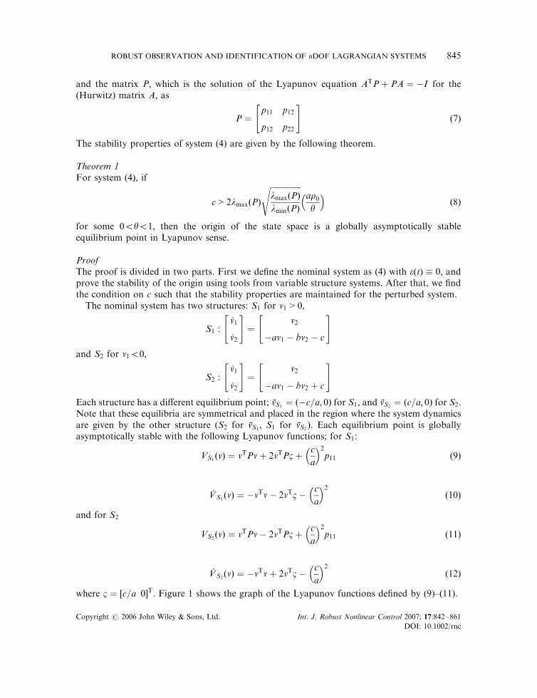
and the matrix P; which is the solution of the Lyapunov equation ATPþ PA ¼ �I for the(Hurwitz) matrix A; as

P ¼p11 p12

p12 p22

" #ð7Þ

The stability properties of system (4) are given by the following theorem.

Theorem 1For system (4), if

c > 2lmaxðPÞ

ffiffiffiffiffiffiffiffiffiffiffiffiffiffiffiffilmaxðPÞlminðPÞ

sar0y

� �ð8Þ

for some 05y51; then the origin of the state space is a globally asymptotically stableequilibrium point in Lyapunov sense.

ProofThe proof is divided in two parts. First we define the nominal system as (4) with eðtÞ � 0; andprove the stability of the origin using tools from variable structure systems. After that, we findthe condition on c such that the stability properties are maintained for the perturbed system.

The nominal system has two structures: S1 for v1 > 0;

S1 :’v1

’v2

" #¼

v2

�av1 � bv2 � c

" #and S2 for v150;

S2 :’v1

’v2

" #¼

v2

�av1 � bv2 þ c

" #Each structure has a different equilibrium point; %vS1

¼ ð�c=a; 0Þ for S1; and %vS2¼ ðc=a; 0Þ for S2:

Note that these equilibria are symmetrical and placed in the region where the system dynamicsare given by the other structure (S2 for %vS1

; S1 for %vS2). Each equilibrium point is globally

asymptotically stable with the following Lyapunov functions; for S1:

VS1ðvÞ ¼ vTPvþ 2vTPBþ

c

a

� �2p11 ð9Þ

’VS1ðvÞ ¼ �vTv� 2vTB�

c

a

� �2ð10Þ

and for S2

VS2ðvÞ ¼ vTPv� 2vTPBþ

c

a

� �2p11 ð11Þ

’VS2ðvÞ ¼ �vTvþ 2vTB�

c

a

� �2ð12Þ

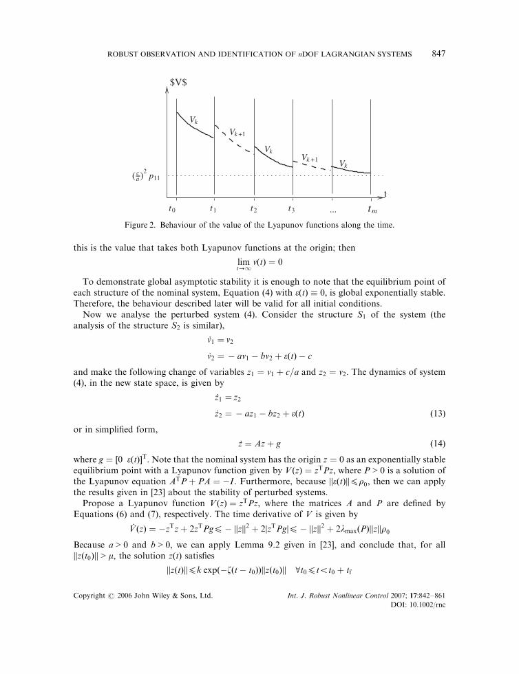
where B ¼ ½c=a 0�T: Figure 1 shows the graph of the Lyapunov functions defined by (9)–(11).



DOI: 10.1002/rnc

A direct application of the criterion given in [22] allows us to conclude that the discontinuitysurface given by s ¼ v1 ¼ 0 is not a sliding surface. Note also that the solutions cross the linev1 ¼ 0 from quadrant II to quadrant I, and from quadrant IV to quadrant III. Functions VSi

ðvÞintersect at the origin with a value VSi

ð0Þ ¼ ðc=aÞ2p11; for i ¼ 1; 2:Define two neighbourhoods ofthe origin, Oe with radio e > 0; and Ob defined in the following form:

Ob ¼O1 [ O2

O1 ¼fv 2 R2jv150;VS1ðvÞ4bg

O2 ¼fv 2 R2jv150;VS2ðvÞ4bg

where b > ðc=aÞ2p11: Finally, define a neighbourhood Od with ratio d5e (d can depend on e andb; dðe;bÞ) such that Od � Ob: Define a set of times T ¼ ft1; t2; . . . ; ti; . . .g; where ti are the timeswhere the system commutes its structures. We assume that t15t25 � � � : If jjvðt0Þjj5d andvðt0Þ 2 Ok � Ob for some k ¼ 1; 2 (the kth structure is active), then the first change of structureappears at time t1; and because ’VSk

50; we have jjvðt0Þjj > jjvðt1Þjj; then VSkðvðt0ÞÞ > VSk

ðvðt1ÞÞ:Now vðt1Þ is the initial condition for the next structure and, by construction of VSi

;VSkðvðt1ÞÞ5VSkþ1ðvðt1ÞÞ by a factor 4jv2ðt1Þjp12ðc=aÞ: The second commutation appears at time

t2; the system goes from Okþ1 to Ok; jjvðt1Þjj > jjvðt2Þjj; VSkþ1ðvðt1ÞÞ > VSkþ1 ðvðt2ÞÞ andVSkþ1ðvðt2ÞÞ > VSk

ðvðt2ÞÞ and so on for all ti 2 T ; Figure 2 shows this phenomenon.Then we see that the sequences W1 ¼ fVSk

ðt1Þ;VSkðt3Þ; . . .g and W2 ¼ fVSkþ1ðt2Þ;VSkþ1 ðt4Þ; . . .g

are strictly decreasing and lower bounded and converge to ðc=aÞp11: Also, it is satisfied thatjjvðtiþ1Þjj5jjvðtiÞjj5 � � �5jjvðt0Þjj5d5e8t > t0; 8i:

For all e > 0 and b > ðc=aÞ2p11 we can find a number d so that the trajectories initiating in Od

will remain within the neighbourhood Oe for all t5t0: Therefore, the origin is stable in theLyapunov sense.

To demonstrate asymptotic stability it is enough to note that

limi!1

VSkðvðtiÞÞ ¼ lim

i!1VSkþ1 ðvðtiÞÞ ¼

c

ap11

–50

5 –5

0

5

0

10

20

30

40

50

60

v 2

v1

V k

Figure 1. Lyapunov functions of each equilibrium point.



DOI: 10.1002/rnc

this is the value that takes both Lyapunov functions at the origin; then

limt!1

vðtÞ ¼ 0

To demonstrate global asymptotic stability it is enough to note that the equilibrium point ofeach structure of the nominal system, Equation (4) with eðtÞ � 0; is global exponentially stable.Therefore, the behaviour described later will be valid for all initial conditions.

Now we analyse the perturbed system (4). Consider the structure S1 of the system (theanalysis of the structure S2 is similar),

’v1 ¼ v2

’v2 ¼ � av1 � bv2 þ eðtÞ � c

and make the following change of variables z1 ¼ v1 þ c=a and z2 ¼ v2: The dynamics of system(4), in the new state space, is given by

’z1 ¼ z2

’z2 ¼ � az1 � bz2 þ eðtÞ ð13Þ

or in simplified form,

’z ¼ Azþ g ð14Þ

where g ¼ ½0 eðtÞ�T:Note that the nominal system has the origin z ¼ 0 as an exponentially stableequilibrium point with a Lyapunov function given by VðzÞ ¼ zTPz; where P > 0 is a solution ofthe Lyapunov equation ATPþ PA ¼ �I : Furthermore, because jjeðtÞjj4r0; then we can applythe results given in [23] about the stability of perturbed systems.

Propose a Lyapunov function VðzÞ ¼ zTPz; where the matrices A and P are defined byEquations (6) and (7), respectively. The time derivative of V is given by

’VðzÞ ¼ �zTzþ 2zTPg4� jjzjj2 þ 2jzTPgj4� jjzjj2 þ 2lmaxðPÞjjzjjr0

Because a > 0 and b > 0; we can apply Lemma 9.2 given in [23], and conclude that, for alljjzðt0Þjj > m; the solution zðtÞ satisfies

jjzðtÞjj4k expð�zðt� t0ÞÞjjzðt0Þjj 8t04t5t0 þ tf

t

$V$

Vk

Vk +1

Vk

Vk

tmt0 t1 t2 t3 ...

Vk +1

( ca)

2p11

Figure 2. Behaviour of the value of the Lyapunov functions along the time.



DOI: 10.1002/rnc

andjjzðtÞjj4m 8t5t0 þ tf

where tf is a finite time, and

k ¼


s; z ¼

ð1� yÞ2lmaxðPÞ

; m ¼ 2lmaxðPÞ


sr0y

for some y; 05y51: This part shows that the ball of radius m; with centre located at ð�c=a; 0Þ; isan attractor for structure S1; denoted as BS1

: Similarly, the solutions of the structure S2

’v1 ¼ v2

’v2 ¼ � av1 � bv2 þ eðt; vÞ þ c

converge to the ball BS2of radius m and centred at ðc=a; 0Þ: Therefore, each structure of the

perturbed system has an attractor (a ball) of radius m; symmetrically located on the v1-axis andat a distance d ¼ c=a from the origin. If this distance d is greater than m; i.e. if

d ¼c

a> m ¼ 2lmaxðPÞ


sr0y

� �ð15Þ

then the two attractor BS1and BS2

do not intersect each other, and the behaviour of thesolutions of the perturbed system (4) will be qualitatively similar to the behaviour of thenominal system, for which these attractors correspond to the equilibrium points ð�c=a; 0Þ; thatis, when m ¼ 0: Therefore, the perturbed system converges to the origin in the same way than thenominal system. &

Also, we can prove that the convergence is exponential in a small vicinity of the origin; in fact,we can find exponential functions that are upper and lower bounds of the solutions near theorigin; the following theorem presents this result.

Theorem 2If c > jeðtÞj; c > jð2=bÞ deðtÞ=dt� eðtÞj for all t 2 ð0;1Þ; system (4) is exponentially stable and thetime of convergence is infinite, i.e. there exists a small neighbourhood L of the origin andconstants s�;sþ;L�;Lþ such that

L�e�s�tðjv1ð0Þj þ v22ð0ÞÞ5 jv1ðtÞj þ v22ðtÞ5Lþe�s

þtðjv1ð0Þj þ v22ð0ÞÞ

v1ð0Þ; v2ð0Þ 2 L 8t 2 ð0;1Þ

ProofConsider a locally positive definite Lyapunov function:z

E ¼ ðc� eðtÞ signðv1ÞÞjv1j þ v22=2þ bv1v2=2

In the small neighbourhood of origin the following inequalities are satisfied:

s1ðjv1j þ v22=2Þ4E4s2ðjv1j þ v22=2Þ for some 05s15s2

zThis function is a generalization of the Lyapunov functions considered in [24, 25].



DOI: 10.1002/rnc

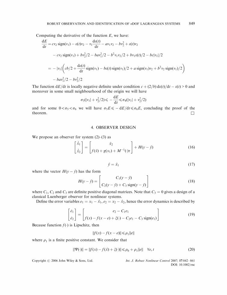
Computing the derivative of the function E; we have:

dE

dt¼ cv2 signðv1Þ � eðtÞv2 � v1

deðtÞdt� av1v2 � bv22 þ eðtÞv2

� cv2 signðv1Þ þ bv22=2� bav21=2� b2v1v2=2þ bv1eðtÞ=2� bcjv1j=2

¼ � jv1j cb=2þdeðtÞdt

signðv1Þ � beðtÞ signðv1Þ=2þ a signðv1Þv2 þ b2v2 signðv1Þ=2� �

� bav21=2� bv22=2

The function dE=dt is locally negative definite under condition cþ ð2=bÞ deðtÞ=dt� eðtÞ > 0 andmoreover in some small neighbourhood of the origin we will have

s3ðjv1j þ v22=2Þ4�dE

dt4s4ðjv1j þ v22=2Þ

and for some 05s55s6 we will have s5E4� dE=dt4s6E; concluding the proof of thetheorem. &

4. OBSERVER DESIGN

We propose an observer for system (2)–(3) as

’#x1

’#x2

" #¼

#x2

f ð #xÞ þ gðx1Þ þM�1ð�Þt

" #þHðy� #yÞ ð16Þ

#y ¼ #x1 ð17Þ

where the vector Hðy� #yÞ has the form

Hðy� #yÞ ¼C1ðy� #yÞ

C2ðy� #yÞ þ C3 signðy� #yÞ

" #ð18Þ

where C1; C2 and C3 are definite positive diagonal matrices. Note that C3 ¼ 0 gives a design of aclassical Luenberger observer for nonlinear systems.

Define the error variables e1 ¼ x1 � #x1; e2 ¼ x2 � #x2; hence the error dynamics is described by

’e1

’e2

" #¼

e2 � C1e1

f ðxÞ � f ðx� eÞ þ xð�Þ � C2e1 � C3 signðe1Þ

" #ð19Þ

Because function f ð�Þ is Lipschitz, then

jjf ðxÞ � f ðx� eÞjj4r1jjejj

where r1 is a finite positive constant. We consider that

jjCð�Þjj ¼ jjf ðxÞ � f ð #xÞ þ xð�Þjj4r0 þ r1jjejj 8e; t ð20Þ



DOI: 10.1002/rnc

Proposition 3For system (19) it is possible to find a set of matrices C1; C2 and C3 such that the origin of theerror space will be a global exponentially stable equilibrium point. Then the system defined by(16) and (17) is an observer for the system defined by (2) and (3).

ProofWe make a change of variables v1 ¼ e1 and v2 ¼ e2 � C1e1: The dynamics of system (19) in thenew state space is given by

’v1 ¼ v2

’v2 ¼ � C2v1 � C1v2 þCð�Þ � C3 signðv1Þð21Þ

This system can be seen as a set of two-dimensional subsystems, with the states v1;i; v2;i;i ¼ 1; . . . ; n; with the same form given by (4). Therefore, if r151=ð2lmaxðPÞÞ; where P is a2� 2 matrix that is the solution of the Lyapunov equation for the nominal system of (21) thenwe can apply Theorem 1 to find the conditions on C1; C2 and C3 such that the origin of system(21) is an exponential stable equilibrium point. &

We can see that the proof is straightforward by taking the result presented in the last section.The matrix inputs c3;i must satisfy Equation (8) 8 i ¼ 1; . . . ; n:

5. PERTURBATIONS AND PARAMETERS IDENTIFICATION

System (21) has a discontinuity surface in v1 ¼ 0 and the term C3 signðv1Þ produces a second-order sliding mode, i.e. the discontinuous output injection appears until the second timederivative of the function defining the discontinuity surface

.v1 ¼ f ðxÞ � f ð #xÞ þ xð�Þ � C2v1 � C1v2 � ueq ¼ 0

Then, the equivalent output injection is present at v1 ¼ v2 ¼ 0; which implies that e1 ¼ e2 ¼ 0and x ¼ #x; therefore, the equivalent output injection ueq is given by

ueq ¼ xð�Þ

¼ �M�1ð�Þðjð.q; ’q; qÞyþ gðtÞÞ

We define

Sð�Þ � �Mð�Þueq ¼ jð.q; ’q; qÞyþ gðtÞ

We can see that, the equivalent output injection gives the disturbance terms and, as we know, itis the average of the term C3 signðv1Þ when the trajectories stay at the origin. In this case, theconvergence to the discontinuity surface is asymptotic; therefore, we can approximate theperturbation term in asymptotic form as

limt!1

C3 signðz1ðtÞÞ ¼ ueq

where the upper bar denotes the average. A way to estimate this average is by filtering thediscontinuous term. A possible implementation is given in Figure 3. If the term xð�Þ does not



DOI: 10.1002/rnc

depend on the parameters, i.e.

xð�Þ ¼ gðtÞ

then the disturbance gðtÞ can be estimated directly from the equivalent output injection, that is,

gðtÞ ¼ �Mð�Þueq ¼ �Mð�Þ limt!1

C3 signðyðtÞ � #yðtÞÞ

Another case considers that the term Sð�Þ depends only on parameters, i.e.

Sð�Þ ¼ jðq; ’q; .qÞy

where jðq; ’q; .qÞ is a n�m matrix and y is a m� 1 vector. We can estimate the vector y from theequivalent output injection using the least-square method (see, for example, [26]). We want tofind the vector y that minimizes

J ¼1

t

Z t

0

ðveq �Cðq; ’q; .qÞyÞTðveq �Cðq; ’q; .qÞyÞ dt

where veq is a n� 1 vector. The optimal solution is given by

y ¼Z t

0

CTð�ÞCð�Þ dt� ��1 Z t

0

CTð�Þveq dt ð22Þ

where the matrix Z t

0

CTðq; ’q; .qÞCðq; ’q; .qÞ dt

must be non-singular. Define a new variable

Gt ¼Z t

0

CTðq; ’q; .qÞCðq; ’q; .qÞ dt� ��1

ð23Þ

Figure 3. Block diagram to obtain the equivalent output injection.



DOI: 10.1002/rnc

Using the following identities:

G�1t Gt ¼ I

G�1t’Gt þ ’G�1t Gt ¼ 0

we have

’Gt ¼ �GtCTð�ÞCð�ÞGt ð24Þ

A parameter identification algorithm based on the equivalent output injection is given, takinginto account (22)–(24), by

’y ¼ GtCTð�Þðveq �Cð�ÞyÞ ð25Þ

Taking into account that the matrix GtCTð�ÞCð�Þ is Hurwitz, we can conclude that Equations (24)and (25) provide the actual values of parameters.

6. A SIMPLE PENDULUM EXAMPLE

Consider a simple pendulum} given by the model

’x1 ¼x2

’x2 ¼ � ax2 � b sinðx1Þ þ ctþ gðtÞ

y ¼x1 ð26Þ

where a ¼ 2:9996�2; b ¼ 67:912; c ¼ 55:549 and gðtÞ is a perturbation term that satisfies thefollowing bound:

jgðtÞj4r

where r is a constant. In this case we suppose that r ¼ 1:Now, the state observer for system (26)is proposed to be

’bx1 ¼ bx2 þ h1

’bx2 ¼ � abx2 � b sinðx1Þ þ ctþ h2

#y ¼ #x1

where h1 and h2 are given by

h1 ¼ c1e1

h2 ¼ c2e1 þ c3 signðe1Þ

and the error dynamics between the plant and the observer is

’e1 ¼ � c1e1 þ e2½t

’e2 ¼ � c2e1 � ae2 þ gðtÞ � c3 signðe1Þ

}These values were taken from an approximated model of a pendulum manufactured by Mechatronics Systems Inc.



DOI: 10.1002/rnc

The change of variables y1 ¼ e1; y2 ¼ �c1e1 þ e2; leads to

’y1 ¼ y2

’y2 ¼ � ðc2 þ ac1Þy1 � ðc1 þ aÞy2 þ gðtÞ � c3 signðy1Þ

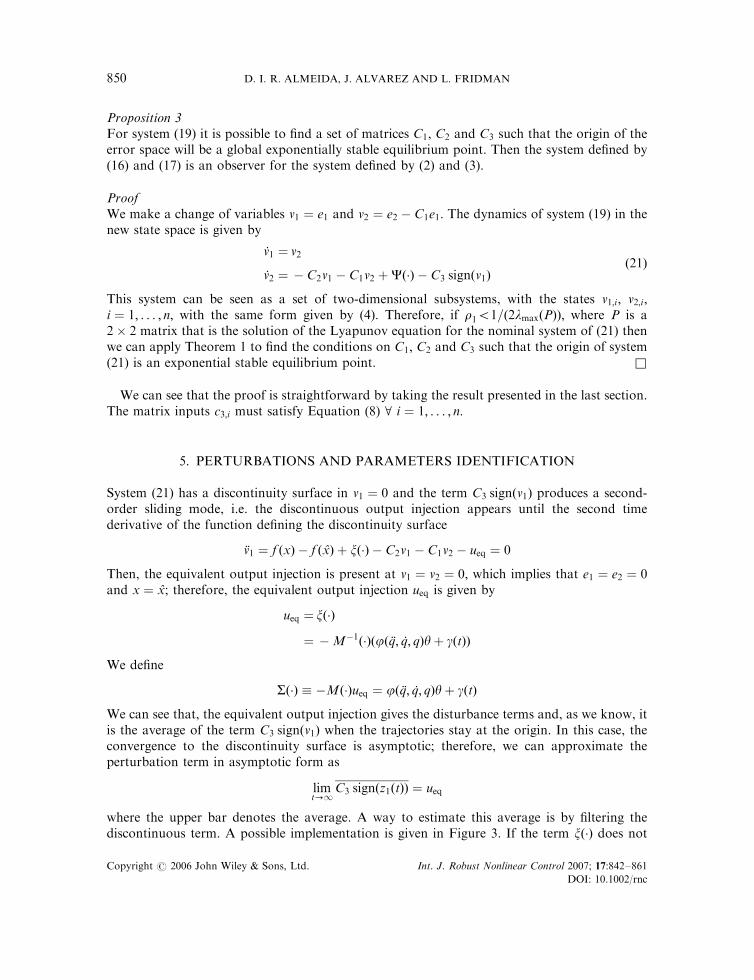
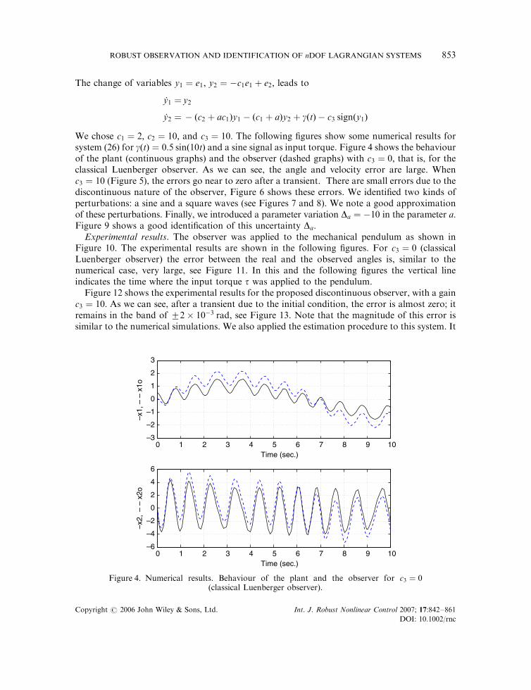
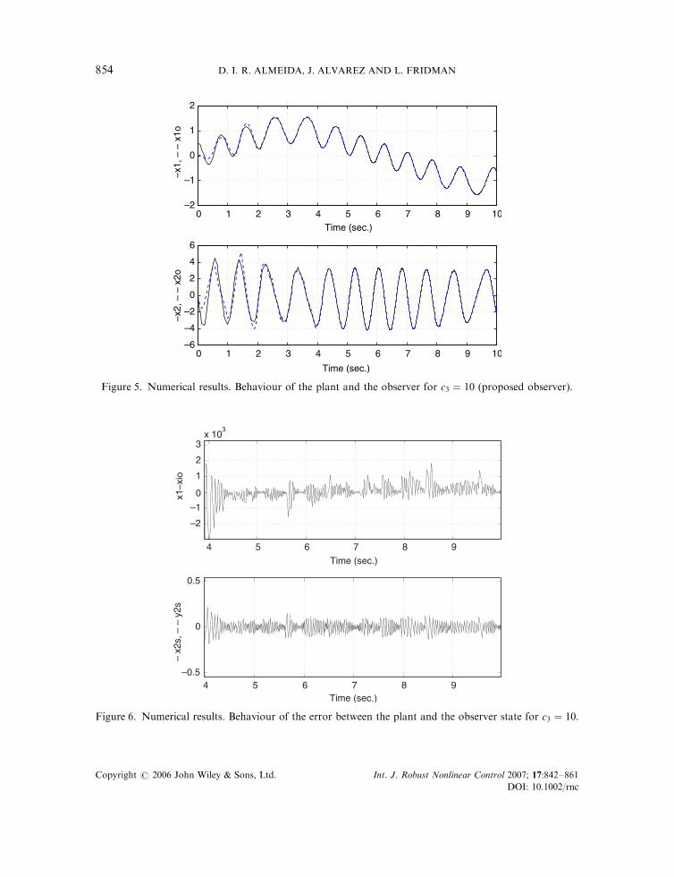
We chose c1 ¼ 2; c2 ¼ 10; and c3 ¼ 10: The following figures show some numerical results forsystem (26) for gðtÞ ¼ 0:5 sinð10tÞ and a sine signal as input torque. Figure 4 shows the behaviourof the plant (continuous graphs) and the observer (dashed graphs) with c3 ¼ 0; that is, for theclassical Luenberger observer. As we can see, the angle and velocity error are large. Whenc3 ¼ 10 (Figure 5), the errors go near to zero after a transient. There are small errors due to thediscontinuous nature of the observer, Figure 6 shows these errors. We identified two kinds ofperturbations: a sine and a square waves (see Figures 7 and 8). We note a good approximationof these perturbations. Finally, we introduced a parameter variation Da ¼ �10 in the parameter a:Figure 9 shows a good identification of this uncertainty Da:

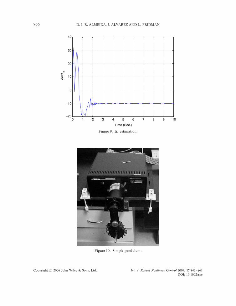
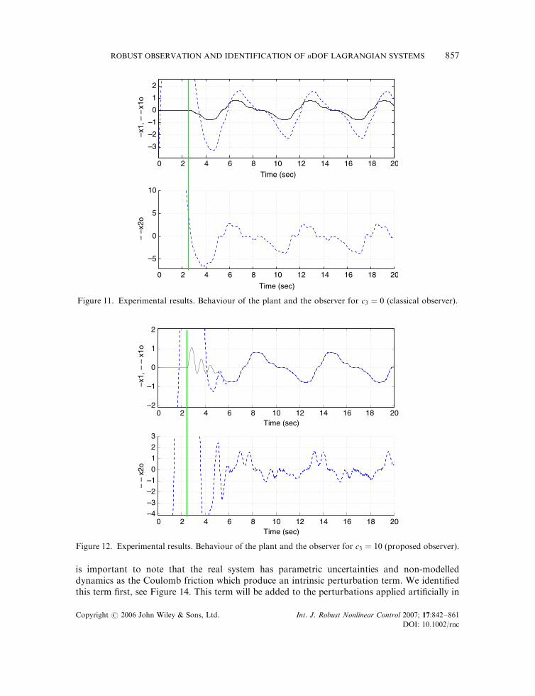
Experimental results. The observer was applied to the mechanical pendulum as shown inFigure 10. The experimental results are shown in the following figures. For c3 ¼ 0 (classicalLuenberger observer) the error between the real and the observed angles is, similar to thenumerical case, very large, see Figure 11. In this and the following figures the vertical lineindicates the time where the input torque t was applied to the pendulum.

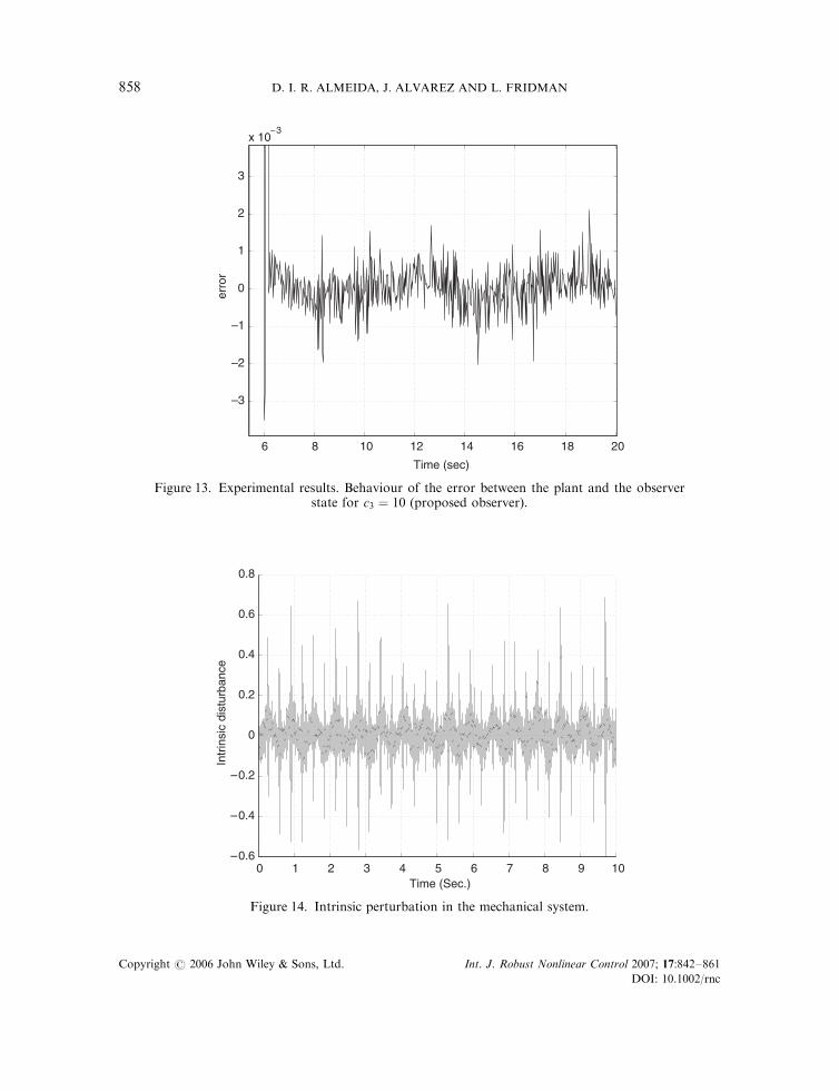
Figure 12 shows the experimental results for the proposed discontinuous observer, with a gainc3 ¼ 10: As we can see, after a transient due to the initial condition, the error is almost zero; itremains in the band of �2� 10�3 rad; see Figure 13. Note that the magnitude of this error issimilar to the numerical simulations. We also applied the estimation procedure to this system. It

0 1 2 3 4 5 6 7 8 9 10–3

–2

–1

0

1

2

3

Time (sec.)

–x1,

– –

x1o

0 1 2 3 4 5 6 7 8 9 10–6

–4

–2

0

2

4

6

Time (sec.)

–x2,

– –

x2o

Figure 4. Numerical results. Behaviour of the plant and the observer for c3 ¼ 0(classical Luenberger observer).



DOI: 10.1002/rnc

0 1 2 3 4 5 6 7 8 9 10–2

–1

0

1

2

Time (sec.)

0 1 2 3 4 5 6 7 8 9 10–6

–4

–2

0

2

4

6

Time (sec.)

–x1,

– –

x1o

–x

2, –

– x

2o

Figure 5. Numerical results. Behaviour of the plant and the observer for c3 ¼ 10 (proposed observer).

4 5 6 7 8 9

–2

–1

0

1

2

3x 10

Time (sec.)

x1–x

io

4 5 6 7 8 9–0.5

0

0.5

Time (sec.)

– x2

s, –

– y

2s

Figure 6. Numerical results. Behaviour of the error between the plant and the observer state for c3 ¼ 10:



DOI: 10.1002/rnc

3 3.5 4 4.5 5 5.5 6 6.5 7 7.5 8

–3

–2

–1

0

1

2

3

Per

, X1

Time (Sec.)

Figure 7. Sinusoidal perturbation signal and perturbation estimation.

3 4 5 6 7 8

–3

–2

–1

0

1

2

3

4

Per

, X1

Time (Sec.)

Figure 8. Square perturbation signal and perturbation estimation.



DOI: 10.1002/rnc

0 1 2 3 4 5 6 7 8 9 10–20

–10

0

10

20

30

40

Time (Sec.)

delta

a

Figure 9. Da estimation.

Figure 10. Simple pendulum.



DOI: 10.1002/rnc

is important to note that the real system has parametric uncertainties and non-modelleddynamics as the Coulomb friction which produce an intrinsic perturbation term. We identifiedthis term first, see Figure 14. This term will be added to the perturbations applied artificially in

0 2 4 6 8 10 12 14 16 18 20

–3

–2

–1

0

1

2

–x1,

– –

x1o

Time (sec)

0 2 4 6 8 10 12 14 16 18 20

–5

0

5

10

– –x

2o

Time (sec)

Figure 11. Experimental results. Behaviour of the plant and the observer for c3 ¼ 0 (classical observer).

0 2 4 6 8 10 12 14 16 18 20–2

–1

0

1

2

–x1,

– –

x1o

Time (sec)

0 2 4 6 8 10 12 14 16 18 20–4

–3

–2

–1

0

1

2

3

– –

x2o

Time (sec)

Figure 12. Experimental results. Behaviour of the plant and the observer for c3 ¼ 10 (proposed observer).



DOI: 10.1002/rnc

6 8 10 12 14 16 18 20

–3

–2

–1

0

1

2

3

x 10− 3

erro

r

Time (sec)

Figure 13. Experimental results. Behaviour of the error between the plant and the observerstate for c3 ¼ 10 (proposed observer).

0 1 2 3 4 5 6 7 8 9 10–0.6

–0.4

–0.2

0

0.2

0.4

0.6

0.8

Intr

insi

c di

stur

banc

e

Time (Sec.)

Figure 14. Intrinsic perturbation in the mechanical system.



DOI: 10.1002/rnc

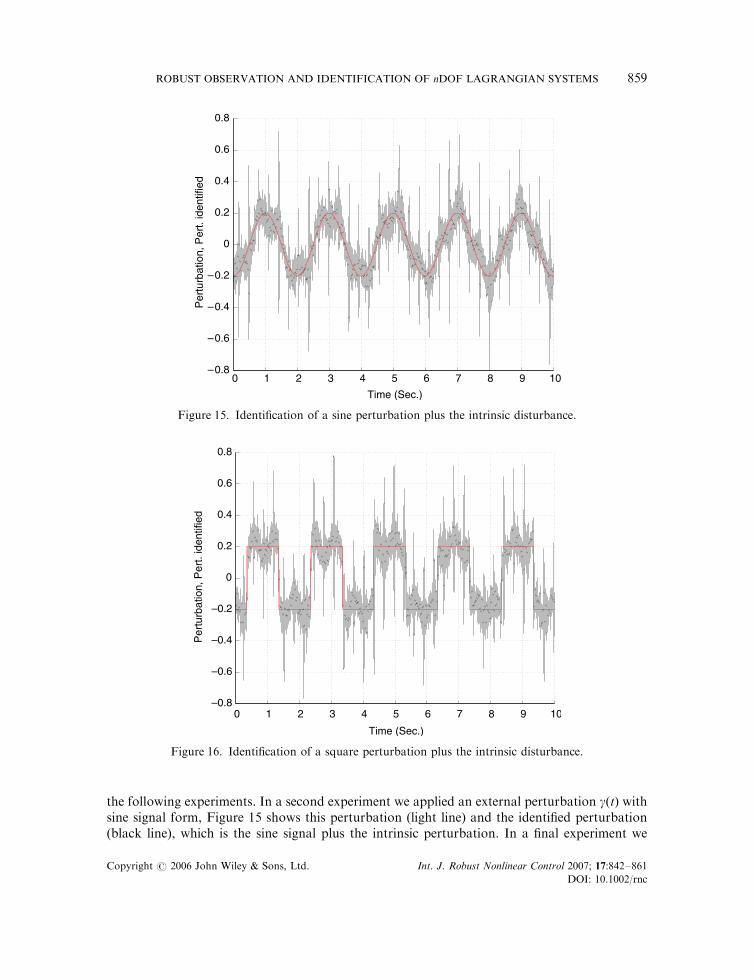
the following experiments. In a second experiment we applied an external perturbation gðtÞ withsine signal form, Figure 15 shows this perturbation (light line) and the identified perturbation(black line), which is the sine signal plus the intrinsic perturbation. In a final experiment we

0 1 2 3 4 5 6 7 8 9 10–0.8

–0.6

–0.4

–0.2

0

0.2

0.4

0.6

0.8

Per

turb

atio

n, P

ert.

iden

tifie

d

Time (Sec.)

Figure 15. Identification of a sine perturbation plus the intrinsic disturbance.

0 1 2 3 4 5 6 7 8 9 10–0.8

–0.6

–0.4

–0.2

0

0.2

0.4

0.6

0.8

Per

turb

atio

n, P

ert.

iden

tifie

d

Time (Sec.)

Figure 16. Identification of a square perturbation plus the intrinsic disturbance.



DOI: 10.1002/rnc

applied perturbation gðtÞ with a square signal form. Figure 16 shows the results, where we cansee that the identified perturbation is the square signal plus the intrinsic perturbation.

7. CONCLUSION

The main contribution of this work is the design of a globally asymptotically stable second-order sliding-mode observer for a class of Lagrangian systems. The observer displays goodcharacteristics of robustness to bounded parametric variation and external perturbations. Forthe case of plants with perturbations this observer has better performance than the observerproposed in [4] because we can guarantee convergence to zero error.

Due to its discontinuous nature, the observer state vector displays chattering; however, in theexperimental results chattering was not an important problem, as we can see in Figure 13, wherethe chattering has very small amplitude.

This observer ensures exponential rate of convergence to the state of the plant in spite of theexistence of non-vanishing bounded perturbations with bounded derivative. The performance ofthe observer has been tested experimentally and results match with the theory.

ACKNOWLEDGEMENTS

This research was supported in part by CONACyT grant 43807-Y, PROMEP, Autonomous University ofBaja California, POPIIT 11703, Mexico.

REFERENCES

1. Nijmeijer H, Fossen T. New Directions in Nonlinear Observer Design. Springer: Berlin, 1999.2. Hautus M. Strong detectability and observers. Linear Algebra and its Applications 1983; 50:353–368.3. Zasadzinki M, Daurouch M, Xu S. Full order observers for linear systems with unknown inputs. IEEE Transactions

on Automatic Control 1994; 39(3):606–609.4. Rapaport A, Gouze J. Practical observers for uncertain affine output injection systems. European Control Conference

(ECC99), 1999.5. Edwards C, Spurgeon S. Sliding Mode Control. Taylor & Francis: London, 1998.6. Utkin VI, Guldner J, Shi J. Sliding Mode Control in Electromechanical Systems. Taylor & Francis: London, 1999.7. Barbot J, Djemai M, Boukhobza T. Sliding mode observers. In Sliding Mode Control in Engineering, Perruquetti W,

Barbot JP (eds). Chapter 4. Marcel Bekker Inc: New York, 2002.8. Edwards C, Spurgeon S, Hebden RG. On development and applications of sliding mode observers. In Variable

Structure Systems: Towards XXIst Century, Xu J, Xu Y (eds). Lecture Notes in Control and Information Science.Springer: Germany, 2002.

9. Poznyak A. Stochastic output noise effects in sliding mode estimations. International Journal of Control 2003;76:986–999.

10. Hashimoto H, Utkin V, Suzuki JH, Harashima F. VSS observer for linear time varying system. Proceedings ofIECON’90, Pacific Grove, CA, 1990; 34–39.

11. Barbot J, Floquet T. A sliding mode approach of unknown input observers for linear systems. 43th IEEE Conferenceon Decision and Control, 2004; 1724–1729.

12. Levant A. Sliding order and sliding accuracy in sliding mode control. International Journal of Control 1993; 58:1247–1263.

13. Levant A. Robust exact differentiation via sliding mode technique. Automatica 1998; 34(3):379–384.14. Davila J, Fridman L. Second order sliding mode observer for mechanical systems. IEEE Transactions on Automatic

Control 2005; 50(11):1785–1789.15. Fridman L, Levant A, Davila J. High-order sliding-mode observer for linear systems with unknown inputs. Nineth

IEEE Workshop on Variable Structure Systems VSS-06, Alghero, Italy, 2006; 202–207.



DOI: 10.1002/rnc

16. Bejarano F, Fridman L, Poznyak A. Output integral sliding mode with application to the LQ-optimal control.Nineth IEEE Workshop on Variable Structure Systems}VSS’06, Alghero, Italy, 2006; 68–73.

17. Floquet T, Barbot J. A canonical form for design of unknown input observers. In: Advances in Variable Structureand Sliding Mode Control, Edwards C, Fossas Colet E, Fridman L (eds). Lecture Notes in Control and InformationSciences, vol. 334. Springer: Berlin, 2006; 195–226.

18. Pisano A, Usai E. Output-feedback control of an underwater vehicle prototype by higher-order sliding modes.Automatica 2004; 40:1525–1531.

19. Shtessel Y, Shkolnikov I, Brown M. An asymptotic second-order smooth sliding mode control. Asian Journal ofControl 2003; 5(4):498–504.

20. Basin M, Ferreira A, Fridman L. LQG-robust sliding mode control for linear stochastic systems with uncertainties.Nineth International Workshop on Variable Structure Systems}VSS’06, Alghero, Italy, 2006; 74–79.

21. Poznyak A, Chairez I, Poznyak T. Sliding mode neurocontrol with applications. Nineth IEEE Workshop on VariableStructure Systems VSS-06, Alghero, Italy, 2006; 5–10.

22. Utkin VI. Sliding Modes in Control and Optimization. Springer: Berlin, 1992.23. Khalil HK. Nonlinear Systems. Prentice-Hall: Englewood Cliffs, NJ, 2002.24. Anosov DV. On stability of equilibrium points of relay systems. Automation and Remote Control 1959; 20(2):

135–149.25. Fridman L. Sliding mode control for systems with fast actuators: singularly perturbed approach. In Variable

Structure Systems: Towards the 21st Century, Yu X, Xu J-X (eds). Lecture Notes in Control and InformationScience. Springer: Germany, 2002.

26. Ljung L, Soderstrom T. Theory and Practice of Recursive Identification. MIT Press: Cambridge, MA, 1983.



DOI: 10.1002/rnc

Robust observation and identification ofnDOF Lagrangian systems

Documents

Transcript of Robust observation and identification ofnDOF Lagrangian systems