Parallelisation of the Lagrangian atmospheric dispersion model NAME

This article appeared in a journal published by Elsevier. The attachedcopy is furnished to the author for internal non-commercial researchand education use, including for instruction at the authors institution

and sharing with colleagues.

Other uses, including reproduction and distribution, or selling orlicensing copies, or posting to personal, institutional or third party

websites are prohibited.

In most cases authors are permitted to post their version of thearticle (e.g. in Word or Tex form) to their personal website orinstitutional repository. Authors requiring further information

regarding Elsevier’s archiving and manuscript policies areencouraged to visit:

http://www.elsevier.com/authorsrights

http://www.elsevier.com/authorsrights

Author's personal copy

Computer Physics Communications 184 (2013) 2734–2745

Contents lists available at ScienceDirect

Computer Physics Communications

journal homepage: www.elsevier.com/locate/cpc

Parallelisation of the Lagrangian atmospheric dispersion model NAMEEike H. Müller a,∗, Rupert Ford b,1, Matthew C. Hort a, Lois Huggett a, Graham Riley b,David J. Thomson a

a Met Office, Fitzroy Road, Exeter EX1 3PB, United Kingdomb School of Computer Science, University of Manchester, Oxford Road, Manchester M13 9PL, United Kingdom

a r t i c l e i n f o

Article history:Received 27 November 2012Received in revised form15 June 2013Accepted 24 June 2013Available online 29 July 2013

Keywords:Atmospheric modellingLagrangian dispersion modelParallel computingOpenMP

a b s t r a c t

TheNAME Atmospheric DispersionModel is a Lagrangian particlemodel used by theMet Office to predictthe propagation and spread of pollutants in the atmosphere. The model is routinely used in emergencyresponse applications, where it is important to obtain results as quickly as possible. This requirement for ashort runtime and the increase in core number of commonly available CPUs, such as the Intel Xeon series,has motivated the parallelisation of NAME in the OpenMP shared memory framework. In this work wedescribe the implementation of this parallelisation strategy in NAME and discuss the performance of themodel for different setups. Due to the independence of themodel particles, the parallelisation of themaincompute intensive loops is relatively straightforward. The random number generator for modelling sub-grid scale turbulent motion needs to be adapted to ensure that different particles use independent sets ofrandom numbers. We find that on Intel Xeon X5680 CPUs the model shows very good strong scaling upto 12 cores in a realistic emergency response application for predicting the dispersion of volcanic ash inthe North Atlantic airspace. We implemented a mechanism for asynchronous reading of meteorologicaldata from disk and demonstrate how this can reduce the runtime if disk access plays a significant role ina model run. To explore the performance on different chip architectures we also ported the part of thecode which is used for calculating the gamma dose from a cloud of radioactive particles to a graphicsprocessing unit (GPU) using CUDA-C. We were able to demonstrate a significant speedup of around oneorder of magnitude relative to the serial CPU version.

Crown Copyright© 2013 Published by Elsevier B.V. All rights reserved.

1. Introduction

1.1. The NAME model

The UK Met Office’s Numerical Atmospheric-dispersion Mod-elling Environment (NAME) is a Lagrangian particle model [1]which is used to predict the transport and dispersion of pollutantsin the atmosphere [2,3]. It was originally designed to provide ad-vice on the spread of airborne radioactive material released in nu-clear accidents, such as the Chernobyl disaster [4,5]. Since then themodel has undergone extensive development and NAME is nowused in a wide range of applications. These include research intoair quality [6,7], support to regulatory bodies in emission moni-toring [8], emergency response applications [9], and the spread ofvectors for bluetongue and foot andmouth disease [10–12]. As part

∗ Correspondence to: Department of Mathematical Sciences, University of Bath,Claverton Down, BA2 7AY, United Kingdom. Tel.: +44 7957463462.

E-mail addresses: [email protected], [email protected](E.H. Müller).1 Present address: Science and Technology Facilities Council, Daresbury Labora-

tory, Warrington, Cheshire, WA4 4AD, United Kingdom.

of the emergency responseworkNAME is used to provide forecastsfor the London volcanic ash advisory centre (VAAC). Recently themodel provided predictions for the spread of volcanic ash in theEuropean and North Atlantic airspace following the eruption of theIcelandic volcano Eyjafjallajökull [13–16] and the May 2011 erup-tion of Grimsvotn. NAME is available under license and requestsfor obtaining the source code should be directed to the Met Officeby emailing [email protected].

Lagrangian particle models track individual model particles,which each represent a certain amount of pollutant, through theatmosphere. The mean velocity of the particle is given by the flowfield U evaluated at the particle position, which can for examplebe output from a numerical weather prediction project such as theMet Office Unified Model (UM) [17]. Turbulence below the gridscale is modelled by adding a random increment du(turb) to theparticle velocity vector at each timestep [18,19]; particle positionand velocity are updated according to the Langevin equation [20],which for homogeneous turbulence is given by

dxi = (Ui + u(turb)i )dt

du(turb)i = −

u(turb)i

τidt +

2σ 2

i

τidξi(t). (1)

0010-4655/$ – see front matter Crown Copyright© 2013 Published by Elsevier B.V. All rights reserved.http://dx.doi.org/10.1016/j.cpc.2013.06.022


E.H. Müller et al. / Computer Physics Communications 184 (2013) 2734–2745 2735

The dξi are Gaussian random variables with mean zero and vari-ance dt which are independent from time step to time step andfrom component to component (so that the dξi can be regarded asincrements of independentWiener processes). For inhomogeneousturbulence where τi and σ 2

i are time dependent functions of posi-tion and depend on the meteorological conditions [21], this equa-tion has to be modified as described in [1,19]. The modificationsusually assume the fixed point velocity distributions are Gaussian,but non-Gaussian options are also implemented in NAME [22]. In-stead of updating both velocity and position of the particle using(1), a simplified integration scheme can be used in which only theposition is updated according to aWiener process without velocitymemory as described by

dxi = Ui dt +

2 Keff dξi(t). (2)

This assumes that the parameters do not depend on position, orvary slowly in the horizontal direction (but different values areused in the atmospheric boundary layer and the free troposphere).

Compared to Eulerian models, which solve the diffusion equa-tion on a fixed three dimensional grid, Lagrangianmodels allow forthe resolution of steep gradients near the source and, as they do notcontain an internal grid scale, can easily be used on a wide rangeof spatial scales. Also, when used with velocity memory as in (1),they allow more sophisticated turbulence parameterisations thanare possible in Eulerian models. The independence of particles inmost applications allows an obvious approach to parallelisation,which, in contrast to Eulerian models, does not require any inter-processor communication during the propagation step.

In addition to the core routine which simulates the propaga-tion of particles,NAMEmodels other physical processes such as forexample wet- and dry-deposition, deep convective mixing, gravi-tational settling and buoyant plume rise [22]. Although the par-ticles do not interact as they propagate through the atmosphere,the model contains a chemistry scheme, which can be used to de-scribe chemical reactions between the various species carried bythe model particles and/or held as background fields on an Eule-rian grid. For a plume of radioactive particles decay chains and halflife decays can also be calculated.

Usually the model output is a set of concentration fields, whichcan represent instantaneous snapshots and temporal and spatialaverages or integrals that are written to disk. Due to the stochasticnature of themodel, the relative error in these fields decreases pro-portional to the inverse square root of the particle number. Flowinformation (i.e. meteorological data, in the following abbreviatedas ‘‘met data’’) is read fromdisk at regular time intervals, andmulti-linearly interpolated in time and space for each Lagrangian particleand model time step.

NAME is a mature and complex model and consists of around110,000 lines of Fortran 90 source code; it should be kept in mindthat the main focus in the original design of the code was modu-larity and maintainability.

1.2. Parallelisation

For quick decision making, emergency response applicationsrequire NAME to provide reliable results as quickly as possible.This need for a reduction of themodel runtime (or the suppressionof statistical noise by an increase in the number of particles ata constant runtime) motivated the parallelisation of the modelwhich is described in this article. Research applications, whichtypically run for days to months and/or require 100 s of separatesimulations, will also benefit from this effort, although in thiscase it is sometimes more effective to simply run different jobssimultaneously on separate CPUs.

As the particles do not interact while they are propagated ac-cording to Eq. (1), parallelisation of certain parts of the model isstraightforward. Each compute unit propagates a set of indepen-dent model particles. Synchronisation is only necessary at times

when met data is read from disk or output fields are written. Asdiscussed in Section 2, several subtleties have to be taken into ac-count to ensure that met data is read from disk efficiently and toguarantee that the correctness of the parallel code can be verified.

Chemistry calculations are often carried out at larger timestepsthan the intrinsic integration timestep, however, they require par-ticles to ‘communicate’ in order to compute the chemical reactions.The information carried by the particles is converted to an Eule-rian grid, the chemistry calculations are carried out on this grid andthen the results are put back on the particles. The Eulerian grid cal-culation can be parallelised by dividing the grid between differentcompute units.

Before particles can be propagated through the atmospherethey have to wait for the flow information for the next met datatime to be read from disk. This can be avoided by reading the metdata asynchronously, i.e. by assigning one compute unit to readingflow information for met data time t + 2 while the other computeunits propagate particles through the flow field which is interpo-lated in the time interval [t, t +1]. We have implemented all threestrategies withinNAME, and also parallelised some less important,but easily parallelisable, loops in the output calculation.

Although in principle this general strategy could be imple-mented in other schemes, such as MPI [23], we decided to use theshared memory model OpenMP [24] for the following reasons:

• Commonly available CPUs, such as the Intel Xeon series, containmore thanone core so that existing hardware canbeused (at theMet Office Intel Xeon processors with four to twelve physicalcores per machine are used to run NAME both for operationalemergency response and research applications).

• OpenMP is easily implemented by adding compiler directives tothe existing source code.

• As OpenMP directives are ignored in serial builds, the paralleland serial source code are identical, which improves maintain-ability and simplifies verification of results. This is particularlyimportant as NAME is used for operational forecasts at the MetOffice for which reliability and correctness of the results has tobe guaranteed.

On commonly available CPUs, such as the Intel Xeon series, thenumber of cores is in the order of tens, and this limits the achiev-able speedup if only OpenMP is used for parallelisation. In contrastto a distributed memory approach, communication is not explicitbut is realised through shared memory access. This makes mem-ory and cache access of an individual core less transparent and canlimit the scalability.

In this article we demonstrate that this relatively straightfor-ward approach leads to a significant speedup and scales well up toaround 10 cores for our typical applications. We have found thatsome loops scale better than others and that scaling is dependenton the hardware that is used.

Previous work on parallelising Lagrangian atmospheric disper-sion models has been reported in [25] where the shared anddistributed memory parallelisation of the Lagrangian OperationalDispersion Integrator (LODI) [26] is described. In the distributedmemory version of the model each processor has a complete copyof the meteorological data and output fields are calculated sep-arately by each processing unit. Parallel communication is re-quired to calculate global output fields. The MPI implementationshows a nearly linear speedup as long as the problem size is largeenough so that the overhead from communication is negligible;for 50,000 model particles strong scaling is good on up to 50–100processors and improves for larger particle numbers. In additiona shared memory approach was used to parallelise the main timestep loop with OpenMP. As in the NAME model this loop containsthe particle advection and physical processes such as gravitationalsettling and deposition processes. In the LODI model this loop typ-ically amounts to ∼85% of the total runtime. Using only the shared


2736 E.H. Müller et al. / Computer Physics Communications 184 (2013) 2734–2745

memory parallelisation the authors find a speedup of 1.44 for abenchmark run with fifty thousand particles on one four core CPUof the ASCI Bluemachine at LLNL. The distributed and sharedmem-ory parallelisation can be used combined by using OpenMP oneach node andMPI communication between the nodes. On 5 nodes(20 cores in total) they report a speedup of 7.3 for this hybridOpenMP/MPI approach.

Some earlier work is described in [27] where a Lagrangianmodel for the one dimensional dispersion in the boundary layeris parallelised on a Distributed Array of Processors (DAP) machine.The DAP consists of 4096 single-bit processing elements which re-ceive a common instruction stream from a central Master ControlUnit and execute code in a SIMD fashion. Relative to the sequen-tial code on an IBM 3084 mainframe computer a 14-fold speedupcould be achieved on a DAP 610machine and the authors estimatethat this could be increased by another factor of five on a DAP 610Cwhich has more powerful compute elements that can process in-structions on the byte level.

1.3. Overview

This article is organised as follows. In Section 2 we describe thestructure and the parallelisation strategy of the NAME model andshow how it can be implemented in OpenMP both for the compu-tationally most expensive loops and for the asynchronous readingof met data. We then investigate performance improvements andin particular the scalability of the model in Section 3 where we fo-cus on results from a realistic emergency response application forthe spread of volcanic ash over the North Atlantic. The parallelisa-tion of the cloud gamma calculation on a graphics processing unit(GPU) is described in Section 4. Our conclusions are presented inSection 5 where we also outline ideas for further performance im-provements and parallelisation.

Some more technical aspects and further results can be foundin the appendices: the parallel random number generator used inNAME is described in Appendix A. The correctness of results is veri-fied in Appendix B and further strong andweak scaling tests are re-ported in Appendix C. Whereas at the Met Office the NAMEmodelis mainly run on Intel Xeon chips, we also show results for thescaling of the code on other systems, most importantly on a 32core Power 6 node of the Met Office IBM supercomputer, in Ap-pendix D. Thread binding and hyperthreading on Intel processorsis discussed in Appendix E.

2. Model structure and parallelisation strategy

The NAME model contains two main timesteps. The intrinsictimestep dt is used to integrate the Langevin Eq. (1). At regularsync time intervals (typically 5 min, 10 min or 15 min) the parti-cles are synchronised to write output to disk, perform chemistrycalculations and release new particles. If the ‘‘cheap’’ integrationscheme in (2) is used, only one internal time step is performed ineach sync time interval. (Often the full scheme is only used near thesource, i.e. for the first 30 min of travel time of each particle.) Metdata is usually only available at even larger time intervals, for runswith global UM data, this can be every three or six hours.2 Flowinformation is only available at the model grid points (these aretens of kilometres apart in the global UM, whereas the resolutionis 1.5 km for the UKV model over the UK, which is a limited areaconfiguration of the UM). The position of Lagrangian model parti-cles is not restricted to grid points and therefore flow information

2 Output from higher-resolution limited area versions of the UM can be morefrequent and is typically available every hour.

Fig. 1. Simplified NAME model structure. Met data is typically generated by theMet Office Unified Model, but other sources can be used as well.

has to be multilinearly interpolated in space. Interpolation in timeis also necessary as the NAME timestep is smaller than the timeinterval of the met data from the UM.

The main loop in the model consists of the following steps(Fig. 1):

1. Check if flow information is available to propagate the particlesover the next synctime step, read met data from disk ifnecessary and update flow fields.

2. Release new particles from the source, if necessary.3. Loop over particles: Propagate particles to next synctime.4. Perform chemistry calculation for chemically active species

(loop over grid boxes).5. Loop over particles: Calculate contribution of particles to output

at synctime.6. Process output and write to disk.7. Continue with step 1., or exit main loop at end of run.

Note that in runs with chemically inert particles the chemistrycalculation is disabled. Also, additional physical processes such asdecay chains of radioactive particles can be simulated in themodel.The cloud gamma calculation discussed in Section 4 is part of theoutput loop.

The parallelisation of the different loops (highlighted in boldabove) is described in the following sections.

The model contains an additional outer loop over different‘‘cases’’ (not shown in Fig. 1), which could be runs based on an en-semble of met data. Results from these cases can be combined sta-tistically at the end of the run to obtain information on the derivedprobability densities, e.g. to calculate percentiles and exceedanceprobabilities. In the following we will not consider this loop, asmost operational runs are based on one case only.

2.1. Particle loops

Typically most of the computational work is done in the follow-ing two loops over model particles:

2.1.1. Main particle loopThe main loop for propagating model particles through the at-

mosphere is contained in one subroutinewhich integrates the par-ticle velocity and position according to (1) or (2) and is often thecomputationally most expensive part of a model run, as demon-strated for an operational emergency response run in Section 3.1.To parallelise this loop, calls to the subroutine are surrounded byan OpenMP parallel region and the loop is parallelised by addingOpenMP directives.

NAME can be set up so that met data is only read from disk ‘‘ondemand’’, i.e. only if the corresponding flow information is needed



for particle propagation. Often this reduces the amount of data thatis read from disk, especially if the plume is very localised. Themostimportant example of this is the use of global met data, whichcan be split up into fourteen smaller regions each covering a smallpart of the globe. Data for one of these regions is only loaded if itcontains model particles. This implies that data can also be loadedfrom inside the particle loop, as soon as a particle enters one ofthese regions. If themodel is run in parallel it is necessary to protectany met updates inside the particle loop to prevent two particleswhich are processed by different threads from loading the samesegment of the globe when they enter it. This was implementedwith OpenMP locks (one for each region of the globe) which can beset and unset through API calls, and ensures that only one threadcan access the critical subroutine at a given time. This approachcan also be used if nested met data is used. If data is available atdifferent resolutions, NAME will only use the most accurate flowfield and again it has to be ensured that this flow information isonly read from disk once.

2.1.2. Particle output loopOutput is calculated at ‘sync’ times in a separate loop over par-

ticles, which in the following is referred to as the ‘‘particle outputloop’’. In this loop concentrations are calculated from the parti-cles and in addition individual particle trajectories can also beoutputted. Again, parallelisation of this loop inOpenMP is straight-forward. Internally particles are stored in an array structure. In thebody of this loop, particles, which are no longer needed in the sim-ulation (for example, because they have left the domain of inter-est or their mass has been depleted by deposition to the ground orradioactive decay), are marked as inactive and removed from thearray of model particles and their slot becomes available for newlyreleasedparticles. Turbulence ismodelled by a randomprocess andwewill see below that this has implications for the implementationof the randomnumber generator and the reproducibility of results.

2.1.3. Parallel random number generatorThe turbulent component of the velocity is calculated using

(pseudo-) random numbers which can be initialised with a fixedseed. Using the Fortran intrinsic random number generator ispotentially dangerous because the sequence of random numbersused by different particles might overlap, or, depending on theimplementation of the random number generator, several threadsmight update the seed simultaneously. The period of the intrinsicgenerator might also be too short. All this could mean that thestatistics of the final results are compromised. To overcome thisproblem, we implemented a portable random number generatorfollowing [28–30]with a very long period (>1018)which generatesa separate set of random numbers for each particle index andwhich uses separate subsequences of this long sequence for eachparticle index. The seeds of the generator at each position in theparticle array are spaced so that the randomsequences for differentparticle indices do not overlap; details of the algorithm can befound in Appendix A.

Keeping in mind that particles are removed from the run in theparallelised particle output loop, this implies a difficulty in obtain-ing reproducible results and hence in verifying the results of a par-allel run by comparing it to an equivalent serial run. If the modelis run in parallel, the order in which particles are marked as inac-tive and in which new particles are assigned to the free positionsin the particle array depends on the order in which the differentthreads process their particles: if a new particle is created with adifferent index it will use a different sequence of random numbers.Consequently the difference between a serial and a parallel run(and potentially between two parallel runs) can grow, after muchparticle recycling, to be of the order of the statistical noise. To stillallow comparison of parallel and serial runs for testing, a repro-ducibility flag was introduced. If this flag is set, the particles are

removed in a separate loopwithin anOpenMP single region so thatthe list of particle indices available for reuse has a reproducible or-der. Otherwise, they are removed in the particle output loop insidean OpenMP critical region. To obtain the timing results presentedin this paper we will always assume that the reproducibility flaghas not been set; further results on verification can be found in Ap-pendix B.

Using our implementation instead of the Fortran intrinsic ran-dom number generator is important for another reason: it wasfound that, when the code was compiled with the IBM xlf com-piler and the intrinsic random number generator was used, onlyone thread at a time can pick a new random number. While thisavoids the problem of overlapping sequences of random numbers,it effectively serialises this part of the code and leads to a huge in-crease in runtime. In fact we found that it causes the code to antis-cale. OnAMDOpteron processors a twofold increase in the runtimewas observed if the internal random number generator is used.

2.2. Chemistry loop

The model particles in a NAME run can carry a number ofdifferent chemical species. This is the case in air quality runs,which model the concentrations of different chemicals affectinghuman health, such as ozone, nitric oxides, sulphates, organiccompounds and other chemicals [6,7,31]. Over the length of a run,these species react and transform into each other. For chemistrycalculations the species carried by the particles are first convertedto concentrations on a three dimensional Eulerian grid. In eachgridbox the concentrations at the next timestep are then calculatedaccording to the chemical reaction rates determined by theseconcentrations. The resulting concentrations are mapped back tothe particles by assigning a relative proportion to each particle. Thecalculations in each gridbox are independent and we parallelisedthe outermost loop over the three dimensional grid. An exampleof a NAME run dominated by the chemistry loop is discussed inSection 3.2.

2.3. Asynchronous reading of met data

In some cases reading NWP met data from disk can make up asignificant proportion of the runtime. This process has been par-allelised by creating a separate IO thread which prefetches metdata for the next met data time while the worker threads prop-agate the particles using already available flow information. Theimplementation of this strategy requires nested OpenMP paralleli-sation. The IO thread is created in an outer OpenMP parallel re-gion and loops over the different met modules3 and updates theflow information by reading new data from disk if one of the mod-ules has beenmarked for prefetching by the worker threads. Threebuffers are used for storing met data: data for the previous andnext timestep is stored in the old and new buffers (at the beginningof the run these buffers are read from file by the worker threads).Both buffers are needed for the interpolation of flow fields betweenthese two times. Data for the following timestep is loaded into aprefetch buffer by the IO thread. Once this prefetched data is avail-able and the worker thread is ready to propagate the particles overthe next time interval, the buffer indices are swapped around ac-cording to prefetch → new, new → old, old → prefetch and a newprefetch request is launched (note that it is not necessary to copydata between the buffers as they are only relabelled). The processis illustrated in Fig. 2.

Updating the flow fields consists of two steps: met data is readfrom disk and subsequently processed in a separate subroutine. To

3 NAME can use different types of met data in a single run, for example nestedglobal, European and UK wide data.



Fig. 2. Asynchronous reading of met data. The worker threads propagate particlesover the time interval [t, t + 1] while the IO thread reads met data for t + 2 fromdisk. Before the next iteration the met data buffer indices are swapped accordingto prefetch → new, new → old, old → prefetch. The worker threads then propagateparticles in the time interval [t + 1, t + 2] while the IO thread reads met data fort + 3 and so on.

allow more fine tuned load balancing between the IO and workerthreads, both steps or only the first can be executed by the IOthread.

Synchronisation between the IO and worker threads is realisedwith OpenMP locks. In Section 3.3 we demonstrate how the asyn-chronous reading of met data can reduce the total runtime byaround 30%. It should also be noted that currently this approachcannot be combined with loading of met data ‘‘on demand’’ as dis-cussed in Section 2.1.1 as this would require knowledge of the par-ticle positions at prefetch time.

3. Results

We verified that the changes resulting from parallelisation ofthe code have no impact on the final output. As discussed in detailin Appendix B, results typically differ from those in a serial runin the least significant digit and are much smaller than statisticalfluctuations if the reproducibility flag is set. Comparing a serial runto a parallel run with one thread shows that the overhead fromparallelisation is around 5% (see Appendix C for details).

In the followingwe present results for the absolute runtime andscaling of the parallelised NAME code for a set of realistic applica-tions, in particular for an operational emergency response run forthe forecast of volcanic ash over the North Atlantic. We also con-sider a run dominated by the chemistry calculation and a differentshort range emergency response run which requires the readingof large data volumes from hard disk. These runs demonstrate thespeedup gained by parallelising different parts of the code, as de-scribed in the previous section. Results for an idealised test caseare reported in Appendix C where both weak and strong scalingare studied in more detail.

All results presented in this section are obtained with the IntelLinux Fortran compiler and on Intel Xeon CPUs. The performanceand scalability of the code on other hardware, in particular on anode of theMet Office IBM supercomputer is shown in Appendix D.

3.1. Scaling of an operational emergency response run

In the following we consider a realistic emergency responserun for a volcanic eruption. Runs in this configuration, but with areduced particle release rate, were used to predict the spread of theash cloud during the 2010 eruption of the Eyjafjallajökull volcanoin Iceland.

The runs were carried out on a Dell server with two Intel XeonX5680 six-core processors with a 3.33 GHz clock rate, 49.4 GB of

Table 1Timing results for an emergency response run for predicting the spread of volcanicash over the North Atlantic. All times are measured in minutes; the code was runon an Intel Xeon X5680 processor with 2× 6 cores. The results for the 1 thread runare linearly extrapolated from those of a run with a smaller number of particles.

Number of threads 1 4 6 8 11 16 24

Particle loop 853.98 220.08 148.38 114.76 89.45 86.23 68.46Particle output loop – 8.72 8.72 8.72 8.75 9.37 9.6Output – 15.68 15.67 15.9 15.81 14.97 14.92MetRead – 5.75 5.62 5.62 5.69 6.85 5.28Total – 248.06 176.36 142.98 117.63 114.38 96.41

Table 2Timing results for an emergency response run for predicting the spread of volcanicash over theNorth Atlanticwith reduced number of particles (half asmany particlesas in Table 1). All times are measured in minutes; the code was run on an IntelXeon X5680 processor with 2×6 cores. The results for the 1 thread run are linearlyextrapolated from those of a run with a smaller number of particles.

Number of threads 1 4 6 8 11

Particle loop 426.99 113.87 75.73 58.52 44.83Particle output loop – 4.36 4.36 4.36 4.37Output – 15.79 15.77 15.86 15.8MetRead – 5.59 4.82 4.64 5.28Total – 137.47 99.1 81.96 68.46

main memory and an L2 (L3) cache of 256 kB (12 MB). To inves-tigate the dependence on the number of particles we carried outruns with two different particle release rates, as described below.Table 1 gives a detailed breakdown of the time spent in differ-ent sections of the code for the first choice of release rate. TheIntel Xeon X5680 processor supports hyperthreading (see alsoAppendix E) andwe include results for runswith 16 and 24 threadsin the results.

In some preliminary runs (not shown here) with this version ofthe model we found that the particle output loop antiscales. Thisloop only accounts for aminute fraction of the runtime andbecauseof this antiscalingwedecided to assign only one thread for process-ing the particle output loop. This turned out to be a technical prob-lemwhich was later fixed. We find that the main particle loop (seeSection 2.1.1) indeed accounts for most of the runtime, the over-head from reading met data from disk and outputting NAME datais small.

A fit of the total run time in Table 1 to Amdahl’s law

T (n; T0, r) = T01 − r +

rn

(3)

gives:

T0 = 865 min, r = 95%, (1 − r)T0 = 41 min. (4)

Here n denotes the number of cores, T0 is the total runtime of a 1-thread run and r the parallel fraction of the code. (1 − r)T0 is thesequential part of the runtime.We repeated the same analysiswitha release rate that was reduced by a factor of two. The results areshown in Table 2 and plotted in Fig. 3 (filled circles) together withthe data from Table 1 (empty circles). Here we find the followingfit results:

T0 = 463 min, r = 94%, (1 − r)T0 = 28 min. (5)

From this we conclude that, as expected, the runtime is approx-imately proportional to the number of particles. The original op-erational runs were carried out in 2010 with an older version ofthe model which did not include some serial improvements whichare contained in the version used to obtain the results above. Dur-ing the 2010 eruption of Eyjafjallajökull the serial version of themodel was run on an Intel Xeon X5560 processor with a clock rateof 2.80 GHz and the release rate was a factor 10 smaller than inTable 2, these runs typically took 1 h and 30 min to complete.



Fig. 3. Total runtime and time spent in the particle loop for two different releaserates in an emergency response run for predicting the spread of volcanic ash overtheNorthAtlantic. The resultswere obtained on an Intel XeonX5680processorwitha clock rate of 3.33 GHz. Only the results for 4, 6, 8 and 11 threads were used forthe linear fit. The total runtime for a run with the larger release rate but on an IntelXeon X7542 processor with a clock rate of 2.67 GHz are also shown (open squares).We also show the runtime of the original run (using an older serial version of themodel) during the 2010 eruption of Eyjafjallajökull with a reduced release rate. Theserial run was carried out on an Intel Xeon X5560 processor with a clock rate of2.80 GHz.

Taking all these improvements into account, we conclude thatwe are now able to repeat these runs with a tenfold increase inparticle number (and the resulting reduction in statistical noise) inthe same length of time as before, if the model is run on 8 cores ofan Intel Xeon X5680 processor.

We repeated the above runs on a system with four IntelXeon X7542 six core processors (2.67 GHz, 64 GB main memory,256 kB/18 MB L2/L3 cache) in the hope of demonstrating scalingbeyond 12 threads. As can be seen from Fig. 3, the performance ofNAME on this processor is not as good as on the X5680 system.While part of the difference can be explained by the ratio of clockspeeds (3.33 GHz versus 2.67 GHz), the X7542 does not show thesame scaling as the X5680 even up to 12 threads.

3.2. Air quality runs

NAME can be used operationally to provide air quality forecasts.Although these runs typically use a large number of particles, asignificant amount of time is spent in the parallelised chemistryroutine.

In the followingwe showresults for an air quality runon an IntelXeon X5680 processor. In the operational setup this run consists oftwo parts. A coarse run on a grid that covers central Europe is usedto initialise the boundary conditions of a fine grid runwith a higherspatial resolution which covers the United Kingdom. When run onone thread, 42% of the time of the coarse grid run is spent in thechemistry loop, followed by the particle output loop (39%) and theparticle loop (14%). The runtime of the fine grid run is dominatedby the chemistry loop (62%), the particle loop and particle outputloop only take 18% and 8% of the total runtime.

The total runtime and the time spent in different sections of thecode is shown for both runs in Table 3 and the self-relative speedupis shown in Fig. 4. For the particle loop the scaling is good up to 6threads in both cases and then deteriorates; the scaling is not asgood as for the operational volcano run in Section 3.1. The scaling ofthe chemistry loop is much poorer and this has a big impact on thetotal runtime, in particular for the fine grid run,which is dominatedby this part of the code.

Initially it was suspected that the poor scaling of the chemistryloop can be traced back to cache and memory access problems

Table 3Time spent in different sections of the code for an air quality benchmark; results forthe coarse grid run are shown at the top and for the fine grid run at the bottom. Thecode was run on an Intel Xeon X5680 processor. All times are measured in minutes.

Number of threads 1 2 4 6 8 12

Chemistry loop 209.0 106.1 73.1 59.5 63.1 56.7Particle loop 73.0 37.1 21.7 14.9 14.3 12.5Particle output loop 194.3 98.0 50.7 34.0 28.4 21.7Total 491.5 255.4 160.4 123.7 121.1 107.4

Chemistry loop 607.6 341.7 233.3 206.0 195.8 212.5Particle loop 178.7 99.3 53.1 37.8 32.2 26.9Particle output loop 86.3 49.3 28.4 20.9 17.5 14.8Total 970.0 589.9 413.3 363.5 344.0 354.0

Fig. 4. Self-relative speedup of different sections of the air quality run (seeSection 3.2), both for the coarse (top) and fine (bottom) grid. Both runs were carriedout on an Intel Xeon X5680 processor. The percentages given are the time fractionsfor the 1 thread run.

due to inefficient array layout. Reordering of the relevant arrayindices gave a speedup of around 10% and slightly improved thescaling of the chemistry loop, but does not fully explain the poorperformance, see Fig. 5.

3.3. Asynchronous reading of met data

The last example we consider is an operational emergencyresponse run in which 200,000 particles of a radioactive species(caesium-137) were released into the atmosphere. The run usesglobal met data. The runtime is dominated by the particle loop andreading and processing of met data. In Fig. 6 we show an activitychart for this run, both without (top) and with (bottom) parallel



Fig. 5. Scaling of the chemistry loop before and after reordering of the datastructures. The resultswere obtained on amachinewith two Intel Xeon X5470 quadcore CPUs with a clock speed of 3.33 GHz.

Fig. 6. Activity charts for asynchronous reading of met data (see Section 3.3),with wall clock time shown on the horizontal axis. Note that the line marked‘‘workerthread’’ refers to the activity of all worker threads, and not only a singlethread. Allmet data is read and processed by theworker threads in the top example;on the bottom the corresponding chart is shown for the case where an additional IOthread is used. LPPAT denotes the time spent in the main particle loop. The numberof worker threads is two in both cases. Note that met data for the first time step isalways read by the worker threads.

reading of met data. Two worker threads were used in both cases,i.e. the latter run uses three threads in total; using parallel readingof met data reduces the total runtime by around 30%.

4. Cloud gamma calculation on GPUs

The results reported so far have been obtained by OpenMP par-allelisation on a multi-core CPU. To explore potential performancebenefits on novel chip architectures we also ported parts of thecode to a General Purpose Graphics Processing Unit.

Table 4Total runtime for a cloud gamma calculation described in Section 4 both for theserial Fortran code on an Intel Xeon E5504 processor with 2.0 GHz clock speed andfor the CUDA-C code on an nVidia Tesla GT200 C1060 GPU. All times are given inseconds. The last column shows the speedup achieved by porting the code to theGPU.

Number of particles Fortran (CPU) CUDA-C (GPU) Speedup

5,000 147 19 7.710,000 293 32 9.220,000 586 59 9.950,000 1500 146 10.3

Fig. 7. Speedup achieved by porting the cloud gamma calculation to a GPUfor different numbers of particles. An nVidia Tesla GT200 C1060 card with 240processor cores and 4 GB memory was used.

For a plume of radioactive particles, the cloud gamma dose ona fixed receptor grid can be calculated inside the particle loop. Foreach particle this requires looping over all grid boxes, calculatingthe distance between the particle and the receptor (which mightrequire the use of spherical coordinates) and deriving the cloudgamma dose. We identified a benchmark with a receptor grid ofsize 101 × 51 × 1 for which the runtime is almost completelydominated by the dosage calculation.

As the body of the loop over the receptor grid boxes is very sim-ple it provides an ideal candidate for a kernel that can be run on agraphics processing unit (GPU). This required rewriting this kernelin C, linking the resulting object file to the rest of the Fortran code,and then adding CUDA-C calls for launching this kernel on the de-vice. It is important to minimise memory transfers between hostand device. To achieve this, the parameters needed for the cloudgamma calculation (such as physical parameters and the grid lay-out) are copied to the device outside the particle loop and outputfields are copied back to the host after all particles have been pro-cessed.

Runs with an nVidia Tesla GT200 C1060 card with 240 proces-sor cores and 4 GBmemory gave a speedup of around a factor of 10relative to a one core CPU run of the original Fortran code; Table 4compares the runtime both of the serial Fortran code and the de-vice code for different numbers of particles. The speedup for differ-ent numbers of model particles is plotted in Fig. 7. Note that thereis potential for further optimisation in theGPU kernel by exploitingthe device specific memory hierarchy (all data is copied to globaldevice memory in our implementation).

As in the CPU implementation, single precision arithmetic wasused on theGPU. The output fields of both runswere compared andfound to differ in the last decimal places, which is the expected sizeof differences for floating point arithmetic (see also Appendix B).



5. Conclusion

In this article we described the parallelisation of the NAME at-mospheric dispersion model. The most compute intensive loopshave been parallelised with OpenMP and a mechanism for asyn-chronously reading meteorological data from disk has been im-plemented. The random number generator for the simulation ofsub-gridscale turbulencewas adapted to ensure that the results fordifferent particles are statistically independent and the results ofparallel runs can be verified by comparison to a serial run, if nec-essary. We find that the scaling of the main particle loop is verygood on Intel Xeon processors. The chemistry loop, which is rele-vant for air quality type runs, scales less well. The good scaling ofthe code was demonstrated for a real-world emergency-responsemodel configuration which is currently used routinely for volcanicash forecasting at the UK Met Office. We also investigated the per-formance on other computer architectures such as IBM Power 6processors; details can be found in Appendix D. For this specificprocessor we found that scaling of the particle loop is good if notmore than eight physical cores are used.

The scalability of individual loops can also depend on themodelconfiguration, for example we observed that the particle outputloop scalesmuch better for the coarse air quality type run describedin Section 3.2 than for the run described in Appendix C.

We have explored the use of General Purpose GraphicsProcessing Units (GPGPUs) and successfully ported the calculationof the cloud gamma dose from a plume of radioactive particleswith CUDA-C. A speedup (relative to a serial CPU run) of aroundten was achieved for the test case we investigated when the codewas run on an nVidia Tesla GT200 C1060 GPU. This speedup has tobe compared to the one obtained through OpenMP parallelisation.Of course, ideally the entire particle loop should be ported to theGPU, as has been done for a simple Lagrangian dispersion modelin [32,33]. While it is worth investigating this approach, it shouldbe noted thatNAME is a well establishedmodel consisting of about110,000 lines of source code and complex data structures, whichmakememory transfers betweenhost and device very challenging;this would require rewriting large parts of the code.

To extend the scalability to a larger number of processes,parallelisation of the particle and chemistry loop with MPI shouldbe explored and there is also potential for further parallelisation ofthe model.

The outer loop over different ‘‘cases’’, which can be based ondifferent members of an ensemble of meteorological data (seeSection 2), is an obvious candidate for parallelisation with MPI oreven simple task farming, if the results are combined outside theNAMEmodel itself.

Acknowledgements

We thank all external users who tested the parallel implemen-tation for feedback, in particular Pete Bedwell (Health ProtectionAgency) and Glenn Carver (University of Cambridge) for useful dis-cussions and for porting the NAME code to the SUN architecture.Paul Selwood and Matthew Glover from the Met Office HPC opti-misation team and Martyn Foster (IBM) provided invaluable helpfor improving the scalability of the code on a node of the Met Of-fice IBM supercomputer. We are particularly grateful to MatthewGlover for pointing out problemswith the Fortran intrinsic randomnumber generator. The work reported in Section 4 was carried outduring a collaborationwith the Edinburgh Parallel Computing Cen-tre (EPCC).

Fig. A.8. Sequence of random numbers. Each particle index uses a subsequenceof length N from the sequence, N has to be chosen greater than the number oftimesteps to ensure that the sequences do not overlap.

Appendix A. Parallel random number generator

This section describes details on the implementation of theparallel random number generator which is used for modellingturbulentmotion inNAME. As already discussed in themain text, itis important that each particle uses a separate sequence of randomnumbers. The particles are stored in a static array structure, whichmight contain more slots than the number of particles currentlyused in the simulation. Conceptually we consider a single randomsequence which is then partitioned into separate subsequences foreach particle index as shown in Fig. A.8.

The randomnumber generator is based on two linear congruen-tial generators as described in [28] which are combined to obtain asingle generatorwith a longer period [29]. For each position i in theparticle array a pair of random number generators is used to gen-erate two sequences r (1,2)

i,j of uniformly distributed integer randomnumbers via the recursion relations

r (1)i,j+1 =

a(1)r (1)

i,j

mod m(1), (A.1)

r (2)i,j+1 =

a(2)r (2)

i,j

mod m(2).

The multipliers a(1,2) are suitably chosen integers and the modulim(1,2) are prime numbers. The index j loops over the modeltimesteps. To ensure that the sequences donot overlap for differentparticles, the seeds s(1,2)i = r (1,2)

i,1 are defined recursively as follows:

s(1)i+1 =

a(1)N s(1)i

mod m(1), (A.2)

s(2)i+1 =

a(2)N s(2)i

mod m(2),

with

s(1)1 = m(1)− 1, s(2)1 = m(2)

− 1. (A.3)

Here N is a number that is greater than the number of time stepsmultiplied by the number of random numbers required at eachtime step, but smaller than the period of the random numbergenerator divided by the maximal number of particles.

If N is a power of two, N = 2p, calculation ofa(1,2)N s

mod m (A.4)

can be carried out in p = log2 N steps as follows: Define a0 = a(1,2)

and calculate

ak =a2k−1

mod m for k = 0, . . . , p. (A.5)

Thena(1,2)N

mod m = ap,a(1,2)N s

mod m =

aps

mod m. (A.6)

In other words to calculate the (i + N)th number from the ithnumber in the sequence it is not necessary to calculate all Nintermediate numbers, but only log2 N steps of increasing size arerequired. Also, the two ap values (corresponding to a(1) and a(2))only need to be calculated once. Once the ap are known the cost is



the same as generating a new randomnumberwith the underlyingserial generator.

Finally, r (1)i,j and r (2)

i,j are combined to obtain a uniformlydistributed random number in the unit interval,

ri,j =r (1)i,j − r (2)

i,j + α(m(1)− 1)

m(1)(A.7)

where the integer α is chosen such that 0 < ri,j < 1. This sequenceis shown in Fig. A.8.

In the current implementation the two multipliers a(1)=

40 014, a(2)= 40 692 and moduli m(1)

= 2 147 483 563,m(2)=

2 147 483 399 are used [29,30]. With these values the pseudoran-dom sequence that is obtained by subtracting the two numbers asin (A.7) has a period of ≈ 2.3 · 1018

≈ 261. The value of N is setto N = 232

≈ 4 · 109, which restricts the number of particles toaround 5 · 108.

An alternative strategy is to set the seeds for the differentparticle indices to be successive randomnumbers in the underlyingserial generator and, for each index i, to move down the sequencein jumps of size N (where N is larger than the number of particles).This is more similar to what occurs with a serial generator in serialruns and would be no more expensive than the approach that isimplemented in the model. This alternative approach follows thatused with a single linear congruential generator in the simulationsdescribed in [34] which were conducted on a Cyber 205 vectormachine.

To generate Gaussian random numbers, two independent nor-mally distributed random numbers n1, n2 can be obtained froma pair of independent uniformly distributed random numbersr1, r2 ∈ (−1, 1) using a Box–Muller transformation [35,36]

n1 = r1

−2

log ss

, n2 = r2

−2

log ss

, (A.8)

where s = r21 + r22 and all r1, r2 which result in s ≥ 1 are rejected.This uses the idea that transforming a uniform distribution on aunit disk to a two dimensional normal distribution is easier thanthe corresponding transformation in one dimension.

Appendix B. Verification

To verify that parallelisation of the code does not change the re-sults we ran the model both in serial mode and with four threads.Fig. B.9 demonstrates that the relative error in the concentrationfield never exceeds one in amillion and ismuch smaller than statis-tical fluctuations in the concentrations due to themodelling of tur-bulence by random trajectories if the reproducibility flag discussedin Section 2.1.3 is set. Achieving bit reproducibility is hard, becausethe output fields are obtained by summing over the contribution ofseveral particles and floating point addition is not associative.

Note also that for a run without the chemistry scheme the in-dividual particle trajectories agree between a serial and the equiv-alent parallel run if the reproducibility flag is set, which providesanother useful test of the parallel code.

Appendix C. Further scaling tests

In this sectionwe presentmore results on a simple particle typerun with a large number of model particles and study both strongand weak scaling. The chemistry scheme is not used in these runs.

In an idealised test case we use met data derived from ob-servations at a single location. The meteorology is assumed tobe horizontally homogeneous, to change in the vertical followingidealised semi-empirical formulae, and to change in time. This sim-ple setup is used for short range applications that only require alimited prediction range (at the order of a few kilometres).

Fig. B.9. Concentration fields for a simple particle run (see Appendix B) with a totalrelease of 100,000 particles. Themodel was run both in serial and with four threadsand the output of the serial run is shown in grey. The relative differences betweenthe output of the serial and parallel, four thread run, are highlighted in colour, withgrid boxes where the results agree exactly shown as uncoloured. NAME uses singleprecision (32-bit) floating point arithmetic with a machine epsilon of around 10−7 .The reproducibility flag (see Section 2.1.2) was set for the parallel run.

Table C.5Time spent in different sections of the code for a simple ‘‘particle’’ type rundescribed in Appendix C with 5 million particles. We show results both for a serialrun and for a parallel run with different numbers of threads. All times are given inminutes; the code was run on a 4 core Intel Xeon E5520 processor.

Number of threads Serial 1 2 3 4

Particle loop – 69.5 35.66 24.34 18.64Particle output loop – 0.16 0.1 0.08 0.06Total 66.9 70.03 36.13 24.79 19.07

Fig. C.10. Strong scaling. Self-relative speedup of different sections of the code for asimple ‘‘particle’’ type run described in Appendix C with a total number of 5 millionparticles. The code was run on a 4 core Intel Xeon E5520 processor. Note that theparticle output loop only accounts for a negligible amount of the runtime.

The following results were obtained on a Intel Xeon E5520processor with 4 physical cores (2.27 GHz, 5.9 GB main memory,256 kB/8 MB L2/L3 cache). Five million particles are released overthe course of the run, which is a significant number of modelparticles (at the same order of magnitude as in the emergencyresponse run studied in Section 3.1), but is designed to result in therun time being dominated by the particle loop. This is confirmedby Table C.5 which shows the time spent in different sections ofthe code. In this instance the particle output loop only makes up avery small fraction of the runtime (less than 1% in a one core run).The total time spent on a serial run is 67 min; the overhead fromparallelisation is about 5% for a one thread run.Strong scaling. In Fig. C.10 we plot the self-relative speedupT (1, npart)/T (n, npart) for the total runtime and the time spent inthe two particle loops. Here npart denotes the number of model



Table C.6Time spent in different sections of the code for a simple ‘‘particle’’ type rundescribed in Appendix C, the total particle number per thread is kept constant at1.25 million particles. The model was run on a 4 core Intel Xeon E5520 processor.

Number of threads 1 2 3 4

Particle loop 17.37 17.83 18.24 18.62Particle output loop 0.04 0.05 0.06 0.06Total 17.54 18.08 18.59 19.05

Fig. C.11. Weak scaling. Parallel efficiency of different sections of the code for asimple ‘‘particle’’ type run described in Appendix C, the total particle number perthread is kept constant at 1.25 million particles. The code was run on a 4 coreIntel Xeon E5520 processor. Note that the particle output loop only accounts fora negligible amount of the runtime.

particles and n the number of threads. The plot demonstrates thevery good scaling of the code up to 4 cores. To quantify this further,we fit the total runtime to Amdahl’s law (3) where T0 and r are fitparameters.We observe that the data is described verywell by thisfunctional relationship and find for the total runtime T0 of a onethread run, the parallel fraction r and the serial proportion of theruntime (1 − r)T0:

T0 = 70 min, r = 97%, (1 − r)T0 = 2 min. (C.1)

Intel Xeon processors support hyperthreading and the as-signment of threads to physical cores can be controlled by set-ting the KMP_AFFINITY environment variable. If this is set tocompact, multiple threads are assigned to one physical core,whereas scatter will attempt to distribute the threads betweendifferent physical cores as far as possible. We carried out runs withboth values of KMP_AFFINITY, but found that the best results areobtained if this variable is not set, i.e. the assignment is done auto-matically. Further details can be found in Appendix E.Weak scaling. Alternatively the computational load (i.e. the num-ber of particles) per thread can be kept constant and one can in-vestigate how the runtime changes as the number of threads isincreased. This is known as weak scaling and is usually easierto achieve. To quantify this we define the parallel efficiency asT (1, npart)/T (n, n×npart), which should be as close to unity as pos-sible.

We have repeated the above runs with a total particle releaseof 1.25 million model particles per thread. Results for the runtimeare shown in Table C.6 and the parallel efficiency is plotted inFig. C.11. The results demonstrate the very goodweak scaling of theparticle loop and the total run time, which increases by less than10% when going from one to four threads. Investigating parallelefficiency is appropriate if the extra threads are not used to reducethe solution time but to increase the number of model particles.The total runtime and the time spent in the particle loop stayconstant as the number of particles increases. As the (relative) error

in the final results decreases proportional to the inverse squareroot of the particle number, going from 1 to n threads reduces thiserror by 1/

√n.

Appendix D. Porting to other hardware

All results in the main text (Section 3) were obtained on IntelXeon CPUs. The code has also been successfully ported to otherarchitectures and in the following we report results on IBM Power6 and AMD Opteron chips.

D.1. IBM Power 6

The model was ported to a node of the IBM supercomputer atthe Met Office. The system consists of IBM Power 6 nodes with 32cores each. The cores on the chip are organised into fourmulti-coremodules (MCMs),with 8 cores each,which sharememory. For eachcore access to memory local to its MCM is fast, and remote (off-MCM) memory access is slower.

Different strategies for distributing the threads between thecores on a node were used:• Each thread has exclusive use of one core.• Two threads share one physical core.

The second option is known as symmetric multithreading (SMT),which is the equivalent of hyperthreading on Intel Xeon proces-sors.

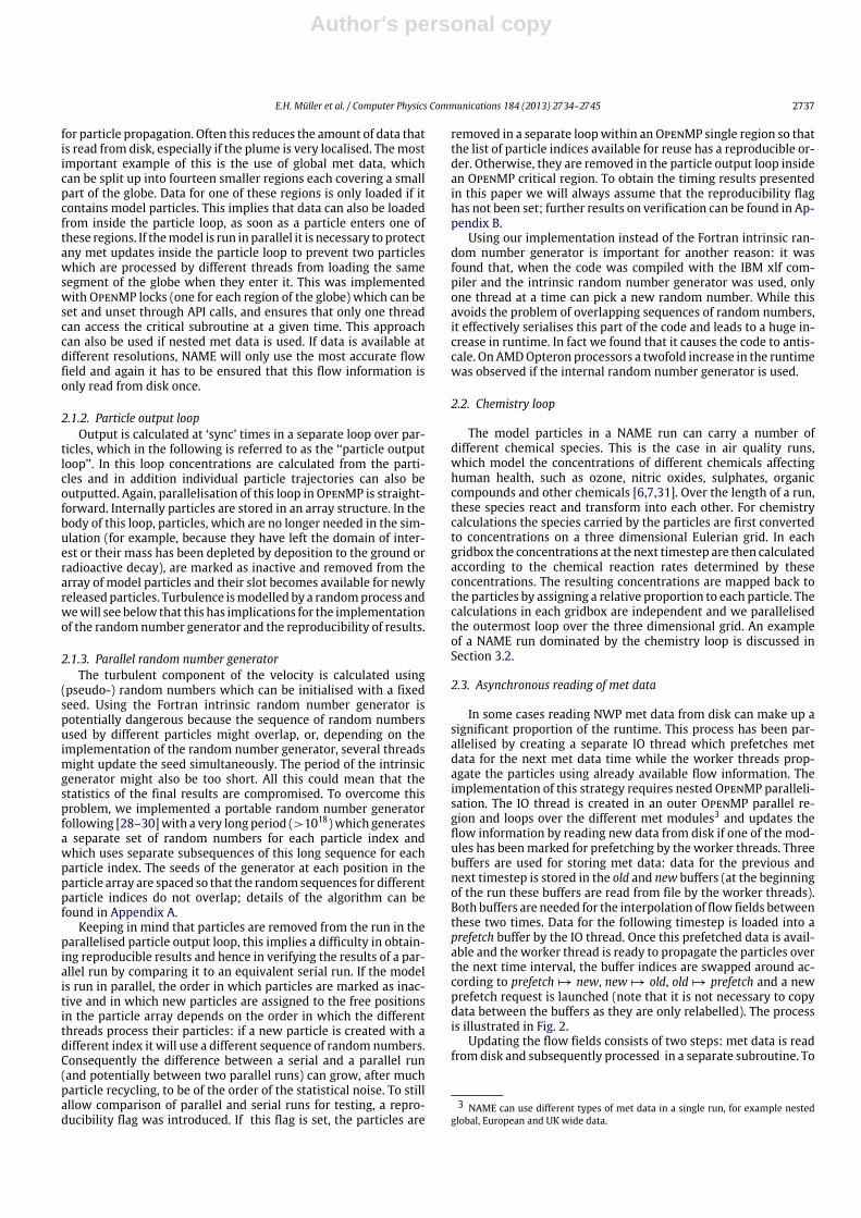
For a fixed number of threadswe expect a tradeoff between twofactors.Without SMT, each thread has exclusive use of the computeresources of one physical core, but (in the case of more than fourthreads) the amount of remote memory access is increased as thethreads are spread between a larger number of cores. On the otherhand, with SMT threads have to share physical cores, but there isless remote memory access as the threads are spread between asmaller number of MCMs. Fig. D.12 shows the speedup of differentparts of the code both with and without SMT. For the particle loop,which dominates the total runtime, scaling is better up to 8 threadsif each of them has exclusive use of one core. Beyond 8 threads thescaling breaks down. On the other hand, if threads share a core,scaling is slightlyworse initially but extends beyond 8 threadswiththe curve only flattening out at beyond 16 threads. This impliesthat for this loop off-MCM memory access is the limiting factor:scaling breaks down as soon as the threads are spread over morethan one MCM.

A similar effect can be observed for the particle output loop, al-though here the explanation is not obvious and further investiga-tions are required to understand the factors limiting the scalability.In contrast to the particle loop, this loop contains frequent writesto shared data structures. As for the results on Intel Xeon chips,presented in Appendix C, the particle output loop does not scale aswell as the particle loop.

D.2. AMD Opteron

The model was also successfully ported to a SUN X4200 serverwith two AMD 275 dual core processors by Glenn Carver at theChemistry Department of the University of Cambridge. The tim-ing results for different thread numbers are listed in Table D.7 andFig. D.13 shows the self-relative speedup on thismachine for a sim-ple particle runwith 5million particles as described in Appendix C.Note that an older version of the model was used, which explainsthe poor scaling of the particle output loop (as already discussedin the main text this problem has now been solved). The overallscaling is not quite as good as on Intel Xeon CPUs but still reason-able up to four threads. It is interesting to note that when the For-tran intrinsic random number generator was used instead of theNAME specific parallel implementation, the runtime increased bya factor of two.



Fig. D.12. Scaling of a simple particle run on a Power 6 node of the Met Office IBMsupercomputer. Results are shown both for runs where each thread had exclusiveuse of a core (empty symbols) and for runs with symmetric multithreading (SMT)where two threads share a single core (filled circles).

Table D.7Time spent in different sections of the code for a simple ‘‘particle’’ type rundescribed in Appendix C. All times are given in minutes; the code was run on twoAMD Opteron 275 dual core processors.

Number of threads 1 2 3 4

Particle loop 92.96 50.98 35.25 27.43Particle output loop 0.59 0.69 1.41 2.03Total 94.06 52.19 37.16 29.96

Fig. D.13. Self-relative speedup on an SUN X4200 server with two AMD 275 dualcore processors. A simple particle test case with 5 million particles as described inAppendix C was used. Note that an older version of the model was used in whichthe scaling of the particle output loop is poor. However, this part of the code onlyamounts to a very small fraction of the runtime and has a negligible effect on thescalability of the overall runtime.

Appendix E. Thread binding on Intel processors

Many Intel Xeon processors support hyperthreading, whichallows running more than one thread on a physical core. On aprocessor with n physical cores, each is split into two logical cores,whichwe label by 1.1, 1.2, 2.1, . . . , n.1, n.2. As Table 1 (and Fig. 3)demonstrate, this can be used to reduce themodel runtime furtherfor emergency response runs on Intel Xeon X5680 processors.

On Intel systems binding to threads is controlled at runtimeby the environment variable KMP_AFFINITY. Thread bindingcan reduce the amount of data movement between cores, as

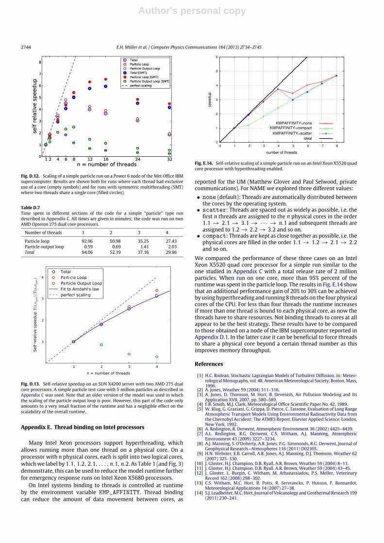
Fig. E.14. Self-relative scaling of a simple particle run on an Intel Xeon X5520 quadcore processor with hyperthreading enabled.

reported for the UM (Matthew Glover and Paul Selwood, privatecommunications). For NAME we explored three different values:• none (default): Threads are automatically distributed between

the cores by the operating system.• scatter: Threads are spaced out as widely as possible, i.e. the

first n threads are assigned to the n physical cores in the order1.1 → 2.1 → 3.1 → · · · → n.1 and subsequent threads areassigned to 1.2 → 2.2 → 3.2 and so on.

• compact: Threads are kept as close together as possible, i.e. thephysical cores are filled in the order 1.1 → 1.2 → 2.1 → 2.2and so on.

We compared the performance of these three cases on an IntelXeon X5520 quad core processor for a simple run similar to theone studied in Appendix C with a total release rate of 2 millionparticles. When run on one core, more than 95% percent of theruntimewas spent in the particle loop. The results in Fig. E.14 showthat an additional performance gain of 20% to 30% can be achievedbyusinghyperthreading and running 8 threads on the four physicalcores of the CPU. For less than four threads the runtime increasesif more than one thread is bound to each physical core, as now thethreads have to share resources. Not binding threads to cores at allappear to be the best strategy. These results have to be comparedto those obtained on a node of the IBM supercomputer reported inAppendix D.1. In the latter case it can be beneficial to force threadsto share a physical core beyond a certain thread number as thisimproves memory throughput.

References

[1] H.C. Rodean, Stochastic Lagrangian Models of Turbulent Diffusion, in: Meteo-rologicalMonographs, vol. 48, AmericanMeteorological Society, Boston,Mass,1996.

[2] A. Jones, Weather 59 (2004) 311–316.[3] A. Jones, D. Thomson, M. Hort, B. Devenish, Air Pollution Modeling and Its

Application XVII, 2007, pp. 580–589.[4] F.B. Smith, M.J. Clark, Meteorological Office Scientific Paper No. 42, 1989.[5] W. Klug, G. Graziani, G. Grippa, D. Pierce, C. Tassone, Evaluation of Long Range

Atmospheric Transport Models Using Environmental Radioactivity Data fromthe Chernobyl Accident: The ATMES Report, Elsevier Applied Science, London,New York, 1992.

[6] A. Redington, R. Derwent, Atmospheric Environment 36 (2002) 4425–4439.[7] A.L. Redington, R.G. Derwent, C.S. Witham, A.J. Manning, Atmospheric

Environment 43 (2009) 3227–3234.[8] A.J. Manning, S. O’Doherty, A.R. Jones, P.G. Simmonds, R.G. Derwent, Journal of

Geophysical Research—Atmospheres 116 (2011) D02305.[9] H.N. Webster, E.B. Carroll, A.R. Jones, A.J. Manning, D.J. Thomson, Weather 62

(2007) 325–330.[10] J. Gloster, H.J. Champion, D.B. Ryall, A.R. Brown, Weather 59 (2004) 8–11.[11] J. Gloster, H.J. Champion, D.B. Ryall, A.R. Brown, Weather 59 (2004) 43–45.[12] J. Gloster, L. Burgin, C. Witham, M. Athanassiadou, P.S. Mellor, Veterinary

Record 162 (2008) 298–302.[13] C.S. Witham, M.C. Hort, R. Potts, R. Servranckx, P. Husson, F. Bonnardot,

Meteorological Applications 14 (2007) 27–38.[14] S.J. Leadbetter,M.C. Hort, Journal of Volcanology andGeothermal Research 199

(2011) 230–241.



[15] H.F. Dacre, A.L.M. Grant, R.J. Hogan, S.E. Belcher, D.J. Thomson, B.J. Devenish,F. Marenco, M.C. Hort, J.M. Haywood, A. Ansmann, I. Mattis, L. Clarisse, Journalof Geophysical Research—Atmospheres 116 (2011) D00U03.

[16] H.N. Webster, D.J. Thomson, B.T. Johnson, I.P.C. Heard, K. Turnbull, F. Marenco,N.I. Kristiansen, J. Dorsey, A. Minikin, B. Weinzierl, U. Schumann, R.S.J. Sparks,S.C. Loughlin, M.C. Hort, S.J. Leadbetter, B.J. Devenish, A.J. Manning, C.S.Witham, J.M. Haywood, B.W. Golding, Journal of Geophysical Research 117(2012) D00U08.

[17] M.J.P. Cullen, Meteorological Magazine 122 (1993) 81–94.[18] G.I. Taylor, Proceedings of the London Mathematical Society s2-20 (1922)

196–212.[19] D. Thomson, Journal of Fluid Mechanics 180 (1987) 529–556.[20] P. Langevin, Comptes Rendus de l’Académie des Sciences Paris 146 (1908)

530–533.[21] H. Webster, D. Thomson, N. Morrison, Met Office Turbulence and Diffusion

Note No. 288, 2003.[22] R.H. Maryon, D.B. Ryall, A.L. Malcolm, Met Office Turbulence and Diffusion

Note No. 262, 1999.[23] Message Passing Interface Forum, 2009. URL: http://www.mpi-forum.org/.[24] OpenMP Architecture Review Board, 2008. URL http://openmp.org/.

[25] D.J. Larson, J.S. Nasstrom, Atmospheric Environment 36 (2002) 1559–1564.[26] J. Nasstrom, G. Sugiyama, J. Leone Jr., D. Ermak, Eleventh Joint Conference on

theApplications of Air PollutionMeteorology, LongBeach, CA, 2000, pp. 84–89,Preprint.

[27] A.K. Luhar, J.J. Modi, Atmospheric Environment. Part A. General Topics 26(1992) 3055–3059.

[28] S.K. Park, K.W. Miller, Communications of the ACM 31 (1988) 1192–1201.[29] P. L’Ecuyer, Communications of the ACM 31 (1988) 742–751.[30] W.H. Press, B.P. Flannery, S.A. Teukolsky,W.T. Vetterling, Numerical Recipes in

Fortran 77: The Art of Scientific Computing, Cambridge University Press, 1992.[31] I.P.C. Heard, A.J. Manning, J.M. Haywood, C. Witham, A. Redington, A. Jones,

L. Clarisse, A. Bourassa, Journal of Geophysical Research 117 (2012) D00U22.[32] E. Pardyjak, B. Singh, A. Norgren, P. Willemsen, 7th Symp. on the Urban

Environment (Paper 14.2), American Meteorological Society, San Diego, 2007.[33] F. Molnar Jr., T. Szakaly, R. Meszaros, I. Lagzi, Computer Physics Communica-

tions 181 (2010) 105–112.[34] D.J. Thomson, Quarterly Journal of the RoyalMeteorological Society 112 (1986)

511–530.[35] G.E.P. Box, M.E. Muller, The Annals of Mathematical Statistics 29 (1958)

610–611.[36] G. Marsaglia, T.A. Bray, SIAM Review 6 (1964) 260–264.

Parallelisation of the Lagrangian atmospheric dispersion model NAME

Documents

Transcript of Parallelisation of the Lagrangian atmospheric dispersion model NAME