Drifter dispersion in the Adriatic Sea: Lagrangian data

and chaotic model

G. Lacorata, E. Aurell, A. Vulpiani

To cite this version:

G. Lacorata, E. Aurell, A. Vulpiani. Drifter dispersion in the Adriatic Sea: Lagrangian data andchaotic model. Annales Geophysicae, European Geosciences Union, 2001, 19 (1), pp.121-129.<hal-00318815>

HAL Id: hal-00318815

https://hal.archives-ouvertes.fr/hal-00318815

Submitted on 1 Jan 2001

HAL is a multi-disciplinary open accessarchive for the deposit and dissemination of sci-entific research documents, whether they are pub-lished or not. The documents may come fromteaching and research institutions in France orabroad, or from public or private research centers.

L’archive ouverte pluridisciplinaire HAL, estdestinee au depot et a la diffusion de documentsscientifiques de niveau recherche, publies ou non,emanant des etablissements d’enseignement et derecherche francais ou etrangers, des laboratoirespublics ou prives.

Annales Geophysicae (2001) 19: 121–129c© European Geophysical Society 2001Annales

Geophysicae

Drifter dispersion in the Adriatic Sea:Lagrangian data and chaotic model

G. Lacorata1, E. Aurell2, and A. Vulpiani3

1Dipartimento di Fisica, Universita dell’Aquila, Via Vetoio 1, I-67010 Coppito, L’Aquila, Italy,Istituto di Fisica dell’Atmosfera, CNR, Via Fosso del Cavaliere, I-00133 Roma, Italy,and Dipartimento di Fisica, Universita di Roma “La Sapienza”, Piazzale Aldo Moro 5, I-00185 Roma, Italy2Department of Mathematics, Stockholm University, S-10691 Stockholm, Sweden3Istituto Nazionale Fisica della Materia, Unita di Roma 1and Dipartimento di Fisica, Universita di Roma “La Sapienza”, Piazzale Aldo Moro 5, I-00185 Roma, Italy

Received: 8 November 1999 – Revised: 14 September 2000 – Accepted: 14 September 2000

Abstract. We analyze characteristics of drifter trajectoriesfrom the Adriatic Sea with recently introduced nonlinear dy-namics techniques. We discuss how in quasi-enclosed basins,relative dispersion as a function of time, a standard analy-sis tool in this context, may give a distorted picture of thedynamics. We further show that useful information may beobtained by using two related non-asymptotic indicators, theFinite-Scale Lyapunov Exponent (FSLE) and the LagrangianStructure Function (LSF), which both describe intrinsic phys-ical properties at a given scale. We introduce a simple chaoticmodel for drifter motion in this system, and show by com-parison with the model that Lagrangian dispersion is mainlydriven by advection at sub-basin scales until saturation setsin.

Key words. Oceanography: General (marginal and semi-closed seas) – Oceanography: Physical (turbulence, diffu-sion, and mixing processes; upper ocean processes)

1 Introduction

Understanding the mechanisms of transport and mixing pro-cesses is an important and challenging task which has widerelevance from a theoretical point of view, e.g. for the studyof diffusion and chaos in geophysical systems in general orfor validating simulation results from a general circulationmodel. It is also a necessary tool in the analysis of problemsof general interest and social impact, such as the dispersionof nutrients or pollutants in sea water with consequent effectson marine life and on the environment (Adler et al., 1996).

Recently, a number of oceanographic programs have beendevoted to the study of the surface circulation of the Adri-atic Sea by the observation of Lagrangian drifters within thelarger framework of drifter-related research in the whole Me-diterranean Sea (Poulain, 1999). The Adriatic Sea is a quasi-enclosed basin, about 800 long by 200 km wide, connected to

Correspondence to:G. Lacorata(Guglielmo.Lacorata@aquila.infn.it)

the rest of the Mediterranean Sea through the Otranto Strait.From a topographic point of view, three major regions can beconsidered. The northern part is the shallowest, about 100 mmaximum depth, and extends down to the latitude of Ancona.The central part extends down to about 260 m in the JabukaPit, and the southern part extends from the Gargano promon-tory to the Otranto Strait. The southern part is the deepest,reaching about 1200 m in the South Adriatic Pit. Reviews onthe oceanography of the Adriatic Sea can be found in Arte-giani et al. (1997), Orlic et al. (1992), Poulain (1999) andZore (1956).

Lagrangian data offer the opportunity to employ techni-ques of analysis well established in the theory of chaotic dy-namical systems to study the behavior of actual trajectoriesand compare those with a kinematic model.

Let us assume that the Lagrangian drifters are passivelyadvected in a two-dimensional flow, e.g. as would be thecase in a frictionless barotropic approximation (Ottino, 1989;Crisanti et al., 1991):

dx

dt= u(x, y, t) and

dy

dt= v(x, y, t) , (1)

where(x(t), y(t)) is the position of a fluid particle at timetin terms of longitude and latitude, andu andv are the zonaland meridional velocity fields respectively.

For the Eulerian description of a geophysical system, oneshould in principle use numerical solutions of the Navier-Stokes equations (or other suitable equations, e.g. the quasi-geostrophic model) to obtain the velocity fields. In practice,direct numerical simulation of these equations on oceano-graphic length scales is of course not possible, and one hasto invoke approximations, i.e. turbulence modeling. Thismotivates one to use instead a simplified kinematic approachby adopting a given Eulerian velocity field. The criteria forthe construction of such a field follows from phenomenolog-ical arguments and/or experimental observation and have re-cently been reviewed in Yang (1996) and Samelson (1996).

Let us consider the relationship between Eulerian and La-grangian properties of a system. A wide range of literature on

122 G. Lacorata et al.: Drifter dispersion in the Adriatic Sea: Lagrangian data and chaotic model

this topic (e.g. Ottino, 1989; Crisanti et al., 1991) allows usto state that, in general, Eulerian and Lagrangian behavioursare not strictly related to each other. It is not rare to haveregular Eulerian behavior, e.g. a time-periodic velocity fieldco-existing with Lagrangian chaos or vice-versa.

In quasi-enclosed basins like the Adriatic Sea, a character-ization of the mechanisms of the mixing is highly non-trivial.We first observe (see below for detailed discussion) that theuse of the standard diffusion coefficients can have rather lim-itated applicability (see Artale et al., 1997). Classical studieson Lagrangian particles in ocean models already contain re-marks on the intrinsic difficulties in using one-particle diffu-sion statistics (Taylor, 1921). In situations where the advec-tive time is not much longer than the typical decorrelationtime scale of the Lagrangian velocity, the diffusivity param-eter related to small-scale turbulent motion cannot convergeto its asymptotic value (Figueroa and Olson, 1994). On theother hand, a generalization of the standard Lyapunov ex-ponent, the Finite-Scale Lyapunov Exponent (FSLE), origi-nally introduced for the predictability problem (Aurell et al.,1996, 1997), has been shown to be a suitable tool to de-scribe non-asymptotic properties of transport. This finite-scale approach to Lagrangian transport measures effectiverates of particle dispersion without assumptions about small-scale turbulent processes. For an alternative method, see Buf-foni et al. (1997) and for a recent review and systematic dis-cussion of non-asymptotic properties of transport and mixingin realistic cases, see Boffetta et al. (2000).

In this paper we report data analysis of surface drifter mo-tion in the Adriatic Sea using relative dispersion, FSLE andLagrangian Structure Function (LSF), a quantity related tothe FSLE. We also introduce a chaotic model for the La-grangian dynamics and use the FSLE and LSF characteris-tics to compare model and data. We show that it can be verydifficult to obtain an estimate of the diffusion coefficient in aquasi-enclosed basin, and/or to look for deviations from thestandard diffusion law. In fact, the time a cluster of parti-cles takes to spread uniformly and reach the boundaries isnot much longer than the largest characteristic time of thesystem. In contrast, the FSLE and the LSF do characterizethe transport properties of Lagrangian trajectories at a fixedspatial scale. Finally, we will show that a simple kinematicmodel reproduces the data.

In Sect. 2 we describe the data set we have used as wellas review relevant concepts and analysis techniques for La-grangian transport and chaos. In Sect. 3 we introduce a kine-matic model of the Lagrangian dynamics, and in Sect. 4, wecompare the data and the model. Section 5 contains a sum-mary and a discussion of the results.

2 Data set and analysis techniques

2.1 Data set

In a large drifter research program in the Mediterranean Sea,started in the late 80’s and continued into the 90’s, Lagrang-

ian data from surface drifters deployed in the Adriatic seahave been recorded from December 1994 to March 1996.These drifters are similar to the CODE (COastal Dynam-ics Experiment) system (Davis, 1985) and they are designedto be sufficiently wind-resistant so as to effectively give adescription of the circulation at their actual depth (1 me-ter). The drifters were tracked by the Argos Data Locationand Collection System (DCLS) carried by the NOAA polar-orbiting satellites. It is assumed that after data processingdrifter positions are accurate to within 200–300 m, and veloc-ities to within 2–3 cm/s. For a description of the experimentalprogram, see Poulain (1999) and for technical details aboutthe treatment of raw data, see Hansen and Poulain (1996),Poulain et al. (1996) and Poulain and Zanasca (1998).

The data have been stored in separate files, one for eachdrifter. In the format used by us each file contains: a num-ber of records (i.e. number of points of the trajectory); thetime in days; the position of the drifter in longitude and lat-itude; the velocity of the drifter along the zonal and merid-ional directions; and the temperature in centigrade degrees.The sampling time is 6 hours. We can identify five maindeployments on which we will concentrate our attention. Se-lecting the tracks by the time of the first record, it is easy toverify that these five subsets consist of drifters deployed inthe same area in the Otranto strait near 19 degrees longitudeeast and 40 degrees latitude north. The experimental strategyof simultaneously releasing the drifters within a distance ofsome kilometers allows us to study dispersion quantitatively.

From a qualitative point of view, what we observe fromthe plot of all the trajectories (Fig. 1) is the shape of two(cyclonic) basin-wide gyres, located in the middle and south-ern regions respectively and, an anti-clockwise boundary cur-rent which moves the drifters north-westward along the eastcoast and south-eastward down the west coast. The latter isa permanent feature of the Adriatic sea (Poulain, 1999). Onthe other hand, it is known that within a year the pattern ofbasin-wide gyres may change between one, two and threegyres over a time-scale of months. The southern gyre is themost steady of the three. The data also suggests the pres-ence of small scale structures, even though these are muchmore likely to be variable in time. The time-scale of the typ-ical recirculation period around a basin-wide gyre is aboutone month and the time needed to travel along the coasts andcomplete one lap of the full basin is in the order of a fewmonths.

2.2 Analysis techniques

We recall here some basic concepts about dynamical sys-tems, diffusion and chaos, and the quantities that we shalluse to characterize the properties of Lagrangian trajectories.

If we haveNc clusters of initially close particles with eachcluster containingnk elements, relative dispersion can becharacterized by the diffusion coefficient

Di = limt→∞

1

2tS2

i (t) (2)

G. Lacorata et al.: Drifter dispersion in the Adriatic Sea: Lagrangian data and chaotic model 123

Fig. 1. Plot of the 37 drifter trajectories in the Adriatic Sea used forthe data analysis. The longitude east and latitude north coordinatesare in degrees. The drifters were deployed on the eastern side of theOtranto strait.

with

S2i (t) =

1

Nc

Nc∑k=1

1

nk

nk∑j=1

(x(k,j)i (t) − 〈xi(t)〉

(k))2 (3)

where

〈xi(t)〉(k)

=1

nk

nk∑j=1

x(k,j)i (t) (4)

x(k,j)i is thei-th spatial coordinate of thej -th particle in the

k-th cluster;S2=

∑i S2

i is the mean square displacement ofthe particles relative to their time evolving mean position. Ifδ(t) is the distance between two trajectoriesx(1) andx(2) ina cluster at timet , relative dispersion is defined as

〈δ2(t)〉 = 〈||x(1)(t) − x(2)(t)||2〉 (5)

where the average is over all pairs of trajectories in the clus-ter. In a standard diffusive regime,x(1)(t) andx(2)(t) be-come independent variables and, fort → ∞, we have〈δ2(t)〉

= 2S2(t). In the following, we shall consider the clustermean square radiusS2(t) as a measure of relative dispersion.Absolute dispersion, which is defined as the mean square dis-placement from an initial position, will not be taken into ac-count in our analysis.

If, in the asymptotic limit,S2i (t) ∼ t2α with α = 1/2, we

have the linear law of standard diffusion for the mean squaredisplacement and theDi ’s are finite. Ifα 6= 1/2, we have

a so-called anomalous diffusion (Bouchaud and Georges,1990).

The difficulty which often arises when measuring the ex-ponentα is that, due to the finite size of the domain, dis-persion cannot reach its true asymptotic behavior. In otherwords, diffusion may not be observable over sufficiently largescales, i.e. much larger than the largest Eulerian length scale.Therefore, we cannot have a robust estimate of the exponentof the asymptotic power law. Moreover, the relevance ofasymptotic quantities, like the diffusion coefficients, is ques-tionable in the study of realistic cases concerning the trans-port problem in finite-size systems (Artale et al., 1997).

The diffusion coefficients characterize long-time (large-scale) dispersion properties. In contrast, at short times (smallscales) the relative dispersion is related to the chaotic behav-ior of the Lagrangian trajectories.

A quantitative measure of instability for the time evolutionof a dynamical system (Lichtenberg and Lieberman, 1992)is commonly given by the Maximum Lyapunov Exponent(MLE) λ, which gives the rate of exponential separation oftwo nearby trajectories

λ = limt→∞

limδ(0)→0

1

tln

δ(t)

δ(0)(6)

whereδ(t) = ||x(1)(t) − x(2)(t)|| is the distance betweentwo trajectories at timet . Whenλ > 0 the system is saidto be chaotic. There exists a well-established algorithm tonumerically compute the MLE introduced by Benettin et al.(1980).

A characteristic time,Tλ, associated to the MLE is the pre-dictability time, defined as the minimum time after which theerror on the state of the system becomes larger than a toler-ance value1, if the initial uncertainty isδ (Lichtenberg andLieberman, 1992):

Tλ =1

λln

1

δ(7)

Let us recall thatλ is a mathematically well-defined quan-tity which measures the growth of infinitesimal errors. Inphysical terms, at any time,δ has to be much less than thecharacteristic size of the smallest relevant length of the ve-locity field. For example, in 3D fully developed turbulence,δ has to be much smaller than the Kolmogorov length.

When the uncertainty reaches non-infinitesimal sizes, i.e.macroscopic scales, the perturbationδ is governed by thenonlinear terms and that renders its growth rate a scale-de-pendent index (Aurell et al., 1996, 1997; Artale et al., 1997).It is useful to introduce the Finite Scale Lyapunov Exponent(FSLE),λ(δ). Assumingr > 1 is a fixed amplification ratioand〈τr(δ)〉 the mean time thatδ takes to grow tor · δ, wehave:

λ(δ) =1

〈τr(δ)〉ln r (8)

The average〈 · 〉 is performed over all the trajectory pairs ina cluster. We note the following properties of the FSLE:

124 G. Lacorata et al.: Drifter dispersion in the Adriatic Sea: Lagrangian data and chaotic model

a) in the limit of infinitesimal separation between trajecto-ries,δ → 0, the FSLE tends to the maximum Lyapunovexponent (MLE);

b) in case of standard diffusion,〈δ(t)2〉 ∼ t , we find that

λ(δ) ∼ δ−2 and the proportionality constant is of theorder of the diffusion coefficient;

c) any slope> −2 for λ(δ) vs δ indicates super-diffusivebehavior, i.e. non-neglectable correlations persist atlong times and advection is still relevant;

d) in particular, whenλ(δ) = constant over a range ofscales, we have exponential separation between tra-jectories at a constant rate within that range of scales(chaotic advection).

Another interesting quantity related to the FSLE is the La-grangian Structure Function (LSF)ν(δ), defined as

ν(δ) =

⟨∣∣∣∣∣∣∣∣dx′

dt−

dx

dt

∣∣∣∣∣∣∣∣⟩δ

(9)

where the value of the velocity difference is taken at thetimes for which the distance between the trajectories entersthe scaleδ and the average is performed over a large numberof realizations. The LSF,ν(δ), is a measure of the velocity atwhich two trajectories depart from each other, as a functionof scale. By dimensional arguments, we expect that the LSFis proportional to the scale of the separation and to the FSLE:

ν(δ) ∼ δ λ(δ) (10)

so that we should find similar behavior forλ(δ) andν(δ)/δ,if independently measured.

In order to study the transport properties of the drifter tra-jectories, we have focused our interest on the measurementof S2

i (t), λ(δ) andν(δ).With regards to the practical definitions of the FSLE and

the LSF, we have chosen a range of scalesδ = (δ0, δ1, ..., δn)

separated by a factorr > 1 such thatδi+1 = r · δi for i =

0, n − 1. The ratior is often referred to as the “doubling”factor even though it is not necessarily equal to 2, e.g. inour case we fixed it at

√2. The r value has naturally an

inferior bound because of the temporal finite resolution ofthe trajectories (i.e. it cannot be arbitrarily close to 1) and itmust be not much larger than 1, if we want to resolve scaleseparation in the system.

The smallest thresholdδ0 is placed just above the ini-tial mean separation between two drifters,∼10 km, and thelargest oneδn is naturally selected by the finite size of thedomain,∼500 km.

Following the same procedure, it is straightforward tocompute the LSF as the mean velocity difference betweentwo trajectories at the moment in which the separationreaches a scaleδ:

ν(δ) =

⟨√(u1 − u2)2 + (v1 − v2)2

⟩δ

(11)

where the average is performed over the number of all thepairs within a set of particles, at the time in which||x′

−x|| =

δ.In Sect. 4 below we shall show the results of our data

analysis and compare them with the simulations from ourchaotic model for the Lagrangian dynamics of the Adriaticdrifters.

3 The chaotic model

In phenomenological kinematic modeling of geophysicalflows, two possible approaches can be considered: stochasticand chaotic. Both procedures generally involve a mean ve-locity field, which gives the motion over large scales, and aperturbation which describes the action of the small scales.The model is stochastic or chaotic if the perturbation is arandom process or a deterministic time-dependent function,respectively. Examples on kinematic mechanisms proposedto model the mixing process can be found in Bower (1991),Samelson (1992), Bower and Lozier (1994), Cencini et al.(1999).

The choice of one or the other depends on what one is in-terested in and what experimental information is available. Inour case, we have opted for a deterministic model since thereare indications that, at the sea surface, the instabilities of theEulerian structures are primarily due to air-sea interactions,which are nearly periodic perturbations.

We want to consider a simple model. So let us assumeas main features of the surface circulation the following ele-ments: an anti-clockwise coastal current; two large cyclonicgyres; and some natural irregularities in the Lagrangian mo-tion induced by the small scale structures.

Let us notice that the actual drifters may leave the Adri-atic sea through the Otranto Strait, but we model our domainwith a closed basin in order to study the effects of the finitescales on the transport and treat it like a 2D system, since thedrifters explore the circulation in the upper layer of the seawithin the first meters of water.

On the basis of the previous considerations, we introduceour kinematic model for the Lagrangian dynamics. Underthe incompressibility hypothesis we write a 2D velocity fieldin terms of a stream function:

u = −∂9

∂yand v =

∂9

∂x. (12)

Let us write our stream function as a sum of three terms:

9(x, y, t) = 90(x, y) + 91(x, y, t) + 92(x, y, t) (13)

defined as follows:

90(x, y) =C0

k0[− sin(k0(y + π)) + cos(k0(x + 2π))] (14)

91(x, y, t) =C1

k1sin(k1(x + ε1 sin(ω1t)))

· sin(k1(y + ε1 sin(ω1t + φ1))) (15)

G. Lacorata et al.: Drifter dispersion in the Adriatic Sea: Lagrangian data and chaotic model 125

Fig. 2. Model stream function isolines at(a) t = 0 and(b) t =

T1/2, with T1 ∼ 30 days. The boundary of the domain is the zeroisoline. The coordinates (x, y) are in km.

92(x, y, t) =C2

k2sin(k2(x + ε2 sin(ω2t)))

· sin(k2(y + ε2 sin(ω2t + φ2))) (16)

whereki = 2π/λi , for i = 0, 1, 2, theλi are the wavelengthsof the spatial structure of the flow; analogouslyωj = 2π/Tj ,for j = 1, 2, and theTj are the periods of the perturbations.In the non-dimensional expression of the equations, the unitsof length and time have been set to 200 km and 5 days, re-spectively. The choice of the values of the parameters is dis-cussed below.

The stationary term90 defines the boundary large scalecirculation with positive vorticity.91 contains the two cy-clonic gyres and it is explicitly time-dependent through a pe-riodic perturbation of the streamlines. The term92 gives themotion over scales smaller than the size of the large gyresand it is time-dependent as well. A plot of the9-isolines atfixed time is shown in Fig. 2. The actual basin is the inner re-gion with negative9 values and the zero isoline is taken as adynamical barrier which defines the boundary of the domain.

The main difference with reality is that the model domainis strictly a closed basin, whereas the Adriatic Sea communi-cates with the rest of the Mediterranean through the Otranto

Strait. This is not crucial as long as we observe the two evo-lutions of experimental and model trajectories within timescales smaller than the mean exit time from the sea, typicallyof the order of a few months. Furthermore, the presence ofthe quasi-steady cyclonic coastal current is compatible withthe interplay between the Po river southward inflow at thenorth-western side and the Otranto channel northward inflowat the south-eastern side of the sea.

The non-stationarity of the stream function is a necessaryfeature of a 2D velocity field in order to have Lagrangianchaos and mixing properties. That is, so that a fluid particlewill visit any portion of the domain after a sufficiently longinterval of time.

We have chosen the parameters as follows. The velocityscalesC0, C1 andC2 are all equal to 1 which, in physicaldimensions, corresponds to∼0.5 m/s. The wave numbersk0, k1 andk2 are fixed at 1/2, 1 and 4π , respectively. In Fig.2a,b we can see two snapshots of the streamlines at fixedtime. The length scales of the model Eulerian structures areof ∼1000 km (coastal current),∼200 km (gyres) and∼50km (eddies). The typical recirculation times for gyres andeddies turns out to be of the order of 1 month and a few days,respectively.

With regards to the time-dependent terms in the streamfunction, the pulsations areω1 = 1 andω2 = 2π , whichdetermine oscillations of the two large-scale vortices over aperiodT1 ' 30 days and oscillations of the small-scale vor-tices over a periodT2 ' 5 days. The respective oscillationamplitudes areε1 = π/5 andε2 = ε1/10 which correspondto ∼100 km and∼10 km.

The choice of the phase factorsφ1 andφ2 determines howmuch the vortex pattern changes during a perturbation pe-riod. We have chosen to set bothφ1 andφ2 to π/4. Thischoice of the parameters for the time-dependent terms in thestream function is only supposed to be physically reasonable,for the experimental data give us limited information aboutthe time variability of the Eulerian structures.

The chaotic advection (Ottino, 1989; Crisanti et al., 1991),occurring in our model makes an ensemble of initially closetrajectories spread apart from one another, until the size ofthe mean relative displacement reaches a saturation valuecorresponding to the finite length scale of the domain.

The scale-dependent degree of chaos is given by the FSLE.Due to the relatively sharp separation between large andsmall scales in the model, we expectλ(δ) to display a step-like behavior with two plateaus, one for each characteristictime, and a cut-off at scales comparable with the size of thedomain. In the limit of small perturbations, the FSLE givesan estimate of the MLE of the system.

The LSFν(δ), on the other hand, is expected to be propor-tional to the size of the perturbation and toλ, as discussed inthe introduction. Therefore, the quantityν(δ)/δ is expectedto be qualitatively proportional toλ(δ), in the sense that themean slopes have to be compatible with each other.

In the following section we will show results of our simu-lations together with the outcome of the data analysis.

126 G. Lacorata et al.: Drifter dispersion in the Adriatic Sea: Lagrangian data and chaotic model

4 Comparison between data and model

The statistical quantities relative to the drifter trajectorieshave been computed according to the following prescription.The number of selected drifters for the analysis is 37, dis-tributed in 5 different deployments in the Strait of Otranto,containing, respectively, 4, 9, 7, 7 and 10 drifters. These arethe only drifter trajectories out of the whole data set whichare long enough to study the Lagrangian motion on the basinscale. To obtain the highest statistics possible, at the priceof losing information on the seasonal variability, the times ofall of the 37 drifters are measured ast − t0, wheret0 is thetime of deployment. Moreover, to restrict the analysis onlyto the Adriatic basin, we impose the condition that a drifteris discarded as soon as its latitude moves south of 39.5 N orits longitude exceeds 19.5 E. Let us consider the referenceframe in which the axes are aligned, respectively, with theshort side, orthogonal to the coasts, which we call the trans-verse direction and the long side, along the coasts, which wecall the longitudinal direction.

Before the presentation of the data analysis, let us brieflydiscuss the problem of finding characteristic Lagrangiantimes. A first obvious candidate is

τ(1)L =

1

λ(17)

Of courseτ(1)L is related to small scale properties. Another

characteristic time, at least if the diffusion is standard, is theso-called integral time scale (Taylor, 1921)

τ(2)L =

1

〈v2〉

∫∞

0C(τ)dτ (18)

whereC(τ) =∑d

i=1〈vi(t)vi(t+τ)〉 is the Lagrangian veloc-ity correlation function and〈v2

〉 is the velocity variance. Wewant to stress that it is always possible (at least in principle)to defineτ (1)

L while to computeτ (2)L (the integral time scale) it

is necessary to be in a standard diffusion case (Taylor, 1921).The relative dispersion curves along the two natural direc-

tions of the basin for data and model trajectories are shownin Figs. 3a and 3b. The curves from the numerical simula-tion of the model are computed observing the spreading of acluster of 104 initial conditions. When a particle reaches theboundary (9 = 0), it is eliminated. Along with observationaland simulation data, we also plot a straight line correspond-ing to a standard diffusion with coefficient 103 m2/s, (Falcoet al., 2000). We discuss this comparison below. Consider-ing the effective diffusion properties, one should expect thatthe shape ofS2

i (t), before the saturation regime, can still beaffected by the action of the coherent structures. Actually,neither the data nor the model dispersion curves display aclear power-law behavior, and are indeed quite irregular. Thegrowth of the mean square radius of a cluster of drifters ap-pears still strongly affected from the details of the system andthe saturation begins no later than∼1 month (∼ the largestcharacteristic Lagrangian time). This prevents any attemptat defining a diffusion coefficient for the effective dispersion

100

1000

10000

100000

0.1 1 10 100

S2 tr

as

time

100

1000

10000

100000

0.1 1 10 100

S2 lo

ng

time

Fig. 3. Relative dispersion curves for data (plus symbol) and model(dashed) trajectories along the two natural directions in the basingeometry:(a) transverse component,(b) longitudinal component.The time is measured indays and the dispersion in km2. The exper-imental curve is computed over the 37 drifter trajectories; the modelcurve is computed over a cluster of 104 particles, initially placed atthe border of the southern gyre with a mean square displacementof ∼50 km2. The straight line with slope 1 has been plotted forcomparison with a standard diffusive scaling with a correspondingdiffusion coefficient∼103 m2/s, typical of marine turbulent mo-tions.

in this system. Although the saturation values are very simi-lar, we can see that, in the intermediate range, the agreementbetween observation and simulation is not good. We pointout that the trouble in reproducing the drifter dispersion intime does not depend much on the statistics. It makes no dif-ference whether there are 37 (data) or 104 (model) trajecto-ries. The problem is that the classic relative dispersion is notthe most suitable quantity to be measured (irregular behavioreven at high statistics).

Let us now discuss the FSLE results. The curve measuredfrom the data has been averaged over the total number ofpairs out of 37 trajectories (∼700), under the condition thatthe evolution of the distance between two drifters is no longerfollowed when any of the two exits the Adriatic basin (seeabove). In Fig. 4 the FSLE’s for data and model are plotted.Phenomenologically, fluid particle motion is expected to befaster at small scales and slower at large scales. The decreaseof λ(δ) at increasingδ reflects the presence of several scales

G. Lacorata et al.: Drifter dispersion in the Adriatic Sea: Lagrangian data and chaotic model 127

0.01

0.1

1

10 100

λ(δ)

δ

Fig. 4. Finite-Scale Lyapunov Exponent for data (continuous line)and model (dashed line) trajectories.δ is in km andλ(δ) is in day−1.The experimental FSLE is computed over all the pairs of trajectoriesout of 37 drifters; the FSLE from the model is averaged over 104

simulations. The simulatedλ(δ) has a step-like behavior with oneplateau at small scales (<50 km) and one at basin scales (>100km), corresponding to doubling times of∼3 days and∼30 days,respectively.

of motions (at least two) involved in the dynamics. In partic-ular, looking at the values ofλ(δ)−1 at the extreme points ofthe δ-range, we see that small-scale (mesoscale) dispersionhas a characteristic time∼4 days and the large-scale (gyrescale) dispersion has a characteristic time∼1 month. Theratio between gyre scale and mesoscale is of the same or-der as the ratio between the inverse of their respective char-acteristic times (∼10), so the slope ofλ(δ) at intermediatescales is about−1. The fact that the slope is larger than−2indicates that relative dispersion is faster than standard dif-fusion up to sub-basin scales, i.e. Lagrangian correlationsare non-vanishing due to coherent structures. It is interest-ing to compare this Lagrangian technique of measuring theeffective Lagrangian dispersion on finite scales to the moretraditional technique of extracting a (standard) diffusivity pa-rameter from the reconstruction of the small-scale anomaliesin the velocity field (Falco et al., 2000). Estimates of thezonal and meridional diffusivity in Falco et al. (2000) areof the order of∼103 m2/s and are compatible with the valueof the effective finite-scale diffusive coefficient given by theFSLE, defined asλ(δ) · δ2, computed atδ = 20 km (∼ themesoscale).

The FSLE computed in the numerical simulations showstwo plateaus, one at small scales and the other at large scales,describing a system with two characteristic time scales andpresents the same behavior, both qualitative and quantitative,as the FSLE is computed for the drifter trajectories.

It is worth noting that it is much simpler for the model toreproduce, even quantitatively, the relation between charac-teristic times and scales of the drifter dynamics (FSLE) ratherthan the behavior of the relative dispersion in time.

The LSV in Fig. 5 shows that the behavior ofν(δ), themean velocity difference between two particle trajectories as

0.01

0.1

1

10 100

ν(δ)

δ

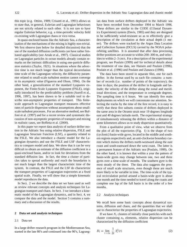
Fig. 5. Lagrangian Structure Function for data (continuous line) andmodel (dashed line) trajectories.δ is in km andν(δ)/δ is in day−1.The experimental LSF is computed over all the pairs of drifters; theLSF from the model is averaged over 104 simulations.

the scale of the separation varies, is compatible with the be-havior of the FSLE as expected by dimensional arguments,i.e. ν(δ)/δ, the LSF divided by the scale at which it is com-puted, has the same slope asλ(δ). This accounts for the ro-bustness of the information given by the finite-scale analysis.

We see the theoretical predictions of FSLE and LSV arefairly well comparable with the corresponding quantities ob-served from the data, if we consider the relatively simplemodel which we used for the numerical simulations. Ofcourse, an agreement exists due to the appropriate choiceof the parameters of the model, capable of reproducing thecorrect relation between scales of motion and characteris-tic times, and because large-scale (∼ sub-basin scales) La-grangian dispersion is weakly dependent on the small-scale(∼ mesoscale) details of the velocity field.

5 Discussion and conclusions

In this paper we have analyzed an experimental data set recor-ded from Lagrangian surface drifters deployed in the Adri-atic sea. The data span the period from December 1994to March 1996, during which five sets of drifters were re-leased at different times in the vicinity of the same point onthe eastern side of the Otranto Strait. Adopting a techniqueborrowed from the theory of dynamical systems, we stud-ied the Lagrangian transport properties by measuring relativedispersionsS2

i , finite-scale Lyapunov exponentsλ(δ), andLagrangian structure functionν(δ). Relative dispersion, asfunction of time, does not provide much information, exceptfor an idea of the size of the domain where saturation sets inat long times. The behavior ofS2

i looks quite irregular andthis is due not to poor statistics but rather to intrinsic reasons.In contrast, the results obtained with the FSLE, i.e. disper-sion rates at different scales of motion, give a more usefuldescription of the properties of the drifter spreading. In par-ticular, λ(δ) detects the characteristic times associated with

128 G. Lacorata et al.: Drifter dispersion in the Adriatic Sea: Lagrangian data and chaotic model

the Eulerian characteristic lengths of the system.We have also introduced a simple chaotic model of the La-

grangian evolution and compared it with the observations. Inour point of view, the actual meaning of the chaotic model,in relation to the behavior of the drifters, is not the best-fitting model. We do not claim that the quite difficult taskof modeling the marine surface circulation driven by windforcing can be exploited by a simple dynamical system. Buta simple dynamical system can give satisfactory results if weare interested in large-scale properties of Lagrangian disper-sion, since they depend much on the topology of the velocityfield and only slightly on the small-scale details of the veloc-ity structures. In this respect, chaotic advection, very likelypresent in every geophysical fluid flow, is crucial for whatconcerns tracer dispersion, since it can easily overwhelm theeffects of small-scale turbulent motions on large-scale trans-port (Crisanti et al., 1991). Even when a standard diffusiv-ity parameter can be computed from the variance and theself-correlation time of the Lagrangian velocity, its relevancefor reproducing the effective dispersion on finite scales, inpresence of coherent structures, is questionable. In addition,practical difficulties arising from both finite resolution andboundary effects suggest a revision of the analysis techniquesto be used for studying Lagrangian motion on finite scales,i.e. in non-asymptotic conditions. Considering that, gener-ally, there is more physical information in a scale-dependentindicator (λ(δ)) rather than in a time function (S2(t)), wecome to the conclusion that the FSLE is a more appropriatetool of investigation of finite-scale transport properties. It isimportant to remark (Aurell et al, 1996; Artale et al., 1997;Boffetta et al., 2000) that, in realistic cases,λ(δ) is not justanother way to look atS2(t) vs t , in particular it is not truethatλ(δ) behaves like(d ln S2(t)/dt)S2=δ2. This is becauseλ(δ) is a quantity which characterizes Lagrangian propertiesat the scaleδ in a non ambiguous way. On the contrary,S2(t)

can depend strongly onS2(0), so that, in non-asymptoticconditions, it is relatively easy to get erroneous conclusionsonly by looking at the shape ofS2(t). In fact, at a giventime, relative dispersion inside a sub-cluster of drifters canbe rather different from other sub-clusters, e.g. due to fluc-tuations in the cross-over time between exponential and dif-fusive regimes. Therefore, when performing an average overthe whole set of trajectories, one may obtain a quite spuri-ous and inconclusive behavior. On the other hand, we haveseen that the analysis of FSLE (and LSF) and the studyingof the transport properties at a given spatial scale, rather thanat a given time, can provide more reliable information on therelative dispersion of tracers.

Acknowledgements.The drifter data set used in this work was kind-ly made available to us by P.-M. Poulain. We warmly thank J.Nycander, P.-M. Poulain, R. Santoleri and E. Zambianchi for con-structive readings of the manuscript and for clarifying discussionsabout oceanographic matters. We also thank E. Bohm, G. Bof-fetta, A. Celani, M. Cencini, K. Doos, D. Faggioli, D. Fanelli, S.Ghirlanda, D. Iudicone, A. Kozlov, E. Lindborg, S. Marullo, P.Muratore-Ginanneschi and V. Rupolo for useful discussions.

This work was supported by a European Science Foundation “TAO

exchange grant” (G. L.), by the Swedish Natural Science ResearchCouncil under contract M-AA/FU/MA 01778-334 (E. A.) and theSwedish Technical Research Council under contract 97-855 (E. A.),and by the I.N.F.M. “Progetto di Ricerca Avanzata TURBO” (A.V.)and MURST, program 9702265437 (A. V.). G. L. thanks the K.T.H.(Royal Institute of Technology) in Stockholm for hospitality. Wethank the European Science Foundation and the organizers of the1999 Tao Study Center for invitations, and for an opportunity towrite up this work.

References

Adler, R. J., Muller, P., and Rozovskii, B. (Eds.), Stochastic model-ing in physical oceanography, Birkhauser, Boston, 1996.

Artale, V., Boffetta, G., Celani, A. , Cencini, M., and Vulpiani, A.,Dispersion of passive tracers in closed basins: beyond the diffu-sion coefficient. Phys. of Fluids, 9, 3162, 1997.

Artegiani, A., Bregant, D., Paschini, E., Pinardi, N., Raicich, F., andRusso, A., The Adriatic Sea general circulation, parts I and II. J.Phys. Oceanogr., 27, 8, 1492–1532, 1997.

Aurell, E., Boffetta, G., Crisanti, A., Paladin, G., and Vulpiani, A.,Predictability in systems with many degrees of freedom, PhysicalReview E, 53, 2337, 1996.

Aurell, E., Boffetta, G., Crisanti, A., Paladin, G., and Vulpiani, A.,Growth of non-infinitesimal perturbations in turbulence, Phys.Rev. Lett., 77, 1262–1265, 1996.

Aurell, E., Boffetta, G., Crisanti, A., Paladin, G., and Vulpiani, A.,Predictability in the large: an extension of the concept of Lya-punov exponent, J. of Phys. A, 30, 1, 1997.

Benettin, G., Galgani, L., Giorgilli, A., and Strelcyn, J. M., Lya-punov characteristic exponents for smooth dynamical systemsand for Hamiltonian systems: a method for computing all ofthem, Meccanica, 15, 9, 1980.

Boffetta, G., Celani, A., Cencini, M., Lacorata, G., and Vulpiani,A., Non-asymptotic properties of transport and mixing, Chaos,Vol. 10, 1, 50–60, 2000.

Boffetta, G., Cencini, M., Espa, S., and Querzoli, G., Experimentalevidence of chaotic advection in a convective flow, Europhys.Lett. 48, 629–633, 1999.

Bouchaud, J. P. and Georges, A., Anomalous diffusion in disorderedmedia: statistical mechanics, models and physical applications,Phys. Rep., 195, 127, 1990.

Bower, A. S., A simple kinematic mechanism for mixing fluidparcels across a meandering jet, J. Phys. Oceanogr., 21, 173,1991.

Bower, A. S. and Lozier, M. S., A closer look at particle exchangein the Gulf Stream, J. Phys. Oceanogr., 24, 1399, 1994.

Buffoni, G., Falco, P., Griffa, A., and Zambianchi, E., Dispersionprocesses and residence times in a semi-enclosed basin with re-circulating gyres. The case of Tirrenian Sea, J. Geophys. Res.,102, C8, 18699, 1997.

Cencini, M., Lacorata, G., Vulpiani, A., and Zambianchi, E.,Mixing in a meandering jet: a Markovian approach, J. Phys.Oceanogr. 29, 2578–2594, 1999.

Crisanti, A., Falcioni, M., Paladin, G., and Vulpiani, A., LagrangianChaos: Transport, Mixing and Diffusion in Fluids, La Rivista delNuovo Cimento, 14, 1, 1991.

Davis, E. E., Drifter observation of coastal currents during CODE.The method and descriptive view, J. Geophys. Res., 90, 4741–4755, 1985.

G. Lacorata et al.: Drifter dispersion in the Adriatic Sea: Lagrangian data and chaotic model 129

Falco P., Griffa, A., Poulain, P.-M., and Zambianchi, E., Transportproperties in the Adriatic Sea as deduced from drifter data, J.Phys. Oceanogr., in press, 2000.

Figueroa, H. O. and Olson, D. B., Eddy resolution versus eddy dif-fusion in a double gyre GCM. Part I: the Lagrangian and Euleriandescription, J. Phys. Oceanogr., 24, 371–386, 1994.

Hansen, D. V. and Poulain, P.-M., Processing of WOCE/TOGAdrifter data, J. Atmos. Oceanic Technol., 13, 900–909., 1996.

Lichtenberg, A. J. and M.A. Lieberman, M. A., Regular and ChaoticDynamics, Springer-Verlag, 1992.

Orlic, M., Gacic, M., and La Violette, P. E., The currents and circu-lation of the Adriatic Sea, Oceanol. Acta, 15, 109–124, 1992.

Ottino, J. M., The kinematic of mixing: stretching, chaos and trans-port, Cambridge University, 1989.

Poulain, P.-M., Warn-Varnas, A., and Niiler, P. P., Near-surface cir-culation of the Nordic seas as measured by Lagrangian drifters,J. Geophys. Res., 101(C8), 18237–18258, 1996.

Poulain, P.-M., Drifter observations of surface circulation in the

Adriatic sea between December 1994 and March 1996, J. Mar.Sys., 20, 231–253, 1999.

Poulain, P.-M. and Zanasca, P., Drifter observation in the Adriaticsea (1994–1996). Data report, SACLANTCEN Memorandum,SM, SACLANT Undersea Research Centre, La Spezia, Italy, inpress, 1998.

Samelson, R. M., Fluid exchange across a meandering Jet, J. Phys.Oceanogr., 22, 431, 1992.

Samelson, R. M., Chaotic transport by mesoscale motions, in R. J.Adler, P. Muller, B. L. Rozovskii (Eds.): Stochastic Modeling inPhysical Oceanography, Birkhauser, Boston, p. 423, 1996.

Taylor, G. I., Diffusion by continuous movements, Proc. Lond.Math Soc. (2) 20, 196–212, 1921.

Yang, H., Chaotic transport and mixing by ocean gyre circulation, inR. J. Adler, P. Muller, B. L. Rozovskii (Eds.): Stochastic Model-ing in Physical Oceanography, Birkhauser, Boston, p. 439, 1996.

Zore, M., On gradient currents in the Adriatic Sea. Acta Adriatic, 8(6), 1–38, 1956.