arX

iv:p

hysi

cs/0

3090

73v3

[ph

ysic

s.ao

-ph]

31

Oct

200

3

Lagrangian turbulence in the Adriatic Sea as

computed from drifter data: effects of

inhomogeneity and nonstationarity

Alberto Maurizi1, Annalisa Griffa2,3, Pierre-Marie Poulain4

Francesco Tampieri1

1Consiglio Nazionale Delle Ricerche, ISAC, Bologna, Italy

2Consiglio Nazionale Delle Ricerche, ISMAR, La Spezia, Italy

3RSMAS/MPO, University of Miami, Miami, Florida, USA

4OGS, Trieste, Italy (PIERRE)

February 2, 2008

Abstract

The properties of mesoscale Lagrangian turbulence in the AdriaticSea are studied from a drifter data set spanning 1990-1999, focus-ing on the role of inhomogeneity and nonstationarity. A preliminarystudy is performed on the dependence of the turbulent velocity statis-tics on bin averaging, and a preferential bin scale of 0.25

◦

is chosen.Comparison with independent estimates obtained using an optimizedspline technique confirms this choice. Three main regions are identi-fied where the velocity statistics are approximately homogeneous: thetwo boundary currents, West (East) Adriatic Current, WAC (EAC),and the southern central gyre, CG. The CG region is found to becharacterized by symmetric probability density function of velocity,approximately exponential autocorrelations and well defined integralquantities such as diffusivity and time scale. The boundary regions,instead, are significantly asymmetric with skewness indicating prefer-ential events in the direction of the mean flow. The autocorrelationin the along mean flow direction is characterized by two time scales,with a secondary exponential with slow decay time of ≈ 11-12 daysparticularly evident in the EAC region. Seasonal partitioning of thedata shows that this secondary scale is especially prominent in thesummer-fall season. Possible physical explanations for the secondary

1

scale are discussed in terms of low frequency fluctuations of forcingsand in terms of mean flow curvature inducing fluctuations in the par-ticle trajectories. Consequences of the results for transport modellingin the Adriatic Sea are discussed.

1 Introduction

The Adriatic Sea is a semienclosed sub-basin of the Mediterranean Sea (Fig.1a).It is located in a central geo-political area and it plays an important role in themaritime commerce. Its circulation has been studied starting from the firsthalf of the nineteen century (Poulain and Cushman-Roisin, 2001), so that itsqualitative characteristics have been known for a long time. A more quantita-tive knowledge of the oceanography of the Adriatic Sea, on the other hand, ismuch more recent, and due to the systematic studies of the last decades usingboth Eulerian and Lagrangian instruments (Poulain and Cushman-Roisin,2001). In particular, a significant contribution to the knowledge of the sur-face circulation has been provided by a drifter data set spanning 1990-1999,recently analyzed by Poulain (2001). These data provide a significant spatialand temporal coverage, allowing to determine the properties of the circula-tion and of its variability.

In Poulain (2001), the surface drifter data set 1990-1999 has been ana-lyzed to study the general circulation and its seasonal variability. The resultsconfirmed the global cyclonic circulation in the Adriatic Sea seen in earlierstudies (Artegiani et al., 1997), with closed recirculation cells in the centraland southern regions. Spatial inhomogeneity is found to be significant notonly in the mean flow but also in the Eddy Kinetic Energy (EKE) pattern,reaching the highest values along the coast in the southern and central ar-eas, in correspondence to the strong boundary currents. The analysis alsohighlights the presence of a marked seasonal signal, with the coastal currentsbeing more developed in summer and fall, and the southern recirculating cellbeing more pronounced in winter.

In addition to the information on Eulerian quantities such as mean flowand EKE, drifter data provide also direct information on Lagrangian proper-ties such as eddy diffusivity K and Lagrangian time scales T , characterizingthe turbulent transport of passive tracers in the basin. The knowledge oftransport and dispersion processes of passive tracers is of primary impor-tance in order to correctly manage the maritime activities and the coastaldevelopment of the area, especially considering that the Adriatic is a highlypopulated basin, with many different antropic activities such as agriculture,tourism, industry, fishing and military navigation.

2

In Poulain (2001), estimates of K and T have been computed providingvalues of K ≈ 2 × 107 cm2 sec−1 and T ≈ 2 days, averaged over the wholebasin and over all seasons. Similar results have been obtained in a previouspaper (Falco et al., 2000), using a restricted data set spanning 1994-1996. InFalco et al. (2000), the estimated values have also been used as input pa-rameters for a simple stochastic transport model, and the results have beencompared with data, considering patterns of turbulent transport and disper-sion from isolated sources. The comparison in Falco et al. (2000) is overallsatisfactory, even though some differences between data and model persist,especially concerning first arrival times of tracer particles at given locations.These differences might be due to various reasons. One possibility is thatthe use of global parameters in the model is not appropriate, since it doesnot take into account the statistical inhomogeneity and nonstationarity ofthe parameter values. Alternatively, the differences might be due to some in-herent properties of turbulent processes, such as non-gaussianity or presenceof multiple scales in the turbulent field, which are not accounted for in thesimple stochastic model used by Falco et al. (2000). These aspects are stillunclear and will be addressed in the present study.

In this paper, we consider the complete data set for the period 1990-1999as in Poulain (2001), and we analyze the Lagrangian turbulent componentof the flow, with the goal of

— identifying the main statistical properties;

— determining the role of inhomogeneity and nonstationarity.

The results will provide indications on suitable transport models for the area.Inhomogeneity and nonstationarity for standard Eulerian quantities such

as mean flow and EKE have been fully explored in Poulain (2001), whileonly preliminary results have been given for the Lagrangian statistics. Fur-thermore, the inhomogeneity of probability density function (pdf) shapes(form factors like skewness and kurtosis) have not been analyzed yet. In thispaper, the spatial dependence of Lagrangian statistics is studied first, divid-ing the Adriatic Sea in approximately homogeneous regions. An attempt isthen made to consider the effects on non-stationarity, grouping the data inseasons, similarly to what done in Poulain (2001) for the Eulerian statistics.

The paper is organized as follows. A brief overview of the Adriatic Seaand of previous results on its turbulent properties are provided in Section2. In Section 3, information on the drifter data set and on the methodologyused to compute the turbulent statistics are given. The results of the analysisare presented in Section 4, while a summary and a discussion of the resultsare provided in Section 5.

3

2 Background

2.1 The Adriatic Sea

The Adriatic Sea is the northernmost semi-enclosed basin of the Mediter-ranean connected to the Ionian Sea at its southern end through the Strait ofOtranto (Fig. 1). The Adriatic basin, which is elongated and somewhat rect-angular (800 km by 200 km), can be divided into three distinct regions gener-ally known as the northern, middle and southern Adriatic (Cushman-Roisin et al.,2001). The northern Adriatic lies on the continental shelf, which slopes gentlysouthwards to a depth of about 100 m. The middle Adriatic begins where thebottom abruptly drops from 100 m to over 250 m to form the Mid-AdriaticPit (also called Jabuka Pit) and ends at the Palagruza Sill, where the bottomrises again to approximately 150 m. Finally, the southern Adriatic, extend-ing from Palagruza Sill to the Strait of Otranto (780 m deep) is characterizedby an abyssal basin called the South Adriatic Pit, with a maximum depthexceeding 1200 m. The western coast describes gentle curves, whereas theeastern coast is characterized by numerous channels and islands of complextopography (Fig. 1a).

The winds and freshwater runoff are important forcings of the AdriaticSea. The energetic northeasterly bora and the southeasterly sirocco winds areepisodic events that disrupt the weaker but longer-lasting winds, which existthe rest of the time (Poulain and Raicich, 2001); the Po River in the northernbasin provides the largest single contribution to the freshwater runoff, butthere are other rivers and land runoff with significant discharges (Raicich,1996). Besides seasonal variations, these forcings are characterized by intensevariability on time scales ranging between a day and a week.

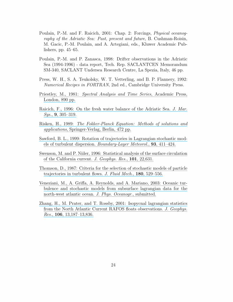
The Adriatic Sea mean surface flow is globally cyclonic (Fig. 1b) due toits mixed positive-negative estuarine circulation forced by buoyancy inputfrom the rivers (mainly the Po River) and by strong air-sea fluxes resultingin loss of buoyancy and dense water formation. The Eastern Adriatic Cur-rent (EAC) flows along the eastern side from the eastern Strait of Otrantoto as far north as the Istrian Peninsula. A return flow (the WAC) is seenflowing to the southeast along the western coast (Poulain, 1999, 2001). Re-circulation cells embedded in the global cyclonic pattern are found in thelower northern, the middle and the southern sub-basins, the latter two beingcontrolled by the topography of the Mid and South Adriatic Pits, respec-tively. These main circulation patterns are constantly perturbed by higher-frequency currents variations at inertial/tidal and meso- (e.g., 10-day timescale; Cerovecki et al., 1991) scales. In particular, the wind stress is an im-portant driving mechanism, causing transients currents that can be an order

4

of magnitude larger than the mean circulation. The corresponding lengthscale is 10-20 km, i.e., several times the baroclinic radius of deformation,which in the Adriatic can be as short as 5 km (Cushman-Roisin et al., 2001).

2.2 Turbulent transport in the Adriatic Sea and pre-

vious drifter studies

Drifter data are especially suited for transport studies since they move ingood approximation following the motion of water parcels (Niiler et al., 1995).As such, drifter data have often been used in the literature to compute pa-rameters to be used in turbulent transport and dispersion models (Davis,1991, 1994). In the Adriatic Sea, as mentioned in the Introduction, turbu-lent parameters have been previously computed by Falco et al. (2000) andPoulain (2001) as global averages over the basin. A brief overview is givenin the following.

2.2.1 Models of turbulent transport and parameter definitions

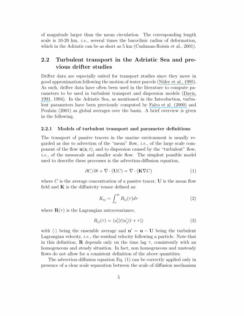
The transport of passive tracers in the marine environment is usually re-garded as due to advection of the “mean” flow, i.e., of the large scale com-ponent of the flow u(x, t), and to dispersion caused by the “turbulent” flow,i.e., of the mesoscale and smaller scale flow. The simplest possible modelused to describe these processes is the advection-diffusion equation,

∂C/∂t + ∇ · (UC) = ∇ · (K∇C) (1)

where C is the average concentration of a passive tracer, U is the mean flowfield and K is the diffusivity tensor defined as:

Kij =∫ ∞

oRij(τ)dτ (2)

where R(τ) is the Lagrangian autocovariance,

Rij(τ) = 〈u′i(t)u

′j(t + τ)〉 (3)

with 〈·〉 being the ensemble average and u′ = u − U being the turbulentLagrangian velocity, i.e., the residual velocity following a particle. Note thatin this definition, R depends only on the time lag τ , consistently with anhomogeneous and steady situation. In fact, non homogeneous and unsteadyflows do not allow for a consistent definition of the above quantities.

The advection-diffusion equation Eq. (1) can be correctly applied only inpresence of a clear scale separation between the scale of diffusion mechanism

5

and the scale of variation of the quantity being transported (Corrsin, 1974).Generalizations of Eq. (1) are possible, for example introducing a “historyterm” in Eq. (1) that takes into account the interactions between U and u′

(e.g., Davis, 1987). Alternatively, a different class of models can be used,that are easily generalizable and are based on stochastic ordinary differentialequation describing the motion of single tracer particles (e.g., Griffa, 1996;Berloff and McWilliams, 2002).

A general formulation was given by Thomson (1987) and further widelyused. The stochastic equations describing the particle state z are

dzi = ai dt + bij dWj (4)

where dW is a random increment from a normal distribution with zero meanand second order moment 〈 dWi(t) dWj(s)〉 = δijδ(t − s) dt.

Equation (1) can be seen as equivalent to the simplest of these stochas-tic models, i.e., the pure random walk model, where the particle state isdescribed by the positions, i.e., z ≡ x only, which are assumed to be Marko-vian while the velocity u′ is a random process with no memory (zero-ordermodel). A more general model can be obtained considering the particle statedefined by its position and velocity. Thus z ≡ (x,u′) are joint Markovian,so that the turbulent velocity u′ has a finite memory scale, T (first-ordermodel). In this case the model can also be applied for times shorter than thecharacteristic memory time T , in contrast to the zeroth-order model. If timesfor which acceleration is significantly correlated is important, second ordermodels should be used (Sawford, 1999). Higher order models are possible(see, e.g., Berloff and McWilliams, 2002) but they require some knowledgeon the supposed universal behavior of very elusive quantities such as timederivatives of tracer acceleration.

For a homogeneous and stationary flow with independent velocity com-ponents, the first-order model can be written for the fluctuating part u′ foreach component and corresponds to the linear Langevin equation (i.e., theOrnstein-Uhlenbeck process, see, e.g., Risken, 1989):

dxi = (Ui + u′i) dt (5)

du′i = −u′

i

Ti

dt +

√

2σ2i

Ti

dWi (6)

where σ2i and Ti are the variance and the correlation time scale of u′

i, respec-tively.

For the model (5–6), u′i is Gaussian and

Rii(τ) = σ2i exp (− τ

Ti

), (7)

6

so that Ti

Ti =1

σ2i

∫ ∞

oRii(τ) =

Kii

σ2i

(8)

corresponds to the e-folding time scale, or memory scale of u′i.

Description of more complex situations as unsteadiness and inhomogene-ity, as well as non-Gaussian Eulerian velocity field, need the more generalformulation of Thomson (1987). An accurate understanding of these situa-tions is thus necessary in order to properly choose the model to be appliedto describe transport processes to the required level of accuracy.

2.2.2 Results from previous studies in the Adriatic Sea

In Falco et al. (2000), the model (5–6) has been applied using the drifter dataset 1994-1996. The pdf for the meridional and zonal components of u′, havebeen computed for the whole dataset and found to be qualitatively close toGaussian for small and intermediate values, while differences appear in thetails.

For each velocity component, the autocovariance Eq. (3) has been com-puted and the parameters Ti and σ2

i have been estimated: σ2i ≈ 100 cm2/sec2,

Ti ≈ 2 days. These values have been used also in Lagrangian prediction stud-ies (Castellari et al., 2001) with good results. Rii(τ) computed in Falco et al.(2000) appears to be qualitatively similar to the exponential shape (Eq. (7)),at least for small τ whereas it appears to be different from exponential fortime lags τ > Ti, since the autocovariance tail maintains significantly differ-ent from zero.

In Poulain (2001), estimates of Rii(τ), Ti and Kii have been computedusing the more extensive data set 1990-1999. A different method than inFalco et al. (2000) has been used for the analysis (Davis, 1991), but the ob-tained results are qualitatively similar to the ones of Falco et al. (2000). Alsoin this case, the autocovariance Rii(τ) does not converges to zero, resultingin a Kii which does not asymptote to a constant.

There might be various reasons for the observed tails in the autocovari-ances and in the pdf. First of all, they might be an effect of poorly resolvedshears in the mean flow U. This aspect has been partially investigated inFalco et al. (2000) and Poulain (2001) using various techniques to computeU(x). Another possible explanation is related to unresolved inhomogeneityand nonstationarity in the turbulent flow. Since the estimates of the pdf andautocovariances are global, over the whole basin and over the whole timeperiod, they might be putting together different properties from different re-gions in space and time, resulting in tails. Finally, the tails might be due toinherent properties of the turbulent field, which might be different from the

7

simple picture of an Eulerian Gaussian pdf and an exponential Lagrangiancorrelation for u′.

In this paper, these open questions are addressed. A careful examinationof the dependence of turbulent statistics on the mean flow U estimation isperformed. Possible dependence on spatial inhomogeneity is studied, par-titioning the domain in approximatively homogeneous regions. Finally, anattempt to resolve seasonal time dependence is performed.

3 Data and methods

3.1 The drifter data set

As part of various scientific and military programs, surface drifters werelaunched in the Adriatic in order to measure the temperature and currentsnear the surface. Most of the drifters were of the CODE-type and followedthe currents in the first meter of water with an accuracy of a few cm/s(Poulain and Zanasca, 1998; Poulain, 1999). They were tracked by, and re-layed SST data to, the Argos system onboard the NOAA satellites. Moredetails on the drifter design, the drifter data and the data processing can befound in Poulain et al. (2003). Surface velocities were calculated from thelow-pass filtered drifter position data and do not include tidal/inertial com-ponents. The Adriatic drifter database includes the data of 201 drifters span-ning the time period between 1 August 1990 and 31 July 1999. It containstime series of latitude, longitude, zonal and meridional velocity componentsand sea surface temperature, all sampled at 6-h intervals. Due to their shortoperating lives (half life of about 40 days), the drifter data distribution isvery sensitive to the specific locations and times of drifter deployments. Themaximum data density occurs in the southern Adriatic and in the Strait ofOtranto. Most of the observations correspond to the years 1995-1999.

3.2 Statistical estimate of the mean flow: averaging

scales

Estimating the mean flow U(x, t) is of crucial importance for the identifi-cation of the turbulent component u′, since u′ is computed as the velocityresidual following trajectories. If the space and time scales of U(x, t) are notcorrectly evaluated, they can seriously contaminate the statistics of u′. Par-ticularly delicate is the identification of the space scales of the mean shearsin U, since they can be relatively small (of the same order as the scales ofturbulent mesoscale variability), and, if not resolved, they can result in per-

8

sistent tails in the autocovariances and spuriously high estimates of turbulentdispersion (e.g., Bauer et al., 1998). Identifying a correct averaging scale La

for estimating U is therefore a very important issue for estimating the u′

statistics.Various methods can be used to estimate U. Here we consider two meth-

ods: the classic methods of bin averaging and a method based on optimizedbicubic spline interpolation (Inoue 1986, Bauer et al., 1998). Results fromthe two methods are compared, in order to test their robustness. The re-sults from bin averaging are discusses first, since the method is simpler andit allows for a more straightforward analysis of the impact of the averagingscales on the estimates.

For the bin averaging method, La simply corresponds to the bin size. Inprinciple, given a sufficiently high number of data, an appropriate averagingscale L̂a can be identified such that the mean flow shear is well resolved.The u′ and U statistics are expected to be independent on La for La < L̂a.In practical applications, though, the number of data is limited and theaveraging scale is often chosen as a compromise between the high resolution,necessary to resolve the mean shear, and the data density per bin, necessaryto ensure significant estimates. In practice, then, La is often chosen as La >L̂a and the asymptotic independency of the statistics on La is not reached.

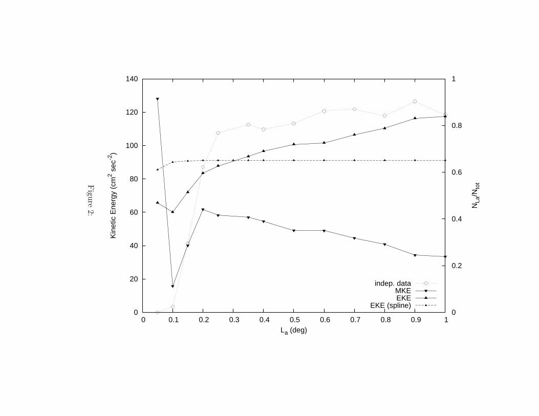
Poulain (2001) tested the dependence of the mean and eddy kinetic en-ergy, MKE and EKE, on the bin averaging scale La for the 1990-1999 dataset. Circular, overlapping bins with radius varying between 400 and 12.5km were considered. It was found that, in the considered range, EKE andMKE (computed over the whole basin) do not converge toward a constantat decreasing La. A similar calculation is repeated here (Fig. 2), consideringsome modifications. First of all, we consider square bins nonoverlapping, tofacilitate the computation of turbulent statistics, such as R(τ), which involveparticle tracking. Also the EKE and MKE estimates are computed consid-ering only “significant” bins, i.e., bins with more than 10 independent data,nbi > 10, where nbi is computed resampling each trajectory with a periodT = 2 days, on the basis of previous results from Falco et al. (2000) andPoulain (2001). Finally, the values of EKE and MKE are displayed in Fig. 2together with a parameter, NLa/Ntot, providing information on the statisticalsignificance of the results at a given La. NLa/Ntot, in fact is the fraction ofdata actually used in the estimates (i.e., belonging to the significant bins)over the total amount of data in the basin Ntot.

The behavior of EKE and MKE in Fig. 2 is qualitatively similar to whatshown in Poulain (2001), even though the considered range is slightly dif-ferent and reaches lower values of La (bin sizes vary between 1

◦

and 0.05◦

).The values of EKE and MKE do not appear to converge at small La, but the

9

interesting point is that they tend to vary significantly for La < 0.25◦

, i.e.,

in correspondence to the drastic decrease of NLa/Ntot. This suggests thatthe strong lack of saturation at small scales is mainly due to the fact thatincreasingly fewer bins are significant and therefore the statistics themseplvesbecome meaningless. These considerations suggest that the “optimal” scaleLa, given the available number of data Ntot is of the order of 0.25

◦

, sinceit allows for the highest shear resolution still maintain a significant num-ber of data (≈ 80%). This choice is in agreement with previous results byFalco et al. (2000) and Poulain (1999).

The binned mean field U obtained with the 0.25◦

bin (i.e., between 19and 28 km) is shown in Fig. 4. As it can be seen, it is qualitatively similarto the U field obtained by Poulain (2001, Fig. 1b) with a 20 km circular binaverage.

As a further check on the binned results and on the La choice, a compari-son is performed with results obtained using the spline method (Bauer et al.,1998, 2002). This method, previously applied by Falco et al., (2000) to the1994-1996 data set, is based on a bicubic spline interpolation (Inoue, 1986)whose parameters are optimized in order to guarantee minimum energy inthe fluctuation field u′ at low frequencies. Notice that, with respect to thebinning average technique, the spline method has the advantage that theestimated U(x) is a smooth function of space. As a consequence, the valuesof the turbulent residuals u′ can be computed subtracting the exact values ofU along trajectories, instead than considering discrete average values insideeach bin. In other words, the spline technique allows for a better resolutionof the shear inside the bins.

Details on the choice of the spline parameters are given in Appendix.The resulting statistics are compared with the binned results in Fig. 2. Theturbulent residual u′ has been computed subtracting the splined U, and theassociated EKE have been calculated as function of La. The EKE dependenceon size for very small scales is due to the fact that EKE is computed as anaverage over significant bins and the number of bins decreases for small La.In the case of the binned U described before, instead, also the estimatesof U and u′ inside each grid change and deteriorate as La decreases. As aconsequence, it is not surprising that the EKE values change much less inthe splined case with respect to the binned case. Notice that the splinedEKE values are very similar to the binned ones for bins in the range between0.35

◦ − 0.25◦

. This provides support to the choice of La = 0.25◦

. Also, adirect comparison between the splined (not shown) and binned U fields showa great similarity, as already noticed also in the case of Falco et al. (2000).

In conclusion, the spline analysis confirms that the choice of La = 0.25◦

is appropriate. La = 0.25◦

, in fact, provides robust estimates while resolv-

10

ing the important spatial variations of the mean flow and averaging themesoscale.

3.3 Homogeneous regions for turbulence statistics

We are interested in identifying regions where the u′ statistics can be consid-ered approximately homogeneous, so that the main turbulent properties canbe meaningfully studied. In a number of studies in various oceans and for var-ious data sets (Swenson and Niiler, 1996; Bauer et al., 2002; Veneziani et al.,2003), “homogeneous” regions have been identified as regions with consistentdynamical and statistical properties. A first qualitative identification of con-sistent dynamical regions in the Adriatic Sea can be made based on theliterature and on the knowledge of the mean flow and of the topographicstructures (Fig. 1).

First of all, two boundary current regions can be identified, along theeastern coast (Eastern Adriatic Current, EAC) and western coast (WesternAdriatic Current, WAC). These regions are characterized by strong meanflows and well organized current structure. A third region can be identi-fied with the central area of the cyclonic gyre in the south/central Adriatic(Central Gyre, CG). This region is characterized by a deep topography (espe-cially in the southern part) and by a weaker mean flow structure. Finally, thenorthern part of the basin, characterized by shallow depth (< 50 m), couldbe considered as a forth region (Northern Region, NR). With respect to theother regions, though, NR appears less dynamically homogeneous, given thatthe western side is heavily dominated by buoyancy forcing related to the Poriver discharge, while the eastern part is more directly influenced by windforcing. Also, NR has a lower data density with respect to the other regions(Poulain, 2001). For these reasons, in the following we will focus on EAC,WAC and CG. A complete analysis of NR will be performed in future works,when more data will be available.

As a second step, a quantitative definition of the boundaries betweenregions must be provided. Here we propose to use as a main parame-ter to discriminate between regions the relative turbulence intensity γ =√

EKE/MKE. The parameter γ is expected to vary from γ < 1 in theboundary current regions dominated by the mean flow, to γ > 1 in the thecentral gyre region dominated by fluctuations.

A scatterplot of γ versus√

MKE is shown in Fig. 3. Two well definedregimes can be seen, with γ < 1 and γ > 1 respectively. The two regimesare separated by

√MKE ≈ 6 − 7 cm sec−1. Based on this result, we use the

(conservative) value√

MKE = 8 cm sec−1 to discriminate between regions.The resulting partition is shown in Fig. 4. As it can be seen, the regions

11

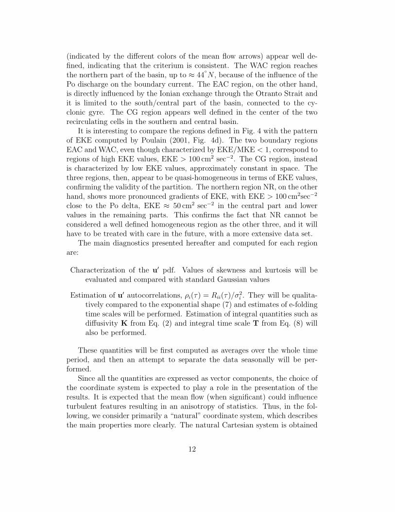
(indicated by the different colors of the mean flow arrows) appear well de-fined, indicating that the criterium is consistent. The WAC region reachesthe northern part of the basin, up to ≈ 44

◦

N , because of the influence of thePo discharge on the boundary current. The EAC region, on the other hand,is directly influenced by the Ionian exchange through the Otranto Strait andit is limited to the south/central part of the basin, connected to the cy-clonic gyre. The CG region appears well defined in the center of the tworecirculating cells in the southern and central basin.

It is interesting to compare the regions defined in Fig. 4 with the patternof EKE computed by Poulain (2001, Fig. 4d). The two boundary regionsEAC and WAC, even though characterized by EKE/MKE < 1, correspond toregions of high EKE values, EKE > 100 cm2 sec−2. The CG region, insteadis characterized by low EKE values, approximately constant in space. Thethree regions, then, appear to be quasi-homogeneous in terms of EKE values,confirming the validity of the partition. The northern region NR, on the otherhand, shows more pronounced gradients of EKE, with EKE > 100 cm2sec−2

close to the Po delta, EKE ≈ 50 cm2 sec−2 in the central part and lowervalues in the remaining parts. This confirms the fact that NR cannot beconsidered a well defined homogeneous region as the other three, and it willhave to be treated with care in the future, with a more extensive data set.

The main diagnostics presented hereafter and computed for each regionare:

Characterization of the u′ pdf. Values of skewness and kurtosis will beevaluated and compared with standard Gaussian values

Estimation of u′ autocorrelations, ρi(τ) = Rii(τ)/σ2i . They will be qualita-

tively compared to the exponential shape (7) and estimates of e-foldingtime scales will be performed. Estimation of integral quantities such asdiffusivity K from Eq. (2) and integral time scale T from Eq. (8) willalso be performed.

These quantities will be first computed as averages over the whole timeperiod, and then an attempt to separate the data seasonally will be per-formed.

Since all the quantities are expressed as vector components, the choice ofthe coordinate system is expected to play a role in the presentation of theresults. It is expected that the mean flow (when significant) could influenceturbulent features resulting in an anisotropy of statistics. Thus, in the fol-lowing, we consider primarily a “natural” coordinate system, which describesthe main properties more clearly. The natural Cartesian system is obtained

12

rotating locally along the mean flow axes. The components of a quantityQ in that system are the streamwise componente Q‖ and the across-streamcomponente Q⊥.

4 Results

4.1 Statistics in the homogeneous regions

Here the statistics of u′ in the three regions identified in Section 3.3 are com-puted averaging over the whole time period, i.e., assuming stationarity overthe 9 years of measurements. In all cases, u′ is computed as residual velocitywith respect to the 0.25

◦ × 0.25◦

binned mean flow, as explained in Section3.2. In some selected cases, results from other bin sizes and from the splinemethod are considered as well, in order to further test the influence of the U

estimation on the results. As in Section 3, the statistics are computed only inthe significant bins, nb > 10. Also, data points with velocities higher than 6times the standard deviations have been removed. They represent an ensem-ble of isolated events that account for 10 data points in total, distributed over4 drifters. While they do not significantly affect the second order statistics,they are found to affect higher order moments such as skewness and kurtosis.

4.1.1 Characterization of the velocity pdf

The pdf of u′ is computed normalizing the velocity locally, using the vari-ance σ2

b computed in each bin (Bracco et al., 2000). This is done in orderto remove possible residual inhomogeneities inside the regions. The pdfs arecharacterized by the skewness Sk = 〈u′3〉/σ3 and the kurtosis Ku = 〈u′4〉/σ4.Here we follow the results of Lenschow et al. (1994), which provide error esti-mates for specific processes at different degrees of non-gaussianity as functionof the total number of independent data Ni. In the range of our data (Ta-ble 1), the mean square errors of Sk and Ku from Lenschow et al. (1994)appear to be (δSk)2 ≈ 10/Ni, (δKu)2 ≈ 330/Ni. Notice that these values canbe considered only indicative, since they are obtained for a specific process.

Before going into the details of the results and discussing them from aphysical point of view, a preliminary statistical analysis is carried out to testthe dependence of the higher moments Sk and Ku from the bin size, similarlyto what done in Section 3.2 for the lower order moments. In Fig. 5a,b, esti-mates of Sk and Ku computed over the whole basin (in Cartesian coordinate)are shown, at varying bin size from 1

◦

to 0.2◦

(smaller bins are not consideredgiven the small number of independent data, see Fig. 2). Given that the totalnumber of independent data is of the order of Ni ≈ 4000, the error estimates

13

from Lenschow et al. (1994) suggest√

(δSk)2 ≈ 0.05,√

(δKu)2 ≈ 0.25. As itcan be seen, the values of Sk and Ku do not change significantly in the range0.5

◦ − 0.25◦

. Values of Sk and Ku have also been computed using splinedestimates (not shown), and they are found to fall in the same range. Theseresults confirm the choice of the 0.25

◦

binning of Section 3.2. Notice that,since Sk and Ku in Fig. 5a,b are computed averaging over different dynamicalregions, their values do not have a straightforward physical interpretation.We will come back on this point in the following, after analyzing the specificregions.

The pdfs for the three regions computed with the 0.25◦

binning are shownin Fig. 6a,b,c in natural coordinates, while the Sk and Ku values are sum-

marized in Table 1. For each region, Ni ≈ 1000, so that√

(δSk)2 ≈ 0.1,√

(δKu)2 ≈ 0.5. Furthermore, a quantitative test on the deviation from gaus-

sianity has been performed using the Kolmogorov-Smirnov test (Priestley,1981; Press et al., 1992). Notice that the K-S test is known to be mostlysensitive to the distribution mode (i.e., to the presence of asymmetry, orequivalently to Sk being different from zero), while it can be quite insensitiveto the existence of tails in the distribution (large Ku). More sophisticatedtests should be used to guarantee sensitivity to the tails.

Let’s start discussing the Eastern boundary region, EAC. The Sk is pos-itive and significant in the along component (Sk‖ ≈ 0.48), while it is onlymarginally different from zero in the cross component (Sk⊥ ≈ −0.14). Pos-itive skewness indicates that the probability of finding high positive valuesof u′

‖ is higher than the probability of negative high values, (while the oppo-site is true for small values). This is also shown by the pdf shape (Fig. 6a).Physically, this indicates the existence of an anisotropy in the current, withthe fluctuations being more energetic in the direction of the mean flow. Thisasymmetry is not surprising, given the existence of a privileged direction inthe mean. This fact has long been recognized in boundary layer flows (e.g.,Durst et al., 1987). The cross component, on the other hand, does not havea privileged direction and its Sk is much smaller, as shown also by the pdfshape. The values of the kurtosis Ku are around 4 for both components,indicating high probability for energetic events. This is clear also from thehigh tails in the pdf.

The K-S statistics computed for the pdfs of Fig. 6a are α = 0.012 for u′‖

indicating rejection of the null hypothesis (that the distribution is Gaussian)at the 95% confidence level. For the cross component u′

⊥, instead, α = 0.09so that the null hypothesis cannot be rejected. It is worth noting that theestimates of α depend on the number of independent data Ni, which in turndepends on T . Here, T is assumed T = 2 days. For the cross component,

14

this is probably an overestimate (as it will be shown in the following, seeFig. 7b), and T = 1 day is probably a better assumption. Even if computedwith T = 1 days, α = 0.04 for u′

⊥, suggesting that the Gaussian hypothesiscan be only marginally rejected.

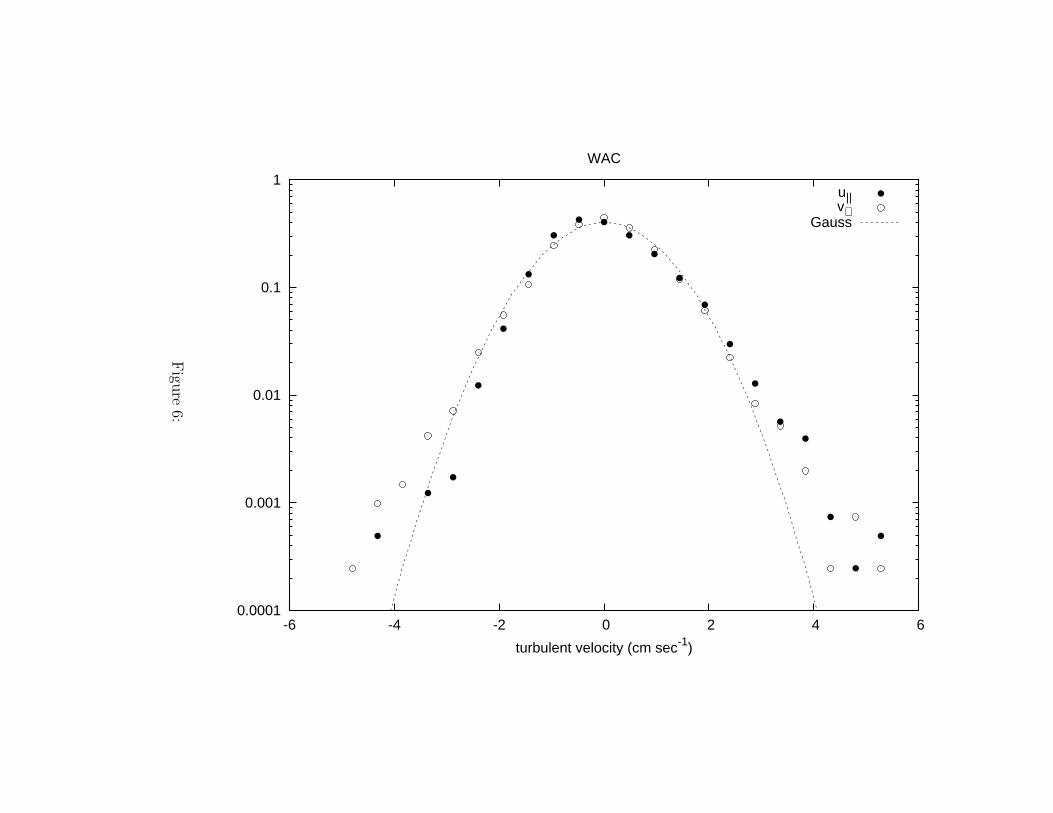
The results for the western boundary region WAC are qualitatively simi-lar to the ones foe EAC. The Sk values in natural coordinates are Sk‖ ≈ 0.52and Sk⊥ ≈ 0.09, suggesting the same along current anisotropy found in EAC.Notice that the total value of Sk computed over the whole basin (Fig. 5a)is approximately zero, because the two contributions from the two boundarycurrents nearly cancel each other when computed in fixed cartesian coordi-nates.

Also the structure of the pdfs (Fig. 6b) are qualitatively similar to theEAC ones, exhibiting a clear asymmetry and high tails, especially for u′

‖.The K-S statistics are α = 0.027 for u′

‖, suggesting a significant deviationfrom gaussianity. For u′

⊥, on the other hand, α = 0.4 (α = 0.097 for T = 1day), which is not significantly different from Gaussian.

The central region, CG, has lower values of Sk in both components (0.16and −0.02 respectively). This is shown also by the pdf patterns (Fig. 6c),which are more symmetric than for EAC and WAC. This is not surprisinggiven that the mean flow is weaker in CG, so that there is no privilegeddirection. The tails, on the other hand, are high also in CG, as shown by theKu values that are in the same range (and actually slightly higher) than forEAC and WAC. The K-S statistics do not show a significant deviation fromgaussianity in any of the two components, α = 0.44 for u′

‖ and α = 0.33 foru′⊥ (α = 0.058 for T = 1 day). This is due to the fact that the K-S test is

mostly sensitive to the mode, as explained above.In summary, the turbulent component along the mean flow is significantly

non Gaussian and, in particular, asymmetric in both boundary currents.The strong mean flow determines the existence of a privileged direction,resulting in anisotropy of the fluctuation, with more energetic events in thedirection of the mean. The central gyre region and the cross component ofthe boundary currents, do not appear significantly skewed. For all regionsand all components, though, the kurtosis is higher than 3 consistently withother recent findings (Bracco et al., 2000). indicating the likelihood of highenergy events.

4.1.2 Autocorrelations of u′

The autocorrelations in natural components are shown in Fig. 7a,b The alongcomponent results ρ‖(τ), are shown in Fig. 7a for the 3 regions and for thewhole basin. Errorbars are computed as 1/N where N is the number of in-

15

dependent data for each time lag t. The autocorrelation for the whole basinshows two different regimes with approximately exponential behavior. Thenature of this shape can be better investigated considering the three homo-geneous regions separately. For small lags exponential behavior is evident inall the three regions, with a slightly different e-folding time scales: τexp ≈ 1.8days for EAC and WAC and ≈ 1.1 days for CG. The above values werecomputed fitting the exponential function on the first few time lags. Thisis consistent with the fact that τexp is representative of fluctuations due toprocesses such as internal instabilities and direct wind forcing, which are ex-pected to be different in the boundary currents and in the gyre center. Atlonger lags τ > 3 − 4 days, the behavior in the three regions become evenmore distinctively different. In region EAC, a clear change of slope occurs,indicating that ρ‖ can be characterized by a secondary exponential behaviorwith a slower decay time of ≈ 11-12 days. Only a hint of this secondary scaleis present in WAC, while there is no sign of it in CG. The behavior of thebasin average ρ‖, then, appears to be determined mostly by the EAC region.

In contrast to the along component behavior, the cross component, ρ⊥,(Fig. 7b) appears characterized by a fast decay in all three region as well as inthe basin average (τexp ≈ 0.5−0.7 days), with a significative loss of correlationfor time lags less than 1 day. This can be qualitatively understood consideringas a reference the behavior of parallel and transverse Eulerian correlationsin homogeneous isotropic turbulence (Batchelor, 1970). It indicates thatthe turbulent fluctuations, linked to mean flow instabilities, tend to developstructures oriented along the mean current. As a consequence, the crossmean flow dispersion is found to be very fast and primarily dominated bya diffusive regime, while the along mean dispersion tends to be slower anddominated by more persistent coherent structures. This result suggest that acorrelation time of 2 days (as estimated in Poulain, 2001; Falco et al., 2000)is actually a measure of mixed properties.

In summary, the results show that the eastern boundary region EACis intrinsically different from the center gyre region CG and also partiallydifferent from the western boundary region WAC. While CG (and partiallyWAC) are characterized by a single scale of the order of 1-2 day, EAC isclearly characterized by 2 different time scales, a fast one (order of 1-2 days)and a significantly longer one (order of 11-12 days). The physical reasonsbehind this two-scale behavior is not completely understood yet, and somepossible hypotheses are discussed below.

Falco et al (2000) suggested that the observed autocorrelation tails couldbe due to a specific late summer 1995 event sampled by a few drifters launchedin the Strait of Otranto. In order to test this hypothesis, we have removedthis specific subset of drifters and re-computed ρ‖. The results (not shown)

16

do not show significant differences and the 2 scales are still evident.A possible hypothesis is that the 2 scales are due to different dynamical

processes co-existing in the system. The short time scale appears almost cer-tainly related to mesoscale instability and wind-driven synoptic processes,while the longer time scale might be related to low frequency fluctuations inthe current, due for instance to changes in wind regimes or to inflow pulsesthrough the Strait of Otranto This is suggested by the presence of a 10 dayperiod fluctuation in Eulerian currentmeter records (Poulain, 1999). Finally,another possibility is that the longer time scale is related to the spatial struc-ture of the mean flow, namely its curvatures. Such curvature appears morepronounced and consistently present in the circulation pattern of the EACthan in the WAC, in agreement with the fact that the the secondary scaleis more evident in EAC. At this point, not enough data are available toquantitatively test these hypotheses and clearly single out one of them.

4.1.3 Estimates of K and T parameters

From the autocorrelations of Fig. 7a,b, the components of the diffusivity andintegral time scale Eq. (2) and Eq. (8) can be computed by integration. T andK are input parameters for models, and are therefore of great importance inpractical applications. Estimates of the natural components of T, T‖(t) andT⊥(t), are shown in Fig. 8a,b for the three regions and for t < 10 days. Thebehavior of the K components is the same as for T, since for each componentT (t) = K(t)/σ2 (8). The values of T‖(t), T⊥(t). K‖(t). K⊥(t) at the end ofthe integration, at t = 10 days, are reported in Table 2.

The along component T‖(t) (Fig. 8a) shows a significantly different be-havior in the three regions. In CG, T‖(t) converges toward a constant, so thatthe asymptotic value is well defined, T‖ ≈ 1.2 day. This approximately corre-sponds to the estimate of τexp ≈ 0.8 from Fig. 7a. In EAC, instead, T‖ is notwell defined, given that T‖(t) keeps increasing, reaching a value of ≈ 2.7 daysat t = 10 days, significantly higher than τexp ≈ 1.4 days. Finally, WAC showsan intermediate behavior, with T‖(t) growing slowly and reaching a value of≈ 1.9 days, slightly higher than τexp ≈ 1.4 days. These results are consistentwith the shape of ρ‖ (Fig. 7a) in the three regions. The values of K‖ (10 days)(Table 2) range between 0.7×106 cm2 sec−1 and 3.8×107 cm2 sec−1 showinga marked variability because of the different EKE in the three regions.

The cross component T⊥(t) (Fig. 8b) shows little variability in all thethree regions, again in keep with the ρ⊥ results (Fig. 7b). In all the regions,T⊥(t) converges toward a constant value of T⊥ ≈ 0.52−0.78 days, in the samerange as the τexp values. More in details, notice that in WAC T⊥(t) tends todecrease slightly, possibly in correspondence to saturation phenomena due

17

to boundary effects. The values of K⊥ (10 days) in Table 2 range between1.4 × 106 cm2 sec−1 and 3.1 × 106 cm2 sec−1.

In summary, the results show that the cross components T⊥ and K⊥ arewell defined in the three regions, with T⊥ approximately corresponding toτexp. The along components T‖ and K‖, instead, are well defined only in CG,while in the boundary regions and especially in EAC, there is no convergenceto an asymptotic value.

The observed values are quite consistent with the averages reported inPoulain (2001). Remarkably, in that paper, the strong inhomogeneity andanisotropy of the flow in the basin was outlined, noting that the estimatesof the time scales for the along flow components in the boundary currents issignificantly larger than the one related to the central gyre.

4.2 Seasonal dependence

As an attempt to consider the effects of non-stationarity, a time partition ofthe data is performed grouping them in seasons. The data are not sufficientto resolve space and time dependence together, since the u′ statistics arequite sensitive involving higher moments and time lagged quantities. For thisreason, averaging is computed over the whole basin and two main extendedseasons are considered. Based on preliminary tests and on previous results byPoulain (2001), the following time partition is chosen: a summer-fall season,spanning July to December, and a winter-spring season, spanning Januaryto June.

As in Section 4.1, u′ is computed as residual velocity with respect to the0.25

◦ × 0.25◦

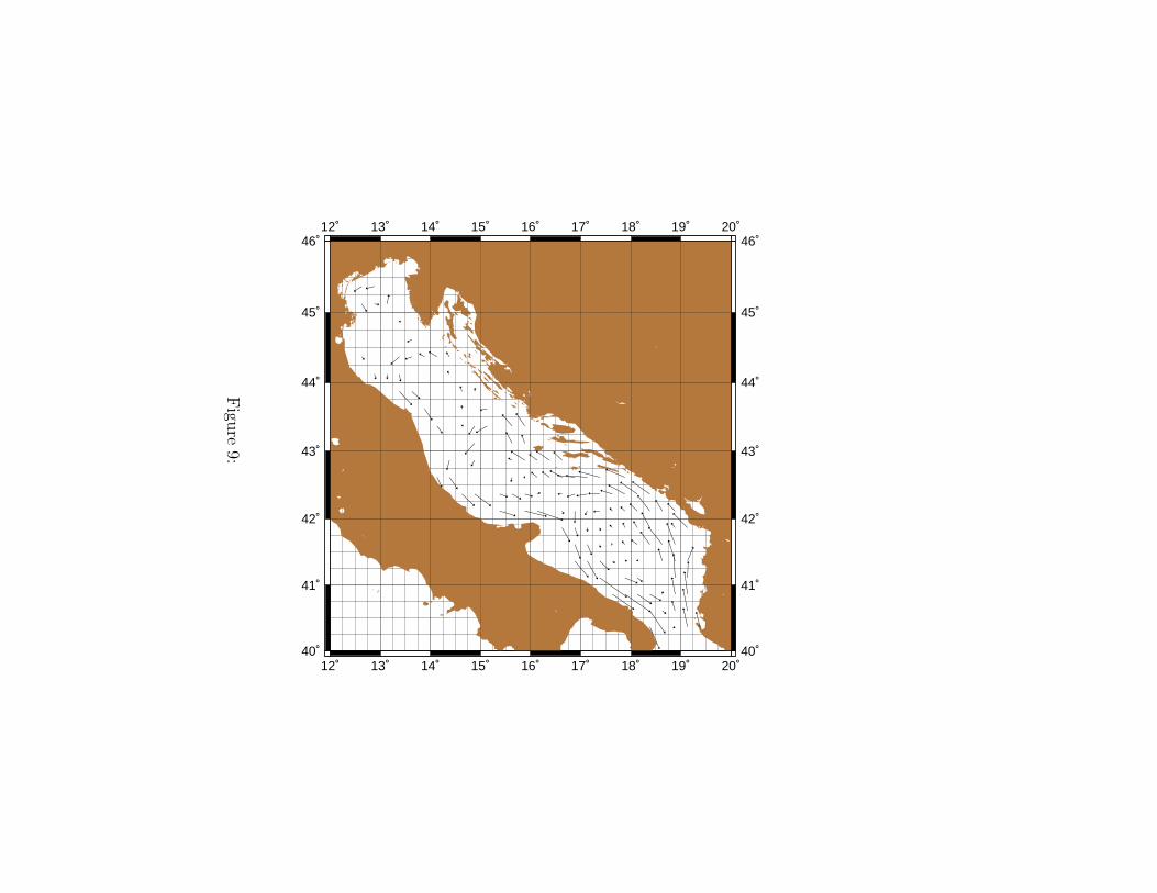
binned mean flow U. Mean flow estimates in the 2 seasonsare shown in Fig. 9a,b. As discussed in Poulain (2001), during summer-fallthe mean circulation appears more energetic and characterized by enhancedboundary currents. During the winter-spring season, instead, mean currentsare generally weaker and the southern recirculating gyre is enhanced.

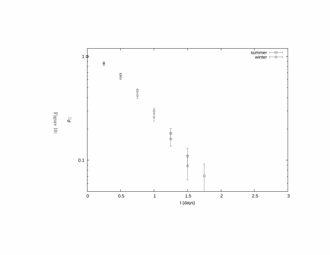
The u′ statistics during the 2 seasons are characterized by the autocorre-lation functions shown in Fig. 10a,b. The along component ρ‖(τ) (Fig. 10a)has a distinctively different behavior in the 2 seasons. In summer-fall, theoverall behavior is similar to the one obtained averaging over the whole pe-riod (Fig. 7a). Two regimes can be seen, one approximately exponential atsmall lags, and a secondary one at longer lags, τ > 3days, with significantlyslower decay. This secondary regime is not observed in winter-spring. As forthe cross component ρ⊥(τ) (Fig. 10b), both seasons appears characterizedby a fast decay, as in the averages over the whole period (Fig. 10b).

Various possible explanations for the longer time scale in ρ‖(τ) have beendiscussed in Section 4.1 for the whole time average. They include low-

18

frequency forcing and current fluctuations, as well as the effects of the meanflow curvature in the boundary currents. The summer-fall intensification ofFig. 10a,b does not rule out any of these explanations, given that the strengthand variability of the boundary currents are intensified especially in the fall.

4.3 Summary and concluding remarks

In this paper, the properties of the Lagrangian mesoscale turbulence u′ inthe Adriatic Sea (1990-1999) are investigated, with special case to give aquantitative estimate of spatial inhomogeneity and nonstationarity.

The turbulent field u′ is estimated as the residual velocity with respect tothe mean flow U, computed from the data using the bin averaging technique.In a preliminary investigation, the dependence of u′ on the bin size La isstudied and a preferential scale La = 0.25

◦

is chosen. This scale allows forthe highest mean shear resolution still maintaining a significant amount ofdata (≈ 80%). Values of higher moments such as skewness Sk and kurtosisKr are found to be approximately constant in the La range around 0.25

◦

.Further support to the choice La = 0.25

◦

is given by the comparison withresults obtained with independent estimates of U based on an optimizedspline technique (Bauer et al., 1998, 2002).

The effects of inhomogeneity and stationarity are studied separately, be-cause there are not enough data to perform a simultaneous partition in spaceand time. The spatial dependence is studied first, partitioning the basin inapproximately homogeneous regions and averaging over the whole time pe-riod. The effects of nonstationarity are then considered, partitioning the dataseasonally, and averaging over the whole basin.

Three main regions where the u′ statistics can be considered approxi-mately homogeneous are identified. They correspond to the two (easternEAC, and western WAC) boundary current regions, characterized by both

strong mean flow and high kinetic energy (√

EKE/MKE < 1)), and thecentral gyre region CG in the southern and central basin, characterized by

weak mean current and low eddy kinetic energy (√

EKE/MKE > 1). Thenorthern region is not included in the study because, in addition to have alower data density with respect to the other regions, it appears less dynami-cally and statistically homogeneous.

The properties of u′ in the three regions are studied considering pdfs,autocorrelations and integral quantities such as diffusivity and integral timescales. Natural coordinates, oriented along the mean flow direction, are used,since they allow to better highlight the dynamical properties of the flow.

The pdfs results indicate that the CG region is in good approximation

19

isotropic with high kurtosis values, while the along components of the bound-ary regions EAC and WAC show significant asymmetry (positive skewness).This is related to energetic events occurring preferentially in the same di-rection as the mean flow. Both boundary regions appear significantly non-Gaussian, while the Gaussian hypothesis cannot be rejected in the CG region.

Both components of the autocorrelation are approximately exponential inCG, and the integral parameters Tii and Kii are well defined, with values ofthe order of 1 day and 6 106 cm2 sec−1 respectively. In the boundary regions,instead, the along component of the autocorrelation shows a significant “tail”at lags τ > 4 days, especially in EAC. This tail can be characterized as asecondary exponential behavior with slower decay time of ≈ 11-12 days.As a consequence, the integral parameters do not converge for times lessthan 10 days. Possible physical reasons for this secondary time scale arediscussed, in terms of low frequency fluctuations in the wind regime and inthe Otranto inflow, or in terms of topographic and mean flow curvaturesinducing fluctuations in the particle trajectories.

The effects of non-stationarity have been partially evaluated partitioningthe data in two extended seasons, corresponding to winter-spring (Januaryto June) and summer-fall (July-December). The secondary time scales in thealong autocorrelation is found to be present only during summer-fall, whenthe mean boundary currents are more enhanced and more energetic.

On the basis of these statistical analysis, the following indications forthe application of transport models can be given. The statistics of u′, andtherefore its modelling description, are strongly inhomogeneous in the threeregions not only in terms of parameter values but also in terms of inherent tur-bulent properties. It is therefore not surprising that the results of Falco et al.(2000) show differences between data and model results, given that the modeluses global parameters and assumes gaussianity over the whole basin. Onlyregion CG can be characterized by homogeneous and Gaussian turbulenceand therefore can be correctly described using a classical Langevin equationsuch as the one used by Falco et al. (2000). The boundary regions and espe-cially EAC, on the other hand, are not correctly described by such a model,because of the presence of a secondary time scale and of significant deviationsfrom gaussianity. Similar deviations have been observed in other Lagrangiandata in various ocean regions (Bracco et al., 2000), even though the ubiq-uity of the result is still under debate (Zhang et al., 2001). Non-Gaussian,multi scale models are known in the literature (e.g., Pasquero et al., 2001;Maurizi and Lorenzani, 2001) and their application is expected to stronglyimprove results of transport modelling in the Adriatic Sea.

20

Appendix: Spline method for estimating U

The spline method used to estimate U (Bauer et al., 1998, 2002) is basedon the application of a bicubic spline interpolation (Inoue, 1986) with opti-mized parameters to guarantee minimum energy of the fluctuation u′ at lowfrequencies. This is done by minimizing a simple metrics which depends onthe integration of the autocovariance R(τ) for τ > T . In other words, theautocovariance tail is required to be “as flat as possible” under some addi-tional smoothing requirements. This method, previously applied by Falco etal. (2000) to the 1994-1996 data set, has been applied 1990-1999 data set.

The spline results depend on four parameters (Inoue, 1986): the values ofthe knot spacing, which determines the number of finite elements, and threeweights associated respectively with the uncertainties in the data, in the firstderivatives (tension) and in the second derivatives (roughness). The tensioncan be fixed a-priori in order to avoid anomalous behavior at the boundaries(Inoue, 1986). The other three parameters have been varied in a wide rangeof values (knot spacing between 1

◦

and 0.1◦

, data uncertainty between 50and 120 cm2sec−2 and roughness between 0.001 and 10000). It is found thatan optimal estimate of U is uniquely defined over the whole parameter spaceexcept for the smallest knot spacing, corresponding to 0.1

◦

. In this case, nooptimal solution is found, in the sense that the metric does not asymptoteand the U field becomes increasingly more noisy as the roughness increases.This indicates that, as it can be intuitively understood, there is a minimumresolution related to the number of data available.

Acknowledgements

The authors are indebted to Fulvio Giungato for providing helpful resultsof a preliminary data analysis performed as a part of his Degree Thesys atUniversity of Urbino, Italy. The authors greatly appreciate the support ofthe SINAPSI Project (A.Maurizi, A. Griffa, F. Tampieri) and of the Of-fice of Naval Research, grant (N00014-97-1-0620 to A. Griffa and grantsN0001402WR20067 and N0001402WR20277 to P.-M. Poulain).

References

Artegiani, A., D. Bregant, E. Paschini, N. Pinardi, F. Raicich, and A. Russo,1997: The Adriatic Sea general circulation, part II: Baroclinic circulationstructure. J. Phys. Oceanogr., 27, 1515–1532.

21

Batchelor, G., 1970: The theory of homogeneous turbulence, Cambridge Uni-versity Press.

Bauer, S., M. Swenson, and A. Griffa, 2002: Eddy-mean flow decompositionand eddy-diffusivity estimates in the tropical pacific ocean. part 2: Results.J. Geophys. Res., 107, 3154–3171.

Bauer, S., M. Swenson, A. Griffa, A. Mariano, and K. Owens, 1998: Eddy-mean flow decomposition and eddy-diffusivity estimates in the tropicalpacific ocean. part 1: Methodology. J. Geophys. Res., 103, 30,855–30,871.

Berloff, P. and McWilliams, 2002: Material transport in oceanic gyres. partii: Hierarchy of stochastic models. J. Phys. Oceanogr., 32, 797–830.

Bracco, A., J. LaCasce, and A. Provenzale, 2000: Velocity pdfs for oceanicfloats. J. Phys. Oceanogr., 30, 461–474.

Castellari, S., A. Griffa, T. Ozgokmen, and P.-M. Poulain, 2001: Prediction ofparticle trajectories in the Adriatic Sea using lagrangian data assimilation.J. Mar. Sys., 29, 33–50.

Cerovecki, I., Z. Pasaric, M. Kuzmic, J. Brana, and M. Orlic, 1991: Ten-dayvariability of the summer circulation in the North Adriatic. Geofizika, 8,67–81.

Corrsin, S., 1974: Limitation of gradient transport models in random walksand in turbulence. Annales Geophysicae, 18A, 25–60.

Cushman-Roisin, B., M. Gacic, P.-M. Poulain, and A. Artegiani, 2001: Phys-

ical oceanography of the Adriatic Sea: Past, present and future, KluwerAcademic Publishers, 316 pp.

Davis, R., 1987: Modelling eddy transport of passive tracers. J. Mar. Res.,45, 635–666.

Davis, R., 1991: Observing the general circulation with floats. Deep-Sea

Research, 38, S531–S571.

Davis, R., 1994: Lagrangian and eulerian measurements of ocean transportprocesses, Ocean Processes in climate dynamics: Global and Mediterranean

examples, P. Malanotte-Rizzoli and A. R. Robinson, eds., Eds., KluwerAcademic Publishers, pp. 29–60.

22

Durst, F., J. Jovanovic, and L. Kanevce, 1987: Probability density distri-butions in turbulent wall boundary-layer flow, Turbulent Shear Flow 5,F. Durst, B. E. Launder, J. L. Lumley, F. W. Schmidt, and J. H. Whitelaw,eds., Springer, pp. 197–220.

Falco, P., A. Griffa, P.-M. Poulain, and A. Zambianchi, 2000: Transportproperties in the Adriatic Sea as deduced from drifter data. J. Phys.

Oceanogr., 30, 2055–2071.

Griffa, A., 1996: Applications of stochastic particle models to oceanographicproblems, Stochastic Modelling in Physical Oceanography, P. M. R.J. Adlerand B. Rozovskii, eds., Birkhauser, pp. 114–140.

Inoue, 1986: A least square smooth fitting for irregularly spaced data: Finiteelement approach using the cubic β-spline. Geophysics, 51, 2051–2066.

Lenschow, D. H., J. Mann, and L. Kristensen, 1994: How long is long enoughwhen measuring fluxes and other turbulence statistics? J. Atmos. Ocean.

Technol., 11, 661–673.

Maurizi, A. and S. Lorenzani, 2001: Lagrangian time scales in inhomogeneousnon-Gaussian turbulence. Flow, Turbulence and Combustion, 67, 205–216.

Niiler, P. P., A. S. Sybrandy, K. Bi, P.-M. Poulain, and D. S. Bitterman,1995: Measurements of the water following capability of holey- and tristardrifters. Deep-Sea Research, 42, 1951–1964.

Pasquero, C., A. Provenzale, and A. Babiano, 2001: Parameterization ofdispersion in two-dimensional turbulence. J. Fluid Mech., 439, 278–303.

Poulain, P.-M., 1999: Drifter observations of surface circulation in the Adri-atic Sea between december 1994 and march 1996. J. Mar. Sys., 20, 231–253.

Poulain, P.-M., 2001: Adriatic Sea surface circulation as derived from drifterdata between 1990 and 1999. J. Mar. Sys., 29, 3–32.

Poulain, P.-M. and B. Cushman-Roisin, 2001: Chap. 3: Circulation, Physical

oceanography of the Adriatic Sea: Past, present and future, B. Cushman-Roisin, M. Gacic, P.-M. Poulain, and A. Artegiani, eds., Kluwer AcademicPublishers, pp. 67–109.

Poulain, P.-M., E. Mauri, C. Fayos, L. Ursella, and P. Zanasca, 2003:Mediterranean surface drifter measurements between 1986 and 1999, Tech.Rep. CD-ROM, OGS, in preparation.

23

Poulain, P.-M. and F. Raicich, 2001: Chap. 2: Forcings, Physical oceanog-

raphy of the Adriatic Sea: Past, present and future, B. Cushman-Roisin,M. Gacic, P.-M. Poulain, and A. Artegiani, eds., Kluwer Academic Pub-lishers, pp. 45–65.

Poulain, P.-M. and P. Zanasca, 1998: Drifter observations in the AdriaticSea (1994-1996) - data report, Tech. Rep. SACLANTCEN MemorandumSM-340, SACLANT Undersea Research Centre, La Spezia, Italy, 46 pp.

Press, W. H., S. A. Teukolsky, W. T. Vetterling, and B. P. Flannery, 1992:Numerical Recipes in FORTRAN, 2nd ed., Cambridge University Press.

Priestley, M., 1981: Spectral Analysis and Time Series, Academic Press,London, 890 pp.

Raicich, F., 1996: On the fresh water balance of the Adriatic Sea. J. Mar.

Sys., 9, 305–319.

Risken, H., 1989: The Fokker-Planck Equation: Methods of solutions and

applications, Springer-Verlag, Berlin, 472 pp.

Sawford, B. L., 1999: Rotation of trajectories in Lagrangian stochastic mod-els of turbulent dispersion. Boundary-Layer Meteorol., 93, 411–424.

Swenson, M. and P. Niiler, 1996: Statistical analysis of the surface circulationof the California current. J. Geophys. Res., 101, 22,631.

Thomson, D., 1987: Criteria for the selection of stochastic models of particletrajectories in turbulent flows. J. Fluid Mech., 180, 529–556.

Veneziani, M., A. Griffa, A. Reynolds, and A. Mariano, 2003: Oceanic tur-bulence and stochastic models from subsurface lagrangian data for thenorth-west atlantic ocean. J. Phys. Oceanogr., submitted.

Zhang, H., M. Prater, and T. Rossby, 2001: Isopycnal lagrangian statisticsfrom the North Atlantic Current RAFOS floats observations. J. Geophys.

Res., 106, 13,187–13,836.

24

Table captions

Table 1. Values of Skewness Sk and Kurtosis Ku in natural coordinates inthe three zones.

Table 2. Values of correlation time T and diffusion coefficient K in the threezones.

Figure captions

Figure 1. The Adriatic Sea: a) Topography and drifter deployment loca-tions; b) Mean flow circulation (Adapted from Poulain, 2001).

Figure 2. Binned Eddy Kinetic Energy (EKE) and Mean Kinetic Energy(MKE) computed over the whole basin versus bin size La. Also indi-cated are EKE from spline estimates and number of independent dataused in the estimates, as ratio between data belonging to significantbins, NLa , and total amount of data, Ntot.

Figure 3. Ratio√

EKE/MKE versus√

MKE for significant 0.25◦ × 0.25

◦

bins in the basin.

Figure 4. Mean flow and homogeneous regions: EAC (green), WAC (red),CG (blue), NR (black).

Figure 5. Binned a) Skewness and b) Kurtosis in Cartesian coordinates(x ≡ zonal, y ≡ meridional) computed over the whole basin versus binsize La. Also indicated is the number of independent data used in theestimates, as ratio between data belonging to significant bins, NLa, andtotal amount of data, Ntot.

Figure 6. Pdfs of turbulent velocity u′ in natural coordinates for the threeregions: a) EAC; b) WAC; c) CG

Figure 7. Autocorrelations ρ of turbulent velocity (logarithmic scale) u′ innatural coordinates for the three regions and for the whole basin: a)along component ρ‖; b) cross component ρ⊥. Results are presentedwith symbols and model fits with solid lines.

Figure 8. Integral time scales T of turbulent velocity u′ in natural coordi-nates for the three regions: a) along component T‖; b) cross componentT⊥

Figure 9. Seasonal mean flow: a) winter-spring season; b) summer-fall sea-son

Figure 10. Autocorrelations ρ of turbulent velocity (logarithmic value) u′

in natural coordinates for the 2 extended seasons computed over thewhole basin: a) along component ρ‖; b) cross component ρ⊥

zone Sk‖ Sk⊥ Ku‖ Ku⊥

EAC 0.48 -0.14 3.9 4.1CG 0.16 -0.02 4.1 4.2

WAC 0.52 0.09 3.8 4.1

Table 1:

zone T‖ T⊥ K‖ K⊥

EAC 2.7 .78 38×106 3.1×106

CG 1.2 .63 6.9×106 2.9×106

WAC 2.0 .52 29×106 1.4×106

Table 2:

Figure 1:

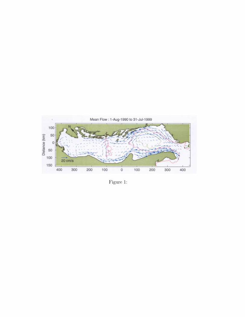
Figure 1:

0

20

40

60

80

100

120

140

0 0.1 0.2 0.3 0.4 0.5 0.6 0.7 0.8 0.9 1 0

0.2

0.4

0.6

0.8

1

Kin

etic

Ene

rgy

(cm

2 sec

-2)

NLa

/Nto

t

La (deg)

indep. dataMKEEKE

EKE (spline)

Figu

re2:

0

0.5

1

1.5

2

2.5

3

3.5

4

4.5

5

0 5 10 15 20 25 30

(EK

E/M

KE

)1/2

(MKE)1/2 (cm sec-1)

Figu

re3:

12˚

12˚

13˚

13˚

14˚

14˚

15˚

15˚

16˚

16˚

17˚

17˚

18˚

18˚

19˚

19˚

20˚

20˚

40˚ 40˚

41˚ 41˚

42˚ 42˚

43˚ 43˚

44˚ 44˚

45˚ 45˚

46˚ 46˚

Figu

re4:

-0.4

-0.2

0

0.2

0.4

0.2 0.3 0.4 0.5 0.6 0.7 0.8 0.9 1 0

0.2

0.4

0.6

0.8

1

Sk

NLa

/Nto

t

La (deg)

SkxSky

indep. data

Figu

re5:

3

3.5

4

4.5

5

5.5

6

0.2 0.3 0.4 0.5 0.6 0.7 0.8 0.9 1 0

0.2

0.4

0.6

0.8

1

Ku

NLa

/Nto

t

La (deg)

KuxKuy

indep. data

Figu

re5:

0.0001

0.001

0.01

0.1

1

-6 -4 -2 0 2 4 6

turbulent velocity (cm sec-1)

EAC

u||v⊥

Gauss

Figu

re6:

0.0001

0.001

0.01

0.1

1

-6 -4 -2 0 2 4 6

turbulent velocity (cm sec-1)

WAC

u||v⊥

Gauss

Figu

re6:

0.0001

0.001

0.01

0.1

1

-6 -4 -2 0 2 4 6

turbulent velocity (cm sec-1)

CG

u||v⊥

Gauss

Figu

re6:

0.1

1

0 2 4 6 8 10

ρ ||

t (days)

EACCG

WACall

Figu

re7:

0.1

1

0 0.5 1 1.5 2 2.5 3

ρ ⊥

t (days)

EACCG

WACall

Figu

re7:

0

0.5

1

1.5

2

2.5

3

0 2 4 6 8 10

T||(

t) (

days

)

t (days)

EACCG

WAC

Figu

re8:

0

0.1

0.2

0.3

0.4

0.5

0.6

0.7

0.8

0 0.5 1 1.5 2 2.5 3

T⊥(t

) (d

ays)

t (days)

EACCG

WAC

Figu

re8:

12˚

12˚

13˚

13˚

14˚

14˚

15˚

15˚

16˚

16˚

17˚

17˚

18˚

18˚

19˚

19˚

20˚

20˚

40˚ 40˚

41˚ 41˚

42˚ 42˚

43˚ 43˚

44˚ 44˚

45˚ 45˚

46˚ 46˚

Figu

re9:

12˚

12˚

13˚

13˚

14˚

14˚

15˚

15˚

16˚

16˚

17˚

17˚

18˚

18˚

19˚

19˚

20˚

20˚

40˚ 40˚

41˚ 41˚

42˚ 42˚

43˚ 43˚

44˚ 44˚

45˚ 45˚

46˚ 46˚

Figu

re9:

0.1

1

0 2 4 6 8 10

ρ ||

t (days)

summerwinter

Figu

re10:

0.1

1

0 0.5 1 1.5 2 2.5 3

ρ ⊥

t (days)

summerwinter

Figu

re10: