Pinned fluxons in a Josephson junction with a

finite-length inhomogeneity∗

Gianne Derks†, Arjen Doelman‡ Christopher J.K. Knight§, Hadi Susanto¶

November 21, 2013

Abstract

We consider a Josephson junction system installed with a finite length inhomogeneity, either of

microresistor or of microresonator type. The system can be modelled by a sine-Gordon equation

with a piecewise-constant function to represent the varying Josephson tunneling critical current.

The existence of pinned fluxons depends on the length of the inhomogeneity, the variation in the

Josephson tunneling critical current and the applied bias current. We establish that a system

may either not be able to sustain a pinned fluxon, or – for instance by varying the length of the

inhomogeneity – may exhibit various different types of pinned fluxons. Our stability analysis shows

that changes of stability can only occur at critical points of the length of the inhomogeneity as a

function of the (Hamiltonian) energy density inside the inhomogeneity – a relation we determine

explicitly. In combination with continuation arguments and Sturm-Liouville theory, we determine

the stability of all constructed pinned fluxons. It follows that if a given system is able to sustain at

least one pinned fluxon, there is exactly one stable pinned fluxon, i.e. the system selects one unique

stable pinned configuration. Moreover, it is shown that both for microresistors and microresonators

this stable pinned configuration may be non-monotonic – something which is not possible in the

homogeneous case. Finally, it is shown that results in the literature on localised inhomogeneities

can be recovered as limits of our results on microresonators.

Keywords: Josephson junction, inhomogeneous sine-Gordon equation, pinned fluxon, stability .

AMS subject classifications: 34D35, 35Q53, 37K50 .

1 Introduction

In this paper we consider a sine-Gordon-type equation describing the gauge invariant phase difference

of a long Josephson junction

φtt = φxx −D sin(φ) + γ − αφt, (1)

where x and t are the spatial and temporal variable respectively; φ(x, t) is the Josephson phase difference

of the junction; α > 0 is the damping coefficient due to normal electron flow across the junction; and

γ is the applied bias current. The parameter D represents the Josephson tunneling critical current,

which can vary as a function of the spatial variable.

∗G. Derks acknowledges a visitor grant of the Dutch funding agency NWO and the NWO-mathematics cluster NDNS+

and the hospitality of the CWI.†Department of Mathematics, University of Surrey, Guildford, Surrey, GU2 7XH (g.derks@surrey.ac.uk)‡Mathematisch Instituut, Leiden University, P.O. Box 9512, 2300 RA Leiden, the Netherlands

(doelman@math.leidenuniv.nl)§Department of Mathematics, University of Surrey, Guildford, Surrey, GU2 7XH (christopher.knight@surrey.ac.uk)¶School of Mathematical Sciences, University of Nottingham, University Park, Nottingham, NG7 2RD

(hadi.susanto@math.nottingham.ac.uk)

1

arX

iv:1

102.

3417

v1 [

nlin

.PS]

13

Feb

2011

When D is constant (without loss of generality, we can take D = 1) and there is no imposed current

and dissipation, i.e., γ = α = 0, the system (1) is completely integrable [1] and has a family of travelling

kink solutions of the form

φ(x, t) = φ0

(x+ vt+ x0√

1− v2

), with φ0(ξ) = 4 arctan(eξ) for any |v| < 1. (2)

In the study of Josephson junctions, this kink represents a fluxon, i.e. a magnetic field with one

flux quantum Φ0 ≈ 2.07 × 10−15 Wb. If there is a small induced current and dissipation but no

inhomogeneity, then there is a unique travelling fluxon whose wave speed in lowest order is given by

v = π√16(α/γ)2+π2

and no stationary fluxons exist, see, e.g., [11].

It was first suggested and shown in [22] that if the critical current D is locally perturbed, stationary

fluxons can exist even if an imposed current is present (γ 6= 0) and that a traveling fluxon (2) can be

pinned by the inhomogeneity. This phenomenon is of interests from physical and fundamental point

of view because such an inhomogeneity could be present in experiments due to the nonuniformity in

the width of the transmission Josephson junction line (see, e.g., [2, 28]) or in the thickness of the oxide

barrier between the superconductors forming the junction (see, e.g., [29, 32]). About a decade after

the first analysis of this phenomenon, it is shown in [17] that the interaction between a soliton and

an inhomogeneity can be non-trivial, i.e. an attractive impurity, which is supposed to pin an incoming

fluxon, could totally reflect the soliton provided that there is no damping in the system. Recently it is

proven that the final state at which a soliton exits a collision depends in a complicated fractal way on

the incoming velocity [12].

So far almost all of the analytical and theoretical work describes the local inhomogeneity by a

delta-like function [12, 16, 17, 22]. Yet, the length of an inhomogeneity in real experiments is varying

from 0.5λJ [29] to 5λJ [2, 28], with λJ being the Josephson penetration depth. Therefore, such

inhomogeneities are not well described by delta-functions. Kivshar et al. [15] have considered the

time-dependent dynamics of a Josephson fluxon in the presence of this more realistic setup, i.e. fluxon

scatterings that take into account the finite size of the defect, within the framework of a perturbation

theory, i.e., when α, γ are small and D ≈ 1. Piette and Zakrzewski [26] recently studied the scattering

of the fluxon on a finite inhomogeneity, extending [17, 12] for finite length defects in the case when

neither applied bias current nor dissipation is present.

In this paper, we consider the problem of a long Josephson junction with a finite-length inhomogene-

ity and give a systematic analysis of the existence and stability of stationary fluxons, i.e., the pinned

fluxons, as they lie at the heart of the interaction of the travelling fluxons with the inhomogeneity. The

Josephson tunneling critical current (denoted by D in (1)) is a function of space and is modelled by

the step-function

D(x;L, d) =

{d, |x| < L,

1, |x| > L.(3)

with d ≥ 0. The inhomogeneity, as modelled by (3), can be fabricated experimentally with a high

controllability and precision, such that the strength and the length of the defect d and 2L can be

made as one wishes (see [33, 34] and references therein for reviews of the experimental setups). When

the parameter d is greater or less than one, the inhomogeneity is called a microresonator respectively

microresistor. They can be thought of as a locally thinned respectively thickened junction, which

provide less respectively more resistance for the Josephson supercurrent to go across the junction

barrier. Note that as (1) without inhomogeneity is translationally invariant, it does not matter where

the inhomogeneity is placed. The existence and stability problem of pinned fluxons in finite Josephson

junctions with inhomogeneity (3) has been considered numerically by Boyadjiev et al. [3, 6, 7]. Here

we consider an infinitely long Josephson junction with inhomogeneity (3) and provide a full analytical

2

study of the existence and stability of pinned fluxons, using dynamical systems techniques, Hamiltonian

systems ideas, and Sturm-Liouville theory.

For the existence of the pinned fluxons we observe that, as D ≡ 1 for |x| large, it follows immediately

that the asymptotic fixed points of (1) are given by sinφ = γ, and the temporally stable stationary

uniform solutions are φ = arcsin γ+ 2kπ. Bu definition, a pinned fluxon is a stationary solution of (1),

which connects arcsin γ and arcsin γ + 2π. Hence a pinned fluxon is a solution of the boundary value

problem

φxx −D(x;L, d) sinφ+ γ = 0;

limx→∞

φ(x) = arcsin γ + 2π and limx→−∞

φ(x) = arcsin γ.(4)

First we observe that pinned fluxons can only exist for bounded values of the applied bias current,

|γ| ≤ 1 (where this upperbound is directly related to our choice to set D ≡ 1 outside the defect).

Moreover, there are symmetries in this system. If φ(x) is a pinned fluxon connecting arcsin γ (at

x → −∞) and arcsin γ + 2π (at x → +∞), then φ(−x) is a solution as well, connecting arcsin γ + 2π

(x → −∞) and arcsin γ (x → +∞). So the second solution is a pinned anti-fluxon. The symmetry

implies that we can focus on pinned fluxons and all results for pinned anti-fluxons follow by using the

symmetry x→ −x. Another important symmetry is

φ(x)→ 2π − φ(−x) and γ → −γ.

Thus if φ(x) is a pinned fluxon with bias current γ, then 2π − φ(−x) is a pinned fluxon with bias

current −γ. This means that we can restrict to a bias current 0 ≤ γ ≤ 1 and the case −1 ≤ γ < 0

follows from the symmetry above.

Furthermore, the differential equation in (4) is a (non-autonomous) Hamiltonian ODE with Hamil-

tonian

H =1

2p2 −D(x;L, d)(1− cosφ) + γφ, where p = φx. (5)

The non-autonomous term has the form of a step function, which implies that on each individual

interval (−∞,−L), (−L,L), and (L,∞) the Hamiltonian is fixed, though the value of the Hamiltonian

will vary from interval to interval. Therefore the solutions of (5) can be found via a phase plane

analysis, consisting of combinations of the phase portraits for the system with D = 1 and D = d, see

also [30] for a similar approach to get existence of π-kinks. In the phase plane analysis, the length

of the inhomogeneity (2L) is treated as a parameter. For x < −L, the pinned fluxon follows one of

the two unstable manifolds of fixed point (arcsin γ, 0) of the reduced ODE (4). Similarly, for x > L

the pinned fluxon follows one of the stable manifolds of the fixed point (arcsin γ + 2π, 0). Finally, for

|x| < L the pinned fluxon corresponds to a part of one of the orbits of the phase portrait for the system

with D = d. The freedom in the choice of the orbit in this system implies the existence of pinned

fluxons for various lengths of the inhomogeneity. See Figure 1 for an example of the construction of a

pinned fluxons when γ = 0.15 and d = 0.2. Orbits of a Hamiltonian system can be characterised by

the value of the Hamiltonian, hence there is a relation between the value of the Hamiltonian inside the

inhomogeneity and the length of the inhomogeneity. The resulting pinned fluxon is in H2(R)∩C1(R).

As the ODE (4) usually implies that the second derivative of the pinned fluxon will be discontinuous,

this is also the best possible function space for the pinned fluxon solutions.

After analysing the existence of the pinned fluxons and having found a plethora of possible pinned

fluxons when a bias current is applied to the Josephson junction (i.e., γ 6= 0), we will consider their

stability. First we will consider linear stability. To derive the linearised operator about a pinned

fluxon φpin(x;L, γ, d), write φ(x, t) = φpin(x;L, γ, d) + eλtv(x, t;L, γ, d) and linearise about v = 0 to

get the eigenvalue problem

Lpinv = Λv, where Λ = λ2 + αλ, (6)

3

Figure 1: Phase portraits when γ = 0.15 and d = 0.2. The dash-dotted red curves are the unstable

manifolds of (arcsin γ, 0), the dashed magenta curves are the stable manifolds of (2π+ arcsin γ, 0), and

the solid blue curves are examples of orbits for the dynamcis inside the inhomogeneity. The bold green

curve is an example of a pinned fluxon.

and the linearisation operator Lpin(x;L, γ, d) is

Lpin(x;L, γ, d) = Dxx −D cosφpin(x;L, γ, d) =

Dxx − cosφpin(x;L, γ, d), |x| > L;

Dxx − d cosφpin(x;L, γ, d), |x| < L.(7)

The natural domain for Lpin is H2(R). We call Λ an eigenvalue of Lpin if there is a function v ∈ H2(R),

which satisfies Lpin(x;L, γ, d) v = Λv. This operator is self-adjoint, hence all eigenvalues will be real.

Furthermore, it is a Sturm-Liouville operator, thus the Sobolev Embedding Theorem gives that the

eigenfunctions are continuously differentiable functions in H2(R). Sturm’s Theorem [31] can be applied,

leading to the fact that the eigenvalues are simple and bounded from above. Furthermore, if v1 is an

eigenfunction of Lpin with eigenvalue Λ1 and v2 is an eigenfunction of Lpin with eigenvalue Λ2 with

Λ1 > Λ2, then there is at least one zero of v2 between any pair of zeros of v1 (including the zeros at

±∞). Hence, the eigenfunction v1 has a fixed sign (no zeros) if and only if Λ1 is the largest eigenvalue

of Lpin. The continuous spectrum of Lpin is determined by the system at ±∞. A short calculation

shows that the continuous spectrum is the interval (−∞,−√

1− γ2).If the largest eigenvalue Λ of Lpin is not positive or if Lpin does not have any eigenvalues, then

the pinned fluxon is linearly stable, otherwise it is linearly unstable. This follows immediately from

analysing the quadratic Λ = λ2 + αλ. If Λ ≤ 0, then both solutions λ have non-positive real part.

However, if Λ > 0 is then there is a solution λ with positive real part. Furthermore, the λ-values of

the continuous spectrum also have non-positive real part as the continuous spectrum of Lpin is on the

negative real axis.

The linear stability can be used to show nonlinear stability. The Josephson junction system without

dissipation is Hamiltonian. Define P = φt, u = (φ, P ), then the equations (1) can be written as a

Hamiltonian dynamical system with dissipation on an infinite dimensional vector space of x-dependent

functions, which is equivalent to H1(R)× L2(R):

d

dtu = J δH(u)− αDu, with J =

(0 1

−1 0

), D =

(0 0

0 1

),

4

and

H(u) = 12

ˆ ∞−∞

[P 2 + φ2x + 2D(x;L, d) (

√1− γ2 − cosφ)

]dx

− γˆ ∞0

[φ− arcsin γ − 2π] dx+ γ

ˆ 0

−∞[φ− arcsin γ] dx.

(8)

Here we have chosen the constants terms in the γ-integrals such that they are convergent for the fluxons.

Furthermore, for any solution u(t) of (1), we have

d

dtH(u) = −α

ˆ ∞−∞

P 2dx ≤ 0. (9)

As a pinned fluxon is a stationary solution, we have DH(φpin, 0) = 0 and the Hessian of H about a

fluxon is

D2H(φpin, 0) =

(−Lpin 0

0 I

).

If Lpin has only strictly negative eigenvalues, then it follows immediately that (φpin, 0) is a minimum of

the Hamiltonian and (9) gives that all solutions nearby the pinned fluxon will stay nearby the pinned

fluxon, see also [10].

After this introduction, we will start the paper with an overview of simulations for the interaction

of travelling fluxons and the inhomogeneity in (1) for various values of d, L, γ and α. This will

motivate the analysis of the existence and stability of the pinned fluxons in the following sections.

We start the analysis of the existence and stability of pinned fluxons by looking at a microresistor

with d = 0. The advantage of the case d = 0 is that several explicit expressions can be derived

and technical difficulties can be kept to a minimum, while it is also representative of the general case

d < 1. It will be shown that for γ = 0 there is exactly one pinned fluxon for each length of the

inhomogeneity. For γ > 0, a plethora of solutions starts emerging. There is a minimum and maximum

length outside which the inhomogeneity cannot sustain pinned fluxons. Between the minimal and the

maximal length there are at least two pinned fluxons, often more. At each length between the minimum

and maximum, there is exactly one stable pinned fluxon. If the length of the interval is (relatively)

large, the stable pinned fluxons are non-monotonic. Note that stable non-monotonic fluxons are not

possible in homogeneous systems, since for a homogeneous system the derivative of the fluxon is an

eigenfunction for the eigenvalue zero of the operator associated with the linearisation about the fluxon.

If the fluxon is non-monotonous, then this eigenfunction has zeros. As the linearisation operator is

a Sturm-Liouville operator, this implies that the operator must have a positive eigenvalue as well,

hence the non-monotonous fluxon is unstable. However, for inhomogeneous systems, the derivative

of the fluxon is usually not differentiable, hence cannot give rise to an eigenvalue zero (since the

eigenfunctions have to be C1) and stable non-monotonic fluxons are in principle possible. This shows

that the inhomogeneity can give rise to qualitatively different fluxons.

For the existence analysis of the pinned fluxons, the length of the inhomogeneity will be treated as

a parameter. The pinned fluxons satisfy an inhomogeneous Hamiltonian ODE whose Hamiltonian is

constant inside the inhomogeneity. It will be shown that the existence and type of pinned fluxons can

be parametrised by the value of this Hamiltonian. The length of the inhomogeneity is determined by

the value of the Hamiltonian and the type of pinned fluxon, leading to curves relating the length 2L

and the value of the Hamiltonian inside the inhomogeneity. In [19] it is shown, in the general setting

of an inhomogeneous wave equation, that changes in stability of the pinned fluxons can be associated

with critical points of the length function relating L and the value of the Hamiltonian. The results of

this paper together with Sturm-Liouville theory give the stability properties of the pinned fluxons in

the general setting.

5

After giving full details for the case d = 0, for which the stability issue can be settled in dependent

of [19], an overview of the results for d > 0 is given. The general microresistor case (0 < d < 1) is

very similar to the case d = 0. The microresonator case (d > 1) has some different features, but the

same techniques as before can be used to analyse the existence and stability. We finish the analysis of

the microresonator case by looking at the special case where microresonators approximate a localised

inhomogeneity. We explicitly look at microresonators with d = µ2L and L very small. For γ, α and µ

small, the asymptotic results from [22] are recovered. Even in the limit of localised inhomogeneities,

our work generalises [22], since our methods allows us to consider γ, α and µ larger as well.

The paper concludes with some further observations, conclusions and ideas for future research.

2 Simulations

To put the analysis of the existence and stability of the pinned fluxons in the next sections in a wider

context, we look first at simulations of the interaction of a travelling fluxon with an inhomogeneity.

Recall that in absence of dissipation and induced currents (α = 0 = γ), the system (1) without an

inhomogeneity (D ≡ 1), has a family of travelling fluxon solutions (2), for each wave speed |v| < 1,

while if there is a small induced current and dissipation, but no inhomogeneity, then there is a unique

travelling fluxon.

First we look at the case α = 0 = γ (no induced current, no dissipation) and the inhomogeneity

of microresistor type with d = 0. If the length is too short, the fluxon will not be captured, but its

speed will be reduced by the passage through the inhomogeneity. If the length of the inhomogeneity

is sufficiently large, the travelling fluxon will be captured. Some radiation is released in this process

and the fluxon “bounces” backwards and forwards around the defect, especially if the length is “just

long enough”. This is consistent with the results in [26] where a detailed analysis of the interaction

of a fluxon with an inhomogeneity is studied in the case that no induced current and dissipation are

present. An illustration is given in Figure 2. Note that the length of the defect which captures the

Figure 2: Simulation of a travelling wave with speed v = 0.1 approaching an inhomogeneity with d = 0

when there is no induced current (γ = 0) or dissipation (α = 0). The inhomogeneity is positioned in

the middle (around the zero position). The length of the inhomogeneity on the left is 0.38 and the

travelling fluxon is captured by the inhomogeneity; note that the “bounce” of the fluxon is a lot larger

than the length of the inhomogeneity. The length of the inhomogeneity on the right is 0.36 and the

pinned fluxon can just escape, but its speed is significantly reduced.

fluxon is a lot smaller than the initial amplitude of the “bounce” of the fluxon. Observations suggest

that the minimal length for the inhomogeneity to capture the travelling fluxon increases if the wave

speed increases.

Next we look at the system with a microresistor with d = 0, now with an induced current γ = 0.1

and varying lengths and values of α. We start again with an inhomogeneity of length 0.38 (L = 0.19).

6

When γ = 0, this microresistor captures a fluxon with speed v = 0.1. With an induced current, it

cannot capture a fluxon, however large we make α, i.e., however slow the fluxon becomes. This is

illustrated in Figure 3. The microresistor slows the fluxon down for a while, but eventually the fluxon

Figure 3: Simulation of a travelling fluxon approaching an inhomogeneity with d = 0 when the induced

current is γ = 0.1. On the left, the length is 0.38. Here the dissipation is α = 0.9, but however large α

is taken, the fluxon is never captured. In the middle and right plots, the length is 0.44. In the middle

the dissipation is α = 0.48 and the fluxon is captured, on the right the dissipation is α = 0.47 and the

fluxon can escape.

escapes with the same speed as it had earlier (as this speed is unique in a system with α, γ 6= 0). The

simulations suggest that the smallest length which can capture a fluxon is 0.44 (L = 0.22). In the next

section, it will be shown that for α, γ 6= 0, there is a minimal length under which no pinned fluxon

can exist. This explains why the inhomogeneity with the shortest length cannot capture even a very

slow travelling fluxon. In Figure 3 it is illustrated that, if the length can sustain pinned fluxons, the

capture depends on the dissipation (hence on the speed of the incoming fluxon). If the dissipation is

sufficiently large, hence the speed sufficiently slow, the pinned fluxon will be captured.

A longish defect in a microresistor will also capture the travelling wave and the resulting pinned

fluxon is not monotonic, see Figure 4! The length of the inhomogeneity is substantial, so the stationary

Figure 4: Simulation of a travelling fluxon approaching a longish inhomogeneity with d = 0 when the

induced current is γ = 0.1 and dissipation is α = 0.5. On the left, the length is 12.5, the travelling

wave is captured and a non-monotonic pinned fluxon is formed. On the right, the length is 35 and the

travelling wave escapes after a while, leaving in its wake a “bump” connecting 2π + arcsin γ at both

ends. Note that the vertical scale and coloring is different in both figures; as a reference point, the

travelling wave on the right is the same in both cases.

7

shape connecting the far field rest states at arcsin γ is a “bump”. This “bump” is present at all the

rest states arcsin γ + 2kπ for γ 6= 0 as arcsin γ + 2kπ is not an equilibrium for the dynamics with

d 6= 1. From a phase plane analysis it can be seen that the amplitude of the homoclinic connection to

arcsin γ+ 2kπ grows with the length L of the defect. As shown in Figure 4, for L = 6.25, the travelling

fluxon travels into this “bump” and gets captured. The resulting pinned fluxon is not monotonic. In

the next section, the family of all possible pinned fluxons is analysed and it is shown that for long

lengths the stable pinned fluxon is non-monotonic. Moreover, it follows that there is an upper limit

on the length of inhomogeneities that can sustain pinned fluxons. This is illustrated on the right in

Figure 4. The travelling fluxon seems to be captured initially by the inhomogeneity, but after a while

it escapes again. However large the dissipation is taken, this will always happen, illustrating that no

pinned fluxons can exist.

Next we consider a microresonator with d = 2. As before, we consider the case without an induced

current (γ = 0) first. In this case, the fluxon is never captured. For the smaller lengths the fluxon

reflects, for larger lengths the fluxon seems to get trapped, but it escapes after a while. This is

illustrated in Figure 5 for a microresonator with length 0.1. In the next section, it will be will shown

that a system with a microresonator and no induced current has indeed no stable pinned fluxons.

Figure 5: Simulation of a travelling wave approaching an inhomogeneity with d = 2 and length 0.1,

when there is no induced current and no dissipation (γ = 0 = α). The speed on the left is 0.21 and the

travelling wave is bounced by the inhomogeneity. The length on the right is 0.22 and at first the pinned

fluxon seems to be captured by the inhomogeneity, but after while it travels through the inhomogeneity

and seems to resume its original speed.

After the induction-less system, we consider a system with a microresonator with d = 2 and an

induced current γ = 0.1. As with the microresistor there is a minimum length, under which the

microresonator cannot capture a fluxon. The simulations suggest that the minimum length is 0.42

(L = 0.21). In Figure 6, it is illustrated that a microresonator with length 0.40 cannot capture a fluxon

with α = 0.9, whilst a microresonator with length 0.42 can capture a fluxon with α = 0.3, but it cannot

for α = 0.29. This is consistent with the results in the next sections where it is shown that for α, γ 6= 0

there exists a minimal length under which no pinned fluxons can be sustained by the inhomogeneity. If

the length can just sustain pinned fluxons, then there are both a stable and an unstable pinned fluxon

close to each other. In the left panels of Figures 6 and 7 it can be observed that initially the travelling

fluxon approaches the unstable pinned fluxon, but then reflects to the stable one and settles down.

Finally we consider a microresonator with a longer length for which the travelling fluxon gets

captured and becomes a non-monotonic pinned fluxon. In Figure 7, it is illustrated that for a microres-

onator with d = 10, length 2 (L = 1), the travelling fluxon at γ = 0.1 and α = 0.2 gets attracted to

a non-monotonic pinned fluxon. Note that for microresonators (i.e., d > 1), the stable non-monotonic

pinned fluxons have a “dip” as opposed to the ones for the microresistors which have a “bump”.

8

Figure 6: Simulation of a travelling wave approaching an inhomogeneity with d = 2 and length 0.1,

when there an induced current (γ = 0.1). On the left and middle is a microresonator with length 0.42.

On the left the dissipation is α = 0.3 and the fluxon is captured, whilst in the middle the dissipation

is α = 0.29 and the fluxon escapes. On the right, the length is 0.4 and the dissipation is α = 0.9 and

the fluxon still escapes as the length is too short for a pinned fluxon to exist.

Figure 7: Simulation of a travelling wave approaching an inhomogeneity with d = 10 and length 2, when

the induced current is γ = 0.1 and the dissipation is α = 0.2. The resulting wave is non-monotonic as

can be seen on the right. Due to the weaker dissipation, it takes some time for the wave to converge to

its stable shape. Initially, the travelling wave approaches the monotonic unstable pinned fluxon, then

deflects from it and converges to the non-monotic stable one.

3 No resistance (d=0)

We now analyse the existence and stability of the pinned fluxons in a microresistor and a microresonator.

First we consider the case when there is no resistance in the inhomogeneity, hence a microresistor with

d = 0. This case provides a good illustration of the richness of the family of pinned fluxons, shows

the essence of the analytic techniques for the existence and stability analysis, and has less technical

complications than the more general values of d. The existence analysis for the case with no bias

current (γ = 0) is quite different from the case when a bias current is applied (γ > 0). So we will

consider them separately.

3.1 Existence of pinned fluxons without applied bias current

For γ = 0, the pinned fluxon has to connect the stationary states at φ = 0 and φ = 2π. In the

background dynamics of the ODE (4) with D ≡ 1, the unstable manifold of (0, 0) coincides with the

stable manifold of (2π, 0), as follows immediately by analysing the Hamiltonian (5) with D ≡ 1. These

coinciding manifolds are denoted by a red curve in the phase portrait sketched in Figure 8. This curve

represents the unperturbed sine-Gordon fluxon (2). The orbits generated by the Hamiltonian system

with D ≡ 0 are straight lines. In Figure 8, samples of these orbits are given by the blue lines. Any

blue line that crosses the red line can be used to form a pinned fluxon. An example is given in the

panel on the right in Figure 8, where the green curve represents a pinned fluxon in H2(R) ∩ C1(R).

As can be seen from Figure 8, the value of the Hamiltonian inside the inhomogeneity is a convenient

parameter to characterise the pinned fluxons. The points of intersection for the blue and red curves

9

Figure 8: Phase portraits of the ODE (4) for γ = 0 and d = 0. The red curve represents the coinciding

stable and unstable manifolds of the asymptotic fixed points. The blue curves are orbits for the system

inside the inhomogeneity. In the sketch on the right, the green curve represents a pinned fluxon.

are denoted by (φin, pin) respectively (φout, pout) for the first respectively second intersection. It follows

immediately that pin = pout and φout = 2π−φin. Furthermore, the expression for the Hamiltonian, (5),

gives the following relations for φin and pin: 0 = 12 p

2in − (1 − cosφin) (D ≡ 1) and h = 1

2 p2in (D ≡ 0),

with 0 < h ≤ 2 where h is the value of the Hamiltonian inside the inhomogeneity. Thus

pin(h) =√

2h and φin(h) = arccos(1− h), with 0 < h ≤ 2. (10)

Inside the inhomogeneity (|x| < L), the pinned fluxon related to the value h satisfies h = 12φ

2x, thus

φx =√

2h. Hence the half-length L and the parameter h are related by

L =

ˆ 0

−Ldx =

ˆ π

φin(h)

dφ

φx=

ˆ π

φin(h)

dφ√2h

=π − arccos(1− h)√

2h. (11)

As the numerator is a monotonic decreasing function of h and the denominator is monotonic increasing,

it follows immediately that L is a monotonic decreasing function of h. The function L takes values

in [0,∞) as limh→0

L(h) = ∞ and limh→2

L(h) = 0. The h-L plot is given in Figure 9. We summarise the

existence results for pinned fluxons without a bias current in the following lemma.

Figure 9: Plot of the length L as a function of h, the value of the Hamiltonian in the inhomogeneity,

for γ = 0 and d = 0.

Lemma 1 Let γ = 0 and d = 0. For any length 2L of the inhomogeneity, there is a unique pinned

fluxon, for which the Hamiltonian inside the inhomogeneity has the value h(L) as implicitly given

by (11). Define x∗ to be the shift such that φ0(−L + x∗) = φin (see (2) for the definition of φ0), then

10

the pinned fluxon is given explicitly by

φpin(x;L, 0, 0) =

φ0(x+ x∗), x < −L,π + π−arccos(1−h)

L x, |x| < L,

φ0(x− x∗), x > L.

(12)

3.2 Existence of pinned fluxons with bias current

For γ > 0, the pinned fluxon has to connect the stationary states at φ = arcsin γ and φ = 2π+arcsin γ.

In the background dynamics with D ≡ 1 the unstable manifold of φ = arcsin γ coincides no longer with

the stable manifold of 2π+ arcsin γ. Furthermore, the orbits of the dynamics inside the inhomogeneity

are parabolic curves instead of straight lines. These two changes add substantial richness to the family

of pinned fluxons.

Let us first consider the phase portraits. In Figure 10 we consider γ = 0.15 as a typical example

to illustrate the ideas. In the dynamics with D ≡ 1, the unstable manifolds to arcsin γ are denoted

by red curves, while the stable manifolds to 2π + arcsin γ are denoted by magenta curves. The larger

γ gets, the wider the gap between the unstable and stable manifold becomes. The dynamics within

Figure 10: Phase portrait at γ = 0.15 and d = 0. On the right is a zoom into the area around

(φ, φx) = (2π, 0).

the inhomogeneity with D ≡ 0 are denoted by blue curves. These blue curves are nested and can be

parametrised with a parameter h, using the Hamiltonian (5) with D ≡ 0:

1

2(φx)2 + γφ = H0(γ) + h,

where H0(γ) is given by the value of the Hamiltonian (5) on the magenta stable manifold (D ≡ 1):

H0(γ) = γ arcsin γ − (1−√

1− γ2) + 2πγ. (13)

Thus the value of h increases as the extremum of the blue curves is more to the right.

For the existence of pinned fluxons, a blue curve has to connect the red unstable manifold with the

magenta stable manifold. In Figure 10, the furthest left possible blue curve for which pinned fluxons

may exist, is the one indicated with h = 0. In the zoom on the right, it can be seen that this curve

just touches the magenta stable manifold. The blue curve intersects the red unstable manifold twice,

both points give rise to a pinned fluxon, as sketched in Figure 11. Obviously, the pinned fluxon in the

11

Figure 11: Phase portrait at γ = 0.15 and d = 0 with the furthest left blue curve for which pinned

fluxons exist. There are two pinned fluxons possible, represented by green line. On the right is a zoom

into the area around (φ, φx) = (2π, 0).

second plot in Figure 11 will occur in a defect with a shorter length than the one in the first plot. The

furthest right possible curve that gives rise to pinned fluxons is marked with hmax in Figure 10. This

blue orbit touches the red unstable manifold and crosses the magenta unstable manifolds in 5 points.

All these points represent different pinned fluxons, hence 5 pinned fluxons can be associated with this

curve. Moreover, for h just below hmax, the blue curve intersects the red curve twice (while it still

intersects the magenta curve 5 times: there are 10 different pinned fluxons associate to such value of h.

In general, the pinned fluxons are determined by two points in the phase plane: the point where

pinned fluxon enters the inhomogeneity (i.e. the crossing from the red unstable manifold to the blue

orbit), this point will be denoted by (φin, pin) and the point where the pinned fluxon leaves the inhomo-

geneity (i.e. the crossing from the blue orbit to the magenta stable manifold), this point will be denoted

by (φout, pout). Thus the points (φin, pin) and (φout, pout) are determined by the set of equations

H0(γ)− 2πγ = 12 p

2in − (1− cosφin) + γφin,

H0(γ) + h = 12 p

2in + γφin,

H0(γ) + h = 12 p

2out + γφout,

H0(γ) = 12 p

2out − (1− cosφout) + γφout.

(14)

Combining the equations in (14), we get expressions for φin and φout:

cosφin = 1− (h+ 2πγ) and cosφout = 1− h. (15)

This is well-defined only if 0 ≤ h ≤ 2(1− πγ). Hence there are maximal values for γ and h, given by

γmax =1

πand hmax = 2(1− πγ).

If γ > γmax, then there is no blue curve that intersects both the red unstable orbit and the magenta

stable orbit, hence no pinned fluxons exist if the applied bias current is larger than γmax. If h > hmax,

then the blue curve does not intersect the red manifold anymore.

Furthermore, φin must lie on the red unstable manifold, hence arcsin γ ≤ φin ≤ φmax(γ), where

φmax(γ) is the maximal φ-value of the orbit homoclinic to arcsin γ. As h ∈ [0, 2(1− πγ)], this implies

that there are two possible values for φin and that pin > 0:

φin = π ± arccos(2πγ − (1− h)) and pin =√

2 (H0(γ) + h− γφin).

Note that the unstable manifold left of arcsin γ only intersects with blue curves that have φx < 0, hence

those orbits can never connect to one of the stable manifolds of 2π + arcsin γ.

12

The point (φout, pout) has to lie on the magenta stable manifolds, so there can be up to five possible

branches of solutions:

1. φout = 2π − arccos(1− h) with pout > 0, for all 0 ≤ h ≤ hmax;

2. φout = 2π + arccos(1− h) with pout ≥ 0, for 0 ≤ h ≤ h2 and pout < 0, for h2 < h ≤ hmax;

3. φout = 2π + arccos(1− h) with pout ≥ 0, for h2 < h ≤ hmax;

4. φout = 4π − arccos(1− h) with pout ≥ 0, for h1 < h ≤ hmax;

5. φout = 4π − arccos(1− h) with pout < 0, for h1 < h ≤ hmax.

Here h2 is the h-value such that the blue orbit intersects the magenta manifolds at the equilibrium

(2π + arcsin γ, 0), i.e., h2(γ) = 1 −√

1− γ2, and h1 is such that the blue orbit touches the magenta

manifold at (2π + φmax(γ), 0), the most-right point, thus h1(γ) = 1 − cos(φmax(γ)). In all cases,

|pout| =√

2 (H0(γ) + h− γφout).To satisfy h2(γ) ≤ hmax(γ), we need that γ ≤ γ2 = 4π

4π2+1≈ 0.3104. If γ > γ2, then only pinned

fluxons with φout = 2π ± arcsin γ and pout > 0 exist. In order to have h1(γ) ≤ hmax(γ), we need that

γ ≤ γ1, where γ1 is the implicit solution of cosφmax(γ1) + 1 = 2πγ1, i.e., γ1 ≈ 0.1811. If γ > γ1, then

no pinned fluxons with φout = 4π − arcsin γ exist. On the intervals of common existence, we have

0 ≤ h2(γ) ≤ h1(γ) ≤ hmax(γ), h1(γ1) = hmax(γ1), h2(γ2) = hmax(γ2), see Figure 12.

Figure 12: The extremal h-values h1(γ), h2(γ) and hmax(γ).

In Figure 13, we have taken γ = 0.15 and h = (h1 + hmax)/2 and have plotted all five possible

pinned fluxons (i.e. all possibilities for (φout, pout)) with φin = π − arccos(2πγ − (1 − h)). Obviously,

five more pinned fluxons with the same (φout, pout) are possible with φin = π + arccos(2πγ − (1− h)).

To determine the length of the inhomogeneity for the pinned fluxons, we use that on the orbits in the

inhomogeneity (blue curves in the phase portrait) φ and φx are related by |φx| =√

2 (H0(γ) + h− γφ).

Integrating this ODE, taking into account the sign of pout, we get that the length of the pinned fluxons

with pout > 0 is given by

2L =

√2

γ

[√H0 + h− γφin −

√H0 + h− γφout

]=pin − pout

γ(16)

and for pout < 0, we have

2L =

√2

γ

[√H0 + h− γφin +

√H0 + h− γφout

]=pin − pout

γ. (17)

13

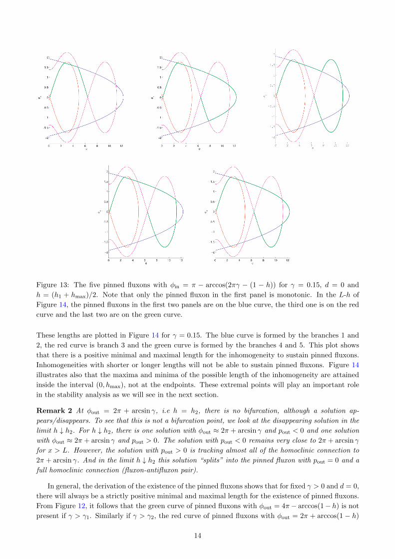
Figure 13: The five pinned fluxons with φin = π − arccos(2πγ − (1 − h)) for γ = 0.15, d = 0 and

h = (h1 + hmax)/2. Note that only the pinned fluxon in the first panel is monotonic. In the L-h of

Figure 14, the pinned fluxons in the first two panels are on the blue curve, the third one is on the red

curve and the last two are on the green curve.

These lengths are plotted in Figure 14 for γ = 0.15. The blue curve is formed by the branches 1 and

2, the red curve is branch 3 and the green curve is formed by the branches 4 and 5. This plot shows

that there is a positive minimal and maximal length for the inhomogeneity to sustain pinned fluxons.

Inhomogeneities with shorter or longer lengths will not be able to sustain pinned fluxons. Figure 14

illustrates also that the maxima and minima of the possible length of the inhomogeneity are attained

inside the interval (0, hmax), not at the endpoints. These extremal points will play an important role

in the stability analysis as we will see in the next section.

Remark 2 At φout = 2π + arcsin γ, i.e h = h2, there is no bifurcation, although a solution ap-

pears/disappears. To see that this is not a bifurcation point, we look at the disappearing solution in the

limit h ↓ h2. For h ↓ h2, there is one solution with φout ≈ 2π + arcsin γ and pout < 0 and one solution

with φout ≈ 2π + arcsin γ and pout > 0. The solution with pout < 0 remains very close to 2π + arcsin γ

for x > L. However, the solution with pout > 0 is tracking almost all of the homoclinic connection to

2π + arcsin γ. And in the limit h ↓ h2 this solution “splits” into the pinned fluxon with pout = 0 and a

full homoclinic connection (fluxon-antifluxon pair).

In general, the derivation of the existence of the pinned fluxons shows that for fixed γ > 0 and d = 0,

there will always be a strictly positive minimal and maximal length for the existence of pinned fluxons.

From Figure 12, it follows that the green curve of pinned fluxons with φout = 4π− arccos(1− h) is not

present if γ > γ1. Similarly if γ > γ2, the red curve of pinned fluxons with φout = 2π + arccos(1 − h)

14

Figure 14: The lengths of the pinned fluxons for γ = 0.15 and d = 0. The lengths of the pinned

fluxons with φout = 4π − arccos(1− h) are plotted in green (branches 4 and 5), the lengths of pinned

fluxons with φout = 2π+arccos(1−h) and pout > 0 are in red (branch 3). The lengths of the remaining

pinned fluxons (branches 1 and 2) are indicated by the blue curves. The panels on the right zoom into

the top and bottom and show that the minimal and maximal length are not obtained for hmax, but a

smaller value.

and pout > 0 are not present. Below we summarise the results for the existence of the pinned fluxons

with an induced current:

Theorem 3 For d = 0 and every 0 < γ ≤ 1π , there are Lmin(γ) and Lmax(γ), such that for every

L ∈ (Lmin, Lmax), there are at least two pinned fluxons (at least one for L =min or Lmax). Furthermore

limγ↓0

Lmin(γ) = 0, limγ↓0

Lmax(γ) =∞,

and

limγ↑1/π

Lmin(γ) = limγ↑1/π

Lmax(γ) =

√π2

(arcsin 1

π +√π2 − 1

)−√

π2

(arcsin 1

π +√π2 − 1− π

)≈ 1.8.

For given L ∈ [Lmin, Lmax], the maximum possible number of simultaneously existing pinned fluxons

is 6. For γ > 1π , there exist no pinned fluxons.

To relate the rich family of pinned fluxons which exists for γ > 0 with the unique pinned fluxons

for γ = 0, we have sketched the L-h curves for γ = 0.001 in Figure 15. The bold blue curve converges

clearly to the curve in Figure 9. These are the lengths associated with the pinned fluxons with φin = π−arccos(2πγ−(1−h)) and φout = 2π−arccos(1−h). Clearly there are some other convergent L-h curves as

well. The length of the blue curve associated with the pinned fluxons with φin = π+arccos(2πγ−(1−h))

and φout = 2π − arccos(1 − h) goes to zero as expected. The convergent red and green curves can be

associated with 4π-fluxons in the case γ = 0. A 4π-fluxon is a connection between 0 and 4π. This is

not possible without an inhomogeneity, but with an inhomogeneity such connections are possible and

some are stable. There are four possible 4π-fluxons if γ = 0 and the green and red curves converge to

those solutions. For more details, see [18].

15

Figure 15: L-h curves of the pinned fluxons for γ = 0.001.

3.3 Stability of the pinned fluxons with d = 0

As seen in the introduction, the stability of the pinned fluxons is determined by the eigenvalues of the

linearisation operator Lpin as defined in (7). For d = 0, the linearisation operator takes the form

Lpin(x;L, γ, 0) =

Dxx − cosφpin(x;L, γ, 0), |x| > L;

Dxx, |x| < L.

where φpin is one of the pinned fluxons found in the previous section.

When there is no induced current (γ = 0), expressions for the eigenvalues of Lpin can be found

explicitly. Recall that for d = 0 and γ = 0, there is a unique pinned fluxon for each length L ≥ 0, see

Lemma 1.

Lemma 4 For γ = 0 and d = 0, the linear operator Lpin associated to the unique pinned fluxon in the

defect with length L has a largest eigenvalue Λmax ∈ (−1, 0) given implicitly by the largest solution of

−µ[µ+ 1

2

√2(1 + cosφin)

]+ 1

2 (1− cosφin) =

−√

1− µ2[µ+ 1

2

√2(1 + cosφin)

]tan

(√1− µ2 π−φin√

2(1−cosφin)

),

(18)

where µ =√

1 + Λmax ∈ (0, 1) and the relation between φin and L is given in (10) and (11).

In Figure 16, Λmax is sketched as function of the half-length L of the pinned fluxon. The proof of

Lemma 4 is quite technical; it is given in appendix A.

Remark 5 For L large (hence φin small), equation (18) has more solutions. Hence for those pinned

fluxons Lpin has some smaller eigenvalues in (−1, 0) too.

Corollary 6 If there is no induced bias current (γ = 0) and the microresistor has d = 0, then the

unique pinned fluxon in the defect with length L is linearly and nonlinearly stable. The pinned fluxon

is asymptotically stable if α > 0.

Next we consider the case that there is an induced bias current (γ > 0). In the previous section

we have seen that in this case the pinned fluxons come in families, characterised by the blue, red and

green curves in Figure 14. Locally along those curves, we can write either L as a function of h, or,

h as a function of L. Along those curves, we will look for changes of stability, i.e., find whether the

16

Figure 16: The largest eigenvalue of the linearised operator Lpin at d = 0 and γ = 0 as function of the

half-length L of the inhomogeneity.

operator Lpin has an eigenvalue 0 (recall that eigenvalues of Lpin must be real. We will show that Lpinhas an eigenvalue 0 if and only if along the L-L curve we have dL

dh = 0 or the pinned fluxon is isolated.

Isolated pinned fluxons occur when γ is maximal, i.e., γ = 1π or when γ = γ1, the maximal γ-value for

which pinned fluxons with φout = 4π − arccos(2πγ − 1) exist. This lemma is a special case of a more

general theorem presented in [19]. The proof simplifies considerably in this case.

Lemma 7 For any γ ≥ 0, the linear operator Lpin(x;L, γ, 0) has an eigenvalue zero if and only if

• dLdh = 0;

• or γ = 1π (this eigenvalue zero is the largest eigenvalue);

• or γ = γ1 ≈ 0.18, the solution of cosφmax(γ1) + 1 = 2πγ1 (see section 3.2), and φpin is such that

φin = π, φout = 4π − arccos(2πγ1 − 1) = 2π + φmax(γ1) (this eigenvalue zero is not the largest

eigenvalue).

Proof First we observe that differentiating (4) with respect to x shows that φ′pin satisfies Lpinφ′pin = 0.

However, it follows immediately from (4) that φ′pin is not continuously differentiable, except when there

exist k± ∈ N such that φin = k−π and φout = k+π. From the existence results, it follows that this

happens only if γ = 1π . In this case, there is only one pinned fluxon and the blue curve in Figure 14

has become a single point (there are no red or green curves).

In all other cases, φ′pin 6∈ C1(R) ⊃ H2(R) so φ′pin is not an eigenfunction with the eigenvalue

zero. However, φ′pin still plays a role in the eigenfunction related to any eigenvalue zero. Indeed,

on both intervals (∞,−L) and (L,∞), the second order linear ODE Lpinψ = 0 has two linearly

independent solutions. As the asymptotic system is hyperbolic, one solution is exponentially decaying

whilst the other is exponentially growing. Thus if the linear operator L has an eigenvalue zero, then

the eigenfunction in the intervals (−∞, L) and (L,∞) must be a multiple of the exponentially decaying

solution. As φ′pin is exponentially decaying for |x| → ∞ and satisfies Lφ′pin = 0 for |x| > L, it follows

that for any eigenvalue zero, the eigenfunction must be a multiple of φ′pin for |x| > L, unless φ′pin ≡ 0.

The case φ′pin ≡ 0 happens only when φout = 2π + arcsin γ and x > L. In this case, the appropriate

eigenfunction is a multiple of e−4√

1−γ2(x−L).

17

Next we look inside the inhomogeneity, i.e., |x| < L. The linearised problem inside the defect for

an eigenvalue zero can be solved explicitly and gives an eigenfunction of the form A+B(x+ L), with

A and B free parameters and |x| < L.

To conclude, if the linear operator Lpin has an eigenvalue zero, and φout 6= 2π + arcsin γ (we will

consider this case later), then the eigenfunction is of the form

ψ =

φ′pin(x), x < −L,

A+B (x+ L), |x| < L,

K φ′pin(x), x > L,

where A, B and K are free parameters. We have to choose the free parameters such that ψ is con-

tinuously differentiable at ±L. As there are only three free parameters and four matching conditions,

this will give us a selection criterion on the length L for which an eigenvalue zero exists. The matching

conditions are

A = φ′pin(−L−), B = φ′′pin(−L−), B = Kφ′′pin(L+), and A+ 2BL = Kφ′pin(L+),

where the notation φ′pin(−L−) = limx↑−L φ′pin(x), φ′pin(L+) = limx↓L φ

′pin(x), etc. Using that pin/out =

φ′pin(∓L) and γ + φ′′pin(±L±) = sinφ(±L) = sinφin/out, this can be written as

A = pin, B = sinφin − γ, B = K(sinφout − γ), and A+ 2BL = Kpout.

Equations (16) and (17) show that L = pin−pout2γ , hence the parameters are given by

A = pin, B = sinφin − γ, and K(sinφout − γ) = sinφin − γ

and the compatibility condition on L, or equivalently h, is

0 = pin sinφin(sinφout − γ)− pout sinφout(sinφin − γ). (19)

To derive this expression, we have multiplied the remaining equation [A+2BL = Kpout] with γ(sinφout−γ). This term would be zero if sinφout = γ, hence φout = 2π + arcsin γ but this case is not considered

now.

For completeness, we also consider the case where we assume that the eigenfunction vanishes for

x < −L. If this is the case, then matching at x = −L gives immediately that A = 0 = B. Thus this

leads to a non-trivial eigenfunction only if φ′pin(L) = 0 = limx↓L φ′′pin(x). In other words, when φpin is a

fixed point for x > L. This happens only if φout = 2π+ arcsin γ. This case we will be considered later.

Next we link the expression (19) to the derivative of L with respect to h. As L = pin−pout2γ , the

derivatives of pin and pout are needed. Differentiating (14) and (15), we get

pindpindh

= 1− γφ′in(h), sinφindφindh

= 1 and poutdpoutdh

= 1− γφ′out(h), sinφoutdφoutdh

= 1.

Thus differentiating L = pin−pout2γ gives that

pin sinφin pout sinφoutdL

dh=

1

2γ[pout sinφout(sinφin − γ)− pin sinφin(sinφout − γ)] (20)

So we have shown that if φout 6= 2π+ arcsin γ and the operator Lpin has an eigenvalue zero, then eitherdLdh (h, γ) = 0 or pin sinφin pout sinφout = 0. Considering pin sinφin pout sinφout = 0 in more detail, we

get:

• sinφout = 0 would mean that φout = 2π. Going back to the compatibility condition (19), this

implies that γpin sinφin = 0, which only happens if also sinφin = 0 or pin = 0. In the existence

section we have seen pin > 0, hence γpin sinφin = 0 can only happen if φin = π, hence if γ = 1π ;

18

• sinφin = 0 implies that φin = π. Going back to the compatibility condition (19), this implies

that γpout sinφout = 0, which only happens if also sinφout = 0 or pout = 0. Hence either γ = 1π

or γ = γ1, as the case φout = 2π + arcsin γ is excluded at this moment;

• pin 6= 0 as we have seen before;

• pout = 0 happens if φout = 2π+ arcsin γ or φout = 2π+φmax(γ). Going back to the compatibility

condition (19), this implies that pin sinφin(sinφout − γ) = 0. Since π − arcsin γ < φmax(γ) < 2π,

this implies this only happens if sinφin = 0, which case is considered before.

So altogether we have if φout 6= 2π+ arcsin γ and the operator Lpin has an eigenvalue zero, then either

• dLdh (h, γ) = 0 or

• φin = π and φout = 2π, which only happens when γ = 1π . The eigenfunction in this case is φ′pin,

which does not have any zeros, hence the eigenvalue zero is the largest eigenvalue.

• φin = π and φout = 2π + φmax(γ) (i.e. pout = 0), which only happens if γ = γ1. In this case the

eigenfunction is φ′pin for x < L and γ1γ1−sinφmax(γ1)

φ′pin for x > L. This eigenfunction has a zero at

x = L, hence the eigenvalue zero is not the largest eigenvalue. Note that when γ = γ1 the green

L(h) curve in Figure 14 has degenerated to an isolated point related to the pinned fluxon φpinconsidered in this case.

To show that the converse is true, we look at the three cases dLdh (h, γ) = 0, γ = 1

π and γ = γ1 and

(φout, pout) = (2π+ φmax, 0). It is straightforward to verify that the eigenfunctions as described earlier

can be constructed in those cases.

Finally we look at the case φout = 2π+ arcsin γ. In this case γ ≤ 4π1+4π2 and h = h2 = 1−

√1− γ2.

Furthermore, the pinned fluxons satisfies φ′pin ≡ 0 for x > L. In this case, the general form of an

eigenfunction for an eigenvalue zero is

ψ =

φ′pin(x), x < −L,

A+B (x+ L), |x| < L,

K e−4√

1−γ2(x−L), x > L,

where A, B and K are free parameters. We have to choose the free parameters such that ψ is contin-

uously differentiable at = ±L, i.e.

A = φ′pin(−L−), B = φ′′pin(−L−), K = A+ 2BL, and B = −K 4√

1− γ2.

As L = pin−pout2γ = pin

2γ , this implies that A = pin, B = sinφin − γ and K = pin sinφinγ , with the matching

condition

γ(sinφin − γ) = − 4√

1− γ2 sinφin pin. (21)

If φin = π + arccos(2πγ −√

1− γ2), then sinφin < 0 and (21) cannot be satisfied as pin > 0 and

γ > 0. If φin = π − arccos(2πγ −√

1− γ2), then the phase portrait in the existence section shows

that sinφin > γ, thus (sinφin− γ) > 0 and again (21) cannot be satisfied. Thus no eigenvalue zero can

occur at φout = 2π + arcsin γ. 2

Lemma 7 allows us to conclude the stability of pinned fluxons.

Theorem 8 For d = 0, every 0 < γ ≤ 1π , and every L ∈ [Lmin(γ), Lmax(γ)], there is exactly one

stable pinned fluxon. This pinned fluxon is linearly and nonlinearly stable (and asymptotically stable

for α > 0). For L sufficiently large

(L >

√π+arcsin γ+arccos(2πγ−

√1−γ2)

2γ

), the stable pinned fluxons are

non-monotonic.

19

Figure 17: Stability for d = 0 and γ = 0.15. The bold magenta curve represents stable solutions, all

other solutions are unstable. On the right there is an example of a stable monotonic pinned fluxon (at

L = 0.38) and a stable non-monotonic one (at L = 10), Both stable pinned fluxons have h = 1, i.e.

they are near minimal respectively maximal length, which are at Lmin = 0.35 and Lmax = 10.13.

See Figure 17 for an illustration of this theorem.

Proof If γ = 1π , then only the inhomogeneity with half-length exactly L =

√π2

(arcsin 1

π +√π2 − 1

)−√

π2

(arcsin 1

π +√π2 − 1− π

)≈ 1.8 has a pinned fluxon. From Lemma 7, it follows that the linearisa-

tion for this pinned fluxon has a largest eigenvalue 0, so this pinned fluxon is linearly stable.

In Corollary 6, we have seen that the unique pinned fluxons for γ = 0 are stable.

If 0 < γ < 1π , then there are at least two pinned fluxons if L ∈ (Lmin, Lmax), see Theorem 3. As

seen before, the L-h curves for the pinned fluxons form three isolated curves: φout = 4π−arccos(1−h)

(green curve), the (red) curve of pinned fluxons with φout = 2π + arccos(1 − h) and pout > 0 (exists

for h > h2), and the other pinned fluxons (blue curve). The colour coding refers to Figures 14 and 17.

The fluxons on the blue curve exist for all 0 ≤ γ ≤ 1π ; the existence of the other curves depends on the

value of γ.

The linearisation about the pinned fluxon at the minimum on the red curve has an eigenvalue zero.

At this point, the associated eigenfunction is a multiple of φ′pin for x > L. On the red curve, pout > 0

and φ′pin(x) < 0 for x large. Thus this eigenfunction has a zero. Using Sturm-Liouville theory, we can

conclude that the eigenvalue zero is not the largest eigenvalue. As there is only one fluxon with dLdh = 0

on the red curves, all pinned fluxons on the red curve are linearly unstable.

Similarly, the minimum and maximum on the green curve are associated with pinned fluxons whose

linearisation has an eigenvalue zero. Again, the associated eigenfunction for x > L is a multiple of

20

φ′pin. As for the red curve, at the minimum we have pout > 0 and φ′pin(x) < 0 for x large. Thus this

eigenfunction has a zero and we can conclude that the eigenvalue zero is not the largest eigenvalue.

The green curve is a closed curve with only two points with dLdh = 0, so the eigenvalue zero at the

maximum cannot be the largest eigenvalue either. So we can conclude that all pinned fluxons on the

green curve are linearly unstable.

Finally we consider the blue curve. We use the stability of the pinned fluxons at d = 0, γ = 0 to get

a conclusion about the stability of the pinned fluxons on this curve. The solutions that can be continued

to γ = 0 are the connections between φin = π − arccos(2πγ − 1 + h) and φout = 2π − arccos(1 − h).

Hence those solutions are stable. Now using that zero eigenvalues can only occur if L(h) has a critical

point, the blue curve can be divided in stable and unstable solutions. The stable solutions are the part

of the curve L(h) curve between the minimum and maximum that contains the pinned fluxons with

φin = π− arccos(2πγ − 1 + h) and φout = 2π− arccos(1− h). The pinned fluxons in the other part are

unstable as the zero eigenvalue is simple. It can be verified that the eigenfunctions related to the zero

eigenvalues on this curve do not have any zeroes indeed.

So altogether we can conclude that for each length there is exactly one stable and at least one

unstable solution. The stable fluxons are non-monotonic if L is larger than the length of the fluxon

at h = h2(γ) = 1 −√

1− γ2 with φin = π − arccos(2πγ −√

1− γ2) and φout = 2π + arcsin γ, hence

L >

√π+arcsin γ+arccos(2πγ−

√1−γ2)

2γ . 2

4 General case (d > 0)

After analysing the existence and stability of pinned fluxons in microresisors with the d = 0 in full

detail, in this section we will sketch the existence and stability of the pinned fluxons for a general

microresistor or microresonator.

4.1 Microresistors (0 < d < 1)

The existence of pinned fluxons for 0 < d < 1 follows from similar arguments as for the case d = 0.

Using the matching of appropriate solutions in the phase planes again, it can be shown that pinned

fluxons exist for 0 ≤ γ ≤ 1−dπ . The Hamiltonian dynamics in the inhomogeneity satisfies the relation

1

2φ2x − d(1− cosφ) + γφ = H0(γ) + h,

where h is a parameter for the value of the Hamiltonian as before. The case γ = 0 (no induced current)

is more or less identical to before, with a unique pinned fluxon for any L > 0. For γ > 0, a similar

calculation as in the case d = 0 shows that there are two possible entry angles:

φin = π − arccos(2πγ−(1−d−h)

1−d

)or φin = π + arccos

(2πγ−(1−d−h)

1−d

)and up to three possible exit angles:

φout = 2π − arccos(1−d−h1−d

), φout = 2π + arccos

(1−d−h1−d

), or φout = 4π − arccos

(1−d−h1−d

),

with 0 ≤ h ≤ 2(1−d−πγ). If γ > d > 0 (i.e., d is sufficiently close to zero), then there is still a minimal

length Lmin(γ) > 0 and a maximal length Lmax(γ) for the inhomogeneity at which pinned fluxons can

exist. However, if γ is less than d (0 < γ ≤ d), then there is no upper bound on the possible length of

the inhomogeneity anymore, i.e., Lmax = ∞. This new phenomenon appears for γ/d ≤ 1, due to the

fact that now the dynamics in the inhomogeneity have fixed points at (φ, p) = (2kπ + arcsin(γ/d), 0),

k ∈ Z. If h corresponds to an orbit which contains such a fixed point, then the length of an orbit

with pout < 0 goes to infinity. To illustrate this, in Figure 18, we have sketched the phase portraits for

d = 0.2 and γ = 0.15 < d and γ = 0.22 > d.

21

Figure 18: Phase portrait at d = 0.2 and γ = 0.15 (left) and γ = 0.22 (right). Note that in the left

graph, the third blue orbit has a fixed point. So the pinned fluxon with φout = 2π + arccos(1−d−h1−d

)and pout < 0 does not exist for this h-value. Nearby pinned fluxons will be in a defect with a length

that goes to infinity. In the right graph, there are no fixed points anymore as γd > 1. Thus the defect

lengths for which pinned fluxons exist are bounded.

As before, the length of the inhomogeneity for the pinned fluxons parametrised with h can be

determined by using the relation |φx| =√

2(H0(γ) + h+ d(1− cosφ)− γφ) and integrating the ODE,

taking care of the sign of φx. The resulting integrals cannot be expressed analytically in elementary

functions anymore, but they can be evaluated numerically. To illustrate this, we have determined the

L-h curves as function of h for d = 0.2 and γ = 0.15 (γ < d) and γ = 0.22 (γ > d). The L-h curves are

presented in Figure 19. Note the unbounded length curve for γ = 0.15.

Figure 19: L-h curves for d = 0.2 and γ = 0.15 (left) and γ = 0.22 (right). For γ = 0.15, the L-h

curves are unbounded as γ is less than d. The color coding is as before, hence the bold magenta curve

correspond to the stable fluxons.

In the following theorem, we summarise the existence of pinned fluxons for 0 < d < 1 and give their

stability.

Theorem 9 For 0 < d < 1 and

• γ = 0, there is a unique stable pinned fluxon for each L ≥ 0;

22

• 0 < γ ≤ min(d, 1−dπ

), there is a minimal length Lmin(γ) > 0 such that for all L > Lmin there

exists at least two pinned fluxons (one for L = Lmin). For each L ≥ Lmin, there is exactly one

stable pinned fluxon;

• d < γ ≤ 1−dπ , there are minimal and maximal lengths, Lmin(γ) > 0 respectively Lmax(γ) such

that for all Lmin < L < Lmax there exists at least two pinned fluxons, one pinned fluxon if L is

maximal or minimal, and no pinned fluxons exist for other lengths. For each Lmin ≤ L ≤ Lmax,

there is exactly one stable pinned fluxon;

• for γ > 1−dπ , there exist no pinned fluxons.

Note that the third case will be relevant only if 0 < d < 1π+1 .

To prove the stability result for the pinned fluxons, we will use Theorem 3.1 from [19]. In [19],

the stability of fronts or solitary waves in a wave equation with an inhomogeneous nonlinearity is

considered. It links the existence of an eigenvalue zero of the linearisation with critical points of the

L-h curve. The proof has similarities with the proof of the case d = 0 in Lemma 7, but several extra

issues have to be overcome. Theorem 3.1 of [19], applied to our pinned fluxons for 0 < d < 1, leads to

the following lemma, which is very similar to Lemma 7 which holds for the microresistor with d = 0.

Lemma 10 If 0 < d < 1, then the linear operator Lpin(x;L, γ, d) has an eigenvalue zero if and only if

• dLdh = 0;

• or γ = 1−dπ (this eigenvalue zero is the largest eigenvalue);

• or γ is such that it solves (1 − d)(cosφmax(γ) + 1) = 2πγ and the pinned fluxon is such that

φin = 2π + φmax(γ) (this eigenvalue zero is not the largest eigenvalue).

The verification of Lemma 10 can be found in [19, §3.5]. As far as the special cases in this lemma is

concerned, if γ = 1−dπ or γ is such that it solves (1− d)(cos(φmax(γ) + 1) = 2πγ and the pinned fluxon

is such that φin = 2π + φmax(γ), then the pinned fluxon under consideration corresponds an isolated

“green” point and dLdh does not exist. In the case of γ = 1−d

π , there is exactly one value of the length L

for which there exists a pinned fluxon. In the other case, there are more pinned fluxons, but on other

branches. In the case of an isolated pinned fluxon, either the derivative of the pinned fluxon is an

eigenfunction with the eigenvalue zero or a combination of multiples of the derivative of the pinned

fluxon is an eigenfunction.

The stability result of Theorem 9 follows by combining Lemmas 4 and 10.

Proof of Theorem 9 The existence is described at the first part of this section, in this proof we

focus on the stability. For 0 ≤ d < 1 and γ = 0, there is a unique pinned fluxon for each length L. It

is straightforward to show that for each 0 ≤ d < 1, the length function L(h) is monotonic decreasing

in h. Thus dLdh 6= 0 and none of the pinned fluxons has an eigenvalue zero. As all pinned fluxons are

nonlinearly stable for d = 0 (Lemma 4) and no change of stability can happen, all pinned fluxons with

γ = 0 are nonlinearly stable for all 0 ≤ d < 1.

If 0 < d < 1 and 0 < γ < 1−dπ , then the L-h curve follows as a smooth deformation from the curve

for d = 0. And the unique stable pinned fluxon for each length follows.

If 0 < d < 1 and γ = 1−dπ , then the pinned fluxon is an isolated point and Lemma 10 gives that it

is stable. 2

23

4.2 Microresonator (d > 1)

The existence results of pinned fluxons for d > 1 are slightly different from the ones for d < 1. The main

difference is the type of solutions used in the inhomogeneous system. For d < 1, we used solutions that

were part of unbounded orbits or homo/heteroclinic orbits in the phase plane. For d > 1, we have to use

periodic orbits. The most simple way to understand this crucial difference between the microresistor

and the microresonator case is to consider the phase portraits without applied bias current (γ = 0) –

see Figure 20. When d < 1, respectively d > 1, the (red) heteroclinic orbit of the system outside the

Figure 20: Phase portraits at γ = 0 for various values of d. The red curve is the heteroclinic connection

at d = 1. The blue curves are orbits for d = 12 and the green ones are orbits for d = 2.

inhomogeneity is outside, resp. inside, the (blue resp. green) heteroclinic orbit of the system inside

the inhomogeneity – see Figure 20. As a consequence, a pinned defect can only be constructed with

(unbounded) orbits that are outside the (blue)inhomogeneous heteroclinic orbit in the microresistor

case, while one has to use bounded, periodic orbits in microresonator case – see the green lines in

Figure 20.

One consequence is that if one solution for a inhomogeneity of a certain length exists, then there

are also solutions for inhomogeneities with lengths that are this length plus a multiple of the length of

the periodic orbit. This implies that the number of pinned fluxons for a defect of length L may grow

without bound as L increases – which is very different from the microresistor (d < 1). We will focus on

the existence of solutions which use less than a full periodic orbit as the other ones follow immediately

from this.

Using similar techniques as in the previous sections, it can be shown that if d is the solution of

−5π2 +arcsin 1

d +√d2 − 1+d−1 = 0, (d ≈ 4.37), then for d > d, pinned fluxons exist for any 0 ≤ γ ≤ 1.

If d ≤ d, then pinned fluxons exist for 0 ≤ γ < γmax, where γmax(d) is the (implicit) solution of

−2πγ − γ(arcsin γ − arcsin γ

d

)+√d2 − γ2 −

√1− γ2 + (d− 1) = 0.

For illustration, phase portraits for d = 4 and various values of γ are sketched in Figure 21. This

illustrates that the solutions used in the inhomogeneous system (blue lines) are all part of a periodic

orbit. Note that for γ > 0 both unstable manifolds of arcsin γ and only the unbounded stable manifold

of 2π+arcsin γ are used as opposed to the microresistor case where only the bounded unstable manifold

of arcsin γ and both stable manifolds of 2π + arcsin γ are used.

As before, the dynamics in the inhomogeneity satisfies the relation

1

2φ2x − d(1− cosφ) + γφ = H0(γ) + h,

24

Figure 21: Phase portrait at d = 4 and γ = 0.2 (left), γ = 0.5 (middle) and γ = 0.95 (right). As before,

the red curves are the unstable manifolds to arcsin γ and the magenta ones are the stable manifolds to

2π + arcsin γ. The blue curves are orbits inside the inhomogeneity. The inner blue curve with angles

between 0 and 2π is the curve with the minimal h-value for which pinned fluxons exist. The blue curves

can continue to relate to pinned fluxons up to (but not including) the blue homoclinic connection to

arcsin(γd ). Some of the periodic orbits with negative angles will also play a role in the construction of

the pinned fluxons. If γ = 0.95 > γmax(d) ≈ 0.9 (right plot), the blue homoclinic orbit (that encloses

the red limit state) does not intersect the magenta stable manifold; illustrating that there cannot be

pinned fluxons for γ > γmax(d).

where h is a parameter for the value of the Hamiltonian. Again it can be shown that the entry and

exit angles satisfy

cosφin =2πγ + d− 1 + h

d− 1and cosφout =

d− 1 + h

d− 1,

where now −2(d − 1) ≤ h < hmax. Here hmax corresponds to the h-value of the orbit homoclinic to

arcsin γd in the inhomogeneous system; it can be shown that hmax < 0. As we use periodic orbits

inside the inhomogeneity, the entry and exit angles will differ by less than 2π. For any h value in

[−2(d− 1), hmax), there will be pinned fluxons with entry angles between arcsin γd and 2π. For γ small

relative to d, entry angles less than arcsin γd are also possible and they can be related to smaller (more

negative) h values. The p-value for the exit points is always positive, while the entry points can have

both positive and negative p-values if the entry angle is larger than arcsin γd . The pinned fluxons

with entry angles less than arcsin γ have only negative pin-values and hence those pinned fluxons are

non-monotonic and “dip down”.

For γ = 0, at least one pinned fluxon exists for each L ≥ 0. If L is sufficiently large, there will

be more pinned fluxons. This is different to the case with d < 1, where for γ = 0, there is a unique

pinned fluxon for each length, it is due to the fact that the pinned fluxons are buiklt from periodic

orbits (that may be travelled in various waus before leaving the inhomogeneity). For γ > 0, there is

minimum length Lmin such that there are at least two pinned fluxons for each length L > Lmin (one

for L minimal). The L-h curves for d = 4 and various γ values are given in Figure 22. Only lengths of

the pinned fluxons that use less than a full periodic orbit are plotted.

In the following theorem, we summarise the existence of pinned fluxons for d > 1 and give their

stability.

Theorem 11 Let d be the solution of −5π2 +arcsin 1

d +√d2 − 1+d−1 = 0 (d ≈ 4.37) and for d > 1, let

γmax(d) be the (implicit) solution of −2πγ−γ(arcsin γ − arcsin γ

d

)+√d2 − γ2−

√1− γ2+(d−1) = 0.

• For d > 1 and γ = 0, there is at least one pinned fluxon for each L ≥ 0 and all pinned fluxons

are unstable;

• For 1 < d ≤ d and 0 < γ < γmax(d), there is a minimal length Lmin(γ) > 0 such that for all

25

Figure 22: L-h curves at d = 4 and γ = 0 (left), γ = 0.2 (middle) and γ = 0.5 (right). The blue and

red curves are associated with pinned fluxons with arcsin γ/d < φin < π. The red curve are pinned

fluxons with pin < 0 and arcsin γ < φin < π. The pinned fluxons in the blue curve have pin > 0 for

φin > arcsin γ and pin < 0 for φin < arcsin γ. The green curves are associated with pinned fluxons with

φin > π. In the middle panel (γ = 0.2) there are also black curves, which are associated with pinned

fluxons with φin < arcsin γd . The solid black curves are lengths for pinned fluxons with −2π+arcsin γ

d <

φin < arcsin γd , the dashed ones for pinned fluxons with −4π + arcsin γ

d < φin < −2π + arcsin γd , the

dotted ones for pinned fluxons −6π + arcsin γd < φin < −4π + arcsin γ

d .

L > Lmin there exist at least two pinned fluxons (one for L = Lmin). For each L ≥ Lmin, there is

at least one stable pinned fluxon.

• For d > d and 0 < γ ≤ 1, there is a minimal length Lmin(γ) > 0 such that for all L > Lmin there

exist at least two pinned fluxons (one for L = Lmin). For each L ≥ Lmin, there is at least one

stable pinned fluxon.

In Figure 22, the stable pinned fluxons are the pinned fluxons on the increasing part of the lower

right blue curve. Note that these pinned fluxons are non-monotonic past the meeting point with the

red curve, hence for most lengths. The fluxons on the other blue curve and red and green curves

are unstable. As before, the proof of the stability properties of Theorem 11 is based on Theorem 3.1

from [19]. The proof of Theorem 11 is very similar to the proof of Theorems 8 and 9. The main

difference is that we can not track our stability arguments back to the case d = 0 (i.e. Lemma 4) as

we did before. The role of Lemma 4 will now be taken over by Lemma 12 in Appendix A, in which it

is explicitly established tht the pinned fluxon on the blue curve has exactly one positive eigenvalue for

γ = 0 and d near one.

The stability of the fluxons on the black curves can not easily be related to fluxons at γ = 0 (they

“split” in a homoclinic “dip” and a fluxon for γ = 0). So a stability analysis for this case goes outside

the scope of this paper. In section 5, we will show numerically that there are some stable fluxons on

the black curve.

26

4.3 A microresonator approximating a localised inhomogeneity

There have been quite a number of investigations on the influence of a localised inhomogeneity, i.e.,

D(x) = (1 + µδ(x)) or D(x) = (1 +∑N

i=1 µiδ(x − xi)) in (1). In this section we will confirm that our

existence and stability results, applied to short microresonators with large d, reproduce in the limit

for L → 0 and d → ∞ the existence and stability results for pinning by microshorts in [22]. In [22] it

is shown that for D(x) = (1 + µδ(x)) and γ, µ, and α of order ε, with ε small and πγµ ≤

43√3

+O(ε),

there are one stable and one unstable pinned fluxon, both approximated by φ0(x−X0) +O(ε), where

X0 are the two solutions of −πγ2µ + sech2X tanhX.

To approximate the localised inhomogeneities of δ-function type with finite length ones, we look at

microresonators with length L = 1/(2d) and d = 1 + µd for d large. Thus the microresonators have

short lengths and we can restrict to pinned fluxons with

φin = arccos

(2πγ + d− 1 + h

d− 1

)= arccos

(1 +

2πγ + h

µd

), pin > 0,

and

φout = arccos

(d− 1 + h

d− 1

)= arccos

(1 +

h

µd

).

Hence the pinned fluxons of [22] correspond to solutions on the lower blue curve in Figure 22. Intro-

ducing h = µdh, we get that −2 < h < 0 and we are interested in h away from 0 as h-values close to

zero correspond to long lengths. Using the expressions for φin, pin φout, and pout and the ODE for the

pinned fluxon, we can derive an asymptotic expression for the length L(h) if d is large and γ, µ are

order ε, where ε is small:

L(h) =πγ

−hµd√

2(2 + h)+O(d−2 + εd−1), ε, d−1 → 0.

Thus L(h) has a minimum at h = −43 + O(d−1 + ε) and the condition L(h) = 1/2d can be satisfied

if the cubic h2(2 + h) = 2π2γ2

µ2+ O(d−1 + ε) can be solved for some h < 0. For h < 0, this cubic has

a maximum at h = −43 + O(d−1 + ε), thus L(h) = 1

2d has two solutions with h between −2 and 0 iffπγµ ≤

43√3

+O(d−1 +ε) (i.e., there are no solutions for γ/µ too large). From the analysis in the previous

section, we can conclude that this corresponds to one stable pinned fluxon (least negative value of h)

and one unstable pinned fluxon.

Finally, for γ = O(ε), with ε small, both the unstable manifold to arcsin γ and the stable manifold

to 2π + arcsin γ are close to the heteroclinic connection for the unperturbed sine-Gordon equation.

Thus for x > L, we have φpin(x) = φ0(x−X0) +O(ε), where φ0 is the shape of the stationary fluxon

in the sine-Gordon equation (and a similar relation for x < −L). Substituting this into the equation

for φout, with L = 1/2d (hence h is a solution of the cubic introduced earlier), we get that X0 is one of

the two solutions of −πγ2µ + sech2X tanhX = 0.

5 Conclusions and further work

This paper exhibits a full analysis for the existence and stability of pinned fluxons in microresistors

and microresonators for which the Josephson tunneling critical current is modelled by a step-function.

It is shown that for fixed d (Josephson tunneling critical current inside the inhomogeneity) and fixed

bias current γ > 0, there is an interval of lengths for which a rich family of pinned fluxons exists. In the

case when an induced current is present, there is a lower bound on the length of inhomogeneities for

which pinned fluxons can exist. If the inhomogeneity is too short, no pinned fluxons can be sustained.

The lower bound on the length increases if the induced current increases. For microresistors with a

sufficiently large induced current, there is also an upper bound on the length for pinned fluxons and

27

the upper and lower bounds collide when the maximal value of the induced current for which pinned

fluxons can exist, is attained

Compared to the case of homogeneous wave equations, a new phenomenon is observed: longer

microresistors and microresonators have non-monotonic stable pinned fluxons. In the case of mi-

croresistors (d < 1), the non-monotonic stable pinned fluxons have a “bump” inside and behind the

inhomogeneity and the values in the bump exceed the asymptotic state 2π + arcsin γ. In the case of

the microresonators (d > 1), the stable pinned fluxons have a “dip” before and near the inhomogeneity

and the values in the dip are between arcsin γ/d and arcsin γ, i.e., below the left asymptotic state.

To complement and illustrate the analytical results in the previous sections, we have numerically

solved the stationary equation (4) for the pinned fluxons and the corresponding linear eigenvalue

problem (6) using a simple finite difference method and presented the results in Figures 23–26. Without

loss of generality as far as stability is concerned, we depict the eigenvalues for α = 0, i.e., Λ = λ2. Thus

an instability is indicated by the presence of a pair of eigenvalues with non-zero real parts.

First, we consider the case of inhomogeneous Josephson junctions for a microresistor with d = 0.

As is shown in Figure 17, when γ = 0.15 and the defect length parameter L = 4.2, there are four

possible pinned fluxons. In Figure 23, the numerically obtained profiles of pinned fluxons are a shown;

all of them are clearly non-monotonous. The insets show the eigenvalues of the fluxons in the complex

plane. Only one of them has no eigenvalues with non-zero real parts, confirming that there is exactly

one stable pinned fluxon, which is non-monotonous for these parameter values. The four pinned fluxons

belong to two different families, the ones with the smallest bump, i.e. panel (a), are on the blue curve

and the others, i.e. panel (b), on the green curve in Figure 17.

(a) (b)

Figure 23: The four pinned fluxons admitted by the Josephson system with d = 0 L = 4.2, and

γ = 0.15. The insets show the eigenvalues of each fluxon; the top inset is related to the upper fluxon

and the bottom inset to the lower fluxon. The vertical dashed lines show the edges of the defect.

In Figure 17, the existence and the stability of the pinned fluxons for fixed d and γ are presented

in the (h, L)-plane and it is shown that each pair of the fluxons collide in a saddle-node bifurcation at

a critical L for a fixed γ. To complement these results, we take L = 4.2 and numerically follow the

largest eigenvalue Λ = λ2 of the various fluxons when the induced current γ changes. The results are

shown in Figure 24. As before, the colouring corresponds to the colouring in Figure 17. Figure 24

shows that there is a critical current for the existence of a pinned fluxon for a given length and depth of

the inhomogeneity. The blue and green fluxons disappear in a saddle-node bifurcation. This happens

28

at a smaller value of γ for the green fluxons (solutions in panel (b) in Figure 23) than for the blue

fluxons (panel (a)). A physical interpretation of the saddle-node bifurcation is that the inhomogeneity

is too short or long to pin a fluxon when the applied current exceeds the critical value. For γ = 0.15,

there are no red fluxons at this length, but they will exist for smaller values of γ. The red fluxons

disappear when the fluxon “splits” in a homoclinic connection to 2π+arcsin γ and a blue pinned fluxon.

Only one curve of red fluxons is visible. In theory, there is a second curve, but this exist in a tiny

γ-interval only and hence is not visible.

Figure 24: The largest eigenvalue Λ = λ2 of the various fluxons as function of the induced current γ.

The maximal eigenvalue at γ = 0.15 of the fluxons in Figure 23 is at the intersection between the

curves and the vertical dashed line. Note that the blue and green fluxons disappear in a saddle-node

bifurcation.

In Figures 25–26, we consider the case of a microresonator with d = 4. From the middle panel in

Figure 22, it follows that there exist five pinned fluxons when γ = 0.2, and L = 0.75. In Figure 25

we show the numerically computed profiles of those pinned fluxons and their eigenvalues, where the

colouring is as in Figure 22. The blue non-monotonic fluxon is stable while the blue monotonic one

and red one are unstable. This confirms our analytical findings (see Theorem 11: there is at least one

stable pinned fluxon). Moreover, it shows that there can be more than one stable fluxon: one of the

fluxons on the black curve is stable too. So for d > 1, there is bi-stability for some values of L and γ.

In Figure 26 we also present the critical eigenvalues of the five fluxons as a function of γ when

L = 0.75 is fixed. Similarly as in Figure 24, the pairs of blue and black fluxons collide in a saddle-node

bifurcation, while the red fluxon breaks up at the maximal value of γ.

For future research, it is of interest to expand our study to the case of two-dimensional Josephson

junction with inhomogeneities. A particular example is the so-called window Josephson junction, which

is a rectangular junction surrounded by an inhomogeneous ’idle’ region with d = 0. The interested

reader is referred to [4, 5, 8] and references therein for reviews of theoretical and experimental results

on window Josephson junctions. Recently, fluxon scatterings in a 2D setup in the presence of a non-zero

defect has been considered as well in [24].

One can also apply our method to study the existence of trapped solitons by inhomogeneities in

Schrodinger equations, such as pinned optical solitons in a nonlinear Bragg media with a finite-size

inhomogeneity (see, e.g., [13] and references therein) and trapped Bose-Einstein condensates by a finite

square-well potential (see, e.g., [9, 23]). In general, the ideas presented in this paper are applicable

29

(a) (b) (c)

Figure 25: The same as in Figure 23, but for a microresonator with d = 4, L = 0.75, and γ = 0.2,

where there are five pinned fluxons.

Figure 26: The same as in Figure 24, but for the five pinned fluxons in Figure 25.

to any system with locally (piecewise constant) varying parameters in the equations as can be seen in

preprints by some of us [21] and [14].

Finally, the simulations in section 2 show how inhomogeneities can capture travelling fluxons. This

suggests that the pinned fluxons analysed in this paper can be attractive or repelling, just as observed

in [22] in case of the localised inhomogeneities. We are currently investigating the attractive and

repelling interaction of the travelling fluxons with the pinned fluxons and will report on this in a future

paper.

Acknowledgement We would like to thank Daniele Avitabile for the use of his suite of simulation

codes.

A Largest eigenvalue of linearisation with no induced current

Proof of Lemma 4 Let γ = 0, d = 0, and fix the length L of the inhomogeneity. We denote the

unique pinned fluxon with length L by φpin(x) (suppressing all other parameters). From (12), we see

that φpin equals the sine-Gordon fluxon outside the inhomogeneity (|x| > L) and the linearisation about

the sine-Gordon fluxon is well-studied. The shifted pinned fluxon φpin(x)−π is an odd function, hence

30

a quick inspection shows that the operator Lpin(x) is even in x (we suppress all other parameters in

Lpin). All eigenvalues of Lpin are simple, thus Lpin(x) being even implies that all eigenfunctions are odd

or even. The eigenfunction for the largest eigenvalue does not have any zeroes, thus this eigenfunction

is even.

For fixed Λ, the linear ODE associated with (Lpin−Λ)Ψ = 0 has two linearly independent solutions.

The asymptotic limits of φpin for x→ ±∞ correspond to saddle points in the ODE (4) and the decay

rate to these fixed points is like e−x. This implies that for Λ > −1, there is one solution of the ODE

(Lpin − Λ)Ψ = 0 that is exponentially decaying at +∞ and there is one solution that is exponentially

decaying at −∞. We denote the exponentially decaying function at −∞ by v−(x;L,Λ).

In [20], the linearisation of the sine-Gordon equation about the the fluxon φ0 is studied in great

detail. Using the results in this paper, we can derive an explicit expression for the solutions v−(x;L,Λ)

(see also [10]), they are

v−(x;L, 0) = sech(x+ x∗(L)), x < −L

v−(x;L,Λ) = eµ(x+x∗(L)) [tanh(x+ x∗(L))− µ], x < −L where µ =

√Λ + 1,

where x∗(L) is given in Lemma 1. In the inhomogeneity, the linearised operator is simply Lpin = Dxx,

hence the even solutions of Lpin − Λ are

vinhom(x; Λ) = A cos(√−Λx), |x| < L, if Λ < 0;

vinhom(x; 0) = A, |x| < L;

vinhom(x; Λ) = A cosh(√

Λx), |x| < L, if Λ > 0.

To have a continuously differentiable solution of (Lpin − Λ)ψ = 0 in H2(R), we have to match v− and

vinhom and its derivatives at x = −L (the conditions for x = L following immediately from this as the

eigenfunction is even). This gives:

• If Λ = 0 (thus µ = 1):

A = sech ξ∗ and 0 = −sech ξ∗ tanh ξ∗

with ξ∗ = −L + x∗(L). This implies that ξ∗ = 0 and A = 0. From the relation for x∗(L) in

Lemma 1, it follows ξ∗ 6= 0 only if L = 0, hence when there is no inhomogeneity. This confirms

that the stationary sine-Gordon fluxon (the pinned fluxon for L = 0) has an eigenvalue zero, but

none of the pinned fluxons with L > 0 will have an eigenvalue zero for its linearisation Lpin.

• If Λ > 0 (thus µ > 1), with y∗ = L√µ2 − 1 and again ξ∗ = −L+ x∗(L):

A cosh y∗ = eµξ∗

[tanh ξ∗ − µ]

−√

1− µ2A sinh y∗ = eµξ∗

[µ(tanh ξ∗ − µ) + sech2ξ∗]

Hence µ (thus Λ) is determined by

µ [tanh ξ∗ − µ] + sech2ξ∗ = −√µ2 − 1 [tanh ξ∗ − µ] tanh y∗.

Using Lemma 1, this can be written as a relation between µ and φin (and hence µ and L as there

is a bijection between φin ∈ (0, π) and L > 0):

−µ[µ+ 1

2

√2(1 + cosφin)

]+ 1

2 (1− cosφin) =√µ2 − 1

[µ+ 1

2

√2(1 + cosφin)

]tanh

(√µ2 − 1 π−φin√

2(1−cosφin)

).

(22)

31

It can be seen immediately that the right-hand side of (22) is positive. The left-hand side of (22)

is always negative for µ > 1 as

−µ (µ+ T ) + 1− T 2 = 1− µ2 − µT − T 2 ≤ −T − T 2 < 0,

where we wrote T = 12

√2(1 + cosφin), hence 1

2 (1−cosφin) = 1−T 2. Thus (22) has no solutions

and there do no exist any eigenvalues Λ > 0.

• If −1 < Λ < 0 (thus 0 < µ < 1), again with ξ∗ = −L+ x∗(L) and now y∗ = L√

1− µ2:

A cos y∗ = eµξ∗

[tanh ξ∗ − µ] and√

1− µ2A sin y∗ = eµξ∗

[µ(tanh ξ∗ − µ) + sech2ξ∗].

Hence µ (thus also Λ) is determined by

µ [tanh ξ∗ − µ] + sech2ξ∗ =√

1− µ2 [tanh ξ∗ − µ] tan y∗.

Using the same relations as before, this can be written as a relation between µ and φin:

−µ[µ+ 1

2

√2(1 + cosφin)

]+ 1

2 (1− cosφin) =

−√

1− µ2[µ+ 1

2

√2(1 + cosφin)

]tan

(√1− µ2 π−φin√

2(1−cosφin)

).

Bringing all terms to the left and writing T (L) = 12

√2(1 + cosφin(L)) ∈ (0, 1) gives on the left

F (L, µ) := −µ [µ+ T ] + 1− T 2 +√

1− µ2 [µ+ T ] tan(√

1− µ2L).

Taking µ = 1 in this expression gives F (L, 1) = −T − T 2 ≤ 0. If L < π2 , then F (L, 0) = 1 −

T 2 + T tanL > 0 as T ∈ (0, 1). If L ≥ π2 , then φin <

π2 and T > 1

2

√2, thus F (L,

√L2−(π/2−ε)2

L ) ≥−2 + (π/2−ε)

√2

2L tan(π2 − ε) = O( 1Lε), for ε → 0. As L is fixed, we can choose ε such that this

expression is positive. Thus we can conclude that for all L > 0, there is at least one µ ∈ (0, 1)

that solves F (L, µ) = 0. If L gets very large, then there will be many solutions, but we are

interested in the largest one.

2

Lemma 12 For γ = 0 and d = 1 + ε with ε small, the linearisation Lpin(x;L, 0, 1 + ε) about the

monotone pinned fluxon φpin(x;L, 0, 1 + ε) has a largest eigenvalue of the form εΛ1 +O(ε2) with

Λ1 =sech2L

[−L2sech4L(1 + tanh2 L) + 2L tanhL(sech4L+ 2(1 + sech2L)) + tanh2 L(6 + sech2L)

]16(Lsech2L+ tanhL)

.

See Figure 27 for a sketch of Λ1. Furthermore, if there are any other eigenvalues, then they must

be near −1. Thus for γ = 0 and d close to 1, the monotone pinned fluxons with d > 1 are linearly

unstable. The nonlinear stability of Theorem 9 is confirmed by the sign of Λ1 for d < 1.

Proof The monotone pinned fluxon for γ = 0 and d = 1 + ε with ε� 1 can be written as

φpin(x;L, 0, 1 + ε) =

φ0(x+ εx∗1(L, ε)), x < −L,

φ0(x) + εφ1(x;L, ε), |x| < L,

φ0(x− εx∗1(L, ε)), x > L.

32

Figure 27: The eigenvalue factor Λ1 as function of L.

Here φ1(x;L, ε) is an odd function satisfying

εDxxφ1 − (1 + ε) sin(φ0 + εφ1) + sinφ0 = 0, |x| < L, (23)

and x∗1(L, ε) is such that φ0(−L + εx∗1) = φin = φ0(−L) + εφ1(−L). To find an approximation for φ1and x∗1, we introduce the notation φ∗0 = φ0(−L), and φ∗1 = φ1(−L), thus εφ∗1 = φin − φ∗0. The half

length L is

L =

ˆ π

φin

dφ√2(h+ (1 + ε)(1− cosφ)

=

ˆ π

φin

dφ√2(1− cosφin + (1 + ε)(cosφin − cosφ))

,

where we used that h = ε(cosφin − 1). With φin = φ∗0 + εφ∗1, this becomes

L =

ˆ π

φ∗0

dφ√2(1− cosφ)

− ε

2

ˆ π

φ∗0

cosφ∗0 − cosφ

(2(1− cosφ))3/2dφ−

ˆ φ∗0+εφ∗1

φ∗0

dφ√2(1− cosφ)

+O(ε2)

= L− ε

2

ˆ π

φ∗0

cosφ∗0 − cosφ

(2(1− cosφ))3/2dφ− ε

ˆ φ∗1

0

dφ√2(1− cosφ∗0)

+O(ε2).

Rearranging this expression and using that cosφ∗0 = 1− 2sech2(L), we get an approximation for φ∗1

φ∗1 = −sechL

8

[2L(1 + tanh2 L)− 2 tanhL

]+O(ε).

Furthermore, x∗1 is given by φ0(−L+ εx∗1) = φ∗0 + εφ∗1. An expansion of φ0(−L+ εx∗1) shows that

φ∗0 + εx∗1φ′0(−L) = φ∗0 −

εsechL

8

[2L(1 + tanh2 L)− 2 tanhL

]+O(ε2).

With φ′0(−L) = 2sech(L), this shows that

x∗1 = − 1

16

[2L(1 + tanh2 L)− 2 tanhL

]+O(ε).

Next, we derive an approximation for the function φ1, using the differential equation (23). Expand-

ing (23) in ε gives

Dxxφ1 − φ1 cosφ0 − sinφ0 = O(ε) or L0φ1 = sinφ0 +O(ε), (24)

33

with L0 = Dxx − cosφ0. The homogeneous problem L0ψ = 0 has two independent solutions: ψb(x) =

sechx and ψu(x) = x sechx + sinhx. In this, ψb(x) = 12ddxφ0(x) is bounded and ψu(x) unbounded as

x→ ±∞. By the variation-of-constants method, we find the general solution to (24),

φ1(x) = x sechx+A sechx+B [x sechx+ sinhx] +O(ε),

with A,B ∈ R. As φ1 must be odd, it follows that A = 0. Furthermore, the boundary condition at

x = −L gives φ∗1 = −B (L sechL+ sinhL)− L sechL+O(ε), hence

B =sechL(L tanh2 L− tanhL− 3L)

4(L sechL+ sinhL).

Altogether we can conclude that φ1(x) = φ11(x) +O(ε) with

φ11(x) = x sechx+ sechL(L tanh2 L−tanhL−3L)4(L sechL+sinhL) [x sechx+ sinhx] .

To find the largest eigenvalue of Lpin(x;h, 0, 1+ε), we will use perturbation theory. First we observe

that for any L ≥ 0, the linearisation L0 := Lpin(x;L, 0, 1) about the fluxon φ0 has largest eigenvalue

Λ = 0 with eigenfunction is φ′0. We have for |x| < L

Lpin(x;h, 0, 1 + ε) = Dxx − (1 + ε) cos(φ0 + εφ1) = L0(x)− ε (cosφ0 − φ1 sinφ0) +O(ε2)

and for x < −L

Lpin(x;h, 0, 1 + ε) = L0(x+ εx∗1) = L0(x) + εx∗1φ′0(x) sinφ0 +O(ε2).

Thus the largest eigenvalue for Lpin(x;h, 0, 1 + ε) is Λ = 0 + εΛ1 + O(ε2) and the eigenfunction is

ψ = φ′0 + εψ1 +O(ε2). The equation for Λ1 and ψ1 is

L0ψ1 = Λ1φ′0 + f0(x), where f0(x) =

−x∗1 sinφ0(φ

′0)

2, x < −L

(cosφ0 − φ11 sinφ0)φ′0, |x| < L

x∗1 sinφ0(ψ′0)

2, x > L

(25)

From (24) and the fact that L0φ′0 = 0, it follows that

L0φ11 = sinφ0, hence L0φ′11 = 2 (cosφ0 − φ11 sinφ0)φ′0

L0φ′0 = 0, hence L0φ′′0 = − sinφ0(φ′0)

2.

Thus,

f0(x) = L0

x∗1φ

′′0(x), x < −L,

12 φ′11(x), |x| < L,

−x∗1φ′′0(x), x > L.

To find Λ1, we multiply the eigenvalue equation (25) with φ′0, integrate it, use integration by parts and

L0φ′0 = 0 and get

Λ1

ˆ ∞−∞

(φ′0)2 dx = 2x∗1

[(φ′′0(L))2 − φ′′′0 (L)φ′0(L)

]− φ′′11(L)φ′0(L) + φ′11(L)φ′′0(L).

with the explicit expressions for φ0 and φ1, we get the expression in the Lemma.

As the linearisation L0 about the sine-Gordon fluxon has exactly one eigenvalue (the one at zero),

it follows immediately that if the perturbed linear operator has more eigenvalues, they have come out

of the continuous spectrum, hence they are near −1. 2

34

References

[1] M.J. Ablowitz, D.J. Kaup, A.C. Newell, and H. Segur, Method for Solving the Sine-Gordon Equa-

tion, Phys. Rev. Lett. 30 (1973), p. 1262.

[2] H. Akoh, S. Sakai, A. Yagi and H. Hayakawa, Real time fluxon dynamics in josephson transmission

line, IEEE Trans. Magn. 21 (1985), pp. 737-740.

[3] O.Yu. Andreeva, T.L. Boyadjiev, and Yu.M. Shukrinov, Vortex structure in long Josephson junc-

tion with two inhomogeneities, Physica C 460-462 (2007), pp. 1315–1316.

[4] A. Benabdallah, J.G. Caputo, and N. Flytzanis, The window Josephson junction: a coupled linear

nonlinear system, Physica D 161 (2002), pp. 79–101.

[5] A. Benabdallah and J.G. Caputo, Influence of the passive region on Zero Field Steps for window

Josephson junctions, J. Appl. Phys. 92 (2002), pp. 3853–3862.

[6] T.L. Boyadjiev, E.G. Semerdjieva, and Yu.M. Shukrinov, Common features of vortex structure

in long exponentially shaped Josephson junctions and Josephson junctions with inhomogeneities,

Physica C 460-462 (2007), pp. 1317–1318.

[7] T.L. Boyadjiev, O.Yu. Andreeva, E.G. Semerdjieva, and Yu.M. Shukrinov, Created by current

states in long Josephson junctions, Europhys. Lett. 83, (2008), p. 47008.

[8] J.G. Caputo, N. Efraimidis, N. Flytzanis, N. Lazaridis, Y. Gaididei, I. Moulitsa, and E. Vavalis,

Static properties and waveguide modes of a wide lateral window Josephson Junction, Int. J. Mod.

Phys. C 11 (2000), pp. 493–518.

[9] L.D. Carr, K.W. Mahmud, and W.P. Reinhardt, Tunable tunneling: An application of stationary

states of Bose-Einstein condensates in traps of finite depth, Phys. Rev. A 64 (2001), p. 033603.

[10] G. Derks, A. Doelman, S.A. van Gils, and H. Susanto, Stability analysis of π-kinks in a 0-π

Josephson junction, SIAM J. Appl. Dyn. Systems 6 (2007), pp. 99–141.

[11] G. Derks, A. Doelman, S.A. van Gils, and T. Visser, Travelling waves in a singularly perturbed

sine-Gordon equation, Physica D 180 (2003), pp. 40–70.

[12] Roy H. Goodman and Richard Haberman, Chaotic Scattering and the n-Bounce Resonance in

Solitary-Wave Interactions, Phys. Rev. Lett. 98 (2007), p. 104103.

[13] Roy H. Goodman and Michael I. Weinstein, Stability and instability of nonlinear defect states in

the coupled mode equations – analytical and numerical study, Phys. D. 237 (2008), pp. 2731-2760.

[14] P.J.A. van Heijster, A. Doelman, T.J. Kaper, Y. Nishiura, K.-I. Ueda, Pinned fronts in heteroge-

neous media of jump type, Preprint, see http://www.dam.brown.edu/people/heijster/ (2010).

[15] Yu.S. Kivshar, A.M. Kosevich, and O.A. Chubykalo, Finite-size effects in fluxon scattering by an

inhomogeneity, Phys. Lett. A 129 (1988), pp. 449–452.

[16] Yuri S. Kivshar and Boris A. Malomed, Dynamics of solitons in nearly integrable systems, Rev.

Mod. Phys. 61 (1989), pp. 763–915; ibid., 63 (1991), p. 211 (Addendum).

[17] Yuri S. Kivshar, Zhang Fei, and Luis Vazquez, Resonant soliton-impurity interactions, Phys. Rev.

Lett. 67 (1991), p. 1177.

35

[18] C.J.K. Knight, Microresistor pinning of 2kπ-fluxons in long Josephson junctions., MMath thesis,

University of Surrey (2008).

[19] C.J.K. Knight, G. Derks, A. Doelman, and H. Susanto, Stability of stationary fronts in inhomo-

geneous wave equations, in preparation.

[20] E. Mann, Systematic perturbation theory for sine-Gordon solitons without use of inverse scattering

methods, J. Phys. A: Math. Gen. 30 (1997), pp. 1227–1241.

[21] R. Marangell, C.K.R.T. Jones, and H. Susanto, Localized standing waves in inhomogeneous

Schrodinger equations, Nonlinearity 23 (2010), pp. 2059.

[22] D.W. McLaughlin and A.C. Scott, Perturbation analysis of fluxon dynamics, Phys. Rev. A 18

(1978), pp. 1652–1679.

[23] N.G. Parker, Numerical Studies of Vortices and Dark Solitons in Atomic Bose-Einstein Conden-

sates, PhD thesis, Durham University (2004)

[24] B. Piette, W.J. Zakrzewski, and J. Brand, Scattering of topological solitons on holes and barriers,

J. Phys. A 38 (2005), pp. 10403-10412.

[25] B. Piette and W.J. Zakrzewski, Dynamical properties of a Soliton in a Potential Well, J. Phys. A

40 (2007), pp. 329-346.

[26] B. Piette and W.J. Zakrzewski, Scattering of Sine-Gordon kinks on potential wells, J. Phys. A 40

(2007), pp. 5995-6010.

[27] H. Sakaguchi and M. Tamura, Scattering and Trapping of Nonlinear Schrodinger Solitons in Ex-

ternal Potentials, J. Phys. Soc. Japan 73 (2004), pp. 503-506.

[28] S. Sakai, H. Akoh and H. Hayakawa, Fluxon transfer devices, Japan. J. Appl. Phys. 24 (1985), p.

L771.

[29] I.L. Serpuchenko and A.V. Ustinov, Experimental observation of the fine structure on the current-

voltage characteristics of long Josephson junctions with a lattice of inhomogeneities, Sov. Phys.

JETP Lett. 46 (1987), p. 549 [Pisma Zh. Eksp. Teor. Fiz. 46 (1987) 435].

[30] H. Susanto, S. A. van Gils, T. P. P. Visser, Ariando, H. J. H. Smilde, and H. Hilgenkamp, Static

semifluxons in a long Josephson junction with π-discontinuity points, Phys. Rev. B. 68 (2003),

pp. 104501–104508.

[31] E.C. Titchmarsh, Eigenfunction expansions associated with second-order differential equations,

2nd edition, Oxford University Press, 1962.

[32] A.N. Vystavkin, Yu.F. Drachevskii, V.P. Koshelets, and I.L. Serpuchenko, First observation of

static bound states of fluxons in long Josephson junctions with inhomogeneities, Sov. J. Low Temp.

Phys. 14 (1988), pp. 357-358 [Fiz. Nizk. Temp. 14 (1988), pp. 646-649.]

[33] M. Weides, M. Kemmler, E. Goldobin, H. Kohlstedt, R. Waser, D. Koelle, and R. Kleiner, 0-π

Josephson tunnel junctions with ferromagnetic barrier, Phys. Rev. Lett. 97 (2006), p. 247001.

[34] M. Weides, H. Kohlstedt, R. Waser, M. Kemmler, J. Pfeiffer, D. Koelle, R. Kleiner, and E.

Goldobin, Ferromagnetic 0− π Josephson junctions, App. Phys. A 89, (2007) pp. 613-617.

36