DOKUZ EYLUL UNIVERSITY

GRADUATE SCHOOL OF NATURAL AND APPLIED

SCIENCES

FAILURE ANALYSIS OF BOLTED AND PINNED

COMPOSITE JOINTS UNDER TEMPERATURE

EFFECTS

by

Đbrahim Fadıl SOYKÖK

October, 2012

ĐZMĐR

FAILURE ANALYSIS OF BOLTED AND PINNED

COMPOSITE JOINTS UNDER TEMPERATURE

EFFECTS

A Thesis Submitted to the

Graduate School of Natural and Applied Sciences of Dokuz Eylül University

In Partial Fulfillment of the Requirements for the Degree of Doctor of

Philosophy in Mechanical Engineering, Mechanics Program

by

Đbrahim Fadıl SOYKÖK

October, 2012

ĐZMĐR

Ph.D. THESIS EXAMINATION RESULT FORM

We have read the thesis entitled "FAILURE ANALYSIS OF BOLTED AND

PII[NED COMPOSITE JOINTS [JNDER TEMPERATURE EFI,ECTS"

completed by İnnı,rrİıvr rı.»rl, soYKÖK under supervision of PROF. DR.

ONUR SAYMAN and we certify that in our opinion it is fully adequate, in scope

and in quality, as a thesis for the degree of Doctor of Philosophy.

Supervisor

?r {/Mp6l nr. Erdal çELİK *ffiprof.Dt/fu,.Ewen ToYGA

Thesis committee Member

Prof. Dr. Ramazan KARAKUZU

Examining Committee Member

Thesis committee Member

Examining Committee Member

DirectorGraduate School of Natural and Applied Sciences

1l

Prof. Dr. Nurettin ARSLAN

iii

ACKNOWLEDGMENTS

I would like to express my sincere gratitude to my advisor Prof. Dr. Onur

SAYMAN for his constant encouragement, valuable guidance and enthusiastic

supervision throughout this study. His inspiration and motivation contributed

tremendously to my study.

My special thanks go to thesis committee members Prof. Dr. Erdal ÇELĐK and

Assoc. Prof. Dr. Evren TOYGAR for their helpful comments and encouragements. I

also would like to thank Prof. Dr. Ramazan KARAKUZU for his valuable advices.

I would like to express also special thanks to Research Assist. Dr. Mustafa ÖZEN,

Assist. Prof. Dr. Yusuf ARMAN, and Assoc. Prof. Dr. Bülent Murat ĐÇTEN for their

valuable assistance with all types technical information during production and

experimental procedure.

I am very thankful to Dokuz Eylul University for giving me the opportunity and

to DEU (BAP) Research Foundation for providing me financial support in

performing this project.

Finally, I am forever indebted to my wife for her understanding, endless patience

and encouragement when it was most required. I hope that my daughter and my little

son will forgive me for not being able to spare enough time for them during my

studies.

Đbrahim Fadıl SOYKÖK

iv

FAILURE ANALYSIS OF BOLTED AND PINNED COMPOSITE JOINTS

UNDER TEMPERATURE EFFECTS

ABSTRACT

In the first part of the study, experimental failure analysis has been carried out to

determine the effects of high temperatures and tightening torques on the failure load

and failure behavior of single lap double serial fastener glass fiber / epoxy composite

joints. 40, 50, 60, 70, and 80 degrees centigrade temperatures were exposed to the

specimens during tensile tests. It was seen that the load-carrying capacity of the joint

is decreased gradually by increasing temperature level. In proportion to the room

temperature, the maximum decrease of failure loads occurs at 70 and 80 degrees

centigrade with the rate of nearly 55 and 70 percent respectively, because of the heat

damage to the resin matrix. In the second part of the study, experimental

investigations were conducted on failure responses of single lap double serial

fastener joints in glass fiber / epoxy composite laminates when subjected to low

temperature environment. The results of experiments, implemented at five different

low temperature levels ranging from 0 to -40 degrees centigrade, were evaluated in

comparison with room temperature tests. Joints exhibited relatively higher load-

carrying capacities with increased stiffness by decreasing temperature. Both in the

first and second part of experiments, bolts were fastened under M= 6 Nm and M= 0

Nm (finger tightened) torques in order to examine tightening torque effects at each

temperature condition. As expected, a greater amount of bearing load could be

carried by the joints with pre-tightened fasteners. The results proved that, tightening

torque is still effective at elevated and low temperature conditions, Furthermore, any

reduction in temperature at subzero degrees centigrade is observed to lift the

effectiveness of tightening torque on the joint strength. In addition, bearing mode, the

most desirable failure type in mechanically fastened joints was monitored as the

main failure mode, regardless of the temperature exposed.

Keywords: glass fiber composites, composite joints, high temperature, low

temperature

v

CIVATALI VE PĐMLĐ KOMPOZĐT BAĞLANTILARIN SICAKLIK

ETKĐLERĐ ALTINDA HASAR ANALĐZĐ

ÖZ

Çalışmanın ilk bölümünde, yüksek sıcaklığın ve sıkma momentinin tek katlı, çift

seri cıvatalı cam elyaf / epoksi kompozit bağlantıların hasar yükleri ve hasar

davranışları üzerindeki etkilerini belirlemek için deneysel hasar analizleri

gerçekleştirilmiştir. Çekme testleri sırasında numunelere 40, 50, 60, 70 ve 80

santigrat derecelerinde sıcaklık kademeleri uygulanmıştır. Görülmüştür ki, sıcaklık

seviyesinin yükselmesiyle birlikle, bağlantının yük taşıma kapasitesi de kademeli

olarak düşmüştür. Reçine matristeki ısıl deformasyon nedeniyle, oda

sıcaklığındakine oranla hasar yükündeki en yüksek azalma 70 ve 80 santigrat derece

sıcaklıklarında sırasıyla yaklaşık yüzde 55 ile 70 seviyelerinde gerçekleşmiştir.

Çalışmanın ikinci bölümünde, düşük sıcaklık ortamına maruz bırakıldığında tek katlı,

çift seri cıvatalı cam elyaf / epoksi kompozit plaka bağlantıların hasar davranışları

üzerine deneysel araştırmalar gerçekleştirilmiştir. 0 ile -40 santigrat dereceleri

arasında değişen beş farklı sıcaklık kademesinde gerçekleştirilen deneylerin

sonuçları oda sıcaklığındaki test sonuçlarıyla karşılaştırmalı olarak

değerlendirilmiştir. Bağlantılar sıcaklık düşüşüne karşılık rijitlik artışı ile birlikte,

nispeten daha yüksek yük taşıma kapasiteleri sergilemişlerdir. Deneylerin birinci ve

ikinci bölümünün her ikisinde de her bir sıcaklık ortamındaki sıkma momenti etkisini

sınayabilmek için cıvatalar M= 6 Nm ve M= 0 Nm (el ile sıkılmış) momentleri ile

sıkılmıştır. Beklendiği üzere, daha yüksek seviyedeki çekme yükleri ön gerilme

uygulanmış cıvatalara sahip bağlantılar tarafından taşınabilmektedir. Sonuçlar, sıkma

momentinin, yüksek ve düşük sıcaklıklarda da halen etkili olduğunu ispat etmektedir.

Ayrıca, sıfır santigrat altındaki sıcaklıklarda, sıcaklıktaki herhangi bir azalmanın

sıkma momentinin bağlantı dayanımı üzerindeki etkisini yükselttiği gözlemlenmiştir.

Buna ek olarak, uygulanan sıcaklığa bağlı olmaksızın, ana hasar mekanizması olarak

mekanik bağlantılarda en çok tercih edilen hasar tipi olan yatak ezilme hasarı

gözlemlenmiştir.

Anahtar sözcükler: cam elyaf kompozitler, kompozit bağlantılar, yüksek sıcaklık, düşük sıcaklık

vi

CONTENTS

Page

THESIS EXAMINATION RESULT FORM............................................................ ii

ACKNOWLEDGEMENTS .................................................................................... iii

ABSTRACT ............................................................................................................ iv

ÖZ ............................................................................................................................ v

CHAPTER ONE – INTRODUCTION................................................................... 1

1.1 Overview ........................................................................................................ 1

1.2 Objectives of the Study ................................................................................. 11

CHAPTER TWO – COMPOSITE MATERIALS .............................................. 12

2.1 Introduction .................................................................................................. 12

2.2 Historical Development of Composite Materials ........................................... 12

2.3 The Major Characteristics of Composites and Comparison with Conventional

Materials ...................................................................................................... 14

2.4 Classifications of Composite Materials ......................................................... 16

2.4.1 Classifications by the Geometry of the Reinforcement .......................... 16

2.4.1.1 Fibrous Composite Materials ......................................................... 16

2.4.1.2 Particulate Composite Materials..................................................... 18

2.4.2 Classifications by the Type of Matrix .................................................... 19

2.4.2.1 Polymer Matrix Composites .......................................................... 19

2.4.2.2 Metal Matrix Composites............................................................... 21

2.4.2.3 Ceramic Matrix Composites........................................................... 22

2.4.2.4 Carbon-Carbon Composites ........................................................... 22

vii

CHAPTER THREE – JOINING OF COMPOSITE STRUCTURES ................ 23

3.1 Introduction .................................................................................................. 23

3.2 Adhesive Bonding ........................................................................................ 25

3.3 Mechanical Fastening ................................................................................... 29

3.4 Hybrid (bolted / bonded) Joining .................................................................. 32

CHAPTER FOUR – STRESS ANALYSIS IN COMPOSITES .......................... 34

4.1 Introduction .................................................................................................. 34

4.2 Macromechanical Behavior of a Lamina ....................................................... 36

4.2.1 Stress-Strain Relations for Anisotropic Materials .................................. 36

4.2.1.1 Anisotropic Material ...................................................................... 38

4.2.1.2 Monoclinic Material ...................................................................... 39

4.2.1.3 Orthotropic Material ..................................................................... 41

4.2.1.4 Transversely Isotropic Material ...................................................... 42

4.2.1.5 Isotropic Material ......................................................................... 42

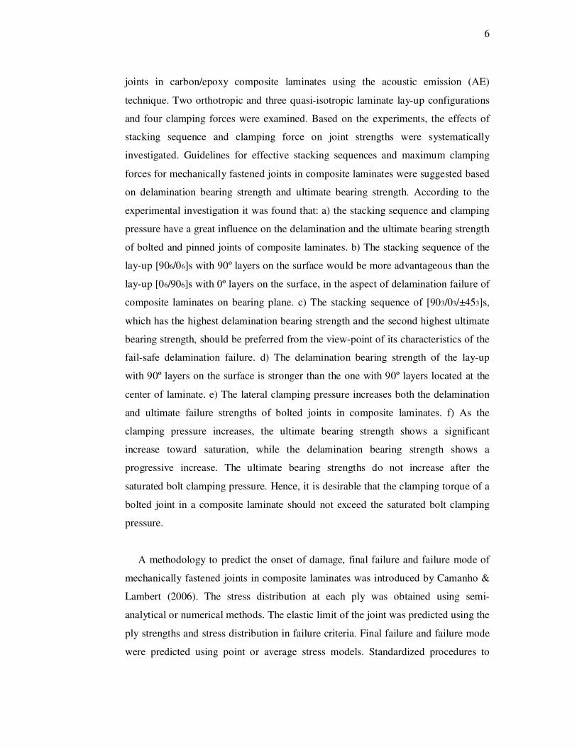
4.2.2 Engineering Constants for Orthotropic Materials ................................... 45

4.2.3 Stress-Strain Relations for Thin Lamina ................................................ 45

4.2.4 Material Orientation in Two-Dimensional Lamina ................................ 45

4.2.5 Elastic Properties of multidirectional laminates ..................................... 48

4.2.5.1 Basic Assumptions ........................................................................ 48

4.2.5.2 Strain Displacement Relations ....................................................... 48

4.2.5.3 Strain and Stress Relations in a Laminate ....................................... 51

4.2.5.4 Force and Moment Resultants ........................................................ 51

4.3 Micromechanical Behavior of a Lamina ....................................................... 55

4.3.1 The prediction of E1 .............................................................................. 56

4.3.2 The prediction of E2 .............................................................................. 57

4.3.3 The prediction of 12ν ............................................................................. 58

4.3.4 The prediction of 12G ............................................................................. 59

viii

CHAPTER FIVE – FAILURE ANALYSYS IN COMPOSITES ........................ 61

5.1 Introduction .................................................................................................. 61

5.2 Failure Criteria of a Lamina .......................................................................... 63

5.2.1 Maximum Stress Failure Criterion ......................................................... 63

5.2.2 Maximum Strain Failure Criterion ......................................................... 64

5.2.3 Tsai-Hill Failure Criterion ..................................................................... 65

5.2.4 Hoffman Failure Criterion ..................................................................... 67

5.2.5 Tsai-Wu Tensor Failure Criterion ......................................................... 68

CHAPTER SIX – DETERMINATION OF BASIC MATERIAL

PROPERTIES ....................................................................................................... 71

6.1 Introduction .................................................................................................. 71

6.2 Test Procedures ............................................................................................ 73

6.2.1 Determination of the Tensile Properties ................................................. 73

6.2.2 Determination of the Compressive Properties ........................................ 74

6.2.3 Determination of the Shear Properties ................................................... 75

6.3 Results of Mechanical Property Tests ........................................................... 78

CHAPTER SEVEN – EXPERIMENTAL STUDY AND RESULTS 0F

SINGLE LAP DOUBLE SERIAL FASTENER JOINTS AT ELEVATED

TEMPERATURES ............................................................................................... 79

7.1 Introduction .................................................................................................. 79

7.2 Explanation of the Problem........................................................................... 79

7.3 Material Production ...................................................................................... 80

7.4 Thermal Test Chamber ................................................................................. 81

7.5 Testing Procedure ......................................................................................... 82

7.6 Results and Discussion ................................................................................. 82

ix

CHAPTER EIGHT – EXPERIMENTAL STUDY AND RESULTS 0F

SINGLE LAP DOUBLE SERIAL FASTENER JOINTS AT LOW

TEMPERATURES ............................................................................................... 92

8.1 Introduction .................................................................................................. 92

8.2 Explanation of the Problem........................................................................... 92

8.3 Experimental Setup and the Cooling Process ................................................ 93

8.4 Testing Procedure ......................................................................................... 94

8.5 Results and Discussion ................................................................................. 94

CHAPTER NINE – CONCLUSIONS ................................................................ 102

REFERENCES ................................................................................................... 104

1

CHAPTER ONE

INTRODUCTION

1.1 Overview

Because of rapid technological development and increased competition in

industry, lightweight, high strength materials with high performance have been the

main need in real applications. The use of composite materials which meets the need

has an ever-expanding trend of variety such as for military and commercial air

vehicles, robot arms, and automotive industry. Especially for use in aviation and

aerospace industry, composite materials, which are lighter than metals and higher

strength in terms of weight, are designed and produced. Trusses, optical benches,

equipment-panels, solar array support systems, and radiators, are some typical

spacecraft structures which should have high specific stiffness, low coefficient of

thermal expansion and dimensional stability during operation. High-performance

composites satisfy these requirements, and also offer the minimum weight material

solution for these structures (Park, 2001). They are also becoming more commonly

used with every generation of aircraft. The Boeing 787 is a prime example, which is

set to include 50% composite material by weight. (Pearce et al., 2010).

It is generally impossible to produce a structure without using joints because of

the limitations of material sizes, and conformity for manufacture or transportation.

Joints are usually the weakest points of a construction so they determine the stability

of composite structure. Composite structures can be assembled by using adhesively

bonded and / or mechanically fastened joints. Although leading to a weight penalty

due to stress concentration created by drilling a hole in the laminate, mechanical

fasteners are widely used in composite joints owing to their unique characteristics

such as lower cost of producing, testing and maintaining and convenience to inspect

load carrying capacity etc.

The above mentioned stress concentrations lead to high tensile stresses in pinned

and bolted composite parts. On the other hand, the front side of the hole is deformed

2

under pressure and the interface between the fastener and the laminate change as

applied load increasing, which results in altering the force distribution in the

interface. Depending on its geometry, a pinned or bolted composite joint can exhibit

four different failure modes, namely the net tension, bearing, shear-out, and cleavage

failure. In practice, combinations of these failure modes are observed. The bearing

and shear-out failure modes are usually more or less ductile, but the net-section and

cleavage ones are brittle and abrupt. The net tension failure mode is defined by

fracture of a laminate across its width from the hole to its edges, the shear-out failure

mode is described by the pull-out fracture between the hole and laminate end, and the

cleavage failure mode is defined by the simultaneous fracture across the width to one

edge and between the hole and the laminate end. The bearing failure mode is thought

to be the desirable mode, since it generally gives a higher strength, and the failure is

less brittle. The other three modes are often considered as premature ones, which

should be prevented through a proper design of the joint geometry and the composite

material it self. These failure types are undesirable, giving rise to an abrupt damage

growth. Finally, a serious problem in designing the joints is the selection of their

geometrical parameters suitable to force the bearing failure (Pekbey, 2008).

An understanding of the stiffness, strength and failure mode of bolted joints is

critical to an efficient design of composite structures. The strength of pinned or

bolted joints depends on many factors, including joint geometry, fiber orientation,

stacking sequence, through thickness pressure, etc. Similarly, the particular failure

mode that is observed in a pinned or bolted connection is also dependent on

geometry, lay up, and loading direction. A large part of the research that has been

done on mechanically fastened joints has been concerned with the experimental and

numerical determination of the influence of geometric factors on the joint strength

and failure type. Several authors carried out the effects of joint geometry, ply

orientation and geometrical parameters such as the end distance-to-diameter (E/D),

width-to-diameter ratios (W/D) on the failure strength and failure modes of

mechanically fastened laminated composite plates (Asi, 2010).

3

Karakuzu et al. (2008) investigated the effects of geometrical parameters such as

the edge distance-to-hole diameter ratio (E/D), plate width-to-hole diameter ratio

(W/D), and the distance between two holes-to-hole diameter ratio (M/D) on the

failure loads and failure modes in woven-glass–vinyl ester composite plates with two

serial pin-loaded holes, experimentally and numerically. In the numerical analysis,

they used the Hashin failure criterion in order to determine failure loads and failure

modes. LUSAS commercial finite element software was utilized during their

analysis. After experimental and numerical studies they showed that the ultimate

load capacity of woven glass– vinyl ester laminates with pin connections increased

by increasing ratios E/D, W/D, and M/D. Besides geometrical parameters, Sayman &

Ozen (2011) investigated the first failure load and the bearing strength behavior of

pinned joints of glass fiber reinforced woven epoxy composite prepregs with two

serial holes subjected to traction forces by two serial rigid pins for immersed and

unimmersed conditions. There was almost no difference between the results of the

immersed and unimmersed specimens under preload moments.

Aktaş et al. (2009) analyzed experimentally and numerically failure mode and

failure load of glass-epoxy plates with single and double parallel-pinned joints. The

distance from the free edge of plate to the diameter of the first hole (E/D) ratios (2, 3,

4, 5) and the width of the specimen to the diameter of the holes (W/D) ratios (2, 3, 4,

5) were investigated during analyses. Experiments were carried out according to

ASTM D953-D and numerical study was performed by means of ANSYS program.

According to experimental and numerical results, from which a good agreement

obtained, the pin hole farthest from the free edge is subjected to the highest stress.

Okutan (2006) investigated the effects of joint geometry and fiber orientation on

the failure strength and failure mode in pinned joint laminated composite plate.

E/glass-epoxy laminated composites were loaded through pins. The specimens were

loaded by single hole and tested to evaluate width to hole diameter (W/D) and the

edge distance to hole diameter (E/D) effects. Six different composite configurations

([0/±45]s–[90/±45]s, [0/90/0]s–[90/0/90]s and [90/0]2s–[±45] 2s) were used. E/D

ratios from 1 to 5 and W/D ratios from 2 to 5 were tested. Testing results showed that

4

the fiber orientations have definite influence on the position around hole

circumference at which failure initiated. Another result was that the ultimate load

capacities of E/glass-epoxy laminate plates with pin connection were increased by

increasing W and E, but if E/D and W/D are increased beyond a critical value it has

not a significant effect on the ultimate load capacity of the connection.

Asi (2010) studied pinned joints of glass fiber reinforced composite filled with

different proportions of Al2O3 particles (as function of filler loading and joint

geometry) and investigated the bearing strength behavior. The weight fractions of the

filler in the matrix were 7,5,10 and 15 %. The single hole pin loaded specimens were

tested in tension. The test results showed that the increase of Al2O3 particle in the

matrix improves the bearing strength of composites. Beyond a critical value of

particle content the bearing strength began to decrease but remained above that of the

unfilled glass reinforced epoxy composites.

In order to determine the influence of the preload moment, the edge distance to

the pin diameter ratio, and the specimen width to the pin diameter ratio on the

strength of the material, Pekbey (2008) investigated the failure strength of a bolted

joint e-glass/epoxy composite plate. Load-displacement curves were obtained for

each test. Experimental results showed that the maximum bearing strength was

reached at max preload moment 4 Nm, max W/D ratio 6 and max E/D ratio 5. At

W/D=2 the most dangerous mode net tension developed and at E/D<2 the shear-out

failure mode occurred, which is another undesirable failure mode.

Ling (1986) considered the effect of clamping on bolted joints and presented a

way to predict critical bearing strength of single-hole joints on the basis of observing

and analyzing the results of experiments. The comparison between the experimental

and the calculated value showed that the estimate method of the ultimate bearing

load is available for bolted joints.

Dano at al. (2000) presented a finite element model including the characteristics

friction, non-linear shear behavior, large deformation theory and property

5

degradation. In particular, the influence of the failure criteria and the inclusion of

geometric and shear non-linearities was discussed in the paper. The deformation

behavior of the pin loaded joint was predicted using a two dimensional finite element

model developed in the commercial software ABAQUS. The composite plate was

modeled using a single layer of CPS4 elements since shell element couldn’t be used

to simulate in plane-contact problems. Because the technique allowed computing the

stresses in each ply, propagation of damage from ply-to-ply could be studied. Then

the progressive failure analysis used to study damage propagation around the hole

was described. To predict the progressive ply failure, the analysis combined Hashin

and the maximum stress failure criteria. From the theoretical and the experimental

results of the study, it can be concluded that when the shear stress-strain relationship

is linear, the use of maximum stress criterion for fiber failure leads to higher and

more realistic strength than Hashin criterion. When a non-linear shear stress-strain

relationship is considered, the predictions from the different failure analysis converge

toward the same predictions. When using mixed failure criteria, including a non-

linear shear behavior has a slight effect for the quasi-isotropic [(0/±45/90)3]s

laminate whereas for the [(0/90)6]s and [(±45)6]s laminates the increase in the

strength prediction was quite important.

Park (2001 a) developed a methodology for assessing the delamination bearing

strength of mechanically fastened joints in finite carbon-epoxy composite laminates

in conjunction with accurate three dimensional contact stress analysis via a quasi-

three-dimensional finite element procedure based on the layer wise theory. The

contact phenomena and stress distribution in the vicinity of joints in composite

laminates were investigated. The lamination bearing failure strengths of

mechanically fastened joints in composite laminates were predicted using modified

Ye-delamination failure criterion based on layer wise finite element contact stress

analysis. Comparisons of the numerical results with experimental data showed the

accuracy and applicability of the analysis.

Park (2001b) examined the effects of stacking sequence and clamping force on

delamination bearing strength and ultimate bearing strength of mechanically fastened

6

joints in carbon/epoxy composite laminates using the acoustic emission (AE)

technique. Two orthotropic and three quasi-isotropic laminate lay-up configurations

and four clamping forces were examined. Based on the experiments, the effects of

stacking sequence and clamping force on joint strengths were systematically

investigated. Guidelines for effective stacking sequences and maximum clamping

forces for mechanically fastened joints in composite laminates were suggested based

on delamination bearing strength and ultimate bearing strength. According to the

experimental investigation it was found that: a) the stacking sequence and clamping

pressure have a great influence on the delamination and the ultimate bearing strength

of bolted and pinned joints of composite laminates. b) The stacking sequence of the

lay-up [906/06]s with 90º layers on the surface would be more advantageous than the

lay-up [06/906]s with 0º layers on the surface, in the aspect of delamination failure of

composite laminates on bearing plane. c) The stacking sequence of [903/03/±453]s,

which has the highest delamination bearing strength and the second highest ultimate

bearing strength, should be preferred from the view-point of its characteristics of the

fail-safe delamination failure. d) The delamination bearing strength of the lay-up

with 90º layers on the surface is stronger than the one with 90º layers located at the

center of laminate. e) The lateral clamping pressure increases both the delamination

and ultimate failure strengths of bolted joints in composite laminates. f) As the

clamping pressure increases, the ultimate bearing strength shows a significant

increase toward saturation, while the delamination bearing strength shows a

progressive increase. The ultimate bearing strengths do not increase after the

saturated bolt clamping pressure. Hence, it is desirable that the clamping torque of a

bolted joint in a composite laminate should not exceed the saturated bolt clamping

pressure.

A methodology to predict the onset of damage, final failure and failure mode of

mechanically fastened joints in composite laminates was introduced by Camanho &

Lambert (2006). The stress distribution at each ply was obtained using semi-

analytical or numerical methods. The elastic limit of the joint was predicted using the

ply strengths and stress distribution in failure criteria. Final failure and failure mode

were predicted using point or average stress models. Standardized procedures to

7

measure the characteristic distances used in the point or average stress models were

proposed. The statistical analysis of the experimental results showed that the

characteristic distances in tension are a function of both the hole diameter and

specimen width. It was also concluded that the characteristic distances in

compression are a function of the clamping conditions applied to the joints and of the

hole diameter. The methodology proposed was proved that it is practical in double-

shear mechanically fastened joints using quasi-isotropic laminates under uniaxial or

multi-axial loading. The predictions were compared with experimental data obtained

in pin-loaded and bolt-loaded joints, and the results indicated that the methodology

proposed could accurately and effectively predict ultimate failure loads as well as

failure modes in composite bolted joints.

Bolt-hole clearance effects on failure behavior have been another issue of interest,

the researchers are dealing with. Kelly and Hallström (2004), examined the effect of

bolt-hole clearance on the bearing strength at 4% hole deformation and at ultimate

load. Significant reduction in bearing strength at 4% hole deformation was found for

both pin-loaded and clamped laminates as a result of bolt-hole clearance. It was

concluded that the effect of bolt-hole clearance is significant with regard to the

design bearing strength of mechanically fastened joints. The magnitude and

distribution of stress at the hole was found to be significantly dependent on the level

of clearance.

Sen et al. (2008) investigated the failure mode and bearing strength of

mechanically fastened bolted-joints in glass fiber reinforced epoxy laminated

composite plates, experimentally. Two different geometrical parameters which are

the edge distance-to-hole diameter ratio (E/D) and plate width-to-hole diameter ratio

(W/D) were studied. E/D ratios were selected from 1 to 5, whereas W/D ratios were

chosen from 2 to 5. Laminated plates were stacked as three different group which are

[0º/0º/45º/−45º]s, [0º/0º/45º/45º]s and [0º/0º/30º /30º]s, to determine material

parameters effect. In addition, the preload moments were applied as 0, 3 and 6 Nm,

to observe the changing of failure mechanism under various preloads. The

experiments were also performed under a clearance, thus the diameters of the bolt

8

and the circular bolt hole were fixed 5 and 6 mm, respectively. Results showed that

failure modes and bearing strengths were affected by the increasing of preloads to a

considerable extent. The maximum values of bearing strengths were calculated for

the group of having 3 Nm torque. Furthermore, when the material and geometrical

parameters of composite bolted joints were changed, the failure behavior and the

values of bearing strengths were fully influenced from this change.

A similar study was conducted by Kishore et al. (2009). The study was aimed to

obtain failure modes and failure loads for multi-pin joints in unidirectional glass

fiber/epoxy composite laminates by finite element analysis and validating the results

with the experimental work. The effect of variation in pitch-to-diameter ratio (P/D),

in addition to side width-to-diameter (S/D) and edge-to-diameter (E/D) ratios were

studied in multi-pin joints. Developing a two-dimensional finite element model with

ANSYS software, Tsai–Wu failure criteria associated with material property

degradation was used in the analysis to predict failure load and to differentiate failure

modes.

An artificial neural network (ANN) method was developed by Sen et al. (2010) to

predict the bearing strength of two serial pinned / bolted E-glass reinforced epoxy

composite joints. The experimental data with different geometrical parameters and

under various applied torques were used for developing the ANN model.

Comparisons of ANN results with desired values showed that ANN is a valid

powerful tool to prediction of bearing strength of two serial pinned / bolted

composite joints. In another study, Sen & Sayman (2011) investigated the effects of

material parameters, geometrical parameters and magnitudes of preload moments on

the failure response of two serial bolted joints in composite laminates. Some

geometrical ratios were found out to be unfavorable and the increasing of preloads

was seen very convenient for safe design of two serial bolted composite joint.

Lie et al. (2000) developed a boundary element formulation for analyzing a

mechanically bolted composite. Boundary equations were formulated for all the

member panels of the composite joints. These equations were solved together with

9

the fastener equations to get the resultant contact forces for all the fasteners involved.

The fasteners were then modeled as 1D springs that are governed by linear

relationship between the fastener forces and the displacements of member panels at

the respective fastener centers. After obtaining all the fastener forces from the global

analysis, detailed stress analysis was performed for region around an individual

fastener. The stress distributions around fastener holes were then used to evaluate the

margin of safety of the composite panels. The numerical predictions on the fastener

forces, failure modes and failure loads of two typical bolted composite joints using

the proposed method were compared and it was found that they agree well with that

of the experimental results.

The onset of local damage in joints, such as delamination, cracking and fastener

loosening can often be difficult to detect and has long-term implications on the

performance of the structure. To develop an innovative technique to monitor the state

of damage in composite structures, Thostenson et al. (2008) reported the capability

of carbon nanotube networks as in situ sensors for sensing local composite damage

and bolt loosening in mechanically fastened glass/epoxy composite joints. According

to their research it was possible to detect the onset and progression of damage in the

joint through careful design of the specimen.

Ekh & Schön (2006) developed a three-dimensional finite element model in order

to determine the load transfer in multi fastener single shear joints. The model was

based on continuum elements and accounted for the mechanisms involved in load

transfer, such as bolt-hole clearances, bolt clamp-up and friction. They conducted an

experimental program in order to validate the finite element model through

measurement of fastener loads, by means of instrumented fasteners. The results

showed that simulations and experiments agreed well and the bold-hole clearance is

the most important factor in terms of load distribution between the fasteners. Any

variation in clearance between the different holes implies that the load is shifted to

the fastener where the smallest clearance occurs. It was also found that sensitivity to

this variation was large, so that temperature changes could significantly affect the

load distribution if member plates with different thermal expansion properties are

10

used. It was concluded that, good accuracy in load transfer predictions requires that

all factors would be taken into consideration and nonlinear kinematics should be

accounted for the solution process.

In some cases, the joints transferring large mechanical loads between composite

panels of advanced vehicles need to be operated at high and low temperature

extremes. Mechanical properties of polymer matrix joints are usually influenced by

the thermal environment. In particular, it is known that temperatures exceeding the

glass transition temperature (Tg) seriously degrade the material properties. The

amount or rate of material degradation varies depending on the material (Song et al.,

2008). At the other end of spectrum, an application of composite joint in a cryogenic

environment would be possible. A computational study investigating thermal effects

on pin bearing behavior of IM7/PETI5 composite joints was reported by Walker

(2002). Pin-bearing tests of several lay-ups at the operating temperatures of -129, 21,

and 177 °C were conducted to generate data on the effect of temperature changes on

the pin-bearing behavior. Thermal residual stresses were combined with the state of

stress due to pin-bearing loads at three-dimensional solution. The presence of

thermal residual stresses intensify the inter laminar stresses predicted at the hole

boundary in the pin-bearing problem. The research showed that changes in material

properties drive pin-bearing strength degradation with increasing temperature.

Sánchez-Sáez et al. (2002) tested carbon fiber reinforced epoxy laminates to

determine the effect of low temperature on the mechanical behavior. Tensile and

bending static tests were carried out on two laminate lay-ups (quasi-isotropic and

cross-ply laminates), determining properties such as the mechanical strength,

stiffness and strain to failure. The results reveal the changes in the mechanical

behavior of this material at different test temperatures (20, -60 and -150 °C). As a

result, three different test temperatures affected the mechanical behavior of the

material. The stiffness of the quasi-isotropic laminate grows as the temperature

decreases. At room temperature, the matrix fails first. As the temperature decreases,

the fiber–matrix interface becomes much weaker and thus the fibers debond from the

matrix.

11

Hirano et al. (2007) investigated the effects of temperature on the bearing failure

of a pinned joint in CF/epoxy quasi-isotropic laminates. Two stacking sequences,

namely, [0/45/−45/90]3S and [90/−45/45/0]3S, were loaded at room temperature

(25°C), high temperature (150°C), and low temperature (-100°C); then, the internal

damages were evaluated. It was found that the bearing failure of a pinned joint is

composed of various damages depending on environmental temperatures; further, the

strength of the pinned joint is closely related to the compressive kinking failure of all

the inner layers.

1.2 Objectives of the Study

As seen in related literature, many authors were interested in material and

geometrical parameters influencing the failure behaviors of mechanically fastened

composite joints. However, a few of them have taken into account the environmental

effects, particularly the temperature extremes that composite joints are exposed

during operation. Among these studies, those associated with glass-fiber reinforced

composites are even more limited.

Through the current experimental study it was intended to investigate the failure

responses of mechanically fastened joints in glass fiber – epoxy composite laminates

at varying high and low temperature levels. The bolted joints were initially subjected

to tensile loadings together with the effects of high thermal conditions from 40 °C up

to 80 °C, gradually increasing chamber temperatures for each test. In the second

phase of experiments, the joints were exposed to low temperature environments,

which were gradually decreased down to – 40 °C during tensile tests. Carefully

observing failure behaviors of joints at varying temperature levels, it was finally

reached to some significant conclusions about mechanically fastened joints under

thermal effects.

12

CHAPTER TWO

COMPOSITE MATERIALS

2.1 Introduction

Composite materials can be defined as materials consisting of two or more

constituents (phases) that are combined at the macroscopic level and are not soluble

in each other. Modern synthetic composites using reinforcement fibers (one phase)

and matrices (another phase) of various types have been introduced as replacement

materials to metals in civilian, military, and aerospace applications (Sheikh-Ahmad,

2009, p.1).

In fact, what expected by using composite materials is to provide different

physical, mechanical or chemical properties by the constituents, having these special

features alone. When analyzing the internal structure of composite materials, which

is highly heterogeneous character at macro level, it is possible to distinguish the body

compounds. The different characteristics of structural components integrate into one

formation. It is therefore impossible to observe the characteristics, all of which

composite material possess, in a single component.

2.2 Historical Development of Composite Materials

In nature, composite materials have been in existent for millions of years. Wood,

bamboo and bone are just a few examples of the natural occurring composite

materials. Man has learned to fabricate composite materials relatively recently.

Perhaps, one of the first evidence of a man-made composite material is the mud-

blocks reinforced with straws. The composite material fabrication technology has

since progressed from straw based mud-blocks to man-made fiber reinforced

composite materials (Choo, 1990, p.2).

In the 20th century, modern composites were used in the 1930s when glass fibers

reinforced resins. Boats and aircraft were built out of these glass composites,

13

commonly called fiber-glass. Since the 1970s, application of composites has widely

increased due to development of new fibers such as carbon, boron, and aramids, and

new composite systems with matrices made of metals and ceramics (Kaw, 2006,

p.1,2).

Figure 2.1 Relative importance of material development through history (Staab, 1999)

The structural materials most commonly used in design can be categorized in four

primary groups: metals, polymers, composites and ceramics. These materials have

been used to various degrees since the beginning of time. Their relative importance

to various societies throughout history has fluctuated (Figure 2.1). The relative

importance of each group of materials is not associated with any specific unit of

measure (net tonnage, etc.). As with many advances throughout history, advances in

material technology (from both manufacturing and analysis viewpoints) typically

have their origins in military applications. Subsequently, this technology filters into

the general population and alters many aspects of society. This has been most

recently seen in the marked increase in relative importance of structural materials

such as composites starting around 1960, when the race for space dominated many

aspects of research and development. Similarly, the Strategic Defense Initiative

14

(SDI) program in the 1980s prompted increased research activities in the

development of new material systems (Staab, 1999, p.2).

2.3 The Major Characteristics of Composites and Comparison with Conventional

Materials

An obvious advantage that the fiber reinforced composite materials have over the

conventional engineering materials such as copper, steel, aluminum, titanium, etc., is

the high specific strength and modulus as seen in Table 2.1. The definition of

specific strength is the ratio of the material strength to the material density and the

specific modulus is defined as the material Young’s modulus per unit material

density. High specific strength and specific modulus have important applications on

the engineering applications of composite materials. It means that the composite

materials are strong and stiff and yet light in weight. Such characteristic are very

desirable in the aeronautical and aerospace industry. The weight savings realized by

fabricating structural components out of composite materials is directly translated

into fuel savings which in turn makes the operation of aeroplane and space vehicle

more economical (Choo, 1990, p.2). A comparative representation of the

performance of typical structural composites from the point of view of specific

properties is shown in Figure 2.2.

Figure 2.2 Performance map of structural composites (Daniel & Ishai, 1994)

15

Table 2.1 Specific Modulus and Specific Strength of Typical Fibers, Composites, and Bulk Metals (Kaw, 2006)

Material Units

Specific Gravity

Young's modulus

(Gpa)

Ultimate strength (Mpa)

Specific modulus

(Gpa-m³/kg)

Specific Strength

(Mpa-m³/kg)

System of Units: SI

Graphite fiber 1.8 230.00 2067.00 0.1278 1.148

Aramid fiber 1.4 124.00 1379.00 0.08857 0.9850

Glass fiber 2.5 85.00 1550.00 0.0340 0.6200

Unidirectional graphite/epoxy 1.6 181.00 1500.00 0.1131 0.9377

Unidirectional glass/epoxy 1.8 38.60 1062.00 0.02144 0.5900

Cross-ply graphite/epoxy 1.6 95.98 373.00 0.06000 0.2331

Cross-ply glass/epoxy 1.8 23.58 88.25 0.01310 0.0490

Quasi-isotropic graphite/epoxy 1.6 69.64 276.48 0.04353 0.1728

Quasi-isotropic glass/epoxy 1.8 18.96 73.08 0.01053 0.0406

Steel 7.8 206.84 648.01 0.02652 0.08309

Aluminum 2.6 68.95 275.80 0.02652 0.1061 Specific gravitiy of a material is the ratio between its density and density of water.

Besides strength, stiffness and lightweight, some additional outstanding

improvements in material properties can be achieved by using composite materials.

Those are, corrosion resistance, abrasion resistance, fatigue life, temperature-

dependent behavior, thermal insulation, thermal and electrical conductivity, acoustic

insulation etc.

As well as these advantages, some disadvantages may also be encountered when

working with composite materials. High costs of production, difficulties in

processing, repairing and in obtaining the required surface quality, lack of recycling

property and low elongation values before fracture are main drawbacks representing

limits when employing composites in structures. In addition, mechanical

characterization of a composite structure is more complex than that of a metal

structure. Properties of composites depend on both the fiber orientation and the lay-

up sequence in the laminate because of anisotropic nature of fiber-reinforced

composites, unlike metals. The other challenge is the impracticability of

nondestructive inspection techniques, such as eddy currents and X-ray which give

satisfying results in metal parts. Ultrasound, laser and acoustic emission techniques

are more convenient to inspect flaws and crack initiation in composite structures. The

mentioned drawbacks forces researchers to develop manufacture processes which is

controlled by the real-time monitoring tools. In order to obtain high quality products,

16

optimum process parameters should be estimated by using a mathematical model,

which is appropriate to the certain manufacturing process.

2.4 Classifications of Composite Materials

2.4.1 Classifications by the Geometry of the Reinforcement

The second constituent is referred to as the reinforcing phase, or reinforcement, as

it enhances or reinforces the mechanical properties of the matrix. In most cases the

reinforcement is harder, stronger and stiffer than the matrix, although there are some

exceptions; for example, ductile metal reinforcement in a ceramic matrix and

rubberlike reinforcement in a brittle polymer matrix. At least one of the dimensions

of the reinforcement is small, say less than 500 µm and sometimes only of the order

of a micron. The geometry of the reinforcing phase is one of the major parameters in

determining the effectiveness of the reinforcement; in other words, the mechanical

properties of composites are a function of the shape and dimensions of the

reinforcement. We usually describe the reinforcement as being either fibrous or

particulate ( Matthews & Rawlings, 1999, p.5).

2.4.1.1 Fibrous Composite Materials

Fibrous Composite Materials are composed of fibers embedded in matrix

material. Such a composite is considered to be a discontinuous fiber or short fiber

composite if its properties vary with fiber length. On the other hand, when the length

of the fiber is such that, any further increase in length does not further increase, the

elastic modulus of the composite, the composite is considered to be continuous fiber

reinforced.

Discontinuous or short-fiber composites contain short fibers or whiskers as the

reinforcing phase (Figure 2.3). These short fibers, which can be fairly long compared

with the diameter, can be either all oriented along one direction or randomly

oriented. In the first instance the composite material tents to be markedly anisotropic

17

or, more specifically, orthotropic, whereas in the second it can be regarded as quasi-

isotropic.

Continuous fiber composites are reinforced by long continuous fibers and are the

most efficient from the point of view of stiffness and strength (Figure 2.3). The

continuous fibers can be all parallel (unidirectional continuous fiber composite), can

be oriented at right angles to each other (crossply or woven fabric continuous fiber

composite), or can be oriented along several directions (multidirectional continuous

fiber composite). In the latter case, for a certain number of fiber directions and

distribution of fibers, the composite can be characterized as a quasi-isotropic material

(Daniel & Ishai, 1994, p.20).

Figure 2.3 Classification of composite materials by the geometry of the reinforcement (Daniel & Ishai, 1994)

18

A fibrous reinforcement is characterized by its length being much greater than its

cross-sectional dimension. Nevertheless, the ratio of length to the cross-sectional

dimension, known as the aspect ratio, can vary considerably. In single-layer

composites long fibers with high aspect ratios give what are called continuous fiber

reinforced composites, whereas discontinuous fiber composites are fabricated using

short fibers of low aspect ratio. The orientation of the discontinuous fibers may be

random or preferred. The frequently encountered preferred orientation in the case of

a continuous fiber composite is termed unidirectional and the corresponding random

situation can be approximated to by bidirectional woven reinforcement ( Matthews &

Rawlings, 1999, p.5)

2.4.1.2 Particulate Composite Materials

Particulate composites consist of particles of various sizes and shapes randomly

dispersed within the matrix (Daniel & Ishai, 1994, p.20). Particulate reinforcements

have dimensions that are approximately equal in all dimensions. The shape of the

reinforcing particles may be spherical, cubic, platelet, or any regular or irregular

geometry. The arrangement of the particulate reinforcement may be random or with a

preferred orientation, and this characteristics is also used as a part of classification

scheme. In the majority of particulate reinforced composites the orientation of the

particles is considered, for practical purposes, to be random ( Matthews & Rawlings,

1999, p.5).

Particulate composites may nonmetallic particles in a nonmetallic matrix

(concrete, glass reinforced with mica flakes, brittle polymers reinforced with

rubberlike particles); metallic particles in nonmetallic matrices (aluminum, particles

in polyurethane rubber used in rocked propellants); metallic particles in metallic

matrices (lead particles in copper alloys to improve machinability); and non metallic

particles in metallic matrices (silicon carbide particles in aluminum, SiC(p)Al)

(Daniel & Ishai, 1994, p.20).

19

2.4.2 Classifications by the Type of Matrix

It has been stated before, that composites consist of two or more distinctly

different materials. In most cases, the composite is made of matrix and reinforcement

materials that are mixed in certain proportions. The matrix material may be made

from metals, ceramics, or polymers. It may be pure, or mixed with other materials

(additives) to enhance its properties. The reinforcement may also be treated to

enhance bonding to the matrix (Sheikh & Ahmad, 2009, p.7).

2.4.2.1 Polymer Matrix Composites

The most common advanced composites are polymer matrix composites (PMCs)

consisting of a polymer (e.g., epoxy, polyester, urethane) reinforced by thin diameter

fibers (e.g., graphite, aramids, boron). For instance, graphite/ epoxy composites are

approximately five times stronger than steel on a weight for- weight basis. The

reasons why they are the most common composites include their low cost, high

strength, and simple manufacturing principles. The main drawbacks of PMCs include

low operating temperatures, high coefficients of thermal and moisture expansion,*

and low elastic properties in certain directions (Kaw, 2006, p.19). Some mechanical

properties of polymer matrix composites are given in Table 2.2.

Glass, graphite, and Kevlar are the most common fibers used in polymer matrix

composites because of the unique advantages, including high strength, low cost, high

chemical resistance, and good insulating properties. On the other hand, low elastic

modulus, poor adhesion to polymers, high specific gravity, sensitivity to abrasion,

and low fatigue strength present obstacles in construction.

The main types are E-glass (also called “fiberglass”) and S-glass. The “E” in E-

glass stands for electrical inasmuch as it was designed for electrical applications.

Nonetheless, it is used for many other purposes now, such as decorations and

structural applications. The “S” in S-glass stands for higher content of silica. It

retains its strength at high temperatures compared to E-glass and has higher fatigue

20

strength. It is used mainly for aerospace applications. Other types available

commercially are C-glass (“C” stands for corrosion) used in chemical environments,

such as storage tanks; R-glass used in structural applications such as construction; D-

glass (dielectric) used for applications requiring low dielectric constants, such as

radomes; and A-glass (appearance) used to improve surface appearance.

Combination types such as E-CR glass (“E-CR” stands for electrical and corrosion

resistance) and AR glass (alkali resistant) also exist (Kaw, 2006, p.19).

Table 2.2 Typical mechanical properties of polymer matrix composites and monoclinic materials

(Kaw, 2006)

Property Units Graphite/

epoxy Glass/ epoxy

Steel Aluminum

System of Units: USCS

Specific gravity --- 1.6 1.8 7.8 2.6

Young’s modulus Msi 26.25 5.598 30.0 10.0

Ultimate tensile stength ksi 217.6 154.0 94.0 40.0

Coefficient of thermal expansion µin./in./°F 0.01111 4.778 6.5 12.8

System of Units: SI

Specific gravity --- 1.6 1.8 7.8 2.6

Young’s modulus GPa 181.0 38.6 206.8 68.95

Ultimate tensile stength MPa 150.0 1062 648.1 275.8

Coefficient of thermal expansion µn./m/°C 0.02 8.6 11.7 23

Graphite fibers are also very common in the applications of aircraft components,

in terms of their high specific modulus and strength, low coefficient of thermal

expansion and high fatigue strength. High cost, low impact resistance, and high

electrical conductivity represent the disadvantages of graphite fibers in polymer

matrix composites.

Aramid fibers are made of an aromatic organic compound, consisting of hydrogen,

carbon, oxygen, and nitrogen. Aramid fibers are inexpensive, resistant to impact, low

density, and high tensile strength, but high moisture uptake and sensitiveness to

sunlight restrain its use in composites.

Epoxy, phenolics, acrylic, urethane, and polyamide are most commonly used

binder materials in polymer matrix composites. Of these types of materials, epoxy is

21

one of the most preferred one, even though it is costlier than other polymer matrices.

Its superior characteristics, such that high strength, low viscosity and low flow rates,

which allow good wetting of fibers and prevent misalignment of fibers during

processing, low volatility during cure, low shrink rates, which reduce the tendency of

gaining large shear stresses of the bond between epoxy and its reinforcement, and its

being available in more than 20 grades to meet specific property and processing

requirements, makes this choice very sensible.

2.4.2.2 Metal Matrix Composites

Metal matrix composites (MMCs), as the name implies, have a metal matrix.

Examples of matrices in such composites include aluminum, magnesium, and

titanium. Typical fibers include carbon and silicon carbide. Metals are mainly

reinforced to increase or decrease their properties to suit the needs of design. To

illustrate, the elastic stiffness and strength of metals can be increased and large

coefficients of thermal expansion and thermal and electric conductivities of metals

can be reduced, by the addition of fibers such as silicon carbide.

Metal matrix composites are mainly used to provide advantages over monolithic

metals such as steel and aluminum. These advantages include higher specific

strength and modulus by reinforcing low density metals, such as aluminum and

titanium; lower coefficients of thermal expansion by reinforcing with fibers with low

coefficients of thermal expansion, such as graphite; and maintaining properties such

as strength at high temperatures.

MMCs have several advantages over polymer matrix composites. These include

higher elastic properties; higher service temperature; insensitivity to moisture; higher

electric and thermal conductivities; and better wear, fatigue, and flaw resistances.

The drawbacks of MMCs over PMCs include higher processing temperatures and

higher densities (Kaw, 2006, p.40).

22

2.4.2.3 Ceramic Matrix Composites

Ceramic matrix composites (CMCs) have a ceramic matrix such as alumina

calcium alumino silicate reinforced by fibers such as carbon or silicon carbide.

Advantages of CMCs include high strength, hardness, high service temperature

limits for ceramics, chemical inertness, and low density. However, ceramics by

themselves have low fracture toughness. Under tensile or impact loading, they fail

catastrophically. Reinforcing ceramics with fibers, such as silicon carbide or carbon,

increases their fracture toughness, because it causes gradual failure of the composite.

This combination of a fiber and ceramic matrix makes CMCs more attractive for

applications in which high mechanical properties and extreme service temperatures

are desired (Kaw, 2006, p.45).

2.4.2.4 Carbon-Carbon Composites

Carbon–carbon composites use carbon fibers in a carbon matrix. These

composites are used in very high-temperature environments of up to 6000°F

(3315°C), and are 20 times stronger and 30% lighter than graphite fibers.

Carbon is brittle and flaw sensitive like ceramics. Reinforcement of a carbon

matrix allows the composite to fail gradually and also gives advantages such as

ability to withstand high temperatures, low creep at high temperatures, low density,

good tensile and compressive strengths, high fatigue resistance, high thermal

conductivity, and high coefficient of friction. Drawbacks include high cost, low shear

strength, and susceptibility to oxidations at high temperatures (Kaw, 2006, p.46).

23

CHAPTER THREE

JOINING OF COMPOSITE STRUCTURES

3.1 Introduction

In practice, it is often unavoidable to apply joints to combine composite parts to

each other or assemble them with other structural components.

Joining of composite materials poses a special challenge. How to achieve joint

strength or other designed-in functionally specific properties anywhere close to those

of the parent composite, since the integrity or continuity of the reinforcement across

the joint is difficult or impossible to retain or re-establish. The irony here is that

composite materials are usually selected for the exceptional properties they offer to

improve performance. Joining is needed to produce the largest and/or most complex

and/or most sophisticated structures. The performance of a structure or an assembly

is critically dependent on the behavior of any joints it contains, and, as just stated,

most contain joints. Hence, the very reason that composite materials may have been

chosen in the first place may be lost if effective methods for joining cannot be found

(Messler, 2004, p.653).

The most common requirements, affecting the joint design in composites is given

in Figure 3.1. It should be kept in mind that, these requirements should be satisfied to

be able to select the most suitable joint configuration. In general, fiber reinforced

plastic (FRPs) structures can be assembled by using adhesively bonded and/or

mechanically fastened joints. Welding or thermal bonding is also a viable option for

thermoplastic polymer matrix composites.

Joints often occur in transitions between major composite parts and a metal feature

or fitting. For instance, such a situation is represented in aircraft by articulated

fittings on control surfaces as well as on wing and tail components, which require the

ability to pivot the element during various stages of operation. Tubular elements such

as power shafting often use metal end fittings for connection to power sources or for

24

articulation where changes in direction are required. In addition, assembly of the

structure from its constituent parts will involve either bonded or mechanically

fastened joints or both (Peters, 1998, p.610).

Figure 3.1 The most common requirement of the joint design

Table 3.1 A comparison of the advantages and disadvantages of adhesively bonded and bolted composite joints (Baker, Dutton, & Kelly, 2004)

Advantages Disadvantages Bonded Joints

� Small stress concentration in adherents � Stiff connection � Excellent fatigue properties � No fretting problems � Sealed against corrosion � Smooth surface contour � Relatively lightweight � Damage tolerant

� Limits to thickness that can be joined with simple joint configuration

� Inspection other than for gross flaws difficult

� Prone to environmental degradation � Sensitive to peel and through-thickness

stresses � Residual stress problems when joining to

metals � Cannot be disassembled � May require costly tooling and facilities � Requires high degree of quality control � May be of environmental concern

Bolted Joints

� Positive connection, low initial risk � Can be disassembled � No thickness limitations � Simple joint configuration � Simple manufacturing process � Simple inspection procedure � Not environmentally sensitive � Provides through-thickness reinforcement; not sensitive to peel

stresses

� Considerable stress concentration � Prone to fatigue cracking in metallic

component � Hole formation can damage composite � Composite’s relatively poor bearing

properties � Prone to fretting in metal � Prone to corrosion in metal � May require extensive shimming

25

In design process, the behavior of joints for certain individual material, geometric,

and environmental conditions must be taken into account. As shown in Figure 3.1,

load transfer from one joint member to the other is typically affected by the type of

load, the environmental conditions, and the materials being joined. Notwithstanding

adhesive bonding is the principal method and offer much greater joining efficiency,

mechanically fastened composite joints are used in specific applications, in case

adhesive bonding is not appropriate or optimum. In terms of being a clue for

choosing the right joint type, the advantages and disadvantages of adhesively bonded

and mechanically fastened joints are given in Table 3.1.

3.2 Adhesive Bonding

Having uniform load distribution in contact areas, little weight penalty with thin

bond lines, smooth external surfaces for improved aerodynamic and hydrodynamic

flow, adhesively bonding is still the principal method for joining composites.

As stated previously, adhesive joints are capable of high structural efficiency and

constitute a resource for structural weight saving because of the potential for

elimination of stress concentrations which cannot be achieved with mechanically

fastened joints. However, due to lack of reliable inspection methods and a

requirement for close dimensional tolerances in fabrication, aircraft designers have

generally avoided bonded construction in primary structure (Peters, 1998, p.610).

In a structural adhesive joint, the load in one component must be transferred

through the adhesive layer to another component. The efficiency with which this can

be done depends on the joint design, the adhesive characteristics and the

adhesive/substrate interface. In order to transfer the load through adhesive, the

substrates (or adherend) are overlapped to place the adhesive in shear. Figure 3.2

shows some typical joint designs for adhesively bonded joints (Campbell, 2004,

p.245).

26

Figure 3.2 Typical adhesively bonded joint configurations (Campbell, 2011)

Obtaining adequate mechanical results from adhesively bonded joint requires an

appropriate preference of adhesive material. The adhesives most often used for

bonding polymer-matrix composites are synthetic polymeric adhesives that are

generally similar to the matrix of the composite, or mutually compatible with the

matrices of mating composites. Thus, thermosetting polymer adhesives are generally

used for adhesive-bonding thermosetting-matrix composites (e.g., epoxy-glass),

while thermoplastic polymer adhesives are generally used with thermoplastic-matrix

composites (e.g., polyetheretherketone (PEEK) graphite). Solvent cementing can also

be used for bonding thermoplastic-matrix composites, just as it can be used for

bonding monolithic thermoplastics (Messler, 2004, P.665).

27

Figure 3.3 The four basic types of adhesive loading. Tension and shear are acceptable loading methods, provided the bond area is sufficient. Cleavage and peel are to be avoided.

The joint design must ensure that the adhesive is loaded in shear as much as

possible. Cleavage and peel loading (Figure 3.3) should be avoided when using

adhesives. Some further considerations for designing adhesively bonded joints are:

� The adhesive must be compatible with the adherents and be able to retain

its required strength when exposed to in-service stresses and environmental

factors.

� The joint should be designed to ensure a failure in one of the adherents rather than a failure within the adhesive bond line.

� Thermal expansion of dissimilar materials must be considered. Because of

the large thermal expansion difference between carbon composite and

aluminum, adhesively bonded joints between these two materials have been

known to fail during cool down from elevated temperature cures as a result

of the thermal stresses induced by their differential expansion coefficients.

� Proper joint design should be used, avoiding peel or cleavage loading

whenever possible. If peel forces can not be avoided, a lower-modulus (non brittle) adhesive having high peel strength should be used.

� Tapered ends should be used on lap joints to feather out the edge-of-joint stresses. The fillet at the end of the exposed joint should not be removed.

� Selection tests for structural adhesives should include durability testing for

heat, humidity, (and/or fluids), and stress, simultaneously (Campbell, 2011, p.250).

Bonded joints must be carefully designed by conducting adhesive joint tests. Tests

should be done on the actual joints that will be used in production. Environmental

conditions (temperature, moisture and any solvents) that the joint was exposed also

28

must be carried out. All test conditions must be carefully controlled including the

surface preparation, the adhesive and the bonding cycle. The failure modes for all

tests specimens should be examined. Some acceptable and unacceptable failure

modes are shown in Figure 3.4. If the specimen exhibits an adhesive failure at the

adherent-adhesive interface rather than a cohesive failure within the adhesive, it may

be an indication of a surface preparation problem that will result in decreased joint

durability (Campbell, 2004, p.251).

Figure 3.4 Typical failure modes of bonded joints (Campbell, 2011)

29

3.3 Mechanical Fastening

In many applications, joining composite plates by using mechanically fasteners

such as, bolts, pins, rivets etc. cannot be avoided because of requirements for

disassembly of the joint for replacement of damaged structure or to achieve access to

underlying structure.

Adhesive joints tend to lack structural redundancy and are highly sensitive to

manufacturing deficiencies including poor bonding technique, poor fit of mating

parts and sensitivity of the adhesive to temperature and environmental effects such as

moisture. Assurance of bond quality has been a continuing problem in adhesive

joints. While non-destructive evaluation techniques (ultrasonic and X-ray inspection)

may reveal gaps in the bond, there is no present technique, which can guarantee that

a bond, which appears to be intact does, in fact, have adequate load transfer

capability. Thus mechanically fastened joints tend to be preferred over bonded

construction in highly critical and safety related applications such as primary aircraft

structural components, especially in large commercial transports, since assurance of

the required level of structural integrity is easier to be guaranteed in mechanically

fastened assemblies. As a rule, bonded joints prove to be more efficient for lightly

loaded/non-flight critical aircraft structures whereas mechanically fastened joints are

more efficient for highly loaded structures. Bonded construction tends to be more

prevalent in smaller aircraft components (Peters, 1998, p.611).

In mechanical fastening, load transfer is accomplished by compression (bearing)

on the faces of holes passing through the joint members by shear (and, less desirably,

bending) of the fasteners. Some of the load is also transferred through friction on the

face of the joint element if the clamping forces imposed by the fasteners are

sufficient. However, in spite of the fact that high clamping forces (bolt-tightening

torque) are very important to develop high-friction forces to maximize

bearing strength, it may not be possible to maintain these levels of clamping force

during prolonged service, for example, due to wear under service loading conditions.

30

Now that high through-thickness reinforcement is provided by the fasteners, peel

failure of the composite is generally not a problem. Nonetheless, problems can arise

resulting from the relatively low bearing and transverse strengths of the composite

compared with those of metals. Bearing failure results in hole elongation, allowing

bending and subsequent fatigue of the bolt or substructure. Alternatively, the fastener

head may pull through the composite.

Figure 3.5 Schematic illustrations of the main failure modes in mechanical joints in composites (Jones, 1999)

Figure 3.5 illustrates the failure modes of a composite joint. They are, briefly,

tension failure, caused by tangential or compressive stresses at the hole edge,

bearing failure mode, governed by compressive stresses acting on the hole surface,

shear-out failure, caused by shear stresses acting in shear-out planes on the hole

boundary in the principal load direction, bolt failure mode, resulted from high shear

stresses acting in the bolt shank.

In addition, mixed-mode failures can occur, including cleavage

tension, essentially mixed tension / shear; bolt-head pulling through the laminate, a

problem particularly with deeply countersunk holes; and bolt failure due to

bearing failure.

31

The type of failure that occurs depends on the ratio of the effective width to the

diameter of the fastener hole w/d, and the ratio of the edge distance to the diameter

e/d. The variation of failure load with w/d and e/d for a quasi isotropic laminate is

indicated in Figure 3.6. For large w/d and e/d, the joint fails in bearing, and the

failure load is independent of w/d or e/d. With reduced w/d tension failure of the net

section will occur with the joint strength dropping to zero when w/d = 1. If the edge

distance e is reduced, shear failure occurs with the strength of the joint dropping to

zero when e/d =0.5 (Baker, Dutton, & Kelly, 2004, p.338).

Figure 3.6 Transition between failure modes with specimen width (rivet pitch) and edge distance (Baker, Dutton, & Kelly, 2004)

The allowable stresses in each of these modes are a function of:

� Geometry of the joint, including thickness.

� Hole size, spacing, and bearing area, allowing for countersink.

� Fastener loading, single or double shear; that is, loading symmetrical, as in a

double-lap joint, or unsymmetrical, as in a single-lap joint.

� Fastener fit tolerance.

� Clamping area and pressure, allowing for any countersink.

32

� Fiber orientation and ply sequence.

� Moisture content and service temperature.

� Nature of stressing: tension, compression, shear; cyclic variation of stressing;

any secondary bending, resulting in out-of-plane loading. Stresses due to

thermal expansion mismatch in metal-to-composite joints may also have an

effect, but these are rarely considered in mechanical joints.

The ply configuration in most bolted joints is usually chosen to be close to quasi-

isotropic, based on 0°, ± 45 °, and 90° fibers. The non-zero fibers are needed to carry

load around the hole to prevent shear or cleavage-type failures, whereas the 0° fibers

carry the primary bearing loads and tension. The desired failure mode is usually net

tension or compression; however, in some situations (the softer or less catastrophic)

bearing failure may be preferred. If stiff (highly orthotropic) laminates are required

for a particular application, a higher proportion of 0° fibers may be used and further

measures may be required to increase hole strength (Baker, Dutton, & Kelly, 2004,

p.340).

3.4 Hybrid (bolted/bonded) Joining

A joint bonded with a structural adhesive is usually much stiffer than a similar

joint joined by mechanical fastening; even when the mechanical joint is optimally

designed and interference fit fasteners are used. Thus it is not possible to design a

joint in which the load is effectively shared between the bonded and fastened

regions. It was shown that for an optimally designed step-lap joint the bolts transmit

only around one percent of the total load. However, fastening and bonding can be

beneficially used together for several reasons:

� Fasteners provide an alternate in-plane load path as well as through-thickness

reinforcement and therefore can contain the spread of damage in thick-section

composite-bonded joints where failure (for example, due to an overload or to

the development of local bond or inter laminar flaws) would occur by

disbonding of the adhesive layer or by delamination of the composite.

33

� Fasteners can be used at the end of a lap joint to reduce peel stresses.

However, this is a somewhat hazardous application because the

fastener holes, unless very carefully sealed, allow environmental ingress into

the bond interface in the most critical region.

� Fasteners can be used both as a jigging aid and to apply pressure during

adhesive bonding of composite components; generally, this approach would

be effective only with paste adhesives.

� Bonding can be used to alleviate local stresses in the metallic component in a

mechanically fastened joint, markedly improving fatigue and static strength

properties. For the reasons mentioned, the bond line carries most of the load,

and the fasteners become effective only after bond failure. This approach is

extensively used with riveting in the metallic longitudinal fuselage splice

region in commercial aircraft. With composite construction, this approach is

more likely to be used for rework of areas found to be prone to damage

(Baker, Dutton, & Kelly, 2004, p.340).

34

CHAPTER FOUR

STRESS ANALYSIS IN COMPOSITES

4.1 Introduction

A lamina can be defined as a thin plane layer of unidirectional fibers or woven

fabric in a matrix. It is generally of a thickness on the order of 0.125 mm. Even

though several layers of fibers actually exist in the same lamina, the modeled lamina

has only a single fiber per layer (Figure 4.1). A laminate is constructed by stacking a

number of such lamina in the direction of the lamina thickness (Figure 4.2).

Mechanical structures made of these laminates, such as a leaf spring suspension

system in an automobile, are subjected to various loads, such as bending and twisting

(Kaw, 2006, p.61). Laminated composite materials have different responses to the

applied loads in different directions. Therefore, the behavior of each individual

lamina must be predicted to analyze the whole body of composite structure.

Figure 4.1 Schematic illustration of actual and modeled lamina (Staab, 1999)

Figure 4.2 Typical laminate made of three laminas

35

The lamina has principal axes and is characterized as an orthotropic material

(Figure 4.1). Axis 1 is the longitudinal fiber direction, Axis 2 is the transverse

direction in the plane of the lamina, and, Axis 3 is normal to the plane of the lamina.

If two or more unidirectional laminas are stacked together at various orientations,

they constitute a composite laminate.

Stress analysis in composites is performed at two different levels, named as

micromechanics and macromechanics. In micromechanics, fiber diameter, particle

size, or matrix interstices between reinforcement are observed and the interactions of

the constituents are studied on the microscopic scale. Stress, strain and deformation

analysis in the constituents, including matrix and fiber, and their interface also are

dealt in micromechanics. Micromechanics is an important scale when studying the

properties, such as fracture toughness, strength, and fatigue life which are strongly

affected by local characteristics, as they can not be integrated or averaged.

Macromechanics is concerned with the average stiffness and strength properties of

the unidirectional lamina, which is considered to be a quasi homogenous anisotropic

material. The whole elastic or elastic-plastic behavior of composite laminates should

be studied at macroscopic level. None of the particular local failure mechanism is

referenced, while expressing failure criteria on the basis of average stresses and

overall lamina strengths.

At laminate level, the macromechanical analysis is applied in the form of

lamination theory dealing with overall behavior as a function of lamina properties

and stacking sequence. Finally, at the component or structure level, methods such as

finite element analysis coupled with lamination theory give the overall behavior of

the structure as well as the state of stress in each lamina (Daniel & Ishai, 1994, p.25).

36

4.2 Macromechanical Behavior of a Lamina

4.2.1 Stress-Strain Relations for Anisotropic Materials

The deformations caused by an arbitrary combination of stresses can be predicted

by using Generalized Hook’s Low. It also reveals that, if a member is exposed a

force (which produce a stress in dimension of application) in one direction, strains in

other directions does not equal to zero. Like an elastic band, when you pull the

material by any of the planes, the other planes move to inward to fill in the space and

it becomes thinner. Therefore, strain is produced without stress in other directions,

too. The Generalized Hook’s Low is a convenient tool to simplify stress-strain

relations for materials having increased symmetries, and reduce three dimensional

formulations to plane stress and plane strain case. In the most general case, the

Generalized Hook’s Low, defining stress-strain relation can be written in indicial

notation as

klijklij C εσ =

3,2,1,,, =lkji (4.1)

klijklij S σε =

where ijσ are stress components as shown in Figure 4.3, klε are the strain

components, ijklC is the stiffness matrix, and ijklS is the compliance matrix. As seen

the compliance matrix ijklS is the inverse of the stiffness matrix ijklC . In general, 81

elastic constants wholly characterize the material. Because of the symmetry in the

stress and strain tensors, the number of elastic constants reduces to 36.

Figure 4.3 State of stress at a point of continuum

37

jiij σσ = , jiij SS = (4.2)

The stress-strain relations for anisotropic materials can be written in contracted

form as follows,

=

12

31

23

3

2

1

666564636261

565554535251

464544434241

363534333231

262524232221

161514131211

12

31

23

3

2

1

γ

γ

γ

ε

ε

ε

τ

τ

τ

σ

σ

σ

CCCCCC

CCCCCC

CCCCCC

CCCCCC

CCCCCC

CCCCCC

or jiji C εσ = (4.3)

6,,1, K=ji

=

12

31

23

3

2

1

666564636261

565554535251

464544434241

363534333231

262524232221

161514131211

12

31

23

3

2

1

τ

τ

τ

σ

σ

σ

γ

γ

γ

ε

ε

ε

SSSSSS

SSSSSS

SSSSSS

SSSSSS

SSSSSS

SSSSSS

or jiji S σε = (4.4)

For elastic materials, the important characteristics of strain energy should be also

considered. Consider a stress component iσ produced an infinitesimal strain idε . The

strain energy in the body per unit volume is:

ii ddW εσ .= (4.5)

Because of stress-strain relationship in Equation (4.3) the strain energy becomes,

ijij dCdW εε .= (4.6)

jiijCW εε2

1= (4.7)

Now, by partial differentiation of Equation (4.7),

ij

ji

Cdd

Wd=

εε

2

(4.8)

and,

38

ji

ij

Cdd

Wd=

εε

2

(4.9)

Because the order of differentiation does not matter, so jiij CC = (4.10)

Thus, the stiffness matrix is deduced to be symmetric and the number of independent

constants is reduced from 36 to 21. This means that the compliance matrix [ ]S in

Equation (4.4) also has only 21 independent constants because of symmetry.

jiij SS = (4.11)

4.2.1.1 Anisotropic Material

After the reduction of material constants from 36 to 21, the stress strain relations

are described,

=

12

31

23

3

2

1

66

5655

464544

36353433

2625242322

161514131211

12

31

23

3

2

1

.

γ

γ

γ

ε

ε

ε

τ

τ

τ

σ

σ

σ

C

CCSym

CCC

CCCC

CCCCC

CCCCCC

(4.12)

=

12

31

23

3

2

1

66

5655

464544

36353433

2625242322

161514131211

12

31

23

3

2

1

.

τ

τ

τ

σ

σ

σ

γ

γ

γ

ε

ε

ε

S

SSSym

SSS

SSSS

SSSSS

SSSSSS

(4.13)

Equation (4.12) and (4.13) are referred to as characterizing anisotropic materials.

Anisotropic materials, (or called alternatively triclinic materials) have no planes of

symmetry for material properties. Even if the material is assumed to be homogenous,

to find the 21 elastic constant, analytic and experimental studies are needed.

39

Fortunately, many natural or synthetic materials possess material symmetries, which

reduce the number of independent elastic constants.

4.2.1.2 Monoclinic Material

If there is one plane of material property symmetry, such a material is called

monoclinic material. For example, elastic body whose properties are symmetric with

respect to the 21 xx − plane is illustrated in Figure 4.4.

Figure 4.4 One plane of symmetry

The stresses and strains of the new coordinate system are related to the original

one by the following relations,

ijljkikl tt σσ ..'= and ijljkikl tt εε ..'= (4.14)

where, ijt are the direction cosines associated with the transformation coordinate

system. The stress and strain transformations to the symmetrical coordinate system

are as follows,

66122211612

55311133531

44233322423

22333333333

22222222222

11111111111

.1.1..'

.1).1(..'

).1.(1..'

).1).(1(..'

.1.1..'

.1.1..'

σσσσσ

σσσσσ

σσσσσ

σσσσσ

σσσσσ

σσσσσ

====

−=−===

−=−===

=−−===

====

====

tt

tt

tt

tt

tt

tt

(4.15)

40

66122211612

55311133531

44233322423

22333333333

22222222222

11111111111

.1.1..'

.1).1(..'

.).1.(1..'

).1).(1(..'

.1.1..'

.1.1..'

εεεεε

εεεεε

εεσεεε

εεεεε

εεεεε

εεεεε

====

−=−===

−=−===

=−−===

====

====

tt

tt

tt

tt

tt

tt

(4.16)

According to Equation (4.3) 4σ and '4σ can be written as,

6465454443431421414 εεεεεεσ CCCCCC +++++= (4.17)

''''''' 6465454443431421414 εεεεεεσ CCCCCC +++++= (4.18)

After summation Equation (4.17) and (4.18), it can be concluded that

046434241 ==== CCCC and 5σ and '5σ can be written as,

6565554543531521515 εεεεεεσ CCCCCC +++++= (4.19)

''''''' 6565554543531521515 εεεεεεσ CCCCCC +++++= (4.20)

Similarly, the summation Equation (4.19) and (4.20) gives that

056535251 ==== CCCC

For the material, having only one plane of symmetry the elastic constants are

reduced to 13. Thus, stress-strain relations in a monoclinic material is,

=

12

31

23

3

2

1

66

55

4544

3633

262322

16131211

12

31

23

3

2

1

0.

0

00

00

00

γ

γ

γ

ε

ε

ε

τ

τ

τ

σ

σ

σ

C

CSym

CC

CC

CCC

CCCC

(4.21)

41

=

12

31

23

3

2

1

66

55

4544

3633

262322

16131211

12

31

23

3

2

1

0.

0

00

00

00

τ

τ

τ

σ

σ

σ

γ

γ

γ

ε

ε

ε

S

SSym

SS

SS

SSS

SSSS

(4.22)

4.2.1.3 Orthotropic Material

In addition to the symmetry plane, if there are two orthogonal planes of

symmetry, so the material has three mutually perpendicular planes of material

property symmetry, it is called orthotropic or orthogonally anisotropic. In such a

case, there are four more constants are equal to zero ( 045362616 ==== CCCC ).

Namely, for orthotropic elastic bodies, such as most composite materials nine elastic

constants exist in three dimensional cases. Thus, stress-strain relations for orthotropic

materials are shaped like this:

=

12

31

23

3

2

1

66

55

44

33

2322

131211

12

31

23

3

2

1

0.

00

000

000

000

γ

γ

γ

ε

ε

ε

τ

τ

τ

σ

σ

σ

C

CSym

C

C

CC

CCC

(4.23)

=

12

31

23

3

2

1

66

55

44

33

2322

131211

12

31

23

3

2

1

0.

00

000

000

000

τ

τ

τ

σ

σ

σ

γ

γ

γ

ε

ε

ε

S

SSym

S

S

SS

SSS

(4.24)

A wooden bar, rolled steel, and a lamina of continuous fiber composite are good

examples for the orthotropic bodies.

42

4.2.1.4 Transversely Isotropic Material

Consider a material; at every point of which there is one plane, that the material

properties are equal in all directions. In that case, the nine independent elastic

constants reduced to five and the material is called Transversely Isotropic. The

stress-strain relationship is

( )

−

=

12

31

23

3

2

1

1211

44

44

33

1311

131211

12

31

23

3

2

1

2

0.

00

000

000

000

γ

γ

γ

ε

ε

ε

τ

τ

τ

σ

σ

σ

CC

CSym

C

C

CC

CCC

(4.25)

( )

−

=

12

31

23

3

2

1

1211

44

44

33

1311

131211

12

31

23

3

2

1

2

0.

00

000

000

000

τ

τ

τ

σ

σ

σ

γ

γ

γ

ε

ε

ε

SS

SSym

S

S

SS

SSS

(4.26)

4.2.1.5 Isotropic Material If there is infinite number of symmetry planes in material, it means that material

properties do not change depending on the direction. This material is named as

Isotropic Material, with only two independent material constants in its stiffness

matrix:

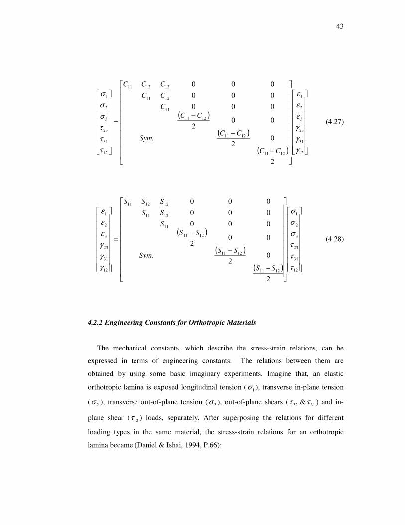
43

( )

( )

( )

−

−

−=

12

31

23

3

2

1

1211

1211

1211

11

1211

121211

12

31

23

3

2

1

2

02

.

002

000

000

000

γ

γ

γ

ε

ε

ε

τ

τ

τ

σ

σ

σ

CC

CCSym

CC

C

CC

CCC

(4.27)

( )

( )

( )

−

−

−=

12

31

23

3

2

1

1211

1211

1211

11

1211

121211

12

31

23

3

2

1

2

02

.

002

000

000

000

τ

τ

τ

σ

σ

σ

γ

γ

γ

ε

ε

ε

SS

SSSym

SS

S

SS

SSS

(4.28)

4.2.2 Engineering Constants for Orthotropic Materials

The mechanical constants, which describe the stress-strain relations, can be

expressed in terms of engineering constants. The relations between them are

obtained by using some basic imaginary experiments. Imagine that, an elastic

orthotropic lamina is exposed longitudinal tension ( 1σ ), transverse in-plane tension

( 2σ ), transverse out-of-plane tension ( 3σ ), out-of-plane shears ( 3132 &ττ ) and in-

plane shear ( 12τ ) loads, separately. After superposing the relations for different

loading types in the same material, the stress-strain relations for an orthotropic

lamina became (Daniel & Ishai, 1994, P.66):

44

−−

−−

−−

=

12

31

23

3

2

1

12

13

23

32

23

1

13

3

32

21

12

3

31

2

21

1

12

31

23

3

2

1

100000

01

0000

001

000

0001

0001

0001

τ

τ

τ

σ

σ

σ

γγ

γγ

γγ

γ

γ

γ

ε

ε

ε

G

G

G

EEE

EEE

EEE

(4.29)

As seen in Equation (4.29), it is easy to express the compliance matrix [ ]S in terms

of the engineering constants. However, the case is different for the stiffness

matrix [ ]C ; such that, converting the compliance matrix, the stress-strain relation is

found as follows:

∆

−

∆

+

∆

+∆

+

∆

−

∆

+∆

+

∆

+

∆

−

=

12

31

23

3

2

1

12

13

23

21

2112

21

132123

32

322131

21

132123

31

3113

31

321312

32

322131

31

321312

32

3223

12

31

23

3

2

1

00000

00000

00000

0001

0001

0001

γ

γ

γ

ε

ε

ε

νννννννν

νννννννν

νννννννν

τ

τ

τ

σ

σ

σ

G

G

G

EEEEEE

EEEEEE

EEEEEE

(4.30)

in which ∆ is defined as

1

1

11

2313

3212

3121

321 νν

νν

νν

−−

−−

−−

=∆EEE

(4.31)

45

4.2.3 Stress-Strain Relations for Thin Lamina

A thin lamina is considered to be a plane stress case, so the stress

components 233 ,τσ , and 31τ are equal to zero. Thus, the stress-strain relationship in

Equation (4.29) is reduced to the following form,

=

12

2

1

66

2212

1211

12

2

1

00

0

0

γ

ε

ε

τ

σ

σ

Q

QQ

QQ

(4.32)

=

12

2

1

66

2212

1211

12

2

1

00

0

0

τ

σ

σ

γ

ε

ε

S

SS

SS

(4.33)

The relations is then can be written by using engineering constants,

−−

−−

=

12

2

1

12

2112

2

2112

121

2112

212

2112

1

12

2

1

00

011

011

γ

ε

ε

νννν

ννν

ν

νν

τ

σ

σ

G

EE

EE

(4.34)

−

−

=

12

2

1

12

21

12

2

21

1

12

2

1

100

01

01

τ

σ

σν

ν

γ

ε

ε

G

EE

EE

(4.35)

4.2.4 Material Orientation in Two-Dimensional Lamina

Unidirectional composite laminas have very low transverse stiffness and strain

properties. Therefore, some of the laminas in laminates were oriented in angled

directions. Obtaining stress-strain relation in an angle lamina is essential

(Kaw, 2006, p.110).

46

The local and the global coordinate systems are used to define the stress-strain

equations of an angle lamina (Figure 4.5). In local coordinate system, direction 1 is

the longitudinal direction, which is parallel to fibers and direction 2 is the transverse

direction oriented perpendicular to the fiber direction. The global coordinate system

is represented by x-y axes. The angle between the two coordinate systems is named

as θ. Here is intended to establish the stress-strain relations in global coordinate

system.

Figure 4.5 Local and global axes of an angle lamina

The stress and strain components in local coordinate system are converted into the

global coordinate system by the transformation matrix [ ]T .

[ ]

=

xy

y

x

T

τ

σ

σ

τ

σ

σ

.

12

2

1

and [ ]

=

xy

y

x

T

γ

ε

ε

γ

ε

ε

2

1.

2

112

2

1

(4.36)

47

[ ]

−−

−=22

22

22

2

2

nmmnmn

mnmn

mnnm

T and θCosm = , θSinn = (4.37)

Putting Equation (4.32) and (4.33), in the inverse form of Equation (4.36) yields,

[ ] [ ] [ ]

=

=

−−

12

2

1

66

1111

11111

12

2

11

2

1.

200

0

0

.

γ

ε

ε

γ

ε

ε

τ

σ

σ

Q

QQ

QQ

TQT

xy

y

x

(4.38)

[ ] [ ] [ ] [ ][ ][ ][ ]

=

=

−−−

xy

y

x

xy

y

x

xy

y

x

RTRQTT

Q

QQ

QQ

T

γ

ε

ε

γ

ε

ε

τ

σ

σ11

66

1111

11111 ...

2

1..

200

0

0

where [ ]R is the Reuter matrix defined as,

[ ]

=

200

010

001

R (4.39)

The transformed reduced stiffness matrix [ ]Q is obtained by

multiplying [ ] [ ] [ ] [ ] [ ] 11,,,,

−−RTRQT .

=

xy

y

x

xy

y

x

QQQ

QQQ

QQQ

γ

ε

ε

τ

σ

σ

.

666261

262221

161211

(4.40)

( )

( ) ( )( )

( ) ( )

( ) ( )

( ) ( )4466

226612221166

3661222

366121126

3661222

366121116

226612

422

41122

2412

2266221112

226612

422

41111

22

2.2

22

22

4

22

nmQnmQQQQQ

nmQQQnmQQQQ

mnQQQnmQQQQ

nmQQmQnQQ

nmQnmQQQQ

nmQQnQmQQ

++−−+=

−−−−−=

−−−−−=

+++=

++−+=

+++=

(4.41)

48

4.2.5 Elastic Properties of multidirectional laminates

4.2.5.1 Basic Assumptions

The stress-strain relations for a single lamina were explained in the previous

sections. Nevertheless, a real composite material consists of more than one lamina,

oriented in different directions. A unidirectional lamina neither has enough thickness

to take realistic loads nor is convenient to carry multidirectional loads because of its

low transverse mechanical properties. Building a laminate by stacking layers at

different angles satisfies the loading and stiffness requirements, although it increases

the cost and weight (Daniel & Ishai, 1994, p.142), (Kaw, 2006, p.320).

It is obvious that, the whole behavior of composite plate is a function of

properties of each individual lamina. The following assumptions are required to

develop the equations according to classical lamination theory.

� Each lamina is orthotropic.

� Each lamina is homogeneous.

� A line straight and perpendicular to the middle surface remains straight and

perpendicular to the middle surface during deformation ( )0== xzxz γγ .

� The laminate is thin and is loaded only in its plane (plane stress)

( 0=== yzxzz ττσ ).

� Displacements are continuous and small throughout the laminate

( hwvu <<,, ), where h is the laminate thickness.

� Each lamina is elastic.

� No slip occurs between the lamina interfaces.

4.2.5.2 Strain Displacement Relations

Figure 4.6 illustrates a section view of a plate normal to the y-axis in the global

coordinate system (x, y, z) before and after deformation. The reference plane ( yx − )

is equal in distance from top and bottom surfaces, that is also z = 0. ,, 00 vu and 0w

49

are the displacements at the middle plane and vu, and w are the displacement

components at any point in yx, and z directions, respectively.

Figure 4.6 Laminate section before (ABCD) and after (A'B'C'D') (Daniel, & Ishai, 1994)

The middle plane displacements 0u , 0v and out-of-plane displacement w are only

the function of x and y .

),(

),(

),(

00

00

yxfw

yxvv

yxuu

=

=

=

(4.42)

At any point the two displacements u and v in yx − plane is dependent on the axial

location of the point and the slope of the laminate middle plane with the x and y

directions.

αzuu −= 0 and x

w

∂

∂= 0α (4.43)

The displacement in x direction is then,

x

wzuu

∂

∂−= 0

0 (4.44)

50

Similarly, other displacement component can be written in the same manner.

y

wzvv

∂

∂−= 0

0 (4.45)

The strain components at any point are expressed,

20

20

x

wz

x

u

x

ux

∂

∂−

∂

∂=

∂

∂=ε (4.46)

20

20

y

wz

y

v

y

vx

∂

∂−

∂

∂=

∂

∂=ε (4.47)

yx

wz

x

v

y

u

x

v

y

uxy

∂∂

∂−

∂

∂+

∂

∂=

∂

∂+

∂

∂= 0

200 2γ (4.48)

Equations (4.46), (4.47), and (4.47) can be combined in matrix form,

∂∂

∂−

∂

∂−

∂

∂−

+

∂

∂+

∂

∂∂

∂∂

∂

=

yx

w

y

wx

w

z

x

v

y

u

y

vx

u

xy

y

x

02

20

2

20

2

00

0

0

2

.

γ

ε

ε

(4.49)

Strains at any point can be written in terms of reference plane strains and laminate

curvatures,

+

=

xy

y

x

xy

y

x

xy

y

x

K

K

K

z0

0

0

γ

ε

ε

γ

ε

ε

(4.50)

Equation (4.50) shows the linear relationship of strains in a laminate to the

curvatures of the laminate. It also indicates that the strains are independent of the

yx − coordinates (Kaw, 2006, p.324).

51

4.2.5.3 Strain and Stress Relations in a Laminate

In case the strains at any point through the laminate thickness are known, the

stresses of each lamina in the global coordinate system can be calculated according

to Equation (4.40). The transformed reduced stiffness matrix, [ ]Q , corresponds the

layer at that point. It can be derived from Equation (4.40) and (4.50),

+

=

xy

y

x

xy

y

x

xy

y

x

K

K

K

QQQ

QQQ

QQQ

z

QQQ

QQQ

QQQ

666261

262221

161211

0

0

0

666261

262221

161211

..

γ

ε

ε

τ

σ

σ

(4.51)

Unlike a linear variation of strain through the thickness of laminate, stress

variations in each lamina changes because transformed reduces stiffness matrix [ ]Q

for each lamina is different.

Figure 4.7 Strain and stress variations through thickness of a laminate

4.2.5.4 Force and Moment Resultants

Consider a laminate manufactured by using N layers as shown in Figure 4.8. The

thickness of the laminate is “ t ”. The resulting forces and moments acting in a

laminate can be found by integrating the stresses in each lamina through thickness.

52

∫−

=2

2

t

t

xx dzN σ ∫−

=2

2

..

t

t

xx dzzM σ (4.52)

Figure 4.8 Coordinate locations of layers in a laminate

Figure 4.9 Force and moment resultants of a flat laminate

The normal force xN and the bending moment xM per unit width of the laminate,

illustrated in Figure 4.9 is calculated with the Equation (4.52) , but the whole

collection of force and moment resultants can be defined as,

∫ ∑ ∫− =

−

=

=

2

2

11

t

t

N

k

Z

Z

kxy

y

x

xy

y

x

xy

y

x k

k

dzdz

N

N

N

τ

σ

σ

τ

σ

σ

(4.53)

53

∫ ∑ ∫− =

−

=

=

2

2

11

...

t

t

N

k

Z

Z

kxy

y

x

xy

y

x

xy

y

x k

k

dzzdzz

M

M

M

τ

σ

σ

τ

σ

σ

(4.54)

Substituting Equation (4.51) in Equation (4.53) and (4.54) resultant forces and

moments is expressed by the middle plane strains and curvatures,

∑ ∫∑ ∫==

−−

+

=

N

k

Z

Z

xy

y

x

k

N

k

Z

Z

xy

y

x

kxy

y

x k

k

k

k

zdz

K

K

K

QQQ

QQQ

QQQ

dz

QQQ

QQQ

QQQ

N

N

N

1

666261

262221

161211

1 0

0

0

666261

262221

161211

11

.

γ

ε

ε

(4.55)

∑ ∫=

−

=

N

k

Z

Z xy

y

x

kxy

y

xk

k

zdz

QQQ

QQQ

QQQ

M

M

M

10

0

0

666261

262221

161211

1

.

γ

ε

ε

∑ ∫=

−

+N

k

Z

Z

xy

y

x

k

k

k

dzz

K

K

K

QQQ

QQQ

QQQ

1

2

666261

262221

161211

1

(4.56)

As seen in Equation (4.55) and (4.56) strains and curvatures are not dependent on the

z coordinate in middle plane. Additionally, transformed reduced stiffness matrix [ ]Q

does not vary in the laminas. For that reason resultant force and moment Equations

can be written like this,

=

∑ ∫=

−0

0

0

1

666261

262221

161211

1xy

y

xN

k

Z

Z

kxy

y

xk

k

dz

QQQ

QQQ

QQQ

N

N

N

γ

ε

ε

+ ∑ ∫=

−

xy

y

xN

k

Z

Z

kK

K

K

zdz

QQQ

QQQ

QQQk

k1

666261

262221

161211

1

(4.57)

54

=

∑ ∫=

−0

0

0

1

666261

262221

161211

1xy

y

xN

k

Z

Z

kxy

y

xk

k

zdz

QQQ

QQQ

QQQ

M

M

M

γ

ε

ε

+ ∑ ∫=

−

xy

y

xN

k

Z

Z

kK

K

K

dzz

QQQ

QQQ

QQQk

k1

2

666261

262221

161211

1

(4.58)

Based on the information )( 1

1

−−=∫−

kk

Z

Z

ttdzk

k

, )(2

1. 2

12

1

−−=∫−

kk

Z

Z

ttdzzk

k

, and

)(3

1. 3

132

1

−−=∫−

kk

Z

Z

ttdzzk

k

Equations (4.57) and (4.58) transform

+

=

xy

y

x

xy

y

x

xy

y

x

K

K

K

BBB

BBB

BBB

AAA

AAA

AAA

N

N

N

662616

262212

161211

0

0

0

662616

262212

161211

γ

ε

ε

(4.59)

+

=

xy

y

x

xy

y

x

xy

y

x

K

K

K

DDD

DDD

DDD

BBB

BBB

BBB

M

M

M

662616

262212

161211

0

0

0

662616

262212

161211

γ

ε

ε

(4.60)

Where, the matrixes, [ ]A , [ ]B and [ ]D are extensional, coupling and bending stiffness

matrixes, respectively. [ ]A relates in-plane loads to in-plane strains; [ ]B relates in-

plane loads to curvatures and moments to in plane strains; and [ ]D relates moments

to curvatures. The components of these matrixes are,

( )[ ]∑=

−−=N

k

kkkijij ttQA1

1 )( , 6,2,1=i ; 6,2,1=j (4.61)

( )[ ]∑=

−−=N

k

kkkijij ttQB1

2

1

2)(

2

1, 6,2,1=i ; 6,2,1=j (4.62)

( )[ ]∑=

−−=N

k

kkkijij ttQD1

3

1

3)(

3

1, 6,2,1=i ; 6,2,1=j (4.63)

55

If the equations are combined into a general expression, which converts reference

plane strain and curvatures into in-plane forces and moments, the final form of the

expression becomes,

=

xy

y

x

xy

y

x

xy

y

x

xy

y

x

K

K

K

DDDBBB

DDDBBB

DDDBBB

BBBAAA

BBBAAA

BBBAAA

M

M

M

N

N

N

0

0

0

662616662616

262212262212

161211161211

662616662616

262212262212

161211161211

γ

ε

ε

(4.64)

4.3 Micromechanical Behavior of a Lamina

The elastic behavior of a lamina can be either examined experimentally or

estimated mathematically. These properties vary depending on the properties and

proportions of fibers and matrix materials. The basic goal of micromechanics is to

find out the relationship between properties of composite material and its

constituents mathematically, as illustrated in Figure 4.10 (Jones, 1999, p.121).

Figure 4.10 Basic goal of micromechanics

The stiffnesses and compliances of composites are calculated by the aid of fiber

and matrix properties ( ),,,,,( mmmfffijij VEVECC νν= ). Here the definitions, fE =

Young’s modulus for an isotropic fiber, fν = Poisson’s ratio for an isotropic fiber,

and fV = Volume of fibers / Total volume of composite material, are analogous to

56

that of matrix material with subscript “m”. The determination of composite material

strengths via the strengths of constituents is also another objective of

micromechanical analysis. For example the composite strengths in functional form

are, ),,,( mimfifii VXVXXX = , where == SYXX i ,, Composite material strengths,

== fffif SYXX ,, Fiber strengths, and fV = Volume of fibers / Total volume of

composite. These definitions are analogous to that of matrix materials.

4.3.1 The prediction of E1

Consider a microscopically heterogeneous element is subjected a tensional stress

in fiber direction (Figure 4.11). In that case, the longitudinal strain ( 1ε ) both for fiber

and matrix material would be the same,

L

L∆=1ε (4.65)

In elastic region, the stresses in fiber direction are,

1εσ ff E= 1εσ mm E= (4.66)

The total load carried by the matrix and fiber is,

mmff AAAP σσσ +== 1 (4.67)

where A is the cross-sectional area, on which 1σ is acting, fA and mA are the cross-

sectional areas of fiber and matrix respectively.

Figure 4.11 Element loaded in direction 1

57

The stress in fiber direction is,

111 εσ E= (4.68)

Thus, the young’s modulus in fiber direction is derived,

A

AE

A

AEE m

m

f

f +=1 (4.69)

Fiber and matrix volume fractions are just related to the areas,

A

AV

f

f = A

AV m

m = (4.70)

mmff VEVEE +=1 (4.71)

4.3.2 The prediction of E2

The young’s modulus in transverse direction to fibers is characterized by 2E . It is

assumed that both fiber and matrix are subjected the same stress level 2σ . Under

transverse loading condition however, it is not possible to approximate or assume

strains in direction 1 and 2 (Figure 4.12).

Figure 4.12 Element loaded in direction 2

The strains in fiber and matrix materials are found from the stress 2σ .

f

fE

2σε =

m

mE

2σε = (4.72)

The total transverse deformation is the summation of fiber and matrix deformations,

mmff WVWVWW εεε +==∆ 2 or mmff VV εεε +=2 (4.73)

Combining Equations (4.72) and (4.73) gives,

m

m

f

fE

VE

V 222

σσε += (4.74)

58

According to the stress-strain relation at macroscopic level,

+==

m

m

f

fE

VE

VEE 222222

σσεσ (4.75)

2E is then expressed in terms of fiber and matrix properties,

mffm

mf

EVEV

EEE

+=2 (4.76)

4.3.3 The prediction of 12ν

Just like the approach, through which 1E obtained the major Poisson’s ratio is

also derived by applying a stress 1σ in fiber direction. When σσ =1 and the other

stresses are equal to zero, the Poisson’s ratio 12ν is defined (Figure 4.13),

1

212

ε

εν −= (4.77)

Figure 4.13 Element loaded in direction 1

Fiber and matrix strains are assumed to be identical and equal to 1ε . On the other

hand, the deformation in transverse direction W∆ is defined as macroscopically,

1122 ενε WWW =−=∆ (4.78)

W∆ is also expressed by its microscopic components, fiber and matrix deformations.

fWmWW ∆+∆=∆ (4.79)

59

Transverse deformations in fiber and matrix are defined approximately,

1εν mmmW WV=∆ 1εν fffW WV=∆ (4.80)

Putting Equation (4.78), (4.79), and (4.80) into one expression and eliminating

W1ε gives,

ffmm VV ννν +=12 (4.81)

4.3.4 The prediction of 12G

While determining 12G in micromechanics, the shear stresses acting on fiber and

matrix materials are assumed to be the same. But the shear deformations can not be

the same and expressed basically,

m

mG

τγ =

f

fG

τγ = (4.82)

The non linearity of the stress-strain behavior in shear loading is ignored and the

relation is presumed linear for convenience,

Figure 4.14 Element loaded in shear

The total shear deformation in macroscopic scale is,

W.γ=∆ (4.83)

Fiber and matrix deformations in microscopic scale are,

mmm WV γ=∆ fff WV γ=∆ (4.84)

60

Because the total deformation is the sum of fiber and matrix components

( fm ∆+∆=∆ ), and eliminating W yields,

ffmm VV γγγ += (4.85)

Total deformation can be written basically,

12G

τγ = (4.86)

When Equation (4.85) is rewritten combining Equation (4.86)

f

f

m

mG

VG

VG

τττ+=

12

(4.87)

As obtained expression for transverse young’s modulus 2E , the shear modulus is

given finally,

mffm

fm

GVGV

GGG

+=12 (4.88)

61

CHAPTER FIVE

FAILURE ANALYSIS IN COMPOSITES

5.1 Introduction

The general nature of failure for orthotropic materials is more complicated than

for an isotropic material. A Mohr's circle analysis would show a principal angle

different from that of an isotropic material, indicating that analysis techniques valid

for isotropic materials are not adequate for composites. A lamina is stronger in the

fiber direction than in the transverse direction, so the largest stress on the lamina may

not be the one that causes failure.

Failure of a unidirectional laminate begins on the microscopic level. Microscopic

failures can become macroscopic and result in catastrophic failure. Initial

microscopic failures can be represented by local failure modes, such as:

� Fiber failure: breakage, micro buckling, dewetting.

� Bulk matrix failure: voids, crazing.

� Interface/flaw dominated failures: crack propagation and edge

delamination (Staab, 1999, p.142).

Most of the experiments, conducted to obtain the material strength are based on

unidirectional state of stresses. In real structures however, two or three dimensional

stresses may be simultaneously acting on the material. It is physically impossible to

obtain strength properties at all possible orientations. Therefore, methods, which

calculate the characteristics at any orientation, using the material characteristics in

principal directions must be determined (Jones, 1999, p.102).

For composite structures, the strength of the laminate is dependent on each

individual lamina. In order to compare the state of stress to failure criteria in the

lamina, failure theories were developed. Basically, all of the theories are related to

the normal and shear strengths of unidirectional lamina.

62

For isotropic materials, failure theories generally based on principal normal

stresses and maximum shear stresses. In a lamina however, failure theories are

originated from the stresses in the material or in the local coordinates thanks to its

orthotropic nature and varying properties at different angles.

Unidirectional laminas have two material axes; those are fiber direction and

perpendicular to fiber direction. Therefore, four normal strength parameters exist

concerning unidirectional lamina, so that one tension and one compression strength

for each two local axes should be specified. Additionally, the shear strength appears

to be fifth parameter in unidirectional laminas, although the shear stresses do not

affect the shear strengths of a unidirectional lamina. The five strength parameters of

a unidirectional lamina are listed below (Kaw, 2006, p.138).

tX : Ultimate longitudinal tensile strength (in direction 1),

cX : Ultimate longitudinal compressive strength (in direction 1),

tY : Ultimate transverse tensile strength (in direction 2),

cY : Ultimate transverse compressive strength (in direction 2), and

S : Ultimate in-plane shear strength (in plane 12).

Figure 5.1 Biaxial stresses generated by off-axis uniaxial loading

63

By an off-axis loading on a unidirectional lamina, biaxial stresses will be

generated to explain each failure criteria as illustrated in Figure 5.1. An off-axis

stress, xσ which is at the angle of θ to the fiber direction produces biaxial stresses in

principal material directions. During examining the failure theories, the material is

going to be regarded as homogenous, although it is orthotropic structure (Jones,

1999, p.105).

5.2 Failure Criteria of a Lamina

5.2.1 Maximum Stress Failure Criterion

In the maximum stress failure criterion, failure occurs whenever normal and shear

stress component in the principal material coordinates is equal or exceeds the

correspondent strengths. The criterion can be written for tensile, compressive and

shear stresses as follows,

tX<1σ tY<2σ cX>1σ cY>2σ S<12τ (5.1)

As seen, the sign of the shear stress has no effect on the shear strength. If any of the

inequality conditions in Equation (5.1) are not satisfied, the material would fail by

the associated failure mechanism. There are actually five failure sub criteria exist and

there is no interaction between them.

In order to evaluate the state of stress and failure in a material according to

maximum stress criterion, the stresses in the principal material coordinates must be

primarily determined. In a uniaxial loading type in Figure 5.1, biaxial stress

components are obtained by stress transformations.

θσσ 21 Cosx= θσσ 2

2 Sinx= θθστ CosSinx .12 −= (5.2)

Then, by putting the expressions 1σ , 2σ , and 12τ in Equation (5.2) to Equation (5.1),

the maximum uniaxial stress must be the smallest of

θσ

θ 22Cos

X

Cos

X t

x

c << θ

σθ 22

Sin

Y

Sin

Y t

x

c << θθ

σCosSin

Sx

.< (5.3)

64

5.2.2 Maximum Strain Failure Criterion

In this criterion, the strains in the material principal directions are limited just as

the stresses in the maximum stress criterion. Failure occurs if one or more of the

following conditions are not satisfied.

t

X εε <1 t

Yεε <2 c

X εε >1 c

Yεε >2 εγ S<12 (5.4)

where,

t

X ε ( )c

X ε : maximum tensile (compressive) normal strain in the direction 1

t

Yε ( )c

Yε : maximum tensile (compressive) normal strain in the direction 2

εS : maximum shear strain in the material coordinates 1-2

Similar to that with the shear strength, the sign of the shear strain does not affect

the maximum shear strain. Initially, the strains in principal directions, 1ε , 2ε , and

12γ must be obtained by transforming the strains in global coordinate system, before

applying this failure criterion.

As studied in maximum failure criterion, a uniaxial load is applied on a

unidirectional lamina at an angle of θ to the longitudinal fiber direction. First

allowable strains are going to be found and then allowable stresses can be calculated

through them.

The two dimensional strain-stress relations in material coordinate system are,

( )

( )

12

1212

1212

2

2

2121

1

1

1

1

G

E

E

τγ

σνσε

σνσε

=

−=

−=

(5.5)

65

Substituting the stress transformation expressions in Equation (5.2) to Equation (5.5),

( )

( )

( ) x

x

x

CosSinG

CosSinE

SinCosE

σθθγ

σθνθε

σθνθε

..1

.1

.1

12

12

221

2

2

2

212

2

1

1

−=

−=

−=

(5.6)

Maximum strains are written in terms of ultimate strengths in linear elastic behavior,

1E

XX t

t=ε

2E

YY t

t=ε

1E

XX c

c=ε

2E

YY c

c=ε

12G

SS =ε (5.7)

Finally, the maximum strain criterion can be constituted in the following form,

θνθ

σθνθ 2

1222

122

SinCos

X

SinCos

X tx

c

−<<

−

θνθ

σθνθ 2

2122

212

CosSin

Y

CosSin

Y t

x

c

−<<

− (5.8)

θθ

σCosSin

Sx

.<

A prominent situation is that the maximum stress criterion, Equation (5.3) and the

maximum strain criterion, Equation (5.8) seem to be similar except for the terms of

Poisson’s ratio. Predictions, made according these two criteria for glass-epoxy

composites have given pronounced differences from the experimental results. Thus,

it is recognized that neither the maximum stress nor maximum strain criterion is

appropriate for e-glass-epoxy composite materials.

5.2.3 Tsai-Hill Failure Criterion

This is a yield criterion, predicting failure boundaries for orthotropic materials.

Tsai-Hill criterion is described in general form,

1222

222)()()(2

12

2

13

2

23

323121

2

3

2

2

2

1

=+++

−−−+++++

τττ

σσσσσσσσσ

NML

FGHGFHFHG (5.9)

This is a related and modified form of von Mises distortional energy yield

criterion for anisotropic materials. In the Equation (5.9), the

66

parameters MLHGF ,,,, , and N are failure strength parameters which are related to

the material strengths, YX , , and S . If the only stress acting on the body is S , then

the equation becomes,

2

12

SN = (5.10)

If 1σ is the only stress, then

2

1

XHG =+ (5.11)

If 2σ is the only stress, then

2

1

YHF =+ (5.12)

Similarly, if 3σ act in the direction 3, then

2

1

ZGF =+ (5.13)

Equation (5.11) + Equation (5.13) - Equation (5.12) is equal to

222

1112

YZXG −+= (5.14)

Equation (5.12) + Equation (5.13) - Equation (5.11) is equal to

222

1112

XZYF −+= (5.15)

Equation (5.11) + Equation (5.12) - Equation (5.13) is equal to

222

1112

ZYXH −+= (5.16)

In plane strain case, intended for a unidirectional lamina, 023133 === ττσ . In

addition to that, for such a lamina, depicted in Figure 5.2 it is obvious that ZY =

because of the geometrical symmetry. The failure criterion in Equation (5.9) can be

written for unidirectional lamina

12

2

12

2

2

2

2

21

2

2

1 =++−SYXX

τσσσσ (5.17)

The signs of 1σ and 2σ determine whether the values will be tX or cX and tY or cY .

If it is an off-axis case, the stress transformation equations (Equation (5.2)) is

combined with the Equation (5.17)

67

22

422

222

4 1..

11

xY

SinSinCos

XSX

Cos

σ

θθθ

θ=+

−+ (5.18)

Figure 5.2 Cross-section of a unidirectional lamina (1 is the fiber direction)

Experimental results for E-glass-epoxy exhibits a good agreement with numerical

solutions in Tsai-Hill failure criterion. It is found to be an appropriate failure

criterion for E-glass-epoxy composite laminas in two dimensional stress fields

although depending on their ductile or brittle nature, maximum stress and maximum

strain can be better for other type of composite materials. It can be also said that the

Tsai-Hill is an important criterion for the materials, whose properties are the same in

tension and compression.

5.2.4 Hoffman Failure Criterion

In addition to the Tsai-Hill’s equation some terms were added to take into account

the disparities between tension and compression strengths.

( ) ( ) ( )

12

129

2

318

2

237362514

2

213

2

132

2

321

=++++++

−+−+−

τττσσσ

σσσσσσ

CCCCCC

CCC (5.19)

The 9 coefficients ( 91 CC K ) are determined by the principal material strengths

( ,,,,,,,, 3123 SSZZYYXX ctctct and 12S ). The Hoffman criterion is more simplified in

plane stress case, where 031233 === ττσ and because of the isotropy in transverse

direction the equities, tt YZ = , cc YZ = , and 1231 SS = are also exist. Thus, the failure

criterion is degraded from Equation (5.19) to,

68

12

12

212

21

2221

21 =+

++

++−+−

SYY

YY

XX

XX

YYXXXX tc

tc

tc

tc

tctctc

τσσ

σσσσ (5.20)

The Hoffman criterion becomes the same as Tsai-Hill criterion while studying the

materials, of which the tension and compression strengths are equal

( XXX tc −=−= and YYY tc −=−= ). This criterion is a convenient tool if it is the

case of materials with different tension and compression strengths. Experiments with

the glass-epoxy, graphite-epoxy, and baron-epoxy materials have given compatible

failure data with the Hoffmann criterion according to Jones (1999).

5.2.5 Tsai-Wu Tensor Failure Criterion

This criterion is based on the postulation by Tsai and Wu, which gives a strength

definition, representing the interaction between stresses in different directions. If a

six dimensional state of stress exist in material then the criterion is defined in indicial

notation as

1=+ jiijii FF σσσ 6,,1, K=ji (5.21)

iF and ijF are representing the second and fourth rank strength tensors, and stress

notations, 54 ,σσ and 6σ are 3123 ,ττ and 12τ , respectively. In the plane stress case of

an orthotropic lamina, the equation is reduced to a less complex form.

12 21122

6662

2222

111662211 =++++++ σσσσσσσσ FFFFFFF (5.22)

Looking at the Equation (5.22) in detail, the linear stress terms are for representation

of different tensile and compressive properties, whereas the quadratic stress terms

characterize the ellipsoidal contour in stress space. The normal stress interactions

between direction 1 and 2 is taken into account by using an independent

parameter 12F .

The parameters in the stress tensor can be defined in terms of the material tension,

compression and shear properties. If only tensile load is applied to the body

12111 =+ tt XFXF (5.23)

69

Similarly, under pure compression,

12111 =+ cc XFXF (5.24)

Upon the joint solution of Equations (5.23) and (5.24)

ct XXF

111 +=

ct XXF

111 −= (5.25)

In similar way,

ct YYF

112 +=

ctYYF

122 −= (5.26)

If thinking of the shear strength being independent of the shear stress signs in

principal coordinates, that means,

06 =F 266

1

SF = (5.27)

For materials with the same tensile and compressive properties ( ct XX −= and

ct YY −= )

01 =F 211

1

XF = 02 =F

222

1

YF = (5.28)

These equations result in the failure criterion to reduce to the following form,

122

212

2

22

21122

21 =+++

SYF

X

τσσσ

σ (5.29)

Equation (5.29) seems to be similar to Equation (5.17) in Tsai-Hill criterion except

for the term 12F which is instead2

1

X− . As 12F is the common product of 1σ and

2σ , it is impossible to obtain 12F from uniaxial tests. Consider a biaxial loading only

in principal directions with a magnitude of σσσ == 21 . From Equation (5.22)

( ) ( ) 12 212221121 =++++ σσ FFFFF (5.30)

Finally, 12F is derived from substituting the definitions of 1121 ,, FFF and 22F into

Equation (5.30).

++

+++−= 2

212

1111111

2

1σσ

σ ctctctct YYXXYYXXF (5.31)

In addition to the tensile biaxial failure stressσ , the definition of 12F is dependent on

several material strengths. Owing to the difficulties of performing biaxial tension

70

tests, Tsai and Wu suggested a 45° off-axis tests or shear tests for determining 12F . It

was also reported that slight variations in fiber orientation can fully disrupt the

determination of 12F . The off-axis tests have given poor results. Another test method

proposed to determine 12F is to restrict deformations in transverse direction of

applied load but nonetheless to find the exact value of 12F remains still unclear

(Staab, 1999, p.161).

71

CHAPTER SIX

DETERMINATION OF BASIC MATERIAL PROPERTIES

6.1 Introduction

Designing composite structures requires an accurate knowledge about mechanical

properties of composite material. Mechanical tests that are used to derive mechanical

properties of conventional metallic materials are not applicable for composite

materials because of anisotropy, coupling effects and different possible failure

modes. Therefore, appropriate test methods were developed and these were evolved

into standards, adopted by the American Society for Testing and Materials (ASTM).

Researches in composite materials always entail basic material properties of

unidirectional laminated composite plates derived from quasi-static experimental

study. The data collected from these tests are used to reveal strength and stiffness

characteristics of the material. For an orthotropic lamina, those are nine independent

constants, each of which is a specific value defining mechanical response. The

strength and stiffness characteristics are listed in Table 6.1 (Gibson, 1994).

Table 6.1 The strength and stiffness characteristics of an orthotropic laminate

Strength characteristics Stiffness characteristics

X Axial or longitudinal strength in

direction 1.

E1,

E2

Longitudinal and

transverse Young modulus

Y Transverse strength in direction 2. ν12 Poisson’s ratio

S Shear strength in plane 1, 2. G12 Shear modulus

72

Table 6.2 ASTM test standards and specimen geometries in determining mechanical characteristics (Okutan, 2001)

Determinable properties

Symbol and Unit

ASTM test method Specimen geometry

Axial or longitudinal

modulus

Axial Poisson’s ratio

Longitudinal tensile strength

E1

(MPa)

ν12

(-)

Xt

(MPa)

ASTM 3039-76

Transverse modulus

Transverse Poisson’s ratio

Transverse tensile strength

E

2

(MPa)

ν21

(-)

Yt

(MPa)

ASTM 3039-76

Shear modulus

G

12 (MPa)

ASTM 3518-76

ASTM D 7078-05

ASTM D 5379

Shear strength

S

(MPa)

ASTM D 5379

ASTM D 7078-05

Longitudinal compressive

strength

Xc

(MPa) ASTM 3410-75

Transverse

compressive strength

Yc

(MPa) ASTM 3410

73

6.2 Test Procedures

In order to assess mechanical responses of a unidirectional lamina, the following

assumptions are needed, in tensile, compressive and shear loading conditions. These

descriptions provide a simplified approach in fiber-matrix interactions (Mallick,

1993).

• Fibers are uniformly distributed throughout the matrix. • Perfect bonding exists between fibers and matrix. • The matrix is free of voids. • Applied loads are either parallel to or normal to the fiber direction. • The lamina is initially in a stress-free state (i.e., no residual stresses are

present) • Both fibers and matrix behave as linearly elastic materials.

6.2.1 Determination of the Tensile Properties

Tensile properties of a unidirectional lamina are Young’s modulus in longitudinal

and transverse directions (E1, E2), Poisson’s ratio (ν12, ν21), longitudinal and

transverse tensile strengths (Xt, Yt). Static tensile tests were applied to the test

specimens having orientations of [00]6 and [900]6 according to the ASTM D3039-76

standard test method. Test specimens were manufactured as straight sided and with a

constant cross section. As illustrated in Figure 6.1, the specimens have 250 mm

length, 13 mm width and a measured thickness of 1.7 mm.

Figure 6.1 Test specimen geometry and dimensions for longitudinal tensile loading

Tests were carried out in the Shimadzu AG-100, 100 KN loading capacity testing

machine, at 0.5 mm/min test speed. A uniaxial tensile loading was applied to the

specimens and the load was raised up step by step until final failure occurred. During

experiments, the longitudinal elongation was measured simultaneously by the aid of

74

a video extensometer with two digital cameras connected to the data acquisition

system of the test machine. The Young’s modulus in fiber direction (E1), and the

axial strength (Xt) were calculated by using the following conventional equations,

A

P=1σ ,

A

PE

11

11

εε

σ== ,

A

PX ult

t = (6.1)

On the other hand, the Young’s modulus in transverse direction (E2) and the

transverse tensile strength (Yt) are found by loading [900]6 test specimens in

perpendicular to the fiber direction. The geometry and dimensions, which is

compatible with the standard test method ASTM D3039-76 are given in Figure 6.2.

Figure 6.2 Test specimen geometry and dimensions for transverse tensile loading

The tensile test speed was 0.5 mm/min, and the load was increased step by step up

to the occurrence of catastrophic failure. Filling the obtained data to Equation (6.2),

the tensile properties in transverse direction can be calculated, easily.

A

P=2σ ,

A

PE

22

22

εε

σ== ,

A

PY ult

t = (6.2)

6.2.2 Determination of the Compressive Properties

Notwithstanding the buckling effect exists in compression loading, selecting the

convenient geometry and dimensions in accordance with ASTM D3410 and using

test fixtures alleviate this effect, significantly. Test specimen geometry with

dimensions and the test fixture is illustrated in Figure 6.3, schematically. The

unidirectional laminated [0º]6 test specimens with the dimensions of 140 mm long,

13 mm wide and 1.7 mm thick were prepared for longitudinal compressive tests and

[90º]6 test specimens with the dimensions of 140 mm long, 25 mm wide and 1.7 mm

thick were prepared for transverse compressive tests. Having recorded the failure

75

loads by compression tests in fiber and perpendicular to fiber directions, longitudinal

and transverse compressive strengths (Xc, Yc ) were calculated.

Figure 6.3 Test specimen geometry and dimensions for compressive loading and its test fixture

6.2.3 Determination of the Shear Properties

It is a very difficult task to obtain the mechanical shear properties of composites.

This difficulty stems from the necessity of creating a pure and a constant magnitude

shear stress in the gage section of specimen. Many test methods have been applied so

far to assess the in-plane-shear properties of composites. The most common of these

methods are listed below:

1. ±45 Shear test,

2. 10o Off-axis test,

3. Torsion tube,

4. Rail shear test,

5. Sandwich cross-beam test,

6. T-specimen shear,

76

7. Iosipescu shear test,

8. V-Notched rail shear test.

In the current study the v-notched rail shear test method was selected inasmuch as

the V-notched rail shear test appears to be well-suited for measuring the in-plane

shear modulus and shear strength of unidirectional and multidirectional composite

laminates. This test method incorporates attractive features from both the Iosipescu

V-notched shear test and the standard two-rail shear test. The V-notched specimen

provides a larger gage section than the standard Iosipescu shear specimen and

enhanced loading capability compared to other existing test methods (Adams et al.,

2003).

The ASTM standard D 7078-05 approved by ASTM Committee in March of 2005

defines the v-notched rail shear test, which determines the shear strength and the

shear stiffness of materials. The standard test fixture and specimen geometry are

given in Figure 6.4. Specimens were prepared in [0°]6 and [90°]6 orientations to get

shear strengths in fiber and perpendicular to the fiber direction.

Figure 6.4 V-notched rail shear test fixture, shown with a standard v-notched specimen and one pair of grip plates removed (www.compositesworld.com)

The specimens for the present tests were produced according to the standard

geometry and dimensions as illustrated in Figure 6.5. The test fixtures were mounted

77

on a SHIMADZU (100 kN) testing machine for loading specimens and in order to

record strain values a digital strain meter TDS-530 was used. The strain gauges were

installed on the specimen between the two notches at 45º as shown in Figure 6.6.

When clamping specimens in grips, the two ends of them were embedded 25 mm

inside the fixture, so only the notched part was left outside and between the grips.

The specimens, on which strain gages stuck were loaded only in elastic region to get

more accurate data, whereas the other specimens were tested until the final failure

was detected.

Figure 6.5 Dimensions (mm) of the V-notched rail shear test specimen

Figure 6.6 V-notched rail shear specimen with strain gage stuck on before testing

Shear properties were calculated by entering the test data to the following

equations. Initially, in-plane shear strength (S) were calculated,

78

tw

PS

.max= (6.3)

Where maxP is the maximum shear failure load, reached; w is the width of the

narrowest point of the notch and t is the thickness of the plate.

6.3 Results of Mechanical Property Tests

In order to determine the longitudinal modulus 1E , transverse modulus 2E ,

longitudinal and transverse tensile strengths tX and tY , longitudinal and transverse

compressive strengths cX and cY , rail-shear strength S and Poison’s ratio 12ν , a

unidirectional glass fiber / epoxy composite plate was produced and a series of

experiments were performed. Following repeated tests, average results obtained by

tensile, compressive and rail-shear tests were calculated for each specimen having 0º

and 90º fiber orientations (Table 6.3).

Table 6.3 Mechanical properties of the glass fiber / epoxy composite material

1E (MPa) 2E (MPa) 12ν tX (MPa) tY (MPa) cX (MPa) cY (MPa) S(MPa)

27200 12800 0.25 586.5 137.7 324.7 200.2 61.96

79

CHAPTER SEVEN

EXPERIMENTAL STUDY AND RESULTS 0F SINGLE LAP DOUBLE

SERIAL FASTENER JOINTS AT ELEVATED TEMPERATURES

7.1 Introduction

Vast researches have been performed on mechanically fastened joints with

different parameters such as material and geometrical properties together with a one

or a combination of failure criterion to predict the failure load and failure mode on

the strength of the joint by experimental, analytical and numerical means. Much of

these previous studies on mechanically fastened composite joints have been carried

out at room temperature except for a few of them, such as the work reported by Song

et al.(2008), a study, aimed to investigate the bearing strength of a blind riveted

single lap joint of a carbon/epoxy composite after heat exposure, but with the present

study it was intended to investigate the failure behavior of bolted glass-epoxy

composite material joints at elevated temperatures concurrent with the thermal

exposure.

In this chapter, the results of an experimental failure analysis, which was carried

out to determine the effects of thermal condition and tightening torque on the failure

load and failure behavior of single lap double serial fastener glass fiber / epoxy

composite joints were given. 40, 50, 60, 70, and 80 ºC temperatures were exposed to

the specimens during tensile tests. Besides thermal effects, 0 and 6 Nm tightening

torques were applied to observe how clamping forces affect the joint strength at high

temperatures.

7.2 Explanation of the Problem

Consider a single shear, composite-to-composite, lap joint with 2 fasteners

arranged in longitudinal direction, subjected to quasi-static loading in tension.

Composite plates were prepared using glass fiber/epoxy with lay-up of [0/90/45/-

45]s configuration. The laminate specimen was then cut into required dimensions,

80

(L=210mm, W=36mm and h was measured as 2mm). The geometrical features of

specimens were prepared in accordance with ASTM D 5961/D 5961M – 01, the

standard test method for bearing response of polymer matrix composite laminates

(Figure 7.1). Two serial holes (D=6mm) were drilled along the centerline of the

plates and doublers made of the same material (S=114mm, W=36mm) were stuck

onto the specimens. Specimens were fastened to each other using rigid bolts with a

nominal diameter of 6mm and the level of torque was either M=6 Nm or M=0Nm

(finger tight) for all fasteners within the same joint (Figure 7.2).

Figure 7.1 Composite specimen geometry for single lap double fastener bearing test

Figure 7.2 Joint of single shear double fastener composite test specimens

7.3 Material Production

The glass fiber / epoxy composite plate used in this study was manufactured using

vacuum assisted resin infusion technique. Prior to the vacuum process, the glass-fiber

81

whose layer has the density of 300 g/m³ was laid on to the heater table according to

specified orientations, [0/90/45/-45]s.

After preparing vacuum bag and evacuating the air by a vacuum pump, the

mixture of Duratek DTE 1000 resin and Duratek DTS 1100 fast hardener was drawn

into the component by vacuum and it was infused into the glass fiber until complete

impregnation. It was cured under 0.1 MPa pressure at 120 ºC for 2 hours. The

measured thickness of composite plate was 2 mm after production.

7.4 Thermal Test Chamber

In order to simulate environmental conditions and observe the behavior of

composite joints at various temperatures, a thermal test chamber with a clamp

resistance heater was designed (Figure 7.3). The chamber was isolated to obtain a

stable temperature, and for setting the temperature to a fixed value, an adjustable

thermostat was mounted inside it.

Figure 7.3 Thermal test chamber (1000 W)

The upper and lower ends of the chamber were also isolated by means of two lids.

Rectangular clefts were cut on to the lids, so that upper and lower ends of the

specimen could be passed through them. To avoid deviations in temperature, it was

checked by measuring via a thermocouple device. During experiments, the sensors of

82

the measuring instrument were in contact with the fastener bolts where bearing

failure usually occurs.

7.5 Testing Procedure

In order to examine the behavior of bolted joints in glass fiber / epoxy laminates

at varying temperature levels under changing clamping forces, a series of

experiments were performed. Specimens were tested at six different chamber

temperatures (Room Temp.(~20ºC), 40-50-60-70-80 ºC) and the tightening torques

of fastener bolts were M= 0 Nm (finger tight) and M= 6Nm. Tests were repeated for

each thermal condition and toque level, after that average values of failure loads

were recorded. All of the experiments were carried out in the Shimadzu AG-100, 100

kN loading capacity testing machine, at 1 mm/min test speed (Figure 7.4).

Figure 7.4 Set-up of thermal test chamber, thermostat and thermocouple

7.6 Results and Discussion

The failure loads of single shear double serial fastener glass fiber / epoxy

composite joints exposed to high temperatures investigated experimentally. Figures

7.5 and 7.6 illustrate the effect of various temperatures on load/displacement curves

in tensile tests of mechanically fastened joints, under M=0 Nm (finger tight) and

M=6 Nm tightening torques, respectively. As seen in the figures, when the test

83

temperature increases, the composite matrix material softens to a large extent and it

affects joint strength, namely the load-bearing capability of the composite gradually

decreases. The non-linear part of deformation appears to be more dominant as the

amount of plastic deformation is large and above 60 ºC the whole load / displacement

curve looks smoother. Nevertheless, slopes of the curves reduce dramatically, which

means reducing load carried by joint for the same bolt-hole displacement rate. On the

other hand, while at the peak values of bearing forces, bolt-hole displacements are

formed to be between 12-14 mm for test temperatures smaller than 60 ºC, it reduces

dramatically below 10 mm for higher temperature levels that approximates the glass

transition temperature of the pure resin. High temperature levels cause resin damage

and shorten residual bearing life of the composite joint.

Figure 7.5 The effect of temperature on load/displacement curves in tensile tests of bolted glass fiber / epoxy composite joint under M= 0 Nm tightening torque.

In Figure 7.5, the curves are almost linear up to some point. Beyond that load, the

joints exhibit intensively non-linear load-displacement curves. It is attributed to the

bearing failure in front of the bolt and pulling-through of the fastener.

84

Figure 7.6 The effect of temperature on load/displacement curves in tensile tests of bolted glass fiber / epoxy composite joint under M= 6Nm tightening torque

For bolted joints, fixed under M= 6 Nm tightening torques (Figure 7.6), due to the

clamping force generated by the fasteners, frictional forces develop between the

plates. Initially, the load transfer is dominated by this friction when the level of

applied load is low. When the load is increased to some point, friction forces are

completely overcome and the composite plates start to slide relative to each other,

causing the load to be picked up by bolts through contact between fastener and hole

edges of the plates. The effect of clamping force, produced by tightening torque can

be observed in load/displacement curves in Figure 7.6. The change in slopes of

curves between 0-2 mm displacement levels is attributed to the frictional forces to be

developed fully.

After exceeding frictional force, load pick-up is undertaken by fastener bolts and

there is no significant difference between the slopes of curves relating to M= 0 Nm

and M= 6 Nm torque levels at even elevated temperatures, as seen in Figure 7.7.

85

(a) (b)

(c) (d)

(e) (f)

Figure 7.7 The effect of bolt tightening torques on load/displacement curves in tensile tests of bolted glass fiber / epoxy composite joint (a) Room Temp. (b) 40 °C, (c) 50 °C, (d) 60 °C (e) 70 °C, (f) 80 °C

86

Once the load is picked up by bolts, the geometrical (the edge distance-to-hole

diameter ratio, (E/D), plate width-to-hole diameter ratio (W/D) etc.) and

environmental (temperature, humidity etc.) parameters, which are the same in both

specimens became important.

The obtained experimental data and some calculated statistical results (maximum

and minimum values, range, mean values and standard deviations) are given Table

7.1 and Table 7.2 for M= 0 Nm and M= 6 Nm preloads, respectively . Under each

temperature and preloading conditions, tests were repeated for three times and the

data recorded. Data distribution and mean values of failure data were also depicted

in Figures 7.8 and 7.10 by generating box plots at which the upper and lower edges

of boxes represent the maximum and minimum failure loads experienced for each

test condition and centers of the circular marks specify the location of mean values.

Note that, some test values appear to be very close to the mean value, whereas some

of them display bigger range and higher standard deviations. As a precise

temperature control was provided during the test period, these fluctuations are

attributed to some probable minor scale geometrical inequalities in specimens.

Table 7.1 Recorded and calculated test results of glass fiber / epoxy composite material joints, at various chamber temperatures under M= 0 Nm tightening torque

Temperature (C°) 20 40 50 60 70 80 Max. Value (N) 10538.30 9961.96 8656.61 7677.19 4899.38 3281.96 Min. Value (N) 10110.30 8940.87 8434.23 7209.86 4789.15 2952.04 Range (N) 428.00 1021.09 222.38 467.33 110.23 329.92 Mean Value (N) 10377.70 9358.82 8555.00 7443.53 4844.27 3117.00 Stnd. Deviation (N) 233.11 535.14 112.42 330.45 77.94 233.28

Table 7.2 Recorded and calculated test results of glass fiber / epoxy composite material joints, at various chamber temperatures under M= 6 Nm tightening torque.

Temperature (C°) 20 40 50 60 70 80 Max. Value (N) 12180.00 9844.56 9856.56 7844.94 5212.47 4039.96 Min. Value (N) 11184.80 9562.24 9488.66 7781.78 5017.12 3077.48 Range (N) 995.20 282.32 367.90 63.16 195.35 962.48 Mean Value (N) 11533.50 9661.19 9612.15 7813.36 5095.39 3571.31 Stnd. Deviation (N) 560.43 158.97 211.67 44.66 103.29 481.73

87

Failu

re L

oad (

N)

80 C°70 C°60 C°50 C°40 C°20 C°

11000

10000

9000

8000

7000

6000

5000

4000

3000

2000

10377,7

9358,82

8555

7443,52

4844,26

3117

Temperature

Figure 7.8 Box plots of failure loads, occurring at different temperatures under M= 0 Nm

Mean o

f F

ailu

re L

oad (

N)

80 C°70 C°60 C°50 C°40 C°20 C°

12000

10000

8000

6000

4000

2000

0

12000

10000

8000

6000

4000

2000

0

10377,7

9358,82

8555

7443,52

4844,26

3117

95% CI for the Mean

Temperature

Figure 7.9 Confidence interval (CI) plots for mean values of failure loads, occurring at different temperatures under M= 0 Nm

88

Failu

re L

oad (

N)

80 C°70 C°60 C°50 C°40 C°20 C°

12000

10000

8000

6000

4000

2000

11533,5

9661,19 9612,15

7813,36

5095,39

3571,31

Temperature

Figure 7.10 Box plots of failure loads, occurring at different temperatures under M= 6 Nm

Mean o

f F

ailu

re L

oad (

N)

80 C°70 C°60 C°50 C°40 C°20 C°

14000

12000

10000

8000

6000

4000

2000

14000

12000

10000

8000

6000

4000

2000

11533,5

9661,19 9612,15

7813,36

5095,39

3571,31

95% CI for the Mean

Temperature Figure 7.11 Confidence interval (CI) plots for mean values of failure loads, occurring at different temperatures under M= 6 Nm

89

While assessing the outstanding effects of the test parameters on the failure

responses of bolted joints, the utilization of mean failure values of repeated test

results was considered to be appropriate based on the Figures 7.9 and 7.11, which are

the confidence interval plots of mean values for M= 0 Nm and M= 6 Nm tightening

torques, respectively. The Figures illustrate mean values and confidence intervals of

mean values, in which they are expected to happen with a confidence level of 95

percent according to the three performed test results. It was shown also, to what

extent the mean values converge to the actual values and how credible they are. Of

course, by increasing the number of experiments, it could be possible to minimize the

size of the confidence intervals, thus it can be converged to the most accurate values.

However, as regular decreases in failure results was observed and mean values of the

ultimate loads follow a particular gradually descending curve, no additional

repetition of tests was considered to be necessary.

In Table 7.1 and Table 7.2, failure loads are presented depending on varying

chamber temperatures and tightening torques for glass fiber / epoxy composite bolted

joints according to tension test results. The effect of temperature and tightening

torque on bearing loads are also illustrated in Figure 7.12. As might be expected and

can be observed in Figure 7.12, the load-carrying capacity of the joint is decreased

by increasing temperature level. When the temperature has risen up, the internal

energy increases and molecular movement of the material becomes easier. Joint is

highly affected by this material degradation, thus failure occurs at lower stress levels.

In comparison with the room temperature results, the reduction in failure loads

between the chamber temperatures 40 ºC and 80 ºC varies from about 10 to 70

percent. Furthermore, the maximum decrease of failure loads occurs at 70 ºC and 80

ºC with the rate of nearly 55 % and 70 % respectively. This rapid fall is attributed to

heat damage to the resin matrix.

The clamping force produced by tightening bolts plays an important role on

bearing behavior of mechanically fastened composite joints. There is every

appearance that, the influence of preload moment is effective not only at room

temperature, but also at higher temperature grades, according the test results. M= 6

90

Nm torque level contributes to the joint strength approximately 5-15 % compared to

the finger tightened ones.

0

2

4

6

8

10

12

14

~20 40 50 60 70 80

Temperature(ºC)

Fa

ilure

loa

d (

kN

)

M=0 Nm

M=6 Nm

Figure 7.12 The effect of temperature and tightening torque on failure load

Figure 7.13 Photo of deformed composite specimens at various temperature levels in tensile tests under M= 0 Nm tightening torque.

Generally speaking, there are three basic pinned joint failure modes related to

composites: These are net-tension, shear-out and bearing. In practice, combinations

of these failure modes are possible. Net-tension and shear-out modes are catastrophic

and result from excessive tensile and shear stresses. Bearing mode is local failure and

progressive, and related to compressive failure (Aktas, 2009), (Asi, 2010). In Figures

7.13 and 7.14, photos of deformed glass fiber / epoxy composite specimens exposed

to six different temperature conditions during tensile loading tests are presented. As

91

it can be seen in the figures, the dominant failure type is bearing mode regardless of

thermal and clamping force conditions. In addition to that, signs of delamination are

observed in the specimens tested at the temperatures of 70 ºC and 80ºC.

Figure 7.14. Photo of deformed composite specimens at various temperature levels in tensile tests under M= 6 Nm tightening torque.

92

CHAPTER EIGHT

EXPERIMENTAL STUDY AND RESULTS 0F SINGLE LAP DOUBLE

SERIAL FASTENER JOINTS AT LOW TEMPERATURES

8.1 Introduction

According to the previous review, many authors were interested in the material

and geometrical parameters influencing the failure behaviors of mechanically

fastened composite joints. Nonetheless, a few of them have taken into account the

environmental effects, particularly the temperature extremes that composite joints are

exposed during operation. Among these studies, those associated with glass-fiber

reinforced composites are even more limited.

The current section reports an experimental investigation on failure responses of

single lap double serial fastener joints in glass fiber / epoxy composite laminates

when subjected to low temperature environment. The results of experiments,

implemented at five different low temperature levels ranging from 0 ºC to -40 ºC,

were evaluated in comparison with room temperature tests.

8.2 Explanation of the Problem

Composite plates with lay-up of [0/90/45/-45]s configuration were prepared using

glass fiber/epoxy. Each specimen has the dimensions of Length (L) = 210mm, Width

(W) = 36mm and h (thickness measured) 2mm which are consistent with ASTM D

5961/D 5961M – 01, the standard test method for bearing response of polymer

matrix composite laminates (Figure 8.1). A single shear, composite-to-composite, lap

joint was formed using two fastener bolts arranged in longitudinal direction. Rigid

bolts having a nominal diameter of 6mm were tightened under M=6 Nm or M=0Nm

(finger tight) torque levels to observe clamping pressure effects in low temperature

quasi-static tensile tests.

93

Figure 8.1 Joint of single shear double fastener composite test specimens.

8.3 Experimental Setup and the Cooling Process

To be able to simulate the low temperature conditions, a quick freezer spray

(FREEZER BR, -50 ºC) was injected on to the joint zone where the stress

concentrations result in the onset damage. The zone was also isolated to maintain the

stability of the test temperature (Figure 8.2). The temperature of the material surface

was measured simultaneously by means of a thermocouple device. Tests were started

as soon as the required temperature level has been reached. During the experiment,

the spray was injected continuously at some intervals, changing with the temperature

level until the test ended, so that the heat losses could be compensated.

Figure 8.2 Set-up of low temperature test, thermocouple and insulation equipment

94

8.4 Testing Procedure

A set of experiments were conducted to examine the behavior of bolted joints in

glass fiber / epoxy laminates at low temperatures under two different clamping

forces. Six different temperature levels (-40, -30, -20, -10, 0 ºC and ~20ºC (room

temperature)) were exposed to the composite joints. When assembling specimen

parts, tightening torques of fastener bolts were set to the values of M= 0 Nm (finger

tight) and M= 6Nm. The torque was applied using a calibrated torque wrench. The

experiments were carried out in Shimadzu AG-100, 100 KN testing machine, at 1

mm/min test speed. The tests were continued until the maximum failure load was

reached and stopped when an instantaneous decrease was experienced in the tensile

force.

8.5 Results and Discussion

The present study aimed to investigate the behavior of single lap double serial

fastener glass fiber / epoxy composite joints in freezing environments,

experimentally. Followed by the application at room temperature, static tensile tests

were implemented to the specimens under low temperature exposure. Fastener bolts

were tightened under the torque levels of M=0 Nm (finger tight) and M=6 Nm.

Experiments were carried out at the temperatures ranging from room temperature

down to -40 °C.

According to the results, the temperature was found to be effective on failure

characteristics of bolted joints in composite laminates. In Figures 8.3 and 8.4, the

load – displacement curves of tensile tests are shown that were implemented under

M= 0 Nm and M= 6 Nm preload moments, respectively. In comparison with those at

room temperature, an increase is observed in slopes of load – displacement curves

depending on the exposed temperature level, so the stiffness of the joint increases

with decreasing temperature. It also means that, the lower the temperature exposed,

the higher load carrying capacity obtained for the same bolt-hole displacement rates.

95

The difference between slopes becomes more evident when the minimum test

temperature was exposed to the test specimen.

Despite the fact that maximum failure loads varies depending on the temperature

level, the failure displacements, at which the peak values of bearing forces are

formed didn’t change significantly when the temperature was decreased. As

expected, there is a reduction in failure displacement when torque was applied to the

fasteners. This occurrence is due to the increased effect of friction associated with

the clamping force, which reduces the relative sliding of the composite laminates

(Chishti et al., 2010). It can be seen clearly in Figures 8.3 and 8.4, in which the

failure bolt-hole displacements appear to be between 13-15 mm and 11-13 mm, for

M= 0 Nm and M= 6 Nm preload moments, respectively.

The load-displacement curves are linear up to a point. After that, the load-

displacement curves deviate from linearity. The slopes of curves alter at more than

one point (Okutan Baba, 2006). Following the first deflection, the curves follow a

zigzag pattern and the load increases more slowly up to the maximum failure load.

This behavior is called as bearing mode, which is the most desired failure mode due

to its higher load carrying capacity. The matrix fracture, delamination between

laminates, fiber breakages, fiber-matrix interface deformation, fiber buckling etc. are

the main reasons for the zigzag formation of the curve (Asi, 2010).

All the specimens exhibited dominantly the bearing failure mode regardless of

temperature and preload level. In the current experiments, no evidence was found

that failure mode is directly affected by the environmental factors.

The load-displacement curves of joints tested under M= 6 Nm tightening torques

were illustrated in Figure 8.4. Until the force level reaches up to specific point, the

load transfer between plates is performed by the frictional forces generated by the

clamping forces that are transmitted by the tightened bolts. The change in slopes of

curves between 0-2 mm displacement levels is attributed to the frictional forces to be

developed completely. In the subsequent section, once friction forces are fully

96

overcome, composite plates start to slide relative to each other, which leads the

fasteners to pick up the carried load, through the contact between bolts and hole

edges. The load transition from friction to the fasteners is getting more drastic at

lower temperatures producing a zigzag line as seen in Figures 8.4a and 8.4b, due to

the mutual adhesion between plate surfaces. After the load is picked up by fasteners,

the geometrical (the edge distance-to-hole diameter ratio E/D, plate with-to-hole

diameter ratio W/D etc.), material (stacking sequence etc.) and environmental

(temperature, humidity etc.) parameters become of primary importance in

determining the failure behavior of mechanically fastened composite joints. Whilst

the maximum force, reached without sliding composite plates relatively, is about

3500 N at room temperature, it gets around to 5500 N at subzero degrees centigrade

(Figure 8.4).

The temperature has an impact on the yield stress and ductility of the matrix.

These effects are clearly observed in the final stage. At low temperatures, the matrix

and each lamina become stiff and mechanically brittle. Thermal residual stresses

increase as the temperature decreases. More importantly, the strength of the matrix

generally increases with decreasing temperature (Hirano et al., 2007). In Table 8.1,

failure loads are presented depending on varying temperatures and tightening torques

for glass fiber / epoxy composite bolted joints according to test results. The decrease

in temperature affects maximum bearing forces as an enhancer factor, as illustrated

in Figure 8.6. When comparing with the room temperature data, the increase in

failure loads between 0 °C and -40 °C varies from 4 to 22 percent and from 16 to 27

percent for M= 0 Nm and M= 6 Nm preload moments, respectively.

Table 8.1 Failure loads of glass fiber / epoxy composite material joints in tension tests at various temperatures and under different tightening torques

Failure Loads (N) Temperature

(ºC) -40 -30 -20 -10 0 20

Tightening torques (Nm)

0 12847.4 12757.0 11839.3 11837.3 10932.1 10511.0

6 14198.6 13837.0 13170.2 13027.8 13031.2 11209.9

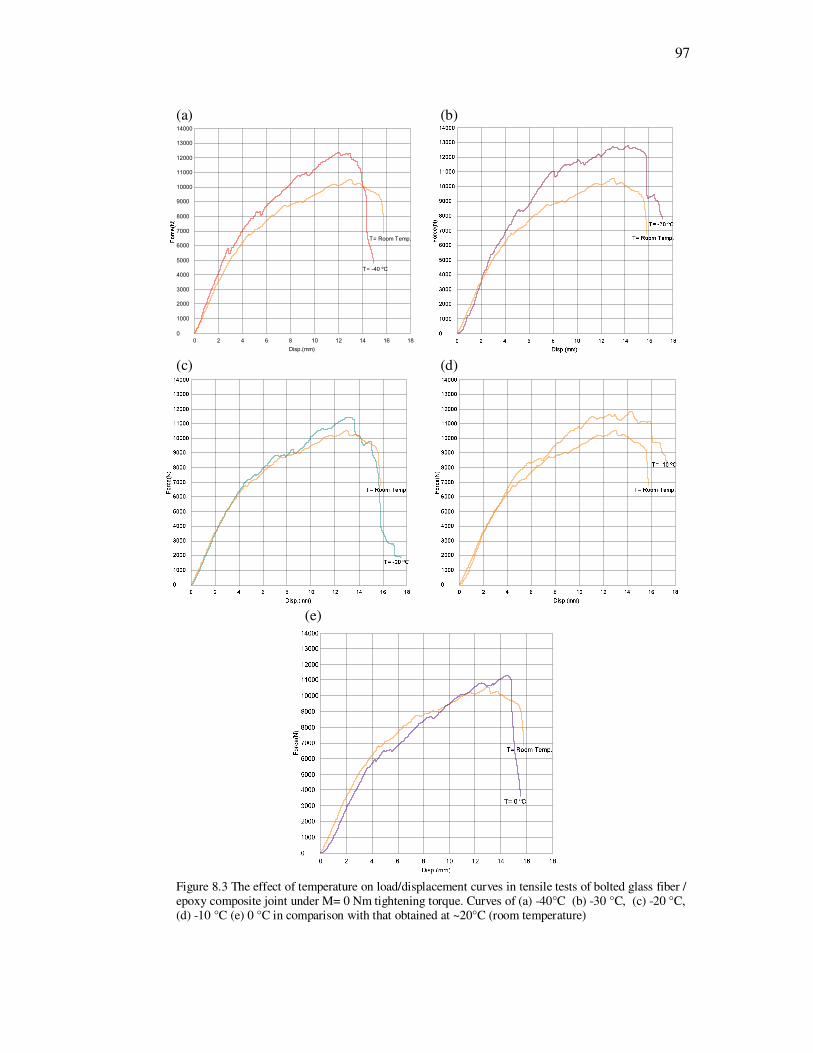
97

0 182 4 6 8 10 12 14 16

14000

0

13000

12000

11000

10000

9000

8000

7000

6000

5000

4000

3000

2000

1000

Disp.(mm)

T= -40 ºC

T= Room Temp.

(a) (b)

(c) (d)

(e)

Figure 8.3 The effect of temperature on load/displacement curves in tensile tests of bolted glass fiber / epoxy composite joint under M= 0 Nm tightening torque. Curves of (a) -40°C (b) -30 °C, (c) -20 °C, (d) -10 °C (e) 0 °C in comparison with that obtained at ~20°C (room temperature)

98

Force(N)

Force(N)

(a) (b)

(c) (d)

(e)

Figure 8.4 The effect of temperature on load/displacement curves in tensile tests of bolted glass fiber / epoxy composite joint under M= 6 Nm tightening torque. Curves of (a) -40°C (b) -30 °C, (c) -20 °C, (d) -10 °C (e) 0 °C in comparison with that obtained at ~20°C (room temperature)

99

Force(N)

(a) (b)

(c) (d)

(e) (f)

Figure 8.5 The effect of bolt tightening torques on load/displacement curves in tensile tests of bolted glass fiber / epoxy composite joint (a)-40°C, (b) -30 °C, (c) -20 °C, (d) -10 °C,(e) 0 °C (f) ~20°C (room temperature)

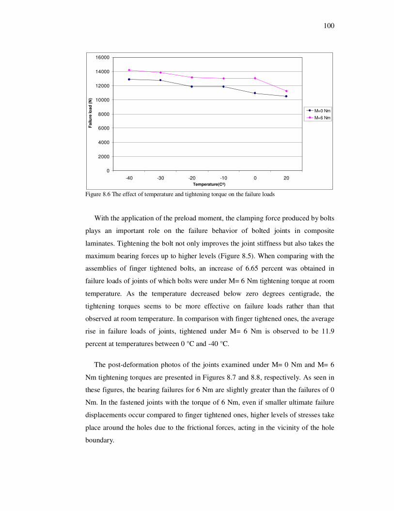
100

0

2000

4000

6000

8000

10000

12000

14000

16000

-40 -30 -20 -10 0 20

Temperature(Cº)

Fa

ilu

re lo

ad

(N

)

M=0 Nm

M=6 Nm

Figure 8.6 The effect of temperature and tightening torque on the failure loads

With the application of the preload moment, the clamping force produced by bolts

plays an important role on the failure behavior of bolted joints in composite

laminates. Tightening the bolt not only improves the joint stiffness but also takes the

maximum bearing forces up to higher levels (Figure 8.5). When comparing with the

assemblies of finger tightened bolts, an increase of 6.65 percent was obtained in

failure loads of joints of which bolts were under M= 6 Nm tightening torque at room

temperature. As the temperature decreased below zero degrees centigrade, the

tightening torques seems to be more effective on failure loads rather than that

observed at room temperature. In comparison with finger tightened ones, the average

rise in failure loads of joints, tightened under M= 6 Nm is observed to be 11.9

percent at temperatures between 0 °C and -40 °C.

The post-deformation photos of the joints examined under M= 0 Nm and M= 6

Nm tightening torques are presented in Figures 8.7 and 8.8, respectively. As seen in

these figures, the bearing failures for 6 Nm are slightly greater than the failures of 0

Nm. In the fastened joints with the torque of 6 Nm, even if smaller ultimate failure

displacements occur compared to finger tightened ones, higher levels of stresses take

place around the holes due to the frictional forces, acting in the vicinity of the hole

boundary.

101

Figure 8.7 Photo of deformed composite specimens at various temperature levels in tensile tests under M= 0 Nm tightening torque.

Figure 8.8 Photo of deformed composite specimens at various temperature levels in tensile tests under M= 6 Nm tightening torque.

102

CHAPTER NINE

CONCLUSIONS

Within the framework of the present study, experimental investigations were

performed to obtain the effects of thermal conditions and preload moments on the

failure behavior of single lap double serial mechanical fastener glass fiber / epoxy

composite joints by means of static tensile tests.

In the first stage, experiments were performed by exposing the joints to five

different high temperature levels (40, 50, 60, 70, 80 ºC), as has been discussed in

detail in chapter eight. Subsequently, especially considering the freezing

environment that the composite structural components of air vehicles are inevitably

exposed, tests were conducted at five low temperature levels ranging from 0 °C

down to -40 °C and results were comprehensively reported in chapter nine. Effects of

exposing high and low temperatures on failure behaviors of bolted composite joints

were discussed in comparison with those tests conducted at room temperature. The

effects of preload applied to the fastener bolts and how this effect is influenced by

temperature changes were also examined during tests. The following conclusions can

be made based on the experimental results:

• Elevated temperatures significantly affect on failure loads of mechanically

fastened composite joints. As the test temperature increases, the load-carrying

capacity of the joint decreases to some extent depending on the temperature level

exposed.

• Low temperature exposure has significant impact on failure loads in

mechanically fastened composite joints. Joints exhibit relatively higher load-

carrying capacity when decreasing temperature. When the temperature decreases

from the room temperature to – 40 °C, the failure load increases gradually.

• The torque applied to the fastener bolts remarkably affects the joint strength of

composites. Higher failure loads are obtained for composite joints under preload

103

moment compared to the finger tightened ones. The increase in failure loads is

getting much greater as the temperature decreases to subzero degrees centigrade.

The positive influence of preload moment is experienced at elevated

temperatures as well.

• Depending on the test temperature, there is no change in failure modes which are

highly affected by material and geometrical parameters. Just as the bearing

failure mode, which is the desirable mode, is observed at room temperature, so it

is monitored at elevated temperatures and at low temperatures, too. Thus, the

selected geometry and material properties are found to be suitable for even low

and high temperature applications.

The following investigations can be performed in the future:

o Hot water aging effects on mechanically fastened composite joints.

o Effects of hot and cold environments on adhesively-bonded joints.

104

REFERENCES

Adams, D. O., Moriarty, J. M., Gallegos, A. M., & Donald F. Adams, D. F. (2003).

Development and evaluation of the v-notched rail shear test for composite

laminates. Atlantic City: Federal Aviation Administration.

Adams, D. (2005). V-Notch Rail Shear test (ASTM D 7078-05). Retrieved July 31,

2012, from http://www.compositesworld.com/articles/v-notch-rail-shear-test-

astm-d-7078-05

Aktaş, A., Đmrek, H. & Cünedinoğlu, Y. (2009). Experimental and numerical failure

analysis of pinned joints in composite materials. Composite Structures, 89 (3),

459-466.

Asi, O. (2010). An experimental study on the bearing strength behavior of al2o3

particle filled glass-fiber reinforced epoxy composite pinned joints. Composite

Structures, 92 (2), 354-363.

Baker, A., Dutton, S., & Kelly, D. (2004). Composite Materials for Aircraft

Structures (2th ed.). USA: American Institute of Aeronautics and Astronautics.

Camanho, P.P., & Lambert, M. (2006). A design methodology for mechanically

fastened joints in laminated composite materials. Composites Science and

Technology, 66 (15), 3004-3020.

Campbell, F. C. (2004). Manufacturing processes for advanced composites (1th ed.).

UK, USA, JAPAN: Elsevier Ltd.

Campbell, F. C. (2011). Joining – understanding the basics (1th ed.). USA: ASM

International.

105

Choo V. K. S. (1990). Fundamentals of composite materials (1th ed.). Delaware:

Knowen Academic Press, INC.

Daniel, I. M., & Ishai, O. (1994). Engineering mechanics of composite materials.(1th

ed.). NY: Oxford University Press

Dano, M.L., Gendron, G., & Picard, A. (2000). Stress and failure analysis of

mechanically fastened joints in composite laminates. Composite Structures, 50

(3), 287-296.

Ekh, J., & Schön, J.(2006). Load transfer in multirow, single shear, composite-to-

aluminum lap joints. Science and Technology, 66 (7-8), 875-885.

Gibson, R.F. (1994). Principals of Composite Material Mechanics (1th ed.). NY:

McGraw-Hill.

Hirano N., Takao Y., & Wang W.X. (2007) Effects of temperature on the bearing

strength of CF / epoxy pinned joints. Journal of Composite Materials, 41 (3),

335-351.

Jones, R. M. (1999). Mechanics of Composite Materials (2th ed.). US: Taylor &

Francis Inc.

Karakuzu R., Çalışkan C.R., Aktaş M., & Đçten B.M. (2008). Failure behavior of

laminated composite plates with two serial pin- loaded holes. Composite

Structures, 82 (2), 225-234.

Kaw, A. K. (2006). Mechanics of composite materials. (2th ed.). NY: Taylor &

Francis Group, LLC.

Kelly G., & Hallström S. (2004). Bearing strength of carbon fiber/epoxy laminates:

effects of bolt-hole clearance. Composites: Part B, 35, 331–343.

106

Kishore A.N., Malhotra S.K., & Prasad N.S. (2009). Failure analysis of multi-pin

joints in glass fibre/epoxy composite laminates. Composite Structures, 91 (3),

266–277.

Lie, S.T., Yu G., & Zhao, Z. (2000). Analysis of mechanically fastened composite

joints by boundary element methods. Composites: Part B, 31 (8), 693-705.

Ling, Y. (1986). An estimation method of bearing strength of bolted joints in fiber

reinforced composite. Applied Mathematics and Mechanics, 7 (1), 103-109.

Mallick, P. K. (1993). Fiber-reinforced composites materials, manufacturing, and

design, (2 nd ed.). NY: Marcel Decker.

Matthews, F.L., & Rawlings, R.D. (1999). Composite materials: engineering and

science (1th ed.). London, UK: Imperial College of Science, Technology and

Medicine.

Messler, R.W. (2004). Joining of materials and structures (1th ed.). USA: Elsevier

Butterworth-Heinemann.

Okutan, B. (2001). Stress and failure analysis of laminated composite pinned joints.

PhD Thesis, Dokuz Eylül University, Izmir.

Okutan Baba, B. (2006). Behavior of pin-loaded laminated composites.

Experimental Mechanics, 46 (5), 589-600.

Ozen M., & Sayman O. (2011). Failure loads of mechanical fastened pinned and

bolted composite joints with two serial holes. Composites Part B, 42 (2), 264-274.

Park, H.J. (2001a). Bearing failure analysis of mechanically fastened joints in

composite laminates. Composite Structures, 53 (2), 199-211.

107

Park, H.J. (2001b). Effects of stacking sequence and clamping force on the bearing

strengths of mechanically fastened joints in composite laminates. Composite

Structures, 53 (2), 213-221.

Pearce, M.G., Johnson, A.F., Thomson, R.S. & Kelly, D.W. (2010). Experimental

investigation of dynamically loaded bolted joints in carbon fibre composite

structures. Appl. Compos Mater, 17 (3), 271-291.

Pekbey, Y. (2008). The bearing strength and failure behavior of bolted e-glass-epoxy

composite joints. Mechanics of Composite Materials, 44 (4), 397-414.

Peters, S. T. (1998). Handbook of composites (2th ed.). London: Chapman & Hall.

Sánchez-Sáez S., Gómez-del Rı́o T., Barbero E., Zaera R., & Navarro C. (2002).

Static behavior of CFRPs at low temperatures. Composites: Part B, 33 (5), 383-

390.

Sen, F., Pakdil, M., Sayman, O., & Benli, S. (2008). Experimental failure analysis of

mechanically fastened joints with clearance in composite laminates under preload.

Materials and Design, 29 (6), 1159-1169.

Sen F., Komur M.A., & Sayman O. (2010). Prediction of bearing strength of two

serial pinned / bolted composite joints using artificial neural networks. Journal of

Composite Materials, 44 (11), 1365-1377.

Sen F., & Sayman O. (2011). Failure response of two serial bolted joints in

composite laminates. Journal of Mechanics, 27 (3), 293-307.

Sheikh-Ahmad J.Y. (2009). Machining of Polymer Composites (1th ed.). NY:

Springer Science + Business Media LLC.

108

Song M.H., Kweon J.H., Kim S.K., Kim C., Lee T.J., Choi S.M., & Seong M.S.

(2008). An experimental study on the failure of carbon/epoxy single lap riveted

joints after thermal exposure. Composite Structures, 86 (1-3), 125-134.

Staab, G. H. (1999). Laminar composites. (1th ed.). USA.: Butterworth-Heinemann.

Thostenson, E.T., & Chou, T.W. (2008). Carbon nanotube-based health monitoring

of mechanically fastened composite joints. Composites Science and Technology,

68 (12), 2557-2561.

Walker S.P. (2002). Thermal effects on the pin-bearing behavior of im7/peti5

composite joints. Journal of Composite Materials, 36 (23), 2623-2651.