Semi-Lagrangian schemes forlinear and fully non-lineardiffusion equationsKristian Debrabanta and Espen R. Jakobsenb

aTechnische Universität Darmstadt, Fachbereich Mathematik, Schloßgartenstr.7, D-64289 Darmstadt, Germany,debrabant@mathematik.tu-darmstadt.debDepartment of Mathematical Sciences, Norwegian University of Science and Technology,N-7491 Trondheim, Norway,erj@math.ntnu.no

Abstract

For linear and fully non-linear diffusion equations of Bellman-Isaacs type, we introduce a class of monotone approxima-tion schemes relying on monotone interpolation. As opposed to classical numerical methods, these schemes converge fordegenerate diffusion equations having general non-diagonal dominant coefficient matrices. Such schemes have to havea wide stencil in general. Besides providing a unifying framework for several known first order accurate schemes, ourclass of schemes also includes more efficient versions, and a new second order scheme that converges only for essentiallymonotone solutions. The methods are easy to implement and analyze, and they are more efficient than some otherknown schemes. We prove stability and convergence of the schemes in the general case, and provide error estimates inthe convex case which are robust in the sense that they apply to degenerate equations and non-smooth solutions. Themethods are extensively tested.

Keywords: Monotone approximation schemes, difference-interpolation methods, stability, convergence, error bound,degenerate parabolic equations, Hamilton-Jacobi-Bellman equations, viscosity solution.

2000 MSC: 65M12, 65M15, 65M06, 35K10, 35K55, 35K65, 49L25, 49L20.

1 Introduction

In this paper we introduce and analyze a class of monotone approximation schemes for fully non-linear diffusion equa-tions of Bellman-Isaacs type,

ut − infα∈A

supβ∈B

n

Lα,β[u](t, x) + cα,β (t, x)u+ f α,β (t, x)o

= 0 in QT , (1.1)

u(0, x) = g(x) in RN , (1.2)

where QT := (0, T]×RN and

Lα,β[u](t, x) = tr[aα,β (t, x)D2u(t, x)] + bα,β (t, x)Du(t, x).

The coefficients aα,β = 12σα,βσα,β>, bα,β , cα,β , f α,β and the initial data g take values respectively in SN , the space of N×N

symmetric matrices, RN , R, R, and R. We will only assume that aα,β is positive semi-definite, thus the equation is allowedto degenerate and does not have any smooth solutions in general. Under suitable assumptions (see Section 2), the initialvalue problem (1.1)-(1.2) has a unique, bounded, Hölder continuous, viscosity solution u. This function is the upper orlower value of a stochastic differential game, or, if A or B is a singleton, the value function of a finite horizon, optimalstochastic control problem [25].

We introduce a family of schemes that we call Semi-Lagrangian (SL) schemes. They are a type difference-interpolationschemes and arise as time-discretizations of the following semi-discrete equation

ut − infα∈A

supβ∈B

n

Lα,βk [Ihu](t, x) + cα,β (t, x)u+ f α,β (t, x)

o

= 0 in X h× (0, T ),

where Lα,βk is a monotone difference approximation of Lα,β and Ih is a monotone interpolation operator on the spatial

grid X h. For more details see Section 3. Typically these scheme are first order wide-stencil schemes, and if the matrix aα,β

is bad enough, the stencil has to keep increasing as the grid is refined to have convergence. They include as special casesschemes from [16, 19, 7, 12], more efficient versions of these schemes, and a new second order compact stencil scheme.There are two main advantages of these schemes: (i) they are easy to understand and implement, and more importantly,(ii) they are consistent and monotone for every positive semi-definite diffusion matrix aα,β = 1

2σα,βσα,β>. The last point

is important because monotone methods are known to converge to the correct solution [3], while non-monotone methodsneed not converge [21] or can even converge to false solutions [23].

Classical finite difference approximations (FDMs) of (1.1) are not monotone (of positive type) unless the matrix aα,β

satisfies additional assumptions like e. g. being diagonally dominant [18]. More general assumptions are given in e. g.[5, 14] but at the cost of increased stencil length. In fact, Dong and Krylov [14] proved that no fixed stencil FDM canapproximate equations with a second derivative term involving a general positive semi-definite matrix function aα,β .Note that this type of result has been known for a long time, see e. g. [20, 12]. Some very simple examples of such “bad”matrices are given by

�

x21

12

x1 x212

x1 x2 x22

�

in [0,1]2,

�

α2 αβ

αβ β2

�

for A= B = [0,1], I −Du⊗ Du

|Du|2,

and these type of matrices appear in Finance, Stochastic Control Theory, and Mean Curvature Motion. The third exampleleads to quasi-linear equations and will not be considered here, we refer instead to [12].

To obtain convergent or monotone methods for problems involving non-diagonally dominant matrices, we know of twostrategies: (i) The classical method of rotating the coordinate system locally to obtain diagonally dominant matrices aα,β ,see e. g. Section 5.4 in [18], and (ii) the use of wide stencil methods. The two solutions seem to be somewhat related,but at least the defining ideas and implementation are different. Both ways lead to methods that have reduced ordercompared to standard schemes for diagonally dominant problems. But it seems to us that it is much more difficult toimplement the first strategy.

In addition to the wide-stencil methods mentioned above, we also mention the method of Bonnans-Zidani [5] which isnot an SL type scheme. Schemes for other types of equations related to our SL schemes have been studied by Crandall-Lions [12] for the Mean Curvature Motion equation, by Oberman [22] for Monge-Ampère equations, and by Camilli andthe second author for non-local Bellman equations [8]. The terminology SL schemes is already used for schemes for

2

transport equations, conservation laws, and first order Hamilton-Jacobi equations. In the Hamilton-Jacobi setting, theseschemes go back to the 1983 paper [9] of Capuzzo-Dolcetta.

The rest of this paper is organized as follows. In the next Section we explain the notation and state a well-posedness andregularity result for (1.1)–(1.2). The SL schemes are motivated and defined in an abstract setting in Section 3, and inSection 4 we prove that they are consistent, monotone, L∞-stable, and convergent. We provide several examples of SLschemes in Section 5, including the linear interpolation SL (LISL) scheme. This is the basic example of this paper, and itis a first order scheme that can be defined on unstructured grids.

Our SL schemes make use of monotone interpolation, and higher order interpolation is not monotone in general. Butfor essentially monotone solutions, we can use monotone cubic Hermite interpolation (see Fritsch and Carlson [17] andEisenstat, Jackson and Lewis [15]) to obtain new second order schemes called monotone cubic interpolation SL (MCSL)schemes. These new schemes are defined in Section 6, and in contrast to the LISL schemes they are compact stencilschemes. Note well that in the special case of first order HJ-equations with monotone solutions, these schemes areconsistent, monotone, second order schemes! To our knowledge, this is the first example of a monotone scheme which ismore than first order accurate in the HJ-setting.

We discuss various issues concerning the SL schemes in Section 7. We compare the LISL scheme to the scheme ofBonnans-Zidani [5] and find that the LISL scheme is much easier to understand and implement, and in general it is muchfaster. However, on bounded domains the LISL scheme will in some cases over-step the boundaries and some ad hocsolution has to be found. This problem is avoided by the Bonnans-Zidani scheme at the cost of being less accurate nearthe boundary than in the interior. Finally, we explain that the SL schemes can be interpreted as collocation methodsfor derivative free equations, or as dynamic programming equations of discrete stochastic differential games or optimalcontrol problems.

In Sections 8, 9 and Appendix B, we produce robust error estimates for convex equations (i. e. B is a singleton in (1.1)).These estimates are obtained through the regularization method of Krylov and apply to degenerate equations, non-smooth solutions, and both the LISL and MCSL schemes. Finally, in Section 10, our methods are extensively tested. Inparticular we find that the LISL and MCSL schemes yield much faster methods to solve the finance problem of Bruder,Bokanowski, Maroso, and Zidani [6].

2 Notation and well-posedness

In this section we introduce notation and assumptions, and give a well-posedness and comparison result for the initialvalue problem (1.1) – (1.2).

We denote by ≤ the component by component ordering in RM and the ordering in the sense of positive semi-definitematrices in SN . The symbols ∧ and ∨ denote the minimum respectively the maximum. By | · | we mean the Euclideanvector norm in any Rp type space (including the spaces of matrices and tensors). Hence if X ∈ RN ,P , then |X |2 =∑

i, j |X i j |2 = tr(X X>) where X> is the transpose of X .

If w is a bounded function from some set Q′ ⊂Q∞ into either R, RM , or the space of N × P matrices, we set

|w|0 = sup(t,y)∈Q′

|w(t, y)|.

Furthermore, for δ ∈ (0,1], we set

[w]δ = sup(t,x)6=(s,y)

|w(t, x)−w(s, y)|(|x − y|+ |t − s|1/2)δ

and |w|δ = |w|0 + [w]δ.

Let Cb(Q′) and C0,δ(Q′), δ ∈ (0,1], denote respectively the space of bounded continuous functions on Q′ and the subsetof Cb(Q′) in which the norm | · |δ is finite. Note in particular the choices Q′ =QT and Q′ = RN . In the following we alwayssuppress the domain Q′ when writing norms.

For simplicity, we will use the following assumptions on the data of (1.1)–(1.2):

(A1) For any α ∈ A and β ∈ B, aα,β = 12σα,βσα,β> for some N×P matrix σα,β . Moreover, there is a constant K independent

of α,β such that

|g|1 + |σα,β |1 + |bα,β |1 + |cα,β |1 + | f α,β |1 ≤ K .

3

These assumptions are standard and ensure comparison and well-posedness of (1.1)–(1.2) in the class of bounded x-Lipschitz functions.

Proposition 2.1. Assume that (A1) holds. Then there exists a unique solution u of (1.1)–(1.2) and a constant C onlydepending on T and K from (A1) such that

|u|1 ≤ C .

Furthermore, if u1 and u2 are sub- and supersolutions of (1.1) satisfying u1(0, ·)≤ u2(0, ·), then u1 ≤ u2.

The proof is standard. Assumption (A1) can be relaxed in many ways, e. g. using weighted norms, Hölder or uniformcontinuity, etc. But in doing so, solutions can become unbounded and less smooth, and the analysis becomes harder andless transparent. Therefore we will not consider such extensions in this paper.

By solutions in this paper we always mean viscosity solutions, see e. g. [11, 25].

3 Definition of SL schemes

In this section we propose a class of monotone approximation schemes for (1.1)–(1.2) which we call Semi-Lagrangian orSL schemes. This class includes (parabolic versions of) the “control schemes” of Menaldi [19] and Camilli and Falcone[7] and the monotone schemes of Crandall and Lions [12]. It also includes SL schemes for first order Bellman equations[9, 16], and it allows for more effective versions of these schemes as discussed in Section 5. For a motivation for thename, we refer to Remark 7.2. For the time discretization we propose a generalized mid-point rule that includes explicit,implicit, and a second order Crank-Nicolson like approximation. Note that the equation is non-smooth in general, so theusual way of defining a Crank-Nicolson scheme would only give a first order scheme in time.

The schemes will be defined on a possibly unstructured family of grids {G∆t,∆x} with

G = G∆t,∆x = {(tn, x i)}n∈N0,i∈N = {tn}n∈N0× X∆x ,

for ∆t,∆x > 0. Here 0= t0 < t1 < · · ·< tn < tn+1 satisfy

maxn∆tn ≤∆t where ∆tn = tn − tn−1,

and X∆x = {x i}i∈N is the set of vertices or nodes for a non-degenerate polyhedral subdivision T ∆x = {T∆xj } j∈N of RN . For

some ρ ∈ (0,1) the polyhedrons T j = T∆xj satisfy

int(T j ∩ Ti) =i 6= j;,

⋃

j∈N

T j = RN , ρ∆x ≤ supj∈N{diam BT j

} ≤ supj∈N{diam T j} ≤∆x ,

where diam is the diameter of the set and BT jis the greatest ball contained in T j .

To motivate the numerical schemes, we write σ = (σ1,σ2, ...,σm, ...,σP) where σm is the m-th column of σ and observethat for k > 0 and smooth functions φ,

1

2tr[σσ>D2φ(x)] =

1

2

P∑

m=1

tr[σmσ>mD2φ(x)]

=P∑

m=1

1

2

φ(x + kσm)− 2φ(x) +φ(x − kσm)k2 +O(k2),

bDφ(x) =φ(x + k2 b)−φ(x)

k2 +O(k2)

=1

2

φ(x + k2 b)− 2φ(x) +φ(x + k2 b)k2 +O(k2).

These approximations are monotone (of positive type) and the errors are bounded by 148

P|σ|40|D4φ|0k2 and 1

2|b|20|D

2φ|0k2

respectively. To relate these approximations to a grid G, we replace φ by its interpolant Iφ on that grid and obtain

1

2tr[σσ>D2φ(x)]≈

P∑

m=1

1

2

(Iφ)(x + kσm)− 2(Iφ)(x) + (Iφ)(x − kσm)k2 ,

bDφ(x)≈1

2

(Iφ)(x + k2 b)− 2(Iφ)(x) + (Iφ)(x + k2 b)k2 .

4

If the interpolation is monotone (positive) then the full discretization is still monotone and represents a typical exampleof the discretizations we consider below.

To construct the general scheme, we generalize the above construction. We now consider general finite differenceapproximations of the differential operator Lα,β[φ] in (1.1) defined as

Lα,βk [φ](t, x) :=

M∑

i=1

φ(t, x + yα,β ,+k,i (t, x))− 2φ(t, x) +φ(t, x + yα,β ,−

k,i (t, x))

2k2 , (3.1)

for k > 0 and some M ≥ 1, where for all smooth functions φ,

|Lα,βk [φ]− Lα,β[φ]| ≤ C(|Dφ|0 + · · ·+ |D4φ|0)k2. (3.2)

This approximation and interpolation yield a semi-discrete approximation of (1.1),

Ut − infα∈A

supβ∈B

n

Lα,βk [IU](t, x) + cα,β (t, x)U + f α,β (t, x)

o

= 0 in (0, T )× X∆x ,

and the final scheme can then be found after discretizing in time using a parameter θ ∈ [0,1],

δ∆tnUn

i = infα∈A

supβ∈B

n

Lα,βk [IUθ ,n

· ]n−1+θi + cα,β ,n−1+θ

i Uθ ,ni + f α,β ,n−1+θ

i

o

(3.3)

in G, where Uni = U(tn, x i), f α,β ,n−1+θ

i = f α,β (tn−1 + θ∆tn, x i), . . . for (tn, x i) ∈ G,

δ∆tφ(t, x) =φ(t, x)−φ(t −∆t, x)

∆t, and φθ ,n

· = (1− θ)φn−1· + θφn

· .

As initial conditions we take

U0i = g(x i) in X∆x . (3.4)

Remark 3.1. For the choices θ = 0, 1, and 1/2 the time discretization corresponds to respectively explicit Euler, implicitEuler and midpoint rule. For θ = 1/2, the full scheme can be seen as generalized Crank-Nicolson type discretizations.

4 Analysis of SL schemes

In this section we prove that the SL scheme (3.3) is consistent and monotone, and we present L∞-stability, existence,uniqueness, and convergence results for these schemes. In Section 8 we also give error estimates when B is a singletonand equation (1.1) is convex.

For the approximation Lα,βk and interpolation I we will assume that

M∑

i=1

[yα,β ,+k,i + yα,β ,−

k,i ] = 2k2 bα,β +O(k4),

M∑

i=1

[yα,β ,+k,i ⊗ yα,β ,+

k,i + yα,β ,−k,i ⊗ yα,β ,−

k,i ] = k2σα,βσα,β> +O(k4),

M∑

i=1

[⊗3j=1 yα,β ,+

k,i +⊗3j=1 yα,β ,−

k,i ] = O(k4),

M∑

i=1

[⊗4j=1 yα,β ,+

k,i +⊗4j=1 yα,β ,−

k,i ] = O(k4).

(Y1)

There are K ≥ 0, r ∈ N such that |(Iφ)−φ|0 ≤ K |Dpφ|0∆x p for (I1)

all N 3 p ≤ r and all smooth functions φ.

There is a non-negative basis of functions {w j(x)} j such that (I2)

(Iφ)(x) =∑

j

φ(x j)w j(x), wi(x j) = δi j , and w j(x)≥ 0 for all i, j ∈ N.

5

Under assumption (Y1), a Taylor expansion shows that Lα,βk is a second order consistent approximation satisfying (3.2).

If we assume also (I1) , it then follows that Lα,βk [Iφ] is a consistent approximation of Lα,β[φ] if ∆x r

k2 → 0. Indeed

|Lα,βk [Iφ]− Lα,β[φ]| ≤ |Lα,β

k [Iφ]− Lα,βk [φ]|+ |L

α,βk [φ]− Lα,β[φ]|,

where |Lα,βk [φ]− Lα,β[φ]| is estimated in (3.2), and by (I1),

|Lα,βk [Iφ]− Lα,β

k [φ]| ≤ C |Drφ|0∆x r

k2 .

Remark 4.1. Assumption (Y1) is similar to the local consistency conditions used in [18]. The O(k4) terms insure that themethod is second order accurate as k→ 0. Convergence will still be achieved if we relax O(k4) to o(k2) as k→ 0.

Remark 4.2. An interpolation satisfying (I2) is said to be positive or monotone and preserves monotonicity of the data.Note that such an interpolation Iφ does not use (exact) derivatives to reconstruct the function φ. Typically I will beconstant, linear, or multi-linear interpolation (i. e. r ≤ 2 in (I1)) since higher order interpolation is not monotone ingeneral. For later use we note that from (I1) and (I2) it follows that

r ≥ 1⇒∑

i

wi(x)≡ 1 and r ≥ 2⇒∑

i

x iwi(x)≡ x . (4.1)

Now we prove that the scheme (3.3)–(3.4) is consistent and monotone. The scheme is said to be monotone if it can bewritten as

supα

infβ

n

Bα,β ,n,nj, j Un

j −∑

i 6= j

Bα,β ,n,nj,i Un

i −∑

i

Bα,β ,n,n−1j,i Un−1

i − Fα,β ,nj

o

= 0 (4.2)

in G, where Bα,β ,n,mi, j ≥ 0 and Fα,β ,n

j does not depend on U .

Lemma 4.1. Assume (I1), (I2), and (Y1) hold.

(a) The consistency error of the scheme (3.3) is bounded by

|1− 2θ |2

|φt t |0∆t + C

�

∆t2�

|φt t |0 + |φt t t |0 + |Dφt t |0 + |D2φt t |0�

+|Drφ|0∆x r

k2 + (|Dφ|0 + · · ·+ |D4φ|0)k2

�

.

(b) The scheme (3.3) is monotone if the following CFL condition holds,

(1− θ)∆thM

k2 − cα,β ,n−1+θi

i

≤ 1 and θ∆t cα,β ,n−1+θi ≤ 1 for all α,β , n, i. (4.3)

Remark 4.3. By parabolic regularity D2 ∼ ∂t which means that e. g. |D2φt t |0 is proportional to |φt t t |0. When θ = 1/2(“Crank-Nicolson”), the scheme (3.3) is second order accurate in time.

Proof. It is immediate that the scheme (3.3) is consistent with (1.1) with a truncation error bounded by

|1− 2θ |2

|φt t |0∆t +1

3|φt t t |0∆t2 + sup

α,β ,n

�

�

�Lα,β[φθ ,n]− Lα,βk [Iφ

θ ,n]�

�

0

+ supα,β ,n

n

�

�Lα,β[φn−1+θ − φθ ,n]�

�

0 +�

�cα,β ,n−1+θ (φn−1+θ − φθ ,n)�

�

0

o

for smooth φ. By (I1) and (3.2), |Lα,β[φθ ,n]− Lα,βk [Iφ

θ ,n]| can be bounded by

C |Drφ|0∆x r

k2 + C(|Dφ|0 + · · ·+ |D4φ|0)k2,

6

while |Lα,β[φn−1+θ − φθ ,n]| is bounded by

∆t2θ(1− θ) supα,β|Lα,β[φt t]|0 ≤ C∆t2θ(1− θ)

n

|Dφt t |0 + |D2φt t |0o

.

Finally, |cα,β ,n−1+θ (φn−1+θ − φθ ,n)�

�≤ Cθ(1− θ)∆t2|φt t |0. Hence part (a) follows.

To prove part (b), we note that since∑

i wi ≡ 1 we have

Lα,βk [Iφ(t, ·)](tn−1+θ , x j) =

∑

i∈Nlα,β ,n−1+θj,i

�

φ(t, x i)−φ(t, x j)�

,

where

lα,β ,n−1+θj,i =

M∑

l=1

wi(x j + yα,β ,+k,l (tn−1+θ , x j)) +wi(x j + yα,β ,−

k,l (tn−1+θ , x j))

2k2 .

This quantity is non-negative by (I2), and∑

i lα,β ,n−1+θj,i = M

k2 by (I1), (I2), and∑

i wi ≡ 1. Therefore the only non-zerocoefficients in (4.2) at (tn, x j) are

Bα,β ,n,nj, j = 1+ θ∆tn (

Mk2 − lα,β ,n−1+θ

j j − cα,β ,n−1+θj ),

Bα,β ,n,n−1j, j = 1− (1− θ)∆tn(

Mk2 − lα,β ,n−1+θ

j j − cα,β ,n−1+θj ),

Bα,β ,n,nj,i = θ∆tnlα,β ,n−1+θ

j,i , Bα,β ,n,n−1j,i = (1− θ)∆tnlα,β ,n−1+θ

j,i ,

where j 6= i. These coefficients are positive if (4.3) holds.

Existence, uniqueness, stability, and convergence results are given below. In the following, we denote by cα,β ,+ thepositive part of cα,β .

Theorem 4.2. Assume (A1), (I1), (I2), (Y1), and (4.3).

(a) There exists a unique bounded solution Uh of (3.3)–(3.4).

(b) The solution Uh of (3.3)–(3.4) is L∞-stable when 2θ∆t supα,β |cα,β ,+|0 ≤ 1:

|Un|0 ≤ e2supα,β |cα,β ,+|0 tn

h

|g|0 + tn supα,β| f α,β |0

i

.

(c) Uh converges uniformly to the solution u of (1.1)–(1.2) as ∆t, k, ∆x r

k2 → 0.

Proof. Existence and uniqueness of bounded solutions follow by induction. Let t = tn and assume Un−1 is a knownbounded function. For ε > 0 we define the operator T by

T Unj = Un

j − ε · (left hand side of (4.2)) for all j ∈ ZM .

Note that the fixed point equation Un = T Un is equivalent to equation (3.3). By the definition and sign of the B-coefficients we see that

T Unj − T Un

j

≤ supα,β

nh

1− ε(1+∆tnθ(Mk2 − cα,β ,n−1+θ

j ))i

(Unj − Un

j ) + ε∆tnθMk2 |Un

· − Un· |0o

≤ (1− ε[1−∆tnθ supα,β|cα,β ,+|0])|Un

· − Un· |0

7

if ε is so small that 1− ε(1+∆tθ( Mk2 − cα,β ,n−1+θ

j )) ≥ 0 and ε(1−∆tnθ supα,β |cα,β ,+|0) < 1 for all j, n,α,β . Taking thesupremum over all j and interchanging the role of U and U proves that T is a contraction on the Banach space of boundedfunctions on X∆x under the sup-norm. Existence and uniqueness then follows from the fixed point theorem (for Un) andfor all of U by induction since U0 = g is bounded.

A similar argument using (4.2) proves L∞-stability for θ∆t supα,β |cα,β ,+|0 ≤12:

|Un|0 ≤�1+ (1− θ)∆t supα,β |cα,β ,+|0

1− θ∆t supα,β |cα,β ,+|0

�h

|Un−1|0 +∆tn supα,β| f α,β |0

i

≤ e2 supα,β |cα,β ,+|0 tn

h

|g|0 + tn supα,β| f α,β |0

i

.

In view of this estimate, convergence of Uh to the solution u of (1.1)–(1.2) follows from the Barles-Souganidis result in[3].

5 Examples of SL schemes

5.1 Examples of approximations Lα,βk

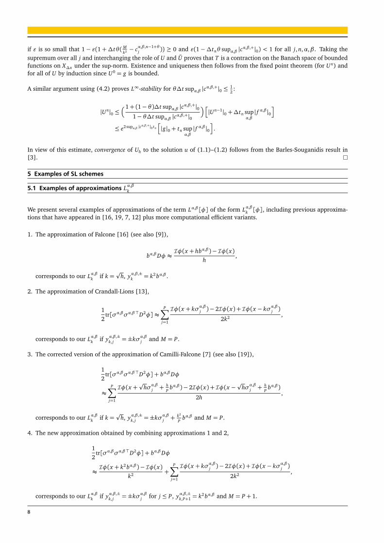
We present several examples of approximations of the term Lα,β[φ] of the form Lα,βk [φ], including previous approxima-

tions that have appeared in [16, 19, 7, 12] plus more computational efficient variants.

1. The approximation of Falcone [16] (see also [9]),

bα,βDφ ≈Iφ(x + hbα,β )− Iφ(x)

h,

corresponds to our Lα,βk if k =

ph, yα,β ,±

k = k2 bα,β .

2. The approximation of Crandall-Lions [13],

1

2tr[σα,βσα,β>D2φ]≈

P∑

j=1

Iφ(x + kσα,βj )− 2Iφ(x) + Iφ(x − kσα,β

j )

2k2 ,

corresponds to our Lα,βk if yα,β ,±

k, j =±kσα,βj and M = P.

3. The corrected version of the approximation of Camilli-Falcone [7] (see also [19]),

1

2tr[σα,βσα,β>D2φ] + bα,βDφ

≈P∑

j=1

Iφ(x +p

hσα,βj + h

Pbα,β )− 2Iφ(x) + Iφ(x −

phσα,β

j + hP

bα,β )

2h,

corresponds to our Lα,βk if k =

ph, yα,β ,±

k, j =±kσα,βj + k2

Pbα,β and M = P.

4. The new approximation obtained by combining approximations 1 and 2,

1

2tr[σα,βσα,β>D2φ] + bα,βDφ

≈Iφ(x + k2 bα,β )− Iφ(x)

k2 +P∑

j=1

Iφ(x + kσα,βj )− 2Iφ(x) + Iφ(x − kσα,β

j )

2k2 ,

corresponds to our Lα,βk if yα,β ,±

k, j =±kσα,βj for j ≤ P, yα,β ,±

k,P+1 = k2 bα,β and M = P + 1.

8

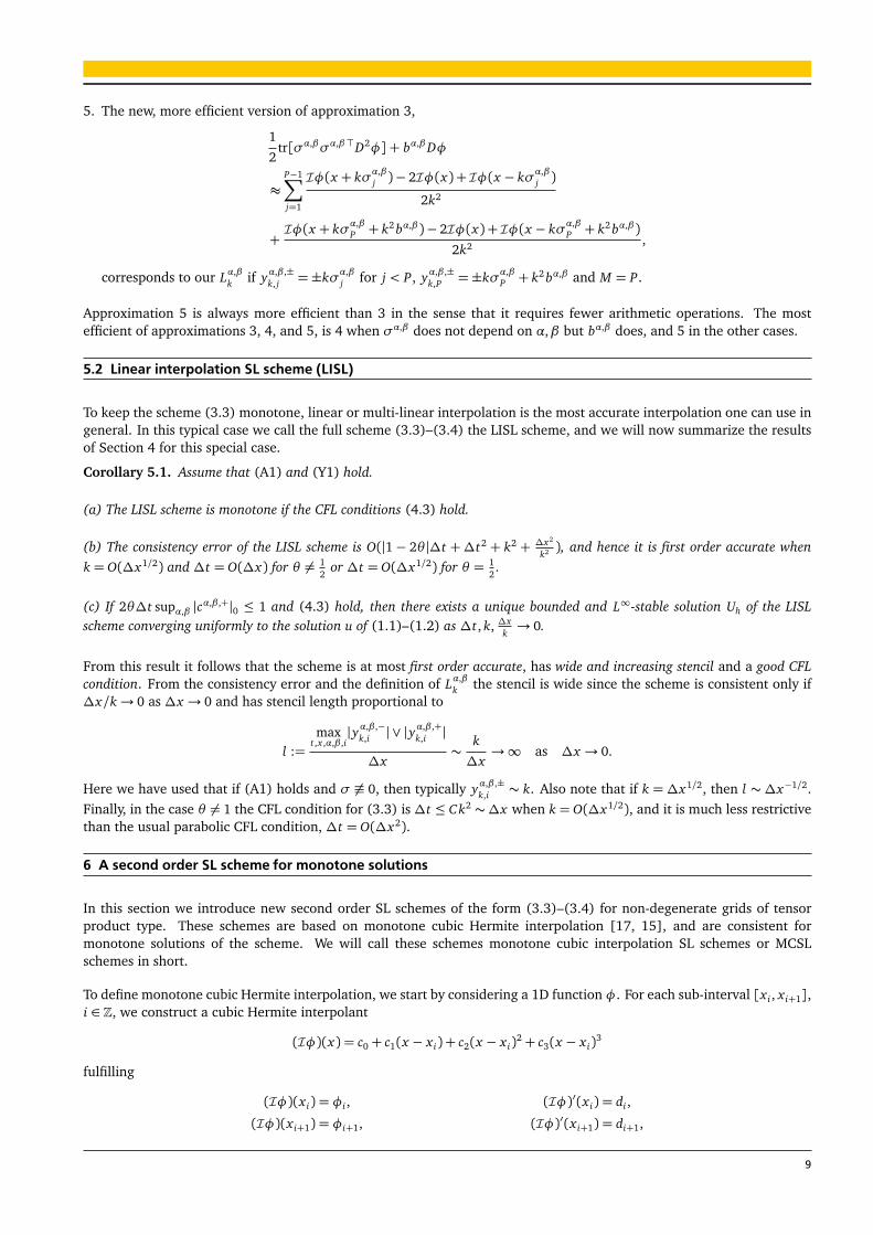
5. The new, more efficient version of approximation 3,

1

2tr[σα,βσα,β>D2φ] + bα,βDφ

≈P−1∑

j=1

Iφ(x + kσα,βj )− 2Iφ(x) + Iφ(x − kσα,β

j )

2k2

+Iφ(x + kσα,β

P + k2 bα,β )− 2Iφ(x) + Iφ(x − kσα,βP + k2 bα,β )

2k2 ,

corresponds to our Lα,βk if yα,β ,±

k, j =±kσα,βj for j < P, yα,β ,±

k,P =±kσα,βP + k2 bα,β and M = P.

Approximation 5 is always more efficient than 3 in the sense that it requires fewer arithmetic operations. The mostefficient of approximations 3, 4, and 5, is 4 when σα,β does not depend on α,β but bα,β does, and 5 in the other cases.

5.2 Linear interpolation SL scheme (LISL)

To keep the scheme (3.3) monotone, linear or multi-linear interpolation is the most accurate interpolation one can use ingeneral. In this typical case we call the full scheme (3.3)–(3.4) the LISL scheme, and we will now summarize the resultsof Section 4 for this special case.

Corollary 5.1. Assume that (A1) and (Y1) hold.

(a) The LISL scheme is monotone if the CFL conditions (4.3) hold.

(b) The consistency error of the LISL scheme is O(|1− 2θ |∆t +∆t2 + k2 + ∆x2

k2 ), and hence it is first order accurate whenk = O(∆x1/2) and ∆t = O(∆x) for θ 6= 1

2or ∆t = O(∆x1/2) for θ = 1

2.

(c) If 2θ∆t supα,β |cα,β ,+|0 ≤ 1 and (4.3) hold, then there exists a unique bounded and L∞-stable solution Uh of the LISLscheme converging uniformly to the solution u of (1.1)–(1.2) as ∆t, k, ∆x

k→ 0.

From this result it follows that the scheme is at most first order accurate, has wide and increasing stencil and a good CFLcondition. From the consistency error and the definition of Lα,β

k the stencil is wide since the scheme is consistent only if∆x/k→ 0 as ∆x → 0 and has stencil length proportional to

l :=max

t,x ,α,β ,i|yα,β ,−

k,i | ∨ |yα,β ,+k,i |

∆x∼

k

∆x→∞ as ∆x → 0.

Here we have used that if (A1) holds and σ 6≡ 0, then typically yα,β ,±k,i ∼ k. Also note that if k = ∆x1/2, then l ∼ ∆x−1/2.

Finally, in the case θ 6= 1 the CFL condition for (3.3) is ∆t ≤ Ck2 ∼∆x when k = O(∆x1/2), and it is much less restrictivethan the usual parabolic CFL condition, ∆t = O(∆x2).

6 A second order SL scheme for monotone solutions

In this section we introduce new second order SL schemes of the form (3.3)–(3.4) for non-degenerate grids of tensorproduct type. These schemes are based on monotone cubic Hermite interpolation [17, 15], and are consistent formonotone solutions of the scheme. We will call these schemes monotone cubic interpolation SL schemes or MCSLschemes in short.

To define monotone cubic Hermite interpolation, we start by considering a 1D function φ. For each sub-interval [x i , x i+1],i ∈ Z, we construct a cubic Hermite interpolant

(Iφ)(x) = c0 + c1(x − x i) + c2(x − x i)2 + c3(x − x i)

3

fulfilling

(Iφ)(x i) = φi , (Iφ)′(x i) = di ,

(Iφ)(x i+1) = φi+1, (Iφ)′(x i+1) = di+1,

9

where φi = φ(x i) and di is an estimate of the derivative of φ at x i . It follows that

c0 = φi , c1 = di , (6.1a)

c2 =3∆i − di+1 − 2di

∆x, c3 =−

2∆i − di+1 − di

∆x2 , (6.1b)

where ∆i =φi+1−φi

∆x. To obtain a fourth order accurate interpolant, φ′i must be at least third order accurate. We will use

the symmetric fourth order approximation

di =φi−2 − 8φi−1 + 8φi+1 −φi+2

12∆x, i ∈ Z. (6.2)

However, the resulting interpolation is not monotone. Necessary and sufficient conditions for monotonicity were foundby Fritsch and Carlson [17] (see also [24]): If ∆i = 0, then monotonicity follows if and only if di = di+1 = 0, and if

αi =di

∆iand βi =

di+1

∆i,

then monotonicity for ∆i 6= 0 follows if and only if (αi ,βi) ∈M=Me ∪Mb where

Me = {(α,β) : (α− 1)2 + (α− 1)(β − 1) + (β − 1)2 − 3(α+ β − 2)≤ 0},Mb = {(α,β) : 0≤ α≤ 3, 0≤ β ≤ 3}.

Eisenstat, Jackson and Lewis [15] give an algorithm that modifies the derivative approximation di such that the aboveconditions are fulfilled, and for monotone data the resulting interpolant is a C1 fourth order approximation. We will onlyconsider C0 interpolants, and in that case their algorithm simplifies to:

Step 1 Compute the initial di using (6.2).

Step 2 Compute ∆i . If ∆i 6= 0 compute αi and βi , else set αi = βi = 1.

Step 3 Set αi :=max{αi , 0} and βi :=max{βi , 0}.

Step 4 If (αi ,βi) /∈M, modify (αi ,βi) as follows:

• If αi ≥ 3 and βi ≥ 3, set αi = βi = 3,

• else if βi > 3 and αi + βi ≥ 4, decrease βi such that (αi ,βi) ∈ ∂M,

• else if βi > 3 and αi + βi < 4, increase αi such that (αi ,βi) ∈ ∂M or αi = 4− βi , in the last casesubsequently decrease βi until (αi ,βi) ∈ ∂M,

• else if αi > 3 and αi + βi ≥ 4, decrease αi such that (αi ,βi) ∈ ∂M,

• else if αi > 3 and αi + βi < 4, increase βi such that (αi ,βi) ∈ ∂M or βi = 4− αi , in the last casesubsequently decrease αi until (αi ,βi) ∈ ∂M.

In each sub-interval [x i , x i+1], we replace di by αi∆i and di+1 by βi∆i in (6.1). Multidimensional interpolation oper-ators are obtained as tensor products of one-dimensional interpolation operators, i. e. by interpolating dimension bydimension.

Lemma 6.1. The above monotone cubic interpolation is always monotone and satisfies (I2). If the interpolated function isstrictly monotone between grid points, then (I1) holds with r = 4 and the method is fourth order accurate.

Proof. Assumption (I2) holds by construction. The error estimate follows from [15], since the above algorithm coincideswith the two sweep algorithm given there when n= 1 interval is considered. In [15] it is proved that this algorithm givesthird order accurate approximations to the exact derivatives and hence the cubic Hermite polynomial constructed usingthis approximation is fourth order accurate.

Remark 6.1. Carlson and Fritsch [10] constructed an alternative monotone bicubic interpolation algorithm for R2. Weare not aware of any work on high order monotone interpolation on unstructured grids.

By the Lemma 6.1 and the results in Section 4 we have the following result:

10

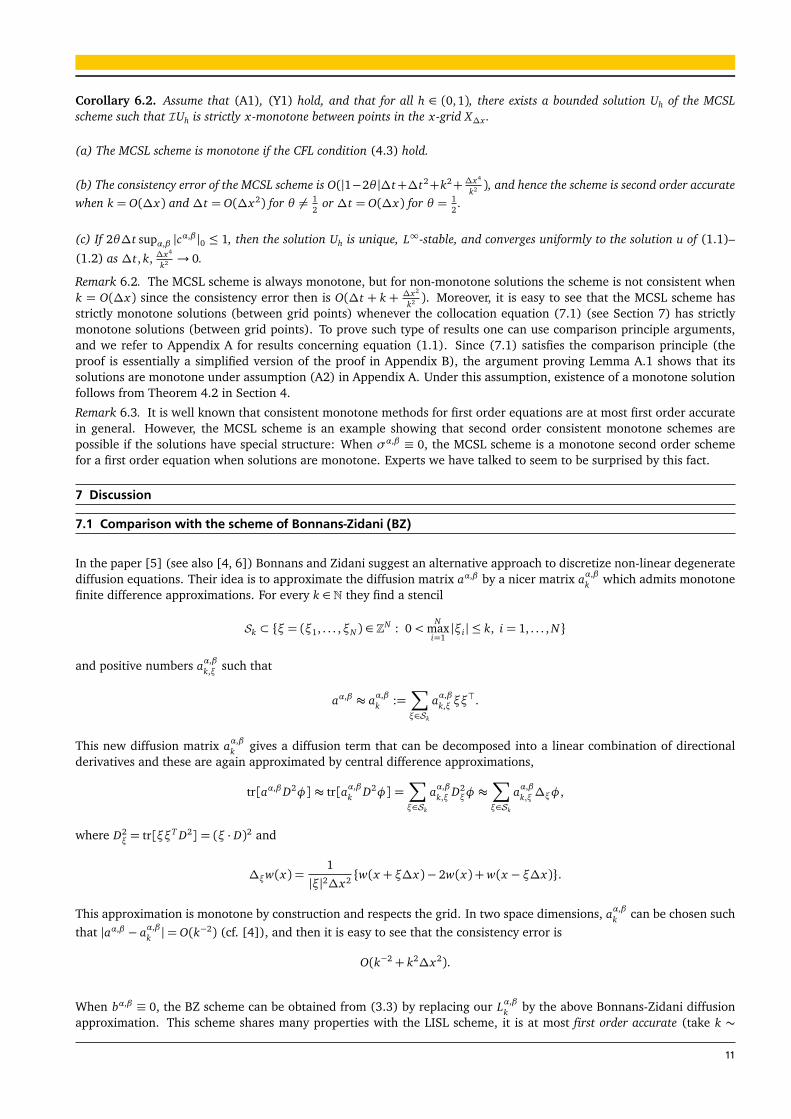
Corollary 6.2. Assume that (A1), (Y1) hold, and that for all h ∈ (0,1), there exists a bounded solution Uh of the MCSLscheme such that IUh is strictly x-monotone between points in the x-grid X∆x .

(a) The MCSL scheme is monotone if the CFL condition (4.3) hold.

(b) The consistency error of the MCSL scheme is O(|1−2θ |∆t+∆t2+k2+ ∆x4

k2 ), and hence the scheme is second order accuratewhen k = O(∆x) and ∆t = O(∆x2) for θ 6= 1

2or ∆t = O(∆x) for θ = 1

2.

(c) If 2θ∆t supα,β |cα,β |0 ≤ 1, then the solution Uh is unique, L∞-stable, and converges uniformly to the solution u of (1.1)–

(1.2) as ∆t, k, ∆x4

k2 → 0.

Remark 6.2. The MCSL scheme is always monotone, but for non-monotone solutions the scheme is not consistent whenk = O(∆x) since the consistency error then is O(∆t + k + ∆x2

k2 ). Moreover, it is easy to see that the MCSL scheme hasstrictly monotone solutions (between grid points) whenever the collocation equation (7.1) (see Section 7) has strictlymonotone solutions (between grid points). To prove such type of results one can use comparison principle arguments,and we refer to Appendix A for results concerning equation (1.1). Since (7.1) satisfies the comparison principle (theproof is essentially a simplified version of the proof in Appendix B), the argument proving Lemma A.1 shows that itssolutions are monotone under assumption (A2) in Appendix A. Under this assumption, existence of a monotone solutionfollows from Theorem 4.2 in Section 4.

Remark 6.3. It is well known that consistent monotone methods for first order equations are at most first order accuratein general. However, the MCSL scheme is an example showing that second order consistent monotone schemes arepossible if the solutions have special structure: When σα,β ≡ 0, the MCSL scheme is a monotone second order schemefor a first order equation when solutions are monotone. Experts we have talked to seem to be surprised by this fact.

7 Discussion

7.1 Comparison with the scheme of Bonnans-Zidani (BZ)

In the paper [5] (see also [4, 6]) Bonnans and Zidani suggest an alternative approach to discretize non-linear degeneratediffusion equations. Their idea is to approximate the diffusion matrix aα,β by a nicer matrix aα,β

k which admits monotonefinite difference approximations. For every k ∈ N they find a stencil

Sk ⊂ {ξ= (ξ1, . . . ,ξN ) ∈ ZN : 0<N

maxi=1|ξi | ≤ k, i = 1, . . . , N}

and positive numbers aα,βk,ξ such that

aα,β ≈ aα,βk :=

∑

ξ∈Sk

aα,βk,ξ ξξ

>.

This new diffusion matrix aα,βk gives a diffusion term that can be decomposed into a linear combination of directional

derivatives and these are again approximated by central difference approximations,

tr[aα,βD2φ]≈ tr[aα,βk D2φ] =

∑

ξ∈Sk

aα,βk,ξ D2

ξφ ≈∑

ξ∈Sk

aα,βk,ξ∆ξφ,

where D2ξ = tr[ξξT D2] = (ξ · D)2 and

∆ξw(x) =1

|ξ|2∆x2 {w(x + ξ∆x)− 2w(x) +w(x − ξ∆x)}.

This approximation is monotone by construction and respects the grid. In two space dimensions, aα,βk can be chosen such

that |aα,β − aα,βk |= O(k−2) (cf. [4]), and then it is easy to see that the consistency error is

O(k−2 + k2∆x2).

When bα,β ≡ 0, the BZ scheme can be obtained from (3.3) by replacing our Lα,βk by the above Bonnans-Zidani diffusion

approximation. This scheme shares many properties with the LISL scheme, it is at most first order accurate (take k ∼

11

∆x−1/2), it has a similar wide and increasing stencil, and it has a similar good CFL condition ∆t ≤ Ck2∆x2 (∼ ∆x whenk ∼ ∆x−1/2). To understand why the stencil is wide, simply note that k by definition is the stencil length and that thescheme is consistent only if k → ∞ and k∆x → 0. The typical stencil length is k ∼ ∆x−1/2, just as it was for the LISLscheme.

The main drawback of this method is that it is costly since we must compute the matrix aα,βk for every x , t,α,β in the

grid. The LISL scheme is easier to understand and implement and runs faster. Later we will see numerical indicationsthat LISL runs at least 10 times faster than the BZ scheme on some test problems. The BZ scheme has the advantage thatit is easy to modify to prevent it from leaving the domain (accuracy is then reduced or monotonicity is lost). It is lessnatural to do this for the LISL scheme. However, in many problems it is not necessary to do any modification near theboundary as we will see below.

The MCSL scheme in the typical case when k = ∆x , is a second order accurate and compact stencil scheme having theusual (not so good) CFL conditions for parabolic problems ∆t ∼ k2 = ∆x2. It is far more efficient than the other twoschemes as can be seen in Section 10, but it is only guaranteed to converge when the computed solutions are essentiallymonotone. The other two schemes “always” converge. We have summarized our findings in the table below.

order CFLwide

stencilboundaryconditions

convergence efficiency

BZ 1 ∆t ∼∆x yes OK always worst

LISL 1 ∆t ∼∆x yesspecial

treatmentalways

MCSL 2 ∆t ∼∆x2 no OKmonotonesolutions

best

Table 1: Comparison between the BZ, LISL, and MCSL schemes.

7.2 Boundary conditions

When solving PDEs on bounded domains, the SL schemes (and the BZ schemes) may exceed the domain if they are notmodified near the boundary. The reason is of course the wide stencil. This may or may not be a problem depending onthe equation and the type of boundary condition: (i) For Dirichlet conditions the scheme needs to be modified near theboundary or boundary conditions must be extrapolated. This may result in a loss of accuracy or monotonicity near theboundary. (ii) Homogeneous Neumann conditions can be implemented exactly by extending in the normal direction thevalues of the solution on the boundary to the exterior. (iii) If the boundary has no regular points, no boundary conditionscan be imposed. In this case the SL schemes may not leave the domain because the normal diffusion tends to zero fastenough when the boundary is approached. Typical examples are Black-Scholes type of equations.

7.3 Interpretation as a collocation method

The scheme (3.3)–(3.4) can be interpreted as a collocation method for a derivative free equation, this is essentially theapproach of Falcone et al. [16, 7]. The idea is that if

W∆x(QT ) =�

u : u is a function on QT satisfying u≡ Iu in QT

denotes the interpolant space associated to the interpolation I, equation (3.3) can be stated in the following equivalentway: Find U ∈W∆x(QT ) solving

δ∆tnUn

i = infα∈A

supβ∈B

n

Lα,βk [U

θ ,n]n−1+θi + cα,β ,n−1+θ

i Uθ ,ni + f α,β ,n−1+θ

i

o

in G. (7.1)

In general W∆x can be any space of approximations which is interpolating on the grid X∆x , e. g. a space of splines. Wedo not consider this case here.

7.4 Stochastic game/control interpretation

In general the scheme (3.3)–(3.4) can be interpreted as the dynamical programming equation of a discrete stochasticdifferential game. We will now try to explain this in the less technical case when B is a singleton and the game simplifiesto an optimal stochastic control problem.

12

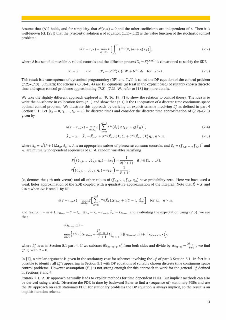
Assume that (A1) holds, and for simplicity, that cα(t, x) ≡ 0 and the other coefficients are independent of t. Then it iswell-known (cf. [25]) that the (viscosity) solution u of equation (1.1)–(1.2) is the value function of the stochastic controlproblem:

u(T − t, x) = minα(·)∈A

Eh

∫ T

t

f α(s)(Xs) ds+ g(XT )i

, (7.2)

where A is a set of admissible A-valued controls and the diffusion process Xs = X t,x ,α(·)s is constrained to satisfy the SDE

X t = x and dXs = σα(s)(Xs) dWs + bα(s) ds for s > t. (7.3)

This result is a consequence of dynamical programming (DP) and (1.1) is called the DP equation of the control problem(7.2)–(7.3). Similarly, the schemes (3.3)–(3.4) are DP equations (at least in the explicit case) of suitably chosen discretetime and space control problems approximating (7.2)–(7.3). We refer to [18] for more details.

We take the slightly different approach explored in [9, 16, 19, 7] to show the relation to control theory. The idea is towrite the SL scheme in collocation form (7.1) and show that (7.1) is the DP equation of a discrete time continuous spaceoptimal control problem. We illustrate this approach by deriving an explicit scheme involving Lαk as defined in part 4Section 5.1. Let {t0 = 0, t1, . . . , tM = T} be discrete times and consider the discrete time approximation of (7.2)–(7.3)given by

u(T − tm, x) = minα∈AM

Eh

M−1∑

k=m

f αk (Xk)∆tk+1 + g(XM )i

, (7.4)

Xm = x , Xn = Xn−1 +σαn(Xn−1) kn ξn + bαn(Xn−1) k

2n ηn, n> m, (7.5)

where kn =p

(P + 1)∆tn, AM ⊂ A is an appropriate subset of piecewise constant controls, and ξn = (ξn,1, . . . ,ξn,P)> andηn are mutually independent sequences of i. i. d. random variables satisfying

P�

(ξn,1, . . . ,ξn,P ,ηn) =±e j

�

=1

2(P + 1)if j ∈ {1, . . . , P},

P�

(ξn,1, . . . ,ξn,P ,ηn) = eP+1

�

=1

P + 1,

(e j denotes the j-th unit vector) and all other values of (ξn,1, . . . ,ξn,P ,ηn) have probability zero. Here we have used aweak Euler approximation of the SDE coupled with a quadrature approximation of the integral. Note that X ≈ X andu≈ u when ∆t is small. By DP

u(T − tm, x) = minα∈AM

Eh

n−1∑

k=m

f αk (Xk)∆tk+1 + u(T − tn, Xn)i

for all n> m,

and taking n = m+ 1, sM−m = T − tm, ∆sm = sm − sm−1, km = kM−m, and evaluating the expectation using (7.5), we seethat

u(sM−m, x) =

minα∈A

n

f α(x)∆sM−m +k2

M−m−1

P + 1Lα

kM−m−1[u](sM−m−1, x) + u(sM−m−1, x)

o

,

where Lαk is as in Section 5.1 part 4. If we subtract u(sM−m−1, x) from both sides and divide by ∆sM−m =k2

M−m−1

P+1, we find

(7.1) with θ = 0.

In [7], a similar argument is given in the stationary case for schemes involving the Lαk of part 3 Section 5.1. In fact it ispossible to identify all Lαk ’s appearing in Section 5.1 with DP equations of suitably chosen discrete time continuous spacecontrol problems. However assumption (Y1) is not strong enough for this approach to work for the general Lαk definedin Sections 3 and 4.

Remark 7.1. A DP approach naturally leads to explicit methods for time dependent PDEs. But implicit methods can alsobe derived using a trick. Discretize the PDE in time by backward Euler to find a (sequence of) stationary PDEs and usethe DP approach on each stationary PDE. For stationary problems the DP equation is always implicit, so the result is animplicit iteration scheme.

13

Remark 7.2. By the definition of Lαk and (Y1), x + yα,±i,k can be seen as a short time approximation of (7.3). Hence the

scheme (3.3) tracks particle paths approximately. In fact by the above discussion we might say that the scheme followsparticles in the mean because of the expectation. For first order PDEs, schemes defined in this way are called SL schemesby e. g. Falcone. Moreover, in this case our schemes will coincide with the SL schemes of Falcone [16] in the explicit case.This explains why we choose to call these schemes SL schemes also in the general case.

8 Error estimates in the convex case

We will derive error bounds in the case when B is a singleton and (1.1) is convex. It is not known how to prove suchresults in the general case. Here and in the following, we do not indicate the trivial β dependence any more. For simplicitywe also take a uniform time-grid, letting G = ∆t {0, 1, . . . , NT } × X∆x in this section. Let Q∆t,T := ∆t {0,1, . . . , NT } ×RN

and consider the intermediate equation

δ∆t Vn(x) = (8.1)

infα∈A

n

Lαk [Vθ ,n](t, x) + cα(t, x)V θ ,n(x) + f α(t, x)

o

t=tn−1+θ

in Q∆t,T ,

V (0, x) = g(x) in RN . (8.2)

The first step is now to find a bound on |U − V |.

Lemma 8.1. Assume that (I1), (I2) and the CFL condition (4.3) hold and that supn |V n|1 ≤ CV . If V solves (8.1)–(8.2) andU solves (3.3)–(3.4), then

|U − V | ≤ C∆x

k2 in G.

Proof. Let W = U − V and subtract the equation for V from the one for U to find

W ni ≤ W n−1

i +∆t supα∈A

n

Lαk [IW θ ,n· ]

n−1+θi + cα,n−1+θ

i W θ ,ni

+ Lαk [I V θ ,n − V θ ,n]n−1+θi

o

in G.

Assuming V n has p bounded derivatives, we rearrange the equation and use (I1) to see that

�

1+ θ∆t�M

k2 − cn−1+θW,i

��

W ni

≤W n−1i +∆t sup

α∈A

n

θ�

Lαk [IW n· ]

n−1+θi +

M

k2 W ni

�

+ (1− θ)�

Lαk [IW n−1· ]n−1+θ

i + cα,n−1+θi W n−1

i

�o

+ 2∆tK supn|Dr∧pV n|0

∆x r∧p

k2 in G

with cn−1+θW,i W n

i = supα cα,n−1+θi W n

i . By the CFL condition (4.3), the coefficients of the above inequality are all non-negative. Hence since W n ≤ |W n|0 := supi |W n

i |, we may replace W n by |W n|0 on the right hand side. Moreover, sinceI|W n|0 = |W n|0 and Lαk [|W

n|0] = 0, the upper bound on the right hand side then reduces to

(1+∆t(1− θ)Cc)|W n−1|0 + θ∆tM

k2 |Wn|0 +∆t K

∆x r∧p

k2 ,

where Cc =maxα |cα,+|0. The same bound holds if we replace W by −W , and hence we can conclude that

(1+∆tθ(M

k2 − Cc))|W n|0 ≤ (1+∆t(1− θ)Cc)|W n−1|0 + θ∆tM

k2 |Wn|0 +∆t K

∆x r∧p

k2 .

Since W 0 ≡ 0 in X∆x , an iteration then reveals that

|W n|0 ≤∆t K∆x r∧p

k2

n∑

m=0

�1+∆t(1− θ)Cc

1−∆tθCc

�m≤ tnK

∆x r∧p

k2 2eCc tn ,

when ∆t is small enough. Since V n is Lipschitz (p = 1), the lemma follows.

14

Next we want to estimate |V − u| when u solves (1.1)–(1.2). This can be done using the regularization method ofKrylov if we can find suitable continuity and continuous dependence results for the scheme. These results rely on thefollowing additional (covariance-type) assumptions: Whenever two sets of dataσ, b and σ, b are given, the correspondingapproximations Lαk , yα,±

k,i and Lαk , yα,±k,i in (3.1) satisfy

M∑

i=1

[yα,+k,i + yα,−

k,i ]− [ yα,+k,i + yα,−

k,i ]≤ 2k2(bα − bα),

M∑

i=1

[yα,+k,i ⊗ yα,+

k,i + yα,−k,i ⊗ yα,−

k,i ] + [ yα,+k,i ⊗ yα,+

k,i + yα,−k,i ⊗ yα,−

k,i ]

−[yα,+k,i ⊗ yα,+

k,i + yα,+k,i ⊗ yα,+

k,i + yα,−k,i ⊗ yα,−

k,i + yα,−k,i ⊗ yα,−

k,i ]

≤ 2k2(σα − σα)(σα − σα)> + 2k4(bα − bα)(bα − bα)>,

(Y2)

when σ, b, y±k are evaluated at (t, x) and σ, b, y±k are evaluated at (t, y) for all t, x , y.

In Section 9 we will prove the following error estimate.

Theorem 8.2. Assume that B is a singleton, that (A1), (Y1), (Y2), and the CFL conditions (4.3) hold, and that k ∈ (0, 1)and ∆t ≤ (2k0 ∧ 2k1)−1. If u and V are bounded solutions of (1.1)–(1.2) and (8.1)–(8.2), then

|V − u| ≤ C(|1− 2θ |∆t1/4 +∆t1/3 + k1/2) in Q∆t,T .

It also follows from the regularity results in Section 9 (see Proposition 9.4) that |V n|1 ≤ 2CT , so by Lemma 8.1 andTheorem 8.2 we have the following result.

Corollary 8.3 (Error Bound). Under (I1), (I2), and the assumptions of Theorem 8.2, if u solves (1.1)–(1.2) and U solves(3.3)–(3.4), then

|u− U | ≤ |u− V |+ |V − U | ≤ C(|1− 2θ |∆t1/4 +∆t1/3 + k1/2 +∆x

k2 ) in G.

This error bound applies to both the LISL and MCSL schemes, and it also holds for unstructured grids. If the solutions aremore regular, it is possible to obtain better error estimates. But general and optimal results are not available. The bestestimate in our case is O(∆x1/5) which is achieved when k = O(∆x2/5) and ∆t = O(k2). Note that the CFL conditions(4.3) already imply that ∆t = O(k2) if θ < 1. Also note that the above bound does not show convergence when k isoptimal for the LISL scheme (k = O(∆x1/2)) or the MCSL scheme (k = O(∆x)).

Remark 8.1. These results are consistent with results for LISL type schemes for stationary Bellman equations. In fact ifall coefficients are independent of time and cα(x) < −c < 0, then by combining the results of [7] and [1], exactly thesame error estimate is obtained for the solution of a particular stationary LISL scheme and the unique stationary Lipschitzsolution of (1.1).

9 Proof of Theorem 8.2

We start by an existence and uniqueness result.

Lemma 9.1. Assume that (A1), (Y1), and the CFL conditions (4.3) hold. Then there exists a unique solution Uh ∈ Cb(QT,∆t)of (8.1)–(8.2).

The proof is similar to (but simpler than) the proof of Theorem 4.2 with the modification that the fixed point is achievedin the Banach space Cb(RN ) instead of the space of bounded functions on X∆x .

We will now give a result comparing subsolutions of (8.1) to supersolutions of

δ∆t Un(x) = inf

α∈A

n

Lαk [Uθ ,n](t, x) + cα(t, x)Uθ ,n + f α(t, x)

o

t=tn−1+θ

in RN , n≥ 1,

U(0, x) = g(x) in RN ,

(9.1)

where Lαk is the operator defined in (3.1), (Y1), (Y2) when σα, bα are replaced by σα, bα.

15

Theorem 9.2. Assume that (A1), (Y2), (4.3) hold for both (8.1) and (9.1). If U ∈ C(QT,∆t) is a bounded above subsolutionof (8.1) and U ∈ C(QT,∆t) a bounded below supersolution of (9.1), then for all k ∈ (0, 1), ∆t ≤ (k0 ∧ k1)−1, x , y ∈ RN ,n ∈ {0, 1, . . . , NT },

U(tn, x)− U(tn, y)≤ Rk0(tn)|(U(0, ·)− U(0, ·))+|0

+ Rk0(tn)Rk1

(tn)(L0 + tn L)|x − y|

+ tn supα∈A

�

|( f − f )+|0 + Rk0(tn)(|U |0 ∧ |U |0)|c − c|0

�

+ t1/2n 2KT sup

α∈A

�

|b− b|0 + |σ− σ|0�

where Rk(t) = 1/(1− k∆t)t/∆t , KT ≤ Rk0(T )Rk1

(T )(L0 + T L),

L0 = |g|1 ∨ | g|1, L = (|cα|1 ∨ |cα|1)(|U |0 ∧ |U |0) + | f α|1 ∨ | f α|1,

k0 = supα|cα,+|0, k1 = 2 sup

α{|σα|21 + |b

α|21 + 1}.

Remark 9.1. The function Rk(n∆t) = 1/(1− k∆t)n satisfies

δ∆tRk(tn) = kRk(tn),

Rk(0) = 1, and Rk(tn)≤ e2ktn when ∆t ≤ 12k

.

This is a key result in this paper, and the proof is given in Appendix B. In the stationary case, results of this type havebeen obtained in [1, 8] for simpler schemes. The result is a joint uniqueness result (take (σ, b, c, f , g) = (σ, b, c, f , g)),continuous dependence result (take x = y), boundedness, and x-Lipschitz continuity result:

Corollary 9.3. Under the assumptions of Theorem 9.2, if k ∈ (0, 1) and ∆t ≤ (2k0 ∧ 2k1)−1, then any bounded solutionU ∈ Cb(QT,∆t) of (8.1) satisfies

(i) |U(tn, ·)|0 ≤ e2k0 tn |g|0 + tn supα | f α|0,

(ii) |U(tn, x)− U(tn, y)| ≤ e2(k0+k1)tn(L0 + tn L)|x − y|,

where the constants, which are defined in Theorem 9.2, are independent of k,∆t,∆x .

Proof. Part (i) follows from Theorem 9.2 and Remark 9.1 since U ≡ 0 satisfies (9.1) with (σα, bα, cα, f α, gα) = (σα, bα, cα, 0, 0).Part (ii) follows by taking U = U and x 6= y.

Now we extend the scheme (8.1) to the whole space QT . One way to do this and to obtain continuous in time solutions, isto pose initial conditions on [0,∆t) by interpolating between g(x) and U(∆t, x) where U is the solution of (8.1)–(8.2).

δ∆t V (t, x) = infα∈A

n

Lαk [Vθ (t, ·)](tθ , x) + cα(tθ , x)V θ (t, x) + f α(tθ , x)

o

(9.2)

in (∆t, T]×RN ,

V (t, x) =�

1−t

∆t

�

g(x) +t

∆tU(∆t, x) in [0,∆t]×RN . (9.3)

where V θ (t, x) = (1− θ)V (t −∆t, x) + θV (t, x) and tθ = t − (1− θ)∆t.

From the previous results for U the existence, uniqueness, and properties of V easily follow.

Proposition 9.4. Assume that (A1), (Y1), (Y2), and the CFL conditions (4.3) hold, and that k ∈ (0, 1) and ∆t ≤ (2k0 ∧2k1)−1.

(a) There exists a unique solution V ∈ Cb(QT ) of (9.2)–(9.3).

(b) There is a constant CT ≥ 0 independent of k,∆t,∆x such that

16

(i) |V |0 ≤ CT ,

(ii) |V (t, x)− V (t, y)| ≤ CT |x − y| for all t ∈ [0, T], x , y,∈ RN ,

(iii) |V (s1, x)− V (s2, x)| ≤ CT |s1 − s2|1/2 for all s1, s2 ∈ [0, T], x ,∈ RN .

(c) Let V ∈ Cb(QT ) and V ∈ Cb(QT ) be sub- and supersolutions of (9.2)–(9.3) corresponding to coefficients (σα, bα, cα, f α, g)and (σα, bα, cα, f α, g) respectively. Then there is a constant CT ≥ 0 independent of k,∆t,∆x such that for all t ∈ [0, T],

|V (t, ·)− V (t, ·)|0 ≤ CT

�

|g − g|0 + t supα[(|U |0 ∧ |U |0)|cα − cα|0 + | f α − f α|0]

+t1/2 supα[|σα − σα|0 + |bα − bα|0]

�

.

Proof. First note that the initial data on [0,∆t] is uniformly bounded and Lipschitz continuous in x and t by constructionand Corollary 9.3.

(a) Existence of a bounded x-continuous solution follows from repeated use of Lemma 9.1 since we have initial conditionson [0,∆t]. Continuity in time follows from Theorem 9.2 (with x = y) since the data is t-continuous.

(b) Part (i) and (ii) follow from Corollary 9.3 since the initial data is uniformly bounded and x-Lipschitz in [0,∆t]. Toprove part (iii) we assume s1 < s2 and let U(t, x) and U(t, x) solve (9.2) with data

(σα(t + s1, x), bα(t + s1, x), cα(t + s1, x), f α(t + s1, x), V (s1, x)) and (0, 0,0, 0, V (s1, x))

respectively. Note that for t ∈ [0, T − s1], U(t, x) ≡ V (s1, x) and U(t, x) ≡ V (t + s1, x) where V is the unique solution of(9.2)–(9.3). By part (c) we then get

|V (t + s1, ·)− V (s1, ·)|0 = |U(t, ·)− U(t, ·)|0

≤ CT

�

0+ t supα[| f α|0 + |V |0|cα|0] + t1/2 sup

α[|σα|0 + |bα|0]

�

for t > 0,

and hence part (iii) follows.

(c) Note that by construction of the initial data and Theorem 9.2 with x = y, the result holds for t ∈ [0,∆t], and thenthe result holds for any t >∆t by another application of Theorem 9.2 with x = y.

Using Krylov’s method of shaking the coefficients, we will now find smooth subsolutions of (9.2). First we introduce theauxiliary equation

δ∆t Vε(t, x) = inf

0≤s≤ε2

|e|≤εα∈A

n

Lαk [τ−e Vε,θ (t, ·)](r + s, x + e) (9.4)

+ cα(r + s, x + e)V ε,θ (t, x) + f α(r + s, x + e)o

r=tθ−∆t−ε2in (∆t, T]×RN ,

V ε(t, x) =�

1−t

∆t

�

g(x) +t

∆tV ε(∆t, x) in [0,∆t]×RN , (9.5)

where τeφ(t, x) = φ(t, x+e) and V ε(∆t, x) is obtained by first solving (9.4) for discrete times tn = n∆t. For this equationto be well-defined for t ∈ (∆t, T], the data and yα,±

k,i must be defined for t ∈ (−∆t − ε2, T + ε2]. But this is ok since onecan easily extend these functions to t ∈ [−r, T + r] for any r > 0 in such a way that (A1), (Y1), (Y2) still hold. Also notethat

Lαk [τ−e Vε,θ (t, ·)](r + s, x + e) =

1

2k2

M∑

i=1

n

V ε,θ (t, x + yα,+k,i (r + s, x + e)) (9.6)

−2V ε,θ (t, x) + V ε,θ (t, x + yα,−k,i (r + s, x + e))

o

,

and hence (9.4) is an equation of the same type as (9.2) (with different A and shifted coefficients) satisfying (A1), (Y1),(Y2) whenever (9.2) does.

17

By Proposition 9.4 there is a unique solution V ε of (9.4)–(9.5) in [0, T +∆t + ε2]×RN . Let Uε(t, x) := V ε(t +∆t + ε2, x)and define by convolution,

Uε(t, x) =

∫

RN

∫ ∞

0

Uε(t − s, x − e)ρε(s, e) ds de, (9.7)

where ε > 0, ρε(t, x) = 1εN+2ρ(

tε2

xε), and

ρ ∈ C∞(RN+1), ρ ≥ 0, supp ρ ⊂ [0,1]× {|x | ≤ 1},∫

ρ = 1.

Note that Uε is well defined on the time interval [−∆t, T]. By the next result it is the sought after smooth subsolution of(9.2).

Proposition 9.5. Under the assumptions of Proposition 9.4, the function Uε defined in (9.7) satisfies

(i) Uε ∈ C∞((−∆t, T )×RN ), |Uε|1 ≤ C , |Dm∂ nt Uε|0 ≤ Cε1−m−2n for n, m ∈ N.

(ii) If V is the solution of (9.2)–(9.3), then |Uε − V | ≤ C(ε+∆t1/2) in QT .

(iii) Uε is a subsolution of (9.2) in QT .

Proof. The regularity estimates in (i) are immediate from properties of convolutions and the regularity of V ε. The boundon Uε − V (in [0, T]) in (ii) follows from Proposition 9.4 (c) and (A1) which imply

|V ε − V |0 ≤ C(ε+∆t1/2),

and regularity of V ε along with properties of convolutions,

|Uε − V ε|0 ≤ |Uε − Uε|0 + |V ε(·+∆t + ε2, ·)− V ε|0 ≤ |Vε|1(ε+∆t1/2).

To see that Uε is a subsolution of (9.2), first note that from the definition of Uε and (9.4) it follows that

δ∆t Uε(t, x)≤ Lαk [τ−eU

ε,θ (t, ·)](tθ + s, x + e)

+ cα(tθ + s, x + e)Uε,θ (t, x) + f α(tθ + s, x + e)

for all (t, x) ∈ [−ε2, T]×RN , |e|, s2 ≤ ε, and α ∈ A. Now we change variables from (t + s, x + e) to (t, x) to find that

δ∆t Uε(t − s, x − e)≤ Lαk [τ−eU

ε,θ (t − s, ·)](tθ , x)

+cα(tθ , x)Uε,θ (t − s, x − e) + f α(tθ , x)

for all (t, x) ∈ [0, T]×RN , |e|, s2 ≤ ε, and α ∈ A. Then we multiply by ρε(s, e) and integrate w. r. t. (s, e). To see what theresult is, note that

Lαk [τ−eUε(t − s, ·)](r, x) =

1

2k2

M∑

i=1

n

Uε(t − s, x + yα,+k,i (r, x)− e)

−2Uε(t − s, x − e) + Uε(t − s, x + yα,−k,i (r, x)− e)

o

,

and hence∫ ∫

Lαk [τ−eUε(t − s, ·)](r, x)ρε(s, e) ds de = Lα[Uε(t, ·)](r, x).

For the whole equation we then have,

δ∆t Uε(t, x)≤ Lαk [Uθε (t, ·)](t

θ , x) + cα(tθ , x)Uθε (t, x) + f α(tθ , x)

for all (t, x) ∈ QT and α ∈ A. Since this inequality holds for all α, it follows that Uε is a subsolution of (9.2) in all ofQT .

18

We are now in a position to prove the error estimate given in Theorem 8.2.

Proof of Theorem 8.2. Let Uε be defined in (9.7). By Proposition 9.5 (i) and Lemma 4.1 (a),

∂t Uε − infα∈A

n

Lα[Uε,θ (t, ·)](tθ , x) + cα(tθ , x)Uε,θ (t, x) + f α(tθ , x)o

≤|1− 2θ |

2|∂ 2

t Uε|0∆t + Cn

(|∂ 2t Uε|0 + |∂ 3

t Uε|0 + |∂ 2t DUε|0 + |∂ 2

t D2Uε|0)∆t2

+ (|DUε|0 + · · ·+ |D4Uε|0)k2o

≤ Cn

|1− 2θ |ε−3∆t + ε−5∆t2 + ε−3k2o

in QT . Moreover, by Proposition 9.5 (ii),

g(x) = U(0, x)≥ Uε(0, x)− C(ε+∆t1/2).

It follows that there is a constant C ≥ 0 such that

Uε − Cesupα |cα|0 tn

ε+∆t1/2 + t�

|1− 2θ |ε−3∆t + ε−5∆t2 + ε−3k2�o

is a classical subsolution of (1.1)–(1.2). By the comparison principle

Uε − Cesupα |cα|0 tn

ε+∆t1/2 + t�

|1− 2θ |ε−3∆t + ε−5∆t2 + ε−3k2�o

≤ u in QT ,

and hence by Proposition 9.5 (ii),

U − u= (U − Uε) + (Uε − u)≤ Cn

ε+∆t1/2 + |1− 2θ |ε−3∆t + ε−5∆t2 + ε−3k2o

.

We minimize w. r. t. ε and find that

u− U ≤

(

C(∆t1/4 + k1/2) if θ 6= 12

C(∆t1/3 + k1/2) if θ = 12

in QT .

The lower bound on u− U follows with symmetric – but much easier – arguments where a smooth supersolution of theequation (1.1) is constructed. Consistency and comparison for the scheme (9.2) is then used to conclude. In view ofLemma 4.1, the lower bound is a direct consequence of Theorem 3.1 (a) in [2].

10 Numerical results

In the following, we apply the LISL and MCSL schemes to linear and convex test problems in two space-dimensions.Hence all problems in this section are independent of β . For the LISL scheme, we choose k =

p∆x and a regular

triangular grid, whereas for the MCSL scheme we choose k =∆x and a regular rectangular grid. If not stated otherwise,we use θ = 0 (explicit methods), CFL condition ∆t = k2, and approximation 5.1.5 for Lα,β . As error measure we willalways use the L∞-norm, and the error rates are calculated as ri =

ln‖ei‖−ln‖ei−1‖ln‖∆x i‖−ln‖∆x i−1‖

. All calculations are done in Matlab,on an INTEL Core2 Duo Mobile T7700, 2.4Ghz Laptop.

10.1 Linear problem with smooth solution

Our first problem is taken from [4] and has exact solution u(t, x) = (2− t) sin x1 sin x2. The coefficients in (1.1) are givenby

f α(t, x) = sin x1 sin x2[(1+ 2β2)(2− t)− 1]

− 2(2− t) cos x1 cos x2 sin(x1 + x2) cos(x1 + x2),

cα(t, x) =0, bα(t, x) = 0, σα(t, x) =p

2

�

sin(x1 + x2) β 0cos(x1 + x2) 0 β

�

.

We consider β2 = 0.1 and β = 0. Note that in the second case, the scheme considered in [4] is not consistent. Table 2gives the (spatial) errors and rates obtained at t = 1 applying the LISL and the MCSL scheme. As expected for smoothsolutions, in both cases we obtain order one for the LISL scheme and order two for the MCSL scheme. Here, we havechosen the grid points such that the solution is monotone in between. Without this, we would still obtain order one forthe LISL scheme, but no convergence for the MCSL scheme. The reason is that for non-monotone data, the interpolationerror of monotone cubic interpolation reduces to second order, and so the choice k =∆x is not longer appropriate.

19

β2 = 0.1 β = 0∆x LISL MCSL LISL MCSL

error rate error rate error rate error rate3.93e-2 3.79e-2 0.86 1.03e-3 3.94e-2 0.87 1.03e-31.96e-2 1.93e-2 0.97 2.57e-4 2.00 1.98e-2 0.99 2.57e-4 2.009.82e-3 9.45e-3 1.03 6.42e-5 2.00 9.94e-3 0.99 6.43e-5 2.004.91e-3 4.50e-3 1.07 1.61e-5 2.00 4.70e-3 1.08 1.61e-5 2.002.45e-3 2.43e-3 0.89 4.01e-6 2.00 2.45e-3 0.94 4.02e-6 2.00

Table 2: Results for the smooth linear problem at t = 1 with β2 = 0.1 and β = 0, grid adapted to monotonicity

10.2 Linear problem with non-smooth solution

The second problem we test is a problem with non-smooth exact solution in [−π,π]2 given by

u(t, x) = (1+ t) sinx2

2

(

sin x1

2for −π < x1 < 0,

sin x1

4for 0< x1 < π.

The coefficients in (1.1) are given by

f α(t, x) = sinx2

2

sin x1

2

�

1+ 1+t4(sin2 x1 + sin2 x2)

�

for −π < x1 < 0

sin x1

4

�

1+ 1+t16(sin2 x1 + 4 sin2 x2)

�

for 0< x1 < π

− sin x1 sin x2 cosx2

2

(

1+t2

cos x1

2for −π < x1 < 0

1+t4

cos x1

4for 0< x1 < π

,

cα(t, x) =0, bα(t, x) = 0, σα(t, x) =p

2

�

sin x1

sin x2

�

,

and we pose Dirichlet boundary conditions. This is a monotone non-smooth problem, and we obtain order one halfapplying the LISL scheme and order one applying the MCSL scheme, i. e. reduced rates, see Table 3.

LISL MCSL∆x error rate error rate

3.90e-2 8.75e-3 4.19e-31.96e-2 6.19e-3 0.50 2.20e-3 0.939.80e-3 4.38e-3 0.50 1.12e-3 0.974.90e-3 3.10e-3 0.50 5.69e-4 0.982.45e-3 2.19e-3 0.50 2.86e-4 0.99

Table 3: Results for the non-smooth linear problem at t = 1

10.3 Optimal control problems with smooth solutions

a) We test an example from [4] with exact solution u(t, x1, x2) =�

32− t�

sin x1 sin x2. The corresponding coefficients andcontrol set in (1.1) are

f α =�

1

2− t�

sin x1 sin x2 +�

3

2− t�

�

p

cos2 x1 sin2 x2 + sin2 x1 cos2 x2

− 2sin(x1 + x2) cos(x1 + x2) cos x1 cos x2

�

,

cα = 0, bα = α, σα =p

2

�

sin(x1 + x2)cos(x1 + x2)

�

, A= {α ∈ R2 : α21 +α

22 = 1}.

As σα does not depend on α but bα does, we choose approximation 5.1.4 for Lα,β and thus need only about half ofthe number of interpolations we would need if we had chosen approximation 5.1.5.

20

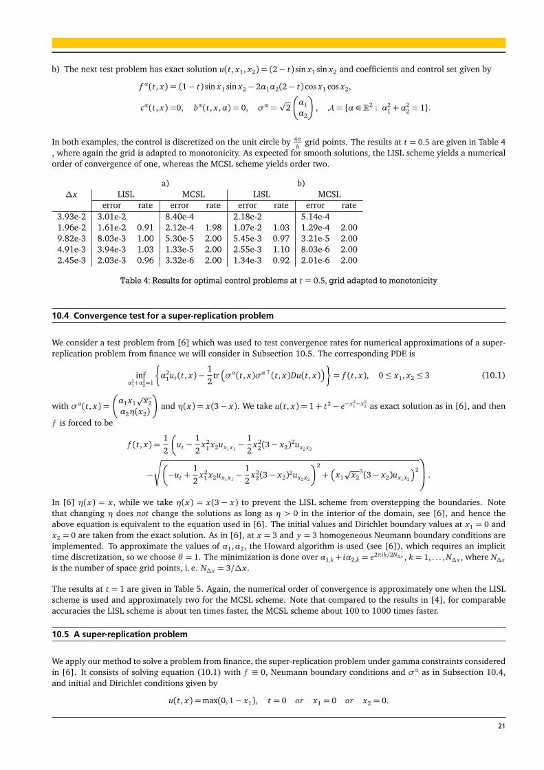
b) The next test problem has exact solution u(t, x1, x2) = (2− t) sin x1 sin x2 and coefficients and control set given by

f α(t, x) = (1− t) sin x1 sin x2 − 2α1α2(2− t) cos x1 cos x2,

cα(t, x) =0, bα(t, x ,α) = 0, σα =p

2

�

α1

α2

�

, A= {α ∈ R2 : α21 +α

22 = 1}.

In both examples, the control is discretized on the unit circle by 4πh

grid points. The results at t = 0.5 are given in Table 4, where again the grid is adapted to monotonicity. As expected for smooth solutions, the LISL scheme yields a numericalorder of convergence of one, whereas the MCSL scheme yields order two.

a) b)∆x LISL MCSL LISL MCSL

error rate error rate error rate error rate3.93e-2 3.01e-2 8.40e-4 2.18e-2 5.14e-41.96e-2 1.61e-2 0.91 2.12e-4 1.98 1.07e-2 1.03 1.29e-4 2.009.82e-3 8.03e-3 1.00 5.30e-5 2.00 5.45e-3 0.97 3.21e-5 2.004.91e-3 3.94e-3 1.03 1.33e-5 2.00 2.55e-3 1.10 8.03e-6 2.002.45e-3 2.03e-3 0.96 3.32e-6 2.00 1.34e-3 0.92 2.01e-6 2.00

Table 4: Results for optimal control problems at t = 0.5, grid adapted to monotonicity

10.4 Convergence test for a super-replication problem

We consider a test problem from [6] which was used to test convergence rates for numerical approximations of a super-replication problem from finance we will consider in Subsection 10.5. The corresponding PDE is

infα2

1+α22=1

�

α21ut(t, x)−

1

2tr�

σα(t, x)σα>(t, x)Du(t, x)�

�

= f (t, x), 0≤ x1, x2 ≤ 3 (10.1)

with σα(t, x) =

�

α1 x1p

x2

α2η(x2)

�

and η(x) = x(3− x). We take u(t, x) = 1+ t2 − e−x21−x2

2 as exact solution as in [6], and then

f is forced to be

f (t, x) =1

2

�

ut −1

2x2

1 x2ux1 x1−

1

2x2

2(3− x2)2ux2 x2

−

È

�

−ut +1

2x2

1 x2ux1 x1−

1

2x2

2(3− x2)2ux2 x2

�2

+�

x1p

x23(3− x2)ux1 x2

�2

.

In [6] η(x) = x , while we take η(x) = x(3− x) to prevent the LISL scheme from overstepping the boundaries. Notethat changing η does not change the solutions as long as η > 0 in the interior of the domain, see [6], and hence theabove equation is equivalent to the equation used in [6]. The initial values and Dirichlet boundary values at x1 = 0 andx2 = 0 are taken from the exact solution. As in [6], at x = 3 and y = 3 homogeneous Neumann boundary conditions areimplemented. To approximate the values of α1,α2, the Howard algorithm is used (see [6]), which requires an implicittime discretization, so we choose θ = 1. The minimization is done over α1,k+ iα2,k = e2πik/2N∆x , k = 1, . . . , N∆x , where N∆x

is the number of space grid points, i. e. N∆x = 3/∆x .

The results at t = 1 are given in Table 5. Again, the numerical order of convergence is approximately one when the LISLscheme is used and approximately two for the MCSL scheme. Note that compared to the results in [4], for comparableaccuracies the LISL scheme is about ten times faster, the MCSL scheme about 100 to 1000 times faster.

10.5 A super-replication problem

We apply our method to solve a problem from finance, the super-replication problem under gamma constraints consideredin [6]. It consists of solving equation (10.1) with f ≡ 0, Neumann boundary conditions and σα as in Subsection 10.4,and initial and Dirichlet conditions given by

u(t, x) =max(0, 1− x1), t = 0 or x1 = 0 or x2 = 0.

21

(a) LISL

∆x error rate time in s1.50e-1 2.01e-1 0.717.50e-2 9.49e-2 1.08 6.763.75e-2 4.29e-2 1.15 75.731.87e-2 1.94e-2 1.15 1115.39

(b) MCSL

∆x error rate time in s3.00e-1 8.21e-2 1.171.50e-1 1.83e-2 2.16 11.587.50e-2 5.03e-3 1.86 149.24

Table 5: Results for the convergence test for the super-replication problem at t = 1

01

23 0

1

2

30

0.2

0.4

0.6

0.8

1

x2x

1

Uh

Figure 1: Numerical solution of super-replication problem at t = 1

The solution obtained with the LISL scheme is given in Figure 1 and coincides with the solution found in [6]. It gives theprice of a put option of strike and maturity 1, and x1 and x2 are respectively the price of the underlying and the price ofthe forward variance swap on the underlying.

A Monotonicity of solutions of (1.1)

We will discuss a condition ensuring that the solution of (1.1)–(1.2) is monotone along some unit direction e ∈ RN .

(A2) Let e ∈ RN , |e|= 1. For all x ∈ RN ,α ∈ A,β ∈ B, h> 0

aα,β (t, x + he) = aα,β (t, x), bα,β (t, x + he) = bα,β (t, x),

cα,β (t, x + he)≥ cα,β (t, x), f α,β (t, x + he)≥ f α,β (t, x),

g(x + he)≥ g(x).

Lemma A.1. Assume (A1) and (A2). If u is a viscosity solution of (1.1)–(1.2), then

u(t, x + he)− u(t, x)≥ 0 for all h> 0, (t, x) ∈ QT .

Proof. Assume that u ≥ 0 and cα,β ≤ 0 and let v(t, x) = u(t, x + he). Since v(t, x) satisfies (1.1)–(1.2) at the point(t, x + he), an application of (A2) shows that it also is a supersolution at the point (t, x). By the comparison principleu ≤ v and the theorem is proved. In the general case consider w = e− supα,β |c|0 t(u+ |u|0), and note that w ≥ 0 and thecorresponding cα,β -coefficient cα,β−supα,β |cα,β |0 is non-positive. The first result then applies to w, and hence the theoremholds for u.

Remark A.1. This result is not so far from optimal when N > 1 and the solution u is non-smooth (e. g. only Lipschitzcontinuous). To see that, we consider the linear case where v = ue := Du · e satisfies

vt = tr[aD2v] + bDv+ cv+ tr[ae D2u] + be Du+ ceu+ fe︸ ︷︷ ︸

f (t,x)

in QT

22

with e-directional derivatives ae, be, ce and fe. If (A1) holds we can conclude from the comparison principle that

ue = v ≥ 0 if f ≥ 0 and ue(0, x)≥ 0.

If u is non-smooth, then f is well-defined only if ae ≡ 0 ≡ be, and the condition that f ≥ 0 is essentially equivalent toassumption (A2). Of course, it is possible to relax (A2) if N = 1 or solutions are more regular.

Remark A.2. It is important to notice that the result of Lemma A.1 also holds for all PDEs that satisfy (A2) after (mono-tone) coordinate transformations. In finance there are many such equations, e. g. the Black-Scholes equation for aEuropean option based on two stocks,

ut =1

2σ2

1 x2ux x +ρσ1σ2 x yux y +1

2σ2

2 y2uy y + r(xux + yuy)− ru, t, x , y > 0,

u(0, x , y) =max(0, K − (x + y)), x , y ≥ 0.

After the change of variables ( x , y) = (ln x , ln y), this equation reduces to a constant coefficient equation. Since the initialdata is decreasing in x and y, the same is true for the solution u by Lemma A.1. Going back to (x , y) variables, we thenfind that u is decreasing also in x and y. (Strictly speaking we must extend u(t, ·, ·) to R2 in a suitable way to applyLemma A.1).

B The proof of Theorem 9.2

We will prove the result when k0 = 0. The general case can be reduced to this case in a standard way by consideringU/Rk0

and U/Rk0instead of U and U . We use doubling of variables techniques similar to those used to prove this type of

results for equation (1.1). We take

m0 = |(U(0, ·)− U(0, ·))+|0,

m= supα

h

|( f α − f α)+|0 + (|U |0 ∧ |U |0)|cα − cα|0i

,

M2 = 4supα

�

|σα − σα|20 + |bα − bα|20

�

,

where φ+ denotes the positive part of φ, and define

W (t, x , y) = U(t, x)− U(t, y),

φ(t, x , y) = m0 + tm+1

2εKT tM2

+1

2Rk1(t)(L0 + t L)(ε+

1

ε|x − y|2) +δ(|x |2 + |y|2),

ψ(t, x , y) =W (t, x , y)−φ(t, x , y)−η(1+ t),

m= supt∈∆tN0x ,y∈RN

ψ(t, x , y) =ψ( t, x , y),

for ε,δ,η > 0 and a maximum point ( t, x , y). A maximum point exists because of the δ-terms in φ. We will prove thatfor any sequence ηl → 0, there is another sequence δl → 0 such that ψ( t l , x l , yl) ≤ o(1) as l →∞. This implies Theorem9.2 when k0 = 0. To see this, fix t > 0, x , y and note that for any ε > 0,

U(t, x)− U(t, y)−m0 − tm−1

2εKT tM2 −

1

2Rk1(t)(L0 + t L)(ε+

1

ε|x − y|2)

≤ψ( t l , x l , yl) +δl(|x |2 + |y|2) +ηl(1+ t)≤ o(1) as l →∞.

In this inequality we send l →∞ and choose

ε = |x − y| ∨ t1/2M

to find that

U(t, x)− U(t, y)≤ m0 + tm+ t1/2KT M + Rk1(t)(L0 + t L)|x − y|,

and hence Theorem 9.2 follows since t > 0, x , y were arbitrary. We will not be explicit about the form of the δ-termsbelow. Their role is only to guarantee that the maximum is attained at a (finite) point ( t, x , y), and their contributionwill always be o(1) as δ→ 0 (see also Section 3 in [1]).

23

It is enough to prove that for every η > 0, ψ( t, x , y) ≤ o(1) as δ→ 0. We proceed by contradiction assuming there is anη > 0 such that limδ→0ψ( t, x , y) > 0. By the definition of ψ we now have W ( t, x , y) > 0 and t > 0 for all δ > 0 smallenough. The last statement is true since

ψ(0, x , y)≤ m0 + L0| x − y| −m0 −L0

2(ε+

1

ε| x − y|2)−η < 0.

The rest of the proof will aim at getting a contradiction for the case t > 0. Even if we do not write it like that, what weshow below is that ψ( t, x , y)−ψ( t−∆t, x , y)

∆t≤ o(1)− η as δ → 0, and this is impossible since ( t, x , y) is a maximum point of

ψ.

We proceed by defining the operator Πα,

Πα[φ(t, ·, ·)](r, x , y) =M∑

i=1

n

φ(t, x + yα,+k,i (r, x), y + yα,+

k,i (r, y))

−2φ(t, x , y) +φ(t, x + yα,−k,i (r, x), y + yα,−

k,i (r, y))o

.

By the definition of Lαk and Lαk and (4.1), it follows that

Πα[W (t, ·, ·)](r, x , y) = 2k2n

Lαk [U(t, ·)](r, x)− Lαk [U(t, ·)](r, y)o

.

We set λ := ∆tk2 and subtract the inequalities defining U and U (see (8.1) and (9.1)) to find that

W (t, x , y)≤W (t −∆t, x , y)

+ supα

nλ

2Πα[W θ (t, ·, ·)](tθ , x , y) +∆t cα(tθ , x)W θ (t, x , y)

o

+∆t L|x − y|+∆t m for (t, x), (t, y) ∈QT ,

where W θ (t, x , y) = (1− θ)W (t −∆t, x , y) + θW (t, x , y) and tθ = t − (1− θ)∆t. Note that this new “scheme” is stillmonotone by the definition of Πα and the CFL condition. Hence we may replace W in the above inequality by any biggerfunction coinciding with W at (t, x , y). By the definition of m,

W ≤ φ +η(1+ t) + m in ∆tN0 ×RN ×RN ,

and equality holds at ( t, x , y). Therefore we find that

φ( t, x , y) +η(1+ t)≤ φ( t −∆t, x , y) +η(1+ t −∆t) (?)

+ supα

λ

2Πα[φθ ( t, ·, ·)]( tθ , x , y) +∆t L| x − y|+∆t m.

Here we also used the fact that Πα[η(1+ t) + m] = 0 and cα ≤ 0. Moreover we can Taylor expand to see that

Πα[φ(t, ·, ·)](r, x , y) =M∑

i=1

n

(Y+i + Y−i ) · Dxφ + (Y+i + Y−i ) · Dyφ

+1

2tr[D2

x xφ · (Y+i Y+>i + Y−i Y−>i )] +

1

2tr[D2

y yφ · (Y+i Y+>i + Y−i Y−>i )]

+1

2tr[D2

x yφ · (Y+i Y+>i + Y+i Y+>i + Y−i Y−>i + Y−i Y−>i )]

o

,

where Y±i = yα,±k,i (r, x) and Y±i = yα,±

k,i (r, y). Note that Y Y> = Y ⊗Y for Y ∈ RN . Now we use (Y2) along with the definitionof φ, to see that

Πα[φ(t, ·, ·)](r, x , y)≤1

εRk1(t)(L0 + t L)

�

2k2(bα(r, x)− bα(r, y))(x − y)

+ k2trh

(σα(r, x)− σα(r, y))(σα(r, x)− σα(r, y))>i

+ k4trh

(bα(r, x)− bα(r, y))(bα(r, x)− bα(r, y))>i

�

+ o(1),

24

as δ→ 0. These considerations lead to the following simplification of (?),

η+φ( t, x , y)−φ( t −∆t, x , y)

∆t

≤ θ1

εRk1( t)(L0 + t L)(

1

2M2 +

1

2k1| x − y|2)

+ (1− θ)1

εRk1( t −∆t)(L0 + ( t −∆t)L)(

1

2M2 +

1

2k1| x − y|2)

+ L| x − y|+m+ o(1)

≤1

εRk1( t)(L0 + t L)(

1

2M2 +

1

2k1| x − y|2) + L| x − y|+m+ o(1) := RHS,

as δ→ 0. Now we proceed to calculate

δ∆tφ(t, x , y) :=φ(t, x , y)−φ(t −∆t, x , y)

∆t.

To do that we note that

δ∆t(uv) = (δ∆tu)v+ uδ∆t v−∆t(δ∆tu)(δ∆t v).

Since δ∆tRk1(t) = k1Rk1

(t) we then see that

δ∆t[Rk1(t)(L0 + t L)] = k1Rk1

(t)(L0 + t L) + Rk1(t)L−∆t Lk1Rk1

(t),

and hence

δ∆tφ( t, x , y) = m+1

2KT

1

εM2 +

1

2Rk1( t)�

k1(L0 + t L) + L−∆tk1 L�

(ε+1

ε| x − y|2).

All of this leads to

η≤ RHS−δ∆tφ( t, x , y)≤ o(1) as δ→ 0.

The last inequality follows from the bound on KT . We have our contradiction and the proof is complete.

Bibliography

[1] G. Barles and E. R. Jakobsen. On the convergence rate of approximation schemes for Hamilton-Jacobi-Bellmanequations. M2AN Math. Model. Numer. Anal. 36(1):33–54, 2002.

[2] G. Barles and E. R. Jakobsen. Error bounds for monotone approximation schemes for parabolic Hamilton-Jacobi-Bellman equations. Math. Comp. 76(240): 1861-1893, 2007.

[3] G. Barles and P. E. Souganidis. Convergence of approximation schemes for fully nonlinear second order equations.Asymptotic Anal. 4(3):271–283, 1991.

[4] F. Bonnans, E. Ottenwaelter, and H. Zidani. A fast algorithm for the two dimensional HJB equation of stochasticcontrol. M2AN Math. Model. Numer. Anal. 38(4):723–735, 2004.

[5] F. Bonnans and H. Zidani. Consistency of generalized finite difference schemes for the stochastic HJB equation.SIAM J. Numer. Anal. 41(3):1008-1021, 2003.

[6] B. Bruder, O. Bokanowski, S. Maroso, and H. Zidani. Numerical approximation for a superreplication problemunder gamma constraints. SIAM J. of Numer. Anal. 47(3), 2009 (online).

[7] F. Camilli and M. Falcone. An approximation scheme for the optimal control of diffusion processes. RAIRO Modél.Math. Anal. Numér. 29(1): 97–122, 1995.

[8] F. Camilli and E. R. Jakobsen. A Finite Element like Scheme for Integro-Partial Differential Hamilton-Jacobi-BellmanEquations. SIAM J. Numer. Anal. 47(4): 2407-2431, 2009 (online).

25

[9] I. Capuzzo-Dolcetta. On a discrete approximation of the Hamilton-Jacobi equation of dynamic programming. Appl.Math. Optim. 10:367-377, 1983.

[10] R. E. Carlson and F. N. Fritsch. Monotone piecewise bicubic interpolation. SIAM J. Numer. Anal. 22(2):386-400,1985.

[11] M. G. Crandall, H. Ishii, and P.-L. Lions. User’s guide to viscosity solutions of second order partial differentialequations. Bull. Amer. Math. Soc. (N.S.), 27(1):1–67, 1992.

[12] M. G. Crandall and P.-L. Lions. Convergent difference schemes for nonlinear parabolic equations and mean curvaturemotion. Numer. Math. 75 (1996), no. 1, 17–41.

[13] M. G. Crandall and P.-L. Lions. Two approximations of solutions of Hamilton-Jacobi equations. Math. Comp.43(167):1–19, 1984.

[14] H. Dong and N. V. Krylov. On the rate of convergence of finte-difference approximations for Bellman equations withconstant coefficients. St. Petersburg Math. J. 17(2): 295–313, 2006.

[15] S. C. Eisenstat, K. R. Jackson and J. W. Lewis. The order of monotone piecewise cubic interpolation. SIAM J. Numer.Anal. 22(6):1220-1237, 1985.

[16] M. Falcone. A numerical approach to the infinite horizon problem of deterministic control theory. Appl. Math.Optim. 15 (1987), no. 1, 1–13.

[17] F. N. Fritsch and R. E. Carlson. Monotone piecewise cubic interpolation. SIAM J. Numer. Anal. 17(2):238-246, 1980.

[18] H. J. Kushner and P. Dupuis. Numerical methods for stochastic control problems in continuous time. Springer-Verlag,New York, 2001.

[19] J.-L. Menaldi Some estimates for finite difference approximations. SIAM J. Control Optim. 27 (1989), no. 3

[20] T. S. Motzkin and W. Wasow. On the approximation of linear elliptic differential equations by difference equationswith positive coefficients. J. Math. Physics 31, (1953). 253–259.

[21] A. M. Oberman. Convergent difference schemes for degenerate elliptic and parabolic equations: Hamilton-Jacobiequations and free boundary problems. SIAM J. Numer. Anal. 44 (2006), no. 2, 879–895

[22] A. Oberman. Wide stencil finite difference schemes for the elliptic Monge-Ampere equation and functions of theeigenvalues of the Hessian. Discrete Contin. Dyn. Syst. Ser. B 10 (2008), no. 1, 221–238.

[23] D. M. Pooley, P. A. Forsyth, and K. R. Vetzal. Numerical convergence properties of option pricing PDEs with uncertainvolatility. IMA J. Numer. Anal. 23 (2003), no. 2, 241–267.

[24] P. J. Rasch and D. L. Williamson. On shape-preserving interpolation and semi-Lagrangian transport. SIAM J. Sci.Statist. Comput. 11(4):656–687, 1990.

[25] J. Young and X. Y. Zhou. Stochastic Controls. Spinger-Verlag, New York, 1999.

26