Fully lexicalized pregroup grammars
370
Lecture Notes in Computer Science 4576 Commenced Publication in 1973 Founding and Former Series Editors: Gerhard Goos, Juris Hartmanis, and Jan van Leeuwen Editorial Board David Hutchison Lancaster University, UK Takeo Kanade Carnegie Mellon University, Pittsburgh, PA, USA Josef Kittler University of Surrey, Guildford, UK Jon M. Kleinberg Cornell University, Ithaca, NY, USA Friedemann Mattern ETH Zurich, Switzerland John C. Mitchell Stanford University, CA, USA Moni Naor Weizmann Institute of Science, Rehovot, Israel Oscar Nierstrasz University of Bern, Switzerland C. Pandu Rangan Indian Institute of Technology, Madras, India Bernhard Steffen University of Dortmund, Germany Madhu Sudan Massachusetts Institute of Technology, MA, USA Demetri Terzopoulos University of California, Los Angeles, CA, USA Doug Tygar University of California, Berkeley, CA, USA Moshe Y. Vardi Rice University, Houston, TX, USA Gerhard Weikum Max-Planck Institute of Computer Science, Saarbruecken, Germany
-
Upload
univ-rennes1 -
Category
Documents
-
view
0 -
download
0
Transcript of Fully lexicalized pregroup grammars
Lecture Notes in Computer Science 4576Commenced Publication in 1973Founding and Former Series Editors:Gerhard Goos, Juris Hartmanis, and Jan van Leeuwen
Editorial Board
David HutchisonLancaster University, UK
Takeo KanadeCarnegie Mellon University, Pittsburgh, PA, USA
Josef KittlerUniversity of Surrey, Guildford, UK
Jon M. KleinbergCornell University, Ithaca, NY, USA
Friedemann MatternETH Zurich, Switzerland
John C. MitchellStanford University, CA, USA
Moni NaorWeizmann Institute of Science, Rehovot, Israel
Oscar NierstraszUniversity of Bern, Switzerland
C. Pandu RanganIndian Institute of Technology, Madras, India
Bernhard SteffenUniversity of Dortmund, Germany
Madhu SudanMassachusetts Institute of Technology, MA, USA
Demetri TerzopoulosUniversity of California, Los Angeles, CA, USA
Doug TygarUniversity of California, Berkeley, CA, USA
Moshe Y. VardiRice University, Houston, TX, USA
Gerhard WeikumMax-Planck Institute of Computer Science, Saarbruecken, Germany

Daniel Leivant Ruy de Queiroz (Eds.)
Logic, Language,Informationand Computation
14th International Workshop, WoLLIC 2007Rio de Janeiro, Brazil, July 2-5, 2007Proceedings
13

Volume Editors
Daniel LeivantIndiana UniversityComputer Science DepartmentBloomington, IN 47405, USAE-mail: [email protected]
Ruy de QueirozUniversidade Federal de PernambucoCentro de InformaticaAv Prof. Luis Freire, s/n Cidade Universitaria, 50740-540 Recife, PE, BrasilE-mail: [email protected]
Library of Congress Control Number: 2007929582
CR Subject Classification (1998): F.1, F.2.1-2, F.4.1, G.1.0, I.2.6
LNCS Sublibrary: SL 1 – Theoretical Computer Science and General Issues
ISSN 0302-9743ISBN-10 3-540-73443-0 Springer Berlin Heidelberg New YorkISBN-13 978-3-540-73443-7 Springer Berlin Heidelberg New York
This work is subject to copyright. All rights are reserved, whether the whole or part of the material isconcerned, specifically the rights of translation, reprinting, re-use of illustrations, recitation, broadcasting,reproduction on microfilms or in any other way, and storage in data banks. Duplication of this publicationor parts thereof is permitted only under the provisions of the German Copyright Law of September 9, 1965,in its current version, and permission for use must always be obtained from Springer. Violations are liableto prosecution under the German Copyright Law.
Springer is a part of Springer Science+Business Media
springer.com
© Springer-Verlag Berlin Heidelberg 2007Printed in Germany
Typesetting: Camera-ready by author, data conversion by Scientific Publishing Services, Chennai, IndiaPrinted on acid-free paper SPIN: 12086542 06/3180 5 4 3 2 1 0

Preface
Welcome to the proceedings of the 14th WoLLIC meeting, which was held in Rio deJaneiro, Brazil, July 2 - 5, 2007. The Workshop on Logic, Language, Information andComputation (WoLLIC) is an annual international forum on inter-disciplinary researchinvolving formal logic, computing and programming theory, and natural language andreasoning. The WoLLIC meetings alternate between Brazil (and Latin America) andother countries, with the aim of fostering interest in applied logic among Latin Amer-ican scientists and students, and facilitating their interaction with the international ap-plied logic community.
WoLLIC 2007 focused on foundations of computing and programming, novel com-putation models and paradigms, broad notions of proof and belief, formal methods insoftware and hardware development; logical approaches to natural language and rea-soning; logics of programs, actions and resources; foundational aspects of informationorganization, search, flow, sharing, and protection. The Program Committee for thismeeting, consisting of the 28 colleagues listed here, was designed to promote theseinter-disciplinary and cross-disciplinary topics.
Like its predecessors, WoLLIC 2007 included invited talks and tutorials as well ascontributed papers. The Program Committee received 52 complete submissions (asidefrom 15 preliminary abstracts which did not materialize). A thorough review processby the Program Committee, assisted by over 70 external reviewers, led to the accep-tance of 21 papers for presentation at the meeting and inclusion in these proceedings.The conference program also included 16 talks and tutorials by 10 prominent invitedspeakers, who graciously accepted the Program Committee’s invitation.
We are sincerely grateful to the many people who enabled the meeting and made ita success: the Program Committee members, for their dedication and hard work overextended periods; the invited speakers, for their time and efforts; the contributors, forsubmitting excellent work and laboriously refining their papers for the proceedings; theexternal reviewers, who graciously agreed to selflessly comment on submitted papers,often providing detailed and highly valuable feedback; and the Organizing Committee,whose work over many months made the meeting possible in the first place.
On behalf of the entire WoLLIC community, we would also like to express our grat-itude to our institutional sponsors and supporters. WoLLIC 2007 was sponsored by theAssociation for Symbolic Logic (ASL), the Interest Group in Pure and Applied Log-ics (IGPL), the European Association for Logic, Language and Information (FoLLI),the European Association for Theoretical Computer Science (EATCS), the SociedadeBrasileira de Computacao (SBC), and the Sociedade Brasileira de Logica (SBL). Gen-erous financial support was provided by the Brazilian government (through CAPES,grant PAEP-0755/06-0), Univ. Fed. Fluminense (UFF), and SBC.
May 2007 Daniel Leivant(Program Chair)Ruy de Queiroz(General Chair)
Organization
Program Committee
Samson Abramsky (Oxford)Michael Benedikt (Bell Labs and Oxford)Lars Birkedal (ITU Copenhagen)Andreas Blass (University of Michigan)Thierry Coquand (Chalmers University, Goteborg)Jan van Eijck (CWI, Amsterdam)Marcelo Finger (University of Sao Paulo)Rob Goldblatt (Victoria University, Wellington)Yuri Gurevich (Microsoft Redmond)Hermann Haeusler (PUC Rio)Masami Hagiya (Tokyo University)Joseph Halpern (Cornell)John Harrison (Intel UK)Wilfrid Hodges (University of London/QMW)Phokion Kolaitis (IBM San Jose)Marta Kwiatkowska (University of Birmingham and Oxford Univeristy)Daniel Leivant (Indiana University) (Chair)Maurizio Lenzerini (University of Rome)Jean-Yves Marion (LORIA Nancy)Dale Miller (Polytechnique, Paris)John Mitchell (Stanford University)Lawrence Moss (Indiana University)Peter O’Hearn (University of London/QM)Prakash Panangaden (McGill, Montreal)Christine Paulin-Mohring (Paris-Sud, Orsay)Alexander Razborov (Moscow University)Helmut Schwichtenberg (Munich Uuniversity)Jouko Vaananen (University of Helsinki)
Organizing Committee
Renata P. de Freitas (Universidade Fed Fluminense)Ana Teresa Martins (Universidade Fed Ceara’)Anjolina de Oliveira (Universidade Fed Pernambuco)Ruy de Queiroz (Universidade Fed Pernambuco, Co-chair)Marcelo da Silva Correa (Universidade Fed Fluminense)Petrucio Viana (Universidade Fed Fluminense, Co-chair)

VIII Organization
External Reviewers
Anonymous (2)Josep Argelich-RomaJoseph BaroneLev BeklemishevJohan van BenthemMauro BirattariGuillaume BonfanteAnne BroadbentAnuj DawarLuc DeRaedtRalph DebusmannJules DesharnaisHans van DitmarschMelvin FittingMatthias FruthZhaohui FuViktor GalliardMichael GasserGiorgio GhelliRajeev GoreCosimo Guido
Anil GuptaJavier Gutierrez-GarciaMasami HagiyaShan HeAndreas HerzigLiang HuangEtienne KerreEvelina LammaChumin LiThorsten LiebigPaolo MancarellaMaarten MarxPascal MatsakisSusan McRoyBernhard MoellerAndrzej MurawskiReinhard MuskensSara NegriJoakim NivreJeff ParisWitold Pedrycz
Mario PorrmannAnne PrellerRobert van RooijAndrzej RoslanowskiMehrnoosh SadrzadehUlrik SchroederLibin ShenYun ShiGuillermo SimariNicholas SmithYoshinori TanabePaolo TorroniPaul VitanyiChistoph WeidenbachLaurent WendlingMatthew WilliamsYehezkel YeshurunChen YuChi Zheru

Table of Contents
A Grammatical Representation of Visibly Pushdown Languages . . . . . . . . 1Joachim Baran and Howard Barringer
Fully Lexicalized Pregroup Grammars . . . . . . . . . . . . . . . . . . . . . . . . . . . . . . 12Denis Bechet and Annie Foret
Bounded Lattice T-Norms as an Interval Category . . . . . . . . . . . . . . . . . . . 26Benjamın C. Bedregal, Roberto Callejas-Bedregal, andHelida S. Santos
Towards Systematic Analysis of Theorem Provers Search Spaces: FirstSteps . . . . . . . . . . . . . . . . . . . . . . . . . . . . . . . . . . . . . . . . . . . . . . . . . . . . . . . . . . . 38
Hicham Bensaid, Ricardo Caferra, and Nicolas Peltier
Continuation Semantics for Symmetric Categorial Grammar . . . . . . . . . . . 53Raffaella Bernardi and Michael Moortgat
Ehrenfeucht–Fraısse Games on Linear Orders . . . . . . . . . . . . . . . . . . . . . . . . 72Ryan Bissell-Siders
Hybrid Logical Analyses of the Ambient Calculus . . . . . . . . . . . . . . . . . . . . 83Thomas Bolander and Rene Rydhof Hansen
Structured Anaphora to Quantifier Domains: A Unified Account ofQuantificational and Modal Subordination . . . . . . . . . . . . . . . . . . . . . . . . . . 101
Adrian Brasoveanu
On Principal Types of BCK-λ-Terms . . . . . . . . . . . . . . . . . . . . . . . . . . . . . . . 120Sabine Broda and Luıs Damas
A Finite-State Functional Grammar Architecture . . . . . . . . . . . . . . . . . . . . 131Alexander Dikovsky
Pregroup Calculus as a Logic Functor . . . . . . . . . . . . . . . . . . . . . . . . . . . . . . 147Annie Foret
A Formal Calculus for Informal Equality with Binding . . . . . . . . . . . . . . . . 162Murdoch J. Gabbay and Aad Mathijssen
Formal Verification of an Optimal Air Traffic Conflict Resolution andRecovery Algorithm . . . . . . . . . . . . . . . . . . . . . . . . . . . . . . . . . . . . . . . . . . . . . . 177
Andre L. Galdino, Cesar Munoz, and Mauricio Ayala-Rincon
An Introduction to Context Logic (Invited Paper) . . . . . . . . . . . . . . . . . . . . 189Philippa Gardner and Uri Zarfaty

X Table of Contents
Numerical Constraints for XML . . . . . . . . . . . . . . . . . . . . . . . . . . . . . . . . . . . 203Sven Hartmann and Sebastian Link
Modules over Monads and Linearity . . . . . . . . . . . . . . . . . . . . . . . . . . . . . . . . 218Andre Hirschowitz and Marco Maggesi
Hydra Games and Tree Ordinals . . . . . . . . . . . . . . . . . . . . . . . . . . . . . . . . . . . 238Ariya Isihara
Spin Networks, Quantum Topology and Quantum Computation(Invited Paper) . . . . . . . . . . . . . . . . . . . . . . . . . . . . . . . . . . . . . . . . . . . . . . . . . . 248
Louis H. Kauffman and Samuel J. Lomonaco Jr.
Symmetries in Natural Language Syntax and Semantics: TheLambek-Grishin Calculus (Invited Paper) . . . . . . . . . . . . . . . . . . . . . . . . . . . 264
Michael Moortgat
Computational Interpretations of Classical LinearLogic (Invited Paper) . . . . . . . . . . . . . . . . . . . . . . . . . . . . . . . . . . . . . . . . . . . . . 285
Paulo Oliva
Autonomous Programmable Biomolecular Devices Using Self-assembledDNA Nanostructures (Invited Paper) . . . . . . . . . . . . . . . . . . . . . . . . . . . . . . . 297
John H. Reif and Thomas H. LaBean
Interval Valued QL-Implications . . . . . . . . . . . . . . . . . . . . . . . . . . . . . . . . . . . 307R.H.S. Reiser, G.P. Dimuro, B.C. Bedregal, and R.H.N. Santiago
Behavioural Differential Equations and Coinduction for Binary Trees . . . 322Alexandra Silva and Jan Rutten
A Sketch of a Dynamic Epistemic Semiring . . . . . . . . . . . . . . . . . . . . . . . . . . 337Kim Solin
A Modal Distributive Law (abstract) (Invited Paper) . . . . . . . . . . . . . . . . . 351Yde Venema
Ant Colony Optimization with Adaptive Fitness Function forSatisfiability Testing . . . . . . . . . . . . . . . . . . . . . . . . . . . . . . . . . . . . . . . . . . . . . . 352
Marcos Villagra and Benjamın Baran
Author Index . . . . . . . . . . . . . . . . . . . . . . . . . . . . . . . . . . . . . . . . . . . . . . . . . . 363

A Grammatical Representation of Visibly
Pushdown Languages
Joachim Baran and Howard Barringer
The University of Manchester, School of Computer Science, Manchester, [email protected], [email protected]
Abstract. Model-checking regular properties is well established and apowerful verification technique for regular as well as context-free programbehaviours. Recently, through the use of ω-visibly pushdown languages(ωVPLs), defined by ω-visibly pushdown automata, model-checking ofproperties beyond regular expressiveness was made possible and shownto be still decidable even when the program’s model of behaviour is anωVPL. In this paper, we give a grammatical representation of ωVPLsand the corresponding finite word languages – VPL. From a specifica-tion viewpoint, the grammatical representation provides a more naturalrepresentation than the automata approach.
1 Introduction
In [AM04], ω-visibly pushdown languages over infinite words (ωVPLs) were in-troduced as a specialisation of ω-context-free languages (ωCFLs), i.e. they arestrictly included in the ωCFLs but more expressive than ω-regular languages(ωRLs). The paper showed that the language inclusion problem is decidable forωVPLs, and thus, the related model-checking problem is decidable as well. Thiswork was presented in the context of (ω)VPLs1 being represented as automataand a monadic second-order logic with matching relation.
In this paper, we define a grammatical representation of (ω)VPLs. We alsopropose that grammars allow us to write more natural specifications than (ω)-visibly pushdown automata ((ω)VPA). Section 2 introduces the formalisms usedin this paper. In Section 3 our grammatical representation is presented. Finally,Section 4 concludes our work.
2 Preliminaries
For an arbitrary set X , we write 2X to denote its power-set. Let Σ denote afinite alphabet over letters a, b, c, . . ., the set of finite (infinite) words over Σ isdenoted by Σ∗ (Σω). We use ε to denote the empty word. For an arbitrary wordw ∈ Σ∗ we will write |w| to denote its length. For the empty word ε, we set
1 Our bracketing of ω abbreviates restating the sentence without the bracketed con-tents.
D. Leivant and R. de Queiroz (Eds.): WoLLIC 2007, LNCS 4576, pp. 1–11, 2007.c© Springer-Verlag Berlin Heidelberg 2007

2 J. Baran and H. Barringer
|ε| = 0. The concatenation of two words w and w′ is denoted by w · w′. Thelength of an infinite word equals the first infinite ordinal ω. Positions in a wordw are addressed by natural numbers, where the first index starts at 1. The i-thletter of a word is referred to as w(i). We use a sans-serif font for meta-variablesand a (meta)-variable’s context is only explicitly stated once.
2.1 Visibly Pushdown Languages
(ω)VPLs are defined over a terminal alphabet of three pairwise disjoint setsΣc, Σi and Σr, which we will use as properties in specifications to denote calls,internal actions and returns respectively. Any call may be matched with a subse-quent return, while internal actions must not be matched at all. A formalisationof (ω)VPLs has been given in terms of automata as well as in terms of logic.
Visibly Pushdown Automata. For (ω)VPA, the current input letter deter-mines the actions the automaton can perform.
Definition 1. A visibly pushdown automaton over finite words (VPA) (visiblypushdown automaton over infinite words (ωVPA)) is a sextuple A = (Q,Σc ∪Σi ∪Σr, Γ, δ,Q′, F ), where Q is a finite set of states {p, q, q0, q1, . . .}, Σc, Σi, Σrare finite sets of terminals representing calls c, c0, c1, . . . , ck, internal actionsi, i0, i1, . . . , il, and returns r, r0, r1, . . . , rm respectively, Γ is a finite set of stacksymbols A,B,C, . . ., including the stack bottom marker ⊥, δ is a finite set oftransition rules between states p, q ∈ Q for inputs c ∈ Σc, i ∈ Σi, or r ∈ Σr andstack contents A,B ∈ (Γ \ {⊥}) of the form p
c,κ/Bκ−−−−→ q for all κ ∈ Γ , pi,κ/κ−−−−→ q
for all κ ∈ Γ , pr,⊥/⊥−−−−→ q, or p
r,A/ε−−−−→ q, Q′ ⊆ Q denotes a non-empty set ofdesignated initial states, F ⊆ Q is the set of final states.
When reading a word w, instantaneous descriptions (q, w, α) are used to describethe current state, the current stack contents and a postfix of w that still has to beprocessed. The binary move relation �A determines possible moves an (ω)VPAA can make. Whenever A in �A is understood from the context, we write �. Inthe following we use � ∗ (�ω) in order to denote a finitely (infinitely) repeatedapplication of � (up to the first infinite ordinal). In conjunction with �ω, weuse Qinf to denote the set of states that appear infinitely often in the resultingsequence.
Definition 2. The language L(A) of a (ω)VPA A = (Q,Σc∪Σi∪Σr, Γ, δ,Q′, F )is the set of finite (infinite) words that are derivable from any initial state inQ′, i.e. L(A) = {w | (p, w,⊥) � ∗ (q, ε, γ) and p ∈ Q′ and q ∈ F} (L(A) ={w | (p, w,⊥) �ω (q, ε, γ) and p ∈ Q′ and Qinf ∩ F = ∅}).
In an arbitrary word of the ωVPLs, calls and returns can appear either matchedor unmatched. A call automatically matches the next following return, which isnot matched by a succeeding call. A call is said to be unmatched, when thereare less or equally many returns than calls following it. Unmatched calls cannot

A Grammatical Representation of Visibly Pushdown Languages 3
be followed by unmatched returns, but unmatched returns may be followed byunmatched calls.
A word w of the form cαr is called minimally well-matched, iff c and r are amatching and α contains no unmatched calls or returns. The set of all minimallywell-matched words is denoted by Lmwm ([LMS04], p. 412, par. 8). In conjunctionwith a given ωVPA A, a summary-edge is a triple (p, q, f), f ∈ {0, 1}, whichabstracts minimally well-matched words that are recognised by A when goingfrom p to q, where on the corresponding run a final state has to be visited (f = 1)or not (f = 0). The set of words represented by a summary edge is denoted byL((p, q, f)).
Definition 3. A pseudo-run of an ωVPA A = (Q,Σc ∪ Σi ∪ Σr, Γ, δ,Q′, F )is an infinite word w = α1α2α3 . . . with αi ∈ (Σc ∪ Σi ∪ Σr ∪
⋃mn=1{Ωn}),
each Ωn denotes a non-empty set of summary-edges of the form (p, q, f) withf ∈ {0, 1}, in case αi = c, then there is no αj = r for i < j, and there is a wordw′ = β1β2β3 . . ., w′ ∈ L(A), so that either αi = βi, or αi = Ωk and βi is aminimally well-matched word that is generated due to A moving from state p toq and (p, q, f) ∈ Ωk. In case f = 1 (f = 0), then a final state is (not) on the pathfrom p to q.
According to [AM04], p. 210, par. 6, a non-deterministic Buchi-automaton canbe constructed that accepts all pseudo-runs of an arbitrary given ωVPA. Forevery pseudo-run that is represented by the Buchi-automaton, there exists acorresponding accepting run of the original ωVPA.
Monadic Second-Order Logic with Matched Calls/Returns. A logicalrepresentation, (ω)MSOμ, of (ω)VPLs was given as an extension of monadicsecond-order logic (MSO) with a matching relation μ, which matches calls andreturns, where the call always has to appear first.
Definition 4. A formula ϕ is a formula of monadic second-order logic of onesuccessor with call/return matching relation ((ω)MSOμ) over an alphabet Σc ∪Σi ∪ Σr, iff it is of the form ϕ ≡ �, ϕ ≡ Ta(i), a ∈ Σ, ϕ ≡ i ∈ X, ϕ ≡ i ≤ j,ϕ ≡ μ(i, j), ϕ ≡ S(i, j), ϕ ≡ ¬ψ, ϕ ≡ ψ1∨ψ2, ϕ ≡ ∃i ψ(i), or ϕ ≡ ∃Xψ(X), whereψ, ψ1, and ψ2 are (ω)MSOμ formula as well, V and W are sets of first-orderand second-order variables respectively, and i, j ∈ V , X ∈W .
We use the standard abbreviations for the truth constant, conjunction and uni-versal quantification. Also, ∀x(y ≤ x ≤ z ⇒ ϕ) is shortened to ∀x∈[y, z]ϕ. Inorder to simplify arithmetic in conjunction with the successor function, we willomit the successor function completely in the following and write i + 1 insteadof j for which S(i, j) holds. Second-order quantifications ∃X1∃X2 . . . ∃Xk are ab-breviated in vector notation as ∃X.
We assume the usual semantics for (ω)MSOμ formulae, where μ(i, j) is truewhen w(i) = c and w(j) = r are a matching call/return pair.
Definition 5. The language L(ϕ) of an (ω)MSOμ formula ϕ is the set of finite(infinite) words w for which there is a corresponding model of ϕ.
4 J. Baran and H. Barringer
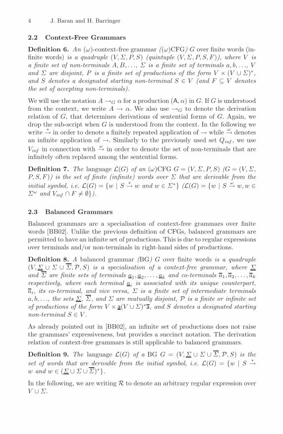
2.2 Context-Free Grammars
Definition 6. An (ω)-context-free grammar ((ω)CFG) G over finite words (in-finite words) is a quadruple (V,Σ, P, S) (quintuple (V,Σ, P, S, F )), where V isa finite set of non-terminals A,B, . . ., Σ is a finite set of terminals a, b, . . ., Vand Σ are disjoint, P is a finite set of productions of the form V × (V ∪ Σ)∗,and S denotes a designated starting non-terminal S ∈ V (and F ⊆ V denotesthe set of accepting non-terminals).
We will use the notation A→G α for a production (A, α) in G. If G is understoodfrom the context, we write A → α. We also use →G to denote the derivationrelation of G, that determines derivations of sentential forms of G. Again, wedrop the sub-script when G is understood from the context. In the following wewrite ∗→ in order to denote a finitely repeated application of→ while ω→ denotesan infinite application of →. Similarly to the previously used set Qinf , we useVinf in connection with ω→ in order to denote the set of non-terminals that areinfinitely often replaced among the sentential forms.
Definition 7. The language L(G) of an (ω)CFG G = (V,Σ, P, S) (G = (V,Σ,P, S, F )) is the set of finite (infinite) words over Σ that are derivable from theinitial symbol, i.e. L(G) = {w | S ∗→ w and w ∈ Σ∗} (L(G) = {w | S ω→ w,w ∈Σω and Vinf ∩ F = ∅}).
2.3 Balanced Grammars
Balanced grammars are a specialisation of context-free grammars over finitewords [BB02]. Unlike the previous definition of CFGs, balanced grammars arepermitted to have an infinite set of productions. This is due to regular expressionsover terminals and/or non-terminals in right-hand sides of productions.
Definition 8. A balanced grammar (BG) G over finite words is a quadruple(V,Σ ∪ Σ ∪ Σ,P , S) is a specialisation of a context-free grammar, where Σand Σ are finite sets of terminals a1, a2, . . . , ak and co-terminals a1, a2, . . . , akrespectively, where each terminal ai is associated with its unique counterpart,ai, its co-terminal, and vice versa, Σ is a finite set of intermediate terminalsa, b, . . ., the sets Σ, Σ, and Σ are mutually disjoint, P is a finite or infinite setof productions of the form V × a(V ∪Σ)∗a, and S denotes a designated startingnon-terminal S ∈ V .
As already pointed out in [BB02], an infinite set of productions does not raisethe grammars’ expressiveness, but provides a succinct notation. The derivationrelation of context-free grammars is still applicable to balanced grammars.
Definition 9. The language L(G) of a BG G = (V,Σ ∪ Σ ∪ Σ,P , S) is theset of words that are derivable from the initial symbol, i.e. L(G) = {w | S ∗→w and w ∈ (Σ ∪Σ ∪Σ)∗}.In the following, we are writing R to denote an arbitrary regular expression overV ∪Σ.

A Grammatical Representation of Visibly Pushdown Languages 5
3 Grammars for Visibly Pushdown Languages
A grammatical representation of (ω)VPLs is presented, where we take a compo-sitional approach that builds on pseudo-runs and minimally well-matched words.We first state our grammatical representation and then decompose it into twotypes of grammars. We show their resemblance of pseudo-runs and minimallywell-matched words, similar to the approach for (ω)VPAs.
3.1 Quasi Balanced Grammars
In order to simplify our proofs, we give an alternative – but expressively equiva-lent – definition of BGs, where only a finite number of productions is admitted.We reformulate occurrences of regular expressionsR in terms of production rulesPR and substitute each R by an initial non-terminal SR that appears on a left-hand side in PR. Therefore, matchings aRa become aSRa, where the derivationof SR resembles L(R).
Definition 10. Let G = (V,Σ ∪Σ ∪Σ,P , S) denote an arbitrary BG, a quasibalanced grammar (qBG) G′ = (V ′, Σ ∪Σ ∪Σ,P, S) generalises G by having afinite set of productions, where productions are either
a) in double Greibach normal form A→ aSRa, orb) of form A→ BC, A→ aC, or A→ ε, where B’s productions are of the form
according to a) and C’s productions are of the form according to b).
Lemma 1. For every BG G = (V,Σ∪Σ∪Σ,P , S) there is a qBG G′ = (V ′, Σ∪Σ ∪Σ,P, S), such that L(G) = L(G′).
3.2 A Grammatical Representation of ωVPLs
Matchings in an ωVPL appear only as finite sub-words in the language, whichwas utilised in the characterisation of pseudo-runs. Summary-edges reflect sub-words of exactly this form, which are in Lmwm. Given an infinite word w, itcan be split into sub-words that are either in Lmwm or in Σc ∪ Σi ∪ Σr, whereno sub-word in Σr follows a sub-word in Σc. We abbreviate the latter con-straint as Σc/Σr-matching avoiding. Our grammatical representation of ωVPLsutilises Σc/Σr-matching avoiding ωRGs to describe languages of pseudo-runs.Languages of summary-edges, i.e. languages with words in Lmwm, are separatelydescribed by qBGs under a special homomorphism. The homomorphism is re-quired to cover matchings of calls c that can match more than one return r,which cannot be reflected as a simple terminal/co-terminal matching a/a. Forexample, the matchings c/r1 and c/r2 are representable as terminal/co-terminalpairs a/a and b/b under the mappings h(a) = h(b) = c, h(a) = r1 and h(b) = r2.Finally, the amalgamation of Σc/Σr-matching avoiding ωRGs and qBGs un-der the aforementioned homomorphism give us a grammatical representation ofωVPLs:

6 J. Baran and H. Barringer
Definition 11. A superficial2 ω-regular grammar with injected balanced gram-mars (ωRG(qBG)+h) G = (V,Σc ∪Σi ∪Σr ∪
⋃mn=1{gn}, P, S, F,
⋃mn=1{Gn}, h),
where
– Σc, Σi, Σr and⋃mn=1{gn} are mutually disjoint,
– G is Σc/Σr-matching avoiding,– Gn = (Vn, Σn, Pn, Sn) is a qBG for n = 1, 2, . . . ,m,3
is an ωCFG G′ = (V ∪⋃mn=1{Vn}, Σ ∪
⋃mn=1{Σn}, P ′, S, F ) with
– disjoint sets V and {V1, V2, . . . , Vm} as well as Σ and {Σ1, Σ2, . . . , Σm}, and– P ′ is the smallest set satisfying• A→G′ aB if A→G aB, where a ∈ (Σc ∪Σi ∪Σr), or• A→G′ SnB if A→G gnB, or• A→G′ α if A→Gn α,
and h is constrained so that it preserves terminals of the injector grammar,h(a) = a for any a ∈ (Σc ∪Σi ∪Σr), and for terminals/co-terminals of injectedgrammars it maps terminals a ∈ Σn to calls c ∈ Σc, maps co-terminals a ∈ Σn
to returns r ∈ Σr, maps terminals a ∈ Σn to internal actions i ∈ Σi.In the following, we refer to the homomorphism h under the constraints whichare given above as superficial mapping h.
Definition 12. The language L(G) of an ωRG(qBG)+h G = (V,Σc ∪ Σi ∪Σr∪
⋃mn=1{gn}, P, S, F,
⋃mn=1{Gn}, h) denotes the set {h(w) | S ω→G′ w and w ∈
(Σ∪Σ1∪Σ2∪. . .∪Σm)ω}, where G′ is the ω-context-free grammar correspondingto G.
Consider an arbitrary ωRG(qBG)+h G = (V,Σc ∪Σi ∪Σr ∪⋃mn=1{gn}, P,
S, F,⋃mn=1{Gn}, h). We call the ωRG G↑ = (V,Σc∪Σi∪Σr∪
⋃mn=1{gn}, P, S, F )
the injector grammar of G, while the qBGs G1, G2, . . .Gm are called injectedgrammars of G.4 When G is clear from the context, we just talk about the in-jector grammar G↑ and the injected grammars G1, . . . , Gm respectively. Thelanguages associated with these grammars are referred to as injector and in-jected languages respectively. In fact, injector languages resemble pseudo-runswith pseudo edges gn, n = 1 . . .m, while injected language resemble matchingscovered by summary-edges.
3.3 ωVPL and ωRL(qBL)+h Coincide
For the equivalence proof of ωVPLs and ωRL(qBL)+hs, we first show that mini-mally well-matched words, as described by summary-edges, can be expressed by
2 Superficial – as understood as being on the surface of something.3 Each Σn is a shorthand for Σn ∪ Σn ∪ Σn.4 This should not be confused with nested words, [AM06], which describe the structure
induced by matchings in finite words.

A Grammatical Representation of Visibly Pushdown Languages 7
qBGs plus an appropriate superficial mapping, and vice versa. It is then straight-forward to prove language equivalence, by translating an arbitraryωRG(qBG)+hinto an expressively equivalent ωMSO formula and an arbitrary ωVPA into anexpressively equivalent ωRG(qBG)+h.
Let VPAmwm and MSOmwm refer to VPA and MSO-formulae whose languagesare subsets of Lmwm respectively, i.e. restricted variants of VPA and MSO-formulae that only accept minimally well-matched words. We show that anyqBG can be translated into an equivalent MSOmwm formula. Since MSOmwm
defines Lmwm, the inclusion qBL ⊆ Lmwm is proven. Second, for an arbitraryVPAmwm a qBG is constructed so that their languages coincide, which gives usqBL ⊇ VPLmwm.
In the following lemma, an MSOmwm formula is constructed from a qBG insuch a way so that their languages coincide. The translation works by quantifyingover each matching in the word and filling in the respective regular expressions.In order for the lemma to hold, we assume that all of the qBG’s productionsare uniquely identified by their terminal/co-terminal pairs. While this clearlyrestricts a grammar’s language in general, the language under a superficial map-ping is preserved.
Lemma 2. Let G = (V,Σ ∪Σ ∪Σ,P, S) denote an arbitrary qBG and let h bean arbitrary superficial mapping. Then the MSOmwm formula
ϕ ≡ ∃X∃i∨
(S→aSRa)∈P(Ψa,a(1, i) ∧ T$(i+ 1) ∧ ∀k ∈ [1, i]Φ(k))
accepts the same language as G, where
Ψa,a(i, j) ≡ Ta(i) ∧ Ta(j) ∧ μ(i, j),
Φ(k) ≡∨
a∈ΣTa(k)⇒ ∃j(μ(k, j) ∧ ϕa(k + 1, j)),
Δ(s, t, k) ≡ ∨(A→aB)∈PR(XA(k) ∧XB(k + 1) ∧ Ta(k)) ∨∨(A → BC,B → bSR′b )∈PR ∃j ∈ [s, t](XA(k) ∧XC(j + 1) ∧ Ψb,b(k, j))
ϕa(s, t) ≡ XSR(s) ∧∧(A,B) ∈ V,A = B ∀k ¬(XA(k) ∧XB(k)) ∧
∀k ∈ [s, t− 1]ϕμ(s, t, k)⇒ Δ(s, t, k) ∧∨(A→ε)∈PR XA(t),
where (A→ aSRa) ∈ P , and ϕμ(s, t, k) ≡ ¬∃i, j ∈ [s, t](μ(i, j) ∧ i < k ≤ j).Proof. Consider an arbitrary qBG+h G and its translation to a MSOmwm for-mula ϕ. We show that every word w$ ∈ L(ϕ) is a word w ∈ L(G) and viceversa.L(ϕ) ⊆ L(G): LetM be an arbitrary model of ϕ that represents the word w.
We write 〈T1, X1〉〈T2, X2〉 . . . 〈T|w|, X|w|〉〈T$, X|w|+1〉 to denote the sequence ofunique predicate pairs of T and X which hold at indices 1 to |w|+ 1 in M.
Occurrences of the form 〈Ta, XB〉 are replaced by 〈Ta,B〉 if (B → ε) ∈ P ,occurrences of the form 〈Ta, XA〉〈Ta,B〉 are replaced by 〈Ta,A〉 if (A→ aB) ∈ P ,

8 J. Baran and H. Barringer
and occurrences of the form 〈Ta, XB〉〈Ta, SR〉〈Tb,C〉 are replaced with 〈Tb,A〉 if(A → BC,B → aSRa) ∈ P . Eventually, 〈Ta, XS〉〈Ta, SR〉 will be left, which isreplaced with S iff (S → aSRa) ∈ P . As a result, we have established a bottomup parse in G for an arbitrary word w$ ∈ L(ϕ), which implies that every wordin L(ϕ) is in L(G).L(G) ⊆ L(ϕ): Let S → α → β → . . . → w denote an arbitrary derivation
in G. With each derivation step, we try to find variable assignments that sat-isfy ϕ, so that after the derivation finishes, w$ is represented by the sequence〈T1, X1〉〈T2, X2〉 . . . 〈T$, X|w|+1〉 of ϕ. The construction of 〈T1, X1〉〈T2, X2〉 . . .〈T$, X|w|+1〉 follows the derivation S → α → β → . . . → w in the sense thatthere is a mapping between the n-th step of the sequence constructed by thevariable assignments and the n-th sentential form reached in the derivation.
We consider triples of the form �A, ψ,B�, where A is a non-terminal as itappears in some sentential form derived from S, ψ denotes the formula which issupposed to derive a word w, where A ∗→ w, and B is a temporary stored non-terminal. When A derives α with A→ α, we try to find variable assignments forψ that represent terminals in α. Since terminals appear only in prefixes/postfixesof α, we remove the ground terms in ψ, add pairs 〈Tk, Xk〉 to the left/rightof �A, ψ,B� accordingly, and replace �A, ψ,B� with �C, ψ′,E� or the sequence�C, ψ′,E��D, ψ′′,F�, depending if α has one non-terminal C or two non-terminalsCD as sub-word. The non-terminals E and F are associated with productionsE→ ε and F→ ε respectively, where they denote the end of a regular expressionembedded between a call and return.
Starting the rewriting process with �S, ϕ,A�, A is chosen arbitrarily, a sequenceof tuples of the form 〈Tk, Xk〉 is eventually left, which indeed represents w, sothat the model for w$ is represented by adding 〈T$, XA〉 to the sequence. ��The reverse inclusion, i.e. qBL ⊇ VPL, can be shown by a number of rewritingsteps of an arbitrary VPAmwm to a BG equipped with a superficial mapping.Since there is a translation from BGs to qBGs, the inclusion is then proven. TheVPAmwm represents hereby L((p, q, f)) of some summary-edge (p, q, f).
Definition 13. Let G = (V,Σc∪Σi∪Σr, P, S) denote the CFG with productionsof the form S → cA, A → cBC, A → iB, and A → r that is obtained from aVPAmwm by the standard translation [HMU01, Theorem 6.14, incl. its proof],then the immediate matching CFG G′ = (V ′, Σc ∪ Σi ∪ Σr, P ′, S′) is obtainedfrom G, so that S′ →G′ c〈A, r〉r iff S →G cA, 〈A, r1〉 →G′ c〈B, r2〉r2〈C, r1〉 iffA→G cBC, 〈A, r〉 →G′ i〈B, r〉 iff A→G iB, 〈A, r〉 →G′ ε iff A→G r.
Lemma 3. The language L(G) of an immediate matching CFG G that is ob-tained from a VPAmwm A is equal to L(A).
Proof (Lemma 3). The translation of Definition 13 is preserving the languageequivalence of the grammars, as it is a special case of the more general translationpresented in [[Eng92, Page 292]. ��In the following transformation steps, productions are rewritten so that match-ings cAr appear exclusively in right-hand sides. Furthermore, we remove all pro-ductions that produce no matchings by introducing language preserving regular
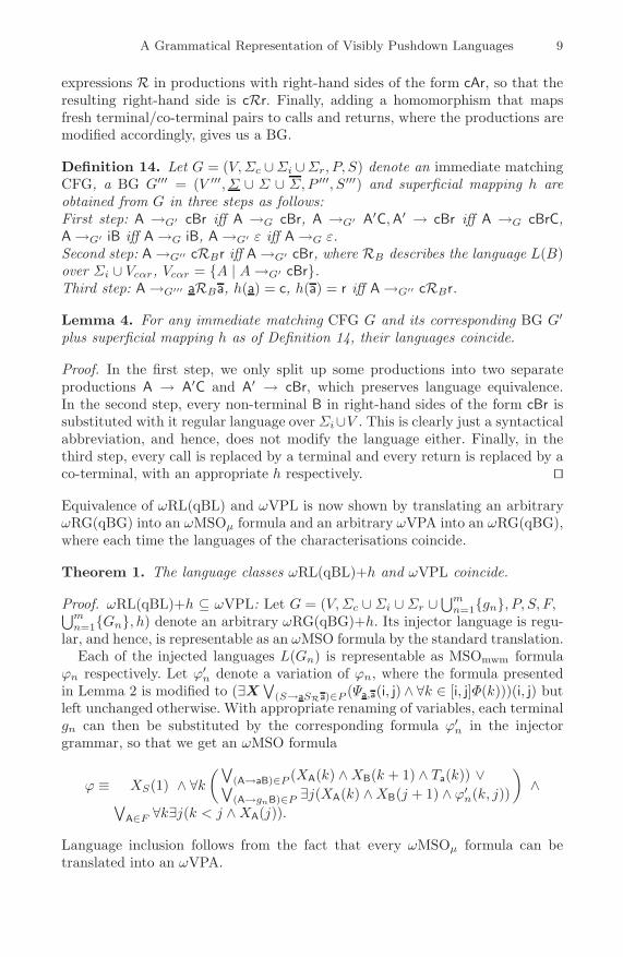
A Grammatical Representation of Visibly Pushdown Languages 9
expressions R in productions with right-hand sides of the form cAr, so that theresulting right-hand side is cRr. Finally, adding a homomorphism that mapsfresh terminal/co-terminal pairs to calls and returns, where the productions aremodified accordingly, gives us a BG.
Definition 14. Let G = (V,Σc ∪Σi ∪Σr, P, S) denote an immediate matchingCFG, a BG G′′′ = (V ′′′, Σ ∪ Σ ∪ Σ,P ′′′, S′′′) and superficial mapping h areobtained from G in three steps as follows:First step: A →G′ cBr iff A →G cBr, A →G′ A′C,A′ → cBr iff A →G cBrC,A→G′ iB iff A→G iB, A→G′ ε iff A→G ε.Second step: A→G′′ cRBr iff A→G′ cBr, where RB describes the language L(B)over Σi ∪ Vcαr, Vcαr = {A | A→G′ cBr}.Third step: A→G′′′ aRBa, h(a) = c, h(a) = r iff A→G′′ cRBr.
Lemma 4. For any immediate matching CFG G and its corresponding BG G′
plus superficial mapping h as of Definition 14, their languages coincide.
Proof. In the first step, we only split up some productions into two separateproductions A → A′C and A′ → cBr, which preserves language equivalence.In the second step, every non-terminal B in right-hand sides of the form cBr issubstituted with it regular language over Σi∪V . This is clearly just a syntacticalabbreviation, and hence, does not modify the language either. Finally, in thethird step, every call is replaced by a terminal and every return is replaced by aco-terminal, with an appropriate h respectively. ��
Equivalence of ωRL(qBL) and ωVPL is now shown by translating an arbitraryωRG(qBG) into an ωMSOμ formula and an arbitrary ωVPA into an ωRG(qBG),where each time the languages of the characterisations coincide.
Theorem 1. The language classes ωRL(qBL)+h and ωVPL coincide.
Proof. ωRL(qBL)+h ⊆ ωVPL: Let G = (V,Σc ∪Σi ∪Σr ∪⋃mn=1{gn}, P, S, F,⋃m
n=1{Gn}, h) denote an arbitrary ωRG(qBG)+h. Its injector language is regu-lar, and hence, is representable as an ωMSO formula by the standard translation.
Each of the injected languages L(Gn) is representable as MSOmwm formulaϕn respectively. Let ϕ′
n denote a variation of ϕn, where the formula presentedin Lemma 2 is modified to (∃X ∨
(S→aSRa)∈P (Ψa,a(i, j)∧ ∀k ∈ [i, j]Φ(k)))(i, j) butleft unchanged otherwise. With appropriate renaming of variables, each terminalgn can then be substituted by the corresponding formula ϕ′
n in the injectorgrammar, so that we get an ωMSO formula
ϕ ≡ XS(1) ∧ ∀k(∨
(A→aB)∈P (XA(k) ∧XB(k + 1) ∧ Ta(k)) ∨∨(A→gnB)∈P ∃j(XA(k) ∧XB(j + 1) ∧ ϕ′
n(k, j))
)
∧∨
A∈F ∀k∃j(k < j ∧XA(j)).
Language inclusion follows from the fact that every ωMSOμ formula can betranslated into an ωVPA.

10 J. Baran and H. Barringer
ωRL(qBL)+h ⊇ ωVPL: Consider an ωVPA A and let A′ = (Q′, Σc ∪Σi ∪Σr ∪⋃mn=1{Ωn}, δ, qi, F ′) denote the Buchi-automaton accepting all pseudo-runs ofA.
A′ can be represented as right-linear injector grammar G↑ with productions ofthe form A→ cB, A→ rB, and A→ (p, q, f)n′B for representing sets of summary-edges Ωn with (p, q, f)n′ ∈ Ωn. Since summary-edges (p, q, f)n′ are treated asterminals in A′, their f component does not contribute to the acceptance of apseudo-run. Hence, for every production A→ (p, q, 1)n′B, it is w.l.o.g. requiredthat B ∈ F ′.
All summary-edges stand for languages in VPLmwm, and hence, are repre-sentable as VPAmwms respectively. Each VPAmwm representing a summary-edge(p, q, f)n′ can be transformed into a qBG Gn′ plus additional superficial mappingh. By combining G↑ and the various Gn′ to a superficial ωRG(qBG), we get thelanguage inclusion. ��The use of qBGs is counter-productive. BGs are more accessible as well as suc-cinct due to the use of regular expressions in their productions. Injecting BGsinstead of qBGs into ωRGs does not change the expressiveness, which is triviallytrue as every BG can be translated into a qBG.
Corollary 1. The language classes (ω)RL(BL)+h and (ω)VPL coincide.
4 Conclusion
In this paper, a grammatical representation of (ω)VPLs was given. We intro-duced an amalgamation of ωRGs and qBGs equipped with a specific homomor-phisms and showed that the resulting language class defined by the new grammarcoincides with the ωVPLs.
Our grammatical approach towards (ω)VPLs provides a more natural repre-sentation of language specifications. As a small example, consider the following.Figure1(a) on the next page shows the code for traversing infinitely many finitebinary trees. Let c denote a call to traverse(...) and let r denote the returnin traverse(...), then the ωVPA in Figure1(b) and the ωRG(BG)+h in Fig-ure1(c) represent all possible traces that can be generated by main, i.e. theyare behavioural specifications of the code. It is apparent that the ωRG(BG)+hresembles the pseudo code in greater detail than the corresponding ωVPA.
main :=do forever
traverse(getTree())
function traverse(node n) :=if ’n is not a leaf’ then
traverse(n’s left child)traverse(n’s right child)
return
S → g1SS1 → aS1S1a | aa
h(a) = c, h(a) = rF = {S}
(a) Pseudo code (b) ωVPA (c) ωRG(BG)+h
Fig. 1. Representations of traverse(...)’s calls and returns

A Grammatical Representation of Visibly Pushdown Languages 11
Acknowledgements. Joachim Baran thanks the EPSRC and the School of Com-puter Science for the research training awards enabling this work to be under-taken, as well as Juan Antonio Navarro-Perez for helpful and valuable discussionsregarding second-order logic.
References
[AM04] Alur, R., Madhusudan, P.: Visibly pushdown languages. In: Proceedings ofthe Thirty-Sixth Annual ACM Symposium on Theory of Computing, pp.202–211. ACM Press, New York (2004)
[AM06] Alur, R., Madhusudan, P.: Adding nesting structure to words. In: Ibarra,O.H., Dang, Z. (eds.) DLT 2006. LNCS, vol. 4036, pp. 1–13. Springer, Hei-delberg (2006)
[BB02] Berstel, J., Boasson, L.: Balanced grammars and their languages. In: Brauer,W., Ehrig, H., Karhumaki, J., Salomaa, A. (eds.) Formal and Natural Com-puting. LNCS, pp. 3–25. Springer, Heidelberg (2002)
[[Eng92] Engelfriet, J.: An elementary proof of double Greibach normal form. Infor-mation Processing Letters 44(6), 291–293 (1992)
[HMU01] Hopcroft, J.E., Motwani, R., Ullman, J.D.: Introduction to AutomataTheory, Languages, and Computation, 2nd edn. Addison-Wesley, Reading(2001)
[LMS04] Loding, C., Madhusudan, P., Serre, O.: Visibly pushdown games. In: Lo-daya, K., Mahajan, M. (eds.) FSTTCS 2004. LNCS, vol. 3328, pp. 408–420.Springer, Heidelberg (2004)

Fully Lexicalized Pregroup Grammars
Denis Bechet1 and Annie Foret2
1 LINA – Universite de Nantes2, rue de la Houssiniere – BP 92208
44322 Nantes Cedex 03 – [email protected]
2 IRISA – Universite de Rennes 1Avenue du General Leclerc
35042 Rennes Cedex – [email protected]
Abstract. Pregroup grammars are a context-free grammar formalism in-troduced as a simplification of Lambek calculus. This formalism is inter-esting for several reasons: the syntactical properties of words are specifiedby a set of types like the other type-based grammar formalisms ; as a log-ical model, compositionality is easy ; a polytime parsing algorithm exists.
However, this formalism is not completely lexicalized because each pre-group grammar is based on the free pregroup built from a set of prim-itive types together with a partial order, and this order is not lexicalinformation. In fact, only the pregroup grammars that are based on prim-itive types with an order that is equality can be seen as fully lexicalized.
We show here how we can transform, using a morphism on types, aparticular pregroup grammar into another pregroup grammar that usesthe equality as the order on primitive types. This transformation is atmost quadratic in size (linear for a fixed set of primitive types), it pre-serves the parse structures of sentences and the number of types assignedto a word.
Keywords: Pregroups, Lambek Categorial Grammars, Simulation.
1 Introduction
Pregroup grammars (PG) [1] have been introduced as a simplification of Lambekcalculus [2]. Several natural languages has been modelized using this formalism:English [1], Italian [3], French [4], German [5,6], Japanese [7], etc. PG are basedon the idea that sentences are produced from words using lexical rules. Thesyntactical properties of each word is characterized by a finite set of types storedin the lexicon. The categories are types of a free pregroup generated by a set ofprimitive types together with a partial order on the primitive types. This partialorder is not independent of the language that corresponds to a PG. For instance,this order is used for English to specify that a yes-or-no question (primitive typeq) is a correct sentence (primitive type s). Thus the partial order says that q ≤ s.
This partial order is not lexicalized but corresponds to global rules that arespecific to a particular PG. Is it then possible to find a PG that is equivalent to a
D. Leivant and R. de Queiroz (Eds.): WoLLIC 2007, LNCS 4576, pp. 12–25, 2007.c© Springer-Verlag Berlin Heidelberg 2007

Fully Lexicalized Pregroup Grammars 13
given PG but where the partial order on primitive types is universal ? Moreover,we hope that the computed PG is not too big if we compare it to the source PGand if it works in a similar way as the source PG.
Using mathematical words, it means that transformation must be polynomialin space (the size of a resulting grammar is polynomially bounded by the sizeof the source grammar) and should be a homomorphism from the source freepregroup to the resulting free pregroup that must also satisfy the converse ofthe monotonicity condition.
The paper defines such a transformation. The size of the resulting grammar isbounded by a second degree polynomial of the initial grammar. Moreover, for allthe PG that are based on the same free pregroup, this transformation is linear.The size of the tranformed PG is bounded by the size of the source PG four timesthe number of primitive types of the free pregroup of this PG, plus a constant.This transformation defines a homomorphism of (free) pregroups. A pregroupgrammar is transformed into another pregroup grammar that associates thesame number of types to a word as the source grammar: a k-valued grammar istransformed into a k-valued grammar.
After an introduction about PG in section 2, the paper proves several lemmasthat are necessary for the correctness of our transformation (the source and theresulting PG must define the same language). The transformation is defined in sec-tion 4.2, its properties are detailed in the remaining sections. Section 7 concludes.
2 Background
Definition 1 (Pregroup). A pregroup is a structure (P,≤, ·, l, r, 1) such that(P,≤, ·, 1) is a partially ordered monoid1 and l, r are two unary operations on Pthat satisfy for all primitive type a ∈ P ala ≤ 1 ≤ aal and aar ≤ 1 ≤ ara.
Definition 2 (Free pregroup). Let (P,≤) be an ordered set of primitive types,P (Z) = {p(i) | p ∈ P, i ∈ Z} is the set of atomic types and T(P,≤) =
(P (Z)
)∗=
{p(i1)1 · · · p(in)
n | 0 ≤ k ≤ n, pk ∈ P and ik ∈ Z} is the set of types. The emptysequence in T(P,≤) is denoted by 1. For X and Y ∈ T(P,≤), X ≤ Y iff thisrelation is deductible in the following system where p, q ∈ P , n, k ∈ Z andX,Y, Z ∈ T(P,≤):
X ≤ X (Id)X ≤ Y Y ≤ Z
(Cut)X ≤ Z
XY ≤ Z(AL)
Xp(n)p(n+1)Y ≤ Z
X ≤ Y Z(AR)
X ≤ Y p(n+1)p(n)Z
1 We briefly recall that a monoid is a structure < M, ·, 1 >, such that · is associativeand has a neutral element 1 (∀x ∈ M : 1 ·x = x · 1 = x). A partially ordered monoidis a monoid < M, ·, 1 > with a partial order ≤ that satisfies ∀a, b, c: a ≤ b ⇒ c · a ≤c · b and a · c ≤ b · c.

14 D. Bechet and A. Foret
Xp(k)Y ≤ Z(INDL)
Xq(k)Y ≤ Z
X ≤ Y q(k)Z(INDR)
X ≤ Y p(k)Z
q ≤ p if k is even, and p ≤ q if k is odd
This construction, proposed by Buskowski, defines a pregroup that extends ≤on primitive types P to T(P,≤).2,3
The Cut Elimination. As for L and NL, the cut rule can be eliminated: everyderivable inequality has a cut-free derivation.
Definition 3 (Simple free pregroup). A simple free pregroup is a free pre-group where the order on primitive type is equality.
Definition 4 (Pregroup grammar). Let (P,≤) be a finite partially orderedset. A pregroup grammar based on (P,≤) is a lexicalized4 grammar G = (Σ, I, s)such that s ∈ T(P,≤) ; G assigns a type X to a string v1, . . . , vn of Σ∗ iff for1 ≤ i ≤ n, ∃Xi ∈ I(vi) such that X1 · · ·Xn ≤ X in the free pregroup T(P,≤). Thelanguage L(G) is the set of strings in Σ∗ that are assigned s by G.
Example 1. Our example is taken from [8] with the primitive types: π2 = secondperson, p2 = past participle, o = object, q = yes-or-no question, q′ = question.This sentence gets type q′ (q′ ≤ s):
whom have you seenq′ollql qpl2π
l2 π2 p2o
l
Remark on Types for Correct Sentences. Usually, type s associated to correctsentences must be a primitive type (s ∈ P ). However, we use here a more generaldefinition where s can be any type in T(P,≤). Our definition does not lead to asignificant modification of PG (the classes of languages is the same) becauseproving that X1 · · ·Xn ≤ X is equivalent5to prove that X1 · · ·XnX
r ≤ 1.We must notice that the transformation given in Section 4 works if we use
a generalized definition of PG as above, where the type associated to correctsentences is not necessarilly a primitive type or if s is neither ≤ nor ≥ to anyother primitive type and thus does not need to be changed by the transformation.
In fact, it is always possible to transform a PG using a composed type S forcorrect sentences into a PG using a primitive type s for correct sentences that is
2 Left and right adjoints are defined by (p(n))l = p(n−1), (p(n))r = p(n+1), (XY )l =Y lXl and (XY )r = Y rXr. We write p for p(0). We also iterate left and right adjointsfor every X ∈ T(P,≤) : X(0) = X, X(n+1) = (Xr)(n) and X(n−1) = (Xl)(n).
3 ≤ is only a preorder. Thus, in fact, the pregroup is the quotient of T(P,≤) by theequivalence relation X ≤ Y &Y ≤ X.
4 A lexicalized grammar is a triple (Σ, I, s): Σ is a finite alphabet, I assigns a finiteset of categories (or types) to each c ∈ Σ, s is a category (or type) associated tocorrect sentences.
5 If Y ≤ X then Y Xr ≤ XXr ≤ 1 ; if Y Xr ≤ 1 then Y ≤ Y XrX ≤ X.

Fully Lexicalized Pregroup Grammars 15
not related to other primitive types by the addition of a right wall Srs (the typecan be seen as the type of the final point of a sentence) for the parsing with thesecond PG because X ≤ S ⇔ XSrs ≤ s.
3 A Preliminary Fact
Proposition 1 (PG equivalence and generative capacity). Let (P,≤) bean ordered set of primitive types, for any pregroup gammar G on (P,≤), we canconstruct a PG G′ based on a simple free pregroup on (P ′,=), a set of primitivetypes with a discrete order, such that G and G′ have the same language.
Proof. This is obvious because PGs define context-free languages and everycontext-free language corresponds to an order 1 classical categorial grammars6
that can be easily simulated by an “order 1” simple PG [9].Another construct is to duplicate the lexical types for each occurrence involved
in an ordering.
Note. However both transformations do not preserve the size of the lexicon ingeneral because the initial types associated to a word can correspond to an expo-nential number of types in the transformed PG. Moreover, the transformationsdo not define a pregroup homomorphism.
We look for a transformation that is polynomial in space (the size of a resultinggrammar is polynomially bounded by the size of the source grammar) and thatis defined using a homomorphism from the source free pregroup to the resultingfree pregroup (that must also satisfy the converse of the monotonicity condition).Next section defines such a transformation. The correctness is given in the lastsections and Appendix.
4 A Pregroup Morphism
4.1 Properties of Free Pregroup Morphisms
In order to simulate a free pregroup by another one with less order postulates,we consider particular mappings on posets that can be extended as a pregrouphomomorphism from the free pregroup based on (P,≤) to the free pregroupbased on another poset (P ′,≤′).
Definition 5 (Order-preserving mapping, pregroup homomorphism)
– A mapping from a poset (P,≤) to a poset (P ′,≤′) is said order-preservingiff for all pi, pj ∈ P : pi ≤ pj implies h(pi) ≤′ h(pj).
– A mapping h from the free pregroup on (P,≤) to the free pregroup on (P ′,≤′),is a pregroup homomorphism iff
6 The order of primitive types is 0 and the order order(A) of compound types is:order(A/B) = order(B\A) = max(order(A,1 + order(B))).

16 D. Bechet and A. Foret
1. ∀X ∈ T(P,≤) : h(X(n)) = h(X)(n)
2. ∀X,Y ∈ T(P,≤) : h(XY ) = h(X)h(Y )3. h(1) = 14. ∀X,Y ∈ T(P,≤) : if X ≤ Y then h(X) ≤′ h(Y ) [Monotonicity]
Proposition 2. Each order-preserving mapping from (P,≤) to (P ′,≤′) can beuniquely extended to a unique pregroup homomorphism on T(P,≤) to T(P ′,≤′).
Proof. The unicity comes from the three first points of the definition of pregrouphomomorphism. The last point is a consequence of order-preservation which iseasy by induction on a derivation D for X ≤ Y , considering the last rule:
- this holds clearly for an axiom: h(X) ≤′ h(X) ;- if the last rule introduces p(n)
i p(n+1)i on the left, we have X = Z1p
ni pn+1i Z2
and Z1Z2 ≤ Y as previous conclusion in D, by induction we get h(Z1)h(Z2) ≤′
h(Y ), and by morphism: h(p(n)i p
(n+1)i ) = h(pi)(n)h(pi)(n+1) ≤′ 1, therefore
h(X) = h(Z1)h(pi)(n)h(pi)(n+1)h(Z2) ≤′ h(Y )- if the last rule uses pi ≤ pj on the left if n is even, we have: X =
Z1p(n)i Z2 and Z1p
(n)j Z2 ≤ Y as previous conclusion in D , by induction we
get h(Z1)h(p(n)j )h(Z2) ≤′ h(Y ), where by morphism h(p(n)
j ) = h(pj)(n) then:h(X) = h(Z1)h(pi)(n)h(Z2) ≤′ h(Y ) since by order-preservation h(pi) ≤′ h(pj)if n is odd, we proceed similarly from Z1p
(n)i Z2 ≤ Y as previous conclusion in D
- Rules on the right are similar (or consider Y = 1, then morphism properties)
In order to have a simulation, we need a converse of monotonicity.
Proposition 3 (Order-reflecting homomorphism). Every homomorphismh from the free pregroup on (P,≤) to the free pregroup on (P ′,≤′) is such that (1)and (2) are equivalent conditions and define order-reflecting homomorphisms:
(1). ∀X,Y ∈ T(P,≤) if h(X) ≤′ h(Y ) then X ≤ Y by (P,≤).(2). ∀X ∈ T(P,≤) if h(X) ≤′ 1 then X ≤ 1 by (P,≤).
Proof. In fact, (2) is obviously a subcase of (1) and (1) is a corollary of (2) asfollows: suppose (2) holds for a pregroup-morphism h with (3) h(X) ≤′ h(Y ),we get (4) h(X Y r) ≤′ 1 by adding h(Y )r on the right of (3) as below:
h(X Y r) = h(X) h(Y )r ≤′ h(Y ) h(Y )r ≤′ 1property (2) then gives (5) X Y r ≤ 1,hence X ≤ Y (by adding Y on the right of (5): X ≤ X Y r Y ≤ Y ).
These order-reflecting properties will be shown in the simulation-morphism de-fined in the next subsection.
4.2 Defining a Simulation-Morphism
Preliminary Remark. The definition has to be chosen carefully as shownby the following pregroup homomorphisms, that are not order-reflecting in thesimplest case of one order postulate.

Fully Lexicalized Pregroup Grammars 17
Example 2. Let P = {p0, p1, . . . , pn} and ≤ be reduced to one postulate p0 ≤ p1,and let ≤′ be = :
– take h(p1) = q , and h(p0) = β β(1) q γ γ(1) with h(pi) = pi if i �∈ {0, 1}where β and γ are fixed types.This defines a homomorphism (using ββ(1) ≤′ 1 and γγ(1) ≤′ 1).
– If we drop β in h of this example (β = 1), the resulting translation hγis a homomorphism but is not order-reflecting as examplified by: X =p(2n−2)0 p
(2n−1)0 p
(2n)1 p
(2n−1)1 , such that X �≤ 1, whereas hγ(X) ≤′ 1 ; simi-
larly, if we drop γ in h, defining hβ , X = p(2n+1)1 p
(2n)1 p
(2n+1)0 p
(2n+2)0 is a
counter-example for hβ7
The Unrestricted Case. In this presentation, we allow to simulate either afragment (represented as Pr below) or the whole set of primitive types ; forexample, we may want not to transform isolated (i.e. not related to anothertype) primitive types, or to proceed incrementally.
Let Pr = {p1, . . . , pn} and P = Pr ∪ Pr′, where no element of Pr is relatedby ≤ to an element of Pr′, and each element of Pr is related by ≤ to anotherelement of Pr.
We introduce new letters q and βk, γk, for each element pk of Pr. 8
We take as poset P ′ = Pr′∪{q}∪{βk, γk | pk ∈ Pr}, with ≤′ as the restrictionof ≤ on Pr′ (≤′ is reduced to identity if Pr′ is empty, corresponding to the caseof a unique connex component).
We then define the simulation-morphism h for Pr as follows:
Definition 6 (Simulation-morphism h for Pr)
h(X(n)) = h(X)(n) h(pi) = λ(0)i q(0)δ
(0)i︸ ︷︷ ︸
h(1) = 1
h(X.Y ) = h(X).h(Y ) for pi ∈ Pr h(pi) = pi if pi ∈ Pr′
where λi is the concatenation of α and all the terms γ(1)k′ γk′ for all the indices
of the primitive types pk′ ∈ P less than or equal to pi and similarly for δi:λi = α γ
(1)k′ γk′︸ ︷︷ ︸
if pk′≤pi
(downto 1). . . γ(1)k′ γk′︸ ︷︷ ︸
if pk′≤pi
, δi = βk β(1)k︸ ︷︷ ︸
if pk≥pi
(from 1). . . βk β(1)k︸ ︷︷ ︸
if pk≥pi
α′
that we also write:λi = α (
∏
for k′=n..1if pk′≤pi
(γ(1)k′ γk′)) and δi = (
∏
for k=1..n,if pk≥pi
(βk β(1)k )) α′
Note the inversion by odd exponents : h(pi)(1) = δ(1)i q(1) λ
(1)i︸ ︷︷ ︸
for pi ∈ Pr
Proposition 4 (h is order-preserving). if pi ≤ pj then h(pi) ≤′ h(pj).It is then a pregroup homomorphism.
7 Details: X = p(0)0 p
(1)0 p
(2)1 p
(1)1
hγ� p1γγ(1)γ(2)γ(1)p(1)1 p
(2)1 p
(1)1
∗�→ 1
X = p(1)1 p
(0)1 p
(1)0 p
(2)0
hβ� p(1)1 p
(0)1 .p
(1)1 β(2)β(1).β(2)β(3)p
(2)1
∗�→ 18 The symbol q can also be written qPr if necessary w.r.t. Pr.

18 D. Bechet and A. Foret
Proof. Easy by construction (if pi ≤ pj, we can check that λi ≤ λj and δi ≤ δj ,using the transitivity of ≤ and inequalities of the form ββ(1) ≤ 1 and 1 ≤ γ(1)γ)
We get the first property required for a simulation, as a corollary:
Proposition 5 (Monotonicity of h)
∀X,Y ∈ T(P,≤) : if X ≤ Y then h(X) ≤′ h(Y )
5 Order-Reflecting Property : Overview and Lemmas
We show in the next subsection that if h(X) ≤′ 1 then X ≤ 1. We proceed byreasoning on a deduction D for h(X) ≤′ 1. We explain useful facts on pregroupderivations when the right side is 1.
5.1 Reasoning with Left Derivations
Let D be the succession of sequents starting from 1 ≤′ 1 to h(X) ≤′ 1, such thatq is not related to any other primitive type by ≤′.
Δ0︸︷︷︸=1
≤′ 1 (by rule (Id)) . . . Δi ≤′ 1 . . . Δm︸︷︷︸=h(X)
≤′ 1
Each occurrence of q in h(X) is introduced by rule (AL). Let k denote the stepof the leftmost introduction of q, let (n), (n+1) be the corresponding exponentsof q, we can write:
...Δk−1 = Γ0 Γ
′0 with Δk−1 ≤′ 1
Δk = Γ0 q(n) q(n+1) Γ ′
0 with Δk ≤′ 1...Δm = Γm−k q(n) Γ ′′
m−k q(n+1) Γ ′
m−k with h(X) = Δm ≤′ 1
Γm−k is obtained from Γ0 by successive applications of rule (AL) or (INDL);similarly for Γ ′
m−k from Γ ′0:
Γm−k ≤′ Γm−k−1 . . . ≤′ Γi ≤′ . . . Γ1 ≤′ Γ0
Γ ′m−k ≤′ Γ ′
m−k−1 . . . ≤′ Γ ′i ≤′ . . . Γ ′
1 ≤′ Γ ′0
Γ ′′m−k is also obtained from Γ0 by successive applications of rule (AL) or
(INDL) but from an empty sequence, in particular:
Γ ′′m−k ≤′ 1
We shall discuss according to some properties of the distinguished occurrenceq(n) and q(n+1): the parity of n and whether they belong to images of pi and ofpj in h(X) such that pi ≤ pj , pj ≤ pi or not.

Fully Lexicalized Pregroup Grammars 19
5.2 Technical Lemmas
Lemma 1. let X = X1 α(2u1) Y 1 α
(2u1+1)
︸ ︷︷ ︸. . . Xk α
(2uk) Y k α(2uk+1)
︸ ︷︷ ︸
. . . Xn α(2un) Y n α
(2un+1)
︸ ︷︷ ︸Xn+1
where all Xk, Yk have no occurrence of α, and α is not related by ≤ to otherprimitive types ;
(i) if X ≤ 1 then :(1) ∀k : Yk ≤ 1(2) X1X2 . . . Xk . . . Xn Xn+1 ≤ 1
(ii) if Y0 α(2v+1) X α(2v+2) ≤ 1 where Y0 has no α, then :
(1) ∀k : Yk ≤ 1(2) X1X2 . . . Xk . . . Xn Xn+1 ≤ 1
The proof is given in Appendix.
Variants. A similar result holds in the odd case (called “Bis version”) forX = X1 α
(2u1−1) Y 1 α(2u1)
︸ ︷︷ ︸. . . Xk α
(2uk−1) Y k α(2uk)
︸ ︷︷ ︸
. . . Xn α(2un−1) Y n α
(2un)
︸ ︷︷ ︸Xn+1
Lemma 2. 9 Let IPr denote the set of indices of elements in Pr. Let Γ =h(X1)Y 1︸ ︷︷ ︸
. . . h(Xk)Y k︸ ︷︷ ︸
. . . h(Xm)Y m︸ ︷︷ ︸
h(Xm+1) (m ≥ 0)
where all Yk have the following form: λ2ui λ
2u+1j or δ2u−1
i δ2uj with i, j ∈ IPr 10
where some Xk may be empty (then considered as 1, with h(1) = 1)(1) If Γ ≤′ 1 then ∀k1 ≤ m : (∀k ≤ k1 : h(Xk) has no q)⇒ (∀k ≤ k1 : Yk ≤′ 1)(2) If Γ ≤′ 1 then X1X2 . . . XmXm+1 ≤ 1(3) If δ(2k)i Γδ
(2k+1)j ≤′ 1, or λ(2k+1)
i Γλ(2k+2)j ≤′ 1
then ∀k1 ≤ m : (∀k ≤ k1 : h(Xk) has no q)⇒ (∀k ≤ k1 : Yk ≤′ 1)(4) If δ(2k)i Γδ
(2k+1)j ≤′ 1, or λ(2k+1)
i Γλ(2k+2)j ≤′ 1 then X1X2 . . . XmXm+1 ≤ 1
Notation : σ(Γ ′) will then denote X1X2 . . .XmXm+1, this writing is unique.11
The proof is technical and is given in Appendix : a key-point is that somederivations are impossible.
6 Main Results
Proposition 6 (Order-reflecting property). The simulation-morphism hfrom the free pregroup on (P,≤) to the free pregroup on (P ′,≤′) satisisfies (1)and (2):
(1). ∀X,Y ∈ T(P,≤) if h(X) ≤′ h(Y ) then X ≤ Y by (P,≤).(2). ∀X,Y ∈ T(P,≤) if h(X) ≤′ 1 then X ≤ 1 by (P,≤).
9 Some complications in the formulation (1) and (3) simplify in fact the discussion inthe proof.
10 We get later pi �≤ pj in the first form, pj �≤ pi in the second form.11 Due to the form of h(pi) and of δi, λi.
20 D. Bechet and A. Foret
In fact, (1) can be shown from Lemma 2 (2) (case m = 0) and (2) is equivalentto (1) as explained before in Proposition 3.
As a corollary of monotonicity and previous proposition, we get:
Proposition 7 (Pregroup Order Simulation). The simulation-morphism hfrom the free pregroup on (P,≤) to the free pregroup on (P ′,≤′) enjoys thefollowing property:∀X,Y ∈ T(P,≤) h(X) ≤′ h(Y ) iff X ≤ Y
Proposition 8 (Pregroup Grammar Simulation). Given a pregroup gram-mar G = (Σ, I, s) on the free pregroup on a poset (P,≤), we consider Pr = P andwe construct the simulation-morphism h from the free pregroup on (P,≤) to thesimple free pregroup on (P ′,≤′) ; we construct a grammar G′ = (Σ, h(I), h(s)),where h(I) is the assignment of h(Xi) to ai for each Xi ∈ I(ai), as a result wehave : L(G) = L(G′)
This proposition applies the transformation to the whole set of primitive types,thus providing a fully lexicalized grammar G′ (with no order postulate). A sim-ilar result holds when only a fragment of P is transformed as discussed in theconstruction of h.
7 Conclusion
In the framework of categorial grammars, pregroups were introduced as a sim-plification of Lambek calculus. Several aspects have been modified. The orderon primitive types has been introduced in PG to simplify the calculus for simpletypes. The consequence is that PG is not fully lexicalized and a parser shouldtake into account this information while performing syntactical analysis.
We have proven that this restriction is not so important because a PG usingan order on primitive types can be transformed into a PG based on a simplefree pregroup using a pregroup morphism whose size is bound by the size ofthe initial PG times the number of primitive types (times a constant which isapproximatively 4). Usually the order on primitive type is not very complex,thus the size of the resulting PG is often much less that this bound. Moreover,this transformation does not change the number of types that are assigned to aword (a k-valued PG is transformed into a k-valued PG).
References
1. Lambek, J.: Type grammars revisited. In: Lecomte, A., Perrier, G., Lamarche, F.(eds.) LACL 1997. LNCS (LNAI), vol. 1582, pp. 22–24. Springer, Heidelberg (1999)
2. Lambek, J.: The mathematics of sentence structure. American MathematicalMonthly 65, 154–170 (1958)
3. Casadio, C., Lambek, J.: An algebraic analysis of clitic pronouns in italian. In: deGroote, P., Morrill, G., Retore, C. (eds.) LACL 2001. LNCS (LNAI), vol. 2099,Springer, Heidelberg (2001)

Fully Lexicalized Pregroup Grammars 21
4. Bargelli, D., Lambek, J.: An algebraic approach to french sentence structure. In:de Groote, P., Morrill, G., Retore, C. (eds.) LACL 2001. LNCS (LNAI), vol. 2099,Springer, Heidelberg (2001)
5. Lambek, J.: Type grammar meets german word order. Theoretical Linguistics 26,19–30 (2000)
6. Lambek, J., Preller, A.: An algebraic approach to the german noun phrase. LinguisticAnalysis 31, 3–4 (2003)
7. Cardinal, K.: An algebraic study of Japanese grammar. McGill University, Montreal(2002)
8. Lambek, J.: Mathematics and the mind. In: Abrusci, V., Casadio, C. (eds.) New Per-spectives in Logic and Formal Linguisitics. In: Proceedings Vth ROMA Workshop,Bulzoni Editore (2001)
9. Buszkowski, W.: Lambek grammars based on pregroups. In: de Groote, P., Morrill,G., Retore, C. (eds.) LACL 2001. LNCS (LNAI), vol. 2099, Springer, Heidelberg(2001)
Appendix
Proof of Lemma 1 (i): By induction on the number n of termsXk α
(2uk) Y k α(2uk+1)
︸ ︷︷ ︸.
◦ If n > 1, let (2uj + 1) denote the rightmost exponent of α such that it isgreater or equal than all exponents of α in X ; consider a derivationofX ≤ 1 and the step when α(2uj+1) appears first in the derivation:Z1α
(2uj)α(2uj+1)Z2 ≤ 1Next steps lead to independent introductions in Z1, Z2 and be-
tween α(2uj) α(2uj+1), by construction of derivations, its endingcan be written:Z ′
1 α(2uj) Z ′
3 α(2uj+1) Z ′
2 ≤ 1 where Z ′3 ≤ 1 and Z ′
1 Z′2 ≤ 1
We now discuss whether Z ′3 = Yj or not.
– If Z ′3 = Yj (where Yj has no α) then :
Z′1 Z′
2 = X1 α(2u1) Y 1 α(2u1+1)
︸ ︷︷ ︸. . . Xj−1 α(2uj−1) Y j−1 α(2uj−1+1)
︸ ︷︷ ︸
Xj Xj+1 α(2uj+1) Y j+1 α(2uj+1+1)
︸ ︷︷ ︸. . . Xn α(2un) Y n α(2un+1)
︸ ︷︷ ︸Xn+1
We then apply the hypothesis to n − 1 termsX ′
k α(2uk) Y ′
k α(2uk+1)
︸ ︷︷ ︸in X ′ = Z ′
1Z′2, taking X ′j := XjXj+1,
X ′j+m := Xj+m−1 and Y ′
j+m := Yj+m−1:(1)’ ∀k �= j : Yk ≤ 1(2) X1X2 . . .Xk . . . Xn Xn+1 ≤ 1
we get full (1) for X from above : Z ′3 = Yj and Z ′
3 ≤ 1.– If Z ′
3 �= Yj , since Xk, Yk have no α, and (2uj+1) is a highest exponent, theremust exist ui, with i < j such that ui = uj , therefore:Z ′
3 = Yi α(2ui+1) Z ′
4Xj α(2ui) Yj where Z ′
4 is either empty or thesequence of successive terms Xk α
(2uk) Y k α(2uk+1)
︸ ︷︷ ︸, for i < k < j.

22 D. Bechet and A. Foret
This is impossible, since the first α(2ui+1) on the left of Z ′3, re-
quires an occurrence of a greater exponent on the right in a deriva-tion for Z ′
3 ≤ 1, whereas α(2ui+1) is a highest exponent.◦ If n = 1, the discussion starts as above, the derivation ending is:
Z ′1 α
(2uj) Z ′3 α
(2uj+1) Z ′2 ≤ 1 where Z ′
3 ≤ 1 and Z ′1 Z
′2 ≤ 1
which coincides with (1) and (2) for X
Proof of Lemma 1 (ii) : By induction on the number n ≥ 1 of termsXk α
(2uk) Y k α(2uk+1)
︸ ︷︷ ︸.
Let (2uj + 1) denote the rightmost exponent of α in X such that it isgreater or equal than all exponents of α in X ; we consider a derivation D ofY0 α
(2v+1)Xα2v+2 ≤ 1 and the step when α(2uj+1) (rightmost maximum in X)appears first in the derivation.
– If the rightmost α(2uj+1) is introduced with the α(2v+2) on its right, theintroduction step in D is of the form:
Z1α(2uj+1)α(2uj+2) ≤ 1 with uj = v and Z1 ≤ 1 as antecedent in D .
The next steps in D are introductions in Z1 and between α(2uj) α(2uj+1), byconstruction of derivations, its ending can be written:
Z ′1 α
(2uj+1) Z ′3 α
(2uj+2) ≤ 1 where Z ′3 ≤ 1 and Z ′
1 ≤ Z1 ≤ 1
The beginning of Z ′1 must be Y0 α
(2v+1), where 2v+1 is the highest exponentof α in Z ′
1 (Y0 having no α). This case is thus impossible, because in aderivation of Z ′
1 ≤ 1, the α(2v+1) in the left of Z ′1 should combine with an
α(2v+2) on its right.– The rightmost α(2uj+1) is thus introduced with an α(2uj) on its left, this step
is:
Z1α(2uj)α(2uj+1)Z2 ≤ 1 with Z1Z2 ≤ 1 as antecedent in D .
Next steps lead to independent introductions in Z1, Z2 and between α(2uj)
α(2uj+1), by construction of derivations, the ending of D can be written:
Z ′1 α
(2uj) Z ′3 α
(2uj+1) Z ′2 ≤ 1 where Z ′
3 ≤ 1 and Z ′1 Z
′2 ≤ 1
The ending of Z ′3 must be Yj . We now detail the possibilities.
If n = 1, by hypothesis Y0 α(2v+1) X1 α
(2u1) Y 1 α(2u1+1)
︸ ︷︷ ︸X2
︸ ︷︷ ︸=X
α(2v+2) ≤ 1,
the inequality Z ′3 ≤ 1 is Y1 = Z ′
3 ≤ 1, that is a part of (1) andZ ′
1 Z′2 ≤ 1 is: Y0 α
(2v+1) X1X2 α(2v+2) where Y0, X1, X2 have no α,therefore, by construction of derivations, we must have Y0 ≤ 1 (theend of (1)) and X1X2 ≤ 1 that is (2).
If n > 1, we first show that we must have Z ′3 = Yj .

Fully Lexicalized Pregroup Grammars 23
– If Z ′3 �= Yj , since Xk, Yk have no α, and (2uj + 1) is a highest exponent in
X , if it not combined with α2v+2, there must exist ui, with i < jsuch that ui = uj , therefore:Z ′
3 = Yi α(2ui+1) Z ′
4Xj α(2ui) Yj where Z ′
4 is either empty or thesequence of successive terms Xk α
(2uk) Y k α(2uk+1)
︸ ︷︷ ︸, for i < k < j.
This is impossible, since the first α(2ui+1) on the left of Z ′3, re-
quires an occurrence of a greater exponent on the right in a deriva-tion for Z ′
3 ≤ 1, whereas α(2ui+1) is a highest exponent.– Z ′
3 = Yj (where Yj has no α) then :Z′
1 Z′2 =
Y0 α2v+1 X1 α(2u1) Y 1 α(2u1+1)
︸ ︷︷ ︸. . . Xj−1 α(2uj−1) Y j−1 α(2uj−1+1)
︸ ︷︷ ︸
Xj Xj+1 α(2uj+1) Y j+1 α(2uj+1+1)
︸ ︷︷ ︸. . .Xn α(2un) Y n α(2un+1)
︸ ︷︷ ︸Xn+1α
2v+2
we apply the hypothesis to n−1 terms X ′k α
(2uk) Y ′k α
(2uk+1)
︸ ︷︷ ︸in X ′ = Z ′
1 Z′2, taking X ′j := XjXj+1, X ′
j+m := Xj+m−1 andY ′j+m := Yj+m−1:(1)’ ∀k �= j : Yk ≤ 1(2) X1X2 . . . Xk . . . Xn Xn+1 ≤ 1we get full (1) for X from above : Z ′
3 = Yj and Z ′3 ≤ 1.
Detailed writing and properties of the auxiliary typesLemma 2 uses the following facts on auxiliary types :
– if pi ≤ pj then λ2ui λ
2u+1j ≤′ 1
– if pi �≤ pj then λ2ui λ
2u+1j �≤′ 1
– if pj ≤ pi then δ2u−1i δ2uj ≤′ 1
– if pj �≤ pi then δ2u−1i δ2uj �≤′ 1
This can be summarized as : the only Yk �≤ 1 of Lemma 2 are λ2ui λ
2u+1j for
pi �≤ pj and δ2u−1i δ2uj for pj �≤ pi
This can be checked using the following detailed writing for the auxiliarytypes
λ2ui λ
2u+1j (i = j): α(2u) (
∏
for k′=n..1if pk′≤pi
(γ(2u+1)k′ γ
(2u)k′ )) (
∏
for k=1..nif pk≤pi
(γ(2u+1)k γ
(2u+1+1)k ))α(2u+1)
δ2u−1i δ2uj (i=j): α′ (2u−1) (
∏
for k′=n..1if pk′≥pi
(β(2u−1+1)k′ β
(2u−1)k′ )) (
∏
for k=1..n,if pk≥pi
(β(2u)k β
(2u+1)k )) α′ (2u)
24 D. Bechet and A. Foret
λ2ui λ
2u+1j (i �=j): α(2u) (
∏
for k′=n..1if pk′≤pi
(γ(2u+1)k′ γ
(2u)k′ )) (
∏
for k=1..nif pk≤pj
(γ(2u+1)k γ
(2u+1+1)k ))α(2u+1)
δ2u−1i δ2u
j (i �= j): α′ (2u−1) (∏
for k′=n..1if pk′≥pi
(β(2u−1+1)k′ β
(2u−1)k′ )) (
∏
for k=1..n,if pk≥pj
(β(2u)k β
(2u+1)k )) α′ (2u)
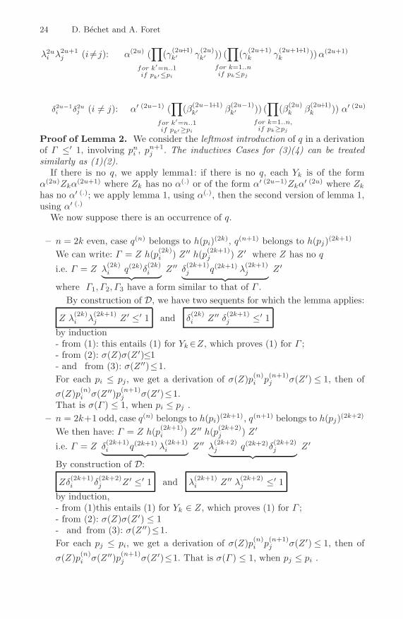
Proof of Lemma 2. We consider the leftmost introduction of q in a derivationof Γ ≤′ 1, involving pni , p
n+1j . The inductives Cases for (3)(4) can be treated
similarly as (1)(2).If there is no q, we apply lemma1: if there is no q, each Yk is of the form
α(2u)Zkα(2u+1) where Zk has no α(.) or of the form α′ (2u−1)Zkα
′ (2u) where Zkhas no α′ (.); we apply lemma 1, using α(.), then the second version of lemma 1,using α′ (.)
We now suppose there is an occurrence of q.
– n = 2k even, case q(n) belongs to h(pi)(2k), q(n+1) belongs to h(pj)(2k+1)
We can write: Γ = Z h(p(2k)i ) Z ′′ h(p(2k+1)
j ) Z ′ where Z has no q
i.e. Γ = Z λ(2k)i q(2k)δ
(2k)i︸ ︷︷ ︸
Z ′′ δ(2k+1)j q(2k+1) λ
(2k+1)j
︸ ︷︷ ︸Z ′
where Γ1, Γ2, Γ3 have a form similar to that of Γ .By construction of D, we have two sequents for which the lemma applies:
Z λ(2k)i λ
(2k+1)j Z ′ ≤′ 1 and δ
(2k)i Z ′′ δ(2k+1)
j ≤′ 1
by induction- from (1): this entails (1) for Yk∈Z, which proves (1) for Γ ;- from (2): σ(Z)σ(Z ′)≤1- and from (3): σ(Z ′′)≤1.For each pi ≤ pj, we get a derivation of σ(Z)p(n)
i p(n+1)j σ(Z ′) ≤ 1, then of
σ(Z)p(n)i σ(Z ′′)p(n+1)
j σ(Z ′)≤1.That is σ(Γ ) ≤ 1, when pi ≤ pj .
– n = 2k+1 odd, case q(n) belongs to h(pi)(2k+1), q(n+1) belongs to h(pj)(2k+2)
We then have: Γ = Z h(p(2k+1)i ) Z ′′ h(p(2k+2)
j ) Z ′
i.e. Γ = Z δ(2k+1)i q(2k+1) λ
(2k+1)i︸ ︷︷ ︸
Z ′′ λ(2k+2)j q(2k+2)δ
(2k+2)j
︸ ︷︷ ︸Z ′
By construction of D:
Zδ(2k+1)i δ
(2k+2)j Z ′ ≤′ 1 and λ
(2k+1)i Z ′′ λ(2k+2)
j ≤′ 1
by induction,- from (1)this entails (1) for Yk ∈ Z, which proves (1) for Γ ;- from (2): σ(Z)σ(Z ′) ≤ 1- and from (3): σ(Z ′′)≤1.For each pj ≤ pi, we get a derivation of σ(Z)p(n)
i p(n+1)j σ(Z ′) ≤ 1, then of
σ(Z)p(n)i σ(Z ′′)p(n+1)
j σ(Z ′)≤1. That is σ(Γ ) ≤ 1, when pj ≤ pi .

Fully Lexicalized Pregroup Grammars 25
– n = 2k, pi �≤ pj : Γ = Z︸︷︷︸no q
λ(2k)i q(2k)δ
(2k)i︸ ︷︷ ︸
Z ′′ δ(2k+1)j q(2k+1) λ
(2k+1)j
︸ ︷︷ ︸Z ′ ,
such that, by construction of D: Z λ(2k)i λ
(2k+1)j Z ′≤′ 1 which is is impossible
by induction (1) applied to it (key point: λ(2k)i λ
(2k+1)j �≤1 )
– n = 2k + 1, pj �≤ pi : Γ =Z︸︷︷︸no q
δ(2k+1)i q(2k+1) λ
(2k+1)i︸ ︷︷ ︸
Z ′′ λ(2k+2)j q(2k+2)δ
(2k+2)j
︸ ︷︷ ︸Z ′ such that,
by construction of D: Z δ(2k+1)i δ
(2k+2)j Z ′≤′ 1
which is impossible by induction (1) applied to it (key point:δ(2k+1)i δ
(2k+2)j �≤1 )
Bounded Lattice T-Norms as an Interval Category
Benjamın C. Bedregal1, Roberto Callejas-Bedregal2, and Helida S. Santos1
1 Federal University of Rio Grande do Norte, Department of Informatics and AppliedMathematics, Campus Universitario s/n, Lagoa Nova, 59.072-970 Natal, Brazil
[email protected] Federal University of Paraıba, Department of Mathematics, Cidade Universitaria - Campus I,
CEP: 58.051-900 Joao Pessoa-PB, [email protected]
Abstract. Triangular norms or t-norms, in short, and automorphisms are veryuseful to fuzzy logics in the narrow sense. However, these notions are usuallylimited to the set [0, 1].
In this paper we will consider a generalization of the t-norm notion for ar-bitrary bounded lattices as a category where these generalized t-norms are theobjects and generalizations of automorphisms are the morphisms of the category.We will prove that, this category is an interval category, which roughly meansthat it is a Cartesian category with an interval covariant functor.
1 Introduction
Triangular norms were introduced by Karl Menger in [23] with the goal of constructingmetric spaces using probabilistic distributions, i.e. values in the interval [0, 1], insteadof the real numbers set as whole, to describe the distance between two elements. How-ever, that original proposal is very wide allowing to model (fuzzy) conjunction as wellas (fuzzy) disjunction. But, with the work of Berthold Schweizer and Abe Sklar in [25]it was given an axiomatic for t-norms as they are used today. In [1], Claudi Alsina,Enric Trillas, and Llorenc Valverde, using t-norms, model the conjunction in fuzzy log-ics, generalizing several previous fuzzy conjunctions, provided, among others, by LotfiZadeh in [31], Richard Bellman and Zadeh in [6] and Ronald Yager in [30]. From at-norm it is also possible to obtain, canonically, fuzzy interpretations for the other usualconnectives [7].
Automorphisms act on t-norms generating in most of the cases a new t-norm. Whenwe see t-norms as a semi-group operation (see for example [21,22]) the automorphismyields an isomorphism between t-norms.
On the other hand in fuzzy logic in the narrow sense, it has been very commonthe use of lattice theory to deal with fuzzy logic in a more general framework, seefor example the L-fuzzy set theory [15], BL-algebras [18], Brouwerian lattices [28],Complete Heyting algebras [13], etc.
In [12,11] it was generalized the t-norm notion to bounded partially ordered sets,which is a more general structure than the bounded lattice. In [24] it was considered anextension of t-norms for bounded lattice which coincides with the one given by [12,11].In this paper we will consider this notion of t-norm for arbitrary bounded lattices.
D. Leivant and R. de Queiroz (Eds.): WoLLIC 2007, LNCS 4576, pp. 26–37, 2007.c© Springer-Verlag Berlin Heidelberg 2007

Bounded Lattice T-Norms as an Interval Category 27
The category theory is an abstract structure composed by a collection of “objects”,together with a collection of “morphisms” between them [27]. The morphisms estab-lish relationships between the objects such that every property of the objects must bespecified through the properties of the morphisms (existence of particular morphisms,its unicity, some equations which are satisfied by them, etc.). Thus, categories provide astrongly formalized language which is appropriated in order to establish abstract prop-erties of mathematical structures. More information about category theory can be foundin [2,3,27]. So, seing the t-norm theory as a category we gain in elegancy and in thecomprehension of the general property of t-norms.
A first contribution of this paper is to provide a generalization of the notion of au-tomorphism to bounded lattices. Since automorphism presuppose the use of the samelattice, we also generalize this notion to t-norm morphism which considers differentlattices for domain and co-domain. Another contribution is to consider the productand interval lattice constructions (see for example [17,26]) to construct t-norms and t-norms morphisms. We also analyze some categorical properties of these constructions,in particular we show that this category is an interval category in the sense of [8] withthe goal of providing a category theoretical foundation for the parametric interval datatype. Roughly, it means that this category is Cartesian and that has an interval t-normconstructor which is a covariant functor. The interval t-norms constructor proposed inthis paper extends for bounded lattices the interval t-norms constructor introduced byBedregal and Takahashi in [5] for usual t-norms.
2 The Interval Constructor and the Category POSET
This section is based on the paper [8]. For more information on category theory see[2,3,27].
We will denote by I(R) the set {[r, s] / r, s ∈ R and r ≤ s} called the real intervalsset. Each interval could be seen as an ordered pair or as a set ([r, s] = {x ∈ R / r ≤x ≤ s}). There are several orders which can be defined on I(R), but in this work wewill take in account the order of Kulisch-Miranker [20] since it is compatible with theorder of the cartesian product:
[a, b] � [c, d] ⇔ ∀x ∈ [a, b] ∃y ∈ [c, d], x ≤ y and ∀y ∈ [c, d] ∃x ∈ [a, b], x ≤ y⇔ a ≤ c and b ≤ d
Notice that this order depends upon the usual real order. Thus, we can generalize thisconstruction by considering, instead of the real set with its usual order, any partiallyorder set, it means that we can think of intervals as a constructor on posets.
Let D = 〈D, ≤〉 be a poset. The poset I(D) = 〈I(D), �〉, where
– I(D) = {[a, b] / a, b ∈ D and a ≤ b}– [a, b] � [c, d] ⇔ a ≤ c and b ≤ d
is called the poset of intervals of D.Posets as objects and monotonic functions as morphisms are a Cartesian closed cat-
egory, denoted by POSET.Let D1 = 〈D1, ≤1〉 and D2 = 〈D2, ≤2〉 be posets. Let f : D1 −→ D2 be a
monotonic function. Then the function I(f) : I(D1) −→ I(D2), defined by I(f)([a, b]) =

28 B.C. Bedregal, R. Callejas-Bedregal, and H.S. Santos
[f(a), f(b)] is also monotonic. Thus we have a covariant functor I : POSET −→POSET.
Let C be a category with product. Then Prod : C −→ C defined by Prod(A) =A × A for each object A of C and if f : A −→ B is a morphism then Prod(f) =f × f : A × A −→ B × B is covariant functor.
Let D=〈D, ≤〉 be a poset. Then m(D) : I(D)−→D×D defined by m(D)([a, b])=(a, b) is a morphism from I(D) into D × D. The collection
m = {m(D) : I(D) −→ Prod(D) / D is a poset }
of morphisms is a natural transformation from I : POSET −→ POSET to Prod :POSET −→ POSET.
An interval category1 is a triple (C, I, m) such that
1. C is a category with product2. I : C −→ C is a covariant functor such that I(A × B) is isomorphic to I(A) × I(B)
for all pair of objects A and B of C3. m is an injective natural transformation from I : C −→ C to Prod : C −→ C4. There exists a covariant functor F : C −→ POSET such that for each A, B ∈
ObjC and for each f : A −→ B morphism we have that
(a) F (I(A)) ∼= I(F (A)),(b) F (I(f)) ∼= I(F (f)),(c) F (A × A) ∼= F (A) × F (A),(d) F (f × f) ∼= F (f) × F (f) and(e) F (m(A)) ∼= m(F (A))
3 Lattices
Let L = 〈L, ∧, ∨〉 be an algebraic structure where L is a nonempty set and ∧ and ∨ arebinary operations. L is a lattice, if for each x, y, z ∈ L
1. x ∧ y = y ∧ x and x ∨ y = y ∨ x2. x ∧ (y ∧ z) = (x ∧ y) ∧ z and x ∨ (y ∨ z) = (x ∨ y) ∨ z3. x ∧ (x ∨ y) = x and x ∨ (x ∧ y) = x
In a lattice L = 〈L, ∧, ∨〉, if there exist two distinguish elements, 0 and 1, such thatfor each x ∈ L, x ∧ 1 = x and x ∨ 0 = x then 〈L, ∧, ∨, 1, 0〉 is said a bounded lattice.
Example 1. Some examples of bounded lattices:
1. L� = 〈{1}, ∧, ∨, 1, 1〉, where 1 ∧ 1 = 1 ∨ 1 = 1.2. B = 〈B, ∧, ∨, 1, 0〉, where B = {0, 1}, ∧ and ∨ are as in the boolean algebra.3. I = 〈[0, 1], ∧, ∨, 1, 0〉, where x ∧ y = min{x, y} and x ∨ y = max{x, y}.
1 This definition is weaker than the original in [8] because it considers isomorphism order in-stead of the equality in the property 4. Nevertheless, as in category theory two isomorphicobjects are essentially the same, the above definition seem more reasonable.

Bounded Lattice T-Norms as an Interval Category 29
4. N = 〈N�, ∧, ∨, �, 0〉, where N is the set of natural numbers and(a) N
� = N ∪ {�},(b) x ∧ � = � ∧ x = x and if x, y ∈ N then x ∧ y = min{x, y},(c) x ∨ � = � ∨ x = � and if x, y ∈ N then x ∨ y = max{x, y}.
As it is well known, each lattice establishes a partial order. Let L = 〈L, ∧, ∨〉 be alattice. Then ≤L⊆ L × L defined by
x ≤L y ⇔ x ∧ y = x
is a partial order where ∧ coincides with the greatest lower bound (infimum) and ∨ withthe least upper bound (supremum).
Let L = 〈L, ∧L, ∨L, 1L, 0L〉 and M = 〈M, ∧M , ∨M , 1M , 0M 〉 be bounded lattices.A function h : L −→ M is a lattice homomorphism2 if
1. h(0L) = 0M ,2. h(1L) = 1M ,3. for each x, y ∈ L then
(a) h(x ∧L y) = h(x) ∧M h(y),(b) h(x ∨L y) = h(x) ∨M h(y).
Proposition 1. Let L and M be bounded lattices. h : L −→ M is a lattice homomor-phism iff h(0L) = 0M , h(1L) = 1M , and h is monotonic w.r.t. the lattice orders.
Proof. It is a well known fact.
Example 2. Let L be a bounded lattice. Then for each α ∈ (0, 1), the function hα :[0, 1] −→ L defined by
hα(x) ={
0L if x ≤ α1L if x > α
is a lattice homomorphism from I into L.
3.1 Operators on Bounded Lattices
Let L and M be bounded lattices. The product of L and M, is L × M = 〈L ×M, ∧, ∨, (1L, 1M ), (0L, 0M )〉, where (x1, x2) ∧ (y1, y2) = (x1 ∧L y1, x2 ∧M y2) and(x1, x2) ∨ (y1, y2) = (x1 ∨L y1, x2 ∨M y2) , is also a bounded lattice.
Let L be a bounded lattice. The interval of L, is IL = 〈IL, ∧, ∨, [1, 1], [0, 0]〉 whereIL = {[X, X] / X, X ∈ L and X ≤L X}, [X, X]∧ [Y , Y ] = [X ∧L Y , X ∧L Y ] and[X, X] ∨ [Y , Y ] = [X ∨L Y , X ∨L Y ], is also a bounded lattice.
The associated order for this lattice agrees with the product order. That is,
[X, X] ≤ [Y , Y ] iff X ≤L Y and X ≤L Y (1)
This partial order (1) generalizes a partial order used for the first time by Kulisch andMiranker [20] in the interval mathematics context.
Clearly, bounded lattices are closed under product and interval operators.2 In [10] the term “homomorphism” was used for a lattice not necessarily bounded. For homo-
morphism preserving bottom and top elements, as considered here, Davey and Priestley usethe term {0, 1}-homomorphism.

30 B.C. Bedregal, R. Callejas-Bedregal, and H.S. Santos
4 T-Norms and Automorphisms on Bounded Lattices
Let L be a bounded lattice. A binary operation T on L is a triangular norm on L,t-norm in short, if for each v, x, y, z ∈ L the following properties are satisfied:
1. commutativity: T (x, y) = T (y, x),2. associativity: T (x, T (y, z)) = T (T (x, y), z),3. neutral element: T (x, 1) = x and4. monotonicity: If y ≤L z then T (x, y) ≤L T (x, z).
Notice that for the lattice I in particular, this notion of t-norm coincides with theusual one. The well known Godel and weak t-norms (also known by minimum anddrastic product t-norm [21]) can be generalized for arbitrary bounded lattice in a naturalway. In particular, the Godel t-norm (TG) coincides with ∧ itself and the weak t-normis defined by
TW (x, y) ={
0 if x �= 1 and y �= 1x ∧ y otherwise
Analogously as we have a partial order on the set of t-norm we can establish a partialorder on the set of all t-norms on a bounded lattice. Let T1 and T2 be t-norms on abounded lattice L. Then T1 is weaker than T2 or, equivalently, T2 is stronger than T1,denoted by T1 ≤ T2 if for each x, y ∈ L, T1(x, y) ≤L T2(x, y).
Proposition 2. Let T be a t-norm on a bounded lattice L. Then
TW ≤ T ≤ TG
Proof. Similar to the classical result (see for example remark 1.5.(i) in [21]).
Corollary 1. Let T be a t-norm on a bounded lattice L. Then T (x, y) = 1L iff x =y = 1L.
Proof. Straightforward.
4.1 T-Norm Morphisms
Let T1 and T2 be t-norms on the bounded lattices L and M, respectively. A latticehomomorphism ρ : L → M is a t-norm morphism from T1 into T2 if for each x, y ∈ L
ρ(T1(x, y)) = T2(ρ(x), ρ(y)) (2)
Straightforward from the fact that ρ is a lattice morphism, ρ is monotonic.If ρ is bijective then ρ is a t-norm isomorphism. When L and M are equals, t-norm
isomorphisms are called automorphisms. In fact, this notion coincides with the usualnotion of automorphism when the lattice is I.
Clearly the composition of two t-norm morphisms is also a t-norm morphism. In fact,let K, L and M be bounded lattices, T1, T2 and T3 be t-norms on K, L, and M, respec-tively, and ρ1 and ρ2 be morphisms between T1 into T2 and between T2 into T3, respec-tively. So, T3(ρ2 ◦ ρ1(x), ρ2 ◦ ρ1(y)) = ρ2(T2(ρ1(x), ρ1(y))) = ρ2(ρ1(T1(x, y))).
Bounded Lattice T-Norms as an Interval Category 31
Since the composition of functions is associative, then the composition of t-normmorphisms is also associative. Notice that for any bounded lattice L, the identityIdL(x) = x is an automorphism such that for each t-norm on L, IdL(T (x, y)) =T (IdL(x), IdL(y)).
Thus, considering the t-norm morphism notion as a morphism and t-norms as objects,we have a category, denoted by T−NORM.
5 T−NORM as a Cartesian Category
5.1 Terminal Object
Proposition 3. Let T� : {(1, 1)} −→ {1} defined by T�(1, 1) = 1. Then T� is at-norm on the bounded lattice L�.
Proof. Straightforward.
Proposition 4. Let T be a t-norm on a bounded lattice L. Then ρ� : L → {1} definedby ρ�(x) = 1 is the unique t-norm morphism from T into T�.
Proof. Straightforward.
Thus, T� is a terminal object of T−NORM.
5.2 Cartesian Product
Proposition 5. Let T1 and T2 be t-norms on bounded lattices L and M, respectively.Then T1 × T2 : (L × M)2 → L × M defined by
T1 × T2((x1, x2), (y1, y2)) = (T1(x1, y1), T2(x2, y2))
is a t-norm on the bounded lattice L × M.
Proof. Straightforward.
Proposition 6. Let T1 and T2 be t-norms on the bounded lattices L and M, respec-tively. Then the usual projections π1 : L × M −→ L and π2 : L × M −→ M definedby
π1(x, y) = x and π2(x, y) = y
are t-norm morphisms from T1 × T2 into T1 and T2, respectively.
Proof. As it is well known, π1 and π2 are lattice morphisms. So, it only remains toprove that it satisfies the equation (2). Let (x1, x2), (y1, y2) ∈ L × M . Then
π1(T1 × T2((x1, x2), (y1, y2))) = π1(T1(x1, y1), T2(x2, y2))= T1(x1, y1)= T1(π1(x1, x2), π1(y1, y2))
The case for π2 is analogous.

32 B.C. Bedregal, R. Callejas-Bedregal, and H.S. Santos
Next we will prove that T−NORM satisfies the universal property of cartesianproduct.
Theorem 1. Let T , T1 and T2 be t-norms on the bounded lattices K, L and M, re-spectively. If ρ1 and ρ2 are t-norm morphisms from T into T1 and T2, respectively, thenthere exists only one t-norm morphism ρ from T into T1 × T2 such that the followingdiagram commutes:
T
T1 � π1�
ρ 1
T1 × T2
ρ
� π2 � T2
ρ2
�
Proof. Let ρ : K −→ L × M be the function:
ρ(x) = (ρ1(x), ρ2(x))
First we will prove that, ρ is a t-norm morphism.ρ(T (x, y)) = (ρ1(T (x, y)), ρ2(T (x, y)))
= (T1(ρ1(x), ρ1(y)), T2(ρ2(x), ρ2(y)))= T1 × T2((ρ1(x), ρ2(x)), (ρ1(y), ρ2(y))= T1 × T2(ρ(x), ρ(y))
Suppose that ρ′ : K −→ L×M is a t-norm morphism which commutes the diagram.Then, π1(ρ′(T (x, y))) = ρ1(T (x, y)) and π2(ρ′(T (x, y))) = ρ2(T (x, y)).
So, ρ′(T (x, y)) = (ρ1(T (x, y)), ρ2(T (x, y))) = ρ(T (x, y)). Therefore, ρ is theunique t-norm morphism commuting the above diagram.
Therefore, we can claim that T−NORM is a cartesian category.
6 T−NORM as an Interval Category
Interval t-norms have been widely studied in the unit lattice (see for example [32,14,5])as well as in certain classes of lattice (see for example [9,26,4]).
6.1 The Functor I
Since the interval constructor is closed on the bounded lattices, the t-norm notion onbounded lattice is sufficient, however, here we see how to transform an arbitrary t-normon a bounded lattice into a t-norm on its interval bounded lattice.
Proposition 7. Let T be a t-norm on the bounded lattice L. Then I[T ] : IL2 −→ ILdefined by
I[T ](X, Y ) = [T (X, Y ), T (X, Y )]
is a t-norm on the bounded lattice IL.

Bounded Lattice T-Norms as an Interval Category 33
Proof. Commutativity, monotonicity and neutral element ([1, 1]) properties of I[T ] fol-low straightforward from the same properties of T . The associativity requests a bit ofattention.
I[T ](X, I[T ](Y, Z)) = I[T ](X, [T (Y , Z), T (Y , Z)])= [T (X, T (Y , Z)), T (X, T (Y , Z))]= [T (T (X, Y ), Z), T (T (X, Y ), Z)]= I[T ]([T (X, Y ), T (X, Y )], Z)= I[T ](I[T ](X, Y ), Z).
Proposition 8. Let T be a t-norm on the bounded lattice L. Then the projections l :IL −→ L and r : IL −→ M defined by
l(X) = X and r(X) = X
are t-norm morphisms from I[T ] into T .
Proof. l(I[T ](X, Y ))=I[T ](X, Y )=[T (X, Y ), T (X, Y )]=T (X, Y )=T (l(X), l(Y ))So, l and, by analogy, r are t-norm morphisms.
Proposition 9. Let T1 and T2 be t-norms on the bounded lattices L and M, respec-tively. If ρ is a t-norm morphism from T1 into T2, then there exists a unique t-normmorphism I[ρ] from I[T1] into I[T2] such that the following diagram commutes:
T1 � lI[T1]
r � T1
T2
ρ
�� l
I[T2]
I[ρ]
� r � T2
ρ
�
Proof. Let I[ρ] : IL1 −→ IL2 defined by
I[ρ](X) = [ρ(l(X)), ρ(r(X))].
Since,
I[ρ](I[T1](X, Y )) = [ρ(l(I[T1](X, Y ))), ρ(r(I[T1 ](X, Y )))]= [ρ(l([T1(X, Y ), T1(X, Y )]), ρ(r([T1(X, Y ), T1(X, Y )])]= [ρ(T1(X, Y )), ρ(T1(X, Y ))]= [T2(ρ(X), ρ(Y )), T2(ρ(X), ρ(Y ))]= I[T2](I[ρ](X), I[ρ](Y )).
I[ρ] is a t-norm morphism from I[T1] into I[T2].Now suppose that ρ′ is a t-norm morphism from I[T1] into I[T2] which commutes
the diagram above. Then
l(ρ′(X)) = ρ(l(X)) and r(ρ′(X)) = ρ(r(X)).
Therefore, ρ′(X) = [l(ρ′(X)), r(ρ′(X))] = [ρ(l(X)), ρ(r(X))] = I[ρ](X).
So I is a covariant functor from T−NORM into T−NORM.

34 B.C. Bedregal, R. Callejas-Bedregal, and H.S. Santos
6.2 The Natural Transformation m
Let T be a t-norm on a bounded lattice L. Define mT : I[T ] −→ Prod(T ) by
mT (I[T ](X, Y )) = T × T ((X, Y ), (X, Y ))
where Prod(T ) = T × T .
Proposition 10. Let T1 and T2 be t-norms on bounded lattices L1 and L2, respectively.Let ρ : T1 −→ T2 be a t-norm morphism. Then the following diagram
I[T1]mT1� T1 × T1
I[T2]
I[ρ]
� mT2� T2 × T2
Prod(ρ)
�
commutes.
Proof. Let X, Y ∈ IL1. Then
Prod(ρ)(mT1 (I[T1](X, Y )) = Prod(ρ)(T1 × T1((X, Y ), (X, Y )))= ρ × ρ(T1(X, Y ), T1(X, Y ))= (ρ(T1(X, Y )), ρ(T1(X, Y )))= (T2(ρ(X), ρ(Y )), T2(ρ(X), ρ(Y )))
On the other hand, by Proposition 9,
mT2(I[ρ](I[T1](X, Y ))) = mT2(I[T2](I[ρ](X), I[ρ](Y )))= T2 × T2((I[ρ](X), I[ρ](Y )), (I[ρ](X), I[ρ](Y )))= (T2(ρ(X), ρ(Y )), T2(ρ(X), ρ(Y )))
So, the above diagram commutes.
The above proposition proves that m is a natural transformation from the functor I tothe functor Prod.
7 The Functor F
Let T be a t-norm on a bounded lattice L. Define the poset F (T ) = 〈LT , ≤T 〉 where
LT = {(x, y, z) ∈ L3 / T (x, y) = z} (3)
(x1, y1, z1) ≤T (x2, y2, z2) iff x1 ≤L x2 and y1 ≤L y2 and z1 ≤L z2 (4)
On the other hand, let T1 and T2 be t-norms on the bounded lattice L1 and L2,respectively. Let ρ be a t-norm morphism from T1 into T2. Then F (ρ) : LT1 −→ LT2
defined byF (ρ)(x, y, z) = (ρ(x), ρ(y), T2(ρ(x), ρ(y))) (5)

Bounded Lattice T-Norms as an Interval Category 35
Proposition 11. let T1 and T2 be t-norms on the bounded lattices L1 and L2, respec-tively. Let ρ be a t-norm morphism from T1 into T2. Then F (ρ) is monotonic, i.e.,
If (x1, y1, z1) ≤T1 (x2, y2, z2) then F (ρ)(x1, y1, z1) ≤T2 F (ρ)(x2, y2, z2)
Proof. If (x1, y1, z1) ≤T1 (x2, y2, z2) then by equation (4) and monotonicity of ρ andT2, (ρ(x1), ρ(y1), T2(ρ(x1), ρ(y1))) ≤T2 (ρ(x2), ρ(y2), T2(ρ(x2), ρ(y2))). Therefore,by equation (5), F (ρ)(x1, y1, z1) ≤T2 F (ρ)(x2, y2, z2).
The above proposition guarantees that F (ρ) is a morphism from the poset F (T1) to theposet F (T2). Thus, F : T−NORM −→ POSET is a covariant functor.
7.1 The Interval Category
Theorem 2. 〈T−NORM, I, m〉 is an interval category.
Proof. Properties 1 to 3 of interval category definition follows straightforward from thediscussions in this section and section 5. The property 4 follows straightforward fromthe definition of F , m and I. We will only show that F (I[T ]) ∼= I(F (T )) for eacht-norm T on a bounded lattice L. First we will prove that ILI[T ] ∼= I(LT ).
Because of that it is sufficient to note that the function i : ILI[T ] −→ I(LT ), definedby
i(X, Y, Z) = [(X, Y , Z), (X, Y , Z)]
is an isomorphism, i.e. is bijective and mononotonic. By monotonicity of T , clearlyZ = T (X, Y ) and so i is well defined. The bijectivity of i is clear and the monotonicityfollows from the interval and cartesian product order.
8 Final Remarks
This is an introductory paper which considers a well known generalization of thet-norm notion for arbitrary bounded lattices and introduces a generalization of the auto-morphism notion for t-norms on arbitrary bounded lattices, named t-norm morphisms.With these two generalizations we can consider a rich category having t-norms as ob-jects and t-norm morphism as morphism. We then prove that this category joint with anatural transformation here introduced and the interval constructor on bounded latticet-norms and t-norm morphisms are an interval category in the sense of [8].
There are several works on categorical or topos-theoretic treatments of fuzzy sets,e.g. [13,15,16,19,29], but none of them consider the t-norms as category and the intervalconstructor. The choice of bounded lattices as subjacent structure instead of completeHeyting algebras, for example, is due to the generality of the first.
As further works we intend to show other category properties of T−NORM, forexample that it is a bi-Cartesian closed category. We also hope to extend for boundedlattices other usual notions of fuzzy theory, such as t-conorms, implications, negations,additive generators, copulas, etc. and see them as categories.

36 B.C. Bedregal, R. Callejas-Bedregal, and H.S. Santos
Acknowledgements
Paul Taylor commutative diagram package was used in this paper. The authors are grate-ful to the reviewers of the paper by their comments and suggestions. This work wassupported in part by the Brazilian Research Council (CNPq) under the process number470871/2004-0.
References
1. Alsina, C., Trillas, E., Valverde, L.: On non-distributive logical connectives for fuzzy settheory. Busefal 3, 18–29 (1980)
2. Asperty, A., Longo, G.: Categories, Types and Structures: An introductionn to category the-ory for the working computer scientist. MIT Press, Cambridge (1991)
3. Barr, M., Well, C.: Category Theory for Computing Scientist. Prentice Hall International(UK) Ltda, Englewood Cliffs (1990)
4. Bedregal, B.C., Santos, H.S., Callejas-Bedregal, R.: T-Norms on Bounded Lattices: t-normmorphisms and operators. In: IEEE Int. Conference on Fuzzy Systems, Vancouver, July 16-21, 2006, pp. 22–28. IEEE Computer Society Press, Los Alamitos (2006)
5. Bedregal, B.C., Takahashi, A.: The best interval representation of t-norms and automor-phisms. Fuzzy Sets and Systems 157, 3220–3230 (2006)
6. Bellman, R.E., Zadeh, L.A.: Decision-making in a fuzzy environment. Management Sci-ence 17, B141–B164 (1970)
7. Bustince, H., Burillo, P., Soria, F.: Automorphisms, negations and implication operators.Fuzzy Sets and Systems 134, 209–229 (2003)
8. Callejas-Bedregal, R., Bedregal, B.C.: Interval categories.In: de Janeiro, R. (ed.) Pro-ceedings of IV Workshop on Formal Methods, pp. 139–150 (2001) (available inhttp://www.dimap.ufrn.br/˜bedregal/main-publications.html)
9. Cornelis, G., Deschrijver, G., Kerre, E.E.: Advances and Challenges in Interval-Valued FuzzyLogic. Fuzzy Sets and Systems 157, 622–627 (2006)
10. Davey, B.A., Priestley, H.A.: Introduction to Lattices and Order. Cambridge University Press,Cambridge (2002)
11. De Baets, B., Mesiar, R.: Triangular norms on product lattices. Fuzzy Sets and Systems 104,61–75 (1999)
12. De Cooman, G., Kerre, E.E.: Order norms on bounded partially ordered sets. Journal FuzzyMathematics 2, 281–310 (1994)
13. Eytan, M.: Fuzzy Sets: A topos-logical point of view. Fuzzy Sets and Systems 5, 47–67(1981)
14. Gehrke, M., Walker, C., Walker, E.: De Morgan systems on the unit interval. InternationalJournal of Intelligent Systems 11, 733–750 (1996)
15. Goguen, J.: L-fuzzy sets. Journal of Mathematics Analisys and Applications 18, 145–174(1967)
16. Gottwald, S.: Universes of Fuzzy Sets and Axiomatizations of Fuzzy Set Theory. Part II:Category Theoretic Approaches. Studia Logica 84, 23–50 (2006)
17. Gratzer, G.: General Lattice Theory. Academic Press, New York (1978)18. Hajek, P.: Metamathematics of Fuzzy Logic. Kluwer Academic Publisher, Dordrecht (1998)19. Hohle, U.: GL-quantales: Q-valued sets and their singletons. Studia Logica 61, 123–148
(1998)20. Kulisch, U., Miranker, W.: Computer Arithmetic in Theory and Practice. Academic Press,
London (1981)

Bounded Lattice T-Norms as an Interval Category 37
21. Klement, E.P., Mesiar, R., Pap, E.: Triangular Norms. Kluwer academic publisher, Dordrecht(2000)
22. Klement, E.P., Mesiar, R.: Semigroups and Triangular Norms. In: Klement, E.P., Mesiar, R.(eds.) Logical, Algebraic, and Probalistic Aspects of Triangular Norms, Elsevier, Amsterdam(2005)
23. Menger, K.: Statical metrics. Proc. Nat. Acad. Sci 37, 535–537 (1942)24. Ray, S.: Representation of a Boolean algebra by its triangular norms. Matheware & Soft
Computing 4, 63–68 (1997)25. Schweizer, B., Sklar, A.: Associative functions and statistical triangle inequalities. Publ.
Math. Debrecen 8, 169–186 (1961)26. Van Gasse, B., Cornelis, G., Deschrijver, G., Kerre, E.E.: On the Properties of a Generalized
Class of t-Norms in Interval-Valued Fuzzy Logics. New Mathematics and Natural Computa-tion 2, 29–42 (2006)
27. Walters, R.F.C.: Categories and Computer Sciences. Cambridge University Press, Cambridge(1991)
28. Wang, Z.D., Yu, Y.D.: Pseudo t-norms an implication operators on a complete Brouwerianlattice. Fuzzy Sets and Systems 132, 113–124 (2002)
29. Wyler, O.: Lecture Notes on Topoi and Quasitopoi. World Scientific, Singapore (1991)30. Yager, R.R.: An approach to inference in approximate reasoning. International Journal on
Man-Machine Studies 13, 323–338 (1980)31. Zadeh, L.A.: Fuzzy sets. Information and Control 8, 338–353 (1965)32. Zuo, Q.: Description of strictly monotonic interval and/or operations. In: APIC’S Proceed-
ings: International Workshop on Applications of Interval Computations, pp. 232–235 (1995)

Towards Systematic Analysis of Theorem ProversSearch Spaces: First Steps
Hicham Bensaid1, Ricardo Caferra2, and Nicolas Peltier2
1 INPTAvenue Allal Al Fassi, Madinat Al Irfane, Rabat, Morocco,
[email protected] LIG INPG/CNRS
46, avenue Félix Viallet38031 Grenoble Cedex, France
[email protected], [email protected]
Abstract. Being able to automatically analyze the search spaces of au-tomated theorem provers is of the greatest importance. A method isproposed to do that. It is inspired by inductive tasks (e.g. discoveringin mathematics and natural sciences). The key idea is to replace im-plicit genetic descriptions of the consequences in search spaces (i.e. theproblem specification) by structural ones (describing the form of suchconsequences). The approach profits from the expressive power of termschematization languages and from the capabilities offered by existingpowerful symbolic computation systems (Mathematica,. . . ). A runningsoftware based on these ideas show evidence of the adequacy of theapproach.
1 Introduction
Since the historical beginning of Automated Deduction (AD), the problem ofhandling overwhelming sets of useless generated formulas (clauses), and con-sequently the importance of the analysis of search spaces were recognized ascrucial in order to make theorem provers able to deal with non ad hoc problems(see e.g. [18]). The main idea behind the present work is to investigate meth-ods allowing to analyze dynamically theorem provers search spaces. To do so welook for regularities in the set of logical consequences produced by automatedtheorem provers (ATPs). This problem is in some sense related to the one at-tacked in other domains (automated learning, inductive logic programming,. . . ):produce a short description, or a general law, explaining (or describing) a set of(so called) positive examples and excluding possible (so called) negative ones.Here the pioneering work by Plotkin [14,15] that brought inductive generaliza-tion into reasoning systems should be mentioned. What we are looking for is astructural description of a given set of consequences (depending on their rank ina list) instead of its genetic (see [11]) description, i.e. a description assimilableto a grammar (e. g. a set of clauses). Admittedly, a structural description of thefull search only exists for sets of formulas belonging to decidable classes. But
D. Leivant and R. de Queiroz (Eds.): WoLLIC 2007, LNCS 4576, pp. 38–52, 2007.c© Springer-Verlag Berlin Heidelberg 2007
Towards Systematic Analysis of Theorem Provers Search Spaces 39
this theoretical limit should not prevent us from studying particular cases of theproblem (e.g. describing subsets of search spaces).
Three kinds of problems in which such capabilities are clearly useful (of coursethe list is not limitative) are:
– The first one is immediate. Given a recursively defined list of non-structuredobjects obtain a formula specifying them in function of their rank in the list.For instance, in Section 4.1, we show how to compute the rank of a givenpair (x, y) in the usual enumeration of rational numbers. The other two arebased on it:
– Theorem provers yield structured objects (terms, formulas) and combinesthem. Their combination give patterns that can be studied via non-structured objects (typically integers powers, e.g. f(. . .), f3(. . .), f7(. . .), . . .).If a law capturing structurally the whole set of consequences of a formula isdiscovered, it can be decided if it will contain or not contradictions thus al-lowing to conclude to the satisfiability of such a formula and (in some cases)to specify (possibly infinite) models.
– It is well known that introducing lemmas can strongly (sometimes non el-ementarily) decrease the lengths of proofs, thus transforming cumbersomeproofs into relatively simple, or at least readable, ones. The capability of de-scribing (abstracting from, generalizing from) a (necessarily finite) particularcases may be most useful in proposing lemmata, specially in proof by induc-tion. The example chosen here follow the so called “induction-inductionless”(see below) approach to proof by induction.
Our approach benefits from the huge amount of existing work onfinding general forms of sequences of integers (see for instance http://www.research.att.com/˜njas/sequences/). Two points deserve to be empha-sized. The first one is that we are not, of course, interested in competing withMathematica or other excellent symbolic computation tools. We are using themin order to add new capabilities to ATP. The second one is that high complexityis not, in principle, crippling for us: our main aim is not proving but structuringsearch spaces, thus obtaining useful information when theorem provers alone failor are useless.
In this paper, we apply these ideas in the context of resolution-based theoremproving (see Section 3.1). Although resolution is less powerful from a theoreticalpoint of view than full logical calculi such as natural deduction or sequent cal-culi with cut, it has the advantage that powerful, purely automatic systems areavailable. We describe a tool able to induce in a pure automatic way structuraldescriptions of sequences of clauses and we show some (hopefully promising)examples of applications, mainly in satisfiability detection (model building andproof by consistency).
2 The Description Language
We first introduce the language used to express the regularities we are lookingfor and to structurally describe sets of clauses.

40 H. Bensaid, R. Caferra, and N. Peltier
First-order terms are of course not expressive enough. Fortunately, languageshave been defined for denoting sequences of structurally similar terms. They arecalled term schematization languages and have been thoroughly studied in thepast decades [5,8,10].
In the context of resolution-based approaches, term schematizations allow todenote infinite sequences of structurally similar clauses, which are frequentlyobtained by applying repeatedly the same axiom or sequence of axioms. In thiswork, we use the language of terms with integer exponents (I-terms), which hasthe advantage to be simple to use, very natural, and expressive enough to denoteseveral interesting sequences arising in practice. In this section we recall some ofthe definitions, in order to make the paper self-contained.
Let Σ be a set of function symbols containing at least one constant, togetherwith an arity function ar. Let X be an infinite set of variables. � is a symbol ofarity 0, called hole. VN is an infinite set of symbols denoting integer variables.A denotes the set of arithmetic expressions that can be built on VN (i.e. the setof terms built on VN , using the constant 0 and the function symbols s and +).
Definition 1. The set T of terms with integer exponents (I-terms) and the setT� of contexts (or terms with a hole) are the least sets that satisfy the followingproperties:f(s1, . . . , sk) ∈ T ⇐ (s1, . . . , sk) ∈ Tar(f)
X ⊂ T , � ∈ T�f(s1, . . . , sk) ∈ T� ⇐ k = ar(f) ∧ ∀i∈ [1..k], si∈T ∪ T� ∧ (∃j ∈ [1..k])sj ∈ T�sn.t ∈ T ⇐ s ∈ T� ∧ t ∈ T ∧ n ∈ A ∧ s = �
For instance, the term t = f(x, g(�))n.a is an I-term. Instances of t are: f(x, g(a))for n = 1, f(x, g(f(x, g(a)))), for n = 2, . . .
In [8] a unification algorithm for I-terms are proposed. In [12], it is proventhat the first-order equational theory of I-terms, including disjunction, negationand existential quantifiers, but using syntactic equality as the only predicatesymbol, is actually decidable . Problems such as the equivalence problem (giventwo sets of I-terms T and S, check whether T and S denote the same set ofground terms), inclusion problem (check whether the set of terms denoted by Tis included into the one denoted by S), the complement problem (describe theterms not denoted by T ) can be formalized as first-order equational formulae onI-terms, thus are decidable by this result.
3 A New Tool for Analyzing Search Spaces
We use the expressive power of I-terms in order to automatically compute –when possible – a structural description of the sequences of standard terms thatare generated during proof search. We only use for this purpose the informationcontained in the set of deduced clauses (the proof procedure itself is not takeninto account).
The proposed ideas would have been just a jeu d’esprit without a tool im-plementing them. We have therefore developed a software based in the ideas

Towards Systematic Analysis of Theorem Provers Search Spaces 41
presented in section 3.1. It is termed DSSS or DS3 (Describing StructurallySearch Spaces) and is implemented in JAVA.
3.1 The Algorithm
Our algorithm works on three passes: a syntactic parsing associated with sim-plification, a classification of (simplified) clauses and a generalization of theseclasses (using an external symbolic computation tool).
Resolution-based Prover. The input of our algorithm is the output of thetheorem prover. Presently only resolution-based provers are considered, but otherinference rules such as paramodulation, superposition etc. are taken into account.DS3 can deal with terms and clauses produced by (basic) resolution and equality-handling rules such as superposition.
Thus the input of our generalization algorithm is the set of clauses that areproduced by the resolution procedure.
We use currently the theorem prover E [16]. Other resolution-based theoremprovers could of course be used instead, with little programming effort.
Simplification: From Trees to I-Terms. The first operation consists in com-pacting terms of the form f(f(f(f(. . . (f(a))))))
︸ ︷︷ ︸n times
in order to represent them as
f(�)n.a for example. The aim is to identify patterns (represented as contexts)that are iterated in the considered terms and clauses.
One can view this process as a systematic (non deterministic) application ofthe following rules:
– Context Creation. t → t[�]1.s where s is a subterm of t such that s = tand t[�] denotes the context obtained by replacing any occurrence of s in tby �.
– Normalization. tn.tm.s → tn+m.s. This rule allows one firstly to providea more compact representation of the clause set and secondly to detect po-tential sequences.
For instance, the term f(a, f(a, f(a, b))) is rewritten by the first rule intof(a, �)1.(f(a, �)1.(f(a, �)1.b)). Using the second rule we obtain f(a, �)3.b.
Clearly, the Context Creation rule can be applied on any term t and anyposition p, yielding a potentially huge number of different contexts. In order toprune the search space, it is only applied on iterated contexts, i.e. when the Nor-malization rule becomes immediately applicable on the obtained term. Termsare analyzed bottom-up (i.e. the two rules above are applied using an innermostrewriting strategy). Currently, our implementation is restricted to contexts inwhich the hole occurs at depth 1 (the depth of the context itself is not bounded).This restriction is clearly one of the present limits of our approach, but it makesthe analysis of huge sets of clauses realistic (in particular, no backtracking isneeded when applying the two rules above). For more complex contexts, heuris-tics are needed to prune the search space. Since only contexts of depth 1 are

42 H. Bensaid, R. Caferra, and N. Peltier
considered, all the obtained I-terms must be of the form f(t1, . . . , tn)n where fis a function symbol, and for any i ∈ [1..n] ti is either a hole � or an I-term.
Classifying Clauses. At the end of the previous step, the terms occurring inthe clauses are represented using I-terms (but without integer variables). Then,the clauses can be classified according to the common contexts that have beenidentified. In order to explain this properly, we need to introduce some furtherdefinitions.
Definition 2. For any integer l, the set C of l-term classes and the set C� ofl-context classes are inductively defined as follows:f(s1, . . . , sk) ∈ C ⇐ (s1, . . . , sk) ∈ Car(f)
X ∈ C, � ∈ C�f(s1, . . . , sk) ∈ C� ⇐ k = ar(f) ∧ ∀i∈ [1..k], si∈C ∪ C� ∧ (∃j∈ [1..k])sj ∈ C�sn1,...,nl .t ∈ C ⇐ s ∈ C� ∧ t ∈ C ∧ n1, . . . , nk ∈ A ∧ s = �
Obviously, any I-term is also a 1-term class. Let l be an integer and let i ≤ l.A term t is said to be an i-instance of a l-term class t if one of the followingconditions holds:
– t = t.– t = f(t1, . . . , tn), t = f(t1, . . . , tn) and for any j = 1, . . . , k, tj is a i-instance
of ti.– t = f(t1, . . . , tn)n1,...,nl .s and t = f(t1, . . . , tn)ni .s where t1, . . . , tn, s arei-instances of t1, . . . , tn, s respectively.
The set of i-instances of a term class t is denoted by I(t). In order to classifythe obtained I-terms, we need an algorithm that, given a term class t and a terms, finds a new term class, denoted by t � s, s.t. I(t)∪{s} = I(t � s). Of course, thisterm class does not necessarily exist. If it exists, it is computed as follows (if N isa sequence and m an integer, N.m denotes the concatenation of N and m).
– t � sdef= f(s1, . . . , sn)(N.m).v if t = f(t1, . . . , tn)N .u, s = f(s1, . . . , sn)m.v, and
where for any i ∈ [1..n], si = ti � si and v = u � v.– t � s
def= f(s1, . . . , sn) if t = f(t1, . . . , tn), s = f(s1, . . . , sn) and si = ti � si,for any i ∈ [1..n].
– Otherwise, t � s does not exist.
It is easy to show that if there exists s s.t. s = t � s, then s must be a k-termclass (for some integer k) and we have I(t) ∪ {s} = I(s).
Literals and clauses are handled in a similar way (of course for clauses therule should be applied modulo the AC properties of ∨). Terms corresponding tothe same class (modulo a renaming of integer variables) can be regrouped. Thealgorithm classifying the clauses is depicted below (where Δ denotes the set ofclause classes).

Towards Systematic Analysis of Theorem Provers Search Spaces 43
Algorithm 1. The classification algorithmfor each clause C (after transformation to I-term form using the rulesabove)
for each clause class C in Δif C′ = C � C exists
Δ := Δ \ {C} ∪ {C′}end if
doneif no class is found
Δ := Δ ∪ {C}end if
done
The Generalization Pass. The last pass aims at analyzing the integer se-quences contained in the obtained classes in order to find a mathematical formulageneralizing each sequence occurring in a given term.
We currently restrict the type of sequence generalization to polynomial se-quences (which are the ones occurring in practice). A lot of work has beendone in the area of finding the general term of a sequence given its first terms.The OEIS http://www.research.att.com/ njas/sequences/ web site pro-vides more than 100000 sequences. To find the polynomial generalizing a se-quence we use the so called binomial transformation [2]. A Mathematica imple-mentation of this transformation (and many other) can be found in this linkhttp://www.research.att.com/˜njas/sequences/seqtranslib.txt
An important problem remains unsolved: it is sometimes necessary to separate“imbricated” sequences. Indeed, there may exist lists of integers Σ such that wecan not find a general description of the elements in Σ, but s.t. if we decomposeΣ into Σ1,...,Σk: Σ = Σ1 ∪ ... ∪ Σk then a general sequence for each Σi exists.The problem then is that this decomposition must be the same for all the integersequences of a given class. This situation can occur if the clauses of a given classare not all generated by the same rule pattern. Considering the information givenby the ATP about the rules used to generate each clause helps to overcome thisproblem.
Our generalization algorithm is “sound” in the sense that the obtained I-terms are always (strict) generalizations of the sequences of terms generated bythe prover. But, of course, since we use an inductive approach, we cannot ensurethat the obtained formulae are logical consequences of the initial one. They mustbe treated as lemmata, which may be useful e.g. to avoid divergence. Thus somea posteriori verification step is needed. Currently, this verification step is notintegrated to our tool.
3.2 Comparison with Existing Approaches
To the best of our knowledge there are neither approaches nor tools based on thesame ideas as those presented in this work. The approaches that have originallybeen proposed to generate automatically I-terms from sequences of standardterms mostly rely on the detection of self-resolving clauses e.g. ¬p(x) ∨ p(f(x)),

44 H. Bensaid, R. Caferra, and N. Peltier
which obviously entail a trivial “cycle”. In many cases, these cycles can be de-tected using simple syntactic criteria, and the corresponding I-terms can beintroduced to describe the whole set of deducible clauses (here ¬p(x)∨p(fn(x)).In [13] a more general approach is proposed, using a sophisticated analysis onthe proof tree in order to detect more complex cycles that are not explicitlygenerated by the proof procedure.
The approach we investigate in this paper is different: it is completely in-dependent on the considered proof procedure and uses inductive generalizationtechniques instead of deduction. Consequently, the generated sequences are notin general logical consequence of the axioms, they can be viewed as useful “con-jectures”. Thus a verification step is needed. But on the other hand the possibilityof getting more information than that conveyed by logical consequences of theaxioms is often useful either to detect satisfiability or to suggest useful lemmata(see Section 4.3).
A work that can be compared in spirit with ours is that of [1] in which ageneralization algorithm à la Plotkin [15] is proposed in order to obtain anI-term generalizing sets of standard terms. Their approach is essentially basedon a enumeration of the set of I-terms, guided by the form of the considered setof terms. Disunification [6,12] is used to discard non minimal generalizations.Iterated I-terms are introduced as follows: given two terms t, s one has first todecompose t and s as iterated I-terms: t = un.v and s = wm.z, where u, v, w, sare terms and v, z are integers (greater than 1). Then, the authors try to finda generalization of u,w and v, z respectively. As far as we know, there is noimplementation of this approach.
This algorithm is suitable for small sets of terms, but when huge sequencesare considered (as in our case) checking all possible decompositions of each termwill become exceedingly costly. Using, as in our work, a generalization algorithmbased on symbolic computation tools has three advantages: firstly, only minimaldecompositions need to be considered1. Secondly, finer characterizations can beobtained because we are not restricted to linear sequences (see Section 4.1).Third, it is very hard to isolate in the whole set of generated clauses, the onescorresponding to a particular sequence. Applying the generalization algorithmof [1] to the whole set of clauses would not yield any relevant generalization(other than a variable). Our approach allows to overcome this limitation. Onthe other hand, our approach has the drawback that only one integer variablecan be introduced at a given point (since we only handle sequences of terms).This variable corresponds to a particular “direction” in the search space. Severalvariables can of course be introduced by repeated applications of our algorithm(see Section 4.1).
Our approach is related to the divergence critic developed in [17] to avoiddivergence in induction proofs. As DS3, the divergence critic is independentof the proof procedure. It uses clever heuristics based on rippling in order to
1 We do not need to consider contexts that can be themselves decomposed as aniteration of a smaller context: t [t[. . . [
︸ ︷︷ ︸n
�] . . .].

Towards Systematic Analysis of Theorem Provers Search Spaces 45
generate general descriptions of sequences of inferred terms. The essential dif-ference with our tool is that the formalism we use to describe the search space(term schematization) is more expressive than first-order terms. Thus more pre-cise generalizations can be obtained.
4 Case Studies
4.1 Characterizing Sequences
The first example is only intended to illustrate how our approach works. Weconsider the following set of Horn clauses, which corresponds to the usual enu-meration of rational numbers (i.e. of the pairs (x, y)).
{p(s(0), s(0), s(0)), p(s(0), s(x), s(n)) ∨ ¬p(x, s(0), n),p(s(x), y, s(n)) ∨ ¬p(x, s(y), n)}.
p(x, y, z) means that xy is the z-th rational number. Using unit positive resolu-
tion (and/or hyper-resolution) a prover generates an infinite number of clauses ofthe form p(1, 1, 1), p(1, 2, 2), p(2, 1, 3), p(1, 3, 4), p(2, 2, 5), p(3, 1, 6), p(1, 4, 7), . . .where the integer k denotes the term sk(0). However, we cannot find directlya relevant generalization, because the value of z depends on two integer vari-ables corresponding to x and y respectively.
Let us fix (interactively) the value of x, for instance x = 1. When restrictedto the corresponding subsequence, DS3 generates the following sequence:
Found 1 different form(s)++p([s,1](0),[s,Plus[1,n]](0),[s,Plus[1,Times[Rational[1,2],n],Times[Rational[1, 2],Power[n,2]]]](0))
Current Form has 14 different instances found
Printing Instances of the current Form++p([s,1](0),[s,1](0),[s,1](0))++p([\textbf{}s,1](0),[s,2](0),[s,2](0))++p([s,1](0),[s,3](0),[s,4](0))++p([s,1](0),[s,4](0),[s,7](0))++p([s,1](0),[s,5](0),[s,11](0))% ... [skipped]**********************
Some explanations about the syntax are necessary here. DS3 displays the listof clause classes found by applying the algorithm in Section 3.1. For each class,the number of instances is printed and the whole list of instances (i.e. the clausesbelonging to this clause class) is displayed.
A term class f(t1, . . . , tn)n.s is written [f,n](s1,...,sn) where si is $ if tiis the hole and si is ti otherwise. In particular, if f is monadic, then [f,n](x)denotes the I-term f(�)n.x, i.e. fn(x). The arithmetic expressions x + y, x ×

46 H. Bensaid, R. Caferra, and N. Peltier
y, xy , x
y are respectively denoted by Plus[x,y], Times[x,y], Rational[x,y]and Power[x,y]. A positive literal p(x, y) is written ++p(x,y) and a negativeliteral ¬p(x, y) is written –-p(x,y). Some parts of the output files are skippedfor the sake of readability.
Thus, the above sequence is: p(s(0), s(�)1+n.0, s(�)1+ 12×n+ 1
2×n2.0).
Note that the generalization algorithm of [1] would only compute the sequencep(s(0), s(sn(0)), s(sm(0))), which is obviously more general (i.e. less precise) thanthe one obtained with DS3. For x = 2, we get:
Found 1 different form(s)++p([s,2](0),[s,Plus[1,n]](0),[s,Plus[3,Times[Rational[3,2],n],Times[Rational[1, 2],Power[n,2]]]](0))
By repeating this process, we obtain a sequence of I-terms. DS3 can be re-cursively applied on this sequence, yielding:
===============================Found 1 different form(s)++p([s,Plus[1,x]](0),[s,Plus[1,n]](0),[s,Plus[1,Times[Rational[1,2],n],Times[Rational[1, 2],Power[n,2]],Times[Rational[3,2],x],Times[n,x],Times[Rational[1, 2],Power[x,2]]]](0))
Printing Instances of the current Form++p([s,1](0),[s,Plus[1,n]](0),[s,Plus[1,Times[Rational[1,2],n],Times[Rational[1, 2],Power[n,2]]]](0))++p([s,2](0),[s,Plus[1,n]](0),[s,Plus[3,Times[Rational[3,2],n],Times[Rational[1, 2],Power[n,2]]]](0))++p([s,3](0),[s,Plus[1,n]](0),[s,Plus[6,Times[Rational[5,2],n],Times[Rational[1, 2],Power[n,2]]]](0)) ... [skipped]************************** End processing
Thus we get: p(s(�)(1+x).0, s(�)1+n.0, s(�)1+ 12×n+ 1
2×n2+ 32×x+n×x+ 1
2×x2.0).
4.2 Detecting Satisfiability and Building Models
We look for a model of the following set of clauses
S = {p(x, x, z), p(f(x, g(z), x), y, z) ∨ ¬p(x, f(y, g(z), y), z),¬p(x, f(x, a, x), z)}.
Though apparently simple, this example is difficult because S has only modelsof infinite cardinality. Thus, finite model builders are useless. Moreover, theusual resolution strategies (as well as other proof procedures such as tableauxor connection methods) do not terminate on S.
The E-prover – using standard setting – would produce an infinite numberof distinct clauses, thus is not able to detect that S is satisfiable. When appliedon the obtained search space, our algorithm generates the following sequence ofclauses:

Towards Systematic Analysis of Theorem Provers Search Spaces 47
Printing the simplified clauses===============================Found 5 different form(s) ++p(X1,X1,X2)Current Form has 1 differentinstances found Printing Instances of the current Form ++p(X1,X1,X2)**********************++p([f,1](X1,[g,1](X2),X1),X3,X2) V --p(X1,[f,1](X3,[g,1](X2),X3),X2)Current Form has 1 differentinstances found Printing Instances of the current Form++p([f,1](X1,[g,1](X2),X1),X3,X2) V --p(X1,[f,1](X3,[g,1](X2),X3),X2)**********************--p(X1,[f,1](X1,[g,1](X2),X1),X2)Current Form has 1 differentinstances found Printing Instances of the current Form--p(X1,[f,1](X1,[g,1](X2),X1),X2)**********************++p({{[f,Plus[2,Times[2,n]]]($,[g,1](X2),$)(X1)}},X1,X2)CurrentForm has 7 different instances foundPrinting Instances of the current Form++p({{[f,2]($,[g,1](X2),$)(X1)}},X1,X2)++p({{[f,4]($,[g,1](X2),$)(X1)}},X1,X2)++p({{[f,6]($,[g,1](X2),$)(X1)}},X1,X2)++p({{[f,8]($,[g,1](X2),$)(X1)}},X1,X2)++p({{[f,10]($,[g,1](X2),$)(X1)}},X1,X2)++p({{[f,12]($,[g,1](X2),$)(X1)}},X1,X2)++p({{[f,14]($,[g,1](X2),$)(X1)}},X1,X2)**********************++p({{[f,Plus[2,n]]($,[g,1](X2),$)(X1)}},X3,X2)V --p(X1,{{[f,Plus[2,n]]($,[g,1](X2),$)(X3)}},X2)Current Form has 9 different instances foundPrinting Instances of the current Form++p({{[f,2]($,[g,1](X2),$)(X1)}},X3,X2)V --p(X1,{{[f,2]($,[g,1](X2),$)(X3)}},X2)++p({{[f,3]($,[g,1](X2),$)(X1)}},X3,X2)V --p(X1,{{[f,3]($,[g,1](X2),$)(X3)}},X2)++p({{[f,4]($,[g,1](X2),$)(X1)}},X3,X2)V --p(X1,{{[f,4]($,[g,1](X2),$)(X3)}},X2)... [skipped]**********************End processing
Thus the following sequence is obtained: p(f(�, g(z), �)2×n.x, x, z).Then, the unit clause {p(f(�, g(z), �)2×n.x, x, z)} defines an Herbrand model
of the above clause set: p(u, v, w) holds if u is of the form f(�, g(w), �)2×n.vfor n ∈ N (see [12,4] for more details on the use of I-terms for representingHerbrand interpretations). This can be automatically checked (but this is notdone currently by the DS3 tool) since the first-order equational theory of I-termsis decidable [12] (the interested reader should consult [4] for more details on the
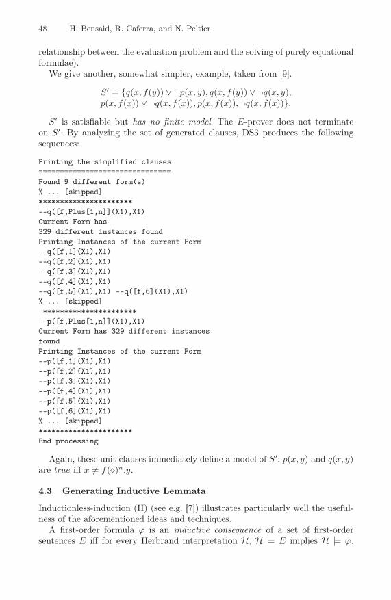
48 H. Bensaid, R. Caferra, and N. Peltier
relationship between the evaluation problem and the solving of purely equationalformulae).
We give another, somewhat simpler, example, taken from [9].
S′ = {q(x, f(y)) ∨ ¬p(x, y), q(x, f(y)) ∨ ¬q(x, y),p(x, f(x)) ∨ ¬q(x, f(x)), p(x, f(x)),¬q(x, f(x))}.
S′ is satisfiable but has no finite model. The E-prover does not terminateon S′. By analyzing the set of generated clauses, DS3 produces the followingsequences:
Printing the simplified clauses===============================Found 9 different form(s)% ... [skipped]**********************--q([f,Plus[1,n]](X1),X1)Current Form has329 different instances foundPrinting Instances of the current Form--q([f,1](X1),X1)--q([f,2](X1),X1)--q([f,3](X1),X1)--q([f,4](X1),X1)--q([f,5](X1),X1) --q([f,6](X1),X1)% ... [skipped]**********************--p([f,Plus[1,n]](X1),X1)Current Form has 329 different instancesfoundPrinting Instances of the current Form--p([f,1](X1),X1)--p([f,2](X1),X1)--p([f,3](X1),X1)--p([f,4](X1),X1)--p([f,5](X1),X1)--p([f,6](X1),X1)% ... [skipped]**********************End processing
Again, these unit clauses immediately define a model of S′: p(x, y) and q(x, y)are true iff x = f(�)n.y.
4.3 Generating Inductive Lemmata
Inductionless-induction (II) (see e.g. [7]) illustrates particularly well the useful-ness of the aforementioned ideas and techniques.
A first-order formula ϕ is an inductive consequence of a set of first-ordersentences E iff for every Herbrand interpretation H, H |= E implies H |= ϕ.

Towards Systematic Analysis of Theorem Provers Search Spaces 49
The idea behind II is to axiomatize the minimal model of E with a finite set ofaxioms, say A, in such a way that ϕ is an inductive consequence of E iff A∪E∪ϕis consistent (satisfiable). II is therefore also named proof by consistency. A iscalled an I-axiomatization.
A very interesting feature of this approach is that a general-purpose theoremprover can be used for proving inductive theorems (instead of having to usespecialized inductive provers such as SPIKE [3]). The only requirement is todesign dedicated strategies [7]. Of course, in most cases, the theorem provers willnot terminate on A ∪E ∪ ϕ thus we will not be able to detect satisfiability [17].In order to obtain a saturated set of clauses, it is often needed to add additionalinductive lemmata (stating properties that are not true in general, but thatare true in Herbrand interpretations). These lemmata must be provided by theuser. An interesting application of our technique is its ability to automaticallygenerate such inductive lemmata.
We give a simple example. Assume that we define a function l0 mappingeach integer n to a list of n elements “0”, and a function count(l) counting thenumber of occurrences of 0 in l. l0 and count can be defined by the followingaxiomatization A:
l0(0) = nil l0(s(n)) = cons(0, l0(n))count(l) = count’(l, 0) count’(nil, n) = n
count’(cons(0, l), n) = count’(l, s(n)) count’(cons(s(n), l),m) = count’(l,m)
Assume that we want to check that for all lists l, we have count(l0(n)) = n.This is an inductive property, because it is easy to check that count(l0(n)) = nis not a logical consequence of A (but any ground instance of count(l0(n)) = n isa consequence of A). We can use II to prove that this inductive property holds.
To this aim we need to add to A both the theorem to prove and an I-axiomatisation (see [7]). Then, we have to check that the obtained clause set issatisfiable. This ensures that there is at least one Herbrand model of A satisfyingcount(l0(n)) = n, and the I-axiomatisation guarantees that this model is minimal.
We use the usual I-axiomatisation:
{0 �= s(x), cons(u, v) �= nil, s(x) �= s(y) ∨ x = y,cons(x, y) �= cons(u, v) ∨ x = u, cons(x, y) �= cons(u, v) ∨ y �= v}.
The E-prover does not terminate on the obtained clause set, thus fails todetect satisfiability. The induction theorem prover SPIKE [3] also diverges on thisexample. But DS3 generates the following sequence: s(�)n.x = count’(l0(x), n).
Printing the simplified clauses===============================Found 20 different form(s)++equal([l0,1](0),nil)Current Form has 1 different instances foundPrinting Instances of the current Form++equal([l0,1](0),nil)% ... [skipped]**********************

50 H. Bensaid, R. Caferra, and N. Peltier
++equal([count_aux,1]([l0,1](X1),[s,Plus[1,n]](0)),[s,Plus[1,n]](X1))Current Form has 202 different instances foundPrinting Instances of the current Form++equal([count_aux,1]([l0,1](X1),[s,1](0)),[s,1](X1))++equal([count_aux,1]([l0,1](X1),[s,2](0)),[s,2](X1))++equal([count_aux,1]([l0,1](X1),[s,3](0)),[s,3](X1))++equal([count_aux,1]([l0,1](X1),[s,4](0)),[s,4](X1))++equal([count_aux,1]([l0,1](X1),[s,5](0)),[s,5](X1))++equal([count_aux,1]([l0,1](X1),[s,6](0)),[s,6](X1))++equal([count_aux,1]([l0,1](X1),[s,7](0)),[s,7](X1))++equal([count_aux,1]([l0,1](X1),[s,8](0)),[s,8](X1))++equal([count_aux,1]([l0,1](X1),[s,9](0)),[s,9](X1))++equal([count_aux,1]([l0,1](X1),[s,10](0)),[s,10](X1))++equal([count_aux,1]([l0,1](X1),[s,11](0)),[s,11](X1))**********************% ... [skipped]**********************++equal([count_aux,1](nil,[s,Plus[1,n]](0)),[s,Plus[1,n]](0))Current Form has 202 different instances foundPrinting Instances of the current Form++equal([count_aux,1](nil,[s,1](0)),[s,1](0))++equal([count_aux,1](nil,[s,2](0)),[s,2](0))++equal([count_aux,1](nil,[s,3](0)),[s,3](0))++equal([count_aux,1](nil,[s,4](0)),[s,4](0))++equal([count_aux,1](nil,[s,5](0)),[s,5](0))++equal([count_aux,1](nil,[s,6](0)),[s,6](0))++equal([count_aux,1](nil,[s,7](0)),[s,7](0))++equal([count_aux,1](nil,[s,8](0)),[s,8](0))++equal([count_aux,1](nil,[s,9](0)),[s,9](0))++equal([count_aux,1](nil,[s,10](0)),[s,10](0))++equal([count_aux,1](nil,[s,11](0)),[s,11](0))**********************++equal([s,Plus[2,n]](X1),[count_aux,1]([l0,1](X1),[s,Plus[2,n]](0)))Current Form has 201 different instances foundPrinting Instances of the current Form++equal([s,2](X1),[count_aux,1]([l0,1](X1),[s,2](0)))++equal([s,3](X1),[count_aux,1]([l0,1](X1),[s,3](0)))++equal([s,4](X1),[count_aux,1]([l0,1](X1),[s,4](0)))++equal([s,5](X1),[count_aux,1]([l0,1](X1),[s,5](0)))++equal([s,6](X1),[count_aux,1]([l0,1](X1),[s,6](0)))++equal([s,7](X1),[count_aux,1]([l0,1](X1),[s,7](0)))++equal([s,8](X1),[count_aux,1]([l0,1](X1),[s,8](0)))++equal([s,9](X1),[count_aux,1]([l0,1](X1),[s,9](0)))++equal([s,10](X1),[count_aux,1]([l0,1](X1),[s,10](0)))++equal([s,11](X1),[count_aux,1]([l0,1](X1),[s,11](0)))++equal([s,12](X1),[count_aux,1]([l0,1](X1),[s,12](0)))**********************++equal([s,Plus[1,n]](0),[s,Plus[1,n]](0))Current Form has 201 different instances foundPrinting Instances of the current Form

Towards Systematic Analysis of Theorem Provers Search Spaces 51
++equal([s,1](0),[s,1](0))++equal([s,2](0),[s,2](0))++equal([s,3](0),[s,3](0))++equal([s,4](0),[s,4](0))++equal([s,5](0),[s,5](0))++equal([s,6](0),[s,6](0))++equal([s,7](0),[s,7](0))++equal([s,8](0),[s,8](0))++equal([s,9](0),[s,9](0))++equal([s,10](0),[s,10](0))++equal([s,11](0),[s,11](0))**********************End processing
This obviously suggests to add the above property as an inductive lemma.However, since the E-prover does not handle I-terms, we need to expressthis property in first-order logic. This is done by introducing an addi-tional symbol f . f(x, n) encodes s(�)n.x. f is defined by the set of axioms:{f(x, 0) = x, f(x, s(n)) = s(f(x, n))}. The above property becomes: f(x, n) =count’(l0(x), n). By adding this property and the above axioms in the clauseset, we obtain a new set of clauses on which the E-prover terminates. Thus,satisfiability is detected and the above induction theorem is proven.
Obviously, the whole process can be automatized. Of course for more com-plicated examples the help of the user may be needed to select the appropriatelemma in a list of candidates.
Remark 1. The above process introduces additional function symbols in theclause set at hand. But this is not a problem. Indeed, it is obvious that if theclause set obtained after transformation is satisfiable, then a model of the origi-nal clause set exists. Thus, proving that the obtained clause set is satisfiable (bysaturation) suffices to prove that the initial clause set is satisfiable hence thatthe inductive theorem holds.
5 Conclusion
We have introduced a technique to analyze search spaces of ATP and shown itsusefulness by presenting three kinds of applications. The most promising one is– to our opinion – the possibility of generating (suggesting) inductive lemmata.Obviously our approach can be useful beyond AD, in all domains in which it isrelevant characterizing structurally (possibly infinite) sets of particular items, asfor example discovering infinite models, analogy, learning or analysis of programstraces,. . . Hopefully this work will help to develop research on search spaces ofautomated theorem provers by characterizing sets of particular consequences andit will open new fruitful possibilities of cooperation between theorem provers andsymbolic computation tools. It could be worth comparing our approach withexisting techniques used by model checkers in order to detect loops in systemexecutions.

52 H. Bensaid, R. Caferra, and N. Peltier
References
1. Amaniss, A., Hermann, M., Lugiez, D.: Set operations for recurrent term schemati-zations. In: Bidoit, M., Dauchet, M. (eds.) CAAP 1997, FASE 1997, and TAPSOFT1997. LNCS, vol. 1214, pp. 333–344. Springer, Heidelberg (1997)
2. Bernstein, M., Sloane, N.J.A.: Some Canonical Sequences of Integers. Linear Alge-bra and its Applications 228(1–3), 57–72 (1995)
3. Bouhoula, A., Kounalis, E., Rusinowitch, M.: SPIKE, an automatic theorem prover.In: Voronkov, A. (ed.) LPAR 1992. LNCS, vol. 624, pp. 460–462. Springer, London,UK (1992)
4. Caferra, R., Leitsch, A., Peltier, N.: Automated Model Building. Applied LogicSeries, vol. 31. Kluwer Academic Publishers, Boston (2004)
5. Chen, H., Hsiang, J.: Logic programming with recurrence domains. In: Leach Al-bert, J., Monien, B., Rodríguez-Artalejo, M. (eds.) Automata, Languages and Pro-gramming. LNCS, vol. 510, pp. 20–34. Springer, Heidelberg (1991)
6. Comon, H.: Disunification: A survey. In: Lassez, J.-L., Plotkin, G. (eds.) Com-putational Logic: Essays in Honor of Alan Robinson, pp. 322–359. MIT Press,Cambridge (1991)
7. Comon, H.: Inductionless induction. In: Robinson, A., Voronkov, A. (eds.) Hand-book of Automated Reasoning, ch. 14, pp. 913–962. North-Holland (2001)
8. Comon, H.: On unification of terms with integer exponents. Mathematical SystemTheory 28, 67–88 (1995)
9. Dreben, B., Goldfarb, W.D.: The Decision Problem, Solvable Classes of Quantifi-cational Formulas. Addison-Wesley, Reading (1979)
10. Hermann, M., Galbavý, R.: Unification of Infinite Sets of Terms schematized byPrimal Grammars. Theoretical Computer Science 176(1–2), 111–158 (1997)
11. Kleene, S.C.: Introduction to Metamathematics. North-Holland, Amsterdam(1952)
12. Peltier, N.: Increasing the capabilities of model building by constraint solving withterms with integer exponents. Journal of Symbolic Computation 24, 59–101 (1997)
13. Peltier, N.: A General Method for Using Terms Schematizations in Automated De-duction. In: Goré, R.P., Leitsch, A., Nipkow, T. (eds.) IJCAR 2001. LNCS (LNAI),vol. 2083, pp. 578–593. Springer, Heidelberg (2001)
14. Plotkin, G.D.: A note on inductive generalization. Machine Intelligence 5, 153–163(1970)
15. Plotkin, G.D.: A Further Note on Inductive Generalization. In: Meltzer, B., Michie,D. (eds.) Machine Intelligence 6, chapter 8, pp. 101–124. Edinburgh UniversityPress, Edinburgh (1971)
16. Schulz, S.: The E Equational Theorem Prover,http://www4.informatik.tu-muenchen.de/~schulz/WORK/eprover.html
17. Walsh, T.: A divergence critic for inductive proof. Journal of Artificial IntelligenceResearch 4, 209–235 (1996)
18. Wos, L.: Automated Reasoning, 33 Basic Research Problems. Prentice-Hall, En-glewood Cliffs (1988)

Continuation Semantics for Symmetric
Categorial Grammar
Raffaella Bernardi1 and Michael Moortgat2,�
1 Free University of Bozen-Bolzano, [email protected]
2 Utrecht Institute of Linguistics OTS, The [email protected]
Abstract. Categorial grammars in the tradition of Lambek [1,2] areasymmetric: sequent statements are of the form Γ ⇒ A, where the succe-dent is a single formula A, the antecedent a structured configuration offormulas A1, . . . , An. The absence of structural context in the succedentmakes the analysis of a number of phenomena in natural languagesemantics problematic. A case in point is scope construal: the different pos-sibilities to build an interpretation for sentences containing generalizedquantifiers and related expressions. In this paper, we explore a symmet-ric version of categorial grammar based on work by Grishin [3]. In addi-tion to the Lambek product, left and right division, we consider a dualfamily of type-forming operations: coproduct, left and right difference.Communication between the two families is established by means ofstructure-preserving distributivity principles. We call the resulting systemLG. We present a Curry-Howard interpretation for LG(/, \, �,�) deriva-tions. Our starting point is Curien and Herbelin’s sequent system for λμcalculus [4] which capitalizes on the duality between logical implication(i.e. the Lambek divisions under the formulas-as-types perspective) andthe difference operation. Importing this system into categorial grammarrequires two adaptations: we restrict to the subsystem where linearity con-ditions are in effect, and we refine the interpretation to take the left-rightsymmetry and absence of associativity/commutativity into account. Wediscuss the continuation-passing-style (CPS) translation, comparing thecall-by-value and call-by-name evaluation regimes.We showthat in the lat-ter (but not in the former) the types of LG are associated with appropriatedenotational domains to enable a proper treatment of scope construal.
1 Background
Lambek-style categorial grammars offer an attractive computational perspectiveon the principle of compositionality: under the Curry-Howard interpretation,� We thank Chris Barker and Ken Shan for sharing their view on continuation seman-
tics with us at an earlier presentation of Lambek-Grishin calculus at the workshopProof Theory at the Syntax-Semantics Interface (LSA Institute, Harvard/MIT, July2005). Special thanks to Peter Selinger, for helpful discussion on the duality be-tween call-by-value and call-by-name during GEOCAL’06 (Marseille-Luminy, Feb-ruary 2006) and to Philippe de Groote for bringing Curien and Herbelin’s work toour attention. All errors remain our own.
D. Leivant and R. de Queiroz (Eds.): WoLLIC 2007, LNCS 4576, pp. 53–71, 2007.c© Springer-Verlag Berlin Heidelberg 2007

54 R. Bernardi and M. Moortgat
derivations are associated with instructions for meaning assembly. In natural lan-guage semantics, scope construal of generalized quantifier expressions presents anideal testing ground to bring out the merits of this approach. Scope construal ex-emplifies a class of phenomena known as in situ binding. An in situ binder syntac-tically occupies the position of a phrase of type A; semantically, it binds an A-typevariable in that position within a context of type B, producing a value of type Cas a result. The inference pattern of (1) (from [5]) schematically captures this be-haviour in the format of a sequent rule. The challenge is to solve the equation forthe type alias q(A, B, C) in terms of the primitive type-forming operations.
Δ[x : A] ⇒ N : B Γ [y : C] ⇒ M : D
Γ [Δ[z : q(A, B, C)]] ⇒ M [y := (z λx.N)] : D . (1)
It is a poignant irony that precisely in the area of scope construal, theperformance of the original Lambek calculus (whether in its associative or non-associative incarnation) is disappointing. For a sentence-level generalized quan-tifier (GQ) phrase, we have A = np, B = C = s in (1). The type-formingoperations available to define q(np, s, s) are the left and right slashes. A firstproblem is the lack of type uniformity. Given standard modeltheoretic assump-tions about the interpretation of the type language, an assignment s/(np\s) toa GQ phrase is associated with an appropriate domain of interpretation (a setof sets of individuals), but with such a type a GQ is syntactically restricted tosubject positions: for phrase-internal GQ occurrences, context-dependent extralexical type assignments have to be postulated. Second, this lexical ambiguitystrategy breaks down as soon as one considers non-local scope construal, wherethe distance between the GQ occurrence and the sentential domain where itestablishes its scope can be unbounded.
The solutions that have been proposed in the type-logical literature we con-sider suboptimal. The type-shifting approach of Hendriks [6] and the multimodalaccounts based on wrapping operations of Morrill and co-workers [7,8] each breakthe isomorphic relation between derivations and terms that is at the heart of theCurry-Howard interpretation. Hendriks introduces a one-to-many dichotomy be-tween syntactic and semantic derivations. Morrill makes the opposite choice: amultiplicity of syntactically distinct implicational operations which collapse atthe semantic level.
The approach we develop in the sections below sticks to the minimal categoriallogic: the pure logic of residuation. We overcome the expressive limitations of theLambek calculi by lifting the single succedent formula restriction and move to asymmetric system where the Lambek connectives (product, left and right division)coexist with a dual family (coproduct, right and left difference). The communica-tion between these two families is expressed in terms of Grishin’s [3] distributiv-ity principles. Figure 1 schematically presents the outline of the paper. In §2 wepresent LG in algebraic format and discuss the symmetries that govern the vo-cabulary of type-forming operations. In §3 we present a ‘classical’ term languagefor the LG type system, and we discuss how a term τ of type A is obtained asthe Curry-Howard image of an LG sequent derivation π. In §4 we then study the

Continuation Semantics for Symmetric Categorial Grammar 55
CPS interpretation of types and terms, comparing the dual call-by-value �·� andcall-by-name �·� regimes. Under the CPS interpretation, the classical terms forLG derivations are transformed into terms of the simply typed lambda calculus— the terms that code proofs in positive intuitionistic logic. The λ→ terms thusobtained adequately reflect NL meaning composition, and (unlike the terms forMultiplicative Linear Logic or its categorial equivalent LP) they are obtained ina structure-preserving way. In §5 we illustrate the approach with a discussion ofscope construal. We investigate under what conditions the lexical constants of theoriginal Lambek semantics can be lifted to the call-by-value �·� and/or call-by-name �·� level, and study how the λ→ terms one obtains after this transformationand β normalisation encode the different possibilities for scope construal. In theconcluding section §6, we point to some directions for future work.
π ≈ τAcbv ��
cbn
��
�τ� : �A��·�
��·∞
�����������
��������
���β
���τ� : �A�
�·���
β�� λ→
Fig. 1. Outline of the paper
Relation to previous work. Lambek [9] was the first paper to bring Grishin’swork under the attention of a wider public. Lambek’s bilinear systems are bothstronger and weaker than what we propose here: they have hard-wired associa-tivity for ⊗, ⊕, which means that control over constituent structure is lost; inaddition, only half of the Grishin laws are taken into account (G1, G3 in Fig-ure 2), an omission that precludes the account of non-peripheral scope construalpresented here. De Groote [10] introduced λμ calculus and continuations into thelinguistic discussion of scope construal; Barker and Shan, in a series of papers([11,12,13] among others), have been advocating this approach for a variety ofsemantic phenomena. We discuss the relation of our proposal to theirs in §6. Du-ality between the call-by-value and call-by-name evaluation strategies has beenobtained in [14,4,15], among others. Our starting point is the Curien/Herbelinsystem because, in contrast to the other cited works, it has implication anddifference as primitive operations.
2 The Lambek-Grishin Calculus
The calculus that we will use in this paper is presented in Figure 2. We refer tothis system as LG. In (2), one finds the extended vocabulary of LG: the famil-iar Lambek operators ⊗, \, / are complemented with a family ⊕, , �. In verbalcommunication, we pronounce B\A as ‘B under A’, A/B as ‘A over B’, B � A
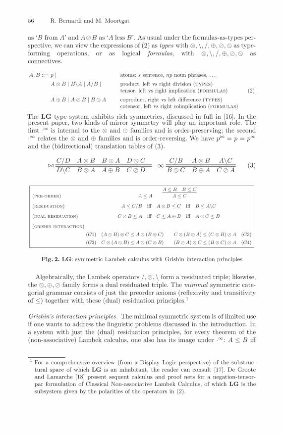
56 R. Bernardi and M. Moortgat
as ‘B from A’ and AB as ‘A less B’. As usual under the formulas-as-types per-spective, we can view the expressions of (2) as types with ⊗, \, /, ⊕, , � as type-forming operations, or as logical formulas, with ⊗, \, /, ⊕, , � asconnectives.
A,B ::= p | atoms: s sentence, np noun phrases, . . .
A⊗B | B\A | A/B | product, left vs right division (types)tensor, left vs right implication (formulas)
A⊕B | AB | B �A coproduct, right vs left difference (types)cotensor, left vs right coimplication (formulas)
(2)
The LG type system exhibits rich symmetries, discussed in full in [16]. In thepresent paper, two kinds of mirror symmetry will play an important role. Thefirst ·�� is internal to the ⊗ and ⊕ families and is order-preserving; the second·∞ relates the ⊗ and ⊕ families and is order-reversing. We have p�� = p = p∞
and the (bidirectional) translation tables of (3).
�C/D A ⊗ B B ⊕ A D � C
D\C B ⊗ A A ⊕ B C D∞
C/B A ⊗ B A\C
B � C B ⊕ A C A(3)
(pre-order) A ≤ A
A ≤ B B ≤ C
A ≤ C
(residuation) A ≤ C/B iff A ⊗ B ≤ C iff B ≤ A\C(dual residuation) C � B ≤ A iff C ≤ A ⊕ B iff A � C ≤ B
(grishin interaction)
(G1) (A � B) ⊗ C ≤ A � (B ⊗ C) C ⊗ (B � A) ≤ (C ⊗ B) � A (G3)
(G2) C ⊗ (A � B) ≤ A � (C ⊗ B) (B � A) ⊗ C ≤ (B ⊗ C) � A (G4)
Fig. 2. LG: symmetric Lambek calculus with Grishin interaction principles
Algebraically, the Lambek operators /, ⊗, \ form a residuated triple; likewise,the �, ⊕, family forms a dual residuated triple. The minimal symmetric cate-gorial grammar consists of just the preorder axioms (reflexivity and transitivityof ≤) together with these (dual) residuation principles.1
Grishin’s interaction principles. The minimal symmetric system is of limited useif one wants to address the linguistic problems discussed in the introduction. Ina system with just the (dual) residuation principles, for every theorem of the(non-associative) Lambek calculus, one also has its image under ·∞: A ≤ B iff
1 For a comprehensive overview (from a Display Logic perspective) of the substruc-tural space of which LG is an inhabitant, the reader can consult [17]. De Grooteand Lamarche [18] present sequent calculus and proof nets for a negation-tensor-par formulation of Classical Non-associative Lambek Calculus, of which LG is thesubsystem given by the polarities of the operators in (2).
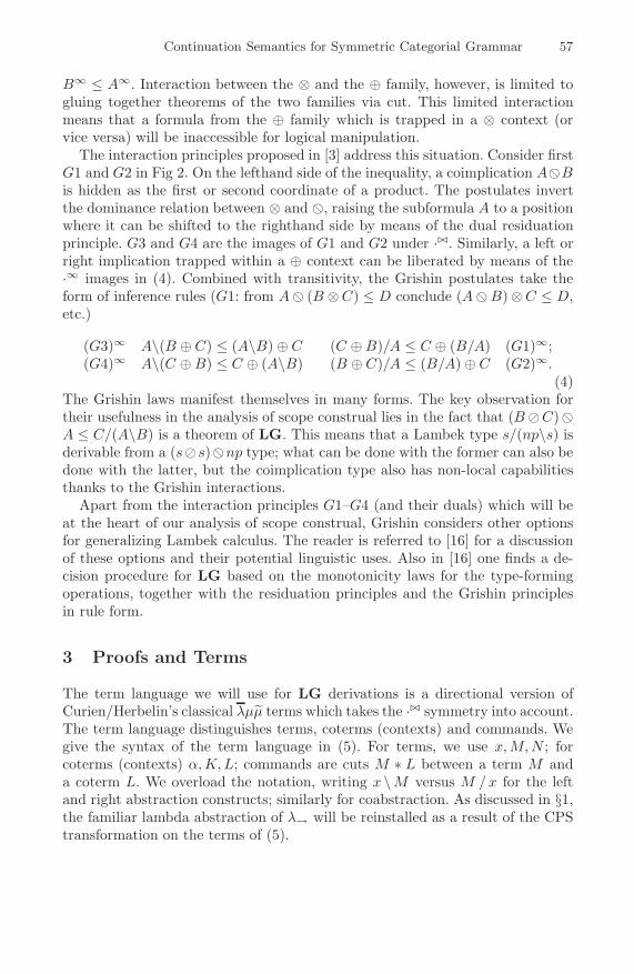
Continuation Semantics for Symmetric Categorial Grammar 57
B∞ ≤ A∞. Interaction between the ⊗ and the ⊕ family, however, is limited togluing together theorems of the two families via cut. This limited interactionmeans that a formula from the ⊕ family which is trapped in a ⊗ context (orvice versa) will be inaccessible for logical manipulation.
The interaction principles proposed in [3] address this situation. Consider firstG1 and G2 in Fig 2. On the lefthand side of the inequality, a coimplication A�Bis hidden as the first or second coordinate of a product. The postulates invertthe dominance relation between ⊗ and �, raising the subformula A to a positionwhere it can be shifted to the righthand side by means of the dual residuationprinciple. G3 and G4 are the images of G1 and G2 under ·��. Similarly, a left orright implication trapped within a ⊕ context can be liberated by means of the·∞ images in (4). Combined with transitivity, the Grishin postulates take theform of inference rules (G1: from A � (B ⊗ C) ≤ D conclude (A � B) ⊗ C ≤ D,etc.)
(G3)∞ A\(B ⊕ C) ≤ (A\B) ⊕ C(G4)∞ A\(C ⊕ B) ≤ C ⊕ (A\B)
(C ⊕ B)/A ≤ C ⊕ (B/A) (G1)∞;(B ⊕ C)/A ≤ (B/A) ⊕ C (G2)∞.
(4)The Grishin laws manifest themselves in many forms. The key observation fortheir usefulness in the analysis of scope construal lies in the fact that (B C)�A ≤ C/(A\B) is a theorem of LG. This means that a Lambek type s/(np\s) isderivable from a (ss)�np type; what can be done with the former can also bedone with the latter, but the coimplication type also has non-local capabilitiesthanks to the Grishin interactions.
Apart from the interaction principles G1–G4 (and their duals) which will beat the heart of our analysis of scope construal, Grishin considers other optionsfor generalizing Lambek calculus. The reader is referred to [16] for a discussionof these options and their potential linguistic uses. Also in [16] one finds a de-cision procedure for LG based on the monotonicity laws for the type-formingoperations, together with the residuation principles and the Grishin principlesin rule form.
3 Proofs and Terms
The term language we will use for LG derivations is a directional version ofCurien/Herbelin’s classical λμμ terms which takes the ·�� symmetry into account.The term language distinguishes terms, coterms (contexts) and commands. Wegive the syntax of the term language in (5). For terms, we use x, M, N ; forcoterms (contexts) α, K, L; commands are cuts M ∗ L between a term M anda coterm L. We overload the notation, writing x \ M versus M /x for the leftand right abstraction constructs; similarly for coabstraction. As discussed in §1,the familiar lambda abstraction of λ→ will be reinstalled as a result of the CPStransformation on the terms of (5).

58 R. Bernardi and M. Moortgat
x ∈ TermA if x ∈ VarA
(l abstraction) x\M ∈ TermB\A if x ∈ VarB ,M ∈ TermA
(r abstraction) M/x ∈ TermA/B if x ∈ VarB ,M ∈ TermA
(l coapplication) K �M ∈ TermB�A if K ∈ CoTermB ,M ∈ TermA
(r coapplication) M �K ∈ TermA�B if K ∈ CoTermB ,M ∈ TermA
(r shift) μα.(x ∗K) ∈ TermB if α ∈ CoVarB , x ∈ VarA,K ∈ CoTermA
α ∈ CoTermA if α ∈ CoVarA
(l application) M �K ∈ CoTermB\A if K ∈ CoTermA,M ∈ TermB
(r application) K �M ∈ CoTermA/B if K ∈ CoTermA,M ∈ TermB
(l coabstr) α�K ∈ CoTermB�A if α ∈ CoVarB ,K ∈ CoTermA
(r coabstr) K α ∈ CoTermA�B if α ∈ CoVarB ,K ∈ CoTermA
(l shift) μx.(M ∗ α) ∈ CoTermA if x ∈ VarA,M ∈ TermB , α ∈ CoVarB
(5)
As in the case of the Lambek calculus, for LG we are interested in the resource-sensitive sublanguage. This means that the (co)abstraction and (co)applicationcases are subject to a linearity condition: the (co)variable bound in a (co)abstraction occurs free exactly once in the body; in the (co)application casethe sets of free (co)variables of the term and coterm involved are disjoint. Ouruse of cut is restricted to patterns x∗K (M ∗α) in the shift right (left) construct,where μ (μ) obeys the single-bind restriction.
The dualities we discussed for the type system extend to the term language:(6) and (7). The latter acts on the directional constructs; identity otherwise.
x∞ = α(x \ M)∞ = M∞ α(M /x)∞ = α � M∞
(M � K)∞ = K∞� M∞
(K � M)∞ = M∞� K∞
(μβ.(x ∗ K))∞ = μy.(K∞ ∗ α)
α∞ = x;(K α)∞ = x \ K∞;(α � K)∞ = K∞ / x;(M � K)∞ = K∞ � M∞;(K � M)∞ = M∞ � K∞;
(μy.(M ∗ α))∞ = μβ.(x ∗ M∞).(6)
(M � K)�� = K�� � M�� (M � K)�� = K��� M��;
(x \ M)�� = M�� / x (K α)�� = α � K��.(7)
3.1 LG Sequent Calculus
In Lambek calculus, sequents are statements Γ ⇒ B, where Γ is a binary treewith formulas A1,. . . ,An at the yield, and B is a single formula. The structure-building operation which puts together the antecedent tree is the counterpartof the ⊗ logical operation. In LG, sequents Γ ⇒ Δ can have structures bothin the antecedent and in the succedent. The sequent interpunction (which wewrite · ◦ ·) is the structural counterpart of ⊗ in the antecedent, and of ⊕in the succedent. Notice that in the absence of associativity, ◦ is a binaryoperation.
In the rules below, we decorate LG derivations with the terms of (5). We distin-
guish sequents ΓM−−→ Δ[B] and cosequents Γ [A] K−−→ Δ with proof term M and

Continuation Semantics for Symmetric Categorial Grammar 59
coterm K respectively. A sequent (cosequent) has precisely one active succedent(antecedent) formula. The active formula is unlabeled. The passive antecedent(succedent) formulas are labeled with distinct variables xi (covariables αi).
For the axiomatic case, we distinguish two versions, depending on whetherthe succedent or the antecedent is the active formula. The rules (�) and (�)make it possible to shift the focus from antecedent to succedent or vice versa.These rules are in fact restricted cuts, where one of the premises is axiomatic(Axiom or Co-Axiom).
x : Ax−−→ A
AxA
α−−→ α : ACo-Ax
. (8)
Γ [A] K−−→ Δ[α : B]
Γ [x : A]μα.(x ∗ K)−−−−−−−−→ Δ[B]
(�)Γ [x : A] M−−→ Δ[B]
Γ [A]�μx.(M ∗ α)−−−−−−−−→ Δ[α : B]
(�).
(9)
Let us now consider the sequent left and right rules for the connectives. Werestrict attention to the (co)implication fragment, i.e. we only cater for ⊗ and⊕ in their ‘structural’ form ◦ as antecedent resp. succedent punctuation. Therules of use for the (co)implications are given in (10): these are two-premiserules, introducing an implication (coimplication) in the antecedent (succedent).Notice that we find the ·�� and ·∞ symmetries here at the level of the in-ference rules, with ·∞ (·��) relating pairs of rules in the horizontal (vertical)dimension.
BK−−→ Δ Δ′ M−−→ Γ [A]
Δ′ M � K−−−−−→ Γ [(A B) ◦ Δ](R)
ΔM−−→ B Γ [A] K−−→ Δ′
Γ [Δ ◦ (B\A)] M � K−−−−−→ Δ′(\L)
(R) ← ·∞ → (\L)↑ ↑
·�� ·��↓ ↓
(�R) ← ·∞ → (/L)
BK−−→ Δ Δ′ M−−→ Γ [A]
Δ′ K � M−−−−−→ Γ [Δ ◦ (B � A)](�R)
ΔM−−→ B Γ [A] K−−→ Δ′
Γ [(A/B) ◦ Δ] K � M−−−−−→ Δ′(/L)
(10)
The rules of proof for the (co)implications are given in (10): these are one-premise rules, introducing an implication (coimplication) in the succedent(antecedent).

60 R. Bernardi and M. Moortgat
x : B ◦ ΓM−−→ Δ[A]
Γx \M−−−−→ Δ[B\A]
(\R) Γ [A] K−−→ Δ ◦ α : B
Γ [A B] K � α−−−−−→ Δ(L)
(\R) ← ·∞ → (L)↑ ↑
·�� ·��↓ ↓
(/R) ← ·∞ → (�L)
Γ ◦ x : BM−−→ Δ[A]
ΓM / x−−−−→ Δ[A/B]
(/R) Γ [A] K−−→ α : B ◦ Δ
Γ [B � A] α � K−−−−−→ Δ(�L)
(11)
Observe that to prove the soundness of the coimplication (implication) rules ofproof from the algebraic presentation, one uses the Grishin interaction principlesto move the B subformula upwards through the ⊗ context (⊕ context), and thenshifts it to the succedent (antecedent) part via the residuation principles. TheGrishin interaction principles, in other words, are absorbed in these rules of proof.We illustrate this in (12) for (\R), writing Γ • (Δ◦) for the formula equivalent ofan antecedent (succedent) structure. The vertical dots abbreviate a successionof Grishin interaction steps.
B ⊗ Γ • ≤ Δ◦[A]Γ • ≤ B\Δ◦[A]....Γ • ≤ Δ◦[B\A] (12)
As indicated in §2, we will use the formula (B C)� A to do the work of thein situ binder schema q(A, B, C). (Alternatively, we could have used its ·�� dualA(C�B).) The (qL) and (qR) rules of Fig 3 have the status of derived inferencerules. We will use them in §5 to present proofs and terms in a more compact for-mat. In §A we give a worked-out derivation of (BC)�A ⇒ C/(A\B), togetherwith further abbreviatory conventions. The reader may want to check that a cutof (qR) against (qL) can be rewritten with cuts on the subformulae A, B, C, asrequired: cobind(MA, KB, βC)∗bind(xA, NB, LC) −→β M∗μx.(μβ.(N∗K)∗L).One should keep in mind that (qL) and (qR) are short-cuts, i.e. ways of abbrevi-ating a sequence of n inference steps as a one-step inference. For some theoremsof LG, one cannot take a short-cut: their derivation requires the individual in-ference rules for the connectives involved. The type transition (B C) � A ⇒((D\B) (D\C)) � A is an example. Its derivation is given in [16].
4 Interpretation: Continuation Semantics
We turn now to an interpretation for LG derivations in the continuation-passing-style (CPS). In the semantics of programming languages, CPS interpretation has

Continuation Semantics for Symmetric Categorial Grammar 61
CL−−→ Δ Γ [x : A]
N−−→ B
Γ [(B � C) � A]bind(x, N, L)−−−−−−−−−−−→ Δ
(qL)
�
CL−−→ Δ Γ [x : A]
N−−→ B
Γ [x : A]N � L−−−−−→ (B � C) ◦ Δ
(�R)
Γ [A]eμx.((N � L) ∗ γ)−−−−−−−−−−−−−→ γ : (B � C), Δ
�
Γ [(B � C) � A]γ � (eμx.((N � L) ∗ γ))−−−−−−−−−−−−−−−−−−→ Δ
(�L)
BK−−→ Δ′ ◦ β : C Γ
M−−→ Δ[A]
Γcobind(M, K, β)−−−−−−−−−−−−−→ Δ[Δ′ ◦ ((B � C) � A)]
(qR)
�
BK−−→ Δ′ ◦ β : C
B � CK � β−−−−−→ Δ′
(�L)
ΓM−−→ Δ[A]
Γ(K � β) � M−−−−−−−−−−→ Δ[Δ′ ◦ ((B � C) � A)]
(�R)
Fig. 3. Derived inference rules for (B � C) � A ≈ q(A,B, C)
been a fruitful strategy to make explicit (and open to manipulation) aspects ofcomputation that remain implicit in a direct interpretation. In the direct in-terpretation, a function simply returns a value. Under the CPS interpretation,functions are provided with an extra argument for the continuation of the com-putation. This explicit continuation argument is then passed on when functionscombine with each other. Key concepts, then, are “computation”, “continua-tion” and “value” and they way they relate to each other for different evaluationstrategies.
Curien and Herbelin [4] develop the CPS interpretation for a classical systemwith an implication and a difference operation; call-by-value (cbv) �·� and call-by-name (cbn) �·� regimes are related by the duality between the implicationand difference operations. For LG we refine the Curien/Herbelin continuationsemantics to accommodate the left/right symmetry. We first consider the effectof the CPS interpretation on the level of types, comparing a call-by-value (cbv)and a call-by-name (cbn) regime; then we define the CPS interpretation on thelevel of the terms of (5).
Types: call-by-value. The target type language has a distinguished type R ofresponses, products and functions; all functions have range R. For each type Aof the source language, the target language has values VA = �A�, continuationsKA = RVA (functions from VA to R) and computations CA = RKA (functionsfrom KA to R).2 Notice that given the canonical isomorphism A × B → C ∼=A → (B → C), one can also think of a VA\B as a function from A values toB computations. For p atomic, �p� = p. In (13), the �·� translations for the(co)implications are related in the vertical dimension by left/right symmetry ·��and in the horizontal dimension by arrow reversal ·∞: right difference is dual toleft division, left difference dual to right division.
2 In the schemas (13) and (14) we use exponent notation for function spaces, for com-parison with [4]. In the text, we usually shift to the typographically more convenientarrow notation, compare AB versus B → A.

62 R. Bernardi and M. Moortgat
�A\B� = R�A×R�B� �B A� = �B� × R�A;
�B/A� = RR�B�×�A �A � B� = R�A × �B�.(13)
Types: call-by-name. Under the call-by-name regime, for each type A of thesource language, the target language has continuations KA = �A� and com-putations CA = RKA . The call-by-name interpretation �·� is obtained as thecomposition of the ·∞ duality map and the �·� interpretation: �A� � �A∞�. Foratoms, �p� = �p∞� = p. For the (co)implications, compare the cbv intepretation(left) with the cbn interpretation (right) in (14).
�A\B� = R�A×R�B�RA�×R�B�
= �B A�;�B A� = �B� × R�A �B� × RA� = �A\B�;
�B/A� = RR�B�×�A RR�B�×A� = �A � B�;�A � B� = R�A × �B� RA� × �B� = �B/A�.
(14)
Notice that for the call-by-name regime, the starting point is the level ofcontinuations, not values as under call-by-value. Let’s take the definition ofB A by means of example. For call-by-value, one starts from �B A� (i.e.,VB�A) that is a pair VB × KA; hence its continuation is KB�A = (VB ×KA) → R and its computation is CB�A = ((VB × KA) → R) → R. Onthe other hand, the call-by-name interpretation starts at the level of contin-uations: �B A� = (KA × CB) → R and from this the computation is obtainedas usual, viz. CB�A = ((KA × CB) → R) → R, hence obtaining a higherorder function than the one computed under the call-by-value strategy. Thisdifference will play an important role in the linguistic application of the twostrategies.
Terms: cbv versus cbn. Given the different CPS types for left and right (co)implications, we can now turn to their interpretation at the term level. In (15),we give the cbv interpretation of terms, in (16) of coterms. We repeat the typinginformation from (5) to assist the reader. The call-by-name regime is the com-position of call-by-value and arrow reversal: �·� � �·∞�. This CPS interpretationof terms is set up in such a way that for sequents with yield A1, . . . , An ⇒ B,the cbv interpretation represents the process of obtaining a B computation fromA1, . . . , An values; the cbn interpretation takes A1, . . . , An computations to a Bcomputation. See Propositions 8.1 and 8.3 of [4].
A �x� = λk.k x x : A
B\A �x \M� = λk.(k λ〈x, β〉.�M� β) x : B, M : A
A/B �M / x� = λk.(k λ〈β, x〉.�M� β) x : B, M : A
B � A �M � K� = λk.(�M� λy.(k 〈y, �K�〉)) M : A, K : B
A B �K � M� = λk.(�M� λy.(k 〈�K�, y〉)) M : A, K : B
B �μα.(x ∗ K)� = λα.(�K� x) α : B, x, K : A
(15)

Continuation Semantics for Symmetric Categorial Grammar 63
A �α� = α α : A
B � A �α � K� = λ〈α, x〉.(�K� x) α : B, K : A
A B �K α� = λ〈x, α〉.(�K� x) α : B, K : A
B\A �M � K� = λk.(�M� λx.(k 〈x, �K�〉)) M : B, K : A
A/B �K � M� = λk.(�M� λx.(k 〈�K�, x〉)) M : B, K : A
A �μx.(M ∗ α)� = λx.(�M� α) x : A, α, M : B(16)
5 Application: Scope Construal
In this section we turn to the linguistic application. Our aim is twofold. First weshow that a type assignment (ss)�np for generalized quantifier phrases solvesthe problems with s/(np\s) mentioned in §1: the type (s s) � np uniformlyappears in positions that can be occupied by ordinary noun phrases, and it givesrise to ambiguities of scope construal (local and non-local) in constructions withmultiple GQ and/or multiple choices for the scope domain. Second, we relatethe CPS interpretation to the original interpretation for Lambek derivationsby defining translations �·�, �·� lifting the lexical constants from the type theyhave in the original Lambek semantics to the type required by the cbv or cbnlevel. To realize this second aim, we assume that the result type R is the typeof truth values. For the rest our modeltheoretic assumptions are standard. Thedomain of interpretation for np values is E (the set of individuals), for s valuesit is {0, 1} (the set of truth values). Out of E and {0, 1} one then constructscomplex domains in terms of function spaces and Cartesian products. In thecase of the original Lambek semantics (or Montague grammar) these domainsof interpretation are obtained indirectly, via a mapping between syntactic andsemantic types where np′ = e, s′ = t and (A\B) = (B/A) = A′ → B′, withDome = E and Domt = {0, 1}.
We start with a fully worked-out example of a ‘S goes to NP VP’ combina-tion, ‘Alice left’. The official sequent derivation is given in (17). Consulting thedictionary of Table 1, we fill in the lexical items alice and left of type np andnp\s respectively for the x and y parameters of the proof term. Call the resultingterm M . We now compare the CPS transformation of M under the cbv and cbnexecution regimes as defined in (15) and (16).
x : npx−−→ np s
α−−→ α : s
x : np ◦ np\sx � α−−−−→ α : s
(\L)
x : np ◦ y : np\sμα.(y ∗ (x � α))−−−−−−−−−−−−→ s
(�)(17)
Consider first cbv, on the left in Figure 4. Recall that under the cbv regimea sequent with yield A1, . . . , An ⇒ B maps the Ai values to a B computation.A value of type np\s (Vnp\s), as we see in Table 1, is a function taking a pairof an np value and an s continuation to the result type R, i.e. Vnp × Ks → R.

64 R. Bernardi and M. Moortgat
μα.(y ∗ (x � α))
lex
��μα.(left ∗ (alice � α)) (= M)
�M�cbv
��������������������M�=�M∞�
cbn������������������������
λc.(�left� 〈�alice�, c〉)�·�
��
λc.(�left� 〈c, �alice�〉)�·���
λc.(λ〈x, c′〉.(c′ (left x)) 〈alice, c〉)
β �������������������λc.(λ〈c′, q〉.(q λx.(c′ (left x))) 〈c, λc.(c alice)〉)
�������������������
λc.(c (left alice))
Fig. 4. ‘Alice left’: cbv versus cbn
Combining Vnp and Vnp\s we obtain an s computation, i.e. (s → R) → R,by giving the Vnp\s function the pair it requires, and abstracting over the Ks
component. This is what we see in �M� = λc.(�left� 〈�alice�, c〉). The next stepis to relate the cbv CPS interpretation to the original semantics of the Lambekcalculus. In the original semantics, ‘Alice’ and ‘left’ would be interpreted interms of constants of type e and e → t respectively. The mapping �·� in Table 2produces terms of type Vnp and Vnp\s from constants alice and left of type eand e → t. Substituting these in �M� (and β conversion) gives λc.(c (left alice)).Combined with the trivial s continuation (the identity function on {0, 1}) oneobtains (left alice).
On the right in Figure 4 we have the cbn interpretation. Under the cbn regime,a sequent with yield A1, . . . , An ⇒ B maps Ai computations to a B computation.We obtain the cbn interpretation by duality: �M� = �M∞� = �μx.((x � alice) ∗left)�, i.e. we read off the cbn interpretation from the mirror image derivation(np◦np\s ⇒ s)∞, which is s ⇒ snp◦np. For the lexical items involved, Table 1gives the continuation types �A� corresponding to the source language types A.To obtain the required types for A computations, we take functions from thesecontinuations into R. Specifically, the verb �left� in this case is interpreted as afunction taking a pair Ks × Cnp into R; the noun phrase argument �alice� alsois of type Cnp, i.e. (Vnp → R) → R. Combining these produces a result of typeCs again by abstracting over the Ks component of the pair given to the verb:
Table 1. Lexical entries. �A� is a value of type A; �A� is a continuation of type A.
word type alias �·� cbv �·� cbnalice, lewis np �np� �np�
left np\s iv R�np�×R�s� �s� × R�np�
teases (np\s)/np tv RR�iv�×�np� R�np� × �iv�thinks (np\s)/s tvs RR�iv�×�s� R�s� × �iv�
somebody s/(np\s) su RR�s�×�iv� R�iv� × �s�

Continuation Semantics for Symmetric Categorial Grammar 65
Table 2. Lifting lexical constants: cbv regime
�alice� = alice�lewis� = lewis�left� = λ〈x, c〉.(c (left x))
�teases� = λ〈v, y〉.(v λ〈x, c〉.(c ((teases y) x)))�somebody� = λ〈c, v〉.(∃ λx.(v 〈x, c〉))
�M� = λc.(�left� 〈c, �alice�〉). The mapping �·� in Table 3 produces terms oftype �np� → R and �np\s� → R (i.e. computations) from constants alice andleft of type e and e → t. Substituting these in �M� (and β conversion) gives thesame result as what we had under the cbv regime.
Table 3. Lifting lexical constants: cbn regime
�alice� = λc.(c alice)�lewis� = λc.(c lewis)
�left� = λ〈c, q〉.(q λx.(c (left x)))�teases� = λ〈q, 〈c, q′〉〉.(q′ λx.(q λy.(c ((teases y) x))))
�somebody� = λ〈v, c〉.(∃ λx.(v 〈c, λc′.(c′ x)〉))
The reader is invited to go throught the same steps for ‘Alice teases Lewis’.The term for the derivation is μα.(teases ∗ ((alice � α) � lewis)) (= M), withthe CPS interpretations in (18). The variable v is of type Knp\s, a verb phrasecontinuation. Consulting the cbv and cbn dictionaries of Tables 2 and 3, wecan substitute the required lambda terms for the lexical constants. After thissubstitution and β reduction, the cbv and cbn interpretations converge on λc.(c ((teases lewis) alice)).
�M� = λc.(�teases� 〈λv.(v 〈�alice�, c〉), �lewis�〉);�M� = λc.(�teases� 〈�lewis�, 〈c, �alice�〉〉). (18)
In Fig 5 we highlight the type structure of the CPS interpretations for thissentence, showing that (i) call-by-value produces terms consisting of functionapplications of values to pairs of values and continuations (left tree), whereas(ii) call-by-name produces terms consisting of the application of computation topairs of computations and continuation types. The observed difference will berelevant for the interpretation of generalized quantifiers expressions to which wenow turn.
Scope construal: simple subject GQ. In Table 1, one finds the CPS image un-der cbv and cbn of a Lambek-style s/(np\s) type assignment for a GQ expres-sion such as ‘somebody’. The corresponding lexical recipes for the cbv and cbnregimes is given in Tables 2 and 3, respectively. We leave it as an exercise for thereader to work through a derivation with these types/terms and to verify that atype assignment s/(np\s) is restricted to subject position and to local scope, as

66 R. Bernardi and M. Moortgat
Kt → R = Ct
R
V(e→(e→t))
teases
Ke→t × Ve
Ke→t
R
v : Ve→t Ve × Kt
Ve
alice
c : Kt
Ve
lewis
Kt → R = Ct
R
C(e→(e→t))
teases
Ce × (Kt × Ce)
Ce
lewis
Kt × Ce
c : Kt Ce
alice
Fig. 5. Type schemas for cbv (left) versus cbn (right)
we saw in §1. Let us turn then to derivations with the type assignment we haveproposed: (s s) � np (alias: gq) — a type assignment that will accommodateboth local and non-local scope construals. In (19) we compute the term for thederivation of ‘somebody left’, using the abbreviatory conventions discussed inthe Appendix (e.g., the 1 in step 2. stands for the proof term computed atstep 1.); in (20) its CPS transformation under cbv and cbn. (z : Vs, q : Cnp,y : Ks�s)
1. μα.(left∗(x�α)) s◦
np
x
(np\s)
left
2. μβ.(somebody∗bind(x, 1 , β))) s◦
gq
somebody
(np\s)
left
(19)
2 = N �N� = λc.((�left� 〈π2�somebody�, λz.(π1�somebody� 〈z, c〉)〉);�N� = λc.((�somebody� λ〈q, y〉.(y 〈c, λc′.(�left� 〈c′, q〉)〉)).
(20)The difference between cbv and cbn regimes observed above with respect to
�·�, �·� in the term in (18) turns out to be of particular interest here. In (21) wegive Vgq and Kgq for the cbv and cbn interpretations respectively. For cbv, thisis a pair of an ss continuation and an np value. This np value would have to berealised as the variable bound by the (logical) constant ∃ (of type (e → t) → t) inthe �·� translation. Such a binding relation cannot be established from the Ks�s
component of the pair. For cbn, the situation is different: �gq� has the requiredstructure to specify the lifted lexical recipe of (22). Q is a function taking a pairof a np computation and an (s s) continuation to the result type R. In thebody of the term, we apply Q to the Cnp term λk.(k x), where x is the e typevariable bound by ∃, and to the closed term λ〈c, p〉.(p c) obtained by applying

Continuation Semantics for Symmetric Categorial Grammar 67
the Cs variable p to the Ks variable c. In combination with �left� given above,�N� simplifies to λc.(∃ λx.(c (left x))) as required. From here on, we stay withthe cbn regime.
�gq� = R�s×R�s� × �np� �gq� = RR�np�×R�s�×R�s�. (21)
�somebody� = λQ.(∃ λx.(Q 〈λk.(k x), λ〈c, p〉.(p c)〉)). (22)
Ambiguous scope construal. First, compare ‘Alice teases Lewis’ with ‘everyoneteases somebody’ involving two GQ expressions. Starting from 1 μα.(teases ∗((x�α)�y)), the derivation can be completed in two ways, depending on whetherwe first bind the object variable y, then the subject variable x, or vice versa.On the left the subject wide scope reading, on the right the object wide scopereading.
1. s◦
np
x
tv
teases
np
yμα.(teases ∗ ((x � α) � y))
2a. s◦
np
x
tv
teases
gq
somebody
μβ.(somebody ∗ bind(y, 1 , β))
3a. s◦
gq
everybody
tv
teases
gq
somebody
μγ.(everybody ∗ bind(x, 2a , γ)))
2b. s◦
gq
everybody
tv
teases
np
y
μγ.(everybody ∗ bind(x, 1 , γ))
3b. s◦
gq
everybodytv
teases
gq
somebody
μβ.(somebody ∗ bind(y, 2b , β)))
By applying the method described with previous examples, one obtains the∀/∃ reading for (3a) and the ∃/∀ reading for (3b). First, the terms are interpretedby means of the definitions in (15) and (16) obtaining the following results:
�3a� = λc.(�evro.� λ〈q, y〉.(�smo.� λ〈p, z〉.(y 〈c, λc′.(z 〈c′, λc′′.(�teases� 〈p, 〈c′′, q〉〉)〉)〉)));�3b� = λc.(�smo.� λ〈p, z〉.(�evro.� λ〈q, y〉.(z 〈c, λc′.(y 〈c′, λc′′.(�teases� 〈p, 〈c′′, q〉〉)〉)〉))). (23)
where the variables p, q of type Cnp are for the object and subject respec-tively. The y, z variables are s s continuations, the (primed) c are s con-tinuations. Secondly, the �·� translation is applied, and the readings reduceto λc.(∀ λx.(∃ λy.(c ((teases y) x)))) and λc.(∃ λy.(∀ λx.(c ((teases y) x)))),respectively.

68 R. Bernardi and M. Moortgat
Local versus non-local scope. Consider the two readings for the sentence ‘Alicethinks somebody left’. The ambiguity arises here from the fact that in this con-text the GQ can non-deterministically select the embedded or the main clauses as its scope domain. We give the terms for these two derivations (local (a)versus non-local (b) scope) in (24), reusing the components 1 and 2 of (19),and the cbn interpretations of these terms in (25). These can be further reducedto (26) via a lexical recipe �thinks� = λ〈p, 〈c, q〉〉.(q λx.(c ((thinks (p λc.c)) x)))expressed in terms of a constant thinks of type t → (e → t).
a. μγ.(thinks ∗ ((alice � γ) � 2 ));b. μγ.(somebody ∗ bind(x, μγ′.(thinks ∗ ((alice � γ′) � 1 )), γ)).
(24)
�a� = λc.(�thinks� 〈λc′.(�somebody� λ〈q, y〉.(y 〈c′, λc′′.(�left� 〈c′′, q〉)〉)), 〈c,�alice�〉〉);�b� = λc.(�somebody� λ〈q, y〉.(y 〈c, λc′.(�thinks� 〈λc′′.(�left� 〈c′′, q〉), 〈c′,�alice�〉〉)〉)). (25)
�a� �β λc.(c ((thinks (∃ left)) alice));�b� �β λc.(∃ λy.(c ((thinks (left y)) alice))). (26)
6 Conclusions, Further Directions
In this paper we have moved from asymmetric Lambek calculus with a singlesuccedent formula to the symmetric Lambek-Grishin calculus, where both theantecedent and the succedent are formula structures, configured in terms of ⊗and ⊕ respectively, and where the ⊗ and ⊕ environments can interact in astructure-preserving way. This move makes it possible to import into the field ofnatural language semantics the powerful tools of λμ-calculus. The main attrac-tion of the proposed continuation semantics, in our view, lies in the fact that LGallows us to fully exploit the duality between Lambek’s directional /, \ implica-tions and the corresponding directional �, difference operations, at the level ofsyntax and at the level of semantics. We thus restore Curry’s original idea of anisomorphism between proofs and terms, rather than the weaker homomorphicview of standard Lambek (or Montagovian) semantics.
Our approach differs in a number of respects from the related work cited in§1. Abstracting away from the directionality issue, de Groote’s original applica-tion of λμ calculus to scope construal syntactically types generalized quantifierphrases as np with meaning representation μαKe(∃ α). As a result, a sentencewith multiple GQ phrases is associated with a unique parse/term; the multi-ple readings for that term are obtained as a result of the non-confluence of λμcalculus, which is considered as a feature, not a bug. Our approach in contrastis true to the principle that multiple readings can only arise as the images ofdistinct proofs, given the Curry-Howard isomorphism between proofs and terms.Barker [19,11] uses a simplified continuation semantics, which lifts types A to(A → R) → R ‘externally’, without applying the CPS transformation to theinternal structure of complex types. This breaks the symmetry which is at theheart of our dual treatment of /, \ vs �, . The structural-rule account of scopeflexibility in [12,13] suffers from commutativity problems.

Continuation Semantics for Symmetric Categorial Grammar 69
The approach described here, like Hendriks’s type-shifting approach, createsall combinatorial possibilities for scope construal. However, it is well known that,depending on the choice of particular lexical items, many of these construals willin fact be unavailable. Bernardi [20] uses the control modalities ♦, � to calibratethe scopal behaviour of particular classes of GQ expressions. Adding ♦, � anda pair of dually residuated modalities to LG is straightforward. In a follow-uppaper, we plan to study the continuation semantics of these operations, relatingthem to the shift and reset constructs one finds in the theory of functionalprogramming languages and that have been considered in [11,13].
Finally, the interpretation given here construes scopal ambiguities in a staticsetting. In a recent paper, de Groote [21] develops a continuation-based approachtowards dynamic interpretation. A natural topic for further research would be toinvestigate how to incorporate this dynamic perspective in our setting, and howto extend the approach of [21] with the difference operations and the concomitantGrishin interaction principles.
References
1. Lambek, J.: The mathematics of sentence structure. American MathematicalMonthly 65, 154–170 (1958)
2. Lambek, J.: On the calculus of syntactic types. In: Jakobson, R. (ed.) Structure ofLanguage and Its Mathematical Aspects. American Mathematical Society, 166–178(1961)
3. Grishin, V.: On a generalization of the Ajdukiewicz-Lambek system. In: Studiesin Nonclassical Logics and Formal Systems. Nauka, Moscow, pp. 315–334 [Eng-lish translation in Abrusci and Casadio (eds.) Proceedings 5th Roma Workshop,Bulzoni Editore, Roma, 2002] (1983)
4. Curien, P., Herbelin, H.: Duality of computation. In: International Conference onFunctional Programming (ICFP’00), pp. 233–243 [2005: corrected version] (2000)
5. Moortgat, M.: Generalized quantifiers and discontinuous type constructors. In:Bunt, H., van Horck, A. (eds.) Discontinuous Constituency, pp. 181–207. Walterde Gruyter, Berlin (1996)
6. Hendriks, H.: Studied flexibility. Categories and types in syntax and semantics.PhD thesis, ILLC, Amsterdam University (1993)
7. Morrill, G.: Discontinuity in categorial grammar. Linguistics and Philosophy. 18,175–219 (1995)
8. Morrill, G., Fadda, M., Valentin, O.: Nondeterministic discontinuous Lambek cal-culus. In: Proceedings of the Seventh International Workshop on ComputationalSemantics (IWCS7), Tilburg (2007)
9. Lambek, J.: From categorial to bilinear logic. In: Schroder-Heister, K.D.P. (ed.)Substructural Logics, pp. 207–237. Oxford University Press, Oxford (1993)
10. de Groote, P.: Type raising, continuations, and classical logic. In: van Rooy, R.,(ed.) Proceedings of the Thirteenth Amsterdam Colloquium, ILLC, Universiteitvan Amsterdam, pp. 97–101 (2001)
11. Barker, C.: Continuations in natural language. In: Thielecke, H. (ed.) CW’04: Pro-ceedings of the 4th ACM SIGPLAN continuations workshop, Tech. Rep. CSR-04-1,School of Computer Science, University of Birmingham, pp. 1–11 (2004)

70 R. Bernardi and M. Moortgat
12. Barker, C., Shan, C.: Types as graphs: Continuations in type logical grammar.Language and Information 15(4), 331–370 (2006)
13. Shan, C.: Linguistic side effects. PhD thesis, Harvard University (2005)14. Selinger, P.: Control categories and duality: on the categorical semantics of the
lambda-mu calculus. Math. Struct. in Comp. Science 11, 207–260 (2001)15. Wadler, P.: Call-by-value is dual to call-by-name. In: ICFP, Uppsala, Sweden (Au-
gust 2003)16. Moortgat, M.: Symmetries in natural language syntax and semantics: the Lambek-
Grishin calculus (this volume). In: Leivant, D., de Queiros, R. (eds.) WoLLIC’07.Proceedings 14th Workshop on Logic, Language, Information and Computation.LNCS, vol. 4576, Springer, Heidelberg (2007)
17. Gore, R.: Substructural logics on display. Logic Journal of IGPL 6(3), 451–504(1997)
18. de Groote, P., Lamarche, F.: Classical non-associative Lambek calculus. StudiaLogica 71, 335–388 (2002)
19. Barker, C.: Continuations and the nature of quantification. Natural language se-mantics 10, 211–242 (2002)
20. Bernardi, R.: Reasoning with Polarity in Categorial Type Logic. PhD thesis,Utrecht Institute of Linguistics OTS (2002)
21. de Groote, P.: Towards a Montagovian account of dynamics. In: Proceedings SALT16, CLC Publications (2006)
A Shorthand Format for Sequent Derivations
As an example of the LG term assignment, (27) gives the derivation showinghow one obtains a Lambek-style GQ type C/(A\B) from a (B C) � A source.
Cα−−→ α : C
z : A z−−→ A Bγ−−→ γ : B
z : A ◦A\B z � γ−−−−→ γ : B(\L)
z : A ◦ y : A\B μγ.(y ∗ (z � γ))−−−−−−−−−−−→ B
(�)
z : A ◦ y : A\B (μγ.(y ∗ (z � γ))) � α−−−−−−−−−−−−−−−→ B C ◦ α : C(R)
A ◦ y : A\B eμz.((μγ.(y ∗ (z � γ))) � α) ∗ β)−−−−−−−−−−−−−−−−−−−−−−→ β : B C ◦ α : C(�)
(B C) �A ◦ y : A\B β � (eμz.((μγ.(y ∗ (z � γ))) � α) ∗ β))−−−−−−−−−−−−−−−−−−−−−−−−−−−→ α : C(�L)
x : (B C) �A ◦ y : A\B μα.(x ∗ (β � (eμz.((μγ.(y ∗ (z � γ))) � α) ∗ β)))−−−−−−−−−−−−−−−−−−−−−−−−−−−−−−−−−−→ C
(�)
x : (B C) �A(μα.(x ∗ (β � (eμz.((μγ.(y ∗ (z � γ))) � α) ∗ β)))) / y−−−−−−−−−−−−−−−−−−−−−−−−−−−−−−−−−−−−−→ C/(A\B)
(/R)(27)
This example shows that except for the most simple derivations, the sequenttree format soon becomes unwieldy. Below we introduce a more user-friendlyline format, which graphically highlights the tree structure of the antecedentand succedent parts. In the line format, each row has (a) a line number, (b) the(co)term for the currently active formula, and the antecedent (c) and succedent(d) structures in tree format. The cursor singles out the currently active formula.It takes the form ·• in the antecedent, and ·◦ in the succedent. With n we re-fer to the (co)term at line n. Compare (27) with the derivation for a sentence‘Somebody left’ in line format.

Continuation Semantics for Symmetric Categorial Grammar 71
line (co)term lhs tree rhs tree1. x np
x
np◦
2. α s• s
α
3. 1 � 2np
x
(np\s)•s
α
4. μα.(left ∗ 3 )np
x
(np\s)
left
s◦
5. β s• s
β
6. 4 � 5np
x
(np\s)
left
(s s)◦ s
β
7. μx.( 6 ∗ γ)np• (np\s)
left
(s s)
γ
s
β
8. γ � 7
((s s) � np)• (np\s)
left
s
β
9. μβ.(somebody ∗ 8 )((s s) � np)
somebody
(np\s)
left
s◦
We reduce the length of a derivation further using the (qL) and (qR) rules ofinference discussed in the main text and folding: a sequence of n (/, \R) (re-spectively (, �L)) one-premise inferences is folded into a one-step one-premiseinference; a (�) step (or (�) respectively) followed by a sequence of n (/, \L)(respectively (, �R)) two-premise inferences is folded into a one-step n + 1premise inference; an n premise inference with m non-lexical axiom premises iscontracted to an n−m premise inference. Where the succedent (antecedent) treeis just a point, we write the highlighted formula as the root of the antecedent(succedent) tree. The result of applying these conventions for the example sen-tence ‘somebody left’ is (19) in the main text.

Ehrenfeucht–Fraısse Games on Linear Orders
Ryan Bissell-Siders
Ryan [email protected]
http://www.math.helsinki.fi/
Abstract. We write strategies for both players in the Ehrenfeucht-Fraisse game played between two linear orders. We prove that our strate-gies win whenever possible. The strategy in a game of fixed, finite lengthfocuses the attention of both players on certain finite sets called ”totalinformation.” These finite sets are semimodels in the sense that if oneplayer does not have a winning strategy, then the other player can win,even when forced to choose only elements of a model which are indicatedby the total information.
These sets are semimodels– finite, nested models, such that a formulais satisfied in a linear order iff the formula is semimodel-satisfied in thecorresponding semimodel. The strategy implies the decidability of thetheory of linear order, and gives a completion of any formula by onewith quantifier rank only 2 larger than the original formula. The strat-egy generalizes directly to the infinitary theory of linear order.
Keywords: Ehrenfeucht–Fraısse game, semimodel, decision procedure,linear order, completion.
1 “Total Information” Is Sufficient for the EF Game
For any linear order λ, let λ+ be the ordered set of cuts in λ, i.e.
Definition 1. λ+ = ({(X,Y ) : X ∪ Y = λ, ∀x ∈ X∀y ∈ Y x < y}; (X,Y ) ≤(W,Z) iff X ⊆W ).
Definition 2. For any linear order λ and element x, let Thlock (λ, x) be {formulas
φ of quantifier rank k with the single variable v free : ∃E ∀A,B,C,D(A + E +B + λ+C + E +D |=[x/v] φ(v))} where A,B,C,D,E range over linear orders.
Our goal is to prove theorem 1, i.e., to find in any linear order λ and for anynatural number k a finite set Ik(λ) ⊆ λ+ such that λ ≡k λ′ iff Ik(λ) = Ik(λ′)and the same k− 1-quantifier local types Thloc
k−1(λ, x) are realized in both λ andλ′ at and between the elements of Ik.
Definition 3. Let Seq be the set of decreasing sequences of natural numbers. Fork any natural number, let Seq(k) be the set of descending sequences of naturalnumbers ≤ k − 2. Let <seq be lexicographical ordering on Seq.
D. Leivant and R. de Queiroz (Eds.): WoLLIC 2007, LNCS 4576, pp. 72–82, 2007.c© Springer-Verlag Berlin Heidelberg 2007
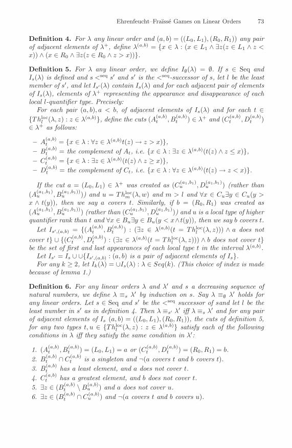
Ehrenfeucht–Fraısse Games on Linear Orders 73
Definition 4. For λ any linear order and (a, b) = ((L0, L1), (R0, R1)) any pairof adjacent elements of λ+, define λ(a,b) = {x ∈ λ : (x ∈ L1 ∧ ∃z(z ∈ L1 ∧ z <x)) ∧ (x ∈ R0 ∧ ∃z(z ∈ R0 ∧ z > x))}.Definition 5. For λ any linear order, we define I∅(λ) = ∅. If s ∈ Seq andIs(λ) is defined and s <seq s′ and s′ is the <seq-successor of s, let l be the leastmember of s′, and let Is′(λ) contain Is(λ) and for each adjacent pair of elementsof Is(λ), elements of λ+ representing the appearance and disappearance of eachlocal l-quantifier type. Precisely:
For each pair (a, b), a < b, of adjacent elements of Is(λ) and for each t ∈{Thloc
l (λ, z) : z ∈ λ(a,b)}, define the cuts (A(a,b)t , B
(a,b)t ) ∈ λ+ and (C(a,b)
t , D(a,b)t )
∈ λ+ as follows:
– A(a,b)t = {x ∈ λ : ∀z ∈ λ(a,b)t(z)→ z > x)},
– B(a,b)t = the complement of At, i.e. {x ∈ λ : ∃z ∈ λ(a,b)(t(z) ∧ z ≤ x)},
– C(a,b)t = {x ∈ λ : ∃z ∈ λ(a,b)(t(z) ∧ z ≥ x)},
– D(a,b)t = the complement of Ct, i.e. {x ∈ λ : ∀z ∈ λ(a,b)(t(z)→ z < x)}.
If the cut a = (L0, L1) ∈ λ+ was created as (C(a1,b1)u , D
(a1,b1)u ) (rather than
(A(a1,b1)u , B
(a1,b1))u )) and u = Thloc
m (λ,w) and m > l and ∀x ∈ Cu∃y ∈ Cu(y >x ∧ t(y)), then we say a covers t. Similarly, if b = (R0, R1) was created as(A(a1,b1)
u , B(a1,b1))u ) (rather than (C(a1,b1)
u , D(a1,b1)u )) and u is a local type of higher
quantifier rank than t and ∀x ∈ Bu∃y ∈ Bu(y < x∧t(y)), then we say b covers t.Let Is′,(a,b) = {(A(a,b)
t , B(a,b)t ) : (∃z ∈ λ(a,b)(t = Thloc
l (λ, z))) ∧ a does notcover t} ∪ {(C(a,b)
t , D(a,b)t ) : (∃z ∈ λ(a,b)(t = Thloc
l (λ, z))) ∧ b does not cover t}be the set of first and last appearances of each local type t in the interval λ(a,b).
Let Is′ = Is ∪ ∪{Is′,(a,b) : (a, b) is a pair of adjacent elements of Is}.For any k ≥ 2, let Ik(λ) = ∪Is(λ) : λ ∈ Seq(k). (This choice of index is made
because of lemma 1.)
Definition 6. For any linear orders λ and λ′ and s a decreasing sequence ofnatural numbers, we define λ ≡s λ′ by induction on s. Say λ ≡∅ λ′ holds forany linear orders. Let s ∈ Seq and s′ be the <seq successor of sand let l be theleast number in s′ as in definition 4. Then λ ≡s′ λ′ iff λ ≡s λ′ and for any pairof adjacent elements of Is (a, b) = ((L0, L1), (R0, R1)), the cuts of definition 5,for any two types t, u ∈ {Thloc
l (λ, z) : z ∈ λ(a,b)} satisfy each of the followingconditions in λ iff they satisfy the same condition in λ′:
1. (A(a,b)t , B
(a,b)t ) = (L0, L1) = a or (C(a,b)
t , D(a,b)t ) = (R0, R1) = b.
2. B(a,b)t ∩C(a,b)
t is a singleton and ¬(a covers t and b covers t).3. B(a,b)
t has a least element, and a does not cover t.4. C(a,b)
t has a greatest element, and b does not cover t.5. ∃z ∈ (B(a,b)
t \B(a,b)u ) and a does not cover u.
6. ∃z ∈ (B(a,b)t ∩C(a,b)
u ) and ¬(a covers t and b covers u).

74 R. Bissell-Siders
7. ∃z ∈ A(a,b)t ∩D(a,b)
u and a doesn’t cover t and b doesn’t cover u.8. B(a,b)
t ∩C(a,b)t = ∅.
Lemma 1. If λ ≡k λ′, then for all s ∈ Seq(k), λ ≡s λ′.Proof: Suppose λ ≡s λ′, but λ �≡s′ λ′, where s′ is the <seq-sucessor of s. Weshow that player I has a winning strategy in EFk(λ, λ′), hence λ �≡k λ′.We first prove, by induction, claim k: If, in the game EFk(λ, λ′), player I playsthe first move in (as, bs) for all s ∈ Seq(k), where if s′ is the <seq-sucessor ofs and s < s′ ∈ Seq(k), then {as′ , bs′} ⊆ Is′ \ Is and as′ = (L(as′), R(as′)) andis defined in Is′ as (A(as,bs)
u(as′ ), B
(as,bs)u(as′)
) where u(as′) was not covered by as, or
as′ = (C(as,bs)u(as′ )
, D(as,bs)u(as′)
) where u(bs′) was not covered by bs, then player II mustanswer in (as, bs), for all s ∈ Seq(k).
Proof: suppose player II answer inside (ar, br), for all r ≤ s, but outside (as′ , bs′).Without loss of generality, suppose player I plays x0 above as′ , and player II playsy0 below as′ . Writing as = (L(as′), R(as′)), this means that player I played inR(as′), and player II played in L(as′).
Let the least number in s′ be l, so that u(as′) = Thlocl (λ, x) is a local type of
quantifier depth l. If x0 is the least element of R(as′), or the greatest element ofL(as′), then player II has lost, for then x0 has quantifier-rank-l local type u(as′),and there is no y ∈ λ′(as,bs) such that Thloc
k (λ′, y) = u(as′) and y < as′ , by theformula defining A and B or C and D in definition 5.
Let the greatest number in s′ be j ≤ k − 2; let j− be the <seq-precessor of(j), with domain {i : i < j}. Player I plays x1 at an element of λ of type u(a(j))
near a(j) in (aj− , bj−), where “near” means: if aj = (A(aj− ,bj− )
u(a(j)), B
(aj− ,bj− )
u(a(j))), then
player I plays x1 ≥ aj in λ and x1 should be the least element of B(aj− ,bj− )
u(aj)if
there is one, and otherwise, for each t ∈ {Thlocj−1(λ, z) : z ∈ λ} (a finite set)
which is realized for some z ∈ λ(aj− ,bj− ), if realizations of t are bounded frombelow in B
(aj− ,bj− )
u(aj), then all of those realizations occur above x1, and if t is
realized below every y ∈ B(aj− ,bj− )
u(aj), then t is realized a large number of times
(say, 10 + 210+210+k
or more) above x1. This is done to assure that I(j)∪r(λ>x1)will contain an ≡(j) copy of I(j)∪r(λ>as) whenever r is a descending sequence of
numbers < j. On the other hand, if aj = (C(aj− ,bj− )
u(a(j)), D
(aj− ,bj− )
u(a(j))), then player I
plays x1 ≤ aj in λ′ near the cut a(j), where, again, “near” means that x1 boundsto the left all quantifier-rank < j local types which can be bound to the left.
If player I plays x1 < a(j) = (C,D) < y0 ∈ λ′, and player II plays y1 inthe interval (aj− , bj−) and y1 < a(j) ∈ I(j), then we may consider the gameEFk−1(λ>y1 , λ′>x1), in which player I has played x0, and player II has answeredwith y0. We will show that this violates the induction hypothesis. We check, forr any decreasing sequence of numbers < j, that the set Ir defined in λ>x1 andλ′>y1 are ≡(j) to the sets I(k ∪ r) defined in λ and λ′ to the right of a(j). In

Ehrenfeucht–Fraısse Games on Linear Orders 75
this case, x1 was played close to as so that the only t ∈ {Thlocj−1(λ, z) : z ∈ λ}
which are realized to the right of x1 are those t which are realized to the rightof as or which are covered by as. A cut c enters I(k ∪ r) only if it was notcovered by a(j). Therefore, player I was able to play x1 < a(j) large enough thatno elements of type c exist in (x1, a(j)), when c ∈ I(k ∪ r). So, by claim k − 1,player II loses. If player I plays x1 < a(s) = (C,D) < y0 ∈ λ′, and player IIplays y1 outside the interval (aj− , bj−), then y1 < aj− , then we may considerthe game EFk−1(λ<a(j) , λ′<a(j) ) in which player I has played x1 and player IIhas played y1. Player II’s move disrespects Is, for s ∈ Seq(j). If player I playsx1 > a(j) = (A,B) ∈ λ, of the type for which a(j) was defined, and player IIplays y1 < a(j) ∈ λ, then we know that y1 is not of the same j-quantifier localtype as x1. This concludes the proof of claim k.
Now we assume λ ≡s λ′ and that player II must answer player I’s movesat the same elements or in the same interval between elements of Is, and weshow that λ �≡s′ λ′ gives player I a winning strategy. The definition of ≡s′ listsconditions under which it fails, so we show that player I can exploit each of thoseeventualities and win. Suppose that ≡s′ fails in the interval (a, b) of Is.
Case 1: Suppose (A(a,b)t , B
(a,b)t ) = (L0, L1) in λ, but not in λ′. That is, elements
of type t exist below any z ∈ λ(a,b). Then player I plays x0 ∈ λ′(a,b) below everyelement of type t in λ′(a,b), where t has quantifier rank l, the least element of s′.By Claim k, player II answers with y0 ∈ λ′(a,b). Now, for each initial segment sjof s the least element of which is > l, player I plays xj near asj in (a(sj)− , b(sj)−),as described in claim k, and player II answers, by claims k − 1 . . . k − j, in thesame intervals. After both players have played xj and yj close to asj , for allinitial segments sj , there is an element z of type t below y0 and above xj or yj(say, xj) in λ′. There may well be an element z′ of type t below x0 and aboveyj in λ, but for any such z′, Il(yj , z′) �≡l Il(yj , as). So player I plays xj+1 = z,and as the remaining l-many moves would prove that Thl(λ, yj+1) �= t, player IIplays some z′ of type t below asj . Player I proceeds, as in claim l, to prove thatIl(yj , z′) �≡l Il(yj , as).
As a result of case 1, we could add the condition – a covers t – to the list ofthe conditions in definition 6, the definition of λ ≡s λ′.Case 2: Suppose z is the only element of B(a,b)
t ∩ C(a,b)t in λ and that there are
two elements z0 < z1 of B(a,b)t ∩C(a,b)
t in λ′. If a does not cover t, player I playsx0 = z1. If b does not cover t, player I plays x0 = z0. If t has quantifier-rank l,then the next k− l− 2-many moves are spent isolating (a, b), after which playerI plays xk−l−1 = z0 after which player I spends the remaining l-many movesdefining Il(zs, z0), where zs = xj or zs = yj, zs is near the cut (L0, L1) = as,and since as did not cover t, the interval (zs, z) has no realization of t.
Case 3: Suppose B(a,b)t has a least element, z ∈ λ(a,b), but no least element in
λ′(a,b) and a does not cover t. Player I plays x0 = z, and then proves that (a, y0)contains an element of type t, as in the previous case.

76 R. Bissell-Siders
Case 4: Suppose z ∈ (B(a,b)t \B(a,b)
u ) in λ but B(a,b)t = B
(a,b)u in λ′, and a does not
cover u. Player I plays x0 = z, and then proves that (a, y0) contains an elementof type u, as in case 2.
Case 5: If b doesn’t cover u, player I plays x0 = an element of type t, x0 ∈(B(a,b)
t ∩ C(a,b)u ) and shows ∃z ∈ (x0, b) of type u. If a doesn’t cover t, player I
plays x0 = an element of type u, x0 ∈ (B(a,b)t ∩C(a,b)
u ) and shows ∃z ∈ (a, x0) oftype t.
Case 6: Player I plays x0 = z and shows (x0, b) contains no element of type uand (a, x0) contains no element of type t.
Case 7: This holds iff ¬∃z(z ∈ λ(a,b) ∧ t(z)). By claim k, player I can play theelement of type t in the model in which such an element exists, and then showthat player II has replied outside λ(a,b). �
Definition 7. For λ any linear order and k any number, let t be the func-tion with domain {min(Bt) : (At, Bt) ∈ Ik and Bt has a minimal element} ∪{max(Ct) : (Ct, Dt) ∈ Ik and Ct has a maximal element}, taking the valueThloc
k−1(λ, x) on argument x; let g be the function with domain I+k taking the
value {Thlock−1(λ, x) : x ∈ λ(a,b)} on argument (a, b). We call Ik, t, g total infor-
mation for λ, k.
Lemma 2. If x ∈ λ, then from Thlock−1(λ, x) and total information for λ, k we
can determine total information for {y ∈ λ : y < x}, k − 1.
Proof: Every element of Ik−1({y ∈ λ : y < x}) is an element of Ik(λ) or anelement of ∩A,BIk−1(A+E+B+{y ∈ λ : y < x}). The value of t on z ∈ Ik−1({y ∈λ : y < x}) ∩ Ik(λ) is determined by finding Thloc
k−2(λ, z) from Thlock−1(λ, z); the
value of t on z ∈ Ik−1({y ∈ λ : y < x})∩∩A,BIk−1(A+E+B+{y ∈ λ : y < x})is the value which the intersection of total information for any large linear orderwhich ends in a copy of {y ∈ λ, : y < x}, i.e, ∩A,BIk−1(A + E + B + {y ∈λ, : y < x}) assigns to z. We can also say that this is the the value which thelocal theory of x in λ assigns to z. If a, b is an adjacent pair of elements ofIk−1({y ∈ λ : y < x}), and both a = (L0, L1) and b = (R0, R1), are in Ik−1({y ∈λ : y < x}) ∩ Ik(λ), then the value g((a, b)) is determined by I(k−2)(λ), whichnames the first and last occurrences of each k− 2-quantifier type between a andb; the k−2-quantifier types realized in (a, b) are, then, those that I(k−2)(λ) findsto exist in (a, b). If both a = (L0, L1) and b = (R0, R1) are in Ik−1({y ∈ λ : y <x})∩ Ik−1({y ∈ λ : y < x})∩ Ik(λ), then the value of g is given by Thloc
k−1(λ, x).The value of g(a, b) for b an element of ∩A,BIk−1(A+E +B+ {y ∈ λ : y < x}),is determined by the location of x in Ik(λ). �For instance, suppose I(k−2)(λ) lists the appearance of quantifier-rank-k−2 localtypes t0 . . . tn left of x, and then lists quantifier-rank-k − 3 local types betweenthese, and x appears between the first appearances of two quantifier-rank-k− 3local types, r0 and r1, but that r0 and r1 both appear between tn−1 and tn.Then, in the gap left of x and all points bound locally to x by lower-rank types,

Ehrenfeucht–Fraısse Games on Linear Orders 77
there appear the quantifier-rank-k − 2 local types t0 . . . tn−1. tn appears left ofx, but only after the disappearance of local type r1, and not before then (sincer1 disappeared between the last appearances of tn−1 and tn).
Theorem 1. For any two linear orders, λ, λ′, and for any number k, Player IIwins EFk(λ, λ′) iff the following holds: For all sequences s <seq (k − 1), thereexists an equivalence λ ≡s λ′ – bijections between Is(λ) and Is(λ′) identifying thecuts (A(a,b)
t , B(a,b)t ) and (C(a,b)
t , D(a,b)t ) in both models, for all t and all adjacent
pairs a, b of elements in ∪r<seqsIr such that whenever Bt has a least element orCt a greatest element, t of that least element is the same in both models, andsuch that in every interval in Ik, g has the same value in both models.
Proof (only if): By claim k in lemma 1, player II must answer player I’s firstmove x0 with some y0 in the same interval in Ik. But then, Player II can go onto win only if Thk−1(λ, x0) = Thk−1(λ′, y0), so Thloc
k−1(λ, x0) = Thlock−1(λ
′, y0).
Proof (if): If k = 2, then Th0(λ, x) = {x = x} = {t0} = Thloc0 (λ, x), so I2 = I(0)
describes the first and last elements of type x = x, and between them determineswhich subset of Thloc
1 (λ, x) = {x = x} = {A+E+B+λ+C +E+D |= ∃y(x >y) ∧ ∃y(y > x)} = {t1} is realized. The reader can check that this accuratelydescribes the various ≡2 classes of linear orders. That the theorem holds fork ≥ 3 is proved by induction on lemma 2. �
Remark 1. The generalization of Is to infinitary logic (where s is a descendingsequence of ordinals) is clear; the lemma that ≡α implies ≡s goes through as well,except that Is is no longer finite, and so we must edit the “covering conditions.”The restriction of the Is to the class of ordinals reproduces known results aboutthe theory of ordinals and the infinitary theory of ordinals. For instance, in afinite linear order, for each sequence s, Is′ identifies the least and greatest elementof the central gap in Is; the number of nontrivial sequences s of numbers ≤ k−2is 2k−1 − 1, so the k-quantifier theory of a finite linear orders identifies thatmany elements on each end of the linear order (If there are any elements of λnot named in that process, they are indistinguishable by formulas of quantifierrank k.
By induction, we build the set of local types {∃xt(x) : t = Thlock (λ, x) in some
model λ} of quantifier-rank k out of structures ILs (where we only consider thecuts of the form (A(a,b)
t , B(a,b)t ), and not of the form (C(a,b)
t , D(a,b)t )), and in turn
the structures Is are built by identifying the first and last elements of each localtype. Thus, defining Is from local types and local types from simplified Is, weconstruct the set of local types of the next quantifier rank. Consistency requiresthat whenever local types t and s are realized and require an element betweenthem which satisfies φ, a local formula of lower quantifier rank, then there issome local type r which extends φ. We can prove that if these necessary andpropositional formulas are satisfied by a set of local types of uniform quantifierrank, then there is a model realizing exactly those local types, via a ModelExistence Game (proving that a model can be constructed element by element,

78 R. Bissell-Siders
and that at no stage is there any obstruction), or by constructing the modelat once and in its entirety. The resulting models involve many arbitrary choicesabout whether to realize s left of t, or t left of s. If we consistently decide torealize both, whenever possible, then the models which are constructed containintervals which are determined by the total information, and intervals in whichall possible types are realized densely.
The inherent complexity of deciding the theory of linear order consists onlyin the difficulty of extending a formula of quantifier rank k to a total infor-mation triple of quantifier rank k, because any total information triple is theneasily extended to a complete piecewise-dense model in quantifier rank k + 2.By comparison, the proof in [1] is surely the most direct proof that the theoryof linear order is atomic, but no reasonable bound on the quantifier rank of thecompletion can be obtained using that argument. In fact, [4] describes the quan-tifier rank of the completion obtained by that method, and finds an enormousupper bound, involving towers of exponents in the arguments (page 341, middleparagraph). Studying the propositional theory of sets of local types describes thecomplexity of the set {total information triples for λ,k : λ is a linear order andk a natural number}. In any case, simply because the theory is propositional,this set is recursively enumerable, thus the theory of linear order is decidable.We have come to that theorem by constructing large finite approximations toa linear order, and I would venture to say that these finite sets are what weredescribed in [2] as the semimodels of a linear order. From our total informationtriples, we can construct semimodels for the linear orders – the proof of Lemma1.1 indicates what elements of the model should be played as corresponding tothe various elements of Is.
2 Semimodels and the Complexity of Deciding Th(LO)
A semimodel for the vocabulary {<} is, in general, a nested sequence of linearorders M = (M0 ⊆M2 ⊆ ...Mk−1, <
Mn) where we intend to evaluate formulas φof quantifier rank ≤ k. We write φs.m. for the result of replacing the subformula∃xψ, when it occurs in φ within the scope of lψ-many quantifiers, by the boundedquantification ∃x ∈Mlψ. More precisely,
Definition 8. A semimodel is a nested sequence M = M0 ⊆ M1 ⊆ ...Mk−1 offinite sets, with an ordering on Mk−1. The rank of M is k.
We say M |=s.m. φ if M |= φs.m., where φs.m. is the relativization of φ inwhich any subformula ∃xjψ(x0 . . . xj) which appears within the scope of j-manyquantifiers is replaced by ∃xj ∈Mjψ(x0 . . . xj), for all j < k.
Theorem 2 (Ehrenfeucht [2]). If U is a class of finite semimodels, and thefollowing hold:
1. U is recursively enumerable,2. For any formula φ and any semimodel L ∈ U such that the rank of L as a
semimodel is the rank of φ as a formula, if L |=s.m. φ, then L extends to afull linear order λ, such that λ |= φs.m.,

Ehrenfeucht–Fraısse Games on Linear Orders 79
3. For any formula φ and any linear order λ such that λ |= φ, φs.m. holds insome semimodel L ∈ U ,
then the theory of linear order is decidable.
Proof: Enumerate the implications of the theory of linear order, and look for ¬φ.Meanwhile, enumerate elements of U , and look for L ∈ U of rank equal to thequantifier rank of φ, such that L |= φ. By condition 2., some linear order modelsφ, too. By condition 3, if φ is consistent, then this procedure terminates in thediscovery of a semimodel of φ. �
Definition 9. If M is a semimodel of rank at least k, and λ is a linear order,we say M ≡s.m.
k λ if for any sentence φ of quantifier rank at most k, λ |= φ justin case M |=s.m. φ.
We write a semimodel of rank k as a string si : i < n of numbers < k, fromwhich Mj = {i : si ≤ j} recovers the semimodel.
Given a semimodel M , let M+ be the semimodel formed by shifting the setsMi; i.e., (M+)i+1 = Mi; (M+)0 = ∅.
Addition of semimodels is the same as addition of orders; if M and N aredisjoint and of the same rank, form (Mk−1, <)+ (Nk−1, <), and let (M +N)i =Mi ∪Ni for i < k.
Definition 10. We call M consistent if when M |=s.m. φ then from φ is notinconsistent with the theory of linear order.
Note that when we determine M |=s.m. φ, we restrict the quantifiers of φ to theranked sets in M , and when we determine whether φ is consistent, we do notrestrict its quantifiers.
For instance, 01 is not a consistent semimodel, since 01 |=s.m. LO∧(∀x∃y(y >x)) ∧ (∀x¬∃y(y < x)), where LO is the theory of linear order. Of course, that isnot consistent.
Theorem 3. For any model M and sentence φ satisfied in M , there is a semi-model N such that N |=s.m. φ.
Proof: To determine that M |= φ, it is never necessary to play more than finitelymany elements of M and M+. To be precise about which elements are playedwas the work of the previous section, where we found that total informationis a finite set, sufficient for determining the k-quantifier theory of M . Turninga total information triple into a semi-model can be done automatically: Theelements of M which appear there should be simply added to the semi-model;elements of M+ which appear in the total information triple represent familiesof types which are realized cofinally often; if that family of types is codified inthe semimodel M , then M+MM is a semimodel in which each of the types inthe family is realized left of any other. �If that sketch of how to write a string from total information triple seems unsat-isfying, I suspect that the problem is mostly that total information triples are

80 R. Bissell-Siders
complicated objects, which obviously are not necessary in so simple a theorem.Below, we will re-prove this theorem, by constructing semi-models for the linearorders used in [3].
As a result of this theorem, deciding the theory of linear order can be done bydeciding which strings are consistent semimodels for the theory of linear order.
Theorem 4. (0)2k−1
(1)2k−2
(2)2k−3
...(k − 1)20 |=s.m. Thk(ω).
Proof: We play the EF game between a semi-model and a model, where in thesemi-model the l-th move is restricted to Ml. We answer a large natural numberwith the last 0. To the right, this leaves the statement of the theorem for k − 1,so we appeal to induction. To the left, this leaves 02k−1−1, whihc is equivalentto any large, finite linear order, as the reader my check, again by induction. �We can also see this proof in terms of total information: For each descendingsequence s of numbers < k − 1, Is contains an element right of those definablein Ir, where r is the predecessor of s. Any of these could be played on the firstmove. This accounts for 2k−1 − 1-many elements on the left end of both ω andthe semi-model. The next element of ω, corresponding to the last element of M0
in the semi-model, is an element not definably close to the left end. It’s k − 1-quantifier type is that it is preceded by a large finite linear order of unknownsize, and followed by something equivk−1ω.
Theorem 5. If E ≡s.m.k η, the dense linear order without endpoints, then E+ +
(0) +E+ ≡s.m.k+1 η. 101 ≡s.m.
2 η; 2120212 ≡s.m.3 η.
Proof: Like E, η has only one type (of quantifier rank k) t(x), and after playingx to any element of η, the k-quantifier theory of η<x or η>x is the k-quantifiertheory of η. Base case: ∅ ≡s.m.
0 η. �
Definition 11. In the game EF s.m.k (L, λ) played on a semi-model and a model,
player I plays in L or λ, and player II replies in the other structure. On thej + 1-th move, the player who assigns xj to an element of L must assign xj toan element of Lj.
Given two semi-models M and N , call M × N the semi-model obtained byreplacing every element x ∈ N such that x ∈ Nj \Nj−1 by a copy of M (+)j
.
Note that player II has a winning strategy in EF s.m.k (L, λ) just in case L ≡s.m.
k λ.
Theorem 6. If M ≡s.m.k μ and L ≡s.m.
k λ, then M × L ≡s.m.k μ× λ.
Proof: Suppose player II has a winning strategy in EF s.m.k (L, λ) and in
EF s.m.k (M,μ). On the j-th move of EF s.m.
k (M×L, μ×λ), if player I has moved inthe same element of λ or L as in the previous move, player II follows the winningstrategy of EF s.m.
k (M,μ) in that copy of M . If player I plays in a new elementof λ or L, player II responds as in EF s.m.
k (L, λ), and in the corresponding copyof M and μ, begins a new game of EF s.m.
k (M,μ). If player I plays in λ×μ, thenplayer II has answered with an element of (M × L)i. �

Ehrenfeucht–Fraısse Games on Linear Orders 81
Definition 12. ([3]) MLL is the smallest set of linear orders containing thesingleton order, 1 and closed under the operations
– +, where M +N forms disjoint copies of M and N , and then orders all theelements of M before any element of N .
– ×ω, where M × ω contains countably many copies of M , indexed by ω, andif n < m ∈ ω, all the elements of Mn occur before any element of Mm.
– ×ω∗, which has the same domain as M × ω, but if n < m, then in M × ω∗
all elements of Mm precede any element of Mn.– σ: Let η be the ordering on the rationals, and let χ be any function from η
to n such that χ−1(i) is dense for each i < n. The domain of σ{Mi : i < n}contains a copy Mq of Mi for each rational number q such that χ(q) = i –and Mq and Mp are disjoint if p �= q – and if p < q then every element ofMp precedes any element of Mq.
If we understand thatM∗ is the ordering with the domain ofM in which a <M∗b
if a >M b, then we could define M × ω∗ = (M∗ × ω)∗.
Definition 13. Let En be the semimodel such that Enj = (En+j−1 + (0))× n+
En+j−1. Let χ map En to n, sending the i-th occurrence of 0 in the construction
of Enj to i, for all j. Let σ({Mi : i < n}) be the semi-model obtained from Enby replacing every element x ∈ En such that χ(x) = i and x ∈ Nj \Nj−1 by a
copy of M (+)j
i .
Theorem 7. Enk ≡s.m.k η. χ−1(i) ≡s.m.
k η. Let En, χ, and σ({Mi : i < n}) beas in the preceding definition. If Mi ≡s.m.
k μi, then the shuffle of the semi-modelsis ≡s.m.
k to the shuffle of the linear orders: σ({Mi : i < n}) ≡s.m.k σ({μi : i < n}).
Proof: As in the proof of the product, Player II follows E,χ ≡s.m.k η, χ, and
begins a new game of EF s.m.k (Mi, μi) whenever whenever player I changes from
one element of E or η to another. Player II follows EF s.m.k (Mi, μi), whenever
player I keeps the element of E or η constant. �We can formulate semi-models of rank k for elements of MLL as follows:
– 1 ≡s.m. 1,– M + L ≡s.m.
k μ+ λ if M ≡s.m.k μ and L ≡s.m. λ,
– M × L ≡s.m.k μ× ω if M ≡s.m.
k μ and L ≡s.m.k ω,
– M × L ≡s.m.k μ× ω∗ if M ≡s.m.
k μ and L ≡s.m.k ω∗,
– σ({Mi : i < n}) ≡s.m.k σ({μi : i < n}) if Mi ≡s.m.
k μi for each i < n.
Now, the set of semi-models M such that M ≡k μ for some μ ∈ MLL isclearly recursively enumerable, and clearly each such M extends to a linearorder (namely, μ), so conditions 1 and 2 in Ehrenfeucht’s theorem are clear. Thefinal, third, condition is what was proved in [3].
What is the complexity of determining whether a string is consistent? We canshow that this question can be determined quickly in the length of a string, i.e.,in linear time. However, the length of a string which represents, as a semi-model,a random k-quantifier equivalence class, has length tower-of-exponential in k.

82 R. Bissell-Siders
References
1. Amit, R., Shelah, S.: The complete finitely axiomatized theories of order are dense.Israel J. Math. 23, 200–208 (1976)
2. Ehrenfeucht, A.: Decidability of the theory of linear ordering relation. AMS Notices,6.3.38, 550–538 (1959)
3. Lauchli, H., Leonard, J.: On the elementary theory of linear order. Fund. Math. LIX,109–116 (1966)
4. Rosenstein, J.: Linear Orderings, pp. 341–342. Academic Press, London (1982)

Hybrid Logical Analyses of the Ambient
Calculus
Thomas Bolander1 and Rene Rydhof Hansen2
1 Informatics and Mathematical Modelling, Technical University of [email protected]
2 Department of Computer Science, University of [email protected]
Abstract. In this paper, hybrid logic is used to formulate a rational re-construction of a previously published control flow analysis for the mobileambients calculus and we further show how a more precise flow-sensitiveanalysis, that takes the ordering of action sequences into account, canbe formulated in a natural way. We show that hybrid logic is very wellsuited to express the semantic structure of the ambient calculus and howfeatures of hybrid logic can be exploited to reduce the “administrativeoverhead” of the analysis specification and thus simplify it. Finally, weuse HyLoTab, a fully automated theorem prover for hybrid logic, bothas a convenient platform for a prototype implementation as well as toformally prove the correctness of the analysis.
Keywords: Hybrid logic, static analysis, mobile ambients.
1 Introduction
With the increased, and increasing, focus on making secure and reliable systemsalso comes an increased need for advanced tools and techniques that can verifyimportant security and reliability properties of a system in all phases of design,modelling, and implementation. In recent years various forms of static analysishas gained popularity as basis for verification tools, in part because static analy-sis can be fully automated and in part because of the ability of static analysis toscale to even the largest systems. There has also been a growing interest in ap-plying static analysis techniques to the verification of more or less formal systemmodels, e.g., models formulated as UML diagrams or process calculi, to verifyrelevant safety and security properties before starting the actual implementation.
The main goal of this paper is to show how hybrid logics can be applied tothe specification, validation, and implementation of static analyses. We do thisby developing three increasingly precise analyses of the mobile ambients processcalculus [6] which is used to model distributed systems with a high degree ofmobility. The analyses are specified using hybrid logics, in a way that is inspiredby the Flow Logic approach [10]; the correctness of the analyses are proved usingthe HyLoTab theorem prover for hybrid logics [11]; and by exploiting the model
D. Leivant and R. de Queiroz (Eds.): WoLLIC 2007, LNCS 4576, pp. 83–100, 2007.c© Springer-Verlag Berlin Heidelberg 2007
84 T. Bolander and R.R. Hansen
generation capabilities of HyLoTab we also automatically obtain implementa-tions of the analyses directly from their respective specifications. In addition tothe obvious convenience of getting an implementation for free, it also obviatesthe need for proving the correctness of the implementation.
Furthermore, we argue that hybrid logics are particularly well-suited for spec-ifying analyses for the mobile ambients calculus because the structure of modelsfor hybrid logic formulae is very similar to the structures underlying the seman-tics of mobile ambients. In addition, the nominals, intrinsic to hybrid logics,provides an easy way to handle the analysis of bound names in the ambient cal-culus and thereby avoid the additional technical complexity otherwise necessary,cf. [7,8].
Finally, while the intention of this paper is to show some of the advantagesof using hybrid logics for static analysis, the developed analyses are not mere“toy”-analyses only useful for demonstration purposes. Indeed the analysis de-scribed in Section 6 is comparable to the 0CFA analyses of [7,8] and the analysisdefined in Section 7 incorporates an element of flow sensitivity, by taking theordering of action sequences into account, that markedly and non-trivially im-proves precision of the analysis. Although this flow-sensitive analysis is unlikelyto be as precise as the “counting analysis” of [7] it does have the advantage ofretaining a simple specification, that is straightforward to prove correct, as wellas being easily implementable.
Related Work
The mobile ambients calculus has been studied in a number of contexts andseveral type systems and static analyses have been developed for it, see forexample [4,5,7,8,2,1,9]. The analyses in this paper are mainly inspired by thecontrol flow analyses developed in the Flow Logic framework [7,8]. However, innone of these works are logics used so pervasively and essentially to obtain clearanalysis specifications, computer assisted correctness proofs, and automated im-plementation. We are also not aware of any prior use of hybrid logics for staticanalysis.
2 Mobile Ambients
Process algebras have long been used for modelling concurrent and distributedsystems. These models have been invaluable in studying and solving some of themany problems inherent in such systems such as deadlocking, synchronisation,fairness etc.
The ambient calculus is a process calculus specifically designed to model mo-bility of processes. This is in contrast to traditional process calculi, such as CSPand the π-calculus, that focus on communication between processes. In partic-ular it is possible for an active process and its environment to move betweensites. The entities that move in the calculus are called ambients and they maycontain other active processes as well as other ambients. This gives rise to a treestructure that changes dynamically as ambients move.

Hybrid Logical Analyses of the Ambient Calculus 85
P, Q ::= (νn)P restriction| 0 inactivity| P | Q composition| !P replication| n[P ] ambient| in n.P capability to enter n| out n.P capability to exit n| open n.P capability to open n
Fig. 1. Ambient Syntax
It is exactly this tree structure the static analyses discussed in later sectionsare designed to approximate. The primary goal of the analyses is to ensurethat all possible concrete tree structures that may occur during the executionof a program are represented in the analysis result. Since this is undecidable ingeneral, the analyses have to over-approximate the set of actual tree structuresand thus an analysis result may contain tree structures that will never actuallyoccur in a program execution.
In this paper we focus on the core calculus and thus do not take communica-tion into account. As shown in [6] the core calculus is Turing-complete.
Syntax
We assume the existence of a countably infinite set Nam of names. The metavari-ables k, l,m, n, and so on, range over names. The syntax of the mobile ambientcalculus is defined in Figure 1. The restriction operator (νn)P creates a newname n with scope P ; the inactive process, i.e., a process that does nothing, isdenoted by 0; processes P and Q running in parallel is represented by P | Q;replication, !P , is equivalent to an unbounded number of copies of P running inparallel, thereby providing a recursive operator.
By n[P ] we denote the ambient named n that has the process P running insideit. The capabilities in n and out n are used to move their enclosing ambientswhereas open n is used to dissolve the boundary of a sibling ambient; this willbe made precise when we define the semantics below. We write fn(P ) for the freenames of P . Trailing occurrences of the inactive process 0 will often be omitted.
Semantics
The semantics of the mobile ambients calculus is defined as a straightforwardreduction semantics (see Figure 3) using a congruence relation (see Figure 2) asis common for process calculi.
The essential idea is that the ambient hierarchy, i.e., the structure determiningwhich ambients are inside which other ambients, can be changed dynamicallyby ambients entering or exiting other ambients or even by dissolving anotherambient. These notions are formalised as the (in), (out), and (open) reductionshown in Figure 3. In later sections these rules will be visualised and explained

86 T. Bolander and R.R. Hansen
P ≡ PP ≡ Q ⇒ Q ≡ PP ≡ Q ∧ Q ≡ R ⇒ P ≡ R
P | Q ≡ Q | P(P | Q) | R ≡ P | (Q | R)!P ≡ P |!P
P ≡ Q ⇒ (νn)P ≡ (νn)QP ≡ Q ⇒ P | R ≡ Q | RP ≡ Q ⇒ !P ≡!QP ≡ Q ⇒ n[P ] ≡ n[Q]
P | 0 ≡ P(νn)0 ≡ 0!0 ≡ 0
P ≡ Q ⇒ in n.P ≡ in n.QP ≡ Q ⇒ out n.P ≡ out n.QP ≡ Q ⇒ open n.P ≡ open n.Q
(νn)(νm)P ≡ (νm)(νn)P(νn)(P | Q) ≡ P | (νn)Q
if n �∈ fn(P )(νn)(m[P ]) ≡ m[(νn)P ]
if n �= m
Fig. 2. Structural congruence
n[ in m.P | Q ] | m[R] → m[ n[P | Q] | R ] (in)
m[ n[out m.P | Q] | R ] → n[P | Q] | m[R] (out)
open n.P | n[Q] → P | Q (open)
P → Q
n[P ] → n[Q](amb)
P → Q
(νn)P → (νn)Q(ν)
P → Q
P | R → Q | R(|) P ′ ≡ P P → Q Q ≡ Q′
P ′ → Q′ (≡)
Fig. 3. Reduction relation
in more detail. The (amb) rule allows processes to be active even when movedaround in the ambient hierarchy. The (ν) rule defines a scope for the namebound at the ν in much the same way that λ acts as a name binder in theλ-calculus. In the ambient calculus α-equivalent processes, i.e., processes thatare identical modulo α-renaming of bound names, are considered to be identical.This equivalence often gives rise to technical difficulties in the design of staticanalyses and heavy technical machinery, like annotating the syntax of processeswith labels or markers that remain stable under α-conversion, frequently has tobe employed to overcome the inherent difficulties in handling α-equivalence. In alater section we show how such difficulties can be completely avoided by encodingambient names as nominals in hybrid logic and thereby significantly simplify thetechnical developments needed for an analysis of the ambient calculus. Processescan be composed in parallel and executed in an interleaved way, as shown bythe (|)-rule. Finally, the (≡)-rule integrates the congruence relation defined inFigure 2 into the reduction rules. We will not go into further detail with thesemantics here but refer the reader to later sections and [6].

Hybrid Logical Analyses of the Ambient Calculus 87
Analysing Ambients
As mentioned earlier, the essential and most basic property to analyse in the am-bient calculus, is how the ambient hierarchy, i.e., the tree structure determinedby which ambients are contained inside which other ambients, may dynamicallydevelop during execution. The analyses described in this paper all compute over-approximations of this dynamically evolving structure. Such analyses are com-parable to computing control flow graphs for imperative languages or performingcontrol flow analysis of a functional language. Indeed, in keeping with [7,8], wecall such analyses of the ambient calculus control flow analyses. In [7,8] the FlowLogic framework is used to define a number of control flow analyses for the ambi-ent calculus. The Flow Logic framework [10] is a specification-oriented frameworkfor defining static analyses where specification of the analysis is clearly separatedfrom the computation of the analysis result.
In the Flow Logic framework analyses are defined by specifying what it meansfor a proposed analysis result to be correct (rather than how to compute it).In this way an analysis designer can focus on high-level aspects such as whatproperties to analyse and what correctness means without having to take low-level implementation issues into account. This approach gives a framework thatis light-weight and well-suited for rapidly developing a large variety of analyses.The analyses described in later sections are developed in a way that is inspiredby the Flow Logic framework.
An analysis specified using Flow Logic is typically implemented by systemati-cally transforming the analysis specification into a constraint generator and thenuse an appropriate constraint solver to perform the actual (fixed-point) compu-tation of the analysis result. It is often a trivial but tedious task to prove thatthe constraint generator correctly implements the analysis specification. In thispaper we show how the model-generating capabilities of the HyLoTab theoremprover for hybrid logics enables us to automatically obtain an implementation forperforming the necessary fixed-point computations directly from the high-levelanalysis specification and thereby obviating the need for proving correctness ofthe implementation: it is correct by construction.
3 Hybrid Logic
Hybrid logic is an extension of propositional modal logic. Both modal and hybridlogic are thoroughly introduced in [3]. Hybrid logic is obtained from propositionalmodal logic by adding a second sort of propositional symbols, called nominals .We assume that a countably infinite set Nom of nominals is given. The metavari-ables a, b, c, and so on, range over nominals. The semantic difference betweenordinary propositional symbols and nominals is that nominals are required to betrue at exactly one world; that is, a nominal “points to a unique world”. In addi-tion to the nominals we have a countable set of ordinary propositional symbols,Prop. We use the metavariables p, q, r, and so on, to range over propositionalsymbols. We assume that the sets Nom and Prop are disjoint. The hybrid logic

88 T. Bolander and R.R. Hansen
we consider has the following syntax:
φ ::= � | p | a | ¬φ | φ ∧ φ | ♦φ | ♦−φ | @aφ | ↓a.φwhere p ∈ Prop and a ∈ Nom. This hybrid logic is usually denoted HL(@,−, ↓).The dual modal operators � and �−, and the propositional connectives nottaken as primitive are defined as usual. We now define models.
Definition 1. A model is a tuple (W,R, V ) where
1. W is a non-empty set, whose elements are usually called worlds.2. R is a binary relation on W called the accessibility relation of the model. If
(w, v) ∈ R we say that v is accessible from w.3. For each propositional symbol p, V (p) is a subset of W . For each nominal
a, V (a) is an element of W . V (a) is called the world denoted by a.
Given a model M = (W,R, V ), a world w ∈ W , and a nominal a, we will useMa
w to refer to the model which is identical to M except V maps a to w.
The relationM, w |= φ is defined inductively, whereM = (W,R, V ) is a model,w is an element of W , and φ is a formula of HL(@,−, ↓).
M, w |= � iff trueM, w |= p iff w ∈ V (p)M, w |= a iff V (a) = wM, w |= ¬φ iff not M, w |= φ
M, w |= φ ∧ ψ iffM, w |= φ and M, w |= ψM, w |= ♦φ iff for some v ∈W , (w, v) ∈ R andM, v |= φM, w |= ♦−φ iff for some v ∈W, (v, w) ∈ R and M, v |= φM, w |= @aφ iffM, V (a) |= φM, w |=↓a.φ iffMa
w, w |= φ.
By conventionM |= φ meansM, w |= φ for every world w ∈ W . A formula φ isvalid if an only ifM |= φ for any modelM. In this case we simply write |= φ. Aformula φ is satisfiable if and only if ¬φ is not valid, that is, if and only if thereexists a modelM and a world w such thatM, w |= φ. A formula φ is satisfiablein a model M = (W,R, V ) if and only there is a world w ∈ W such thatM, w |= φ. When φ is satisfiable in a model M we also say that M satisfies φ.
If φ and ψ are formulae and χ is a subformula of φ, we use φ[ψ/χ] to denotethe formula obtained from φ by replacing all occurrences of χ by ψ. Later we willneed the following well-known and basic result which we state without proof.
Lemma 1. Let φ and ψ be formulae of hybrid logic, and let p be propositionalsymbol occurring in φ. If |= φ then |= φ[ψ/p].
In later sections nominals are used to represent the names of the ambient cal-culus. To simplify matters we take Nam to be a subset of Nom thus allowingambient names to be represented directly as nominals in a hybrid logic formula.This further has the great advantage that α-renaming in the ambient calculuscan be directly modelled by α-renaming in hybrid logic, and thereby dispensewith the need for more technically involved solutions.

Hybrid Logical Analyses of the Ambient Calculus 89
4 Modelling Ambients in Hybrid Logic
Our inspiration for modelling ambients using hybrid logic comes from the wayexpressions in the ambient calculus are usually visualised. To make things simple,let us start by considering only the following fragment of the ambient calculus:
P,Q ::= 0 | P |Q | n[P ]. (1)
Consider the process Ps in this fragment given by Ps = n[ v[0] | k[u[0]] ] | m[0].The standard visualisation of Ps is given in Figure 4.
n
v
0
∣∣∣
k
u
0
∣∣∣m
0
Fig. 4. Box visualisation of the process Ps
•�����
����
�����
��
•�������
n
�����
�� •m
•v •���
����k
•u
Fig. 5. Tree visualisation of the process Ps
The idea is here to visualise each ambient expression n[P ] as a box, using thename n of the ambient as a label on the box, and P as the content of the box. Ifthe process P itself contains ambients, these will be visualised as boxes nestedinside the box labelled n. This gives the system of boxes nested within each othera tree-like structure, and it seems obvious to try to visualise this structure as atree instead of a system of boxes. Ambient names can then be used to label thenodes of the tree, so the process Ps would become represented by the tree givenin Figure 5. Such a tree can be interpreted as a hybrid logical model with theambient names interpreted as nominals. In fact, we can even describe the tree ofFigure 5 directly a hybrid logical formula, φs = ♦
(n∧♦v∧♦(k∧♦u)
)∧♦m. The
formula φs represents the tree in the sense that any hybrid logical model M inwhich φs is satisfiable will contain the tree of Figure 5 as a subtree (unless someof the nominals are mapped into identical worlds, but if needed this possibilitycan be excluded by replacing φs by φs ∧
∧x �=y ¬@xy). Thus the formula φs can
be considered as a syntactic representation of the tree in Figure 5, which in turnrepresents the process Ps. Indeed the original process and the correspondinghybrid formula are quite similar:
Ps = n[
v[0] | k[u[0]]] | m[0].
φs = ♦(n∧ ♦v ∧ ♦(k ∧ ♦u)
) ∧ ♦m.Inspired by this similarity we can define a direct translation from processes ofthe fragment (1) into hybrid logical formulae. We define such a translation (·)∗recursively by:
0∗ = �(P | Q)∗ = P ∗ ∧Q∗
(n[P ])∗ = ♦(n ∧ P ∗).

90 T. Bolander and R.R. Hansen
n
in m.P | Q
∣∣∣m
R→
m
n
P | Q
∣∣∣R
Fig. 6. Box visualisation of the (in) axiom
◦
�������
���
�����
���
•in mn
����
�
��������
Q
����
����
P
• m
����
�
R
→
◦
�����
���
•n
����
�
��������
Q
����
����
P
•m��
����
�
R
Fig. 7. Tree visualisation of the (in) axiom
◦
������
����
�����
���
•n
↓x.(♦−♦m → @m♦x)
����
�
��������
Q
����
����
P
• m
����
�
R
→
◦
�����
���
•n
����
�
��������
Q
����
����
P
• m��
����
�
R
Fig. 8. Hybrid logical visualisation of the (in) axiom
It is easy to check that P ∗s is logically equivalent to φs. The point is now that if
we take a process P , translate it into the hybrid logical formula P ∗, and calculatea modelM of P ∗ thenM will actually be an analysis of P . This is because theaccessibility relation of M will be encoding the containment relation betweenthe ambients appearing in Q.
Consider now the following extended fragment of the ambient calculus includ-ing the three capabilities in, out and open:
P,Q ::= 0 | P |Q | n[P ] | in n.P | out n.P | open n.P.
Capabilities are expressing actions that can be performed on the surroundingambients. Consider the axiom (in) of Figure 3. A standard visualisation of thisaxiom is given in Figure 6. What happens in the reduction step of the axiom isthat we “execute” the capability in m.P which tells the surrounding ambientn to move inside the sibling ambient named m. Using trees instead of boxes, asimple representation of the (in) axiom could be as in Figure 7. In the figurethe root is marked by ◦. We will use this as a general convention in the follow-ing. From the figure we see that the capability essentially removes one edge andadds another. Since our analyses of the ambient calculus are going to be over-approximations, we will concentrate on edges that are added and ignore edgesthat are removed. Ignoring the removed edge, the capability ‘in m’ can be seen

Hybrid Logical Analyses of the Ambient Calculus 91
as expressing “if m is my sibling, then add an edge from m to me” (compareFigure 7). In hybrid logic this translates into: ↓x.(♦−♦m→ @m♦x). The hybridlogical formula expresses: “At the current node x, if it is possible to go one stepbackwards and then one step forwards to find the node m then there is an edgefrom m to x”. Or simply: “If m is a sibling of the current node x then there is anedge from m to x”. This suggests extending the translation (·)∗ defined aboveto translate in-capabilities in the following way:
(in n.P )∗ = P ∗∧ ↓x.(♦−♦n→ @n♦x).
Graphically we can then replace the capability ‘in m’ in Figure 7 by the hybridlogical formula ↓x.(♦−♦m → @m♦x), as is done in Figure 8. The point is nowthat if we have a hybrid logical model containing the tree on the left hand sideof the reduction arrow in Figure 8, then it will also contain the tree on the righthand side. This is because the translated capability ↓x.(♦−♦m → @m♦x) at nforces there to be an edge from m to n. We can make translations of the out andopen capabilities that behave in a similar way. In the end we obtain a translation(·)∗ satisfying the following property:
Let P and Q be processes. If a hybrid logical modelM satisfies P ∗ andif P can be reduced to Q, then M also satisfies Q∗.
This is a subject reduction result, which is a central property of any analysisbased in Flow Logic. As we shall see in the following section, it follows directlyfrom this subject reduction result that the translation (·)∗ gives rise to a correctanalysis of the calculus.
Note that the above translation of ambient calculus processes into hybridlogic formulae merges all occurrences of ambients with the same name, i.e., thetranslation is unable to distinguish between two different syntactic occurencesof the same name. This results in a slight imprecision (when analysing processeswith non-bound names) in the analyses described in later sections. However, thisdoes not affect the correctness of the analyses and it is easily remedied in therare cases where the extra precision is needed, e.g., by adding more structure toambient names or even by annotating ambients with labels, cf. [7,8].
5 The Naive Analysis
We now develop the ideas introduced above in detail. Our first analysis is rathersimple, and we thus call it the ‘the naive analysis’. The naive analysis is based ona simple operator (·)0 taking a process P and returning a hybrid logical formulaP0. The operator is defined inductively by the following clauses.
((νn)P )0 = P0
00 = �(P | Q)0 = P0 ∧Q0
(!P )0 = P0
(n[P ])0 = ♦(n ∧ P0)(in n.P )0 = P0∧ ↓x.(♦−♦n→ @n♦x)

92 T. Bolander and R.R. Hansen
(out n.P )0 = P0∧ ↓x.(♦−n→ @n�−♦x)(open n.P )0 = P0 ∧ (♦n→ n).
For the translation operator (·)0 we have the following results.
Lemma 2. For all processes P and Q, if P ≡ Q then |= P0 ↔ Q0.
Proof (Sketch). We need to show that for each of the rules of Figure 2 we geta true statement if we replace each congruence P ≡ Q appearing in the ruleby |= P0 ↔ Q0. It is easy to check that this is indeed the case using the basicproperties of the logical connectives ↔ and ∧.Theorem 1 (Subject Reduction for (·)0). For all processes P and Q, ifP → Q then |= P0 → Q0.
Proof. The proof proceeds by induction on the depth of the proof tree for P → Q.In the base case we consider proof trees of depth 0 corresponding to the axioms(in), (out) and (open). Consider first the case of the (in) axiom. If P → Q isan instance of the (in) axiom then there must be processes P ′, Q′, R′ and namesn,m such that P = n[ in m.P ′ | Q′ ] | m[R′] and Q = m[ n[P ′ | Q′] | R′ ]. Thisimplies
P0 = ♦(n ∧ P ′
0 ∧Q′0∧ ↓x.(♦−♦m→ @m♦x)
)∧ ♦
(m ∧R′
0
)
Q0 = ♦(m ∧R′
0 ∧ ♦(n ∧ P ′0 ∧Q′
0)).
We now need to prove |= P0 → Q0. By Lemma 1, it suffices to prove validity ofthe formula ψ = (P0 → Q0)[p/P ′
0, q/Q′0, r/R
′0], where p, q and r are arbitrarily
chosen propositional symbols. The theorem prover HyLoTab can be used to verifythe validity of ψ in the following way. First ψ is negated, and then the negatedformula is translated into the syntactic form expected by HyLoTab (see [12]):
-((<>conj(c0,p0,p1,Dx.(<∼><>c1 -> @c1 <>x))& <>conj(c1,p2)) -> <>conj(c1,p2,<>conj(c0,p0,p1))).
(2)
To conform to the HyLoTab syntax, n has been replaced by c0, m by c1, p byp0, q by p1 and r by p2. Now HyLoTab is run with the formula (2) as input,and it is checked that HyLoTab terminates with output “not satisfiable”. SinceHyLoTab thus proves ¬ψ to be non-satisfiable, ψ must be valid, as required.This concludes the case of the (in) axiom. The cases of the (out) and (open)axioms are similar, and have been verified by HyLoTab as well. Thus the basecases are completed. We now turn to the induction step. Assume that P → Qis the root of a proof tree of depth n, and suppose that for any reduction stepP ′ → Q′ with a proof tree of depth less than n we have |= P ′
0 → Q′0. There are
now four cases to consider, one for each of the four possible proof rules (amb),(ν), (|) and (≡) that could have produced the reduction step P → Q. Considerfirst the case of the (amb) rule. If P → Q has been produced by (amb) thenthere must exist processes P ′, Q′ and a name n such that P = n[P ′], Q = n[Q′],

Hybrid Logical Analyses of the Ambient Calculus 93
and there is a proof tree of depth n − 1 for the reduction step P ′ → Q′. Byinduction hypothesis we then get |= P ′
0 → Q′0. Furthermore, by the definition of
(·)0 we get P0 = ♦(n ∧ P ′0) and Q0 = ♦(n ∧ Q′
0). Since P ′0 → Q′
0 is valid it iseasy to see that P0 → Q0 must be valid as well, as required. This concludes thecase of the (amb) rule. The cases of the three remaining rules, (ν), (|) and (≡),are equally simple. In the case of the (≡) rule, Lemma 2 immediately gives therequired conclusion.
We will now show how the translation (·)0 gives rise to a correct analysis of theambient calculus. First we need a few new notions. Let M = (W,R, V ) be amodel. The nominal accessibility relation ofM is the following relation:
{(m,n) ∈ Nom2 | (V (m), V (n)) ∈ R}.Thus the nominal accessibility relation contains the set of pairs of nominals(m,n) for which the world denoted by n is accessible from the world denotedby m. It is simply the accessibility relation of M translated into a relation onnominals. Let P be a process and let m and n be names occurring in P . We saythat m contains n in P , written m >P n, if there exists a subprocess P ′ of Psatisfying P ′ ≡ m[ Q | n[R] ]. The intuition here is that ‘m contains n’ meansthat the ambient named n runs immediately inside the ambient named m. Acorrect analysis of a process P is a set M of pairs of ambient names satisfying:
For any process Q and any pair of ambient names m and n, if P →∗ Qand m >Q n then (m,n) ∈M .
Thus if M is a correct analysis of a process P and if (m,n) is a pair of namesnot belonging to M , then we know that it is impossible for n to end up runningimmediately inside m. This is what allows one to prove security properties ofe.g. firewalls using correct analyses: If a correct analysis of a process P does notcontain a pair (m,n) then we have verified that n can never enter m.
Theorem 2 (Correctness). Given any process P and any modelM satisfyingP0, the nominal accessibility relation of M is a correct analysis of P .
Proof (Sketch). First it is proved that the following holds:
For all processes Q, all ambient names m,n, and all modelsM,if m >Q n andM = (W,R, V ) satisfies Q0 then (V (m), V (n)) ∈ R. (3)
This property is proved by induction on the syntactic structure of Q. We leaveout the details, as all cases in the induction proof are easily carried out usingthe relevant clauses in the definition of (·)0. Now assume P is a process andM = (W,R, V ) is a model satisfying P0. What we need to prove is the following:
If Q is a process such that P →∗ Q and m >Q n then (V (m), V (n)) ∈ R.
Let thus a process Q be given such that P →∗ Q and m >Q n. By subjectreduction, Theorem 1, we get |= P0 → Q0. Since M satisfies P0 it must alsosatisfy Q0. We can now apply (3) to conclude (V (m), V (n)) ∈ R, as required.This concludes the proof.

94 T. Bolander and R.R. Hansen
The theorem above shows that to make an analysis of a process P we simply needto find a model of P0. This can be done e.g. by using HyLoTab, since HyLoTab isa tableau-based theorem prover, and given a satisfiable formula as input it willreturn a model of that formula. Let us consider an example.
Example 1 (A simple process). Consider the simple process P given by P =a[ open b.c[0] | b[0] ]. We see that b is contained in a in this process. Applyingthe (open) axiom and the (amb) rule to the process we get P → a[ c[0] | 0 ]. SoP reduces to a process in which c is contained in a. Thus a correct analysis of Pmust contain at least the pairs (a, b) and (a, c)—where the first pair correspondsto the fact that a contains b in P , and the second pair corresponds to the factthat P can be reduced to a process in which a contains c. We will now try toapply the machinery above to construct an analysis of P . By the correctnesstheorem above, Theorem 2, the nominal accessibility relation of any model ofP0 will be a correct analysis. We can use HyLoTab to compute a model of P0 bysimply giving the formula as input to HyLoTab. HyLoTab then returns the modelM = (W,R, V ) given by: W = {w1, w2, w3}; R = {(w1, w2), (w2, w2), (w2, w3)};V (a) = w2, V (b) = w2, V (c) = w3. This model is illustrated in Figure 9. From
•w1
��
•w3 c
•
���������w2
a, b
Fig. 9. Model of P0
the figure we see that the nominal accessibility relation ofM is {a, b}×{a, b, c}.This set constitutes, by Theorem 2, a correct analysis of the process P . We seethat the analysis contains the pairs (a, b) and (a, c) as expected. However, italso contains the pair (b, a) which actually does not correspond to a possibleconfiguration, since it is easily seen that no sequence of reduction steps canreduce P to a process where b contains a. This is because our treatment of theopen capability in the translation (·)0 is a bit too simplistic.
Let us take a closer look at how we translate the open capability. A tree visu-alisation of the open axiom (open n.P | n[Q] → P | Q) is given in Figure 10.Replacing the capability open n in Figure 10 by its translation ♦n → n we getthe hybrid logical visualisation given in Figure 11. Consider the left-hand tree inthis figure. Since the formula ♦n→ n holds at the root of this tree, and since thenode labelled n is accessible from the root, the nominal n must also hold at theroot of the tree. Since nominals are true at unique worlds, the two nodes must beidentical. In other words, the two nodes are collapsed into one, corresponding tothe right-hand tree in the figure. This shows that the translation of the open ca-pability behaves as expected. However, there is one complication. The collapsednode will obviously be labelled by n, but the root of the right-hand tree is notlabelled by n. Since a correct analysis is an over-approximation, adding n as label

Hybrid Logical Analyses of the Ambient Calculus 95
◦��
���
P
open n •��
���
Q
n→
◦��
���
����
����
Q
����
����
P
Fig. 10. Tree visualisation of the open axiom
◦��
���
P
♦n → n •��
���
Q
n→
◦��
���
����
����
Q
����
����
P
Fig. 11. Hybrid logical visualisation of the open axiom using (·)0
◦
��������
�� ��
↓x.(♦n → @n�♦−x)
P
•
����
����
���
����
����
�
����
�
��Q
n
• •→
◦��
���
����
����
Q
����
����
P
Fig. 12. A better hybrid logical visualisation of the open axiom
to some node can never affect correctness, but it can affect the precision of theanalysis. What we would like is a more precise translation of the open capabilitythat does not add n as label to the root node. That is, we seek a translationthat ‘copies’ the subtree Q at the node labelled n to the root node, but does notalso copy the label n. Such a ‘copying’ of Q can be performed by the followingprocess: For every node u in Q, if there is an edge from n to u then add an edgefrom the root to u. We can also express this process as a hybrid logical formula atthe root node: ↓x.(♦n → @n�♦−x). If we translate the open capability by thisformula rather than simply ♦n→ n then we get the hybrid logical visualisationin Figure 12. The dashed edges correspond to the edges that are added by thenew translation. In the following section we show that using this more compli-cated translation of the open capability actually yields a more precise analysis.In particular, it will solve the imprecision problem discussed in Example 1.
6 The Not-So-Naive Analysis
We now try to construct a slightly more precise analysis. It is based on a translation(·)1 from processes into hybrid logical formulae given by the following clauses.
((νn)P )1 = P1
01 = �(P | Q)1 = P1 ∧Q1
(!P )1 = P1
(n[P ])1 = ♦(n ∧ P1)(in n.P )1 = P1 ∧ ♦�− ↓x.(♦−♦n→ @n♦x)(out n.P )1 = P1 ∧ ♦�− ↓x.(♦−n→ @n�−♦x)(open n.P )1 = P1 ∧ ♦�− ↓x.(♦n→ @n�♦−x).
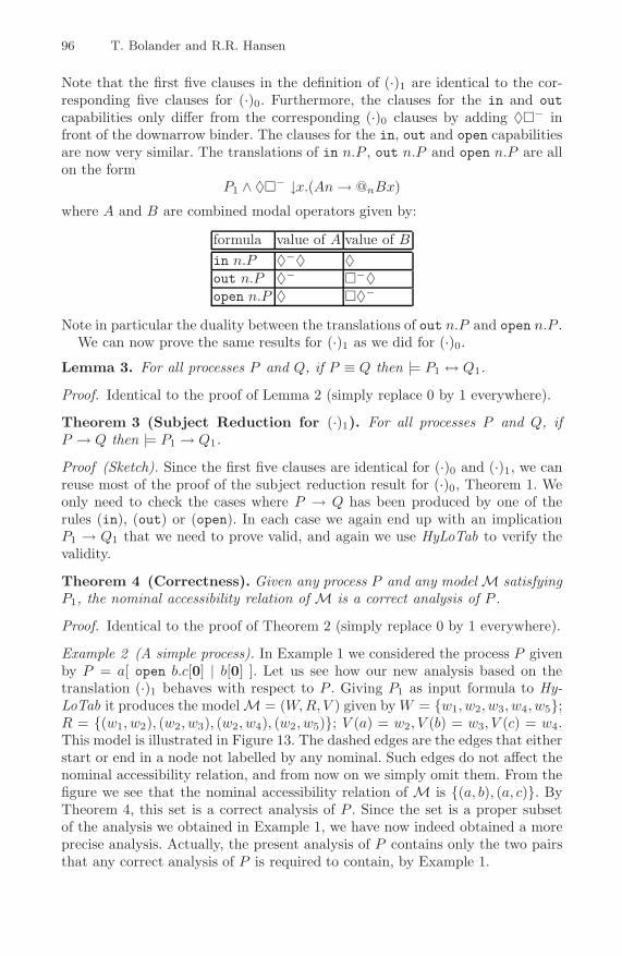
96 T. Bolander and R.R. Hansen
Note that the first five clauses in the definition of (·)1 are identical to the cor-responding five clauses for (·)0. Furthermore, the clauses for the in and outcapabilities only differ from the corresponding (·)0 clauses by adding ♦�− infront of the downarrow binder. The clauses for the in, out and open capabilitiesare now very similar. The translations of in n.P , out n.P and open n.P are allon the form
P1 ∧ ♦�− ↓x.(An→ @nBx)
where A and B are combined modal operators given by:
formula value of A value of Bin n.P ♦−♦ ♦out n.P ♦− �−♦open n.P ♦ �♦−
Note in particular the duality between the translations of out n.P and open n.P .We can now prove the same results for (·)1 as we did for (·)0.
Lemma 3. For all processes P and Q, if P ≡ Q then |= P1 ↔ Q1.
Proof. Identical to the proof of Lemma 2 (simply replace 0 by 1 everywhere).
Theorem 3 (Subject Reduction for (·)1). For all processes P and Q, ifP → Q then |= P1 → Q1.
Proof (Sketch). Since the first five clauses are identical for (·)0 and (·)1, we canreuse most of the proof of the subject reduction result for (·)0, Theorem 1. Weonly need to check the cases where P → Q has been produced by one of therules (in), (out) or (open). In each case we again end up with an implicationP1 → Q1 that we need to prove valid, and again we use HyLoTab to verify thevalidity.
Theorem 4 (Correctness). Given any process P and any modelM satisfyingP1, the nominal accessibility relation of M is a correct analysis of P .
Proof. Identical to the proof of Theorem 2 (simply replace 0 by 1 everywhere).
Example 2 (A simple process). In Example 1 we considered the process P givenby P = a[ open b.c[0] | b[0] ]. Let us see how our new analysis based on thetranslation (·)1 behaves with respect to P . Giving P1 as input formula to Hy-LoTab it produces the modelM = (W,R, V ) given by W = {w1, w2, w3, w4, w5};R = {(w1, w2), (w2, w3), (w2, w4), (w2, w5)}; V (a) = w2, V (b) = w3, V (c) = w4.This model is illustrated in Figure 13. The dashed edges are the edges that eitherstart or end in a node not labelled by any nominal. Such edges do not affect thenominal accessibility relation, and from now on we simply omit them. From thefigure we see that the nominal accessibility relation of M is {(a, b), (a, c)}. ByTheorem 4, this set is a correct analysis of P . Since the set is a proper subsetof the analysis we obtained in Example 1, we have now indeed obtained a moreprecise analysis. Actually, the present analysis of P contains only the two pairsthat any correct analysis of P is required to contain, by Example 1.

Hybrid Logical Analyses of the Ambient Calculus 97
•w1
����
�� • w3b
•
���������
����
��
w2
a•
w4
c
•w5
Fig. 13. Model of P1
•w1
������
���
a• w3
d
•
���������w2
c
•w4
b
Fig. 14. Model of Q1
Example 3 (Nested capabilities). Let us consider a slightly more complex exam-ple. Let Q be the process given by Q = a[ open b.open c.0 | c[ d[0] ] ]. Using Q1 asinput to HyLoTab we get the modelM illustrated in Figure 14. Its nominal acces-sibility relation is {(a, c), (a, d), (c, d)}. This is the same analysis as provided bythe 0CFA analysis of [7]. However, the analysis is not completely precise. Thereare no non-trivial reductions that can be made on Q since there is no ambientnamed b that the outermost open capability can be applied to. Thus we wouldexpect a precise analysis to only give the pairs (a, c) and (c, d) corresponding tothe fact that a contains c and c contains d in Q. The reason that the presentanalysis and the 0CFA of [7] do not give this result is that they both ignore thenesting order on the capabilities. In the case of Q this means that the relativeordering of the two capabilities open b and open c is ignored. Using the hybridlogical machinery we have developed it is fortunately quite easy to improve theanalysis and obtain one which takes the ordering of capabilities into account.
Consider the following sequence of capabilities: in k.out l.open m.0. Using thepresent translation we get:
(in k.out l.open m.0)1 = (in k.0)1 ∧ (out l.0)1 ∧ (open m.0)1.
This implies that each of the three individual capabilities in k, out l andopen m will be ‘executed’ in the same world of the Kripke model induced by thetranslated formula. This of course means that the translation is flow-insensitive:The ordering of the capabilities is not preserved under the translation. However,since we are working with graphs, there is a simple way to solve this problem.Instead of translating a capability like in k.P into a formula of the form P1 ∧ ψwe could translate it into a formula of the form ♦(P1 ∧ψ). Then each capabilitywill add a new edge to the graph because of the ♦ in front of the formula, andthe body of the capability will be ‘executed’ at the world that this new edgeleads to. Thus sequences of capabilities will be translated into paths, and theordering of them will thus be preserved. In the following section we show howto construct such a flow-sensitive translation.
7 A Better Analysis
We now try to construct an even more precise analysis. It is based on a trans-lation (·)2 from processes into hybrid logical formulae given by the followingclauses.

98 T. Bolander and R.R. Hansen
((νn)P )2 = P2
02 = �(P | Q)2 = P2 ∧Q2
(!P )2 = P2
(n[P ])2 = ♦(n ∧ P2)(in n.P )2 = ♦(P2∧ ↓y.�−↓x.(♦−♦n→ @n♦x ∧@y�♦−x))(out n.P )2 = ♦(P2∧ ↓y.�−↓x.(♦−n→ @n�−♦x ∧@y�♦−x))(open n.P )2 = ♦(P2∧ ↓y.�−↓x.(♦n→ @n�♦−x ∧@y�♦−x)).
Note that the first five clauses in the definition of (·)2 are identical to the corre-sponding five clauses for (·)0 and (·)1. Furthermore, the clauses for the in, outand open capabilities are quite similar to the corresponding clauses for (·)1. Thetranslation of in n.P , out n.P and open n.P are now all on the form
♦(P2∧ ↓y.�− ↓x.(An→ @nBy ∧@x�♦−y))
where A and B are the same combined modal operators as for (·)1.Lemma 4. For all processes P and Q, if P ≡ Q then |= P2 ↔ Q2.
Proof. Identical to the proof of Lemma 2 (simply replace 0 by 2 everywhere).
Theorem 5 (Subject Reduction for (·)2). For all processes P and Q, ifP → Q then |= P2 → Q2.
Proof. Since the first five clauses are identical for (·)0, (·)1 and (·)2, we againonly need to consider the rules (in), (out) and (open). These cases are treatedsimilarly to the corresponding cases in the proof of subject reduction for (·)1and (·)0.Theorem 6 (Correctness). Given any process P and any modelM satisfyingP2, the nominal accessibility relation of M is a correct analysis of P .
Proof. Identical to the proof of Lemma 2 (simply replace 0 by 2 everywhere).
Example 4 (Nested capabilities). In Example 3 we considered the processQ givenbyQ = a[ open b.open c.0 | c[ d[0] ] ]. As mentioned in Example 3, the translation(·)1 gave us an analysis ofQ which was not completely precise. Let us see whetherthe translation (·)2 performs better. Giving Q2 as input to HyLoTab we obtainthe model M presented in Figure 15. This model is exactly as the model of Q1
•w1
��������
�a
• w3
d•
���������w2
c
•w4
b
Fig. 15. Model of Q2

Hybrid Logical Analyses of the Ambient Calculus 99
except that the edge from w1 to w3 is no longer present. Thus we instead getthe following nominal accessibility relation: {(a, c), (c, d)}. This relation is theanalysis we expected and it is seen to be more precise than both our analysisbased on (·)1 and the 0CFA analysis of [7]. This improved precision is gainedby making the analysis of capability sequences flow sensitive (cf. the concludingdiscussion at the end of Section 6).
8 Complexity Issues and Future Work
So far in this paper we have not dealt with questions concerning computabilityand complexity. Since the full hybrid logic HL(@,−, ↓) is actually undecidable,it is not immediately obvious that the formulae generated by our translationsare always computable. Fortunately, the translations are designed in such a waythat they translate into a decidable fragment of hybrid logics called the innocentfragment [11]. A formula φ is called innocent if every binder subformula ↓x.ψ isonly outscoped by ♦’s being in the scope of an even number of negation operators(when counting negation operators it is assumed that φ uses only the primitiveoperators, that is, not →, � or �−). It is easily seen that our translations allfall within the innocent fragment. In [11] van Eijck proves that HyLoTab decidesthe innocent fragment. Thus given any process P , HyLoTab will necessarilyterminate on any translation of P resulting in a model for the translation andthereby an analysis of P .
Furthermore, it appears that the fragment of hybrid logic used in our transla-tions is sufficiently simple that it is possible to obtain a complexity bound on themodel generation that is comparable to existing analysis tools for the ambientcalculus. However, we leave this investigation for future work. Another line offuture work we are interested in is to try to make even better analyses than theone provided by (·)2. We believe that the possibilities of using hybrid logic forprecise and yet compact as well as clear analysis of the ambient calculus are yetfar from exhausted.
References
1. Amtoft, T., Kfoury, A.J., Pericas-Geertsen, S.M.: What are polymorphically-typedambients? In: Sands, D. (ed.) ESOP 2001 and ETAPS 2001. LNCS, vol. 2028, pp.206–220. Springer-Verlag, Heidelberg (2001)
2. Amtoft, T., Makholm, H., Wells, J.B.: Polya: True type polymorphism for mobileambients. In: Levy, J.-J., Mayr, E.W., Mitchell, J.C. (eds.) TCS 2004. 3rd IFIPInternational Conference on Theoretical Computer Science, Toulouse, France, Au-gust 2004, pp. 591–604. Kluwer Academic Publishers, Dordrecht (2004)
3. Blackburn, P., de Rijke, M., Venema, Y.: Modal Logic. Cambridge Tracts in Theo-retical Computer Science, vol. 53. Cambridge University Press, Cambridge (2001)
4. Cardelli, L., gordon, A.D.: Types for Mobile Ambients. In: Conference Record ofthe Annual ACM Symposium on Principles of Programming Languages, POPL’99,pp. 79–92. ACM Press, New York (1999)

100 T. Bolander and R.R. Hansen
5. Cardelli, L., Gordon, A.D.: Anytime, Anywhere: Modal logics for mobile ambients.In: Conference Record of the Annual ACM Symposium on Principles of Program-ming Languages, POPL’00, pp. 365–377. ACM Press, New York (2000)
6. Cardelli, L., Gordon, A.D.: Mobile ambients. Theoretical Computer Science 240,177–213 (2000)
7. Nielson, F., Hansen, R.R., Nielson, H.R.: Abstract Interpretation of Mobile Ambi-ents. Science of Computer Programming 47(2–3), 145–175 (2003)
8. Nielson, F., Hansen, R.R., Nielson, H.R.: Validating Firewalls using Flow Logics.Theoretical Computer Science 283(2), 381–418 (2002)
9. Nielson, H.R., Nielson, F.: Shape analysis for mobile ambients. In: ConferenceRecord of the Annual ACM Symposium on Principles of Programming Languages,POPL’00, pp. 142–154. ACM Press, New York (2000)
10. Nielson, H.R., Nielson, F.: Flow Logic: a multi-paradigmatic approach to staticanalysis. In: Mogensen, T., Schmidt, D.A., Sudborough, I.H. (eds.) The Essence ofComputation. LNCS, vol. 2566, pp. 223–244. Springer, Heidelberg (2002)
11. van Eijck, J.: Constraint tableaux for hybrid logics. Manuscript, CWI, Amsterdam(2002)
12. van Eijck, J.: Hylotab—tableau-based theorem proving for hybrid logics.Manuscript, CWI, Amsterdam (2002)
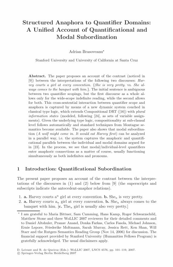
Structured Anaphora to Quantifier Domains:
A Unified Account of Quantificational andModal Subordination
Adrian Brasoveanu�
Stanford University and University of California at Santa Cruz
Abstract. The paper proposes an account of the contrast (noticed in[9]) between the interpretations of the following two discourses: Har-vey courts a girl at every convention. {She is very pretty. vs. She al-ways comes to the banquet with him.}. The initial sentence is ambiguousbetween two quantifier scopings, but the first discourse as a whole al-lows only for the wide-scope indefinite reading, while the second allowsfor both. This cross-sentential interaction between quantifier scope andanaphora is captured by means of a new dynamic system couched inclassical type logic, which extends Compositional DRT ([16]) with pluralinformation states (modeled, following [24], as sets of variable assign-ments). Given the underlying type logic, compositionality at sub-clausallevel follows automatically and standard techniques from Montague se-mantics become available. The paper also shows that modal subordina-tion (A wolf might come in. It would eat Harvey first) can be analyzedin a parallel way, i.e. the system captures the anaphoric and quantifi-cational parallels between the individual and modal domains argued forin [23]. In the process, we see that modal/individual-level quantifiersenter anaphoric connections as a matter of course, usually functioningsimultaneously as both indefinites and pronouns.
1 Introduction: Quantificational Subordination
The present paper proposes an account of the contrast between the interpre-tations of the discourses in (1) and (2) below from [9] (the superscripts andsubscripts indicate the antecedent-anaphor relations).
1. a. Harvey courts au girl at every convention. b. Sheu is very pretty.2. a. Harvey courts au girl at every convention. b. Sheu always comes to the
banquet with him. [c. Theu girl is usually also very pretty.]� I am grateful to Maria Bittner, Sam Cumming, Hans Kamp, Roger Schwarzschild,
Matthew Stone and three WoLLIC 2007 reviewers for their detailed comments andto Daniel Altshuler, Pranav Anand, Donka Farkas, Carlos Fasola, Michael Johnson,Ernie Lepore, Friederike Moltmann, Sarah Murray, Jessica Rett, Ken Shan, WillStarr and the Rutgers Semantics Reading Group (Nov 14, 2006) for discussion. Thefinancial support provided by Stanford University (Humanities Fellows Program) isgratefully acknowledged. The usual disclaimers apply.
D. Leivant and R. de Queiroz (Eds.): WoLLIC 2007, LNCS 4576, pp. 101–119, 2007.c© Springer-Verlag Berlin Heidelberg 2007

102 A. Brasoveanu
Sentence (1a/2a) by itself is ambiguous between two quantifier scopings: it“can mean that, at every convention, there is some girl that Harvey courts orthat there is some girl that Harvey courts at every convention. [. . . ] Harveyalways courts the same girl [. . . ] [or] it may be a different girl each time” ([9]:377). The contrast between the continuations in (1b) and (2b) is that the formerallows only for the ‘same girl’ reading of sentence (1a/2a), while the latter isalso compatible with the ‘possibly different girls’ reading.
Discourse (1) raises the following question: how can we capture the fact that asingular anaphoric pronoun in sentence (1b) can interact with and disambiguatequantifier scopings1 in sentence (1a)? That number morphology on the pronounshe is crucial is shown by the discourse in (3) below, where the (preferred) relativescoping of every convention and a girl is the opposite of the one in discourse (1).
3. a. Harvey courts au girl at every convention. b. Theyu are very pretty.
Discourse (2) raises the following questions. First, why is it that adding anadverb of quantification, i.e. always/usually, makes both readings of sentence(2a) available? Moreover, on the newly available reading of sentence (2a), i.e.the every convention>>a girl scoping, how can we capture the intuition thatthe singular pronoun she and the adverb always in sentence (2b) elaborate onthe quantificational dependency between conventions and girls introduced insentence (2a), i.e. how can we capture the intuition that we seem to have si-multaneous anaphora to the two quantifier domains and to the quantificationaldependency between them?
The phenomenon instantiated by discourses (1) and (2) is subsumed underthe more general label of quantificational subordination (see [13]: 139, (2)), whichcovers a variety of phenomena involving interactions between generalized quan-tifiers and morphologically singular cross-sentential anaphora. The main goal ofthis paper is give an account of quantificational subordination couched withina new compositional dynamic system which straightforwardly generalizes to anaccount of modal subordination, thereby capturing the anaphoric and quantifi-cational parallels between the individual and modal domains argued for in [23],[1], [22], [5] and [7] among others (building on [18] and [19]).
2 Plural Compositional DRT (PCDRT)
This section introduces the semantic framework in which the analysis of dis-courses (1) and (2) is couched. The main proposal is that (compositionally) as-signing natural language expressions finer-grained semantic values (finer grainedthan the usual meanings assigned in static Montague semantics) enables us to
1 To see that it is indeed quantifier scopings that are disambiguated, substitute exactlyoneu girl for au girl in (1a); this yields two truth-conditionally independent scop-ings: (i) exactly one girl>>every convention, which is true in a situation in whichHarvey courts more than one girl per convention, but there is exactly one (e.g. FayeDunaway) that he never fails to court, and (ii) every convention>>exactly one girl.

Structured Anaphora to Quantifier Domains 103
capture the interaction between generalized quantifiers, singular pronouns andadverbs of quantification exhibited by the contrast between (1) and (2).
Accounting for cross-sentential phenomena in semantic terms (as opposedto purely/primarily pragmatic terms) requires some preliminary justification.First, the same kind of finer-grained semantic values (to be introduced presently)are independently motivated by intra-sentential phenomena (see the account ofmixed weak & strong donkey sentences in [2]). Second, the phenomenon instan-tiated by (1) and (2) is as much intra-sentential as it is cross-sentential. Notethat there are four separate components that come together to yield the con-trast in interpretation between (1) and (2): (i) the generalized quantifier everyconvention, (ii) the indefinite a girl, (iii) the singular number morphology onthe pronoun she and (iv) the adverb of quantification always/usually. To derivethe intuitively correct interpretations for (1) and (2), we have to attend to boththe cross-sentential connections a girl–she and every convention–always/usuallyand the intra-sentential interactions every convention–a girl and always–she.
I conclude that an account of the contrast between (1) and (2) that involves arevamping of semantic values has sufficient initial plausibility to make its pursuitworthwhile. To this end, I introduce a new dynamic system couched in classical(many-sorted) type logic which extends Compositional DRT (CDRT, [16]) intwo ways: (i) with plural information states and (ii) with selective generalizedquantification. The resulting system is dubbed Plural CDRT (PCDRT).
2.1 Plural Information States
The main technical innovation relative to CDRT is that, just as in DynamicPlural Logic ([24]), information states I, J etc. are modeled as sets of variableassignments i, j etc.; such plural info states can be represented as matrices withassignments (sequences) as rows, as shown below.
Info State I . . . u u′ . . .i1 . . . x1 (i.e. ui1) y1 (i.e. u′i1) . . .i2 . . . x2 (i.e. ui2) y2 (i.e. u′i2) . . .i3 . . . x3 (i.e. ui3) y3 (i.e. u′i3) . . .. . . . . . . . . . . . . . .
Quantifier domains (sets)are stored columnwise: {x1,x2, x3, . . . }, {y1, y2, y3, . . . }
Quantifier dependencies (relations)are stored rowwise: {(x1, y1), (x2, y2),(x3, y3), . . . }
Plural info states enable us to encode discourse reference to both quantifierdomains, i.e. values, and quantificational dependencies, i.e. structure. The val-ues are the sets of objects that are stored in the columns of the matrix, e.g. adiscourse referent (dref) u for individuals stores a set of individuals relative to aplural info state given that u is assigned an individual by each assignment/row.The structure is encoded in the rows of the matrix: for each assignment/row inthe info state, the individual assigned to a dref u by that assignment is struc-turally correlated with the individual assigned to some other dref u′ by the sameassignment.

104 A. Brasoveanu
2.2 The Outline of the Proposed Account
Thus, plural info states enable us to pass information about both quantifierdomains and quantificational dependencies across sentential/clausal boundaries,which is exactly what we need to account for the interpretation of discourses (1)and (2). More precisely, we need the following two ingredients.
First, we need a suitable meaning for selective generalized determiners thatwill store two things in the input plural info state: (i) the restrictor and nu-clear scope sets of individuals that are introduced and related by the deter-miner; (ii) the quantificational dependencies between the individuals in therestrictor/nuclear scope set and any other quantifiers/indefinites in the restric-tor/nuclear scope of the quantification, e.g. between every convention in (1a/2a)and the indefinite a girl in its nuclear scope. Given that plural info states storeboth sets of individuals and dependencies between them, both kinds of informa-tion are available for subsequent anaphoric retrieval; for example, always andshe in (2b) are simultaneously anaphoric to both the sets of conventions andgirls and the dependency between these sets introduced in (2a).
The second ingredient is a suitable meaning for singular number morphologyon pronouns like sheu in (1b) and (2b) above. This meaning has to derive theobserved interactions between (i) singular pronouns, (ii) quantifiers and indef-inites in the previous discourse, e.g. every convention and au girl in (1a/2a),and (iii) quantifiers in the same sentence, e.g. the adverb always in (2b). Inparticular, I will take singular number morphology on sheu to require the set ofu-individuals stored by the current plural info state to be a singleton. The set ofu-individuals is introduced by the indefinite au girl and is available for anaphoricretrieval irrespective of whether the indefinite has wide or narrow scope in sen-tence (1a/2a). Thus, once again, plural info states are crucial for the analysis:they enable us to store and pass on structured sets of individuals, so that wecan constrain their cardinality by subsequent, non-local anaphoric elements.
If the indefinite au girl has narrow scope relative to every convention, thesingleton requirement contributed by sheu applies to the set of all girls thatare courted by Harvey at some convention or other. Requiring this set to be asingleton boils down to removing from consideration all the plural info statesthat would satisfy the narrow-scope indefinite reading every convention>>au
girl, but not the wide-scope reading au girl>>every convention. We thereforederive the intuition that, irrespective of which quantifier scoping we assume forsentence (1a), any plural info state that we obtain after a successful update withsentence (1b) is bound to satisfy the representation in which the indefinite au
girl (or a quantifier like exactly oneu girl) takes wide scope.In discourse (2), however, the adverb of quantification always in (2b), which
is anaphoric to the nuclear scope set introduced by every convention in (2a),can take scope either below or above the singular pronoun sheu. If always takesscope below sheu, we obtain the same reading as in discourse (1). If always takesscope above sheu, it ‘breaks’ the input plural info state storing all the conventionsinto smaller sub-states, each storing a particular convention. Consequently, thesingleton requirement contributed by sheu is enforced locally, relative to each of

Structured Anaphora to Quantifier Domains 105
these sub-states, and not globally, relative to the whole input info state, so weend up requiring the courted girl to be unique per convention and not across theboard.
The remainder of this section presents the basics of the compositional dynamicsystem, while Section 3 introduces the PCDRT meanings for selective generalizeddeterminers, indefinites and singular/plural pronouns.
2.3 DRS’s and Conditions in PCDRT
We work with a Dynamic Ty2 logic, i.e. with the Logic of Change in [16] whichreformulates dynamic semantics ([8], [12]) in Gallin’s Ty2 ([6]). We have threebasic types: type t (truth-values), type e (individuals; variables: x, x′ etc.) andtype s (‘variable assignments’; variables: i, j etc.). A suitable set of axiomsensures that the entities of type s do behave as variable assignments2.
A dref for individuals u is a function of type se from ‘assignments’ is toindividuals xe (the subscripts on terms indicate their type). Intuitively, the in-dividual useis is the individual that the ‘assignment’ i assigns to the dref u.Dynamic info states I, J etc. are plural: they are sets of ‘variable assignments’,i.e. terms of type st. An individual dref u stores a set of individuals with respectto a plural info state I, abbreviated as uI := {useis : is ∈ Ist}, i.e. uI is theimage of the set of ‘assignments’ I under the function u.
A sentence is interpreted as a Discourse Representation Structure (DRS),which is a relation of type (st)((st)t) between an input state Ist and an outputstate Jst, as shown in (4) below. A DRS requires: (i) the input info state I todiffer from the output state J at most with respect to the new dref’s and (ii)all the conditions to be satisfied relative to the output state J . For example, theDRS [u1, u2|girl{u1}, convention{u2}, courted at{u1, u2}] abbreviates the termλIst.λJst. I[u1, u2]J ∧ girl{u1}J ∧ convention{u2}J ∧ courted at{u1, u2}J . Thedefinition of dref introduction (a.k.a. random assignment) is given in (5) below3.
4. [new dref’s | conditions] := λIst.λJst. I[new dref’s]J ∧ conditionsJ5. [u] := λIst.λJst. ∀is ∈ I(∃js ∈ J(i[u]j)) ∧ ∀js ∈ J(∃is ∈ I(i[u]j))
DRS’s of the form [conditions] := λIst.λJst. I = J ∧ conditionsJ are tests,e.g. [girl{u1}] := λIst.λJst. I = J∧girl{u1}J tests that the input state I satisfiesthe condition girl{u1}. Conditions are interpreted distributively relative to aplural info state, e.g. courted at{u1, u2} is basically the term λIst. I �= ∅∧∀is ∈I(courted at(u1i, u2i)) of type (st)t, i.e. it denotes a set of information states;see Subsect. 3.1 below for the general definition of atomic conditions.
2.4 Compositionality
Given the underlying type logic, compositionality at sub-clausal level follows au-tomatically and standard techniques from Montague semantics (e.g. type shift-ing) become available. In more detail, the compositional aspect of interpretation2 See [16] for more details.3 See [2] for its justification.

106 A. Brasoveanu
in an extensional Fregean/Montagovian framework is largely determined by thetypes for the (extensions of the) ‘saturated’ expressions, i.e. names and sen-tences. Abbreviate them as e and t. An extensional static logic identifies e withe and t with t. The denotation of the noun girl is of type et, i.e. et: girl� λxe. girlet(x). The generalized determiner every is of type (et)((et)t), i.e.(et)((et)t).
PCDRT assigns the following dynamic types to the ‘meta-types’ e and t: tabbreviates (st)((st)t), i.e. a sentence is interpreted as a DRS, and e abbreviatesse, i.e. a name is interpreted as a dref. The denotation of the noun girl is stillof type et, as shown in (6) below. Moreover, the determiner every is still oftype (et)((et)t) – and its definition is provided in the next section.
6. girl � λve. [girlet{v}], i.e. girl � λve.λIst.λJst. I = J ∧ girlet{v}J
3 Generalized Quantification in PCDRT
We turn now to the definition of selective generalized quantification in PCDRT.The definition has to satisfy four desiderata, the first three of which are aboutanaphoric connections that can be established internally (within the generalizedquantification), i.e. between antecedents in the restrictor and anaphors in thenuclear scope, and the last of which is about anaphora that can be establishedexternally, i.e. between antecedents introduced by/within the quantification andanaphors that are outside the quantification.
Let us begin with internal anaphora. First, we want our definition to be ableto account for the fact that anaphoric connections between the restrictor andthe nuclear scope of the quantification can in fact be established, i.e. we want toaccount for donkey anaphora (Everyu farmer who owns au
′donkey beats itu′).
Second, we want to account for such anaphoric connections while avoidingthe proportion problem that unselective quantification (in the sense of [15]) runsinto. That is, we need generalized determiners to relate sets of individuals (i.e.sets of objects of type e) and not sets of ‘assignments’ (i.e. sets of objects of types). The sentence Mostu farmers who own au
′donkey beat itu′ provides a typical
instance of the proportion problem: intuitively, this sentence is false in a situationin which there are ten farmers, nine have a single donkey each and they do notbeat it, while the tenth has twenty donkeys and he is busy beating them all.The unselective interpretation of the most -quantification, however, incorrectlypredicts that the sentence is true in this situation because more than half ofthe (farmer, donkey) pairs (twenty out of twenty-nine) are such that the farmerbeats the donkey.
The third desideratum is that the definition of selective generalized quantifi-cation be compatible with both strong and weak donkey readings: we want toallow for the different interpretations associated with the donkey anaphora in(7) (from [13]) and (8) (from [20]) below. Sentence (7) is interpreted as assert-ing that most slave-owners were such that, for every (strong reading) slave theyowned, they also owned his offspring. Sentence (8) is interpreted as assertingthat every dime-owner puts some (weak reading) dime of her/his in the meter.

Structured Anaphora to Quantifier Domains 107
7. Mostu people that owned au′slave also owned hisu′ offspring.
8. Everyu person who has au′dime will put itu′ in the meter.
The fourth desideratum is concerned with external anaphora – and this bringsus back to the discourses in (1) and (2). These discourses indicate that we needto make the restrictor and nuclear scope sets of individuals related by generalizeddeterminers available for subsequent anaphora – and we also need to make avail-able for anaphoric take-up the quantificational dependencies between differentquantifiers and/or indefinites. In particular, generalized quantification supportsanaphora to two sets: (i) the maximal set of individuals satisfying the restrictorDRS, i.e. the restrictor set, and (ii) the maximal set of individuals satisfyingthe restrictor and nuclear scope DRS’s, i.e. the nuclear scope set4. Note that thelatter set is the nuclear scope that emerges as a consequence of the conserva-tivity of natural language quantification – and, as [24] (among others) observes,we need to build conservativity into the definition of dynamic quantification toaccount for the fact that the nuclear scope DRS can contain anaphors dependenton antecedents in the restrictor.
The discourse in (9) below exemplifies anaphora to nuclear scope sets: sen-tence (9b) is interpreted as asserting that the people that went to the beachare the students that left the party after 5 a.m. (which, in addition, formed amajority of the students at the party). The discourses in (10) and (11) belowexemplify anaphora to the restrictor sets contributed by the downward mono-tonic quantifiers nou student and very fewu people respectively. Consider (10)first: any successful update with a nou quantification ensures that the nuclearscope set is empty and anaphora to it is therefore infelicitous; the only possibleanaphora in (10) is restrictor set anaphora. Restrictor set anaphora is the onlypossible one in (11) also, because nuclear scope anaphora yields a contradictoryinterpretation for (11b): most of the people with a rich uncle that inherit hisfortune don’t inherit his fortune.
9. a. Mostu students left the party after 5 a.m. b. Theyu went directly to thebeach.
10. a. Nou student left the party later than 10 pm. b. Theyu had classes earlyin the morning.
11. a. Very fewu people with a rich uncle inherit his fortune. b. Most of themu
don’t.
Thus, a selective generalized determiner receives the translation in (12) below,which is in the spirit – but fairly far from the letter – of [24]5.
12. det u,u′�u �
λPet.λP′et. maxu(〈u〉(P (u))); maxu
′�u(〈u′〉(P ′(u′))); [DET{u, u′}]4 Throughout the paper, I will ignore anaphora to complement sets, i.e. sets obtained
by taking the complement of the nuclear scope relative to the restrictor, e.g. Veryfew students were paying attention in class. They were hungover.
5 Cf. Definition (4.1), [24]: 149.

108 A. Brasoveanu
As expected, det u,u′�u relates a restrictor dynamic property Pet and a nu-
clear scope dynamic property P ′et. When these dynamic properties are applied
to individual dref’s, i.e. P (u) and P ′(u′), we obtain a restrictor DRS P (u) anda nuclear scope DRS P ′(u′) of type t. Moreover, a generalized determiner intro-duces two individual dref’s: u stores the restrictor set and u′ the nuclear scopeset. These two dref’s and the two dynamic properties P and P ′ are the basicbuilding blocks of the three separate updates in (12).
The first update, namely maxu(〈u〉(P (u))), ensures that the restrictor set u isthe maximal set of individuals, i.e. maxu(. . . ), such that, when we take each u-individual separately, i.e. 〈u〉(. . . ), this individual satisfies the restrictor dynamicproperty, i.e. P (u). The second update, namely maxu
′�u(〈u′〉(P ′(u′))), ensuresthat the nuclear scope set u′ is obtained in much the same way as the restrictorset u, except for the requirement that u′ is the maximal structured subset of u,i.e. maxu
′�u(. . . ). Finally, the third update, namely [DET{u, u′}], is a test: wetest that the restrictor set u and the nuclear scope set u′ stand in the relationdenoted by the corresponding static determiner DET.
The three distinct updates in (12) are conjoined and, as (13) below shows,dynamic conjunction “;” is interpreted as relation composition. Note the differ-ence between dynamic conjunction, which is an abbreviation, and the official,classical, static conjunction “∧”.
13. D;D′ := λIst.λJst. ∃Hst(DIH ∧D′HJ), where D,D′ are DRS’s (type t).
To formally spell out the PCDRT meaning for generalized determiners in (12)above and the meanings for indefinites and pronouns, we need: (i) two opera-tors over plural info states, namely a selective maximization operator maxu(. . . )and a selective distributivity operator 〈u〉(. . . ) and (ii) a notion of structuredinclusion u′ � u that requires the subset to preserve the quantificational depen-dencies, i.e. the structure, associated with the individuals in the superset.
3.1 Structured Inclusion
Let us start with the notion of structured subset. Recall that plural info statesstore both values (in the columns of the matrix) and structure (in the rows ofthe matrix). Requiring one dref u3 to simply be a value-subset of another drefu1 relative to an info state I is defined as shown in (14) below; for example, theleftmost u3 column in the table below satisfies the condition u3 ⊆ u1 becauseu3I = {x1, x2, x3} ⊆ u1I = {x1, x2, x3, x4}. Condition (14) requires only valueinclusion and disregards structure completely. The correlation between the u1-individuals and the u2-individuals, i.e. the relation {(x1, y1), (x2, y2), (x3, y3),(x4, y4)}, is lost in going from the u1-superset to the u3-subset: as far as u3 andu2 are concerned, x1 is still correlated with y1, but it is now also correlated withy3; moreover, x2 is now correlated with y4 (not y2) and x3 with y2 (not y3).
14. u3 ⊆ u1 := λIst. u3I ⊆ u1I
15. u3 � u1 := λIst. ∀is ∈ I(u3i = u1i ∨ u3i = #)

Structured Anaphora to Quantifier Domains 109
Info State I u1 u2 u3 (u3 ⊆ u1, u3 �� u1) u3 (u3 � u1)i1 x1 y1 x1 x1
i2 x2 y2 x3 x2
i3 x3 y3 x1 #i4 x4 y4 x2 x4
If we use the notion of value-only subset in (14), we make incorrect empiricalpredictions. Consider, for example, the discourse in (16) below, where u1 storesthe set of conventions6 and u2 stores the set of corresponding girls; furthermore,assume that everyu1 convention takes scope over au2 girl and that the correla-tion between u1-conventions and courted u2-girls is the one represented in thetable above. Intuitively, the adverb usually in (16b) is anaphoric to the set ofconventions introduced in (16a) and (16b) is interpreted as asserting that, atmost conventions, the girl courted by Harvey at that convention comes to thebanquet with him. The leftmost dref u3 in the table above does store most u1-conventions (three out of four), but it does not preserve the correlation betweenu1-conventions and u2-girls established in sentence (16a).
We obtain similarly incorrect results for donkey sentences like the one in (17)below: the restrictor of the quantification introduces a dependency between allthe donkey-owning u1-farmers and the u2-donkeys that they own; the nuclearscope set u3 needs to contain most u1-farmers, but in such a way that thecorrelated u2-donkeys remain the same. That is, the nuclear scope set contains amost -subset of donkey-owning farmers that beat their respective donkey(s). Thenotion of value-only inclusion in (14) is, yet again, inadequate.
16. a. Harvey courts au2 girl at everyu1 convention. b. Sheu2 usuallyu3⊆u1 comesto the banquet with him.
17. Mostu1,u3⊆u1 farmers who own au2 donkey beat itu2 .
Thus, to capture the intra- and cross-sentential interaction between anaphoraand quantification, we need the notion of structured inclusion defined in (15)above, whereby we go from a superset to a subset by discarding rows in thematrix. We are therefore guaranteed that the subset will contain only the de-pendencies associated with the superset (but not necessarily all dependencies –see below). To implement this, I follow [24] and introduce a dummy/exceptionindividual # that is used as a tag for the cells in the matrix that should bediscarded in order to obtain a structured subset u3 of a superset u1 – as shownby the rightmost u3 column in the table above.
Unlike [24], I do not take the introduction of the dummy individual # torequire making the underlying logic partial, i.e. I will not take a lexical relationthat has # as one of its arguments, e.g. girl(#) or courted at(#, x1), to beundefined. I will just require the dummy individual # to make any lexical relation
6 In the case of a successful every-quantification, the restrictor and nuclear scope setsare identical with respect to both value and structure, so we can safely identify them.

110 A. Brasoveanu
false7. This allows us to keep the underlying type logic classical while makingsure that we do not accidentally introduce # and inadvertently discard a cellwhen we evaluate another lexical relation later on. Thus, lexical relations (i.e.,atomic conditions) are interpreted distributively relative to the non-dummy sub-state of the input plural info state I, as shown in (19) below.
18. Iu1 �=#,...,un �=# := {is ∈ I : u1i �= # ∧ . . . ∧ uni �= #}19. R{u1, . . . , un} :=
λIst. Iu1 �=#,...,un �=# �= ∅ ∧ ∀is ∈ Iu1 �=#,...,un �=#(R(u1i, . . . , uni))
The notion of structured inclusion � in (15) above ensures that the subsetinherits only the superset structure – but we also need it to inherit all the su-perset structure, which we achieve by means of the second conjunct in definition(20) below. This conjunct is needed (among others) to account for the donkeysentence in (7) above, which is interpreted as talking about every slave ownedby any given person, i.e. the nuclear scope set, which is a most -subset of therestrictor set, needs to inherit all the superset structure (each slave owner in thenuclear scope set needs to be associated with every slave that s/he owned).
20. u′ � u := λIst. (u′ � u)I ∧ ∀is ∈ I(ui ∈ u′Iu′ �=# → ui = u′i)
3.2 Maximization and Distributivity
We turn now to the maximization and distributivity operators maxu and distu,which are defined in the spirit – but not the letter – of the corresponding oper-ators in [24]. Selective maximization and selective distributivity together enableus to dynamize λ-abstraction over both values (individuals, i.e. quantifier do-mains) and structure (quantificational dependencies); that is, maxu and distuenable us to extract and store the restrictor and nuclear scope structured setsneeded to define dynamic generalized quantification.
Consider the definition of maxu in (21) below first: the first conjunct intro-duces u as a new dref, i.e. [u], and makes sure that each individual in uJ satisfiesD, i.e. we store only individuals that satisfy D. The second conjunct enforcesthe maximality requirement: any other set uK obtained by a similar procedure,i.e. any other set of individuals that satisfies D, is included in uJ – that is, uJstores all individuals that satisfy D.
21. maxu(D) := λIst.λJst. ([u];D)IJ ∧ ∀Kst(([u];D)IK → uKu�=# ⊆ uJu�=#)22. maxu
′�u(D) := maxu′([u′ � u];D)
23. Iu=x = {is ∈ I : ui = x}24. distu(D) := λIst.λJst. uI = uJ ∧ ∀xe ∈ uI(DIu=xJu=x) 8
7 We ensure that any lexical relation R of arity n (i.e. of type ent, defined recursivelyas in [16]: 157-158, i.e. as e0t := t and em+1t := e(emt)) yields falsity whenever # isone of its arguments by letting R ⊆ (DM
e \ {#})n.8 In general, distu1,...,un(D) is defined as:
λIst.λJst. ∀x1 . . .∀xn(Iu1=x1,...,un=xn �= ∅ ↔ Ju1=x1,...,un=xn �= ∅)∧∀x1 . . .∀xn(Iu1=x1,...,un=xn �= ∅ → DIu1=x1,...,un=xnJu1=x1,...,un=xn).

Structured Anaphora to Quantifier Domains 111
Definition (24) states that updating an info state I with a DRSD distributivelyover a dref u means: (i) generating the u-partition of I, i.e. {Iu=x : x ∈ uI}, (ii)updating each cell Iu=x in the partition with the DRS D and (iii) taking theunion of the resulting output info states. The first conjunct in (24) is requiredto ensure that there is a bijection between the partition induced by the dref uover the input state I and the one induced over the output state J ; withoutthis requirement, we could introduce arbitrary new values for u in the outputstate J , i.e. arbitrary new partition cells9. The second conjunct is the one thatactually defines the distributive update: the DRS D relates every partition cellin the input state I to the corresponding partition cell in the output state J .
3.3 Generalized Quantifiers and Indefinites
The PCDRT meanings for generalized determiners and weak/strong indefinitesare provided in (28), (29) and (30) below10.
25. u(D) := λIst.λJst. Iu=# = Ju=# ∧ Iu�=# �= ∅ ∧ distu(D)Iu�=#Ju�=#
26. 〈u〉(D) := λIst.λJst. Iu=# = Ju=# ∧(Iu�=# = ∅ → I = J) ∧ (Iu�=# �= ∅ → distu(D)Iu�=#Ju�=#)
27. DET{u, u′} := λIst. DET(uIu�=#, u′Iu′ �=#), where DET is a static det.
28. det u,u′�u �
λPet.λP′et. maxu(〈u〉(P (u))); maxu
′�u(〈u′〉(P ′(u′))); [DET{u, u′}]29. awk:u � λPet.λP
′et. [u]; u(P (u)); u(P ′(u))
30. a str:u � λPet.λP′et. maxu(u(P (u)); u(P ′(u)))
The max-based definition of generalized quantification correctly predicts thatanaphora to restrictor/nuclear scope sets is always anaphora to maximal sets,i.e. E-type anaphora11. That is, the maximality of anaphora to quantifier sets isan automatic consequence of the fact that we independently need max-operatorsto formulate truth-conditionally correct dynamic meanings for quantifiers. Thisis one of the major results in [24], preserved in PCDRT.
The existential commitment associated with dref introduction is built into(i) the definition of lexical relations in (19) above (i.e. Iu1 �=#,...,un �=# �= ∅) and(ii) the definition of the operator u(. . . ) in (25) above (i.e. Iu�=# �= ∅)12.
There is, however, no such existential commitment in the definition of gener-alized determiners det u,u
′�u, which employs the distributivity operator 〈u〉(. . . )
9 [17]: 87 was the first to observe that we need to add the first conjunct in (24) to theoriginal definition of distributivity in (18), [24]: 145.
10 See [2] for the justification of the account of weak/strong donkey ambiguities interms of weak/strong indefinite articles and see [4] for a detailed investigation ofvarious kinds of indefinites within a related dynamic framework.
11 Recall the Evans examples Few senators admire Kennedy and they are very junior.and Harry bought some sheep. Bill vaccinated them. and (9), (10) and (11) above.
12 We need these non-emptiness requirements because the pair (∅st, ∅st) belongs, on theone hand, to the denotation of [u] for any dref u (see (5) above) and, on the otherhand, to the denotation of distu(D) for any dref u and DRS D (see (24) above).

112 A. Brasoveanu
defined in (26) above. The use of 〈u〉(. . . ) enables us to capture the meaning ofboth upward and downward monotonic quantifiers by means of the same defini-tion. The problem posed by downward monotonic quantifiers is that their nuclearscope set can or has to be empty; for example, after a successful update witha no u,u
′�u quantification, the nuclear scope set u′ is necessarily empty, i.e. thedref u′ will always store only the dummy individual # relative to the output infostate; this, in turn, entails that no lexical relation in the nuclear scope DRS thathas u′ as an argument can be satisfied. The second conjunct in the definition of〈u〉(. . . ), i.e. Iu�=# = ∅ → I = J , enables us to resolve the conflict between theemptiness requirement enforced by a no -quantification and the non-emptinessrequirement enforced by lexical relations13,14.
3.4 Singular Number Morphology
Let us turn now to the last component needed for the account of discourses (1)and (2), namely the representation of singular pronouns. Their PCDRT trans-lation, provided in (32) below, has the expected Montagovian form: it is thedistributive type-lift of the dref u they are anaphoric to, with the addition of thecondition unique{u}. The condition is contributed by singular number morphol-ogy and requires uniqueness of the non-dummy value of the dref u relative to thecurrent plural info state I. In contrast, plural pronouns do not require unique-ness, as shown in (33) below. The meanings for singular and plural anaphoricdefinite articles in (34) and (35) below (we need them to interpret the anaphoricDP the girl in (2c) above among others) exhibit the same kind of unique/non-unique contrast as the meanings for singular and plural pronouns.
The uniqueness enforced by the condition unique{u} is weak in the sensethat it is relativized to the current plural info state. However, we can requirestrong uniqueness, i.e. uniqueness relative to the entire model, by combiningthe maxu operator and the unique{u} condition, as shown by the Russellian,non-anaphoric meaning for definite descriptions provided in (36) below. Thisalternative meaning for definite articles, which requires existence and stronguniqueness, is needed to interpret the DP the banquet in (2b) above.
31. unique{u} := λIst. Iu�=# �= ∅ ∧ ∀is ∈ Iu�=#∀i′s ∈ Iu�=#(ui = ui′)13 Even if definition (28) allows for empty restrictor and nuclear scope sets, we can
still capture the fact that subsequent anaphora to such empty sets is infelicitous(e.g. anaphora to the nuclear scope sets in (10) and (11) above) because pronominalmeanings are defined in terms of the operator u(. . . ) – see, for example, the PCDRTtranslations for she and they in (32) and (33) below.
14 The fact that the second conjunct in (26) requires the identity of the input andoutput states I and J correctly predicts that anaphora to both empty restric-tor/nuclear scope sets and indefinites in restrictor/nuclear scope DRS’s associatedwith such empty sets is infelicitous. For example, the nuclear scope DRS of a suc-cessful no u,u′�u-quantification, i.e. maxu′�u(〈u′〉(P
′(u′))), will always be a test;hence, we correctly predict that anaphora to any indefinites in the nuclear scope of ano -quantification is infelicitous, e.g. Harvey courts au′′
girl at nou,u′�u convention.#Sheu′′/Theyu′′ is/are very pretty.

Structured Anaphora to Quantifier Domains 113
32. she u � λPet. [unique{u}]; u(P (u))33. they u � λPet. u(P (u))34. the sg u � λPet.λP
′et. [unique{u}]; u(P (u)); u(P ′(u))
35. the pl u � λPet.λP′et. u(P (u)); u(P ′(u))
36. the sg u � λPet.λP′et. maxu(u(P (u))); [unique{u}]; u(P ′(u))
The PCDRT translation for proper names and the definitions of dynamicnegation and truth are provided in (37), (38) and (39) below. I take the defaultcontext of interpretation for all discourses, i.e. the default input info state relativeto which a DRS is true/false, to be the singleton info state {i#} , where i# isthe ‘assignment’ that stores the dummy individual # relative to all individualdref’s. Finally, the abbreviations in (40) and (41) below and the equivalences in(42) and (43) enable us to simplify – and, therefore, enhance the readability of– some very common PCDRT representations.
37. Harvey u � λPet. [u|u � Harvey]; u(P (u)),where Harvey := λis. harveye (i.e. Harvey is a ‘rigid’ individual dref).
38. ∼ D := λIst. I �= ∅ ∧ ∀Hst �= ∅(H ⊆ I → ¬∃Kst(DHK))39. A DRS D of type t is true with respect to an input state Ist iff ∃Jst(DIJ).40. u(C) := λIst. Iu�=# �= ∅ ∧ ∀xe ∈ uIu�=#(CIu=x),
where C is a condition (type (st)t).41. u(u1, . . . , un) := λIst.λJst. Iu=# = Ju=# ∧ Iu�=#[u1, . . . , un]Ju�=#,
where u �∈ {u1, . . . , un} and [u1, . . . , un] := [u1]; . . . ; [un].42. u([C1, . . . , Cm]) = [u(C1), . . . , u(Cm)]43. u([u1, . . . , un |C1, . . . , Cm]) = [u(u1, . . . , un) | u(C1), . . . , u(Cm)]
4 Quantificational Subordination in PCDRT
This section presents the PCDRT analysis of discourses (1) and (2). We startwith the two possible quantifier scopings for the discourse-initial sentence(1a/2a). For simplicity, I will assume that the two scopings are due to the twodifferent lexical entries for the ditransitive verb court at , provided in (44) and(45) below15: court at 1 assigns the indefinite a girl wide scope relative toevery convention , while court at 2 assigns it narrow scope. I assume that thebasic syntactic structure of the sentence is the one given in (46).
44. court at 1 � λQ′(et)t.λQ
′′(et)t.λve. Q
′(λv′e. Q′′(λv′′e . [court at{v, v′, v′′}]))45. court at 2 � λQ′
(et)t.λQ′′(et)t.λve. Q
′′(λv′′e . Q′(λv′e. [court at{v, v′, v′′}]))46. Harvey [ [court at1/2 [a girl]] [every convention] ]
Turning to the meaning of the quantifier every convention , note that we cansafely identify the restrictor and nuclear scope dref’s u and u′ of any every u,u
′�u-quantification: the definition in (28) above entails that, if J is an arbitrary output15 But it should be clear that PCDRT is compatible with any of the quantifier scoping
mechanisms proposed in the literature; for a version of PCDRT that incorporatesQuantifying-In / Quantifier Raising, see [2].

114 A. Brasoveanu
state of a successful every u,u′�u-quantification, u and u′ have to be identical with
respect to both value and structure, i.e. ∀js ∈ J(uj = u′j). We can thereforeassume that every contributes only one dref, as shown in (47) below. I will alsoassume that the restrictor set of the every u1 -quantification is non-empty, so wecan safely replace the operator 〈u1〉(. . . ) with the operator u1(. . . ). The PCDRTrepresentations of the two quantifier scopings for sentence (1a/2a) are providedin (50) and (51) below. For simplicity, I take the translation of the proper nameHarvey to be λPet. P (Harvey) instead of the more complex one in (37) above16.
47. every u1 � λPet.λP′et. maxu1(u1 (P (u1))); u1(P ′(u1))
48. every u1 convention � λPet. maxu1([convention{u1}]); u1(P (u1))49. awk:u2 girl � λPet. [u2 | girl{u2}]; u2(P (u2))50. awk:u2 girl>>everyu1 convention � [u2 | girl{u2}];
u2(maxu1([convention{u1}])); [u2(court at{Harvey, u2, u1})]51. every u1 convention>>awk:u2 girl � maxu1([convention{u1}]);
[u1(u2) | u1(girl{u2}), u1(court at{Harvey, u2, u1})]The representation in (50) updates the default input info state {i#} as follows.
First, we introduce some non-empty (i.e. non-dummy) set of individuals relativeto the dref u2. Then, we test that each u2-individual is a girl. Then, relative toeach u2-individual, we introduce the set of all conventions and store it in thedref u1. Finally, we test that, for each u2-girl and for each of the correspondingu1-conventions (i.e., in this case: for every convention), Harvey courted her atthe convention. The output info state obtained after updating with (50) containsa non-empty set of u2-girls that where courted by Harvey at every conventionand, relative to each u2-girl, u1 stores the set of all conventions.
The representation in (51) updates the default input info state {i#} as follows.First, we introduce the set of all conventions relative to the dref u1. Then, for eachu1-convention, we introduce a u2-set of individuals. Finally we test that, for eachu1-convention, each of the corresponding u2-individuals are girls and are suchthat Harvey courted them at the convention under consideration. The outputinfo state obtained after updating with (51) stores the set of all conventionsunder the dref u1 and, relative to each u1-convention, the dref u2 stores a non-empty set of girls (possibly different from convention to convention) that Harveycourted at that particular convention.
We can now see how sentence (1b) – in particular, the singular number morphol-ogy on the pronoun she u2 – forces the ‘wide-scope indefinite’ reading: the condi-tion unique{u2} (see (52) and (53) below) effectively conflates the two scopingsby requiring the set of u2-girls obtained after updating with (50) or (51) to be a sin-gleton. This requirement leaves the truth-conditions derived on the basis of (50)untouched, but makes the truth-conditions associated with (51) strictly stronger.
52. she u2 � λPet. [unique{u2}]; u2(P (u2))53. [unique{u2}, very pretty{u2}]16 The reader can check that this simplification does not affect the PCDRT truth-
conditions for the discourses under consideration.

Structured Anaphora to Quantifier Domains 115
In contrast, sentence (2b) contains the adverb of quantification always u1 ,which can take scope above or below the singular pronoun she u2 . In the formercase, the u2-uniqueness requirement is weakened (i.e., in a sense, neutralized) bybeing relativized to u1-conventions. As shown in (54) below, I take the mean-ing of always u1 to be a universal quantification over an anaphorically retrievedrestrictor, i.e. over the nuclear scope set introduced by the quantifier every u1
convention in the preceding sentence. Since always is basically interpreted asevery (modulo the anaphorically retrieved restrictor), its translation is parallelto the translation for every in (47) above. The general format for the interpre-tation of quantifiers that anaphorically retrieve their restrictor set is providedin (55).
54. always u1 � λPet. u1(P (u1))55. det u
′�uu � λPet. maxu
′�u(〈u′〉(P (u′))); [DET{u, u′}]
The definite description the banquet in (2b) is intuitively a Russellian def-inite description (see (36) above), which contributes existence and a relativized(i.e. anaphoric) form of uniqueness: we are talking about a unique banquet perconvention. For simplicity, however, I will assume that sentence (2b) contributesa transitive predication of the form come with Harvey to the banquet of re-lating girls and conventions17, which, as shown in (56) and (57) below, can betranslated in two different ways corresponding to the two possible relative scopesof she u2 and always u1 (that is, the scoping technique is the same as in (44) and(45) above). The translation in (56) gives the pronoun she u2 wide scope over theadverb always u1 , while the translation in (57) gives the pronoun narrow scoperelative to the adverb. The corresponding PCDRT representations, obtained onthe basis of the syntactic structure in (58), are provided in (59) and (60) below.
56. come to banquet of 1 � λQ(et)t.λQ′(et)t. Q
′(λv′e. Q(λve. [c.t.b.of{v′, v}]))57. come to banquet of 2 � λQ(et)t.λQ
′(et)t. Q(λve. Q′(λv′e. [c.t.b.of{v′, v}]))
58. she [[always] come to banquet of1/2]
59. she u2 >>alwaysu1 � [unique{u2}, u2(c.t.b.of{u2, u1})]60. always u1 >>she u2 � [u1(unique{u2}), u1(c.t.b.of{u2, u1})]
Thus, there are two possible PCDRT representations for sentence (2a) andtwo possible representations for sentence (2b). Out of the four combinations,three end up requiring the indefinite awk:u2 girl to have wide scope relativeto every u1 convention . The fourth combination (51+60), provided in (61) be-low, encodes the ‘narrow-scope indefinite’ reading that is intuitively available fordiscourse (2), but not for (1). The PCDRT representation in (61) updates the
17 The relevant PCDRT translation for the definite article is the u3u1 �
λPet.λP ′et. u1(maxu3(u3(P (u3))); [unique{u3}]; u3(P
′(u3))), which, together witha relational interpretation of the noun banquet as banquet of it u1 �λve. [banquet{v}, of{v, u1}], yields the following PCDRT translation for our Rus-sellian definite description with relativized uniqueness: the u3
u1 banquet of it u1 �λPet. u1(maxu3([banquet{u3}, of{u3, u1}]); [unique{u3}]; u3(P (u3))).

116 A. Brasoveanu
default input info state {i#} as follows: first, we introduce the set of all conven-tions relative to the dref u1, followed by the introduction of a non-empty set ofu2-individuals relative to each u1-convention; the remainder of the representa-tion tests that, for each u1-convention, the corresponding u2-set is a singletonset whose sole member is a girl that is courted by Harvey at the u1-conventionunder consideration and that comes with him to the banquet of that convention.
61. maxu1([convention{u1}]); [u1(u2) | u1(girl{u2}),u1(court at{Harvey, u2, u1}), u1(unique{u2}), u1(c.t.b.of{u2, u1})]
Summarizing, PCDRT enables us to formulate a compositional dynamicaccount of the intra- and cross-sentential interaction between generalized quan-tifiers, anaphora and number morphology exhibited by the quantificational sub-ordination discourses in (1) and (2) above. The main proposal is that plural infostates together with a suitable dynamic reformulation of the independently moti-vated denotations for generalized determiners and number morphology in staticMontague semantics enable us to account for quantificational subordination interms of structured anaphora to quantifier domains.
5 A Parallel Account of Modal Subordination
In this section, I will briefly indicate how PCDRT can be extended to give acompositional account of modal subordination discourse like the one in (62)below (based on [21]).
62. a. Au wolf might come in. b. Itu would attack Harvey first.
Under its most salient interpretation, (62) asserts that, for all the speakerknows, it is possible that a wolf comes in. Moreover, in any such epistemicpossibility, the wolf attacks Harvey first. Discourse (62) is parallel to discourse(2) above: the interaction between the indefinite a u wolf and the modal mighton the one hand and the singular pronoun it u and the modal would on theother hand is parallel to the interaction between a u girl -every convention
and she u-always .The addition of another basic type w for possible worlds together with dref’s
p, p′ etc. of type sw is almost everything that is needed to account for discourse(62). In the resulting Intensional PCDRT (IP-CDRT) system, the dref’s p, p′
etc. store sets of possible worlds, i.e. propositions, relative to a plural info state,e.g. pI := {pswis : is ∈ Ist}, i.e. pI is the image of the set of ‘assignments’ Iunder the function p. The basic IP-CDRT system is very much parallel to thePCDRT system introduced in the previous sections, so I provide only some of therelevant definitions. In particular, the definition of structured inclusion for setsof worlds in (65) below employs a dummy/exception world #w
18 which makesevery lexical relation false just as the dummy/exception individual #e does.18 We can take the dummy world #w to be the world where no individual whatsoever
exists, hence all the lexical relations are false because a relation between certainindividuals obtains at a particular world w only if those individuals exist in w.
Structured Anaphora to Quantifier Domains 117
63. Rp{u1, . . . , un} :=λIst. Ip�=#,u1 �=#,...,un �=# �= ∅ ∧ ∀is ∈ Ip�=#,u1 �=#,...,un �=#(Rpi(u1i, . . . , uni))19
64. [p] := λIst.λJst. ∀is ∈ I(∃js ∈ J(i[p]j)) ∧ ∀js ∈ J(∃is ∈ I(i[p]j))65. p′ � p := λIst. (p′ � p)I ∧ ∀is ∈ I(pi ∈ p′Ip′ �=# → pi = p′i),
where p′ � p := λIst. ∀is ∈ I(p′i = pi ∨ p′i = #).
In an intensional Fregean/Montagovian framework, the compositional aspectof interpretation is largely determined by the types for the extensions of the‘saturated’ expressions, i.e. names and sentences, plus the type that enablesus to build intensions out of these extensions. Let us abbreviate them as e, tand s respectively. We preserve the dynamic types that PCDRT assigns to the‘meta-types’ e and t, i.e. t := (st)((st)t) and e := se; predictably, IP-CDRTuses possible-word dref’s to build intensions, i.e. s := sw. Just as generalizeddeterminers in PCDRT relate dynamic properties P , P ′ etc. of type et (see (28)above), modal verbs relate dynamic propositions P, P
′ etc. of type st, as shownin (66) below. Moreover, just as a pronoun anaphorically retrieves an individualdref and makes sure that a dynamic property holds of that dref (see the meaningfor she in (32) above), the indicative verbal mood anaphorically retrieves p∗,which is the designated dref for the actual world, and makes sure that a dynamicproposition holds of p∗, as shown in (67) below.
Finally, just as the quantifier always in (2b) is anaphoric to the nuclearscope set introduced by every convention in (2a), the modal quantifier wouldin (62b) is anaphoric to the nuclear scope set introduced by might in (62a). Thegeneral format for the translation of anaphoric modal quantifiers is provided in(68) below (cf. the translation of anaphoric determiners in (55) above).
66. if p + modal p′�pμ,ω � λPst.λP
′st.λqs.
maxp(〈p〉(P(p))); maxp′�p(〈p′〉(P′(p′))); [MODALq,μ,ω{p, p′}]
67. indicative p∗ � λPst. [unique{p∗}]; p∗(P(p∗))68. modal p
′�pμ,ω � λPst.λqs. maxp
′�p(〈p′〉(P(p′))); [MODALq,μ,ω{p, p′}]This concludes our brief survey of IP-CDRT. It is hopefully clear by now that
IP-CDRT enables us to provide an analysis of the modal subordination discoursein (62) above that is parallel to the analysis of the quantificational subordina-tion discourse in (2); see [2] for a detailed account showing that the parallelsbetween anaphora and quantification in the individual and modal domains aresystematically captured in IP-CDRT.
6 Comparison with Previous Approaches
PCDRT differs from most previous dynamic approaches in at least three respects.The first difference is conceptual: PCDRT captures the idea that reference tostructure is as important as reference to value and that the two should be treated19 The definition of atomic conditions in (63) assumes static lexical relations
Rw(x1, . . . , xn) of the expected intensional type en(wt), where enτ (for any typeτ ) is defined as: e0τ := τ and em+1τ := e(emτ ).

118 A. Brasoveanu
in parallel. This is primarily encoded in the definition of new dref introduction in(5) above, which differs from the corresponding definitions in [24], [11] and [17](among others) with respect to the treatment of discourse reference to structure.
The second difference is empirical: the motivation for plural information statesis provided by several distinct kinds of phenomena, including singular intra- andcross-sentential individual-level anaphora and modal anaphora and subordina-tion, in contrast to the previous literature (e.g. [24], [11] and [17]), which reliesmostly on plural individual-level anaphora (but see [25] for an analysis of ques-tions and modal subordination in a related dynamic system). Consequently, theempirical coverage of (Intensional) PCDRT is correspondingly broader.
Finally, from a formal point of view, PCDRT accomplishes two non-trivialgoals for the first time. On the one hand, it is not obvious how to recast van denBerg’s Dynamic Plural Logic in classical type logic, given that the former logic ispartial and conflates discourse-level plurality (i.e. the use of plural informationstates) and domain-level plurality (i.e. non-atomic individuals)20.
On the other hand, Intensional PCDRT – which builds on and unifies [14]/[10],[16], [24] and [23] – is, to my knowledge, the first dynamic framework that sys-tematically and explicitly captures the anaphoric and quantificational parallelsbetween the individual and modal domains while, at the same time, keeping theunderlying logic classical and preserving the Montagovian approach to compo-sitionality21.
References
1. Bittner, M.: Topical Referents for Individuals and Possibilities. In: Hastings, R. etal. (eds.) Proceedings of SALT 11, CLC, Cornell University, pp. 36-55 (2001)
2. Brasoveanu, A.: Structured Nominal and Modal Reference. PhD dissertation, Rut-gers University (2007a)
3. Brasoveanu, A.: Donkey Pluralities: Plural Information States vs. Non-atomic In-dividuals. In: The Proceedings of Sinn und Bedeutung 11 (to appear)
4. Farkas, D.F.: Varieties of Indefinites. In: Jackson, B. (ed.) The Proceedings ofSALT 12, CLC, Cornell University, pp. 59–84 (2002)
5. Frank, A.: Context Dependence in Modal Constructions. PhD dissertation,Stuttgart University (1996)
6. Gallin, D.: Intensional and Higher-Order Modal Logic with Applications to Mon-tague Semantics. North-Holland Mathematics Studies, Amsterdam (1975)
7. Geurts, B.: Presuppositions and Pronouns. Elsevier, Amsterdam (1999)8. Kamp, H.: A theory of truth and semantic representation. In: Groenendijk, J.,
Janssen, T., Stokhof, M. (eds.) Formal Methods in the Study of Language. Part 1,pp. 277–322. Mathematical Center, Amsterdam (1981)
9. Karttunen, L.: Discourse Referents. In: McCawley, J.D. (ed.) Syntax and SemanticsVol. 7, pp. 363–385. Academic Press, New York (1976)
10. Kratzer, A.: The Notional Category of Modality. In: Eikmeyer, H.J., Rieser, H.(eds.) Words, Worlds, and Contexts, pp. 38–74. Walter de Gruyter, Berlin (1981)
20 See [3] for more discussion of discourse-level vs. domain-level plurality.21 See [2] for a more detailed comparison with alternative accounts, e.g. Skolem function
based approaches and dynamic approaches that employ discourse relations (e.g. [26]).

Structured Anaphora to Quantifier Domains 119
11. Krifka, M.: Parametric Sum Individuals for Plural Anaphora. Linguistics and Phi-losophy 19, 555–598 (1996)
12. Heim, I.: The Semantics of Definite and Indefinite Noun Phrases. PhD dissertation,UMass Amherst (1982)
13. Heim, I.: E-Type Pronouns and Donkey Anaphora. Linguistics and Philosophy 13,137–177 (1990)
14. Lewis, D.: Counterfactuals. Harvard University Press (1973)15. Lewis, D.: Adverbs of Quantification. In: Keenan, E. (ed.) Formal Semantics of
Natural Language, pp. 3–15. Cambridge University Press, Cambridge (1975)16. Muskens, R.: Combining Montague Semantics and Discourse Representation. Lin-
guistics and Philosophy 19, 143–186 (1996)17. Nouwen, R.: Plural Pronominal Anaphora in Context. PhD Dissertation, Univer-
sity of Utrecht (2003)18. Partee, B.: Some Structural Analogies between Tenses and Pronouns in English.
Journal of Philosophy 70, 601–609 (1973)19. Partee, B.: Nominal and Temporal Anaphora. Linguistics and Philosophy 7, 243–
286 (1984)20. Pelletier, F.J., Schubert, L.K.: Generically Speaking or Using Discourse Represen-
tation Theory to Interpret Generics. In: Chierchia, G., Partee, B.H., Turner, R.(eds.) Properties, Types, and Meanings, Vol. 2, pp. 193–268. Kluwer, Dordrecht(1989)
21. Roberts, C.: Modal Subordination, Anaphora and Distributivity. PhD dissertation,UMass Amherst (1987)
22. Schlenker, P.: Ontological Symmetry in Language: A Brief Manifesto. In: Mind &Language ( to appear)
23. Stone, M.: Reference to Possible Worlds. RuCCS Report 49, Rutgers University,New Brunswick (1999)
24. van den Berg, M.: Some Aspects of the Internal Structure of Discourse. PhD dis-sertation, University of Amsterdam (1996)
25. van Rooy, R.: Modal subordination in Questions. In: Hulstijn, J., Nijholt, A. (eds.)The Proceedings of Twendial 1998, pp. 237–248 (1998)
26. Wang, L., McCready, E., Asher, N.: Information Dependency in QuantificationalSubordination. In: Turner, K., von Heusinger, K. (eds.) Where Semantics MeetsPragmatics, Elsevier, Amsterdam (2006)

On Principal Types of BCK-λ-Terms
Sabine Broda and Luıs Damas
DCC-FCUP & LIACCUniversidade do Porto, Portugal
Abstract. Condensed BCK-logic, i.e. the set of BCK-theorems prov-able by the condensed detachment rule of Carew Meredith, has beenshown to be exactly the set of principal types of BCK-λ-terms. In 1993Sachio Hirokawa gave a characterization of the set of principal types ofBCK-λ-terms in β-normal form based on a relevance relation that hedefined between the type variables in a type. We define a symmetric no-tion of this and call it dependence relation. Then, using the notion ofβS-reduction introduced by de Groote, we obtain a characterization ofthe complete set of principal types of BCK-λ-terms.
Keywords: Typed lambda-calculus; principal types; condensed BCK-logic.
1 Introduction
A λ-term M is a BCK-λ-term when in every subterm of M each variable occursfree at most once. Every BCK-term is typable, cf. [4], and the type-schemesof BCK-terms form the implicational fragment of BCK-logic. Both the BCK-λ-calculus as well as BCK-logic have been a major topic of study over the years.Since BCK-terms normalize in linear time, they are of interest to several areas ofcomputation, such as functional programming languages or compilation. In [6]one can find a summary of the main properties and an extensive list of referencesto work performed in this area.
Condensed BCK-logic, i.e. the set of BCK-theorems provable by the condenseddetachment rule of Carew Meredith, cf. [5], is identical to the set of principaltypes of closed BCK-λ-terms. Sachio Hirokawa presented in [7] a method ofdeciding if a type σ is a principal type for a given BCK-term M in β-normalform. An algorithm that decides if there exists a BCK-term M in β-normal formwith principal type σ and that in the affirmative case actually constructs M ,can be found in [1]. A very neat characterization of the set of principal types ofclosed BCK-λ-terms in β-normal form has been given in [8], also by Hirokawa.Actually, his result solves, as a corollary for the particular case in which typevariables occur exactly twice, the corresponding problem for the BCI-λ-calculus.Furthermore, the subject-expansion property of the BCI-calculus has as a conse-quence that the principal types of BCI-λ-terms in β-normal form are exactly theprincipal types of all BCI-λ-terms. Thus Hirokawa’s characterization, restrictedto types in which type variables occur twice, is also a characterization of the
D. Leivant and R. de Queiroz (Eds.): WoLLIC 2007, LNCS 4576, pp. 120–130, 2007.c© Springer-Verlag Berlin Heidelberg 2007
On Principal Types of BCK-λ-Terms 121
complete set of principal types of BCI-terms. The subject-expansion propertydoes not hold in the BCK-λ-calculus, which makes the general problem, i.e. notrestricted to β-normal forms, substantially more complicated, contrary to theBCI-fragment where both cases are identical. In the present paper we give acharacterization of the complete set of principal types of closed BCK-λ-terms,and consequently of the set of theorems of condensed BCK-logic.
We recall some results by Hirokawa and de Groote in Sect.2 that we willneed in the remainder of the paper. In Sect.3 we identify a restricted class ofwell structured BCK-λ-terms whose principal types are still the principal typesof all BCK-λ-terms. A principal type algorithm for the terms in this class isgiven in Sect.4 and the simplicity of the algorithm enables us then to identifyseveral properties of BCK-principal types. In Sect.5 we relate the structure ofthe terms in the restricted class with the structure of the relevance graph of theirtypes. The relevance relation defined between the type variables in a type is theone given by Hirokawa in [8]. In Sect.6 we define a somehow symmetric notionof this and call it dependence relation. This relation captures the constraintson initial abstraction sequences in the terms and allows us finally to give acharacterization of the principal types of closed BCK-λ-terms in Theorem 2.A link to a document containing the proofs of the presented results, togetherwith some additional lemmata that are necessary, can be found at the homepageof the first author in http://www.ncc.up.pt/˜sbb/publications.html. Notethat the proof of Theorem 2 is constructive in the sense that it provides analgorithm for constructing a closed BCK-λ-term with principal type σ wheneverσ matches the conditions in the theorem.
Although this work has been guided by the intuition given by the formula-treemethod, cf. [2], we have chosen to present it in an autonomous way in order tosimplify the relation with Hirokawa, cf. [8].
2 Background
In this paper we consider, at some times, the simply typed λ-calculus enrichedwith a distinguished constant K with principal type a → b → a. A λ-termM is a BCK-λ-term when in every subterm of M each variable occurs freeat most once. Note that every BCK-term in the enriched calculus correspondsdirectly to a BCK-term in the simply typed λ-calculus with the same principaltype, obtained by substituting each occurrence of K by λxy.x. On the otherhand, every BCK-term in the simply typed λ-calculus is also a BCK-term in theenriched calculus. Consequently, the set of principal types of closed BCK-termsis identical to the set of principal types of closed BCK-terms with the additionalconstant K.
Throughout this paper we will use repeatedly three terms M1, M2 and M3 givenin Example 1 to illustrate definitions and results.
Example 1. The terms M1 = λxyuv.xy(λz.uv), M2 = λxyz.Kx(λw.z(w(λt.yt)))and M3 = λxyr.x(λz.z)(λuv.Kv(λw.u(λs.y(λt.Kw(λo.tro))))) are all BCK-terms,respectively with principal type

122 S. Broda and L. Damas
σM1 = (ay → (az → au)→ ax)→ ay → (av → au)→ av → ax,
σM2 = ax → (at → ay)→ (aw → az)→ ax
and σM3 = ((az → az) → (((as → ay) → au) → av → av) → ax) → (((ar →ao → at)→ aw)→ ay)→ ar → ax.
2.1 The Relevance Relation
In this subsection we recall some notation and results from [8], where Hirokawaprovides a characterization of the set of principal type-schemes of closed BCK-λ-terms in β-normal form.
Definition 1. The occurrence of a type σ in itself is a positive occurrence.If an occurrence of γ is positive (resp. negative) in β, then the occurrence ofγ in σ → β is positive (resp. negative) in σ → β. If an occurrence of γ ispositive (resp. negative) in σ, then the occurrence of γ in σ → β is negative(resp. positive) in σ → β. The core of a type σ is the rightmost type variable inσ. We denote it by core(σ).
Definition 2. A type is balanced if and only if every type variable occurs atmost twice in it and if twice, then with opposite signs. A type variable withexactly one occurrence in a balanced type is called positive if this occurrence ispositive and negative otherwise. A type variable with exactly one positive andone negative occurrence in a balanced type is called neutral.
Example 2. The core of σM1 , of σM2 as well as of σM3 is ax and all three types arebalanced. When we adorn the occurrences of type variables in σM1 and σM2 withtheir polarities, we obtain
σM1 = (a+y → (a−z → a+
u )→ a−x )→ a−y → (a+v → a−u )→ a−v → a+
x
andσM2 = a−x → (a+
t → a−y )→ (a+w → a−z )→ a+
x .
To characterize the set of principal types of BCK-λ-terms in normal form,Hirokawa defined a relevance relation between type variables in a type.
Definition 3. Let b and c be type variables in a type σ. Then, b �σ c if andonly if σ contains a negative occurrence of a subtype of the form σ1 → . . . →(γ → . . . → γk → b+) → . . . → σl → c−. The relevance relation ��σ is definedas the transitive and reflexive closure of �σ. When b ��σ c, one says that b isrelevant to c in σ.
The relevance graph of σ, denoted by G(σ), is the directed graph whose nodesare type variables in σ and whose edges are ordered pairs (b, c) of types-variablesin σ such that b �σ c.

On Principal Types of BCK-λ-Terms 123
Example 3. The relevance graphs of σM1 , σM2 and σM3 are respectively
G(σM1) =
ax
���� ��
��
ay au
av
a−z , G(σM2) = ax
a−y
a+t
a−z
a+w
and G(σM3) =ax
���� ��
��
az av
a−t
���� ��
��
ar a+o
a−u
ay
a+w
a−s .
Note that we draw the graphs upside-down, unlike Hirokawa, and that wemarked type variables that are positive (resp. negative) in σ with a positive(resp. negative) sign. Neutral variables are not marked. Note also that a typevariable b is relevant to c in σ if and only if b = c or b is a descendant of c inG(σ).
The characterization of the set of principal types of BCK-λ-terms in normalform given in [8] is equivalent to the following.
Theorem 1. A type σ is a principal type of a closed BCK-λ-term in normalform if and only if σ satisfies the following conditions.
(a) σ is balanced and there are no positive variables in σ.(b) (i) every neutral type variable in σ is relevant to core(σ);
(ii) if b ��σ c and c ��σ b, then b = c;(iii) if d �σ b and d �σ c, then b = c;(iv) if b is a negative variable in σ, then there is no variable c in σ such
that c �σ b.(c) if b is a neutral variable in σ with an occurrence (positive or negative) in a
subtype γ, then b ��σ core(γ).
Example 4. Clearly, the only type in Example 1 satisfying these conditions is σM1 .
2.2 βS-Normal Forms
In [3] de Groote defines an I-redex as being a β-redex (λx.M)N such that x ∈FV (M) and calls it otherwise, i.e. if x �∈ FV (M), a K-redex. He also defines βI -and βK-reduction respectively by the contraction rules (λx.M)N →βI M [N/x]and (λx.M)N →βK M . Finally, he defines the structural notion of βS-reductionby the contraction rule
(λx.M)PN →βS (λx.MN)P if x �∈ FV (M),
and proves the postponement-property of βK-contractions: “Let M,N,O be λ-terms such that M →βK N and N →βIβS O. Then, there exists a λ-term P

124 S. Broda and L. Damas
such that M →βIβS P and P →K O.” De Groote also proved the Church-Rosserproperty of βIβS-reduction. As a consequence every BCK-λ-term has a uniqueβIβS-normal form.
3 Standardized (βIβS + K)-Normal Forms
We begin our study by identifying a restricted class of well structured BCK-λ-terms in the enriched calculus, whose principal types are exactly the principaltypes of all BCK-λ-terms. The following result states that the subject-expansionproperty holds for βIβS-reduction of BCK-λ-terms.
Lemma 1. Let M and N be BCK-λ-terms and let (Γ, τ) be a pair such thatM →βIβS N and Γ − N : τ . Then, Γ −M : τ .
The previous result has as a consequence, that the principal types of BCK-λ-terms are exactly the principal types of BCK-λ-terms in βIβS-normal form.Next we argue that for every βIβS-normal form in the simply typed λ-calculus,there is a term, in a canonical form, with the same principal type. Note thatthe only redexes in a βIβS-normal form are K-redexes of the form (λk.M)N ,where k �∈ FV (M) and such that (λk.M) has no further argument other thanN . On the other hand, for typable terms M and N and such that k �∈ FV (M),the terms (λk.M)N and KMN have the same principal type. We call a βIβS-normal form, where every redex (λk.M)N has been substituted by KMN a(βIβS + K)-normal form. It is easy to show that every BCK-λ-term M in thesimply typed λ-calculus has a unique (βIβS+K)-normal form N in the enrichedcalculus and that every occurrence of K in N has exactly two arguments.
Now, we introduce the notion of β�-reduction defined by the contraction rules
K(λx.M)N →β� λx.KMN and K(KMN)L→β� KM(KNL).
Note that every β�-redex admits exactly the same types as its contractum.Furthermore, given a (βIβS+K)-normal formM , there is no infinite β�-reductionsequence starting in M1. Thus, every (βIβS + K)-normal form M admits (atleast) one β�-normal form and any β�-normal form of M admits the same typesasM . We conclude that the set of principal types of BCK-λ-terms equals the setof principal types of β�-normal forms obtained from BCK-λ-terms in (βIβS+K)-normal form. We will call these terms standardized (βIβS + K)-normal forms,or abbreviated standardized (βIβS + K)-nfs, and analyze their principal typesin the rest of this paper.1 Every application of the first rule moves an occurrence of K inside an abstraction
and an application of the second rule does not change the number of abstractionsover the occurrences of K. Since there is only a finite number of abstractions in M ,the first rule can only be applied a finite number of times. Thus, every infinite β�-reduction sequence starting in M would contain an infinite sequence of applicationsof the second rule. This is impossible, since every application of this rule movesparenthesis to the right, which clearly can only be performed a finite number oftimes.

On Principal Types of BCK-λ-Terms 125
For M of the form λx1 . . . xn.xP1 . . . Pk or λx1 . . . xn.K(xP1 . . . Pk)D , with k ≥ 0,
let PT(M) = type(x1, M) → . . . → type(xn, M) → a+x ,
where
type(y, P ) =
⎧⎪⎪⎨
⎪⎪⎩
PT(N1) → . . . → PT(Nm) → a−y if yN1 . . . Nm is a subterm of P
for some m ≥ 0 such thaty has exactly m arguments;
a−y if y has no occurrence in P .
Fig. 1. The PT - Algorithm
The following characterization of standardized (βIβS + K)-normal forms re-sults directly from the definition of βIβS- and β�-reduction.
Corollary 1. Every standardized (βIβS + K)-normal form M is of either oneof the following two forms
M ≡ λx1 . . . xn.xP1 . . . Pk or M ≡ λx1 . . . xn.K(xP1 . . . Pk)D,
where n, k ≥ 0 and such that P1, . . . , Pk and D are standardized (βIβS + K)-normal forms.
Definition 4. Let M be a standardized (βIβS + K)-nf as in the previous corol-lary. The complete subterms of M are M itself and all complete subterms ofP1, . . . , Pk and D. We call x the head-variable of M , x1, . . . , xn its initial ab-straction sequence and P1, . . . , Pk the arguments of x.
4 Computing the Principal Types
In this section we define a principal type algorithm for standardized (βIβS +K)-nfs and use it to identify several properties of BCK-principal types. In thefollowing definition we use only type variables with names of the form ax, wherex is a term-variable, as we have already done for the principal types given in theexamples. Also, all occurrences of type variables will be marked with positive(resp. negative) signs according as the corresponding occurrences in the typethat is being computed are positive (resp. negative) occurrences.
Definition 5. Let M be a standardized (βIβS + K)-nf. Then, PT(M) is definedas in Fig.1.
Proposition 1. Let M be a closed standardized (βIβS +K)-nf. Then PT(M) isa principal type for M .
Example 5. Naturally, PT(Mi) = σMi , for i = 1, 2, 3.
By inspection of the PT-algorithm, it is easy to verify that every negative(resp. positive) occurrence of a type variable ax in PT(M) is due to an oc-currences of x in M that is (resp. is not) in an abstraction sequence. As such,

126 S. Broda and L. Damas
we call occurrences of term-variables in M negative if and only if they are inabstraction sequences and positive otherwise.
Using the PT-algorithm we obtain several properties of BCK-principal types.
Proposition 2. Every principal type of a standardized (βIβS + K)-nf is bal-anced.
Definition 6. A balanced type is called acyclic if and only if its relevance graphis acyclic.
Proposition 3. Every principal type of a standardized (βIβS+K)-nf is acyclic.
Proposition 4. Consider a balanced acyclic type σ and its relevance graphG(σ). Then, the following hold.
1. If there are n ≥ 0 negative type variables b1, . . . , bn in σ, then G(σ) consistsof exactly n + 1 connected components, all of which are trees, denoted byT0, . . . , Tn.
2. The roots of T0, T1, . . . , Tn are respectively core(σ), b1, . . . , bn.3. All internal nodes of T0, T1, . . . , Tn are neutral type variables.
In the sequel we assume that the Ti are labelled in such a way that the root ofT0 is always core(σ) and that the root of Ti is bi, for 1 ≤ i ≤ n. We conclude thefollowing from propositions 2, 3 and 4.
Corollary 2. Every BCK-principal type satisfies the conditions of the previousproposition.
Let σ be a balanced type σ whose relevant graph consists of trees T0, T1, . . . , Tn.From now on, and as we have already done in the examples, we will considerT0, T1, . . . , Tn as ordered trees such that
– if b and c are both children of a node a in some Ti, and the (corresponding)positive occurrence of b is to the left of the positive occurrence of c in σ,then node b is to the left of node c in Ti.
5 Discards and Discarding Variables
In this section we identify special subterms of standardized (βIβS + K)-nfs,that correspond directly to the trees T0, . . . , Tn in the relevance graph of PT(M),cf. proposition 4.
Definition 7. Consider a standardized (βIβS +K)-normal form M . The set ofdiscarding variables in M is inductively defined as follows.
– The variables in the initial abstraction sequence of D are discarding, forevery subterm of M of the form λx1 . . . xn.K(xP1 . . . Pk)D.
– All variables in the initial abstraction sequence of an argument of anotherdiscarding variable in M are discarding.

On Principal Types of BCK-λ-Terms 127
Strip(λx1 . . . xn.K(xP1 . . . Pk)D, M) = Strip(λx1 . . . xn.xP1 . . . Pk, M)Strip(λx1 . . . xn.xP1 . . . Pk, M) ={
λx1 . . . xn.x if x is a discarding variable in M ;λx1 . . . xn.x Strip(P1, M) . . . Strip(Pk, M) otherwise.
Fig. 2. The Strip Algorithm
A term D is called a discard in M iff
– the head-variable of D is not discarding and– M has a subterm of the form λx1 . . . xn.K(xP1 . . . Pk)D or D is the argument
of a discarding variable in M .
Example 6. All three terms M1, M2 as well as M3 are standardized (βIβS + K)-normal forms. Term M1, from [8], is in fact even a β-normal form. As such,M1 has neither discards nor discarding variables. The term M2 has discardingvariables w and t and discards in M2 are (λw.z(w(λt.yt))) and λt.yt. Finally, M3has two discards λw.u(λs.y(λt.Kw(λo.tro))) and λo.tro. The variables w and oare discarding in M3 and all other variables are non-discarding.
Definition 8. Given a closed standardized (βIβS + K)-nf M and a completesubterm N of M , we define the term Strip(N,M) as in Fig.2.
Example 7. Consider again the terms M2 and M3. For M2 = λxyz.Kx(λw.z(w(λt.yt))) with discards D1 = λw.z(w(λt.yt)) and D2 = λt.yt, there is Strip(M2, M2) = λxyz.x, Strip(D1, M2) = λw.zw and Strip(D2, M2) = λt.yt, respec-tively with Bohm trees
λxyz.xλw.z
w
λt.y
t
Compare their structure and head-variables labelling the nodes with the struc-ture and type variables in the relevance graph of its principal type G(σM2) =
ax
a−z
a+w
a−y
a+t
The term M3 = λxyr.x(λz.z)(λuv.Kv(λw.u(λs.y(λt.Kw(λo.tro))))) has two discardsD1 = λw.u(λs.y(λt.Kw(λo.tro))) and D2 = λo.tro. We have, Strip(M3, M3) =λxyr.x(λz.z)(λuv.v), Strip(D1, M3) = λw.u(λs.y(λt.w)) and Strip(D2, M3) =λo.tro, respectively with Bohm trees

128 S. Broda and L. Damas
λxyr.x
�����
λz.z λuv.v
λw.u
λs.y
λt.w
λo.t
��
��
r o
and relevance graph G(σM3 ) =
ax
���� ��
��
az av
a−u
ay
a+w
a−t
���� ��
��
ar a+o
a−s
Example 7 suggests the following result.
Proposition 5. Consider a standardized (βIβS + K)-normal form M and itsprincipal type PT(M) with relevance graph G. Let {D1, . . . , Dk} be the set ofdiscards in M and {zk+1, . . . , zn} the set of all non-discarding variables withno positive occurrence in M , where 0 ≤ k ≤ n. Finally let BT0, BT1, . . . , BTk bethe Bohm trees of Strip(M,M), Strip(D1,M), . . . , Strip(Dk,M) respectively.Then, G consists of n trees
T0, T1, . . . , Tk, Tk+1, . . . , Tnsuch that
– T0, T1, . . . , Tk have respectively the structure of BT0, BT1, . . . , BTk and nodesare labelled according to the head-variables in the Bohm trees;
– for i ∈ {k + 1, . . . , n}, tree Ti consists of just one node azi .
6 The Dependence Relation
In the previous section we established a direct correspondence between the struc-ture of the relevance graph of the principal type σ of a standardized (βIβS+K)-normal form M and the terms obtained from M and its discards by algorithmStrip. We now introduce a somehow symmetric relation on the type variablesin σ that captures the constraints on initial abstraction sequences in M . Thiswill finally allow us to give a characterization of principal BCK-λ-terms in The-orem 2.
Definition 9. Consider a balanced type σ and two type variables b and c in σ.We write b �σ c if and only if σ contains a positive occurrence of a subtype ofthe form
σ1 → . . .→ (γ1 → . . .→ γk → b−)→ . . .→ σl → c+.
Whenever b �σ c, then we say that b depends on c.

On Principal Types of BCK-λ-Terms 129
Lemma 2. Let M , Ti, BTi, etc. be as in proposition 5. If ax and ay are re-spectively vertices in trees Ti and Tj , for some 0 ≤ i, j ≤ n, then the followinghold.
1. ax �σ ay if and only if there is a node of the form λ . . . x . . . .y in BTj andthis node is not the root of one of BT1, . . . , BTk.
2. if i = j, then ax �σ ay ⇒ ax ��σ ay;Example 8. Consider again M3 and its principal type σ3 and compare the depen-dence relation for this type, given by
ax �σ3 ax ay �σ3 ax ar �σ3 ax az �σ3 azau �σ3 av av �σ3 av as �σ3 ay at �σ3 aw
with the Bohm trees corresponding to M3.
λxyr.x
�����
λz.z λuv.v
λw.u
λs.y
λt.w
λo.t
��
��
r o
The characterization of BCK-principal types is given in the following theorem.
Theorem 2. Consider a balanced acyclic type σ, with relevance graph G con-sisting of n ≥ 0 trees T0, T1, . . . , Tn. Then, σ is the principal type of a closedBCK-λ-term if and only if
1. There are no positive variables in T0.2. If ax and ay are vertices in the same tree and ax �σ ay, then ax ��σ ay.3. There is a tree T with nodes T0, T1, . . . Tn such that, for every two nodes Ti
and Tj and vertices ax and ay, respectively in Ti and Tj, the following hold.(a) If ax �σ ay and i �= j, then Ti is a descendent of Tj in T.(b) If Ti and Tj occur in a subtree of a node Tk in T and if there are vertices
az and at in Tk such that ax �σ az and ay �σ at, then az ��σ at orat ��σ az.
For BCK-principal types of β-normal forms we obtain the following simple char-acterization, equivalent to Theorem 1.
Corollary 3. Consider a balanced acyclic type σ, with relevance graph G con-sisting of n ≥ 0 trees T0, T1, . . . , Tn. Then, σ is the principal type of a closedBCK-λ-term in β-normal form if and only if
1. There are no positive variables in T0;2. if a, b ∈ T0, then a �σ b implies a ��σ b;3. T1, . . . , Tn consist of isolated nodes b1, . . . , bn.
Finally the characterization of BCI-principal types reads as follows.

130 S. Broda and L. Damas
Corollary 4. A type σ is a principal type of a BCI-λ-term if and only if
1. all type variables in σ have exactly one positive and one negative occurrence;2. if a, b ∈ σ, then a �σ b implies a ��σ b.
Acknowledgments. The work presented in this paper has been partially sup-ported by funds granted to LIACC through Programa de Financiamento Pluri-anual, Fundacao para a Ciencia e Tecnologia and Programa POCTI.
References
1. Broda, S., Damas, L.: On principal types of combinators. Theoretical ComputerScience 247, 277–290 (2000)
2. Broda, S., Damas, L.: On Long Normal Inhabitants of a Type. Journal of Logic andComputation 15(3), 353–390 (2005)
3. de Groote, P.: The Conservation Theorem revisited. In: Bezem, M., Groote, J.F.(eds.) TLCA 1993. LNCS, vol. 664, pp. 163–178. Springer, Heidelberg (1993)
4. Hindley, J.R.: BCK-combinators and linear λ-terms have types. Theoretical Com-puter Science 64, 97–105 (1989)
5. Hindley, J.R., Meredith, D.: Principal type-schemes and condensed detachment.Journal of Symbolic Logic, 55, 901–105 (1990)
6. Hindley, J.R.: BCK and BCI logics, condensed detachment and the 2-property. NotreDame J. Formal Logic 34(2), 231–250 (1993)
7. Hirokawa, S.: Principal types of BCK-lambda-terms. Theoretical Computer Sci-ence 107, 253–276 (1993)
8. Hirokawa, S.: The Relevance Graph of a BCK-Formula. Journal of Logic and Com-putation 3(3), 269–285 (1993)

A Finite-State Functional Grammar Architecture
Alexander Dikovsky
LINA FRE-CNRS 2729, Université de Nantes, [email protected]
Abstract. We describe a simple and efficiently implementable gram-matical architecture for generating dependency trees from meaning struc-tures. It is represented by finite state tree top-down transducers appliedto feature trees to convert them into sequences of typed forms (typed sen-tences). The correctness of the generated types is checked using a simpleand efficient dependency calculus. The corresponding dependency struc-ture is extracted from the correctness proof. Using an English example, itis demonstrated that this transduction can be carried out incrementallyin the course of composition of the meaning structure.
1 Introduction
The issue under study in this paper is how to design the grammar so that thesurface representation of sentences were incrementally generated in the course ofplanning their meaning. So stated, this issue does not fit the standard generativis-tic frame, nor even in its modern form [4,15]. The closest suitable frame is thatof functional grammar, more specifically, the Prague Functional Generative De-scription [21], where a similar issue was already studied [22] and the Lexical Func-tional Grammar [19], especially the Optimal Syntax (OS) proposal [3]. As withOS, the input meaning representation we consider is underspecified with respectto the logical form. This representation, called discourse plan (DP), inspired byDRT [17] and Frame Semantics [13] was introduced in [8] and developed in [11].The DP are a kind of feature trees which combine argument thematic roles,lexical types, topic/focus/background partitioning, distributive/non-distributivecollectivity, co-reference, scope hierarchy etc., and are interpreted using typedlambda-terms. The DP underspecification is completely different from the uni-versally adopted “scope-precedence-abstraction” underspecification common tomany proposals (cf. [20,2,5,14]). Its distinguishing feature is that, theoretically,DP should uniquely encode argument scopes through their communicative ranksin semantic diatheses, a concept close to the argument perspective in Frame Se-mantics. This fundamental difference has far-reaching semantic consequences.E.g., an adequate DP of the sentence Every linguist knows two languages repre-sents only its ∀∃ reading (the dual one needs a different perspective expressedthrough a different wording). Another consequence is that ideally, in contrast toOS, the correspondence mapping between DP and surface structures should befunctional. In our approach to generation, we make two important choices: wechoose dependency structures (DS) as the surface structure representation and
D. Leivant and R. de Queiroz. (Eds.): WoLLIC 2007, LNCS 4576, pp. 131–146, 2007.c© Springer-Verlag Berlin Heidelberg 2007

132 A. Dikovsky
we use Categorial Dependency Grammars (CDG) [9,6] as the basic grammaticalformalism. CDG are lexicalized type grammars defined using a simple depen-dency type calculus. They are significantly more expressive than CF-grammarsand are parsed in polynomial time. In contrast to OS and similar parallel cor-respondence syntactic theories originating from LFG, in the generation archi-tecture described in this paper, the functional correspondence mapping convertsDP into sequences of typed surface forms. The DP is feasible if the generatedtyping is proved correct in the dependency calculus. The corresponding surfaceDS is extracted from the proof. So, at least theoretically, this architecture canbe seen as a “generate and check” process. The well-typing proof may or maynot be a part of the conversion. In the first case, the conversion may also be seenas incremental “generation-while-planning”. One can expect that the generationprocess is substantially simpler than the corresponding parsing process. Indeed,such hard problems as lexical ambiguity, anaphora resolution, ellipsis etc. donot arise while generation. This is why we choose deterministic finite state treetransducers (FST) as a formal model of the functional correspondence mapping.
In what follows, we sketch out the DP and the CDG dependency calculus, nextwe define FST over general feature trees and finally we describe their subclassconverting DP into typed sequences (DP-DS-converters). The architecture isillustrated by a fragment of a modular DP-DS-converter for the English. Thisexample shows that at least the core part of this architecture allows generation-while-planning.
2 Discourse Plans
Our choice of DP in the role of input meaning representation is principally ex-plained by the way it represents the (verb) argument structure. In DP, as inFrame Semantics, one and the same structure (situation in DP terms) may havedifferent arguments when seen from different perspectives, and the argumentsare identified with thematic roles and provided with lexical types. In the DP be-low, are used the most general proto-roles. E.g., the role Sbj corresponds to thesemantic subject/agent, Obj corresponds to the semantic patient/object/theme,Instr corresponds to the semantic instrument/mediator. We don’t choose be-tween different theories of thematic roles (cf. [16]) and proceed from the follow-ing assumptions. Firstly, the roles are labels for classes of semanteme argumentswhich uniquely identify the arguments for every semanteme of a given lexicaltype. Secondly, the thematic roles form a semantic prominence hierarchy withthe effect that if a role R1 is more prominent than a role R2 (R1 > R2, e.g.,Sbj>Obj) co-occuring in a situation S, then the R1-argument overscopes the R2-argument of S. This assumption is perfectly conformable to the main approachesto the prominence order: the logical approach [12], where some variables in theentailed characteristic properties of “less prominent” role arguments are boundwith values instantiated in the properties of “more prominent” role arguments,and the approach of lexical semantics (cf. [16]) in which “less prominent” means“deeper in the event structure defining the situation’s lexical meaning”. The
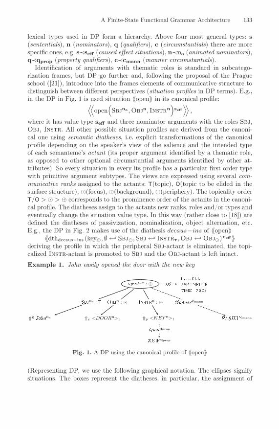
A Finite-State Functional Grammar Architecture 133
lexical types used in DP form a hierarchy. Above four most general types: s(sententials), n (nominators), q (qualifiers), c (circumstantials) there are morespecific ones, e.g. s≺seff (caused effect situations), n≺na (animated nominators),q≺qprop (property qualifiers), c≺cmann (manner circumstantials).
Identification of arguments with thematic roles is standard in subcatego-rization frames, but DP go further and, following the proposal of the Pragueschool ([21]), introduce into the frames elements of communicative structure todistinguish between different perspectives (situation profiles in DP terms). E.g.,in the DP in Fig. 1 is used situation 〈〈open〉〉 in its canonical profile:
⟨⟨open
(Sbjna ,Objn, Instrn
)seff
⟩⟩,
where it has value type seff and three nominator arguments with the roles Sbj,Obj, Instr. All other possible situation profiles are derived from the canoni-cal one using semantic diatheses, i.e. explicit transformations of the canonicalprofile depending on the speaker’s view of the salience and the intended typeof each semanteme’s actant (its proper argument identified by a thematic role,as opposed to other optional circumstantial arguments identified by other at-tributes). So every situation in every its profile has a particular first order typewith primitive argument subtypes. The views are expressed using several com-municative ranks assigned to the actants: T(topic), O(topic to be elided in thesurface structure), �(focus), ⊕(background), (periphery). The topicality orderT/O > � > ⊕ corresponds to the prominence order of the actants in the canoni-cal profile. The diatheses assign to the actants new ranks, roles and/or types andeventually change the situation value type. In this way (rather close to [18]) aredefined the diatheses of passivization, nominalization, object alternation, etc.E.g., the DP in Fig. 2 makes use of the diathesis decaus−ins of 〈〈open〉〉
〈〈dthdecaus−ins (key⊕, ∅ ←↩ Sbj�,Sbj←↩ InstrT,Obj←↩ Obj�) seff 〉〉deriving the profile in which the peripheral Sbj-actant is eliminated, the topi-calized Instr-actant is promoted to Sbj and the Obj-actant is left intact.
Example 1. John easily opened the door with the new key
seff : ⊕
⇑g na
na :
⇑x <DOORn>1
n : �
⇑y <KEY n>1
n : ⊕
qprop
qprop
cmann
cmann
Fig. 1. A DP using the canonical profile of 〈〈open〉〉
(Representing DP, we use the following graphical notation. The ellipses signifysituations. The boxes represent the diatheses, in particular, the assignment of

134 A. Dikovsky
communicative ranks to the actants. Solid lines link the actants to their seman-temes and are labeled with roles. Dashed lines link circumstantials to their gov-ernor semantemes and are labeled with names of attributes. Several non-optionalattributes represent the so called discourse status and state the situation’s illoc-utive status, the aspect and the semantic time). Diamonds represent embeddedfunctions: e.g. the ι−operator. ⇑g stands for global context references and ⇓x,⇑xstand for anaphoric references introduction and access. The superscripts corre-spond to lexical types.)
Example 2. The new key easily opened the door
dthdecaus−insseff
openseff : ⊕
[Sbjna : ] Objn : � Instrn : T
ill=dclasp=neutrtime=pres
DS
⇑x <KEY n>1
Sbjn
NEW qprop
Qualqprop
⇑y <DOORn>1
Objn
EASILY cmann
Mannercmann
Fig. 2. DP DPdecaus using a semantic derivative of 〈〈open〉〉
From the semantic perspective, the DP may be seen as first order typed termsserving for compositional definition of semantic expressions. From the syntacticperspective, they are a special kind of feature trees.
Definition 1. The set of feature trees (f-trees) over functors F = {f/n || n ≥ 0}and sorts Σ is the least set T (F,Σ) which (i) contains all constants f/0 ∈ F, and(ii) contains all expressions f(b1 : t1, . . . , bn : tn) for all f/n ∈ F, all pairwisedifferent sorts b1, . . . , bn ∈ Σ and all f-trees t1, . . . , tn ∈ T (F,Σ).
In particular, a DP using as its main situation a situation K in derived pro-file dthd(K), can be seen as the f-tree dthd(K)(s1 : π1, . . . , sm : πm), wherethe sorts si are either the roles of shifted actants with non-null ranks or theattributes identifying present circumstantials, and πi are the f-trees represent-ing the corresponding argument sub-plans. For instance, in the DP in Fig. 1using 〈〈open〉〉 in canonical profile, s1 = Sbjna , s2 = Objn, s3 = Instrn,s4 = Mannercmann . On the other hand, in the f-tree representing the DP inFig. 2, which uses the derivative 〈〈dthdecaus−ins(open)〉〉, s1 = Sbjn, s2 = Objn
and s3 = Mannercmann .

A Finite-State Functional Grammar Architecture 135
3 Generalized Categorial Dependency Grammars
The generalized categorial dependency grammars (gCDG) recently introducedin [9] and studied in [6,7] are categorial grammars generating sentences togetherwith their dependency structures (DS). The DS may be trees (DT) as it is thecase in Fig. 3 or not (cf. Fig . 4). Whatever is the case, they are linearly orderedand this order may be projective, as in Fig. 3(a), or not, as in Fig. 3(b). Thenon-projective order is due to discontinuous dependencies in which the governorg is separated from the subordinate s by a word not dominated by g (as it is thecase of the auxiliary verb a in Fig. 3(b) separating the participle donnee fromits pronominalized objects).
(a) A projective DT
(b) A non-projective DT (French: ∗she itfem to-him has given)
Fig. 3.
Like the classical categorial grammars, gCDG are lexicalized, i.e. are definedby a lexicon: a function λ assigning to each word a finite set of its dependencytypes. A type has the form [lm\ . . . \l1 v/rn . . . /r1]P , where v is the (continu-ous) dependency on the governor, lm, . . . , l1 and rn, . . . , r1 are the (continuous)dependencies of left and right subordinates in the reverse order, and P is asequence of polarized valencies (the potential) determining discontinuous depen-dencies. Types with empty potentials determine projective DT. E.g., the DT inFig. 3(a) is determined by the type assignments:
the �→ det key �→ [modif ∗ \det\pred] new �→ modifeasily �→ circ opened �→ [circ ∗ \pred\S/dobj] door �→ [det\dobj]
where the types modif and circ are iterated and S is the sentence type. Thepolarized valencies are of four kinds: ↙ d (negative: that of the distant rightgovernor through dependency d), ↘ d (same on the left), ↖ d (positive: thatof a distant left subordinate through dependency d), ↗ d (same on the right).A pair of dual valencies ↙ d and ↖ d (↗ d and ↘ d) define a discontinuousdependency d. A negative valency can be anchored on a host word using anchor

136 A. Dikovsky
types #(↙ d), #(↘ d). E.g., the lexicon below uniquely determines the DT inFig. 3(b) (↙clit−dobj,↙clit−iobj are anchored on the auxiliary a):
elle �→ pred la �→ [#(↙clit−dobj)]↙clit−dobj lui �→ [#(↙clit−iobj)]↙clit−iobja �→ [#(↙clit−iobj)\#(↙clit−dobj)\pred\S/aux] donnée �→ [aux]↖clit−dobj↖clit−iobj
Such dependency types are formalized with the following calculus 1
Ll. CP1 [C\β]P2 � [β]P1P2
Il. CP1 [C∗\β]P2 � [C∗\β]P1P2
Ωl. [C∗\β]P � [β]P
Dl. αP1(↙C)P (↖C)P2 � αP1PP2 , if (↙C)P (↖C) satisfies the pairing ruleFA (first available): P has no occurrences of ↙C,↖C.
Ll is the classical elimination rule. Eliminating the argument subtype C �=#(α) it constructs the (projective) dependency C and concatenates the poten-tials. C = #(α) creates no dependency. Il derives k > 0 instances of C. Ωl servesfor the case k = 0.Dl derives discontinuous dependencies. It pairs and eliminatesdual valencies satisfying the rule FA to create the discontinuous dependency C.
For a DS D and a string x, let G(D,x) denote the relation: D is constructedin a proof Γ � S for some Γ ∈ λ(x). Then the language generated by G is theset L(G)=df {w || ∃D G(D,w)}.
The gCDG are very expressive. Evidently, they generate all CF-languages.They can also generate non-CF languages.
Example 3. The gCDG
Gabc : a �→ A↙A, [A\A]↙A, b �→ [B/C]↖A, [A\S/C]↖A, c �→ C, [B\C]
generates the language {anbncn | n > 0} [9]. For instance, Gabc(D(3), a3b3c3)holds for the dependency structure (DS) in Fig. 4 and the string a3b3c3 due tothe proof in Fig. 5.
Fig. 4. Dependency structure for a3b3c3
[A]↙A[A\A]↙A(Ll)
[A]↙A↙A [A\A]↙A(Ll)
[A]↙A↙A↙A[A\S/C]↖A
[B/C]↖A
[B/C]↖AC(Lr)
B↖A [B\C](Ll)
C↖A(Lr)
B↖A↖A [B\C](Ll)
C↖A↖A(Ll)
[A\S]↖A↖A↖A(Ll)
[S]↙A↙A↙A↖A↖A↖A(Dl × 3)
S
Fig. 5. Dependency structure correctness proof1 We show left-oriented rules. The right-oriented are symmetric.

A Finite-State Functional Grammar Architecture 137
Recently, it was shown that the family of gCDG-languages L(gCDG) is anAFL [7]. Seemingly, it is incomparable with the mildly CS languages [24], gen-erated by multi-component TAG, linear CF rewrite systems, minimalist gram-mars [23]. L(gCDG) contains non-TAG languages, e.g. L(m) = {an1an2 ...anm || n ≥1} for allm > 0. In particular, it contains the languageMIX = {w ∈ {a, b, c}+ |||w|a = |w|b = |w|c}, for which E. Bach conjectures that it is not mildly CS. Onthe other hand, we conjecture [6] that this family does not contain the copylanguage Lcopy = {xx || x ∈ {a, b}∗}, which is TAG 2. gCDG have an efficientpolynomial time parsing algorithm [6,7] which rests upon a property of indepen-dence of basic categories and polarized valencies in the proofs in the dependencycalculus. This property is expressed in terms of projections of categories and“well-bracketing” criteria for potentials.
For a sequence of categories γ, its local projection ‖γ‖l and de valency projec-tion ‖γ‖v are defined as follows:
1. ‖ε‖l = ‖ε‖v = ε; ‖αγ‖l = ‖α‖l‖γ‖l and ‖αγ‖v = ‖α‖v‖γ‖v for a category α.2. ‖CP ‖l = C et ‖CP ‖v = P for every category CP .
To speak about “well-bracketing” of potentials, we interpret ↙ d and ↗ das left brackets and ↖ d and ↘ d as right brackets. For a left bracket valencyα, the corresponding (dual) right bracket valency is denoted α. The set of left-bracket valencies is denoted V l. That of right-bracket valencies is denoted V r.V=df V
l ∪ V r. A potential is balanced if it is well bracketed in the usual sense.For a potential P and dual valencies α ∈ V l, α ∈ V r, the values
Δα(P ) = max{|P ′|α − |P ′|α || P ′ is a suffix of P},Δα(P ) = max{|P ′|α − |P ′|α || P ′ is a prefix of P}
(where |γ|α is the number of occurrences of α in γ) express the deficits of rightand left α−brackets in P (i.e. the maximal number of right and left bracketα-valencies which need to be added to P on the right (left) so that it be-came balanced. It is not difficult to prove that a potential P is balanced iff∑
α∈VΔα(P ) = 0.
Let c be the projective core of the dependency calculus, consisting of therules L, I and Ω and �c denote the provability relation in this sub-calculus. Oneof the key results of [6,7] is the following property of projections independenceproviding the abovementioned polynomial time parsing algorithm.
Theorem 1. For a gCDG G with dictionary λ and a string x, x ∈ L(G) iffthere is Γ ∈ λ(x) such that ‖Γ‖l �c S and ‖Γ‖v is balanced.
By the way, from this theorem it follows that the correctness of an assignmentof categories to words in a sentence is recognized in real time.
Corollary 1. For every sequence of types γ with distinguished constituents (i.e.without elimination ambiguity), the problem of provability γ � S in the depen-dency calculus is resolved in real time |γ| using one stack and v counters, wherev is the number of polarized valency names.2 It doesn’t prevent that gCDG explain the cross-serial dependencies [10].

138 A. Dikovsky
4 Finite State Converters of F-Trees into D-Structures
First of all, we explain how the general f-trees are converted into DS. Next, wewill adapt this conversion to the DP.
Definition 2. Deterministic FS transducer (DFS transducer) is an automatonon f-trees Γ = (F,Σ,W,Q, q0, γ, δ), where T (F,Σ) is the set of f-trees over Fand Σ, W is a set of words, Q is a finite set of states, q0 being the initial state,γ is a lexical interpretation, i.e. a function F × Q → W and δ is a transitionfunction defined as follows.
Let B = {b1, . . . , bk} ⊆ Σ be a set of sorts and f/k ∈ F be a functor, k ≥ 0.Then Π(f,B,Q) denotes the set of all strings x over (F ×Q)∪(B×Q) such thatx has at most one occurrence (f, q) for some q ∈ Q and at most one occurrenceof (b, q) for some q ∈ Q for every sort b ∈ B 3. In these terms, δ is a function{δ : (f(b1, . . . , bk), q) �→ β || β ∈ Π(f, {b1, . . . , bk}, Q)}. Elementary associations((f(b1, . . . , bk), q) �→ β) ∈ δ are called transitions.
For an f-tree π and a state q ∈ Q, Γ ((π, q)) is defined by:Γ ((πn, qn) . . . (πn, qn)) = Γ ((π1, q1)) . . . Γ ((π1, qn)).Γ ((f, q)) = γ(f, q), for all f ∈ F.Γ ((f(b1 : π1, . . . , bk : πk), q)) = Γ (σ(δ(f(b1, . . . , bk), q))),where σ is the natural morphism σ((bi, q))=(πi, q), σ(α)=α for α /∈ {b1, . . . , bk}.
The transduction Γ : T (F,Σ)→W+ is defined by Γ (π) = Γ ((π, q0)).
Definition 3. FT-DS converter T = (Γ,G) is a DFS transducer Γ whose lexicalinterpretation γT is coordinated with the lexicon λ of a gCDG G through a typingfunction type : Q→ ⋃
w∈Wλ(w) as follows: γT (f, q) = w : type(q) and type(q) ∈
λ(w). T uniquely determines the following relation between the f-trees, the stringsand the D-structures: T (π, x,D) iff Γ (π) = w1 : C1 . . . wm : Cm, where x =w1 . . . wm, C1 . . . Cm � S and D is constructed in this proof.Language of T : L(T ) = {x ∈W+ || ∃π,D(T (π, x,D))}.Example 4. It is not difficult to see that the following FT-DS converter Tabcgenerates the language L(Tabc) = {anbncn || n > 0}.
Tabc =
⎧⎪⎪⎪⎪⎪⎪⎨
⎪⎪⎪⎪⎪⎪⎩
(h(1, 2), q0)→ (1,−)(2, S) (f(1, 2), S)→ (f, S)(1,+)(2, \)(g(1),−)→ (1,−)(g,−) (f, S)→ b : [A\S/C]↖A
(g,−)→ a : [A\A]↙A (f(1, 2),+)→ (f,+)(1,+)(2, \)(g0,−)→ a : A↙A (f,+)→ b : [B/C]↖A
(e, \)→ c : [B\C] (f1(1),+)→ (f,+)(1, C)(e, C)→ c : C
For instance,Tabc converts the f-treeπ(3) inFig. 6 into the typed string (a : A↙A)(a :[A\A]↙A)(a : [A\A]↙A)(b : [A\S/C]↖A)(b : [B/C]↖A)(b : [B/C]↖A)(c : C)(c : [B\C])(c : [B\C]). So Tabc(π(3), a3b3c3, D(3)), where D(3) is the DSin Fig. 4.3 This is a resource sensitive, “no copy" constraint.

A Finite-State Functional Grammar Architecture 139
2
h
e
ef1
f
fg
g
g0
21
1
1
1
1
1
e
2
π(3) :
Fig. 6.
The FT-DS converters have the same weak generative power as gCDG in thefollowing sense.
Theorem 2. The family L(FT −DS(RTL)) of languages T (L), where L is aregular f-tree language and T is an FT-DS converter, coincides with L(gCDG).
Proof scheme. 1. The inclusion L(gCDG) ⊆ L(FT −DS(RTL)) is evident.2. The inverse inclusion follows from the established in [1] weak equivalence ofgCDG to dependency structure grammars (DSG), a class of rule based generatingdependency grammars. Due to the no copy constraint, for every given signatureof functors F and sorts Σ, every FS-DT T applied to T (F,Σ) can be convertedinto a DSG ΓT generating the language T (T (F,Σ)). It remains to remark thatfor every FS-DT T and every finite automaton A on f-trees there is an FS-DTTA such that T (Δ(A)) = TA(T (F,Σ)), where Δ(A) is the set of f-trees acceptedby A. The latter is proved using the classical construction of a finite automatonfor the intersection of languages accepted by finite automata.
5 DP-DS Converters
DP-DS converters are a special kind of the FT-DS converters, where the DP areused in the place of arbitrary f-trees. It is significant that the set of all DP is aregular f-tree language.
In order to arrive at a syntax of DP-DS converters usable in practice, we codethe DP and the converter transitions using HPSG-like feature structures. In par-ticular, we use states with two substructures, a semantic one: DS[ill, asp, time],standing for the discourse status of the converted DP and a morpho-syntacticone: GS[left, right, value, ptn, GrCl (grammatical class), tns (tense),num (number), pers (person)] 4, standing for the features of the correspond-ing surface construction (see Fig. 7-17). Four selected features value, left,right and ptn in GS serve to define the dependency type type(q). Namely,type(q) = [α1\...\αl\γ/β1/.../βr]P if q.GS.left = α1\...\αl, q.GS.right =β1/.../βr, q.GS.value = γ and q.GS.ptn = P.
4 Both lists are open.

140 A. Dikovsky
Like in HPSG, we make use of partially defined (i.e. generalized) structuresand of their specializations (denoted tgener � tspec). In particular, t1 = t2 � tmeans that t is a specialization of the most general unifier of t1 and t2. Theunification is constrained by the hierarchy of primitive types. We also use defaultvalues. E.g., the default value ptn = ε stands for the projective dependencytypes. Another example: for the attributes (sorts of optional arguments) listed inthe situation argument frames under the name optargs (see Fig. 7), the defaultvalue A = ε stands for the absent arguments A. optargs = ∅ means that alloptional arguments are absent.
The transitions are also represented by partial feature structures and so can beconsecutively specialized. The right hand side of a transition is represented as thevalue of the sort to.The values of the sort PO stand for right hand side orderings.
A fragment of DP-DS transitions for EnglishBelow, we present several transition schemes sufficient to generate the sentencesin examples 1,2 from the corresponding DP. Fig. 7 presents the necessary argu-ment frames.
dict
⎡
⎢⎢⎢⎢⎢⎢⎢⎢⎣
key openprofile canonSbj [type na]Obj [type n]Instr [type n]optargs listvtype seff
⎤
⎥⎥⎥⎥⎥⎥⎥⎥⎦
(a) Canonical profile of 〈〈open〉〉
dict
⎡
⎢⎢⎢⎢⎢⎢⎢⎢⎢⎢⎢⎢⎢⎢⎢⎢⎢⎢⎢⎢⎢⎢⎢⎢⎢⎢⎢⎢⎢⎢⎢⎢⎣
key open
profile dth
⎡
⎢⎢⎢⎢⎢⎢⎢⎢⎢⎢⎢⎢⎢⎢⎢⎢⎢⎢⎢⎢⎢⎢⎣
name decaus-ins
shifts
⎡
⎢⎢⎢⎢⎢⎢⎢⎢⎢⎢⎢⎢⎢⎢⎢⎢⎣
Sbj
⎡
⎣type na
rank shift ∅
⎤
⎦
Obj
⎡
⎢⎢⎣
type nrank �shift Objtshift n
⎤
⎥⎥⎦
Instr
⎡
⎢⎢⎣
type nrank Tshift Sbjtshift n
⎤
⎥⎥⎦
⎤
⎥⎥⎥⎥⎥⎥⎥⎥⎥⎥⎥⎥⎥⎥⎥⎥⎦
value[type sefftshift seff
]
⎤
⎥⎥⎥⎥⎥⎥⎥⎥⎥⎥⎥⎥⎥⎥⎥⎥⎥⎥⎥⎥⎥⎥⎦
Sbj [type n]Obj [type n]optargs listvtype seff
⎤
⎥⎥⎥⎥⎥⎥⎥⎥⎥⎥⎥⎥⎥⎥⎥⎥⎥⎥⎥⎥⎥⎥⎥⎥⎥⎥⎥⎥⎥⎥⎥⎥⎦
(b) Diathesis 〈〈dthdecaus−ins〉〉 of 〈〈open〉〉
dict
⎡
⎢⎢⎣
key Kprofile Ref < K >varoptargs listvtype ncomm
⎤
⎥⎥⎦
(c) nominator
dict
⎡
⎣key Koptargs listvtype cmann
⎤
⎦
(d) circumstantial
dict
⎡
⎣key Koptargs listvtype qprop
⎤
⎦
(e) qualifier
Fig. 7. Argument frames
tcanon[sem dict
[profile canon
] ]
tdecaus−ins[sem dict
[profile dth
[name decaus− ins ] ] ]
Fig. 8. Transition schemes for profile selection

A Finite-State Functional Grammar Architecture 141
Two transition schemes in Fig. 8 serve to select the argument frame corre-sponding to the situation profile. Fig. 9 presents a transition scheme applied tothe main situations with Obj-argument in declarative DP. So it applies to bothprofiles of 〈〈open〉〉 in Fig. 7(a),(b). Its specific cases assign the axiom value typeS to the main transitive verb (e.g. 〈〈open〉〉) in the surface form.
t(dcl,obj)
⎡
⎢⎢⎣
sem dict
[Obj xobjvtype s
]
state[DS
[ill dcl
] ]
to[head
[state
[GS
[value S
] ] ] ]
⎤
⎥⎥⎦
Fig. 9. Transition scheme for declarative Obj-argument situations
The scheme in Fig. 10 applies to the situations in semantical past time andneutral aspect corresponding in English to the surface simple past tense of mainverbs. The transitions fitting this scheme assign to the situation’s surface verbform form(K, f) its left and right subordinates’ subtypes, propagates the cor-responding value types to Sbj-sort and Obj-sort subplans and, at the sametime, positions these subplans with respect to the verb. A similar scheme forsemantical past time and perfect aspect is found in Fig. 11.
tPN
⎡
⎢⎢⎢⎢⎢⎢⎢⎢⎢⎢⎢⎢⎢⎢⎢⎢⎣
sem dict[key K
]
state[
DS[asp neutrtime past
]]
to
⎡
⎢⎢⎢⎢⎢⎢⎢⎢⎢⎢⎣
Sbj[state
[GS
[value pred
] ] ]
head
⎡
⎢⎢⎢⎢⎣
state
⎡
⎢⎢⎣GS f
⎡
⎢⎢⎣
left circ ∗ \pred\right /circ ∗ /dobjtns PastSimpleGrCl Vt
⎤
⎥⎥⎦
⎤
⎥⎥⎦
lex form(K, f)
⎤
⎥⎥⎥⎥⎦
Obj[state
[GS
[value dobj
] ] ]
po {Sbj < head < Obj}
⎤
⎥⎥⎥⎥⎥⎥⎥⎥⎥⎥⎦
⎤
⎥⎥⎥⎥⎥⎥⎥⎥⎥⎥⎥⎥⎥⎥⎥⎥⎦
Fig. 10. Transition scheme for situations in neutral aspect past time
The transition schemes in Fig. 12 and 13 apply to the situations in neutral(respectively, perfect) aspect and semantical past time if there is a Manner-circumstantial. E.g., the transitions fitting the neutral aspect scheme place thisargument between the Sbj-sort argument and the verb representing the situa-tion if the circumstantial is an adverbial. Otherwise, it places this argument onthe right of the Obj-sort argument. Fig. 14 presents an example of a terminaltransition scheme for adverbials without (optional) arguments. The cases of thisscheme select the corresponding form and finalize the dependency type assign-ing type(q) = q.GS.value (i.e. q.GS.ptn = q.GS.left = q.GS.right = ε). Asimilar scheme for adjective modifiers is found in Fig. 17.

142 A. Dikovsky
tPP
⎡
⎢⎢⎢⎢⎢⎢⎢⎢⎢⎢⎢⎢⎢⎢⎢⎢⎢⎢⎢⎢⎢⎢⎢⎢⎢⎢⎢⎢⎢⎢⎢⎢⎢⎢⎢⎢⎣
dict[
K]
qs
[ [ ]]
⎡
⎢⎢⎢⎢⎢⎢⎢⎢⎢⎢⎢⎢⎢⎢⎢⎢⎢⎢⎢⎢⎢⎢⎢⎢⎢⎢⎢⎢⎢⎢⎣
⎡
⎣
⎡
⎣
⎡
⎣predf.f.
⎤
⎦
⎤
⎦
⎤
⎦
⎡
⎢⎢⎢⎢⎢⎢⎢⎢⎣
⎡
⎢⎢⎢⎢⎢⎢⎣
f
⎡
⎢⎢⎢⎢⎢⎢⎣
circ ∗ \pred\/aux
aux
qs. .qs. .
⎤
⎥⎥⎥⎥⎥⎥⎦
⎤
⎥⎥⎥⎥⎥⎥⎦
form( , f)
⎤
⎥⎥⎥⎥⎥⎥⎥⎥⎦
⎡
⎢⎢⎢⎢⎢⎢⎣
⎡
⎢⎢⎢⎢⎣
g
⎡
⎢⎢⎢⎢⎣
auxcirc ∗ \/circ ∗ /dobj
⎤
⎥⎥⎥⎥⎦
⎤
⎥⎥⎥⎥⎦
form(K, g)
⎤
⎥⎥⎥⎥⎥⎥⎦
[ [ [dobj
] ] ]
{ < < < }
⎤
⎥⎥⎥⎥⎥⎥⎥⎥⎥⎥⎥⎥⎥⎥⎥⎥⎥⎥⎥⎥⎥⎥⎥⎥⎥⎥⎥⎥⎥⎥⎦
⎤
⎥⎥⎥⎥⎥⎥⎥⎥⎥⎥⎥⎥⎥⎥⎥⎥⎥⎥⎥⎥⎥⎥⎥⎥⎥⎥⎥⎥⎥⎥⎥⎥⎥⎥⎥⎥⎦
Fig. 11. Transition scheme for perfect aspect situations in past time
t(PN,cmann)
⎡
⎢⎢⎢⎢⎢⎢⎢⎢⎢⎢⎣
dict[ [ [
cmann
] ] ][ [ ] ]⎡
⎢⎢⎢⎢⎢⎢⎣
xsbjhxobj[ [ [
circ] ] ]
{< < if (↓ ). . . =< otherwise
}
⎤
⎥⎥⎥⎥⎥⎥⎦
⎤
⎥⎥⎥⎥⎥⎥⎥⎥⎥⎥⎦
Fig. 12. Transition scheme for manner circumstantials in neutral aspect past time
t(PP,cmann)
⎡
⎢⎢⎢⎢⎢⎢⎢⎢⎢⎢⎣
dict[ [ [
cmann
] ] ][ [ ]]
⎡
⎢⎢⎢⎢⎣
hxobj[ [ [
circ] ] ]
{< < if (↓ ). . . =< < otherwise
}
⎤
⎥⎥⎥⎥⎦
⎤
⎥⎥⎥⎥⎥⎥⎥⎥⎥⎥⎦
Fig. 13. Transition scheme for manner circumstantials in past perfect
Then follow special cases of transition schemes for nominator type subplansin the positions of Sbj and Obj-arguments in examples 1,2. In particular, thatin Fig. 15 places the definite article on the left of a referenced nominator se-manteme, whereas, that in Fig. 16 places between them an optional qualifier, ifany.

A Finite-State Functional Grammar Architecture 143
t(c,noargs)
⎡
⎢⎢⎢⎢⎢⎢⎢⎢⎢⎢⎢⎢⎣
dict
⎡
⎣K∅c
⎤
⎦
[ [t] ]
⎡
⎢⎢⎢⎢⎣
⎡
⎢⎢⎢⎢⎣
⎡
⎢⎢⎣ qc
⎡
⎢⎢⎣
tεε
⎤
⎥⎥⎦
⎤
⎥⎥⎦
form(K, qc)
⎤
⎥⎥⎥⎥⎦
⎤
⎥⎥⎥⎥⎦
⎤
⎥⎥⎥⎥⎥⎥⎥⎥⎥⎥⎥⎥⎦
Fig. 14. Transition scheme for adverbials
t(n,def)
⎡
⎢⎢⎢⎢⎢⎢⎢⎢⎢⎢⎢⎢⎢⎢⎢⎢⎢⎢⎢⎢⎢⎢⎢⎢⎢⎢⎣
dict
[ ⇑ref< K >1
n
]
⎡
⎢⎢⎢⎢⎢⎢⎢⎢⎢⎢⎢⎢⎢⎢⎢⎢⎢⎢⎢⎢⎢⎢⎣
⎡
⎢⎢⎢⎢⎢⎢⎢⎢⎣
⎡
⎢⎢⎢⎢⎢⎢⎣
qd
⎡
⎢⎢⎢⎢⎢⎢⎣
εεdet
def
3sg
⎤
⎥⎥⎥⎥⎥⎥⎦
⎤
⎥⎥⎥⎥⎥⎥⎦
form( , qd)
⎤
⎥⎥⎥⎥⎥⎥⎥⎥⎦
⎡
⎢⎢⎢⎢⎢⎢⎣
⎡
⎢⎢⎢⎢⎣
qN
⎡
⎢⎢⎢⎢⎣
modif ∗ \det\/attr∗comm
qd.qd.
⎤
⎥⎥⎥⎥⎦
⎤
⎥⎥⎥⎥⎦
form(K, qN )
⎤
⎥⎥⎥⎥⎥⎥⎦
{ < }
⎤
⎥⎥⎥⎥⎥⎥⎥⎥⎥⎥⎥⎥⎥⎥⎥⎥⎥⎥⎥⎥⎥⎥⎦
⎤
⎥⎥⎥⎥⎥⎥⎥⎥⎥⎥⎥⎥⎥⎥⎥⎥⎥⎥⎥⎥⎥⎥⎥⎥⎥⎥⎦
Fig. 15. Transition scheme for determined nominators
t(n,Qual)
⎡
⎢⎢⎢⎢⎣
dict[ [ [
qprop
] ] ]⎡
⎢⎢⎣
hd[ [ [
modif] ] ]
{ < < }
⎤
⎥⎥⎦
⎤
⎥⎥⎥⎥⎦
Fig. 16. Transition scheme for qualifiers of determined nominators
t(q,noargs)
⎡
⎢⎢⎢⎢⎢⎢⎢⎢⎢⎢⎢⎢⎣
dict
⎡
⎣K∅q
⎤
⎦
[ [t] ]
⎡
⎢⎢⎢⎢⎣
⎡
⎢⎢⎢⎢⎣
⎡
⎢⎢⎣ qAdj
⎡
⎢⎢⎣
tεε
⎤
⎥⎥⎦
⎤
⎥⎥⎦
form(K, qAdj)
⎤
⎥⎥⎥⎥⎦
⎤
⎥⎥⎥⎥⎦
⎤
⎥⎥⎥⎥⎥⎥⎥⎥⎥⎥⎥⎥⎦
Fig. 17. Transition scheme for adjective modifiers

144 A. Dikovsky
In Fig. 18 is shown a computation of a DP-DS-converter whose transitionsare determined by the transition schemes in Fig. 8-17. In the course of thiscomputation, the sentence The new key easily opened the door is generated fromthe DP DPdecaus in Fig. 2 using five transitions:tdecaus−ins = t(dcl,obj) = tPN = t(PN,cmann) � t1,t(n,Qual) = t(n,def,K=KEY ) � t2, t(q,noargs,K=NEW ) =� t3,t(c,noargs,K=EASILY ) =� t4, t(n,def,K=DOOR,optargs=∅) � t5.
(DPdecaus, q0)
(THE, q11) (DPQUAL, q12) (KEY, q13)
(DPDOOR, q4)(DPEASILY , q2)
t4
t1
t2
t3
t5
(NEW, q121)
(EASILY, q21) (DOOR, q42)(THE, q41)
(DPKEY , q1) (OPENED, q3)
[det]
[modif ]
[modif ∗ \det\pred] [circ]
[circ ∗ \pred\S/dobj]
[det] [modif ∗ \det\dobj]
Fig. 18. Generation of The new key easily opened the door
[det]
[modif ][modif ∗ \det\pred](Il)
[modif ∗ \det\pred](Ωl)
[det\pred](Ll)
[pred]
[circ][circ ∗ \pred\S/dobj](Il)
[circ ∗ \pred\S/dobj](Ωl)
[pred\S/dobj][det]
[modif ∗ \det\dobj](Ωl)
[det\dobj](Ll)
[dobj](Lr)
[pred\S](Ll)
[S]
Fig. 19. A correctness proof
A proof of correctness of this computation is shown in Fig. 19. It is easy tosee that in this proof is constructed the D-tree in Fig. 3(a).
Properties of DP-DS-conversion architecture. Our English example illus-trates the following important properties of the DP-DS-conversion.
1. The transition schemes are either terminal (lexical or referential), or one ar-gument, or they decompose a situation profile into constituents which fix theelimination order of local dependencies’ subtypes.

A Finite-State Functional Grammar Architecture 145
2. The specific transition schemes are not guessed, but uniquely determined(through unification) by the substructures to which they apply.3. The transitions do not copy or move a material. Unbounded discontinuousdependencies are established through dual valencies in correctness proofs.4. In the place of a general proof search is used a real time type checking proof(see Corollary 1) witnessing for or against the feasibility of a DP when appliedto the type sequence generated from it.
One can see that due to these properties the finite-state conversion and thetype checking can be carried out in parallel in the course of DP composition.
6 Conclusion
This work is theoretical. It presents a new compositional generativistic architec-ture in which the surface syntax is defined in terms of dependency types, themeaning structures uniquely encode the arguments’ scopes, surface forms andprecedence, and where the meaning structure is converted into the correspond-ing surface structure using a deterministic fs-tree transducer. An experimentalwork is needed to make sure that this deterministic architecture can be realizedthrough a system of thematic roles, semantic diatheses, lexical definitions andfs-transitions in a way that the resulting DP-DS-conversion of the set of inputDP would be complete with respect to the underlying gCDG.
References
1. Béchet, D., Dikovsky, A., Foret, A.: Dependency structure grammars. In: Blache,P., Stabler, E.P., Busquets, J.V., Moot, R. (eds.) LACL 2005. LNCS (LNAI),vol. 3492, pp. 18–34. Springer, Heidelberg (2005)
2. Bos, J.: Predicate logic unplugged. In: Dekker, P., Stokhof, M. (eds.) Proc. of the10th Amsterdam Colloquium, pp. 133–142 (1995)
3. Bresnan, J.: Optimal syntax. In: Dekkers, J., van der Leeuw, F., van de Weijer,J. (eds.) Optimal theory: Phonology, Syntax and Acquisition, pp. 334–385. OxfordUniversity Press, Oxford (2000)
4. Chomsky, N.: The Minimalist Program. MIT Press, Cambridge, Massacusetts(1995)
5. Copestake, A., Flickinger, D., Malouf, R., Riehemann, S., Sag, I.: Translation usingminimal recursion semantics. In: TMI95. Proc. of the 6th Int. Conf. on Theoreticaland Methodological Issues in Machine Translation, Leuven, Belgium (1995)
6. Dekhtyar, M., Dikovsky, A.: Categorial dependency grammars. In: Moortgat, M.,Prince, V. (eds.) Proc. of Intern. Conf. on Categorial Grammars, pp. 76–91, Mont-pellier (2004)
7. Dekhtyar, M., Dikovsky, A.: Generalized categorial dependency grammars (2007)Submitted paper available fromhttp://www.sciences.univ-nantes.fr/info/perso/permanents/dikovsky/
8. Dikovsky, A.: Linguistic meaning from the language acquisition perspective. In:FG 2003. Proc. of the 8th Intern. Conf. Formal Grammar 2003, Vienna, Austria,pp. 63–76 (August 2003)

146 A. Dikovsky
9. Dikovsky, A.: Dependencies as categories. In: Recent Advances in DependencyGrammars. COLING’04 Workshop, pp. 90–97 (2004)
10. Dikovsky, A.: Multimodal categorial dependency grammars (Submitted paper)11. Dikovsky, A., Smilga, B.: Semantic roles and diatheses for functional discourse
plans. In: MTT 2005. Proc. of the 2nd International Conference Meaning-TextTheory, pp. 98–109 (2005)
12. Dowty, D.R.: Thematic proto-roles and argument selection. Language 67, 547–619(1991)
13. Fillmore, C.: Frame semantics. In: Linguistic Society of Korea (ed.) Linguistics inthe Morning Calm, pp. 111–138, Seoul, Hanshin (1982)
14. Fox, C., Lappin, S.: Underspecified interpretations in a curry-typed representationlanguage. Journal of Logic and Computation 15(2), 131–143 (2005)
15. Grimshaw, J.: Projection, heads and optimality. Linguistic Inquiry 28, 373–422(1997)
16. Hovav, M.R., Levin, B.: Deconstructing the thematic hierarchy. In: 38th SeoulLinguistics Forum, December 10-11, Seoul National University, Seoul, Korea (2004)
17. Kamp, H., Reyle, U.: From Discourse to Logic: An introduction to modeltheoreticsemantics, formal logic and Discourse Representation Theory. Kluwer AcademicPublishers, Dordrecht (1993)
18. Padučeva, E.V.: Dynamic models in lexical semantics. Jazyki slavjanskoj kul’tury,Moscow (Russ.) (2004)
19. Kaplan, R., Bresnan, J.: Lexical functional grammar: A formal system for gram-matical representation. In: Bresnan, J.W. (ed.) The Mental Representation ofGrammatical Relations, pp. 173–281. MIT Press, Cambridge (1982)
20. Reyle, U.: Dealing with ambiguities by underspecification. Journal of Seman-tics 10(2), 123–179 (1993)
21. Sgall, P., Hajičová, E., Panevová, J.: The Meaning of the Sentence in its Semanticand Pragmatic Aspects. Academia, Dordrecht/Reidel/Prague (1986)
22. Sgall, P.: A dependency based specification of topic and focus ii. SMIL. Journal ofLinguistic Calculus (1-2) 110–140 (1980)
23. Stabler, E.: Derivational minimalism. In: Retoré, C. (ed.) LACL 1996. LNCS(LNAI), vol. 1328, pp. 68–95. Springer, Heidelberg (1997)
24. V.-Shanker, K., Weir, D.J.: The equivalence of four extensions of context-free gram-mars. Mathematical Systems Theory 27, 511–545 (1994)

Pregroup Calculus as a Logic Functor
Annie Foret
IRISA –Rennes 1Avenue du General Leclerc
35042 Rennes Cedex - France
Abstract. The concept of pregroup was introduced by Lambek for nat-ural language analysis, with a close link to non-commutative linear logic.We reformulate the pregroup calculus so as to extend it by compositionwith other logics and calculii. The cut elimination property and the de-cidability property of the sequent calculus proposed in the article areshown. Properties of composed calculii are also discussed.
Keywords: Pregroups, Lambek Categorial Grammars, Logic Functor,Cut Elimination.
1 Introduction
The pregroup formalism introduced by Lambek [11] is an efficient and elegantalternative to other categorial grammars used for modeling natural languages.It has been applied to various language syntaxes such as English, French, Italianand Turkish, see e.g. [1,6].
This is a lexicalized formalism: the rules are fixed, each particular grammaris determined by its lexicon assigning a set of type formulas to each word. Theset of rules defines a type calculus that has a close link with non-commutativelinear logic. Type logical grammars, including pregroups, enjoy the following niceproperty : a syntactic analysis corresponds to a derivation in the type calculus(a logical proof). Categorical aspects are given for example in [12,13]. In theirbasic form, pregroup grammars are equivalent to context-free grammars. Someextensions have been proposed : in [7,10] pregroups are enriched with modalitiesallowing to limit associativity.
The purpose of this paper is to give an adaptation of the basic calculus that al-lows modular and rich combinations of type expressions, such as those needed tomodel fine-grained natural language features, while maintaining good propertiesof the formalism. We aim to keep the cut elimination and decidability of the rulesystem, to provide modularity and composability in calculus and modelizationlevels, and to allow conciseness and simplicity in the grammar design.
This adaptation is performed following a “logic functor paradigm”, as in [8],in order to consider new logics as the composition of abstract and reusablecomponents, all logics sharing common specifications, including a subsump-tion relation. Logic functors are functions from logics to logics, (those withoutparameter are standalone but reusable logics). The “logic functor paradigm”
D. Leivant and R. de Queiroz (Eds.): WoLLIC 2007, LNCS 4576, pp. 147–161, 2007.c© Springer-Verlag Berlin Heidelberg 2007

148 A. Foret
also results in concrete software: the LogFun tool [9] offers both a library oflogic functors and a logic composer. For instance, the functor Prop(A) is theclassical propositional logic abstracted over its atoms, that allows to replaceatoms in the classical propositional logic by formulas of the logic given asparameter.
In this article, we provide a functor for pregroups, called FPG(A) in somesense similar to the functor Prop(A), that can be viewed as parameterized pre-groups abstracted over the atoms. One difficulty was to design appropriate rules,generalizing those of original pregroups (recovering pregroups as the particularcase) while maintaining cut elimination and decidability of the calculus.
The definition of pregroups (recalled in Section 2) may seem at first very closeto such a functor, because a partial order is already assumed on basic types,treated as constants (pregroup grammars allow postulates as a finite number ofspecial axioms of the form p � q). In Section 3, a first version of parameterizedpregroup calculus, written SAdj
[A] is defined from Buszkowski’s sequent calculusSAdj for pregroups. Although natural, this version SAdj
[A] lacks the subformulaproperty, which is a disadvantage to establish decidability. A second version ofparameterized pregroup calculus, that we call S[A] is then proposed, to avoidthis drawback. Section 4 gives the main properties; the key proofs of this articleare shown for S[A]. Detailed proofs can be found in Section 5 and at the endthis paper. Section 6 concludes.
2 Preliminaries
2.1 Pregroups
Definition 1. A pregroup (or PG in short) is a structure (P,≤, ·, l, r, 1) suchthat (P,≤, ·, 1) is a partially ordered monoid1 and l, r are two unary operationson P that satisfy for all a ∈ P : ala ≤ 1 ≤ aal and aar ≤ 1 ≤ ara.
Example 1. Groups are a special case a pregroups, for which the left and rightadjoint are the same.
Algebraic properties and iterated adjoints. In a pregroup, we have :
(XY )l = Y lX l and (XY )r = Y rXr;(X l)r = X and (Xr)l = X1l = 1r = 1
Iterated left and right adjoints can be written using integer exponents by:
p(n−1) = (p(n))l and p(n+1) = (p(n))r, we write p for p(0).
Note also that if X ≤ Y then Y l ≤ X l and Y r ≤ Xr (order-reversing)1 We briefly recall that a monoid is a structure < M, ·, 1 >, such that · is associative
and has a neutral element 1 (∀x ∈ M : 1 ·x = x · 1 = x). A partially ordered monoidis a monoid M, ·, 1) with a partial order ≤ that satisfies ∀a, b, c: a ≤ b ⇒ c · a ≤c · b and a · c ≤ b · c.

Pregroup Calculus as a Logic Functor 149
2.2 Free Pregroups
We recall definitions and results, mainly from [4,5] , we also introduce notations.
Definition 2. Let (P,≤) be an ordered set of primitive types, we use integerexponents on P :
– the set of atomic types is : P (Z) = {p(i) | p ∈ P, i ∈ Z}– the set of types is Cat(P,≤) =
(P (Z)
)∗= {p(i1)
1 · · · p(in)n | 0 ≤ k ≤ n, pk ∈
P and ik ∈ Z}– the relation ≤ on Cat(P,≤) is the smallest reflexive and transitive relation,
satisfying these conditions for all p, q ∈ Pr, X,Y ∈ Cat(P,≤) and n ∈ Z:Xp(n)p(n+1)Y ≤ XY (contraction), XY ≤ Xp(n+1)p(n)Y (expansion), andXp(n)Y ≤ Xq(n)Y , if p ≤ q with n even or q ≤ p with n odd (induction)
– the free pregroup generated by (P,≤) is defined on classes [...] modulo ∼such that X∼Y iff X≤Y and Y ≤X with 1 = [ε], [x].[y] = [xy], [x]l = [xl],[x]r = [xr] and [x] ≤ [y] iff x ≤ y (with [xy]l = [ylxl], [xy]r = [yrxr]).
Buszkowski has proposed a sequent calculus, written SAdj below; he has shownits equivalence with ≤ on Cat(P,≤) as in the above definition. SAdj also char-acterizes deductibility in the free pregroup generated by (P,≤), where 1 is theempty string.
Definition 3 (The Sequent calculus of Adjoints SAdj). Let (P,≤) be anordered set of primitive types, system SAdj is made of the following rules, wherep, q ∈ P , n, k ∈ Z and X,Y, Z ∈ Cat(P,≤):
X ≤ X (Id)X ≤ Y Y ≤ Z
(Cut)X ≤ Z
XY ≤ Z(AL)
Xp(n)p(n+1)Y ≤ ZX ≤ Y Z
(AR)X ≤ Y p(n+1)p(n)Z
Xp(k)Y ≤ Z(INDL)
Xq(k)Y ≤ ZX ≤ Y p(k)Z
(INDR)X ≤ Y q(k)Z
q ≤ p if k is even, and p ≤ q if k is odd
Simple free pregroup. A simple free pregroup is a free pregroup where the orderon primitive type is equality.
We mention an interesting link, explored by Kislak and Buszkowski, betweenpregroups and other types-logical grammars (the reader not familiar with Lam-bek grammars may consult [2] for details).
Free pregroup interpretation. Let FP denotes the simple free pregroup with P asprimitive types. We associate with each formula C of the Lambek Calculus L orits non-associative version NL, an element in FP written [[C]] as follows: [[A]] = A

150 A. Foret
if A is a primitive type, [[C1\C2]] = [[C1]]r[[C2]], [[C1 /C2]] = [[C1]][[C2]]l, [[C1 •C2]] =[[C1]][[C2]]. The notation extends to sequents by: [[A1, . . . , An]] = [[A1]] · · · [[An]].
The following property states that FP is a model for L (hence for NL): ifΓ �L C then [[Γ ]] ≤FP [[C]].
Note however that the converse does not hold [3].
Cut elimination. As for the Lambek Calculus L or its non-associative versionNL, the cut rule can be eliminated in SAdj : every derivable inequality has a cut-free derivation [4,5]. This property is important to get a proof-search algorithmbased on the system rules.
2.3 Categorial Grammars and Languages
We first consider categorial grammars in general, these are lexicalized grammars,involving an alphabet Σ, a set of types Tp that is usually generated from a setof primitive types P and given connectives, and a system of rules defining aderivation relation on types.
Definition 4 (Categorial grammar). A categorial grammar is a structureG = (Σ, I, S) where: Σ is a finite alphabet (the words in the sentences); I : Σ �→Pf(T ) is a function that maps a set of types to each element of Σ (the possiblecategories of each word); S ∈ P is the main type associated to correct sentences.
A sentence belongs to the language of G, provided its words can be assignedtypes that derive S according to the rules of the type calculus.
Definition 5 (Pregroup grammar and language). A pregroup grammar(PG-grammar in short) based on a finite poset (P,≤) is a categorial grammarG = (Σ, I, s), such that: s ∈ P , I assigns types in Cat(P,≤).
The language L(G) of a PG-grammar G = (Σ, I, s), based on a finite poset(P,≤) is the set of strings, that can be assigned a string of types deriving s inthe free pregroup on (P,≤):
L(G) = {v1 . . . vn ∈ Σ∗ : ∀i, 1 ≤ i ≤ n, ∃Xi ∈ I(vi) such that X1 . . .Xn ≤ s}The following property, shown in [3], characterizes the generative capacity ofPGs.
Proposition 1. The languages generated by PG-grammars based on finite posetsare the context-free languages (without the empty string).
Example 2. We consider the following grammar fragment, with a parsed sentence(the type assignments are below each word, underlinks indicate contractions oftypes), the string of types derives s1 ≤ s:
sentence: The film explains this situationtypes: (ns c
l ) c (π3r s1 ol) (ns c
l) c
using primitive types and order postulates as follows:

Pregroup Calculus as a Logic Functor 151
c = count noun (film, situation)ns ≤ π3 ns = singular noun phrase (John)
πk = kth personal subject pronoun (π3=he/she/it)ns ≤ o o = direct objects1 ≤ s ≤ s s1 = statement in present tense
s = declarative sentence (the tense does not matter)s=indirect sentence
Using the [[. . .]] translation to Lambek calculus L, this sentence is also parsedin L:
s1
ns
Thens / c
filmc
π3\s1
explains(π3\s1) / o
ns
thisns / c
situationc
where types ns, π3, o . . . are to be replaced with complex types such that:ns � π3, ns � o, and s1 � s � s.
3 Towards a Logic Functor
We propose an adaptation of pregroup following a “logic functor paradigm”, asin [8,9], written FPG. In [9], a logic A is viewed as the association of an abstractsyntax ASA, a semantics SA, an implementation PA, and a type TA made ofa set of properties, including a subsumption (or entailment) relation, ≤A. Theclass of these logics is denoted by L. A logic functor F takes logics of L as pa-rameters and returns a logic in L; it is also viewed as a tuple (ASF , SF , PF , TF )of functions such that (ASF (L1,...,Ln), SF (L1,...,Ln), PF (L1,...,Ln), TF (L1,...,Ln)) =(ASF (ASL1 , . . . , ASLn), SF (SL1 , . . . , SLn), PF (PL1 , . . . , PLn), TF (TL1 , . . . , TLn)).
This paper does not deal with all those aspects (the semantics part is left).The adaptation proposed here can be viewed as parameterized pregroups ab-
stracted over the atoms. We detail the syntax ASFPG and properties for imple-mentation and module composition ; we focus on the subsumption relation andits implementation PFPG based on a sequent calculus formulation.
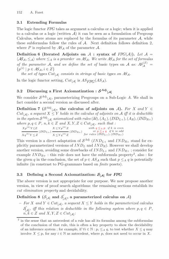
152 A. Foret
3.1 Extending Formulas
The logic functor FPG takes as argument a calculus or a logic; when it is appliedto a calculus or a logic (written A) it can be seen as a formulation of PregroupCalculus, where atoms are replaced by the formulas of its parameter A, whilethese subformulas follow the rules of A. Next definition follows definition 2,where P is replaced by ASA of the parameter A.
Definition 6 (Iterated Adjoints on A : syntax of FPG(A)). Let A =〈ASA,≤A〉 where ≤A is a preorder on ASA. We write ASA for the set of formulasof the parameter A, and we define the set of basic types on A as: AS(Z)
A ={p(i) | p ∈ ASA, i ∈ Z}
the set of types Cat[A] consists in strings of basic types on ASA.
In the logic functor setting, Cat[A] is ASFPG(ASA).
3.2 Discussing a First Axiomatization : SAdj[A]
We consider SAdj[A], parameterizing Pregroups on a Sub-Logic A. We shall in
fact consider a second version as discussed after.
Definition 7 (SAdj[A], the calculus of adjoints on A). For X and Y ∈
Cat[A], a sequent X ≤ Y holds in the calculus of adjoints on A iff it is deductiblein the system SAdj
[A] axiomatized with rules (Id), (AL), (INDL+), (AR), (INDR+)where p, q ∈ P , n, k ∈ Z and X,Y, Z ∈ Cat[A], such that :
Xp(k)Y≤Z(INDL+)
Xq(k)Y ≤Z
X ≤Y p(k)Z(INDR+)
X ≤Y q(k)Z
with q ≤A p if k is evenor p ≤A q if k is odd
for rules (INDL+), (INDR+)
This version is a direct adaptation of SAdj (INDL+ and INDR+ stand for ex-plicitly parameterized versions of INDL and INDR). However we shall developanother version, avoiding some drawbacks of INDL+ and INDR+ ; consider forexample INDR+ : this rule does not have the subformula property2, also : forthe given q in the conclusion, the set of p ∈ ASA such that p ≤A q is potentiallyinfinite (in constrast to PG-grammars based on finite posets).
3.3 Defining a Second Axiomatization: S[A] for FPG
The above version is not appropriate for our purpose. We now propose anotherversion, in view of proof search algorithms: the remaining sections establish itscut elimination property and decidability.
Definition 8 (S[A] and S ′[A], a parameterized calculus on A)
– For X and Y ∈ Cat[A], a sequent X ≤ Y holds in the parameterized calculusS ′[A], iff this relation is deductible in the following system where p, q ∈ P ,n, k ∈ Z and X,Y, Z ∈ Cat[A]:
2 in the sense that an antecedent of a rule has all its formulas among the subformulasof the conclusion of that rule, this is often a key property to show the decidabilityof an inference system ; for example, if ∀i ∈ N : pi ≤A q, to test whether X ≤ q mayinvolve X ≤ pi for any i ∈ N as antecedent, where pi does not need to occur in X.
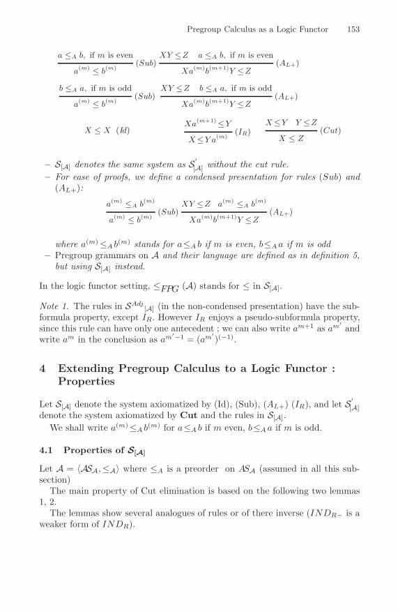
Pregroup Calculus as a Logic Functor 153
a ≤A b, if m is even(Sub)
a(m) ≤ b(m)
XY ≤Z a ≤A b, if m is even(AL+)
Xa(m)b(m+1)Y ≤Z
b ≤A a, if m is odd(Sub)
a(m) ≤ b(m)
XY ≤Z b ≤A a, if m is odd(AL+)
Xa(m)b(m+1)Y ≤Z
X ≤ X (Id)Xa(m+1)≤Y
(IR)X≤Y a(m)
X≤Y Y ≤Z(Cut)
X ≤ Z
– S[A] denotes the same system as S ′[A] without the cut rule.
– For ease of proofs, we define a condensed presentation for rules (Sub) and(AL+):
a(m) ≤A b(m)
(Sub)a(m) ≤ b(m)
XY ≤Z a(m) ≤A b(m)
(AL+)Xa(m)b(m+1)Y ≤Z
where a(m)≤A b(m) stands for a≤A b if m is even, b≤Aa if m is odd
– Pregroup grammars on A and their language are defined as in definition 5,but using S[A] instead.
In the logic functor setting, ≤FPG (A) stands for ≤ in S[A].
Note 1. The rules in SAdj[A] (in the non-condensed presentation) have the sub-
formula property, except IR. However IR enjoys a pseudo-subformula property,since this rule can have only one antecedent ; we can also write am+1 as am′
andwrite am in the conclusion as am′−1 = (am′
)(−1).
4 Extending Pregroup Calculus to a Logic Functor :Properties
Let S[A] denote the system axiomatized by (Id), (Sub), (AL+) (IR), and let S ′[A]
denote the system axiomatized by Cut and the rules in S[A].We shall write a(m)≤A b
(m) for a≤A b if m even, b≤Aa if m is odd.
4.1 Properties of S[A]
Let A = 〈ASA,≤A〉 where ≤A is a preorder on ASA (assumed in all this sub-section)
The main property of Cut elimination is based on the following two lemmas1, 2.
The lemmas show several analogues of rules or of there inverse (INDR− is aweaker form of INDR).
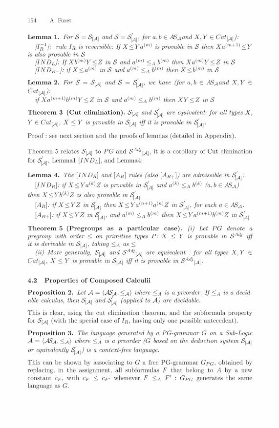
154 A. Foret
Lemma 1. For S = S[A] and S = S ′[A], for a, b ∈ ASAand X,Y ∈ Cat[A]):
[I−1R ]: rule IR is reversible: If X≤Y a(m) is provable in S then Xa(m+1)≤Y
is also provable in S[INDL]: If Xb(m)Y ≤Z in S and a(m) ≤A b(m) then Xa(m)Y ≤Z in S[INDR−]: if X≤a(m) in S and a(m) ≤A b(m) then X≤b(m) in S
Lemma 2. For S = S[A] and S = S ′[A], we have (for a, b ∈ ASAand X,Y ∈
Cat[A]):if Xa(m+1)b(m)Y ≤Z in S and a(m) ≤A b(m) then XY ≤Z in S
Theorem 3 (Cut elimination). S[A] and S ′[A] are equivalent: for all types X,
Y ∈ Cat[A], X ≤ Y is provable in S[A] iff it is provable in S ′[A].
Proof : see next section and the proofs of lemmas (detailed in Appendix).
Theorem 5 relates S[A] to PG and SAdj[A], it is a corollary of Cut elimination
for S ′[A], Lemma1 [INDL], and Lemma4:
Lemma 4. The [INDR] and [AR] rules (also [AR+]) are admissible in S ′[A]:
[INDR]: if X≤Y a(k)Z is provable in S ′[A] and a(k) ≤A b(k) (a, b ∈ ASA)
then X≤Y b(k)Z is also provable in S ′[A]
[AR]: if X≤Y Z in S ′[A] then X≤Y a(n+1)a(n)Z in S ′
[A], for each a ∈ ASA.
[AR+]: if X≤Y Z in S ′[A], and a(m) ≤A b(m) then X≤Y a(m+1)b(m)Z in S ′
[A]
Theorem 5 (Pregroups as a particular case). (i) Let PG denote apregroup with order ≤ on primitive types P : X ≤ Y is provable in SAdj iffit is derivable in S[A], taking ≤A as ≤
(ii) More generally, S[A] and SAdj[A] are equivalent : for all types X,Y ∈
Cat[A], X ≤ Y is provable in S[A] iff it is provable in SAdj[A].
4.2 Properties of Composed Calculii
Proposition 2. Let A = 〈ASA,≤A〉 where ≤A is a preorder. If ≤A is a decid-able calculus, then S[A] and S ′
[A] (applied to A) are decidable.
This is clear, using the cut elimination theorem, and the subformula propertyfor S[A] (with the special case of IR, having only one possible antecedent).
Proposition 3. The language generated by a PG-grammar G on a Sub-LogicA = 〈ASA,≤A〉 where ≤A is a preorder (G based on the deduction system S[A]
or equivalently S ′[A]) is a context-free language.
This can be shown by associating to G a free PG-grammar GPG, obtained byreplacing, in the assignment, all subformulas F that belong to A by a newconstant cF , with cF ≤ cF ′ whenever F ≤A F ′ : GPG generates the samelanguage as G.

Pregroup Calculus as a Logic Functor 155
5 Cut Elimination in S ′[A] : Proof Details
This proof assumes lemmas 1, 2, delailed in the Appendix. Clearly a proof inS[A] is also a proof in S ′
[A]; to show the converse, we proceed by induction on the
number of Cut and the length of a derivation D in S ′[A], ending in Cut:
D with its final cut rule is:γl
⎧⎨
⎩
...Rl
X ≤ Yγr
⎧⎨
⎩
...Rr
Y ≤ ZCut
X ≤ Z
– If Rl is the axiom rule, the last rule (cut) can be suppressed since Rr hasthe same conclusion as D. If Rr is the axiom rule, the last rule (cut) can alsobe suppressed since Rl has the same conclusion as D. We now assume thatneither Rl nor Rr is the axiom rule.
– If Rl is the Cut rule, the induction hypothesis applies to γl, this Cut canbe suppressed, in a proof γ′l , and the final Cut can be suppressed in thisdeduction. If Rr is the Cut rule, we proceed similarly.
We now assume that neither γl or γr has a Cut rule.– We shall prove Cut elimination for Y simple, that is of the form p(u), withp ∈ P (we consider 1 separately); the general case is proved by induction onY , using I−1
R and Lemma2:
-if Y = Y1p(u): D �→
X
...≤Y = Y1p
(u)
I−1R
Xp(u+1) ≤ Y1
Y = Y1p(u)
...≤ZIR
Y1 ≤ Zp(u−1)
rec. on Y
Xp(u+1) ≤ Zp(u−1)
I−1R
Xp(u+1)p(u)≤ZLemma2
X≤Z
– We consider the remaining possibilitieswhen Y is simple,for Rl (left part) and Rr (right part):(no AL+ on the right as Rr,no IR on the left as Rl, for Y simple)these cases are detailed blow.
Rl Rr methodSub IR lemma1 [INDL]AL+ Sub lemma1 [INDR−]AL+ IR permute Rl with cutSub Sub transitivity of ≤A
– When Y = 1 (empty string), the only case is [Rl, Rr]=[AL+, IR] and can betreated as for Y simple (permute Rl with Cut )
– Cut elimination details for Y simple

156 A. Foret
[Sub, IR]
a(m) ≤A b(m)
SubX = a(m) ≤ b(m) = Y
D′
⎧⎪⎪⎨⎪⎪⎩
Y p(u+1)
...≤Z1
IR
Y = b(m) ≤ Z1p(u) = Z
CutX ≤ Z
�→D′
⎧⎪⎪⎨⎪⎪⎩
Y p(u+1)
...≤Z1
IR
Y = b(m) ≤ Z1p(u) = Z
a(m) ≤A b(m)
[INDL]X = a(m) ≤ Z1p
(u) = Z
(for Y simple)
[AL+, Sub]D′
⎧⎪⎪⎨⎪⎪⎩
X1X2
...≤Y = a(m) c(n) ≤A d(n)
AL+
X = X1c(n)d(n+1)X2 ≤ Y = a(m)
a(m) ≤A b(m)
Sub
Y = a(m) ≤ b(m) = Z
CutX ≤ Z
�→D′
⎧⎪⎪⎨⎪⎪⎩
X1X2
...≤Y = a(m) c(n) ≤A d(n)
AL+
X = X1c(n)d(n+1)X2 ≤ Y = a(m)
a(m) ≤A b(m)
[INDR−]X ≤ b(m) = Z
(for Y simple or 1)
[AL+, IR]X1X2
...≤Y a(m) ≤A b(m)
AL+
X = X1a(m)b(m+1)X2 ≤ Y
D′
⎧⎪⎪⎨⎪⎪⎩
Y p(u+1)
...≤Z1
IR
Y ≤ Z1p(u) = Z
CutX ≤ Z
�→ X1X2
...≤Y
D′
⎧⎪⎪⎨⎪⎪⎩
Y p(u+1)
...≤Z1
IR
Y ≤ Z1p(u) = Z
CutX1X2 ≤ Z1p
(u) = Za(m) ≤A b(m)
AL+
X = X1a(m)b(m+1)X2 ≤ Z
6 Conclusion and Perspectives
We have reformulated and proposed to extend the pregroup calculus, so as toallow its composition with other logics and calculii. The cut elimination propertyand the decidability property of this proposed formulation have been shown. It isthus ready to be implemented as a decision procedure and a parsing algorithm.

Pregroup Calculus as a Logic Functor 157
Integrating pregroups as a logic functor component should allow to customizesuch a calculus to actual applications in a rather easy way. Parameterized pre-groups may take a calculus as parameter, providing more structure to the basictypes. But they may also in turn become the argument of another logic functor,such as Prop available in [9]. An interesting example is the extension with inter-section types, such that t ≤ c ∧ d iff t ≤ c and t ≤ d going beyond context-freelanguages, as already explained by Lambek. As more logic functors become de-fined and implemented, more interesting compositions can be considered, thatcan enrich the type formulas of categorial grammars themselves, in a clear way,both formally and practically. This may give another view, other reformulationsand investigations on these frameworks, with experimental tools at the sametime for the composed logics and customized calculii.
Acknowledgments. Thanks to S. Ferre, O. Ridoux and the LIS team for usefuldiscussions on logic functors.
References
1. Bargelli, D., Lambek, J.: An Algebraic Approach to French Sentence Structure. In:de Groote, P., Morill, G., Retore, C. (eds.) LACL 2001. LNCS (LNAI), vol. 2099,Springer, Heidelberg (2001)
2. Buszkowski, W.: Mathematical linguistics and proof theory. In: van Benthem, J.,ter Meulen, A. (eds.) Handbook of Logic and Language, pp. 683–736. Elsevier,North-Holland (1997)
3. Buszkowski, W.: Lambek grammars based on pregroups. In: de Groote, P., Morrill,G., Retore, C. (eds.) LACL 2001. LNCS (LNAI), vol. 2099, Springer, Heidelberg(2001)
4. Buszkowski, W.: Cut elimination for the Lambek calculus of adjoints. In: NewPerspectives in Logic and Formal Linguisitics, Proceedings Vth ROMA Workshop,Bulzoni Editore
5. Buszkowski, W.: Sequent systems for compact bilinear logic. Mathematical LogicQuarterly 49(5), 467–474 (2003)
6. Casadio, C., Lambek, J.: An Algebraic Analysis of Clitic Pronouns in Italian. In:de Groote, P., Morill, G., Retore, C. (eds.) LACL 2001. LNCS (LNAI), vol. 2099,Springer, Heidelberg (2001)
7. Fadda, Mario,: Towards flexible pregroup grammars. In: New Perspectives in Logicand Formal Linguistics, pp. 95–112. Bulzoni Editore, Roma (2002)
8. Ferre, S., Ridoux, O.: A Framework for Developing Embeddable Customized Logic.In: Pettorossi, A. (ed.) LOPSTR 2001. LNCS, vol. 2372, pp. 191–215. Springer,Heidelberg (2002)
9. Ferre, S., Ridoux, O.: Logic Functors : a Toolbox of Components for BuildingCustomized and Embeddable Logics. Research report, no RR-5871, Inria (March2006) http://www.inria.fr/rrrt/rr-5871.html
10. Kislak-Malinowska, Aleksandra, Pregroups with modalities, FG2006: the 11th con-ference on Formal Grammar, Malaga, Spain (July 2006)
11. Lambek, J.: Type grammars revisited. In: Lecomte, A., Perrier, G., Lamarche, F.(eds.) LACL 1997. LNCS (LNAI), vol. 1582, pp. 22–24. Springer, Heidelberg (1999)

158 A. Foret
12. Preller, A.: Category Theoretical Semantics for Pregroup Grammars. In: Blache, P.,Stabler, E., Busquets, J.V., Moot, R. (eds.) LACL 2005. LNCS (LNAI), vol. 3492,Springer, Heidelberg (2005)
13. Preller, A., Lambek, J.: Free compact 2-categories. Mathematical Structures forComputer Sciences (January 2007)
A Appendix: Lemma in S[A] and S ′[A] : Proof Details
A.1 Lemma1 [I−1R ]: Proof by Induction on Derivations of:
if...
Rl
X≤Y a(m)
in S then...
Xa(m+1)≤Yin S
– Case Rl is Id : X = Y a(m) then AL+ applies ( ≤A refl.)
Y ≤ Y a(m) ≤A a(m)
AL+
Y a(m)a(m+1)≤Y– Case Rl is Sub: Y = 1, X = c(m) with c(m) ≤A a(m) then AL+ applies
Y ≤ Y c(m) ≤A a(m)
AL+
c(m)a(m+1) = Y c(m)a(m+1)≤Y– Case Rl is AL+
...
X1≤Y a(m) c(n) ≤A d(n)
AL+
X1c(n)d(n+1)≤Y a(m)
�→X1
...≤Y a(m)
rec.
X1a(m+1)≤Y
c(n) ≤A d(n)
AL+
X1c(n)d(n+1)a(m+1)≤Y
– Case Rl is IR, the antecedent is the desired sequent Xa(m+1)≤Y– (Case Rl is Cut)
...
X≤Z
...
Z≤Y a(m)
Cut
X≤Y a(m)
�→
X
...≤Z
AL+
Xa(m+1)a(m+2)≤ZIR
Xa(m+1)≤Za(m+1)
Z
...≤Y a(m)
rec.
Za(m+1)≤YCut
Xa(m+1)≤Y

Pregroup Calculus as a Logic Functor 159
A.2 Lemma1 [INDL] We Prove That:
if
...Rl
Xb(m)Y ≤Zin S and a(m) ≤A b(m) then
...
Xa(m)Y ≤Zin S12
– Case Rl is Id, then Z = Xb(m)Y , we proceed by induction on Y
-if Y is empty �→
X ≤ X a(m)≤A b(m)
AL+
Xa(m)b(m+1)≤XIR
Xa(m)≤Xb(m) = Z
-if Y = Y1p(u) �→
Xb(m)Y1 ≤ Xb(m)Y1 a(m) ≤A b(m)
rec. on Y
Xa(m)Y1≤Xb(m)Y1
p ≤A p
AL+
Xa(m)Y1p(u)p(u+1)
≤Xb(m)Y1IR
Xa(m)Y1p(u)≤Xb(m)Y1p
(u) = Z
– Case Rl is Sub, then X and Y are empty, Z = c(m), with b(m) ≤ c(m), weget the conclusion a(m) ≤ c(m) by transitivity of ≤A.
– Case Rl is AL+
X1X2
...≤Z c(n) ≤A d(n)
AL+
Xb(m)Y = X1c(n)d(n+1)X2≤Z
- if b(m) ∈ X1, X1 =Xb(m)X4�→
X1X2
...≤Z a(m) ≤A b(m)
rec.
Xa(m)X4X2≤Zc(n) ≤A d(n)
AL+
Xa(m)Y =Xa(m)X4c(n)d(n+1)X2≤Z
-if b(m) ∈ X2, the transformation is similar ;-if X = X1, b(m) = c(n), Y = d(n+1)X2, we use AL+ for a(m) ≤A d(n)
(transitivity) and get: X1a(m)d(n+1)X2 = Xa(m)Y ≤Z
-if X =X1c(n), b(m) = d(n+1), Y = X2, we use AL+ for c(n) ≤A a(m−1) and
get: X1c(n)a(m)X2 = Xa(m)Y ≤Z
– Case Rl is IR, then Z = Z1p(u) and the antecedent is Xb(m)Y p(u+1)≤Z1,
by rec. we get Xa(m)Y p(u+1)≤Z1, then the desired sequent by IR: Xa(m)
Y ≤Z1p(u)
– (Case Rl is Cut)
Xb(m)Y
...≤Z ′ Z ′
...≤ZCut
Xb(m)Y ≤Z�→
Xb(m)Y
...≤Z ′ a(m) ≤A b(m)
rec.
Xa(m)Y ≤Z ′ Z ′...≤ZCut
Xa(m)Y ≤Z

160 A. Foret
A.3 Lemma2 : We Prove, Using Lemma1 That
if
...Rl
Xa(m+1)b(m)Y ≤Zin S and a(m) ≤A b(m) then
...
XY ≤Zin S
we proceed by induction on Y and I−1R , IR :
- if Y = Y1p(u) : by I−1
R , Xa(m+1)b(m)Y ≤Z implies Xa(m+1)b(m)Y1≤Zp(u−1),by induction on Y , this gives XY1≤Zp(u−1), then by IR, XY = XY1p
(u)≤Z.A proof is given below for Y =∅;
– Case Rl is Id (Y =∅), Z = Xa(m+1)b(m) �→
X ≤ X (Id) a(m) ≤A b(m)
AL+
Xb(m+1)a(m+2) ≤ XIR
Xb(m+1) ≤ Xa(m+1)
IR
X ≤ Xa(m+1)b(m) = Z
– Case Rl is Sub (Y=∅), impossible (complex formula on the left by Rl)– Case Rl is AL+ (Y =∅)
D′ : X1X2
...≤Z c(n)
≤A d(n)
AL+
Xa(m+1)b(m) = X1c(n)d(n+1)X2≤Z
- if X2 = X ′2a
(m+1)b(m)
with X = X1c(n)d(n+1)X ′
2
�→
D′ : X1X
′
2a(m+1)b(m)
...≤Z a(m)
≤A b(m)
rec.
X1X′
2≤Z c(n)≤A d(n)
AL+
X = X1c(n)d(n+1)X ′
2≤Z
- if X2 �= ∅ and X2 = b(m) then a(m+1) = d(n+1) and X = X1c(n) ; the
antecedent is X1X2 = X1b(m)≤Z ; we have c(n) ≤A d(n) = a(m) ≤A b(m),
hence by Lemma1 [INDL], using c(n) ≤A b(m) (transitivity):X = X1c(n)≤Z
-if X2 = ∅, X = X1, but exponents m+ 1 = n and m = n+ 1 are impossible– Case Rl is IR (Y =∅), then Z = Z1p
(u) and the antecedent is Xa(m+1)b(m)
p(u+1)≤Z1, by rec. we get Xp(u+1)≤Z1, finally by IR: X≤Z1p(u) = Z
– (Case Rl is Cut)(Y =∅)...
Xa(m+1)b(m) = X1≤Z ′
...
Z ′≤ZCut
Xa(m+1)b(m) = X1≤Z
�→Xa(m+1)b(m) = X1
...≤Z ′rec.
X≤Z ′
...
Z ′≤ZCut
X≤Z
A.4 Lemma1 [INDR−] Proof by Induction, According to Rl of:
if...Rl
X≤a(m)
in S and a(m) ≤A b(m) then...
X≤b(m)
in S

Pregroup Calculus as a Logic Functor 161
– Case Rl is (Id), then X = a(m), the result X≤b(m) is an application of Sub.– Case Rl is (Sub), the antecedent is X = c(n) ≤A a
(m), where c(n) ≤A a(m)
and a(m) ≤A b(m), the result X = c(n)≤b(m), comes from the transitivity of≤A and from Sub.
– Case Rl is (AL+),
X1X2
...≤a(m)
AL+
X = X1c(n)d(n+1)X2≤a(m)
�→X1X2
...≤a(m) a(m) ≤A b(m)
rec.
X1X2≤b(m)c(n) ≤A d(n)
AL+
X = X1c(n)d(n+1)X2≤b(m)
– Case Rl is (IR), the antecedent is Xa(m+1) ≤ 1 to which we apply Lemma1INDL using a(m) ≤A b(m): Xb(m+1) ≤ 1 we then apply IR and get X ≤ b(m)
– (Case Rl is Cut), with antecedent X ≤ Y and Y ≤ a(m), we apply theinduction hypothesis to Y ≤ a(m), then Cut on Y
A.5 Proof of Lemma4: [INDR] and [AR] (also [AR+]) AreAdmissible Rules in S ′
[A]
- Proof of [INDR]using Cut �→ X
...≤Y a(m)Z
Y b(m)Z≤Y b(m)Z (Id) a(m) ≤A b(m)
[INDL]Y a(m)Z≤Y b(m)Z
CutX≤Y b(m)Z
- Proof of[AR+]using Cut
�→ X
...≤Y1Y2
Y1a(m+1)b(m)Y2≤Y1a
(m+1)b(m)Y2 (Id) a(m) ≤A b(m)
Lemma2Y1Y2≤Y1a
(m+1)b(m)Y2
CutX≤Y1a
(m+1)b(m)Y2

A Formal Calculus for Informal Equality
with Binding
Murdoch J. Gabbay1 and Aad Mathijssen2
1 School of Mathematical and Computer Sciences, Heriot-Watt UniversityEdinburgh EH14 4AS, Scotland, Great Britain
[email protected] Department of Mathematics and Computer Science, Eindhoven University of
Technology, P.O. Box 513, 5600 MB Eindhoven, The [email protected]
Abstract. In informal mathematical usage we often reason using lan-guages with binding. We usually find ourselves placing capture-avoidanceconstraints on where variables can and cannot occur free. We describea logical derivation system which allows a direct formalisation of suchassertions, along with a direct formalisation of their constraints. We baseour logic on equality, probably the simplest available judgement form. Inspite of this, we can axiomatise systems of logic and computation suchas first-order logic or the lambda-calculus in a very direct and naturalway. We investigate the theory of derivations, prove a suitable semanticssound and complete, and discuss existing and future research.
1 Introduction
The theory of equalities t = u is perhaps the simplest of all foundational logicaltheories. Informal specification of logic and computation often involves equalitieswith binding and subject to conditions about freshness. For example:
• λ-calculus: λx.(tx) = t if x is fresh for t• π-calculus: νx.(P | Q) = P | νx.Q if x is fresh for P• First-order logic: ∀x.(φ ⊃ ψ) = φ ⊃ ∀x.ψ if x is fresh for φ
and for any binder ζ ∈ {λ, ν, ∀}:• Substitution: (ζy.u)[x �→ t] = ζy.(u[x �→ t]) if y is fresh for t
It is not hard to extend this short list with many more examples.In the equalities above there are two levels of variable; x and y are variables
of the system being axiomatised, we call these object-level variables; t, u,P , Q, φ, and ψ range over terms of that syntax, we call them meta-levelvariables. Unfortunately these equalities are subject to freshness side-conditionswhich make them something other than ‘just equalities’.
Ways have been developed to attain the simplicity and power of the theoryof equality between terms. For example we can work with combinators [1] or
D. Leivant and R. de Queiroz (Eds.): WoLLIC 2007, LNCS 4576, pp. 162–176, 2007.c© Springer-Verlag Berlin Heidelberg 2007

A Formal Calculus for Informal Equality with Binding 163
combinatory logic [2], cylindric algebra [3], higher-order algebra [4] or higher-order logic [5]. Roughly speaking: combinatory approaches reject object-levelvariables entirely; cylindric approaches also reject them as independent syntacticentities but enrich the language of term-formers to regain some lost expressivity;higher-order approaches model the difference between the two using a hierarchyof types. These approaches do not permit a direct representation of the two-levelstructure which informal syntax displays in terms such as λx.t or ∀x.φ.
In this paper we describe Nominal Algebra. This is a logic based on equalitywhich embraces the two-level variable structure by representing it directly in itssyntax. Informal equivalences can be represented as axioms almost symbol-for-symbol. For example the equalities above are represented by:
• λ-calculus: a#X � λ[a](Xa) = X• π-calculus: a#X � ν[a](X | Y ) = X | ν[a]Y• First-order logic: a#X � ∀[a](X ⊃ Y ) = X ⊃ ∀[a]Y• Substitution: b#X � (ζ[b]Y )[a �→ X ] = ζ[b](Y [a �→ X ])
Here a and b are distinct atoms representing object-level variables; X and Yare unknowns representing meta-level variables. Each equality is equipped witha freshness condition of the form a#X that guarantees that X can only beinstantiated to a term for which a is fresh. The rest of this paper makes thisformal.
In Sect. 2 we introduce the syntax of nominal algebra. In Sect. 3 we define anotion of derivation. In Sect. 4 we define a notion of validity, and in Sect. 5 weprove soundness and completeness. Sections 6 and 7 discuss related work anddraw conclusions.
2 Syntax
Fix a countably infinite collection of atoms a, b, c, . . . representing object-levelvariables. We shall use a permutative convention that a, b, c, . . . range permuta-tively over atoms, so that for example a and b are always distinct. Also, fix acountably infinite collection of unknowns X,Y, Z, . . . representing meta-levelvariables. Fix term-formers f to each of which is associated some unique arityn which is a nonnegative number. Assume these collections are disjoint.
There is no proper sorting system so it will be possible to write ‘silly’ terms.There is no problem in principle with extending the system with a sort or typesystem if convenient, perhaps along the lines of other work [6, 7].
Let π range over (finitely supported) permutations. So π bijects atomswith themselves and there is a finite set of atoms S such that π(a) = a forall atoms not in S. Write Id for the identity permutation such that Id(a) = aalways. Write π ◦ π′ for functional composition and write π-1 for inverse. Thismakes permutations into a group — write P for the set of all permutations.
Then nominal terms t, u, v are inductively defined by:
t ::= a | π ·X | [a]t | f(t1, . . . , tn)
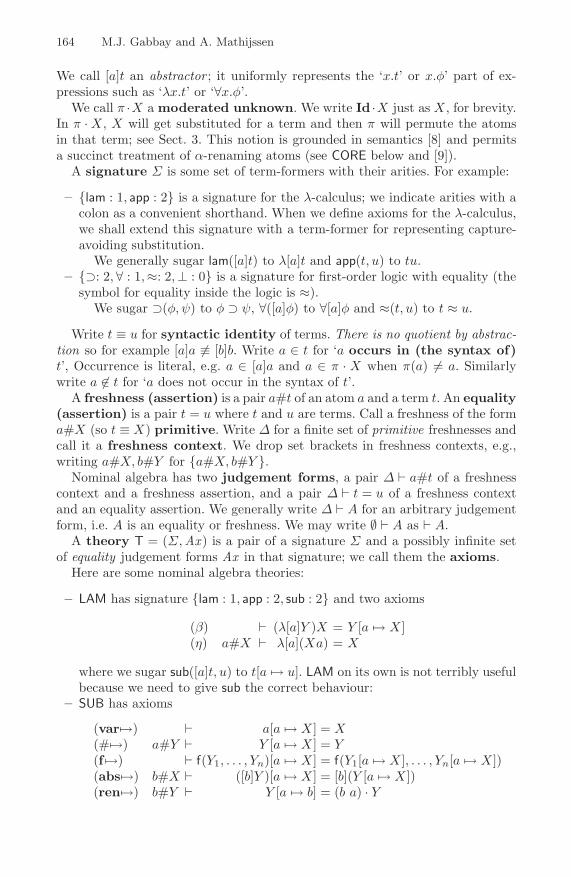
164 M.J. Gabbay and A. Mathijssen
We call [a]t an abstractor ; it uniformly represents the ‘x.t’ or x.φ’ part of ex-pressions such as ‘λx.t’ or ‘∀x.φ’.
We call π ·X a moderated unknown. We write Id ·X just as X , for brevity.In π ·X, X will get substituted for a term and then π will permute the atomsin that term; see Sect. 3. This notion is grounded in semantics [8] and permitsa succinct treatment of α-renaming atoms (see CORE below and [9]).
A signature Σ is some set of term-formers with their arities. For example:
– {lam : 1, app : 2} is a signature for the λ-calculus; we indicate arities with acolon as a convenient shorthand. When we define axioms for the λ-calculus,we shall extend this signature with a term-former for representing capture-avoiding substitution.
We generally sugar lam([a]t) to λ[a]t and app(t, u) to tu.– {⊃: 2, ∀ : 1,≈: 2,⊥ : 0} is a signature for first-order logic with equality (the
symbol for equality inside the logic is ≈).We sugar ⊃(φ, ψ) to φ ⊃ ψ, ∀([a]φ) to ∀[a]φ and ≈(t, u) to t ≈ u.
Write t ≡ u for syntactic identity of terms. There is no quotient by abstrac-tion so for example [a]a �≡ [b]b. Write a ∈ t for ‘a occurs in (the syntax of)t’, Occurrence is literal, e.g. a ∈ [a]a and a ∈ π · X when π(a) �= a. Similarlywrite a �∈ t for ‘a does not occur in the syntax of t’.
A freshness (assertion) is a pair a#t of an atom a and a term t. An equality(assertion) is a pair t = u where t and u are terms. Call a freshness of the forma#X (so t ≡ X) primitive. Write Δ for a finite set of primitive freshnesses andcall it a freshness context. We drop set brackets in freshness contexts, e.g.,writing a#X, b#Y for {a#X, b#Y }.
Nominal algebra has two judgement forms, a pair Δ � a#t of a freshnesscontext and a freshness assertion, and a pair Δ � t = u of a freshness contextand an equality assertion. We generally write Δ � A for an arbitrary judgementform, i.e. A is an equality or freshness. We may write ∅ � A as � A.
A theory T = (Σ,Ax) is a pair of a signature Σ and a possibly infinite setof equality judgement forms Ax in that signature; we call them the axioms.
Here are some nominal algebra theories:
– LAM has signature {lam : 1, app : 2, sub : 2} and two axioms
(β) � (λ[a]Y )X = Y [a �→ X ](η) a#X � λ[a](Xa) = X
where we sugar sub([a]t, u) to t[a �→ u]. LAM on its own is not terribly usefulbecause we need to give sub the correct behaviour:
– SUB has axioms
(var�→) � a[a �→ X ] = X(#�→) a#Y � Y [a �→ X ] = Y(f �→) � f(Y1, . . . , Yn)[a �→ X ] = f(Y1[a �→ X ], . . . , Yn[a �→ X ])(abs �→) b#X � ([b]Y )[a �→ X ] = [b](Y [a �→ X ])(ren�→) b#Y � Y [a �→ b] = (b a) · Y

A Formal Calculus for Informal Equality with Binding 165
Axiom (f �→) represents three axioms, one for each of f ∈ {lam, app, sub}. Atheory of substitution for a different signature would have a suitable axiomfor each term-former f. Note the heavy use of freshness side-conditions tomanage the relationship between atoms and unknowns.
But there is one more axiom. We would like λ[a]a to be equal to λ[b]b. Inother words we want α-equivalence:
– CORE has just one axiom
(perm) a#X, b#X � (b a) ·X = X
Lemma 3.2 below shows that this axiom with the derivation rules of nomi-nal algebra give the native notion of α-equivalence on nominal terms fromprevious work [9].
See [10] for an axiomatisation of first-order logic. Similar development for othersystems with binding, such as System F [11] and the π-calculus [12], should alsobe possible.
3 A Derivation System
Now we need a notion of derivation which represents freshness assumptions onmeta-variables, and permits axioms involving abstraction and conditioned onfreshness assumptions, just like we do in informal reasoning.
We define a permutation action π · t by:
π · a ≡ π(a) π · (π′·X) ≡ (π ◦ π′) ·X π · [a]t ≡ [π(a)](π · t)π · f(t1, . . . , tn) ≡ f(π · t1, . . . , π · tn)
A substitution σ is a finitely supported function from unknowns to terms.Here, finite support means: for some finite set of unknowns σ(X) �≡ X , and forall other unknowns σ(X) ≡ X . Write [t1/X1, . . . , tn/Xn] for the substitution σsuch that σ(Xi) ≡ ti and σ(Y ) ≡ Y , for all Y �≡ Xi, 1 ≤ i ≤ n.
We can define a substitution action tσ on terms by:
aσ ≡ a (π ·X)σ ≡ π · σ(X) ([a]t)σ ≡ [a](tσ)f(t1, . . . , tn)σ ≡ f(t1σ, . . . , tnσ)
Substitution for an unknown does not avoid capture with abstraction, for ex-ample ([a]X)[a/X ] ≡ [a]a. This is designed to mirror informal practice, whereinstantiation of meta-variables does not avoid capture with binding.
Extend notation for permutation and substitution action to freshness contextsΔ pointwise to the terms it contains. It reduces parentheses to give substitutiona higher priority than permutation and abstraction, so we do. The followingcommutation is easy to prove [9, 6]:

166 M.J. Gabbay and A. Mathijssen
Lemma 3.1. π · tσ ≡ (π · t)σ.Define derivability on freshnesses (in some signature Σ) by the rules in Fig. 1.Here f ranges over the term-formers of Σ, and in accordance with our permu-tative convention a and b range over distinct atoms. Write Δ � a#t when a#tmay be derived from Δ.
Define derivability on equalities (between terms in the signature of T) by therules in Fig. 2. Here (fr) is subject to a condition that a �∈ t, u,Δ and the squarebrackets denote discharge of assumptions in natural deduction style [13]. WriteΔ �
Tt = u when we may derive t = u from Δ, using the signature from theory
T and admitting only the axioms it contains. We write Δ �TA as a convenient
shorthand for Δ �Tt = u when A is t = u and Δ � a#t when A is a#t (subscript
T disappears in the freshness case).
(#ab)a#b
π-1(a)#X(#X)
a#π · X(#[]a)
a#[a]t
a#t(#[]b)
a#[b]t
a#t1 · · · a#tn
(#f)a#f(t1, . . . , tn)
Fig. 1. Derivation rules for freshness
(refl)t = t
t = u(symm)
u = t
t = u u = v(tran)
t = v
π · Δσ(axΔ�t=u)
π · tσ = π · uσ
t = u(cong[])
[a]t = [a]u
t = u(congf)
f(. . . , t, . . .) = f(. . . , u, . . .)
[a#X1, . . . , a#Xn] Δ···t = u
(fr)t = u
Fig. 2. Derivation rules for equality
(ax�t=u) allows us to permutatively rename atoms and to instantiate un-knowns. This gives the effect that atoms in axioms can be understood to rangeover any (distinct) atoms, and unknowns can be understood to range over anyterms. So these derivations
(axβ)(λ[b]a)b = a[b �→ b]
(axβ)(λ[b]b)a = b[b �→ a]
are valid in theory LAM. The right derivation also shows that substitution ofterms for unknowns does not avoid capture, reflecting informal practice.
The use of the (axΔ�t=u) rule introduces new proof obligations on the fresh-ness side-conditions in Δ, as the following derivations show:
(#ab)a#b
(axη)λ[a](ba) = b
a#a(axη)
λ[a](aa) = a
The left derivation is valid but the right one is not, because a#a is not derivable.
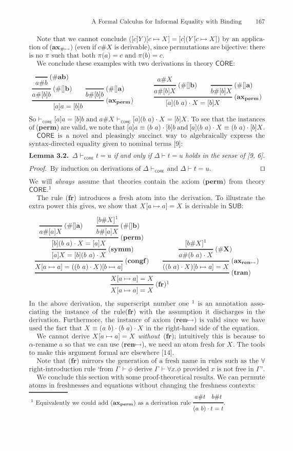
A Formal Calculus for Informal Equality with Binding 167
Note that we cannot conclude ([c]Y )[c �→ X ] = [c](Y [c �→ X ]) by an applica-tion of (ax# �→) (even if c#X is derivable), since permutations are bijective: thereis no π such that both π(a) = c and π(b) = c.
We conclude these examples with two derivations in theory CORE:
(#ab)a#b
(#[]b)a#[b]b
(#[]a)b#[b]b
(axperm)[a]a = [b]b
a#X(#[]b)
a#[b]X(#[]a)
b#[b]X(axperm)
[a](b a) ·X = [b]X
So �CORE
[a]a = [b]b and a#X �CORE
[a](b a) ·X = [b]X. To see that the instancesof (perm) are valid, we note that [a]a ≡ (b a) · [b]b and [a](b a) ·X ≡ (b a) · [b]X.
CORE is a novel and pleasingly succinct way to algebraically express thesyntax-directed equality given to nominal terms [9]:
Lemma 3.2. Δ �CORE
t = u if and only if Δ � t = u holds in the sense of [9, 6].
Proof. By induction on derivations of Δ �CORE
and Δ � t = u. ��We will always assume that theories contain the axiom (perm) from theoryCORE.1
The rule (fr) introduces a fresh atom into the derivation. To illustrate theextra power this gives, we show that X [a �→ a] = X is derivable in SUB:
(#[]a)a#[a]X
[b#X ]1(#[]b)
b#[a]X(perm)
[b](b a) ·X = [a]X(symm)
[a]X = [b](b a) ·X(congf)
X [a �→ a] = ((b a) ·X)[b �→ a]
[b#X ]1(#X)
a#(b a) ·X(axren �→)
((b a) ·X)[b �→ a] = X(tran)
X [a �→ a] = X(fr)1
X [a �→ a] = X
In the above derivation, the superscript number one 1 is an annotation asso-ciating the instance of the rule(fr) with the assumption it discharges in thederivation. Furthermore, the instance of axiom (ren�→) is valid since we haveused the fact that X ≡ (a b) · (b a) ·X in the right-hand side of the equation.
We cannot derive X [a �→ a] = X without (fr); intuitively this is because toα-rename a so that we can use (ren�→), we need an atom fresh for X . The toolsto make this argument formal are elsewhere [14].
Note that (fr) mirrors the generation of a fresh name in rules such as the ∀right-introduction rule ‘from Γ � φ derive Γ � ∀x.φ provided x is not free in Γ ’.
We conclude this section with some proof-theoretical results. We can permuteatoms in freshnesses and equations without changing the freshness contexts:
1 Equivalently we could add (axperm) as a derivation rulea#t b#t
(a b) · t = t.

168 M.J. Gabbay and A. Mathijssen
Theorem 3.3. For any permutation π′, if Δ �TA then Δ �
Tπ′ ·A.
Proof. By induction on derivations. For (#X) we note that permutations arebijective and π′(a)#π′ ◦ π ·X if and only if π-1(a)#X . For (fr) we might haveto rename the freshly chosen atom a if π′(a) �= a.2 ��We can substitute terms for unknowns provided those terms violate no freshnessassumptions made on the unknowns:
Theorem 3.4. If Δ �TA then Δ′ �
TAσ for all Δ′ such that Δ′ �
TΔσ.
Proof. Natural deduction derivations are such that the conclusion of one deriva-tion may be ‘plugged in’ to an assumption in another derivation. For (#X) weuse Theorem 3.3. For (fr) we might have to rename the freshly chosen atom a ifit is mentioned by σ (see footnote 2). ��
4 Semantics
A model of a nominal algebra theory T is a nominal set which interprets theterm-formers so as to make the axioms valid. We use nominal sets [8] becausethey permit a direct semantic interpretation of freshness judgements a#x andpermutations π · x, an interpretation which is not conveniently definable on‘ordinary’ sets.
A nominal set is a pair (X, ·) of a(n ordinary) set X with a group action by P
such that each x ∈ X has finite support.3 This means that there is some finiteset of atoms {a1, . . . , an} such that for any π if π(ai) = ai for each 1 ≤ i ≤ n,then π · x = x. It is a fact ([8, Proposition 3.4]) that a unique least such set ofatoms exists, we call it the support of x. We write a#x when a is not in thesupport of x, and call a fresh for x. For example:
– The set A = {a, b, c, . . .} of atoms with action π · a = π(a) is a nominal set;the support of a ∈ A is {a}, so b#a but not a#a.
– The powerset P(A) = {U | U ⊆ A} of A with action π · U = {π · u | u ∈ U},is not a nominal set; {a1, a3, a5, . . .} ∈ P(A) does not have finite support,since for no finite set of atoms is it the case that all permutations fixing thatset map {a1, a3, a5, . . .} to itself. Note that the support of A ∈ P(A) is ∅, soa#A for any a.
– If X and Y are nominal sets write X× Y for {(x, y) | x ∈ X, y ∈ Y} withaction π · (x, y) = (π · x, π · y). This is also a nominal set; the support of(x, y) ∈ X× Y is the union of the supports of x and y.
It is useful to write Xn for
n︷ ︸︸ ︷X× · · · × X, so we do.
2 It is easy to prove that the resulting ‘name-clash-avoiding’ derivation is a deriva-tion, and we can use induction on depth of derivations to preserve the inductivehypothesis. However, we have used the principle of meta-level Fraenkel-Mostowksiequivariance [8], which lets us rename atoms permutatively without losing structuralinductive properties, so our structural induction is actually perfectly valid.
3 · is a function P × X → X such that Id · x = x and π · (π′ · x) = (π ◦ π′) · x.

A Formal Calculus for Informal Equality with Binding 169
We assume these permutation actions on these sets henceforth.
Lemma 4.1. For any nominal set X and element x ∈ X, if a#x and b#x then(a b) · x = x.
Proof. Since a, b �∈ supp(x), (a b)(c) = c for every c ∈ supp(x). ��Functions f ∈ X→ Y (on the underlying sets) have a natural conjugation per-mutation action given by (π · f)(x) = π · (f(π-1 · x)). Call f equivariant if π·(f(x)) = f(π · x) always.
Lemma 4.2. For any nominal sets X,Y, equivariant function f ∈ X → Y andx ∈ X, if a#x then a#f(x).
Proof. By an elementary calculation using the fact that π · (f(x)) = f(π · x). ��We can now give a semantics to nominal algebra theories. An interpretation� � of a signature is a nominal set T with equivariant functions
– � �T ∈ A→ T to interpret atoms;– [ ] ∈ A× T→ T such that a#[a]x always, to interpret abstraction;– �f� ∈ T
n → T for each term-former f : n, to interpret term-formers.
A valuation ς maps unknowns X to elements ς(X) ∈ T. The pair of an inter-pretation and a valuation extend easily to terms �t�ς :
�a�ς = �a�T �π·X�ς = π·ς(X) �[a]t�ς = [a]�t�ς�f(t1, . . . , tn)�ς = �f�(�t1�ς , . . . , �tn�ς)
This extends to a notion of validity for our judgement forms:
�a#t�ς (is valid) when a#�t�ς �t = u�ς when �t�ς = �u�ς
�Δ�ς when a#ς(X) for each a#X ∈ Δ �Δ � A�ς when �Δ�ς implies �A�ς
�Δ � A� when �Δ � A�ς for all valuations ς
A model of a theory T is an interpretation � � such that �Δ � t = u� for allaxioms Δ � t = u of T — we say the model validates the axioms.
Write Δ |=TA when �Δ � A� for all models � � of T.
5 Soundness and Completeness
Derivability of freshness and equality is sound for the semantics presented in theprevious section.
Theorem 5.1 (Soundness). If Δ �TA then Δ |=
TA.
Proof. Let � � be a model of T. We must show that if A is derived from Δ then�Δ�ς implies �A�ς for any valuation ς. We work by induction on derivation rules.

170 M.J. Gabbay and A. Mathijssen
– (#ab). By definition, �a#b�ς when a#�b�T. By Lemma 4.2 this followsfrom a#b, which is a standard property of (semantic) freshness.
– (#X). By properties of the group of permutations, a#π · x when π-1(a)#x.– (#[]a). a#[a]x for any x ∈ T by construction.– (#[]b). By Lemma 4.2, a#x implies a#[b]x.– (#f ). Take any f : n. If a#�ti�ς for 1 ≤ i ≤ n then a#�f�(�t1�ς , . . . , �tn�ς)
follows using Lemma 4.2.– (refl), (symm), (tran), (cong[]), (congf). By properties of equality.– (axΔ′�t=u). This follows from the definition of what it is to be a model,
and the fact that �π · tσ�ς = π · �t�ς′ where ς ′(X) = �σ(X)�ς .– (fr). Suppose there is a derivation of t = u from Δ, a#X1, . . . , a#Xn, and
suppose that a �∈ t, u,Δ. If a is amongst the atoms in the support of ς(Xi)for any Xi, rename a in the derivation to avoid this. By inductive hypothesis�t�ς = �u�ς follows from �Δ, a#X1, . . . , a#Xn�ς . So �t�ς = �u�ς as required.
��In order to show completeness of derivability of equality, we need some technicalmachinery. Given a theory T we construct a term model � �T of T as follows:
– For each n > 0 introduce a term-former dn : n.– Take as T the set of closed terms of sort T (terms without unknowns) in the
enriched signature, quotiented by provable equality, with the permutationaction given pointwise.
– Take �a�T = {t | �Tt = a, t closed}, [a]x = {t | �
Tt = [a]u, t closed, u ∈ x},
and for each term-former f : n take as �f�T the function defined by
�f�T (x1, . . . , xn) = {t | �Tt = f(t1, . . . , tn), t closed, ti ∈ xi}.
We have to enrich the signature with the dn to ensure the term model hasenough elements; term-formers must be interpreted by equivariant functions sothe usual method of adding constants c (0-ary term-formers) would add onlyelements such that �
Tπ · c = c always, and this does not suffice. This idea goes
back to [15].It is possible to prove by some elementary calculations that the definition
above is well-defined and an interpretation; that is, that T is a nominal set, that� �T, [ ] , and all �f�T are equivariant, and that a#�[a]t�T always.
Lemma 5.2. If a#�t�Tς then there is some t′ ∈ �t�Tς such that �Ta#t′.
Proof. Take b fresh (so b does not occur in t or ς). Then b#�t�Tς . Since alsoa#�t�Tς we obtain (b a) ·�t�Tς = �t�Tς by Lemma 4.1. But then also �
T(b a) ·t = t,
by construction. Take t′ ≡ (b a) · t. ��To show why Lemma 5.2 is not trivial, consider a theory IOTA with one axiom� a = b. It is easy to verify that a#�a�Tς (since �a�Tς = A) but a#a is not deriv-able. Of course a = b and a#b are derivable. Similarly in LAM it is a fact thata#�(λ[a]b)a�Tς but a#(λ[a]b)a is not derivable; of course (λ[a]b)a = b and a#bare derivable.

A Formal Calculus for Informal Equality with Binding 171
Theorem 5.3. The term model � �T of T is a model.
Proof. We show that if Δ � t = u is an axiom of T then �Δ � t = u�Tς is validfor any ς. By definition, we must show that if a#ς(X) for each a#X ∈ Δ, then�t�Tς = �u�Tς . Use Lemma 5.2 to choose a term t′ ∈ ς(X) such that � a#t′ for eacha#X ∈ Δ. By (axΔ�t=u), taking π = Id and σ(X) ≡ t′ for each a#X ∈ Δ weobtain �
Ttσ = uσ, since � a#σ(X). Then �tσ�Tς = �uσ�Tς by Theorem 5.1. By
construction �t�Tς = �tσ�Tς and �u�Tς = �uσ�Tς , so �t�Tς = �u�Tς as required. ��A certain amount of technical subtlety is hidden in Theorem 5.4 and in particularin its use of the extra term-formers d:
Theorem 5.4 (Completeness). If Δ |=Tt = u then Δ �
Tt = u.
Proof. By assumption �Δ � t = u�ς is valid for any model � � of T and anyvaluation ς. Let � � be � �T , the term model of T. In order to choose a suitableς, we introduce the following:
– Let S be the set of atoms mentioned anywhere in Δ, t, and u.– Let X1, . . . , Xn be the set of unknowns mentioned anywhere in Δ, t, or u,
(not just in Δ!) in some arbitrary order.– For each 1 ≤ i ≤ n let Si be the set of all atoms a ∈ S such that a#Xi �∈ Δ.– For each 1 ≤ i ≤ n let σ(Xi) ≡ di(a1, . . . , ani) where Si = {a1, . . . , ani}.
Here we extend the signature with distinct term-formers di. Let ς map Xi to�σ(Xi)�Tς , for 1 ≤ i ≤ n. By construction �Δ�Tς , so by assumption �t�Tς = �u�Tς ,and by definition this means that tσ = uσ is derivable. This derivation can betransformed rule by rule into a derivation of Δ �
Tt = u, since the only fresh-
nesses and equalities we can assert of the di are those we can also assert of theXi. The only complication is when perhaps for some fresh b we use a freshnessderivation to derive b#vσ for some fresh b; then we modify the derivation to use(fr) instead. ��
5.1 The Status of Freshness Derivations
Completeness holds for equalities — but not for freshnesses. That is, Δ |=Tb#t
does not imply Δ � b#t necessarily; for counterexamples see the discussion in-volving theories IOTA and LAM just after Lemma 5.2.
To understand why this is desirable we must draw a distinction between theintension and the extension of a term.
‘� a#(λ[a]b)a’ has the status of ‘x is fresh for (λx.y)x’; both are false. Yet(λx.y)x is β-convertible to y and x is fresh for y. A freshness judgement Δ � a#tis a(n intensional) judgement on concrete syntax; call this syntactic freshness.4
All the capture-avoidance side-conditions we know of are in accordance with theslogan ‘ε away from informal practice’, this is what Δ � a#t models.
Nominal sets is unusual amongst semantics in that it has a(n extensional)semantic notion of freshness a#x. In fact, semantic freshness is hiding in nominalalgebra — but in a slightly unexpected place; in the theory of equality.4 The reader familiar with a theorem-prover such as Isabelle [16] might like to imagine
that # maps to Prop and = maps to o.

172 M.J. Gabbay and A. Mathijssen
Theorem 5.5. Suppose {X1, . . . , Xn} and {a1, . . . , am} are the unknowns andatoms mentioned in Δ and t. Suppose that b is fresh (so b �∈ {a1, . . . , am}).Δ |=
Ta#t if and only if Δ, b#X1, . . . , b#Xn �T
(b a) · t = t.
Proof. Choose a model and any ς such that b#ς(X1), . . . , b#ς(Xn); it followsby an induction on syntax that b#�t�ς . It is a fact that a#�t�ς if and only if(b a) · �t�ς = �t�ς (see [8] for details). Also, since term-formers are interpreted byequivariant functions, we rewrite (b a) · �t�ς as �(b a) · t�ς .
Now suppose Δ |=Ta#t. By definition a#�t�ς for any �-� and ς such that
�Δ�ς . By the arguments above �(b a) · t�ς = �t�ς if b#ς(X1), . . . , b#ς(Xn). ByTheorem 5.4 it follows that Δ, b#X1, . . . , b#Xn �T
(b a) · t = t. The reverse im-plication is similar. ��Recall the examples we used just after Lemma 5.2. Theorem 5.5 tells us that|=
IOTAa#a if and only if �
IOTAb = a (which follows by the axiom � a = b), and
that |=LAM
a#(λ[a]b)a if and only if �LAM
(λ[a]b)a = (λ[c]b)c (which follows sinceboth sides are derivably equal to b).
So the semantic freshness Δ |=Ta#t can be expressed as an equality axiom.
Any undecidability or algorithmic complexity is isolated in the equality judge-ment form.
6 Related Work
Nominal algebra is derived from Fraenkel-Mostowski set theory. This provideda semantics for names and gave an unexpected set-theoretic semantics for parsetrees (abstract syntax trees) with α-equivalence [8]. Existing technology includedDe Bruijn indexes [17], higher-order abstract syntax [18], the theory of con-texts [19], TWELF [20], and other approaches. In this crowded arena approachesbased on Fraenkel-Mostowski sets were catchily labelled ‘nominal’ by Pitts. Thederivation rules expressed in this paper by the theory CORE are from this se-mantics. The name ‘nominal algebra’ acknowledges this debt.
Nominal unification considers the computational aspects of unifying trees-with-binding [9]. Nominal logic describes inductive programming and reasoningprinciples for trees-with-binding [21]. FreshML is a programming language... fortrees-with-binding [22] in ML [23] style.
Aside from applications to trees-with-binding, ideas from nominal techniqueshave been used in logic [24] (this was still reasoning on trees, since the logic hada fixed syntactic model) and recently in semantics [25].
Nominal rewriting considers equalities between terms not directly to do withan underlying model of trees [6]. α-prolog [26] takes a similar tack but in logicprogramming. Still, the emphasis is squarely on the computational benefits com-pared to those of other approaches.
Nominal algebra champions nominal techniques as a logical framework torepresent and reason about semantic structures — i.e. functions, sets, and othermathematical structures. That is new, and this paper sets it on a sound seman-tic/logical basis.

A Formal Calculus for Informal Equality with Binding 173
The full case for nominal algebra as a framework for applications in whichhigher-order logic can be used [27] remains to be made. However we can makesome remarks:
Unification of nominal terms is decidable whereas higher-order unification isnot [28]. (First-order) logic can be axiomatised [10] and the treatment of quan-tification is very smooth. In particular it closely models the informal specificationof quantification; the ∀-intro rule in Isabelle is
∧x.[P =⇒ ∀x.P ]
(see [16]) and this is not like the usual rule used by logicians
‘from Γ � P deduce Γ � ∀x.P if x is fresh for Γ ’.
We believe (though we have not yet checked this in detail) that treatments ofsubstructural logics are possible in nominal algebra; they are not necessarily so inhigher-order logic because structural properties of the framework’s connectives‘infect’ those of the logic being axiomatised.
Since the conception of nominal algebra, Pitts and Clouston have derived nom-inal equational logic [29]. Nominal equational logic makes some slightly differentdesign decisions, notably it cannot express syntactic freshness (see Sect. 5.1).
Higher-order algebra [4] uses typed λ-calculus up to αβ-equivalence and canserve as a foundational framework. The simply-typed λ-calculus itself [16, Fig-ures 6 and 7] can also be used. Other algebraic systems, such as Sun’s exten-sional binding algebras [30, Definition 2.2.3] introduce dedicated systems basedon functional semantics.
A host of ‘cylindric’ algebraic techniques exist. These embrace meta-variablesand reject object-level variables, preferring to encode their expressive powerin the term-formers. Examples are lambda-abstraction algebras [31] for the λ-calculus and cylindric algebras [32, 33] for first-order logic. Polyadic algebrashave a slightly more general treatment, for a brief but clear discussion of the de-sign of these and related systems is in [34, Appendix C]. Combinators [1] rejectobject-level variables altogether. Algebras over (untyped) combinators can thenexpress first-order predicate logic [35]. These systems are effective for their ap-plications but there are things that nominal algebra allows us to say particularlynaturally, because of the way it isolates abstraction, has explicit meta-variables,and permits freshness side-conditions on equalities.
7 Conclusions
Nominal terms embrace the difference between the object-level and the meta-level; there are two classes of variables, atoms a and unknowns X . Substitutionfor X does not avoid capture in abstraction by a. Freshness side-conditions of theform a#X manage the interaction between the two levels and ‘recover’ capture-avoidance where this is required.

174 M.J. Gabbay and A. Mathijssen
Previous ‘nominal’ work has considered reasoning on datatypes of syntax upto α-equivalence. In this paper we use nominal terms as a foundational syntaxfor mathematics, and we have constructed a logic for them using a suitabletheory of equality. The two-level variable structure permits the framework toget exceptionally close to informal practice; see the end of the Introduction forexamples.
Nominal algebra could be suitable to specify and reason algebraically on lan-guages with binding; we have in mind particularly process calculi such as thosederived from the π-calculus, which often feature quite complex binding side-conditions and for which algebraic reasoning principles are frequently devel-oped [36, 37, 38].
It is possible to extend nominal algebra with abstractions of the form [t]u,and freshness judgements of the form t#u. Other extensions are possible andcase studies will tell which of them are most important.
We see nominal algebra as the first of a family of two-level logics as yet tobe created. We intend to begin by creating a first-order logic with two levels ofvariable. For example we would like to be able to write an expression like
∀[X ]∀[a](a#X ⊃ (X ⇔ ∀[a]X)).
We made a start in that direction by designing one-and-a-halfth order logic [10].However that system does not allow quantification of unknowns, and we are nowworking on lifting that restriction.
In our semantics object-level variables are first-class entities in the denotation;a represents an object-level variable symbol in the syntax and in the semanticsof nominal algebra. Yet we may impose equalities, such as theory SUB fromSect. 2. If we can substitute for a then it has the flavour of a variable ‘rangingover’ denotational elements; so SUB is a theory of ‘variables in denotation’.Nominal algebra is the beginning of an intriguing investigation into what thisenrichment of the denotation does to the theory of validity and proof.
We are also interested in developing logics with hierarchies of variables. Sincenominal algebra offers two levels of variable, why not extend this to allow an infi-nite hierarchy of variables, by analogy with type hierarchies in the λ-calculus [1],or stratification in set theory [39]? The first author has considered this extensionof nominal terms in other publications [40, 41] but introducing such a hierarchyin a logical context poses unique challenges, and in particular, we have not yetobtained a satisfactory notion of model. This too is current research.
References
[1] Barendregt, H.P.: The Lambda Calculus: its Syntax and Semantics. North-Holland (revised edn.)
[2] Curry, H.B., Feys, R.: Combinatory Logic. vol. 1, North Holland (1958)[3] Henkin, L., Monk, J.D., Tarski, A.: Cylindric Algebras. North Holland (1971,
1985) Parts I and II[4] Meinke, K.: Universal algebra in higher types. Theoretical Computer Sci-
ence 100(2), 385–417 (1992)

A Formal Calculus for Informal Equality with Binding 175
[5] Leivant, D.: Higher order logic. In: Gabbay, D., Hogger, C., Robinson, J. (eds.)Handbook of Logic in Artificial Intelligence and Logic Programming. vol. 2, pp.229–322. Oxford University Press, Oxford, UK (1994)
[6] Fernandez, M., Gabbay, M.J.: Nominal rewriting. Information and Computation(in press)
[7] Fernandez, M., Gabbay, M.J.: Curry-style types for nominal rewriting. In:TYPES’06 (2006)
[8] Gabbay, M.J., Pitts, A.M.: A new approach to abstract syntax with variablebinding. Formal Aspects of Computing 13(3–5), 341–363 (2001)
[9] Urban, C., Pitts, A.M., Gabbay, M.J.: Nominal unification. Theoretical ComputerScience 323(1–3), 473–497 (2004)
[10] Gabbay, M.J., Mathijssen, A.: One-and-a-halfth-order logic. In: PPDP ’06. Proc.of the 8th ACM SIGPLAN symposium on Principles and Practice of DeclarativeProgramming, pp. 189–200. ACM Press, New York (2006)
[11] Girard, J.Y., Taylor, P., Lafont, Y.: Proofs and types. Cambridge University Press,Cambridge (1989)
[12] Parrow, J.: An introduction to the pi-calculus. In: Bergstra, J., Ponse, A., Smolka,S. (eds.) Handbook of Process Algebra, pp. 479–543. Elsevier, Amsterdam (2001)
[13] Hodges, W.: Elementary predicate logic. In: Gabbay, D., Guenthner, F. (eds.)Handbook of Philosophical Logic, 2nd edn. vol. 1, pp. 1–131. Kluwer AcademicPublishers, Dordrecht (2001)
[14] Gabbay, M.J., Mathijssen, A.: Capture-avoiding substitution as a nominal algebra.In: Barkaoui, K., Cavalcanti, A., Cerone, A. (eds.) ICTAC 2006. LNCS, vol. 4281,pp. 198–212. Springer, Heidelberg (2006)
[15] Gabbay, M.J.: Fresh logic. Journal of Logic and Computation (2006) In press.[16] Paulson, L.C.: The foundation of a generic theorem prover. Journal of Automated
Reasoning 5(3), 363–397 (1989)[17] de Bruijn, N.G.: Lambda calculus notation with nameless dummies, a tool for
automatic formula manipulation, with application to the church-rosser theorem.Indagationes Mathematicae 5(34), 381–392 (1972)
[18] Pfenning, F., Elliot, C.: Higher-order abstract syntax. In: PLDI ’88. Proc. of theACM SIGPLAN 1988 conf. on Programming Language design and Implementa-tion, pp. 199–208. ACM Press, New York (1988)
[19] Miculan, M.: Developing (meta)theory of lambda-calculus in the theory of con-texts. ENTCS 1(58) (2001)
[20] Pfenning, F., Schurmann, C.: System description: Twelf - a meta-logical frame-work for deductive systems. In: Ganzinger, H. (ed.) CADE-16. LNCS (LNAI),vol. 1632, pp. 202–206. Springer, Heidelberg (1999)
[21] Pitts, A.M.: Nominal logic, a first order theory of names and binding. Informationand Computation 186(2), 165–193 (2003)
[22] Shinwell, M.R., Pitts, A.M., Gabbay, M.J.: FreshML: Programming with bindersmade simple. In: ICFP 2003. Eighth ACM SIGPLAN Int’l Conf. on FunctionalProgramming, Uppsala, Sweden, pp. 263–274. ACM Press, New York (2003)
[23] Paulson, L.C.: ML for the working programmer (2nd eds ). Cambridge UniversityPress, Cambridge (1996)
[24] Luıs Caires, L.C.: A spatial logic for concurrency (part II). Theoretical ComputerScience 322(3), 517–565 (2004)
[25] Benton, N., Leperchey, B.: Relational reasoning in a nominal semantics for stor-age. In: Urzyczyn, P. (ed.) TLCA 2005. LNCS, vol. 3461, pp. 86–101. Springer,Heidelberg (2005)

176 M.J. Gabbay and A. Mathijssen
[26] Cheney, J., Urban, C.: System description: Alpha-Prolog, a fresh approach tologic programming modulo alpha-equivalence. In: de Valencia, U.P. (ed.) Proc.17th Int. Workshop on Unification, UNIF’03, 15–19 (2003)
[27] Paulson, L.C.: Isabelle: the next 700 theorem provers. In: Odifreddi, P. (ed.) Logicand Computer Science, pp. 361–386. Academic Press, London (1990)
[28] Huet, G.: Higher order unification 30 years later. In: Carreno, V.A., Munoz, C.A.,Tahar, S. (eds.) TPHOLs 2002. LNCS, vol. 2410, pp. 3–12. Springer, Heidelberg(2002)
[29] Clouston, R.A., Pitts, A.M.: Nominal equational logic. ENTCS 172, 223–257(2007)
[30] Sun, Y.: An algebraic generalization of frege structures - binding algebras. Theo-retical Computer Science 211, 189–232 (1999)
[31] Salibra, A.: On the algebraic models of lambda calculus. Theoretical ComputerScience 249(1), 197–240 (2000)
[32] Burris, S., Sankappanavar, H.: A Course in Universal Algebra. Springer, Heidel-berg (1981)
[33] Andreka, H., Nemeti, I., Sain, I.: Algebraic logic. In: Gabbay, D., Guenthner, F.(eds.) Handbook of Philosophical Logic, 2nd edn. pp. 133–249. Kluwer AcademicPublishers, Dordrecht (2001)
[34] Blok, W.J., Pigozzi, D.: Algebraizable logics. Memoirs of the AMS 77(396) (1989)[35] Barendregt, H., Dekkers, W., Bunder, M.: Completeness of two systems of illative
combinatory logic for first-order propositional and predicate calculus. Archive furMathematische Logik 37, 327–341 (1998)
[36] Abadi, M., Gordon, A.D.: A calculus for cryptographic protocols: the spi calculus.In: CCS ’97. Proc. of the 4th ACM conf, pp. 36–47. ACM Press, New York (1997)
[37] Luttik, B.: Choice Quantification in Process Algebra. PhD thesis, University ofAmsterdam (2002)
[38] Katoen, J.P., D’Argenio, P.R.: General distributions in process algebra. In: Lec-tures on formal methods and performance analysis: first EEF/Euro summer schoolon trends in computer science, Springer, pp. 375–429. Springer, Heidelberg (2002)
[39] Forster, T.: Quine’s NF, 60 years on. American Mathematical Monthly 104(9),838–845 (1997)
[40] Gabbay, M.J.: A new calculus of contexts. In: PPDP ’05. Proc. of the 7th ACMSIGPLAN int’l conf. on Principles and Practice of Declarative Programming, pp.94–105. ACM Press, New York (2005)
[41] Gabbay, M.J.: Hierarchical nominal rewriting. In: LFMTP’06: Logical Frameworksand Meta-Languages: Theory and Practice, pp. 32–47 (2006)

Formal Verification of an Optimal Air Traffic
Conflict Resolution and Recovery Algorithm�
Andre L. Galdino1,��, Cesar Munoz2, and Mauricio Ayala-Rincon1,��
1 Universidade de Brasılia, Brazil{galdino,ayala}@unb.br
2 National Institute of Aerospace, [email protected]
Abstract. Highly accurate positioning systems and new broadcastingtechnology have enabled air traffic management concepts where the re-sponsibility for aircraft separation resides on pilots rather than on airtraffic controllers. The Formal Methods Group at the National Instituteof Aerospace and NASA Langley Research Center has proposed and for-mally verified an algorithm, called KB3D, for distributed three dimen-sional conflict resolution. KB3D computes resolution maneuvers whereonly one component of the velocity vector, i.e., ground speed, verticalspeed, or heading, is modified. Although these maneuvers are simple toimplement by a pilot, they are not necessarily optimal from a geometricalpoint of view. In general, optimal resolutions require the combination ofall the components of the velocity vector. In this paper, we propose atwo dimensional version of KB3D, which we call KB2D, that computesresolution maneuvers that are optimal with respect to ground speed andheading changes. The algorithm has been mechanically verified in thePrototype Verification System (PVS). The verification relies on algebraicproof techniques for the manipulation of the geometrical concepts rele-vant to the algorithm as well as standard deductive techniques availablein PVS.
1 Introduction
Air traffic management concepts such as Free Flight [12,5] and Distributed Air/-Ground Traffic Management [10] target the predicted increase of air traffic bydistributing the responsibility for separation among pilots and air traffic con-trollers. This new mode of operation is supported by advances in surveillance,communications, and software technologies. In particular, conflict detection andresolution (CD&R) systems are designed to increase traffic awareness and pro-vide corrective maneuvers for impending conflicts [7]. On-board CD&R systems
� This work was supported by the National Aeronautics and Space Administration,Langley Research Center under the Research Cooperative Agreement No. NCC-1-02043 and by the Brazilian Research Council CNPq under Grant 471791/2004-0.
�� Authors partially supported by the Brazilian Research Council CNPq.
D. Leivant and R. de Queiroz (Eds.): WoLLIC 2007, LNCS 4576, pp. 177–188, 2007.c© Springer-Verlag Berlin Heidelberg 2007

178 A.L. Galdino, C. Munoz, and M. Ayala-Rincon
are particularly attractive as they support the required decentralized decisionmaking of new air traffic management concepts.
KB3D [2] is a three dimensional (3D) distributed CD&R algorithm, designedand formally verified by the Formal Methods Group at NIA and NASA LangleyResearch Center. Since KB3D uses state information, e.g., position and velocityvectors, to detect and solve conflicts between two aircraft, namely, ownship andtraffic, it can be characterized as a pairwise tactical algorithm. KB3D assumesthat the ownship and traffic aircraft are surrounded by a cylindrical protectedzone of diameter D and height H centered at the aircraft’s positions. A loss ofseparation between the two aircraft is defined as the overlapping of their pro-tected zones. A conflict is a predicted loss of separation within a lookahead timeT . When a conflict is detected, KB3D outputs a choice of resolution maneuversfor the ownship. Each resolution maneuver is expressed as a new velocity vectorfor the ownship that yields a conflict-free trajectory. The resolutions computedby KB3D modify only one component of the ownship’s velocity vector:
– Vertical speed : the aircraft keeps the horizontal component of its velocityvector, but modifies its vertical speed;
– Ground speed : the aircraft keeps its heading and vertical speed but modifiesits ground speed;
– Heading: the aircraft keeps its ground speed and vertical speed but modifiesits heading.
Not all conflict situations have all three kinds of resolutions. However, if theaircraft are in conflict but they are still separated, KB3D guarantees at leastone theoretical vertical solution.
Two important extensions to KB3D are (1) time arrival constraints and (2)coordinated strategies.
1. Time Arrival Constraints. KB3D has been extended to compute recoverymaneuvers [4,8]. A recovery maneuver brings back the ownship to its targetpoint at the scheduled time, once the conflict has been avoided.
2. Coordinated Strategies. A strategy is a procedure that selects a subsetof the resolution maneuvers proposed by a CD&R algorithm. A strategy iscoordinated if it ensures separation when both aircraft simultaneously ma-neuver to solve the conflict. Coordinated strategies guarantee that aircraftusing the same CD&R system will not fly into each other during the res-olution maneuver. The coordination is implicit if the only communicationrequired to achieve the coordination is the broad-casted state information ofthe aircraft. It has been formally verified that KB3D supports an implicitlycoordinated resolution strategy [3].
KB3D resolutions yield trajectories for the ownship where the protected zonesof the aircraft touch but not overlap. These trajectories require a small changeof course for the ownship. However, since KB3D resolutions modify only onecomponent of the original velocity vector, i.e., heading, vertical speed, or groundspeed; KB3D resolutions are not necessarily optimal from a geometrical point

Formal Verification of an Optimal Air Traffic Conflict Resolution 179
of view. In general, an optimal resolution requires simultaneous variations in allthree components. In this paper, we propose a two dimensional (2D) version ofKB3D, called KB2D, that computes optimal resolution maneuvers for combinedvariations of ground speed and heading. As KB3D, KB2D has been extendedwith time arrival constraints and coordinated resolutions. Moreover, KB2D hasbeen specified and mechanically verified in the Prototype Verification System(PVS) [11]. In addition to the standard deductive techniques available in PVS,we have extensively used strategies in the PVS packages Field [9] and Manip [13].These packages provide tools for the algebraic manipulations required to dealwith the geometrical concepts used by the algorithm.
This paper is organized as follows. Section 2 introduces the geometric frame-work for specifying the 2D CD&R problem. Section 3 presents the KB2D algo-rithm. The formal proofs that the resolution and recovery maneuvers computedby KB2D are correct and optimal, and that KB2D supports coordinated ma-neuvers are presented in Section 4.
2 Geometric Framework
We consider the airspace as a 2D Cartesian coordinate system in R2. The own-ship’s and traffic’s initial positions, at time t = 0, are given by the vectorsso = (sox, soy) and si = (six, siy), respectively. The ownship’s and traffic’s orig-inal velocity vectors are given by vo = (vox, voy) and vi = (vix, viy), respectively.
The representation of the airspace by a 2D Cartesian system hints that theKB2D logic is based on a flat earth assumption. Indeed, we represent aircraftdynamics by a simple point moving at constant speed along a linear trajectory,Hence, the course of an aircraft can be described by a position, a velocity vector,and a time interval. We also assume that aircraft can change course and speedin zero time. All these unrealistic assumptions are typical of tactical CD&Rsystems with short lookahead times (usually, T = 5 minutes) and large protectedzones (usually, D = 5 nautical miles and H = 1000 feet), to be defined below.
As it simplifies the mathematical development, we consider the ownship’smotion relative to the traffic aircraft. Hence, we introduce a relative coordinatesystem where the traffic’s position is at the origin, and the relative position andvelocity vectors of the ownship with respect to the traffic aircraft are given bys = (sx, sy) = so − si and v = (vx, vy) = vo − vi, respectively. In the relativecoordinate system, the protected zone P is a cylinder of diameter 2D located inthe center of the coordinate system:
P = {(x, y, 0) | x2 + y2 < D2}. (1)
Consequently, we define loss of separation at time t as the incursion of theownship in the relative protected zone of the traffic aircraft at time t, i.e.,
s + tv ∈ P. (2)
Given a lookahead time T , the aircraft are said to be in conflict if there exists atime 0 < t < T when they are predicted to lose separation.

180 A.L. Galdino, C. Munoz, and M. Ayala-Rincon
We note that the relative protected zone P is twice the size of each individualprotected zone in the absolute coordinate system. It can be easily checked thatthe definitions of “conflict” and “loss of separation” in the relative coordinatesystem are equivalent to the definitions in the absolute one.
A resolution is a new velocity vector v′o for the ownship. The resolution is
correct if for all t > 0,
s + t(v′o − vi) �∈ P. (3)
A resolution v′o for the ownship is smaller than a resolution v′
a, denoted by theorder relation v′
o � v′a, if and only if
||v′o − vo|| ≤ ||v′
a − vo||, (4)
where ||v|| denotes the norm of v.Resolutions v′
o and v′i are coordinated for the ownship and traffic aircraft,
respectively, if for all t > 0,
s + t(v′o − v′
i) �∈ P. (5)
An arrival time t′′ > 0 determines a way point s′′, called target point:
s′′ = s + t′′v. (6)
A resolution/recovery maneuver for an arrival time t′′ is a triple (t′,v′o,v
′′o ) where
t′ > 0 is a time of switch, v′o is a resolution velocity for the ownship, and v′′
o is arecovery velocity for the ownship. The resolution/recovery maneuver is correctif and only if
– v′o is a correct resolution for the ownship, and
– v′′o is a correct recovery for the ownship, i.e., for all times 0 ≤ t ≤ t′′ − t′,
s + t′v′ + tv′′ /∈ P, and (7)
s + t′v′ + (t′′ − t′)v′′ = s′′, (8)
where v′ = v′o − vi and v′′ = v′′
o − vi.
3 KB2D
KB2D, like KB3D, computes resolution maneuvers that yield trajectories thatare tangent to the protected zone in the relative coordinate system. Figure 1shows a conflict situation and the resolution and recovery courses in a two dimen-sional geometry. This figure illustrates two symmetries in the conflict resolutionand recovery problem. First, resolution and recovery maneuvers are solved in asymmetric way, i.e., a recovery course for the conflicting situation described bythe relative position and velocity vectors s, v, and arrival time t′′ is a resolution

Formal Verification of an Optimal Air Traffic Conflict Resolution 181
t’
s"
s’
v
q’
s vo
vi
t’qq"
t"q
Traffic
t=0
Recovery Course
v"
Resolution Course
Ownship
Protected Zone
v ’
t"Original Course
Alternative Resolution CourseAlternative Recovery Course
Fig. 1. Resolution and recovery courses (2D)
course for the conflicting situation described by the target point s′′ = s + t′′v,relative velocity vector −v, and arrival time t′′.
The second symmetry is due to the fact that for any relative position s exteriorto P , i.e., s2x+s
2y > D2, there are two tangent courses to the protected zone. Each
tangent to the protected zone determines a family of resolution and recoverymaneuvers. Intuitively, the optimal relative resolution maneuver, with respectto the order relation � defined by Formula 4, is member of one of these families.Furthermore, for each family, the optimal relative resolution maneuver v′ is theperpendicular projection of the relative vector v on the corresponding tangentcourse.
Based on all these observations, we define two functions kb2d and recovery.The function kb2d has as inputs
– the initial relative ownship’s position s = (sx, sy),– the absolute velocities vo = (vox, voy), vi = (vix, viy) of the ownship and
traffic aircraft, respectively, and– a parameter e = ±1, which determines a particular tangent for the resolution
course.
It returns a couple (v′ox, v′oy) that defines a resolution velocity vector for the
ownship v′o = (v′ox, v
′oy). The function recovery has the same inputs as kb2d
and, additionally, an arrival time t′′. It returns a triple (t′, v′′ox, v′′oy) that definesa time of switch t′ (from resolution to recovery) and a recovery velocity vectorfor the ownship v′′
o = (v′′ox, v′′oy). The functions are defined in Listing 1.1.We have formally verified that the resolution/recovery maneuvers computed
by kb2d and recovery are correct, i.e., they satisfy formulas 3, 7, and 8. Inother words, if the ownship flies the resolution course from time 0 to t′ and therecovery course from time t′ to t′′, then
(a) it shall not be in conflict at any time and(b) it shall arrive to the target point s′′ at the arrival time t′′.
Furthermore, we also show that the resolution v′o computed by kb2d is optimal
with respect to the order � defined by Formula 4, and that it is coordinated with

182 A.L. Galdino, C. Munoz, and M. Ayala-Rincon
Listing 1.1. The functions kb2d and recovery
kb2d(sx,sy,vox,voy,vix,viy ,e) : [real,real] =let (vx, vy) = (vox − vix, voy − viy) inlet (q′x, q′y) = (Q(sx,sy ,e),Q(sy ,sx,−e)) inlet t′q = contact time(sx,sy ,q′x,q′y ,vx,vy ,e) inif t′q > 0 then ((q′x − sx)/t′q + vix , (q′y − sy)/t′q + viy)elsif t′q = 0 then(vix,viy)else (0,0)endif
recovery(sx,sy,vox,voy ,vix,viy ,t′′,e) : [real,real,real] =let (vx, vy) = (vox − vix, voy − viy) inlet (s′′x, s′′y ) = (sx + t′′vx, sy + t′′vy) inlet (v′
ox,v′oy) = kb2d(sx,sy,vox,voy,vix,viy ,e) in
let (v′x, v′
y) = (v′ox − vix, v′
oy − viy) inlet t′ = switching time(sx,sy,s′′x,s′′y ,v′
x,v′y ,e) in
if t′ > 0 AND t′′ − t′ > 0 then(t′, (t′′vx − t′v′
x)/(t′′ − t′) + vix,(t′′vy − t′v′y)/(t′′ − t′) + viy)
else (0,0,0)endif
alpha(sx,sy) : real = D2/(sx2 + sy
2)
beta(sx,sy) : real = D√
sx2 + sy
2 − D2/(sx2 + sy
2)
Q(sx,sy,e):real = alpha(sx,sy)sx + e beta(sx,sy)sy
contact time(sx,sy,qx,qy ,vx,vy ,e) : real =let d = vx(qx − sx) + vy(qy − sy) in
if d �= 0 then ((qx − sx)2 + (qy − sy)2)/delse 0endif
switching time(sx,sy,s′′x,s′′y ,v′x,v′
y ,e) : real =
if s′′x2
+ s′′y2
> D2 thenlet (q′′x , q′′y ) = (Q(s′′x,s′′y ,−e),Q(s′′y ,s′′x,e)) inlet (ux, uy) = (q′′x − s′′x, q′′y − s′′y) inlet d = v′
yux − v′xuy in
if d �= 0 then ((sx − s′′x)uy + (s′′y − sy)ux)/delse 0endif
else 0endif

Formal Verification of an Optimal Air Traffic Conflict Resolution 183
respect to the resolution v′i computed for the traffic aircraft, i.e., v′
o and v′i satisfy
Formula 5.These properties are proven under the following assumptions:
– Absolute ground speeds are different from zero, i.e., v2ox + v2
oy �= 0 andv2ix + v2
iy �= 0.– Initial relative position s and target point s′′ are external to P , i.e., s, s′′ ∈{(x, y) | x2 + y2 > D2}.
– The aircraft are in conflict before t′′, i.e., s+tv ∈ P for some time 0 < t < t′′.
4 Formal Verification of KB2D
In this section, we present the verification of KB2D in the Prototype VerificationSystem. The full PVS development is available at http://research.nianet.org/fm-at-nia/KB3D/kb2d.dump. The proofs use general results on real analysisavailable in the NASA PVS Libraries,1 and strategies for the manipulation ofreal expressions from the PVS packages Field [9] and Manip [13]. We also adaptsome predicates and results from the formal verification of KB3D [8].
4.1 Geometrical Analysis
The function kb2d discriminates left and right maneuvers (in the relative coor-dinate sytem) by using the parameter e (= ±1). For a given value of e, kb2dfinds a point q′, which defines a line L that is tangent to the protected zone(see Figure 2). The time when the velocity vector v′ reaches the point q′ is
s
v
q’
vivi−
vi−
L
v’D
OwnshipO=(0,0)
TrafficA
B
vo
v ’o
Fig. 2. Geometrical analysis of kb2d
called contact time. The relative resolution vector v′ is defined as the vectorthat lies on the tangent line L and such that its ending point B is the orthog-onal projection of the ending point A of the original relative velocity vector v.Finally, kb2d returns the absolute ownship resolution v′
o = v′ + vi. Special care
1 http://shemesh.larc.nasa.gov/fm/ftp/larc/PVS-library/pvslib.html

184 A.L. Galdino, C. Munoz, and M. Ayala-Rincon
is taken when the contact time is negative or when v′ does not point toward q.In those cases, a null value is returned to indicate that there is no solution.
The function recovery first finds the time of switch t′ which defines a pointthat lies on L and on the tangent line that passes through the target point s′′.Then, it uses the fact that resolution and recovery maneuvers are solved in asymmetric way to compute the relative recovery vector v′′. Finally, recoveryreturns a triple formed by the time of switch t′ and the components of theabsolute ownship recovery vector v′′
o = v′′ + vi.The predicate conflict?(s,v,T ) holds if the aircraft are in conflict, i.e., if there
is a time 0 < t < T that satisfies Formula 2:
conflict?(s,v, T ) ≡ ∃0 < t < T : (sx + tvx)2 + (sy + tvy)2 < D2.
or equivalently, ∃0 < t < T : s + tv ∈ P according to Equation 2.The predicate separation?(s,v) holds if the relative velocity v guarantees sep-
aration for all time t > 0:
separation?(s,v) ≡ ∀t > 0 : (sx + tvx)2 + (sy + tvy)2 ≥ D2.
or equivalently, ∀t > 0 : s + tv /∈ P according to Equation 2.A moving point s + tv intersects the surface of the protected zone P if and
only if
(sx + tvx)2 + (sy + tvy)2 = D2. (9)
Since we consider that the ground speed is not null, i.e., v2x + v2
y �= 0, Formula 9reduces to a quadratic equation in t:
t2(v2x + v2
y) + 2t(sxvx + syvy) + s2x + s2y −D2) = 0. (10)
The discriminant of Formula 10, Δ(s,v), is defined as
Δ(s,v) = D2(v2x + v2
y)− (sxvy − syvx)2. (11)
If Δ(s,v) < 0 then the moving point does not intersect P . Furthermore, ifΔ(s,v) = 0 we have the tangent case.
Lemma 1 (tangent correctness). For all s, v �= 0,
s2x + s2
y ≥ D2 ∧Δ(s, v) = 0⇒separation?(s,v).
Proof. See Maddalon et al [8]. �A resolution maneuver is said to be a line solution for parameter e if it lies onthe tangent corresponding to e. Formally [3],
line solution?(s,v, e) ≡ sxvy − syvx = eD(sxvx + syvy)
√sx2 + sy2 −D2
. (12)
The corresponding resolution maneuvers of two conflicting aircraft are coordi-nated if they are line solutions for the same parameter e.

Formal Verification of an Optimal Air Traffic Conflict Resolution 185
Lemma 2 (coordinated line). For all s, v = vo − vi, T > 0, D > 0, v′ =v′
o − v′i, e = ±1,
conflict?(s,v,T ) ∧s2
x + s2y > D2 ∧
line solution?(s,v′o − vi,e) ∧
line solution?(−s,v′i − vo,e)
⇒separation?(s,v′).
Proof. See Dowek and Munoz [3]. �
4.2 Correctness of Resolution
The following theorem states that if the resolution computed by kb2d is not null,then it is correct, i.e., the resolution verifies Formula 3.
Theorem 1 (kb2d correct). For all s, v = vo − vi, T > 0, D > 0, v′, v′o,
e = ±1,
conflict?(s,v,T ) ∧s2
x + s2y > D2 ∧
v′o = kb2d(sx,sy,vox,voy,vix,viy,e) ∧
v′ = v′o − vi ∧ v′
o �= 0⇒separation?(s,v′).
Proof (Sketch). We prove that the line L is tangent to the protected zone andthat the relative velocity vector v′ lies on L; i.e., Δ(s,v′) = 0. We conclude byusing Lemma 1 (tangent correctness). �
4.3 Optimality
We prove that the resolution velocity v′o computed by kb2d is optimal with
respect to any velocity vector v′a, where v′
a − vi lies on the same tangent L, i.e,v′
o � v′a as defined by Formula 4.
Theorem 2 (kb2d optimal). For all s, v = vo − vi, T > 0, D > 0, v′, v′o,
v′a, k, t′q, e = ±1,
conflict?(s,v,T ) ∧s2
x + s2y > D2 ∧
v′o = kb2d(sx,sy,vox,voy,vix,viy,e) ∧
t′q = contact time(sx, sy, qx, qy, vx, vy , e) ∧ t′q > 0 ∧v′
a − vi = kv′
⇒v′
o � v′a.

186 A.L. Galdino, C. Munoz, and M. Ayala-Rincon
Proof (Sketch). The result follows by establishing that the factor1t′q
minimizes
the distance between the point A (ending point of v) and the ending point of avelocity vector that lies on L. As this factor is used for the definition of v′, wehave that for all k, ||v′−v|| ≤ ||kv′−v||. Therefore, ||v′
o−vo|| ≤ ||v′a−vo||. �
4.4 Correctness of Recovery
The following theorem states that if the time of switch satisfies the condition0 < t′ < t′′ and the resolution velocity computed by recovery is not null, thenthe recovery is correct, i.e., it satisfies formulas 7 and 8.
Theorem 3 (recovery correct). For all s, s′, v = vo − vi, T > 0, D > 0,v′, v′
o, v′′, v′′o , t′, t′′, e = ±1,
conflict?(s,v,T ) ∧s2
x + s2y > D2 ∧
s′′ = s + t′′v ∧s′′x
2+ s′′y
2> D2 ∧
v′o = kb2d(sx,sy,vox,voy,vix,viy,e) ∧
(t′, v′′o ) = recovery(sx,sy,vox,voy,vix,viy,t
′′,e) ∧v′ = v′
o − vi ∧ v′′ = v′′o − vi ∧
s′ = s + t′v′ ∧ 0 < t′ < t′′ ∧v′
o �= 0⇒separation?(s′,v′′) ∧s′ + (t′′ − t′)v′′ = s′′.
Proof (Sketch). We proof that the time of switch t′ defines a point s′ = s + t′v′
that lies on both the tangent line L and the tangent line that passes through thetarget point s′′. We conclude by using Theorem 1 and the fact that a recoverymaneuver is a resolution maneuver for the conflicting situation described by thetarget point s′′, relative velocity vector −v, and arrival time t′′. �
4.5 Coordinated Maneuvers
Let v′o and v′
i be the resolutions computed by kb2d for the ownship and trafficaircraft, respectively. If neither the resolution velocity vector v′
o nor v′i are null,
then they are coordinated, i.e., they verify Formula 5.
Theorem 4 (kb2d coordinated). For all s, v = vo − vi, T > 0, D > 0,v′ = v′
o − v′i, e = ±1,
conflict?(s,v,T ) ∧s2
x + s2y > D2 ∧
v′o = kb2d(sx,sy,vox,voy,vix,viy,e) ∧
v′i = kb2d(−sx,−sy,vix,viy,vox,voy,e) ∧
v′o �= 0 ∧ v′
i �= 0⇒¬ conflict?(s,v′,T ).

Formal Verification of an Optimal Air Traffic Conflict Resolution 187
Proof (Sketch). Notice that the time of loss of separation is the same for bothaircraft and that the relative positions computed by each aircraft are opposite,that is; the relative position of ownship is s and that of traffic is −s. Hence,it is not difficult to see that KB2D always selects the same e to compute atangent trajectory for both aircraft. Then, we show that v′
o and v′i are line
solutions for the same e, i.e., they satisfy Formula 12. We conclude by usingLemma 2 (coordinated line). �
5 Conclusions and Future Work
We proposed a pairwise resolution and recovery algorithm for two dimensional airtraffic conflicts. The algorithm, which we call KB2D, computes maneuvers that arecorrect, i.e., they guarantee traffic separation, and coordinated, i.e, the separationis guaranteed even if both aircraft simultaneously maneuver to solve the conflict.This coordination is achieved without explicit exchange of intent information.
KB2D is strongly inspired on KB3D [2], a three dimensional algorithm de-signed and formally verified by the Formal Methods Group at NIA and NASALangley Research Center. In contrast to KB3D, resolution maneuvers computedby KB2D are geometrically optimal for simultaneous changes of heading andground speed. KB2D, like KB3D, uses the geometrical analysis proposed by K.Bilimoria in [1]. However, KB2D and Bilimoria’s geometric optimization algo-rithm are completely different solutions to the same problem. In particular, weintentionally avoid the use of trigonometric functions in KB2D. Therefore, weconjecture that our algorithm is less susceptible to numerical instability due tofloating point errors.
Using computer algebra tools, F. Kirchner has solved the optimality problemfor a 3D geometry [6]. A purely geometrical optimization for a 3D airspace maynot be practical since horizontal and vertical velocity changes compare differentlyin terms of fuel efficiency, passenger comfort, and aircraft performance. Futurework includes the development of a verification framework for optimal CD&Rfor a parametric cost function.
Finally, we stress the fact that KB2D has been mechanically verified in PVS[11]. The PVS development consists of 37 lemmas and 800 lines of specification.Given the critical nature of conflict detection and resolution systems, we believethat formal verification of CD&R algorithms is a necessary step toward the safetyanalysis of new air traffic management concepts.
References
1. Bilimoria, K.: A geometric optimization approach to aircraft conflict resolution.In: Guidance, Navigation, and Control Conference, vol. AIAA 2000-4265, Denver,CO (August 2000)
2. Dowek, G., Geser, A., Munoz, C.: Tactical conflict detection and resolution in a3-D airspace. In: Proceedings of the 4th USA/Europe Air Traffic ManagementR&DSeminar, ATM 2001, Santa Fe, New Mexico, 2001. A long version appears asreport NASA/CR-2001-210853 ICASE Report No. 2001-7 (2001)
188 A.L. Galdino, C. Munoz, and M. Ayala-Rincon
3. Dowek, G., Munoz, C., Carreno, V.: Provably safe coordinated strategy for dis-tributed conflict resolution. In: Dowek, G. (ed.) Proceedings of the AIAA GuidanceNavigation, and Control Conference and Exhibit 2005, San Francisco, California,AIAA-2005-6047 (2005)
4. Geser, A., Munoz, C., Dowek, G., Kirchner, F.: Air Traffic Conflict Resolution andRecovery. ICASE Report 2002-12, ICASE, Langley Research Center (2002)
5. Hoekstra, J., Ruigrok, R., van Gent, R., Visser, J., Gijsbers, B., Valenti, M., Hees-been, W., Hilburn, B., Groeneweg, J., Bussink, F.: Overview of NLR free flightproject 1997-1999. Technical Report NLR-CR-2000-227, National Aerospace Lab-oratory (NLR) (May 2000)
6. Kirchner, F.: Optimal unconstrained solution to conflict resolution in 3-d airspace.Manuscript (2001)
7. Kuchar, J., Yang, L.: A review of conflict detection and resolution modeling meth-ods. IEEE Transactions on Intelligent Transportation Systems 1(4), 179–189 (2000)
8. Maddalon, J., Butler, R., Geser, A., Munoz, C.: Formal verification of a conflict res-olution and recovery algorithm. Technical Report NASA/TP-2004-213015, NASALangley Research Center, NASA LaRC, Hampton VA 23681-2199, USA (April2004)
9. Munoz, C., Mayero, M.: Real automation in the field. ICASE Interim Report 39NASA/CR-2001-211271, NASA Langley Research Center, NASA Langley ResearchCenter (December 2001)
10. NASA: Concept definition for Distributed Air/Ground Traffic Management (DAG-TM), version 1.0. Advanced Air Transportation Technologies (AATT) Project.NASA Ames and Langley Research Centers (1999)
11. Owre, S., Rushby, J.M., Shankar, N.: PVS: A Prototype Verification System. In:Kapur, D. (ed.) Automated Deduction - CADE-11. LNCS, vol. 607, pp. 748–752.Springer, Heidelberg (1992)
12. RTCA: Final report of the RTCA board of directors’ select committee on freeflight. Technical Report Issued 1-18-95, RTCA, Washington, DC (1995)
13. Di Vito, B.L.: Manip User’s Guide, Version 1.1. NASA Langley Research Center,Hampton, Virginia (February 18, 2003)

An Introduction to Context Logic
Philippa Gardner and Uri Zarfaty
Imperial College, London{pg,udz}@doc.ic.ac.uk
Abstract. This paper provides a gentle introduction to Context Logic.It contains work previously published with Calcagno [1,2], and is basedon Gardner’s notes for her course on Local Reasoning about Data Updateat the Appsem PhD summer school [3] and Zarfaty’s thesis [4].
1 Introduction
Structured data update is pervasive in computer systems: examples include heapupdate on local machines, information storage on hard disks, the update of dis-tributed XML databases, and general term rewriting. Programs for manipulatingsuch dynamically-changing data are notoriously difficult to write correctly. Wetherefore need analysis techniques and verification tools for reasoning about suchprograms. Hoare reasoning is a well-known technique for reasoning about pro-grams that alter memory. In contrast, such reasoning has hardly been studied forother examples of update, such as tree update, and there has been little attemptat an integrated theory.
There has been a recent breakthrough in Hoare reasoning. Researchers previ-ously used Hoare reasoning based on First-order Logic to specify how programsinteracted with the whole memory. O’Hearn, Reynolds and Yang instead intro-duced local Hoare reasoning based on Separation Logic (SL) [5]. The key ideais to specify how programs interact with the small, local part of the memory(the footprint) touched by a program. Their work is proving to be essential formodular reasoning about large programs [6], and for reasoning about modernapplications involving concurrent, distributed programming [7]. Inspired by thiswork, Calcagno, Gardner and Zarfaty studied local Hoare reasoning about treeupdate (XML update) [1]. We initially assumed that we could base our reasoningon Cardelli and Gordon’s Ambient Logic (AL) [8], since AL analyses static trees(firewalls, XML [9]) in a similar way to the SL-analysis of heaps. In fact, weproved that this is not possible [10]. Instead, we had to fundamentally changethe way we reason about structured data, by introducing Context Logic (CL)for reasoning about data and contexts.
Local data update typically identifies the portion of data to be replaced, re-moves it, and inserts new data in the same place. CL reasons about both dataand this place of insertion (contexts). In this paper, we provide a gentle introduc-tion to the theory of CL. We first introduce the general theory of CL, describingthe models and forcing semantics. We then describe an extension of CL whichincorporates an additional zero formula for specifying empty data, since many
D. Leivant and R. de Queiroz (Eds.): WoLLIC 2007, LNCS 4576, pp. 189–202, 2007.c© Springer-Verlag Berlin Heidelberg 2007

190 P. Gardner and U. Zarfaty
example models have such empty data. This extension yields interesting logicalstructure. Finally, we study the application of CL to specific examples of struc-tured data: sequences, heaps, trees and terms. This paper illustrates that thereis an intuitive, albeit ad hoc, way of applying CL to our examples of structureddata. One future challenge is to capture the spirit of this informal intuition, byapplying CL reasoning to an appropriate general account of structured data.
2 What Is Context Logic?
Context Logic (CL) is a logic which analyses both data and contexts using thesimple idea of ‘context application’. Here we provide a general account of CL,analogous to Bunched Logic (BI) of O’Hearn and Pym [11,12]. CL consists oftwo sets of formulæ: one for reasoning about data, the other contexts. Both setscontain additive formulæ constructed from the standard boolean connectives,and structural formulæ constructed from an application connective and its twocorresponding adjoints. In Section 4, we apply CL to specific models of structureddata, extending CL to include specific formulæ determined by the model.
Definition 1 (CL formulæ). The formulæ of CL consist of a set of dataformulæ P ∈ P and context formulæ K ∈ K, described by the grammars
P ::= K · P | K � P| P ⇒ P | false
K ::= P � P | I structural formulæ| K ⇒ K | False additive formulæ
The other standard formulæ are derived as usual. Binding precedence, from tight-est to loosest, is ¬, ·, ∧, ∨, {�,�} and ⇒.
The nub of CL lies in its four structural formulæ. The context application for-mula K · P is satisfied by the result of inserting data satisfying P into contextssatisfying K. Its two right adjoints, meanwhile, express the corresponding ad-junct implications. The left-triangle formula K � P is satisfied by some dataif, whenever any context satisfying K is applied to it, the resulting data sat-isfies P . Similarly, the right-triangle formula P1 � P2 describes contexts that,when applied to any subdata satisfying P1, result in data satisfying P2. Finally,the identity context formula I describes a context or set of contexts that doesnot affect data, acting as a left-identity for context application.
We interpret CL formulæ using a forcing semantics. The CL models consistof a set of contexts, a set of data, a partial application function, and a subset ofthe contexts acting as the ‘identity contexts’. Data formulæ are interpreted onmembers of the data set, and context formulæ on members of the context set.A more general approach permits context application to be a relation [10], butpartial functions are simpler, more intuitive and sufficient for this paper.
Definition 2 (CL models). A CL model M = (C,D, ap, I) consists of a set Cof contexts, a set D of data, a partial application function ap: C × D ⇀ D anda subset I ⊆ C that acts as a left-identity for ap:

An Introduction to Context Logic 191
∀d ∈ D. (∃i ∈ I. ap(i, d) = d) ∧ (∀i ∈ I. ap(i, d)↓ ⇒ ap(i, d) = d)
where ap(c, d)↓ denotes that ap(c, d) is defined.
Definition 3 (CL forcing semantics). Given a CL model M, the forcingsemantics is given by two satisfaction relations M, d �D P and M, c �C Kdefined inductively on the structure of data and context formulæ:
M, d �D K · P ⇔ ∃c ∈ C, d′ ∈ D.(d = ap(c, d′) ∧M, c �C K ∧M, d′ �D P )M, d �D K � P ⇔ ∀c ∈ C.((ap(c, d)↓ ∧M, c �C K)⇒M, ap(c, d) �D P )M, d �D P1 ⇒ P2 ⇔M, d �D P1 ⇒M, d �D P2
M, d �D false never
M, c �C P1 � P2 ⇔ ∀d ∈ D.((ap(c, d)↓ ∧M, d �D P1)⇒M, ap(c, d) �D P2)M, c �C I ⇔ c ∈ IM, c �C K1 ⇒ K2 ⇔M, c �C K1 ⇒M, c �C K2
M, c �C False never
It is possible to prove a soundness and completeness result for CL, by interpret-ing CL as a modal logic and applying a general theory due to Salqvist to thisparticular setting [10,4].
Example 1 (CL models). The following are all models of CL:
1. Emp = (∅, ∅, ∅ : ∅ → ∅, ∅), the empty model.2. FunD = (D → D,D, ap, {i}), the function model, where D is an arbitrary
set, contexts are total functions on D, ap is function application, and i is theidentity function on D.
3. PartFunD,I = (D ⇀ D,D, ap, I), the partial function model, where D is anarbitrary set, contexts are partial functions on D, ap is function application,and I is a set of partial identity functions, the union of whose domains isthe whole of D. Note that different choices of I result in different models.
4. MonD,◦,0 = (D,D, ◦, {0}), the monoid model, where D is a monoid withmonoidal operator ◦ and identity 0.
5. PartMonD,◦,0 = (D,D, ◦, {0}), the partial monoid model, where D is a par-tial monoid with monoidal operator ◦ and identity 0.
Example 2 (CL constructions). Given two CL models, M1 = (C1,D1, ap1, I1)andM2 = (C2,D2, ap2, I2), it is possible to construct the following derived mod-els, for arbitrary ci ∈ Ci, di ∈ Di:
1. M1+M2 = (C1∪C2,D1∪D2, ap, I1∪I2), the union model, where ap(ci, dj) =api(ci, dj) if i = j and is undefined otherwise;
2. M1 ×M2 = (C1 × C2,D1 ×D2, ap, I1 × I2), the product model, whereap((c1, c2), (d1, d2)) = (ap1(c1, d1), ap2(c2, d2)) if both applications are de-fined, and is undefined otherwise;
3. MA1 = (A × C1,A × D1, ap,A × I1), the set-indexed model, where A is an
arbitrary index set, and ap((a1, c1), (a2, d1)) = (a1, ap1(c1, d1)) if a1 = a2
and is undefined otherwise, for arbitrary a1, a2 ∈ A.

192 P. Gardner and U. Zarfaty
Note that the set-indexed model MA1 corresponds to MA ×M1, where MA �
(A,A, ap,A) and ap(a1, a2) = a1 if a1 = a2 and is undefined otherwise.
In addition to the core definitions above, it is also useful to define various derivedformulæ. Two simple but useful examples are the existential duals of the contextapplication adjoints, and formulæ corresponding to somewhere and everywheremodalities.
Definition 4 (Derived formulæ). The existential duals of the application ad-joints (left) and the somewhere and everywhere modalities (right) are defined by:
P1 � P2 � ¬(P1 � ¬P2) ♦P � True · PK � P � ¬(K � ¬P ) P � ¬(♦¬P )
The existential duals of the adjoints describe existential, as opposed to universal,properties. Thus K �P is satisfied by some data if it is possible to apply a con-text satisfying K to that data and obtain data satisfying P . Similarly, P1 � P2
is satisfied by a context if it is possible to insert in that context data satis-fying P1 and obtain data satisfying P2. In our presentation of CL as a modallogic [10], these existential duals are the fundamental connectives rather thanthe universally-quantified right adjoints. The somewhere and everywhere modal-ities, meanwhile, concern the possibility and necessity of context splitting. Theformer, ♦P , states that it is possible to split data into a context and some sub-data satisfying P . The latter, P , states that however one splits some data intoa context and subdata, the subdata must satisfy P .
3 Extending Context Logic
Apart from the basic context structure given above, certain groups of CL modelsdisplay additional shared structural properties: one example is the many modelsthat permit composition of contexts; another is the models that contain ‘empty’data elements. CL can easily be extended to analyse such structural properties.
Here we concentrate on extending CL to analyse empty data. Many (but notall) structured data models have an element, or set of elements, that correspondto empty data: heap models, for example, have the empty heap, and tree modelsthe empty tree. In contrast, fixed-arity terms (discussed in Section 4) have nonatural empty element. To analyse empty data, we add a zero formula to CL.
Definition 5 (CL∅ formulæ). The formulæ of Context Logic with Zero (CL∅)consist of the same formulæ as in CL, with an additional formula for zero:
P ::= · · · | 0 K ::= · · ·
Empty data elements in structured data typically satisfy a number of commonproperties. For example, our trees (Defn. 19) always contain the empty tree assubdata. It is always possible to apply the empty tree to a tree context and obtain

An Introduction to Context Logic 193
a unique result. It is not possible to split the empty tree into a context and a non-empty tree. Here we extend CL models with the condition that the projectionrelation obtained by placing a zero element in a context is a total, surjectivefunction. This condition corresponds to the first two properties mentioned fortrees, and is enough to provide some interesting results.
Definition 6 (CL∅ models). A CL∅ modelM = (C,D, ap, I, 0) is a CL modelwith the addition of a zero set 0 ⊆ D for which the relation p ⊆ C × D definedby (c, d) ∈ p⇔ ∃o ∈ 0. ap(c, o) = d is a total, surjective function.
Definition 7 (CL∅ forcing semantics). Given a CL∅ model, the forcing se-mantics extends that of CL, given in Defn. 3, with the additional case:
M, d �D 0⇔ d ∈ 0
Example 3 (CL∅ models). The following extensions to CL models from Exam-ple 1 are all models of CL∅:
1. Emp = (∅, ∅, ∅ : ∅ → ∅, ∅, ∅), the empty model.2. FunD = (D → D,D, ap, {i}, {d}), the function model, where the zero set
contains an arbitrary data element d ∈ D.3. MonD,◦,0 = (D,D, ◦, {0}, {0}), the monoid model.4. PartMonD,◦,0 = (D,D, ◦, {0}, {0}), the partial monoid model. Note that the
commutative PartMonD,◦,0 models, where ◦ is commutative, correspond tothe BI models characterised by the partial commutative monoids (D, ◦, 0) [12].
The CL model PartFunD,I does not admit a zero, since nothing can be placedinside the everywhere undefined context, contradicting the totality condition.
Example 4 (CL∅ constructions). Given twoCL∅ models,M1 =(C1,D1, ap1, I1, 01)andM2 = (C2,D2, ap2, I2, 02), it is possible to extend the constructions given inExample 2 as follows:
1. M1 +M2 = (C1 ∪ C2,D1 ∪ D2, ap, I1 ∪ I2, 01 ∪ 02), the union model ;2. M1 ×M2 = (C1 × C2,D1 ×D2, ap, I1 × I2, 01 × 02), the product model ;3. MA
1 = (A× C1,A×D1, ap,A× I1,A× 01), the set-indexed model.
One particularly interesting property of zero is its use in defining a naturalstructural binary connective, plus its two corresponding right adjoints, on dataformulæ. This connective, though not in general commutative or associative, iscalled ∗, as it corresponds to the ∗ of BI for the commutative PartMonD,◦,0
models described above.
Definition 8 (Star connective). For CL∅, the logical data connective ∗ andits two adjoints are defined as follows:
P1 ∗ P2 � (0 � P1) · P2P1 ∗− P � (0 � P1)� PP2 −∗ P � ¬(¬(P2 � P ) · 0)

194 P. Gardner and U. Zarfaty
The formula P1 ∗ P2 splits the data into two parts: subdata satisfying P2 and acontext which, when zero is put in its hole, satisfies P1. The intuition for the defi-nitions of the two right adjoints is not so obvious; these definitions are determinedby the required adjoint properties (see [4] for details). The interpretation of ∗ onspecific structured data models is given in the following section. In addition, ∗can be used to prove a strong embedding result for BI. As noted previously, theBI models (D, ◦, 0) correspond to the commutative PartMonD,◦,0 models. Forthese models, the derived ∗ of CL coincides precisely with the ∗ connective ofBI, and the two derived adjoints coincide with the −∗ of BI. Furthermore, wehave the following expressivity result:
Theorem 1 (BI embedding result). Boolean BI for the model (D, ◦, 0) isjust as expressive as CL∅ for the model PartMonD,◦,0.
Proof. See [4].
4 Structured Data Models
CL is a natural logic for reasoning about structured data models. This finalsection illustrates the application of CL to sequences, heaps, trees and terms.
4.1 Sequences
Sequences provide a simple example of structured data that illustrates well thedifferences in reasoning between CL and BI. The sequences in this section aregenerated from an alphabet A, with a concatenation operation : and an emptysequence 0. Sequence contexts are sequences with a hole in the middle, whilecontext application corresponds to inserting a sequence into the hole.
Definition 9 (Sequences). Given an infinite set A = {a, . . . } of elements,sequences s ∈ S and sequence contexts c ∈ C are defined by the grammars
s ::= 0 | a | s : s c ::= − | c : s | s : c
with a structural congruence ≡ specifying that the concatenation operation : isassociative with identity 0. The insertion of sequences into sequence contexts isgiven by a total application function (which is well-defined up to congruence):
ap(−, s) = s ap(c : s′, s) = ap(c, s) : s′ ap(s′ : c, s) = s′ : ap(c, s)
It is easy to show that Seq = (S, C, ap, {−}, {0}) is a model of CL∅. CL∅ for-mulæ, however, are not enough to provide useful reasoning about sequences: forexample, there is no formula which differentiates between different elements. Wetherefore add sequence-specific formulæ to the logic for analysing the sequencestructure, just as SL adds heap-specific formulæ to BI in order to analyse heaps.
The additional structural formulæ are chosen to correspond directly to thedata structure definitions in Defn. 9. There are already formulæ correspondingto the empty context − and empty sequence 0, which means we need to addformulæ only for singleton sequences a and the concatenation operation : .

An Introduction to Context Logic 195
Definition 10 (CLseq formulæ). The formulæ of Context Logic for Sequences(CLseq) consist of the same formulæ as CL∅ (Defn. 5), with the addition ofspecial formulæ for singleton sequences and context concatenation:
P ::= · · · | a ∈ A K ::= · · · | P :K | K : P
The interpretation of the new formulæ is straightforward: the data formula ais satisfied by the empty singleton sequence a; the context formula P : K issatisfied by the result of concatenating a context satisfying K to the right of asequence satisfying P ; and the context formula K : P is satisfied by the resultof concatenating the context to the left. Thus, for example, both (a : I) · b and(I : b) · a describe the two-element sequence a : b. Note that it is not necessaryto include a formula P1 :P2 to express the concatenation of two sequences, sincethis is derivable using the context concatenation connectives; the formula P1 :P2
can be expressed either as (P1 : I) · P2 or as (I : P2) · P1. While the connectivecan therefore be omitted from the logic, its simpler notation is still used forshorthand.
Definition 11 (CLseq forcing semantics). The semantics of CLseq extendsthat of CL∅ for the model Seq, defined in Defn. 7, by the following cases:
s �D a ⇔ s ≡ a
c �C P :K ⇔ ∃s ∈ S, c′ ∈ C. (s �D P ∧ c′ �C K ∧ c ≡ s : c′)c �C K : P ⇔ ∃s ∈ S, c′ ∈ C. (s �D P ∧ c′ �C K ∧ c ≡ c′ : s)
As noted in Sections 2 and 3, it is possible to define derived operators such asthe somewhere modality ♦ (Defn. 4) and the ∗ connective on data (Defn. 8). Thesomewhere modality describes arbitrary subsequences: ♦P holds for a sequenceif it contains a subsequence satisfying P . The star connective, meanwhile, de-scribes the insertion of one sequence into another: P1 ∗P2 holds for a sequence ifit is possible to remove a subsequence satisfying P2 and obtain a sequence sat-isfying P1. In addition to these derived connectives, it is also possible to definethe adjoints of the concatenation connective, which describe the addition of se-quences to either side of a sequence. Thus, the adjoint P1−:P2 holds if whenevera sequence satisfying P1 is concatenated on the right, the result satisfies P2; theother adjoint P1 :− P2 is similar, involving concatenating on the left.
Definition 12 (Concatenation adjoints). The adjoints of concatenation are:
P1 −: P2 � (I : P1)� P2 P1 :− P2 � (P1 : I)� P2
Example 5 (CLseq formulæ). The following are examples of formulæ in CLseq ,together with their interpretations on sequences:
1. a : b : a or (a : I) · ((b : I) · a) or (a : I) · ((I : a) · b)the sequence containing a then b then a.
2. a : true or (a : I) · true or (I : true) · aany sequence beginning with an a.

196 P. Gardner and U. Zarfaty
3. a ∗ true or (0� a) · true or (true : a) ∨ (a : true)a sequence that either begins or ends with an a.
4. ♦a or True · a or true ∗ a or true : a : trueany sequence that contains an a.
5. (a−: P ) : b or ((a : I)� P ) : ba sequence ending in b that would satisfy P were the b replaced by an a.
6. (a−∗ P ) ∗ b or (0� ((a� P ) · 0)) · ba sequence containing a b that would satisfy P were the b removed and ana added anywhere in the sequence.
7. (a� P ) · ba sequence containing a b that would satisfy P were the b removed and ana added in the same place.
8. 0+ � true, (n+ 1)+ � ¬I · n+ and n � n+ ∧ ¬(n+ 1)+ for all n ∈ N
any sequence with at least n elements (for n+) or precisely n (for n).9. (1⇒ a) or ¬♦(1 ∧ ¬a)
any sequence containing just a’s
4.2 Heaps and Stores
Heaps form the main reasoning target of SL, and provide a good example whereCL reasoning collapses to BI reasoning. A heap is typically viewed as a set oflocations, with values at each location. Heap contexts, meanwhile, correspondto heaps with a hole. Unlike in sequences, this hole is not ‘located’ anywhere,making heap contexts structurally equivalent to heaps. For simplicity, the heapsconsidered in this section contain only pointer values, which are either locationaddresses or ‘nil’. To allow the modelling of pointer arithmetic, addresses arerepresented by the positive integers, while nil is represented by zero.
Definition 13 (Heaps). Heaps h ∈ H are defined by the grammar
h ::= emp | n �→ v | h ∗ h
with n ∈ N+, v ∈ N, and a structural congruence ≡ specifying that the composi-
tion operator ∗ is associative and commutative with identity emp. Well-formedheaps are those with unique locations, making ∗ a partial operation.
Apart from heaps, SL also considers variable stores, which map variables tovalues. This allows reasoning about variable-based heap update languages. Torefer to locations and values, we also include value expressions, which incorporateconstants, variables and pointer arithmetic.
Definition 14 (Variable stores). Given an infinite set Var = {x, y, . . . } ofvariables, a variable store s ∈ S is a total function s : Var → N.
Definition 15 (Expressions). A value expression E is given by the grammar
E ::= v | x | E + E | E − Ewhere v ∈ N. The valuation of E on a store s is written �E�s.

An Introduction to Context Logic 197
It is easy to show that Heap = (H,H, ∗, {emp}, {emp}) is a simple monoidalmodel of CL∅. By Thm. 1, we see that CL∅ for this model is just as expressive asBI for the model (H, ∗, emp). A more difficult question is how to incorporate storevariables into this model. In fact, this is straightforward using the set-indexingconstruction defined in Example 2: HeapS describes a heap-store model whereevery heap and heap context is indexed by a store s ∈ S and context applicationis only defined for states with matching stores.
Again, we extend the logic with formulæ specific to the data model. In thiscase, however, we need only add formulæ for singleton heaps and (if desired) forvariable quantification. It is unnecessary to add any formulæ for the star opera-tion, as this is already expressible using context application: P1 ∗P2 is defined as(0� P1) · P2 and corresponds to the derived star operation from Section 3. Theformula expressing singleton heaps is written E �→ F, and uses expressions torefer to both the heap location and its value. Note that the presence of variablesin the expression language means that this formula can depend on the store, aswell as the heap.
Definition 16 (CLheap formulæ). The formulæ of Context Logic for Heaps(CLheap) consist of the same formulæ as CL∅ with the addition of an atomicformula for specifying a cell in the heap, and quantification over variables:
P ::= · · · | E �→ F | ∃n.P K ::= · · · | ∃n.KDefinition 17 (CLheap forcing semantics). The semantics of CLheap extendsthat of CL∅ for the model Heap, defined in Defn. 7, by the following cases:
s, h �D E �→ F ⇔ h ≡ �E�s �→ �F�ss, h �D ∃x.P ⇔ ∃v ∈ N. [s|x← v], h �D P
s, c �C ∃x.K ⇔ ∃v ∈ N. [s|x← v], c �C K
The same derived formulæ can be defined for heaps as for sequences, and allcorrespond to standard SL formulæ. Moreover, it is possible to use the � com-position adjoint, together with the empty context I, to derive a formula for ex-pression equality. Expression inequality, likewise, can be expressed using equalityand quantification.
Definition 18 (Booleans). Equality and inequality are defined as follows:
(E = F) � (I ∧ (E �→ E � F �→ F)) · true(E < F) � ∃x. (E + x = F) ∧ ¬(x = 0)
Example 6 (CLheap formulæ). The following are examples of formulæ in CLheap,together with their interpretation on heaps and variable stores:
1. 1 �→ 2 ∗ 2 �→ nil or (0� (1 �→ 2)) · (2 �→ nil)the 2-cell heap representing a null-terminated list with locations 1 and 2.
2. x �→ y ∗ y �→ xa 2-cell heap representing a circular list from (the value of) x to (the valueof) y and back. Note that x cannot equal y.

198 P. Gardner and U. Zarfaty
3. x �→ y ∧ y �→ x or x �→ x ∧ x = ya 1-cell heap representing a circular list at x, which must equal y.
4. ♦x �→ y ∧ ♦ y �→ xan arbitrary heap either containing a circular list at x, if x = y, or one fromx to y and back, if x �= y.
5. (1 �→ 2� P ) · (∃x.(1 �→ x)) or (1 �→ 2−∗ P ) · (∃x.(1 �→ x))a heap with location 1 that would satisfy P were the value at 1 updated to 2.
4.3 Trees
The next example considered is trees. Trees were the original reasoning target ofCL. Indeed, one of the main reasons for introducing CL was that AL was not ex-pressive enough to be used for local Hoare reasoning about tree update [1,10]. Incontrast, CL forms a natural specification language for tree update commands.Our original work [1,13] used fairly complicated tree structures including point-ers, data and variable. For simplicity, the trees considered here consist of abasic unordered forest structure with unique node identifiers n ∈ N , and areconstructed using a branching operation n[−] and a commutative compositionoperation |. We also consider tree contexts, which are simply trees (forests) witha hole inside.
Definition 19 (Trees and tree contexts). Trees t ∈ T and contexts c ∈ Care defined as follows, together with the obvious context application operation.
t ::= 0 | n[t] | t | tc ::= − | n[c] | t | c | c | t
ap(−, t) � t
ap(n[c], t) � n[ap(c, t)]ap(t | c, t′) � t | (ap(c, t′))ap(c | t, t′) � ap(c, t′) | t
Trees and contexts satisfy a structural congruence ≡ stating that | is associative,and that 0 is its left and right identity. Well-formed trees and tree contexts arethose with unique identifiers, making both the structural constructors and contextapplication partial operations.
It is easy to show that Tree = (T , C, ap, {−}, {0}) is a model of CL∅. As before,we introduce new formulæ to the logic that correspond to the tree and con-text data structure definitions. This can be done at just the context level, withthe data connectives derivable using context application. Thus, we introduce acontext composition formula P |K, describing the composition of a tree satisfy-ing P and a context satisfying K, and use it to define tree composition P |P ′ as(P | I) · P ′. Likewise, we define a context branching formula n[K], describing atree with a root node n and a subcontext satisfying K, and use it to derive treebranching n[P ] as n[I] · P .
Definition 20 (CLtree formulæ). The formulæ of Context Logic for Trees(CLtree) consist of the same formulæ as CL∅ with the addition of formulæ rep-resenting branching contexts and parallel composition:
P ::= · · · K ::= · · · | n[K] | P |K

An Introduction to Context Logic 199
Definition 21 (CLtree forcing semantics). The semantics of CLtree extendsthat of of CL∅ for the model Tree, defined in Defn. 7, by the following cases:
s, c �C n[K] ⇔ ∃n ∈ N , c′ ∈ C. (s, c′ �C K ∧ c ≡ n[c′])s, c �C P |K ⇔ ∃t ∈ T , c′ ∈ C. (s, t �D P ∧ s, c′ �C K ∧ c ≡ t | c′)
As before, we define the derived formulæ ♦ and ∗. The somewhere modality ♦allows us to reason about properties satisfied by subtrees arbitrarily deep in-side a tree: ♦P holds for any tree with a subtree satisfying P . The star con-nective ∗, meanwhile, describes an interesting way of combining two trees: theembedding (0 � P ) describes adding a hole at some arbitrary location in a treesatisfying P ; thus P1 ∗ P2 � (0 � P1) · P2 describes the insertion of a tree sat-isfying P2 into an arbitrary location inside a tree satisfying P1. Note that thisoperation is neither commutative nor associative.
Like for heaps, we can also derive a formula expressing value equality. Sim-ilarly, we derive the adjoints of both composition and branching, like we didfor sequence concatenation. These correspond to standard AL connectives, andillustrate how AL can be neatly expressed inside CL.
Definition 22 (Derived formulæ). Value equality (left) and the adjoints ofcomposition and branching (right) are defined as follows:
n1 = n2 � (I ∧ (n1[0]� n2[0])) · trueP1 −| P2 � (P1 | I)� P2
P @ n � n[I]� P
Example 7 (CLtree formulæ). The following are examples of formulæ in CLtree,together with their interpretations on trees:
1. n[true] or n[−] · truea tree with root node n.
2. ♦n[true] or True · n[true] or true ∗ n[true]a tree containing a node n.
3. n[0] ∗ true or (0 � n[0]) · true or n[true] ∨ (n[0] | true)a tree with root node n and either a subforest or siblings.
4. (n[true]� P ) · n[0]a tree containing an orphan node n to which it is possible to add a subforestand obtain a tree satisfying P ; in other words, the result of deleting thesubforest at n from a tree satisfying P .
5. (n[0]� P ) · n[true]a tree containing n that would satisfy P were the subforest at n removed; inother words, the result of ‘restoring’ a subforest at n to a tree satisfying P .
4.4 Terms
The final example in this paper consists of simple terms. These are constructedfrom a set of function symbols F with fixed arities. For us, terms are an interest-ing example of structured data, as they do not generally contain a zero elementin the sense of Section 3. The fixed arities of the function symbols mean that

200 P. Gardner and U. Zarfaty
there can be no ‘invisible’ empty term as for heaps and trees, although there areconstant terms of zero arity. Assuming there is more than one such constant,then no set of terms defines a total surjective function from contexts to terms:surjectivity means the set must contain all the zero arity constants; functional-ity, meanwhile, means that the set must be a singleton. In the case where thereis just one constant, then that constant does play the role of a zero element.
Definition 23 (Terms). Given a set F = {f, . . . } of function symbols and asignature Σ : F → N mapping function symbols to arities (where at least onesymbol has arity zero), terms t ∈ T and term contexts c ∈ C are defined by:
t ::= f(t1, . . . , tk) k = Σ(f)c ::= − | f(t1, . . . ti−1, c, ti+1, . . . , tk) k = Σ(f) ≥ i ≥ 1
The insertion of terms into term contexts is given by:
ap(−, t) = t ap(f(t1, . . . , c, . . . , tk), t) = f(t1, . . . , ap(c, t), . . . , tk)
It is easy to show that Term = (T, C, ap, {−}) forms a model of CL. As before, weextend CL with special formulæ corresponding to the data structure definitions.We add formulæ of the form f(P1, . . . ,K, . . . , Pk), which enable us to define aterm connective f(P1, P2, . . . , Pk) as f(I, P2, . . . , Pk) · P1. We also directly addthe zero-arity functions as formulæ.
Definition 24 (CLterm formulæ). The formulæ of Context Logic for Terms(CLterm) consist of the same formulæ as CL with the addition of formulæ forzero-arity terms and term contexts: assuming Σ(f) = 0 and Σ(g) = k ≥ i ≥ 1,
P ::= · · · | f K ::= · · · | g(P1, . . . , Pi−1,K, Pi+1, . . . , Pk)
Definition 25 (CLterm forcing semantics). The semantics of CLterm ex-tends that of CL for the model Term, defined in Defn. 3, by the following cases:
s, t �D f ⇔ t = f
s, c �C g(P1, . . . , Pi−1,K, Pi+1, . . . , Pk)⇔ ∃
1≤j≤k
j �=i
tj ∈ T, c ∈ C. (t = g(t1, . . . , c, . . . , tk) ∧ s, c �C K ∧∧
1≤j≤k
j �=i
s, tj �D Pj)
As before, we can derive operators such as the somewhere modality. Unlike forsequences and trees however, we cannot derive the ∗ operator, since this dependson the presence of a zero. This illustrates the fact that there is no general wayof combining two terms without adding or removing function symbols.
Example 8 (CLterm formulæ). Consider a function symbol set F = N∪{ ,+,×},where the naturals N are constants of arity zero, represents the unary minusand has arity one, and + and × have arity two. Then the following are examplesof CLterm formulæ, together with their interpretations on terms:

An Introduction to Context Logic 201
1. ×(2,+(1, 3)) or ×(I,+(1, 3)) · 2 or ×(2, I) ·+(1, 3)the multiplication term ×(2,+(1, 3)).
2. +(true, true)any addition term.
3. ♦ ( (true))a term that contains a double negation.
4. nat � ¬((¬I) · true)any zero-arity term: that is, a natural number.
5. (+(true, true) ∨ ( (I) ∨ I)·nat )a potentially nested sum of positive or negative integers.
6. (+(1, 1)� P ) · 2a term that contains a 2 which would satisfy P were the 2 replaced by theterm +(1, 1); in other words, this describes the result of performing a singlerewrite on a term satisfying P , folding +(1, 1) into a constant.
5 Additional Work
Whilst this paper provides a gentle introduction to CL, CL has been exploredin much more depth elsewhere (for example, see [2] and Zarfaty’s thesis [4]). Inparticular, in [4] there is a detailed account of special classes of formulæ withinteresting properties, which is not touched upon here.
A different presentation of CL as a modal logic is given in [10]. Using a generaltheorem of modal logic due to Salqvist, this paper presents a completeness prooffor CL. Perhaps more significantly, the paper provides parametric inexpressivityresults for CL and SL, demonstrating for example that CL for trees is strictlymore expressive than AL, and in addition that SL (CL for heaps) is strictly moreexpressive than First-order Logic with additional atomic heap formulæ. Theseinexpressivity results capture our intuition that the structural connectives area genuine source of additional expressivity. They are in marked contrast withprevious results of Lozes [14,15], showing that the structural formulæ for SL andAL can be eliminated using a weaker form of expressivity.
We introduced CL to provide local Hoare reasoning about tree update. Thisupdate story has been omitted from this paper. It has been published in a numberof places. The original CL paper [1] and the journal paper [2] demonstrate howto apply local Hoare reasoning based on CL to tree update, heap update andlocal term rewriting. In [13], our reasoning about tree update is extended toincorporate pointers, query languages and updates at multiple locations. Thispaper raised some particularly interesting questions regarding the role of so-called small specifications in local reasoning.
A variety of other work is on-going and as yet unpublished. Calcagno, Dinsd-ale-Young and Gardner are proving adjoint elimination results for CL appliedto trees (in the style of Lozes), which require an extension of CL to include con-text composition and multi-holed contexts. Gardner and Zarfaty are studyingthe integration of CL reasoning about high-level tree update with SL reasoningabout a low-level implementation of tree update. With Smith, we are also pro-viding a formal specification of DOM [16], a high-level specification language for

202 P. Gardner and U. Zarfaty
XML update written in English. Finally, Gardner and and Raza are studyingan abstract account of local Hoare reasoning, following Calcagno, O’Hearn andYang’s work on abstract SL [17].
References
1. Calcagno, C., Gardner, P., Zarfaty, U.: Context logic & tree update. In: Proceedingsof POPL, pp. 271–282. ACM Press, New York (2005)
2. Calcagno, C., Gardner, P., Zarfaty, U.: Local reasoning about data update (toappear)
3. Gardner, P.: A note on context logic Notes accompanying a lecture course for theAPPSEM summer school (2005)
4. Zarfaty, U.: Context Logic and Tree Update. PhD thesis, Imperial College (2007)5. O’Hearn, P., Reynolds, J., Yang, H.: Local reasoning about programs that alter
data structures. In: Fribourg, L. (ed.) CSL 2001 and EACSL 2001. LNCS, vol. 2142,pp. 1–19. Springer, Heidelberg (2001)
6. Berdine, J., Calcagno, C., Cook, B., Distefano, D., O’Hearn, P., Wies, T., Yang,H.: Shape analysis for composite data structures. CAV 2007 (to appear)
7. O’Hearn, P.: Resources, concurrency and local reasoning. Theoretical ComputerScience 375(1), 271–307 (2007)
8. Cardelli, L., Gordon, A.: Anytime, anywhere: modal logics for mobile ambients.In: Proceedings of POPL, pp. 365–377. ACM Press, New York (2000)
9. Cardelli, L., Gordon, A.: TQL: a query language for semistructured data based onthe ambient logic. Mathematical Structures in Computer Science 14(3), 285–327(2004)
10. Calcagno, C., Gardner, P., Zarfaty, U.: Context logic as modal logic: Completenessand parametric inexpressivity. In: Proceedings of POPL, ACM Press, New York(2007)
11. O’Hearn, P.W., Pym, D.: The logic of bunched implications. Bulletin of SymbolicLogic 5(2), 215–244 (1999)
12. Pym, D., O’Hearn, P.W., Yang, H.: Possible worlds and resources: the semanticsof BI. Theoretical Computer Science 315(1), 257–305 (2004)
13. Zarfaty, U., Gardner, P.: Local reasoning about tree update. In: Proceedings ofMFPS. ENTCS, vol. 158, pp. 399–424. Elsevier, Amsterdam (2006)
14. Lozes, E.: Elimination of spatial connectives in static spatial logics. TheoreticalComputer Science 330(3), 475–499 (2005)
15. Lozes, E.: Comparing the expressive power of separation logic and classical logic.Short Presentation (2004)
16. W3C: DOM: Document Object Model. W3C recommendation (April 2004) Avail-able at http://www.w3.org/DOM/DOMTR
17. Calcagno, C., O’Hearn, P., Yang, H.: Local action and abstract separation logic.LICS 2007 (to appear)

Numerical Constraints for XML�
Sven Hartmann and Sebastian Link
Information Science Research Centre, Massey University, New Zealand{s.hartmann, s.link}@massey.ac.nz
Abstract. We introduce numerical constraints into the context of XMLwhich restrict the number of nodes within subtrees of an XML tree thatcontain specific value-equal subnodes. We demonstrate the applicabilityof numerical constraints by optimising XML queries and predicting thenumber of XML query answers, updates and encryptions.
In order to effectively unlock the wide range of XML applicationsdecision problems associated with numerical constraints are investigated.The implication problem is coNP -hard for several restricted classes ofnumerical constraints. These sources of intractability direct our attentiontowards numerical keys that permit the specification of upper bounds.Keys, as introduced by Buneman et al., are numerical keys with upperbound 1. Numerical keys are finitely satisfiable, finitely axiomatisable,and their implication problem is decidable in quadratic time.
1 Introduction
The eXtensible Markup Language (XML,[6]) provides a high degree of syntacticflexibility and is therefore widely used for data exchange and data integration.On the other hand XML shows significant shortcomings to specify the semanticsof its data. Consequently, the study of integrity constraints has been recognisedas one of the most important yet challenging areas of XML research [12]. Theimportance of XML constraints is due to a wide range of applications rangingfrom schema design, query optimisation, efficient storing and updating, dataexchange and integration, to data cleaning [12]. Therefore, several classes ofintegrity constraints have been defined for XML [3,7,9,16,18,19,26]. The complexstructure of XML data makes it challenging to balance the tradeoff between theexpressiveness of constraint classes and the efficient solution of their associateddecision problems [12].
In this paper we will identify numerical constraints as a highly useful andnatural class of XML constraints. In order to make effective use of this class invarious XML applications we investigate its satisfiability and implication prob-lem. Numerical constraints are defined independently from any specification suchas a DTD [6] or XSD [25], and are based on the representation of XML dataas trees. This data model is commonly used by DOM [2], XSL [21], and XMLSchema [25]. Figure 1 shows such a representation in which nodes are annotatedby their type: E for element, A for attribute, and S for text (PCDATA).� This research is supported by the Marsden Fund Council from Government funding,
administered by the Royal Society of New Zealand.
D. Leivant and R. de Queiroz (Eds.): WoLLIC 2007, LNCS 4576, pp. 203–217, 2007.c© Springer-Verlag Berlin Heidelberg 2007

204 S. Hartmann and S. Link
A
"1"
@no
E
E
A
E
S
E
S
E
E course
A
E semester
E
S
E
S
E
E course
A
E semester
E
S
E
S
E
A
A
E
E
S
E
S
E
S
EA@sid
"007"
E
S
E
S
E
S
EA@sid
"007"A
@sid
"007"
E
S
E
S
E
S
EA
@sid
"247"E
S
E
S
E
S
E
year
db
@calendar
"2007"
"maths"
nametitle
teacher
@name
nametitle
teacher
@name
"physics"
"2"
nametitle
teacher
@name
"PE"
@no
course
Principal Skinner SkinnerPrincipalPrincipal Skinner
first last
student
grade first last
student
grade first last
student
gradefirst last
student
grade
Bart Simpson A+ Bart Simpson A− Bart Simpson A+ Lisa Simpson B−
Fig. 1. An XML tree
Numerical constraints are defined in terms of path expressions, and restrictthe number of nodes that have the same (complex) values on some selectedsubnodes. Such restrictions can be specified either for the entire document orrelative to selected context nodes. For the XML tree T in Figure 1 the followingnumerical constraint may be specified for the subtrees rooted at semester -nodes:each student/@sid -value that occurs under some course-node actually occurs asa student/@sid -value under between two and four course-nodes in the samesemester -subtree. In other words, each student who is studying in a certainsemester must enrol in at least two and may enrol in up to four courses. Anothernumerical constraint that may be specified for the subtrees rooted at year -nodesis the following: if there are semester -children then there must be precisely two.While T violates the first constraint it does satisfy the second.
Students may want to query the database for their grades within a particularyear using their cell phone, but may only choose this service in case the costsare reasonable. A database management system capable of reasoning about nu-merical constraints is able to foresee that the number of answers to the followingXQuery [5] query is at most eight:
for $s in doc(“enrol.xml”)/year[@calendar=”2007”]//course/studentwhere $s/@sid=”007”return 〈grade〉{$s/grade}〈/grade〉
(1)
Numerical Constraints for XML 205
Without querying the database itself the student can be informed of the max-imal costs that will be charged for this service, and decide accordingly.
Suppose the database designer has specified the additional numerical constraintthat in each year a teacher can teach up to three different courses. Applying rea-soning techniques an XML query optimiser can transform the XQuery query
for $c in doc(“enrol.xml”)/year[@calendar=”2007”]/semester/coursewhere $c/student/@sid=”247” and $c/teacher=”Principal Skinner”return 〈course〉{$c/@name}〈/course〉
into the equivalent query
for $c in doc(“enrol.xml”)/year[@calendar=”2007”]/semester/coursewhere $c/teacher=”Principal Skinner” and $c/student/@sid=”247”return 〈course〉{$c/@name}〈/course〉
which performs better due to the smaller selectivity of course nodes based onteachers rather than students.
The idea of numerical constraints is not new in database practice: theyare commonly known as cardinality or participation constraints in conceptualdatabase design, in particular Entity-Relationship modelling [15]. To the bestof our knowledge numerical constraints have not yet been considered in XML.This is to some degree surprising since these constraints occur naturally in XMLdata and are very useful for many XML applications as the examples above al-ready indicate. On the other hand the generalisation of constraints to XML ischallenging [12], in particular the identification of classes that can be reasonedabout efficiently.
Contributions. We introduce numerical constraints into the context of XML.We believe that numerical constraints are naturally exhibited by XML data anda thorough study of these constraints can significantly improve the semanticcapabilities of XML. Moreover, they generalise both the class of XML keys [7,16]and several classes of cardinality constraints studied in the context of Entity-Relationship models [15].
In order to take full advantage of these constraints in various XML applica-tions, it is necessary to reason about them. Similarly to many other classes ofXML constraints reasoning about numerical constraints is intractable in general.We show that the finite and unrestricted satisfiability problem are different inthe presence of both lower and upper bounds, and locate three different sourcesof intractability for the finite implication problem of numerical constraints.
We identify numerical keys as a large tractable subclass of numerical con-straints. They permit the specification of upper bounds on the number of nodeswith value-equal subnodes. In particular, numerical keys subsume XML keys[7,16] where the upper bound is always 1.
Unlike many other classes of XML constraints, numerical keys can be rea-soned about efficiently. Specifically, any finite set of numerical keys is finitelysatisfiable, and the (finite) implication of numerical keys is finitely axiomatis-able. Furthermore, numerical key implication is decidable in time quadratic in

206 S. Hartmann and S. Link
the size of the numerical keys given. Therefore, numerical keys are more ex-pressive than XML keys but the time-complexity of their associated implicationproblems is the same [16].
Finally, we demonstrate the applicability of numerical keys for many XMLapplications. In the presence of these constraints upper bounds on the numberof query answers for XPath [11] and XQuery queries can be predicted. In thesame spirit one can obtain upper bounds on the number of updates using theXQuery update facility [10] or on the number of en- and decryptions using XMLencryption [20]. Moreover, we outline how the selection of indexes can benefitfrom their specification.
In summary, we believe that numerical constraints and numerical keys formnatural classes of constraints that can be utilised effectively by XML designersand XML applications. Notice that even incomplete sets of sound inference rulesfor their implication can be of great assistance for various XML applications.In this paper, we shall concentrate on numerical keys as the complexity of theirassociated decision problems indicates that they can be maintained efficientlyby database systems.
Related Work. Constraints have been extensively studied in the context of therelational data model [24]. Dependencies have also been investigated in nesteddata models, see for instance [14,17]. For a brief survey on recent work on XMLconstraints see [12] which also includes many more references. To the best of ourknowledge numerical constraints, in particular numerical keys, have not beenstudied for XML before. They extend the class of XML keys [7,16] as well ascardinality constraints studied in the context of Entity-Relationship models [15].
The minOccurs and maxOccurs-attributes of XML Schema [25] restrict thenumber of a node’s children but do this independently from the data that is ac-tually occurring. In sharp contrast numerical constraints restrict the number ofnodes in XML subtrees based on the data that can be found on selected subnodes.
Organisation. We introduce numerical XML constraints in Section 2 basedon the common XML tree model. It is shown that reasoning about numericalconstraints is computationally intractable in general. Subsequently, we identifynumerical keys as a tractable subclass. In Section 3 we provide (i) a finite axioma-tisation , and (ii) a quadratic upper time bound for numerical key implication.The applicability of numerical keys to several XML applications is further illus-trated in Section 4. Section 5 concludes and briefly looks at future work. Prooftechniques and proofs will be given in the full version of the paper.
2 Numerical XML Constraints
In this section we recall the basics of the XML tree model, the notion of value equal-ity, and describe the path language used to locate sets of nodes within an XMLdocument. Subsequently, we introduce numerical constraints for XML and showthat reasoning about these constraints is computationally intractable. Finally, weidentify numerical keys as an important subclass of numerical constraints.

Numerical Constraints for XML 207
2.1 The XML Tree Model
XML documents can be modelled as node-labelled trees. We assume that thereis a countably infinite set E denoting element tags, a countably infinite set Adenoting attribute names, and a singleton {S} denoting text (PCDATA). Wefurther assume that these sets are pairwise disjoint, and put L = E ∪A ∪ {S}.We refer to the elements of L as labels.
An XML tree is a 6-tuple T = (V, lab, ele, att, val, r) where V denotes a set ofnodes, and lab is a mapping V → L assigning a label to every node in V . A nodev ∈ V is called an element node if lab(v) ∈ E, an attribute node if lab(v) ∈ A,and a text node if lab(v) = S. Moreover, ele and att are partial mappings definingthe edge relation of T : for any node v ∈ V , if v is an element node, then ele(v)is a list of element and text nodes in V and att(v) is a set of attribute nodes inV . If v is an attribute or text node then ele(v) and att(v) are undefined. val isa partial mapping assigning a string to each attribute and text node: for eachnode v ∈ V , val(v) is a string if v is an attribute or text node, while val(v) isundefined otherwise. Finally, r is the unique and distinguished root node.
An XML tree is said to be finite if V is finite, and is said to be empty if Vconsists of the root node only. For a node v ∈ V , each node w in ele(v) or att(v)is called a child of v, and we say that there is an edge (v, w) from v to w inT . An XML tree has a tree structure: for each node v ∈ V , there is a unique(directed) path of edges from the root r to v.
We can now define value equality for pairs of nodes in an XML tree. Informally,two nodes u and v of an XML tree T are value equal if they have the same labeland, in addition, either they have the same string value if they are text orattribute nodes, or their children are pairwise value equal if they are elementnodes. More formally, two nodes u, v ∈ V are value equal, denoted by u =v v,if and only if the subtrees rooted at u and v are isomorphic by an isomorphismthat is the identity on string values. That is, two nodes u and v are value equalwhen the following conditions are satisfied:
(a) lab(u) = lab(v),(b) if u, v are attribute or text nodes, then val(u) = val(v),(c) if u, v are element nodes, then (i) if att(u) = {a1, . . . , am}, then att(v) ={a′1, . . . , a′m} and there is a permutation π on {1, . . . ,m} such that ai =v a
′π(i)
for i = 1, . . . ,m, and (ii) if ele(u) = [u1, . . . , uk], then ele(v) = [v1, . . . , vk]and ui =v vi for i = 1, . . . , k.
For example, all teacher -nodes in Figure 1 are value equal.
2.2 Path Languages
In order to define numerical constraints we need a path language that is ex-pressive enough to be practical, yet sufficiently simple to be reasoned aboutefficiently. This is the case for the path languages PLs and PL [7,8].
A path expression is a (possibly empty) finite list of symbols. In this paper,a simple path expression is a path expression that consists of labels from L. We

208 S. Hartmann and S. Link
Table 1. The path languages PLs and PL
Path Language Syntax
PLs P ::= ε | �.PPL Q ::= ε | � | Q.Q | ∗
use the languages PLs and PL to describe path expressions. Both languagesare fragments of regular expressions. PLs expressions and PL expressions aredefined by the grammars in Table 1. Herein, ε denotes the empty path expression,“.” denotes the concatenation of two path expressions, and � denotes any elementof L. The language PL is a generalisation of PLs that allows the distinguishedsymbol “ ∗” to occur. We call ∗ the don’t care symbol. It serves as a combinationof the wildcard “ ” and the Kleene star “∗”. Note that every PLs expression isa PL expression, too.
We now introduce some more terminology [7,16] used throughout this paper.Note that for PL expressions, the equalities Q.ε = ε.Q = Q for all Q ∈ PL, and∗. ∗ = ∗ hold. A PL expression Q in normal form does not contain consecutive∗, and it does not contain ε unless Q = ε. A PL expression can be transformed
into normal form in linear time, just by removing superfluous ∗ and ε symbols.To simplify discussion, we usually assume that PL expressions are already givenin normal form. The length |Q| of a PL expression Q is the number of labels inQ plus the number of ∗ in the normal form of Q. The empty path expression εhas length 0.
When replacing all ∗ in a PL expression Q by simple path expressions, weobtain a simple path expression P and write P ∈ Q. Thus, a PL expression Qgives rise to a regular language of simple path expressions P ∈ Q. In particular,a PLs expression represents a single simple path expression. For convenience,we will refer to PLs expressions as simple path expressions, too.
We will use path expressions to describe sets of paths in an XML tree T . Recallthat each attribute or text node is a leaf in T . Therefore, a path expression is saidto be valid if it does not contain a label � ∈ A or � = S in a position other thanthe last one. In the sequel, we use a valid PL expression to represent only validsimple path expressions. For example, ∗.course is a valid PL expression thatrepresents (among others) the valid simple path expression year.semester.course.
A path p is a sequence of pairwise distinct nodes v0, . . . , vm where (vi−1, vi)is an edge for i = 1, . . . ,m. We call p a path from v0 to vm, and say that vm isreachable from v0 following the path p. The path p gives rise to a valid simplepath expression lab(v1). · · · .lab(vm), which we denote by lab(p). Let P be asimple path expression, and Q a PL expression. A path p is called a P -pathif lab(p) = P , and a Q-path if lab(p) ∈ Q. If p is a path from v to w, thenw is said to be reachable from v following a P -path or Q-path, respectively.We also write T |= P (v, w) and T |= Q(v, w) when w is reachable from vfollowing a P -path or Q-path, respectively, in an XML tree T . For example, inthe XML tree in Figure 1, all teacher nodes are reachable from the root followinga year.semester.course.teacher -path. Consequently, they are also reachable fromthe root following a ∗.teacher-path.
Numerical Constraints for XML 209
For a node v of an XML tree T , let v[[Q]] denote the set of nodes in T thatare reachable from v by following the PL expression Q, i.e., v[[Q]] = {w | T |=Q(v, w)}. We shall use [[Q]] as an abbreviation for r[[Q]] where r is the root of T .For example, let v be the second semester node in Figure 1. Then v[[ ∗.student]] isthe set of all student nodes that are children of the second semester. Furthermore,[[ ∗.teacher]] is the set of all teacher nodes in the entire XML tree.
For nodes v and v′ of T , the value intersection of v[[Q]] and v′[[Q]] is givenby v[[Q]] ∩v v′[[Q]] = {(w,w′) | w ∈ v[[Q]], w′ ∈ v′[[Q]], w =v w′} [8]. That is,v[[Q]] ∩v v′[[Q]] consists of all those node pairs in T that are value equal and arereachable from v and v′, respectively, by following Q-paths.
A PL expression Q is said to be contained in a PL expression Q′, denoted byQ ⊆ Q′, if for any XML tree T and any node v of T we have v[[Q]] ⊆ v[[Q′]]. Thatis, every node that is reachable from v by following a Q-path is also reachablefrom v by following a Q′-path. Note that Q ⊆ Q′ holds if and only if every validpath expression P ∈ Q satisfies P ∈ Q′ [8]. The containment problem of PLis to decide, given any PL expressions Q and Q′, whether Q ⊆ Q′ holds. Thecontainment problem of PL is decidable in O(|Q| × |Q′|) time [8].
Note that although we have presented the language PL using the syntax ofregular expressions, there is an easy conversion of PL expressions to XPathexpressions, just be replacing “ ∗” of a PL expression with “//”, and “.” with“/”. Also, if a PL expression is meant to start from the root, the converted pathis preceded with the symbol “/”.
The choice of a path language is directly influenced by the complexity of itscontainment problem. Buneman et al. [7,8] argue that PL is simple yet expressiveenough to be adopted by XML designers and maintained by systems for XMLapplications.
2.3 Numerical Constraints
Let N denote the positive integers, and N denote the positive integers togetherwith ∞.
Definition 1. A numerical constraint ϕ for XML is an expression
card(Q, (Q′, {Q1, . . . , Qk})) = (min,max)
where Q,Q′, Q1, . . . , Qk are PL expressions such that Q.Q′ is a valid path ex-pression if k = 0, and Q.Q′.Qi are valid path expressions for all i = 1, . . . , k ifk > 0, where k is a non-negative integer, and where min ∈ N and max ∈ N withmin ≤ max. Herein, Q is called the context path, Q′ is called the target path,Q1, . . . , Qk are called key paths, min is called the lower bound, and max the up-per bound of ϕ. If Q = ε, we call ϕ absolute; otherwise ϕ is called relative. ��If ϕ denotes a numerical constraint, then Qϕ denotes its context path, Q′
ϕ itstarget path, Qϕ1 , . . . , Q
ϕkϕ
its key paths, minϕ its lower bound and maxϕ itsupper bound. The size |ϕ| of a numerical constraint ϕ is defined as the sum ofthe lengths of all path expressions in ϕ, i.e., |ϕ| = |Qϕ|+ |Q′
ϕ|+∑kϕ
i=1 |Qϕi |.Let �S denote the cardinality of a finite set S, i.e., the number of its elements.

210 S. Hartmann and S. Link
Definition 2. Let ϕ = card(Q, (Q′, {Q1, . . . , Qk)) = (min,max) be a numericalconstraint. An XML tree T satisfies ϕ, denoted by T |= ϕ, if and only if forall q ∈ [[Q]], for all q′ ∈ q[[Q′]] such that for all x1, . . . , xk with xi ∈ q′[[Qi]] fori = 1, . . . , k, the following holds:
min ≤ �{q′′ ∈ q[[Q′]] | ∃y1, . . . , yk such thatyi ∈ q′′[[Qi]] and xi =v yi for i = 1, . . . , k} ≤ max . ��
To illustrate the definitions above, we formalise the constraints from the intro-duction. Let T be the XML tree in Figure 1. The constraint
card( ∗.semester, (course, { ∗.sid})) = (2, 4)
says that in every semester each student who decides to study must enrol in atleast two and at most four courses. T violates this constraint since Bart Simpsonis only enrolled in one course in the second semester of 2007. However, T doessatisfy the second constraint
card(year, (semester, ∅)) = (2, 2)
that states that each year -node has either precisely two semester -children ornone at all. The numerical constraint
card(year, ( ∗.course, {teacher})) = (3, 6)
is satisfied while card( ∗.semester, (course, {teacher})) = (3, 3) is violated by Tsince Principal Skinner only teaches maths and physics within semester 1 of2007. An example of an absolute numerical constraint is
card( ∗.course, {name, student.sid}) = (1, 3),
i.e., a student may attempt to pass the same course up to 3 times. XML keysas introduced by Buneman et al. [7] and further studied in [8,16] are completelycovered by numerical constraints. More specifically, the numerical constraint ϕis an XML key precisely when minϕ = maxϕ = 1. Major observations thathold for the definition of XML keys [7,16] therefore also apply to numericalconstraints. Some examples of XML keys are card(ε, (year, {calendar}) = (1, 1)stating that year -nodes can be identified by the value of their calendar -child,card(year, (semester, {no}) = (1, 1) stating that semester -nodes can be identifiedby their no-child relatively to the year, card( ∗.semester, (course, {name}) =(1, 1) stating that course-nodes can be identified by their name-child relatively tothe semester, and card( ∗.course, (student, {sid}) = (1, 1) stating that student-nodes can be identified by their sid -child relatively to the course.
2.4 Satisfiability and Implication
In this section we define fundamental decision problems associated with variousclasses of constraints. Let Σ be a finite set of constraints in a class C and T be

Numerical Constraints for XML 211
an XML tree. We say that T satisfies Σ if and only if T |= σ for every σ ∈ Σ.The (finite) satisfiability problem for C is to determine, given any finite set Σ ofconstraints in C, whether there is a (finite) XML tree satisfying Σ.
Let Σ∪{ϕ} be a finite set of constraints in C. We say that Σ (finitely) impliesϕ, denoted by Σ |=(f) ϕ, if and only if every (finite) XML tree T that satisfiesΣ also satisfies ϕ. The (finite) implication problem is to decide, given any finiteset of constraints Σ ∪ {ϕ}, whether Σ |=(f) ϕ. If Σ is a finite set of constraintsin C let Σ∗ denote its semantic closure, i.e., the set of all constraints implied byΣ. That is, Σ∗ = {ϕ ∈ C | Σ |= ϕ}.
2.5 Computational Intractability
For XML keys, the finite and the unrestricted implication problem coincide [8].For numerical constraints, however, the situation is already different for thesatisfiability problem.
Theorem 1. The satisfiability problem and the finite satisfiability problem forthe class of numerical constraints do not coincide. ��Still, satisfiability for numerical constraints can be decided easily. This is dueto the fact that the empty XML tree satisfies every numerical constraint thatcontains at least one label from L. Deciding implication, on the other hand,is not that easy. We now demonstrate that reasoning is likely to be computa-tionally intractable already for very restricted classes of numerical constraints.We call a numerical constraint card(P, P ′, {P1, . . . , Pk}) = (min,max) simple ifP, P ′, P1, . . . , Pk are all simple path expressions in PLs.
Theorem 2. The finite implication problem for the class of all simple absolutenumerical constraints with a non-empty set of key paths is coNP -hard. ��The previous result suggests that computational intractability may result fromthe specification of both lower and upper bounds. The next result indicates thatan empty set of key paths may cause computational intractability.
Theorem 3. The finite implication problem for the class of all simple absolutenumerical constraints where the lower bound is fixed to 1 is coNP -hard. ��The next theorem suggests another source of computational intractability: thepermission to have arbitrary path expressions in both target- and key paths.
Theorem 4. The finite implication problem for the class of all absolute numeri-cal constraints that have a non-empty set of key paths and where the lower boundis fixed to 1 is coNP -hard. ��
2.6 Numerical Keys
In order to take advantage of XML applications effectively it becomes necessaryto reason about constraints efficiently. The results from the last section motivatethe study of a large subclass of numerical constraints that, as we shall show inthis paper, turns out to be computationally tractable.
212 S. Hartmann and S. Link
Definition 3. A numerical key for XML is a numerical constraint
card(Q, (Q′, {P1, . . . , Pk})) = (1,max)
where k is a positive integer and P1, . . . , Pk are simple path expressions in PLs.We will use card(Q, (Q′, {P1, . . . , Pk})) ≤ max to denote numerical keys. Let Ndenote the class of all numerical keys. ��Notice that numerical keys are still much more expressive than XML keys. Morespecifically, a numerical key ϕ becomes a key precisely when maxϕ = 1. Thenext result states that every finite set of numerical keys can be satisfied by somefinite XML tree: we can just choose the empty XML tree. This extends a resultfor XML keys [8].
Theorem 5. Every finite set of numerical keys is finitely satisfiable. ��Moreover, the coincidence of finite and unrestricted implication carries over fromkeys to numerical keys. In what follows we will therefore speak of the implicationproblem for numerical keys.
Theorem 6. The implication and finite implication problems for numerical keyscoincide. ��
3 Numerical Key Implication
The notion of derivability (�R) with respect to a set R of inference rules can bedefined analogously to the notion in the relational data model [1, pp. 164-168].In the first part of this section we will find a set R of inference rules whichis sound, i.e. Σ+
R ⊆ Σ∗, and complete, i.e. Σ∗ ⊆ Σ+R, for the implication of
numerical keys, and where Σ+R = {ϕ | Σ �R ϕ} denotes the syntactic closure
of Σ under inference using R. In the second part of this section we will providean upper bound for the time-complexity of deciding numerical key implication.
3.1 Axiomatisation
Table 2 shows a set of inference rules for the implication of numerical keys.The majority of these rules are extensions of the inference rules for keys [8,16].Moreover, infinity, weakening and superkey rule form an axiomatisation for max-cardinality constraints in the Entity-Relationship model [15].
The infinity axiom introduces a numerical key that is satisfied by any XMLtree since ∞ does not put any restriction on the tree. The weakening rule indi-cates that a numerical key with upper bound max <∞ implies infinitely manynumerical keys with less restrictive upper bounds max′ > max. Therefore, Σ∗ isinfinite in general.
A significant rule is multiplication. The interaction rule for keys [8,16] appearsas the special case of multiplication where max = 1 = max′. We will illustratethe multiplication rule by the following example.

Numerical Constraints for XML 213
Table 2. An axiomatisation for numerical keys
card(Q, (Q′, S)) ≤ ∞ card(Q, (ε, S)) ≤ 1(infinity) (epsilon)
card(Q, (Q′, S)) ≤ max
card(Q, (Q′, S)) ≤ max +1
card(Q, (Q′, S)) ≤ max
card(Q, (Q′, S ∪ {P})) ≤ max(weakening) (superkey)
card(Q, (Q′.P, {P ′})) ≤ max
card(Q, (Q′, {P.P ′})) ≤ max
card(Q, (Q′.Q′′, S)) ≤ max
card(Q.Q′, (Q′′, S)) ≤ max(subnodes) (context target)
card(Q, (Q′, S)) ≤ max
card(Q′′, (Q′, S)) ≤ maxQ′′⊆Q
card(Q, (Q′, S)) ≤ max
card(Q, (Q′′, S)) ≤ maxQ′′⊆Q′
(context-path-containment) (target-path-containment)
card(Q, (Q′, S ∪ {ε, P})) ≤ max
card(Q, (Q′, S ∪ {ε, P.P ′})) ≤ max
card(Q, (Q′.P, {ε, P ′})) ≤ max
card(Q, (Q′, {ε, P.P ′})) ≤ max(prefix-epsilon) (subnodes-epsilon)
card(Q, (Q′, {P.P1, . . . , P.Pk})) ≤ max, card(Q.Q′, (P, {P1, . . . , Pk})) ≤ max′
card(Q, (Q′.P, {P1, . . . , Pk})) ≤ max ·max′(multiplication)
Example 1. Imagine a Dodgeball sports league in which teams compete againsteach other during a season. The numerical key
σ1 = card( ∗.season, (month, {match.home,match.away}) ≤ 3
indicates that during a season there are at most 3 months in which the samehome team and the same away team can both play a match. Furthermore, thesame home team can match up against the same away team twice during eachmonth of the season, i.e.,
σ2 = card( ∗.season.month, (match, {home,away}) ≤ 2.
The soundness of the multiplication rule tells us now that
card( ∗.season, (month.match, {home,away}) ≤ 6
is implied by these two numerical keys. That is, during every season the samehome team can host the same away team up to 6 times. Suppose that the rulesof the league suggest that the same home team plays the same away team atmost 5 times during a season. This constraint ϕ, i.e.,
card( ∗.season, (month.match, {home,away}) ≤ 5
is not implied by σ1 and σ2 as the XML tree in Figure 2 shows. Therefore, thisnumerical key must be specified in addition to σ1 and σ2. ��

214 S. Hartmann and S. Link
E monthE month E month
E awayEhome
E
S S S
S S SSS S
E awayEhome
E
SS
E awayEhome
E
S S
E awayEhome
E
S S
E awayEhome
E
S S S S
E awayEhome
E
S S
E season
S
SE
E
matchmatch match match match
sports
db
match
CatsDogs Dogs Cats Dogs Cats Dogs Cats Dogs Cats Dogs Cats
1 7 35 391514
May June July
2006
Dodgeball
Fig. 2. A counter-example for the implication of ϕ by Σ = {σ1, σ2} from Example 1
It is not difficult to show the soundness of the inference rules in Table 2 for theimplication of numerical keys. The completeness argument uses shortest pathmethods and significantly extends our technique applied to XML keys [16].
Theorem 7. The inference rules from Table 2 are sound and complete for theimplication of numerical keys in N .
3.2 Time-Complexity of Deciding Implication
The technique of proving completeness can be extended to obtain an algorithmfor deciding numerical key implication in time quadratic in the size of the con-straints. This significantly generalises the algorithm proposed for deciding keyimplication [16].
Theorem 8. Let Σ∪{ϕ} be a finite set of numerical keys in N . The implicationproblem Σ |= ϕ can be decided in time O(|ϕ| · (||Σ||+ |ϕ|)). ��
4 Updating, Encrypting and Indexing
The introduction has already revealed that several XML recommendations wouldbenefit from the specification of numerical keys. In particular, we have seenexamples for predicting the number of query answers for XPath and XQueryqueries in the presence of numerical keys. In the same way one is able to makepredictions for the number of updates, using for instance the XQuery updatefacility. For example, the XQuery query
for $s in doc(“enrol.xml”)/year[@calendar=”2007”]/semester[@no=”2”]//student[@sid=”247”]
return do replace value of $s/last with “Milhouse”
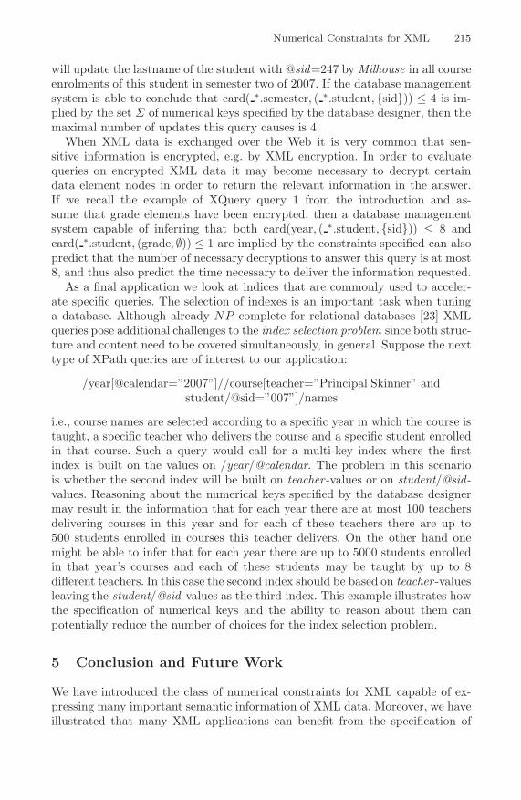
Numerical Constraints for XML 215
will update the lastname of the student with @sid=247 by Milhouse in all courseenrolments of this student in semester two of 2007. If the database managementsystem is able to conclude that card( ∗.semester, ( ∗.student, {sid})) ≤ 4 is im-plied by the set Σ of numerical keys specified by the database designer, then themaximal number of updates this query causes is 4.
When XML data is exchanged over the Web it is very common that sen-sitive information is encrypted, e.g. by XML encryption. In order to evaluatequeries on encrypted XML data it may become necessary to decrypt certaindata element nodes in order to return the relevant information in the answer.If we recall the example of XQuery query 1 from the introduction and as-sume that grade elements have been encrypted, then a database managementsystem capable of inferring that both card(year, ( ∗.student, {sid})) ≤ 8 andcard( ∗.student, (grade, ∅)) ≤ 1 are implied by the constraints specified can alsopredict that the number of necessary decryptions to answer this query is at most8, and thus also predict the time necessary to deliver the information requested.
As a final application we look at indices that are commonly used to acceler-ate specific queries. The selection of indexes is an important task when tuninga database. Although already NP -complete for relational databases [23] XMLqueries pose additional challenges to the index selection problem since both struc-ture and content need to be covered simultaneously, in general. Suppose the nexttype of XPath queries are of interest to our application:
/year[@calendar=”2007”]//course[teacher=”Principal Skinner” andstudent/@sid=”007”]/names
i.e., course names are selected according to a specific year in which the course istaught, a specific teacher who delivers the course and a specific student enrolledin that course. Such a query would call for a multi-key index where the firstindex is built on the values on /year/@calendar. The problem in this scenariois whether the second index will be built on teacher -values or on student/@sid -values. Reasoning about the numerical keys specified by the database designermay result in the information that for each year there are at most 100 teachersdelivering courses in this year and for each of these teachers there are up to500 students enrolled in courses this teacher delivers. On the other hand onemight be able to infer that for each year there are up to 5000 students enrolledin that year’s courses and each of these students may be taught by up to 8different teachers. In this case the second index should be based on teacher -valuesleaving the student/@sid -values as the third index. This example illustrates howthe specification of numerical keys and the ability to reason about them canpotentially reduce the number of choices for the index selection problem.
5 Conclusion and Future Work
We have introduced the class of numerical constraints for XML capable of ex-pressing many important semantic information of XML data. Moreover, we haveillustrated that many XML applications can benefit from the specification of

216 S. Hartmann and S. Link
such constraints. While reasoning about numerical constraints is intractable ingeneral we have identified the large subclass of numerical keys that are finitelysatisfiable, finitely axiomatisable, and whose implication problem can be decidedin quadratic time. Numerical keys form a very natural class of XML constraintsthat can be utilised effectively by designers, and the complexity of their asso-ciated decision problems indicates that they can be maintained efficiently bydatabase systems for XML applications.
One area that warrants future research is the study of (numerical) keys withrespect to more expressive path languages [4,22].
Furthermore, (numerical) keys should be investigated in the presence of aschema specification, such as a DTD or an XSD. As already observed for keys[8] numerical keys may behave completely differently under such specifications.
We would like to extend numerical dependencies from relational databases toXML documents. However, since the implication problem for relational numer-ical dependencies is computationally infeasible [13], future work will focus onidentifying useful restricted classes of such XML constraints.
As already indicated one should further explore the impact of numerical con-straints on various XML applications, in particular on query optimisation, queryrewriting, numbering schemes and indexing techniques. These applications canalready benefit greatly from incomplete sets of sound inference rules for the im-plication of numerical constraints. While reasoning may be intractable in generalone may develop efficient decision algorithms for those subclasses syntacticallydefined by some set of sound inference rules.
References
1. Abiteboul, S., Hull, R., Vianu, V.: Foundations of Databases. Addison-Wesley,Reading (1995)
2. Apparao, V., et al.: Document object model (DOM) Level 1 Specification, W3CRecommendation (October 1998), http://www.w3.org/TR/REC-DOM-Level-1/
3. Arenas, M., Libkin, L.: A normal form for XML documents. TODS 29(1), 195–232(2004)
4. Benedikt, M., Fan, W., Kuper, G.: Structural properties of XPath fragments.TCS 336(1), 3–31 (2005)
5. Boag, S., Chamberlin, D., Fernandez, M., Florescu, D., Robie, J., Simeon, J.:XQuery 1.0: An XML query language, W3C Recommendation (January 2007),http://www.w3.org/TR/xquery/
6. Bray, T., Paoli, J., Sperberg-McQueen, C.M., Maler, E., Yergeau, F.: Extensiblemarkup language (XML) 1.0 (Fourth Edition) W3C Recommendation (August2006), http://www.w3.org/TR/xml/
7. Buneman, P., Davidson, S., Fan, W., Hara, C., Tan, W.: Keys for XML. ComputerNetworks 39(5), 473–487 (2002)
8. Buneman, P., Davidson, S., Fan, W., Hara, C., Tan, W.: Reasoning about keys forXML. Inf. Syst. 28(8), 1037–1063 (2003)
9. Buneman, P., Fan, W., Simeon, J., Weinstein, S.: Constraints for semi-structureddata and XML. SIGMOD Record 30(1), 47–54 (2001)
10. Chamberlin, D., Florescu, D., Robie, J.: XQuery Update Facility, W3C WorkingDraft, (July 2006), http://www.w3.org/TR/xqupdate/

Numerical Constraints for XML 217
11. Clark, J., DeRose, S.: XML path language (XPath) Version 1.0, W3C Recommen-dation (November 1999), http://www.w3.org/TR/xpath
12. Fan, W.: XML constraints. In: DEXA Workshops, pp. 805–809 (2005)13. Grant, J., Minker, J.: Inferences for numerical dependencies. TCS 41, 271–287
(1985)14. Hara, C., Davidson, S.: Reasoning about nested functional dependencies. In: PODS,
pp. 91–100 (1999)15. Hartmann, S.: On the implication problem for cardinality constraints and func-
tional dependencies. Ann. Math. Art. Intell. 33, 253–307 (2001)16. Hartmann, S., Link, S.: Unlocking keys for XML trees. In: ICDT 2007. LNCS,
vol. 4353, pp. 104–118. Springer, Heidelberg (2007)17. Hartmann, S., Link, S., Schewe, K.-D.: Functional and multivalued dependencies
in nested databases generated by record and list constructor. Ann. Math. Art.Intell. 46, 114–164 (2006)
18. Hartmann, S., Link, S., Trinh, T.: Efficient reasoning about XFDs with pre-imagesemantics. In: DASFAA. LNCS, vol. 4443, pp. 1070–1074. Springer, Heidelberg(2007)
19. Hartmann, S., Trinh, T.: Axiomatising functional dependencies for XML with fre-quencies. In: Dix, J., Hegner, S.J. (eds.) FoIKS 2006. LNCS, vol. 3861, pp. 159–178.Springer, Heidelberg (2006)
20. Imamura, T., Dillaway, B., Simon, E.: XML encryption syntax and processing,W3C Recommendation (December 2002), http://www.w3.org/TR/xmlenc-core/
21. Kay, M.: XSL transformations (XSLT) Version 2.0 W3C Recommendation (Jan-uary 2007), http://www.w3.org/TR/xslt20/
22. Miklau, G., Suciu, D.: Containment and equivalence for a fragment of XPath. J.ACM 51(1), 2–45 (2004)
23. Piatetsky-Shapiro, G.: The optimal selection of secondary indices is NP-complete.SIGMOD Record 13(2), 72–75 (1983)
24. Thalheim, B.: Dependencies in Relational Databases. Teubner (1991)25. Thompson, H., Beech, D., Maloney, M., Mendelsohn, N.: XML Schema Part 1:
Structures second edition, W3C Recommendation (October 2004),http://www.w3.org/TR/xmlschema-1/
26. Vincent, M., Liu, J., Liu, C.: Strong functional dependencies and their applicationto normal forms in XML. TODS 29(3), 445–462 (2004)

Modules over Monads and Linearity
Andre Hirschowitz1 and Marco Maggesi2
1 LJAD, Universite de Nice Sophia–Antipolis, CNRShttp://math.unice.fr/~ah
2 Universita degli Studi di Firenzehttp://www.math.unifi.it/~maggesi
Abstract. Inspired by the classical theory of modules over a monoid,we give a first account of the natural notion of module over a monad. Theassociated notion of morphism of left modules (”linear” natural trans-formations) captures an important property of compatibility with sub-stitution, in the heterogeneous case where ”terms” and variables thereincould be of different types as well as in the homogeneous case. In thispaper, we present basic constructions of modules and we show examplesconcerning in particular abstract syntax and lambda-calculus.
1 Introduction
Substitution is a major operation. Its relevance to computer sciences has beenstressed constantly (see e.g. [7]). Mathematicians of the last century have coinedtwo strongly related notions which capture the formal properties of this opera-tion. The first one is the notion of monad, while the second one is the notion ofoperad. We focus on the notion of monad. A monad in the category C is a monoidin the category of endofunctors of C (see 2 below) and as such, has right and leftmodules. Apriori these are endofunctors (in the same category) equipped withan action of the monad. In fact, we introduce a slightly more general notion ofmodules over a monad, based on the elementary observation that we can readilyextend the notion of a right action of a monad in C to the case of a functorfrom any category B to C, and symmetrically the notion of a left action of amonad in C to the case of a functor from C to any category D. We are mostlyinterested in left modules. As usual, the interest of the notion of left moduleis that it generates a companion notion of morphism. We call morphisms thosenatural transformations among (left) modules which are compatible with thestructure, namely which commute to substitution (we also call these morphismslinear natural transformations).
Despite the natural ideas involved, the only mention of modules over monadswe have been able to find is on a blog by Urs Schreiber.1 On the other hand,modules over operads have been introduced by M. Markl ([16,17]) and are com-monly used by topologists (see e.g. [9,14,4]). In [8], such modules over operadshave been considered, under the name of actions, in the context of semantics.
1 http://golem.ph.utexas.edu/string/archives/000715.html
D. Leivant and R. de Queiroz (Eds.): WoLLIC 2007, LNCS 4576, pp. 218–237, 2007.c© Springer-Verlag Berlin Heidelberg 2007

Modules over Monads and Linearity 219
We think that the notions of module over a monad and linear transformationsdeserve more attention and propose here a first reference for basic properties ofcategories of left modules, together with basic examples of morphisms of leftmodules, hopefully showing the adequacy of the language of left modules forquestions concerning in particular (possibly higher-order) syntax and lambda-calculus.
In section 2, we briefly review the theory of monads and their algebras. Insection 3, we develop the basic theory of modules. In section 4, we sketch atreatment of syntax (with variable-binding) based on modules. In the remainingsections, we show various linear transformations concerning lists and the lambda-calculus (typed or untyped). The appendix discusses the formal proof in the Coqproof assistant of one of our examples.
2 Monads and Algebras
We briefly recall some standard material about monads and algebras. Experi-enced readers may want to skip this section or just use it as reference for ournotations. Mac Lane’s book [15] can be used as reference on this material.
Let C be a category. A monad over C is a monoid in the category C → C ofendofunctors of C. In more concrete terms:
Definition 1 (Monad). A monad R = 〈R,μ, η〉 is given by a functor R : C→C, and two natural transformations μ : R2 → R such that the following diagramscommute:
R3
μR
��
Rμ �� R2
μ
��R2
μ �� R
I · R
1R ������
����
�ηR �� R2
μ
��
R · I
1R������
����
�
R�
R
The μ and η natural transformations are often referred as product (or composi-tion) and unit of the monad M . In the programming language Haskell, they arenoted join and return respectively.
Given a monad R and an arrow f : X → RY , we define the function bind f :RX → RY given by bind f := μ · Rf . The functoriality and the compositionof the monad can be defined alternatively in terms of the unit and the bindoperator. More precisely, we have the equations
μX = bind 1X , Rf = bind(η · f).
Moreover, we have the following associativity and unity equations for bind
bind g · bind f = bind(bind g · f), bind ηX = 1RX , bind f · η = f (1)
for any pair of arrows f : X → RY and g : Y → RZ.In fact, to give a monad is equivalent to give two operators unit and bind as
above which satisfy equations 1.
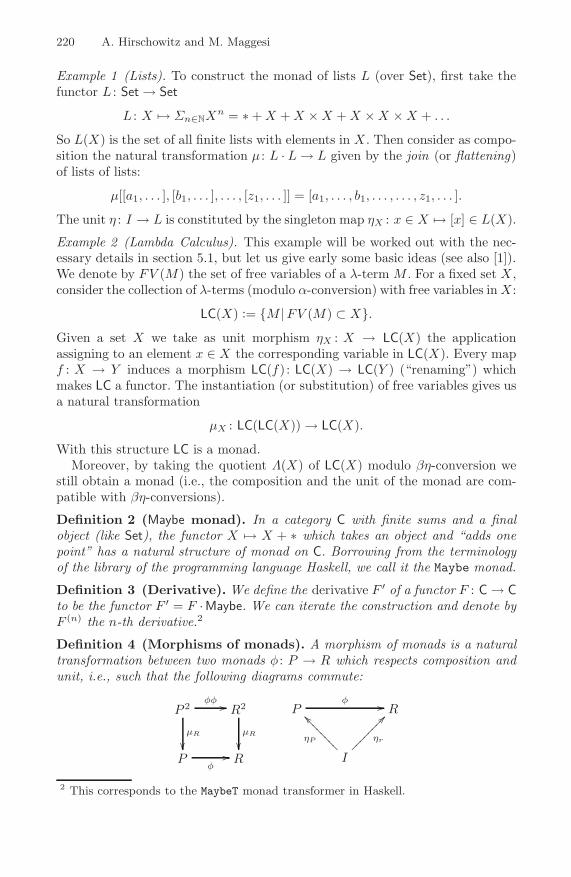
220 A. Hirschowitz and M. Maggesi
Example 1 (Lists). To construct the monad of lists L (over Set), first take thefunctor L : Set→ Set
L : X �→ Σn∈NXn = ∗+X +X ×X +X ×X ×X + . . .
So L(X) is the set of all finite lists with elements in X . Then consider as compo-sition the natural transformation μ : L · L→ L given by the join (or flattening)of lists of lists:
μ[[a1, . . . ], [b1, . . . ], . . . , [z1, . . . ]] = [a1, . . . , b1, . . . , . . . , z1, . . . ].
The unit η : I → L is constituted by the singleton map ηX : x ∈ X �→ [x] ∈ L(X).
Example 2 (Lambda Calculus). This example will be worked out with the nec-essary details in section 5.1, but let us give early some basic ideas (see also [1]).We denote by FV (M) the set of free variables of a λ-term M . For a fixed set X ,consider the collection of λ-terms (modulo α-conversion) with free variables inX :
LC(X) := {M |FV (M) ⊂ X}.Given a set X we take as unit morphism ηX : X → LC(X) the applicationassigning to an element x ∈ X the corresponding variable in LC(X). Every mapf : X → Y induces a morphism LC(f) : LC(X) → LC(Y ) (“renaming”) whichmakes LC a functor. The instantiation (or substitution) of free variables gives usa natural transformation
μX : LC(LC(X))→ LC(X).
With this structure LC is a monad.Moreover, by taking the quotient Λ(X) of LC(X) modulo βη-conversion we
still obtain a monad (i.e., the composition and the unit of the monad are com-patible with βη-conversions).
Definition 2 (Maybe monad). In a category C with finite sums and a finalobject (like Set), the functor X �→ X + ∗ which takes an object and “adds onepoint” has a natural structure of monad on C. Borrowing from the terminologyof the library of the programming language Haskell, we call it the Maybe monad.
Definition 3 (Derivative). We define the derivative F ′ of a functor F : C→ Cto be the functor F ′ = F ·Maybe. We can iterate the construction and denote byF (n) the n-th derivative.2
Definition 4 (Morphisms of monads). A morphism of monads is a naturaltransformation between two monads φ : P → R which respects composition andunit, i.e., such that the following diagrams commute:
P 2
μR
��
φφ �� R2
μR
��P
φ�� R
Pφ �� R
I
ηP
���������� ηr
����������
2 This corresponds to the MaybeT monad transformer in Haskell.

Modules over Monads and Linearity 221
It can be easily seen that morphisms of monads form a category.
For our purpose it is relevant to observe that there are a number of naturaltransformations which arise in the above examples which fail to be morphismsof monads. We take the following as paradigmatic example.Example 3 (Abstraction is not a morphism of monads). Abstraction on λ-termsgives a natural transformation abs : LC′ → LC which takes a λ-termM ∈ LC(X+∗)and binds the “variable” ∗. This fails to be a morphism of monads because it doesnot respect substitution in the sense of monads: a careful inspection reveals thatthe transformation
LC(LC(X + ∗) + ∗) μ−→ LC(X + ∗) abs−→ LC(X)
binds all stars under a single abstraction while
LC(LC(X + ∗) + ∗) abs abs−→ LC(LC(X))μ−→ LC(X)
not. In fact, we will see later that LC′ is a left module over LC and abs is aLC-linear morphism.Now let R be a monad over C.
Definition 5 (Algebra). An algebra over R is given by an object A and amorphism ρ : R(A)→ A in C such that the following diagrams commute:
R2(A)
μA
��
Rρ �� R(A)
ρ
��R(A)
ρ �� A
A
1A ����
����
�ηA �� R(A)
ρ
��A
Definition 6. Let A, B be two algebras over a monad R. An arrow f : A→ Bin C is said to be a morphism of algebras if it is compatible with the associatedactions, i.e., the two induced morphisms from R(A) to B are equal:
ρB ·R(f) = f · ρAAs we will see later, algebras can be regarded as special kind of right modules.
Example 4 (Monoids). In the category of sets, algebras over the monad L oflists are sets equipped with a structure of monoid; given a monoid A, the corre-sponding action L(A) → A is the product (sending a list to the correspondingproduct).
3 Modules over Monads
Being a monoid in a suitable monoidal category, a monad has associated left andright modules which, a-priori, are objects in the same category, acted upon bythe monoid.
Although we are mostly interested in left modules, let us remark that from thisclassical point of view, algebras over a monad are not (right-)modules. We givea slightly more general definition of modules which is still completely natural.According to this extended definition, algebras turn out to be right-modules.

222 A. Hirschowitz and M. Maggesi
3.1 Left Modules
We start first by concentrating ourselves on left modules over a given monad Rover a category C.
Definition 7 (Left modules). A left R-module in D is given by a functorM : C→ D equipped with a natural transformation ρ : M ·R→M , called action,which is compatible with the monad composition, more precisely, we require thatthe following diagrams commute
M · R2
ρR
��
Mμ �� M ·Rρ
��M ·R ρ �� M
M ·Rρ
��
M · I
1M���������
M�
M
We will refer to the category D as the range of M .
Remark 1. The companion definition of modules over an operad (c.f. e.g. [17,9])follows easily from the observation [19] that operads are monoids in a suitablemonoidal category. This monoidal structure is central in [6].
Given a left R-module M , we can introduce the mbind operator which, to eacharrow f : X → RY , associates an arrow mbind f := MX → MY defined bymbind f := ρ ·Mf . The axioms of left module are equivalent to the followingequations over mbind:
mbind g ·mbind f = mbind(bind g · f), mbind ηX = 1X
Example 5. We can see our monad R as a left module over itself (with range C),which we call the tautological module.
Example 6. Any constant functor W : C→ D, W ∈ D is a trivial left R-module.
Example 7. For any functor F : D → E and any left R-module M : C → D, thecomposition F ·M is a left R-module (in the evident way).
Definition 8 (Derived module). As for functors and monads, derivation iswell-behaved also on left modules: for any left R-module M , the derivative M ′ =M ·Maybe has a natural structure of left R-module where the action M ′ ·P →M ′
is the composition
M ·Maybe ·R Mγ−→M ·R ·MaybeρMaybe−→ M ·Maybe
and γ is the natural arrow Maybe · R→ R ·Maybe.
Definition 9 (Morphisms of left modules). We say that a natural transfor-mation of left R-modules τ : M → N is linear if it is compatible with substitution:
M ·RρM
��
τR �� N · RρN
��M
τ �� N
We take linear natural transformations as left module morphisms.

Modules over Monads and Linearity 223
Remark 2. Here the term linear refers to linear algebra: linear applications be-tween modules over a ring are group morphisms compatible with the action ofthe ring. It is compatible with the usual flavor of the word linear (no duplication,no junk) as the following example shows.
Example 8. We consider the monad M on Set generated by two binary construc-tions + and ∗ and we build (by recursion) a natural transformation n : M →Mas follows: for a variable x, n(x) is x+ x, while for the other two cases we haven(a+ b) = n(a) ∗ n(b) and n(a ∗ b) = n(a) + n(b). It is easily verified that n is anon-linear natural transformation (check the diagram against n(var(x ∗ x))).Example 9. We easily check that the natural transformation of a left moduleinto its derivative is linear. Note that there are two natural inclusions of thederivative M ′ into the second derivative M ′′. Both are linear.
Example 10. Consider again the monad of lists L. The concatenation of two listsis a L-linear morphism L× L→ L.
Definition 10 (Category of left modules). We check easily that linear mor-phisms between left R-modules with the same range yield a subcategory of thefunctor category. We denote by ModD(R) the category of left R-modules withrange D.
Definition 11 (Product of left modules). We check easily that the cartesianproduct of two left R-modules as functors (having as range a cartesian categoryD) is naturally a left R-module again and is the cartesian product also in thecategory ModD(R). We also have finite products as usual. The final left module∗ is the product of the empty family.
Example 11. Given a monad R on Set and a left R-module M with range in afixed cartesian categoryD, we have a natural “evaluation” morphism eval : M ′×R→M , where M ′ is the derivative of M .
Proposition 1. Derivaton yields a cartesian endofunctor on the category of leftR-modules with range in a fixed cartesian category D
3.2 Right Modules
Let R be a monad over a category C. The definition of right module is similarto that of left module.
Definition 12 (Right modules). A right R-module (from D) is given by afunctor M : D→ C equipped with a natural transformation ρ : R ·M →M whichmakes the following diagrams commutative
R2 ·MRρ
��
μM �� R ·Mρ
��R ·M ρ �� M
I ·M
1M �����������ηM �� R ·M
ρ
��M
As for left modules, we will call corange of M the category D.

224 A. Hirschowitz and M. Maggesi
We remark that for any right R-module M and any object X ∈ D the imageM(X) is an R-algebra. Then a right R-module is simply a functor from thecorange category D to the category of R-algebras.
Example 12. Our monad R is a right module over itself.
Example 13. If A is an R-algebra, then for any category D the constant functorA : X �→ A has a natural structure of right R-module. In particular, we canidentify our algebra with the corresponding functor A : ∗ → C, where ∗ is thecategory with one object and one arrow.
Example 14. Let φ : R → P be a morphism of monads. Then P is a right andleft R-module with actions given respectively by P · R φR−→ R · R μR−→ R andR · P Pφ−→ R · R μR−→ R.
Definition 13 (Morphisms of right modules). A morphism of right R-modules is a natural transformation τ : M → N which is compatible with substi-tution, i.e., such that the following diagram commutes:
R ·MρM
��
Rτ �� R ·NρN
��M
τ �� N
Definition 14 (Category of right R-modules). We check easily that modulemorphisms among right R-modules with the same corange yield a subcategory ofthe functor category.
3.3 Limits and Colimits of Left Modules
Limits and colimits in the category of left modules can be constructed pointwise.For instance:
Lemma 1 (Limits and colimits of left modules). If D is complete (resp.cocomplete), then ModD(R) is complete (resp. cocomplete).
Proof. Suppose first that D be a complete category and G : I → ModD(R) be adiagram of left modules over the index category I. For any object X ∈ C we havea diagram G(X) : I→ D and for any arrow f : X → Y in C we have a morphismof diagrams G(X)→ G(Y ). So define
U(X) := limG(X)
Next, given an arrow f : X → R(Y ), we have an induced morphism of diagramsG(X) → G(Y ) by the module structure on each object of the diagram. Thisinduces a morphism mbind f : U(X)→ U(Y ). It is not hard to prove that mbindsatisfies the module axioms and that U is the limit ofG. The colimit constructionis carried analogously.

Modules over Monads and Linearity 225
3.4 Base Change
Definition 15 (Base change). Given a morphism f : A → B of monads anda left B-module M , we have an A-action on M given by
M ·A Mf−→M · B ρM−→M.
We denote by f∗M the resulting A-module and we refer to f∗ as the base changeoperator.
Lemma 2. The base change of a left module is a left module.
Proof. Our thesis is the commutativity of the diagram
M ·B ·A
ρA
��
M · A ·AMfA��
Mff
��
Mμ �� M ·AMf
��M ·B ·BρB
��
Mμ �� M · Bρ
��M · A
Mf�� M · B ρ
�� M
which follows from the commutativity of the three pieces: M is a left B-module,the map from M(B( ))→M( ) is functorial, and f is a morphism.
Definition 16 (Base change (functoriality)). We upgrade the base changeoperator into a functor f∗ : ModD(B)→ ModD(A) by checking that if g : M → Nis a morphism of left B-modules, then so is the natural transformation f∗g :f∗M → f∗N .
Proposition 2. The base change functor commutes with products and withderivation.
Proposition 3. Any morphism of monads f : A→ B yields a morphism of leftA-modules, still denoted f , from A to f∗B.
4 Initial Algebra Semantics
To ease the reading of the forthcoming sections, we collect in this section someclassical ideas about Initial Algebra Semantics.
Given a category C and an endofunctor T : C → C, a T -algebra3 is given byan object A ∈ C and an arrow
σA : TA→ A.
3 There is a lexical conflict here with algebra of monads introduced in section 2, whichis deeply rooted in the literature anyway. We hope that this will not lead to anyconfusion.

226 A. Hirschowitz and M. Maggesi
A morphism of T -algebras is an arrow f : A → B which commutes with thestructural morphism σ
TA
σA
��
Tf �� TB
σB
��A
f�� B
This defines the category of T -algebras. Notice that, for any T -algebraA, there isan induced T -algebra structure on TA given by TσA : T (TA)→ TA, turning σAinto a morphism of algebras. An initial T -algebra is called a (least) fixpoint of T .Given one such fixpoint U and any other T -algebraA we denote by foldA : U → Athe induced initial morphism. We observe that σU is an isomorphism whoseinverse is foldTU since σU · foldTU = 1U by the universal property of U and fromthe naturality of fold follows that the diagram
TU
σU
��
1T U
��T foldT U �� T (TU)
TσU
��U
foldT U
�� TU
is commutative.Let us show how this general framework can work in the case of (polymorphic)
lists.
Example 15. Take C = Set → Set the category of endofunctors of Set and con-sider the functor T : (Set→ Set)→ (Set→ Set) defined by
T (F ) := X �→ ∗+X × FX.
The least fix point of T is (the underlying functor of) the monad of lists L in-troduced in section 2. The T -algebra structure ∗ + X × LX = TL L givesthe constructors (nil, cons) and the corresponding destructors. We would like torecognise this structural isomorphism as an L-linear morphism. Unfortunately,we do not have on TL a structure of left L-module corresponding to our expec-tation (notice that the identity functor is not an L-module in a natural way). Wewill explain in section 6 how this phenomenon can be considered a consequenceof the lack of typing.
5 Monads over Sets
In this section we consider more examples of linear morphisms over monads onthe category of sets.

Modules over Monads and Linearity 227
5.1 Untyped Syntactic Lambda Calculus
Consider the functor T := (Set→ Set)→ (Set→ Set) given by
TF : X �→ X + FX × FX + F ′X
where F ′ denotes the derived functor X �→ F (X + ∗). It can be shown that Tpossesses a least fixpoint that we denote by LC (LC standing for λ-calculus, cfr.the example in section 2). We consider LC(X) as the set of λ-terms with freevariables taken fromX (see also [3]). In fact, the structural morphism TLC→ LCgives the familiar constructors for λ-calculus in the locally nameless encoding,namely, the natural transformations
var : I → LC, app : LC× LC→ LC, abs : LC′ → LC.
As already observed, the substitution (instantiation) of free variables gives amonad structure on LC where var is the unit.
We would like to express that these constructors are well behaved with respectto substitution. Again, as in the case of lists, TLC has no natural structure ofleft LC-module. However, we can consider the functor T as built of two partsTF = I + T0F where T0F := F × F + F ′ (in other words we are tackling apartvar, the unit of the monad, from the other two constructors app and abs). NowT0LC is a left LC-module and we can observe that the algorithm of substitutionis carried precisely in such a way that the induced morphism
app, abs : T0LC→ LC
is LC-linear or, equivalently, the natural transformations app : LC × LC → LCand abs : LC′ → LC are LC-linear. To make the idea clearer, we reproduce ashort piece of code in the Haskell programming language which implements thealgorithm of substitution.
module LC where
import Monad (liftM)
data LC a = Var a | App (LC a) (LC a) | Abs (LC (Maybe a))
instance Monad LC where
return = Var
Var x >>= f = f x
App x y >>= f = App (x >>= f) (y >>= f)
Abs x >>= f = Abs (x ‘mbind‘ f)
mbind :: LC (Maybe a) -> (a -> LC b) -> LC (Maybe b)
mbind x f = x >>= maybe (Var Nothing) (liftM Just . f)
In the above code, mbind constitutes the left LC-module structure on LC′. It isnow evident that the recursive calls in the definition of (>>=) are exactly thosegiven by the linearity of app and abs.
We can go further and try to make the linearity more explicit in the syntacticdefinition of λ-calculus. This can be done as follows.

228 A. Hirschowitz and M. Maggesi
Theorem 1. Consider the category MonT0 where objects are monads R oversets endowed with a R-linear morphism T0R → R while arrows are given bycommutative diagrams
T0R
��
T0f �� f∗T0P
��R
f �� f∗P
where all morphisms are R-linear (we are using implicitly the fact that the basechange functor commutes with derivation and products). The monad LC is initialin MonT0 .
In fact, the previous theorem can be generalized as follows (interested readersmay also want to look at other works on higher order abstract syntax, e.g.,[6,13,10] see also our [12]). Let R be a monad over Set. We define an arity to bea list of nonnegative integers. We denote by N
∗ the set of arities. For each arity(a1, . . . , ar), and for any R-module M , we define the R-module T aM by
T aM = M (a1) × · · · ×M (ar),
where M (n) denotes the n-th derivative of M , and we say that a linear morphismT aR→ R is a R-representation of a (or a representation of a in R). For instance,the app and abs constructors are LC-representations of the arities (0, 0) and (1)respectively.
Next, we consider signatures which are family of arities. For each signatureΣ : I → N
∗, and for any R-module M , we define the R-module TΣM by
TΣM =∑
i∈ITΣiM
and we say that a linear morphism TΣR → R is a R-representation of Σ (or arepresentation of Σ in R). Altogether app and abs give a LC-representation ofthe signature ((0, 0), (1)).
As in the special case of the λ-calculus, representations of a given signatureΣ form a category.
Theorem 2. For any signature Σ, the category of Σ-representations has aninitial object.
5.2 Untyped Semantic Lambda Calculus
For any set X , consider the equivalence relation ≡βη on LC(X) given by thereflexive symmetric transitive closure of β and η conversions and define Λ(X) :=LC(X)/ ≡βη. It can be shown that ≡βη is compatible with the structure of LCso Λ has a structure of monad, the projection LC→ Λ is a morphism of monads,and we have an induced morphism T0Λ→ Λ which is Λ-linear.

Modules over Monads and Linearity 229
Now the key fact is that the abstraction abs : Λ′ → Λ is a linear isomorphism!In fact, it is easy to construct its inverse app1 : Λ→ Λ′:
app1 x = app(x, ∗)where x �→ x denotes the natural inclusion Λ→ Λ′. The equation
abs · app1 = 1Λ
clearly corresponds to the η-rule while the other equation
app1 · abs = 1Λ′
can be considered the ultimate formulation of the β-rule. In fact, there is a moreclassical formulation of the β-rule which can be stated as the commutativity ofthe diagram
Λ′ × Λ abs×Λ ��
subst Λ× Λ
app
��Λ
Again, we can present this situation from a more syntactical point of view.For this, consider the category of exponential monads : an exponential monad is amonad R endowed with a R-linear isomorphism with its derivative expR : R′ →R. An arrow is a monad morphism f such that
R′
expR
��
f ′�� f∗P ′
expP
��R
f �� f∗P
is a commutative diagram of R-modules (we are implicitly using the commuta-tivity of base change with derivation).
Theorem 3. The monad Λ is initial in the category of exponential monads.
We have developed a formal proof of the above theorem in the Coq proof assistant[5] which is discussed in the appendix.
6 Monads over Types
So far we mostly considered examples of monads and modules on the categoryC = Set of small sets. Other interesting phenomena can be captured by takinginto account monads and modules on other categories. In this section we considerthe case C = Setτ the category of sets fibered over a fixed set τ . This is the cate-gory given by maps φX : X → τ , called τ -sets, where arrows 〈X,φX〉 → 〈Y, φY 〉are given by maps f : X → Y which commute with the structural morphisms,i.e., φY · f = φX . For each t ∈ τ and each τ -set X , we denote by Xτ := φ−1
X (t)the preimage of t in t. We regard τ as a “set of types” and the fibers Xt as a setof “terms of type t”.

230 A. Hirschowitz and M. Maggesi
6.1 Typed Lists
Here we show how, in the context of typed lists, the constructors nil and consmay appear as linear. To this effect, we introduce a distinction between the basetype ∗, the type of lists list ∗, the type of lists of lists, etc. Thus we take τ = N
the inductive set of types generated by the grammar τ = ∗ | list τ , and considerthe category Setτ .
For each t ∈ τ we define Lt : Setτ → Set by setting Lt(X) to be the set ofterms of type t built out from (typed) variables in X by adding, as usual, termsobtained through the nil and cons constructions. By glueing these Lt together,we obtain an endofunctor L in Setτ . It is easily seen to be a monad (the presentstructure of monad has nothing to do with flattening).
For each t ∈ τ , Lt is a left L-module (by Example 7). The nil and consconstructors constitute a family of natural transformations parametrized by t ∈ τ
nilt : ∗ −→ Llist t, const : Lt × Llist t −→ Llist t.
Hence we have here examples of heterogeneous modules since ∗, Lt and Llist t
are L-modules in Set. And nilt and const are easily seen to be morphisms amongthese modules.
We may also want to glue for instance these const into a single cons. For this,we need shifts. Given X ∈ Setτ we have the associated shifts X [n] which areobtained by adding n to the structural map X → N. The shift (·)[n] : X �→ X [n]gives an endofunctor over Setτ . Given a functor F from any category to thecategory Setτ , we consider the shifted functors F [n] obtained as composition ofF followed by (·)[n]. From the remarks of section 3, it follows at once that if Fis an L-module, then so is F [n]. With these notations, glueing yields
nil : ∗ [1] −→ L, cons : L[1]× L −→ L
where ∗ denotes the final functor in the category of endofunctors of Setτ . Againnil and cons are easily checked to be L-linear.
6.2 Simply Typed Lambda Calculus
Our second example of typed monad is the simply-typed λ-calculus. We denoteby τ the set of simple types τ := ∗ | τ → τ . Following [22], we consider thesyntactic typed λ-calculus as an assignment V �→ LCτ (V ), where V =
∑t∈τ (Vt)
is a (variable) set (of typed variables) while
LCτ (V ) =∑
t∈τ(LCτ (V ))t
is the set of typed λ-terms (modulo α-conversion) built on free variables takenin V .
Given a type t we set LCt(X) := (LCτ (X))t which gives a functor over τ -sets, which is equipped with substitution, turning it into a (heterogeneous) leftmodule over LCτ . And given two types s, t, we have
apps,t : LCs→t × LCs −→ LCt
which is linear.

Modules over Monads and Linearity 231
For the abs construction, we need a notion of partial derivative for a module.For a left module M over τ -sets, and a type t ∈ τ , we set
δtM(V ) := M(V + ∗t)
where V + ∗t is obtained from V by adding one element with type t. It is easilychecked how δtM is again a left module. Now, given two types s and t, it turnsout that
abss,t : δsLCt −→ LCs→t
is linear.As in the untyped case, we can consider the functor Λτ obtained by quoti-
enting modulo βη conversion. This is again a monad over the category of τ -setsand the natural quotient transformation LCτ → Λτ is a morphism of monads.For this semantic monad, the above left module morphisms induce semanticcounterparts: apps,t : Λs→t × Λs −→ Λt and abss,t : δsΛt −→ Λs→t.
Here we need a new notion of arity and signature, which we will introducein some future work, in order to state and prove a typed counterpart of ourtheorem 2. For a typed counterpart of our theorem 3, see [22].
6.3 Typed Lambda Calculus
Our final example of typed monad is just a glance to more general typed λ-calculi. The point here is that the set of types is no more fixed. Thus our monadstake place in the category Fam of set families: an object in Fam is an applicationp : I → Set while a morphism m : p→ p′ is a pair (m0,m1) with m0 : I → I ′, andm1 : (i : I)p(i)→ p′(m0(i)). We say that I is the set of types of p : I → Set. FromFam there are two forgetful functors T, T ot : Fam→ Set where T (p : I → Set) :=I and Tot(p) := �i∈T (p)p(i), and a natural transformation proj : Tot → T ,defined by proj(p) = p in the obvious sense. Given a monad R on Fam, we thushave a morphism of R-modules projR : Tot ◦R→ T ◦R.
We need also two may-be monads on Fam: the first one F �→ F ∗ adds one(empty) type (tnew) to F , while the second one, F �→ F ∗/∗ adds one type(tnew) with one element (new). Given a monad R on Fam, we thus have two“derived” R-modules: R∗ := F �→ R(F ∗) and R∗/∗ := F �→ R(F ∗/∗).
Now when should we say that R is a lambda-calculus in this context? At leastwe should have a module morphism arrow : (T ◦ R)2 → T ◦ R. and a modulemorphism for abstraction, abs : R∗/∗ → R∗ (the “arity” for application is notso simple). We hope this example shows the need for new notions of arity andsignature, as well as the new room opened by modules for such concepts.
7 Monads over Preordered Sets
Our last example is about monads and modules over the category of preorderedsets (sets with a reflexive and transitive binary relation). Preordering is used
here to model the relationβη−→∗ generated by the reflexive and transitive closure

232 A. Hirschowitz and M. Maggesi
of the β and η conversions. In fact, the construction given in this section canbe considered a refinement of those of section 5.1 where we used the reflexive,symmetric and transitive closure ≡βη.
Let us consider again the monad LC of λ-terms. Given a preordered set X ,we consider the preordering on LC(X) given by the rules
x ≤ y =⇒ var x ≤ var y,
S ≤ S′ ∧ T ≤ T ′ =⇒ app(S, T ) ≤ app(S′, T ′),T ≤ T ′ =⇒ abs(T ) ≤ abs(T ′),
T −→βη T′ =⇒ T ≤ T ′.
It is not hard to verify that with this new structure LC is now a monad overpreordered sets. It turns out that the app and abs constructions are still LC-linearwith respect to this richer structure.
8 Conclusions and Related Works
We have introduced the notion of module over a monad, and more importantlythe notion of linearity for transformations among such modules and we havetried to show that this notion is ubiquitous as soon as syntax and semantics areconcerned. Our thesis is that the point of view of modules opens some new roomfor initial algebra semantics, as we sketched for typed λ-calculus (see also [12]).
The idea that the notion of monad is suited for modelling substitution con-cerning syntax (and semantics) has been retained by many recent contributionsconcerned with syntax (see e.g. [2,11,18]) although some other settings have beenconsidered. Notably in [6] the authors work within a setting roughly based onoperads (although they do not write this word down; the definition of operad ison Wikipedia; operads and monads are not too far from each other). As theymention, their approach is, to some extent, equivalent to an approach throughmonads. It has been both applied e.g. in [21] and generalized e.g. in [20]. Anotherapproach to syntax with bindings, initiated by Gabbay and Pitts [10], relies ona systematic consideration of freshness, an issue which is definitely ignored inthe monadic or operadic approach.
While the notion of module over a monad has been essentially ignored tillnow, the notion of module over an operad has been introduced more than tenyears ago, and has been incidentally considered in the context of semantics, aswe already mentioned in our introduction.
References
1. Altenkirch, T., Reus, B.: Monadic presentations of lambda terms using generalizedinductive types. In: Flum, J., Rodrıguez-Artalejo, M. (eds.) CSL 1999. LNCS,vol. 1683, pp. 453–468. Springer, Heidelberg (1999)
2. Bird, R., Paterson, R.: Generalised folds for nested datatypes. Formal Aspects ofComputing 11(2), 200–222 (1999)
Modules over Monads and Linearity 233
3. Bird, R.S., Paterson, R.: De Bruijn notation as a nested datatype. Journal ofFunctional Programming 9(1), 77–91 (1999)
4. Ching, M.: Bar constructions for topological operads and the Goodwillie derivativesof the identity. Geom. Topol. 9, 833–933 (2005)
5. The Coq Proof Assistant. http://coq.inria.fr
6. Fiore, M., Plotkin, G., Turi, D.: Abstract syntax and variable binding (extendedabstract). In: 14th Symposium on Logic in Computer Science, Trento, 1999, pp.193–202. IEEE Computer Society Press, Los Alamitos (1999)
7. Fiore, M.P.: On the structure of substitution. In: Invited address for the 22ndMathematical Foundations of Programming Semantics Conf (MFPS XXII), DISI,University of Genova, Italy (2006)
8. Fiore, M.P., Turi, D.: Semantics of name and value passing. In: Logic in ComputerScience, pp. 93–104 (2001)
9. Fresse, B.: Koszul duality of operads and homology of partition posets. In: Homo-topy theory: relations with algebraic geometry, group cohomology, and algebraicK-theory, vol. 346 of Contemp. Math., pp. 115–215. Amer. Math. Soc., Providence,RI (2004)
10. Gabbay, M., Pitts, A.: A new approach to abstract syntax involving binders. In:14th Symposium on Logic in Computer Science, Trento, 1999, pp. 214–224. IEEEComputer Society Press, Los Alamitos (1999)
11. Ghani, N., Uustalu, T.: Explicit substitutions and higher-order syntax. In: MER-LIN ’03. Proceedings of the 2003 ACM SIGPLAN workshop on Mechanized rea-soning about languages with variable binding, Uppsala, Sweden, pp. 1–7. ACMPress, New York, NY, USA (2003)
12. Hirschowitz, A., Maggesi, M.: The algebraicity of the lambda-calculus.arXiv:math/0607427v1 (2007)
13. Hofmann, M.: Semantical analysis of higher-order abstract syntax. In: 14th Sym-posium on Logic in Computer Science, Trento, 1999, pp. 204–213. IEEE ComputerSociety Press, Los Alamitos (1999)
14. Livernet, M.: From left modules to algebras over an operad: application to combi-natorial Hopf algebras. arXiv:math/0607427v1 (2006)
15. Lane, S.M.: Categories for the working mathematician. In: Graduate Texts inMathematics, 2nd edn., vol. 5, Springer-Verlag, New York (1998)
16. Markl, M.: Models for operads. arXiv:hep-th/9411208v1 (1994)
17. Markl, M.: A compactification of the real configuration space as an operadic com-pletion. arXiv:hep-th/9608067v1 (1996)
18. Matthes, R., Uustalu, T.: Substitution in non-wellfounded syntax with variablebinding. Theor. Comput. Sci. 327(1-2), 155–174 (2004)
19. Smirnov, V.A.: Homotopy theory of coalgebras. Math. USSR Izv, 27, 575–592(1986)
20. Tanaka, M., Power, J.: A unified category-theoretic formulation of typed bindingsignatures. In: MERLIN ’05. Proceedings of the 3rd ACM SIGPLAN workshop onMechanized reasoning about languages with variable binding, Tallinn, Estonia, pp.13–24. ACM Press, New York, NY, USA (2005)
21. Tanaka, M., Power, J.: Pseudo-distributive laws and axiomatics for variable bind-ing. Higher Order Symbol. Comput. 19(2-3), 305–337 (2006)
22. Zsido, J.: Le lambda calcul vu comme monade initiale. Master’s thesis, Universitede Nice – Laboratoire J. A. Dieudonne, 2005/06. Memoire de Recherche – master 2.

234 A. Hirschowitz and M. Maggesi
A Appendix: Formal Proof of Theorem 3
In this section we present our formal proof of theorem 3 in the Coq proof assistant[5]. We recall the statement of the theorem
The monad Λ of semantic untyped λ-calculus is an initial object in thecategory of exponential monads.
We include here only a small fraction of the code without proofs. The full sourcescan be found at http://www.math.unifi.it/~maggesi.
A.1 Structure of the Formalisation
The structure of our proof can be outlined in the following four major parts: (1)axioms and support library; (2) formalisation of monads, modules and exponen-tial monads; (3) formalisation of syntactic and semantic λ-calculus; (4) the maintheorem.
The second and third part are independent of each other. As for what thispaper is concerned, the first part (files Misc.v, Congr.v) can be considered asan extension of the Coq system for practical purposes. This part contains somemeta-logical material (tactics and notations) and declares the following axioms:functional choice, proof irrelevance, dependent extensionality. We include heretheir declarations:Axiom functional_choice : forall (A B : Type) (R : A -> B -> Prop),
(forall x : A, exists y : B, R x y) -> exists f : A -> B, (forall x : A, R x (f x)).
Axiom proof_irrelevance : forall (A : Prop) (H1 H2 : A), H1 = H2.
Axiom extens_dep : forall (X : Type) (T : X -> Type) (f g : forall x : X, T x),
(forall x : X, f x = g x) -> f = g.
Moreover, we use an axiomatic definition of quotient types (file Quot.v) toconstruct semantic λ-calculus as quotient of syntactic λ-calculus.
A.2 Formalisation of Monads and Modules
After the preliminary material, our formalisation opens the theory of monadsand (left) modules (files Monad.v, Mod.v, Derived Mod.v). This is constructedstarting from a rather straightforward translation of the Haskell monad library.As an example, we report here our definitions of monads and modules in theCoq syntax.
Record Monad : Type := {
monad_carrier :> Set -> Set;
bind : forall X Y : Set, (X -> monad_carrier Y) -> monad_carrier X -> monad_carrier Y;
unit : forall X : Set, X -> monad_carrier X;
bind_bind : forall (X Y Z : Set) (f : X -> monad_carrier Y) (g : Y -> monad_carrier Z)
(x : monad_carrier X),
bind Y Z g (bind X Y f x) = bind X Z (fun u => bind Y Z g (f u)) x;
bind_unit : forall (X Y : Set) (f : X -> monad_carrier Y) (x : X),
bind X Y f (unit X x) = f x;
unit_bind : forall (X : Set) (x : monad_carrier X), bind X X (unit X) x = x
}.
Notation "x >>= f" := (@bind _ _ _ f x).

Modules over Monads and Linearity 235
Record Mod (U : Monad) : Type := {
mod_carrier :> Set -> Set;
mbind : forall (X Y: Set) (f : X -> U Y) (x : mod_carrier X), mod_carrier Y;
mbind_mbind : forall (X Y Z : Set) (f : X -> U Y) (g : Y -> U Z) (x : mod_carrier X),
mbind Y Z g (mbind X Y f x) = mbind X Z (fun u => f u >>= g) x;
unit_mbind : forall (X : Set) (x : mod_carrier X), mbind X X (@unit U X) x = x
}.
Notation "x >>>= f" := (@mbind _ _ _ _ f x).
The library also includes the definition of morphism of monads and modulesand other related categorical material. Other definitions which are specific toour objective are those of derived module and exponential monad. The latterreads as follows:Record ExpMonad : Type := {
exp_monad :> Monad;
exp_abs : Mod_Hom (Derived_Mod exp_monad) exp_monad;
exp_app : Mod_Hom exp_monad (Derived_Mod exp_monad);
exp_eta : forall X (x : exp_monad X), exp_abs _ (exp_app _ x) = x;
exp_beta : forall X (x : Derived_Mod exp_monad X), exp_app _ (exp_abs _ x) = x
}.
and comes with its associated notion of morphism:
Record ExpMonad_Hom (M N : ExpMonad) : Type := {
expmonad_hom :> Monad_Hom M N;
expmonad_hom_app : forall X (x : M X),
expmonad_hom _ (exp_app M _ x) = exp_app N _ (expmonad_hom _ x);
expmonad_hom_abs : forall X (x : Derived_Mod M X),
expmonad_hom _ (exp_abs M _ x) = exp_abs N _ (expmonad_hom _ x)
}.
A.3 Formalisation of the λ-Calculus
This part contains the definition of syntactic and semantic λ-calculus (files Slc.vand Lc.v respectively). We use nested datatypes to encode λ-terms in the Calcu-lus of (Co)Inductive Constructions as already shown in the Haskell fragment ofsection 5.1 for which we report below the equivalent Coq code. Notice that thisencoding can be considered a typeful variant of the well-known de Bruijn encod-ing [3]. As the de Bruijn encoding, it represents λ-terms modulo α-conversion.
Inductive term (X : Set) : Set := var : X -> term X
| app : term X -> term X -> term X
| abs : term (option X) -> term X.
Fixpoint fct (X Y : Set) (f : X -> Y) (x : term X) { struct x } : term Y :=
match x with var a => var (f a)
| app x y => app (x //- f) (y //- f)
| abs x => abs (x //- (optmap f)) end
where "x //- f" := (@fct _ _ f x).
Definition shift X (x : term X) : term (option X) := x //- @Some X.

236 A. Hirschowitz and M. Maggesi
Definition comm (X Y : Set) (f : X -> term Y) (x : option X) : term (option Y) :=
match x with Some a => shift (f a) | None => var None end.
Fixpoint subst (X Y : Set) (f : X -> term Y) (x : term X) { struct x } : term Y :=
match x with var x => f x
| app x y => app (x //= f) (y //= f)
| abs x => abs (x //= comm f) end
where "x //= f" := (@subst _ _ f x).
Once the basic definitions are settled, we prove a series of basic lemmas whichincludes the associativity of substitution
Lemma subst_subst : forall (X Y Z : Set) (f : X -> term Y) (g : Y -> term Z) (x : term X),
x //= f //= g = x //= fun u => f u //= g.
which is the most important ingredient to prove that the λ-calculus is a monad.Finally, we introduce the beta-eta equivalence relation on lambda termsInductive lcr (X : Set) : term X -> term X -> Prop :=
| lcr_var : forall a : X, var a == var a
| lcr_app : forall x1 x2 y1 y2 : term X, x1 == x2 -> y1 == y2 -> app x1 y1 == app x2 y2
| lcr_abs : forall x y : term (option X), x == y -> abs x == abs y
| lcr_beta : forall x y : term X, Beta x y -> x == y
| lcr_eta : forall x : term X, abs (app1 x) == x
| lcr_sym : forall x y : term X, y == x -> x == y
| lcr_trs : forall x y z : term X, lcr x y -> lcr y z -> lcr x z
where "x == y" := (@lcr _ x y).
and prove some compatibility lemmas for constructors and other operations. Thecompatibility of substitution is stated as follows:Lemma lcr_subst : forall (X Y : Set) (f g : X -> term Y) (x y : term X),
(forall u, f u == g u) -> x == y -> x //= f == y //= g.
A.4 Proof of the Main Theorem
The fourth and last part summarises the results proved in the other parts andproves the main theorem. It starts by glueing together the previous two sectionsby proving that our definitions of syntactic and semantic lambda calculus pro-vides indeed two monads, denoted SLC and LC respectively, and by showing thatthe two morphisms abs and app1 constitute morphisms of modules:
Definition SLC : Monad := Build_Monad term subst var subst_subst subst_var var_subst.
Definition LC : Monad :=
Build_Monad lc lc_subst lc_var lc_subst_assoc lc_subst_var lc_var_subst.
Let abs_hom : Mod_Hom (Derived_Mod LC) LC :=
Build_Mod_Hom (Derived_Mod LC) LC lc_abs lc_abs_hom.
Let app1_hom : Mod_Hom LC (Derived_Mod LC) :=
Build_Mod_Hom LC (Derived_Mod LC) lc_app1 lc_app1_hom.
One more glueing step is the proof that LC is an exponential monad, which isstated in Coq through the following definition:Definition ELC : ExpMonad := Build_ExpMonad abs_hom app1_hom lc_eta lc_beta.
Next comes the construction of the initial morphism which is initially defined asa fixpoint on terms.

Modules over Monads and Linearity 237
Variable M : ExpMonad.
Fixpoint iota_fix X (x : term X) { struct x } : M X :=
match x with var a => unit M a
| app x y => exp_app M _ (iota_fix x) >>= default (@unit M X) (iota_fix y)
| abs x => exp_abs M _ (iota_fix x) end.
Then we prove that iota fix is compatible with the βη equivalence relation andthus it factors through the monad LC.
Let iota X : lc X -> M X := lc_factor (@iota_fix X) (@iota_fix_wd X).
The construction of the initial morphism ends with the verification that it isactually a morphism of exponential monads.Let iota_monad : Monad_Hom LC M := Build_Monad_Hom LC M iota iota_subst iota_var.
Let exp_iota : ExpMonad_Hom ELC M :=
Build_ExpMonad_Hom ELC M iota_monad iota_app1 iota_abs.
Finally, we prove that iota monad is unique.
Theorem iota_unique : forall j : ExpMonad_Hom ELC M, j = exp_iota.
The Coq terms ELC, iota monad and iota unique altogether form the formalproof of the initiality of the monad LC in the category of exponential monads.

Hydra Games and Tree Ordinals
Ariya Isihara
Department of Computer Science, Vrije Universiteit, [email protected]
Abstract. Hydra games were introduced by Kirby and Paris, for theformulation of a result which is independent from Peano arithmetic butdepends on the transfinite structure of ε0. Tree ordinals are a well-knownsimple way to represent countable ordinals. In this paper we study therelation between these concepts; an ordinal less than ε0 is canonicallytranslated into both a hydra and a tree ordinal term, and the reduc-tion graph of the hydra and the normal form of the term syntacticallycorrespond to each other.
1 Introduction
Tree ordinals are one of the simplest ways known for representing countableordinals. The main concept of tree ordinals is to represent limit ordinals byfundamental sequences themselves. The notation of tree ordinals naturally fitsto Dedekind’s TRS [2], which gives a simple definition for basic arithmetics forordinals — addition, multiplication, and exponentiation. With these arithmeticfunctions, we can represent ordinals up to ε0 by finite expressions.
On the other hand, Hydra games were invented by Kirby and Paris [4] forthe formulation of an undecidable statement. The termination of hydra gamescannot be proved within Peano arithmetic, but under the assumption that theordinal ε0 is well-ordered. There, nondeterministic behaviour of hydrae takesplace to represent infiniteness of transfinite ordinals.
In the present work we translate infinite sequences in tree ordinals and non-deterministic reductions in hydra games into each other. Thereby we will see asyntactical correspondence between tree ordinals and hydra games.
Overview
In Section 2 we present Dedekind’s TRS on tree ordinals. In Section 3 we recallthe definition of hydra games. Section 4 shows the correspondence between hydragames and tree ordinals. Section 5 gives a concluding remark.
2 Tree Ordinals
Definition 1. The set T of tree ordinal terms consists of the possibly infiniteterms generated by the following symbols
D. Leivant and R. de Queiroz (Eds.): WoLLIC 2007, LNCS 4576, pp. 238–247, 2007.c© Springer-Verlag Berlin Heidelberg 2007

Hydra Games and Tree Ordinals 239
arity symbol(s)0 0,ω1 succ, nats2 cons,Add,Mul,Exp
with the rewrite rules
Add(x, 0)→ x
Add(x, succ(y))→ succ(Add(x, y)Add(x, cons(y, z))→ cons(Add(x, y),Add(x, z))
Mul(x, 0)→ 0
Mul(x, succ(y))→ Add(Mul(x, y), x)Mul(x, cons(y, z))→ cons(Mul(x, y),Mul(x, z))
Exp(x, 0)→ succ(0)Exp(x, succ(y))→ Mul(Exp(x, y), x)
Exp(x, cons(y, z))→ cons(Exp(x, y),Exp(x, z))ω → nats(0)
nats(x)→ x : nats(succ(x)).
Observe that the rules are orthogonal and that there exists only one collapsingrule. The system is thus CR∞ and UN∞ (See [7] or [5]). We write nf (t) to denotethe (possibly infinite) normal form of t, if it exists.
We write t : s for cons(t, s), where ‘:’ is right-associative; t0 : t1 : t2 : . . .represents a infinite sequence of terms t0, t1, t2, . . . .
Definition 2. The set T O ⊂ T of tree ordinals is given as the smallest set thatsatisfies the following conditions:
0 ∈ T Osucc(t) ∈ T O (t ∈ T O)
t0 : t1 : t2 : . . . ∈ T O (t0, t1, t2, · · · ∈ T O)
with semantics [[−]] : T O → Ω inductively given by
[[0]] = 0[[succ(t)]] = [[t]] + 1
[[t0 : t1 : t2 : . . .]] = lim supi∈N
[[ti]]
where Ω denotes the set of countable ordinals.
Definition 3. We define a certain subset E0 of T given by the following BNF:
E0 ::= 0 | Add(E0, E0) | Exp(ω, E0).

240 A. Isihara
Let ∼ be the equivalence relation generated by
Add(Add(t, s), u) ∼ Add(t,Add(s, u))Add(t, 0) ∼ tAdd(0, t) ∼ t
and let [E0] be the set of equivalence classes of E0 modulo ∼.
We write∑ni=1 ti and ωt for Add(t1, . . .Add(tn−1, tn)) and Exp(ω, t), respec-
tively. We regard∑0
i=1 ti as 0.
Proposition 4 (Induction on [E0]). For any t ∈ E0, there exist n ∈ N andt1, . . . tn ∈ E0 such that t ∼ ∑n
i=1 ωti . Moreover, the equivalence classes in [E0]are enumerated by this construction. Namely, the following induction princi-ple holds: Let P ⊂ [E0]. If
∑ni=1 ωti ∈ P for all n ∈ N and t1, . . . tn ∈ P , then
P = [E0]. ��
In the remainder of this section we state some propositions on the productivityof our system, without proofs. Since the system forms a subclass of the systempresented in [6], please see ibid. for the proofs.
Lemma 5. For any t ∈ E0, nf (t) does exist. ��
Lemma 6. If t ∼ s, then nf (t) = nf (s). The function nf : [E0]→ T is thuscanonically defined. ��
Let T OE0 be the image of [E0] via nf .
Proposition 7. We have T OE0 ⊂ T O. ��
Theorem 8. Let t, s ∈ E0. Then the following equations hold:
[[nf (0)]] = 0[[nf (Add(t, s))]] = [[nf (t)]] + [[nf (s)]]
[[nf (Exp(ω, t))]] = ω[[nf (t)]].
And therefore the image of T OE0 via [[−]] is ε0. ��
Definition 9. For any α in ε0, the nested Cantor normal form of α, writtenncn(α), is inductively defined by
(i) if α = 0, then ncn(α) = 0.(ii) if α = β + 1, then ncn(α) = ncn(β) + Exp(ω, 0).(iii) if α is a limit ordinal, then there exist unique β, γ < α such that α = ωβ+γ.
Let ncn(α) = Exp(ω,ncn(β)) + ncn(γ).

Hydra Games and Tree Ordinals 241
For example, ncn(ω × 2) is computed as follows:
ncn(ω × 2) = ncn(ω1 + ω1)
= ωncn(1) + ncn(ω1)
= ωncn(0+1) + ωncn(0+1)
= ωncn(0)+ω0
+ ωncn(0)+ω0)
∼ ωω0
+ ωω0
.
Proposition 10. We have [[−]] ◦ nf ◦ ncn = idε0 . Thus, the system [E0] cancompute every ordinal less than ε0. ��
3 Hydra Games
In this section, we present hydra games [4] with a minor change.
Definition 11. A hydra is an unlabeled finite tree with arbitrary finite branches.As a hydra, a leaf node is called a head. A head is short if the immediate parentof the head is the root; long if it is neither short nor the root (See Figure 1).The empty hydra is called dead and written ©.
© ←− long head
short head −→ © ©
©
������
������ ←− root
Fig. 1. A hydra
Thus, formally, the set H of hydrae is inductively defined as follows:
(h1, . . . , hn) ∈ H if h1, . . . , hn ∈ Hwhere (), in the case n = 0, is regarded as ©.
As in the original paper, Herakles chops a head of a hydra. However, in thispaper Herakles chops only the rightmost-head of the hydra. Hence, we are mainlyinterested in the rightmost structure of a hydra so that we take the notation
(h1(h2(. . . (hn©))))
to describe a given hydra, where hi denotes the juxtaposition of ni many hydrashi1 . . . hini . This hydra is dipicted by Figure 2. Observe that, for any hydra,there exists a unique representation of this form.
Now we define the chopping-relation on the hydrae.

242 A. Isihara
hn ©
©
��������
��������
h2
h11
h1︷ ︸︸ ︷
...h1n1 ©
���������
��������
©
�������������������
��������
Fig. 2. The hydra (h1(h2(. . . (hn©))))
Definition 12. Let h be a hydra.
(i) (short-head chopping) As in Figure 3, if the rightmost-head of h is short,
i.e. h = (h1©), then we write h!
� h′ where h′ = (h1).(ii) (long-head chopping) As in Figure 4, if the rightmost-head of h is long, i.e.
h = (. . . (hn−1(hn©))), then we write hm� h′m where
h′m = (. . . (hn−1(
m times︷ ︸︸ ︷hn . . .hn))).
for any m ∈ N.
h1 ©
©
���������
������
�������
!�
h1
©
�������
Fig. 3. Short-Head chopping
Remark 13. As proved in [4], any hydra will die after finite many times chopping;note that you can choose any m for any long-head chopping step.
Thus, given a hydra h, the head-chopping reduction graph of h is uniquely de-cided. Moreover, by the above remark, no graph has any infinite path in it.
Definition 14. The function gr : H → T O is defined via the head-choppingreduction graph of a hydra. Let h be a hydra. Then gr(h) is inductively givenby the following case analysis:
(i) if h has no chopping-reduction, i.e. h =©, then gr (h) = 0.
(ii) if h has a short-head chopping h!
� h′, then gr(h) = succ(gr(h′)).

Hydra Games and Tree Ordinals 243
hn ©
hn−1 ©
���������
������
�������
©
���������
�������
��������
m�
hn
m times︷ ︸︸ ︷
hn
hn−1 ©
�������
������� ©
�������
������
©
����������
�������
������
������������
Fig. 4. Long-Head chopping
(iii) if h has a long-head chopping hm� hm indexed by m, then
gr (h) = gr(h0) : gr(h1) : gr(h2) : . . . .
Observe that one and only one of the above case is met for each h. Notice alsothat by the above remark gr is well-defined.
4 The Correspondence
We give a bijection between H and [E0].Definition 15. The translation (−) : H → [E0] is inductively defined by
(h1 . . . hn) =n∑
i=1
ωhi
and the translation (−) : [E0]→ H is inductively defined by
(
n∑
i=1
ωti
)
= (t1 . . . tn).
Proposition 16. We have (−) ◦ (−) = idH and (−) ◦ (−) = id[E0]. ��
For an example of the above proposition, we compute (©((©)©)). We have
(©((©)©)) = ω© + ω((©)©)
= ω0 + ωω(©)+ω©
= ω0 + ωωω©+ω0
= ω0 + ωωω0+ω0

244 A. Isihara
and
(ω0 + ωωω0+ω0
)=
(0
(ωω0 + ωz
))
=(©(ωz 0)
)
= (©((0)©))= (©((©)©)).
Before we state our main result, we show some lemmas.
Lemma 17. The following propositions hold:
(i) Let t, s ∈ E0. Then nf (t+ s) = nf (s)[0 := nf (t)].(ii) Let h1, . . . hn ∈ H where n > 0. Then we have
gr(h1 . . . hn) = gr(hn)[0 := gr(h1 . . . hn−1)].
Proof. (i) By induction on nf (s).(ii) Notice that for any h ∈ H such that h
m� h′ where m ∈ {!} ∪ N, we have
(h1 . . . hn−1h)m� (h1 . . . hn−1h
′).
Thus, the claim follows by induction on gr(hn).
Lemma 18. Let t ∈ [E0]. Then the following holds:
(i) If [[nf (t)]] = 0, then t = 0.(ii) If [[nf (t)]] is a successor ordinal, then t is of the form
∑ni=1 ωti where tn = 0.
Proof. (i) Suppose t =∑n
i=1 ωti . Then from Theorem 8 we have
[[nf (t)]] = ω[[nf (t1)]] + · · ·+ ω[[nf (tn)]].
Since ωα > 0 for every ordinal α, we have n = 0.(ii) Suppose t =
∑ni=1 ωti . Similarly, we have n > 0 and that ω[[nf (tn)]] is a suc-
cessor ordinal. Hence, [[nf (tn)]] = 0. From the above result, we have tn = 0.
Lemma 19. Let t ∈ [E0]. Then one of the following conditions holds:
(i) [[nf (t)]] = 0.(ii) There exists t′ ∈ T OE0 such that nf (t) = succ(t′) and [[nf (t)]] = [[nf (t′)]]+1.(iii) There exist t0, t1, · · · ∈ T OE0 such that nf (t) = t0 : t1 : . . . and [[ti]] <
[[nf (t)]] for all i ∈ N.
Proof. Using Theorem 8, it easily follows by induction on t.
Now we set P = {t ∈ [E0] | nf (t) = gr(t)}.

Hydra Games and Tree Ordinals 245
Lemma 20. Let t1, . . . , tn ∈ E0. If ti ∈ P for all applicable i, then∑n
i=1 ti ∈ P .
Proof. By mathematical induction on n. It is trivial for the case n = 0. Forinsuction step, we assume
∑n−1i=1 ti ∈ P . We have
nf
(n∑
i=1
ti
)
= nf (tn)
[
0 := nf
(n−1∑
i=1
)]
and
gr
⎛
⎝n∑
i=1
ti
⎞
⎠ = gr(tn)
⎡
⎣0 := gr
⎛
⎝n−1∑
i=1
ti
⎞
⎠
⎤
⎦
by Lemma 17. Thus, by induction hypothesis, we have
nf
(n∑
i=1
)
= gr
⎛
⎝n∑
i=1
ti
⎞
⎠ ,
implying∑n
i=1 ∈ P .
Lemma 21. If t ∈ P , then ωt ∈ P .
Proof. Transfinite induction on [[nf (t)]]. We suppose that [[nf (s)]] < [[nf (t)]] im-plies s ∈ P . Case analysis by Lemma 19.
(i) If [[nf (t)]] = 0, then from Lemma 18 we have t = 0 and thus
nf (ωt) = gr(t) = succ(0).
Hence, ωt ∈ P .(ii) If nf (t) = succ(s) where [[nf (t)]] = [[s]] + 1, then from Lemma 18 we have
t =∑n−1
i=1 ωti + ω0 with nf(∑n−1
i=1
)= s. Let t′ =
∑n−1i=1 . Then
nf (ωt) = nf (ωt′+succ(0))
= nf (Mul(ωt′ ,ω))
= 0 : nf (ωt′) : nf (Add(ωt′ + ωt′)) : . . .
and
gr(ωt) = gr(t′ (©))
= gr(©) : gr(t′) : gr(t′ t′) : . . . .
We have nf (∑m
i=1 t′) = gr(
∑mi=1 t
′) = gr(
m times︷ ︸︸ ︷
t′ . . . t′ ) for all m ∈ N, by induc-tion hypothesis and Lemma 20. Therefore, we have nf (ωt) = gr(ωt), im-plying ωt ∈ Px.
Theorem 22. We have nf ◦ (−) = gr and gr ◦ (−) = nf .
Proof. The latter equation follows from Proposition 4 and the above two lemmas.The other one then immediately follows, using Propositon 16.

246 A. Isihara
5 Conclusion
We have presented the syntactical correspondence between hydra games and acertain subclass of tree ordinals. The contribution of the paper is dipicted byFigure 5, where the upper-left triangle commutes.
Since Buchholz [1] gives a variation of hydra games which is related to a muchlarger ordinal, it is expected that there exists an extension of this TRS which isrelated to Buchholz’s hydra games.
In addition, a visualisation tool for the original hydra games due to Kirby andParis is available at [3]; Figure 6 is a screenshot of the tool.
H(−) ��
gr
�����
����
��� [E0]
(−)
��
nf
������
����
��
T OE0[[−]]
�� ε0
ncn
��
Fig. 5. The diagram which relates hydra games and tree ordinals
Fig. 6. Screenshot of hydra (JavaApplet)
Acknowledgement
I would thank Andreas Weiermann, Jan Willem Klop and Vincent van Oost-rom. Andreas noticed the underlying similarity on hydra games and tree or-dinals. Jan Willem showed me interest on my draft idea. Vincent gave me achance to present my draft idea in TeReSe meeting in Utrecht. I also acknowl-edge Roel de Vrijer and Clemens Grabmayer for their helpful comments.

Hydra Games and Tree Ordinals 247
References
1. Buchholz, W.: An independence result for (Π11-CA) + BI. Annals of Pure and Ap-
plied Logic 33(2), 131–155 (1987)2. Dedekind, R.: Was sind und was sollen die Zahlen? Vieweg (1888)3. Isihara, A.: hydra (JavaApplet). Available at
http://www.few.vu.nl/∼ariya/app/hydra/hydra.html4. Kirby, L., Paris, J.: Accessible independence results for Peano Arithmetic. Bulletin
of the London Mathematical Society 14, 285–293 (1982)5. Klop, J.W., de Vrijer, R.: Infinitary normalization. In: Artemov, S., Barringer, H.,
d’Avila Garcez, A., Lamb, L., Woods, J. (eds.) We Will Show Them: Essays inHonour of Dov Gabbay, vol. 2, pp. 169–192. College Publications (2005)
6. Kwiatkowski, M.: Ordinal arithmetic through infinitary term rewriting. Master’sthesis, Vrije Universiteit, Amsterdam, The Netherlands (2006)
7. Terese,: Term Rewriting Systems. Cambridge University Press, Cambridge (2003)

Spin Networks, Quantum Topology and
Quantum Computation
Louis H. Kauffman1 and Samuel J. Lomonaco Jr.2
1 Department of Mathematics, Statistics and Computer Science (m/c 249), 851 SouthMorgan Street, University of Illinois at Chicago, Chicago, Illinois 60607-7045, USA
[email protected] Department of Computer Science and Electrical Engineering, University ofMaryland Baltimore County, 1000 Hilltop Circle, Baltimore, MD 21250, USA
Abstract. We review the q-deformed spin network approach to Topo-logical Quantum Field Theory and apply these methods to produce uni-tary representations of the braid groups that are dense in the unitarygroups. The results are applied to the quantum computation of coloredJones polynomials.
Keywords: braiding, knotting, linking, spin network, Temperley – Liebalgebra, unitary representation.
1 Introduction
This paper, a short version of [13], describes the background for topologicalquantum computing in terms of Temperely – Lieb Recoupling Theory. This is arecoupling theory that generalizes standard angular momentum recoupling the-ory, generalizes the Penrose theory of spin networks and is inherently topological.Temperely – Lieb Recoupling Theory is based on the bracket polynomial modelfor the Jones polynomial. It is built in terms of diagrammatic combinatorialtopology. The same structure can be explained in terms of the SU(2)q quantumgroup, and has relationships with functional integration and Witten’s approachto topological quantum field theory. Nevertheless, the approach given here willbe unrelentingly elementary. Elementary, does not necessarily mean simple. Inthis case an architecture is built from simple beginnings and this archictectureand its recoupling language can be applied to many things including: coloredJones polynomials, Witten–Reshetikhin–Turaev invariants of three manifolds,topological quantum field theory and quantum computing.
In quantum computing, the application is most interesting because the recou-pling theory yields representations of the Artin Braid group into unitary groupsU(n). These represententations are dense in the unitary group, and can be usedto model quantum computation universally in terms of representations of thebraid group. Hence the term: topological quantum computation.
In this paper, we outline the basics of the Temperely – Lieb Recoupling The-ory, and show explicitly how unitary representations of the braid group arise
D. Leivant and R. de Queiroz (Eds.): WoLLIC 2007, LNCS 4576, pp. 248–263, 2007.c© Springer-Verlag Berlin Heidelberg 2007
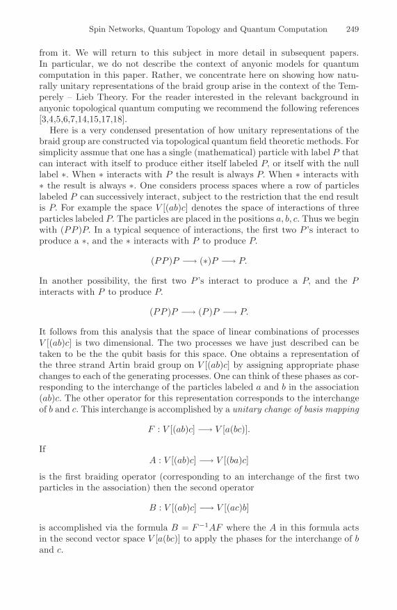
Spin Networks, Quantum Topology and Quantum Computation 249
from it. We will return to this subject in more detail in subsequent papers.In particular, we do not describe the context of anyonic models for quantumcomputation in this paper. Rather, we concentrate here on showing how natu-rally unitary representations of the braid group arise in the context of the Tem-perely – Lieb Theory. For the reader interested in the relevant background inanyonic topological quantum computing we recommend the following references[3,4,5,6,7,14,15,17,18].
Here is a very condensed presentation of how unitary representations of thebraid group are constructed via topological quantum field theoretic methods. Forsimplicity assmue that one has a single (mathematical) particle with label P thatcan interact with itself to produce either itself labeled P, or itself with the nulllabel ∗. When ∗ interacts with P the result is always P. When ∗ interacts with∗ the result is always ∗. One considers process spaces where a row of particleslabeled P can successively interact, subject to the restriction that the end resultis P. For example the space V [(ab)c] denotes the space of interactions of threeparticles labeled P. The particles are placed in the positions a, b, c. Thus we beginwith (PP )P. In a typical sequence of interactions, the first two P ’s interact toproduce a ∗, and the ∗ interacts with P to produce P.
(PP )P −→ (∗)P −→ P.
In another possibility, the first two P ’s interact to produce a P, and the Pinteracts with P to produce P.
(PP )P −→ (P )P −→ P.
It follows from this analysis that the space of linear combinations of processesV [(ab)c] is two dimensional. The two processes we have just described can betaken to be the the qubit basis for this space. One obtains a representation ofthe three strand Artin braid group on V [(ab)c] by assigning appropriate phasechanges to each of the generating processes. One can think of these phases as cor-responding to the interchange of the particles labeled a and b in the association(ab)c. The other operator for this representation corresponds to the interchangeof b and c. This interchange is accomplished by a unitary change of basis mapping
F : V [(ab)c] −→ V [a(bc)].
IfA : V [(ab)c] −→ V [(ba)c]
is the first braiding operator (corresponding to an interchange of the first twoparticles in the association) then the second operator
B : V [(ab)c] −→ V [(ac)b]
is accomplished via the formula B = F−1AF where the A in this formula actsin the second vector space V [a(bc)] to apply the phases for the interchange of band c.

250 L.H. Kauffman and S.J. Lomonaco Jr.
In this scheme, vector spaces corresponding to associated strings of particle in-teractions are interrelated by recoupling transformations that generalize the map-ping F indicated above. A full representation of the Artin braid group on eachspace is defined in terms of the local intechange phase gates and the recouplingtransfomations. These gates and transformations have to satisfy a number of iden-tities in order to produce a well-defined representation of the braid group. Theseidentities were discovered originally in relation to topological quantum field the-ory. In our approach the structure of phase gates and recoupling transformationsarise naturally from the structure of the bracket model for the Jones polynomial[8]. Thus we obtain a knot-theoretic basis for topological quantum computing.
2 Spin Networks and Temperley – Lieb RecouplingTheory
In this section we discuss a combinatorial construction for spin networks thatgeneralizes the original construction of Roger Penrose [16]. The result of this gen-eralization is a structure that satisfies all the properties of a graphical TQFT asdescribed in our paper on braiding and universal quantum gates [12], and spe-cializes to classical angular momentum recoupling theory in the limit of its basicvariable. The construction is based on the properties of the bracket polynomial[9]. A complete description of this theory can be found in the book “Temperley– Lieb Recoupling Theory and Invariants of Three-Manifolds” by Kauffman andLins [11].
The “q-deformed” spin networks that we construct here are based on thebracket polynomial relation. View Figure 1 and Figure 2.
In Figure 1 we indicate how the basic projector (symmetrizer, Jones-Wenzlprojector) is constructed on the basis of the bracket polynomial expansion [9].In this technology, a symmetrizer is a sum of tangles on n strands (for a choseninteger n). The tangles are made by summing over braid lifts of permutations inthe symmetric group on n letters, as indicated in Figure 1. Each elementary braidis then expanded by the bracket polynomial relation, as indicated in Figure 1, sothat the resulting sum consists of flat tangles without any crossings (these canbe viewed as elements in the Temperley – Lieb algebra). The projectors have theproperty that the concatenation of a projector with itself is just that projector,and if you tie two lines on the top or the bottom of a projector together, thenthe evaluation is zero. This general definition of projectors is very useful for thistheory. The two-strand projector is shown in Figure 2. Here the formula for thatprojector is particularly simple. It is the sum of two parallel arcs and two turn-around arcs (with coefficient −1/d, with d = −A2−A−2 is the loop value for thebracket polynomial. Figure 2 also shows the recursion formula for the generalprojector. This recursion formula is due to Jones and Wenzl and the projectorin this form, developed as a sum in the Temperley – Lieb algebra (see Section 5of this paper), is usually known as the Jones–Wenzl projector.
The projectors are combinatorial analogs of irreducible representations of agroup (the original spin nets were based on SU(2) and these deformed nets are

Spin Networks, Quantum Topology and Quantum Computation 251
...
...
n strands
=n
n= (A )-3 t( )σ ~σ(1/{n}!) Σ
σ ε Sn
~=
A A-1
= -A2 -2- A
= +
{n}! = Σσ ε Sn
(A )t( )σ-4
=n
n
= 0
= d
Fig. 1. Basic Projectors
= −1/δ
= −Δ /Δn n+1
n 1 1 n 1 1
n1
=2
δ Δ
1Δ =-1 = 0 Δ 0
Δ n+1 = Δ n - n-1
Fig. 2. Two Strand Projector
based on the quantum group corresponding to SU(2)). As such the reader canthink of them as “particles”. The interactions of these particles are governedby how they can be tied together into three-vertices. See Figure 3. In Figure 3we show how to tie three projectors, of a, b, c strands respectively, together toform a three-vertex. In order to accomplish this interaction, we must share linesbetween them as shown in that Figure so that there are non-negative integersi, j, k so that a = i + j, b = j + k, c = i+ k. This is equivalent to the condition

252 L.H. Kauffman and S.J. Lomonaco Jr.
a b
c
ij
k
a b
c
i + j = aj + k = bi + k = c
Fig. 3. Trivalent Vertex
that a+b+c is even and that the sum of any two of a, b, c is greater than or equalto the third. For example a + b ≥ c. One can think of the vertex as a possibleparticle interaction where [a] and [b] interact to produce [c]. That is, any two ofthe legs of the vertex can be regarded as interacting to produce the third leg.
There is a basic orthogonality of three vertices as shown in Figure 4. Here ifwe tie two three-vertices together so that they form a “bubble” in the middle,then the resulting network with labels a and b on its free ends is a multiple ofan a-line (meaning a line with an a-projector on it) or zero (if a is not equalto b). The multiple is compatible with the results of closing the diagram in theequation of Figure 4 so the the two free ends are identified with one another.On closure, as shown in the Figure, the left hand side of the equation becomes aTheta graph and the right hand side becomes a multiple of a “delta” where Δa
denotes the bracket polynomial evaluation of the a-strand loop with a projectoron it. The Θ(a, b, c) denotes the bracket evaluation of a theta graph made fromthree trivalent vertices and labeled with a, b, c on its edges.
There is a recoupling formula in this theory in the form shown in Figure 5.Here there are “6-j symbols”, recoupling coefficients that can be expressed, asshown in Figure 7, in terms of tetrahedral graph evaluations and theta graphevaluations. The tetrahedral graph is shown in Figure 6. One derives the formu-las for these coefficients directly from the orthogonality relations for the trivalentvertices by closing the left hand side of the recoupling formula and using orthog-onality to evaluate the right hand side. This is illustrated in Figure 7.
Finally, there is the braiding relation, as illustrated in Figure 8.With the braiding relation in place, this q-deformed spin network theory sat-
isfies the pentagon, hexagon and braiding naturality identities needed for a topo-logical quantum field theory. All these identities follow naturally from the basicunderlying topological construction of the bracket polynomial. One can applythe theory to many different situations.
2.1 Evaluations
In this section we discuss the structure of the evaluations for Δn and the thetaand tetrahedral networks. We refer to [11] for the details behind these formulas.

Spin Networks, Quantum Topology and Quantum Computation 253
= Θ( , , )Δ
a
b
a c
a
c d d
aδ
ab
ac d
a=
a
= Θ( , , )a c d
a a= = Δ a
Fig. 4. Orthogonality of Trivalent Vertices
{ }a bc d
i
jΣ=j
aa
bb
cc dd
i j
Fig. 5. Recoupling Formula
b
c d
a=k [ ]Tet
a bc d
ik
i
Fig. 6. Tetrahedron Network
Recall that Δn is the bracket evaluation of the closure of the n-strand projector,as illustrated in Figure 4. For the bracket variable A, one finds that
Δn = (−1)nA2n+2 −A−2n−2
A2 −A−2.

254 L.H. Kauffman and S.J. Lomonaco Jr.
{ }a bc d
i
jΣ=j
aa
bb
c c dd
i jk
Σ=j
Θ( , , )a Θ( , , )c d Δb j j j δj
k
k{ }a bc d
i
j
= Θ( , , )a Θ( , , )c dΔ
b{ }a bc d
ik
k k
k
=Θ( , , )
{ }a bc d
ik
[ ]Teta bc d
ik
Θ( , , )k kdca b
Δj Δ
j
Δ k
Fig. 7. Tetrahedron Formula for Recoupling Coefficients
a bcλ
a ab b
c c
(a+b-c)/2 (a'+b'-c')/2
x' = x(x+2)
a bcλ
=
= (-1) A
Fig. 8. LocalBraidingFormula
One sometimes writes the quantum integer
[n] = (−1)n−1Δn−1 =A2n −A−2n
A2 −A−2.
IfA = eiπ/2r

Spin Networks, Quantum Topology and Quantum Computation 255
where r is a positive integer, then
Δn = (−1)nsin((n+ 1)π/r)
sin(π/r).
Here the corresponding quantum integer is
[n] =sin(nπ/r)sin(π/r)
.
Note that [n + 1] is a positive real number for n = 0, 1, 2, ...r − 2 and that[r − 1] = 0.
The evaluation of the theta net is expressed in terms of quantum integers bythe formula
Θ(a, b, c) = (−1)m+n+p [m+ n+ p+ 1]![n]![m]![p]![m+ n]![n+ p]![p+m]!
wherea = m+ p, b = m+ n, c = n+ p.
Note that(a+ b+ c)/2 = m+ n+ p.
When A = eiπ/2r, the recoupling theory becomes finite with the restrictionthat only three-vertices (labeled with a, b, c) are admissible when a+b+c ≤ 2r−4.All the summations in the formulas for recoupling are restricted to admissibletriples of this form.
2.2 Symmetry and Unitarity
The formula for the recoupling coefficients given in Figure 7 has less symmetrythan is actually inherent in the structure of the situation. By multiplying all thevertices by an appropriate factor, we can reconfigure the formulas in this theoryso that the revised recoupling transformation is orthogonal, in the sense that itstranspose is equal to its inverse. This is a very useful fact. It means that whenthe resulting matrices are real, then the recoupling transformations are unitary.
Figure 9 illustrates this modification of the three-vertex. Let V ert[a, b, c]denote the original 3-vertex of the Temperley – Lieb recoupling theory. LetModV ert[a, b, c] denote the modified vertex. Then we have the formula
ModV ert[a, b, c] =
√√ΔaΔbΔc
√Θ(a, b, c)
V ert[a, b, c].
Lemma. For the bracket evaluation at the root of unity A = eiπ/2r the factor
f(a, b, c) =
√√ΔaΔbΔc
√Θ(a, b, c)

256 L.H. Kauffman and S.J. Lomonaco Jr.
a b
c
a b
c
=Δ Δ Δ
Θ( , , )
a b c
ca b
Fig. 9. Modified Three Vertex
= Θ( , , )Δ
a
b a c
a
ca
b
aa
b c
a
= Δ Δ Δ a b c
a
b c
a
=
a
Θ( , , )a cb
ab cΔ
Δ Δ
a
b c
a
Fig. 10. Modified Bubble Identity
is real, and can be taken to be a positive real number for (a, b, c) admissible (i.e.with a+ b+ c ≤ 2r − 4).
Proof. By the results from the previous subsection,
Θ(a, b, c) = (−1)(a+b+c)/2Θ(a, b, c)
where Θ(a, b, c) is positive real, and
ΔaΔbΔc = (−1)(a+b+c)[a+ 1][b+ 1][c+ 1]
where the quantum integers in this formula can be taken to be positive real. Itfollows from this that
f(a, b, c) =
√√[a+ 1][b+ 1][c+ 1]
Θ(a, b, c),
showing that this factor can be taken to be positive real. This completes theproof.

Spin Networks, Quantum Topology and Quantum Computation 257
In Figure 10 we show how this modification of the vertex affects the non-zeroterm of the orthogonality of trivalent vertices (compare with Figure 4). We referto this as the “modified bubble identity.” The coefficient in the modified bubbleidentity is
√ΔbΔc
Δa= (−1)(b+c−a)/2
√[b+ 1][c+ 1]
[a+ 1]
where (a, b, c) form an admissible triple. In particular b+ c−a is even and hencethis factor can be taken to be real.
We rewrite the recoupling formula in this new basis and emphasize that therecoupling coefficients can be seen (for fixed external labels a, b, c, d) as a matrixtransforming the horizontal “double-Y ” basis to a vertically disposed double-Ybasis. In Figures 11, 12 and 13 we have shown the form of this transforma-tion,using the matrix notation
M [a, b, c, d]ij
Σ=j
aa
bb
c c dd
i
k
Σ= Δj δ
j
k
k
=
d
= [ ]ModTeta bc d
ia bc d i j
=b
c d
ai j
Δ Δ Δ Δ a b c d
a bc d i
a bc d
i
j
a b cΔ
Δ ΔΔ
Δ Δj j
k
k k
Δj
j
da bc d
i
a b cΔ
Δ ΔΔ
Δ Δj j
j
Δj
da b cΔ
Δ ΔΔ
Δ Δj j
Fig. 11. Derivation of Modified Recoupling Coefficients
a bc d i jΣ=
j
aa
bb
cc d
d
ij
Fig. 12. Modified Recoupling Formula

258 L.H. Kauffman and S.J. Lomonaco Jr.
a bc d i j
=b
c d
ai j
Δ Δ Δ Δ a b c d
M[a,b,c,d]i j
=a bc d i j
Fig. 13. Modified Recoupling Matrix
a bc d
=b
c
d
aij
Δ Δ Δ Δ a b c d
b
c d
ai j
Δ Δ Δ Δ a b c d
a bc d
T -1
==Fig. 14. Modified Matrix Transpose
for the modified recoupling coefficients. In Figure 11 we derive an explicit for-mula for these matrix elements. The proof of this formula follows directly fromtrivalent–vertex orthogonality (See Figures 4 and 7.), and is given in Figure 11.The result shown in Figure 11 and Figure 12 is the following formula for therecoupling matrix elements.
M [a, b, c, d]ij = ModTet
(a b ic d j
)
/√ΔaΔbΔcΔd

Spin Networks, Quantum Topology and Quantum Computation 259
where√ΔaΔbΔcΔd is short-hand for the product
√ΔaΔb
Δj
√ΔcΔd
ΔjΔj
= (−1)(a+b−j)/2(−1)(c+d−j)/2(−1)j√
[a+ 1][b+ 1][j + 1]
√[c+ 1][d+ 1]
[j + 1][j + 1]
= (−1)(a+b+c+d)/2√
[a+ 1][b+ 1][c+ 1][d+ 1]
In this form, since (a, b, j) and (c, d, j) are admissible triples, we see that thiscoeffient can be taken to be real, and its value is independent of the choice of iand j. The matrix M [a, b, c, d] is real-valued.
It follows from Figure 12 (turn the diagrams by ninety degrees) that
M [a, b, c, d]−1 = M [b, d, a, c].
In Figure 14 we illustrate the formula
M [a, b, c, d]T = M [b, d, a, c].
It follows from this formula that
M [a, b, c, d]T = M [a, b, c, d]−1.
Hence M [a, b, c, d] is an orthogonal, real-valued matrix.
Theorem. In the Temperley – Lieb theory we obtain unitary (in fact real or-thogonal) recoupling transformations when the bracket variable A has the formA = eiπ/2r. Thus we obtain families of unitary representations of the Artin braidgroup from the recoupling theory at these roots of unity.
Proof. The proof is given the discussion above.
Remark. The density of these representations will be taken up in a subsequentpaper.
3 Quantum Computation of Colored Jones Polynomialsand the Witten-Reshetikhin-Turaev Invariant
In this section we make some brief comments on the quantum computationof colored Jones polynomials. This material will be expanded in a subsequentpublication.
First, consider Figure 15. In that figure we illustrate the calculation of theevalutation of the (a) - colored bracket polynomial for the plat closure P (B) of abraid B. The reader can infer the definition of the plat closure from Figure 15.One takes a braid on an even number of strands and closes the top strands with

260 L.H. Kauffman and S.J. Lomonaco Jr.
= 0a
b
if b = 0
Σ=
0 00
=x
y,
xy 0
B(x,y)
0 00
=
a a
a a a a
a a
a a
Σ=x
y,
xy 0
B(x,y)
a a
=0
a a
B(0,0) 0 0
= B(0,0) Δ a( ) 2
BP(B)
Fig. 15. Evaluation of the Plat Closure of a Braid
each other in a row of maxima. Similarly, the bottom strands are closed with arow of minima. It is not hard to see that any knot or link can be represented asthe plat closure of some braid. Note that in this figure we indicate the action ofthe braid group on the process spaces corresponding to the small trees attachedbelow the braids.
The (a) - colored bracket polynonmial of a link L, denoted < L >a, is theevaluation of that link where each single strand has been replaced by a parallelstrands and the insertion of Jones-Wenzl projector. We then see that we can useour discussion of the Temperley-Lieb recoupling theory to compute the value ofthe colored bracket polynomial for the plat closure PB. As shown in Figure 15,we regard the braid as acting on a process space V a,a,···,a0 and take the case ofthe action on the vector v whose process space coordinates are all zero. Thenthe action of the braid takes the form
Bv(0, · · · , 0) = Σx1,···,xnB(x1, · · · , xn)v(x1, · · · , xn)
where B(x1, · · · , xn) denotes the matrix entries for this recoupling transforma-tion and v(x1, · · · , xn) runs over a basis for the space V a,a,···,a0 . Here n is evenand equal to the number of braid strands. In the figure we illustrate with n = 4.Then, as the figure shows, when we close the top of the braid action to formPB, we cut the sum down to the evaluation of just one term. In the general casewe will get
< PB >a= B(0, · · · , 0)Δn/2a .
The calculation simplifies to this degree because of the vanishing of loops in therecoupling graphs.
The colored Jones polynomials are normalized versions of the colored bracketpolymomials, differing just by a normalization factor.

Spin Networks, Quantum Topology and Quantum Computation 261
In order to consider quantumn computation of the colored bracket or coloredJones polynomials, we therefore can consider quantum computation of the matrixentries B(0, · · · , 0). These matrix entries in the case of the roots of unity A =eiπ/2r and for the a = 2 Fibonacci model with A = e3iπ/5 are parts of thediagonal entries of the unitary transformation that represents the braid groupon the process space V a,a,···,a0 . We can obtain these matrix entries by using theHadamard test. As a result we get relatively efficient quantum algorithms forthe colored Jones polynonmials at these roots of unity, in essentially the sameframework as we described in section 4, but for braids of arbitrary size. Thecomputational complexity of these models is essentially the same as the modelsfor the Jones polynomial discussed in [1].
Remark on the Hadamard Test. In order to (quantum) compute the trace ofa unitary matrix U , one can use the Hadamard test to obtain the diagonal matrixelements 〈ψ|U |ψ〉 of U. The trace is then the sum of these matrix elements as|ψ〉 runs over an orthonormal basis for the vector space. We first obtain
12
+12Re〈ψ|U |ψ〉
as an expectation by applying the Hadamard gate H
H |0〉 = 1√2(|0〉+ |1〉)
H |1〉 = 1√2(|0〉 − |1〉)
to the first qubit of
CU ◦ (H ⊗ 1)|0〉|ψ〉 = 1√2(|0〉 ⊗ |ψ〉+ |1〉 ⊗ U |ψ〉.
Here CU denotes controlled U, acting as U when the control bit is |1〉 and theidentity mapping when the control bit is |0〉. We measure the expectation forthe first qubit |0〉 of the resulting state
12(H |0〉 ⊗ |ψ〉+H |1〉 ⊗ U |ψ〉) =
12((|0〉+ |1〉)⊗ |ψ〉+ (|0〉 − |1〉)⊗ U |ψ〉)
=12(|0〉 ⊗ (|ψ〉 + U |ψ〉) + |1〉 ⊗ (|ψ〉 − U |ψ〉)).
This expectation is
12(〈ψ|+ 〈ψ|U †)(|ψ〉+ U |ψ〉) =
12
+12Re〈ψ|U |ψ〉.
The imaginary part is obtained by applying the same procedure to
1√2(|0〉 ⊗ |ψ〉 − i|1〉 ⊗ U |ψ〉

262 L.H. Kauffman and S.J. Lomonaco Jr.
This is the method used in [1], and the reader may wish to contemplate itsefficiency in the context of this model. Note that the Hadamard test enables thisquantum computation to estimate the trace of any unitary matrix U by repeatedtrials that estimate individual matrix entries 〈ψ|U |ψ〉. In the case of the quantumcomputation of a colored Jones polynomial evaluation for the plat closure of alink, we need only obtain a single entry of the unitary matrix that representsthe corresponding braiding transformation. Thus, if one is given the quantumcomputer hardware for the braiding, already provided, the actual computationis quite efficient.
Remark on the WRT invariant. It is worth remarking here that these al-gorithms give not only quantum algorithms for computing the colored bracketand Jones polynomials, but also for computing the Witten-Reshetikhin-Turaev(WRT) invariants at the above roots of unity. The reason for this is that theWRT invariant, in unnormalized form is given as a finite sum of colored bracketpolynomials:
WRT (L) = Σr−2a=0Δa < L >a,
and so the same computation as shown in Figure 60 applies to the WRT. Thismeans that we have, in principle, a quantum algorithm for the computation of theWitten functional integral [19] via this knot-theoretic combinatorial topology.It would be very interesting to understand a more direct approach to such acomputation via quantum field theory and functional integration.
Finally, we note that in the case of the Fibonacci model, the (2)-coloredbracket polynomial is a special case of the Dubrovnik version of the Kauffmanpolynomial [10]. See Figure 16 for diagammatics that resolve this fact. The skein
δA4 -4= A + +
δA 4-4= A+ +
- = 4A A-4-( ) -( )
- = 4A A-4-( ) -( )
= A8
Fig. 16. Dubrovnik Polynomial Specialization at Two Strands

Spin Networks, Quantum Topology and Quantum Computation 263
relation for the Dubrovnik polynomial is boxed in this figure. Above the box,we show how the double strands with projectors reproduce this relation. Thisobservation means that in the Fibonacci model, the natural underlying knotpolynomial is a special evaluation of the Dubrovnik polynomial, and the Fi-bonacci model can be used to perform quantum computation for the values ofthis invariant.
References
1. Aharonov, D., Jones, V., Landau, Z.: A polynomial quantum algorithm for approx-imating the Jones polynomial, quant-ph/0511096.
2. Aharonov, D., Arad, I.: The BQP-hardness of approximating the Jones polynomial,quant-ph/0605181.
3. Freedman, M.: A magnetic model with a possible Chern-Simons phase, quant-ph/0110060v1 9 October 2001 (preprint)
4. Freedman, M.: Topological Views on Computational Complexity. DocumentaMathematica - Extra Volume ICM, 453–464 (1998)
5. Freedman, M., Larsen, M., Wang, Z.: A modular functor which is universal forquantum computation, quant-ph/0001108v2 (February 1 2000)
6. Freedman, M.H., Kitaev, A., Wang, Z.: Simulation of topological field theo-ries by quantum computers. Commun. Math. Phys. 227, 587–603 (2002) quant-ph/0001071.
7. Freedman, M.: Quantum computation and the localization of modular functors,quant-ph/0003128.
8. Jones, V.F.R.: A polynomial invariant for links via von Neumann algebras, Bull.Amer. Math. Soc. 129, 103–112 (1985)
9. Kauffman, L.H.: State models and the Jones polynomial. Topology 26, 395–407(1987)
10. Kauffman, L.H.: An invariant of regular isotopy. Trans. Amer. Math. Soc. 318(2),417–471 (1990)
11. Kauffman, L.H.: Temperley – Lieb Recoupling Theory and Invariants of Three-Manifolds, Princeton University Press, Annals Studies, 114 (1994)
12. Kauffman, L.H., Lomonaco Jr., S.J.: Braiding Operators are Universal QuantumGates. New Journal of Physics 6(134), 1–39 (2004)
13. Kauffman, L.H., Lomonaoco Jr., S.J.: q - deformed spin networks, knot polynomialsand anyonic topological computation, quant-ph/0606114 ( to appear in JKTR)
14. Kitaev, A.: Anyons in an exactly solved model and beyond, arXiv.cond-mat/0506438 v1 (17 June 2005)
15. Marzuoli, A., Rasetti, M.: Spin network quantum simulator. Physics Letters A 306,79–87 (2002)
16. Penrose, R.: Angular momentum: An approach to Combinatorial Spacetime. In:Bastin, T. (ed.) Quantum Theory and Beyond, Cambridge University Press, Bastin(1969)
17. Preskill, J.: Topological computing for beginners, (slide presentation), LectureNotes for Chapter 9 - Physics 219 - Quantum Computation.http://www.iqi.caltech.edu/preskill/ph219
18. Wilczek, F.: Fractional Statistics and Anyon Superconductivity. World ScientificPublishing Company, Singapore (1990)
19. Witten, E.: Quantum field Theory and the Jones Polynomial. Commun. Math.Phys. 1989, 351–399 (1989)
Symmetries in Natural Language Syntax and
Semantics: The Lambek-Grishin Calculus
Michael Moortgat�
Utrecht Institute of Linguistics OTS, The [email protected]
Abstract. In this paper, we explore the Lambek-Grishin calculus LG:a symmetric version of categorial grammar based on the generalizationsof Lambek calculus studied in Grishin [1]. The vocabulary of LG com-plements the Lambek product and its left and right residuals with a dualfamily of type-forming operations: coproduct, left and right difference.The two families interact by means of structure-preserving distributivityprinciples. We present an axiomatization of LG in the style of Curry’scombinatory logic and establish its decidability. We discuss Kripke mod-els and Curry-Howard interpretation for LG and characterize its notionof type similarity in comparison with the other categorial systems. Fromthe linguistic point of view, we show that LG naturally accommodatesnon-local semantic construal and displacement — phenomena that areproblematic for the original Lambek calculi.
1 Background
The basic Lambek calculus [2] is a logic without any structural rules: grammat-ical material cannot be duplicated or erased without affecting well-formedness(absence of Contraction and Weakening); moreover, structural rules affectingword order and constituent structure (Commutativity and Associativity) areunavailable. What remains (in addition to the preorder axioms for derivability)is the pure logic of residuation of (1).
residuated triple A→ C/B iff A⊗B → C iff B → A\C (1)
The type-forming operations have two kinds of semantics. One is a structuralsemantics, where they are interpreted with respect to a ternary composition re-lation (or ‘Merge’, as it is called in generative grammar). The truth conditions for� Linguistic exploration of Lambek-Grishin calculus started at ESSLLI’04 (Nancy) in
discussion with Raffaella Bernardi and Rajeev Gore; I thank them, and NatashaKurtonina, for the stimulating exchange of ideas throughout the period reported onhere. The material of this paper was the subject of a series of lectures at MoscowState University (Sept 2006, April 2007). I thank Mati Pentus and Barbara Parteefor accommodating these talks in their seminars and for providing such perceptiveaudiences. The support of the Dutch-Russian cooperation program NWO/RFBR,project No. 047.017.014 “Logical models of human and mechanical reasoning” isgratefully acknowledged.
D. Leivant and R. de Queiroz (Eds.): WoLLIC 2007, LNCS 4576, pp. 264–284, 2007.c© Springer-Verlag Berlin Heidelberg 2007
Symmetries in Natural Language Syntax and Semantics 265
this interpretation are given in (2); one finds the basic soundness/completenessresults in [3]. The second interpretation is a computational one, along the linesof the Curry-Howard formulas-as-types program. Under this second interpreta-tion, Lambek derivations are associated with a linear (and structure-sensitive)sublanguage of the lambda terms one obtains for proofs in positive Intuitionis-tic logic. The slashes /, \ here are seen as directional implications; eliminationof these operations corresponds to function application, introduction to lambdaabstraction.
x � A⊗B iff ∃yz.R⊗xyz and y � A and z � By � C/B iff ∀xz.(R⊗xyz and z � B) implies x � Cz � A\C iff ∀xy.(R⊗xyz and y � A) implies x � C
(2)
The original Lambek calculus, like its predecessors the Ajdukiewicz/Bar Hil-lel (AB) calculi, and later systems such as Combinatory Categorial Grammar(CCG), adequately deals with linguistic subcategorization or valency. It greatlyimproves on AB and CCG systems in fully supporting hypothetical reasoning:the bidirectional implications of the residuation laws are fully symmetric withrespect to putting together larger phrases out of their subphrases, and takingapart compound phrases in their constituent parts. AB systems lack the secondfeature completely; the combinatory schemata of CCG provide only a weak ap-proximation. Consequences of hypothetical reasoning are the theorems of typelifting and argument lowering of (3) below; type transitions of this kind haveplayed an important role in our understanding of natural language semantics.
A→ B/(A\B) (B/(A\B))\B → A\B (3)
It is ironic that precisely in the hypothetical reasoning component the Lambekgrammars turn out to be deficient. As one sees in (3), hypothetical reasoningtypically involves higher order types, where a slash occurs in a negative en-vironment as in the schema (4) below. Given Curry-Howard assumptions, theassociated instruction for meaning assembly has an application, correspondingto the elimination of the main connective /, and an abstraction, correspondingto the introduction of the embedded \.
C/(A\B) (M λxA.NB)C (4)
The minimal Lambek calculus falls short in its characterization of which A-typehypotheses are ‘visible’ for the slash introduction rule: for the residuation rulesto be applicable, the hypothesis has to be structurally peripheral (left peripheralfor \, right peripheral for /). One can distinguish two kinds of problems.
Displacement. The A-type hypothesis occurs internally within the domain oftype B. Metaphorically, the functor C/(A\B) seems to be displaced fromthe site of the hypothesis. Example: wh ‘movement’.
Non-local semantic construal. The functor (e.g. C/(A\B)) occupies thestructural position where in fact the A-type hypothesis is needed, and re-alizes its semantic effect at a higher structural level. (The converse of theabove.) Example: quantifying expressions.

266 M. Moortgat
The initial reaction to these problems has been to extend the basic systemwith structural rules of Associativity and/or Commutativity, resulting in thehierarchy of Fig 1. From a linguistic point of view, a global implementation ofthese structural options is undesirable, as it entails a complete loss of sensitivityfor word order and/or constituent structure.
LP
NLP
�����������L
�����������
NL
�����������
�����������
Fig. 1. The Lambek hierarchy
A significant enhancement of the Lambek systems occurred in the mid Ninetiesof the last century, when the vocabulary was extended with a pair of unarytype-forming operations (Moortgat [4]). Like their binary relatives, ♦,� form aresiduated pair, satisfying (5), and with interpretation (6).
residuated pair ♦A→ B iff A→ �B (5)
x � ♦A iff ∃y (R♦xy and y � A)y � �A iff ∀x (R♦xy implies x � A) (6)
From a purely logic point of view, the unary modalities introduce facilities forsubtyping, in the sense that any type A is now derivationally related to a morespecific type ♦�A and a more general type �♦A.
♦�A→ A→ �♦A (7)
Bernardi [5] makes good use of the patterns in (7) to fine-tune the construal ofscope-bearing expressions, and to capture the selectional restrictions governingthe distribution of polarity sensitive items. In addition to this logical use of ♦,�,one can also use them to provide controlled versions of structural rules that, in aglobal form, would be deleterious. The set of postulates in (8) make left branches(P1, P2) or right branches (P3, P4) accessible for hypothetical reasoning.
(P1) ♦A⊗ (B ⊗ C)→ (♦A⊗B)⊗ C (C ⊗ B)⊗ ♦A→ C ⊗ (B ⊗ ♦A) (P3)(P2) ♦A⊗ (B ⊗ C)→ B ⊗ (♦A ⊗ C) (C ⊗ B)⊗ ♦A→ (C ⊗ ♦A) ⊗B (P4)
(8)Vermaat [6] uses these postulates in a cross-linguistic study of wh extractionconstructions, relating the choice between P1, P2 and P3, P4 to the typologicaldistinction between head-initial versus head-final languages.

Symmetries in Natural Language Syntax and Semantics 267
Structural control. The general situation with respect to the expressivity ofmodally controlled structural rules is captured by Thm 1. We consider a sourcelogic L and a target logic, which is either an upward (L↑) or a downward (L↓)neighbor in the Lambek hierarchy. The target logic has control modalities ♦,�which are lacking in the source logic. In terms of these modalities, one definestranslations from the formulas of the source logic to the formulas of the tar-get logic. The ·↓ translations impose the structure-sensitivity of the source logicin a logic with a more liberal structural regime; the ·↑ translations recover theflexibility of an upward neighbor by addingR♦ — the image under ·↑ of the struc-tural rules that discriminate source from target. An example is the translation(A ⊗ B)↓ = ♦(A↓ ⊗ B↓), which blocks associativity by removing the structuralconditions for its application.
Theorem 1. Structural control (Kurtonina and Moortgat [7]). For logics L, L↑,L↓ and translations ·↓ and ·↑ as defined above,
L � A→ B iff L↑♦ � A↓ → B↓ constraining
L � A→ B iff L↓♦ +R♦ � A↑ → B↑ licensing
Summarizing. Viewed from a foundational point of view, one can see Lambek-style categorial grammars as modal logics of natural language resources. In suchlogics, the vocabulary for analyzing the assembly of form and meaning consistsof n-ary type-forming operations (or connectives, under Curry’s formulas-as-types view); these operations are given a Kripke-style interpretation in termsof (n+1)-ary ‘merge’/composition relations. Grammatical invariants, in this ap-proach, are laws that do not impose restrictions on the interpreting compositionrelations; language diversity results from the combination of the invariant baselogic with a set of non-logical axioms (and the corresponding frame constraints).These axioms (possibly language-specific) characterize the structural deforma-tions under which the basic form-meaning correspondences are preserved. Thereader is referred to [8] for an overview of this line of work.
2 Lambek-Grishin Calculus
Assessing the merits of the above approach, one can identify two problematicaspects. One is of a computational nature, the other relates to the cognitiveimplications of the Lambek framework.
Complexity. Structural rules (whether implemented globally or under modalcontrol) are computationally expensive. Whereas the basic Lambek calcu-lus has a polynomial recognition problem [9], already the simplest extensionwith an associative regime is known to be NP complete [10]; one reachesa PSPACE upper bound for the extension with a ♦,� controlled struc-tural module consisting of resource-respecting (i.e. linear, non-expanding)axioms [11].

268 M. Moortgat
Invariants versus structural postulates. On the cognitive level, the limitedexpressivity of the standard vocabulary means one is forced to accept thata considerable part of grammatical organization is beyond the reach of thetype-forming constants. By considering a broader vocabulary of connectivesit becomes possible to characterize larger portions of a language’s grammarin terms of linguistic invariants, rather than through non-logical postulates.
In a remarkable paper written in 1983, V.N. Grishin [1] has proposed a frame-work for generalizing the Lambek calculi that provides an alternative to thestructural rule approach. The starting point for Grishin’s generalization is asymmetric extension of the vocabulary of type-forming operations: in additionto the familiar ⊗, \, / (product, left and right division), one also considers a dualfamily ⊕,�,�: coproduct, right and left difference.1
A,B ::= p | atoms: s sentence, np noun phrases, . . .A⊗B | B\A | A/B | product, left vs right divisionA⊕B | A�B | B �A coproduct, right vs left difference
(9)We saw that algebraically, the Lambek operators form a residuated triple; like-wise, the ⊕ family forms a dual residuated triple.
residuated triple A→ C/B iff A⊗B → C iff B → A\Cdual residuated triple C �B → A iff C → A⊕B iff A� C → B
(10)Dunn’s [12] framework of gaggle theory brings out the underlying algebraic struc-ture in a particularly clear way. In Fig 2, we consider ordered sets (X,≤), (Y,≤′)with mappings f : X −→ Y , g : Y −→ X . In the categorial setting, we haveX = Y = F (the set of types/formulas). The pair of operations (f, g) is calledresiduated if it satisfies the defining biconditionals of the upper left cell; the lowerright cell characterizes dual residuated pairs. Whereas the concept of residuationpairs the (co)product with a (co)implication, the closely related concept of (dual)Galois connected pairs links the (co)implications among themselves. The definingbiconditionals fill the lower left and upper right cells. For ∗ ∈ {/,⊗, \,�,⊕,�},we write −∗ (∗−) for the operation that suffixes (prefixes) a fixed type to itsoperand, for example: A→ C/B iff B → A\C instantiates the pattern (/−,−\).
iff x ≤ gy gy ≤ x
fx ≤′ y(−⊗,−/)(⊗−, \−)
(−�,�−)(�−,−�)
y ≤′ fx(−\, /−)(/−,−\)
(−⊕,−�)(⊕−,�−)
Fig. 2. Residuated and Galois connected pairs and their duals
1 A little pronunciation dictionary: read B\A as ‘B under A’, A/B as ‘A over B’,B � A as ‘B from A’ and A � B as ‘A less B’.

Symmetries in Natural Language Syntax and Semantics 269
The patterns of Fig 2 reveal that on the level of types and derivability theLambek-Grishin system exhibits two kinds of mirror symmetry characterizedby the bidirectional translation tables in (11): �� is order-preserving, ∞ order-reversing: A�� → B�� iff A→ B iff B∞ → A∞.
��C/D A⊗B B ⊕A D � C
D\C B ⊗A A⊕B C �D ∞ C/B A⊗B A\CB � C B ⊕A C �A (11)
Interaction principles. The minimal symmetric categorial grammar (which wewill refer to as LG∅) is given by the preorder axioms for the derivability relation,together with the residuation and dual residuation principles of (10). LG∅ byitself does not offer us the kind of expressivity needed to address the problemsdiscussed in §1. The real attraction of Grishin’s work derives from the interactionprinciples he proposes for structure-preserving communication between the ⊗and the ⊕ families. In all, the type system allows eight such principles, configuredin two groups of four. Consider first the group in (12) which we will collectivelyrefer to as G↑.2(G1) (A�B)⊗ C → A� (B ⊗ C) C ⊗ (B �A)→ (C ⊗B)�A (G3)(G2) C ⊗ (A�B)→ A� (C ⊗B) (B �A)⊗ C → (B ⊗ C)�A (G4)
(12)On the lefthand side of the derivability arrow, one finds a ⊗ formula which hasa formula with the difference operation (A � B or B � A) in its first or secondcoordinate. The Grishin principles rewrite this configuration in such a way thatthe difference operations �, � become the main connective. Combined withtransitivity, the principles take the form of the inference rules in (13).
A� (B ⊗ C)→ D
(A�B)⊗ C → DG1
(A⊗B)� C → D
A⊗ (B � C)→ DG3
B � (A⊗ C)→ D
A⊗ (B � C)→ DG2
(A⊗ C)�B → D
(A�B)⊗ C → DG4
(13)
These rules, from a backward-chaining perspective, have the effect of bringingthe A subformula to a position where it can be shifted to the righthand side of→ by means of the dual residuation principles. The images of (12) under ·∞ aregiven in (14): in rule form, they rewrite a configuration where a left or right slashis trapped within a ⊕ context into a configuration where the A subformula canbe shifted to the lefthand side of → by means of the residuation principles. Oneeasily checks that the forms in (14) are derivable from (12) — the derivation ofG1′ from G1 is given as an example in (19).
(G1′) (C ⊕B)/A→ C ⊕ (B/A)(G2′) (B ⊕ C)/A→ (B/A) ⊕ C
A\(B ⊕ C)→ (A\B)⊕ C (G3′)A\(C ⊕B)→ C ⊕ (A\B) (G4′) (14)
2 In Grishin’s original paper, only one representative of each group is discussed; com-putation of the remaining three is left to the reader. Earlier presentations of [1] suchas [13,14] omit G2 and G4. The full set of (12) is essential for the intended linguisticapplications.

270 M. Moortgat
An alternative direction for generalizing the Lambek calculus is given by theconverses of the G↑ principles obtained by turning around the derivability ar-row. We refer to these individually as Gn−1, and to the group as G↓. The generalpicture that emerges is a landscape where the minimal symmetric Lambek cal-culus LG∅ can be extended either with G1–G4 or with their converses, or withthe combination of the two. We discuss potential linguistic applications for G↑and G↓ in §3. First, we review some prooftheoretic and modeltheoretic resultsrelating the Lambek-Grishin calculus to the original Lambek systems. These re-sults have focused on the combination LG∅+G↑, which in the remainder we willrefer to simply as LG.
2.1 Decidable Proof Search
The axiomatization we have considered so far contains the rule of transitivity(from A→ B andB → C conclude A→ C) which, in the presence of complexity-increasing type transitions, is an unpleasant rule from a proof search perspective.For decidable proof search, we are interested in an axiomatization which hastransitivity as an admissible rule. Such an axiomatization for LG can be given interms of the identity axiom 1A : A→ A together with the residuation principles(10), the Grishin axioms in rule form (16), and the monotonicity rules of (17).3
We give these rules with combinator proof terms, so that in the remainder wecan succinctly refer to derivations by their combinator. First the residuationrules of (15).
f : A⊗B → C
�f : B → A\Cf : C → A⊕B
�f : A� C → B
f : A⊗B → C
�f : A→ C/B
f : C → A⊕B�f : C �B → A
(15)
These rules are invertible; we write �′,�′,�′,�′ for the reverse direction. Nextthe Grishin axioms in rule form, for use in the lhs of derivability statements.
f : A� (B ⊗ C)→ D
�f : (A�B)⊗ C → D
f : (A⊗B)� C → D
�f : A⊗ (B � C)→ D
f : B � (A⊗ C)→ D
��f : A⊗ (B � C)→ D
f : (A⊗ C)�B → D
��f : (A�B)⊗ C → D
(16)
Finally, (17) gives the monotonicity rules. As is well-known, the monotonicityrules are derivable rules of inference in an axiomatization with residuation andtransitivity (cut). The purpose of the present axiomatization is to show that the
3 The axiomatization presented here is a close relative of Display Logic, see [14] fora comprehensive view on the substructural landscape. In Display Logic, the Gr-ishin rules and residuation principles are expressed at the structural level; structuralconnectives are introduced by explicit rewriting steps. Our combinator presentationis entirely formula-based, i.e. the distinction between a ‘logical’ and a ‘structural’occurrence of a type-forming operation is implicit.

Symmetries in Natural Language Syntax and Semantics 271
combination monotonicity plus residuation effectively absorbs cut. Admissibilityof cut is established in Appendix A, extending the earlier result of [15] to thecase of symmetric LG.
f : A→ B g : C → D
f ⊗ g : A⊗ C → B ⊗Df : A→ B g : C → D
f ⊕ g : A⊕ C → B ⊕Df : A→ B g : C → D
f/g : A/D → B/C
f : A→ B g : C → D
f � g : A�D → B � Cf : A→ B g : C → D
g\f : D\A→ C\Bf : A→ B g : C → D
g � f : D �A→ C �B
(17)
The symmetries we have studied before on the level of types and theorems nowmanifest themselves on the level of proofs.
∞ h/g f ⊗ g f\hg � h g ⊕ f h� f ∞ �f �f �′f �′f
�f �f �′f �′f(18)
As an example, consider (19). On the left, we derive G1′ = G1∞ from G1;on the right we derive G1 from G1′. Notice that these derivations provide themotivation for our choice to posit ∞ as the basic order-reversing duality, ratherthan � which we define as ��∞.
(c ⊕ b)/a → (c ⊕ b)/a((c ⊕ b)/a)⊗ a → c ⊕ b �′
c � (((c ⊕ b)/a)⊗ a)→ b�
(c � ((c ⊕ b)/a))⊗ a → b�
c � ((c ⊕ b)/a)→ b/a�
(c ⊕ b)/a → c ⊕ (b/a) �′
a� (b⊗ c)→ a� (b⊗ c)b ⊗ c→ a⊕ ((a� (b⊗ c)) �′
b→ (a⊕ ((a� (b⊗ c)))/c �b→ a⊕ ((a� (b ⊗ c))/c) �∞
a� b→ (a� (b ⊗ c))/c �(a� b)⊗ c→ a� (b⊗ c) �′
(�′ � � � �′ 1(c⊕b)/a)∞ = �′ � �∞ � �′ 1a�(b⊗c)
(19)
We close this section with an open question on complexity. The minimal sym-metric system LG∅ is proved to preserve the polynomiality of the asymmetricNL in [16]. Capelletti [17] provides a constructive polynomial algorithm for acombinator-style axiomatization of LG∅ that allows agenda-driven chart-basedparsing. Whether the methods developed in [17] can be extended to include theGrishin interaction principles remains to be investigated.
2.2 The Group of Grishin Interactions
The �� and ∞ dualities deserve closer scrutiny: as a matter of fact, they hidesome interesting grouptheoretic structure.4 First of all, from �� and the identity
4 This section reports on work in progress with Lutz Strassburger (Ecole Polytech-nique, Paris) and with Anna Chernilovskaya (Moscow State University).

272 M. Moortgat
transformation 1 we obtain two further order-preserving symmetries � and �: onthe ⊗ family � acts like ��, on the ⊕ family it is the identity; � acts like �� onthe ⊕ family, and as the identity on the ⊗ family.
� �Frm(/,⊗, \) �� 1Frm(�,⊕,�) 1 ��
(20)
One easily checks that the Grishin postulates (12) are related horizontally by ��,vertically by � and diagonally by �. Together with the identity transformation,��, � and � constitute D2 — the dihedral group of order 4 (also known as theKlein group). This is the smallest non-cyclic abelian group. Its Cayley table isgiven in (21) below.
◦ 1 �� � �1 1 �� � ��� �� 1 � �� � � 1 ��� � � �� 1
(21)
Similarly, from∞ we obtain three further order-reversing symmetries: � =��∞,and the mixed forms † and ‡ in (22) below.
† ‡Frm(/,⊗, \) � ∞Frm(�,⊕,�) ∞ �
(22)
Together with the order-preserving transformations {1, ��, �, �}, the set {∞, �, †, ‡}constitutes a group of order 8. We can now consider a cube of Grishin interactions.
G1′ G3′
∞G2′���
G4′���
G1 G3
G2 ��
����G4
�
����
(23)
The lower plane is the square (12) which we saw is characterized by D2. Thetransformation ∞ reflects (12) to the upper plane (14). The remaining trans-formations connect vertices of the lower plane to those of the upper plane viathe diagonals. It will not come as a surprise that we have D4, which contains2×D2 as subgroups: {1, ��, �, �} and {1,∞, �, ��}. Notice that D4, unlike its D2
subgroups, is not abelian. Consider for example †∞ = � �= � =∞†. The compo-sition †∞ relates G1 to G4 via G1′; the composition ∞† brings us from G1 toG2 via G2′.
2.3 Type Similarity
The notion of type similarity is a powerful tool to study the expressivity ofcategorial logics with respect to derivational relationships. The similarity

Symmetries in Natural Language Syntax and Semantics 273
relation ∼ is introduced in the algebraic remarks at the end of [18] as the re-flexive, transitive, symmetric closure of the derivability relation: A ∼ B iff thereexists a sequence C1 . . . Cn (1 ≤ n) such that C1 = A, Cn = B and Ci → Ci+1
or Ci+1 → Ci (1 ≤ i<n). Lambek proves that A ∼ B if and only if one of thefollowing equivalent statements hold (the so-called diamond property): (i) ∃Csuch that A → C and B → C; (ii) ∃D such that D → A and D → B. In otherwords, given a join type C for A and B, one can compute a meet type D, andvice versa. The solutions for D and C in [18] are given in (24). It is shown in[19] that these solutions are in fact adequate for the pure logic of residuation,i.e. the non-associative calculus NL.
NL : D = (A/((C/C)\C)) ⊗ ((C/C)\B), C=(A⊗ (D\D))/(B\(D ⊗ (D\D)))(24)
For associative L, [20] has the shorter solution in (25). The possibility of re-bracketing the types for D and C is what makes this solution work. In LG alsoa length 5 solution is available, this time dependent on the Grishin interactionprinciples, see (26).
L : D = (A/C)⊗ (C ⊗ (C\B)), C = (D/A)\(D/(B\D)) (25)
LG : D = (A/C)⊗ (C � (B � C)), C = (A�D)⊕ (D/(B\D)) (26)
Table 1. Models for type equivalence
calculus interpretation
NL free quasigroup (Foret [19])L free group (Pentus [20])
LP free Abelian group (Pentus [20])LG free Abelian group (Moortgat and Pentus [21])
The similarity relation for various calculi in the categorial hierarchy has beencharacterized in terms of an algebraic interpretation of the types �·�, in thesense that A ∼ B iff �A� =S �B� in the relevant algebraic structures S. Table1 gives an overview of the results. For the pure residuation logic NL, S is thefree quasigroup generated by the atomic types, with �·� defined in the obviousway: �p� = p, �A/B� = �A�/�B�, �B\A� = �B�\�A�, �A ⊗ B� = �A� · �B�.5 Inassociative L, type similarity coincides with equality in the free group generatedby the atomic types (free Abelian group for associative/commutative LP). Thegroup interpretation is (27).
�p� = p, �A⊗B� = �A� · �B�, �A/B� = �A� · �B�−1, �B\A� = �B�−1 · �A� (27)
We see in Table 1 that for the systems in the Lambek hierarchy, expressivityfor ∼ is inversely proportional to structural discrimination: the structural rules5 Recall that a quasigroups is a set equipped with operations /, ·, \ satisfying the
equations (x/y) · y = x, y · (y\x) = x, (x · y)/y = x, y\(y · x) = x.

274 M. Moortgat
of associativity and commutativity destroy sensitivity for constituent structureand word order. The result below shows that LG achieves the same level ofexpressivity with respect to ∼ as the associative/commutative calculus LP anddoes so without inducing loss of structural discrimination.
Theorem 2. (Moortgat and Pentus [21]) In LG A ∼ B iff �A� = �B� in thefree Abelian group generated by Atm ∪ {�}.The group interpretation proposed in [21] for LG is a variant of that in (27); forLG one adds an extra element � to keep track of the operator count, defined asin (28). It is well known that Abelian group equality can be expressed in terms ofa balancing count of (input/output) occurrences of literals. The operator count,together with the count of literals, is sufficient to characterize LG type similarity.It is in fact enough to keep track of only one of the operator counts since theequalities |A|⊗ = |B|⊗ and |A|⊕ = |B|⊕ are equivalent provided that |A|p = |B|pfor all p. The equality
∑p |A|p−|A|⊗−|A|⊕ = 1 has an easy proof by induction
on the structure of A.
|p|⊗ = |p|⊕ = 0
|A⊗B|⊗ = |A|⊗ + |B|⊗ + 1|A⊕B|⊗ = |A|⊗ + |B|⊗|A/B|⊗ = |A|⊗ − |B|⊗ − 1|B \A|⊗ = |A|⊗ − |B|⊗ − 1|A�B|⊗ = |A|⊗ − |B|⊗|B �A|⊗ = |A|⊗ − |B|⊗
|A⊗B|⊕ = |A|⊕ + |B|⊕|A⊕B|⊕ = |A|⊕ + |B|⊕ + 1|A/B|⊕ = |A|⊕ − |B|⊕|B \A|⊕ = |A|⊕ − |B|⊕|A�B|⊕ = |A|⊕ − |B|⊕ − 1|B �A|⊕ = |A|⊕ − |B|⊕ − 1
(28)
Some examples: operator balance fails for a/b vs a� b (these formulas have bal-ancing literal counts), and holds for pairs of formulas such as (b� c)�a, c/(a\b)and a/b, (a� c)/(b� c) — pairs which are indeed in the ∼ relation.
We will discuss a possible use of ∼ in linguistic analysis in §3. Below wereproduce a step in the proof of Thm 2 which highlights the fact that LG hasthe kind of expressivity we expect for LP.
Claim. For arbitrary LG types A, B we have B\A ∼ A/B. To prove this claim,we provide a meet type, i.e. a type X such that X → B\A and X → A/B,which by residuation means
B ⊗X → A and X ⊗ B → A
Let us put X := Y � Z and solve for
B ⊗ (Y � Z)→ A and (Y � Z)⊗ B → A
which by Grishin mixed associativity or commutativity follows from
B ⊗ Y → A⊕ Z and Y ⊗B → A⊕ ZWe have a solution with Z := (A � B) and Y the meet for C the join of B\Band B/B, i.e.
C := ((b\((b⊗b)�b))⊕ (b/b))) and Y := ((b/b)/C)⊗ (C� ((b\b)�C)) .

Symmetries in Natural Language Syntax and Semantics 275
2.4 Relational Semantics
Let us turn now to the frame semantics for LG. We have seen in (2) that fromthe modal logic perspective, the binary type-forming operation ⊗ is interpretedas an existential modality with ternary accessibility relation R⊗. The residual/ and \ operations are the corresponding universal modalities for the rotationsof R⊗. For the coproduct ⊕ and its residuals, the dual situation obtains: ⊕here is the universal modality interpreted w.r.t. an accessibility relation R⊕;the coimplications are the existential modalities for the rotations of R⊕. Noticethat, in the minimal symmetric logic, R⊕ and R⊗ are distinct accessibility rela-tions. Frame constraints corresponding to the Grishin interaction postulates willdetermine how their interpretation is related.
x � A⊕B iff ∀yz.R⊕xyz implies (y � A or z � B)y � C �B iff ∃xz.R⊕xyz and z �� B and x � Cz � A� C iff ∃xy.R⊕xyz and y �� A and x � C
(29)
Completeness for NL and its extension with ♦,� can be established on the basisof a canonical model construction where the worlds are simply formulas fromFrm(/,⊗, \,♦,�). For systems with richer vocabulary, Kurtonina [22] unfoldsa systematic approach towards completeness in terms of filter -based canonicalmodels. In the absence of the lattice operations6, for LG we can do with thesimplest filter-based construction, which construes the worlds as weak filters,i.e. sets of formulas closed under derivability. Let us write F↑ for the set offilters over the LG formula language Frm(/,⊗, \,�,⊕,�). The set of filters F↑is closed under the operations · ⊗ ·, · � · defined in (30).
X ⊗ Y = {C | ∃A,B (A ∈ X and B ∈ Y and A⊗B → C)}X � Y = {B | ∃A,C (A �∈ X and C ∈ Y and A� C → B}, alternatively
= {B | ∃A,C (A �∈ X and C ∈ Y and C → A⊕ B}(30)
To lift the type-forming operations to the corresponding operations in F↑, let�A� be the principal filter generated by A, i.e. �A� = {B | A→ B} and �A� itsprincipal ideal, i.e. �A� = {B | B → A}. Writing X∼ for the complement of X ,we have
(†) �A⊗B� = �A� ⊗ �B� (‡) �A� C� = �A�∼ � �C� (31)
The equations of (31) can then be used to prove the usual truth lemma thatfor any formula A ∈ F and filter X ∈ F↑, X � A iff A ∈ X . The proof is byinduction on the complexity of A. The base case is handled by the canonicalvaluation V c in the model below.
6 Allwein and Dunn [23] develop a richer theory of Kripke models for a hierarchyof substructural logics, accommodating both the lattice operations and (co)productand (co)implications.

276 M. Moortgat
Canonical model. ConsiderMc = 〈W c, Rc⊗, Rc⊕, V
c〉 with
W c = F↑Rc⊗XY Z iff Y ⊗ Z ⊆ XRc⊕XY Z iff Y �X ⊆ ZV c(p) = {X ∈W c | p ∈ X}
Theorem 3. Soundness and completeness (Kurtonina and Moortgat [24]).
LG∅ � A→ B iff |= A→ B
For LG∅ extended with the Grishin interaction principles, one imposes the frameconstraints corresponding to the set of postulates one wishes to adopt (G↑, G↓ orboth), and one shows that in the canonical model these constraints are satisfied.For example, for (G1) we have the constraint in (32) (where R(−2)xyz = Rzyx).
∀xyzwv (R⊗xyz ∧ R(−2)⊕ ywv)⇒ ∃t (R(−2)
⊕ xwt ∧ R⊗tvz) (32)
Observe that the construction employed is neutral with respect to the directionof the Grishin interaction principles: it accommodates G1–G4 and the converseG1−1–G4−1 in an entirely similar way. Further research would have to showwhether more concrete models exist with a bias towards either G1–G4 or theconverse principles, and whether one could relate these models to the distinctionbetween ‘overt’ and ‘covert’ forms of displacement which we illustrate in §3.
2.5 Computational Semantics
The second type of semantics we want to consider is the Curry-Howard inter-pretation of LG derivations. In Bernardi and Moortgat [25], one finds a contin-uation semantics based on (a directional refinement of) Curien and Herbelin’s[26] work on the λμ calculus. The source language for this interpretation is aterm language coding LG sequent proofs. The sequent presentation of LG pre-sented in [25] essentially relies on the Cut rule, which cannot be eliminatedwithout losing completeness. In the present section, we give a semantics in thecontinuation-passing style (CPS) for the axiomatization of §2.1 which, as wehave demonstrated, has an admissible cut rule.
Functions, under the CPS interpretation, rather than simply returning a valueas in a direct interpretation, are provided with an extra argument for the continu-ation of the computation. We distinguish a call-by-value (cbv) and a call-by-name(cbn) interpretation regime. On the type level, the call-by-value transformation�·� is defined as in (33), where R is the distinguished type of responses. For patomic, �p� = p. Notice that the �·� translations for the (co)implications arerelated vertically by left/right symmetry ·�� and in the horizontal dimensionby arrow reversal ·∞. Under cbv, for every type A of the source language, onehas values �A�, continuations (functions from values into R) and computations(functions from continuations into R).
�A\B� = R�A�×R�B� �B �A� = �B� ×R�A�;
�B/A� = RR�B�×�A� �A�B� = R�A� × �B�.
(33)

Symmetries in Natural Language Syntax and Semantics 277
The call-by-name interpretation �·� is obtained by duality: �A� � �A∞�. Undercbn, for every type A of the source language, we have continuations �A� andcomputations (functions from continuations into R).
Let us turn then to the interpretation of proofs, i.e. arrows f : A → B. As-suming countably infinite sets of variables xi and covariables αi, we inductivelyassociate each arrow f : A → B with two closed terms, f� and f�, dependingon whether we focus on A or B as the active formula. The induction is set upin such a way that we obtain the mappings of (34).
�f�� : �A� �→ RR�B�
and �f�� : R�B� �→ R�A� (34)
i.e. call-by-value �f�� maps from A values to B computations; �f�� from Bcontinuations to A continuations; call-by-name is dual, with (f�)∞ = (f∞)�,(f�)∞ = (f∞)�: �f�� = �f�� maps B computations to A computations. Thebasis of the induction is given by the interpretation of the identity arrow 1A :A→ A in (35).7 For the recursive cases, we define either the f� or the f� version.The missing case is obtained by swapping the lhs and rhs arguments.
�(1A)�� x = λk.(k x) �(1A)�� α = λx.(α x) (35)
Monotonicity. Given f : A→ B and g : C → D we have the monotonicity rulesof (36). We use curly brackets to distinguish the meta-application of the functiondefinition from the actual target language lambda term computed.
�(g\f)�� y = λk.(k λ〈x, β〉.({�g�� x} λm.(y 〈m, {�f�� β}〉)))�(f/g)�� x = λk.(k λ〈α, y〉.({�g�� y} λm.(x 〈{�f�� α},m〉)))�(f � g)�� α = λ〈x, δ〉.({�f�� x} λy.(α 〈y, {�g�� δ}〉))�(g � f)�� β = λ〈δ, x〉.({�f�� x} λy.(β 〈{�g�� δ}, y〉))
(36)
Residuation. For the typing of the arrows f , see (15).
�(�f)�� y = λk.(k λ〈x, γ〉.({�f�� 〈x, y〉} γ))�(�f)�� x = λk.(k λ〈γ, y〉.({�f�� 〈x, y〉} γ))�(�′f)�� 〈x, y〉 = λγ.({�f�� y} λn.(n 〈x, γ〉))�(�′f)�� 〈x, y〉 = λγ.({�f�� x} λm.(m 〈γ, y〉))
�(� f)�� α = λ〈z, β〉.({f� 〈α, β〉} z)�(� f)�� β = λ〈α, z〉.({f� 〈α, β〉} z)�(�′ f)�� 〈α, β〉 = λz.({�f�� α} 〈z, β〉)�(�′ f)�� 〈α, β〉 = λz.({�f�� β} 〈α, z〉)
(37)
Grishin interaction rules. The Grishin rules simply recombine the factors of theinput structure. We work this out for G1 and its dual G1′, leaving the othercases for the reader.
f : A� (B ⊗ C)→ D
�f : (A�B)⊗ C → D
f∞ : D → (C ⊕B)/A(�f)∞ : D → C ⊕ (B/A)
7 We follow usual functional programming practice writing the function definitionsequationally, e.g. �(1A)�� is the function λxλk.(k x).
278 M. Moortgat
�(�f)�� 〈〈w, v〉, z〉 = λδ.((�f�� 〈w, 〈v, z〉〉) δ)�(�f)�� = �((�f)∞)�� 〈γ, δ〉 = λz.(δ λ〈β, x〉.((�(f∞)�� λm.(m 〈〈γ, β〉, x〉)), z))
(38)
Example. We contrast the cbv (left) and cbn (right) interpretations of a simplesentence ‘somebody left’ involving a generalized quantifier expression of type (s�s) � np. Literals are indexed to facilitate identification of the axiom matchings.
np2 � np3
s4 � s0 s1 � s5(s4 � s5) � (s0 � s1) �s4 � ((s0 � s1)⊕ s5) �′
(np3\s4) � (np2\((s0 � s1)⊕ s5)) \(np2 ⊗ (np3\s4)) � ((s0 � s1)⊕ s5) �′
((s0 � s1) � (np2 ⊗ (np3\s4))) � s5 �(((s0 � s1) � np2)⊗ (np3\s4)) � s5 �
s5 � s1 s0 � s4(s1\s0) � (s5\s4) \
(s5 ⊗ (s1\s0)) � s4 �′np3 � np2
((s5 ⊗ (s1\s0))� np2) � (s4 � np3)�
(s5 ⊗ (s1\s0)) � ((s4 � np3)⊕ np2)�′
s5 � (((s4 � np3)⊕ np2)/(s1\s0)) �s5 � ((s4 � np3)⊕ (np2/(s1\s0))) �∞
(cbv) λc.((�left� 〈π2�somebody�, λz.(π1�somebody� 〈z, c〉)〉)(cbn) λc.((somebody λ〈q, y〉.(y 〈c, λc′.(left 〈c′, q〉)〉))
3 Linguistic Applications
In-depth discussion of the linguistic applications of LG is beyond the scopeof this paper. We suffice with some very simple illustrations. Recall the twoproblems with Lambek calculus discussed in §1: non-local semantic construal anddisplacement. These problems find a natural solution in the symmetric Lambek-Grishin systems. As shown in (39), in both cases the solution starts from a lexicaltype assignment from which the usual Lambek type is derivable.
someone (s� s) � np � s/(np\s)which (n\n)/((s� s)⊕ (s/np)) � (n\n)/(s/np) (39)
Non-local scope construal. An example would be a sentence of the type ‘Al-ice suspects someone is cheating’. The sentence has two natural interpretations:there could be a particular player whom Alice suspects of cheating (for example,because she sees a card sticking out of his sleeve), or she could have the feel-ing that cheating is going on, without having a particular player in mind (forexample, because she finds two aces of spades in her hand). A Lambek type as-signment s/(np\s) for ‘someone’ is restricted to local construal in the embeddedclause, i.e. the second interpretation. The assignment (s � s) � np also allowsconstrual at the main clause level as required for the first interpretation. In (40)one finds a summary derivation8 for the reading where ‘someone’ has wide scope.
8 Full proof for the endsequent under ·∞ is �′ �′�
� � � � � � �′(�′ �′ (�′(1s �1np) � (1s � 1np))/1s).
Symmetries in Natural Language Syntax and Semantics 279
By means of the Grishin interactions, the (s � s) subformula moves to the toplevel leaving behind a np resource in situ; (s � s) then shifts to the succedentby means of the dual residuation principle, and establishes scope via the dualapplication law. Under the CPS interpretation discussed above, the derivationis associated with the term in (41). The reader is invited to consult [25] for aCPS interpretation of the lexical constants which associates this term with thereading (∃ λx.((suspects (cheating x)) alice)) as required.
np ⊗ (((np\s)/s)⊗ (np ⊗ (np\s))) � s s � (s � s)⊕ snp ⊗ (((np\s)/s)⊗ (np ⊗ (np\s))) � ((s � s)⊕ s) trans
((s � s) � (np ⊗ (((np\s)/s)⊗ (np ⊗ (np\s))))) � s drp
np ⊗ (((np\s)/s)⊗ (((s � s) � np)︸ ︷︷ ︸
someone
⊗(np\s))) � s G2 (40)
λc.(someone λ〈q, y〉.(y 〈c, λc′.(suspect 〈λc′′.(cheating 〈c′′, q〉), 〈c′,alice〉〉)〉))(41)
Displacement. The second example deals with wh dependencies as in ‘(moviewhich) John (np) saw ((np\s)/np = tv) on TV ((np\s)\(np\s) = adv)’. Theshorthand derivation in (42) combines the Grishin principles of (12) and theirconverses. The (s/np) subformula is added to the antecedent via the dual resid-uation principle, and lowered to the target tv via applications of (Gn−1). The tvcontext is then shifted to the succedent by means of the (dual) residuation prin-ciples, and the relative clause body with its np hypothesis in place is reconfiguredby means of (Gn) and residuation shifting.
np⊗ ((tv ⊗ np)⊗ adv) � s s � (s� s)⊕ snp⊗ ((tv ⊗ np)⊗ adv) � (s� s)⊕ s trans
tv � ((np\(s� s))/adv)⊕ (s/np)Gn, rp
np⊗ ((tv � (s/np))⊗ adv) � s� s rp,drp
(np⊗ (tv ⊗ adv))� (s/np) � s� s Gn−1
np⊗ (tv ⊗ adv) � (s� s)⊕ (s/np)drp
(42)
The derivation can be summarized in the derived rule of inference (†), whichachieves the same effect as the extraction rule under modal control (‡). Anattractive property of LG is that the expressivity resides entirely in the Grishininteraction principles: the composition operation⊗ in itself (or the dual⊕) allowsno structural rules at all, which means that the LG notion of wellformednessis fully sensitive to linear order and constituent structure of the grammaticalmaterial.
Γ [Δ ◦B]⇒ C
Γ [Δ]⇒ (C � C)⊕ (C/B)† Γ [Δ ◦B]⇒ C
Γ [Δ]⇒ C/♦�B ‡ (43)
Similarity. Rotations of the type ((A\C)/B ∼ A\(C/B), (C/B)/A ∼ (C/A)/Bmake it possible to promote any embedded argument to a left or right peripheral

280 M. Moortgat
position where it is visible for slash introduction. Since the original and therotated types are in the ∼ relation, one can lexically assign their meet typeaccording to the algorithm given in the previous section. Below we look at ex-traction and head adjunction from this perspective. We show how the stategy ofassigning a meet type can be used to overcome the limitations of the Lambek cal-culus (both NL and L), and how overgeneration can be avoided by appropriatemodal decoration.
Phenomena of head adjunction likewise give rise to dependencies for which therotation invariant proves useful. In (44) below one finds a schematic representa-tion of a crossed dependency in Dutch, as in the phrase ‘(dat Jan) boeken (c)wil (a/b) lezen (c\b)’ with the order object–modal auxiliary–transitive infinitive.One would like to derive type a (tensed verb phrase) for this structure. As withextraction, there is a double challenge: one wants to allow the transitive infinitiveto communicate with its direct object across the intervening modal auxiliary; atthe same time, one has to rule out the ungrammatical order (a/b)⊗ (c⊗ (c\b))which with the indicated types would make a derivable.
⊗
����
����
����
����
c ⊗
����
����
a/b c\b
(44)
To bring our strategy into play, note that
c\b (lifting)∼ c\((a/b)\a) (rotation)∼ (a/b)\(c\a)
For the original c\b and the rotated (a/b)\(c\a) we have join C and meet D:
C = ((a/b)\a)⊕ (c\(a� a))
D = ((c\b)/C)⊗ (C � (((a/b)\(c\a)) � C))
To make the ungrammatical order modal auxiliary–object–transitive infinitiveunderivable, we can impose subtyping constraints using modal decoration. Itis enough to change the type of the modal auxiliary to a/♦�b, and modify Daccordingly, marking the rotated argument:
D′ = ((c\b)/C)⊗ (C � (((a/♦�b)\(c\a)) � C))
Recall that ♦�A � A. The join type C in other words can remain as it was since
(a/♦�b)\(c\a) � ((a/b)\a)⊕ (c\(a� a))

Symmetries in Natural Language Syntax and Semantics 281
4 Conclusions
Natural languages exhibit mismatches between the articulation of compound ex-pressions at the syntactic and at the semantic level; such mismatches seem toobstruct a direct compositional interpretation. In the face of this problem, twokinds of reaction have been prominent. The first kind is exemplified by Curry’s[27] position in his contribution to the 1960 New York conference where also [2]was presented: Curry criticizes Lambek for incorporating syntactic considera-tions in his category concept, and retreats to a semantically biased view of cate-gories. The complementary reaction is found in Chomskyan generative grammar,where precedence is given to syntax, and where the relevance of modeltheoreticsemantics is questioned.
The work reviewed in this paper maintains the strong view that the type-forming operations are constants both in the syntactic and in the semantic di-mension. Semantic uniformity is reconciled with structural diversity by means ofstructure-preserving interactions between the composition operation ⊗ and itsresiduals and a dual family ⊕; the symmetries among these families restore thestrong Curry-Howard view on derivational semantics.
References
1. Grishin, V.: On a generalization of the Ajdukiewicz-Lambek system. In: Studiesin Nonclassical Logics and Formal Systems. Nauka, Moscow (1983) 315–334 [En-glish translation in Abrusci and Casadio (eds.) Proceedings 5th Roma Workshop,Bulzoni Editore, Roma (2002)]
2. Lambek, J.: On the calculus of syntactic types. In: Jakobson, R. (ed.) Structure ofLanguage and Its Mathematical Aspects, pp. 166–178 (1961)
3. Dosen, K.: A brief survey of frames for the Lambek calculus. Zeitschrift fur math-ematischen Logik und Grundlagen der Mathematik 38, 179–187 (1992)
4. Moortgat, M.: Multimodal linguistic inference. Language and Information 5(3–4),349–385 (1996)
5. Bernardi, R.: Reasoning with polarities in categorial type logic. PhD thesis, UtrechtInstitute of Linguistics OTS, Utrecht University (2002)
6. Vermaat, W.: The logic of variation. A cross-linguistic account of wh-questionformation. PhD thesis, Utrecht Institute of Linguistics OTS, Utrecht University(2006)
7. Kurtonina, N., Moortgat, M.: Structural control. In: Blackburn, P., de Rijke, M.(eds.) Specifying Syntactic Structures, pp. 75–113. CSLI Publications, Stanford,CA (1997)
8. Moortgat, M.: Categorial type logics. In: van Benthem, J., ter Meulen, A. (eds.)Handbook of Logic and Language. Elsevier/MIT Press, 93–177 (1997)
9. de Groote, P.: The non-associative Lambek calculus with product in polynomialtime. In: Murray, N.V. (ed.) TABLEAUX 1999. LNCS (LNAI), vol. 1617, pp. 128–139. Springer, Heidelberg (1999)
10. Pentus, M.: Lambek calculus is NP-complete. Theoretical Computer Science 357,186–201 (2006)
11. Moot, R.: Proof Nets for Linguistic Analysis. PhD thesis, Utrecht Institute ofLinguistics OTS, Utrecht University (2002)

282 M. Moortgat
12. Dunn, J.M.: Gaggle theory: An abstraction of galois connections and residuationwith applications to negation, implication, and various logical operations. In: vanEijck, J. (ed.) JELIA 1990. LNCS, vol. 478, pp. 31–51. Springer, Heidelberg (1991)
13. Lambek, J.: From categorial to bilinear logic. In: Schroder-Heister, K.D.P. (ed.)Substructural Logics, Oxford University Press, Oxford (1993)
14. Gore, R.: Substructural logics on display. Logic Journal of IGPL 6(3), 451–504(1997)
15. Moortgat, M., Oehrle, R.: Proof nets for the grammatical base logic. In: Abrusci,M., Casadio, C. (eds.) Dynamic perspectives in logic and linguistics, Roma, Bulzonipp. 131–143 (1999)
16. De Groote, P., Lamarche, F.: Classical non-associative Lambek calculus. StudiaLogica 71, 335–388 (2002)
17. Capelletti, M.: Parsing with structure-preserving categorial grammars. PhD thesis,Utrecht Institute of Linguistics OTS, Utrecht University (2007)
18. Lambek, J.: The mathematics of sentence structure. American MathematicalMonthly 65, 154–170 (1958)
19. Foret, A.: On the computation of joins for non-associative Lambek categorial gram-mars. In: Levy, J., Kohlhase, M., Niehren, J., Villaret, M. (eds.) Proceedings of the17th International Workshop on Unification, UNIF’03 Valencia, pp. 25–38 (2003)
20. Pentus, M.: The conjoinability relation in Lambek calculus and linear logic. ILLCPrepublication Series ML–93–03, Institute for Logic, Language and Computation,University of Amsterdam (1993)
21. Moortgat, M., Pentus, M.: Type similarity for the Lambek-Grishin calculus. AIpreprint series, Utrecht University (2007) (Submitted to the 12th Formal GrammarConference, Dublin)
22. Kurtonina, N.: Frames and Labels. A Modal Analysis of Categorial Inference. PhDthesis, OTS Utrecht, ILLC Amsterdam (1995)
23. Allwein, G., Dunn, J.M.: Kripke models for Linear Logic. Journal of SymbolicLogic 58(2), 514–545 (1993)
24. Kurtonina, N., Moortgat, M.: Relational semantics for the Lambek-Grishin calcu-lus. Technical report, AI Preprint Series, Utrecht (2007) (Submitted to MOL’10,UCLA, Los Angeles)
25. Bernardi, R., Moortgat, M.: Continuation semantics for symmetric categorial gram-mar. In: Leivant, D., de Queiros, R. (eds.) Proceedings 14th Workshop on Logic,Language, Information and Computation (WoLLIC’07) 2007, LNCS, vol. 4576,Springer, Heidelberg (this volume)
26. Curien, P., Herbelin, H.: Duality of computation. In: International Conference onFunctional Programming (ICFP’00), 2000, pp. 233–243 [2005: corrected version]
27. Curry, H.B.: Some logical aspects of grammatical structure. In: Jacobson, R. (ed.)Structure of Language and its Mathematical Aspects. Volume XII of Proceedings ofthe Symposia in Applied Mathematics. American Mathematical Society, pp. 56–68(1961)
A Admissibility of Cut
Acut-elimination algorithm for theFrm(/,⊗, \) fragment (i.e.NL) is presented inMoortgat and Oehrle [15]. Induction is on the degree of a cut inference, measured asthe number of type-forming operations in the factors involved (|A|+|B|+|C|, where

Symmetries in Natural Language Syntax and Semantics 283
B is the cut formula, A the left premise lhs, C the right premise rhs). Targets forelimination are ‘uppermost’ cut inferences: instances of cut which are themselvesderived without the aid of the cut rule. One shows that such an instance of cut canbe replaced by one or more cuts of lower degree; the basis of the induction beingthe case where one of the cut premises is an instance of the axiom schema. Theelimination process is iterated until the derivation is cut-free.
For the transformations one distinguishes principal cuts from permutationcases. Principal cuts, in the combinator presentation of §2.1, are cases where thecut formula in the two premises is introduced by the monotonicity rules. Suchcuts are replaced by cuts on the four subformulas involved, with a reduction ofthe complexity degree. For the non-principal cases, one shows that the applica-tion of cut can be pushed upwards, again reducing complexity. The extension ofthe procedure of [15] to Frm(�,⊕,�) is immediate via arrow reversal. In Fig 3and Fig 4 we give the ⊕ and � cases with the corresponding equations on theproof terms; the � case is symmetric. This covers the minimal symmetric systemLG∅. For full LG (the extension of LG∅ with the G↑ interaction principles of(12)), what remains to be shown is that applications of cut never have to beimmediately preceded by applications of the Grishin interaction rules. In Fig 5is an instance of cut immediately preceded by �. We have unfolded the left
h : D → A ⊕ B
f : A → A′ g : B → B′
A ⊕ B → A′ ⊕ B′....
A ⊕ B → C
D → C �
h : D → A ⊕ B
D � B → A�
f : A → A′
D � B → A′
D → A′ ⊕ B�′
A′� D → B
�g : B → B′
A′� D → B′
D → A′ ⊕ B′ �′
....
D → C
Fig. 3. k[f ⊕ g] ◦ h = k[�′(g ◦ � �′ (f ◦ �h))]
f : C′ → C g : B → B′
C′ � B′ → C � B....
D → C � B h : C � B → A
D → A �
f : C′ → C
h : C � B → A
C → A ⊕ B�′
C′ → A ⊕ B
A � C′ → B�
g : B → B′
A � C′ → B′
C′ → A ⊕ B′ �′
C′ � B′ → A�
....
D → A
Fig. 4. h ◦ k[f � g] = k[� �′ (g ◦ �(�′h ◦ f))]

284 M. Moortgat
g : A → A′ f : B′ → B
A′� B′ → A � B
....
k1[g � f ] : E′ → A � B h : C′ → C
E′ ⊗ C′ → (A � B) ⊗ C....
k′1[k1[g � f ] ⊗ h] : E → (A � B) ⊗ C
k2 : A � (B ⊗ C) → D
� k2 : (A � B) ⊗ C → D
� k2 ◦ k′1[k1[g � f ] ⊗ h] : E → D
Fig. 5. An instance of G1 feeding cut
h : C′ → C
f : B′ → B
k2 : A � (B ⊗ C) → D
B ⊗ C → A ⊕ D�′
(B ⊗ C) � D → A�
g : A → A′
(B ⊗ C) � D → A′
B ⊗ C → A′ ⊕ D�′
B → (A′ ⊕ D)/C�
B′ → (A′ ⊕ D)/C
B′ ⊗ C → A′ ⊕ D�′
C → B′\(A′ ⊕ D)�
C′ → B′\(A′ ⊕ D)
B′ ⊗ C′ → A′ ⊕ D�′
A′� (B′ ⊗ C′) → D
�(A′
� B′) ⊗ C′ → D�
A′� B′ → D/C′ �
....
E′ → D/C′
E′ ⊗ C′ → D�′
....
E → D
� k2 ◦ k′1[k1[g � f ] ⊗ h] = k′
1[�′k1[� � � �′ (� �′ (� �′ (g ◦ � �′ k2) ◦ f) ◦ h)]]
Fig. 6. Permutability of Grishin and cut
cut premise so as to unveal the applications of the � and ⊗ monotonicity ruleswithin their contexts. This derivation can be rewritten as in Fig 6 where the cuton (A�B) ⊗ C is replaced by cuts on the factors A, B and C, followed by theGrishin inference �.

Computational Interpretations of Classical Linear Logic
Paulo Oliva
Department of Computer ScienceQueen Mary, University of London
London E1 4NS, [email protected]
http://www.dcs.qmul.ac.uk/˜pbo
Abstract. We survey several computational interpretations of classical linearlogic based on two-player one-move games. The moves of the games are higher-order functionals in the language of finite types. All interpretations discussed treatthe exponential-free fragment of linear logic in a common way. They only differin how much advantage one of the players has in the exponentials games. We dis-cuss how the several choices for the interpretation of the modalities correspondto various well-known functional interpretations of intuitionistic logic, includingGodel’s Dialectica interpretation and Kreisel’s modified realizability.
1 Introduction
This article surveys several interpretations [3,16,17,18] of classical linear logic basedon one-move two-player (Eloise and Abelard) games. As we will see, these are relatedto functional interpretations of intuitionistic logic such as Godel’s Dialectica interpre-tations [11] and Kreisel’s modified realizability [14].
The intuition behind the interpretation is that each formula A defines an adjudicationrelation between arguments pro (Eloise’s move) and against (Abelard’s move) the truthof A. If the formula is in fact true, then Eloise should have no problem in winning thegame. The interpretation of each of the logical connectives, quantifiers and exponen-tials corresponds to constructions that build new games out of given games. Given thesymmetry of the interpretation, the game corresponding to the linear negation of A issimply the game A with the roles of the two players swapped. The simplest interpre-tation of the exponential games view these as games where only one player needs tomake a move. For instance, in the game ?A, only Abelard makes a move, and Eloisewill win in case she has a winning move for the game A with the given Abelard’s move.A symmetric situation occurs in the case of the game !A, only that Abelard now has theadvantage. The idea is that the exponentials ? and ! serve as trump cards for Eloise andAbelard, respectively.
The paper is organised as follows. The basic interpretation of the exponential-freefragment of classical linear logic is presented in Section 2, and soundness of the in-terpretation is proved. Completeness of the interpretation is presented in Section 3. Asimple form of branching quantifier is used for the proof of completeness. In Section 4,we discuss the various possibilities for the interpretation of the exponentials.
D. Leivant and R. de Queiroz (Eds.): WoLLIC 2007, LNCS 4576, pp. 285–296, 2007.c© Springer-Verlag Berlin Heidelberg 2007
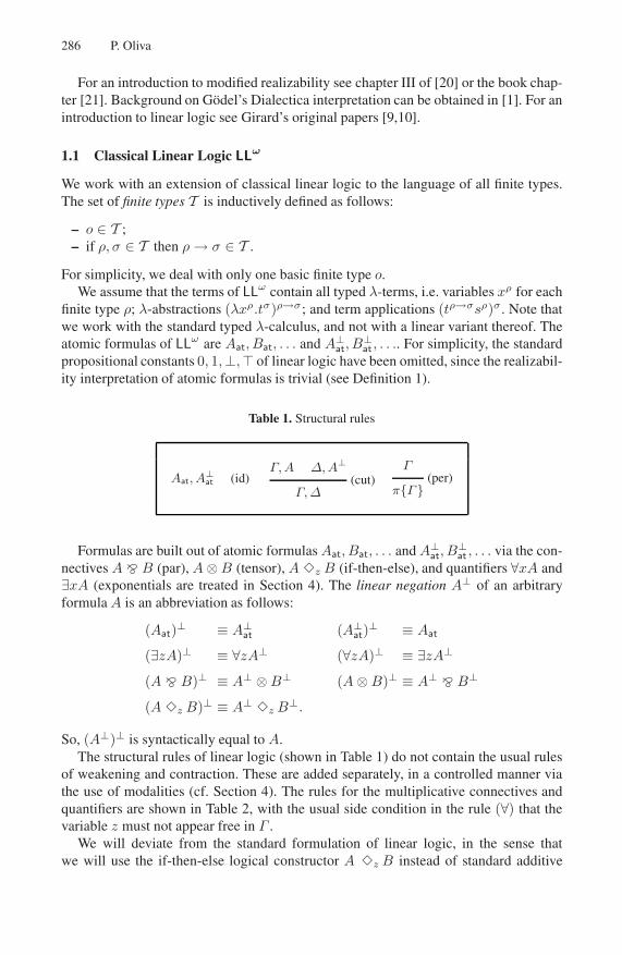
286 P. Oliva
For an introduction to modified realizability see chapter III of [20] or the book chap-ter [21]. Background on Godel’s Dialectica interpretation can be obtained in [1]. For anintroduction to linear logic see Girard’s original papers [9,10].
1.1 Classical Linear Logic LLω
We work with an extension of classical linear logic to the language of all finite types.The set of finite types T is inductively defined as follows:
– o ∈ T ;– if ρ, σ ∈ T then ρ → σ ∈ T .
For simplicity, we deal with only one basic finite type o.We assume that the terms of LLω contain all typed λ-terms, i.e. variables xρ for each
finite type ρ; λ-abstractions (λxρ.tσ)ρ→σ; and term applications (tρ→σsρ)σ . Note thatwe work with the standard typed λ-calculus, and not with a linear variant thereof. Theatomic formulas of LLω are Aat, Bat, . . . and A⊥
at, B⊥at , . . .. For simplicity, the standard
propositional constants 0, 1, ⊥, � of linear logic have been omitted, since the realizabil-ity interpretation of atomic formulas is trivial (see Definition 1).
Table 1. Structural rules
Aat, A⊥at (id)
Γ, A Δ, A⊥(cut)
Γ, Δ
Γ(per)
π{Γ}
Formulas are built out of atomic formulas Aat, Bat, . . . and A⊥at, B
⊥at , . . . via the con-
nectives A � B (par), A ⊗ B (tensor), A �z B (if-then-else), and quantifiers ∀xA and∃xA (exponentials are treated in Section 4). The linear negation A⊥ of an arbitraryformula A is an abbreviation as follows:
(Aat)⊥ ≡ A⊥at (A⊥
at)⊥ ≡ Aat
(∃zA)⊥ ≡ ∀zA⊥ (∀zA)⊥ ≡ ∃zA⊥
(A � B)⊥ ≡ A⊥ ⊗ B⊥ (A ⊗ B)⊥ ≡ A⊥ � B⊥
(A �z B)⊥ ≡ A⊥ �z B⊥.
So, (A⊥)⊥ is syntactically equal to A.The structural rules of linear logic (shown in Table 1) do not contain the usual rules
of weakening and contraction. These are added separately, in a controlled manner viathe use of modalities (cf. Section 4). The rules for the multiplicative connectives andquantifiers are shown in Table 2, with the usual side condition in the rule (∀) that thevariable z must not appear free in Γ .
We will deviate from the standard formulation of linear logic, in the sense thatwe will use the if-then-else logical constructor A �z B instead of standard additive
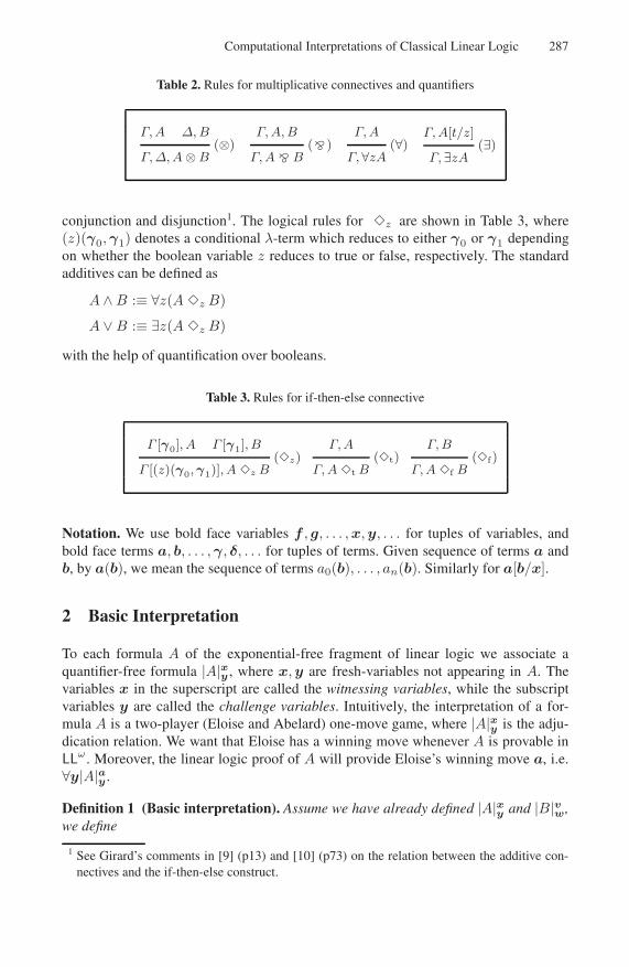
Computational Interpretations of Classical Linear Logic 287
Table 2. Rules for multiplicative connectives and quantifiers
Γ, A Δ, B(⊗)
Γ, Δ, A ⊗ B
Γ, A, B(� )
Γ, A � B
Γ, A(∀)
Γ,∀zA
Γ, A[t/z](∃)
Γ,∃zA
conjunction and disjunction1. The logical rules for �z are shown in Table 3, where(z)(γ0, γ1) denotes a conditional λ-term which reduces to either γ0 or γ1 dependingon whether the boolean variable z reduces to true or false, respectively. The standardadditives can be defined as
A ∧ B :≡ ∀z(A �z B)
A ∨ B :≡ ∃z(A �z B)
with the help of quantification over booleans.
Table 3. Rules for if-then-else connective
Γ [γ0], A Γ [γ1], B(�z)
Γ [(z)(γ0, γ1)], A �z B
Γ, A(�t)
Γ, A �t B
Γ, B(�f)
Γ, A �f B
Notation. We use bold face variables f , g, . . . , x, y, . . . for tuples of variables, andbold face terms a, b, . . . , γ, δ, . . . for tuples of terms. Given sequence of terms a andb, by a(b), we mean the sequence of terms a0(b), . . . , an(b). Similarly for a[b/x].
2 Basic Interpretation
To each formula A of the exponential-free fragment of linear logic we associate aquantifier-free formula |A|xy , where x, y are fresh-variables not appearing in A. Thevariables x in the superscript are called the witnessing variables, while the subscriptvariables y are called the challenge variables. Intuitively, the interpretation of a for-mula A is a two-player (Eloise and Abelard) one-move game, where |A|xy is the adju-dication relation. We want that Eloise has a winning move whenever A is provable inLLω. Moreover, the linear logic proof of A will provide Eloise’s winning move a, i.e.∀y|A|ay .
Definition 1 (Basic interpretation). Assume we have already defined |A|xy and |B|vw,we define
1 See Girard’s comments in [9] (p13) and [10] (p73) on the relation between the additive con-nectives and the if-then-else construct.

288 P. Oliva
|A � B|f ,gv,w :≡ |A|fw
v � |B|gvw
|A ⊗ B|x,vf ,g :≡ |A|xfv ⊗ |B|vgx
|A �z B|x,vy,w :≡ |A|xy �z |B|vw
|∃zA(z)|x,zf :≡ |A(z)|xfz
|∀zA(z)|fy,z :≡ |A(z)|fzy .
The interpretation of atomic formulas are the atomic formulas themselves, i.e.
|Aat| :≡ Aat
|A⊥at| :≡ A⊥
at.
Notice that for atomic formulas the tuples of witnesses and challenges are both empty.
It is easy to see that |A⊥|yx ≡ (|A|xy)⊥. We now prove the soundness of the basic inter-pretation, i.e. we show how Eloise’s winning move in the game |A|xy can be extractedfrom a proof of A in classical linear logic (exponentials treated in Section 4).
Theorem 1 (Soundness). Let A0, . . . , An be formulas of LLω, with z as the only free-variables. If
A0(z), . . . , An(z)
is provable in LLω then from this proof terms a0, . . . , an can be extracted such that
|A0(z)|a0x0
, . . . , |An(z)|anxn
is also provable in LLω, where FV(ai) ∈ {z, x0, . . . , xn}\{xi}.
Proof. The proof is by induction on the derivation of A0, . . . , An. The only relevantrule where free-variables matter is the universal quantifier rule. Therefore, for all theother rules we will assume the tuple of parameters z is empty. The cases of the axiom,permutation rule and if-then-else are trivial. The other rules are treated as follows:
Multiplicativies.
|Γ |γ[x]v , |A|ax
[fbx ]
|Γ |γ[fb]v , |A|afb
|Δ|δ[y]w , |B|by
[gay ]
|Δ|δ[ga]w , |B|bga (⊗)
|Γ |γ[fb]v , |Δ|δ[ga]
w , |A|afb ⊗ |B|bga (D1)|Γ |γ[fb]
v , |Δ|δ[ga]w , |A ⊗ B|a,b
f ,g
|Γ |γv , |A|a[y]x , |B|b[x]
y(�)
|Γ |γv , |A|a[y]x � |B|b[x]
y(D1)
|Γ |γv , |A � B|λy.a[y],λx.b[x]x,y
Cut.
|Γ |γ[x]v , |A|ax
[a−x ]
|Γ |γ[a−]v , |A|aa−
|Δ|δ[x−]w , |A⊥|a−
x−[ ax− ]
|Δ|δ[a]w , |A⊥|a−
a
|Δ|δ[a]w , (|A|aa−)⊥
(cut)|Γ |γ[a−]
v , |Δ|δ[a]w

Computational Interpretations of Classical Linear Logic 289
Note that the assumption that the tuple of variables x (respectively x−) does not appearfree in a (respectively a−) is used crucially in the soundness of the cut rule in orderremove any circularity in the two simultaneous substitutions.
Quantifiers.
|Γ |γ[z]v , |A|a[z]
x(D1)
|Γ |γ[z]v , |∀zA|λz.a[z]
x,z
|Γ |γ[x]v , |A(t)|ax
[gtx ]
|Γ |γ[gt]v , |A(t)|agt
(D1)|Γ |γ[gt]
v , |∃zA(z)|a,tg
This concludes the proof. �
3 Completeness
In this section we investigate the completeness of the interpretation given above. Moreprecisely, we ask the question: for which extension of classical linear logic LL� it is thecase that if there are terms a0, . . . , an such that |A0(z)|a0
x0, . . . , |An(z)|an
xnis provable
in LL� then the sequence A0, . . . , An is also provable in LL�? The idea that a formulaA is interpreted as a symmetric game |A|xy between two players suggests that A isequivalent to
Æxy |A|xy , using a simple form of branching quantifier to ensure that no
player has an advantage over the other. This simple branching quantifier (we will referto these as simultaneous quantifiers2) can be axiomatised with the rule:
A0(a0, y0), . . . , An(an, yn)(
Æ
)Æx0y0
A0(x0, y0), . . . ,
Æxn
ynAn(xn, yn)
with the side-condition: yi may only appear free in the terms aj , for j �= i. In particular,we will have that each yi will not be free in the conclusion of the rule.
The standard quantifier rules can be obtained from this single rule. The rule (∀)can be obtained in the case when only the tuple yn is non-empty. The rule (∃) can beobtained in the case when only the tuple xn is non-empty. Hence, for the rest of thissection we will consider that standard quantifiers ∀xA and ∃xA are in fact abbreviationsfor
Æ
xA and
ÆxA, respectively.In terms of games, the new quantifier embodies the idea of the two players perform-
ing their moves simultaneously. The most interesting characteristic of this simultaneousquantifier is with respect to linear negation, which is defined as
(
Æxy A)⊥ ≡
Æyx A⊥
and corresponds precisely to the switch of roles between the players. Let us refer to theextension of LLω with the new simultaneous quantifier by LLω
q .
2 According to Hyland [13] (footnote 18) “the identification of a sufficiently simple tensor asa Henkin quantifier is a common feature of a number of interpretations of linear logic”. Thesimultaneous quantifier can be viewed as a simplification of Henkin’s (branching) quantifier[4,12], in which no alternation of quantifiers is allowed on the two branches. See Bradfield [5]as well, where this simple form of branching quantifier is also used.

290 P. Oliva
Theorem 2. Extend the interpretation (Definition 1) to the system LLωq by defining
|
ÆvwA(v, w)|f ,v
g,w :≡ |A(v, w)|fwgv .
Theorem 1 holds for the extended system LLωq .
Proof. The rule for the simultaneous quantifier is handled as follows:
|A0(a0, w0)|b0y0
, . . . , |An(an, wn)|bnyn giai
yi|A0(a0, w0)|b′0
g0a0 , . . . , |An(an, wn)|b′n
gnan
(D1)|
Æv0w0
A0(v0, w0)|λw0.b′0,a0
g0,w0 , . . . , |
Ævn
wnAn(vn, wn)|λwn.b′
n,angn,wn
where b′j is the sequence of terms bj after the substitutions giai/yi, for i �= j. �
In fact, since the simultaneous quantifiers are eliminated, we obtain an interpretation ofLLω
q into LLω. Let us proceed now to define an extension of LLωq which is complete with
respect to the interpretation of Section 2. First we need some simple facts about LLωq .
Lemma 1. The following are derivable in LLωq
Æfy,zA(fz, y, z) � ∀z
Æxy A(x, y, z)
Æxy A(y) ⊗
ÆvwB(w) � Æx,v
f ,g (A(fv) ⊗ B(gx)).
Proof. These can be derived as
A⊥(fz, y, z), A(fz, y, z)(
Æ)Æy,z
f A⊥(fz, y, z),
Æxy A(x, y, z)
(∀)Æy,zf A⊥(fz, y, z), ∀z
Æxy A(x, y, z)
andA⊥(fv), A(fv) B⊥(gx), B(gx)
(⊗)A⊥(fv), B⊥(gx), A(fv) ⊗ B(gx)
(
Æ
)Æyx A⊥(y),
Æwv B⊥(w),
Æx,vf ,g (A(fv) ⊗ B(gx))
(�)Æyx A⊥(y) �
Æwv B⊥(w),
Æx,vf ,g (A(fv) ⊗ B(gx))
respectively. �
The converse of the implications in Lemma 1, however, require extra logical principles.Consider the following principles for the simultaneous quantifier
ACs : ∀z
Æxy A(x, y, z) � Æf
y,zA(fz, y, z)
ACp :
Æx,vf ,g (A(fv) ⊗ B(gx)) � Æx
y A(y) ⊗
ÆvwB(w)
for quantifier-free formula A and B. We refer to these as the sequential choice ACs andparallel choice ACp. For those familiar with the modified realizability of intuitionisticlogic, the principle ACs corresponds to the standard (intentional) axiom of choice, whileACp is a generalisation of the independence of premise principle (case when tuples x, vand w are empty).

Computational Interpretations of Classical Linear Logic 291
Lemma 2. The principles ACs and ACp are sound for our interpretation, i.e. for anyinstance P of these principles, there are terms t such that |P |ty is derivable in LLω.
Proof. Consider an instance of ACs
∀z
Æxy A(x, y, z) � Æf
y,zA(fz, y, z).
Since A is quantifier-free, it is easy to see that premise and conclusion have the sameinterpretation, namely
|∀z
Æxy A(x, y, z)|fy,z ≡ A(fz, y, z)
|
Æfy,zA(fz, y, z)|fy,z ≡ A(fz, y, z).
The same is true for the premise and conclusion of ACp. �
Let us denote by LLωq+ the extension of LLω
q with these two extra schemata ACs andACp. The next lemma shows that, in fact, these extra principles are all one needs toshow the equivalence between A and its interpretation
Æxy |A|xy .
Lemma 3. The equivalence between A and
Æxy |A|xy can be derived in the system LLω
q .
Proof. By induction on the logical structure of A. Consider for instance the case ofA ⊗ B.
A ⊗ B(IH)↔
Æxy |A|xy ⊗
Ævw|B|vw
(L1,ACp)↔
Æx,vf ,g (|A|xfv ⊗ |B|vgx).
The other cases are treated similarly. �
Theorem 3. Let A be a formula in the language of LLω. Then A is derivable in LLωq+
if and only if |A|ty is derivable in LLω, for some sequence of terms t.
Proof. The forward direction can be obtained with an extension of Theorem 1 given byLemma 2. The converse follows from Lemma 3. �
4 Possible Interpretations of Exponentials
The exponential-free fragment of LLω, despite its nice properties, bears little relationto the standard logical systems of classical and intuitionistic logic. In order to recoverthe full strength of classical logic, we need to add back contraction and weakening.These are recovered in linear logic in a controlled manner, with the help of modalities(exponentials) ?A and !A (cf. Table 4). The exponentials are dual to each other, i.e.
(?A)⊥ ≡ !A⊥ (!A)⊥ ≡ ?A⊥.
Girard’s points out in several places (cf. [10] (p84)) that these modalities, contraryto the other connectives, are not canonical. More precisely, if we add new modalities?′A and !′A with the same rules as shown in Table 4, we will not be able to derive theequivalences ?A ↔ ?′A and !A ↔ !′A. This is reflected in the flexibility with whichwe can interpret these modalities discussed below.

292 P. Oliva
Table 4. Rules for the exponentials
?Γ, A(!)
?Γ, !A
Γ, A(?)
Γ, ?A
Γ, ?A, ?A(con)
Γ, ?A
Γ(wkn)
Γ, ?A
4.1 Interpretation 1: Kreisel’s Modified Realizability
The first alternative for the interpretation of the exponentials we consider is one inwhich the game ?A gives maximal advantage to Eloise, and game !A gives maximaladvantage to Abelard. The maximal advantage corresponds to the player in questionnot needing to make any move, with their best possible move being played for them.More precisely, the interpretation is defined as:
|!A|x :≡ !∀y|A|xy|?A|y :≡ ?∃x|A|xy .
It is easy to see that Theorem 1 still holds when Definition 1 is extended in this way.For instance, the soundness of the rules (!) and (con) are obtained as:
|?Γ |v, |A|ay(∀)
|?Γ |v, ∀y|A|ay(!)
|?Γ |v, !∀y|A|ay|?Γ |v, |!A|a
|Γ |γ[y0,y1]v , |?A|y0
, |?A|y1 [ yy0
, yy1
]|Γ |γ[y,y]
v , |?A|y , |?A|y(con)
|Γ |γ[y,y]v , |?A|y
We have shown [16] that when combined with the embedding of intuitionistic logicinto linear logic, this choice for the interpretation of the exponentials corresponds toKreisel’s modified realizability interpretation [14] of intuitionistic logic.
Note that given this interpretation for the exponentials the relation |A|xy is no longerquantifier-free. It is the case, however, that formulas in the image of the interpretation(we call these fixed formulas) are also in the kernel of the interpretation. More, precisely,if A is in the kernel of the interpretation then |A| ≡ A. The completeness result ofSection 3 needs to be calibrated, as the schemata ACs and ACp need to be taken forall fixed-formulas (and not just quantifier-free formulas). Moreover, we need an extraprinciple
TA : !
Æxy A � ∃x!∀yA
called trump advantage, for fixed-formulas A, in order to obtain the equivalences in-volving exponentials, i.e. equivalence between !
Æxy A and ∃x!∀yA.
4.2 Interpretation 2: Diller-Nahm Interpretation
Another possibility for the interpretation is to give the player in question a restrictedadvantage by simply allowing the player to see the opponent’s move, and then select

Computational Interpretations of Classical Linear Logic 293
a finite set of moves. If any of these is a good move the player wins. This leads to thefollowing interpretation of the exponentials:
|!A|xf :≡ !∀y∈fx |A|xy|?A|fy :≡ ?∃x∈fy |A|xy .
Again, an extension of Definition 1 in this direction would also make the SoundnessTheorem 1 valid for the full classical linear logic. For instance, the soundness of thecontraction rule is obtained as:
|Γ |γ[y0,y1]v , |?A|a0
y0, |?A|a1
y1 (def)|Γ |γ[y0,y1]
v , ?∃x0 ∈a0y0|A|x0y0
, ?∃x1 ∈a1y1|A|x1y1 [ y
y0, y
y1]
|Γ |γ[y,y]v , ?∃x∈(a0y) ∪ (a1y)|A|xy ,
(con)|Γ |γ[y,y]
v , |?A|λy((a0y)∪(a1y))y
while the rules (!) is dealt with as follows:
|?Γ |γ[y]v , |A|a[v]
y(∀)
|?Γ |∪y∈f(a[v])(γ[y]v)v , ∀y∈f (a[v]) |A|a[v]
y(!)
|?Γ |λv.∪y∈f(a[v])(γ[y]v)v , |!A|a[v]
f
It is clear in this case that enough term construction needs to be added to the verifyingsystem in order to deal with finite sets of arbitrary type. This choice for the treatmentof the exponentials corresponds to a variant of Godel’s Dialectica interpretation due toDiller and Nahm [6].
4.3 Interpretation 3: Stein’s Interpretation
A hybrid interpretation between options 1 and 2 can also be given for each parametern ∈ N. The natural number n dictates from which type level we should use option 2(Diller-Nahm), and up to which level we should choose option 1 (modified realizabil-ity). The slogan is “only higher-type objects are witnessed”. Given a tuple of variablex, we will denote by x the sub-tuple containing the variables in x which have type level≥ n, whereas x denotes the sub-tuple of the variables in x which have type level < n.For each fixed type level n ∈ N we can define an interpretation of the exponentials as:
|!A|xf :≡ !∀y∈ rng(fx)∀y |A|xy|?A|fy :≡ ?∃x∈ rng(fy)∃x |A|xy .
where ∀y∈ rng(b(n−1)→ρ)A[y] and ∃y∈ rng(b(n−1)→ρ)A[y] are used as an abbrevia-tion for ∀in−1A[bi] and ∃in−1A[bi], respectively (n − 1 is the pure type of type leveln − 1).
This choice corresponds to Stein’s interpretation [19], and again leads to a soundinterpretation of full classical linear logic.

294 P. Oliva
4.4 Interpretation 4: Bounded Dialectica Interpretation
In [7,8], a “bounded” variant of Godel’s Dialectica interpretation was developed in orderto deal with strong analytical principles in classical feasible analysis. The interpretationmakes use of Howard-Bezem’s strong majorizabilty relation ≤∗ between functionals(cf. [2]). Using the majorizability relation, we can define well-behaved bounded setswhich can be used as moves in the treatment of the exponential games. More precisely,the interpretation of the exponentials can also be given as:
|!A|xf :≡ !∀y≤∗fx |A|xy|?A|fy :≡ ?∃x≤∗fy |A|xy .
As argued in [15], in this case we must first perform a relativisation of the quanti-fiers to Bezem’s model M of strongly majorizable functionals. After that, all candidatewitnesses and challenges are monotone, and the soundness of the contraction rule canbe derived as
|Γ |γ[y0,y1]v , |?A|a0
y0, |?A|a1
y1 (def)|Γ |γ[y0,y1]
v , ?∃x0 ≤∗a0y0|A|x0y0
, ?∃x1 ≤∗a1y1|A|x1y1 [ y
y0, y
y1]
|Γ |γ[y,y]v , ?∃x≤∗max(a0y, a1y)|A|xy ,
(con)|Γ |γ[y,y]
v , |?A|λy. max(a0y,a1y)y
where max(xρ, yρ) is the pointwise maximum.Besides being sound for the principles ACs, ACp of Section 3, and the principle TA of
Section 4.1, the Dialectica interpretation of LLω will also interpret the linear counterpartof the bounded Markov principle
MPB : ∀z!∀x≤∗z A � !∀xA
for bounded formulas A. The completeness for the bounded interpretation can then beextended to deal with the exponentials as
!
Æxy A
TA�
�LLω
q
∃x!∀yA
LLω
�
�MPB
∃x∀z!∀y≤∗z A
LLωq�
�ACs
Æxf !∀y≤∗fxA
MPB in particular implies the majorizability axiom by taking A(x, y) ≡ (x = y).In fact, the principles ACs, ACp, TA, MPB can be viewed as refinements of the (linearlogic versions of) the extra principles used in the bounded functional interpretation [7].For instance, the bounded Markov principle translates into linear logic as
(!∀yA � B) � ∃b(!∀y≤∗ b A � B)
for bounded formulas A and B. This can be derived as: By TA we get from !∀yA � Bto ∀b!∀y≤∗ b A � B. Then by ACp we get ∃b(!∀y≤∗ b A � B).

Computational Interpretations of Classical Linear Logic 295
4.5 Interpretation 5: Godel’s Dialectica Interpretation
The most restricted interpretation is the one in which the player’s advantage in the ex-ponential game is minimal. The only head-start will be to be able to see the opponentsmove. Based on the opponent’s move the player will then have to make a single move.This leads to an extension of the interpretation given in Definition 1 with the interpre-tation of the exponentials as
|!A|xf :≡ !|A|xfx
|?A|fy :≡ ?|A|fyy .
Note that in this case the target of the interpretation is again a quantifier-free calcu-lus (as in the basic interpretation of Section 2). For the soundness, however, we mustassume that quantifier-free formulas are decidable (a usual requirement for Dialecticainterpretations) in order to satisfy the contraction rule
|Γ |γ[y0,y1]v , |?A|a0
y0, |?A|a1
y1 (def)|Γ |γ[y0,y1]
v , ?|A|a0y0y0
, ?|A|a1y1y1 [ y
y0, y
y1]
|Γ |γ[y,y]v , ?|A|ay
y ,(con)
|Γ |γ[y,y]v , |?A|ay
where
ay :={
a0y if ?|A|a0yy
a1y otherwise.
The soundness of the weakening rule, and the rules (!) and (?) is trivial. This in-terpretation corresponds to Godel’s Dialectica interpretation [11] intuitionistic logic,used in connection to a partial realisation of Hilbert’s consistency program (the consis-tency of classical first-order arithmetic relative to the consistence of the quantifier-freecalculus T).
Besides being sound for the principles ACs, ACp (Section 3) and the principle TA(Section 4.1) the Dialectica interpretation of LLω will also be sound for the followingprinciple
MPD : ∀x!A � !∀xA
for quantifier-free formulas A. This is the linear logic counterpart of the (semi) intu-itionistic Markov principle. In fact, these are all the extra principles needed to show theequivalence between A and its Dialectica interpretation
Æxy |A|xy . For instance, in the
case of the exponentials we have
!
Æxy A
TA �
�LLω
q
∃x!∀yA
LLω
�
�MPD
∃x∀y!A
LLωq �
�ACs
Æxf !A[fx/y]
Acknowledgements. The interpretations presented here come from work of de Paiva[17], Blass [3], Shirahata [18] and recent work of the author [16]. The author gratefullyacknowledges support of the Royal Society under grant 516002.K501/RH/kk.

296 P. Oliva
References
1. Avigad, J., Feferman, S.: Godel’s functional (“Dialectica”) interpretation. In: Avigad, J., Fe-ferman, S. (eds.) Handbook of proof theory. Studies in Logic and the Foundations of Mathe-matics, vol. 137, pp. 337–405. North Holland, Amsterdam (1998)
2. Bezem, M.: Strongly majorizable functionals of finite type: a model for bar recursion con-taining discontinuous functionals. The Journal of Symbolic Logic 50, 652–660 (1985)
3. Blass, A.: Questions and answers – a category arising in linear logic, complexity theory, andset theory. In: Girard, J.-Y., Lafont, Y., Regnier, L. (eds.) Advances in Linear Logic. LondonMath. Soc. Lecture Notes, vol. 222, pp. 61–81 (1995)
4. Blass, A., Gurevich, Y.: Henkin quantifiers and complete problems. Annals of Pure and Ap-plied Logic 32, 1–16 (1986)
5. Bradfield, J.: Independence: Logic and concurrency. In: Proceedings of Computer ScienceLogic (2000)
6. Diller, J., Nahm, W.: Eine Variant zur Dialectica-interpretation der Heyting Arithmetikendlicher Typen. Arch. Math. Logik Grundlagenforsch 16, 49–66 (1974)
7. Ferreira, F., Oliva, P.: Bounded functional interpretation. Annals of Pure and AppliedLogic 135, 73–112 (2005)
8. Ferreira, F., Oliva, P.: Bounded functional interpretation in feasible analysis. Annals of Pureand Applied Logic 145, 115–129 (2007)
9. Girard, J.-Y.: Linear logic. Theoretical Computer Science 50(1), 1–102 (1987)10. Girard, J.-Y.: Towards a geomery of interaction. Contemporary Mathematics, 92 (1989)11. Godel, K.: Uber eine bisher noch nicht benutzte Erweiterung des finiten Standpunktes. Di-
alectica 12, 280–287 (1958)12. Henkin, L.: Some remarks on infinitely long formulas. In: Infinitistic methods, pp. 167–183.
Pergamon Press, New York, and Polish Scientific Publishers, Warsaw (1961)13. Hyland, J.M.E.: Proof theory in the abstract. Annals of Pure and Applied Logic 114, 43–78
(2002)14. Kreisel, G.: Interpretation of analysis by means of constructive functionals of finite types. In:
Heyting, A. (ed.) Constructivity in Mathematics, pp. 101–128. North Holland, Amsterdam(1959)
15. Oliva, P.: Unifying functional interpretations. Notre Dame Journal of Formal Logic 47(2),263–290 (2006)
16. Oliva, P.: Modified realizability interpretation of classical linear logic. In: Proc. of the Eigh-teenth Annual IEEE Symposium on Logic in Computer Science LICS’07, IEEE ComputerSociety Press, Los Alamitos (2007)
17. de Paiva, V.C.V.: A Dialectica-like model of linear logic. In: Dybjer, P., Pitts, A.M., Pitt,D.H., Poigne, A., Rydeheard, D.E. (eds.) Category Theory and Computer Science. LNCS,vol. 389, pp. 341–356. Springer, Heidelberg (1989)
18. Shirahata, M.: The Dialectica interpretation of first-order classical linear logic. Theory andApplications of Categories 17(4), 49–79 (2006)
19. Stein, M.: Interpretationen der Heyting-Arithmetik endlicher Typen. Arch. Math. LogikGrundlag 19, 175–189 (1979)
20. Troelstra, A.S.: Metamathematical Investigation of Intuitionistic Arithmetic and Analysis.Lecture Notes in Mathematics, vol. 344. Springer, Heidelberg (1973)
21. Troelstra, A.S.: Realizability. Handbook of proof theory 137, 408–473 (1998)

D. Leivant and R. de Queiroz (Eds.): WoLLIC 2007, LNCS 4576, pp. 297–306, 2007. © Springer-Verlag Berlin Heidelberg 2007
Autonomous Programmable Biomolecular Devices Using Self-assembled DNA Nanostructures*
John H. Reif1 and Thomas H. LaBean2
1 Department of Computer Science, Duke University, Durham, NC 27708 USA 2 Department of Chemistry, Duke University, Durham, NC 27708 USA
1 Introduction
1.1 Why Computer Science Is Relevant to the Nano-scale
The particular molecular-scale devices that are the topic of this article are known as DNA nanostructures. As will be explained, DNA nanostructures have some unique advantages among nanostructures: they are relatively easy to design, fairly predictable in their geometric structures, and have been experimentally implemented in a growing number of labs around the world. They are constructed primarily of synthetic DNA. A key principle in the study of DNA nanostructures is the use of self-assembly processes to actuate the molecular assembly. Since self-assembly operates naturally at the molecular scale, it does not suffer from the limitation in scale reduction that so restricts lithography or other more conventional top-down manufacturing techniques.
This article particularly illustrates the way in which computer science techniques and methods have impact on this emerging field. Some of the key questions one might ask about biomolecular devices are:
• What is the theoretical basis for these devices? • How will such devices be designed? • How can we simulate them prior to manufacture? • How can we optimize their performance? • How will such devices be manufactured? • How much do the devices cost? • How scalable is the device design? • How will I/O be done? • How will they be programmed? • What efficient algorithms can be programmed? • What will be their applications? • How can we correct for errors or repair them?
Note that these questions are exactly the sort of questions that computer scientists routinely ask about conventional computing devices. The discipline of computer science
* Supported by NSF grants CCF-0523555, CCF-0432038, CCF-0432047. An extended version of
this paper is at http://www.cs.duke.edu/~reif/paper/AutonomousDNA/ AutonomousDNA.pdf

298 J.H. Reif and T.H. LaBean
has developed a wide variety of techniques to address such basic questions, and we will later point out some which have an important impact to molecular-scale devices.
1.2 Introducing DNA Nanotechnology and Its Use to Assemble Molecular-Scale Devices
In general, nanoscience research is highly interdisciplinary. In particular, DNA self-assembly uses techniques from multiple disciplines such as biochemistry, physics, chemistry, and material science, as well as computer science and mathematics. While this makes the topic quite intellectually exciting, it also makes it challenging for a typical computer science reader. Having no training in biochemistry, he or she must obtain a coherent understanding of the topic from a short article. For this reason, this article was written with the expectation that the reader is a computer scientist with little background knowledge of chemistry or biochemistry. See Sidebar 1 for a brief introduction to DNA. In Sidebar 2 we list some reasons why DNA is uniquely suited for assembly of molecular-scale devices.
Sidebar 1: A Brief Introduction to DNASingle stranded DNA (denoted ssDNA) is a linear polymer consisting of a sequence of DNA bases oriented along a backbone withchemical directionality. By convention, the base sequence is listed starting from the 5-prime end of the polymer and ending at the 3-prime end (these names refer to particular carbon atoms in the deoxyribose sugar units of the sugar-phosphate backbone, thedetails of which are not critical to the present discussion). The consecutive bases (monomer units) of an ssDNA molecule are joinedvia covalent bonds. There are 4 types of DNA bases adenine, thymine, guanine and cytosine typically denoted by the symbols A, T,G, and C, respectively. These bases form the alphabet of DNA; the specific sequence comprises DNA s information content. Thebases are grouped into complementary pairs (G, C) and (A, T).The most basic DNA operation is hybridization where two ssDNA oriented in opposite directions can bind to form a double strandedDNA helix (dsDNA) by pairing between complementary bases. DNA hybridization occurs in a buffer solution with appropriatetemperature, pH, and salinity.
Structure of a DNA double helix (Created by Michael Ströck and released under the GNU Free DocumentationLicense(GFDL).)Since the binding energy of the pair (G, C) is approximately half-again the binding energy of the pair (A, T), theassociation strength of hybridization depends on the sequence of complementary bases, and can be approximated by knownsoftware packages. The melting temperature of a DNA helix is the temperature at which half of all the molecules are fully hybridizedas double helix, while the other half are single stranded. The kinetics of the DNA hybridization process is quite well understood; itoften occurs in a (random) zipper-like manner, similar to a biased one-dimensional random walk.Whereas ssDNA is a relatively floppy molecule, dsDNA is quite stiff (over lengths of less than 150 or so bases) and has the wellcharacterized double helix structure. The exact geometry (angles and positions) of each segment of a double helix depends slightlyon the component bases of its strands and can be determined from known tables. There are about 10.5 bases per full rotation onthis helical axis. A DNA nanostructure is a multi-molecular complex consisting of a number of ssDNA that have partially hybridizedalong their sub-segments.
In Sidebar 3 we list some known enzymes used for manipulation of DNA nanostructures.
The area of DNA self-assembled nanostructures and robotics is by no means simply a theoretical topic - many dramatic experimental demonstrations have already been made and a number of these will be discussed. The complexity of these demonstrations have been increasing at an impressive rate (even in comparison to the rate of improvement of silicon-based technologies).

Autonomous Programmable Biomolecular Devices 299
Sidebar 2: Why use DNA to Assemble Molecular-Scale Devices?There are many advantages of DNA as a material for building things at the molecular scale.(a) From the perspective of design, the advantages are:
• The structure of most complex DNA nanostructures can be reduced to determining the structure of short segments ofdsDNA. The basic geometric and thermodynamic properties of dsDNA are well understood and can be predicted byavailable software systems from key relevant parameters like sequence composition, temperature and buffer conditions.
• Design of DNA nanostructures can be assisted by software. To design a DNA nanostructure or device, one needs todesign a library of ssDNA strands with specific segments that hybridize to (and only to) specific complementary segmentson other ssDNA. There are a number of software systems (developed at NYU, Caltech, and Duke University) for design ofthe DNA sequences composing DNA tiles and for optimizing their stability, which employ heuristic optimization proceduresfor this combinatorial sequence design task.
(b) From the perspective of experiments, the advantages are:• The synthesis of ssDNA is now routine and inexpensive; a test tube of ssDNA consisting of any specified short sequence
of bases (<150) can be obtained from commercial sources for modest cost (about half a US dollar per base at this time); itwill contain a very large number (typically at least 1012) identical ssDNA molecules. The synthesized ssDNA can haveerrors (premature termination of the synthesis is the most frequent error), but can be easily purified by well-knowntechniques (e.g., electrophoresis as mentioned below).
• The assembly of DNA nanostructures is a very simple experimental process: in many cases, one simply combines thevarious component ssDNA into a single test tube with an appropriate buffer solution at an initial temperature above themelting temperature, and then slowly cools the test tube below the melting temperature.
• The assembled DNA nanostructures can be characterized by a variety of techniques. One such technique iselectrophoresis. It provides information about the relative molecular mass of DNA molecules, as well as some informationregarding their assembled structures, depending on what type (denaturing or native, respectively) of electrophoresis isused. Other techniques like Atomic Force Microscopy (AFM) and Transmission Electron Microscopy (TEM) provide imagesof the actual assembled DNA nanostructures on 2D surfaces.
Sidebar 3: Manipulation of DNAIn addition to the hybridization reaction, there are a wide variety of known enzymes and other proteinsused for manipulation of DNA nanostructures that have predictable effects. (Interestingly, these proteinswere discovered in natural bacterial cells and tailored for laboratory use.) These include:
• Restriction enzymes, some of which can cut (or nick, which is to cut only one strand)strands of a DNA helix at locations determined by short specific DNA base sequences.
• Ligase enzymes that can heal nicks in a DNA helix.
• Polymerase, which given an initial “primer” DNA strand hybridized onto a segment of atemplate DNA strand, can extend the primer strand in the 5 to 3 direction by appendingfree nucleotides complementary to the template s nucleotides.
Besides their extensive use in other biotechnology, the above reactions, together with hybridization, areoften used to execute and control DNA computations and DNA robotic operations. The restriction enzymereactions are programmable in the sense that they are site specific, only executed as determined by theappropriate DNA base sequence. The latter two reactions, using ligase and polymerase, require theexpenditure of energy via consumption of ATP molecules, and thus can be controlled by ATPconcentration.
Molecular-scale devices using DNA nanostructures have been engineered to have various capabilities, ranging from (i) execution of molecular-scale computation, (ii) use as scaffolds or templates for the further assembly of other materials (such as scaffolds for various hybrid molecular electronic architectures or perhaps

300 J.H. Reif and T.H. LaBean
high-efficiency solar-cells), (iii) robotic movement and molecular transport, and (iv) exquisitely sensitive molecular detection and amplification of single molecular events (v) transduction of molecular sensing to provide drug delivery.
2 Adelman’s Initial Demonstration of a DNA-Based Computation
2.1 Adleman’s Experiment
The field of DNA computing began in 1994 with a laboratory experiment described in [A98]. The goal of the experiment was to find a Hamiltonian path in a graph, which is a path that visits each node exactly once. To solve this problem, a set of ssDNA were designed based on the set of edges of the graph. When combined in a test tube and cooled, they self-assembled into dsDNA. Each of these DNA nanostructures was a linear DNA helix that corresponded to a path in the graph. If the graph had a Hamiltonian path, then one of these DNA nanostructures encoded the Hamiltonian path. By conventional biochemical extraction methods, Adelman was able to isolate only DNA nanostructures encoding Hamiltonian paths, and by determining their sequence, the explicit Hamiltonian path. It should be mentioned that this landmark experiment was designed and experimentally demonstrated by Adleman alone, a computer scientist with limited training in biochemistry.
2.2 The Non-scalability of Adelman ‘s Experiment
While this experiment founded the field of DNA computing, it was not scalable in practice, since the number of different DNA strands needed increased exponentially with the number of nodes of the graph. Although there can be an enormous number of DNA strands in a test tube (1015 or more, depending on solution concentration), the size of the largest graph that could be solved by his method was limited to at most a few dozen nodes. This is not surprising, since finding the Hamiltonian path is an NP complete problem, whose solution is likely to be intractable using conventional computers. Even though DNA computers operate at the molecular-scale, they are still equivalent to conventional computers (e.g., deterministic Turing machines) in computational power. This experiment taught a healthy lesson to the DNA computing community (which is now well-recognized): to carefully examine scalability issues and to judge any proposed experimental methodology by its scalability.
2.3 Autonomous Biomolecular Computation
Shortly following Adleman‘s experiment, there was a burst of further experiments in DNA computing, many of which were quite ingenious. However, almost none of these DNA computing methods were autonomous, and instead required many tedious

Autonomous Programmable Biomolecular Devices 301
laboratory steps to execute. In retrospect, one of the most notable aspects of Adleman’s experiment was that the self-assembly phase of the experiment was completely autonomous - it required no exterior mediation. This autonomous property makes an experimental laboratory demonstration much more feasible as the scale increases. The remaining article mostly discusses autonomous devices for bio-molecular computation based on self-assembly.
3 Self-assembled DNA Tiles and Lattices
Sidebar 4: DNA NanostructuresRecall that a DNA nanostructure is a multi-molecular complex consisting of a number of ssDNA that havepartially hybridized along their sub-segments. The field of DNA nanostructures was pioneered by Seeman[S04].Particularly useful types of motifs often found in DNA nanostructures include:
Figure of a Stem-Loop and a Sticky End. A stem-loop (A), where ssDNA loops back tohybridize on itself (that is, one segment of the ssDNA (near the 5 end) hybridizes with another segmentfurther along (nearer the 3 end) on the same ssDNA strand). The shown stem consists of the dsDNAregion with sequence CACGGTGC on the bottom strand. The shown loop consists of the ssDNA regionwith sequence TTTT. Stem-loops are often used to form patterning on DNA nanostructures. A sticky end(B), where unhybridized ssDNA protrudes from the end of a double helix. The sticky end shown (ATCG)protrudes from dsDNA (CACG on the bottom strand). Sticky ends are often used to combine two DNAnanostructures together via hybridization of their complementary ssDNA. The figure shows the antiparallelnature of dsDNA with the 5 end of each strand pointing toward the 3 end of its partner strand.
Figure of a Holliday Junction (Created by Miguel Ortiz-Lombardía, CNIO, Madrid, Spain.)A Holliday junction, where two parallel DNA helices form a junction with one strand of each DNA helix(blue and red) crossing over to the other DNA helix. Holliday junctions are often used to tie togethervarious parts of a DNA nanostructure.

302 J.H. Reif and T.H. LaBean
3.1 Computation by Self-assembly
The most basic way that computer science ideas have impacted DNA nanostructure design is via the pioneering work by theoretical computer scientists on a formal model of 2D tiling due to Wang in 1961, which culminated in a proof by Berger in 1966 that universal computation could be done via tiling assemblies. Winfree was the first to propose applying the concepts of computational tiling assemblies to DNA molecular constructs. His core idea was to use tiles composed of DNA to perform computations during their self-assembly process. To understand this idea, we will need an overview of DNA nanostructures, as presented in Sidebar 4.
3.2 DNA Tiles and Lattices
A DNA tile is a DNA nanostructure that has a number of sticky ends on its sides, which are termed pads. A DNA lattice is a DNA nanostructure composed of a group of DNA tiles that are assembled together via hybridization of their pads. Generally the strands composing the DNA tiles are designed to have a melting temperature above those of the pads, ensuring that when the component DNA molecules are combined together in solution, first the DNA tiles assemble, and only then, as the solution is further cooled, do the tiles bind together via hybridization of their pads.
Sidebar 5: DNA Tiles
(a) (b) (c) (d) AFM image of 2D Lattice using Cross-Over tiles
(a) Seeman and Winfree in 1998 developed a family of DNA tiles known collectively as DX tiles (see left tile (a)) that consisted of twoparallel DNA helices linked by immobile Holliday junctions. They demonstrated that these tiles formed large 2D lattices, as viewed byAFM. (b) Subsequently, other DNA tiles were developed to provide for more complex strand topology and interconnections, includinga family of DNA tiles known as TX tiles (see b) [L00] composed of three DNA helices. Both the DX tiles and the TX tiles arerectangular in shape, where two opposing edges of the tile have pads consisting of ssDNA sticky ends of the component strands. Inaddition, TX tiles have topological properties that allow for strands to propagate in useful ways though tile lattices (this property isoften used for aid in patterning DNA lattices as described below). (c) Other DNA tiles known as Cross-Over tiles (see c) [Y03b] areshaped roughly square, and have pads on all four sides, allowing for binding of the tile directly with neighbors in all four directions inthe lattice plane.
To program a tiling assembly, the pads of tiles are designed so that tiles assemble together as intended. Proper designs ensure that only the adjacent pads of neighboring tiles are complementary, so only those pads hybridize together. Sidebar 5 describes some principal DNA tiles.

Autonomous Programmable Biomolecular Devices 303
4 Autonomous Finite State Computation Using Linear DNA Nanostructures
Sidebar 6: Sequential Boolean Computation via a Linear DNA Tiling Assembly
This figure is adapted with permission from [M00]. It shows a unit TX tile (a) and the sets of input and output tiles (b) withgeometric shapes conveying sticky-end complementary matching. The tiles of (b) execute binary computations dependingtheir pads, as indicated by the table in (b). The (blue) input layer and (green) corner condition tiles were designed toassemble first (see example computational assemblies (c) & (d)). The (red) output layer then assemble specificallystarting from the bottom left using the inputs from the blue layer. (See [M00] for more details of this molecularcomputation.) The tiles were designed such that an output reporter strand ran through all the n tiles of the assembly bybridges across the adjoining pads in input, corner, and output tiles. This reporter strand was pasted together from the shortssDNA sequences within the tiles using ligation enzyme mentioned previously. When the solution was warmed, this outputstrand was isolated and identified. The output data was read by experimentally determining the sequence of cut sites (seebelow). In principle, the output could be used for subsequent computations.
4.1 The First Experimental Demonstration of Autonomous Computations Using Self-assembly of DNA Nanostructures
The first experimental demonstrations of computation using DNA tile assembly was [M00]. It demonstrated a 2-layer, linear assembly of TX tiles that executed a bit-wise cumulative XOR computation. In this computation, n bits are input and n bits are output, where the ith output is the XOR of the first i input bits. This is the computation occurring when one determines the output bits of a full-carry binary adder circuit. The experiment [M00] is described further in Sidebar 6.
This experiment [M00] provided answers to some of the most basic questions of concern to a computer scientist:
• How can one provide data input to a molecular computation using DNA tiles?
In this experiment the input sequence of n bits was defined an “input” ssDNA strand with the input bits (1’s & 0’s) encoded by distinct short subsequences. Two different tile types (depending on whether the input bit was 0 or 1, these had specific stick-ends and also specific subsequences at which restriction enzymes can cut the

304 J.H. Reif and T.H. LaBean
DNA backbone) were available to assemble around each of the short subsequences comprising the input strand, forming the blue input layer illustrated in Sidebar 6.
The next question of concern to a computer scientist is:
• How can one execute a step of computation using DNA tiles?
To execute steps of computation, the TX tiles were designed to have pads at one end that encoded the cumulative XOR value. Also, since the reporter strand segments ran though each such tile, the appropriate input bit was also provided within its structure. These two values implied the opposing pad on the other side of the tile be the XOR of these two bits.
The final question of concern to a computer scientist is:
• How can one determine and/or display the output values of a DNA tiling computation?
The output in this case was read by determining which of two possible cut sites (endonuclease cleavage sites) were present at each position in the tile assembly. This was executed by first isolating the reporter strand, then digesting separate aliquots with each endonuclease separately and the two together, finally these samples were examined by gel electrophoresis and the output values were displayed as banding patterns on the gel.
Another method for output (presented below) is the use of AFM observable patterning. The patterning was made by designing the tiles computing a bit 1 to have a stem loop protruding from the top of the tile, The sequence of this molecular patterning was clearly viewable under appropriate AFM imaging conditions.
Although only very simple computations, the experiments of [M00] and [Y03b] did demonstrate for the first time methods for autonomous execution of a sequence of finite-state operations via algorithmic self-assembly, as well as for providing inputs and for outputting the results.
4.2 Autonomous Finite-State Computations Via Disassembly of DNA Nanostructures
An alternative method for autonomous execution of a sequence of finite-state transitions was subsequently developed by [S06]. Their technique essentially operated in the reverse of the assembly methods described above, and instead was based on disassembly. They began with a linear DNA nanostructure whose sequence encoded the inputs, and then they executed series of steps that digested the DNA nanostructure from one end. On each step, a sticky end at one end of the nanostructure encoded the current state, and the finite transition was determined by hybridization of the current sticky end with a small “rule“ nanostructure encoding the finite-state transition rule. Then a restriction enzyme, which recognized the sequence encoding the current input as well as the current state, cut the appended end of the linear DNA nanostructure, to expose a new a sticky end encoding the next state.

Autonomous Programmable Biomolecular Devices 305
5 Conclusions
Other topics that were originally intended but have been dropped because of the space limitations (see the extended version of this paper at http://www.cs.duke.edu/~reif/ paper/AutonomousDNA/AutonomousDNA.pdf) are:
• Assembling patterned and addressable 2D DNA lattices, such as attaching materials to DNA [Y03c], and methods for programmable assembly of patterned 2D DNA lattices [Y03a, R06a, R04, P06].
• Autonomous molecular transport devices self-assembled from DNA [Y04, M00].
• Future challenges for self-assembled DNA nanostructures, such as error correction and self-repair at the molecular-scale [R06b], and 3D DNA lattices.
In attempting to understand these modern developments, it is worth recalling that mechanical methods for computation date back to the very onset of computer science, for example to the cog-based mechanical computing machine of Babbage. Lovelace stated in 1843 that Babbage’s “Analytical Engine weaves algebraic patterns just as the Jacquard-loom weaves flowers and leaves”. In some of the recently demonstrated methods for biomolecular computation, computational patterns were essentially woven into molecular fabric (DNA lattices) via carefully controlled and designed self-assembly processes [Y03a, R04, P06]. We have observed that many of these self-assembly processes are computational-based and programmable, and it seems likely that computer science techniques will be essential to the further development of this emerging field of biomolecular computation.
References
[A98] Adleman, L.: Computing with DNA. Scientific American 279(2), 34–41 (1998) [D06] Deng, Z., Chen, Y., Tian, Y., Mao, C.: A fresh look at DNA nanotechnology. In: Chen,
J., Jonoska, N., Rozenberg, G. (eds.) Nanotechnology: Science and Computation, Natural Computing, pp. 23–34. Springer, Heidelberg (2006)
[M00] Mao, C., LaBean, T.H., Reif, J.H., Seeman,: Logical Computation Using Algorithmic Self-Assembly of DNA Triple-Crossover Molecules. Nature 407, 493–495 (2000)
[R04] Rothemund, P.W.K., Papadakis, N., Winfree, E.: Algorithmic Self-Assembly of DNA Sierpinski Triangles, PLoS Biology 2 (12) (December 2004)
[R06a] Rothemund, P.W.K.: Folding DNA to create nanoscale shapes and patterns. Nature 440, 297–302 (2006)
[R06b] Reif, J.H., Sahu, S., Yin, P.: Compact Error-Resilient Computational DNA Tiling Assemblies. In: John, H., Jonoska, N., Rozenberg, G. (eds.) Nanotechnology: Science and Computation, Natural Computing, pp. 79–104. Springer, Heidelberg (2006)
[S04] Seeman, N.C.: Nanotechnology and the Double Helix. Scientific American 290(6), 64–75 (2004)
[S06] Shapiro, E., Benenson, Y.: Bringing DNA Computers to Life. Scientific American, 45–51 (May 2006)

306 J.H. Reif and T.H. LaBean
[Y03a] Yan, H., LaBean, T.H., Feng, L., Reif, J.H.: Directed Nucleation Assembly of Barcode Patterned DNA Lattices. PNAS 100(14), 8103–8108 (2003)
[Y03b] Yan, H., Feng, L., LaBean, T.H., Reif, J.: DNA Nanotubes, Parallel Molecular Computations of Pairwise Exclusive-Or (XOR) Using DNA String Tile. Self-Assembly in Journal of American Chemistry Society(JACS) 125(47), 14246–14247 (2003)
[Y03c] Yan, H., Park, S.H., Finkelstein, G., Reif, J.H., LaBean, T.H.: DNA-Templated Self-Assembly of Protein Arrays and Highly Conductive Nanowires. Science 301, 1882–1884 (2003)
[Y04] Yin, P., Yan, H., Daniel, X.G., Turberfield, A.J., Reif, J.H.: A Unidirectional DNA Walker Moving Autonomously Along a Linear Track. Angewandte Chemie [International Edition] 43(37), 4906–4911 (2004)

Interval Valued QL-Implications
R.H.S. Reiser1, G.P. Dimuro1, B.C. Bedregal2, and R.H.N. Santiago2
1 Programa de Pos-Graduacao em Informatica, Universidade Catolica de PelotasRua Felix da Cunha 412, 96010-000 Pelotas, Brazil
{reiser,liz}@ucpel.tche.br2 Depto de Informatica e Matematica Aplicada, Universidade Federal do Rio Grande do Norte
Campus Universitario s/n, 59072-970 Natal, Brazil{bedregal,regivan}@dimap.ufrn.br
Abstract. The aim of this work is to analyze the interval canonical representa-tion for fuzzy QL-implications and automorphisms. Intervals have been used tomodel the uncertainty of a specialist’s information related to truth values in thefuzzy propositional calculus: the basic systems are based on interval fuzzy con-nectives. Thus, using subsets of the real unit interval as the standard sets of truthdegrees and applying continuous t-norms, t-conorms and negation as standardtruth interval functions, the standard truth interval function of an QL-implicationcan be obtained. Interesting results on the analysis of interval canonical repre-sentation for fuzzy QL-implications and automorphisms are presented. In ad-dition, commutative diagrams are used in order to understand how an intervalautomorphism acts on interval QL-implications, generating other interval fuzzyQL-implications.
1 Introduction
The tolerance for imprecision and the ability to make decisions under uncertainties ofcontrol systems provide the seminal motivation for development of fuzzy set theory.Under its mathematical approach, the fuzzy logic, concerned with the narrow sense offuzzy approach, has been developed as a system of formal deductive systems with acomparative notion of truth to formalize deduction under vagueness. Thus, fuzzy logicgives foundations for approximate reasoning using imprecise propositions based onfuzzy set theory. And, all these matters involve the knowledge of the basic characteris-tics of approximative reasoning processes response from the viewpoint of uncertaintyor incomplete available information and knowledge of the parameters that affect humanreasoning and need to be subjected to scientific investigation.
The extension of classical logic connectives to the real unit interval is fundamentalfor the studies on fuzzy logic and therefore are essential to the development of fuzzysystems. This extension must preserve the behaviors of the connectives at the intervalendpoints (crisp values) and important properties, such as commutativity and associa-tivity, which results in the notions of triangular norms and triangular conorms. Fuzzyimplications play an important role in fuzzy logic, both in the broad sense (heavily
D. Leivant and R. de Queiroz (Eds.): WoLLIC 2007, LNCS 4576, pp. 307–321, 2007.c© Springer-Verlag Berlin Heidelberg 2007

308 R.H.S. Reiser et al.
applied to fuzzy control, analysis of vagueness in natural language and techniques ofsoft-computing) and in the narrow sense (developed as a branch of many-valued logicwhich is able to investigate deep logical questions). However, there is no consensusamong researchers which extra properties fuzzy implications should satisfy. In the lit-erature, several fuzzy implication properties have already been considered and theirinterrelationship with the other kinds of connectives are generally presented. There ex-ist three main classes of fuzzy implications associated to fuzzy connectives, namelyR-implications (generated from t-norms), S-implications (generated from t-conormsand fuzzy negations) and QL-implications, which are generated from t-norms,t-conorms joint with fuzzy negations.
In another formal approach, the correctness and optimality of interval mathematicshave been applied in technological and scientific computations to provide accuracy ofcalculations together with the automatic and rigorous control of the errors that occur innumerical computations [1]. In this sense, interval computation is adequate to deal withthe imprecision of the input values or imprecision caused by the rounding errors whichoccur during the computation [2,3].
Interval mathematics is another form of information theory which is related to butindependent from fuzzy logic. However, when intervals can be considered as a partic-ular type of fuzzy set or when the interval membership degree is considered to be animprecision in the belief degree of a specialist, it seems natural and interesting to dealwith the interval fuzzy approach.1
Among several papers connecting these areas [6,9,10,11,12,13,14], we consider Be-dregal and Takahashi’s [15,16] work, which has provided interval extensions for thefuzzy connectives considering both correctness (accuracy) and optimality aspects, asproperly shown in [17].
This paper is organized as follows. In Sect. 2, we consider the conditions to obtainthe interval representation of a real function and recall the related definition of bestinterval. The interval extension of fuzzy t-conorms (t-norms) and fuzzy negations arepresented in sections 3 and 4, respectively. Further analysis of properties met by fuzzyQL-implications are studied in Sect. 5. Section 6 shows that minimal properties of fuzzyimplications may be extended from interval fuzzy degrees, in a natural way. In Sect. 6.1,commutative classes of interval fuzzy QL-implications are discussed. In Sect 7, weshow how the initial uncertainties of the membership degrees are propagated by the bestinterval representations of QL-implications. The action of an interval automorphismon interval QL-implication is analyzed in Sect. 8. The canonical construction of anautomorphism of an interval automorphism is introduced in Sect. 8.1, including its bestinterval representation (Sect. 8.2) and the relation between interval implications andautomorphism (Sect. 8.3). Section 9 is the Conclusion.
1 Interval membership degrees are useful to map the uncertainty and the difficulty of an expert indetermining which is the fairest membership degree for an element with respect to a linguisticterm. In this case, the radius of the interval indicates a maximal bound for the error [4,5,6],providing an estimation of that uncertainty. Interval degrees also can summarize the opinionof several experts with respect to the exact membership degree for an element with respect toa linguistic term. In this case, the left and right interval endpoints are, respectively, the leastand the greatest degrees provided by a group of experts [6,7,8,9].

Interval Valued QL-Implications 309
2 Interval Representations
Consider the real unit interval U = [0, 1] ⊆ �. Let U = {[a, b] | 0 ≤ a ≤ b ≤ 1} bethe set of subintervals of U . The interval set has two projections l, r : U → U definedby l([a, b]) = a and r([a, b]) = b, respectively. As a convention, for each X ∈ U theprojections l(X) and r(X) will also be denoted by X and X , respectively.
Several natural partial orders may be defined on U [18]. The most used orders in thecontext of interval mathematics and considered in this work, are the following:
1. Product: X ≤ Y if and only if X ≤ Y and X ≤ Y .2. Inclusion order: X ⊆ Y if and only if X ≥ Y and X ≤ Y
Since these orders are partial, not all pairs of intervals present maximum and min-imum, but there are always an infimum and a supremum. For the case of the productorder, it holds that:
inf{X, Y } = [min{X, Y }, min{X, Y }]sup{X, Y } = [max{X, Y }, max{X, Y }].
Let X and Y be interval representations of a real number α, that is, α ∈ X andα ∈ Y . X is a better representation of α than Y if X is narrower than Y , that is, ifX ⊆ Y .
Definition 1. A function F : Un −→ U is an interval representation of a function
f : Un −→ U if, for each X ∈ Un and x ∈ X , f(x) ∈ F (X) [17]2.
An interval function F : Un −→ U is a better interval representation of f : Un −→ U
than G : Un −→ U, denoted by G � F , if, for each X ∈ U
n, F (X) ⊆ G(X).
2.1 Best Interval Representation
Definition 2. According to [17], the best interval representation of a real function f,f : Un −→ U , is the interval function f : U
n −→ U defined by
f(X) = [inf{f(x) : x ∈ X}, sup{f(x) : x ∈ X}]. (1)
The interval function f is well defined and for any other interval representation F of f ,F � f . The interval function f returns a narrower interval than any other interval rep-resentation of f . Thus, f has the optimality property of interval algorithms mentionedby Hickey et al. [1], when it is seen as an algorithm to compute a real function f .
Remark 1. The best interval representation of a function f : Un −→ U coincides withthe range of f , that is, for each X ∈ U
n, f(X) = {f(x) : x ∈ X} = f(X), if andonly if f is continuous in the usual sense [17].
The main result in [17] can be adapted to our context, for Un instead of �, as shownbelow:
Theorem 1. For a function f : Un −→ U , the following statements are equivalent: (i)f is continuous; (ii) f is Scott continuous; (iii) f is Moore continuous.
2 Other authors, e.g., [19,20,21], also consider this definition but with other name and purpose.
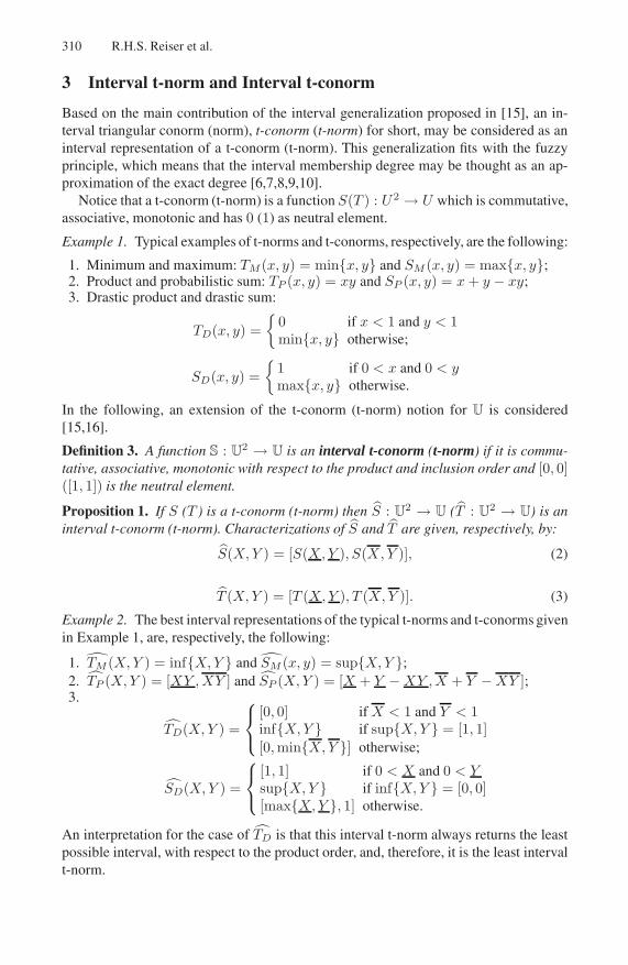
310 R.H.S. Reiser et al.
3 Interval t-norm and Interval t-conorm
Based on the main contribution of the interval generalization proposed in [15], an in-terval triangular conorm (norm), t-conorm (t-norm) for short, may be considered as aninterval representation of a t-conorm (t-norm). This generalization fits with the fuzzyprinciple, which means that the interval membership degree may be thought as an ap-proximation of the exact degree [6,7,8,9,10].
Notice that a t-conorm (t-norm) is a function S(T ) : U2 → U which is commutative,associative, monotonic and has 0 (1) as neutral element.
Example 1. Typical examples of t-norms and t-conorms, respectively, are the following:
1. Minimum and maximum: TM (x, y) = min{x, y} and SM (x, y) = max{x, y};2. Product and probabilistic sum: TP (x, y) = xy and SP (x, y) = x + y − xy;3. Drastic product and drastic sum:
TD(x, y) ={
0 if x < 1 and y < 1min{x, y} otherwise;
SD(x, y) ={
1 if 0 < x and 0 < ymax{x, y} otherwise.
In the following, an extension of the t-conorm (t-norm) notion for U is considered[15,16].
Definition 3. A function S : U2 → U is an interval t-conorm (t-norm) if it is commu-
tative, associative, monotonic with respect to the product and inclusion order and [0, 0]([1, 1]) is the neutral element.
Proposition 1. If S (T ) is a t-conorm (t-norm) then S : U2 → U (T : U
2 → U) is aninterval t-conorm (t-norm). Characterizations of S and T are given, respectively, by:
S(X, Y ) = [S(X, Y ), S(X, Y )], (2)
T (X, Y ) = [T (X, Y ), T (X, Y )]. (3)
Example 2. The best interval representations of the typical t-norms and t-conorms givenin Example 1, are, respectively, the following:
1. TM (X, Y ) = inf{X, Y } and SM (x, y) = sup{X, Y };2. TP (X, Y ) = [XY , XY ] and SP (X, Y ) = [X + Y − XY , X + Y − XY ];3.
TD(X, Y ) =
⎧⎨
⎩
[0, 0] if X < 1 and Y < 1inf{X, Y } if sup{X, Y } = [1, 1][0, min{X, Y }] otherwise;
SD(X, Y ) =
⎧⎨
⎩
[1, 1] if 0 < X and 0 < Ysup{X, Y } if inf{X, Y } = [0, 0][max{X, Y }, 1] otherwise.
An interpretation for the case of TD is that this interval t-norm always returns the leastpossible interval, with respect to the product order, and, therefore, it is the least intervalt-norm.

Interval Valued QL-Implications 311
4 Interval Fuzzy Negation
A function N : U → U is a fuzzy negation if
N1: N(0) = 1 and N(1) = 0;N2: If x ≥ y then N(x) ≤ N(y), ∀x, y ∈ I .
In addition, fuzzy negations satisfying the involutive property are called strong fuzzynegations [22,23]:
N3: N(N(x)) = x, ∀x ∈ U .
Example 3. A typical example of a strong fuzzy negation is the complement, that is,the function NC(x) = 1 − x.
When the t-norm is considered, it is also possible to establish a partial order on fuzzynegations in a natural way. Considering two fuzzy negations N1 and N2, define:
N1 ≤ N2 if, for each x ∈ U, N1(x) ≤ N2(x).
Remark 2. If N1 ≤ N2 and x ≥ y then N1(x) ≤ N2(y).
Definition 4. An interval function N : U −→ U is an interval fuzzy negation if, forany X , Y in U, the following properties hold:
N1 : N([0, 0]) = [1, 1] and N([1, 1]) = [0, 0];N2 : If X ≥ Y then N(X) ≤ N(Y );N3 : If X ⊆ Y then N(X) ⊆ N(Y ).
If N also meets the involutive property, it is said to be a strong interval fuzzy negation:
N4 : N(N(X)) = X , ∀X ∈ U.
Let N : U −→ U be a fuzzy negation. A characterization of N is given by:
N(X) = [N(X), N(X)]. (4)
Example 4. The best interval representation of the strong negation NC , given in Exam-ple 3, is NC(X) = [1 − X, 1 − X].
Theorem 2. Let N : U −→ U be a (strong) fuzzy negation. Then N is a (strong)interval fuzzy negation.
5 Fuzzy Implication
Several definitions for fuzzy implication together with related properties have beengiven (see, e.g., [23,24,25,26,27,28,29,30,31,32,33]). The unique consensus in thesedefinitions is that the fuzzy implication should have the same behavior as the classi-cal implication for the crisp case. Thus, a binary function I : U2 −→ U is a fuzzyimplication if I meets the minimal boundary conditions:

312 R.H.S. Reiser et al.
I(1, 1) = I(0, 1) = I(0, 0) = 1 and I(1, 0) = 0.
Several reasonable extra properties may be required for fuzzy implications. The onlytwo properties considered in this paper are the following:
I1: If y ≤ z then I(x, y) ≤ I(x, z) (second place isotonicity);I2: I(1, x) = x, (left neutrality principle);
5.1 QL-Implication
Let S be a t-conorm, N be a strong fuzzy negation and T be a t-norm. A fuzzy impli-cation, called QL-implication, is defined by
IS,N,T (x, y) = S(N(x), T (x, y)), ∀(x, y) ∈ [0, 1]. (5)
Example 5. The QL-implications defined from the t-norms and the t-conorms given inExample 1 and the strong negation presented in Example 3 are the following:
1.
ITM ,SM ,NC (x, y)=max{1−x, min{x, y}}=
⎧⎨
⎩
1 − x if x ≤ 0.5min{x, y} if min{x, y} ≥ 0.5max{1 − x, y} otherwise.
2. ITP ,SP ,NC(x, y) = 1 + x2y − x.3.
ITD ,SD ,NC(x, y) =
⎧⎨
⎩
1 if y = 1;y if x = 1 and y < 1;1 − x otherwise.
Based on Sect. 3.3. in [34], a result relating the QL-implications presented abovewith the properties I1 and I2 is seen in the following proposition.
Proposition 2. Let I : U2 → U be a fuzzy implication. If I is an QL-implication thenthe properties I1 and I2 hold.
6 Interval Fuzzy Implication
According to the idea that values in interval mathematics are identified with degenerateintervals, the minimal properties of fuzzy implications can be naturally extended frominterval fuzzy degrees, when the respective degenerate intervals are considered. Thus, afunction I : U
2 −→ U is an interval fuzzy implication if the following conditions hold:
I([1, 1], [1, 1]) = I([0, 0], [0, 0]) = I([0, 0], [1, 1]) = [1, 1] and I([1, 1], [0, 0]) = [0, 0].
The two extra properties of fuzzy implication seen in the previous section can be natu-rally extended.

Interval Valued QL-Implications 313
I1 : If Y ≤ Z then I(X, Y ) ≤ I(X, Z);I2 : I([1, 1], X) = X .
Starting from any fuzzy implication I , it is always possible to obtain canonically aninterval fuzzy implication I. Then, the interval fuzzy implication I also meets the opti-mality property and preserves the same properties satisfied by the fuzzy implication I .In the following two propositions, the best interval representation I of fuzzy implicationI is shown as an inclusion-monotonic function in both arguments. The related proofsare constructed straightforwardly from the definition of the interval fuzzy implicationI . See [16].
Proposition 3. If I is a fuzzy implication then I is an interval fuzzy implication.
We can recover the original fuzzy implication from its best interval representation.
Proposition 4. If I is a fuzzy implication then, for each x, y ∈ U , it holds thatI(x, y) = l(I([x, x], [y, y])) = r(I([x, x], [y, y])).
Proposition 5. Let I be a fuzzy implication. For each X1, X2, Y1, Y2 ∈ U, if X1 ⊆ X2and Y1 ⊆ Y2 then I(X1, Y1) ⊆ I(X2, Y2).
Proof. If X1 ⊆ Y1 and X2 ⊆ Y2, then, since I(X, Y ) = {I(x, y) : x ∈ X and y ∈ Y },it holds that I(X1, Y1) ⊆ I(X2, Y2). So, we have that inf I(X1, Y1) ≥ inf I(X2, Y2)and sup I(X1, Y1) ≤ sup I(X2, Y2). Thus, since I(X, Y ) = [inf I(X, Y ),sup I(X, Y )], it holds that I(X1, Y1) ⊆ I(X2, Y2).
Theorem 3. Let I be a fuzzy implication. I satisfies the property I1 (I2) iff I satisfiesthe property I1 (I2).
Proof. (⇒) If I satisfies I1, then, for each X, Y, Z ∈ U, I(X, Y ) = [inf{I(x, Y ) : x ∈X}, sup{I(x, Y ) : x ∈ X}] and I(X, Z) = [inf{I(x, Z) : x ∈ X}, sup{I(x, Z) :x ∈ X}]. Therefore, if Y ≤ Z , then I(X, Y ) ≤ I(X, Z) and, thus, I satisfies I1.
If I satisfies I2, then, for each x ∈ X , I(1, x) = x and, thus, {I(1, x) : x ∈ X} =X . Thus, since I([1, 1], X) is the narrowest interval containing {I(1, x) : x ∈ X}, thenI([1, 1], X) = X and so I satisfies I2.
(⇐) Consider y, z ∈ U such that y ≤ z. Then, it holds that [y, y] ≤ [z, z]. Thus, ifI satisfies I1, then, for each x ∈ U, I([x, x], [y, y]) ≤ I([x, x], [z, z]) and, therefore,l(I([x, x], [y, y])) ≤ l(I([x, x], [z, z])). Hence, by Prop. 4, I(x, y) ≤ I(x, z) and, thus,I satisfies I1.
If I satisfies I2, then for each x ∈ U , I([1, 1], [x, x])) = [x, x]. So, from Prop. 4, itholds that I(1, x) = l(I([1, 1], [x, x])) = l([x, x]) = x. Therefore, I satisfies I2.
6.1 Interval QL-Implication
An interval fuzzy implication I is an interval QL-implication if there are an intervalt-conorm S, a strong interval fuzzy negation N and an interval t-norm T such that
IS,N,T(X, Y ) = S(N(X), T(X, Y )). (6)
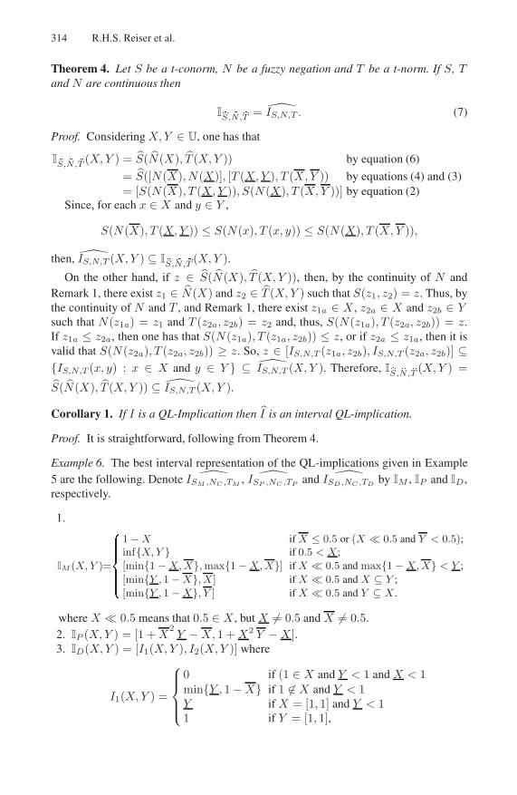
314 R.H.S. Reiser et al.
Theorem 4. Let S be a t-conorm, N be a fuzzy negation and T be a t-norm. If S, Tand N are continuous then
I�S, �N,�T = IS,N,T . (7)
Proof. Considering X, Y ∈ U, one has that
I�S, �N,�T (X, Y ) = S(N(X), T (X, Y )) by equation (6)
= S([N(X), N(X)], [T (X, Y ), T (X, Y )) by equations (4) and (3)= [S(N(X), T (X, Y )), S(N(X), T (X, Y ))] by equation (2)
Since, for each x ∈ X and y ∈ Y ,
S(N(X), T (X, Y )) ≤ S(N(x), T (x, y)) ≤ S(N(X), T (X, Y )),
then, IS,N,T (X, Y ) ⊆ I�S, �N,�T (X, Y ).
On the other hand, if z ∈ S(N(X), T (X, Y )), then, by the continuity of N andRemark 1, there exist z1 ∈ N(X) and z2 ∈ T (X, Y ) such that S(z1, z2) = z. Thus, bythe continuity of N and T , and Remark 1, there exist z1a ∈ X , z2a ∈ X and z2b ∈ Ysuch that N(z1a) = z1 and T (z2a, z2b) = z2 and, thus, S(N(z1a), T (z2a, z2b)) = z.If z1a ≤ z2a, then one has that S(N(z1a), T (z1a, z2b)) ≤ z, or if z2a ≤ z1a, then it isvalid that S(N(z2a), T (z2a, z2b)) ≥ z. So, z ∈ [IS,N,T (z1a, z2b), IS,N,T (z2a, z2b)] ⊆{IS,N,T (x, y) : x ∈ X and y ∈ Y } ⊆ IS,N,T (X, Y ). Therefore, I
�S, �N,�T (X, Y ) =
S(N(X), T (X, Y )) ⊆ IS,N,T (X, Y ).
Corollary 1. If I is a QL-Implication then I is an interval QL-implication.
Proof. It is straightforward, following from Theorem 4.
Example 6. The best interval representation of the QL-implications given in Example5 are the following. Denote ISM ,NC ,TM , ISP ,NC ,TP and ISD ,NC ,TD by IM , IP and ID ,respectively.
1.
IM (X, Y )=
�����������
1 − X if X ≤ 0.5 or (X � 0.5 and Y < 0.5);inf{X, Y } if 0.5 < X;[min{1 − X, X}, max{1 − X, X}] if X � 0.5 and max{1 − X, X} < Y ;[min{Y , 1 − X}, X] if X � 0.5 and X ⊆ Y ;[min{Y , 1 − X}, Y ] if X � 0.5 and Y ⊆ X.
where X � 0.5 means that 0.5 ∈ X , but X = 0.5 and X = 0.5.2. IP (X, Y ) = [1 + X
2Y − X, 1 + X2 Y − X ].
3. ID(X, Y ) = [I1(X, Y ), I2(X, Y )] where
I1(X, Y ) =
⎧⎪⎪⎨
⎪⎪⎩
0 if (1 ∈ X and Y < 1 and X < 1min{Y , 1 − X} if 1 ∈ X and Y < 1Y if X = [1, 1] and Y < 11 if Y = [1, 1],

Interval Valued QL-Implications 315
I2(X, Y ) =
⎧⎨
⎩
1 if 0 ∈ X or 1 ∈ Ymax{Y , 1 − X} if 1 ∈ X , Y < 11 − X 1 ∈ X .
Proposition 6. Let I be an interval fuzzy implication. If I is an interval QL-implicationthen the properties I1 and I2 hold.
Proof. Consider I as an interval QL-implication and X, Y, Z ∈ U.I1: Based on the monotonicity of the interval t-norm T and the interval t-conorm S,if Y ≤ Z then S(N(X), T(X, Y )) ≤ S(N(X), T(X, Z)). Therefore, IS,N,T(X, Y ) ≤IS,N,T(X, Z).I2: IS,N,T([1, 1], X) = S(N([1, 1]), T([1, 1], X)) = S([0, 0], X) = X .
Denote by C(S), C(T ), C(N) and C(I) the classes of continuous t-conorms, continuoust-norms, strong fuzzy negations and continuous QL-implications, respectively. The re-lated interval extensions are indicated by C(S), C(T), C(N) and C(I), respectively. Theresults in Sect. 6.1 together with Theorem 4 state the commutativity of the diagram inFig. 1.
C(S) × C(N) × C(T )eq(5) � C(I)
C(S) × C(N) × C(T)
(eq(2), eq(4), eq(3))
� eq(6) � C(I)
eq(7)
�
Fig. 1. Commutative classes of interval implications
7 Propagation of an Interval Uncertainty in IntervalQL-Implications
In this section, we show how the initial uncertainties of the membership degrees arepropagated by the best interval representations of QL-implications, analyzing the inter-val QL-implication IM presented in Example 6. Observe that the measure of the un-certainty of an interval X is given by its width (ou diameter), defined as width(X) =X − X .
If X ≤ 0.5, one has that IM (X, Y ) = 1 − X , and, therefore, the measure of theuncertainty of IM (X, Y ) is given by the width of X . Observe that the width of Y doesnot have any influence in the result.
When 0.5 < X , the measure of the uncertainty of IM (X, Y ) is given by the widthof the interval Z = inf{X, Y }, which is always smaller or equal than width(X), orwidth(Y ), or both.
If X � 0.5 and 0.5 < Y , then one has that IM (X, Y ) = 1 − X , and, therefore, themeasure of the uncertainty of IM (X, Y ) is given by the width of X .
If X � 0.5 and X ⊆ Y (or Y ⊆ X), then the measure of the uncertainty ofIM (X, Y ) is between the widths of X and Y .

316 R.H.S. Reiser et al.
If X and Y are degenerate intervals, then the best interval representation of a QL-implication also returns a degenerate interval.
In the case of IP , the uncertainty always increases, or, in the best case, it remains thesame (for example, for degenerate intervals).
Summarizing, the propagation of the uncertainty in the case of a multi-level rea-soning process using interval QL-implication depends on the particular case, that is,for some interval QL-implications it always either increases or remains the same, but,for other cases, it may always either diminish or remain the same. However, for themajority, the uncertainty will increase for some cases and diminish for other cases.
8 Interval Automorphism
Definition 5. A mapping ρ : U −→ U is an automorphism if it is bijective andmonotonic: x ≤ y ⇒ ρ(x) ≤ ρ(y) [35,36].
An equivalent definition is given in [23], where ρ : U −→ U is an automorphism if it isa continuous and strictly increasing function such that ρ(0) = 0 and ρ(1) = 1. Aut(U)denotes the set of all automorphisms on U . Automorphisms are closed under composi-tion: if ρ and ρ′ are automorphisms then ρ ◦ ρ′(x) = ρ(ρ′(x)) is also an automorphism.The inverse of an automorphism is also an automorphism. Let ρ be an automorphismand I be a fuzzy implication. The action of ρ on I , denoted by Iρ, defined as follows
Iρ(x, y) = ρ−1(I(ρ(x), ρ(y))) (8)
is a fuzzy implication. Moreover, if I is an QL-implication then Iρ is also an QL-implication.
8.1 Canonical Construction of an Interval Automorphism
A mapping � : U −→ U is an interval automorphism if it is bijective and monotonicw.r.t. the product order [37,38], that is, X ≤ Y implies that �(X) ≤ �(Y ). The set of allinterval automorphisms on U is denoted by Aut(U). In what follows, the equation (9)provides a canonical construction of interval automorphisms from automorphisms and,therefore, a bijection between the sets Aut(U) and Aut(U). See Theorem 3 of [37].
Theorem 5. Let � : U −→ U be an interval automorphism. Then there exists an auto-morphism ρ : U −→ U such that
�(X) = [ρ(X), ρ(X)]. (9)
8.2 The Best Interval Representation of an Automorphism
Interval automorphisms can be generated as best interval representations of automor-phisms. The following results were proved in [15].

Interval Valued QL-Implications 317
Theorem 6 (Automorphism representation theorem). Let ρ : U → U be an auto-morphism. ρ is an interval automorphism and its characterization is given by
ρ(X) = [ρ(X), ρ(X)]. (10)
Corollary 2. Consider � : U −→ U. � is an interval automorphism iff there is anautomorphism ρ : U → U , such that � = ρ.
Proof. It is straightforward, following from Theorems 5 and 6.
Thus, each interval automorphism is the best interval representation of some automor-phism. Notice that t-conorms were required by definition to satisfy ⊆-monotonicity.Nevertheless, this property was not required by the definition of interval automorphism.As described in [15], interval automorphisms are ⊆-monotonic.
Corollary 3. If � is an interval automorphism then � is inclusion monotonic, that is, ifX ⊆ Y then �(X) ⊆ �(Y ).
Analogously, considering the definition of automorphism used by [23], we can providealternative characterizations for interval automorphisms based on the Moore and Scottcontinuities. Consider � : U −→ U. � is strictly increasing if, for each X, Y ∈ U, ifX < Y (i.e. X ≤ Y and X = Y ) then �(X) < �(Y ).
Proposition 7. Consider � : U −→ U. � is an interval automorphism iff � is Moore-continuous, strictly increasing, �([0, 0]) = [0, 0] and �([1, 1]) = [1, 1].
Corollary 4. Let � : U −→ U be a Moore-continuous and strictly increasing functionsuch that �([0, 0]) = [0, 0] and �([1, 1]) = [1, 1]. Then there exists an automorphism ρsuch that � = ρ.
The case of Scott-continuity follows the same setting.
Lemma 1. Let �1 and �2 be interval automorphisms. Then it holds that (�1 ◦ �2)−1 =�−12 ◦ �−1
1 .
Lemma 2. Let ρ be an automorphism. Then it holds that
ρ−1 = ρ−1. (11)
In the following theorem, an interval automorphism � acts on an interval fuzzy impli-cation I, generating a new interval fuzzy implication I
�.
Theorem 7. Let � : U −→ U be an interval automorphism and I : U2 −→ U be an
interval implication. Then the mapping I� : U
2 −→ U, defined by
I�(X, Y ) = �−1(I(�(X), �(Y ))), (12)
is an interval implication.
Theorem 8. Let I be a an implication and ρ be an automorphism. Then it holds thatIρ = I�ρ.

318 R.H.S. Reiser et al.
Proof. Considering X, Y ∈ U, one has that
Iρ(X, Y ) = [inf{Iρ(x, y) : x ∈ X and y ∈ Y },sup{Iρ(x, y) : x ∈ X and y ∈ Y }] by equation (1)
= [inf{ρ−1(I(ρ(x), ρ(y))) : x ∈ X and y ∈ Y },sup{ρ−1(I(ρ(x), ρ(y))) : x ∈ X and y ∈ Y }] by equation (8)
= [ρ−1(inf{I(ρ(x), ρ(y)) : x ∈ X and y ∈ Y }),ρ−1(sup{I(ρ(x), ρ(y)) : x ∈ X and y ∈ Y })] by continuity of ρ−1
= ρ−1([inf{I(ρ(x), ρ(y)) : x ∈ X and y ∈ Y },sup{I(ρ(x), ρ(y)) : x ∈ X and y ∈ Y }]) by equation( 8)
= ρ−1([inf{I(x, y) : x ∈ ρ(X) and y ∈ ρ(Y )},sup{I(x, y) : x ∈ ρ(X) and y ∈ ρ(Y )}]) by continuity of ρ
= ρ−1([inf{I(x, y) : x ∈ ρ(X) and y ∈ ρ(Y )},sup{I(x, y) : x ∈ ρ(X) and y ∈ ρ(Y )}]) by Remark 1
= ρ−1(I(ρ(X), ρ(Y ))) by equation (1)= ρ−1(I(ρ(X), ρ(Y ))) by equation (11)= I�ρ(X, Y ) by equation (12)
Proposition 8. Let I be an interval implication and �1 and �2 be interval automor-phisms. Then it holds that (I�1 )�2 = I
�1◦�2 .
Proposition 9. Let N be an interval fuzzy negation and � be an interval automorphism.Then it is valid that
N�(X) = �−1(N(�(X))). (13)
In the following, we apply the results presented in the last subsection, concerned withthe generation of new interval implications based on the action of interval automor-phisms. In particular, we consider the interval extensions of QL-implications.
8.3 Interval Automorphism Acting on Interval QL-Implication
Theorem 9. Let � : U −→ U be an interval automorphism and I : U2 −→ U be an
interval QL-implication. Then I� : U
2 −→ U is an interval QL-implication defined by
I�S,N,T(X, Y ) = S
�(N�(X), T�(X, Y )). (14)
Proof. Considering X, Y ∈ U, we have thatI�S,N,T(X, Y ) = �−1(IS,N,T (�(X), �(Y ))) by equation (12)
= �−1(S(N(�(X)), T(�(X), �(Y )))) by equation (6)= �−1(S(� ◦ �−1(N(�(X))), � ◦ �−1(T(�(X), �(Y )))))= �−1(S(�(N�(X)), �(T�(X, Y )))) by equations(13)
and (7) in [15]= S
�(N�(X), T�(X, Y ))
According to Theorem 8, the commutative diagram pictured in Fig. 2 holds.Based on Theorems 8 and 9, (interval) QL-implications and (interval) automor-
phisms can be seen as objects and morphisms of the category C(C(I), Aut(I)) (C(C(I),

Interval Valued QL-Implications 319
C(I)eq(8) � C(I)
C(I)
eq(7)
� eq(14) � C(I)
eq(7)
�
Fig. 2. Commutative classes of interval QL-implications and automorphisms
Aut(I))), respectively. In a categorical approach, the action of an interval automor-phism on an interval QL-implication can be conceived as a covariant functor whoseapplication over the QL-implications and automorphisms in C(C(I), Aut(I)) returnsthe related best interval representations in C(C(I), Aut(I)). Therefore, interval auto-morphisms can be used to deal with optimality of interval fuzzy algorithms.
9 Conclusion and Final Remarks
This work emphasized that both interval mathematics and fuzzy set theory are firmlyintegrated with principles of information theory used to underlying logic system for ex-pert systems. Thus, this paper complements the results of previous work [15], extendingthe generalization of the main properties of interval fuzzy QL-implication and intervalautomorphisms. The interval extension considers the best interval representation of areal function to deal with the imprecision of a specialist in providing an exact value tomeasure membership uncertainty.
In this work, intervals are used to model the uncertainty of a specialist’s informationrelated to truth values in the fuzzy propositional calculus. The basic systems are basedon interval t-conorms. Using subsets of the real unit interval as the standard sets oftruth degrees and applying continuous t-conorms and negation as standard truth intervalfunctions, the standard truth interval function of an QL-implication can be obtained.
In addition, we mainly discussed under which conditions generalized fuzzy QL-implications applied to interval values preserve properties of canonical forms gener-ated by interval t-conorms and interval t-norms. It is shown that properties of fuzzylogic may be naturally extended for interval fuzzy degrees considering the respectivedegenerate intervals. The significance of interval fuzzy QL-implication is emphasized,showing that interval QL-implications can be constructed from interval automorphisms,which are preserved by the interval canonical representation. These results are impor-tant not only to analyze deductive systems in mathematical depth but also as founda-tions of methods based on interval fuzzy logic. They provide the accuracy criteria andthe optimality property of computer computations integrated to a formal mathematicaltheory for the representation of uncertainty, concerned with fuzzy set theory.
Acknowledgments
This work was partially supported by the Brazilian funding agency CNPq (Proc. 470871/2004-0). We are are very grateful to the referees for their valuable suggestions that helpus to improve the paper.

320 R.H.S. Reiser et al.
References
1. Hickey, T., Ju, Q., Emdem, M.: Interval arithmetic: from principles to implementation. Jour-nal of the ACM 48(5), 1038–1068 (2001)
2. Moore, R.: Methods and Applications of Interval Analysis. SIAM, Philadelphia (1979)3. Alefeld, G., Herzberger, J.: Introduction to Interval Computations. Academic Press, New
York (1983)4. Moore, R.E.: Interval Arithmetic and Automatic Error Analysis in Digital Computing. PhD
thesis, Stanford University, Stanford (1962)5. Kearfort, R.B., Kreinovich, V. (eds.): Applications of Interval Computations. Kluwer Acad-
emic Publishers, Boston (1996)6. Nguyen, H., Kreinovich, V., Zuo, Q.: Interval-valued degrees of belief: applications of inter-
val computations to expert systems and intelligent control. International Journal of Uncer-tainty, Fuzziness, and Knowledge-Based Systems 5(3), 317–358 (1997)
7. Walley, P.: Statistical Reasoning with Imprecise Probabilities. Chapman & Hall, London(1991)
8. Walley, P.: Measures of uncertainty. Artificial Intelligence 83, 1–58 (1996)9. Dubois, D., Prade, H.: Interval-valued fuzzy sets, possibility theory and imprecise probabil-
ity. In: Proc. Intl. Conf. Fuzzy Logic and Technology, Barcelona, pp. 314–319 (2005)10. Lodwick, W.: Preface. Reliable Computing 10(4), 247–248 (2004)11. Turksen, I.: Fuzzy normal forms. Fuzzy Sets and Systems 69, 319–346 (1995)12. Moore, R., Lodwick, W.: Interval analysis and fuzzy set theory. Fuzzy Sets and Sys-
tems 135(1), 5–9 (2003)13. Gasse, B.V., Cornelis, G., Deschrijver, G., Kerre, E.: On the properties of a generalized class
of t-norms in interval-valued fuzzy logics. New Mathematics and Natural Computation 2,29–42 (2006)
14. Zadeh, L.A.: The concept of a linguistic variable and its application to approximate reasoning- I. Information Sciences 6, 199–249 (1975)
15. Bedregal, B., Takahashi, A.: The best interval representation of t-norms and automorphisms.Fuzzy Sets and Systems 157(24), 3220–3230 (2006)
16. Bedregal, B., Takahashi, A.: Interval valued versions of t-conorms, fuzzy negations and fuzzyimplications. In: IEEE Proc. Intl. Conf. on Fuzzy Systems, Vancouver, Vancouver, pp. 9553–9559. IEEE Computer Society Press, Los Alamitos (2006)
17. Santiago, R., Bedregal, B., Acioly, B.: Formal aspects of correctness and optimality in inter-val computations. Formal Aspects of Computing 18(2), 231–243 (2006)
18. Callejas-Bedregal, R., Bedregal, B.: Intervals as a domain constructor. TEMA 2(1), 43–52(2001), http://www.sbmac.org.br/tema
19. Kearfott, R.B.: Rigorous Global Search: Continuous problems. Kluwer Academic Publish-ers, Dordrecht (1996)
20. Caprani, O., Madsen, K., Stauning, O.: Existence test for asynchronous interval iteration.Reliable Computing 3(3), 269–275 (1997)
21. Jaulin, L., Kieffer, M., Didrit, O., Walter, E.: Applied Interval Analisys: With examples inparameter and state estimation, robust control and robotic. Springer, Heidelberg (2001)
22. Klement, E., Mesiar, R., Pap, E.: Triangular Norms. Kluwer Academic Publishers, Dordrecht(2000)
23. Bustince, H., Burilo, P., Soria, F.: Automorphism, negations and implication operators. FuzzySets and Systems 134, 209–229 (2003)
24. Baczynski, M.: Residual implications revisited. Notes on the Smets-Magrez. Fuzzy Sets andSystems 145(2), 267–277 (2004)

Interval Valued QL-Implications 321
25. Balasubramaniam, J.: Yager’s new class of implications Jf and some classical tautologies.Information Sciences (2006)
26. Fodor, J.C.: On fuzzy implication operators. Fuzzy Sets and Systems 42, 293–300 (1991)27. Fodor, J., Roubens, M.: Fuzzy Preference Modelling and Multicriteria Decision Support.
Kluwer Academic Publishers, Dordrecht (1994)28. Horcik, R., Navara, M.: Validation sets in fuzzy logics. Kybernetika 38(2), 319–326 (2002)29. Leski, J.: ε-insensitive learning techniques for approximate reasoning system. International
Jour. of Computational Cognition 1(1), 21–77 (2003)30. Ruan, D., Kerre, E.: Fuzzy implication operators and generalized fuzzy methods of cases.
Fuzzy Sets and Systems 54, 23–37 (1993)31. Yager, R.: On the implication operator in fuzzy logic. Information Sciences 31, 141–164
(1983)32. Yager, R.: On global requirements for implication operators in fuzzy modus ponens. Fuzzy
Sets and Systems 106, 3–10 (1999)33. Yager, R.: On some new classes of implication operators and their role in approximate rea-
soning. Information Sciences 167, 193–216 (2004)34. Shi, Y., Ruan, D., Kerre, E.E.: On the characterizations of fuzzy implications satisfying I(x,y)
= I(x,I(x,y)). Information Sciences 177(14), 2954–2970 (2007)35. Klement, E., Navara, M.: A survey on different triangular norm-based fuzzy logics. Fuzzy
Sets and Systems 101, 241–251 (1999)36. Navara, M.: Characterization of measures based on strict triangular norms. Mathematical
Analysis and Applications 236, 370–383 (1999)37. Gehrke, M., Walker, C., Walker, E.: Some comments on interval valued fuzzy sets. Interna-
tional Journal of Intelligent Systems 11, 751–759 (1996)38. Gehrke, M., Walker, C., Walker, E.: Algebraic aspects of fuzzy sets and fuzzy logics. In:
Proc. of the Work. on Current Trends and Development in Fuzzy Logic, Thessaloniki, pp.101–170 (1999)

Behavioural Differential Equations and
Coinduction for Binary Trees
Alexandra Silva1,� and Jan Rutten1,2
1 Centrum voor Wiskunde en Informatica (CWI)2 Vrije Universiteit Amsterdam (VUA)
{ams,janr}@cwi.nl
Abstract. We study the set TA of infinite binary trees with nodes la-belled in a semiring A from a coalgebraic perspective. We present coin-ductive definition and proof principles based on the fact that TA carriesa final coalgebra structure. By viewing trees as formal power series, wedevelop a calculus where definitions are presented as behavioural differ-ential equations. We present a general format for these equations thatguarantees the existence and uniqueness of solutions. Although techni-cally not very difficult, the resulting framework has surprisingly niceapplications, which is illustrated by various concrete examples.
1 Introduction
Infinite data structures are often used to model problems and computing solu-tions for them. Therefore, reasoning tools for such structures have become moreand more relevant. Coalgebraic techniques turned out to be suited for provingand deriving properties of infinite systems.
In [6], a coinductive calculus of formal power series was developed. In closeanalogy to classical analysis, the definitions were presented as behavioural dif-ferential equations and properties were proved in a calculational (and very nat-ural) way. This approach has shown to be quite effective for reasoning aboutstreams [6,7] and it seems worthwhile to explore its effectiveness for other datastructures as well.
In this paper, we shall take a coalgebraic perspective on a classical data struc-ture – infinite binary trees, and develop a similar calculus, using the fact thatbinary trees are a particular case of formal power series.
The contributions of the present paper are: a coinductive calculus, based on thenotion of derivative, to define and to reason about trees and functions on trees;a set of illustrative examples and properties that show the usefulness and expres-siveness of such calculus; the formulation of a general format that guarantees theexistence and uniqueness of solutions of behavioural differential equations.
Infinite trees arise in several forms in other areas. Formal tree series (functionsfrom trees to an arbitrary semiring) have been studied in [3], closely related to� Partially supported by the Fundacao para a Ciencia e a Tecnologia, Portugal, under
grant number SFRH/BD/27482/2006.
D. Leivant and R. de Queiroz (Eds.): WoLLIC 2007, LNCS 4576, pp. 322–336, 2007.c© Springer-Verlag Berlin Heidelberg 2007

Behavioural Differential Equations and Coinduction for Binary Trees 323
distributive Σ-algebras. The work presented in this paper is completely differentsince we are concerned with infinite binary trees and not with formal series overtrees. In [5], infinite trees appear as generalisations of infinite words and anextensive study of tree automata and topological aspects of trees is made. Wehave not yet addressed the relation of our work with automata theory. Here weemphasize coinductive definition and proof principles for defining and reasoningabout (functions on) trees.
At the end of the paper, in Section 6, the novelty of our approach is discussedfurther. Also several directions for further applications are mentioned there.
2 Trees and Coinduction
We introduce the set TA of infinite node-labelled binary trees, show that TAsatisfies a coinduction proof principle and illustrate its usefulness.
The set TA of infinite node-labelled binary trees, where to each node is as-signed a value in A, is the final coalgebra for the functor FX = X ×A×X andcan be formally defined by:
TA = {t | t : {L,R}∗ → A}The set TA carries a final coalgebra structure consisting of the following
function:〈l, i, r〉 : TA → TA ×A× TA
t �→ 〈λw.t(Lw), t(ε), λw.t(Rw)〉where l and r return the left and right subtrees, respectively, and i gives the labelof the root node of the tree. Here, ε denotes the empty word and, for b ∈ {L,R},bw denotes the word resulting from prefixing the word w with the letter b.
These definitions of the set TA and the respective coalgebra map may notseem obvious. The follow reasoning justifies its correctness:
– It is well known from the literature [4] that the final system for the functorG(X) = A×XB is (AB
∗, π), where
π : AB∗ → A× (AB
∗)B
π(φ) = 〈φ(ε), λb v. φ(bv)〉– The functor F is isomorphic to H(X) = A×X2.– Therefore, the set A2∗
is the final coalgebra for the functor F . Considering2 = {L,R} we can derive the definition of 〈l, i, r〉 from the one presentedabove for π.
The fact that TA is a final coalgebra means that for any arbitrary coalgebra〈lt, o, rt〉 : U → U × A × U , there exists a unique f : U → TA, such that thefollowing diagram commutes:
U∃!f ������������
〈lt,o,rt〉��
TA
〈l,i,r〉��
U ×A× Uf×idA×f
�� TA ×A× TA

324 A. Silva and J. Rutten
The existence part of this statement gives us a coinductive definition principle.Every triplet of functions lt : U → U , o : U → A and rt : U → U defines afunction h : U → TA, such that:
i(h(x)) = o(x) l(h(x)) = h(lt(x)) r(h(x)) = h(rt(x))
We will see a more general formulation of this principle in section 3, wherethe right hand side of the above equations will be more general.
Taking A = R we present the definition of the elementwise sum as an example.
f g
c
a
d e
b +w x
t
r
u v
s =
f+w g+x
c+t
a+r
d+u e+v
b+s
By the definition principle presented above, taking o(〈σ, τ〉) = i(σ) + i(τ),lt(〈σ, τ〉) = 〈l(σ), l(τ)〉 and rt(〈σ, τ〉) = 〈r(σ), r(τ)〉 there is a unique function+ : TR × TR → TR satisfying:
i(σ + τ) = i(σ) + i(τ) l(σ + τ) = l(σ) + l(τ) r(σ + τ) = r(σ) + r(τ)
Note that in the first equation above we are using + to represent both thesum of trees and the sum of real numbers.
Now that we have explained the formal definition for the set TA and how onecan uniquely define functions into TA, another important question is still to beanswered: how do we prove equality on TA? In order to prove that two trees σand τ are equal it is necessary and sufficient to prove
∀w∈{L,R}∗ σ(w) = τ(w) (1)
The use of induction on w (prove that σ(ε) = τ(ε) and that wheneverσ(w) = τ(w) holds then σ(aw) = τ(aw) also holds, for a ∈ {L,R}) clearly is acorrect method to establish the validity of (1). However, we will often encounterexamples where there is not a general formula for σ(w) and τ(w). Instead, wetake a coalgebraic perspective on TA and use the coinduction proof principlein order to establish equalities. This proof principle is based on the notion ofbisimulation. A bisimulation on TA is a relation S ⊆ TA × TA such that, for allσ and τ in TA,
(σ, τ) ∈ S ⇒ σ(ε) = τ(ε) ∧ (l(σ), l(τ)) ∈ S ∧ (r(σ), r(τ)) ∈ SWe will write σ ∼ τ whenever there exists a bisimulation that contains (σ, τ).
The relation ∼, called the bisimilarity relation, is the union of all bisimulations(one can easily check that the union of bisimulation is itself a bisimulation).
The following theorem expresses the proof principle mentioned above.
Theorem 1 (Coinduction). For all trees σ and τ in TA, if σ ∼ τ then σ = τ .
Proof. Consider two trees σ and τ in TA and let S ⊆ TA×TA be a bisimulationrelation which contains the pair (σ, τ). The equality σ(w) = τ(w) now follows
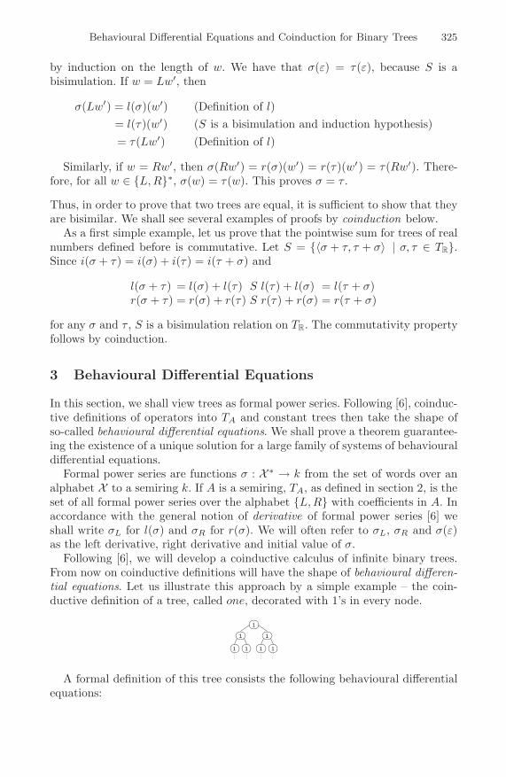
Behavioural Differential Equations and Coinduction for Binary Trees 325
by induction on the length of w. We have that σ(ε) = τ(ε), because S is abisimulation. If w = Lw′, then
σ(Lw′) = l(σ)(w′) (Definition of l)= l(τ)(w′) (S is a bisimulation and induction hypothesis)= τ(Lw′) (Definition of l)
Similarly, if w = Rw′, then σ(Rw′) = r(σ)(w′) = r(τ)(w′) = τ(Rw′). There-fore, for all w ∈ {L,R}∗, σ(w) = τ(w). This proves σ = τ .
Thus, in order to prove that two trees are equal, it is sufficient to show that theyare bisimilar. We shall see several examples of proofs by coinduction below.
As a first simple example, let us prove that the pointwise sum for trees of realnumbers defined before is commutative. Let S = {〈σ + τ, τ + σ〉 | σ, τ ∈ TR}.Since i(σ + τ) = i(σ) + i(τ) = i(τ + σ) and
l(σ + τ) = l(σ) + l(τ) S l(τ) + l(σ) = l(τ + σ)r(σ + τ) = r(σ) + r(τ) S r(τ) + r(σ) = r(τ + σ)
for any σ and τ , S is a bisimulation relation on TR. The commutativity propertyfollows by coinduction.
3 Behavioural Differential Equations
In this section, we shall view trees as formal power series. Following [6], coinduc-tive definitions of operators into TA and constant trees then take the shape ofso-called behavioural differential equations. We shall prove a theorem guarantee-ing the existence of a unique solution for a large family of systems of behaviouraldifferential equations.
Formal power series are functions σ : X ∗ → k from the set of words over analphabet X to a semiring k. If A is a semiring, TA, as defined in section 2, is theset of all formal power series over the alphabet {L,R} with coefficients in A. Inaccordance with the general notion of derivative of formal power series [6] weshall write σL for l(σ) and σR for r(σ). We will often refer to σL, σR and σ(ε)as the left derivative, right derivative and initial value of σ.
Following [6], we will develop a coinductive calculus of infinite binary trees.From now on coinductive definitions will have the shape of behavioural differen-tial equations. Let us illustrate this approach by a simple example – the coin-ductive definition of a tree, called one, decorated with 1’s in every node.
1 1
1
1
1 1
1
A formal definition of this tree consists the following behavioural differentialequations:

326 A. Silva and J. Rutten
differential equations initial valueoneL = oneoneR = one
one(ε) = 1
The fact that there exists a unique tree that satisfies the above equationswill follow from the theorem below, which presents a general format for be-havioural differential equations guaranteeing the existence and uniqueness ofsolutions.
Behavioural differential equations will be used not just to define single con-stant trees but also functions on trees. We shall see examples below. Beforewe present the main result of this section, we need one more definition. Wewant to be able to view any element n ∈ A as a tree (which we will denoteby [n]):
0 0
0
n
0 0
0
The tree [n] is formally defined as
[n](ε) = n[n](w) = 0 w �= ε
Next we present a syntax describing the format of behavioural differential equa-tions that we will consider. Let Σ be a set of function symbols, each with anarity r(f) ≥ 0 for f ∈ Σ. (As usual we call f a constant if r(f) = 0.) LetX = {x1, x2, . . .} be a set of (syntactic) variables, and let XL = {xL | x ∈ X},XR = {xR | x ∈ X}, [X(ε)] = {[x(ε)] | x ∈ X} and X(ε) = {x(ε) | x ∈ X}be sets of notational variants of them. The variables x ∈ X will play the roleof place holders for trees τ ∈ TA. Variables xL, xR, and [x(ε)] will then act asplace holders for the corresponding trees τL, τR and [τ(ε)] in TA, while x(ε)(without the square brackets) will correspond to τ ’s initial value τ(ε) ∈ A. Wecall a behavioural differential equation for a function symbol f ∈ Σ with arityr = r(f) well-formed if it is of the form
differential equations initial valuef (x1, . . . , xr )L = t1f (x1, . . . , xr )R = t2
( f (x1, . . . , xr ) ) (ε) = c(x1(ε), . . . , xr(ε))
where c : Ar → A is a given function, and where t1 and t2 are terms built outof function symbols in Σ and variables in {x1, . . . , xr} and their correspondingnotational variants in XL, XR and [X(ε)]. A well-formed system of equationsfor Σ will then consist of one well-formed equation for each f ∈ Σ. A solutionof such a system of equations is a set of tree functions

Behavioural Differential Equations and Coinduction for Binary Trees 327
Σ = {f : (TA)r → TA | f ∈ Σ}satisfying, for all f ∈ Σ with arity r and for all τ1, . . . , τr ∈ TA,
(f(τ1, . . . , τr)
)(ε) = c(τ1(ε), . . . , τr(ε))
and (f(τ1, . . . , τr)
)
L= t1 and
(f(τ1, . . . , τr)
)
R= t2
where the tree t1 ∈ TA (and similarly for t2) is obtained from the term t1by replacing (all occurrences of) xi by τi, (xi)L by (τi)L, (xi)R by (τi)R, and[xi(ε)] by [τi(ε)], for all i = 1, . . . , r, and all function symbols g ∈ Σ by theircorresponding function g.
Theorem 2. Let Σ be a set of function symbols. Every well-formed system ofbehavioural differential equations for Σ has precisely one solution of tree func-tions Σ.
Proof. Please see appendix A.
Let us illustrate the generality of this theorem by mentioning a few examplesof systems of differential equations that satisfy the format above. As a firstexample, take Σ = {one} consisting of a single constant symbol (with arity 0)and X = ∅. We observe that the differential equations for one mentioned at thebeginning of this section satisfy the format of the theorem. For a second example,let Σ = {+,×} with arities r(+) = r(×) = 2 and let X = {σ, τ}. Consider thefollowing equations:
differential equations initial value(σ + τ)L = σL + τL(σ + τ)R = σR + τR
(σ + τ)(ε) = σ(ε) + τ(ε)
differential equations initial value(σ × τ)L = (σL × τ) + ([σ(ε)]× τL)(σ × τ)R = (σR × τ) + ([σ(ε)] × τR) (σ × τ)(ε) = σ(ε) × τ(ε)
These equations define the operations of sum and convolution product of trees,to be further discussed in Section 4. Note that the right-hand side of the equationfor (σ × τ)L (and similarly for (σ × τ)R) is a good illustration of the generalformat: it is built from the functions + and ×, applied to (a subset of) thevariables on the left (τ), their derivatives (σL and τL), and their initial valuesviewed as trees ([σ(ε)]).
Clearly there are many interesting interesting instances of well-formed differ-ential equations. Note, however, that the format does impose certain restrictions.The main point is that in the right-hand sides of the equations, only single L andR derivatives are allowed. The following is an example of a system of equationsthat is not well-formed and that does not have a unique solution.
Let Σ = {f}, with arity r(f) = 1, and let X = {σ}. The equations for f are

328 A. Silva and J. Rutten
differential equations initial valuef(σ)L = f(f(σLL))f(σ)R = [0] f(σ)(ε) = σ(ε)
Both g(σ) = [σ(ε)] + (L × [σLL(ε)]) and h(σ) = [σ(ε)] + (L × [σLL(ε)] + L2 ×(1− L)−1) are solutions.
All the examples of systems of behavioural differential equations that willappear in the rest of this document fit into the format of Theorem 2. Therefore,we will omit proofs of the existence and uniqueness of solutions for those systems.
In the next section we will define operators on trees, based on some generaloperators on formal power series [6].
4 Tree Calculus
In this section, we present operators on trees, namely sum, convolution productand inverse, and state some elementary properties, which we will prove usingcoinduction.
The sum of two trees is defined as the unique operator satisfying:
differential equations initial value(σ + τ)L = σL + τL(σ + τ)R = σR + τR
(σ + τ)(ε) = σ(ε) + τ(ε)
Note that this is a generalisation of the sum on trees of real numbers definedin section 2 and that again we are overloading the use of + to represent bothsum on trees and sum on the elements of the semiring.
Sum satisfies some desired properties, easily proved by coinduction, such ascommutativity or associativity:Theorem 3. For all σ, τ and ρ in TA, σ+0 = σ, σ+τ = τ+σ and σ+(τ+ρ) =(σ + τ) + ρ.Here, we are using 0 as a shorthand for [0]. We shall use this convention (forall n ∈ A) throughout this document. We define the convolution product of twotrees as the unique operation satisfying:
differential equations initial value(σ × τ)L = (σL × τ) + (σ(ε)× τL)(σ × τ)R = (σR × τ) + (σ(ε)× τR) (σ × τ)(ε) = σ(ε)× τ(ε)
Note that in the above definition we use × for representing both multiplicationon trees and on the elements of the semiring. Following the convention mentionedabove σ(ε) × τL and σ(ε) × τR are shorthands for [σ(ε)] × τL and [σ(ε)] × τR.We shall also use the standard convention of writing στ for σ × τ .
The general formula to compute the value of σ according to a path given bythe word w ∈ {L,R}∗ is:
(σ × τ)(w) =∑
w=u·vσ(u)× τ(v)
where · denotes word concatenation.

Behavioural Differential Equations and Coinduction for Binary Trees 329
To give the reader some intuition about this operation we will give a concreteexample. Take A to be the Boolean semiring B = {0, 1}, with operations + = ∨and × = ∧. Then, TA corresponds to the languages over a two letter alphabet,and in this case the tree product operator coincides with language concatenation.
The following theorem states some familiar properties of this operator.
Theorem 4. For all σ, τ, ρ in TA and a, b in A, σ × 1 = 1 × σ = σ, σ × 0 =0 × σ = 0, σ × (τ + ρ) = (σ × τ) + (σ × ρ), σ × (τ × ρ) = (σ × τ) × ρ and[a]× [b] = [a× b].Proof. An exercise in coinduction. In [7], these properties are proved for streams.
Note that the convolution product is not commutative. Before we present theinverse operation, let us introduce two (very useful) constants, which we shallcall left constant L and right constant R. They will have an important role in thetree calculus that we are about to develop and will turn out to have interestingproperties when interacting with the product operation. The left constant L isa tree with 0’s in every node except in the root of the left branch where it hasa 1:
0 0
0
0
0 0
1L =
It is formally defined asL(w) = 1 if w = LL(w) = 0 otherwise
Similarly, the right constant R is only different from 0 in the root of its rightbranch:
0 0
1
0
0 0
0R =
and is defined asR(w) = 1 if w = RR(w) = 0 otherwise
These constants have interesting properties when multiplied by an arbitrary tree.L×σ produces a tree whose root and right subtrees are null and the left branchis σ:
0 0
0
0
0 0
1 Xf g
c
a
d e
b =
0
f g
c
a
d e
b 0
0
0
Dually, R×σ produces a tree whose root and left subtrees are null and the rightbranch is σ:
0 0
1
0
0 0
0 Xu v
r
p
s t
q =
0
u v
r
p
s t
q0
0
0
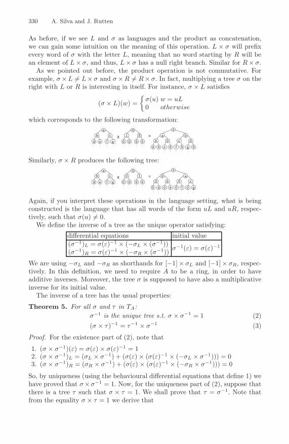
330 A. Silva and J. Rutten
As before, if we see L and σ as languages and the product as concatenation,we can gain some intuition on the meaning of this operation. L × σ will prefixevery word of σ with the letter L, meaning that no word starting by R will bean element of L× σ, and thus, L× σ has a null right branch. Similar for R× σ.
As we pointed out before, the product operation is not commutative. Forexample, σ×L �= L× σ and σ×R �= R× σ. In fact, multiplying a tree σ on theright with L or R is interesting in itself. For instance, σ × L satisfies
(σ × L)(w) ={σ(u) w = uL0 otherwise
which corresponds to the following transformation:
0 0
0
0
0 0
1Xf g
c
a
d e
b =
0
a
d 0
b
e 0
0
0
f 0
c
g 0
0
Similarly, σ ×R produces the following tree:
0 0
1
0
0 0
0Xf g
c
a
d e
b =
0
0
0 d
0
0 e
b
a
0 f
0
0 g
c
Again, if you interpret these operations in the language setting, what is beingconstructed is the language that has all words of the form uL and uR, respec-tively, such that σ(u) �= 0.
We define the inverse of a tree as the unique operator satisfying:
differential equations initial value(σ−1)L = σ(ε)−1 × (−σL × (σ−1))(σ−1)R = σ(ε)−1 × (−σR × (σ−1)) σ
−1(ε) = σ(ε)−1
We are using −σL and −σR as shorthands for [−1]× σL and [−1]× σR, respec-tively. In this definition, we need to require A to be a ring, in order to haveadditive inverses. Moreover, the tree σ is supposed to have also a multiplicativeinverse for its initial value.
The inverse of a tree has the usual properties:
Theorem 5. For all σ and τ in TA:σ−1 is the unique tree s.t. σ × σ−1 = 1 (2)(σ × τ)−1 = τ−1 × σ−1 (3)
Proof. For the existence part of (2), note that
1. (σ × σ−1)(ε) = σ(ε)× σ(ε)−1 = 12. (σ × σ−1)L = (σL × σ−1) + (σ(ε)× (σ(ε)−1 × (−σL × σ−1))) = 03. (σ × σ−1)R = (σR × σ−1) + (σ(ε) × (σ(ε)−1 × (−σR × σ−1))) = 0
So, by uniqueness (using the behavioural differential equations that define 1) wehave proved that σ×σ−1 = 1. Now, for the uniqueness part of (2), suppose thatthere is a tree τ such that σ × τ = 1. We shall prove that τ = σ−1. Note thatfrom the equality σ × τ = 1 we derive that

Behavioural Differential Equations and Coinduction for Binary Trees 331
1. τ(ε) = σ(ε)−1
2. τL = σ(ε)× (−σL × τ)3. τR = σ(ε) × (−σR × τ)
Thus, by uniqueness of solutions for systems of behavioural differential equations,τ = σ−1.
For (3), note that (σ× τ)× τ−1 × σ−1 = σ× (τ × τ−1)× σ−1 = 1. Therefore,using the uniqueness property of (2), (σ × τ)−1 = τ−1 × σ−1.
5 Applications of Tree Calculus
We will illustrate the usefulness of our calculus by looking at a series of inter-esting examples. In order to compute closed formulae for trees we will be usingthe following identity:
∀σ∈TA σ = σ(ε) + (L× σL) + (R× σR) (4)
which can be easily proved by coinduction. We will now show how to use thisidentity to construct the closed formula for a tree.
Recall our first system of behavioural differential equations:
differential equations initial valueoneL = oneoneR = one
one(ε) = 1
There we saw that the unique solution for this system was the tree with 1’s inevery node. Alternatively, we can compute the solution using (4) as follows.
one = one(ε) + (L × oneL) + (R× oneR)⇔ one = 1 + (L× one) + (R× one)⇔ (1− L−R)one = 1⇔ one = (1− L−R)−1
Therefore, one can be represented by the (very compact) closed formula1 (1 −L−R)−1.
Let us see a few more examples. From now on we will work with A = R, wherewe have the extra property: [n]× σ = σ × [n], for all n ∈ R and σ ∈ TR.
The tree where every node at level k is labelled with the value 2k, called pow,
4 4
2
1
4 4
2
is defined by the following system:
1 Note the similarity of this closed formula with the one obtained for the stream(1, 1, . . .) in [7]: (1 − X)−1.

332 A. Silva and J. Rutten
differential equations initial valuepowL = 2× powpowR = 2× pow pow(ε) = 1
We proceed as before, applying (4):
pow = pow(ε) + (L× powL) + (R × powR)⇔ pow = 1 + (2L× pow) + (2R× pow)⇔ (1− 2L− 2R)pow = 1⇔ pow = (1− 2L− 2R)−1
which gives us a nice closed formula for pow2.The tree with the natural numbers
6 7
3
1
4 5
2
is represented by the following system of differential equations:
differential equations initial valuenatL = nat+ pownatR = nat+ (2× pow) nat(ε) = 1
Applying identity (4):
nat = nat(ε) + (L× natL) + (R × natR)⇔ nat = 1 + (L × (nat+ pow)) + (R× (nat+ 2pow))⇔ (1− L−R)nat = 1 + L(1− 2L− 2R)−1 + 2R(1− 2L− 2R)−1
⇔ (1− L−R)nat = (1 − L)× (1− 2L− 2R)−1
⇔ nat = (1 − L−R)−1 × (1− L)× (1− 2L− 2R)−1
The Thue-Morse sequence [1] can be obtained by taking the parities of the countsof 1’s in the binary representation of non-negative integers. Alternatively, it canbe defined by the repeated application of the substitution map {0→ 01; 1→ 10}:
0→ 01→ 0110→ 01101001→ . . .
We can encode this substitution map in a binary tree, called thue, which at eachlevel k will have the first 2k digits of the Thue-Morse sequence:
1 0
1
0
0 1
0
In this example, we take for A the Boolean ring 2 = {0, 1} (where 1 + 1 = 0).The following system of differential equations defines thue:
2 Again, there is a strong similarity with streams: the closed formula for the stream(1, 2, 4, 8, . . .) is (1 − 2X)−1.

Behavioural Differential Equations and Coinduction for Binary Trees 333
differential equations initial valuethueL = thuethueR = thue+ one
thue(ε) = 0
Note that thue+one equals the (elementwise) complement of thue. Applying (4)to thue, we calculate:
thue = (L× thue) + (R× (thue+ one))⇔ (1− L−R)× thue = R× one⇔ thue = (1− L−R)−1 ×R× one
which then leads to the following pretty formula for thue:
thue = one×R× one
Let us present another example – a substitution operation, which given two treesσ and τ , replaces the left subtree of σ by τ .
( )
L R=subst( ),
( )
R
It is easy to see that the equations that define this operation are:
differential equations initial valuesubst(σ, τ)L = τsubst(σ, τ)R = σR
subst(σ, τ)(ε) = σ(ε)
Then, we apply (4) and we reason:
subst(σ, τ) = σ(ε) + (L × τ) + (R× σR)⇔ subst(σ, τ) = σ − (L× σL) + (L× τ)⇔ subst(σ, τ) = σ − L(σL − τ)
Note that in the second step, we applied identity (4) to σ. Moreover, remarkthat the final closed formula for subst(σ, τ) gives us the algorithm to computethe substitution:
( )
0 R
+0
0
- 0
L 0
( )
L R=subst( ),
( )
R
We can now wonder how to define a more general substitution operation that hasan arbitrary path P ∈ {L,R}+ as an extra argument and replaces the subtreeof σ given by this path by τ . It seems obvious to define it as

334 A. Silva and J. Rutten
subst(σ, τ, P ) = σ − P (σP − τ)where, in the right hand side, P = a1a2 . . . an is interpreted as a1× a2× . . .× anand the derivative σP is defined as
σP ={σδ P = δ(σδ)P ′ P = δ.P ′
with δ being either L or R.Let us check that our intuition is correct. First, we present the definition for
this operation:
differential equations initial value
subst(σ, τ, P )δ =
⎧⎨
⎩
τ P = δsubst(σδ, τ, P ′) P = δ.P ′
σδ P = δ′.P ′subst(σ, τ, P )(ε) = σ(ε)
where δ′ �= δ. Now, observe that
R={〈subst(σ, τ, P ), σ −P (σP − τ)〉 |σ, τ ∈ TR, P ∈ {L,R}+}∪{〈σ, σ〉 | σ ∈ TR}is a bisimulation relation because:
1. (σ − P (σP − τ))(ε) = σ(ε) = subst(σ, τ, P )(ε)2. For δ ∈ {L,R},
(σ − P (σP − τ))δ = σδ − Pδ(σP − τ)
=
⎧⎨
⎩
τ P = δσδ − P ′((σδ)P ′ − τ) P = δ.P ′
σδ P = δ′.P ′
R
⎧⎨
⎩
τ P = δsubst(σδ, τ, P ′) P = δ.P ′
σδ P = δ′.P ′
= subst(σ, τ, P )δ
Therefore, by Theorem 1, subst(σ, τ, P ) = σ − P (σP − τ).Using this formula we can now prove properties about this operation. For in-
stance, one would expect that subst(σ, σP , P ) = σ and also subst(subst(σ, τ, P ),σP , P ) = σ.
The first equality follows easily: subst(σ, σP , P ) = σ − P (σP − σP ) = σ. Forthe second one we have:
subst(subst(σ, τ, P ), σP , P )= subst(σ − P (σP − τ), σP , P ) (Definition of subst)= σ − P (σP − τ) − P ((σ − P (σP − τ))P − σP ) (Definition of subst)= σ − P (σP − τ) − P (τ − σP ) ((σ − P (σP − τ))P = σP − σP + τ = τ)= σ
Remark that this operation is a standard example in introductory courses onalgorithms and data structures. It is often presented either as a recursive ex-pression (very much in the style of our differential equations) or as a contrived

Behavioural Differential Equations and Coinduction for Binary Trees 335
iterative procedure. This example shows that our compact formulae constitutea clear way of presenting algorithms and that they can be used to eliminaterecursion. Moreover, the differential equations are directly implementable algo-rithms (in functional programming) and our calculus provides a systematic wayof reasoning about such programs.
6 Discussion
We have modelled binary trees as formal power series and, using the fact that thelatter constitute a final coalgebra, this has enabled us to apply some coalgebraicreasoning. Technically, none of this is very difficult. Rather, it is an applicationof well known coalgebraic insights. As is the case with many of such applications,it has the flavour of an exercise. At the same time, the result contains severalnew elements that have surprised us. Although technically Theorem 2 is aneasy extension of a similar such theorem for streams, the resulting format fordifferential equations for trees is surprisingly general and useful. It has allowed usto define various non-trivial trees by means of simple differential equations, andto compute rather pleasant closed formulae for them. We have also illustratedthat based on this, coinduction is a convenient proof method for trees. As anapplication, all of this is new, to the best of our knowledge. (Formal tree series,which have been studied extensively, may seem to be closely related but are not:here we are dealing with differential equations that characterise single trees.)In addition to the illustrations of the present differential calculus for trees, wesee various directions for further applications: (i) The connection with (varioustypes of) automata and the final coalgebra TA of binary trees needs furtherstudy. For instance, every Moore automaton with input in 2 = {L,R} andoutput in A has a minimal representation in TA. Details of these automata (andon weighted variants of them) are not complicated but have not been workedout here because of lack of space. (ii) The closed formula that we have obtainedfor the (binary tree representing the) Thue-Morse sequence suggests a possibleuse of coinduction and differential equations in the area of automatic sequences[2]. Typically, automatic sequences are represented by automata. The presentcalculus seems an interesting alternative, in which properties such as algebraicityof sequences can be derived from the tree differential equations that define them.(iii) Finally, the closed formulae that we obtain for tree substitution suggestmany further applications of our tree calculus to (functional) programs on trees,including the analysis of their complexity.
References
1. Allouche, J.-P., Shallit, J.: The ubiquitous Prouhet-Thue-Morse sequence. In: Ding,C., Helleseth, T., H., N. (eds.) Sequences and their applications, Proceedings ofSETA’98, pp. 1–16. Springer, Heidelberg (1999)
2. Allouche, J.-P., Shallit, J.: Automatic sequences: theory, applications, generaliza-tions. Cambridge University Press, Cambridge (2003)
336 A. Silva and J. Rutten
3. Esik, Z., Kuich, W.: Formal tree series. Journal of Automata, Languages and Com-binatorics 8(2), 219–285 (2003)
4. Manes, E.G., Arbib, M.A.: Algebraic approaches to program semantics. Springer,Heidelberg (1986)
5. Perrin, D., Pin, J.-E.: Infinite Words, Pure and Applied Mathematics. Pure andApplied Mathematics, vol. 141. Elsevier, Amsterdam (2004)
6. Rutten, J.J.M.M.: Behavioural differential equations: a coinductive calculus ofstreams, automata, and power series. Theor. Comput. Sci. 308(1-3), 1–53 (2003)
7. Rutten, J.J.M.M.: A coinductive calculus of streams. Mathematical Structures inComputer Science 15(1), 93–147 (2005)
A Proof of Theorem 2
Proof (Proof of theorem 2). Consider a well-formed system of differential equa-tions for Σ, as defined above. We define a set T of terms t by the followingsyntax: t ::= τ (τ ∈ TA) | f(t1, . . . , tr(f)) (f ∈ Σ)
where for every tree τ ∈ TA the set T contains a corresponding term, denoted byτ , and where new terms are constructed by (syntactic) composition of functionsymbols from Σ with the appropriate number of argument terms. Next we turnT into an F -coalgebra by defining a function 〈l, o, r〉 : T → (T × A × T ) byinduction on the structure of terms, as follows. First we define o : T → A by
o(τ ) = τ(ε)o(f(t1, . . . tr(f))
)= c
(o(t1), . . . , o(tr(f))
)
(where c is the function used in the equations for f). Next we define l : T → Tand r : T → T by l(τ) = τL and r(τ ) = τR, and by
l ( f(t1, . . . tr) ) = t1 and l ( f(t1, . . . tr) ) = t2
Here the terms t1 and t2 are obtained from the terms t1 and t2 used in theequations for f , by replacing (every occurrence of) xi by ti, (xi)L by l(ti), (xi)Rby r(ti), and [xi(ε)] by [o(t)], for i = 1, . . . , r. Because TA is a final F -coalgebra,there exists a unique homomorphism h : T → TA. We can use it to define treefunctions f : (TA)r → TA, for every f ∈ Σ, by putting, for all τ1, . . . , τr ∈ TA,
f(τ1, . . . , τr) = h(f(τ1, . . . , τr)
)
This gives us a set Σ of tree functions. One can prove that it is a solution of oursystem of differential equations by coinduction, using the facts that h(τ ) = τ ,for all τ ∈ TA, and
h ( f(t1, . . . , tr) ) = f (h(t1), . . . , h(tr) )
for all f ∈ Σ and ti ∈ T . This solution is unique because, by finality of TA, thehomomorphism h is.

A Sketch of a Dynamic Epistemic Semiring
Kim Solin�
Abo Akademi, Abo, [email protected]
Abstract. This paper proposes a semiring formulation for reasoningabout an agent’s changing beliefs: a dynamic epistemic semiring (DES).A DES is a modal semiring extended with epistemic-action operators.The paper concentrates on the revision operator by proposing an ax-iomatisation, developing a basic calculus and deriving the classical AGMrevision axioms in the algebra.
1 Introduction
Formal reasoning about epistemic and doxastic notions in the 20th century canbe traced back to Georg Henrik von Wright’s An Essay in Modal Logic [26] andHintikka’s Knowledge and Belief [13]. These books were written as attempts tophilosophically clarify our notions of knowledge and belief using modal logic.In the works of von Wright and Hintikka, the ones believing or knowing – theagents – cannot change their beliefs, i.e. only static aspects of an agent’s be-liefs can be reasoned about. Alchourron, Gardenfors and Makinson presented asemiformal framework for reasoning about an agent’s changing beliefs [1] – thisconstituted the prelude for the vast amount of research on belief revision donein the last two decades. Segerberg was one of the first to make these streamsflow together. In an array of papers (see for example [20, 21, 22]) he proposesand develops a fully formal framework for reasoning about an agent’s changingbeliefs: dynamic doxastic logic. Dynamic doxastic logic is, as the name discerns,a blend of dynamic and doxastic logic. In more recent times, formal reasoningabout knowledge has been put to use in computer science, the standard refer-ences seem to be [12,14,25]. (The epithet epistemic is usually used in computerscience, whereas in philosophical logic one tends to distinguish between epis-temic and doxastic. We will henceforth use ‘epistemic’, except when referring toSegerberg’s logic.)
Since Kozen published his axiomatisation of Kleene algebra (an idempotentsemiring with the Kleene star as the least fixpoint with respect to the canonicalorder) [15] and also showed how to use an elaboration of it for program reason-ing [16], there has been significant development and application of somethingthat could be called semiring structures (some form of semiring equipped withadditional operators). The spirit in this development lies very much in the cal-culational prospect of abstract algebra – tedious model-theoretic reasoning can� Supported by TUCS (Turku Centre for Computer Science).
D. Leivant and R. de Queiroz (Eds.): WoLLIC 2007, LNCS 4576, pp. 337–350, 2007.c© Springer-Verlag Berlin Heidelberg 2007

338 K. Solin
be reduced to simple, perspicuous, symbol-pushing calculations. One importantdevelopment are the modal semirings by Desharnais, Moller and Struth [10]. Amodal semiring is a semiring structure including a domain operator facilitatingthe definition of modal operators in the sense of dynamic logic.
Our intent in this paper is to let yet another stream run up to Segerberg’suniting work by viewing some aspects of dynamic doxastic logic from the pointof modal semirings. In this paper we propose a modal semiring extended with anepistemic-action operator: a dynamic epistemic semiring. This structure allowsus to reason about an agent’s changing beliefs in a transparent, calculationalfashion. The carrier elements of the algebra are viewed as epistemic actions –actions working on the agent’s beliefs. To check whether the agent believes aproposition we introduce special actions: epistemic tests. Epistemic tests worklike guards in program theory, i.e. programs that check if some predicate holdsor not.
In comparison to the semi-formal approach of the AGM trio, and the logicalapproaches of Segerberg [20, 21, 22]; Baltag, Moss and Solecki [5, 4] and the socalled Amsterdam school centered around van Benthem [7] – our approach isabstract-algebraic. The work that comes closest to ours is the elegant algebraicapproach to dynamic epistemic reasoning by Baltag, Coecke, and Sadrzadeh[2, 3, 6]. But when they use systems (a combination of a complete sup-lattice, aquantale and a right-module structure on the lattice) as the underlying structurein order to achieve an axiomatisation, we use modal semirings. Baltag, Coeckeand Sadrzadeh’s approach is perhaps more thoroughly developed to match theoriginal framework by Alchourron, Gardenfors and Makinson than ours, whereasour treatment, on the other hand, is more perspicuous in that it has a (at leastto our mind) simpler algebraic structure underneath, and it also easily facilitatesiterated action.
The structure of the paper is: Sect. 2 defines modal semirings. In Sect. 3 therevision operator is introduced, in Sect. 4 we provide a relational model andin Sect. 5 we develop a basic calculus. In Sect. 6 we derive the classical AGM-axioms for revision in the algebra. The final section contains some concludingremarks. Only the most interesting proofs are included in the paper; App. Acontains detailed proofs of the claims that are not proved.
We want to emphasise that the main purpose of this paper not is to considerapplications or the philosophy of formal epistemology, but to lay an initial foun-dation to using semirings for reasoning about belief in change. The paper, then,primarily provides a concise technical framework, that connects earlier work onformal epistemic reasoning with the recent work on applications of semirings.
2 Modal Semirings
By an idempotent semiring we shall understand a structure over the signature(+, ; , 0, 1) such that the reduct over (+, 0) is a commutative and idempotentmonoid, and the reduct over (; , 1) is a monoid such that ; distributes over +and has 0 as a left and right annihilator. When no risk for confusion arises ; will
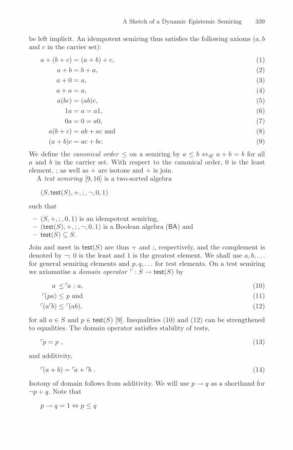
A Sketch of a Dynamic Epistemic Semiring 339
be left implicit. An idempotent semiring thus satisfies the following axioms (a, band c in the carrier set):
a+ (b + c) = (a+ b) + c, (1)a+ b = b+ a, (2)a+ 0 = a, (3)a+ a = a, (4)a(bc) = (ab)c, (5)
1a = a = a1, (6)0a = 0 = a0, (7)
a(b + c) = ab+ ac and (8)(a+ b)c = ac+ bc. (9)
We define the canonical order ≤ on a semiring by a ≤ b ⇔df a + b = b for alla and b in the carrier set. With respect to the canonical order, 0 is the leastelement, ; as well as + are isotone and + is join.
A test semiring [9, 16] is a two-sorted algebra
(S, test(S),+, ; ,¬, 0, 1)
such that
– (S,+, ; , 0, 1) is an idempotent semiring,– (test(S),+, ; ,¬, 0, 1) is a Boolean algebra (BA) and– test(S) ⊆ S.
Join and meet in test(S) are thus + and ;, respectively, and the complement isdenoted by ¬; 0 is the least and 1 is the greatest element. We shall use a, b, . . .for general semiring elements and p, q, . . . for test elements. On a test semiringwe axiomatise a domain operator � : S → test(S) by
a ≤ �a ; a, (10)�(pa) ≤ p and (11)�(a�b) ≤ �(ab), (12)
for all a ∈ S and p ∈ test(S) [9]. Inequalities (10) and (12) can be strengthenedto equalities. The domain operator satisfies stability of tests,
�p = p , (13)
and additivity,
�(a+ b) = �a+ �b . (14)
Isotony of domain follows from additivity. We will use p→ q as a shorthand for¬p+ q. Note that
p→ q = 1⇔ p ≤ q

340 K. Solin
follows from shunting. With the aid of the domain operator, we can define modaloperators [10] by
〈a〉p =df �(ap) and [a]p =df ¬〈a〉¬p . (15)
Therefore we shall call a test semiring with a domain operator modal. The dia-mond can be read “it is possible to successfully perform a so that p will hold”and the box as “after every successful way of performing a it will be the casethat p holds”.1 The following fact
if p ≤ q and [a]p = 1, then [a]q = 1 (16)
is not hard to prove and will be used later.
Example 1. (From [9]) Given two binary relations S, T ⊆ Σ × Σ, define thebinary operators ; and + and the unary operator � on the relations by thefollowing:
(x, y) ∈ (S;T )⇔df ∃z ∈ Σ • (x, z) ∈ S and (z, y) ∈ T, (17)(x, y) ∈ (S + T )⇔df (x, y) ∈ S or (x, y) ∈ T and (18)
(x, x) ∈ �S ⇔df (x, y) ∈ S for some y ∈ Σ. (19)
Moreover, denote the identity relation by Δ, let Ø denote the empty relationand let ¬ denote the complement relative to Δ. Then the structure
(℘(Σ ×Σ), ℘(Δ),+, ;¬, � ,Ø, Δ)
is a modal semiring.
3 Dynamic Epistemic Semirings
When reasoning about an agent’s beliefs and changes in the agent’s beliefs acommon way to go is to talk about the agent’s belief set and operators that workon this set. The classical framework centered around Alchourron, Gardenfors andMakinson [1] had three such operators, namely
– addition: add a belief to the agent’s belief set,– revision: add a belief to agent’s belief set and revise the set (without remov-
ing the added belief) so that it becomes consistent, and– contraction: remove a belief and ensure that it is not implied by the remain-
der.
In the present paper we will concentrate on the revision operator – the heartof dynamic epistemic reasoning – but we will not have anything to say about
1 In the tradition following Dijkstra [11] the box corresponds to the weakest liberalprecondition of a with respect to q: if a terminates, p will hold. Our ‘successful’corresponds to ‘terminating’.

A Sketch of a Dynamic Epistemic Semiring 341
exactly how the revision is done; what we are saying is that if a revision is done,then certain properties will hold.
It is possible for the agent to be ignorant (or indifferent) regarding a certainproposition: the agent might not believe a proposition, but this does not meanthat he believes the negation of the proposition either. A non-ignorant agentthus believes in exactly one possible world, so to speak, whereas an ignorantagent possibly does not know exactly in which possible world (or state) he is in,but only in which subset of possible worlds he is in. For an ignorant agent, if theproposition holds or does not hold in all the possible worlds in his current beliefset, then the agent believes or does not believe the proposition, respectively.If, however, this subset of possible worlds is a singleton set, then the agent ofcourse knows exactly in which world he is; Baltag and Sadrzadeh call these sets“complete (fully determined) situations” [6].
We shall now define ‘dynamic epistemic semiring’, but first we provide aninformal intuition. The carrier set should be seen as consisting of actions on theagent’s beliefs and upon these actions we shall work with four operators:
– + is choice: do the left or the right action,– ; is sequential composition of actions,– �a denotes those states of belief from which it is possible to successfully
perform the action a, and– �p revises the agents beliefs with p (it is always possible to successfully
perform this action, apart from when p is the contradiction).
We shall have two distinguished actions, the fail action 0 which always fails andthe idle action 1 that leaves everything as it is. The tests (defined according tothe test semirings and named et) should be seen as actions that check whetherthe agent believes a proposition or not: epistemic tests. If the agent believes theproposition, the epistemic test will hold and behave like the idle action, otherwiseit will behave like the fail action. If a ≤ b the action b results in anything that awould result in and possibly more. The diamond and the box can be interpretedas above.
We now propose a set of axioms for the revision operator. This set is to be seenas a mere suggestion, since the main thrust of this paper is not to promote a cer-tain axiomatisation of revision, but to promote the abstract-algebraic method.These axioms are chosen because we find them reasonable and because the stan-dard AGM-axioms for revision follow from them (see Sect 6); depending onone’s needs, another axiomatisation could be chosen and the abstract-algebraicframework should then work equally well.
Definition 2. A dynamic epistemic semiring (DES) is a two-sorted algebra
D = (D, et(D),+, ; ,¬,�, �, 0, 1)
such that the reduct structure over
(D, et(D),+, ; ,¬, �, 0, 1)
is a modal semiring and � : et(D)→ D is a unary prefix operator such that

342 K. Solin
p ≤ �p, (20)�p; �p ≤ �p, (21)
�p; q ≤ �(pq), (22)�(p+ q); p = �p, (23)
�p ≤ �q ⇒ p ≤ q and (24)��p = 1, p �= 0 (25)
hold for any p, q ∈ et(D) when ≤ is the canonical order. �
An intuition for the axioms can briefly be given as follows. The first axiom saysthat successfully performing a choice between p and �p is equal to successfullyperforming �p. The second axiom says that revising with p and then revisingwith p again can be done away with by revising with p just once. The thirdaxiom says that revising with p and then checking that q holds can be replacedby a revision with the conjunction p and q.2 If the agent first revises his beliefsby the disjunction p+q and then – with success – checks if p holds this is equal torevising his beliefs with p; this is what the fourth axiom says. The fifth one saysthat if a successful execution of a choice between revising with p or q is equalto directly revising with q then p implies q. The last axiom says that the action�p can always be performed successfully as long as p is not the contradiction.
4 A Relational Model for Revision
We now give a relational interpretation satisfying the axioms of the above struc-ture. However, we want to emphasise that this rough relational model is notto be seen as the model for our algebra; it is simply an example of a structurethat satisfies our axioms (showing that our axiomatisation has got a model and,so, is sound). It does not do much for intuition, for example, revision in thismodel is “absolute” in that all previous knowledge is forgotten when a revisionis performed – this, however, should not follow from the axioms. There are other,more suitable, relational models for belief revision, but since our main concernin this paper is the abstract algebra, we shall not go into these. That these more“realistic” models can be connected with our algebra follows from the fact thatcounterparts to the classical AGM-axioms can be derived in our framework (seeSect. 6).
Example 3. Let Σ be any set and let Δ be the identity relation. Define theunary prefix operator
� : ℘(Δ)→ ℘(Σ ×Σ)
by, for any given P ⊆ Δ,
� P =df {(x, p) | x ∈ Σ and (p, p) ∈ P}. (26)2 The inequalities (21) and (22) can in fact be strengthened to equalities.

A Sketch of a Dynamic Epistemic Semiring 343
Then the structure
(℘(Σ ×Σ), ℘(Δ), ; ,+,¬, � ,�,Ø, Δ)
is a DES when the operators and the constants are interpreted as above and asin Ex. 1.
5 A Basic Calculus
In this section we develop a basic calculus for DESs. The first two propositionsare helpful tools.
Proposition 1. In any DES the equations
� p; p = �p, (27)p ≤ p; �p and (28)
�p;¬p = 0 (29)
hold.
Statement (27) above says that revising the agent’s beliefs by p and then checkingwhether the agent believes p is equal to just revising the agent’s beliefs with p.The epistemic test will act as an idle action, since the agent certainly believesa proposition after just having added it. Statement (29) says something similar:after revising with p the epistemic test ¬p will fail. Statement (28) says thatp could always be replaced by p; �p. Note, however, that the other directiondoes not hold, since revision by p might result in the agent “losing” information.Having p hold before the revision does not mean that the revision is idle: therevision might weaken the agent’s beliefs.
The next proposition settles that �p is an idempotent element for ; (for any p).This means that repeated revision with the same predicate has no more effectthan revising once.
Proposition 2. In any DES the equation
� p; �p = �p (30)
holds.
Next we establish additivity and isotony of �. The intuition is that if the agentis to change his beliefs to a set of states where p or q holds this is equal to achoice between changing it to a set of states where p holds or changing it to aset of states where q holds. The intuition behind the isotony is similar to theone of axiom (24).
Proposition 3. In any DES the equations
� (p+ q) = �p+ �q and (31)p ≤ q ⇒ �p ≤ �q (32)
hold.

344 K. Solin
The following proposition establishes some relations between the constants, thedomain operator and the epistemic operators. As shown by the first and thesecond statement, respectively, revising with the contradiction always fails andthis action cannot be performed.
Proposition 4. In any DES the equations
� 0 = 0 and (33)��0 = 0 (34)
hold.
6 Deriving the AGM Axioms for Revision
To connect our framework to the classical work on belief revision, we now showthat the well-known AGM axioms for the revision operator can be derived in ouralgebra. First, we encode the axioms following the encoding of the revision axiomsinto dynamic doxastic logic (see for example Cantwell [8]). We refrain from writingout the intuition of the axioms, but just recall that p→ q = 1⇔ p ≤ q and notethat, informally, p should be seen as Bp in the language of dynamic doxastic logicand as p ∈ K in the language of AGM, when K is the belief set; [�p] should beseen as [∗p] in dynamic doxastic logic and as K ∗ p in AGM theory.
The AGM axioms for revision are then encoded in our algebra as follows:
[�p]p = 1, (*2)[�p]q ≤ p→ q, (*3)
¬¬p; (p→ q) ≤ [�p]q, (*4)[�p]¬0 = 1, when p �= 0, (*5)
[�p]r = [�q]r, whenever p = q, (*6)[�(pq)]r ≤ [�p](q → r) and (*7)
[�p]q; [�p](q → r) ≤ [�(pq)]r. (*8)
The first classical AGM axiom (*1) for revision says that when revising a propo-sition, the agent should believe all its consequences. This is taken care of bythe underlying epistemic-test structure, and need thus not be stipulated explic-itly (similarly to dynamic doxastic logic, where it follows from the normality ofthe underlying logic). The epistemic-test structure also entails that the doublenegation in axiom (*4) disappears and that ¬0 in axiom (*5) equals 1.
We now derive axioms (*2)–(*8) as calculational derivations in the algebra.The second axiom (*2) can be shown to follow from the algebra by the calculation
[�p]p = 1⇔ {definition of box (15)}¬�(�p¬p) = 1
⇔ {(29)}
A Sketch of a Dynamic Epistemic Semiring 345
¬�0 = 1⇔ {modal semiring properties}
true.
The third axiom (*3) follows from
[�p]q ≤ ¬p+ q⇔ {definition of box (15)}¬�(�p;¬q) ≤ ¬p+ q
⇔ {de Morgan}¬�(�p;¬q) ≤ ¬(p;¬q)
⇔ {stability of tests}¬�(�p;¬q) ≤ ¬�(p;¬q)
⇔ {contraposition}�(p;¬q) ≤ �(�p;¬q)
⇐ {isotony}p ≤ �p
⇔ {axiom}true,
and the fourth axiom (*4) follows from (*2), the definition of → and isotony ofbox (16). The fifth axiom follows from
[�p]¬0 = 1⇔ {definition of box (15), double negation}¬�(�p; 0) = 1
⇔ {axiom}¬�0 = 1
⇔ {stability of tests, test BA}true,
and the sixth axiom (*6) is a direct consequence of the definition of box, theisotony of domain and the isotony of revision. The seventh axiom (*7) followsfrom the derivation
[�(pq)]r ≤ [�p](q → r)⇔ {definition of box (15), contraposition, de Morgan}
�(�p; q¬r) ≤ �(�(pq)¬r)⇐ {isotony}
�p; q ≤ �(pq)⇔ {axiom}
true;
and the derivation
[�p]q; [�p](q → r) ≤ [�(pq)]r⇔ {definition of box (15), de Morgan}¬(�(�p;¬q) + �(�p; q;¬r)) ≤ ¬�(�(pq);¬r)
⇔ {contraposition, additivity of domain}

346 K. Solin
�(�(pq);¬r) ≤ �(�p;¬q + �p; q;¬r)⇔ {axiom, absorption}
�(�(pq);¬r) ≤ �(�p; (¬q + ¬r))⇐ {isotony}
true
shows that the last axiom (*8) follows.
7 Concluding Remarks
This paper takes a modest first step towards epistemic reasoning with semirings.A possible elaboration is to incorporate real action into the framework (assumingthat the beliefs are not a part of the world, real actions are actions on the world),and another possibility is to extend the underlying semiring to a Kleene algebrain order to enable reasoning about iterated action – we pursue this in [24]. Inforthcoming work, we intend to look at contraction and addition in a similarframework. How more elaborate models than the relational one presented inthis paper (such as hypertheories) relate to our algebra is also an interestingquestion that we shall return to. Finally, many of the recent abstract-algebraicapproaches have proved practical in applications, see for example [27, 17, 23]; inan epistemic context, modal semirings have recently been applied by Moller [18].It is a promising thought that the dynamic epistemic semiring would prove usefulin applications involving epistemic notions.
Acknowledgements. The author is grateful to Bernhard Moller, Larissa Meinicke,Georg Struth and Peter Hofner for helpful remarks. He also highly appreciatedthe remarks of the anonymous referees – due to lack of time, however, not allsuggestions could be followed.
References
1. Alchourron, C.E., Gardenfors, P., Makinson, D.: On the logic of theory change:partial meet contraction and revision functions. Journal of Symbolic Logic 50(2),510–530 (1985)
2. Baltag, A., Coecke, B., Sadrzadeh, M.: Epistemic actions as resources. In: Pro-ceedings of the Logics for Resources Processes Programs Workshop at LiCS 2004(2004)
3. Baltag, A., Coecke, B., Sadrzadeh, M.: Algebra and sequent calculus for epistemicactions. Electronic Notes in Theoretical Computer Science 126, 27–52 (2005)
4. Baltag, A., Moss, L.: Logic for epistemic programs. Synthese 139(2), 165–224 (2004)5. Baltag, A., Moss, L., Solecki, S.: The logic of common knowledge, public announce-
ments, and private suspisions. In: Gilboa, I. (ed.) Proceedings of the 7th Conferenceon Theoretical Aspects of Rationality and Knowledge (TARK’98), pp. 43–56 (1998)
6. Baltag, A., Sadrzadeh, M.: The algebra of multi-agent dynamic belief revision.Electronic Notes in Theoretical Computer Science 157(4), 37–56 (2006)
7. van Benthem, J.: Dynamic logic for belief revision. ILLC Technical Report, Uni-versity of Amsterdam, (2006)

A Sketch of a Dynamic Epistemic Semiring 347
8. Cantwell, J,: Non-Linear Belief Revision. Foundations and Applications. Disserta-tion. Uppsala: Acta Universitatis Upsaliensis (2000)
9. Desharnais, J., Moller, B., Struth, G.: Kleene algebra with domain. ACM Trans-actions on Computational Logic 7(4), 798–833 (2006)
10. Desharnais, J., Moller, B., Struth, G.: Modal Kleene algebra and applications.Journal on Relational Methods in Computer Science 1(1), 93–131 (2004)
11. Dijkstra, E.W.: A Discipline of Programming. Prentice-Hall, Englewood Cliffs(1976)
12. Fagin, R., Halpern, J., Moses, Y., Vardi, M.Y.: Reasoning About Knowledge. MITPress, Cambridge, MA (1995)
13. Hintikka, J.: Knowledge and Belief: an Introduction to the Logic of the Two No-tions. Cornell University Press, Ithaca, N. Y (1962)
14. Meyer, J.-J.C., van der Hoek, W.: Epistemic Logic for Computer Science and Arti-ficial Intelligence. In: Meyer, J.-J. (ed.) Cambridge Tracts in Theoretical ComputerScience 41, Cambridge University Press, Cambridge (1995)
15. Kozen, D.: A completeness theorem for Kleene algebras and the algebra of regularevents. Information and Computation 110(2), 366–390 (1994)
16. Kozen, D.: Kleene algebra with tests. ACM Transactions on Programming Lan-guages and Systems 19(3), 427–443 (1997)
17. Moller, B.: Lazy Kleene algebra. In: Kozen, D. (ed.) MPC 2004. LNCS, vol. 3125,pp. 252–273. Springer, Heidelberg (2004)
18. Moller, B.: Knowledge and games in nodal semirings. Technischer Bericht 2007-3,Institut fur Informatik, Universitat Augsburg (February 2007)
19. de Rijke, M.: Meeting some neighbours: A dynamic modal logic meets theories ofchange and knowledge representation. In: van Eijk, J., Visser, A. (eds.) Logic andinformation flow, pp. 170–196. MIT Press, Cambridge, MA (1994)
20. Segerberg, K.: Proposal for a theory of belief revision along the lines of Lindstromand Rabinowicz. Fundamenta Informatica 32, 183–191 (1997)
21. Segerberg, K.: Two traditions in the logic of belief: bringing them together. In:Ohlback, H.J., Reyle, U. (eds.) Logic, Language and Reasoning, pp. 134–147.Kluwer, the Netherlands (1999)
22. Segerberg, K.: The basic dynamic doxastic logic of AGM. In: Williams, M.-A.,Rott, H. (eds.) Frontiers in Belief Revision, pp. 57–84. Kluwer, the Netherlands(1999)
23. Solin, K.: On two dually nondeterministic refinement algebras. In: Schmidt, R.A.(ed.) RelMiCS/AKA 2006. LNCS, vol. 4136, pp. 373–387. Springer, Heidelberg(2006)
24. Solin, K.: Dynamic Epistemic Semirings. Manuscript, Abo Akademi, March, 2007.Preliminary version as Technischer Bericht 2006-17, Institut fur Informatik, Uni-versitat Augsburg, (June 2006)
25. Wooldridge, M.: An Introduction to Multiagent Systems. John Wiley & Sons, Eng-land (2002)
26. Wright, G.H., von Wright, G.H.: An Essay in Modal Logic. North-Holland, Ams-terdam (1951)
27. von Wright, J.: von: From Kleene algebra to refinement algebra. In: Boiten, E.A.,Moller, B. (eds.) MPC 2002. LNCS, vol. 2386, Springer, Heidelberg (2002)

348 K. Solin
A Detailed Proofs
Soundness with Respect to the Relational Model
The only axioms that need to be verified are those concerning �, the rest havebeen verified in [9]. The first axiom is verified by
(p, p) ∈ P⇒ {property of binary relations}
(p, p) ∈ {(x, p) | x ∈ Σ and (p, p) ∈ Σ}⇔ {definition of �}
(p, p) ∈ �P,
the second by
(x, y) ∈ �P ; �P⇔ {definition of ;}∃z ∈ Σ • (x, z) ∈ �P and (z, y) ∈ �P
⇒ {definition of �}(x, y) ∈ �P,
the third by
(x, y) ∈ �P ;Q⇔ {definition of ;}∃z ∈ Σ • (x, z) ∈ �P and (z, y) ∈ Q
⇔ {definition of �P}∃z ∈ Σ • (x, z) ∈ �P, (z, z) ∈ P and (z, y) ∈ Q
⇒ {P,Q ⊆ Δ}∃z ∈ Σ • (x, z) ∈ �P, (z, z) ∈ P ∩Q and z = y
⇒ {P,Q ⊆ Δ, so P ∩Q = P ;Q}(x, y) ∈ �(P ;Q)
the fourth by
(x, y) ∈ �(P ∪Q);P⇔ {definition of ; and P ⊆ Δ}
(x, y) ∈ �(P ∪Q) and (y, y) ∈ P⇔ {definition of �}
(x, y) ∈ �P,
the fifth by
�P ⊆ �Q⇔ {definition of �}{(x, p) | x ∈ Σ and (p, p) ∈ P} ⊆ {(x, q) | x ∈ Σ and (q, q) ∈ Q}
⇒ {property of binary relations}P ⊆ Q

A Sketch of a Dynamic Epistemic Semiring 349
and, finally,
��P⇔ {definition of �}
�{(x, p) | x ∈ Σ and (p, p) ∈ P}⇔ {definition of � and P �= Ø}Δ
verifies the last axiom.
Proof of Proposition 1
The first statement follows from axiom (23) setting q = 0. The second statementfollows from epistemic tests being a BA, isotony of ; and axiom (20). The thirdstatement is proved by
�p¬p= {(27)}
�pp¬p= {epistemic tests BA}
�p0= {0 strict}
0.
Proof of Proposition 2
The statement is proved by
�p= {(27)}
�pp≤ {(20)}
�p� p
and axiom (21).
Proof of Proposition 3
The first statement (additivity) is proved by
�(p+ q)= {(27)}
�(p+ q)(p+ q)= {; distributive over +}
�(p+ q)p+ �(p+ q)q= {(23) and commutativity of +}
�p+ �q,
the second one (isotony) is straightforward from the first.

350 K. Solin
Proof of Proposition 4
The first part is proved by
�0= {(27)}
�00= {0 strict}
0.
The second part follows from the first statement and the fact that �0 = 0.

A Modal Distributive Law (abstract)
Yde Venema�
Institute for Logic, Language and Computation, Universiteit van AmsterdamPlantage Muidergracht 24, 1018 TV Amsterdam, Netherlands
In our talk we consider the coalgebraic, or cover modality ∇ which, in modallogic, goes back to the work of Fine on normal forms. The connective, taking aset of formulas as its argument, can be defined in terms of the usual box anddiamond operators:
∇Φ := �∨
Φ ∧∧
�Φ,
where �Φ denotes the set {�ϕ | ϕ ∈ Φ}. Conversely, the standard modalitiescan be defined in terms of the cover modality, from which it follows that we mayequivalently base our modal language on ∇ as a primitive symbol:
�ϕ ≡ ∇{ϕ, �}�ϕ ≡ ∇∅ ∨ ∇{ϕ}.
The main purpose of the talk is to underline the fundamental importance ofthe following equivalence, which we call a distributive law since it shows howconjunctions distribute over nabla’s (and disjunctions):
∇Φ ∧ ∇Φ′ ≡∨
Z∈Φ��Φ′∇{ϕ ∧ ϕ′ | (ϕ, ϕ′) ∈ Z}. (1)
Here Φ �� Φ′ denotes the set of relations R ⊆ Φ × Φ′ that are full in the sensethat for all ϕ ∈ Φ there is a ϕ′ ∈ Φ′ with (ϕ, ϕ′) ∈ R, and vice versa.
As an important corollary of (1) and the equidefinability of ∇ and {�, �},every modal formula can be rewritten into a distributive normal form in whichthe only conjunctions are of the form
∧P ∧∇Φ, where P is a set of literals, i.e.,
proposition letters and negations of proposition letters.We then move on to some consequences of this fact. First we show that for-
mulas in distributive normal form allow a direct, inductive definition of uniforminterpolants. And second, we briefly review the work of Janin and Walukiewiczon automata for the modal μ-calculus (which is where the notion of distributivenormal form stems from).
Finally, we turn to some of our recent work in this area. We discuss ouraxiomatization of (positive) modal logic based on the cover modality, and, timepermitting, sketch its connection with the Vietoris construction in topology. Wefinish with putting the cover modality into the wider, coalgebraic perspective,introduced by Moss, and discuss the meaning of the associated distributive lawin this more general setting.� The research of the author has been made possible by vici grant 639.073.501 of the
Netherlands Organization for Scientific Research (nwo).
D. Leivant and R. de Queiroz (Eds.): WoLLIC 2007, LNCS 4576, p. 351, 2007.c© Springer-Verlag Berlin Heidelberg 2007

Ant Colony Optimization with
Adaptive Fitness Functionfor Satisfiability Testing
Marcos Villagra1,2 and Benjamın Baran2
1 Catholic University of AsuncionAsuncion, P.O. Box 1683, Paraguay
marcos [email protected] National University of Asuncion
San Lorenzo, P.O. Box, 2169, [email protected]
Abstract. Ant Colony Optimization (ACO) is a metaheuristic inspiredby the foraging behavior of ant colonies that has been successful inthe resolution of hard combinatorial optimization problems. This workproposes MaxMin-SAT, an ACO alternative for the satisfiability pro-blem (SAT). MaxMin-SAT is the first ACO algorithm for SAT thatimplements an Adaptive Fitness Function, which is a technique usedfor Genetic Algorithms to escape local optima. To show effectiveness ofthis technique, three different adaptive fitness functions are compared:Stepwise Adaptation of Weights, Refining Functions, and a mix of theprevious two. To experimentally test MaxMin-SAT, a comparison withWalksat (a successful local search algorithm) is presented. Even thoughMaxMin-SAT cannot beat Walksat when dealing with phase transitioninstances, experimental results show that it can be competitive with thelocal search heuristic for overconstrained instances.
Keywords: SAT, Ant Colony Optimization, Local Search, Adaptive Fit-ness Function.
1 Introduction
The satisfiability problem in propositional logic or SAT is the problem of findingan assignment of values to Boolean variables for a given propositional formulato make it true. SAT was the first problem proved to be N P-complete [1], andas such is amongst the most important problems in computer science.
There exist several algorithms to solve SAT. These algorithms can be dividedin two classes: Complete algorithms and Incomplete algorithms. Complete algo-rithms state whether a given formula is true or not and return an assignmentof values to variables. One of the most efficient algorithms is the Davis-Putnammethod [2,3]. Nowadays, the best performing complete algorithms are based onthis method [4]. Incomplete algorithms try to find an assignment that approxi-mates the satisfiability of the formula. These algorithms are mainly based onlocal search, where Walksat [5] is one of the most famous.
D. Leivant and R. de Queiroz (Eds.): WoLLIC 2007, LNCS 4576, pp. 352–361, 2007.c© Springer-Verlag Berlin Heidelberg 2007
ACO with Adaptive Fitness Function for Satisfiability Testing 353
Ant Colony Optimization (ACO) is a metaheuristic proposed by Dorigo etal. [6] that is inspired by the foraging behavior of ant colonies. ACO has em-pirically shown its effectiveness in the resolution of several different N P-hardcombinatorial optimization problems [7]. Despite all this success, ACO cannotcompete against state-of-the-art local search algorithms for SAT [8]. The scien-tific community is more interested in solving Constraint Satisfaction Problems(CSP) than SAT1. Hence, there are more ACO algorithms solving CSPs [9,10,11].One of them is Ant-Solver [10], which uses a generic CSP heuristic for choosingthe next variable to assign a value. Also, it includes a novel pheromone mecha-nism based on the solution constructed so far and a preprocessing stage. Roli [12]proposed one of the first ACO algorithms for SAT, named ACO-MAXSAT. Thisalgorithm was based on the Ant Colony System [13], and uses a heuristic basedon the breakcount of the Walksat algorithm [5], i.e., number of satisfied clausesthat would become unsatisfied. This approach showed to be inefficient since theheuristic need to be calculated each time a variable assignment is made.
Evolutionary algorithms also had problems solving SAT [14]. In general,population-based metaheuristics have not shown to be competitive when com-pared against local search algorithms [8]. Previous works showed classical geneticalgorithms being unsuitable for the MAX-SAT fitness function [15]. However,other authors suggest that evolutionary algorithms can yield good results forSAT when equipped with additional techniques like adaptive fitness functions,problem-specific variation operators, and local optimization [14]. In that sense,this work proposes an ACO alternative for SAT called MaxMin-SAT, derivedfrom the MAX − MIN Ant System [7], that implements several adaptive fit-ness functions [14]. This is the first time that adaptive fitness function techniquesare used with ACO algorithms, which is expected to get similar improvementsthan the ones obtained for genetic algorithms [14].
The remainder of this work is organized as follows. Section 2 presents the SATproblem. Section 3 introduces the ACO metaheuristic and the way to code SATfor this kind of algorithms. In section 4, the concept of adaptive fitness functionis introduced. Section 5 presents experimental results. Finally, the conclusionsand future work are left for section 6.
2 The SAT Problem
SAT is defined by a set of Boolean variables X = {x1, . . . , xn} and a Booleanformula or sentence φ : {0, 1}n → {0, 1} where n represents the number ofvariables. The objective is to find a variable assignment m = 〈x1, . . . , xn〉 ∈{0, 1}n (i.e., a model) where φ(m) = 1. The formula is called satisfiable if sucha model exists, and unsatisfiable otherwise. A literal is a variable (also calledatom or symbol) or its negation. A clause is a disjunction of literals, i.e., literalsconnected by an ∨ operator. The formula φ is in conjunctive normal form (CNF)if φ(m) = c1(m) ∧ · · · ∧ cp(m), where each ci is a clause and p is the number ofclauses. The family of k-CNF sentences has exactly k literals per clause. SAT1 SAT is a particular case of CSP.
354 M. Villagra and B. Baran
can be assumed having CNF formulae without loss of generality [16], and k-SATonly contains sentences in k-CNF. While 2-SAT is solvable in polynomial time,k-SAT is N P-complete for k ≥ 3 [17].
MAX-SAT is an optimization variant of SAT. Given a set of clauses, MAX-SAT is the problem of finding a model m that maximizes the number of satisfiedclauses f(m). In weighted MAX-SAT each clause ci has a weight wi assignedto it, while unweighted MAX-SAT uses wi = 1 for all i. The following equationdefines the MAX-SAT objective function:
f(m) =p∑
i=1
wi · ci(m) (1)
where ci(m) = 1 if the clause ci is satisfied under the model m, and 0 otherwise.Thus, when searching for a solution to MAX-SAT, one is actually looking
for models to SAT formulae. Therefore, solutions refer to models and vice versa.There are only some differences between particular cases of SAT and MAX-SAT,where MAX-k-SAT is N P-hard for k ≥ 2 [17].
In 3-SAT, rapid transitions in solvability can be observed [18]. This phenome-non is called phase transition. If the problem has a very few number of clausesit is said to be underconstrained and it is easy to find a model. If there is alarge number of clauses it is said to be overconstrained and a good heuristicwill be able to quickly cut-off most of the search tree. Phase Transition occurswhen going through instances that are underconstrained to instances that areoverconstrained [19]. Hard instances are between these two kinds of instances,when 50% of them are satisfiable with approximately p
n ≈ 4.3 [19]. This point isknown as the crossover point [19].
3 Ant Colony Optimization
Ant Colony Optimization (ACO) is a metaheuristic inspired by the foraging be-havior of ant colonies [6]. ACO algorithms make use of simple agents called antswhich iteratively construct candidate solutions. The ants are guided by (artifi-cial) pheromone trails and problem-dependent heuristic information. This workpresents MaxMin-SAT, derived from the MAX − MIN Ant System algorithmproposed in [7], and adjusted to solve MAX-SAT. MaxMin-SAT follows the clas-sical ACO algorithm scheme for static combinatorial optimization problems [6],as shown in algorithm 1.
The MAX-SAT problem is coded as a fully connected graph (called the con-struction graph) where artificial ants lay pheromone and search for a minimumpath cost. Each node represents an assignment 〈xi, vi〉, where xi is a Booleanvariable and vi ∈ {0, 1} is the value assigned to the variable. Figure 1 shows theconstruction graph for an instance with three variables.
A model is represented as a path of length n on the construction graph,m = {〈x1, v1〉, . . . , 〈xn, vn〉} such that for each 〈xi, vi〉 ∈ m, then 〈xi, vj〉 /∈ mfor vi = vj . This constraint avoids cycles and inconsistencies in the solution [12].

ACO with Adaptive Fitness Function for Satisfiability Testing 355
Algorithm 1. MaxMin-SAT algorithmic schemeSet parameters and initialize pheromone valuesrepeat
for all ants in the colony doConstruct an asignment
end forUpdate pheromone values
until end condition is met
¬x1
¬x2
¬x3
x3
x1
x2
Fig. 1. Construction graph for a SAT instance with n = 3 variables. The correspon-dence between nodes and assignments are: 〈x1, 0〉 ≡ ¬x1, 〈x1, 1〉 ≡ x1, 〈x2, 0〉 ≡ ¬x2,〈x2, 1〉 ≡ x2, 〈x3, 0〉 ≡ ¬x3, 〈x3, 1〉 ≡ x3.
Pheromone is deposited on nodes, where τi represents the quantity of pheromoneon node i. The heuristic information (also known as visibility [6]) is denoted byηi, and represents the desirability for an ant to choose node i. As proposed inthe MAX − MIN Ant System [7], lower and upper bounds are imposed on thepheromones with 0 < τmin < τmax. The goal is to favor a larger exploration ofthe search space by preventing the relative differences between pheromone valuesfrom becoming too extreme during processing. Also, pheromone values are setto τmax at the beginning of the algorithm, thus, achieving a higher explorationof the search space during the first cycles.
3.1 Construction of Assignments by Ants
The colony contains q ants. Let N be the set of unvisited nodes, each ant aconstructs a model m by choosing a node i in the construction graph accordingto the following probabilistic rule2 [6]:
pai =
⎧⎪⎨
⎪⎩
ταi ·ηβ
i�j∈N τα
j ·ηβj
if i ∈ N
0 otherwise
(2)
2 Known as random-proportional rule.

356 M. Villagra and B. Baran
The heuristic information η is the well-known Most Constrained Variable(MCV) heuristic used for CSPs [20], i.e., variables that appear in most clausesare more desirable by ants. Parameters α and β define the relative influencebetween the heuristic information and the pheromone levels. The constructionof complete assignments by ants is depicted in algorithm 2.
Algorithm 2. Assignment construction algorithmic schemeConstruction of model m
m ← ∅while |m| < n do
Choose an assignment 〈x, v〉 with probability given by equation 2m ← m ∪ {〈x, v〉}
end while
3.2 Updating Pheromone Values
After every ant has constructed a model, pheromone values are updated accor-ding to ACO rules: (i) all pheromone values are decreased uniformly in orderto simulate evaporation, allowing ants to forget bad assignments, and then (ii)the best ant of the iteration deposits pheromone. At the end of each cycle, thequantity of pheromone on each node 〈x, v〉 is updated as follows [7]:
τ(〈x, v〉) ← ρ · τ(〈x, v〉) + Δτ(〈x, v〉)
if τ(〈x, v〉) < tmin then τ(〈x, v〉) ← τmin
if τ(〈x, v〉) > tmax then τ(〈x, v〉) ← τmax
with Δτ(〈x, v〉) ={
f(x) if 〈x, v〉 ∈ m∗
0 if 〈x, v〉 /∈ m∗
(3)
where (1 − ρ) is the evaporation parameter such that 0 ≤ ρ ≤ 1 and m∗ is thecurrent best solution. The quantity of pheromone laid is directly proportionalto the objective function f(x), i.e., the number of satisfied clauses. The limitson the pheromone levels were established according the recommendations givenin [7]: τmax = p
1−ρ and τmin = τmax
2p .
4 Adaptive Fitness Functions
This work focuses on adaptive fitness functions (AFF) techniques for ACO u-sing the MaxMin-SAT algorithm. Particularly, three kinds of AFFs are studied:Stepwise Adaptation of Weights (SAW) [21], Refining Functions (RF) [22], anda mix of the previous two.

ACO with Adaptive Fitness Function for Satisfiability Testing 357
4.1 Stepwise Adaptation of Weights (SAW)
The SAW principle uses the fitness function presented in equation 1. Each weightis initialized to 1, and in some stages some of them are increased in order toidentify the clauses that are difficult to satisfy. In this work, every time 250models are constructed, weights are updated according to the following formula:
wi = wi + 1 − ci(m∗) (4)
The number 250 was chosen following the works of Eiben and van der Hauw[23]. This adaptation scheme increases only those weights that correspond tounsatisfied clauses [23]. Thus, the weights bias the search towards clauses thatare difficult to satisfy.
4.2 Refining Functions (RF)
The idea of refining functions was inspired by the observation that many diffe-rent models have the same quality considering the MAX-SAT objective function(eq. 1), which makes impossible for an algorithm to distinguish between them[22]. Additional heuristic knowledge can be captured in a refining function r :{0, 1}n → [0, 1) that maybe used within the following refined fitness function [14]which replaces equation 1:
fREF (m) = f(m) + θ · r(m) (5)
where the influence of r is controlled by θ > 0. For this work θ was experimentallytuned to 1, what assures that if f(m1) > f(m2) then fREF (m1) > fREF (m2)given that r(m) < 1. Following the recomendation given in [23], the refiningfunction used for this work is given by:
r(m) =12
(
1 +∑n
i=1 K(xi)ui
1 +∑n
i=1 abs(ui)
)
(6)
where K : {0, 1} → {−1, 1} is defined by K(1) = 1 and K(0) = −1, and ui ∈ R
is the weight associated to variable xi. High positive weights indicate that thecorresponding variables are favored to be 1, while negative weights express apreference to 0 [23].
In order to escape from local optima, the adaptation of ui is defined as:
ui = ui − K(m∗i ) · |Ui(m∗)| (7)
where Ui(m∗) is the set of unsatisfied clauses containing variable xi when consi-dering model m∗ and | · | denotes cardinality. This scheme adjusts the weights ui
towards the complement of m∗ and is referred as RF. Also, a hybridized schemethat incorporates SAW to accelerate the adaptation process is considered. Thescheme, referred as RFSAW, updates the variable weights according to:
ui = ui − K(m∗i )
∑
cj∈Ui(m∗)
wj (8)
where the clause weights are adjusted according to SAW. Note that RF is aspecial case of RFSAW with wi = 1 [23]. In this work, variable weights areadapted during each iteration of the MaxMin-SAT algorithm.

358 M. Villagra and B. Baran
5 Experimental Results
Performance of MaxMin-SAT using the different adaptive fitness function men-tioned above is presented in this section. The well-known local search algorithmWalksat is used as a point of reference, given that ACO-MAXSAT performedvery poorly in our experiments, coincident with results reported in [12].
5.1 Environment
Considering the incomplete nature of Walksat3 and the three proposed versionsof MaxMin-SAT (SAW, RF, RFSAW), each algorithm runs 10 times on eachbenchmark. For the 3 ACO solvers, the number of iterations was limited to10000, and for Walksat to 10000 tries.
For the experimental test, 50 randomly generated instances were created fol-lowing the rules given in [24]. This set of 50 instances was divided in one setof 25 instances with n = 50 and p = 215, and another set of 25 instances withn = 50 and p = 323. Clearly, the first set contains phase transition instances,and the second set, overconstrained instances.
The algorithms were implemented using C++ compiled with gcc v4.1.0, andtested on a computer with a 4GHz Pentium 4 processor and 1GB of RAM. Walk-sat was imposed a maximum number of 106 flips per try, and noise parameter of0.5. The parameters for MaxMin-SAT were experimentally tuned on a differentset of random instances and set to: q = 10, ρ = 0.95, α = β = 1.
5.2 Comparative Results
Three criterions are used to evaluate each version of MaxMin-SAT. The firstone is the mean value of the objective function; the second is the success rate(SR); and the last criterion is the number of iterations of the ACO algorithms,or number of tries for Walksat.
Experimental results for phase transition and overconstrained instances canbe seen in tables 1 and 2 respectively. When a problem is not solved, the numberof unsatisfiable clauses of the best result is presented in parentheses.
Table 1 shows that Walksat clearly outperforms the ACO algorithms for thephase transition instances, as it is well known in the literature [12]. In fact, tothis day, there is not a metaheuristic able to undoubtedly outperform Walksaton phase transition instances. However, table 2 shows that MaxMin-SAT can becompetitive with Walksat for overconstrained instances, reporting a first relativesuccess of an ACO based algorithm in the resolution of overconstrained MAX-SAT instances.
When comparing the three MaxMin-ACO alternatives proposed in this pa-per, it is clear that the adaptive fitness function RF outperforms the other twoalternatives, as shown in tables 1 and 2.
3 The version of Walksat is v46.

ACO with Adaptive Fitness Function for Satisfiability Testing 359
Table 1. Experimental results for the phase transition instances
instance mean SR iterations mean SR iterations mean SR iterations mean SR tries1 211 212.4 210.8 215 1 3.82 212.4 0.2 276 212.4 0.1 119 212.1 0.1 81 215 1 13 212.5 213.2 0.1 90 214 0.4 449 215 1 14 211.8 212.6 212.5 215 1 15 209.6 211.9 208.6 2146 207.2 210.1 208.9 2147 209.8 0.1 102 211.2 210.3 215 1 1.18 209.2 212.6 211 215 1 19 207.2 211.7 210.6 215 1 1.110 210.8 211.7 212.1 215 1 111 212.2 213.5 212.1 215 1 112 209.2 211.3 208.9 21413 211 211.8 211.1 215 1 1.214 211.3 212.1 211 215 1 1.115 212.5 0.1 113 213.2 212.9 215 116 210.2 212.1 209.8 21417 211 211.5 211.3 0.1 761 215 1 1.218 210.6 0.1 129 212.7 0.1 103 211.3 0.1 93 215 1 119 213.2 0.4 140.33 213.4 0.1 248 212.3 215 1 120 210.7 212.7 211.9 0.1 130 215 1 121 208 213 211.6 215 1 1.222 210.4 211 208.9 215 1 4.923 212.3 213.2 212.4 21424 211.3 212.9 212.1 21425 210.9 211.9 211.1 214
WalksatPhase Transition
(1 clause)(1 clause)(2 clauses)
(1 clause)
(1 clause)(1 clause)(2 clauses)
(1 clause)(2 clauses)(1 clause)(2 clauses)
(1 clause)(1 clause)(1 clause)(2 clauses)
(1 clause)(2 clauses)(1 clause)
(2 clauses)
(1 clause)(2 clauses)(2 clauses)(3 clauses)(2 clauses)
(1 clause)
(1 clause)(1 clause)(1 clause)
(4 clauses)(1 clause)(1 clause)
(3 clauses)
(3 clauses)(4 clauses)(1 clauses)(1 clause)
(1 clause)(1 clause)(2 clauses)(4 clauses)
SAW RF RFSAW
(1 clause) (2 clauses)
(1 clause)(4 clauses)(2 clauses)(1 clause)(1 clause)(1 clause)(1 clause)(1 clause)(2 clauses)(1 clause)(1 clause)(1 clause)
(1 clause)(2 clauses)(1 clause)
(2 clauses)
(1 clause)
(1 clause)(3 clauses)
(1 clause)(1 clause)(1 clause)
(1 clause)(1 clause)
(1 clause)
(1 clause)
6 Conclusions and Future Work
Since, in the literature, there is no successful Ant Colony Optimization (ACO)algorithm for MAX-SAT, this work presents a new MAX-SAT solver based onAnt Colony Optimization which implements a technique known as AdaptiveFitness Function (AFF). This technique was selected to be used for the firsttime with ACO algorithms given its success for genetic algorithms. Three kindsof AFFs were compared, the Stepwise Adaptation of Weights (SAW), RefiningFunctions (RF), and a mix of the previous two (RFSAW). Experimental resultsshowed that still population-based metaheuristic can not beat Walksat; however,it can improve a lot the quality of the solutions found, to the point of beco-ming competitive for overconstrained instances. This fact suggests that adaptivefitness functions techniques for ACO seems a promising approach. Also, it wasexperimentally proved that the best performing AFF seems to be RF, whichfound better approximations than the other two AFFs.
Still a lot of work remains to be done, since ACO can not compete withWalksat in phase transition instances, hence, other techniques can be added to-gether with AFFs. An effective and efficient heuristic for selection of variablesand clauses during the construction of models by ants can be considered. Re-search in hybrid ACO algorithms implementing techniques taken from completemethods is being carried out at this moment, with improvements on the model

360 M. Villagra and B. Baran
Table 2. Experimental results for the overconstrained instances
instance mean SR iterations mean SR iterations mean SR iterations mean SR tries1 304.4 313.8 304.2 3172 307.1 314.3 309.9 3183 308.4 314.6 305.6 3174 312 315.7 313.2 3185 303 312.8 301.1 3166 307.4 315.2 308 3187 305.2 314.6 306 3188 305.3 314.5 305.5 3179 304.2 312.4 304.8 31610 307 313.8 307.8 31811 308 314.9 305.4 31812 304.5 313.8 305.6 31713 305.3 315.6 310.7 31814 312.6 316 313.3 32015 307.9 313.9 307.3 31716 311.3 314.8 311.1 31917 311.4 318.2 313.4 32018 301.1 311.9 300.8 31619 303.5 312.2 305.9 31620 305.6 313.7 305.3 31721 303.2 312.4 303.7 31722 304.6 313.1 304.6 31623 302.6 311.5 303.6 31624 305.5 313.9 307.2 31825 309.8 314.8 310.1 318
(11 clauses)(8 clauses)
(11 clauses)(14 clauses)(12 clauses)(10 clauses)
(7 clauses)(6 clauses)
(16 clauses)(12 clauses)
(10 clauses)(9 clauses)(5 clauses)(9 clauses)
(8 clauses)(13 clauses)(9 clauses)
(16 clauses)
(7 clauses)(7 clauses)
(14 clauses)(6 clauses)
(12 clauses)(6 clauses)
(17 clauses)(8 clauses)
(13 clauses)
(8 clauses)(8 clauses)(8 clauses)
(10 clauses)
(6 clauses)(4 clauses)(9 clauses)
(10 clauses)
(7 clauses)(6 clauses)(4 clauses)(7 clauses)
(6 clauses)(8 clauses)(7 clauses)(7 clauses)
(9 clauses)
(16 clauses)(12 clauses)
(7 clauses)(7 clauses)(7 clauses)(5 clauses)(8 clauses)(6 clauses)(7 clauses)
(13 clauses)(16 clauses)(11 clauses)(9 clauses)
(8 clauses)(6 clauses)
(13 clauses)(13 clauses)
(12 clauses)(12 clauses)(13 clauses)(5 clauses)
(11 clauses)(13 clauses)(11 clauses)
(11 clauses)
SAW RF RFSAW
(6 clauses)
(10 clauses)
(10 clauses)(8 clauses)
(15 clauses)
(6 clauses)
(13 clauses)
(6 clauses)
(3 clauses)(7 clauses)
(5 clauses)
(6 clauses)(7 clauses)
(5 clauses)
Walksat
(5 clauses)
(6 clauses)
(4 clauses)
(5 clauses)
(5 clauses)(3 clauses)
(7 clauses)
(7 clauses)
(5 clauses)
Overconstrained
(6 clauses)(5 clauses)(6 clauses)(5 clauses)
(5 clauses)(6 clauses)(7 clauses)
(7 clauses)
construction procedure and new ways to handle pheromone values. Also, waysto build a parallel team of algorithms cooperating together seems a promisingapproach according the first experiments.
References
1. Cook, S.: The complexity of theorem proving procedures. In: Proceedings of the3rd. ACM Symposium on Theory of Computing, Shaker Heights, Ohio, pp. 151–156(1971)
2. Davis, M., Putnam, H.: A computing procedure for quantification theory. Journalof the ACM 7(3), 201–215 (1960)
3. Davis, M., Logemann, G., Loveland, D.: A machine program for theorem-proving.Communications of the ACM 5, 394–397 (1962)
4. Prasad, M., Biere, A., Gupta, A.: A survey of recent advances in SAT-based formalverification. Software Tools for Technology Transfer 7(2), 156–173 (2005)
5. Selman, B., Kautz, H., Cohen, B.: Noise strategies for improving local search. In:Proceedings of the AAAI’94. vol. 1, pp. 337–343 (1994)
6. Dorigo, M., Maniezzo, V., Colorni, A.: The ant system: Optimization by a colony ofcooperating agents. IEEE Transactions on Systems, Man, and Cybernetics 26(1),1–13 (1996)
7. Stutzle, T., Hoos, H.: MAX −MIN ant system. Future Generation ComputerSystems 16(8), 889–914 (2000)

ACO with Adaptive Fitness Function for Satisfiability Testing 361
8. Stutzle, T., Hoos, H., Roli, A.: A review of the literature on local search algorithmsfor MAX-SAT. Technical Report AIDA-01-02, Technische Universitat Darmstadt(2006)
9. Schoofs, L., Naudts, B.: Ant colonies are good at solving constraint satisfactionproblems. In: Proceedings of the 2000 Congress on Evolutionary Computation.vol. 2 1190–1195 (2000)
10. Pimont, S., Solnon, C.: A generic ant algorithm for solving constraint satisfactionproblems. In: Proceedings of ANTS 2000 (2000)
11. Solnon, C.: Ants can solve constraint satisfaction problems. IEEE Transactions onEvolutionary Computation 6(4), 347–357 (2002)
12. Roli, A.: Metaheuristics and Structure in Satisfiability Problems. PhD thesis, Fa-colta de Ingegneria, Universita degli Studi di Bologna (2003)
13. Dorigo, M., Gambardella, L.M.: Ant colony system: a cooperative learning ap-proach to the traveling salesman problem. IEEE Trans. Evolutionary Computa-tion 1(1), 53–66 (1997)
14. Gottlieb, J., Marchiori, E., Rossi, C.: Evolutionary algorithms for the satisfiabilityproblem. Evolutionary Computation 10(1), 35–50 (2002)
15. Rana, S., Whitley, D.: Genetic algorithm behavior in the maxsat domain. In: PPSNV: Proceedings of the 5th International Conference on Parallel Problem Solvingfrom Nature, pp. 785–794. Springer, Heidelberg (1998)
16. Tseitin, G.: On the complexity of derivation in propositional calculus. Studies inConstructive Mathematics and Mathematical Logic 2, 115–125 (1968)
17. Garey, M., Johnson, D.: Computers and Intractability: a Guide to the Theory ofN P-completeness. W.H. Freeman & Company, San Francisco, California (1979)
18. Cheeseman, P., Kanelfy, B., Taylor, W.: Where the really hard problems are. In:Proceedings of IJCAI’91, San Mateo, California, pp. 331–337. Morgan Kaufmann,San Francisco (1991)
19. Crawford, J., Auton, L.: Experimental results on the crossover point in satisfiabilityproblems. In: Proceedings of the 11th National Conference on Artificial Intelligence(1993)
20. Russell, S., Norvig, P.: Artificial Intelligence: A Modern Approach, 2nd edn.Prentice-Hall, Englewood Cliffs (2003)
21. Eiben, A., van der Hauw, J.: Solving 3-SAT with adaptive genetic algorithms. In:Eiben, A. (ed.) Proceedings of the 4th IEEE Conference on Evolutionary Compu-tation, Piscataway, pp. 81–86. IEEE Press, New Jersey, USA (1997)
22. Gottlieb, J., Voss, N.: Representations, fitness functions and genetic operators forthe satisfiability problem. In: Hao, J.-K., Lutton, E., Ronald, E., Schoenauer, M.,Snyers, D. (eds.) AE 1997. LNCS, vol. 1363, pp. 53–68. Springer, Heidelberg (1998)
23. Gottlieb, J., Voss, N.: Adaptive fitness functions for the satisfiability problem. In:Deb, K., Rudolph, G., Lutton, E., Merelo, J.J., Schoenauer, M., Schwefel, H.-P.,Yao, X. (eds.) Parallel Problem Solving from Nature-PPSN VI. LNCS, vol. 1917,pp. 621–630. Springer, Heidelberg (2000)
24. Hoos, H., Stutzle, T.: An online resource for research on SAT. In: Gent, P., Maaren,H., Walsh, T. (eds.) Proceedings of the SAT 2000, IOS Press, Amsterdam (2000)

Author Index
Ayala-Rincon, Mauricio 177
Baran, Benjamın 352Baran, Joachim 1Barringer, Howard 1Bechet, Denis 12Bedregal, Benjamın C. 26, 307Bensaid, Hicham 38Bernardi, Raffaella 53Bissell-Siders, Ryan 72Bolander, Thomas 83Brasoveanu, Adrian 101Broda, Sabine 120
Caferra, Ricardo 38Callejas-Bedregal, Roberto 26
Damas, Luıs 120Dikovsky, Alexander 131Dimuro, G.P. 307
Foret, Annie 12, 147
Gabbay, Murdoch J. 162Galdino, Andre L. 177Gardner, Philippa 189
Hansen, Rene Rydhof 83Hartmann, Sven 203Hirschowitz, Andre 218
Isihara, Ariya 238
Kauffman, Louis H. 248
LaBean, Thomas H. 297Link, Sebastian 203Lomonaco Jr., Samuel J. 248
Maggesi, Marco 218Mathijssen, Aad 162Moortgat, Michael 53, 264Munoz, Cesar 177
Oliva, Paulo 285
Peltier, Nicolas 38
Reif, John H. 297Reiser, R.H.S. 307Rutten, Jan 322
Santiago, R.H.N. 307Santos, Helida S. 26Silva, Alexandra 322Solin, Kim 337
Venema, Yde 351Villagra, Marcos 352
Zarfaty, Uri 189