Inductive theorem proving using tree grammars
256
D Inductive theorem proving using tree grammars Ausgeführt zum Zwecke der Erlangung des akademischen Grades eines Doktors der technischen Wissenschaften unter der Leitung von Assoc. Prof. Dr. techn. Stefan Hetzl E104 – Institut für Diskrete Mathematik und Geometrie eingereicht an der Technischen Universität Wien Fakultät für Mathematik und Geoinformation von Gabriel Ebner (Matrikelnummer 0726022) Max Havelaarlaan 355A 1183LW Amstelveen Wien, am Gabriel Ebner
-
Upload
khangminh22 -
Category
Documents
-
view
0 -
download
0
Transcript of Inductive theorem proving using tree grammars

Dissertation
Inductive theorem provingusing tree grammars
Ausgeführt zum Zwecke der Erlangung des akademischen Grades einesDoktors der technischen Wissenschaften unter der Leitung von
Assoc. Prof. Dr. techn. Stefan HetzlE104 – Institut für Diskrete Mathematik und Geometrie
eingereicht an der Technischen Universität WienFakultät für Mathematik und Geoinformation
von
Gabriel Ebner(Matrikelnummer 0726022)
Max Havelaarlaan 355A1183LW Amstelveen
Wien, am
Gabriel Ebner

Deutsche Kurzfassung der Dissertation
Der Satz von Herbrand [45], ein grundlegendes Ergebnis der Logik und Be-weistheorie, charakterisiert die Gültigkeit von quanti�zierten Formeln derklassischen Logik erster Ordnung durch die Existenz einer tautologischenendlichen Menge von quantorenfreien Grundinstanzen. Im einfachsten Fallentspricht einer gültigen, rein existenziellen Formel ∃G i (G) eine tautologischeDisjunktion i (C1) ∨ · · · ∨ i (C=), eine sogenannte Herbrand-Disjunktion.
Schnittfreie Beweise enthalten die zur Bildung einer solchen Herbrand-Disjunktion notwendigen Terme [16] unmittelbar in ihren Quantorenschlüssen.Die fundamentalste Operation der Beweistheorie, die Gentzensche Schnitteli-mination [43], enthält einen Algorithmus, der aus Beweisen die Schluss�gurdes Schnitts eliminiert, und somit aus einem Beweis einer rein existenziellenFormel eine Herbrand-Disjunktion berechnet.
Ein moderner Ansatz, um diese Schnittelimination auf Ebene der Quantoren-schlüsse mittels formalsprachlichen Methoden zu verstehen, wurde von Hetzlvorgestellt [46]: jedem Beweis c in einer geeigneten Klasse wird eine Gram-matik� (c) auf solche Art zugeordnet, dass die Grammatik unter der Schnitte-liminationsoperation erhalten bleibt. Die von der Grammatik erzeugte Spra-che !(� (c)) ist dann isomorph zu einer Herbrand-Disjunktion; um die Schnit-telimination zu verstehen, reicht es folglich, diese Grammatiken zu verstehen.
Die erste Instanz dieses Homomorphismus in [46] verbindet Beweise vonschwach quanti�zierten Pränexsequenten, deren Schnittformeln aus Pränex-formeln ohne Quantorenalternation bestehen, mit vektoriellen totalrigidenBaumgrammatiken (VTRATGs). Darau�olgende Verallgeimeinerungen auf um-fangreichere und kompliziertere Beweisklassen verlangen dementsprechendausdrucksstärkere Grammatikklassen [31, 55, 2].
Für Beweise mit Induktion ist es sogar erforderlich, den Begri� der Herbrand-Disjunktion selbst zu verallgemeinern. Ein Beweis c von ∀G i (G) in einergeeigneten Klasse von Beweisen mit Induktion induziert auf natürliche Weisefür jeden Konstruktorterm C einen induktionsfreien Instanzbeweis cC von i (C).Somit entsteht eine durch Konstruktorterme indizierte Familie von Herbrand-Disjunktionen (!(cC ))C , die jeweils durch die von der Grammatik des Indukti-onsbeweises instanzierten Grammatik � (� (c), C) ⊇ !(cC ) überdeckt werden.
2

Die Umkehrung der Schnittelimination ist vielleicht die größte Herausforde-rung der Beweistheorie überhaupt. Beweise mit Schnitt können im allgemeinennicht-elementar kleiner sein als schnittfreie Beweise; eine Umkehrung derSchnittelimination, in anderen Worten eine Schnitteinführung, ermöglicht da-her direkt eine enorme Beweiskompression. Weiters fasst die Schluss�gurdes Schnitts auf formale Weise den Begri� des mathematischen Satzes; dieSchnitteinführung führt somit auch Hilfssätze in Beweise ein, und entdecktfolglich in einem gewissen Sinne sogar neue mathematischen Konzepte.
Auf Ebene der Gentzenschen Schnittreduktionsrelation ist die Umkehrungder Schnittelimination jedoch völlig aussichtslos: allein um nur einen einzigenSchritt umzukehren, gibt es schon unendliche viele Möglichkeiten (man denkenur an den Fall der Verdünnungsreduktion). Unter dem Bild des grammatikali-schen Homomorphismus hingegen betrachtet, entbart sich die Schnitteinfüh-rung nicht nur als praktisch erfolgreich durchführbar [36], sondern sie zerfälltsogar in zwei klar abgegrenzte Teilprobleme. Angenommen wir beginnen miteinem schnittfreien Beweis c . Dann bildet ersteres Teilproblem das direkteformalsprachliche Gegenstück zur Umkehrung der Schnittelimination, undbesteht aus der Lösung des Überdeckungsproblem, also eine Grammatik � zu�nden, sodass !(�) ⊇ !(c). Das zweite Teilproblem übersetzt die Grammatikaus der formalsprachlichen Welt zurück zu einem Beweis c , sodass � (c) = � .
Derselbe grammatikalische Ansatz glückt auch für die Einführung vonInduktionsschluss�guren, wobei im Unterschied zur Schnitteinführung dieNichtanalytizität der Induktionsformeln—dass sie also nicht bereits wörtlich imzu beweisenden Sequent vorkommen—von essenziellem und unerlässlichemCharakter ist. Eberhard und Hetzl [31] schlagen diesen Ansatz als zukunftswei-sendes Paradigma für das induktive Beweisen vor: schnittfreie Instanzbeweisesind durch automatische Theorembeweiser mühelos zu erzeugen, und könnendann zu einem Beweis mit Induktion verallgemeinert werden.
Diese Dissertation nimmt sich das Ziel, eine praktisch einsetzbare Imple-mentierung dieses neuen Paradigmas umzusetzen. Diesem Ziel vorangehend,erkunden wir zunächst ein reichhaltiges Spektrum an theoretischen Fragestel-lungen, die unser Verständnis für die zugrundelegenden Strukturen vertiefen.
Eine grundlegende Frage, die sich beim Finden von überdeckenden Gram-matiken stellt, ist eine komplexitätstheoretische: wie schwierig ist es, eine
3

kleinstmögliche überdeckende Grammatik zu �nden? Wie schwierig ist esüberhaupt, festzustellen, ob eine Grammatik eine gegebene Termmenge über-deckt? Oder ob zwei Grammatiken dieselbe Sprache erzeugen? Fragen dieserArt werden wir in Kapitel 3 für unterschiedliche Klassen von Grammatikenuntersuchen und auch mit anderen formalsprachlichen Modellen in Beziehungsetzen.
Darau�olgend ergibt sich natürlich die Frage, wie wir praktisch überdecken-de Grammatiken �nden können. Dazu stellen wir in Kapitel 4 drei unterschied-liche Algorithmen vor.
Das Erzeugen einer überdeckenden Grammatik ist jedoch nur der erste Zwi-schenschritt: danach gilt es, einen Beweis zu erzeugen, dem diese Grammatikzugeordnet ist. Konkret sind die Matrizen der Schnitt- und Induktionsformelnzu �nden. Die Bedingungen, denen diese Matrizen zu genügen haben, bildeneine sogenannte Formelgleichung, welche in engem Zusammenhang mit demLemma von Ackermann [1] auf der theoretischen Seite, und mit bedingtenHornklauseln [12] auf der praktischen Seite stehen. In Kapitel 5 beschreibenwir diesen Zusammenhang, untersuchen Fragestellungen zur Lösbarkeit vonden relevanten Formelgleichungen, und stellen zwei Lösungsalgorithmen vor.
Um Herbrand-Disjunktionen von automatischen Theorembeweisern zuerhalten, stellen wir in Kapitel 6 einen neuen Algorithmus vor. Dieser wan-delt Resolutionsbeweise in Expansionsbäume—eine Verallgemeinerung vonHerbrand-Disjunktionen—um, ohne als Zwischenschritt einen schnittfreienBeweis zu konstruieren.
Zum Schluss, in Kapitel 7, fügen wir die Puzzlesteine aus den vorange-henden Kapiteln zu einer vollständigen Implementierung zusammen, undevaluieren diese. Die Testergebnisse erschließen einen tie�iegenden Unter-schied zwischen automatisch erzeugten Beweisen und Beweisen, die aus derInduktionselimination gewonnen sind. Diese Andersartigkeit ist selbst aufEbene der Herbrand-Disjunktionen eindeutig erkennbar.
4

Acknowledgements
I would like to thank my advisor, Stefan Hetzl, without whom this thesis wouldhave found neither a beginning nor an end.
5


Contents
1 Introduction 11
2 Proofs with induction 152.1 Calculus . . . . . . . . . . . . . . . . . . . . . . . . . . . . . . 152.2 Cut- and induction-reduction . . . . . . . . . . . . . . . . . . . 202.3 Cut-free proofs and tree languages . . . . . . . . . . . . . . . . 272.4 Term encoding of formulas . . . . . . . . . . . . . . . . . . . . 282.5 Vectorial totally rigid acyclic tree grammars . . . . . . . . . . 312.6 Derivations in VTRATGs . . . . . . . . . . . . . . . . . . . . . 332.7 Grammars for simple proofs . . . . . . . . . . . . . . . . . . . 392.8 Grammars for simple induction proofs . . . . . . . . . . . . . 44
2.8.1 Simple induction problems . . . . . . . . . . . . . . . . 442.8.2 Simple induction proofs . . . . . . . . . . . . . . . . . 452.8.3 Induction grammars . . . . . . . . . . . . . . . . . . . 46
2.9 Reversing cut- and induction-elimination . . . . . . . . . . . . 502.10 Regularity and reconstructability . . . . . . . . . . . . . . . . 51
3 Decision problems on grammars 573.1 Computational complexity and the polynomial hierarchy . . . 593.2 Membership . . . . . . . . . . . . . . . . . . . . . . . . . . . . 623.3 Emptiness . . . . . . . . . . . . . . . . . . . . . . . . . . . . . 643.4 Containment . . . . . . . . . . . . . . . . . . . . . . . . . . . . 673.5 Disjointness . . . . . . . . . . . . . . . . . . . . . . . . . . . . 683.6 Equivalence . . . . . . . . . . . . . . . . . . . . . . . . . . . . 693.7 Minimal cover . . . . . . . . . . . . . . . . . . . . . . . . . . . 70
3.7.1 Minimal cover for terms . . . . . . . . . . . . . . . . . 703.7.2 Minimal cover for words . . . . . . . . . . . . . . . . . 73
7

Contents
3.8 Minimization . . . . . . . . . . . . . . . . . . . . . . . . . . . . 773.9 Decision problems on Herbrand disjunctions . . . . . . . . . . 783.10 The treewidth measure on graphs . . . . . . . . . . . . . . . . 813.11 The case of bounded treewidth . . . . . . . . . . . . . . . . . . 83
3.11.1 Membership . . . . . . . . . . . . . . . . . . . . . . . . 863.11.2 Emptiness . . . . . . . . . . . . . . . . . . . . . . . . . 893.11.3 Containment . . . . . . . . . . . . . . . . . . . . . . . 893.11.4 Disjointness . . . . . . . . . . . . . . . . . . . . . . . . 903.11.5 Equivalence . . . . . . . . . . . . . . . . . . . . . . . . 913.11.6 Minimization . . . . . . . . . . . . . . . . . . . . . . . 923.11.7 Cover . . . . . . . . . . . . . . . . . . . . . . . . . . . 92
3.12 Decision problems on induction grammars . . . . . . . . . . . 943.12.1 Membership . . . . . . . . . . . . . . . . . . . . . . . . 943.12.2 Emptiness . . . . . . . . . . . . . . . . . . . . . . . . . 983.12.3 Containment . . . . . . . . . . . . . . . . . . . . . . . 1033.12.4 Disjointness . . . . . . . . . . . . . . . . . . . . . . . . 1053.12.5 Equivalence . . . . . . . . . . . . . . . . . . . . . . . . 1063.12.6 Minimization . . . . . . . . . . . . . . . . . . . . . . . 1073.12.7 Cover . . . . . . . . . . . . . . . . . . . . . . . . . . . 108
4 Practical algorithms to find small covering grammars 1134.1 Least general generalization and matching . . . . . . . . . . . 1154.2 Delta-table . . . . . . . . . . . . . . . . . . . . . . . . . . . . . 119
4.2.1 The delta-vector . . . . . . . . . . . . . . . . . . . . . 1204.2.2 The delta-table . . . . . . . . . . . . . . . . . . . . . . 1214.2.3 Incompleteness . . . . . . . . . . . . . . . . . . . . . . 1234.2.4 Row-merging . . . . . . . . . . . . . . . . . . . . . . . 123
4.3 Using MaxSAT . . . . . . . . . . . . . . . . . . . . . . . . . . . 1254.3.1 Rewriting grammars . . . . . . . . . . . . . . . . . . . 1264.3.2 Stable terms . . . . . . . . . . . . . . . . . . . . . . . . 1294.3.3 Stable grammars . . . . . . . . . . . . . . . . . . . . . 1334.3.4 Computing all stable terms . . . . . . . . . . . . . . . 1344.3.5 Minimization . . . . . . . . . . . . . . . . . . . . . . . 139
4.4 Induction grammars . . . . . . . . . . . . . . . . . . . . . . . . 143
8

Contents
4.5 Reforest . . . . . . . . . . . . . . . . . . . . . . . . . . . . . . . 1464.5.1 TreeRePair . . . . . . . . . . . . . . . . . . . . . . . . . 1464.5.2 Adaptation to tree languages . . . . . . . . . . . . . . 148
4.6 Experimental evaluation . . . . . . . . . . . . . . . . . . . . . 151
5 Formula equations and decidability 1615.1 Formula equations . . . . . . . . . . . . . . . . . . . . . . . . . 1625.2 Solvability of VTRATGs . . . . . . . . . . . . . . . . . . . . . . 1635.3 Solvability of induction grammars . . . . . . . . . . . . . . . . 1675.4 Decidability and existence of solutions . . . . . . . . . . . . . 1705.5 Examples of di�cult formula equations . . . . . . . . . . . . . 1775.6 Solution algorithm using forgetful inference . . . . . . . . . . 1815.7 Solution algorithm using interpolation . . . . . . . . . . . . . 187
6 Algorithm for proof import 1956.1 Resolution proofs . . . . . . . . . . . . . . . . . . . . . . . . . 1976.2 Expansion proofs . . . . . . . . . . . . . . . . . . . . . . . . . 2016.3 Extraction . . . . . . . . . . . . . . . . . . . . . . . . . . . . . 2066.4 De�nition elimination . . . . . . . . . . . . . . . . . . . . . . . 2106.5 Complexity . . . . . . . . . . . . . . . . . . . . . . . . . . . . . 2136.6 Empirical evaluation . . . . . . . . . . . . . . . . . . . . . . . 2136.7 Direct elimination of Avatar-inferences . . . . . . . . . . . . . 216
7 Implementation and evaluation 2197.1 Re�nement loop to �nd induction grammars . . . . . . . . . . 2207.2 Implementation . . . . . . . . . . . . . . . . . . . . . . . . . . 2217.3 Evaluation as automated inductive theorem prover . . . . . . 2247.4 Evaluation of reversal of induction-elimination . . . . . . . . . 2287.5 Case study: doubling . . . . . . . . . . . . . . . . . . . . . . . 231
8 Conclusion 235
Bibliography 241
9


1 Introduction
Herbrand’s theorem [45, 16] captures the fundamental insight in logic thatthe validity of a quanti�ed formula is characterized by the existence of atautological �nite set of quanti�er-free instances. In the simplest case, aproof of a purely existential formula ∃G i (G) gives rise to the existence ofa tautological disjunction of quanti�er-free instances i (C1) ∨ · · · ∨ i (C=), aHerbrand disjunction.
The fundamental importance of Herbrand’s theorem is underlined by thevariety of its applications. Herbrand disjunctions directly contain the answersubstitutions of logic programs. Luckhardt [66] used them to give a polynomialbound for Roth’s theorem. Herbrand’s theorem also turns up in automatedreasoning. The leaves of a ground resolution refutation are the instances in aHerbrand disjunction. Lifting the ground refutation to a �rst-order refutationthen shows the completeness of �rst-order resolution [9]. Even going beyondclassical logic, we can use the information contained in Herbrand disjunctionsto constructivize classical proofs into intuitionistic proofs in a practically highlye�ective way [35]. Closer to the topic of this thesis, compressing Herbranddisjunctions using tree grammars has been used to introduce non-analyticquanti�ed lemmas [51, 50, 48, 36], and prove theorems with induction in [31].
The information necessary to form Herbrand disjunctions is directly con-tained in the quanti�er inferences in cut-free proofs [45, 16]. Herbrand dis-junctions generalize naturally to Herbrand sequents, where the validity of aprenex sequent is characterized by the existence of a tautological sequent of in-stances. Another generalization of Herbrand disjunctions are expansion trees,where the validity of a (not necessarily prenex) sequent is characterized bythe existence of an expansion sequent whose deep sequent is tautological [71].The last characterization reaches beyond �rst-order logic and even applies toelementary type theory.
11

1 Introduction
Gentzen’s cut-elimination [43] is perhaps the most fundamental operationin proof theory. It provides an algorithmic means to eliminate cut inferencesfrom proofs, and hence compute Herbrand disjunctions. By extending cut-elimination to also unfold induction inferences into sequences of cuts, it ispossible to eliminate induction and cut inferences from proofs of existentialformulas, thus showing the consistency of Peano arithmetic [41].
Cut-elimination transforms complicated proofs with cuts into simple proofsin a cut-free normal form. Concretely, cut inferences formalize the notion oflemmas, which capture the deep mathematical insights contained in proofs.Understanding cut-elimination is thus one of the most important endeavoursin mathematical logic, and allows us to gain insight in very nature of lem-mas. If we understood cut-elimination well-enough to be able to reverse italgorithmically, then we would have an algorithm to �nd interesting lemmas,compress large proofs, and structure automatically-generated proofs.
One novel approach to understand cut-elimination based on formal lan-guages was introduced by Hetzl [46], introducing a connection between aclass of proofs where cut formulas are restricted to purely universally or exis-tentially quanti�ed prenex formulas and totally rigid regular tree grammars.In this approach there is a function that assigns to every proof c a grammar� (c) such that the language generated by the grammar !(� (c)) correspondsto a Herbrand sequent. This grammar describes the quanti�er inferences inthe proof c , and is also preserved under cut-elimination in a suitable way.Cut-elimination hence corresponds to language generation of the grammar.In order to understand cut-elimination on the level of quanti�er inferences, itsu�ces to understand the language generation operation of the grammars.
This correspondence has been extended to a class of proofs with inductionin [31]. Given proof c of ∀G i (G) in that class (where G ranges over thenatural numbers), we get for every numeral = a proof c= of the instance i (=).The grammar � (c) for the induction proof is then instantiated to a grammar� (� (c), C) for the proof c=, and !(� (� (c), C)) is a Herbrand sequent of theinstance for =. In this setting, language generation of the grammar correspondsto induction- and cut-elimination.
Understanding induction- and cut-elimination on the level of grammarsallows us to reverse this process [51, 50, 48, 31, 36]. Starting from a Herbrand
12

sequent or cut-free proof, we can �rst �nd a grammar that covers the Herbrandsequent (i.e., !(�) ⊇ ! where ! corresponds to the Herbrand sequent). Thisgrammar determines the quanti�er inferences in the proof with cut. In thenext step we need to �nd the quanti�er-free matrices of the cut formulas,these form the solution to a so-called formula equation that is induced by thegrammar.
An analogous approach allows us to reverse induction-elimination (in therestricted class of proofs with induction that we consider). Starting from a�nite family of proofs of instances i (=1), . . . , i (=:), we �rst �nd a coveringgrammar and then solve the induced formula equation. The case for proofswith induction is more complicated than for cuts: the induced formula equa-tion might not be solvable in general. The proofs of i (=1), . . . can also beproduced by automated theorem provers: then this approach yields an auto-mated inductive theorem prover. On a theoretical level this was introducedin [31].
This thesis builds a practical implementation of this approach to automatedinductive theorem proving. Each of the steps in the approach poses challenges.The �rst step requires us to construct algorithms that �nd small coveringgrammars. For this it is important to have a general understanding of thecomplexity of decision problems on the classes of grammars that we consider.For example, it is a priori not even clear how hard it is to decide whether agrammar covers a set of terms. (It is NP-hard for all classes that we consider,as we will see in Theorems 3.2.1 and 3.12.2.) We will explore these complexityquestions in Chapter 3. Equipped with this knowledge, we will then discussconcrete algorithm to �nd covering grammars in Chapter 4.
The central concept of the second step is that of a formula equation. Asolution to the formula equation induced by a grammar will contain exactlythe information necessary to produce a proof with this grammar. These formulaequations and algorithms to solve them will be discussed in Chapter 5.
One way to obtain the Herbrand sequents (or cut-free proofs) consists ofusing automated theorem provers. Chapter 6 presents an e�cient algorithmto convert resolution proofs produced by such automated theorem provers toexpansion proofs, a generalization of Herbrand sequents.
Finally, we will combine these puzzle pieces in Chapter 7, describing a prac-
13

1 Introduction
tical implementation of the approach. We will evaluate this implementation onreal-world benchmarks. The results of this evaluation will uncover an interest-ing di�erence between automatically generated proofs and proofs generatedby induction elimination. A detailed case study will illustrate this di�erencethat even leaves traces on the level of Herbrand disjunctions.
14

2 Proofs with induction
In this chapter we will de�ne the basic notation that we require. We willbegin with the sequent calculus that we use and the cut-reduction for thissystem. Based on this calculus, we will de�ne several classes of proofs andcorresponding classes of tree grammars that describe the cut-elimination ofthe proofs, in such a way that the language of the grammar is isomorphic aHerbrand sequent. One typical example of such a theorem that will describethe relation between proofs and grammars will be Lemma 2.7.5, stating that (fora class of proofs where all cut formulas are purely universally or existentiallyquanti�ed) the language generated by the grammar is preserved under cut-reduction. This implies in particular that cut-elimination commutes withlanguage generation in the following sense:
c c∗
� (c) !(� (c)) ⊇ !(c∗)
cut
2.1 Calculus
We treat many-sorted terms as a subset of terms in a simply-typed lambda cal-culus, i.e. those terms consisting only of constants, variables, and applicationsthat are of �rst-order type. The arity of a function symbol is the number ofthe arguments it can be applied to. In this sense, constants are just nullaryfunctions. A vector of terms C = (C1, . . . , C=) is a �nite sequence of terms. If afunction symbol 5 has type U→ V→ W and C, B have types U, V , resp., then wewrite the application as 5 (C, B).
Positions ? are �nite sequences of natural numbers; Pos(C) is the set ofpositions in a term, C |? is the subterm of C at position ? , and C [B]? is the term C
15

2 Proofs with induction
where the position ? is replaced by another term B . The depth depth(C) of aterm C is the maximum length of a position ? ∈ Pos(C). The set st(C) = {C |? |? ∈ Pos(C)} is the set of subterms of C . We also de�ne the relations C E B i�C ∈ st(B), and C C B i� C ∈ st(B) \ {B}. The set of subterms st(!) of a set of terms! ⊆ T (O) is given by st(!) = ⋃
C∈! st(!). A term C subsumes a term B , writtenC � B , if there exists a substitution f such that Cf = B .
For a term C , the set FV(C) is called the set of free variables in C , the term C
is called ground if FV(C) = ∅. Variables can be substituted by terms: letG1, . . . , G: ∈ - be variables and B1, . . . , B: ∈ T (O ∪- ) be terms, then a (parallel)substitution f = [G1\B1, G2\B2, . . . , G:\B:] is a �nite map from variables to termsof the same type, and is extended to all terms recursively. The domain thesubstitution f is the set of variables dom(f) = {G1, . . . , G:} being substituted.Each of the terms B8 may contain any variable, including any of the variables G 9 .We write Cf for the application of a substitution f to a term C . Substitutions areextended to vectors as well by substituting in each element: Cf = (C1f, . . . , C=f).We will also de�ne substitutions using vectors: [G\C] = [G1\C1, . . . , G=\C=].
We consider a many-sorted �rst-order logic where some sorts are struc-turally inductive data types. A structurally inductive data type is a sort d withdistinguished functions 21, . . . , 2= called constructors. Each constructor 28 hasthe type g8,1→· · ·→g8,=8→d , that is, the arguments have the types g8,1, . . . , g8,=8and the return type of the constructor is d . It may be the case that g8, 9 = d ,then the index 9 of such an argument is called a recursive occurrence in theconstructor 28 . We do not consider mutually inductive types, etc. The intendedsemantics is that d is the set of �nite terms freely generated by the constructorsand values of the other argument types. Our proof system will only ensurethat d is inductively generated by the constructors, other properties of the freeterm algebra will be explicit assumptions in the proofs.
Example 2.1.1. Natural numbers have the type l with constructors 0l andBl→l . The �rst argument of B is a recursive occurrence.
Example 2.1.2. Let g be a type, then the lists with elements from g have thetype list with the constructors nillist and consg→list→list. The constructor conshas two arguments, one representing the �rst element of the list, the otherrepresenting the rest of the list. Only the second argument is a recursive
16

2.1 Calculus
occurrence.
A sequent � ` J consists of two multisets of formulas � and J, and isinterpreted as the formula
∧� →∨
J. The multiset � is called the antecedentand J is the succedent of the sequent. Figure 2.1 shows the sequent calculusLK() ) that we consider.
We assume a background theory ) , and the inference rule T then allows usto infer any atomic sequent that follows from the background theory. The mainbackground theory that we will use is the theory of equality; the inferencerule T can then infer sequents such as 0 = 1, 5 (1) = 1 ` 6(1) = 6(5 (5 (5 (0)))).For an atomic sequent, it is decidable whether it follows from the theoryequality. This is the main motivation for the restriction to atomic sequentshere. Another way to incorporate equality would be to add inference rules forrewriting and re�exivity:
re�` C = C� ` J, C = B i (C), N ` L rw→
;�, i (B), N ` J, L
However this choice of inference complicates cut-elimination, as it wouldrequire us to permute the rewriting inference with inferences in the twosubproofs. If we move equational reasoning into the leaves, then it does notget in the way. In addition, the formalism becomes more general, for examplewe could also use Presburger arithmetic as a background theory.
Given an inference rule such as the right-introduction rule ∧A for conjunc-tion:
� ` J,i N ` L,k ∧A�, N ` J, L, i ∧k
The sequents � ` J,i and N ` L,k on top are called the premises of theinference, and the sequent �, N ` J, L, i ∧k below is called the conclusion.The formulas i andk in the premises are called auxiliary formulas, the formulai ∧k in the conclusion is called the main formula. The inferences ∀; and ∃Aare called weak quanti�er inferences, and ∀A and ∃; are called strong quanti�erinferences.
For every inductive sort d there is a corresponding structural induction rule.This rule has one premise for each constructor 28 of the inductive type, and forevery recursive argumentU 9; of the constructor there is an inductive hypothesis.
17

2 Proofs with induction
ax (if i is an atomic formmula)i ` i
� ` J F;i, � ` J
� ` J FA� ` J,i
i, i, � ` J2;
i, � ` J� ` J,i, i
2A� ` J,i
� ` J,i i, N ` Lcut
�, N ` J, L
T (if � ` J is an atomic sequent entailed by ) )� ` J
>A` > ⊥;⊥ `� ` J,i ¬;¬i, � ` J
i, � ` J ¬A� ` J,¬i
� ` J,i,k ∨A� ` J,i ∨k
i, � ` J k, N ` L ∨;i ∨k, �, N ` J, L
i,k, � ` J ∧;i ∧k, � ` J
� ` J,i N ` L,k ∧A�, N ` J, L, i ∧k
�, i ` k →A� ` i→k
� ` J,i k, N ` L →;i→k, �, N ` J, L
� ` J,i (C) ∃A� ` J, ∃G i (G)
i (U), � ` J ∃;∃G i (G), � ` J
i (C), � ` J ∀;∀G i (G), � ` J� ` J,i (U) ∀A� ` J,∀G i (G)
�, i (U 91), . . . , i (U 9:8 ) ` J,i (28 (U1, . . . , U<8 )) (for each 28 ) indd� ` J,i (C)
Figure 2.1: The calculus LK() ) for classical many-sorted �rst-order logic withbackground theory ) . The variable U in the ∃; and ∀A inferencesis called an eigenvariable, and may not occur in �, J,∀G i (G) as afree variable.
18

2.2 Cut- and induction-reduction
The variables U1, . . . , U<8 (for each constructor 28 ) are eigenvariables of theinference, that is, they may not occur in � or J. The term C is called the mainterm of the induction inference.
Example 2.1.3. Consider the instance of the induction inference indlist forlists. There are two premises, one for each constructor. The inference hastwo eigenvariables, U1 and U2, both occurring in the premise for the consconstructor. The eigenvariable U2 is a recursive occurrence (of type list) andhence has a corresponding induction hypothesis in the antecedent of thatpremise: i (U2). The other eigenvariable U1 is not a list, and is hence not arecursive occurrence and therefore has no corresponding induction hypothesis.
� ` J,i (nil) i (U2), � ` J,i (cons(U1, U2)) indlist� ` J,i (C)
Given a proof c of a sequent � ` J, we can apply a substitution f to theproof to obtain a proof cf of �f ` Jf . This substitution can be computedrecursively: for all inferences except∀A and ∃; it is enough to apply the substitu-tion recursively to the premises and to the sequents in the inference. Howeverfor the strong quanti�er inferences we might need to rename the eigenvariableto satisfy the eigenvariable condition of the inference:
©«(c)
� ` J,i (U) ∀A� ` J,∀G i (G)
ª®¬f =
(c [U\V]f)�f ` Jf,i (V)f ∀A
�f ` Jf, (∀G i (G))f
Where the variable V does not occur in the domain or range of the substi-tution f , nor as free variable in the sequent � ` J,∀G i (G). This renamingin proof substitution is analogous to the capture-avoiding substitution oflambda calculus terms, where we have to rename the bound variable G in(_G G~) [~\G] = (_I IG).
De�nition 2.1.1. Let c be an LK() )-proof. Then |c | is the number of in-ferences in c (counted as a tree), and |c |@ is the number of weak quanti�erinferences (∀; , ∃A ).
19

2 Proofs with induction
(c1)� ` J FA� ` J,i
(c2)i, N ` L
cut�, N ` J, L
cut→(c1)� ` J F∗
;,F∗A
�, N ` J, L
(c1)� ` J,i
(c2)N ` L F;i, N ` L
cut�, N ` J, L
cut→(c2)N ` L F∗
;,F∗A
�, N ` J, L
Figure 2.2: Erasing reduction rules for weakening (the double line indicates anabbreviation of multiple inferences)
axi ` i
(c)i, � ` J
cuti, � ` J
cut→ (c)i, � ` J
(c)� ` J,i ax
i ` icut
� ` J,i
cut→ (c)� ` J,i
T� ` J,i T
i, N ` Lcut
�, N ` J, Lcut→ T
�, N ` J, L
Figure 2.3: Grade-reduction rules for axioms
2.2 Cut- and induction-reduction
The cut inference can be eliminated from proofs without induction. This resultgoes back to Gentzen [43] and uses local rewriting rules to simplify the cuts bypushing them upwards towards the leaves of the proof and thereby eliminatethem.
We will use three reduction relations: non-erasing cut-reduction ne→ (Fig-ures 2.3 to 2.7), cut-reduction cut→ (in addition Figure 2.2), and combined cut-and induction-reduction ind→ (in addition Figure 2.8). Each extends the previousone: ne→ ⊂ cut→ ⊂ ind→. All of the three relations are closed under re�exivity,transitivity, and congruences.
The rank-reduction rules in Figure 2.7 have subtle implications. First, let us
20

2.2 Cut- and induction-reduction
(c1)� ` J,i, i
2A� ` J,i
(c2)i, N ` L
cut�, N ` J, L
cut→
(c1)� ` J,i, i
(c2)i, N ` L
cut�, N ` J, L, i
(c2)i, N ` L
cut�, N, N ` J, L, L
2∗;, 2∗A
�, N ` J, L
(c1)� ` J,i
(c2)i, i, N ` L
2;i, N ` L
cut�, N ` J, L
cut→
(c1)� ` J,i
(c1)� ` J,i
(c2)i, i, N ` L
cuti, �, N ` J, L
cut�, �, N ` J, J, L
2∗;, 2∗A
�, N ` J, L
Figure 2.4: Grade-reduction rules for contraction
note that they also apply for d = cut, i.e., we can permute cuts:
(c1)� ` J,i
(c2)N ` L,k
(c3)i,k, O ` M
cuti, N, O ` L,M
cut�, N, O ` J, L,M
cut→
(c2)N ` L,k
(c1)� ` J,i
(c3)i,k, O ` M
cut�,k, O ` J,M
cut�, N, O ` J, L,M
Using the same reduction rule, we can also permute the cuts back. Thisis one reason why ne→ is already non-terminating. Another subtlety is thatpermuting a cut with a strong quanti�er rule (i.e., ∀A or ∃; ) may require us to
21

2 Proofs with induction
(c1)i, � ` J ¬A� ` J,¬i
(c2)N ` L,i ¬;¬i, N ` L
cut�, N ` J, L
cut→(c2)
N ` L,i(c1)
i, � ` Jcut
�, N ` J, L
(c1)� ` J,i (C) ∃A
� ` J, ∃G i (G)
(c2)i (U), N ` L ∃;∃G i (G), N ` L
cut�, N ` J, L
cut→
(c1)� ` J,i (C)
(c2 [U\C])i (C), N ` L
cut�, N ` J, L
(c1)� ` J,i (U) ∀A� ` J,∀G i (G)
(c2)i (C), N ` L ∀;∀G i (G), N ` L
cut�, N ` J, L
cut→
(c1 [U\C])� ` J,i (C)
(c2)i (C), N ` L
cut�, N ` J, L
Figure 2.5: Grade-reduction rules for ¬, ∃,∀
22

2.2 Cut- and induction-reduction
(c1)� ` J,i,k ∨A� ` J,i ∨k
(c2)i, N ` L
(c3)k, O ` M ∨;
i ∨k, N, O ` L,Mcut
�, N, O ` J, L,M
cut→
(c1)� ` J,i,k
(c2)i, N ` L
cut�, N ` J, L,k
(c3)k, O ` M
cut�, N, O ` J, L, O
(c1)� ` J,i
(c2)N ` L,k ∧A
�, N ` J, L, i ∧k
(c3)i,k, O ` M ∧;i ∧k, O ` M
cut�, N, O ` J, L,M
cut→
(c2)� ` J,k
(c1)N ` L,i
(c3)i,k, O ` M
cutk, N, O ` L,M
cut�, N, O ` J, L,M
(c1)�, i ` k →A� ` i→k
(c2)N ` L,i
(c3)k, O ` M →;
i→k, N, O ` L,Mcut
�, N, O ` J, L,M
cut→
(c2)N ` L,i
(c1)�, i ` k
cut�, N ` J, L,k
(c3)k, O ` M
cut�, N, O ` J, L,M
Figure 2.6: Grade-reduction rules for ∨,∧,→
23

2 Proofs with induction
(c1)� ` J,i
d� ′ ` J′, i
(c2)i, N ` L
cut� ′, N ` J′, L
cut→(c1)
� ` J,i(c2)
i, N ` Lcut
�, N ` J, L d� ′, N ` J′, L
(c1)� ` J,i
(c2)i, N ` L
di, N ′ ` L′
cut�, N ′ ` J, L′
cut→(c1)
� ` J,i(c2)
i, N ` Lcut
�, N ` J, L d�, N ′ ` J, L′
(c1)� ` J
(c2)N ` L,i
d� ′, N ′ ` J ′, L′, i
(c3)i, O ` M
cut� ′, N ′, O ` J ′, L′, M
cut→ (c1)� ` J
(c2)N ` L,i
(c3)i, O ` M
cutN, O ` L,M d
� ′, N ′, O ` J ′, L′, M
(c1)� ` J,i
(c2)N ` L
d� ′, N ′ ` J ′, L′, i
(c3)i, O ` M
cut� ′, N ′, O ` J ′, L′, M
cut→
(c1)� ` J,i
(c3)i, O ` M
cut�, O ` J,M
(c2)N ` L d
� ′, N ′, O ` J ′, L′, M
(c1)� ` J,i
(c2)i, N ` L
(c3)O ` M
di, N ′, O ′ ` L′, M ′
cut�, N ′, O ′ ` J, L′, M ′
cut→
(c1)� ` J,i
(c2)i, N ` L
cut�, N ` J, L
(c3)O ` M d
�, N ′, O ′ ` J, L′, M ′
(c1)� ` J,i
(c2)N ` L
(c3)i, O ` M
di, N ′, O ′ ` L′, M ′
cut�, N ′, O ′ ` J, L′, M ′
cut→ (c2)N ` L
(c1)� ` J,i
(c3)i, O ` M
cut�, O ` J,M d
�, N ′, O ′ ` J, L′, M ′
Figure 2.7: Rank-reduction rules for unary/binary inference rules d
24

2.2 Cut- and induction-reduction
rename the eigenvariable of the inference, if for example the eigenvariable Uoccurs as a free variable in � or J:
(c1)� ` J,i
(c2)i, N ` L,k (U) ∀Ai, N ` L,∀G k (G)
cut�, N ` J, L
cut→
(c1)� ` J,i
(c2 [U\V])i, N ` L,k (V)
cut�, N ` J, L,k (V) ∀A
�, N ` J, L,∀G k (G)
Gentzen’s proof [43] shows a subtly di�erent result, namely that this is truein a di�erent calculus where we replace the cut inference by a mix inference:
(c1)� ` J,i, . . . , i
(c2)i, . . . , i, N ` L
mix�, N ` J, L
However it will be important that we have the result directly on the calculusLK() ) (i.e., with cut instead of mix) and using the reduction rules shown inFigures 2.2 to 2.7 because the grammars and Herbrand sequents of proofs willbe preserved under those reduction rules.
Lemma 2.2.1 ([43]). Let c1 and c2 be cut- and induction-free LK() )-proofs of thesequents � ` J,i and i, N ` L, resp. Then there exists a cut- and induction-freeLK() )-proof c∗ such that:
(c1)� ` J,i
(c2)i, N ` L
cut�, N ` J, L
cut→ c∗
Proof. See [47, Corollary 2.2] or [26, Theorem 3 and Lemma 16] for versionsof this lemma in inessentially di�erent versions of LK. The most signi�cantdi�erence is that our calculus has a theory inference T, but this is an unprob-lematic addition because we have a reduction for a cut on two T-inferences inFigure 2.3. �
Theorem 2.2.1 ([43]). Let c be an induction-free LK() )-proof, then there is aninduction-free LK() )-proof c∗ such that c
cut→ c∗.
Proof. Iteratively eliminate each top-most cut using Lemma 2.2.1. �
25

2 Proofs with induction
We also extend the cut-reduction relation to proofs with induction usingan extended reduction relation ind→ ⊃ cut→ as described in Figure 2.8. Wheneverthe main term of an induction inference is a constructor application, then wecan unfold that induction to several cuts and induction inferences whose mainterms are the recursive occurrences of the constructor term. This procedureallows us to reduce (some) induction inferences to nested cuts, thereby elimi-nating them. Clearly we cannot eliminate all induction inferences since theaddition of the induction rule is not conservative over �rst-order logic. Forexample, the following LK(∅)-proof with a single induction inference proves a�rst-order statement that is not valid in �rst-order logic:
ax% (0) ` % (0)
ax% (a) ` % (a) ax
% (B (a)) ` % (B (a)) →;% (a), % (a) → % (B (a)) ` % (B (a)) ∀;
% (a),∀G (% (G) → % (B (G))) ` % (B (a))ind
% (0),∀G (% (G) → % (B (G))) ` % (U) ∀A% (0),∀G (% (G) → % (B (G))) ` ∀G % (G)
It is nevertheless possible to use such a reduction to eliminate inductionfrom proofs of existential statements, as Gentzen has showed [41, 42].
Example 2.2.1. Let us consider induction-reduction on an example:
(c1)` % (nil)
(c2)% (U2) ` % (cons(U1, U2)) indlist` % (cons(0, nil))
In the �rst step, this proof reduces to a cut on an induction inference with asmaller main term:
· · · ind→
(c1)` % (nil)
(c2)% (U2) ` % (cons(U1, U2)) indlist` % (nil)
(c2 [U1\0, U2\nil])% (nil) ` % (cons(0, nil)) cut` % (cons(0, nil))
In the second step, we can eliminate the remaining induction inference:
· · · ind→(c1)` % (nil)
(c2 [U1\0, U2\nil])% (nil) ` % (cons(0, nil)) cut` % (cons(0, nil))
26
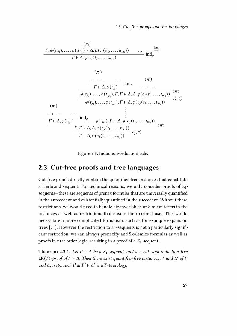
2.3 Cut-free proofs and tree languages
(c8)�, i (U 91), . . . , i (U 9:8 ) ` J,i (28 (U1, . . . , U<8 )) . . .
indd� ` J,i (28 (C1, . . . , C<8 ))
ind→
(c8)· · · ` · · · · · ·
indd� ` J,i (C 9:8 )
(c8)· · · ` · · · · · ·
indd� ` J,i (C 91)
(c8)· · · ` · · ·
cuti (C 92), . . . , i (C 9:8 ), � , � ` J, J, i (2 9 (C1, . . . , C< 9
))2∗;, 2∗A
i (C 92), . . . , i (C 9:8 ), � ` J,i (2 9 (C1, . . . , C< 9))
i (C 9:8 ), � ` J,i (2 9 (C1, . . . , C< 9))
cut�, � ` J, J, i (2 9 (C1, . . . , C< 9
))2∗;, 2∗A
� ` J,i (2 9 (C1, . . . , C< 9))
Figure 2.8: Induction-reduction rule.
2.3 Cut-free proofs and tree languages
Cut-free proofs directly contain the quanti�er-free instances that constitutea Herbrand sequent. For technical reasons, we only consider proofs of O1-sequents—these are sequents of prenex formulas that are universally quanti�edin the antecedent and existentially quanti�ed in the succedent. Without theserestrictions, we would need to handle eigenvariables or Skolem terms in theinstances as well as restrictions that ensure their correct use. This wouldnecessitate a more complicated formalism, such as for example expansiontrees [71]. However the restriction to O1-sequents is not a particularly signi�-cant restriction: we can always prenexify and Skolemize formulas as well asproofs in �rst-order logic, resulting in a proof of a O1-sequent.
Theorem 2.3.1. Let � ` J be a O1-sequent, and c a cut- and induction-freeLK() )-proof of � ` J. Then there exist quanti�er-free instances � ′ and J′ of �and J, resp., such that � ′ ` J′ is a ) -tautology.
27

2 Proofs with induction
Proof. For a detailed proof, see Buss [16]. We �rst permute the quanti�erinferences in the proof down as far as possible. Since the end-sequent isprenex, the resulting proof can be divided into two parts: the lower partwhich only consists of quanti�er inferences (as well as the structural rulesof contraction and weakening), and the upper part which does not containany quanti�er rules. The sequent in the middle is a quanti�er-free sequent ofinstances of the end-sequent. And furthermore it is a ) -tautology since thereis a proof above it. �
Example 2.3.1. Consider the LK(∅)-proof shown in Figure 2.9 with the end-sequent ∀~ % (0, ~),∀G∀~ (% (G, 5 (~))→% (B (G), ~)) ` % (B2(0), 2). Following theproof of Theorem 2.3.1 we can extract an Herbrand sequent from this proof.The proof above is already of the form required after the rule permutations:the part below the lowest→; -inference only consists of ∀; and 2; -inferencesand there are no quanti�er inferences above it. Hence the conclusion of thelowest→; -inference is a Herbrand sequent:
% (0, 5 2(2)),% (0, 5 2(2)) → % (B (0), 5 (2)),% (B (0), 5 (2)) → % (B2(0), 2)` % (B2(0), 2)
2.4 Term encoding of formulas
To connect proofs and grammars, as well as Herbrand sequents and languages,we need to convert between formulas and terms. This is because Herbrandsequents contain formulas, and tree grammars generate a set of terms. Forinstance, recall the Herbrand sequent from Example 2.3.1 (we write 5 2(2) as aconvenient abbreviation for 5 (5 (2))):
% (0, 5 2(2)),% (0, 5 2(2)) → % (B (0), 5 (2)),% (B (0), 5 (2)) → % (B2(0), 2)` % (B2(0), 2)
28

2.4 Term encoding of formulas
ax%(0,52 (2))`%(0,52 (2))
ax%(B(0),5(2))`%(B(0),5(2))
ax%(B
2 (0),2)`
%(B
2 (0),2)→
;%(B(0),5(2)),%(B(0),5(2))→%(B
2 (0),2)`
%(B
2 (0),2)→
;%(0,52 (2)),%(0,52 (2))→%(B(0),5(2)),%(B(0),5(2))→%(B
2 (0),2)`
%(B
2 (0),2)
∀ ;%(0,52 (2)),%(0,52 (2))→%(B(0),5(2)),∀~(%(B(0),5(~))→%(B
2 (0),~))`%(B
2 (0),2)∀ ;
%(0,52 (2)),%(0,52 (2))→%(B(0),5(2)),∀G∀~(%(G,5(~))→%(B(G),~))`%(B
2 (0),2)∀ ;
%(0,52 (2)),∀~(%(0,5(~))→%(B(0),~)),∀G∀~(%(G,5(~))→%(B(G),~))`%(B
2 (0),2)∀ ;
%(0,52 (2)),∀G∀~(%(G,5(~))→%(B(G),~)),∀G∀~(%(G,5(~))→%(B(G),~))`%(B
2 (0),2)2 ;
%(0,52 (2)),∀G∀~(%(G,5(~))→%(B(G),~))`%(B
2 (0),2)∀ ;
∀~%(0,~),∀G∀~(%(G,5(~))→%(B(G),~))`%(B
2 (0),2)
Figu
re2.9
:Pro
ofus
edin
Exam
ple
2.3.1.
29

2 Proofs with induction
We want to associate to this Herbrand sequent a set of terms !. One potentialchoice would be to treat the predicate symbols and logical connectives of � asfunction symbols, and negate the formulas in the succedent:
{% (0, 5 2(2)),% (0, 5 2(2)) → % (B (0), 5 (2)),% (B (0), 5 (2)) → % (B2(0), 2),¬% (B2(0), 2)}
However this representation is large and computationally unwieldy, so weencode formulas instances as term by introducing a new function symbol foreach formula:
De�nition 2.4.1. Let ∀G1 i1, . . . ,∀G< i< ` ∃G<+1 i<+1, . . . , ∃G= i= be a O1-sequent. Then we associate to each formula i8 a fresh function symbol A8(whose type is such that A8 (G8) has type >).
• The formula instance i8 [G8\C] encodes to the term A8 (C), which we writeas � (i8 [G8\C]) = A8 (C).
• Terms of the form A8 (C) for some 8 where C does not contain A 9 for any 9are called decodable
Example 2.4.1. The formula instance % (B (0), 5 (2))→% (B2(0), 2) encodes to theterm � (% (B (0), 5 (2)) → % (B2(0), 2)) = A2(B (0), 2). The term A2(B9(2), 5 (B (0)))is decodable, but A2(A1, 0) and A27(0) are not.
We can now extend this term encoding to sequents as well.
De�nition 2.4.2. Let � ` J be a O1-sequent.
• If � ′ ` J′ is a sequent of formula instances of � ` J, then � ′ ` J′
encodes to the set of terms � (� ′ ` J′) = {� (i) | i ∈ � ′ ∪ J′}.
• A set of terms ! is called decodable if all C ∈ ! are decodable.
• Given a decodable set of terms !, we de�ne � (!) as the unique sequentsuch that � (� (!)) = !.
30

2.5 Vectorial totally rigid acyclic tree grammars
Example 2.4.2. The Herbrand sequent of Example 2.3.1 encodes to the followinglanguage: � (� ) = {A1(5 2(2)), A2(0, 5 (2)), A2(B (0), 2), A3}
We de�ne the language of a cut-free proof to be the encoded Herbrandsequent:
De�nition 2.4.3. Let c be a cut- and induction-free LK() )-proof of a O1-sequent � ` J. Then we de�ne the Herbrand language !(c) = � (� ′ ` J′)where � ′ ` J′ is the Herbrand sequent as in Theorem 2.3.1.
Example 2.4.3. For the LK(∅)-proof c from Example 2.3.1, we have !(c) ={A1(5 2(2)), A2(0, 5 (2)), A2(B (0), 2), A3}.
2.5 Vectorial totally rigid acyclic tree grammars
In this section we will de�ne a special class of tree grammars called vectorialtotally rigid acyclic tree grammars, or VTRATGs for short. These are di�erentfrom regular tree grammars (as presented for example in [23]) in two ways:nonterminals are vectors, and the derivation relation is highly restricted. Theterminology of rigidity goes back to a similar restriction on the derivationrelation which was introduced with rigid tree automata [60].
Non-terminals are special variables. We will write T (O ∪- ∪# ) for the setof terms containing constants (including function symbols) from a signature O ,variables from - , and nonterminals from # ; the set of constants is alwaysdisjoint from the set of variables. We write 5 /= ∈ O if the function symbol 5has arity =. Non-terminals are special variables, and variables are nullaryfunction symbols.
De�nition 2.5.1. Let O be a set of function symbols with arity. A VTRATG�is given by a tuple � = (#, O, %,�):
1. � ∈ # is the start symbol.
2. # is a �nite set of nonterminal vectors. A nonterminal vector is a�nite sequence of nonterminals, and a nonterminal is a nullary functionsymbol. The nonterminals need to be pairwise distinct.
31

2 Proofs with induction
3. O is a �nite signature such that O ∩ # = ∅.
4. % is a �nite set of vectorial productions. A vectorial production is a pair� → C , where � ∈ # is a nonterminal vector and C = (C1, . . . , C:) is avector of terms of the same length as as �, and C8 has the same type as�8 for all 8 ≤ : .
5. there exists a strict linear order ≺ on the nonterminal vectors such that� ≺ � whenever �→ C ∈ % for some C and 9, : such that C 9 contains thenonterminal �: .
The last condition for the productions expresses the requirement that � isacyclic.
Example 2.5.1. With #, O, % de�ned as follows, � = (#, O, %,�) is a VTRATG:
# = {(�), (�1, �2)},O = {5 /3, 2/0, 3/0, 4/0},% = {(�) → (5 (�1, �2, �2)), (?1)
(�) → (5 (�2, �1, �1)), (?2)(�1, �2) → (2, 3) (?3)(�1, �2) → (3, 4)}. (?4)
We will often omit the parentheses for nonterminal vectors that consistof only a single nonterminal, i.e. we write � instead of (�). In addition, wetypically only specify the productions of a VTRATG, leaving �, O, # implicit.We would then just de�ne � to be the VTRATG with the productions:
�→ 5 (�1, �2, �2) | 5 (�2, �2, �1)(�1, �2) → (2, 3) | (3, 4)
We will compute the language generated by � in the next section, in Exam-ple 2.6.7.
Sometimes we will consider VTRATGs where every nonterminal vector haslength one. These non-vectorial VTRATGs are called TRATGs (totally rigidacyclic tree grammars):
32

2.6 Derivations in VTRATGs
De�nition 2.5.2. A TRATG is a VTRATG � = (#, O, %,�) such that all non-terminals vectors � ∈ # are of length |� | = 1.
There are several reasonable ways to measure the size of a grammar, e.g. wecould count the number of symbols in a textual representation. However, forour applications the most natural measurement that we will use by default isthe number of productions. The number of productions will correspond thenumber of quanti�er inferences in the simple proof described by the VTRATG(as we will see in Lemma 2.7.4). Counting the numbers of productions is alsothe size measure used by Bucher [15] in descriptional complexity.
De�nition 2.5.3. Let � = (#, O, %,�) be a VTRATG. Its size |� | = |% | is thenumber of its productions.
2.6 Derivations in VTRATGs
So far we have only de�ned VTRATGs, but not their language, that is, theset of terms generated by a VTRATG. A term is generated by a VTRATG ifthere is a derivation of the term. There are several equivalent ways to de�nederivations (and hence languages of VTRATGs):
(1⇒) A derivation is a �nite sequence of terms, such that in every step a
nonterminal is replaced by the right-hand side of a production, using atmost one production for every nonterminal vector.
(2⇒) A derivation is a �nite sequence of terms, such that in every step a
nonterminal is replaced by the right-hand side of a production, ful�llinga certain rigidity condition. (This de�nition only works for TRATGs.)
(3⇒) A derivation is a �nite subset of the productions, containing at most one
production for every nonterminal vector. The derived term is then givenby an iterated substitution using the productions.
Let us begin with the de�nition using1⇒: we �rst de�ne a single-step deriva-
tion relation1⇒? , which describes replacing a single nonterminal using the
33

2 Proofs with induction
production ? . This single-step relation is then extended to the rigid deriva-tion relation
1⇒A
� , which is a �nite sequence of1⇒? steps, using at most one
production per nonterminal vector.
De�nition 2.6.1. Let� = (#, O, %,�) be a VTRATG, ? = �→ B a production,and C1, C2 terms. Then C1
1⇒? C2 i� there exists a position @ ∈ Pos(C1) such thatC1 |@ = �8 and C2 = C1 |? [B8] for some 8 . We de�ne C1
1⇒� C2 i� there exists aproduction ? ∈ % such that C1
1⇒� C2.
Example 2.6.1 (continuing Example 2.5.1).
�1⇒?1 5 (�1, �2, �2)
1⇒?3 5 (2, �2, �2)1⇒?3 5 (2, �2, 3)
1⇒?3 5 (2, 3, 3)
A set of pairs - is called a partial function if 1 = 1′ for all (0, 1) ∈ - and(0, 1′) ∈ - . Since productions are by de�nition pairs, a set of productions isa partial function if and only if it contains at most one production for everynonterminal vector.Example 2.6.2 (continuing Example 2.5.1). {?1, ?3} is a partial function, but{?3, ?4} is not.
De�nition 2.6.2. Let � = (#, O, %,�) be a VTRATG, and B, C ∈ T (O ∪ # ).Then B
1⇒A
� C i� there exists a sequence B = C11⇒?1 C2
1⇒?2 . . .1⇒?= C= = C such
that the set {?1, . . . , ?=} ⊆ % is a partial function.
Such a sequence of terms is called a derivation.
Example 2.6.3 (continuing Example 2.5.1). �1⇒A
� 5 (2, 3, 3) since the set ofproductions {?1, ?3} used in the sequence in Example 2.6.1 is a partial function.Using De�nition 2.6.2, we will be able to compute !(�) = {C ∈ T (O) | � 1⇒
A
�
C} = {5 (2, 3, 3), 5 (3, 2, 2), 5 (3, 4, 4), 5 (4, 3, 3)}. Note that � 6 1⇒A
� 5 (2, 4, 4), sincewe would need to use two di�erent productions for �.
The size of a1⇒-derivation is bounded by the size of the term and the number
of nonterminal vectors in the grammar:
Lemma 2.6.1. Let � = (#, O, %,�) be a VTRATG, and B, C ∈ T (O ∪ # ). Then= ≤ |Pos(C) | |# | for any sequence B = C1
1⇒?1 C21⇒?2 . . .
1⇒?= C= = C with ?8 ∈ %for all 8 .
34

2.6 Derivations in VTRATGs
Proof. Each of the steps replaces a nonterminal with its right-hand side at asingle position. There are at most |Pos(C) | such positions. It is possible thatwe have multiple steps that replace at the same position, for example withproductions of the form �→� . However due to the acyclicity of � , this canonly happen |# | times per position. �
For TRATGs, we can use a slightly more interesting side condition on thesequence of terms C1, . . . , C= in De�nition 2.6.2. Instead of characterizing theset of used productions as a partial function, we can give a side condition onthe equality of subterms of C = C=: if a nonterminals occurs twice as C8 |@ = C8 ′ |@′ ,then both occurrences expand to the same subterm C |@ = C |@′ in C :
De�nition 2.6.3. Let� = (#, O, %,�) be a TRATG, and B, C ∈ T (O∪# ). ThenB
2⇒A
� C i� there exists a sequence B = C11⇒?1 C2
1⇒?2 . . .1⇒?= C= = C such that
?8 ∈ % for all 1 ≤ 8 ≤ =, and: for any 1 ≤ 8, 8′ ≤ = and positions @, @′ whereC8 |@ = C8 ′ |@′ is a nonterminal, we have C |@ = C |@′ .
The side condition on the sequence in De�nition 2.6.3 is called total rigidityand is named after a corresponding notion for regular tree automata [61].
Example 2.6.4. Let� be the TRATG with the productions ?1 = �→5 (�, �), ?2 =�→2 and ?3 = �→3 . In the sequence�
1⇒?1 5 (�, �)1⇒?2 5 (2, �)
1⇒?2 5 (2, 2),the nonterminal � occurs three times as � = C2 |1 = C2 |2 = C3 |2. The subterms of5 (2, 2) |1 = 2 and 5 (2, 2) |2 = 2 are equal, and hence�
2⇒A
� . As a counterexample,consider the sequence �
1⇒?1 5 (�, �)1⇒?2 5 (2, �)
1⇒?3 5 (2, 3). It does notful�ll the rigidity condition in De�nition 2.6.3: we have � = C2 |1 = C3 |2 but5 (2, 3) |1 = 2 ≠ 5 (2, 3) |2 = 3 .
Remark 2.6.1. We cannot use this rigidity condition for derivations in VTRATGsas this would result in a di�erent notion of language. Consider the VTRATG�with the productions�→5 (�,�) and (�,�)→(3,3) | (4, 4). Then the sequence� ⇒2
�5 (�,�) ⇒2
�5 (3,�) ⇒2
�5 (3, 4) ful�lls the rigidity condition, but it
uses two di�erent productions for the nonterminal vector (�,�) and hencederives a term 5 (3, 4) ∉ !(�).
The third way to de�ne derivations,3⇒, directly characterizes the used
productions. We associate to every partial function % ′ ⊆ % of the produc-
35

2 Proofs with induction
tions a substitution f% ′. The derivable terms are then the images of the startnonterminal � under these substitutions.
De�nition 2.6.4. Let � = (#, O, %,�) be a VTRATG, and % ′ ⊆ % a partialfunction. We can order the nonterminal vectors on the left-hand sides of % ′
as dom(% ′) = {�1 ≺ �2 ≺ · · · ≺ �=} (where ≺ is as in De�nition 2.5.1). Thenwe de�ne f% ′ = [�1\C1] · · · [�=\C=] where C8 is the unique vector of terms suchthat �8 → C8 ∈ % ′ for 1 ≤ 8 ≤ =.
Example 2.6.5 (continuing Example 2.5.1). The nonterminal vectors are orderedas � ≺ � and we have f{?1,?3} = [�\5 (�1, �2, �2)] [�1\2, �2\3].Remark 2.6.2. The reason we use partial functions and not just functions inDe�nition 2.6.4 is because the VTRATG might contain a nonterminal vector� such that there is no production of the form �→ . . . . There are nontrivialexamples of such VTRATGs: consider for example the VTRATG � with theproductions � → � and (�,�) → (�, 4) (where � is a nonterminal vector,which clearly does not have any associated productions). Then !(�) = {4}.The term 4 has the⇒3
�-derivation {�→�, (�,�) → (�, 4)}. We cannot make
this partial function total since there is no production for � .
Lemma 2.6.2. Let� = (#, O, %,�) be a VTRATG, and % ′ ⊆ % a partial function.Then � 9f% ′ = B 9f% ′ for any 9 and �→ B ∈ % ′.
Proof. With �1 ≺ · · · ≺ �= as in De�nition 2.6.4, let 8 be such that � = �8 andB 9 = C8, 9 . Then:
� 9f% ′ = � 9 [�1\C1] · · · [�=\C=]= � 9 [�2\C2] · · · [�=\C=]...
= � 9 [�8\C8] · · · [�=\C=]= B 9 [�8+1\C8+1] · · · [�=\C=]= B 9 [�8\C8] · · · [�=\C=]...
= B 9 [�1\C1] · · · [�=\C=]= B 9f% ′
36

2.6 Derivations in VTRATGs
The substitutions [�:\C:] are the identity on � 9 for : < 8 , and the identityon B 9 for : ≤ 8 , since �: and FV(� 9 ) (resp., FV(B 9 )) are disjoint. �
De�nition 2.6.5. Let � = (#, O, %,�) be a VTRATG, and C ∈ T (O). Then�
3⇒� C i� there exists a partial function % ′ ⊆ % such that C = �f% ′ .
Example 2.6.6 (continuing Example 2.6.5). �3⇒� 5 (2, 3, 3) since �f{?1,?3} =
5 (2, 3, 3).
Lemma 2.6.3. Let % ′ be a set of productions that is a partial function, and C1⇒? B
where ? ∈ % ′. Then Cf% ′ = Bf% ′ .
Proof. Let � → A ∈ % ′ and 9, @ be such that C |@ = � 9 and C |@ [A 9 ] = B . Itsu�ces to show that C |@f% ′ = B |@f% ′ since that is the only common position atwhich the two terms di�er. This is the case i� � 9f% ′ = B 9f% ′ , which is true byLemma 2.6.2. �
Theorem 2.6.1. Let� = (#, O, %,�) be a VTRATG, and C ∈ T (O) a term. Thenthe following are equivalent:
1. �1⇒A
� C
2. �3⇒� C
Proof. 1⇒ 2. By De�nition 2.6.2, there exists a sequence � = C11⇒?1 C2
1⇒?2
. . .1⇒?= C= = C such that the set % ′ = {?1, . . . , ?=} ⊆ % is a partial function. By
Lemma 2.6.3, C8f% ′ = C8+1f% ′ for any 1 ≤ 8 ≤ = and hence �f% ′ = C=f% ′ = C .2⇒ 1. By De�nition 2.6.5, there exists a partial function % ′ ⊆ % such that
C = �f% ′ = [�1\B1] · · · [�=\B=]. De�ne a sequence C1 · · · C= that performs thissubstitution using
1⇒-steps with the productions in % ′. �
Theorem 2.6.2. Let � = (#, O, %,�) be a TRATG, and C ∈ T (O) a term. Thenthe following are equivalent:
1. �1⇒A
� C
2. �2⇒A
� C
37

2 Proofs with induction
3. �3⇒� C
Proof. We have already shown 1⇔ 3 in Theorem 2.6.1.1⇒ 2. A
1⇒-derivation already ful�lls the total rigidity condition of De�ni-tion 2.6.5 since C8 |@f% ′ = C |@ for any 8 and position @ by Lemma 2.6.3.2 ⇒ 3. By De�nition 2.6.3, there exists a sequence � = C1
1⇒?1 C21⇒?2
. . .1⇒?= C= = C such that C |@ = C |@′ whenever C8 |@ = C8 ′ |@′ is a nonterminal.
Hence we can de�ne a substitution d in such a way that C8 |@d = C |@ for all8 and positions @ ∈ Pos(C8). Let % ′ ⊆ {?1, . . . , ?=} be a partial function thatcontains a production for every nonterminal occurring in C1, . . . , C=. Let # =
{�1 ≺ �2 ≺ · · · ≺ �:}. We now show that � 9d = � 9X% ′ for every 9 by reverseinduction on 9 , that is, starting with 9 = : . Let � 9 → B 9 ∈ % ′. Then there isan 8 such that C8
1⇒� 9→B 9 C8+1 and hence � 9d = B 9d . We also have � 9f% ′ = B 9f% ′since � 9 → B 9 ∈ % ′. Now B 9d = B 9f% ′ by the induction hypothesis since B 9 onlycontains nonterminals � such that � 9 ≺ � . Thus � 9d = � 9f% ′ by transitivity.Finally we have �f% ′ = �d = C and hence �
3⇒ C . �
Theorems 2.6.1 and 2.6.2 show that all the three ways to de�ne derivationsare equivalent in the sense that they allows us to derive the same set of terms.Formally, we pick
3⇒ as the o�cial de�nition of derivation:
De�nition 2.6.6. Let � = (#, O, %,�) a VTRATG. A derivation X in � is asubset X ⊆ % of the productions such that X is a partial function and �f% ′ ∈T (O). The derivation X derives the term �f% ′ .
We will often implicitly use the derivation X as a substitution: that is, wewrite �X as an abbreviation for �fX .
De�nition 2.6.7. Let� = (#, O, %,�) be a VTRATG. The language generatedby � is the set of derivable terms !(�) = {C ∈ T (O) | � 3⇒� C}.
Example 2.6.7 (continuing Example 2.5.1). We can compute the language of �as follows: !(�) = {5 (2, 3, 3), 5 (3, 4, 4), 5 (3, 2, 2), 5 (4, 3, 3)}.
The languages of VTRATGs are �nite. In fact the language of a VTRATGcontains at most exponentially more terms than the number of productions inthe VTRATG:
38

2.7 Grammars for simple proofs
Lemma 2.6.4. Let � = (#, O, %,�) be a VTRATG, and for every � ∈ # de�ne%�= {? ∈ % | ∃C ? = �→ C}. Then |!(�) | ≤ ∏
�∈#,%�≠∅ |%� |.
Proof. By counting the derivations: observe that if X ⊆ X′ for two deriva-tions X, X′ in � , then �X = �X′. Hence we can assume that a derivation X isde�ned for all nonterminal vectors � such that %
�≠ ∅. Hence we need to count
the number of subsets X ⊆ % that are functions with domain {� ∈ # | %�≠ ∅}.
This number is exactly the stated bound. �
If a VTRATG contains a production for every nonterminal vector, then wecan also give another equivalent de�nition of !(�):
Lemma 2.6.5. Let � = (#, O, %,�0) be a VTRATG with the nonterminals # =
{�0 ≺ �1 ≺ · · · ≺ �=} such that for every 8 there is a production �8 → C ∈ % forsome C . Then:
!(�) = {�0 [�0\B0] [�1\B1] · · · [�=\B=] | ∀8 �8 → B8 ∈ %}
Proof. The substitution is f% ′ where % ′ ⊆ % such that % ′ is a total function.Thus the right-hand side is included in !(�). Since �X = �X′ for derivationsX ⊆ X′ and there is a production for every nonterminal vector, we can extendany derivation to a total function. Therefore !(�) is also included in theright-hand side. �
2.7 Grammars for simple proofs
We will now look at the class of proofs described by VTRATGs. The mainrestriction is that the cut formulas in the proofs may not contain quanti�eralternations. In addition, we require that the cut formulas are prenex. Formally,we call this class of proofs the simple proofs:
De�nition 2.7.1. A simple proof is an induction-free LK() )-proof such that:
1. All cut formulas are of the form ∀G i (G) or ∃G i (G) where i (G) isquanti�er-free.
2. The end-sequent is a O1-sequent.
39

2 Proofs with induction
3. Whenever a formula with strong quanti�ers occurs in the proof then itis immediately preceded by an ∀A or ∃; inference.
4. Every strong quanti�er inference (∀A , ∃; ) has a di�erent eigenvariable,none of the eigenvariables occur in the end-sequent.
5. No weakening inferences are applied to quanti�ed formulas, unless theweakened formula is an ancestor of a cut-formula or a formula in theend-sequent.
Only the �rst restriction is signi�cant. Restricting the logical complexity ofthe cut formulas has an e�ect on proof size. While we can of course alwaysreduce cuts of higher complexity to the cuts allowed in simple proofs, thisincurs a size increase.
The second restriction on the end-sequent simpli�es the theory since wedo not have to deal with eigenvariables from the end-sequent. We can al-ways Skolemize and prenexify the end-sequent, producing an equi-satis�ablesequent.
The restriction on the strong quanti�ers. It only has a local e�ect on the cutinferences because the only strong quanti�ers in the proof occur in the cuts. Itmeans that the cuts are of the following form:
� ` J,i (U)∀∗A
� ` J,∀G i (G) ∀G i (G), N ` Lcut
�, N ` J, LThat is, the cut inference always occurs together with the ∀A -block (or ∃; -
block) as an inseparable package. This also simpli�es the correspondencebetween proofs and grammars, because now there is only one vector of eigen-variables for each cut. The following cut is hence forbidden:
k ` i (U) ∀Ak ` ∀G i (G)
\ ` i (V) ∀A\ ` ∀G i (G) ∧;
k ∧ \ ` ∀G i (G) ∀G i (G) ` jcut
k ∧ \ ` j
The restriction on the eigenvariables is a purely technical one, known as“regularity” in the literature. (We will avoid this terminology here to avoid
40

2.7 Grammars for simple proofs
confusion with another interesting kind of regularity, namely that a familyof instance proofs comes from a proof with induction.) Requiring the eigen-variables to be di�erent means that we can reuse them as the nonterminalsin the VTRATG that corresponds to the proof. We can always rename theeigenvariables to ful�ll this condition.
The last restriction on weakening inferences on quanti�ed formulas ensuresthat the number of quanti�er inferences in the proof corresponds to the numberof productions in the grammar (up to a constant factor). We can always ensurethis restriction by permuting the weakening inferences downwards, this onlydecreases the size of the proof. Another way to satisfy this restriction is toalways instantiate all quanti�ers of a formula at once (as if the quanti�er blockwas a single quanti�er), with no other inferences in between. An example of aforbidden weakening is the following:
� ` J F;∀~ i (2,~), � ` J ∀;∀G∀~ i (G,~), � ` J
Lemma 2.7.1. Let c be a simple proof and ccut→c ′, then c ′ is also a simple proof
(up to a potential renaming of eigenvariables).
Proof. Each of the restrictions is preserved under cut-reduction, except forthe condition on the eigenvariables. This may be violated in a reduction of acontraction inference, which duplicates a subproof. �
In Section 2.4 we introduced the isomorphism between a subset of termsand formula instances. We called the terms that encode formula instancesdecodable (De�nition 2.4.1). We now extend this notion to VTRATGs:
De�nition 2.7.2. Let ( be a O1-sequent, and � = (#, O,�, %) be a VTRATG.Then � is called decodable i� all the following are true:
• � has type >
• For every production �→ C ∈ % , the right-hand side C is decodable.
• For every production �→ C ∈ % where � ≠ �, the right-hand side C doesnot contain A8 for any 8 .
41

2 Proofs with induction
Example 2.7.1. The VTRATG with the productions {�→A1(�) | A2(5 (�)), �→2 | 3} is decodable, the one with the productions {�→ �, �→ A2(2)} is not(even though its language {A2(2)} would be decodable).
One consequence of this de�nition is that the language of a decodableVTRATG is decodable:
Lemma 2.7.2. Let � be a decodable VTRATG, then !(�) is decodable as well.
We can now assign to every simple proof a VTRATG containing the data ofthe quanti�er inferences:
De�nition 2.7.3. Let c be a simple proof. We de�ne the VTRATG � (c) withthe start symbol � containing the following productions:
• For every quanti�ed cut with the eigenvariables U and a weak quanti�erinstance of the cut-formula with the terms C , we add the productionU → C : (and analogously for existential formulas)
· · · ` · · · , i (U)∀∗A· · · ` · · · ,∀G i (G)
i (C), · · · ` · · · ∀∗;, . . .
∀G i (G), · · · ` · · ·
∀G i (G), · · · ` · · ·cut· · · ` · · ·
• For every instance i (C) of a formula of the end-sequent, we add theproduction �→ � (i (C)): (and analogously for existential formulas)
i (C), · · · ` · · · ∀∗;, . . .
∀G i (G), · · · ` · · ·
∀G i (G), · · · ` · · ·
42

2.7 Grammars for simple proofs
Example 2.7.2. Consider the following LK(∅)-proof of the sequent ∀G % (G) `% (5 (2)):
ax% (5 (U)) ` % (5 (U)) ∀;∀G % (G) ` % (5 (U)) ∀A∀G % (G) ` ∀G % (5 (G))
ax% (5 (2)) ` % (5 (2)) ∀;∀G % (5 (G)) ` % (5 (2))
cut∀G % (G) ` % (5 (2))
The VTRATG � (c) as de�ned by De�nition 2.7.3 then has the followingproductions:
�→ A1(5 (U)) | A2U → 2
The language it generates is !(� (c)) = {A1(5 (2)), A2}. This language decodesto the Herbrand sequent % (5 (2)) ` % (5 (2)).
It is easy to see that � (c) is decodable:
Lemma 2.7.3. Let c be a simple proof. Then � (c) is decodable.
The size of� (c) is proportional to the number of quanti�er inferences |c |@ ,where the constant factor only depends on the end-sequent and the maximumsize of a non-terminal vector in � (c). The di�erence is due to non-terminalvectors: one production like (�1, �2) → (C, B) typically corresponds to twoquanti�er inferences in the proof. The bound of the following theorem can bemade precise by using more sophisticated size measures [32].
Lemma 2.7.4. Let c be a simple proof, and� (c) = (#, O, %,�). Then |� (c) | −� ≤ |c |@ ≤ |� (c) | · � · max�∈# |� |, where � is the maximum number ofquanti�ers in a formula of the end-sequent of c , and� is the number of quanti�er-free formulas in the end-sequent.
Let us conclude by stating the main theorem connecting simple proofs andtheir corresponding VTRATGs, namely that cut-reduction is compatible withlanguage generation:
Lemma 2.7.5 ([46]). Let c, c ′ be simple proofs such that ccut→c ′, then !(� (c)) ⊇
!(� (c ′)). If c ne→ c ′, then !(� (c)) = !(� (c ′)).
43

2 Proofs with induction
Corollary 2.7.1. Let c be a simple proof, then !(� (c)) is a ) -tautology.
This correspondence has since been extended to a larger class of proofs, withno restrictions on the quanti�er complexity of the cut formulas [2]. Howeveras the cuts become more complicated, the grammars used to describe thequanti�er inferences need to become more complicated as well. The class ofgrammars used for the general case is a special form of higher-order recursionschemes.
Theorem 2.7.1 ([2, Lemma 7.2]). For every induction-free proof c of a O1-sequent such that all cut formulas in c are prenex there is a higher-order recursionscheme � (c), where this function � has the property that !(� (c)) ⊇ !(� (c ′))whenever c
cut→ c ′.
2.8 Grammars for simple induction proofs
2.8.1 Simple induction problems
We can also assign grammars to another class of proofs, namely some proofscontaining induction of the following kind of sequents:
De�nition 2.8.1. A simple induction problem is a sequent � ` ∀G i (G) where� is a list of universally quanti�ed prenex formulas, i (G) quanti�er-free, andthe quanti�er ∀G ranges over an inductive sort d .
Example 2.8.1. ∀~ % (0, ~),∀G∀~ (% (G, 5 (~)) → % (B (G), ~)) ` ∀G % (G, 2)
For technical reasons, we only consider the case of a single universal quan-ti�er in the conclusion. We can still treat problems that would naturally bestated using multiple quanti�ers by instantiating all but one quanti�er withfresh constants: e.g. for commutativity we get the simple induction problem� ` ∀G G + 2 = 2 + G .
Given such a simple induction problem � ` ∀G i (G), we will consider in-stance problems � ` i (C) for terms C . If these terms are built from constructors,then we will be able to unfold a proof with induction of � ` ∀G i (G) into aproof with cuts. The following de�nition makes this notion concrete:
44

2.8 Grammars for simple induction proofs
De�nition 2.8.2. Let d be an inductive type with constructors 21, . . . , 2= . Theset of constructor terms of type d is the smallest set of terms containing foreach constructor 28 all terms 28 (A1, . . . , A8= ) whenever it contains all A 9 where 9is a recursive occurrence in 28 . A free constructor term is a constructor termwhere all subterms of a type other than d are pairwise distinct fresh constants.We denote the set of free constructor terms by C.
Example 2.8.2. For natural numbers, the terms 0, B (0), B (B (0)) are free construc-tor terms, but B (G) is not; all constructor terms are already free constructorterms. If we consider lists of natural numbers with the constructors nil andcons, then nil, cons(01, nil), cons(01, cons(02, nil)) are free constructor terms,but cons(G + G, cons(G, nil)) is a constructor term that is not a free constructorterm.
De�nition 2.8.3. Let � ` ∀G i (G) be a simple induction problem, and C afree constructor term of type d . Then � ` i (C) is the instance problem for theparameter C .
Example 2.8.3. The Example 2.3.1 that we considered earlier was an instanceproblem for Example 2.8.1.
2.8.2 Simple induction proofs
We can now de�ne the class of simple induction proofs, these consist of asingle induction followed by a cut. Note that the end-sequents of the proofs c8and c2 are ) -tautologies.
De�nition 2.8.4. Let d be an inductive type, � ` ∀G i (G) a simple inductionproblem,k (G,F,~) a quanti�er-free formula, �1, . . . , �=, �2 quanti�er-free in-stances of � , and C8, 9,: , D: term vectors. Then a simple induction proof is a proofc of the following form, where c1, . . . , c=, c2 are cut-free proofs:
(c ′1)... · · ·
(c ′=)...indd
� ` ∀~ k (U, U,~)
(c2)�2,k (U, U,D:), · · · ` i (U) ∀∗
;,F∗
;�,∀~ k (U, U,~) ` i (U) cut, 2∗
;� ` i (U) ∀A� ` ∀G i (G)
45

2 Proofs with induction
where c ′8 =
(c8)�8,k (U, a8,8; , C8,8; ,:), · · · ` k (U, 28 (a8), W) ∀∗
;,F∗
;, 2∗;,∀∗A
�,∀~ k (U, a8,8; , ~), · · · ` ∀~ k (U, 28 (a8), ~)
Example 2.8.4. We consider a simple induction proof of Example 2.8.1 with theinduction formula ∀~ k (U, a,~) wherek (U, a,~) = % (a,W). Formally the proofcontains the following instances and terms:
�2 = {% (a, 5 (W)) → % (B (a), W)}�1 = {% (0, W)}�2 = ∅
C2,1,1 = 5 (W)D1 = 2
Lemma 2.8.1. Let � ` ∀G i (G) be a simple induction problem. If there exists asimple induction proof c for the simple induction problem, then for every C thereexists a �rst-order proof cC for the instance problem with parameter C .
Proof. Inspecting De�nition 2.8.4, there is a subproof c ′ of c with the end-sequent � ` i (U). By substitution we obtain a proof c ′′ = c ′[U\C] of � ` i (C).This proof c ′′ contains a single induction inference with the main term C . SinceC is a free constructor term, we can unfold the induction inference in c ′′ in atmost |C | steps using the ind→ reduction, yielding c ′′ ind→ cC . �
2.8.3 Induction grammars
Just as sets of terms describe the quanti�er inferences in proofs of the se-quents of the instance problems (via their decoding to Herbrand sequents),and VTRATG describe the quanti�er inferences in the instance proofs withcuts, we use induction grammars to describe the quanti�er inferences in thesimple induction proof.
De�nition 2.8.5. An induction grammar � = (g, U, (a2)2, W, %) consists of:
1. the start nonterminal g of type > ,
2. a nonterminal U whose type d is an inductive sort,
46

2.8 Grammars for simple induction proofs
3. a family of nonterminal vectors (a2)2 , such that for each constructor 2 ofthe inductive sort d the term 2 (a2) is well-typed,
4. a nonterminal vector W , and
5. a set of vectorial productions % , where each production is of the formg → C [U, a8, W] or W → C [U, a8, W] for some 8 .
Example 2.8.5. The induction grammar corresponding the simple inductionproof in Example 2.8.4 has the following productions:
g → A1(W) | A2(a,W) | A3W → 5 (W) | 2
An induction grammar generates a family of languages: each constructorterm induces a language.
De�nition 2.8.6. A family (!C )C∈� of languages is a function from a set of freeconstructor terms � to languages.
We will not directly de�ne derivations and the generated language forinduction grammars. Instead we will de�ne an instantiation operation thatresults in a VTRATG, and de�ne the language of the induction grammar asthe language of the VTRATG obtained via instantiation. The instantiationoperation depends on a constructor term A as parameter, in the same way asthe instance problem � ` i (A ) uses a constructor term. Instantiation of aninduction grammar into a VTRATG closely mirrors how the induction rule isunfolded into a series of nested cuts in Lemma 2.8.1.
De�nition 2.8.7. Let � = (g, U, (a2)2, W, %) be an induction grammar, and Aa constructor term of the same type as U . The instance grammar � (�, A ) =(g, # , % ′) is a VTRATG with nonterminal vectors # = {g} ∪ {WB | B E A } andproductions % ′ = {?′ | ∃? ∈ % (? { ?′)}. The instantiation relation ? { ?′ isde�ned as follows:
• g → C [U, a8, W] { g → C [A, B, W28 (B)] for 28 (B) E A
• W → C [U] { WB → C [A ] for B E A
47

2 Proofs with induction
• W → C [U, a8, W] { WB 9 → C [A, B, W28 (B)] for 28 (B) E A ,where 9 is a recursive occurrence in 28
Example 2.8.6. Let us instantiate the induction grammar in Example 2.8.5 withthe parameter B (B (0)). The instance grammar � (�, B (B (0))) has the nontermi-nals g , W0, WB (0) , and WB (B (0)) , and contains all productions on the right-hand side(we use the abbreviation ? { ?′1 | ?′2 for ? { ?′1 ∧ ? { ?′2).
g → A1(W) { g → A1(W0) | g → A1(WB (0)) | g → A1(WB (B (0)))g → A2(a,W) { g → A2(0, WB (0)) | g → A2(B (0), WB (B (0)))W → 5 (W) { W0→ 5 (WB (0)) | WB (0)→ 5 (WB (B (0)))
W → 2 { W0→ 2 | WB (0)→ 2 | WB (B (0))→ 2
We can now de�ne the language in terms of the instance grammar. Thereis a di�erent language for each constructor term. Alternatively, we can alsothink of the induction grammar generating a family of languages.
De�nition 2.8.8. Let � = (g, U, (a2)2, W, %) be an induction grammar, and C aconstructor term of the same type as U . Then we de�ne the language for theparameter C as !(�, C) = !(� (�, C)).
Example 2.8.7. The induction grammar in Example 2.8.5 produces the followinglanguage for the parameter B (B (0)), which decodes to a tautology:
!(�, B (B (0))) = {A1(2), A1(5 (2)), A2(5 (5 (2)),A2(0, 2), A2(0, 5 (2)), A2(B (0), 2),A3}
In Example 2.3.1 we have already seen an instance proof of the sequent of ourrunning example. Its Herbrand sequent uses only a subset of the instanceshere. We have � (� ) ⊆ !(�, B (B (0))) for the encoded set of terms we computedin Example 2.4.2.
Recall that !(� (c), C) is a set of terms that encodes a Herbrand sequent forthe instance problem with parameter C . The computation of the Herbrandsequent on the term-level using grammars closely mirrors the Herbrand se-quents obtained via induction-unfolding and cut-elimination on the level of
48

2.8 Grammars for simple induction proofs
proofs (that is, !(c∗C )): the language generated by the grammar is a superset ofthe language extracted from the proof. That !(� (c), C) is (in general) a strictsuperset of !(c∗C ) (and not exactly equal) is a subtlety introduced by weakeninginferences in c : quanti�er inferences may be deleted when reducing weaken-ing inferences during cut-elimination. But the grammar still generates thesedeleted terms, since it intentionally abstracts away from the propositionalreasoning of the proof.
Theorem 2.8.1. Let c be a simple induction proof and C an instance term. Then!(� (c), C) ⊇ !(c∗C ).
c cC c∗C
� (c) � (cC ) !(� (c), C) ⊇ !(c∗C )
ind cut
Proof. Unfolding the induction in c yields a proof cC without induction as inLemma 2.8.1. The instantiation relation in De�nition 2.8.7 is chosen so that� (� (c), C) ⊇ � (cC ). Then !(� (c), C) = !(� (� (c), C)) ⊇ !(� (cC )) ⊇ !(c∗C ) forany c∗C such that cC
cut→ c∗C by Lemma 2.7.5. �
In particular, Theorem 2.8.1 tells us that induction grammars extracted fromproofs produce tautological languages for every instance:
De�nition 2.8.9. A family of languages (!C )C∈� is called () -)tautological if !Cis ) -tautological for every C . An induction grammar � is called tautological if(!(�, C))C∈C is tautological, i.e., the language !(�, C) is) -tautological for everyconstructor term C .
Corollary 2.8.1 (of Theorem 2.8.1). Let c be a simple induction proof. Thenthe induction grammar � (c) is tautological.
Similar to Lemma 2.7.4 for the VTRATG of a simple proof, the quanti�er com-plexity of the simple induction proof c is related to the number of productions|� (c) | in the induction grammar:
Lemma 2.8.2. Let c be a simple induction proof, and � (c) = (g, U, (a2)2, W, %).Then |� (c) | −� ≤ |c |@ ≤ � · |� (c) | · |W |, where� and � are constant that onlydepends on the end-sequent of c .
49

2 Proofs with induction
2.9 Reversing cut- and induction-elimination
In the previous sections we have seen that we can use grammars to computeHerbrand sequents for proofs. For a proof with N1-cuts we can extract aVTRATG whose language then decodes to a Herbrand sequent. For a simpleinduction proof we can extract an induction grammar that for every parametergenerates a language that decodes to a Herbrand sequent.
An interesting application is to reverse this process. On the level of thereduction relations of cut- and induction-elimination it is virtually hopelessto reverse the reduction, even going back one step there are in�nitely manyproofs that reduce in one step to the current one. Undoing the reduction of aweakening inference, we would even need to choose an arbitrary subproof.
The concept that connects grammars and proofs is the one of formulaequations, which will collect the conditions necessary to produce a proof for agiven grammar. That is, we will assign to a grammar� a formula equationQ�such thatQ� has a quanti�er-free solution i�� is the grammar of a proof. Wewill discuss these induced formula equations in more detail in Chapter 5, aswell as practically e�ective algorithms to solve them.
De�nition 2.9.1. A formula equation ∃-1 . . . ∃-=R is a formula whereR isa �rst-order formula and -1, . . . , -= are second-order predicate variables. Asolution modulo the theory ) is a substitution f of the predicate variables-1, . . . , -= to �rst-order formulas such that ) entailsRf .
A solution is called quanti�er-free if -1f, . . . , -=f are all quanti�er-free.
Example 2.9.1. The FE R = ∃- ((% (0) → - (0)) ∧ (- (1) → % (1))) has thesolution [-\_G % (G)] modulo any theory ) . The predicate variable - couldstand for the quanti�er-free matrix of a cut formula, solving the formulaequations then amounts to �nding a suitable matrix for the cut formula.
On the level of grammars, the reversal of cut- and induction-eliminationis feasible in practice. For simple proofs, this process of cut-introduction wasintroduced in [51]. Starting from a Herbrand sequent of a cut-free proof c∗
encoded as a term language !, we �rst �nd a VTRATG� such that !(�) ⊇ !.As the second step we need to �nd a simple proof c such that � (c) = � . Thisis equivalent to solving the induced formula equation Q� . (Remember that
50

2.10 Regularity and reconstructability
solution of the formula equation consists of the quanti�er-free matrices ofthe cut formulas in the simple proof). Given a VTRATG � whose languageis tautological (which it is because � ⊇ ! = !(c∗)), we can always solve theformula equationQ� , as we will see in Theorem 5.2.1. There are a number oftechniques to post-process these formulas to obtain short and human-readablecut-formulas [48, 36]. In practice this algorithm can produce interesting cutformulas, such as automatically synthesizing a lemma stating the transitiv-ity of the order in a lattice, given a proof from only axioms for the meetoperation [36].
We can also use reverse the process of induction-elimination [31]. Here westart with a family (!8)8∈� of Herbrand sequents, one for the instance problem ofeach parameter. First, we �nd a induction grammar� such that ∀8 !(�, 8) ⊇ !8 .Here we need to solve a more complicated formula equation in the secondstep. The solution to this formula equation is the quanti�er-free matrix ofthe induction formula. This problem is much harder than the correspondingproblem in cut-introduction, and for some grammars there may not even existsuch a matrix (even though the language of the grammar is tautological foreach parameter, see Theorem 5.4.1 [31]).
We do not have to start with proofs obtained by induction-elimination either,the languages !8 could also be produced by an automated theorem prover. Thiscombination produces an automated inductive theorem prover.
2.10 Regularity and reconstructability
On a theoretical level, we can also view the reversal of induction-eliminationof the preceding Section 2.9 as a way to recover the induction grammar ofa given simple induction proof from the Herbrand sequents of its inducedinstance proofs, and �nding a solution to the formula equation amounts torecovering the induction formula. In this section we will study this problemon a theoretical level, namely in how far it is decidable whether a familyof languages comes from induction-elimination, and whether we can theinduction-reversal on the level of grammars is computable. It turns out that thisreversal of induction-elimination is computable (in the limit). The interesting
51

2 Proofs with induction
question that we will hence address in the rest of this thesis is how to dothis in a feasible way in practice. We assume that ) |= i is decidable forquanti�er-free formulas i .
We will consider two kinds of regularity of families of languages in thissection: one is whether the family can come from an induction grammar(grammatical regularity), and the other is whether the family can come froma simple induction proof. Let us �rst study the problem whether a family oftautological languages can actually come from a simple induction proof, i.e., ifit is covered by the language of an induction grammar.
De�nition 2.10.1. Let (!C )C∈� be a family of ) -tautological languages. Then(!C )C∈� is regular if and only if ∃c ∀C !C ⊆ !(c∗C ), and grammatically regular ifand only if ∃� ∀C !C ⊆ !(�, C).
Every regular family (!C )C∈� is also grammatically regular by Theorem 2.8.1.Grammatical regularity is a statement purely on the level of formal languages,it does not imply the existence of an induction formula. However, if there isany simple induction proof for the problem at all, then grammatical regularityand regularity are equivalent:
Theorem 2.10.1. Let (!C )C∈� be a grammatically regular family. Then (!C )C∈� isregular if and only if there exists a simple induction proof for the problem.
Proof. If the family is regular then there exists a simple induction proof byde�nition. For the other direction, assume that � is an induction grammarcovering the family and c is a simple induction proof with induction invarianti .Consider the induction grammar �′ = � ∪ � (c) (taking the union of theproductions). Since i is a solution for Q� , it is easy to see that it is also asolution for Q� ′. Hence we can construct a simple induction proof c ′ with� (c ′) = �′ by Theorem 5.3.1, which witnesses the regularity of (!C )C∈� . �
For �nite families, grammatical regularity is decidable but regularity is not(which we will see in Theorem 2.10.4):
Theorem 2.10.2. The set of grammatically regular families (!C )C∈� with �nite �is decidable.
52

2.10 Regularity and reconstructability
Proof. First we show that grammatical regularity is decidable. Note that when-ever there is a induction grammar � such that !(�, C) ⊇ !C for all C ∈ � , thereis also one that contains only generalizations of subterms in (!C )C∈�—hencethere is a straightforward upper bound on the symbolic complexity of � (i.e.,the number of bits required to represent�) and we can simply iterate throughall induction grammars of smaller symbolic complexity to �nd it. If we can�nd a covering induction grammar, then the family is grammatically regular,otherwise not. �
To show that regularity is not decidable, we �rst note the unsurprising resultthat proof by simple induction proof is undecidable:
Theorem 2.10.3 ([31]). The set of sequents that have a simple induction proofis computably enumerable (but not decidable).
Theorem 2.10.4. The set of regular families (!C )C∈� with �nite � is computablyenumerable (but not decidable).
Proof. To show computable enumerability, we just enumerate all possiblesimple induction proofs and check whether !(c∗C ) ⊇ !C for all C ∈ � , allof which are computable operations. For undecidability, set � = ∅ and useTheorem 2.10.3. �
Let us now turn to algorithms on in�nite families (!C )C∈C . Formally, weassume that the family is given as an oracle that returns !C when given C ∈ C.
Theorem 2.10.5. For families (!C )C∈C , grammatical regularity and regularityare both undecidable.
Proof. Fix a regular family (!C )C∈C . Any algorithm that decides (grammatical)regularity returns a result in �nite time and hence only accesses a �nite sub-family (!C )C∈� for � ⊆ C �nite. Hence it necessarily returns the same result forany other family that extends (!C )C∈� .
An easy example for a family that is not regular is one that grows toofast—by straightforward counting we see that |!(�, C) | ≤ |% | |C | where |% | isthe number of productions in � , thus any family that grows faster cannotbe (grammatically) regular. Hence we can extend (!C )C∈� to a family (!′C )C∈C
53

2 Proofs with induction
which is not grammatically regular, but which the algorithm claims to be(grammatically) regular. �
While regularity is undecidable, we can approximate the decision problemin a computable way. Namely it is computable in the limit. We can givean algorithm whose output will converge to a covering grammar or simpleinduction proof as we give it more languages from the in�nite family.
Theorem 2.10.6 (learnability in the limit). There is an algorithm that takes afamily (!C )C∈C as input, and produces a sequence of induction grammars (�=)=≥0with the following property: if (!C )C∈C is grammatically regular, then there existsan # ≥ 0 such that �= = �# for all = ≥ # , and !(�# , C) ⊇ !C for all C .
(The sequence (�=)=≥0 is eventually constant if and only if (!C )C∈C is gram-matically regular.)
Proof. Enumerate the free constructor terms as C = {C1, C2, . . . }. Now for 8 ≥ 0compute an induction grammar �8 such that !(�8, C 9 ) ⊇ !C 9 for 9 ≤ 8 and �8 isof minimal symbolic complexity. As in Theorem 2.10.4, we can iterate throughall induction grammars of a certain size to �nd�8 . The output of the algorithmis then�8 =
⋃9≤8 �8 where the union operation on grammars is de�ned as the
union of the sets of productions.If (!C )C∈C is grammatically regular, i.e., there exists a covering induction
grammar � , then the symbolic complexity of �8 is bounded by the symboliccomplexity of� for all 8 . Hence there are only �nitely many possibilities for�8 ,and also for �8 . Since (�8)8 is monotonically increasing, it must be eventuallyconstant with value �# . We have !(�# , C 9 ) = !(�#+ 9 , C 9 ) ⊇ !(�#+ 9 , C 9 ) ⊇ !C 9by construction. �
Unfortunately the construction in Theorem 2.10.6 is only guaranteed toresult in a covering induction grammar. It is possible that this inductiongrammar is not the grammar of any simple induction proof (because there isno possible induction formula).
Theorem 2.10.7 ([31]). There exists a regular family (!C )C∈C and an inductiongrammar� such that !(�, C) ⊇ !C for all C , but there is no simple induction proofc with � = � (c).
54

2.10 Regularity and reconstructability
Therefore we have to take a di�erent approach to handle regularity, namelywe actually have to enumerate the simple induction proofs:
Theorem 2.10.8 (reconstructability in the limit). There is an algorithm thattakes a family (!C )C∈C as input, and produces a sequence (c=)=≥0, where each c=is either a simple induction proof or ∅. The output has the following property:if (!C )C∈C is regular, then there exists an # ≥ 0 such that c= = c# ≠ ∅ for all= ≥ # , and !((c# )∗C ) ⊇ !C for all C .
(The sequence (c=)=≥0 is eventually constant if and only if (!C )C∈C is regular.)
Proof. Enumerate all simple induction proofs as k0,k1, . . . . De�ne c= as the�rstk 9 which proves the current simple induction problem with 9 ≤ =, or ∅if none exists. By Theorem 2.10.7 it is possible that !((c=)∗C ) + !C , we will �xthis as in Theorem 2.10.1. Let�= be as in Theorem 2.10.6; de�ne c= as a simpleinduction proof with � (c=) = �= ∪ � (c=) if c (=) ≠ ∅, and ∅ otherwise. If(!C )C∈C is regular, then (c=)=≥0 and (�=)=≥0 are the desired eventually constantsequences. �
The simple induction proof c obtained by reconstruction is not unique. Itcan be di�erent from the original proof in two important aspects: �rst, theinduction grammar � (c) can be di�erent—e.g., it can contain extra produc-tions. Second, the induction formula may be di�erent—e.g., it could be anypropositionally equivalent formula.
55


3 Decision problems ongrammars
We have seen in Lemma 2.7.5 and Theorem 2.8.1 that cut- and induction-elimination correspond to the language generation process of grammars. Whenreversing cut- and induction-elimination on the level of grammars, the �rst stepis hence to reverse the language generation. We will investigate the algorithmicside of this problem in Chapter 4, that is, how to e�ectively compute a grammarthat covers a given set of terms.
Finding such covering grammars raises interesting questions: if we havea grammar, how di�cult is it to decide whether it actually covers the set ofterms? Maybe we want to change the grammar a little, how di�cult is it to�gure out whether it still generates the same language as the old grammar, orto decide whether it generates a superset? In this chapter we will therefore�rst investigate the computational complexity of these and related problemson several classes of grammars.
Table 3.1 shows an overview of the obtained complexity results. Many of theproblems turn out to be surprisingly hard, e.g. even the problem of decidingwhether a VTRATG generates a given term is NP-complete. The main openproblem is the complexity of minimal cover, deciding whether there exists acovering grammar whose size is less than a given bound. Except for VTRATGs(where the problem is trivial due to the used size measure), we could only showthat the problem is in NP. It remains open whether any of these problems areNP-hard as well (Open Problems 3.7.1, 3.11.1, 3.12.1 and 3.12.2).
The complexity results for TRATGs were previously published as [30]. Forother models these complexity questions have been studied as well by otherauthors: e.g. regular tree automata in [23, Section 1.7], regular expressions,�nite automata, and context-free grammars in [90, 59].
57

3 Decision problems on grammars
VTRATGTRATG
tw≤:
IndInd
(|W|≤:)
Membership
NP-com
plete(Theorem
3.2.1)NP-com
plete(Theorem
3.2.1)P
(Theorem3.11.2)
NP-com
plete(Theorem
3.12.2)P
(Theorem3.12.1)
EmptinesscoN
P-complete
(Theorem3.3.1)
P
(Theorem3.3.2)
P
(Theorem3.11.3)
PSPACE-com
plete(Theorem
3.12.4)P
(Theorem3.12.5)
ContainmentN%2 -com
plete(Theorem
3.4.1)N%2 -com
plete(Theorem
3.4.1)coN
P-complete
(Theorem3.11.4)
undecidable(Theorem
3.12.6)undecidable
(Theorem3.12.6)
Disjointness
coNP-com
plete(Theorem
3.5.1)coN
P-complete
(Theorem3.5.1)
coNP-com
plete(Theorem
3.11.5)undecidable
(Theorem3.12.7)
undecidable(Theorem
3.12.7)
Eqivalence
N%2 -com
plete(Theorem
3.6.1)N%2 -com
plete(Theorem
3.6.1)coN
P-complete
(Theorem3.11.6)
undecidable(Theorem
3.12.8)undecidable
(Theorem3.12.8)
Minimization
NP-com
plete(Theorem
3.8.1)NP-com
plete(Theorem
3.8.1)NP-com
plete(Theorem
3.11.7)NP-com
plete(Theorem
3.12.9)NP-com
plete(Theorem
3.12.10)
CoverP
(Corollary3.7.1)
NP-com
plete?(O
penProblem
3.7.1)NP-com
plete?(O
penProblem
3.11.1)NP-com
plete?(O
penProblem
3.12.1)NP-com
plete?(O
penProblem
3.12.2)
=-CoverP
(Lemm
a3.7.1)
NP-com
plete(Theorem
3.7.2)NP-com
plete(Theorem
3.11.9)n/a
n/a
Table3.1:Com
plexityofdecision
problems
onVTRATG
s,TRATGs,VTRATG
sw
ithdependency
graphofbounded
treewidth,induction
gramm
ars,andinduction
gramm
arswhere
Whasa
boundedlength.
58

3.1 Computational complexity and the polynomial hierarchy
3.1 Computational complexity and thepolynomial hierarchy
Let us �rst review some basic and well-known notions of complexity theory;the reader is referred to textbooks such as [77] for more details. Formally,a computational (decision) problem is de�ned by the set of accepting inputvalues, encoded as binary words:
De�nition 3.1.1. A computational problem is a set of words ! ⊆ {0, 1}∗.
We often call a set of words a language. There are famously many equivalentways to de�ne computability, so let us use Turing machines to de�ne when afunction (between binary words) computable.
De�nition 3.1.2. A function 5 : {0, 1}∗→{0, 1}∗ is called computable if thereis a Turing machine such that for any given input 0 ∈ {0, 1}∗ it produces theoutput 5 (0). The function 5 is called polynomial-time computable if thereadditionally exists a polynomial ? such that the number of steps of the Turingmachine on input 0 is bounded by ? ( |0 |) where |0 | is the length of 0. The classof polynomial-time computable languages is called P.
We can then extend the notion of computability to sets, by saying that a setis computable if its characteristic function is computable:
De�nition 3.1.3. A set ! ⊆ {0, 1}∗ is computable if its characteristic functionj! : {0, 1}∗→ {0, 1} is computable, where j! (0) = 1 i� 0 ∈ !. The set ! ispolynomial-time computable if j! is polynomial-time computable.
It seems plausible that some languages are easier to compute than others.One way to make this intuition concrete is by studying certain kinds of reduc-tions from one language to another. If !1 can be reduced to !2, then !1 is insome sense simpler than !2. There are various kinds of reductions that we canstudy, typically a reduction consists of a program that can use !2 in a restrictedway to compute !1. Notions of reduction can then vary along several axes:�rst, in how they can use the other language. The program could use !2 like aconstant-time function call (a so-called oracle), this gives us Turing reductions.
59

3 Decision problems on grammars
Or it could translate an input 0 ∈ !1 to an input 5 (0) ∈ !2, these are calledmany-to-one reductions. On a second axis, they can also di�er by resourcelimitations imposed on the program. For example, we can require the programto terminate in polynomial time.
De�nition 3.1.4. Let�, � ⊆ {0, 1}∗. A polynomial-time many-to-one reductionfrom � to � is a polynomial-time computable function 5 : {0, 1}∗→ {0, 1}∗
such that � = 5 −1(�). We then say the � is polynomial-time many-to-onereducible to �, and write � ≤% �.
The condition � = 5 −1(�) means that we can use 5 to translate questionsabout the set � to questions about �, because we have G ∈ � i� 5 (G) ∈ �for all G . The polynomial-time hierarchy was �rst introduced to show thatuniversality of regular expressions is hard for every level of the polynomial-time hierarchy [70]. The lowest level of the hierarchy are the polynomial-timecomputable sets, the further levels are built by iterating the NP(·) and coNP(·)operations:
De�nition 3.1.5. Let C ⊆ P({0, 1}∗) be a class of languages. The class NP(C)is the class of languages accepted by non-deterministic polynomial-time Turingmachines with oracles from C. A non-deterministic Turing machine withaccepts a wordF ∈ {0, 1}∗ if there exists an execution with inputF where themachine outputs 1. Such a Turing machine has polynomial-time runtime ifthere exists a �xed polynomial which bounds the number of steps taken forevery execution and for every input.
The class coNP(C) consists of the sets for which the non-deterministicTuring machine outputs 1 on every execution. Equivalently, we de�ne it as thecomplements of NP(C):
De�nition 3.1.6. The class coNP(C) = {{0, 1}∗ \ ! | ! ∈ NP(C)} consists ofthe complements of sets in NP(C).
De�nition 3.1.7. The polynomial hierarchy is de�ned recursively by O%0 =
N%0 = P, and O%=+1 = NP(N%
= ) as well as N%=+1 = coNP(O%= ). We de�ne NP = O%1
and coNP = N%1 .
60

3.1 Computational complexity and the polynomial hierarchy
Each of the levels of the polynomial hierarchy is contained in the every levelabove it:
Lemma 3.1.1. O%8 ⊆ O%9 , O%8 ⊆ N%9 , N
%8 ⊆ O%9 , and N%
8 ⊆ N%9 for all 8 < 9 .
O%3 = NP(N%2 ) N%
3 = coNP(O%2 )
O%2 = NP(N%1 ) N%
2 = coNP(O%1 )
O%1 = NP = NP(P) N%1 = coNP = coNP(P)
P
It is an open problem whether the inclusions in Lemma 3.1.1 are strict. Henceif we want to show that a given ! ⊆ {0, 1}∗ is complicated, we cannot hope toprove that e.g. ! ∈ NP \ P. Instead we can only show that it is as hard as anyother set in NP, as measured by the ≤% reduction:
De�nition 3.1.8. Let C ⊆ P({0, 1}∗) be a class of languages. Then a set! ∈ {0, 1}∗ is called C-hard if � ≤% ! for every � ∈ C. If additionally ! ∈ C,then ! is called C-complete.
The classical NP-complete problem is propositional satis�ability:
Problem 3.1.1 (SAT).Given a propositional formula � , is � satis�able?
Theorem 3.1.1. SAT is NP-complete.
There are analogous O%= - and N%= -complete problems, which determine the
truth of quanti�ed Boolean formulas (QBFs). QBFs allow in addition to thepropositional connectives also the quanti�ers ∀, ∃ over the Booleans. Thecanonical N%
= -complete problem consists of deciding the truth of QBFs in N= ,that is, closed prenex QBFs whose quanti�er pre�x has = blocks alternating
61

3 Decision problems on grammars
between blocks of universal and existential quanti�ers, starting with universalquanti�ers (and analogously for O%= and O=-QBFs).
For illustration, we can express the satis�ability of the formula 0 ∧ 1 ∨ 2 asthe truth of the QBF ∃0∃1∃2 (0 ∧1 ∨ 2). Truth of closed QBFs is easily seen tobe decidable: we can recursively replace ∀G i (G) by i (>) ∧i (⊥), and ∃G i (G)by i (>) ∨ i (⊥), resulting in a formula without quanti�ers or variables thatcan be immediately evaluated.
Problem 3.1.2 (N=-TQBF).Given a closed QBF k = ∀G1∃G2∀G3 . . . &G= i where i is quanti�er-free, is ktrue?
Problem 3.1.3 (O=-TQBF).Given a closed QBFk = ∃G1∀G2∃G3 . . . &G= i where i is quanti�er-free, isktrue?
Lemma 3.1.2. N=-TQBF is N%= -complete and O=-TQBF is O%= -complete for all =.
We can hence intuitively see the complexity classN%= as the class of problems
that have a description like ∀G1∃G2 . . . &G= i (G1, . . . , G=) where G1, . . . , G= ∈{0, 1}∗ and i (G1, . . . , G=) is polynomially-time computable. For instance, thetypical problem in N%
2 has the form ∀G∃~ i (G,~); for every G we can non-deterministically pick a “certi�cate” ~ and then check it in polynomial time.
3.2 Membership
Let us �rst determine the complexity of the membership problem for VTRATGs,that is, whether a grammar generates a given term. The term in this problem isrepresented as a DAG instead of a tree since this is required for the reductionsin the following sections. The complexity of the problem would however beunchanged if we represent the term as a tree instead.
Problem 3.2.1 (VTRATG-Membership).Given a VTRATG � and a term C represented as a DAG, is C ∈ !(�)?
Problem 3.2.2 (TRATG-Membership).Given a TRATG � and a term C represented as a DAG, is C ∈ !(�)?
62

3.2 Membership
Clearly VTRATG-Membership is in NP, since we can guess a derivation(which is a subset of the productions whose size is clearly bounded by the sizeof �) and check whether C ∈ !(�) in polynomial time. In De�nition 2.5.3, wede�ned the size of a VTRATG as the number of its production. In order to avoidconfusion, we use the term symbolic size to refer to the size of a representationin bits; polynomial-time hence means that the runtime is bounded by a polyno-mial in the symbolic size of the input. Terms are always represented as DAGs,unless noted otherwise. Given sets � and �, we write � ≤% � if there exists apolynomial-time many-to-one reduction from � to �. For the NP-hardness ofVTRATG-Membership, we will show that 3SAT ≤% VTRATG-Membership:
Problem 3.2.3 (3SAT).Given a propositional formula � in 3CNF, is � satis�able?
For simplicity, we assume that the formula � is represented in the followingsyntax: the propositional variables occurring in � are exactly x1, . . . , x< , andthere are exactly = clauses, each containing at most 3 literals. Literals are eitherx 9 or neg(x 9 ) for some 1 ≤ 9 ≤ <. Clauses are written or(;1, ;2, ;3) where ;8 istrue, false, or a literal for 8 ∈ {1, 2, 3}. The formula � is then and(21, . . . , 2=)where 28 is a clause for each 1 ≤ 8 ≤ =. We can now de�ne a TRATG Sat=,<that will encode 3SAT for = clauses and< variables.
De�nition 3.2.1. Let=,< > 0. We de�ne the TRATG Sat=,< with the followingproductions:
A→ and(Clause1, . . . ,Clause=)Clause8 → or(True8,Any8,1,Any8,2)Clause8 → or(Any8,1,True8,Any8,2)Clause8 → or(Any8,1,Any8,2,True8)Any8,: → x1 | neg(x1) | · · · | x< | neg(x<) | false | trueTrue8 → Value1 | · · · | Value< | trueValue 9 → x 9 | neg(x 9 )
In fact Sat=,< generates exactly the satis�able CNFs. Rigidity provides themain ingredient for this construction: since we can use at most one production
63

3 Decision problems on grammars
per nonterminal, we can “synchronize” across di�erent clauses and make surethat we assign consistent values to the propositional variables. Which valuewe assign to the x 9 variable is determined by the choice of the production forthe Value 9 nonterminal. It is clear that Sat=,< can be computed in polynomialtime depending on< and =.
Lemma 3.2.1. Let =,< > 0, and � be a propositional formula in 3CNF withexactly = clauses and at most< variables. Then � ∈ !(Sat=,<) i� � is satis�able.
Proof. Let X be a derivation of � in Sat=,< . We de�ne an interpretation �X suchthat �X (x 9 ) = 1 i� Value 9 → x 9 ∈ X , for all 9 ≤ <. Now we need to showthat indeed �X |= � . By case analysis on the chosen productions, we haveValuej ∈ dom(fX ) and �X |= Value 9fX for all 1 ≤ 9 ≤ <, then �X |= True8fX and�X |= Clause8fX for all 1 ≤ 8 ≤ =, and hence �X |= � since � = AfX .
On the other hand, let � = and(21, . . . , 2=) and � |= � be a satisfying interpre-tation. We construct a derivation X with A→ and(Clause1, . . . ,Clause=) ∈ X ,Value 9 → x 9 ∈ X if � |= x 9 , and Value 9 → neg(x 9 ) ∈ X if � 6 |= x 9 .
For 1 ≤ 8 ≤ =, we de�ne the productions for Clause8 , Any8,1, Any8,2, andTrue8 depending on which literal is true in the 8-th clause. Let or(;1, ;2, ;3) bethe 8-th clause, and let 9 be such that ;1 = x 9 or ;1 = neg(x 9 ). If � |= ;1, we letClause8) → or(True8,Any8,1,Any8,2) ∈ X , True8 → Value 9 ∈ X , Any8,1→ ;2 ∈ Xand Any8,2→ ;3 ∈ X . The cases where the second or third literal are true arehandled analogously. We can see that this set X is then indeed a derivation of� in Sat=,< . �
Theorem 3.2.1. The TRATG-Membership and VTRATG-Membership problemsare NP-complete.
Proof. By reduction from 3SAT using Lemma 3.2.1. �
3.3 Emptiness
In Theorem 3.2.1 we have seen that the membership problem for VTRATGsis NP-complete. An even more basic property about VTRATGs is emptiness,that is: does the grammar not generate any terms at all?
64

3.3 Emptiness
Problem 3.3.1 (VTRATG-Emptiness).Given a VTRATG � , is !(�) = ∅?
This property is not trivial: if there are no productions for some nonterminal,then the language is not necessarily empty. And it is not su�cient to removethe production-less nonterminal, as it might occur in an unused part of avector:
Example 3.3.1. In the following VTRATG, there is no production for the non-terminal vector � . However the language !(�) = {3} is non-empty since theproduction �→ �1 only contains �1 and not �2.
�→ �1
(�1, �2) → (3,�)
Clearly VTRATG-Emptiness is in coNP, since we can guess a subset of theproductions (whose size is clearly bounded by the size of�) and check whetherit is a derivation in polynomial time. For the coNP-hardness of VTRATG-Emptiness, we will show a reduction from the complement of 3SAT.
Theorem 3.3.1. VTRATG-Emptiness is coNP-complete.
Proof. By reduction from the complement of 3SAT. Let i = and(21, . . . , 2=)with 28 = or(;8,1, . . . , ;8,3) and ;8,: ∈ {x 98,: , neg(x 98,: )}. We want decide whetheri is unsatis�able. De�ne ?8, 9 = 1 if ;8,: = x 98,: and ?8, 9 = 2 if ;8,: = neg(x 98,: );this number ?8, 9 indicates whether the literal is negated and will be used as anindex in Value 9,?8,: . We de�ne the VTRATG � with the following productions:
A→ and(Clause1, . . . ,Clause=)Clause8 → or(Value 98,1,@1,Value 98,2,@2,Value 98,3,@3)
(for each 8 ≤ = and @1, @2, @3 ∈ {1, 2}such that @1 = ?8,1 ∨ @2 = ?8,2 ∨ @3 = ?8,3)
(Value 9,1,Value 9,2) → (True, False) | (False,True) (for each 9 ≤ <)True→ true
It remains to show that !(�) ≠ ∅ i� there is a satisfying assignment for i . If Xis a derivation in � , then for every 9 ≤ <, either Value 9,1 or Value 9,2 (but not
65

3 Decision problems on grammars
both) can occur in X , depending on which production was chosen for Value 9 .If the �rst production was chosen, then Value 9,2 can not occur in X , since Falsehas no productions (and vice versa for the other production).
De�ne an assignment � such that � |= x 9 if Value 9,1 occurs in X , and � 6 |= x 9
if Value 9,2 occurs in X . We have chosen the ?8, 9 in such a way that � |= ;8, 9 ifValue 9,?8, 9 occurs in X . We will now show that � |= i : X contains the productionClause8 → or(Value 98,1,@1,Value 98,2,@2,Value 98,3,@3) for some @1, @2, @3 ∈ {1, 2}. If@ 9 = ?8, 9 , then Value8,?8, 9 occurs in X and � |= ;8, 9 and hence � |= 28 . Since thisholds for every clause 28 , we have � |= i .
If on the other hand � is a satisfying assignment, then we get a derivation X byusing the productionValue 9→(True, False) if � |= x 9 andValue 9→(True, False)if � 6 |= x 9 . For each clause, we pick the production for Clause8 depending onwhich literal evaluates to true. �
For TRATGs, we can decide emptiness much easier—in polynomial time:
Problem 3.3.2 (TRATG-Emptiness).Given a TRATG � , is !(�) = ∅?
Theorem 3.3.2. TRATG-Emptiness ∈ P.
Proof. Let � = (#, O, %,�). De�ne the set of “productive” nonterminals #by � ∈ # i� there exists a production �→ C ∈ % such that � ∈ # for everynonterminal � that occurs in C . This set # is computable in polynomial time.We only need to show !(�) ≠ ∅ i� � ∈ # .
Assume � ∈ # . Then we have for every nonterminal in # a productionsatisfying the conditions above. This set of productions is a derivation of someterm in !(�): it contains at most one production per nonterminal, and thederived term contains no nonterminal: whenever a nonterminal � appears inthe derivation from a production �→ C (i.e., where � occurs in C ), then � willbe replaced later on (since � ∈ # ).
If on the other hand X is a derivation of some term in !(�), then # con-tains all nonterminals occurring in X , including �. (This is the di�erence toVTRATGs: if a nonterminal occurs in the derivation of a TRATG, then theright-hand side of the production and all of its nonterminals occur as well. In
66

3.4 Containment
a derivation of a VTRATG, it is possible that only a part of the right-hand sideappears in the derivation.) �
3.4 Containment
We will now consider the problem of determining whether the generatedlanguages of two (V)TRATGs are contained in one another:
Problem 3.4.1 (VTRATG-Containment).Given VTRATGs �1 and �2, is !(�1) ⊆ !(�2)?
Problem 3.4.2 (TRATG-Containment).Given TRATGs �1 and �2, is !(�1) ⊆ !(�2)?
We will show that VTRATG-Containment is complete for N%2 = coNP(NP)
by showing N2-TQBF =% N2-3TQBF ≤% VTRATG-Containment. We use asyntactic variant of N=-TQBF where the matrix is restricted to formulas in3CNF, to apply our results from the earlier Section 3.2.
Problem 3.4.3 (N2-3TQBF).Given a closed QBF ∀y1 · · · ∀y:∃x1 · · · ∃x< � where � is in 3CNF, is � true?
A N2-QBF is true if and only if the propositional matrix � is satis�able forall instances of the universal quanti�ers. Theorem 3.2.1 showed that we canencode satis�ability as TRATG-Membership. It only remains to encode theinstantiation of the universal quanti�ers as a TRATG. We will thus de�ne aTRATG that generates exactly the instances of the QBF where we substitutethe universal variables by either true or false:
De�nition 3.4.1. Let � = and(21, . . . , 2=) be a propositional formula in 3CNF.We de�ne the TRATG Inst�,y with the following productions:
A→ � [y1\Y1, . . . , y:\Y:]Y 9 → true | false for 9 ≤ :
Lemma 3.4.1. Let & = ∀y1 · · · ∀y:∃x1 · · · ∃x< � be a closed QBF such that� = and(21, . . . , 2=) is in 3CNF. Then & is true i� !(Inst�,y) ⊆ !(Sat=,:+<).
67

3 Decision problems on grammars
Proof. The QBF& is true if and only if every instance � [y1\E1, . . . , y:\E:] is sat-is�able where E1, . . . , E: ∈ {true, false}. The TRATG Inst�,y generates exactlythese instances. Hence & is true i� !(Inst�,y) ⊆ !(Sat=,<) by Lemma 3.2.1. �
Theorem 3.4.1. TRATG-Containment and VTRATG-Containment are N%2 -
complete.
Proof. VTRATG-Containment is in N%2 because we can guess a derivation
X of a term C in �1, and then check whether C ∈ !(�2). Each derivation canbe produced in polynomial time, and checking whether C ∈ !(�2) is in NPper Theorem 3.2.1. For hardness, we reduce the N%
2 -complete N2-TQBF toTRATG-Containment via Lemma 3.4.1. �
3.5 Disjointness
The complexity of the disjointness problem follows straightforwardly from(the complement of) VTRATG-Membership.
Problem 3.5.1 (VTRATG-Disjointness).Given VTRATGs �1 and �2, is !(�1) ∩ !(�2) = ∅?
Problem 3.5.2 (TRATG-Disjointness).Given TRATGs �1 and �2, is !(�1) ∩ !(�2) = ∅?
Theorem 3.5.1. TRATG-Disjointness and VTRATG-Disjointness are coNP-complete.
Proof. We �rst show that VTRATG-Disjointness is in coNP. For all deriva-tions X1 of a term C1 in �1 and X2 of a term C2 in �2, we check that C1 ≠ C2: asusual we can generate a derivation in polynomial time, and checking equalityof terms is polynomial as well. Hardness follows via a reduction from thecomplement of TRATG-Membership: C ∉ !(�) if and only if !(�) ∩!(�C ) = ∅,where �C is a TRATG such that !(�C ) = {C} (such as �C = ({�}, O, %,�) with% = {A→ C}). �
68
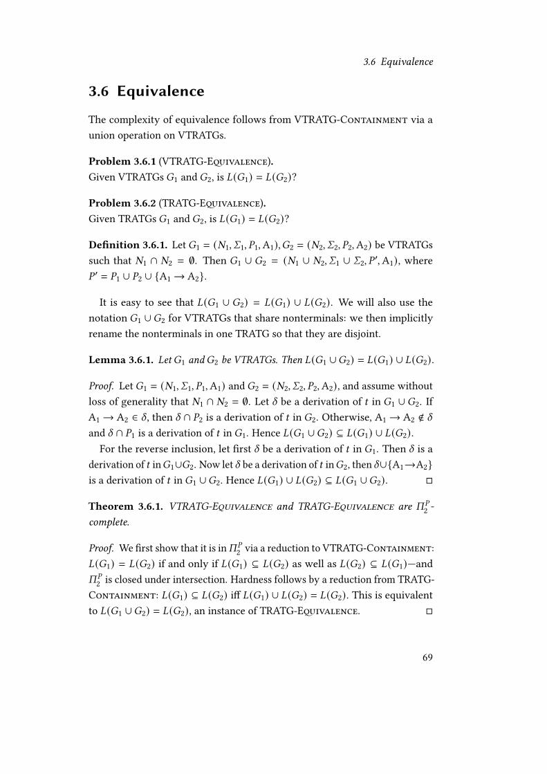
3.6 Equivalence
3.6 Equivalence
The complexity of equivalence follows from VTRATG-Containment via aunion operation on VTRATGs.
Problem 3.6.1 (VTRATG-Eqivalence).Given VTRATGs �1 and �2, is !(�1) = !(�2)?
Problem 3.6.2 (TRATG-Eqivalence).Given TRATGs �1 and �2, is !(�1) = !(�2)?
De�nition 3.6.1. Let �1 = (#1, O1, %1,A1),�2 = (#2, O2, %2,A2) be VTRATGssuch that #1 ∩ #2 = ∅. Then �1 ∪ �2 = (#1 ∪ #2, O1 ∪ O2, % ′,A1), where% ′ = %1 ∪ %2 ∪ {A1→ A2}.
It is easy to see that !(�1 ∪ �2) = !(�1) ∪ !(�2). We will also use thenotation �1 ∪�2 for VTRATGs that share nonterminals: we then implicitlyrename the nonterminals in one TRATG so that they are disjoint.
Lemma 3.6.1. Let�1 and�2 be VTRATGs. Then !(�1 ∪�2) = !(�1) ∪ !(�2).
Proof. Let �1 = (#1, O1, %1,A1) and �2 = (#2, O2, %2,A2), and assume withoutloss of generality that #1 ∩ #2 = ∅. Let X be a derivation of C in �1 ∪�2. IfA1→ A2 ∈ X , then X ∩ %2 is a derivation of C in �2. Otherwise, A1→ A2 ∉ X
and X ∩ %1 is a derivation of C in �1. Hence !(�1 ∪�2) ⊆ !(�1) ∪ !(�2).For the reverse inclusion, let �rst X be a derivation of C in �1. Then X is a
derivation of C in�1∪�2. Now let X be a derivation of C in�2, then X∪{A1→A2}is a derivation of C in �1 ∪�2. Hence !(�1) ∪ !(�2) ⊆ !(�1 ∪�2). �
Theorem 3.6.1. VTRATG-Equivalence and TRATG-Equivalence are N%2 -
complete.
Proof. We �rst show that it is inN%2 via a reduction to VTRATG-Containment:
!(�1) = !(�2) if and only if !(�1) ⊆ !(�2) as well as !(�2) ⊆ !(�1)—andN%2 is closed under intersection. Hardness follows by a reduction from TRATG-
Containment: !(�1) ⊆ !(�2) i� !(�1) ∪ !(�2) = !(�2). This is equivalentto !(�1 ∪�2) = !(�2), an instance of TRATG-Eqivalence. �
69

3 Decision problems on grammars
3.7 Minimal cover
3.7.1 Minimal cover for terms
We saw in Chapter 2 that cut-elimination of proofs withN1-cuts corresponds tothe computation of the language of VTRATGs. To reverse cut-elimination weneed to �nd a grammar that covers a given language. There are trivial solutionsto �nd such a VTRATG. For example, given a �nite set of terms ! we mightreturn a VTRATG with one nonterminal � and productions �→ C for everyC ∈ !. However such trivial grammars correspond to trivial cuts. If we want tointroduce interesting structure into proofs, we need to impose extra conditionson the grammar. A good condition is that the grammar should be small. Smallgrammars correspond to small proofs (see Lemmas 2.7.4 and 2.8.2), and it is areasonable hypothesis that small proofs typically contain interesting structure.In the case of induction there is an even more signi�cant size di�erence: wewant to �nd a �nite grammar that generates an in�nite and unbounded familyof sets of terms. Thus we are looking for grammars of minimal size, that is,with the least number of productions.
The �nite set ! corresponds to a tautological set of instances. Since supersetsof tautological disjunctions are tautological as well, we require that the TRATGcovers the given �nite set of terms, as opposed to !(�) = !. The coveringcondition !(�) ⊇ ! is similar to (but di�erent from) the one imposed on coverautomata [17, 18]: there an automaton � is sought such that !(�) ⊇ !, butin addition it is required that !(�) \ ! consists only of words longer thanany word in !. Another related notion is that of the grammatical complexityof a �nite language as de�ned in [15] and studied further in [13, 3, 14, 98]:the grammatical complexity of a �nite language ! is de�ned as the minimalnumber of productions of a grammar � with !(�) = !. In this way, each classof grammars gives rise to a measure of descriptional complexity.
As a �rst attempt, we might formalize the problem as a decision problem onVTRATGs:
Problem 3.7.1 (VTRATG-Cover).Given a �nite set of terms ! and : ≥ 0, is there a VTRATG� such that |� | ≤ :and !(�) ⊇ !?
70
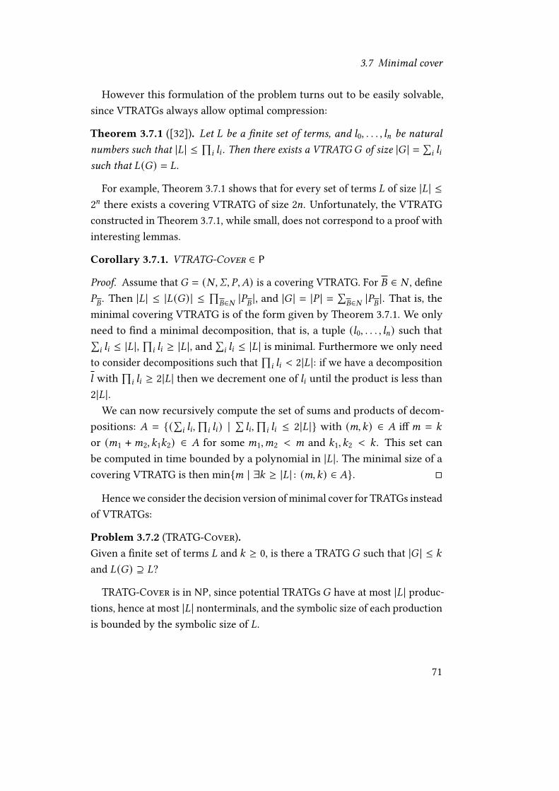
3.7 Minimal cover
However this formulation of the problem turns out to be easily solvable,since VTRATGs always allow optimal compression:
Theorem 3.7.1 ([32]). Let ! be a �nite set of terms, and ;0, . . . , ;= be naturalnumbers such that |! | ≤ ∏
8 ;8 . Then there exists a VTRATG � of size |� | = ∑8 ;8
such that !(�) = !.
For example, Theorem 3.7.1 shows that for every set of terms ! of size |! | ≤2= there exists a covering VTRATG of size 2=. Unfortunately, the VTRATGconstructed in Theorem 3.7.1, while small, does not correspond to a proof withinteresting lemmas.
Corollary 3.7.1. VTRATG-Cover ∈ P
Proof. Assume that � = (#, O, %,�) is a covering VTRATG. For � ∈ # , de�ne%�. Then |! | ≤ |!(�) | ≤ ∏
�∈# |%� |, and |� | = |% | = ∑�∈# |%� |. That is, the
minimal covering VTRATG is of the form given by Theorem 3.7.1. We onlyneed to �nd a minimal decomposition, that is, a tuple (;0, . . . , ;=) such that∑8 ;8 ≤ |! |,
∏8 ;8 ≥ |! |, and
∑8 ;8 ≤ |! | is minimal. Furthermore we only need
to consider decompositions such that∏8 ;8 < 2|! |: if we have a decomposition
; with∏8 ;8 ≥ 2|! | then we decrement one of ;8 until the product is less than
2|! |.We can now recursively compute the set of sums and products of decom-
positions: � = {(∑8 ;8,∏8 ;8) |
∑;8,
∏8 ;8 ≤ 2|! |} with (<,:) ∈ � i� < = :
or (<1 +<2, :1:2) ∈ � for some <1,<2 < < and :1, :2 < : . This set canbe computed in time bounded by a polynomial in |! |. The minimal size of acovering VTRATG is then min{< | ∃: ≥ |! | : (<,:) ∈ �}. �
Hence we consider the decision version of minimal cover for TRATGs insteadof VTRATGs:
Problem 3.7.2 (TRATG-Cover).Given a �nite set of terms ! and : ≥ 0, is there a TRATG � such that |� | ≤ :and !(�) ⊇ !?
TRATG-Cover is in NP, since potential TRATGs� have at most |! | produc-tions, hence at most |! | nonterminals, and the symbolic size of each productionis bounded by the symbolic size of !.
71

3 Decision problems on grammars
Open Problem 3.7.1. Is TRATG-Cover NP-complete?
So far a solution to Open Problem 3.7.1 remains elusive. However we willshow that the following version of TRATG-Cover with a �xed parameter isNP-complete:
Problem 3.7.3 (TRATG-=-Cover).Given a �nite set of terms ! and : ≥ 0, is there a TRATG� = (#, O, %,A) suchthat |# | ≤ =, |% | ≤ : , and !(�) ⊇ !?
Theorem 3.7.2. TRATG-=-Cover is NP-complete for = ≥ 2.
The proof of NP-hardness in the following Section 3.7.2 only requires regulargrammars for words. A similar approach to prove lower bounds for TRATGs us-ing regular grammars for words was already successfully used in descriptionalcomplexity [32].
For grammars on words, the shortest grammar problem—given a stringand size, is there a context-free grammar of at most this size generating justthe singleton containing the string—is known to be NP-complete [92, 19] andseveral approximation algorithms are known. The most important di�erencebetween the classical setting and ours is that a TRATG does not compress asingle string or tree but a �nite set of trees. We compress with regard to thenumber of production rules as opposed to, e.g., the size of the grammar as abinary string. Moreover, we cover the input language instead of reproducingit exactly.
Just as Problem 3.7.1 turned out to be polynomial-time computable dueto trivial optimally compressing VTRATG of Theorem 3.7.1, the restrictedproblem analogous to TRATG-=-Cover for VTRATGs is polynomial-timecomputable as well:
Problem 3.7.4 (VTRATG-=-Cover).Given a �nite set of terms ! and : ≥ 0, is there a VTRATG � = (#, O, %,A)such that |# | ≤ =, |% | ≤ : , and !(�) ⊇ !?
Lemma 3.7.1. VTRATG-=-Cover ∈ P.
72

3.7 Minimal cover
Proof. Similar to Corollary 3.7.1. For every<, the set�< = {(∑8≤< ;8,∏8≤< ;8) |∑
8≤< ;8,∏8≤< ;8 ≤ 2|! |} is polynomial-time computable. Observe that there
exists such a covering VTRATG i� there exists a tuple (;0, . . . , ;<) with< ≤ =,∑8 ;8 ≤ : , and
∏8 ;8 ≥ |! |, this is the case i� ∃< ≤ = ∃? ≥ |! | ∃B ≤ : (?, B) ∈
�< . �
3.7.2 Minimal cover for words
It is well known that we can represent words as trees by using unary functionsymbols instead of letters. We may hence represent the word hello as the treeh(e(l(l(o(n))))), for example. Under this correspondence, TRATGs with onlyunary functions and constants correspond exactly to acyclic regular grammars:
De�nition 3.7.1. A regular grammar� = (#, O, %,A) is a tuple consisting ofa start symbol A ∈ # , a �nite set of nonterminals # , a �nite set of letters Osuch that # ∩ O = ∅, and a �nite set of productions % ⊆ # × O∗(# ∪ {n}). Wecall � acyclic if there exists a strict linear order ≺ on the nonterminals suchthat B ≺ C whenever B→FC ∈ % for someF ∈ O∗.
The one-step derivation relation⇒� is de�ned byFB⇒� FE for B→E ∈ %and F ∈ O∗. The language !(�) = {F ∈ O∗ | A⇒∗
�F} then consists of the
derivable words. We write |� | = |% | for the number of productions. In thecase of acyclic regular grammars, the derivations and the generated languagecorrespond exactly to those for TRATGs. Note that there is no need to requirerigidity for derivations here: derivations in acyclic regular grammars can neveruse more than one production per nonterminal. Rigidity only plays a role forterms, where we can have multiple parallel occurrences of a nonterminal.
Problem 3.7.5 (Regular-Cover).Given a �nite set of words ! and : ≥ 0, is there an acyclic regular grammar �such that |� | ≤ : and !(�) ⊇ !?
Lemma 3.7.2. Regular-Cover ≤% TRATG-Cover.
Proof. Treat words as terms with unary function symbols and vice versa. �
73

3 Decision problems on grammars
Regular-Cover corresponds to TRATG-Cover, and is in NP. Furthermore,if Regular-Cover is NP-hard then so is TRATG-Cover. However the pre-cise complexity of Regular-Cover is open, similar to the case for terms weconjecture it to be NP-complete.
Open Problem 3.7.2. Is Regular-Cover NP-complete?
Clearly, Open Problem 3.7.2 implies Open Problem 3.7.1. In the rest of thissection, we will show that the restriction of Regular-Cover to a boundednumber of nonterminals is NP-hard.
Problem 3.7.6 (Regular-=-Cover).Given a �nite set of words ! and : ≥ 0, is there an acyclic regular grammar� = (#, O, %,A) such that |# | ≤ =, |% | ≤ : , and !(�) ⊇ !?
We will show the NP-hardness of Regular-=-Cover in several steps: �rstwe reduce 3SAT to Regular-2-Cover using an intermediate problem wherewe can not only specify words that must be generated by the grammar, butalso productions that must be included:
Problem 3.7.7 (Regular-2-Cover-Extension).Given a �nite set of words !, an acyclic regular grammar� = (#, O, %,A) suchthat # = {A,B}, F contains B whenever A→ F ∈ % , and : ≥ 0, is there asuperset % ′ ⊇ % of the productions such that |% ′| ≤ |% | + : , and !(�′) ⊇ !where �′ = (#, O, % ′,A)?
Lemma 3.7.3. 3SAT ≤% Regular-2-Cover-Extension.
Proof. Consider a propositional formula in CNF with < clauses �1, . . . ,�<
and = variables (called G1, . . . , G=). The number of variables = will be usedas the : parameter in Regular-2-Cover-Extension. Assume without lossof generality that G 9 ∨ ¬G 9 is a clause in this formula for all 9 ≤ =. We willencode the literals as unary natural numbers. First we de�ne the naturalnumbers 0 9 = 2 9 and 1 9 = 2 9 + 1 that correspond to G 9 and ¬G 9 , resp. Thenumber 2 = 2= + 1 is their upper bound.
Let ! = {s2o;,8 | 8 ≤ <, ; ≤ 2=} and O = {o;,8 | ; ≤ 2=, 8 ≤ =} ∪ {s}.Furthermore, de�ne the acyclic regular grammar � = (#, O, %,A) where
74

3.7 Minimal cover
# = {A, B}, and the productions % are the following:
B→ s2−0 9o;,8 for G 9 ∈ �8 and ; ≤ 2=B→ s2−1 9o;,8 for ¬G 9 ∈ �8 and ; ≤ 2=
It remains to show that � is satis�able i� there exists a set of productions% ′ ⊇ % such that |% ′| ≤ |% | + = and !(�′) ⊇ ! where �′ = (#, O, % ′,A).Left-to-right direction. Let � |= � be a satisfying interpretation, then we
construct an acyclic regular grammar �′ by adding the following productionsto � . We clearly have |�′| = |� | + =, and also !(�′) ⊇ !.
A→ s0 9B if � |= G 9 A→ s1 9B if � 6 |= G 9
Right-to-left direction. Let �′ = (#, O, % ′,A) such that % ′ ⊇ % , !(�′) ⊇ !,and |% ′| ≤ |% | + =. By symmetry, all productions from the nonterminal A areof the form A→ sAB for some A ≥ 0. Otherwise there would be an 8 ≤ < suchthat all constants o;,8 appear in productions from A, and we would have atleast 2= new productions.
Let X be a derivation of s2o;,8 ∈ ! in�′. Then X uses the production A→ sABfor some A , and we have that A = 0 9 and G 9 ∈ �8 or A = 1 9 and ¬G 9 ∈ �8 . SinceG 9 ∨ ¬G 9 ∈ � for all 9 ≤ =, we have A→ s0 9B ∈ % ′ or A→ s1 9B ∈ % ′ for all9 ≤ =. Because there are at most = such productions, we cannot have boths0 9B ∈ % ′ and s1 9B ∈ % ′.
Now de�ne an interpretation � such that � |= G 9 i� A→ s0 9B ∈ % ′. Notethat � 6 |= G 9 i� A→ s1 9B ∈ % ′, and hence � is a model for � by the previousparagraph. �
Lemma 3.7.4. Regular-2-Cover-Extension ≤% Regular-2-Cover.
Proof. Let !, � = (#, O, %,A), # = {A,B}, and : be as in the de�nition ofRegular-2-Cover-Extension. We set< = |! |+ |� |. Without loss of generality,assume that ! ≠ ∅. Take 4< fresh letters a1, . . . , a3<, b1, . . . , b< . We extend thelanguage ! to !′:
!′ = ! ∪ {a8F | B→F ∈ %, 8 ≤ 3<}∪ {Fb 9 | A→FB ∈ %, 9 ≤ <}∪ {a8b 9 | 8 ≤ 3<, 9 ≤ <}
75

3 Decision problems on grammars
We need to construct an acyclic regular grammar �′ = (#, O′, % ′,A) withO′ = O ∪ {a1, . . . , a3<, b1, . . . , b<} such that !(�′) ⊇ !′ and |�′| ≤ |� | +: + 4<if and only if there exists an acyclic regular grammar �′′ = (#, O, % ′′,A) suchthat % ⊆ % ′′, |�′′| ≤ |� | + : , and !(�′) ⊇ !.Left-to-right direction. Let us �rst assume that such a grammar �′ exists.
We can assume that |�′| ≤ |! | + |� | + 4< = 5< since there exists a coveringgrammar of that size with the productions {A→F | F ∈ !} ∪ % ∪ {A→ a8 |8 ≤ 3<} ∪ {B→ b 9 | 9 ≤ <}.
Without loss of generality, assume that the letters a8 occur only as the �rstletter of productions of the nonterminal A. We can drop any production thatcontains a8 in the middle since a8 can only occur at the beginning of wordsin !′. For the same reason we can then replace each production B→ a8F byA→ a8F .
Furthermore, we can assume that �′ is symmetric in the new symbols, thatis, A→ a8F ∈ % ′ if and only if A→ a 9F ∈ % ′ for all 8, 9 ≤ 3< and words F .Otherwise pick an 8 ≤ 3< such that, = {F | A→ a8F ∈ % ′} is of minimalsize. We then remove all productions containing an a 9 for some 9 ≤ 3<, andreplace them by the productions A→ a 9F forF ∈, . The resulting grammarstill covers !′ since !′ is symmetric under permutation of the letters a8 .
Now for every 8 ≤ 3< there is at most one production of the form A→ a8F
for someF—if there were two, then by a8-symmetry we would have 2 ·3< = 6<productions, exceeding the previously obtained upper bound of 5< productions.This also implies that B→ b 9 ∈ % ′ for all 9 ≤ <. By a symmetry argument forb 9 there are no other productions that contain b 9 . We also have that B→F ∈ % ′
whenever B→F ∈ % .We can now construct the acyclic regular grammar �′′ by removing all
productions from �′ that contain one of the new symbols a8 or b 9 . We have!(�′′) ⊇ ! since !(�′) ⊇ ! and because productions that contain the newsymbols cannot be used in derivations of words in !. Furthermore, |�′′| ≤|�′|−4< = |� | +: . It remains to show that A→FB ∈ % ′whenever A→FB ∈ %for someF ∈ O∗. Recall that !′ containsFb 9 for all 9 ≤ <. However the onlyoccurrence of b 9 in % ′ is in the production B→ b 9 ∈ % ′. Hence A→FB ∈ % ′.Right-to-left direction. In the other case, we assume that such a grammar
�′′ exists, and need to construct �′. We obtain this grammar �′ by adding the
76

3.8 Minimization
productions A→ a8B and B→ b 9 for all 8 ≤ 3< and 9 ≤ <. Then �′ has 4<more productions than �′′ and covers !′. �
Lemma 3.7.5. Regular-=-Cover ≤% Regular-(= + 1)-Cover.
Proof. Let ! be a �nite set of words, : ≥ 0, and de�ne< = 2: . Assume that|! | ≥ 1, : ≥ 2, and = ≥ 1—otherwise we can directly compute the answer.Take< + 1 fresh letters a1, . . . , a<, b. We de�ne !′ = {a1, . . . , a<} · (! ∪ {b}).It remains to show that there exists an acyclic regular grammar � with =nonterminals such that |� | ≤ : and !(�) ⊇ ! if and only if there exists anacyclic regular grammar�′ with = + 1 nonterminals such that |�′| ≤ : +< + 1and !(�′) ⊇ !′.Left-to-right direction. Let � = (#, O, %,B) be an acyclic regular grammar
such that |# | = =, |� | ≤ : , and !(�) ⊇ !. We set �′ = (# ∪ {A}, O ∪ O′, % ∪% ′,A) where A is a fresh nonterminal, O′ = {a1, . . . , a<, b}, and % ′ = {A→a8B |8 ≤ <} ∪ {B→ b}. Clearly |# ∪ {A}| = = + 1, |�′| = |� | +< + 1 ≤ : +< + 1,and !(�′) ⊇ !′.Right-to-left direction. Let �′ = (#, O, % ′,A) be an acyclic regular grammar
such that |# | = = + 1, |� | ≤ : +< + 1, and !(�′) ⊇ !′. Via the same argumentas used in the proof of Lemma 3.7.4 and noting that 2< > : +<, we can assumethat there exists a nonterminal B ≠ A such that all productions from A are ofthe form A→ a8B for some 8 ≤ <. Let % ⊆ % ′ be the set of productions whoseleft side is not A and whose right side is not b. The acyclic regular grammar� = (# \ {A}, O, %, B) then has the desired properties. �
Theorem 3.7.3. Regular-=-Cover is NP-complete for = ≥ 2.
Proof. By reduction from 3SAT using Lemmas 3.7.3 to 3.7.5. �
Proof (of Theorem 3.7.2, the NP-completeness of TRATG-=-Cover). Follows di-rectly from Theorem 3.7.3 by representing words as terms and vice versa. �
3.8 Minimization
Problem 3.8.1 (VTRATG-Minimization).Given a VTRATG � = (#, O, %,A), a set of terms ! such that !(�) ⊇ !, and
77

3 Decision problems on grammars
: ≥ 0, is there a subset % ′ ⊆ % of the productions such that |% ′| ≤ : and!(�′) ⊇ ! where �′ = (#, O, % ′,A)?
This optimization problem will play a central role in the MaxSAT algorithmto �nd minimal covering VTRATGs that we will see in Section 4.3. We willnow show that VTRATG-Minimization is NP-complete via reduction fromSet Cover.
Problem 3.8.2 (Set Cover).Given a �nite set - , a �nite collection� ⊆ P(- ) of subsets such that
⋃� = - ,
and : ≥ 0, is there a sub-collection �′ ⊆ � such that⋃� = - and |�′| ≤ :?
Theorem 3.8.1. VTRATG-Minimization is NP-complete.
Proof. The problem is in NP because we can check |% ′| ≤ : in polynomialtime, and reduce !(�′) ⊇ ! to VTRATG-Membership. Hardness follows byreduction from Set Cover: we pick a fresh nonterminal A, set # = {A} ∪�(treating the subsets as nonterminals), ! = - , and % = {A→ * | * ∈ �} ∪{* → G | G ∈ * ∈ �}. A subset % ′ ⊆ % of the productions of with : + |- |elements then directly corresponds to a sub-collection�′ of such that |�′| ≤ : :for every G ∈ - , there is at least one production* → G ∈ % ′ for some* ∈ � .These are |- | productions, there are hence at most : productions of the formA→* for some* , which yield the sub-collection�′ = {* | A→* ∈ % ′}. �
3.9 Decision problems on Herbranddisjunctions
Each of these decision problems on VTRATGs corresponds to a decision prob-lem on simple proofs: for instance, VTRATG-Membership decides whether aformula is contained in the Herbrand disjunction of a non-erasing cut-normalform.
As we have seen in Lemma 2.7.5, in general, cut-elimination can decrease thelanguage of the grammar of a proof. This is due to the reduction of weakeninginferences, which can delete parts of the proof and hence remove instances.However, without reduction of weakenings, the language is preserved bycut-elimination:
78

3.9 Decision problems on Herbrand disjunctions
De�nition 3.9.1 (non-erasing cut reduction, [53]). ne→ is the cut-reductionrelation without reduction on weakening inferences.
Theorem 3.9.1 ([53]). Let c, c ′ be simple proofs. If cne→ c ′, then !(� (c)) =
!(� (c ′)).
If c is a simple proof, and c∗ a non-erasing cut-normal form such thatc
ne→∗c∗, then !(c∗) = !(� (c)). Any simple proof has a ne→-normal form. If
in addition, c only contains weakening inferences introducing quanti�er-freeformulas, then c∗ does not contain quanti�ed cuts. Given a ne→-normal form c∗
of a proof c with only quanti�er-free weakening, we can hence directly extracta Herbrand disjunction � (c∗) such that � (c∗) = !(� (c∗)) = !(� (c)).
Problem 3.9.1 (H-Membership).Given a simple proof c with only quanti�er-free weakening and a formula i ,is there a ne→-normal form c
ne→∗c∗ such that i ∈ � (c∗)?
Problem 3.9.2 (H-Containment).Given a simple proofs c1, c2 with only quanti�er-free weakening, are therene→-normal forms c8
ne→ c∗8 for 8 ∈ {1, 2} such that � (c∗1 ) ⊆ � (c∗2 )?
Problem 3.9.3 (H-Disjointness).Given a simple proofs c1, c2 with only quanti�er-free weakening, are therene→-normal forms c8
ne→ c∗8 for 8 ∈ {1, 2} such that � (c∗1 ) ∩ � (c∗2 ) = ∅?
Problem 3.9.4 (H-Eqivalence).Given a simple proofs c1, c2 with only quanti�er-free weakening, are therene→-normal forms c8
ne→ c∗8 for 8 ∈ {1, 2} such that � (c∗1 ) = � (c∗2 )?
The restriction of only allowing weakening on quanti�er-free correspondsto a restriction on the productions on the VTRATG: for every nonterminalvector � there has to be at least one production �→ C .
Lemma 3.9.1. There is a formula i (G) containing G such that: let � be aVTRATG such that there is a production for every nonterminal vector and everynonterminal vector is nonempty. Then there is a simple proof c� of ` ∃Gi (G) suchthat c� does not contain quanti�ed weakening and !(c∗
�) = {A1(C) | C ∈ !(�)}
for anyne→-normal form c∗
�. This proof c� is polynomially-time computable
from � .
79

3 Decision problems on grammars
Proof. Choose i (G) := '(G) → '(G) for a relation symbol '. We could alsouse > instead of i (G), but then the terms would not appear in the formulas.Let � ≺ �1 ≺ · · · ≺ �= be the nonterminal vectors of � . The proof c� thenhas = cuts, each with the formula q8 = ∀G8 ¬
∨9 i (G8, 9 ) where G8 is a variable
vector of the same size and types as the nonterminal vector �8 . For the cutwith the cut formula q8 we will use the eigenvariable vector U8 . We de�ne asequence of proofs c8 for 1 ≤ 8 ≤ = + 1. For 8 ≤ =, c8 is de�ned as followswhere �8 → C1, . . . , �8 → C< are all the productions for the nonterminal vector�8 :
(c8+1)` ∃G i (G)
FA` ¬∨9 i (U8, 9 ), ∃G i (G) ∀∗A` q8, ∃G i (G)
'(C1,1) ` '(C1,1) →A` i (C1,1)FA ,∨A` ∨
9 i (C1, 9 ) ¬∗;¬∨
9 i (C1, 9 ) `F∗;¬∨
9 i (C1, 9 ), . . . ,¬∨9 i (C1, 9 ) ` ∀∗
;, 2∗;q8 ` cut
k1, . . . ,k8−1 ` ∃G i (G)We de�ne c=+1 as follows where �→ C1 | · · · | C< are all the productions forthe nonterminal �:
'(C1) ` '(C1) →A` i (C1)F∗A` i (C1), . . . , i (C<) ∃∗A , 2∗A` ∃G i (G)
Finally we set c� = c1. By looking at c� , we have � (c� ) ' � , i.e., � hasthe production �→ C i� � (c� ) has the production �→ A1(C). We then have!(c∗
�) = !(� (c� )) = {A1(C) | C ∈ !(�)} by Theorem 3.9.1. �
A similar (and less arti�cial) construction is also present in [46, Theorem25], however that construction gives a proof of a larger sequent i1, . . . , i= `∃G '1(G) where the formula i8 depends on the productions for the nonter-minal �8 and the instances of i8 encode the terms derivable from �8 . TheHerbrand sequent of the proof hence contains more terms than the languageof the grammar, and for example !(�1) ⊆ !(�2) would in general not beequivalent to � (c∗
�1) ⊆ � (c∗
�2) where c�1, c�2 are de�ned as in [46].
Theorem 3.9.2. The following complexity results hold:
80

3.10 The treewidth measure on graphs
• H-Membership is NP-complete
• H-Containment is N%2 -complete
• H-Disjointness is coNP-complete
• H-Equivalence is N%2 -complete
Proof. Hardness follows from the corresponding Theorems 3.2.1, 3.4.1, 3.5.1and 3.6.1 for VTRATGs via Lemma 3.9.1, since we have � (c∗
�) = � (!(c∗
�)) =
� (!(� (c� ))) = {A1(C) | C ∈ !(�)} ' !(�) and all the VTRATGs used in thehardness proofs have the property that every nonterminal vector has at leastone production. �
3.10 The treewidth measure on graphs
Many problems on graphs are easier to solve on trees. For example coloring agraph using a given number of colors (such that no two adjacent vertices havethe same color) is a well-known NP-complete problem; however it is trivial tocolor a tree using just two colors. We could expect that such problems can alsobe easily solved on graphs that are in some sense “close” to being a tree. Thenotion of treewidth makes this intuition concrete. The treewidth of a graph isa natural number that indicates how close it is to a tree: non-empty trees (aswell as forests) have treewidth 1, and graphs with larger tree widths are lesslike trees. The concept of treewidth was originally introduced under the name“dimension” in [10] to study tractable subclasses of optimization problems, andlater called treewidth in [84].
De�nition 3.10.1 (tree decomposition). Let � = (+ , �) be an undirectedgraph. Then a pair (), (-C )C∈+) ) of a tree) = (+) , �) ) together with a function- : +) → P(+ ), which assigns to every node of the tree a “bag” of verticesof � , is called a tree decomposition of � if:
1. For any vertex E ∈ + , there exists a vertex C ∈ +) such that E ∈ -C .
2. For any edge 4 = {E1, E2} ∈ �, there exists a vertex C ∈ +) such that4 ⊆ -C .
81

3 Decision problems on grammars
3. Let C1 . . . C= be a path in ) , and E ∈ -C1 ∩ -C= . Then E ∈ -C8 for any C8 onthe path.
The width of a tree decomposition ) is the maximum of |-C | − 1 for C ∈ +) .
De�nition 3.10.2 (treewidth). Let � be an undirected graph. Then tw(�) isthe minimum width of a tree decomposition of � .
The treewidth of a graph is 1 if and only if it is a forest. The treewidth is 0if and only if the graph has no edges. For every : ≥ 0, there is a polynomial-time algorithm that computes a tree decomposition of width ≤ : , if such adecomposition exists [6]. If : is not �xed, the problem of determining whethera given graph has treewidth : is NP-complete [6]. Let us �rst prove some basicfacts about treewidth.
Lemma 3.10.1. Let = ≥ 1 and let = be the complete graph on = vertices.Then tw( =) = = − 1.
Proof. It is easy to see that tw( =) ≤ = − 1 using a tree decomposition withtree consisting of a single vertex. For tw( =) ≥ = − 1, let (), (-C )C∈+) ) be a treedecomposition of =. We need to show that this tree decomposition has atleast width = − 1. If) contains a leaf E connected to) via the edge {E, E′}, suchthat -E ≠ + = , then we can make a smaller tree decomposition by removing E :let 8 ∈ + = \-E . In order to show that () \ {E}, - ) is still a tree decomposition,we need to show that for every edge {F,F ′} ∈ � = , we still have a nodeE ∈ +) \ {E} such that {F,F ′} ⊆ -E . Since (),- ) is a tree decomposition thereexist E1, E2 ∈ +) such that {F, 8} ⊆ -E1 and {F ′, 8} ⊆ -E2 . If {F,F ′} ⊆ -E of theremoved node, then {F,F ′} ⊆ -E ′ since the adjacent node lies on the pathsto E1, E2. �
Lemma 3.10.2. Let �,� be graphs such that � is a subgraph of � . Thentw(�) ≤ tw(� ).
Proof. Every tree decomposition of � induces a tree decomposition of � ofthe same width or less, by restricting the -E sets to the vertices of � . �
82

3.11 The case of bounded treewidth
3.11 The case of bounded treewidth
The NP-hardness result of VTRATG-Membership in Theorem 3.2.1 was basedon the observation that we can encode Boolean satis�ability as the TRATGSat=,< . This TRATG makes use of the fact that derivations in VTRATGs can onlyuse a single production for each nonterminal, and we can hence “synchronize”across many productions to choose a consistent interpretation. There is a veryrelevant natural class of VTRATGs where this synchronization occurs in onlya very limited amount, namely instance grammars:Example 3.11.1. Consider the following induction grammar � :
g → A (W)W → 2 | 5 (W)
Then the instance grammar � (�, B= (0)) has the following form:
g → A (W0) | · · · | A (W=)W0→ 2 | 5 (W1)W1→ 2 | 5 (W2)...
W=−1→ 2 | 5 (W=)W=→ 2
Note that the productions for each nonterminal W8 only contain the “next”nonterminal W8+1. The treewidth will hence be small. Concretely, the treewidthwill be at most 2 for each instance grammars � (�, B= (0)).
In this section we will show that the notion of treewidth captures how muchof this kind of synchronization can occur across nonterminals in a VTRATG:if the treewidth is bounded, then the membership problem will be computablein polynomial time.
For VTRATGs we consider the treewidth of a so-called dependency graphof the grammar. (For TRATGs, the directed version of this dependency graphis acyclic by De�nition 2.5.1, since it embeds into the linear order ≺ of theVTRATG.) Given a set of nonterminal vectors # ′ ⊆ # , we write
⋃# ′ = {�8 |
� ∈ # ′} for the set of all nonterminals contained in #0 .
83

3 Decision problems on grammars
De�nition 3.11.1 (dependency graph). Let� = (#, O, %,�) be a TRATG. Thenthe dependency graph � (�) = (⋃#, �) has the nonterminals as vertices, andtwo nonterminals �,� are adjacent if there exists a production �′→ C ∈ %and 9 such that C contains� and � = �′8 for some 8 , or if � = �8 and� = � 9 forsome nonterminal vector � and 8 ≠ 9 .
Example 3.11.2. Consider the TRATG � with the productions:
�→ 5 (�,�)�→ �
�→ �
�→ 2 | 3
This TRATG � has the following dependency graph � (�):
�
� �
�
The dependency graph � (�) has treewidth tw(� (�)) = 2, witnessed by thefollowing tree decomposition of width 2 (labelling each vertex C in the treedecomposition with its associated set -C ):
{�, �, �}
{�,�, �}
Intuitively, the nonterminal � occurs in both the productions for � and for � .Hence the two nonterminals � and � need to “synchronize” the result for � .In the tree decomposition this causes � to be in every -C set.
Example 3.11.3. Let � be the VTRATG with the productions �→ 5 (�,�) and(�,�) → (2, 3). Then � has the following dependency graph:
�
� �
84

3.11 The case of bounded treewidth
The dependency graph has treewidth tw(� (�)) = 2, as witnessed by the treedecomposition {�, �,�} (consisting of a single vertex and no edges).
Example 3.11.4. Bounding tw(� (�)) restricts the amount of synchronization,but not the size of the generated language. The generated language !(�) canstill be exponentially larger, even if tw(� (�)) = 1 as in the following grammarof size 2= + 1 whose language has size |!(�) | = 2=:
�→ 5 (�1) | 6(�1)�1→ 5 (�2) | 6(�2)...
�=−1→ 5 (�=) | 6(�=)�=→ 2
Lemma 3.11.1. Let � = (#, O, %,�) be a VTRATG. Then |� | ≤ tw(� (�)) + 1for all � ∈ # .
Proof. Let� = (�1, . . . , �=). Then�8 and� 9 are adjacent in� (�) for every 8 ≠ 9 ,so � (�) contains an isomorphic copy of = as a subgraph. If = = 0, thentrivially = ≤ tw(� (�)) + 1. Otherwise, |� | = = = tw( =) + 1 ≤ tw(� (�)) + 1by Lemmas 3.10.1 and 3.10.2. �
There is a good reason why we de�ne the dependency graph on nonter-minals and not on the nonterminal vectors. Call the analogously de�neddependency graph on nonterminal vectors �′(�), i.e., the vertices of �′(�)are the nonterminal vectors, and two nonterminal vectors � and� are adjacenti� there exists a production �→ C such that C contains � 9 for some 9 . Thenfor every VTRATG � there is a (polynomial-time computable) VTRATG �′
such that !(�) = !(�′) and tw(�′(�′)) = 1. That is, even for bounded tw ◦�′
the membership problem is already NP-complete by Theorem 3.2.1. The con-struction of this VTRATG �′ is straightforward: let � have the nonterminalvectors�0 ≺ �1 ≺ · · · ≺ �= (and without loss of generality, let there be at leastone production for every nonterminal vector). Then�′ has the nonterminalvectors �0 ≺ �1 ≺ · · · ≺ �=, where �8 = (�8,8, . . . , �8,=) such that 8 ≥ 1 and|�8, 9 | = |� 9 |. That is, �8 consists of copies of the nonterminal vectors�8, . . . , �= ,
85

3 Decision problems on grammars
stacked on each other. A production �8 → C [�8+1, . . . , �=] in � is translated toa production �8→ (C [�8+1,8+1, . . . �8+1,=], �8+1,8+1, . . . , �8+1,=). Clearly �′(�′) is atree and hence tw(�′(�′)) = 1. This construction even preserves the size ofthe VTRATG |�′| = |� |. De�ning the dependency graph on nonterminals alsoallows us to bound the length of a nonterminal vector by the treewidth.
3.11.1 Membership
Bounding the treewidth of the dependency graph restricts the amount ofsynchronization that can occur between nonterminals in a VTRATG. Thisrestriction allows us to decide the membership problem in polynomial time ifthe treewidth is bounded.
Problem 3.11.1 ((tw ≤ :)-Membership).Given a term C and a VTRATG � such that tw(� (�)) ≤ : , is C ∈ !(�)?
For the rest of this subsection, �x a term C , a VTRATG� = (#, O, %,�), anda tree decomposition ) = (+) , �) ) of � (�) with bags -E for E ∈ +) . We willconstruct a polynomial-time decision procedure for (tw ≤ :)-Membership.Choose a root E0 ∈ +) of the tree decomposition such that � ∈ -E0 and orientthe edges in ) away from the root. In this way, every vertex E ∈ +) induces asubtree )E containing all vertices reachable from E .
The decision procedure will be implemented by recursion on the tree de-composition: starting with the root of the decomposition, we determine allterms generated by the nonterminals -E . The possible assignments from non-terminals to terms are captured by the following de�nition. Given a set ofnonterminals " ⊆ ⋃
# , we de�ne the set " ⊆ # of all nonterminal vectorsthat contain some nonterminal in " , i.e., " = {� ∈ # | ∃8 �8 ∈ "}.
De�nition 3.11.2. Let E ∈ +) be a node in the tree decomposition. A partialassignment for E is a pair (5 , ?) such that:
1. 5 ⊆ -E × st(C) is a partial function,
2. ? ⊆ % is a partial function such that dom(?) ⊆ -E ,
3. for every production �→ B ∈ ? and 8 such that �8 ∈ dom(5 ):
86

3.11 The case of bounded treewidth
a) 5 (�8) � B8b) 5 (�) = � (5 (�8)/B8) for every nonterminal � such that � occurs
in B8
Example 3.11.5 (continuing Example 3.11.2). Let E be the vertex in the treedecomposition with -E = {�, �, �}, and let C = 5 (2, 3) be the term where wewant to decide C ∈ !(�). Then ({(�, 5 (2, 3)), (�, 2), (�, 2)}, {�→ 5 (�,�), �→�,�→ 2}) is a partial assignment for E .
In a partial assignment, the terms 50 (�) are the terms that we want to parse(where � ∈ ⋃
# is a nonterminal), that is, where we want to �nd a derivationX such that �X = 50 (�). It is important that the assignment from nonterminalsto terms is partial: consider a term 5 (2) and a VTRATG with the productions�→ 5 (�) | 5 (�), �→ 2,�→ 3 . Here, there is no subterm B E 5 (2) such that� expands to B .
Furthermore, the partial assignment �xes the productions used in the deriva-tion. This is due to another reason: we might have a term 5 (2, 2), a VTRATGwith the productions �→ 5 (�,�) | 5 (�, �), �→ 2,�→ 3 and a tree decom-position {�, �} − {�} − {�,�}. If we did not include the production for �in the partial assignment, then the partial assignments for {�, �} and {�,�}could disagree about the production for �. If two partial assignments agree onthe productions and terms for the common nonterminals, then we call themcompatible:
De�nition 3.11.3. Let (5 , ?) and (5 ′, ?′) be partial assignments for E, E′ ∈ +) ,resp. The partial assignments are compatible i� 5 � (-E ∩-E ′) = 5 ′ � (-E ∩-E ′)and ? � (-E ∩ -E ′) = ?′ � (-E ∩ -E ′).
We now give a characterization of !(�) in terms of partial assignmentson the tree decomposition. In a sense, we split up a derivation into smalloverlapping parts, and each node E in the tree decomposition stores the partabout the nonterminals -E :
Theorem 3.11.1. C ∈ !(�) i� there exists a function 0 that assigns to everyvertex E ∈ +) of the tree decomposition a partial assignment 0(E) for E in such away that 0(E) and 0(E′) are compatible for all adjacent E and E′, and (0(E))1(�) =C for some E .
87

3 Decision problems on grammars
Proof. First, assume that C ∈ !(�) and X is a derivation of C in � . Then wede�ne 0(E) = (5E , ?E ) as follows: 5E (�) = �X if � ∈ -E and �X E C , andunde�ned otherwise. For productions, we set � → B ∈ ?E i� � ∈ -E and� → B ∈ X . Clearly 0(E) is a partial assignment for every E , and all of thesepartial assignments are compatible.
On the other hand, let 0 be a function as required by the theorem. Let 5 and ?be partial functions such that (0(E))1 = 5 �-E and (0(E))2 = ?�-E for all E ∈ +) .The partial function 5 exists, as the function values in the partial assignmentsneed to agree for adjacent vertices and all vertices where -E contains a givennonterminal are connected in ) since ) is a tree decomposition. We clearlyhave 5 (�) = C . Furthermore, given � ∈ # and 8, 9 , all vertices E such that-E contains �8 or � 9 are connected (by de�nition of the dependency graph).Hence the partial function ? exists as well. From 5 and ? we can now de�ne aderivation X using the set of productions ? . We now have 5 (�) = �X for everynonterminal � ∈ ⋃
# and hence X is a derivation of C in � . �
Example 3.11.6 (continuing Example 3.11.2). Let C = 5 (2, 2). Then C ∈ !(�) aswitnessed by the derivation using the productions �→ 5 (�,�), �→ �,�→�, �→ 2 . The corresponding function 0 is given as follows (where E0, E1 arethe vertices such that -E0 = {�, �, �} and -E1 = {�,�, �}):
0(E0) = ({(�, 5 (2, 2)), (�, 2), (�, 2)}, {�→ 5 (�,�), �→ �,�→ 2})0(E1) = ({(�, 5 (2, 2)), (�, 2), (�, 2)}, {�→ 5 (�,�),�→ �, �→ 2})
We can now use the characterization of Theorem 3.11.1 to show that (tw ≤:)-Membership is computable in polynomial time.
Theorem 3.11.2. (tw ≤ :)-Membership ∈ P for all : .
Proof. We compute for every E ∈ +) the set �E of partial assignments for Esuch that 1 ∈ �E i� there exists a function 0 that assigns to every E′ ∈ +)E apartial assignment for E′ such that 0(E) = 1 and 0(E′) and 0(E′′) are compatiblewhenever E′ and E′′ are adjacent. This set can be computed recursively: givena partial assignment 1 for E , 1 ∈ �E i� for every child E′ of E there exists acompatible partial assignment 1′ ∈ �E ′. There are only polynomially manypartial assignments for every E , so the recursive algorithm runs in polynomial
88

3.11 The case of bounded treewidth
time. By Theorem 3.11.1, C ∈ !(�) if and only if there exists a (5 , ?) ∈ �E with5 (�) = C . �
3.11.2 Emptiness
We can also use Theorem 3.11.1 to e�ectively decide the emptiness problemfor VTRATGs with dependency graphs of bounded treewidth:
Problem 3.11.2 ((tw ≤ :)-Emptiness).Given a VTRATG � such that tw(� (�)) ≤ : , is !(�) = ∅?
Theorem 3.11.3. (tw ≤ :)-Emptiness ∈ P for all : .
Proof. Compute the sets �E of partial assignments as in the proof of Theo-rem 3.11.2. We have C ∈ !(�) i� there exists a (5 , ?) ∈ �E with 5 (�) = C .Hence !(�) ≠ ∅ i� there exists a (5 , ?) ∈ �E such that 5 (�) is de�ned. �
3.11.3 Containment
Having determined the complexity of membership, we can now turn towardscontainment. In contrast to the unconstrained case where containment wasN%2 -complete (Theorem 3.4.1), for bounded treewidth it will turn out to be only
coNP-complete:
Problem 3.11.3 ((tw ≤ :)-Containment).Given VTRATGs �1,�2 such that tw(� (�1)) ≤ : and tw(� (�2)) ≤ : , is!(�1) ⊆ !(�2)?
Theorem 3.11.4. (tw ≤ :)-Containment is coNP-complete for : ≥ 1.
Proof. The problem is in coNP since for any C (whose symbolic size we canbound by a polynomial in the symbolic size of�1), we can check in polynomialtime whether C ∉ !(�1) or C ∈ !(�2). Hardness follows via reduction from thecomplement of 3SAT. Hence let i be a formula in 3CNF with the variables G .We choose �1 = Insti,G , which generates exactly the substitution instancesof i where we replace the variables by either true or false. We clearly havetw(� (�1)) = 1.
89

3 Decision problems on grammars
For the reduction we want to �nd a TRATG �2 such that !(�1) ⊆ !(�2) i�i is unsatis�able. Ideally !(�2) would contain exactly the false substitutioninstances of i , however this grammar would likely have a dependency graphof unbounded treewidth since we need to choose the same substitution forevery clause. Therefore we use a slightly di�erent grammar �2 that generatesfalse formulas of the same “shape” as i , in particular it generates all falseinstances of i :
�→ and(�1, . . . ,�8−1, � ,�8+1, . . . ,�=) (for each 8 ≤ =)�8 → or(�8,1, �8,2, �8,3)�8, 9 → false | neg(true) | true | neg(false) (for each 8 ≤ = and 9 ≤ 3)� → or(�1,�2,�3)� 9 → false | neg(true) (for each 9 ≤ 3)
Each nonterminal �8 expands to a substitution instance of a clause. Thenonterminal � expands to such instances as well, but only to those which aresemantically false. We clearly have tw(� (�2)) = 1. Since � expands to a falseclause, every formula in !(�2) is equivalent to false. So if !(�1) ⊆ !(�2), theni is unsatis�able. On the other hand, !(�2) contains every false substitutioninstance of i : if the instance is false, then at least one conjunct of the top-leveland is false and we can construct a derivation in �2 using the correspondingproduction for �. So we have a reduction from the complement of 3SAT; it ispolynomial-time since the grammars �1,�2 can be computed in polynomialtime from i . �
3.11.4 Disjointness
Interestingly, bounding the treewidth of the dependency graph does not changethe complexity of the disjointness problem. In both the unconstrained and thetreewidth-bounded case, the problem is coNP-complete. However we need touse a di�erent proof for coNP-hardness: in the unconstrained case, we could re-duce the complement of the NP-complete membership problem to disjointness.But this approach does not work here, since treewidth-bounded membershipis in P. Therefore we use a similar proof as for (tw ≤ :)-Containment inTheorem 3.11.4.
90

3.11 The case of bounded treewidth
Problem 3.11.4 ((tw ≤ :)-Disjointness).Given VTRATGs �1,�2 such that tw(� (�1)) ≤ : and tw(� (�2)) ≤ : , is!(�1) ∩ !(�2) = ∅?
Theorem 3.11.5. (tw ≤ :)-Disjointness is coNP-complete for : ≥ 1.
Proof. The problem is in coNP since for every derivation of a term C ∈ !(�1)we can check whether C ∉ !(�2) in polynomial time by Theorem 3.11.2. ForcoNP-hardness, we show a reduction from the complement of 3SAT as in theproof of Theorem 3.11.4. So let i be a formula in 3CNF with the variables G .We set�1 = Insti,G . For�2 we pick a TRATG that generates only true formulas,including all true substitution instances of i :
�→ and(�1, . . . , �=)�8 → or(�8, �8,1, �8,2) | or(�8,1,�8, �8,2) | or(�8,1, �8,2,�8)�8 → true | neg(false)�8, 9 → true | false | neg(false) | neg(false)
The nonterminal �8 expands to an instance of a clause where at least one literalevaluates to true, �8 expands to a true instance of a literal, and �8, 9 expands toan arbitrary instance of a literal. As usual, we have tw(� (�2)) = 1 and �2 isalso polynomial-time computable. As in Theorem 3.11.4, !(�1) ∩ !(�2) = ∅i� i is unsatis�able, i.e., there is a substitution instance of i that evaluates totrue. �
3.11.5 Equivalence
The complexity of the equivalence problem follows directly from containmentusing the same reduction as for the unconstrained case in Theorem 3.6.1 usingthe union operation on VTRATGs.
Problem 3.11.5 ((tw ≤ :)-Eqivalence).Given VTRATGs �1,�2 such that tw(� (�1)) ≤ : and tw(� (�2)) ≤ : , is!(�1) = !(�2)?
Theorem 3.11.6. (tw ≤ :)-Equivalence is coNP-complete for : ≥ 1.
91

3 Decision problems on grammars
Proof. We �rst show that the problem is in coNP via a reduction to (tw ≤ :)-Containment: !(�1) = !(�2) ↔ !(�1) ⊆ !(�2)∧!(�2) ⊆ !(�1)—and coNPis closed under intersection. Hardness follows by a reduction from (tw ≤ :)-Containment: !(�1) ⊆ !(�2) i� !(�1) ∪ !(�2) = !(�2). This is equivalentto !(�1 ∪�2) = !(�2), an instance of (tw ≤ :)-Eqivalence. �
3.11.6 Minimization
The minimization problem has the same complexity as in the unconstrainedcase: it is NP-complete.
Problem 3.11.6 ((tw ≤ :)-Minimization).Given a VTRATG � = (#, O, %,A) with tw(�) ≤ : , a set of terms ! such that!(�) ⊇ !, and = ≥ 0, is there a subset % ′ ⊆ % of the productions such that|% ′| ≤ = and !(�′) ⊇ ! where �′ = (#, O, % ′,A)?
Note that such a grammar �′ also has the property that tw(� (�′)) ≤ : .
Theorem 3.11.7. (tw ≤ :)-Minimization is NP-complete for : ≥ 1.
Proof. The problem is in NP because it is a special case of the VTRATG-Minimization problem. Hardness follows by reduction from Set Coveras in Theorem 3.8.1: the grammar used in the proof of Theorem 3.8.1 has theproperty that tw(� (�)) = 1. �
3.11.7 Cover
The complexity of the Cover and =-Cover problems is also unchanged fromthe unconstrained case.
Problem 3.11.7 ((tw ≤ :)-Cover).Given a �nite set of terms ! and = ≥ 0, is there a VTRATG� such that |� | ≤ =,tw(� (�)) ≤ : , and !(�) ⊇ !?
In contrast to Corollary 3.7.1 for VTRATG-Cover, there is no obvious trivialsolution to (tw ≤ :)-Cover. The optimally compressing grammar given byTheorem 3.7.1 has a dependency graph of unbounded treewidth.
92

3.11 The case of bounded treewidth
Theorem 3.11.8. (tw ≤ :)-Cover ∈ NP.
Proof. By Lemma 3.11.1, the maximum length of a nonterminal vector isbounded by : + 1. A covering VTRATG of size ≤ = then has at most = pro-ductions of length : + 1, and we can guess such a VTRATG in polynomialtime and check whether tw(� (�)) ≤ : . Checking !(�) ⊇ ! is also in NP byTheorem 3.2.1. �
Once again, it is open whether the cover problem is NP-complete:
Open Problem 3.11.1. Is (tw ≤ :)-Cover NP-complete?
And the variant where we bound the number of nonterminals isNP-completeby reduction from Regular-=-Cover and verifying that the TRATGs have adependency graph of bounded treewidth:
Problem 3.11.8 ((tw ≤ :)-=-Cover).Given a �nite set of terms ! and ; ≥ 0, is there a VTRATG � = (#, O, %,�)such that |� | ≤ ; , tw(� (�)) ≤ : , |# | ≤ =, and !(�) ⊇ !?
Theorem 3.11.9. (tw ≤ :)-=-Cover is NP-complete for = ≥ 2 and : ≥ 1.
Proof. The problem is in NP analogously to Theorem 3.11.8: checking the extracondition |# | ≤ = can be done in polynomial time. For hardness we need toanalyze the TRATGs used in the proofs of Lemmas 3.7.3 to 3.7.5 and verifythat the treewidth of their dependency graph is at most one. In Lemmas 3.7.3and 3.7.4 we use TRATGs� with at most 2 nonterminals, hence tw(� (�)) = 1.In Lemma 3.7.5, we transform a TRATG by adding a new start symbol � atthe beginning; we add two kinds of productions: productions which do notcontain a nonterminal on the right-hand side, these do not contribute to thedependency graph. And productions from the new start symbol �, which onlycontain a single nonterminal on the right-hand side, namely �. Hence thedependency graph is only extended by a single new vertex� and an edge�−�,preserving the treewidth (which is one). �
93

3 Decision problems on grammars
3.12 Decision problems on induction grammars
3.12.1 Membership
We have motivated the class of treewidth-bounded VTRATGs in Section 3.11 byinstance grammars, which are a natural class of VTRATGs whose dependencygraph has bounded treewidth. There is however a small technical issue, whichwe will now explain. Let us �rst recall Example 3.11.1:Example 3.12.1. Consider the following induction grammar � :
g → A (W)W → 2 | 5 (W)
Then the instance grammar � (�, B= (0)) has the following form:
g → A (W0) | · · · | A (W=)W0→ 2 | 5 (W1)W1→ 2 | 5 (W2)...
W=−1→ 2 | 5 (W=)W=→ 2
The treewidth of the dependency graph is tw(� (� (�, B= (0)))) ≤ 2, as witnessedby the following tree decomposition. That is, the treewidth is uniformlybounded for all instance terms.
{g,W0, W1} − {g,W1, W2} − · · · − {g,W=−1, W=}
However, a small issue arises if the inductive datatype has a constructorwith two recursive occurrences since the instance grammars have nonterminalvectors WB for every subterm B , even if it occurs multiple times:Example 3.12.2. Consider the inductive type of binary trees with the construc-tors ;g and =g→g→g and the following induction grammar:
g → A (W)W → 2 | 5 (W)
94

3.12 Decision problems on induction grammars
De�ne the (free constructor) terms C8+1, 9+1 = =(C8, 9+1, C8+1, 9 ), C8+1,0 = C0,8+1 =
=(C8,0, C8,0), C0,0 = ; . Then the subterm structure of C8, 9 contains a grid, wheretwo subterms are connected by an edge if they are direct subterms (there aremore edges than shown here, since C8, 9 = C 9,8 is symmetric):
C8,0 C8,1 . . . C8, 9−1 C8, 9
C8−1,0 C8−1,1 . . . C8−1, 9−1 C8−1, 9
......
. . ....
...
C1,0 C1,1 . . . C1, 9−1 C1, 9
C0,0 C0,1 . . . C0, 9−1 C0, 9
The treewidth of such a (8 × 9)-grid is exactly min(8, 9), and this grid is asubgraph of � (� (�, C8, 9 )). Thus tw(� (� (�, C8,8))) ≥ 8 is not uniformly bounded.
This minor technical issue is easily solved by using a slightly di�erentde�nition for the instance grammar, with nonterminals W? for every position ?(instead of WB for every subterm):
De�nition 3.12.1. Let � = (g, U, (a2)2, W, %) be an induction grammar, andA a constructor term of the same type as U . The modi�ed instance grammar� ′(�, A ) = (g, # , % ′) is a VTRATG with nonterminal vectors # = {g} ∪ {W? |? ∈ Pos(A )} and productions % ′ = {?′ | ∃? ∈ % (? { ?′)}. The instantiationrelation ? {′ ?′ is de�ned as follows:
• g → C [U, a8, W] {′ g → C [A, B, W?] for ? ∈ Pos(A ) with A |? = 28 (B)
• W → C [U] { W? → C [A ] for ? ∈ Pos(A )
• W → C [U, a8, W] { W? 9 → C [A, B, W?] for ? ∈ Pos(A ) such that A |? = 28 (B),where 9 is a recursive occurrence in 28
95

3 Decision problems on grammars
How do the VTRATGs � (�, A ) and � (�, A ) di�er? They only di�er (ignoringthe names of the nonterminals) if A contains a subterm that occurs at twodi�erent positions. In general, A regarded as a tree can be exponentiallylarger than A regarded as a DAG. The VTRATG � ′(�, A ) treats A as a treesince it is de�ned in terms of the positions of A , while � (�, A ) treats A as aDAG since it is de�ned in terms of the subterms of A . For example, the termC8,0 = =(C8−1,0, C8−1,0) = . . . in Example 3.12.2 contains 8 + 1 subterms, but 28+1− 1positions.
The VTRATG � ′(�, A ) is polynomial-time computable from a tree representa-tion of A , and � (�, A ) is polynomial-time computable from a DAG representationof A . There is a size di�erence between � (�, A ) and � ′(�, A ): the tree represen-tation of A can be exponentially larger than the DAG representation. In thiscase, � ′(�, A ) will also be exponentially larger than � (�, A ).
Lemma 3.12.1. !(�, 8) = !(� (�, 8)) = !(� ′(�, 8)).
Proof. We can transform derivations between the two de�nitions of instancegrammars. If we have a derivation in � (�, 8) then we can pick the correspondingproductions in � ′(�, 8) to derive the same term (every nonterminal vector in� (�, 8) corresponds to at most one nonterminal vector in � ′(�, 8), so it is clearwhich production to pick.)
On the other hand if we have a1⇒-derivation in � ′(�, 8), then it only contains
nonterminal vectors W? for positions ? along a single branch of the term 8 . (Wecan see this by looking at the productions.) That is, there is a position ?0 suchthat ? ⊆ ?0 for every nonterminal vector W? occurring in the derivation. Everynonterminal vector in � (�, 8) corresponds to at most one such nonterminalvector W? (since we do not have parallel occurrences). And we get a derivationof the same term in � (�, 8) by picking the corresponding productions. �
Lemma 3.12.2. Let � = (g, U, (a2)2, W, %) be an induction grammar. Thentw(� (� ′(�, C))) ≤ 2|W |.
Proof. We construct a tree decomposition with the vertices +) = {n} ∪ {? ∈Pos(C) | ? is a recursive occurrence}. Two vertices are adjacent if they arepositions of direct subterms, i.e. �) = {{?, ?8} | ?8 ∈ +) }. For every ?8 ∈ +)
96

3.12 Decision problems on induction grammars
we de�ne -?8 = {g} ∪W? ∪W?8 , and -n = {g} ∪Wn . This tree decomposition hasthe desired width. �
Lemma 3.12.2 allows us to reduce the membership problem for inductiongrammars the one for VTRATGs with dependency graph of bounded treewidth.
Problem 3.12.1 (( |W | ≤ :)-Ind-Membership).Given an induction grammar � = (g, U, (a2)2, W, %) such that |W | ≤ : , a freeconstructor term 8 , and a term C represented as a tree, is C ∈ !(�, 8)?
Theorem 3.12.1. ( |W | ≤ :)-Ind-Membership ∈ P for all : .
Proof. By Lemma 3.12.1, C ∈ !(�, 8) i� C ∈ !(� ′(�, 8)). This is an instance of(tw ≤ 2|W |)-Membership by Lemma 3.12.2, which is in P by Theorem 3.11.2.
�
The restriction of |W | ≤ : is necessary in Theorem 3.12.1 (assuming P ≠ NP).If the size of |W | is not bounded, then the membership problem becomes NP-complete:
Problem 3.12.2 (Ind-Membership).Given an induction grammar � = (g, U, (a2)2, W, %), a free constructor term 8
represented as a tree, and a term C , is C ∈ !(�, 8)?
This is because we can encode any given VTRATG � as an induction gram-mar by making W as wide as necessary. The general idea is that we use theinstance grammar with = nonterminal vectors to simulate a VTRATG with =nonterminal vectors. This induction grammar will generate !(�) in the sensethat !(Embed� , =) ∩ T (O) = !(�) as we will see in Lemma 3.12.3. We needto restrict the language of the induction grammar to the original signaturesince the induction grammar also generates junk terms, which correspond to“derivations” (in �) that do not substitute all the nonterminals. The reason forthese junk terms is that we want every nonterminal vector in the instancegrammars to have at least one production, yielding a stronger result.
All of the induction grammars that we construct for the hardness and unde-cidability proofs will be for the natural numbers. This is no signi�cant restric-tion, we could perform the same construction for any other datatype that has
97

3 Decision problems on grammars
free constructor terms of unbounded size (or equivalently, if it has in�nitelymany up to renaming). In the case of the natural numbers, !(Embed% , =) pro-duces the language of the VTRATG. In the general setting, we would get that!(Embed% , C) produces that language for any free constructor term C of termdepth = − 1.
De�nition 3.12.2. Let � = (#, O, %,�) be a VTRATG with and # = {� ≺�1 ≺ · · · ≺ �=}. Let AV be a new constant for every type V , and for every �8 ,de�ne A8 = (AV1, . . . , AV:8 ) with the same types as �8 . We de�ne the inductiongrammar Embed� = (g, U, (a2)2, W, % ′) with W = (�1, . . . , �=) and the followingproductions:
g → B for every production �→ B ∈ %W → (A1, . . . , A8−1, B, �8+1, . . . , �=) for every production �8 → B ∈ %
Lemma 3.12.3. Let � = (#, O, %,�) be a VTRATG. Then !(Embed� , =) ∩T (O) = !(�) for all = ≥ |# | − 1.
Proof. If X is a derivation in � , then the derivation X′ with the correspondingproductions in � (�, C) derives the same term. On the other hand if X is aderivation of a term @ ∈ T (O), then @ does not contain AV for any V andthe derivation X′ using the corresponding productions in� derives the sameterm @. �
Theorem 3.12.2. Ind-Membership is NP-complete.
Proof. By a reduction from VTRATG-Membership, which is NP-complete byTheorem 3.2.1, using Lemma 3.12.3. �
3.12.2 Emptiness
The complexity of the emptiness problem on induction grammars is surprising:in this section, we will show that it is PSPACE-complete. In a sense it standsbetween the (relatively tractable) NP-complete membership problem and theundecidable containment, equivalence, and disjointness problems that we willconsider in the following sections.
98

3.12 Decision problems on induction grammars
Problem 3.12.3 (Ind-Emptiness).Given an induction grammar � , is !(�, 8) = ∅ for all free constructor terms 8?
Problem 3.12.4 (( |W | ≤ :)-Ind-Emptiness).Given an induction grammar� = (g, U, (a2)2, W, %) such that |W | ≤ : , is !(�, 8) =∅ for all free constructor terms 8?
These problems are deeply connected to another model in formal languagetheory, namely non-deterministic �nite automata. Intuitively, the hardness ofemptiness in induction grammars is due to a large size of W = (W1, . . . , W=). Ifwe only care about the set of occurring nonterminals, applying a productionW → C (to be precise, an instance of the production in the instance grammar)then has the e�ect of replacing one set of nonterminals {W3, W5, W8} occurringby an other set {W7, W9}. The language of the induction grammar is empty i�we can never reach the empty set. On the level of the automaton, W1, . . . , W= willbe the states, the sequence of productions in a derivation will be a word, andreaching the empty set means that a word is not accepted by the automaton(since the empty set obviously contains no �nal states).
De�nition 3.12.3. A non-deterministic �nite automaton (NFA) is a quintuple� = (&, O, X, @0, � ) where & is a �nite set of states, O is an alphabet, X ⊆& × O ×& is a transition relation, @0 ∈ & is the initial state, and � ⊆ & is theset of �nal states.
We extend the transition relation X recursively to a relation X ⊆ & × O∗ ×&by setting (@, n, @′) ∈ X i� @ = @′, and (@, 01, @′) ∈ X i� ∃@′′ (@, 0, @′′) ∈ X ∧(@′′, 1, @′) ∈ X . The language !(�) accepted by � is de�ned as !(�) = {F ∈O∗ | ∃@ ∈ � (@0,F, @) ∈ X}.
In our construction, the language of an induction grammar will be empty i�the automation accepts all words. Interestingly, this universality problem forNFAs is PSPACE-complete:
Problem 3.12.5 (NFA-Universality).Given an NFA � = (&, O, X, @0, � ), is !(�) = O∗?
Meyer and Stockmeyer �rst considered the complexity of NFA-Universalityin [70], where they also introduce the polynomial-time hierarchy. While they
99

3 Decision problems on grammars
do not explicitly state that the problem is PSPACE-complete, they show thatit is N%
:-hard for every : , and exhibit a polynomial-time reduction from the
membership problem for context-sensitive grammars, which is PSPACE-hard.
Theorem 3.12.3 ([70], Lemma 2.3). NFA-Universality is PSPACE-complete.
Our strategy is now as follows: we will assign to every induction grammaran NFA, such that the NFA is (almost) universal i� the language of the inductiongrammar is empty. Given an induction grammar� = (g, U, (a2)2, W, %) we de�nethe sets of productions %g = {? ∈ % | ∃C ? = g → C} and %W = {? ∈ % | ∃C ? =
W → C}. To simplify the construction of the automaton, we do not aim foruniversality but for !(�) = %g%∗W . This is not a signi�cant problem, since thecomplement of %g%∗W is recognized by a small DFA so it will be easy to reduce!(�) = %g%∗W to !(�′) = O∗ for some only polynomially larger automaton �′.
De�nition 3.12.4. Let � = (g, U, (a2)2, W, %) be an induction grammar suchthat W = (W1, . . . , W=). We de�ne the NFA �empty(�) = (&, O, X, @0, � ) as follows:
• & = {g,W1, . . . , W=}
• O = %
• @0 = g
• � = & \ {g}
• (@, ?, @′) ∈ X i� one of the following cases applies:
– @ = g , ? = g → C , and @′ occurs in C
– @ = W8 , ? = W → C , and @′ occurs in C8 .
Example 3.12.3. Consider the induction grammar � with the following pro-ductions:
g → A (W1, W2) (?1)(W1, W2, W3) → (W2, W3, W1) (?2)(W1, W2, W3) → (2,W3, W2) (?3)
Then the corresponding NFA�empty(�) has the following states and transitions.As we can clearly see, the word ?1?3?2?3 is not accepted and the language ofthe induction grammar is hence nonempty.
100
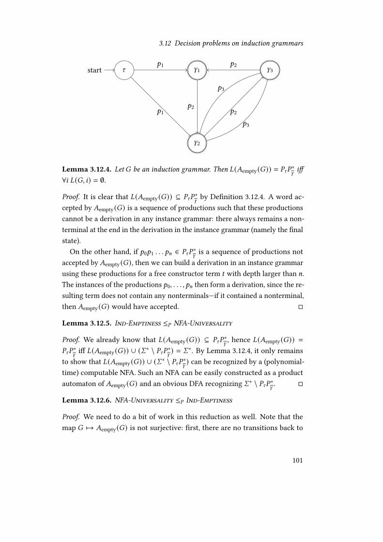
3.12 Decision problems on induction grammars
gstart W1
W2
W3?1
?1?2
?2
?2
?3
?3
Lemma 3.12.4. Let� be an induction grammar. Then !(�empty(�)) = %g%∗W i�∀8 !(�, 8) = ∅.
Proof. It is clear that !(�empty(�)) ⊆ %g%∗W by De�nition 3.12.4. A word ac-cepted by �empty(�) is a sequence of productions such that these productionscannot be a derivation in any instance grammar: there always remains a non-terminal at the end in the derivation in the instance grammar (namely the �nalstate).
On the other hand, if ?0?1 . . . ?= ∈ %g%∗W is a sequence of productions notaccepted by �empty(�), then we can build a derivation in an instance grammarusing these productions for a free constructor term C with depth larger than =.The instances of the productions ?0, . . . , ?= then form a derivation, since the re-sulting term does not contain any nonterminals—if it contained a nonterminal,then �empty(�) would have accepted. �
Lemma 3.12.5. Ind-Emptiness ≤% NFA-Universality
Proof. We already know that !(�empty(�)) ⊆ %g%∗W, hence !(�empty(�)) =
%g%∗W
i� !(�empty(�)) ∪ (O∗ \ %g%∗W ) = O∗. By Lemma 3.12.4, it only remainsto show that !(�empty(�)) ∪ (O∗ \ %g%∗W ) can be recognized by a (polynomial-time) computable NFA. Such an NFA can be easily constructed as a productautomaton of �empty(�) and an obvious DFA recognizing O∗ \ %g%∗W . �
Lemma 3.12.6. NFA-Universality ≤% Ind-Emptiness
Proof. We need to do a bit of work in this reduction as well. Note that themap � ↦→ �empty(�) is not surjective: �rst, there are no transitions back to
101

3 Decision problems on grammars
the start symbol, and second (and more importantly), all states in �empty(�)are �nal. At least implicitly, we will have to take care of these two issues.
So we are given an NFA � = (&, O, X, @0, � ), and we will construct aninduction grammar � . If there is a non-accepting word F ∉ !(�), thenwe want a suitable instance language !(�, 8) ≠ ∅ to be nonempty. Let& = (@0, . . . , @=), we set W = (W0, . . . , W=, W=+1). De�ne the transition func-tion X (@, 0) = {@′ | (@, 0, @′) ∈ X}. Assign to every set of states a term� ({@81, . . . , @8= }) = 5 (W81, 5 (W82, . . . 5 (W8= , 2) . . . )) containing exactly the W-non-terminals corresponding to the states. Then� contains the following produc-tions:
g → A (W0)W → (C0,0, . . . , C0,=, W=+1) for each 0 ∈ O , where C0,8 = � (X (@8, 0))W → (B0, . . . , B8, W=+1) where B8 = 2 if @8 ∉ � , and B8 = W=+1 otherwise
Call the productions ?0, ?0 , and ?� , respectively. LetF = 01 . . . 0= ∉ !(�) be anon-accepting word, that is, X (@0,F) ∉ � . Then ?0?01 . . . ?0=?� is a derivationin � (�, C) for some large enough C . On the other hand let !(�, 8) ≠ ∅ witnessedby a derivation X with the productions ?0?1 . . . ?= . If ?8 = ?� for 8 < =, then wecan drop the remaining productions. So X uses the productions ?0?01 . . . ?0= or?0?01 . . . ?0=?� . Now 01 . . . 0= is a non-accepting word. �
Theorem 3.12.4. Ind-Emptiness is PSPACE-complete.
Proof. By Lemmas 3.12.5 and 3.12.6, there is a polynomial reduction to andfrom NFA-Universality, which is PSPACE-complete by Theorem 3.12.3. �
If |W | is bounded by a �xed constant, then �empty(�) has only a boundednumber of states, thus making the problem tractable:
Theorem 3.12.5. ( |W | ≤ :)-Ind-Emptiness ∈ P
Proof. By Lemma 3.12.4, emptiness is equivalent to !(�empty(�)) = %g%∗f . Sincethe number of states in �empty(�) is bounded by : + 1, we can compute anequivalent DFA in constant time, and then verify !(�empty(�)) = %g%
∗f
inconstant time. �
102

3.12 Decision problems on induction grammars
3.12.3 Containment
We will show undecidability of containment, disjointness, and equivalenceof induction grammars by exhibiting a reduction from the undecidable Postcorrespondence problem [81]:
Problem 3.12.6 (Post-Correspondence).Given two �nite lists of wordsF1, . . . ,F= and E1, . . . , E= , is there a sequence ofindices 81, . . . , 8: for some : ≥ 1 such thatF81 . . .F8: = E81 . . . E8:?
Such a sequence 81, . . . , 8: is called a solution.
Problem 3.12.7 (Ind-Containment).Given induction grammars �1,�2 for the same datatype, is !(�1, C) ⊆ !(�2, C)for all free constructor terms C?
To show that containment is undecidable, we construct two induction gram-mars: the �rst one generates all pairs (F81 . . .F8: , E81 . . . E8: ). The second onegenerates all pairs (D, E) where D ≠ E are di�erent words. As usual, we encodea word 012 as the term 0(1 (2 (n))). Given a word 0102 · · ·0= (with 0 9 ∈ O forall 9 ) and a term C , we de�ne (0102 · · ·0=) · C = 01(02(· · ·0= (C) · · · )).
De�nition 3.12.5. Let % = ((F1, . . . ,F=), (E1, . . . , E=)) be an instance of Post-Correspondence. The induction grammar Image% has the following produc-tions:
g → A (W1, W2)(W1, W2) → (F1 · W1, E1 · W2) | · · · | (F= · W1, E= · W2)(W1, W2) → (F1, E1) | · · · | (F=, E=)
Lemma 3.12.7. !(Image% , :) = {A (F81 · · ·F8; , E81 · · · E8; ) | 1 ≤ ; ≤ : + 1}
Proof. Obvious from the construction. �
The second induction grammar that we use to show the undecidability ofcontainment produces all di�erent words. The idea is that (W3, W4) expands to(possibly equal) words E,F , while (W1, W2) expands to di�erent words.
103

3 Decision problems on grammars
De�nition 3.12.6. Let O be a set of letters and ; ≥ 1. Then the inductiongrammar Di�O,; has the following productions (where C,D, E,F range over allwords in O∗, and W = (W1, W2, W3, W4)):
g → A (W1, W2) (3.1)W → (C · W1, D · W2, E · W3,F · W4) (|C | = |D | = ; , and max( |E |, |F |) ≤ ; ) (3.2)W → (C · W3, D · W4, E · W3,F · W4) (|C | = |D | ≤ ; , C ≠ D, and max( |E |, |F |) ≤ ; )
(3.3)
W → (C,D, E,F) (max( |C |, |D |, |E |, |F |) ≤ ; and C ≠ D) (3.4)
Lemma 3.12.8. !(Di�O,; , :) = {A (E,F) | E,F ∈ O∗ ∧ E ≠ F ∧max( |E |, |F |) ≤; (: + 1)}
Proof. The instance grammar � (Di�O,; , :) has the following : + 1 nontermi-nal vectors: g, (W1,1, W1,2, W1,3, W1,4), . . . , (W:,1, W:,2, W:,3, W:,3). The pair (W8,3, W8,4) ex-pands to exactly all pairs of words (E,F) such that max( |E |, |F |) ≤ (: − 8 + 1); .The production (3.4) starts with ≤ ; letters at the end, and the other two pro-ductions (3.2) and (3.3) prepend ≤ ; many letters as well. Now we can see thatthe pair (W8,1, W8,2) expands to exactly all pairs of words (E,F) such that E ≠ Fand max( |E |, |F |) ≤ (: − 8 + 1); . The production (3.3) clearly generates alldi�erent words of the desired size. For larger words, there are two possibilities:either the words di�er within the �rst ; letters, then they are generated byproduction (3.3). Or their �rst ; letters are the same, then they are generatedby production (3.2). �
The induction grammar Di�O,; is not polynomial-time computable. Its sizeis exponential in ; (if |O | ≥ 2). However this poses no problem since we onlyuse it in a reduction to show undecidability, where there are no constraints onthe runtime.
Lemma 3.12.9. Let % = ((F1, . . . ,F=), (E1, . . . , E=)) be an instance of Post-Correspondence, let O be a �nite alphabet such thatF8, E8 ∈ O∗ for all 8 , andlet ; ≥ 1 be such that |F8 |, |E8 | ≤ ; for all 8 . Then % has a solution i� there exists a: such that !(Image% , :) * !(Di�O,; , :).
104

3.12 Decision problems on induction grammars
Proof. The wordsF81 · · ·F8< and E81 · · · E8< necessarily have both have length|F81 · · ·F8< |, |E81 · · · E8< | ≤ ;< ≤ ; (: + 1) due to the choice of ; . So by Lem-mas 3.12.7 and 3.12.8, !(Image% , :) * !(Di�O,; , :) if and only if there is atuple (81, . . . , 8<) such that < ≤ : + 1 and F81 . . .F8< = E81 . . . E8< . Hence!(Image% , :) * !(Di�O,; , :) i� % has a solution of length ≤ : + 1. �
Theorem 3.12.6. Ind-Containment is undecidable.
Proof. By Lemma 3.12.9, the undecidable Post-Correspondence problem canbe reduced to Ind-Containment. �
3.12.4 Disjointness
To show that the disjointness problem is undecidable on induction grammars,we use a similar reduction from Post-Correspondence as in Lemma 3.12.9.
Problem 3.12.8 (Ind-Disjointness).Given induction grammars�1,�2 for the same datatype, is !(�1, C)∩!(�2, C) ≠∅ for all free constructor terms C?
However as the second grammar we now use EqualO,; instead of Di�O,; ,which generates all equal words:
De�nition 3.12.7. Let O be a set of letters and ; ≥ 1. Then the inductiongrammar EqualO,; has the following productions (where C,D, E,F range overall words in O∗):
g → A (W,W)W →F · W | F (F ∈ O∗ and |F | ≤ ; )
Lemma 3.12.10. !(EqualO,; , :) = {A (F,F) | F ∈ O∗, |F | ≤ ; (: + 1)}
Proof. Obvious by construction. �
Lemma 3.12.11. Let % = ((F1, . . . ,F=), (E1, . . . , E=)) be an instance of Post-Correspondence, let O be a �nite alphabet such thatF8, E8 ∈ O∗ for all 8 , andlet ; ≥ 1 be such that |F8 |, |E8 | ≤ ; for all 8 . Then % has a solution i� there exists a: such that !(Image% , :) ∩ !(EqualO,; , :) ≠ ∅.
105

3 Decision problems on grammars
Proof. Similar to Lemma 3.12.9. Again, we know that |F81 · · ·F8< |, |E81 · · · E8< | ≤;< ≤ ; (: + 1) due to the choice of ; . So by Lemmas 3.12.7 and 3.12.10,!(Image% , :) ∩ !(EqualO,; , :) ≠ ∅ if and only if there is a tuple (81, . . . , 8<)such that< ≤ : + 1 andF81 . . .F8< = E81 . . . E8< , which by de�nition is the caseif and only if % has a solution of length ≤ : + 1. �
Theorem 3.12.7. Ind-Disjointness is undecidable.
Proof. We can reduce Post-Correspondence to Ind-Disjointness usingLemma 3.12.11. �
3.12.5 Equivalence
Just as we did for VTRATGs, we can reduce equivalence to containment usinga union operation on grammars.
Problem 3.12.9 (Ind-Eqivalence).Given induction grammars �1,�2 for the same datatype, is !(�1, C) = !(�2, C)for all free constructor terms C?
De�nition 3.12.8. Let �1 = (g, U, (a2)2, W1, %1) and �2 = (g, U, (a2)2, W2, %2)be induction grammars such that W1 and W2 are disjoint and %8 contains aproduction W 8→ C for 8 ∈ {1, 2} such that C does not contain any nonterminals.Then we de�ne the induction grammar �1 ∪�2 = (g, U, (a2)2, (W1, W2), % ′) withthe following productions % ′:
g → C if g → C ∈ %1 ∪ %2(W1, W2) → (C1, C2) if W1→ C1 ∈ %1, W2→ C2 ∈ %2, and
(W1, W2) → (C1, C2) is a possible production
Lemma 3.12.12. !(�1 ∪�2, C) = !(�1, C) ∪ !(�2, C).
Proof. Let X be derivation in � (�1 ∪ �2, C). Then X contains a productiong → C ∈ %1 ∪ %2. Without loss of generality, assume that g → C ∈ %1. We cannow construct a derivation of the same term in � (�1, C) by replacing everyproduction (W1, W2) → (C1, C2) in X by W1→ C1.
106

3.12 Decision problems on induction grammars
If on the other hand X is a derivation in � (�1, C) (the case for�2 is symmetric),then we can construct a derivation in � (�1 ∪�2, C) as follows: �rst, pick someproduction W2→ C ′ in �2 such that C ′ does not contain any nonterminals. Nowreplace every production W1→ C by (W1, W2) → (C, C ′) �
Theorem 3.12.8. Ind-Equivalence is undecidable.
Proof. We can reduce Ind-Containment to Ind-Eqivalence by noting that!(�1, C) ⊆ !(�2, C) ↔ !(�1 ∪�2, C) = !(�2, C). �
3.12.6 Minimization
The minimization problem for induction grammars is also NP-complete. Forthe hardness proof we can use essentially the same reduction from Set Coveras in Theorem 3.8.1.
Problem 3.12.10 (Ind-Minimization).Given an induction grammar� = (g, U, (a2)2, W, %), a �nite family of languages(!8)8∈� such that !(�, 8) ⊇ !8 for all 8 , and = ≥ 0, is there a subset % ′ ⊆ %
of the productions such that |% ′| ≤ = and !(�′, 8) ⊇ !8 for all 8 where �′ =(g, U, (a2)2, W, %))?
Theorem 3.12.9. Ind-Minimization is NP-complete.
Proof. The problem is in NP since we can guess the subset of productions inpolynomial time and checking !(�, 8) ⊇ !8 is in NP. Hardness follows by areduction from Problem 3.8.1, which is NP-complete by Theorem 3.8.1. Let� = (#, O, %,�) be a VTRATG, = ≥ 0, ! a set such that !(�) ⊇ !. Then�′ ⊆ �i� Embed� ′ ⊆ Embed� , !(�′) ⊇ ! i� !(Embed� ′, |# |) ⊇ ! by Lemma 3.12.3,and |Embed� ′ | ≤ = i� |�′| ≤ =. �
We can also show NP-completeness for the minimization problem for induc-tion grammars with bounded |W |. However this requires a di�erent reductionfrom Regular-2-Cover:
Problem 3.12.11 (( |W | ≤ :)-Ind-Minimization).Given an induction grammar � = (g, U, (a2)2, W, %) such that |W | ≤ : , a �nite
107

3 Decision problems on grammars
family of languages (!8)8∈� such that !(�, 8) ⊇ !8 for all 8 , and = ≥ 0, is there asubset % ′ ⊆ % of the productions such that |% ′| ≤ = and !(�′, 8) ⊇ !8 for all 8where �′ = (g, U, (a2)2, W, %))?
Theorem 3.12.10. ( |W | ≤ :)-Ind-Minimization is NP-complete for : ≥ 1.
Proof. By reduction from Regular-2-Cover, which is NP-complete by The-orem 3.7.3. We can reduce Regular-2-Cover to a grammar minimizationproblem on acyclic regular grammars (for words): Regular-2-Cover requiresus to �nd (the size of) a minimal grammar �′ = (#, O, % ′, �) with # = {�, �}and !(�′) ⊇ ! for some given !. We can assume that the right-hand sides ofproductions in�′ are all substrings of words in ! (otherwise they cannot in aderivation of a word in !). Since ! is a set of words, there are only quadrati-cally many substrings of !. Hence we can de�ne an acyclic regular grammar� = (#, O, %,�) with % = {� → F | � ∈ #,F substring of word in !} suchthat �′ ⊆ � . Instead of �nding a minimal grammar covering !, we can nowsearch for a minimal subgrammar �′ ⊆ � such that !(�′) ⊇ ! (an instanceof VTRATG-Minimization if we treat words as terms). As in Theorem 3.12.9,we can reduce it to ( |W | ≤ :)-Ind-Minimization using Lemma 3.12.3: wenow search for a minimal � ′ ⊆ Embed� with !(� ′, 1) ⊇ !. Inspecting De�ni-tion 3.12.2, we see that |W | = 1. �
3.12.7 Cover
The complexity of the cover problem is hard to determine for induction gram-mars as well. Even showing that the problem is in NP requires some e�ort.And just as for the other types of tree grammars considered in this chapter, itis open whether Ind-Cover is NP-complete:
Problem 3.12.12 (Ind-Cover).Given a �nite family of languages (!8)8∈� and = ≥ 0, is there an inductiongrammar � such that |� | ≤ = and !(�, 8) ⊇ !8 for all 8?
Open Problem 3.12.1. Is Ind-Cover NP-complete?
To show that Ind-Cover is in NP, we will need to bound the size of thenonterminal vector W . So as a �rst step, let us show that the cover problem isin NP if we bound the size of W :
108

3.12 Decision problems on induction grammars
Problem 3.12.13 (( |W | ≤ :)-Ind-Cover).Given a �nite family of languages (!8)8∈� and = ≥ 0, is there an inductiongrammar � such that |� | ≤ =, |W | ≤ : , and !(�, 8) ⊇ !8 for all 8?
In the following proof of Lemma 3.12.13, we do not just get an algorithm forevery : but a single polynomial-time algorithm that works for all : . In short,the assumption |W | ≤ : is only necessary because we do not know yet that |W |is polynomially bounded.
Lemma 3.12.13. ( |W | ≤ :)-Ind-Cover ∈ NP.
Proof. Let us �rst compute an upper bound to the productions we might needin a covering induction grammar: each term C ∈ !8 can use at most |st(8) | + 1productions in � (�, 8) since � (�, 8) has only |st(8) |+1many nonterminal vectors.Hence |% | ≤ ∑
8 |!8 | ( |st(8) | + 1). We can also assume that each term in theright-hand side of a production in % subsumes a subterm of some C ∈ !8 forsome 8 (otherwise we can replace the term in the right-hand side by a constant).Therefore the symbolic size of each production is bounded by : times thesymbolic size of (!8)8∈� . The symbolic size of a covering grammar is hencepolynomial-sized since both the symbolic size of each production as well asthe number of productions is bounded polynomially in the symbolic size ofthe input and : . Hence we can guess the induction grammar in polynomialtime, and checking !(�, 8) ⊇ !8 is also in NP by Theorem 3.2.1. �
Open Problem 3.12.2. Is ( |W | ≤ :)-Ind-Cover NP-complete?
For VTRATGs we could use Theorem 3.7.1 to bound the size of the nontermi-nal vectors by exhibiting a trivial covering VTRATG of optimal size. Howeverthe same trick does not work for induction grammars. Here we will take agiven covering grammar and iteratively reduce the size of the nonterminalvectors until they are bounded by a suitable polynomial. Let us �rst show thisapproach on VTRATGs:
Lemma 3.12.14. Let ! be a set of terms and� = (#, O, %,�) a VTRATG suchthat !(�) ⊇ !. Then there exists a VTRATG �′ = (# ′, O, % ′, �) such that|�′| ≤ |� |, |# ′| = |# |, !(�′) ⊇ ! and |� | ≤ |# |∑C∈! |Pos(C) | for all � ∈ # .
109

3 Decision problems on grammars
Proof. Let XC be a1⇒-derivation of C in � for every C ∈ !. That is, � = XC,1
1⇒XC,2
1⇒ · · · 1⇒ XC,=C = C for every C . Let �C,8 be the nonterminal that is beingreplaced in XC,8 , and de�ne the set of nonterminals used in the derivation ofC as #C = {�C,1, . . . , �C,=C−1} ⊆
⋃# . We can now count the number of these
nonterminals and obtain |#C | ≤ =C ≤ |Pos(C) | |# | by Lemma 2.6.1.Since the derivation XC only contains nonterminals from #C , we can change
the right-hand side of, or even drop, any other nonterminal in⋃# \ #C , and
C can still be derived in the changed grammar. In total, we used |⋃C∈! #C | ≤∑C∈! |#C | ≤ |# |
∑C∈! |Pos(C) | nonterminals. We then obtain�′ = (# ′, O, % ′, �)
by deleting all nonterminals in⋃# \ #C from � (and also deleting the corre-
sponding lines in the productions). The number of nonterminal vectors in�′ isthe same as in� since we did not remove any of them, and the length of everynonterminal vector� ∈ # ′ is bounded by |� | ≤ |⋃# | ≤ |# |∑C∈! |Pos(C) |. �
Using Lemma 3.12.14 we can bound the size of a nonterminal vector in acovering VTRATG of minimal size (in a di�erent way than Theorem 3.7.1):there are at most |% | ≤ |! | productions, hence at most |# | ≤ |% | nonterminalvectors, and thus |� | ≤ |! |∑C∈! |Pos(C) |, a polynomial bound in the symbolicsize of !.
Lemma 3.12.15. Let (!8)8∈� be a �nite family of languages, and the inductiongrammar� = (g, U, (a2)2, W, %) be such that !(�, 8) ⊇ !8 for all 8 . Then there existsan induction grammar�′ = (g, U, (a2)2, W ′, % ′) such that |�′| ≤ |� |, !(�′, 8) ⊇ !8for all 8 , and |W ′| ≤ ∑
8∈� (1 + |st(8) |)∑C∈!8 |Pos(C) |.
Proof. As in Lemma 3.12.14, we count the number of nonterminals used inthe derivations of C ∈ !8 . The instance grammar � (�, 8) has 1 + |st(8) | nonter-minal vectors. So the derivations use at most
∑8∈� (1 + |st(8) |)
∑C∈!8 |Pos(C) |
nonterminals in the instance grammars. Hence we can only need to keep thisnumber of nonterminals in W . �
Theorem 3.12.11. Ind-Cover ∈ NP.
Proof. By reduction to ( |W | ≤ :)-Ind-Cover: if there is a covering induc-tion grammar � = (g, U, (a2)2, W, %) with |� | ≤ =, then there is one with|W | ≤ ∑
8∈� (1 + |st(8) |)∑C∈!8 |Pos(C) | by Lemma 3.12.15. As in Lemma 3.12.13,
110

3.12 Decision problems on induction grammars
this gives a polynomial bound on the symbolic size of a covering inductiongrammar. We can then guess an induction grammar of that size and check thatit covers (!8)8∈� . �
111


4 Practical algorithms to findsmall covering grammars
We saw in Chapter 2 that cut- and induction-elimination correspond to thecomputation of the language of grammars. To reverse cut-elimination andinduction-elimination we need to �nd a grammar that covers a given language.We are hence looking for algorithms that achieve the following:
1. Given a �nite set of terms !, return a VTRATG � such that !(�) ⊇ !.
2. Given a �nite family of terms (!8)8∈� (where � is a �nite set of freeconstructor terms), return an induction grammar� such that !(�, 8) ⊇ !8for all 8 ∈ � .
There are trivial solutions for these problems as formulated above. Forexample, given a �nite set of terms ! we might return a VTRATG with onenonterminal � and productions �→ C for every C ∈ !. However such triv-ial grammars correspond to trivial cuts. If we want to introduce interestingstructure into proofs, we need to impose extra conditions on the grammar.One condition that we have already seen in TRATG-Cover was that the sizeof the grammar should be minimal. We also want to avoid another kind oftriviality: there are trivial VTRATGs of minimal size if we do not bound thenonterminal vectors (by Corollary 3.7.1 and Theorem 3.7.1). From a practicalpoint of view however, we also present algorithms which do not always pro-duce grammars of minimal size. For example, the Reforest algorithm we willdescribe in Section 4.5 will be fast but without any guarantees on the size ofthe resulting grammar. Only one of the algorithms in this chapter will havesuch a correctness guarantee to always return a grammar of minimal size,solving the following problems:
113

4 Practical algorithms to �nd small covering grammars
Problem 4.0.1 (Parameterized Language Cover).Given a �nite set of terms ! and a sequence of nonterminal vectors # , �nd aVTRATG � = (#, O, %,�) of minimal size such that !(�) ⊇ !.
Problem 4.0.2 (Parameterized Indexed Termset Cover).Given a �nite family of sets of terms (!8)8∈� , a structurally inductive datatype dwith constructors (a2)2 , and a nonterminal vector W , �nd an induction grammar� = (g, U, (a2)2, W, %) of minimal size such that !(�, 8) ⊇ !8 for all 8 ∈ � .
Describing a large set of terms using a small grammar can be viewed as akind of compression. For strings, grammars are used in several popular com-pressions algorithms [91, 75, 64, 63]. Tree grammars are a standard techniquefor the compression of XML documents [86]. In the context of data compres-sion, grammars have the practical advantage that many operations can bedirectly performed on the compressed representation [65]. These compressionalgorithms di�er from our application in several aspects:
1. Such grammar-based algorithms for text or document compression typ-ically compress a single string or tree. We compress a set of terms oreven a family of sets of terms.
2. For compression algorithms, we can choose any class of grammar. Themain objective is to produce a small description, with the potentialgoal of supporting operations on the compression representation. Bycontrast, we need to use classes of grammars that correspond to thecut/induction-elimination operation, that is, VTRATGs and inductiongrammars.
3. We are considering a form of lossy compression: when compressing a�nite set of terms !, we are looking for a minimal grammar � such that!(�) ⊇ ! instead of reproducing ! perfectly.
In this chapter we will describe three algorithms that �nd covering VTRATGs.Section 4.2 describing the delta-table is based on [36, Section 3], and the algo-rithm in Section 4.3 based on MaxSAT was previously published as the journalarticle [29]. Both articles [36, 29] only treat the single-sorted case, in thischapter we consider the general case for many-sorted terms and grammars.
114

4.1 Least general generalization and matching
4.1 Least general generalization and matching
Least general generalization (alternatively called anti-uni�cation) is a usefuloperation on terms that is central to several algorithms in this chapter. As thename implies, it �nds a common generalization of two (or more) terms. Thisoperation was �rst introduced by Plotkin [80, 79] and Reynolds [83].
De�nition 4.1.1. Let C, B ∈ T (O∪- ) be terms. The term C subsumes B (writtenC � B) i� there exists a substitution f such that Cf = B .
If C � B then C and B have the same type since B = Cf for some f andsubstitution preserves types. The subsumption relation � is a preorder onT (O ∪ - ). Every preorder induces an equivalence relation where C ≈ B i�C � B and B � C . In the subsumption order, two terms are equivalent if theydi�er only by variable renaming. If C, B are terms without common variables,and f a most general uni�er of C and B , then Cf = Bf is their least upper bound.The least general generalization is then the greatest lower bound in this order,and can be recursively computed as follows:
De�nition 4.1.2. The least general generalization lgg(C, B) of two terms C, B ∈T (O∪- ) of the same type can be computed recursively, where GC,B is a di�erentvariable for each pair (C, B):
lgg(5 (C1, . . . , C=), 5 (B1, . . . , B=)) = 5 (lgg(C1, B1), . . . , lgg(C=, B=))lgg(C, B) = GC,B otherwise
Example 4.1.1. lgg(5 (2, 2, 4), 5 (3,3, 4)) = 5 (G, G, 4).
Note that the least general generalization is only unique up to variablerenaming, and we will often choose the variables to be fresh. As a greatestlower bound of terms in the subsumption preorder, the least general gener-alization satis�es lgg(C, B) ≈ lgg(B, C), lgg(lgg(C, B), A ) ≈ lgg(C, lgg(B, A )), andalso lgg(C, B) � C for all terms C, B, A . Since the least general generalizationis associative-commutative, we will also write lgg(!) for the least generalgeneralization of a non-empty set of terms ! of the same type; this is evenwell-de�ned if ! is in�nite: given a term C there are only �nitely many terms Bsuch that B � C (up to variable renaming):
115

4 Practical algorithms to �nd small covering grammars
Lemma 4.1.1. Let C ∈ T (O ∪- ). Then the set {B ∈ T (O ∪- ) | B � C} of lowerbounds of C is �nite (identifying terms up to renaming).
Proof. Each term B � C can be uniquely described by its set of positionsPos(B) ⊆ Pos(C) and the equivalence relation ≡B on these subterms, where? ≡B @ ↔ B |? = B |@ . The set of positions determines at which positions in Bthere are variables, and ≡B determines which of the variables are equal. Thereare only �nitely many such subsets and equivalence relations. �
De�nition 4.1.3. Let C, B ∈ T (O ∪- ) be terms such that C � B . We de�ne B/Cas the unique substitution such that C (B/C) = B , and G (B/C) = G for all variablesG ∉ FV(C).
The substitution B/C is called a matching from C to B . The set of matchingsubstitutions to the lgg are in a sense orthogonal: they can distinguish anytwo terms.
Lemma 4.1.2. Let ) ⊆ T (O) be a nonempty set of ground terms of the sametype, and A, B ∈ T (O ∪ - ). Let D = lgg() ), and for every C ∈ ) , let ]C := C/D. IfA]C = B]C for all C ∈ ) , then A = B .
Proof. By induction on A . The critical case is when A is a variable and A ∉ FV(B).If A ∉ FV(D), then A]C = A for all C and hence B is necessarily a variable as
well. When additionally B ∈ FV(D), we can choose two terms C and C ′ such thatB]C ≠ B]C ′ (otherwise D would not be the greatest lower bound), a contradictionto B]C = B]C ′ = A . Otherwise B ∉ FV(D) and B = B]C = A]C = A with any C .
Hence A ∈ FV(D). We have already handled the case that B is a variable andB ∉ FV(D) by symmetry. If B ∈ FV(D), then we have A ≠ B because of A ∉ FV(B)and there exists a C such that A]C ≠ B]C .
So we have that B = 5 (B1, . . . , B=) is a function application. Choose terms Cand C ′ such that A]C and A]C ′ have a di�erent root function symbol. One of theroot symbols is di�erent from 5 , a contradiction. �
We can obtain an interesting variant on the least general generalization byconsidering a restriction to the terms with at most = variables T= (O ∪ - ) ⊂T (O ∪ - ). Let us call the greatest lower bound on this subset lgg= (C, B),if it exists. Observe that if lgg= (C, B) exists, then clearly lgg= (C, B) � C and
116

4.1 Least general generalization and matching
lgg= (C, B) � B so necessarily lgg= (C, B) � lgg(C, B). This generalization of the lggwill be used as an alternative way to compute generalizations in the delta-tablealgorithm in Section 4.2.
C B
lgg(C, B)
lgg= (C, B)
Another way to view this situation is to consider the map lgg(C, B) ↦→lgg= (C, B): this is the partial function c= that assigns to every term C ∈ T (O ∪- ) the greatest lower bound in T= (O ∪ - ) if it exists. In that case we havelgg= (C, B) = c= (lgg(C, B)).
De�nition 4.1.4. Let= be a natural number, then c= : T (O∪- )→T= (O∪- ) isthe partial function such that c= (C) is the greatest lower bound of C in T= (O∪- )if it exists, and unde�ned otherwise.
Lemma 4.1.3. lgg= (C, B) = c= (lgg(C, B)) if either side exists.
Proof. Both sides of the equation are de�ned as greatest lower bounds: theleft-hand side of the set {C, B}, and the right-hand side of {lgg(C, B)}. Howeverthese two sets have the same lower bounds: A � {C, B} ⇔ (A � C ∧ A � B) ⇔A � lgg(C, B). �
Example 4.1.2. c1(5 (G,~)) = G , c2(5 (G,~)) = 5 (G,~), c0(5 (G,~)) is not de-�ned.
We can now characterize the numbers = for which lgg= is a total function.The results depends a bit on the signature: if the signature only containsunary function symbols and constants, then every lgg could contain at mostone variable and lgg= would be total for all = ≥ 1. Therefore we require thatthere exists at least one constant and one binary function symbol (ternary,quaternary, quinary, etc. function symbols would also su�ce).
117

4 Practical algorithms to �nd small covering grammars
Theorem 4.1.1. Let = be a natural number, and O a signature containing aconstant 2U and a binary function symbol 5 U→U→U for some type U . Then thefollowing are equivalent:
1. lgg= (C, B) exists for all C, B ∈ T= (O ∪ - ) of the same type.
2. c= (C) exists for all C ∈ T (O ∪ - ).
3. = ∈ {1, 2}.
Proof. 2⇒ 1. By Lemma 4.1.3.1 ⇒ 2. We show that for every term C ∈ T (O ∪ - ) there exist ground
terms C1, C2 ∈ T (O) ⊆ T= (O ∪ - ) such that C = lgg(C, B) (up to renaming).Once we have showed that, c= (C) exists by Lemma 4.1.3. De�ne the sequenceof terms (38)8∈N by 30 = 2 and 38+1 = 5 (2, 38). These terms will be usedas a kind of additional constants: we have for example lgg(30, 31) = G andlgg(5 (30, 30), 5 (38, 3 9 )) = 5 (G,~) for 8 ≠ 9 . Let FV(C) = {G1, . . . , G<}. We cannow set C1 = C [G1\30, G2\30, . . . , G<\30] and C2 = C [G1\31, G2\32, . . . , G<\3<] andhave C = lgg(C1, C2) (up to renaming).3 ⇒ 2. We can construct c= (C) explicitly as the supremum of all lower
bounds of C , i.e., c= (C) =∨{B ∈ T= (O ∪ - ) | B � C}. There are only �nitely
many such lower bounds by Lemma 4.1.1. We only need to show that {B ∈T= (O∪- ) | B � C} is nonempty, and that T= (O∪- ) is closed under most generaluni�cation (i.e., binary least upper bounds) of uni�able terms (in T (O ∪ - )).The set is nonempty because it contains all variables of the same type as C . Forclosure under most general uni�cation, consider the standard algorithm tocompute the most general uni�er of two terms B1 and B2 (in our case, B1 andB2 have disjoint variables): we start with the equation B1 ¤=B2 and iterativelydecompose it to obtain a unifying substitution. In general, the number ofvariables in the uni�ed term is bounded by the number of variables in B1 and B2;every variable that is assigned during uni�cation reduces this number by one.If B1 and B2 have one or two variables in total, then the uni�ed term will haveat most 2 − 1 variables since one variable will be assigned. Hence T1(O ∪ - )is closed under most general uni�cation (of uni�able terms). If B1 has onevariable and B2 has two variables, the resulting uni�ed term has at most twovariables by the same argument. If both B1 and B2 have two variables, then
118

4.2 Delta-table
pick one variable B8 |? for some 8 with |? | minimal, and call it G . This variablewill be assigned during uni�cation. Since B8 contains two variables, there isanother variable ~ = B8 |@ . Unless there exists a variable I = B3−8 |@′ for a pre�x@′ of @, the variable ~ will be assigned during uni�cation. Otherwise I ≠ G willbe assigned. In either case, the uni�ed term will have at most 4 − 2 variablesand T2(O ∪ - ) is closed under most general uni�cation (of uni�able terms).¬3 ⇒ ¬2. If = = 0, then c0(G) would need to be a variable and is hence
not de�ned. For = > 2, we simulate 8-ary function symbols 68 by de�ning60 = 2 and 68+1(C1, C2, . . . , C8+1) = 5 (C1, 68 (C2, . . . , C8+1)). Consider the term C =
6=−1(G1, G2, G3, . . . , G=−3, 5 (G=−2, G=−1), 5 (G=, G=+1)) ∈ T (O ∪- ) \ T= (O ∪- ). Itsu�ces to exhibit two terms 0, 1 ∈ T= (O ∪ - ) such that 0, 1 � C and that theirleast upper bound (in T (O ∪ - )) is given by 0 ∨ 1 = lgg(C, B) ∉ T= (O ∪ - ):
0 = 6=−1(G1, G2, G3, . . . , G=−2, 5 (G=, G=+1))1 = 6=−1(G1, G2, G3, . . . , 5 (G=−2, G=−1), G=) �
Example 4.1.3. lgg1(5 (6(2, 3), 6(2, 3)), 5 (6(0, 1), 6(0, 1))) = 5 (G, G),lgg2(5 (6(2, 3), 6(2, 3)), 5 (6(0, 1), 6(0, 1))) = 5 (6(G,~), 6(G,~)).
4.2 Delta-table
The delta-table algorithm was �rst described in [49, 48] and produces VTRATGswith two non-terminal vectors�, � where the length of the nonterminal vector� is determined by the algorithm. The algorithm is based on the observationthat we can to some degree reverse language generation and recover theoriginal productions of a VTRATG by computing the lgg of subsets of thelanguage:
Example 4.2.1. Let � = (�, {�, �}, O, %) be a VTRATG with the set of produc-tions % = {�→ 5 (�,ℎ(�)) | 6(�, �), �→ 2 | 3}. This grammar generates thelanguage !(�) = {5 (2, ℎ(2)), 6(2, 2), 5 (3,ℎ(3)), 6(3, 3)}. We can recover theproductions of the nonterminal � by computing lgg{5 (2, ℎ(2)), 5 (3,ℎ(3))} =5 (G, ℎ(G)) as well as lgg{6(2, 2), 6(3, 3)} = 6(G, G). The productions of thenonterminal � can be obtained from the corresponding matching substitutions:6(2, 2)/6(G, G) = [G\2] and 6(3,3)/6(G, G) = [G\3].
119

4 Practical algorithms to �nd small covering grammars
The algorithm is based on an operation called delta-vector, which computessubstitutions that correspond to VTRATGs with only one production from thestart symbol A covering subsets of the input language !. They are stored in adata structure called delta-table, which is later processed and combined intothe covering VTRATG. The delta-table algorithm is incomplete in the sensethat it does not always return a VTRATG of minimal size, as we will see inSection 4.2.3.
4.2.1 The delta-vector
Given a non-empty set of ground terms ) , the delta-vector for ) is a pair ofthe lgg and the matching substitutions. To have a canonical result term, weuse the names G1, . . . , G= for the variables in lgg(C, B), read left-to-right.
De�nition 4.2.1. Let) be a �nite non-empty set of ground terms of the sametype. Then we de�ne its delta-vector as J () ) = (lgg() ), {C/lgg() ) | C ∈ ) }).
We can also de�ne the variant J= () ) = (lgg= () ), {C/lgg= () ) | C 8=) }). ByTheorem 4.1.1, J= () ) is de�ned for = ∈ {1, 2}. The name delta-vector wasintroduced in [49] for the operation J1; there it is de�ned on sequences ofterms. The order of the terms in the set ) is not relevant; so for simplicity wede�ne the delta-vector on sets here. J was then called generalized delta-vectorin [48].
Example 4.2.2. Consider the set of terms ) = {5 (0, 1), 5 (2, 3)}, then:
J () ) = (5 (G1, G2), {[G1\0, G2\1], [G1\2, G2\3]})J1() ) = (5 (G), {[G\5 (0, 1)], [G\5 (2, 3)]})
The delta-vectors correspond to VTRATGs covering a subset of the inputlanguage !, namely to VTRATGs where there is only a single production ofthe start symbol �:
Example 4.2.3. Consider the set of terms ) ⊆ !:
) = {5 (2, ℎ(2)), 5 (3, ℎ(3))} ⊆ ! = {5 (2, ℎ(2)), 6(2, 2), 5 (3,ℎ(3)), 6(3, 3)}
120

4.2 Delta-table
Then the delta-vector is J () ) = (5 (G1, ℎ(G1)), {[G1\2], [G1\3]}) and corre-sponds to the VTRATG with the following productions:
�→ 5 (G1, ℎ(G1))�→ 2 | 3
Observe that the right-hand side of the single production of the start symbol� is the lgg in the delta-vector. In grammars that describe proofs, productionsof the start symbol � have the special property that the root symbol of theright-hand side indicates the instantiated formula as in De�nition 2.7.2. Thatis, the right-hand side is not a nonterminal; we cannot have a production ofthe form �→ �. With this observation, we de�ne non-trivial delta-vectors,and will subsequently ignore trivial delta-vectors:
De�nition 4.2.2. A delta-vector J () ) = (D, () is called non-trivial if D is nota variable.
4.2.2 The delta-table
The delta-table is a data-structure that stores all non-trivial delta-vectors ofsubsets of !, indexed by their sets of substitutions. Some of these are latercombined into a grammar covering !.
De�nition 4.2.3. A delta-row is a pair (→* where ( is a set of substitutions,and* is a set of pairs (D,) ) such that D( = {Df | f ∈ (} = ) . A delta-table isa map where every key-value pair is a delta-row.
Algorithm 1 computes a delta-table containing the delta-vectors for allsubsets of) . As an optimization, we do not iterate over all subsets. Instead weincrementally add terms to the subset, stopping as soon as the delta-vector istrivial. This optimization is justi�ed by the following lemma:
Theorem 4.2.1. Let ) be a set of terms. If J () ) is trivial, then so is J () ′) forevery ) ′ ⊇ ) .
Proof. Let J () ) = (D, () and J () ′) = (D′, (′). Since we have that D = lgg() ) �lgg(lgg() ), lgg() ′)) = lgg() ′ ∪ ) ) = lgg() ′), there is a substitution f suchthat D′f = D. So if D is a variable, then D′ is necessarily a variable as well. �
121

4 Practical algorithms to �nd small covering grammars
Algorithm 1 Delta-table algorithmfunction Populate(" : delta-table, !: list of terms, ) : set of terms)
if ! is non-empty then) ′← ) ∪ {Head(!)}(D, () ← J-vector() ′)if D is not a variable then
" [(] ← " [(] + (D,) ′)Populate(",Tail(!),) ′)
end ifPopulate(",Tail(!),) )
end ifend function
function DeltaTableAlgorithm(!: set of terms, row-merging: boolean)" ← new delta-tablePopulate(", !, ∅)if row-merging then
MergeSubsumedRows(M)end ifCompleteRows(", !)return FindMinimalGrammar(M)
end function
After having computed the delta-table, we use it to compute a coveringVTRATG. Each row in the delta-table corresponds to a VTRATG in the follow-ing way: given a row (→* , let G1, . . . , G= be the variables in ( . The resultingVTRATG � ((→* ) has the nonterminals �, (�1, . . . , �=) and the productions�→ D for (D,) ) ∈ * and �→ Gf for f ∈ ( . However this VTRATG may notgenerate the whole input set !, we have !(� ((→* )) = ⋃
(D,) )∈* ) . Therefore,we �rst “complete” each row of the delta-table by adding the pairs (C, {C}) to* for every C ∈ ! as a post-processing step.
Then we minimize each of the completed rows by removing pairs from*
under the side condition that⋃(D,) )∈* ) = !. The side condition ensures that
the resulting VTRATG covers !. Each of the minimized rows then corresponds
122

4.2 Delta-table
to a covering VTRATG, we pick the VTRATG with the smallest size.
4.2.3 Incompleteness
The delta-table algorithm does not always �nd VTRATGs of minimal size.Consider for example the following set of terms:
! = {A (2), A (5 (2)), . . . , A (5 8(2)), B (3), B (6(3)), . . . , B (68(3))}
There is a covering VTRATG of size 12:
�→ A (�) | A (5 3(�)) | A (5 6(�)) | B (�) | B (63(�)) | B (66(�))�→ 2 | 5 (2) | 5 (5 (2)) | 3 | 6(3) | 6(6(3))
However the set of substitutions corresponding to this small VTRATG doesnot occur as the second component of the delta-vector for any subset ) ⊆ !:
{[G1\2], [G1\5 (2)], [G1\5 (5 (2))], [G1\3], [G1\6(3)], [G1\6(6(3))]}
Hence the delta-table algorithm only �nds the following VTRATG of size 14(or the symmetric version where A, 5 , 2 and B, 6, 3 are swapped):
�→ A (�) | A (5 3(�)) | A (5 6(�)) | B (3) | B (6(3)) | · · · | B (68(3))�→ 2 | 5 (2) | 5 (5 (2))
4.2.4 Row-merging
One approach to ameliorate the issue of incompleteness is to merge rows inthe table. Consider as a di�erent example the following set !:
! = !1 ∪ !2 ∪ !3!1 = {@(0, 1, 2), @(1, 2, 0), @(2, 0, 1)}!2 = {A (0, 1, 2), A (1, 2, 0), A (2, 0, 1)}!3 = {B (1, 0), B (2, 1), B (0, 2)}
The delta-table algorithm will not �nd the following VTRATG as the substi-tutions in the delta-vector do not match—for B (0, 1), B (1, 2), B (2, 0) we have a
123

4 Practical algorithms to �nd small covering grammars
substitution of two variables, and in the other cases three variables.
�→ @(�1, �2, �3) | A (�1, �2, �3) | B (�1, �2)�→ (0, 1, 2) | (1, 2, 0) | (2, 0, 1)
In particular the delta-table will contain the following two rows (for spacereasons, we abbreviate [G1\0, G2\1, G3\2] as [0, 1, 2] and [G1\0, G2\1] as [0, 1]):
{[0, 1, 2], [1, 2, 0], [2, 0, 1]} → {(@(G1, G2, G3), !1), (A (G1, G2, G3), !2)}{[1, 0], [2, 1]} → {(B (G1, G2), !3)}
If we could just put the contents of the second row into the �rst one, thenwe would �nd the desired VTRATG immediately. Intuitively, the reason wecan merge the rows without violating the invariant of the delta-table algorithmis because the substitutions of the second row are in a sense contained in thesubstitutions of the �rst row. The following de�nition makes this intuitionprecise:
De�nition 4.2.4 (substitution-set subsumption). Let (1, (2 be sets of substi-tutions. Then (1 subsumes (2, written (1 � (2, if and only if there exists arenaming substitution f with the following property:
∀g1 ∈ (1 ∃g2 ∈ (2 ∀G ∈ dom(g1) Gg1 = Gfg2
The reason why we only consider renaming substitutions here is to simplifythe implementation: we do not need to compute matching during subsumption.Substitution-set subsumption is re�exive and transitive; it is also monotone: if(′1 ⊆ (1 and (′2 ⊇ (2, then (1 � (2 implies (′1 � (′2.
Example 4.2.4. {[1, 0], [2, 1]} � {[0, 1, 2], [1, 2, 0]} with f = [G1\G2, G2\G1].
Lemma4.2.1 (row-merging). Let (1→'1 and (2→'2 be delta-rows, and (1 � (2with the substitution f witnessing this subsumption. Then (2→ ('2 ∪ '1f) is adelta-row as well.
Proof. Let (D,) ′) ∈ '1. We need to show that Df(2 = ) ′. But this follows fromD(1 = )
′ since (1 � (2 via f . �
124

4.3 Using MaxSAT
After the initial computation of the delta-table, we use this lemma to mergeall pairs of rows where one set of substitutions subsumes the other. Wheneverwe have rows (1→ '1 and (2→ '2 such that (1 � (2, we replace (2→ '2 by(2→ '2 ∪ '1f and keep the (1 row as it is. This increases the set of possibleVTRATGs that we can �nd, since we did not remove any elements of therows. This allows to �nd the desired VTRATGs in the example. We have{[1, 0], [2, 1]} � {[0, 1, 2], [1, 2, 0], [2, 0, 1]} via the substitution [G1\G2, G2\G1],and generate the following new row:
{[0, 1, 2], [1, 2, 0], [2, 0, 1]} → {(@(G1, G2, G3), !1),(A (G1, G2, G3), !2),(B (G2, G1), !3)}
While row-merging signi�cantly improves the number of grammars thedelta-table algorithm can �nd as we will see in Section 4.6, there are still caseswhere it will not �nd a minimal covering grammar. For example, the examplefrom Section 4.2.3 will still produce a non-minimal grammar of size 14.
4.3 Using MaxSAT
In this section we present a second algorithm to generate covering VTRATGs.Compared to the delta-table algorithm this algorithm has several advantages:it always generates grammars of minimal size, and with any desired (but �xed)number of nonterminals. MaxSAT is an optimization variant of the Booleansatisfaction problem (SAT); the algorithm uses a MaxSAT solver as a backend,and proceeds in the following three steps:
1. Compute a large grammar that covers the term set and contains a cover-ing subgrammar of minimal size, in polynomial time.
2. Produce a MaxSAT problem that encodes the minimization of this largegrammar.
3. Use an o�-the-shelf solver to obtain a solution to the MaxSAT problem,and return the minimal VTRATG corresponding to this solution.
125

4 Practical algorithms to �nd small covering grammars
The crucial and critical challenge here is to de�ne this large grammar, showthat it contains a covering subgrammar of minimal size, and that it is e�cientlycomputable. To this end we will de�ne a rewriting operation @! on termsdescribing the regularities of terms in the input term set ! in Section 4.3.2. Sucha rewriting operation de�nes a set of normal forms—and the large grammar(#,! will contain exactly those productions whose right-hand side is in normalform with regards to @! .
In order to show that (#,! contains a subgrammar of minimal size, we willlift the rewriting operation to grammars and languages in Section 4.3.1 andshow that these two lifted rewriting operations commute in Theorem 4.3.1.The main tool to show the polynomial-time computability of (#,! will beTheorem 4.3.5, which gives a strong characterization of the normal forms of @!in terms of the lgg. The encoding of the minimization problem in Section 4.3.5is comparatively straightforward.
4.3.1 Rewriting grammars
The goal of this section is to show that term rewriting and language generationcommutes, i.e., instead of applying a rewriting relation to a grammar and thengenerate the language, we can also generate the language from the originalgrammar and apply the rewriting to the language. (Note that the rewriterelation we will be using is non-con�uent, and that the results of rewriting aretherefore not deterministic.)
� �′
!(�) !(�′)
'
'
Following [27], we will de�ne a (single-step) rewrite relation as binaryrelation that is closed under substitution (called fully invariant) and congruence(called monotonic). Since we work with many-sorted terms, we also requirethat both sides of the relation have the same type:
De�nition 4.3.1. Let→' be a binary relation on T (O∪- ). Then→' is calledtype-preserving i� C and B such that C →' B the terms C and B have the sametype.
126

4.3 Using MaxSAT
De�nition 4.3.2. Let→' be a type-preserving binary relation on T (O ∪ - ).Then→' is called monotonic if B→' C implies D [B]? →' D [C]? for all B, C, D ∈T (O ∪- ) and ? ∈ Pos(D). It is called fully invariant if B→' C implies Bf→' Cf
for all B, C ∈ T (O ∪ - ) and substitutions f . It is called a rewrite relation if it isboth monotonic and fully invariant.
We will now show how to lift the rewriting from terms to productions,to derivations, to grammars, and then describe the e�ect the rewriting hason the generated language. For the rest of the section, let →' be a �xedrewrite relation, and→∗
'its re�exive and transitive closure. (In the following
sections, the relation will always be→' =→∗'= v! , which we will de�ne in
De�nition 4.3.4.)
De�nition 4.3.3. Let # = {�0, �1, . . . , �=}, ! ⊆ T (O ∪ - ∪ # ) be a set ofterms, � = (#, O, %,�0) and �′ = (#, O, % ′, �0) VTRATGs, ? = (�→ B) ∈ % ,?′ = (�→ B′) ∈ % ′ be productions, and X = [�0\B0] [�1\B1] · · · [�=\B=], X′ =[�0\B′0] [�1\B′1] · · · [�=\B′=] be derivations. We extend rewriting on terms tosets, derivations, productions, and grammars in the natural way as follows:
• !→∗'!′ i� for all C ′ ∈ !′ there exists a C ∈ ! such that C→∗
'C ′ and for all
C ∈ ! there exists a C ′ ∈ !′ such that C →∗'C ′.
• X→∗'X′ i� B8, 9 →∗' B′8, 9 for all 8 and 9 .
• (�→ B) →∗'(�→ B′) i� B 9 →∗' B′9 for all 9 .
• �→∗'�′ i� for all ?′ ∈ % ′ there exists a ? ∈ % such that ?→∗
'?′ and for
all ? ∈ % there exists a ?′ ∈ % ′ such that ?→∗'?′.
The extension of→∗'
from terms to sets of terms is a very natural de�ni-tion that coincides with the image P(→∗
') under the usual powerset func-
tor P : Rel→ Rel on the category of sets with relations as morphisms [85,11]. There, the powerset functor maps a relation ' ⊆ � × � to a relationP(') ⊆ P(�) × P(�) on the powersets such that 0 P(') 1 ↔ (∀G ∈ 0∃~ ∈1 G'~) ∧ (∀~ ∈ 1∃G ∈ 0 G'~).
The following two easy lemmas allow us to move rewriting out of theright-hand side of a production, and to the end of a derivation, respectively:
127

4 Practical algorithms to �nd small covering grammars
Lemma 4.3.1. Let C be a term, and [G\B] a substitution. If B8→∗' B′8 for all 8 , thenC [G\B] →∗
'C [G\B′].
Proof. This follows from the fact that→∗'
is monotonic and re�exive-transitive.�
Lemma 4.3.2. Let f be a substitution, and C, C ′ terms. If C→∗'C ′, then Cf→∗
'C ′f .
Proof. The result is clear for single step rewritings, and then extends to thetransitive closure. �
Using these two lemmas, we can now lift rewriting to derivations:
Lemma 4.3.3. Let X, X′ be derivations such that X →∗'X′. Then CX →∗
'CX′ for
any term C .
Proof. Let X = [�0\B0] [�1\B1] · · · [�=\B=], and X′ = [�0\B′0] [�1\B′1] · · · [�=\B′=],We will now iteratively change the derivation X to the rewritten derivationX8 = [�0\B′0] · · · [�8−1\B′8−1] [�8\B8] · · · [�=\B=] while maintaining the invariantthat X →∗
'X8 . At step 8 we rewrite the substitution [�8\B8]. First we apply
Lemma 4.3.1:
C [�0\B′0] · · · [�8−1\B′8−1] [�8\B8]→∗' C [�0\B′0] · · · [�8−1\B′8−1] [�8\B′8 ]
And then we apply Lemma 4.3.2:
C [�0\B′0] · · · [�8−1\B′8−1] [�8\B8] [�8+1\B8+1] · · · [�=\B=]→∗' C [�0\B′0] · · · [�8−1\B′8−1] [�8\B′8 ] [�8+1\B8+1] · · · [�=\B=]
At the end X= = X′ and we have X→∗'X′. �
We can now prove that rewriting a grammar changes the generated languageby rewriting as well:
Theorem 4.3.1. Let � = (#, O, %,�) and �′ = (#, O, % ′, �) be VTRATGs. If� →∗
'�′, then !(�) →∗
'!(�′).
128

4.3 Using MaxSAT
Proof. Let �X ∈ !(�). Since � →∗'�′, there exists a derivation X′ in �′ such
that X→∗'X′. By Lemma 4.3.3, hence�X→∗
'�X′ ∈ !(�). On the other hand, let
�X′ ∈ !(�′). By a symmetric argument, there exists a X such that �X ∈ !(�)and �X→∗
'�X′. Thus !(�) →∗
'!(�′). �
In contrast to this result on rewriting VTRATGs, there is no correspond-ing result for regular tree grammars. Consider for example the regular treegrammar � with the productions �→ 5 (�,�) | 2 | 3 and the rewrite relation→' given by ' = {5 (G, G) → 3}. Then�→∗
'�′ where�′ has the productions
�→ 2 | 3 , and !(�′) = {2, 3}. However, 5 (2, 3) ∈ !(�) but 5 (2, 3) 6 →∗'2 and
5 (2, 3) 6 →∗'3 .
There are important di�erences: VTRATGs only produce �nite languagesand we are concerned with the preservation of size, while for regular tree gram-mars the question is whether the resulting in�nite language can be generatedat all. However, the results of [40] suggest a correspondence: they show thatthe language obtained by rewriting a regular tree language can be recognizedby a tree automaton with equality and disequality constraints. A VTRATGwhere every nonterminal vector has length 1 can also be recognized by a treeautomaton with equality constraints of similar size.
4.3.2 Stable terms
The set of terms ! that we would like to cover often has some regularity. Wewill make use of this regularity to simplify grammars using a rewrite relationv! derived from !. This rewrite relation consists of all the transformationsthat keep every subterm of ! intact. We then obtain a characterization of thefully simpli�ed grammars—those are called stable grammars.
Example 4.3.1. The following set of terms ! has some obvious regularities: the�rst and second arguments of 5 are always the same, and in addition the thirdargument is always 4:
! = {5 (2, 2, 4), 5 (3, 3, 4)}
The VTRATG� given by the following productions covers !without making
129

4 Practical algorithms to �nd small covering grammars
use of these regularities:
�→ 5 (�,�, �)�→ 2 | 3�→ 2 | 3�→ 4
Clearly the right hand side of the production�→ 5 (�,�, �) is unnecessarilygeneral, we could have simpli�ed it to 5 (�, �, 4) (thus saving 2 nonterminalsand 3 productions).
De�nition 4.3.4. Let ! be a set of terms, and C, C ′ be any terms of the sametype. Then C v! C ′ i� Cf ∈ st(!) implies Cf = C ′f for all substitutions f . Wealso de�ne the strict relation @! by: C @! C ′ i� C v! C ′ and C ′ 6v! C .
Example 4.3.2. For ! = {5 (2, 2, 4), 5 (3, 3, 4)}, we have 5 (G,~, 4) v! 5 (G, G, 4)—this expresses the fact that the �rst two arguments to 5 are always equalin !. But also less meaningful statements such as 2 v! 2 are true, or even5 (5 (G,~, 4), I, 4) v! 2 . It is not the case that 5 (G,~, 4) v! 5 (2, 2, 4), as f =
[G\3,~\3] is a counterexample: we have 5 (G,~, 4)f = 5 (3, 3, 4) ∈ st(!), but5 (G,~, 4)f = 5 (3,3, 4) ≠ 5 (2, 2, 4) = 5 (2, 2, 4)f .
It follows via routine arguments that v! is a preorder and @! a strict partialorder.
Lemma 4.3.4. Let ! be a set of terms, then the relation v! is a rewrite relation.
Proof. Let B and C be such that B v! C . For monotonicity, we need to showthat D [B]? v! D [C]? for all D and ? . So let f be such that D [B]?f ∈ st(!). Thenclearly Bf ∈ st(!) as well, we have Bf = Cf , and thus D [B]?f = D [C]?f .
To show that v! is fully invariant, we need to show that Bf v! Cf for all f .So let g be such that (Bf)g ∈ st(!), then clearly B (fg) ∈ st(!) and Bfg = Cfg
by assumption. �
Let→ ∈ � × � be a binary relation on a set �. An element C is called anormal form with respect to the relation→ if there is no B such that C→ B , i.e.,if it cannot be reduced using→. The relation→ is called weakly normalizing
130

4.3 Using MaxSAT
if for every 0 ∈ � there is a normal form 0′ ∈ � such that 0→∗ 0′, where→∗ denotes the re�exive-transitive closure of→. Simplifying a productioncorresponds to taking normal forms under @! .
De�nition 4.3.5. A term C is said to be stable if C is in normal form withrespect to @! . The set ( (!) consists of all stable terms (with respect to !).
For a stable term C there exists no term B such that C @! B .
Example 4.3.3. Let ! = {5 (2, 2, 4), 5 (3, 3, 4)}, then the terms 5 (I, I, 4) and 2 arestable, but 5 (G,~, 4) is not.
Example 4.3.4. We can now simplify the grammar from Example 4.3.1: therewe had the production �→ 5 (�,�, �). If we apply 5 (G,~, 4) v! 5 (G, G, 4) tothe right hand side of this production, we obtain the production�→ 5 (�, �, 4),as promised.
Lemma 4.3.5. Let ! be a set of terms and C ∈ ( (!). Then C subsumes a subtermof !.
Proof. Let g be the type of C . If ! contains no subterm of type g , then B v! Afor any terms B and A of type g (since Bf ∉ st(!) for any substitution f). HenceC ∉ B (!), a contradiction. So let C0 ∈ st(!) be of type g . Assume towards acontradiction that C subsumes no subterm of !. In particular C � C0 and henceC ≠ C0. Since Cf ∉ st(!) for any substitution f , we have C v! I, where I is afresh variable of type g . We also have I 6v! C , since C0 = I [I\C0] ≠ C [I\C0] = Ceven though I [I\C0] = C0 ∈ st(!). Hence C @! I and C ∉ ( (!). �
Example 4.3.5. Let ! = {ℎ(5 (2, 2, 4)), ℎ(5 (3, 3, 4))}. Then 5 (I, I, 4) ∈ ( (!)subsumes 5 (2, 2, 4) E ℎ(5 (2, 2, 4)) ∈ !, and 6(2) ∉ ( (!) does not subsume anysubterm of !.
We will use the relation v! to simplify VTRATGs that cover !. Recall thatwhen rewriting a grammar, the generated language is rewritten using the samerelation by Theorem 4.3.1. But if we rewrite using v! , then any term in !remains unchanged:
Lemma 4.3.6. Let ! be a set of terms, then ! ⊆ ( (!).
131

4 Practical algorithms to �nd small covering grammars
Proof. Let C ∈ !, we need to show that C ∈ ( (!) as well. Assume towards acontradiction that C @! B for some B , and let f be the identity substitution.Then Cf = C ∈ ! ⊆ st(!) and hence C = Cf = Bf = B , a contradiction. �
We will now show that @! is weakly normalizing, from which we can thenconclude that we can rewrite every term into a stable term.
Lemma 4.3.7. Let ! be a set of terms and C v! B . If C subsumes a subterm of !,then B subsumes that subterm as well, and FV(C) ⊇ FV(B).
Proof. Let f be a substitution such that Cf = A ∈ st(!). By de�nition ofC v! B , we then have Cf = Bf = A . For the second property, assume towards acontradiction that G ∈ FV(B) \ FV(C). Let I1 ≠ I2 be two distinct variables ofthe same type as G . Consider the substitutions f8 = [G\I8]f for 8 ∈ {1, 2}. Wehave Cf1 = Cf2 = A ∈ st(!) but Bf1 ≠ Bf2, and hence Cf1 ≠ Bf1 or Cf2 ≠ Bf2, incontradiction to C v! B . �
Theorem 4.3.2. Let ! ≠ ∅ be a set of terms, then @! is weakly normalizing.
Proof. Let C be a term. We need to show that there exists a term B such thatC v! B and B 6@! A for any term A . If C does not subsume a subterm of !, thenwe have C v! C ′ for any C ′ ∈ ! ⊆ ( (!) ≠ ∅. Hence assume without loss ofgenerality that C subsumes a subterm A ∈ st(!). If C is a normal form of @! ,then we are done. Otherwise by Lemma 4.3.7, for any term B such that C @! B ,it is the case that B subsumes A as well, and FV(B) ⊆ FV(C). Since there are only�nitely many such terms by Lemma 4.1.1, and @! is transitive and irre�exive,at least one such term B is a normal form of C . �
The following crucial result guarantees that we can rewrite grammars intoa form that we can e�ectively search for—namely those grammars where allproductions are stable. Hence we need to show that we can rewrite every terminto a stable term:
Corollary 4.3.1. Let ! ≠ ∅ be a set of terms, and C a term. Then there exists aterm C ′ ∈ ( (!) such that C v! C ′.
Proof. Take any @!-normal form of C . �
132

4.3 Using MaxSAT
4.3.3 Stable grammars
Being able to rewrite grammars allows us to transform any grammar until allright-hand sides of productions are stable or, seen di�erently, to transformany grammar into a subgrammar of the grammar consisting of all stableproductions—without increasing its size. The resulting subgrammar still coversthe input term set: by Theorem 4.3.1, the language is rewritten with v! , butby Lemma 4.3.6, v! keeps every C ∈ ! unchanged!
De�nition 4.3.6. Let ! be a set of ground terms, and # = (�0, . . . , �=) asequence of nonterminal vectors. Then the stable grammar (#,! = (#, O, %,�0)contains all productions with stable right hand sides:
% = {�8 → B | B 9 ∈ ( (!) for all 9 ∧ FV(B) ⊆ {�8+1, . . . , �=}}
If ! is �nite, then (#,! has only �nitely many productions: by Lemma 4.3.5,all right-hand sides of productions in (#,! subsume subterms of !, and thereare only �nitely many such terms in T (O ∪ # ) by Lemma 4.1.1. Hence (#,! isa well-de�ned and �nite grammar. In Corollary 4.3.3, we will even see that(#,! is only polynomially larger than ! for �xed # .
De�nition 4.3.7. Let�1 = (#, O, %,�) and�2 = (# ′, O′, % ′, �′) be VTRATGs.�1 is a subgrammar of �2, written �1 ⊆ �2, if % ⊆ % ′, � = �′, # = # ′, andO = O′.
We can now prove the main result about the stable grammar (#,!:
Theorem 4.3.3. Let � = (#, O, %,�) be a VTRATG, and ! a set of terms suchthat ! ⊆ !(�). Then there exists a VTRATG �′ = (#, O, % ′, �) such that:
1. � v! �′
2. �′ ⊆ (#,!
3. |�′| ≤ |� |
4. ! ⊆ !(�′)
133

4 Practical algorithms to �nd small covering grammars
Proof. Let % ′ be the set of productions that is obtained by v!-rewriting theright hand side of each production in % to a stable term, this is possible byCorollary 4.3.1. We have � v! �′ and �′ ⊆ (#,! . Since this rewriting does notincrease the number of productions, we also have |�′| ≤ |� |. Let C ∈ ! ⊆ !(�).By Theorem 4.3.1, there is a C ′ ∈ !(�′) such that C v! C ′. But C is in ! ⊆ ( (!),so C ′ = C . Hence C ∈ !(�′), and therefore ! ⊆ !(�′). �
Corollary 4.3.2. Let ! be a �nite set of terms, and # a sequence of nonterminalvectors. Then the VTRATG (#,! contains a subgrammar � ⊆ (#,! of minimalsize covering !.
4.3.4 Computing all stable terms
In Section 4.3.5, we will minimize the grammar (#,! in order to produce a so-lution for Parameterized Language Cover. Hence we need to compute (#,! .Let # = (�0, �1, . . . , �=) be a sequence of nonterminal vectors, and :0, . . . , :=be the lengths of these vectors; then the right-hand side of a production in (#,!may contain up to :1 + · · · + := di�erent nonterminals.
The right hand sides of the productions in (#,! are therefore included in thesubset of ( (!) of terms with at most:1+· · ·+:= variables (treating nonterminalsas variables). In this section, we will show how to compute this subset from !.To this end, we will characterize stable terms as generalizations of least generalgeneralizations with injective matching. Substitutions are injective i� wecannot express one variable in terms of the others:
Lemma 4.3.8. Let f be a substitution. Then f is injective on T (O ∪ - ) i�Df ≠ Gf for all variables G ∈ - and terms D such that FV(D) ⊆ - \ {G}.
Proof. If there are D and G such that Df = Gf , then clearly f is not injective.For the converse, we prove that Cf = Bf implies C = B by induction on C : If C is avariable, we distinguish three cases: the �rst case is C ∉ FV(B), here we have acontradiction to the assumption. The second (trivial) case is C = B . In the thirdcase both C ≠ B and C ∈ FV(B), then C is a strict subterm of B , a contradiction toCf = Bf . If B is a variable, a symmetric argument applies.
If now C and B are both functions, we have two cases: �rst, if C and B sharethe same root symbol, then C |8f = B |8f for all arguments, hence C |8 = B |8 by
134

4.3 Using MaxSAT
the inductive hypothesis, and C = B by congruence. Second, if C and B havedi�erent root symbols, then already Cf = Bf is a contradiction. �
With this de�nitions, we can now proceed to characterize the stable terms:in Theorem 4.3.4, we will show that C ∈ ( (!) if and only if the matching tolgg(!C ) is injective on T (O ∪ FV(C)), where !C is the set of subterms of !subsumed by C . We will then prove an even stronger result: it su�ces to onlyconsider bounded subsets of !C , where the bound only depends on the numberof variables in C . Since there are only polynomially many such bounded subsets,we will be able to e�ectively use this characterization to compute the stableterms with a bounded number of variables in Theorem 4.3.6.
Theorem 4.3.4. Let ! be a set of ground terms, C a term that subsumes a subtermof !. De�ne !C := {B ∈ ! | B � C}. If FV(C) ∩ FV(lgg(!C )) = ∅, then C ∈ ( (!) ifand only if f = lgg(!C )/C is injective on T (O ∪ FV(C)).
Proof. First, we show that C ∈ ( (!), assuming that f is injective. Let B beany term such that C v! B . For every A ∈ !C let ]A := A/lgg(!). We haveCf]A = A ∈ st(!), and Cf]A = Bf]A by C v! B . By Lemma 4.1.2 we obtain Cf = Bf ,hence C = B by injectivity of f , and thus C 6@! B and C ∈ ( (!).
In order to show that f is injective, we apply Lemma 4.3.8, and have G,D suchthat Gf = Df and G ∈ FV(C) \ FV(D). First, we have C [G\D] 6v! C because ofLemma 4.3.7. We will now show that C v! C [G\D], which contradicts C ∈ ( (!)since C [G\D] 6v! C . Let g be a substitution such that Cg ∈ st(!), then Cg ∈ !C aswell and there exists a substitution d such that g = fd . We can now computeC [G\D]g = C [G\D]fd = Cfd = Cg , where [G\D]f = f because the variables in Dand the domain of f are disjoint. �
Theorem 4.3.5. Let ! be a set of ground terms, and C ∈ ( (!). Then there existsa subset !′ ⊆ !C such that f′ = lgg(!′)/C is injective on T (O ∪ FV(C)) and|!′| ≤ |FV(C) | + 1.
Proof. We construct !′ in stages: we will de�ne a sequence of !0 ⊆ !1 ⊆ · · · ⊆!= = !
′ such that |!8 | ≤ 8+1. In each step we have a substitution f: = lgg(!:)/C ,in the end f′ = f=. First, pick a term B0 ∈ !C and set !0 = {B0}, then we haveCf0 = B0. We can now order the variables G1, . . . , G= in C in such a way thatG8f0 C G 9f0 implies 8 < 9 .
135

4 Practical algorithms to �nd small covering grammars
By Lemma 4.3.8, it will su�ce to show that G8f′ ≠ Af′ for any G8 and A suchthat G8 ∉ FV(A ). Note that due to symmetry, we can assume without loss ofgenerality that if A = G 9 is a variable as well, then 9 < 8 . Furthermore, if thedisequality G8f: ≠ Af: already holds for some f: , then it also holds for f′ sincef: = f
′(lgg(!:)/lgg(!′)).In step 8 we now ensure that that there are is no A such that G8f8 = Af8 and
G8 ∉ FV(A ), and 9 < 8 in the case that A = G 9 is a variable. Assume that thereis such an A with G8f8−1 = Af8−1 (otherwise we can set !8 = !8−1). With theserestrictions, we can show that this A is unique: let A ′ ≠ A be another suchterm, then we have Af8−1 = A ′f8−1. Similar to Lemma 4.3.8, we can assume thatat least one of A or A ′ is a variable. If A = G 9 and A ′ = G: are both variables,then without loss of generality 9 < : < 8 and hence G:f8−1 = G 9f8−1 is acontradiction to the inductive hypothesis. If A is a function and A ′ = G 9 is avariable (or vice versa), then G 9f8−1 = Af8−1 is also a contradiction.
Now there is a unique A such that G8f8−1 = Af8 with the restrictions above.We have C 6v! C [G8\A ] because of C ∈ ( (!) and Lemma 4.3.7. Hence thereexists a substitution g such that Cg ∈ st(!) and Cg ≠ C [G8\A ]g . FurthermoreCg ∈ !C and G8g ≠ Ag . Set !8 = !8−1 ∪ {Cg}. Now g = f8 (Cg/lgg(!8)) and henceG8f8 ≠ Af8 . �
Example 4.3.6. Consider ! = {5 (6(0), 6(0), 4), 5 (6(1), 6(1), 4), 5 (6(2), 6(2), 4)}.The term C = 5 (G, G, 4) is in ( (!), and hence the substitution f = [G\6(~)]is injective, where Cf = lgg(!C ) = 5 (6(~), 6(~), 4). But since C has only 1free variable, there is a subset !′ ⊆ !C with the same property and at most1+1 elements: for example !′ = {5 (6(2), 6(2), 4), 5 (6(3), 6(3), 4)}. The groundterm C2 = 5 (6(2), 6(2), 4) has 0 variables, hence there is a subset !′2 ⊆ ! withat most 0 + 1 elements such C2f′2 = lgg(!′2). This set !′2 is necessarily thesingleton !′2 = {C2}.
Our strategy for computing stable terms will be to compute all terms C suchthat f is injective, where Cf = !′ for some subset !′ ⊆ st(!). We enumerate allsubsets of st(!′) of the bounded size given by Theorem 4.3.5, and then infer thestable term C from !′ by generalization. However, in general there exists morethan one term C that has an injective substitution f satisfying Cf = lgg(!′): forexample, with !′ = {5 (5 (2)), 5 (5 (3))}, all of the terms G , 5 (G), and 5 (5 (G))
136

4.3 Using MaxSAT
have an injective substitution to lgg(!′).Let < : T (- ∪ O) → - be a type-preserving partial function from terms
to variables. Then '< : T (- ∪ O) → T (- ∪ O) denotes the replacementfunction that replaces all occurrences of the terms in the domain of< by thecorresponding variables.
Example 4.3.7. Recall that the terms G , 5 (G), and 5 (5 (G)) are all in ( (!) where! = {5 (5 (2)), 5 (5 (3))}. Let <1 = {5 (5 (~))) ↦→ G}, <2 = {5 (~) ↦→ G}, and<3 = {~ ↦→ G}. If we consider the least general generalization lgg(!) =
lgg{5 (5 (2)), 5 (5 (3))} = 5 (5 (~)), then we can obtain the three stable termsfrom it using '<8 : '<1 (lgg(!)) = G , '<2 (lgg(!)) = 5 (G), and '<3 (lgg(!)) =5 (5 (G)).
If a partial function< is injective, its inverse<−1 = {(B ↦→ C) | (C ↦→ B) ∈<}is a partial function as well. If< : - → . is a partial function, and / ⊆ - isa subset of its domain, then< � / = {(B ↦→ C) | (B ↦→ C) ∈ < ∧ B ∈ / } is therestriction of< to / .
Since terms are equivalent modulo variable renaming in the subsumption or-der, in the following lemmas we will assume without loss of generality that thevariables in the least general generalization lgg(!) are distinct from the vari-ables in - . The following lemma now shows how least general generalizationsand stable terms relate:
Lemma 4.3.9. Let : ∈ T (O ∪ - ), and :f = lgg(!), where f is injective onT (O ∪ - ). Then : = '(f�- )−1 (lgg(!)).
Proof. Follows homomorphically from '(f�st(:))−1 (Af) = A for all A ∈ st(:) ∩- . �
Example 4.3.8. Let ! = {5 (6(2)), 5 (6(3))}, lgg(!) = 5 (6(~)), and : = 5 (G).Then :f = lgg(!) for f = [G\6(~)] and indeed '{6(~) ↦→G} (5 (6(~))) = 5 (G).
We now have enough constraints on stable terms to enumerate all of them(with a given bound on the number of variables) in polynomial time by sim-ply applying all possible replacements to all least general generalizations.However, this would also produce many terms that are not stable if we usereplacements that correspond to non-injective substitutions. For example,
137

4 Practical algorithms to �nd small covering grammars
take ! = {5 (2, 4), 5 (3, 4)}, : = 5 (G, 4) = lgg(!) � !, and - = {~, I}. Usingthe replacement < = (f � - )−1 = {G ↦→ ~, 4 ↦→ I} we can obtain the term'< (5 (G, 4)) = 5 (~, I), which is not in ( (!). Hence it is important to check thatthe substitutions are injective:
Lemma 4.3.10. Let f be a substitution and - a set of variables. Then we candecide in polynomial time whether f is injective on T (O ∪ - ).
Proof. We de�ne a binary predicate B on variables and terms:
B (G, C) :↔ ∃D ∈ T (O ∪ - \ {G}), Df = C
This predicate can be computed recursively:
B (G, C) ↔
> if ~f = C for some ~ ≠ G
B (G, C1) ∧ · · · ∧ B (G, C=) if C = 5 (C1, . . . , C=)⊥ otherwise
By Lemma 4.3.8, f is injective i� ∀G ∈ - ¬B (G, Gf). The runtime of B isquadratic in the size of C and - , and we iterate it for every G ∈ - , hence it haspolynomial runtime in - and f . �
We can now give the algorithm that computes the stable terms, and prove itscorrectness. The runtime of the algorithm depends on the symbolic complexity|! |B of the set of terms !: the symbolic complexity is the sum of the number ofpositions of each term in !.
Theorem 4.3.6. Let ! be a set of ground terms and - a set of variables, then theset of all terms : ∈ ( (!) such that FV(:) ⊆ - can be computed as follows:
1. For each subset !′ ⊆ st(!) such that |!′| ≤ |- | + 1:
2. Compute lgg(!′).
3. For each injective partial function< : st(lgg(!′)) → - :
4. Check that<−1 is injective on T (O ∪ - ).
5. Then output : = '< (lgg(!′)).
138

4.3 Using MaxSAT
The runtime of this procedure is bounded by a polynomial in |! |B for �xed |- |.
Proof. Let us �rst show the correctness of the algorithm, i.e., that it does indeedgenerate exactly the terms : ∈ ( (!) such that FV(:) ⊆ - . Assume that : issuch a term. Then by Theorem 4.3.4, there exists an injective substitution fsuch that :f = lgg(!:). By Theorem 4.3.5, we then have an !′ ⊆ !: such that|!′| ≤ |: |+1 ≤ |- |+1 and the substitution f′ such that:f′ = lgg(!′) is injectiveas well. By Lemma 4.3.9, the injective partial function < := (f � st(:))−1
satis�es : = '< (lgg(!′)). Hence the algorithm outputs : . On the other hand,every term in the output is in ( (!) by Theorem 4.3.4.
In step (1), there are at most( st(!)|- |+1
)= $ ( |! | |- |+1B ) possible subsets; in step (3),
there are at most |! |B positions in lgg(!′) and hence at most$ ( |! | |- |+1B ) partialfunctions f . Computing least general generalizations and replacements islinear in the input, checking injectivity is also polynomial due to Lemma 4.3.10,therefore the total runtime is polynomial in |! |B . �
Corollary 4.3.3. Let a sequence of nonterminals # be �xed. Then the grammar(#,! is polynomial-time computable from a �nite set of ground terms !.
Proof. Apply Theorem 4.3.6 to - = # . �
4.3.5 Minimization
In Corollary 4.3.3, we have produced a polynomial-time computable VTRATG(#,! that is guaranteed to contain a subgrammar � covering ! of minimalsize. In particular, this subgrammar � solves the Parameterized LanguageCover for ! and # . Since we can e�ciently compute (#,! , we have reducedParameterized Language Cover to VTRATG-Minimization.
We will reduce this problem to MaxSAT by giving a propositional formulaexpressing the property that the subgrammar � covers !. MaxSAT is an opti-mization variant of the Boolean satisfaction problem (SAT), for which a numberof e�cient o�-the-shelf solvers exist, see the yearly MaxSAT competition [5]for a list of solvers. We only consider the partial and unweighted variant ofMaxSAT, and simply call it MaxSAT:
139
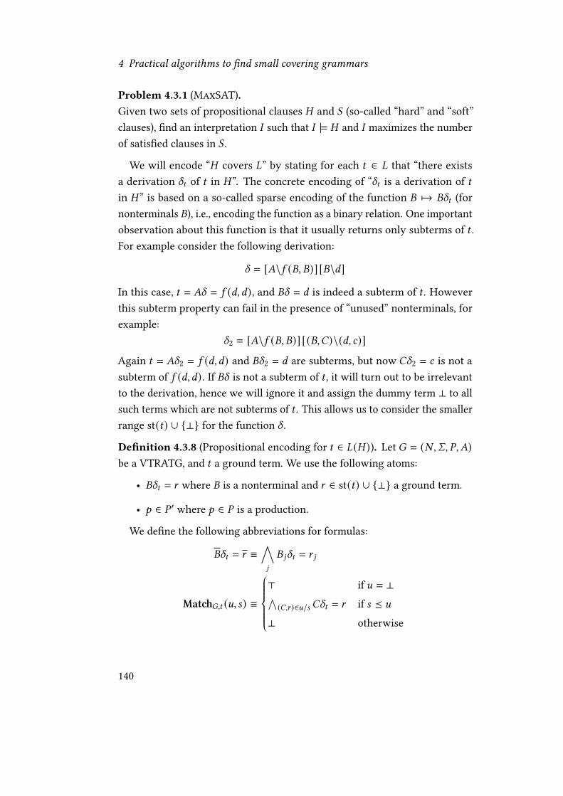
4 Practical algorithms to �nd small covering grammars
Problem 4.3.1 (MaxSAT).Given two sets of propositional clauses � and ( (so-called “hard” and “soft”clauses), �nd an interpretation � such that � |= � and � maximizes the numberof satis�ed clauses in ( .
We will encode “� covers !” by stating for each C ∈ ! that “there existsa derivation XC of C in �”. The concrete encoding of “XC is a derivation of Cin �” is based on a so-called sparse encoding of the function � ↦→ �XC (fornonterminals �), i.e., encoding the function as a binary relation. One importantobservation about this function is that it usually returns only subterms of C .For example consider the following derivation:
X = [�\5 (�, �)] [�\3]
In this case, C = �X = 5 (3,3), and �X = 3 is indeed a subterm of C . Howeverthis subterm property can fail in the presence of “unused” nonterminals, forexample:
X2 = [�\5 (�, �)] [(�,�)\(3, 2)]
Again C = �X2 = 5 (3, 3) and �X2 = 3 are subterms, but now �X2 = 2 is not asubterm of 5 (3,3). If �X is not a subterm of C , it will turn out to be irrelevantto the derivation, hence we will ignore it and assign the dummy term ⊥ to allsuch terms which are not subterms of C . This allows us to consider the smallerrange st(C) ∪ {⊥} for the function X .
De�nition 4.3.8 (Propositional encoding for C ∈ !(� )). Let� = (#, O, %,�)be a VTRATG, and C a ground term. We use the following atoms:
• �XC = A where � is a nonterminal and A ∈ st(C) ∪ {⊥} a ground term.
• ? ∈ % ′ where ? ∈ % is a production.
We de�ne the following abbreviations for formulas:
�XC = A ≡∧9
� 9XC = A 9
Mat��,C (D, B) ≡
> if D = ⊥∧(�,A )∈D/B �XC = A if B � D⊥ otherwise
140

4.3 Using MaxSAT
Case�,C (�,D) ≡ �XC = D→∨
�→B∈%
(�→ B ∈ % ′ ∧
∧9
Mat��,C (D 9 , B 9 ))
Func�,C ≡( ∧� nonterminal
∨B∈st(C)∪{⊥}
�XC = B
∧∧
� nonterminal
∧B1≠B2∈st(C)∪{⊥}
¬(�XC = B1 ∧ �XC = B2))
GenTerm�,C ≡ �XC = C ∧ Func�,C ∧∧�∈#
∧B∈(st(!)∪⊥) |� |
Case�,C (8, B)
The formula Mat��,C (D, B) encodes BXC = D, extending the �XC = D atom toarbitrary terms B . In order to ensure the correctness of the whole encoding,we have to add implied constraints for each possible function value of XCand for each nonterminal vector �: the Case�,C (�,D) formula encodes theseconstraints. Then Func�,C states that X : # → st(C) ∪ {⊥} is a function, andGenTerm�,C combines the other formulas to encode that X is a derivation of Cusing only the productions from the subset % ′ ⊆ % , i.e., those which are presentin � .
Example 4.3.9. Consider C = 5 (2, 2, 4), # = {�, �}, and � = (#, O, %,�) withthe following productions % = {?1, ?2, ?3, ?4}:
?1 = �→ 5 (�, �, �) ?3 = �→ 2
?2 = �→ 5 (�, �, 4) ?4 = �→ 3
Then we encode C ∈ !(� ) using the following formula GenTerm�,C (slightlysimpli�ed propositionally):
Case�,C (�, 5 (2, 2, 4)) ≡ �XC = 5 (2, 2, 4) → (?2 ∈ % ′ ∧ �XC = 2)Case�,C (�, 2) ≡ �XC = 2→⊥Case�,C (�, 4) ≡ �XC = 4→⊥Case�,C (�,⊥) ≡ �XC = ⊥→>
Case�,C (�, 5 (2, 2, 4)) ≡ �XC = 5 (2, 2, 4) → ⊥Case�,C (�, 2) ≡ �XC = 2→ (?3 ∈ % ′)Case�,C (�, 4) ≡ �XC = 4→⊥
141

4 Practical algorithms to �nd small covering grammars
Case�,C (�,⊥) ≡ �XC = ⊥→>
GenTerm�,C ≡ �XC = 5 (2, 2, 4) ∧ Func�,C ∧∧�,B
Case�,C (�, B)
Many of the formulas Case�,C (�, B) are of the form (· · ·→⊥); these correspondto derivations that are impossible: for example we have �XC = 2→⊥ becausethere is no production of � that has 2 as the root symbol. In this example,GenTerm�,C entails ?2 ∈ % ′ ∧ ?3 ∈ % ′, hence any covering subgrammar � ⊆ �necessarily includes these two productions; the minimal covering subgrammarconsists precisely of these two productions.
Lemma 4.3.11. Let � = (#, O, %,�) be a VTRATG, � = (#, O, % ′, �) ⊆ � asubgrammar of� , and C a term. Then for every derivation X of C in� , there existsa satisfying interpretation � |= GenTerm�,C such that for all ? ∈ % , � |= ? ∈ % ′
i� ? ∈ % ′.Conversely, if � |= GenTerm�,C is a satisfying interpretation such that for all
? ∈ % , � |= ? ∈ % ′ i� ? ∈ % ′, then there exists a derivation of C in � .
Proof. We need to construct a satisfying interpretation � for every derivationX in � . So we would like to set � |= �XC = A if and only if �X = A ; but this couldfail if A is not a subterm of C . But the following assignment only results in ⊥ orsubterms of C , as required:
� |= �XC = A ⇔A = �X if � is a subterm of CA = ⊥ otherwise
It remains to verify that � |= Case�,C (�, B) for all 8 and B , that is, � |=Mat��,C (� 9XC , B 9 ) for all 9 , where �→ B is the chosen production in X . Thisis trivial if � 9X is not a subterm of C—then Mat��,C (� 9XC , B 9 ) expands to >—inthe other case, it is clear from the de�nition of a derivation.
Conversely, let � be a satisfying interpretation for GenTerm�,C such that� |= ? ∈ % ′ i� ? ∈ % ′. We will now construct an actual derivation X in� such that �X = C . By Func�,C there is a unique value for each �XC in� , let 5 (�) ∈ st(C) ∪ {⊥} be the term such that � |= �XC = 5 (�). Hence� |= Case�,C (�, (5 (�1), . . . , 5 (� |� |))), and we can choose the production �→
142

4.4 Induction grammars
(B�1, . . . , B� |� | ) for X such that � |= �→(B�1, . . . , B� |� | ) ∧∧9 Mat��,C (5 (� 9 ), B� 9 ).
This immediately ensures that X really is a derivation in the subgrammar.We will now verify that 5 (�) ≠ ⊥ implies �X = 5 (�) for all �, by backwards
induction on the index of � in the nonterminal vector # : if 5 (�) ≠ ⊥, thenMat��,C (5 (�), B�) ≡
∧; �;X = A; . Because the nonterminals in B� can only be
of the form � where � occurs after � in # , computing �X �rst substitutes �with B� , and then each�; with A; , since�;X = A; per induction hypothesis. Nowsince 5 (�) = C ≠ ⊥, we conclude that X is a derivation of �X = C . �
So far we have only considered the encoding for the derivability of a singleterm C , we will now turn to derive multiple terms.
Theorem 4.3.7. VTRATG-Minimization ≤% MaxSAT.
Proof. Let � = (#, O, %,�) be the VTRATG, and ! ⊆ !(�) the set of terms.We need to �nd a subset % ′ ⊆ % of minimal size such that the grammar� = (#, O, % ′, �) still satis�es ! ⊆ !(� ). By Lemma 4.3.11, any interpretation� satisfying
∧C∈! GenTerm�,C corresponds to a covering VTRATG. Set the hard
clauses of the MaxSAT problem to a CNF of this formula. (Such a CNF can beobtained in polynomial time by a Tseitin transformation [97].)
For each production ? ∈ % , we add the soft clause ¬(? ∈ % ′). The numberof satis�ed soft clauses is then exactly |% | − |% ′|, the number of productionsnot included in the minimized VTRATG. Maximizing the number of softclauses then minimizes the number of productions in the VTRATG given bythe interpretation. From a solution � to this MaxSAT problem, we obtain theminimal covering VTRATG by setting % ′ = {? | � |= ? ∈ % ′}, which is thecorresponding subgrammar according to Lemma 4.3.11. �
4.4 Induction grammars
In Section 4.3, we developed the theory for stable grammars underlying theMaxSAT algorithm in a very general way. We can now apply this theoryto induction grammars as well, and thereby extend the MaxSAT algorithmto solve Parameterized Indexed Termset Cover. First, we will show thatlanguage generation and rewriting commutes:
143

4 Practical algorithms to �nd small covering grammars
Algorithm 2 Solution of the Parameterized Language Cover Problem viaMaxSAT
Input: set of ground terms !, and a sequence of nonterminals # .Output: minimal VTRATG � with nonterminals # such that ! ⊆ !(� ).� = stableGrammar(# , !)i = minimizationFormula(� , !)� = maxSatSolver(i , softClauses(�))� = grammarFromAssignment(� )
De�nition 4.4.1. Let � = (g, U, (a2)2, W, %) and �′ = (g, U, (a2)2, W, % ′) be in-duction grammars, and→' a rewrite relation. Then�→∗
'�′ i� for all ?′ ∈ % ′
there exists a ? ∈ % such that ?→∗'?′ and for all ? ∈ % there exists a ?′ ∈ % ′
such that ?→∗'?′.
Lemma 4.4.1. Let→' be a rewrite relation, and �,�′ be induction grammarssuch that � →∗
'�′. Then � (�, C) →∗
'� (�′, C) and !(�, C) →∗
'!(�′, C) for all C .
Proof. We have � (�, C)→∗'� (�′, C) since all productions in the instance grammar
are substitution instances of productions in� and�′, and→' is a rewrite rela-tion. Commutation of language generation and rewriting !(�, C) →∗
'!(�′, C)
directly lifts from the result for VTRATGs in Theorem 4.3.1. �
Similar to Theorem 4.3.3, we can now show that we can transform grammarsinto subgrammars of the stable grammar without increase in size.
De�nition 4.4.2. Let (!8)8∈� be a family of languages, and U, (a2)2, W as inDe�nition 2.8.5. Then the stable grammar ( ((!8)8∈� ) = (g, U, (a2)2, W, %) containsall possible productions where the right-hand side is a stable term of theappropriate type, that is:
% = {^→ C [U, a8, W] | ^ ∈ {g,W} ∧ C [U, a8, W] ∈ ((⋃
8
!8)}
De�nition 4.4.3. Let � = (g, U, (a2)2, W, %) and �′ = (g, U, (a2)2, W, % ′) be in-duction grammars. We say that �′ is a subgrammar of � , written �′ ⊆ � , i�% ′ ⊆ % .
144

4.4 Induction grammars
Theorem4.4.1. Let (!8)8∈� be a �nite family of languages, and� = (g, U, (a2)2, W, %)an induction grammar that covers (!8)8∈� . Then there exists an induction grammar�′ = (g, U, (a2)2, W, % ′) such that:
• �′ covers (!8)8∈�
• |�′| ≤ |� |
• �′ ⊆ ( ((!8)8∈� )
Proof. We obtain the induction grammar �′ by replacing the right-hand sideof every production in� by one of its @!-normal forms, which are in ( ((!8)8∈� ).The resulting induction grammar�′ still covers (!8)8∈� by applying Lemma 4.4.1to v! since we have � v∗
!�′. �
We can now turn to the problem of induction grammar minimization, anal-ogous to VTRATG-Minimization. For this part we can reuse the MaxSATencoding of De�nition 4.3.8, de�ning the minimization of induction grammarin terms of the instance grammars:
De�nition 4.4.4. Let (!8)8∈� be a �nite family of languages, and� = (g, U, (a2)2, W, %)an induction grammar. We de�ne the propositional formula Gen(�, (!8)8∈� ) asthe following formula:∧
8∈�
∧C∈!8
GenTerm′(� (�, 8), C) ∧∧8∈�
∧? ′
(?′ ∈ % ′
� (�,8)→∨?{8?
′? ∈ %
)The formula GenTerm′ is a syntactical variant of GenTerm, which di�ers onlyin the names of the propositional variables:
• ?′ ∈ % ′� (�,8) instead of ?′ ∈ % ′
• XC,� (�,8) instead of XC
Theorem 4.4.2. Let (!8)8∈� be a �nite family of languages, � an inductiongrammar, and �′ ⊆ � a subgrammar. Then the formula Gen(�, (!8)8∈� ) ∧∧{¬? ∈ % ′ | ? ∈ � \�′} is satis�able if and only if �′ covers (!8)8∈� .
145

4 Practical algorithms to �nd small covering grammars
Proof. By Lemma 4.3.11, the formula is satis�able i� for all 8 ∈ � , the instancegrammar � (�′, 8) covers!8 . The second conjunct of De�nition 4.4.4 then ensuresthat whenever an instantiated production is used to cover a term in the instancegrammar, it is already included in the induction grammar. �
Algorithm 3 Cover a family of languages by an induction grammarprocedure FindGrammar(f, g, (!8)8 )
S← ( ((!8)8)hard← Gen(S, (!8)8)soft← {¬? ∈ % ′ | ? ∈ S}if Sat(I) ← MaxSAT(hard, soft) then
return {? | I |= ? ∈ % ′}else
failend if
end procedure
Lemma 4.4.2. Let (!8)8∈� be a �nite family of languages, then Algorithm 3produces an induction grammar covering (!8)8∈� of minimal size, or fails if thereis no covering grammar.
Proof. First, assume that there exists a covering induction grammar; by The-orem 4.4.1 there is a grammar � covering (!8)8∈� of minimal size such that� ⊆ ( ((!8)8∈� ). By Theorem 4.4.2, the formula hard ∧∧
?∈S\G ¬(? ∈ % ′)) issatis�able. Hence the interpretation � returned by the MaxSAT solver sets atmost |� | many ? ∈ % ′ atoms to true, corresponding to a grammar with at most|� | productions. If there is no covering grammar, then MaxSAT will returnunsatis�able as return status, and Algorithm 3 will fail. �
4.5 Reforest
4.5.1 TreeRePair
Given the close relation of the problem of �nding small covering VTRATGsand grammar-based text- and document compression, we can also try to adapt
146

4.5 Reforest
algorithms from grammar-based compression. In this section we will describesuch an adaptation of the TreeRePair [65] algorithm to produce coveringVTRATGs. TreeRePair compresses XML documents (formally, ranked andunranked trees, i.e. single-sorted �rst-order terms with function symbols ofvariable arity) using context-free tree grammars.
De�nition 4.5.1. A context-free tree grammar � = (#, O, %,�) is a tupleconsisting of a start symbol � ∈ # of arity 0, a set of function symbols # asnonterminals (whose arity is not necessarily 0), and a set of productions % .A production is a pair �(G) → C of two terms of the same type such that Gis a vector of pairwise distinct variables and FV(C) ⊆ G . The grammar � isacyclic i� the relation ≺ on nonterminals, de�ned by � ≺ � i� there exists aproduction �(G) → C ∈ % such that C contains � , is acyclic. The grammar � isstraight-line i� for every nonterminal � ∈ # , there is exactly one productionof the form �(. . . ) → . . . in % .
De�nition 4.5.2. Let � = (#, O, %,�) be a context-free tree grammar. Thesingle-step derivation relation ⇒� is a binary relation on terms de�ned byC ⇒� C? [A [G\B]] i� C? = �(B) and �(G) → A ∈ % for some position ? . A termC ∈ T (O) is derivable in � i� � ⇒∗
�C . The language !(�) = {C ∈ T (O) |
�⇒∗�C} consists of all derivable terms.
The context-free tree grammars produced by TreeRePair are acyclic andstraight-line. Such grammars produce exactly a single term (the originalXML document). The central concept behind the algorithm are digrams: adigram is a triple (5 , 8, 6) consisting of two function symbols 5 , 6 and a naturalnumber 8 . This digram describes the pattern 5 (G1, . . . , G8−1, 6(~), I8+1, . . . , I=),i.e., an occurrence of 5 where the 8-th argument has 6 as root symbol. Adigram can be compressed by �rst introducing a new nonterminal � withthe production �(G,~, I) → 5 (G, 6(~), I), and then replacing all occurrences5 (C, 6(B), A ) by �(C, B, A ). Given a term C to compress, TreeRePair starts withthe trivial grammar with the single production �→ C and then repeatedlycompresses the most frequent digram by adding a new production as describedbefore. (There is also an additional post-processing step called “pruning” thatwe do not show here, and which does not apply in the example below.)
147

4 Practical algorithms to �nd small covering grammars
Example 4.5.1. TreeRePair compresses the term 5 8(2) in the following steps:
%0 = {�→ 5 8(2)} (the most frequent digram is (5 , 0, 5 ))%1 = {�→ �4(2), �(G) → 5 (5 (2))} (the most frequent digram is (�, 0, �))%2 = {�→�2(2), �(G) → 5 (5 (2)),� (G) → �(�(G))}
The resulting context-free tree grammar � then has the productions %2 andsatis�es !(�) = {5 8(2)}.
Looking at the digram compression step again, the generated productionhas a noteworthy property: it is linear, that is, each variable occurs at mostonce on the right hand side. In our adaption, we will also generate productionsthat are non-linear to better capture the rigid behavior of VTRATGs.
4.5.2 Adaptation to tree languages
There are two general big di�erences from our setting to that of TreeRePair:�rst, we do not want to compress just a single term but a set of terms. Andsecond, we expect a lossy compression that does not reproduce the input termset exactly, but can produce a superset. Similar to the delta-table algorithm,we consider only the introduction of a single nonterminal in the resultingcovering VTRATG. That is, given a �nite set of terms ! we produce a coveringVTRATG with the nonterminals �, � where the length of � is chosen by thealgorithm. This adaptation, called Reforest, proceeds in three steps:
1. Produce a trivial context-free tree grammar �0.
2. Iteratively compress �0 by introducing abbreviating productions.
3. Use the compressed context-free tree grammar to directly read o� theproductions for the covering VTRATG.
We then iterate this process to produce a VTRATG with more nonterminals.The �rst two steps are already present in TreeRePair, albeit in a simpler way.The third step is speci�c to our adaptation. In the �rst step we produce thecontext-free tree grammar �0 = {�→ C | C ∈ !}. This grammar is no longerstraight-line, since it produces multiple terms: namely !(�0) = !. However the
148

4.5 Reforest
%0 = {�→ A (2, 2) | · · · | A (5 7(2), 5 7(2))}%1 = {�→ A (2, 2) | A (5 (2), 5 (2)) | A (�(2), �(2)),
�→ A (5 (�(2)), 5 (�(2))) | A (�2(2), �2(2)) | A (5 (�2(2)), 5 (�2(2))),�→ A (�3(2), �3(2)) | A (5 (�3(2)), 5 (�3(2))),�(G) → 5 (5 (G))}
%2 = {�→ A (2, 2), | A (5 (2), 5 (2)) | A (�(2), �(2)),�→ A (5 (�(2)), 5 (�(2))) | A (� (2),� (2)) | A (5 (� (2)), 5 (� (2))),�→ A (�(� (2)), �(� (2))) | A (5 (�(� (2))), 5 (�(� (2)))),�(G) → 5 (5 (G)),� (G) → �(�(G))}
%3 = {�→ � (2) | � (5 (2)) | � (�(2)) | � (5 (�(2)))�→ � (� (2)) | � (5 (� (2))) | � (�(� (2))) | � (5 (�(� (2)))),�(G) → 5 (5 (G)),� (G) → �(�(G)), � (G) → A (G, G)}
%4 = {�→ � (2) | � (2) | � (�(2)) | � (�(2)),�→ � (� (2)) | � (� (2)) | � (�(� (2))) | � (�(� (2)))�(G) → 5 (5 (G)),� (G) → �(�(G)), � (G) → A (G, G), � (G) → � (5 (G))}
%5 = {�→ � (2) | � (2) | � (�(2)) | � (�(2)),�→ � (� ) | � (� ) | � (�(� )) | � (�(� )),�(G) → 5 (5 (G)),� (G) → �(�(G)), � (G) → A (G, G), � (G) → � (5 (G)),� →� (2)}
%6 = {�→ � (2) | � (2) | � (2) | � (�(2)),�→ � (� ) | � (� ) | � (� ) | � (�(� )),�(G) → 5 (5 (G)),� (G) → �(�(G)), � (G) → A (G, G), � (G) → � (5 (G)),� →� (2),� (G) → � (�(G))}
%7 = {�→ � (2) | � (2) | � (2) | � (2),�→ � (� ) | � (� ) | � (� ) | � (� ),�(G) → 5 (5 (G)),� (G) → �(�(G)), � (G) → A (G, G), � (G) → � (5 (G)),� →� (2),� (G) → � (�(G)), � (G) → � (�(G))}
Figure 4.1: Run of the �rst compression step in the Reforest algorithm on! = {A (2, 2), A (5 (2), 5 (2)), . . . , A (5 7(2), 5 7(2))}.
149

4 Practical algorithms to �nd small covering grammars
context-free tree grammars that we will produce will be almost straight-line:for any nonterminal � ≠ �, there will be at most one production �(. . . ) → . . . .
In the second step, we introduce two kinds of abbreviating productions:digrams (as in TreeRePair), and rigid trigrams. A rigid trigram is a triple(5 , 8, 9) of a function symbol 5 and two natural numbers 8 and 9 . It describesthe pattern 5 (G1, . . . , G8−1, G8, G8+1, . . . , G 9−1, G8, G 9+1, . . . , G=), i.e., an occurrenceof 5 where the 8-th and 9-th argument are the same term. This rigid trigram canbe abbreviated by introducing a production �(G,~, I,F) → 5 (G,~, I,~,F). Wethen iteratively compress the most frequent feature, which is either a digramor a rigid trigram.
Example 4.5.2. Let ! = {A (2, 2), A (5 (2), 5 (2)), . . . , A (5 7(2), 5 7(2))}. Reforest�rst produces the context-free tree grammar %7 by abbreviating digrams andrigid trigrams as shown in Section 4.5.2. This compression has introduced newstructure into the term set: instead of the “homogeneous” terms A (5 = (2), 5 = (2)),the productions of the start symbol� are now all combinations of the 6 di�erentsymbols � (·), � (·),� (·), � (·) and 2, � .
In the third step, we now inspect the compressed context-free tree gram-mar�= and use it to construct a covering VTRATG. Since all nonterminals in�=except� have at most one production, we can de�ne C ⇓�= to be the unique termderivable from C in�= provided that C does not contain�. We now look at all theproductions�→ 5 (C) in�= . If all the function symbols 5 such that there existsa production �→ 5 (C) have the same arity, then we produce a VTRATG withthe productions {�→ (5 (G) ⇓�= ) [G\�] | �→ 5 (C)} ∪ {�→ C ⇓�= | �→ 5 (C)}.If the function symbols do not have the same arity, we pad them with dummyconstants.
Example 4.5.3 (continuing Example 4.5.2). From the �-productions in %7 weget the function symbols �, �,�, � and the arguments 2, � and we produce theVTRATG with the following 6 productions:
�→ � (�) ⇓ | � (�) ⇓ | � (�) ⇓ | � (�) ⇓�→ 2 ⇓ | � ⇓
150

4.6 Experimental evaluation
After expanding ⇓:
�→ A (�, �) | A (5 (�), 5 (�)) | A (5 2(�), 5 2(�)) | A (5 3(�), 5 3(�))�→ 2 | 5 4(2)
4.6 Experimental evaluation
In this chapter we have presented three di�erent algorithms to �nd smallcovering grammar. All of these algorithms are implemented in the GAPTframework. We benchmarked their implementation in GAPT 2.2 on two datasets:
1. Synthetic examples bundled with GAPT1. These are sequences of proofsparameterized by a natural number and produce sets of terms simi-lar to Example 4.5.2. For example one of these synthetic examples,LinearExampleProof(=), constructs a proof of the following sequent:
% (0),∀G (% (G) → % (B (G))) ` % (B= (G))
2. Proofs from the TSTP collection produced by automated theorem provers(Thousands of Solutions from Theorem Provers [93]; all proofs from theFOF and CNF categories as of November 2015). From the total 137989proofs in the TSTP, we could import term sets from 68185 proofs (49.41%).
Both data sets consist of single-sorted languages. We have extracted termsets from the TSTP collection of proofs produced by automated theoremprovers (Thousands of Solutions from Theorem Provers [93]; all proofs fromthe FOF and CNF categories as of November 2015). Unfortunately many ofthese proofs are in custom formats that we have been unable to import. How-ever from the total 137989 proofs in the TSTP, we could import term sets from68185 proofs (49.41%). Of these 68185 term sets, 35467 (52.02%) can not becompressed using VTRATGs (with regard to our size measure) as each termhas a di�erent root symbol.
1These can be found in the gapt.examples package.
151

4 Practical algorithms to �nd small covering grammars
For each of the data sets, we show two plots: one comparing the runtimeof the algorithms when they produce a VTRATG (for Reforest we only countgrammars with fewer productions than the size of the term set). The secondone compares the runtime in the cases where the cut-introduction algorithmin GAPT could use the grammar to generate a non-trivial lemma [36]. We alsoshow the results for a “virtual best” method which has the minimum runtimeof the others, i.e., it behaves as if we ran all the algorithms in parallel in aportfolio mode and terminated as soon as one of them �nishes.
We compared the implementation of these three algorithms in a prereleaseversion2 of GAPT 2.3 [37] and used GNU parallel [96] for scheduling. TheMaxSAT solver we used is OpenWBO version 2.0 [67]. The comparison wasconducted on a Debian Linux system with an Intel i5-4570 CPU and 8 GiB RAM,with a time limit of 60 seconds. In the Figures 4.2 and 4.3 we use the followingnames for the grammar generation algorithms:<_maxsat is the MaxSAT algo-rithm with the parameter # = {�, (�1, . . . , �<)},<_=_maxsat is the MaxSATalgorithm with parameter # = {�, (�1, . . . , �<), (�1, . . . ,�=)}, many_dtable isthe delta-table algorithm without row-merging, many_dtable_ss is the delta-table algorithm with row-merging, 1_dtable is the delta-table algorithm usinglgg1 instead of lgg.
In an earlier evaluation we compared the delta-table algorithm and theMaxSAT algorithm [29] in GAPT 2.0 on the same proofs from the TSTP. Thereare surprising di�erences in the results: the most striking di�erence concernsthe proof import. The GAPT 2.3 release introduced an algorithm that directlyconverts resolution proofs (as imported from the TSTP) to expansion proofs,without constructing LK proofs as an intermediate step. (We will discuss thisalgorithm in more detail in Chapter 6.) Using this new and improved algorithmwe can import almost twice as many proofs as term sets, increasing the numberfrom 36494 term sets in GAPT 2.0 to 68185 term sets in GAPT 2.3.
Another noteworthy change in GAPT 2.3 is the rewrite of the delta-tableimplementation that was necessary to �x several bugs. As a side e�ect, theperformance of the delta-table algorithm was signi�cantly improved. Whilethe MaxSAT algorithm was signi�cantly more successful in the previous eval-
2git revision 9b9909820744046ff57af9b399965824bf3a4919
152

4.6 Experimental evaluation
uation [29], in the present evaluation the delta-table algorithm is more com-petitive now.
Figure 4.2 compares the runtime for the synthetic examples. Here Reforest�nds the largest number of grammars by a signi�cant margin. It �nds morethan 600 compressing VTRATGs, three times as many as the next algorithm,1_maxsat, which �nds about 200. The line for Reforest also almost coincideswith the virtual best: only very few term sets can be compressed by anotheralgorithm but not by Reforest. The next most successful algorithm is theMaxSAT algorithm with the parameter # = {(�), (�)}. Many of the syntheticproblems have short natural proofs with cuts that only have a single universalquanti�er, this is most likely why that parameter is the most successful choice.
If we only consider the grammars that could actually be successfully usedby cut-introduction to produce a nontrivial lemma, then the gap shortens abit: Reforest is still ahead by a signi�cant margin, but the margin is smaller.Reforest �nds more than 200 useful grammars, and 1_maxsat �nds about 150.There are two explanations for this result: one is that for our proof-theoreticapplications in the form of cut-introduction it is not just important to �nda compressing VTRATG, but that there are additional qualitative featuresnecessary for a VTRATG to correspond to an interesting proof with cut. Theother explanation is that the algorithm used to �nd the actual formula forthe lemma is exponential in the number of nonterminal vectors; and Reforestproduces a larger number of nonterminal vectors than the other algorithms.
Within a timeout of 60 seconds per term set, the delta-table algorithm �ndsgrammars for 6873 term sets. Algorithm 2 improves on this and �nds grammarsfor 7503 term sets. This is a signi�cant improvement, since the additional 630term sets are the most di�cult instances solved, even though they only accountfor a 9% increase in solutions.
The results for the TSTP data set in Figure 4.3 are completely di�erent: here,the delta-table algorithm is the most successful one, tied with the MaxSATalgorithm with parameter # = {�, (�1, �2)}. Reforest is the (second) leastsuccessful algorithm both by the number of compressing grammars, and thenumber of grammars that were useful for cut-introduction. This is probablycaused by the di�erent nature of the proofs in the TSTP: only very few of theseproofs contain purely repetitive structures such as {2, . . . , 5 = (2)}, variants of
153

4 Practical algorithms to �nd small covering grammars
0 100 200 300 400 500 600 700# produced covering grammars (synthetic examples)
0
2
4
6
8
10
CPU
runt
ime
(sec
onds
)
reforest1_maxsat2_maxsat1_1_maxsat2_2_maxsat1_dtablemany_dtablemany_dtable_ssvirtual best
0 50 100 150 200 250 300# grammars that lead to a non-trivial lemma (synthetic examples)
0
2
4
6
8
10
CPU
runt
ime
(sec
onds
)
reforest1_maxsat2_maxsat1_1_maxsat2_2_maxsat1_dtablemany_dtablemany_dtable_ssvirtual best
Figure 4.2: Cactus plot of grammar generation runtime on synthetic examples.
154

4.6 Experimental evaluation
0 5000 10000 15000 20000# produced covering grammars (TSTP)
0
2
4
6
8
10
CPU
runt
ime
(sec
onds
)reforest1_maxsat2_maxsat1_1_maxsat2_2_maxsat1_dtablemany_dtablemany_dtable_ssvirtual best
0 2000 4000 6000 8000 10000 12000# grammars that lead to a non-trivial lemma (TSTP)
0
2
4
6
8
10
CPU
runt
ime
(sec
onds
)
reforest1_maxsat2_maxsat1_1_maxsat2_2_maxsat1_dtablemany_dtablemany_dtable_ssvirtual best
Figure 4.3: Cactus plot of grammar generation runtime on proofs from theTSTP.
155

4 Practical algorithms to �nd small covering grammars
Figure 4.4: Runtime performance comparison on the TSTP proofs. Each pointrepresents an input term set, and its size is proportional to theruntime of each algorithm.
156

4.6 Experimental evaluation
Figure 4.5: Comparison of the performance di�erence to the compression ra-tio and overall runtime. Each point represents an input term setfrom the TSTP data set. The size of a point is proportional to thecombined runtime of both algorithms.
which occur in many of the synthetic examples.For easy term sets—those which take a short time to compress—the delta-
table algorithm is much faster than the MaxSAT algorithm; there the curve forthe delta-table algorithm is below the one for the MaxSAT algorithm. As faras we can tell, the performance di�erence on the easy examples is due to theoverhead of constructing the stable grammar and the minimization formula.On average, this reduction makes up for 72% of the runtime for term sets wherethe total runtime is less than 1 second, whereas the situation is almost reversedfor term sets where the total runtime is more than 10 seconds: there about 69%of the runtime is spent inside the MaxSAT solver.
This dichotomy between easy and hard problems is not only apparent onthe aggregate data set, but also for individual term sets: Figure 4.5 shows theCPU runtime ratio (x-axis) in comparison to the compression ratio (y-axis) andtotal runtime (size of the points). On the top right there is a cluster of smallpoints: these are the easy problems, and while the delta-table algorithm is
157

4 Practical algorithms to �nd small covering grammars
faster by a factor of 10, both algorithms can solve the problems in a reasonabletime. Then there is a large cluster on the left: these are the hard problems,which generally admit a better compression, and here the MaxSAT algorithmis faster by a factor of 10.
Figure 4.4 shows a scatter plot of term set size against achieved compressionratio (ratio of grammar size to term set size, i.e., number of productions tonumber of terms). The size of each point in Figure 4.4 is proportional to theruntime of the algorithm: we see that Reforest is typically much faster than theother algorithms. The reason for the di�erence between Figures 4.3 and 4.4 ismainly that the TSTP contains many small proofs, for which it is important to�nd even very small opportunities for compression. Hence for the small termsets it is more advantageous to use algorithmically more complex methodsas they can exploit these subtle features in a more e�ective way and �ndcompressing grammars at all.
Only the MaxSAT algorithm and Reforest can �nd grammars whose sizeis less than 25% of the input term set; however Reforest only achieves thesecompression ratios for larger term sets. For the MaxSAT algorithm, the choiceof parameter is crucial: while a larger parameter # would theoretically allowus to �nd more grammars (and hence lower compression ratios), in practicethese larger parameters just increase the runtime and we hence �nd fewergrammars in the given time limit.
With Reforest we have an interesting algorithm to �nd covering VTRATGsthat uses very di�erent techniques to the delta-table and MaxSAT algorithm.Due to its roots in grammar-based compressed, it is better from an algorithmicperspective: the introduction of a single nonterminal could potentially be donein linear time using the implementation tricks used in TreeRePair [65]. (TheReforest implementation takes quadratic time.) Even iterating this processto introduce multiple nonterminals only has cubic cost. In comparison, boththe MaxSAT and delta-table algorithms rely on algorithms for NP-completeoptimization problems (MaxSAT and set cover, respectively). The crucialtrick that allows Reforest to �nd covering VTRATGs without relying on back-tracking search is the heuristic of most frequent digrams, which allows us todeterministically choose a compression.
However it is not obvious how to generalize Reforest to produce induction
158

4.6 Experimental evaluation
grammars. Digram compression exponentially compresses sequences of theform {A (2), . . . , A (5 2=−1(2))} using the VTRATG�→A (�2) | A (5 (�2)), �2→�3 |5 2
2 (�3), . . . , �=−2→�=−1 | 5 2=−2 (�=−1), �=−1→2 | 5 2=−1 (2). While for induction
grammars, we would hope to obtain a production g → A (a). Since digramcompression is central to the algorithm, this behavior seems to be hard toavoid.
159


5 Formula equations anddecidability
In the previous chapters we have studied the grammars of simple proofs andsimple induction proofs. The grammars contain only the quanti�er infer-ence terms in these proofs. Generating their language corresponds to cut-elimination. However not every grammar is the grammar of a proof. Forexample, a grammar generating the empty language will not correspond to aproof (since the empty sequent is not derivable). In this chapter we will studythe conditions under which grammars can be extended to proofs, and whatproperties the proposed cut formula and induction formulas need to satisfy.These conditions will be collected in a so-called formula equation.
The algorithms devised in Chapter 4 allow us to �nd grammars that cover agiven set of terms. If we start from a cut-free proof c and �nd a VTRATG �
that covers !(c), then we know the quanti�er inference terms for a small proofwith cuts (i.e., a proof with a small quanti�er complexity). It only remainsto algorithmically �nd suitable cut formulas, i.e., a solution to the formulaequation. This approach of introducing cuts into an existing cut-free proof iscalled cut-introduction [51, 48, 50, 49, 36].
A procedurally similar approach can also be used for automated inductivetheorem proving [31]. There we start from cut-free proofs of instances ofthe sequent and �nd a covering induction grammar. In both applications it iscrucial to automatically solve the induced formula equations. Hence we willstudy two algorithms that solve formula equations in this chapter. The �rstone in Section 5.6 will be based on forgetful inference, while the second one inSection 5.7 will be based on interpolation.
161

5 Formula equations and decidability
5.1 Formula equations
We have already seen the de�nition of a formula equation in Section 2.9. Aneasy observation is that if the formula equation is solvable, then it is valid inhigher-order logic, both in Henkin semantics as well as full semantics.
Example 5.1.1. The formula equation ∃- R withR = ∀G ((% (G) →- ) ∧ (- →% (G)) has no solution (modulo ) = ∅) since R implies ∀G (% (G) → - ) and∀~ (-→% (~)) and therefore ∀G∀~ (% (G)→% (~)), which is not a valid formula.If the quanti�er ∀G was not present in the formula equation, it would have thesolution - (G). One way to view this situation is that the quanti�er ∀G in theformula equation has the e�ect that G may not occur in the solution.
The concept of formula equations can be traced back to the 19th century,see [102] for an overview. Formula equations are connected to second-orderquanti�er elimination. In this context, Ackermann proved the following lemmawhich allows us to eliminate a single second-order quanti�er.
Lemma 5.1.1 (Ackermann’s lemma [1]). Let Q be a formula equation suchthatQ = ∃- ∃. (∀G (\ (G) → . (G)) ∧k ) where . does not occur in \ and onlyoccurs negatively ink . Then:
1. Q is ) -solvable i�Q′ = ∃- k [.\\ ] is solvable
2. IfQ has the ) -solution f , thenQ′ has the ) -solution f � - .
3. IfQ′ has the ) -solution f thenQ has the ) -solution [.\\ ]f .
Proof. Let us �rst show ) ` ∀G (\ (G) → . (G)) ∧k →k [.\_G \ (G)]. This istrue because . only occurs negatively ink . Whenever we can prove j′→ j
for some formulas j, j′ then we can replace all negative occurrences of j byj′ ink while preserving provability (this is an easy induction onk ). From thisobservation we conclude 2.
For 3, assume ) ` k [.\\ ]f . We need to show ) ` (∀G (\ (G) → . (G)) ∧k ) [.\\ ]f . By moving [.\\ ]f , this is equivalent to) ` ∀G (\f (G) →\f (G)) ∧k [.\\ ]f , which directly follows from the assumption. Finally, 1 follows from2 and 3. �
162

5.2 Solvability of VTRATGs
We can relax the syntactic restriction in Lemma 5.1.1 a bit to formula equa-tions of the form Q = ∃- ∃. ∀G (\ (G) → . (C)) ∧ k where . does not oc-cur in \ and only negatively in k . This formula equation is equivalent toQ = ∃- ∀~ (∃G (\ (G) ∧ ~ = C) → . (~)) ∧ k . Therefore Q is solvable i�∃- k [.\_~ ∃G (\ (G) ∧ ~ = C)] is solvable.
Example 5.1.2. LetQ = ∃- (∀G (% (G) → - (G)) ∧ (- (0) → % (1))). ThenQ issolvable i� % (0) → % (1) is solvable. And % (0) → % (1) is not ∅-solvable.
Example 5.1.3. Let Q = ∃- (∀G (- (G) → - (B (G))) ∧ (- (0) → % (1))). ThenLemma 5.1.1 does not apply since \ (G) = - (G) contains - .
5.2 Solvability of VTRATGs
Let us �rst study the case of VTRATGs and simple proofs. That is: given adecodable VTRATG � such that every nonempty nonterminal vector has aproduction, is there a simple proof c such that � (c) = �?
Remark 5.2.1. Requiring a production of every nonterminal vector is a subtlecondition, but does not pose a large restriction in practice: given a VTRATG�
such that there is no production for the nonterminal vector �, we can add aproduction �→(2, . . . , 2) with dummy constants 2 . This only slightly increasesthe size of the grammar. Furthermore the language of the extended grammar�′
is a superset of !(�), so if !(�) is tautological, then !(�′) is tautological aswell.
This situation is of course a small mismatch: we can have a simple proof csuch that � (c) has a nonterminal vector without productions, and then theformula equation for� (c) is not de�ned—even though we could reasonably ex-pect it to exist, and furthermore have a solution consisting of the cut-formulasin c . The fundamental reason for this mismatch stems from the di�erenttreatment of weakening inferences in proofs and VTRATGs. As we haveseen in Lemma 2.7.5 and Theorem 3.9.1, all steps in cut-elimination exceptfor the ones for weakening preserve the language of the grammar exactly.Only the steps for weakening can make the language smaller. The case thata nonterminal vector has no productions corresponds to a cut where the cutformula is completely introduced by a weakening on the weak side. During
163

5 Formula equations and decidability
cut-elimination, all quanti�er instances on the strong side are hence discarded.However on the level of the grammar we essentially only discard those termswhich contain nonterminals. The language of a grammar explicitly excludesterms with nonterminals—recall De�nition 2.6.6.
There are other approaches as well. For example, we could make the func-tion � (·) partial, and only de�ne � (c) if c does not introduce cut formulasusing weakening. This would break the correspondence between instancegrammars and grammars of instance proofs in Theorem 2.8.1: the instancegrammar of an induction grammar can introduce (some or all) cut formulasusing weakening, so � (� (c, C)) we be unde�ned. Another choice would be topreprocess the simple proofs by permuting weakening inferences downward,assigning to every simple proof c a proof c ′ where no cut-formula is intro-duced using weakening. This breaks Theorem 2.8.1 in a di�erent way: now� (� (c, C)) ' � (� (c, C)′) may have fewer nonterminal vectors than � (� (c), C).Eliminating these weakening inferences from the proof with induction directlyis in general not possible. Yet another option is to change how the languageof a grammar is de�ned, by iteratively pruning nonterminal vectors withoutproductions and productions that reference these nonterminals. This compli-cated de�nition would be highly unnatural from the point of view of formallanguages.
Let the nonterminals of such a VTRATG � be � ≺ �1 ≺ . . . �=. Then aproof c with � (c) = � has = cuts; in the general case these cuts are nested ina linear way as shown in Figure 5.1.
The sequent �8 ` J8 consists of the instances of � ` J (corresponding to theproductions from the nonterminal �) that only contain eigenvariables fromU8+1, . . . , U=. That is, if �→ B is a production in � and B only contains non-terminals from �8+1, . . . , �= , then �8 ` J8 contains the corresponding formulainstance. Similarly, the terms C8, 9 range over all right-hand sides of productionsof �8 .
The formula equationQ� in the following De�nition 5.2.1 is just the con-junction of all the leaves in Figure 5.1. If this formula equation is solvable,then there is a simple proof c with � (c) = � (namely the one in Figure 5.1).And also the other way around, as we will see in Theorem 5.2.1: if !(�) is
164

5.2 Solvability of VTRATGs
�0 ` J0, i= (U=), . . . , i2(U2), i1(U1)� ` J,i= (U=), . . . , i2(U2), i1(U1)
� ` J,i= (U=), . . . , i2(U2),∀G1 i1(G1)�1, i1(C1,1), · · · ` J1, i= (U=), . . . , i2(U2)�,∀G1 i1(G1) ` J,i= (U=), . . . , i2(U2)
� ` J,i= (U=), . . . , i2(U2)
� ` J,i= (U=)� ` J,∀G= i= (G=)
�=, i= (C=,1), · · · ` J=�,∀G= i= (G=) ` J
� ` J
Figure 5.1: General case of a simple proof with = cuts corresponding to aVTRATG with = + 1 nonterminal vectors.
tautological, then the formula equation is solvable.
De�nition 5.2.1. Let � = (#, O,�, %) be a decodable VTRATG with # =
{� ≺ �1 ≺ . . . �=}. We de�ne the formula equationQ� = ∃- R� , whereR� isthe conjunction of the following formulas:
• ∀U1 . . .∀U=( ∧
�0→∨J0 ∨ -= (U=) ∨ · · · ∨ -1(U=, . . . , U1)
)• ∀U8+1 . . .∀U=
( ∧�8 ∧
∧C∈%
�8
-8 (U=, . . . , U8+1, C) →∨J8 ∨ -= (U=) ∨ · · · ∨
-8+1(U=, . . . , U8+1))
for 1 ≤ 8 ≤ =
where:
• %�= {C | �→ C ∈ %} for every nonterminal vector � ∈ # .
• )8 = {C ∈ %� | FV(C) ⊆⋃�8+1 ∪ · · · ∪
⋃�=} for 0 ≤ 8 ≤ =.
• �8 ` J8 is the sequent consisting of all formula instances correspondingto terms in )8 .
The formula equation for a VTRATG is directly of the form required by aniterated application of Lemma 5.1.1: if we eliminate -1, . . . , -= in this order,then there is always exactly one positive occurrence of -8 in the 8-th iteration,and the other negative occurrences are in other implications. What we obtain inthis way is the so-called “canonical solution”. Whenever the formula equation
165

5 Formula equations and decidability
is solvable or even just valid, this canonical solution will solve the formulaequation:
De�nition 5.2.2. Let � = (#, O,�, %) be a decodable VTRATG with # =
{� ≺ �1 ≺ . . . �=}. Then the canonical solution �� = [-1\��1 , . . . , -=\��= ] isde�ned as follows:
��1 (U=, . . . , U1) =∧
�0 ∧ ¬∨
J0
��8+1(U=, . . . , U8+1) =(∧
�8 ∧ ¬∨
J8
)∧
∧C∈%
�8
�8 (U=, . . . , U8+1, C)
Lemma 5.2.1. Let � be a decodable VTRATG such that there is a production ofevery nonempty nonterminal vector. Then
∧!(�) ↔R� [-\�� ].
Proof. By iterated application of Lemma 5.1.1. �
In a sense, the canonical solution ��8 is the conjunction of all instances ofthe end-sequent that are available in the proof at the 8-th cut. We could hopethat this means that the canonical solution is maximal, that it implies everyother solution. However this is not the case:Example 5.2.1. For a VTRATG � , the canonical solution is not necessarilymaximal in the sense that it implies any other solution to the FEQ� . Considerfor example the sequent:
∀G % (G),∀G (& (G) →& (B (G))) ` & (0) →& (B (B (0)))
And the following VTRATG � :
�→ A1(�) | A2(�) | A3�→�
�→ 0 | B (0)
This VTRATG induces the formula equationQ� :
∃-∃.(∀V ∀W (% (V) ∧ (& (W) →& (B (W)))→
(& (0) →& (B (B (0)))) ∨ . (W) ∨ - (W, V))∧ ∀W ((& (W) →& (B (W))) ∧ - (W,W) → (& (0) →& (B (B (0)))) ∨ . (W))∧ (. (0) ∧ . (B (0)) → (& (0) →& (B (B (0)))))
)166

5.3 Solvability of induction grammars
Then [-\_W_V ⊥, .\_W (& (W) →& (B (W)))] is a solution forQ� . But ⊥ is notimplied by ��1 (W, V) = (% (V) ∧ (& (W) →& (B (W))) ∧ ¬(& (0) →& (B (B (0))))).
For VTRATGs, all reasonable ways to de�ne the solvability of the associatedformula equation are equivalent:
Theorem 5.2.1. Let � be a decodable VTRATG such that there is a productionof every nonempty nonterminal vector, then the following are equivalent:
1. There exists a simple proof c such that � (c) = �
2. !(�) is ) -tautological
3. �� is a ) -solution forQ�
4. Q� has a quanti�er-free ) -solution
5. Q� is ) -solvable
6. ) |= Q� in Henkin semantics
7. ) |= Q� in full higher-order semantics
Proof. We have 1 ⇒ 2 by Corollary 2.7.1, and 2 ⇒ 3 by Lemma 5.2.1. Since�� is quanti�er-free we also have 3⇒ 4⇒ 5. As we have a concrete formulafor the solution, the solution also exists in all Henkin models (and a fortiorialso in all full higher-order models), hence 5⇒ 6⇒ 7. Since the equivalence!(�) ↔R� [-\�� ] of Lemma 5.2.1 is also valid in Henkin semantics, we get7 ⇒ 2. Furthermore Q� consists of the initial sequents of a proof c with� (c) = � , so 3⇒ 1. �
Corollary 5.2.1. Let � be a decodable VTRATG such that every nonemptynonterminal vector has a production. Then it is decidable whether� is ∅-solvableor not.
5.3 Solvability of induction grammars
Similar to De�nition 5.2.1 for VTRATGs, we can also collect the conditions nec-essary to construct a simple induction proof with a given induction grammarinto a formula equation:
167
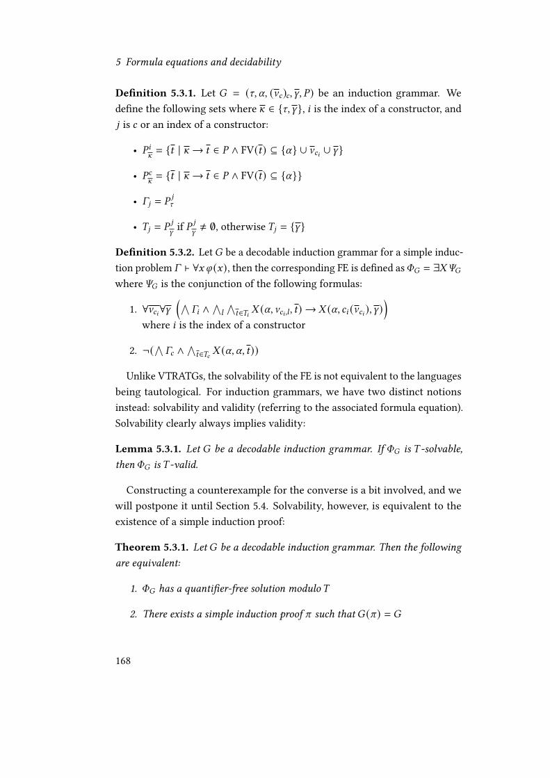
5 Formula equations and decidability
De�nition 5.3.1. Let � = (g, U, (a2)2, W, %) be an induction grammar. Wede�ne the following sets where ^ ∈ {g,W}, 8 is the index of a constructor, and9 is 2 or an index of a constructor:
• % 8^= {C | ^→ C ∈ % ∧ FV(C) ⊆ {U} ∪ a28 ∪ W}
• %2^= {C | ^→ C ∈ % ∧ FV(C) ⊆ {U}}
• �9 = % 9g
• )9 = % 9W if % 9W≠ ∅, otherwise )9 = {W}
De�nition 5.3.2. Let� be a decodable induction grammar for a simple induc-tion problem � ` ∀G i (G), then the corresponding FE is de�ned asQ� = ∃-R�whereR� is the conjunction of the following formulas:
1. ∀a28∀W(∧
�8 ∧∧;
∧C∈)8 - (U, a28 ,; , C) → - (U, 28 (a28 ), W)
)where 8 is the index of a constructor
2. ¬(∧ �2 ∧∧C∈)2 - (U, U, C))
Unlike VTRATGs, the solvability of the FE is not equivalent to the languagesbeing tautological. For induction grammars, we have two distinct notionsinstead: solvability and validity (referring to the associated formula equation).Solvability clearly always implies validity:
Lemma 5.3.1. Let � be a decodable induction grammar. If Q� is ) -solvable,thenQ� is ) -valid.
Constructing a counterexample for the converse is a bit involved, and wewill postpone it until Section 5.4. Solvability, however, is equivalent to theexistence of a simple induction proof:
Theorem 5.3.1. Let � be a decodable induction grammar. Then the followingare equivalent:
1. Q� has a quanti�er-free solution modulo )
2. There exists a simple induction proof c such that � (c) = �
168

5.3 Solvability of induction grammars
Proof. The formulas in De�nition 5.3.2 are equivalent to the initial sequents inthe simple induction proof in De�nition 2.8.4. Hence whenever the FEQ� hasa quanti�er-free solution modulo the background theory ) , we can constructa simple induction proof c with the solution as induction formula such that� (c) = � . Vice versa, if we have a simple induction proof c then its inductionformula is a solution forQ� . �
Example 5.3.1. The induction grammar � in Example 2.8.5 induces the follow-ing FE:
∃-(- (U, 0, W) ∧ (- (U, U, 0) → 3 (U) = U + U) ∧
∀a∀W(- (U, a,W) ∧ - (U, a, a) ∧ - (U, a, 0) ∧ B (W) + B (a) = B (B (W) + a) ∧
W + B (a) = B (W + a) ∧ B (a) + B (a) = B (B (a) + a) → - (U, B (a), W)) )
This FE has the solution i (U, a,W) := (B (W) + a = B (W + a) ∧ 3 (a) = a + a).
Let us now show that the language is tautological i� the formula equation isvalid. In the following Section 5.4, we will then discuss that validity in generaldoes not imply solvability for the formula equations induced by inductiongrammars. The following technical condition just ensures that � (�, C) has aproduction for every nonempty nonterminal vector:
De�nition 5.3.3. An induction grammar � is called suitable i� %2W≠ ∅ or
W = ().
Unlike VTRATGs, we cannot give a uniform solution to the formula equa-tions induced by induction grammars. (Since the problem of �nding a solutionis undecidable, as we will see in Theorem 5.4.2.) However the analogous de�-nition is still useful, as we can use it characterize the validity of the formulaequation.
De�nition 5.3.4. Let � be a decodable induction grammar. Then for everyfree constructor term C , we de�ne the canonical solution�C (U,W) recursively asfollows:
�28 (B) (U,W) =∧
�8 [a8\B] ∧∧;
∧C∈)8
�B; (U, C)
169

5 Formula equations and decidability
Theorem 5.3.2. Let � be a suitable decodable induction grammar. Then thefollowing are equivalent:
1. � is ) -tautological.
2. !(�, C) is ) -tautological for all free constructor terms C .
3. Q� (�,C) is ) -solvable for all free constructor terms C .
4.∧B∈%2
W�C (C, B) → i (C) is ) -tautological for all free constructor terms C .
5. ) |= Q� in full semantics.
Proof. 1 ⇔ 2 by De�nition 2.8.9; and 2 ⇔ 3 by Theorem 5.2.1. For 5 ⇒ 3note that |= Q� →Q� (�,C) even in Henkin semantics. For 2⇔ 4 note that theformula
∧B∈%2
W�C (C, B) → i (C) is equivalent to
∧!(�, C). It remains to show
3⇒ 5. So assume ) |= Q� (�,C) for all free construct terms C and letM be a fullhigher-order model of ) . In a full higher-order model, we can clearly evaluatein�nite conjunctions and disjunctions, and de�ne predicates that contain thesein�nite connectives. A direct way to de�ne the witness for the existentialquanti�er inQ� is by case distinction over all free constructor terms C : we set- = _U_a_W
∧C (a = C →�C (U,W)). (This de�nition does not require or imply
that the constructors are injective.) Every formula listed in De�nition 5.3.2 issatis�ed: 1. due to the de�nition of canonical solution, and 2. since !(�, C) is) -tautological for all C . �
Remark 5.3.1. Theorem 5.3.2 constructs the set - in the model using a least�xed-point construction.
5.4 Decidability and existence of solutions
On a practical level, we want to algorithmically solve the formula equationsinduced by VTRATGs and induction grammars. For VTRATGs, we have seenin Theorem 5.2.1 that this is possible (as long as the language is tautological),and we can even give a nice (albeit exponentially large) canonical solution.For induction grammars, the situation is more complicated:
170

5.4 Decidability and existence of solutions
1. The formula equation may not have a solution, even if the language istautological:
Theorem 5.4.1 ([31]). There exists a suitable decodable induction gram-mar� with |W | = 1 such thatQ� is valid butQ� does not have a quanti�er-free solution modulo ∅.
2. It is undecidable whether the formula equation induced by a giveninduction grammar is solvable:
Theorem 5.4.2 ([33]). There exists a computable sequence of suitabledecodable induction grammars (�=)=≥0 with |W | = 1 such thatQ�= is validfor all =, but the set {= | Q�= has a quanti�er-free solution modulo ∅} isundecidable.
In short, there is no algorithm to solve formula equations, even if we assumeas a precondition that the FE is valid. The proofs of Theorems 5.4.1 and 5.4.2are both based on a similar construction: the following induction grammar �for the sequent ∀G (% (G) → % (B (G))) ` ∀G (% (0) → % (G)):
g → A1(W)W → B (W) | 0
A more straightforward induction grammar would use the single productiong → A1(a). The trick of replacing a by W prevents the straightforward solution% (0) → % (a) to the formula equation. The proofs of Theorems 5.4.1 and 5.4.2then analyse a potential solution and deduce that such a solution needs tocontain arbitrarily large numerals B# (. . . ), a contradiction. This approachcrucially depends on the fact that the solution is quanti�er-free modulo anempty theory.
It turns out to be practically hard to algorithmically (or even manually)�nd solutions to formula equations such as the ones induced by inductiongrammars. We could hope that this problem becomes easier by restricting theinduction grammars, for example only considering induction grammars with|W | = 0—precluding the grammar used by Theorems 5.4.1 and 5.4.2. Another
171

5 Formula equations and decidability
option is to consider more solutions, for example quanti�ed solutions: for someapplications it is not absolutely important that we �nd a simple induction proofwith the speci�ed induction grammar (a quanti�ed solution to the FE wouldin general result in a proof that is not a simple induction proof).
In the rest of this section we will hence work towards a generalizationof Theorems 5.4.1 and 5.4.2, showing that solving the formula equations in-duced by induction grammars is hard even if we restrict the class of inductiongrammars and relax the notion of solution. Concretely, we generalize the un-solvability result of Theorem 5.4.1 in both of these directions: we will constructan induction grammar with |W | = 0 such that the induced formula equation isvalid modulo the empty theory, but is not ) -solvable for a �xed theory ) . It isunfortunately not yet clear how to extend the approach of this section to anundecidability result like Theorem 5.4.2.
Theorem 5.4.3. Let ) be a computably enumerable consistent extension of PA.Then there exists an induction grammar � = (g, U, (a2)2, W, %) with W = () suchthatQ� is ∅-valid butQ� is not ) -solvable.
The rest of this section is devoted to a proof of Theorem 5.4.3. We will workin an arithmetical theory with function symbols such as 3 (which in our casedoubles the input). In the sequent � ` ∀G i (G) that we will construct, theantecedent � will only consist of formulas that are provable in IOpen ⊆ PA (aweak fragment of Peano arithmetic where induction is restricted to quanti�er-free formulas). We will choose the formula ∀G i (G) such that it expresses theconsistency of a �xed computable enumerable theory ) . On a very abstractedlevel, the general plan could be described as follows: we consider the sequentPA ` Con() ), and use Gödel’s second incompleteness theorem to show thatthere can be no simple induction proof with the constructed induction grammar(and hence no solution to the formula equation) if ) ⊇ PA.
Remark 5.4.1. Most of this argument also works if we replace PA by IOpen.In fact, the condition ) ⊇ IOpen would su�ce to show that there are noquanti�er-free ) -solutions to the constructed formula equation. The use ofPA is only necessary to show the stronger statement that there no quanti�edsolutions as well.
172

5.4 Decidability and existence of solutions
One requirement for this approach is that the constructed induction gram-mar is tautological. As a small example, consider the sequent ∀G 3 (B (G)) =B (B (3 (G))),∀G B (G) > 0 ` ∀G (G ≠ 0→ 3 (G) > 0) with the following inductiongrammar � :
g → A1(a) | A2(a)
Then Q� (�,=) is equivalent to the following formula, saying that the �rst= instances of the antecedent imply the conclusion. By Theorem 5.3.2, � istautological i� this formula is tautological for all =:∧0≤8<=
(3 (B8+1(0)) = B (B (3 (B8 (0)))) ∧ B8+1(0) > 0
)︸ ︷︷ ︸
�= (U)
→(B= (0) ≠ 0→3 (B= (0)) > 0)
This formula happens to be not tautological for = > 0, since the instancesfor B (G) > 0 are not enumerated “fast enough”—we would need the instancefor 2=, but we only get the instances until =. And this brings us to the maintechnical challenges of choosing the � in � ` Con() ): 1) we need to producethe instances “fast enough” so thatQ� (�,=) is tautological, and 2) each formulain � can only have a single universal quanti�er. (Syntactically we can of coursehave multiple quanti�ers, but the instances can only vary in one “direction”:namely a . Hence we might as well assume that there is a single universalquanti�er instantiated with a .) That is, we cannot directly use all instances ofa formula such as ∀G∀~ (G + ~ = ~ + G).
Particularly the restriction of a single universal quanti�er makes the choiceof � interesting. De�nition 5.4.1 de�nes part of the formula that we pick. Asusual, 0 is zero and B is the successor. The function 3 (G) = 2G doubles itsargument, and ℎ(G) = bG/2c halves its argument. The predicate 4 (G) is true i�G is even. The function 2 codes pairs, and c1, c2 project to the �rst and secondcomponent, resp. The coding of pairs is de�ned by interleaving the digits in abase 2 representation, i.e. c1((0= . . . 01)2) = (. . . 0301)2 and c2((0= . . . 01)2) =(. . . 0402)2. Note that as a binary function, 2 (G,~) is only de�ned for G < "
where " is a �xed bound since we only have a single universal quanti�er.We will use 2 to encode a wordF1 . . .F= as 2 (F1, 2 (F2, . . . , 2 (F=, 0))) (i.e., as alinked list with 2 as the “cons” operation).
173

5 Formula equations and decidability
De�nition 5.4.1. Let " > 0. The formula \" (G) is de�ned as:
0 ≠ B (0)∧ 3 (0) = 0 ∧ 3 (B (G)) = B (B (3 (G)))∧ ℎ(0) = 0 ∧ ℎ(B (0)) = 0 ∧ ℎ(B (B (G))) = B (ℎ(G))∧ 4 (0) ∧ ¬4 (B (0)) ∧ (4 (B (G)) ↔ ¬4 (G))∧ (4 (G) → c1(G) = 3 (c1(ℎ(ℎ(G)))))∧ (¬4 (G) → c1(G) = B (3 (c1(ℎ(ℎ(G))))))∧ c2(G) = c1(ℎ(G))∧ 2 (0, 0) = 0
∧∧28<"(4 (G) → 2 (B28 (0), G) = 3 (3 (2 (B8 (0), ℎ(G)))))
∧∧28<"(¬4 (G) → 2 (B28 (0), G) = 3 (B (3 (2 (8, ℎ(G))))))
∧∧
28+1<"2 (B28+1(0), G) = B (2 (B28 (0), G))
The instances∧8<= \" (8) in De�nition 5.4.1 su�ce to compute =, 3, ℎ, 4, c1,
and c2 for input values up to =:
Lemma 5.4.1. Let us make conversion of numbers to numerals explicit by writing= = B= (0), and extend this notation to truth values via ⊥ = ⊥ and > = > as well.Then for any",= > 0:∧
8<=
\" (8) ` 0 = 1 ↔ 0 = 1 for all 0, 1 < =∧8<=
\" (8) ` 3 (0) = 3 (0) for all 0 < =∧8<=
\" (8) ` ℎ(0) = ℎ(0) for all 0 < =∧8<=
\" (8) ` 4 (0) ↔ 4 (0) for all 0 < =∧8<=
\" (8) ` c1(0) = c1(0) for all 0 < =∧8<=
\" (8) ` c2(0) = c2(0) for all 0 < =
174

5.4 Decidability and existence of solutions∧8<=
\" (8) ` 2 (0, 1) = 2 (0, 1) for all 0 < " and 02 + 212 < =
We call the functions 3, ℎ, c1, c2 and the predicates =, 4 quickly representablesince they can be computed for all arguments less than =.
Proof. All of the claims are proven by recursion on 0 and 1; the argumentsalways strictly decrease in the recursive de�nition of the functions and pred-icates. For example for ℎ, we can prove ℎ(0) = 0 and ℎ(B (0)) = 0 since thisalready occurs literally in \" (0). And we can prove ℎ(0 + 2) = B (ℎ(0)) forany 0 < =; by the induction hypothesis we can already prove ℎ(0) = ℎ(0).
The case for = is interesting since it is the only binary predicate where wecan show quick representation. Clearly if 0 = 1, then we can prove 0 = 1 byre�exivity. Otherwise 4 (ℎ8 (0)) = 4 (ℎ8 (1)) for some suitably chosen 8 . �
Note that some combinations may not be quickly representable: for examplewe cannot prove ℎ(3 (0)) = 0 for 0 < 0 ≤ = since the intermediate result 3 (0)is too large.
We can now turn towards de�ning the formula that will express the consis-tency of the theory ) . We will formalize the assertion that a given program %
does not terminate. (Later on in the proof of Theorem 5.4.3, we will instantiate %by a program that searches for a proof of a contradiction from ) .) Concretely,the program % will be represented as an instance of Post-Correspondence,i.e., % = ((F1
1, . . . ,F1=), (F2
1, . . . ,F2=)). Recall that a solution is a non-empty �-
nite sequence (81, . . . , 8:) such thatF181. . .F1
8:= F2
81. . . ‘F2
8:. The predicate � (G)
is true i� G is a non-empty sequence of the form (81, . . . , 8:). The sequence isrepresented as a list using the 2 function. The function 5 1(2 (81, . . . 2 (8=, 0) . . . ))(and analogously 5 2) maps the input sequence to the resulting concatenationF181. . .F1
8:(also represented as a list).
De�nition 5.4.2. Let % = ((F11, . . . ,F
1=), (F2
1, . . . ,F2=)) be an instance of Post-
Correspondence. De�ne Fℎ8, 9 as the 9-th letter of Fℎ
8 for 1 ≤ 9 ≤ |Fℎ8 |, and
assume that letters are natural numbers such that 0 < Fℎ8, 9 < " for some " .
175

5 Formula equations and decidability
De�ne the following sequent:
∀G \" (G),
∀G∧
ℎ∈{1,2}
∧8≤=
(c1(G) = 8→ 5 ℎ (G) = 2 (Fℎ
8,1, . . . 2 (Fℎ
8,|Fℎ8|, 5
ℎ (c2(G))))),
∀G∧
ℎ∈{1,2}
∧8≤=
(c1(G) = 8→ c1(5 ℎ (G)) = Fℎ
8,1 ∧ · · · ∧
c1(c|Fℎ8 |−12 (5 ℎ (G))) = Fℎ
8,|Fℎ8| ∧ c
|Fℎ8 |2 (5 ℎ (G)) = 5 ℎ (c2(G))
),
¬� (0),∀G (� (G) ↔ (c2(G) = 0 ∨ � (c2(G))) ∧∨8≤=
c1(G) = 8)
`∀G (� (G) → 5 1(G) ≠ 5 2(G))
And de�ne the induction grammar Solve% :
g → A1(0) | · · · | A1(") | A1(a) | A2(a) | A3 | A4(a)
Lemma 5.4.2. Let % be an instance of Post-Correspondence. ThenQSolve% is∅-valid i� % has no solution.
Proof. We need to show that �= (U) → � (=) → 5 1(=) ≠ 5 2(=) is provable. In asimilar way as in Lemma 5.4.1, we can easily see that � is quickly representable.To see that 5 1(=) = 5 2(=) is quickly representable as well, we make a casedistinction. If the two sides of the equality are di�erent, then the stringsthey represent are di�erent at position 9 and we can prove c1(c 92 (5 1(=))) ≠c1(c 92 (5 1(=))) for this position 9 . (This is the reason we added the instancesup to " in the induction grammar: so that we can prove all inequalitiesbetween letters.) If 5 1(=) = 5 2(=) are equal, then we can unfold both sides toidentical terms of the form 2 (B ... (0), . . . 2 (B ... (0), 0)). HenceQ� (Solve% ,=) is ∅-validi� � (=) → 5 1(=) ≠ 5 2(=) is true in the standard model, and this is the case i�= does not code a solution to % . �
Proof of Theorem 5.4.3. There exists a program that terminates if and only if) is inconsistent—e.g. by searching for a proof of false. That such a programexists is provable in PA. Since Post-Correspondence is Turing-complete,there is an instance % of Post-Correspondence such that % is solvable i� )
176

5.5 Examples of di�cult formula equations
is inconsistent; and this is provable in PA as well. Set � = Solve% . Since ) isconsistent by assumption,Q� is ∅-valid by Lemma 5.4.2. IfQ� were) -solvable,then ) proves that % has no solution and hence ) ` Con() ), a contradictionto Gödel’s second incompleteness theorem. �
5.5 Examples of di�icult formula equations
Before we come to algorithms that solve formula equations, let us �rst lookat some concrete practical examples. Recall that our motivation for formulaequations was to, ultimately, �nd the matrix of the induction formula for asimple induction proof. We have already �gured out the quanti�er inferencesby �nding an induction grammar that covers some �nite family of instancelanguages. Solving the formula equation induced by this induction grammaris hence the only step missing to the construction of a proof with induction.
Many of these induced formula equations are surprisingly hard to solve inpractice. It appears to be even harder to show for a concrete formula equationthat it has no solutions (unless it is not valid). In this section we will showseveral such formula equations that are induced by induction grammars forreal-world problems from the TIP library ([21]) and a formalization of thefundamental theorem of arithmetic in GAPT (we will come back to these inSection 7.4). All formula equations have ) = ∅. For none of these formulaequations could we �nd a solution or conversely, show that there is no solution.
subpl
Here we consider a property of the predecessor function ? on natural numbers,namely that it commutes with the truncating subtraction (−). (The constant 2comes from Skolemization.)
∀G (G − 0 = G),∀G ∀~ (G − B (~) = ? (G) − ~),` ∀G (? (2) − G = ? (2 − G))
The MaxSAT algorithm produces the following induction grammar (covering
177

5 Formula equations and decidability
the languages of proofs generated by an automatic theorem prover):
g → A1(W) | A2(W, a) | A3W → ?2(W) | ? (2) | 2
It is easy to see that this induction grammar is tautological, and that theinduced formula equation is hence valid. Fix the parameter =. First observethat for 8 > 0, the instance grammar generates the instances ?8+1(2) −B=−8 (0) =?8+2(2) − B=−8−1(0). However this happens in a refreshingly di�erent way: �rstthe instance production corresponding to W → ?2(W) is applied b8/2c times,and then W → 2 or W → ? (2) depending on the parity of 8 . (A more naturaland human way would be to use a production W → ? (W). We would need touse that production 8 − 1 times, followed by W → ? (2).) Hence we can derive? (2) − B= (0) = ?=+1(2) − 0 from the instance language.
In a similar way, the instances ?8 (2) − B=−8 (0) = ?8+1(2) − B=−8−1(0) aregenerated. This allows us to derive 2−B= (0) = ?= (2)−0. Since also ?= (2)−0 = 0is generated (again by a similar argument), we get ? (2) − B= (0) = ? (2 − B= (0))and the instance language is tautological.
However because of the unconventional way the instances are generated,there is no obvious choice for a solution to the induced formula equation:
∃-(∀W (W − 0 = W → - (U, 0, W)) ∧
∀a ∀W (- (U, a, ?2(W)) ∧ - (U, a, 2) ∧ - (U, a, ? (2)) ∧ W − 0 = W ∧W − B (a) = ? (W) − a→ - (U, B (a), W)) ∧
(- (U, U, 2) ∧ - (U, U, ? (2)) → ? (2) − U = ? (2 − U)))
subps
This formula equation is induced by an induction grammar for similar lemmaas subpl, also produced by the MaxSAT algorithm as a covering induction
178

5.5 Examples of di�cult formula equations
grammar for proofs produced by an ATP.
∀G (G − 0 = G),∀G ∀~ (G − B (~) = ? (G) − ~),∀G (? (B (G)) = G),` ∀G (? (B (2) − G) = 2 − G)
It is easy to see that every solution for the FE in subpl also solves thefollowing FE, and it is just as unclear whether the FE has a solution or not:
∃-(∀W (W − 0 = W ∧ ? (B (2)) = 2→ - (U, 0, W)) ∧
∀a ∀W (- (U, a, ?2(W)) ∧ - (U, a, B (2)) ∧ - (U, a, ? (B (2))) ∧ W − 0 = W ∧? (B (2)) = 2 ∧ W − B (a) = ? (W) − a→ - (U, B (a), W)) ∧
(- (U, U, B (2)) ∧ - (U, U, ? (B (2))) ∧ ? (B (2)) = 2→? (B (2) − U) = 2 − U)
)prod/prop_13
This problem from the TIP library (hence the di�erent names for zero andsuccessor) states a property of the halving function ℎ(G) = b G2 c:
∀G (/ + G = G),∀G ∀~ (( (G) + ~ = ( (G + ~)),ℎ(/ ) = / ∧ ℎ(( (/ )) = /,∀G (ℎ(( (( (G))) = ( (ℎ(G))),` ∀G (ℎ(G + G) = G)
The MaxSAT algorithm produces the following tautological induction gram-mar:
g → A1(W) | A2(a,W) | A3 | A4((2(a + a))W → U | W | a
As a �rst guess, we might think that ℎ(a + a) = a could be a solution tothe induced formula equation. Alas, this does not work because we do not
179

5 Formula equations and decidability
have the instance a + ( (a) = ( (a + a). Another potential “solution” that comesto mind is a + W = (a (W) ∧ ℎ((2a (0)) = (a (0), this would work if not for thefact that is not a �rst-order formula. So it is still open whether the followingformula equation has a solution or not:
∃-(∀W (/ + W = W ∧ ℎ(/ ) = / → - (U, /,W)) ∧
∀a ∀W (- (U, a, U) ∧ - (U, a,W) ∧ - (U, a, a) ∧ / + W = W ∧ ℎ(/ ) = / ∧ℎ((2(a + a)) = ( (ℎ(a + a)) ∧ ( (a) + W = ( (a + W) →- (U, ( (a), W)) ∧(- (U, U, U) ∧ ℎ(/ ) = / → ℎ(U + U) = U)
)isaplanner/prop_03
Here we show that the number of occurrences of an element in a list increasesif we append something to the list. Lists are an inductive data type with theconstructors =8; and 2>=B; e.g. 2>=B (0, 2>=B (1, =8;)) is a two-element list. Thefunction 2 (=, ;) counts how often = occurs in the list ; ; concatenation of lists isdenoted by 0(;1, ;2), 4 (<,=) is a predicate expressing the equality of elements< and =. The constants = and ~B are obtained from Skolemization.
∀G ;4 (/, G),∀G ∀~ (;4 (( (G), ( (~)) ↔ ;4 (G,~)),∀F (2 (F,=8;) = / )∀F ∀G ∀; (¬4 (F, G) → 2 (F, 2>=B (G, ;)) = 2 (F, ;))∀F ∀G ∀; (4 (F, G) → 2 (F, 2>=B (G, ;)) = ( (2 (F, ;)))∀G (0(=8;, G) = G)∀G ∀~ ∀I (0(2>=B (G,~), I) = 2>=B (G, 0(~, I)))` ∀G (;4 (2 (=, G), 2 (=, 0(G,~B))))
The following formula equation is induced by an induction grammar found
180

5.6 Solution algorithm using forgetful inference
by the MaxSAT algorithm. It is unknown whether it has a solution or not:
∃-(∀W0 ∀W1 (;4 (/, 2 (=,~B)) ∧ 2 (=, =8;) = / ∧
(¬4 (=,W1) → 2 (=, 2>=B (W1, W0)) = 2 (=,W0)) ∧(4 (=,W1) → 2 (=, 2>=B (W1, W0)) = ( (2 (=,W0))) ∧0(=8;,~B) = ~B→ - (U, =8;, W0, W1)) ∧
∀a ∀a0 ∀W0 ∀W1 (- (U, a0, 0(a0, ~B), a) ∧ - (U, a0, a0, a) ∧;4 (/, 2 (=,~B)) ∧ 2 (=, =8;) = / ∧(¬4 (=,W1) → 2 (=, 2>=B (W1, W0)) = 2 (=,W0)) ∧(4 (=,W1) → 2 (=, 2>=B (W1, W0)) = ( (2 (=,W0))) ∧(;4 (( (2 (=, a0)), ( (2 (=, 0(a0, ~B)))) ↔;4 (2 (=, a0), 2 (=, 0(a0, ~B)))) ∧
0(=8;,~B) = ~B ∧ 0(2>=B (a, a0), ~B) = 2>=B (a, 0(a0, ~B)) →- (U, 2>=B (a, a0), W0, W1)) ∧
∀W0 ∀W1 (- (U, U,W0, W1) ∧ ;4 (/, 2 (=,~B)) ∧ 2 (=, =8;) = / ∧0(=8;,~B) = ~B→ ;4 (2 (=, U), 2 (=, 0(U,~B))))
)5.6 Solution algorithm using forgetful
inference
On a practical level, given a tautological grammar we want to algorithmicallygenerate a proof with that grammar. If we recall Theorems 5.2.1 and 5.3.1, thismeans that we need to �nd a solution to the associated formula equation forthe grammar. For VTRATGs, this problem is decidable as we can always use the(in general exponentially large) canonical solution as given by De�nition 5.2.2.For induction grammars, this problem is undecidable by Theorem 5.4.2. Animpractical algorithm to solve the formula equations induced by inductiongrammars would be to enumerate all formulas, and for every formula checkwhether it is a solution and return it if it is indeed a solution.
A practically more e�ective (however incomplete in the sense that it will not�nd a solution for every solvable formula equation) algorithm was introduced
181

5 Formula equations and decidability
in [31] and is based on an algorithm that improves the solutions for formulaequations induced by VTRATGs which was introduced in [51]. (See also [36]for a newer presentation that is closer to the formalism of this section.)
The central idea behind this improvement algorithm is forgetful inference:we regard the solution to the formula equation as a formula in conjunctivenormal form, and then apply inferences such as resolution to these clauses.It is called forgetful because whenever we do an inference we remove thepremises from the CNF.
De�nition 5.6.1 (simpli�cation of CNFs). We de�ne the binary relationsB?,BA ,B5 on the set of clauses (where a clause is a set of literals) as the smallestrelations containing the following:
C ∪ {� ∪ {; = A }, � [;]} B? C ∪ {� ∪ � [A ]}C ∪ {� ∪ {; = A }, � [A ]} B? C ∪ {� ∪ � [;]}C ∪ {� ∪ {;}, {¬;} ∪ �} BA C ∪ {� ∪ �}
C ∪ {�} B5 C
The relations B?,BA ,B5 are called simpli�cation by forgetful resolution, for-getful paramodulation, and forgetting, respectively. We de�ne the relationB = BA ∪ B? ∪ B5 as their union.
We also lift the simpli�cation relation B to solutions of formula equations,by rewriting a single formula at a time:
De�nition 5.6.2 (simpli�cation of solutions of formula equations). Let i =
(i1, . . . , i=) and k = (k1, . . . ,k=) be a sequences of formulas. Then i Bk i�there exists a 9 such that i 9 Bk 9 and i8 = k8 for all 8 ≠ 9 .
Example 5.6.1. Consider the sequent ∀G (% (G) → % (B (G))) ` % (0) → % (B4(0))and the following tautological VTRATG � :
�→ A1(�) | A1(B (�)) | A2�→ 0 | B2(0)
Then the canonical solution �� is given by:
(% (U) → % (B (U))) ∧ (% (B (U)) → % (B2(U))) ∧ ¬(% (0) → % (B4(U)))
182

5.6 Solution algorithm using forgetful inference
Via simpli�cation we get a much nicer solution:
�� B5 (% (U) → % (B (U))) ∧ (% (B (U)) → % (B2(U)))BA % (U) → % (B2(U))
Of course the relationB can also lead to formulas that are no longer solutionsof the formula equation. In the actual algorithm that simpli�es the solutionwe hence need to check that the formula is still a solution. The functionFindConseqences(Q,k ) in Algorithm 4 computes the B-simpli�ed solutionsfor a formula equationQ , skipping the branches where the simpli�ed formula isnot a solution. The way we use this function to compute a “nice” solution to theformula equations induced by a VTRATG � is as follows: we compute the B-consequences using FindConseqences(Q� ,�� ) and then return the smallestsolution we have found (e.g. counting the number of logical connectives).
Algorithm 4 Compute B-consequences for solution improvementfunction FindConseqences(Q : formula equation, i : solution forQ)
yield ifor eachk such that i Bk do
if k is a solution forQ and we did not processk before thenFindConseqences(Q ,k )
end ifend for
end function
The FindConseqences algorithm is practically e�ective; starting fromthe analytic content of the canonical solution, which essentially is just aconjunction of instances of the end-sequent, it generates short and interestingnon-analytic solutions. In an evaluation on the TPTP [36], we got meaningfulsolutions such as complement(complement(G)) = G (this solution was foundfor the formula equation induced by a small covering VTRATG for the SET190-6problem).
An obvious and practical optimization in Algorithm 4 is to perform thesimpli�cation steps B?,BA ,B5 in a particular order: we can always move the B5steps to the end, without decreasing the set of found consequences. Practically,
183

5 Formula equations and decidability
we �rst compute all (B? ∪BA )-consequences, and then forget clauses. Anotherstep-permutation concerns formula equations for VTRATGs with more thantwo non-terminals (and hence more than one predicate variable). Clearly,performing simpli�cation on the di�erent predicate variables is independent.However it may be the case that one permutation of the steps may producea sequence of formulas that is not a solution as an intermediate step. Let usconsider the case for two predicate variables as an example:
∃-1∃-2(∀V ∀W (�0→ -2(W) ∨ -1(W, V))∧ ∀W (�1 ∧ -1(W, C1) ∧ · · · ∧ -1(W, C<) → -2(W))∧ (�2 ∧ -2(B1) ∧ · · · ∧ -2(B=) → ⊥)
)Observe that -8 for 8 ∈ {1, 2} only occurs negatively in one conjunct, the
only other occurrences are positive and before that conjunct. For this reason,we can always permute the simpli�cation steps in such a way that we �rstperform all simpli�cations for -2 and then the ones for -1.
A possible extension is to include consequences modulo an equationalbackground theory ) . We add an additional simpli�cation step B4 such thatC ∪ {� [;f]} B4 C ∪ {� [Af]} for ; = A ∈ ) , and only search for consequenceswhere we use an equation ; = A ∈ ) at most once. That is, FindConseqencesaccepts the list of equations) as an additional argument and removes the usedequation in the recursive call.
The solution algorithm for formula equations induced by induction gram-mars is now based on the improvement algorithm described above. In a certainsense, we run FindConseqences on an instance of the formula equation fora particular free constructor term:
De�nition 5.6.3. Let � be an induction grammar and C a free constructorterm. Then de�ne the formula equation Q�,C as follows:
Q�,C = ∃- R�,C = ∃-(∀W (�C (U,W) → - (U, C, W)) ∧
(∧
�2 ∧∧B∈)2
- (U, U, B) → i (U)))
Let us collect some easy observations about this instantiated formula equa-tion Q�,C :
184

5.6 Solution algorithm using forgetful inference
Lemma 5.6.1. Let � be an induction grammar and C a free constructor term.Then:
1. `R� → R�,C
2. IfQ� has i as a solution, then Q�,C also has the solution i .
3. If i (U, a,W) is a solution for Q�,C , then so is i (U, C, W).
4. If � is tautological, then Q�,C has the solution �C (U,W).
So to sum up Lemma 5.6.1, the solutions of Q�,C andQ� di�er in two ways:Q�,C has more solutions, and the solutions of Q�,C do not distinguish between aand C . We will need to take both of these issues into account.
Algorithm 5 Heuristic solution for formula equations induced by inductiongrammars
function SolveIndFE(� : induction grammar, C : free constructor term)for each i yielded by FindConseqences(Q�,C , �C (U,W)) do
for every i′ such that i′[a\C] = i doif i′ is a solution ofQ� then
return i′
end ifend for
end forreturn none
end function
Algorithm 5 is obviously incomplete since it always terminates: there existinduction grammars whose induced formula equation is solvable, yet thealgorithm will not return a solution. Let us consider an easy example where itfails to �nd a solution:
Example 5.6.2. Consider the following sequent stating that a number is even if
185

5 Formula equations and decidability
and only it is not odd:
4 (0) ∧ ¬> (0),∀G (4 (B (G)) ↔ ¬4 (G)),∀G (> (B (G)) ↔ ¬> (G))` ∀G (4 (G) ↔ ¬> (G))
The following induction grammar for this sequent is tautological:
g → A1 | A2(a) | A3(a)
We can also solve the induced formula equation using the solution 4 (a) ↔¬> (a). However if try to solve it using Algorithm 5, then we �rst compute thefollowing canonical solution �C (U) for example for C = B (0), consisting of thefollowing clauses in CNF:
4 (0)¬> (0)
4 (B (0)) ∨ 4 (0)¬4 (B (0)) ∨ ¬4 (0)> (B (0)) ∨ > (0)
¬> (B (0)) ∨ ¬> (0)
Resolution of these clauses (no matter the choice of C ) can only produceclauses of the form±> (B= (0)),±4 (B= (0)),±> (B= (0))∨±> (B< (0)), or±4 (B= (0))∨±4 (B< (0)). There are no clauses that mix 4 and > as in the natural solution.An important observation is that any solution to the formula equation willbe true in the standard model (the natural numbers with 4 interpreted aseven, and > as odd). If we build a solution as a conjunction of these clauses,then every clause will be valid. For example, 4 (B (0)), 4 (a) ∨ 4 (B (B (a))) can-not be clauses in a solution. So assume that we have such a CNF � (a)where � (U) ∧ 4 (0) ∧ ¬> (0) → (4 (U) ↔ ¬> (U)) is provable. Without lossof generality � (a) contains no clause of the form ±4 (B< (a)) ∨ ±4 (B= (0)) or±> (B< (a)) ∨ ±> (B= (0)): if such a clause is true in the standard model, thenone of its literal is valid as well and we can replace the clause by the literal.
186

5.7 Solution algorithm using interpolation
Now every clause in � (a) has the property that either all literals containa , or else none contain a . We can now construct a counter-model " for� (U) ∧ 4 (0) ∧¬> (0) → (4 (U) ↔ ¬> (U)): we use the standard model, but inter-pret > di�erently. Interpret U as the smallest number larger than all numeralsoccurring in the formula. This has the e�ect that the subterms containing Uand the subterms not containing U are interpreted as disjoint subsets. Thepredicate 4 is interpreted as the even numbers, however the predicate > isinterpreted di�erently for large numbers: interpret > (=) as = is odd if = < U"
and as = is even if = ≥ U" .
5.7 Solution algorithm using interpolation
Formula equations are closely related to the concept of constrained Hornclauses studied in program veri�cation [12]. Similarly to how the formulaequations of this chapter capture the conditions for formulas to be cut formulasand induction formulas, sets of constrained Horn clauses capture the necessaryconditions for formulas to be program invariants (such as loop invariants orpre-/postconditions). Solving a set of constrained Horn clauses hence amountsto �nding the correct invariants, and thus proving a given correctness propertyof the program.
A constrained Horn clause is a formula of the form� (G1, . . . , G=, ~)∧-1(G1)∧· · · ∧ -= (G=) → . (~) or � (G1, . . . , G=) ∧ -1(G1) ∧ · · · ∧ -= (G=) → ⊥ where-1, . . . , -=, . are predicate variables and the constraint� is a formula that doesnot contain any predicate variables. The term “Horn” refers to the structureof the predicate variables, the formula � can be arbitrarily complex and alsocontain additional negations, etc. Just as with formula equations, a solutionis a substitution for the predicate variables that validates all clauses. Given aset of constrained Horn clauses C, we will regard it as the formula equation∃- ∧
�∈C ∀G∨� . We will also call formula equations of this form constrained
Horn clause problems.There is a considerable amount research on the automatic solution of con-
strained Horn clause problems, using a plethora of techniques ranging frompredicate abstraction [44, 57], randomized enumeration [38], machine learn-
187

5 Formula equations and decidability
ing [103], abstract interpretation [56], to even tree automata [62]. Most ofthese approaches rely on SMT solvers in their implementations.
The typical setting for these solvers is to consider constrained Horn clausesin an expressive background theory that is well supported by SMT solvers (suchas e.g. Presburger arithmetic), and to disallow uninterpreted function symbols.A typical constrained Horn clause might be ~ < G ∧- (G,~) →- (G + 1, G + ~)where G and ~ range over the integers. For this setting, there is a large numberof state-of-the-art provers that can solve even large industrial problems, cf. theresults of the yearly CHC competition [20].
When solving the formula equations induced by induction grammars orVTRATGs, we typically work with a weaker background theory (usually justequality) but with uninterpreted function symbols. In this section we willuse an approach for constrained Horn clauses to solve formula equations asinduced by VTRATGs and induction grammars. The Duality solver [69] usesinterpolation at its core to �nd the solutions.
From a practical point of view, the Duality implementation in Z3 was unfor-tunately removed in version 4.8.01 as the underlying interpolation code wasunmaintained. Even before the removal, the solver often failed for our formulaequations due to unsupported inferences in the proofs generated by Z3. Sincewe use the solver in a very di�erent setting compared to what it was intendedto solve (many uninterpreted function symbols modulo equality as opposedto none modulo Presburger arithmetic), it is not unexpected to encounteredge cases in the implementation. Hence we opted for a reimplementation ofthe algorithm in GAPT, specialized to the class of formula equations that weconsider.
Each constrained Horn clause problem induces a directed graph with theoccurrences of the predicate variables (including ⊥ if there is no predicatevariable on the right side) as vertices. There is an edge from an occurrence- 1(C) to . 2(B) (using superscripts to disambiguate occurrences) i� either:
a) Both occurrences are in the same clause such that - 1(C) is on the left and. 2(B) on the right side, or
b) - = . , - 1(C) occurs on the right side, and . 2(B) occurs on the left side.1https://github.com/Z3Prover/z3/pull/1646
188

5.7 Solution algorithm using interpolation
Constrained Horn clause problems are called recursive if the graph is cyclic,daglike if the graph is acyclic, and treelike if the graph is a tree. Treelikeproblems can be easily solved using interpolation, daglike problems will re-quire a potentially exponential unrolling step; the real di�culty lies in therecursive case. (Cf. the di�culty in solving formula equations for VTRATGsand induction grammars, resp.)
Example 5.7.1. The following constrained Horn clause problem is treelike sinceits graph - (G) → - (0) → ⊥ is a tree (even a path in this case):
∃-(∀G (% (G) → - (G)) ∧ (- (0) ∧ ¬% (0) → ⊥)
)Example 5.7.2. The following constrained Horn clause problem is daglike butnot treelike:
∃-(∀G (% (G) → - (G)) ∧ (- (0) ∧ - (1) ∧ ¬(% (0) ∧ % (1)) → ⊥)
)It has the following graph, which is acyclic:
- (G)
- (0) - (1)
⊥
Example 5.7.3. The formula equations induced by induction grammars areconstrained Horn clause problems (after applying some propositional equiva-lences to bring them into the correct syntactic form—mainly adding the ⊥).For example consider the following (not particularly meaningful but small)one:
∃-((% (0) → - (0)) ∧ ∀a (% (0) ∧ - (a) → - (B (a))) ∧ (- (U) ∧ ¬% (0) → ⊥)
)It has the following graph, which contains a cycle at - (a):
189

5 Formula equations and decidability
- (0)
- (a) - (B (a))
- (U)
⊥
Conceptually, on a very abstracted level, Duality solves formula equationsusing two unrolling operations. The �rst unrolling turns a recursive formulaequation into a daglike one, the second unrolling step turns a daglike oneinto a treelike one. There is a straightforward way to solve treelike formulaequations using interpolation. The solutions to the unrolled treelike formulaequations can then always be turned into a solution for the daglike formulaequation. Only the last step is hard, where we need to convert a solution to theunrolled daglike formula equation to a solution to the original recursive one.
Solving treelike formula equations. Given a treelike formula equationwe can always bring it in a form where all occurrences of a predicate variablesare applied to the same variables. This is accomplished by adding additionalequalities:
∃-1∃-2(∀G ((% (G) → % (B (G))) → -1(G)) ∧
∀G ((% (G) → % (B (G))) → -2(G)) ∧
(-1(0) ∧ -2(B (0)) ∧ % (0) → % (B2(0))))
For the occurrence -1(0), we abstract the term 0 into the variable G1 and
190

5.7 Solution algorithm using interpolation
then replace -1(0) by - (G1) and add the equality G1 = 0:
∃-1∃-2(∀G1 ((% (G1) → % (B (G1))) → -1(G1)) ∧
∀G2 ((% (G2) → % (B (G2))) → -2(G2)) ∧
∀G1 ∀G2 (-1(G1) ∧ G1 = 0 ∧ -2(G2) ∧ G2 = B (0) ∧ % (0) → % (B2(0))))
Such a formula equation directly corresponds to a tree. This tree containsone node for every clause in the formula equation, which is labelled with thequanti�er-free part of the clause. The conjunction of the formulas in this treeis then unsatis�able if and only if the formula equation was valid.
G1 = 0 ∧ G2 = B (0) ∧ ¬(% (0) → % (B2(0)))
% (G1) → % (B (G1)) % (G2) → % (B (G2))-1 -2
By Craig interpolation [24], if we have a proof of �, N ` J, L then we cancompute a formula � and proofs of � ` J, � and � , N ` L in polynomial timewhere � only contains function and predicate symbols that occur in both � ∪Jand N ∪ L. For quanti�er-free formulas with equality as a background theory,this interpolant is quanti�er-free as well [68].
In order to compute the solution for the predicate variable -1 we dividethe tree into two parts: the part below the -1 node, and the rest. The onlycommon symbols are the variables of the predicate variable (i.e., G1), and hencethe solution is directly given by the interpolant. The collection of all of theseinterpolants—one for every subtree—is also known as a tree interpolant (a termintroduced by the Duality paper [69]).
Solving daglike formula equations. We can now extend the approachto the daglike case by unrolling the formula equation into a treelike one by
191

5 Formula equations and decidability
duplicating clauses as needed.
∃-(∀G ((% (G) → % (B (G))) → - (G)) ∧
(- (0) ∧ - (B (0)) ∧ % (0) → % (B2(0))))
The predicate variable has two occurrences on the left side of the last clause,- (0) and - (B (0)). Hence we need to make two copies of it:
∃-1∃-2(∀G ((% (G) → % (B (G))) → -1(G)) ∧
∀G ((% (G) → % (B (G))) → -2(G)) ∧
(-1(0) ∧ -2(B (0)) ∧ % (0) → % (B2(0))))
The important part about this unrolling is that we can easily translatesolutions of the unrolled problem to solutions of the original daglike problem:if we have a solution i1, i2 for -1, -2, resp., then we get a solution for theoriginal- by taking the conjunction of the solution for the duplicated predicatevariables. That is, i1 ∧ i2 is a solution for the daglike formula equation.
Solving recursive formula equations. Finally, recursive formula equa-tions are handled by unrolling them into non-recursive ones. As before, this isachieved by duplicating predicate variables and clauses. In the Duality solver,this is actually handled in an incremental way so that new clauses are gener-ated on demand and the decision which clauses to generate is driven by thecounter-model computed by the SMT solver. This is important to scale to largeproblems with many predicate variables. For the formula equations inducedby induction grammars however there is little to decide, since we only have asingle predicate variable and a very small number of clauses.
∃-((% (0) → - (0))∧
∀G ((% (G) → % (B (G))) ∧ - (G) → - (B (G))) ∧
(- (2) → % (2)))
192

5.7 Solution algorithm using interpolation
Here we duplicate the predicate variable - into the variables -1, . . . -=:
∃-((% (0) → -1(0)) ∧
∀G ((% (G) → % (B (G))) ∧ -1(G) → -2(B (G))) ∧...
∀G ((% (G) → % (B (G))) ∧ -=−1(G) → -= (B (G))) ∧
(-1(2) → % (2)) ∧ · · · ∧ (-= (2) → % (2)))
The solution for the unrolled formula equation is then translated back tothe original formula equation by combining it in a disjunction. In the example,a possible solution would be % (0) ∧ G = 0, % (G), . . . , % (G). We would then geta candidate solution (% (0) ∧ G = 0) ∨ % (G) for the original formula equation.In this case, it actually solves the formula equation. But this is of course nottrue in general.
Constrained Horn clauses for VTRATGs. The attentive reader will havenoticed that while the formula equations induced by induction grammars aredirectly constrained Horn clause problems, the formula equations induced byVTRATGs are not of this form, in general. If there are more than two nonter-minal vectors, then the induced formula equation will not be a constrainedHorn clause problem (because there will be more than one predicate variableon the right side of a clause). However we can de�ne a di�erent version of theformula equationQ� which is Horn:
De�nition 5.7.1. Let � = (#, O,�, %) be a decodable VTRATG with # =
{� ≺ �1 ≺ . . . �=}. We de�ne the formula equationQ′�= ∃- R′
�, whereR′
�is
the conjunction of the following formulas:
• ∀U1 . . .∀U=( ∧
�0→∨J0 ∨ -1(U=, . . . , U1)
)• ∀U8+1 . . .∀U=
( ∧�8∧
∧C∈%
�8
-8 (U=, . . . , U8+1, C)→∨J8∨-8+1(U=, . . . , U8+1)
)for 1 ≤ 8 ≤ =
where %�,)8 , and �8 are as in De�nition 5.2.1.
193

5 Formula equations and decidability
This de�nition di�ers from De�nition 5.2.1 only in that there is just a singlepredicate variable on the right-hand side of the implication.
Lemma 5.7.1. Let � be a decodable VTRATG. ThenR′�→R� is provable, and
every ) -solution ofQ′�is a ) -solution ofQ� as well.
Proof. Observe thatR′�
is obtained fromR� by replacing positive subformulasby > and propositional equivalences. �
Lemma 5.7.2. Let � be a decodable VTRATG such that there is a production ofevery nonterminal vector. If !(�) is ) -tautological, then �� is a ) -solution forQ′�.
Proof. Analogously to the proof of Lemma 5.2.1. �
Theorem 5.7.1. Let� be a decodable VTRATG such that there is a production ofevery nonterminal vector. ThenQ� is ) -solvable if and only ifQ′
�is ) -solvable.
Proof. IfQ� is solvable, then� is tautological by Theorem 5.2.1 and the canon-ical solution solvesQ′
�by Lemma 5.7.2. On the other hand, ifQ′
�is solvable,
then the same solution works forQ� by Lemma 5.7.1. �
The formula equationQ′�
is then a daglike constrained Horn clause problemthat can be solved using the interpolation-based approach.
194

6 Algorithm for proof import
Cut-free proofs have a variety of applications. In the preceding chapters, wehave seen one of them: given a cut-free proof in the form of a Herbrand sequent,we can algorithmically introduce structure in the form of cuts or inductioninferences. Starting from proofs obtained from automated theorem provers,we can introduce these inferences to structure these automatically generatedproofs. In this chapter we will investigate a practical way to get expansionproofs from theorem provers. These expansion trees were introduced in [71] togeneralize Herbrand’s theorem to higher-order logic in the form of elementarytype theory (simple type theory without choice or extensionality). In �rst-orderlogic, they provide a technically convenient formalism to store the tautologicalinstances of non-prenex formulas.
There is a generic way to solve the problem of importing proofs by automatedtheorem provers: since every inference generated by the theorem prover isvalid in �rst-order logic we could translate the proof into the calculus LK(with say, one cut per inference). We could then apply a general-purposecut-elimination algorithm to this proof and extract an expansion proof fromthe resulting cut-free proof.
However for our applications we are only interested in the quanti�er in-stance terms as contained in an Herbrand disjunction, or expansion tree. Giventhat we are only interested in this speci�c aspect of the proofs, we can hopeto devise more e�cient proof import procedures that do not produce a fullproof including propositional reasoning, but only the expansion proof. In thischapter we will present such an algorithm and evaluate its implementation inGAPT.
Some of the most e�ective theorem provers in classical �rst-order logic arebased on the resolution and superposition calculi; therefore we aim to importproofs generated by these provers. Algorithms to translate automatically
195

6 Algorithm for proof import
generated resolution proofs to expansion proofs have already been proposedin the context of the TPS [78] and GAPT [52] systems.
The approach in [52] transforms a resolution refutation �rst into a sequentcalculus proof with atomic cuts, and then extracts an expansion proof in asecond step; Skolemization is not handled in the algorithm and is insteadtreated as a preprocessing step of the formula.
More closely related to the approach in this chapter is the algorithm in [78]:it directly transforms a resolution refutation into an expansion proof. Skolem-ization is handled explicitly during the translation, and Skolem terms areautomatically converted to variables. However this treatment has two un-fortunate consequences: �rst, only outer Skolemization can be used in thisway—and this con�icts with the goal to reduce the number of Skolem functionsand the number of the arguments, which is necessary for e�cient proof search.Additionally, the deskolemization is incompatible with built-in equationalinferences which implicitly make use of congruences for Skolem functions.
Both of the approaches require a naive distributivity-based transformationof the input formula into clause normal form (CNF), which can increase thesize of the problem exponentially. Moreover, neither approach can handlesplitting inferences as used by SPASS [100] or Vampire [99].
The solution we present in this chapter includes clausi�cation and splittingsteps as inferences of the resolution proof in a similar way as higher-orderresolution calculi [4], conveniently keeping track of introduced subformulade�nitions for structural clausi�cation and Skolem functions in the same datastructure as the resolution refutation.
The algorithm as shown in Algorithm 6 proceeds in three main steps: �rstwe extract an expansion proof of an extended sequent, possible containingcuts. If the resolution proof did not contain subformula de�nitions or Avatarsplitting, then this is already the �nal expansion proof. To eliminate thecuts corresponding to Avatar splitting, the next step is a cut-elimination onexpansion proof. The subformula de�nitions are then removed in the third and�nal step. Skolemization remains in the output proof (and could be eliminatedafterwards as well, if desired).
In Sections 6.1 and 6.2 we describe the resolution and expansion proofcalculi used, respectively. Basic operations on expansion proofs, merge- and
196

6.1 Resolution proofs
Algorithm 6 Transforming expansion proofs to resolution proofsfunction Transform(c)�1 ← Extract(c) (see Section 6.3)�2 ← EliminateCuts(�1) (see Lemma 6.2.2)�3 ← EliminateDefinitions(�2) (see Lemmas 6.4.1 and 6.4.2)return �3
cut-reduction, are introduced in Section 6.2 as well. Section 6.3 then explainsthe extraction of expansion proofs from resolution proofs. The subformulade�nitions are eliminated in Section 6.4. In Section 6.6 we then evaluate theperformance and clausi�cation quality of an implementation of this algorithm.At the end in Section 6.7, we revisit the splitting inferences and show how toeliminate them directly from resolution proofs.
6.1 Resolution proofs
As a calculus for resolution proofs we consider a �rst-order variant of Andrew’ssystem R [4], extended with inferences to support subformula de�nitions andAvatar splitting. This system R is a system for reasoning in higher-orderlogic, we use it in �rst-order logic for practical reasons: inference rules forclausi�cation are included as part of the calculus. If we were to consider a�rst-order calculus where every inference step ended in a clause, then wewould need to keep track of an additional data structure that describes howthe clauses are derived from the input formula given to the prover. With thecalculus considered in this section, this information is part of the proof.
The inferences in this calculus as shown in Figure 6.1 operate on sequents,which are pairs of multisets of formulas. Let i be the closed formula that is tobe proven, a resolution proof then starts with the sequent i ` (using the Inputinference) and ends with the empty sequent `.
Resolution proofs of �rst-order formulas can typically be roughly dividedinto an upper part starting with i ` that performs clausi�cation inferences ap-plied during preprocessing, and a lower part that ends with ` and correspondsto the relevant steps taken during the actual proof search with resolution,
197

6 Algorithm for proof import
Clausification inferences:
Inputi ` >, � ` J TopL
� ` J� ` J,⊥ BotR� ` J
¬i, � ` J NegL� ` J,i
� ` J,¬i NegRi, � ` J
i ∧k, � ` JAndL
i,k, � ` J� ` J,i ∧k
AndR1� ` J,i
� ` J,i ∧kAndR2
� ` J,k� ` J,i ∨k
OrR� ` J,i,k
i ∨k, � ` JOrL1
i, � ` Ji ∨k, � ` J
OrL2k, � ` J
� ` J,i→k ImpRi, � ` J,k
i→k, � ` J ImpL1� ` J,i
i→k, � ` J ImpL2k, � ` J
� ` J,∀G iAllR
� ` J,i∀G i, � ` J
AllL (where C sk↦→ ∀G i)i [G\C], � ` J∃G i, � ` J
ExLi, � ` J
� ` J, ∃G iExR (where C sk↦→ ∃G i)� ` J,i [G\C]
Subformula definition inferences:
i, � ` JAbbrL
� (C), � ` J� ` J,i
AbbrR� ` J, � (C)
(where � (C) def↦→ i)
DefLi ` � (C) DefR
� (C) ` i (where � (C) def↦→ i)
Logical inferences:
� ` J,� �, N ` L Res�, N ` J, L
� ` J,�,� Factor� ` J,�
�,�, � ` J Factor�, � ` J
Taut� ` � � ` J Subst
�f ` JfRe�` C = C
� ` J, C = B �[C], N ` LRw
�[B], � , N ` J, L� ` J, C = B �[B], N ` L
Rw�[C], � , N ` J, L
� ` J, C = B N ` L,�[C]Rw
�, N ` J, L,�[B]� ` J, C = B N ` L,�[B]
Rw�, N ` J, L,�[C]
Avatar spli�ing inference:
S1 ++ S2 AvSplitS1 :+ �AvIntro
� +: S2
(where � def↦→ ∀G S2 and FV(S1) ∩ FV(S2) = ∅)
Figure 6.1: Calculus for resolution proofs.198

6.1 Resolution proofs
rewriting, factoring, and other inferences. There is no implicit uni�cation inthe inferences, substitution is handled explicitly using an extra inference.
Both Skolemization and subformula de�nition inferences make use of globaldictionaries that store the interpretation of the de�ned atoms and Skolemfunctions, respectively. De�ned atoms and Skolem functions are fresh symbolsthat do not occur in the problem. For de�nitions, the entry � (G) def↦→ k meansthat the atom � (G) is de�ned to bek , that is, ∀G (� (G) ↔ k ) is assumed. ForSkolem functions, the entry B (G) sk↦→ ∀~ i [~] means that B (G) is the Skolemterm used to instantiate ∀~ i [~], that is, ∀G (i [B (G)] → ∀~ i [~]) is assumed.We use both relations also for substitution instances of the de�nitions, i.e.we write � (C) def↦→ k [G\C] as well as B (C) sk↦→ (∀~ i [~]) [G\C]. Furthermore, werequire these de�nitions to be acyclic.
The AvSplit and AvIntro inferences here are the minimal version necessary torepresent Avatar splitting [99] in the resulting proofs. This calculus augmentsthe clauses derived in the theorem prover with a �nite set of so-called assertions.Splitting in general is based on the observation that if the literals of a clausecan be partitioned into two parts with disjoint variables, then the clause isequivalent to a disjunction of two clauses. For example:
∀G ∀~ (% (G) ∨& (~)) ↔ (∀G % (G)) ∨ (∀~ & (~))
A minimal nonempty subset of the literals whose variables are disjoint fromthe rest of the clause is called a component. It is typically bene�cial to keepthe number of literals in a clause small. So if we derive such a splittable clause,then we could consider two cases: �rst ∀G % (G), and then ∀~ & (~). In this way,we would subdivide the proof search like a tree if we had multiple clauses tosplit. (This is essentially the approach taken by the SPASS prover [101].) TheAvatar approach in contrast lets a SAT solver determine which of these casesto consider at any moment. The assertions that are added to the clauses henceindicate to which case they belong. Let us consider what happens when theA-clause % (G) ∨& (~) ← �1,�2 (which already has two assertions) is split1:
% (G) ∨& (~) ← �1,�2% (G) ← �3 & (~) ← �4 ¬[�1] ∨ ¬[�2] ∨ [�3] ∨ [�4]
1The precise details may be subtly di�erent in di�erent implementations.
199

6 Algorithm for proof import
Two new assertions are introduced: �3 and �4. The prover derives two �rst-order clauses that it keeps in the saturation loop. The �rst one is % (G) ← �3.We can read this as: if�3, then∀G% (G). It is useful to think of the assertion�3 asan abbreviation for ∀G % (G). The third derived clause is not used for saturationbut is passed to the SAT solver. The syntax [�1] refers to the propositionalatom associated with the component �1. The clause for the SAT solver isequivalent to the original clause if we replace�3 by ∀G % (G) and�4 by ∀~& (~).
The distinction between the clause and its assertions is only relevant forproof search. Inferences (such as resolution or superposition) are only per-formed on the clause, but not on the assertions. However for proof transfor-mations, such as the one in this chapter, this distinction is irrelevant: herewe represent A-clauses by combining the assertion and the clause part into asingle clause [�1], . . . , [�:], 01, . . . , 0< ` 11, . . . 1= .
We de�ne prepending an element to the antecedent as i +: (� ` J) =(� ∪ {i} ` J), appending an element to the succedent as (� ` J) :+ i = (� `J∪{i}), and concatenating sequents as (� ` J)++(N ` L) = (�∪N ) ` (J∪L).
During proof search, splitting takes a clause S1 ++S2 that can be partitionedinto two (or more) clauses S1 and S2 with pairwise disjoint free variables,and splits it into three clauses: �1 +: S1 and �2 +: S2 plus an additional clause` �1, �2. (This third clause is ground. During proof search it is directly passedto the SAT solver, and is not considered by the �rst-order reasoning part ofthe prover.) In our calculus we represent this step as follows:
S1 ++ S2 AvSplitS1 :+ �2 AvSplit` �1, �2
AvIntro�8 +: S8
Other splitting schemes such as the one implemented in SPASS [100] can besimulated using these inferences as well. The splitting dependencies a clauseimplicitly depends on are simply translated to explicit splitting atoms. Foreach split we then take the resulting proofs of the two branches and resolveon the opposing splitting atoms.
We assume a few minor technical restrictions on resolution proofs: there areno AbbrL inferences below Rw, Re�, and Taut, and DefR with the same de�nedatom. These are not particularly large restrictions, as they simply re�ect the
200

6.2 Expansion proofs
fact that clausi�cation typically happens as a preprocessing step before proofsearch. It is also important to note that we only allow subformula de�nitionsin a single polarity here—if we want to abbreviate a formula i that occurs onboth sequent sides, then we need to introduce a di�erent �8 atom for each side.This is a larger restriction since it precludes certain kinds of preprocessing: forexample such de�nitions would occur if we wanted to abbreviate a subformulaof the input formula that occurs multiple times (and in both polarities) by thesame atom.Example 6.1.1. The following is natural proof of a variant of the Drinker’sformula. We label the subproofs on the left-hand side for later reference.
(c0) ∃G∀~ (% (G) → % (~)) ` (Input)
(c1) ∀~ (% (G) → % (~)) ` (ExL(c0))
(c2) % (G) → % (B (G)) ` (AllL(c1))
(c3) ` % (G) (ImpL(c2))
(c4) % (B (G)) ` (ImpR(c2))
(c5) ` % (B (G)) (Subst(c3))
(c6) ` (Res(c4, c5))
6.2 Expansion proofs
The proof formalism of expansion trees was introduced in [71] to describeHerbrand disjunctions in higher-order logic. We use them in �rst-order logicas well, since they are an elegant and convenient data structure. The centralidea is that each expansion tree � comes with a shallow formula sh(�) anda quanti�er-free deep formula dp(�). The deep formula corresponds to theHerbrand disjunction, the shallow formula is the quanti�ed formula. If thedeep formula is a quasi-tautology (a tautology modulo equality), then theshallow formula is valid.
Expansion trees have two polarities, − and +. We write −? for the inversepolarity of ? , i.e. −− = + and −+ = −. Polarity only changes on the left
201

6 Algorithm for proof import
side of the connective → and inside the connective ¬. This distinction isimportant since we must instantiate positive occurrences of ∀ (resp. negativeoccurrences of ∃, called “strong quanti�ers”) with an eigenvariable or Skolemterm, while we can instantiate the negative ones with whatever terms we want(“weak quanti�ers”). An atom is a predicate such as % (G,~) or an equality; theformulas >,⊥ are not atoms. For example, consider the case that we want toprove the formula (∀G i) ∧ ¬(∀G i). Here, the �rst universal quanti�er haspositive polarity, and the second one negative polarity.
We base the development on [54] and include several extensions here: �rst,there are subformula de�nition nodes to represent the AbbrL inferences in theresolution calculus. We also add cut nodes as in [54], these cuts are similarto cuts in a sequent calculus and will be used to represent Avatar splittinginferences. Finally we also add Skolem nodes to represent the Skolemizationsteps.
De�nition 6.2.1. We inductively de�ne the set ET? (i) of expansion trees withpolarity ? ∈ {+,−} and shallow formula i :
i formulawk? (i) ∈ ET? (i)
�1 ∈ ET? (i) �2 ∈ ET? (i)�1 t �2 ∈ ET? (i)
� atom/>/⊥�? ∈ ET? (�)
� ∈ ET? (i)¬� ∈ ET−? (¬i)
�1 ∈ ET? (i) �2 ∈ ET? (k )�1 ∧ �2 ∈ ET? (i ∧k )
�1 ∈ ET? (i) �2 ∈ ET? (k )�1 ∧ �2 ∈ ET? (i ∨k )
�1 ∈ ET−? (i) �2 ∈ ET? (k )�1 ∧ �2 ∈ ET? (i→k )
� (C) def↦→ i
i +def �? (C) ∈ ET? (i)�1 ∈ ET+(i) �2 ∈ ET−(i)
Cut(�1, �2) ∈ ET−(>)
� ∈ ET+(i [G\~])∀G i +~ev � ∈ ET+(∀G i)
� ∈ ET+(i [G\C]) Csk↦→ ∀G i
∀G i +Csk � ∈ ET+(∀G i)�1 ∈ ET−(i [G\C1]) · · · �= ∈ ET−(i [G\C=])
∀G i +C1 �1 · · · +C= �= ∈ ET−(∀G i)� ∈ ET−(i [G\~])
∃G i +~ev � ∈ ET−(∃G i)� ∈ ET−(i [G\C]) C
sk↦→ ∃G i∃G i +Csk � ∈ ET−(∃G i)
�1 ∈ ET+(i [G\C1]) · · · �= ∈ ET+(i [G\C=])∃G i +C1 �1 · · · +C= �= ∈ ET+(∃G i)
202
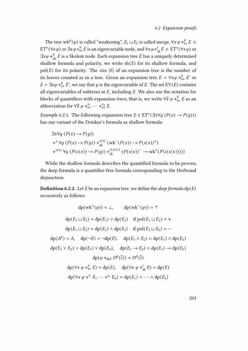
6.2 Expansion proofs
The tree wk? (i) is called “weakening”, �1 t�2 is called merge, ∀G i +~ev � ∈ET+(∀Gi) or ∃Gi+~ev� is an eigenvariable node, and ∀Gi+Csk� ∈ ET+(∀Gi) or∃Gi +~sk � is a Skolem node. Each expansion tree � has a uniquely determinedshallow formula and polarity, we write sh(�) for its shallow formula, andpol(�) for its polarity. The size |� | of an expansion tree is the number ofits leaves counted as in a tree. Given an expansion tree � = ∀Gi +~ev �′ or� = ∃Gi +~ev �′, we say that ~ is the eigenvariable of �. The set EV(�) containsall eigenvariables of subtrees in �, including �. We also use the notation forblocks of quanti�ers with expansion trees, that is, we write ∀G i +Gev � as anabbreviation for ∀G i +G1ev · · · +G=ev �.
Example 6.2.1. The following expansion tree � ∈ ET+(∃G∀~ (% (G) → % (~)))has our variant of the Drinker’s formula as shallow formula:
∃G∀~ (% (G) → % (~))
+G ∀~ (% (G) → % (~)) +B (G)sk (wk−(% (G)) → % (B (G))+)
+B (G) ∀~ (% (B (G)) → % (~)) +B (B (G))sk (% (B (G))−→wk+(% (B (B (G)))))
While the shallow formula describes the quanti�ed formula to be proven,the deep formula is a quanti�er-free formula corresponding to the Herbranddisjunction:
De�nition 6.2.2. Let � be an expansion tree, we de�ne the deep formula dp(�)recursively as follows:
dp(wk+(i)) = ⊥, dp(wk−(i)) = >
dp(�1 t �2) = dp(�1) ∨ dp(�2) if pol(�1 t �2) = +
dp(�1 t �2) = dp(�1) ∧ dp(�2) if pol(�1 t �2) = −
dp(�?) = �, dp(¬�) = ¬dp(�), dp(�1 ∧ �2) = dp(�1) ∧ dp(�2)
dp(�1 ∨ �2) = dp(�1) ∨ dp(�2), dp(�1→ �2) = dp(�1) → dp(�2)
dp(i +def �? (C)) = �? (C)
dp(∀G i +~ev �) = dp(�), dp(∀G i +Csk �) = dp(�)
dp(∀G i +C1 �1 · · · +C= �=) = dp(�1) ∧ · · · ∧ dp(�=)
203

6 Algorithm for proof import
dp(∃G i +~ev �) = dp(�), dp(∃G i +Csk �) = dp(�)
dp(∃G i +C1 �1 · · · +C= �=) = dp(�1) ∧ · · · ∧ dp(�=)
Example 6.2.2. The expansion tree � in Example 6.2.1 has the following tauto-logical deep formula: dp(�) = (>→ % (B (G))) ∨ (% (B (G)) → ⊥)
Eigenvariable nodes add a small technical complication to the de�nition ofan expansion proof. (But we need them since they arise during the extractionof splitting inferences.) Not only is it necessary that the deep formula is quasi-tautological, but the eigenvariables also need to be acyclic in a certain sense(this is a similar restriction to the eigenvariable condition in sequent calculi).We formalize this acyclicity using a dependency relation, which we will requireto be acyclic:
De�nition 6.2.3. Let � be an expansion tree. The dependency relation <� isa binary relation on variables where G <� ~ i� � contains a subtree �′ suchthat G ∈ FV(sh(�′)) and ~ ∈ EV(�′).
De�nition 6.2.4. An expansion sequent E is a sequent of expansion trees. Itsdependency relation <E =
⋃�∈E <� is the union of the dependency relations
of its trees. Its shallow sequent and deep sequent consists of the shallow anddeep formulas of its expansion trees, respectively.
An expansion sequent is positive(negative) i� the trees in the succedenthave positive(negative) polarity and the trees in the antecedent have nega-tive(positive) polarity. The size |E | of an expansion sequent is the sum of thesizes of its expansion trees.
De�nition 6.2.5. An expansion proof E is a positive expansion sequent suchthat:
1. <E is acyclic (i.e., can be extended to a linear order) and there are noduplicate eigenvariables,
2. dp(E) is a quasi-tautology
Example 6.2.3. Let � be as in Example 6.2.1. The sequent dp(` �) is a tautology,and the dependency relation of ` � is empty and hence acyclic. So ` � is anexpansion proof.
204

6.2 Expansion proofs
Expansion proofs are sound and complete for �rst-order logic. That is, ifS is a sequent, then there exists an expansion proof E with S as the shallowsequent if and only if S is valid. Completeness follows easily from cut-freecompleteness of the sequent calculus LK: we can recursively assign to everyproof c in LK with end-sequent S an expansion proof E such that sh(E) = S(as done for example in [71]).
Given a substitution f that maps eigenvariables to variables, we can applyit to expansion trees and expansion sequents, written �f and Ef , respectively.The calculus for expansion proofs we presented is redundant: it is still com-plete even without the t, +def , and Cut nodes. We also only need either theeigenvariable or Skolem nodes.
Two important reductions were introduced in [54] that will eliminate the tand Cut nodes. The elimination of +def will be discussed in Section 6.4.
The relation t{ pushes merge nodes to the leaves of an expansion tree until
they disappear, for example (�1 ∧ �2) t (�3 ∧ �4)t{ (�1 t �3) ∧ (�2 t �4)
reduces merges on conjunctions.
Lemma 6.2.1. The relationt{ on expansion sequents has the following proper-
ties:
1.t{ is terminating.
2. Whenever E t{ E′, then dp(E) → dp(E′) is a tautology.
3.t{ preserves acyclicity of the dependency relation.
4.t{ preserves polarity and the shallow formula.
5. If E does not contain Skolem or de�nition nodes, then itst{-normal forms
do not contain merge nodes.
In particular thet{-normal forms of expansion proofs without Skolem or de�ni-
tion nodes are merge-free expansion proofs.
Proof. Analogous to Lemmas 12 and 13 in [54]. Note that merge reduction canget stuck on merges of two Skolem nodes with di�erent Skolem terms, or twode�nition nodes with di�erent de�nitions, hence the condition in point 5. �
205

6 Algorithm for proof import
Cuts can be reduced and eventually eliminated as well. The cut-reductionrelation cut
{ (written as ↦→ in [54]) extends merge-reduction and reduces quan-ti�ed cuts via substitution.
Lemma 6.2.2.cut{ preserves quasi-tautology of the deep formula, and is weakly
normalizing. If no de�nition or Skolem nodes appear in cuts, then thecut{-normal
forms are cut-free.
Proof. See Lemma 16 and Theorem 33 in [54]. Just as in Lemma 6.2.1, cut-reduction can get stuck on cuts with Skolem nodes such as Cut(∀G i +Gsk. . . ,∀G i +C . . . ). �
The following lemma will bound the complexity introduced by Avatar split-ting inferences, since they will be translated to cuts on formulas of the form∀G � (G) where � (G) is a clause.
Lemma 6.2.3. Let |E | be an expansion proof with = cuts such that all cut
formulas are universally quanti�ed closed prenex formulas, and let E cut{∗E∗
such that E∗ is cut-free. Then |E∗ | ≤ |E |2= .
Proof. Merge reduction and propositional reduction steps reduce the size ofthe expansion proof and keep the number of cuts constants. Each quanti�erreduction step decreases the number of cuts by one and increases the size ofthe proof at most quadratically: essentially we duplicate the proof< times,where< is the number of weak quanti�er term blocks in the cut—and< isless than the size of the expansion proof. �
6.3 Extraction
In this section we convert a resolution proof of a formula i into an expansionproof with a shallow sequent of the following form:
∀G (i1(G) → �1(G)), · · · ,∀G (i= (G) → �= (G)),∀G (�=+1(G) → i=+1(G)), · · · ,∀G (�< (G) → i< (G)) ` i
That is, the expansions in the antecedent describe subformula de�nitionsand have de�nition axioms ∀G (i (G)→� (G)) or ∀G (� (G)→i (G)) as shallow
206

6.3 Extraction
formulas where � (G) def↦→ i (G). Furthermore the resulting expansion proof willnot have any eigenvariable nodes. We will eliminate the additional expansiontrees for de�nitions in Section 6.4.
The extraction proceeds bottom-up, starting from the proof ending in theempty clause, propagating expansions trees upward until they are at the Input-rules. At every point, each subproof is assigned a �nite set of expansionsequents. Formally, we describe the extraction as a binary relation on theseassignments of expansion sequents, called extraction states:
De�nition 6.3.1. An extraction state P;S is a pair consisting of a set P andan expansion sequent S. Each element of P is a pair (c, E), where c is asubproof ending in T and E is a negative expansion sequent such that thereexists a substitution f with Tf = sh(E). The deep formula of the extractionstate is de�ned as:
dp(P;S) =( ∧(c,E)∈P
dp(E))→ dp(S)
Note that the trees of the negative expansion sequents here have the oppositepolarity as in the expansion sequents in Section 6.2. This is due to the fact thatresolution proofs are proofs by refutation. The resolution proof starts withi ` while the expansion proof has ` i as the shallow sequent—observe that ioccurs in opposite polarities here.
Given a resolution proof c , the initial extraction state is Cc = ({(c, `)}; `).We can now de�ne a relation{ on extraction states, that transforms the initialextraction state into extraction state of the form ∅; E, where E is the desiredexpansion proof. This relation preserves the quasi-tautologyhood of the deepformula—we will prove this crucial property in Lemma 6.3.2. The relation{is the smallest relation containing the following cases:
P, (c, E1), (c, E2);S { P, (c, E1 t E2);S if sh(E1) = sh(E2)P;�1 +: �2 +: S { P;�1 t �2 +: S if sh(�1) = sh(�2)P;S :+ �1 :+ �2 { P;S :+ �1 t �2 if sh(�1) = sh(�2)
207

6 Algorithm for proof import
Logical connectives:
P, (Input, � `);S { P;S :+ �
P, (TopL(c), E);S { P, (c,>+ +: E);SP, (BotR(c), E);S { P, (c, E :+ ⊥−);S
P, (NegL(c), E :+ �1);S { P, (c,¬�1 +: E);SP, (NegR(c), �1 +: E);S { P, (c, E :+ ¬�1);S
P, (AndL(c), �1 +: �2 +: E);S { P, (c, (�1 ∧ �2) :+ E);SP, (AndR1(c), E :+ �1);S { P, (c, E :+ (�1 ∧wk−(. . . )));SP, (AndR2(c), E :+ �2);S { P, (c, E :+ (wk−(. . . ) ∧ �2));SP, (OrR(c), E :+ �1 :+ �2);S { P, (c, E :+ (�1 ∨ �2));SP, (OrL1(c), �1 +: E);S { P, (c, (�1 ∨wk+(. . . )) +: E);SP, (OrL2(c), �2 +: E);S { P, (c, (wk+(. . . ) ∨ �2) +: E);S
P, (ImpR(c), �1 +: E :+ �2);S { P, (c, E :+ (�1→ �2));SP, (ImpL1(c), E :+ �1);S { P, (c, (�1→wk+(. . . )) +: E);SP, (ImpL2(c), �2 +: E);S { P, (c, (wk−(. . . ) → �2) +: E);SP, (AllR(c), E :+ �1);S { P, (c, E :+ (∀G i +Gf �1));SP, (AllL(c), �1 +: E);S { P, (c, (∀G i +Csk �1) +: E);SP, (ExL(c), �1 +: E);S { P, (c, (∃G i +Gf �1) +: E);SP, (ExR(c), E :+ �1);S { P, (c, E :+ (∃G i +Csk �1));S
(where if = sh(�1))
Subformula definitions:
P, (AbbrL(c), �+(C) +: E);S { P, (c, (i +def �+(C)) +: E));SP, (AbbrR(c), E :+ �−(C));S { P, (c, E :+ (i +def �−(C)));S
P, (DefR(� (C)), �� ` �i );S { P;∀G (� (G) → i) +C (�� → �i ) +: S
P, (DefL(� (C)), �i ` ��);S { P;∀G (i→ � (G)) +C (�i → ��) +: S
208

6.3 Extraction
Avatar spli�ing:
P, (AvSplit(c), E1 :+ �−);S {P, (c, E1 ++ S−2 [G\~]); (∀G S2 +~ S+2 [G\~] → �−) +: S
(where S2 is as in the inference rule, and ~ are fresh variables)
∅;�1→ �−, �+→ �2,S { ∅; Cut(�1, �2) +: S if � does not occur in S
P, (AvIntro(�), �� +: E);S { P;�+→ (∀G S2 +C E) +: S
Logical inferences:
P, (Res(c1, c2), E1 E2);S { P, (c1, E1 :+ i−), (c2, i+ +: E2);SP, (Factor(c), E :+ �1);S { P, (c, E :+ �1 :+ �1);S
P, (Subst(c), E);S { P, (c, E);SP, (Taut(i), �1 ` �2);S { P;SP, (Re�, ` (C = C)−) { P;S
And the following transition for Rw:
P, (Rw(c1, c2), E1 ++ E2 :+ �3 [B]);{P, (c1, E1 :+ (C = B)−), (c2, E2 :+ �3 [C]);S
Example 6.3.1. Let c6 be the resolution proof in Example 6.1.1. Then the relation{ extracts the expansion proof as follows, where iG = ∀~ (% (G) → % (~)):
(c6, `); ` { (c4, % (B (G))︸ ︷︷ ︸=�1
`), (c5, ` �1); ` { (c4, �1 `), (c3, ` �1); `
{2 (c2,wk−(% (G)) → �1︸ ︷︷ ︸=�2
`), (c2, �1→wk+(% (B (B (G))))︸ ︷︷ ︸=�3
`); `
{2 (c1, iG +B (G)sk �2 `), (c1, iB (G) +B (B (G))sk �3 `); `
{2 (c1,∀GiG +G iG +Gsk �2︸ ︷︷ ︸=�4
`), (c1,∀GiG +B (G) iB (G) +B (G)sk �3︸ ︷︷ ︸=�5
`); `
{ (c1, �4 t �5 `); ` { ∅; ` �4 t �5
209

6 Algorithm for proof import
De�nition 6.3.2. Let c be a resolution proof. Then |c |C and |c |3 denote thenumber of its inferences when counted as a tree or a DAG, respectively.
Lemma 6.3.1. { is terminating.
Proof. Let P;S be a extraction state, we de�ne a function | · |= as its termina-tion measure by |P;S|= = |S|2 + 2
∑(c,E)∈P |c |C where |S|2 is the number of
expansion trees in S. Each case of the relation{ decreases this terminationmeasure. �
Lemma 6.3.2. Let C1 { C2, then dp(C1) → dp(C2) is a quasi-tautology. If �1
is acyclic, then so is C2.
Proof. Straightforward induction on{. �
Lemma 6.3.3. Let c be a resolution proof where all Input inferences have theformula i , and let Cc {∗ (P,S1 ` S2). Then P = ∅, and:
1. for every � ∈ S1, sh(�) is either > or ∀G (� (G) → i) where � (C) def↦→ i ,and
2. for every � ∈ S2, sh(�) = i .
Proof. If P ≠ ∅, then we can apply one of the cases of{. Properties 1. and 2.are preserved in every case. �
Using the relation{ we obtain an expansion proof with cuts. Since thereare no Skolem or de�nition nodes in these cuts, we can eliminate them (seeLemma 6.2.2) to obtain a cut-free expansion proof E∗ with de�nitions: Cc {∗
(∅, E) cut{∗(∅, E∗)
6.4 Definition elimination
Consider now a cut-free expansion proof E without eigenvariable nodes wherethe shallow sequent contains only de�nition axioms in the antecedent (this isthe form of expansion proofs that are produced by the extraction in Section 6.3).
210

6.4 De�nition elimination
Assume that all de�nitions axioms are in the same polarity, that is, the in-troduced atom is on the left side. (The other polarity is treated analogously.)
E = (��1 , · · · , ��= ` �i ), sh(��8 ) = ∀G (i8 (G) → �8 (G)), sh(�i ) = i (6.1)
The expansions of i8 (C) may contain de�nition nodes as well. Due to theacyclicity of the AbbrL-inferences, we can assume that each expansion ofi8 (C) only contains de�nition nodes +def � 9 (. . . ) where 9 < 8 . We will nowsuccessively eliminate each of the de�nition axioms, starting with the one for=. The expansion tree for ∀G (i= (G) → �= (G)) has the following form:
∀G (i= (G) → �= (G)) +C1(�1→ �= (C1)−
)· · · +C:
(�: → �= (C:)−
)For performance reasons, we consider two cases here: in the �rst case the
deep sequent is tautological, in the second case the deep sequent is only quasi-tautological. In both cases, we replace de�nition nodes +def �= (. . . ) in theexpansion proof by subtrees of ��= . However in the second case we performmany duplications, and we want to avoid this if possible.
Tautological deep sequent. If dp(E) is not just quasi-tautological but tau-tological (this is the case if the resolution proof did not use the built-in equa-tional inference Rw and Re�), then we merely need to replace each occurrenceof a de�nition node +def �= (C8)+ with the corresponding expansion tree �8 . Wede�ne a function ' [·] that performs this replacement on de�nition nodes for�= , and recursively maps over the other possible nodes:
' [i= (C) +def �= (C)+] ={�8 if there exists 8 such that C = C8wk+(i= (C8)) otherwise
Lemma 6.4.1. Let E be an expansion sequent as in Equation (6.1). If dp(E) istautological, then dp
(��1 , · · · , ��=−1 ` ' [i]
)is tautological as well.
Proof. Let � be a counter-model for dp(��1 , · · · , ��=−1 ` ' [i]
). Assume without
loss of generality that � is not de�ned for any of the atoms �= (C); we extend� by setting � (�= (C8)) = � (dp(�8)) for all 8 , and � (�= (C)) = 0 otherwise. Wenow have � (dp(��= )) = 1 as well as � (dp(' [i= (C) +def �= (C)+])) = � (�= (C))and thus � (dp(' [�i ])) = � (dp(�i )) since �= only occurs in �i in de�nitionnodes. Hence � is a counter-model for dp(E) as well. �
211

6 Algorithm for proof import
�asi-tautological deep sequent. In general, the sequent dp(E) may bejust quasi-tautological. In particular the following congruence scheme is quasi-tautological and not tautological:
C1 = B1 ∧ · · · ∧ C< = B<→ (� (C1, · · · , C<) ↔ � (B1, · · · , B<))
Hence it is no longer su�cient to replace a de�nition node +def �= (C8)+
by just the expansion tree where the arguments are syntactically equal. Wereplace it by all the expansion trees �1, · · · , �=, suitably replacing the termvectors C8 so that the shallow formulas match. To perform this replacement, wede�ne a generalization operation� . We �rst de�ne the generalized tree �, andthen de�ne the replacement operation 'eq uniformly for all de�nition atoms:
� = �i (G) (�1) t · · · t�i (G) (�=)
'eq [i= (C) +def �= (C)+] = � [G\C]
De�nition 6.4.1. Let i,k be �rst-order formulas such thatkf = i for somesubstitution f , and � ∈ ET? (i) an expansion tree without de�nition nodes.Then we recursively de�ne its generalization �k (�) ∈ ET? (k ):
�k (�?) = k? �¬k (¬�) = ¬�k (�) �k (wk? (i)) = wk? (k )�k (�1 t �2) = �k (�1) t�k (�2)
�k1∧k2 (�1 ∧ �2) = �k1 (�1) ∧�k2 (�2)�∀Gk (∀Gi +~ev �) = ∀Gi +
~ev �k [G\~] (�)
�∀Gk (∀Gi +Csk �) = ∀Gi +Csk �k [G\C] (�)
�∀Gk (∀Gi +C1 �1 · · · +C= �=) = ∀Gi +C1 �k [G\C1] (�1) · · · +C= �k [G\C=] (�=)
Lemma 6.4.2. Let E be an expansion sequent as in Equation (6.1). If dp(E) isquasi-tautological, then dp
(��1 , · · · , ��=−1 ` 'eq [i]
)is quasi-tautological as well.
Proof. Similar to Lemma 6.4.1, except we now set � (�= (0)) = � (dp(�) [G\0])for all 0 in the domain of the counter-model. �
212

6.5 Complexity
6.5 Complexity
We will now give a double-exponential upper bound on the complexity of thewhole algorithm as summarized in Algorithm 6. Without Avatar inferencesand de�nition inferences, this bound would be just single-exponential. We donot know whether this double-exponential bound is actually attained in theworst case, the best known lower bound is single-exponential (as is necessaryin any conversion from resolution proofs to expansion proofs).
Lemma 6.5.1. Whenever Cc {∗ (∅; E), then |E | ≤ 4|c |3+1.
Proof. Let P;S be a extraction state, we de�ne its size as |P;S| = |S| +∑(c,E)∈P 2|c |C |c |< + |E|, where |c |< is the maximum length of a sequent oc-
curring in c . No case of the relation { increases this size. Observe that|c |< ≤ 2|c |3 , and hence |E | ≤ |Cc | ≤ 2|c |C |c |< ≤ 2|c |3+2 |c |3 ≤ 4|c |3+1. �
Lemma 6.5.2. Let c be a resolution proof, then |Transform(c) | ≤ 24 |c |3 .
Proof. Let �1, �2, �3 be as in Algorithm 6. From Lemma 6.5.1 we know that|�1 | ≤ 4|c |3+1. Note that there are fewer than |c |3 splitting and de�nitioninferences in c , and hence fewer than |c |3 cuts and de�nitions in �1 and�2. The cost of cut-elimination is shown in Lemma 6.2.3, we have |�2 | ≤|�1 |2
2 where 2 < |c |3 is the number of cuts. We have a similar bound forde�nition elimination: each step increases the size at most quadratically andwe have |�3 | ≤ |�2 |2
3 where 3 < |c |3 is the number of de�nitions. Hence|Transform(c) | ≤ 4( |c |3+1)22+3 ≤ 24 |c |3 . �
6.6 Empirical evaluation
We evaluated the implementation in three experiments using GAPT 2.9, whichcontains Algorithm 6 as the ResolutionToExpansionProof function.
First, we compared it against the LK-based method for expansion proofextraction from resolution proofs described in [52], which is also implementedin GAPT. The TSTP library (Thousands of Solutions from Theorem Provers,see [94]) contains proofs from a variety of automated theorem provers. Weloaded all 6341 Prover9 proofs into GAPT, and measured the runtime of each
213

6 Algorithm for proof import
0 2000 4000 6000 8000 10000dag-like size of resolution proof
100
101
102
103
104
num
ber o
f im
porte
d pr
oofs
All Prover9 proofs in the TSTPAlgorithm from this chapterLK-based method
Figure 6.2: Comparison of the number of successfully imported Prover9 proofsin the TSTP using Algorithm 6 and the LK-based algorithm in [52].
of the algorithms with a timeout of 120 seconds. GAPT is unable to read 40 ofthe proofs at all since Prover9’s prooftrans executable fails. Of the remainingproofs, the LK-based method in [52] imports 5479 proofs (87.0%). Algorithm 6imports 6125 proofs (97.2%), it only fails on 176 proofs due to the timeout.There is no proof where the LK-based method is successful, but Algorithm 6fails.
Figure 6.2 plots the number of successfully imported proofs using each of thealgorithms against the DAG-like size of the resolution proof. The algorithmin this chapter manages to import almost all Prover9 proofs in the TSTPincluding very large proofs; proofs between 1000 and 10000 inferences can notbe imported by the LK-based method at all.
As the second experiment, we evaluated the quality of the clausi�cationallowed by the resolution calculus used in this chapter. We took the 662problems in the �rst-order FEQ, FNE, FNN, and FNQ divisions of the CASC-26 competition whose size was less than one megabyte after including theseparate axiom �les. On these 662 problems, we compared the performance ofthe E theorem prover [87] version 2.1 (as submitted to CASC) when directly
214

6.6 Empirical evaluation
running on the problems, and when running on the clausi�cation produced byGAPT.
GAPT fails to clausify 19 of the problems due to excessive runtime. Theseproblems (e.g. HWV053+1) have blocks of more than a thousand quanti�ers.On the remaining ones we ran E in both the default con�guration, and theauto-scheduling mode (as used in the CASC), both with a timeout of 60 seconds.In the default mode the E clausi�cation results in 81 found proofs, the GAPTclausi�cation in 89. With auto-scheduling enabled the result is reversed butstill close, and E’s own clausi�cation produces more proofs (308) than GAPT’sclausi�cation (285). These results show that the clausi�cation allowed by thecalculus presented in this chapter is competitive with the ones implementedin state-of-the-art automated theorem provers. We believe that the reversedresults for the auto-scheduling mode are indicative of a larger trend in �rst-order theorem provers: many provers train their strategy selection algorithmson the exact problems from the TPTP and thus rely very closely on the syntacticfeatures of these problems.
Finally, we wanted to compare the runtime of Algorithm 6 with the runtimeof the �rst-order prover. To this end, we again used the same 662 �rst-orderproblems from CASC-26 and used GAPT’s external prover interface to obtainexpansion proofs from E. This prover interface uses the clausi�cation of theresolution calculus described in this chapter to create a CNF, sends this CNFto E, then parses and reconstructs a resolution proof using proof replay, and�nally constructs an expansion proof using Algorithm 6. We measured themean runtime of each phase on the successfully imported proofs (only 7 proofscould not be imported in the time limit of 2 minutes). The E prover itself takesup 62%, the largest part of the runtime. Algorithm 6 only takes 7.2% of thetotal runtime. The rest of the runtime is spent mainly in proof replay (15.6%)and clausi�cation (4.6%).
Since the expansion proof extraction is only a fraction of the prover runtime,we believe that it is practically feasible to generate expansion proofs instead ofresolution proofs. Even though expansion proofs can be exponentially largerin the worst case, this situation seems to occur only rarely in practice.
215

6 Algorithm for proof import
6.7 Direct elimination of Avatar-inferences
When importing resolution proofs with Avatar splitting using the proceduredescribed in this chapter, each cut in the expansion proof corresponds to anatom introduced using Avatar splitting. The cut-elimination of the expansionproof then corresponds to the elimination of the splitting inferences.
This naturally leads to the question whether and how we can eliminateAvatar inferences directly on the resolution proof itself. There are applicationfor resolution proofs which require that the proofs do not contain splittinginferences: for example we can extract interpolants from resolution proofs [58],or use them in the cut-elimination method CERES [8]. In this section we willpresent a method to eliminate splitting inferences from resolution proofs atexponential cost.
The basic idea is that we eliminate all resolution inferences on splittingatoms. That is, resolution inferences where the resolved atom 3
def↦→ ∀G S3 is ade�ned atom as used in the inferences AvSplit and AvIntro:
(c1)S1 :+ �
(c2)� +: S2 ResS1 ++ S2
Once we have eliminated all such resolution steps, the resulting proof willno longer contain splitting inferences as the introduced splitting atoms canonly be removed using the resolution inference. We eliminate each resolutionstep separately. As a �rst step, we show how to transform the left sub-proof(c1) into a proof of S1 ++ S� :
Lemma 6.7.1. Let 3def↦→ ∀G S3 be a splitting atom, and c a resolution proof
ending in S :+ � · · · :+ � . We implicitly assume that S and S� have disjoint setsof free variables. Then there exists a resolution proof % (c, �) of S ++ S� suchthat |% (c, �) |3 ≤ |c |3 |S� |.
Proof. The interesting case is when c is an AvSplit-inference, so let c end inan AvSplit inference:
(c ′)S ++ S� AvSplitS :+ �
216

6.7 Direct elimination of Avatar-inferences
In this case we can just leave out the AvSplit-inference and set % (c, �) = c ′.If � is not the main formula of the inference, then we can proceed recursively.Consider representatively the case where c is a Res-inference:
(c1)S1 :+ � · · · :+ � :+ i
(c2)i +: S2 :+ � · · · :+ �
ResS1 ++ S2 :+ � · · · :+ �Then we construct % (c, �) as follows:
(% (c1, �))S1 ++ S� :+ i
(% (c2, �))i +: S2 ++ S� ResS1 ++ S2 ++ S� ++ S� Factor+S1 ++ S2 ++ S�
We can permute % (·, �) and Subst inferences. We can also permute Fac-tor/Rw inferences where � is the main formula, by repeating the Factor/Rwinference for every atom in S� . If c is an AbbrR-inference, we replace it byAllR and OrR inferences. Note that� is not the main formula of a clausi�cationinference, since splitting atoms do not occur in the input formula or in de�nedsubformulas. Furthermore � cannot be the main formula of a Re�-inferencesince it is not an equation. �
We can now plug the left subproof into all the AvIntro inferences in theright subproof:
Lemma 6.7.2. Let �def↦→ ∀G S� be a splitting atom, c� a resolution proof ending
inS′++S� , and c a resolution proof ending in�+:. . . �+:S. We implicitly assumethatS, S� , andS′ have pairwise disjoint sets of free variables. Then there exists aresolution proof'(c, c� , �) ofS++S′ such that |'(c, c� , �) |3 ≤ |c |3 |S� |+|c� |3 .
Proof. The interesting case is when c is a AvIntro-inference with � as a mainformula:
AvIntro� +: (�
In this case we can set '(c, c� , �) to c� . The other cases are as in Lemma 6.7.1.�
Combining the two previous Lemmas 6.7.1 and 6.7.2, we can now eliminatea single resolution inference on a splitting atom:
217

6 Algorithm for proof import
Lemma 6.7.3. Let c be a top-most resolution inference on a splitting atom
�def↦→ ∀G S� (that is, c1 and c2 do not contain any resolution inferences on
splitting atoms):
(c1)S1 :+ �
(c2)� :+ S2 ResS1 ++ S2
Then c ′ = '(c2, % (c1, �), �) is a resolution proof of S1 ++ S2 without resolutioninferences on splitting atoms such that |c ′|3 ≤ 2|c |3 |S� |.
Proof. Neither % (·, ·) nor'(·, ·, ·) introduce resolution inferences on new atoms,hence c ′ does not contain resolution inferences on splitting atoms. The sizebound is the combination of the results from Lemmas 6.7.1 and 6.7.2. �
Finally, we eliminate all resolution inferences one after another:
Theorem 6.7.1. Let c be a resolution proof ending in the empty sequent, thenthere is a resolution proof without splitting c ′ also ending in the empty sequentsuch that |c ′|3 ≤ 2 |c |3 for some constant 2 that only depends on the maximumsize of a splitting component.
Proof. If there is an AvSplit or AvIntro inference in c then then there is aresolution inference on a splitting atom below it. This is because the proofends in the empty sequent and there is no other way for the splitting atom togo away.
Hence it su�ces to eliminate all resolution inferences on splitting atoms.By Lemma 6.7.3 we know how to eliminate a single such resolution inference.We now iteratively eliminate these inferences going from top to bottom, ineach iteration the size of the proof is at most increased by a factor of 2 =
2max�def↦→∀G S�
|S� |. �
Theorem 6.7.1 gives a exponential bound on the size of a resolution proofwithout splitting in terms of a resolution proof with splitting.
Open Problem 6.7.1. Is the bound in Theorem 6.7.1 optimal? Can Avatarsplitting inferences be removed at subexponential cost?
218

7 Implementation andevaluation
We set out in Section 2.9 to reverse induction-elimination. In the previouschapters we have evaluated individual algorithms that are parts of this reversal:Chapter 6 shows how to obtain instance proofs, Chapter 4 and Section 4.4describe an algorithm to �nd an induction grammar covering the proofs, andChapter 5 explains how to solve the induced formula equation. In this chapterwe will evaluate the main algorithm, and its implementation in the GAPTsystem.
The implementation and empirical evaluation of proof-theoretic algorithmssuch as this one provides valuable practical insight. Proof-theoretic algorithmsoften have large worst-case runtime. For example, cut-elimination in �rst-order logic necessarily has non-elementary runtime complexity. This resultwould lead one to believe at �rst that cut-elimination is utterly infeasible. Yetcut-elimination is perfectly practical for many proofs that occur in practice, atleast if implemented e�ciently [34].
A similar performance question also arises for the algorithms that we haveseen so far. All the major individual algorithms we have seen so far have atleast exponential worst-case runtime. From a purely theoretical point of view,we can only say that they work. But it is possible that the worst-case is actuallycommon in practice. Thus we need to conduct experiments to evaluate theperformance on actual examples.
There is an even more fundamental model assumption that we have brie�ytouched upon in Section 2.10: that the instance proofs have a certain formof regularity. The whole approach depends crucially on this feature: thatinstance proofs are similar to proofs obtained by induction-elimination. If theinstance proofs were completely di�erent, then there would be little hope of
219

7 Implementation and evaluation
Obtain proofs (c8)8∈�
Find grammar �
Random testing: is !(�, C)always ) -tautological?
Find solution
Output proof
Obtain additional proof cC
counterexample found
1.
2.
Figure 7.1: Re�nement loop to �nd induction grammars
generalizing them to a proof with induction. A priori, we might even expectinstance proofs to have this regularity. Whether this is actually the case forautomatically generated proofs is a question that can only be answered bypractical experiments. We will answer this question in Sections 7.4 and 7.5.
7.1 Refinement loop to find inductiongrammars
The algorithm we saw in Section 4.4 produces an induction grammar of minimalsize that covers a given (�nite) family of languages (!C )C∈� . However there isno obvious choice for this set � . We could e.g. take � to be the set of all freeconstructor terms of size less than 2. However in practice, this choice oftenresults in induction grammars � such that !(�, C) is not ) -tautological forsome C of size larger than 2. In this case,Q� cannot be ) -solvable (rememberLemma 5.3.1 and Theorem 5.3.2).
Therefore, we use a re�nement loop to �nd induction grammars. In eachiteration we check the generated induction grammar � and verify that !(�, C)
220

7.2 Implementation
is ) -tautological for a large number of free constructor terms C . If the checksucceeds, then we work under the assumption that � is ) -tautological. Thischeck is only a necessary requirement. Unfortunately it could still be possiblethat� might not be solvable, as there are some tautological induction grammarswhose formula equation is not solvable (Theorems 5.4.1 and 5.4.3). We alsocannot check for solvability of formula equations (even the ones induced byinduction grammars) in general, as this is undecidable by Theorem 5.4.2.
On the other hand, if we �nd a C such that !(�, C) is not ) -tautological,then we obtain a new proof c of the instance problem for the parameter C ,extend the family (!C )C∈� to (!C )C∈�∪{C} by setting !C = !(cC ). Note that since !Cis) -tautological, any induction grammar�′ covering the extended family willsatisfy that !(�′, C) is ) -tautological. Hence we will not encounter the samecounterexample C in the following iterations of the loop. The overall structureof the method, combining the re�nement loop as well as the algorithms tosolve formula equations from Sections 5.6 and 5.7, is shown schematicallyin Figure 7.1.
7.2 Implementation
The open source GAPT framework [37] (short for General Architecture forProof Theory) contains implementations of a large variety of algorithms re-lated to expansion proofs (as a generalization of Herbrand sequents) and prooftheory in general. Since version 2.9 (released in August 2018), it also contains al-gorithms for the computation of covering induction grammars as in Section 4.4and solving formula equations using forgetful inference as in Section 5.6 (aversion restricted to natural numbers following the formalism of [31] wasalready released in version 2.0 in January 2016).
To give a short overview of the implementation, let us look at how theconcepts in each chapter are implemented in GAPT. The grammars intro-duced in Chapter 2 are in the gapt.grammars package; the classes VTRATG
and InductionGrammar model the respective concepts. The term encoding offormulas of Section 2.4 is implemented as InstanceTermEncoding(sequent),i.e., we have a di�erent term encoding for each sequent. Interestingly enough,
221

7 Implementation and evaluation
0 1 2
size of equational theory0
10
20
30
40
50 proof foundgrammar found
Figure 7.2: Results for the experiment where we pick an equational theoryfrom equations in the antecedent. We tried all combinations ofup to two equations. Only the solution algorithm using forgetfulinference is used. The benchmark set is an earlier version of theTIP, containing only 319 problems.
there has been little practical need to implement the map that assigns to eachproof a corresponding grammar; this map is only implemented for simpleinduction proofs. The function extractInductionGrammar actually operateson a slightly more general level, namely on expansion proofs (recall Section 6.2;technically, the induction inference is encoded as a higher-order assumption).
The algorithms to �nd covering grammars from Chapter 4 are contained inthe package gapt.grammars, in deltaTableAlgorithm, findMinimalVTRATG,Reforest, and findMinimalInductionGrammar. For the algorithms based onMaxSAT, GAPT contains interfaces to several MaxSAT solvers. The solverwe used for the evaluations is the external program OpenWBO [67]. Often itis useful to have a solver that does not require any extra dependencies, forexample when running tests. For this reason, GAPT also bundles the Sat4jlibrary, which includes a MaxSAT solver that is available via the MaxSat4j
class.
222

7.2 Implementation
Given an induction grammar, we can compute the induced formula equa-tion using InductionBUP.formula1. The solution algorithm using forgetfulinference (Section 5.6) is implemented as hSolveQBUP, and the the functionsolveBupViaInterpolationConcreteTerms implements the algorithm usinginterpolation (Section 5.7).
The re�nement loop is implemented in the class TreeGrammarProver. Thereis a parser for problems in the TIP format [21] in TipSmtParser.
Instance proofs are obtained using standard �rst-order theorem proversbased on superposition. GAPT contains interfaces to several external �rst-order provers such as Vampire, E, etc. However for the evaluation in thischapter we use the built-in Escargot prover of GAPT. Instance problems aretypically easy to prove, therefore there is little need to use stronger proverslike Vampire.
There is a second point in the algorithm where we make use of automatedtheorem provers: when we check whether !(�, C) is ) -tautological. The for-mula corresponding to !(�, C) is quanti�er-free. If ) is empty, this formula ishence in the QF_UF fragment e�ciently decidable by SMT solvers. If ) ≠ ∅,then we use the SMT solver as a semi-decision procedure: we also pass it thequanti�ed formulas in ) . The SMT solver will then apply heuristic instantia-tion to the formulas in ) . We also use a time limit to prevent non-termination.For the evaluation, we use CVC4 as the SMT solver.
For problems imported from external benchmark sets, there is typicallyno clear choice of equational theory. To evaluate how much of an e�ectan equational theory could have, we performed an initial experiment on anearlier version of the TIP benchmark suite. For every problem, we picked anequational theory consisting of equations in the antecedent of the sequent.We tried all combinations of up to two equations. Only the solution algorithmbased on forgetful inference was used. The results are shown in Figure 7.2.Using an equational theory has a small negative e�ect on the number of proofsfound. With one equation taken from the antecedent one extra proof is found,but with two equations the number of found proofs is signi�cantly lower. One
1In GAPT, formula equations are often referred to as Boolean uni�cation problems, sincethey can be seen as instances of Boolean uni�cation with predicates [33].
223

7 Implementation and evaluation
0 10 20 30 40number of solved problems
0
2
4
6
8
10to
tal r
untim
e (s
econ
ds)
Figure 7.3: Cactus plot of the runtime on TIP benchmarks. For each successfullysolved problem we plot the shortest runtime on the y-axis.
explanation is that the solution algorithm constructs the solution formulaout of the instances; using an equational theory reduces the number of theseinstances and hence reduces the amount of “raw material” that can be used.The number of candidate grammars found increases signi�cantly with a singleequation. This is not surprising, because it is easier to cover smaller termsets. Eliminating the instances of one axiom (the equation) also reduces theamount of irregularity that could prevent us from �nding a grammar. For theevaluation we hence use the empty theory ) = ∅.
7.3 Evaluation as automated inductive theoremprover
First we evaluate the algorithm as an automated inductive theorem prover.Given just a sequent, we want to �nd a simple induction proof. As a bench-mark set we use problems from the TIP benchmark suite (tons of inductive
224

7.3 Evaluation as automated inductive theorem prover
problems [21]). This TIP benchmark suite aggregates benchmarks used toevaluate the IsaPlanner [28], Zeno [89], and HipSpec [22] provers. The bench-marks mostly concern the veri�cation of functional programs; so far no publiccompetitions have been held.
Some of the problems are not syntactically of the form required by simpleinduction proofs: their conclusion contains more than one universal quanti�er,the formulas are not prenex or contain strong quanti�ers. There is a smallpreprocessing step that Skolemizes and prenexi�es the sequents. If there aremultiple universal quanti�ers in the conclusion, we Skolemize all but one ofthem (and try all choices). We use a time limit of 10 minutes.
There are 543 problems in the TIP benchmark suite, 529 of which are quan-ti�ed. For 62 of these problems, the algorithm �nds a candidate grammarthat is tautological for the random instances that were checked. There are38 problems where no grammar can cover the term sets produced by the�rst-order prover. (This can be detected by the algorithm from Section 4.4because it is guaranteed to �nd such a grammar, if it exists.) This indicatesvery irregular instance proofs that cannot be generalized to an inductive proof.In the remaining 429 problems, the re�nement loop times out.
Figure 7.3 shows a cactus plot of the runtime of the prover on the successfullysolved TIP problems. We picked the minimum runtime for each problem (aswe tried multiple con�gurations, such as for example multiple algorithms tosolve the induced formula equation).
The mean number of iterations of the re�nement loop is 2.4. We observea relatively small di�erence in the mean number of iterations dependingon whether we can �nd a grammar and/or a proof. In the cases where thealgorithm �nds a proof, the mean number of iterations is 2.15. In the caseswhere it �nds a grammar but no proof, the mean is 2.83. We can also visuallyobserve this di�erence in Figure 7.4: this �gure reinforces the picture that thereis exists a dichotomy between regular instance proofs, where the re�nementloop converges quickly and the induced formula equation is solvable, versusirregular instance proofs, where the re�nement loop converges slowly and theformula equation is not solvable.
In the cases where it cannot even �nd a candidate grammar, the meannumber of iterations in the re�nement loop is 2.39. However in this case there
225

7 Implementation and evaluation
0 10 20 30 40number of problems
0
1
2
3
4
5
num
ber o
f ite
ratio
ns
FE not solvedFE solved
Figure 7.4: Cactus plot of the number of iterations of the re�nement loop onTIP benchmarks where a candidate grammar was found.
is a larger variance. The maximal number of iterations is 17 when no grammarcould be found. All grammars that have been found were found after at most5 iterations.
We also tried di�erent weighing schemes for the grammars, preferringgrammars with 1) fewer productions or 2) smaller number of symbols. Thechoice of weighing scheme has almost no e�ect on the number of iterations orthe success of the algorithm (on the TIP benchmark set).
Of the 62 problems where a grammar has been successfully found, 48 canbe completed to a simple induction proof by solving the induced formulaequation. We used both the method based on forgetful inference as well asthe one based on interpolation described in Sections 5.6 and 5.7. The forgetfulinference method solves 30 formula equations, the interpolation method solves36 formula equations. There are hence 18 problems that both methods couldsolve. Figure 7.5 plots the runtime of the two algorithms. We see a very clearperformance di�erence: the interpolation-based algorithm never takes morethan a second, while the runtime of the algorithm based on forgetful inference
226

7.3 Evaluation as automated inductive theorem prover
0 5 10 15 20 25 30 35number of solved problems
10 1
100
101
102ru
ntim
e of
FE
solv
er (s
econ
ds) forgetful inference
interpolation
Figure 7.5: Cactus plot of the runtime of the algorithms solving the inducedformula equation on TIP benchmarks. The y-axis is scaled logarith-mically to make the results easier to compare given the signi�cantdi�erence in magnitude.
quickly grows exponentially. This comes to no surprise: it needs to computethe canonical solution, whose size is exponential in the instance term. Thefollowing step of applying forgetful inferences also has exponential runtimein the worst case.
GAPT also contains two other automated inductive theorem provers: oneis an analytic induction prover which heuristically instantiates the inductionscheme with variants of the goal and then runs a �rst-order prover. Spinintegrates an induction inference in the superposition loop of the Escargotprover in GAPT [39] similar to Zipperposition [25]. On the TIP, the analyticinduction prover solves 78 problems with the independent induction scheme,and 115 with the sequential scheme; Spin solves 142 problems in the defaultmode, 133 if generalization is disabled, and 94 if counterexample testing isdisabled [39].
There is one TIP problem that the algorithm presented here can solve, butnone of the other methods in GAPT: isaplanner/prop_59. The problem is
227

7 Implementation and evaluation
∀G∀~ (~ = nil→ last(G ++ ~) = last(G)). The natural induction formula,∀G (G ++ nil = G), is not analytic and is not found by Spin either.
In this evaluation on the TIP benchmark set, the algorithm often fails to �nda candidate grammar that covers the automatically generated instance proofs.This situation could arise from an algorithmic issue, where the algorithm thatwe use to compute covering grammars is too slow or �nds “inappropriate”grammars that do not describe a proof with induction. It could also arise froman intrinsic quality of the generated instance proof: that the automaticallyfound proofs do not possess the regularity necessary to generalize them to aproof with induction. To determine the cause of this issue, we will conduct anadditional experiment in Section 7.4, where we start with induction proofs andrun the algorithm on families of induction-eliminated instance proofs (whichare hence regular and should be generalizable into a proof with induction). Thisexperiment will allow us to tell whether the failure is due to the irregularity ofthe automatically generated instance proofs or not.
In a smaller number of cases, the algorithm also fails to �nd a solution to theformula equation induced by the grammar. We will provide an explanation inSection 7.5 by closely examining one of the problems as a detailed case study.
7.4 Evaluation of reversal ofinduction-elimination
For the second evaluation, we start out with 73 simple induction proofs manu-ally formalized in GAPT concerning basic properties of operations on naturalnumbers and lists. Of these, 25 are proofs of problems in the TIP benchmarksuite. GAPT contains 92 formal proofs of TIP problems as example data to testinduction-elimination, and 25 of these happen to be simple induction proofs.The other 48 proofs in this evaluation are lemmas from a formalization ofthe fundamental theorem of arithmetic in GAPT that happen to be simpleinduction proofs.
For each proof, we performed essentially two experiments. First, we usedinduction-elimination to compute the instance proofs and perform the recon-struction. As the second experiment, we generated the instance proofs using
228

7.4 Evaluation of reversal of induction-elimination
0 10 20 30 40 50 60number of constructed induction proofs
0
2
4
6
8
10to
tal r
untim
e (s
econ
ds)
induction-eliminationind-elim. (minimized)ATP
Figure 7.6: Cactus plot of the runtime on induction proofs in GAPT, depend-ing on whether the instance proofs are generated via inductionelimination or by an automatic theorem prover.
an automated theorem prover (Escargot, just as in Section 7.3). As we seein the following summary, the proofs obtained by induction-elimination areclearly di�erent from the proofs produced by the automated theorem prover:the algorithm always �nds a grammar for induction-elimination, but onlyfor about two thirds of the ATP proofs. There is a smaller di�erence in thesecond solution-�nding phase. Interestingly for every problem where the al-gorithm failed to solve the induced formula equation from the ATP proofs, thealgorithm also failed to solve the FE for the proofs from induction-elimination.
#problems #grammars #solutionsind.-elim. 73 73 63
ATP 73 39 32
The di�erence is also visible from the cactus plot in Figure 7.6: the runtimefor the instance proofs generated with the automated theorem prover is alwayslarger (to little surprise), but it diverges quickly, indicating that the proofsbecome more irregular. Figure 7.6 also shows data for another experiment:
229

7 Implementation and evaluation
we computed expansion proofs for the induction-eliminated instance proofsand minimized them before giving them to the algorithm. Minimization hereconsists of taking a minimal subset of tautological instances. The line forthe minimized instance proofs is very similar but slightly worse than theline for the non-minimized instance proofs. This shows that the regularitynecessary for induction-reversal to succeed does not require instance proofswhose language is exactly the language of an induction grammar, but thattheir languages may also be a subset.
In many cases the computed grammar does not match the grammar of theoriginal simple induction proof exactly. One relatively common situation oc-curring in 10 reconstructed proofs is that we can replace a quanti�ed inductionformula by a quanti�er-free one.
This happens for example in isaplanner.prop_06, which proves ∀G∀~ G −(G +~) = 0 using ∀~ (G − (G +~) = 0) as the induction formula2. The inductiongrammar of the proof with the quanti�ed induction formula is as follows,where I is a free variable in the proof:
g → A1(0 + W) | A2(a, a + W) | A3(a,W) | A4W → W | I
The induction proof found by the algorithm replaces the induction formulaby a quanti�er-free formula G − (G + ~) = 0 where ~ is an eigenvariable of theend-sequent. On the level of the induction grammar, this corresponds to theelimination of the productions W → W | ~ (which are not very useful since thenonterminal W will always expand to ~):
g → A1(0 + ~) | A2(a, a + ~) | A3(a,~) | A4
This experiment shows two things: on the one hand, we see that the algo-rithm can e�ective generate proofs with induction, as long as the input proofsare su�ciently regular. There are hence no obvious algorithmic de�cienciesor implementation bugs. On the other hand, we also observe that there arequalitative di�erences in the proofs produced by induction-elimination andthe proofs produced by automated theorem provers. Namely, that the proofs
2The binary operation − denotes truncating subtraction, i.e. G − ~ = max{G − ~, 0}.
230

7.5 Case study: doubling
produced by the ATP often do not possess the regularity that we are interestedin.
7.5 Case study: doubling
Let us now examine one of the examples in more detail, where the algorithm�nds a candidate grammar but cannot solve the induced formula equation. Theexample is prod/prop_01 from the TIP library, which shows that ∀G 3 (G) =G + G where 3 is a recursively de�ned doubling function:
∀G G + 0 = G, (A1)∀G∀~ G + B (~) = B (G + ~), (A2)3 (0) = 0, (A3)∀G 3 (B (G)) = B (B (3 (G))) (A4)` ∀G 3 (G) = G + G (A5)
To keep the size of the grammar and formula equation manageable, we putsome of the formulas from the antecedent of the sequent into the backgroundtheory ) = {3 (0) = 0, 3 (B (G)) = B (B (3 (G))), G + 0 = G}. This choice e�ectivelyignores the instances of all formulas except (A3), which contains interestinginformation about the induction.
Let us �rst consider how a “natural” simple induction proof of this sequentwould look like. We might be inclined to prove ∀G ∀~ B (G) + ~ = B (G + ~)as a lemma �rst, but a simple induction proof only contains one inductioninference. Combining the goal with the lemma, an induction formula thatworks is ∀W (B (W) + a = B (W + a) ∧ 3 (a) = a + a). The quanti�er instances in asimple induction proof with this induction formula can be described by theinduction grammar with the following productions:
g → A2(B (W), a) | A2(W, a) | A2(B (a), a) | A5W → W | a | 0
231

7 Implementation and evaluation
This grammar induces the following formula equation:
∀W - (U, 0, W) ∧ (- (U, U, U) → 3 (U) = U + U) ∧∀a∀W (- (U, a,W) ∧ - (U, a, a) ∧ - (U, a, 0) ∧B (W) + B (a) = B (B (W) + a) ∧ W + B (a) = B (W + a) ∧B (a) + B (a) = B (B (a) + a) → - (U, B (a), W))
The grammars produced by the algorithm are smaller and di�erent in aninteresting way. First, let us look at the grammar computed for induction-eliminated instance proofs. Like in Section 7.4, algorithm �nds a grammarwith fewer productions:
g → A2(W, a) | A5W → W | a | U
We do not know if the induced formula equation has a solution (modulo ) )or not:
∃-(∀W - (U, 0, W) ∧ (- (U, U, U) → 3 (U) = U + U) ∧∀a∀W (- (U, a,W) ∧ - (U, a, a) ∧ - (U, a, U) ∧W + B (a) = B (W + a) → - (U, B (a), W))
)Looking at the grammar computed for the instance proofs generated by the
automated theorem prover, it is even simpler. It is so simple, it only consists oftwo productions:
g → A2(U, a) | A5It is also qualitatively di�erent: there is no occurrence of W , so there would
even be a simple induction proof with a quanti�er-free induction formula,assuming that the induced formula equation is solvable. Alas, we do not knowwhether this FE is solvable either:
∃-(- (U, 0) ∧ (- (U, U) → 3 (U) = U + U) ∧∀a (- (U, a) ∧ U + B (a) = B (U + a) → - (U, B (a)))
)It is instructive to compare the instance proofs from induction-elimination
of Example 2.8.4 with the proofs produced by the automated theorem prover.
232

7.5 Case study: doubling
100 101
101
102
ind-elim. expansion proofATP superposition proofATP expansion proof
101
102
103
linearquadratic
Figure 7.7: Proof size of the instance proofs from Section 7.5. The y-axis scaleon the left-hand side is the expansion proof size, the scale on right-hand side is the superposition proof size. The two scales are di�er-ent to make the comparison easier.
The straightforward way for a prover to prove the instance problems is totreat the assumptions (A1)–(A4) as a term rewriting system and to rewrite theconjectured equation 3 (B= (0)) = B2= (0) into normal form:
3 (B= (0))(A4)� B2= (3 (0))
(A3)� B2= (0)
B= (0) + B= (0)(A2)� B= (B= (0) + 0)
(A1)� B2= (0)
Looking closely, this proof uses the instances A2(B= (0), B8 (0)) for 0 ≤ 8 <=. This set of instances corresponds to the formula U + B (a) = B (U + a) inthe formula equation. Note also that there are no “repeating” equations inthis sequence that could give rise to an induction formula. By contrast, theproof obtained via induction-elimination contains instances for a much more
233

7 Implementation and evaluation
roundabout rewriting of the right-hand side, iterating the following part:
B8+1(0) + B8+1(0)(A2)� B8+1(B8+1(0) + 0)
(A1)� B28+2(0)
(A1)� B8+2(B8 (0) + 0)
(A2)� B2(B8 (0) + B8 (0))
Empirically, this di�erence is also re�ected in the proof sizes. Figure 7.7shows a double-logarithmic plot of the proof sizes of the instance proofs for0 ≤ = ≤ 30. The sequence of instance proofs obtained via induction- andcut-elimination from a simple induction proofs grows quadratically. The plotshows the size of the corresponding expansion proof: this size correspondsto the size of the instance language. The proof size is quadratic because thegrammar contains the productions g→A2(W, a) andW→W | a . TheW-productionhence expands to all numerals greater than a and A2(W, a) expands to all A2(:, ;)where ; < : ≤ =.
By contrast, the proofs that are found by the automated theorem prover areof linear size. (The built-in Escargot prover is used in this experiment.) Boththe superposition proof directly produced by Escargot as well as the expansionproofs are of linear size. This is precisely because the superposition proofcontains a rewriting sequence of the form described in this section.
234

8 Conclusion
We have presented a practical implementation of the approach to automatedinductive theorem proving proposed in [31]. This required the development orextension of the algorithms presented in Chapters 4 to 6. On a theoretical side,this endeavour has lead to interesting questions. The study of the complexityof decision problems on grammars in Chapter 3 was motivated by the desireto �nd better algorithms producing covering grammars. The questions aboutformula equations leading to Theorem 5.4.3 were sparked by the necessityof algorithmically solving these formula equations. The practical evaluationof the approach lead to even more empirical questions about the nature ofautomatically generated proofs which we illuminated in Sections 5.5 and 7.5.
For various classes of grammars we have determined the computationalcomplexity of the membership, containment, disjointness, equivalence, non-emptiness, and minimization problems in Chapter 3. The main open problemis the complexity of minimal cover as a decision problem, where we only knowthat is in NP. We were only able to show NP-completeness for the variantwhere the number of nonterminals is bounded. Surprisingly, the general casewith an unbounded number of nonterminals is even open for the correspondingproblem on regular grammars for words (Open Problem 3.7.2), even thoughthat model has been studied much more extensively.
The reductions used for the hardness proofs generally use an unboundednumber of symbols. However this is undesirable from a complexity point ofview. In particular, the reductions for minimal cover require this unbound-edness in an essential way to constrain the covering grammar. It remains asfuture work to study reductions which do not increase the number of symbols.
We have presented three algorithms in Chapter 4 that produce VTRATGscovering a given set of terms. Just as it is surprisingly hard to show that theTRATG-Cover problem is NP-complete, it is also hard to construct algorithms
235

8 Conclusion
that �nd minimal covering VTRATGs. Of the three algorithms, only theMaxSAT algorithm �nds grammars that are guaranteed to be of minimal size.
The mathematical key insight behind the MaxSAT algorithm is that there isa polynomial time computable VTRATG which contains a minimal grammaras a subgrammar. This allows the polynomial reduction of the grammarcompression problem to a MaxSAT problem for which highly e�cient solversare available.
Also from an application point of view, the MaxSAT algorithm is the mostversatile and easy to extend. The only currently available algorithm to producecovering induction grammars is the one described in Section 4.4. The generaltheory of stable grammars behind underlying the MaxSAT algorithms makessuch an extension straightforward and transparent.
In principle the MaxSAT algorithm could be adapted to any class of gram-mars that are closed under rewriting. It could also be extended to other notionsof grammar size: [32] introduces the tree complexity measure, which preciselycorresponds to the number of weak quanti�er inferences in a proof (as opposedto the constant factor that we have had to introduce in Lemmas 2.7.4 and 2.8.2).The MaxSAT-reduction of the minimization problem itself in Section 4.3.5could be extended to other classes of grammars or automata as well, for exam-ple to �nd tree automata with a �xed number of states and minimal numberof transitions that accept a given �nite set of terms.
We have discussed two algorithms to solve formula equations in Chapter 5.Both of them are heuristic: they are not complete, in the sense that they are notguaranteed to �nd a solution if one exists. As we have seen in Section 7.3, thetwo algorithms seem to be complementary in practice with the interpolation-based one having a small lead. Half of the formula equations solved by one arenot solved by the other and vice versa. The success of the interpolation-basedmethod modeled after the Duality algorithm for constrained Horn clausessuggests that the extension of CHC solvers to the theory of equality withuninterpreted function symbols is an interesting application.
On a theoretical level we could improve on a result of [31] on the existenceof tautological induction grammars whose induced formula equation is notsolvable. Theorem 5.4.3 both reduces the nonterminals in the grammar as wellas extends it to strong background theories. It remains as future work to see
236

in how far this technique allows us to extend the result on the undecidabilityof the solvability of induction grammars (Theorem 5.4.2) in a similar way.
The transformation from resolution proofs to expansion proofs described inChapter 6 has been used as the default method to generate expansion proofsfrom resolution proofs in GAPT since version 2.2. Using it, GAPT can e�ec-tively interface with six di�erent external resolution-based provers, includingSPASS and Vampire with their splitting rules. The modular integration ofstructural clausi�cation makes it possible to reuse it for non-resolution proversas well: the interface to the connection-based prover LeanCoP [76, 82] in GAPTuses the same code for clausi�cation and de�nition elimination.
A noteworthy limitation of the clausi�cation in Chapter 6 is that it canexpand each de�nition only in a single polarity. Lifting this restriction wouldproduce cuts in the de�nition elimination phase. However, these cuts wouldcontain Skolem nodes and cannot be eliminated directly. In the equality-freecase, there is a reliable deskolemization procedure [7] which can be used as apreprocessing step to enable cut-elimination. Such a procedure is yet missingfor proofs with equational reasoning. Reliable deskolemization would alsoenable a straightforward adaptation of the clausi�cation produced by externalprovers using proof replay.
Many of the techniques used come from higher-order logic, both Andrew’scalculus R and expansion trees originate in that setting. It seems only naturalto extend this transformation to higher-order logic, and there seem to be noimmediate obstacles except for the built-in equational inferences. But thesecould be straightforwardly translated to explicit Leibniz equality.
Many clausi�cation procedures perform propositional simpli�cation rules asa pre-processing step, for example rewriting i ∧> ↦→ i or converting to nega-tion normal form. These simpli�cations could be helpful in the clausi�cationhere as well, since they potentially enable sharing of subformula de�nitionsand Skolem functions. These could be supported by adding new inferencerules to the resolution calculus and adapting the expansion tree extraction inthe natural way.
For simplicity the SMT refutations in proofs using Avatar are convertedto resolution proofs �rst. However there is no fundamental reason why weneed to perform this costly conversion, since the SMT refutation is purely
237

8 Conclusion
ground and is essentially discarded in this translation. Adding a new rule torepresent this part of the proof in a single inference would deliver even greaterperformance.
Finally, we have evaluated the implementation of the whole approach inChapter 7. The empirical results show that there is a clear di�erence in the suc-cess of the approach if we compare proofs obtained from induction-eliminationand the proofs found by an automated theorem prover. In order to successfully�nd a proof with induction, the instance proofs must have a certain form ofregularity.
One potential way to obtain more regular families of proofs is to modifythe search procedure of the automated theorem prover, for example to use anoutermost-�rst strategy for rewriting, which sometimes seems bene�cial in ourexperience. Another option would be to perform a heuristic post-processingto regularize the instance proofs.
Instead of �nding more regular families of instance proofs, we could alsoextend the grammars so that they can cover more irregular families. Theinduction grammars in this paper need to cover the term sets for the instanceproofs exactly, without taking the background theory into account. We couldextend the grammar generation algorithm so that it generates grammars thatcover the input term sets modulo the background theory—that is, where everyterm in the input term set is ) -equivalent to a term in the generated language.
There are several con�guration options that are currently set manually orwhere we simply try all possibilities, such as the number of quanti�ers in theinduction formula (i.e., how long is W and what types do the nonterminalshave) or the equational theory. For quantitative options such as the numberof quanti�ers, heuristics and portfolio modes could be used in a productionimplementation.
These empirical results also shed light on the nature of cut- and induction-elimination. A priori we might expect that it actually eliminates all traces ofthe cuts and inductions in the original proof. But what we have seen in theempirical results is that there is observable and signi�cant evidence left behindby induction-elimination. And these are not just faint traces: we can even getback a proof that is closely related to the original one on the level of quanti�erinferences. This phenomenon—that there is interesting structure in cut-free
238

proofs—is typically not studied in proof theory. Usually the focus lies on thesize increase of induction- or cut-elimination.
The related concept of analyticity is usually formulated as the subformulaproperty [88]: in �rst-order logic this means that every formula occurring inthe proof is a substitution instance of the formula to be proven. Proofs withcut or induction are in general non-analytic, as they contain new inductioninvariants or cut formulas.
However this view of analyticity as being the subformula property ignoresall structure contained on the term level. What we have seen is that induction-elimination shifts the structure from the non-analytic induction invariantin the formulas to a certain kind of regularity in the terms in the quanti�erinferences. And there remains enough structure on the term level to get backa proof with induction.
In in�nitary proofs cut-elimination also leaves behind regularity, albeit in adi�erent form. Applying cut-elimination to in�nitary derivations correspond-ing to proofs in PA results in proofs with rank bounded by n0 [95].
We can observe a related phenomenon in mathematical logic with a moredirect re�ection of formulas as term-level structures: for example the set theoryZFC is not �nitely axiomatizable due to the axiom scheme of replacement,which is parameterized by a formula. By encoding this formula parameter as aterm we get the �nitely axiomatized conservative extension NBG [74]. Thetheories PA and ACA0 are related in a similar way. These phenomena di�erfrom our observations as the induction formula is explicitly encoded as a term,whereas we investigate the incidental regularity in the quanti�er instanceterms, which implicitly indicates the provenance of induction-elimination.
It would also be interesting to �nd more direct characterizations of regu-larity on the level of formal languages that give insight into the features oflanguages which cause irregularity, along the lines of Myhill-Nerode [72, 73]for regular word languages and regular tree languages [23]. Developing similarcharacterizations for regularity in TRATGs and induction grammars couldhelp illuminate the phenomenon of regularity in inductive proofs.
239


Bibliography
[1] Wilhelm Ackermann. “Untersuchungen über das Eliminationsproblemder mathematischen Logik”. In: Mathematische Annalen 110.1 (1935),pp. 390–413.
[2] Bahareh Afshari, Stefan Hetzl, and Graham E. Leigh. “Herbrand’s theo-rem as higher order recursion”. In: Annals of Pure and Applied Logic171.6 (2020), p. 102792.
[3] Brian Alspach, Peter Eades, and Gordon Rose. “A lower-bound for thenumber of productions required for a certain class of languages”. In:Discrete Applied Mathematics 6.2 (1983), pp. 109–115.
[4] Peter B. Andrews. “Resolution in Type Theory”. In: Journal of SymbolicLogic 36.3 (1971), pp. 414–432.
[5] Josep Argelich, Chu Min Li, Felip Manya, and Jordi Planes. “The Firstand Second Max-SAT Evaluations.” In: Journal on Satis�ability, BooleanModeling and Computation 4.2-4 (2008), pp. 251–278.
[6] Stefan Arnborg, Derek G Corneil, and Andrzej Proskurowski. “Com-plexity of �nding embeddings in a:-tree”. In: SIAM Journal on AlgebraicDiscrete Methods 8.2 (1987), pp. 277–284.
[7] Matthias Baaz, Stefan Hetzl, and Daniel Weller. “On the complexityof proof deskolemization”. In: Journal of Symbolic Logic 77.2 (2012),pp. 669–686.
[8] Matthias Baaz and Alexander Leitsch. “Cut-elimination and Redundancy-elimination by Resolution”. In: Journal of Symbolic Computation 29.2(2000), pp. 149–176.
241

Bibliography
[9] Leo Bachmair and Harald Ganzinger. “Resolution Theorem Proving”.In: Handbook of Automated Reasoning (Volume 1). Ed. by John AlanRobinson and Andrei Voronkov. Elsevier and MIT Press, 2001, pp. 19–99.
[10] Umberto Bertelé and Francesco Brioschi. Nonserial Dynamic Program-ming. 1972.
[11] Richard Bird and Oege de Moor. Algebra of Programming. 1997.
[12] Nikolaj Bjørner, Arie Gur�nkel, Ken McMillan, and Andrey Rybalchenko.“Horn clause solvers for program veri�cation”. In: Fields of Logic andComputation II. Springer, 2015, pp. 24–51.
[13] Walter Bucher. “A Note on a Problem in the Theory of GrammaticalComplexity”. In: Theoretical Computer Science 14 (1981), pp. 337–344.
[14] Walter Bucher, Hermann A. Maurer, and Karel Culik II. “Context-FreeComplexity of Finite Languages”. In: Theoretical Computer Science 28(1984), pp. 277–285.
[15] Walter Bucher, Hermann A. Maurer, Karel Culik II, and Detlef Wotschke.“Concise Description of Finite Languages”. In: Theoretical ComputerScience 14 (1981), pp. 227–246.
[16] Samuel R. Buss. “On Herbrand’s Theorem”. In: Logic and ComputationalComplexity. Vol. 960. Lecture Notes in Computer Science. Springer,1995, pp. 195–209.
[17] Cezar Câmpeanu, Nicolae Santean, and Sheng Yu. “Minimal Cover-Automata for Finite Languages”. In: Third International Workshop onImplementing Automata (WIA’98). Ed. by Jean-Marc Champarnaud,Denis Maurel, and Djelloul Ziadi. Vol. 1660. Lecture Notes in ComputerScience. Springer, 1999, pp. 43–56.
[18] Cezar Câmpeanu, Nicolae Santean, and Sheng Yu. “Minimal cover-automata for �nite languages”. In: Theoretical Computer Science 267.1-2(2001), pp. 3–16.
242

[19] Katrin Casel, Henning Fernau, Serge Gaspers, Benjamin Gras, andMarkus L. Schmid. “On the Complexity of Grammar-Based Compres-sion over Fixed Alphabets”. In: 43rd International Colloquium on Au-tomata, Languages, and Programming (ICALP 2016). Ed. by IoannisChatzigiannakis, Michael Mitzenmacher, Yuval Rabani, and DavideSangiorgi. Vol. 55. Leibniz International Proceedings in Informatics(LIPIcs). 2016, 122:1–122:14.
[20] CHC-COMP: Constrained Horn Clause competition. 2018–2019. url:https://chc-comp.github.io/.
[21] Koen Claessen, Moa Johansson, Dan Rosén, and Nicholas Smallbone.“TIP: Tons of Inductive Problems”. In: Conferences on Intelligent Com-puter Mathematics. Ed. by Manfred Kerber, Jacques Carette, CezaryKaliszyk, Florian Rabe, and Volker Sorge. 2015, pp. 333–337.
[22] Koen Claessen, Dan Rosén, Moa Johansson, and Nicholas Smallbone.“Automating Inductive Proofs using Theory Exploration”. In: 24th In-ternational Conference on Automated Deduction. 15. 2013, pp. 392–406.
[23] H. Comon, M. Dauchet, R. Gilleron, C. Löding, F. Jacquemard, D. Lugiez,S. Tison, and M. Tommasi. Tree Automata Techniques and Applications.2007.
[24] William Craig. “Three uses of the Herbrand-Gentzen theorem in relat-ing model theory and proof theory”. In: The Journal of Symbolic Logic22.3 (1957), pp. 269–285.
[25] Simon Cruanes. “Superposition with Structural Induction”. In: Frontiersof Combining Systems - 11th International Symposium, FroCoS 2017,Brasília, Brazil, September 27-29, 2017, Proceedings. Ed. by Clare Dixonand Marcelo Finger. Vol. 10483. Lecture Notes in Computer Science.Springer, 2017, pp. 172–188.
[26] Vincent Danos, Jean-Baptiste Joinet, and Harold Schellinx. “A NewDeconstructive Logic: Linear Logic”. In: Journal of Symbolic Logic 62.3(1997), pp. 755–807.
[27] Nachum Dershowitz and David A. Plaisted. “Rewriting”. In: Handbookof Automated Reasoning. Vol. 1. 2001, pp. 535–610.
243

Bibliography
[28] Lucas Dixon. “A Proof Planning Framework for Isabelle”. PhD thesis.University of Edinburgh, 2005.
[29] Sebastian Eberhard, Gabriel Ebner, and Stefan Hetzl. “AlgorithmicCompression of Finite Tree Languages by Rigid Acyclic Grammars”.In: ACM Transactions on Computational Logic 18.4 (2017), 26:1–26:20.
[30] Sebastian Eberhard, Gabriel Ebner, and Stefan Hetzl. “Complexity ofDecision Problems on Totally Rigid Acyclic Tree Grammars”. In: De-velopments in Language Theory - 22nd International Conference, DLT.Ed. by Mizuho Hoshi and Shinnosuke Seki. Vol. 11088. Lecture Notesin Computer Science. Springer, 2018, pp. 291–303.
[31] Sebastian Eberhard and Stefan Hetzl. “Inductive theorem proving basedon tree grammars”. In: Annals of Pure and Applied Logic 166.6 (2015),pp. 665–700.
[32] Sebastian Eberhard and Stefan Hetzl. “On the compressibility of �nitelanguages and formal proofs”. In: Information and Computation 259(2018), pp. 191–213.
[33] Sebastian Eberhard, Stefan Hetzl, and Daniel Weller. “Boolean uni�ca-tion with predicates”. In: Journal of Logic and Computation 27.1 (2017),pp. 109–128.
[34] Gabriel Ebner. “Fast Cut-Elimination using Proof Terms: An EmpiricalStudy”. In: Proceedings Seventh International Workshop on ClassicalLogic and Computation, CL&C 2018, Oxford (UK), 7th of July 2018. Ed.by Stefano Berardi and Alexandre Miquel. Vol. 281. EPTCS. 2018, pp. 24–38.
[35] Gabriel Ebner. “Herbrand Constructivization for Automated Intuitionis-tic Theorem Proving”. In: Automated Reasoning with Analytic Tableauxand Related Methods - 28th International Conference, TABLEAUX 2019,London, UK, September 3-5, 2019, Proceedings. Ed. by Serenella Cerritoand Andrei Popescu. Vol. 11714. Lecture Notes in Computer Science.Springer, 2019, pp. 355–373.
244

[36] Gabriel Ebner, Stefan Hetzl, Alexander Leitsch, Giselle Reis, and DanielWeller. “On the generation of quanti�ed lemmas”. In: Journal of Auto-mated Reasoning (2018), pp. 1–32.
[37] Gabriel Ebner, Stefan Hetzl, Giselle Reis, Martin Riener, Simon Wolf-steiner, and Sebastian Zivota. “System Description: GAPT 2.0”. In: In-ternational Joint Conference on Automated Reasoning (IJCAR). Ed. byNicola Olivetti and Ashish Tiwari. Vol. 9706. Lecture Notes in ComputerScience. Springer, 2016, pp. 293–301.
[38] Grigory Fedyukovich, Samuel J Kaufman, and Rastislav Bodík. “Sam-pling invariants from frequency distributions”. In: 2017 Formal Methodsin Computer Aided Design (FMCAD). IEEE. 2017, pp. 100–107.
[39] Andreas Halkjær From. “Spin – Superposition with Structural Induc-tion”. Internship report. Technische Universität Wien, 2019.
[40] Adrià Gascón, Guillem Godoy, and Florent Jacquemard. “Closure ofTree Automata Languages under Innermost Rewriting”. In: ElectronicNotes in Theoretical Computer Science 237 (2009). Proceedings of the8th International Workshop on Reduction Strategies in Rewriting andProgramming (WRS 2008), pp. 23–38.
[41] Gerhard Gentzen. “Die Widerspruchsfreiheit der reinen Zahlentheorie”.In: Mathematische Annalen 112 (1936), pp. 493–565.
[42] Gerhard Gentzen. “Neue Fassung des Widerspruchsfreiheitsbeweisesfür die reine Zahlentheorie”. In: Forschungen zur Logik und zur Grundle-gung der exakten Wissenschaften 4 (1938), pp. 19–44.
[43] Gerhard Gentzen. “Untersuchungen über das logische Schließen I”. In:Mathematische Zeitschrift 39.1 (1935), pp. 176–210.
[44] Sergey Grebenshchikov, Nuno P Lopes, Corneliu Popeea, and AndreyRybalchenko. “Synthesizing software veri�ers from proof rules”. In:ACM SIGPLAN Notices. Vol. 47. 6. ACM. 2012, pp. 405–416.
[45] Jacques Herbrand. “Recherches sur la théorie de la démonstration”.PhD thesis. Université de Paris, 1930.
245

Bibliography
[46] Stefan Hetzl. “Applying Tree Languages in Proof Theory”. In: Languageand Automata Theory and Applications. Ed. by Adrian-Horia Dediu andCarlos Martín-Vide. Vol. 7183. Lecture Notes in Computer Science.Springer, 2012, pp. 301–312.
[47] Stefan Hetzl. “Characteristic Clause Sets and Proof Transformations”.PhD thesis. Technische Universität Wien, 2007.
[48] Stefan Hetzl, Alexander Leitsch, Giselle Reis, Janos Tapolczai, andDaniel Weller. “Introducing Quanti�ed Cuts in Logic with Equality”. In:International Joint Conference on Automated Reasonin (IJCAR). Ed. byStéphane Demri, Deepak Kapur, and Christoph Weidenbach. Vol. 8562.Lecture Notes in Computer Science. Springer, 2014, pp. 240–254.
[49] Stefan Hetzl, Alexander Leitsch, Giselle Reis, and Daniel Weller. Algo-rithmic introduction of quanti�ed cuts. (This preprint contains additionalmaterial on the delta-table algorithm not present in the conferenceversion from IJCAR.) 2014. url: https://arxiv.org/abs/1401.4330.
[50] Stefan Hetzl, Alexander Leitsch, Giselle Reis, and Daniel Weller. “Al-gorithmic introduction of quanti�ed cuts”. In: Theoretical ComputerScience 549 (2014), pp. 1–16.
[51] Stefan Hetzl, Alexander Leitsch, and Daniel Weller. “Towards Algorith-mic Cut-Introduction”. In: Logic for Programming, Arti�cial Intelligenceand Reasoning (LPAR-18). Vol. 7180. Lecture Notes in Computer Science.Springer, 2012, pp. 228–242.
[52] Stefan Hetzl, Tomer Libal, Martin Riener, and Mikheil Rukhaia. “Under-standing Resolution Proofs through Herbrand’s Theorem”. In: 22nd In-ternational Conference on Automated Reasoning with Analytic Tableauxand Related Methods, TABLEAUX. 2013, pp. 157–171.
[53] Stefan Hetzl and Lutz Straßburger. “Herbrand-Con�uence”. In: LogicalMethods in Computer Science 9.4 (2013).
[54] Stefan Hetzl and Daniel Weller. Expansion Trees with Cut. 2013. url:https://arxiv.org/abs/1308.0428.
246

[55] Stefan Hetzl and Sebastian Zivota. “Tree Grammars for the Eliminationof Non-prenex Cuts”. In: 24th EACSL Annual Conference on ComputerScience Logic, CSL 2015, September 7-10, 2015, Berlin, Germany. Ed. byStephan Kreutzer. Vol. 41. LIPIcs. Schloss Dagstuhl – Leibniz-Zentrumfür Informatik, 2015, pp. 110–127.
[56] Kryštof Hoder, Nikolaj Bjørner, and Leonardo de Moura. “`Z–an e�-cient engine for �xed points with constraints”. In: International Confer-ence on Computer Aided Veri�cation. Springer. 2011, pp. 457–462.
[57] Hossein Hojjat and Philipp Rümmer. “The ELDARICA Horn Solver”. In:2018 Formal Methods in Computer Aided Design (FMCAD). IEEE. 2018,pp. 1–7.
[58] Guoxiang Huang. “Constructing Craig Interpolation Formulas”. In:Computing and Combinatorics, First Annual International Conference,COCOON ’95, Xi’an, China, August 24-26, 1995, Proceedings. Ed. by Ding-Zhu Du and Ming Li. Vol. 959. Lecture Notes in Computer Science.Springer, 1995, pp. 181–190.
[59] Harry B. Hunt III, Daniel J. Rosenkrantz, and Thomas G. Szymanski.“On the Equivalence, Containment, and Covering Problems for theRegular and Context-Free Languages”. In: Journal of Computer andSystem Sciences 12.2 (1976), pp. 222–268.
[60] Florent Jacquemard, Francis Klay, and Camille Vacher. “Rigid treeautomata”. In: Language and Automata Theory and Applications (LATA)2009. Ed. by Adrian Horia Dediu, Armand-Mihai Ionescu, and CarlosMartín-Vide. Vol. 5457. Lecture Notes in Computer Science. Springer,2009, pp. 446–457.
[61] Florent Jacquemard, Francis Klay, and Camille Vacher. “Rigid TreeAutomata and Applications”. In: Information and Computation 209.3(2011), pp. 486–512.
[62] Bishoksan Ka�e, John P Gallagher, and José F Morales. “RAHFT: A toolfor verifying Horn clauses using abstract interpretation and �nite treeautomata”. In: International Conference on Computer Aided Veri�cation.Springer. 2016, pp. 261–268.
247
Bibliography
[63] John C. Kie�er and En-hui Yang. “Grammar Based Codes: A NewClass of Universal Lossless Source Codes”. In: IEEE Transactions onInformation Theory 46.3 (2000), pp. 737–754.
[64] N. Jesper Larsson and Alistair Mo�at. “O�ine Dictionary-Based Com-pression”. In: Data Compression Conference (DCC 1999). IEEE ComputerSociety, 1999, pp. 296–305.
[65] Markus Lohrey, Sebastian Maneth, and Roy Mennicke. “XML tree struc-ture compression using RePair”. In: Information Systems 38.8 (2013),pp. 1150–1167.
[66] Horst Luckhardt. “Herbrand-Analysen zweier Beweise des Satzes vonRoth: Polynomiale Anzahlschranken”. In: The Journal of Symbolic Logic54.1 (1989), pp. 234–263.
[67] Ruben Martins, Vasco M. Manquinho, and Inês Lynce. “Open-WBO: AModular MaxSAT Solver,” in: Theory and Applications of Satis�abilityTesting - SAT 2014. 2014, pp. 438–445.
[68] Kenneth L. McMillan. “An interpolating theorem prover”. In: TheoreticalComputer Science 345.1 (2005), pp. 101–121.
[69] Kenneth L. McMillan and Andrey Rybalchenko. Solving ConstrainedHorn Clauses using Interpolation. Tech. rep. MSR-TR-2013-6. MicrosoftResearch, 2013.
[70] Albert R. Meyer and Larry J. Stockmeyer. “The Equivalence Problemfor Regular Expressions with Squaring Requires Exponential Space”.In: 13th Annual Symposium on Switching and Automata Theory, CollegePark, Maryland, USA, October 25-27, 1972. IEEE Computer Society, 1972,pp. 125–129.
[71] Dale A. Miller. “A Compact Representation of Proofs”. In: Studia Logica46.4 (1987), pp. 347–370.
[72] John Myhill. Finite automata and the representation of events. Tech. rep.WADD TR-57-624. Wright Patterson AFB, Ohio, 1957.
[73] Anil Nerode. “Linear Automaton Transformations”. In: Proceedings ofthe American Mathematical Society 9.4 (1958), pp. 541–544.
248

[74] John von Neumann. “Eine Axiomatisierung der Mengenlehre”. In: Jour-nal für die reine und angewandte Mathematik 154 (1925), pp. 219–240.
[75] Craig G. Nevill-Manning and Ian H. Witten. “Identifying Hierarchi-cal Structure in Sequences: A Linear-Time Algorithm”. In: Journal ofArti�cial Intelligence Research 7 (1997), pp. 67–82.
[76] Jens Otten. “leanCoP 2.0 and ileanCoP 1.2: High Performance Lean The-orem Proving in Classical and Intuitionistic Logic”. In: 4th InternationalJoint Conference on Automated Reasoning, IJCAR. 2008, pp. 283–291.
[77] Christos H Papadimitriou. Computational complexity. John Wiley andSons Ltd., 2003.
[78] Frank Pfenning. “Analytic and Non-analytic Proofs”. In: 7th Interna-tional Conference on Automated Deduction, CADE. Ed. by Robert E.Shostak. Vol. 170. Lecture Notes in Computer Science. Springer, 1984,pp. 394–413.
[79] Gordon D. Plotkin. “A further note on inductive generalization”. In:Machine Intelligence 6 (1971), pp. 101–124.
[80] Gordon D. Plotkin. “A note on inductive generalization”. In: MachineIntelligence 5.1 (1970), pp. 153–163.
[81] Emil L Post. “A variant of a recursively unsolvable problem”. In: Bulletinof the American Mathematical Society 52.4 (1946), pp. 264–268.
[82] Giselle Reis. “Importing SMT and Connection proofs as expansiontrees”. In: Fourth Workshop on Proof eXchange for Theorem Proving,PxTP. 2015, pp. 3–10.
[83] John C. Reynolds. “Transformational systems and the algebraic struc-ture of atomic formulas”. In: Machine Intelligence 5.1 (1970), pp. 135–151.
[84] Neil Robertson and Paul D. Seymour. “Graph Minors. II. AlgorithmicAspects of Tree-Width”. In: Journal of Algorithms 7.3 (1986), pp. 309–322.
[85] Jan J. M. M. Rutten. “Relators and Metric Bisimulations”. In: ElectronicNotes in Theoretical Computer Science 11 (1998), pp. 252–258.
249

Bibliography
[86] Sherif Sakr. “XML compression techniques: A survey and comparison”.In: Journal of Computer and System Sciences 75.5 (2009), pp. 303–322.
[87] Stephan Schulz. “System Description: E 1.8”. In: 19th International Con-ference on Logic for Programming, Arti�cial Intelligence, and Reasoning(LPAR). Ed. by Ken McMillan, Aart Middeldorp, and Andrei Voronkov.Vol. 8312. LNCS. Springer, 2013.
[88] Raymond M. Smullyan. First-order logic. 1968.
[89] William Sonnex, Sophia Drossopoulou, and Susan Eisenbach. “Zeno:An Automated Prover for Properties of Recursive Data Structures”. In:Tools and Algorithms for the Construction and Analysis of Systems - 18thInternational Conference, TACAS 2012. Ed. by Cormac Flanagan andBarbara König. Vol. 7214. Lecture Notes in Computer Science. Springer,2012, pp. 407–421.
[90] Larry J. Stockmeyer and Albert R. Meyer. “Word Problems RequiringExponential Time: Preliminary Report”. In: Symposium on Theory ofComputing. Ed. by Alfred V. Aho, Allan Borodin, Robert L. Constable,Robert W. Floyd, Michael A. Harrison, Richard M. Karp, and H. Ray-mond Strong. ACM, 1973, pp. 1–9.
[91] James A. Storer and Thomas G. Szymanski. “Data Compression viaTextual Substitution”. In: Journal of the ACM 29.4 (1982), pp. 928–951.
[92] James A. Storer and Thomas G. Szymanski. “The Macro Model for DataCompression (Extended Abstract)”. In: Proceedings of the Tenth AnnualACM Symposium on Theory of Computing (STOC ’78). New York, NY,USA: ACM, 1978, pp. 30–39.
[93] G. Sutcli�e. “The TPTP World - Infrastructure for Automated Reason-ing”. In: Proceedings of the 16th International Conference on Logic forProgramming Arti�cial Intelligence and Reasoning. Ed. by E. Clarke andA. Voronkov. Lecture Notes in Arti�cial Intelligence 6355. Springer-Verlag, 2010, pp. 1–12.
[94] Geo� Sutcli�e. “The TPTP Problem Library and Associated Infras-tructure: The FOF and CNF Parts, v3.5.0”. In: Journal of AutomatedReasoning 43.4 (2009), pp. 337–362.
250

[95] William Walker Tait. “Normal derivability in classical logic”. In: Thesyntax and semantics of in�nitary languages. Vol. 72. Springer, 1968,pp. 204–236.
[96] O. Tange. “GNU Parallel - The Command-Line Power Tool”. In: ;login:The USENIX Magazine 36.1 (Feb. 2011), pp. 42–47.
[97] Grigori S. Tseitin. “On the complexity of derivation in propositional cal-culus”. In: Automation of Reasoning: Classical Papers in ComputationalLogic. Vol. 2. Springer, 1983, pp. 466–483.
[98] Zsolt Tuza. “On the context-free production complexity of �nite lan-guages”. In: Discrete Applied Mathematics 18.3 (1987), pp. 293–304.
[99] Andrei Voronkov. “AVATAR: The Architecture for First-Order TheoremProvers”. In: 26th International Conference on Computer Aided Veri�-cation, CAV 2014. Ed. by Armin Biere and Roderick Bloem. Vol. 8559.Lecture Notes in Computer Science. Springer, 2014, pp. 696–710.
[100] Christoph Weidenbach. “Combining Superposition, Sorts and Splitting”.In:Handbook of Automated Reasoning. Ed. by Alan Robinson and AndreiVoronkov. Vol. 2. 2001. Chap. 27, pp. 1965–2013.
[101] Christoph Weidenbach, Dilyana Dimova, Arnaud Fietzke, Rohit Kumar,Martin Suda, and Patrick Wischnewski. “SPASS Version 3.5”. In: 22ndInternational Conference on Automated Deduction (CADE). Ed. by RenateA. Schmidt. Vol. 5663. Lecture Notes in Computer Science. Springer,2009, pp. 140–145.
[102] Christoph Wernhard. “The Boolean Solution Problem from the Per-spective of Predicate Logic”. In: Frontiers of Combining Systems - 11thInternational Symposium, FroCoS 2017, Brasília, Brazil, September 27-29,2017, Proceedings. Ed. by Clare Dixon and Marcelo Finger. Vol. 10483.Lecture Notes in Computer Science. Springer, 2017, pp. 333–350.
[103] He Zhu, Stephen Magill, and Suresh Jagannathan. “A data-driven CHCsolver”. In: ACM SIGPLAN Notices. Vol. 53. 4. ACM. 2018, pp. 707–721.
251


Curriculum vitae
Gabriel [email protected]
https://gebner.org
Academic background
MSc in mathematics 2015Technische Universität Wien, AustriaTopic: Finding loop invariants using tree grammarsAdvisor: Stefan Hetzl
BSc in mathematics 2013Technische Universität Wien, AustriaTopic: The Solovay modelAdvisor: Martin Goldstern
Professional experience
Vrije Universiteit Amsterdam, The Netherlands 2019–2021Faculty of Science, Theoretical Computer ScienceResearcher
Technische Universität Wien, Austria 2014–2019Institute for Discrete Mathematics and GeometryProject assistant
Catalysts GmbH, Austria 2011, 2013–2015Software engineer
253

Curriculum vitae
Short research stays
Carnegie Mellon University 2016Host: Jeremy Avigad
Journal articles
On the generation of quanti�ed lemmas 2019(with S. Hetzl, A. Leitsch, G. Reis, and D. Weller)Journal of Automated Reasoning 63(1), 2019
Algorithmic compression of �nite tree languages by 2017rigid acyclic grammars(with S. Eberhard and S. Hetzl)ACM Transactions on Computational Logic 18(4), 2017
Conference papers
Maintaining a library of formal mathematics 2020(with F. van Doorn and R. Y. Lewis)13th Conference on Intelligent Computer Mathematics (CICM 2020),Benzmüller C. and Miller B. (eds.)
Herbrand constructivization for 2019automated intuitionistic theorem proving28th International Conference on Automated Reasoning with Analytic Tableauxand Related Methods (TABLEAUX 2019),S. Cerrito and A. Popescu (eds.)
Complexity of decision problems on totally rigid acyclic tree grammars 201822nd International Conference on Developments in Language Theory(DLT 2018),Hoshi M. and Seki S. (eds.)
254

A metaprogramming framework for formal veri�cation 2017(with S. Ullrich, J. Roesch, J. Avigad, and L. de Moura)22nd ACM SIGPLAN International Conference on Functional Programming(ICFP 2017)
System description: GAPT 2.0 2016(with S. Hetzl, G. Reis, M. Riener, S. Wolfsteiner, and S. Zivota)8th International Joint Conference on Automated Reasoning (IJCAR 2016),N. Olivetti and A. Tiwari (eds.)
Peer-reviewed workshop papers
Fast cut-elimination using proof terms: an empirical study 20187th International Workshop on Classical Logic and Computation (CL&C 2018),S. Berardi and A. Miquel (eds.)
E�cient translation of sequent calculus proofsinto natural deduction proofs 2018(with M. Schlaipfer)6th Workshop on Practical Aspects of Automated Reasoning (PAAR 2018),B. Konev, J. Urban, and P. Rümmer (eds.)
Membership in program commi�ees
13th NASA Formal Methods Symposium (NFM) 2021
7th Workshop on Practical Aspects of Automated Reasoning (PAAR) 2020
22nd Symposium on Practical Aspects of Declarative Languages (PADL) 2020
255

Curriculum vitae
Funding
Cloud computing for Lean’s mathlib 2020Microsoft Research Azure grantJoint PI with R. Y. Lewis
Teaching
Logical Veri�cation 2020MSc course, Vrije Universiteit AmsterdamLecture together with J. C. Blanchette and R. Y. Lewis
Algebra and Discrete Mathematics 2015Analysis 2012Analysis 2 2012Algebra and Discrete Mathematics 2011Exercise part of BSc courses for computer science students,Technische Universität Wien
256