Magneto-Inductive Communication and Localization
262
ETH Library Magneto-Inductive Communication and Localization: Fundamental Limits with Arbitrary Node Arrangements Doctoral Thesis Author(s): Dumphart, Gregor Publication date: 2020 Permanent link: https://doi.org/10.3929/ethz-b-000445440 Rights / license: In Copyright - Non-Commercial Use Permitted This page was generated automatically upon download from the ETH Zurich Research Collection . For more information, please consult the Terms of use .
-
Upload
khangminh22 -
Category
Documents
-
view
2 -
download
0
Transcript of Magneto-Inductive Communication and Localization

ETH Library
Magneto-Inductive Communicationand Localization: FundamentalLimits with Arbitrary NodeArrangements
Doctoral Thesis
Author(s):Dumphart, Gregor
Publication date:2020
Permanent link:https://doi.org/10.3929/ethz-b-000445440
Rights / license:In Copyright - Non-Commercial Use Permitted
This page was generated automatically upon download from the ETH Zurich Research Collection.For more information, please consult the Terms of use.
Diss. ETH No. 26890
Magneto-Inductive Communication andLocalization: Fundamental Limits with
Arbitrary Node Arrangements
A thesis submitted to attain the degree ofDOCTOR OF SCIENCES of ETH ZURICH
(Dr. sc. ETH Zurich)
presented by
GREGOR DUMPHART
Dipl.-Ing., Graz University of Technologyborn on August 27, 1987
citizen of Austria
accepted on the recommendation ofProf. Dr.-Ing. Armin Wittneben, examinerProf. Dr.-Ing. Robert Schober, co-examiner
2020

Day of Complete Draft: November 15th, 2019Day of Examination: July 23rd, 2020
Abstract
Wireless sensors are a key technology for many current or envisioned applications in in-dustry and sectors such as biomedical engineering. In this context, magnetic inductionhas been proposed as a suitable propagation mechanism for wireless communication,power transfer and localization in applications that demand a small node size or op-eration in challenging media such as body tissue, fluids or soil. Magnetic inductionfurthermore allows for load modulation at passive tags as well as improving a link byplacing passive resonant relay coils between transmitter and receiver. The existingresearch literature on these topics mostly addresses static links in well-defined arrange-ment, i.e. coaxial or coplanar coils. Likewise, most studies on passive relaying considercoil arrangements with equidistant spacing on a line or grid. These assumptions areincompatible with the reality of many sensor applications where the position and ori-entation of sensor nodes is determined by their movement or deployment.
This thesis addresses these shortcomings by studying the effects and opportunitiesin wireless magnetic induction systems with arbitrary coil positions and orientations.As prerequisite, we introduce appropriate models for near- and far-field coupling be-tween electrically small coils. Based thereon we present a general system model formagneto-inductive networks, applicable to both power transfer and communicationwith an arbitrary arrangement of transmitters, receivers and passive relays. The modelaccounts for strong coupling, noise correlation, matching circuits, frequency selectivity,and relevant communication-theoretic nuances.
The next major part studies magnetic induction links between nodes with ran-dom coil orientations (uniform distribution in 3D). The resulting random coil cou-pling gives rise to a fading-type channel; the statistics are derived analytically andthe communication-theoretic implications are investigated in detail. The study con-cerns near- and far-field propagation modes. We show that links between single-coilnodes exhibit catastrophic reliability: the asymptotic outage probability ε ∝ SNR−1/2
for pure near-field or pure far-field propagation, i.e. the diversity order is 1/2 (even1/4 for load modulation). The diversity order increases to 1 in the transition betweennear and far field. We furthermore study the channel statistics and implications forrandomly oriented coil arrays with various spatial diversity schemes.
A subsequent study of magneto-inductive passive relaying reveals that arbitrarilydeployed passive relays give rise to another fading-type channel: the channel coefficient
iii

Abstract
is governed by a non-coherent sum of phasors, resulting in frequency-selective fluctua-tions similar to multipath radio channels. We demonstrate reliable performance gainswhen these fluctuations are utilized with spectrally aware signaling (e.g. waterfilling)and that optimization of the relay loads offers further and significant gains.
We proceed with an investigation of the performance limits of wireless-poweredmedical in-body sensors in terms of their magneto-inductive data transmission capa-bilities, either with a transmit amplifier or load modulation, in free space or conductivemedium (muscle tissue). A large coil array is thereby assumed as power source anddata sink. We employ previous insights to derive design criteria and study the interplayof high node density, passive relaying, channel knowledge and transmit cooperation indetail. A particular focus is put on the minimum sensor-side coil size that allows forreliable uplink transmission.
The developed models are then used in a study of the fundamental limits of nodelocalization based on observations of magneto-inductive channels to fixed anchor coils.In particular, we focus on the joint estimation of position and orientation of a single-coilnode and derive the Cramér-Rao lower bound on the estimation error for the case ofcomplex Gaussian observation errors. For the five-dimensional non-convex estimationproblem we propose an alternating least-squares algorithm with adaptive weightingthat beats the state of the art in terms of robustness and runtime. We then present acalibrated system implementation of this paradigm, operating at 500 kHz and compris-ing eight flat anchor coils around a 3 m×3 m area. The agent is mounted on a positionerdevice to establish a reliable ground truth for calibration and evaluation; the systemachieves a median position error of 3 cm. We investigate the practical performancelimits and dominant error source, which are not covered by existing literature.
The thesis is complemented by a novel scheme for distance estimation between twowireless nodes based on knowledge of their wideband radio channels to one or multipleauxiliary observer nodes. By exploiting mathematical synergies with our theory ofrandomly oriented coils we utilize the random directions of multipath components fordistance estimation in rich multipath propagation. In particular we derive closed-formdistance estimation rules based on the differences of path delays of the extractablemultipath components for various important cases. The scheme does not require preciseclock synchronization, line of sight, or knowledge of the observer positions.
iv

Kurzfassung
Drahtlose Sensoren gelten als Schlüsseltechnologie für viele aktuelle und künftigeAnwendungen, etwa industrieller Art oder in der Medizintechnik. Magnetische In-duktion gilt als geeigneter Ausbreitungsmechanismus für drahtlose Kommunikation,Energieübertragung und Positionsbestimmung in Sensoranwendungen, die nur sehrkleine Geräte erlauben oder in schwierigen Umgebungen operieren, z.B. in Gewebe,Flüssigkeiten oder unterirdisch. Magnetische Induktion ermöglicht darüber hinausLastmodulation an passiven Sensoren sowie Übertragungsverbesserungen durch dasPlatzieren von passiven resonanten Relayspulen zwischen Sender und Empfänger. Diedazugehörige Fachliteratur befasst sich hauptsächlich mit wohldefinierten Anordnungenvon koaxialen oder koplanaren Spulen, welche äquidistant auf einer Linie oder Gitterplatziert sind. Diese Annahmen sind jedoch unvereinbar mit der Realität vieler Senso-ranwendungen, in denen Knotenpositionen und -ausrichtungen meist durch Mobilitätoder Einsatzzweck bestimmt sind.
Diese Arbeit reagiert auf diese Mängel, indem die Auswirkungen und Möglichkeitenvon beliebigen Spulenpositionen und -ausrichtungen in magnetisch-induktiven Über-tragungssystemen untersucht werden. Vorbereitend führen wir adäquate Modelle fürNah- und Fernfeldkopplung zwischen elektrisch kleinen Spulen ein. Darauf aufbauendpräsentieren wir ein allgemeines Systemmodell, das Energieübertragung und Kommu-nikation in einer beliebigen Anordnung von Sendespulen, Empfangsspulen und passivenRelays beschreibt. Das Modell berücksichtigt starke Kopplung, Rauschkorrelation, An-passung, Frequenzabhängigkeit und relevante kommunikationstheoretische Nuancen.
Der nächste grosse Abschnitt befasst sich mit der Übertragung zwischen Spulen mitzufälliger Ausrichtung (Gleichverteilung in 3D), wobei die resultierende zufällige Spu-lenkopplung zu einem Fadingkanal führt. Wir leiten dessen statistische Verteilung herund untersuchen die kommunikationstheoretischen Eigenschaften sowohl für Nah- alsauch Fernfeldausbreitung. Wir zeigen, dass die Übertragung zwischen einzelner solcherSpulen katastrophale Zuverlässigkeit aufweist: Die asymptotische Ausfallwahrschein-lichkeit erfüllt ε ∝ SNR−1/2 für reine Nah- oder Fernfeldausbreitung, d.h. der Di-versitätsexponent beträgt 1/2 (sogar 1/4 für Lastmodulation). Wir zeigen, dass derWert im Nah-Fern-Übergang auf 1 steigt. Des Weiteren studieren wir räumliche Diver-sitätsverfahren für zufällig gedrehte Spulenarrays und die resultierende Kanalstatistik.
Ein Abschnitt über passive Relays zeigt zunächst, dass diese in zufälliger Anord-
v

Kurzfassung
nung ebenfalls Fading hervorrufen: Eine nicht kohärenten Summe von komplexwertigenZeigern bestimmt den Kanalkoeffizienten, was (ähnlich der Mehrwegeausbreitung) fre-quenzabhängige Schwankungen zur Folge hat. Wir demonstrieren, dass die Nutzungdieser Schwankungen mittels sendeseitiger Kanalkenntnis (z.B. Waterfilling) und vorallem die Optimierung der Relaylasten verlässlich für erhebliche Verbesserungen sorgen.
Ein weiterführender Teil untersucht die Performancegrenzen sehr kleiner medi-zinischer in-vivo Sensoren in puncto induktiver Datenübertragung, entweder mittelsSendeverstärker oder Lastmodulation, für Freiraumausbreitung oder in einem leiten-den Medium (Muskelgewebe). Ein grosses Spulenarray ausserhalb des Körpers wird alsLeistungsquelle und Datensenke betrachtet. Wir leiten Designkriterien aus früherenErkenntnisse ab und untersuchen die Auswirkungen hoher Knotendichte, passivem Re-laying, Kanalkenntnis und kooperativer Übertragung im Detail. Ein besonderer Fokusliegt auf der minimalen sensorseitigen Spulengrösse für zuverlässige Übertragung.
Die entwickelten Modelle werden dann in einer Untersuchung der magnetisch-induktiven Knotenlokalisierung, basierend auf Kanalmessungen zu Ankerspulen, ver-wendet. Der Fokus liegt auf den grundlegenden Grenzen der gemeinsamen Schätzungvon Position und Ausrichtung eines Knotens; hierfür wird die Cramér-Rao-Schrankefür den Fall komplexer Gaussscher Messfehler hergeleitet. Für dieses fünfdimensionalenichtkonvexe Schätzproblem schlagen wir eine alternierende und adaptiv gewichteteMethode der kleinsten Quadrate vor, die hinsichtlich Robustheit und Laufzeit denStand der Technik schlägt. Anschliessend stellen wir eine kalibrierte Systemimplemen-tierung dieses Paradigmas vor, die bei 500 kHz arbeitet und acht flache Ankerspulen umeine 3 m× 3 m Fläche verwendet. Um eine zuverlässige Ground Truth für Kalibrierungund Auswertung sicherzustellen ist der mobile Knoten auf einer Positioniervorrichtungmontiert. Das System erreicht einen Medianpositionsfehler von 3 cm. Wir untersuchendie praktischen Leistungsgrenzen und die (im momentanen Wissenstand unbekannte)dominante Fehlerquelle solcher Systeme.
Ein ergänzendes Kapitel widmet sich einem neuen Ansatz zur Abstandsschätzungzwischen zwei drahtlosen Knoten, deren breitbandige Funkkanäle zu einem odermehreren Beobachtern bekannt sind. Dabei nutzen wir die zufälligen Richtungen vonMehrwegekomponenten bei ausgeprägter Mehrwegeausbreitung aus. Basierend auf denVerzögerungsunterschieden der extrahierbaren Mehrwegekomponenten leiten wir Ab-standsschätzungsformeln für mehrere wichtige Fälle her. Der Ansatz erfordert wedergenaue Synchronisation, Sichtverbindung noch Kenntnis der Beobachterpositionen.
vi

Contents
1 Motivation and Contributions 11.1 Wireless Sensors: Technological Situation . . . . . . . . . . . . . . . . . 11.2 Magnetic Induction for Wireless Sensors . . . . . . . . . . . . . . . . . 31.3 State of the Art, Open Issues, Contributions . . . . . . . . . . . . . . . 51.4 Acknowledgments and Joint Work . . . . . . . . . . . . . . . . . . . . . 14
2 Essential Physics for Electrically Small Coils 172.1 Mutual Impedance Between Wire Loops . . . . . . . . . . . . . . . . . 172.2 Coil Self-Impedance . . . . . . . . . . . . . . . . . . . . . . . . . . . . . 322.3 Coil Interaction . . . . . . . . . . . . . . . . . . . . . . . . . . . . . . . 36
3 General Modeling and Analysis of Magneto-Inductive Links 413.1 Signal Propagation and Transmit Power . . . . . . . . . . . . . . . . . 413.2 Noise Statistics . . . . . . . . . . . . . . . . . . . . . . . . . . . . . . . 463.3 Useful Equivalent Models . . . . . . . . . . . . . . . . . . . . . . . . . . 483.4 Power Transfer Efficiency . . . . . . . . . . . . . . . . . . . . . . . . . . 493.5 Achievable Rates . . . . . . . . . . . . . . . . . . . . . . . . . . . . . . 503.6 Matching Strategies . . . . . . . . . . . . . . . . . . . . . . . . . . . . . 543.7 Channel Structure and Special Cases . . . . . . . . . . . . . . . . . . . 593.8 Spatial Degrees of Freedom . . . . . . . . . . . . . . . . . . . . . . . . 633.9 Limits of Cooperative Load Modulation . . . . . . . . . . . . . . . . . . 67
4 The Channel Between Randomly Oriented Coils in Free Space 714.1 SISO Channel Statistics . . . . . . . . . . . . . . . . . . . . . . . . . . 754.2 SISO Channel: Performance and Outage . . . . . . . . . . . . . . . . . 844.3 Spatial Diversity Schemes . . . . . . . . . . . . . . . . . . . . . . . . . 884.4 Further Stochastic Results . . . . . . . . . . . . . . . . . . . . . . . . . 94
5 Randomly Placed Passive Relays: Effects and Utilization 975.1 Effects and General Properties . . . . . . . . . . . . . . . . . . . . . . . 995.2 One Passive Relay Near the Receiver . . . . . . . . . . . . . . . . . . . 1045.3 Random Relay Swarm Near the Receiver . . . . . . . . . . . . . . . . . 1085.4 Utilizing Spectral Fluctuations . . . . . . . . . . . . . . . . . . . . . . . 114
vii

CONTENTS
6 A Study of Magnetic Induction for Small-Scale Medical Sensors 1196.1 Biomedical Setup and Link Design . . . . . . . . . . . . . . . . . . . . 1206.2 Wireless Powering Downlink . . . . . . . . . . . . . . . . . . . . . . . . 1256.3 Data Uplink . . . . . . . . . . . . . . . . . . . . . . . . . . . . . . . . . 1276.4 Cooperative Data Uplink . . . . . . . . . . . . . . . . . . . . . . . . . . 135
7 Position and Orientation Estimation of an Active Coil in 3D 1397.1 Problem Formulation and Channel Modeling . . . . . . . . . . . . . . . 1417.2 Position-Related Information in Measured Channel Coefficients . . . . . 1467.3 CRLB-Based Study of Accuracy Regimes . . . . . . . . . . . . . . . . . 1537.4 Localization Algorithm Design . . . . . . . . . . . . . . . . . . . . . . . 1567.5 Indoor Localization System Implementation . . . . . . . . . . . . . . . 1687.6 Investigation of Practical Performance Limits . . . . . . . . . . . . . . 171
8 Distance Estimation from UWB Channels to Observer Nodes 1778.1 Distance Estimates from Delay Differences . . . . . . . . . . . . . . . . 1808.2 Performance Evaluation . . . . . . . . . . . . . . . . . . . . . . . . . . 1878.3 Technological Comparison and Opportunities . . . . . . . . . . . . . . . 193
9 Summary 195
APPENDICES 199
A Fields Generated by a Circular Loop: Vector Formula 199
B Coupling Formulae Correspondences and Propagation Modes 203
C Maximum PTE over a Two-Port Network: Z-Parameter Formula 207
D Resonant SISO Channels: Power Allocation and Capacity 211
E The Role of Transients in Load Modulation Receive Processing 217
viii

Notation
Scalars x are written lowercase italic, vectors x lowercase boldface and matrices Xuppercase boldface. An exception are established physical field vectors like ~E and~B, but these occur only briefly in Sec. 2.1 and are otherwise represented by theircomplex phasors e and b. All vectors are column vectors unless transposed explicitly.x indicates an estimate of x (not a unit vector). ‖x‖ is the Euclidean norm of vectorx. We denote the N ×N unit matrix by IN , the M ×N all-ones matrix by 1M×N , andthe imaginary unit by j (fulfilling j2 = −1). We will use the trace tr(X), determinantdet(X), and the m-th eigenvalue λm(X) of a matrix X. For a random variable x wedenote the probability density function (PDF) as fx(x) and the cumulative distributionfunction (CDF) as Fx(x), i.e. we use the same symbol for the random variable and therealization to avoid an unnecessarily bloated notation. We will often just write f(x)for the PDF of x when there is no risk of confusion. The indicator function 1S(x) forsome set S is characterized by 1S(x) = 1 if x ∈ S and 1S(x) = 0 otherwise.
ix

List of Common Symbols
Symbol Set or Value Description
Communication and Power Transfer:NT N number of transmittersNR N number of receiversNY N number of passive relaysPT R+ ·W (watt) transmit power (active power)x CNT ·
√W transmit signal vector
y CNR ·√
W received signal vectorG CNR×NT current gain matrixH CNR×NT channel matrixh CNR channel vector (SIMO)h C channel coefficient (SISO)η [0, 1] power transfer efficiency∆f R+ · Hz (hertz) narrow bandwidthK CNR×NR ·W noise covariance matrixH CNR×NT ·W− 1
2 noise-whitened channel matrixSNR R+ signal-to-noise ratioD R+ · bit/s data rateC R+ · bit/s channel capacity
Link Geometry:pT R3 ·m transmitter positionpR R3 ·m receiver positionr R+ ·m Euclidean distance r = ‖pR − pT‖oT R3, ‖oT‖ = 1 orientation of transmit coil axisoR R3, ‖oR‖ = 1 orientation of receive coil axisu R3, ‖u‖ = 1 transmitter-to-receiver direction u = (pR − pT)/rβNF R3, βNF ∈ [1
2 , 1] scaled near field βNF = 12(3uuT−I3)oT
βFF R3, βFF ∈ [0, 1] scaled far field βFF = (I3 − uuT)oTJNF JNF ∈ [−1, 1] near-field alignment factor JNF = oT
RβNFJFF JFF ∈ [−1, 1] far-field alignment factor JFF = oT
RβFFOT R3×NT transmit array orientation OT = [oT,1 . . .oT,NT ]OR R3×NR receive array orientation OR = [oR,1 . . .oR,NR ]Qu R3×3,QT
uQu =I3 orthogonal matrix fulfilling uTQu = [1 0 0]
x

CONTENTS
Symbol Set or Value Description
Physics and Circuits:f R · Hz temporal frequencyω R+ · 1
s radial frequency ω = 2πfλ R+ ·m wavelength λ = c
f
k R+ · 1m wave number (spatial frequency) k = 2π
λ= ω
c
R R+ · Ω (ohm) resistanceX R · Ω reactanceZ C · Ω impedance Z = R + jXL R+ · H (henry) self-inductanceM R · H mutual inductanceRref 50 Ω reference impedanceµ R+ · T·m
A permeabilityZC:RT CNR×NT · Ω transmitter-to-receiver mutual impedancesZC:T CNT×NT · Ω transmit array mutual impedancesZC:R CNR×NR · Ω receive array mutual impedancesZ3DoF C3×3 · Ω mut. imp. Z3DoF = Qu diag(Zcoax
RT , ZcoplRT , Zcopl
RT ) QTu
H3DoF C3×3 description of spatial channels H3DoF = Z3DoF√4RTRR
Localization:N N number of anchor coilshmeas CN channel vector by measurementhmodel CN channel vector by modelε CN model error ε = hmeas − hmodelKε CN×N model error covariance matrix Kε = E[εεH ]pag R3 ·m estimate of agent positionoag R3, ‖oag‖ = 1 estimate of agent orientationφag (−π, π] agent orientation azimuth angleθag [0, π] agent orientation polar angleψ R5 estimation parameter vector ψ = [pT
ag, φag, θag]TIIIψ R5×5 Fisher information matrix of ψ
xi

List of Acronyms
This work avoids acronyms for the most part but they occur in various variables,subscripts and plots.
Acronym Meaning
CDF cumulative distribution function
CRLB Cramér-Rao lower bound
LNA low-noise amplifier
MIMO multiple-input and multiple-output
MISO multiple-input and single-output
MLE maximum-likelihood estimate
MQS magnetoquasistatic
MRC maximum-ratio combining
PDF probability density function
PEB position error bound
PSD power spectral density
PTE power transfer efficiency
RFID radio-frequency identification
RX receiver
SC selection combining
SIMO single-input and multiple-output
SISO single-input and single-output
SNR signal-to-noise ratio
TX transmitter
UMVUE uniform minimum-variance unbiased estimate
UWB ultra-wideband
xii

Chapter 1
Motivation and Contributions
This chapter describes contemporary research goals regarding wireless sensors and theassociated need for wireless communication, powering, and localization. We discussthe potential benefits of magnetic induction and our goals in this context, associatedopen research problems, the corresponding state of the art and its shortcomings as wellas the structure and contributions of this dissertation.
1.1 Wireless Sensors: Technological Situation
Information and communication technology has revolutionized most processes in indus-try, health care, business administration and daily life. In particular, remarkable ad-vances in integrated circuits, computing, sensors, displays and battery technology gaverise to powerful wireless communication technology. Prominent examples are tabletcomputers and smart phones equipped with antennas and chipsets for local area net-working via the IEEE 802.11ac standard [1], cellular networking via LTE-Advanced [2],and reception of navigation satellite signals. They are capable of reliable digital com-munication over wireless channels with high data rate and can determine their locationwithin a few meters of accuracy [3]. These devices are rather large and expensive [4]and have considerable energy consumption [5, 6]. Apart from such consumer electron-ics, modern wireless communication technology also finds important uses in devicesfor sensing and actuation (henceforth referred to as wireless sensors). The topic hasreceived a lot of attention by the wireless industry and research community, mostly un-der the umbrella of wireless sensor networks (WSN) [7–11] and the Internet of Things(IoT) [12–15]. Wireless sensors are used for all kinds of sensing and monitoring tasksin the military [9, 16], power grid [17], large machines [18] and a multitude of indus-trial processes [10]. Envisioned environmental applications comprise the detection ofhazardous materials and contamination cleanup [19]. Medical in-body applications ofwireless sensors could disrupt the field of health care: futuremedical microrobots are ex-pected to provide untethered diagnostic sensing, targeted drug delivery and treatment(e.g. removing a kidney stone or tumor) [20–25].
1

1 Motivation and Contributions
Wireless sensors rely on wireless technology to transmit acquired sensor data, re-ceive commands, coordinate actions, and to determine their location [8, 26]. Theirtechnical requirements and limitations are however stricter than those of consumerelectronics. First, many target applications require wireless sensors to be deployed invast numbers, which constrains the unit cost and thus also the hardware complexity.Secondly, wireless sensors are usually battery-powered but required to stay operationalfor a long period of time [7]. The use of low-power hardware and transmission schemescan remedy the problem [11, 27, 28], but even despite these measures a wireless sen-sor may be energy-limited to an extend where the fulfillment of its basic tasks is injeopardy. This holds especially for the task of transmitting vast data to a remote datasink [28, 29]. The problem is even more pronounced when the maximum device sizeis constrained by the application [23, 26, 30, 31]: with current technology, a severelysize-constrained wireless sensor can not be equipped with a battery of any useful ca-pacity [26] (although some progress is made in that regard [32]). A prime exampleare medical microrobots which must be sufficiently small to fit in cavities of the hu-man body in a minimally invasive way. Their application-specific maximum device sizeranges from ≈ 3 cm for gastrointestinal cameras down to a few µm for maneuveringthe finest capillary vessels [22, 23, 31]. As an alternative to a battery, energy can besupplied via the electromagnetic field (wireless power transfer) [7, 33, 34] or gatheredfrom environmental processes (energy harvesting) [14,35].
Most contemporary wireless technology relies on conventional radio with antennaswhose size is matched to the employed wavelength λ for efficient radiation and receptionof electromagnetic waves. It is the technology of choice for long-range communicationbecause the link amplitude gain h (a.k.a. channel coefficient) of a free-space radio linkdecays with only h ∝ r−1 versus the link distance r. Conventional radio is howeverinadequate for certain wireless sensor applications. The link gain is usually way below−50 dB and thus insufficient for wireless power transfer [36, Fig. 5.1]. Further signifi-cant attenuation occurs when an antenna shall fit into a small device because then therealizable aperture is limited [37, Sec. 8.4]. Likewise, for conventional radio, a maxi-mum antenna size implies a maximum wavelength λ, i.e. a minimum carrier frequencyfc. For example, a dipole antenna whose λ/2 length is set to just 0.5 mm (e.g. becauseit is integrated into a medical microrobot) radiates efficiently at fc = 300 GHz. Fieldsof such large frequency may however be subject to severe medium attenuation [38], e.g.caused by conducting body fluids and tissue [39, 40]. Other challenging propagationenvironments for wireless sensor applications are the underground [41–43], underwa-ter [44], oil reservoirs [45–48], engines [18], hydraulic systems [48] and battlefields [9].
2

1.2 Magnetic Induction for Wireless Sensors
High-frequency radio waves interact with the environment: they are reflected, scat-tered and diffracted by objects. They are thus hard to predict in dense environ-ments [49], which constitutes a huge problem for accurate radio localization. In partic-ular, multipath propagation and non-line-of-sight situations deteriorate time-of-arrivallocalization schemes [50] and, likewise, the associated multipath fading and shadowingcause fluctuations that deteriorate received-signal-strength schemes heavily [51].
1.2 Magnetic Induction for Wireless Sensors
Low-frequency magnetic induction is an alternative propagation mechanism to con-ventional radio. It uses antenna coils whose dimensions are significantly smaller thanthe employed wavelength. Such electrically small coils feature a very small radiationresistance and thus usually a small overall coil resistance (determined by the ohmicresistance of the coil wire). This allows to drive a strong current through a resonant1
transmit coil with a given available transmit power, resulting in a strong generatedmagnetic field and strong induced currents at a resonant receive coil.
The chosen wavelength will often be larger than the intended link distance. In thiscase the receiver is in the near field of the transmit coil and the link amplitude gain heffectively scales like h ∝ r−3. This limits the usable range of low-frequency magneticinduction. Another disadvantage is that a low carrier frequency naturally limits thecommunication bandwidth and thus the achievable data rate.
Yet, in comparison to the described problems of conventional radio, low-frequencymagnetic induction offers various advantages to wireless sensor technology:
1. Low-frequency magnetic fields penetrate various relevant materials (e.g. tissue,soil, water) with little attenuation [41, 54, 55] due to the large wavelength andfavorable material permeability. Water for example hardly affects the magneticfield (µr ≈ 1) but attenuates the electric field amplitude by a factor of εr ≈ 80.
2. Low-frequency magnetic fields hardly interact with the environment and canthus be predicted by a free-space model [56–61]. Also, the amplitude gain of amagneto-inductive link is very sensitive to position and orientation of the trans-mit and receive coils (cf. h ∝ r−3) and thus bears rich geometric information.Magnetic induction is thus suitable for accurate wireless localization.
1Many texts present resonance as a distinctive aspect of magnetic induction. However, we notethat usually any radio antenna is operated at resonance in the sense that its electrical reactanceis compensated by reactive matching circuits in order to maximize the antenna current for a givenavailable transmit power [52,53].
3

1 Motivation and Contributions
3. Increasing the number of coil turns is a very effective means of increasing the linkgain in order to realize strong mid-range links. To some extend the number ofturns can be increased while maintaining a coil geometry that is integrable intoa device of limited volume (e.g. a cylindrical casing). No equivalent mechanismis available for electric antennas [62, Sec. 5.2.3].
4. At very low frequencies, the use of high-permeability magnetic cores can vastlyincrease the link gain.
5. With a low carrier frequency (i.e. a large carrier period time), phase synchroniza-tion between distributed nodes can feasibly be established. Cooperating sensorscan then form a distributed antenna array for beamforming to achieve an arraygain, a diversity gain, and possibly even a spatial multiplexing gain.
6. The severe path loss of near-field systems allows for vast spatial reuse and securityagainst remote eavesdropping (e.g. for contactless payment with NFC).
The mere presence of a passive resonant coil can cause a significant alteration of thelocal magnetic field. This can be utilized to a technological advantage in various ways:
7. Inductive radio-frequency identification (RFID) tags use the effect for data trans-mission via load modulation. Thereby a tag modulates information bits by switch-ing between two different termination loads for its coil. The receiver (an RFIDreader) detects the field changes to decode the transmitted bits. [63]
8. One can place passive resonant coils between a transmitter-receiver pair in orderto act as passive relays; a technique also known as magneto-inductive waveguide.The primary magnetic field generated by the transmit coil induces currents inthe passive relay coils, giving rise to a secondary magnetic field which propagatesto the receiver. This can improve the link. [64–68]
9. Significant link gain improvements can be achieved by putting a resonant passiverelay coil right next to the transmit coil (coaxial and as a part of the transmit-ter device) and/or next to the receive coil (coaxial and as a part of the receiverdevice). Such multi-coil designs, which utilize the effect of strongly coupled mag-netic resonances, allow for capable wireless power transfer systems. [69–75]
In summary, low-frequency magnetic induction with multi-turn coils is a suitablepropagation mechanism for short- and mid-range power transfer, localization, and com-munication (either from an active transmitter or from a passive tag that uses load mod-ulation). This holds especially for small devices in harsh propagation environments.
4

1.3 State of the Art, Open Issues, Contributions
It furthermore allows for link improvements by placing passive resonant coils. Majordrawbacks are the severe path loss and the small bandwidth. The low-frequency aspectis henceforth implied for magnetic induction and will not be pointed out repeatedly.
1.3 State of the Art, Open Issues, Contributions
1.3.1 Opening Remarks: Greater Goal and Focus
This dissertation is motivated by the greater (and currently open) problem of under-standing the full capabilities of magnetic induction in the context of wireless sensorswhen the full technological potential is utilized. This problem context has been for-mulated in detail in the dissertation of Slottke [26]. A particularly interesting regimeare small-scale applications with a potentially high node density such as medical mi-crorobots. We desire a thorough understanding of the interplay of wireless powering,reach, radiation, achievable rates, the impact of coil arrangement and channel knowl-edge, outage and diversity, node cooperation, array techniques and mutual coupling,spatial degrees of freedom, passive relaying, miniaturization and high node density, aswell as load modulation. A good understanding thereof would allow for an educatedcomparison to competing propagation mechanisms for medical microrobots, namely ul-trasonic acoustic waves [76], molecular communication [24], and optical approaches [77].
Figure 1.1: Concept art of several medical microrobots operating inside a blood vessel.They are equipped with a single-layer solenoid coil for wireless transmission and receptionvia magnetic induction. Integrated circuits for sensing and digital logic are indicated.
5

1 Motivation and Contributions
Clearly this greater problem divides into a multitude of subproblems, a subset ofwhich will be addressed by the dissertation at hand. The remainder of the sectiondescribes this problem subset in detail, in relation to the current state of the art andwith a focus on the physical layer and signal processing research literature.
1.3.2 Magneto-Inductive Coupling Models
State of the Art: All fundamental aspects of coil coupling are covered by classi-cal electromagnetism; the general approach to coupling problems (e.g. via Maxwell’sequations) is however associated with numerical approaches to partial differential equa-tions [78]. Existing formal studies of communication or power transfer via magneticinduction (e.g., [65–68]) thus, to the best of our knowledge, all employ at least two sim-plifying assumptions: (i) the coils are electrically small and AC circuit theory applies,(ii) the magnetoquasistatic assumption, i.e. no radiation occurs whatsoever.
Identified Shortcomings: The magnetoquasistatic assumption requires that thewavelength exceeds the link distance by orders of magnitude. This limits a model’sscope of validity and is particularly problematic because there is engineering incentivefor choosing a small wavelength: using a larger frequency results in a larger inducedreceiver voltage. Furthermore, radiation can be desired to increase the reach (cf. mid-field power transfer [75]) and to obtain an additional phase-shifted field componentwhich could help against receive-coil misalignment. Radiation should thus be consid-ered in the analysis of a magneto-inductive link, even for electrically small coils.
Chapter and Contribution: In Cpt. 2 we work out coupling formulas forelectrically-small coils that do include radiation. In particular we present (i) a formulafor arbitrary coil geometries and (ii) a dipole-type formula based on linear algebra,which allows for convenient interfacing with communication theory.
Associated Publications: The formulas appeared in our paper [79, Eq. 11 and 12]and the dipole formula was used in our paper on magneto-inductive localization [80].
1.3.3 Modeling and Analysis of Magneto-Inductive Links
State of the Art: The established approach to modeling magneto-inductive linksuses an equivalent circuit description. This way the maximum power transfer efficiencybetween two coils (magnetoquasistatic regime) was stated by Ko [81, Eq. 6]. A rudi-mentary analysis of the channel capacity in thermal noise was given in [82] for coaxialcoils and the assumption of a flat channel over the 3 dB-bandwidth of the system. They
6

1.3 State of the Art, Open Issues, Contributions
observe a rate-optimal coil Q-factor depending on the distance. Sun and Akyildiz stud-ied magnetic induction with passive relaying for underground communication betweencoaxial coils in [41] and compared the approach to conventional radio for different soilconditions. They study the bit error rate of narrowband BPSK. In [65] they investigatethe communication limits of underground networks of coplanar coils for various networktopologies while exploiting the spatial reuse advantage. They use the 3 dB bandwidthas communication bandwidth and assume a flat channel thereover. The papers [83,84]are dedicated to the optimization of technical parameters for capacity maximization ofmagneto-inductive channels, whereby the evaluation in [83] assumes a frequency-flatchannel and noise spectral density over a heuristically chosen communication band-width. Kisseleff et al. [67, 85] formulate the channel capacity under due considerationof colored noise (thermal noise shaped by the receiver circuit) and the proper capacity-achieving spectral power allocation via waterfilling. They furthermore study practicaldigital transmission schemes over the frequency-selective (and thus time-dispersive)magneto-inductive channel in [86] and simultaneous wireless information and powertransfer in [87]. The work in [88] investigates user cooperation for magneto-inductivecommunication.
Antenna arrays offer crucial advantages to wireless systems, namely array gain,diversity, and spatial multiplexing [89]. The use of arrays is thus vastly popular in radiocommunications [1, 2, 90] and has been proposed for magnetic induction for wirelesspower beamforming [91–93] and selection combining [94], underwater sensor networks[44], localization [59,95–98], and beamforming for body-area sensor networks [99].
Identified Shortcomings: Simplifying assumptions are prevalent in the litera-ture, e.g., the exclusive use of a dipole coupling model, narrowband assumptions, weakcoupling, coaxial arrangement, thermal noise only, white noise, and heuristic spectralpower allocation. The multi-stage transformer model [41,65,83] disregards coupling be-tween non-neighboring coils but results in a more complicated formalism than a generalapproach (e.g. in terms of impedance matrices [26, 87, 100]). Most work assumes justa series capacitance as matching circuit even though it does in general not maximizepower delivery from source to load.
A coil array usually exhibits mutual coupling among the associated coils. Suchinter-array coupling has significant implications for matching and performance thatare well-understood for MIMO radio communications [53, 101–103] but, to the best ofour knowledge, are currently not considered by research on magnetic induction.
In conclusion, we identify the lack of a well-structured general system model for
7

1 Motivation and Contributions
magneto-inductive links that would remedy the described shortcomings.A related shortcoming is that load modulation has not received attention from com-
munication theorists despite its use in disruptive RFID technology with great commer-cial success [63].
Chapter and Contribution: Cpt. 3 presents a concise and general system modelfor magneto-inductive communication and power transfer in any arrangement of trans-mitter (or transmit array) and receiver (or receive array). It accounts for array cou-pling, the statistics of noise signals from various sources, the desired matching strategyand its frequency-dependent effects. We state the channel capacity for narrowbandand broadband cases, for a constraint on the available sum power or on the per-nodepowers. We discuss special cases such as weakly-coupled links, perfectly-matched links,orthogonal coil arrays as well as the associated degrees of freedom in detail. We fur-thermore present a treatise on cooperative load modulation with a reader array andthe associated communication-theoretic performance limits.
Associated Publications: A summary of the MIMO system model appeared inour paper [79, Sec. II and III].
1.3.4 Impact of Arbitrary Coil Arrangement
State of the Art: The location of a wireless sensor is determined by its move-ment and the deployment strategy (which is either arbitrary or according to someapplication-specific criterion). In any case, the sensor position and orientation can beconsidered random by the communications engineer, which amounts to considering arandom channel [83]. For magneto-inductive sensors an unfavorable coil orientationmay result in severe link attenuation or outage. This trade-off between favorable coilarrangement and mobility has been noted in [33,83] and is the topic of [104] which stud-ies the connectivity of magneto-inductive ad-hoc sensors. In [83] they identified theoutage capacity as a meaningful performance measure of randomly arranged magneto-inductive communication links.
An appropriate coil coupling model provides a formal description of coil misalign-ment (i.e. the link attenuation due to deviations from coaxial arrangement), cf.Sec. 1.3.2. Most studies of coil misalignment are concerned with small lateral or angu-lar deviations in the context of efficient short-distance power transfer [105–109]. Thespecific coil geometries must be considered in this regime, which complicates a math-ematical analysis. At larger distances the much simpler dipole model (e.g. as statedin [67]) is appropriate.
8

1.3 State of the Art, Open Issues, Contributions
Identified Shortcomings: The referenced studies [105–109] do not address theeffect of a fully random coil orientation on the link gain, although this circumstanceis to be expected for wireless sensors with high mobility such as medical microrobots.The impact of an arbitrary node orientation on the performance (and performancestatistics) has not been studied so far, neither for single-input single-output (SISO)links nor for links with coil arrays. The need for an appropriate statistical channelmodel is highlighted by [110] who assumed a Rayleigh fading model for the effect ofRFID coil misalignment because of the lack of a better model. Similarly, [83] workedwith a Gaussian-distributed channel capacity with heuristically chosen variance.
The effect of coil arrays with a diversity combining scheme for misalignment miti-gation so far (to the best of our knowledge) has also not been studied formally.
Chapter and Contribution: Cpt. 4 presents an analytic study of the statisticsof the random fading-type channel that arises with random coil orientations (with auniform distribution in 3D). The outage implications on the power transfer efficiencyand channel capacity are investigated in detail. The SISO case is shown to exhibitcatastrophic outage behavior: the diversity order is 1/2 for pure near-field or purefar-field propagation (even 1/4 for load modulation). The diversity order increases to1 when both modes are present. The results are contrasted with the channel statisticsfor randomly oriented coil arrays after the application of a spatial diversity scheme.
Associated Publications: The channel statistics results for the pure near-fieldcase with and without diversity combining appeared in our paper [111].
1.3.5 Magneto-Inductive Passive Relaying
State of the Art: Magneto-inductive passive relaying (as described in Item 8 ofSec. 1.2) was first proposed by Shamonina et al. [64] as a novel method of forminga waveguide. Thereby the relay elements were assumed in coaxial and equidistantarrangement between the transmitter and receiver coils. The merits of the conceptfor wireless powering or communication have been studied by [41, 65–68] for regulararrangements and with simplifying assumptions on the node couplings. For example,in [68] they analyze magneto-inductive communication over a 2-D grid of relays. Theauthors of [41, 65] consider only couplings between neighboring coils in networks ofequidistant coplanar relays. The work contains an analysis of failure or misplacementof a single relay. The effect of coupling between non-adjacent relays in such a setup wasstudied in [66] for wireless power transfer. In [67] the communication performance ofmagneto-inductive relaying networks is optimized by adjusting the coil orientations for
9

1 Motivation and Contributions
interference zero-forcing. The notion of random errors in relay deployment locationswas introduced by [83] and its effect was investigated as part of [86]. The link SNRstatistics for one randomly deployed relay were investigated in [26, Fig. 4.13]. Vari-ous researches pointed out the complicated effect of the relay density on the channelfrequency response [41,64,83,112,113] and on the noise spectral density [114].
Identified Shortcomings: The literature on magneto-inductive passive relayingconsiders very specific regular arrangements or just small deviations thereof while sim-plifying assumptions on the node couplings are prevalent. We envision a cooperativescheme in (possibly very dense and arbitrarily arranged) magneto-inductive networksby which idle nodes may act as relays to improve the channel between the currentlyoperating transmitter-receiver pair. Thereby we consider the node locations and orien-tations as completely arbitrary because sensor networks are often mobile or deployedin an ad-hoc fashion. The effects and technical merits of passive relays in such denseand random configurations are currently unknown and not described by any existingmodel. Dense swarms of nodes are of particular interest because they are an importantenvisioned use case for medical microrobots [115], where passive relaying might yieldsignificant gains for magneto-inductive power transfer or communication.
Chapter and Contribution: In Cpt. 5 we analyze magneto-inductive passiverelaying and its impact on the channel for arbitrary arrangements. Their effect isrigorously integrated into the system model of Cpt. 3 with one simple formula. A nu-merical evaluation of the channel statistics shows that randomly deployed relays causefrequency-selective fading: they can cause significant channel improvement or attenu-ation, depending on the density and individual geometric realization of the network.This is primarily caused by a non-coherent superposition of individual relay contribu-tions to the link coefficient. The practical merits of such passive relay swarms are thuslimited when a fixed operating frequency is used, but adapting the transmit signal tothe frequency-selective channel allows for significant gains. For better utilization of therelays channel we study an optimization scheme based on the deactivation of individualrelays by load switching and demonstrate considerable and reliable improvements.
Associated Publications: The content appeared in parts in our paper [116].
10

1.3 State of the Art, Open Issues, Contributions
1.3.6 Magneto-Inductive Medical In-Body Sensors:Wireless Powering, Capabilities, Feasibility
State of the Art: Magnetic induction with its suitability for miniaturizationand the other outlined advantages has been proposed for wireless-powered small-scalesensors with potential medical in-body applications [26, 117]. To this effect, the workof [26] contains an investigation on the miniaturization limits of magneto-inductivesensors. The authors of [118] discuss wireless powering of medical implants underconsideration of tissue absorption. Coil designs for 4 mm-sized bio-implants and theresulting power transfer efficiency (PTE) in free space and tissue are presented in [119].
As discussed earlier, antenna arrays play a crucial role for modern wireless tech-nology. The reach of energy-limited wireless nodes can be improved by forming adistributed array through user cooperation (e.g., see [28, 29, 88]), depending on theavailability of channel knowledge and distributed phase synchronization.
Identified Shortcomings: The state of the art lacks an understanding of thebehavior and performance capabilities of small magneto-inductive wireless nodes underexploitation of all technological aspects (arrays, cooperation, passive relaying, loadmodulation). This holds especially true for dense swarm networks, a relevant usecase in envisioned applications of medical microrobots [22, 115] and an opportunityto the wireless engineer: physical layer cooperation between in-body devices allowsfor an array gain and spatial diversity in the uplink. Furthermore, dense swarmsof strongly-coupled resonant coils can give rise to a passive relaying effect, associatedwith the complicated frequency-selective channel described in Sec. 1.3.5. These channelfluctuations should be exploited by the signaling scheme.
Chapter and Contribution: Cpt. 6 presents a technical evaluation of magneticinduction for small-scale in-body sensors. The sensors are assumed to receive powerwirelessly and transmit data to a massive external coil array, which serves as data sinkand power source (1W). We discuss key aspects of the wireless channel and appropriatelink design and compare propagation in muscle tissue to free space. For sensor devices5 cm deep beneath the skin and an assumed 50 nW required chip activation power weproject a minimum coil size of about 0.3 mm. However, a coil larger than 1 mm canbe necessary depending on the data rate and reliability requirements as well as theavailability of channel knowledge. We compare the cases of full channel knowledge,no knowledge, and sensor location knowledge. We find that an operating frequencyof 300 MHz is suitable for this use case, although a much smaller frequency must be
11

1 Motivation and Contributions
chosen if a larger penetration depth is desired. Moreover, we study resonant sensornodes in dense swarms, a key aspect of envisioned biomedical applications. In par-ticular, we investigate the occurring passive relaying effect and cooperative transmitbeamforming. We show that the frequency- and location-dependent signal fluctuationsin such swarms allow for significant performance gains when utilized with adaptivematching, spectrally-aware signaling and node cooperation. We show that passive re-lays are particularly capable in this context when their load capacitance is optimizedand, furthermore, that load optimization can compete with active transmission if thereceiving external device can measure with high fidelity (e.g., if thermal noise is theonly impairment).
Associated Publications: Some of the content appeared in similar form in ourpaper [79, Sec. IV and V].
1.3.7 Magneto-Inductive Localization
State of the Art: In dense propagation environments, radio localization facessevere challenges from radio channel distortions such as line-of-sight blockage or mul-tipath propagation [51,120,121]. Magnetic near-fields, in contrast, are hardly affectedby the environment as long as no major conducting objects are nearby [56–61]. In con-sequence the magnetic near-field at some position relative to the source (a driven coilor a permanent magnet) can be predicted accurately with a free-space model. This en-ables the localization of an agent coil in relation to stationary coils of known locations(anchors) [58–61,98]. In particular, position and orientation estimates can be obtainedby fitting a channel model to measurements [59–61, 98]. The problem of estimatingposition and orientation of a single-coil agent or a permanent magnet was tackledleast-squares estimation problem by [122–125]. Various system implementations formagneto-inductive localization have been published, e.g. [57–61].
Identified Shortcomings: The fundamental limits of magneto-inductive 3D lo-calization are not addressed by existing research even though a rich set of tools for thispurpose has been developed for radio localization [50,126,127].
The least-squares approach to position and orientation estimation with a gradient-based solver is slow and unreliable because the cost function is non-convex and hasa five-dimensional parameter space. A fast and robust solution remains as an openalgorithmic problem.
While magnetic induction presents the prospect of highly accurate localization (cf.Item 2 of Sec. 1.2) only mediocre accuracy is reported for practical systems, with a
12
1.3 State of the Art, Open Issues, Contributions
relative position error of at least 2% [57–61] (details are given in Cpt. 7). Thereby it isunclear which error source causes the accuracy bottleneck. Candidates are noise andinterference, quantization, an inadequate signal model, the estimation algorithm, poorcalibration, unconsidered radiation and field distortion due to nearby conductors.
Chapter and Contribution: In Cpt. 7 we first derive the Cramér-Rao lowerbound (CRLB) on the position error for unknown agent orientation, based on thecomplex-valued dipole model from Cpt. 2 and a Gaussian error model. Therewith westudy the potential localization accuracy on the indoor scale.
For this parametric estimation problem we find that numerical standard approachesare slow and often highly inaccurate due to missing the global cost function minimum.To this effect we design two fast and robust localization algorithms, enabled by a di-mensionality reduction from 5D to 3D via eliminating the agent orientation parametersand by means for smoothing the cost function.
Based on these algorithms we present a system implementation with flat spiderwebcoils tuned to 500 kHz. We evaluate the achievable accuracy in an office setting aftera thorough calibration. During the calibration procedure we attempt to compensatefield distortions and multipath propagation. The measurements are acquired with amultiport network analyzer, i.e. the agent is tethered and furthermore mounted on acontrolled positioner device. We investigate the different sources of error and conjecturethat field distortions due to reinforcement bars cause the accuracy bottleneck. Usingthe CRLB we project the potential accuracy in more ideal circumstances.
Associated Publications: Our paper [128] contains the proposed WLS3D algo-rithm and the CRLB result for the magnetoquasistatic case. These were generalizedby our paper [80] which also presents the system implementation and evaluation.
1.3.8 Wideband Radio Localization
The work described in the following relates to wideband radio localization of wirelesssensors in indoor environments with rich multipath propagation. It was conducted inthe context of an industry project.
State of the Art: Most proposals for wireless radio localization rely on dis-tance estimates to fixed infrastructure nodes (anchors) to determine the position of amobile node [120], e.g. via trilateration. Cooperative network localization furthermoreemploys the distances between different mobile nodes [120, 121, 129, 130]. Given anexchanged radio signal between two nodes, a distance estimate can be obtained fromthe received signal strength (RSS) or the time of arrival (TOA).
13

1 Motivation and Contributions
Identified Shortcomings: RSS-based estimates have poor accuracy due to sig-nal fluctuations [51, 131]. A TOA-based estimate can be very accurate but requireswideband signaling, a round-trip protocol for synchronization [50, 120] and involvedhardware. It furthermore suffers from synchronization errors and processing de-lays [50, 132–134]. Yet the main problem is ensuring a sufficient number of anchorsin line of sight (LOS) to all relevant mobile positions [135]. TOA thus exhibits a largerelative error at short distances and is not well-suited for dense and crowded settings.
Chapter and Contribution: Cpt. 8 presents a novel paradigm for (short) dis-tance estimation between ultra-wideband radio nodes in dense multipath environments,with various significant advantages over state-of-the-art indoor localization schemes.The scheme does not consider the channel between the two nodes whose distance is ofinterest but instead consider the presence an observer node. Consequently, the distanceestimate is obtained by comparing the channels to that observer. We use the assump-tion of multipath components with random direction with a uniform distribution in 3Dand, this way, utilize mathematical synergies with Cpt. 4.
Associated Publications: The content of Cpt. 8 appeared in our paper [136] andthe core idea resulted in the patent applications [137,138].
1.4 Acknowledgments and Joint Work
A number of people supported the creation of this thesis with technical advice and con-tributions. In particular I would like to express my gratitude to my supervisor ArminWittneben for his guidance and countless crucial pointers, Robert Schober for acting asreferee, Marc Kuhn and Henry Schulten for many important hints and discussions, TimRüegg for many things, Eric Slottke for advice on magneto-inductive technology andscientific computing, Yahia Hassan for advice on circuit theory and system modeling,Erwin Riegler and the contributors at stackexchange.com for mathematical consulting,Steven Kisseleff for fruitful discussions, and all collaborators listed in the following.Parts of Cpt. 5 emerged in collaboration with Eric Slottke. An earlier SISO-case vari-ant of the system model in Cpt. 3 was used in [26] based on an earlier unpublisheddocument [139] by the author of the thesis at hand (cf. [26, cited reference 33]). Thiswork [139] comprised passive relaying evaluations of the kind [26, Fig. 4.9, 4.11, 4.12].The collaboration with Henry Schulten in [140] laid the foundation of Appendix E.Cpt. 6 and Cpt. 7 benefited from simulations by Bertold Bitachon [141] and BharatBhatia [142], respectively. The localization system implementation in Cpt. 7 received
14

1.4 Acknowledgments and Joint Work
valuable contributions by Christoph Sulser, Manisha De [143], Bharat Bhatia [144], andHenry Schulten. The idea of alternating position and orientation estimates in Cpt. 7is from Wolfgang Utschick. The work on Cpt. 8 was supported by the Commissionfor Technology and Innovation CTI, Switzerland and conducted in cooperation withSchindler Aufzüge AG. This ultra-wideband approach received inputs by Marc Kuhn,Malte Göller [145] and Robert Heyn and employed the ray tracer used in [127,135,146]which was graciously provided by the group of Klaus Witrisal at Graz University ofTechnology. Fig. 1.1 was created in collaboration with Philipp Gosch; a snippet wasused on the cover of [26] with permission.
On a personal note, I would like to express my gratitude to my family for continu-ously supporting my endeavours. To my father Franz and sister Helga for introducingme to engineering and higher mathematics. To Rahel for much joy and comfort duringthe later PhD stages. To Armin, Marc and all colleagues at the Wireless Communi-cations Group for their support, many life lessons, and fostering a constructive andrespectful work culture. To my Telematik colleagues from TU Graz for the many spir-ited exchanges and their invaluable support. To the SPSC researchers at TU Grazfor introducing us to the engineering sciences and the beautiful associated theories.To Alfred Strauß for imposing his emphatic reality checks on the Styrian youth andJoachim Maderer for a precious hard-line introduction to computer science. To everyvisitor and Signalöler for compensating the sometimes stuffy ways of Zurich. To ev-eryone who supported my relocation, despite the turmoil. To the great scientists ofages past. To the taxpayers of Switzerland and Austria for funding my education andresearch. And finally I want to thank all the keen people at the ITET department andthe IEEE for tirelessly advancing our field.
15

1 Motivation and Contributions
16

Chapter 2
Essential Physics for ElectricallySmall Coils
In Sec. 1.3.2 we argued that radiative propagation modes should be included in amagneto-inductive coupling model, even if the involved coils are electrically small (i.e.much smaller than the employed wavelength). To this effect, Sec. 2.1 derives respectiveformulas for the mutual impedance between coils. We furthermore state necessary coilself-impedance formulas for relevant coil geometries in Sec. 2.2 and a description of coilinteraction in terms of impedance matrices in Sec. 2.3. The exposition is preceded bya wrap-up of the essential physics.
2.1 Mutual Impedance Between Wire Loops
When an electric current iT (complex-valued phasor, unit ampere) is applied at theterminals of a transmit antenna, the resulting induced voltage at a receive antenna is
vR = ZRT iT (2.1)
where ZRT is the complex-valued mutual impedance ZRT (a.k.a. transimpedance) be-tween the two antennas. It is a key quantity for the description of a wireless link. Thissection is concerned with mathematical descriptions of ZRT between two coils, giventheir wire geometries and relative posture. The situation is illustrated in Fig. 2.1. Thespecific objectives of this section are:
• Providing an insightful derivation of the general formula (2.16) for ZRT betweenelectrically small thin-wire coils, comprising near- and far-field propagation.
• Introduction of the simple linear-algebraic formula (2.23) for ZRT, valid for coilswhose turns have consistent surface orientation and for link distances appreciablylarger than the coil dimensions.
Before we dive into details about magnetic induction we want to wrap up keyprinciples of electromagnetism in order to recall the mechanisms and establish the
17

2 Essential Physics for Electrically Small Coils
magnetic field
gapGiT
−+ −
vR = jωΦ+
receive wiredriventransmit wire
CT
CR
Figure 2.1: A basic magneto-inductive link. A current iT drives the transmit coil wirewhose geometry is described by the one-dimensional smooth curve CT (whose direction isillustrated as well). The induced voltage vR is measured between the terminals of the smoothcurve CR, which describes the geometry of the receive coil wire.
notation. All quantities are in SI units. It is assumed that the reader is familiar withvector fields over space and time and with the basiscs of vector calculus such as thecurl and divergence of fields as well as line and surface integrals.
Electromagnetism describes the forces on electrically charged particles due to thepresence and movement of other electrical charges (the so-called field sources). Wirelesssystems use this mechanism in the fashion "move electrons at the transmitter to makeelectrons move at the receiver". In particular, the force ~F = q ( ~E + ~v × ~B) applies toa particle with electrical charge q and velocity ~v where ~E and ~B are the electric andmagnetic field, respectively, at the particle position [147, Cpt. 18]. These fields arise dueto the field sources, which are described by the volume charge density % and the currentdensity ~J . Calculating ~E and ~B from given % and ~J over space and time is a difficultproblem; a complete framework to do so is given by Maxwell’s famous four equations[148, 149] which are well-documented in modern physics literature [147] and wirelessengineering literature [52, 62, 150, 151]. To describe Maxwell’s equations in a nutshell,charges are sources and sinks of ~E according to the divergence ∇· ~E = %/ε0 while ~B hasno such sources or sinks, i.e. ∇· ~B = 0. The law ∇× ~B = µ0( ~J+ε0 ∂ ~E/∂t) states that asolenoidal ~B-field arises around a current or around a time-variant electric field (hencecalled a displacement current). Finally, by the law of induction ∇× ~E = −∂ ~B/∂t fromFaraday [152], a solenoidal ~E-field arises around a time-variant magnetic field.
For most purposes in wireless engineering the above laws are unnecessarily generaland a description for harmonic quantities at some radial frequency ω = 2πf suffices.
18

2.1 Mutual Impedance Between Wire Loops
Following the proposal of [52, Eq. 1.14] we write Maxwell’s equations in phasor notation
∇ · e = ρ/ε0 , (2.2)∇ · b = 0 , (2.3)∇× e = −jω b , (2.4)∇× b = µ0 ( j + jω ε0e ) (2.5)
in terms of complex-valued phasors e, b, ρ, j. The original quantities relate to thephasors via
~B =√
2 Rebejωt (2.6)
and so forth. Thereby e is Euler’s number and j is the imaginary unit. An overviewof the relevant quantities for the following exposition is given in Table 2.1.
Symbol Set or Value DescriptioniT C · A (ampere) transmit current phasorvR C · V (volt) receive voltage phasorρ C · C
m3 charge density phasorj C3 · A
m2 current density phasore C3 · V
m electric field phasorb C3 · V·s
m2 = C3 · T (tesla) magnetic field (a.k.a. flux density) phasorΦ C · V · s magnetic flux phasorϕ C · V electric potential phasora C3 · T ·m magnetic vector potential phasorCT ⊂ R3 ·m, dim(CT) = 1 directed curve, describes transmit wireCR ⊂ R3 ·m, dim(CR) = 1 directed curve, describes receive wirer R ·m distance between wire pointsd` R3 ·m directed length elementds R3 ·m2 directed surface elementµ0 ≈ 4π · 10−7 T·m
A vacuum permeability [153, App. 2]ε0 ≈ 8.854 · 10−12 C
V·m vacuum permittivityc = 1√
µ0ε0≈ 3 · 108 m
s vacuum speed of light
Table 2.1: Overview of the relevant physical quantities of Sec. 2.1. Every complex phasorquantity x represents a harmonic signal X(t) =
√2 Rexejωt whereby both x and X(t)
are position-dependent, which is not denoted explicitly. The factor√
2 ensures that |x|2equals the mean square value of X(t). The same conversion rule ~X(t) =
√2 Rexejωt holds
between a field vector ~X and its complex phasor representation x.
19

2 Essential Physics for Electrically Small Coils
A more compact description of electromagnetic effects is given by the electric po-tential ϕ and the magnetic vector potential a. The relations
e = −∇ϕ− jω a , (2.7)b = ∇× a (2.8)
constitute a full description of e and b over space. In many circumstances, ϕ and acan be calculated more easily than e and b. In particular, one can calculate φ from ρ
and a from j separately. [147, Sec. 18–6 and 21-3]
2.1.1 Voltage Induced in a Receive Wire
We consider a surface A (a two-dimensional manifold) with boundary CR = ∂A (aclosed curve). On both sides of the vector equation ∇× e = −jω b from (2.4) we formthe surface integral over A, giving
A(∇×e) ·ds = −jω
A b ·ds. By applying Stokes’
theorem to the left-hand side we obtain the law of induction in integral formCR
e · d`R = −jωΦ (2.9)
where Φ is the magnetic flux through surface A,
Φ =A
b · dsR =CR
a · d`R . (2.10)
The latter formulation in terms of the line integral of a is a welcome mathematicalsimplification. It follows from b = ∇× a in conjunction with Stokes’ theorem.
Now consider a thin receive wire along a non-closed curve W ⊂ CR, i.e. with twoterminals and a gap between (see Fig. 2.1). The voltage across the wire terminals is
vR = −CR
e · d`R = jωΦ (2.11)
by the following argument (which is analogous to [147, Sec. 22-1]). Let G denote thestraight line between the terminals, running from the end terminal to the start terminalofW such that the union CR =W ∪ G forms a closed curve. Inside the wire, e must bezero if the material has high conductivity. Then
W e ·d`R = 0 and the law of induction
(2.9) dictatesCR
e ·d`R =G e ·d`R = −jωΦ. Let vR denote the voltage acrossW , i.e.
between start terminal (considered as plus pole) and end terminal (minus pole). This
20

2.1 Mutual Impedance Between Wire Loops
path is along the gap but in opposite direction as G, hence VR = −G e · d`R = jωΦ,
which proves (2.11).1
2.1.2 Fields Generated by a Driven Coil
The magnetic field b at some reference position pR due to a current density j in aninfinitesimal volume element dVT at position pT is given by
b(pR) = µ0
4πj× (pR − pT)
r3 e−jkr dVT . (2.12)
Mathematically this formula is rather intricate due to the cross product. As an alter-native we use the vector potential a, which features the much simpler description2
a(pR) = µ0
4πj e−jkr
rdVT . (2.13)
For the lengthy derivations of (2.12) and (2.13) we refer to [147, Cpt. 18 and 21]. Theformulas incorporate the concept of retarded time: the field at position pR and time tis due to a source at pR at the earlier time t− r/c because the effect propagates overthe distance r = ‖pR−pT‖ at the speed of light c. This means that the complex sourcephasor must be retarded, which is accomplished by multiplying with e−jkr. This termuses the wavenumber k = ω
c= 2π
λat the considered frequency. The significance of this
subtle detail to wireless engineering was emphasized by Ramo, "When retardation isneglected in the analysis of a circuit, the result will inevitably contain no possibilityfor radiation of energy" [154, Sec. 5-16].
1The notion of a voltage is problematic in the magnetic induction context where line integrals of eare path dependent due to non-zero curl ∇×e. In the lumped element context this problem is fixed byassuming that magnetic fields are zero (or at least negligible) outside of the black box that representsan inductance, leading to a curl-free e between the terminals [147, Sec. 22-1]. We circumvented theissue by using a straight line G as integration path. This convenient but arbitrary choice is meaningfulby the following argument. Consider the decomposition e = eind +ewire where eind is the electric fieldthat would be observed in the absence of the wire and ewire is due to the charge density in the wire. Thealternative voltage definition V ′R = −
G ewire · d`R is path independent because ewire is a conservative
field. We note that |V ′R − VR| = |G eind · d`R| ≤ max ‖eind‖ · `G with gap width `G . A vanishing gap
size `G → 0 implies |V ′R−VR| → 0, although |V ′R| does not vanish. Hence, the approximation V ′R ≈ VRis very accurate for a small gap. The discussion also shows that the induced voltage can be affectedquite significantly by the shape of the feed wires and other termination circuitry (i.e. by the technicalrealization of a gap-closing curve G).
2This formula holds under Lorenz gauge ∇·a = −jωφ/c2, a popular choice for fixing the arbitrarydivergence of a (which is left unspecified by the requirement ∇ × a = b). The divergence of a isnot relevant to our derivations because we use a only in almost-closed line integrals (cf. Footnote 1)whose values depends only on the curl of a (cf. Helmholtz decomposition and Stokes’ theorem).
21

2 Essential Physics for Electrically Small Coils
We consider a small element of a driven transmit wire. The element has directedlength d`T, volume dVT, and carries a current iT. The current density j may notbe constant across the wire cross section (cf. skin effect). We note that (2.13) islinear in j and denote javg for the mean current density in dVT. If the wire is thinthen javg determines the contribution of this element to the vector potential a at aremote point pR. This is subsequently assumed. We proceed by using the propertyiT d`T = javg dVT in (2.13). By superposition of many such small elements we find thatthe vector potential generated by a wire of geometry CT carrying a current iT is
a(pR) = µ0
4π
CT
iT e−jkr d`T
r. (2.14)
As outlined, we are ultimately interested in the effect of the transmit current iTand the resulting vector potential (2.14) on the receive wire CR. By using a from (2.14)and the law of induction in the form vR = jω
CR
a · d`R from (2.11) we obtain theinduced voltage between the receive-wire terminals due to iT running through CT,
vR = jωµ0
4π
CR
CT
iT e−jkr d`T · d`R
r. (2.15)
Within the laws of classical physics and special relativity this is a general law forharmonic signals, a thin transmit wire3 along the curve CT, and a receive wire withjust a small gap along the closed curve CR. Regarding the integrand, note that iT is afunction of pT ∈ CT while the distance r = ‖pR − pT‖ depends on both pT ∈ CT andpR ∈ CR.
2.1.3 The Low-Frequency Case
We now consider a transmit coil that is electrically small, i.e. its wire length is smallcompared to the employed wavelength (`T λ). As a consequence, iT is constant overCT according to Kirchhoff’s current law for low-frequency operation on circuits. This isbacked up by the results of Storer [155, Fig. 3] which show that the current distributionover a thin-wire single-turn circular loop is approximately constant for `T ≤ λ/10. Thesame rough criterion `T ≤ λ/10 is stated by Balanis [62, Sec. 5.3.2].
3In stating (2.15) we silently neglected the charge density ρ over the transmit wire which, by thecharge conservation law [147, Sec. 13-2], necessarily arises if the current iT(pT) varies over this wire.This ρ of course causes an electric potential φ [147, Eq. 21.15] which may affect the voltage vR betweenthe receive coil terminals. We neglect the effect because the voltage change goes to zero when theterminals are close (cf. Footnote 1), hence vR is dominated by magnetic induction for a small gap.
22

2.1 Mutual Impedance Between Wire Loops
If iT is indeed spatially constant then it can be pulled out of the integral (2.15) andthe equation takes the form vR = ZRT iT. The mutual impedance ZRT is given by thefollowing proposition, which summarizes the preceding exposition.
Proposition 2.1. The mutual impedance between two wires, evaluated at radial fre-quency ω = 2πf , is given by the double line integral
ZRT = jωµ0
4π
CR
CT
e−jkrd`T · d`R
r(2.16)
under the conditions:
1. The current-carrying transmit wire along the curve CT is thin.
2. The receive wire along curve CR is closed except for a small gap for the terminals.
3. The transmit wire is electrically small, i.e. the wire length is small compared tothe wavelength λ to ensure an approximately constant spatial current distribution.
The formula (2.16) is reciprocal in structure since the same formula applies whenthe roles of transmitter and receiver are exchanged. This holds for all coupling formulaspresented in the following. This reciprocity is a general property of linear antennas [156]and electromagnetics [52, Sec. 1.9] rather than a magneto-inductive peculiarity.
2.1.4 The Magnetoquasistatic Regime
We consider the interesting special case kr 1, which occurs when the link distancer is much smaller than a wavelength or, likewise, when the operating frequency is verysmall. In this case one can neglect the retardation term by arguing e−jkr ≈ ej0 = 1. Inconsequence, the mutual impedance (2.16) takes the purely imaginary value
ZRT ≈ jωM , M = µ0
4π
CR
CT
d`T · d`R
r(2.17)
whereby the real-valued mutual inductance M does not depend on frequency. Thisequation is known as Neumann formula [157] and describes inductive coupling betweentwo wires in terms of their geometries and relative arrangement. An attempt of an in-tuitive explanation was made by Feynman, "It depends on a kind of average separationof the two circuits, with the average weighted most for parallel segments of the twocoils" [147, Sec. 17-6].
23

2 Essential Physics for Electrically Small Coils
Formula (2.17) is exact in the magnetoquasistatic (MQS) physical system whereMaxwell’s equation (2.5) is changed from ∇×b = µ0 ( j + jω ε0e ) to just ∇×b = µ0 j,i.e. one discards time-variant electric fields as cause of solenoidal magnetic fields.This eliminates the possibility of coupling through radiated waves because the crucialinterplay of e and b was discarded.
2.1.5 Small Loops, Circular Loops, Magnetic Dipoles
For certain transmit coil shapes the generated magnetic field has special geometricaland mathematical structure. In particular, we consider a coil with NT turns as illus-trated in Fig. 2.2. We require that the area enclosed by each turn is describable by asurface element whose orientation is consistent across all turns. Hence the turns mustbe reasonably flat but the shape of their outline can be arbitrary. This class of coilscomprises, for example, solenoids with a small pitch angle and spider web coils. Wework with the following geometric quantities:
• pT denotes the loop center position.
• oT is a unit vector describing the loop axis orientation which is orthogonal to theflat turns (the right-hand rule determines the sign).
• pR is the reference point where we want to determine the magnetic field.
• r = ‖pR − pT‖ is the distance to the reference point.
• u = 1r(pR − pT) is a unit vector in direction of the reference point.
• AT is the mean area enclosed by the wire turns.
Proposition 2.2. Consider an electrically small coil that carries a current iT and hasNT wire turns. Each turn roughly sits in a 2D plane and the perpendicular orientationoT is consistent across all turns. Then the generated magnetic field (unit tesla) incomplex phasor representation is, with good approximation, given by
b = µ0ATNTk3
2π e−jkr((
1(kr)3 + j
(kr)2
)βNF + 1
2kr βFF
)iT . (2.18)
The formula is accurate when r is large compared to the coil dimensions. It is exact fora magnetic dipole or a circular single-turn loop with pR outside the loop. The formula
24

2.1 Mutual Impedance Between Wire Loops
u
pT
iT
AT
oTr
pR
−+
b
Figure 2.2: A coil with multiple flat turns (here NT = 2) driven by a current iT. Thecoil center is located at position pT. The sketch shows the relevant geometric quantitiesfor calculating the magnetic field b at a reference point pR. Similar illustrations are foundin [151, Fig. 2.10] and [147, Fig. 14-6].
uses the unitless field vector quantities βNF and βFF, which we call the scaled near fieldand the scaled far field, respectively. They are given by4
βNF = FNF oT , FNF = 12(3uuT − I3
), (2.19)
βFF = FFF oT , FFF = I3 − uuT . (2.20)
The statement is derived in Appendix A, based on an existing trigonometric fielddescription for a circular loop. The formula is accurate at larger distance r becausethere the field is accurately described by a magnetic dipole at pT with dipole momentATNTiToT. The extension to multi-turn solenoids follows from superposition of mul-tiple single-turn loops (an appropriate model when the pitch angle is small) and thefact that, for large r, the offset between the coil center pT and the individual turn cen-ters becomes negligible. Likewise, the proposition extends to arbitrary outline shapesbecause the current around AT can be modeled equivalently as superposition of manysmall loops distributed across AT, each carrying iT and canceling each other on theinterior (a common argument in the context of Stokes’ theorem, cf. [147, Fig. 3-9]).The extensions also follow by requiring a reciprocal mutual impedance between a small
4It shall be noted that the linear transforms FNF,FFF ∈ R3×3 from (2.19) and (2.20) depend on thetransmitter-to-receiver direction u because our formalism allows for an arbitrary choice of coordinatesystem. They would be constant if the coordinate system was fixed with respect to u (e.g. by settingu = [1 0 0]T). Another noteworthy aspect is that the linear transform βFF = FFF oT = oT−u(uToT)simply removes the u-component from oT, like a step of a Gram-Schmidt process. This correspondsto the fact that transverse electromagnetic waves have no radial field component. Hence βFF vanisheswhen u ≈ oT, corresponding to the radiation pattern zero on the axis of a circular loop antenna,which can be seen in [62, Fig. 5.8(a)].
25

2 Essential Physics for Electrically Small Coils
circular coil and a coil of more complicated shape (cf. Proposition 2.4 later on).
oT
βNF
radial distance
axiald
istan
ce
(a) scaled near field βNF
oT
βFF
radial distanceax
iald
istan
ce
(b) scaled far field βFF
Figure 2.3: Scaled near and far field illustrated as vector fields around a transmitting coil,whose axis orientation is described by unit vector oT. They are scaled in the sense that nopath loss occurs and their maximum magnitude is 1. In particular, βNF = 1 holds on the coilaxis (u = ±oT) and βFF = 1 holds in the plane where u is orthogonal to oT. On this plane,βNF attains its smallest magnitude βNF = 1
2 . The far field fades to βFF = 0 on the coil axis.
The introduced vector fields βNF and βFF have rotational symmetry around thetransmit coil axis oT. They are unitless and scaled such they have no path loss: theirmaximum magnitude is 1. They are illustrated and explained by Fig. 2.3.
Proposition 2.3. The magnitudes of the scaled near field and scaled far field are
βNF := ‖βNF‖ = 12√
1 + 3(uToT)2 ,12 ≤ βNF ≤ 1 , (2.21)
βFF := ‖βFF‖ =√
1− (uToT)2 , 0 ≤ βFF ≤ 1 . (2.22)
Proof. Many equivalent statements are found in standard literature on dipoles anddipole antennas, e.g. [147, Eq. 6.14], so this shall just provide a short derivation in ournotation. We note that β2
NF = βTNFβNF = oT
T F2NF oT and calculate F2
NF = 14(I3+3uuT).
Hence β2NF = 1
4(oTTI3oT + 3(oT
Tu)(uToT)) = 14(1 + 3(uToT)2). Taking the square root
yields the formula for βNF. For βFF the proof is analogous and facilitated by F2FF = FFF.
The value ranges are a trivial consequence of the magnitude formulas.
26

2.1 Mutual Impedance Between Wire Loops
In fact one can express βFF = sin θT where θT is the angle between u and oT,i.e. uToT = cos θT. For βNF no noteworthy insight is obtained from a trigonometricformulation. We use the vector formulation throughout this thesis because it providesa convenient interface to the linear-algebraic approach to communication theory asexercised in [158, Cpt. 2] and [90, 159] and this thesis (in particular later in Sec. 2.3.2and Sec. 3.8).
To comprehend the meaning of a complex field vector such as b in (2.18), recallfrom (2.6) that the phasor b represents an oscillating field ~B(t) =
√2 Reb cos(ωt)−
√2 Imb sin(ωt). If Reb and Imb are linearly independent then ~B oscillates on
an ellipsis. For linearly dependent parts, the ellipsis degenerates to a line. In Cpt. 4we will see that this aspect has significant implications for the outage probability of alink between arbitrarily oriented coils.
Proposition 2.4. Consider a receive coil with center position pR and wire geometrysuch that the area enclosed by the turns can be meaningfully described by flat surfaceswith equal orientations. The transmit coil geometry and distance are such that Propo-sition 2.2 holds. Then the mutual impedance between the coils is approximated by
ZRT = jωµ0ATNTARNR k3
2π e−jkr((
1(kr)3 + j
(kr)2
)JNF + 1
2kr JFF
)(2.23)
which uses the (unitless) alignment factors
JNF = oTRβNF = oT
R FNF oT , JNF ∈ [−βNF, βNF] ⊆ [−1, 1] , (2.24)JFF = oT
RβFF = oTR FFF oT , JFF ∈ [−βFF, βFF] ⊆ [−1, 1] . (2.25)
Proof. If the receive-wire geometry can be meaningfully represented by flat surfaceswith area AR enclosed by NR turns and with equal orientation oR, then the magneticflux Φ =
AR
b · dsR is approximated by the scalar product Φ ≈ ARNRoTR b(pR).
Combining this with the b-field description (2.18) and ZRT = vR/iT = jωΦ/iTyields the proposition. The value range of JNF (analogously, of JFF) follows fromthe Cauchy–Schwarz inequality |JNF| = |oT
RβNF| ≤ ‖oR‖ · ‖βNF‖ = 1 · βNF.
27

2 Essential Physics for Electrically Small Coils
oT
oR
ur
transmit coil:
NT turns,
area AT
receive coil:
NR turns,
area AR
iT
vR
+−
Figure 2.4: Magneto-inductive link between two coils. The unit vector u points fromtransmitter to receiver while the unit vectors oT and oR describe the axis orientations ofthe transmit and receive coils, respectively. The relation vR = ZRTiT is characterized by themutual impedance ZRT, which is described by Proposition 2.4.
Proposition 2.5. Under the same conditions as in Proposition 2.4, the mutual induc-tance between two coils is accurately approximated by5
M = µ0ATNTARNR
2πJNF
r3 . (2.26)
Proof. RequireM = ZRT/(jω) according to (2.17). Substitute (2.23) for ZRT and, withthe resulting expression, form the low-frequency limit k → 0 to obtain the formula.
A necessary criterion for (2.23) being accurate is that b(pR) is representative ofthe mean-b over the coil. This holds when the dimensions of the receive coil are smallcompared to r. To summarize the criteria with a tangible statement, (2.23) is accuratewhen (i) both coils have dimensions much smaller than minr, λ and (ii) either coilgeometry can be modeled in terms of a composition of flat single-turn loops with equalsurface orientation. The quantities ATNT and ARNR can be replaced by∑NT
n=1AT,n and∑NRn=1AR,n when the enclosed areas are not equal, e.g. for a printed coil or a spiderweb
coil. The formula (2.23) demonstrates reciprocity in the term ATNTARNR and in thebilinear forms JNF = oT
RFNF oT and JFF = oTRFFF oT whereby the matrices FNF,FFF
are symmetric and invariant under a sign flip u′ = −u. Example values and situationsfor the near- and far-field alignment factors are shown in Fig. 2.5.
5The quantity J was introduced by Kisseleff et al. [67, 160] for near-field links between arbitrarilyoriented coils. They called J the polarization factor and describe it in terms of three trigonometricangles. These angles need to be measured with correct sign which is tricky in 3D. Our vector for-mulation is more straightforward to use (a sign error would, at worst, flip the sign of J and not leadto a completely different result) and is compatible with the linear algebra of communication theory.Our definition exhibits JNF ∈ [−1, 1] such that 10 log10 J
2NF characterizes the misalignment loss of a
near-field link in dB (or rather 10 log10 J4NF for RFID load modulation). The definition of [67, 160]
uses a different value range [−2, 2], their formula for M is however equivalent to (2.26).
28

2.1 Mutual Impedance Between Wire Loops
oT
transmit coil
magic angle:
JNF =0, βNF = 1√
2,
uT
oT = 1√
3
coaxial: JNF =βNF =1, uT
oT =1
coplanar:
JNF =−
1
2, βNF = 1
2,
uT
oT =0
JNF =βNF = 1√
2,
uT
oT = 1√
3
JNF =0, βNF = 1
2,
uT
oT =0
oR
oR
oR
oR
oR
u
u
uu
u
(a) near-field alignment factor JNF
oT
coplanar: JFF =βFF =1,
uT
oT =0
coaxial: JFF =βFF =0, uT
oT =1
JFF =0, βFF =1,
uT
oT =0
oR
oR
oR
u
u
u
transmit coil
(b) far-field alignment factor JFF
Figure 2.5: Example arrangements of coil pairs and the associated values of the near-fieldalignment factor JNF ∈ [−1, 1] and the far-field alignment factor JFF ∈ [−1, 1].
In the following we introduce an equivalent formulation of ZRT in (2.23) which willprove very useful later in the thesis. It is a bilinear form of the two coil orientations
ZRT = oTR Z3DoF oT , (2.27)
Z3DoF = Z0
((1
(kr)3 + j
(kr)2
)FNF + 1
2kr FFF
), (2.28)
Z0 = jωµ0ATNTARNR k3
2π e−jkr . (2.29)
29

2 Essential Physics for Electrically Small Coils
The specific case of coaxial coil arrangement (i.e. oT = oR = u) exhibits
ZcoaxRT = Z0
(1
(kr)3 + j
(kr)2
)through JNF = 1, JFF = 0 . (2.30)
Likewise, coplanar coil arrangement (i.e. oT = oR are orthogonal to u) exhibits
ZcoplRT = Z0
2
(− 1
(kr)3 −j
(kr)2 + 1kr
)through JNF = −1
2 , JFF = 1. (2.31)
These are in fact eigenvalues of Z3DoF because Z3DoFu = ZcoaxRT u and Z3DoFu⊥ =
ZcoplRT u⊥ for any u⊥ that is orthogonal to u (hence the eigenvalue Zcopl
RT has a geometricmultiplicity of two). This leads to the eigenvalue decomposition
Z3DoF = Qu
ZcoaxRT 0 00 Zcopl
RT 00 0 Zcopl
RT
QTu (2.32)
where any orthogonal matrix Qu ∈ R3×3 with u in the first column holds a suitableset of eigenvectors. As an illustrative example, if the coordinate system is fixed so thatu = [1 0 0]T and the canonical choice Qu = I3 is made, we obtain the diagonalizedform Z3DoF = diag(Zcoax
RT , ZcoplRT , Zcopl
RT ). The same decomposition was stated for the purenear-field case in [95].
It shall be noted that formulas analogous to (2.23) and (2.27) hold for the mutualimpedance between two electric dipoles (just with a different multiplier Z0) due toelectromagnetic duality [62, Sec. 3.7]. The coupling between a magnetic and an electricdipole could be calculated using the electric-field formula (A.4) from Appendix A.
Given a link with fixed kr and u, an interesting question is the optimal choice of coilorientations oT,oR such that |ZRT| is maximized. The above eigenvalue decompositionreveals that coaxial arrangement is optimal for small kr ≤ krth and that coplanararrangement is optimal otherwise. The threshold is found to be (and was also statedin [161])
krth =√√
37 + 52 = 2.3540 ⇐⇒ rth = 0.3747 · λ . (2.33)
The case kr = krth exhibits |ZcoaxRT | = |Z
coplRT | and thus has the property Z3DoFZH
3DoF =|Zcoax
RT |2 I3 = |ZcoplRT |2 I3. We will revisit this property in the context of spatial multi-
plexing over MIMO links.
30

2.1 Mutual Impedance Between Wire Loops
For the different introduced formulas for ZRT in this section, Appendix B discussesthe mathematical correspondences between them. It furthermore shows the mathe-matical cause of the different propagation modes (including radiation) arising fromelectrically small coils.
2.1.6 Effect of Propagation Medium
So far we discussed formulas for the magnetic field and mutual impedance in the absenceof a propagation medium, i.e. in free space. In the following we summarize the simpleextension to a homogeneous medium that is furthermore linear and isotropic, withrelative permeability µr and relative permittivity εr (hence µ = µrµ0 and ε = εrε0).The phase velocity of wave propagation changes to cp = c√
µrεr= 1√
µε, whereby the
speed of light c was the phase velocity in free space. [52, Sec. 1.4]Let us first consider a lossless medium (a.k.a. non-conducting medium or dielectric).
This case is incorporated into the formulas simply by replacing any occurrence of µ0
by µ and by now calculating the wavenumber according to k = ωcp
= ω√µε.
We now consider a lossy medium with a non-zero conductivity σ (unit 1Ω·m). Instead
of the wavenumber, this case is characterized by the complex propagation constant [52,Eq. 1.52]
γ = jω
√µε(
1− jσ
ωε
). (2.34)
Now the exponential function e−γr replaces every occurrence of e−jkr in the mutualimpedance formulas. Hence, any field magnitude or link coefficient will be proportionalto the term e−γr = e−Re(γ)r e−jIm(γ)r whereby Re(γ) is the exponential decay rate. Inother words, the medium conductivity causes an amplitude attenuation of e−1 overa distance of 1
Re(γ) which is called the skin depth or depth of penetration. The terme−jIm(γ)r on the other hand is associated with spatial frequency Im(γ) and phase velocitycp = ω
Im(γ) . For good conductors (σ ωε) the more specific formulas γ ≈ (1 + j)√
ωµσ2
and 1Re(γ) ≈
√2
ωµσapply. We note that the depth of penetration decays with frequency
according to 1Re(γ) ∝
√1ω, a manifestation of the material penetration advantage of
low-frequency magnetic induction.When the propagation medium is non-homogeneous, e.g., when the environment
comprises various conducting and dielectric objects, then usually the propagation char-acteristics can not be described in closed form. This is the domain of wireless channelmodeling. A notable exception is the field generated by a coil near a perfectly con-
31

2 Essential Physics for Electrically Small Coils
ducting half-space: the field is the sum of the free-space solutions for the actual coillocation and for the coil location mirrored at the plane that separates the conductinghalf-space [61].
2.1.7 Iron Cores
The use of coils with a high-permeability ferromagnetic iron core can yield an immenseincrease of the magnetic flux density and thus a link improvement. At larger frequencieshowever core loses become drastic, e.g. at around 200 Hz for laminated ferromagneticcores [162] and around 300 kHz for ferrite cores [163]. Furthermore the added mass,occupied volume and potential biocompatibility problems [164] of an iron core may beundesired from an application perspective (e.g. medical in-body applications). Ironcores are thus not considered any further by this dissertation; they are however certainlyan interesting aspect for future work.
2.2 Coil Self-Impedance
A suitable model for the self-impedance of a coil is required to describe its electricalinteraction with connected circuitry. The complex-valued self-impedance Zself relatesvoltage v and current i at the coil terminals via v = Zself i. We model its value as afunction of frequency f in terms of the equivalent circuit shown in Fig. 2.6.
Zself
C
Rohm Rrad
L
Figure 2.6: Equivalent circuit description of the self-impedance of an electrically small coil,taken from [62, Fig. 5.4]. It comprises four lumped elements: the self-inductance L, ohmicresistance Rohm, radiation resistance Rrad, and self-capacitance C. The values of Rohm andRrad are frequency-dependent.
According to this equivalent circuit the self-impedance value is
Zself(f) = Zself(f)1 + jωCZself(f)
(2.35)
32

2.2 Coil Self-Impedance
where Zself is the value when the self-capacitance C is neglected (e.g. at low f) or zero,
Zself(f) = Rohm(f) +Rrad(f) + jωL . (2.36)
The ohmic resistance Rohm, radiation resistance Rrad, self-inductance L, and self-capacitance C all depend on the specific coil geometry; formulas will be given in thefollowing subsection.
Tightly wound multi-turn coils usually exhibit a self-resonance frequency fres.Thereby the interplay of inductance and inter-turn capacitance compensates the coilreactance, i.e. Im(Zself(f)) = 0 at f = fres. According to a circuit analysis,
ωres = 2πfres =√
1LC−(R
L
)2 high Q≈ 1√
LC. (2.37)
The frequency-dependent resistance R = Rohm + Rrad prevents a direct evaluation ofthe precise formula. A simple workaround is to compute fres with the approximation,evaluate R at this frequency and then compute a refined value of fres. Most literaturejust uses the approximation because the relative error, given by 1 −
√1− 1
Q2 ≈ 12Q2 ,
is very small for reasonably large Q. At f = fres the self-impedance takes the largeresistive value Zself = L
RC= RQ2. The coil quality factor relating to self-resonance is
Q = ωresL
R= 1ωresRC
= fresB3dB
. (2.38)
The same Q-factor formula applies when resonance is realized at a different fres byconnecting the coil with a serial or parallel capacitance (or a more involved matchingnetwork). In this context please also note that R is f -dependent.
Caution is advised when an equivalent circuit model is used to describe Zself(f)of a multi-turn coil near and above fres because the effect of C is associated with adistributed charge density and a spatially varying current over the wire, i.e. the coil cannot be considered electrically small. A proper description of these effects would requirea transmission line model with distributed inductance and capacitance [69, 165], andone would have to consider the field generated by the charge density. Put differently, theequivalent circuit model of Zself(f) is certainly appropriate if f is appreciably smallerthan fres and also λ = c
fis much longer than the wire.
The coil self-capacitance will not be depicted explicitly in circuit diagrams through-out this thesis in order to keep them simple and avoid confusion with matching circuits;it is however considered in all numerical results. The presented self-impedance model
33

2 Essential Physics for Electrically Small Coils
is compared to measurements later in Fig. 7.13 of Sec. 7.5.
2.2.1 Formulas for Circular Single-Layer Solenoid Geometry
The general geometry is shown in Fig. 2.7a. The electrical properties are characterizedby the coil diameter Dc, axial coil length `c, wire diameter Dw, wire length `w =√
(πDcN)2 + `2c, turn number N , enclosed area A = π
4D2c , the permeability µ of the
surrounding medium and the conductivity σ of the wire material (e.g., σ ≈ 6 · 107 1Ω·m
for copper).
Dc
Dw` c
(a) multi-turn case
Dc
Dw
(b) single-turn case
Figure 2.7: Circular single-layer solenoid coil geometry (feed wires are not considered).
The ohmic resistance of a single-layer solenoid coil is given by [62, Sec. 5.2.3]
Rohm = `wσAδ
(1 + Rp
R0
)(2.39)
where Aδ = π(Dw2 )2−π(Dw
2 −δ)2 = πδ(Dw−δ) is the wire cross-sectional area where cur-
rent effectively flows. It is determined by the current skin depth δ = minDw2 ,
√2
ωµσ
(cf. depth of penetration 1Re(γ) in Sec. 2.1.6) [26, Eq. 3.26]. If the skin depth is δ =
√2
ωµσ
and appreciably larger than Dw2 (i.e. for f > 4
πD2wµσ
) then Aδ ≈ πDwδ and the ohmicresistance scales like Rohm ∝ 1
Aδ∝ 1
δ∝√f due to the skin effect. The ratio Rp
R0≥ 0
describes the relative increase of the ohmic resistance due to the proximity effect, i.e.the added resistance due to the interaction of magnetic fields by nearby coil turns. Itsvalue as a function of turn spacing and turn number is given by Fig. 2.8.
The radiation resistance is given by [62, Sec. 5.2.3]
Rrad =õ
ε
A2k4N2
6π = 13 µk
3fA2N2 (2.40)
for an electrically small coil, i.e. the formula is valid for about `w ≤ λ10 or rather
34

2.2 Coil Self-Impedance
1 1.5 2 2.5 3 3.5 40
0.5
1
1.5
2
2.5
turn numberN = 2, 3, 4, 6, 8
Rp/R
0(proximity
effect)
relative turn spacing
Figure 2.8: Relative increase of the ohmic coil resistance due to the proximity effect, plottedversus relative turn spacing `c/(DwN) for different turn numbers. Neighboring turns toucheach other at a relative turn spacing of 1. This is a reproduction of the numerical resultsin [62, Fig. 5.3] which originate from [166]; please consult these sources for the most accurateresults.
f ≤ c10`w . Note that Rrad ∝ f 4 in this regime since k = 2πf
c.
The self-inductance L in unit henry is given by [167]
L = µN2A
3π`c
(4`c ˜D2
c(F − E) + 4˜
`cE − 4Dc
`c
)(2.41)
whereby ˜ =√`2c +D2
c . Furthermore, F and E are the elliptic integrals of the firstand second kind, evaluated at Dc/˜. It shall be noted that the formula (2.41) specifiesthe so-called external inductance; the actual coil inductance is the sum of externalinductance and the internal inductance of the wire given by Lint = `w
πDw
õ
2ωσ [62, Eq. 5-38]. This contribution is often negligibly small.
For the coil self-capacitance with unit farad we use the empirical formula [165,Sec. 5.3] (an adaptation of [168]),
C = 4 ε `cπa2
(1 + 1.78 · S
)(2.42)
where ε is the medium permittivity, a = πDcN/`w is the cosine of the turn pitch angle,and S = 0.71744
(Dc`c
)+ 0.93305
(Dc`c
)1.5+ 0.106
(Dc`c
)2. Clearly C increases with the coil
flatness Dc`c. The formula is valid for about Dc
`c≤ 5, i.e. not for very flat coils.
An interesting special case is a coil with just a single flat circular turn (i.e. N = 1,`c = 0, `w = πDc) as shown in Fig. 2.7b. For this case the simpler inductance formulaL = 1
2µDc(log(8Dc
Dw)− 2
)is available [62, Eq. 5-37a]. Here, self-capacitance is not a
35

2 Essential Physics for Electrically Small Coils
relevant concept because of the absence of tightly spaced turns, hence C = 0 can beassumed. In consequence, the coil will not be self-resonant at any frequency where itis electrically small. Likewise, there is no proximity effect and so Rp
R0= 0.
We conclude the exposition on single-layer solenoids with the evaluation in Fig. 2.9of Re(Zself) and the realizable Q-factor (which multiplies the maximum power gain overa weakly-coupled link, as we will see later) over frequency.
103 104 105 106 107 108
f [Hz]
10-2
100
102
104
106
108
Re(
Zse
lf ) [
]
wavelength / wire length = 10self-resonance
103 104 105 106 107 108
f [Hz]
100
101
102
103
104
real
izab
le Q
-fac
tor
wavelength / wire length = 10self-resonance
turn numberN = 1, 5, 20, 50, 100
N = 1, 5, 20, 50, 100
Figure 2.9: Evolution of selected electrical properties of single-layer solenoid coils overfrequency f , plotted for varying turn number N . The coil diameter Dc = 100 mm, the wirediameter Dw = 2 mm, and the coil length `c = N · 4 mm, hence the relative turn spacing`c
NDw= 2. The dotted line indicates that the coil may not be considered electrically small
at such f . We observe that the maximum Q-factor that can be realized with an electricallysmall coil is similar for all N (but the associated f depends heavily on N).
2.3 Coil Interaction
We consider an arbitrary arrangement of N coils. The coil ports are characterized byvoltage vn and current in at the coil terminals n = 1, . . . , N , as illustrated in Fig. 2.10.
The m-th port voltage is the superposition of the self-induced voltage Zm,mim andthe induced voltages Zm,nin due to the currents in all other coils n 6= m. In short,
v1
v2...vN
=
Z1,1 Z1,2 · · · Z1,N
Z2,1 Z2,2...
... . . . ...ZN,1 · · · · · · ZN,N
·i1
i2...iN
(2.43)
36

2.3 Coil Interaction
+ - + - + -v1 v2 . . . vN
i1 i2 iN
. . .
mutual coupling
multiport network with impedance matrix Z
Figure 2.10: Mutual coupling between a set of coils modeled in terms of an N -port networkwith impedance matrix Z. This model was also employed by [26,169].
or v = Zi in matrix notation. The N×N impedance matrix Z characterizes the N -portnetwork between all N coil terminals.6 This multiport description is appropriate be-cause electrically small coils fulfill the port condition (in equals the exiting current atthe opposite terminal of the n-th port). This impedance-matrix approach for magneticinduction has also been used by [26,70,87].
This multiport network between the N coils is passive and reciprocal [26], i.e. itexhibits a symmetric (not hermitian) impedance matrix Z = ZT (every passive networkis reciprocal unless it contains certain special materials such as plasmas [170]). Also,for every passive network the real part Re(Z) is a positive semidefinite matrix, i.e. theactive power into the network Re(iHZi) = iHRe(Z)i ≥ 0 for all current vectors i.
2.3.1 Partially Terminated Multiport Network
Now consider that the N coils are partitioned according to N = Np + Ns with Np
coils on the primary side and Ns coils on the secondary side. According to (2.43) theirelectrical signals are related by vp
vs
= Zp Zp,s
Zs,p Zs
· ip
is
. (2.44)
6If the n-th coil is open circuited then, in this formulation, in = 0 (no current can flow throughthe coil) and the voltages vm for m 6= n are thus unaffected by the n-th coil. Thereby we howeverimplicitly neglect the effect that an open-circuited coil can have on the rest of the network near itsself-resonance frequency [69, 165]. We neglect this aspect because we mostly consider operation wellbelow the self-resonance frequency and because of the mathematical difficulty of describing the currentdistribution across a self-resonant coil, as described in Sec. 2.2 (and emphasized by the heuristic choiceof a sinusoidal current distribution in [69]).
37

2 Essential Physics for Electrically Small Coils
If the secondary-side coils do not affect the magnetic field at the primary side (e.g. ifthey are open circuited or only weakly coupled to the primary side) then vp = Zp ipholds on the primary side. We are however interested in the relation vp = Z′p ip inthe presence of terminated secondary-side coils whose induced currents do affect themagnetic field and thus also affect Z′p. For example, the termination loads could beresonance capacitors. We can capture this aspect with the following formula.
+
-
+
-
+
-
+
-
vp,1
vp,Np
vs,1
vs,Ns
ip,1
ip,Np
is,1
is,Ns
[Zp Zp,sZs,p Zs
]ZL
... ...
Figure 2.11: Partially loaded multiport network: terminating the Ns secondary-side portswith ZL reduces the (Np +Ns)-port network to a Np-port network between the primary-sideports. Proposition 2.6 states that the primary-side electrical signals are related by vp = Z′p ipthrough the impedance matrix Z′p = Zp − Zp,s (Zs + ZL)−1 Zs,p. The formula previouslyappeared in [100] and [26, Sec. 2.2].
Proposition 2.6. Consider a network with Np +Ns ports that are partitioned into Np
primary-side ports and Ns secondary-side ports as in (2.44). When the secondary-sideports are terminated by an Ns-port network with impedance matrix ZL ∈ CNs×Ns, asshown in Fig. 2.11, then the port relation at the primary side is
vp = Z′p ip , Z′p = Zp − Zp,s (Zs + ZL)−1 Zs,p . (2.45)
Proof. The second row of (2.44) is the equation vs = Zs,pip + Zsis but vs and isare also related by vs = −ZLis through the load (Ohm’s law). Combined they giveis = −(Zs + ZL)−1Zs,pip. We use this expression in the first row of (2.44) to obtainvp = Zpip + Zp,sis = (Zp − Zp,s(Zs + ZL)−1Zs,p) ip.
Let us ponder the implications of Proposition 2.6 for inductive coupling in the mag-netoquasistatic regime. There, Zp,s = jωM and Zs,p = jωMT, whereby M ∈ RNp×Ns
38

2.3 Coil Interaction
holds the mutual inductances between primary and secondary side. Subsequently,(2.45) gives Z′p = Zp + ω2M(Zs + ZL)−1MT.
We want to study the case shown in Fig. 2.12 with a single secondary-side coil(Ns = 1). The coil is loaded with a resonant reactive load ZL = −jIm(Zs), givingZ′p = Zp + ω2
Re(Zs)mmT. Consider the active power P into the primary side for givenport currents ip. We find that P = iHp Re(Z′p)ip = iHp Re(Zp)ip + ω2
Re(Zs) |mTip|2 whereby
both summands are positive since Re(Zp) is positive semidefinite. Thus, the presenceof the terminated secondary-side coil increases the active power into the primary-sideports for fixed currents ip. The increase ω2
Re(Zs) |mTip|2 is strictly positive unless ip and
m are orthogonal (associated with zero net induced voltage at the secondary side).
+
-
+
-
+
-
vp,1
vp,Np
ip,1
ip,Np
vs
is ZL = −jIm(Zs)
network with Np + 1 ports
primary-sidecoils ... ...
secondary-side coil withresonant termination load
Figure 2.12: Example of a partially loaded (Np +1)-port network between Np primary-sidecoils and one secondary-side coil with a resonant load termination. We are interested in theimpedance matrix Z′p between the remaining Np ports.
When either side is equipped with just a single coil, then Z ′p = Zp + ω2M2
Zs+ZL, which
becomes Z ′p = Zp+ ω2M2
Re(Zs) when the load is an ideal resonance capacitor. This change inencountered primary-side coil impedance is the essential mechanism that enables loadmodulation at passive RFID tags [63,171]. The mechanism has also been proposed forimproving passive tag localization in [26,172].
2.3.2 Z between Colocated Arrays: Dipole Formula
We consider a MIMO link described by the center-to-center distances rm,n and directionvectors um,n between transmit and receive coils. Thereby we use a receive-coil indexm = 1, . . . , NR and a transmit-coil index n = 1, . . . , NT. If the array sizes are small
39

2 Essential Physics for Electrically Small Coils
compared to the average rm,n then rm,n and um,n are near-constant over all m,n andthe link geometry can be described by a single distance r and a single direction u. Theargument is exact for colocated arrays of coils. If furthermore the transmit coils haveflat turns (cf. Proposition 2.2) and r is appreciably larger than the coil dimensions,then the transmitter-to-receiver mutual impedances are given by the NR ×NT matrix
ZRT = OTR Z3DoFOT . (2.46)
This follows from a simple extension of (2.27) to the case at hand. The matrices
OR = [oR,1 . . .oR,NR ] ∈ R3×NR , (2.47)OT = [oT,1 . . .oT,NT ] ∈ R3×NT (2.48)
hold all the coil orientations. We note that rank(ZRT) ≤ min3, NT, NR because thematrix Z3DoF has dimension 3× 3.
40
Chapter 3
General Modeling and Analysis ofMagneto-Inductive Links
This chapter introduces the system model which is used throughout this thesis, whichis based on the properties from Cpt. 2. In particular, we state a general multiple-inputmultiple-output (MIMO) signal model for magnetic induction links with an arbitrarynumber of transmit and receive coils in Sec. 3.1 and the accompanying noise model inSec. 3.2, and clarify some formalities like noise whitening in Sec. 3.3. Based thereonwe state the limits on the achievable power transfer efficiency and data rate (narrow-and broadband cases) in Sec. 3.4 and Sec. 3.5, respectively. Sec. 3.6 covers necessarymatching network aspects for system modeling. We then discuss important specialcases and mathematical structure in Sec. 3.7, spatial degrees of freedom in Sec. 3.8,and formalize the limits of communication via load modulation in Sec. 3.9.
3.1 Signal Propagation and Transmit Power
Consider a setup with NT transmit coils for forward transmission (not load modulationwith passive tags) and NR receiver coils. We employ the notion of (2.43) and describethe electrical interaction between those NT +NR coils in terms of the impedance matrix
ZC = ZC:T ZC:TR
ZC:RT ZC:R
∈ C(NT+NR)×(NT+NR) · Ω (3.1)
with unit Ω (ohm). Hereby, the NT × NT matrix ZC:T describes the transmit coils’interaction if the receive coils are absent or open circuited or if ZC:RT = 0; the analogousstatement holds for the NR × NR matrix ZC:R. The diagonal elements of ZC:T andZC:R hold the coil self-impedances which are described by (and can be calculated with)Sec. 2.2. All other elements are mutual impedances and described by Sec. 2.1. Note thatthe transmitter-receiver role assignment does not affect the electrical description: anycurrent induces voltages in all coils, irrespective of their roles in the wireless application.
41

3 General Modeling and Analysis of Magneto-Inductive Links
’G’transmit
generators1 . . . NT
’C’coil coupling via
near and far field,coil self-impedances
’L’receiverloads
1 . . . NR
’T’transmitmatching
network(s)
’R’receiver
matchingnetwork(s)
iT,1
iT,NT
Rref
Rref
ZT
ZC
ZR
Tx coil 1
Tx coil NT
Rx coil 1
Rx coil NR
iR,1
iR,NR
Rref
Rref
RrefINTZ
in
TZ
out
TZ
in
CZ
out
CZ
in
RZ
out
RRrefINR
.........
...
Figure 3.1: Circuit abstraction of NT transmitting and NR receiving loop antennas (coils)for wireless communication, power transfer, or localization. The circuit model specifies therelationship iR = GiT between the currents iT delivered by the transmit generators and thecurrents iR into the receiver loads (e.g. LNA inputs). The multiport matching networks arejust an abstraction of any desired matching strategy, e.g., fully connected multiport designsor individual two-port networks per coil-load pair. This model is inspired by [53, Fig. 2].
In a wireless application the coils are terminated by transmit and receive circuits atthe respective ports. Fig. 3.1 shows a general circuit description1 of this circumstance.It is divided into five stages:
G: transmit generatorsT: transmitter matching network(s)C: coils, coupling, channelR: receiver matching network(s)L: receiver loads
1The modeling approach with the three electrical networks, characterized by their impedancematrices, and the subsequent formula(3.5) for signal propagation from multiple transmit generatorsto multiple receiver loads are according to the multiport circuit theory of communication by Ivrlacand Nossek [53, 170, 173]. The importance of circuit aspects for MIMO systems with coupled arrayswas studied earlier by Wallace and Jensen [101] whose formalization uses scattering parameters. Forrich introductory information and details on the employed concepts please consult these sources.
42

3.1 Signal Propagation and Transmit Power
The transmit matching network connects transmit generators to the transmit coilswhile the receive matching network connects the receive coils to the receiver loads. Wecharacterize the matching networks in terms of their impedance matrices
ZT = ZT:G ZT
T:CG
ZT:CG ZT:C
∈ C2NT×2NT · Ω , (3.2)
ZR = ZR:C ZT
R:LC
ZR:LC ZR:L
∈ C2NR×2NR · Ω (3.3)
whereby the notation ZT:CG qualifies the block of ZT which relates generators (G) tocoils (C). The multiport networks ZT and ZR shall be considered as an abstractionthat can account for any desired matching strategy (resonant power matching or noisematching) in any desired constellation (co-located coil arrays with multiport matchingnetworks, distributed nodes with individual two-port networks, SISO, SIMO and MISOcases). This will be the subject of Sec. 3.6; to get an idea about possible matchingnetwork architectures see Fig. 3.4 to 3.6. The receiver loads are either the inputs tolow-noise amplifiers (LNAs) of a communication receiver or tank circuits of a powerreceiver. We assume that each generator and each receiver load has the referenceimpedance Rref = 50 Ω at any frequency.
In the following we present a general model for signal propagation in noise,
iR = GiT + iN (3.4)
from the transmit generator currents iT = [iT,1 . . . iT,NT ]T to the receiver load currentsiR = [iR,1 . . . iR,NR ]T, distorted by noise iN. The model can serve for any magneto-inductive evaluation (communication, power transfer, or sensing) and entails any con-ceivable SISO, SIMO and MISO case. In the process we establish the relation betweenthe currents and transmit power as well as received power. This shall allow for theformulation of physically meaningful power constraints and power transfer efficiencies.
In the power transfer context we are concerned with the noiseless model iR = GiTwhereby iT and iR are the complex phasors of AC currents at the evaluation frequency.Their relation is linear because the electric network is linear. In the communicationcontext, where iT and iR are information-bearing, the quantities iT, iR, iN are consideredas symbol-discrete samples of band-limited complex baseband signals; relation to theactual AC signals is described in [37]. The symbol time index is implied.
43

3 General Modeling and Analysis of Magneto-Inductive Links
Proposition 3.1. The transmitter-to-receiver current gain G ∈ CNR×NT is given by
G = (RrefINR + ZR:L)−1ZR:LC(ZinR + ZC:R)−1ZC:RT(Zin
C + ZT:C)−1ZT:CG . (3.5)
We use the impedance matrix encountered between input ports of a multiport networkwhen the respective output ports are terminated,
ZinT = ZT:G − ZT
T:CG
(ZT:C + Zin
C
)−1ZT:CG , (3.6)
ZinC = ZC:T − ZC:TR
(ZC:R + Zin
R
)−1ZC:RT , (3.7)
ZinR = ZR:C − ZT
R:LC
(ZR:L +RrefINR
)−1ZR:LC . (3.8)
Note the intuitive role of the mutual impedance matrix ZC:RT, which relates trans-mit and receive coils, at the core of G in (3.5).
For later use we shall also state the impedance matrices encountered at outputports in the case of terminated input ports; they are given by
ZoutT = ZT:C − ZT:CG
(ZT:G +RrefINT
)−1ZT
T:CG , (3.9)
ZoutC = ZC:R − ZC:RT
(ZC:T + Zout
T
)−1ZC:TR , (3.10)
ZoutR = ZR:L − ZR:LC
(ZR:C + Zout
C
)−1ZT
R:LC . (3.11)
Proof. All input and output impedance matrices follow directly from successive applica-tion of Proposition 2.6. The relation (3.5) is given almost equivalently2 by [53, Eq. 16].To prove it we consider the transmit coil currents iinC into Zin
C (out of ZT). We note thatiinC = (Zin
C + ZT:C)−1ZT:CGiT follows from vinC = ZT:CGiT − ZT:CiinC (as part of the port
relation of ZT) together with vinC = Zin
C iinC . Repeating the same concept for the currentgain past ZC and then one more time past ZR yields iL as described by (3.5).
The active power into the receiver loads is PR,m = |iR,m|2Rref where Rref = 50 Ω isthe load impedance. The received sum-power is therefore PR = ∑NR
m=1 PR,m = ‖iR‖2Rref.We are also interested in the relation between iT and transmit power to formulatephysically meaningful power constraints [53, 173], a key requirement for a meaningfulmodel of an energy-limited sensor network. This requires special care.
2The channel matrix formula (3.5) is equivalent to [53, Eq. 16] apart from the fact that we donot rely on the unilateral assumption ZC:TR ≈ 0. This assumption is well-justified for weak Tx-Rxcoupling (the usual case in radio communications) but not for strong links as required for efficientpower transfer. Note that verifying the equivalence of some formulas requires cumbersome applicationsof the Woodbury matrix identity (equivalent descriptions may seem different at first glance).
44

3.1 Signal Propagation and Transmit Power
Proposition 3.2. The active power delivered by the n-th transmit generator is
PT,n = Re(ZinT iTiHT)n,n . (3.12)
For a random information-bearing transmit signal we can formulate a constraint onthe average active power E[PT,n ] delivered by the n-th transmit generator:
Re(ZinT Qi)n,n ≤ P avail
T,n , (3.13)Qi = E[iTiHT ] . (3.14)
Proof. For the NT-port network with ZinT faced by the transmit generators, consider
the n-th port voltage vT,n and port current iT,n. By [174, Sec. 3.1.1.6] the active powerinto this port is PT,n = Re(vT,ni
∗T,n) = Re(vTiHT)n,n = Re(Zin
T iTiHT)n,n, which proves(3.12). Furthermore, EiT [PT,n ] = EiT [Re(Zin
T iTiHT)n,n ] = Re(ZinT EiT [iTiHT ])n,n.
The transmit power formulation is made complicated by the fact that PT,n dependson the entire iT: the n-th port voltage depends on all port currents, not just iT,n. Thesimpler statement PT,n = Re(Z in
T )n,n |iT,n|2 holds iff ZinT is diagonal, e.g. for a decou-
pled array. A per-generator constraint is synonymous with a per-node or per-antennaconstraint in the case of a distributed transmit array, e.g., for transmit cooperationbetween distributed sensor nodes.
Proposition 3.3. The active sum-power delivered by the transmit generators is
PT = iHT Re(ZinT ) iT . (3.15)
For information-bearing random transmit signals, we can formulate a constraint on theaverage active sum-power E[PT ] delivered by the transmit amplifiers,
E[ iHTRe(ZinT ) iT ] ≤ P avail
T . (3.16)
Proof. The same statement is found in [53]; we derive it for completeness and intu-ition: PT = ∑NT
n=1 PT,n = ∑NTn=1 Re(Zin
T iTiHT)n,n = tr(Re(ZinT iTiHT)) = Re(tr(Zin
T iTiHT)) =Re(tr(iHTZin
T iT)) = Re(iHTZinT iT) where we used PT,n from (3.12), the cyclic permutation
property of the trace, and that tr(z) = z for a scalar. We write ZinT = R + jX in terms
of real and imaginary part. Because ZinT represents a passive reciprocal network, R and
X are symmetric. Thus iHTRiT and iHTXiT are real-valued for any iT ∈ CNT . We obtainPT = Re(iHTRiT + j · iHTXiT) = iHTRiT, equivalent to (3.15).
45

3 General Modeling and Analysis of Magneto-Inductive Links
3.2 Noise Statistics
The statistics of the receiver noise vector iN affect the communication performance ofa link in a crucial way. Hence, an adequate noise model is required for subsequentstudies. We employ the well-established assumption of a circularly-symmetric complexGaussian distribution [90, Appendix A]
iN ∼ CN (0,Ki) (3.17)
considered over a narrow frequency band of width ∆f . The remainder of the sectionshall describe the employed model for the covariance matrix Ki = E[iNiHN ] of the noisecurrents iN into the receiver loads. In particular we use the model
Ki = E[iNiHN ] = σ2iid
R2ref
INR + YL(Σtherm + Σext + ΣLNA
)YH
L (3.18)
which is analogous to [53,175]. Thereby σ2iidINR accounts for uncorrelated noise between
the different receivers which may arise at the low-noise amplifier (LNA) outputs, atlater stages of the RF chain, or may model the limited resolution of the analog-to-digitalconverters. The standard deviation σiid characterizes an equivalent noise voltage at theLNA input. Furthermore YL = (RrefINR + Zout
R )−1 is the serial admittance of thereceiver load circuit and Rref = 50 Ω is the receiver load impedance.
iN,1
iN,NR
Rref
Rref
Zout
C ZR
Zout
R.
.
.
.
.
.
.
.
.
vext,1
vext,NR
vtherm,1
vtherm,NR
vLNA,1
vLNA,NR
iLNA,1
iLNA,NR
Figure 3.2: Circuit abstraction of considered receive-side noise sources: extrinsic noise,thermal noise, and noise added by the low-noise amplifiers (LNAs). The circuit determinestheir propagation to the receiver loads. The same model was given in [53].
Furthermore, the model accounts for thermal noise (the random motion of electronsin the receiver circuits) in Σtherm, extrinsic noise due to picked up radiation in Σext,
46

3.2 Noise Statistics
and noise contributed by imperfect LNAs in ΣLNA. These covariance matrices areassociated with noise voltage sources that are in series with the receiver loads.
Passive reciprocal electrical networks have a convenient property: the covariancematrix of the thermal noise voltages (encountered at the ports when open circuited) isproportional to the real part of the network impedance matrix [176, 177]. Hence, thethermal noise contribution by the network represented by Zout
R is3
Σtherm = 4kBT∆f Re(ZoutR ) (3.19)
with Boltzmann constant kB, (actual) receiver temperature T , and the considered(narrow, single-sided) bandwidth ∆f . Matrix Σtherm may be non-diagonal due to arraycoupling (non-diagonal Zout
C ) and/or due to the matching network ZR.Extrinsic noise from background radiation and other unwanted field sources unre-
lated to the considered system is characterized by
Σext = 4kBTA∆f DRR12rad Φ R
12rad DH
R (3.20)
where TA is the antenna temperature (an established measure for the intensity ofthis phenomenon [150, Sec. 16.7]) and matrix Rrad = diag(Rrad
1 , . . . , RradNR
) holds theradiation resistances of the receive coils, which were described earlier in Sec. 2.2. Thespatial correlation matrix Φ ∈ CNR×NR holds the correlation coefficients between thedifferent induced receive voltages, fulfilling Φm,m = 1 and |Φm,n| ≤ 1 for all m,n.The matrix DR = ZR:LC(ZR:C + Zout
C )−1 is the voltage gain past the receiver matchingnetwork. For electrically large antennas, Σext usually dominates over Σtherm [53, Sec.II-E]. However, even for electrically small coils with Rrad
m Rohmm , extrinsic noise can
be dominant because the antenna temperature TA can be exorbitantly large at lowfrequencies [178, Fig. 2].
For the noise added by each low-noise amplifier (LNA) we account with an estab-lished model [53, Sec. II-E] of two equivalent (and possibly correlated) noise sources: avoltage source vLNA in series and a current source iLNA in parallel to the load resistancesand the ports of Zout
R . The resulting contribution to iN is given by [175, Eq. 7]
ΣLNA = σ2i
(R2
NINR + ZoutR (Zout
R )H − 2RNRe(ρ∗ZoutR )
)(3.21)
3If Re(ZoutR ) is significantly affected by the radiation resistances (i.e. at large f) then (3.19) is
inadequate; for rigorous results one would have to single out the ohmic parts. However, since we donot expect noteworthy differences for electrically small coils and because the validity of the equivalentcircuit model is in question in the discussed situation, we refrain from this detailed approach.
47

3 General Modeling and Analysis of Magneto-Inductive Links
whereby the quantities σ2i , RN, ρ are the LNA noise parameters which describe the
statistics of the corresponding equivalent noise sources in Fig. 3.2. In detail, σ2i =
E[|iLNA|2 ] is the current variance, RN = 1σi
√E[|vLNA|2 ] the so-called noise resistance,
and ρ = 1σ2iRN
E[vLNAi∗LNA ] ∈ C the correlation coefficient which of course fulfills |ρ| ≤ 1.
3.3 Useful Equivalent Models
The MIMO model iR = G iT + iN from (3.4) is in terms of electrical currents and thusoffers intuition and a direct interface to physical power. Yet, certain equivalent modelsoffer more convenient mathematical properties in various circumstances. To this effect,we consider the equivalent MIMO signal and noise model
y = Hx + w , w ∼ CN (0,K) (3.22)
which is related to the current model via the simple linear transformation and scaling
y = R12ref iR , H = R
12ref G Re(Zin
T )− 12 , x = Re(Zin
T ) 12 iT , w = R
12ref iN . (3.23)
This transformation was introduced by [53] with the intend of establishing consistencybetween information theory and active physical power. In particular, it fulfills therelations
PR = ‖y‖2 , PR,m = |ym|2 , PT = ‖x‖2 , K = Rref Ki (3.24)
where PR = ‖iR‖2Rref is the received active sum-power, PR,m = |iR,m|2Rref the activepower into the m-th receiver load, PT the transmitted active sum-power (3.15), andKi the covariance matrix of noise currents from (3.18). The vectors x,y,w have unit√
W. This model is useful for studying links with a colocated transmit array where theavailable sum-power can be shared among the generators. An important related factis that xn does not characterize the signals at the n-th transmit port and |xn|2 is notequal4 to the per-generator transmit power (3.12) unless Zin
T is diagonal. Per-generatorpower constraints must therefore be formulated strictly according to Proposition 3.2.
For communication-theoretic analyses the noise-whitened MIMO models
y = GiT + w , (3.25)y = Hx + w , E[wwH ] = INR (3.26)
48

3.4 Power Transfer Efficiency
are convenient because of the unit noise covariance matrix. They follow from a receive-side whitening operation y = K−
12
i iR or rather y = K− 12 w. The associated channel
matrices G = K−12
i G and H = G Re(ZinT )− 1
2 will be used for the calculation of achiev-able rates. In particular H is the model of choice when a sum-power constraint appliesand G when per-generator power constraints apply.
3.4 Power Transfer Efficiency
For power transfer considerations we disregard noise and utilize the power-consistencyproperties of the model y = Hx from (3.23), namely that PT = ‖x‖2 and PR = ‖y‖2.Hence we can define a power transfer efficiency (PTE)
η = PR
PT= ‖Hx‖2
‖x‖2 (3.27)
from the transmit generators to the receiver loads. In the case of multiple transmitantennas, η depends on the direction of the transmit signal vector x and is upper-bounded by the largest eigenvalue of HHH,
η ≤ ηmrc = λmax(HHH
). (3.28)
With the availability of channel state information at the transmitter (CSIT), the upperbound can be attained by setting x =
√PT
v∗‖v‖ where v is an eigenvector associated
with the eigenvalue λmax. This transmit beamforming scheme is called maximum-ratiocombining [89]. If the transmit side uses just a single antenna then η is unaffected by
4In fact, given ZinT without special structure (e.g. diagonal), no linear transform x = AiT can
establish the property |xn|2 = PT,n for all iT ∈ CNT . This is proven in the following. First, wenote that |xn|2 = (xxH)n,n = (AiTiHTAH)n,n. With PT,n from (3.12), we would require that for alliT and n = 1 . . . NT the equation (AiTiHTAH)n,n = Re(Zin
T iTiHT)n,n is fulfilled. We show that thisrequirement leads to a contradiction. We denote AH = [a1 . . .aNT ] as well as (Zin
T )H = [z1 . . . zNT ]and the requirement becomes |aH
n iT|2 = Re(zHn iT i∗T,n). We consider transmit currents iT 6= 0 with
iT,m = 0 for some transmitter m. The requirement for this transmitter n = m is |aHmiT|2 = 0, i.e.
am must be orthogonal to iT. This must hold for any iT with iT,m = 0 and thus the vector musthave the structure am = [0 . . . 0Am,m 0 . . . 0]T. By repeating the argument for m = 1 . . . NT we findthat matrix A must be diagonal. On the other hand, ‖x‖2 = ‖AiT‖2 must equal the sum power, i.e.iHTAHAiT = iHTRe(Zin
T )iT must hold for all ZinT and iT. Hence, AHA = Re(Zin
T ) must hold, but givena non-diagonal Re(Zin
T ) this can not be satisfied by a diagonal A, which is a contradiction.
49

3 General Modeling and Analysis of Magneto-Inductive Links
the transmit signal phase and takes the simpler form
SIMO case: η = ‖h‖2 , (3.29)SISO case: η = |h|2 . (3.30)
The presented MIMO- and SIMO-case formulas are meaningful only when the receive-power quantity of interest actually conforms with the sum power PR = ∑NR
m=1 PR,m.This is the case when either (i) we are interested in the sum power picked up by separatereceivers (this will be the case in Cpt. 6) or (ii) when a colocated receiver is actuallyperforming a summation of powers, e.g., if every receiver load charges an individualbattery. Other approaches for power combining may lead to different results.5
3.5 Achievable Rates
We study the data rate over magneto-inductive wireless links in terms of achievablerates D and the channel capacity C (the largest achievable rate). A data rate isachievable if encoding and decoding functions for error-correcting codes exist such thatthe block error rate goes to zero with increasing block length at the given informa-tion rate [158, 180]. Near-capacity data rates can be realized with practical digitalmodulation schemes (for example 1024-QAM) in combination with a turbo code [181],low-density parity-check code [182], or polar code [183] for forward error correction.
3.5.1 Narrowband Rate Under Sum-Power Constraint
We are interested in the achievable data rate in bit/s over a narrow frequency band(bandwidth ∆f ) for reception in additive white Gaussian noise (AWGN) with the avail-able transmit power P avail
T (which can be distributed arbitrarily among the generators).A famous result [159, 184] states: if the transmit signaling uses x ∼ CN (0,Qx) withstatistically independent sampling for different symbol time indices and fulfills the
5A possible power combining strategy could employ coherent addition of the amplitudes ym (e.g.after co-phasing them with analog phase shifters) which leads to the dependency η ∝ (
∑NRm=1 |ym|)2.
This may suggest formidable PTE but, to the best of our knowledge, passive analog addition of signalamplitudes is possible only with severe losses. For example, a passive summing junction of resistorsonly allows for amplitude averaging, yielding η = ( 1
NR
∑NRm=1 |ym|)2 = 1
N2R
(∑NRm=1 |ym|)2 ≤ 1
NRηmrc.
Componentwise lossless DC-conversion and a passive summing junction would give the same result.This poor performance is beaten even by receive-side selection combining which exhibits ηsc ≥ 1
NRηmrc.
Performing an actual addition of analog signals requires an amplifier [179, Sec. 4.2.4] whose powerconsumption however defeats the purpose of a wireless power receiver.
50

3.5 Achievable Rates
sum-power constraint tr(Qx) ≤ P availT , then the information rate
D = ∆f log2 det(INR + HQxHH
)(3.31)
in bit/s is achievable. Thereby H is the noise-whitened channel matrix from (3.26). Forexample, D = ∆f log2 det(INR + P avail
TNT
HHH) is achievable by allocating Qx = P availTNT
INT .If H is known to the transmitter then Qx can be adapted to the channel. In
particular, by allocating Qx = V diag(P1 . . . PNT)VH tailored to the singular valuedecomposition H = UΣVH, we find that the achievable rate takes the form
D =NDoF∑m=1
∆f log2(1 + λmPm) ,NDoF∑m=1
Pm ≤ P availT (3.32)
where λm = (ΣΣH)m,m are the eigenvalues of HHH. The spatial degrees of freedomNDoF = rank(HHH) ≤ minNT, NR quantify the number of usable parallel spatialchannels. We assume that no power is assigned to useless channels, i.e. Pm = 0for m > NDoF. The channel capacity C (the largest achievable rate D) is found byallocating power to the parallel channels according to the waterfilling rule [90, Eq. 5.43]
Pm = max0, µ− 1λm . (3.33)
The quantity µ (colloquially called the "water level") can be computed by solving theequation P avail
T = ∑NDoFm=1 max0, µ − 1
λm for µ. This equation asserts that the power
allocation Pm uses just the available sum power.Allocating all power exclusively to the strongest spatial channel amounts to
maximum-ratio combining on both ends and yields D = ∆f log2(1+λmax(HHH)P availT ).
This rate is the channel capacity in the low-SNR case or if NDoF = 1. The situationNDoF = 1 of course comprises SIMO or MISO setups, associated with channel capacityC = ∆f log2(1+‖h‖2P avail
T ), and SISO setups which exhibit C = ∆f log2(1+ |h|2P availT ).
3.5.2 Broadband Rate Under Sum-Power Constraint
We consider a frequency band f ∈ [fLO, fHI] whose bandwidth B = fHI − fLO canbe larger than the coherence bandwidth of the frequency-selective channel. We dividethis wide band into Nf smaller sub-bands whereby their width ∆f = B
Nfis chosen
sufficiently small such that H is approximately constant over each sub-band.6 The6A continuous-frequency formulation, as used in [67, 85] for the SISO case, is avoided in order to
maintain a simple notation (sums instead of integrals) and to highlight that the broadband MIMO
51

3 General Modeling and Analysis of Magneto-Inductive Links
sub-band center frequencies are denoted fk for k = 1 . . . Nf . The associated noise-whitened channel matrices are denoted Hk. They describe Nf parallel MIMO channels
yk = Hkxk + wk , wk ∼ CN (0, INR) , k = 1, . . . , Nf (3.34)
whereby any pair wk, wk′ with k 6= k′ is statistically independent [90, Sec. 5.3.3].Those parallel channels can be subsumed in a large abstract MIMO model with ablock-diagonal channel matrix diag(H1 . . . HNf ) of dimensions (NRNf )× (NTNf ) andnoise covariance matrix INRNf . Hence (3.32) from Sec. 3.5.1 applies: any data rate
D =Nf∑k=1
NDoF,k∑m=1
∆f log2(1 + λk,mPk,m) ,Nf∑k=1
NDoF,k∑m=1
Pk,m ≤ P availT (3.35)
is achievable. Thereby λk,m is them-th eigenvalue of HkHHk andNDoF,k = rank(HkHH
k ).The channel capacity is found by allocating Pk,m with the waterfilling rule (3.33).
As a special case we point out the SISO case NT = NR = NDoF,k = 1 with achievablerate D = ∑Nf
k=1 ∆f log2(1 + |hk|2Pk) subject to ∑Nfk=1 Pk ≤ P avail
T . An illustrative exam-ple of the key quantities is given by Fig. 3.3. Clearly, the waterfilling solution and theresulting SNR(f) exhibit a systematic structure. In Appendix D we exploit this struc-ture and solve the capacity problem in closed form for the SISO case with high-Q coilsin AWGN. In particular, we find that transmit power should be allocated over a band|f − fres| ≤ B/2 with B = B3dB
(6 |hres|2P availT
N0B3dB
)1/3. Thereby B3dB is the 3-dB bandwidth
of the resonant channel, N0 the single-sided noise spectral density, and hres the linkcoefficient at resonance (i.e. at the design frequency). The associated channel capacityis (in good approximation) given by C = 2
log(2)(B−2B3dB arctan( B2B3dB
)). Furthermore,the upper bound C ≤ |hres|2P avail
Tlog(2)N0
is tight in the power-limited regime (Shannon limit)and the lower bound C ≥ 2
log(2)(B−πB3dB) is tight for severe bandwidth-limitation. Fordetails on the power allocation and modeling assumptions please consult Appendix D.
3.5.3 Narrowband Rate, Per-Generator Constraint
We consider the noise-whitened model y = G iT +w with w ∼ CN (0, INR) from (3.25).By Proposition 3.2, a constraint on the average power delivered by the n-th transmitgenerator reads Re(Zin
T Qi)n,n ≤ P availT,n with Qi = E[iTiHT ]. By the argument of [185]
capacity problem is conceptionally equivalent to the narrowband problem: in both cases power isallocated optimally across parallel AWGN channels. Furthermore, a practical realization in terms oforthogonal frequency-division multiplexing (OFDM) would operate in a frequency-discrete fashion.
52

3.5 Achievable Rates
0.95 0.96 0.97 0.98 0.99 1 1.01 1.02 1.03 1.04f [MHz]
-150
-140
-130
-120
-110
h [d
B]
r = 3m, 2.5m, 2m
practicalmatching networks
ideal broadbandmatching networks
0.95 0.96 0.97 0.98 0.99 1 1.01 1.02 1.03 1.04 1.05f [MHz]
-172
-171
-170
-169
-168
-167
-166
nois
e P
SD
[dB
-mW
/Hz]
ideal broadbandreceive matching network
practical receive matchingnetwork (T-structure)
0.95 0.96 0.97 0.98 0.99 1 1.01 1.02 1.03 1.04 1.05f [MHz]
0
0.2
0.4
0.6
0.8
1
1.2
1.4
wat
erfil
ling
tran
smit
PS
D [m
W/H
z]
10-4
r = 3m, 2.5m, 2m
0.95 0.96 0.97 0.98 0.99 1 1.01 1.02 1.03 1.04 1.05f [MHz]
0
0.5
1
1.5
2
2.5
SN
R (
linea
r)
r = 3m, 2.5m, 2m
Figure 3.3: SISO link at different distances r between two coplanar coils with 1 cm diameterand 6 turns. The resonant design frequency is 1 MHz and the transmit power 1 mW. Therelation to the frequency-discrete quantities of Sec. 3.5.2 is as follows: over a small band∆f at fk, the noise power spectral density (PSD) is 1
∆fE[|wk|2 ], the transmit PSD 1
∆fPk,
and the SNR |hk|2Pk. This numerical experiment assume a lumped element L-structure fortransmit-side power matching and a T-structure for receive-side noise matching. The lattercauses the noise PSD notch at the design frequency; the LNA noise correlation parameterwas set to ρ = 0.5 + 0.3j (details follow in Sec. 3.6).
in reference to [159], because the noise is Gaussian and the channel is known at thereceiver, capacity is achieved with a transmit distribution iT ∼ CN (0,Qi) also in thiscase. The capacity-achieving transmit covariance matrix Qi is found by solving theoptimization problem
C = maxQi
∆f log2 det(INR + GQiGH
)subject to Qi 0,
Re(ZinT Qi)n,n ≤ P avail
T,n ∀n ∈ 1 . . . NT . (3.36)
This is a convex problem because the objective function and all constraints are convex(which can be assessed with the theory in [186]). Hence, it can is solved efficiently byestablished numerical methods [186]. A closed-form solution is unavailable.
53

3 General Modeling and Analysis of Magneto-Inductive Links
A natural suboptimal approach is a diagonal allocation Qi = diag(σ21 . . . σ
2NT
). Ithas the very convenient consequence that the average power constraint of the n-thgenerator becomes Re(Z in
T )n,n σ2n ≤ P avail
T,n which now concerns only the n-th port ofZin
T . Thus, we can just set the current variances to σ2n = P avail
T,n /Re(Z inT )n,n in order to
obtain the achievable rate
D = ∆f log2 det(INR + GQiGH
), Qi = diag
n=1...NT
(P avail
T,n
Re(Z inT )n,n
). (3.37)
3.5.4 Broadband Rate, Per-Generator Constraint
Analogous to Sec. 3.5.2, we consider parallel MIMO channels yk = GkiT,k + wk
with wk ∼ CN (0, INR) for the narrow sub-bands k = 1 . . . Nf . The data rateD = ∑Nf
k=1 ∆f log2 det(INR + GkQi,kGH
k
)is achievable, whereby the covariance ma-
trices Qi,k of the transmit currents must fulfill ∑Nfk=1 Re(Zin
T (fk) Qi,k)n,n ≤ P availT,n for
all generators n = 1 . . . NT. The capacity-achieving transmit covariance matrices Qi,k
have no known analytical solution (cf. the efforts in [187] regarding the broadbandMISO capacity problem) and we do not attempt a numerical solution. Instead we willallocate the matrices Qi,k with situation-specific heuristics when required.
3.6 Matching Strategies
This section discusses target values for the impedance matrices ZT and ZR of thetransmit- and receive side matching network(s), respectively, and circuit designs whichaim to attain these target values. There are different possible objectives for this de-sign process; we consider maximizing the delivered power and maximizing the receivesignal-to-noise ratio (SNR). Ideally, a matching network is composed of purely re-active elements and thus lossless; corresponding to symmetric and purely imaginaryimpedance matrices ZT = jXT and ZR = jXR. [170]
The active power delivered by the transmit generators to the transmit antennasis maximized by transmit-side power matching. Likewise, the power delivered by thereceive antennas to the receiver loads is maximized by transmit-side power matching.Ideally these strategies enforce (at the considered frequency)
ideal transmit-side power matching ⇐⇒ RrefINT = ZinT , Zout
T = (ZinC )∗ , (3.38)
ideal receive-side power matching ⇐⇒ (ZoutC )∗ = Zin
R , ZoutR = RrefINR . (3.39)
54

3.6 Matching Strategies
The transmit-side power matching condition (3.38) is achieved when the matching-network impedance matrix ZT takes the specific value [53, Eq. 103]
ZT = ZT:G ZT
T:CG
ZT:CG ZT:C
= 0NT ±jR
12ref Re(Zin
C ) 12
±jR12ref Re(Zin
C ) 12 −jIm(Zin
C )
. (3.40)
Analogously, the receive-side power matching condition (3.39) is achieved for7
ZR = ZR:C ZT
R:LC
ZR:LC ZR:L
= −jIm(Zout
C ) ±jR12ref Re(Zout
C ) 12
±jR12ref Re(Zout
C ) 12 0NR
. (3.41)
These rules, of course, also apply to the SISO case where all matrix blocks are scalars.If both conditions (3.38) and (3.39) are fulfilled simultaneously, then the power
transfer from the transmit generators to the receiver loads is maximized. If howeverthe transmitter-receiver coupling is strong, Zout
T will affect ZoutC and Zin
R will affect ZinC
appreciably. In this case the value of ZT affects the design of ZR and vice versa. Toour knowledge, such simultaneous matching problems have closed-form solutions onlyfor the SISO case. This solution is presented in Appendix C in compact Z-parameterform, where we also state formulas for the necessary Zout
T and Z inR . A possible heuristic
approach to simultaneous matching of SIMO, MISO and MIMO links is an iterativeround-robin alternation of transmitter matching (3.40) and receiver matching (3.41).
Maximizing the receive SNR under the employed noise model from Sec. 3.2 requiresa different receiver matching strategy, called noise matching [53, Sec. IV.B]. Thereby,part of the strategy is to establish uncoupled outputs with
ZoutR = ZoptINR , Zopt = RN
(√1− (Im ρ)2 + jIm ρ
)(3.42)
whereby the SNR-optimal output impedance value Zopt is determined by the noiseparameters of the low-noise amplifier: the noise resistanceRN and correlation coefficientρ given in Sec. 3.2. In particular, noise matching can be realized with a receive matchingnetwork whose impedance matrix ZR has the value
ZR:C ZTR:LC
ZR:LC ZR:L
= −jIm(Zout
C ) ±j√
Re(Zopt) Re(ZoutC ) 1
2
±j√
Re(Zopt) Re(ZoutC ) 1
2 jIm(Zopt) INR
. (3.43)
7Formally, the off-diagonal ± can be chosen by preference but must be equal for both elements.A good strategy would be to choose the sign such that the matching network can be designed withmostly capacitors while inductors are avoided. In [53, Eq. 103] they employ a minus sign.
55

3 General Modeling and Analysis of Magneto-Inductive Links
Satisfying the above conditions requires a fully connected multiport network; a pos-sible design approach is illustrated in Fig. 3.4. Implementing such a network for arrayswith NT > 1 or NR > 1 antennas however gives rise to a plethora of practical issues:the usable bandwidth may become very small or there may be significant ohmic lossesor deviations from the target Z-value due to component drift. Furthermore, capacitorsor inductors with unrealistically large or small component values may be required. Apossible resort is to use an individual two-port matching network per generator-coilpair or coil-load pair (this is also the only meaningful design for distributed arrays).This way only block-diagonal ZT and ZR can be realized and finding their power- orSNR-optimal values is a complicated problem for coupled arrays (i.e. for non-diagonalZin
C or ZoutC ). Possible approaches include numerical optimization or heuristics like
matching just for the diagonal of ZinC or Zout
C . [103,175]
+
-
+
-
+
-
+
-
−Y3,1
−Y4,2
−Y2,1 −Y4,3−Y4,1 −Y3,2
4∑n=1
Y1,n4∑
n=1Y3,n
4∑n=1
Y2,n4∑
n=1Y4,n
v1
v2
v3
v4
Figure 3.4: Approach for designing an 2N -port matching network with desired electricalproperties from a total of N(2N+1) one-port elements (e.g., lumped elements) in Π-structure[188, 189]. The sketch shows a four-port network which can be used to match an array oftwo coils and two loads; the approach however transfers to larger N . The admittance valuesYm,n are the entries of a symmetric admittance matrix Y = Z−1 whereby Z is the desiredsymmetric impedance matrix at f = fdesign. For a purely imaginary Z = jX all elements ofY are purely imaginary as well, hence the network can be implemented with reactive lumpedelements (capacitors and inductors).
A finished design then determines Z(f) for any f which, for f 6= fdesign, will usuallydeviate from the desired electrical behavior.
The example in Fig. 3.7 shall give an idea of the effects and problems involved inmatching a strongly coupled array. An important take-away message is that disregard-ing strong coupling to neighboring coils leads to very poor performance (we observeconsiderable resonant mode splitting). In contrary, good performance can be achieved
56

3.6 Matching Strategies
by adapting the matching to the coupling conditions, even with the simple approachof one individual two-port network per coil-load pair. A full multiport design offersa systematic way to achieve optimal performance at the design frequency but mayfeature a small matching bandwidth. For a detailed discussion on the topic we referto [103,188,189].
+
-
+
-
+
-
+
-
v1
vN
vN+1
v2N
.........
Z(1)
Z(N)
Z =
Z(1)1,1 0 Z
(1)1,2 0
. . . . . .0 Z
(N)1,1 0 Z
(N)1,2
Z(1)2,1 0 Z
(1)2,2 0
. . . . . .0 Z
(N)2,1 0 Z
(N)2,2
Figure 3.5: 2N -port matching network design in terms ofN two-port networks (one per coil-load pair). Compared to the fully connected design in Fig. 3.4 this design can be build withfar less components (e.g. 2N lumped elements with L-structure two-port networks) and thusoffers more robustness to component drift and a larger usable bandwidth. The drawback isthat only impedance matrices Z with the shown structure can be realized, i.e. the strategies(3.40),(3.41),(3.43) can not be implemented for N > 1. This approach is mandatory fordistributed arrays where no wired connection is possible across the array. [103]
+
-
+
-
jXs1 jXs2
jXp
Z = j
[Xs1 +Xp Xp
Xp Xs2 +Xp
](a) T-structure
+
-
+
-
jXs
jXp
Z = j
[Xs +Xp XpXp Xp
](b) L-structure
+
-
+
-
jXs
jXp
Z = j
[Xp XpXp Xs +Xp
](c) L-structure
Figure 3.6: Useful structures for two-port matching network design out of reactive lumpedelements (capacitances and inductances), accompanied by the realizable structure of the2× 2 impedance matrix. Finding the T-structure for a given symmetric Z = jX such as the2 × 2 versions of the rules (3.40),(3.41),(3.43) is straightforward: use lumped elements withreactance values Xp = X21, Xs1 = X11 −Xp, and Xs2 = X22 −Xp. The L-structures on theother hand allow for power-matching of an antenna to a load resistance (e.g. to 50 Ω) withjust two lumped elements; for the necessary formulas see [52, Sec. 5.1].
57

3 General Modeling and Analysis of Magneto-Inductive Links
rmin = 2 m (not to scale)
Dc = 10 mm
lc = 10 mm5 mm
5 mm
5 mm
5 mm
receive coil array, NR = 5
single-coil transmitter
(a) considered 5× 1 SIMO setup
47 48 49 50 51 52 53
f [MHz]
-30
-25
-20
-15
-10
-5
0
5
10
15
SN
R [d
B]
noise matchingpower matching
T-pad two-portsadapted to arraycoupling
ideal broadband multiportmatching network
matching network
T-pad two-portsfor uncoupledcoil impedance
(b) SNR after maximum-ratio combining
47 48 49 50 51 52 53
f [MHz]
-160
-150
-140
-130
-120
-110
-100
-90
|hm
(f)|
2 [d
B]
noise matching; central RX coil (m=3)noise matching; outer RX coil (m=1)power matching; central RX coil (m=3)power matching; outer RX coil (m=1)
(c) channel coefficients
47 48 49 50 51 52 53
f [MHz]
-160
-150
-140
-130
-120
-110
-100
-90
||h(f
)||2
[dB
]
noise matchingpower matching
T-pad two-portsadapted to arraycoupling
ideal broadband multiportmatching network
matching networkT-pad two-portsdesigned foruncoupled coil
(d) norm of channel vector
Figure 3.7: Example of a SIMO link with a receive array of five strongly coupled coils and thespectral performance metrics resulting from different matching strategies. The experimentuses the same coil parameters and 50 MHz design frequency as Cpt. 5. The two-port networksadapted to the coupling conditions were obtained by re-matching each two-port network infive round-robin iterations. Any re-matching step considers the impedance Zm of the receivecoil when all other coupled receive coils are terminated by their matched loads, given byZm = 1/Ym,m − (Z in
R )m,m with Y = (ZoutC + Zin
R )−1. The SNR results assume 1 mW oftransmit power allocated uniformly over the shown 6 MHz band.
58

3.7 Channel Structure and Special Cases
3.7 Channel Structure and Special Cases
The presented model may not be very accessible in its general form. It however attainssimpler and more intuitive structure in various important special cases.
3.7.1 SISO Link with Simultaneous Power Matching
For a link between two coils, where a 2×2 impedance matrix ZC describes the coil cou-pling, the simultaneous matching problem can be solved analytically. In Appendix Cwe derive the formula for the power transfer efficiency
η = |h|2 = |ZC:RT|2
RTRR
(√1− Re(ZC:RT)2
RTRR+√
1 + Im(ZC:RT)2
RTRR
)2 (3.44)
whereby we use the shorthand notation RTRR := Re(ZC:T) Re(ZC:R). In the magne-toquasistatic case ZC:RT = jωM where Re(ZC:RT) = 0, the expression (3.44) conformswith a well-known formula for inductive power transfer [81, Eq. 6], [190]. An importantobservation is that η in (3.44) increases when |ZC:RT|2
RTRRincreases, which can be seen by
verifying ∂η/∂(Re(ZC:RT)2
RTRR) ≥ 0 and ∂η/∂( Im(ZC:RT)2
RTRR) ≥ 0. An important limiting case of
(3.44) is obtained for weak transmitter-receiver coupling,
|ZC:RT|2
RTRR 1 =⇒ η = |h|2 ≈ |ZC:RT|2
4RTRR. (3.45)
Furthermore η = 1 for Re(ZC:RT)2
RTRR= 1 or Im(ZC:RT)2
RTRR→∞.
3.7.2 Unilateral Assumption for Weakly-Coupled Links
A very useful simplification is the so-called unilateral assumption: [53,170]
set ZC:TR = 0 =⇒ ZinC = ZC:T, Zout
C = ZC:R . (3.46)
It establishes that the transmit-side impedances are unaffected by the presence of thereceiver and vice versa, which reflects the reality of weakly coupled links.8 A veryconvenient consequence is that the transmit- and receive-side coils can be matchedindividually. Furthermore, the channel matrix becomes linear in ZC:RT because the
59

3 General Modeling and Analysis of Magneto-Inductive Links
impedances on both ends (specifically ZinT ,Zin
C ,ZoutC ,Zout
R ) are now unaffected by ZC:RT.
3.7.3 Weak Link with Ideal Matching
We employ the unilateral assumption, as is adequate for a weakly coupled link, andassume ideal power matching at both ends (i.e. the conditions (3.38) and (3.39) arefulfilled, either by design or by assumption). The channel matrix takes the form
G = H = 12 Re(ZC:R)− 1
2 ZC:RT Re(ZC:T)− 12 . (3.47)
Similar expressions are common in the MIMO literature, e.g., in [191, Eq. 10], [192,Eq. 11] and [193, Eq. 6]. When noise matching is used at the receive-side instead ofpower matching then the same formula applies with a different scaling factor: 1
2 is
replaced by√Rref·Re(Zopt)Rref+Zopt
.In the SISO case, where G and H become the scalar coefficients g and h, the
equation (3.47) takes the particularly simple form
g = h = ZC:RT√4RTRR
(3.48)
with coil resistances RT and RR and mutual impedance ZC:RT. The PTE follows asη = |h|2 = |ZC:RT|2
4RTRR, equivalent to the small-ZC:RT approximation of η in (3.44). A
comparison suggests that the unilateral assumption is adequate if |ZC:RT|2 RTRR.An important special case is the SISO link where ZC:RT is according to the dipole
formula (2.23), resulting in
h = oTRH3DoFoT (3.49)
whereby the central 3× 3 matrix is just a scaled version of Z3DoF from (2.28),
H3DoF = Z3DoF√4RTRR
= α
((1
(kr)3 + j
(kr)2
)FNF + 1
2kr FFF
), (3.50)
α = Z0√4RTRR
= µ0ATNTARNRfk3
√4RTRR
je−jkr . (3.51)
To understand the interface between this formalism and related introduced quantities8Setting ZC:TR = 0 is a mathematically convenient and meaningful step, but violates the property
ZC:TR = ZTC:RT inflicted by network reciprocity. For weakly coupled links this violation is negligible
from a technical perspective while the obtained mathematical simplifications are significant. [170]
60

3.7 Channel Structure and Special Cases
recall the definitions FNF = 12(3uuT− I3) and FFF = I3−uuT, the scaled field vectors
βNF = FNFoT and βFF = FFFoT from (2.19) and (2.20), and the alignment factorsJNF = oT
RβNF ∈ [−1, 1] and JFF = oTRβFF ∈ [−1, 1] from (2.24) and (2.25).
3.7.4 Channel Between Colocated Arrays
We consider the setup of Sec. 2.3.2 with a MIMO link between a transmit coil arrayand a receive coil array. Both arrays are either strictly colocated or their sizes aremuch smaller than the link distance. In (2.46) we showed that the formula ZC:RT =OT
R Z3DoFOT applies for the NR×NT transmitter-to-receiver mutual impedance matrixwhereby Z3DoF is a 3×3 matrix given in (2.28), OR = [oR,1 . . .oR,NR ] holds the receiverorientation vectors and OT = [oT,1 . . .oT,NT ] holds the transmitter orientation vectors.If the link is furthermore weakly coupled (which is to be expected because the aboveformula requires a rather large link distance r; in principle however high-Q coils canhave strong coupling at large r) and power-matched on both ends, then by (3.47) thechannel matrix is
H = 12 Re(ZC:R)− 1
2 OTR Z3DoFOT Re(ZC:T)− 1
2 (3.52)
(noise matching gives the same result apart from a different scaling factor). For thechannel rank we note that rank(H) ≤ 3 because matrix Z3DoF has dimension 3× 3.
As an interesting example consider that all transmit coils have the same orientationoT and all receive coils the same oR, i.e. OT = oT 11×NT and OT
R = 1NR×1 oTR. The
resulting channel matrix H = oTRZ3DoFoT
2 · Re(ZC:R)− 12 1NR×NT Re(ZC:T)− 1
2 . To obtainsome intuition let us assume uncoupled arrays with Re(ZC:R) = RRINR and Re(ZC:T) =RTINT (thereby ignoring that a colocated array will usually be coupled), resulting inH = hSISO 1NR×NT with hSISO = oT
RH3DoFoT. Clearly H has rank one which prohibitsspatial multiplexing, yet an array gain can be achieved. With (3.28) we find thatmaximum-ratio beamforming on both ends yields a power transfer efficiency of η =|hSISO|2λmax(1NR×NT1NT×NR) = |hSISO|2NT · λmax(1NR×NR) = |hSISO|2NTNR wherebythe factor NTNR is the array gain (cf. [159, Example 1]). Different results shouldbe expected for strongly coupled arrays because some eigenvalues of Re(ZC:T) andRe(ZC:R) may be much larger than the individual coil resistances.
61

3 General Modeling and Analysis of Magneto-Inductive Links
3.7.5 Weak 3 × 3 Link Between Orthogonal Colocated Arrays
We consider a 3 × 3 link under the assumptions of Sec. 3.7.4, but now the colocatedNT = 3 transmit coils have orthogonal axes and also the colocated NR = 3 receive coilshave orthogonal axes (tri-axial coils) as shown in Fig. 3.8. Formally, that means thatOT and OR are orthogonal matrices. Such arrays are in fact uncoupled if the coils areelectrically small [194], hence ZC:T and ZC:R are diagonal matrices. We consider thecase where all coils in an array have the same parameters and thus ZC:T = RTINT andZC:R = RRINR . Hence (3.52) simplifies to
H = OTRH3DoFOT ∈ R3×3 (3.53)
in complete analogy to (3.49). In more generality, H = a ·OTRH3DoFOT with a = 1 for
a power-matched receive array and a =√
4R·Re(Zopt)R+Zopt
for a noise-matched receive array.
oT,1
oT,2
oT,3
oR,1
oR,2
oR,3
ur
OT =[oT,1 oT,2 oT,3] OR =[oR,1 oR,2 oR,3]
Figure 3.8: Magneto-inductive 3 × 3 MIMO link whereby each array consists of threecolocated coils with orthogonal axes.
For this setup we can furthermore expect a scaled-identity noise covariance matrixK = σ2I3: by inspecting (3.18) we find that Σtherm and ΣLNA are both scaled identitybecause Zout
R is scaled identity. Likewise, the covariance matrix Σext of extrinsicallyinduced noise voltages is scaled identity for an orthogonal and uncoupled array if weassume i.i.d. impinging field components in x-, y- and z-direction.
Apart from communication, the 3 × 3 link described by (3.53) has powerful prop-erties for localization. We note that the maximum eigenvalue fulfills λmax(HHH) =λmax(H3DoFHH
3DoF) and is given by either |hcoax|2 = |α|2(
1(kr)6 + 1
(kr)4
)in the near field
or |hcopl|2 in the far field. So after observing H through channel estimation, the equation1
(kr)6 + 1(kr)4 = 1
|α|2λmax(HHH) can be solved for r to obtain a near-field case distance es-timate (the approach is easily generalized with a case distinction). The approximation
62
3.8 Spatial Degrees of Freedom
r ≈ 1k|α| 13 (λmax(HHH))− 1
6 applies in the near-field region and r ≈ |α|2k (λmax(HHH))− 1
2
applies in the far-field region. This idea has been used by [59] for the magnetoqua-sistatic near-field case. However, this theory can also be used for direction finding:we can compute the transmitter-to-receiver direction u up a ±u uncertainty from theeigenvalue decomposition of HHH because a unit-length eigenvector associated withλmax(HHH) equals either u or −u.
3.8 Spatial Degrees of Freedom
3.8.1 Colocated Coil Arrays
In Sec. 3.7.4 we showed that magneto-inductive links between colocated arrays exhibita channel matrix with bounded rank(H) ≤ 3, hence a maximum of three parallelstreams are available for spatial multiplexing. This is due to the three componentsbx, by, bz of the magnetic field b at the receive position, which can be used to conveythree independent streams of information to the receiver. Spatial multiplexing overa direct link (i.e. without any multipath propagation) between colocated arrays hasbeen considered for satellite communication which utilizes two orthogonal electric-fieldcomponents (polarization) [195]. The result compares to a maximum of six spatialchannels that are available between colocated arrays if both the magnetic field and theelectric field are utilized [196].
The three spatial degrees of freedom are particularly accessible for the 3 ×3 link between orthogonal coil arrays discussed in Sec. 3.7.5. There we de-rived a noise-whitened channel matrix H = a
σOT
RH3DoFOT. We rewrite H =aσOT
RQu diag(hcoax, hcopl, hcopl)QTuOT using the eigenvalue decomposition (2.32) and the
particular SISO link coefficients between coaxial or coplanar coil pairs,
hcoax = α
(1
(kr)3 + j
(kr)2
), hcopl = α
2
(− 1
(kr)3 −j
(kr)2 + 1kr
). (3.54)
Since Qu is an orthogonal matrix, (OTRQu) and (QT
uOT) are orthogonal too and canbe compensated by transmit beamforming and receive beamforming without affectingthe transmit power or noise statistics (i.e. the array orientations are irrelevant). Inconsequence, the narrowband channel capacity is characterized by the equivalent noise-
63

3 General Modeling and Analysis of Magneto-Inductive Links
whitened channel matrix
H′ = a
σ
hcoax
hcopl
hcopl
(3.55)
which reveals the available spatial channels: one with amplitude gain hcoax correspond-ing to a coaxial SISO link and two with channel gain hcopl corresponding to coplanarSISO links. One spatial channel is lost in the far field because hcoax decays faster thanr−1. An intuitive explanation is that the magnetic far field generated at the receiverposition can only be realized on the plane orthogonal to the radial direction (two de-grees of freedom), but not in radial direction. No such restriction applies in the nearfield, where all three degrees of freedom are available.
3.8.2 Distributed Coil Arrays
Spreading out the coils of the arrays involved in a magneto-inductive MIMO link cangive rise to additional spatial degrees of freedom by increasing the channel rank. Thecircumstance is analogous to line-of-sight MIMO [197] which also aims for spatial mul-tiplexing gains via spread arrays, possibly without any multipath propagation. Weinvestigate the basic mechanism in terms of the eigenvalues λm(HHH) for magneto-inductive 2 × 2 links in Fig. 3.9 between two pairs of coplanar coils and in Fig. 3.10between two pairs of coaxial coils, as a function of array spread (angle γ) and innear-, mid- and far-field regimes (the mid-field value krth = 2.354 is the threshold from(2.33)). For simplicity these numerical results assume uncoupled arrays in the sensethat Re(ZC:R) = RRINR and Re(ZC:T) = RTINT .
We observe that at α = 90 both eigenvalues attain |hcoax|2 in the near-field cases,|hcoax|2 = |hcopl|2 in the specific mid-field cases and |hcopl|2 in the coplanar far-field case.This is because α = 90 effectively gives rise to two parallel (non-interfering) SISO linkswith just those power gains. For the same cases we observe that λmax is 4 times the90-value due to a array gain of NTNR = 4 for near-colocated arrays (see the example inSec. 3.7.4). An exception is the coaxial far-field case where the channel fades for α = 0
and α = 90 because the far-field link vanishes for a coaxial pair of coils; appreciableeigenvalues however emerge near α = 55. Furthermore, note that the coaxial near-field case has equal eigenvalues at the magic angle α = arccos( 1√
3) = 54.74 and thecoplanar near-field case at α = 90 − 54.74 = 35.26, because in these situations thediagonal links fade to zero (as seen earlier in Fig. 2.5).
64

3.8 Spatial Degrees of Freedom
rmin (fixed)
NT = 2 coils NR = 2 coils
γ
γ
(a) considered 2× 2 MIMO link
0 15 30 45 60 75 90
angle [ ° ]
10-3
10-2
10-1
100
101
m(
HH
H)
/ |h
coax
|2
•γ(b) pure near field
0 15 30 45 60 75 90
angle [ ° ]
10-3
10-2
10-1
100
101
m(
HH
H)
/ |h
coax
|2
•γ(c) krmin = krth = 2.354 (mid field)
0 15 30 45 60 75 90
angle [ ° ]
10-3
10-2
10-1
100
101
m(
HH
H)
/ |h
copl
|2dashed lines:pure far field, phase ignored
•γ(d) krmin = 20 (far field)
Figure 3.9: Eigenvalues of HHH for a 2× 2 link with pairwise coplanar coils.
rmin (fixed)
NT = 2 coils NR = 2 coils
γ
γ
(a) considered 2× 2 MIMO link
0 15 30 45 60 75 90
angle [ ° ]
10-3
10-2
10-1
100
101
m(
HH
H)
/ |h
coax
|2
•γ(b) pure near field
0 15 30 45 60 75 90
angle [ ° ]
10-3
10-2
10-1
100
101
m(
HH
H)
/ |h
coax
|2
•γ(c) krmin = krth = 2.354 (mid field)
0 15 30 45 60 75 90
angle [ ° ]
10-3
10-2
10-1
100
101
m(
HH
H)
/ |h
copl
|2
dashed line:pure far field, phase ignored
•γ(d) krmin = 20 (far field)
Figure 3.10: Eigenvalues of HHH for a 2× 2 link with pairwise coaxial coils.
65

3 General Modeling and Analysis of Magneto-Inductive Links
α
α
rmin (fixed)
NT = 6 coils NR = 6 coils
•
•
γ
γ
(a) considered 6× 6 MIMO link
0 15 30 45 60 75 90
angle [ ° ]
10-3
10-2
10-1
100
101
m(
HH
H)
/ |h
coax
|2
•γ(b) pure near field
0 15 30 45 60 75 90
angle [ ° ]
10-3
10-2
10-1
100
101
m(
HH
H)
/ |h
coax
|2
•γ(c) krmin = krth = 2.354 (mid field)
0 15 30 45 60 75 90
angle [ ° ]
10-3
10-2
10-1
100
101
m(
HH
H)
/ |h
copl
|2
dashed lines:pure far field, phase ignored
•γ(d) krmin = 20 (far field)
Figure 3.11: Eigenvalues of HHH for the shown 6× 6 link with four tri-axial coil clusters.
We proceed with a study of magneto-inductive 6×6 MIMO links of the kind shownin Fig. 3.11a. A first important observation concerns the structure of the channelmatrix following from (3.53),
H =OT
R,1H(1,1)3DoFOT,1 OT
R,1H(1,2)3DoFOT,2
OTR,2H
(2,1)3DoFOT,1 OT
R,2H(2,2)3DoFOT,2
=OT
R,1
OTR,2
︸ ︷︷ ︸
unitary
H(1,1)3DoF H(1,2)
3DoF
H(2,1)3DoF H(2,2)
3DoF
OT,1
OT,2
︸ ︷︷ ︸
unitary
(3.56)
which means that the orientations (or rather rotations) of the orthogonal coil clustersdo not affect the channel eigenvalues, hence we do not have to specify them. Thearguments extends to all MIMO links between arrays that consist of such orthogonalcoil clusters. In the numerical results we again observe that two non-interfering 3× 3links emerge for large γ, each with one spatial channel that corresponds to a coaxialcoil pair (which fades in the far-field, see Fig. 3.11d) and two spatial channels thatcorrespond to coplanar coil pairs. For α = 0 we observe the same three spatial channelsagain with an array gain of 4 in terms of power, except for the pure far-field case which
66

3.9 Limits of Cooperative Load Modulation
misses the spatial channel corresponding to a coaxial SISO link (also at α = 90).
3.9 Limits of Cooperative Load Modulation
We consider the load modulation system in Fig. 3.12 where a number of tags transmitbits by switching between two different load terminations according to the currentlytransmitted bit. Meanwhile a receiving reader device attempts to decode those bits.The tags are cooperating in the sense that all tags transmit the same bit in eachtime slot (perfect synchronization is assumed). The reader drives the constant ACcurrents i = [i1 . . . iNR ]T through its coil array and measures the resulting voltagesv = [v1 . . . vNR ]T across the same coils. The bits are decoded based on the observationsv. The electrical aspects of this approach were described in Proposition 2.6 and theaccompanying examples. In this conceptual investigation we do not consider technicaldetails of the reader circuits.
−
+
−
+
Z(b)
v1
vNR
i1
iNR
readercoil 1
readercoil NR
passivetag 1
passivetag NT
Z(0)L,1 Z
(1)L,1
bit b=0 b=1
Z(0)L,NT
Z(1)L,NT
bit b=0 b=1
cooperativelytransmit thesame bit b
Figure 3.12: Circuit description of the considered cooperative load modulation scheme.We consider a total of NT passive tags which cooperatively transmit the same bit stream(synchronization is assumed), which is decoded by a reader device with an array of NR coils.The approach can be regarded as an idealized MIMO version of the SISO load modulationsystem in [63, Fig. 3.16]. Reasonable choices for the load impedances would be a resonancecapacitance for all Z(0)
L,n and a vastly different load (e.g., some resistance) for all Z(1)L,n .
Let Z denote the impedance matrix of the reader device coil array. The core ideaof load modulation is that the tag switching state affects Z and thus also the voltages
67

3 General Modeling and Analysis of Magneto-Inductive Links
v = Zi [26, 63]. We denote Z(b) for the value of Z when bit b ∈ 0, 1 is transmitted.In doing so we assume that the bit rate fb is sufficiently small for transients to dieout between switching instants.9 As a consequence of Proposition 2.6, the differenceZ(1)−Z(0) is usually very small because the tag-to-reader coupling applies twice. Hencewe can describe the coarse electrical properties of the array with Z = 1
2(Z(1) + Z(0))instead of the momentary Z(b).
We consider erroneous measurements v which might lead to bit errors, especiallywhen Z(1) − Z(0) is small. In particular we use the model
v = Z(b)i + vN , vN ∼ CN (0,Kv) (3.57)
whereby the Gaussian model for vN is motivated by the same arguments as in Sec. 3.2.The most optimistic model for the covariance matrix Kv would be thermal noise only,i.e. Kv = 4kBTfb Re(Z) with Boltzmann constant kB and temperature T . A mean-ingful more sophisticated model is Kv = 4kBTfb Re(Z) + σ2
v INR + σ2i Z(Z)H, which
also considers fluctuations in the measurement of v and imperfections in establishingthe currents i, which can certainly exceed thermal noise by orders of magnitude. Forexample, the values σv = 1µV + 10−5 · ‖Zi‖√
NRand σi = 10−5 · ‖i‖√
NRcould be reasonable
for a capable reader.
Proposition 3.4. The bit error probability of a maximum a-posteriori bit detector forequiprobable load-modulated bits is given in terms of the Q-function,
ε = Q(√
SNR) , SNR = 12 ‖K
− 12v (Z(1) − Z(0))i‖2 . (3.58)
Proof. We apply noise whitening y = K−1/2v v and obtain the model y = y(b) + w
with w ∼ CN (0, INR). The two signal points y(b) = K−1/2v Z(b)i ∈ CNR have Euclidean
distance√
2 SNR = ‖y(1) − y(0)‖. The quantity Re(aHy) with a = y(1)−y(0)
‖y(1)−y(0)‖ is asufficient statistic for the detection of bit b [90, Eq. A-49]. Equivalently we consider thestatistic z =
√2 ·Re(aH(y− 1
2(y(1)−y(0)))), yielding the signal model z = ±√
SNR+wzwith wz ∼ N (0, 1). The decision threshold z = 0 minimizes the error probability of bitdetection if b = 0 and b = 1 are equiprobable [37], giving ε = Q(
√SNR).
9In Appendix E we show how transients can be incorporated in the receive processing of loadmodulation systems, with the conclusion that neither the consideration nor the ignoring of transientsis associated with significant gain or deterioration. Based on this insight we do not consider transientsin the investigation at hand.
68

3.9 Limits of Cooperative Load Modulation
Proposition 3.5. For a given source sum-power P , the SNR-maximizing currentvector is given by the rule i = Re(Z)− 1
2 x whereby the vector x is an eigenvector ofRe(Z)−H
2 (Z(1) − Z(0))HK−1v (Z(1) − Z(0))Re(Z)− 1
2 that corresponds to the largest eigen-value and has magnitude ‖x‖ =
√P .
Proof. The goal is to maximize SNR = 12 iH(Z(1)−Z(0))HK−1
v (Z(1)−Z(0))i subject to thepower constraint iHRe(Z)i ≤ P . With the transformation x = Re(Z) 1
2 i the constraintbecomes ‖x‖2 ≤ P and the statement follows from basic linear algebra.
Proposition 3.6. Let the noise voltages vN be statistically independent across differentbit indices and consider a receive decoder for long blocks of redundantly coded informa-tion. If the decoder is preceded by hard bit detection (i.e. 1-bit quantization) with errorprobability ε then the channel capacity (the largest achievable information rate) Chard
in bit/s is given by
Chard
fb= 1− ε log2
(1ε
)− (1− ε) log2
( 11− ε
). (3.59)
If the decoder instead uses the raw measurements without any quantization then theformula Csoft
fb= 1 − 1√
2π
∞−∞e
− 12 (y−
√SNR)2 log2(1 + e−2y
√SNR)dy applies for the channel
capacity Csoft in bit/s. Thereby 0 ≤ Chard ≤ Csoft ≤ fb ·min1, 12 log2(1 + SNR).
Proof. The formula for Chard is the capacity of the binary symmetric channel, a basicresult from information theory [180, Sec. 7.1.4]. The formula for Csoft is from [198].Thereby Chard ≤ Csoft by the data processing inequality, Chard ≤ fb and Csoft ≤ fb
because the source entropy is 1 bit, and furthermore the binary-input capacity Csoft
must be smaller than the AWGN-channel capacity of 12 log2(1 + SNR) bit per channel
use (which uses an entropy-maximizing Gaussian input distribution).
Note that we did not make any assumptions about the internals of the tags andthe coupling: the process is entirely based on the variation of impedance matrix Z be-tween the reader coil array. Yet, a thorough understanding of the internals is certainlyrequired for establishing large Z-variation through load switching.
Finally, we note that the SNR expression (3.58) can be written as SNR =12 iHZH
RT∆HZ∗RTK−1v ZRT∆ZT
RTi with ∆ = (ZT + diagn Z(0)L,n)−1 − (ZT + diagn Z
(1)L,n)−1.
An important aspect is that SNR is proportional to the fourth power of the tag-to-reader coupling ZRT. This implies a path loss scaling of SNR ∝ r−12 and a frequency-dependence SNR ∝ f 4 in the magnetoquasistatic regime. Far-field operation with
69

3 General Modeling and Analysis of Magneto-Inductive Links
electrically small coils on the other hand gives SNR ∝ r−4 but SNR ∝ f 12. Hence, theusable range of low-frequency load modulation is severely limited.
A numerical evaluation of a cooperative load modulation scenario will be given atthe end of Cpt. 6, based on the presented theory.
70

Chapter 4
The Channel Between RandomlyOriented Coils in Free Space
The position and orientation of a wireless sensor device is subject to the deploymentstrategy and mobility and can be considered random in the context of wireless linkdesign and performance analysis (as motivated in Sec. 1.3.4). A random coil orientationhas a particularly significant impact: it causes severe attenuation for the transmitter-to-receiver mutual impedance ZRT and the resulting channel coefficient h. In Sec. 1.3.4we discussed the associated state of the art, which is mostly focused on the effect ofsmall lateral and angular offsets on efficient power transfer over short-distance links.This chapter in contrary considers the mathematically tractable domain of the dipolemodel from (3.49) and studies links between coils with fully random orientation: theorientation vectors oT and oR are assumed to have uniform distributions on the 3D unitsphere (statistically independent). The approach is illustrated in Fig. 4.1 and modelssituations like a fully ad-hoc scenario or a moving wireless sensor in an underwateror medical in-body application. In particular, the channel coefficient is given by1
random orientations withuniform distribution on the
3D unit sphere (i.i.d.)
random channelcoefficient h
oT
oR
Figure 4.1: Illustration of a SISO link with random coil orientations on both ends, bothwith a uniform distribution on the 3D unit sphere (all directions are equiprobable).
h = oTRH3DoFoT according to the dipole model (3.49), which applies for mid- and
long-range links between coils whose turns are rather flat and have consistent surfaceorientation. Now h is a random variable because it is a function of the random unitvectors oT,oR.
We shall illustrate the significance of this random channel with a motivating experi-ment. Fig. 4.2 shows a Monte-Carlo simulation of the statistics of the power attenuation
71

4 The Channel Between Randomly Oriented Coils in Free Space
-100 -90 -80 -70 -60 -50 -40 -30 -20 -10 010-5
10-4
10-3
10-2
10-1
100
kr = 1000
kr = krth = 2.354
kr = 10
kr = 1
kr = 100
kr = 0.1
coil misalignment loss |h/hopt|2 [dB]
empiric
alCDF
Figure 4.2: Statistics of the channel attenuation due to coil misalignment compared tothe absolute-value-optimal channel coefficient (hcoax in the near field, hcopl in the far field).Severe attenuation occurs with non-negligible probability, especially in the pure near fieldand pure far field. The transition region benefits from a polarization diversity effect.
|h/hopt|2 that results from the described distributions of the coil orientations. Therebythe absolute-value-optimal channel coefficient is the coaxial value hopt = hcoax for near-field distances kr ≤ krth, cf. (2.33), and the coplanar value hopt = hcopl otherwise.We observe that severe attenuation occurs with significant probability. In the pure
near field the attenuation is worse than −23.7 dB in 10% of cases and even worse than−43.7 dB in 1% of cases; the pure far field shows very similar behavior.2 Such lossescan certainly cause outage problems in applications with arbitrarily arranged coils.In the transition region between near and far field the attenuation statistics are notas disastrous (yet significant). The reason is the magnetic field polarization in thisregime: the magnetic field vector is rotating on an ellipse instead of alternating on aline, as discussed earlier below Proposition 2.3. For the link to be in outage, oR mustbe near-orthogonal to the ellipse, which is less probable than near-orthogonality to a
1Matrix H3DoF = α(( 1(kr)3 + j
(kr)2 )FNF + 12kr FFF) from (3.50) with FNF from (2.19) and FFF
from (2.20) is a function of the transmitter-to-receiver direction vector u. Yet we do not have tospecify u since i.i.d. 3D uniform distributions are assumed for oT and oR and any choice of u leadsto the same channel statistics. Hence one can just set u = [1 0 0]T in this context, associated withFNF = diag(1,− 1
2 ,−12 ) and FFF = diag(0, 1, 1).
2The results concern an active transmitter with a transmit amplifier, where |h/hopt|2 ≈ J2NF in the
near field. For load modulation at a passive RFID tag, the relation becomes |h/hopt|2 ≈ J4NF and the
misalignment loss dB-values double (cf. the last paragraph of Sec. 3.9).
72

line. Polarization diversity is well-studied in the radio context [150, 199, 200] but, tothe best of our knowledge, has not been considered for magnetic induction despite thestriking benefits seen in Fig. 4.2.
We want to understand all the aspects outlined above in detail. We are furthermoreinterested in mitigating misalignment loss with coil arrays in combination with a spatialdiversity scheme. To this effect, this chapter features the following core results.
• For the random channel between randomly oriented coils we derive the channelstatistics in the pure near-field and pure far-field cases in closed form. We showthat they are associated with diversity order 1
2 .
• We derive the channel statistics in the mid field (near-far field transition) andshow that the associated diversity order is 1.
• We conduct an outage analysis in terms of outage power transfer efficiency, outagecapacity, and bit error probability.
• We study spatial diversity schemes for 1× 3 and 3× 3 links involving colocatedorthogonal coil arrays. We study the worst-case performance and performancestatistics of the schemes.
To formalize our approach we repeat the channel coefficient formula (3.49)
h = α
((1
(kr)3 + j
(kr)2
)JNF + 1
2kr JFF
)(4.1)
where α = µ0ATNTARNRfk3
√4RTRR
je−jkr from (3.51) summarizes all technical quantities thatare subsidiary for this chapter. We recall the definitions (2.24) and (2.25) of the near-and far-field alignment factors
JNF = oTRβNF , JNF ∈ [−βNF, βNF] ⊆ [−1, 1] , (4.2)
JFF = oTRβFF , JFF ∈ [−βFF , βFF ] ⊆ [−1, 1] , (4.3)
and the definitions (2.19) and (2.20) of the scaled near field and the scaled far field
βNF = 12(3uuT − I3) oT , βNF = ‖βNF‖ = 1
2√
1+3(uToT)2 ∈ [12 , 1] , (4.4)
βFF = (I3 − uuT)oT , βFF = ‖βFF‖ =√
1−(uToT)2 ∈ [0, 1] . (4.5)
73

4 The Channel Between Randomly Oriented Coils in Free Space
Particularly interesting are the specific values of h from (3.54),
hcoax = α
(1
(kr)3 + j
(kr)2
), hcopl = α
2
(− 1
(kr)3 −j
(kr)2 + 1kr
). (4.6)
We note that α and kr do not depend on the coil orientations; this dependency iscompletely covered by JNF and JFF. When the coil orientations are random (and whenthey constitute the only randomness in h), then the statistics of h are determined bythe joint PDF of JNF and JFF.
Before we embark on this general case, we first study the marginal distributions ofJNF and JFF. Those are particularly important because they determine the statisticsof h at very small and very large distances, respectively. The formal reason is
h ≈ hcoaxJNF if kr 1 (pure near field3) , (4.7)h ≈ hcoplJFF if kr 1 (pure far field) (4.8)
whereby hcopl ≈ α2kr in the latter case.
To obtain more intuition about misalignment loss we consider the power attenuation|h/hcoax|2 = J2
NF of the pure near-field case and decompose its dB-value into two effects:
10 log10(J2NF) = 20 log10(βNF)︸ ︷︷ ︸
field magnitude loss
+ 20 log10 | cos θR|︸ ︷︷ ︸misalignment betweencoil axis and field vector
, cos θR = oTRβNFβNF
. (4.9)
The worst-case field magnitude loss is −6 dB when βNF = 12 ; a deep fade JNF ≈ 0 is thus
always caused by near-orthogonality between receive-coil orientation oR and field vector(i.e. cos θR ≈ 0). However this does not imply that oR is a more critical parameter thanoT: counterarguments are the symmetry of JNF = oT
RFNF oT = oTTFNF oR and the fact
that a deep fade can always be prevented by adjusting the direction of βNF throughoT. A similar statement is possible for JFF, in this case however the field magnitudeloss is unbounded due to the zero of the radiation pattern on the loop antenna axis(where βFF = 0). This can cause a deep fade by itself, although we will find that thisaspect is statistically insignificant for SISO links.
3Of course one can argue that 1(kr)3 1
(kr)2 for kr 1, hence discard the 1(kr)2 summand and use
h ≈ α(kr)3 JNF in the pure near field (equivalent to a magnetoquasistatic assumption), but this would
harm the physical accuracy of our exposition without yielding a useful mathematical advantage.
74

4.1 SISO Channel Statistics
4.1 SISO Channel Statistics
This rather technical section derives the channel statistics for a weakly-coupled SISOlink between randomly oriented coils (uniform distribution in 3D) and shall providethe mathematical foundation of the outage and diversity analysis that follows.
4.1.1 Near- and Far-Field Marginal Distributions
Lemma 4.1. Let o ∈ R3 be a random vector with uniform distribution o ∼ U(S) onthe 3D unit sphere S = x ∈ R3 | ‖x‖2 = 1. The projection oTa onto any non-randomnon-zero vector a ∈ R3 with magnitude a = ‖a‖2 has uniform distribution
oTa ∼ U(−a, a) . (4.10)
This special property of 3D space follows as a corollary to well-documented relatedstatements4, yet there appears to be no documentation of the specific result. Thuswe state a short proof which boils down to the basic geometry formula for the lateralsurface area of a sphere cap, which is proportional to its height.
Proof. We consider a unit vector a; the general statement follows with a simplescaling. Due to the symmetry of distribution o ∼ U(S), oTa has the same distri-bution for any unit vector a. Hence we can prove the statement by showing thato1 = [1 0 0]To ∼ U(−1, 1). We consider the cumulative distribution function (CDF)F (x) = Pr(o1 ≤ x). The uniform distribution on S allows to write the CDF as ratioF (x) = area(Cx) / area(S) where Cx = q ∈ S | q1 ≤ x is a sphere cap of height 1 + x.By established formulas [204, Sec. 2.5], area(S) = 4π and area(Cx) = 2π(1 +x). HenceF (x) = 1
2(1 + x), which increases linearly from F (−1) = 0 to F (1) = 1 and thusamounts to a uniform distribution on [−1, 1].
4An equivalent statement to Lemma 4.1 is Archimedes’ hat-box theorem about area-preservingprojections from a unit sphere onto a surrounding cylinder [201, 202]. A related and more generalstatement is: if o has uniform distribution on the K-dimensional unit sphere, then its first K − 2coordinates have uniform distribution inside the (K−2)-dimensional unit ball [203, Corollary 4]. Thedistribution is also a special case of the Von Mises-Fisher distribution for zero concentration.
75

4 The Channel Between Randomly Oriented Coils in Free Space
Lemma 4.2. The cumulative distribution function (CDF) F and probability densityfunction (PDF) f of the marginal distributions of the scaled field magnitudes are
FβNF(βNF) =
√4β2
NF − 1√
3, fβNF(βNF) = 4√
3βNF√
4β2NF − 1
, βNF ∈ [12 , 1] , (4.11)
FβFF(βFF) = 1−√
1− β2FF , fβFF(βFF) = βFF√
1− β2FF
, βFF ∈ [0, 1] . (4.12)
The PDFs are illustrated in Fig. 4.3a and 4.3b. The following statistical moments hold:E[β2
NF ] = 12 , E[β4
NF ] = 310 , E[β2
FF ] = 23 , E[β4
FF ] = 815 .
Proof. Let X := oTTu and note that X ∼ U(−1, 1) by Lemma 4.1. We use the magni-
tude formulas (2.21),(2.22) to write the CDFs as FβNF(βNF) = P[ 12
√1 + 3X2 ≤ βNF ] =
P[ |X| ≤√
4β2NF−13 ] and FβFF(βFF) = P[
√1−X2 ≤ βFF ] = P[ |X| ≥
√1− β2
FF ].Since |X| ∼ U(0, 1), the property P[ |X| ≤ a ] = a as well as P[ |X| ≥ a ] = 1 − a
holds for a ∈ [0, 1], which yields the CDF results. The PDFs follow from differenti-ation and the statistical moments from integration, e.g. E[β2
NF ] =R β
2NFfβNFdβNF =
4√3
112
β3NF dβNF√4β2
NF−1= 2β2
NF+16
√4β2
NF−13
∣∣∣112
= 12 .
Now we bring the random receiver orientation oR ∼ U(S) into the picture andformulate the alignment factors JNF = oT
RβNF and JFF = oTRβFF in terms of inner
products. From Lemma 4.1 we immediately obtain the uniform conditional distribu-tions
JNF | βNF ∼ U(−βNF, βNF) , (4.13)JFF | βFF ∼ U(−βFF , βFF) (4.14)
given the field magnitudes βNF and βFF. The distribution JNF | βNF is illustrated bythe dashed lines in Fig. 4.3c for different values of βNF.
With random transmitter orientation, βNF and βFF are random as well and their dis-tributions are described by Lemma 4.2. This allows for the calculation of the resultingdistributions of JNF and JFF.
76

4.1 SISO Channel Statistics
Proposition 4.1. When the transmit and receive coil orientations have uniform distri-butions oT,oR
i.i.d.∼ U(S) on the 3D unit sphere S, then the near-field alignment factoris distributed according to the PDF in Fig. 4.3c which is given by
fJNF(JNF) = 12βNF
·
1 |JNF| ≤ 1
2
1− arcosh(2|JNF|)arcosh(2)
12 < |JNF| < 1
0 1 ≤ |JNF|. (4.15)
For smaller arguments |JNF| ≤ 12 the PDF fJNF is equal to the uniform fJNF|βNF of
(4.13) conditioned on βNF = βNF, whereby βNF is the equivalent field magnitude value
βNF =√
32 arcosh(2) = 0.6576 =− 3.64 dB . (4.16)
The distribution of the far-field alignment factor has the PDF in Fig. 4.3d, given by
fJFF(JFF) = 12
(π
2 − arcsin |JFF|), JFF ∈ [−1, 1] . (4.17)
The distributions have zero mean, variances E[J2NF ] = 1
6 and E[J2FF ] = 2
9 , as well asfourth moments E[J4
NF ] = 350 and E[J4
FF ] = 875 .
Proof. We denote J∗, β∗ in equations that hold for both JNF, βNF and JFF, βFF. The uni-form conditional J∗ | β∗ ∼ U(−β∗, β∗) from (4.13) has PDF fJ∗|β∗ = 1
2β∗1[−β∗,β∗](J∗). For|J∗| ≤ 1 we find fJ∗(J∗) =
R fJ∗ |β∗fβ∗ dβ∗ =
101[−β∗,β∗](J∗)
2β∗ fβ∗ dβ∗ = 12
1|J∗|
1β∗fβ∗ dβ∗
with marginalization. For the specific PDF fβFF from (4.12), the antiderivative 1βFF
fβFFdβFF =
dβFF√1−β2
FF= arcsin(βFF) immediately yields fJFF . For the other spe-
cific PDF fβNF from (4.11), 12
1βNF
fβNFdβNF = 2√3
dβNF√4β2
NF−1= 1√
3 arcosh(2βNF) but wenote that supp fβNF = [ 1
2 , 1] can be a subset of the integration domain βNF ∈ [|JNF|, 1]depending on the value JNF at which fJNF is evaluated. Hence, the integration domainmust be restricted to the cut set βNF ∈ [|JNF|, 1]∩ [ 1
2 , 1], i.e. to βNF ∈ [ 12 , 1] if |JNF| ≤ 1
2
or to βNF ∈ [|JNF|, 1] if 12 < |JNF| < 1. Applying the above antiderivative to those
cases and using arcosh(1) = 0 concludes the derivation.The moments are E[JN∗ ] = Eβ∗ [EJ∗|β∗ [JN∗ ]] with J∗|β∗ ∼ U(−β∗, β∗) by (4.13).
Thus EJ∗|β∗ [JN∗ ] = 12β∗
+β∗−β∗ J
N∗ dJ∗ = βN
N+1 for even N , so E[JN∗ ] = 1N+1Eβ∗ [β
N∗ ] and the
statistical moments Eβ∗ [βN∗ ] are given by Lemma 4.2 for N = 2, 4.
77

4 The Channel Between Randomly Oriented Coils in Free Space
0 0.25 0.5 0.75 1
0
2
4
PD
Fo
fβNF
(a) PDF of near-field magnitude βNF
0 0.25 0.5 0.75 1
0
2
4
PD
Fo
fβFF
(b) PDF of far-field magnitude βFF
-1 -0.5 0 0.5 1
0
.5
1
PD
Fo
fJNF
f(JNF|βNF= 1
2)
f(JNF|βNF= βNF)
f(JNF|βNF=1)
f(JNF)
-βNF βNF
(c) PDF of alignment factor JNF
-1 -0.5 0 0.5 1
0
.5
1
PD
Fo
fJFF
(d) PDF of alignment factor JFF
0 0.25 0.5 0.75 1
0
1
2
3
4
PD
Fo
fJ2 NF βNF =
1
2
βNF = 1
(e) PDF of squared factor J2NF
0 0.25 0.5 0.75 1
0
1
2
3
4
PD
Fo
fJ2 NF
βFF = 1
(f) PDF of squared factor J2FF
-1 -0.5 0 0.5 1
0
0.25
0.5
0.75
1
CD
Fo
fJNF
βNF =1
2
βNF = 1
(g) CDF of alignment factor JNF
-1 -0.5 0 0.5 1
0
0.25
0.5
0.75
1
CD
Fo
fJFF
βFF=0 βFF = 1
(h) CDF of alignment factor JFF
10-4
10-3
10-2
10-1
100
10-2
10-1
100
CD
Fo
fJ2 NF
βNF =1
2
βNF = 1
(i) CDF of J2NF, logarithmic scale
10-4
10-3
10-2
10-1
100
10-2
10-1
100
CD
Fo
fJ2 FF
βFF = 1
(j) CDF of J2FF, logarithmic scale
Figure 4.3: Marginal distributions of relevant quantities for the free-space SISO casewith random coil orientations on both ends, described by uniformly distributed unit vec-tors oT,oR
i.i.d.∼ U(S) in 3D.
78

4.1 SISO Channel Statistics
The squared alignment factors J2NF, J
2FF apply to received power and thus to the
power transfer efficiency (PTE) η and the signal-to-noise ratio (SNR). Hence, thestatistics of J2
NF, J2FF are crucial for the study of outage. Their PDFs follow from (4.15)
and (4.17) and the change-of-variables rule fY (y) = fX(√y)√y
which holds for Y = X2
and an even PDF fX (fJNF and fJFF are both even). Therefrom the CDFs
FJ2NF
(s) =
√s/βNF 0 ≤ s ≤ 1
4fJNF(
√s)√
4s+√
4s−13
14 <s ≤ 1
1 1 <s, (4.18)
FJ2FF
(s) = 1−√
1− s+√s(π
2 − arcsin√s)
(4.19)
can be obtained by integration. Their behavior for smaller arguments is described by
FJ2NF
(s) = 1βNF
√s = 1.5207 ·
√s , (4.20)
FJ2FF
(s) ≈ π
2√s = 1.5708 ·
√s . (4.21)
These formulas will prove particularly important for the study of outage performance.
4.1.2 General Case: Near-Far Field Transition
In the transition region between near and far field, neither kr 1 nor kr 1 holdsand the approximations (4.7) and (4.8) are both inadequate. By (4.1), the channelcoefficient is the superposition h = α
(1
(kr)3 + j(kr)2
)JNF + α 1
2krJFF of a near- and afar-field channel. These two summands cannot cancel each other because the termj
(kr)2 asserts that they have different phase. This is the essential mechanism of theintroduced polarization diversity aspect: h can only fade if both JNF and JFF fade. Inthe following, we investigate this phenomenon analytically.
In order to describe the channel statistics of this general case, we prepare thenecessary set of mathematical tools in the following.
Lemma 4.3. A random unit vector o with uniform distribution on the 3D unit spherehas covariance matrix C = E[ooT ] = 1
3 I3.
Proof. The covariance matrix C is given by E[ooT ] because o has zero mean. Thediagonal elements are Cn,n = E[o2
n ] = 13 as a consequence of on ∼ U(−1, 1). The
off-diagonal elements Cm,n = E[omon ] = 14π
S omonds = 1−1
4π
S,om≥0 omonds = 0.
79

4 The Channel Between Randomly Oriented Coils in Free Space
Lemma 4.4. Consider a random unit vector o with uniform distribution on the 3Dunit sphere and a set of non-random vectors A = [a1 . . . aN ] ∈ C3×N . The projectionsao = AHo ∈ CN are random with zero mean and covariance matrix E[aoaH
o ] = 13AHA.
Proof. E[aoaHo ] = AH E[ooT ]A with E[ooT ] = 1
3 I3 by Lemma 4.3.
Lemma 4.5. Consider a random unit vector o with uniform distribution on the 3Dunit sphere S and two orthonormal vectors m,n ∈ S. The projections mo = mTo andno = nTo are random with joint PDF
f(mo, no) = ψ(m2o + n2
o
), ψ(x) := 1[0,1](x)
2π√
1− x. (4.22)
For ε ∈ [0, 1] the probability pε = P[m2o + n2
o ≤ ε ] = 1−√
1− ε, whereby ε2 ≤ pε ≤ ε.
Proof. Due to the symmetry of S we can prove the statement by deriving the joint PDFof o1 and o2, i.e. of the projections of o onto m = [1 0 0]T and n = [0 1 0]T. We usepolar coordinates (o1, o2) = (R cosφ,R sinφ) and note that R =
√o2
1 + o22 =
√1− o2
3
is determined by o3 since ‖o‖ = 1. The marginal PDF f(o3) = 12 leads to PDF
fR(R) = R√1−R2 for radius R ∈ [0, 1]. On the other hand, conditioned on o3, the pair
(o1, o2) has uniform distribution on a circle of radius R; hence fφ|R = fφ = 12π and the
joint PDF fR,φ = fR · fφ|R = R2π√
1−R2 . The joint PDF fo1,o2 now follows from a changeof variables from r, φ to o1, o2 which is a bijective map [0, 1]× [0, 2π]→ [−1, 1]2. Withthe appropriate Jacobian determinant, fo1,o2 = 1
RfR,φ = 1
2π√
1−R2 with R2 = o21 + o2
2.The event o2
1 +o22 ≤ ε ⇐⇒ 1−o2
3 ≤ ε ⇐⇒ |o3| ≥√
1− ε has probability 1−√
1− εbecause |o3| ∼ U(0, 1) by Lemma 4.1. Basic rearrangements prove the bounds.
Proposition 4.2. Consider a random unit vector o with uniform distribution on the3D unit sphere and two linearly independent vectors a,b ∈ R3 with magnitudes a, band correlation coefficient ρ = aTb
ab. The joint PDF of the projections ao = aTo and
bo = bTo is
fao,bo(ao, bo) = 1ab√
1− ρ2 ψ
(∥∥∥∥E−1[ aobo
]∥∥∥∥2), E :=
a 0bρ b
√1− ρ2
(4.23)
where function ψ is as in Lemma 4.5.5 The covariance matrix of [ao bo]T is 13 [a b]T[a b]
by Lemma 4.4.
5The PDF (4.23) in expanded form is fao,bo(ao, bo) = 12πab (1− ρ2 − (ao
a )2 − ( bo
b )2 + 2ρaobo
ab )− 12 for
80

4.1 SISO Channel Statistics
Proof. Using the Gram-Schmidt process we construct orthonormal vectors m = aaand
n = (I3−mmT)b‖(I3−mmT)b‖ to express a = am and b = b(ρm +
√1− ρ2 n) and, equivalently,
[a b] = [m n]ET. The projections [ao ao] = oT[a b] = oT[m n]ET are related to theprojections mo, no onto the orthonormal base by the linear map [ao bo]T = E[mo no]T.The joint PDF fmo,no is given by Lemma 4.5 and leads to fao,bo with the followinggeneral change-of-variables argument. For a random vector [mo no]T with PDF fmo,no
and an invertible linear map E, the vector [ao bo]T = E [mo no]T has PDF
fao,bo
( [ aobo
] )= 1
det(E)fmo,no(
E−1[ aobo
] ).
The SISO channel coefficient (4.1) is an inner product h = vToR of the receiverorientation oR and a complex field vector v = α(( 1
(kr)3 + j(kr)2 )βNF + 1
2krβFF) ∈ C3.Of particular importance are the real and imaginary parts v = a + jb as they giverise to polarization diversity if linearly independent. This can be seen by the term|h|2 = (aToR)2 + (bToR)2 which vanishes only when oR is orthogonal to both a and b.A precise analysis of this circumstance is enabled by Proposition 4.2 which provides afull description of the statistics of h given a complex field vector v = a + jb.
Proposition 4.3. Consider a channel coefficient of the form h = vToR with a non-random vector v ∈ C3 and random receiver orientation oR with uniform distributionon the 3D unit sphere. If a = Re(v) and b = Im(v) are linearly independent, then thestatistics of h are described by Proposition 4.2 and the CDF F|h|2(s) = P[ |h|2 ≤ s ] iswithin the bounds
s
2ab√
1− ρ2 ≤ F|h|2(s) ≤ s
2ab√
1− ρ2
(1− s
s0
)− 12
(4.24)
under the condition s < s0. Thereby, a = ‖a‖, b = ‖b‖, ρ = aTbab
, and
s0 = a2+b2
2 −√(
a2+b2
2
)2− a2b2(1− ρ2) . (4.25)
(ao
a )2 + ( bo
b )2 − 2ρaobo
ab ≤ 1− ρ2 and fao,bo(ao, bo) = 0 otherwise. Remarkably, this complicated joint
distribution has uniform marginal distributions ao ∼ U(−a, a) and bo ∼ U(−b, b) by Lemma 4.1, withcov(ao, bo) = aTb
3 by Lemma 4.4. It is important to note that orthogonal a,b and thus cov(ao, bo) = 0do not imply statistical independence between ao and bo, which would amount to a uniform f(ao, bo)over the box [−a, a]× [−b, b]. The actual f(ao, bo) for orthogonal a,b is supported only on an ellipsisin standard form that is enclosed by the aforementioned box. The statistical dependence is evidentby the implications ao = ±a ⇒ bo = 0 and bo = ±b ⇒ ao = 0.
81

4 The Channel Between Randomly Oriented Coils in Free Space
-2 0 2
Re h 10-3
-6
-4
-2
0
2
4
6
Im h
10-3
0 2 4 6|h| 10-3
0
50
100
150
200
250
300
350
PD
F
black = max
white = 0
f(h |uToT = 12 )
(a) kr = 0.5
-5 0 5Re h 10-5
-1
0
1
Im h
10-4
0 0.5 1 1.5|h| 10-4
0
0.5
1
1.5
2
2.5
3
PD
F
104
f(h |uToT = 12 )
black = max
white = 0
(b) kr = π
Figure 4.4: Conditional PDFs of h ∈ C and of the resulting |h| given uToT (the cosine ofthe angle of departure). The PDF of h is according to Proposition 4.2; therefrom the PDF of|h| was obtained by numerical integration. In the color plots the probability density is zeroin the white areas and infinite on the black boundary ellipse.
Proof. Proposition 4.2 describes the joint statistics of projections ao = aToR andbo = bToR. The linear map E from (4.23) maps points from the 2D unit ball onto the el-lipse that is the support of fao,bo . The threshold s0 is the smaller eigenvalue of ETE andthe associated formula (4.25) is found by solving for the roots of the characteristic poly-nomial det(siI3−ETE). Therefore, a2
o+b2o < s0 guarantees that (ao, bo) is in the interior
of supp fao,bo , where fao,bo < ∞. In particular, fao,bo = ψ(‖E−1[ao bo]T‖2)ab√
1−ρ2≤ ψ(s0)
ab√
1−ρ2and
P[ |h|2 ≤ s ] =a2
0+b20≤s
fao,bodaodbo ≤ψ(s0)
ab√
1−ρ2
a2
0+b20≤s
daodbo = ψ(s0)ab√
1−ρ2πs which, by
furthermore using the definition of ψ in (4.22), proves the upper bound. Analogously,the lower bound follows from fao,bo ≥
ψ(0)ab√
1−ρ2= 1
2πab√
1−ρ2for (ao, bo) ∈ supp fao,bo
which is guaranteed for a2o + b2
o ≤ s0.
By investigating Proposition 4.3 we find that the upper bound approaches the lowerbound for s s0 because then (1− s
s0)− 1
2 ≈ 1. In this case F|h|2(s) ≈ s
2ab√
1−ρ2in very
good approximation, hence F|h|2(s) ∝ s for small s.The general-case PDF of h ∈ C for random coil orientations on both ends and
some fixed kr is given by fh = 12
+1−1 fh|uToT=xdx, i.e. by the marginalization of all
ellipses. Unfortunately we are unable to evaluate this integral in closed form. Numericalevaluations are shown in Fig. 4.5 and 4.6, whereby a very specific shape can be observed.In particular, the support of fh (a subset of C illustrated by Fig. 4.6c) is the rhombusx · hcoax + y · hcopl
∣∣∣x, y ∈ R, |x| + |y| ≤ 1. The corner points ±hcoax are reached
82

4.1 SISO Channel Statistics
-2 0 2Re h 10-3
-5
0
5
Im h
10-3
(a) kr = 0.5
-5 0 5Re h 10-4
-1.5
-1
-0.5
0
0.5
1
1.5
Im h
10-3
(b) kr = 1
-2 -1 0 1 2Re h 10-4
-2
-1
0
1
2
Im h
10-4
(c) kr = 2
-5 0 5Re h 10-6
-1.5
-1
-0.5
0
0.5
1
1.5
Im h
10-5
(d) kr = 10π
Figure 4.5: Scatter plots of h for coil orientations with 3D uniform distributions oT,oRi.i.d.∼
U(S) plotted for different values kr (i.e. for distances of kr2π wavelengths). For kr 1 or
kr 1, the set of possible realizations degenerates to a line.
-1 0 1Re h 10-4
-1.5
-1
-0.5
0
0.5
1
1.5
Im h
10-4
(a) scatter plot of h
-1 0 1Re h 10-4
-1.5
-1
-0.5
0
0.5
1
1.5
Im h
10-4
fh
white = 0black = max
(b) PDF of h (numerical)
-1 0 1Re h 10-4
-1.5
-1
-0.5
0
0.5
1
1.5
Im h
10-4
(c) illustration of supp fh
Figure 4.6: Distribution of h for kr = π, i.e. when the distance r is half a wave-length. Fig. 4.6a shows a Monte Carlo simulation and Fig. 4.6b shows the PDF of h,obtained by computing 1
2 +1−1 fh|uToT=xdx numerically for every point h with fh|uToT from
Proposition 4.2. Fig. 4.6c illustrates how the rhombus-shaped support of fh arises: fora fixed uToT, supp fh|uToT is an ellipse and supp fh is the union of all such ellipses foruToT ∈ [−1, 1]. The illustration shows that this results in the rhombus. The plot shows el-lipses for uToT ∈ 0, 0.1, 0.3, 0.5, 0.7, 0.9, 1, which degenerate to a line for uToT ∈ 0, 1.The ellipses for uToT ≈ 0 cause a significant concentration of probability mass, correspondingto the red line in Fig. 4.6b.
83

4 The Channel Between Randomly Oriented Coils in Free Space
by a degenerated ellipsis in the cases uToT = ±1 and the corner points ±hcopl by adegenerated ellipsis in the case uToT = 0. Most probability mass is near the line thatconnects ±hcopl because, loosely speaking, the 3D coil orientations oT and oR are morelikely to be near-coplanar than near-coaxial due to an extra degree of freedom.
4.2 SISO Channel: Performance and Outage
4.2.1 Power Transfer: Loss and Outage
We first study the statistics of the power transfer efficiency (PTE) η = |h|2 over theconsidered SISO link. Due to the random coil orientations, η is a random fraction of itsmaximum value |hopt|2 for the given distance and technical parameters in α. Considera required PTE ηreq, e.g., the necessary PTE to sustain the operation of a sensor. Anoutage event occurs when η < ηreq. The outage probability
ε = P [η < ηreq ] = P[|h|2 < ηreq
]= F|h|2(ηreq) (4.26)
is characterized in its behavior by the CDF of |h|2. It makes sense to refer to theη-value which corresponds to a given outage probability ε as the outage PTE
ηε = F−1|h|2(ε) . (4.27)
We investigate these quantities in the pure near-field case (4.7) with η = |hcoax|2J2NF
and the pure far-field case (4.8) with η = |hcopl|2J2FF, giving
ε ≈ FJ2NF
(ηreq|hcoax|2
)=
√ηreq
βNF |hcoax|≈
(kr)3√ηreqβNF |α|
for kr 1 (4.28)
ε ≈ FJ2FF
(ηreq|hcopl|2
)≈π√ηreq
2 |hcopl|≈πkr√ηreq
|α|for kr 1 (4.29)
whereby the more detailed expressions hold for ηreq|hcoax|2 ≤
14 and ηreq
|hcopl|2 1, respectively.
The scaling behavior of these expressions reveals the drastic effect of random coilmisalignment: to decrease ε by a factor of 10 one must lower the target ηreq by a factor
84

4.2 SISO Channel: Performance and Outage
of 100, i.e. tolerate −20 dB received power. The associated outage PTE values are
ηε = F−1J2
NF(ε) · |hcoax|2 = β2
NFε2 |hcoax|2 = 0.4324 · ε2 |hcoax|2 for kr 1 (4.30)
ηε = F−1J2
FF(ε) · |hcopl|2 ≈
4π2 ε
2|hcopl|2 = 0.4053 · ε2 |hcopl|2 for kr 1 (4.31)
whereby the detailed expressions holds for ε ≤ arcosh(2)√3 = 0.7603 and ε 1, respec-
tively. The drastic robustness problems of these setups are highlighted by the depen-dence ηε ∝ ε2. For example, the near-field PTE ηε=0.01 that can be supported with99% reliability is −43.6 dB below |hcoax|2, making robust power transfer extremely in-efficient. This problem would not be solved by fixing the transmitter orientation: thiscase shows the same scaling behavior ηε = β2
NFε2 |hcoax|2. Because of channel reciprocity
the same holds true if only the receiver is fixed.
Remarkably, the pure far-field case exhibits the same scaling behavior as the purenear-field case (apart from the distance dependence) even though βFF can fade to zerowhile βNF is lower-bounded by 1
2 . We infer that this effect is overshadowed by theimpact of misalignment between receive-coil orientation and field vector.
Interesting related results are the expected values E[η ] = E[J2NF ]·|hcoax|2 = 1
6 |hcoax|2
(i.e. −7.8 dB) in the pure near field and E[η ] = E[J2FF ]·|hcopl|2 = 2
9 |hcopl|2 (i.e. −6.5 dB)
in the pure far field, following from the statistical moments in Proposition 4.1.
We extend the analysis to the general case where both near- and far-field propa-gation are considered. We begin with the setting where oT is fixed and the channelcoefficient h = oT
Rv is characterized by a given field vector v. The PDF fh|uToT issupported on an ellipse in C. Proposition 4.3 states that if v = a + jb has linearlyindependent real and imaginary parts a and b then F|h|2(s) ≈ 1
cs with c = 2ab
√1− ρ2
and ρ = aTbab
. In this case the outage probability ε = 1cηreq is linear in ηreq and the
outage PTE ηε = c ·ε is linear in ε. We notice a clear advantage over the pure near- andfar-field cases due to the polarization diversity, reminiscent of the behavior witnessedearlier in Fig. 4.2. This implies that the described behavior transfers to the case whereboth oT and oR are random, with the PDF fh shown in Fig. 4.5 and 4.6. This isintuitive because linear dependence occurs probability zero: Re(v) and Im(v) can notbe linearly dependent unless uToT = 0 or uToT = ±1 (the simple proof is omitted). Arigorous argument for the scaling behavior is however unavailable because we can notevaluate the marginalization integral fh = 1
2
+1−1 fh|uToT=x dx in closed form.
It is worthwhile to compare the results to the well-studied Rayleigh fading modelh ∼ CN (0, 1) for radio channels with rich multipath propagation. The relevant de-
85

4 The Channel Between Randomly Oriented Coils in Free Space
scriptions are f|h|(x) = 2x · e−x2 and f|h|2(s) = e−s as well as F|h|2(s) = 1 − e−s. Forsmall arguments F|h|2(s) ≈ s, associated with diversity order 1. Again, Re(h) andIm(h) are non-zero with probability 1. If the distribution would degenerate to a line inC, e.g. with the purely real-valued distribution h ∼ N (0, 1), then the diversity orderwould also drop to 1
2 because, loosely speaking, one half of the propagation mechanismswere lost. An interesting parallel is that we can describe Rayleigh fading as h = oT
Rvwith v ∼ CN (0, I3); the distribution of oR is irrelevant because of the symmetry ofCN (0, I3). Again, Re(v) and Im(v) are linearly independent with probability 1.
4.2.2 Outage Capacity
We shift our focus to the communication performance of this random channel forreception in additive white Gaussian noise (AWGN) with variance σ2. The signal-to-noise ratio SNR = ηPT/σ
2 is a random variable because it is multiplied by the randomPTE η. Hence all the statements made above for ηreq, ηcoax, ηcopl, ηε hold analogouslyfor SNRreq, SNRcoax, SNRcopl, SNRε. In this context a well-established quantity is the(narrowband) outage capacity [90, Eq. 5.57]
Cε = ∆f log2
1 +F−1|h|2(ε) · PT
σ2
= ∆f log2
(1 + ηε PT
σ2
), (4.32)
the largest data rate that can be supported with an outage probability that does notexceed a fixed ε. With log-linearization we obtain Cε ≤ ∆f
log(2)ηε PTσ2 which is tight in
the power-limited regime ηε PTσ2 1 (we already established that ηε is small often).
In the pure near-field case this translates to Cε ≤ ∆f
log(2)|hcoax|2PT
σ2 · 0.4324 · ε2. Againwe find that Cε ∝ ε2 leads to terrible performance whenever some level of robustness(low ε) is required. In contrary, in the bandwidth-limited regime we can identify anabsolute data rate penalty of ∆f log2(0.4324 · ε2) due to misalignment. In Fig. 4.7a weillustrate the behavior of Cε as a function of SNRcoax = |hcoax|2PT
σ2 and in comparison tothe narrowband capacity of a coaxial near-field link Ccoax = ∆f log2(1 + SNRcoax).
4.2.3 Bit Error Probability and Diversity Order
Another popular characteristic of a random channel is the mean bit error probabilityof antipodal signaling (BPSK modulation) in AWGN, given by pe = E[Q(
√2 SNR )]
where SNR is considered as a random variable affected by the channel fluctuations.We consider the pure near- and far-field cases, first with fixed transmitter orientation
86

4.2 SISO Channel: Performance and Outage
-30 -20 -10 0 10 20 30 40 50
SNRcoax [dB]
10-4
10-3
10-2
10-1
100
data
rat
e lo
ss C
/ C
coax 1×3 MRC,
= .5, 0
1×1 (no diversity), = .5, .1, .01, .001
(a) near field
-30 -20 -10 0 10 20 30 40 50
SNRcopl [dB]
10-4
10-3
10-2
10-1
100
data
rat
e lo
ss C
/ C
copl
1×3 MRC, = .5, .1, .01, .001
1×1, = .5, .1,.01, .001
(b) far field
Figure 4.7: Outage capacity Cε = ∆f log2(1 + F−1J2∗
(ε)SNR∗) in comparison to the channelcapacity ∆f log2(1 + SNR∗) under ideal coil alignment.
(only oR is random). Here SNR ≈ J2NFSNRcoax and SNR ≈ J2
FFSNRcopl, respectively,and by (4.13) and (4.14) this case is associated with uniform conditional distributionsJ∗|β∗ ∼ U(−β∗,+β∗) given the field magnitude β∗ (the placeholder ∗ represents NF orFF and coax or copl). For this simple distribution we can evaluate the expected value inclosed form through integration by parts (the steps are omitted), giving
pe = 12β∗
+β∗
−β∗Q(√
2J2∗ SNR∗ ) dJ∗ = Q
(√2β2∗ SNR∗
)+ 1− e−β2
∗ SNR∗√4πβ2
∗ SNR∗. (4.33)
With Q(x) < 1x
1√2πe−x2/2 we find the upper bound pe ≤ 1
β∗√
4π SNR−12∗ which is tight at
large SNR. This expression has the standard form for fading channels pe = c · SNR−L
from [90, Eq. 3.158]; by comparison we deduce that the diversity order L = 12 .
An important insight is that this upper bound also applies to the fully random SISO-case (where the coils on both ends have random orientation) if we set β∗ according to
12β∗ = fJ∗(0). This establishes an appropriate description of the fading behavior andholds because both fJNF and fJFF are even with maximum value fJ∗(0) that is non-zeroand finite. In particular we obtain the bounds
pure near field: pe ≤arcosh(2)√
3πSNR−1/2
coax = 0.4290 · SNR−1/2coax , (4.34)
pure far field: pe ≤√π
4 SNR−1/2copl = 0.4431 · SNR−1/2
copl (4.35)
87

4 The Channel Between Randomly Oriented Coils in Free Space
which are again tight for large SNR∗. Therefore, the distributions of JNF and JFF areboth associated with a diversity order of just 1
2 . The 1×1-curves in Fig. 4.8 show pe asa function of SNR∗, whereby the above high-SNR descriptions are clearly observable.
-20 -10 0 10 20 30 40
SNRcoax
[dB]
10-6
10-5
10-4
10-3
10-2
10-1
100
BE
R
1×1 (no diversity)
1×3 SC
1×3 MRC
3×3 MRC orcoaxial 1×1(pure AWGN chan.)
3×3 SC/MRCHybrid
3×3 SC
(a) near-field
-20 -10 0 10 20 30 40
SNRcopl
[dB]
10-6
10-5
10-4
10-3
10-2
10-1
100
BE
R
1×3 SC
1×3 MRC
1×1 (no diversity)
3×3 SC
3×3 MRC orcoplanar 1×1(pure AWGN chan.)
3×3 SC/MRCHybrid
(b) far field
Figure 4.8: Bit error rate (BER) over SNR for a magneto-inductive SISO link between coilswith random orientations (all 3D directions are equiprobable) as well as randomly orientedSIMO (or MISO) and MIMO links with orthogonal arrays of three coils and the use of differentspatial diversity schemes (the topic of Sec. 4.3).
The performance is far from the pure AWGN channel associated with a perfectly alignedSISO link (i.e. without fading). The near-field case has a small advantage of 0.281 dBover the far-field case (the same effect as a coding gain).
4.3 Spatial Diversity Schemes
In this section we study the use of orthogonal coil arrays in combination with a spatialdiversity scheme for misalignment mitigation, motivated by the terrible outage perfor-mance of the randomly arranged SISO link. We exclusively consider the pure near-and far-field cases and characterize any scheme in terms of equivalent alignment factors
88

4.3 Spatial Diversity Schemes
JNF and JFF of an equivalent SISO link in the sense that
η = J2NF|hcoax|2 for kr 1 (4.36)
η = J2FF|hcopl|2 for kr 1 (4.37)
describe the actual PTE η that is achieved with the spatial diversity scheme underinvestigation. Thereby hcoax and hcopl concern a SISO link with the same link distanceand technical parameters as the SIMO, MISO or MIMO scheme at hand.
Ideally a diversity scheme should establish a strictly positive worst-case valuemin J2
∗ > 0 in order to assert η ≥ |h∗|2 ·min J2∗ > 0 and thereby prevent deep fading.
Furthermore J2∗ should take on large values with high probability. For simplicity we
define that the realized J∗ is always positive. Fig. 4.9 shows the statistics of JNF andJFF for all considered diversity schemes, which shall provide guidance.
0 0.25 0.5 0.75 10
1
2
3
4
5
6
1×1(no diversity)
1×3SC
1×3MRC
3×3SC
3×3SC/MRCHybrid
3×3MRC
JNF
(a) near field
0 0.25 0.5 0.75 10
1
2
3
4
5
6
1×1(no diversity)
1×3MRC
3×3SC/MRCHybrid
3×3MRC
1×3SC
3×3SCPD
F
JFF
(b) far field
Figure 4.9: Statistics of the equivalent near- and far-field alignment factors JNF and JFFfor magneto-inductive links between nodes with random orientations (all 3D directions areequiprobable) in SISO, SIMO (or MISO), and MIMO configuration and the use of differ-ent spatial diversity schemes. Any array consists of three colocated, orthogonal coils. Thetransmitter and receiver orientations are statistically independent.
89

4 The Channel Between Randomly Oriented Coils in Free Space
4.3.1 SIMO Maximum-Ratio Combining
Consider a magneto-inductive SIMO6 setup with one transmit coil and a colocatedreceive array of NR = 3 coils with orthogonal orientations OR = [oR,1, oR,2, oR,3].According to (3.49) the channel vector is given by the projections h = OT
Rv of a fieldvector v = α
((1
(kr)3 + j(kr)2
)βNF + 1
2kr βFF
). In (3.28) we established that maximum-
ratio combining (MRC) leads to η = ‖h‖2 or rather η = ‖OTRv‖2 = ‖v‖2 because OR
is an orthogonal matrix. Hence an equivalent SISO channel coefficient is given by ‖v‖and, more specifically, by hcoaxβNF in the pure near-field case and hcoplβFF in the purefar-field case. Thus the scaled field magnitudes constitute JNF = βNF and JFF = βFF
according to (4.37). We know that βNF ∈ [12 , 1] and βFF ∈ [0, 1] from (4.4) and (4.5).
Therefore, when using MRC in the discussed SIMO-setup, deep fades are prevented inthe near field but can still occur in the pure far field. The intuitive reason is: if thereceive array is located in the radiation pattern zero of the transmit coil then all receivecoils are faded, which can not be fixed by a receive diversity scheme. The statisticaldescription is readily available in Lemma 4.2: the PDF fJNF
= fβNF and fJFF= fβFF .
An important observation in this context is that fβFF(βFF) ≈ βFF for small argu-ments, which follows from a first-order Taylor series at zero and can be seen in Fig. 4.3b.This behavior is associated with a CDF Fβ2
FF(β2
FF) ≈ β2FF and thus FJ2
FF(J2
FF) ≈ J2FF
for small arguments. Hence SIMO MRC in the pure far-field has a diversity order ofjust 1 due to the radiation pattern zero of the single-coil end.
4.3.2 SIMO Selection Combining
We consider the same setup as in Sec. 4.3.1 but now with selection combining as spatialdiversity scheme, which just uses the receive coil with the best channel. In this case theequivalent alignment factors JNF = maxm=1,2,3 |JNF| and JFF = maxm=1,2,3 |JFF|. Theworst cases are characterized by JNF = minβNF√
3 = 12√
3 and JFF = minβFF√3 = 0 whereby
the factor 1√3 occurs when all receive-coil orientations OR = [oR,1, oR,2, oR,3] are at
the same angle to the impinging field. To see this, consider OR = I3 and βNF = βNFa‖a‖
with vector a = [1 1 1]T, resulting in OTRβNF = βNF√
3 [1 1 1]T.
6For every evaluation of a 1× 3 SIMO setup in this section, the equivalent spatial diversity schemeapplied to a 3× 1 MISO setup leads to the same results. This will not be pointed out repeatedly. Inour exposition we prefer the SIMO setup because it is more suitable from a didactic perspective.
90

4.3 Spatial Diversity Schemes
Proposition 4.4. For SIMO selection combining the conditional PDF
fJ∗|β∗(J∗|β∗) =
3β∗
(1− 4
πarccos |J∗|√
β2∗−J2
∗
)β∗√
3 ≤ J∗ <β∗√
23β∗
β∗√2 ≤ J∗ ≤ β∗
0 otherwise
(4.38)
holds; the PDFs of JNF and JFF are obtained by computing fJ∗ = 1
0 fJ∗|β∗ fβ∗ dβ∗.
0 0.25 0.5 0.75 10
1
2
3
4
5
6
J for SIMO SC
PDFofJ
near field(deep fade prevented)
far field(deep fade possible)
conditionalfor β∗ = 1
2
conditionalfor β∗ = 1
Figure 4.10: Performance statistics of SIMO selection combining (SC) and illustration ofthe mathematical background.
Proof. We set β∗ = 1 and discard the symbol (the general result follows from simplescaling). Let sel1 denote the event where coil 1 gets selected because J2
1 ≥ maxJ22 , J
23.
Due to the uniformly distributed array orientation f(J) = f(|J1|∣∣∣ sel1), so we derive
this PDF instead. With β∗ = 1 in the SIMO case, j∗ = OTRβ∗ is a unit vector, so
J21 + J2
2 + J23 = 1. If J2
1 > 12 then J2
1 is obviously largest, so P[sel1|J21 > 1
2 ] = 1,but P[sel1|J2
1 < 13 ] = 0 in contrary. The remaining transitional case 1
3 ≤ J21 ≤ 1
2 isnon-trivial: with J1 fixed, j∗ has uniform distribution on a circle of radius R =
√1− J2
1
and the largest element depends on the particular position on that circle. We use theparameterization j∗ = [J1 R cos(φ) R sin(φ)]T with φ ∼ U(0, 2π). Depending on φ,
91

4 The Channel Between Randomly Oriented Coils in Free Space
J22 > J2
1 or J23 > J2
1 may hold (but not both because 13 ≤ J2
1 ). Thus,
P[sel1 | 1
3 ≤ J21 ≤ 1
2
]= 1− 2 · P
[J2
2 > J21 | 1
3 ≤ J21 ≤ 1
2
]= 1− 2 · P
[cos2(φ) > J2
1R2
]
= 1− 2 · P[φ
2π <1
2π arccos( |J1|R
)]= 1− 4
πarccos
( |J1|R
).
We note that P[sel1 ] = 13 due to symmetry and f|J1| = 1 because J1 ∼ U(−1, 1). With
Bayes’ rule we determine the PDF f|J1| | sel1 = 1P[sel1 ]P[sel1 | |J1| ] · f|J1| = 3 ·P[sel1 | |J1| ].
Collecting the results for P[sel1 | |J1| ] for the three different cases finishes the proof.
Also for SIMO SC we find that the PDF of JFF is linear for small arguments,i.e. fJFF
≈ c · JFF (we deduce√
2 ≤ c ≤√
3 with basic estimates and c ≈ 1.5152numerically). As discussed in Sec. 4.3.1 this is associated with diversity order 1.
4.3.3 MIMO Maximum-Ratio Combining
We consider a 3× 3 link between orthogonal arrays with orientations OT and OR; thesetup studied earlier in Sec. 3.7.5. The channel matrix H = OT
RH3DoFOT accordingto (3.53). With maximum-ratio combining η = λmax(HHH) according to (3.28). Wefind that the array orientations are irrelevant, hence η = λmax(HH
3DoFH3DoF). Theeigenvalues of H3DoF are hcoax and hcopl and we obtain η = |hcoax|2 for kr ≤ krth
and η = |hcopl|2 for kr > krth. This corresponds to JNF = 1 and JFF = 1, i.e. nomisalignment loss.
4.3.4 MIMO Selection Combining
We consider the same 3×3 link as above and consider selection combining on both ends,yielding η = maxm,n |(H)m,n|. We do not attempt the complicated task of deriving thestatistics of the associated JNF and JFF and instead focus on their worst-case values.
Proposition 4.5. Selection combining on both ends limits the misalignment loss of theconsidered 3× 3 MIMO link according to
0.47978 ≤ JNF ≤ 1 , (4.39)√3 +√
214 = 0.56152 ≤ JFF ≤ 1 (4.40)
whereby the value 0.47978 is the greatest real root of (24x3 − 8x2 − x+ 1)2 − 16x3.
92

4.3 Spatial Diversity Schemes
Proof. We denote J for the smallest positive JNF that occurs by 3×3 selection com-bining. It is the solution of J = minOT,OR maxm,n |(JNF)m,n| over all orthogonal arrayorientations OR,OT whereby JNF = OT
R diag(1,−12 ,−
12) OT. By numerical simulation
(a rigorous argument is unavailable at this moment) we found that any J -achievingmatrix JNF has six elements with absolute value J and two with the same absolutevalue a. Furthermore, by flipping coil orientations and indices, which does not affectoptimality, any J -attaining JNF can be transformed to
JNF =
J J JJ J a
J a b
, λ1(JNF) = 1 , λ2(JNF) = 12 , λ3(JNF) = −1
2 (4.41)
with the specific stated eigenvalues. They give tr(JNF) = 1 and det(JNF) = −14 as
well as tr(J2NF) = 3
2 . However trace and determinant can also be expressed in terms ofJ , a, b from the given structure of JNF. We equate the terms to obtain the system ofequations 2J + b = 1, J (J − a)2 = 1
4 , 6J 2 + 2a2 + b2 = 32 with the numerical solution
J = 0.479788, a = −0.242059, b = 0.040423. By substitution we find that J is a realroot of (24J 3 − 8J 2 − J + 1)2 − 16J 3; it turns out J is the greatest real root.
We now consider the far-field quantity and denote Γ for the smallest occurringpositive JFF. By the same arguments as above we find a Γ-attaining setup with
JFF =
Γ Γ ΓΓ −Γ c
Γ c 0
, λ1(JFF) = 1 , λ2(JFF) = −1 , λ3(JFF) = 0 . (4.42)
Equating det(JFF) due to the structure and due to the eigenvalues yields the equation2cΓ2 + Γ3 − c2Γ = 0 which we rearrange to 4c2Γ2 − (c2 − Γ2)2 = 0. Likewise, equatingtr(J2
FF) due to structure and eigenvalues yields 6Γ2 + 2c2 = 2, hence c2 = 1− 3Γ2. Wesubstitute this into the first equation and after some calculation obtain Γ4−3
7Γ2+ 128 = 0,
a quadratic equation in Γ2 with solutions Γ2 = 3±√
214 . A comparison to numerical
experiments suggests the positive solution of Γ2 = 3+√
214 (and c = −
√5−3√
214 ).
4.3.5 MIMO MRC/SC Hybrid
Again we consider a magneto-inductive 3× 3 link between orthogonal coil arrays, nowwith maximum-ratio combining on one end and selection combining on the other end.
93
4 The Channel Between Randomly Oriented Coils in Free Space
Proposition 4.6. The worst-case misalignment loss of the MIMO MRC/SC hybridscheme is characterized by JNF ≥ 1√
2 = 0.7071 and JFF ≥√
23 = 0.8165.
Proof. As seen in Sec. 4.3.1, receive-side MRC captures the entire field magnitude β∗,hence transmit-side SC corresponds to J∗ = maxn β∗,n for transmit coils n = 1, 2, 3.For the near field βNF,n = 1
2
√1 + 3(uToT,n)2. With the argument of Sec. 4.3.2 we
find that the minimum value of JNF is attained when all βNF,n are equal because ofuToT,n = 1√
3 ∀n, hence min JNF = 12
√1 + 31
3 = 1√2 . With βFF,n =
√1− (uToT,n)2 an
analogous argument yields min JNF =√
1− 13 =
√23 .
4.4 Further Stochastic Results
As outlined in Cpt. 1 and Sec. 3.9, an important use of magnetic induction is datatransmission from passive tags with the use of load modulation, primarily in RFIDtechnology. By writing the rather general SNR-result from Sec. 3.9 for a SISO link(single tag, single-coil reader) we obtain the proportionality SNR ∝ |ZRT|4 where ZRT
is the coil mutual impedance. In the pure near field (the typical regime for an RFIDsystem) this implies SNR ∝ J4
NF, associated with even more severe misalignment lossesthan the previously considered setup with an active transmitter: the dB-loss-valuesdouble and the diversity order drops from 1
2 to an extremely poor 14 . In Fig. 4.11 we
show the behavior of the bit error probability for this random channel.Next up, we apply the developed theory of random coil orientations to magneto-
inductive massive MIMO links, in particular in the context of Sec. 3.7.4.
Proposition 4.7. Consider a weakly-coupled MIMO link between two massive arrays,both colocated (or near-colocated) and uncoupled by assumption. All coils have i.i.d.random orientation with uniform distribution on the 3D unit sphere and full CSI isavailable. The reception is subject to AWGN with covariance matrix σ2INR. Then thechannel capacity is characterized by the equivalent 3×3 noise-whitened channel matrix
H′ = 1σ
√NT
3
√NR
3 H3DoF (4.43)
which is equivalent to a 3 × 3 MIMO link between orthogonal arrays, cf. (3.55), butwith an array gain of NT
3 ·NR3 in terms of SNR.
Proof. The NR × NT link has noise-whitened channel matrix H = 1σOT
RH3DoFOT asa result of (3.52) and uncoupled arrays. With the singular value decompositions
94

4.4 Further Stochastic Results
-20 -10 0 10 20 30 4010-6
10-5
10-4
10-3
10-2
10-1
100
bit e
rror
pro
babi
lity
SNRcoax
[dB]
1×1 (no diversity)
3×3 SC
1×3 SC
1×3 MRC
coaxial 1×1(pure AWGN channel)
3×3 SC/MRCHybrid
(a) near-field load modulation
-20 -10 0 10 20 30 4010-6
10-5
10-4
10-3
10-2
10-1
100
bit e
rror
pro
babi
lity
SNRcopl
[dB]
1×1 (no diversity)
1×3 SC
1×3 MRC
coplanar 1×1(pure AWGN channel)
3×3 SC/MRCHybrid
3×3 SC
(b) far-field load modulation
Figure 4.11: Bit error probability pe over SNR∗ for magneto-inductive load modulation overSISO links between coils with random orientation (all 3D directions are equiprobable) as wellas SIMO and MIMO links between randomly oriented orthogonal arrays with different spatialdiversity schemes. Coil misalignment has a particularly drastic effect for load modulationbecause of the backscatter nature of the approach (the wireless channel applies twice).
of OR and OT we obtain H = 1σVT
RΣTRURH3DoFUTΣTVT
T. The unitary VR andVT can be compensated with signal processing without affecting the capacity. Fur-thermore ΣR ≈
√NR3 I3×NR in the large-NR limit and and ΣT ≈
√NT3 I3×NT in the
large-NT limit because 1NR
OROTR ≈ 1
3I3 and 1NT
OTOTT ≈ 1
3I3 by Lemma 4.3. Thus1σ
√NR3
√NT3 INR×3URH3DoFUTI3×NT is an equivalent channel matrix. We note that all
elements apart from the upper-left 3 × 3 block are zero and thus can not be usedfor communication, hence this block 1
σ
√NR3
√NT3 URH3DoFUT constitutes an equiva-
lent channel matrix. Again, the unitary matrices do not affect capacity and can bediscarded, leaving only 1
σ
√NR3
√NT3 H3DoF.
Another interesting application of the developed stochastic theory is the studyof spatial correlation. In particular we are interested in the covariance between thechannel coefficients between different fixed-orientation transmit coils and a single-coilreceiver with random orientation. The setup is illustrated in Fig. 4.12 and the resultwill be used for the design of localization algorithms in Cpt. 7.
95

4 The Channel Between Randomly Oriented Coils in Free Space
h1
h2
. . .hNT
TX coil 1
TX coil 2
TX coil NT
receive coil withrandom orientation
Figure 4.12: MISO link between fixed-orientation transmit coils and a receive coil withrandom orientation (uniform distribution in 3D).
Proposition 4.8. Consider a MISO link between a (possibly distributed) array of NT
fixed-orientation coils and a receive coil whose random orientation oT has uniformdistribution on the 3D unit sphere. We assume a receive coil that is small comparedto the link distances and has consistent turn surface orientation such that the linkcoefficients are scalar products hn = oT
Rvn (the field vector vn ∈ C3 is due to the n-thtransmitter). Then the channel coefficients have covariance
cov(hm, hn) = E[hmh∗n ] = 13vT
mv∗n . (4.44)
Hence the covariance matrix of the channel vector is 13VHV with V = [v∗1 . . .v∗NT
].
Proof. cov(hm, hn) is given by E[hmh∗n ] because E[hn ] = 0 ∀n. We expand the termE[hmh∗n ] = vT
mE[oRoTR ]v∗n = vT
m(13I3)vn = 1
3vTmv∗n with the use of Lemma 4.3.
96

Chapter 5
Randomly Placed Passive Relays:Effects and Utilization
In Cpt. 1 we discussed passive relaying as an interesting opportunity for magneto-inductive wireless systems. The idea is to place resonant passive relay coils in thevicinity of the transmitter and/or receiver. The magnetic field generated by the trans-mitter induces a current in the relay coils which subsequently generates a secondarymagnetic field. The effect of this additional magnetic field at the receiver position canimprove the link, e.g., for range extension or higher data rates. The corresponding stateof the art was detailed in Sec. 1.3.5, where we argued that existing studies of magneto-inductive passive relaying almost exclusively consider well-arranged scenarios such ascontiguous waveguides of coplanar or coaxial relays, allowing simplified assumptionson the mutual coil couplings. Such well-defined arrangements are however meaninglessfor mobile or ad-hoc sensor applications, which demand a study of magneto-inductivepassive relaying in arbitrary (or random) arrangement. The effects and performancestatistics of this context are currently unclear.
In this regards, this chapter contains the following specific contributions.
• We present an analysis of magneto-inductive passive relaying in arbitrary ar-rangements, with a focus on the case of passive relays in close vicinity of one linkend.
• We show that the resulting channel has characteristics similar to multipath fad-ing: the channel gain is governed by a noncoherent sum of phasors, resulting inincreased frequency selectivity. We decompose the relaying gain into two majoreffects: the gain from the transmitter-receiver mutual impedance change and theloss from increased encountered coil resistance (due to coupling with lossy relays).
• For better utilization of the relaying channel we propose an optimization schemebased on adaption of the passive relay loads via load switching. We demonstratereliable and significant performance gains and thus establish the scheme as apowerful opportunity for magneto-inductive wireless applications.
97

5 Randomly Placed Passive Relays: Effects and Utilization
• We characterize the random frequency-selective fading channel caused by a ran-dom cluster of passive relays, in terms of coherence bandwidth and affected band-width versus relay density. We find that this channel offers significant frequencydiversity which, when utilized with a channel-aware transmission scheme suchas waterfilling, yields great data rate improvements even without any relay opti-mization.
As a preparatory step for the intended study we integrate the effect of NY passiverelays into the system model of Cpt. 3. The only required change is the adaptationof the (NT + NR) × (NT + NR) impedance matrix ZC in (3.1) that holds all self-and mutual impedances of and between all transmit and receive coils. The adaptedimpedance matrix (comprising the action of loaded passive relays) is denoted ZC. Todo so we first express the impedance matrix between all transmit, receive, and relaycoils
ZC:T ZC:TR ZC:TY
ZC:RT ZC:R ZC:RY
ZC:YT ZC:YR ZC:Y
=
ZC:TYZC ZC:RY
ZC:YT ZC:YR ZC:Y
∈ CN×N · Ω (5.1)
where N = NT + NR + NY is the total number of coils. We now terminate the relayports with passive loads with impedance matrix ZL ∈ CNY×NY · Ω. The concept isillustrated in Fig. 5.1; the depicted relay loads are resonance capacitors and thus theimpedance matrix ZL = diagl=1...NY
1jωCl
. With the use of (2.45) we directly obtain theadapted impedance matrix between all NT +NR transmit and receive coils,
ZC = ZC:T ZC:TR
ZC:RT ZC:R
= ZC −
ZC:TY
ZC:RY
(ZC:Y + ZL)−1 [
ZC:YT ZC:YR
]. (5.2)
This notion has been employed previously by [26, 87, 100, 103]. The charm of thisapproach is that through just replacing ZC by ZC the MIMO signal and noise modelpresented in Cpt. 3 applies without further ado and yields the channel matrix H andnoise covariance matrix K.1
1This simple adaptation even accounts for changes in the thermal noise statistics due to passiverelays near the receive coils: Zout
C changes to ZoutC and Zout
R to ZoutR and this alters the noise covariance
matrix K. Recall from (3.19) that the thermal-noise portion of K (which is given by RrefKi) isproportional to Re(Zout
R ).
98

5.1 Effects and General Properties
NT+NR ports, ZC
NT+NR+NY ports
passive loads, ZL (diagonal)
coil ofTx 1
coil ofTx NT
coil ofRx 1
coil ofRx NR
coil of passiverelay 1
coil of passiverelay NY
.
.
.
.
.
.
.
.
.
.
.
.
. . .
. . .
Figure 5.1: Incorporating the effect of NY passive relays into the (NT +NR)-port networkbetween all transmit and receive coils, using the formula (5.2) from Fig. 5.1.
5.1 Effects and General Properties
The effect of passive relays can be described most compactly with the channel matrixexpression H = 1
2 Re(ZC:R)− 12 ZC:RT Re(ZC:T)− 1
2 from (3.47) which concerns a MIMOlink with ideal power matching on both ends and weak transmitter-receiver coupling.The resulting SISO-case channel power gain (i.e. the power transfer efficiency) is
η = |h|2 = |ZC:RT|2
4 · Re(ZC:R) · Re(ZC:T)(5.3)
which conforms with the weak-coupling limit of the η formula for simultaneous powermatching in (3.44) (e.g., the formula (5.3) would be invalid for the dense coaxial relayingarrangement in Fig. 5.3). Due to the crucial role of the mutual impedance ZC:RT in(5.3), a main goal of passive relaying is to increase |ZC:RT|. However also Re(ZC:T)or Re(ZC:R) of the denominator can increase significantly if passive relays are nearthe transmitter or the receiver, respectively, as discussed earlier below Proposition 2.6.This effect is obviously detrimental to the goal of achieving large |h|2. The problemstems from the fact that the presence of passive relays near the transmitter increases thetransmit power PT = |iT|2Re(ZC:T) necessary for running a target current iT throughthe transmit coils. The analogous effect may occur at the receive side, where thenecessary induced voltage for inducing a target current increases.
An interesting question is the specification of the relay loads. A natural choice
99

5 Randomly Placed Passive Relays: Effects and Utilization
is one resonance capacitor per relay coil [26, 70, 86] as indicated in Fig. 5.1, i.e. ZL
becomes a diagonal matrix with (ZL)l,l = −jIm(ZC:Y)l,l for l = 1 . . . NY. In themagnetoquasistatic case this results in the structure
ZC:Y + ZL = diagl=1...NY
(RY,l + 1
jωCl
)+ jωM (5.4)
where M ∈ RNY×NY holds the mutual inductances between the relay coils in its off-diagonal elements and the self-inductances LY,l on the diagonal. With a resonant designat some ωres the diagonal elements of (5.4) attain the real value (ZC:Y + ZL)l,l = RY,l
for ω = ωres while the off-diagonal values are purely imaginary. We will see that thismethod of specifying the loads is not necessarily the best choice. A more sophisticated(but technically more costly) method choosing the loads such that some performancemetric is maximized. Analogous load-optimization approach have been studied formagneto-inductive waveguides in [83] and for the utilization of passive radio antennasin compact arrays in [100].
The inverse (ZC:Y + ZL)−1, which plays a crucial role in (5.2), exhibits a vastly in-volved dependence on ω and on all other setup parameters. This complicates analyticor intuitive attempts of understanding passive relaying in general arrangements. Nev-ertheless we attempt just that in the following. For this purpose we consider only theoff-diagonal element ZC:RT of ZC, i.e. the transmitter-to-receiver mutual impedance,which can be rearranged as follows:
ZC:RT = ZC:RT − zTC:RY (ZC:Y + ZL)−1 zC:YT (5.5)
MQS= jωMRT + ω2mTRY (ZC:Y + ZL)−1 mYT (5.6)
= jωMRT + ω2NY∑l=1
NY∑i=1
MRY,l((ZC:Y + ZL)−1
)l,iMYT,i (5.7)
uncoupledrelays= jωMRT + ω2
NY∑l=1
MRY,lMYT,l
RY,l + jωLY,l + ZL,l(5.8)
resonantloading= jωresMRT + ω2
res
NY∑l=1
MRY,lMYT,l
RY,l(5.9)
= ωres
√LRLT
jκRT +NY∑l=1
κRY,l κYT,lQY,l
. (5.10)
Thereby κRT = MRT/√LTLR ∈ [−1,+1] is the coupling coefficient between transmitter
and receiver and QY,l = ωresLY,l/RY,l is the Q-factor of the l-th relay coil.
100

5.1 Effects and General Properties
Before discussing the implications of the above mathematics we shall study twointroductory examples in terms of equivalent circuits. A first example in Fig. 5.2ashows of a SISO link affected by one resonant passive relay (NY = 1, ω = ωres). From
transmit coil receive coilMRT
MYT MRY
(a) one passive relay
transmit coil receive coilMRT
MYT,1
MYT,2
M2,1MRY,2
(b) two passive relays
MRY,1
Figure 5.2: Introductory examples of passive relaying in terms of equivalent circuits, de-scribing the two-port network between transmit coil and receive coil in the presence of oneor two resonant passive relay coils. The illustration indicates the possible propagation pathsfrom transmitter to receiver, via the direct path or via the passive relay(s).
(5.9) we obtain the MQS transmitter-to-receiver mutual impedance at the resonancefrequency,
ZC:RT = jωresMRT︸ ︷︷ ︸direct path,imaginary
+ ω2resMRYMYT
RY︸ ︷︷ ︸via relay,real valued
. (5.11)
We note that |ZC:RT| ≥ |ZC:RT| = |ωresMRT| because the above summands are the realand imaginary parts of ZC:RT. In words, the presence of a single resonant relay can onlyincrease the (absolute value of the) transmitter-to-receiver mutual impedance. This isan exclusive property of the magnetoquasistatic case (where ZC:RT, ZC:RY, ZC:YT areall purely imaginary, and where the relay introduces 90 phase shift between inducedcurrent and generated field) at the resonant design frequency and does not hold ingeneral (which will be seen later in Fig. 5.6b).
Fig. 5.2b shows the same experiment for the presence of two passive relay coils(NY = 2), again evaluated at ω = ωres. The two relay coils are assumed to have thesame resistance RY. By considering (5.4) for this case and computing its inverse in
101

5 Randomly Placed Passive Relays: Effects and Utilization
closed form we obtain
(ZC:Y + ZL)−1 = RY jωresM1,2
jωresM2,1 RY
−1
= 1R2
Y + ω2resM
22,1
RY −jωresM1,2
−jωresM2,1 RY
(5.12)
The matrix is symmetric due to reciprocity but not written that way for didacticpurposes. According to (5.6) this results in a SISO-case mutual impedance
ZC:RT =direct path︷ ︸︸ ︷jωresMRT + ω2
resR2
Y + ω2resM
22,1
( via relay 1︷ ︸︸ ︷MRY,1RYMYT,1 +
via relay 2︷ ︸︸ ︷MRY,2RYMYT,2
− jωresMRY,1M1,2MYT,2︸ ︷︷ ︸via relay 1 after 2
−jωresMRY,2M2,1MYT,1︸ ︷︷ ︸via relay 2 after 1
)(5.13)
The expression is involved as a result of the inter-relay coupling (M1,2, M2,1). The fiveconceivable propagation paths observable in Fig. 5.2b also emerge mathematically: thedirect path (90 phase shift), two paths via a single relay each (180), and two pathsvia both relays (270). For ω 6= ωres the factor ω2
resR2
Y+ω2resM
22,1
is replaced by the involvedcomplex-valued expression ω2
(RY+jωLY+ 1jωCY
)2+ω2M22,1, affecting gain and phase shift.
After these specific examples we shall now discuss the implications of the moregeneral statements (5.5)-(5.10). A particularly interesting expression is (5.7); it showsthat the mutual impedance ZC:RT is the sum of 1 + N2
Y complex numbers. For anarbitrary relay arrangement the elements (ZC:Y + ZL)−1)l,i have general phase, hencethe sum is noncoherent. In consequence |ZC:RT| can be very large if the complexnumbers happen to add up constructively, or close to zero if destructive addition occursby virtue of the arrangement realization. Furthermore, ZC:RT clearly depends on ω
in a complicated way. We will later find that this gives rise to frequency-selectivefading. The circumstance is comparable to Rayleigh fading of radio channels with richmultipath propagation, which also results from the non-coherent sum of many complexpath amplitudes.
The dependencies are less convoluted if the coupling between relays is zero, as seenat(5.8) where the number of summands reduces to 1+NY (one from the direct path, oneper passive relay). When furthermore the considered frequency is the resonant designfrequency then the direct path determines Im(ZC:RT) and the passive relays determineRe(ZC:RT), see (5.9) and (5.10).
102

5.1 Effects and General Properties
An interesting question are the conditions for a passive relay to have a significanteffect on the transmitter-to-receiver link. From expression (5.10) for the case of a singlepassive relay, i.e. for NY = 1, we find the criterion
|κRY κYT|QY 6 |κRT| =⇒ passive relay has an appreciable effect (5.14)
where 6 denotes "not much smaller than". This criterion can be fulfilled by differentcircumstances. Firstly, if transmitter and receiver are misaligned so that the direct linkis in a deep fade κRT ≈ 0, then the propagation path via the passive relays becomessignificant (assuming of course that neither κYT nor κRY are faded). This is analogousto multipath propagation allowing for a radio link in a non-line-of-sight situation.Another way for a passive relay to have an appreciable effect is strong coupling toeither the transmitter or the receiver. To see this, assume a setup where the passiverelay is close to the transmitter and |κRT| ≈ |κRY| (as they relate to similar distances),which yields the criterion |κYT|QY 6 1. The corresponding criterion for proximity tothe receiver is |κRY|QY 6 1. Note that a small coupling coefficient can be compensatedby a large coil quality factor, e.g., strong coupling could occur for a distant relay madeof superconducting material. Lastly we note that (5.14) is a sufficient but not necessarycriterion: e.g., if κRY ≈ 0 due to misalignment then the link can still be heavily affectedby the relay if κYT is large. In this case the presence of the passive relay affects ZC:T
by detuning the transmit coil.In summary, we state the following conditions on passive relays to improve |h|2 of
the transmitter-receiver link: (i) |ZC:RT| is appreciably larger than |ZC:RT| , i.e. atleast one passive relay has an appreciable effect and no destructive phasor additionoccurs, and ii) power dissipation by the relay circuits does not outweigh the increase in|ZC:RT|. While these insights explain important aspects of magneto-inductive passiverelaying, the behavior of arbitrarily arranged networks is still obscured by the analyticalintractability of (ZC:Y + ZL)−1 in the general case and the geometric dependencies ofthe mutual coil couplings. Therefore we will now shift the focus to simulation results;the parameters assumed throughout the chapter are listed in Table 5.1.
As first simulation example we consider a magneto-inductive waveguide betweentransmitter and receiver, constituted by equidistantly spaced passive relays, wherebyall coils are in coaxial arrangement. Here the idea is to achieve a large link gain by es-tablishing a contiguous paths of strongly coupled relays from the transmitter to the re-ceiver. This approah is followed by many studies on magneto-inductive passive relayingin the literature [64–68]. At high relay density the channel power gain |h|2 approaches
103

5 Randomly Placed Passive Relays: Effects and Utilization
number of turns N 10coil diameter Dc 10 mmcoil length (height) lc 10 mmcoil wire diameter Dw 0.5 mmdesign frequency fres 50 MHztemperature T 300 Kantenna temperature TA 300 KLNA noise variance σ2
i /∆f 2 · 10−22 A2/HzLNA noise resistance RN 40 ΩLNA noise corr. coeff. ρ 0.5 + 0.7jiid noise variance σ2
iid/∆f 10−19 V2/Hz(a) specified parameters
wavelength λ 6 mwavenumber k 1.047 1
mcoil Q-factor at fres ≈ 474coil 3 dB bandwidth ≈ 106 kHzcoil self-resonance f ≈ 258 MHzcoil wire length lw 0.326 melectrical size lw/λ 0.054 ( 1)
(b) resulting parameters
Table 5.1: The simulation parameters used throughout this chapter. The electrical sizeof the coil is sufficiently small for AC circuit theory to apply but also sufficiently largefor radiation to occur appreciably. The effect of the chosen noise parameters has orderof magnitude σ2
iRref = −170 dB-mW/Hz, R2Nσ
2i /Rref ≈ −172 dB-mW/Hz, and σ2
iid/Rref ≈−177 dB-mW/Hz, which compares to kBT ≈ −174 dB-mW/Hz of thermal noise. For theantenna temperature we choose a small value of just 300 K because we assume a shieldedenvironment, otherwise it could be much larger for low-frequency operation [178, Fig. 2].
0 dB because then the arrangement essentially forms a cable between transmitter andreceiver. In this case the channel bandwidth widens significantly due to the stronginteraction of the many resonant modes (such resonant mode splitting is described bycoupled mode theory [205] and specifically for magnetic induction in [69,206,207]).
5.2 One Passive Relay Near the Receiver
Placing many passive relays between transmitter and receiver in order to form a denseand contiguous waveguide as in Fig. 5.3a is clearly an elusive idea for any sensor appli-cation with mobile ad-hoc character. Yet, there is an interesting use case for magneto-inductive passive relays in the sensor context: a passive relay in close proximity tothe transmitter or the receiver can yield a significant link gain (although certainly shyfrom the large gains in Fig. 5.3b) by utilizing the effect of strongly coupled magneticresonances [69, 70, 206]. The concept is detailed in Fig. 5.4 which shows that, undercertain technical conditions, a 3 dB gain is achieved by just placing a resonant passiverelay near the receiver.
For ease of exposition we consider the relay near the receiver and never near thetransmitter. The receive coil impedance is affected if the relay is in close proximity,
104

5.2 One Passive Relay Near the Receiver
transmitter-to-receiver distance r = 50 cm
a total of NY resonant passive relays(equidistant spacing, 10 mm coil length)transmit coil receive coil
(a) waveguide formed by equidistant coaxial passive relays
45 46 47 48 49 50 51 52 53 54 55f [MHz]
-90
-80
-70
-60
-50
-40
-30
-20
-10
0
= |h
|2 [d
B]
TX and RX matched for uncoupled coil Zsimultaneous TX-RX matching at 50 MHzsimultaneous TX-RX matching at all freq.
NY
=35
NY
=25
NY
=15
NY
=10
no relay
(b) channel frequency response
Figure 5.3: Magneto-inductive passive relaying in the coaxial waveguide arrangement pre-sented in the original publication [64]. The placement is adapted to the number of relaysNY; the coils are equidistantly spaced for any NY. The available space can hold NY ≤ 49relays. All mutual impedances are calculated by evaluating the double line integral (2.16)numerically.
hence the evaluation in Fig. 5.4 assumes adaptive power matching as in [190]. We as-sume such adaptive matching throughout the chapter in order to focus on the potentialof passive relaying rather than matching. For the relay load capacitance CY we considertwo different cases: (i) CY is set such that the relay is resonant at fres = 50 MHz and(ii) CY is set to the value which maximizes |h|2 (adaptively for any relay placement).This is realized by solving a one-dimensional optimization problem.
The evaluation studies the passive relaying gain, which is the effect of the relay on|h|2 from (5.3). This gain is decomposed into the two key influences: the gain from theincreased mutual impedance |ZC:RT| and the loss from the increased real part Re(ZC:R)of the encountered receive coil impedance in (5.3). The case of a constant resonant relayload hardly yields any gain because the two influences compensate each other. Notethat this poor relaying gain holds for adaptive receiver matching; with static matchingthe passive relay would mostly have a detrimental effect (not shown for brevity). An
105

5 Randomly Placed Passive Relays: Effects and Utilization
transmitter-to-receiver distance r = 50 cm
relay-receiver distance
transmit coil resonant passive relay receive coil
(a) magneto-inductive passive relaying setup in coaxial arrangement
12345678910
relay-receiver distance [cm]
-3
0
3
6
9
pass
ive
rela
ying
gai
n [d
B]
relay load is optimized C
relay load is constant C
upper bound: RX and relaycoils form an array, use MRC
(b) gain and decomposition into two effects
1234relay-receiver distance [cm]
49
50
51
52
53
54
55
rela
y re
sona
nce
freq
uenc
y [M
Hz]
relay load is optimized C
relay load is constant C
(c) relay resonance frequency
Figure 5.4: Relaying gain achieved with a magneto-inductive passive relay in close proximityto the receive coil, evaluated for a constant relay load capacitance (for resonance at the designfrequency) as well as an optimized load capacitance to maximize the link power gain. Thereceiver uses adaptive power matching. All coils are single-layer solenoids with 1 cm diameterand 1 cm length.
optimized relay load capacitance however gives rise to a significant link gain whichapproaches 3 dB as well as the baseline of a two-coil receive array (associated with3 dB array gain). This is because the relay and receiver coils together manage to drawtwice the power from the magnetic field, and the strong relay-receiver coupling allowsfor near-lossless power transport from the relay to the receiver. Thereby the optimizedcapacitance prevents resonant mode splitting from destroying the link at fres in thecase of strong relay-receiver coupling. The optimized system behaves like a receive coilwith doubled turn number, associated with +6 dB from doubled induced voltage and−3 dB from the doubled resistance due to the longer wire.
The above experiment with coaxial coil arrangement is not representative of sensorapplications with mobile ad-hoc character, where the application dictates the nodepositions and orientations. Following the tone of this thesis, we shall now study thepotential of a randomly placed relay with random orientation in a setting with arbitrary
106

5.2 One Passive Relay Near the Receiver
transmitter and receiver orientations. In particular, we evaluate the setup of Fig. 5.4abut now the relay is randomly placed near the receiver, as shown in Fig. 5.5, with acertain given relay-receiver distance. The transmitter-receiver distance is now 2 m.
transmitter-receiver distance r = 2 m(not drawn to scale)
transmit coil
resonantpassive relay
receive coil
Figure 5.5: Considered scenario with one passive relay (NY = 1) randomly placed on asphere, which is centered around the receiver, with uniform distribution. The sphere radiusspecifies the relay-receiver distance. The transmitter-receiver distance is 2 m. All coils haverandom orientation whereby all directions in 3D are equiprobable.
The random arrangement renders |h|2 a random variable; its statistics are shownas a function of the relay-receiver distance in Fig. 5.6. We observe that, remarkably,the presence of the passive relay with a constant resonant load hardly affects thestatistics of |h|2 even though it does affect the two major influences significantly. Again,optimization of the relay load capacitance is crucial and yields a relaying gain that isoften significant and never negative (in any case a severely detuned load can be chosen,such that the relay does not affect the link). While the scheme is capable of improvingan already decent link by 3 dB, its most important feat is the prevention of deep fadingdue to transmitter-receiver misalignment.2 This is apparent in the scatter plots of hin Fig. 5.7: the presence of a load-optimized passive relay prevents that the channelfades close to zero. With the chosen parameters the passive relay is effective up to arelay-receiver distance of about 6 cm (six times its coil size).
We conclude that a single magneto-inductive passive relay has the potential forsignificant performance gains even in a setting with random node positions and ori-
2Note that the considered link distance r = 2 m compares to a wavelength λ = 6 m (and kr = 2π3 )
at the chosen 50 MHz, i.e. the receiver is located in the near-far-field transition and benefits from thepolarization diversity effect described in Sec. 4.2. In the pure near field the misalignment losses (andthe relay’s ability to compensate them) would be much more drastic. Yet, the observed misalignmentcompensation abilities of passive relaying are significant even in the near-far-field transition.
107

5 Randomly Placed Passive Relays: Effects and Utilization
2345678
relay-receiver distance [cm]
-120
-115
-110
-105
-100
chan
nel g
ain
|h|2
[dB
]
relay load is optimized Crelay load is constant Cno relay
2345678
relay-receiver distance [cm]
-15
-10
-5
0
5
10
15
pass
ive
rela
ying
gai
n [d
B] relay load is optimized C
relay load is constant C
(a) performance metrics
2345678
relay-receiver distance [cm]
-5
0
5
10
15
20
25
gain
from
incr
ease
d |Z
C:R
T| [
dB]
relay load is optimized Crelay load is constant C
2345678
relay-receiver distance [cm]
-25
-20
-15
-10
-5
0
loss
from
incr
ease
d R
e(Z
C:R
) [d
B]
relay load is optimized Crelay load is constant C
(b) decomposition into two key effects
Figure 5.6: Link performance statistics for the case of a single magneto-inductive passiverelay that is placed randomly near the receive coil, whereby all three involved coils haverandom orientation. In particular, the statistics of |h|2, the passive relaying gain and itstwo key influences (same as in Fig. 5.4) are shown. The solid lines are the median value, thecolored areas span from the 5th to the 95th percentile (i.e. they comprise 90% of realizations).A related evaluation was done in [26, Fig. 4.13].
entations and large transmitter-receiver separation, given that the relay is stronglycoupled to either the transmitter or the receiver. In the following section we increasethe number of randomly placed passive relays.
5.3 Random Relay Swarm Near the Receiver
For the same problem context as in the previous section, we want to study the potentialof a random swarm of many passive relays around the receiver. The considered setupis depicted in Fig. 5.8.
In all following experiments we specify the (volumetric) relative relay density ρY.For example, the value ρY = 0.03 means that a random point in the ball hits one ofthe cylindrical volumes that encloses a passive relay with 3% chance. This density
108

5.3 Random Relay Swarm Near the Receiver
-1 -0.5 0 0.5 1Re(h) 10-5
-1
-0.5
0
0.5
1
Im(h
)
10-5
(a) no relay
-1 -0.5 0 0.5 1Re(h) 10-5
-1
-0.5
0
0.5
1
Im(h
)
10-5
(b) resonant relay load
-1 -0.5 0 0.5 1Re(h) 10-5
-1
-0.5
0
0.5
1
Im(h
)
10-5
(c) optimized relay load
Figure 5.7: Scatter plot of the random channel coefficient h resulting from random orienta-tions of transmitter, receiver and passive relay as well as random relay placement on a spherearound the receiver. The transmitter-receiver distance is 2 m, the relay-receiver distance is2.5 cm (comparing to a coil size of 1 cm). The no-relay case is almost equivalent to Fig. 4.5c(there kr = 2, here kr = 4π
6 = 2.094).
transmitter-receiver distance r = 2 m(not drawn to scale)
transmit coil
resonant passiverelays
receive coil
Figure 5.8: Henceforth considered scenario with NY = 20 passive relays randomly placedinside a ball around the receiver (with uniform distribution but without collisions). The ballradius follows from the specified the relative relay density. The transmitter-receiver distanceis 2 m. All relays have random orientation whereby all directions in 3D are equiprobable.
together with NY = 20 determines the radius of the ball (e.g., the radius is 16.3 cm forρY = 1‰ (0.001) or 7.6 cm for ρY = 10‰). The passive relay positions are sampledfrom a uniform distribution (iid) in this ball, which is repeated until no collision between(the cylindrical hulls of) the coils occurs. All relay coil orientations are random withall possible directions being equiprobable.
To understand the effect of such a swarm of passive relays around the receiver welook at some example realizations of the channel frequency spectrum in Fig. 5.10. To
109
5 Randomly Placed Passive Relays: Effects and Utilization
ensure the comparability to the no-relays case (direct path) we fixed the orientations ofthe transmit and receive coils; we choose orientations such that the near-field alignmentfactor equals its RMS value JNF = 1/
√6 from Proposition 4.1. We observe that the
presence of passive relays introduces spectral channel fluctuations, sometimes with again and sometimes with a loss. The affected bandwidth is significantly larger thanthe coil 3 dB-bandwidth, which is consistent with the theory on resonant node splittingthat occurs for strongly coupled resonances [205]. Based on these observations it makessense to characterize the random passive relay channel as a frequency-selective fadingchannel, consistent with the sum-of-noncoherent-phasors arguments in Sec. 5.1. Theintensity of the fluctuation and the affected bandwidth increases with the relay density(somewhat comparable to the variance of Rician fading, which increases when theK-factor decreases [36]).
For the described random arrangement, Fig. 5.10 shows the channel statistics overfrequency for different relay density. The implications are analogous to the precedingdiscussion: the presence of resonant passive relays may yield a significant gain but mayalso cause a deep fade at the 50 MHz design frequency. Clearly the probability for thenoncoherent phasors in (5.7) to add up destructively is significant, but the probabilityof highly coherent phasors is very low for a random arrangement.
In the following we use available degrees of freedom to enforce constructive addi-tion of coherent phasors: the relay load capacitances, which allow some control overthe gain and phase shift induced by a passive relay. In particular we choose the loadswitching strategy illustrated in Fig. 5.11 because it allows for an effective optimiza-tion method and furthermore suggests a low-complexity circuit implementation of theadaptive loading concept. Such load adaptation at passive relays has been studied forsum rate maximization in interference radio channels [100] and for resolving ambigui-ties in near-field localization [26]. We assume that the passive relay is equipped withsome logic for opening and closing switches after receiving corresponding commands.This requirement could be realized with effort in terms of hardware and protocol.
Out of the (Ns + 1)NY possible switching states of the passive relay swarm networkwe want to find the switching state that maximizes |h|2 at the design frequency. Thisbinary optimization problem is intractable for NY = 20, but genetic algorithms arean efficient means to find decent heuristic solutions [208]. We therefore employ agenetic algorithm for relay load switching: starting from random switching states, wesimulate 100 generations whereby in each generation the 30 strongest individuals (i.e.the load switching states of largest |h|2) survive. Per generation, every individualproduces a mutated child (i.e. a similar switching state with a few switches flipped at
110

5.3 Random Relay Swarm Near the Receiver
45 46 47 48 49 50 51 52 53 54 55
f [MHz]
-106
-104
-102
-100
|h(f
)|2 [d
B]
w/ relays, example 1w/ relays, example 2w/ relays, example 3no relays
(a) relay density = 2‰
45 46 47 48 49 50 51 52 53 54 55
f [MHz]
-114
-112
-110
-108
-106
-104
-102
-100
-98
|h(f
)|2 [d
B]
w/ relays, example 1w/ relays, example 2w/ relays, example 3no relays
(b) relay density = 30‰
Figure 5.9: Example channel frequency spectra resulting from a random swarm realizationaround the receive coil, shown for different relay densities.
45 46 47 48 49 50 51 52 53 54 55
f [MHz]
-120
-118
-116
-114
-112
-110
-108
-106
-104
-102
-100
|h(f
)|2 [d
B]
with passive relays (median)no passive relay
(a) relay density = 2‰
45 46 47 48 49 50 51 52 53 54 55
f [MHz]
-120
-118
-116
-114
-112
-110
-108
-106
-104
-102
-100
|h(f
)|2 [d
B]
with passive relaysno passive relay
95th precentile
5th precentile
empirical median
(b) relay density = 30‰
Figure 5.10: Statistics of the channel frequency spectrum resulting from a random swarmaround the receive coil, shown for different relay densities.
random, which may or may not improve |h|2) while 10 parent individuals give birth to45 recombined individuals (two switching states combined with a XOR operation) toalleviate the problem of local maxima. We do not claim to attain global optimality withthis approach. Fig. 5.12 shows an example frequency response of the passive relayingchannel after load switching optimization with the described genetic algorithm, whichestablishes a strong peak at the design frequency. The implementation uses Ns = 100whereby the ratio between C1, . . . , CNs is the same as between the first hundred primenumbers. Furthermore C0 is chosen for resonance at 1
2π√LYC0
= 45 MHz (i.e. when
111

5 Randomly Placed Passive Relays: Effects and Utilization
s0 s1 sNs
. . .
C0 C1 CNs
Figure 5.11: Circuit representation of a passive relay with an adaptive load capacitance,realized in the form of Ns + 1 capacitances with open-circuit switches in parallel. The netcapacitance is CY = ∑Ns
i=0 siCi and the resonance frequency of the relay fres = 12π√LYCY
.The binary switching states si ∈ 0, 1 allow for adaptation of the capacitive load. Thelarger capacitance C0 establishes resonance near 50 MHz (if s0 = 0 then the passive relay isessentially deactivated) while the smaller capacitances C1, . . . , CNs allow for fine tuning ofthe resonance frequency near 50 MHz.
45 46 47 48 49 50 51 52 53 54 55
f [MHz]
-110
-108
-106
-104
-102
-100
-98
-96
-94
|h|2
[dB
]
strong peak at thedesign frequency,obtained byoptimizing thepassive relay loadcapacitances
Figure 5.12: Example of a channel frequency response after maximizing the channel gainat the 50 MHz design frequency via load switching and a genetic algorithm. The consideredscenario has a random swarm of passive relays around the receive coil. The relative relaydensity is high (30‰).
only switch 0 is closed) and furthermore 12π√LYCmax
= 55 MHz with Cmax = ∑Nsi=0Ci (all
switches closed).We consider two additional and particularly simple protocols for load switching.
Firstly, a 1-relay scheme where only the one relay that yields the largest |h|2 is activated(after an exhaustive search over all NY relays) with the idea of mitigating transmitter-receiver misalignment and possibly achieving a small relay gain beyond that. Secondly,an NY−1 relay scheme where only the one relay whose deactivation leads to the largest|h|2 is open-circuited, while all other relays remain resonant at 50 MHz. The idea is toprevent destructive phasor addition by deactivating a detrimental relay and, this way,
112
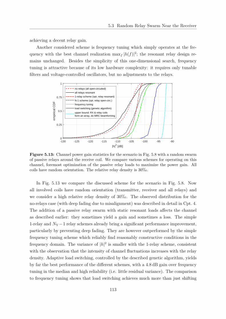
5.3 Random Relay Swarm Near the Receiver
achieving a decent relay gain.Another considered scheme is frequency tuning which simply operates at the fre-
quency with the best channel realization maxf |h(f)|2; the resonant relay design re-mains unchanged. Besides the simplicity of this one-dimensional search, frequencytuning is attractive because of its low hardware complexity: it requires only tunablefilters and voltage-controlled oscillators, but no adjustments to the relays.
-130 -125 -120 -115 -110 -105 -100 -95 -90
|h|2 [dB]
0
0.25
0.5
0.75
1
empi
rical
CD
F
no relays (all open-circuited)
all relays resonant
1-relay scheme (opt. relay resonant)
N-1 scheme (opt. relay open-circ.)
frequency tuning
load switching (genetic algorithm)
upper bound: RX & relay coilsform an array, do MRC beamforming
Figure 5.13: Channel power gain statistics for the scenario in Fig. 5.8 with a random swarmof passive relays around the receive coil. We compare various schemes for operating on thischannel, foremost optimization of the passive relay loads to maximize the power gain. Allcoils have random orientation. The relative relay density is 30‰.
In Fig. 5.13 we compare the discussed scheme for the scenario in Fig. 5.8. Nowall involved coils have random orientation (transmitter, receiver and all relays) andwe consider a high relative relay density of 30‰. The observed distribution for theno-relays case (with deep fading due to misalignment) was described in detail in Cpt. 4.The addition of a passive relay swarm with static resonant loads affects the channelas described earlier: they sometimes yield a gain and sometimes a loss. The simple1-relay and NY−1 relay schemes already bring a significant performance improvement,particularly by preventing deep fading. They are however outperformed by the simplefrequency tuning scheme which reliably find reasonably constructive conditions in thefrequency domain. The variance of |h|2 is smaller with the 1-relay scheme, consistentwith the observation that the intensity of channel fluctuations increases with the relaydensity. Adaptive load switching, controlled by the described genetic algorithm, yieldsby far the best performance of the different schemes, with a 4.8 dB gain over frequencytuning in the median and high reliability (i.e. little residual variance). The comparisonto frequency tuning shows that load switching achieves much more than just shifting
113

5 Randomly Placed Passive Relays: Effects and Utilization
resonance peaks back to the design frequency. The scheme is only 4.5 dB (median)below the highly optimistic baseline which relates to a hypothetical coil array consistingof the receive coil and all 20 relay coils, performing coherent receive beamforming.This shows that the presence of a passive relay swarm with optimized loads allows thereceiver to draw significantly more power from the magnetic field (the effect of thepassive relays is comparable to a parabolic reflector near a radio antenna).
5.4 Utilizing Spectral Fluctuations
In this final section we conduct a communication-theoretic study of the spectral fluctu-ations induced by magneto-inductive passive relays with static resonant loads. We areparticularly interested in the utilization for high data-rate communication. With theplots in Fig. 5.9 and 5.10 we already demonstrated that randomly deployed magneto-inductive passive relays give rise to a frequency-selective fading channel when stronglycoupled to one of the communicating nodes. In order to study this phenomenon sys-tematically we consider the correlation coefficient between the channel at the resonantdesign frequency h(fres) and the channel h(fres + ∆) for a frequency shift ∆, given by
ρ(∆) = E[AB∗ ]√E[|A|2 ] · E[|B|2 ]
, A = h(fres)− E[h(fres)], (5.15)
B = h(fres + ∆)− E[h(fres + ∆)] .
Naturally, the correlation coefficient fulfills |ρ(∆)| ≤ 1. We define the channel coherencebandwidth [90, Fig. 2.13] as one half of the main lobe width of ρ(∆), measured betweentwo points3 with a decorrelation of ρ(∆) = 1√
2 .In the discussion of Fig. 5.9 and 5.10 we already noted that the channel bandwidth
which is significantly affected by passive relays increases with the relay density. Wewant to capture this effect quantitatively. For that purpose we consider for the channelcoefficient the relative RMS deviation
σrel(f) =
√E[|h(f)− h0(f)|2 ]
|h0(f)| (5.16)
compared to the channel response h0(f) when no relays are present. We fix the trans-mitter and receiver orientation the same way as for Fig. 5.9 and 5.10 so that h0(f)
3At low relay density, side lobes which also reach ρ(∆) = 1√2 may occur; these are disregarded by
our definition of coherence bandwidth.
114

5.4 Utilizing Spectral Fluctuations
becomes deterministic. σrel(f) is the relative RMS deviation of h from h0 at a fre-quency of interest f . We define the affected bandwidth as the main lobe width of ρ(∆),measured between two points which fulfill σrel(f) = 1
10 .Fig. 5.14a shows the evolution of ρ(∆) over frequency shift ∆ for high relay den-
sity. We observe that the channel decorrelates significantly even for small ∆, i.e. thecoherence bandwidth is small. It decays with increasing relay density and attains avalue similar to the coil 3 dB bandwidth. However ρ(∆) never decays to zero (nofull decorrelation occurs) which we explain as follows. Each relay swarm realizationestablishes a general trend across most affected frequencies, i.e. by virtue of the re-alization the channel is either rather weak or rather strong across most frequencies.This explanation is supported by Fig. 5.9 to some extend. The evolution of σrel(f) inFig. 5.14b confirms the earlier discussion: the intensity of the channel fluctuations andthe affected bandwidth increases with the relay density.
-5 -4 -3 -2 -1 0 1 2 3 4 5
= f - fD
[MHz]
0
0.1
0.2
0.3
0.4
0.5
0.6
0.7
0.8
0.9
1
corr
elat
ion
coef
ficie
nt
()
volumetric
volumetric
(a) correlation coefficient
45 46 47 48 49 50 51 52 53 54 55
f [MHz]
0
0.1
0.2
0.3
0.4
0.5
0.6
0.7
0.8
0.9
1
RM
S r
el. c
hang
e du
e to
rel
ays
rel(f
)
volumetric
volumetric
(b) relative change
0 0.005 0.01 0.015 0.02 0.025 0.03
relative volumetric relay density
10-1
100
101
band
wid
th [M
Hz]
bandwidth significantly affectedby passive relays
coherence bandwidth
(c) evolution of coherence bandwidth and affected bandwidth
Figure 5.14: Characterization of the random frequency-selective magneto-inductive passiverelaying channel that arises from a random swarm of passive relays around the relay coil.
115

5 Randomly Placed Passive Relays: Effects and Utilization
We note that the affected bandwidth is much larger than the coherence bandwidthat high relay density. We conclude the availability of multiple frequency bands whosefading statistics are decorrelated to some extend (note that the channel spectrum isdetermined by 20 statistically independent relay deployments). This can be utilizedby the transmission scheme to achieve frequency diversity over this SISO channel.
In other words, when the channel is faded at the design frequency there is still agood chance to find a good channel at a different frequency: the peak(s) may haveshifted due to resonant mode splitting. This can be utilized by adapting the transmitpower allocation to the channel spectrum (ideally with the waterfilling principle) whenchannel state information is available at the transmitter. We investigate the resultingperformance in Fig. 5.15 in terms of the achievable data rates with a transmit powerof PT = 10µW. When the transmit power allocation is adapted to the channel via thewaterfilling principle then the presence of passive relays, even without any optimizationmeasures, gives rise to significant and reliable data rate improvements. This notion ofimproving the communication performance over a fading channel with transmit-sidechannel state information is well-known in the radio communication context (concern-ing fluctuations in time, frequency, and space) [90, Sec. 5.4.6]. It is particularly effectiveat low SNR, where using just the most constructively faded band proves very benefi-cial. The results in Fig. 5.15 also include the achievable rate with waterfilling after theadaptive load switching scheme (controlled by the genetic algorithm described earlier)has been used to maximize |h(fres)|2. This yields further significant improvements,consistent with the comparison of frequency tuning and load switching in Fig. 5.13.
We showed that passive relaying gives rise to significant and reliable improvementsof the communications performance if (i) the transmit signaling is adapted to thechannel spectrum realization which results from the specific coil arrangement or (ii)the relay loads are adapted in order to optimize the channel at the operating frequency.In any case the matching of the affected end (e.g. the receiver matching) must beadapted to the coupling conditions at hand. Future work should investigate possibleforms of coordinating load adaptation (e.g., load switching) with little to no intelligenceand communication capabilities at the passive relays. A possible approach could be agreedy scheme where each passive relay adapts its load capacitance in an attempt tomaximize its own induced current.
116

5.4 Utilizing Spectral Fluctuations
0 0.005 0.01 0.015 0.02 0.025 0.03
volumetric relay density
103
104
105
106
achi
evab
le r
ate
[bit/
s]
waterfillinguniform allocation between 50 MHz ± 0.5·B
3dB
medians
95th percentile values
5th percentile values
103 104 105 106
achievable rate [bit/s]
0
0.25
0.5
0.75
1
empi
rical
CD
F
no relays
PT allocated with
waterfilling &channeloptimizedvia relay loads
PT allocated uniformly
btw. fopt ± 0.5·B3dB
PT allocated uniformly
between 50 MHz ± 0.5·B3dB
waterfilling
Figure 5.15: Communication performance statistics over the random frequency-selectivemagneto-inductive passive relaying channel that arises from a random swarm of passive relaysaround the relay coil. We consider different signaling schemes and different channel states (norelays present, resonant relays present, relays with optimized load capacitances present). Theassumed transmit power is PT = 10µW. The frequency tuning scheme allocates the transmitpower in a band around fopt = arg max |h(f)|2 (bandwidth equal coil 3 dB bandwidth),determined for each realization individually.
117

5 Randomly Placed Passive Relays: Effects and Utilization
118

Chapter 6
A Study of Magnetic Induction forSmall-Scale Medical Sensors
With the use of the introduced concepts, this chapter studies the highly relevant tech-nological context of enabling wireless powering and communication for medical in-bodymicrosensors (microrobots). In Cpt. 1 we already discussed that this significant goal ofbiomedical research is expected to provide untethered diagnostic sensing and treatmentin future medical applications. A big problem of the approach is that, on the one hand,the sensors must be sufficiently small for minimally-invasive maneuvering in cavitiesof the human body but, on the other hand, a very small sensor device can not beequipped with a useful battery. Wireless powering as a potential alternative howeveralso does not allow for an arbitrarily small device size because efficient wireless powerreception requires a rather large antenna aperture. This holds especially true in thebiomedical context where tissue absorption causes significant signal attenuation.
In the face of these problems, a natural question is the minimum sensor size thatstill allows for running the device with wireless powering. Related questions concernthe achievable data rate of wireless data transmission from the sensor to an externaldevice (uplink) and whether this transmission should be realized in an active or passivefashion, i.e. whether a transmit amplifier or load modulation via circuit switchingshould be employed at the sensor. In this chapter we consider magnetic induction inthis context, because of its capabilities in terms of power transfer and media penetration(see Cpt. 1). Specifically, this chapter makes the following contributions:
• We develop the biomedical sensor problem context from a wireless engineeringperspective and discuss key design considerations and trade-offs.
• We evaluate the data uplink from a wireless-powered in-body sensor using activetransmission and compare the results to load modulation. We do so for differ-ent important cases of the transmission scheme and assumptions on the channelknowledge (full knowledge, sensor location knowledge, no knowledge).
• We show that placing several small-scale passive relay coils near the sensor nodeyields significant performance gains if (and only if) the relay loads are optimized.
119
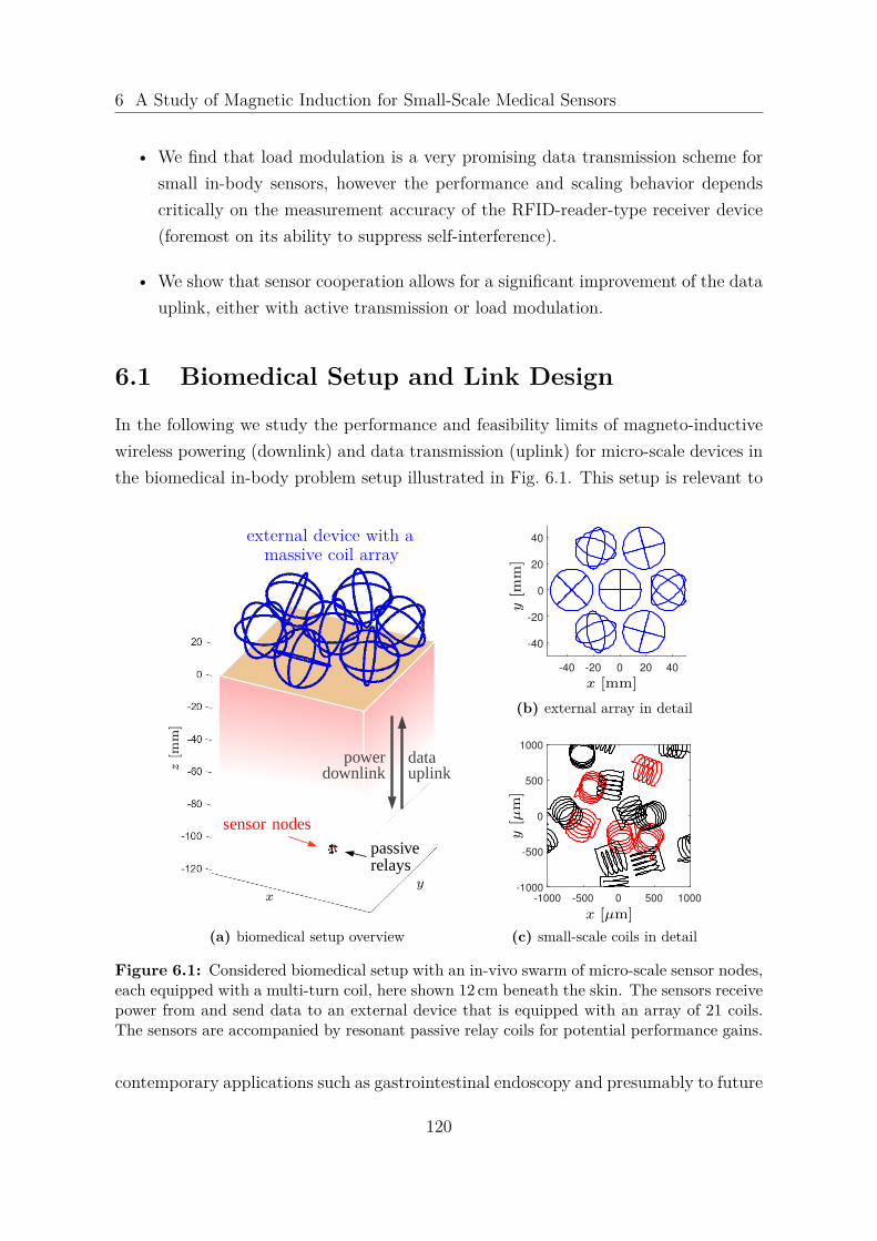
6 A Study of Magnetic Induction for Small-Scale Medical Sensors
• We find that load modulation is a very promising data transmission scheme forsmall in-body sensors, however the performance and scaling behavior dependscritically on the measurement accuracy of the RFID-reader-type receiver device(foremost on its ability to suppress self-interference).
• We show that sensor cooperation allows for a significant improvement of the datauplink, either with active transmission or load modulation.
6.1 Biomedical Setup and Link Design
In the following we study the performance and feasibility limits of magneto-inductivewireless powering (downlink) and data transmission (uplink) for micro-scale devices inthe biomedical in-body problem setup illustrated in Fig. 6.1. This setup is relevant to
y
x
z[m
m]
sensor nodes
passiverelays
powerdownlink
datauplink
external device with amassive coil array
(a) biomedical setup overview
-40 -20 0 20 40
-40
-20
0
20
40
x [mm]
y[m
m]
-1000 -500 0 500 1000
-1000
-500
0
500
1000
x [µm]
y[µ
m]
(b) external array in detail-40 -20 0 20 40
-40
-20
0
20
40
x [mm]
y[m
m]
-1000 -500 0 500 1000
-1000
-500
0
500
1000
x [µm]
y[µ
m]
(c) small-scale coils in detail
Figure 6.1: Considered biomedical setup with an in-vivo swarm of micro-scale sensor nodes,each equipped with a multi-turn coil, here shown 12 cm beneath the skin. The sensors receivepower from and send data to an external device that is equipped with an array of 21 coils.The sensors are accompanied by resonant passive relay coils for potential performance gains.
contemporary applications such as gastrointestinal endoscopy and presumably to future
120

6.1 Biomedical Setup and Link Design
applications of medical microrobots. The setup comprises several micro-scale in-bodysensors beneath the skin. An external device, which sits above the skin, serves as thetransmitting field source for wireless powering (downlink) as well as the receiving datasink of sensor data (uplink). We assume a downlink transmit power of PT,DL = 1 W forwireless powering, which is deemed sufficiently small to prevent any thermal injuriesto the patient. The device features a massive array of 21 coils in order to obtain vastspatial diversity, an array gain, and potentially even a spatial multiplexing gain (seeSec. 3.7.5, Sec. 3.8.2, and Sec. 4.3).
We will later also consider the sensor coil(s) being accompanied by resonant passiverelay coils of equal size, as indicated in the illustration. These passive relay coils couldbe inactive sensor nodes engaging in passive cooperation. We are interested in thepassive relaying gains (e.g., as seen in Cpt. 5) available in this biomedical context.
6.1.1 Choosing the Operating Frequency
The operating frequency (or rather: the design frequency of the matching circuits)fc should be as large as possible for strong magnetic induction (cf. the role of ω in(2.23)) but sufficiently low to penetrate tissue and, furthermore, to avoid a performancelimitation due to the radiation resistance. In other words, the wavelength should exceedthe coil wire length considerably. We note that a wavelength with similar order ofmagnitude as the link distance would provide the polarization diversity effect of thenear-far-field transition described in Cpt. 4. Based on these arguments we considerfc = 300 MHz as an interesting design frequency (associated with 1 m wavelength).
6.1.2 External Coil Design
After a careful study based on the theory in Sec. 2.2, we choose the following external-side coil geometry in order to achieve a large Q-factor and thus a good link performanceat the chosen 300 MHz. We choose circular single-turn coils with 10 cm circumference,which is about the maximum size where they are still electrically small ( 1
10 of thedesign wavelength). We choose a large wire diameter of 3 mm to establish a smallohmic resistance. This coil geometry exhibits Rohm ≈ 45 mΩ and Rrad ≈ 19 mΩ as wellas a realizable Q-factor of ≈ 1380 at the 300 MHz design frequency.
121

6 A Study of Magnetic Induction for Small-Scale Medical Sensors
6.1.3 Tissue Attenuation and Sensor Depth
We shall now investigate the choice of operating frequency in more detail and underdue consideration of the desired sensor depth and the electrical properties of tissue.We employ the theory from Sec. 2.1.6 to account for tissue attenuation: the penetratedmaterial is modeled in terms of its complex propagation constant
γ = jω
√µε(
1− jσ
ωε
)(6.1)
as stated earlier in (2.34). We assume that the penetrated material consist entirelyof muscle tissue and evaluate γ as a function of frequency with the use of numericalvalues for the permittivity ε and conductivity σ given by the so-called Debye modelfor muscle tissue in [209, Fig. 3]. In the process we assume a relative permeabilityof 1 which is adequate for most organisms (humans, animals, plants) [54]. The effectof tissue on channel coefficients is calculated as follows. Any link distance r of anexternal-to-internal link is decomposed into a distance rfree traveled in free space and adistance rtissue traveled in tissue, i.e. r = rfree + rtissue. We then replace the factor e−jkr
that would apply to the free-space channel coefficient with e−jkrfreee−γrtissue , whereby kis the wavenumber. From Sec. 2.1.6 we recall the depth of penetration 1/Re(γ), thedistance into tissue where an amplitude attenuation of e−1 = −8.7 dB applies [52].
105 106 107 108
f [Hz]
0
5
10
15
20
25
30
dept
h of
pen
etra
tion
[cm
]
0 5 10 15 20
sensor depth [cm]
-70
-60
-50
-40
-30
-20
-10
0
atte
nuat
ion
due
to ti
ssue
[dB
]
at 300 MHz
at 5 MHz
Figure 6.2: Depth of penetration 1/Re(γ) and attenuation 20 log10 e−Re(γ)·rtissue in muscle
tissue, based on the complex propagation constant γ from (6.1). The calculation uses per-mittivity and conductivity values over frequency given by the Debye model in [209, Fig. 3].
The numerical evaluation in Fig. 6.2 of this tissue attenuation model shows thedecrease of penetration depth with increasing frequency. We observe that a sensordepth of 12 cm is associated with severe attenuation if the operating frequency exceeds
122

6.1 Biomedical Setup and Link Design
about 4 MHz. Smaller sensor depths such as 5 cm allow the use of a much largerfrequency (and hence stronger induction and more communication bandwidth) withlittle attenuation. The implications are analogous to those in [209, Fig. 6], where theysuggest a frequency slightly above 1 GHz for sensor depths of a few centimeters. Formore detailed studies on magnetic fields in tissue we refer to [209–211].
6.1.4 Sensor Coil Design
As a next step towards a detailed study we need to define the geometry of the sen-sor coils. First we note that micro-scale coils are certainly electrically small at anymeaningful operating frequency. We consider the following size constraint on the coilgeometry: the coil must fit into a cube of a given size. The sensor coil design objectiveis to achieve a large Q-factor within this limited volume. This is achieved by choosinga large turn number, coil diameter, and wire diameter without violating the constraint.Using the formulas in Sec. 2.2 we find a suitable design in the form of a single-layersolenoid coil whose height equals its diameter (henceforth called size, which is equal tothe edge length of the aforementioned cube) as seen in Fig. 6.1c. After careful compar-isons we decide to use 5 turns and a turn spacing of 1.5 wire diameters. For the wirematerial we assume the conductivity of copper.
We note that, in order to obtain a decent Q-factor, the coil geometry must be spreadout such that the size constraints are exhausted in all three dimensions. For example,a flat printed coil is a bad design because its small wire cross section would result inlarge ohmic resistance and thus a small Q-factor. Because of this volume-limitationproblem we also decide to use a single coil per sensor device instead of an array ofeven smaller coils (thereby we sacrifice potential gains from further spatial diversityand spatial multiplexing but keep the complexity small).
Finally we have to specify the sensor-side matching network. Each sensor coilis matched individually with a two-port matching network of two capacitors in L-structure (as in Fig. 3.6b). Thereby we use power matching via the 2 × 2 versionof rule (3.39). This matching network applies to both the down- and uplink. Thematching bandwidth is large because the coil is small and the Q-factor decreases withthe coil size (e.g., Q ≈ 63.7 for 0.5 mm size, Q ≈ 23.5 for 0.2 mm size, and Q ≈ 10 for0.1 mm size).
123

6 A Study of Magnetic Induction for Small-Scale Medical Sensors
6.1.5 Tissue Attenuation and Sensor Depth Revisited
Now that we have decided on specific coil designs, we shall proceed with a more detailedstudy of tissue attenuation at the example of the wireless powering downlink. Weconsider a setup similar to Fig. 6.1 but much simpler, with just a SISO link betweena single external coil (one of the central tri-axial cluster) as transmitter and just asingle sensor as receiver. We assume that the two coils are in coplanar arrangement.Furthermore, we do not consider any passive relays. Fig. 6.3 shows an evaluation ofthe power transfer efficiency over frequency for two different cases in terms of sensorsize and depth. The results show that the operating frequency must be chosen under
105 106 107 108
f [Hz]
10-9
10-8
10-7
10-6
10-5
10-4
rece
ived
pow
er [W
] free space
in muscle tissue
required to activate sensor
(a) 5 cm sensor depth (0.5 mm coil size)
105 106 107 108
f [Hz]
10-9
10-8
10-7
10-6
10-5
10-4
rece
ived
pow
er [W
]
required to activate sensor
free space
in muscle tissue
(b) 12 cm sensor depth (2 mm coil size)
Figure 6.3: A simple evaluation of SISO power transfer efficiency versus frequency. Thetransmitter is a single external coil (of the central cluster), the receiver a single sensor coil.The two coils are in coplanar arrangement.
due consideration of the desired sensor depth. This is made apparent by the significantdifferences between the black graphs of the two cases. For the low-frequency regime,where the depth of penetration exceeds the sensor depth, we note that increasing thefrequency is always beneficial. At larger frequencies, where tissue causes severe signalattenuation, we observe that a frequency increase can yield limited gains or significantlosses, depending on the sensor depth. In all subsequent experiments we will considerthe smaller sensor depth of 5 cm and stick with the 300 MHz operating frequency.
The red line in each plot indicates the assumed minimum downlink received powerP0 = 50 nW that is required to activate the sensor chip (for comparison, the 2009paper [212] describes a biomedical sensor implementation that required 450 nW).
124

6.2 Wireless Powering Downlink
6.2 Wireless Powering Downlink
This section studies the performance of the MISO downlink from the 21-coil array toa single sensor, with transmit beamforming used at the array. Before that we have toclarify a few last design aspects though.
6.2.1 Array Transmit Matching and Spacing
First, we specify the placement of the coils that constitute the external array whichconsists of seven tri-axial coil clusters. Their orientations are chosen in a heuristic fash-ion with the idea of limiting the inter-array coupling. For all subsequent experimentswe choose a hull-to-hull (not center-to-center) spacing of 3 cm between neighboringtri-axial coil clusters. This choice will be dictated by the uplink reception propertiesof the array and argued in detail later in Sec. 6.3.1.
We assume that the transmit amplifiers of the high-complexity external device arecapable of driving any desired currents through the coil array. Our primary interest arethereby the coil currents, which determine the power of the generated electromagneticfield and the resulting exposure for the patient. Potential intrinsic power losses, e.g.due to mismatch or the use of class A amplifiers with high linearity but poor powerefficiency, are of secondary nature. To this effect, we employ the assumption of idealtransmit-side power matching from (3.47) for the powering downlink because it is thesimplest formal way of capturing just the effects of interest.
6.2.2 Downlink Performance
The performance of transmit beamforming depends critically on the employed schemeand the availability of channel information, i.e. whether the channel vector is knownto the external device. We study three different cases:
• Maximum-Ratio Combining: The transmit signal vector is set x = h∗√PT,DL
based on full knowledge of the channel vector h. This way we attain the maximumreceived-power value PR,DL = |hTx|2 = ‖h‖2PT,DL (cf. Sec. 3.4).
• Using Sensor Location Knowledge: Since the receiving sensor coil is a single-layer solenoid with small pitch angle, we can use the channel vector descriptionh = VHoR in terms of projections of field vectors generated by the external coilsonto the receive-coil orientation oR (cf. Sec. 3.7.3 and Proposition 4.3). We
125

6 A Study of Magnetic Induction for Small-Scale Medical Sensors
assume that the sensor location is known and that, consequently, the field vec-tors in V can be calculated.1 The sensor coil orientation oR is however assumedunknown and random with a uniform distribution in 3D. For this case, Proposi-tion 4.8 states that the channel vector covariance matrix is E[hhH ] = 1
3VHV. Weutilize this property for beamforming: the transmit vector is set to x = q
√PT,DL
where q is a unit-length eigenvector of VHV associated with its largest eigen-value. This way we maximize EoR [PR,DL ] = EoR [|hTx|2 ] and attain the valueEoR [PR,DL ] = 1
3 · λmax(VHV) · PT,DL, although without robustness guaranteesregarding the actual realizations of PR,DL (i.e. fading may occur).
• Random Beamforming: When no channel information is available, we resortto the use of a random transmit vector x = u
‖u‖
√PT,DL where u is sampled from
a complex-valued Gaussian distribution u ∼ CN (0, INT) with NT = 21. Fadingwill occur whenever the chosen x is near-orthogonal to the channel vector.
10-9 10-8 10-7 10-6 10-5 10-40
0.25
0.5
0.75
1
full channel knowledgelocation knowledgeno channel knowledge
in muscle tissue free space
required sensoractivation power
Figure 6.4: Statistics of the received power at a sensor device with random orientationvia the MISO downlink, evaluated for different transmit beamforming schemes. The sensordepth is 5 cm, the sensor coil size is 0.5 mm, and the transmitting external 21-coil array usesa sum power of PT,DL = 1 W. This is a single-frequency evaluation at 300 MHz.
The received power statistics for a randomly oriented sensor are shown in Fig. 6.4.As expected, the availability of channel knowledge and resulting choice of beamformingscheme has a huge effect on the mean performance and robustness. To interpret the
1We note that this location-knowledge-based transmit beamforming scheme, which employs Propo-sition 4.8, is based on the simplified propagation model described in Sec. 6.1.3. The field vector direc-tion may be different (and hard to predict for a given position) in an actual biomedical application,where propagation is affected by various types and shapes of tissue and medium transitions.
126

6.3 Data Uplink
results we shall first note that the sensor depth (or, put differently, the operatingfrequency) is too small to really benefit from the polarization diversity effect in the near-far-field transition.2 The misalignment losses are thus essentially characterized by thepure near-field regime. This is consistent with the observed performance of maximum-ratio combining, which varies in a 6 dB window, as predicted by JNF = βNF ∈ [1
2 , 1]in Sec. 4.3.1 (this is just the field magnitude loss, cf. (4.9)). Thereby, devastatingorthogonality between field vector and coil axis is prevented.
This mechanism is unavailable to the location-knowledge scheme, which, as a result,frequently results in severe losses. In particular, the location-knowledge scheme justmaximizes the field magnitude at the sensor location without regarding the sensororientation. This provision establishes a large median received power, which makes itan appealing for biomedical applications where the approximate sensor location willoften be known. However, the CDF tail for very small values shows that the outagebehavior of the location-knowledge scheme is even worse than that of the randombeamforming scheme. This is an effect of the dominance of near-field propagation inthis setting, in particular because the eigenvector q associated with λmax(VHV), whichdetermines the transmit vector x = q
√PT,DL , exhibits near-collinearity of Re(q) and
Im(q) (and because the channel vector h has the same behavior).3 In contrast, therandom beamforming scheme x = u
‖u‖
√PT,DL with u ∼ CN (0, I21) typically exhibits
near-orthogonal Re(x) and Im(x), resulting in slightly better outage behavior.
6.3 Data Uplink
While supplying power to a sensor is an interesting challenge in its own right, we shallnow shift our focus to the data transmission capabilities of micro-scale in-body sensors.We first consider the data uplink via active transmission, i.e. the sensor device drivesits coil with its own transmit amplifier. The uplink transmit power is assumed to be
PT,UL = max
0, 12(PR,DL − P0)
(6.2)
2At 300 MHz, kr ≈ 0.414 applies between the external coils of the central triaxial cluster anda 5 cm deep sensor coil. Through Fig. 4.2 we find that, in this regime, polarization diversity onlyaffects misalignment losses that are already worse than −30 dB. The polarization diversity effectwould be most pronounced at a distance of 0.3747 m, which corresponds to the near-far thresholdvalue kr = 2.3540 from (2.33).
3This suggests a possible adaptation to the location-knowledge beamforming scheme: set the trans-mit signal according to x = 1√
2 (q1+jq2)√PT,DL where q1 and q2 are eigenvectors of VHV correspond-
ing to the largest and second-largest eigenvalue, respectively. This adaptation improves the outagebehavior but sacrifices the discussed optimality property regarding the maximization of EoR [PR,DL ].
127

6 A Study of Magnetic Induction for Small-Scale Medical Sensors
or in words, PT,UL is half of the received downlink power in excess of the assumed chipactivation power P0 = 50 nW. For simplicity we make the idealistic assumption thatthe power downlink and data uplink operate simultaneously in a full-duplex fashion.An investigation of appropriate practical duplexing schemes is out of scope.
6.3.1 Array Receive Matching and Spacing Revisited
The assumptions on the receive matching network of the external coil array requirecareful consideration in order to obtain practically relevant results for the uplink per-formance. A reactive noise matching network fulfilling (3.43) would be SNR-optimal atthe design frequency and could theoretically be realized with the approach in Fig. 3.7.However, such a network between the 2 · 21 = 42 ports at hand would exhibit a verysmall matching bandwidth and can not realistically be implemented (see the discussionin Sec. 3.6). Hence we discard this approach. Instead we choose to match the arraywith an individual two-port network per coil-load pair, each consisting of three reactivelumped elements in T-pad structure (i.e. we use a total of 21 two-port networks; theconcept is described by Fig. 3.5 together with Fig. 3.6a).
Tuning the component value of these two-port networks is crucial and challengingif the spacing between the seven tri-axial coil clusters is small, because then stronginter-array coupling occurs between these high-Q coils (we demonstrated the associatedproblems in Fig. 3.7). Choosing a small spacing is however incentivized by the desire ofmaintaining short distances between outer clusters and sensors. We shall demonstrateand study this trade-off for the data uplink for different array matching paradigms:
1. Full 21-coil array with 21 individual T-pad two-port networks for noise matchingeach coil individually for its uncoupled impedance.
2. Same as above but the two-port networks are iteratively adapted to the inter-array coupling conditions in a round robin fashion and according to the two-portnoise matching rule, using the encountered coil impedance.
3. Same as above but numerically optimized for maximum average SNR at thedesign frequency, averaged over the random sensor orientation and optimizedwith a single run of an iterative gradient-search algorithm.
4. Baseline: ideal multiport noise-matching network (implementation unrealistic).
5. Baseline: using just the 3-coil array constituted by the central tri-axial sub-array.
128

6.3 Data Uplink
0 2 4 6 8 10 12 14106
107
108
109
1010
5.) baseline: array is just one tri-axial cluster
1.) T-pad two-ports, designed for uncoupled conditions
2.) T-pad two-ports, re-matched iteratively (round robin)
3.) T-pad two-ports, numerically optimized
4.) baseline: ideal multiport matching
Figure 6.5: Data uplink performance versus external array spacing. The plotted per-formance measure is the squared norm ‖hUL‖2 = hH
ULK−1hUL of the noise-whitened uplinkchannel vector hUL. In particular we evaluate its mean value; the randomness stems from theassumed random orientation of the sensor coil. The considered noise bandwidth is 100 kHz.The evaluation considers muscle tissue, 300 MHz carrier frequency, 5 cm sensor depth, and0.5 mm sensor size.
We observe that using more than one tri-axial cluster is beneficial (owing to a receivearray gain) if and only if an appropriate matching strategy is employed. Approachingthe performance of the theoretically ideal multiport strategy with a practical strat-egy requires significant optimization effort; simplistic practical matching strategies areclearly associated with significant losses.
Based on the observed behavior we decide on a 3 cm array spacing between tri-axial coil clusters. We use matching strategy number 3, i.e. individual T-pad two-portnetworks whose component values are tuned with an iterative gradient search thatmaximizes the mean ‖hUL‖2, without claiming global optimality. In particular, we aimfor a larger matching bandwidth by maximizing the sum of mean ‖hUL‖2 values in dBat the frequency points 296, 298, 300, 302, 304 MHz (the 300 MHz summand has doubleweight). This shall allow for large uplink data rates despite the small 3-dB bandwidthof the external coils (≈ 215 kHz). The outcome is seen in Fig. 6.6c.
6.3.2 Achievable Rates with Active Transmission
We will now study the system from a broadband perspective, i.e. we carefully con-sider and utilize spectral channel fluctuations. The frequency spectra of various key
129

6 A Study of Magnetic Induction for Small-Scale Medical Sensors
280 290 300 310 320 330 340
-110
-100
-90
-80
-70
-60
-50
no passive relays19 passive relays near sensor
(a) squared norm of downlink channel vector
290 295 300 305 310
-110
-100
-90
-80
-70
-60
-50
(b) squared norm of uplink channel vector
290 295 300 305 310104
105
106
107
108
(c) squared norm of noise-whitened uplink - - -- - - -channel vector hUL for 100 kHz bandwidth
290 295 300 305 310
-174
-173
-172
(d) uplink receiver noise PSD
Figure 6.6: Frequency spectra of the key quantities that determine uplink communicationperformance. The evaluation considers a sensor of 0.5 mm size which is located 5 cm deep inmuscle tissue. The transmitting sensor uses an L-pad two-port matching network designedat 300 MHz, the receiving external array is matched as described in Sec. 6.3.1. The passiverelays near the sensors (which are of equal size) only have a minor effect because their Q-factor is small due to the small coil size. The shown noise PSD is of the horizontal coil of thecentral cluster.
quantities are depicted in Fig. 6.6. We note that Fig. 6.6a yields very useful insightsfor wireless powering downlink: the PTE spectrum exhibits a significant resonancepeak at 304 MHz, a consequence of the strong inter-array coupling.4 We choose to usethese 304 MHz instead of 300 MHz for the downlink and this way obtain a spectacular19.5 dB gain for wireless powering.
4Future work should study the precise conditions for such resonance peaks to arise and the feasi-bility of realizing them in practice. At this point we can only state that they are caused by strong
130

6.3 Data Uplink
0 0.25 0.5 0.75 1 1.25 1.5
sensor size [mm]
0
1
2
3
4
5
6
7
8
uplin
k da
ta r
ate
[Mbi
t/s]
mean rate
5% outage rate
no channelknowledge
sensor locationknowledge
full channelknowledge
Figure 6.7: Achievable rate of the data uplink whereby the transmit power is determinedby the downlink received power. The wireless-powered sensor is 5 cm deep into muscle tissue,the required sensor activation power is 50 nW. The external array is the receiving end.
Given the available uplink transmit power PT,UL we are interested in the achievableuplink data rate (in the information-theoretic sense as in Sec. 3.5) for reception inadditive Gaussian noise5 according to the model in Sec. 3.2. We consider the samethree cases of channel knowledge as earlier in Fig. 6.4. We conduct receive beamformingat the external array, which formally transforms the broadband SIMO channel into abroadband SISO channel. For the case of full channel knowledge we assume receive-sidemaximum-ratio combining, for the other cases we assume selection combining.
Fig. 6.7 shows the evolution of achievable uplink data rate over sensor coil size. Thedata rate is random due to the random sensor orientation; the plot shows the meanvalue as well as the 5th-percentile value. With full transmit-side channel knowledge, weachieve channel capacity by using waterfilling as in (3.33) for spectral power allocation,based on the norm of the noise-whitened channel vector. In the other cases the poweris allocated uniformly over the 3-dB bandwidth of the external array.
inter-array coupling. One potential issue of the evaluation at hand is that the array as a whole, whoseouter circumference of ≈ 48.9 cm is about one half of the 1 m wavelength, may not qualify as anelectrically small circuit (although its constituent coils are indeed electrically small) and thus may notbe eligible for AC circuit analysis. Also, capacitive coupling and feed wires might have a significanteffect. These aspects should be clarified by comparing to full-wave simulation and/or experiments.
5This experiment (and all subsequent active-uplink considerations) use the noise parameters inTable 5.1 of Cpt. 5. To describe the spatial correlation matrix Φ of extrinsic noise, which occursat the external array and impairs reception in the uplink, we account for spatial correlation withthe model Φmn = J0(krmn) oT
mon, which uses the center-to-center coil distance rmn, the orientationvectors om and on of the involved coils, and the Bessel function J0 (cf. [103,213]).
131

6 A Study of Magnetic Induction for Small-Scale Medical Sensors
We observe that a sensor can be activated and transmit data to outside the body ifits coil size is larger than about 0.35 mm. Such size would be sufficiently small for manymedical target applications [23]. With increasing size, the data rate grows rapidly asthe sensor coil Q-factor and the mutual impedances to the external coils increase. Weobserve that the required minimum sensor size depends heavily on the availability ofchannel information and the desired outage rate.
6.3.3 Small-Scale Swarms of Passive Relays
We are interested in potential performance gains from passive relays, whose capabilitieshave been demonstrated in Cpt. 5, in the biomedical context. We consider a randomlyarranged swarm of 19 passive resonant relay coils around the sensor node (and with thesame coil geometry, now with an assumed 0.35 mm size). They could be placed in hopesof a performance gain or just represent nearby idle sensor nodes. Strong coupling toa relay causes resonance splitting and induced frequency shifts of the resonance peakson the order of the sensor-coil 3 dB bandwidth, which is ≈ 7 MHz for the considered0.35 mm coil size. Likewise, dense and arbitrarily arranged swarms of passive relayscause f -selective fading as described in Cpt. 5. We are interested in the implications forour application. All coil orientations are random with uniform distribution in 3D, seeFig. 6.1c, and the passive relay locations are sampled per coordinate from a Gaussiandistribution about the sensor location (the standard deviation is two times the coil sizeand we re-sample until no coils collide in terms of their cylindrical hulls). All relay coilorientations are random whereby all possible directions being equiprobable. The sensormatching is adapted to the relay coupling conditions. We use the dominant peak at304 MHz in the downlink and waterfilling in the uplink.
Fig. 6.8 shows the resulting uplink rates for many realizations of the random swarmgeometry. We observe that, without further ado, the presence of passive relays hardlyaffects the performance statistics. This is in contrary to the results of the previouschapter, in particular to Sec. 5.4, where the utilization of passive-relay-induced spectralchannel fluctuations together with transmit-side channel information (waterfilling) ledto significant data rate improvements. This discrepancy can be accredited to the vastasymmetry of the link: the coil 3-dB bandwidth is 32 times larger on the sensor sidecompared to the external side. Because of this, a large portion of the relay-inducedchannel fluctuation falls outside the essentially usable frequency band(s).
Still, a large performance gain can be realized when relay load capacitances areoptimized in a controlled fashion. Specifically, we employ the load switching scheme
132

6.3 Data Uplink
0 1 2 3 4 5 6 7 8 9 10
uplink data rate [Mbit/s]
0
0.25
0.5
0.75
1em
piric
al C
DF
no passive relays19 passive relays, resonant at 304 MHz19 passive relays, load capacitances optimized
Figure 6.8: Data uplink performance of a single actively transmitting sensor in close vicinityof a dense cluster of passive relays. The coils are 0.35 mm in size and located 5 cm deep intissue. The scheme employs adaptive sensor matching, frequency-tuning in the poweringdownlink and waterfilling in the uplink. Optimization of relay load capacitances is done viathe genetic-algorithm-based switching scheme from Sec. 5.3.
from Sec. 5.3, which uses a genetic algorithm, to maximize ‖hDL‖2 at 304 MHz. Out-of-band effects are not an issue with this controlled approach. We observe vast resultingperformance improvements, especially to the lower percentile of data rates (i.e. tocases with a severely misaligned sensor orientation). In this context note that passiverelaying here improves both the downlink and the uplink.
In conclusion, we can state that this form of passive cooperation poses an interestingand powerful technique also in this biomedical context. How such an optimizationscheme could be coordinated between passive nodes, equipped with minimal technicalcapabilities, is left as an open problem.
6.3.4 Achievable Rates with Load Modulation
Finally we want to investigate the data uplink via load modulation at a passive sensorand decoding of the transmitted bit at the external array, which now acts like an RFIDreader. Here we do not assume a minimum required power to activate the device(e.g., it might gather sufficient power from energy harvesting to run the load switchingprocess). The evaluation follows the theory in Sec. 3.9, i.e. the data rate is evaluatedwith the capacity formula (3.59) for the binary symmetric channel, expressed in bit perchannel use. The data rate is random because the sensor orientation is random; againwe evaluate the mean rate and 5th-percentile value. We do so for two cases: (i) basedon full knowledge of the channel, the current vector at the external array is set to its
133

6 A Study of Magnetic Induction for Small-Scale Medical Sensors
SNR-optimal value under a 1 W sum-power constraint based on Proposition 3.5 and(ii) without channel knowledge we use a random current vector with the appropriatesum power. We assume that the noise bandwidth equals the channel access rate fb (thenumber of channel uses per second). The maximum channel access rate is determinedby transients signal at the high-quality external coils; we choose fb = 2 · 105 which isvery close to the ratio fc/Qext. We compare two different noise models: thermal noiseonly and the more pessimistic model described below (3.57), which comprises errorfrom limited fidelity and residual self-interference.
0 0.1 0.2 0.3 0.4 0.5 0.6 0.7
sensor size [mm]
10-4
10-3
10-2
10-1
100
load
mod
ulat
ion
data
rat
e [b
pcu]
mean rate5% outage rate
no channelknowledge
with channelknowledge
(a) thermal noise only
2 4 6 8 10
sensor size [mm]
10-4
10-3
10-2
10-1
100
load
mod
ulat
ion
data
rat
e [b
pcu]
mean rate5% outage rate
no channelknowledge
with channel knowledge
(b) pessimistic error model
Figure 6.9: Uplink data rate with load modulation at a passive sensor, 5 mm deep intomuscle tissue. The results are expressed in terms of channel capacity (3.59) in bit per chan-nel use. The access rate is 2 · 105 channel uses per second, associated with 200 kHz noisebandwidth. The external array, which acts like an RFID reader in this case, uses 1 W forfield generation. The data rate is random by virtue of the random sensor coil orientation.
The results in Fig. 6.9 show that load modulation can be a powerful low-complexityalternative to active transmission: if thermal noise constitutes the only limitation, thendecent data rates can be achieved reliably with a sensor smaller than 1 mm. However,the performance depends critically on the measurement accuracy and fidelity of thereceiving array. In particular, when the external array suffers from significant self-induced errors, i.e. it drives an inaccurate current and/or fails to cancel the self-inducedvoltage (a problem described in detail by [63]), then a sensor size larger than 5 mm(which is incompatible with most in-body applications) is required for somewhat usefulperformance. Future work should study these practical limits, especially feasible noiselevels in between the discussed optimistic and pessimistic model, in greater detail.
134

6.4 Cooperative Data Uplink
6.4 Cooperative Data Uplink
We consider a swarm of small-scale in-body sensors as illustrated in 6.1c. All sensordevices are equipped with transmit amplifiers and are supplied with power wirelesslyas described in 6.2. Assume that one of the sensors has the acute need to transmitdata to the external device while all other sensors are idle. Instead of remaining idle,they assist in the uplink data transmission via physical layer cooperation (distributedbeamforming). This requires that the initiating sensor broadcasts its data to the othersensors, but because of the short distances between the sensors we assume that thisfirst hop does not constitute a limitation. Instead we focus on the final hop: the MIMOlink from the distributed sensor coils to the external coil array. We assume that thesensors can establish phase synchronization which is feasible because of the sub-GHzoperating frequency. Furthermore, full channel knowledge is assumed for both ends.
We also consider a scenario where the sensor swarm is intertwined with a swarm of15 passive relays. Those shall propel spectral and spatial channel variations, which canbe exploited by the transmit signaling. The positions and orientations of the sensorand relay coils are randomly sampled like in Sec. 6.3.3. In any scenario, the sensormatching networks are adapted to the swarm coupling conditions.
0 2 4 6 8 10 12 14
uplink data rate [Mbit/s]
0
0.25
0.5
0.75
1
empi
rical
CD
F
no passive relayspassive relays present, resonant at 300 MHz
achievable ratewith general Q
i
single sensortransmission
upper bound: capacity withpower sharing among sensors(sum-power constraint)
achievable ratewith diagonal Q
i
five sensors,cooperativetransmission
Figure 6.10: Uplink data rates from five cooperating in-body sensors, with and withoutnearby passive resonant relay coils in random arrangement, to an external 21-coil array.Either case considers 20 in-body coils of 0.35 mm size, 5 cm deep into muscle tissue. Theexternal device uses 1 W to supply power wirelessly. The results are shown as cumulativedistribution function (CDF). The data rate is random because of the random orientation ofthe sensor coils and passive relays.
The wireless powering downlink uses maximum-ratio transmit combining at the ex-
135

6 A Study of Magnetic Induction for Small-Scale Medical Sensors
ternal array to maximize the received sum power over this frequency-selective MIMOchannel (which results in a concentration of transmit power into the 304 MHz frequencydescribed in Sec. 6.3.2). This way we feed vast power to sensors with a good channel,with the idea that those sensors should also see a good channel in the uplink (which de-pends on array matching and noise statistics though). The beamforming is constrainedto activate the initiating sensor (i.e. assert received power ≥ P0) whenever possible.
The resulting uplink transmit power PT,n of the n-th sensor (n = 1 . . . 5) is accord-ing to (6.2). Therewith, we operate on the frequency-selective MIMO uplink channelas follows. We allocate the transmit power PT,n = ∑
k Pk,n available at the n-th sensorto frequency bands k with a heuristic approach: via waterfilling over the hypotheticalparallel SISO channels that would arise when all other sensors are silent (but present)and maximum-ratio combining is done at the receiving external array in each band k.The achievable uplink rate is DUL = ∑
k ∆fDk whereby Dk is the achievable MIMOrate in the narrow band k. For each k, we evaluate Dk in various different way. First,the suboptimal but easy-to-determine achievable rate (3.37), resulting from a diagonaltransmit covariance matrix. Second, the channel capacity under per-transmitter powerconstraints given by Pk,n for the coupled transmitters n = 1 . . . 5, given by (3.36),which is calculated by numerically solving the optimization problem. For comparisonwe include the channel capacity under a sum-power constraint (3.32), which could beachieved if the sensors were able to share their available power. We also compare tothe case without cooperation (i.e. to Sec. 6.3.2).
Fig. 6.10 shows that physical layer cooperation yields a significant increase of uplinkdata rate (while the same power is fed into the system). This is the result of utilizingspatial signal fluctuations with distributed cooperation. We furthermore observe thatthe introduction of passive relays, in combination with the spectral and spatial aware-ness of the chosen transmit signaling, gives rise to appreciable performance gains. Theeffect is limited though, because of the rather small Q-factor of the small-scale relaycoils (as discussed in Sec. 6.3.3).
To complete the picture we also want to evaluate node cooperation for load modu-lation. We employ the ideas and assumptions of Sec. 3.9: all sensors simultaneouslytransmit the same bit by switching to the appropriate load for the bit duration. Thisshall achieve a stronger effect at the receiver (comparable to an array gain) and spatialdiversity. Perfect synchronization and data exchange are assumed. On the one hand westudy the use of canonical switching loads: a capacitance for resonance at 300 MHz forbit 0, an open circuit for bit 1. On the other hand we also study optimized switchingloads, whereby the optimization was conducted with an iterative gradient search for
136

6.4 Cooperative Data Uplink
maximization of the SNR in (3.58).
0 0.1 0.2 0.3 0.4 0.5 0.6 0.7 0.8 0.9 1data rate of cooperative load modulation [bpcu]
0
0.25
0.5
0.75
1em
piric
al C
DF
5 tags w/ standard loads, 15 relays5 tags w/ optimized loads, 15 relays5 tags w/ standard loads5 tags w/ optimized loads1 tag with standard loads
Figure 6.11: Uplink data rate with load modulation of five cooperating passive sensor tags,with and without optimized switching loads, with and without passive relays present nearby.The results are expressed in terms of channel capacity (3.59) in bit per channel use (bpcu).The access rate is 2 ·105 channel uses per second. The coils are 0.25 mm large and 5 mm deepinto muscle tissue. Full channel knowledge is assumed. All other assumpations are analogousto Sec. 6.3.4.
The results in Fig. 6.11 show that passive relays are not helpful here; they arerather slightly harmful. We accredit this to their power consumption outweighingtheir benefits for this scheme. More importantly, we observe that cooperation yields alarge performance gain over load modulation of a single sensor. This promises a largeperformance potential of cooperative load modulation between a massive number ofsensors, even when their load terminations are left unoptimized. The coordination ofthe distributed scheme remains as an open problem.
137

6 A Study of Magnetic Induction for Small-Scale Medical Sensors
138

Chapter 7
Position and Orientation Estimationof an Active Coil in 3D
In Cpt. 1 we emphasized the technological need for localizing wireless devices, i.e. de-termining their position and (if desired) their orientation. Besides acoustic or camera-based localization techniques, radio localization is a natural approach for devices thatare already equipped with wireless technology. Thereby one evaluates the geometricalinformation contained in signals received via the wireless channel, in particular the sig-nal phase or time of arrival, the angle of arrival, or the received signal strength [214].Radio localization however faces severe challenges from radio channel distortions indense propagation environments [51,120,121]. In particular, the effects of line-of-sightblockage and multipath propagation drastically limit its use inside of buildings, in theunderground or underwater, or in medical applications. In contrast, low-frequencymagnetic near-fields are hardly affected by the environment as long as no major con-ducting objects are nearby [56–61] (see item 2 of Sec. 1.2). Thus, the magnetic near-fieldat some position relative to the source (a driven coil or a permanent magnet) can bepredicted accurately with a free-space model. This allows to localize an agent1 rela-tive to a stationary setup of coils with known locations (anchor coils) [58–61, 98]. Inparticular, position and orientation estimates can be obtained by fitting a free-spacechannel model (e.g., a dipole model) to measurements of induced voltage or of a relatedquantity [59–61,98].2
While these circumstances present the prospect of highly accurate localization viamagneto-inductive signal measurements, no such system appears to be in widespreaduse. We shall review published accuracy information for magneto-inductive localiza-tion system implementations. An average error of 11 cm is reported by [57] for a (7 m)2
setup with a tri-axial magnetometer and a two-coil anchor (4 W power, 270 turns,2071 Hz) in a magnetic laboratory. They mention calibration and interference as possi-
1We exclusively consider localization of an active agent. This is in contrary to localizing a passiveresonant coil such as a near-field RFID tag, which has been studied, e.g., by [26]. This latter case hasa severely limited range due to SNR ∝ r−12 for larger r in the pure near field (cf. Sec. 3.9).
2An alternative approach would be location fingerprinting which had some success in the contextof magnetic fields [215]. We refrain from this technique because of the effort in acquiring a databaseof tuples (hmeas,pag,oag) that adequately cover the five-dimensional sample space of pag and oag.
139

7 Position and Orientation Estimation of an Active Coil in 3D
ble imperfections. Pasku et al. [58] achieve 30 cm average error (2D) over a 15 m×12 moffice space using coplanar coils (20 turns with 7 cm radius, 0.14 W, 24.4 kHz). A 50-turn coil wound around a football, driven with 0.56 W at 360 kHz, is localized in a(27 m)2 area with 77 cm mean error in [60]. They use large receivers and techniques tomitigate self-interference from induced signals in the long cables. Abrudan et al. [59]report 30 cm mean accuracy in undistorted environments and 80 cm otherwise overabout 10 m distance. They use tri-axial 80-turn coils at 2.5 kHz.
From the listed performance data we observe that the relative error (the ratio oftypical position error to setup size) of the referenced system implementations does notbeat ≈ 2%, although no work identifies the error source responsible for this appar-ent performance bottleneck. The identification of this bottleneck is, in our opinion,currently the most important research question in magneto-inductive localization. Wesuspect the following error sources as potential bottlenecks:
• The employed localization algorithm.
• Noise, interference, and quantization.
• Channel model inadequacies such as weak coupling, the dipole assumption, poorlycalibrated model parameters, or unconsidered propagation effects such as radia-tion3 (direct path or multipath) or field distortion due to eddy currents inducedin nearby conductors.4
Regarding these shortcomings, this chapter makes the following contributions.
• In Sec. 7.1, for the purpose of localization, we employ the free-space dipole model(3.49), a complex-valued model that comprises mid- and far-field propagationmodes and phase shifts. A slight adaptation yields a great measurement fit.
• Sec. 7.2 formalizes joint estimation of the position pag and orientation oag of anagent coil from measurements of magneto-inductive channel coefficients hmeas,n toanchor coils n = 1 . . . N . We state the likelihood function and Fisher informationmatrix and consequently derive and discuss the Cramér-Rao lower bound on theposition error (called the position error bound [126]) and orientation error.
3The authors of [60] note that radiative propagation should be considered by future solutions.4When such distortions are due to a large conducting ground (e.g. a building floor with reinforcing
bars) then they can be captured by an image source model. This led to appreciable but limitedimprovements of the localization accuracy in [60,61].
140

7.1 Problem Formulation and Channel Modeling
• In Sec. 7.3 the position error bound is used as a tool for studying the potentialaccuracy on the indoor scale. This way we determine a suitable operating point.
• After demonstrating the poor convergence behavior of attempted likelihood func-tion maximization by iterative gradient search, we design and investigate variousalternative algorithms in Sec. 7.4. We propose two algorithms with robust real-time capabilities. Firstly, a weighted least squares algorithm termed WLS3Dwhere the orientation parameter is effectively eliminated and the cost functionrelaxed by a position-dependent weighting. Secondly, an algorithm termed Mag-netic Gauss based on the random misalignment theory developed in Cpt. 4.
• In Sec. 7.5 we present a system implementation which uses flat spiderweb coilstuned to 500 kHz for N = 8 anchors. We evaluate the achievable accuracy inan office setting after thorough calibration. To allow for a rigorous evaluation,all measurements are made with a multiport network analyzer, i.e. the agent istethered and furthermore mounted on a controlled positioner device.
• In Sec. 7.6 we investigate the different error sources and conjecture that field dis-tortions due to reinforcement bars cause the accuracy bottleneck for our system.We conclude with accuracy projections for more ideal circumstances, based onthe position error bound.
7.1 Problem Formulation and Channel Modeling
We consider a single-coil agent5 with center position pag ∈ R3 and coil axis orientationoag ∈ R3 (unit vector). We furthermore consider the presence of N single-coil anchorswith center positions pn ∈ R3 and coil axis orientations on ∈ R3 (unit vectors) forn = 1 . . . N . An exemplary setup is illustrated in Fig. 7.1. If we assume for the momenta transmitting agent (the transmission direction is irrelevant to our formalism) then weencounter a SIMO channel from the agent coil to the anchor coils. All coils are assumedto be power matched at the same design frequency; we consider the narrowband channelat the design frequency. We assume that the agent is never very close to an anchor,such that all anchor-agent couplings are weak at all times in the sense of Sec. 3.7.2.This allows to use the simple model h = 1
2 Re(ZC:R)− 12 zC:RT Re(ZC:T)− 1
2 from (3.47).5Various related work considers orthogonal tri-axial coil arrays, e.g. [59, 61, 216, 217], however we
deem the form factor and hardware complexity of such arrays undesired for many applications. We, incontrary, assume an unobtrusive setup consisting of planar coils, allowing for an integrated agent coiland anchor coils which could be flush-mounted on walls without obstructing any activities in between.
141

7 Position and Orientation Estimation of an Active Coil in 3D
agent coil
N = 8anchor coils
Figure 7.1: Three-dimensional localization setup withN = 8 single-coil anchors surroundinga cubic space with 3 m side length. The single-coil agent has position pag ∈ R3 somewherein this volume and arbitrary orientation oag ∈ R3 (unit vector). The coils are considered flatsuch that the anchors could be flush-mounted on room walls or furniture and the agent couldbe an integrated printed coil. The coils are not drawn to scale.
The distributed array constituted by the anchor coils is just weakly coupled, i.e. theimpedance matrix between the anchor coils ZC:R is approximately diagonal and thusRe(ZC:R) ≈ diag(R1, . . . , RN), because the inter-anchor distances are much larger thanthe coil diameters. Likewise we denote Re(ZC:T) = Rag. We obtain a componentwisedescription hn = (zC:RT)n√
4RnRagand furthermore note that an individual two-port matching
network per anchor coil (as in Fig. 3.5) suffices for power matching of the array.
We consider that a measurement of the channel vector hmeas ∈ CN is available, i.e.channel estimation has been performed. The channel vector is furthermore describedby a deterministic model hmodel ∈ CN which is considered as a function hmodel(p,o) ofa position hypothesis p and an orientation hypothesis o, given full knowledge of theanchor topology and all other technical parameters. Any channel model will exhibit a
142

7.1 Problem Formulation and Channel Modeling
model error
ε = hmeas − hmodel(pag,oag) , ε ∈ CN (7.1)
whereby hmodel is evaluated at the true pag and oag. If the model is an adequatedescription of the physical reality then ε will be small and seemingly random as itresults from minor model inaccuracies as well as noise, interference and quantization.In this case pag and oag can be estimated by fitting hmodel to the observed hmeas.One possible way to do so is least-squares estimation: calculate the values p and owhich minimize ‖hmeas − hmodel(p,o)‖2 (this and other computational options will bediscussed in detail in Sec. 7.4). Such an approach will however yield poor results ifhmodel is inaccurate, e.g., if it does not account for a relevant propagation mechanismor if the model parameters are poorly calibrated.
Throughout this chapter we use the deterministic channel model
hmodel,n = αn (vDir,n + vMP,n)T oag , n = 1 . . . N (7.2)
whereby all occurring quantities are unitless. The model is equivalent to the free-spacemodel (3.49) apart from the constant field vector vMP,n ∈ C3, which will be explainedlater. The unitless direct-path field vector vDir,n ∈ C3 is given by6
vDir,n = je−jkrn((
1(krn)3 + j
(krn)2
)βNF,n + 1
2krnβFF,n
)(7.3)
which uses the wavenumber k and link distance rn = ‖pag − pn‖. Furthermore thescaled near-field vector βNF,n = 1
2(3 unuTn − I3)on by (2.19) and the scaled far-field
vector βFF,n = (I3−unuTn )on by (2.20), which use the direction vector un = 1
rn(pag−pn)
from the center of the n-th anchor coil to the center of the agent coil. These quantitiesand the link geometry are illustrated in Fig. 7.2.
6At this point it might be useful to recall the relation to the actual physical quantities. We considerthe case where the anchors are transmitting. According to this model, the complex phasor of theassociated magnetic field (unit tesla) at the reference point and generated by the n-th anchor is givenby bn = µ0
2π iTAnNnk3(vDir,n + vMP,n), cf. Proposition 2.2. Thereby iT =
√PT/Rn is the phasor of
the transmit coil current which follows from the active transmit power PT and the coil resistance Rn.The actual magnetic field vector (unit tesla) follows as ~B =
√2 Rebejωt by (2.6). The magnetic
dipole moment phasor of the n-th anchor coil is iTAnNnon when transmitting. The induced voltagephasor at the agent coil is vn = bT
noagAagNag and the active received power is |vn|2/(4Rag).
143
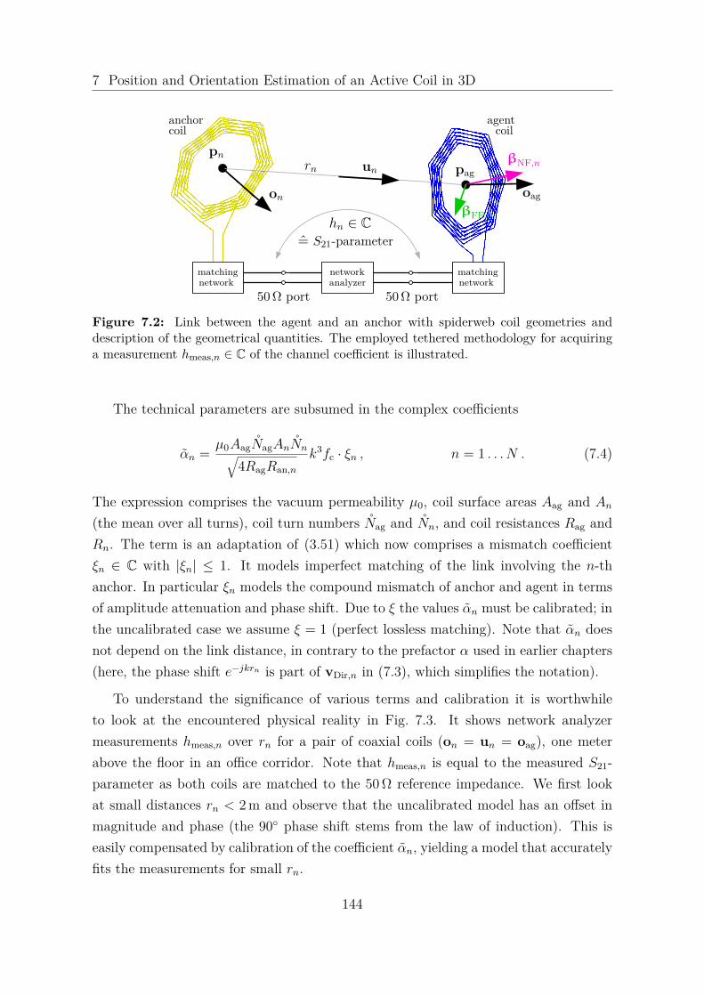
7 Position and Orientation Estimation of an Active Coil in 3D
rn un
hn ∈ C= S21-parameter
50 Ω port 50 Ω port
pn
on
pag
oagβFF,n
βNF,n
networkanalyzer
matchingnetwork
matchingnetwork
anchorcoil
agentcoil
Figure 7.2: Link between the agent and an anchor with spiderweb coil geometries anddescription of the geometrical quantities. The employed tethered methodology for acquiringa measurement hmeas,n ∈ C of the channel coefficient is illustrated.
The technical parameters are subsumed in the complex coefficients
αn = µ0AagNagAnNn√4RagRan,n
k3fc · ξn , n = 1 . . . N . (7.4)
The expression comprises the vacuum permeability µ0, coil surface areas Aag and An(the mean over all turns), coil turn numbers Nag and Nn, and coil resistances Rag andRn. The term is an adaptation of (3.51) which now comprises a mismatch coefficientξn ∈ C with |ξn| ≤ 1. It models imperfect matching of the link involving the n-thanchor. In particular ξn models the compound mismatch of anchor and agent in termsof amplitude attenuation and phase shift. Due to ξ the values αn must be calibrated; inthe uncalibrated case we assume ξ = 1 (perfect lossless matching). Note that αn doesnot depend on the link distance, in contrary to the prefactor α used in earlier chapters(here, the phase shift e−jkrn is part of vDir,n in (7.3), which simplifies the notation).
To understand the significance of various terms and calibration it is worthwhileto look at the encountered physical reality in Fig. 7.3. It shows network analyzermeasurements hmeas,n over rn for a pair of coaxial coils (on = un = oag), one meterabove the floor in an office corridor. Note that hmeas,n is equal to the measured S21-parameter as both coils are matched to the 50 Ω reference impedance. We first lookat small distances rn < 2 m and observe that the uncalibrated model has an offset inmagnitude and phase (the 90 phase shift stems from the law of induction). This iseasily compensated by calibration of the coefficient αn, yielding a model that accuratelyfits the measurements for small rn.
144

7.1 Problem Formulation and Channel Modeling
100 101distance r [m]
-80
-60
-40
-20
chan
nel g
ain
[dB
] MeasurementModel: uncalibratedModel: calib., v
mp = 0
Model: and vmp
calib.
100 101
distance r [m]
75
90
105
120
135
150
phas
e [ °
]
Figure 7.3: Channel coefficient h ∈ C of a coaxial link between two spider coils versusthe link distance r. We compare network analyzer measurements at 500 kHz in an officecorridor to the channel model (7.2) with various calibrations (which are based on fitting themeasurements). For cases other than coaxial arrangement, analogous evaluations are givenin [144].
For larger distances, about rn ≥ 3 m, the measured h levels off and does not followa simple path-loss law anymore; it seems to approach a limit value instead. This effectis certainly not caused by the direct-path mid- or far-field (the terms 1
(kr)2 and 12kr
in (7.3)) because the considered distance are near-field dominated (kr ≈ 0.03 1).We attribute the effect to electromagnetic interaction with the environment giving riseto a superimposed magnetic field. To some extend this interaction comprises inducedcurrents in nearby conductors as well as multipath wave propagation (radiated long-waves which are reflected and scattered at buildings, mountains, and the ground).7
We assume that multipath wave propagation is the dominant cause which allows usto consider all vMP,n ∈ C3 as constant across our entire setup. This assumption issupported by the observed limit value hmodel,n ≈ αnvT
MP,noag for larger rn and by
7The following observations support that multipath wave propagation plays a significant role inthis effect (although we can not make a firm statement based on the available measurements). Fromdesigns at different frequencies fc we found that the limit value magnitude increases rapidly with fc,which is expected for a radiation effect in this regime. Near-field distortions as cause would showstrong path loss according to the image model and thus contradict the observed limit value. Still anear-field effect could play a role, e.g., the building’s reinforcement bar mesh acting as passive relays.For localization, however, this aspect is secondary: the model is beneficial as it empirically improvesthe fit between measurement and model.
145

7 Position and Orientation Estimation of an Active Coil in 3D
the well-known fact that spatial variations of a scatter field are on the order of awavelength [36] (here λ ≈ 600 m far exceeds our setup size). We do not attempt ageometry-based calculation of vMP,n; instead it shall be determined by calibration (inthe uncalibrated case we assume vMP,n = 0). As seen in Fig. 7.3, a calibration of bothαn and vMP,n leads to a great fit between measurement and model at all distances ofinterest.
7.2 Position-Related Information in MeasuredChannel Coefficients
We shall briefly discuss the geometry-related information content in wireless receivedsignals and its significance for low-frequency magneto-inductive localization based onan observed channel vector hmeas.
If the channel spectrum hmeas,n(f) is observed over f ∈ [fc − B2 , fc + B
2 ] with asufficiently large bandwidth B, then the time of arrival can be estimated after aninverse Fourier transform. The time of arrival yields a distance estimate with thepotential for particularly high accuracy with appropriate signaling: the error is onthe order of λ = c/fc with coherent processing8 (employing the carrier phase) or onthe order of c/B otherwise [218]. This allows for cm-accuracy localization of aircraftby radar systems, for example operating at fc = 50 GHz. In a dense environment(e.g. indoors) such an approach faces severe problems from multipath propagation[50,214,219] but nevertheless can be fruitful if B is sufficiently large (so that multipathcomponents can be resolved) [135]. In this chapter we use a different approach: wechoose a very low frequency fc = 500 kHz (and B = 5 kHz) to minimize interactionwith the environment. This signaling is very slow in relation to propagation delays,hence we can not use the time of arrival (cf. the disastrous time-of-arrival accuracyprojections of c/fc = 600 m or even c/B = 60 km).
The observed signal phase can be particularly valuable when the typical distancern is on the order of λ, i.e. when the receiver is located in the transition region betweennear and far field. Then the interplay of the phase-shifted summands of (7.3) allowsfor an estimate of rn from the phase of hmeas,n. The use of such an approach for indoorlocalization is described in [220]. We aim for typical rn of a few meters, however
8Establishing phase synchronization between distributed infrastructure can be a major challenge,for example for radar with extremely high frequency [218]. The henceforth considered magneto-inductive setup merely requires synchronization of a 500 kHz carrier among anchors which are a fewmeters apart, which is easily feasible.
146

7.2 Position-Related Information in Measured Channel Coefficients
choosing a similar λ would result in vast distortion and multipath propagation effects(cf. the discussion of vMP,n) that would interfere heavily with the direct path. Hencewe choose a larger λ and abandon this specific approach.
Angle of arrival estimation from propagation delays would require a distributedarray whose size is comparable to the wavelength. For the reasons stated above, ourtarget λ is too large for such an approach to be meaningful.
An observed amplitude attenuation |hmeas,n| contains information about the distancern because of the distance-dependent signal path loss. Such an approach to localization,usually termed received signal strength, is notoriously inaccurate at radio frequencieswhere the attenuation is subject to severe spatial and temporal fluctuation due tomultipath fading and shadowing [51, 131, 214]. These effects are however specificallyavoided by the low-frequency magnetic induction approach, which presents the prospectof drawing precise location information from amplitude attenuation. Yet, also in ourcase there is no direct relationship between |hmeas,n| and rn due to the effect of theunknown coil orientations relative to the link direction. In the following we provide ananalytic description of this uncertainty, based on the theory of Cpt. 4.
Proposition 7.1 (ranging likelihood functions). Assume that an observed channelcoefficient hmeas,n is accurately described by the employed direct-path channel model,i.e. hmeas,n = hmodel,n with vMP,n = 0. Furthermore assume that the direction vectorsun and oag are random with i.i.d. uniform distributions on the unit sphere.
• In the magnetoquasistatic regime9 the likelihood function of distance rn given|hmeas,n| is
Ln(rn) = r3n
|αn| / k3 ·
1 r3
n ≤|αn| / k3
2·|hmeas,n|
1−arcosh
(r3n
2·|hmeas,n||αn| / k3
)arcosh(2)
|αn| / k3
2·|hmeas,n| < r3n <
|αn| / k3
|hmeas,n|
0 |αn| / k3
|hmeas,n| ≤ r3n
(7.5)
which is shown in Fig. 7.4a. The maximum-likelihood distance estimate is
rMLn = arg maxLn =
(12 ·|αn| / k3
|hmeas,n|
)1/3
. (7.6)
9The r−2n mid-field term could be included but would vastly complicate the formula.
147

7 Position and Orientation Estimation of an Active Coil in 3D
• In the pure far field the likelihood function of distance rn given |hmeas,n| is
Ln(rn) = 2krn|αn|
(π
2 − arcsin(
2krn|αn||hmeas,n|
))(7.7)
for rn ≤ |αn|2k|hmeas,n| and Ln(rn) = 0 otherwise. The function is shown in Fig. 7.4b.
distance rnrMLn rcoaxn
00
likelihoo
dfunc
tion
(a) magnetoquasistatic casedistance rn
rMLn rcopln
00
likelihoo
dfunc
tion
(b) pure far-field case
Figure 7.4: Likelihood function of the link distance rn given an error-less link coefficientmeasurement hmeas,n, under the assumption that the coils on both ends have random ori-entation with uniform distribution on the 3D unit sphere. Comparable distance likelihoodfunctions for multipath radio channels can be found in [221, Fig. 3].
The two cases of the likelihood function are illustrated in Fig. 7.4. The near-field-case ML estimate is equivalent to a distance calculation for two coils fixed incoplanar arrangement (JNF = 1
2 ). This estimate is(
12
)1/3times the maximum possible
distance given hmeas,n (coaxial arrangement). We observe that the likelihood is moreconcentrated around the ML estimate in the magnetoquasistatic case, which is mainlycaused by the much stronger path loss of this regime.
Proof. An error-less magnetoquasistatic channel coefficient is given by hmeas,n =hmodel,n = αn
(krn)3JNF. We take the absolute value and write the equation as |hmeas,n| =|αn| / k3
r3n|JNF|. The PDF f|JNF| is according to (4.15). The random variable |hmeas,n|,
which is just a deterministic scaling of |JNF|, has PDF r3n
|αn| / k3f|JNF|(r3n
|αn| / k3 |hmeas,n|)which proves (7.5). In the pure far-field case without model error, hmeas,n = αn
2krnJFF.The likelihood function is derived analogously to above via the PDF (4.17).
The remainder of the section states the Cramér-Rao lower bound (CRLB) on theroot-mean-square (RMS) position error of the considered magneto-inductive localiza-
148

7.2 Position-Related Information in Measured Channel Coefficients
tion problem. This quantity, also called the position error bound (PEB), is an estab-lished tool in radio localization [126]. It highlights the impact of the setup parameters,poses a benchmark for the position error achieved by practical localization algorithmsand allows for projections of estimation accuracy in a simple fashion. In this contextwe assume that the model error ε is random with known statistics. Then any estimatepag returned by some localization algorithm is also random. If the estimation rule isunbiased then the CRLB applies to the error variances of the estimated componentsof pag. The PEB is the resulting lower bound on
√E[‖pag − pag‖2 ]. It is well-known
that maximum-likelihood estimation attains the CRLB asymptotically for N → ∞.So we can expect the PEB to be a tight lower bound for any well-designed localizationalgorithm when the number of anchors N is sufficiently large and especially when theSNR-like ratio E[‖hmodel‖2 ] /E[‖ε‖2 ] is large (cf. [222]). Therefore, the PEB allows formeaningful accuracy projections. [126,223]
As preparation for the CRLB results we note that for estimating pag from hmeas wemust consider the unknown oag as nuisance parameter because it affects the statisticsof hmeas. Hence we engage in joint estimation of pag and oag (the same approach appliesif an estimate of oag is of interest to the application). Thereby the constraint ‖oag‖ = 1causes some mathematical trouble but this can easily be bypassed with the use of thestandard spherical parametrization10
oag =
cosφag sin θag
sinφag sin θag
cos θag
(7.8)
in terms of azimuth angle φag and polar angle θag. Thus, the considered estimationparameter is the vector
ψ :=
pag
φag
θag
∈ R5 (7.9)
which constitutes a full description of the agent deployment. The discussion of esti-mation algorithms later in the chapter will show that the phase of hmeas,n (especiallythe sign of Im(hmeas,n)) is essential for estimating oag. Hence we consider schemes thatprocess the complex numbers hmeas,n in their very form instead of drawing a simpler
10An alternative mathematical approach to incorporating a constraint such as ‖oag‖ = 1 into CRLBstatements is provided by the theory in [224].
149

7 Position and Orientation Estimation of an Active Coil in 3D
metric like |hmeas,n| that might discard location information.
Proposition 7.2 (Position Error Bound). If ψ is an unbiased estimate of ψ andthe regularity condition of the Cramér-Rao lower bound is fulfilled (for the detailedcondition we refer to [223]), then the Cramér-Rao lower bound on the estimation errorvariance is
var[ψi ] = E[(ψi − ψi)2 ] ≥(III−1ψ
)i,i, i ∈ 1, 2, 3, 4, 5 (7.10)
where IIIψ ∈ R5×5 is the Fisher information matrix of ψ.The related position error bound (PEB) states that
√E[‖pag − pag‖2 ] ≥ PEB( pag,oag) , (7.11)
PEB( pag,oag) =√
tr(III−1ψ
)1:3,1:3
=√
trIII−1
pag
. (7.12)
The last expression uses the equivalent Fisher information matrix
IIIpag =(IIIψ)
1:3,1:3−(IIIψ)
1:3,4:5
(IIIψ)−1
4:5,4:5
(IIIψ)
4:5,1:3(7.13)
which shows the effect of orientation uncertainty on position estimation. If the agentorientation is precisely known a-priori then IIIpag = (IIIψ)1:3,1:3 applies.
Proof. The CRLB (7.10) for a vector parameter is a basic statement of estimationtheory [223, Eq. 3.20]. The position error bound has been derived by [126]; it followsby forming the sum of (7.10) for i ∈ 1, 2, 3 to obtain E[∑3
i=1(ψi−ψi)2 ] ≥ ∑3i=1(III−1
ψ )i,ior rather E[‖pag − pag‖2 ] ≥ ∑3
i=1(III−1ψ )i,i. The equivalent Fisher information matrix
follows from block-wise matrix inversion via the Schur complement; it was introducedby [126] in the context of position estimation with nuisance parameters.
The Fisher information matrix IIIψ is determined by the function hmodel(ψ) in (7.2)and the distribution of ε. For a general definition please refer to [223]; the followingproposition states the result for the case that the model error ε ∈ CN has a zero-meanGaussian distribution. The adequacy of a Gaussianity assumption is supported bySec. 3.2 and the measurement results presented later in the chapter.
150

7.2 Position-Related Information in Measured Channel Coefficients
Proposition 7.3 (Fisher Information Matrix). Let the model error ε ∈ CN havecircularly-symmetric complex Gaussian distribution with zero mean ε ∼ N (0,Kε).Then the log-likelihood function of ψ given an observed hmeas is
L(ψ) = log f(hmeas |ψ) =−N log(π)− log det(Kε)− (hmeas − hmodel)HK−1
ε (hmeas − hmodel) (7.14)
where hmodel (and possibly also Kε) is a deterministic function of ψ. The Fisherinformation matrix IIIψ ∈ R5×5 associated with ψ is given by [223, Eq. 15.52]
(IIIψ)m,n = 2 Re(∂hH
model∂ψm
K−1ε
∂hmodel
∂ψn
)+ tr
(K−1ε
∂Kε
∂ψmK−1ε
∂Kε
∂ψn
)(7.15)
for elements m,n ∈ 1, . . . , 5. The right-hand summand vanishes if Kε does notdepend on ψ, yielding the compact formula11
IIIψ = 2 Re(∂hH
model∂ψ
K−1ε
∂hmodel
∂ψT
). (7.16)
These statements require the 5×N Jacobian matrix of hmodel from (7.2) with respectto ψ, which holds derivatives of hmodel,n with respect to the components of pag as wellas φag and θag. These derivatives are given by the following involved proposition.
Proposition 7.4 (Geometric Gradient). The spatial gradient of the channel coefficientis given by
∂hmodel,n
∂pag= αn
∂vTDir,n
∂pagoag, (7.17)
∂vTDir,n
∂pag= −jk unvT
Dir,n + je−jkrnΓ (7.18)
11We note that N ≥ 5 is a necessary condition for IIIψ in (7.16) being invertible. This is consistentwith the fact that we would require at least five observations hmeas,n to determine the five-dimensionalψ even in the error-less case.
151

7 Position and Orientation Estimation of an Active Coil in 3D
where Γ ∈ C3×3 is another Jacobian matrix with respect to position, given by
Γ = ∂
∂pag
((1
(krn)3 + j
(krn)2
)βT
NF,n + 12krn
βTFF,n
)(7.19)
=(
1(krn)3 + j
(krn)2
)∂βT
NF,n
∂pag+ 1
2krn∂βT
FF,n
∂pag
−(
3k(krn)4 + 2jk
(krn)3
)unβT
NF,n −k
2(krn)2 unβTFF,n .
The above uses the spatial Jacobians of the scaled near- and far-field vectors
∂βTNF,n
∂pag= 3
21rn
(onuT
n + (oTnun)(I3 − 2unuT
n )), (7.20)
∂βTFF,n
∂pag= − 1
rn
(onuT
n + (oTnun)(I3 − 2unuT
n )). (7.21)
The gradients with respect to orientation are ∂hmodel,n∂φag
= αn(vDir,n+vMP,n)T ∂oag∂φag
with∂oag∂φag
= [− sin(φag) sin(θag), cos(φag) sin(θag), 0]T and ∂hmodel,n∂θag
= αn(vDir,n+vMP,n)T ∂oag∂θag
with ∂oag∂θag
= [cos(φag) cos(θag), sin(φag) cos(θag), − sin(θag)]T.
Proof Sketch. We note that the vectors vMP,n are considered constant while vDir,n de-pend on pag but not on φag or θag, leading to (7.17). Then (7.18) follows from theproduct rule, ∂
∂page−jkrn = −jk ∂rn
∂pag· e−jkrn , and ∂rn
∂pag= un which is easily shown
by writing rn = (x2 + y2 + z2) 12 and computing ∂rn
∂x, ∂rn∂y, ∂rn∂z
(cf. [146]). Then (7.19)is expanded with basic rules. The near- and far-field Jacobians (7.20) and (7.21)are obtained by writing βT
NF,n = 32(uT
non)uTn − 1
2oTn and βT
FF,n = −(uTnon)uT
n + oTn ,
then noting ∂βTNF,n
∂pag= 3
2∂(uT
non)uTn
∂pagand ∂βT
FF,n∂pag
= −∂(uTnon)uT
n
∂pag. The common term
∂(uTnon)uT
n
∂pag= ∂uT
n
∂pagonuT
n + uTnon ∂uT
n
∂pagis expanded with the use of ∂uT
n
∂pag= 1
rn(I3 − unuT
n ).This last equality can be proven by writing rn = [x y z]T and un = 1
rnrn to expand
∂un∂x
= 1rn
∂rn∂x− 1
r2n
∂rn∂x
rn = 1rn
([1 0 0]T − (un)x un) where (un)x is the x-componentof un. Repeating the above for ∂un
∂yand ∂un
∂zand a few rearrangements conclude the
derivation. The derivatives with respect to φag and θag follow from basic calculus.
Later in the chapter, in the evaluation of the practical system implementation inSec. 7.5, we will encounter a distribution of ε that does not exhibit circular symmetry,even for a thoroughly calibrated model. We will nevertheless require an appropriateformula for the Fisher information matrix, which is given in the following.
152
7.3 CRLB-Based Study of Accuracy Regimes
Proposition 7.5. If the model error vector ε ∈ CN has a general complex Gaussiandistribution with zero mean, modeled in terms of the real-valued stack vector
εstack = Re ε
Im ε
∼ N (0,Kstack) , (7.22)
then the Fisher information matrix IIIψ ∈ R5×5 is given by [223, Eq. 3.31]
(IIIψ)m,n = sTm K−1
stack sn + 12 tr
(K−1
stack∂Kstack
∂ψmK−1
stack∂Kstack
∂ψn
)(7.23)
for elements m,n ∈ 1, . . . , 5. Thereby sm ∈ R2N is the m-th column of the stackedJacobian S ∈ R2N×5 stated below. If Kstack does not depend on ψ then
IIIψ = STK−1stackS , S =
Re(∂hmodel/∂ψT)
Im(∂hmodel/∂ψT)
(7.24)
applies. The statements encompass circularly-symmetric distributions ε ∼ CN (0,Kε)as a special case; the conversion is via
Kstack = 12
Re(Kε) −Im(Kε)Im(Kε) Re(Kε)
. (7.25)
7.3 CRLB-Based Study of Accuracy Regimes
In this section we evaluate the potential performance of low-frequency magneto-inductive localization for realistic technical parameters and a setup size of a few meters(e.g. indoor localization). The anchors are installed in the pattern indicated in Fig. 7.1which is motivated by the compromise of establishing a large anchor spread in all threedimensions while maintaining small rn to most positions in the volume (an extensivestudy of optimal anchor deployment is left for future work).
The following evaluation assumes a random agent deployment whereby oag hasuniform distribution on the 3D unit sphere and pag has a uniform distribution on acube with the same center position as the anchor setup and 80% of its side length (i.e.2.4 m). This way we prevent that pag occurs very close to any pn. We are interestedin the resulting statistics of the position error bound (7.12) in different setting.
All αn are set such that the agent-to-anchor channel gain would be−40 dB over rn =1 m in coaxial arrangement (this choice is made for all considered wavelengths). For
153
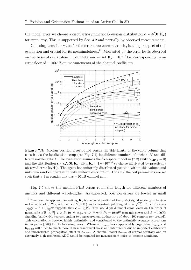
7 Position and Orientation Estimation of an Active Coil in 3D
the model error we choose a circularly-symmetric Gaussian distribution ε ∼ N (0,Kε)for simplicity. This is supported by Sec. 3.2 and partially by observed measurements.
Choosing a sensible value for the error covariance matrix Kε is a major aspect of thisevaluation and crucial for its meaningfulness.12 Motivated by the error levels observedon the basis of our system implementation we set Kε = 10−10 IN , corresponding to anerror floor of −100 dB on measurements of the channel coefficient.
1 2 3 4 5 6 7 8 9 10
side length of cubic setup [m]
10-4
10-3
10-2
10-1
100
101
med
ian
posi
tion
erro
r bo
und
[m]
5 anchors8 anchors12 anchors20 anchors
= 10 m
= 600 m
henceforthconsideredoperating point
= 1 m (prediction isunrealistic for typicalmultipath)
Figure 7.5: Median position error bound versus the side length of the cubic volume thatconstitutes the localization setup (see Fig. 7.1) for different numbers of anchors N and dif-ferent wavelengths λ. The evaluation assumes the free-space model in (7.2) (with vMP,n = 0)and the distribution ε ∼ CN (0,Kε) with Kε = IN · 10−10 (a choice motivated by practicallyobserved error levels). The agent has uniformly distributed position within this volume andunknown random orientation with uniform distribution. For all λ the coil parameters are setsuch that a 1 m coaxial link has −40 dB channel gain.
Fig. 7.5 shows the median PEB versus room side length for different numbers ofanchors and different wavelengths. As expected, position errors are lowest in small
12One possible approach for setting Kε is the consideration of the SIMO signal model y = hx+ win the sense of (3.23), with w ∼ CN (0,K) and a constant pilot signal x =
√PT. Now observing
1√PT
y = h + 1√PT
w suggests that ε = 1PT
K. This would yield model error levels on the order ofmagnitude of E[|εn|2 ] ≈ 1
PTB ·10−20, e.g., ≈ 10−16 with PT = 10 mW transmit power and B = 100 Hz
signaling bandwidth (corresponding to a measurement update rate of about 100 samples per second).This calculation is however highly optimistic (and contributed to the optimistic accuracy projectionsin our paper [128]) for the following reason. Whenever hmeas has a appreciably large value, hmeas andhmodel will differ by much more than measurement noise and interference due to imperfect calibrationand unconsidered propagation effect in hmodel. A channel model hmodel of surreal accuracy and anextremely high-resolution ADC would be required for measurement noise to become dominant.
154

7.3 CRLB-Based Study of Accuracy Regimes
rooms with many anchors. Remarkably, the projected accuracies for λ = 600 m andλ = 10 m are not vastly different for small setup sizes. This is because in either casethe typical link distances hardly exceed the near field. For larger setups the smallerwavelength promises a better accuracy because of the reduced path loss in the mid-and far-field regimes. From a practical perspective however, the choice λ = 10 mis disastrous because one must expect vast interaction with the environment, whichinterferes with the direct path and thus gives rise to huge model errors ε (we observedthis clearly in an experiment conducted at 13.56 MHz ⇔ λ = 22.1 m).
The problem would be even more pronounced at λ = 1 m where hmeas would begoverned by small-scale fading through rich scattering. The accuracy projections incombination with our practical experiments in the course of [143] show that λ = 600 mis suitable for our magneto-inductive localization approach. We identify the N = 8case with 3 m setup side length, which shows a median PEB of 13 mm, as an attractiveuse case with reasonable infrastructure cost. We will use this operating point for theremainder of the chapter.
10-3 10-2 10-1
position error bound [m]
0
0.1
0.2
0.3
0.4
0.5
0.6
0.7
0.8
0.9
1
empi
rical
CD
F
joint estimation withunknown orientation
orientation isknown a-priori
(a) position estimation
10-2 10-1 100 101 102
angle error bound [ ° ]
0
0.1
0.2
0.3
0.4
0.5
0.6
0.7
0.8
0.9
1
empi
rical
CD
F
polar angle
azimuth angle .
joint estimation withunknown position
position isknown a-priori
θag
φag
(b) orientation estimation
Figure 7.6: The plots show the statistics of the CRLB on the RMS errors of the positionestimate and the orientation angle estimates for random agent deployment in a 3 m×3 m×3 mroom using 8 anchors and λ = 600 m (fc = 500 kHz). Also shown are bounds which ignorethe uncertainty in the respective other domain.
Fig. 7.6 shows the statistics of the PEB at the chosen operating point. We notethat accuracies of 42 mm and 2.8 are feasible for 95% of all random agent deploy-ments. If the agent orientation was known a-priori then the position accuracy wouldapproximately double (the median PEB improves from 13 mm to 6.4 mm). The plotsof the RMS orientation angle errors show that azimuth and polar angle have similarerror statistics. Here the accuracy would improve by about a factor of three if the
155

7 Position and Orientation Estimation of an Active Coil in 3D
position parameter was known a-priori. This indicates that orientation estimation isslightly more sensitive to position uncertainty than vice versa.
7.4 Localization Algorithm Design
We are interested in a localization algorithm that is fast, accurate, and robust (i.e.outliers in the sense of occasional very inaccurate estimates should not occur). In orderwords, we seek computational procedure which reliably returns an accurate estimatepag (and possibly also oag) given the observation hmeas ∈ CN and full knowledge ofthe anchor topology and technical parameters, based on a channel model hmodel. Thelatter is throughout considered as a function of an agent position hypothesis p and anorientation hypothesis o (as opposed to the true pag and oag).
We shall review the related work on magneto-inductive localization algorithms. Thejoint estimation of position and orientation of a dipole-like magnet through distributedsensors, each measuring one field component, was studied by [122] and by [123, 124]for medical gastrointestinal applications. In [125], a medical microrobot estimatesits position and orientation from voltages induced in its near-field antenna due toeight active anchors. For the 5D non-linear least squares problem associated withthese works, the Levenberg-Marquardt (LM) algorithm was identified as a suitablesolver [122,123]. The authors of [123] emphasized the importance of an accurate initialguess for LM because of local cost function minima. The magnetic field Jacobian wasprovided to the LM algorithm in [124] for performance enhancement. Most papers onnear-field localization employ the dipole approximation, e.g., [58,59,61,122–124,217]. Indistinction from planar coil setups, the use of tri-axial coil arrays at the anchors and/orthe agent allows for simpler localization schemes [59, 96, 217, 225]. In particular, [225]uses a simplified localization algorithm to initialize the LM solver applied to the originalnon-linear least squares problem.
In the following we review the standard approach(es) and the associated problemsto then proceed with the design of more suitable localization algorithms. It shallbe noted that we study location estimation from an instantaneous observation hmeas
without temporal filtering (which could easily be applied to instantaneous estimates).
7.4.1 Least-Squares and Maximum-Likelihood Estimation
We consider hmodel = [ hmodel,1 . . . hmodel,N ]T as a function of pag and oag while themodel parameters αn, vMP,n, pn, on are fixed ∀n. The least-squares estimate of pag
156

7.4 Localization Algorithm Design
and oag is obtained by solving the optimization problem
(pag, oag) ∈ arg minp,o
‖hmeas − hmodel‖2 subject to ‖o‖2 = 1. (7.26)
The spherical parametrization (7.8) of o yields an unconstrained non-linear leastsquares problem in five dimensions,
(pag, φag, θag
)= arg min
p, φ, θ‖hmeas− hmodel‖2
2 = arg minp, φ, θ
N∑n=1|hmeas,n− hmodel,n|2 . (7.27)
If the model error ε has a circularly-symmetric Gaussian distribution ε ∼ CN (0,Kε)then the maximum-likelihood estimate (MLE) is given by those values p, φ, θ whichmaximize the log-likelihood function (7.14). If furthermore Kε does not depend on theagent location then the maximum-likelihood estimate becomes
(pag, φag, θag
)= arg min
p, φ, θ(hmeas − hmodel)HK−1
ε (hmeas − hmodel) . (7.28)
The extension to the case without circular symmetry is straightforward. If Kε is ascaled identity matrix Kε = σ2IN then the least-squares estimate (7.27) and the MLE(7.28) are equivalent.
Closed-form solutions are unavailable for these optimization problems because of theinvolved non-linear function hmodel(p, φ, θ). Still, we can tackle them with numericaloptimization methods. In particular we focus on iterative gradient-based methodswhich are suitable because the objective is a continuous and continuously differentiablefunction. To this effect, related optimization methods such as simulated annealing orparticle swarm optimization (as used by [226] for magneto-inductive localization) arenot considered. We apply a nonlinear least-squares solver (namely the Matlab functionlsqnonlin with the levenberg-marquardt algorithm option [227])13 to (7.28), usinga certain ψ as initialization. We refer to this procedure as the ML5D algorithm.The objective function is non-convex (this can be seen at the example in Fig. 7.8)and thus the gradient search may converge to a local minimum [228]. In this case the
13The trust-region-reflective algorithm option results in very similar estimation accu-racy as the levenberg-marquardt option but is a bit slower computationally, hence we preferlevenberg-marquardt. The solver is provided the 5 × N Jacobian holding all the geometric er-ror gradients, which follow directly from Proposition 7.4. In this context it shall be noted that duringthe gradient search there is no need to constrain the value range of φ and θ because any periodicalambiguity leads to the same oag. Such constraints could even cause a solver to get stuck at an intervalboundary and thus impair its ability to find the global optimum. Likewise, we do not constrain theposition search space in any way.
157

7 Position and Orientation Estimation of an Active Coil in 3D
estimate will usually deviate severely from the actual MLE.14 We will find that thishappens frequently. Moreover, the ML5D approach has a large mean execution timewhich prevents real-time localization with a fast update rate. It is thus unsuitable foraccurate real-time localization with a fast update rate. In order to improve on theseshortcomings we propose and study alternative algorithms in the following.
7.4.2 Multilateration from Hard Distance Estimates
Given the measurements hmeas,n we compute the maximum-likelihood distance esti-mates rML
n with the simple formula (7.6) for all anchors n = 1 . . . N . These distanceestimates are then used for multilateration, i.e. we estimate the agent position byapplying a gradient-based solver (quasi-Newton method) to the least-squares problem
pag = arg minp
N∑n=1
(rn(p)− rML
n
)2. (7.29)
Its appealing mathematical properties are discussed in [229, Sec. 4.4.1.2]. We will findthat this method converges exceptionally fast but has very poor accuracy. We interpretthis as a consequence of the rough distance estimates and of general shortcomings ofthe multilateration method for involved distance error statistics (e.g., see [51]).
7.4.3 Magnetic Eggs Algorithm
The above multilateration approach might be improvable by considering the soft dis-tance information in the likelihood functions LNF,n(rn) from (7.5), e.g. by heuristicallycalculating p which minimizes ∏N
n=1 LNF,n(rn(p)), instead of using the hard estimatesrMLn . In the following we describe a similar yet mathematically simpler approach whichpays more attention to the geometrical information per anchor.
First, we consider channel model (7.2), discard the far-field term, and assume thatthis model is without error (εn ≡ 0). Then hmeas,n = hmodel,n = αn( 1
(kr)3 + j(kr)2 )JNF,n and
14By ’actual MLE’ we refer to the formally true solution of the maximum-likelihood optimizationproblem (7.28), irregardless of any problems that may occur in computing it. In the following eval-uations we emulate the actual MLE by running ML5D initialized at true agent location ψ. Themeaningfulness of this emulation was confirmed by omitted experiments which showed that the biasand deviation between RMS error and position error bound are both negligibly small with this ap-proach. Those properties are characteristic for the MLE when N is large [223] (our choice N = 8 isreasonably large). In this context note that if hmodel was an affine map of ψ then ψ ∼ N (ψ,III−1
ψ )would hold for the MLE; thus the position error bound would hold with equality. This is not the case,however the property holds in good approximation because hmodel can be described by a first-orderTaylor approximation (which is affine) in a vicinity of the true ψ (a small vicinity at high SNR).
158

7.4 Localization Algorithm Design
we obtain |hmeas,n| = |αn|√
1(kr)6 + 1
(kr)4 |JNF,n|. For fixed pag but random oag (uniformdistribution in 3D) we know from (4.13) that |JNF,n|
∣∣∣ βNF,n ∼ U(0, βNF,n), associatedwith the PDF 1
βNF,n1[0,βNF,n](|JNF,n|). A change of variables yields the PDF of |hmeas,n|,
f(|hmeas,n|; pag
)=1[0, βNF,ngn](|hmeas,n|)
βNF,n gn, gn = |αn|
√1
(krn)6 + 1(krn)4 . (7.30)
Note that the dependence on pag is via both rn and βNF,n. We generalize the re-sult to the case of an erroneous measurement according to the pragmatic model|hmeas,n|
∣∣∣ |hmodel,n| ∼ N (|hmodel,n|, σ2). By performing the convolution of the Gaus-sian PDF and the uniform PDF of |hmodel,n| one can show that the resulting PDF is
1βNF,n gn
(Q( |hmeas,n|−βNF,ngn
σ
)−Q
(|hmeas,n|
σ
)), reminiscent of a soft indicator function on
the interval [0, βNF,ngn] and with smoothness parameter σ. We note that the non-sensical circumstance |hmeas,n| < 0 can occur under this error model; the right-handQ-function is an artifact thereof and is thus discarded. We obtain
f(|hmeas,n| ; pag
)=Q( |hmeas,n|−βNF,ngn
σ
)βNF,n gn
. (7.31)
Given measurements hmeas,1, . . . , hmeas,N we consider the product of likelihood functionsL(p) = ∏N
n=1 f(|hmeas,n|; p) which is itself considered as a likelihood function. If thedistributions |JNF,n|
∣∣∣ βNF,n (as well as the errors with variance σ2) were statisticallyindependent across n = 1 . . . N then L(p) would be a legitimate likelihood function,although we know from Cpt. 4 that this is not the case. Yet we use this heuristicconstruct for localization and refer to the minimization of − logL(pag) with a gradient-based solver (quasi-Newton method) as the Magnetic Eggs algorithm.
To best understand the concept and the naming we consider the magnetoquasistaticregime where gn = |αn|
(krn)3 and we furthermore set σ = 0, i.e. we use (7.30). We obtain
f(|hmeas,n| ; p
)=
r3n
βNF,n|αn/k3| 0 ≤ rn ≤∣∣∣βNF,nαn/k
3
hmeas,n
∣∣∣1/30 otherwise
. (7.32)
In the considered simple case it is supported inside an egg-shaped manifold in R3
(formally not an ellipsoid, but with very similar shape) which is illustrated in Fig. 7.7a.It is centered at the anchor position pn and its major axis, which is 3
√2 times longer
than the minor axes15, is along on. With σ > 0 we would see a smooth transition to
159

7 Position and Orientation Estimation of an Active Coil in 3D
x position
y po
sitio
n
0
max
likel
ihoo
d
agentcoil
anchorcoil
(a) egg concept (one anchor)x position
y po
sitio
n0
max
likel
ihoo
d
anchor 3
anchor 1
anchor 2
agentcoil
(b) product of eggs (N = 3 anchors)
Figure 7.7: Illustration of the likelihood function underlying the introduced Magnetic Eggsalgorithm, evaluated for the magnetoquasistatic and error-free case described by (7.32). Thesame egg shape was indicated in [104] and a related distance bounding idea given in [26].
zero at the egg boundary instead of the immediate drop. The illustration in Fig. 7.7bshows an example of ∏N
n=1 f(|hmeas,n| ; p) for N = 3, i.e. the intersection of threeeggs. We observe that the true agent position deviates significantly from the positionwith maximum likelihood. This deviation is due to the wrong assumption of statisticalindependence between JNF,1 . . . JNF,N that underlies the approach.
7.4.4 Dimensionality Reduction (ML3D Algorithm)
We attribute the convergence problems of ML5D to its high-dimensional parameterspace, which is reduced to 3D in a rigorous fashion in the following. We write theemployed channel model (7.2) as
hmodel = VTpo , Vp =
[α1(vDir,1 + vMP,1) , . . . , αN(vDir,N + vMP,N)
](7.33)
whereby Vp ∈ R3×N is indicated as a function of position hypothesis p. For thefollowing approach we consider p fixed and for pragmatic reasons require hmeas ≈ VT
po
15It is noteworthy that the maximum-likelihood distance estimate rMLn in (7.6) is equal to the minor
axis length of the egg shape. One can see how the likelihood function of rn in Fig. 7.4a would emergesfrom the egg shape in Fig. 7.7a by marginalization of the anchor-to-agent direction u if it had uniformdistribution in 3D.
160

7.4 Localization Algorithm Design
in order to obtain an estimate op given p. In particular we compute
op = arg mino
(hmeas −VTpo)HK−1
ε (hmeas −VTpo) subject to ‖o‖2 = 1 . (7.34)
analogous to the maximum-likelihood rule (7.28). We demonstrate that this problemcan be solved analytically. We use the error-whitened and real-valued reformulation
op = arg mino
‖γ −ATpo‖2 subject to ‖o‖2 = 1 (7.35)
with γ = [Re(K−1/2ε hmeas)T, Im(K−1/2
ε hmeas)T]T ∈ R2N and, likewise, ATp ∈ R2N×3 is
formed by stacking the real- and imaginary parts of K−1/2ε VT
p . The optimization prob-lem (7.35) is a linear least-squares problem with a quadratic equality constraint whichis solved in the following according to the theory presented in [230]. By consideringthe stationary points of the Lagrange function associated with (7.35) we find
op(λ) =(ApAT
p + λ I3)−1
Ap γ (7.36)
as a function of the Lagrange multiplier λ (not to be confused with the wavelength).The solution to (7.34) is given by op(λ∗) where λ∗ is the largest λ which satisfiesthe constraint ‖op(λ)‖2 = 1 (we do not elaborate on special cases that occur withprobability zero for our estimation problem from a random observation; for detailsplease refer to [230]). In order to find λ∗, we use a reformulation [230]
‖op(λ)‖2 =3∑i=1
µic2i
(µi + λ)2 = 1 (7.37)
based on the eigenvalue decomposition of 3 × 3 matrix ApATp = ∑3
i=1 µiaiaTi and
ci = aTi γ. We can now compute λ∗ efficiently by finding the largest real root of a sixth-
order polynomial in λ which arises by multiplying (7.37) with its three denominators.
Using this rule for op, we can compute a maximum-likelihood position estimate bysolving an unconstrained optimization problem with 3D parameter space,
pag = arg minp
‖γ −ATp op‖2 (7.38)
= arg minp
(hmeas −VTp op)HK−1
ε (hmeas −VTp op) .
The interplay of (7.34) and (7.38) can be regarded as alternating minimization [231,Eq. 1.1] of the negative log-likelihood in (7.28), whereby the very fast and reliable rule
161

7 Position and Orientation Estimation of an Active Coil in 3D
for computing op however effectively reduces the problem from 5D to 3D (op can beregarded as a simple function of p).
We define the ML3D algorithm as the application of the Levenberg-Marquardtsolver to (7.38), using a certain initial p. Later in the chapter we will see that ML3Dhas much faster convergence speed than ML5D, owing to the dimensionality reduction.The robustness improvement is minor though: just like ML5D, ML3D does not convergeto the global optimum reliably. This flaw is tackled in the following.
7.4.5 Smoothing the Cost Function (WLS3D Algorithm)
The introduced ML5D and ML3D algorithms suffer from convergence to local costfunction extrema. We attribute part of the problem to the high dynamic measurementrange due to path loss: the values hmeas,n with largest absolute value will usuallydominate the squared-error term (7.38) at most position hypotheses. As a result,the majority of anchors is effectively ignored in early solver iterations, which hindersconvergence to the global optimum. Apparently this problem could be avoided with amore balanced cost function.
We consider the distances between a hypothesis p and the anchor positions pn,collected in
Rp = diag(r1(p), . . . , rN(p)
), rn(p) = ‖p− pn‖ . (7.39)
We use them in the computation of a weighted least-squares position estimate
pag = arg minp
N∑n=1
∣∣∣r3n(p)
(hmeas,n− hmodel,n(p, op)
)∣∣∣2 (7.40)
= arg minp‖R3
p(hmeas −VTp op)‖2
where Vp is from (7.33). As corresponding orientation estimate we compute
op = arg mino‖R3
p(hmeas −VTpo)‖2 subject to ‖o‖2 = 1 (7.41)
which is solved analytically just like (7.35). We refer to the application of theLevenberg-Marquardt non-linear least squares solver to (7.40) as WLS3D algorithm.16
The idea of this distance-dependent weighting r3n(p) is to map all observations
16In our implementation we multiply the cost function by the constant N/ tr(Kε) to avoid that theoutput values are many orders of magnitude smaller than those of ML5D and ML3D.
162

7.4 Localization Algorithm Design
onto a common value range. To see this, consider the magnetoquasistatic modelhmodel,n = αn
(kr)3JNF,n and the weighted term r3nhmodel,n = αn
k3 JNF,n. This term shouldhave similar order of magnitude across all n (at least at p = pag); the same applies forthe weighted observation r3
nhmeas,n. This prevents a degenerated value range of the costfunction summands and achieves an effect comparable to a cost function relaxation incomparison to ML3D, as can be observed in Fig. 7.8.
0 0.5 1 1.5 2 2.5 3
x-coordinate of position hypothesis [m]
cost
func
tion
ML5D
ML3D
true agent position
MagneticEggs
MisalignedGauss
WLS3D
Multilateration
ML5D, orient.45° off
ML5D, orientation 90° off
Figure 7.8: An example showing the spatial cost function evolution of the introducedgradient-based location estimation algorithms. The example considers agent position hy-potheses p on a line inside the anchor setup of Fig. 7.1. The particular line is p =[x, 0.5 m, 1.5 m]T for x ∈ [0 m, 3 m]; it comprises the true pag at x = 2 m. The evalua-tion shows three different choices for the orientation hypothesis required by the ML5D costfunction: the true orientation orientations, one offset by by 45, and one orthogonal. Thecost values were scaled and shifted to the same value range for visualization purposes.
Even in the case of global optimality, the WLS3D algorithm may exhibit slightlylower accuracy than ML3D and ML5D. This is because of the absence of noise whiteningand because the weighting affects the model error components individually and, inconsequence, the estimates (7.40) and (7.41) deviate from the maximum-likelihoodestimate. This is however easily mitigated by cascading WLS3D and ML3D (initializedat the WLS3D estimate).
7.4.6 Misaligned Gauss Algorithm
We present a last algorithm design based on the same ideas as WLS3D, but now thedimensionality reduction is achieved via the random misalignment theory developed in
163

7 Position and Orientation Estimation of an Active Coil in 3D
Cpt. 4. In this sense, we assume that oag is random with uniform distribution on the3D unit sphere. We use hmodel = VT
po as defined by (7.33). Inspired by Sec. 7.4.4 weuse the distant-dependent scaling δ = R3
phmodel with Rp = diag(r1 . . . rN), leading tothe model δ = Bpoag with Bp = R3
pVTp ∈ CN×3. From Proposition 4.8 we know that
the random vector δ = Bpoag has zero mean and covariance matrix 13BpBH
p .
We consider the scaled measurement ζ = R3phmeas and assume that ζ and δ deviate
by a random error e = ζ − δ (statistically independent of oag) with zero mean andcovariance matrix Σ. As a result the observation ζ = Bpoag + e has zero meanand covariance matrix 1
3BpBHp + Σ. To keep the mathematics tractable we assume a
Gaussian distribution ζ ∼ CN (0, 13BpBH
p + Σ). This certainly contradicts the specificPDF given by Proposition 4.2 with its ellipse-shaped support, although the color plotsin Fig. 4.4 indicate that a Gaussian model with the same covariance matrix is at leasta sensible approximation. For this Gaussian model we can easily state the PDF of ζ,
f(ζ; p) =exp
(−ζH(1
3BpBHp + Σ)−1ζ
)πN det
(13BpBH
p + Σ) (7.42)
which is parameterized by the position hypothesis p. For a fixed measurement hmeas theexpression becomes a likelihood function of p. By writing the negative log-likelihoodfunction and discarding irrelevant summands we obtain the cost function
C(p) = log det(
13BpBH
p + Σ)
+ ζH(
13BpBH
p + Σ)−1
ζ . (7.43)
We define the Misaligned Gauss algorithm as the application of a gradient-based solver(quasi-Newton method) for the three-dimensional minimization of this cost function.
We have yet to discuss the covariance matrix Σ. Formally it should have the valueR3
pKεR3p based on the covariance matrix Kε of the model error ε = hmeas − hmodel.
However, we found that the algorithm becomes vastly more robust with a fixed choice,e.g. Σ = σ2IN with σ = 10−6 as error level.17 The considered key purpose of Σ issmoothing the cost function and ensuring that 1
3BpBHp + Σ has full rank rather than
accurately reflecting the error statistics.
17With a scaled identity covariance matrix Σ = σ2IN the matrix inversion ( 13BpBH
p + Σ)−1 =( 1
3BpBHp + σ2IN )−1 in (7.43) can equivalently be written as 1
σ2
(IN − 1
3Bp( 13BH
p Bp + σ2I3)−1BHp)
via the Woodbury matrix identity. This reduces the computational effort to a 3× 3 inversion.
164
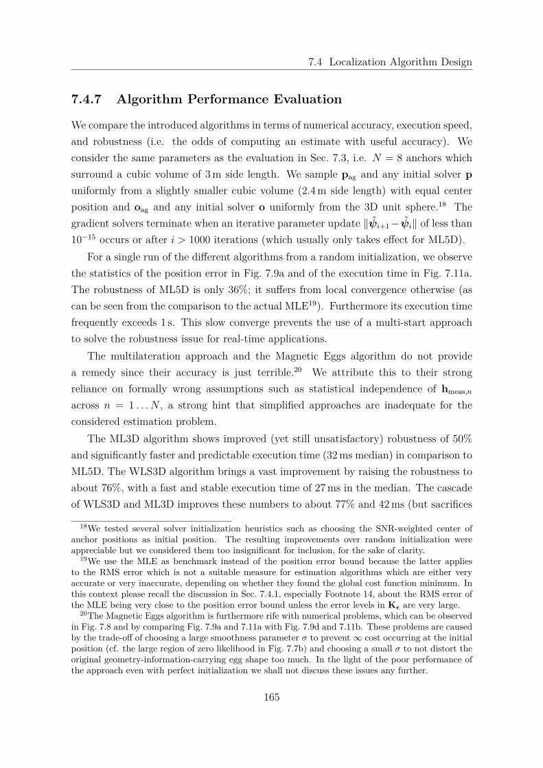
7.4 Localization Algorithm Design
7.4.7 Algorithm Performance Evaluation
We compare the introduced algorithms in terms of numerical accuracy, execution speed,and robustness (i.e. the odds of computing an estimate with useful accuracy). Weconsider the same parameters as the evaluation in Sec. 7.3, i.e. N = 8 anchors whichsurround a cubic volume of 3 m side length. We sample pag and any initial solver puniformly from a slightly smaller cubic volume (2.4 m side length) with equal centerposition and oag and any initial solver o uniformly from the 3D unit sphere.18 Thegradient solvers terminate when an iterative parameter update ‖ψi+1−ψi‖ of less than10−15 occurs or after i > 1000 iterations (which usually only takes effect for ML5D).
For a single run of the different algorithms from a random initialization, we observethe statistics of the position error in Fig. 7.9a and of the execution time in Fig. 7.11a.The robustness of ML5D is only 36%; it suffers from local convergence otherwise (ascan be seen from the comparison to the actual MLE19). Furthermore its execution timefrequently exceeds 1 s. This slow converge prevents the use of a multi-start approachto solve the robustness issue for real-time applications.
The multilateration approach and the Magnetic Eggs algorithm do not providea remedy since their accuracy is just terrible.20 We attribute this to their strongreliance on formally wrong assumptions such as statistical independence of hmeas,n
across n = 1 . . . N , a strong hint that simplified approaches are inadequate for theconsidered estimation problem.
The ML3D algorithm shows improved (yet still unsatisfactory) robustness of 50%and significantly faster and predictable execution time (32 ms median) in comparison toML5D. The WLS3D algorithm brings a vast improvement by raising the robustness toabout 76%, with a fast and stable execution time of 27 ms in the median. The cascadeof WLS3D and ML3D improves these numbers to about 77% and 42 ms (but sacrifices
18We tested several solver initialization heuristics such as choosing the SNR-weighted center ofanchor positions as initial position. The resulting improvements over random initialization wereappreciable but we considered them too insignificant for inclusion, for the sake of clarity.
19We use the MLE as benchmark instead of the position error bound because the latter appliesto the RMS error which is not a suitable measure for estimation algorithms which are either veryaccurate or very inaccurate, depending on whether they found the global cost function minimum. Inthis context please recall the discussion in Sec. 7.4.1, especially Footnote 14, about the RMS error ofthe MLE being very close to the position error bound unless the error levels in Kε are very large.
20The Magnetic Eggs algorithm is furthermore rife with numerical problems, which can be observedin Fig. 7.8 and by comparing Fig. 7.9a and 7.11a with Fig. 7.9d and 7.11b. These problems are causedby the trade-off of choosing a large smoothness parameter σ to prevent∞ cost occurring at the initialposition (cf. the large region of zero likelihood in Fig. 7.7b) and choosing a small σ to not distort theoriginal geometry-information-carrying egg shape too much. In the light of the poor performance ofthe approach even with perfect initialization we shall not discuss these issues any further.
165

7 Position and Orientation Estimation of an Active Coil in 3D
10-4 10-3 10-2 10-1 100 101
position error [m]
0
0.1
0.2
0.3
0.4
0.5
0.6
0.7
0.8
0.9
1
empi
rical
CD
F
ML5DML3DMultilaterationMagnetic EggsWLS3D
Misaligned Gauss
benchmark: actual MLE
(a) one random init
10-4 10-3 10-2 10-1 100 101
position error [m]
0
0.1
0.2
0.3
0.4
0.5
0.6
0.7
0.8
0.9
1
empi
rical
CD
F
benchmark: actual MLE
(b) two random inits
10-4 10-3 10-2 10-1 100 101
position error [m]
0
0.1
0.2
0.3
0.4
0.5
0.6
0.7
0.8
0.9
1
empi
rical
CD
F
benchmark: actual MLE
(c) three random inits
10-4 10-3 10-2 10-1 100 101
position error [m]
0
0.1
0.2
0.3
0.4
0.5
0.6
0.7
0.8
0.9
1
empi
rical
CD
F
actual MLEattained by:ML5D, ML3D,
(d) perfect init
Figure 7.9: Statistics of the position error ‖pag−pn‖ of the different algorithms with N = 8anchors and random initialization.
10-1 100 101 102
orientation error [ ° ]
0
0.1
0.2
0.3
0.4
0.5
0.6
0.7
0.8
0.9
1
empi
rical
CD
F
ML5DML3DWLS
benchmark: actual MLE
(a) 1 random init
10-1 100 101 102
orientation error [ ° ]
0
0.1
0.2
0.3
0.4
0.5
0.6
0.7
0.8
0.9
1
empi
rical
CD
F
actual MLEattained by:ML5D, ML3D,
(b) perfect init
Figure 7.10: Statistics of the orientation error arccos(oTagoag) of the different algorithms
with N = 8 anchors and random initialization.
some execution time stability). Even better performance numbers are demonstrated bythe cascade of Misaligned Gauss and ML3D, which features 85% robustness at 40 ms
166

7.4 Localization Algorithm Design
10-2 10-1 100
algorithm execution time [s]
0
0.2
0.4
0.6
0.8
1
empi
rical
CD
F
ML5DML3DMultilaterationMagnetic EggsWLS3D
Misaligned Gauss
(a) 1 random init
10-2 10-1 100
algorithm execution time [s]
0
0.2
0.4
0.6
0.8
1
empi
rical
CD
F
(b) perfect init.
Figure 7.11: Statistics of the algorithm execution times with N = 8 anchors and randominitialization. The experiments were conducted on a personal computer with an Intel Corei7-4790 processor (3.6 GHz) and 16 GB RAM.
median execution time (about 79% and 24 ms for the standalone Misaligned Gauss).A further advantage of the cascading approaches WLS3D → ML3D and MisalignedGauss→ML3D is that they mitigate the slight accuracy deviations of the WLS3D andMisaligned Gauss standalone approaches from the theoretical limit (constituted by theMLE). The success of cascading indicates the cost function minimum associated withWLS3D or Misaligned Gauss is usually close to the position of maximum likelihood.
To some extend the remaining non-convexity issues21 can be addressed by runningan algorithm several times from different initializations and then picking the estimatewith the smallest residual cost. Fig. 7.9c shows the error statistics for 3 randominitializations. We observe a robustness of 94% for the WLS3D → ML3D cascadeand even 96% for the Misaligned Gauss → ML3D cascade. These are very promisingnumbers for instantaneous estimates with no temporal filtering (yet). We conclude thatthese two algorithms are suitable for robust and real-time operation of a low-frequencymagneto-inductive localization system for a single-coil agent.
21It is noteworthy that recent work has employed magneto-inductive passive relays (the topic ofCpt. 5) to improve magneto-inductive localization. In particular, they have been considered forresolving ambiguities in position estimation [26,172] and to improve the localization accuracy [232].
167

7 Position and Orientation Estimation of an Active Coil in 3D
7.5 Indoor Localization System Implementation
We present a system implementation for the purpose of accompanying the theoreticalaccuracy results with practical ones and investigating the practical performance limits.
7.5.1 System & Coil Design
We present a system implementation with N = 8 anchor coils, operating at fc =500 kHz (λ = 600 m). The employed anchor topology is shown in Fig. 7.12; it is verysimilar to the topology considered throughout the theoretical results (minor differencesare due to obstacles such as the depicted bookshelf and tripod adjustability). Thesystem repeatedly acquires measurements hmeas ∈ CN of the agent-to-anchor channelcoefficients. For the presented study this is implemented by connecting all nine matchedcoils (the agent and eight anchors) to a multiport network analyzer (Rohde & SchwarzZNBT8) via coaxial cables and measuring the respective S-parameters. This way weestablish phase synchronization, which would be a challenge (and potential source oferror) if done wirelessly. The network analyzer is configured to use a 6 dBm probingsignal and 5 kHz measurement bandwidth.
At each node, we use a spiderweb coil wounded on a plexiglas body with 10 turnseach, i.e. Nag = Nan = 10. The inner and outer coil diameters are 100 mm and 130 mm,respectively. We use fairly thick wire with 1 mm diameter (including insulation) tokeep ohmic resistance low. The operating frequency of 500 kHz is well below the coilself-resonance frequency of about 8.7 MHz. Single-link measurements between suchcoils have been presented earlier in Fig. 7.3. The design frequency fc = 500 kHz waschosen based on the trade-off between achieving large channel gains at smaller distances(fc should be large) and suppressing interaction with the environment (fc should besmall).22 Since the wire is orders of magnitude shorter than the 600 m wavelength, itis safe to assume a spatially constant current distribution which is necessary for ourchannel model (7.2) to hold. The coils have a measured resistance of 0.68 Ω and aself-inductance of 17.3µH; the measured coil impedance is plotted versus frequency inFig. 7.13.
22This was concluded by comparison to a 1 MHz design. When doubling fc in this regime, thedecaying graph at smaller r in Fig. 7.3 gains 3 dB (+6 dB from doubled induced voltages and −3 dBfrom the skin effect increasing the coil resistance) but for the leveled graph at larger r we suspect a15 dB gain (it seems to scale like the far-field term in (7.3)). This effectively reduces the reach of thedecaying graph which however holds particularly valuable location information. For an experiment atthe 13.56 MHz ISM frequency, radiation was dominant and localization was impossible.
168

7.5 Indoor Localization System Implementation
(a) setup with 8 anchors, agent on positioner, NWA (b) an anchor coil
(c) setup sketch, side view (d) setup sketch, top view
Figure 7.12: Setup with N = 8 stationary anchor coils (yellow) and a mobile agent coil(blue). The anchor-to-agent measurements are acquired with the multiport network analyzershown in (a). The anchors are distributed on the border of a 3 m× 3 m area as shown in (a),(c) and (d). Note the alternating elevation of the anchors: the anchors n ∈ 1, 3, 5, 7 are2 m above the floor, those with n ∈ 2, 4, 6, 8 are at 68 cm. This is to establish ample anchorspread in all three dimensions. In (c) and (d), the 45 predefined agent positions pag whichare visited via the positioner device are shown in blue. Not shown are the six different agentorientations oag that will be assumed.
At each coil we use a two-port network to match the coil impedance to the con-necting 50 Ω coaxial cable. In particular, each matching network is an L-structure oftwo capacitors, cf. Fig. 3.6. We use capacitors with a high Q-factor to prevent thattheir resistance impairs the Q-factor of the matched coil.
The agent coil is mounted on a positioner device (HIGH-Z S-1000 three-axis posi-
169

7 Position and Orientation Estimation of an Active Coil in 3D
105 106 107 108
f [ Hz ]
10-1
100
101
102
103
104
105
106
| Zse
lf | [
]
measuredsimulated
105 106 107 108
f [ Hz ]
-90
-45
0
45
90
arg(
Zse
lf ) [
° ]
measuredsimulated
self resonance
operating point
operating point
105 106 107 108
f [ Hz ]
10-1
100
101
102
103
104
105
106
Re(
Zse
lf )
[ ]
measuredsimulated
105 106 107 108
f [ Hz ]
-1000
-500
0
500
1000
Im(
Zse
lf )
[ ]
measuredsimulated
operating point
operating point
Figure 7.13: Measured impedance of a spiderweb coil versus frequency. The data is com-pared with a coil impedance simulation in the sense of Sec. 2.2, for a single-layer solenoidcoil of comparable coil diameter (Dc = 117 mm), coil length (lc = 25 mm) and wire diameter(Dw = 0.5 mm) and the same turn number (N = 10). The simulation predicts a largerself-resonance frequency because the self-capacitance C is underestimated; the actual C ispossibly increased by the permittivity of the insulation and plexiglas body and the close turnproximity of the spiderweb geometry. The simulation is unreliable for larger frequencies ofabout f > 8 MHz where the coil is not electrically small (when λ/10 is shorter than the wire).
tioner) which is controlled via Matlab. This allows for accurate and automated adjust-ment of pag. In particular, the agent coil is mounted to the positioner with a 2-DoFjoint. This allows to adjust orientation oag, whereby the resultant change of coil centerposition pag is duly considered. The measurement acquisition time is about 14 ms,which is a bit faster than the typical execution times of the proposed algorithms.
7.5.2 Accuracy of the Calibrated System
The following presents an evaluation of the localization accuracy of the system afterthorough calibration. The positioner device was placed in the middle of the anchors(see Fig. 7.12) and was used to visit 45 different positions pag of the mounted agent
170

7.6 Investigation of Practical Performance Limits
coil, as illustrated in Fig. 7.12c and 7.12d. These positions were visited six times withsix different orientations oag. In particular, we chose for oag the canonical x, y andz directions as well as directions at 45 to the axes in the xy, yz and xz planes. Intotal, we establish 45 · 6 = 270 different agent deployments (pag,oag). At each of these270 deployments the S-Parameters were measured with the network analyzer, resultingin a set of channel vector measurements hmeas,i for i = 1, . . . , 270. In order to avoidoverfitting we partition the measurements into an evaluation subset i ∈ 1, 3, 5, . . .and a calibration subset i ∈ 2, 4, 6, . . ..
We consider an essential calibration which adjusts all αn and vMP,n and a full cali-bration which additionally tunes the anchor positions and orientations to compensateminor inaccuracies of the installation. Hence, essential and full calibration adjust 8 and13 real-valued parameters per anchor, respectively. All αn and vMP,n parameters arecalibrated with least-squares estimation per anchor. Afterwards, if a full calibration isconducted, each individual anchor position and orientation is calibrated individuallyby maximum a posteriori (MAP) estimation with informative priors. This proceduresare described in full detail in [144].
The system employs the cascade of WLS3D and ML3D as localization algorithm, ina multi-start fashion from 3 random initializations. Thereby ML3D uses the empiricalcovariance matrix Kε for whitening. This algorithm is applied individually to eachchannel vector in the measurement evaluation subset. Fig. 7.14 shows the resultinglocalization error statistics. We observe a median position error of about 53 mm withessential calibration. Full calibration even achieves 29.9 mm median error and a 90%confidence to be below 65 mm. The median error of orientation estimation is below 3
for both calibrations. Finally it shall be noted that the whitening operation does yielda slight accuracy improvement but is certainly not crucial.
7.6 Investigation of Practical Performance Limits
While the achieved accuracy may be sufficient for various applications, one might ex-pect better results from a thoroughly calibrated system (see also item 2 of Sec. 1.2).The system seems to face a similar bottleneck as the related work and we want toinvestigate the cause. As discussed below (7.1), the key to accurate localization viaparameter estimation is a small model error ε = hmeas − hmodel (with hmodel evaluatedat the true pag,oag,). Therefore, the observed residue model error is a key quantityfor the study of accuracy limits as it reflects the unconsidered effect(s). Finding its
171

7 Position and Orientation Estimation of an Active Coil in 3D
10-3 10-2 10-1 100
position error [m]
0.1
0.2
0.3
0.4
0.5
0.6
0.7
0.8
0.9
1
empi
rical
CD
F
(attenuations,phase shifts,anchor topology)
(attenuations,phase shifts)
full calibration
uncalibrated
essential calibration
10-1 100 101 102
orientation error [ ° ]
0.1
0.2
0.3
0.4
0.5
0.6
0.7
0.8
0.9
1
empi
rical
CD
F
uncalibrated
essential calibration
full calibration
Figure 7.14: Performance of the 3D localization system in terms of position and orienta-tion estimation error. The results are shown in terms of cumulative distribution function(CDF) of the localization error over the different visited agent deployments (pag,oag) (the135 deployments of the evaluation set) and for different calibrations.
dominant contribution corresponds to isolating the system’s performance bottleneckand might allow to even further improve the accuracy. Fig. 7.15a shows and discussesthe realizations of the model error εi after full calibration for the different agent deploy-ments i (for brevity we depict only the first component, i.e. n = 1). We analyze therelative model error |εn,i|
/|hmeas:n,i| = |hmeas:n,i − hmodel:n,i|
/|hmeas:n,i| over the entire
evaluation set and find a median relative error of 0.055 and 90th percentile of 0.302.
As first possible cause we investigate measurement noise. Its statistics can be ob-served in the fluctuations of channel gain measurements about their empirical mean fora stationary agent as illustrated in Fig. 7.15b. By comparing the deviation magnitudesin Fig. 7.15a and Fig. 7.15b, it can be seen that measurement noise is not the limitingfactor for our system and that the system is not SINR limited. This also means thatnoise averaging of the measurement error would not improve the accuracy significantlywhereas it would harm the real-time capabilities of the system.
Another possible performance bottleneck are the errors due to the assumptions thatunderlie the signal model of Sec. 7.1. Even in free space, the employed model is exactonly between two dipoles or between a thin-wire single-turn circular loop antenna andan infinitesimally small coil. The actual coil apertures and spiderweb geometry arehowever neglected by the model. We evaluate the associated performance impact withthe following procedure. Instead of acquiring hmeas,i by measurement, we synthesize itwith a simulation that would be exact between thin-wire spiderweb coils in free space.In particular, we solve the double line integral of Proposition 2.1 numerically based ona 3D model of the coil geometry and the feed wire seen in Fig. 7.12b. Subsequently,
172

7.6 Investigation of Practical Performance Limits
-2 -1 0 1 2Re(model error) 10-4
-4
-3
-2
-1
0
1
2
3
4
Im(m
odel
err
or)
10-4
(a) model error (anchor 1)
-4 -2 0 2 4Re(meas. error) 10-5
-4
-3
-2
-1
0
1
2
3
4
Im(m
eas.
err
or)
10-5
(b) measurement error for stationary coils
Figure 7.15: Scatter plot (a) shows the first component (anchor n = 1) of the model errorεi = hmeas,i − hmodel,i of the fully calibrated system. Thereby, i indexes the visited agentdeployments (evaluation subset i = 1, 3, 5, . . . , 269). The points are close to a line at about80 to the real axis, an angle that can also be observed in Fig. 7.3 at small distances: in thenear-field the phase is always close to ±90 depending on polarity, with a small offset due tomismatch ξ. Now ξ multiplies hmeas,i and hmodel,i and thus also εi, resulting in the observedangle of the cloud. Scatter plot (b) shows the errors of channel coefficient measurementsacquired over time between stationary coils whereby the mean was subtracted. This shows theerror magnitude due to noise, interference, and quantization. We observe that the standarddeviation of this error carries over to the model error in (a) and how it spreads the associatedcloud (red circle). Please note the different axis scales and that (a) and (b) were obtainedwith completely different methodology. Thus there is no one-to-one correspondence betweendata points of the two plots.
we apply the same calibration and evaluation routines to the synthesized hmeas,i aspreviously. This results in a relative model error with median 0.0114 and a 90thpercentile of 0.0615, which are significantly lower than the practically observed values.Hence, this aspect does not pose the performance bottleneck.
As third possible cause investigate the model error due to unconsidered nearbyconductors which react with the generated magnetic field. To this effect, we testedthe impact that the ferro-concrete building structures of the setup room have on singlelink measurements. Indeed, moving the coils closer to a wall or the floor can affecthmeas considerably. In an experiment of two coplanar coils (parallel to the floor, i.e.vertical orientation vectors) at r = 2 m link distance, we compared the impact ofdifferent elevations by first choosing 0.5 m and then 1 m elevation above the floor forboth coils. Although the links should be equal according to the free space model, we
173

7 Position and Orientation Estimation of an Active Coil in 3D
observed a relative deviation of 0.11 between the two hmeas. This exceeds the 0.055median relative model error of our fully-calibrated system, which is a strong hint thatnearby ferro-concrete building structures pose a significant performance bottleneck forour localization system.
The remainder of the section presents accuracy projections under more ideal cir-cumstances, based on the position error bound (PEB). We evaluate PEB( pag,oag)for the same agent deployments as in Sec. 7.5.2, for different possible values of Kε oftechnical relevance. In particular we determine the value of Kε for the following cases.
1. Empirically from model errors εi after full calibration.
2. Empirically from the measurement fluctuations observed while the agent is sta-tionary.
3. Same as 2) but the transmitting agent coil was disconnected and replaced by a50 Ω termination.
4. Same as 1) but the observations hmeas,i were obtained by free-space EM simulationfor thin-wire spiderweb coils (using the coupling model from Proposition 2.1)instead of actual measurements.
5. Thermal noise and typical background noise picked up by the anchors at fc =500 kHz, as described by Sec. 3.2. We use the same spatial correlation model asCpt. 6, using a Bessel function of kd times the inner product of the two associatedanchor orientations.
6. Independent thermal noise of power N0B at each anchor. We assume the mini-mum noise spectral density at room temperature, i.e. N0 = −174 dBm per Hz.The bandwidth is B = 5 kHz as specified in Sec. 7.5.1.
The results are shown in Fig. 7.16. First of all, the PEB for case 1 matches thepractically achieved accuracy in Fig. 7.14 well (again it shall be noted that the PEBapplies to the RMSE and not to single error realizations). The results for the cases 2 and3 indicate the performance limit assuming that noise, interference and/or quantizationdetermine the achievable accuracy. This case would allow for sub-cm accuracy. ThePEB-results for case 4 also exhibit sub-cm accuracy in most cases but are slightly worsethan cases 2 and 3. This case 4 is particularly important as it represents the accuracylimit of parametric location estimation based on an analytical signal model such as(7.2). This indicates that sub-cm accuracy is infeasible for this approach and a systemof our scale, even in a distortion- and interference-free environment. The cases 5 and 6
174

7.6 Investigation of Practical Performance Limits
use noise power estimates from communication theory and yield projections between 20and 200 µm. As discussed earlier, these are vastly optimistic because they would requirean extremely high-resolution ADC and a precise and well-calibrated signal model thataccounts for any appreciable physical detail.
10-5 10-4 10-3 10-2 10-1 100
position error bound [m]
0.25
0.5
0.75
1
empi
rical
CD
F
6)thermalnoise
5) thermal andbackground
2) observednoise level
3) ... withdisconnectedtransmit coil
1)observedmodel error(full calibration)
4)dipolemodelerror
Figure 7.16: Distribution of the position error bound (PEB) over various agent deploymentswithin the 3 m×3 m room, evaluated for six different hypotheses on the statistics of the modelerror ε = hmeas − hmodel. The results serve as accuracy projections for various (idealistic)circumstances. We suspect that the significant differences between cases 2 and 3 are causedby the way the network analyzer adapts the probing signal to the link, e.g. adding dithernoise to mitigate ADC non-linearity and quantization error.
175

7 Position and Orientation Estimation of an Active Coil in 3D
176

Chapter 8
Distance Estimation from UWB Channelsto Observer Nodes
In the previous chapter we studied an approach which operated at a very low frequencyfc in order to avoid significant interaction with the environment to begin with. Therebyassociated large wavelength λ and small signal bandwidth B limited our options inlocation estimation. Now we shift our focus to a different (and more established)paradigm for localization: the use of a signal bandwidth B in the GHz range. Suchultra-wideband (UWB) signaling allows for extraction of the time of arrival from a re-ceived signal, as discussed in Sec. 7.2. Now the inevitably large fc will cause significantinteraction with the environment, namely multipath propagation (reflection, scatteringand diffraction) of radiated wave. In the UWB regime, however, there is a saving grace:if the duration of a transmitted pulse (which is about 1/B) is much shorter than thedelay spread of the propagation channel, then individual multipath components canbe resolved in the received signal [36, 233]. This comprises the line-of-sight path (i.e.direct path) if it is unobstructed.
In this domain, this chapter proposes and studies a novel approach in the local-ization context. We study the estimation of distance r between two wireless nodes bymeans of their wideband channels to a third node, called observer. The motivatingprinciple is that the channel impulse responses are similar for small r and drift apartwhen r increases. In particular we make the following contributions.
• In Sec. 8.1 we propose specific distance estimators based on the differences ofpath delays of the extractable multipath components. In particular, we derivesuch estimators for rich multipath environments and various important cases:with and without clock synchronization as well as errors on the extracted pathdelays (e.g. due to limited bandwidth). The estimators readily support (andbenefit from) the presence of multiple observers.
• Sec. 8.2 presents an error analysis and, using ray tracing in an exemplary indoorenvironment, shows that the estimators perform well in realistic conditions.
• Sec. 8.3 describes possible localization applications of the proposed scheme and
177

8 Distance Estimation from UWB Channels to Observer Nodes
highlights its major advantages: it requires neither precise synchronization norline-of-sight connection. This could make wireless user tracking feasible in dy-namic indoor settings with reasonable infrastructure requirements.
We shall position our approach in relation to the state of the art in indoor localiza-tion. Most proposals for wireless localization systems rely on distance estimates to fixedinfrastructure nodes (anchors) to determine the position of a mobile node [120], e.g.via trilateration. Cooperative network localization furthermore employs the distancesbetween different mobile nodes [120,121,129,130]. A simple way to obtain such inter-node distance estimates is from the received signal strength (RSS) but the resultantaccuracy is usually very poor due to shadowing, small-scale fading, and antenna pat-terns [51,131]. A much more sophisticated method measures the time-of-arrival (TOA)with wideband signaling and a round-trip protocol for synchronization [50,120].
TOA-based localization schemes require involved hardware at both ends and sufferfrom synchronization errors and processing delays [50,132–134]. Yet the main problemis ensuring a sufficient number of anchors in line of sight (LOS) to all relevant mobilepositions [135]. TOA thus exhibits a large relative error at short distances and isnot well-suited for dense and crowded settings such as lobbies, metro stations, accessgates, and large events. These however entail important use cases (e.g., see [234]). Therelated time difference of arrival (TDOA) scheme does not offer a solution because itsuffers the same non-LOS problem as TOA, requires precise synchronization betweenthe anchors (which hinders their distribution and coverage), and cannot be used forinter-mobile distance estimation.
We propose and study an alternative paradigm for inter-node distance estimation(which, to the best of our knowledge, has not received attention so far) with the aimof alleviating the outlined problems of wireless localization systems. To begin with,we abandon the notion that an estimate of the distance r between two nodes A andB should be based on a direct measurement such as the TOA or RSS between them.Instead, we consider the presence of another node, henceforth called observer node.We furthermore assume the availability of the channel impulse response (CIR) hA(τ)of the channel between node A and the observer as well as CIR hB(τ) between nodeB and the observer. The CIRs can be obtained via channel estimation at the observerafter transmitting wideband training sequences at A and B [233]. The basic setup isshown in Fig. 8.1a. The starting point of this paper is the observation that the CIRshA(τ) and hB(τ) are similar for small r and that this similarity vanishes steadily withincreasing r. A good metric for the similarity between the CIRs could give rise to an
178

accurate estimate d as a function of this metric, with the prospect of particularly goodperformance at short distances (due to the focus on local channel variations) and norequirements for LOS connections.
(a) single observer
r observernode
node A walls of indoor environment
node B
hA(τ)
hB(τ)
r
node A
node B
multipleobservernodes
(b) multiple observers
r
node A
node B
also mobilescan serve asobservers
(c) mobile observers, e.g. for network localization
Figure 8.1: Proposed scheme for estimation of the distance r between two wireless nodesA and B in different possible setups. The estimation shall be based on the similarity of theCIRs hA(τ) and hB(τ) to an observer node (or the similarity of all their respective CIRs tomultiple observer nodes). The gray walls indicate indoor environments with rich multipathpropagation.
From an application perspective (details follow in Sec. 8.3), the setup in Fig. 8.1aevaluates proximity to a stationary node, e.g. some point of interest. If distanceestimates to multiple stationary nodes at known positions are obtained, trilaterationof the mobile position can be performed. Fig. 8.1b and 8.1c are concerned with inter-mobile distances, e.g. for network localization. They also show the possibility of usingmultiple observers, which can be fixed infrastructure (8.1b) or other mobiles (8.1c).
To tap the great potential of the proposed paradigm, this chapter focuses on aspecific realization that is based on the multipath delay structure of the CIRs.
179

8 Distance Estimation from UWB Channels to Observer Nodes
8.1 Distance Estimates from Delay Differences
We consider the setup in Fig. 8.2 with the nodes A and B with distance r and anobserver node located in a multipath propagation environment. We express r = ‖r‖ interms of the displacement vector r = pB − pA ∈ R3 from node A at position pA ∈ R3
to node B at pB ∈ R3. The unit vectors ek ∈ R3 denote the multipath directions ofdeparture at pA.
Given hA(τ) and hB(τ) from nodes A and B to the observer, we want to determine rby a comparison of the CIRs. If those CIRs are estimated with large bandwidth, severalmultipath components (MPCs) are usually resolvable and can be extracted [233]. Weconsider only the subset of MPCs that occur in both CIRs (propagation paths thatemerge from both pA and pB to the observer, cf. [135]) and that were successfullyextracted from both. We denote τA,k and τB,k for the MPC path delays, wherebyindexation k = 1 . . . K is such that delays of equal k arise from the same propagationpath1 (e.g. via the same reflector or scatterer). K is the number of MPCs that wereextracted from both CIRs.
The node displacement causes delay differences2
∆k = τB,k − τA,k , k = 1, . . . , K (8.1)
over equal propagation paths, as illustrated in Fig. 8.2b. The enabling fact for ourapproach is that all ∆k are subject to the bounds3 −r ≤ c∆k ≤ r due to propagationat the speed of light c. Because of this geometric significance we consider ∆k as keyobservable quantity for distance estimation: each value yields a lower bound r ≥ c|∆k|on the distance. With all observations considered we get r ≥ c · maxk |∆k|, a tightbound whenever the direction of r is similar to ek or −ek for any k. This is highlyprobable when K is large and the MPCs have diverse directions, which is characteristicfor dense indoor or urban environments. In this case, we can compute an accurate
1We note from Fig. 8.2b that the association between the MPCs across the two CIRs (comprisingthe problem of finding the subset of common MPCs) is a non-trivial task; a nearest neighbor schemewill usually fail unless r is very small. Such association problems however have been studied thor-oughly, e.g., for a single temporal snapshot in [235] and for temporal tracking in [135, and referencestherein]. In this paper we assume perfect association and leave an evaluation of the cited methods inthis context to future work.
2The same delay-difference quantities have been employed for microphone synchronization in audioengineering [236].
3To obtain these bounds formally, denote pk ∈ R3 for the k-th MPC virtual sink position, e.g., theobserver position mirrored at the wall(s) of a reflection [135]. Write c∆k = ‖pB − pk‖ − ‖pA − pk‖and, using r = ‖pB − pA‖, obtain c∆k ≥ −r and c∆k ≤ r from the triangle inequality.
180

8.1 Distance Estimates from Delay Differences
e1
e2
e3
e4
pA
pB
r
observer node
3 m
(a) multipath propagation from nodes A and B to the observer
15 20 25 30 35 40 45 50 55 60 65
|h∗(τ)|
τ [ns]
hA(τ) hB(τ)
∆1
∆2
∆3 ∆4
(b) CIR hA(τ) from node A to observer node;CIR hB(τ) from node B to observer node
Figure 8.2: Concept of distance estimation between two nodes A and B by comparing(the path delays of) their wideband CIRs to an observer node. The upper plot depicts thisapproach in an indoor environment with two walls, also showing the significant propagationpaths. The plot below shows the two corresponding CIRs (responses to raised-cosine pulsesof 1 GHz bandwidth) with K = 4 MPCs and illustrates the delay differences concept.
distance estimate
r (sync) = c ·maxk|∆k|. (8.2)
Measuring the values ∆k however requires precise time synchronization betweenthe two nodes (sub-ns precision) which can hardly be achieved with mobile consumerelectronics. An alternative is to consider asynchronous delay differences
∆k = ∆k + ε (8.3)
as observations, subject to an unknown clock offset ε (the same for all k). In this caseestimation rule (8.2) cannot be applied. Yet we can find a meaningful distance estimate
181

8 Distance Estimation from UWB Channels to Observer Nodes
by looking at the value range cε − r ≤ c∆k ≤ cε + r, again an interval of width 2r.For large K and diverse MPC directions we expect c · mink ∆k and c · maxk ∆k closeto the lower and upper bounds, respectively. We are hence able to compute a distanceestimate from asynchronous observations
r (asyn) = c
2
(maxk
∆k −mink
∆k
). (8.4)
So far our approach has been heuristic and we like to formalize it by means ofestimation theory. For this we need to establish statistics for the observations ∆k. Wedo so with the following assumptions on the MPC directions ek:
I: The MPC directions ek are the same at pA and pB.
II: ek is random and all directions are equiprobable, i.e. ek has uniform distributionon the 3D unit sphere.
III: The directions ek and el of different paths k 6= l are statistically independent.
By I we assume a locally constant MPC geometry.4 This is equivalent to a plane-waveapproximation if the observer was transmitting and is supported by the example inFig. 8.2a to a large extend. Therewith we can relate the delay differences to projectionsc∆k = −eT
k r of the displacement vector.5 By c∆k = −eTk r, the assumptions II and III,
as well as Lemma 4.1 from page 75, the resultant observation statistic is the uniformdistribution
c∆ki.i.d.∼ U(−r,+r). (8.5)
We are now ready for an estimation-theoretic study of the proposed distance esti-mation scheme. In the following we state our key findings for four relevant cases.
8.1.1 Delays Extracted Without Error; Synchronous Clocks
We assume the delay differences ∆k are available exactly as defined in (8.1). Thisrequires that (i) the delays τA,k and τB,k were extracted from the respective CIRswithout error, e.g. by using a very large bandwidth, and (ii) the clocks of node A
4In detail, assumption I is valid when r is much smaller than the distances from pA and pB to thevirtual sink of the MPC in question (cf. [135]).
5If the directions ek were known, r could be determined from the linear system of K equationsc∆k = −eT
k r, but this would require specific knowledge about the environment as in multipath-assistedlocalization [127,135] and is not possible with our statistical description of the ek.
182

8.1 Distance Estimates from Delay Differences
and B are perfectly synchronous. For this case and the assumed MPC statistics, wefind that r (sync) in (8.2) is the maximum likelihood estimate (MLE) of r. It is anunderestimate with probability 1 (because any ek hits the exact direction of r or −rwith probability 0) and the bias is E[r (sync) ]− r = − r
K+1 . A simple bias correction of(8.2) leads to an unbiased estimate
r(sync)UMVUE = K + 1
Kc ·max
k|∆k| (8.6)
which is in fact the uniform minimum-variance unbiased estimate (UMVUE) for thisproblem.
Proof. To estimate r from observed c∆ki.i.d.∼ U(−r, r) we can equivalently consider
c|∆k|i.i.d.∼ U(0, r). The MLE (8.2) is easily found by maximizing the conditional PDF.
To analyze the statistics of the estimates, consider xk = cr|∆k|
i.i.d.∼ U(0, 1). Weemploy the order statistics [237] of xk with notation x(k) such that x(1) ≤ x(2) ≤ . . . ≤x(K). The key consequence is x(k) ∼ Beta(k,K − k + 1) and thus
E[x(k)] = k
K + 1 , var[x(k)] = k(K − k + 1)(K + 1)2(K + 2) . (8.7)
Now E[r (sync)] = rE[x(K)] and std[r (sync)] = r var[x(K)]1/2 with (8.7) yield the remainingresults, including that (8.6) is unbiased. It is thus the UMVUE by the Lehmann–Scheffétheorem as max
|∆k|
is a complete sufficient statistic.
8.1.2 Delays Extracted Without Error; Asynchronous Clocks
We consider the case where time synchronization is not established or required butasynchronous delay differences ∆k are available as defined in (8.3). The estimate r (asyn)
in (8.4) is the MLE for the assumed MPC statistics. The bias is E[r (asyn) ]− r = − 2rK+1
and, therefrom, an unbiased estimate
r(asyn)UMVUE = K + 1
K − 1 ·c
2
(maxk
∆k −mink
∆k
)(8.8)
is obtained, which is the UMVUE for this problem.It is worth noting the associated clock offset estimate
ε(asyn)UMVUE = 1
2
(maxk
∆k + mink
∆k
)(8.9)
183

8 Distance Estimation from UWB Channels to Observer Nodes
which could be useful by itself for distributed synchronization in dense multipath. Itis both the MLE and the UMVUE.6
Proof. From the observations c∆ki.i.d.∼ U(cε − r, cε + r), the joint MLE (8.4), (8.9)
of r and ε is found by careful maximization of the conditional PDF. To prove thebias and RMSE results, consider the i.i.d. xk = 1
2
(cr∆k + 1
)∼ U(0, 1) and their
order statistics x(k) with mean and variance in (8.7). With ∆k = ∆k + ε, we findmax ∆k − min ∆k = max ∆k − min ∆k = 2r
c(x(K) − x(1)) and further E[r (asyn)] =
r(E[x(K)]− E[x(1)]
)= r K−1
K+1 . Thus r(asyn)UMVUE is unbiased. It is the UMVUE because it
uses the minimum and maximum sample which form a complete sufficient statistic ofthe uniform distribution. The RMSE follows from var
[r (asyn)
]= var
[r(x(K)− x(1)
)]=
r2(var[x(K)] + var[x(1)]− 2 cov[x(K), x(1)]
). We argue cov[x(K), x(1)] ≈ 0 for sufficiently
large K and through (8.7) obtain var[r (asyn)] ≈ r2 2K(K+1)2(K+2) and finally (8.20) by
expanding std[r (asyn)UMVUE] = K+1K−1var[r (asyn)]1/2. For ε (asyn)UMVUE the RMSE and zero bias
follow analogously.
8.1.3 General Case With Synchronous Clocks
When the path delays are measured with error (e.g., due to limited bandwidth), thedistance estimates introduced so far might get distorted heavily: they are very suscep-tible to outliers since they regard only the maximum and minimum delay difference.It is thus sensible to include such errors in the statistical model and derive accordingdistance estimates.
We first consider the case of perfectly synchronous nodes but with observed delaydifferences Tk = ∆k + nk subject to random errors nk (as a result of delay extractionerrors). We assume that the distribution of nk is known and furthermore that nk andnl are statistically independent for k 6= l. The resulting distance MLE is given by theoptimization problem
r (sync,gen) ∈ arg maxr
1rK
K∏k=1
Ik(Tk, r), (8.10)
Ik(Tk, r) = Fnk(Tk + r/c)− Fnk(Tk − r/c) (8.11)
where Fnk is the cumulative distribution function (CDF) of the observation error nk.6It can be shown that (8.2), (8.4), (8.9) are the MLE also for the respective 2D cases with analogous
assumptions on ek. Instead of (8.5), this case features f(∆k|r) = cπ (r2 − c2∆2
k)−1/2 as observationPDF. The details are omitted.
184

8.1 Distance Estimates from Delay Differences
Hence Ik can be regarded as a soft indicator function of cTk ∈ [−r, r ]. If the errorshave Gaussian distribution7 nk ∼ N (0, σ2
k) we can use the Q-function to write
Ik(Tk, r) = Q
(Tk − r/c
σk
)−Q
(Tk + r/c
σk
). (8.12)
Estimate (8.10) is biased in general. This is seen by the example of errorless ex-traction: nk ≡ 0 results in Ik(Tk, r) = 1[−r,r ](cTk) (the actual indicator function) andconsequently (8.10) yields (8.2) as a special case (the proof is straightforward) whichwe know is a biased estimate.
Proof. The likelihood function (LHF) of r from one observation Tk = ∆k + nk is theconditional PDF given by the convolution
f(Tk | r) =Rfnk(n) f∆k|r(Tk − n | r) dn. (8.13)
With ∆k|r ∼ U(−r/c, r/c) from (8.5) we furthermore obtain
f(Tk|r) = c
2r
Tk+r/c
Tk−r/cfnk(n) dn = c
2r Ik(Tk, r) (8.14)
where we use definition (8.11). The LHF of r given T1, . . . , TK is the product of theindividual f(Tk|r), i.e.
L(r) = f(T1, . . . , TK | r) =(c
2r
)K K∏k=1
Ik(Tk, r) (8.15)
because the observations are assumed statistically independent. A distance r thatmaximizes L(r) is an MLE, giving (8.16).
8.1.4 General Case With Asynchronous Clocks
Finally, we consider the case where erroneous asynchronous delay differences Tk =Tk + ε = ∆k + nk + ε are observed, i.e. subject to a clock offset ε and an extraction
7A Gaussian error on the delay differences could be the result of the delays τA,k and τB,k beingextracted subject to uncorrelated Gaussian errors. This model is suggested by [238] for high SNR.
185

8 Distance Estimation from UWB Channels to Observer Nodes
error nk. The joint MLE of distance and clock offset is given by
(r (asyn,gen), ε (asyn,gen)
)∈ arg max
r,ε
1rK
K∏k=1
Ik(Tk − ε, r). (8.16)
This distance estimate is biased in general (an unbiased estimate remains as anopen problem). This is seen at the special case of error-less extraction, analogous toSec. 8.1.3: for nk ≡ 0 it can be shown that (8.16) yields the biased (8.4).
0.8 0.85 0.9 0.95 1 1.05
7.5
8
8.5
0
max
0.8 0.85 0.9 0.95 1 1.05
7.5
8
8.5
0
max
errorless-delays-case MLE
truevalue
MLE UMVUE
general-caseMLE
errorless-delays-case UMVUE
truevalue
distance r [m]
clockoff
setε
[ns]
likelihoo
d
(a) Likelihood function (8.18) and associated estimates for delay differences with-out extraction errors, i.e. for nk ≡ 0 and Ik(Tk, r) = 1[−r,r ](cTk)
0.8 0.85 0.9 0.95 1 1.05
7.5
8
8.5
0
max
0.8 0.85 0.9 0.95 1 1.05
7.5
8
8.5
0
max
errorless-delays-case MLE
truevalue
MLE UMVUE
general-caseMLE
errorless-delays-case UMVUE
truevalue
distance r [m]
clockoff
setε
[ns]
likelihoo
d
(b) Likelihood function (8.18) and various estimates for delay differences withGaussian errors nk, i.e. using (8.12)
Figure 8.3: Color plots of examples for the asynchronous-case likelihood function L(r, ε).Plot (a) is based on observations ∆k without extraction errors and (b) is based on Tk ∼N (∆k, σ
2). We assumed a true distance r = 1 m, an error level of cσ/r = 0.2, and a total ofK = 15 MPCs.
Proof. The only difference to the above case are the asynchronous Tk = Tk + ε. As ε ismodeled non-random and Tk = Tk − ε,
fTk|r,ε(Tk|r, ε) = fTk|r(Tk − ε|r) = c
2r Ik(Tk − ε, r). (8.17)
186

8.2 Performance Evaluation
The joint MLE (8.16) given T1, . . . , TK follows from the likelihood function
L(r, ε) =(c
2r
)K K∏k=1
Ik(Tk − ε, r) (8.18)
of which two examples are illustrated in Fig. 8.3.
8.1.5 Technical Aspects and Comments
A subtle but important aspect is that the presented estimators can incorporate multipleobserver nodes without further ado by simply considering the MPCs from nodes A andB to all observer nodes (use index k on this set). The increased number of observationscan improve performance considerably.
We never assumed or required knowledge of the observer positions, synchronizationbetween observer(s) and the other two nodes, or synchronization among multiple ob-servers as such circumstances would not even improve the scheme. These are the keycomplexity advantages of our proposal.
Another fortunate aspect is that assumption I is almost superfluous because anyMPC relevant to estimation (an MPC where |∆k| is large) fulfills it quite naturally:large |∆k| corresponds to ek being similar to the direction of r or −r and, thus, ekhardly changes when moving by r.
The properties of optimization problems (8.10) and (8.16) depend on the errorCDFs Fnk . With Gaussian error statistics (8.12) the problems are non-convex (becausethe Q-function is non-convex) yet very amenable: in all conducted experiments, thelikelihood function was unimodal and the problems could be solved with very fewiterations of a gradient-based solver.
8.2 Performance Evaluation
This section discusses various sources of error and their effect on the accuracy of theproposed distance estimates.
8.2.1 Impact of Unknown MPC Directions
An important source of error are the unknown ek which determine the observed delaydifferences. Because of the mathematical simplicity of the observation statistics (8.5),
187

8 Distance Estimation from UWB Channels to Observer Nodes
the resulting estimation error statistics can be described in closed form (for derivationssee the appendix).
The root-mean-squared error (RMSE) of the synchronous-case UMVUE (8.6) isgiven by its standard deviation
std[r(sync)UMVUE
]= r√
K(K + 2)(8.19)
while the RMSE of asynchronous estimates (8.8) and (8.9) is characterized by thelarge-K approximations
std[r(asyn)UMVUE
]≈ r
K − 1
√2KK + 2 , (8.20)
std[ε(asyn)UMVUE
]≈ r/c
K + 1
√2KK + 2 (8.21)
which are accurate for about K ≥ 5. All errors are proportional to r/K asymptotically.In other words, the error of distance estimation based on unknown MPC directionsincreases linearly with distance.
For reliable estimation of the distance between synchronous nodes, a single ek sim-ilar to the direction of either r or −r suffices. The asynchronous case, in contrary,requires ek similar to the directions of both r and −r to occur and is thus more relianton diverse ek. This fundamental difference is due to the unknown clock offset ε and isapparent when comparing (8.2) to (8.4). The performance difference can be quantifiedas std[r (asyn)UMVUE] ≈
√2 std[r (sync)UMVUE] under our assumptions.
8.2.2 Impact of Delay Extraction Errors
The errors nk on the delay differences, which stem from delay extraction errors, causeadditional performance degradation. We will now evaluate how the relative error(r − r)/r of various distance estimates is affected by independent Gaussian errorsnk ∼ N (0, σ2) while the statistics of ∆k are according to the assumptions in Sec. 8.1.We do not assume a specific setup geometry but instead specify the ratio of cσ (thedistance-translated error standard deviation) to r as it determines the statistics of therelative error. To implement the general-case MLEs we use (8.12) in (8.10) and (8.16)and solve the respective optimization problems with a gradient-based solver (quasi-Newton method). Fig. 8.4 shows the impact of σ and K on the relative error.
When cσ/r is considerably large, we observe that the estimators designed for error-
188

8.2 Performance Evaluation
2 4 6 8 10 12 14 16 18-0.5
0
0.5
1
Using errorless-delays-case UMVUEUsing general-case MLE
asynchronous
synchronous
relative
bias
number of common detected MPCs K
2 4 6 8 10 12 14 16 180
0.2
0.4
0.6
0.8
1 Using errorless-delays-case UMVUEUsing general-case MLE
relative
RMSE
number of common detected MPCs K
(a) impact of K with fixed cσ/r = 0.5
0 0.1 0.2 0.3 0.4 0.5-0.5
0
0.5
1
Using errorless-delays-case UMVUEUsing general-case MLE
relative
bias
normalized delay error standard deviation cσ/r
0 0.1 0.2 0.3 0.4 0.50
0.2
0.4
0.6
0.8
1 Using errorless-delays-case UMVUEUsing general-case MLE
relative
RMSE
normalized delay error standard deviation cσ/r
(b) impact of σ with fixed K = 18
Figure 8.4: The plots show the dependence of the relative bias E[r ]/r − 1 and the relativeRMSE std[r ]/r on the number of common detected delays K and the standard deviationσ of the Gaussian error on each ∆k. The black and red graphs represent synchronous andasynchronous estimates, respectively.
less delay extraction are heavily distorted. This effect is even amplified with increasingK (giving rise to more outliers). In this case, the asynchronous estimate outperformsthe synchronous estimate as it uses not one but two delay-differences (the extrema)which amounts to some error averaging.
In the high cσ/r regime, the general-case estimators perform much better becausethey are tailored to the observation statistics at hand. We observe that bias and RMSEconverge to zero with increasing K and that the bias is very small even at high errorlevels. If cσ is very small, e.g. with a capable ultra-wideband system, then cσ/r issignificant only for small r. This short-range regime is of particular practical interestthough, as argued in the introduction of the chapter.
We conclude that the simple proposed estimates (8.6) and (8.8) perform well ifcσ/r is less than about 0.1. For larger error levels the general-case estimates (8.10)and (8.16) should instead be used, e.g. at close proximity or with small bandwidth.
189

8 Distance Estimation from UWB Channels to Observer Nodes
8.2.3 Impact of Realistic MPC Directions
We will now evaluate how the proposed estimates, which were designed for the propa-gation assumptions of Sec. 8.1, perform in realistic indoor propagation conditions andwith a signaling bandwidth of 1 GHz for estimation of the CIRs. In particular, weconsider a room with the floor plan shown in Fig. 8.5a and a static observer node, astatic node A, and a mobile node B that can be located anywhere in the room. Weemploy ray tracing to simulate reflection paths of up to three bounces whereby each
0 1 2 3 4 5 6 7 8 9 10
0
1
2
3
4
-1
-0.5
0
0.5
1
(a) synchronous case, single observer
node A (static)
observernode
distan
ceest.
error
[m]
x [m]
y[m
]
-1
-0.5
0
0.5
1
(b) asynchronous case, single observer
distan
ceest.
error
[m]
-1
-0.5
0
0.5
1
(c) asynchronous case, three observers
distan
ceest.
error
[m]
Figure 8.5: Distance estimation error between a static node A (•) and a mobile node B(anywhere in the room) in an indoor environment of the shown floor plan. This experimentassumes error-less delay extraction (and uses the according UMVUEs), yet estimation er-rors occur because of the reliance on unknown MPC directions. We use an MPC detectionthreshold SINR ≥ 0 dB assuming diffuse multipath and additive noise at 1 GHz bandwidth.
190

8.2 Performance Evaluation
0 1 2 3 4 5 6 7 8 9 10
0
1
2
3
4
4
5
6
7
(a) single observerx [m]
y[m
]
node A (static)
observernode
numbe
rof
common
detected
MPC
sK
0 1 2 3 4 5 6 7 8 9 10
0
1
2
3
4
12
14
16
18
20
(b) three observersx [m]
y[m
]
node A (static)
observernode
observernode
observernode
numbe
rof
common
detected
MPC
sK
Figure 8.6: Number of common detected MPCs between the channel(s) from static node A(•) to the observer(s) and the channel(s) from mobile node B (anywhere in the room) to theobserver(s). The figure is associated with the SINR-based MPC detection criterion describedin Sec. 8.2.3 with the same floor plan and node setup as in Fig. 8.5.
bounce is assumed to cause 3 dB attenuation [127,135]. We consider reflections via theside walls as well as the floor and ceiling. The assumed room height is 3 m and alldevices are 1.2 m above the floor.
To obtain practically meaningful results we need to define a criterion for the de-tection of a MPC. We use the detection threshold SINRk ≥ 0 dB based on the signal-to-interference-plus-noise ratio whereby the interference is due to diffuse multipathpropagation. In particular, we employ the definition SINRk = |ak|2/(N0 + TpSν(τk))from [127, Eq. 14] where ak is the k-th path amplitude (which is subject to free-spacepath loss), N0 the single-sided noise spectral density, Tp the effective pulse duration(inversely proportional to bandwidth), and Sν(τ) the power delay profile of the diffusemultipath portion in the CIRs. Following the proposal of [127, Tab. 1], we choose adouble-exponential Sν(τ) with 5 ns rise time, 20 ns decay time constant, and 1.16 ·10−6
normalized power.Fig. 8.5 shows the distance estimation error (the color at any point x, y in the
191

8 Distance Estimation from UWB Channels to Observer Nodes
room marks the error when the mobile node B is at that position) for the UMVUEsin the absence of extraction errors. We observe a significant performance advantagewith synchronization in Fig. 8.5a over the asynchronous case in Fig. 8.5b. The reasonis that with a single observer, K is small and the MPC directions tend to be similarto the LOS direction rather than uniformly distributed. This heavily impairs theasynchronous estimate. With the three observer deployment of Fig. 8.5c however, Kincreases vastly (from 6 or 7 to about 20 for most positions) and the ek are spreadmore evenly, which results in great performance even in asynchronous mode.
For the three-observer setup, Fig. 8.7 shows the RMSE as a function of r around thestatic node (computed from error realizations on a circle of radius r). We observe almostconstant slopes, consistent with the scaling behavior described in Sec. 8.2.2. At r = 3 m,we measure a relative RMSE of 4.39% (synchronous) and 8.51% (asynchronous) whichcompare to analytical projections of 4.77% and 7.10%, respectively, from (8.19) and(8.20). We infer that this setup faces no performance degradation due to non-uniformek with established synchronization and just a slight degradation in the asynchronouscase.
0 0.5 1 1.5 2 2.5 3 3.5 4 4.5 50
0.1
0.2
0.3
0.4
0.5
Errorless extracted delays, using UMVUE
Gaussian errros at B = 1 GHz, using MLE
asynchronous
synchronous
distance r [m]
distan
ceRMSE
[m]
Figure 8.7: For the three-observer setup of Fig. 8.5c, the plot shows the RMSE of distanceestimation as a function of distance r around the static node. The plot compares distanceestimation performance under error-less and erroneous delay extraction. We assume 1 GHzbandwidth and use the MPC detection criterion SINRk ≥ 0 dB. The values of the near-constant slopes conform with the predictions of Sec. 8.2.1 (the RMSE ∝ r for error-lessextraction).
Fig. 8.7 also shows the performance for erroneous MPC extraction and using thegeneral-case MLEs. The chosen error model is nk ∼ N (0, σ2
k) where σ2k = σ2
A,k + σ2B,k
is the sum of the variances of assumed independent Gaussian errors on τA,k and τB,k,respectively, which are set to the minimum variance according to the Cramér-Rao lowerbound (CRLB) for delay extraction (neglecting path overlap) in diffuse multipath andnoise as presented in [127]. For the details we refer to [127, Sec. III.-B]. The resulting
192

8.3 Technological Comparison and Opportunities
cσk are between 5 cm and 10 cm and thus the extraction errors should have a significantimpact for about r ≤ 1 m (i.e. cσk/r ≤ 0.1), which agrees with the numerical resultsin large part. Extraction errors obviously impair the performance but do not changethe order of magnitude of the estimation errors, which stay below 20 cm in a circleof at least r ≤ 2 m around the static node. We conclude that the proposed distanceestimators are viable in realistic conditions.
8.3 Technological Comparison and Opportunities
A performance comparison to related distance estimation schemes is in order. Withthe parameters of our evaluation in Fig. 8.7, a TOA distance estimate to fixed in-frastructure (e.g. from node A to an observer position) would have an RMSE lowerbound [127] of cσA,1 ≈ 2.7 cm, which implies high accuracy but requires LOS andperfect time synchronization. When a synchronization error ε occurs, a TOA estimatesuffers a distance error cε (e.g. cε = 30 cm error from just ε = 1 ns) which is particularlysevere for short distances. Yet, to the best of our knowledge, distributed synchroniza-tion with sub-ns precision is currently not feasible with reasonable complexity. Ourscheme compares well to reported TOA ranging errors of up to 2 m in [239] (500 MHzbandwidth) and [133] (1 GHz) or up to 10 m in [129] (125 MHz) and [133] (200 MHz),although a thorough comparison is out of scope.
As indicated in the chapter introduction, our proposal has various promising appli-cations in indoor localization. Due to the conceptual individuality, a direct performancecomparison to existing schemes is not possible at this point. Instead we highlight themajor technological opportunities and benefits in the following.
The absence of synchronization and LOS requirements qualifies the proposal forlocalization in dense and crowded settings. It allows for accurate ranging betweenlow-complexity nodes, which only need to transmit pilot sequences and do not requirehigh-resolution wideband receivers (only the observers do). The scheme is thus aprime candidate for estimating distances between mobiles for the purpose of networklocalization and, at that, does not require interaction of the mobiles. Thereby, thefact that mobiles can be observers (as knowledge of observer positions is not required)promises particularly great performance scaling with network density: N − 2 out of Nmobiles can be observers for each distance estimation.
As described earlier, the proposal can be used for localization via trilateration whendistances to multiple stationary nodes (henceforth called beacons) are obtained. The
193

8 Distance Estimation from UWB Channels to Observer Nodes
low complexity requirements allow for battery-powered transmit-only beacons withouta wired connection. They can thus be deployed easily and in vast numbers. This isa major advantage over state-of-the-art systems, e.g., TDOA systems which requireprecisely synchronized anchor infrastructure with LOS coverage. A vast amount ofdistance estimates between many beacons and mobiles together with all the inter-mobile distances promises accurate and robust network localization. The mobiles canalso be of low complexity, as all processing and hardware complexity could be pushedto fixed observer infrastructure.
The single-beacon ranging application of Fig. 8.1a is similar to wideband locationfingerprinting [240] but does not rely on offline training: The beacon-to-observer CIRcan be estimated online, enabling robust operation in dynamic environments.
Our proposal utilizes multipath propagation without using any specific knowledgeabout the environment. This is in contrary to multipath-assisted localization [127,135]which uses an a-priori known floor plan or online learning in order to utilize reflectedpaths for localization (which softens requirements on LOS conditions and number ofanchors).
194

Chapter 9
Summary
This thesis focused on low-frequency magnetic induction for wireless communication,power transfer and localization in the context of wireless sensor networks. The use ofmagnetic induction is motivated by attractive properties in terms of material penetra-tion and field predictability, the ability to realize strong mid-range links between size-limited devices, as well as powerful opportunities for passive communication and co-operation (load modulation and passive relaying). Considering the high industrial rel-evance of the topic (e.g., wireless charging, RFID, NFC), the existing communication-theoretic corpus of knowledge is small and leaves important questions unanswered.This thesis shall fill a considerable portion of these academic white spaces.
A major focus was put on general modeling of magneto-inductive systems and theconsequent application of theoretical tools for the study of the performance limitsand behavior of such systems. A first aspect of this general approach concerned thepreviously open problem of an analytically tractable model for coil coupling that doesconsider radiation and the near-far-field transition. We derived two such models inCpt. 2: a slight adaption of the mutual inductance double-line-integral formula ofNeumann and a particularly simple dipole-type formula. At the core of Cpt. 3 isa general frequency-dependent model of the channel matrix H and noise covariancematrix K of a magneto-inductive link. This description encompasses MIMO, MISO,SIMO and SISO links from either a narrowband or a broadband perspective. Thismodel enabled a study of the fundamental performance limits of magneto-inductivelinks in terms of power transfer efficiency and achievable data rate. The approach isbased on concepts that should be familiar to the radio communication theorist, namelychannel and noise modeling, achievable rates and channel capacity, array techniques,degrees of freedom in frequency and space, and different paradigms for matching circuitsand transmit signaling. The exposition is supplemented by novel channel capacityresults for resonant channels (active transmission) and load modulation systems (witha single passive tag or multiple cooperating passive tags).
In Cpt. 4 we presented the first study of the random channel between two coils(or two dipoles) with random arrangement, in the form of fully random coil orien-tations on both ends. We derived the channel statistics in terms of the closed-form
195

9 Summary
PDF of the channel coefficient in the pure near-field case, the near-far-field transition,and the pure far-field case. The performance implications were analyzed with familiarcommunication-theoretic tools, namely outage probability, diversity order, and outagecapacity. We demonstrated the particularly intense fading and resulting terrible reli-ability in the pure near- and far-field cases, whose outage behavior is resembled by achannel coefficient that is just the real part of a Rayleigh-distributed random variable.Accordingly, the derived diversity orders are 1/2 for active transmission (and even 1/4for load modulation, where the channel applies twice like in backscatter communica-tion). The near-far-field transition at least exhibits the outage behavior of a Rayleighchannel (diversity order 1) because two linearly-independent field components with aphase shift arise. A resulting wireless design guideline is that this powerful polarizationdiversity effect can be utilized to the fullest if the typical link distance is close to 0.3747times the employed wavelength. The chapter furthermore studied tri-axial coil arraystogether with diversity combining schemes and the resulting channel statistics and per-formance. We concluded with auxiliary implications of the developed theory of randomorientations, namely a capacity result between coil arrays in the massive MIMO limitand a spatial correlation result which gave rise to a novel localization-knowledge-basedbeamforming scheme in Cpt. 6 and a novel localization algorithm in Cpt. 7.
The topic of magneto-inductive passive relaying was reconsidered in Cpt. 5 fromthe perspective of arbitrary random arrangements. In an introductory discourse wedecomposed the effect of passive relays into two opposing effects: (i) the losses fromthe relay coil resistances and (ii) the gain from increased mutual impedance betweentransmitter and receiver. We demonstrate that this mutual impedance is a noncoher-ent sum of phasors which causes frequency-selective fading. We decompose the relayinggain into two major effects: the gain from the transmitter-receiver mutual impedancechange and the loss from increased encountered coil resistance (due to coupling withlossy relays). We proceeded with a simulation of one passive relay randomly placednear the transmitter or receiver of a randomly arranged link. We found that the relayallows for significant improvement of the channel gain at the design frequency. Thesegains stem mostly from misalignment mitigation, i.e. the relay recovers the link froma random-orientation-induced deep fade, and require optimization of the relay load ca-pacitance (or equivalently: the relay resonance frequency). An unoptimized passiverelay hardly affects the channel statistics with random placement. Finally, we stud-ied random swarms of passive relays around a node and characterized the resultantfrequency-selective fading channel in terms of coherence bandwidth and affected band-width. Exploiting these fluctuations via transmit-side channel knowledge (i.e. using
196

frequency tuning or waterfilling) allows for reliable performance gains. To draw evenlarger gains from a set of randomly arranged relays we propose a low-complexity op-timization scheme based on load switching. The method yielded a 10.1 dB gain overan unoptimized relay swarm , used at the design frequency, and a 4.8 dB gain overfrequency tuning in terms of median channel gain, in a setting with high local relaydensity. Load switching at passive relays is thus a promising means to enable reliablecommunication and power transfer in dense magneto-inductive sensor networks.
The exposition in Cpt. 6 presented a thorough evaluation of medical microsen-sors which receive power and transmit data via low-frequency magnetic induction.Due consideration was given to practice-oriented modeling, tissue attenuation, scalingbehavior, arbitrary arrangement, array design and spacing, matching circuits, choiceof operating frequency and the highly asymmetric frequency-dependent links. For awireless-powered sensor 5 cm deep into muscle tissue, the determined minimum coilsize for copper wire is about 0.35 mm. Such size allows for a mean uplink data rate inexcess of 1 Mbit/s. This result is however critically dependent on the sensor depth andassociated with full channel knowledge and low reliability requirements; a vastly largercoil is required otherwise. In the same context, load modulation at passive sensorswas shown to be a very promising approach to realize mediocre uplink data rates fromvery small sensors. Thereby, the minimum passive sensor size is crucially affected bythe fidelity of the external RFID-reader-type receiver, whose practical aspects shouldreceive attention by future work. A subsequent study of transmit cooperation betweendistributed sensor nodes, either via active transmission or load modulation, showedthat the potential rate and reliability improvements should be well worth the technicaleffort. We furthermore showed that the passive relaying effect in dense swarms of res-onant nodes can lead to performance improvement, although realizing significant gainsrequires relay load optimization and adaptive matching as well as adaptation of the sig-naling to the spectral and spatial channel fluctuations. Future research should extendthe evaluation of medical microrobots to advanced materials with very high conduc-tivity (e.g., iron cores, graphene, carbon nanotubes) and conduct a critical comparisonbetween magnetic induction, acoustic propagation, and optical propagation.
Cpt. 7 presented various contributions to magneto-inductive localization, in partic-ularly on 3D localization on the indoor scale with flat anchor coils and an unknownarbitrary agent orientation. The discussion of the associated 5D estimation problem isthe first to consider radiation and (to some extend) multipath propagation. We openedwith a qualitative comparison between magneto-inductive localization and other wire-less localization approaches. After deriving the Cramér-Rao lower bound (CRLB) on
197

9 Summary
the position and orientation error, we studied its dependence on room size and an-chor count and found cm-accuracy being feasible in a square room of 3 m side length.We investigated the opportunities in terms of localization algorithm design and, inthe process, we highlighted the problems of standard approaches: multilateration anddistance bounding approaches are vastly inadequate and a 5D least-squares approachstruggles with the complicated non-convex cost function. These problems were reme-died by the derivation of a tailored weighted least-squares algorithm and an equallycapable algorithm called Magnetic Gauss, which is based on the random orientationtheory from Cpt. 4. The algorithms’ parameter spaces are only 3D as they get rid ofthe complexity associated with estimating the agent orientation as nuisance parame-ter. Both algorithms perform near the CRLB with high robustness and consistentlylow computational cost. The developed theory was then applied to a system imple-mentation with 8 flat anchor coils which localize an arbitrarily oriented agent coil.After thorough calibration we achieve an accuracy better than 10 cm in 92% of cases inan office environment. A quantitative investigation of the potential accuracy-limitingfactors identified distortions due to conductive building structures to be dominant. Weproject that 1 cm accuracy is possible in a distortion-free environment or by accuratelymodeling any appreciable impact of nearby conductors (which would however vastlycomplicate the system deployment). Much better than 1 cm accuracy seems to be in-feasible for magneto-inductive indoor localization via parameter estimation based onan analytical signal model.
The exposition on ulta-wideband radio localization in Cpt. 8 is an outlier in thisotherwise magneto-inductive thesis but has mathematical synergies with Cpt. 4. Itproposes a novel paradigm to estimate the distance between two wireless nodes bya comparison of the impulse responses of their channels to auxiliary observer nodes.Based on the multipath delay structure of the CIRs, we derived distance estimatorsand their properties for different relevant cases. A numerical evaluation showed thatan accuracy of 20 cm can be achieved over large parts of a typical-size office roomwhen using three observers (which could be other mobiles), 1 GHz signaling band-width, and no synchronization requirements whatsoever. The scheme could improveindoor localization in various important use cases: (i) spacious buildings because thedistributed infrastructure could be mostly simple transmit-only beacons, (ii) crowdedsettings because it does not rely on line of sight, or (iii) network localization becauseit promises to be well-suited for the estimation of small distances between mobiles.Future work should evaluate the performance of the scheme with practical extractionand association techniques for multipath components.
198

Appendix A
Fields Generated by a Circular Loop:Vector Formula
This appendix derives a linear-algebraic formula for the magnetic field b generated bya driven single-turn circular loop that is electrically small (i.e. the circumference ismuch shorter than the employed wavelength) in free space. In particular, we considera loop with axis orientation oT (unit vector) and a reference point at distance r anddirection u (unit vector) from the loop center position. We show that the magneticfield in tesla at the reference point is
b = µ0mk3
2π e−jkr((
1(kr)3 + j
(kr)2
)βNF + 1
2kr βFF
), (A.1)
βNF = 12(3uuT − I3
)oT , (A.2)
βFF =(I3 − uuT
)oT (A.3)
and the electric field (unit V/m) at the reference point is
e = Zwmk3
4π e−jkr(
j
(kr)2 −1kr
)u× oT . (A.4)
Thereby m = ATiT is the magnetic dipole moment of the driven loop due to currentiT (complex phasor, effective value) and enclosed area AT = D2
cπ4 . Furthermore Zw =√
µ0/ε0 = µ0c0 ≈ 377 Ω is the wave impedance of free space. The vectors b ande are complex phasor representations of the physical fields ~B =
√2 Reb ejωt and
~E =√
2 Ree ejωt. In the front matter the result is extended to related importantcases such a non-circular multi-turn loops, which is achieved with superposition andlarge-r arguments.
The derivation is based on trigonometric field formulas from Balanis [62] and pro-ceeds as follows. We first derive the statement in a coordinate system that is fixedsuch that the axis orientation oT = [0 0 1]T is along the z-axis. We represent the field
199

Fields Generated by a Circular Loop: Vector Formula
phasors in the orthonormal base
b = brcr + bφcφ + bθcθ , (A.5)e = ercr + eφcφ + eθcθ (A.6)
consisting of the radial, azimuthal, and polar unit vectors [241]
cr =
sin θ cosφsin θ sinφ
cos θ
, cφ =
− sinφcosφ
0
, cθ =
cos θ cosφcos θ sinφ− sin θ
(A.7)
whereby φ is the azimuth angle of direction vector u and θ = arccos(uToT) its polarangle.
We employ exact descriptions of these field components stated in [62, Eq.5-18 andEq.5-19]. In fact bφ, er and eθ are zero and the description simplifies to
b = brcr + bθcθ , (A.8)e = eφcφ , (A.9)
br = µ0mk3
2π
(1
(kr)3 + j
(kr)2
)cos(θ) e−jkr , (A.10)
bθ = µ0mk3
4π
(1
(kr)3 + j
(kr)2 −1kr
)sin(θ) e−jkr , (A.11)
eφ = −Z0mk3
4π
(j
(kr)2 −1kr
)sin(θ) e−jkr . (A.12)
These expressions can be written as
br = TNF cos(θ) , bθ =( 1
2 TNF − TFF
)sin(θ) , eφ = Te sin(θ) (A.13)
with the short-hand notations
TNF := A
(1
(kr)3 + j
(kr)2
), TFF := A
12kr , (A.14)
A := µ0mk3
2π e−jkr , Te := −Zwmk3
4π
(j
(kr)2 −1kr
)e−jkr . (A.15)
200

Appendix A
After these preparations, we can expand the electric field
e = eφcφ = Te sin(θ)
− sinφcosφ
0
= −Te
sin θ cosφsin θ sinφ
cos θ
×
001
= −Te u× oT .
(A.16)
For the magnetic field we write
b = TNF cos(θ)
sin θ cosφsin θ sinφ
cos θ
+( 1
2 TNF − TFF
)sin(θ)
cos θ cosφcos θ sinφ− sin θ
= TNF βNF + TFF βFF (A.17)
whereby the vector quantities hold involved trigonometric expressions. These can berearranged to
βNF =
32 sin θ cos θ cosφ32 sin θ cos θ sinφcos2 θ − 1
2 sin2 θ
= 32
sin θ cosφsin θ sinφ
cos θ
cos(θ)− 12
001
= 3
2u cos(θ)− 12oT = 3
2u(uToT)− 12oT = 1
2(3uuT − I3
)oT , (A.18)
βFF =
− sin θ cos θ cosφ− sin θ cos θ sinφ
sin2 θ
=
001
−
sin θ cosφsin θ sinφ
cos θ
cos θ
= oT − u(uToT) =(I3 − uuT
)oT . (A.19)
Substituting the final expressions into b = TNF βNF +TFF βFF concludes the derivationfor oT = [0 0 1]T.
The formulas however hold in any Cartesian coordinate system, which can be seenby the following argument. First, fix the coordinate system such that oT = [0 0 1]T
and consider u,b, e. A change of coordinate system by a rotation matrix Q gives riseto the corresponding quantities oT = QoT, u = Qu, e = Qe, b = Qb, βNF = QβNF,
201

Fields Generated by a Circular Loop: Vector Formula
βFF = QβFF. Now
e = Qe = Q(−Teu× oT)= −Te Q(u× oT) = −Te (Qu)× (QoT) = −Te u× oT (A.20)
by a property of a rotation matrix applied to a cross product. This is just the sameformula in the new coordinate system. For the magnetic field we analogously obtain
b = Q(TNF βNF + TFF βFF) = TNF βNF + TFF βFF . (A.21)
This also leads to an equivalent formula because the expressions
βFF = QβFF = Q(I3 − uuT)oT = (Q−QuuT)oT
= (QQT −QuuTQT)QoT = (I3 − uuT)oT , (A.22)
βNF = QβNF = 12Q(3uuT − I3)oT = 1
2(3QuuT −Q)oT
= 12(3QuuTQT −QQT)QoT = 1
2(3uuT − I3)oT (A.23)
are equivalent to the definitions in the other coordinate system, cf. (2.19) and (2.20).
202

Appendix B
Coupling Formulae Correspondences andPropagation Modes
This appendix discusses mathematical correspondences between the different formulasfor the mutual impedance ZRT between two coils that were introduced in Cpt. 2. Theanalysis also points out the mathematical cause of the different propagation modes(reactive near field and radiated far field) in detail.
We start with the magnetoquasistatic regime, where ZRT = jωM holds. The mutualinductance M is given by the Neumann formula (2.17),
M = µ0
4π
CR
CT
d`T · d`R
r. (B.1)
We also introduced an approximation for flat-turn coils (2.26), given by
M = µ0ATNTARNR
2πJNF
r3 (B.2)
where r is the center-to-center distance. A comparison prompts the question why (B.2)decays with r−3 even though the integrand of (B.1) scales as r−1. The reason is thealternating sign of the integrand d`T·d`R
r, which is due to the inner product d`T · d`R.
Over wires CT, CT that resemble closed loops, the integrand will have a fairly symmetricdistribution around zero when the wire separation is large (in which case 1
ris almost
constant). Thus, the value of the full integral will be very small. This circumstanceis similar to forming the expected value of a random variable with significant variancebut a very small mean value.
To investigate this aspect formally, we write the distance r between wire points as
r = rmin + δ , rmin = min‖pR − pT‖
∣∣∣ pT ∈ CT,pR ∈ CR. (B.3)
Note that δ ≥ 0 holds ∀pR,pT. We expand the Taylor series 1r≈ 1
rmin− δ
r2min
+ δ2
r3min
to
203

Coupling Formulae Correspondences and Propagation Modes
approximate the integral (B.1), yielding
M ≈ µ0
4π
CR
CT
(1rmin− δ
r2min
+ δ2
r3min
)d`T · d`R . (B.4)
The first summand is zero under the integral if CT is a closed loop or CR is a closedloop (or both). In this case,
M ≈ µ0
4π
(1r3min
CR
CT
δ2 d`T · d`R −1r2min
CR
CT
δ d`T · d`R
). (B.5)
The weighting kernels δ2 ≥ 0 and δ ≥ 0 of the integrals attenuate contributions fromthe closest pairs of points (δ ≈ 0) while pairs that are far apart (large δ) are weightedmost. This mitigates the discussed cancellation effect under the integral. Thereby, δ2
is the more aggressive weighting kernel. The linear kernel δ apparently does not havea strong mitigation effect:
CR
CTδ d`T · d`R decays with at least r−1
min for closed loopsand large rmin. Otherwise M would decay slower than r−3
min, which would contradictthe approximation M in (B.2). We conclude the investigation on the path loss of themutual inductance between closed loops with the statement
M ≈ µ0
4π1r3min
INF , INF =CR
CT
δ(δ − rmin) d`T · d`R . (B.6)
and the understanding that INF converges to a finite value for rmin → ∞. This finitevalue is different from zero for most coil arrangements.
We proceed with an investigation of the correspondences between formulas for themutual impedance ZRT in the general case (i.e. without a magnetoquasistatic assump-tion). We introduced the integral formulation (2.16) for arbitrary wires, given by
ZRT = jωµ0
4π
CR
CT
e−jkrd`T · d`R
r, (B.7)
as well as the approximation (2.23) for electrically small flat-turn coils (here r is againthe center-to-center distance), given by
ZRT = jωµ0ATNTARNR k3
2π e−jkr((
1(kr)3 + j
(kr)2
)JNF + 1
2kr JFF
). (B.8)
An inspection of the mathematical structure prompts another important question:how does the subtle retardation term e−jkr in (B.7) give rise to propagation modes that
204

Appendix B
decay with r−2 and r−1? After all, such modes do not arise from the magnetoquasistaticformulation in (B.1). Again, we conduct an investigation with the decompositionr = rmin + δ and a Taylor approximation
e−jkr = e−jkrmine−jkδ ≈ e−jkrmin
(1− jkδ − (kδ)2
2
), δ ≥ 0. (B.9)
which is accurate for electrically small antennas because they fulfill kδ 1 for anyoccurring δ. By using (B.9) in (B.7) and doing a few rearrangements we find that
ZRT = jωµ0
4π e−jkrmin
CR CT
d`T ·d`R
r︸ ︷︷ ︸near field,cubic decay
−jk
CR CT
δd`T ·d`R
r︸ ︷︷ ︸transition,
quadratic decay
−k2
2
CR CT
δ2 d`T ·d`R
r︸ ︷︷ ︸far field,
linear decay
(B.10)
which now exhibits a striking mathematical correspondence to (B.8). A comparisonsuggests that the integrals decay with r−3, r−2 and r−1, respectively, which highlightsthe effect of the positive weighting kernels δ and δ2. The leftmost integral is directlyfrom the Neumann formula (B.1) whose rapid decay was discussed above.
To reveal the mathematical correspondence between the two formulas (B.7)and (B.8) in more detail we use a more elaborate approach: for the integrand of (B.7)we consider the second-order Taylor approximation
e−jkr
r≈ e−jkrmin
rmin
(1−
( 1rmin
+ jk)δ +
(1r2min
+ jk
rmin− 1
2k2)δ2)
(B.11)
= e−jkrmin
rmin
(1 + 1
rmin
(δ2
rmin− δ
)+ jk
(δ2
rmin− δ
)− k2
2 δ2)
= e−jkrmin
rmin+ k3e−jkrmin
((1
(krmin)3 + j
(krmin)2
)δ(δ − rmin) + −δ2
2krmin
).
We use this expression in formula (B.7) for ZRT. The leftmost summand of (B.12) is
205

Coupling Formulae Correspondences and Propagation Modes
again constant and thus zero under a closed line integral. We thus obtain
ZRT ≈jωµ0k
3
4π e−jkrmin
((1
(krmin)3 + j
(krmin)2
)CR
CT
δ(δ − rmin) d`T · d`R
+ 12krmin
CR
CT
−δ2 d`T · d`R
)(B.12)
= jωµ0k3
4π e−jkrmin
((1
(krmin)3 + j
(krmin)2
)INF + 1
2krminIFF
)(B.13)
with INF from (B.6), i.e. the same factor that multiplies mutual inductance in themagnetoquasistatic case, and with IFF =
CR
CT−δ2 d`T · d`R. The expression is now
completely analogous to (B.8), which is what we wanted to achieve. A comparisonbetween (B.8) and (B.13) suggests that the alignment factors fulfill
JNF = 12ATNTARNR
limrmin→∞
INF , INF =CR
CT
δ(δ − rmin) d`T · d`R , (B.14)
JFF = 12ATNTARNR
limrmin→∞
IFF , IFF =CR
CT
−δ2 d`T · d`R (B.15)
which we were able to confirm in numerical experiments.In the process, we revealed the mathematical background of how the retardation
term e−jkr gives rise to a radiative r−1 propagation mode and a transition mode de-caying with r−2. The above also explains why the near-field mode and the transi-tion mode are subject to the same alignment factor JNF (they are both multiplied byINF ≈ 2ATNTARNRJNF) but the far-field mode to a different alignment factor JFF.
206

Appendix C
Maximum PTE over a Two-Port Network:Z-Parameter Formula
Consider the simultaneous power matching problem depicted in Fig. C.1: given a two-port network with 2×2 impedance matrix Z, we want to find the source impedance ZG
and load impedance ZL which establish power matching (conjugate matching) ZG = Z∗in
and ZL = Z∗out simultaneously. This problem is non-trivial because ZG affects Zout andZL affects Zin, hence ZG and ZL must be optimized jointly. In this thesis the two-portnetwork of interest is a magneto-inductive link with impedance matrix ZC among thecoil ports. A related goal is the calculation of the power transfer efficiency η fromsource to load in the case of successful simultaneous power matching (which maximizesthe power into the load). These problems can be solved with established tools suchas the transducer power gain formula for S-parameters [242, Eq. 28] [52, Eq. 12.13]or with generalized S-parameters [242, Eq. 29] (then η = |S21|2). Those approacheshowever obfuscate the dependence of η on intuitive technical quantities such as coilmutual impedance and self-impedances: the transducer power gain formula is quitecomplicated and the conversion to generalized S-parameters uses a matrix determinant.For this reason we prefer a formula for η in terms of Z-parameters, which directly reflectthe intuitive quantities.
vG
ZG=Z∗
in
Zin
[
Z1,1 Z2,1
Z2,1 Z2,2
]
Zout ZL=Z∗
out
(a) circuit description
v′
G
Zout
ZL=Z∗
out
(b) load-side equivalent circuit
Figure C.1: Simultaneous power matching problem for a reciprocal two-port network.
207

Maximum PTE over a Two-Port Network: Z-Parameter Formula
In particular, in this appendix we derive a novel Z-parameter formula for the powertransfer efficiency
η = ζ2 + χ2(√1− ζ2 +
√1 + χ2
)2ζ2+χ21≈ ζ2 + χ2
4 = |Z2,1|2
4 Re(Z1,1) Re(Z2,2) (C.1)
in the case of simultaneous power matching for a reciprocal two-port network (i.e. Zis symmetric). Thereby ζ ∈ [−1,+1] and χ ∈ R are metrics of Z, defined as
ζ = Re(Z2,1)√Re(Z1,1) Re(Z2,2)
, χ = Im(Z2,1)√Re(Z1,1) Re(Z2,2)
. (C.2)
In the process we show that simultaneous power matching of a reciprocal two-portnetwork is established with the impedances
ZG = Z∗in =(√
1− ζ2√
1 + χ2 + jζχ)
Re(Z1,1)− jIm(Z1,1) , (C.3)
ZL = Z∗out =(√
1− ζ2√
1 + χ2 + jζχ)
Re(Z2,2)− jIm(Z2,2) . (C.4)
These results are derived in the following.
From Proposition 2.6 and the requirements ZG = Z∗in and ZL = Z∗out we obtain
Zin = Z1,1 −Z2
2,1
Z2,2 + ZL=⇒ Zin
!= Z1,1 −Z2
2,1
Z2,2 + Z∗out, (C.5)
Zout = Z2,2 −Z2
2,1
Z1,1 + ZG=⇒ Z∗out
!= Z∗2,2 −(Z2
2,1)∗
Z∗1,1 + Zin. (C.6)
The two right-hand side equations determine the two unknown complex variables Zin
and Z∗out. By rearrangements and substitution we obtain two individual quadraticequations for Zin and Zout,
(Zin − Z1,1)(2 Re(Z2,2)(Z∗1,1 + Zin)− (Z2,1)∗
)+ Z2
2,1(Z∗1,1 + Zin) = 0 , (C.7)
(Zout − Z2,2)(2 Re(Z1,1)(Z∗2,2 + Zout)− (Z2,1)∗
)+ Z2
2,1(Z∗2,2 + Zout) = 0 . (C.8)
They are solved with the standard formula for quadratic equations. By also cancelingand merging terms (the process is omitted), we find the solutions (C.3) and (C.4) ofZin and Zout. The other solutions are physically meaningless due to negative real parts.
The Helmholtz-Thévenin equivalent source voltage v′T of the load-side equivalent
208

Appendix C
circuit as in Fig. C.1b is given by v′T = vT · Z2,1 / (Z1,1 + Z∗in). Therewith we canformulate the ratio of the power wave emitted by the source to the power wave intothe load,
v′G/√
4 ReZout
vG/√
4 ReZin= ζ + jχ
1 +√
1− ζ2√
1 + χ2 + jζχ=: h (C.9)
which is interpreted as link coefficient h ∈ C, comprising magnitude attenuation anda phase shift. Its squared absolute value is the power transfer efficiency
η = |h|2 = ζ2 + χ2(1 +√
1− ζ2√
1 + χ2)2
+ ζ2χ2(C.10)
= ζ2 + χ2
1 + (1− ζ2)(1 + χ2) + 2√
1− ζ2√
1 + χ2 + ζ2χ2 (C.11)
= ζ2 + χ2
(1− ζ2) + (1 + χ2) + 2√
1− ζ2√
1 + χ2 (C.12)
which proves (C.1) after applying the binomial formula x2 + y2 + 2xy = (x+ y)2.A noteworthy aspect is that the power wave ratio (C.9) suggests that h is the gen-
eralized S21-parameter of the two-port network. In fact, after lengthy rearrangementsof the S-parameter results in [242], we find that the associated scattering matrix is
S = (A− γ∗I2)(A + γI2)−1 (C.13)
whereby the occurring variables relate to our formalism according to
A = 1 ζ + jχ
ζ + jχ 1
, γ =√
1− ζ2√
1 + χ2 + jζχ . (C.14)
An interesting related statement is
Z =√Re(Z1,1) 0
0√
Re(Z2,2)
A√Re(Z1,1) 0
0√
Re(Z2,2)
. (C.15)
209

Maximum PTE over a Two-Port Network: Z-Parameter Formula
210

Appendix D
Resonant SISO Channels:Power Allocation and Capacity
We study the fundamental limits of information transfer from a resonant transmittingcoil to a resonant receive coil with reception in additive white Gaussian noise (AWGN).We work with the frequency-dependent channel coefficient h(f) and the single-sidedpower spectral density (PSD) Sww(f) = N0 of the white Gaussian noise process w(t).In particular, the contents of this appendix are as follows.
• We exploit the mathematical structure of |h(f)|2 for a resonant channel to formu-late a detailed closed-form expression for the waterfilling solution of the transmitPSD,
Sxx(f) =
N0|hres|2
((B/2BR
)2−(f−fresBR
)2)
if |f − fres| ≤ B/2
0 otherwise(D.1)
where BR is the 3-dB bandwidth of the receive coil and B is the effectively usedbandwidth, given by
B = BR
(6 |hres|2PT
N0BR
)1/3
. (D.2)
The fact B ∝ 3√PT shows that a considerable increase of transmit power is
required to warrant an increase of the used bandwidth.
• For the resulting channel capacity we derive the formula
C = 2log(2)
(B − 2BR arctan
(B
2BR
)). (D.3)
• For the above formula we derive the upper bound
C ≤ BR
6 · log(2)
(B
BR
)3= |hres|
2PT
log(2)N0, (D.4)
211
Resonant SISO Channels: Power Allocation and Capacity
which agrees with the capacity upper bound that is obtained with log-linearization in the power-limited regime over a small bandwidth (where thechannel is flat).
The results rely on an approximation that is accurate for coils with a large Q-factor.
Continuous-Frequency Waterfilling in General
First consider a general channel h(f) with single-sided noise PSD Sww(f). The transmitsignal x(t) has PSD Sxx(f) and power
∞0 Sxx(f) df = PT. This channel can be modeled
as a set of parallel AWGN channels, each with an infinitesimally bandwidth df andchannel capacity df · log2(1 + SNR(f)). The information rate [83,85]
D = ∞
0log2
(1 + |h(f)|2 Sxx(f)
Sww(f)
)df (D.5)
in bit/s is achievable over this channel. Clearly D depends on the spectral powerallocation Sxx(f). The channel capacity C (the largest achievable rate D) is obtainedwhen Sxx(f) is allocated with waterfilling [90, Eq. 5.43] [243], i.e. by setting
Sxx(f) = max
0, µ− Sww(f)|h(f)|2
. (D.6)
The so-called water level µ is found by solving the equation ∞
0max
0, µ− Sww(f)
|h(f)|2
df = PT . (D.7)
for µ. Since the integral is monotonically increasing with µ, the problem is easily solvednumerically for general Sww(f) and h(f), e.g, for the complicated h(f) of a widebandoutdoor radio channel. In our case, we are able to evaluate C and the associated Sxx(f)analytically because of the specific resonant shape of h(f) and constant Sww(f) = N0.
Considered Resonant Link Model
We study a communication system described by the equivalent circuit in Fig. D.1. Theseries impedance of the transmit circuit ZT = 2RT + jωLT + 1
jωCTand of the receive
circuit ZR = 2RR +jωLR + 1jωCR
whereby both circuits are tuned to the same resonancefrequency 2πfres = ωres = 1/
√LTCT = 1/
√LRCR. The coil quality factors are QT =
ωresLTRT
and QR = ωresLRRR
. We consider the power wave x =√RTiT =
√RTvTZT
as transmit
212

Appendix D
−
+
−+
M
LT LR
RT RR
CT CR
vT
vR
RT
RR
power-matched transmitamplifier output
transmit coil receive coil power-matched receiveamplifier input
Figure D.1: Equivalent circuit description of the considered magneto-inductive SISO link.For mathematical simplicity the model comprises series capacitances for resonant matchinginstead of two-port networks in L- or T-structure.
signal. Thereby |x|2 is the active power into the transmit coil. Likewise y = vR√RR
isthe considered received signal. For the weak-coupling case (unilateral assumption, i.e.the presence of the transmitter does not affect the receive-side electrical properties andvice versa) it is easy to show that signal propagation is according to y = hx with
h(f) = f
fres
2RR
ZRhres , hres = jωresM√
4RTRR= jk
√QTQR
2 (D.8)
where k = M√LTLR
is the coupling coefficient and ZR = 2RR + j2πfLR + 1j2πfCR
isthe serial impedance of the receive-side circuit. The term 2RR
ZRrepresents receive-side
resonance mismatch that occurs for f 6= fres. At f = fres the value 2RRZR
= 1 is attained.
As a preparation for the following derivation we consider the ratio
|hres|2
|h(f)|2 = f 2resf 2
(|ZR|2RR
)2
. (D.9)
With ZR = 2RR + j2πfLR + 1j2πfCR
= 2RR(1 + jQR
2f2−f2
resffres
)we obtain
|hres|2
|h(f)|2 = f 2resf 2
∣∣∣∣∣1 + jQR
2(f − fres)(f + fres)
ffres
∣∣∣∣∣2
(D.10)
which shows a quite complicated dependence on f . To simplify the term drastically weassume that the value of f is close to fres, which will typically be the case for operation
213

Resonant SISO Channels: Power Allocation and Capacity
with a high-Q coil. We obtain
|hres|2
|h(f)|2 ≈f 2resf 2res
∣∣∣∣∣1 + jQR
2(f − fres)(2fres)
f 2res
∣∣∣∣∣2
=∣∣∣∣∣1 + jQR
f−fresfres
∣∣∣∣∣2
= 1 +(f−fresBR
)2
.
(D.11)
Derivation of the Core Results
The above yields Sww(f)|h(f)|2 = N0
|hres|2
(1 +
(f−fresBR
)2)
and the water level equation (D.7)becomes
∞0
max 0, µ− N0
|hres|2
1 +(f − fresBR
)2 df = PT . (D.12)
We observe that the integrand is symmetric about f = fres and monotonically decreas-ing with |f − fres|. Therefore, the integrand must vanish right at values f = fres±B/2where B is the effectively used bandwidth. Based thereon we determine the water levelµ = N0
|hres|2
(1 +
(B/2BR
)2)
which is used in the above integral (under due considerationof the support of the integrand) to obtain
fres+B/2
fres−B/2
µ− N0
|hres|2
1 +(f − fresBR
)2 df = µB − N0
|hres|2
(B + 1
B2R
+B/2
−B/2s2ds
)
= N0
|hres|2
(B + B3
4B2R−B − 1
B2R
+B/2
−B/2s2ds
)= N0
|hres|2
(B3
4B2R− B3
12B2R
)
= N0
|hres|2B3
B2R
(14 −
112
)= N0
|hres|2B3
6B2R.
This last expression must be equal to the available power PT. As a result we obtain theeffectively used bandwidth B = BR
3
√6 |hres|2PTN0BR
which proves (D.2). Thus we allocate
the transmit PSD according to Sxx(f) = N0|hres|2
((B/2BR
)2−(f−fresBR
)2)if |f − fres| ≤ B/2
and Sxx(f) = 0 outside that band. Thereby we have proven (D.1).
214

Appendix D
We use this allocation in the capacity integral (D.5), resulting in
C = fres+B/2
fres−B/2log2
(1 + |h(f)|2 Sxx(f)
N0
)df
= fres+B/2
fres−B/2log2
(1 + |h(f)|2
N0
(µ− N0
|h(f)|2
))df =
fres+B/2
fres−B/2log2
(µ|h(f)|2N0
)df
= fres+B/2
fres−B/2log2
N0
|hres|2
1 +(B/2BR
)2 |h(f)|2
N0
df= B log2
1 +(B/2BR
)2− fres+B/2
fres−B/2log2
1 +(f − fresBR
)2 df
= B log2
(1 + (B/2)2
B2R
)− 2
B/2
0log2
(1 + s2
B2R
)ds (D.13)
and by solving the integral B/2
0log2
(1 + s2
B2R
)ds = B
2 log2
(1 + (B/2)2
B2R
)− B
log(2) + 2BR
log(2) arctan(B/2BR
)
we obtain the channel capacity C = 2log(2)
(B − 2BR arctan
(B/2BR
))which proves (D.3).
The Taylor series arctan(x) ≈ x − 13x
3 is a lower bound arctan(x) ≥ x − 13x
3 forpositive x and thus, after canceling terms, yields C ≤ BR
6·log(2)
(BBR
)3as in (D.4).
A Comment on Transmit-Side Mismatch
In the above exposition the transmit-side mismatch does not have an impact because,throughout this thesis and in related literature such as [53], the transmit power PT =|x|2 is defined as the active power into the transmit coil. Thereby we do not considerpower that is possibly reflected back into or dissipated in the transmit amplifier. Theseeffects are certainly of practical relevance but, to the best of our knowledge, are notcaptured by any simple existing model. We can however get an idea of the behaviorby instead defining h as the voltage gain from transmitter to receiver, i.e. vR = hvT
plus noise, which is given by h = ffres
2RRZR
2RTZT
hres and does indeed show transmit-side mismatch in the term 2RT
ZT. Thereby ZT = 2RT + j2πfLT + 1
j2πfCTis the serial
impedance of the transmit-side circuit. With the same high-Q approximation approach
215

Resonant SISO Channels: Power Allocation and Capacity
as earlier we obtain
|hres|2
|h(f)|2≈
1 +(f − fresBR
)21 +
(f − fresBT
)2 (D.14)
which now exhibits signal attenuation due to resonance mismatch at the receiver andalso the transmitter. Repeating all the calculations for this case (the details are omit-ted) yields the fifth-order equation
Bpass
6
(B
Bpass
)3
+ Bstop
20
(B
Bstop
)5
= |h(fres)|2 PT
N0(D.15)
for the determination of the effectively used bandwidth B from all technical parame-ters. The equation uses the system bandwidth Bpass = 1/
√1/B2
T + 1/B2R and Bstop =
√BTBR. They compare according to Bpass ≤ minBT, BR ≤ Bstop ≤ maxBT, BR
and their meaning is that h(f) is hardly attenuated for |f − fres| < 12Bpass but heavily
attenuated for |f − fres| > 12Bstop.
In the power-limited regime the used bandwidth will be B Bpass and thus thecubic term dominates in (D.15). On the other hand, the fifth-order term dominatesfor B Bstop. For these cases we can therefore approximate
B ≈ Bpass
(6 |h(fres)|2PT
N0Bpass
)1/3
for B Bpass , (D.16)
B ≈ Bstop
(20 |h(fres)|2PT
N0Bstop
)1/5
for B Bstop (D.17)
(both expressions are in fact upper bounds). We find that (D.16) is completely analo-gous to (D.2), it just uses the system bandwidth Bpass instead of the 3-dB bandwidthBR of just the receive coil. The formula (D.17) shows the drastic effect of the effectivelyband-limited channel when a large |h(fres)|2 and/or excess transmit power is available:one has to increase the transmit power by a factor of 25 = 32 in order to warrantdoubling the communication bandwidth.
216

Appendix E
The Role of Transients inLoad Modulation Receive Processing
In this appendix we discuss the role of transients in near-field communication via loadmodulation. This modulation has not received much attention by the academic worlddespite being used by billions of devices for radio-frequency identification (RFID) andcontact-less payment [63]. In particular, we will propose a receive processing thatregards the signal transients after the load switching instants and, consequently, showpossible improvements to the bit error probability when the transients are considered.Thereby we employ signal space concepts from basic communication theory.
−
+
iR(t)=I0 cos(ω0t)
vR(t)
CR
RR RT
LR LT
M
CTRL0 RL1
reader device (receives information) passive tag (transmits information)
transmitbit 0
transmitbit 1
Figure E.1: Considered near-field communication system with load modulation. The readerdevice (R) drives a stationary current iR(t) through its coil which, by magnetic induction,powers the tag (T). The tag transmits bits to the reader by choosing either RL0 or RL1as load resistance for t ∈ [(n − 1)Tb, nTb] according to the value of the n-th bit. The loadresistance affects the tag coil current and thus also vR(t) which is measured at the readerand allows to detect the transmitted bits.
Fig. E.1 shows a circuit description of the considered load modulation system,analogous to a description in [63]. An AC current source with frequency f0 drivesthe reader coil which then also drives the tag coil due to their mutual inductance M .The tag chooses a load resistance RL ∈ RL0, RL1 according to the value of the n-thbit which is transmitted during t ∈ [(n − 1)Tb, nTb]. The reader observes the signaly(t) = vR(t)− vNo Tag
R (t) in order to detect the bits. Thereby, vRNo Tag(t) is the voltage
217

The Role of Transients in Load Modulation Receive Processing
over the resonant reader coil for the case that no tag is present (we assume that thissignal is known and can be canceled).1
The time-variant load resistance together with the reactive elements (inductancesand capacitances) lead to transient signals and memory. Thus, strictly speaking, thesignal y(t) at any time t depends on the entire history of the load resistance (i.e.all previously transmitted bits) which results in inter-symbol interference. Due tothis complication, the prevalent state-of-the-art approach for receive processing is toonly regard the received signal at times where the transients died out for the mostpart [244, Fig. 27], [245, Fig. 8]. This approach seems suboptimal and negligent fromthe communication-theoretic point of view because vast portions of the received signalare being ignored. We want to understand the degree of this negligence and, if possible,propose a more suitable processing.
In order to study this system, we must describe the evolution of the electricalsignals. We exploit the fact that RL is constant for a bit duration. The correspondingcircuit is depicted in Fig. E.2. It shall be noted that iT(t) is continuous because ofthe inductance LT and iL(t) is continuous because of the parallel capacitance CT. By
− +
RT
LT
CTRL
iT(t) iL(t)
vT(t) = Mi′R(t) = −ω0MI0 sin(ω0t)
Figure E.2: Equivalent circuit description of the transmitting tag for the duration of a bit.Over this time interval the resistance RL ∈ RL0, RL1 is constant which leads to a differentialequation with constant coefficients. vT(t) is the voltage induced by the magnetic field fromthe reader device.
applying the Kirchhoff laws to the tag circuit we find the differential equation system iT
′(t)i′L(t)
= −RT
LT−RLLT
1RLCT
− 1RLCT
︸ ︷︷ ︸
=: A
iT(t)iL(t)
+ −ω0
MLTI0 sin(ω0t)0
. (E.1)
1In practical RFID systems (e.g. ISO/IEC 14443 standard) sideband modulation is used in orderto facilitate the isolation of the information-bearing signal from the dominant f0-oscillation at thereader. [63]
218

Appendix E
In particular, this is a linear inhomogeneous system of first-order ordinary differentialequations with constant coefficients. It has the solution [246, Sec. 16.13.2]
iT(t)iL(t)
= D1eλ1tv1 +D2e
λ2tv2︸ ︷︷ ︸homogeneous solution
+ g11 g12
g21 g22
cos(ω0t)sin(ω0t)
︸ ︷︷ ︸
particular solution
(E.2)
where λ1, λ2 ∈ C are the eigenvalues and v1,v2 ∈ C3 the respective eigenvectors of A.By requiring that the particular solution fulfills (E.1) and exploiting the orthogonalityof sine and cosine, one can show that the related coefficients are given by
g11
g21
g12
g22
= A −ω0I2
ω0I2 A
−1
00
ω0MLTI0
0
. (E.3)
The constants D1, D2 ∈ C follow from the initial value problem given the values ofiT(tn−1) and iL(tn−1) at the switching instant tn−1 = (n−1)Tb. The resulting solutionsiT(t) and iL(t) will of course be real valued. The received signal, which is the inducedvoltage at the reader coil due to iT(t), then follows from y(t) = Mi′T(t). Fig. E.3 showsexemplary signals for the transmitted bit sequence 0110010. Significant transients canbe observed after any switching instant (after a bit change).
Although the communication-theoretic implications of time-dispersive effects andinter-symbol interference are well-understood for linear modulation over linear time-invariant channels [37,158], there seems to be no meaningful way to apply this theoryto the load modulation system (which is governed by differential equations). This factcomplicates the analysis of the communication performance. However, we can identifycertain aspects that facilitate the analysis. A first simplification is the assumption of anideal current source at the reader. Therewith, and without any further assumptions, thereactive elements at the reader do not get involved in the differential equations (a finitesource resistance, e.g. 50 Ω, would lead to a system of four differential equations). Thekey simplification however is based on the observation that usually the time constantof the transients is smaller than a bit duration (i.e. QT/f0 < Tb), which means thatthe transients effectively wear off before the next load-switching instant. Thus, onlythe previous bit interferes appreciably with the current bit because y(t) approaches itsstationary state near the end of each bit interval. As a result, the received signal canbe described as a concatenation of waveforms that are drawn from only four prototype
219

The Role of Transients in Load Modulation Receive Processing
waveforms y00(t), y01(t), y10(t), and y11(t). These arise from the four possible bittransitions 0→0, 0→1, 1→0, and 1→1. For example, y01(t) is the waveform duringa bit duration when the previous bit was 0 and the current bit is 1. This aspect canbe observed clearly in Fig. E.3. For notational convenience we define that all fourwaveforms are supported for t ∈ [0, Tb].
We are now going to expand orthonormal basis functions for these waveforms withthe goal of later using them to transform received waveforms to signal space vectors.
0 1 2 3 4 5 6 7
t [ s]
-150
-100
-50
0
50
100
150
tag
coil
curr
ent i
T(t
) [m
A]
0 1 2 3 4 5 6 7
t [ s]
-10
-5
0
5
10
tag
load
cur
rent
i L(t
) [m
A]
0 1 2 3 4 5 6 7
t / Tb
-600
-400
-200
0
200
400
600
read
er v
olta
ge c
hang
e y(
t) [m
V]
(a) case f0Tb = 10, QT = 10
0 0.5 1 1.5 2 2.5 3 3.5
t [ s]
-50
0
50
tag
coil
curr
ent i
T(t
) [m
A]
0 0.5 1 1.5 2 2.5 3 3.5
t [ s]
-20
-10
0
10
20
tag
load
cur
rent
i L(t
) [m
A]
0 1 2 3 4 5 6 7
t / Tb
-100
-50
0
50
100
read
er v
olta
ge c
hang
e y(
t) [m
V]
(b) case f0Tb = 5, QT = 2
Figure E.3: Electrical signals over time for load modulation of the bit sequence 0110010.The currents at the tag and the received signal y(t) (the tag-induced voltage difference at thereader) are shown. The quantities relate to the circuits in Fig. E.1 and E.2. The simulationuses a current source with f0 = 10 MHz and peak amplitude I0 such that 100 mW are burntat the resonant reader coil (QR = 500). Both coils have 5 Ω resistance. We consider twodifferent tag coil qualities and bit rates (a) and (b). The coupling coefficient κ = 1
100 . Thecapacitances CR and CT are chosen such that both coils are resonant in uncoupled condition,i.e. CT is chosen such that 1
ZT= 1
RT+jω0LT+ jω0CT is real valued. The two load resistances
are set to RL0 = 12ZT and RL1 = 3
2ZT.
220

Appendix E
Since y00(t) and y11(t) are very accurately described by stationary oscillations withconstant amplitude and phase (depending on the validity of the assumption of thesystem having only a memory of one bit memory) we select the cosine (in-phase) andsine (quadrature-phase) as our first orthonormal basis functions
φI(t) =√
2Tb
cos(ω0t) , (E.4)
φQ(t) =√
2Tb
sin(ω0t) . (E.5)
We compute two more basis functions by applying the Gram-Schmidt process to y01(t)and y10(t), which are the waveforms with significant transients. We obtain
φrise(t) = zrise(t)√ Tb0 z2
rise(τ)dτ, (E.6)
zrise(t) = y01(t)− φI(t) Tb
0φI(τ)y01(τ)dτ − φQ(t)
Tb
0φQ(τ)y01(τ)dτ ,
φfall(t) = zfall(t)√ Tb0 z2
fall(τ)dt, (E.7)
zfall(t) = y10(t)− φI(t) Tb
0φI(τ)y10(τ)dτ − φQ(t)
Tb
0φQ(τ)y10(τ)dτ
− φrise(t) Tb
0φrise(τ)y10(τ)dτ .
As a result, φI(t), φQ(t), φrise(t), φfall(t) is an orthonormal basis for the waveformsy00(t), y01(t), y10(t), and y11(t).
Following the proposal of basic communication theory we consider a receiver thatcorrelates the received signal with each basis function and this way yields a vector inthe signal space. In particular, the waveform y(t) for t ∈ [(n−1)Tb, nTb] is transformedinto a four-dimensional signal point via
yn =
yI
yQ
yrise
yfall
n
= Tb
0
φI(t)φQ(t)φrise(t)φfall(t)
y (t+ (n− 1)Tb) dt . (E.8)
The associated signal flow diagram is shown in Fig. E.4. The correlator outputs inresponse to the four prototype waveforms yield four constellation points which we
221

The Role of Transients in Load Modulation Receive Processing
denote as y00,y01,y10,y11 ∈ R4.
The basis functions that arise from the simulated waveforms in Fig. E.3 are shown
φI(t)
φQ(t)
φrise(t)
φfall(t)
Tb0 . . . dt
Tb0 . . . dt
Tb0 . . . dt
Tb0 . . . dt
yI
yQ
yrise
yfall
vR(t)
vNoTagR (t)
−y(t)
Figure E.4: Correlator bank for receive processing of load-modulated signals based onorthonormal basis functions. The output is a four-dimensional vector in the signal space.
0 200 400 600 800 1000
t [ns]
-5000
-2500
0
2500
5000
norm
aliz
ed b
asis
func
tion
I(t)
Q(t)
rise(t)
fall(t)
(a) case f0Tb = 10, QT = 10
0 100 200 300 400 500
t [ns]
-7500
-5000
-2500
0
2500
5000
7500
norm
aliz
ed b
asis
func
tion
I(t)
Q(t)
rise(t)
fall(t)
(b) case f0Tb = 5, QT = 2
Figure E.5: Orthonormal basis functions that arise from the described approach, whichinvolves the Gram-Schmidt process, to the prototype waveforms of the simulations in Fig. E.3.Their support is t ∈ [0, Tb], i.e. one bit duration.
222

Appendix E
1 2 3 4 5 6 7
bit index n
-0.5
0
0.5
1
1.5
2
2.5
3
com
pone
nt o
f sig
nal p
oint
y
10-4
yI
yQ
yrise
yfall
(a) case f0Tb = 10, QT = 10
1 2 3 4 5 6 7
bit index n
-0.5
0
0.5
1
1.5
2
2.5
3
com
pone
nt o
f sig
nal p
oint
y
10-5
yI
yQ
yrise
yfall
(b) case f0Tb = 5, QT = 2
Figure E.6: The received signal vector, which is the output of the bank of correlators inFig. E.4, is plotted versus the bit time index. In this example the transmitted bit sequenceis 0110010 and the associated electrical signals are shown in Fig. E.3. The connecting linesare for visualization purposes only.
in Fig. E.5. We observe that φrise(t) and φfall(t) naturally put their focus on the tran-sients after the switching instant and (to some extend) frequency offsets from f0. Theevolution of the signal space vector over time, i.e. the result of subsequent applicationof Fig. E.4 to bit intervals for bits n ∈ Z, is shown in Fig. E.6. Since the simula-tion is noiseless, any signal point yn takes the value of one of the constellation pointsyn ∈ y00,y01,y10,y11 depending on which bit transition occurred (slight deviationsoccur because the assumption of only the previous bit interfering is not perfectly valid).We note that the occurring lie mostly in the I and Q dimensions, which is intuitive.However, the signal has a significant ’rise’ component whenever the bit transition 0→1occurs. The ’fall’ dimension is always close to zero because the transients of the wave-form y10(t) seem to get captured already by the other three dimensions (this is alsocaused by y10(t) being used last in the Gram-Schmidt process).
The signal space approach offers a rich set of analytic properties [37, 158] whichare convenient for the evaluation of the communication performance of our approach.Foremost, when the received signal y(t) is subject to additive white Gaussian noisewith single-sided noise spectral density N0 (a very common assumption), then yn willbe subject to Gaussian noise with covariance matrix N0
2 I3 (statistically independent
223

The Role of Transients in Load Modulation Receive Processing
between different time indices). Let us for the moment assume that the previousbit was 0 and correctly detected as such. Then, the error probability of maximum-likelihood detection of the current bit is Q(
√SNR) with SNR = (d0x/2)2
N0/2 when bothbits are equiprobable. Thereby, we use the Q-function and d0x = ‖y01 − y00‖ is theEuclidean distance between the relevant constellation points. Likewise, if the previousbit was 1, then the same formulas hold with SNR = (d1x/2)2
N0/2 and d1x = ‖y11 − y10‖instead.
In order to evaluate the merit of the proposed receive processing with the extrasignal dimension, we want to compare the Euclidean distances d0x and d1x to those ob-tained with simpler receive processing. As a first step, we compare the four-dimensionalapproach to just I/Q processing (using only dimensions one and two). We can quantifythe gain due to increased euclidean distance as either G0x,Full over I/Q = d2
0x / d20x,I/Q or
G1x,Full over I/Q = d21x / d
21x,I/Q, depending on the previously transmitted bit. Thereby,
d20x,I/Q = (yI,01− yI,00)2 + (yQ,01− yQ,00)2. The signal space approach with orthonormal
bases ensures that this gain directly translates to an SNR gain in the case of additivewhite Gaussian noise. The values resulting from the conducted simulations are sum-marized in Table E.1. The table also states the gains of d0x,I/Q and d1x,I/Q over theEuclidean distances in the similar orthonormal basis
φI,wait(t) =√
5 · φI(t) t ∈ [45Tb, Tb]
0 Otherwise, (E.9)
φQ,wait(t) =√
5 · φQ(t) t ∈ [45Tb, Tb]
0 Otherwise(E.10)
which considers only the last 20% of a bit duration. This shall model the state-of-the-art approach of waiting for the transients to wear off (see above). For stationaryoscillations with frequency f0, e.g., the transient-free waveforms y00(t) and y11(t), thisamounts to a 7 dB loss compared to I/Q processing over the entire bit interval since80% of the signal power is discarded. The simulation results show that for bit intervalsafter a switch the difference can even exceed 7 dB as the transients are captured byI/Q processing which, surprisingly, increases the Euclidean distance.
224

Appendix E
Gains case casef0Tb = 10, QT = 10 f0Tb = 5, QT = 2
old bit Full over I/Q I/Q over Wait Full over I/Q I/Q over Wait0 +0.357 dB +9.038 dB +0.530 dB +7.737 dB1 +0.052 dB +7.444 dB +0.158 dB +7.067 dB
Table E.1: Symbol separation gains by projecting the received signal over a bit durationonto the four-dimensional basis (E.4),(E.5),(E.6),(E.7) versus only onto the two-dimensionalI/Q basis (E.4),(E.5). Also shown is the gain of using I/Q basis (E.4),(E.5) over the full bitduration versus the I/Q basis (E.9),(E.10) that considers only the last 20% end of the bitduration to wait for the transients to die out.
Based on the observed results we draw the following conclusions:
• Most signal power is captured by I/Q processing at the operating frequency f0.
• Processing the received waveform over the entire bit duration leads to vastlyimproved SNR compared to the state-of-the-art approach of waiting for the tran-sients to wear off.
• Observing extra signal dimensions which relate to transients after a load switchyields an SNR gain which is appreciable but limited in the conducted experiments.The gains are more pronounced for low f0Tb and QT and can exceed 1.5 dB forvery small f0Tb and QT (not shown). This could be interesting for high datarate transmission from micro-scale tags which necessarily have low Q-factor dueto physical constraints [26]. In particular, a low QT causes stronger momentarysignal disturbance, which could also be useful for synchronization.
Some interesting communication-theoretic questions about load modulation remainunanswered. Foremost, a study of the communication limits, e.g. in terms of the Shan-non capacity of this channel, without any limited-memory assumption is a worthwhileresearch goal. An even higher-dimensional signal space expansion that pays regardto more than two neighboring bits could be a first step. Loads with more than twodifferent states or even arbitrary evolutions RL(t) over time give rise to further inter-esting opportunities. An interesting open research question is to identify all possiblereceived signal waveforms that can be realized with an arbitrary RL(t) within physicalconstraints, e.g., RL(t) ≥ 0 ∀t, and the implications on communications performance.
225

The Role of Transients in Load Modulation Receive Processing
226

Bibliography
[1] O. Bejarano, E. W. Knightly, and M. Park, “IEEE 802.11 ac: from channelizationto multi-user MIMO,” IEEE Communications Magazine, vol. 51, no. 10, pp. 84–90, 2013.
[2] A. Ghosh, R. Ratasuk, B. Mondal, N. Mangalvedhe, and T. Thomas, “LTE-Advanced: next-generation wireless broadband technology,” IEEE WirelessCommunications, vol. 17, no. 3, pp. 10–22, 2010.
[3] Global Positioning System Standard Positioning Service Performance Standard,4th ed., DoD Positioning, Navigation, and Timing Executive Committee, 6000Defense Pentagon, Washington, DC 20310-6000, Sep. 2008.
[4] “Sunday debate: Are phones getting too big?” GSMArena arti-cle. Online: https://www.gsmarena.com/are_phones_getting_too_big-news-33523.php, Sep. 2018.
[5] M. Koziol, “5G’s waveform is a battery vampire,” IEEE Spectrum, Jul. 2019.
[6] P. J. Mankowski, J. Kanevsky, P. Bakirtzian, and S. Cugno, “Cellular phonecollateral damage: A review of burns associated with lithium battery poweredmobile devices,” Burns, vol. 42, no. 4, pp. 61–64, 2016.
[7] R. Du, A. Ozcelikkale, C. Fischione, and M. Xiao, “Optimal energy beamformingand data routing for immortal wireless sensor networks,” in IEEE InternationalConference on Communications (ICC), 2017.
[8] I. F. Akyildiz, W. Su, Y. Sankarasubramaniam, and E. Cayirci, “Wireless sensornetworks: a survey,” Computer Networks, vol. 38, no. 4, pp. 393–422, 2002.
[9] W. Pawgasame, “A survey in adaptive hybrid wireless sensor network for militaryoperations,” in Asian Conference on Defence Technology (ACDT). IEEE, 2016,pp. 78–83.
[10] Z. Sheng, C. Mahapatra, C. Zhu, and V. C. Leung, “Recent advances in indus-trial wireless sensor networks toward efficient management in IoT,” IEEE Access,vol. 3, pp. 622–637, 2015.
227

BIBLIOGRAPHY
[11] C. Almhana, V. Choulakian, and J. Almhana, “An efficient approach for datatransmission in power-constrained wireless sensor network,” in IEEE Interna-tional Conference on Communications (ICC), 2017.
[12] “Cellular IoT evolution for industry digitalization,” Ericsson white paper, Jan.2019, online: https://www.ericsson.com/en/white-papers/cellular-iot-evolution-for-industry-digitalization.
[13] R. S. Sinha, Y. Wei, and S.-H. Hwang, “A survey on LPWA technology: LoRaand NB-IoT,” ICT Express, vol. 3, no. 1, pp. 14–21, 2017.
[14] F. Benkhelifa, Z. Qin, and J. McCann, “Minimum throughput maximization inLoRa networks powered by ambient energy harvesting,” in IEEE InternationalConference on Communications (ICC), May 2019.
[15] W. Shi, J. Li, N. Cheng, F. Lyu, Y. Dai, H. Zhou, and X. S. Shen, “3D multi-drone-cell trajectory design for efficient IoT data collection,” in IEEE Interna-tional Conference on Communications (ICC), 2019.
[16] M. Tortonesi, A. Morelli, M. Govoni, J. Michaelis, N. Suri, C. Stefanelli, andS. Russell, “Leveraging internet of things within the military network environ-ment — challenges and solutions,” inWorld Forum on Internet of Things. IEEE,2016, pp. 111–116.
[17] V. C. Gungor, B. Lu, and G. P. Hancke, “Opportunities and challenges of wirelesssensor networks in smart grid,” IEEE Transactions on Industrial Electronics,vol. 57, no. 10, pp. 3557–3564, 2010.
[18] E. Slottke, M. Kuhn, A. Wittneben, H. Luecken, and C. Cartalemi, “UWB ma-rine engine telemetry sensor networks: enabling reliable low-complexity commu-nication,” in IEEE Vehicular Technology Conference (VTC Fall), 2015.
[19] W. Gao and J. Wang, “The environmental impact of micro/nanomachines: areview,” ACS Nano, vol. 8, no. 4, pp. 3170–3180, 2014.
[20] H. Ceylan, I. C. Yasa, U. Kilic, W. Hu, and M. Sitti, “Translational prospectsof untethered medical microrobots,” Progress in Biomedical Engineering, vol. 1,no. 1, 2019.
[21] M. Sitti, “Miniature soft robots—road to the clinic,” Nature Reviews Materials,vol. 3, no. 6, p. 74, 2018.
228

BIBLIOGRAPHY
[22] M. Sitti, H. Ceylan, W. Hu, J. Giltinan, M. Turan, S. Yim, and E. Diller,“Biomedical applications of untethered mobile milli/microrobots,” Proceedingsof the IEEE, vol. 103, no. 2, pp. 205–224, 2015.
[23] B. J. Nelson, I. K. Kaliakatsos, and J. J. Abbott, “Microrobots for minimallyinvasive medicine,” Annual Review of Biomedical Engineering, vol. 12, pp. 55–85,2010.
[24] I. Akyildiz, M. Pierobon, S. Balasubramaniam, and Y. Koucheryavy, “The in-ternet of bio-nano things,” IEEE Communications Magazine, vol. 53, no. 3, pp.32–40, 2015.
[25] C. Steiger, A. Abramson, P. Nadeau, A. P. Chandrakasan, R. Langer, andG. Traverso, “Ingestible electronics for diagnostics and therapy,” Nature ReviewsMaterials, vol. 4, pp. 83––98, 2019.
[26] E. Slottke, “Inductively coupled microsensor networks,” Ph.D. dissertation, ETHZürich, 2016.
[27] S.-M. Oh and J. Shin, “An efficient small data transmission scheme in the 3GPPNB-IoT system,” IEEE Communications Letters, vol. 21, no. 3, pp. 660–663,Mar. 2017.
[28] K. Alexandris, G. Sklivanitis, and A. Bletsas, “Reachback WSN connectivity:Non-coherent zero-feedback distributed beamforming or TDMA energy harvest-ing?” IEEE Transactions on Wireless Communications, vol. 13, no. 9, pp. 4923–4934, 2014.
[29] H. Ju and R. Zhang, “User cooperation in wireless powered communication net-works,” in IEEE Global Communications Conference (GLOBECOM), 2014.
[30] J. Grosinger, W. Pachler, and W. Bosch, “Tag size matters: Miniaturized RFIDtags to connect smart objects to the internet,” IEEE Microwave Magazine,vol. 19, no. 6, pp. 101–111, Sep. 2018.
[31] E. Diller, M. Sitti et al., “Micro-scale mobile robotics,” Foundations and Trendsin Robotics, vol. 2, no. 3, pp. 143–259, 2013.
[32] M. Beidaghi and Y. Gogotsi, “Capacitive energy storage in micro-scale devices:recent advances in design and fabrication of micro-supercapacitors,” Energy &Environmental Science, vol. 7, no. 3, pp. 867–884, 2014.
229

BIBLIOGRAPHY
[33] S. Bi, C. Ho, and R. Zhang, “Wireless powered communication: Opportunitiesand challenges,” IEEE Communications Magazine, vol. 53, no. 4, pp. 117–125,2015.
[34] B. Luo, P. L. Yeoh, R. Schober, and B. S. Krongold, “Optimal energy beamform-ing for distributed wireless power transfer over frequency-selective channels,” inIEEE International Conference on Communications (ICC), May 2019.
[35] T. D. Nguyen, J. Y. Khan, and D. T. Ngo, “An effective energy-harvesting-aware routing algorithm for WSN-based IoT applications,” in IEEE InternationalConference on Communications (ICC), 2017.
[36] A. F. Molisch, Wireless Communications. John Wiley & Sons, 2012.
[37] S. Haykin, Communication Systems. Wiley, 2001.
[38] M. Shafi, J. Zhang, H. Tataria, A. F. Molisch, S. Sun, T. S. Rappaport, F. Tufves-son, S. Wu, and K. Kitao, “Microwave vs. millimeter-wave propagation channels:key differences and impact on 5G cellular systems,” IEEE Communications Mag-azine, vol. 56, no. 12, pp. 14–20, 2018.
[39] C. Andreu, C. Garcia-Pardo, A. Fomes-Leal, M. Cabedo-Fabrés, and N. Car-dona, “UWB in-body channel performance by using a direct antenna designingprocedure,” in European Conference on Antennas and Propagation (EUCAP).IEEE, 2017, pp. 278–282.
[40] C. Andreu, S. Castelló-Palacios, C. Garcia-Pardo, A. Fornes-Leal, A. Vallés-Lluch, and N. Cardona, “Spatial in-body channel characterization using an accu-rate UWB phantom,” IEEE Transactions on Microwave Theory and Techniques,vol. 64, no. 11, pp. 3995–4002, 2016.
[41] Z. Sun and I. Akyildiz, “Magnetic induction communications for wireless un-derground sensor networks,” IEEE Transactions on Antennas and Propagation,vol. 58, no. 7, pp. 2426–2435, 2010.
[42] A. Markham and N. Trigoni, “Magneto-inductive networked rescue system (min-ers): taking sensor networks underground,” in ACM International Conference onInformation Processing in Sensor Networks, 2012, pp. 317–328.
230

BIBLIOGRAPHY
[43] S. Kisseleff, I. F. Akyildiz, and W. H. Gerstacker, “Survey on advances in mag-netic induction based wireless underground sensor networks,” IEEE Internet ofThings Journal, 2018.
[44] I. F. Akyildiz, P. Wang, and Z. Sun, “Realizing underwater communicationthrough magnetic induction,” IEEE Communications Magazine, vol. 53, no. 11,2015.
[45] A. A. Alshehri, S.-C. Lin, and I. F. Akyildiz, “Optimal energy planning forwireless self-contained sensor networks in oil reservoirs,” in IEEE InternationalConference on Communications (ICC), 2017.
[46] N. G. Franconi, A. P. Bunger, E. Sejdić, and M. H. Mickle, “Wireless commu-nication in oil and gas wells,” Energy Technology, vol. 2, no. 12, pp. 996–1005,2014.
[47] Z. Sun, P. Wang, M. C. Vuran, M. A. Al-Rodhaan, A. M. Al-Dhelaan, and I. F.Akyildiz, “MISE-PIPE: Magnetic induction-based wireless sensor networks forunderground pipeline monitoring,” Ad Hoc Networks, vol. 9, no. 3, pp. 218–227,2011.
[48] C. H. Martins, A. A. Alshehri, and I. F. Akyildiz, “Novel mi-based (fracbot)sensor hardware design for monitoring hydraulic fractures and oil reservoirs,”in Ubiquitous Computing, Electronics and Mobile Communication Conference(UEMCON), 2017, pp. 434–441.
[49] O. Renaudin, T. Zemen, and T. Burgess, “Ray-tracing based fingerprinting forindoor localization,” in IEEE International Workshop on Signal Processing Ad-vances in Wireless Communications (SPAWC), 2018.
[50] D. Dardari, A. Conti, U. Ferner, A. Giorgetti, and M. Z. Win, “Ranging with ul-trawide bandwidth signals in multipath environments,” Proceedings of the IEEE,vol. 97, no. 2, pp. 404–426, 2009.
[51] H. Schulten, M. Kuhn, R. Heyn, G. Dumphart, A. Wittneben, and F. Trösch,“On the crucial impact of antennas and diversity on BLE RSSI-based indoor lo-calization,” in IEEE Vehicular Technology Conference (VTC Spring), May 2019.
[52] D. Pozar, Microwave Engineering. Wiley, 2004.
231

BIBLIOGRAPHY
[53] M. T. Ivrlac and J. A. Nossek, “Toward a circuit theory of communication,”IEEE Transactions on Circuits and Systems I: Regular Papers, vol. 57, no. 7, pp.1663–1683, 2010.
[54] A. K. Sharma, S. Yadav, S. N. Dandu, V. Kumar, J. Sengupta, S. B. Dhok, andS. Kumar, “Magnetic induction-based non-conventional media communications:A review,” IEEE Sensors Journal, vol. 17, no. 4, pp. 926–940, 2016.
[55] R. K. Gulati, A. Pal, and K. Kant, “Experimental evaluation of a near-fieldmagnetic induction based communication system,” in IEEE Wireless Communi-cations and Networking Conference (WCNC), 2019.
[56] R. Barr, D. L. Jones, and C. Rodger, “ELF and VLF radio waves,” Journal ofAtmospheric and Solar-Terrestrial Physics, vol. 62, no. 17-18, pp. 1689–1718,2000.
[57] A. Sheinker, B. Ginzburg, N. Salomonski, and A. Engel, “Localization of a mobileplatform equipped with a rotating magnetic dipole source,” IEEE Transactionson Instrumentation and Measurement, 2018.
[58] V. Pasku, A. De Angelis, M. Dionigi, G. De Angelis, A. Moschitta, and P. Car-bone, “A positioning system based on low-frequency magnetic fields,” IEEETransactions on Industrial Electronics, vol. 63, no. 4, pp. 2457–2468, 2016.
[59] T. E. Abrudan, Z. Xiao, A. Markham, and N. Trigoni, “Distortion rejectingmagneto-inductive three-dimensional localization (magloc),” IEEE Journal onSelected Areas in Communications, vol. 33, no. 11, pp. 2404–2417, 2015.
[60] D. D. Arumugam, J. D. Griffin, D. D. Stancil, and D. S. Ricketts, “Three-dimensional position and orientation measurements using magneto-quasistaticfields and complex image theory,” IEEE Antennas and Propagation Magazine,vol. 56, pp. 160–173, 2014.
[61] O. Kypris, T. E. Abrudan, and A. Markham, “Magnetic induction-based posi-tioning in distorted environments,” IEEE Transactions on Geoscience and Re-mote Sensing, vol. 54, no. 8, pp. 4605–4612, 2016.
[62] C. A. Balanis, Antenna Theory: Analysis and Design. Wiley, 2005.
[63] K. Finkenzeller, RFID-Handbuch: Grundlagen und praktische Anwendungen vonTranspondern, kontaktlosen Chipkarten und NFC. Carl Hanser Verlag, 2015.
232
BIBLIOGRAPHY
[64] E. Shamonina, V. Kalinin, K. Ringhofer, and L. Solymar, “Magneto-inductivewaveguide,” Electronics letters, vol. 38, no. 8, pp. 371–373, 2002.
[65] Z. Sun and I. F. Akyildiz, “On capacity of magnetic induction-based wirelessunderground sensor networks,” in INFOCOM. IEEE, 2012, pp. 370–378.
[66] C. K. Lee, W. Zhong, and S. Hui, “Effects of magnetic coupling of nonadjacentresonators on wireless power domino-resonator systems,” IEEE Transactions onPower Electronics, vol. 27, no. 4, 2012.
[67] S. Kisseleff, I. Akyildiz, and W. Gerstacker, “Throughput of the magnetic induc-tion based wireless underground sensor networks: Key optimization techniques,”IEEE Transactions on Communications, vol. 62, no. 12, pp. 4426–4439, 2014.
[68] C. W. Chan and C. J. Stevens, “Two-dimensional magneto-inductive wave datastructures,” in European Conference on Antennas and Propagation (EUCAP).IEEE, 2011.
[69] A. Kurs, A. Karalis, R. Moffatt, J. D. Joannopoulos, P. Fisher, and M. Soljacic,“Wireless power transfer via strongly coupled magnetic resonances,” science, vol.317, no. 5834, pp. 83–86, 2007.
[70] A. K. RamRakhyani, S. Mirabbasi, and M. Chiao, “Design and optimizationof resonance-based efficient wireless power delivery systems for biomedical im-plants,” IEEE Transactions on Biomedical Circuits and Systems, vol. 5, no. 1,pp. 48–63, 2011.
[71] M. Kiani, U.-M. Jow, and M. Ghovanloo, “Design and optimization of a 3-coilinductive link for efficient wireless power transmission,” IEEE Transactions onBiomedical Circuits and Systems, vol. 5, no. 6, pp. 579–591, 2011.
[72] A. RamRakhyani and G. Lazzi, “On the design of efficient multi-coil telemetrysystem for biomedical implants,” IEEE Transactions of Biomedical Circuits andSystems, vol. 7, no. 1, pp. 11–23, 2013.
[73] O. C. Onar, S. L. Campbell, L. E. Seiber, C. P. White, and M. Chinthavali, “Ahigh-power wireless charging system development and integration for a ToyotaRAV4 electric vehicle,” in IEEE Transportation Electrification Conference andExpo (ITEC), 2016.
233

BIBLIOGRAPHY
[74] D. Patil, M. K. McDonough, J. M. Miller, B. Fahimi, and P. T. Balsara, “Wire-less power transfer for vehicular applications: Overview and challenges,” IEEETransactions on Transportation Electrification, vol. 4, no. 1, pp. 3–37, 2017.
[75] K. Agarwal, R. Jegadeesan, Y.-X. Guo, and N. V. Thakor, “Wireless powertransfer strategies for implantable bioelectronics,” IEEE Reviews in BiomedicalEngineering, vol. 10, pp. 136–161, 2017.
[76] T. C. Chang, M. J. Weber, J. Charthad, S. Baltsavias, and A. Arbabian, “End-to-end design of efficient ultrasonic power links for scaling towards submillimeterimplantable receivers,” IEEE Transactions on Biomedical Circuits and Systems,vol. 12, no. 5, pp. 1100–1111, 2018.
[77] S. Wirdatmadja, P. Johari, A. Desai, Y. Bae, E. K. Stachowiak, M. K. Sta-chowiak, J. M. Jornet, and S. Balasubramaniam, “Analysis of light propagationon physiological properties of neurons for nanoscale optogenetics,” IEEE Trans-actions on Neural Systems and Rehabilitation Engineering, vol. 27, no. 2, pp.108–117, 2019.
[78] A. Bossavit, “Generalized finite differences in computational electromagnetics,”Progress In Electromagnetics Research, vol. 32, pp. 45–64, 2001.
[79] G. Dumphart, B. I. Bitachon, and A. Wittneben, “Magneto-inductive poweringand uplink of in-body microsensors: Feasibility and high-density effects,” in IEEEWireless Communications and Networking Conference (WCNC), 2019.
[80] G. Dumphart, H. Schulten, B. Bhatia, C. Sulser, and A. Wittneben, “Practicalaccuracy limits of radiation-aware magneto-inductive 3D localization,” in IEEEInternational Conference on Communications (ICC) Workshops, May 2019.
[81] W. H. Ko, S. P. Liang, and C. D. Fung, “Design of radio-frequency powered coilsfor implant instruments,” Medical and Biological Engineering and Computing,vol. 15, no. 6, pp. 634–640, 1977.
[82] H. C. Jing and Y. E. Wang, “Capacity performance of an inductively couplednear field communication system,” in IEEE Antennas and Propagation SocietyInternational Symposium, 2008.
234

BIBLIOGRAPHY
[83] Z. Sun, I. F. Akyildiz, S. Kisseleff, and W. Gerstacker, “Increasing the capacityof magnetic induction communications in RF-challenged environments,” IEEETransactions on Communications, vol. 61, no. 9, pp. 3943–3952, 2013.
[84] K. Lee and D.-H. Cho, “Maximizing the capacity of magnetic induction commu-nication for embedded sensor networks in strongly and loosely coupled regions,”IEEE Transactions on Magnetics, vol. 49, no. 9, pp. 5055–5062, 2013.
[85] S. Kisseleff, W. Gerstacker, R. Schober, Z. Sun, and I. F. Akyildiz, “Channelcapacity of magnetic induction based wireless underground sensor networks un-der practical constraints,” in IEEE Wireless Communications and NetworkingConference (WCNC), 2013, pp. 2603–2608.
[86] S. Kisseleff, I. Akyildiz, and W. Gerstacker, “Digital signal transmission in mag-netic induction based wireless underground sensor networks,” IEEE Transactionson Communications, vol. 63, no. 6, 2015.
[87] S. Kisseleff, I. F. Akyildiz, and W. H. Gerstacker, “Magnetic induction basedsimultaneous wireless information and power transfer for single information andmultiple power receivers,” IEEE Transactions on Communications, 2016.
[88] M. Masihpour, “Cooperative communication in near field magnetic inductioncommunication systems,” Ph.D. dissertation, University of Technology, Sydney,2012.
[89] A. Goldsmith, Wireless communications. Cambridge University Press, 2005.
[90] D. Tse and P. Viswanath, Fundamentals of Wireless Communication. CambridgeUniversity Press, 2005.
[91] J. Jadidian and D. Katabi, “Magnetic MIMO: how to charge your phone in yourpocket,” in ACM International Conference on Mobile Computing and Network-ing, 2014, pp. 495–506.
[92] G. Yang, M. R. V. Moghadam, and R. Zhang, “Magnetic MIMO signal process-ing and optimization for wireless power transfer,” IEEE Transactions on SignalProcessing, vol. 65, no. 11, pp. 2860–2874, 2017.
[93] H. Sun, F. Zhu, H. Lin, and F. Gao, “Robust magnetic resonant beamformingfor secured wireless power transfer,” IEEE Signal Processing Letters, 2018.
235

BIBLIOGRAPHY
[94] B. Lenaerts and R. Puers, “Inductive powering of a freely moving system,” Sen-sors and Actuators A: Physical, vol. 123, pp. 522–530, 2005.
[95] F. H. Raab, E. B. Blood, T. O. Steiner, and H. R. Jones, “Magnetic position andorientation tracking system,” IEEE Transactions on Aerospace and Electronicsystems, no. 5, pp. 709–718, 1979.
[96] C. Hu, M. Q.-H. Meng, and M. Mandal, “A linear algorithm for tracing magnetposition and orientation by using three-axis magnetic sensors,” IEEE Transac-tions on Magnetics, vol. 43, no. 12, pp. 4096–4101, 2007.
[97] C. Hu, M. Li, S. Song, R. Zhang, M. Q.-H. Meng et al., “A cubic 3-axis magneticsensor array for wirelessly tracking magnet position and orientation,” SensorsJournal, vol. 10, no. 5, pp. 903–913, 2010.
[98] H. Dai, S. Song, X. Zeng, S. Su, M. Lin, and M. Q.-H. Meng, “6-D electromagnetictracking approach using uniaxial transmitting coil and tri-axial magneto-resistivesensor,” IEEE Sensors Journal, vol. 18, no. 3, pp. 1178–1186, 2018.
[99] S. Kisseleff, I. Akyildiz, and W. Gerstacker, “Distributed beamforming for mag-netic induction based body area sensor networks,” in IEEE Global Communica-tions Conference (GLOBECOM), 2016.
[100] Y. Hassan, B. Gahr, and A. Wittneben, “Rate maximization in dense interferencenetworks using non-cooperative passively loaded relays,” in Asilomar Conferenceon Signals, Systems, and Computers, Nov. 2015.
[101] J. W. Wallace and M. A. Jensen, “Mutual coupling in MIMO wireless systems:A rigorous network theory analysis,” IEEE Transactions on Wireless Communi-cations, vol. 3, no. 4, pp. 1317–1325, 2004.
[102] B. K. Lau, J. B. Andersen, G. Kristensson, and A. F. Molisch, “Impact of match-ing network on bandwidth of compact antenna arrays,” IEEE Transactions onAntennas and Propagation, vol. 54, no. 11, pp. 3225–3238, 2006.
[103] Y. Hassan, “Compact multi-antenna systems: Bridging circuits to communica-tions theory,” Ph.D. dissertation, ETH Zurich, 2018.
[104] Z. Zhang, E. Liu, X. Qu, R. Wang, H. Ma, and Z. Sun, “Connectivity of magneticinduction-based ad hoc networks,” IEEE Transactions on Wireless Communica-tions, vol. 16, no. 7, pp. 4181–4191, Jul 2017.
236

BIBLIOGRAPHY
[105] F. Flack, E. James, and D. Schlapp, “Mutual inductance of air-cored coils: Effecton design of radio-frequency coupled implants,” Medical and biological engineer-ing, vol. 9, no. 2, pp. 79–85, 1971.
[106] E. S. Hochmair, “System optimization for improved accuracy in transcutaneoussignal and power transmission,” IEEE Transactions on Biomedical Engineering,no. 2, pp. 177–186, 1984.
[107] M. Soma, D. C. Galbraith, and R. L. White, “Radio-frequency coils in im-plantable devices: misalignment analysis and design procedure,” IEEE Trans-actions on Biomedical Engineering, no. 4, pp. 276–282, 1987.
[108] K. Fotopoulou and B. W. Flynn, “Wireless power transfer in loosely coupled links:Coil misalignment model,” IEEE Transactions on Magnetics, vol. 47, no. 2, pp.416–430, 2011.
[109] B. Essaid and N. Batel, “Evaluation of RF power attenuation in biomedicalimplants: Effect of a combination of coils misalignment with a biological tissueabsorption,” in IEEE International Conference on Modelling, Identification andControl (ICMIC), 2016, pp. 689–694.
[110] C. Angerer, R. Langwieser, and M. Rupp, “RFID reader receivers for physicallayer collision recovery,” IEEE Transactions on Communications, vol. 58, no. 12,pp. 3526–3537, 2010.
[111] G. Dumphart and A. Wittneben, “Stochastic misalignment model for magneto-inductive SISO and MIMO links,” in IEEE International Symposium on Per-sonal, Indoor, and Mobile Radio Communications (PIMRC), Sep. 2016.
[112] R. Syms, I. Young, and L. Solymar, “Low-loss magneto-inductive waveguides,”Journal of Physics D: Applied Physics, vol. 39, no. 18, 2006.
[113] R. R. Syms and T. Floume, “Parasitic coupling in magneto-inductive cable,”Journal of Physics D: Applied Physics, vol. 50, no. 22, 2017.
[114] R. Syms and L. Solymar, “Noise in metamaterials,” Journal of Applied Physics,vol. 109, no. 12, 2011.
[115] A. Servant, F. Qiu, M. Mazza, K. Kostarelos, and B. J. Nelson, “Controlledin vivo swimming of a swarm of bacteria-like microrobotic flagella,” AdvancedMaterials, vol. 27, no. 19, pp. 2981–2988, 2015.
237

BIBLIOGRAPHY
[116] G. Dumphart, E. Slottke, and A. Wittneben, “Magneto-inductive passive re-laying in arbitrarily arranged networks,” in IEEE International Conference onCommunications (ICC), May 2017.
[117] B. Gulbahar, “Theoretical analysis of magneto-inductive THz wireless communi-cations and power transfer with multi-layer graphene nano-coils,” IEEE Trans-actions on Molecular, Biological and Multi-Scale Communications, vol. 3, no. 1,pp. 60–70, 2017.
[118] T. Campi, S. Cruciani, V. De Santis, F. Maradei, and M. Feliziani, “Near fieldwireless powering of deep medical implants,” Energies, vol. 12, no. 14, p. 2720,2019.
[119] P. Feng, P. Yeon, Y. Cheng, M. Ghovanloo, and T. G. Constandinou, “Chip-scale coils for millimeter-sized bio-implants,” IEEE Transactions on BiomedicalCircuits and Systems, vol. 12, no. 5, pp. 1088–1099, 2018.
[120] R. M. Buehrer, H. Wymeersch, and R. M. Vaghefi, “Collaborative sensor networklocalization: Algorithms and practical issues,” Proceedings of the IEEE, vol. 106,no. 6, pp. 1089–1114, 2018.
[121] S. Mazuelas, A. Conti, J. C. Allen, and M. Z. Win, “Soft range information fornetwork localization,” IEEE Transactions on Signal Processing, vol. 66, no. 12,pp. 3155–3168, 2018.
[122] V. Schlageter, P.-A. Besse, R. Popovic, and P. Kucera, “Tracking system with fivedegrees of freedom using a 2D-array of hall sensors and a permanent magnet,”Sensors and Actuators A: Physical, vol. 92, no. 1, pp. 37–42, 2001.
[123] C. Hu, M. Q.-H. Meng, and M. Mandal, “Efficient magnetic localization and ori-entation technique for capsule endoscopy,” International Journal of InformationAcquisition, vol. 2, no. 01, pp. 23–36, 2005.
[124] S. Song, C. Hu, M. Li, W. Yang, and M. Q.-H. Meng, “Real time algorithm formagnet’s localization in capsule endoscope,” in IEEE International Conferenceon Automation and Logistics, 2009, pp. 2030–2035.
[125] H. Li, G. Yan, and G. Ma, “An active endoscopic robot based on wireless powertransmission and electromagnetic localization,” The International Journal of
238

BIBLIOGRAPHY
Medical Robotics and Computer Assisted Surgery, vol. 4, no. 4, pp. 355–367,2008.
[126] Y. Shen and M. Z. Win, “Fundamental limits of wideband localization - part i: Ageneral framework,” IEEE Transactions on Information Theory, vol. 56, no. 10,pp. 4956–4980, 2010.
[127] E. Leitinger, P. Meissner, C. Rüdisser, G. Dumphart, and K. Witrisal, “Evalu-ation of position-related information in multipath components for indoor posi-tioning,” IEEE Journal on Selected Areas in Communications, vol. 33, no. 11,pp. 2313–2328, 2015.
[128] G. Dumphart, E. Slottke, and A. Wittneben, “Robust near-field 3D localizationof an unaligned single-coil agent using unobtrusive anchors,” in InternationalSymposium on Personal, Indoor, and Mobile Radio Communications (PIMRC),Oct. 2017.
[129] S. Li, M. Hedley, and I. B. Collings, “New efficient indoor cooperative localizationalgorithm with empirical ranging error model,” IEEE Journal on Selected Areasin Communications, vol. 33, no. 7, pp. 1407–1417, 2015.
[130] Y. Liu, Y. Shen, D. Guo, and M. Z. Win, “Network localization and synchroniza-tion using full-duplex radios,” IEEE Transactions on Signal Processing, vol. 66,no. 3, pp. 714–728, 2018.
[131] R. Heyn, M. Kuhn, H. Schulten, G. Dumphart, J. Zwyssig, F. Trösch, and A. Wit-tneben, “User tracking for access control with bluetooth low energy,” in IEEEVehicular Technology Conference (VTC Spring), May 2019.
[132] H. Wymeersch, J. Lien, and M. Z. Win, “Cooperative localization in wirelessnetworks,” Proceedings of the IEEE, vol. 97, no. 2, pp. 427–450, 2009.
[133] B. Alavi and K. Pahlavan, “Modeling of the TOA-based distance measurementerror using UWB indoor radio measurements,” IEEE Communications Letters,vol. 10, no. 4, pp. 275–277, 2006.
[134] D. B. Jourdan, D. Dardari, and M. Z. Win, “Position error bound for UWBlocalization in dense cluttered environments,” IEEE transactions on aerospaceand electronic systems, vol. 44, no. 2, 2008.
239

BIBLIOGRAPHY
[135] K. Witrisal, P. Meissner, E. Leitinger, Y. Shen, C. Gustafson, F. Tufvesson,K. Haneda, D. Dardari, A. F. Molisch, A. Conti et al., “High-accuracy localizationfor assisted living: 5G systems will turn multipath channels from foe to friend,”IEEE Signal Processing Magazine, vol. 33, no. 2, pp. 59–70, 2016.
[136] G. Dumphart, M. Kuhn, A. Wittneben, and F. Trösch, “Inter-node distanceestimation from multipath delay differences of channels to observer nodes,” inIEEE International Conference on Communications (ICC), May 2019.
[137] F. Trösch, A. Wittneben, G. Dumphart, and M. Kuhn, “System und Verfahrenzur Positionsbestimmung in einem Gebäude,” European Patent Office, Patentapplication No. EP18 200 011.7, Oct., 2018.
[138] ——, “Zugangskontrollsystem und Verfahren zum Betreiben eines Zugangskon-trollsystems,” European Patent Office, Patent application No. EP18 200 002.6,Oct., 2018.
[139] G. Dumphart, “System model for magnetoinductive communication,” Commu-nication Technology Laboratory, ETH Zurich, Tech. Rep., Jul. 2015.
[140] H. Schulten, “ISI-free load modulation with RRC pulses for passive near-fieldtags,” semester thesis, ETH Zürich, 2016.
[141] B. Bitachon, “Magneto-inductive wireless networks: Active and passive cooper-ation for channel-aware transmission,” Master’s thesis, ETH Zürich, 2017.
[142] B. Bhatia, “Dimensionality reduction and phase recovery for magnetic near-fieldlocalization algorithms,” semester thesis, ETH Zürich, 2017.
[143] M. De, “Development of a near-field 3D localization system prototype,” semesterthesis, ETH Zürich, 2018.
[144] B. Bhatia, “Calibration and evaluation of a magnetic-field-based 3D localizationsystem,” Master’s thesis, ETH Zürich, 2019.
[145] M. Göller, “Inter-user distance estimation based on channel impulse responsesfor indoor localization,” Master’s thesis, ETH Zürich, 2017.
[146] G. Dumphart, E. Leitinger, P. Meissner, and K. Witrisal, “Monostatic indoorlocalization: Bounds and limits,” in IEEE International Conference on Commu-nications (ICC) Workshops, 2015, pp. 865–870.
240

BIBLIOGRAPHY
[147] R. P. Feynman, R. B. Leighton, and M. Sands, The Feynman Lectures on Physics(The New Millenium Edition) Volume II: Mainly Electromagnetism and Matter.Basic Books, 2011, vol. 2, available at www.feynmanlectures.caltech.edu.
[148] J. C. Maxwell, “On physical lines of force,” Philosophical Magazine, vol. 21, no.139, pp. 161–175, 1861.
[149] O. Heaviside, Electromagnetic Theory. Electrician Printing and Publishing Com-pany, 1893, vol. 1.
[150] S. J. Orfanidis, Electromagnetic waves and antennas. Rutgers University, 2002.
[151] S. Ramo, J. Whinnery, and T. Van Duzer, Fields and Waves in CommunicationElectronics. Wiley, 1994.
[152] M. Faraday, Experimental Researches in Electricity. Richard and John EdwardTaylor, 1839, vol. 1 and 2.
[153] M. Stock, R. Davis, E. de Mirandés, and M. J. Milton, “The revision of the SI —the result of three decades of progress in metrology,” Metrologia, vol. 56, no. 2,2019.
[154] S. Ramo and J. R. Whinnery, Fields and Waves in Modern Radio, 2nd ed. Wiley,1953.
[155] J. E. Storer, “Impedance of thin-wire loop antennas,” IEEE Transactions of theAmerican Institute of Electrical Engineers, Part I: Communication and Electron-ics, vol. 75, no. 5, pp. 606–619, 1956.
[156] M. S. Neiman, “The principle of reciprocity in antenna theory,” Proceedings ofthe IRE, vol. 31, no. 12, pp. 666–671, 1943.
[157] F. E. Neumann, “Allgemeine Gesetze der inducirten elektrischen Ströme,” An-nalen der Physik, vol. 143, no. 1, pp. 31–44, 1846.
[158] R. G. Gallager, Information theory and reliable communication. Springer, 1968,vol. 2.
[159] E. Telatar, “Capacity of multi-antenna gaussian channels,” European transactionson telecommunications, vol. 10, no. 6, pp. 585–595, 1999.
241

BIBLIOGRAPHY
[160] S. Kisseleff, I. Akyildiz, andW. Gerstacker, “Interference polarization in magneticinduction based wireless underground sensor networks,” in IEEE InternationalSymposium on Personal, Indoor and Mobile Radio Communications (PIMRC)Workshops, Sep. 2013, pp. 71–75.
[161] Propagation model and interference range calculation for inductive systems 10kHz - 30 MHz (ERC Report 69), European Radiocommunications Committee(ERC) within the European Conference of Postal and Telecommunications Ad-ministrations (CEPT), Marbella, Feb 1999.
[162] K. Trela and K. M. Gawrylczyk, “Frequency response modeling of power trans-former windings considering the attributes of ferromagnetic core,” in Interna-tional Interdisciplinary PhD Workshop. IEEE, 2018, pp. 71–73.
[163] C. Cuellar, W. Tan, X. Margueron, A. Benabou, and N. Idir, “Measurementmethod of the complex magnetic permeability of ferrites in high frequency,” inIEEE International Instrumentation and Measurement Technology Conference,2012, pp. 63–68.
[164] A. Tomitaka, A. Hirukawa, T. Yamada, S. Morishita, and Y. Takemura, “Bio-compatibility of various ferrite nanoparticles evaluated by in vitro cytotoxicityassays using HeLa cells,” Journal of Magnetism and Magnetic Materials, vol. 321,no. 10, pp. 1482–1484, 2009.
[165] D. W. Knight, “The self-resonance and self-capacitance of solenoid coils,” 2016,DOI: 10.13140/RG.2.1.1472.0887. [Online]. Available: http://g3ynh.info/zdocs/magnetics/appendix/self_res/self-res.pdf
[166] G. Smith, “Radiation efficiency of electrically small multiturn loop antennas,”IEEE Transactions on Antennas and Propagation, vol. 20, no. 5, pp. 656–657,1972.
[167] H. C. Miller, “Inductance formula for a single-layer circular coil,” Proceedings ofthe IEEE, vol. 75, no. 2, pp. 256–257, 1987.
[168] R. Medhurst, “HF resistance and self-capacitance of single-layer solenoids,” Wire-less Engineer, vol. 24, 1947.
242

BIBLIOGRAPHY
[169] S. Kisseleff, X. Chen, I. F. Akyildiz, and W. Gerstacker, “Localization of a silenttarget node in magnetic induction based wireless underground sensor networks,”in IEEE International Conference on Communications (ICC), 2017.
[170] M. Ivrlac, “Network theory for communication,” 2011, lecture notes, TechnischeUniversität München.
[171] M. Catrysse, B. Hermans, and R. Puers, “An inductive power system with inte-grated bi-directional data-transmission,” Sensors and Actuators A: Physical, vol.115, no. 2–3, pp. 221–229, 2004.
[172] E. Slottke and A. Wittneben, “Single-anchor localization in inductively coupledsensor networks using passive relays and load switching,” in Asilomar Conferenceon Signals, Systems, and Computers, Nov. 2015.
[173] M. T. Ivrlac and J. A. Nossek, “The multiport communication theory,” IEEECircuits and Systems Magazine, vol. 14, no. 3, pp. 27–44, 2014.
[174] IEEE Std 1459-2010 (Revision of IEEE Std 1459-2000) Standard Definitions forthe Measurement of Electric Power Quantities Under Sinusoidal, Nonsinusoidal,Balanced, or Unbalanced Conditions, IEEE Power & Energy Society, IEEE, 3Park Avenue, New York, USA, March 2010.
[175] Y. Hassan and A. Wittneben, “Adaptive uncoupled matching network design forcompact MIMO systems with MMSE receiver,” in IEEE Wireless Communica-tions and Networking Conference (WCNC), 2015.
[176] H. Nyquist, “Thermal agitation of electric charge in conductors,” Physical review,vol. 32, no. 1, p. 110, 1928.
[177] R. Twiss, “Nyquist’s and Thevenin’s theorems generalized for nonreciprocal linearnetworks,” Journal of Applied Physics, vol. 26, no. 5, pp. 599–602, 1955.
[178] Recommendation ITU-R P.372-13 Radio noise, ITU-R, Geneva, Sep 2016, avail-able at www.itu.int/rec/R-REC-P.372.
[179] J. Dostal, Operational Amplifiers. Butterworth-Heinemann, 1993.
[180] T. M. Cover and J. A. Thomas, Elements of Information Theory. John Wiley& Sons, 2006.
243

BIBLIOGRAPHY
[181] C. Berrou, A. Glavieux, and P. Thitimajshima, “Near shannon limit error-correcting coding and decoding: Turbo-codes. 1,” in IEEE International Con-ference on Communications (ICC), vol. 2, 1993, pp. 1064–1070.
[182] T. J. Richardson, M. A. Shokrollahi, and R. L. Urbanke, “Design of capacity-approaching irregular low-density parity-check codes,” IEEE Transactions onInformation Theory, vol. 47, no. 2, pp. 619–637, 2001.
[183] E. Arikan, “Channel polarization: A method for constructing capacity-achievingcodes,” in IEEE International Symposium on Information Theory (ISIT), 2008,pp. 1173–1177.
[184] G. J. Foschini and M. J. Gans, “On limits of wireless communications in a fadingenvironment when using multiple antennas,” Wireless personal communications,vol. 6, no. 3, pp. 311–335, 1998.
[185] M. Vu, “MIMO capacity with per-antenna power constraint,” in IEEE GlobalCommunications Conference (GLOBECOM), Dec 2011.
[186] S. Boyd and L. Vandenberghe, Convex optimization. Cambridge UniversityPress, 2004.
[187] S. Goguri, R. Mudumbai, D. R. Brown, S. Dasgupta, and U. Madhow, “Ca-pacity maximization for distributed broadband beamforming,” in IEEE Interna-tional Conference on Acoustics, Speech and Signal Processing (ICASSP), 2016,pp. 3441–3445.
[188] D. Nie, B. M. Hochwald, and E. Stauffer, “Systematic design of large-scale mul-tiport decoupling networks,” IEEE Transactions on Circuits and Systems I: Reg-ular Papers, vol. 61, no. 7, pp. 2172–2181, 2014.
[189] S. Shen and R. D. Murch, “Impedance matching for compact multiple antennasystems in random RF fields,” IEEE Transactions on Antennas and Propagation,vol. 64, no. 2, pp. 820–825, 2016.
[190] R.-F. Xue, K.-W. Cheng, and M. Je, “High-efficiency wireless power transfer forbiomedical implants by optimal resonant load transformation,” IEEE Transac-tions on Circuits and Systems I: Regular Papers, vol. 60, no. 4, pp. 867–874,2013.
244

BIBLIOGRAPHY
[191] M. L. Morris and M. A. Jensen, “Network model for MIMO systems with coupledantennas and noisy amplifiers,” IEEE Transactions on Antennas and Propaga-tion, vol. 53, no. 1, pp. 545–552, 2005.
[192] S. Lu, H. Hui, and M. Bialkowski, “Optimizing MIMO channel capacities underthe influence of antenna mutual coupling,” IEEE Antennas and Wireless Propa-gation Letters, vol. 7, pp. 287–290, 2008.
[193] A. A. Abouda and S. Häggman, “Effect of mutual coupling on capacity of MIMOwireless channels in high SNR scenario,” Progress In Electromagnetics Research,vol. 65, pp. 27–40, 2006.
[194] Y. Huang, A. Nehorai, and G. Friedman, “Mutual coupling of two collocatedorthogonally oriented circular thin-wire loops,” IEEE Transactions on Antennasand Propagation, vol. 51, no. 6, pp. 1307–1314, 2003.
[195] P.-D. Arapoglou, P. Burzigotti, M. Bertinelli, A. B. Alamanac, and R. De Gau-denzi, “To MIMO or not to MIMO in mobile satellite broadcasting systems,”IEEE Transactions on Wireless Communications, vol. 10, no. 9, pp. 2807–2811,2011.
[196] M. R. Andrews, P. P. Mitra et al., “Tripling the capacity of wireless communica-tions using electromagnetic polarization,” Nature, vol. 409, no. 6818, pp. 316–318,2001.
[197] L. Liu, W. Hong, H. Wang, G. Yang, N. Zhang, H. Zhao, J. Chang, C. Yu, X. Yu,H. Tang et al., “Characterization of line-of-sight MIMO channel for fixed wirelesscommunications,” IEEE Antennas and Wireless Propagation Letters, vol. 6, pp.36–39, 2007.
[198] J. J. Komo and L. L. Joiner, “Upper and lower bounds on the binary inputAWGN channel capacity,” Communications in Applied Analysis, vol. 10, no. 1,pp. 1–8, 2006.
[199] R. G. Vaughan, “Polarization diversity in mobile communications,” IEEE Trans-actions on Vehicular Technology, vol. 39, no. 3, pp. 177–186, Aug 1990.
[200] R. U. Nabar, H. Bölcskei, V. Erceg, D. Gesbert, and A. J. Paulraj, “Performanceof multiantenna signaling techniques in the presence of polarization diversity,”IEEE Transactions on Signal Processing, vol. 50, no. 10, pp. 2553–2562, 2002.
245

BIBLIOGRAPHY
[201] Archimedes, “On the sphere and cylinder,” 225 BC.
[202] V. De Silva, “A generalisation of archimedes’ hatbox theorem,” The MathematicalGazette, vol. 90, no. 517, pp. 132–134, 2006.
[203] F. Barthe, O. Guédon, S. Mendelson, A. Naor et al., “A probabilistic approachto the geometry of the `np -ball,” The Annals of Probability, vol. 33, no. 2, pp.480–513, 2005.
[204] G. Merziger, G. Mühlbach, D. Wille, and T. Wirth, Formeln + Hilfen zur höherenMathematik, 6th ed. Binomi Verlag, 2010.
[205] H. A. Haus and W. Huang, “Coupled-mode theory,” Proceedings of the IEEE,vol. 79, no. 10, pp. 1505–1518, 1991.
[206] M. Kiani and M. Ghovanloo, “The circuit theory behind coupled-mode magneticresonance-based wireless power transmission,” IEEE Transactions on Circuitsand Systems I: Regular Papers, vol. 59, no. 9, pp. 2065–2074, 2012.
[207] A. Karalis, J. D. Joannopoulos, and M. Soljacic, “Efficient wireless non-radiativemid-range energy transfer,” Annals of Physics, vol. 323, no. 1, pp. 34–48, 2008.
[208] L. Davis, Handbook of genetic algorithms. Van Nostrand Reinhold, 1991.
[209] A. S. Poon, S. O’Driscoll, and T. H. Meng, “Optimal frequency for wirelesspower transmission into dispersive tissue,” IEEE Transactions on Antennas andPropagation, vol. 58, no. 5, pp. 1739–1750, 2010.
[210] J. S. Ho, A. J. Yeh, E. Neofytou, S. Kim, Y. Tanabe, B. Patlolla, R. E. Beygui,and A. S. Poon, “Wireless power transfer to deep-tissue microimplants,” Pro-ceedings of the National Academy of Sciences, vol. 111, no. 22, pp. 7974–7979,2014.
[211] S. Gabriel, R. Lau, and C. Gabriel, “The dielectric properties of biological tissues:III. parametric models for the dielectric spectrum of tissues,” Physics in Medicine& Biology, vol. 41, no. 11, p. 2271, 1996.
[212] X. Zou, X. Xu, L. Yao, and Y. Lian, “A 1-V 450-nW fully integrated pro-grammable biomedical sensor interface chip,” IEEE Journal of Solid-State Cir-cuits, vol. 44, no. 4, pp. 1067–1077, 2009.
246

BIBLIOGRAPHY
[213] P. D. Teal, T. D. Abhayapala, and R. A. Kennedy, “Spatial correlation for generaldistributions of scatterers,” IEEE Signal Processing Letters, vol. 9, no. 10, pp.305–308, 2002.
[214] S. Gezici, Z. Tian, G. B. Giannakis, H. Kobayashi, A. F. Molisch, H. V. Poor,and Z. Sahinoglu, “Localization via ultra-wideband radios: a look at positioningaspects for future sensor networks,” IEEE Signal Processing Magazine, vol. 22,no. 4, pp. 70–84, 2005.
[215] H. Xie, T. Gu, X. Tao, H. Ye, and J. Lu, “A reliability-augmented particlefilter for magnetic fingerprinting based indoor localization on smartphone,” IEEETransactions on Mobile Computing, vol. 15, no. 8, pp. 1877–1892, 2015.
[216] A. Markham, N. Trigoni, D. W. Macdonald, and S. A. Ellwood, “Undergroundlocalization in 3-d using magneto-inductive tracking,” IEEE Sensors Journal,vol. 12, no. 6, pp. 1809–1816, 2012.
[217] A. Sheinker, B. Ginzburg, N. Salomonski, L. Frumkis, and B.-Z. Kaplan, “Local-ization in 3-D using beacons of low frequency magnetic field,” IEEE Transactionson Instrumentation and Measurement, vol. 62, no. 12, pp. 3194–3201, 2013.
[218] H. Godrich, A. M. Haimovich, and R. S. Blum, “Target localization accuracygain in MIMO radar-based systems,” IEEE Transactions on Information Theory,vol. 56, no. 6, pp. 2783–2803, 2010.
[219] D. B. Jourdan, D. Dardari, and M. Z. Win, “Position error bound for UWBlocalization in dense cluttered environments,” IEEE Transactions on Aerospaceand Electronic Systems, vol. 44, no. 2, pp. 613–628, 2008.
[220] H. G. Schantz, “A real-time location system using near-field electromagneticranging,” in 2007 IEEE Antennas and Propagation Society International Sympo-sium. IEEE, 2007, pp. 3792–3795.
[221] A. Conti, S. Mazuelas, S. Bartoletti, W. C. Lindsey, and M. Z. Win, “Soft infor-mation for localization-of-things,” Proceedings of the IEEE, 2019.
[222] D. Dardari, C.-C. Chong, and M. Z. Win, “Improved lower bounds on time-of-arrival estimation error in realistic UWB channels,” in 2006 IEEE InternationalConference on Ultra-Wideband. IEEE, 2006, pp. 531–537.
247

BIBLIOGRAPHY
[223] S. Kay, Fundamentals of Statistical Signal Processing: Estimation Theory. Pren-tice Hall Signal Processing Series, 1993.
[224] P. Stoica and B. C. Ng, “On the Cramér-Rao bound under parametric con-straints,” IEEE Signal Processing Letters, vol. 5, no. 7, pp. 177–179, 1998.
[225] C. Hu, S. Song, X. Wang, M. Q.-H. Meng, and B. Li, “A novel positioning andorientation system based on three-axis magnetic coils,” IEEE Transactions onMagnetics, vol. 48, no. 7, pp. 2211–2219, 2012.
[226] S. Song, B. Li, W. Qiao, C. Hu, H. Ren, H. Yu, Q. Zhang, M. Q.-H. Meng, andG. Xu, “6-d magnetic localization and orientation method for an annular mag-net based on a closed-form analytical model,” IEEE Transactions on Magnetics,vol. 50, no. 9, pp. 1–11, 2014.
[227] Matlab Optimization Toolbox - Choosing the Algorithm, MathWorks, Math-Works, 2019, online: https://www.mathworks.com/help/optim/ug/choosing-the-algorithm.html.
[228] T. F. Coleman and Y. Li, “An interior trust region approach for nonlinear min-imization subject to bounds,” SIAM Journal on optimization, vol. 6, no. 2, pp.418–445, 1996.
[229] J. Dattorro, Convex optimization & Euclidean distance geometry. Lulu, 2010.
[230] W. Gander, “Least squares with a quadratic constraint,” Numerische Mathe-matik, vol. 36, no. 3, pp. 291–307, 1980.
[231] I. Csiszár and G. Tusnády, “Information geometry and alternating minimizationprocedures,” Statistics and Decisions, 1984.
[232] H. Schulten and A. Wittneben, “Magneto-inductive localization: Fundamentalsof passive relaying and load switching,” in IEEE International Conference onCommunications (ICC), Jun. 2020.
[233] A. F. Molisch, “Ultra-wide-band propagation channels,” Proceedings of the IEEE,vol. 97, no. 2, pp. 353–371, 2009.
[234] M. O. Gani, G. M. T. Ahsan, D. Do, W. Drew, M. Balfas, S. I. Ahamed, M. Arif,and A. J. Kattan, “An approach to localization in crowded area,” in IEEE Inter-national Conference on e-Health Networking, Applications and Services (Health-com), 2016.
248

BIBLIOGRAPHY
[235] I. Dokmanić, R. Parhizkar, A. Walther, Y. M. Lu, and M. Vetterli, “Acousticechoes reveal room shape,” Proceedings of the National Academy of Sciences, vol.110, no. 30, pp. 12 186–12 191, 2013.
[236] N. Ono, H. Kohno, N. Ito, and S. Sagayama, “Blind alignment of asynchronouslyrecorded signals for distributed microphone array,” in Workshop on Applicationsof Signal Processing to Audio and Acoustics, 2009, pp. 161–164.
[237] H. A. David and H. N. Nagaraja, Order statistics. Wiley, 1970.
[238] Y. Qi, “Wireless geolocation in a non-line-of-sight environment,” Ph.D. disserta-tion, Princeton University, 2003.
[239] Y. Chen, “Evaluating off-the-shelf hardware for indoor positioning,” Master’sthesis, Lund University, 2017.
[240] C. Steiner and A. Wittneben, “Low complexity location fingerprinting with gen-eralized UWB energy detection receivers,” IEEE Transactions on Signal Process-ing, vol. 58, no. 3, pp. 1756–1767, 2010.
[241] E. W. Weisstein, “Spherical coordinates,” From MathWorld – A Wolfram WebResource. http://mathworld.wolfram.com/SphericalCoordinates.html.
[242] J. Rahola, “Power waves and conjugate matching,” IEEE Transactions on Cir-cuits and Systems II: Express Briefs, vol. 55, no. 1, 2008.
[243] P. Grover and A. Sahai, “Shannon meets Tesla: wireless information and powertransfer,” in IEEE International Symposium on Information Theory (ISIT), 2010,pp. 2363–2367.
[244] PN7120 Antenna Design and Matching Guide, NXP Semiconduc-tors, Apr. 2016, Application Note AN11564 Rev. 1.1, Online:https://www.nxp.com/docs/en/application-note/AN11564.pdf.
[245] EMVco reference design, austriamicrosystems AG, Apr. 2012, Applica-tion Note AS3911 Rev. 0V6, Online: https://www.all-electronics.de/wp-content/uploads/migrated/article-pdf/119201/ams-456ag1012-app9-pdf.pdf.
[246] G. Merziger and T. Wirth, Repetitorium der höheren Mathematik, 5th ed.Binomi Verlag, 2006.
249