Magneto -Transport in Engineered Vacuum Fields
155
ETH Library Magneto -Transport in Engineered Vacuum Fields Doctoral Thesis Author(s): Paravicini Bagliani, Gian Lorenzo Simone Publication date: 2019 Permanent link: https://doi.org/10.3929/ethz-b-000335080 Rights / license: In Copyright - Non-Commercial Use Permitted This page was generated automatically upon download from the ETH Zurich Research Collection . For more information, please consult the Terms of use .
-
Upload
khangminh22 -
Category
Documents
-
view
0 -
download
0
Transcript of Magneto -Transport in Engineered Vacuum Fields

ETH Library
Magneto -Transport in EngineeredVacuum Fields
Doctoral Thesis
Author(s):Paravicini Bagliani, Gian Lorenzo Simone
Publication date:2019
Permanent link:https://doi.org/10.3929/ethz-b-000335080
Rights / license:In Copyright - Non-Commercial Use Permitted
This page was generated automatically upon download from the ETH Zurich Research Collection.For more information, please consult the Terms of use.

Diss. ETH No. 25707
Magneto-transport in engineeredvacuum fields
A thesis submitted to attain the degree of
DOCTOR OF SCIENCES of ETH ZURICH
(Dr. sc. ETH Zurich)
presented by
GIAN LORENZO SIMONE PARAVICINI BAGLIANI
Master of Science in Physics, ETH Zürich
born on 04.08.1989
citizen of Luzern LU - Switzerland
accepted on the recommendation ofProf. Dr. Jérôme Faist, examiner
Prof. Dr. Cristiano Ciuti, co-examinerProf. Dr. Thomas Ebbesen, co-examiner
Dr. Giacomo Scalari, co-examiner
2019


Contents
Abstract v
Zusammenfassung viii
Acknowledgement x
Publications xv
1 Introduction 11.1 Vacuum field - an important problem in physics . . . . . . . 11.2 Engineering vacuum fields with cavities . . . . . . . . . . . 3
1.2.1 Modification of magneto-transport . . . . . . . . . . 51.3 The terahertz spectral region . . . . . . . . . . . . . . . . . 61.4 Outline of the manuscript . . . . . . . . . . . . . . . . . . . 8
2 Quantum description of Landau Polaritons 92.1 Matter part . . . . . . . . . . . . . . . . . . . . . . . . . . . 102.2 Light part . . . . . . . . . . . . . . . . . . . . . . . . . . . . 132.3 Hopfield model . . . . . . . . . . . . . . . . . . . . . . . . . 14
3 Theory of magneto-transport coupled to vacuum fields 193.1 Magneto-transport without a cavity . . . . . . . . . . . . . 20
3.1.1 Drude and Boltzmann transport at low B-fields . . . 20

Contents
3.1.2 Magneto-transport with Landau quantization . . . . 243.2 Magneto-transport in a cavity . . . . . . . . . . . . . . . . . 28
3.2.1 Qualitative arguments for electric vacuum field fluc-tuations affecting transport . . . . . . . . . . . . . . 28
3.2.2 Theory for vacuum-dressed cavity magneto-transport 29
4 Measurement Setups 374.1 THz time domain spectroscopy (THz-TDS) . . . . . . . . . 384.2 Janis Cryostat . . . . . . . . . . . . . . . . . . . . . . . . . 404.3 Dilution Refrigerator Setup (Bluefors) . . . . . . . . . . . . 40
4.3.1 Measurement circuit . . . . . . . . . . . . . . . . . . 424.3.2 Cooling the electron gas . . . . . . . . . . . . . . . . 424.3.3 Electron gas temperature measurement . . . . . . . 45
5 Sample Design and Fabrication 475.1 Hall bar design . . . . . . . . . . . . . . . . . . . . . . . . . 485.2 Cavity design . . . . . . . . . . . . . . . . . . . . . . . . . . 505.3 Combined system . . . . . . . . . . . . . . . . . . . . . . . . 545.4 Sample fabrication . . . . . . . . . . . . . . . . . . . . . . . 56
6 Magneto-Plasmon Polaritons 596.1 Description of Magneto-plasmon polaritons . . . . . . . . . 606.2 Sample design . . . . . . . . . . . . . . . . . . . . . . . . . . 636.3 Finite element simulation of the coupled system . . . . . . . 656.4 THz transmission measurements . . . . . . . . . . . . . . . 67
6.4.1 Effective electron mass . . . . . . . . . . . . . . . . . 75
7 Magneto-transport coupled to a few Polaritons 777.1 Measurement technique . . . . . . . . . . . . . . . . . . . . 80
7.1.1 Setup for transport under illumination . . . . . . . . 817.1.2 Radiation induced polariton population . . . . . . . 85
7.2 Photo-response measurements . . . . . . . . . . . . . . . . . 87
8 Magneto-transport in Vacuum Fields 978.1 Comparing different cavities . . . . . . . . . . . . . . . . . . 98
8.1.1 Measures to allow comparison of different samples . 988.1.2 Measurements and comparison to theoretical traces . 99
ii

8.2 Vacuum field mode tuned in-situ . . . . . . . . . . . . . . . 1048.2.1 Concept of experiment . . . . . . . . . . . . . . . . . 1058.2.2 FE simulations with the Tip . . . . . . . . . . . . . 1078.2.3 Technicalities of measurement setup . . . . . . . . . 1098.2.4 Magneto-transport coupled to in-situ tuned vacuum
fields . . . . . . . . . . . . . . . . . . . . . . . . . . . 112
9 Outlook 119
A Growth Design 121
B Sample fabrication 123
Bibliography 127

Contents
iv

Abstract
Quantum electrodynamics predicts a non-trivial ground state for an elec-tromagnetic mode. In the absence of photons, the so called zero-pointenergy of 1
2~ω remains. It gives rise to vacuum electric field fluctuationsand important physical effects such as the spontaneous emission, the Lambshift and the Casimir effect. Experimentally, it remains difficult to tunevacuum field modes and directly observe their physical consequences. Byengineering vacuum fields in cavities one can reach a peculiar situation:an electronic excitation of matter can be revived after its decay by photonemission. In this so called strong light-matter coupling regime, the hybridlight-matter excitations (polaritons) are mostly probed with photonic ex-citations. Such an approach hides, that the coupling arises already fromthe vacuum field fluctuations in absence of photons.In this work, we develop an experimental platform allowing to probe theelectronic part of the polaritonic ground state. Intriguingly, we can tunevacuum field modes, while observing the response in the matter part. Itis implemented with a cavity-embedded 2D electron gas in the ultrastrongcoupling regime and probed by magneto-transport. Transport–dependingon virtual transitions to excited states–is modified, as these transitionsbecome the polaritons in presence of a vacuum Rabi splitting. After atheoretical discussion, we experimentally show that few polariton excita-tions and also vacuum fields alone modify transport. This opens the wayto vacuum-field-controlled many-body states in quantum Hall systems.
v

Contents
vi

Zusammenfassung
Die Quantenelektrodynamik sagt einen nicht-trivialen Grundzustand füreine elektromagnetische Mode voraus. Ohne Photonen (Lichtteilchen),bleibt die sogenannte Nullpunktsenergie 1
2~ω übrig. Daraus resultierenVakuumfluktuationen elektrischer Felder, welche wichtige physikalische Ef-fekte hervorrufen, wie z.B. die spontane Emission, die Lamb-Verschiebungund den Casimir Effekt. Experimentell ist es jedoch weiterhin schwierig,Vakuumfeldmoden zu verändern und dabei die physikalischen Konsequen-zen zu beobachten. Mit elektromagnetischen Hohlräumen lassen sich Vaku-umfelder so verändern, dass ein eigenartiger Prozess abläuft: Eine elek-tronische Anregung von Materie kann wiederbelebt werden nachdem siedurch Photon-Emission zerfallen ist. In diesem sogenannten starken Licht-Materie-Kopplungsregime, werden die gemischten Anregungen (Polarito-nen) meistens mit photonischen Anregungen untersucht. Diese Vorge-hensweise verbirgt allerdings die Tatsache, dass diese Kopplung bereitsdurch das reine Vakuumfeld erzeugt wird - in Abwesenheit von realenPhotonen.In dieser Arbeit entwickeln wir eine experimentelle Plattform, welche eserlaubt, den elektronischen Teil des polaritonischen Grundzustandes zuuntersuchen. Faszinierenderweise können wir damit auch die Vakuumfeld-mode verändern und dabei die Konsequenzen auf den elektronischen Teildes Polaritons beobachten. Implementiert ist die Plattform mit einem ineinem Hohlraum eingebetteten Elektronengas im ultrastarken Kopplungs-
vii

Contents
regime, dessen Magneto-Widerstand gemessen wird. Der Magneto-Trans-port, welcher von den virtuellen Übergängen zu angeregten Zuständen ab-hängt, wird verändert, da diese Übergänge im Vorhandensein einer grossenVakuum-Rabi-Frequenz durch die Polaritonen ersetzt werden. Nach einertheoretischen Diskussion werden das Design der Probe und des experi-mentellen Aufbaus behandelt. Danach zeigen wir experimentell, dass sichder Magneto-Transport durch die Präsenz von wenigen Polariton Anre-gungen und durch Vakuumfelder alleine bereits verändern.
viii

Acknowledgement
First and foremost, I would like to thank Jérôme Faist who provided valu-able leadership and guidance scientifically and also personally. I stronglyappreciate his strong enthusiasm for scientific questions, his talent to con-stantly create new ideas and learning from him how to re-frame hard prob-lems in the right way to tackle them. Thanks to his exceptional social abil-ities, I also always felt challenged to develop my abilities beyond my ownlimitations. Many times he guided me in the right direction, while givingme a lot of trust to develop and execute my own ideas. With this, I foundan environment in his group, which was very valuable for my personal andprofessional development.Especially I would like to thank Giacomo Scalari, who was always availablefor discussions and providing every type of support in the lab. Very fruitfuldiscussions and ideas resulted from this.I am also very delighted and grateful to have Prof. Thomas Ebbesen andProf. Cristiano Ciuti as co-examiners of my thesis. Their own researchhas also been a great source of inspiration for the present work.Curdin Maissen and Federico Valmorra taught me how to perform THztransmission experiments and magneto-transport measurements and tookthe time for countless discussions, for which I am very grateful.A very special gratitude goes to Felice Appugliese and Johan Andberger- two exceptionally talented PhD students who will continue developingthis line of research. It was a very enjoyable and fruitful time together
ix

Contents
with them in the lab over the last part of my PhD. They have contributedwith discussions, programming, running the complex experimental setupand continuously developing it further. I further would like to thank EliRichter and Eleni Mavrona for their contributions to measurements.I am also grateful to Nicola Bartolo for discussions on the theory andSusanne Müller, Beat Bräm, Szimon Hennel, Peter Märki, Prof. ThomasIhn and Prof. K. Ensslin for discussions and assistance on the experimentalsetup.Further, I am grateful for many people in the group, who have all providedan inspiring and open social environment. I have a lot of positive memo-ries from attending conferences, concerts and other leisure activities withJanine Keller, Cristina Benea-Chelmus and Markus Rösch, sharing manynice moments and discussions about sociology, life and politics. It has alsobeen a pleasure to share the office with Sabine Riedi, Christopher Bonzon,Giancarlo Cerulo, Markus Geiser and Markus Rösch in the beginning ofmy PhD and later with Urban Senica, Shima Rajaballi, Andres Forrer andJanine Keller.This work would not have been possible without the efficient support frommany facilities at ETH, providing support with IT, immediate supply oflaboratory products and flawless maintenance of the FIRST clean roomfacility. Especially, Isabelle Altdorfer with her group provided many thou-sands of litres of helium and nitrogen and Andreas Stuker with his groupproduced dozens of custom parts of any material needed with impressiveprecision to build the experimental setup.
x

Publications
Journal publicationsParts of this thesis have been published in the following papers:
• G. L. Paravicini-Bagliani, F. Appugliese, E. Richter, F. Valmorra,J. Keller, M. Beck, N. Bartolo, C. Rössler, T. Ihn, K. Ensslin, C.Ciuti, G. Scalari, J. Faist, "Magneto-transport controlled by Landaupolariton states", Nat. Phys. 15, 186-190 (2019).
• J. Keller, J. Haase, F. Appugliese, S. Rajabali, Z. Wang,G. L. Paravicini-Bagliani, C. Maissen, G. Scalari, J. Faist, "Superra-diantly limited linewidth in complementary THz metamaterials onSi-membranes", Adv. Opt. Mater. 1800210 (2018).
• G. L. Paravicini-Bagliani, G. Scalari, F. Valmorra, J. Keller, C. Mais-sen, M. Beck, J. Faist, "Gate and magnetic field tunable ultrastrongcoupling between a magnetoplasmon and the optical mode of an LCcavity", Phys. Rev. B 95, 205304 (2017).
• J. Keller, C. Maissen, J. Haase, G. L. Paravicini-Bagliani, F. Val-morra, J. Palomo, J. Mangenev, J. Tignon, S. S. Dhillon, G. Scalari,J. Faist, "Coupling Surface Plasmon Polariton Modes to Comple-mentary THz Metasurfaces Tuned by Inter Meta-Atom Distance",Adv. Opt. Mater. 5(6):1600884 (2017).
xi

Contents
• G. L. Paravicini-Bagliani, V. Liverini, F. Valmorra, G. Scalari, F.Gramm, J. Faist, "Enhanced current injection from a quantum wellto a quantum dash in magnetic field", New J. Phys. 16, 083029(2014).
International Conferences - Invited talks
• G. L. Paravicini-Bagliani, G. Scalari, F. Appugliese, G. Scalari, J.Andberger, E. Richter, J. Keller, F. Valmorra, C. Maissen, M. Beck,C. Rössler, T. Ihn, K. Ensslin and J. Faist "Direct observation ofvacuum field in Quantum Hall transport", 8th NCCR Quantum Sci-ence and Technology General Meeting (national conference), Arosa,Switzerland, January 2018, Invited Talk
• G. L. Paravicini-Bagliani, G. Scalari, F. Valmorra, J. Keller, C. Mais-sen, M. Beck, and J. Faist "Gate tunable Magneto-Plasmon ultra-strongly coupled to LC cavity", 41st International Conference on In-frared, Millimeter and Terahertz Waves (IRMMW), Copenhagen,Denmark, September 2016, Keynote Invited Talk
• G. L. Paravicini-Bagliani, V. Liverini, G. Cerulo, F. Valmorra, G.Scalari, F. Gramm, J. Faist, "Towards a quantum dot based quan-tum cascade laser", 22nd International Symposium "Nanostructures:Physics and Technology", Saint Petersburg, Russia, June 2015, In-vited Talk
International Conferences - First Authorships
• G. L. Paravicini-Bagliani, F. Appugliese, G. Scalari, E. Richter, J.Keller, M. Beck and J. Faist "Magneto-transport of 2DEGs ultra-stongly coupled to vacuum fields - probed by weak microwave irra-diation", International Conference on the physics of semiconductors(ICPS), Montpellier, France, July/Aug. 2018, Talk
• G. L. Paravicini-Bagliani, F. Appugliese, G. Scalari, E. Richter, J.Keller, M. Beck and J. Faist "Tomography of an ultrastrongly coupledpolariton state using Quantum Hall transport under irradiation", Ad-vanced Photonics Congress 2018 (APC), Zurich, Switzerland, July2018, Talk
xii

Contents
• G. L. Paravicini-Bagliani, F. Appugliese, J. Andberger, E. Richter,F. Valmorra, J. Andberger, J. Keller, M. Beck, C. Rössler, T. Ihn, K.Ensslin, G. Scalari and J. Faist "Magneto-transport of 2DEGs ultra-stongly coupled to vacuum fields - probed by weak THz irradiation",International Symposium on Quantum Hall Effects and Related Top-ics, Stuttgart, Germany, June 2018, Poster
• G. L. Paravicini-Bagliani, F. Appugliese, J. Andberger, E. Richter,F. Valmorra, J. Keller, M. Beck, G. Scalari and J. Faist "Gate tun-able Magneto-Plasmon ultrastrongly coupled to LC cavity: TowardsQuantum Hall Transport in the ultra strong coupling regime", Quan-tum Fluids of Light and Matter (QFLM), Les Houches, France, June2018, Poster
• G. L. Paravicini-Bagliani, F. Appugliese, G. Scalari, F. Valmorra,E. Richter, J. Keller, C. Maissen, M. Beck, C. Rössler, T. Ihn, K.Ensslin and J. Faist "Quantum Hall transport coupled to strong cav-ity vacuum electric fields probed by weak microwave illumination",20th International Winterschool on New Developments in Solid StatePhysics, Mauterndorf, Austria, February 2018, Poster
• G. L. Paravicini-Bagliani, G. Scalari, F. Valmorra, E. Richter, J.Keller, C. Maissen, M. Beck, C. Rössler, T. Ihn, K. Ensslin and J.Faist "Ultra strong light-matter coupling measured by electron trans-port", 22nd International Conference on Electronic Properties of TwoDimensional Systems (EP2DS-22), Penn State, Pennsylvania, USA,August 2017, Talk
• G. L. Paravicini-Bagliani, G. Scalari, F. Valmorra, J. Keller, C. Mais-sen, M. Beck and J. Faist "Gate tunable Magneto-Plasmon ultra-strongly coupled to LC cavity: Towards Quantum Hall Transport inthe ultra strong coupling regime", Quantum Fluids of Light and Mat-ter (QFLM), Cargese (Corsica), France, May 2017, Talk
• G. L. Paravicini-Bagliani, G. Scalari, F. Valmorra, J. Keller, C. Mais-sen, M. Beck and J. Faist "Gate tunable Magneto-Plasmon ultra-strongly coupled to LC cavity: Towards Quantum Hall Transport
xiii

Contents
in the ultra strong coupling regime", Optical Terahertz Science andTechnology (TST), London, United Kingdom, April 2017, Talk
• G. L. Paravicini-Bagliani, G. Scalari, F. Valmorra, J. Keller, C. Mais-sen, M. Beck, C. Rössler, K. Ensslin and J. Faist "Transport and op-tical Transmission through an ultra strongly coupled system", JointHUJI & Weizmann & ETHZ Quantum Engineering Workshop,Jerusalem/Tel Aviv, Israel, November 2016, Poster
• G. L. Paravicini-Bagliani, G. Scalari, F. Valmorra, J. Keller, C. Mais-sen, M. Beck, and J. Faist "Tunable Ultra-strong coupling betweenMagneto-Plasmon and split-ring Cavity", International Conferenceon the physics of semiconductors (ICPS), Beijing, China, Jul./Aug.2016, Talk
• G. L. Paravicini-Bagliani, G. Scalari, F. Valmorra, J. Keller, C. Mais-sen, M. Beck, and J. Faist "Tunable Ultra-strong coupling betweenMagneto-Plasmon and split-ring Cavity", 5th EOS Topical Meetingon Terahertz Science and Technology (TST), Pecs, Hungary, May2016, Talk
• G. L. Paravicini-Bagliani, V. Liverini, F. Valmorra, K. Otani, G.Scalari, L. Nevou, M. Beck, F. Gramm, J. Faist, "Resonance effects inmagneto-transport through Quantum Dash Cascade Laser Structure",International Quantum Cascade Lasers School and Workshop 2014(IQCLSW), Policoro, Italy, September 2014, Poster
• G. L. Paravicini-Bagliani, V. Liverini, F. Valmorra, K. Otani, G.Scalari, L. Nevou, M. Beck, F. Gramm, J. Faist, "Resonance effectsin injection from QW to quantum dashes by magneto-tunneling inRTD", International Conference on the physics of semiconductors(ICPS), Austin, Texas, USA, August 2014, Poster
• G. L. Paravicini-Bagliani, V. Liverini, F. Valmorra, K. Otani, G.Scalari, L. Nevou, M. Beck, F. Gramm, J. Faist, "Evidence for res-onance effects in injection from QW to quantum dashes by magne-totunneling in RTD", International Conference on Quantum Dots(QD2014), Pisa, Italy, May 2014, Poster
xiv

Contents
• G. L. Paravicini-Bagliani, V. Liverini, F. Valmorra, G. Scalari, L.Nevou, F. Castellano, A. Bismuto, F. Gramm, M. Beck, J. Faist, "In-tersublevel transition study of InAs/AlInAs quantum dashes by ab-sorption, electroluminescence and magneto-tunneling spectroscopy",Joint Annual Meeting of ÖPG, SPG, ÖGAA und SGAA, Linz, Aus-tria, September 2013, Talk
Prizes and organised Conferences
• G. L. Paravicini-Bagliani, G. Scalari, F. Valmorra, J. Keller, C. Mais-sen, M. Beck, and J. Faist "Gate tunable Magneto-Plasmon ultra-strongly coupled to LC cavity", 41st International Conference on In-frared, Millimeter and Terahertz Waves (IRMMW), Copenhagen,Denmark, September 2016, 3rd place for "Outstanding studentpaper"
• G. L. Paravicini-Bagliani and J. Keller, "4 days with 26 participantsfrom 19 different research groups within the NCCR QSIT network",Quantum Science and Technology Junior meeting, Chur, Switzer-land, June 2015, Conference Organisation
xv

Contents
xvi

CHAPTER 1
Introduction
1.1 Vacuum field - an important problem in physics
What is vacuum? This question is very old and has produced a surprisingwealth of different answers in the course of the history of physics. Startingfrom Isaac Newton’s who suggested the existence of a luminiferous aether,which was thought to be a necessary medium for light transmission in oth-erwise mass empty space. Many increasingly complex experiments wherecarried out in an attempt to observe such a medium, e.g. in the famousMichelson-Morley experiment [1]. In lack of an experimental confirmation,Albert Einstein developed the theory later referred to as special relativ-ity [2], which postulates the same speed of light in all frames of referenceand does not rely on the existence of a supporting medium.A new understanding of the vacuum started to arise with the ‘new Quan-tum theory’, which introduced a quantized description of the electromag-netic field with a non-trivial electromagnetic ground state. It was realizedthat the latter ground state’s vacuum field fluctuations might have im-portant physical effects on various different systems. For instance, Diracgave a quantum theory of emission and absorption of atoms [3] in 1927.Thereby, he expanded Einstein’s semi-classical model with the famous Ein-stein coefficients A and B, which was assuming a quantized atomic excita-
1

1.1. Vacuum field - an important problem in physics
tion spectrum but a continuous electromagnetic field. Dirac instead useda quantized description of the electromagnetic field, introducing the con-cept of creation and annihilation operators of particles (e.g. photons).His theory was the precursor of quantum electrodynamics (QED). Theelectromagnetic field has a ground state, the QED vacuum. The groundstate of the electromagnetic environment can mix the stationary excitedstates of the atom and cause them to spontaneously decay [3]. So, spon-taneous emission can be seen as nothing else than stimulated emission byvacuum photons. Also note, that due to the quasi infinite number of finalstates the electrodynamic environment usually provides, the spontaneousemission process is effectively irreversible.
The 1947 discovery of the Lamb shift [4] and its subsequent theoreticalattribution [5] to the presence of vacuum fields differently affecting the2S1/2 and 2P1/2 states in a hydrogen atom was a strong confirmation.But despite a further confirmation of the presence of vacuum fields bythe correct prediction of the modification of the gyromagnetic ratio of theelectron [6,7], all these effects remained indirect invocations of the presenceof the vacuum field and thus controversial [8].
Later, additional interesting consequences of the presence of a QED vac-uum have been found with the prediction of the Casimir effects [9–11], theUnruh effect [12] and Hawking radiation [13]. It is even being discussedthat the entire universe is the result of a vacuum field fluctuation [14]and its expansion is caused by the zero-point energy in the λCMD-theory.However, the latter three effects - if experimentally confirmed - are alsoonly indirect invocations of the vacuum field. This is in principle differentfor the Casimir effect, where the zero-point energy of modes between twoparallel conductive plates is distance dependant, resulting in a force on theplates. It is hence possible to tune the plate position, while observing thevacuum field induced Casimir force.
Recent experiments have allowed to more directly access and tune proper-ties of vacuum fields using electro-optic sampling measuring vacuum noiseand correlation properties [15, 16]. Another example is the observation ofthe spatial and spectral density of vacuum fluctuations using the sponta-neous emission lifetime of an atom as a local probe [17]. Today even sometechnological implications are emerging involving vacuum fields, which ex-
2

Chapter 1. Introduction
ploit the control of de-coherence in superconducting qubits [18] or thedynamical Casimir effect in nano-mechanics [19]. An intriguing applica-tion of vacuum field physics is also emerging in quantum chemistry [20],where e.g. chemical reactivities [21] and an organic semiconductor’s con-ductivity [22] have been shown to be tunable with the coupling to vacuumfield modes.
1.2 Engineering vacuum fields with cavities
A more direct observation of the presence of vacuum fields eventually camefrom the idea of engineering vacuum fields using a cavity. Such a cavitycan greatly modify the quasi infinite photonic density of states in free spaceand thus the spontaneous emission lifetime. This was first demonstratedby Purcell [23].
Strong coupling regime Cavity quantum electrodynamics (CQED)goes a step further and engineers the vacuum modes with a cavity, al-lowing to obtain even a reversible decay process, referred to as quantumrevival. In 1963, Jaynes and Cummings developed a model describing atwo-level atom interacting with a quantized mode of an optical cavity [24].This resulted in the possibility to engineer the rate of spontaneous emissionby the control of the electrodynamic environment, thus the QED groundstate. It further successfully described the revival of the excited state pop-ulation of a 2-level system after its decay - called a Rabi cycle. The rate atwhich such an oscillation of the upper state population occurs is the Rabifrequency Ω, which is given by the following product
Ω = ~d× ~Evac ×√Ne/~, (1.1)
where ~d is the dipole moment of the atom (or some other matter tran-sition), ~Evac the vacuum electric field, and Ne the number of equivalentatoms inside the relevant electromagnetic mode of the cavity. A necessarycondition for the observation of a Rabi cycle, is the coupling rate Ω hasto be larger than the total losses γtot of the matter excitation and rele-vant cavity mode. Therefore, it is mostly necessary to use high Q-factorcavities, since the Q-factor is inversely proportional to the cavity loss rate
3

1.2. Engineering vacuum fields with cavities
γcav.Haroche and co-workers demonstrated the strong coupling regime in 1983using a beam of Rydberg atoms passing through an optical cavity [25].The regime was soon after also reached with single atoms interacting witha microwave cavity [26] and with an optical cavity [27]. Excitations ofelectron gases in semiconductor heterostructures have proven to be a goodplatform for the matter part. The main reason is the number of identicalmatter excitations
√Ne that can be placed inside the cavity mode volume
can be made very large [28, 29]. This increases the coupling, as shown inequation 1.1. The first demonstration in a solid state system was madeby Weisbuch et al. [30] using a interband transitions in quantum wellscoupled to a epitaxially grown microcavity. The first demonstration thatused intersubband transitions came from Dini et al. [31].
Ultrastrong light-matter coupling Solid-state systems have not onlyallowed to implement the strong coupling regime, but also to go further intothe peculiar ultrastrong coupling regime [32,33]. This regime is defined bythe normalized Rabi frequency that becomes comparable or larger than theuncoupled light and matter excitations (Ω/ωcav ≥ 10%). The interestingfeatures of this system predicted theoretically [28,32,33], triggered a strongexperimental work towards its practical realization. Various excitationsin 2DEGs have been successfully used to reach the ultrastrong couplingregime, such as mid-IR [34,35] and THz intersubband transitions [36,37],plasmons [38–40], excitons in organic molecules [22,41–44] and vibrationaldegrees of freedom in molecules [45,46].The ultrastrong coupling regime offers new intriguing features which gosignificantly beyond what is found in the strong coupling regime. Due tothe ultrastrong coupling, the rotating wave approximation (RWA) cannotbe made. This means that previously dropped terms in the Hamiltonianneed to be kept. These anti-resonant terms are also known to give rise tothe Bloch-Siegert shift in magnetic resonance experiments [47]. As a result,the properties of the ground state of the ultrastrongly coupled system areexpected to be modified [28, 29, 48]. It is also interesting to note, thatthanks to the very large coupling rate Ω, the loss rates which are so difficultto exceed in the strong coupling regime become almost irrelevant in the
4

Chapter 1. Introduction
ultrastrong coupling regime. In a system with a normalized light-mattercoupling ratio of Ω/ωcav = 100%, a cavity Q-factor as low as 1 is sufficientto be in the strong coupling regime. In fact, the ultrastrong couplingregime deserves to be regarded as a completely separate regime and notjust the mere extreme case of the strong coupling regime. This is due tothe fact, that the ultrastrong coupling regime and the modifications of theground state can exist without satisfying the strong coupling condition(γtot < Ω) [49].
1.2.1 Modification of magneto-transport
It was suggested already some time ago, that there should be a cavityquantum electrodynamic correction to magneto-transport [29]. Magneto-transport is an experimental platform which reveals a rich set of propertiesabout a 2DEG [50], e.g. the Drude lifetime the quantum lifetime of theelectron momentum state via the so called Shubnikov-de Haas oscillations[51]. It is especially sensitive to the electrons within kT around the Fermienergy and thus electrons which are simultaneously part of the polaritonstate formed by the coupling to the cavity.Magneto-transport in high mobility electron gases is in itself a large re-search topic in physics, that has attracted a lot of attention in past dueto a few intriguing features. E.g. at higher magnetic fields in the Quan-tum Hall regime, the off-diagonal conductance σxy takes quantized valuesσ = ν e
2
hat integer filling factors ν, that are completely independent of
material parameters and only depend on fundamental constants [52]. Fur-ther, the longitudinal component ρxx displays dissipation-less transportin the integer quantum Hall regime. The fractional quantum Hall ef-fect shows a similar phenomenology for certain fractional filling factors ν,due to the appearance of charge-magnetic flux composites where electron-electron correlations become central [53].Magneto-transport is therefore a great probe for the aforementioned ex-pected modifications of the ground state induced by the ultrastrong cou-pling regime. Furthermore, the characterisation of the ultrastrong couplingregime using transport gives the possibility to detect the matter part ofthe polariton rather than the photonic part as most experiments do.A first transport experiment suggesting such an alteration was a performed
5
1.3. The terahertz spectral region
by E. Orgiu et al. [22]. They showed that hopping-type electronic trans-port in J-aggregates can be significantly enhanced when coupled to a cavityvacuum field. In quick succession, this expanded the number of related the-oretical proposals describing transport in various systems [54–66] showingthe interest in the topic.For the concrete implementation of the experiment, it is necessary to havean ultrastrongly coupled electron gas, that at the same time shows a highmobility to obtain typical magneto-transport and Quantum Hall physics.The cyclotron transition [67] and also the magneto-plasmon transition [38–40] have been demonstrated to be suitable matter transitions in a 2DEGwith a large dipole moment. With both, the ultrastrong coupling regimehas been reached. The cyclotron and magneto-plasmon frequencies aretypically in the THz frequency range. An introduction thereof is given infollowing section.
1.3 The terahertz spectral region
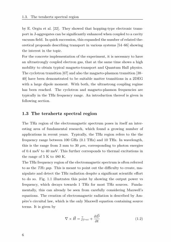
The THz region of the electromagnetic spectrum poses in itself an inter-esting area of fundamental research, which found a growing number ofapplications in recent years. Typically, the THz region refers to the thefrequency range between 100 GHz (0.1 THz) and 10 THz. In wavelength,this is the range from 3 mm to 30 µm, corresponding to photon energiesof 0.4 meV to 40 meV. This further corresponds to thermal excitations inthe range of 5 K to 480 K.The THz frequency region of the electromagnetic spectrum is often referredto as the THz gap. This is meant to point out the difficulty to create, ma-nipulate and detect the THz radiation despite a significant scientific effortto do so. Fig. 1.1 illustrates this point by showing the output power vsfrequency, which decays towards 1 THz for most THz sources. Funda-mentally, this can already be seen from carefully considering Maxwell’sequations. The creation of electromagnetic radiation is described by Am-père’s circuital law, which is the only Maxwell equation containing sourceterms. It is given by
∇× ~H = ~jfree + ∂ ~D
∂t(1.2)
6

Chapter 1. Introduction
Figure 1.1: THz Gap Output power of different sources in the THz frequencyrange. Figure adapted from Ref. [68]
Using ~D = ε0 ~E + ~P we obtain
∇× ~H =(~jfree + ∂ ~P
∂t
)+ ε0
∂ ~E
∂t, (1.3)
where the two terms in the bracket represent two different types of currentand thus source terms that can produce radiation. Of course, a current isalways caused by the motion of charge. Nevertheless the distinction is use-ful, since on one hand the first term describes current produced by free car-riers (e.g. in metals) that can move over large distances (’macro-currents’).On the other hand, the polarisation field ~P dependent contribution ∂ ~P/∂tdescribes the displacement of charge strongly confined typically within anatom (’micro-current’). The first contribution can efficiently produce ra-diation at frequencies below the THz region in the domain of electronics.But they fail at higher frequencies due to the inevitable presence of par-asitic capacitances and inductances giving an upper frequency limit forthe efficient generation of radiation. The second term does not suffer thislimitation, since microscopically displaced charges are cancelled by theiropposite charge on the microscopic scale. This allows for generation ofradiation in the domain of optics using atoms or many forms of artificialatoms. But this generation mechanism also breaks down when moving to-
7

1.4. Outline of the manuscript
wards lower frequencies, eventually also breaking down in the THz region.The reason is more subtle, but related to the interaction with the ther-mal phonon bath, where kT is similar to the transition energy of the THzradiation to be produced. Many sources in the THz therefore can only op-erate at cryogenic temperatures to escape this problem. The same appliesfor detectors which is in principle the reverse process where radiation getsconverted into a measurable current.
1.4 Outline of the manuscript
The goal of this thesis is to experimentally observe a modification ofmagneto-transport induced by a large vacuum Rabi splitting between theelectron’s cyclotron transition in the Hall bar and a vacuum field mode ina cavity.In Chapter 2, the theoretical basis for the ultrastrong light-matter cou-pling is presented, while Chapter 3 introduces the concepts needed tounderstand magneto-transport at low temperatures as well as the theoret-ical prediction of transport dressed by vacuum fields. To experimentallyobserve the latter effect, we present the three experimental setups neededin Chapter 4 and the sample design and fabrication in Chapter 5. Chapter6 then discusses the optical properties of this new experimental platform.With this understanding at hand, we can finally attempt to experimentallyobserve vacuum fields acting on transport. The key difficulty is to havea good reference measurement for the transport measurement coupled tovacuum fields. We employ two different approaches: In Chapter 7, we in-tentionally create a small polariton population with a THz source, whichallows to compare measurements to the case without real polaritons in thesystem. In Chapter 8, we achieve to observe changes to transport inducedby the vacuum field alone in two ways thanks to major technological im-provements in the sample design and process as well as in the stability ofthe measurement setup described in the previous Chapters.
8

CHAPTER 2
Quantum description of LandauPolaritons
In this Chapter we discuss the basics of the ultrastrong coupling regime,whose critical elements are shown in Fig. 2.1. The ultrastrong couplingregime is loosely defined to be reached when the vacuum Rabi frequencyΩ
Ω = ~d×√Ne × ~Evac/~. (2.1)
Figure 2.1: Elements of an ultrastrongly coupled system N equivalentdipoles (green) are located in an electromagnetic mode of a cavity formed by twomirrors. Adapted from Kockum et al. [32]
9

2.1. Matter part
exceeds 10 % of the bare light and matter frequencies [32,33]. Above, ~d isthe dipole moment of the matter excitation, Ne the number of equivalentdipoles inside the relevant electromagnetic mode of the cavity and ~Evac thevacuum electric field produced by the cavity. The former two are mainlydefined by the choice of the matter part whose implementation is discussedin section 5.1, while the choice of the cavity and its effective mode volumediscussed in section 5.2 defines the strength of the vacuum electric field~Evac.As already discussed in the first prediction of 2005 [28], an importantapproach to reach such a high normalized light-matter coupling ratio Ω/ωis to use collective matter excitations in solid state systems [30, 31, 69],hence a large Ne. Practically all demonstrations have used this approach[22, 32–40, 43, 67, 70–75], with the exception of experiments using a singleflux qubit as matter transition [71,76].In the following we derive the properties of the matter and light transitionsused for our specific implementation of the ultrastrong coupling regime insections 2.1 and 2.2, followed by a description of the coupled system withthe Hopfield model in section 2.3.
2.1 Matter part
A two dimensional electron gas (2DEG) placed in a perpendicular magneticfield leads to the formation of so called Landau Levels shown in Fig. 2.2.Among the two neighbouring levels closest to the Fermi energy, we canexcite the cyclotron transition. It has a very large dipole moment andis easily tunable with magnetic field. This implementation of the matterpart has not only allowed to reach the ultrastrong coupling regime [67],but is also usable for a magneto-transport experiment.
Solution of the Schrödinger equation Here, we briefly discuss theimportant properties of the Landau levels and the cyclotron transitionneeded for the light-matter coupling. In section 3.1, we elaborate theseconcepts further to understand the magneto-transport in presence of Lan-dau levels.Following the discussion in [50], one obtains Landau Levels as the exact
10

Chapter 2. Quantum description of Landau Polaritons
Figure 2.2: Landau levels and cyclotron transition Due due Pauli block-ing, only electrons in the highest filled Landau level can be excited to the nexthigher level. Adapted from Hagenmüller et al. [29]
solution of the effective mass Hamiltonian for a parabolic band as we haveit in a GaAs/AlGaAs quantum well. The Hamiltonian reads
H = (~p− e ~A)2
2m∗ + V (z), (2.2)
where V (z) is the confinement potential defined by the crystal growth,and ~A = (−By,0,0) describes the vector potential corresponding to themagnetic field B along the z-direction. The Hamiltonian can be separatedin an in plane and out of plane component. The latter describes theformation of the magnetic field independent bound states of the quantumwell, of which only the lowest is populated in our experiments. The in-plane part
Hxy =(px + eBzy)2 + p2
y
2m∗ + V (z), (2.3)
contains the magnetic field dependence. We can solve it by making theAnsatz
ψ(x,y) = eikxxη(y), (2.4)
which leads to the following eigenvalue problem[p2y
2m∗ + 12m∗ω2
c
(y − ~kx
eBz
)2]ηkx(y) = Eηkx(y). (2.5)
11

2.1. Matter part
Here we introduced the cyclotron frequency
ωc = eB
m∗, (2.6)
which linearly increases with the magnetic field B. This equation describesa one-dimensional quantum harmonic oscillator with the kx-dependentcenter coordinate y0 = ~kx
eBz= kxl
20. Here, we introduced also the mag-
netic length
l0 =√
~/eB. (2.7)
The equally spaced quantized energy states - the Landau Levels - are givenby
En = ~ωc(n+ 1
2
). (2.8)
Degeneracy and density of states (DOS) Note the independence ofEn from the quantum number kx. Assuming a sample of length Lx andwidth Ly, we have a density of kx states of Lx/2π and thus a finite numberof center coordinates y0 located in the given sample dimensions. We thusobtain the number
nL = 2eB/h (2.9)
of degenerate states per unit area (neglecting the spin degeneracy). Thisallows us to define the filling factor, as a ratio with the sheet carrier densityne:
ν = nenL
= hne2eB , (2.10)
which describes the number of filled Landau levels as function of the mag-netic field at zero temperature. This allows us to write the density of statesas
D2D = nL∑n
δ(E − En
). (2.11)
Of course, an energetic broadening appears due finite temperatures and
12

Chapter 2. Quantum description of Landau Polaritons
sample imperfections. These are further discussed in the context of Quan-tum Hall transport in the next Chapter.
Transition dipole moment and linewidth Due to Pauli blockingthe cyclotron transition is possible for electrons with energies E fulfillingEF − ~ωc < E < EF , as a photon with energy ~ωirr = ~ωc can exciteelectrons above the Fermi energy EF (see Fig. 2.2). The dipole momentfor the transition to the next Landau level depends on the magnetic lengthin equation 2.7 and on the filling factor in equation 2.10 as follows
d = el0√ν. (2.12)
Depending on the filling factor, the energy range EF − ~ωc < E < EF
might contain two partially filled Landau levels. We further note, thatthe cyclotron linewidth at high carrier densities observed in transmissionexperiments is super radiantly limited and given by [77]
ΓCR = 4πe2nem∗(1 + nGaAs)c
(2.13)
In contrast to transport experiments, a transmission experiment hencereveals little about 2DEG properties beyond the carrier density and mass.It especially does not reveal the carrier mobility, scattering properties orthe filling factor.
2.2 Light part
In order to reach the ultrastrong coupling regime (see equation 2.1), onecontribution comes from minimizing the effective cavity volume, as theresulting vacuum electric field is given by
Evac =√
~ωcavεε0Vcav
. (2.14)
In the optical domain, subwavelength cavities with acceptable losses aredifficult to make. The diffraction limit sets a minimum cavity volume ofVcav ≈ (λ/2)3 for the confinement of a transverse electromagnetic wave.For longitudinal electromagnetic waves, subwavelength cavities are possi-
13

2.3. Hopfield model
ble, but these require the use of metals which support longitudinal surfaceplasmon polaritons (SPPs). These are lossy at optical frequencies. On theother hand, in electronics, subwavelength cavities are common e.g. in theform of LC circuits and have acceptable losses in the THz range. How-ever, losses for now have a secondary role, as in contrast to the strongcoupling regime, the ultrastrong coupling regime does not directly dependthe cavity quality factor Q.
2.3 Hopfield model
As our experimental platform uses Landau polaritons [67, 78], both thelight and matter transitions occur between harmonic ladders of states. Insuch a case, the so called Hopfield model successfully describes the coupledsystem used in this work [29,66]. We assume only one cavity mode, whichis a good approximation for the lowest frequency mode if the other modesare far away in frequency.
Light-matter coupling Hamiltonian The Hopfield Hamiltonian [29,32,66] is given by
Hlm = ~ωcava†a+ ~ωcb†b+HI +HD (2.15)
where a† and b† are the bare light and matter creation operators. Thelight-matter coupling HI can be written as
HI = i~Ω(a+ a†)(b− b†) (2.16)
while HD describes the diamagnetic energy term growing with D = ~Ω2
ωc:
HD = ~Ω2
ωc(a+ a†)2. (2.17)
Note, the terms scaling quadratically in the Rabi frequency as well asterms containing a†b†, which simultaneously create or annihilate light andmatter excitations are kept in the Hopfield model to correctly describe theultrastrongly coupled system. The model reduces to the Jaynes-Cummingsmodel without those terms.
14

Chapter 2. Quantum description of Landau Polaritons
Bright collective excitation operator Concretely, the cyclotron ex-citation in the 2DEG acting as a matter excitation is created and tunedby an out of plane magnetic field along z. As its dipole moment d = el0
√ν
(equation 2.12) is in-plane, we assume a single linearly polarized cavityelectric field mode along y. In the second quantization framework, one candefine the fermionic operators c†nκ and cnκ (n: Landau Level index), whichcreate and annihilate an electron in the single-particle Landau level state|nκ〉, with |κ| < AnL from equation 2.9 and A = LxLy the sample surface.One can now introduce the bright collective excitation operator
b† = 1√nL
n 6=0∑nκ
√nc†nκcn−1κ, (2.18)
which behaves approximately as a bosonic operator ([b,b†] ' 1) in thethermodynamic limit (nL 1). This collective excitation of the two-dimensional electron gas can directly couple to the cavity photon mode.As we will see, the current operator responsible for magneto-transportintriguingly also only depends on the bright excitation and cavity modeoperators and not the other n-1 optically inactive excitations.
Hopfield-Bogoliubov transformation Exploiting the bosonicity of b†
in the weak excitation limit, the Hamiltonian can be diagonalized with theHopfield-Bogoliubov transformation [28,79]. One obtains
Hlm = EGS + ~ωLP p†LP pLP + ~ωUP p†UP pUP , (2.19)
where EGS is the ground state energy, while ωr and p†r are the frequenciesand bosonic creation operators for the upper and lower polariton excita-tions r ∈ LP,UP. The polariton operators expressed in the old basis aregiven by pr = wra+xrb+yra†+zrb† where the vector vr = (wr,xr,yr,zr)T
is the solution of the eigenvalue equation Mvr = ωrvr, with the Hopfieldmatrix
15

2.3. Hopfield model
M =
ωcav + 2D −iΩ −2D −iΩ
iΩ ωc −iΩ 02D −iΩ −ωcav − 2D −iΩ−iΩ 0 iΩ −ωc
. (2.20)
The coefficients satisfy the normalization condition |wr|2 + |xr|2 + |yr|2 +|zr|2 = 1. Note, that the last two coefficients are due to the counter-rotating-wave terms and would be zero in the strong coupling regime, butcannot be neglected in the ultrastrong coupling regime. The electronicand photonic weights of the polaritons are given by We,r = |xr|2 − |zr|2
and Wp,r = |wr|2 − |yr|2 and are plotted in Fig. 2.3b below the computedpolariton dispersions in 2.3a.
Polariton dispersions The relevant positive eigenvalues of the eigen-problem are then given by
ω(UP )(LP ) = 1√
2
√ω2c + 4Ω2 + ω2
cav ±G, (2.21)
where
G =√−4ω2
cω2cav + (−ω2
c − 4Ω2 − ω2cav)2 (2.22)
describes the polariton gap. The smallest separation of the two branchesω(UP ) − ω(LP ) = 2Ω is reached when the cyclotron dispersion becomesresonant with the cavity, thus ωc = ωcav = ω. The polariton branchesare plotted in Fig. 2.3a for realistic experimental parameters (Ω = 30%,ωcav= 140 GHz, m∗ = 0. 07m0).
Modification of the ground state properties An intriguing featureof the ultrastrong coupling regime lies in its modified ground state prop-erties. While for small normalized light-matter coupling ratios Ω/ωcav theground state simply consists of an an empty cavity and a matter part inits ground state, it becomes energetically favourable for larger couplingsto have matter and light excitations in the ground state [32]. As theseexcitations are part of the ground state of the coupled system, they arehard to detect from outside. There is a wealth of proposals to detect such
16

Chapter 2. Quantum description of Landau Polaritons
0.1 0.2 0.3 0.4 0.5 0.6 0.7 0.8 0.9 1
100
200
300
400
00
Magnetic field (T)
Magnetic field (T)
Freq
uen
cy [G
Hz]
0.1 0.2 0.3 0.4 0.5 0.6 0.7 0.8 0.9 1
0.5
1
00
Wei
gh
t
(a)
(b)
Figure 2.3: Polariton dispersions and mixing fractions a Computedpolariton dispersions (magenta) which appear as the bare cyclotron dispersion(green) anti-crosses with the magnetic field independent cavity resonance (red).The smallest separation between the two branches is given by 2Ω. b Electronicweights for the upper (black) and lower (red) polariton, which are defined asWe,r = |xr|2 − |zr|2. In the ultrastrong coupling regime, they both reach 50 %at a magnetic field higher than the anti-crossing field.
virtual excitations [32], e.g. by observing the Lamb shift of an ancillaryprobe qubit in the near field of the cavity [80], or by observing the radia-tion pressure exploiting physics related to the dynamical Casimir effect inan optomechanical system [81]. Many other proposals use the approach torapidly modulate any of the parameters responsible for the coupling (barecavity and matter frequencies or the Rabi frequency Ω) on time scalesshorter than ∼ πΩ−1 (see [32] for an overview).In our system, this ultra-fast switching could be implemented using super-conducting LC-circuits, which could be switched into the normally con-
17

2.3. Hopfield model
ducting phase using a femtosecond laser pulse. Exploiting the much largerelectron kinetic inductance of electrons in the superconducting state, thecavity could be switched to another frequency in this time scale. In thispresent work, we develop another platform, which might lead to a possi-bility to observe virtual excitations using the matter part itself as probeof these virtual excitations, observable by means of a Lamb shift type ofeffect of the electronic density of states probed by magneto-transport. Inthe following Chapter, we discuss theoretically how magneto-transport ismodified when dressed by the vacuum field of the cavity.
18

CHAPTER 3
Theory of magneto-transport coupled tovacuum fields
The ultra-strong coupling regime described in Chapter 2 has so far mostlybeen investigated experimentally by interrogating the photonic compo-nent of the polariton quasi-particle weakly probing the coupled systemwith low photon fluxes [25,30,31,37–39,43,67,69–73,82–86]. This lets oneoverlook the fact, that the ultrastrong coupling regime does not requireany real photons in the cavity. Few experiments exist so far, which probethe ultrastrongly coupled system in the absence of polaritonic excitations.Notably, exceptions are the measurement of the matter part of an exci-ton polariton condensate with an excitonic 1s-2p transitions [87] and atransport experiment in molecules coupled to a plasmonic resonance [22].The latter work inspired a number of theoretical works, discussing vac-uum field induced changes to magneto-transport of excitons using variousmodels [56, 58, 59, 61, 62]. Other works predict vacuum induced changesto charge transport in quantum dots [54, 88, 89] and also cavity mediatedsuperconductivity [63,90].
In this Chapter, we discuss the theoretical basis for magneto-transport intwo dimensional electron gas (2DEG) coupled to a cavities vacuum field. Insection 3, we briefly discuss the relevant experimental quantities describing
19

3.1. Magneto-transport without a cavity
charge transport in a 2DEG without a cavity [50]. The present discussionis mostly along the lines of the former reference. In section 3.2 we thendiscuss magneto-transport coupled to a cavity mode. We first give fewsimple qualitative arguments, why high frequency vacuum fields couplingto electrons in a Hall bar must change its dc longitudinal resistance. In thesecond part the recently presented theoretical description by N. Bartoloand C. Ciuti [66] is discussed.
3.1 Magneto-transport without a cavity
In this section, we summarize the relevant properties of the 2DEG resis-tivity as function of magnetic field, along the lines of the discussion inSemiconductor Nanostructures by T. Ihn [50].
3.1.1 Drude and Boltzmann transport at low B-fields
Conductivity and resistivity Ohm’s law U = RI in the local form fora homogeneous anisotropic material is given by
j = σE (3.1)
where j is the electrical current density and E is the electric field. Theelectrical conductivity tensor is given by
σ =
(σxx σxy
−σxy σyy
), (3.2)
while the resistivity tensor ρ fulfilling E = ρj is obtained by tensor in-version. Note that in 2 dimensions, the the resistivity tensor ρ and theresistance R have the same units and differ only by a geometrical factor.The resistivity tensor is hence experimentally obtained by measuring Vxxand Vxy as shown in Fig. 3.1 applying an electric field Ex
ρxx = VxxI
W
Land ρxy = Vxy
I. (3.3)
Drude conductivity (longitudinal) The simple Drude model lets usdefine already a number of useful quantities. In the diffusive transport
20

Chapter 3. Theory of magneto-transport coupled to vacuum fields
y
x
Figure 3.1: Four-terminal measurement of resistivity tensor A currentI passed from source to drain does not allow to measure R2DEG directly dueto significant contact resistances RC . Instead, ρxx and ρxy are obtained from afour point measurement using equation 3.3. This geometry unfortunately cannotbe used to measure also ρyx and ρyy on the physically same Hall bar.
regime, electron momenta are randomized within a length scale given bythe mean free path l. In equilibrium, the rate at which electrons gainmomentum due to the electric field during a mean time τ between (back-)scattering events is the same as the loss of momentum due to scattering.The equilibrium is described by m∗vd
τ= eE. Hence, we get an expression
for the drift velocity
vd = eτ
m∗E (3.4)
and for the carrier mobility defined using vd = µE
µ = eτ
m∗. (3.5)
We can further obtain an expression for the Drude conductivity from thedefinition of the current density j = neevd = σE as
σxx = eneµ = ne2τ
m∗, (3.6)
where n is the sheet carrier density. The above expressions remain a goodapproximation in the low magnetic field limit in the absence of the Landau
21

3.1. Magneto-transport without a cavity
quantisation in the diffusive limit.
Classical Hall effect (transverse resistivity) In a perpendicular mag-netic field with an in-plane current, one finds the classical Hall effect, in-ducing a transverse Hall voltage, which in two dimensions is geometryindependent and given by
UH = BI
neeand thus ρxy = B
nee. (3.7)
Drude model in magnetic field Also at low magnetic fields, the clas-sical Drude model gives a descriptive result. In a magnetic field per-pendicular to the sample, electrons perform the classical cyclotron orbits.Scattering with a random angle e.g. at impurities, results in a drift of thecyclotron orbit center along the y-direction (along the E ×B direction).In a magnetic field, the Drude conductivity 2x2-tensor becomes
σxx(B) = nee2τ
m∗1
1 + ω2cτ2 (3.8)
σxy(B) = nee2τ
m∗ωcτ
1 + ω2cτ2 . (3.9)
Upon tensor inversion, the resistivity writes
ρxx(B) = m∗
nee2τ(3.10)
ρxy(B) = B
ene. (3.11)
Despite the simplicity of the model, this results remains correct in a semi-classical and also quantum mechanical treatment of the problem. However,the latter models add significantly to the understanding of the meaning ofτ in the above equations. Furthermore, of course, τ becomes oscillatoryat higher magnetic fields in the presence of the Landau quantization.
Conductivity in the Boltzmann framework The current is describedtaking into account the Fermi statistics of electrons as follows:
22

Chapter 3. Theory of magneto-transport coupled to vacuum fields
j = − eA
∑nkn
vn(kn)fn(k), (3.12)
where A is the normalization area, and fn the probability density for theoccupation of a state nkn and vn(kn) the (group) velocity of an electronin subband n. Assuming a homogeneous electron gas and a parabolicdispersion
En(kn) = En + ~2k2n
2m∗ , (3.13)
the distribution fn(k) can be obtained solving the Boltzmann equation inthe relaxation time approximation.For weak electric fields in the steady state and neglecting intersubbandscattering, we can write the distribution fn(k) as the equilibrium Fermi-Dirac distribution, but shifted by δk = eτcosθ|E|/~, where θ = µB isthe Hall angle. In other words the result of the E × B-field is a shift ofthe Fermi-circle. With a Taylor expansion the effect of the perturbativeE×B-field becomes dependent on the energy derivative of the Fermi-Diracdistribution. At low temperatures, this is almost a delta-like functionaround the Fermi energy. Its width is given by the thermal broadeningkT EF .The conductivity, still taking the same form as obtained from Drude, nowdepends more specifically on the scattering time at the Fermi energy τ =τe := τ(EF ).
Microscopic picture for Drude scattering time τ0 At low magneticfields, we can express the Drude scattering time τ0 = τ(EF )|B=0 in amicroscopic picture as
~τ0
= niD(E)∫ 2π
0dφ〈|v(i)(q)|2〉imp(1− cosφ), (3.14)
where ni = Ni/A is the areal density of impurity scatterers, D(E) thedensity of states, and v(i)(q) the scattering matrix element between twoelectron momentum states separated by momentum q = k′ − k. Most im-portantly note the factor (1−cosφ), which enhances the weight of backscat-tering events and makes small angle scattering events have a negligable
23

3.1. Magneto-transport without a cavity
influence on the τ0 consistent with Drudes original model.
Fermi gas The density dependent Fermi wave-vector kF is given by
kF =√
2πne. (3.15)
Via the Fermi velocity vF = ~kFm∗ and using equation 3.5, we can obtain an
expression for the mean free path l of the electrons between backscatteringevents, dependent only on the electron density and mobility,
l = vF τ = ~µ√
2πnee
. (3.16)
Experimental determination of carrier density and mobility Us-ing equation 3.7, we can experimentally determine the electron densityfrom the Hall resistance at low magnetic fields as
n = 1edρxy/dB|B=0
(3.17)
and the mobility is obtained using equation 3.6 and 3.5
µ = dρxy/dB|B=0
ρxx(B = 0) . (3.18)
3.1.2 Magneto-transport with Landau quantization
As already discovered around 1930 by L. Shubnikov and W. J. de Haasin three dimensional metallic bismuth samples, the longitudinal resistiv-ity shows periodic oscillations in 1/B. These are induced by the Landauquantization (see section 2.1) causing sharp peaks in the density of states,which in turn result in an oscillatory electron lifetime at the Fermi level.As we saw before, the lifetime τ going into the conductivity and resistivitytensor in equations 3.8, 3.9 and 3.10 has to be interpreted as τe := τ(EF ),hence resulting in resistivity oscillations.
Landau level broadening and quantum lifetime τq For high mobil-ity GaAs-based 2DEGs at low temperatures, the dominating broadeningmechanism comes from scattering off spatial potential fluctuations inducedby charged dopants [50]. We can write the mean scattering rate between
24

Chapter 3. Theory of magneto-transport coupled to vacuum fields
−0.6 −0.4 −0.2 0 0.2 0.4 0.60
5
10
15
20
25
Magnetic field [T]
Re
sist
an
ce [Ω
]
Figure 3.2: Shubnikov-de Haas oscillations Longitudinal resistance ρxx asfunction of magnetic field. At low fields, the resistance is constant and is constantas predicted by Drude (see equation 3.10). Above around 30 mT, the Shubnikov-de Haas oscillations appear as a result of an oscillatory electron density of stateswhich causes the electron momentum scattering time to oscillate periodically in1/B.
momentum states as 1/τq, where τq is the quantum lifetime. Using Heisen-bergs time-energy uncertainty, the broadening of a Landau level is thengiven by Γ = ~/τq.
At low magnetic fields, we can estimate the scattering rate between mo-mentum states at the Fermi energy τq(EF ) as
~τq(E) = niD(E)
∫ 2π
0dφ〈|v(i)(q)|2〉imp = 2πniD(E)v2, (3.19)
where ni = Ni/A is the areal density of impurity scatterers, D(E) thedensity of states, and v(i)(q) the scattering matrix element between twomomentum states separated by momentum q = k′ − k. Note, that incontrast to the Drude scattering time τ0, the quantum lifetime broadeningof the momentum states has no enhanced weight for backscattering. Thescattering angle is not relevant here. The measurement of the quantumlifetime is hence a sensitive probe for scattering processes in the 2DEGnear the Fermi energy.
25

3.1. Magneto-transport without a cavity
Oscillatory magnetoresistance Here we use only plausibility argu-ments to reach the main result, which was derived by Ando et al. [91].We assume that the density of states lineshape of every Landau level isa Lorentzian L with width Γ = ~/τq independently of the Landau Levelindex. We can therefore write the density of states as
D(E,B) = 2nL∑
Ln(E − ~ωc(n+ 1/2)). (3.20)
At low magnetic fields, where E ~/τ holds, one can use Poisson’s sum-mation formula and rewrite the density of states as
D(E,B) = m∗
π~2
[1 + ∆D
D
]. (3.21)
The density of states is now written as the sum of the zero magneticfield two-dimensional density of states and perturbation which is small forsufficiently low magnetic fields. Using only the first term of Poisson’s sum,we obtain
∆DD
= −2 exp(− π
ωcτq
)cos(2πE/(~ωc)). (3.22)
The exponential factor is known as Dingle factor, and accounts for thequantum lifetime broadening of the Landau levels. It can be argued thatsimilarly to equation 3.19, the electron scattering rate at the Fermi energyτe should scale with the available density of states as
1τe
= 1τ0
(1 + ∆D
D
)(3.23)
and explicitly
1τe
= 1τ0
(1− 2 exp
(− π
ωcτq
)cos(2πE~ωc
)). (3.24)
To obtain the Ando et al. expression for the resistivity [91], we only needto plug τe into Drude’s result in equations 3.8, 3.9 and 3.10. Keeping onlylinear perturbation terms, the longitudinal resistivity obtained again bytensor inversion and replacing EF /~ωc = hn/2eB writes
26

Chapter 3. Theory of magneto-transport coupled to vacuum fields
ρxx = m∗
nee2τ0
[1− 2e−π/ωcτq 2π2kBT/~ωc
sinh(2π2kBT/~ωc)cos(
2π hn
2eB
)]. (3.25)
The prefactor represents the Drude resistivity around which the magneto-resistance oscillates periodically in 1/B. As we saw above, the second partrepresents the density of states with Lorentzian broadened Landau levels.While the exponential Dingle factor represents the quantum lifetime τqbroadening of the Landau levels, the sinh-term describes the broadeninginduced by the finite temperature T.
In summary, the longitudinal resistivity can be seen to a good approxima-tion either as a probe of the density of states at the Fermi level (withinkT) or as a probe of the electron scattering time τe at the Fermi energy.
2 4 6 8 10
100
1/B [T-1]
∆ρ
xx/ρ
xx
,B=
0χ(Τ)
101
Figure 3.3: Dingle plot obtained from a measurement (Sample RH in Fig. 7.2)of the oscillation amplitude of the longitudinal resistance ρxx as function of mag-netic field.
Experimental determination of the quantum lifetime τq From theabove expression 3.25 τq can be extracted from the experimental longitu-dinal resistance trace ρxx(B) as the slope of ∆ρxx/ρxx,B=0χ(T,B) plottedversus 1/B, also known as Dingle plot [92] as shown above for a measure-ment (Sample RH in Fig. 7.2). χ(T,B) is defined as sinh(X)/X, whereX = 2π2kBT/(~ωc).
27

3.2. Magneto-transport in a cavity
3.2 Magneto-transport in a cavity
With the knowledge of the resistivity properties of a high mobility 2DEGdiscussed in the previous section 3, we can now discuss how the coupling toa cavities’ vacuum field affects the resistivity. In section 3.2.1, we give a fewqualitative arguments, why the resistivity should be affected by the cou-pling. The section 3.2.2 then gives a rigorous discussion recently publishedby our collaborators [66]. Herby, we focus on the regime, where Shubnikov-de Haas oscillations appear, but the spin splitting and the Quantum Hallregime are not yet developed.
3.2.1 Qualitative arguments for electric vacuum fieldfluctuations affecting transport
The following arguments have been the working hypothesis for most of theexperimental work presented in the following Chapters.
Electrons affected by the ultrastrong coupling regime are near theFermi energy EF and due to Pauli-blocking, all electrons able to cou-ple to the cavity must be located in the energy range EF − ~ωc . E ≤EF . In contrast, electrons contributing to magneto-transport are locatedwithin kT around the Fermi energy, where in our experimental conditionskT/(~ωc) ∼ 1%. Hence, electron transport occurs exclusively via elec-tronic states which ultrastrongly couple to the cavity vacuum field.
Cyclotron frequency The value of the cyclotron frequency ωc is a veryimportant parameter for the conductivity of an electron gas, as it definesShubnikov-de Haas oscillation amplitude, its shape and temperature de-pendence (see equation 3.25). The ultrastrong coupling regime on theother hand - at least when observed with optical means - replaces the barecyclotron dispersion by the polariton dispersions (see Chapter 2). Sucha replacement might at least in some aspects be visible also in transportwhich is so intimately connected to the cyclotron frequency.
Vacuum fields are also electric fields The electro-magnetic groundstate of the cavity mode (QED ground state) has no energy quanta avail-
28

Chapter 3. Theory of magneto-transport coupled to vacuum fields
able to excite electrons as it is the ground state. However, the vacuumelectric field can still act on charges and cause energy conserving processese.g. elastic scattering of an electron to which transport is highly sensitive(see section 3). Further, it can cause originally orthogonal electronic statesto couple, similarly to the finite spontaneous emission lifetime of an atomwhich appears due to a disturbed orthogonality of atoms electronic statesin the presence of vacuum fields.
Physics comparable to Lamb shift The Lamb shift [4] describes aDC energy shift of the s electron orbital due to the presence of randomlyfluctuating vacuum electric fields, which distort the atoms electric poten-tial probed by the electron. The effect does not average to zero due to thenon-linearity of the atom potential, which result in a contribution scalingwith the vacuum electric field squared. A similar mechanism might resultin a DC change of magneto-transport.
Energy scale of light-matter coupling In the ultrastrong light-mattercoupling regime, the large Rabi frequency Ω defines a large energy scale~Ω, which can significantly exceed the Landau level linewidth ~/τq and isalso comparable to the cyclotron transition energy. It would hence not besurprising, if the regime has a consequence directly on the electronic den-sity of states, which is directly probed by magneto-transport (see section3.1).
3.2.2 Theory for vacuum-dressed cavity magneto-transport
In this section we present the theoretical description of magneto-transportof a 2-dimensional electron gas modified by the coupling to a cavity in itsground state, as recently presented by N. Bartolo and C. Ciuti [66] in closecollaboration with our experimental work.1
Linear response Kubo ansatz Under the action of an electric bias offrequency ω, the linear response of the 2DEG can be determined usingthe Kubo approach [93]. For known eigenstates |ξ〉 and energies Eξ of
1Compared to the Ref. [66], we invert the x and y coordinates for consistency withthe other parts of this manuscript.
29

3.2. Magneto-transport in a cavity
the manybody Hamiltonian, the magneto-conductivity according to Kuboreads:
σij = i∑ξ 6=ξ′
e−βEξ′ − e−βEξAZ(Eξ − Eξ′)
〈ξ| Ji |ξ′〉 〈ξ′| Jj |ξ〉(ω + i/τξξ′) + (ωξ − ωξ′)
, (3.26)
where i,j ∈ x,y, A the 2DEG area, β = 1/(kBT ) the inverse thermalenergy, Z the partition function and τξξ′ the transport scattering time.The current operator going into the matrix elements of the Kubo formulawrites J = − e
m∗
∑i(pi + eAi). With some algebra, we can express the
current operators as function of the single photon and bright collectiveexcitation operators:
Jx = −
√~ωcNee2
2m∗ (b+ b†),
Jy = −
√~ωcNee2
2m∗[i(b− b†) + 2Ω
ωc(a+ a†)
],
(3.27)
where Ne = neA. It is important to note here, that the current operatorsdepends only on the collective bright excitation and cavity mode operators,the same operators relevant for the description of the ultra-strong couplingregime.
Current operator in polariton basis The operators a and b can nowbe expressed in terms of polariton operators p†r and pr introduced in theprevious section 2.3:
a = w∗LP pLP + w∗UP pUP − yLP p†LP − yUP p†UP ,
b = x∗LP pLP + x∗UP pUP − zLP p†LP − zUP p†UP .
(3.28)
With this, the current operators read:
30

Chapter 3. Theory of magneto-transport coupled to vacuum fields
Jx = −
√~ωcNee2
2m∗∑r
[(xr − zr)∗pr + H.c.] ,
Jy = −
√~ωcNee2
2m∗∑r
iωrωc
[(xr − zr)∗pr −H.c.] .
(3.29)
Here it is clear that magneto-transport coupled to a cavity is directlymediated by the polariton states [66]. In other words, the light-mattercoupling can also fundamentally change the basis of states relevant fortransport.
Low temperature limit An important simplification is possible in thelow-temperature limit (β → ∞), as |ξ〉 and |ξ′〉 can only be the groundstate |GS,ζ〉 or 0 < ζ <
(nLANn
)-permutations thereof, where Nn is the
number of electrons in the partially filled highest Landau level. Further,the current operator in equation 3.29 only couples the ground state topolariton states |LP,ζ〉 = p†LP |GS,ζ〉 and |UP,ζ〉 = p†UP |GS,ζ〉 which actas virtual intermediate states for magneto-transport. The Kubo transportscattering rates τξξ′ hence take only the two values τr := τr,GS with r ∈LP,UP. For low temperatures, the partition function also simplifies toZ ' e−βEGS . As each permuation ζ gives the same contribution to σij ,the conductivity tensor in the dc limit (ω → 0) writes
σdcij =∑
r∈LP,UP
2τr~ωr
<[Θ(r)ij
]− ωrτr=
[Θ(r)ij
]1 + (ωrτr)2 , (3.30)
where
Θ(r)ij = 〈GS,ζ| Jj |r,ζ〉 〈r,ζ| Ji |GS,ζ〉 . (3.31)
Polariton mediated conductivity tensor To reach the final analyticresult, we only need to insert equation 3.29 in the above result:
31

3.2. Magneto-transport in a cavity
0.1 0.2 0.3 0.4 0.5 0.6 0.7 0.8 0.9 1
100
200
300
400
00
Magnetic field (T)
Magnetic field (T)
Freq
uen
cy [G
Hz]
0.1 0.2 0.3 0.4 0.5 0.6 0.7 0.8 0.9 1
0.5
1
00
Wei
gh
t
(a)
(b)
Figure 3.4: Polaritons and transport weights a Computed polariton dis-persions (magenta) which appear as the bare cyclotron dispersion (green) anti-crosses with the magnetic field independent cavity resonance (red). The small-est separation between the branches is given by 2Ω. b Electronic weights forthe upper (black) and lower (red) polaritons (full lines), which are defined asWe,r = |xr|2 − |zr|2. In the ultrastrong coupling regime, they both reach 50% at a magnetic field higher than the anti-crossing field. In contrast, dashedlines show the conductivity weights Ce,r = |xr − zr|2 in the sum of equation3.32. They cross where the bare dispersions cross in a and the upper polaritonsconductivity contribution never becomes 1.
σdc = nee2
m∗
∑r
|xr − zr|2τr1 + (ωrτr)2
(ωcωr
ωrτr
−ωrτr ωrωc
). (3.32)
The resistivity tensor ρdc shown in the measurements in the followingChapters can be obtained by tensor inversion from σdc = (ρdc)−1.
32

Chapter 3. Theory of magneto-transport coupled to vacuum fields
Comparison to Drude conductivity The standard Drude conductiv-ity tensor derived in equations 3.8 and 3.9 is given by
σdc = nee2
m∗τe
1 + (ωcτe)2
(1 ωcτe
−ωcτe 1
). (3.33)
For no cavity coupling (Ω = 0), the dressed conductivity in equation 3.32recovers the Drude-like magneto-conductivity shown above. An importantconsequence of the presence of the cavity is that the dressed conductivityis a sum of two weighted contributions associated to the two fundamen-tal polariton excitations, which replace the single contribution dependingonly on the cyclotron frequency - similarly to what is expected in THztransmission (Fig. 2.3). Unfortunately, the interpretation of the resistivityis less intuitive, as a tensor inversion of the sum mixes the two polaritoncontributions.The conductivity weights for the summands are Ce,r = |xr − zr|2, whichdiffer from the electronic weight of the polariton We,r = |xr|2 − |zr|2. Asshown in Fig. 3.4b, in contrast to the polariton mixing fractionsWe,r whichreach both 50% at magnetic fields beyond the anti-crossing, the crossingof the conductivity weights Ce,r occurs where the bare matter and lightdispersions cross. Further, the upper polaritons conductivity weight Ce,rdoes not converge to 1 at low fields.
Transport scattering time τr The polariton transport scattering timeτr in equation 3.32 stemming from Kubo’s formalism replaces τe in theDrude conductivity expression in equation 3.33. It can be written as asum, with the weights being the electronic and photonic mixing fractionsof the polariton [66]
1τr
= We,r
τe+ Wp,r
τp. (3.34)
Here τe the electron scattering rate at the Fermi energy derived in equation3.24 after replacing EF /~ωc = hn/2eB and using the definition of thefilling factor in equation 2.10:
1τe
= 1τ0
(1− 2 exp
(− π
ωcτq
)cos(πν)
). (3.35)
33

3.2. Magneto-transport in a cavity
One may note a theoretical difficulty here, as τr as defined in the Kuboformalism τr := τr,GS is a intersubband scattering rate between the groundstate |GS,ζ〉 and first excited state |r,ζ〉, while τe used to define τr in equa-tion 3.34 is derieved from intrasubband scattering directly at the Fermienergy not involving other subbands.The second time τp in equation 3.34 is a transport scattering time dueto environmental fluctuation affecting the cavity mode and can be muchlonger than the cavity photon lifetime defining the low Q-factor of thecavity. In can be seen as the first order coherence g1 of the vacuum fieldmode, which is not necessarily the same as the g1 of a real photon. Thelatter is fixed by the cavity Q-factor via the Wiener-Khinchin theorem.Unfortunately, τp is not an experimentally accessible parameter in ourcase, but we can assume τp τe.Fig. 3.5 shows the prediction of the theory as presented by N. Bartolo andC. Ciuti [66] for different normalized light-matter coupling strengths andfor the cavity vacuum field polarized a along or b orthogonal to the sourcedrain current. The other parameters are chosen close to the experimentalconditions presented in section 8.1.2. Notably, a vacuum field inducedchange in carrier mobility is observed for the parallel case. For the caseEvac ⊥ ISD, one can observe a SdH modulation amplitude reduction in abroad range near the anti-crossing field. Also the Drude resistance valuearound which the oscillations occurs appears to be reduced near the anti-crossing for large τp > τ0.
Other possiblity to express τr The expression τr introduced ad hocin equation 3.34 might also be written using τq for the electron lifetime andτQ for the cavity life time rather than τe and experimentally inaccessiblephoton lifetime τp. It might make more sense, that vacuum fields causesmall angle scattering described by τq rather than large angle scatteringdescribed by τp. Unfortunately, with the present experimental parameters,this question cannot be answered, since both pairs of values have approx-imately the same values and don’t result in obvious modifications of theresistivity traces. Qualitatively, such a theory also leads to a SdH ampli-tude reduction around the resonant magnetic field, but no change of theDrude resistance value around which the SdH oscillations occur. While
34

Chapter 3. Theory of magneto-transport coupled to vacuum fields
W/w = 0%
10%
20%
30%
40%
(a)
0 0.2 0.4 0.6 0.8 10
5
10
15
Magnetic field [T]
ryy
[W]
W/w = 0%
10%
20%
30%
40%
(b)
0 0.2 0.4 0.6 0.8 10
5
10
15
Magnetic field [T]
rxx
[W]
Figure 3.5: Dressed resistance traces for two vacuum polarisationsComputed longitudinal magneto-resistance for different realistic normalized lightmatter couplings and for a Evac ‖ ISD and b Evac ⊥ ISD, where ISD is thesource drain current. The model parameters chosen close to the experimentalparameters discussed in the next Chapter are ne = 3 × 1011cm−2, τ0 = 131ps,τq = 2. 8ps, m∗ = 0. 07×m0, ωcav = 100GHz and τp = 300ps
this per se is not consistent with experiments presented in Chapter 7 and8, this might be explained by the presence of localized electronic stateswhich cannot contribute to the polariton and hence leave the SdH minimaunchanged.
35

3.2. Magneto-transport in a cavity
36

CHAPTER 4
Measurement Setups
For the experimental study of magneto-transport coupled to vacuum fields,three different experimental setups have been used. In a first step, a goodunderstanding of the ultrastrongly coupled system needs to be obtainedby performing free space transmission experiments through an array ofcoupled cavities. For this purpose, a THz time domain spectroscopysetup maintained by Dr. Curdin Maissen and Janine Keller is used. It isbriefly discussed in section 4.1 and most measurements with the setup arepresented in Chapter 6.With this understanding, the magneto-transport characteristics of thesample can be assessed with two further transport setups with very dif-ferent characteristics. As this project required the development of a newsample process, an entirely new sample design and a - to our group - unfa-miliar magneto-transport measurement technique, discussed in Chapter 5,it was very useful to use a liquid Helium cooled magneto-transportsetup from Janis Research company presented in section 4.2. Thissetup was mostly developed by Dr. Federico Valmorra and later improvedby myself. This setup allows to exchange samples within around 1 hour- a useful feature when testing dozens of samples until we converged tothe design presented in Chapter 5. Limited by the too high base tempera-ture of 1.3 K (corresponding 0.11 meV or 26 GHz) and a for this purpose
37

4.1. THz time domain spectroscopy (THz-TDS)
unacceptable stability of the system, an new Helium-3 dilution refrig-erator form Bluefors Cryogenics was bought and developed for thispurpose. It is presented in section 4.3. With a base temperature of only6 mK, an electron temperature of around 30 mK (2 µeV or 0.6 GHz) andan impressive stability allowing to compare measurements taken a week ormore apart. An exchange of a sample however takes 5 to 7 days, as theentire setup needs to be warmed up to room temperature in between.
4.1 THz time domain spectroscopy (THz-TDS)
For the optical characterisation of the samples, a THz-time domain spec-troscopy (THz-TDS) setup as shown in Fig. 4.1 is used. A detailed de-scription is given in the thesis of Curdin Maissen [94]. First demonstratedin the 1990’s by Griskovsky [95], the technique is sensitive to amplitudeand phase of a transmitted broadband single cycle THz pulse.
Figure 4.1: Sketch of THz-TDS Short near infrared pulses generated by theMaiTai laser are separated into pump and probe beams (red). NIR pump pulsescreate THz pulses at the photo-conductive switch (yellow), which are focussedonto the sample with off axis parabolic mirrors. Recombining the THz beamwith the probe beam, the detection is performed exploiting a ξ(2)-non-linearityand ellipsometry performed with a λ/4-plate, a Wollaston prism and two NIRphoto-detectors. Figure adapted from [94]
38

Chapter 4. Measurement Setups
As shown in Fig. 4.1, short near infrared (NIR) pulse trains generated bythe MaiTai Ti:Sapphire pulsed laser (70 fs pulse length, 80 MHz repetitionrate) are separated into pump and probe beams (red). The stronger NIRpump pulse beam is used to create THz pulses at the photo-conductiveswitch [96]. The latter conducts current between two biased electrodes forabout a picosecond after a NIR pulse hits the switch, resulting in THzradiation being emitted. The switch bias is modulated at 15.5 kHz fora lock-in detection. With off-axis parabolic mirrors, the (almost) singlecycle THz beam (yellow) is focussed on the sample and then recombinedwith the weaker NIR probe beam. For the detection, the electro-opticPockels-effect [97] is exploited, where a change of birefringence is inducedby the sum and difference frequency generation of the NIR and THz fieldsin the crystal. The initially linearly polarized NIR probe beam is changedproportional to the THz electric field amplitude. With the help of a λ/4-plate and a Wollaston prism, the beam is split into to NIR beams with asimilar power Pi, whose difference is proportional to the THz electric fieldamplitude (balanced detection)
P2 − P1
P2 + P1∝ ETHz (4.1)
Figure 4.2: Typical THz-TDS transmission measurement in a time andb frequency domain.
With a delay stage, the electric field of a THz pulse can be detected asfunction of time delay (corresponding to the phase) as shown in Fig. 4.2a.As the amplitude and phase information is available a Fourier transform
39

4.2. Janis Cryostat
allows one to retrieve the transmission spectrum shown in Fig. 4.2 b on avery broad frequency range, between around 50 GHz and 3.5 THz in thebest case.
4.2 Janis Cryostat
Many sample design and processing changes were tested in a liquid-He4cooled superconducting magnet from Janis Research Company, which al-lows to reach magnetic fields of 12 T and a sample base temperature ofaround 1.3 K in pumped liquid Helium. A detailed description of the setupis presented in the thesis of Federico Valmorra who developed the systemto perform magneto-transport measurements in this setup. Compared tothe Bluefors presented in the section below, the practical advantages of thesystem are the fast sample exchange (1 hour vs. 5 days), the higher max-imum magnet sweep rate (540 mT/min vs <10 to 50 mT/min), and themaximum magnetic field (12 T vs. 6 T). However, the high base tempera-ture of 1.3 K (corresponding 0.11 meV or 26 GHz) does not allow to studyvacuum field effects of the cavity at 140 GHz, as the thermal photon pop-ulation is non-negligible, besides the fact that magneto-transport greatlybenefits from lower temperatures, as demonstrated below in Fig. 4.6. Thisis why all measurements presented in this thesis are performed with thedilution refrigerator presented below.
4.3 Dilution Refrigerator Setup (Bluefors)
We use a dry dilution refrigerator from Bluefors Cryogenics. A pulse tuberefrigerator driven with He-4 is used to cool the system down to around3 Kelvin, from where a second He-4/He-3 mixture circulation allows toreach a base temperature of around 7 mK at the mixing chamber. Asshown in Fig. 4.3a and b, the system has different temperature stages ataround 45 K, 4 K, 1 K and 6 mK. The former 3 have a thermal shieldattached to it to block blackbody radiation coming from the vacuum canat 300 K. A magnet in Helmholtz configuration from American Magneticsis connected to the 4 K shield and allows for an optical access from 5different directions, one of which will be used in Chapter 7. The 4 K
40

Chapter 4. Measurement Setups
shield and the magnet mounted at its lower end is shown in Fig. 4.3c. Thesample is mounted on a copper cold finger holding a chip carrier with 24usable electrical connections shown in Figs. 4.3d and e. Additionally, onecan see an optical fibre (yellow), which is used to illuminate the samplebefore measurements at low temperature with IR light. The electricalconnection onto the GaAs chip are made with 18 µm thick gold bondingwires as shown in Fig. 4.3f.
B
Split-coil magnet
4K
Vacuum shield 45 K-shield
1 K-shield
Sample (6 mK)4 K
1 K
6 mK
300 K
45 K
a)
d)c)
b)
e) f )
Figure 4.3: Bluefors setup a Dry dilution refrigerator showing part of thevacuum can (white) and the different gold coated plates at different temperatureto which thermal shields are mounted. b 4 K thermal shield with magnet attachedat the lower end. The thick yellow wires carry the ∼100 A current for the magnet.c Sample holder at the end of a copper cold finger. d Chip socket with 24 resistivewires soldered at the back and a chip carrier clamped into it. f The electricalconnection between the pins of the chip carrier and the processed GaAs chip isprovided with 18 µm thick gold bonding wires
41

4.3. Dilution Refrigerator Setup (Bluefors)
4.3.1 Measurement circuit
A simplified measurement circuit is sketched in Fig. 4.4. A small current ofI ∼ 10nA modulated at typically 14 Hz is applied from source to the drain(blue). It is obtained from the oscillator voltage output of the lock-in andconverted to a current with a large 10 or 100 MΩ resistor. The voltagedifferences Vxx and Vxy for each Hall bar (e.g. 2 Hall bars with and withoutcavity shown in the Fig. 4.4) are measured using up to 7 commercial digitalMFLI Lock-in amplifiers from Zurich Instruments in parallel in conjunctionwith a home-made AC differential voltage pre-amplifier (purple).
4.3.2 Cooling the electron gas
For the measurement, 24 phosphor-bronze wires are installed from roomtemperature to the mixing chamber and interfaced with a non-magneticmicro-D CINCH connector. At such low temperatures, the heat exchangebetween electrons and phonons of their host material becomes extremelyweak [98], resulting in very different lattice and electron temperatures. Ef-fectively, heat conductivity is consequently highly correlated with electricalconductivity. While the lattice eventually cools to 6 mK base tempera-ture, the electrons remain at much higher temperatures. Here, we brieflydiscuss the measures taken to cool the system, with more details here [99]:
Instrument and environment noise Via measurement lines, the sam-ple is electrically connected to up to 7 lock-in amplifiers as well as currentand voltage sources. From these instruments, but also via electromagneticpick up from other noise sources in the lab, e.g. at 50 Hz, the electrontemperature is significantly affected. As we use a lock-in-technique toavoid noise in measurements, we use two 4-channel AC differential voltageamplifiers with an input noise of 1 nV/
√Hz at 10 Hz to minimize envi-
ronment noise injected into the cryostat1. Of course, the amplifier needsto be located as close as possible to the cryostat (and in principle best in-side), and wire pairs should be twisted on the non-amplified side to avoidpick-up.
1They are homebuilt by Peter Märki in the group of Prof. Klaus Ensslin
42

Chapter 4. Measurement Setups
Figure 4.4: Electrical measurement scheme Longitudinal and transverseresistance of two Hall bars in series with one inside a cavity measured at thesame time. On all measurement lines, there are low pass filters, thermalisationcoils and low noise AC differential voltage amplifiers (pink). The measurementsare performed with Zurich instrument lockins.
Johnson-Nyquist noise The next important contribution is Johnson-Nyquist noise [100] (or blackbody radiation) produced by electrons in partsof the wires located at room temperature and connecting the measurementinstruments. Pre-installed thermalisation coils (see A in Fig. 4.5) fromBluefors at every temperature stage help to couple the hot electron bathin the wires to the cryostat by thermal conduction still efficient at highertemperatures. With this the electron temperature is still somewhere above100 mK. After the Bluefors thermalisation coil, we have added a Therma-ud-25G low pass filter cutting at 160 kHz on all 24 measurement lines (seeB in Fig. 4.5), then another thermally anchored coil and a second low passfilter at 16 kHz. With this a electron temperature of around 40 to 50mK can be reached. Adding yet another thermally anchored coil shouldbring the temperature down into the range of 30 mK (to be experimentally
43

4.3. Dilution Refrigerator Setup (Bluefors)
confirmed). All these elements are marked with a low pass filter symbolin Fig. 4.4.
A
B
Figure 4.5: Setup to cool electrons Low pass filters on all measurementlines (A) and thermalisation coils (B) anchored to the mixing chamber plate.
Current heating A third source of heating is produced by low frequencyor DC currents applied through the sample itself. One contribution cancome from ground loops. This is avoided by running all instruments fromthe same power plug which also defines the common ground and manyother measures discussed in detail in this book [99]. Another contributionwhich can be the limiting factor is the intentionally source-drain current,which requires to lower the current to values between 1 and 10 nA.
Magnetic impurities When the magnetic field is ramped and changespolarity, magnetic impurities in measurement wires, parts nearby or in-side the magnet, can cause very sharp heating spikes and also electricalspikes, which appear at magnetic-fields specific to each impurity. To helpavoid this issue, everything employed in the setup should be non-magnetic,including e.g. specially made non-magnetic CINCH connectors. It is how-ever unavoidable to have some of these impurities in the system. Thisis why it can be useful - if the measurement allows - to simply avoid to
44

Chapter 4. Measurement Setups
change the polarity of the magnet in a measurement and measure only atpositive fields. This avoids almost all spikes.
4.3.3 Electron gas temperature measurement
0 0.2 0.8 1B [T]
0
10
20
30
ρxx[Ω]
0
1.0
2.0
3.0
200
400
600
800
1000
1200
Temperature
[mK]
0
ρxy[kΩ]
0.4 0.6
Figure 4.6: Measurment of electron temperature Temperature sweep ofthe mixing chamber temperature performed with sample a standard Hall barwithout cavity on chip EV2124-32 (details on the sample in the next Chapter5). Courtesy of J. Andberger
The electron gas temperature can be measured indirectly using the temper-ature measured at the mixing chamber. Increasing the latter with a heaterallows one to find the threshold temperature at which the sample resistancebecomes limited by the mixing chamber temperature. This temperature isin good approximation the electron temperature. Fig. 4.6 shows a temper-ature sweep with a trace measured every 15 mK from 0 to 1.2 K with thesetup as described above but with only one additional thermalisation coil.One can see that different parts of the resistance trace have very differ-ent temperature sensitivity. The Drude resistance at near zero magneticfield is insensitive to temperature in this range, while Shubnikov-de Haasoscillation amplitudes are strongly damped. The highest temperature sen-sitivity can be observed in resistance minima of spin-split Landau levels
45

4.3. Dilution Refrigerator Setup (Bluefors)
(e.g. minimum at 0.4 T), which represent a great temperature sensor. Weobserve electron base temperature between 30 and 45 mK.
46

CHAPTER 5
Sample Design and Fabrication
In order to reach the overall goal of this thesis - the observation of avacuum field induced modification of magneto-transport - developing thedesign of the sample is a very critical part. As we will see in the lastpart of the thesis in Chapter 8, the experimental setup used to reachthe above goal, is extremely similar to many other setups used in themagneto-transport community: A GaAs based Hall bar, whose resistivitytensor is measured at very low temperatures with a metallic tip nearby -moved by piezo actuators to modify the electromagnetic environment ofthe electrons. The key difference in our experiments runs down to a mereplacement of a correctly patterned layer of gold with the right shape ontop of the Hall bar. The conceptual process necessary to arrive to sucha design is far longer and since it requires concepts developed in cavityquantum electrodynamics (CQED), which probably appear to have littleimportance seen from a magneto-transport perspective.In this Chapter we present the sample design which allows to measure thelongitudinal and transverse resistivity of an electron gas in the ultrastrongcoupling regime. We want to require, that the ultrastrong coupling regimeis reached, hence ~Ω = ~d×
√Ne× ~Evac ≥ 10% (see equation 2.1). Further,
the entire electron gas needed to probe the resistivity is located insidethe cavity mode and that the dimensions of the electron gas is sufficiently
47

5.1. Hall bar design
large to have diffusive transport. Additionally, it should be possible tonot only characterize the samples resistivity but also to characterize theoptical properties of the sample and hence access the degree of light-mattercoupling. The technicalities on the sample fabrication are presented in theappendix B.
5.1 Hall bar design
As discussed in Chapter 2, intersubband transitions provide very largedipole moments [28]. Among them, the cyclotron transition has success-fully been used to reach record high normalized light-matter coupling ratiosΩ/ωcav [67], recently exceeding 100 % [74].
Large dipole moment d and number of dipoles Ne To reach theultrastrong coupling regime, the matter part needs to provide a large num-ber of dipoles Ne, which are each as large as possible. The dipole momentof the cyclotron transition can exceed the dipole moment of an intersub-band transition defined by a quantum well. While in such a case thedipole moment is in the order of the quantum well width (typically tensof nanometers), the in-plane cyclotron transition dipole moment is givenby (see equation 2.12)
d = el0√ν ∝ B−1 (5.1)
and e.g. reaches d=200 nme for our experimental parameters Bres =0. 33T and ns = 3× 1011cm−2.A 2DEG is obtained creating a quantum confinement in one direction bygrowing layers with alternating compositions using MBE. The differentmaterial compositions give rise to different band gaps and thus resultingin sharp conduction band offsets in the growth direction that result inan electron confinement. The most studied 2DEG type is created at aGaAs/AlGaAs interface, and allowed to reach record high mobilities ofµ = 35 × 106cm2V −1 [101]. The detailed growth design for the layerEV2124 used for most experiments discussed in this thesis is given inAppendix A. Typically, the sheet carrier density of such a 2DEG is aroundns = 3 × 1011cm−2, allowing to accommodate a very large number of
48

Chapter 5. Sample Design and Fabrication
matter excitations Ne in the cavity mode volume, which is relevant toobtain a high coupling.
Diffusive transport In this work, we further want to require that thedimensions of the Hall bar are sufficiently large such that we can measuremagneto-transport in the diffusive regime. This allows one to obtain theresistivity tensor which is independent of the precise geometry of the Hallbar. However, it is conceivable, that transport in the ballistic regime mightbe equally or even more sensitive to the coupling to vacuum fields of thecavity.The mobility dependent mean free path l given in equation 3.16 roughlydefines a lower limit for the Hall bar length Lx, since diffusive transportrequires l Lx. For the parameters of the epilayer used, one obtains
l = vF τ = ~µ√
2πne
= 28µm ∝ µ√n. (5.2)
Further, to minimize edge-to-edge scattering, the mean free path shouldbe smaller than the Hall bar width ∼ 2Ly.
Plasmon frequency As discussed in the following Chapter 6, a furthercondition for the Hall bar width Ly is given by the plasma frequency [102]
ωp =√
nse2π
2m∗εε0W. (5.3)
It results in an important correction of the cyclotron dispersion due to themesoscopic confinement introduced by the finite Hall bar width W = Ly.It is a well known resonance excited upon irradiation with light polarizedalong the y-direction across the Hall bar. The collective plasmon excita-tions makes the electron gas metal like and screens most of the externalradiation with frequency below the plasmon frequency. As discussed inChapter 6, a large light matter coupling is hence best obtained if the plas-mon frequency is below the cavity frequency. For a Ly = 40µm, andassuming the dielectric constant to be the average of the values for GaAsand vacuum ε = 1
2 (12. 89 + 1), one obtains 144 GHz, which is close to theexperiment shown in Fig. 7.12a.
49

5.2. Cavity design
The next section discusses the cavity design, which should contain theentire Hall bar, but nevertheless have the minimal possible cavity volumeto enable sufficiently high coupling.
5.2 Cavity design
fie
ld e
nh
an
ce
me
nt
0
30
60
x
y
Evac
Evaacc
(a) (b)CH140 CH205
230 μm
13
5 μ
m
Lx=170 μm
Ly=40 μm
230 μm
Ly=40 μm
Figure 5.1: Cavity designs used a CH140 cavity formed by a patterned thinlayer of titanium/gold (yellow area). The structure can be seen as a LC oscillatorcircuit, with two inductive parallel loops marked with red arrows connect the twosides of the capacitive gap in the center. FE element simulations of the absoluteelectric field at the resonance frequency of 140 GHz are overlapped and confirmsuch a picture. b CH205 has the same central gap area as CH140, but no arms,which increases its frequency to 205 GHz, and can be seen as a slot antenna.
As a cavity, we use complementary split-ring resonators, which have beendemonstrated to be suitable cavities to reach the ultrastrong couplingregime [67,78]. Fig. 5.2a shows a sketch of such a resonator (called ’CH140’from now on), formed by thin layer of gold (yellow area) into which a smallcircuit is patterned. The red arrows illustrate the current path inside thegold, forming two loops taking the role of two parallel inductors with in-ductance L. The capacitance C is formed by the central gap, which alsodefines the light polarisation with which the cavity can be excited by anexternal source in the far-field. Thanks to the counter rotating currents(red arrows), the resonator has only an electric response and no magneticresponse. The electric dipole allows for a coupling to the far-field whichenables to experimentally access its frequency using a THz-TDS system
50

Chapter 5. Sample Design and Fabrication
(see section 4.1). However, the quality factor of the cavity is then also lim-ited by radiative losses [78], which in principle could be mostly removedby using quadrupolar resonators. Fig. 5.2b shows a second cavity ’CH205’,which qualitatively has the same current distribution, but with a shorterpath, as the cavity has no ’arms’. Its mode can be interpreted as the one ofa slot antenna. Note, that this is the highest possible frequency resonatordesign, that has the same central gap area as CH140, into which we willfit the Hall bar. As CH205 resonator only differs from CH140 by its arms,which are far away from the electron gas in the Hall bar, it can be assumedthat potential strain effects and refractive index changes induced by themetal are identical for the two cavities.
Bare cavity vacuum field Finite element (FE) simulations (CST mi-crowave studio) of the electromagnetic mode distribution of the two cavi-ties are overlayed as colormaps in Figs. 5.1a and b. The colormaps show thecavity in-plane electric field distribution Ex,y =
√|Ex|2 + |Ey|2 scaled as
the local field enhancement at the cavities lowest resonance frequency. Asexpected, both cavities create a strong vacuum electric field inside the cen-tral gap. The simulated transmission for both cavities is shown in Fig. 5.2,showing the LC resonance of CH140 at 140 GHz and the λ/2-resonance ofCH205 at 205 GHz as full lines.
0 150 3000
0.3
0.6
Frequency [GHz]
Tra
nsm
issi
on
E-field||y-CH140E-field||x-CH140E-field||y-CH205
Figure 5.2: Optical cavity properties Simulated transmission of an arrayof cavities of type CH140 (blue) and CH205 (red) as function of frequency.
51

5.2. Cavity design
We can approximate effective cavity volume for both cavities as the areaof the slit (40 µm × 170 µm) times the out of plane extension of thefield which is in the order of the gap width (40 µm). Thus one obtains astrongly subwavelength cavity volume of Vcav ≈ 2×10⁻⁴(λ140GHz/2)3 and7 × 10−4(λ205GHz/2)3 for the cavities at CH140 and CH205 respectively.This is close to 4 orders of magnitude less than a Fabry Perot cavity thathas at least a volume of 1× (λ/2)3.For CH140, assuming again ε = (12. 89 + 1)/2, we obtain a vacuum fieldinside the cavity as
Ephoton =√
~ωcavεε0Vcav
∼ 2. 4V/m. (5.4)
Design rule for large Ω/ωcav despite large Vcav The present cavitydesign as shown in Fig. 5.1 has a several orders of magnitude larger cavityvolume Vcav compared to most studies used to reach very high coupling ra-tios using the present experimental platform [67,74,103]. This is necessaryhere, as the goal is to fit a sufficiently large Hall bar into the cavity, whichshows dissipative transport also with high carrier mobilities and minimaledge-to-edge scattering requiring a long and wide Hall bar (see Chapter3). Here we show, that the gap of a resonator can be significantly enlargedkeeping the resulting light-matter coupling constant, if scaled up correctly.The normalized light-matter coupling rate for the present system can bewritten as [29,78,104]
Ωωcav
=√λcavSe4πVcav
√ανres (5.5)
where λcav = 2πcωcav
is the wavelength corresponding to the cavities reso-nance frequency ωcav in free space, Vcav the effective cavity volume and Sethe active mode area. The latter allows us to write the number of coupledelectrons filling the same area Se as Ne = Se
neνres
, where νres is the fillingfactor at resonance of the cyclotron and cavity frequencies.As shown by C. Maissen et al. [104], simply scaling all resonator dimensionsup by a factor a in both in-plane dimensions, increases the mode volumeas Vcav ∝ a3, the effective mode area as Se ∝ a2, the free space cavityresonance wavelength as λc ∝ a and the cavity resonance frequency as
52

Chapter 5. Sample Design and Fabrication
ωcav ∝ a−1. Therefore, the normalized light-matter coupling scales for alinear scaling of all in-plane resonator dimensions as [104]
Ωωcav
∝√ν ∝√a, (5.6)
where for the last step we used νres = neheBres
∝ B−1res ∝ ωcav ∝ a−1 (Bres:
magnetic field at resonance). Hence, scaling down the resonance frequencyωcav in this way by a factor a allows to increase the maximum Hall barstill fitting inside the capacitive gap a factor a in both length and widthand even gain coupling strength by a factor
√a. Such a scaling is however
limited by the above stated condition, that the cavity resonance shouldstill be observable using a THz-TDS, whose detection limit is at around100 GHz (see Chapter 4). Hence, we choose ωcav = 2π140 GHz, downfrom typically 500 GHz in previous studies [67, 78]. Relaxing this condi-tion would however not allow a much further reduction, as the cyclotronresonance, even at low temperatures, does not appear before reaching fieldsin the order of 50 mT.
To further increase the Hall bar area LxLy ≈ Se, the cavity frequencyωcav and the gap length Lx is kept fixed, while the gap width Ly is scaledby a factor g and the shape of the resonator ’arms’ is allowed to changeto keep the frequency fixed. The three geometrical factors appearing inequation 5.5 scale as follows: Sc ∝ g, Vcav ∝ g2 and λc = const. Hence,the normalized light-matter coupling scales as Ω
ωcav∝√g−1. For both
scalings combined, we hence find Ωωcav
∝√a/g. Setting a = g, leaves
the light matter coupling unchanged. Starting from resonator B in [78]with ωcavB = 480GHz showing 27 % at a similar carrier density of ne =3. 2×1011cm−2, the frequency of the present resonator shown in Fig. 5.1 isa = 3. 4 times lower. The gap is 10 times larger, which is roughly ag = a2.As we will see experimentally in the next section and in Fig. 5.4a, thecoupling for the present cavity design is found to be almost unchangedwith Ω
ωcav= 30%. Note, that additionally some optimizations can be
made by increasing the ’arm’-width, to reduce stray capacitances, thatgive an unwanted frequency reduction.
53

5.3. Combined system
5.3 Combined system
(a)
230μm
135μm
W=40μm
2.5μm
32.5μm
L=166.5μm
current I
1 2
3 4
5 6
7 8
CH140
230μm
166.5μm
40μmcurrent I
1 2
3 4
CH205
field
en
ha
nce
me
nt
0
30
60
(b)
Ti/Au
resonator
Ti/Au
resonator
GaAscurrent I
200 nm
40 mm
x
y
z
40 mm
1 mm
RH
1 mm1 mm1 mm1 mm1 mm1 mm1 mm1 mm1 mm1 mm1 mm1 mm
RHRHRHRHRHRHRHRHRHRHRHRHRHRHRH
current I
CH140CH205
S D
1 2
3 4
5 6
7 8
1*2*
3*4*
1†2†
3† 4†
RH
Ti/Au-patchx
y
(c)
(d)
Figure 5.3: Complete sample a, b: Detail micrographs of ‘CH140’ and‘CH205’ consisting of the Hall bar closely surrounded by the capacitive gap ofthe two respective cavities. c (top) SEM picture of a y-z cross-section acrossthe Hall bar channel. (bottom) Zoom-in on the edges of the Hall bar showingthe capacitive gap of the resonator (yellow) formed by a Ti/Au-layer very closelysurrounding both sides of the Hall bar without covering it. d Sample micro-graph: The Hall bars ‘CH205’,‘CH140’ and ‘RH’ (reference without a cavity) arearranged in series along one of the 40 µm wide stripes. The Hall bars are part ofan array of additional 140 GHz cavities used for more signal in transmission. Thecontacts for each Hall bar are numbered with ‘*’ and ‘†’ denoting the contactsfor ‘CH205’ and ‘RH’ respectively.
Figs. 5.3a and b shows the complete Hall bars CH140 and CH205 includ-ing 8 and 4 voltage probes respectively inside the capacitive gap of theresonator. An SEM picture of the y-z cross-section across the Hall barchannel is shown in Fig. 5.3c. The capacitive gap of the LC resonatorcavity closely surrounds the Hall bar without having metal on top of theHall bar but still fills the gap almost completely. In order to confirm thatthe ultrastrong coupling regime is reached, an array of type CH140 andCH205 is probed in THz transmission using THz-TDS (see Chapter 4).The complete array for CH140 is shown in Fig. 5.3d, where many cavitiesare arranged in a rectangular array deposited on top of a series of etchedelectron gas stripes. Along one of the stripes between the source S anddrain D contacts, one 140 GHz-cavity is replaced by 205 GHz cavity. Ad-
54

Chapter 5. Sample Design and Fabrication
ditionally a reference Hall bar ’RH’ without a cavity is placed in seriesalong the same stripe.
0 0.2 0.4 0.6 0.8 10
100
300
400
Magnetic field [T]
Irra
dia
tio
n F
req
. [G
Hz]
0.003
0.02
TH
z tr
an
smis
sio
n
200
CH140
0 0.2 0.4 0.6 0.8 10
100
300
400
Magnetic field [T]
Irra
dia
tio
n F
req
. [G
Hz]
0.02
0.08
200
TH
z tr
an
smis
sio
nCH205
(a) (b)
Figure 5.4: Optical sample properties a, b Free space THz transmissiontrough a sample featuring an array of Hall bars of type CH140 and another samplewith an array of type CH205 (Tsample = 2. 9 K). Magneto plasmon polaritondispersion fits [40] are overlayed as magenta curves. We observe a normalizedlight-matter coupling ratio Ω/ωcav = 30% and 20 % respectively.
THz transmission measurement The THz transmission measurementsshown in Figs. 5.4a and b show the anti-crossing behaviour of the cy-clotron (white curve) strongly coupled to the cavity resonance (red). Aswe will discuss in depth in Chapter 6, the mesoscopic confinement intro-duced to define a Hall bar requires to replace the cyclotron dispersion bythe magneto-plasmon dispersion (green). The resulting polariton (MPP)dispersions are theoretically predicted (magenta lines) using a slightlyadapted model from Chapter 2 discussed in Chapter 6. We find a nor-malized light-matter coupling Ω/ωcav equal to 30% and 20% (±5%) forCH140 and CH205, respectively.
0 0.2 0.4 0.6 0.8 10
100
300
400
Magnetic !eld [T]
Irra
dia
tio
n F
req
. [G
Hz]
0
0.1
200
Tra
nsm
issi
on
0 0.2 0.4 0.6 0.8 10
100
300
400
Magnetic !eld [T]
Irra
dia
tio
n F
req
. [G
Hz]
0.81
0.83
200
Tra
nsm
issi
on
0 0.2 0.4 0.6 0.8 10
100
300
400
Magnetic !eld [T]
Irra
dia
tio
n F
req
. [G
Hz]
0
0.1
200
Tra
nsm
issi
on
(a) (b) (c) CH205CH140
Figure 5.5: Finite element simulations THz transmission of an array of 40µm wide 2DEG stripes a alone, b in an LC cavity as used for CH140 and ca complementary λ/2-cavity as used for CH205. The magneto plasmon disper-sion is overlapped in green. Figs. b and c additionally show the fitted MPPdispersions (magenta), bare cavity frequency (red) and the cyclotron dispersion(white).
55

5.4. Sample fabrication
FE simulation of the coupled system In order to also simulate theexpected coupling, we model the 2DEG stripe as a electric gyrotropicmedium as described in Chapter 6. The colormap in Fig. 5.5a shows thefinite element simulated transmission through an array of such stripes, re-sulting in a plasmon frequency of 135 GHz, along with a fit (green dashedline) using equation 6.2. Figs. 5.5b and c show the simulated magnetoplasmon polariton dispersions for CH140 and CH205 respectively. Thetheoretical dispersions given in equation 2.21 are overlapped (magenta)where the Rabi frequency Ω and the plasmon frequency ωp are fit param-eters. We obtain normalized coupling ratios Ω/ωcav of 50 % and 33 % forCH140 and CH205 respectively. While this is overestimating the couplingobserved experimentally (30 % and 20 % respectively in Figs. 5.4a/7.8band 5.4b/7.8c respectively), we can correctly reproduce the ratio betweenthe two (3/2).Further, the plasmon frequency for both cavities is reduced from 135 GHz(green dashed) to around 70 GHz (green line) due to the gold nearby, whichincreases the effective dielectric permittivity ε (see Chapter 6 or [40] for afurther discussion). This is consistent with the experimental finding (seefigures 5.4 and 7.8 below).
5.4 Sample fabrication
Here, the process briefly presented, while technical details on photo-resists,annealing and atomic layer deposition receipies are presented in appendixA. Starting with a 2DEG grown by MBE (layer structure presented inappendix A), we etch an array of 4 mm long and 40 µm wide stripe asshown in Fig. 5.6a. The etch depth must at least large enough remove thedoping layer or better the entire triangular quantum well. A typical etchdepth used is 200 nm. Along the center stripe we add 3 sets of voltageprobes which allow us to measure longitudinal and transverse resistancesof the Hall bar at different locations. One set consists of 2 voltage probesseparated by 166.5 µm on each side of the Hall bar. The etch design isshown in Fig. 5.6a. Ohmic contacts as shown in Fig. 5.6b are obtainedby evaporating and annealing 18/48/15/150-nm-thick Ge/Au/Ni/Au. Onthe stripes we deposit a patch of 7/200-nm-thick Ti/Au into which the
56

Chapter 5. Sample Design and Fabrication
3
40B
(a) (b)
(c) (d)
Figure 5.6: Photolithography mask a Positive design for etching of the2DEG. b Negative design for Ge/Au/Ni/Au evaporation to obtain ohmic con-tacts. c Negative design for Ti/Au deposition to obtain complementary LC cavityarray. The same evaporation is used to redeposit gold also on the contact, whichmakes wire bonding easier when between the chip and the chip carrier after theprocess. d Example of a completely processed sample (EV2124-22).
different complementary resonators are patterned (see Fig. 5.6c and detailsin Fig. 5.4a and b). To avoid current leakage from the Ti/Au layer to the2DEG anywhere on the large area, we deposited 300 atomic layers of Al2O3
using atomic layer deposition at 150 C in between. Al2O3 has a very largebreakdown voltage of 5-20 MV/cm [105]. Note, in principle the insulatingGaAs cap layer grown in the MBE is insulating, but imperfections in theprocess and very small tunnelling currents can still have significant effectson our large area samples. To obtain a spatially uniform electron densitywe sometimes further deposit a 2-nm-thick chromium layer on top of theresonator patch. While the layer is conductive for a dc gate bias, itsthickness is far below the skin depth at a few hundred GHz and does
57

5.4. Sample fabrication
therefore not change the behaviour of the LC cavity at THz frequencies[40, 106], nor the plasmon dispersion [107]. This is confirmed by our ownresults discussed in Chapter 6. The reference Hall bar (referred to as ‘RH’)is placed sufficiently far from the Ti/Au patch, and not covered by it (seeFig. 5.3b).
58

CHAPTER 6
Magneto-Plasmon Polaritons
The experimental platform to study ultrastrong light matter interactions[67,78] allows to reach record-high normalized light-matter coupling ratiosΩ/ωcav > 1 [74] in high mobility electron gases. The platform is thereforean attractive candidate to also study the consequences of the ultrastronglight-matter coupling regime and vacuum fields in general on magneto-transport. As discussed in Chapter 5, the only unavoidable modificationto the platform demonstrated by Scalari et al. [67] is the mesoscopic re-striction of the 2DEG in one dimension to form a stripe to perform thetransport experiments discussed in Chapters 7 and 8. In this Chapter1, wediscuss the consequences of the mesoscopic confinement on the ultrastrongcoupling physics using THz-TDS introduced in section 4.1.In section 6.1, we discuss the physics of plasmons and magneto-plasmonpolaritons, as well as the correction of the polariton dispersion. To avoidthe limitations of a THz-TDS appearing at low frequencies, the sample de-sign introduced in Chapter 5 is scaled to obtain higher cavity and plasmonfrequencies. The adapted design is shown in 6.2 and then characterizedwith finite element simulations in section 6.3. In the final section 6.4, we
1Most of the content of this Chapter appeared, in some parts verbatim, in Gian L.Paravicini-Bagliani et al., Gate and magnetic field tunable ultrastrong couplingbetween a magnetoplasmon and the optical mode of an LC cavity, Phys. Rev. B95 205304 (2017)
59

6.1. Description of Magneto-plasmon polaritons
discuss the experimental results.
6.1 Description of Magneto-plasmon polaritons
Stripes of 2DEG have been studied intensively in the past using transportexperiments as well as with optical/electronic transmission or reflectionmeasurements and often in magnetic fields. In optical/microwave trans-mission experiments, the most prominent feature is the plasmon resonancecaused by the collective excitation of the entire electron gas first predictedin 1967 [102]. Experimental observations of plasmons have been madewith many different materials and device geometries [108–113] and havereceived continued interest to this date [114] thanks to new materials asgraphene [115–117] and GaN [118], new physics such as relativistic ef-fects [119] and plasmons coupled to cavities [38,39,120] as well as for theirpotential applications [107,121,122] to name a few.Here we show ultra strong coupling of magneto-plasmon and cyclotron ex-citations in a 2DEG stripe to a subwavelength LC cavity. This allows tospectroscopically study their dispersions with a free space optical transmis-sion experiment in the THz. Ultra strong coupling to magneto-plasmonshas previously been shown in the microwave regime using coplanar microresonators [38] and patch resonators [39] in GaAs based 2DEGs as well asusing split ring resonators coupled to graphene nano ribbons [120].
Plasmon excitation To lowest order, the plasmon frequency ωp in thelong wavelength approximation is determined by the width W of the 2DEGstripe, its density ns and effective electron mass m∗, as well as effectivedielectric permittivity ε of the surrounding medium [102]
ωp =√
nse2π
2m∗εε0W. (6.1)
Due to the small dimension used in the present study, retardation effectsare not relevant here [123] and no corrections to the simple model in equa-tion 6.1 are necessary.
Magneto-Plasmon excitation In a perpendicular B-field, the result-ing magneto-plasmon dispersion is well described by
60

Chapter 6. Magneto-Plasmon Polaritons
0 1 2 3 40
800
1200
1600
400Fre
qu
en
cy (
GH
z)
Magnetic field (T)
0.98
0.99
1.00
Am
plit
ud
e tra
nsm
issio
n
E-field
Figure 6.1: Bare magneto-plasmon resonance Measured amplitude trans-mission vs. B-field of sample R at 3 Kelvin (black dots) and fit (black line) usingequation 6.2. (Slow drifts of the background over the course of the measurementare subtracted with a linear fit. The large blue area between 1 and 2 Tesla athigh frequencies is due to such a drift.) Inset: sample sketch and transmittedlight polarisation.
ω2MP = ω2
p + ω2c . (6.2)
where ωc = eBm∗ is the cyclotron dispersion to which the magneto-plasmon
dispersion converges to in the high frequency limit. This is often consideredas a hybridization of the plasmon with the cyclotron dispersion [111, 112,124].Fig. 6.1 shows the magneto-plasmon resonance observed in THz transmis-sion through sample R (EV2124-6B), an array of 3.4 µm wide stripes asfunction of magnetic field. Overlapped is a fit using equation 6.2 (blackline). We find an effective mass of 0.070×m0. One can also see that noresonance is observed at the cyclotron frequency marked as a white dashedline.
Azbel’-Kaner-like cyclotron resonance Some microwave experimentsshow that the magneto-plasmon excitation can coexist with the cyclotronexcitation [125, 126], but the later remains very hard to observe if nearbythe magneto-plasmon resonance due to screening of the incident electricfield. A more recent study by Andreev et al. [127] identified the appear-
61

6.1. Description of Magneto-plasmon polaritons
ance of a cyclotron excitation despite the presence of ’metal-like’ plasmonscreening, as the two dimensional version of the Azbel’-Kaner cyclotronresonance in bulk metals.
A cyclotron resonance in bulk metal is not observable in the Faraday ge-ometry (B-field parallel to light propagation and perpendicular to samplesurface). Instead, it is observable in the Voigt geometry, where the B-fieldpoints along the metal surface. Exploiting the short screening length atirradiation frequencies below the plasmon frequency results in a field in-homogeneity over a cyclotron orbit consequently revealing the cyclotronresonance.
A strong electric field inhomogeneity in our two dimensional system, isalso caused by a piece of metal near the electron gas as it is present in oursample design. This can result in the appearance of a cyclotron resonancedespite the presence of the efficient plasmon screening [127].
Magneto-plasmon polaritons dispersions In equation 2.21 we dis-cussed the cyclotron polariton dispersions. Here, we now alter the model,by replacing ωc with the magneto-plasmon frequency ωMP from equa-tion 6.2. The single particle cyclotron and the collective magneto-plasmonexcitation are quite different in nature, but both behave approximatelybosonic. The polariton hence explicitly take the form
ω(UP )(LP ) = 1√
2
√ω2MP + 4Ω2 + ω2
cav ±G, (6.3)
where
G =√−4ω2
MPω2cav + (−ω2
MP − 4Ω2 − ω2cav)2. (6.4)
The magneto-plasmon polariton dispersions can now be fitted using equa-tion 6.3 with the Rabi frequency Ω and ωp as main free parameters. Thelatter comes from plugging in equation 6.2 into 6.3. The effective masstherein is a further fit parameter, but as we will see in section 6.4.1, wefind a mass consistent with the one found from the measurement of thebare magneto-plasmon dispersion shown in Fig. 6.1.
62

Chapter 6. Magneto-Plasmon Polaritons
0 0.5 1 1.5 20
200
400
600
800
1000
1200
Fre
qu
en
cy (
GH
z)
Magnetic field (T)
sample B
sample R/A1/A2cavity
cyclotron
Figure 6.2: Bare dispersions Bare cyclotron dispersion ωc (blue dashed), barecavity frequency ωcav (black dashed) and the computed lowest order magneto-plasmon dispersion expected for samples R/A1/A2 (green) and sample B (greendashed) are also shown.
6.2 Sample design
We use the same geometry as described in Chapter 5, but scaled to higherfrequencies. The the carrier mobility is around µ = 2×106 cm2/Vs and theelectron density is ns = 2. 7×1011 cm−2 at zero gate bias. See appendix Aand B for details on the epi-layer and sample fabrication. For samples A1(EV2124-7A) and A2 (EV2124-15-4A) we etched several 4 mm long, 3.4µm wide stripes spaced by 300 µm. For sample B (EV2124-4A), the stripesare 1.4 µm wide instead. Note, the effective width of the electron gas isapproximately 0.4 µm smaller, due to a depletion of the first 200 nm neareach stripe edge [128]. For a gate on sample A2, we add ohmic contacts byevaporating and annealing 18/48/15/150 nm thick Ge/Au/Ni/Au at bothends of each stripe. A two dimensional square array of complementarysplit-ring resonators with an LC resonance frequency of around 500 GHzand a pitch of 300 µm is placed on the stripes of all three samples (seeFig. 6.3a). The resonance frequency is chosen to be in a range where theTHz-TDS system has a good sensitivity (see Chapter 4), while still havinga not too small stripe width. The latter is limited by the capacitive gapwidth, into which the stripe has to fit as shown in Fig. 6.3b.Fig. 6.3c shows a transmission measurement though the array (red line),which reveals the LC resonance at 500 GHz and a low Q-factor λ/2-
63

6.2. Sample design
0 0.5 1 1.5 20
0.5
1
Frequency (THz)
Transmission (arb.units)
Fie
ld e
nh
an
cem
en
t
0
50
100
150
30μm
44μ
m
3.4μm
4.5μm
4.5μmGold
2DEG
stripe
LCλ/2
GaAs
meas.sim.
E-field
(a) (b)
E-field (c)4.5μm
Figure 6.3: Sample properties a SEM picture of A1 with a FE simulation ofthe in-plane electric field distribution normalized to the incident field overlappedas colormap. The probing THz field is polarized across the gap. b ZoomedSEM picture showing the stripe and the capacitive gap of the resonator and theiralignment. Sample A2 is nominally identical apart from an additional 2 nm gate,while sample B has a 1.4 µm wide stripe instead. c Simulated and measuredtransmission spectrum of the bare resonator with light polarized as sketched ina shows LC mode at 500 GHz, and λ/2 resonance at 1.7 THz. The latter is faraway from ωp and thus negligible in our study.
resonance. The latter has a relatively high frequency of almost 2 THzdue to the smaller resonator dimension (30µm) along the incident electricfield polarisation.
The patch of 7/200 nm thick Ti/Au into which the complementary res-onators are patterned, is 3.5 mm across. To obtain a proper gate coveringthe entire stripe area of sample A2, a 2 nm thick chromium layer is de-posited on top of the resonators. While this layer gives a conducting layerfor a DC gate bias, its thickness is far below the skin depth at a few hundredGHz and does therefore not inhibit the transmission of THz light [106], nordoes it change the plasmon dispersion [107]. In order to directly measurethe bare magneto-plasmon dispersion, we use sample R, which has 3.4 µmwide stripes with a closer spacing of 40 µm to have a better spectroscopicsignal but still far enough to not change the magneto-plasmon dispersion.For clarity, Fig. 6.2 shows again the computed cyclotron dispersion (blue
64

Chapter 6. Magneto-Plasmon Polaritons
dashed), the cavity frequency (black dashed) and the magneto-plasmondispersions for samples R, A1, A2 (green) as well as for the narrowerstripes of sample B (green dashed).
6.3 Finite element simulation of the coupled system
We can simulate the cavity and electron gas stripe as well as their interac-tion under irradiation as function of magnetic field with CST microwavestudio.
Cavity The cavity made out of gold is simulated using the standardgold lossy metal from the CST material library. For the substrate we usethe loss less GaAs from the library. Using periodic boundary conditionswe obtain the transmission through the uncoupled cavity array as plotted(blue dashed line) in Fig. 6.3c.Further, the colormap overlapped on a scanning electron microscope (SEM)picture of the sample (see Fig. 6.3a) shows the electric field distributionof the LC mode of the resonator. The colormap shows the cavity in-planeelectric field distribution Ex,y =
√|Ex|2 + |Ey|2, normalized to the inci-
dent electric field. It thus shows the local field enhancement factor. Asexpected, the cavity field mainly points across the 4.5 µm-wide slit per-pendicular to the stripe (marked with a red arrow).
2DEG The bare 2DEG stripe is modelled as a electric gyrotropic medium.The thickness of the stripe in z-direction is chosen to be 250 nm, to im-prove the numerical stability. The plasma frequency containing the elec-tron density and the collision frequency describing the damping, are chosento reproduce the measured bare magneto-plasmon dispersion shown in Fig.6.1. With the model parameters used, we obtain a plasmon frequency of492 GHz. The FE simulated magneto-plasmon dispersion of the 2DEGstripe alone is shown in Fig. 6.4a and is fitted with the model in equation6.2 (orange line).
Combined system The FE simulation of the combined resonator-stripesystem is shown as a colormap in Fig. 6.4b. For comparison, the magneto-plasmon polariton dispersions (magenta) fitted using the analytic equation
65

6.3. Finite element simulation of the coupled system
0 0.2 0.4 0.6 0.8 1 1.2 1.4 1.6200
300
400
500
600
700
Magnetic field (T)
Fre
qu
en
cy (
GH
z)
FE simulated Transmission
Am
plit
ud
e tra
nsm
issio
n
0.005
0.01
0.015
0.02
0 0.2 0.4 0.6 0.8 1 1.2 1.4 1.6200
300
400
500
600
700
Magnetic field (T)
Fre
qu
en
cy (
GH
z)
FE simulated Transmission
Am
plit
ud
e tra
nsm
issio
n
0.814
0.82
0.826a)
b)
Figure 6.4: FE simulation and theoretical model comparison a Thecolormap shows the FE simulation of an electron gas stripe alone, with the fittedanalytic expression from equation 6.2 overlapped as orange line. b FE simulationof an electron gas stripe in the slit of the LC resonator shown as colormap. Thebare cyclotron dispersion (white dashed) and the bare cavity resonance frequency(black dashed) are overlapped. The fitted analytic magneto-plasmon polaritondispersions from equation 6.3 are shown in magenta (see text), along with theinferred effective magneto-plasmon dispersion (green dashed). Note, the discrep-ancy between the latter and the dispersion obtained from the electron gas stripealone in a. The plasmon frequency reduction by 120 GHz is due to the gold’shigh electric permittivity.
6.3 are superimposed. The free parameters along with their values are thenormalized light-matter coupling Ω/ωcav
∣∣sim
= 22% and the bare plasmonfrequency ωp= 372 GHz. The corresponding bare magneto-plasmon dis-persion is shown in dashed green. The cyclotron dispersion correspondingto the effective mass of m∗=0.070×m0 is also shown as dashed white line.
66

Chapter 6. Magneto-Plasmon Polaritons
Plasmon frequency lowered due to high permittivity of metalAs one can see in Figs. 6.4a and b, we obtain significantly different re-sults for the FE simulated plasmon frequency of the 2DEG stripe alone(orange line in 6.4a) and the plasmon frequency inferred from the analyticmagneto-plasmon polariton dispersions from equation 6 (green dashed linein 6.4b). The difference of 120 GHz at zero B-field stems from the pres-ence of metal right next to the electron gas in the second case, increasingthe effective electric permittivity the plasmon sees and hence reducing theresulting plasmon frequency (see equation 6.1). This is consistent withthe measurements discussed in Fig. 6.5, where we experimentally see aplasmon frequency reduction of around 130 GHz.
Vacuum electric field Here we estimate the vacuum electric field cre-ated by the cavity using equation 2.14. The effective cavity volume is ap-proximately given by the product of the in-plane area of the slit 4.5×36µmtimes the out-of-plane extension of the field, which is approximately equalto the gap diameter. Thus one obtains a cavity volume of Vcav = 3 ×10⁻⁵(λ/2)3, where (λ/2)3 is the free space volume of a photon at 500GHz. This results in strong vacuum electric field fluctuations in the orderof
Evac =√
~ωcavεε0Vcav
≈ 100V/m (6.5)
at the LC resonance frequency, where ε = (12. 89 + 1)/2.The field is polarized across the electron gas stripe and hence can couple tocyclotron transitions, requiring an in-plane electric field, as well as to themagneto-plasmon requiring light polarized across the stripe. Therefore,this system is well suited to study the ultra strong coupling physics ofboth excitations.
6.4 THz transmission measurements
In the following section we place the sample into a helium cryostat with asuperconducting magnet in Faraday geometry at a temperature of around3 Kelvin. THz time domain spectroscopy (THz-TDS) is used to perform
67

6.4. THz transmission measurements
transmission measurements through the arrays of stripes and resonators(see section 4.1 and [78] for more details on the setup).Fig. 6.1 shows the transmission of sample R normalized to a GaAs sub-strate measured with THz-TDS for different magnetic fields. The resultingdip in amplitude transmission is around 1 %. The black curve shows a fitusing the model of the magneto-plasmon dispersion from equation 6.2. Areduced effective stripe width of 3.0 µm is used due to depletion at theedges of the stripe [129]. For the effective permittivity ε of the surround-ing medium, the average permittivity of GaAs and vacuum is used, thusε = (12. 89+1)/2. From the fit one then obtains an effective electron massof 0.070 ×m0 and an electron density of ns = 2. 7×1011 cm−2 correspond-ing to a plasmon frequency of 470 GHz. The density is consistent withtransport measurements and the mass is the same as the one obtained forthe bare cyclotron dispersion measured in transmission.
0 0.2 0.4 0.6 0.8 1 1.2 1.4 1.6200
300
400
500
600
700
Magnetic field (T)
Fre
qu
en
cy (
GH
z)
Transmission
0.006
0.008
0.01
Am
plit
ud
e tra
nsm
issio
n
0.004E
Figure 6.5: Magneto-plasmon polaritons Sample A1 (without gate): THztransmission spectra measured with THz-TDS at 3 Kelvin at different B-fields.The cavity frequency obtained from the high B-field limit (dashed black line) is500 GHz. Dashed green shows the bare magneto-plasmon dispersion inferred fromfitting the magneto-plasmon polariton curves (see theory section). The effectivemass is 0.070×m0. This defines the cyclotron dispersion (dashed white). Bottomright inset: Sample sketch and incident light polarisation.
Observation of magneto-plasmon polaritons The colormap in Fig.6.5 shows the THz transmission amplitude spectra of sample A1 at 3 Kelvin
68

Chapter 6. Magneto-Plasmon Polaritons
for different B-fields from 0 T to 1.6 T. As discussed before, the polari-ton branches result in transmission peaks since we are using complemen-tary resonators [78]. A higher transmission amplitude indicates a morecavity-like polariton. One can see the upper polariton branch emerge froma horizontal line (shifted cavity frequency) at zero B-field and convergeto the magneto-plasmon dispersion (matter part) - similarly to cyclotronpolaritons [67]. In contrast, the lower polariton shows a fundamentallydifferent behaviour than cyclotron polaritons. It does not emerge from thelinear cyclotron dispersion (dashed white line in Fig. 6.5) and converge tothe empty cavity resonance frequency (black dashed). Instead the lowerpolariton already exists at zero B-field with a frequency of around 320GHz. With increasing B-field it then crosses the cyclotron dispersion tothen converge to the cavity frequency at high B-fields. It is clear thatthe bare magneto-plasmon dispersion takes over the role of the linear cy-clotron dispersion as the matter part. Despite the significant detuningof the magneto-plasmon and the cavity, the existence of two polaritonsat zero B-field suggests that the ultra strong coupling regime is alreadyreached at zero B-field.
The two magenta curves in Fig. 6.5 also show the computed magneto-plasmon polariton frequencies obtained from the model discussed in thetheory section above. Further the bare magneto-plasmon dispersion consis-tent with the polariton dispersion is shown in green. The free parametersin the model along with their value found by fitting the curve are theplasmon frequency ωp = 340 GHz and the coupling Ω/ωcav = 16%. Theeffective mass found is identical with the value of m∗=0.070×m0 foundin the reference measurement in Fig. 6.1 and to the mass of the barecyclotron dispersion found for the layer EV2124. As expected, the light-matter coupling is lower than for resonators on a full 2DEG, since the stripefills a smaller fraction of the cavity volume compared to a full 2DEG (seeFig. 6.3a). The obtained plasmon frequency in contrast is 130 GHz lowerthan the 470 GHz value obtained from transmission through uncovered2DEG stripes of the same width (Fig. 6.1). As found in the FE sim-ulations, this can be attributed to the larger effective permittivity ε themagneto-plasmon wavefunction sees with the presence of the metal nearthe electron gas stripe (see Fig. 6.4 and section 6.3 for details).
69

6.4. THz transmission measurements
0 0.2 0.4 0.6 0.8 1 1.2 1.4 1.6200
300
400
500
600
700
Magnetic field (T)
Fre
qu
en
cy (
GH
z)
0.005
0.01
0.015
0.02
Am
plit
ud
e tra
nsm
issio
n0 0.2 0.4 0.6 0.8 1 1.2 1.4 1.6
200
300
400
500
600
700
Magnetic field (T)
Fre
qu
en
cy (
GH
z)
0.005
0.01
0.015
0.02
Am
plit
ud
e tra
nsm
issio
n
Transmission
Gate +0.5 V (high dens.)
Gate -2.0 V (low dens.)
E
+-
(a)
(b)
Figure 6.6: Tuning magneto-plasmon polariton with gate bias SampleA2 (with chromium gate): THz amplitude transmission spectra a at +0.5V andb at -2V gate bias measured with THz-TDS as function of B-field. Black dotsmark local maxima above the threshold signal shown on the colorbar (red tick).The cavity frequency obtained from the high B-field limit (dashed black line) is506 GHz for A1 and 508 for A2 sample. Dashed green shows the bare magneto-plasmon dispersion inferred from fitting the magneto-plasmon polariton curves(see theory section). The plasmon frequencies at B = 0 are 360 and 220 GHz fora and b respectively. The effective mass is 0.070×m0. This defines the cyclotrondispersion (dashed white), which causes a deviation from the computed magneto-plasmon polariton curve when it crosses the lower polariton. Inset: Sketch ofsample with gate bias applied between resonator plane and 2DEG stripe andincident light polarisation.
Gate tuning magneto-plasmon polaritons Figs. 6.6a and b showssample A2, which is a redo of A1 but with a 2 nm thick chromium gateon top of the resonators. The measurement with a gate bias of +0.5V
70

Chapter 6. Magneto-Plasmon Polaritons
to obtain a higher density is shown in Fig. 6.6a. As expected we finda higher plasmon frequency of 360 GHz (see equation 6.2). Despite thehigher density, the normalized light-matter coupling of 12% is lower thanfor sample A1 and the lower polariton is consequently not visible all theway to zero B-field anymore. The reason for the reduction is not fully clearbut might be due to a less optimal resonator-stripe alignment.Fig. 6.6b shows again sample A2 at a gate bias of -2V. The negative gatebias reduces the electron density and thus also the plasmon frequencyfrom 360 GHz down to 220 GHz (see equation 6.2). One can observe a fewclear differences to the measurement in Fig. 6.6a, which we attribute tothe nature of magneto-plasmon polaritons. First, the anti-crossing at lowelectron density moves from 0.9 T at +0.5 V gate voltage to 1.15 T. Forcyclotron polaritons, no shift occurs for a change in carrier density sincethe matter part is the density independent cyclotron dispersion.Second, for the low density measurement in Fig. 6.6b the transmissionamplitude of the upper branch at B = 0 T has almost the same amplitudeas at high B-fields. In contrast, the amplitude is significantly smallerat high carrier densities in Fig. 6.6a. The latter is attributed to thehigher plasmon frequency which can push the system into the ultra strongcoupling regime already at B = 0 T. This results in an upper polariton atB = 0 T that is less cavity-like and more weakly coupled to free space.Further, the separation between the upper polariton and the bare cavityfrequency of 30 GHz is about 2 times larger than what is expected from cy-clotron polaritons with the same coupling of 12 % [130]. This also confirmsthat we are coupling to a magneto-plasmon and not to the cyclotron.Third, the coupling reduces from Ω/ωcav = 12% to around 6.5 %. Ifwe assume, that the coupling for magneto-plasmon polaritons also scaleswith the square root of the carrier density, the above tuning is roughlyconsistent with the tuning range of the plasmon frequency (which has thesame carrier density dependence, see equation 6.2).It is further interesting to note that the strong gate dependence of thetransmission allows to design an electrically tunable transmission device.In our sample, the optimal configuration is found at around 0.8 T (compareFigs. 6.6a and b, where the transmission of a 520 GHz can be reducedby a factor 5 by changing the gate from -2 V to +0.5 V. Optimizing this
71

6.4. THz transmission measurements
system (by increasing the plasmon frequency) might allow to obtain sucha switching behaviour also at 0 T and with a higher extinction ratio.
0 0.2 0.4 0.6 0.8 1 1.2 1.4 1.6
300
500
700
900
Magnetic field (T)
Fre
qu
en
cy (
GH
z)
Am
plit
ud
e tra
nsm
issio
n
0.004
0.006
0.008
0.01Transmission
0 1 2 30.005
0.01
0.015
Magnetic !eld [T]
Transmission
E+ + --
Figure 6.7: Plasmon frequency above cavity frequency Sample B: THzamplitude transmission spectra (not gated) measured with THz-TDS as functionof B-field. Black dots mark local maxima above the threshold signal markedon the colorbar (red tick). The cavity frequency obtained from the high B-fieldlimit (dashed black line) is 506 GHz. Dashed green line shows the estimatedbare magneto-plasmon dispersion. It is expected to be at least
√3 times higher
than for samples A1 and A2 due to its 3 times narrower width (see equation 6.2)and a smaller effective ε. The measurement data is best described by cyclotronpolaritons (magenta lines), resulting from an anticrossing of the bare cyclotrondispersion with a lower effective mass of 0.066×m0 and the cavity resonance(dashed black). Bottom left inset: Sketch of sample cross-section showing chargeaccumulation at the edges of the 2DEG stripe in response to the AC field appliedby the resonator. Bottom right inset: Sample sketch and incident light polari-sation. Top right inset: Peak transmission as function of B-field showing dip atanti-crossing.
Cyclotron polariton despite magneto-plasmon screening Fig. 6.7shows a measurement of sample B that also has a 500 GHz resonator butwith a narrower stripe of 1.4 µm and an effective width of 1 µm passingthrough its gap. This shifts the magneto-plasmon frequency
√3 times
higher than for samples A1 and A2 to above 800 GHz. The presence ofthe metal probably does not reduce the frequency as much as in sam-ples A1/A2, since the resonator gap is significantly wider than the 2DEGstripe, leaving a 2 µm gap (compared to <0.5 µm) between the metal andthe 2DEG. In this configuration, we expect little to no coupling between
72

Chapter 6. Magneto-Plasmon Polaritons
the resonator and the plasmon due to the significant detuning. As shownin Fig. 6.7, we can still observe a clear coupling at 1.2 T, between the res-onator and an excitation in the 2DEG, which is consistent with the barecyclotron dispersion with a lighter effective mass ofm∗=0.066×m0 (see dis-cussion in section 6.4.1). The top right inset shows the peak transmissionamplitude versus B-field and an arrow marks where the cyclotron disper-sion is resonant to the cavity. Fig. 6.7 also shows the computed cyclotronpolariton dispersion (magenta) that is the result of the anti-crossing be-tween the linear cyclotron dispersion (white dashed) and the cavity (blackdashed). The coupling strength estimated from the fit is Ω/ω ≈ 5 %. Thisis around 1 order of magnitude lower than the cyclotron coupling obtainedbetween a resonator and full 2DEG, but relatively similar to the resultsobtained for the case ωp ≈ ωcav (samples A1/A2), if one considers thenumber of electrons in the cavity is 3 times lower reducing the couplingby a factor
√3. This is a surprising result, since the electron gas should
be able to screen part of the external electric field by accumulating chargeat the edges of the stripe (see Fig. 6.7 bottom left sketch). As discussedsection 6.1, the visibility of the cyclotron resonance in the presence ofscreening by the plasmon can be attributed to strong local electric fieldinhomogeneities produced by the metal, thus reproducing physics similarto the one observed in three dimensional metals with the Azbel’ Kanercyclotron resonance.
Coexistence of magneto-plasmon and cyclotron excitations Herewe want to better explore the interaction between the cyclotron and themagneto-plasmon excitations and understand their interaction with thecavity. First note, the lower polariton branch in Fig. 6.6a clearly differsfrom our model (magenta line) between 1 T and 1.2 T. This is the B-fieldrange at which the cyclotron dispersion (white dashed line) is within thelinewidth of the lower magneto-plasmon polariton branch. A similar butslightly less clear deviation is also observable in Figs. 6.5 and 6.6b. This isfurther consistent with the result obtained from sample B, where we sawstrong coupling to the cyclotron transition below the usually dominatingplasmon resonance.The coexistence of the two excitations is further confirmed by measuring
73

6.4. THz transmission measurements
-1 -0.5 0 0.5200
300
400
500
600
700
Gate bias (V)
Fre
qu
ency (
GH
z)
Transmission
0.005
0.01
0.015
0.02
Am
plit
ud
e tra
nsm
issio
n
E
+-
ωc
Figure 6.8: Gate sweep - Sample A2 THz amplitude transmission spectrameasured as function of gate bias with THz-TDS at a fixed B = 1. 1T . Blackdots mark local maxima above the threshold signal marked on the colorbar (redtick). The computed magneto-plasmon polaritons (magenta), the bare cavityfrequency (dashed black) and bare magneto-plasmon dispersion (dashed green)are also shown - with the parameters obtained from the measurement in Fig.6.6b. We only assume the density is constant below -1V and linearly increasesbetween -1 V and +0.8 V. One can see the intensity and frequency increasing inthe low density side (left) of the plot - consistent with the expected behaviour ofmagneto-plasmon polaritons (magenta). On the high density (right) side of theplot the behaviour is reversed, which is caused by the cyclotron coupling thatgives a significant contribution due to growing detuning of the magneto-plasmonfrom the cavity. Bottom right inset: Sketch of sample with gate bias appliedbetween resonator plane and 2DEG stripe and incident light polarisation.
transmission spectra at different gate voltages between -1 V and +0.8 Vwhile keeping the B-field fixed at 1.1 T. The result is shown in Fig. 6.8.The computed magneto-plasmon frequency at 1.1 T is shown as a greendashed curve. It is obtained assuming that the density changes linearlywith the gate voltage between -1 V and +0.5 V and stays constant below-1 V. Below -1 V, no influence is observed on the transmission spectra -confirmed by all 8 gate sweeps performed at different B-fields (not shown).We use the extracted effective plasmon frequencies from Fig. 6.6 and theformula 6.2 to obtain the green dashed line. The computed cyclotron fre-quency at 1.1 T is 460 GHz and marked with a grey arrow in Fig. 6.8.Further, the computed magneto-plasmon polariton dispersions are shown(magenta line), obtained with our model and assuming that the coupling
74

Chapter 6. Magneto-Plasmon Polaritons
scales with the square root of the carrier density, as it does for cyclotronpolaritons [78]. Consistent with the magneto-plasmon polariton model,the upper magneto-plasmon polariton polariton branch increases in fre-quency as the density grows towards larger gate biases. The transmissionat the upper polariton frequency decreases since the polariton becomesless cavity-like and more weakly coupled to free space. The lower polari-ton deviates from the magneto-plasmon polariton model as seen before inFigs. 6.6a and b. The striking feature is that the transmission and ampli-tude of the lower polariton branch increases at first with increasing density(thus becomes more cavity-like as expected), but then reduces again (tobecome less cavity-like again). We attribute this to the coexistence ofthe magneto-plasmon and cyclotron excitations in the system. At lowdensities, the magneto-plasmon is approximately resonant to the cavity.With increasing density (and thus increasing detuning between magneto-plasmon and resonator) the lower polariton becomes more cavity like andtherefore allowing more transmission. At high densities, the cyclotron res-onance coupling starts to kick in as its coupling becomes stronger andthe previously dominant contribution from the magneto-plasmon starts toweaken due to detuning from the resonator. The latter also causes ourmagneto-plasmon polariton model to fail at high densities.
6.4.1 Effective electron mass
We have observed two different effective electron masses on the same epi-layer. They are are related to different excitations and conditions. Tosummarize, we observe the higher mass m∗=0.070×m0 for the magneto-plasmon excitation both in transmission (Fig. 6.1) and transport underillumination (Fig. 7.12 top panel), for cyclotron polaritons on a full 2DEG(ωp ωcav on EV2124-18), and for magneto-plasmon polaritons in trans-mission (e.g. Fig. 6.5) and transport under illumination (Fig. 7.8a up-per panel). In contrast, the lower mass of m∗=0.066×m0 appears forscreened cyclotron polaritons (Fig. 6.7), also plasmon screened higher or-der cyclotron transitions in transport forbidden by optical selection rules(Fig. 7.8b lower panel). A similar reduced mass ofm∗=0.064×m0 (EV2124-19 [131]) is also extracted from the so called microwave induced resistanceoscillations (MIRO) [132]. They are a result of higher order Landau level
75

6.4. THz transmission measurements
transitions at the Fermi level, appearing again most likely due to a sec-ond order process due to optical selection rules. The origin of MIRO ishowever still disputed [132]. Also Hatke et al. [133] find two coexistingmasses, one related to magneto-plasmons and one related to MIRO. Thelower MIRO-related mass stays the same independently of the fact if thecyclotron is larger or smaller than the plasmon frequency. From these re-sults it is difficult to find a consistent explanation. However, it can be said,that the mass seems to be lower, for non-optical second order transitionsindependently of the plasmon frequency (MIRO and Fig. 7.8b lower panel)and for plasmon screened transitions (Fig. 6.7). The higher mass seems tooccur only in presence of a coupling to the electromagnetic environment.The effective mass might hence be a parameter sensitive to vacuum fields.
Summary In this Chapter we adapted the cavity quantum electrody-namic system first demonstrated by Scalari et al. [67], in order to make itpossible to study magneto-transport in the presence of the ultrastrong cou-pling regime. We show ultra strong coupling to magneto-plasmons in anetched 2DEG stripe. Thanks to the special geometry, we can spectroscopi-cally study the cyclotron resonance in the presence of the strong magneto-plasmon resonance. This system has 3 regimes. In the first regime, whereωp ωcav, normalized light-matter coupling ratios of around 100% havebeen demonstrated with cyclotron polaritons [78]. Second, with ωp ≈ ωcav,we obtain magneto-plasmon polaritons with a coupling of around 10-20%.It can further result in ultra strong coupling at zero B-field. A modifica-tion of the model from Hagenmüller et al. [29] can successfully describetheir dispersion. A good agreement with finite element simulations is alsoobtained. We can further spectroscopically observe the coexistence of thebare cyclotron resonance in this regime. Third, in the regime ωp ωcav
we observe again a coupling to the cyclotron excitation, but this timeassociated to a lower effective mass of 0.066×m0.In the next Chapter, we can expand the present system to a Hall barcompletely inside the slit of the LC resonator by adding voltage probes onthe side of the stripe as discussed in Chapter 5. Since we demonstratedhere, that this system still shows ultrastrong coupling, this puts us in theposition to study magneto-transport in such a regime.
76

CHAPTER 7
Magneto-transport coupled to a fewPolaritons
In Chapter 6 we showed that the stripe geometry introduced in Chap-ter 5, necessary to measure magneto-transport, still allows to reach theultrastrong coupling regime. This now puts us into the position to studymagneto-transport coupled to strong vacuum fields. We will see that trans-port is controlled by virtual polariton excitations. This is supported byexperiment and theory.
The main experimental challenge is that it is not possible to turn off vac-uum fields like real photon sources. This makes it difficult to perform agood reference measurement without vacuum fields. In this and the fol-lowing Chapter 8 we employ two different approaches, to find a referencemeasurement for a transport measurement coupled to vacuum fields. Insection 7.1 we present our first approach, where we circumvent the problemusing a tunable single frequency sub-THz irradiation source. The sourcecreates only a few polariton excitations and we hence remain in the weakexcitation limit. This approach simply lets us reference the measurementto the case without the source. Section 7.2 discusses the results, which re-veal rich polariton physics in the photo-response as function of illumination
77

frequency, fractional filling factor and magnetic field.1 In the next Chap-ter 8, we will present a second approach to look at vacuum field inducedeffects on magneto-transport without an illumination source. Instead, wetune the cavities electromagnetic ground state in-situ and observing theeffect on the electronic ground state.
Introduction The (ultra-)strong coupling regime has so far mostly beeninvestigated by addressing the photonic component of the polariton quasi-particle weakly probing the coupled system with low photon fluxes [22,25,30, 31, 37–39, 43, 67, 69–73, 82–85, 134] as has also been done in Chapter 6.Notable exceptions have been the measurements of the matter part of anexciton polariton condensate with an excitonic 1s-2p transition [87] and atransport experiment in molecules coupled to a plasmonic resonance [22].In this Chapter we show that with the sample design developed in Chapter5, we can access the matter part of the polariton [22,134]. This approachunlocks the study of the pure ground state of the light-matter coupledsystem which is normally inaccessible in the case of exciton-polaritons[30,135,136] and will be discussed in the next Chapter 8.Because of Pauli blocking, only the fraction 1/ν of the electrons are ef-fectively interacting with light, where ν is the filling factor of the LandauLevels. If the system is probed at very low temperatures, an even smallerpart of the electrons with Energy within kBTel from the Fermi energy(kBT≈100mK/(~ω200GHz) ∼ 1%) couples to the cavity mode and is simul-taneously responsible for the magneto-transport. Thanks to the tunabilityof the cyclotron energy with magnetic field, this leads to the unique oppor-tunity to perform magneto-transport spectroscopy of the polariton statewith a very high energy resolution [69] which is essentially only limited bythe electronic temperature kBTel.Here we use longitudinal magneto-transport in conjunction with an ex-tremely weak excitation of the system with a tunable narrow band source.Detecting the induced change of the longitudinal resistance of the elec-tron gas inside the cavity, reveals the response of the polariton state in asmall energy slice ∆E ≈ kBTel around the Fermi energy. In order to only
1Most of the content of this Chapter appeared, in some parts verbatim, in GianL. Paravicini-Bagliani et al., Magneto-transport controlled by Landau polaritonstates, Nat. Phys. 15, 186-190 (2019)
78

Chapter 7. Magneto-transport coupled to a few Polaritons
be sensitive to the electrons that build the polariton in the ultra-strongcoupling regime, we make use of the stripe geometry introduced in theprevious Chapter 5. Such a (mesoscopically) confined 2DEG in one di-mension, allows to obtain the resistivity of the electron gas entirely insidethe cavity.
CH140
Vxx
current I
S
D
1
2 4
Ti/Au patch
3
5
6
7
8
Figure 7.1: Sample concept and micrograph Sample schematic: An ACcurrent (I = 100 nA) is applied along a 40 µm wide GaAs/AlGaAs Hall barbetween source (S) and drain (D) contacts. ‘CH140’ sketched here shows voltageprobes located entirely inside the region where the vacuum field created by thecavity (patterned patch of gold around Hall bar) has its maximum. Fig. 5.3 andChapter 5 discusses all details on the sample properties.
Sample The simplified concept for sample EV2124-19-40A-140-ALD isshown in Figs. 7.1 (see also Fig. 5.3). A GaAs/Al0.3Ga0.7As-based trian-gular quantum well is etched to form a 40 µm wide Hall bar with voltageprobes along its length. On top, a patch of Ti/Au (7/180 nm) is depositedinto which we pattern different microwave resonators. An AC current ispassed from source (S) to drain (D), allowing to measure the longitudi-nal and transverse resistivities of the electron gas inside the cavity usingcontacts 1 to 4.The two dimensional electron gas (2DEG) is characterized by an electron
79

7.1. Measurement technique
density ns = 3. 3 × 1011cm−2 and a mobility µ = 3. 1 × 106cm2/V s. Thedensity and mobility are enhanced by illuminating the sample at low tem-peratures with red laser light.We use two different geometries displaying resonant field enhancement at140 GHz and 205 GHz (referred to as ‘CH140’ and ‘CH205’, respectively,shown in Fig. 5.3). As a reference, we use a completely uncovered Hall bar‘RH’. All the Hall bars share the same source and drain contacts.
7.1 Measurement technique
This section discusses a first experimental measurement approach to iden-tify vacuum field induced changes to magneto-transport.
0 0.2 0.4 0.6 0.8 10
10
20
30
40
50
Magnetic !eld [T]
ρxx
[Ω]
RH - No Cavity
CH205-Cavity 205GHz
CH140-Cavity 140GHz
Figure 7.2: EV2014-19: Longitudinal magneto resistance ρxx with andwithout cavity measured at Tsample = 20mK and Telectron = 100mK with acurrent I = 100nA.
Transport properties The sample is placed in a He3/He4 -dilutionfridge, in the center of a split-coil superconducting magnet in Helmholtzconfiguration with the sample surface perpendicular to the magnetic fieldaxis. All measurements are performed using a standard Lock-in techniqueat a modulation frequency of 14 Hz and a current of I =100 nA. Themeasured voltage differences in the four point measurement are amplifiedwith an AC differential voltage amplifier. See Chapter 4 for details on thesetup to measure magneto-transport.
80

Chapter 7. Magneto-transport coupled to a few Polaritons
Fig. 7.2 shows the longitudinal magneto-resistance ρxx = VxxWIL
of RH,CH205 and CH140 with no THz illumination measured between contacts 1and 2. We observe the well known Shubnikov-de Haas oscillations. Thanksto optimizations of the sample process (see Chapter 5), one can see thatthe difference between the Hall bar RH and the two cavity Hall bars is verysmall but nevertheless shows some distinct differences. The density ns =3. 3 × 1011cm−2 and mobility µ = 3. 1 × 106cm2/V s are identical within2% for the cavity Hall bars and the reference RH despite the presence ofthe metal in the former. The main difference appearing here is a lowerSdH-amplitude for the two cavity samples, especially for CH140 which hasa higher normalized light matter coupling ratio. These differences will bediscussed in more depth in section 8.1.In the following we illuminate with the weak single frequency tunable sub-THz source as an additional experimental ‘knob’ to better understandwhether this difference can be attributed to the coupling to vacuum fields.
7.1.1 Setup for transport under illumination
100 600
0.1
Frequency [GHz]
Po
we
r [µ
W] 1
Figure 7.3: THz source Output power versus frequency obtained from aphotocurrent measurement using the detector of Toptica Photonics with a knownresponsivity.
Source We obtain tunable single frequency THz-source from the dif-ference frequency of two temperature tunable distributed diode feedbacklasers from Toptica Photonics. This results in a single frequency source
81

7.1. Measurement technique
tunable from around 60 GHz to 600 GHz with an output power of around1 µW at 100 GHz and quickly decreasing towards higher frequencies asshown in Fig. 7.3. Fig. 7.4a shows a sketch of the setup and Fig. 7.4ban actual picture of the experimental apparatus. The divergent THz lightsource produced is collected with a 1 inch parabolic mirror, passed throughHDPE windows at the vacuum can, the 50 Kelvin- and 4 Kelvin-shields,and focussed with a lens onto the sample. Since HDPE is not fully opaqueto visible light to which the sample is very sensitive, a black polyethylenefoil is used to prevent visible light to enter the vacuum can. The sam-ple temperature in this configuration is around T = 20 − 30mK underillumination while the electron temperature is at around 100 mK.
Fabry Perot fringes The measurements of the longitudinal resistanceρilluxx (B,ωirr) are obtained by frequency tuning the THz source from ωirr =600 GHz down to 0 GHz and back to 600 GHz while keeping the B-fieldfixed. The later allows to correct for a small frequency shift due to sometime delay of the temperature controlled source. Due to the long wave-length (e.g. λ100GHz = 3mm), the optical elements’ width and their sep-aration is often only a few multiples of the wavelength. Unavoidably, thisresults in a large number of Fabry Perrot cavities and resonances formedalong the optical path and a strong frequency dependence of the power de-posited on the sample. Fig. 7.5 shows the longitudinal resistance of CH140at 0.78 T resonant a SdH minimum (between two spin-split Landau lev-els) as function of the irradiation frequency changed in small steps with along waiting time for the temperature controlled source to stabilize. Theresistance shows sharp peaks due to the Fabry perot resonances, which arereproducible when sweeping the source frequency from 300 GHz down to 0GHz (blue) and back to 300 GHz (red). But as expected, the peaks movein frequency when changing distances between optical elements along theoptical path. Such a measurement takes around 1 hour, and still does notgive perfect reproducibility in the amplitude of the signal, due to the sharp-ness of the features and the limitations in the temperature stabilization ofthe diode lasers.
82

Chapter 7. Magneto-transport coupled to a few Polaritons
a)
b)
Figure 7.4: Setup a Sketch of setup: The strongly diverging sub-THz poweris collected at a parabolic mirror and passed through 3 HDPE windows mountedon each shield and a lens just before the sample mounted on the 1 Kelvin shield.b Photograph of the setup
Measurement scheme We thus choose another measurement scheme,which is faster and gives better comparability of the signal amplitudeswe are interested in. The linewidth of the polariton resonances we arelooking for are around 30 GHz and hence more than 1 order of magnitudewider than the Fabry perot resonances. This allows us to integrate overthe sharp resonances by continuously sweeping the source and integratingthe response with a long integration time on the Lock-in measuring thelongitudinal resistance.The B-field is then changed in small steps. Since the power of the source at600 GHz is only a few percent of the power at 100 GHz (see supplementary
83

7.1. Measurement technique
0 50 100 150 200 250 3000
2
4
6
8
10
12
Irradiation Frequency [GHz]
Re
sist
an
ce [
a.u
.]
Figure 7.5: Fabry perrot fringes Longitudinal resistance of CH140 as func-tion of microwave irradiation frequency at 0.78 T swept up (red) and down (blue)with very high sampling. The reproducible sharp peaks are Fabry Perot reso-nances along the optical path while the broad features stem from the varyingresponsivity of the sample.
Fig. 7.3), we use the resistance observed at 600 GHz as the dark resistanceρdarkxx . This also has the advantage that the sample temperature and allother parameters are very close to the condition where the resistance underillumination is measured. The power output and the performance of theTHz windows and lenses strongly changes with frequency. The effective ra-diation power impinging on each of the Hall bars is therefore best estimatedusing the Hall bars themselves. We average the photo-response over theentire B-field measured Pirr ≈ (∆B)−1 ∫
∆B |ρilluxx (B,ωirr) − ρdarkxx (B)|dB.
This makes the result almost independent of the comparatively sharp res-onances that appear in the data. The resulting effective power curves forall three Hall bars measured sweeping up (blue) and down (red) is shownin Fig. 7.6 in a log-log plot. One can see that the Fabry Perot resonancesdisappeared. Differences between the curves mainly at low frequenciesarise due to the antenna effect of the cavities and the Hall bars distancefrom the beam axis. Nevertheless, amplitudes of resonances in the follow-ing measurements can only be reliably compared if appearing at the sameirradiation frequency.
84

Chapter 7. Magneto-transport coupled to a few Polaritons
100 1000
0.01
1
Frequency [GHz]
50050 200
Pe
ff [
a.u
.]
CH140
CH205
RH
Figure 7.6: Effective irradiation power impinging on the 3 different Hallbars obtained while sweeping the frequency up (blue) and down (red).
7.1.2 Radiation induced polariton population
Intentionally induced polariton population by source Here weroughly estimate the number of excited polaritons in the system. At theresonance frequency of CH140, the power of the source is around P=2µW with a beam cross-section of A ≈ 10cm2. Assuming 90 %-loss in thebeam path and using I = P/A = 1
2 εcE2, we obtain an electric field of
E ∼ 0. 4 V/m. Using the field enhancement factor created by the cavitiesof around 50 obtained from finite element simulations shown in Fig. 5.1, weobtain a cavity field of around Ecav ∼ 20 V/m. Using the cavity volume ofVcav ≈ 2×10⁻⁴(λ140GHz/2)3 computed in Chapter 5 and ε = (12. 89+1)/2,we can estimate the field created by one photon inside the cavity as
Ephoton =√
2~ωcavεε0Vcav
∼ 3. 3V/m. (7.1)
Hence, we expect Ecav/Ephoton ∼ 6 polariton excitations acting on theelectrons in the Hall bar. Using a filling factor of 20 at the anti-crossing,the known electron density and Hall bar dimensions, we have 1. 1×10⁶ elec-trons in the Hall bar in the optically active highest Landau level. Hence,the number of excitations is only a small fraction (∼ 2× 10⁻⁵) of the pos-
85

7.1. Measurement technique
sible matter excitations in the system (equal to number of optically activeelectrons), which shows that we are in the weak excitation limit.
Unintentionally induced polariton population by blackbody Fur-ther, we want to compare the intentionally induced polariton popula-tion with the one induced by the black body radiation entering throughthe beam path used to illuminate the sample. The blackbody radia-tion spectrum at 300 K enters the cryostat through a window with areaA300Kπ(1. 5cm)2 and then has to pass a 1 cm wide lens 18 cm away(see Fig. 7.4a). We assume all the light hitting the lens will also hitthe cavity. Hence, the total blackbody induced power hitting the sampleis given by the integral PBlackbody =
∫A300K
dA∫ 2π
0
∫ θ0
∫ νmax0 Bν(300K),
where θ = tan−1(0. 5/18) defines the maximum angle to the window nor-mal to still hit the lens and Bν(T ) = 2hν3
c21
exp( hνkT−1)
is the spectral ra-diance given by Planck’s law. For νmax = 600 GHz - which generouslyaccounts for all photons than can potentially excite a polariton - we obtainPBlackbody = 3nW , or a negligibly small number of 10−3 excited polari-tons. Hence, without intentional illumination, the polariton populationcan be considered zero. In contrast, for νmax = 2 THz, one obtains 4µW ,which explains the temperature increase of the mixing chamber from 6 mKwithout microwave access to around 20 mK.
Estimate of responsivity The responsivity of the longitudinal resis-tance to sub-THz photons is very high, and can reach values as high as108 V/W, growing with mobility and lower temperatures [137]. In ourexperiment, we observe resistance changes in the order of 1 Ω (see cap-tion of Fig. 7.8), which corresponds to a voltage response of 40 nV (usingρxx = VxxW
IL). Assuming a roughly 10−4-fraction of the source output-
power of 1 µW (see Fig. 7.3) hits one of the Hall bars, this would suggesta responsivity of only 4 × 10²V/W . One can see that the required re-sponsivity to get a 40 nV signal is far below what has been shown in thecommunity. Although the two experiments are not perfectly comparable,such a signal for 6 polaritons is plausible.
86

Chapter 7. Magneto-transport coupled to a few Polaritons
7.2 Photo-response measurements
CH205
0 0.2 0.4 0.6 0.8 10
100
300
Magnetic !eld [T]
Irra
dia
tio
n F
req
ue
ncy
[G
Hz]
-2
1
R=D
ρxx
/Pir
r [a
.u.]
200
ν=7ν=10ν=20ν=50
20
40
ρxx
[Ω]
0
Figure 7.7: Magneto-transport in CH205 Irradiation-induced change of thelongitudinal resistance ρxx of CH205 normalized to irradiation power R(B,ωirr)as a function of irradiation frequency and magnetic field. The black trace aboveshows the dark (no microwave irradiation) trace of ρxx. The resistance changedepends strongly on the value of the resistance ρxx, thus on the filling factor νmarked with black arrows. (Tsample = 100 mK).
Longitudinal photo-response measurement The upper panel of Fig.7.7 shows the longitudinal resistance ρxx = VxxW
ILof CH205 with no THz
illumination measured between contacts 1 and 2. The longitudinal re-sistance under weak illumination ρilluxx (B,ωirr) is obtained by tuning thesingle frequency source at a rate of 5 GHz/s from ωirr = 60 GHz up to600 GHz, while keeping the magnetic field fixed. Such a frequency sweepis repeated for different values of the magnetic field scanning it in smallsteps.As the illumination power Pirr changes with illumination frequency ωirr(see Fig. 7.3), the colormap in Fig. 7.7 shows the photo-response underirradiation R(B,ωirr) = (ρilluxx − ρdarkxx )/Pirr of CH205 as a function ofmagnetic field and irradiation frequency. Like the longitudinal resistanceρxx, R(B,ωirr) oscillates in phase with the density of states (DOS) at
87

7.2. Photo-response measurements
the Fermi energy EF periodically with the (spin degenerate) filling factorν = hns/(2eB). In contrast, the THz-transmission measured with THztime-domain spectroscopy through an array of the same 140 GHz and 205GHz cavities (Figs. 5.4a, 5.4b) is independent of the location of the Fermilevel relative to the ladder of Landau energy levels En.
Filling factor dependent response To highlight the filling factor de-pendence of the photo-response, we construct two color plots in Fig. 7.8bwith two subsets of the ‘CH205’-data from Fig. 7.7, selecting only mea-surements at integer and half-integer filling factors, respectively, withspline interpolation in between. The equivalent for CH140 is shown inFig. 7.8c. The top panels in Figs. 7.8b, 7.8c show measurements takenwith EF = En
2 (ν is half-integer), corresponding to the resonance of theFermi energy with the Landau level with energy En. The bottom panelsshow measurements where EF = En+ 1
2~ωc (ν is integer). The dark tracesρdarkxx are shown in the central panels, with the red and green dots over-layed showing which measurements have been selected for the respectivecolormaps.The response at half integer filling factors (top panels) shows clear sig-natures of the cavity-coupled quasi-particle: a photo-response change oc-curs when ωirr is resonant to the magneto plasmon polariton dispersions.Hence transport exhibits the same resonances at polariton frequencies asthe THz-transmission experiment shown in Fig. 5.4a and b. In contrast, atinteger filling factors (bottom panels) we observe a set of linear dispersions,which are attributed to the excitation of an inter-Landau level transitionand its higher orders. The first 5 orders are shown as black dashed linesin the bottom panels of Figs. 7.8b and c). Their slopes are consistent withthe reduced cyclotron mass m∗ = 0. 066×m0, in agreement with previousfindings [40] discussed in section 6.4.1.
2We plot the measurements taken at slightly lower B-fields than where the Shubnikov-de Haas maxima are reached. This doesn’t change the picture at low B-fields, butallows to also see the polariton branches all the way to 1 Tesla where the spinsplitting starts. The tail of each spin resistance peak contains localized stateswhich approximately lye at the Fermi energy when the resistance maximum forthe opposite spin is reached. This is the case between around 0.6T and 0.9 T,where the spin-splitting is not yet well resolved.
88

Chapter
7.Magneto-transport
coupledto
afew
Polaritons
(b) (c)
0
100
300
400
Irra
dia
tio
n F
req
. [G
Hz]
-2.5
-0.5
R=D
ρxx
/Pir
r [a
.u.]
200
0 0.2 0.4 0.6 0.8 10
100
300
Magnetic field [T]
Irra
dia
tio
n F
req
. [G
Hz]
0
1.5
R=D
ρxx
/Pir
r [a
.u.]
200
n=7n=10
n=20n=5020
40
ρxx
[W]
0
0
100
300
400
Irra
dia
tio
n F
req
. [G
Hz]
-3.5
0.5
R=D
ρxx
/Pir
r [a
.u.]
200
CH205 CH140
CH205
E-E
F [ħw]
0
1
-1
2
DOS [a.u.]
EF
E-E
F [ħw]
0
1
-1
2
ħw
G=ħ/tq
DOS [a.u.]
kTE
F
DEdeloc
n=7n=10
n=20n=5020
40ρ
xx [W
]
0
0 0.2 0.4 0.6 0.8 10
100
300
Magnetic field [T]
Irra
dia
tio
n F
req
. [G
Hz]
0
1
R=D
ρxx
/Pir
r [a
.u.]
200
(a)
Figure 7.8: Filling-factor-dependent photo-response a Sketch of the total electronic density of states as sum of Lorentzianwith width Γ = ~/τq (τq : momentum scattering time) versus energy (blue line) around the Fermi energy EF (dashed black line)in the case when EF is inside one Landau Level (top panel) and exactly in between (bottom). The electrons relevant to transportare distributed within a narrow range of width kBT around EF , marked as white line showing f(1 − f), where f is the Fermidistribution. Delocalized and localized electrons are shown in green and red. b CH205: The center panel shows the longitudinalresistance in the dark ρdarkxx (black trace) with the filling factor marked with arrows. For the top and bottom panels, we selectonly the measurements marked in the center panel with red and green dots overlapped on the black trace. These approximatelycorrespond to the half integer and integer filling factors respectively, where ρdarkxx reaches its maxima and minima. (top) Thelongitudinal photo-response R = ∆ρxx/Pirr shows a change when resonant to the magneto plasmon polariton dispersions (withfitted magenta curves). When resonant to the polaritons, we have −3Ω . ∆ρxx . −1Ω. (bottom) At integer filling factors, aset of linear dispersions appears (black dashed). These are attributed to the inter-Landau level transition (∆ρxx ∼ +1Ω) and itshigher orders (∆ρxx ∼ +0. 3Ω) of localized electronic states in the tails of a Landau level. c Corresponding figures for CH140.
89

7.2. Photo-response measurements
Fig. 7.9 illustrates the different response by showing vertical cuts of Fig. 7.7at half-integer (red) and integer (blue) filling factors for two different mag-netic fields. At half integer filling factors, two dips appear at the polaritonfrequencies, while at integer filling factors mainly the first order cyclotrontransition of localized states appears.
0 200 400-4
-2
2
4
Frequency [GHz]
R [
a.u
.]
0
374mT
ν=18
384mT
ν=18.5495mT
ν=13.5
480mT
ν=14
Figure 7.9: Photo-response at different filling factors The traces recordednear the resonant magnetic field at integer half-integer (red) and integer (blue)filling factors show how strongly the response differs for the two cases. The bluearrows mark the (first order) cyclotron frequency, while the red arrows mark theexpected magneto-plasmon polariton frequencies at the specific magnetic fields.
We understand the change of the longitudinal photo-response upon irra-diation in the following way. First, we note that the absorption does notchange with filling factor (as it is apparent in Fig.5.4a and b). We alsonote that a simple bolometric (thermal) response will not explain our data,as the reduction of the maximum resistivity at the peak of the Shubnikov-de Haas oscillation is not accompanied by a concomitant increase at theminima. In a bolometric response picture, the two colorplots shown inFig. 7.8b and c should give an inverted contrast of each other (also seenin Fig. 7.9).
Localized states map polariton decay channels As schematicallyshown in the upper (lower) panel of Fig. 7.8a, the Fermi energy lies inthe delocalized (localized) electronic states for half-integer (integer) fillingfactors. Extended states - responsible for the polariton formation - have aspatial extension given by the magnetic length l0 =
√~/(eB) and hence
90

Chapter 7. Magneto-transport coupled to a few Polaritons
a large dipole moment proportional to the square root of the filling factor(d ∼ el0
√ν) [29]. In contrast, localized states exhibit a strongly reduced
dipole matrix element due their localized nature. This is consistent withexperimentally observed long excited state lifetimes [137,138]. Exhibitinga greatly reduced dipole moment compared to extended states, localizedstates have a negligible overlap with the polariton wavefunction. Note also,that this is consistent with our finding in the next chapter in Fig. 8.1a,where SdH minima (integer filling factors), in contrast to SdH maxima,are almost unaffected by vacuum fields.We therefore attribute the contrast seen in the lower panel of Fig. 7.8b andc to a second order process. This is also supported by the finding, thatwe observe higher order cyclotron excitations (black dashed lines), whichcannot be directly excited by a photon due to optical selection rules. Inagreement with the picture shown in the lower panel of Fig. 7.10, weobserve that the photo-response maps the non-radiative decay channelsof the polaritons into higher Landau levels. A polariton excitation (broadmagenta line) can decay into the matter part and excite a localized electronfrom its ground state to a higher Landau Level (black dashed lines). Thiswill occur most efficiently when the energy of the polariton matches thatof the excited Landau level (marked with red ovals where this condition ismet).
Comparison to theory under illumination So far, we found experi-mentally, that the polariton is mainly formed by extended states which areresponsible for the Shubnikov-de Haas oscillation maxima. Although thisdistinction has not been made in the theoretical framework to describemagneto-transport in a cavity [66] discussed in Chapter 3.2, the theorydescribes the response of the resistance maxima correctly.The theory for transport in vacuum fields [66] can be extended to accountfor a finite polariton population inducing a change of the electronic scat-tering time as presented by N. Bartolo and C.Ciuti in [75].The probability pr (r = LP,UP ) of having one polariton is proportionalto the absorption of the external radiation:
pr ∝Pirrγ
2r
γ2r + (ωirr − ωr)2 , (7.2)
91

7.2. Photo-response measurements
CH205
0 0.2 0.4 0.6 0.8 10
100
300
Magnetic field [T]
2D
EG
Ex
cit
ati
on
s in
Ca
vit
y [
GH
z]
200
a) b)
Fermi energy
Polariton
excitations
elastic
scattering
decay via delocalized
Landau levels
Ene
rgy
x
Figure 7.10: Non-radiative polariton decay process a Upon THz irradia-tion, polariton excitations are created, as shown by broad magenta lines. Thesewill decay non-radiatively most efficiently when they are energetically resonantwith empty Landau levels above the Fermi energy (black lines). The intersectionbetween these two sets of curves (red ovals) indicates the regions where the mag-neto resistance increases in the situation where the Fermi energy lies between twoLandau levels (see Fig. 7.8, lower panels). b Excitations above the Fermi energyat 0.24 T (marked with vertical dashed line in a): The upper and lower polari-tons formed by delocalized states are excited by incoming photons (magenta),but only the lower polariton can elastically scatter to a Landau state formed bylocalized states. From there it can decay back to the Fermi energy (within kT),where it is observable in the photo-response.
where Pirr and ωirr are, respectively, the irradiation power and frequency,while ωr and γr are the frequency and linewidth of the polaritonic reso-nances.
Without illumination, the electronic scattering time depends on the single-particle density of states at the Fermi energy as τe ∝ 1/DOS(EF ) (seeequation 3.24). Under irradiation, the single-particle states which are rele-vant for the scattering have energies in the energy window [EF − ~ωirr,EF ].Hence, the effective scattering time for the photo-assisted transport canbe approximated by the following average:
τeτ irre
= 1~ωirrDOS(EF)
∫ EF
EF−~ωirr
DOS(E) dE. (7.3)
Finally, the components of the conductivity tensor in the presence of weak
92

Chapter 7. Magneto-transport coupled to a few Polaritons
Theory
0 0.2 0.4 0.6 0.8 10
100
300
Magnetic field [T]
Irra
dia
tio
n F
req
. [G
Hz]
1.2
R=D
ρxx
/Pir
r [a
.u.]
200
400
0
-1.5
Figure 7.11: Theoretical response at half integer filling factors Theo-retically computed photo-response at half integer filling factors shows a responsewhen resonant to the polariton branches as seen in the experiment.
irradiation are given by
σdc,irrii =
∑r=LP,UP
2τrA~ωr
∣∣〈GS|Ji|r〉∣∣2
1 + (τrωr)2 ×[1− pLP − pUP + pr
(2 τ
irrr
τr
1 + (τrωr)2
1 + (τ irrr ωr)2 − 1)]
, (7.4a)
σdc,irrij = −i
∑r=LP,UP
2τrA~ωr
〈GS|Ji|r〉〈r|Jj |GS〉1 + (τrωr)2 ×[
1− pLP − pUP + pr
(2(τ irrr
τr
)2 1 + (τrωr)2
1 + (τ irrr ωr)2 − 1
)], (7.4b)
where the current operators are defined as in Chapter 3.2, A is the area ofthe 2DEG, and the polaritonic (irradiated) scattering times are obtainedby mixing τe (τ irre ) with τp as described in [66]. Upon inversion of theconductivity tensor given by Eqs. (7.4), one obtains the resistivity. Theresulting resistivity at half integer filling factors in presence of a polaritonpopulation is presented in Fig. 7.11. As found experimentally in the toppanel of Fig. 7.8b, the theory predicts a photo-response when resonant tothe polariton branches.
93

7.2. Photo-response measurements
Comparison to reference Hall bar Although the use of the illumi-nation frequency as an additional tuning knob has allowed us to clearlyobserve the effects of polaritons on magneto-transport without relying ona reference measurement of a Hall bar without cavity, it is nevertheless in-teresting to use the developed measurement technique with our standardHall bar RH without cavity.The colormap in Fig. 7.12 shows the illumination induced resistance changeR(B,ωirr) of RH. Similarly to what we found for the cavity Hall bars, wesee the extended states (upper panel) responding to the plasmon excita-tion, which has the largest dipole in the system. In contrast, the localizedstates, again unable to participate in the magneto-plasmon oscillation, mapout the decay path of the magneto-plasmon excitation. Interestingly, sincethe plasmon excitation does not cross the cyclotron dispersion, such a de-cay is almost only possible when the higher order Landau level transitionsenergetically coincide with the plasmon. A small signal is neverthelessobserved at the first order cyclotron transition (especially around 0.2 T).While optical selection rules allow such a cyclotron transition in a firstorder process, it is mostly screened by the plasmon and only visible dueto Azbel’-Kaner-like effect [127] discussed in chapter 6.
Summary We measured the photo-response under THz irradiation of ahybrid sample which integrates a Hall bar and a sub-wavelength metallicmicrowave resonator. Our results demonstrate a cavity quantum elec-trodynamic correction to magneto-transport. We find that mixed light-matter states - polaritons - take over the role of the cyclotron transitionin controlling dc magneto-transport. This is supported by theory andexperiment. Under weak single frequency microwave illumination, we re-veal the signatures of the ultrastrong coupling regime by measuring thelongitudinal resistance of the two dimensional electron gas. Intriguingly,the response is strongly filling factor dependent up to filling factors ofν ∼ 50. Transport through delocalized states in the center of a LandauLevel are clearly subject to coupling to the cavities’ vacuum field fluc-tuations. In contrast, localized states in the tails of each Landau Levelappear to be mostly ‘immune’ to the severe modification of the cavityquantum electrodynamic environment. Transport in this regime maps the
94

Chapter 7. Magneto-transport coupled to a few Polaritons
20
40
ρxx
[Ω]
0
0
100
300
Irra
dia
tio
n F
req
. [G
Hz]
0
2
R=D
ρxx
/Pir
r [a
.u.]
200
0 0.2 0.4 0.6 0.8 1Magnetic "eld [T]
0
100
300Ir
rad
iati
on
Fre
q. [
GH
z]
-3
-0.5
R=D
ρxx
/Pir
r [a
.u.]
200
400
Figure 7.12: Reference Hall bar RH: The center panel shows the longitudi-nal resistance in the dark ρdarkxx (black trace). For the top and bottom panels, weselect only the measurements marked in the center panel with red and green dotsoverlapped on the black trace. These approximately correspond to the half inte-ger and integer filling factors respectively, where ρdarkxx reaches its maxima andminima. (top) The longitudinal photo-response R = ∆ρxx/Pirr shows a changewhen resonant to the magneto plasmon dispersion (green dashed). (bottom) Atinteger filling factors, a response appears when the magneto plasmon dispersioncrosses or is nearby the previously observed linear dispersions (black dashed).
non-radiative decay channels of the polariton. The finding that magneto-transport carries signatures of the vacuum field fluctuations mediated bythe polaritonic interaction paves the way towards vacuum-field-controlledmany-body states in quantum Hall systems.In the following Chapter we omit the illumination source, and replacesuch a tuning knob by in-situ tuning of the cavity mode. By detectingsimultaneously the magneto-transport properties of the 2DEG, we canobserve what the response of the matter part of the polariton upon changeof it’s light part.
95

7.2. Photo-response measurements
96

CHAPTER 8
Magneto-transport in Vacuum Fields
In the previous Chapter 7, we used a frequency tunable illumination sourceas a crucial tuning knob to probe and understand the modification of the2DEG excitation spectrum induced by the cavity. While this approach,differs from most other works which probe the polariton via its photonicpart [22, 25, 30, 31, 37–39, 43, 67, 69–73, 82, 85, 134] with only few excep-tions [22, 87], our system allows to go a step further and observe modifi-cations to the matter component in the complete absence any polaritonexcitations. The only excitation needed is the one to drive the source-drain current, which is negligible compared to ~ωr. Experimentally this ismore challenging, as it is difficult to find a good reference for a transportmeasurement under vacuum fields. Note, in the previous Chapter withthe illumination source, the physically same sample could be used as areference, by simply turning off the illumination source. As this is notpossible with vacuum fields, we discuss two approaches to gain back a wayto perform a reference measurement.In section 8.1, we present the first approach which is simply to use physi-cally different samples, which are as comparable as possible1. As magneto-
1Most of the content of this section appeared, in some parts verbatim, in GianL. Paravicini-Bagliani et al., Magneto-transport controlled by Landau polaritonstates, Nat. Phys. 15, 186-190 (2019)
97

8.1. Comparing different cavities
transport is extremely sensitive to many (partially uncontrolled) param-eters, this requires some statistics. A similar approach was also used byOrgiu et al. [22], where many different cavities where compared to eachother and to a cavity-less reference. This approach is also supported bya comparison to the recent theoretical prediction [66] presented in section3.2. In section 8.2, we attempt to modify the properties of the cavity orvacuum field in-situ, which allows us then to observe in the matter partthe changes to the polariton induced in its light part. Of course, this canonly be a comparison between different vacuum field modes and not acomparison to the case without vacuum fields at all.
8.1 Comparing different cavities
8.1.1 Measures to allow comparison of different samples
In order to enable a comparison between physically different samples andcavities, any other differences related to the sample process, differences tocreate actually different cavities, and changes in measurement conditionsneed to be far lower than the vacuum field induced effects. Here, we brieflysummarize the measures taken in order to achieve such a condition.
Reproducible measurement conditions across different cooldownsare almost impossible to achieve when performing magneto-transport ex-periments. Typically the density and mobility vary by 5 percent betweencooldowns. This results in differences in the longitudinal resistance, whichcan exceed the vacuum field effects we are looking for. It is hence vital tomeasure different Hallbars in the same cooldown and best even simulta-neously with up to 7 Lock-in-amplifiers (see discussion in Chapter 4). Ingood conditions, the drift in density within one cooldown is less than ∼0.1% per week or sometimes not even observable.
Sample fabrication Comparability across different cavity Hall barsprocessed on the same chip is on one side achieved by the use of an in-sulating Al2O3 layer between the 2DEG and Ti/Au-layer used to formthe cavities(see Chapter 5). This avoids uncontrolled leakage currents ap-pearing in random places on the chip. For comparability across different
98

Chapter 8. Magneto-transport in Vacuum Fields
chips on the same epi-layer, we use an MBE optimized for high epi-layerhomogeneity. Further, it is vital to control the electric potential of theTi/Au-layer by e.g. grounding it. On the other hand, it is critical to alignthe cavities well with the Hall bar below (see e.g. Fig. 5.3), as a badalignment changes and reduces the local vacuum field, and might causegold to be deposited on the Hall bar, which greatly changes the densityand mobility of the electron gas below the gold (the mobility can be inthe order of a factor 5 lower). It further might induce different strain inthe GaAs crystal below in which the 2DEG is embedded. With the abovemeasures we obtain the same carrier density and mobility across differentHall bars and even separately processed samples within 1 or 2 %.
Sample design The unavoidable difference between between the Hallbars to be compared is the cavity shape, as we want to compare magneto-transport subject to different vacuum field modes. The optimal comparisonis achieved by leaving the parts of the cavity near the Hall bar unchangedand only change the ’arms’ of the resonator which are far away from theHall bar. This has been implemented with the two cavities CH140 andCH205 which only differ by there shape far away from the Hall bar (seeChapter 5).
8.1.2 Measurements and comparison to theoretical traces
Measurement results Now we discuss the magneto-transport experi-ments conducted without any THz illumination, were the computed ther-mal photon population is negligible at the resonator frequency at Tsample =100 mK (see section 7.1.2). Fig. 8.1a shows the longitudinal resistanceρxx = VxxW
ILversus magnetic field for the three Hall bars on chip EV2124-
19-40A-140-ALD measured between contacts 1 and 2 (as marked in Fig.5.3a). Again, we observe the well known Shubnikov-de Haas oscillations.As visible from Fig. 8.1a, the upper envelope of the Shubnikov-de Haasoscillations is modified by the presence of the cavities: a clear reductionof the maxima is observed in a wide range around the resonant magneticfield and depending on the coupling Ω/ω to the cavities’ vacuum field. Thedensity ns = 3. 3×1011cm−2 and mobility µ = 3. 1×106cm2/V s are iden-tical within 2% for all Hall bars despite the presence of the metal around
99

8.1. Comparing different cavities
the resonator Hall bars. It is important to note that the data in Fig. 8.1ais measured in the same cooling run and the measurements for RH andCH140 have been taken simultaneously to ensure optimal comparability,while CH205 has also been measured in the same cooling run. Furthermeasurements under different conditions testifying the reproducibility ofthis effect are shown below.
Theoretical magneto-resistance traces As a comparison, Fig. 8.1bshows computed magneto-resistance traces in the presence of the polari-tonic vacuum [66] as presented in Chapter 3.2. The theory does not takeinto account spin split maxima and higher cavity resonances appearing atmagnetic fields above 0.6T in the experimental trace, and also magneto-plasmon effects shifting the anti-crossing magnetic field to lower values.Apart from the cavity related scattering τp = 300ps, all parameters arefixed by the experiment as discussed below. The theoretical curves inFig. 8.1b strikingly also predict a reduction of the oscillation maxima,while leaving the minima and phase of the SdH oscillations almost un-changed.
Parameters for theoretical resistance trace under vacuum fieldsWe use the following experimentally accessible parameters for comput-ing the theoretical resistance traces shown in Fig. 8.1b: electron den-sity ns = 3. 3 × 1011cm−2 obtained from the slope of the Hall trace ρxy,Drude lifetime τ0 = µm∗
e= 131ps, quantum lifetime τq = 2. 8ps obtained
from a Dingle analysis (see Chapter 3), m∗ = 0. 07 × m0 obtained fromfitting the magneto-plasmon polariton dispersions in THz transmission(see Chapter 6), consistent with the results from transport (top panelFig. 7.8b), normalized light-matter coupling ratio Ω/ωcav = 30% and 20%for CH140 and CH205 respectively (see Fig. 5.4), as well as the cavityresonance frequencies ωcav = 2πfcav with fcav=140 and 205 GHz respec-tively. The only not directly accessible parameter of the theory is τp, forwhich τp τcav = Q
ωcav∼ 6ps holds [66]. We choose τp = 300ps and note
that the qualitative result remains unchanged for other values, as long asτp τcav.
100

Chapter
8.Magneto-transport
inVacuum
Fields
(a)
0 0.2 0.4 0.6 0.8 10
10
20
30
40
50
Magnetic field [T]
rxx
[W]
RH - W/w = 0%
CH205 - 20%
CH140 - 30%
Experiment
(no illumination)
(b)
0 0.2 0.4 0.6 0.8 10
5
10
15
Magnetic field [T]
rxx
[W]
RH - W/w = 0%
CH205 - 20%
CH140 - 30%
Theory
va
c [
T]
0 0.4 1
-0.15
-0.05
0
Magnetic field [T]
-0.1
0.2 0.80.6
RH - W/w = 0%
CH205 - 20%
CH140 - 30%
va
c [
T]
0 0.4 1
-0.4
0
Magnetic field [T]
-0.2
0.2 0.80.6
RH - W/w = 0%
CH205 - 20%
CH140 - 30%
(c) (d)
Figure 8.1: Transport in vacuum fields. a Longitudinal resistance ρxx for the three Hall bars shows a reduced Shubnikov-deHaas modulation amplitude in presence of light-matter coupling. (Tsample = 100 mK, 〈npolariton〉 < 10−3). A second series ofoscillations appearing above B=0.6 T is due to the spin-split Landau levels and not taken into account in the theory in b. bTheoretically computed resistance [66] for 0%(gray),20%(red) and 30%(blue) normalized light-matter coupling corresponding tothe three measurements in a. The traces correctly predict depressed oscillation maxima in a wide magnetic field range, while theoscillation phase and minima remain almost unchanged. c/d Vacuum field induced resistivity change integrated over each SdHperiod ∆Ivac for the two cavities for the experimental/theory traces. The red and blue shaded regions, graphically show that∆Ivac represent the vacuum field induced change of the area under a peak. For the higher coupling and lower resonance frequencyHall bar CH140, the reduction appears already at lower fields and over a larger magnetic field range. The theory prediction of∆Ivac for the two cavities shows a good qualitative agreement with the experimental curves in c.
101

8.1. Comparing different cavities
Comparison between theory and experiment To enable a bettercomparison of experiment and theory while removing additional featuresdue to spin splitting not taken into account in the theory, we report inFig. 8.1c and d the vacuum field induced integrated resistivity change over
each SdH period ∆Ivac =∫ B(i+1)
min
B(i)min
(ρxx,cavity − ρxx,RH)dB where B(i)min
are minima of ρxx(B) fulfilling ρxx(B(i)min) < ρxx(B = 0) - interpreted as
change of area under each SdH oscillation. As in the theory prediction inFig. 8.1d, the integrated resistivity in Fig. 8.1c is strongly reduced over awide range of magnetic fields. The latter effect already occurs at smallermagnetic fields for the lower frequency resonator CH140 that also exhibitsthe stronger coupling. This shows the strong dependence of the magneto-transport on the vacuum Rabi splitting.
Reproducibility Here we show, that the reduction of the envelope ofthe maxima is reproducible across different cooling runs and on differentsamples. It is known, that the envelope of the SdH oscillations in thesample without cavity is sensitive to the specific disorder of the sample andto the temperature and density. Instead we show here that the differentialcavity-induced effects are robust and show the same behaviour in all thesamples and experimental conditions, which we have investigated.Fig. 8.2a shows a measurement of RH and CH140 of the same sample asshown in Fig. 2a, but in a separate cooldown at a lower electron tem-perature of around ≈70 mK. It is apparent that the reference trace RHis significantly altered with a much higher SdH amplitude at low mag-netic fields and an onset of the spin splitting appearing at significantlylower magnetic fields. Nevertheless, we observe that the SdH oscillationamplitude of CH140 is again reduced over a wide range and also for theopposite magnetic field polarity. The corresponding vacuum field inducedresistivity change integrated over each SdH period ∆Ivac for the presentmeasurement is shown in 8.2b. We again find the same trend as shown inthe main text in Figs. 8.1c and 8.1d.Fig. 8.3a and b shows measurements for all three Hall bars processed ona physically different sample, but still on the same epilayer with the samedesign as shown in Fig. 5.3a. With setup optimizations (addition of a
102

Chapter 8. Magneto-transport in Vacuum Fields
second electron thermalisation coil in the mixing chamber as discussed inChapter 4), a yet lower electron temperature of around 50 mK is achievedin this measurement. To change the conditions further, we measure ata lower electron density (obtained by changing the infrared illuminationconditions during the sample cooldown) of ns = 1. 9 × 1011cm−2, whichalso results in a lower mobility of µ = 1. 9×106cm2/V s (both values within5 % for all Hall bars). Again, it is clear that the SdH amplitude reductionand the trend of ∆Ivac is reproduced in the low magnetic field part and infact appears to become more pronounced when reducing the temperature.It is apparent however, that at lower temperatures and higher magneticfields (in this measurement starting already at 0.4 T), new effects appearwhich are not included in the theory. These give a positive contributionto the resistance and cause ∆Ivac to become positive.
(a)
-0.6 0 0.60
10
20
30
40
50
Magnetic field [T]
rxx
[W]
RH - W/w=0%
CH140 - 30%
RH - W/w=0%
CH140 - 30%
Experiment
(no illumination)
-0.6 0 0.6
-0.2
-0.1
0
Magnetic field [T]
(b)
va
c [
T]
Figure 8.2: Reproducibility: Transport in vacuum fields at ≈70mK aLongitudinal resistance ρxx for CH140 and RH: Again a depressed Shubnikov-deHaas modulation amplitude appears in the presence of light-matter coupling. Asecond series of oscillations appearing above B=0.4 T is due to the spin-splitLandau levels. b Comparison of the vacuum field induced resistivity change inte-grated over each SdH period ∆Ivac for the CH140 cavity: The trend reproducesthe findings in Fig. 8.1.
103

8.2. Vacuum field mode tuned in-situ
0.3 0.6
Magnetic field [T]
-0.4
-0.3
-0.2
-0.1
0
0.1
0
va
c [
T]
(a)
0 0.3 0.60
10
20
30
40
50
Magnetic field [T]
rxx
[W]
RH - W/w= 0%
CH205 - 20%
CH140 - 30%
RH - W/w= 0%
CH205 - 20%
CH140 - 30%
(b)
Figure 8.3: Reproducibility: Transport in vacuum fields at ≈50mKa Longitudinal resistance ρxx for the three Hall bars with a lower density andmobility processed on a separate chip on the same epilayer. Again we observea clear vacuum field induced reduction of the Shubnikov-de Haas modulationamplitude at low magnetic fields. The effect appears to grow as the temperatureis lowered. A second series of oscillations appearing above B=0.4 T is due to thespin-split Landau levels. b Comparison of the vacuum field induced resistivitychange integrated over each SdH period ∆Ivac for the two cavities: For thehigher coupling and lower resonance frequency, the reduction appears already atlower fields as found in Fig. 2. It is clear, that for this very low temperature,new effects (probably still related to vacuum fields) appear at higher magneticfields leading to other faster oscillations in the resistance trace in a and a positive∆Ivac. These are not described in the theoretical traces in Figs. 2b and d.
8.2 Vacuum field mode tuned in-situ
In the previous section, we showed by comparing different cavity sam-ples, that vacuum fields alone already significantly modify the magneto-resistance of an electron gas. The observed reduction of the Shubnikov-deHaas amplitude maxima is not achievable by tuning other typical magneto-transport parameters (gate voltage, source-drain current, temperature, il-
104

Chapter 8. Magneto-transport in Vacuum Fields
lumination conditions etc.). In this section, we want to modify the vacuumfield of a given cavity while observing the response in magneto-transport.While experimentally difficult to implement, it is an important confir-mation of the above result. Such a tuning should allow to change themagneto-resistance trace with a parameter, that is irrelevant for the resis-tance in the absence of a cavity.
8.2.1 Concept of experiment
In this experiment, we would like to tune the normalized vacuum Rabisplitting Ωvac, while leaving all typical magneto-transport parameters un-changed. This can be achieved either by tuning the overlap of the matterpart with the vacuum field mode or by tuning the vacuum field itself. Theformer option would require to separate the cavity and the Hall bar, whichprobably makes it experimentally difficult to obtain a sizeable coupling byapproaching the two objects close enough. We hence attempt to tune thevacuum field of the cavity located directly on the sample CH140 previ-ously studied. We note, that we only focus on the lowest frequency cavitymode, which should result in changes of the resistance trace at the lowestmagnetic fields.As vacuum fields modes cannot be turned off but only tuned in frequencyor spatial distribution, the options for their tuning are very limited. Fur-thermore, the extreme sensitivity of magneto-transport to many environ-mental conditions exploited to detect vacuum fields, plays against us here,as many options for the modification of the cavity vacuum field used inother experiments cannot be used here.Magneto-transport is very sensitive to:
• temperature (ρxx depends directly on kT in equation 3.25)
• static voltages which change the carrier density and mobility
• infrared light (changes carrier density by activating trapped carriersin DX-centers [139])
• THz light (changes cavity polariton population)
105

8.2. Vacuum field mode tuned in-situ
• Local strain induced by anything touching or lying on the GaAscrystal (changes general 2DEG properties) and
• past sample conditions such as the one listed above (excluding THzlight) permanently and irreproducibility change the properties of theelectron gas to a degree far exceeding the vacuum field effects we arelooking for.
Especially due to the last point, one cannot not only use any of thesetechniques during measurements but also in between measurements. Theabove list hence excludes the use of superconductors switched to the nor-mal state, nearby piezo electric elements to change electric circuits, letalone materials that change their refractive index upon heating, transmit-ted currents or light.
x y
z
Figure 8.4: Concept of experiment A large gold coated copper tip with aflat front is approached to the gap of the LC cavity. Courtesy of J. Andberger.
We hence choose to modify the effective electric circuit of the LC resonatorby approaching a metallic tip with a flat front as shown in the illustrationin Fig. 8.4. As shown in a sketch of the sample cross section in Fig. 8.5aand b, this effectively adds a parallel capacitance to the LC circuit, whichenlarges the total capacitance of the circuit and hence lowers the cavityLC resonance frequency. But most importantly, it ‘deviates’ a part of
106
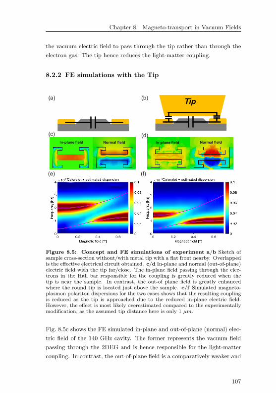
Chapter 8. Magneto-transport in Vacuum Fields
the vacuum electric field to pass through the tip rather than through theelectron gas. The tip hence reduces the light-matter coupling.
8.2.2 FE simulations with the Tip
Tip
In-plane field Normal field In-plane field Normal field
(a) (b)
(c)
(e)
(d)
(f)
Figure 8.5: Concept and FE simulations of experiment a/b Sketch ofsample cross-section without/with metal tip with a flat front nearby. Overlappedis the effective electrical circuit obtained. c/d In-plane and normal (out-of-plane)electric field with the tip far/close. The in-plane field passing through the elec-trons in the Hall bar responsible for the coupling is greatly reduced when thetip is near the sample. In contrast, the out-of plane field is greatly enhancedwhere the round tip is located just above the sample. e/f Simulated magneto-plasmon polariton dispersions for the two cases shows that the resulting couplingis reduced as the tip is approached due to the reduced in-plane electric field.However, the effect is most likely overestimated compared to the experimentallymodification, as the assumed tip distance here is only 1 µm.
Fig. 8.5c shows the FE simulated in-plane and out-of-plane (normal) elec-tric field of the 140 GHz cavity. The former represents the vacuum fieldpassing through the 2DEG and is hence responsible for the light-mattercoupling. In contrast, the out-of-plane field is a comparatively weaker and
107

8.2. Vacuum field mode tuned in-situ
unused stray field. Fig. 8.5d shows the situation with the metallic tiprepresented by a cylinder of 100 µm diameter 1 µm above the samplesgold surface. The shown cavity mode is now shifted down to around 100GHz and has significantly less in-plan field and strong out-of-plane fieldwhere the round tip is located just above the cross-sectional plane used todraw the field mode. This is consistent with the simple picture of a addedparallel capacitance as shown above in Fig. 8.5b.Using again the FE simulation involving a gyrotropic medium to describethe 2DEG properties as discussed in section 6.3, the resulting polaritondispersions can be obtained for the cases when the tip is close or far. Theresulting dispersions are shown in Fig. 8.5e and f respectively. One can see,that the two main effects induced by the tip are the reduction of the cavityresonance frequency as well as the reduction of the vacuum field passingtrough the 2DEG which results in a reduced vacuum Rabi frequency Ωvac.
Limitations of CST simulations While these simulations are veryuseful for the qualitative understanding of the effects produced by the tip,it is difficult to obtain quantitatively reliable results to compare with theexperiment. This is related to the fact that CST is a classical electro-dynamic solver and hence does not include vacuum field modes per se.This problem is easy to circumvent when simulating a transmission exper-iment, as vacuum field modes are identical real photon modes in a cavity.This allows to use periodic boundary conditions. For the simulation of thepresent experiment, periodic boundary conditions are nevertheless used,even though the real experiment has only one tip and not infinite numberof them acting on each cavity of the array. This is probably an acceptableassumption as any vacuum field mode obtained due to periodic boundaryconditions has a far larger mode volume and is hence irrelevant. Moreproblematic is the fact, a usual electromagnetic solver is geared towardstransmission. It will hence miss modes that are not coupled to the far field(e.g. quadrupolar modes and modes with dipoles along the transmissiondirection), which can still dominate the near field. These questions cannotbe fully answered with a classic electrodynamic solver. Nevertheless, it canbe said, that a metallic tip of any shape should change vacuum field modesand let one observe the resulting changes in the resistance. However, for
108

Chapter 8. Magneto-transport in Vacuum Fields
a more quantitative understanding in future experiments, it is useful tohave a tip with a well defined and known mode spectrum. An example isthe direct λ/2-cavity evaporated on the tip chip as mentioned before.
8.2.3 Technicalities of measurement setup
Attocube positioners Beyond the setup described in Chapter 4, themetallic tip needs to be very accurately positioned with respect to the sam-ple. As shown in Figs. 8.6a and b, a stack of three piezo-driven slip-stickpositioners (ANP series) from attocube systems, referred to as attocubes,is used for a three-dimensional control of the tip position. These posi-tioners are intended for use at low temperatures in the Kelvin range andin strong magnetic fields and have in principle a positioning accuracy inthe nanometer scale while being able to move over several millimeters.Movements over short distances up to around 800 nm can be obtainedby applying a DC voltage across the piezo crystal between 0 and 150 V.Distances beyond this value can be obtained by ramping the voltage be-tween 0 and 60 V at a rate of less than 3V/ms, where an actual movementoccurs and then ramping the voltage back to the initial value at a rateexceeding 3V/ms (sawtooth function). In such a case, the slip-stick slides,resulting in a net movement. Such cycle is referred to as a step. Whenoperating attocubes at mK temperatures, unfortunately significant diffi-culties appear which need to be taken into account when operating themat low temperatures:Heating due to slip-stick movement The sliding movement of the slip-stick occurring with each step is a significant source of heating. Alreadyone single step can double the mixing chamber temperature at 10 mK for afew minutes. For extensive movements over millimetres this can even leadto the breakdown of the He3-dilution refrigerator circulation. While suchheating is unavoidable, the best solution is to have a computer controlledwaiting time between the movement and the measurement, resulting in aat least reproducible temperature when recording a specific measurement.Position reading The positions of the attocubes are read by the con-troller by applying 2 Volt over a resistor whose resistance changes withattocube position. While this of course also causes a lot of heating (from10 mK to 60 mK for 3 attocubes reading their positions continuously), the
109

8.2. Vacuum field mode tuned in-situ
reading needs to be off when not needed. However, as the reading bias isturned on, the resistor heats up causing a drift in the resistance and hencethe position reading. Absolute position measurements are hence hard toachieve. A reproducible computer controlled measurement for a fixed timeafter the turn on of the reading hence needs to be used. The noise on thereading, despite averaging is mostly in the order of several microns andhence far beyond the positioning accuracy. An external more accurateposition reading would be necessary. Unfortunately, despite a significanteffort, such a method could not be found for our experiment, as commonmethods use light interference. The latter cannot be used due to the highlight-sensitivity of a quantum Hall system. Another approach is measurethe distance dependent capacitance between the resonator plane and metaltip. This however also leads to serious changes to the electron gas whichcan only be inverted by a temperature cycle to above ∼150 Kelvin. Sofar, attocubes own position reading is the best available method. Thelatter could be improved by reading the resistance while applying 6 Voltinstead. While this causes overheating, it might be possible for a shortmeasurement time starting at a very low temperature. All measurementspresented rely on position measurements applying 2 V.Step size and yield Another approach is to infer the distance travelledis to count steps performed with the attocubes. An average step size isdirection, step frequency, highly temperature and most likely also loaddependent. As it depends on so many parameters, it can only be usedas a rough check of the distance travelled, especially also because certainsteps seem not to actually work. For steps performed every 200 ms at basetemperature we obtain 220 nm and 250 nm for the two directions.
Metallic tips In contrast to typical scanning gate experiments [140]requiring tips with very small front cross sectional areas and distancesto the sample at the nanometer scale, the tip for this experiment needsto have a very large and flat front and should modify transport alreadyat distances at the micrometer scale. Together with F. Appugliese andthe Mechanical Workshop at ETH Zurich, we have produced a numberof metallic tips using different methods and tip dimensions as shown inFig. 8.6c and d. The former has a diameter of 400 µm and was produced
110

Chapter 8. Magneto-transport in Vacuum Fields
(a) (c)
(d)
(b)
Figure 8.6: Experimental setup a Cold finger with three attocubes on topof each other holding the mount for the movable tip. b Zoom in of a showingmetallic tip pointing (left) onto the chip carrier (right) on which the sample ismounted. c SEM picture of micro machined tip used for the experiment shownin Fig. 8.7 d Optimized tip as described in the text with a surface roughness ofless than 1 µm. SEM pictures taken by E. Mavrona and F. Appugliese.
by micro machining, while second was produced with a very high qualitycopper and polished to obtain a slightly curved surface with a roughnessbelow 1 µm. While the tip shown in Fig. 8.6c, allowed to successfullymodify the vacuum field as shown below in Fig. 8.7, it remains a challengingexperiment, as it is almost impossible to mount the tip on the attocubeswith the perfect angle to the sample. Already small errors in the angleresult in an effectively too large distance to the sample.To solve this issue, yet another approach was used. Instead of metal tip,a small atomically flat doped semiconductor chip is used as a tip (referredto as tip chip). In order to obtain the perfect angle between the samplesurface and the tip chip, the latter can be glued onto a holder and thenpressed against the sample by moving the attocubes before the glue candry. In such a way, the two surfaces self align and get fixed in this position.This approach has a further advantage, as it allows to process resonantstructures onto the tip chip (e.g. a λ/2-resonator), which have a controlledand known vacuum field mode spectrum. This is not the case for metallictips or uniformely gold coated tip chips, which have many and unknown
111

8.2. Vacuum field mode tuned in-situ
low frequency vacuum field modes.
8.2.4 Magneto-transport coupled to in-situ tuned vacuumfields
0 5 10 15 200
0.5
1
1.5
0 0.1 0.2 0.3 0.4 0.50.1
5
10
15
20
25
30
0.09 0.1 0.11
10
14
18
Magnetic field [T]R
esi
sta
nc
e r
xx [W
]
Magnetic field [T]
Re
sist
an
ce
rx
x [W
]
Re
sist
an
ce
rx
x [W
]
(a) (b)
(c)
Figure 8.7: Magneto-transport in a changing cavity vacuum field aMagneto-transport trace of CH140 with the tip close (blue) and then with in-creasing distance of 25µm between steps up to 150 µm (red). Compared tothe unperturbed cavity (red), the Shubnikov-de Haas amplitude increases mostlyaround 0.1 T and in a broad range above 0.25 T. b Zoom in the trace in aaround 0.1 T. c Fourier transform of the data shown in b results in a peak,whose height represents the tip position dependent oscillation amplitude and canbe interpreted as the density of states peak of a Landau level (see equation 3.22).
Fig. 8.7a shows magneto-resistance traces of sample EV2124-26-40B-140-ALD measured for different tip distances from the sample. The blue traceis measured with the front of the tip separated by only a few 100 nm fromthe sample surface while sweeping the magnetic field towards 0 Tesla. Inorder to know, that the initial distance is only a few 100 µm, we apply avery small bias difference between tip and sample (10 mV). This allows tomeasure a current of 1 nA when the tip is in contact with the sample. Fromthere, the tip is retracted by 1 step until we are not touching anymore.Then the bias difference is turned off. This is clearly an imperfection
112

Chapter 8. Magneto-transport in Vacuum Fields
of the measurement, as it induces very small density changes. In futuremeasurements, this needs to be avoided by improving the measurementscheme.
Before every subsequent measurement, the tip is retracted by around 25µm up to a distance of around 150 µm. Fig. 8.7b shows a zoomed versionof the trace around 0.1 T, which clearly shows a dependence of the oscil-lation amplitude as function of the tip distance. It is important to note,that the phase and frequency of the oscillations Fig. 8.7a is practically un-changed as the tip is moved. The latter are defined by the carrier densitywhich is shown in Fig. 8.8 for the tip positions measured (index 1 is closeto the sample). As one can see, the carrier density in measurements shownin Fig. 8.7a obtained while sweeping the magnetic field down (blue dots)is constant up to a very small relative change of 2× 10⁻³. The differenceof 1 % upon change of magnetic field sweep direction is due to the param-agnetism of the magnet. The observed mobility is 2. 2 × 10⁶V s/cm2 andconstant as function of tip position within the measurement accuracy.
1 2 3 4 5 6tip position (index)
1.99
2
2.01
2.02
2.03
carr
ier
dens
ity [c
m-2
]
1011 Electron density vs tip position
sweep upsweep down
Figure 8.8: Carrier density extracted from the transverse resistance as func-tion of tip position (1 means tip close) for measurements where the magneticfield was swept up (red) or down (blue).
113

8.2. Vacuum field mode tuned in-situ
(a)
0
25
75
100
Tip
dis
tan
ce in
[µ
m]
0.97
1.1
∆ρ
xx ,a
mp
litu
de
50
0 0.5 1.0Tip distance in [µm]
(b)
0.1
0.2
no
rma
lize
d c
ou
plin
g
1.0
1.2
∆ρ
xx ,a
mp
litu
de
0 0.5 1.0Magnetic field
Experiment
Theory
Figure 8.9: Amplitude change due to changes to vacuum field modea The oscillation amplitude obtained from Fourier transforms of the resistivitytrace as shown in Fig. 8.7c, normalized to amplitude when the tip is far away,thus the tip induced amplitude change is shown versus tip position and magneticfield as a colormap. An amplitude increase is observed as the tip is approached onboth sides of the anti-crossing by around 10%. The observed behaviour also con-firms the results discussed in the previous section8.1. b Equivalent plot obtainedfrom theoretical dressed magneto-resistance traces, by assuming that the maineffect of a nearby tip is a reduction of the normalized light-matter coupling. Thequalitative result is independent of the precise tuning range of the coupling as-sumed in the theory. The qualitative agreement with the experimental colormapis very good.
114

Chapter 8. Magneto-transport in Vacuum Fields
Fourier analysis To obtain a more qualitative understanding of themeasurements, we perform Fourier transformations of the trace in B−1,where the Shubnikov-de Haas oscillations are periodic (see equation 3.25).We choose a small window of with 0.8 T .1 containing a few oscillationsand apodized with a Hanning window function. The result for a windowcentered around 0.1 T is shown in Fig. 8.7c. The amplitude of the peakrepresents the local oscillation amplitude, which can now be evaluated asfunction of tip position and also magnetic field. Fig. 8.9 shows the ampli-tude as function of the those two parameters normalized to the amplitudeobserved when the tip is far away (an average of all measurements takenbetween 100 and 150 µm distance) and hence recovering our known CH140cavity.From Fig. 8.9 one can see that as the tip is approached, the oscillationamplitude increases by around 10 % at around 0.1 T and in a broad rangeabove 0.25 T. Using the insight from the FE simulations in Fig. 8.5, thatthe presence of the tip reduces the normalized vacuum Rabi frequencyΩcav/ω, we find that a lower coupling increases the oscillation amplitude.Intriguingly, this is consistent with our findings in Fig. 8.1 from compar-ing the two cavities CH205 (red) and CH140 (blue) with the reference RH(gray). There we had found an vacuum field induced reduction of the oscil-lation maxima at very low magnetic fields around 0.15 T, a relatively smalland coupling independent effect at around 0.5 T and greater amplitude re-duction again at higher magnetic fields. Unfortunately, the absolute valuesare not fully comparable as the present measurement has been performedwith a 30% lower carrier density, which reduces the plasmon frequencyand the coupling. Nevertheless, this is a strong confirmation, that vacuumfields change magneto-transport.
Comparison to theoretical magneto-resistance traces Here, weattempt to qualitatively compare the experimental results with the theory[66] presented in Chapter 3.2. We assume here, that the main effect oftip is a reduction of the coupling, starting from a value of Ω/ω = 20% forCH140when the tip is far, down to an arbitrary value of 10% when the tipis close. The latter value is highly dependent on how close the tip can beapproached and it is dependent on the precise shape of the tip. However,
115

8.2. Vacuum field mode tuned in-situ
(b)
0.93
1.0
∆ρ
xx,a
ve
rag
e
0 0.5 1.0Magnetic field [T]
(c)
1.0
1.4
∆ρ
xx,a
mp
litu
de
0 0.5 1.0Magnetic field [T]
0
40
ρxx[Ω]
0 0.5 1.0Magnetic field [T]
(a)
Figure 8.10: Theoretical dressed resistivity versus light-matter cou-pling a Dressed magneto-resistance traces for different light-matter couplingsfrom 20% (red) to 10% (blue) computed using equation 3.32. The trace withoutcoupling is shown in black. b Reduction of the Drude resistivity (without oscilla-tory part) as function of coupling normalized to the cavity-less trace. c Change ofoscillation amplitude as function of coupling normalized to the highest couplingof 20%. This is the same normalization as performed for the experimental datashown in Fig. 8.9a
the qualitative result will not depend on these values.Fig. 8.10a shows the theoretical traces computed as discussed in section8.1.2, for normalized light-matter couplings between 20% (red) and 10%(blue). Fig. 8.10b shows the reduction of the mean value around which theoscillation occurs (Drude resistivity value in equation 3.25). Note that theamplitude of the reduction is almost coupling independent, while the mag-netic field range over which such a vacuum field induced Drude resistivityreduction occurs growth with the light-matter coupling. A similar phe-nomenology is observed for the oscillation amplitude as shown in Fig. 3.5b.In order to reproduce the experimental colormap shown in Fig. 8.9a, theoscillation amplitude vs. magnetic field curve at a given coupling is nor-malized to the curve at 20% coupling. This reproduces the situation ofthe experimental colormap 8.9a, where we normalized to the measurementwhen the tip is far away. The resulting theoretical colormap is shown in8.9b. There is a good qualitative agreement, as both colormaps show no
116

Chapter 8. Magneto-transport in Vacuum Fields
or little change in the oscillation amplitude near the anti-crossing, but asignificant amplitude increase on both sides of the resonant magnetic fieldas the tip is approached and the light-matter coupling is reduced.
Summary We have observed a clear modification of magneto-resistanceinduced by the coupling to vacuum fields. The two experimental ap-proaches used - comparison of different cavity samples and in-situ tuningof a single cavity - gave consistent results, which are supported by thetheoretical results by N. Bartolo and C. Ciuti [66]. The vacuum field af-fects magneto-transport at low magnetic fields mainly via a change of theeffective quantum lifetime.
117

8.2. Vacuum field mode tuned in-situ
118

CHAPTER 9
Outlook
We have developed a new experimental platform: It allows to observeelectric field fluctuations of the quantum electrodynamic (QED) groundstate acting on the resistivity of a high mobility electron gas. To reachthis result, we use the ultrastrong light-matter coupling regime, definedby a large vacuum Rabi frequency. It creates hybrid excitations calledpolaritons, which share properties of the cavity vacuum mode and theexcitations of the electron gas. We observe surprisingly large changes tomagneto-transport of an electron gas even in the complete absence of realpolariton excitations. With this platform it is further possible to tune vac-uum fields in-situ, while observing the effects in magneto-transport. Thevacuum effects on low magnetic field transport appear via the modifica-tions of the virtual excitations and their lifetimes.This platform opens up intriguing perspectives. The integer and fractionalquantum Hall transport regime heavily rely on electron-electron interac-tions, topological properties and the appearance of gaps in the electrondensity of states. Besides changing the virtual excitations and their life-times, vacuum fields in this regime may also change the electron density ofstates itself. A situation could be attained, where an energetically narrowLandau level and a very broad (lower) polariton state are simultaneously atthe Fermi energy. While the former is mainly responsible for transport, the
119

latter is probed by providing additional elastic scattering channels or evenremoving them when inside the polaritonic bandgap leading to a narrowingof the associated resistance peak. First experiments in the Quantum Hallregime at higher magnetic fields appear consistent with such a picture.A tantalizing perspective is also to study new aspects of the ultrastronglight-matter coupling regime, as we have now gained the possibility toaccess the matter part of the polaritons. It could for example be feasibleto observe the proposed Dicke phase transition in magneto-transport. Thephase transition theoretically described by the Dicke model which setsthe diamagnetic term D to zero. The transition is characterized by thelower polariton being pushed to zero frequency (DC), where it is predictedto hybridize with the ground state and become super-radiant. It shouldfurther contain a non-zero mean photon occupation number [141, 142]. Itappears clear, that such a phase transition should result in clear changesto magneto-transport. While for GaAs, D is not zero, the diamagneticterm seems to be greatly reduced for non-parabolic 2D heavy-holes ins-Ge quantum wells. My colleague Janine Keller showed, that couplingin such a quantum well, the lower polariton branch can be pushed toalmost zero frequency and hence supposedly very close to the Dicke phasetransition [143].The physics induced by a large vacuum Rabi splitting as studied in thisthesis under extreme physical conditions (e.g. extreme temperature andsample mobility) might give the impression that it is limited to the domainof fundamental research. It is exciting to see, that many potential applica-tions are arising in chemistry using cavity photon energies larger than thethermal broadening at room temperature (25.7 meV or 6.2 THz) [20]. Ithas been shown, that the cavity zero-point energy can tune chemical reac-tivities [21,144,145], energy transfer [146] and an organic semiconductor’sconductivity [22, 147]. In this perspective, our platform provides a ’clean’experimental system which allows to study the fundamental physical im-plications of this regime, with applications in other domains.
120

APPENDIX A
Growth Design
Growth design of EV2124
In this work, we used the 3-inch epilayer EV2124 grown by Molecular BeamEpitaxy (MBE). As the MBE used is optimized for large area epilayerhomogeneity, the observed carrier density and mobilities across the layerare the same within the measurement accuracy and hence allow for a verygood comparability also across different samples.The 2DEG is based on a GaAs/Al0.3Ga0.7As single triangular quantumwell 90 nm below the sample surface. A Si δ-doping layer with a densityof 3. 5×1012cm−2 placed 50 nm below the surface, results in a two dimen-sional electron gas (2DEG) with electron density ns = 3. 3 × 1011cm−2,mobility µ = 3. 1 × 106cm2/V s and effective mass m∗ = 0. 070 × m0 ifpreviously illuminated by infrared light and measured at 1.3 K. With-out such illumination, one typically obtains an electron density of ns =2. 2×1011cm−2 and a mobility of µ = 2. 0×106cm2/V s. The precise valuesunder given experimental conditions are stated in the individual chapters.The growth design is stated below:
121

Table A.1: Growth design of EV2124.
Layer Composition Thickness Doping(Å) cm−2
Cap GaAs 50Barrier AlGaAs 450
GaAs 6Doping Si δ-doping 0 3.53×10¹²
GaAs 6Spacer AlGaAs 400Channel & Buffer GaAs 5000Superlattice ×10 AlAs 25
GaAs 25Buffer GaAs 5000
3 inch Semi-Insulating GaAs Wafer
122

APPENDIX B
Sample fabrication
Here, we summarize the recipes needed in the six processing steps, con-sisting of
1. Hallbar etching
2. Ohmic contacts
3. Deposition and etching of the insulating layer
4. Cavity deposition
5. Chromium top gate (optional)
1. Hallbar etching Here, a thin resist is used, to get a optimum controlon the Hallbar dimensions. To minimize the distance of the photolithog-raphy mask from the sample, the resist accumulating at the sample edgesis removed before the illumination. This step needs to be especially clean,as any dust particle on the active areas of the Hallbars or on a narrow partof the contacts makes them uncomparable, especially for the experimentsdiscussed in section 8.1.Photoresist AZ 1505 (positive)
• Prebake 60s @ 110 C
123

• Spinning 4/40/4000
• Bake for 60s at 110 C
• Resist edge removal with a Q-tip with sample lying on aluminiumfoil to avoid dust from clean room paper
• Align sample in Ma6 using mask shown in Fig. 5.6a (use vacuumprogram)
• Expose 20 mJ at 365 nm (takes ∼ 10s)
• Develop with AZ726 for 20 s and then water. Results in an etch deptof ∼ 200nm
• Etch in slow sulphoric acid 1:8:60 H2SO4:H2O2:H2O
2. Ohmic contacts Here, we don’t mind some imprecisions in align-ment or feature dimensions. Hence a thicker resist making the lift-offeasier.Photoresist ma-N1410 (negative)
1. Prebake 90s @ 100 C
2. Spinning 3/30/3000
3. Bake for 90s at 100 C
4. Align sample in Ma6 using mask shown in Fig. 5.6b
5. Expose 350 mJ at 365 nm (takes ∼ 1. 5min)
6. Develop with Ma-D 533/s for 40 s and then water
Deposition and lift off
1. Argon sputtering for 1 min (etches surface oxide layer around 3 nm)
2. Deposition of Ge/Au/Ni/Au 18/48/15/150 nm
3. Lift off in 50 C aceton, supported by a pipette creating a flux ofaceton
Annealing of contacts
1. 120 s at 400 C and then 80 s at 450 C
124

Appendix B. Sample fabrication
3. Insulating layer Here we want to deposite an insulating layer toavoid current leakage between 2DEG and the resonator plane depositedabove. Unfortunately, atomic layer deposition does not allow the use ofphotoresist, which is why an etching step is needed to remove the insulatinglayer on the ohmic contacts after the deposition.
1. 300 atomic layers of Al2O3 deposited at 150 K by atomic layer de-position (resulting thickness is around ∼ 25nm)
2. Additional photolithography with photoresist ma-N1410 (negative)using a mask similar to the one shown in Fig. 5.6b.
3. Etch for 15 seconds in buffered 1:6 HF:H_2O.
4. Cavity deposition In this step, a good alignment with the etchedHallbar is vital to obtain comparable Hallbars. The Hallbar width afteretching is 39.4 µm while the gap of the resonator obtained after lift-off isaround 40 µm. This hence leaves room for only a few 100 nm of misalign-ment as shown in Fig. 5.3c. As a good alignment marker for the angle,one can use 3 mm long lines etched in the first step as shown in Fig. 5.6ato be aligned with the upper and lower end of the resonator plane. Forthe alignment in the y-direction, one can use the optical ’brightness’ ofthe gap between the edge of the Hallbar and the edge of the gap of theresonator. This gap is only ∼ 300nm wide, and hence subwavelength forvisible light, but comparing the brightness of these lines allows to alignthe mask at this few hundered nm scale with an acceptable yield.Photoresist ma-N1405 (negative)
1. Prebake 60s @ 100 C
2. Spinning 3/30/3000
3. Bake for 60s at 100 C
4. Align sample in Ma6 using mask shown in Fig. 5.6c (use vacuumprogram)
5. Resist edge removal with a Q-tip with sample lying on aluminiumfoil
125

6. Expose 250 mJ at 365 nm (takes ∼ 1min)
7. Develop with Ma-N 533/s for 40 s and then water
8. Lift off in 50 C aceton, supported by a pipette creating a flux ofaceton
5. Chromium gate A only 2 nm thick chromium layer can be depositedon top of the entire resonator plane. This results in a uniform gate at DCbut is still transparent for THz.Use the same receipe as for the previous step, depositing only 2 nm ofChromium at 0.1 nm/s.
126

Bibliography
[1] A. A. Michelson, E. W. Morley. “On the Relative Motion of the Earth andof the Luminiferous Ether”. Sidereal Messenger, vol. 6, pp. 306-310 6, pp.306–310 (1887)
[2] A. Einstein. “Zur Elektrodynamik bewegter Körper”. Annalen der Physik322 (10), pp. 891–921 (1905)
[3] P. A. M. Dirac. “The quantum theory of the emission and absorption ofradiation”. Proc. R. Soc. Lond. A 114 (767), pp. 243–265 (1927)
[4] W. E. Lamb Jr, R. C. Retherford. “Fine structure of the hydrogen atomby a microwave method”. Physical Review 72 (3), p. 241 (1947)
[5] H. A. Bethe. “The electromagnetic shift of energy levels”. Physical Review72 (4), p. 339 (1947)
[6] J. Schwinger. “On quantum-electrodynamics and the magnetic moment ofthe electron”. Physical Review 73 (4), p. 416 (1948)
[7] T. A. Welton. “Some observable effects of the quantum-mechanical fluc-tuations of the electromagnetic field”. Physical Review 74 (9), p. 1157(1948)
[8] S. K. Lamoreaux. “Casimir forces: Still surprising after 60 years”. Phys.Today 60 (2), pp. 40–45 (2007)
[9] H. Casimir, D. Polder. “The influence of retardation on the London-vander Waals forces”. Physical Review 73 (4), p. 360 (1948)
[10] G. T. Moore. “Quantum Theory of the Electromagnetic Field in a Variable-Length One-Dimensional Cavity”. Journal of Mathematical Physics 11 (9),pp. 2679–2691 (1970)
[11] C. Wilson, G. Johansson, A. Pourkabirian, M. Simoen, J. Johansson,T. Duty, F. Nori, P. Delsing. “Observation of the dynamical Casimir effectin a superconducting circuit”. Nature 479 (7373), p. 376 (2011)
[12] W. G. Unruh. “Notes on black-hole evaporation”. Physical Review D 14 (4),p. 870 (1976)
[13] S. W. Hawking. “Black hole explosions?” Nature 248 (5443), p. 30 (1974)[14] E. P. Tryon. “Is the universe a vacuum fluctuation?” Nature 246 (5433),
p. 396 (1973)
127

Bibliography
[15] C. Riek, D. Seletskiy, A. S. Moskalenko, J. Schmidt, P. Krauspe, S. Eckart,S. Eggert, G. Burkard, A. Leitenstorfer. “Direct sampling of electric-fieldvacuum fluctuations”. Science (p. aac9788) (2015)
[16] I.-C. Benea-Chelmus, F. F. Settembrini, G. Scalari, J. Faist. “Electric fieldcorrelation measurements on the electromagnetic vacuum state”. arXivpreprint arXiv:1809.01785 (2018)
[17] I.-C. Hoi, A. Kockum, L. Tornberg, A. Pourkabirian, G. Johansson, P. Dels-ing, C. Wilson. “Probing the quantum vacuum with an artificial atom infront of a mirror”. Nature Physics 11 (12), p. 1045 (2015)
[18] A. A. Houck, J. A. Schreier, B. R. Johnson, J. M. Chow, J. Koch, J. M.Gambetta, D. I. Schuster, L. Frunzio, M. H. Devoret, S. M. Girvin, R. J.Schoelkopf. “Controlling the Spontaneous Emission of a SuperconductingTransmon Qubit”. Phys. Rev. Lett. 101, p. 080502 (2008)
[19] H. B. Chan, V. A. Aksyuk, R. N. Kleiman, D. J. Bishop, F. Capasso.“Quantum mechanical actuation of microelectromechanical systems by theCasimir force”. Science 291 (5510), pp. 1941–1944 (2001)
[20] T. W. Ebbesen. “Hybrid Light–Matter States in a Molecular and Ma-terial Science Perspective”. Accounts of Chemical Research 49 (11), pp.2403–2412 (2016). PMID: 27779846
[21] A. Thomas, J. George, A. Shalabney, M. Dryzhakov, S. J. Varma, J. Moran,T. Chervy, X. Zhong, E. Devaux, C. Genet, et al.. “Ground-State Chemi-cal Reactivity under Vibrational Coupling to the Vacuum ElectromagneticField”. Angewandte Chemie International Edition 55 (38), pp. 11462–11466 (2016)
[22] E. Orgiu, J. George, J. Hutchison, E. Devaux, J. Dayen, B. Doudin, F. Stel-lacci, C. Genet, J. Schachenmayer, C. Genes, et al.. “Conductivity in or-ganic semiconductors hybridized with the vacuum field”. Nature Materials14, pp. 1123–1129 (2015)
[23] E. Purcell. “Proceedings of the American Physical Society”. Phys. Rev.69, pp. 674–674 (1946)
[24] E. T. Jaynes, F. W. Cummings. “Comparison of quantum and semiclassicalradiation theories with application to the beam maser”. Proceedings of theIEEE 51 (1), pp. 89–109 (1963)
[25] J.-M. Raimond, M. Brune, S. Haroche. “Manipulating quantum entangle-ment with atoms and photons in a cavity”. Reviews of Modern Physics73 (3), p. 565 (2001)
[26] D. Meschede, H. Walther, G. Müller. “One-atom maser”. Physical reviewletters 54 (6), p. 551 (1985)
[27] R. Thompson. “RJ Thompson, G. Rempe, and HJ Kimble, Phys. Rev.Lett. 68, 1132 (1992).” Phys. Rev. Lett. 68, p. 1132 (1992)
[28] C. Ciuti, G. Bastard, I. Carusotto. “Quantum vacuum properties of theintersubband cavity polariton field”. Physical Review B 72 (11), p. 115303(2005)
[29] D. Hagenmüller, S. De Liberato, C. Ciuti. “Ultrastrong coupling between acavity resonator and the cyclotron transition of a two-dimensional electrongas in the case of an integer filling factor”. Physical Review B 81 (23), p.235303 (2010)
128

Bibliography
[30] C. Weisbuch, M. Nishioka, A. Ishikawa, Y. Arakawa. “Observation ofthe coupled exciton-photon mode splitting in a semiconductor quantummicrocavity”. Physical Review Letters 69 (23), p. 3314 (1992)
[31] D. Dini, R. Köhler, A. Tredicucci, G. Biasiol, L. Sorba. “Microcavity polari-ton splitting of intersubband transitions”. Physical review letters 90 (11),p. 116401 (2003)
[32] A. F. Kockum, A. Miranowicz, S. De Liberato, S. Savasta, F. Nori.“Ultrastrong coupling between light and matter”. arXiv preprintarXiv:1807.11636 (2018)
[33] P. Forn-Díaz, L. Lamata, E. Rico, J. Kono, E. Solano. “Ultrastrong cou-pling regimes of light-matter interaction”. arXiv preprint arXiv:1804.09275(2018)
[34] G. Günter, A. A. Anappara, J. Hees, A. Sell, G. Biasiol, L. Sorba, S. De Lib-erato, C. Ciuti, A. Tredicucci, A. Leitenstorfer, et al.. “Sub-cycle switch-onof ultrastrong light–matter interaction”. Nature 458 (7235), pp. 178–181(2009)
[35] P. Jouy, A. Vasanelli, Y. Todorov, A. Delteil, G. Biasiol, L. Sorba, C. Sir-tori. “Transition from strong to ultrastrong coupling regime in mid-infraredmetal-dielectric-metal cavities”. Applied Physics Letters 98 (23), p. 231114(2011)
[36] Y. Todorov, A. M. Andrews, R. Colombelli, S. De Liberato, C. Ciuti,P. Klang, G. Strasser, C. Sirtori. “Ultrastrong light-matter coupling regimewith polariton dots”. Physical review letters 105 (19), p. 196402 (2010)
[37] M. Geiser, F. Castellano, G. Scalari, M. Beck, L. Nevou, J. Faist. “Ultra-strong coupling regime and plasmon polaritons in parabolic semiconductorquantum wells”. Physical Review Letters 108 (10), p. 106402 (2012)
[38] V. Muravev, I. Andreev, I. Kukushkin, S. Schmult, W. Dietsche. “Ob-servation of hybrid plasmon-photon modes in microwave transmission ofcoplanar microresonators”. Physical Review B 83 (7), p. 075309 (2011)
[39] V. Muravev, P. Gusikhin, I. Andreev, I. Kukushkin. “Ultrastrong couplingof high-frequency two-dimensional cyclotron plasma mode with a cavityphoton”. Physical Review B 87 (4), p. 045307 (2013)
[40] G. L. Paravicini-Bagliani, G. Scalari, F. Valmorra, J. Keller, C. Maissen,M. Beck, J. Faist. “Gate and magnetic field tunable ultrastrong couplingbetween a magnetoplasmon and the optical mode of an LC cavity”. PhysicalReview B 95 (20), p. 205304 (2017)
[41] T. Schwartz, J. A. Hutchison, C. Genet, T. W. Ebbesen. “Reversibleswitching of ultrastrong light-molecule coupling”. Physical review letters106 (19), p. 196405 (2011)
[42] S. Kéna-Cohen, S. A. Maier, D. D. Bradley. “Ultrastrongly CoupledExciton–Polaritons in Metal-Clad Organic Semiconductor Microcavities”.Advanced Optical Materials 1 (11), pp. 827–833 (2013)
[43] S. Gambino, M. Mazzeo, A. Genco, O. Di Stefano, S. Savasta, S. Patanè,D. Ballarini, F. Mangione, G. Lerario, D. Sanvitto, et al.. “Exploringlight–matter interaction phenomena under ultrastrong coupling regime”.ACS Photonics 1 (10), pp. 1042–1048 (2014)
129

Bibliography
[44] A. Genco, A. Ridolfo, S. Savasta, S. Patanè, G. Gigli, M. Mazzeo. “BrightPolariton Coumarin-Based OLEDs Operating in the Ultrastrong CouplingRegime”. Advanced Optical Materials 6 (17), p. 1800364 (2018)
[45] F. Benz, M. K. Schmidt, A. Dreismann, R. Chikkaraddy, Y. Zhang,A. Demetriadou, C. Carnegie, H. Ohadi, B. de Nijs, R. Esteban, et al..“Single-molecule optomechanics in ’picocavities”’. Science 354 (6313), pp.726–729 (2016)
[46] J. George, T. Chervy, A. Shalabney, E. Devaux, H. Hiura, C. Genet, T. W.Ebbesen. “Multiple Rabi splittings under ultrastrong vibrational coupling”.Physical review letters 117 (15), p. 153601 (2016)
[47] F. Bloch, A. Siegert. “Magnetic resonance for nonrotating fields”. PhysicalReview 57 (6), p. 522 (1940)
[48] C. Ciuti, I. Carusotto. “Input-output theory of cavities in the ultrastrongcoupling regime: The case of time-independent cavity parameters”. Physi-cal Review A 74 (3), p. 033811 (2006)
[49] S. De Liberato. “Virtual photons in the ground state of a dissipative sys-tem”. Nature Communications 8 (2017)
[50] T. Ihn. Semiconductor nanostructures. Oxford University Press (2010)[51] W. De Haas, P. Van Alphen. “The dependence of the susceptibility of
diamagnetic metals upon the field”. Proc. Netherlands Roy. Acad. Sci33 (1106), p. 170 (1930)
[52] K. v. Klitzing, G. Dorda, M. Pepper. “New method for high-accuracy deter-mination of the fine-structure constant based on quantized Hall resistance”.Physical Review Letters 45 (6), p. 494 (1980)
[53] H. Stormer, D. Tsui. “The quantized Hall effect”. Science 220 (4603), pp.1241–1246 (1983)
[54] O. Kibis. “Dissipationless electron transport in photon-dressed nanostruc-tures”. Physical review letters 107 (10), p. 106802 (2011)
[55] O. Kibis. “How to suppress the backscattering of conduction electrons?”EPL (Europhysics Letters) 107 (5), p. 57003 (2014)
[56] J. Feist, F. J. Garcia-Vidal. “Extraordinary exciton conductance inducedby strong coupling”. Physical Review Letters 114 (19), p. 196402 (2015)
[57] S. Morina, O. V. Kibis, A. Pervishko, I. A. Shelykh. “Transport propertiesof a two-dimensional electron gas dressed by light”. Physical Review B91 (15), p. 155312 (2015)
[58] J. Schachenmayer, C. Genes, E. Tignone, G. Pupillo. “Cavity-enhancedtransport of excitons”. Physical review letters 114 (19), p. 196403 (2015)
[59] C.-C. Chang, G.-Y. Chen, L. Lin. “Dressed Photons Induced ResistanceOscillation and Zero Resistance in Arrayed Simple Harmonic Oscillatorswith No Impurity”. Scientific Reports 6 (2016)
[60] K. Dini, O. Kibis, I. Shelykh. “Magnetic properties of a two-dimensionalelectron gas strongly coupled to light”. Physical Review B 93 (23), p.235411 (2016)
[61] D. Hagenmüller, J. Schachenmayer, S. Schütz, C. Genes, G. Pupillo.“Cavity-enhanced transport of charge”. Physical review letters 119 (22),p. 223601 (2017)
130
Bibliography
[62] D. Hagenmüller, S. Schütz, J. Schachenmayer, C. Genes, G. Pupillo.“Cavity-assisted mesoscopic transport of fermions: Coherent and dissipa-tive dynamics”. Physical Review B 97 (20), p. 205303 (2018)
[63] F. Schlawin, A. Cavalleri, D. Jaksch. “Cavity-mediated electron-photonsuperconductivity”. arXiv preprint arXiv:1804.07142 (2018)
[64] I. Dinu, V. Moldoveanu, P. Gartner. “Many-body effects in transportthrough a quantum-dot cavity system”. Physical Review B 97 (19), p.195442 (2018)
[65] V. Gudmundsson, N. R. Abdullah, A. Sitek, H.-S. Goan, C.-S. Tang,A. Manolescu. “Current correlations for the transport of interacting elec-trons through parallel quantum dots in a photon cavity”. Physics LettersA 382 (25), pp. 1672–1678 (2018)
[66] N. Bartolo, C. Ciuti. “Vacuum-dressed cavity magnetotransport of a two-dimensional electron gas”. Phys. Rev. B 98, p. 205301 (2018)
[67] G. Scalari, C. Maissen, D. Turčinková, D. Hagenmüller, S. De Liberato,C. Ciuti, C. Reichl, D. Schuh, W. Wegscheider, M. Beck, et al.. “Ultra-strong coupling of the cyclotron transition of a 2D electron gas to a THzmetamaterial”. Science 335 (6074), pp. 1323–1326 (2012)
[68] M. Tonouchi. “Cutting-edge terahertz technology”. Nature photonics 1 (2),p. 97 (2007)
[69] S. Smolka, W. Wuester, F. Haupt, S. Faelt, W. Wegscheider, A. Imamoglu.“Cavity quantum electrodynamics with many-body states of a two-dimensional electron gas”. Science 346 (6207), pp. 332–335 (2014)
[70] A. A. Anappara, S. De Liberato, A. Tredicucci, C. Ciuti, G. Biasiol,L. Sorba, F. Beltram. “Signatures of the ultrastrong light-matter couplingregime”. Physical Review B 79 (20), p. 201303 (2009)
[71] T. Niemczyk, F. Deppe, H. Huebl, E. Menzel, F. Hocke, M. Schwarz,J. Garcia-Ripoll, D. Zueco, T. Hümmer, E. Solano, et al.. “Circuit quan-tum electrodynamics in the ultrastrong-coupling regime”. Nature Physics6 (10), p. 772 (2010)
[72] P. Forn-Díaz, J. Lisenfeld, D. Marcos, J. J. García-Ripoll, E. Solano,C. Harmans, J. Mooij. “Observation of the Bloch-Siegert shift in a qubit-oscillator system in the ultrastrong coupling regime”. Physical review letters105 (23), p. 237001 (2010)
[73] Q. Zhang, M. Lou, X. Li, J. L. Reno, W. Pan, J. D. Watson, M. J. Manfra,J. Kono. “Collective non-perturbative coupling of 2D electrons with high-quality-factor terahertz cavity photons”. Nature Physics 12 (11), pp. 1005–1011 (2016)
[74] A. Bayer, M. Pozimski, S. Schambeck, D. Schuh, R. Huber, D. Bougeard,C. Lange. “Terahertz Light–Matter Interaction beyond Unity CouplingStrength”. Nano Letters 17 (10), pp. 6340–6344 (2017)
[75] G. L. Paravicini-Bagliani, F. Appugliese, E. Richter, F. Valmorra, J. Keller,M. Beck, N. Bartolo, C. Rössler, T. Ihn, K. Ensslin, et al.. “Magneto-transport controlled by Landau polariton states”. Nature Physics 13, pp.186–190 (2019)
[76] F. Yoshihara, T. Fuse, S. Ashhab, K. Kakuyanagi, S. Saito, K. Semba.“Superconducting qubit–oscillator circuit beyond the ultrastrong-couplingregime”. Nature Physics 13 (1), p. 44 (2017)
131

Bibliography
[77] Q. Zhang, T. Arikawa, E. Kato, J. L. Reno, W. Pan, J. D. Watson, M. J.Manfra, M. A. Zudov, M. Tokman, M. Erukhimova, et al.. “Superradiantdecay of cyclotron resonance of two-dimensional electron gases”. Physicalreview letters 113 (4), p. 047601 (2014)
[78] C. Maissen, G. Scalari, F. Valmorra, M. Beck, J. Faist, S. Cibella, R. Leoni,C. Reichl, C. Charpentier, W. Wegscheider. “Ultrastrong coupling in thenear field of complementary split-ring resonators”. Physical Review B90 (20), p. 205309 (2014)
[79] D. Gerace, L. C. Andreani. “Quantum theory of exciton-photon couplingin photonic crystal slabs with embedded quantum wells”. Physical ReviewB 75 (23), p. 235325 (2007)
[80] J. Lolli, A. Baksic, D. Nagy, V. E. Manucharyan, C. Ciuti. “Ancillaryqubit spectroscopy of vacua in cavity and circuit quantum electrodynam-ics”. Physical review letters 114 (18), p. 183601 (2015)
[81] M. Cirio, K. Debnath, N. Lambert, F. Nori. “Amplified optomechanicaltransduction of virtual radiation pressure”. Physical review letters 119 (5),p. 053601 (2017)
[82] R. Thompson, G. Rempe, H. Kimble. “Observation of normal-mode split-ting for an atom in an optical cavity”. Physical Review Letters 68 (8), p.1132 (1992)
[83] M. Sidler, P. Back, O. Cotlet, A. Srivastava, T. Fink, M. Kroner, E. Demler,A. Imamoglu. “Fermi polaron-polaritons in charge-tunable atomically thinsemiconductors”. Nature Physics 13 (3), pp. 255–261 (2017)
[84] S. Ravets, S. Faelt, M. Kroner, W. Wegscheider, A. Imamoglu. “Polaron-Polaritons in the Integer and Fractional Quantum Hall Regimes”. arXivpreprint arXiv:1701.01029 (2017)
[85] N. Samkharadze, G. Zheng, N. Kalhor, D. Brousse, A. Sammak, U. Mendes,A. Blais, G. Scappucci, L. Vandersypen. “Strong spin-photon coupling insilicon”. Science 359 (6380), pp. 1123–1127 (2018)
[86] X. Li, M. Bamba, Q. Zhang, S. Fallahi, G. C. Gardner, W. Gao, M. Lou,K. Yoshioka, M. J. Manfra, J. Kono. “Vacuum Bloch–Siegert shift in Lan-dau polaritons with ultra-high cooperativity”. Nature Photonics 12, pp.324–329 (2018)
[87] J.-M. Ménard, C. Pöllmann, M. Porer, U. Leierseder, E. Galopin,A. Lemaître, A. Amo, J. Bloch, R. Huber. “Revealing the dark side ofa bright exciton–polariton condensate”. Nature communications 5, p. 4648(2014)
[88] N. Lambert, C. Flindt, F. Nori. “Photon-mediated electron transport inhybrid circuit-QED”. EPL (Europhysics Letters) 103 (1), p. 17005 (2013)
[89] L. Henriet, A. N. Jordan, K. Le Hur. “Electrical current from quantumvacuum fluctuations in nanoengines”. Physical Review B 92 (12), p. 125306(2015)
[90] M. Sentef, M. Ruggenthaler, A. Rubio. “Cavity quantum-electrodynamicalpolaritonically enhanced electron-phonon coupling and its influence on su-perconductivity.” ArXiv e-prints. (2018)
[91] T. Ando, A. B. Fowler, F. Stern. “Electronic properties of two-dimensionalsystems”. Reviews of Modern Physics 54 (2), p. 437 (1982)
132

Bibliography
[92] A. Isihara, L. Smrcka. “Density and magnetic field dependences of theconductivity of two-dimensional electron systems”. Journal of Physics C:Solid State Physics 19 (34), p. 6777 (1986)
[93] S. G. Louie, M. L. Cohen. Conceptual Foundations of Materials: A Stan-dard Model for Ground-and Excited-State Properties, vol. 2. Elsevier (2006)
[94] C. M. Maissen. Ultrastrong Light-Matter Coupling with Metasurfaces.Ph.D. thesis, ETH Zurich (2016)
[95] D. Grischkowsky, S. Keiding, M. Van Exter, C. Fattinger. “Far-infraredtime-domain spectroscopy with terahertz beams of dielectrics and semicon-ductors”. JOSA B 7 (10), pp. 2006–2015 (1990)
[96] C. W. Berry, N. Wang, M. R. Hashemi, M. Unlu, M. Jarrahi. “Significantperformance enhancement in photoconductive terahertz optoelectronics byincorporating plasmonic contact electrodes”. Nature communications 4, p.1622 (2013)
[97] P. C. Planken, H.-K. Nienhuys, H. J. Bakker, T. Wenckebach. “Mea-surement and calculation of the orientation dependence of terahertz pulsedetection in ZnTe”. JOSA B 18 (3), pp. 313–317 (2001)
[98] M. L. Roukes, M. R. Freeman, R. S. Germain, R. C. Richardson, M. B.Ketchen. “Hot electrons and energy transport in metals at millikelvintemperatures”. Phys. Rev. Lett. 55, pp. 422–425 (1985)
[99] S. Baer, K. Ensslin. Transport spectroscopy of confined fractional quantumhall systems, vol. 183. Springer (2015)
[100] J. B. Johnson. “Thermal agitation of electricity in conductors”. Physicalreview 32 (1), p. 97 (1928)
[101] V. Umansky, M. Heiblum, Y. Levinson, J. Smet, J. Nübler, M. Dolev.“MBE growth of ultra-low disorder 2DEG with mobility exceeding 35×106 cm2/V s”. Journal of Crystal Growth 311 (7), pp. 1658–1661 (2009)
[102] F. Stern. “Polarizability of a two-dimensional electron gas”. Physical Re-view Letters 18 (14), p. 546 (1967)
[103] J. Keller, G. Scalari, S. Cibella, C. Maissen, F. Appugliese, E. Giovine,R. Leoni, M. Beck, J. Faist. “Few-electron ultrastrong light-matter couplingat 300 GHz with nanogap hybrid LC microcavities”. Nano letters 17 (12),pp. 7410–7415 (2017)
[104] C. Maissen, G. Scalari, M. Beck, J. Faist. “Asymmetry in polariton disper-sion as function of light and matter frequencies in the ultrastrong couplingregime”. New Journal of Physics 19 (4), p. 043022 (2017)
[105] H. Lin, P. Ye, G. Wilk. “Leakage current and breakdown electric-fieldstudies on ultrathin atomic-layer-deposited Al 2 O 3 on GaAs”. Appliedphysics letters 87 (18), p. 182904 (2005)
[106] J. Kröll, J. Darmo, K. Unterrainer. “Metallic wave-impedance matchinglayers for broadband terahertz optical systems”. Optics express 15 (11),pp. 6552–6560 (2007)
[107] M. Białek, M. Czapkiewicz, J. Wróbel, V. Umansky, J. Łusakowski. “Plas-mon dispersions in high electron mobility terahertz detectors”. AppliedPhysics Letters 104 (26), p. 263514 (2014)
133

Bibliography
[108] C. Grimes, G. Adams. “Observation of two-dimensional plasmons andelectron-ripplon scattering in a sheet of electrons on liquid helium”. PhysicalReview Letters 36 (3), p. 145 (1976)
[109] S. Allen Jr, D. Tsui, R. Logan. “Observation of the two-dimensional plas-mon in silicon inversion layers”. Physical Review Letters 38 (17), p. 980(1977)
[110] T. Theis, J. Kotthaus, P. Stiles. “Wavevector dependence of the two-dimensional plasmon dispersion relationship in the (100) silicon inversionlayer”. Solid State Communications 26 (9), pp. 603–606 (1978)
[111] T. N. Theis. “Plasmons in inversion layers”. Surface Science 98 (1), pp.515–532 (1980)
[112] D. Heitmann. “Two-dimensional plasmons in homogeneous and laterallymicrostructured space charge layers”. Surface Science 170 (1), pp. 332–345(1986)
[113] M. S. Kushwaha. “Plasmons and magnetoplasmons in semiconductor het-erostructures”. Surface Science Reports 41 (1), pp. 1–416 (2001)
[114] J. Łusakowski. “Plasmon–terahertz photon interaction in high-electron-mobility heterostructures”. Semiconductor Science and Technology 32 (1),p. 013004 (2016)
[115] Z. Fei, A. Rodin, G. Andreev, W. Bao, A. McLeod, M. Wagner, L. Zhang,Z. Zhao, M. Thiemens, G. Dominguez, et al.. “Gate-tuning of grapheneplasmons revealed by infrared nano-imaging”. Nature 487 (7405), pp. 82–85(2012)
[116] L. Ju, B. Geng, J. Horng, C. Girit, M. Martin, Z. Hao, H. A. Bechtel,X. Liang, A. Zettl, Y. R. Shen, et al.. “Graphene plasmonics for tun-able terahertz metamaterials”. Nature nanotechnology 6 (10), pp. 630–634(2011)
[117] P. Q. Liu, F. Valmorra, C. Maissen, J. Keller, G. Scalari, J. Faist. “Large-area gate-tunable terahertz plasmonic metasurfaces employing graphenebased structures”. In SPIE OPTO, (pp. 935707–935707). InternationalSociety for Optics and Photonics (2015)
[118] A. Muravjov, D. Veksler, V. Popov, O. Polischuk, N. Pala, X. Hu, R. Gaska,H. Saxena, R. Peale, M. Shur. “Temperature dependence of plasmonicterahertz absorption in grating-gate gallium-nitride transistor structures”.Applied Physics Letters 96 (4), p. 042105 (2010)
[119] V. Muravev, P. Gusikhin, I. Andreev, I. Kukushkin. “Novel relativisticplasma excitations in a gated two-dimensional electron system”. Physicalreview letters 114 (10), p. 106805 (2015)
[120] P. Q. Liu, I. J. Luxmoore, S. A. Mikhailov, N. A. Savostianova, F. Val-morra, J. Faist, G. R. Nash. “Highly tunable hybrid metamaterials employ-ing split-ring resonators strongly coupled to graphene surface plasmons”.Nature communications 6 (2015)
[121] G. C. Dyer, G. R. Aizin, S. J. Allen, A. D. Grine, D. Bethke, J. L. Reno,E. A. Shaner. “Induced transparency by coupling of Tamm and defectstates in tunable terahertz plasmonic crystals”. Nature Photonics 7 (11),pp. 925–930 (2013)
134

Bibliography
[122] Y. Li, H. Yan, D. B. Farmer, X. Meng, W. Zhu, R. M. Osgood, T. F.Heinz, P. Avouris. “Graphene plasmon enhanced vibrational sensing ofsurface-adsorbed layers”. Nano letters 14 (3), pp. 1573–1577 (2014)
[123] S. A. Mikhailov, N. Savostianova. “Microwave response of a two-dimensional electron stripe”. Physical Review B 71 (3), p. 035320 (2005)
[124] I. Kukushkin, V. Muravev, J. Smet, M. Hauser, W. Dietsche, K. von Klitz-ing. “Collective excitations in two-dimensional electron stripes: Transportand optical detection of resonant microwave absorption”. Phys. Rev. B 73,p. 113310 (2006)
[125] O. Fedorych, M. Potemski, S. Studenikin, J. Gupta, Z. Wasilewski,I. Dmitriev. “Quantum oscillations in the microwave magnetoabsorptionof a two-dimensional electron gas”. Physical review. B, Condensed matterand materials physics 81 (20), pp. 201302–1 (2010)
[126] V. Muravev, I. Andreev, S. Gubarev, V. Belyanin, I. Kukushkin. “Finestructure of cyclotron resonance in a two-dimensional electron system”.Physical Review B 93 (4), p. 041110 (2016)
[127] I. Andreev, V. Muravev, V. Belyanin, I. Kukushkin. “Azbel’-Kaner-likecyclotron resonance in a two-dimensional electron system”. Physical ReviewB 96 (16), p. 161405 (2017)
[128] K. Choi, D. Tsui, K. Alavi. “Experimental determination of the edge de-pletion width of ahe two-dimensional electron gas in GaAs/Al x Ga1- xAs”. Applied physics letters 50 (2), pp. 110–112 (1987)
[129] D. Smetnev, V. M. Muravev, I. Andreev, I. V. Kukushkin. “Study ofedge magnetoplasma excitations in two-dimensional electron systems withvarious edge depletion profiles”. JETP letters 94 (2), pp. 137–141 (2011)
[130] G. Scalari, C. Maissen, S. Cibella, R. Leoni, C. Reichl, W. Wegscheider,M. Beck, J. Faist. “THz ultrastrong light-matter coupling”. Il NuovoSaggiatore 31 (3-4) (2015)
[131] E. Richter. Magneto-transport of ultra-strongly coupled 2DEGs. Master’sthesis, ETH Zurich (2017)
[132] I. Dmitriev, A. Mirlin, D. Polyakov, M. Zudov. “Nonequilibrium phenom-ena in high Landau levels”. Reviews of Modern Physics 84 (4), p. 1709(2012)
[133] A. Hatke, M. Zudov, J. Watson, M. Manfra, L. Pfeiffer, K. West. “Effec-tive mass from microwave photoresistance measurements in GaAs/AlGaAsquantum wells”. In Journal of Physics: Conference Series, vol. 456, (p.012040). IOP Publishing (2013)
[134] Y. Todorov, A. Andrews, I. Sagnes, R. Colombelli, P. Klang, G. Strasser,C. Sirtori. “Strong light-matter coupling in subwavelength metal-dielectricmicrocavities at terahertz frequencies”. Physical review letters 102 (18), p.186402 (2009)
[135] J. Kasprzak, M. Richard, S. Kundermann, A. Baas, P. Jeambrun, J. M. J.Keeling, F. M. Marchetti, M. H. Szymanska, R. Andre, J. L. Staehli,V. Savona, P. B. Littlewood, B. Deveaud, L. S. Dang. “Bose-Einstein con-densation of exciton polaritons”. Nature 443 (7110), pp. 409–414 (2006)
[136] A. Amo, D. Sanvitto, F. P. Laussy, D. Ballarini, E. del Valle, M. D. Mar-tin, A. Lemaitre, J. Bloch, D. N. Krizhanovskii, M. S. Skolnick, C. Tejedor,L. Vina. “Collective fluid dynamics of a polariton condensate in a semi-conductor microcavity”. Nature 457 (7227), pp. 291–U3 (2009)
135

Bibliography
[137] Y. Kawano, Y. Hisanaga, H. Takenouchi, S. Komiyama. “Highly sensitiveand tunable detection of far-infrared radiation by quantum Hall devices”.Journal of Applied Physics 89 (7), pp. 4037–4048 (2001)
[138] T. Arikawa, K. Hyodo, Y. Kadoya, K. Tanaka. “Light-induced electronlocalization in a quantum Hall system”. Nature Physics 13 (7), p. 688(2017)
[139] P. Mooney. “Electrical properties of DX centers in GaAs and AlGaAs”.Radiation Effects and Defects in Solids 111 (1-2), pp. 281–298 (1989)
[140] M. Topinka, B. LeRoy, S. Shaw, E. Heller, R. Westervelt, K. Maranowski,A. Gossard. “Imaging coherent electron flow from a quantum point con-tact”. Science 289 (5488), pp. 2323–2326 (2000)
[141] C. Emary, T. Brandes. “Chaos and the quantum phase transition in theDicke model”. Physical Review E 67 (6), p. 066203 (2003)
[142] B. Kristian. Experimental Realization of the Dicke Quantum Phase Tran-sition. Ph.D. thesis, ETH Zurich (2011)
[143] J. Keller, G. Scalari, F. Appugliese, S. Rajabali, C. Maissen, M. Beck,J. Haase, C. A. Lehner, W. Wegscheider, M. Failla, et al.. “Softening ofcavity cyclotron polariton modes in strained germanium 2D hole gas in theultra-strong coupling regime”. arXiv preprint arXiv:1708.07773 (2017)
[144] J. A. Hutchison, T. Schwartz, C. Genet, E. Devaux, T. W. Ebbesen. “Mod-ifying Chemical Landscapes by Coupling to Vacuum Fields”. AngewandteChemie International Edition 51 (7), pp. 1592–1596 (2012)
[145] H. Hiura, A. Shalabney, J. George. “Cavity Catalysis–Accelerating Reac-tions under Vibrational Strong Coupling–” (2018)
[146] X. Zhong, T. Chervy, S. Wang, J. George, A. Thomas, J. A. Hutchison,E. Devaux, C. Genet, T. W. Ebbesen. “Non-Radiative Energy TransferMediated by Hybrid Light-Matter States”. Angewandte Chemie 128 (21),pp. 6310–6314 (2016)
[147] G. G. Rozenman, K. Akulov, A. Golombek, T. Schwartz. “Long-rangetransport of organic exciton-polaritons revealed by ultrafast microscopy”.ACS Photonics 5 (1), pp. 105–110 (2017)
136