Gradualizing the Calculus of Inductive Constructions - arXiv
83
Gradualizing the Calculus of Inductive Constructions MEVEN LENNON-BERTRAND, Gallinette Project-Team, Inria, France KENJI MAILLARD, Gallinette Project-Team, Inria, France NICOLAS TABAREAU, Gallinette Project-Team, Inria, France ÉRIC TANTER, PLEIAD Lab, Computer Science Department (DCC), University of Chile, Chile We investigate gradual variations on the Calculus of Inductive Construction (CIC) for swifter prototyping with imprecise types and terms. We observe, with a no-go theorem, a crucial tradeoff between graduality and the key properties of normalization and closure of universes under dependent product that CIC enjoys. Beyond this Fire Triangle of Graduality, we explore the gradualization of CIC with three different compromises, each relaxing one edge of the Fire Triangle. We develop a parametrized presentation of Gradual CIC (GCIC) that encompasses all three variations, and develop their metatheory. We first present a bidirectional elaboration of GCIC to a dependently-typed cast calculus, CastCIC, which elucidates the interrelation between typing, conversion, and the gradual guarantees. We use a syntactic model of CastCIC to inform the design of a safe, confluent reduction, and establish, when applicable, normalization. We study the static and dynamic gradual guarantees as well as the stronger notion of graduality with embedding-projection pairs formulated by New and Ahmed, using appropriate semantic model constructions. This work informs and paves the way towards the development of malleable proof assistants and dependently-typed programming languages. CCS Concepts: • Theory of computation → Type theory; Type structures; Program reasoning. Additional Key Words and Phrases: Gradual typing, proof assistants, dependent types 1 INTRODUCTION Gradual typing arose as an approach to selectively and soundly relax static type checking by endowing programmers with imprecise types [Siek and Taha 2006; Siek et al. 2015]. Optimistically well-typed programs are safeguarded by runtime checks that detect violations of statically-expressed assumptions. A gradual version of the simply-typed lambda calculus (STLC) enjoys such expressive- ness that it can embed the untyped lambda calculus. This means that gradually-typed languages tend to accommodate at least two kinds of effects, non-termination and runtime errors. The smooth- ness of the static-to-dynamic checking spectrum afforded by gradual languages is usually captured by (static and dynamic) gradual guarantees which stipulate that typing and reduction are monotone with respect to precision [Siek et al. 2015]. Originally formulated in terms of simple types, the extension of gradual typing to a wide variety of typing disciplines has been an extremely active topic of research, both in theory and in practice. As part of this quest towards more sophisticated type disciplines, gradual typing was bound to meet with full-blown dependent types. This encounter saw various premises in a variety of approaches to integrate (some form of) dynamic checking with (some form of) dependent types [Dagand et al. 2018; Knowles and Flanagan 2010; Lehmann and Tanter 2017; Ou et al. 2004; Tanter and Tabareau 2015; Wadler and Findler 2009]. Naturally, the highly-expressive setting of dependent types, in which terms and types are not distinct and computation happens as part of typing, raises a lot of ∗ This work is partially funded by ANID FONDECYT Regular Project 1190058, and Inria Équipe Associée GECO. To appear in ACM Transactions in Programming Languages and Systems, 2022, doi:10.1145/3495528 Authors’ addresses: Meven Lennon-Bertrand, Gallinette Project-Team, Inria, Nantes, France; Kenji Maillard, Gallinette Project-Team, Inria, Nantes, France; Nicolas Tabareau, Gallinette Project-Team, Inria, Nantes, France; Éric Tanter, PLEIAD Lab, Computer Science Department (DCC), University of Chile, Santiago, Chile. arXiv:2011.10618v4 [cs.PL] 17 Nov 2021
-
Upload
khangminh22 -
Category
Documents
-
view
1 -
download
0
Transcript of Gradualizing the Calculus of Inductive Constructions - arXiv

Gradualizing the Calculus of Inductive Constructions
MEVEN LENNON-BERTRAND, Gallinette Project-Team, Inria, France
KENJI MAILLARD, Gallinette Project-Team, Inria, France
NICOLAS TABAREAU, Gallinette Project-Team, Inria, France
ÉRIC TANTER, PLEIAD Lab, Computer Science Department (DCC), University of Chile, Chile
We investigate gradual variations on the Calculus of Inductive Construction (CIC) for swifter prototyping with
imprecise types and terms. We observe, with a no-go theorem, a crucial tradeoff between graduality and the
key properties of normalization and closure of universes under dependent product that CIC enjoys. Beyond
this Fire Triangle of Graduality, we explore the gradualization of CIC with three different compromises, each
relaxing one edge of the Fire Triangle. We develop a parametrized presentation of Gradual CIC (GCIC) that
encompasses all three variations, and develop their metatheory. We first present a bidirectional elaboration
of GCIC to a dependently-typed cast calculus, CastCIC, which elucidates the interrelation between typing,
conversion, and the gradual guarantees. We use a syntactic model of CastCIC to inform the design of a safe,
confluent reduction, and establish, when applicable, normalization. We study the static and dynamic gradual
guarantees as well as the stronger notion of graduality with embedding-projection pairs formulated by New
and Ahmed, using appropriate semantic model constructions. This work informs and paves the way towards
the development of malleable proof assistants and dependently-typed programming languages.
CCS Concepts: • Theory of computation→ Type theory; Type structures; Program reasoning.
Additional Key Words and Phrases: Gradual typing, proof assistants, dependent types
1 INTRODUCTIONGradual typing arose as an approach to selectively and soundly relax static type checking by
endowing programmers with imprecise types [Siek and Taha 2006; Siek et al. 2015]. Optimistically
well-typed programs are safeguarded by runtime checks that detect violations of statically-expressed
assumptions. A gradual version of the simply-typed lambda calculus (STLC) enjoys such expressive-
ness that it can embed the untyped lambda calculus. This means that gradually-typed languages
tend to accommodate at least two kinds of effects, non-termination and runtime errors. The smooth-
ness of the static-to-dynamic checking spectrum afforded by gradual languages is usually captured
by (static and dynamic) gradual guarantees which stipulate that typing and reduction are monotone
with respect to precision [Siek et al. 2015].
Originally formulated in terms of simple types, the extension of gradual typing to a wide variety
of typing disciplines has been an extremely active topic of research, both in theory and in practice.
As part of this quest towards more sophisticated type disciplines, gradual typing was bound to meet
with full-blown dependent types. This encounter saw various premises in a variety of approaches
to integrate (some form of) dynamic checking with (some form of) dependent types [Dagand et al.
2018; Knowles and Flanagan 2010; Lehmann and Tanter 2017; Ou et al. 2004; Tanter and Tabareau
2015; Wadler and Findler 2009]. Naturally, the highly-expressive setting of dependent types, in
which terms and types are not distinct and computation happens as part of typing, raises a lot of
∗This work is partially funded by ANID FONDECYT Regular Project 1190058, and Inria Équipe Associée GECO.
To appear in ACM Transactions in Programming Languages and Systems, 2022, doi:10.1145/3495528
Authors’ addresses: Meven Lennon-Bertrand, Gallinette Project-Team, Inria, Nantes, France; Kenji Maillard, Gallinette
Project-Team, Inria, Nantes, France; Nicolas Tabareau, Gallinette Project-Team, Inria, Nantes, France; Éric Tanter, PLEIAD
Lab, Computer Science Department (DCC), University of Chile, Santiago, Chile.
arX
iv:2
011.
1061
8v4
[cs
.PL
] 1
7 N
ov 2
021

2 Meven Lennon-Bertrand, Kenji Maillard, Nicolas Tabareau, and Éric Tanter
subtle challenges for gradualization. In the most elaborate effort to date, Eremondi et al. [2019]
present a gradual dependently-typed programming language, GDTL, which can be seen as an effort
to gradualize a two-phase programming language such as Idris [Brady 2013]. A key idea of GDTL
is to adopt an approximate form of computation at compile-time, called approximate normalization,
which ensures termination and totality of typing, while adopting a standard gradual reduction
semantics with errors and non-termination at runtime. The metatheory of GDTL however still
needs to be extended to account for inductive types.
This paper addresses the open challenge of gradualizing a full-blown dependent type theory,
namely the Calculus of Inductive Constructions (hereafter, CIC) [Coquand and Huet 1988; Paulin-
Mohring 2015], identifying and addressing the corresponding metatheoretic challenges. In doing
so, we build upon several threads of prior work in the type theory and gradual typing literature:
syntactic models of type theories to justify extensions of CIC [Boulier et al. 2017], in particular
the exceptional type theory of Pédrot and Tabareau [2018], an effective re-characterization of the
dynamic gradual guarantee as graduality with embedding-projection pairs [New and Ahmed 2018],
as well as the work on GDTL [Eremondi et al. 2019].
Motivation. We believe that studying the gradualization of a full-blown dependent type theory
like CIC is in and of itself an important scientific endeavor, which is very likely to inform the
gradual typing research community in its drive towards supporting ever more challenging typing
disciplines. In this light, the aim of this paper is not to put forth a unique design or solution, but to
explore the space of possibilities. Nor is this paper about a concrete implementation of gradual
CIC and an evaluation of its applicability; these are challenging perspectives of their own, which
first require the theoretical landscape to be unveiled.
This being said, as Eremondi et al. [2019], we can highlight a number of practical motivating
scenarios for gradualizing CIC, anticipating what could be achieved in a hypothetical gradual
version of Coq, for instance.
Example 1 (Smoother development with indexed types). CIC, which underpins languages and
proof assistants such as Coq, Agda and Idris, among others, is a very powerful system to program in,
but at the same time extremely demanding. Mixing programs and their specifications is attractive
but challenging.
Consider the classical example of length-indexed lists, of type vec A n as defined in Coq:1
Inductive vec (A : □) : N → □ :=
| nil : vec A 0
| cons : A → forall n : N, vec A n → vec A (S n ).
Indexing the inductive type by its length allows us to define a total head function, which can
only be applied to non-empty lists:
head : forall A n , vec A (S n) → A
Developing functions over such structures can be tricky. For instance, what type should the
filter function be given?
filter : forall A n (f : A → B), vec A n → vec A . . .
The size of the resulting list depends on how many elements in the list actually match the given
predicate f! Dealing with this level of intricate specification can (and does) scare programmers
away from mixing programs and specifications. The truth is that many libraries, such as Math-
Comp [Mahboubi and Tassi 2008], give up on mixing programs and specifications even for simple
1We use the notation □𝑖 for the predicative universe of types Type𝑖 , and omit the universe level 𝑖 when not required.

Gradualizing the Calculus of Inductive Constructions 3
structures such as these, which are instead dealt with as ML-like lists with extrinsically-established
properties. This tells a lot about the current intricacies of dependently-typed programming.
Instead of avoiding the obstacle altogether, gradual dependent types provide a uniform and
flexible mechanism to a tailored adoption of dependencies. For instance, one could give filter the
following gradual type, which makes use of the unknown term ? in an index position:
filter : forall A n (f : A → B), vec A n → vec A ?This imprecise type means that uses of filterwill be optimistically accepted by the typechecker,
although subject to associated checks during reduction. For instance:
head N ? (filter N 4 even [ 0 ; 1 ; 2 ; 3 ])
typechecks, and is successfully convertible to 0, while:
head N ? (filter N 2 even [ 1 ; 3 ])
typechecks but fails upon reduction, when discovering that the assumption that the argument to
head is non-empty is in fact incorrect.
Example 2 (Defining general recursive functions). Another challenge of working in CIC is to
convince the type checker that recursive definitions are well founded. This can either require tight
syntactic restrictions, or sophisticated arguments involving accessibility predicates. At any given
stage of a development, one might not be in a position to follow any of these. In such cases, a
workaround is to adopt the “fuel pattern”, i.e., parametrizing a function with a clearly syntactically
decreasing argument in order to please the typechecker, and to use an arbitrary initial fuel value.
In practice, one sometimes requires a simpler way to unplug termination checking, and for that
purpose, many proof assistants support external commands or parameters to deactivate termination
checking.2
Because the use of the unknown type allows the definition of fix-point combinators [Eremondi
et al. 2019; Siek and Taha 2006], one can use this added expressiveness to bypass termination
checking locally. This just means that the external facilities provided by specific proof assistant
implementations now become internalized in the language.
Example 3 (Large elimination, gradually). One of the argued benefit of dynamically-typed lan-
guages, which is accommodated by gradual typing, is the ability to define functions that can return
values of different types depending on their inputs, such as:
def foo(n )(m) { if (n > m) then m + 1 else m > 0 }
In a gradually-typed language, one can give this function the type ?, or even N → N → ? inorder to enforce proper argument types, and remain flexible in the treatment of the returned value.
Of course, one knows very well that in a dependently-typed language, with large elimination, we
can simply give foo the dependent type:
foo : forall (n m : N), if (n > m) then N else B
Lifting the term-level comparison n > m to the type level is extremely expressive, but hard to
work with as well, both for the implementer of the function and its clients.
In a gradual dependently-typed setting, one can explore the whole spectrum of type-level
precision for such a function, starting from the least precise to the most precise, for instance:
foo : ?foo : N → N → ?foo : N → N → if ? then N else ?foo : forall (n m : N), if (n > m) then N else ?
2such as Unset Guard Checking in Coq, or {-# TERMINATING #-} in Agda.

4 Meven Lennon-Bertrand, Kenji Maillard, Nicolas Tabareau, and Éric Tanter
foo : forall (n m : N), if (n > m) then N else B
At each stage from top to bottom, there is less flexibility (but more guarantees!) for both the
implementer of foo and its clients. The gradual guarantee ensures that if the function is actually
faithful to the most precise type then giving it any of the less precise types above does not introduce
any new failure [Siek et al. 2015].
Example 4 (Gradually refining specifications). Let us come back to the filter function from
Example 1. Its fully-precise type requires appealing to a type-level function that counts the number
of elements in the list that satisfy the predicate (notice the dependency to the input vector v):
filter : forall A n (f : A → B) (v : vec A n ), vec A (count_if A n f v)
Anticipating the need for this function, a gradual specification could adopt the above signature
for filter but leave count_if unspecified:
Definition count_if A n (f : A → B) (v: vec A n) : N := ? .
This situation does not affect the behavior of the program compared to leaving the return type
index unknown. More interestingly, one could immediately define the base case, which trivially
specifies that there are no matching elements in an empty vector:
Definition count_if A n (f : A → B) (v : vec A n) : N :=
match v with
| nil _ _ ⇒ 0
| cons _ _ _ ⇒ ?end.
This slight increment in precision provides a little more static checking, for instance:
head N ? (filter N 4 even [])
does not typecheck, instead of failing during reduction.
Again, the gradual guarantee ensures that such incremental refinements in precision towards
the proper fully-precise version do not introduce spurious errors. Note that this is in stark contrast
with the use of axioms (which will be discussed in more depth in §2). Indeed, replacing correct
code with an axiom can simply break typing! For instance, with the following definitions:
Axiom to_be_done : N.
Definition count_if A n (f : A → B) (v: vec A n) : N := to_be_done.
the definition of filter does not typecheck anymore, as the axiom at the type-level is not convert-
ible to any given value.
Note: Gradual programs or proofs? When adapting the ideas of gradual typing to a dependent type
theory, one might expect to deal with programs rather than proofs. This observation is however
misleading: from the point of view of the Curry-Howard correspondence, proofs and programs
are intrinsically related, so that gradualizing the latter begs for a gradualization of the former.
The examples above illustrate mixed programs and specifications, which naturally also appeal to
proofs: dealing with indexed types typically requires exhibiting equality proofs to rewrite terms.
Moreover, there are settings in which one must consider computationally-relevant proofs, such
as constructive algebra and analysis, homotopy type theory, etc. In such settings, using axioms
to bypass unwanted proofs breaks reduction, and because typing requires reduction, the use of
axioms can simply prevent typing, as illustrated in Example 4.

Gradualizing the Calculus of Inductive Constructions 5
Contribution. This article reports on the following contributions:
• Weanalyze, from a type theoretic point of view, the fundamental tradeoffs involved in gradualizing
a dependent type theory such as CIC (§2), and establish a no-go theorem, the Fire Triangle of
Graduality, which does apply to CIC. In essence, this result tells us that a gradual type theory3
cannot satisfy at the same time normalization, graduality, and conservativity with respect to CIC.
We explain each property and carefully analyze what it means in the type theoretic setting.
• We present an approach to gradualizing CIC (§3), parametrized by two knobs for controlling
universe constraints on the dependent function space, resulting in three meaningful variants
of Gradual CIC (GCIC), that reflect distinct resolutions of the Fire Triangle of Graduality. Each
variant sacrifices one key property.
• We give a bidirectional and mutually-recursive elaboration of GCIC to a dependently-typed
cast calculus CastCIC (§ 5). This elaboration is based on a bidirectional presentation of CIC,
which has been recently studied in details by Lennon-Bertrand [2021], and of which we give a
comprehensive summary in §4. Like GCIC, CastCIC is parametrized, and encompasses three
variants. We develop the metatheory of GCIC, CastCIC and elaboration. In particular, we prove
type safety for all variants, as well as the gradual guarantees and normalization, each for two of
the three variants.
• To further develop the metatheory of CastCIC, we appeal to various models (§6). First, to prove
strong normalization of two CastCIC variants, we provide a syntactic model of CastCIC with a
translation to CIC extended with induction-recursion [Dybjer and Setzer 2003; Ghani et al. 2015;
Martin-Löf 1996]. Second, to prove the stronger notion of graduality with embedding-projection
pairs [New and Ahmed 2018] for a normalizing variant, we provide a model of CastCIC that
captures the notion of monotonicity with respect to precision. Finally, we present an extension of
Scott’s model based on 𝜔-complete partial orders [Scott 1976] to prove graduality for the variant
with divergence.
• We describe how to handle indexed inductive types in GCIC, either directly or via different
encodings, under some constraints on indices (§7).
We then elucidate the current limitations of this work regarding three important features of
CIC—impredicativity, [-equality and propositional equality (§8). We finally discuss related work
(§9) and conclude (§10). Some detailed proofs are omitted from the main text and can be found in
appendix.
2 FUNDAMENTAL TRADEOFFS IN GRADUAL DEPENDENT TYPE THEORYBefore exposing a specific approach to gradualizing CIC, we present a general analysis of the main
properties at stake and tensions that arise when gradualizing a dependent type theory.
We start by recalling two cornerstones of type theory, namely progress and normalization, and
allude to the need to reconsider them carefully in a gradual setting (§2.1). We explain why the
obvious approach based on axioms is unsatisfying (§2.2), as well as why simply using a type theory
with exceptions [Pédrot and Tabareau 2018] is not enough either (§2.3). We then turn to the gradual
approach, recalling its essential properties in the simply-typed setting (§2.4), and revisiting them
in the context of a dependent type theory (§2.5). This finally leads us to establish a fundamental
impossibility in the gradualization of CIC, which means that at least one of the desired properties
has to be sacrificed (§2.6).
3Note that we sometimes use “dependent type theory” in order to differentiate from the Gradual Type Theory of New et al.
[2019], which is simply typed. But by default, in this article, the expression "type theory" is used to refer to a type theory
with full dependent types, such as CIC.
6 Meven Lennon-Bertrand, Kenji Maillard, Nicolas Tabareau, and Éric Tanter
2.1 Safety and Normalization, EndangeredAs a well-behaved typed programming language, CIC enjoys (type) Safety (S), meaning that
well-typed closed terms cannot get stuck, i.e., the normal forms of closed terms of a given type are
exactly the canonical forms of that type. In CIC, a closed canonical form is a term whose typing
derivation ends with an introduction rule, i.e., a _-abstraction for a function type, and a constructor
for an inductive type. For instance, any closed term of type B is convertible (and reduces) to either
true or false. Note that an open term can reduce to an open canonical form called a neutral term,
such as not x.As a logically consistent type theory, CIC enjoys (strong) Normalization (N ), meaning that
any term is convertible to its (unique) normal form.N together with S imply canonicity: any closed
term of a given type must reduce to a canonical form of that type. When applied to the empty type
False, canonicity ensures logical consistency: because there is no canonical form for False, thereis no closed proof of False. Note that N also has an important consequence in CIC. Indeed, in
this system, conversion—which coarsely means syntactic equality up-to reduction—is used in the
type-checking algorithm. N ensures that one can devise a sound and complete decision procedure
(a.k.a. a reduction strategy) in order to decide conversion, and hence, typing.
In the gradual setting, the two cornerstones S and N must be considered with care. First, any
closed term can be ascribed the unknown type ? first and then any other type: for instance, 0 :: ? :: Bis a well-typed closed term of type B.4 However, such a term cannot possibly reduce to either
true or false, so some concessions must be made with respect to safety—at least, the notion of
canonical forms must be extended.
Second,N is endangered. The quintessential example of non-termination in the untyped lambda
calculus is the term Ω := 𝛿 𝛿 where 𝛿 := (_ 𝑥 . 𝑥 𝑥). In the simply-typed lambda calculus (hereafter
STLC), as in CIC, self-applications like 𝛿 𝛿 and 𝑥 𝑥 are ill-typed. However, when introducing gradual
types, one usually expects to accommodate such idioms, and therefore in a standard gradually-
typed calculus such as GTLC [Siek and Taha 2006], a variant of Ω that uses (_ 𝑥 : ?. 𝑥 𝑥) for 𝛿 is
well-typed and diverges, that is, admits no normal form. The reason is that the argument type of 𝛿 ,
the unknown type ?, is consistent with the type of 𝛿 itself, ? → ?, and at runtime, nothing prevents
reduction from going on forever. Therefore, if one aims at ensuring N in a gradual setting, some
care must be taken to restrict expressiveness.
2.2 The Axiomatic ApproachLet us first address the elephant in the room: why would one want to gradualize CIC instead of
simply postulating an axiom for any term (be it a program or a proof) that one does not feel like
providing (yet)?
Indeed, we can augment CIC with a general-purpose wildcard axiom ax:
Axiom ax : forall A, A .
The resulting theory, called CIC+ax, has an obvious practical benefit: we can use (ax A), hereafternoted axA, as a wildcard whenever we are asked to exhibit an inhabitant of some type A and we do
not (yet) want to. This is exactly what admitted definitions are in Coq, for instance, and they do
play an important practical role at some stages of any Coq development.
However, we cannot use the axiom axA in any meaningful way as a value at the type level. For
instance, going back to Example 1, one might be tempted to give to the filter function on vec-
tors the type forall A n (f : A → B), vec A n → vec A axN, in order to avoid the complications
related to specifying the size of the vector produced by filter. The problem is that the term:
4We write 𝑎 :: 𝐴 for a type ascription, which is syntactic sugar for (_𝑥 : 𝐴.𝑥) 𝑎 [Siek and Taha 2006]; in other systems, it
can be taken as a primitive notion [Garcia et al. 2016].

Gradualizing the Calculus of Inductive Constructions 7
head N axN (filter N 4 even [ 0 ; 1 ; 2 ; 3 ])
does not typecheck because the type of the filtering expression, vec A axN, is not convertible to
vec A (S axN), as required by the domain type of head N axN.
So the axiomatic approach is not useful for making dependently-typed programming any more
pleasing. That is, using axioms goes in total opposition to the gradual typing criteria [Siek et al.
2015] when it comes to the smoothness of the static-to-dynamic checking spectrum: given a well-
typed term, making it “less precise” by using axioms for some subterms actually results in programs
that do not typecheck or reduce anymore.
Because CIC+ax amounts to working in CICwith an initial context extended with ax, this theorysatisfies normalization (N ) as much as CIC, so conversion remains decidable. However, CIC+axlacks a satisfying notion of safety because there is an infinite number of open canonical normal
forms (more adequately called stuck terms) that inhabit any type A. For instance, in B, we not onlyhave the normal forms true, false, and axB, but an infinite number of terms stuck on eliminations
of ax, such as match axA with ... or axN→B 1.
2.3 The Exceptional ApproachPédrot and Tabareau [2018] present the exceptional type theory ExTT, demonstrating that it is
possible to extend a type theory with a wildcard term while enjoying a satisfying notion of safety,
which coincides with that of programming languages with exceptions.
ExTT is essentially CIC+err, that is, it extends CIC with an indexed error term errA that caninhabit any type A. But instead of being treated as a computational black box like axA, errA isendowed with computational content emulating exceptions in programming languages, which
propagate instead of being stuck. For instance, in ExTT we have the following conversion:
match errB return N with | true → O | false → 1 end ≡ errN
Notably, such exceptions are call-by-name exceptions, so one can only discriminate exceptions
on positive types (i.e., inductive types), not on negative types (i.e., function types). In particular, in
ExTT, errA→B and _ _ : A ⇒ errB are convertible, and the latter is considered to be in normal
form. So errA is a normal form of A only if A is a positive type.
ExTT has a number of interesting properties: it is normalizing (N ) and safe (S), taking errA intoaccount as usual in programming languages where exceptions are possible outcomes of computation:
the normal forms of closed terms of a positive type (e.g., B) are either the constructors of that type(e.g., true and false) or err at that type (e.g., errB). As a consequence, ExTT does not satisfy
full canonicity, but it does satisfy a weaker form of it. In particular, ExTT enjoys (weak) logical
consistency: any closed proof of False is convertible to errFalse, which is discriminable at False.It has been shown that we can still reason soundly in an exceptional type theory, either using a
parametricity requirement [Pédrot and Tabareau 2018], or more flexibly, using different universe
hierarchies [Pédrot et al. 2019].
It is also important to highlight that this weak form of logical consistency is the most one can
expect in a theory with effects. Indeed, Pédrot and Tabareau [2020] have shown that it is not possible
to define a type theory with full dependent elimination that has observable effects (from which
exceptions are a particular case) and at the same time validates traditional canonicity. Settling for
less, as explained in §2.2 for the axiomatic approach, leads to an infinite number of stuck terms,
even in the case of booleans, which is in opposition to the type safety criterion of gradual languages,
which only accounts for runtime type errors.
Unfortunately, while ExTT solves the safety issue of the axiomatic approach, it still suffers from
the same limitation as the axiomatic approach regarding type-level computation. Indeed, even

8 Meven Lennon-Bertrand, Kenji Maillard, Nicolas Tabareau, and Éric Tanter
though we can use errA to inhabit any type, we cannot use it in any meaningful way as a value at
the type level. The term:
head N errN (filter N 4 even [ 0 ; 1 ; 2 ; 3 ])
does not typecheck, because vec A errN is still not convertible to vec A (S errN). The reason is
that errN behaves like an extra constructor to N, so S errN is itself a normal form, and normal
forms with different head constructors (S and errN) are not convertible.
2.4 The Gradual Approach: Simple TypesBefore going on with our exploration of the fundamental challenges in gradual dependent type
theory, we review some key concepts and expected properties in the context of simple types [Garcia
et al. 2016; New and Ahmed 2018; Siek et al. 2015].
Static semantics. Gradually-typed languages introduce the unknown type, written ?, which is
used to indicate the lack of static typing information [Siek and Taha 2006]. One can understand such
an unknown type in terms of an abstraction of the set of possible types that it stands for [Garcia
et al. 2016]. This interpretation provides a naive but natural understanding of the meaning of
partially-specified types, for instance B → ? denotes the set of all function types with B as domain.
Given imprecise types, a gradual type system relaxes all type predicates and functions in order
to optimistically account for occurrences of ?. In a simple type system, the predicate on types is
equality, whose relaxed counterpart is called consistency.5For instance, given a function f of type
B → ?, the expression (f true) + 1 is well-typed because f could plausibly return a number, given
that its codomain is ?, which is consistent with N.
Note that there are other ways to consider imprecise types, for instance by restricting the un-
known type to denote base types (in which case ?would not be consistent with any function type), orto only allow imprecision in certain parts of the syntax of types, such as effects [Bañados Schwerter
et al. 2016], security labels [Fennell and Thiemann 2013; Toro et al. 2018], annotations [Thiemann
and Fennell 2014], or only at the top-level [Bierman et al. 2010]. Here, we do not consider these
specialized approaches, which have benefits and challenges of their own, and stick to the main-
stream setting of gradual typing in which the unknown type is consistent with any type and can
occur anywhere in the syntax of types.
Dynamic semantics. Having optimistically relaxed typing based on consistency, a gradual lan-
guage must detect inconsistencies at runtime if it is to satisfy safety (S), which therefore has to be
formulated in a way that encompasses runtime errors. For instance, if the function f above returns
false, then an error must be raised to avoid reducing to false + 1—a closed stuck term, denoting a
violation of safety. The traditional approach to do so is to avoid giving a direct reduction semantics
to gradual programs, and instead, to elaborate them to an intermediate language with runtime casts,
in which casts between inconsistent types raise errors [Siek and Taha 2006]. Alternatively—and
equivalently from a semantics point of view—one can define the reduction of gradual programs
directly on gradual typing derivations augmented with evidence about consistency judgments,
and report errors when transitivity of such judgments is unjustified [Garcia et al. 2016]. There are
many ways to realize each of these approaches, which vary in terms of efficiency and eagerness of
checking [Bañados Schwerter et al. 2020; Herman et al. 2010; Siek et al. 2009; Siek and Wadler 2010;
Tobin-Hochstadt and Felleisen 2008; Toro and Tanter 2020].
Conservativity. A first important property of a gradual language is that it is a conservative
extension of a related static typing discipline: the gradual and static systems should coincide on
5Not to be confused with logical consistency!

Gradualizing the Calculus of Inductive Constructions 9
static terms. This property is hereafter called Conservativity (C), and parametrized with the
considered static system. For instance, we write that GTLC satisfies C/STLC. Technically, Siek and
Taha [2006] prove that typing and reduction of GTLC and STLC coincide on their common set
of terms (i.e., terms that are fully precise). An important aspect of C is that the type formation
rules and typing rules themselves are also preserved, modulo the presence of ? as a new type and
the adequate lifting of predicates and functions [Garcia et al. 2016]. While this aspect is often left
implicit, it ensures that the gradual type system does not behave in ad hoc ways on imprecise terms.
Note that, despite its many issues, CIC+ax (§2.2) satisfies C/CIC: all pure (i.e., axiom-free) CIC
terms behave as they would in CIC. More precisely, two CIC terms are convertible in CIC+axiff they are convertible in CIC. Importantly, this does not mean that CIC+ax is a conservative
extension of CIC as a logic—which it clearly is not!
Gradual guarantees. The early accounts of gradual typing emphasized consistency as the central
idea. However, Siek et al. [2015] observed that this characterization left too many possibilities for the
impact of type information on program behavior, compared to what was originally intended [Siek
and Taha 2006]. Consequently, Siek et al. [2015] brought forth type precision (denoted ⊑) as thekey notion, from which consistency can be derived: two types A and B are consistent if and only
if there exists T such that T ⊑ A and T ⊑ B. The unknown type ? is the most imprecise type of all,
i.e., T ⊑ ? for any T. Precision is a preorder that can be used to capture the intended monotonicity
of the static-to-dynamic spectrum afforded by gradual typing. The static and dynamic gradual
guarantees specify that typing and reduction should be monotone with respect to precision: losing
precision should not introduce new static or dynamic errors. These properties require precision
to be extended from types to terms. Siek et al. [2015] present a natural extension that is purely
syntactic: a term is more precise than another if they are syntactically equal except for their type
annotations, which can be more precise in the former.
The static gradual guarantee (SGG) ensures that imprecision does not break typeability:
Definition 1 (SGG). If t ⊑ u and t : T, then u : U for some U such that T ⊑ U.
The SGG captures the intuition that “sprinkling ? over a term” maintains its typeability. As such,
the notion of precision ⊑ used to formulate the SGG is inherently syntactic, over as-yet-untyped
terms: typeability is the consequence of the SGG theorem.
The dynamic gradual guarantee (DGG) is the key result that bridges the syntactic notion of
precision to reduction: if t ⊑ u and t reduces to some value v, then u reduces to some value v ' suchthat v ⊑ v ' ; and if t diverges, then so does u. This property entails that t ⊑ u means that t may
error more than u, but otherwise they should behave the same. Instead of the original formulation of
the DGG by Siek et al. [2015], New and Ahmed [2018] appeal to the semantic notion of observational
error-approximation to capture the relation between two terms that are contextually equivalent
except that the left-hand side term may fail more:6
Definition 2 (Observational error-approximation). A term Γ ⊢ 𝑡 : 𝐴 observationally error-approximates
a term Γ ⊢ 𝑢 : 𝐴, noted 𝑡 ≼𝑜𝑏𝑠 𝑢, if for all boolean-valued observation contexts C : (Γ ⊢ 𝐴) ⇒ (⊢ B)closing over all free variables, either
• C[𝑡] and C[𝑢] both diverge.
• Otherwise if C[𝑢]{∗ errB, then C[𝑡]{∗ errB.
Using this semantic notion, the DGG simply states that term precision implies observational
error-approximation:
Definition 3 (DGG). If t ⊑ u then t ≼𝑜𝑏𝑠 u.
6Observational error-approximation does not mention the case where C[𝑡 ] reduces to true or false but the quantificationover all contexts ensures that, in that case, C[𝑢 ] must reduce to the same value.

10 Meven Lennon-Bertrand, Kenji Maillard, Nicolas Tabareau, and Éric Tanter
While often implicit, it is important to highlight that the DGG is relative to both the notion of
precision ⊑ and the notion of observations ≼𝑜𝑏𝑠. Indeed, it is possible to study alternative notions
of precisions beyond the natural definition stated by Siek et al. [2015]. For instance, following the
Abstracting Gradual Typing methodology [Garcia et al. 2016], precision follows from the definition
of gradual types as a concretization to sets of static types. This opens the door to justifying
alternative precisions, e.g., by considering that the unknown type only stands for specific static
types, such as base types. Additionally, variants of precision have been studied in more challenging
typing disciplines where the natural definition seems incompatible with the DGG, see e.g., [Igarashi
et al. 2017]. As we will soon see below, it can also be necessary in certain situations to consider
another notion of observations.
Graduality. As we have seen, the DGG is relative to a notion of precision, but what should this
relation be? To go beyond a syntactic axiomatic definition of precision, New and Ahmed [2018]
characterize the good dynamic behavior of precision: the runtime checking mechanism used to
define a gradual language, such as casting, should only perform typechecking, and not otherwise
affect behavior. Specifically, they mandate that precision gives rise to embedding-projection pairs
(ep-pairs): the cast induced by two types related by precision forms an adjunction, which induces a
retraction. In particular, going to a less precise type and back is the identity: for any term a of type
A, and given A ⊑ B, then a :: B :: A should be observationally equivalent to a (recall from Footnote 4
that :: is a type ascription). For instance, 1 :: ? :: N should be equivalent to 1. Dually, when gaining
precision, there is the potential for errors: given a term b of type B, b :: A :: Bmay fail. By considering
error as the least precise term, this can be stated as b :: A :: B ⊑ b. For instance, with the imprecise
successor function f := _ n :? ⇒ (S n) :: ? of type ?→?, we have f :: N→B :: ?→? ⊑ f, becausethe ascribed function will fail when applied.
Technically, the adjunction part states that if we have A ⊑ B, a term a of type A, and a term bof type B, then a ⊑ b :: A ⇔ a :: B ⊑ b. The retraction part further states that t is not only more
precise than t :: B :: A (which is given by the unit of the adjunction) but is equi-precise to it, noted
t ⊒⊑ t :: B :: A. Because the DGG dictates that precision implies observational error-approximation,
equi-precision implies observational equivalence, and so losing and recovering precision must
produce a term that is observationally equivalent to the original one.
A couple of additional observations need to be made here, as they will play a major role in the
development of this article:
• These two approaches to characterizing gradual typing highlight the need to distinguish
syntactic from semantic notions of precision. Indeed, with the usual syntactic precision from
Siek et al. [2015], one cannot derive the ep-pair property, in particular the equi-precision
stated above. This is why New and Ahmed [2018] introduce a semantic precision, defined on
well-typed terms. This semantic precision serves as a proxy between the syntactic precision
and the desired observational error-approximation.
• A type-based semantic precision cannot be used for the SGG. Indeed, this theorem (not
addressed by New and Ahmed [2018]) requires a syntactic notion of precision that predates
typing: well-typedness of the less precise term is the consequence of the theorem. Therefore
a full study of a gradual language that covers SGG, DGG, and embedding-projection pairs
needs to consider both syntactic and semantic notions of precision.
• The embedding-projection property does not per se imply the DGG: one could pick precision
to be the universal relation, which trivially induces ep-pairs, but does not imply observational
error-approximation. It appears that, in the simply-typed setting considered in prior work, the
DGG implies the embedding-projection property. In fact, New and Ahmed [2018] essentially
advocate ep-pairs as an elegant and compositional proof technique to establish the DGG.

Gradualizing the Calculus of Inductive Constructions 11
But as we uncover later in this article, it turns out that in certain settings—and in particular
dependent types—the embedding-projection property imposes more desirable constraints on
the behavior of casts than the DGG alone.
In this paper, we use the term Graduality (G) for the DGG established with respect to a notion of
precision that also induces embedding-projection pairs.
2.5 The Gradual Approach: Dependent TypesExtending the gradual approach to a setting with full dependent types requires reconsidering
several aspects.
Newcomers: the unknown term and the error type. In the simply-typed setting, there is a clear
stratification: ? is at the type level, err is at the term level. Likewise, type precision, with ? asgreatest element, is separate from term precision, with err as least element. In the absence of a
type/term syntactic distinction as in CIC, this stratification is untenable:
• Because types permeate terms, ? is no longer only the unknown type, but it also acts as the
“unknown term”. In particular, this makes it possible to consider unknown indices for types,
as in Example 1. More precisely, there is a family of unknown terms ?A , indexed by their type
A. The traditional unknown type is just ?□, the unknown of the universe □.• Dually, because terms permeate types, we also have the “error type”, err□. We have to deal
with errors in types.
• Precision must be unified as a single preorder, with ? at the top and err at the bottom. The
most imprecise term of all is ??□ (? for short)—more exactly, there is one such term per type
universe. At the bottom, errA is the most precise term of type A.
Revisiting safety. The notion of closed canonical forms used to characterize legitimate normal
forms via safety (S) needs to be extended not only with errors as in the simply-typed setting, but
also with unknown terms. Indeed, as there is an unknown term ?A inhabiting any type A, we haveone new canonical form for each type A. In particular, ?B cannot possibly reduce to either true or
false or errB, because doing so would collapse the precision order. Therefore, ?A should propagatecomputationally, like errA (§2.3).The difference between errors and unknown terms is rather on their static interpretation. In
essence, the unknown term ?A is a dual form of exceptions: it propagates, but is optimistically
comparable, i.e., consistent with, any other term of type A. Conversely, errA should not be consistentwith any term of type A. Going back to the issues we identified with the axiomatic (§ 2.2) and
exceptional (§2.3) approaches when dealing with type-level computation, the term:
head N ?N (filter N 4 even [ 0 ; 1 ; 2 ; 3 ])
now typechecks: vec A ?N can be deemed consistent with vec A (S ?N), because S ?N is consistent
with ?N. This newly-brought flexibility is the key to support the different scenarios from the
introduction. So let us now turn to the question of how to integrate consistency in a dependently-
typed setting.
Relaxing conversion. In the simply-typed setting, consistency is a relaxing of syntactic type
equality to account for imprecision. In a dependent type theory, there is a more powerful notion
than syntactic equality to compare types, namely conversion (§ 2.1): if t :T and T{U, then t :U.For instance, a term of type T can be used as a function as soon as T is convertible to the type
forall (a :A ), B for some types A and B. The proper notion to relax in the gradual dependently-typedsetting is therefore conversion, not syntactic equality.

12 Meven Lennon-Bertrand, Kenji Maillard, Nicolas Tabareau, and Éric Tanter
Garcia et al. [2016] give a general framework for gradual typing that explains how to relax
any static type predicate to account for imprecision: for a binary type predicate P, its consistentlifting Q(A ,B) holds iff there exist static types A ' and B ' in the denotation (concretization in abstract
interpretation parlance) of A and B, respectively, such that P(A ', B ') . As observed by Castagna et al.
[2019], when applied to equality, this defines consistency as a unification problem. Therefore, the
consistent lifting of conversion ought to be that two terms t and u are consistently convertible iff
they denote some static terms t ' and u ' such that t ' { u'. This property is essentially higher-orderunification, which is undecidable.
It is therefore necessary to adopt some approximation of consistent conversion (hereafter called
consistency for short) in order to be able to implement a gradual dependent type theory. And there
lies a great challenge: because of the absence of stratification between typing and reduction, the
static gradual guarantee (SGG) already demands monotonicity for conversion, a demand very close
to that of the DGG.7
Dealing with neutrals. Prior work on gradual typing usually only considers reduction on closed
terms in order to establish results about the dynamics, such as the DGG. But in dependent type
theory, conversion must operate on open terms, yielding neutral terms such as 1 :: X :: N where X is
a type variable, or x+1 where x is of type N or ?□. Such neutral terms cannot reduce further, and
can occur in both terms and types. Depending on the upcoming substitutions, neutrals can fail
or not. For instance, in 1 :: X :: N, if ?□ is substituted for X, the term reduces to 1, but fails if B is
substituted instead.
Importantly, less precise variants of neutrals can reduce more. For instance, both 1 :: ?□ :: N and
?N+1 are less precise than the neutrals above, but do evaluate further (typically, to 1 and to ?N,
respectively). This interaction between neutrals, reduction, and precision spices up the goal of
establishing DGG and G. In particular, this re-enforces the need to consider semantic precision,
because a syntactic precision is likely not to be stable by reduction: 1 :: X :: N ⊑ 1 :: ? :: N is obvious
syntactically, but 1 :: X :: N ⊑ 1 is not.
DGG vs Graduality. In a dependently-typed setting, it is possible to satisfy the DGG while not
satisfying the embedding-projection pairs requirement of G. To see why, consider a system in
which any term of type A that is not fully-precise immediately reduces to ?A . This system would
satisfy C, S, N , and . . . the DGG. Recall that the DGG only requires reduction to be monotone
with respect to precision, so using the most imprecise term ?A as a universal redux is surely valid.
This collapse of the DGG is impossible in the simply-typed setting because there is no unknown
term: it is only possible when ?A exists as a term. It is therefore possible to satisfy the DGG while
being useless when computing with imprecise terms. Conversely, the degenerate system breaks the
embedding-projection requirement of graduality stated by New and Ahmed [2018]. For instance,
1 :: ?□ :: N would be convertible to ?N, which is not observationally equivalent to 1. Therefore, the
embedding-projection requirement of graduality goes beyond the DGG in a way that is critical in a
dependent type theory, where it captures both the smoothness of the static-to-dynamic checking
spectrum, and the proper computational content of valid uses of imprecision.
Observational refinement. Let us come back to the notion of observational error-approximation
used in the simply-typed setting to state the DGG. New and Ahmed [2018] justify this notion
because in “gradual typing we are not particularly interested in when one program diverges more
than another, but rather when it produces more type errors.” This point of view is adequate in the
simply-typed setting because the addition of casts may only produce more type errors; in particular,
7In a dependently-typed programming language with separate typing and execution phases, this demand of the SGG is
called the normalization gradual guarantee by Eremondi et al. [2019].
Gradualizing the Calculus of Inductive Constructions 13
adding casts can never lead to divergence when the original term does not diverge itself. Therefore,
in that setting, the definition of error-approximation includes equi-divergence. The situation in
the dependent setting is however more complicated, if the theory admits divergence. There exist
non-gradual dependently-typed programming languages that admit divergence (e.g., Dependent
Haskell [Eisenberg 2016], Idris [Brady 2013]); we will also present one such theory in this article.
In a gradual dependent type theory that admits divergence, a diverging term is more precise
than the unknown term ?. Because the unknown term in itself does not diverge, this breaks the
left-to-right implication of equi-divergence. Note that this argument does not rely on any specific
definition of precision, just on the fact that the unknown term is the most imprecise term (at its
type). Additionally, an error at a diverging type 𝑋 may be ascribed to ?□ then back to 𝑋 . Evaluating
this roundtrip requires evaluating 𝑋 itself, which makes the less precise term diverge. This breaks
the right-to-left implication of equi-divergence.
To summarize, the way to understand these counterexamples is that in a dependent and non-
terminating setting, the motto of graduality ought to be adjusted: more precise programs produce
more type errors or diverge more. This leads to the following definition of observational refinement.
Definition 4 (Observational refinement). A term Γ ⊢ 𝑡 : 𝐴 observationally refines a term Γ ⊢ 𝑢 : 𝐴,
noted 𝑡 ⊑𝑜𝑏𝑠 𝑢 if for all boolean-valued observation context C : (Γ ⊢ 𝐴) ⇒ (⊢ B) closing over all freevariables, if C[𝑢]{∗ errB or diverges, then either C[𝑡]{∗ errB or C[𝑡] diverges.
In this definition, errors and divergence are collapsed. Thus, in a gradual dependent theory that
admits divergence, equi-refinement does not imply observational equivalence, because one term
might diverge while the other reduces to an error. Of course, if the gradual dependent theory is
strongly normalizing, then both notions ≼𝑜𝑏𝑠(Definition 2) and ⊑𝑜𝑏𝑠
(Definition 4) coincide.
2.6 The Fire Triangle of GradualityTo sum up, we have seen four important properties that can be expected from a gradual type theory:
safety (S), conservativity with respect to a theory 𝑋 (C/𝑋 ), graduality (G), and normalization (N ).
Any type theory ought to satisfy at least S. Unfortunately, we now show that mixing the three
other properties C, G and N is impossible for STLC, as well as for CIC.
Preliminary: regular reduction. To derive this general impossibility result, by relying only on the
properties and without committing to a specific language or theory, we need to assume that the
reduction system used to decide conversion is regular, in that it only looks at the weak head normal
form of subterms for reduction rules, and does not magically shortcut reduction, for instance based
on the specific syntax of inner terms. As an example, 𝛽-reduction is not allowed to look into the
body of the lambda term to decide how to proceed.
This property is satisfied in all actual systems we know of, but formally stating it in full generality,
in particular without devoting to a particular syntax, is beyond the scope of this paper. Fortunately,
in the following, we need only rely on a much weaker hypothesis, which is a slight strengthening
of the retraction hypothesis of G. Recall that retraction says that when A ⊑ B, any term t of type Ais equi-precise to t :: B :: A. We additionally require that for any context C, if C[t] reduces at least 𝑘steps, then C[t :: B :: A] also reduces at least 𝑘 steps. Intuitively, this means that the reduction of
C[t :: B :: A], while free to decide when to get rid of the embedding-to-B-projection-to-A, cannotuse it to avoid reducing t. This property is true in all gradual languages, where type information at
runtime is used only as a monitor.
Gradualizing STLC. Let us first consider the case of STLC. We show that Ω is necessarily a
well-typed diverging term in any gradualization of STLC that satisfies the other properties.
14 Meven Lennon-Bertrand, Kenji Maillard, Nicolas Tabareau, and Éric Tanter
Theorem 5 (Fire Triangle of Graduality for STLC). Suppose a gradual type theory that satisfies
properties C/STLC and G. Then N cannot hold.
Proof. We pose Ω := 𝛿 (𝛿 :: ?) with 𝛿 := _ 𝑥 : ?. (𝑥 :: ? → ?) 𝑥 and show that it must necessarily be
a well-typed diverging term. Because the unknown type ? is consistent with any type (§2.4) and
? → ? is a valid type (by C/STLC), the self-applications in Ω are well-typed, 𝛿 has type ? → ?, and Ωhas type ?. Now, we remark that Ω = 𝐶 [𝛿] with 𝐶 [·] = [·] (𝛿 :: ?).
We show by induction on 𝑘 that Ω reduces at least 𝑘 steps, the initial case being trivial. Suppose
that Ω reduces at least 𝑘 steps. By maximality of ?with respect to precision, we have that ? → ? ⊑ ?,so we can apply the strengthening of G applied to 𝛿 , which tells us that 𝐶 [𝛿 :: ? :: ? → ?] reducesat least 𝑘 steps because 𝐶 [𝛿] reduces at least 𝑘 steps. But by 𝛽-reduction, we have that Ω reduces
in one step to 𝐶 [𝛿 :: ? :: ? → ?]. So Ω reduces at least 𝑘 + 1 steps.
This means that Ω diverges, which is a violation of N . □
This result could be extended to all terms of the untyped lambda calculus, not only Ω, in order
to obtain the embedding theorem of GTLC [Siek et al. 2015]. Therefore, the embedding theorem
is not an independent property, but rather a consequence of C and G—that is why we have not
included it as such in our overview of the gradual approach (§2.4).
Gradualizing CIC. We can now prove the same impossibility theorem for CIC, by reducing it to
the case of STLC. Therefore this theorem can be proven for type theories others than CIC, as soon
as they faithfully embed STLC.
Theorem 6 (Fire Triangle of Graduality for CIC). A gradual dependent type theory cannot simulta-
neously satisfy properties C/CIC, G and N .
Proof. We show that a gradual dependent type theory satisfying C/CIC and G must contain a
diverging term, thus contravening N . The typing rules of CIC contain the typing rules of STLC,
using only one universe□0, where the function type is interpreted using the dependent product and
the notions of reduction coincide, so CIC embeds STLC; a well-known result on PTS [Barendregt
1991]. This means that C/CIC implies C/STLC. Additionally, G can be specialized to the simply-typed
fragment of the theory, by setting the unknown type ? to be ?□0. Therefore, we can apply Theorem 5
and we get a well-typed term that diverges, finishing the proof. □
The Fire Triangle in practice. In non-dependent settings, all gradual languages where ? is universaladmit non-termination and therefore compromiseN . Garcia and Tanter [2020] discuss the possibility
to gradualize STLC without admitting non-termination, for instance by considering that ? is notuniversal and denotes only base types (in such a system, ? → ? ⊑ ?, so the argument with Ω is
invalid). Without sacrificing the universal unknown type, one could design a variant of GTLC that
uses some mechanism to detect divergence, such as termination contracts [Nguyen et al. 2019].
This would yield a language that certainly satisfies N , but it would break G. Indeed, because thecontract system is necessarily over-approximating in order to be sound (and actually imply N ),
there are effectively-terminating programs with imprecise variants that yield termination contract
errors.
To date, the only related work that considers the gradualization of full dependent types with ?as both a term and a type, is the work on GDTL [Eremondi et al. 2019]. GDTL is a programming
language with a clear separation between the typing and execution phases, like Idris [Brady 2013].
GDTL adopts a different strategy in each phase: for typing, it uses Approximate Normalization
(AN), which always produces ?A as a result of going through imprecision and back. This means
that conversion is both total and decidable (satisfies N ), but it breaks G for the same reason as the
degenerate system we discussed in §2.5 (notice that the example uses a gain of precision from the
unknown type to N, so the example behaves just the same with AN). In such a phased setting, the

Gradualizing the Calculus of Inductive Constructions 15
lack of computational content of AN is not critical, because it only means that typing becomes
overly optimistic. To execute programs, GDTL relies on standard GTLC-like reduction semantics,
which is computationally precise, but does not satisfy N .
3 GCIC: OVERALL APPROACH, MAIN CHALLENGES AND RESULTSGiven the Fire Triangle of Graduality (Theorem 6), we know that gradualizing CIC implies making
some compromise. Instead of focusing on one possible compromise, this work develops three novel
solutions, each compromising one specific property (N , G, or C/CIC), and does so in a common
parametrized framework, GCIC.
This section gives an informal, non-technical overview of our approach to gradualizing CIC,
highlighting the main challenges and results. As such, it serves as a gentle roadmap to the following
sections, which are rather dense and technical.
3.1 GCIC: 3-in-1To explore the spectrum of possibilities enabled by the Fire Triangle of Graduality, we develop a
general approach to gradualizing CIC, and use it to define three theories, corresponding to different
resolutions of the triangular tension between normalization (N ), graduality (G) and conservativity
with respect to CIC (C/CIC).The crux of our approach is to recognize that, while there is not much to vary within STLC itself
to address the tension of the Fire Triangle of Graduality, there are several variants of CIC that can
be considered by changing the hierarchy of universes and its impact on typing—after all, CIC is
but a particular Pure Type System (PTS) [Barendregt 1991].
In particular, we consider a parametrized version of a gradual CIC, called GCIC, with two
parameters (Fig. 3):
• The first parameter characterizes how the universe level of a Π type is determined in typing
rules: either as taking the maximum of the levels of the involved types, as in standard CIC,
or as the successor of that maximum. The latter option yields a variant of CIC that we call
CIC↑(read “CIC-shift”). CIC
↑is a subset of CIC, with a stricter constraint on universe levels.
In particular CIC↑loses the closure of universes under dependent product that CIC enjoys.
As a consequence, some well-typed CIC terms are not well-typed in CIC↑.8
• The second parameter is the dynamic counterpart of the first parameter: its role is to enforce
that universe levels are coherent through type casts during the reduction of casts. Note
that we only allow this reduction parameter to be loose (i.e., using maximum) if the typing
parameter is also loose. Indeed, letting the typing parameter be strict (i.e., using successor)
while the reduction parameter is loose breaks subject reduction, and hence S.Based on these parameters, this work develops the following three variants of GCIC, whose
properties are summarized in Table 1 with pointers to the respective theorems—because GCIC is
one common parametrized framework, we are able to establish most properties for all variants at
once:
(1) GCICG : a theory that satisfies both C/CIC and G, but sacrifices N . This theory is a
rather direct application of the principles discussed in §2 by extending CIC with errors and
unknown terms, and changing conversion with consistency. This results in a theory that is
not normalizing.
(2) GCIC↑: a theory that satisfies bothN andG, and supports Cwith respect toCIC↑.This
theory uses the universe hierarchy at the typing level to detect the potential non-termination
8A minimal example of a well-typed CIC term that is ill typed in CIC
↑is narrow : N → □, where narrow n is the type of
functions that accept n arguments. Such dependent arities violate the universe constraint of CIC↑.

16 Meven Lennon-Bertrand, Kenji Maillard, Nicolas Tabareau, and Éric Tanter
S N C/𝑋 G SGG DGG
GCICG ✓(Th. 8) ✗ CIC (Th. 23) ✓(Th. 34) ✓(Th. 24) ✓(Th. 25)
GCIC↑ ✓(idem) ✓(Th. 9 & 26) CIC
↑(idem) ✓(Th. 32) ✓(idem) ✓(Th. 25)
GCICN ✓(idem) ✓(idem) CIC (idem) ✗ ✗ ✗
S: safety, N: normalization, C/𝑋 : conservativity wrt theory 𝑋 , G: graduality (DGG + ep-pairs),
SGG: static gradual guarantee, DGG: dynamic gradual guarantee
Table 1. GCIC variants and their properties
induced by the use of consistency instead of conversion. This theory simultaneously satisfies
G, N and C/CIC↑ .
(3) GCICN : a theory that satisfies both C/CIC and N , but does not fully validate G. This
theory uses the universe hierarchy at the computational level to detect potential divergence.
Such runtime check failures invalidate the DGG for some terms, and hence G, as well as the
SGG.
Practical implications of GCIC variants. Regarding the examples from §1, all three variants of
GCIC support the exploration of the type-level precision spectrum for the functions described
in Examples 1, 3 and 4. In particular, we can define filter by giving it the imprecise type
forall A n (f : A → B), vec A n → vec A ?N in order to bypass the difficulty of precisely char-
acterizing the size of the output vector. Any invalid optimistic assumption is detected during
reduction and reported as an error.
Unsurprisingly, the semantic differences between the three GCIC variants crisply manifest in
the treatment of potential non-termination (Example 2), more specifically, self application. Let
us come back to the term Ω used in the proof of Theorem 6. In all three variants, this term is
well-typed. In GCICG, it reduces forever, as it would in the untyped lambda calculus. In that sense,
GCICGcan embed the untyped lambda calculus just as GTLC [Siek et al. 2015]. In GCIC
N, this
term fails at runtime because of the strict universe check in the reduction of casts, which breaks
graduality because ?□𝑖→ ? □𝑖
⊑ ?□𝑖tells us that the upcast-downcast coming from an ep-pair
should not fail. A description of the reductions in GCICGand in GCIC
Nis given in full details in
§5.3. In GCIC↑, Ω fails in the same way as in GCIC
N, but this does not break graduality because of
the shifted universe level on Π types. A consequence of this stricter typing rule is that in GCIC↑,
?□𝑖→ ?□𝑖
⊑ ?□𝑗for any 𝑗 > 𝑖 , but ?□𝑖
→ ?□𝑖⊑ ?□𝑖
. Therefore, the casts performed in Ω do not
come from an ep-pair anymore and can legitimately fail.
Another scenario where the differences in semantics manifest is functions with dependent arities.
For instance, the well-known C function printf can be embedded in a well-typed fashion in
CIC: it takes as first argument a format string and computes from it both the type and number
of later arguments. This function brings out the limitation of GCIC↑: since the format string can
specify an arbitrary number of arguments, we need as many →, and printf cannot typecheck
in a theory where universes are not closed under function spaces. In GCICN, printf typechecks
but the same problem will appear dynamically when casting printf to ? and back to its original
type: the result will be a function that works only on format strings specifying no more arguments
than the universe level at which it has been typechecked. Note that this constitutes an example of
violation of graduality for GCICN, even of the dynamic gradual guarantee. Finally, in GCIC
Gthe
function can be gradualized as much as one wants, without surprises.
Which variant to pick? As explained in the introduction, the aim of this paper is to shed light on
the design space of gradual dependent type theories, not to advocate for one specific design. We

Gradualizing the Calculus of Inductive Constructions 17
believe the appropriate choice depends on the specific goals of the language designer, or perhaps
more pertinently, on the specific goals of a given project, at a specific point in time.
The key characteristics of each variant are:
• GCICGfavors flexibility over decidability of type-checking. While this might appear heretical
in the context of proof assistants, this choice has been embraced by practical languages such
as Dependent Haskell [Eisenberg 2016], a dependently-typed Haskell where both divergence
and runtime errors can happen at the type level. The pragmatic argument is simplicity: by
letting programmers be responsible, there is no need for termination checking techniques
and other restrictions.
• GCIC↑is theoretically pleasing as it enjoys both normalization and graduality. In practice,
though, the fact that it is not conservative wrt full CIC means that one would not be able to
simply import existing libraries as soon as they fall outside of the CIC↑subset. In GCIC
↑, the
introduction of ? should be done with an appropriate understanding of universe levels. This
might not be a problem for advanced programmers, but would surely be harder to grasp for
beginners.
• GCICNis normalizing and able to import existing libraries without restrictions, at the expense
of some surprises on the graduality front. Programmers would have to be willing to accept
that they cannot just sprinkle ? as they see fit without further consideration, as any dangeroususage of imprecision will be flagged during conversion.
In the same way that systems like Coq, Agda or Idris support different ways to customize
their semantics (such as allowing Type-in-Type, switching off termination checking, using the
partial/total compiler flags)—and of course, many programming languages implementations
supporting some sort of customization, GHC being a salient representative—one can imagine a
flexible realization of GCIC that give users the control over the two parameters we identify in
this work, and therefore have access to all three GCIC variants. Considering the inherent tension
captured by the Fire Triangle of Graduality, such a pragmatic approach might be the most judicious
choice, making it possible to gather experience and empirical evidence about the pros and cons of
each in a variety of concrete scenarios.
3.2 Typing, Cast Insertion, and ConversionAs explained in §2.4, in a gradual language, whenever we reclaim precision, we might be wrong
and need to fail in order to preserve safety (S). In a simply-typed setting, the standard approach is
to define typing on the gradual source language, and then to translate terms via a type-directed cast
insertion to a target cast calculus, i.e., a language with explicit runtime type checks, needed for a
well-behaved reduction [Siek and Taha 2006] . For instance, in a call-by-value language, the upcast
(loss of precision) ⟨? ⇐ N⟩ 10 is considered a (tagged) value, and the downcast (gain of precision)
⟨N ⇐ ?⟩ 𝑣 reduces successfully if 𝑣 is such a tagged natural number, or to an error otherwise.
We follow a similar approach for GCIC, which is elaborated in a type-directed manner to a
second calculus, named CastCIC (§5.1). The interplay between typing and cast insertion is however
more subtle in the context of a dependent type theory. Because typing needs computation, and
reduction is only meaningful in the target language, CastCIC is used as part of the typed elaboration
in order to compare types (§5.2). This means that GCIC has no typing on its own, independent of
its elaboration to the cast calculus.9
9This is similar to what happens in practice in proof assistants such as Coq [The Coq Development Team 2020, Core
language], where terms input by the user in the Gallina language are first elaborated in order to add implicit arguments,
coercions, etc. The computation steps required by conversion are performed on the elaborated terms, never on the raw
input syntax.

18 Meven Lennon-Bertrand, Kenji Maillard, Nicolas Tabareau, and Éric Tanter
In order to satisfy conservativity with respect to CIC (C/CIC), ascriptions in GCIC are required to
satisfy consistency: for instance, true :: ? :: N is well-typed by consistency (twice), but true :: N is
ill typed. Such ascriptions inCastCIC are realized by casts. For instance 0 :: ? :: B inGCIC elaborates
(modulo sugar and reduction) to ⟨B ⇐ ?□⟩ ⟨?□ ⇐ N⟩ 0 in CastCIC. A major difference between
ascriptions in GCIC and casts in CastCIC is that casts are not required to satisfy consistency: a
cast between any two types is well-typed, although of course it might produce an error.
Finally, standard presentations of CIC use a standalone conversion rule, as usual in declarative
presentations of type systems. To gradualize CIC, we have to move to a more algorithmic presenta-
tion in order to forbid transitivity, otherwise all terms would be well-typed by way of a transitive
step through ?. But C/CIC demands that only terms with explicitly-ascribed imprecision enjoy its
flexibility. This observation is standard in the gradual typing literature [Garcia et al. 2016; Siek and
Taha 2006, 2007]. As in prior work on gradual dependent types [Eremondi et al. 2019], we adopt a
bidirectional presentation of typing for CIC (§4), which allows us to avoid accidental transitivity
and directly derive a deterministic typing algorithm for GCIC.
3.3 Realizing a Dependent Cast Calculus: CastCICTo inform the design and justify the reduction rules provided for CastCIC, we build a syntactic
model of CastCIC by translation to CIC augmented with induction-recursion [Dybjer and Setzer
2003; Ghani et al. 2015; Martin-Löf 1996] (§6.1). From a type theory point of view, what makes
CastCIC peculiar is first of all the possibility of having errors (both “pessimistic” as err and
“optimistic” as ?), and the necessity to do intensional type analysis in order to resolve casts. For
the former, we build upon the work of Pédrot and Tabareau [2018] on the exceptional type theory
ExTT. For the latter, we reuse the technique of Boulier et al. [2017] to account for typerec, anelimination principle for the universe □, which requires induction-recursion to be implemented.
We call the syntactic model of CastCIC the discrete model, in contrast with a semantic model
motivated in the next subsection. The discrete model of CastCIC captures the intuition that
the unknown type is inhabited by “hiding” the underlying type of the injected term. In other
words, ?□𝑖behaves as a dependent sum Σ A :□𝑖 . A. Projecting out of the unknown type is realized
through type analysis (typerec), and may fail (with an error in the ExTT sense). Note that here,
we provide a particular interpretation of the unknown term in the universe, which is legitimized
by an observation made by Pédrot and Tabareau [2018]: ExTT does not constrain in any way the
definition of exceptions in the universe. The syntactic model of CastCIC allows us to establish
that the reduction semantics enjoys strong normalization (N ), for the two variants CastCICN
and CastCIC↑. Together with safety (S), this gives us weak logical consistency for CastCIC
Nand
CastCIC↑.
3.4 Precisions and PropertiesAs explained earlier (§2.5), we need two different notions of precision to deal with SGG and G. At
the source level (GCIC), we introduce a notion of syntactic precision that captures the intuition of a
more imprecise term as “the same term with subterms and/or annotated types replaced by ?”, andis defined without any assumption of typing. In CastCIC, we define a notion of structural precision,
which is mostly syntactic except that, in order to account for cast insertion during elaboration, it
tolerates precision-preserving casts (for instance, ⟨𝐴 ⇐ 𝐴⟩ 𝑡 is related to 𝑡 by structural precision).
Armed with these two notions of precision, we prove elaboration graduality (Theorem 24), which is
the equivalent of SGG in our setting: if a term 𝑡 of GCIC elaborates to a term 𝑡 ′ of CastCIC, then a
term 𝑢 less syntactically precise than 𝑡 in GCIC elaborates to a term 𝑢 ′less structurally precise
than 𝑡 ′ in CastCIC.

Gradualizing the Calculus of Inductive Constructions 19
Because DGG is about the behavior of terms, it is technically stated and proven for CastCIC. We
show in §5.5 that DGG can be proven for CastCIC (in its variants CastCICGand CastCIC
↑) on the
structural precision. However, as explained in §2.4, we cannot expect to prove G for these CastCIC
variants with respect to structural precision directly. In order to overcome this problem, we build an
alternative model of CastCIC called themonotone model (§6.2 to 6.5). This model endows types with
the structure of an ordered set, or poset. In the monotone model, we can reason about the semantic
notion of propositional precision and prove that it gives rise to embedding-projection pairs [New and
Ahmed 2018], thereby establishing G for CastCIC↑(Theorem 32). The monotone model only works
for a normalizing gradual type theory, thus we then establish G for CastCICGusing a variant of the
monotone model based on Scott’s model [Scott 1976] of the untyped _-calculus using 𝜔-complete
partial orders (§6.7).
4 PRELIMINARIES: BIDIRECTIONAL CIC
We develop GCIC on top of a bidirectional version of CIC, whose presentation was folklore among
type theory specialists [McBride 2019], and that has recently been studied in details by Lennon-
Bertrand [2021]. As explained before, this bidirectional presentation is mainly useful to avoid
multiple uses of a standalone conversion rule during typing, which becomes crucial to preserve
C/CIC in a gradual setting where conversion is replaced by consistency, which is not transitive. We
give here a comprehensive summary of the bidirectional version of CIC that will help the reader
follow the presentation of GCIC in §5.
Syntax. Our syntax for CIC terms, featuring a predicative universe hierarchy□𝑖 , is the following
(in Backus-Naur form):
TermCIC ∋ 𝑡 ::= 𝑥 | □𝑖 | 𝑡 𝑡 | _ 𝑥 : 𝑡 .𝑡 | Π𝑥 : 𝑡 .𝑡 | 𝐼@{i}(t) | 𝑐@{i}(t, t) | ind𝐼 (𝑡, 𝑧.𝑡, 𝑓 .y.t)(Syntax of CIC)
We reserve letters 𝑥,𝑦, 𝑧 to denote variables. Other lower-case and upper-case Roman letters are
used to represent terms, with the latter used to emphasize that the considered terms should be
thought of as types (although the difference does not occur at a syntactic level in this presentation).
Finally Greek capital letters are for contexts (lists of declarations of the form 𝑥 : 𝑇 ). We also use bold
lettersX to denote sequences of objects𝑋1, . . . , 𝑋𝑛 and 𝑡 [a/y] for the simultaneous substitution of afor y. We present generic inductive types 𝐼 with constructors 𝑐 , although we restrict to well-formed
(and in particular, strictly positive) ones to preserve normalization, following [Giménez 1998]. At
this point we consider only inductive types without indices; we consider indexed inductive types
in §7. Inductive types are formally annotated with a universe level @{i}, controlling the level of
its parameters: for instance List @{i}(𝐴) expects 𝐴 to be a type in □𝑖 . This level is omitted when
inessential. An inductive type at level 𝑖 with parameters a is noted 𝐼@{i}(a), and we use Params(𝐼 , 𝑖)to denote the types of those parameters. The well-formedness condition on inductives in particular
enforces that the 𝑘-th parameter Params𝑘 (𝐼 , 𝑖) only contains 𝑘 − 1 variables, corresponding to the
previous 𝑘 − 1 parameters. Thus if a is a list of terms of the same length as Params(𝐼 , 𝑖) we denoteas Params(𝐼 , 𝑖) [a] the list where in parameter type Params𝑘 (𝐼 , 𝑖), the 𝑘 − 1 first elements of a havebeen substituted for the 𝑘 − 1 free variables. Similarly 𝑐𝐼
𝑘@{i}(a, b) denotes the 𝑘-th constructor of
the inductive 𝐼 , taking parameters a and arguments b. Again, the type of parameters is denoted
Params(𝐼 , 𝑖), and the type of the arguments Args(𝐼 , 𝑖, 𝑐𝑘 ). Similarly as for parameters, we also
use Args(𝐼 , 𝑖, 𝑐𝑘 ) [a, b] for the list where in the𝑚-th argument type a have been substituted for
parameter variables, and the first𝑚 − 1 elements of b for argument variables.
The inductive eliminator ind𝐼 (𝑠, 𝑧.𝑃, 𝑓 .y.t) corresponds to a fixpoint immediately followed by a
match. In Coq, one would write it

20 Meven Lennon-Bertrand, Kenji Maillard, Nicolas Tabareau, and Éric Tanter
fix 𝑓 𝑠 := match 𝑠 as 𝑧 return 𝑃 with | 𝑐1 y ⇒ 𝑡1 ... | 𝑐𝑛 y ⇒ 𝑡𝑛 end
In particular, the return predicate 𝑃 has access to an extra bound variable 𝑧 for the scrutinee, and
similarly the branches 𝑡𝑘 are given access to variables 𝑓 and y, corresponding respectively to the
recursive function and the arguments of the corresponding constructor. Describing the exact guard
condition to ensure termination is outside the scope of this presentation, again see [Giménez 1998].
We implicitly assume in the rest of this paper that every fixpoint is guarded.
Bidirectional Typing. In the usual, declarative, presentation of CIC, conversion between types
is allowed at any stage of a typing derivation through a free-standing conversion rule. However,
when conversion is replaced by a non-transitive relation of consistency, this free-standing rule
is much too permissive and would violate C/CIC. Indeed, as every type should be consistent with
the unknown type ?□, using such a rule twice in a row makes it possible to change the type of
a typable term to any arbitrary type: if Γ ⊢ 𝑡 : 𝑇 , because 𝑇 ∼ ?□ and ?□ ∼ 𝑆 , we could derive
Γ ⊢ 𝑡 : 𝑆 . This in turn would allow typeability of any term, including fully-precise terms, which is
in contradiction with C/CIC.Thus, we rely on a bidirectional presentation of CIC typing, presented in Fig. 1, where the
usual judgment Γ ⊢ 𝑡 : 𝑇 is decomposed into several mutually-defined judgments. The difference
between the judgments lies in the role of the type: in the inference judgment Γ ⊢ 𝑡 ⊲𝑇 , the type isconsidered an output, whereas in the checking judgment Γ ⊢ 𝑡 ⊳𝑇 , the type is instead seen as an
input. Conversion can then be restricted to specific positions, namely to mediate between inference
and checking judgments (see Check), and can thus never appear twice in a row.
Additionally, in the framework of an elaboration procedure, it is interesting to make a clear
distinction between the subject of the rule (i.e., the object that is to be elaborated), inputs that can
be used for this elaboration, and outputs that must be constructed during the elaboration. In the
context checking judgment ⊢ Γ, Γ is the subject of the judgment. In all the other judgments, the
subject is the term, the context is an input, and the type is either an input or an output, as we just
explained.
An important discipline, that goes with this distinction, is that judgments should ensure that
outputs are well-formed, under the hypothesis that the inputs are. All rules are built to ensure
this invariant. This distinction between inputs, subject and output, and the associated discipline,
are inspired by McBride [2018, 2019]. This is also the reason why no rule for term elaboration
re-checks the context, as it is an input that is assumed to be well-formed. Hence, most properties
we state in an open context involve an explicit hypothesis that the involved context is well-formed.
Constrained Inference. Apart from inference and checking, we also use a set of constrained
inference judgments Γ ⊢ 𝑡 ▶•𝑇 , with the same modes as inference. These judgments infer the type
𝑇 but under some constraint •: for instance that it should be a universe at some level (• = □), aΠ-type (• = Π), or an instance of an inductive 𝐼 (• = I). Constrained inference judgments come from
a close analysis of typing algorithms, such as the one of Coq, where in some places, an intermediate
judgment between inference and checking happens: inference is performed, but then the type
is reduced to expose its head constructor, which is imposed to be a specific one. A stereotypical
example is App: one starts by inferring a type for 𝑡 , but want it to be a Π-type so that its domain
can be used to check 𝑢. To the best of our knowledge, these judgments have never been formally
described elsewhere. Instead, in the rare bidirectional presentations of CIC, they are inlined in some
way, as they only amount to some reduction. However, this is no longer true in a gradual setting: ?introduces an alternative, valid solution to the constrained inference, as a term of type ? can be
used where a term with a Π-type is expected. Thus, we will need multiple rules for constrained
inference, which is why we make it explicit already at this stage.

Gradualizing the Calculus of Inductive Constructions 21
⊢ Γ
⊢ ·Empty
⊢ Γ Γ ⊢ 𝑇 ▶□□𝑖
⊢ Γ, 𝑥 : 𝑇Concat
Γ ⊢ 𝑡 ⊲𝑇
Γ ⊢ □𝑖 ⊲□𝑖+1
Univ
(𝑥 : 𝑇 ) ∈ Γ
Γ ⊢ 𝑥 ⊲𝑇Var
Γ ⊢ 𝐴 ▶□□𝑗 Γ, 𝑥 : 𝐴 ⊢ 𝐵 ▶□□𝑖
Γ ⊢ Π𝑥 : 𝐴.𝐵 ⊲□max(𝑖, 𝑗)Prod
Γ ⊢ 𝐴 ▶□□𝑖 Γ, 𝑥 : 𝐴 ⊢ 𝑡 ⊲𝐵Γ ⊢ _ 𝑥 : 𝐴.𝑡 ⊲Π𝑥 : 𝐴.𝐵
Abs
Γ ⊢ 𝑡 ▶Π Π𝑥 : 𝐴.𝐵 Γ ⊢ 𝑢 ⊳𝐴
Γ ⊢ 𝑡 𝑢 ⊲𝐵 [𝑥/𝑢]App
Γ ⊢ 𝑎𝑘 ⊳ Params𝑘 (𝐼 , 𝑖) [a]Γ ⊢ 𝐼@{i}(a) ⊲□𝑖
Ind
Γ ⊢ 𝑎𝑘 ⊳ Params𝑘 (𝐼 , 𝑖) [a] Γ ⊢ 𝑏𝑚 ⊳Args𝑚 (𝐼 , 𝑖, 𝑐) [a, b]Γ ⊢ 𝑐𝐼@{i}(a, b) ⊲ 𝐼@{i}(a)
Cons
Γ ⊢ 𝑠 ▶I 𝐼@{i}(a) Γ, 𝑧 : 𝐼 (a) ⊢ 𝑃 ▶□□𝑗
Γ, 𝑓 : (Π 𝑧 : 𝐼@{i}(a).𝑃), y : Args(𝐼 , 𝑖, 𝑐𝑘 ) [a, y] ⊢ 𝑡𝑘 ⊳ 𝑃 [𝑐𝐼𝑘@{i}(a, y)/𝑧]Γ ⊢ ind𝐼 (𝑠, 𝑧.𝑃, 𝑓 .y.t) ⊲ 𝑃 [𝑠/𝑧]
Fix
Γ ⊢ 𝑡 ⊳𝑇Γ ⊢ 𝑡 ⊲𝑇 ′ 𝑇 ′ ≡ 𝑇
Γ ⊢ 𝑡 ⊳𝑇Check
Γ ⊢ 𝑡 ▶•𝑇
Γ ⊢ 𝑡 ⊲𝑇 𝑇 {∗Π𝑥 : 𝐴.𝐵
Γ ⊢ 𝑡 ▶Π Π𝑥 : 𝐴.𝐵
Prod-Inf
Γ ⊢ 𝑡 ⊲𝑇 𝑇 {∗ 𝐼@{i}(a)Γ ⊢ 𝑡 ▶
I 𝐼@{i}(a)Ind-Inf
Γ ⊢ 𝑡 ⊲𝑇 𝑇 {∗□𝑖
Γ ⊢ 𝑡 ▶□□𝑖
Univ-Inf
𝑡 { 𝑢 (congruence rules omitted)
(_ 𝑥 : 𝐴.𝑡) 𝑢 { 𝑡 [𝑢/𝑥] ind𝐼 (𝑐𝑘 (a, b), 𝑧.𝑃, 𝑓 .y.t) { 𝑡𝑘 [_ 𝑥 : 𝐼 (a). ind𝐼 (𝑥, 𝑧.𝑃, 𝑓 .y.t)/𝑓 ] [b/y]𝑡 ≡ 𝑢
𝑡 ≡ 𝑢 := ∃𝑣 𝑣 ′, 𝑡{∗ 𝑣 ∧ 𝑢{∗ 𝑣 ′ ∧ 𝑣 =𝛼 𝑣 ′
where =𝛼 denotes syntactic equality up-to renaming
Fig. 1. CIC: Bidirectional typing
Reduction. From here on, we impose no reduction strategy by default, and use { and the
unqualified word "reduction" for full reduction, i.e., reduction that can be performed at an arbitrary
place in a term, and{∗for its reflexive, transitive closure. Most of the properties would however
carry over if we fixed weak-head reduction instead, and we sketch at the end of some proofs how
they would carry over to such a fixed strategy. As uniqueness of inferred types and elaborated

22 Meven Lennon-Bertrand, Kenji Maillard, Nicolas Tabareau, and Éric Tanter
𝑠Π (𝑖, 𝑗) := max(𝑖, 𝑗) 𝑐Π (𝑖) := 𝑖 (GCICG-CastCIC
G)
𝑠Π (𝑖, 𝑗) := max(𝑖, 𝑗) 𝑐Π (𝑖) := 𝑖 − 1 (GCICN-CastCIC
N)
𝑠Π (𝑖, 𝑗) := max(𝑖, 𝑗) + 1 𝑐Π (𝑖) := 𝑖 − 1 (GCIC↑-CastCIC
↑)
Fig. 2. Universe parameters
terms becomes stronger with a deterministic reduction strategy, we discuss weak-head reduction
specifically in that case.
Finally, we observe that the equivalence of this bidirectional formulation with standardCIC relies
on the transitivity of conversion; this has been very recently spelled out in details and formalized
by Lennon-Bertrand [2021]. However, in the gradual setting, this property does not hold. This is
precisely the point of using a bidirectional formulation: since consistency is not a transitive relation,
a standard presentation of typing is not appropriate.
5 FROM GCIC TO CastCIC
We now present the elaboration from the source gradual system GCIC to the cast calculus CastCIC.
We start with CastCIC, describing its typing, reduction and metatheoretical properties (§5.1). We
next describe GCIC and its elaboration to CastCIC, along with few direct properties (§5.2). This
elaboration is mainly an extension of the bidirectional CIC presented in the previous section. We
illustrate the semantics of the different GCIC variants by considering the Ω term (§5.3). We finally
expose technical properties of the reduction of CastCIC (§5.4) used to prove the most important
theorems on elaboration: conservativity over CIC or CIC↑, as well as the gradual guarantees (§5.5).
5.1 CastCIC
Syntax. The syntax of CastCIC10extends that of CIC (§4) with three new term constructors: the
unknown term ?𝑇 and dynamic error err𝑇 of type 𝑇 , as well as the cast ⟨𝑇 ⇐ 𝑆⟩ 𝑡 of a term 𝑡 of
type 𝑆 to type 𝑇
TermCastCIC ∋ 𝑡 ::= · · · | ?𝑡 | err𝑡 | ⟨𝑡 ⇐ 𝑡⟩ 𝑡 (Syntax of CastCIC)
with casts associating to the right: ⟨𝑆 ′ ⇐ 𝑆⟩ ⟨𝑇 ⇐ 𝑇 ′⟩ 𝑡 is ⟨𝑆 ′ ⇐ 𝑆⟩ (⟨𝑇 ′ ⇐ 𝑇 ⟩ 𝑡). We also compress
successive ones in the following way: ⟨𝑇 ′′ ⇐ 𝑇 ′ ⇐ 𝑇 ⟩ 𝑡 is shorthand for ⟨𝑇 ′′ ⇐ 𝑇 ′⟩ ⟨𝑇 ′ ⇐ 𝑇 ⟩ 𝑡 .The unknown term and dynamic error both behave as exceptions as defined in ExTT [Pédrot and
Tabareau 2018]. Casts keep track of the use of consistency during elaboration, implementing a
form of runtime type-checking, raising the error err𝑇 in case of a type mismatch. We call static the
terms of CastCIC that do not use any of these new constructors—static CastCIC terms correspond
to CIC terms.
Universe parameters. CastCIC is parametrized by two functions, described in Fig. 2, to account
for the three different variants of GCIC we consider (§3.1). The first function 𝑠Π computes the
level of the universe of a dependent product, given the levels of its domain and codomain (see the
updated Prod rule in Fig. 3). The second function 𝑐Π controls the universe level in the reduction of
a cast between ? → ? and ? (see Fig. 5).
Typing. Fig. 3 gives the typing rules for the three new primitives of CastCIC. Apart from the
modified Prod rule, which uses the 𝑠Π parameter, all other typing rules are exactly the same as in
CIC. When disambiguation is needed, we note this typing judgment as ⊢cast. The typing rules Unk10Written using a blue color.

Gradualizing the Calculus of Inductive Constructions 23
Γ ⊢ 𝑡 ⊲𝑇. . .
Γ ⊢ 𝐴 ▶□□𝑗 Γ, 𝑥 : 𝐴 ⊢ 𝐵 ▶□□𝑖
Γ ⊢ Π𝑥 : 𝐴.𝐵 ⊲□𝑠Π (𝑖, 𝑗)Prod . . .
Γ ⊢ 𝑇 ▶□□𝑖
Γ ⊢ ?𝑇 ⊲𝑇Unk
Γ ⊢ 𝑇 ▶□□𝑖
Γ ⊢ err𝑇 ⊲𝑇Err
Γ ⊢ 𝐴 ▶□□𝑖 Γ ⊢ 𝐵 ▶□□𝑗 Γ ⊢ 𝑡 ⊳𝐴Γ ⊢ ⟨𝐵 ⇐ 𝐴⟩ 𝑡 ⊲𝐵
Cast
Fig. 3. CastCIC: Bidirectional typing (extending CIC Fig. 1, replacing Prod)
Head, head : TypeCastCIC
→ Head and germ : Head → TypeCastCIC
Head ∋ ℎ ::= □𝑖 | Π | 𝐼
head (Π𝑥 : 𝐴.𝐵) := Π head (□𝑖 ) := □𝑖 head (𝐼 (a)) := 𝐼
germ𝑖 □𝑗 :=
{□𝑗 if 𝑗 < 𝑖
err□𝑖if 𝑗 ≥ 𝑖
germ𝑖 𝐼 := 𝐼 (?Params(𝐼 ,𝑖) )
germ𝑖 Π :=
{?□𝑐Π (𝑖 ) → ?□𝑐Π (𝑖 ) if 𝑐Π (𝑖) ≥ 0
err□𝑖if 𝑐Π (𝑖) < 0
Fig. 4. Head constructor and germ
and Err say that both ?𝑇 and err𝑇 infer 𝑇 when 𝑇 is a type. Note that in CastCIC, as is sometimes
the case in cast calculi [New and Ahmed 2018; Siek and Wadler 2010], no consistency premise is
required for a cast to be well-typed. Here, consistency only plays a role in GCIC, but disappears
after elaboration. Instead, we rely on the usual conversion, defined as in CIC as the existence of
𝛼-equal reducts for the reduction described hereafter. The Cast rule only ensures that both the
source and target of the cast are indeed types, and that the casted term indeed has the source type.
Reduction. The typing rules provide little insight on the new primitives; the interesting part
really lie in their reduction behavior. The reduction rules of CastCIC are given in Fig. 5 (congruence
rules omitted). Reduction relies on two auxiliary functions relating head constructors ℎ ∈ Head
(Fig. 4) to those terms that start with either Π, □ or 𝐼 , the set of which we call TypeCastCIC
. The
first is the function head , which returns the head constructor of a type. In the other direction, the
germ11function germ𝑖 ℎ constructs the least precise type with head ℎ at level 𝑖 . In the case where
no such type exists (e.g., when 𝑐Π (𝑖) < 0), this least precise type is the error.
The design of the reduction rules is mostly dictated by the discrete and monotone models of
CastCIC presented later in §6. Nevertheless, we now provide some intuition about their meaning.
Let us start with rules Prod-Unk, Prod-Err,Match-Unk andMatch-Err. These rules specify
11The germ function corresponds to an abstraction function as in AGT [Garcia et al. 2016], if one interprets the head ℎ as the
set of all types whose head type constructor is ℎ. Wadler and Findler [2009] christened the corresponding notion a ground
type, later reused in the gradual typing literature. This terminology however clashes with its prior use in denotational
semantics [Levy 2004]: there a ground type is a first-order datatype. Note that Siek and Taha [2006] also call ground types
the base types of the language, such as B and N. We therefore prefer the less overloaded term germ, used by analogy with
the geometrical notion of the germ of a section [MacLane and Moerdijk 1992]: the germ of a head constructor represents an
equivalence class of types that are locally the same.

24 Meven Lennon-Bertrand, Kenji Maillard, Nicolas Tabareau, and Éric Tanter
𝑡 { 𝑡 Propagation rules for ? and err
Prod-Unk : ?Π(𝑥 :𝐴) .𝐵 { _(𝑥 : 𝐴).?𝐵
Prod-Err : errΠ(𝑥 :𝐴) .𝐵 { _(𝑥 : 𝐴). err𝐵
Match-Unk : ind𝐼 (?𝐼 (a) , 𝑧.𝑃, 𝑓 .y.t) { ?𝑃 [?𝐼 (a) /𝑧 ]
Match-Err : ind𝐼 (err𝐼 (a) , 𝑧.𝑃, 𝑓 .y.t) { err𝑃 [err𝐼 (a) /𝑧 ]
Ind-Unk : ⟨𝐼 (a′) ⇐ 𝐼 (a′′)⟩ ?𝐼 (a) { ?𝐼 (a′)
Ind-Err : ⟨𝐼 (a′) ⇐ 𝐼 (a′′)⟩ err𝐼 (a) { err𝐼 (a′)
Down-Unk : ⟨𝑋 ⇐ ?□⟩ ??□ { ?𝑋
Down-Err : ⟨𝑋 ⇐ ?□⟩ err?□ { err𝑋
Reduction rules for cast
Prod-Prod : ⟨Π(𝑦 : 𝐴2).𝐵2 ⇐ Π(𝑥 : 𝐴1).𝐵1⟩ (_ 𝑥 : 𝐴.𝑡) {
_𝑦 : 𝐴2.⟨𝐵2 ⇐ 𝐵1 [⟨𝐴1 ⇐ 𝐴2⟩𝑦/𝑥]⟩ (𝑡 [⟨𝐴 ⇐ 𝐴2⟩𝑦/𝑥])
Univ-Univ : ⟨□𝑖 ⇐ □𝑖⟩𝐴 { 𝐴
Ind-Ind : ⟨𝐼 (a2) ⇐ 𝐼 (a1)⟩ 𝑐 (a, 𝑏1, . . . , 𝑏𝑛) { 𝑐 (a′, b′1, . . . , b′n)
with b′k := ⟨Args𝑘 (𝐼 , 𝑖, 𝑐) [a′, b′] ⇐ Args𝑘 (𝐼 , 𝑖, 𝑐) [a, b]⟩ 𝑏𝑘
Head-Err : ⟨𝑇 ′ ⇐ 𝑇 ⟩ 𝑡 { err𝑇 ′ when 𝑇,𝑇 ′ ∈ TypeCastCIC
and head𝑇 ≠ head𝑇 ′
Dom-Err : ⟨𝑇 ⇐ err□⟩ 𝑡 { err𝑇
Codom-Err : ⟨err□ ⇐ 𝑇 ⟩ 𝑡 { errerr□ when 𝑇 ∈ TypeCastCIC
Prod-Germ : ⟨?□𝑖⇐ Π𝑥 : 𝐴.𝐵⟩ 𝑓 { ⟨?□𝑖
⇐ germ𝑖 Π ⇐ Π𝑥 : 𝐴.𝐵⟩ 𝑓
when Π𝑥 : 𝐴.𝐵 ≠ germ𝑗 Π for 𝑗 ≥ 𝑖
Ind-Germ : ⟨?□𝑖⇐ 𝐼 (a)⟩ 𝑡 { ⟨?□𝑖
⇐ germ𝑖 𝐼 ⇐ 𝐼 (a)⟩ 𝑡 when 𝐼 (a) ≠ germ𝑗 𝐼 for 𝑗 ≥ 𝑖
Up-Down : ⟨𝑋 ⇐ ?□𝑖⇐ germ𝑖 ℎ⟩ 𝑡 { ⟨𝑋 ⇐ germ𝑖 ℎ⟩ 𝑡 when germ𝑖 ℎ ≠ err□𝑖
Size-Err : ⟨?□𝑖⇐ 𝐴⟩ 𝑡 { err?□𝑖
when min{ 𝑗 | ∃ℎ ∈ Head, germ𝑗 ℎ = 𝐴} > 𝑖
Fig. 5. CastCIC: Reduction rules (extending Fig. 1, congruence rules omitted)

Gradualizing the Calculus of Inductive Constructions 25
the exception-like propagation behavior of both ? and err at product and inductive types. Rules
Ind-Unk and Ind-Err similarly propagate ? and err when cast between the same inductive type,
and rules Down-Unk and Down-Err do the same from the unknown type to any type 𝑋 .
Next are rules Prod-Prod, Ind-Ind and Univ-Univ, which correspond to success cases of
dynamic checks, where the cast is between types with the same head. In that case, casts are either
completely erased when possible, or propagated. As usual in gradual typing, directly inspired by
higher-order contracts [Findler and Felleisen 2002], Prod-Prod distributes the function cast in two
casts, one for the argument and one for the body; note the substitution in the source codomain
in order to account for dependency. Also, because constructors and inductives are fully-applied,
this Prod-Prod rule cannot be blocked on a partially-applied constructor or inductive. Regarding
inductive types, the restriction to reduce only on constructors means that a cast between N and
N is blocked until its argument term is a constructor, rather than disappearing right away as for
the universe. We follow this somewhat non-optimal strategy to be consistent between inductive
types, because for more complex inductive types such as lists, the propagation of casts on subterms
cannot be avoided.
On the contrary, rule Head-Err specifies failure of a dynamic check when the considered types
have different heads. Similarly, rules Dom-Err, Codom-Err specify that cast to or from the error
type is always an error.
Finally, there are specific rules pertaining to casts to and from ?, showcasing its behaviour as
a universal type. Rules Prod-Germ and Ind-Germ decompose an upcast into ? as an upcast to a
germ followed by an upcast from the germ to ?. This decomposition of an upcast to ? into a series
of "atomic" upcasts from a germ to ? is a consequence of the way the cast operation is implemented
in §6, but similar decompositions appear e.g. in Siek et al. [2015], where the equivalent of our
germs are called ground types. The side conditions guarantee that this rule is used when no other
applies. Rule Up-Down erases the succession of an upcast to ? and a downcast from it. Note that
in this rule the upcast ⟨?□𝑖⇐ germℎ 𝑖⟩ 𝑡 works like a constructor for ?□𝑖
and ⟨𝑋 ⇐ ?□𝑖⟩ as a
destructor—a view reflected by the canonical and neutral forms of Fig. 7 for ?□.12 Finally, ruleSize-Err corresponds to a peculiar kind of error, which only happens due to the presence of a type
hierarchy: ?□𝑖is only universal with respect to types at level 𝑖 , and so a type might be of a level
too high to fit into it. To detect such a case, we check whether 𝐴 is a germ for a level that is below
𝑖 , and when not throw an error.
Meta-Theoretical Properties. The typing and reduction rules just given ensure two of the meta-
theoretical properties introduced in § 2: S for the three variants of CastCIC, as well as N for
CastCICN
and CastCIC↑. Before turning to these properties, let us establish a crucial lemma,
namely the confluence of the rewriting system induced by reduction.
Lemma 7 (Confluence of CastCIC). If 𝑡 and 𝑢 are related by the symmetric, reflexive, transitive closure
of{, then there exists 𝑠 such that 𝑡{∗ 𝑠 and 𝑢{∗ 𝑠 .
Proof. We extend the notion of parallel reduction (⇛) for CIC from [Sozeau et al. 2020] to account
for our additional reduction rules and show that the triangle property—the existence, for any term
𝑡 , of an optimal reduced term 𝜌 (𝑡) in one step (Fig. 6a)—still holds. From the triangle property, it
is easy to deduce confluence of parallel reduction in one step (Fig. 6b), which implies confluence
because parallel reduction is between one-step reduction and iterated reductions. This proof method
12In a simply-typed language such as GTLC [Siek et al. 2015], where there are no neutrals at the type level, casts from
a germ/ground type to the unknown type are usually interpreted as tagged values [Siek and Taha 2006]. Here, these
correspond exactly to the canonical forms of ?□, but we also have to account for the many neutral forms that appear in
open contexts.

26 Meven Lennon-Bertrand, Kenji Maillard, Nicolas Tabareau, and Éric Tanter
𝑡
� �(𝑢 *4 𝜌 (𝑡)
(a) The triangle property.
𝑡
q}
�
!-𝑢
,𝑢 ′
q~𝜌 (𝑡)
(b) The triangle property implies confluence.
Fig. 6. Representation of the triangle property (left) and its consequence on confluence (right).
is basically an extension of the Tait-Martin Löf criterion on parallel reduction [Barendregt 1984;
Takahashi 1995]. □
Let us now turn to S, which we prove using the standard progress and subject reduction
properties [Wright and Felleisen 1994]. Progress describes a set of canonical forms, asserting that
all terms that do not belong to such canonical forms are not in normal form, i.e., can take at least
one reduction step. Fig. 7 provides the definition of canonical forms, considering head reduction.
As standard in dependent type theories, we distinguish between canonical forms and neutral
terms. Neutral terms correspond to (blocked) destructors, waiting for a substitution to happen,
while other canonical forms correspond to constructors. Additionally, the notion of neutral terms
naturally induces a weak-head reduction strategy that consists in either applying a top-level
reduction or reducing the (only) argument of the top-level destructor that is in a neutral position.
The canonical forms for plain CIC are given by the first three lines of Fig. 7. The added rules deal
with errors, unknown terms and casts. First, an error err𝑡 or an unknown term ?𝑡 is neutral when 𝑡is neutral, and is canonical only when 𝑡 is□ or 𝐼 (a), but not a Π-type. This is because exception-liketerms reduce on Π-types [Pédrot and Tabareau 2018]. Second, there is an additional specific form
of canonical inhabitants of ?□: these are upcasts from a germ, which can be seen as a term tagged
with the head constructor of its type, in a matter reminiscent of actual implementations of dynamic
typing using type tags. As we explained when presenting Fig. 5, these canonical forms work as
constructors for ?□. Finally, the cast operation behaves as a destructor on the universe □—as if itwere an inductive type of usual CIC. This destructor first scrutinizes the source type of the cast.
This is why the cast is neutral as soon as its source type is neutral. When the source type reduces
to a head constructor, there are two possibilities. Either that constructor is ?□, in which case the
cast scrutinizes its argument to be a canonical form ⟨?□ ⇐ 𝑡⟩ germ𝑖 ℎ and is neutral when this is
not the case. In all other cases, it first scrutinizes the target type, so the cast is neutral when the
target type is neutral. Finally, when both types have head constructors, the cast might still need its
argument to be either a _-abstraction or an inductive constructor to reduce.
Equipped with the notion of canonical forms, we can state S for CastCIC:
Theorem 8 (Safety of the three variants of CastCIC (S)). CastCIC enjoys:
Progress: if 𝑡 is a well-typed term of CastCIC, then either canonical 𝑡 or there is some 𝑡 ′ such that
𝑡 { 𝑡 ′.Subject reduction: if Γ ⊢cast 𝑡 ⊲𝐴 and 𝑡 { 𝑡 ′ then Γ ⊢cast 𝑡 ′ ⊳𝐴.
Thus CastCIC enjoys S.
Proof. Progress: The proof is by induction on the typing derivation of 𝑡 . As standard, we show that
in all cases, either a reduction on a subterm happens, 𝑡 itself reduces because some canonical
form was not neutral and creates a redex, or 𝑡 is neutral.

Gradualizing the Calculus of Inductive Constructions 27
canonical 𝑡, neutral 𝑡
canonical _ 𝑥 : 𝐴.𝑡 canonical 𝑐 (a, b) canonical Π𝑥 : 𝐴.𝐵
canonical□ canonical 𝐼 (a)neutral 𝑡
canonical 𝑡
neutral𝑥
neutral 𝑡
neutral 𝑡 𝑢
neutral 𝑡
neutral ind𝐼 (𝑡, 𝑧.𝑃, f .y.b)
𝑇 ∈ { □, 𝐼 (a), ?□, err□ }canonical ?𝑇
neutral 𝑡
neutral ?𝑡
𝑇 ∈ { □, 𝐼 (a), ?□, err□ }canonical err𝑇
neutral 𝑡
neutral err𝑡
canonical⟨?□𝑖⇐ germ𝑖 ℎ⟩ 𝑡
neutral 𝑆
neutral⟨𝑇 ⇐ 𝑆⟩ 𝑡neutral 𝑡
neutral⟨𝑇 ⇐ ?□⟩ 𝑡
neutral𝑇
neutral⟨𝑇 ⇐ □⟩ 𝑡neutral𝑇
neutral⟨𝑇 ⇐ Π𝑥 : 𝐴.𝐵⟩ 𝑡neutral 𝑡
neutral⟨Π𝑥 : 𝐴′.𝐵′ ⇐ Π𝑥 : 𝐴.𝐵⟩ 𝑡
neutral𝑇
neutral⟨𝑇 ⇐ 𝐼 (a)⟩ 𝑡neutral 𝑡
neutral⟨𝐼 (a′) ⇐ 𝐼 (a)⟩ 𝑡
Fig. 7. Head neutral and canonical forms for CastCIC
Subject reduction: Subject reduction can be derived from the injectivity of type constructors,
which is a direct consequence of confluence. See [Sozeau et al. 2020] for a detailed account of
this result in the simpler setting of CIC.
□
We now establish normalization of CastCICNand CastCIC
↑, although the proof below relies on
the discrete model defined in §6.1.
Theorem 9 (Normalization of CastCICNand CastCIC
↑(N )). Every reduction path for a well-typed
term in CastCICNor CastCIC
↑is finite.
Proof. The translation induced by the discrete model presented in §6.1 maps each reduction step to
at least one step (Theorem 26). So strong normalization holds because the target calculus of the
translation is normalizing. □
5.2 Elaboration from GCIC to CastCIC
Now that CastCIC has been described, we move on to GCIC. The typing judgment of GCIC is
defined by an elaboration judgment from GCIC to CastCIC, based upon Fig. 1, augmenting all
judgments with an extra output: the elaborated CastCIC term. This definition of typing using
elaboration is required because of the intricate interdependency between typing and reduction
exposed in §3.

28 Meven Lennon-Bertrand, Kenji Maillard, Nicolas Tabareau, and Éric Tanter
𝑡 ∼𝛼 𝑡
𝑥 ∼𝛼 𝑥 □𝑖 ∼𝛼 □𝑖𝐴 ∼𝛼 𝐴′ 𝑡 ∼𝛼 𝑡 ′
_ 𝑥 : 𝐴.𝑡 ∼𝛼 _ 𝑥 : 𝐴′.𝑡 ′𝐴 ∼𝛼 𝐴′ 𝐵 ∼𝛼 𝐵′
Π𝑥 : 𝐴.𝐵 ∼𝛼 Π𝑥 : 𝐴′.𝐵′𝑡 ∼𝛼 𝑡 ′ 𝑢 ∼𝛼 𝑢 ′
𝑡 𝑢 ∼𝛼 𝑡 ′ 𝑢 ′
a ∼𝛼 a′
𝐼 (a) ∼𝛼 𝐼 (a′)a ∼𝛼 a′ b ∼𝛼 b′
𝑐𝑘 (a, b) ∼𝛼 𝑐𝑘 (a′, b′)𝑠 ∼𝛼 𝑠 ′ 𝑃 ∼𝛼 𝑃 ′ t ∼𝛼 t′
ind𝐼 (𝑠, 𝑧.𝑃, 𝑓 .y.t) ∼𝛼 ind𝐼 (𝑠 ′, 𝑧.𝑃 ′, 𝑓 .y.t′)
𝑡 ∼𝛼 𝑡 ′
𝑡 ∼𝛼 ⟨𝐵′ ⇐ 𝐴′⟩ 𝑡 ′𝑡 ∼𝛼 𝑡 ′
⟨𝐵 ⇐ 𝐴⟩ 𝑡 ∼𝛼 𝑡 ′ 𝑡 ∼𝛼 ?𝑇 ′ ?𝑇 ∼𝛼 𝑡
Fig. 8. CastCIC: 𝛼-consistency
Syntax. The syntax of GCIC13
extends that of CIC with a single new term constructor ?@{i},
where 𝑖 is a universe level. From a user perspective, one is not given direct access to the failure and
cast primitives, those only arise through uses of ?.
Consistent conversion. Before we can describe typing, we should focus on conversion. Indeed, to
account for the imprecision introduced by ?, elaboration employs consistent conversion to compare
CastCIC terms rather than usual conversion relation.
Definition 5 (Consistent conversion). Two CastCIC terms are 𝛼-consistent, written ∼𝛼 , if they are
in the relation defined by the inductive rules of Fig. 8.
Two terms are consistently convertible, or simply consistent, noted 𝑠 ∼ 𝑡 , if and only if there exists
𝑠 ′ and 𝑡 ′ such that 𝑠{∗ 𝑠 ′, 𝑡{∗ 𝑡 ′ and 𝑠 ′ ∼𝛼 𝑡 ′.
Thus 𝛼-consistency is an extension of 𝛼-equality that takes imprecision into account. Apart from
the standard rules making ? consistent with any term, 𝛼-consistency optimistically ignores casts,
and does not consider errors to be consistent with themselves. The first point is to prevent casts
inserted by the elaboration from disrupting valid conversions, typically between static terms. The
second is guided by the idea that if errors are encountered at elaboration already, the term cannot
be well behaved, so it must be rejected as early as possible and we should avoid typing it. The
consistency relation is then built upon 𝛼-consistency in a way totally similar to how conversion
in Figs. 1 and 5 is built upon 𝛼-equality. Also note that this formulation of consistent conversion
makes no assumption of normalization, and is therefore usable as such in the non-normalizing
GCICG.
An important property of consistent conversion, and a necessary condition for the conservativity
of GCIC with respect to CIC (C/CIC), is that it corresponds to conversion on static terms.
Proposition 10 (Properties of consistent conversion).
(1) Two static terms are consistently convertible if and only if they are convertible in CIC.
(2) If 𝑠 and 𝑡 have a normal form, then 𝑠 ∼ 𝑡 is decidable.
Proof. (1) First remark that 𝛼-consistency between static terms corresponds to 𝛼-equality of terms.
Thus, and because the reduction of static terms in CastCIC is the same as the reduction of CIC,
two consistent static terms must reduce to 𝛼-equal terms, which in turn implies that they are
convertible. Conversely two convertible terms of CIC have a common reduct, which is 𝛼-consistent
with itself.
13We use green for terms of GCIC. To maintain a distinction in the absence of colors, we also use tildes (𝑡 ) for terms in
GCIC in expressions mixing both source and target terms.

Gradualizing the Calculus of Inductive Constructions 29
Γ ⊢ 𝑡⇝ 𝑡 ⊲𝑇(𝑥 : 𝑇 ) ∈ Γ
Γ ⊢ 𝑥⇝𝑥 ⊲𝑇Var
Γ ⊢ □𝑖⇝□𝑖 ⊲□𝑖+1
Univ
Γ ⊢ ��⇝𝐴▶□□𝑖 Γ, 𝑥 : 𝐴 ⊢ ��⇝𝐵 ▶□□𝑗
Γ ⊢ Π𝑥 : ��.��⇝Π𝑥 : 𝐴.𝐵 ⊲□𝑠Π (𝑖, 𝑗)Prod
Γ ⊢ ��⇝𝐴▶□□𝑖 Γ, 𝑥 : 𝐴 ⊢ 𝑡⇝ 𝑡 ⊲𝐵
Γ ⊢ _ 𝑥 : ��.𝑡⇝ _ 𝑥 : 𝐴.𝑡 ⊲Π𝑥 : 𝐴.𝐵Abs
Γ ⊢ 𝑡⇝ 𝑡 ▶Π Π𝑥 : 𝐴.𝐵 Γ ⊢ �� ⊳𝐴⇝𝑢
Γ ⊢ 𝑡 ��⇝ 𝑡 𝑢 ⊲𝐵 [𝑢/𝑥]App
Γ ⊢ ?@{i}⇝ ??□𝑖⊲ ?□𝑖
Unk
Γ ⊢ 𝑎𝑘 ⊳ Params𝑘 (𝐼 , 𝑖) [a]⇝𝑎𝑘
Γ ⊢ 𝐼@{i}(a)⇝ 𝐼@{i}(a) ⊲□𝑖Ind
Γ ⊢ 𝑎𝑘 ⊳ Params𝑘 (𝐼 , 𝑖) [a]⇝𝑎𝑘 Γ ⊢ ˜𝑏𝑚 ⊳Args𝑚 (𝐼 , 𝑖, 𝑐) [a, b]⇝𝑏𝑚
Γ ⊢ 𝑐𝑘@{i}(a, b)⇝ 𝑐 (a, b) ⊲ 𝐼 (a)Cons
Γ ⊢ 𝑠⇝ 𝑠 ▶I 𝐼 (a) Γ, 𝑧 : 𝐼 (a) ⊢ 𝑃⇝ 𝑃 ▶□□𝑖
Γ, 𝑓 : (Π 𝑧 : 𝐼 (a), 𝑃), y : Args(𝐼 , 𝑖, 𝑐𝑘 ) [a, y] ⊢ 𝑡𝑘 ⊳ 𝑃 [𝑐𝑘 (a, y)/𝑧]⇝ 𝑡𝑘
Γ ⊢ ind𝐼 (𝑠, 𝑧.𝑃, 𝑓 .y.t)⇝ ind𝐼 (𝑠, 𝑧.𝑃, f .y.t) ⊲ 𝑃 [𝑠/𝑧]Fix
Γ ⊢ 𝑡 ⊳𝑇 ⇝ 𝑡Γ ⊢ 𝑡⇝ 𝑡 ⊲𝑇 𝑇 ∼ 𝑆
Γ ⊢ 𝑡 ⊳ 𝑆⇝⟨𝑆 ⇐ 𝑇 ⟩ 𝑡Check
Γ ⊢ 𝑡⇝ 𝑡 ▶•𝑇
Γ ⊢ 𝑡⇝ 𝑡 ⊲𝑇 𝑇 {∗□𝑖
Γ ⊢ 𝑡⇝ 𝑡 ▶□□𝑖Inf-Unk
Γ ⊢ 𝑡⇝ 𝑡 ⊲𝑇 𝑇 {∗ ?□𝑖+1
Γ ⊢ 𝑡⇝⟨□𝑖 ⇐ 𝑇 ⟩ 𝑡 ▶□□𝑖Inf-Univ?
Γ ⊢ 𝑡⇝ 𝑡 ⊲𝑇 𝑇 {∗Π𝑥 : 𝐴.𝐵
Γ ⊢ 𝑡⇝ 𝑡 ▶Π Π𝑥 : 𝐴.𝐵
Inf-Prod
Γ ⊢ 𝑡⇝ 𝑡 ⊲𝑇 𝑇 {∗ ?□𝑖𝑐Π (𝑖) ≥ 0
Γ ⊢ 𝑡⇝⟨germ𝑖 Π ⇐ 𝑇 ⟩ 𝑡 ▶Π germ𝑖 Π
Inf-Prod?
Γ ⊢ 𝑡⇝ 𝑡 ⊲𝑇 𝑇 {∗ 𝐼 (a)Γ ⊢ 𝑡⇝ 𝑡 ▶
I 𝐼 (a)Inf-Ind
Γ ⊢ 𝑡⇝ 𝑡 ⊲𝑇 𝑇 {∗ ?□𝑖
Γ ⊢ 𝑡⇝⟨germ𝑖 𝐼 ⇐ 𝑇 ⟩ 𝑡 ▶I germ𝑖 𝐼
Inf-Ind?
Fig. 9. Type-directed elaboration from GCIC to CastCIC
(2) If 𝑠 and 𝑡 are normalizing, they have a finite number of reducts, thus to decide their consistency
it is sufficient to check each pair of reducts for the decidable 𝛼-consistency. Comparing normal
forms is not enough, because a term 𝑡might be stuck because of a cast while another one 𝑠 can be
𝛼-consistent with it and reduce further, so that the normal form of 𝑡 and 𝑠 are not 𝛼-consistent
while 𝑡 and 𝑠 are consistent. □
Elaboration. Elaboration from GCIC to CastCIC is given in Fig. 9, closely following the bidi-
rectional presentation of CIC (Fig. 1) for most rules, simply carrying around the extra elaborated
terms. Note that only the subject of the judgment is a source term in GCIC; other inputs (that
have already been elaborated), as well as outputs (that are to be constructed), are target terms in
CastCIC. Let us comment a bit on the specific modifications and additions compared to Fig. 1.

30 Meven Lennon-Bertrand, Kenji Maillard, Nicolas Tabareau, and Éric Tanter
The most salient feature of elaboration is the insertion of casts that mediate between merely
consistent but not convertible types. They of course are needed in the rule Check where the terms
are compared using consistency. But this is not enough: casts also appear in the newly-introduced
rules Inf-Univ? Inf-Prod? and Inf-Ind? for constrained inference, where the type ?□𝑖is replaced
by the least precise type of the appropriate universe level having the constrained head constructor,
which is exactly what the germ function gives us. Note that in the case of Inf-Univ? we could have
replaced □𝑖 with germ𝑖+1□𝑖 to make for a presentation similar to the other two rules. The role of
these three rules is to ensure that a term of type ?□𝑖can be used as a function, or as a scrutinee of
a match, by giving a way to derive constrained inference for such a term.
It is interesting to observe that the rules for constrained elaboration in a gradual setting bear a
close resemblance with those described by Cimini and Siek [2016, Section 3.3], where a matching
operator is introduced to verify that an output type can fit into a certain type constructor—either
by having that type constructor as head symbol or by virtue of being ?. Such a form of matching
was already present in our static, bidirectional system, because of the presence of reduction in
types. In a way, both Cimini and Siek [2016] and Lennon-Bertrand [2021] have the same need of
separating the inferred type from operations on it to recover its head constructor, and our mixing
of both computation and gradual typing makes that need even clearer.
Rule Unk also deserves some explanation: ?@{i} is elaborated to ??□𝑖, the least precise term of the
least precise type of the whole universe □𝑖 . This avoids unneeded type annotations on ? in GCIC.
Instead, the context is responsible for inserting the appropriate cast, e.g., ? :: 𝑇 elaborates to a term
reducing to ?𝑇 . We do not drop annotations altogether because of an important property on which
bidirectional CIC is built: any well-formed term should infer a type, not just check. Thus, we must
be able to infer a type for ?. The obvious choice is to have ? infer ?, but this ? is a term of CastCIC,
and thus needs a type index. Because this ? is used as a type, this index must be□, and the universelevel of the source ? is there to give us the level of this □. In a real system, this should be handled
by typical ambiguity,14alleviating the user from the need to give any annotations when using ?.
Direct properties. As the elaboration rules are completely syntax-directed, they immediately
translate to an algorithm for elaboration. Coupled with decidability of consistency (Prop. 10),
this makes elaboration decidable whenever{∗is normalizing; when{∗
is not normalizing, the
elaboration algorithmmight diverge, resulting in only semi-decidability of typing (as in, for instance,
Dependent Haskell [Eisenberg 2016]).
Theorem 11 (Decidability of elaboration). The relations of inference, checking and partial inference
of Fig. 9 are decidable in GCICNand GCIC
↑. They are semi-decidable in GCIC
G.
Let us now establish two important properties of elaboration that we can prove at this stage:
elaboration is correct, insofar as it produces well-typed CastCIC terms, and functional, in the sense
that a given GCIC term can be elaborated to at most one CastCIC term up to conversion.
Theorem 12 (Correctness of elaboration). The elaboration produces well-typed terms in a well-formed
context. Namely, given Γ such that ⊢cast Γ, we have that:• if Γ ⊢ 𝑡⇝ 𝑡 ⊲𝑇 , then Γ ⊢cast 𝑡 ⊲𝑇 ;• if Γ ⊢ 𝑡⇝ 𝑡 ▶•𝑇 then Γ ⊢cast 𝑡 ▶•𝑇 (with • denoting the same index in both derivations);
• if Γ ⊢ 𝑡 ⊳𝑇 ⇝ 𝑡 and Γ ⊢cast 𝑇 ▶□□𝑖 , then Γ ⊢cast 𝑡 ⊳𝑇 .
14Typical ambiguity [Harper and Pollack 1991] is the possibility to avoid giving explicit universe levels, letting the system
decide whether a consistent assignment of levels can be found. In Coq, for instance, one almost never has to be explicit
about universe levels when writing Type.

Gradualizing the Calculus of Inductive Constructions 31
Proof. The proof is by induction on the elaboration derivation, mutually with similar properties for
all typing judgments. In particular, for checking, we have an extra hypothesis that the given type is
well-formed, as it is an input that should already have been typed.
Because the bidirectional typing rules ofCIC are very similar to theGCIC-to-CastCIC elaboration
rules, the induction ismostly routine. Let us point however that the careful design of the bidirectional
rules already in CIC regarding the input/output separation is important here. Indeed, we have that
inputs to the successive premises of a rule are always well-formed, either as inputs to the conclusion,
or thanks to previous premises. In particular, all context extensions are valid, i.e., Γ, 𝑥 : 𝐴 is used
only when Γ ⊢ 𝐴 ▶□□𝑖 , and similarly only well-formed types are used for checking. This ensures
that we can always use the induction hypothesis.
The only novel points to consider are the rules where a cast is inserted. For these, we rely on
the validity property (an inferred type is always well-typed itself) to ensure that the domain of
inserted casts is well-typed, and thus that the casts can be typed. □
Because of the absence of a fixed, deterministic reduction strategy, the elaborated term is not
unique. Indeed, since a type can be reduced to multiple product types in rule §5.2, a term can
infer multiple, different types, and since those appear later on in casts, the elaborated terms can
differ by having different, albeit convertible, types in their casts. We thus state two theorems: one
is uniqueness up to conversion, in case full reduction is used. The second is a strengthening if a
weak-head reduction strategy is imposed for reduction.
Theorem 13 (Uniqueness of elaboration—Full reduction). Elaborated terms are convertible:
• if Γ ⊢ 𝑡⇝ 𝑡 ⊲𝑇 and Γ ⊢ 𝑡⇝ 𝑡 ′ ⊲𝑇 ′, then 𝑡 ≡ 𝑡 ′ and 𝑇 ≡ 𝑇 ′
;
• if Γ ⊢ 𝑡⇝ 𝑡 ▶•𝑇 and Γ ⊢ 𝑡⇝ 𝑡 ′ ▶•𝑇 ′then 𝑡 ≡ 𝑡 ′ and 𝑇 ≡ 𝑇 ′
;
• if Γ ⊢ 𝑡 ⊳𝑇 ⇝ 𝑡 and Γ ⊢ 𝑡 ⊳𝑇 ⇝ 𝑡 ′ then 𝑡 ≡ 𝑡 ′.
(Recall that conversion ≡ in CastCIC is defined (similarly as in CIC) as the existence of 𝛼-equal
reducts for the reduction given in Fig. 5.)
Theorem 14 (Uniqueness of elaboration—Weak-head reduction). If in Fig. 9, {∗is replaced by
weak-head reduction, then elaborated terms are unique:
• given Γ and 𝑡 , there is at most one 𝑡 and one 𝑇 such that Γ ⊢ 𝑡⇝ 𝑡 ⊲𝑇 ;
• given Γ and 𝑡 , there is at most one 𝑡 and one 𝑇 such that Γ ⊢ 𝑡⇝ 𝑡 ▶•𝑇 ;• given Γ, 𝑡 and 𝑇 , there is at most one 𝑡 such that Γ ⊢ 𝑡 ⊳𝑇 ⇝ 𝑡 .
Proof. Like for Theorem 12, those are proven mutually by induction on the typing derivation.
The main argument is that there is always at most one rule that can apply to get a typing
conclusion for a given term. This is true for all inference statements because there is exactly one
inference rule for each term constructor, and for checking because there is only one rule to derive
checking. In those cases simply combining the hypothesis of uniqueness is enough.
For ▶Π, by confluence of CastCIC the inferred type cannot at the same time reduce to ?□ and
Π𝑥 : 𝐴.𝐵, because those do not have a common reduct. Thus, only one of the two rules Inf-Prod
and Inf-Prod? can apply. It is enough to conclude for Theorem 13, because reducts of convertible
types are still convertible. For Theorem 14 the deterministic reduction strategy ensures that the
inferred type is indeed unique, rather than unique up to conversion. The reasoning is similar for
the other constrained inference judgments. □
5.3 Illustration: Back to OmegaNow that GCIC has been entirely presented, let us come back to the important example of Ω, andexplain in detail the behavior described in §3.1 for the three GCIC variants.
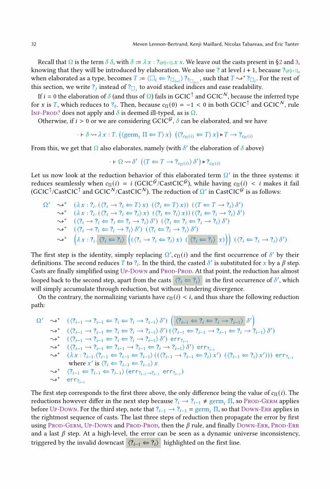
32 Meven Lennon-Bertrand, Kenji Maillard, Nicolas Tabareau, and Éric Tanter
Recall that Ω is the term 𝛿 𝛿 , with 𝛿 := _ 𝑥 : ?@{i+1}.𝑥 𝑥 . We leave out the casts present in §2 and 3,
knowing that they will be introduced by elaboration. We also use ? at level 𝑖 + 1, because ?@{i+1},
when elaborated as a type, becomes 𝑇 := ⟨□𝑖 ⇐ ?□𝑖+1⟩ ??□𝑖+1
, such that 𝑇 {∗ ?□𝑖. For the rest of
this section, we write ?𝑗 instead of ?□𝑗to avoid stacked indices and ease readability.
If 𝑖 = 0 the elaboration of 𝛿 (and thus of Ω) fails in GCIC↑and GCIC
N, because the inferred type
for 𝑥 is 𝑇 , which reduces to ?0. Then, because 𝑐Π (0) = −1 < 0 in both GCIC↑and GCIC
N, rule
Inf-Prod? does not apply and 𝛿 is deemed ill-typed, as is Ω.Otherwise, if 𝑖 > 0 or we are considering GCIC
G, 𝛿 can be elaborated, and we have
· ⊢ 𝛿⇝ _ 𝑥 : 𝑇 .(⟨germ𝑖 Π ⇐ 𝑇 ⟩ 𝑥
) (⟨?𝑐Π (𝑖) ⇐ 𝑇 ⟩ 𝑥
)⊲𝑇 → ?𝑐Π (𝑖)
From this, we get that Ω also elaborates, namely (with 𝛿 ′ the elaboration of 𝛿 above)
· ⊢ Ω⇝𝛿 ′(⟨𝑇 ⇐ 𝑇 → ?𝑐Π (𝑖)⟩ 𝛿 ′
)⊲ ?𝑐Π (𝑖)
Let us now look at the reduction behavior of this elaborated term Ω′in the three systems: it
reduces seamlessly when 𝑐Π (𝑖) = 𝑖 (GCICG/CastCIC
G), while having 𝑐Π (𝑖) < 𝑖 makes it fail
(GCIC↑/CastCIC
↑and GCIC
N/CastCIC
N). The reduction of Ω′
in CastCICGis as follows:
Ω′ {∗ (_ 𝑥 : ?𝑖 . (⟨?𝑖 → ?𝑖 ⇐ 𝑇 ⟩ 𝑥) (⟨?𝑖 ⇐ 𝑇 ⟩ 𝑥)) (⟨𝑇 ⇐ 𝑇 → ?𝑖⟩ 𝛿 ′){∗ (_ 𝑥 : ?𝑖 . (⟨?𝑖 → ?𝑖 ⇐ ?𝑖⟩ 𝑥) (⟨?𝑖 ⇐ ?𝑖⟩ 𝑥)) (⟨?𝑖 ⇐ ?𝑖 → ?𝑖⟩ 𝛿 ′){∗ (⟨?𝑖 → ?𝑖 ⇐ ?𝑖 ⇐ ?𝑖 → ?𝑖⟩ 𝛿 ′) (⟨?𝑖 ⇐ ?𝑖 ⇐ ?𝑖 → ?𝑖⟩ 𝛿 ′){∗ (⟨?𝑖 → ?𝑖 ⇐ ?𝑖 → ?𝑖⟩ 𝛿 ′) (⟨?𝑖 ⇐ ?𝑖 → ?𝑖⟩ 𝛿 ′){∗
(_ 𝑥 : ?𝑖 . ⟨?𝑖 ⇐ ?𝑖⟩
((⟨?𝑖 → ?𝑖 ⇐ ?𝑖⟩ 𝑥) ( ⟨?𝑖 ⇐ ?𝑖⟩ 𝑥)
))(⟨?𝑖 ⇐ ?𝑖 → ?𝑖⟩ 𝛿 ′)
The first step is the identity, simply replacing Ω′, 𝑐Π (𝑖) and the first occurrence of 𝛿 ′ by their
definitions. The second reduces 𝑇 to ?𝑖 . In the third, the casted 𝛿 ′ is substituted for 𝑥 by a 𝛽 step.
Casts are finally simplified using Up-Down and Prod-Prod. At that point, the reduction has almost
looped back to the second step, apart from the casts ⟨?𝑖 ⇐ ?𝑖⟩ in the first occurrence of 𝛿 ′, whichwill simply accumulate through reduction, but without hindering divergence.
On the contrary, the normalizing variants have 𝑐Π (𝑖) < 𝑖 , and thus share the following reduction
path:
Ω′ {∗ (⟨?𝑖−1 → ?𝑖−1 ⇐ ?𝑖 ⇐ ?𝑖 → ?𝑖−1⟩ 𝛿 ′)(⟨?𝑖−1 ⇐ ?𝑖 ⇐ ?𝑖 → ?𝑖−1⟩ 𝛿 ′
){∗ (⟨?𝑖−1 → ?𝑖−1 ⇐ ?𝑖 ⇐ ?𝑖 → ?𝑖−1⟩ 𝛿 ′) (⟨?𝑖−1 ⇐ ?𝑖−1 → ?𝑖−1 ⇐ ?𝑖 → ?𝑖−1⟩ 𝛿 ′){∗ (⟨?𝑖−1 → ?𝑖−1 ⇐ ?𝑖 ⇐ ?𝑖 → ?𝑖−1⟩ 𝛿 ′) err?𝑖−1
{∗ (⟨?𝑖−1 → ?𝑖−1 ⇐ ?𝑖−1 → ?𝑖−1 ⇐ ?𝑖 → ?𝑖−1⟩ 𝛿 ′) err?𝑖−1
{∗ (_ 𝑥 : ?𝑖−1.⟨?𝑖−1 ⇐ ?𝑖−1 ⇐ ?𝑖−1⟩ ((⟨?𝑖−1 → ?𝑖−1 ⇐ ?𝑖⟩ 𝑥 ′) (⟨?𝑖−1 ⇐ ?𝑖⟩ 𝑥 ′))) err?𝑖−1
where 𝑥 ′is ⟨?𝑖 ⇐ ?𝑖−1 ⇐ ?𝑖−1⟩ 𝑥
{∗ ⟨?𝑖−1 ⇐ ?𝑖−1 ⇐ ?𝑖−1⟩ (err?𝑖−1→?𝑖−1err?𝑖−1
){∗ err?𝑖−1
The first step corresponds to the first three above, the only difference being the value of 𝑐Π (𝑖). Thereductions however differ in the next step because ?𝑖 → ?𝑖−1 ≠ germ𝑖 Π, so Prod-Germ applies
before Up-Down. For the third step, note that ?𝑖−1 → ?𝑖−1 = germ𝑖 Π, so that Down-Err applies in
the rightmost sequence of casts. The last three steps of reduction then propagate the error by first
using Prod-Germ, Up-Down and Prod-Prod, then the 𝛽 rule, and finally Down-Err, Prod-Err
and a last 𝛽 step. At a high-level, the error can be seen as a dynamic universe inconsistency,
triggered by the invalid downcast ⟨?𝑖−1 ⇐ ?𝑖⟩ highlighted on the first line.

Gradualizing the Calculus of Inductive Constructions 33
5.4 Precision is a simulation for reductionEstablishing the graduality of elaboration—the formulation of the static gradual guarantee (SGG) in
our setting—is no small feat, as it requires properties about computations in CastCIC that amount
to the dynamic gradual guarantee (DGG). Indeed, to handle the typing rules for checking and
constrained inference, it is necessary to know how consistency and reduction evolve as a type
becomes less precise. As already explained in § 3.4, we cannot directly prove graduality for a
syntactic notion of precision. However, we can still show that this relation is a simulation for
reduction. While weaker than graduality, this property implies the DGG and suffices to conclude
that graduality of elaboration holds. The purpose of this section is to establish it. Our proof is partly
inspired by the proof of DGG by Siek et al. [2015].15We however had to adapt to the much higher
complexity of CIC compared to STLC. In particular, the presence of computation in the domain
and codomain of casts is quite subtle to tame, as we must in general reduce types in a cast before
we can reduce the cast itself.16
Technically, we need to distinguish between two notions of precision, one for GCIC and one
for CastCIC: (i) syntactic precision on terms in GCIC, which corresponds to the usual syntactic
precision of gradual typing [Siek et al. 2015], (ii) structural precision on terms in CastCIC, which
corresponds to syntactic precision together with a proper account of casts. In this section, we
concentrate on properties of structural precision in CastCIC. We only state and discuss the various
lemmas and theorems on a high level, and refer the reader to Appendix B.2 for the detailed proofs.
Structural precision for CastCIC. As emphasized already, the key property we want to establish
is that precision is a simulation for reduction, i.e., that less precise terms reduce at least as well
as more precise ones. This property guides the quite involved definition we are about to give for
structural precision: it is rigid enough to give the induction hypotheses needed to prove simulation,
while being lax enough to be a consequence of syntactic precision after elaboration, which is the
key point to establish elaboration graduality (Theorem 24), our equivalent of the static gradual
guarantee.
Similarly to ∼𝛼 , precision can ignore some casts, in order to handle casts that might appear or
disappear in one term but not the other during reduction. But in order to control what casts can be
ignored, we impose some restriction on the types involved. In particular, we want to ensure that
ignored casts would not have raised an error: e.g., we want to prevent 0 ⊑𝛼 ⟨B ⇐ N⟩ 0. Thus the
definition of structural precision relies on typing, and to do this we need to record the contexts of
the two compared terms. We do so by using double-struck letters to denote contexts where each
variable is given two types, writing Γ, 𝑥 : 𝐴 | 𝐴′for context extensions. We use Γ𝑖 for projections,
i.e., (Γ, 𝑥 : 𝐴 | 𝐴′)1 := Γ1, 𝑥 : 𝐴, and write Γ | Γ′ for the converse pairing operation.
Definition 6 (Structural and definitional precision in CastCIC).
Structural precision, denoted Γ ⊢ 𝑡 ⊑𝛼 𝑡 ′, is defined in Fig. 10, mutually with definitional precision,
denoted Γ ⊢ 𝑡 ⊑{ 𝑡 ′, which is its closure by reduction. We write Γ ⊑𝛼 Γ′ and Γ ⊑{ Γ′ for the pointwiseextensions of those to contexts.
Although Γ ⊢ 𝑡 ⊑{ 𝑡 ′ is defined in a stepwise way, it is equivalent to the existence of 𝑠 and 𝑠 ′ suchthat 𝑡{∗ 𝑠 , 𝑡 ′{∗ 𝑠 ′ and Γ ⊢ 𝑠 ⊑𝛼 𝑠 ′. The situation is the same as for consistency (resp. conversion),
which is the closure by reduction of 𝛼-consistency (resp. 𝛼-equality). However, here definitional
precision is also used in the definition of structural precision, in order to permit computation in
15Lemma 7 in Siek et al. [2015] is similar to our Theorem 20, and Fig. 10 draws from their Fig. 9, especially for Cast-R and
Cast-L. Also, while we do not make them explicit here, Lemmas 8, 10 and 11 also appear in our proofs.
16Thus, while Lemmas 17 and 18 correspond roughly to Lemma 9 in Siek et al. [2015], Lemmas 15 and 16 are completely
novel.

34 Meven Lennon-Bertrand, Kenji Maillard, Nicolas Tabareau, and Éric Tanter
Γ ⊢ 𝑡 ⊑𝛼 𝑡 ′
Γ ⊢ □𝑖 ⊑𝛼 □𝑖
Diag-Univ
Γ ⊢ 𝐴 ⊑𝛼 𝐴′ Γ, 𝑥 : 𝐴 | 𝐴′ ⊢ 𝐵 ⊑𝛼 𝐵′
Γ ⊢ Π𝑥 : 𝐴.𝐵 ⊑𝛼 Π𝑥 : 𝐴′.𝐵′ Diag-Prod
Γ ⊢ 𝐴 ⊑{ 𝐴′ Γ, 𝑥 : 𝐴 | 𝐴′ ⊢ 𝑡 ⊑𝛼 𝑡 ′
Γ ⊢ _ 𝑥 : 𝐴.𝑡 ⊑𝛼 _ 𝑥 : 𝐴′.𝑡 ′Diag-Abs
Γ ⊢ 𝑡 ⊑𝛼 𝑡 ′ Γ ⊢ 𝑢 ⊑𝛼 𝑢 ′
Γ ⊢ 𝑡 𝑢 ⊑𝛼 𝑡 ′ 𝑢 ′ Diag-App
Γ ⊢ 𝑥 ⊑𝛼 𝑥Diag-Var
Γ ⊢ 𝐴 ⊑𝛼 𝐴′ Γ ⊢ 𝐵 ⊑𝛼 𝐵′ Γ ⊢ 𝑡 ⊑𝛼 𝑡 ′
Γ ⊢ ⟨𝐵 ⇐ 𝐴⟩ 𝑡 ⊑𝛼 ⟨𝐵′ ⇐ 𝐴′⟩ 𝑡 ′Diag-Cast
Γ ⊢ a ⊑𝛼 a′ 𝑖 = 𝑖 ′
Γ ⊢ 𝐼@{i}(a) ⊑𝛼 𝐼@{i’}(a′)Diag-Ind
Γ ⊢ a ⊑𝛼 a′ Γ ⊢ b ⊑𝛼 b′ 𝑖 = 𝑖 ′
Γ ⊢ 𝑐@{i}(a, b) ⊑𝛼 𝑐@{i’}(a, b)Diag-Cons
Γ ⊢ 𝑠 ⊑𝛼 𝑠 ′ Γ1 ⊢ 𝑠 ▶I 𝐼 (a) Γ2 ⊢ 𝑠 ′ ▶
I 𝐼 (a′) Γ, 𝑧 : 𝐼 (a) | 𝐼 (a′) ⊢ 𝑃 ⊑𝛼 𝑃 ′
Γ, 𝑓 : (Π 𝑧 : 𝐼 (a), 𝑃) | (Π 𝑧 : 𝐼 (a′), 𝑃 ′), y : Yk [a/x] | Yk [a′/x] ⊢ 𝑡𝑘 ⊑𝛼 𝑡 ′𝑘
Γ ⊢ ind𝐼 (𝑠, 𝑧.𝑃, f .y.t) ⊑𝛼 ind𝐼 (𝑠 ′, 𝑧.𝑃 ′, f .y.t′)Diag-Fix
Γ1 ⊢ 𝑡 ⊲𝑇 Γ ⊢ 𝑇 ⊑{ 𝐴′ Γ ⊢ 𝑇 ⊑{ 𝐵′ Γ ⊢ 𝑡 ⊑𝛼 𝑡 ′
Γ ⊢ 𝑡 ⊑𝛼 ⟨𝐵′ ⇐ 𝐴′⟩ 𝑡 ′Cast-R
Γ2 ⊢ 𝑡 ′ ⊲𝑇 ′ Γ ⊢ 𝐴 ⊑{ 𝑇 ′ Γ ⊢ 𝐵 ⊑{ 𝑇 ′ Γ ⊢ 𝑡 ⊑𝛼 𝑡 ′
Γ ⊢ ⟨𝐵 ⇐ 𝐴⟩ 𝑡 ⊑𝛼 𝑡 ′Cast-L
Γ1 ⊢ 𝑡 ⊲𝑇 Γ ⊢ 𝑇 ⊑{ 𝑇 ′
Γ ⊢ 𝑡 ⊑𝛼 ?𝑇 ′Unk
Γ1 ⊢ 𝐴 ▶□□𝑖 𝑖 ≤ 𝑗
Γ ⊢ 𝐴 ⊑𝛼 ?□𝑗
Unk-Univ
Γ2 ⊢ 𝑡 ′ ⊲𝑇 ′ Γ ⊢ 𝑇 ⊑{ 𝑇 ′
Γ ⊢ err𝑇 ⊑𝛼 𝑡 ′Err
Γ1 ⊢ 𝑡 ′ ▶Π Π𝑥 : 𝐴′.𝐵′ Γ ⊢ Π𝑥 : 𝐴.𝐵 ⊑{ Π𝑥 : 𝐴′.𝐵′
Γ ⊢ _ 𝑥 : 𝐴. err𝐵 ⊑𝛼 𝑡 ′Err-Lambda
Γ ⊢ 𝑡 ⊑{ 𝑡 ′Γ ⊢ 𝑡 ⊑𝛼 𝑡 ′
Γ ⊢ 𝑡 ⊑{ 𝑡 ′Γ ⊢ 𝑠 ⊑{ 𝑡 ′ 𝑡 { 𝑠
Γ ⊢ 𝑡 ⊑{ 𝑡 ′Γ ⊢ 𝑡 ⊑{ 𝑠 ′ 𝑡 ′ { 𝑠 ′
Γ ⊢ 𝑡 ⊑{ 𝑡 ′
Fig. 10. Structural precision in CastCIC
types—recall that in a dependently-typed setting the two types involved in a cast may need to
reduce before the cast itself can reduce—and thus the two notions are mutually defined.
Let us now explain the rules defining structural precision. Diagonal rules are completely structural,
apart from the Diag-Fix rule, where typing assumptions provide us with the contexts needed to
compare the predicates. More interesting are the non-diagonal rules. First, ?𝑇 is greater than any
term of the ”right type”. This incorporates loss of precision (rule Unk), and accommodates for a

Gradualizing the Calculus of Inductive Constructions 35
small bit of cumulativity (rule Unk-Univ). This is needed because of technical reasons linked with
possibility to form products between types at different levels. On the contrary, the error is smaller
than any term (rule Err), even in its extended form on Π-types (rule Err-Lambda), with a typing
premise similar to that of rule Unk. Finally, casts on the right-hand side can be ignored as long as
they are performed on types that are less precise than the type of the term on the left (rule Cast-R).
Dually, casts on the left-hand side can be ignored as long as they are performed on types that are
more precise than the type of the term on the right (rule Cast-L).
Catch-up lemmas. The fact that structural precision is a simulation relies on a series of lemmas
that all have the same form: under the assumption that a term 𝑡 ′ is less precise than a term 𝑡 with a
known head (□, Π, 𝐼 , _ or 𝑐), the term 𝑡 ′ can be reduced to a term that either has the same head, or
is some ?. We call these catch-up lemmas, as they enable the less precise term to catch up to the
more precise one whose head is already known. Their aim is to ensure that casts appearing in a
less precise term never block reduction, as they can always be reduced away.
The lemmas are established in a descending fashion: first, on the universe in Lemma 15, then
on other types in Lemma 16, and finally on terms, namely on _-abstractions in Lemma 17 and
inductive constructors in Lemma 18. Each time, the previously proven catch-up lemmas are used to
reduce types in casts appearing in the less precise term, apart from Lemma 15, where the induction
hypothesis of the lemma being proven is used instead.
Lemma 15 (Universe catch-up).
Under the hypothesis that Γ1 ⊑𝛼 Γ2, if Γ ⊢ □𝑖 ⊑{ 𝑇 ′and Γ2 ⊢ 𝑇 ′ ▶□□𝑗 , either 𝑇
′{∗ ?□𝑗with
𝑖 < 𝑗 , or 𝑇 ′{∗□𝑖 .
Lemma 16 (Types catchup). Under the hypothesis that Γ1 ⊑𝛼 Γ2, we have the following:
• if Γ ⊢ ?□𝑖⊑𝛼 𝑇 ′
and Γ2 ⊢ 𝑇 ′ ▶□□𝑗 , then 𝑇′{∗ ?□𝑗
and 𝑖 ≤ 𝑗 ;
• if Γ ⊢ Π𝑥 : 𝐴.𝐵 ⊑𝛼 𝑇 ′, Γ1 ⊢ Π𝑥 : 𝐴.𝐵 ⊲□𝑖 and Γ2 ⊢ 𝑇 ′ ▶□□𝑗 then either𝑇
′{∗ ?□𝑗and 𝑖 ≤ 𝑗 ,
or 𝑇 ′{∗Π𝑥 : 𝐴′.𝐵′
for some 𝐴′and 𝐵′
such that Γ ⊢ Π𝑥 : 𝐴.𝐵 ⊑𝛼 Π𝑥 : 𝐴′.𝐵′;
• if Γ ⊢ 𝐼 (a) ⊑𝛼 𝑇 ′, Γ1 ⊢ 𝐼 (a) ⊲□𝑖 and Γ2 ⊢ 𝑇 ′ ▶□□𝑗 then either 𝑇 ′{∗ ?□𝑗
and 𝑖 ≤ 𝑗 , or
𝑇 ′{∗ 𝐼 (a′) for some 𝑎′ such that Γ ⊢ 𝐼 (a) ⊑𝛼 𝐼 (a′).Lemma 17 (_-abstraction catch-up).
If Γ ⊢ _ 𝑥 : 𝐴.𝑡 ⊑𝛼 𝑠 ′, where 𝑡 is not an error, Γ1 ⊢ _ 𝑥 : 𝐴.𝑡 ⊲Π𝑥 : 𝐴.𝐵 and Γ2 ⊢ 𝑠 ′ ▶Π Π𝑥 : 𝐴′.𝐵′
,
then 𝑠 ′{∗ _ 𝑥 : 𝐴′.𝑡 ′ with Γ ⊢ _ 𝑥 : 𝐴.𝑡 ⊑𝛼 _ 𝑥 : 𝐴′.𝑡 ′.This holds in CastCIC
G, CastCIC
↑, and for terms without ? in CastCIC
N.
Lemma 18 (Constructors and inductive error catch-up).
If Γ ⊢ 𝑐 (a, b) ⊑𝛼 𝑠 ′, Γ1 ⊢ 𝑐 (a, b) ⊲ 𝐼 (a) and Γ2 ⊢ 𝑠 ′ ▶I 𝐼 (a′), then either 𝑠 ′{∗ ?𝐼 (a′) or 𝑠 ′{∗ 𝑐 (a′, b′)
with Γ ⊢ 𝑐 (a, b) ⊑𝛼 𝑐 (a′, b′).Similarly, ifΓ ⊢ ?𝐼 (a) ⊑𝛼 𝑠 ′,Γ1 ⊢ ?𝐼 (a) ⊲ 𝐼 (a) andΓ2 ⊢ 𝑠 ′ ▶
I 𝐼 (a′), then 𝑠 ′{∗ ?𝐼 (a′) withΓ ⊢ 𝐼 (a) ⊑{ 𝐼 (a′).Note that for Lemma 18, we need to deal with unknown terms specifically, which is not necessary
for Lemma 17 because the unknown term in a Π-type reduces to a _-abstraction.
Lemma 17 deserves a more extensive discussion, because it is the critical point where the
difference between the three variants ofCastCICmanifests. In fact, it does not hold in full generality
for CastCICN. Indeed, the fact that 𝑖 ≤ 𝑐Π (𝑠Π (𝑖, 𝑗)) and 𝑗 ≤ 𝑐Π (𝑠Π (𝑖, 𝑗)) is used crucially to ensure
that casting from a Π-type into ? and back does not reduce to an error, given the restrictions on typesin Cast-R. This is the manifestation in the reduction of the embedding-projection property [New
and Ahmed 2018]. In CastCICNit holds only if one restricts to terms without ?, where such casts
never happen. This is important with regard to conservativity, as elaboration produces terms with
casts but without ?, and Lemma 17 ensures that for those precision is still a simulation, even in
CastCICN.
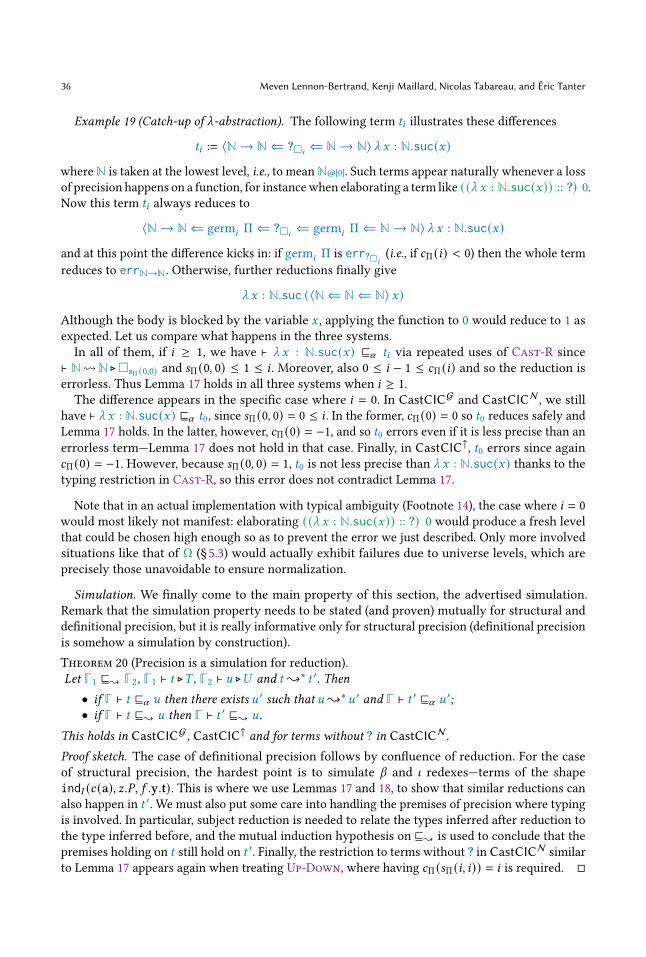
36 Meven Lennon-Bertrand, Kenji Maillard, Nicolas Tabareau, and Éric Tanter
Example 19 (Catch-up of _-abstraction). The following term 𝑡𝑖 illustrates these differences
𝑡𝑖 := ⟨N → N ⇐ ?□𝑖⇐ N → N⟩ _ 𝑥 : N.suc(𝑥)
where N is taken at the lowest level, i.e., to mean N@{0}. Such terms appear naturally whenever a loss
of precision happens on a function, for instancewhen elaborating a term like ((_ 𝑥 : N.suc(𝑥)) :: ?) 0.
Now this term 𝑡𝑖 always reduces to
⟨N → N ⇐ germ𝑖 Π ⇐ ?□𝑖⇐ germ𝑖 Π ⇐ N → N⟩ _ 𝑥 : N.suc(𝑥)
and at this point the difference kicks in: if germ𝑖 Π is err?□𝑖(i.e., if 𝑐Π (𝑖) < 0) then the whole term
reduces to errN→N. Otherwise, further reductions finally give
_ 𝑥 : N.suc (⟨N ⇐ N ⇐ N⟩ 𝑥)
Although the body is blocked by the variable 𝑥 , applying the function to 0 would reduce to 1 as
expected. Let us compare what happens in the three systems.
In all of them, if 𝑖 ≥ 1, we have ⊢ _ 𝑥 : N.suc(𝑥) ⊑𝛼 𝑡𝑖 via repeated uses of Cast-R since
⊢ N⇝N ⊲□𝑠Π (0,0) and 𝑠Π (0, 0) ≤ 1 ≤ 𝑖 . Moreover, also 0 ≤ 𝑖 − 1 ≤ 𝑐Π (𝑖) and so the reduction is
errorless. Thus Lemma 17 holds in all three systems when 𝑖 ≥ 1.
The difference appears in the specific case where 𝑖 = 0. In CastCICGand CastCIC
N, we still
have ⊢ _ 𝑥 : N.suc(𝑥) ⊑𝛼 𝑡0, since 𝑠Π (0, 0) = 0 ≤ 𝑖 . In the former, 𝑐Π (0) = 0 so 𝑡0 reduces safely and
Lemma 17 holds. In the latter, however, 𝑐Π (0) = −1, and so 𝑡0 errors even if it is less precise than an
errorless term—Lemma 17 does not hold in that case. Finally, in CastCIC↑, 𝑡0 errors since again
𝑐Π (0) = −1. However, because 𝑠Π (0, 0) = 1, 𝑡0 is not less precise than _ 𝑥 : N.suc(𝑥) thanks to the
typing restriction in Cast-R, so this error does not contradict Lemma 17.
Note that in an actual implementation with typical ambiguity (Footnote 14), the case where 𝑖 = 0
would most likely not manifest: elaborating ((_ 𝑥 : N.suc(𝑥)) :: ?) 0 would produce a fresh level
that could be chosen high enough so as to prevent the error we just described. Only more involved
situations like that of Ω (§5.3) would actually exhibit failures due to universe levels, which are
precisely those unavoidable to ensure normalization.
Simulation. We finally come to the main property of this section, the advertised simulation.
Remark that the simulation property needs to be stated (and proven) mutually for structural and
definitional precision, but it is really informative only for structural precision (definitional precision
is somehow a simulation by construction).
Theorem 20 (Precision is a simulation for reduction).
Let Γ1 ⊑{ Γ2, Γ1 ⊢ 𝑡 ⊲𝑇 , Γ2 ⊢ 𝑢 ⊲𝑈 and 𝑡{∗ 𝑡 ′. Then
• if Γ ⊢ 𝑡 ⊑𝛼 𝑢 then there exists 𝑢 ′such that 𝑢{∗ 𝑢 ′
and Γ ⊢ 𝑡 ′ ⊑𝛼 𝑢 ′;
• if Γ ⊢ 𝑡 ⊑{ 𝑢 then Γ ⊢ 𝑡 ′ ⊑{ 𝑢.
This holds in CastCICG, CastCIC
↑and for terms without ? in CastCIC
N.
Proof sketch. The case of definitional precision follows by confluence of reduction. For the case
of structural precision, the hardest point is to simulate 𝛽 and ] redexes—terms of the shape
ind𝐼 (𝑐 (a), 𝑧.𝑃, 𝑓 .y.t). This is where we use Lemmas 17 and 18, to show that similar reductions can
also happen in 𝑡 ′. We must also put some care into handling the premises of precision where typing
is involved. In particular, subject reduction is needed to relate the types inferred after reduction to
the type inferred before, and the mutual induction hypothesis on ⊑{ is used to conclude that the
premises holding on 𝑡 still hold on 𝑡 ′. Finally, the restriction to terms without ? in CastCICNsimilar
to Lemma 17 appears again when treating Up-Down, where having 𝑐Π (𝑠Π (𝑖, 𝑖)) = 𝑖 is required. □

Gradualizing the Calculus of Inductive Constructions 37
From this theorem, we get as direct corollaries the following properties, that are required to handle
reduction (Corollary 21) and consistency (Corollary 22) in elaboration. Again those corollaries hold
in GCICG, GCIC
↑and for terms in GCIC
Ncontaining no ?.
Corollary 21 (Monotonicity of reduction to type constructor).
Let Γ, 𝑇 and 𝑇 ′be such that Γ1 ⊢ 𝑇 ▶□□𝑖 , Γ2 ⊢ 𝑇 ′ ▶□□𝑗 , Γ ⊢ 𝑇 ⊑𝛼 𝑇 ′
. Then
• if 𝑇 {∗ ?□𝑖then 𝑇 ′{∗ ?□𝑗
with 𝑖 ≤ 𝑗 ;
• if 𝑇 {∗□𝑖−1 then either 𝑇 ′{∗ ?□𝑗with 𝑖 ≤ 𝑗 , or 𝑇 ′{∗□𝑖−1;
• if 𝑇 {∗Π𝑥 : 𝐴.𝐵 then either 𝑇 ′{∗ ?□𝑗
with 𝑖 ≤ 𝑗 , or 𝑇 ′{∗Π𝑥 : 𝐴′.𝐵′
and
Γ ⊢ Π𝑥 : 𝐴.𝐵 ⊑𝛼 Π𝑥 : 𝐴′.𝐵′;
• if 𝑇 {∗ 𝐼 (a) then either 𝑇 ′{∗ ?□𝑗with 𝑖 ≤ 𝑗 , or 𝑇 ′{∗ 𝐼 (a′) and Γ ⊢ 𝐼 (a) ⊑𝛼 𝐼 (a′).
Proof. It suffices to simulate the reductions of 𝑇 by using Theorem 20, and then use Lemmas 15
and 16 to conclude. Note that head reductions are simulated using head reductions in Theorem 20,
and the reductions of Lemmas 15 and 16 are also head reductions. Thus the corollary still holds
when fixing weak-head reduction as a reduction strategy. □
Corollary 22 (Monotonicity of consistency). If Γ ⊢ 𝑇 ⊑𝛼 𝑇 ′, Γ ⊢ 𝑆 ⊑𝛼 𝑆 ′ and 𝑇 ∼ 𝑆 then 𝑇 ′ ∼ 𝑆 ′.
Proof. By definition of ∼, we get some 𝑈 and 𝑉 such that 𝑇 {∗𝑈 and 𝑆{∗𝑉 , and 𝑈 ∼𝛼 𝑉 .
By Theorem 20, we can simulate these reductions to get some 𝑈 ′and 𝑉 ′
such that 𝑇 ′{∗𝑈 ′
and 𝑆 ′{∗𝑉 ′, and also Γ1 ⊢ 𝑈 ⊑𝛼 𝑈 ′
and Γ1 ⊢ 𝑉 ⊑𝛼 𝑉 ′. Thus we only need to show that 𝛼-
consistency is monotone with respect to structural precision, which is direct by induction on
structural precision. □
5.5 Properties of GCICWe now have enough technical tools to prove most of the properties of GCIC. We state those
theorems in an empty context in this section to make them more readable, but they are of course
corollaries of similar statements including contexts, proven by mutual induction. The complete
statements and proofs can be found in Appendix B.3.
Conservativity with respect to CIC. Elaboration systematically inserts casts during checking, thus
even static terms are not elaborated to themselves. Therefore we use a (partial) erasure function
Y that translates terms of CastCIC to terms of CIC by erasing all casts. We also introduce the
notion of erasability, characterizing terms that contain “harmless” casts, such that in particular the
elaboration of a static term is always erasable.
Definition 7 (Equiprecision). Two terms 𝑠 and 𝑡 are equiprecise in a context Γ, denoted Γ ⊢ 𝑠 ⊒⊑𝛼 𝑡
if both Γ ⊢ 𝑠 ⊑𝛼 𝑡 and Γ ⊢ 𝑡 ⊑𝛼 𝑠 .
Definition 8 (Erasure, erasability). Erasure Y is a partial function from the syntax of CastCIC to the
syntax of CIC, which is undefined on ? and err, is such that Y (⟨𝐵 ⇐ 𝐴⟩ 𝑡) = Y (𝑡), and is a congruencefor all other term constructors.
Given a context Γ we say that a term well-typed in Γ1 𝑡 is erasable if Y (𝑡) is defined, well-typed inΓ2, and equiprecise to 𝑡 in Γ. Similarly a context Γ is called erasable if it is pointwise erasable. When Γis erasable, we say that a term 𝑡 is erasable in Γ to mean that it is erasable in Γ | Y (Γ).
Conservativity holds in all three systems, typeability being of course taken into the corresponding
variant of CIC: full CIC for GCICGand GCIC
N, and CIC
↑for GCIC
↑.
Theorem 23 (Conservativity). Let 𝑡 be a static term ( i.e., is a term of GCIC that is also a term of CIC).
If ⊢CIC 𝑡 ⊲𝑇 for some type 𝑇 , then there exists 𝑡 and 𝑇 ′such that ⊢ 𝑡⇝ 𝑡 ⊲𝑇 ′
, and moreover Y (𝑡) = 𝑡
and Y (𝑇 ′) = 𝑇 . Conversely if ⊢ 𝑡⇝ 𝑡 ⊲𝑇 for some 𝑡 and 𝑇 , then ⊢CIC 𝑡 ⊲ Y (𝑇 ).

38 Meven Lennon-Bertrand, Kenji Maillard, Nicolas Tabareau, and Éric Tanter
𝑥 ⊑G
𝛼 𝑥 □𝑖 ⊑G
𝛼 □𝑖
𝐴 ⊑G
𝛼 𝐴′ 𝐵 ⊑G
𝛼 𝐵′
Π𝑥 : 𝐴.𝐵 ⊑G
𝛼 Π𝑥 : 𝐴′.𝐵′𝐴 ⊑G
𝛼 𝐴′ 𝑡 ⊑G
𝛼 𝑡 ′
_ 𝑥 : 𝐴.𝑡 ⊑G
𝛼 _ 𝑥 : 𝐴.𝑡
𝑡 ⊑G
𝛼 𝑡 ′ 𝑢 ⊑G
𝛼 𝑢 ′
𝑡 𝑢 ⊑G
𝛼 𝑡 ′ 𝑢 ′a ⊑G
𝛼 a′
𝐼 (a) ⊑G
𝛼 𝐼 (a′)a ⊑G
𝛼 a′ b ⊑G
𝛼 b′
𝑐 (a, b) ⊑G
𝛼 𝑐 (a′, b′)
𝑎 ⊑G
𝛼 𝑎′ 𝑃 ⊑G
𝛼 𝑃 ′ t ⊑G
𝛼 t′
ind𝐼 (𝑎, 𝑧.𝑃, f .y.t) ⊑G
𝛼 ind𝐼 (𝑎′, 𝑧.𝑃 ′, f .y.t′) 𝑡 ⊑G
𝛼 ?
Fig. 11. Syntactic precision for GCIC
Proof sketch. Because 𝑡 is static, its typing derivation in GCIC can only use rules that have a
counterpart in CIC, and conversely all rules of CIC have a counterpart inGCIC. The only difference
is about the reduction/conversion side conditions, which are used on elaborated types in GCIC,
rather than their non-elaborated counterparts in CIC.
Thus, the main difficulty is to ensure that the extra casts inserted by elaboration do not alter
reduction. For this we maintain the property that all terms 𝑡 considered in CastCIC are erasable,
and in particular that any static term 𝑡 that elaborates to some 𝑡 is such that Y (𝑡) = 𝑡 . From the
simulation property of structural precision (Theorem 20), we get that an erasable term 𝑡 has the
same reduction behavior as its erasure, i.e., if 𝑡{∗ 𝑠 then Y (𝑡){∗ 𝑠 ′ with 𝑠 ′ and 𝑠 equiprecise, andconversely if Y (𝑡){∗ 𝑠 ′ then 𝑡{∗ 𝑠 with 𝑠 ′ and 𝑠 equiprecise. Using that property, we prove thatconstraint reductions (▶Π,
▶□ and ▶I) in CastCIC and CIC behave the same on static terms. □
Elaboration Graduality. Next, we turn to elaboration graduality, the equivalent of the static
gradual guarantee (SGG) of Siek et al. [2015] in our setting. We state it with respect to a notion of
precision for terms in GCIC, syntactic precision ⊑G
𝛼 , defined in Fig. 11. Syntactic precision is the
usual and expected source-level notion of precision in gradual languages: it is generated by a single
non-trivial rule 𝑡 ⊑G
𝛼 ?@{i}, and congruence rules for all term formers.
In contrast with the simply-typed setting, the presence of multiple unknown types ?, one foreach universe level 𝑖 , requires an additional hypothesis relating elaboration and precision. We say
that two judgments 𝑡 ⊑G
𝛼 ?@{i} and Γ ⊢ 𝑡⇝ 𝑡 ⊲𝑇 are universe adequate if the universe level 𝑗 given by
the well-formedness judgment Γ ⊢ 𝑇 ▶□□𝑗 induced by correction of the elaboration satisfies 𝑖 = 𝑗 .
More generally, 𝑡 ⊑G
𝛼 𝑠 and ⊢ 𝑡⇝ 𝑡 ⊲𝑇 are universe adequate if for any subterm 𝑡0 of 𝑡 inducing
judgments 𝑡0 ⊑G
𝛼 ?@{i} and Γ0 ⊢ 𝑡0⇝ 𝑡 ⊲𝑇 , those are universe adequate. Note that this extraneous
technical assumption on universe levels is not needed if we use typical ambiguity (Footnote 14),
since universe levels are not given explicitly.
Theorem 24 (Elaboration Graduality / Static Gradual Guarantee). In GCICGand GCIC
↑, if 𝑡 ⊑G
𝛼 𝑠
and ⊢ 𝑡⇝ 𝑡 ⊲𝑇 are universe adequate, then ⊢ 𝑠⇝ 𝑠 ⊲ 𝑆 for some 𝑠 and 𝑆 such that ⊢ 𝑡 ⊑𝛼 𝑠 and
⊢ 𝑇 ⊑𝛼 𝑆 .
Proof sketch. The proof is by induction on the elaboration derivation for 𝑡 . All cases for inference
consist in a straightforward combination of the hypotheses, with the universe adequacy hypothesis
used in the case where 𝑠 is ?@{i}. Here again the technical difficulties arise in the rules involving
reduction. This is where Corollary 21 is useful, proving that the less structurally precise term
obtained by induction in a constrained inference reduces to a less precise type. Thus either the
same rule can still be used, or one has to trade a Inf-Unk, Inf-Prod or Inf-Ind rule respectively
for a Inf-Univ?, Inf-Prod? or Inf-Ind? rule in case the less precise type is some ?□𝑖and the more

Gradualizing the Calculus of Inductive Constructions 39
precise type is not. Similarly, Corollary 22 proves that in the checking rule the less precise types are
still consistent. Note that again, because Corollary 21 holds when restricted to weak-head reduction,
elaboration graduality also holds when fixing a weak-head strategy in Fig. 9. □
Dynamic Gradual Guarantee. Following Siek et al. [2015], using the fact that structural precision
is a simulation (Theorem 20), we can prove the DGG for CastCICGand CastCIC
↑(stated using the
notion of observational refinement ⊑𝑜𝑏𝑠from Definition 4).
Theorem 25 (Dynamic Gradual Guarantee for CastCICGand CastCIC
↑). Suppose that Γ ⊢ 𝑡 ⊲𝐴 and
Γ ⊢ 𝑢 ⊲𝐴. If moreover Γ | Γ ⊢ 𝑡 ⊑𝛼 𝑢 then 𝑡 ⊑𝑜𝑏𝑠 𝑢.
Proof. Let C : (Γ ⊢ 𝐴) ⇒ (⊢ B) closing over all free variables. By the diagonal rules of structural
precision, we have Γ | Γ ⊢ C[𝑡] ⊑𝛼 C[𝑢]. By progress (Theorem 8), C[𝑡] either reduces to true,false, ?B, errB or diverges, and similarly for C[𝑢]. If C[𝑡] diverges or reduces to errB, we are
done. If it reduces to either true, false or ?B, then by the catch-up Lemma 18, C[𝑢] either reducesto the same value, or to ?B. In particular, it cannot diverge or reduce to an error. □
Note that Example 19 provides a counter-example to this theorem for CastCICN, by choosing
the context indN (• 0, 𝑧.B, 𝑓 .true, 𝑓 .𝑛.true), because in that context the function _ 𝑥 : N.suc(𝑥)reduces to true while the less precise casted function reduces to errB.
As observed in §2.4, graduality—and in particular the fact that precision induces ep-pairs—is
inherently semantic, and thus cannot rely on the syntactic precision ⊑G
𝛼 introduced in this section.
Therefore, we defer the proof of G for CastCIC↑and CastCIC
Gto the next section, where the
semantic notion of propositional precision is introduced.
6 REALIZING CastCIC AND GRADUALITYTo prove normalization of CastCIC
Nand CastCIC
↑, we now build a model of both theories with a
simple implementation of casts using case-analysis on types as well as exceptions, yielding the
discrete model, allowing us to reduce the normalization of both theories to the normalization of the
target theory (§6.1).
Then, to prove graduality of CastCIC↑, we build a more elaborate monotone model inducing
a precision relation well-behaved with respect to conversion. Following generalities about the
interpretation ofCIC’s types as posets in §6.2, we describe the construction of a monotone unknown
type ¥? in §6.3 and a hierarchy of universes in §6.4 and put these pieces together in §6.5, culminating
in a proof of graduality for CastCIC↑(§6.6). In both the discrete and monotone case, the parameters
𝑐Π (−) and 𝑠Π (−,−) appear when building the hierarchy of universes and tying the knot with the
unknown type.
Finally, to deduce graduality for the non-terminating variant, CastCICG, we describe at the end
of this section a model based on 𝜔-complete partial orders, extending the seminal model of Scott
[1976] for _-calulus to CastCICG(§6.7).
The discrete model embeds into a variant of CIC extended with induction-recursion [Dybjer
and Setzer 2003], noted CICIR, and the monotone model into a variant that additionally features
quotients (and hence also function extensionality [Shulman 2011]), noted CICIR
QIT.
Formalization in Agda. We use Agda [Norell 2009] as a practical tool to typecheck the components
of the models and assume that Agda satisfies standard metatheoretical properties, namely subject
reduction and strong normalization.
The correspondence between the notions developed in the following sections and the formal
development in Agda [Lennon-Bertrand et al. 2020] is as follows. The formalization covers most com-
ponent of the discrete (DiscreteModelPartial.agda) and monotone model (UnivPartial.agda)in a partial (non-normalizing) setting and only the discrete model is proved to be normalizing

40 Meven Lennon-Bertrand, Kenji Maillard, Nicolas Tabareau, and Éric Tanter
assuming normalization of the type theory implemented by Agda (no escape hatch to termina-
tion checking is used in DiscreteModelTotal). The main definitions surrounding posets can be
found in Poset.agda: top and bottom elements (called Initial and Final in the formalization),
embedding-projection pairs (called Distr) as well as the notions corresponding to indexed families
of posets (IndexedPoset, together with IndexedDistr). It is then proved that we endow can the
translation of each type formers fromCastCICwith a poset structure: natural numbers in nat.agda,booleans in bool.agda, dependent product in pi.agda. The definition of the monotone unknown
type ¥? is defined in the subdirectory Unknown/. It is more involved since we need to use a quotient
(that we axiomatize together with a rewriting rule in Unknown/Quotient.agda). Finally, all thesebuilding blocks are put together when assembling the inductive-recursive hierarchies of universes
(UnivPartial.agda, DiscreteModelPartial.agda and DiscreteModelTotal.agda).
6.1 Discrete Model of CastCICThe discrete model explains away the new term formers of CastCIC (Syntax of CastCIC) by a
translation into CIC using two important ingredients from the literature:
• Exceptions, following the approach of ExTT [Pédrot and Tabareau 2018]: each inductive type
is extended with two new constructors, one for ? and one for err. As alluded to early on
(§2.5), both ? and err are exceptional terms in their propagation semantics, and only differ
in their static interpretation: ?A is consistent with any other term of type A, while errA is notconsistent with any such term.
• Case analysis on types [Boulier et al. 2017] to define the cast operator. The essence of the
translation is to interpret types as codes when they are seen as terms, and as the semantics of
those codes when they are seen as types. This allows us to get the standard interpretation
for a term inhabiting a type, but at the same time, it allows functions taking terms in the
universe □□𝑖 to perform a case analysis on the code of the type, because this time, the type is
seen as a term in □□𝑖 .
The latter ingredient for intensional type analysis requires the target theory of the translation to
be an extension of CIC with induction-recursion [Dybjer and Setzer 2003], noted CICIR. We write
{IR and ⊢IR to denote the reduction and typing judgments of CICIR, respectively.
Inductive types. Following the general pattern of ExTT, we interpret each inductive type 𝐼 by an
inductive type ¥𝐼 featuring all constructors of 𝐼 and extended with two new constructors ⊤¥𝐼 and ⊥¥𝐼 ,corresponding respectively to ?𝐼 and err𝐼 of CastCIC. The constructors ⊤¥𝐼 and ⊥¥𝐼 of ¥𝐼 are calledexceptional by opposition to the other constructors that we call non-exceptional. For instance, the
inductive type used to interpret natural numbers,¥N, thus has 4 constructors: the non-exceptional
constructors 0 and suc, and the exceptional constructors ⊤ ¥N, ⊥ ¥N. In the rest of this section, we
only illustrate inductive types on natural numbers.
Universe and type-case. Case analysis on types is obtained through an explicit inductive-recursive
description of the universes [Martin-Löf 1984; McBride 2010] to build a type of codes □□𝑖 described
in Fig. 12. Codes are noted with · and the universe type contains codes for dependent product (Π),
universes (□□𝑗 ), inductive types (e.g., N) as well as ? for the unknown type and err for the error
type. The main subtlety here is that the code Π𝐴𝐵 is at level 𝑠Π (𝑖, 𝑗) when𝐴 is at 𝑖 and 𝐵 is a family
at 𝑗 , emulating the rule of Fig. 3. Accompanying the inductive definition of □□𝑖 , the recursively
defined decoding function El provides a semantics for these codes. The semantics of Π is given by
the dependent product in the target theory, applying El on the domain and the codomain of the
code. The semantics of □□𝑗 is precisely the type of codes □□𝑗 . The semantics of N is given by the
extended natural numbers¥N, explained above.

Gradualizing the Calculus of Inductive Constructions 41
𝐴 ∈ □□𝑖 𝐵 ∈ El𝐴 → □□𝑗
Π𝐴𝐵 ∈ □□𝑠Π (𝑖, 𝑗)
𝑗 < 𝑖
□□𝑗 ∈ □□𝑖N ∈ □□𝑖 ?𝑖 ∈ □□𝑖 err𝑖 ∈ □□𝑖
El (Π𝐴𝐵) = Π(𝑎 : El𝐴) El(𝐵 𝑎) El □□𝑗 = □□𝑗 El N = ¥N El ?𝑖 = ¥Σ Head𝑖 germ𝑖 El err𝑖 = unit
Fig. 12. Inductive-recursive encoding of the discrete universe hierarchy
?Π𝐴𝐵
:= _ 𝑥 : El𝐴.?El (𝐵 𝑥) ?
□□𝑗:= ?𝑗 ?
N:= ⊤ ¥N ??𝑗 := ⊤
El □□𝑗?�err𝑗 := ()
errΠ𝐴𝐵
:= _ 𝑥 : El𝐴. errEl (𝐵 𝑥) err
□□𝑗:= �err𝑗 err
N:= ⊥ ¥N err?𝑗
:= ⊥El □□𝑗
err�err𝑗 := ()
Fig. 13. Realization of exceptions
Intuitively, the semantics of ?𝑖 is that an inhabitant of the unknown type corresponds to a
pair of a type and an inhabitant of that type. More precisely, we first define a notion of germ
for codes where we stratify the head constructors Head (see Fig. 4) according to the universe
level 𝑖 , e.g. �germ𝑖 Π := Π □□𝑐Π (𝑖) (_(𝑥 : □□𝑐Π (𝑖) ).□□𝑐Π (𝑖) ) when 𝑐Π (𝑖) ≥ 0, and its decoding to types
germ𝑖 ℎ := El (�germ𝑖 ℎ). The unknown type ?𝑖 is then decoded to the extended dependent sum
¥Σ Head𝑖 germ𝑖 whose elements are either:
• one of the two freely added constructors ⊤ ¥Σ,⊥ ¥Σ following the interpretation scheme of
inductive types;
• or a dependent pair (ℎ; 𝑡) of a head constructor ℎ ∈ Head𝑖 together with an element 𝑡 ∈germ𝑖 ℎ.
Finally, the error type err𝑖 is decoded to the unit type unit containing a unique element ().
Variants of CastCIC. Crucially, the code for Π-types (Fig. 12) depends on the choice made
for 𝑠Π (𝑖, 𝑗). Observe that for the choice of parameters corresponding to CastCICG, the inductive-
recursive definition of□□𝑖 is ill-founded since 𝑐Π (𝑠Π (𝑖, 𝑖)) = 𝑠Π (𝑖, 𝑖).We can thus inject germ 𝑠Π (𝑖,𝑖)Π =
El ?𝑠Π (𝑖, 𝑖) → El ?𝑠Π (𝑖, 𝑖) into El ?𝑠Π (𝑖, 𝑖) and project back in the other direction, exhibiting an
embedding-retraction suitable to interpret the untyped _-calculus and hence Ω.17
In order to maintain normalization, the construction of the unknown type and the universe
therefore needs to be stratified, which is possible when 𝑐Π (𝑠Π (𝑖, 𝑖)) < 𝑠Π (𝑖, 𝑖). This strict inequalityoccurs for both CastCIC
Nand CastCIC
↑. We then proceed by strong induction on the universe
level, and note that thanks to the level gap, the decoding El ?𝑖 of the unknown type at a level 𝑖 can
be defined solely from the data of smaller universes available by inductive hypothesis, without any
reference to □□𝑖 . We can then define the rest of the universe □□𝑖 and the decoding function El at
level 𝑖 in a well-founded manner, validating the strict positivity criterion of Agda’s termination
checker.
Exceptions. The definition of exceptions ?𝐴, err𝐴 : El 𝐴 at an arbitrary code 𝐴 then follows
by case analysis on the code, as shown in Fig. 13. On the code for the universe, □□𝑗 , we directly
use the code for the unknown and the error types respectively. On codes that have an inductive
interpretation—N, ?𝑖—we use the two added constructors. On the code for dependent functions,
17In the Agda implementation, we deactivate the termination checker on the definition of the universe for the model
interpreting CastCICG, thus effectively working in a partial, inconsistent type theory.

42 Meven Lennon-Bertrand, Kenji Maillard, Nicolas Tabareau, and Éric Tanter
cast (Π𝐴d𝐴c) (Π 𝐵d 𝐵c) 𝑓 := _ 𝑏 : El𝐵d . let𝑎 = cast 𝐵d 𝐴d 𝑏 in cast (𝐴c 𝑎) (𝐵c 𝑏) (𝑓 𝑎)cast (Π𝐴d𝐴c) ?𝑖 𝑓 := (Π; cast (Π𝐴d𝐴c) (�germ𝑖 Π) 𝑓 ) if �germ𝑖 Π ≠ err
cast (Π𝐴d𝐴c) 𝑋 𝑓 := err𝑋 otherwise
cast N N 𝑛 := 𝑛
cast N ?𝑖 𝑛 := (N;𝑛)cast N 𝑋 𝑛 := err𝑋
cast err𝑖 𝑍 () := err𝑍
cast □□𝑗 □□𝑗 𝐴 := 𝐴
cast □□𝑗 ?𝑖 𝐴 := (□𝑗 ;𝐴) if 𝑗 < 𝑖
cast □□𝑗 𝑋 𝐴 := err𝑋 otherwise
cast ?𝑖 𝑍 (𝑐;𝑥) := cast (�germ𝑖 𝑐) 𝑍 𝑥
cast ?𝑖 𝑍 ⊤El ?𝑖
:= ?𝑍cast ?𝑖 𝑍 ⊥
El ?𝑖:= err𝑍
Fig. 14. Definition of cast (discrete model)
J·K := ·
J𝐴K := El [𝐴]
[𝑥] := 𝑥
[□𝑖 ] := □□𝑖
[Π𝑥 : 𝐴.𝐵] := Π [𝐴] (_ 𝑥 : J𝐴K.[𝐵])[𝑡 𝑢] := [𝑡] [𝑢][_ 𝑥 : 𝐴.𝑡] := _ 𝑥 : J𝐴K.[𝑡]
JΓ, 𝑥 : 𝐴K := JΓK, 𝑥 : J𝐴K
[N] := N[0] := 0
[suc] := suc[indN] 𝑃 ℎ0 ℎsuc := ind ¥N 𝑃 ℎ0 ℎsuc ?𝑃 ? ¥N err(𝑃 err ¥N)
[?𝐴] := ?[𝐴][err𝐴] := err[𝐴][⟨𝐵 ⇐ 𝐴⟩ 𝑡] := cast [𝐴] [𝐵] [𝑡]
Fig. 15. Discrete translation from CastCIC to CICIR
exceptions are defined by re-raising the exception at the codomain in a pointwise fashion. Finally,
on the error type err, exceptions are degenerated and forced to take the only value () : unit18 ofits interpretation as a type.
Casts. Equipped with exceptions and type analysis, we define cast : Π(𝐴 : □□𝑖 ) (𝐵 : □□𝑗 ).𝐴 → 𝐵
by induction on the universe levels and case analysis on the codes of the types 𝐴 and 𝐵 (Fig. 14). In
the total setting (when 𝑐Π (𝑠Π (𝑖, 𝑖)) < 𝑠Π (𝑖, 𝑖)), the definition of cast is well-founded: each recursive
call happens either at a strictly smaller universe (the two cases for Π) or on a strict subterm of the
term being cast (case of inductives, i.e., N and ?). Note that each of the defining equations of castcorresponds straightforwardly to a reduction rule of Fig. 5.
Discrete translation. We can finally define the discrete syntactic model of CastCIC in CICIR
(Fig. 15). The translations [−] and J−K are defined by induction on the syntax of terms and types.
A type 𝐴 is translated to its corresponding code [𝐴] in □□𝑖 when seen as a term, and is translated
to the interpretation of this code J𝐴K := El [𝐴] when seen as a type. ?𝐴 and err𝐴 are directly
translated using the exceptions defined in Fig. 13. The following theorem shows that the translation
is a syntactic model in the sense of Boulier et al. [2017].
18This definition is indeed uniform if unit is seen as the record type with no projection.

Gradualizing the Calculus of Inductive Constructions 43
0 ⊑N0 ⊥ ¥N ⊑N 𝑛
0 ⊑N ⊤ ¥N ⊤ ¥N ⊑N ⊤ ¥N
𝑛 ⊑N 𝑚
suc𝑛 ⊑N suc𝑚
𝑛 ⊑N ⊤ ¥N
suc𝑛 ⊑N ⊤ ¥N
Fig. 16. Order structure on extended natural numbers
Theorem 26 (Discrete syntactic model). The translation defined in Fig. 15 preserves conversion and
typing derivations:
(1) if Γ ⊢cast 𝑡 { 𝑢 then JΓK ⊢IR [𝑡] {+IR
[𝑢], in particular JΓK ⊢IR [𝑡] ≡ [𝑢],(2) if Γ ⊢cast 𝑡 : 𝐴 then JΓK ⊢IR [𝑡] : J𝐴K.
Proof. (1) All reduction rules from CIC are preserved without a change so that we only need to be
concerned with the reduction rules involving exceptions or casts. A careful inspection shows that
these reductions are preserved too once we observe that the terms of the shape ⟨?□𝑖⇐ germ𝑖 ℎ⟩ 𝑡
that are stuck in CastCIC are in one-to-one correspondence with the one-step reduced form of its
translation (ℎ; [𝑡]) : ¥Σ Head𝑖 germ𝑖 . (2) Proved by a direct induction on the typing derivation of
Γ ⊢cast 𝑡 : 𝐴, using the fact that exceptions and casts are well-typed—that is ⊢IR ? : Π(𝐴 : □□𝑖 ) El𝐴
, ⊢IR err : Π(𝐴 : □□𝑖 ) El𝐴, and ⊢IR cast : Π(𝐴 : □□𝑖 ) (𝐵 : □□𝑖 )El𝐴→El𝐵—and relying on assertion
(1) to handle the conversion rule. □
As explained in Theorem 9, Theorem 26 implies in particular that CastCIC↑and CastCIC
Nare
strongly normalizing.
6.2 Poset-Based Models of Dependent Type TheoryThe simplicity of the discrete model comes at the price of an inherent inability to characterize
which casts are guaranteed to succeed, i.e., a graduality theorem. To overcome this limitation, we
develop a monotone model on top of the discrete model where, by construction, each type 𝐴 comes
equipped with an order structure ⊑𝐴—a reflexive, transitive, antisymmetric and proof-irrelevant
relation—modelling precision between terms. In particular, the exceptions err𝐴 and ?𝐴 correspond
respectively to the smallest and greatest element of 𝐴 for this order. We note □≤for a universe of
types equipped with the structure of a poset together with smallest and greatest elements. Each
term and type constructor is enforced to be monotone with respect to these orders, providing
a strong form of graduality. This implies in particular that such a model cannot be defined for
CastCICNbecause this type theory lacks graduality, as shown by Example 19.
As an illustration, the order on extended natural numbers (Fig. 16) makes⊥ ¥N the smallest element
and ⊤ ¥N the biggest element.19The standard natural numbers – 0 or suc 𝑛 for a standard natural
number 𝑛 – then stand between failure and indeterminacy, but are never related to each other by
precision. Indeed, in order to ensure conservativity with respect to CIC, ⊑Nmust coincide with
CIC’s conversion on static closed natural numbers.
Beyond the precision order on types, the nature of dependency forces us to spell out what the
precision between types entails. Following the analysis of New and Ahmed [2018], a relation 𝐴 ⊑ 𝐵
between types should induce an embedding-projection pair (ep-pair): a pair of an upcast ↑ : 𝐴→𝐵
and a downcast ↓ : 𝐵→𝐴 satisfying a handful of properties with gradual guarantees as a corollary.
Definition 9 (Embedding-projection pairs). An ep-pair 𝑑 : 𝐴 ◁ 𝐵 between posets 𝐴, 𝐵 : □≤consists
of
19We abusively note
¥N for both the poset and its carrier to avoid introducing too many notations.

44 Meven Lennon-Bertrand, Kenji Maillard, Nicolas Tabareau, and Éric Tanter
• an underlying relation 𝑑 ⊆ 𝐴 × 𝐵 such that
𝑎′ ⊑𝐴 𝑎 ∧ 𝑑 (𝑎, 𝑏) ∧ 𝑏 ⊑𝐵 𝑏 ′ =⇒ 𝑑 (𝑎′, 𝑏 ′)
• that is bi-represented by ↑𝑑 : 𝐴 → 𝐵, ↓ 𝑑 : 𝐵 → 𝐴, i.e.,
↑𝑑 𝑎 ⊑𝐵 𝑏 ⇔ 𝑑 (𝑎, 𝑏) ⇔ 𝑎 ⊑𝐴 ↓𝑑 𝑏,
• such that the equality ↓𝑑 ◦ ↑𝑑 = id𝐴 holds.
Note that here equiprecision of the retraction becomes an equality because of antisymmetry.
Under these conditions, ↑𝑑 : 𝐴 ↩→ 𝐵 is injective, ↓𝑑 : 𝐵 ↠ 𝐴 is surjective and both preserve bottom
elements, explaining that we call 𝑑 : 𝐴 ◁ 𝐵 an embedding-projection pair. The definition of ep-pairs
is based on a relation rather than just its pair of representing functions to highlight the connection
between ep-pairs and parametricity [New et al. 2020]. Assuming function extensionality, being an
ep-pair is a property of the underlying relation: there is at most one pair (↑ 𝑑 , ↓𝑑 ) representing the
underlying relation of 𝑑 . An ep-pair straightforwardly induces the following relations that will be
used in later proofs.
Lemma 27 (Properties of ep-pairs). Let 𝑑 : 𝐴 ◁ 𝐵 be an ep-pair between posets.
(1) If 𝑎 : 𝐴 then 𝑑 (𝑎, ↑𝑑 𝑎) and 𝑎 ⊑𝐴↓𝑑↑𝑑 𝑎.
(2) If 𝑏 : 𝐵 then 𝑑 (↓𝑑 𝑏,𝑏) and ↑𝑑↓𝑑 𝑏 ⊑𝐵 𝑏.
Posetal families. By monotonicity, a family 𝐵 : 𝐴 → □≤over a poset 𝐴 gives rise not only to a
poset 𝐵 𝑎 for each 𝑎 ∈ 𝐴, but also to ep-pairs 𝐵𝑎,𝑎′ : 𝐵 𝑎 ◁ 𝐵 𝑎′ for each 𝑎 ⊑𝐴 𝑎′. These ep-pairsneed to satisfy functoriality conditions:
𝐵𝑎,𝑎 = ⊑𝐵 𝑎and 𝐵𝑎,𝑎′′ = 𝐵𝑎′,𝑎′′ ◦ 𝐵𝑎,𝑎′ whenever 𝑎 ⊑𝐴 𝑎′ ⊑𝐴 𝑎′′.
In particular, this ensures that heterogeneous transitivity is well defined:
𝐵𝑎,𝑎′ (𝑏, 𝑏 ′) ∧ 𝐵𝑎′,𝑎′′ (𝑏 ′, 𝑏 ′′) ⇒ 𝐵𝑎,𝑎′′ (𝑏,𝑏 ′′).
Dependent products. Given a poset 𝐴 and a posetal family 𝐵 over 𝐴, we can form the poset
Πmon 𝐴𝐵 of monotone dependent functions from 𝐴 to 𝐵, equipped with the pointwise order. Its
inhabitants are dependent functions 𝑓 : Π(𝑎 : 𝐴).𝐵 𝑎 such that 𝑎 ⊑𝐴 𝑎′⇒𝐵𝑎,𝑎′ (𝑓 𝑎, 𝑓 𝑎′). Moreover,
given ep-pairs 𝑑𝐴 : 𝐴 ◁ 𝐴′and 𝑑𝐵 : 𝐵 ◁ 𝐵′
, we can build an induced ep-pair 𝑑Π : Πmon 𝐴𝐵 ◁
Πmon 𝐴′ 𝐵′
with underlying relation
𝑑Π (𝑓 , 𝑓 ′) := 𝑑𝐴 (𝑎, 𝑎′) ⇒ 𝑑𝐵 (𝑓 𝑎, 𝑓 ′ 𝑎′),↑ 𝑑Π 𝑓 := ↑𝑑𝐵 ◦ 𝑓 ◦ ↓ 𝑑𝐴 and ↓ 𝑑Π 𝑓 := ↓𝑑𝐵 ◦ 𝑓 ◦ ↑ 𝑑𝐴 .
The general case where 𝐵 and 𝐵′actually depend on 𝐴,𝐴′
is obtained with similar formulas, but a
larger amount of data is required to handle the dependency: we refer to the accompanying Agda
development for details.
Inductive types. Generalizing the case of natural numbers, the order on an arbitrary extended
inductive type ¥𝐼 uses the following scheme:
(1) ⊥¥𝐼 is the least element
(2) ⊤¥𝐼 ⊑¥𝐼 ⊤¥𝐼
(3) 𝑐 t ⊑¥𝐼 ⊤¥𝐼 whenever 𝑡𝑖 ⊑𝑋𝑖 ⊤𝑋𝑖for all 𝑖
(4) each constructor 𝑐 is monotone with respect to the order on its arguments
The precondition on subterms in the third case is unnecessary in simple cases and is kept to be
uniform with definition of order on the monotone unknown type in the following section.

Gradualizing the Calculus of Inductive Constructions 45
Similarly to dependent product, an ep-pair X ◁ X′between the parameters of an extended
inductive type ¥𝐼 induces an ep-pair ¥𝐼 X ◁ ¥𝐼 X′. For instance, ep-pairs 𝑑𝐴 : 𝐴 ◁ 𝐴′
and 𝑑𝐵 : 𝐵 ◁ 𝐵′
induce an ep-pair 𝑑 ¥Σ : ¥Σ𝐴𝐵 ◁ ¥Σ𝐴′ 𝐵′defined by 𝑑 ¥Σ ((𝑎, 𝑏), (𝑎′, 𝑏 ′)) := 𝑑𝐴 (𝑎, 𝑎′) ∧ 𝑑𝐵 (𝑏,𝑏 ′).
6.3 Microcosm: the Monotone Unknown Type ¥?The interpretation ¥?𝑖 of the unknown type in the monotone model should morally group together
approximations of every type at the same universe level. Working in (bi)pointed orders, ¥?𝑖 canbe realized as a coalesced sum [Abramsky and Jung 1995, section 3.2.3] of the family germ𝑖 ℎ
indexed by head constructors ℎ ∈ Head𝑖 . A concrete presentation of ¥?𝑖 is obtained as the quotient
of ¥Σ Head𝑖 germ𝑖 identifying ⊥ ¥Σ Head𝑖 germ𝑖with any pair (ℎ; err�germ𝑖 ℎ
). The equivalence classesof (ℎ;𝑥) is noted as [ℎ;𝑥], ⊥ ¥Σ Head𝑖 germ𝑖
as ⊥¥?𝑖 and ⊤ ¥Σ Head𝑖 germ𝑖as ⊤¥?𝑖 . The obtained type ¥?𝑖 is
then equipped with a precision relation defined by the rules:
⊥¥?𝑖 ⊑?𝑖 𝑧 ⊤¥?𝑖 ⊑
?𝑖 ⊤¥?𝑖𝑥 ⊑�germ𝑖 ℎ 𝑥 ′
[ℎ;𝑥] ⊑?𝑖 [ℎ;𝑥 ′][ℎ;𝑥] ⊑?𝑖 ⊤¥?𝑖 (1)
These rules ensure that the exceptions⊥¥?𝑖 and⊤¥?𝑖 are respectively the smallest and biggest elements
of ¥?𝑖 . Non-exceptional elements are comparable only if they have the same head constructor ℎ
and if so are compared according to the interpretation of that head constructor as an ordered type
germ𝑖 ℎ . Because of the quotient, it is not immediate that this presentation of ⊑¥?𝑖is independent
of the choice of representatives in equivalence classes and that it forms a proof-irrelevant relation.
In the formal development, we define the relation by quotient-induction on each argument, thus
verifying that it respects the quotient, and also show that it is irrelevant. This relies crucially on
equality being decidable on head constructors when comparing [ℎ;𝑥] and [ℎ′;𝑥 ′].
In order to globally satisfy G, ¥?𝑖 should admit an ep-pair 𝑑ℎ : germ𝑖 ℎ ◁ ¥?𝑖 whenever we have ahead constructor ℎ ∈ Head𝑖 such that �germ𝑖 ℎ ⊑ ?𝑖 (we return to that point in the next section §6.4).
Embedding an element 𝑥 ∈ germ𝑖 ℎ by ↑𝑑ℎ 𝑥 = [ℎ;𝑥] and projecting out of germ𝑖 ℎ by the following
equations form a reasonable candidate:
↓𝑑ℎ [ℎ′;𝑥] =
{𝑥 if ℎ = ℎ′
errgerm𝑖 ℎotherwise
↓𝑑ℎ ⊤¥?𝑖 = ?germ𝑖 ℎ↓𝑑ℎ ⊥¥?𝑖 = errgerm𝑖 ℎ
Note that we rely again on Head having decidable equality to compute the ↓ 𝑑ℎ . Moreover ↑𝑑ℎ⊣↓𝑑ℎshould be adjoints; in particular, the following precision relation needs to hold:
errgerm𝑖 ℎ⊑germ𝑖 ℎ ↓ 𝑑ℎ⊥¥?𝑖 ⇐⇒ [ℎ; errgerm𝑖 ℎ
] = ↑𝑑ℎ errgerm𝑖 ℎ⊑¥?𝑖 ⊥¥?𝑖
Since ⊑¥?𝑖should be antisymmetric, this is possible only if [ℎ; errgerm𝑖 ℎ
] and ⊥¥?𝑖 are identified in
¥?𝑖 , explaining why we have to quotient in the first place.
6.4 Realization of the Monotone Universe HierarchyFollowing the discrete model, the monotone universe hierarchy is also implemented through an
inductive-recursive datatype of codes □□𝑖 together with a decoding function El : □□𝑖 → □, bothpresented in Fig. 17. The precision relation ⊑ : □□𝑖 → □□𝑗 → □ presented below is an order
(Theorem 28) on this universe hierarchy. The “diagonal” inference rules, providing evidence for
relating type constructors from CIC, coincide with those of binary parametricity [Bernardy et al.
2012]. Outside the diagonal, err is placed at the bottom. More interestingly, the derivation of
a precision proof 𝐴 ⊑ ? provides a unique decomposition of 𝐴 through iterated germs directed
by the relevant head constructors. For instance, in the gradual systems CastCICGand CastCIC
↑

46 Meven Lennon-Bertrand, Kenji Maillard, Nicolas Tabareau, and Éric Tanter
Monotone universes □□𝑖 and decoding function El : □□𝑖 → □≤(cases distinct from Fig. 12)
𝐴 ∈ □□𝑖 𝐵 ∈ Πmon (𝑎 : El𝐴) .□□𝑗
Π𝐴𝐵 ∈ □□𝑠Π (𝑖, 𝑗)El (Π𝐴𝐵) = Π
mon (𝑎 : El𝐴) . El(𝐵 𝑎) El ?𝑖 = ¥?𝑖
Precision order ⊑ on the universes (where 𝑖 ≤ 𝑗 )
err-⊑𝐴 : □□𝑗
err𝑖 ⊑ 𝐴
N-⊑
N ⊑ N
□□-⊑
□□𝑖 ⊑ □□𝑖
?-⊑
?𝑖 ⊑ ?𝑗
Π-⊑𝐴 ⊑ 𝐴′ 𝑎 : El𝐴, 𝑎′ : El𝐴′, 𝑎𝜖 : 𝑎 ⊑𝐴 𝐴′ 𝑎
′ ⊢ 𝐵 𝑎 ⊑ 𝐵′ 𝑎′
Π𝐴𝐵 ⊑ Π𝐴′ 𝐵′
Head-⊑ℎ = head𝐴 ∈ Head𝑖 𝐴 ⊑ �germ𝑗 ℎ
𝐴 ⊑ ?𝑗
Precision on terms ⊑𝐴 𝐵
:= ElY (𝐴⊑𝐵)
ElY (err-⊑)𝑎 : El 𝐴
() ⊑err 𝐴
𝑎
ElY (N-⊑), ElY (□□- ⊑)𝐴 = N, □□𝑖 𝑥 ⊑El 𝐴 𝑦
𝑥 ⊑𝐴 𝐴 𝑦
ElY (?-⊑)𝑧 : ¥?𝑗
err?𝑖⊑
?𝑖 ?𝑗𝑧
𝑧 : ¥?𝑖𝑧 ⊑?𝑖 ?𝑗
??𝑗
𝑥 ⊑�germ𝑖 ℎ �germ𝑗 ℎ𝑥 ′
[ℎ;𝑥] ⊑?𝑖 ?𝑗
[ℎ;𝑥 ′]
ElY (Π-⊑)𝑎 : El𝐴, 𝑎′ : El𝐴′, 𝑎𝜖 : 𝑎 ⊑𝐴 𝐴′ 𝑎
′ ⊢ 𝑓 𝑎 ⊑𝐵 𝑎 𝐵′ 𝑎′ 𝑓′ 𝑎′
𝑓 ⊑Π𝐴𝐵 Π𝐴′ 𝐵′ 𝑓
′
ElY (Head -⊑)𝑎 ⊑
𝐴 �germ𝑗 (head𝐴) 𝑥
𝑎 ⊑𝐴 ?𝑗
[head𝐴;𝑥]𝑎 : El 𝐴
𝑎 ⊑𝐴 ?𝑗
??𝑗
Fig. 17. Monotone universe of codes and precision
where the equation 𝑐Π (𝑠Π (𝑖, 𝑗)) = max(𝑖, 𝑗) holds for any universe levels 𝑖, 𝑗 , the derivation of
(N→N)→N ⊑ ? canonically decomposes as:
(N→N)→N ⊑ (?→?)→N ⊑ ?→? ⊑ ?
This unique decomposition is at the heart of the reduction of the cast operator given in Fig. 5, and
it can be described informally as taking the path of maximal length between two related types.20
Such a derivation of precision𝐴 ⊑ 𝐵 gives rise through decoding to ep-pairs ElY (𝐴⊑𝐵) : El𝐴 ◁ El𝐵,
with underlying relation noted ⊑𝐴 𝐵
: El𝐴 → El𝐵 → □. This decoding function ElY is described on
generators of ⊑ at the bottom of Fig. 17. ElY (err-⊑) states that the unique value () of El err = unit
is smaller than any other value. The diagonal cases ElY (N-⊑) and ElY (□□- ⊑) reuse the order
specified on the carrier. The ep-pair ElY (?-⊑) between two unknown types ¥?𝑖 ◁ ¥?𝑗 at potentiallydistinct universe levels 𝑖 ≤ 𝑗 stipulate that err?𝑖 and ??𝑗 are respectively smaller and greater than
any other value, and that the comparison between two injected terms with same head is induced
by their second component. Note that these rules are redundant since ¥? is obtained through a
quotient. Functions 𝑓 , 𝑓 ′ are related by ElY (Π-⊑) when they map related elements 𝑎 ⊑𝐴 𝐴′ 𝑎
′to
related elements 𝑓 𝑎 ⊑𝐵 𝑎 𝐵′ 𝑎′ 𝑓
′ 𝑎′. Finally, ElY (Head -⊑) embeds a type 𝐴 into ¥? through its head .
20This decomposition is already present in [New and Ahmed 2018] and to be contrasted with the AGT approach [Garcia
et al. 2016], which tends to pair a value with the most precise witness of its type, i.e., canonical path of minimal length.

Gradualizing the Calculus of Inductive Constructions 47
It is interesting to observe what happens in CastCICN, where 𝑐Π (𝑠Π (𝑖, 𝑗)) ≠ max(𝑖, 𝑗), for
instance on the previous example:
N→N @ err = �germ0Π ⊑ ?
So N→N is not lower than ? in that setting.
One crucial point of the monotone model is the mutual definition of codes □□𝑖 together with the
precision relation, particularly salient on codes for Π-types: in Π𝐴𝐵, 𝐵 : El𝐴 → □□𝑖 is a monotone
function with respect to the order on El𝐴 and the precision on □□𝑖 . This intertwining happens
because the order is required to be reflexive, a fact observed previously by Atkey et al. [2014] in the
similar setting of reflexive graphs. Indeed, a dependent function 𝑓 : Π(𝑎 : El𝐴). El (𝐵 𝑎) is relatedto itself 𝑓 ⊑
Π𝐴𝐵 Π𝐴𝐵𝑓 if and only if 𝑓 is monotone.
Theorem 28 (Properties of the universe hierarchy).
(1) ⊑ is reflexive, transitive, antisymmetric and irrelevant so that (□□𝑖 , ⊑) is a poset.(2) □□𝑖 has a bottom element err𝑖 and a top element ?𝑖 ; in particular, 𝐴 ⊑ ?𝑖 for any 𝐴 : □□𝑖 .
(3) El : □□𝑖 → □ is a family of posets over □□𝑖 with underlying relation ⊑𝐴 𝐵
whenever 𝐴 ⊑ 𝐵.
(4) □□𝑖 and El 𝐴 for any 𝐴 : □□𝑖 verify UIP21: the equality on these types is irrelevant.
Proof sketch. All these properties are proved mutually, first by strong induction on the universe
levels, then by induction on the codes of the universe or the derivation of precision. Here, we
only sketch the proof of point (1) and refer to the Agda development (cf. UnivPartial.agda) fordetailed formal proofs.
For reflexivity, all cases are immediate but for Π𝐴𝐵: the induction hypothesis provides 𝐴 ⊑ 𝐴
and by point (3) ElY (𝐴 ⊑ 𝐴) = ⊑𝐴so we can apply the monotonicity of 𝐵.
For anti-symmetry, assuming 𝐴 ⊑ 𝐵 and 𝐵 ⊑ 𝐴, we prove by induction on the derivation of
𝐴 ⊑ 𝐵 and case analysis on the other derivation that 𝐴 ≡ 𝐵. Note that we never need to consider
the rule Head-⊑. The case Π-⊑ holds by induction hypothesis and because the relation 𝐴 ⊑𝐴 is
reflexive. All the other cases follow from antisymmetry of the order on universe levels.
For transitivity, assuming 𝐴𝐵 : 𝐴 ⊑ 𝐵 and 𝐵𝐶 : 𝐵 ⊑ 𝐶 , we prove by induction on the (lexico-
graphic) pair (𝐴𝐵, 𝐵𝐶) that 𝐴 ⊑ 𝐶:
Case 𝐴𝐵 = ?-⊑, necessarily 𝐵𝐶 = ?-⊑, we conclude by ?-⊑.Case 𝐴𝐵 = Head -⊑, necessarily 𝐵𝐶 = ?-⊑, ?𝑗 ⊑ ?𝑗 ′ , we can thus apply the inductive hypothe-
sis to 𝐴 ⊑ �germ𝑗 (head𝐴) and �germ𝑗 (head𝐴) ⊑ �germ𝑗 (head𝐴) in order to conclude with
Head -⊑.Case 𝐴𝐵 = err-⊑, we conclude immediately by err-⊑.Case 𝐴𝐵 = N-⊑, 𝐵𝐶 = N-⊑ we conclude with N-⊑.Case 𝐴𝐵 = □□-⊑, 𝐵𝐶 = □□-⊑ immediate by □□-⊑.Case 𝐴𝐵 = Π-⊑, 𝐵𝐶 = Π-⊑ by hypothesis we have
𝐴 = Π𝐴d𝐴c 𝐵 = Π 𝐵d 𝐵c 𝐶 = Π𝐶d𝐶c 𝐴d ⊑ 𝐵d 𝐵d ⊑ 𝐶d
𝐴𝐵c: ∀𝑎 𝑏, 𝑎 ⊑
𝐴d 𝐵d𝑏 → 𝐴c 𝑎 ⊑ 𝐵c 𝑏 𝐵𝐶c
: ∀𝑏 𝑐, 𝑏 ⊑𝐵d 𝐶d
𝑐 → 𝐵c 𝑏 ⊑ 𝐶c 𝑐
By induction hypothesis applied to 𝐴d ⊑ 𝐵dand 𝐵d ⊑ 𝐶d
, the domains of the dependent
product are related 𝐴d ⊑ 𝐶d. For the codomains, we need to show that for any 𝑎 : 𝐴d, 𝑐 : 𝐶d
such that 𝑎 ⊑𝐴d 𝐶d
𝑐 we have 𝐴c 𝑎 ⊑ 𝐶c 𝑐 . By induction hypothesis, it is enough to prove
that 𝐴c 𝑎 ⊑ 𝐵c (↑𝐴d⊑𝐵d 𝑎) and 𝐵c (↑𝐴d⊑𝐵d 𝑎) ⊑ 𝐶c 𝑐 . The former follows from 𝐴𝐵capplied to
21Uniqueness of Identity Proofs; in HoTT parlance, □□𝑖 and El𝐴 are hSets.

48 Meven Lennon-Bertrand, Kenji Maillard, Nicolas Tabareau, and Éric Tanter
𝑎 ⊑𝐴d 𝐵d
↑𝐴d⊑𝐵d 𝑎 ⇔ 𝑎 ⊑𝐴d ↓ ↑ 𝑎 ⇔ 𝑎 ⊑𝐴d
𝑎 which holds by reflexivity, and the latter follows
from 𝐵𝐶capplied to ↑𝐴d⊑𝐵d 𝑎 ⊑
𝐵d 𝐶d𝑐 ⇔ 𝑎 ⊑
𝐴d 𝐶d𝑐 .
Otherwise, we are left with the cases where 𝐴𝐵 = N-⊑, Π-⊑ or □□-⊑ and 𝐵𝐶 = Head -⊑, we applythe inductive hypothesis to 𝐴𝐵 and 𝐵 ⊑ �germ𝑗 (head𝐵) in order to conclude with Head -⊑.
Finally, we show proof-irrelevance, i.e., that for any 𝐴, 𝐵 there is at most one derivation of 𝐴 ⊑ 𝐵.
Since the conclusions of the rules do not overlap, we only have to prove that the premises of
each rules are uniquely determined by the conclusion. This is immediate for Π-⊑. For Head -⊑,ℎ = head𝐴 ∈ Head𝑖 with 𝑖 = pred 𝑗 are uniquely determined by the conclusion so it holds too. □
6.5 Monotone Model of CastCIC↑
The monotone translation {−} presented in Fig. 18 brings together the monotone interpretation
of inductive types (e.g.¥N), dependent products, the unknown type ¥? as well as the universe
hierarchy. Following the approach of New and Ahmed [2018], casts are derived out of the canonical
decomposition through the unknown type using the property (2) from Theorem 28:
{⟨𝐵 ⇐ 𝐴⟩ 𝑡} := ↓ElY {𝐵 } ⊑? ↑ElY {𝐴} ⊑? {𝑡}
Note that this definition formally depends on a chosen universe level 𝑗 for ? : □□𝑗 , but the resulting
operation is independent of this choice thanks to the section-retraction properties of ep-pairs. The
difficult part of the model, the monotonicity of cast, thus holds by design. However, the translationof some terms do not reduce as in CastCIC: cast can get stuck on type variables eagerly, e.g., on a
Down-Err step.22These reduction rules still hold propositionally though so that we have at least
a model in an extensional variant of the target theory (i.e., in which two terms are definitionally
equal whenever they are propositionally so).
Lemma 29. If Γ ⊢cast 𝑡 { 𝑢 then there exists a CICIR
QITterm 𝑒 such that {Γ} ⊢IR 𝑒 : {𝑡} = {𝑢} .
We can further enhance this result using the fact that we assume functional extensionality in our
target and can prove that the translation of all our types satisfy UIP. Under these assumptions, the
conservativity results of Hofmann [1995] and Winterhalter et al. [2019] apply, so we can recover a
translation targeting CICIR
QIT.
Theorem 30 (Monotone model). The translation {−} of Fig. 18 extends to a model of CastCIC
into CIC extended with induction-recursion and functional extensionality: if Γ ⊢cast 𝑡 : 𝐴 then
{| Γ |} ⊢IR {𝑡} : {|𝐴 |} .It is unlikely that the principle that we demand in the target calculus CIC
IR
QITare optimal. We
conjecture that a variation of the translation described here could be developed in CIC extended
only with induction-induction to describe the intensional content of the codes □□ in the universe,
and strict propositions [Gilbert et al. 2019] following the construction of the setoid models of type
theory [Altenkirch 1999; Altenkirch et al. 2021, 2019].
6.6 Back to GradualityThe precision order equipping each types of the monotone model can be reflected back to CastCIC,
giving rise to the propositional precision judgment:
Γ ⊢cast 𝑡 ⊑𝑇 𝑈 𝑢 := ∃𝑒, {| Γ |}Y ⊢IR 𝑒 : {𝑡} ⊑{𝑇 } {𝑈 } {𝑢} . (2)
By the properties of the monotone model (Theorem 28), there is at most one witness up to propo-
sitional equality in the target that this judgment holds. This precision relation bears a similar
relationship to the structural precision ⊑𝛼 as propositional equality with definitional equality in
22An analysis of the correspondence between the discrete and monotone models can be found in Appendix C.

Gradualizing the Calculus of Inductive Constructions 49
Monotone translation of contexts{| · |} := ·{| · |}Y := ·
{| Γ, 𝑥 : 𝐴 |} := {| Γ |}, 𝑥 : {|𝐴 |}{| Γ, 𝑥 : 𝐴 |}Y := {| Γ |}Y , 𝑥0 : {|𝐴 |}
0, 𝑥1 : {|𝐴 |}
1, 𝑥Y : {|𝐴 |}Y 𝑥0 𝑥1
Monotone translation on terms and types
{|𝐴 |} := El {𝐴} : □≤
{𝑥} := 𝑥
{□𝑖 } := □□𝑖
{Π𝑥 : 𝐴.𝐵} := Π {𝐴} {_ 𝑥 : 𝐴.𝐵}Y{𝑡 𝑢} := {𝑡} {𝑢}{_ 𝑥 : 𝐴.𝑡} := _ 𝑥 : {|𝐴 |} .{𝑡}{N} := N{?𝐴} := ?{𝐴}{err𝐴} := err{𝐴}{⟨𝐵 ⇐ 𝐴⟩ 𝑡} := ↓
ElY {𝐵 } ⊑? ↑ElY {𝐴} ⊑? {𝑡}
{|𝐴 |}Y := ElY {𝐴}Y : {|𝐴 |} ◁ {|𝐴 |}
{𝑥}Y := 𝑥Y
{□𝑖 }Y := □□-⊑𝑖
{Π𝑥 : 𝐴.𝐵}Y := Π-⊑ {𝐴}Y {_ 𝑥 : 𝐴.𝐵}Y{𝑡 𝑢}Y := {𝑡}Y {𝑢}0
{𝑢}1{𝑢}Y
{_ 𝑥 : 𝐴. 𝑡}Y := _(𝑥0 𝑥1 : {|𝐴 |}) (𝑥Y : {|𝐴 |}Y 𝑥0 𝑥1). {𝑡}Y{N}Y := N-⊑{?𝐴}Y := refl {|𝐴 |} ?{𝐴}{err𝐴}Y := refl {|𝐴 |} err{𝐴}{⟨𝐵 ⇐ 𝐴⟩ 𝑡}Y := ↓
ElY {𝐵 } ⊑? -mon ↑ElY {𝐴} ⊑?-mon {𝑡}Y
{−}𝛼 and {| − |}𝛼 where 𝛼 ∈ {0, 1} stand for the variable-renaming counterparts of {−} and {| − |} .Fig. 18. Translation of the monotone model
CIC. On the one hand, propositional precision can be used to prove precision statements inside
the target type theory, for instance we can show by a straightforward case analysis on 𝑏 : B that
𝑏 : B ⊢cast if 𝑏 then 𝐴 else 𝐴 ⊑□ □ 𝐴, a judgment that does not hold for syntactic precision.
In particular, propositional precision is compatible with propositional equality, and a fortiori it is
invariant by conversion in CastCIC: if 𝑡 ≡ 𝑡 ′, 𝑢 ≡ 𝑢 ′and Γ ⊢cast 𝑡 ⊑
𝑇 𝑈𝑢 then Γ ⊢cast 𝑡 ′ ⊑
𝑇 𝑈𝑢 ′.
On the other hand, propositional precision is not decidable, thus not suited for typechecking, where
structural precision has to be used instead.
Lemma 31 (Compatibility of structural and propositional precision).
(1) If ⊢cast 𝑡 : 𝑇 , ⊢cast 𝑢 : 𝑈 and ⊢ 𝑡 ⊑𝛼 𝑢 then ⊢cast 𝑡 ⊑𝑇 𝑈
𝑢.
(2) Conversely, if the target of the translation CICIR
QITis logically consistent and ⊢cast 𝑣1 ⊑B B 𝑣2 for
normal forms 𝑣1, 𝑣2, then ⊢ 𝑣1 ⊑𝛼 𝑣2.
Proof. For the first statement, we strengthen the inductive hypothesis, proving by induction on the
derivation of structural precision the stronger statement:
If Γ ⊢ 𝑡 ⊑𝛼 𝑢, Γ1 ⊢cast 𝑡 : 𝑇 and Γ2 ⊢cast 𝑢 : 𝑈 then there exists a term 𝑒 such that
{|Γ |} ⊢IR 𝑒 : {𝑡} ⊑{𝑇 } {𝑈 } {𝑢} .The cases for variables (Diag-Var) and universes (Diag-Univ) hold by reflexivity. The cases involv-
ing ? (Unk, Unk-Univ) and err (Err, Err-Lambda) amount to {?} and {err} being respectivelyinterpreted as top and bottom elements at each type. For Cast-R, we have 𝑢 = ⟨𝐵′ ⇐ 𝐴′⟩ 𝑡 ′, 𝐵′ = 𝑈 ,
and by induction hypothesis {| Γ |} ⊢ 𝑒 : {𝑡} ⊑{𝑇 } {𝐴′ } {𝑡 ′} and {| Γ |} ⊢ {𝑇 } ⊑ {𝐵′} . Let 𝑗 bea universe level such that {𝐴′} ⊑ ?𝑗 , {𝐵′} ⊑ ?𝑗 . By (heterogeneous) transitivity of precision
applied to 𝑒 and a witness of {|Γ |} ⊢ {𝑡 ′} ⊑{𝐴′ } ?𝑗
↑{𝐴′ } ⊑?𝑗 {𝑡′} (Lemma 27), we obtain a proof 𝑒 ′ of
{|Γ |} ⊢ 𝑒 ′ : {𝑡} ⊑{𝑇 } {𝐵′ }↑{𝐴′ } ⊑?𝑗 {𝑡′} and finally, using the adjunction property, a proof 𝑒 ′′ of
{|Γ |} ⊢ 𝑒 : {𝑡} ⊑{𝑇 } {𝐵′ }↓{𝐵′ } ⊑?𝑗↑{𝐴′ } ⊑?𝑗 {𝑡′} ≡ {⟨𝐵′ ⇐ 𝐴′⟩ 𝑡 ′} ≡ {𝑢} .

50 Meven Lennon-Bertrand, Kenji Maillard, Nicolas Tabareau, and Éric Tanter
The case Cast-L proceeds in an entirely symmetric fashion since we only use the adjunction laws.
All the other cases, being congruence rules with respect to some term constructor, are consequences
of the monotonicity of said term constructor with a direct application of the inductive hypothesis
and inversion of the typing judgments.
For the second statement, by progress (Theorem 8), both 𝑣1 and 𝑣2 are canonical booleans, so we
can proceed by case analysis on the canonical forms 𝑣1 and 𝑣2 that are either true, false, errB
or ?B, ruling out the impossible cases by inversion of the premise ⊢cast 𝑣1 ⊑B B 𝑣2 and logical
consistency of ⊢IR. Out of the 16 cases, we obtain that only the following 9 cases are possible:
⊢cast errB ⊑B BerrB ⊢cast errB ⊑B Btrue ⊢cast errB ⊑B Bfalse⊢cast errB ⊑B B?B ⊢cast true ⊑B Btrue ⊢cast true ⊑B B?B
⊢cast false ⊑B Bfalse ⊢cast false ⊑B B?B ⊢cast ?B ⊑B B?B
For each case, a corresponding rule exists for the structural precision, proving that ⊢ 𝑣1 ⊑𝛼 𝑣2. □
With a similar method, we show that CastCIC↑satisfies graduality, which is the key missing
point of §5 and the raison d’etre of the monotone model.
Theorem 32 (Graduality for CastCIC↑). For Γ ⊢cast 𝑡 : 𝑇, Γ ⊢cast 𝑡 ′ : 𝑇 and Γ ⊢cast 𝑢 : 𝑈 , we have
• (DGG) If Γ ⊢cast 𝑡 ⊑𝑇 𝑇
𝑡 ′ then 𝑡 ⊑𝑜𝑏𝑠 𝑡 ′;• (Ep-pairs) If Γ ⊢cast 𝑇 ⊑□ □ 𝑈 then
Γ ⊢cast ⟨𝑈 ⇐ 𝑇 ⟩ 𝑡 ⊑𝑈 𝑈 𝑢 ⇔ Γ ⊢cast 𝑡 ⊑𝑇 𝑈 𝑢 ⇔ Γ ⊢cast 𝑡 ⊑𝑇 𝑇 ⟨𝑇 ⇐𝑈 ⟩𝑢,
Furthermore, Γ ⊢cast ⟨𝑇 ⇐𝑈 ⟩ ⟨𝑈 ⇐ 𝑇 ⟩ 𝑡 ⊒⊑ 𝑡 .
Proof.
• (DGG) Let C[−] : (Γ ⊢ 𝑇 ) ⇒ (⊢ B) be an observation context, by monotonicity of the
translation ⊢cast C[𝑡] ⊑B B C[𝑡 ′]. By progress, subject reduction (Theorem 8) and strong
normalization (Theorem 9) of CastCIC↑, there exists canonical forms ⊢cast 𝑣, 𝑣 ′ : B such that
C[𝑡] ≡ 𝑣 and C[𝑡 ′] ≡ 𝑣 ′. Since propositional precision is stable by conversion in CastCIC,
⊢cast 𝑣 ′ ⊒⊑ 𝑣 . Finally, we conclude that 𝑣 ≡ 𝑣 ′ by a case analysis on the boolean normal
forms 𝑣 and 𝑣 ′, that are either true, false, errB or ?B: if 𝑣 and 𝑣′are distinct normal forms
then ⊢cast 𝑣 ′ ⊒⊑ 𝑣 is a closed proof of an empty type, contradicting the consistency of the
target.
• (Ep-pairs) The fact that propositional precision induces an adjunction is a direct reformulation
of the fact that the relation ⊑{𝑇 } {𝑈 } underlies an ep-pair (Theorem 28.(3)), using the fact that
there is at most one upcast and downcast between two types. Similarly, the equi-precision
statement is an application of the first point to the proofs{{| Γ |} ⊢IR _ : {𝑡} ⊑{𝑇 } {𝑇 } {⟨𝑈 ⇐ 𝑇 ⟩ ⟨𝑇 ⇐𝑈 ⟩ 𝑡}{| Γ |} ⊢IR _ : {⟨𝑇 ⇐𝑈 ⟩ ⟨𝑈 ⇐ 𝑇 ⟩ 𝑡} ⊑{𝑇 } {𝑇 } {𝑡}
which holds because ↓ {𝑇 } ⊑{𝑈 }◦ ↑ {𝑇 } ⊑{𝑈 } = id in the monotone model.
□
We conjecture that the target CICIR
QITmentioned in the above theorem and propositions is consis-
tent relative to a strong enough metatheory,23that is the assumed inductive-recursive definition for
the universe does not endanger consistency. As can be seen from the proof, this hypothesis allows
to move from a contradiction internal to CICIR
QITto a contradiction in the ambient metatheory.
23For instance, ZFC + the existence of Mahlo cardinals [Dybjer and Setzer 2003; Forsberg 2013; Setzer 2000].
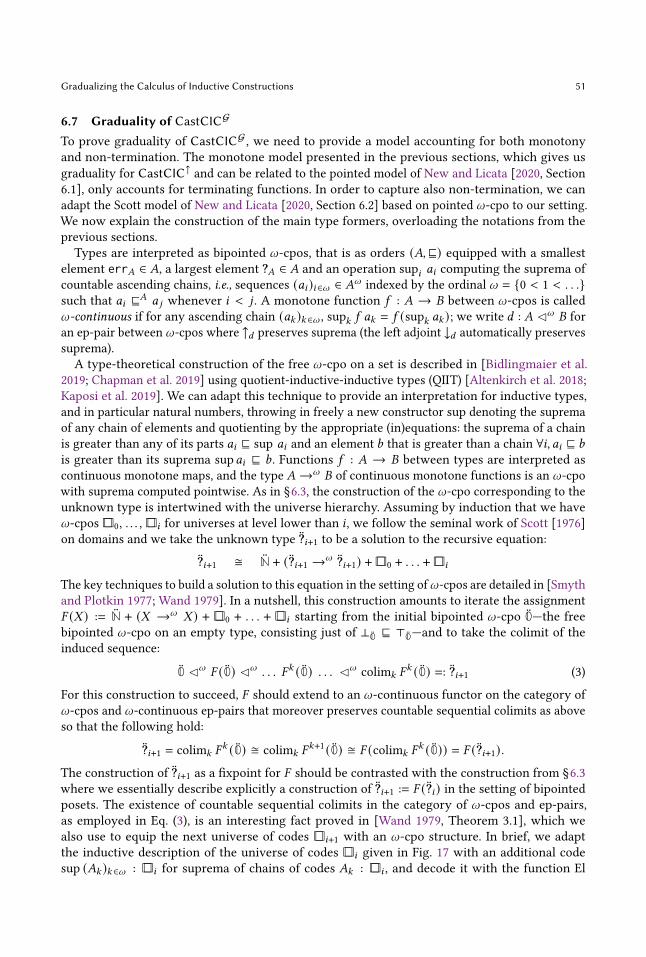
Gradualizing the Calculus of Inductive Constructions 51
6.7 Graduality of CastCICG
To prove graduality of CastCICG, we need to provide a model accounting for both monotony
and non-termination. The monotone model presented in the previous sections, which gives us
graduality for CastCIC↑and can be related to the pointed model of New and Licata [2020, Section
6.1], only accounts for terminating functions. In order to capture also non-termination, we can
adapt the Scott model of New and Licata [2020, Section 6.2] based on pointed 𝜔-cpo to our setting.
We now explain the construction of the main type formers, overloading the notations from the
previous sections.
Types are interpreted as bipointed 𝜔-cpos, that is as orders (𝐴, ⊑) equipped with a smallest
element err𝐴 ∈ 𝐴, a largest element ?𝐴 ∈ 𝐴 and an operation sup𝑖 𝑎𝑖 computing the suprema of
countable ascending chains, i.e., sequences (𝑎𝑖 )𝑖∈𝜔 ∈ 𝐴𝜔indexed by the ordinal 𝜔 = {0 < 1 < . . .}
such that 𝑎𝑖 ⊑𝐴 𝑎 𝑗 whenever 𝑖 < 𝑗 . A monotone function 𝑓 : 𝐴 → 𝐵 between 𝜔-cpos is called
𝜔-continuous if for any ascending chain (𝑎𝑘 )𝑘∈𝜔 , sup𝑘 𝑓 𝑎𝑘 = 𝑓 (sup𝑘 𝑎𝑘 ); we write 𝑑 : 𝐴 ◁𝜔 𝐵 for
an ep-pair between 𝜔-cpos where ↑𝑑 preserves suprema (the left adjoint ↓𝑑 automatically preserves
suprema).
A type-theoretical construction of the free 𝜔-cpo on a set is described in [Bidlingmaier et al.
2019; Chapman et al. 2019] using quotient-inductive-inductive types (QIIT) [Altenkirch et al. 2018;
Kaposi et al. 2019]. We can adapt this technique to provide an interpretation for inductive types,
and in particular natural numbers, throwing in freely a new constructor sup denoting the suprema
of any chain of elements and quotienting by the appropriate (in)equations: the suprema of a chain
is greater than any of its parts 𝑎𝑖 ⊑ sup 𝑎𝑖 and an element 𝑏 that is greater than a chain ∀𝑖, 𝑎𝑖 ⊑ 𝑏
is greater than its suprema sup𝑎𝑖 ⊑ 𝑏. Functions 𝑓 : 𝐴 → 𝐵 between types are interpreted as
continuous monotone maps, and the type 𝐴 →𝜔 𝐵 of continuous monotone functions is an 𝜔-cpo
with suprema computed pointwise. As in §6.3, the construction of the 𝜔-cpo corresponding to the
unknown type is intertwined with the universe hierarchy. Assuming by induction that we have
𝜔-cpos □□0, . . . , □□𝑖 for universes at level lower than 𝑖 , we follow the seminal work of Scott [1976]
on domains and we take the unknown type ¥?𝑖+1 to be a solution to the recursive equation:
¥?𝑖+1 � ¥N + (¥?𝑖+1 →𝜔 ¥?𝑖+1) +□□0 + . . . +□□𝑖
The key techniques to build a solution to this equation in the setting of𝜔-cpos are detailed in [Smyth
and Plotkin 1977; Wand 1979]. In a nutshell, this construction amounts to iterate the assignment
𝐹 (𝑋 ) := ¥N + (𝑋 →𝜔 𝑋 ) + □□0 + . . . + □□𝑖 starting from the initial bipointed 𝜔-cpo ¥0—the free
bipointed 𝜔-cpo on an empty type, consisting just of ⊥ ¥0 ⊑ ⊤ ¥0—and to take the colimit of the
induced sequence:
¥0 ◁𝜔 𝐹 ( ¥0) ◁𝜔 . . . 𝐹𝑘 ( ¥0) . . . ◁𝜔colim𝑘 𝐹
𝑘 ( ¥0) =: ¥?𝑖+1 (3)
For this construction to succeed, 𝐹 should extend to an 𝜔-continuous functor on the category of
𝜔-cpos and 𝜔-continuous ep-pairs that moreover preserves countable sequential colimits as above
so that the following hold:
¥?𝑖+1 = colim𝑘 𝐹𝑘 ( ¥0) � colim𝑘 𝐹
𝑘+1 ( ¥0) � 𝐹 (colim𝑘 𝐹𝑘 ( ¥0)) = 𝐹 (¥?𝑖+1).
The construction of ¥?𝑖+1 as a fixpoint for 𝐹 should be contrasted with the construction from §6.3
where we essentially describe explicitly a construction of ¥?𝑖+1 := 𝐹 (¥?𝑖 ) in the setting of bipointed
posets. The existence of countable sequential colimits in the category of 𝜔-cpos and ep-pairs,
as employed in Eq. (3), is an interesting fact proved in [Wand 1979, Theorem 3.1], which we
also use to equip the next universe of codes □□𝑖+1 with an 𝜔-cpo structure. In brief, we adapt
the inductive description of the universe of codes □□𝑖 given in Fig. 17 with an additional code
sup (𝐴𝑘 )𝑘∈𝜔 : □□𝑖 for suprema of chains of codes 𝐴𝑘 : □□𝑖 , and decode it with the function El
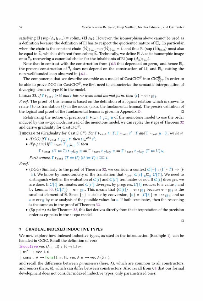
52 Meven Lennon-Bertrand, Kenji Maillard, Nicolas Tabareau, and Éric Tanter
satisfying El (sup (𝐴𝑘 )𝑘∈𝜔 ) � colim𝑘 (El 𝐴𝑘 ). However, the isomorphism above cannot be used as
a definition because the definition of El has to respect the quotiented nature of □□𝑖 . In particular,
when the chain is the constant chain (N)𝑘∈𝜔 , sup (N)𝑘∈𝜔 = N and thus El (sup (N)𝑘∈𝜔 ) must also
be equal to¥N, which is different from colim𝑘
¥N. Technically, we define El𝐴 as its isomorphic image
onto ¥?𝑖 , recovering a canonical choice for the inhabitants of El (sup (𝐴𝑘 )𝑘∈𝜔 ).Note that in contrast with the construction from §6.3 that depended on germ𝑖 and hence El𝑖 ,
the present construction of ¥?𝑖 does not depend on the construction of □□𝑖 and El𝑖 , cutting the
non-wellfounded loop observed in §6.1.
The components that we describe assemble as a model of CastCICGinto CIC
IR
QIT. In order to
be able to prove DGG for CastCICG, we first need to characterize the semantic interpretation of
diverging terms of type B in the model.
Lemma 33. If Γ ⊢cast 𝑡 ⊲B and 𝑡 has no weak head normal form, then {𝑡} = err{B} .
Proof. The proof of this lemma is based on the definition of a logical relation which is shown to
relate 𝑡 to its translation {𝑡} in the model (a.k.a. the fundamental lemma). The precise definition of
the logical and proof of the fundamental lemma is given in Appendix D. □
Relativizing the notion of precision Γ ⊢cast 𝑡 ⊑𝑇 𝑆
𝑢 of the monotone model to use the order
induced by this𝜔-cpo model instead of the monotone model, we can replay the steps of Theorem 32
and derive graduality for CastCICG.
Theorem 34 (Graduality for CastCICG). For Γ ⊢cast 𝑡 : 𝑇, Γ ⊢cast 𝑡 ′ : 𝑇 and Γ ⊢cast 𝑢 : 𝑈 , we have
• (DGG) If Γ ⊢cast 𝑡 ⊑𝑇 𝑇
𝑡 ′ then 𝑡 ⊑𝑜𝑏𝑠 𝑡 ′;• (Ep-pairs) If Γ ⊢cast 𝑇 ⊑□ □ 𝑈 then
Γ ⊢cast ⟨𝑈 ⇐ 𝑇 ⟩ 𝑡 ⊑𝑈 𝑈 𝑢 ⇔ Γ ⊢cast 𝑡 ⊑𝑇 𝑈 𝑢 ⇔ Γ ⊢cast 𝑡 ⊑𝑇 𝑇 ⟨𝑇 ⇐𝑈 ⟩𝑢,Furthermore, Γ ⊢cast ⟨𝑇 ⇐𝑈 ⟩ ⟨𝑈 ⇐ 𝑇 ⟩ 𝑡 ⊒⊑ 𝑡 .
Proof.
• (DGG) Similarly to the proof of Theorem 32, we consider a context C[−] : (Γ ⊢ 𝑇 ) ⇒ (⊢B). We know by monotonicity of the translation that ⊢cast C[𝑡] ⊑B B C[𝑡 ′]. We need to
distinguish whether the evaluation of C[𝑡] and C[𝑡 ′] terminates or not. If C[𝑡] diverges, weare done. If C[𝑡] terminates and C[𝑡 ′] diverges, by progress, C[𝑡] reduces to a value 𝑣 and
by Lemma 33, {C[𝑡 ′]} = err{B} . This means that {C[𝑡]} = err{B} because err{B} is thesmallest element of
¥B. Since {−} is stable by conversion, {𝑣} = {C[𝑡]} = err{B} , and so
𝑣 = errB by case analysis of the possible values for 𝑣 . If both terminates, then the reasoning
is the same as in the proof of Theorem 32.
• (Ep-pairs) As for Theorem 32, this fact derives directly from the interpretation of the precision
order as ep-pairs in the 𝜔-cpo model.
□
7 GRADUAL INDEXED INDUCTIVE TYPESWe now explore how indexed inductive types, as used in the introduction (Example 1), can be
handled in GCIC. Recall the definition of vec:
Inductive vec (A : □) : N → □ :=
| nil : vec A 0
| cons : A → forall n : N, vec A n → vec A (S n ).
and recall the difference between parameters (here, A), which are common to all constructors,
and indices (here, n), which can differ between constructors. Also recall from §4 that our formal
development does not consider indexed inductive types, only parametrized ones.

Gradualizing the Calculus of Inductive Constructions 53
This section first explains two alternatives to indexed inductive types that can directly be
expressed in GCIC (§7.1). We then describe how these alternatives actually behave in the gradual
setting (§7.2 and 7.3). Finally, we present an extension of CastCIC to directly support indexed
inductive types, focusing on the specific case of vectors (§ 7.4), showing that it combines the
advantages of the other approaches. §7.5 summarizes our findings.
7.1 Alternatives to indexed inductive typesIndexed inductive types make it possible to define structures that are intrinsically characterized by
some property, which holds by construction, as opposed to extrinsically establishing such properties
after the fact. There are two well-known alternatives to indexed inductive types for capturing
properties intrinsically: type-level fixpoints, and “forded” inductive types.
Type-level fixpoint. The vector can be defined as a recursive function on the index, at the type
level. For instance, the following formulation represents sized lists as nested pairs:
Fixpoint vec` (A : □) (n : N) :□ := match n with 0 ⇒ unit | S n ⇒ A ∗ vec` A n end.
Type-level fixpoints can be used as soon as the indices are concretely forceable [Brady et al.
2004]. Intuitively, concretely forceable indices are those that can be matched upon (like n in
this example definition). See Gilbert et al. [2019] for a description of a general translation.
Forded inductive type. Instead of using an indexed inductive type, one can use a parametrized
inductive type, with explicit equalities as arguments to constructors.24For instance, vectors
can be defined in this style as follows:
Inductive vec𝑓 (A : □) (n : N) : □ :=
| nil𝑓 : eqN 0 n → vec𝑓 A n
| cons𝑓 : A → forall m : N, eqN (S m) n → vec𝑓 A m → vec𝑓 A n.
Note that this definition uses eqN, the type of decidable equality proofs over natural numbers,
for expressing the constraints on n instead of propositional equalities (e.g., 0=n), becausepropositional equality is not available in GCIC (§8.3).
In CIC, these two alternative presentations of an indexed inductive type can be shown internally
to be equivalent. But each of these presentations has advantages and drawbacks depending on the
considered system and scenarios of use, so practitioners have different preferences in that respect.
More important to us here, these presentations are not equivalent in GCIC.
7.2 Type-level fixpointsConstructors. The definition of vec` above can directly be written in GCIC, as it uses only
inductive types with parameters (here the unit and product types and natural numbers). The vector
constructors can be defined as:
Definition nil` (A:□) : vec` A 0 := tt.
Definition cons` (A:□) (a:A) (n:N) (v:vec` A n) : vec` A (S n) := (a , v).
whose definitions typecheck because vec` computes on its indices.
Behavior. Let us now look at the type computed at ?N. Because ?N is an exceptional term, the
fixpoint has to return unknown in the universe: vec` A ?N {∗ ?□. This means that the mechanism
for casting a vector into a vector with the unknown index is directly inherited from the generic
mechanism for casting to the unknown type. Therefore, we get for free the following computation
rules, because they involve embedding-projection pairs:
24This technique has reportedly been coined “fording” by McBride [1999, §3.5]. Fording is in allusion to the Henry Ford
quote “Any customer can have a car painted any color that he wants, so long as it is black.”
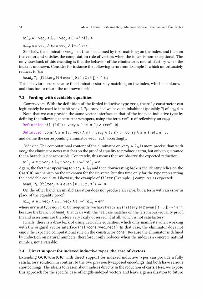
54 Meven Lennon-Bertrand, Kenji Maillard, Nicolas Tabareau, and Éric Tanter
nil` A :: vec` A ?N :: vec` A 0{∗ nil` A
nil` A :: vec` A ?N :: vec` A 1{∗ err
Similarly, the eliminator vec`_rect can be defined by first matching on the index, and then on
the vector and satisfies the computation rule of vectors when the index is non-exceptional. The
only drawback of this encoding is that the behavior of the eliminator is not satisfactory when the
index is unknown. Consider for instance the following term from Example 1, which unfortunately
reduces to ?N:
head` ?N (filter` N 4 even [ 0 ; 1 ; 2 ; 3 ]){∗ ?N
This behavior occurs because the eliminator starts by matching on the index, which is unknown,
and thus has to return the unknown itself.
7.3 Fording with decidable equalitiesConstructors. With the definition of the forded inductive type vec𝑓 , the nil𝑓 constructor can
legitimately be used to inhabit vec𝑓 A ?N, provided we have an inhabitant (possibly ?) of eqN 0 n.Note that we can provide the same vector interface as that of the indexed inductive type by
defining the following constructor wrappers, using the term refl n of reflexivity on eqN:
Definition nil' (A :□) : vec𝑓 A 0 := nil𝑓 A (refl 0).
Definition cons' A a n (v : vec𝑓 A n) : vec𝑓 A (S n) := cons𝑓 A a n (refl n) v .
and define the corresponding eliminator vec_rect' accordingly.
Behavior. The computational content of the eliminator on vec𝑓 A ?N is more precise than with
vec` : the eliminator never matches on the proof of equality to produce a term, but only to guarantee
that a branch is not accessible. Concretely, this means that we observe the expected reduction:
nil𝑓 A e :: vec𝑓 A ?N :: vec𝑓 A 0{∗ nil𝑓 A e
Again, the fact that upcasting to vec𝑓 A ?N and then downcasting back is the identity relies on the
CastCIC mechanism on the unknown for the universe, but this time only for the type representing
the decidable equality. Likewise, the example of filter (Example 1) computes as expected:
head𝑓 ?N (filter𝑓 N 4 even [ 0 ; 1 ; 2 ; 3 ]){∗0
On the other hand, an invalid assertion does not produce an error, but a term with an error in
place of the equality proof:
nil𝑓 A e :: vec𝑓 A ?N :: vec𝑓 A 1{∗ nil𝑓 A err
where err is at type eqN 1 0. Consequently, we have head𝑓 ?N (filter𝑓 N 2 even [ 1 ; 3 ]){∗ err,because the branch of head𝑓 that deals with the nil case matches on the (erroneous) equality proof.
Invalid assertions are therefore very lazily observed, if at all, which is not satisfactory.
Finally, there is a drawback of using decidable equalities, which only manifests when working
with the original vector interface (nil'/cons'/vec_rect'). In that case, the eliminator does not
enjoy the expected computational rule on the constructor cons'. Because the eliminator is defined
by induction on natural numbers, therefore it only reduces when the index is a concrete natural
number, not a variable.
7.4 Direct support for indexed inductive types: the case of vectorsExtending GCIC/CastCIC with direct support for indexed inductive types can provide a fully
satisfactory solution, in contrast to the two previously-exposed encodings that both have serious
shortcomings. The idea is to reason about indices directly in the reduction of casts. Here, we expose
this approach for the specific case of length-indexed vectors and leave a generalization to future

Gradualizing the Calculus of Inductive Constructions 55
canonical nil? 𝐴 canonical(cons? 𝐴 𝑎 𝑛 𝑣)
V-cons-? : ⟨vec 𝐵 ?N ⇐ vec 𝐴 (𝑆 𝑛)⟩ (cons 𝐴 𝑎 𝑘 𝑣) { cons? 𝐵 (⟨𝐵 ⇐ 𝐴⟩ 𝑎) 𝑛 (⟨vec 𝐵 𝑛 ⇐ vec 𝐴 𝑘⟩ 𝑣)
V-cons : ⟨vec 𝐵 (𝑆 𝑚) ⇐ vec 𝐴 (𝑆 𝑛)⟩ (cons 𝐴 𝑎 𝑘 𝑣) { cons 𝐵 (⟨𝐵 ⇐ 𝐴⟩ 𝑎) 𝑚 (⟨vec 𝐵 𝑚 ⇐ vec 𝐴 𝑘⟩ 𝑣)
V-cons-nil : ⟨vec 𝐵 0 ⇐ vec 𝐴 (𝑆 𝑛)⟩ (cons 𝐴 𝑎 𝑘 𝑣) { errvec 𝐵 0
V-rect-nilu : vec_rect 𝑃 𝑃𝑛𝑖𝑙 𝑃𝑐𝑜𝑛𝑠 nil? 𝐴 { ⟨𝑃 ?N ⇐ 𝑃 0⟩ (vec_rect 𝑃 𝑃𝑛𝑖𝑙 𝑃𝑐𝑜𝑛𝑠 nil 𝐴)
V-rect-consu : vec_rect 𝑃 𝑃𝑛𝑖𝑙 𝑃𝑐𝑜𝑛𝑠 (cons? 𝐴 𝑎 𝑛 𝑣) {
⟨𝑃 ?N ⇐ 𝑃 (𝑆 𝑛)⟩ (vec_rect 𝑃 𝑃𝑛𝑖𝑙 𝑃𝑐𝑜𝑛𝑠 (cons 𝐴 𝑎 𝑛 𝑣))
Fig. 19. New canonical forms and reduction rules for vectors in CastCIC (excerpt).
work. Appendix E describes the extension for vectors in full details; here, we only present selected
rules (Fig. 19) and illustrate how reduction works.
Constructors. We add two new canonical forms, corresponding to the casts of nil and cons tovec 𝐴 ?N: namely, nil? 𝐴 and cons? 𝐴 𝑎 𝑛 𝑣 (Fig. 19). Note that we cannot simply declare casts
such as ⟨vec 𝐴 ?N ⇐ vec 𝐴 𝑛⟩ 𝑡 to be canonical, because they involve non-linear occurrences of
types (here, 𝐴).
Reduction rules. We add reduction rules to conduct casts between vectors in canonical forms.
Fig. 19 presents these rules when the argument of the cast is a cons. Rule V-cons-? propagatesthe cast on the arguments, but using the newly-introduced cons?, effectively converting precise
information to less precise information. Rule V-cons applies when both source and target indices
are successors, and propagates the cast of the arguments, just like the standard rule for casting a
constructor. As expected, Rule V-cons-nil raises an error when the indices do not match.
For the eliminator, there are two new computation rules, one for each new constructor: v-
rect-nilu and v-rect-consu. They both apply the eliminator to the underlying non-exceptional
constructor, and then cast the result back to 𝑃 ?N. Intuitively, these rules transfer the cast on vectors
to a cast on the returned type of the predicate.
Behavior. Given these rules, we can actually realize the behavior described in Example 1. For
instance, we have both
nil A :: vec A ?N :: vec A 0{∗ nil A
nil A :: vec A ?N :: vec A 1{∗ errA
and coming back to Example 1, in all three GCIC variants the term:
head ?N (filter N 4 even [ 0 ; 1 ; 2 ; 3 ])
typechecks and reduces to 0. Additionally, as expected:
head ?N (filter N 2 even [1 ; 3])
typechecks and fails at runtime. And similarly for Example 4.
Note that to be able to define the action of casts on vectors, we have crucially used the fact that
it is possible to discriminate between 0, S n and ?N in the reduction rule.

56 Meven Lennon-Bertrand, Kenji Maillard, Nicolas Tabareau, and Éric Tanter
7.5 SummaryTo summarize, the different approaches to define structures with intrinsic properties in GCIC
compare as follows:
• The type-level fixpoint coincides with the indexed inductive presentation on non-exceptional
terms, but is extremely imprecise in presence of unknown indices.
• The forded inductive is more accurate when dealing with unknown indices, but is arguably
too permissive with invalid index assertions.
• The direct support of the indexed inductive type with additional constructors and reduction
rules yields a satisfactory solution. We conjecture that this presentation can be generalized to
support arbitrary indexed inductive types as long as they have concretely forceable indices;
we leave such a general construction for future work.
Recall that fording is only an option in GCIC when the indices pertain to a type with decidable
equality; properly handling general propositional equality in a gradual type theory is an open
question (§8.3). The constraint of indices being concretely forceable (for type-level fixpoints, direct
support) are intuitively understandable and expected: gradual typing requires synthesizing dynamic
checks, therefore these checks need to be somehow computable.
8 LIMITATIONS AND PERSPECTIVESUp to now, we have left aside three important aspects of CIC, namely, impredicativity, [-equality
and propositional equality. This section explains the challenges induced by each feature, and
possibly, venues to explore.
8.1 ImpredicativityIn this work, we do not deal with the impredicative sort Prop, for multiple reasons. The models
used in §6 to justify termination and graduality crucially rely on the predicativity of the universe
hierarchy for the inductive-recursive definition of codes to be well-founded. Moreover, the results
of Palmgren [1998, Theorem 6.1] show that it is not possible to endow an impredicative universe
with an inductive-recursive structure in a consistent and strongly-normalizing theory, hinting
that it may be difficult to devise an inductively-defined cast function between types that belong
to an impredicative universe. Additionally, it seems difficult to avoid the divergence of Ω with
an impredicative sort, as no universe levels can be used to prevent a self-application from being
well-typed.
8.2 [-equalityIn most presentations of CIC, and in particular its Coq implementation, conversion satisfies an
additional rule, called [-equality, which corresponds to an extensional property for functions:
Γ ⊢ 𝑓 ≡ _ 𝑥 : 𝐴.𝑓 𝑥 when Γ ⊢ 𝑓 : Π𝑥 : 𝐴.𝐵.
The difficulty of integrating [-equality in the setting of GCIC is that the conversion we consider in
CastCIC is entirely induced by a notion of reduction: two terms are convertible exactly when they
have a common reduct up to 𝛼-equivalence. It is well-known that [-equality cannot be easily mod-
eled using a rewrite rule, as both [-expansion and [-reduction have significant drawbacks [Goguen
2005], and so we would have to consider another approach to the one we took if we were to
integrate [-equality. The most prominent alternative way is to define conversion as an alterna-
tion of reduction steps (for instance using a weak-head reduction strategy) not containing [ and
comparison of terms up to congruence and [-equality.

Gradualizing the Calculus of Inductive Constructions 57
This approach has been recently formalized by Abel et al. [2018] in a fully-typed setting. That is,
types participate crucially in the conversion relation: they are maintained during conversion, so
that for instance comparison of terms at a Π-type systematically [-expands them before recursively
calling conversion at the domain types. Defining a gradual variant of such a typed conversion
might be quite interesting, but would require a significant amount of work.
On the contrary, a precise, formalized, account is still missing for [-equality for an untyped
conversion as used in practice in the Coq proof assistant and in GCIC. The MetaCoq project, which
aims at such a formalized account, leaves the treatment of [-equality to future work [Sozeau et al.
2020]. While we envision no specific issues to the adaptation to this approach to gradual typing
once a clear and precise solution for CIC itself has been reached, solving the issue in a satisfactory
way for CIC is obviously out of scope for this article. Thus, while it should in principle be possible
to add [-equality to GCIC, either via typed or untyped conversion, we leave this for future work.
8.3 Propositional equalityIn CIC, propositional equality eq A x y, corresponds to the Martin-Löf identity type [Martin-Löf
1975], with a single constructor refl for reflexivity, and the elimination principle known as J:
Inductive eq (A : □) (x : A) : A → □ := refl : eq A x x .
J : forall (A : □) (P : A → □) (x : A) (t : P x) (y : A) (e : eq A x y ), P y
together with the conversion rule:
J A P x t x (refl A x) ≡ t
For the sake of exposing the problem, suppose that we can define this identity type in GCIC,
while still satisfying canonicity, conservativity with respect to CIC and graduality. This means that
for an equality t = u involving closed terms t and u of CIC, there should only be three possible
canonical forms: refl A t whenever t and u are convertible terms (of type A), as well as err and ?.Just under these assumptions, we can show that there exist two functions that are pointwise
equal in CIC, and hence equal by extensionality, but are no longer equivalent in GCIC/CastCIC.
Consider the two functions idN and add0 below:
idN := _ n : N ⇒ n add0 := _ n : N ⇒ n + 0
In CIC, these functions are not convertible, but they are observationally equivalent. However, they
would not be observationally equivalent in GCIC. To see why, consider the following term:
test := _ f ⇒ J (N → N) (_ _ ⇒ B) idN true f (refl idN :: ?□ :: idN = f)
We have test idN {∗ true because, by G, refl idN :: ?□ :: idN = idN {
∗ refl idN. However,
because add0 is not convertible to idN, refl idN :: idN = add0 cannot possibly reduce to refl,and thus would need to reduce either to err or ?; and so does test add0.
This means that a model for such a gradual type theory would need to be intensional, conversely
to the extensional models usually used to justify type theories. Studying such a model as well as
exploring alternatives approaches to propositional equality in a gradual type theory are interesting
venues for future work.
9 RELATEDWORKBidirectional typing and unification. Our framework uses a bidirectional version of the type system
of CIC. Although this presentation is folklore among type theory specialists [McBride 2019],
the type system of CIC is rarely presented in this way on paper and has been studied in details
only recently [Lennon-Bertrand 2021]. However, the bidirectional approach becomes necessary
when dealing with unification and elaboration of implicit arguments. Bidirectional elaboration is a
common feature of proof assistant implementations, for instance [Asperti et al. 2012], as it clearly

58 Meven Lennon-Bertrand, Kenji Maillard, Nicolas Tabareau, and Éric Tanter
delineates what information is available to the elaboration system in the different typing modes.
In a context with missing information due to implicit arguments, those implementations face the
undecidable higher order unification [Dowek 2001]. In this error-less context, the solution must
be a form of under-approximation, using complex heuristics [Ziliani and Sozeau 2017]. Deciding
consistency is very close to unification, as observed by Castagna et al. [2019], but our notion of
consistency over-approximates unification, making sure that unifiable terms are always consistent,
relying on errors to catch invalid over-approximations at runtime.
Dependent types with effects. As explained in this paper, introducing the unknown type of gradual
typing also require, in a dependently-typed setting, to introduce unknown terms at any type. This
means that a gradual dependent type theory naturally endorses an effectful mechanism which is
similar to having exceptions. This connects GCIC to the literature on dependent types and effects.
Several programming languages mix dependent types with effectful computation, either giving up
on metatheoretical properties, such as Dependent Haskell [Eisenberg 2016], or by restricting the
dependent fragment to pure expressions [Swamy et al. 2016; Xi and Pfenning 1998]. In the context
of dependent type theories, Pédrot and Tabareau [2017, 2018] have leveraged the monadic approach
to type theory, at the price of a weaker form of dependent large elimination for inductive types. The
only way to recover full elimination is to accept a weaker form of logical consistency, as crystallized
by the fire triangle between observable effects, substitution and logical consistency [Pédrot and
Tabareau 2020].
Ordered and directed type theories. The monotone model of CastCIC interpret types as posets
in order to give meaning to the notion of precision. Interpretations of dependent type theories in
ordered structures goes back to various works on domain theoretic and realizability interpretations
of (partial) Martin-Löf Type Theory [Ehrhard 1988; Palmgren and Stoltenberg-Hansen 1990]. More
recently, Licata and Harper [2011] and North [2019] extend type theory with directed structures
corresponding to a categorical interpretation of types, a higher version of the monotone model we
consider.
Hybrid typing. [Ou et al. 2004] present a programming language with separate dependently- and
simply-typed fragments, using arbitrary runtime checks at the boundary. Knowles and Flanagan
[2010] support runtime checking of refinements. In a similar manner, [Tanter and Tabareau 2015]
introduce casts for subset types with decidable properties in Coq. They use an axiom to denote
failure, which breaks weak canonicity. Dependent interoperability [Dagand et al. 2018; Osera et al.
2012] supports the combination of dependent and non-dependent typing through deep conversions.
All these approaches are more intended as programming languages than as type theories, and none
support the notion of (im)precision that is at the heart of gradual typing.
Dependent contracts. [Greenberg et al. 2010] relates hybrid typing to dependent contracts, which
are dynamically-checked assertions that can relate the result of a function application to its
argument [Findler and Felleisen 2002]. The semantics of dependent contracts are subtle because
contracts include arbitrary code, and in particular one must be careful not to violate the precondition
on the argument in the definition of the postcondition contract [Blume and McAllester 2006]. Also,
blame assignment when the result and/or argument are themselves higher-order is subtle. Different
variants of dependent contracts have been studied in the literature, which differ in terms of the
violations they report and the way they assign blame [Dimoulas et al. 2011; Greenberg et al. 2010].
An in-depth exploration of blame assignment for gradual dependent type theories such as GCIC is
an important perspective for future work.
Gradual typing. The blame calculus of Wadler and Findler [2009] considers subset types on
base types, where the refinement is an arbitrary term, as in hybrid type checking [Knowles and
Flanagan 2010]. It however lacks the dependent function types found in other works. Lehmann
and Tanter [2017] exploit the Abstracting Gradual Typing (AGT) methodology [Garcia et al. 2016]

Gradualizing the Calculus of Inductive Constructions 59
to design a language with imprecise formulas and implication. They support dependent function
types, but gradual refinements are only on base types refined with decidable logical predicates.
Eremondi et al. [2019] also use AGT to develop approximate normalization and GDTL. While being
a clear initial inspiration for this work, the technique of approximate normalization cannot yield a
computationally-relevant gradual type theory (nor was its intent, as clearly stated by the authors).
We hope that the results in our work can prove useful in the design and formalization of such
gradual dependently-typed programming languages. Eremondi et al. [2019] study the dynamic
gradual guarantee, but not its reformulation as graduality [New and Ahmed 2018], which as we
explain is strictly stronger in the full dependent setting. Finally, while AGT provided valuable
intuitions for this work, graduality as embedding-projection pairs was the key technical driver in
the design of CastCIC.
10 CONCLUSIONWe have unveiled a fundamental tension in the design of gradual dependent type theories between
conservativity with respect to a dependent type theory such as CIC, normalization, and graduality.
We explore several resolutions of this Fire Triangle of Graduality, yielding three different gradual
counterparts of CIC, each compromising with one edge of the Triangle. We develop the metatheory
of all three variants of GCIC thanks to a common formalization, parametrized by two knobs
controlling universe constraints on dependent product types in typing and reduction.
This work opens a number of perspectives for future work, in addition to addressing the limita-
tions discussed in §8. The delicate interplay between universe levels and computational behavior
of casts begs for a more flexible approach to the normalizing GCICN, for instance using gradual
universes. The approach based on multiple universe hierarchies to support logically consistent
reasoning about exceptional programs [Pédrot et al. 2019] could be adapted to our setting in order
to provide a seamless integration inside a single theory of gradual features together with standard
CIC without compromising normalization. This could also open the door to supporting consistent
reasoning about gradual programs in the context of GCIC. On the more practical side, there is still
a lot of challenges ahead in order to implement a gradual incarnation of GCIC in Coq or Agda,
possibly parametrized in order to support the three variants presented in this work.
REFERENCESAndreas Abel, Joakim Öhman, and Andrea Vezzosi. 2018. Decidability of Conversion for Type Theory in Type Theory.
Proceedings of the ACM on Programming Languages 2, POPL, Article 23 (Jan. 2018), 29 pages. https://doi.org/10.1145/
3158111
Samson Abramsky and Achim Jung. 1995. Domain Theory. Oxford University Press, Inc., USA, 1–168.
Thorsten Altenkirch. 1999. Extensional Equality in Intensional Type Theory. In Proceedings of the 14th Symposium on Logic
in Computer Science (LICS 2002). IEEE Computer Society Press, Trento, Italy, 412–420. https://doi.org/10.1109/LICS.1999.
782636
Thorsten Altenkirch, Simon Boulier, Ambrus Kaposi, Christian Sattler, and Filippo Sestini. 2021. Constructing a universe for
the setoid model (Lecture Notes in Computer Science, Vol. 12650), Stefan Kiefer and Christine Tasson (Eds.). Springer, 1–21.
https://doi.org/10.1007/978-3-030-71995-1_1
Thorsten Altenkirch, Simon Boulier, Ambrus Kaposi, and Nicolas Tabareau. 2019. Setoid Type Theory - A Syntactic
Translation (Lecture Notes in Computer Science, Vol. 11825), Graham Hutton (Ed.). Springer, 155–196. https://doi.org/10.
1007/978-3-030-33636-3_7
Thorsten Altenkirch, Paolo Capriotti, Gabe Dijkstra, Nicolai Kraus, and Fredrik Nordvall Forsberg. 2018. Quotient Inductive-
Inductive Types (Lecture Notes in Computer Science, Vol. 10803), Christel Baier and Ugo Dal Lago (Eds.). Springer, 293–310.
https://doi.org/10.1007/978-3-319-89366-2_16
Andrea Asperti, Wilmer Ricciotti, Claudio Sacerdoti Coen, and Enrico Tassi. 2012. A Bi-Directional Refinement Algorithm
for the Calculus of (Co)Inductive Constructions. Volume 8, Issue 1 (2012). https://doi.org/10.2168/LMCS-8(1:18)2012
Robert Atkey, Neil Ghani, and Patricia Johann. 2014. A relationally parametric model of dependent type theory. In The
41st Annual ACM SIGPLAN-SIGACT Symposium on Principles of Programming Languages, POPL ’14, San Diego, CA, USA,

60 Meven Lennon-Bertrand, Kenji Maillard, Nicolas Tabareau, and Éric Tanter
January 20-21, 2014, Suresh Jagannathan and Peter Sewell (Eds.). ACM, 503–516. https://doi.org/10.1145/2535838.2535852
Felipe Bañados Schwerter, Alison M. Clark, Khurram A. Jafery, and Ronald Garcia. 2020. Abstracting Gradual Typing
Moving Forward: Precise and Space-Efficient. arXiv:2010.14094 [cs.PL]
Felipe Bañados Schwerter, Ronald Garcia, and Éric Tanter. 2016. Gradual Type-and-Effect Systems. Journal of Functional
Programming 26 (Sept. 2016), 19:1–19:69.
Henk Barendregt. 1991. Introduction to Generalized Type Systems. Journal of Functional Programming 1, 2 (April 1991),
125–154.
Henk P. Barendregt. 1984. The Lambda Calculus: Its Syntax and Semantics. North-Holland.
Jean-Philippe Bernardy, Patrik Jansson, and Ross Paterson. 2012. Proofs for free: Parametricity for dependent types. Journal
of Functional Programming 22, 2 (March 2012), 107–152.
Martin E. Bidlingmaier, Florian Faissole, and Bas Spitters. 2019. Synthetic topology inHomotopy Type Theory for probabilistic
programming. (2019). arXiv:1912.07339 http://arxiv.org/abs/1912.07339
Gavin Bierman, Erik Meijer, and Mads Torgersen. 2010. Adding Dynamic Types to C#. In Proceedings of the 24th European
Conference on Object-oriented Programming (ECOOP 2010) (Lecture Notes in Computer Science, 6183), Theo D’Hondt (Ed.).
Springer-Verlag, Maribor, Slovenia, 76–100.
M. Blume and D. McAllester. 2006. Sound and complete models of contracts. Journal of Functional Programming 16, 4-5
(2006), 375–414.
Rastislav Bodík and Rupak Majumdar (Eds.). 2016. Proceedings of the 43rd ACM SIGPLAN-SIGACT Symposium on Principles
of Programming Languages (POPL 2016). ACM Press, St Petersburg, FL, USA.
Simon Boulier, Pierre-Marie Pédrot, and Nicolas Tabareau. 2017. The next 700 syntactical models of type theory. In
Proceedings of the 6th ACM SIGPLAN Conference on Certified Programs and Proofs, CPP 2017, Paris, France, January 16-17,
2017. 182–194. https://doi.org/10.1145/3018610.3018620
Edwin Brady. 2013. Idris, a General Purpose Dependently Typed Programming Language: Design and Implementation.
Journal of Functional Programming 23, 5 (Sept. 2013), 552–593.
Edwin Brady, Conor McBride, and James McKinna. 2004. Inductive Families Need Not Store Their Indices. In Types for
Proofs and Programs (TYPES 2004) (Lecture Notes in Computer Science, Vol. 3085). Springer-Verlag, 115–129.
Giuseppe Castagna (Ed.). 2009. Proceedings of the 18th European Symposium on Programming Languages and Systems (ESOP
2009). Lecture Notes in Computer Science, Vol. 5502. Springer-Verlag, York, UK.
Giuseppe Castagna, Victor Lanvin, Tommaso Petrucciani, and Jeremy G. Siek. 2019. Gradual typing: a new perspective.
See[POPL 2019 2019], 16:1–16:32.
James Chapman, Tarmo Uustalu, and Niccolò Veltri. 2019. Quotienting the delay monad by weak bisimilarity. Math. Struct.
Comput. Sci. 29, 1 (2019), 67–92. https://doi.org/10.1017/S0960129517000184
Matteo Cimini and Jeremy Siek. 2016. The gradualizer: a methodology and algorithm for generating gradual type systems,
See [Bodík and Majumdar 2016], 443–455.
Thierry Coquand and Gérard Huet. 1988. The Calculus of Constructions. Information and Computation 76, 2-3 (Feb. 1988),
95–120.
Pierre-Évariste Dagand, Nicolas Tabareau, and Éric Tanter. 2018. Foundations of Dependent Interoperability. Journal of
Functional Programming 28 (2018), 9:1–9:44.
Christos Dimoulas, Robert Bruce Findler, Cormac Flanagan, and Matthias Felleisen. 2011. Correct blame for contracts: no
more scapegoating. In Proceedings of the 38th annual ACM SIGPLAN-SIGACT Symposium on Principles of Programming
Languages (POPL 2011). ACM Press, Austin, Texas, USA, 215–226.
Gilles Dowek. 2001. Chapter 16 - Higher-Order Unification and Matching. In Handbook of Automated Reasoning, Alan
Robinson and Andrei Voronkov (Eds.). North-Holland, 1009–1062. https://doi.org/10.1016/B978-044450813-3/50018-7
Peter Dybjer and Anton Setzer. 2003. Induction-recursion and initial algebras. Ann. Pure Appl. Log. 124, 1-3 (2003), 1–47.
https://doi.org/10.1016/S0168-0072(02)00096-9
Thomas Ehrhard. 1988. A Categorical Semantics of Constructions. In Proceedings of the Third Annual Symposium on
Logic in Computer Science (LICS ’88), Edinburgh, Scotland, UK, July 5-8, 1988. IEEE Computer Society, 264–273. https:
//doi.org/10.1109/LICS.1988.5125
Richard A. Eisenberg. 2016. Dependent Types in Haskell: Theory and Practice. arXiv:1610.07978 [cs.PL]
Joseph Eremondi, Éric Tanter, and Ronald Garcia. 2019. Approximate Normalization for Gradual Dependent Types. See[ICFP
2019 2019], 88:1–88:30.
Luminous Fennell and Peter Thiemann. 2013. Gradual Security Typing with References. In Proceedings of the 26th Computer
Security Foundations Symposium (CSF). 224–239.
Robert Bruce Findler and Matthias Felleisen. 2002. Contracts for Higher-Order Functions. In Proceedings of the 7th ACM
SIGPLAN Conference on Functional Programming (ICFP 2002). ACM Press, Pittsburgh, PA, USA, 48–59.
Fredrik Nordvall Forsberg. 2013. Inductive-inductive definitions. Ph.D. Dissertation. Swansea University, UK. http:
//ethos.bl.uk/OrderDetails.do?uin=uk.bl.ethos.752308

Gradualizing the Calculus of Inductive Constructions 61
Ronald Garcia, Alison M. Clark, and Éric Tanter. 2016. Abstracting Gradual Typing, See [Bodík and Majumdar 2016],
429–442. See erratum: https://www.cs.ubc.ca/ rxg/agt-erratum.pdf.
Ronald Garcia and Éric Tanter. 2020. Gradual Typing as if Types Mattered. In Informal Proceedings of the ACM SIGPLAN
Workshop on Gradual Typing (WGT20).
Neil Ghani, Lorenzo Malatesta, and Fredrik Nordvall Forsberg. 2015. Positive Inductive-Recursive Definitions. Log. Methods
Comput. Sci. 11, 1 (2015). https://doi.org/10.2168/LMCS-11(1:13)2015
Gaëtan Gilbert, Jesper Cockx, Matthieu Sozeau, and Nicolas Tabareau. 2019. Definitional proof-irrelevance without K.
See[POPL 2019 2019], 3:1–3:28. https://doi.org/10.1145/3290316
Eduardo Giménez. 1998. Structural Recursive Definitions in Type Theory. In ICALP. 397–408.
Healfdene Goguen. 2005. A Syntactic Approach to Eta Equality in Type Theory. SIGPLAN Not. 40, 1 (Jan. 2005), 75–84.
https://doi.org/10.1145/1047659.1040312
Michael Greenberg, Benjamin C. Pierce, and Stephanie Weirich. 2010. Contracts Made Manifest, See [POPL 2010 2010],
353–364.
Robert Harper and Robert Pollack. 1991. Type checking with universes. Theoretical Computer Science 89, 1 (1991). https:
//doi.org/10.1016/0304-3975(90)90108-T
David Herman, Aaron Tomb, and Cormac Flanagan. 2010. Space-efficient gradual typing. Higher-Order and Sympolic
Computation 23, 2 (June 2010), 167–189.
Martin Hofmann. 1995. Conservativity of Equality Reflection over Intensional Type Theory. In Types for Proofs and Programs,
International Workshop TYPES’95, Torino, Italy, June 5-8, 1995, Selected Papers. 153–164. https://doi.org/10.1007/3-540-
61780-9_68
ICFP 2019 2019.
Yuu Igarashi, Taro Sekiyama, and Atsushi Igarashi. 2017. On Polymorphic Gradual Typing. Proceedings of the ACM on
Programming Languages 1, ICFP (Sept. 2017), 40:1–40:29.
Ambrus Kaposi, András Kovács, and Thorsten Altenkirch. 2019. Constructing quotient inductive-inductive types. See[POPL
2019 2019], 2:1–2:24. https://doi.org/10.1145/3290315
Kenneth Knowles and Cormac Flanagan. 2010. Hybrid type checking. ACM Transactions on Programming Languages and
Systems 32, 2 (Jan. 2010), Article n.6.
Nico Lehmann and Éric Tanter. 2017. Gradual Refinement Types. In Proceedings of the 44th ACM SIGPLAN-SIGACT Symposium
on Principles of Programming Languages (POPL 2017). ACM Press, Paris, France, 775–788.
Meven Lennon-Bertrand. 2021. Complete Bidirectional Typing for the Calculus of Inductive Constructions. In 12th
International Conference on Interactive Theorem Proving (ITP 2021) (Leibniz International Proceedings in Informatics
(LIPIcs), Vol. 193), Liron Cohen and Cezary Kaliszyk (Eds.). Schloss Dagstuhl – Leibniz-Zentrum für Informatik. https:
//doi.org/10.4230/LIPIcs.ITP.2021.24
Meven Lennon-Bertrand, Kenji Maillard, Éric Tanter, and Nicolas Tabareau. 2020. https://github.com/pleiad/GradualizingCIC
Paul Blain Levy. 2004. Call-By-Push-Value: A Functional/Imperative Synthesis. Semantics Structures in Computation, Vol. 2.
Springer.
Daniel R. Licata and Robert Harper. 2011. 2-Dimensional Directed Type Theory. In Twenty-seventh Conference on the
Mathematical Foundations of Programming Semantics, MFPS 2011, Pittsburgh, PA, USA, May 25-28, 2011 (Electronic Notes
in Theoretical Computer Science, Vol. 276), Michael W. Mislove and Joël Ouaknine (Eds.). Elsevier, 263–289. https:
//doi.org/10.1016/j.entcs.2011.09.026
Saunders MacLane and Ieke Moerdijk. 1992. Sheaves in Geometry and Logic: A First Introduction to Topos Theory. Springer-
Verlag.
Assia Mahboubi and Enrico Tassi. 2008. Mathematical Components.
Per Martin-Löf. 1975. An intuitionistic theory of types: predicative part. In Logic Colloquium ’73, Proceedings of the
Logic Colloquium, H.E. Rose and J.C. Shepherdson (Eds.). Studies in Logic and the Foundations of Mathematics, Vol. 80.
North-Holland, 73–118.
Per Martin-Löf. 1984. Intuitionistic type theory. Studies in proof theory, Vol. 1. Bibliopolis.
Per Martin-Löf. 1996. On the Meanings of the Logical Constants and the Justifications of the Logical Laws. Nordic Journal
of Philosophical Logic 1, 1 (1996), 11–60.
Conor McBride. 1999. Dependently Typed Functional Programs and their Proofs. Ph.D. Dissertation. University of Edinburgh.
Conor McBride. 2010. Outrageous but meaningful coincidences: dependent type-safe syntax and evaluation, Bruno C.
d. S. Oliveira and Marcin Zalewski (Eds.). ACM, 1–12. https://doi.org/10.1145/1863495.1863497
Conor McBride. 2018. Basics of Bidirectionalism. https://pigworker.wordpress.com/2018/08/06/basics-of-bidirectionalism/
Conor McBride. 2019. Check the Box!. In 25th International Conference on Types for Proofs and Programs. Invited presentation.
Max S. New and Amal Ahmed. 2018. Graduality from Embedding-Projection Pairs. , 73:1–73:30 pages.
Max S. New, Dustin Jamner, and Amal Ahmed. 2020. Graduality and Parametricity: Together Again for the First Time.
See[POPL 2020 2020], 46:1–46:32.

62 Meven Lennon-Bertrand, Kenji Maillard, Nicolas Tabareau, and Éric Tanter
Max S. New and Daniel R. Licata. 2020. Call-by-name Gradual Type Theory. Logical Methods in Computer Science Volume
16, Issue 1 (Jan. 2020). https://doi.org/10.23638/LMCS-16(1:7)2020
Max S. New, Daniel R. Licata, and Amal Ahmed. 2019. Gradual Type Theory. See[POPL 2019 2019], 15:1–15:31.
Phuc C. Nguyen, Thomas Gilray, and Sam Tobin-Hochstadt. 2019. Size-change termination as a contract: dynamically
and statically enforcing termination for higher-order programs. In Proceedings of the 40th ACM SIGPLAN Conference on
Programming Language Design and Implementation (PLDI 2019). ACM Press, Phoenix, AZ, USA, 845–859.
Ulf Norell. 2009. Dependently Typed Programming in Agda. In Advanced Functional Programming (AFP 2008) (Lecture Notes
in Computer Science, Vol. 5832). Springer-Verlag, 230–266.
Paige Randall North. 2019. Towards a Directed Homotopy Type Theory. In Proceedings of the Thirty-Fifth Conference on
the Mathematical Foundations of Programming Semantics, MFPS 2019, London, UK, June 4-7, 2019 (Electronic Notes in
Theoretical Computer Science, Vol. 347), Barbara König (Ed.). Elsevier, 223–239. https://doi.org/10.1016/j.entcs.2019.09.012
Peter-Michael Osera, Vilhelm Sjöberg, and Steve Zdancewic. 2012. Dependent Interoperability. In Proceedings of the 6th
workshop on Programming Languages Meets Program Verification (PLPV 2012). ACM Press, 3–14.
Xinming Ou, Gang Tan, Yitzhak Mandelbaum, and David Walker. 2004. Dynamic Typing with Dependent Types. In
Proceedings of the IFIP International Conference on Theoretical Computer Science. 437–450.
Erik Palmgren. 1998. On universes in type theory. In Twenty Five Years of Constructive Type Theory., G. Sambin and J. Smith
(Eds.). Oxford University Press, 191–204.
Erik Palmgren and Viggo Stoltenberg-Hansen. 1990. Domain Interpretations of Martin-Löf’s Partial Type Theory. Ann. Pure
Appl. Log. 48, 2 (1990), 135–196. https://doi.org/10.1016/0168-0072(90)90044-3
Christine Paulin-Mohring. 2015. Introduction to the Calculus of Inductive Constructions. In All About Proofs, Proofs for All,
Bruno Woltzenlogel Paleo and David Delahaye (Eds.). College Publications.
Pierre-Marie Pédrot and Nicolas Tabareau. 2017. An effectful way to eliminate addiction to dependence. In 32nd Annual
ACM/IEEE Symposium on Logic in Computer Science, LICS 2017, Reykjavik, Iceland, June 20-23, 2017. IEEE Computer
Society, 1–12. https://doi.org/10.1109/LICS.2017.8005113
Pierre-Marie Pédrot and Nicolas Tabareau. 2018. Failure is Not an Option - An Exceptional Type Theory. In Proceedings of
the 27th European Symposium on Programming Languages and Systems (ESOP 2018) (Lecture Notes in Computer Science,
Vol. 10801), Amal Ahmed (Ed.). Springer-Verlag, Thessaloniki, Greece, 245–271.
Pierre-Marie Pédrot and Nicolas Tabareau. 2020. The fire triangle: how to mix substitution, dependent elimination, and
effects. See[POPL 2020 2020], 58:1–58:28.
Pierre-Marie Pédrot, Nicolas Tabareau, Hans Fehrmann, and Éric Tanter. 2019. A Reasonably Exceptional Type Theory.
See[ICFP 2019 2019], 108:1–108:29.
POPL 2010 2010. Proceedings of the 37th annual ACM SIGPLAN-SIGACT Symposium on Principles of Programming Languages
(POPL 2010). ACM Press, Madrid, Spain.
POPL 2019 2019. . Vol. 3. ACM Press.
POPL 2020 2020. . Vol. 4. ACM Press.
Dana Scott. 1976. Data Types as Lattices. SIAM J. Comput. 5, 3 (1976), 522–587.
Anton Setzer. 2000. Extending Martin-Löf Type Theory by one Mahlo-universe. Arch. Math. Log. 39, 3 (2000), 155–181.
https://doi.org/10.1007/s001530050140
Michael Shulman. 2011. An interval type implies function extensionality. Blog article. https://homotopytypetheory.org/
2011/04/04/an-interval-type-implies-function-extensionality/
Jeremy Siek, Ronald Garcia, and Walid Taha. 2009. Exploring the Design Space of Higher-Order Casts, See [Castagna 2009],
17–31.
Jeremy Siek and Walid Taha. 2006. Gradual Typing for Functional Languages. In Proceedings of the Scheme and Functional
Programming Workshop. 81–92.
Jeremy Siek and Walid Taha. 2007. Gradual Typing for Objects. In Proceedings of the 21st European Conference on Object-
oriented Programming (ECOOP 2007) (Lecture Notes in Computer Science, 4609), Erik Ernst (Ed.). Springer-Verlag, Berlin,
Germany, 2–27.
Jeremy Siek and Philip Wadler. 2010. Threesomes, with and without blame, See [POPL 2010 2010], 365–376.
Jeremy G. Siek, Michael M. Vitousek, Matteo Cimini, and John Tang Boyland. 2015. Refined Criteria for Gradual Typing.
In 1st Summit on Advances in Programming Languages (SNAPL 2015) (Leibniz International Proceedings in Informatics
(LIPIcs), Vol. 32). Schloss Dagstuhl–Leibniz-Zentrum fuer Informatik, Asilomar, California, USA, 274–293.
Michael B. Smyth and Gordon D. Plotkin. 1977. The Category-Theoretic Solution of Recursive Domain Equations (Extended
Abstract). IEEE Computer Society, 13–17. https://doi.org/10.1109/SFCS.1977.30
Matthieu Sozeau, Simon Boulier, Yannick Forster, Nicolas Tabareau, and Théo Winterhalter. 2020. Coq Coq correct!
verification of type checking and erasure for Coq, in Coq. Proc. ACM Program. Lang. 4, POPL (2020), 8:1–8:28. https:
//doi.org/10.1145/3371076

Gradualizing the Calculus of Inductive Constructions 63
Nikhil Swamy, Catalin Hritcu, Chantal Keller, Aseem Rastogi, Antoine Delignat-Lavaud, Simon Forest, Karthikeyan Bharga-
van, Cédric Fournet, Pierre-Yves Strub, Markulf Kohlweiss, Jean Karim Zinzindohoue, and Santiago Zanella Béguelin.
2016. Dependent types and multi-effects in F★, See [Bodík and Majumdar 2016], 256–270.
M. Takahashi. 1995. Parallel Reductions in _-Calculus. Information and Computation 118, 1 (1995), 120 – 127. https:
//doi.org/10.1006/inco.1995.1057
Éric Tanter and Nicolas Tabareau. 2015. Gradual Certified Programming in Coq. In Proceedings of the 11th ACM Dynamic
Languages Symposium (DLS 2015). ACM Press, Pittsburgh, PA, USA, 26–40.
The Coq Development Team. 2020. The Coq proof assistant reference manual. https://coq.inria.fr/refman/ Version 8.12.
Peter Thiemann and Luminous Fennell. 2014. Gradual Typing for Annotated Type Systems. In Proceedings of the 23rd
European Symposium on Programming Languages and Systems (ESOP 2014) (Lecture Notes in Computer Science, Vol. 8410),
Zhong Shao (Ed.). Springer-Verlag, Grenoble, France, 47–66.
Sam Tobin-Hochstadt and Matthias Felleisen. 2008. The Design and Implementation of Typed Scheme. In Proceedings of the
35th ACM SIGPLAN-SIGACT Symposium on Principles of Programming Languages (POPL 2008). ACM Press, San Francisco,
CA, USA, 395–406.
Matías Toro, Ronald Garcia, and Éric Tanter. 2018. Type-Driven Gradual Security with References. ACM Transactions on
Programming Languages and Systems 40, 4 (Nov. 2018), 16:1–16:55.
Matías Toro and Éric Tanter. 2020. Abstracting Gradual References. Science of Computer Programming 197 (Oct. 2020), 1–65.
Philip Wadler and Robert Bruce Findler. 2009. Well-Typed Programs Can’t Be Blamed, See [Castagna 2009], 1–16.
Mitchell Wand. 1979. Fixed-Point Constructions in Order-Enriched Categories. Theor. Comput. Sci. 8 (1979), 13–30.
https://doi.org/10.1016/0304-3975(79)90053-7
Théo Winterhalter, Matthieu Sozeau, and Nicolas Tabareau. 2019. Eliminating reflection from type theory. In Proceedings of
the 8th ACM SIGPLAN International Conference on Certified Programs and Proofs, CPP 2019, Cascais, Portugal, January
14-15, 2019, Assia Mahboubi and Magnus O. Myreen (Eds.). ACM, 91–103. https://doi.org/10.1145/3293880.3294095
Andrew K. Wright and Matthias Felleisen. 1994. A syntactic approach to type soundness. Journal of Information and
Computation 115, 1 (Nov. 1994), 38–94.
Hongwei Xi and Frank Pfenning. 1998. Eliminating array bound checking through dependent types. In Proceedings of the
ACM SIGPLAN Conference on Programming Language Design and Implementation (PLDI ’98). ACM Press, 249–257.
Beta Ziliani and Matthieu Sozeau. 2017. A comprehensible guide to a new unifier for CIC including universe polymorphism
and overloading. 27 (2017). https://doi.org/10.1017/S0956796817000028

64 Meven Lennon-Bertrand, Kenji Maillard, Nicolas Tabareau, and Éric Tanter
A INDEX OF NOTATIONS
Description Symbol Ref Remark
Section 4
Universe □𝑖 Page 18 At level 𝑖
Inductive type 𝐼@{i}(a) Page 18 At level 𝑖 with parameters aInductive constructor 𝑐𝐼
𝑘@{i}(a, b) Page 18 𝑘-th constructor of 𝐼 at level 𝑖 with
parameters a and arguments bInductive destructor ind𝐼 (𝑠, 𝑧.𝑃, 𝑓 .y.b) Page 18 corresponds to fix + match in Coq
Substitution 𝑡 [𝑢/𝑥] Page 18 extended to parallel substitution
Types of parameters Params(𝐼 , 𝑖) Page 19 of inductive 𝐼 at level 𝑖
Types of arguments Args(𝐼 , 𝑖, 𝑐𝑘 ) Page 19 of constructor 𝑘 of inductive 𝐼 at
level 𝑖
Substitution in parameters Params(𝐼 , 𝑖) [a] Page 19
Substitution in arguments Args(𝐼 , 𝑖, 𝑐𝑘 ) [a, b] Page 19
Context checking ⊢ Γ Fig. 1
Type inference Γ ⊢ 𝑡 ⊲𝑇 Fig. 1
Type checking Γ ⊢ 𝑡 ⊳𝑇 Fig. 1
Constrained inference Γ ⊢ 𝑡 ▶• Fig. 1 • is either Π, 𝐼 or □One-step reduction { Fig. 1 full, i.e., with all congruences
Reduction {∗Fig. 1 reflexive, transitive closure of{
Conversion ≡ Fig. 1
Section 5
Unknown type ?𝑇 Page 21 in CastCIC
Error err𝑇 Page 21
Cast ⟨𝑇 ′ ⇐ 𝑇 ⟩ 𝑡 Page 21
Level of product type 𝑠Π (𝑖, 𝑗) Fig. 2
Level of product germ 𝑐Π (𝑖) Fig. 2
Type heads Head Fig. 4
Head of a type head (𝑇 ) Fig. 4
Germ germ𝑖 ℎ Fig. 4 Least precise type with head ℎ at
level 𝑖
Parallel reduction ⇛ Lemma 7
Canonical term canonical 𝑡 Fig. 7 inductive caracterization
Neutral term neutral 𝑡 Fig. 7 inductive caracterization
𝛼-consistency 𝑡 ∼𝛼 𝑡 ′ Fig. 8
Consistent conversion 𝑡 ∼ 𝑡 ′ Definition 5 Also called consistency
Unknown type ?@{i} Page 27 in GCIC, at level 𝑖
Elaboration (inference) Γ ⊢ 𝑡⇝ 𝑡 ′ ⊲𝑇 Fig. 9
Elaboration (checking) Γ ⊢ 𝑡 ⊳𝑇 ⇝ 𝑡 ′ Fig. 9
Elaboration (constrained) Γ ⊢ 𝑡⇝ 𝑡 ′ ▶•𝑇 Fig. 9
Structural precision Γ ⊢ 𝑡 ⊑𝛼 𝑡 ′ Fig. 10 extended to contexts pointwise
Definitional precision Γ ⊢ 𝑡 ⊑{ 𝑡 ′ Fig. 10 extended to contexts pointwise
Typing in CIC/CastCIC ⊢CIC / ⊢cast §5.5 to differentiate between systems
Equiprecision Γ ⊢ 𝑡 ⊒⊑𝛼 𝑡 ′ Definition 7
Erasure Y (𝑡) Definition 8
Syntactic precision 𝑡 ⊑G
𝛼 𝑡 ′ Fig. 11

Gradualizing the Calculus of Inductive Constructions 65
Description Symbol Ref Remark
Section 6
CIC + Induction-Recursion CICIR
§6.1 Target for the discrete model
Judgements for CICIR ⊢IR
CICIR+ quotients CIC
IR
QITTarget for the monotone models
Universe of codes □□ Fig. 12
Bipointed poset on inductive I ¥𝐼 §6.1
Top element in ¥𝐼 ⊤¥𝐼 §6.1
Bottom element in ¥𝐼 ⊥¥𝐼 §6.1
Bipointed poset on N ¥N §6.1
Bipointed poset on Σ ¥Σ §6.1
Code for nat N §6.1
Code for dependent product Π §6.1
Code for universes □□𝑖 §6.1
Code for unknown types ?𝑖 §6.1
Code for error type err §6.1
Decoding function to types El Figs. 12 and 17 El : □□→ □≤
Type heads Head𝑖 Fig. 4
Head of a type head (𝑇 ) Fig. 4
Germ as a code �germ𝑖 ℎ §6.1
Germ germ𝑖 ℎ Fig. 4 Least precise type with head
ℎ ∈ Head𝑖 at level 𝑖
Cast in discrete model cast Fig. 14
Discrete translation of types J·K Fig. 15
Discrete translation of terms [·] Fig. 15
Order on type 𝐴 ⊑𝐴§6.2
Type of posets □≤§6.2
Monotone dependent product Πmon 𝐴𝐵 §6.2
Ep-pairs 𝐴 ◁ 𝐵 Definition 9
Upcast ↑𝑑 Definition 9 Embedding part of an ep-pair 𝑑
Downcast ↓𝑑 Definition 9 Projection part of an ep-pair 𝑑
Monotone unknown type ¥?𝑖 §6.3
Quotiented pairs in ¥?𝑖 [ℎ;𝑥] §6.3
Top element in ¥?𝑖 ⊤¥?𝑖 §6.3
Bottom element in ¥?𝑖 ⊥¥?𝑖 §6.3
Decoding function to ep-pairs ElY Fig. 17 ElY (𝐴⊑𝐵) : El𝐴 ◁ El𝐵
Precision on terms ⊑𝐴 𝐵
Fig. 17
Monotone translation of types {| · |} Fig. 18
Monotone translation of terms {·} Fig. 18
Propositional precision Γ ⊢cast 𝑡 ⊑𝑇 𝑈
𝑢 Eq. (2)
𝜔-continuous maps 𝐴 →𝜔 𝐵 §6.7 𝐴, 𝐵 𝜔-cpos
𝜔-continuous ep-pair 𝐴 ◁𝜔 𝐵 §6.7

66 Meven Lennon-Bertrand, Kenji Maillard, Nicolas Tabareau, and Éric Tanter
B COMPLEMENTS ON ELABORATION AND CastCIC
This section gives an extended account of §5. The structure is the same, and we refer to the main
section when things are already spelled out there.
B.1 CastCIC
We state and prove a handful of standard, technical properties of CastCIC, that are useful in the
next sections. They should not be very surprising, the main specific point here is their formulation
in the bidirectional setting.
Property 1 (Weakening). If Γ ⊢ 𝑡 ⊲𝑇 then Γ,Δ ⊢ 𝑡 ⊲𝑇 , and similarly for the other typing judgments.
Proof. We show by (mutual) induction on the typing derivation the more general statement that if
Γ, Γ′ ⊢ 𝑡 ⊲𝑇 then Γ,Δ, Γ′ ⊢ 𝑡 ⊲𝑇 . It is true for the base cases (including the variable), and we can
check that all rules preserve it. □
Property 2 (Substitution). If Γ, 𝑥 : 𝐴,Δ ⊢ 𝑡 ⊲𝑇 and Γ ⊢ 𝑢 ⊳𝐴 then Γ,Δ[𝑢/𝑥] ⊢ 𝑡 [𝑢/𝑥] ⊲ 𝑆 with
𝑆 ≡ 𝑇 [𝑢/𝑥].Proof. Again, the proof is by mutual induction on the derivation. In the checking judgment, we use
the transitivity of conversion to conclude. In the constrained inference, we need injectivity of type
constructors, which is a consequence of confluence. □
Property 3 (Validity). If Γ ⊢ 𝑡 ⊲𝑇 and ⊢ Γ, then Γ ⊢ 𝑇 ▶□□𝑖 for some 𝑖 .
Proof. Once again, this is a routine induction on the inference derivation, using subject reduction
to handle the reductions in the constrained inference rules, to ensure that the reduced type is still
well-formed. The hypothesis of context well-formedness is needed for the base case of a variable,
to get that the type obtained from the context is indeed well-typed. □
B.2 Precision and ReductionStructural lemmas. Let us start our lemmas by counterparts to the weakening and substitution
lemmas for precision.
Lemma 35 (Weakening of precision). If Γ ⊢ 𝑡 ⊑𝛼 𝑡 ′, then Γ,∆ ⊢ 𝑡 ⊑𝛼 𝑡 ′ for any ∆.
Proof. This is by induction on the precision derivation, using weakening of CastCIC to handle the
uses of typing. □
Lemma 36 (Substitution and precision). If Γ, 𝑥 : 𝑆 | 𝑆 ′,∆ ⊢ 𝑡 ⊑𝛼 𝑡 ′, Γ ⊢ 𝑢 ⊑𝛼 𝑢 ′, Γ1 ⊢ 𝑢 ⊳ 𝑆 and
Γ2 ⊢ 𝑢 ′ ⊳ 𝑆 ′ then Γ,∆[𝑢 | 𝑢 ′/𝑥] ⊢ 𝑡 [𝑢/𝑥] ⊑𝛼 𝑡 ′[𝑢 ′/𝑥].Proof. The substitution property follows from weakening, again by induction on the precision
derivation. Weakening is used in the variable case where 𝑥 is replaced by 𝑢 and 𝑢 ′, and the
substitution property of CastCIC appears to handle the uses of typing. □
Catch-up lemmas. With these structural lemmas at hand, let us turn to the proofs of the catch-up
lemmas.
Proof of Lemma 15. We want to prove the following: under the hypothesis that Γ1 ⊑𝛼 Γ2, if Γ ⊢□𝑖 ⊑{ 𝑇 ′
and Γ2 ⊢ 𝑇 ′ ▶□□𝑗 , then either 𝑇 ′{∗ ?□𝑗with 𝑖 + 1 ≤ 𝑗 , or 𝑇 ′{∗□𝑖 .
The proof is by induction on the precision derivation, mutually with the same property where
⊑{ is replaced by ⊑𝛼 .
Let us start with the proof for ⊑𝛼 . Using the precision derivation, we can decompose 𝑇 ′into
⟨𝑆𝑛 ⇐𝑈𝑛−1⟩ . . . ⟨𝑆2 ⇐𝑈1⟩𝑇 ′′, where the casts come from Cast-R rules, and 𝑇 ′′
is either □𝑖 (rule
Diag-Univ) or ?𝑆 for some 𝑆 (rule Unk), and we have Γ ⊢ □𝑖+1 ⊑{ 𝑆𝑘 , Γ ⊢ □𝑖+1 ⊑{ 𝑇𝑘 and
Γ ⊢ □𝑖+1 ⊑{ 𝑆 . By induction hypothesis, all of 𝑆𝑘 , 𝑇𝑘 and 𝑆 reduce either to □𝑖+1 or some ?□𝑙with

Gradualizing the Calculus of Inductive Constructions 67
𝑖 + 1 ≤ 𝑙 . Moreover, because 𝑇 ′type-checks against □𝑗 , we must have 𝑆𝑛 ≡ □𝑗 . This implies that
𝑆𝑛 cannot reduce to ?□𝑙by confluence, and thus it must reduce to □𝑖+1.
Using that 𝑖 + 1 ≤ 𝑙 and rules Down-Unk, Univ-Univ and Up-Down giving respectively
⟨𝑋 ⇐ ?□𝑙⟩ ??□𝑙
{ ?𝑋⟨□𝑖+1 ⇐ □𝑖+1⟩ 𝑡 { 𝑡
⟨𝑋 ⇐ ?□𝑙⟩ ⟨?□𝑙
⇐ □𝑖+1⟩ 𝑡 { ⟨𝑋 ⇐ □𝑖+1⟩ 𝑡we can reduce away all casts. We thus get 𝑇 ′{∗□𝑖 or 𝑇
′{∗ ?□𝑖+1, as expected.
For ⊑{ , if Γ ⊢ □𝑖 ⊑{ 𝑇 ′then by decomposing the precision derivation there is an 𝑆 ′ such that
𝑇 ′{∗ 𝑆 ′, Γ ⊢ □𝑖 ⊑𝛼 𝑆 ′, and by subject reduction Γ1 ⊢ 𝑆 ′ ▶□□𝑗 . By induction hypothesis, either
𝑆 ′{∗□𝑖 or 𝑆′{∗
?□𝑖+1, and composing both reductions we get the desired result. □
Proof of Lemma 16. The proof of those catch-up lemmas is very similar to the previous one for
structural precision, but this time without the need for induction—we use Lemma 15 instead. We
show the one for product types, the others are identical.
First, let us show the property for ⊑𝛼 . Decompose 𝑇 ′into ⟨𝑆𝑛 ⇐𝑈𝑛−1⟩ . . . ⟨𝑆2 ⇐𝑈1⟩𝑇 ′′
, where
𝑇 ′′is not a cast, but either some ?𝑆 or a product type structurally less precise than Π𝑥 : 𝐴.𝐵. Now
by Lemma 15,𝑈𝑘 ,𝑇𝑘 and possibly 𝑆 all reduce to □ or ?□. Using the same reduction rules as before,
all casts can be reduced away, leaving us with either ?□ or a product type structurally less precise
than Π𝑥 : 𝐴.𝐵, as stated.
□
Proof of Lemma 17. The proof still follows the same idea: decompose the less precise term as a
series of casts, and show that all those casts can be reduced, using Lemma 16 for product types.
However it is somewhat more complex, because the reduction of a cast between product types does
a substitution, which we need to handle using the previous substitution lemma for precision.
Let us now detail the reasoning. First, decompose 𝑠 ′ into ⟨𝑆𝑛 ⇐𝑈𝑛−1⟩ . . . ⟨𝑆2 ⇐𝑈1⟩𝑢 ′, where 𝑢 ′
is either _ 𝑥 : 𝐴′′.𝑡 ′′ or ?𝑆 for some 𝑆 . All of the 𝑆𝑘 ,𝑈𝑘 and possibly 𝑆 are definitionally less precise
than Π𝑥 : 𝐴.𝐵. By definition of ⊑{ they all reduce to a term structurally less precise than a reduct
of Π𝑥 : 𝐴.𝐵, which must be a product type, and thus by Lemma 16 they all reduce to either some
?□𝑗or some product type. Moreover, given the typing hypothesis and confluence 𝑆𝑛 can only be in
the second case. By rule Down-Unk, we get
⟨𝑋 ⇐ ?□⟩ ??□{?𝑋
so if 𝑆 is ?□ we can reduce the innermost casts until it is (knowing that we will encounter one
because 𝑆𝑛 is a product type), then use rule Prod-Unk on 𝑢 ′if it applies, so that without loss of
generality we can suppose that 𝑢 ′is an abstraction.
Now we show that all casts reduce, and that this reduction preserves precision, starting with the
innermost one. There are three possibilities for that innermost cast.
If it is ⟨?□𝑗⇐ germ𝑗 Π⟩𝑢 ′
, then by typing this cannot be the outermost cast, and thus rule
Up-Down applies to get
⟨𝑋 ⇐ ?□𝑗⟩ ⟨?□𝑗
⇐ germ𝑗 Π⟩𝑢 ′ { ⟨𝑋 ⇐ germ𝑗 Π⟩𝑢 ′
In the second case, the cast is some ⟨Π𝑥 : 𝐴2.𝐵2 ⇐ Π𝑥 : 𝐴1 .𝐵1⟩ _ 𝑥 : 𝐴′′.𝑡 ′′, and rule Prod-Prodapplies to give
⟨Π𝑥 : 𝐴2.𝐵2 ⇐ Π𝑥 : 𝐴1.𝐵1⟩ _ 𝑥 : 𝐴′′.𝑡 ′′ {_ 𝑥 : 𝐴′′.⟨𝐵2 ⇐ 𝐵1 [⟨𝐴1 ⇐ 𝐴2⟩ 𝑥/𝑥]⟩ 𝑡 ′′[⟨𝐴′′ ⇐ 𝐴2⟩ 𝑥/𝑥]
Moreover, using the precision hypothesis of Cast-R, we know that Γ ⊢ Π𝑥 : 𝐴.𝐵 ⊑{ Π𝑥 : 𝐴1.𝐵2
and Γ ⊢ Π𝑥 : 𝐴.𝐵 ⊑{ Π𝑥 : 𝐴2.𝐵2. From the first one, using substitution and rule Cast-R, we get
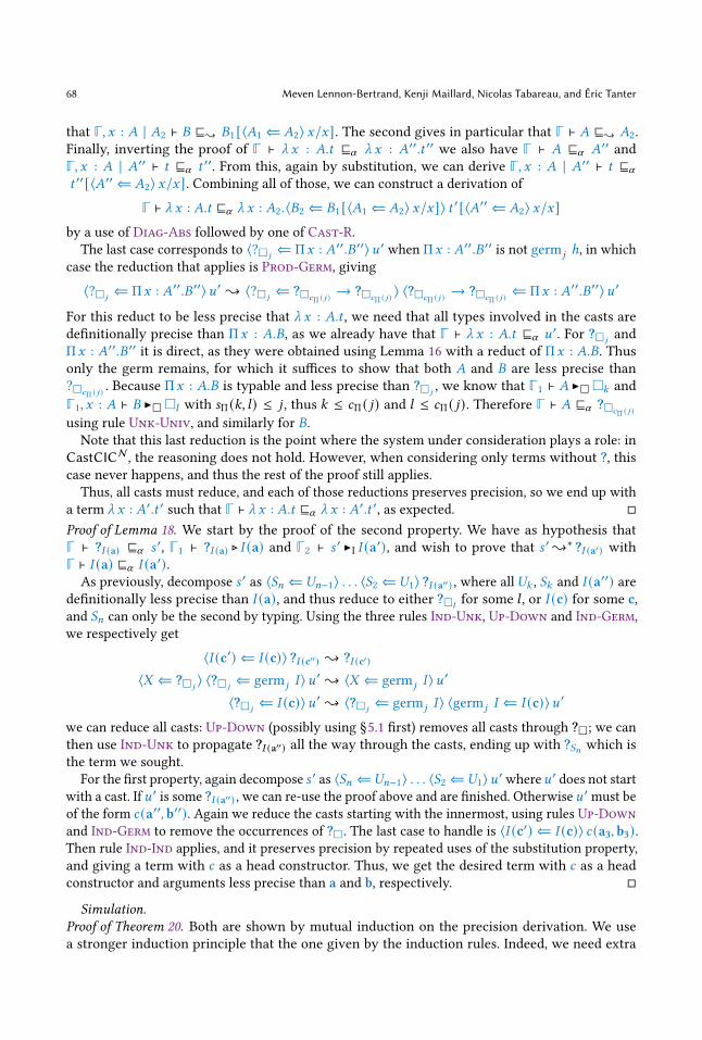
68 Meven Lennon-Bertrand, Kenji Maillard, Nicolas Tabareau, and Éric Tanter
that Γ, 𝑥 : 𝐴 | 𝐴2 ⊢ 𝐵 ⊑{ 𝐵1 [⟨𝐴1 ⇐ 𝐴2⟩ 𝑥/𝑥]. The second gives in particular that Γ ⊢ 𝐴 ⊑{ 𝐴2.
Finally, inverting the proof of Γ ⊢ _ 𝑥 : 𝐴.𝑡 ⊑𝛼 _ 𝑥 : 𝐴′′.𝑡 ′′ we also have Γ ⊢ 𝐴 ⊑𝛼 𝐴′′and
Γ, 𝑥 : 𝐴 | 𝐴′′ ⊢ 𝑡 ⊑𝛼 𝑡 ′′. From this, again by substitution, we can derive Γ, 𝑥 : 𝐴 | 𝐴′′ ⊢ 𝑡 ⊑𝛼
𝑡 ′′[⟨𝐴′′ ⇐ 𝐴2⟩ 𝑥/𝑥]. Combining all of those, we can construct a derivation of
Γ ⊢ _ 𝑥 : 𝐴.𝑡 ⊑𝛼 _ 𝑥 : 𝐴2 .⟨𝐵2 ⇐ 𝐵1 [⟨𝐴1 ⇐ 𝐴2⟩ 𝑥/𝑥]⟩ 𝑡 ′[⟨𝐴′′ ⇐ 𝐴2⟩ 𝑥/𝑥]by a use of Diag-Abs followed by one of Cast-R.
The last case corresponds to ⟨?□𝑗⇐ Π𝑥 : 𝐴′′.𝐵′′⟩𝑢 ′
when Π𝑥 : 𝐴′′.𝐵′′is not germ𝑗 ℎ, in which
case the reduction that applies is Prod-Germ, giving
⟨?□𝑗⇐ Π𝑥 : 𝐴′′.𝐵′′⟩𝑢 ′ { ⟨?□𝑗
⇐ ?□𝑐Π ( 𝑗 ) → ?□𝑐Π ( 𝑗 ) ⟩ ⟨?□𝑐Π ( 𝑗 ) → ?□𝑐Π ( 𝑗 ) ⇐ Π𝑥 : 𝐴′′.𝐵′′⟩𝑢 ′
For this reduct to be less precise that _ 𝑥 : 𝐴.𝑡 , we need that all types involved in the casts are
definitionally precise than Π𝑥 : 𝐴.𝐵, as we already have that Γ ⊢ _ 𝑥 : 𝐴.𝑡 ⊑𝛼 𝑢 ′. For ?□𝑗
and
Π𝑥 : 𝐴′′.𝐵′′it is direct, as they were obtained using Lemma 16 with a reduct of Π𝑥 : 𝐴.𝐵. Thus
only the germ remains, for which it suffices to show that both 𝐴 and 𝐵 are less precise than
?□𝑐Π ( 𝑗 ) . Because Π𝑥 : 𝐴.𝐵 is typable and less precise than ?□𝑗, we know that Γ1 ⊢ 𝐴 ▶□□𝑘 and
Γ1, 𝑥 : 𝐴 ⊢ 𝐵 ▶□□𝑙 with 𝑠Π (𝑘, 𝑙) ≤ 𝑗 , thus 𝑘 ≤ 𝑐Π ( 𝑗) and 𝑙 ≤ 𝑐Π ( 𝑗). Therefore Γ ⊢ 𝐴 ⊑𝛼 ?□𝑐Π ( 𝑗 )using rule Unk-Univ, and similarly for 𝐵.
Note that this last reduction is the point where the system under consideration plays a role: in
CastCICN, the reasoning does not hold. However, when considering only terms without ?, this
case never happens, and thus the rest of the proof still applies.
Thus, all casts must reduce, and each of those reductions preserves precision, so we end up with
a term _ 𝑥 : 𝐴′.𝑡 ′ such that Γ ⊢ _ 𝑥 : 𝐴.𝑡 ⊑𝛼 _ 𝑥 : 𝐴′.𝑡 ′, as expected. □
Proof of Lemma 18. We start by the proof of the second property. We have as hypothesis that
Γ ⊢ ?𝐼 (a) ⊑𝛼 𝑠 ′, Γ1 ⊢ ?𝐼 (a) ⊲ 𝐼 (a) and Γ2 ⊢ 𝑠 ′ ▶I 𝐼 (a′), and wish to prove that 𝑠 ′{∗ ?𝐼 (a′) with
Γ ⊢ 𝐼 (a) ⊑𝛼 𝐼 (a′).As previously, decompose 𝑠 ′ as ⟨𝑆𝑛 ⇐𝑈𝑛−1⟩ . . . ⟨𝑆2 ⇐𝑈1⟩ ?𝐼 (a′′) , where all 𝑈𝑘 , 𝑆𝑘 and 𝐼 (a′′) are
definitionally less precise than 𝐼 (a), and thus reduce to either ?□𝑙for some 𝑙 , or 𝐼 (c) for some c,
and 𝑆𝑛 can only be the second by typing. Using the three rules Ind-Unk, Up-Down and Ind-Germ,
we respectively get
⟨𝐼 (c′) ⇐ 𝐼 (c)⟩ ?𝐼 (c′′) { ?𝐼 (c′)⟨𝑋 ⇐ ?□𝑗
⟩ ⟨?□𝑗⇐ germ𝑗 𝐼 ⟩𝑢 ′ { ⟨𝑋 ⇐ germ𝑗 𝐼 ⟩𝑢 ′
⟨?□𝑗⇐ 𝐼 (c)⟩𝑢 ′ { ⟨?□𝑗
⇐ germ𝑗 𝐼 ⟩ ⟨germ𝑗 𝐼 ⇐ 𝐼 (c)⟩𝑢 ′
we can reduce all casts: Up-Down (possibly using §5.1 first) removes all casts through ?□; we canthen use Ind-Unk to propagate ?𝐼 (a′′) all the way through the casts, ending up with ?𝑆𝑛 which is
the term we sought.
For the first property, again decompose 𝑠 ′ as ⟨𝑆𝑛 ⇐𝑈𝑛−1⟩ . . . ⟨𝑆2 ⇐𝑈1⟩𝑢 ′where𝑢 ′
does not start
with a cast. If𝑢 ′is some ?𝐼 (a′′) , we can re-use the proof above and are finished. Otherwise𝑢 ′
must be
of the form 𝑐 (a′′, b′′). Again we reduce the casts starting with the innermost, using rules Up-Down
and Ind-Germ to remove the occurrences of ?□. The last case to handle is ⟨𝐼 (c′) ⇐ 𝐼 (c)⟩ 𝑐 (a3, b3).Then rule Ind-Ind applies, and it preserves precision by repeated uses of the substitution property,
and giving a term with 𝑐 as a head constructor. Thus, we get the desired term with 𝑐 as a head
constructor and arguments less precise than a and b, respectively. □
Simulation.
Proof of Theorem 20. Both are shown by mutual induction on the precision derivation. We use
a stronger induction principle that the one given by the induction rules. Indeed, we need extra

Gradualizing the Calculus of Inductive Constructions 69
induction hypothesis on the inferred type for a term. Proving this stronger principle is done by
making the proof of Property 3 slightly more general: instead of proving that an inferred type is
always well-formed, we prove that any property consequence of typing is true of all inferred types.
Let us now detail the most important cases of the inductive proof.
Definitional precision. We start with the easier second point. The proof is summarized by the
following diagram:
𝑡 ⊑{ 𝑡 ′
𝑠 𝑢 ⊑𝛼 𝑢 ′
𝑣 ⊑𝛼 𝑣 ′
By definition of ⊑{ , there exists𝑢 and𝑢 ′, reducts respectively of 𝑡 and 𝑡 ′, and such that Γ ⊢ 𝑢 ⊑𝛼 𝑢 ′
.
By confluence, there exists some 𝑣 that is a reduct of both 𝑢 and 𝑠 . By subject reduction, 𝑢 and
𝑢 ′are both well-typed, and thus by induction hypothesis there exists 𝑣 ′ such that 𝑢 ′{∗ 𝑣 ′ and
Γ ⊢ 𝑣 ⊑𝛼 𝑣 ′. But then 𝑣 is a reduct of 𝑠 and 𝑣 ′ is a reduct of 𝑡 ′, and so Γ ⊢ 𝑠 ⊑{ 𝑡 ′.This implies in particular that if Γ ⊢ 𝑡 ⊲𝑇 , Γ ⊢ 𝑇 ⊑{ 𝑇 ′
, 𝑡{∗ 𝑠 and Γ1 ⊢ 𝑠 ⊲ 𝑆 , then Γ ⊢ 𝑆 ⊑{ 𝑇 ′.
Indeed Γ1 ⊢ 𝑠 ⊳𝑇 by subject reduction, thus 𝑆 and 𝑇 are convertible, and have a common reduct 𝑈
by confluence. The property just stated then gives Γ ⊢ 𝑈 ⊑{ 𝑇 ′, hence Γ ⊢ 𝑆 ⊑{ 𝑇 ′
.
Syntactic precision—Non-diagonal precision rules. Let us now turn to ⊑𝛼 . It is enough to show
that one step of reduction can be simulated, by induction on the path 𝑡{∗ 𝑠 .First, we get rid of most cases where the last rule used for Γ ⊢ 𝑡 ⊑𝛼 𝑡 ′ is not a diagonal rule. For
Unk we must handle the side-condition involving the type of 𝑡 . However, by the previous property,
the inferred type of 𝑠 is also definitionally less precise than 𝑇 ′. Thus the reduction in 𝑡 can be
simulated by zero reduction steps. The reasoning for rules Err and Err-Lambda is similar. As for
rule Diag-Univ, subject reduction is enough to get what we seek, without even resorting to the
previous property. Rule Cast-R is treated in the same way as Unk, as the typing side-conditions
are similar. Thus the only non-diagonal rule left for ⊑𝛼 is Cast-L.
Syntactic precision—Non-top-level reduction. Next, we can get rid of reductions that do not happen
at top level. Indeed, if the last rule used was Cast-L, and the reduction happens in one of the types
of the cast, the same reasoning as for Cast-R applies. If it happens in the term, we can use the
induction hypothesis on this term to conclude. Also, if the last rule used was a diagonal rule, then
the reduction in 𝑡 can be simulated by a similar congruence rules in 𝑡 ′.So we are left with the simulation of a reduction that happens at the top-level in 𝑡 , and where
the last precision rule used is either Cast-L or a diagonal one, and this is the real core of the proof.
Syntactic precision—non-diagonal cast. Let us first turn to the case where the last precision rule
is Cast-L, and that cast reduces. More precisely, 𝑡 is some ⟨𝑇 ⇐ 𝑆⟩𝑢, with Γ ⊢ 𝑢 ⊑𝛼 𝑡 ′. There arefour possibilities for the reduction.
• The cast fails. When it does, whatever the rule, it always reduces to err𝑇 . But then we know
that Γ2 ⊢ 𝑡 ′ ⊲𝑇 ′and Γ ⊢ 𝑇 ⊑{ 𝑇 ′
. Thus Γ ⊢ err𝑇 ⊑𝛼 𝑡 ′ by rule Err, and the reduction is
simulated by zero reductions.
• The cast disappears (Univ-Univ) or expands into two casts without changing 𝑢 (Ind-Germ,
Prod-Germ). In those cases the reduct of 𝑡 is still smaller than 𝑡 ′. In the case of cast expansion,

70 Meven Lennon-Bertrand, Kenji Maillard, Nicolas Tabareau, and Éric Tanter
wemust use Cast-L twice, and thus prove that the type of 𝑡 ′ is less precise than the introducedgerm. But by the Cast-L rule that was used to prove Γ ⊢ 𝑡 ⊑𝛼 𝑡 ′, we know that 𝑡 ′ infers atype 𝑇 ′
which is definitionally less precise than some ?□𝑖. Thus, 𝑇 ′
reduces to some 𝑆 ′ suchthat Γ ⊢ ?□𝑖
⊑𝛼 𝑆 ′, and this implies that also Γ ⊢ germ𝑖 ℎ ⊑𝛼 𝑆 ′, i.e., what we sought.• Both 𝑇 and 𝑆 are either product types or inductive types, and 𝑢 starts with an abstraction or
an inductive constructor. In that case, by Lemmas 17 and 18, 𝑡 ′ reduces to a term 𝑢 ′with the
same head constructor as 𝑢 or some ?𝐼 (a) . In the first case, by the substitution property of
precision we have Γ ⊢ 𝑠 ⊑𝛼 𝑢 ′. In the second, we can use Unk to conclude.
• The reduction rule is Up-Down, that is 𝑡 is ⟨𝑇 ⇐ ?□𝑖⟩ ⟨?□𝑖
⇐ germ𝑖 ℎ⟩𝑢 which reduces to
⟨𝑇 ⇐ germ𝑖 ℎ⟩𝑢. If ruleCast-Lwas used twice in a row thenwe directly haveΓ ⊢ 𝑢 ⊑𝛼 𝑡 ′ andso Γ ⊢ ⟨𝑋 ⇐ germ𝑖 ℎ⟩𝑢 ⊑𝛼 𝑡 ′. Otherwise, rule Diag-Cast was used, 𝑡 ′ is some ⟨𝑇 ′ ⇐ 𝑆 ′⟩𝑢 ′
andwe haveΓ ⊢ 𝑢 ⊑𝛼 𝑢 ′andΓ1 ⊢ germ𝑖 ℎ ⊑{ 𝑆 ′. Moreover,Cast-L also givesΓ1 ⊢ 𝑋 ⊑{ 𝐵′
,
since Γ2 ⊢ ⟨𝐵′ ⇐ 𝐴′⟩𝑢 ′ ⊲𝐵′. Thus Γ ⊢ ⟨𝑋 ⇐ germ𝑖 ℎ⟩𝑢 ⊑𝛼 ⟨𝐵′ ⇐ 𝐴′⟩𝑢 ′
by a use of Diag-
Cast.
Syntactic precision—𝛽 redex. Next we consider the case where 𝑡 is a 𝛽 redex (_ 𝑥 : 𝐴.𝑡1) 𝑡2. Becausethe last applied precision rule is diagonal, 𝑡 ′ must also decompose as 𝑡 ′′
1𝑡 ′2. If 𝑡1 is some err𝑇 , then
the reduct is err𝑇 and must be still smaller that 𝑡 ′. Otherwise, Lemma 17 applies, thus 𝑡 ′′1reduces
to some _ 𝑥 : 𝐴′.𝑡 ′1that is syntactically less precise than _ 𝑥 : 𝐴.𝑡1. Then the 𝛽 reduction of 𝑡 can
be simulated with a 𝛽 reduction in 𝑡 ′, and using the substitution property we conclude that the
redexes are still related by precision.
Syntactic precision—] redex. If 𝑡 is a ] redex ind𝑐 (a,b) (𝐼 , 𝑧.𝑃, f .y.t), the reasoning is similar. Because
the last precision rule is diagonal, 𝑡 ′must also be a fixpoint.We thus can use Lemma 18 to ensure that
its scrutinee reduces either to 𝑐 (a′, b′) or ?𝐼 (a′) . In the first case, a ] reduction of 𝑡 ′ and the substitutionproperty is enough to conclude. In the second case, 𝑡 ′ reduces to a term 𝑠 ′ := ?𝑃 ′ [?𝐼 (a′) /𝑧 ] , and we
must show this term to be less precise than 𝑠 , which is 𝑡𝑘 [_ 𝑥 : 𝐼 (a). ind𝐼 (𝑥, 𝑧.𝑃, f .y.t)/𝑧] [b/y]. Let𝑆 be the type inferred for 𝑠 , by rule Unk, it is enough to show Γ ⊢ 𝑆 ⊑{ 𝑃 ′[?𝐼 (a′)/𝑧]. By subject
reduction, 𝑆 and 𝑃 [𝑐𝑘 (a, b)/𝑧] (the type of 𝑡 ) are convertible, thus they have a common reduct 𝑈 .
Now we also have by substitution that Γ ⊢ 𝑃 [𝑐𝑘 (a, b)/𝑧] ⊑𝛼 𝑃 ′[?𝐼 (a′)/𝑧]. Because 𝑃 [𝑐𝑘 (a, b)/𝑧] isthe inferred type for 𝑡 , the induction hypothesis applies to it, and thus there is some𝑈 ′
such that
𝑃 ′[?𝐼 (a′)𝑧/]{∗𝑈 ′and also Γ ⊢ 𝑈 ⊑𝛼 𝑈 ′
.
Syntactic precision—err and ? reductions. For reductions Prod-Err, i.e., when errΠ𝑥 :𝐴.𝐵 {_ 𝑥 : 𝐴. err𝐵 , we can replace the use of Err by a use of Err-Lambda. For reduction Ind-Err,
i.e., when 𝑡 is ind𝐼 (err𝐼 (a) , 𝑧.𝑃, f .y.t) we distinguish three cases depending on 𝑡 ′. If 𝑡 ′ is ?𝑇 ′ (the
precision rule between 𝑡 and 𝑡 ′ was Unk) or ⟨𝑇 ′ ⇐ 𝑆 ′⟩ 𝑡 ′, then Γ ⊢ 𝑃 [err𝐼 (a)/𝑧] ⊑{ 𝑇 ′, and thus
Γ ⊢ err𝑃 [err 𝐼 (a) /𝑧 ] ⊑𝛼 𝑡 ′ by using Err. Otherwise, the last rule was Diag-Fix, and again we can
conclude using Err and the substitution property of ⊑𝛼 .
Conversely, let us consider the reduction rules for ?. If 𝑡 is ?Π𝑥 :𝐴.𝐵 and reduces to _ 𝑥 : 𝐴.?𝐵 ,then 𝑡 ′ must be ?𝑇 , possibly surrounded by casts. If there are casts, they can all be reduced away
until we are left with ?𝑇 ′ for some 𝑇 ′such that Γ ⊢ Π𝑥 : 𝐴.𝐵 ⊑{ 𝑇 . By Lemma 16, 𝑇 {∗ ??□ or
𝑇 {∗𝑇Π𝑥 :𝐴′.𝐵′ . In the first case, ??□ is still less precise than _ 𝑥 : 𝐴.𝐵, and in the second case, ?Π𝑥 :𝐴′.𝐵′
can reduce to _ 𝑥 : 𝐴′.?𝐵′ , which is less precise than 𝑠 ′. If 𝑡 is ind𝐼 (?𝐼 (a) , 𝑃, b), reducing to ?𝑃 [?𝐼 ( (𝑎) ) /𝑧 ] ,we use the second part of Lemma 18 to conclude that also 𝑡 ′ reduces to some ind𝐼 (?𝐼 (a′) , 𝑃 ′, b′) thatis less precise than 𝑡 . From this, 𝑡 ′ { ?𝑃 ′ [?𝐼 ( (𝑎′) ) /𝑧 ] , which is less precise than 𝑠 .
Syntactic precision—diagonal cast reduction. This only leaves us with the reduction of a cast when
the precision rule isDiag-Cast: we have some ⟨𝑇 ⇐ 𝑆⟩𝑢 and ⟨𝑇 ′ ⇐ 𝑆 ′⟩𝑢 ′that are pointwise related

Gradualizing the Calculus of Inductive Constructions 71
by precision, such that ⟨𝑇 ⇐ 𝑆⟩ 𝑡{∗ 𝑠 by a head reduction, and we must show that ⟨𝑇 ⇐ 𝑆⟩𝑢simulates that reduction.
First, if the reduction for ⟨𝑇 ⇐ 𝑆⟩ 𝑡 is any reduction to an error, then the reduct is err𝑇 , andsince Γ2 ⊢ ⟨𝑇 ′ ⇐ 𝑆 ′⟩𝑢 ′ ⊲𝑇 ′
and Γ ⊢ 𝑇 ⊑{ 𝑇 ′we can use rule Err to conclude.
Next, consider Prod-Prod.We are in the situationwhere 𝑡 is ⟨Π𝑥 : 𝐴2 .𝐵2 ⇐ Π𝑥 : 𝐴1.𝐵1⟩ _ 𝑥 : 𝐴.𝑣 .
If 𝑣 is err𝐵1then the reduct is more precise than any term. Otherwise, by Lemma 16, 𝑆 ′ reduces
either to ?□ or to a product type. In the first case, 𝑢 ′must reduce to ??□ by Lemma 17, since it is
less precise than _ 𝑥 : 𝐴.𝑣 and by typing it cannot start with a _. In that case, ⟨𝑇 ′ ⇐ 𝑆 ′⟩𝑢 ′ { ?𝑇 ′ ,
and since Γ ⊢ Π𝑥 : 𝐴2.𝐵2 ⊑{ 𝑇 ′, we have that Γ ⊢ 𝑠 ⊑𝛼 ?𝑇 ′ . Otherwise 𝑆 ′ reduces to some
Π𝑥 : 𝐴′1.𝐵′
1. By Lemma 17, 𝑡 ′ reduces either to some ? or to an abstraction. In the first case, the
previous reasoning still applies. Otherwise, 𝑡 ′ reduces to some _ 𝑥 : 𝐴′.𝑣 ′. Again, by Lemma 16, 𝑇 ′
reduces either to a product type or to ?. In the first case 𝑡 ′ can simply do the same cast reduction
as 𝑡 , and the substitution property of precision enables us to conclude. Thus, the only case left
is that where 𝑡 ′ is ⟨?□𝑖⇐ Π𝑥 : 𝐴′
1.𝐵′
1⟩ _ 𝑥 : 𝐴′.𝑣 ′. If Π𝑥 : 𝐴′
1.𝐵′
1is germ𝑖 Π, then all of 𝐴, 𝐴1, 𝐴2,
𝐵1 and 𝐵2 are more precise than ?□𝑐Π (𝑖 ) , and this is enough to conclude that 𝑠 is less precise than
⟨germ𝑖 Π ⇐ ?□𝑖⟩ _ 𝑥 :?□𝑐Π (𝑖 ) .𝑢
′, using the substitution property of precision to relate 𝑢 ′
with the
substituted 𝑢, and the Diag-Abs, Cast-L and Cast-R rules. The last case is when Π𝑥 : 𝐴′1.𝐵′
1is
not a germ. Then the reduction of 𝑡 ′ first does a cast expansion through germ𝑖 Π, followed by a
reduction of the cast between Π𝑥 : 𝐴′1.𝐵′
1and germ𝑖 Π. The reasoning of the two previous cases
can be used again to conclude. The proof is similar for rule Ind-Ind.
Next, let us consider Prod-Germ, that is when 𝑡 is ⟨?□𝑖⇐ Π𝑥 : 𝐴1 .𝐵1⟩ 𝑓 . We have that𝑇 ′ { ?□𝑗
by Lemma 16 with 𝑖 ≤ 𝑗 , and thus Γ ⊢ germ𝑖 Π ⊑{ 𝑇 ′. Thus, using Diag-Cast for the innermost
cast in 𝑠 , and Cast-L for the outermost one, we conclude Γ ⊢ 𝑠 ⊑𝛼 ⟨𝑇 ′ ⇐ 𝑆 ′⟩𝑢 ′. Again, the
reasoning is similar for Ind-Germ.
As for Univ-Univ, 𝑡 is ⟨□𝑖 ⇐ □𝑖⟩𝐴, and we can replace rule Diag-Cast by rule Cast-R. Indeed
Γ1 ⊢ 𝐴 ⊳□𝑖 by typing, thus Γ1 ⊢ 𝐴 ⊲𝑇 for some𝑇 such that𝑇 { □𝑖 . Therefore, since Γ ⊢ □𝑖 ⊑{ 𝑇 ′,
we have Γ ⊢ 𝑇 ⊑{ 𝑇 ′and similarly Γ ⊢ 𝑇 ⊑{ 𝑆 ′. Thus, rule Cast-R gives Γ ⊢ 𝐴 ⊑𝛼 𝑡 ′.
The last case left is the one ofUp-Down, where 𝑡 is ⟨𝑋 ⇐ ?□𝑖⟩ ⟨?□𝑖
⇐ germ𝑖 ℎ⟩ 𝑣 . We distinguish
on the rule used to prove Γ ⊢ ⟨?□𝑖⇐ germ𝑖 ℎ⟩ 𝑣 ⊑𝛼 𝑢 ′
. If it is Cast-L, then we simply have
Γ ⊢ ⟨𝑋 ⇐ germ𝑖 ℎ⟩ 𝑡 ⊑𝛼 ⟨𝑇 ′ ⇐ 𝑆 ′⟩𝑢 ′using rule Diag-Cast, as Γ ⊢ germ𝑖 ℎ ⊑{ 𝑆 ′ since Γ ⊢
?□𝑖⊑{ 𝑆 ′. Otherwise the rule is Diag-Cast, 𝑡 ′ reduces to ⟨𝑇 ′ ⇐ ?□𝑗
⟩ ⟨?□𝑗⇐𝑈 ′⟩𝑢 ′
, using
Lemma 16 to reduce types less precise than ?□𝑖to some ?□𝑗
with 𝑖 ≤ 𝑗 . We can use Diag-Cast on
the outermost cast, and Cast-R on the innermost to prove that this term is less precise than 𝑠 , as
Γ ⊢ germ𝑖 ℎ ⊑{ ?□𝑗since 𝑖 ≤ 𝑗 . □
B.3 Properties of GCICConservativity is an equivalence, so to prove it we break it down into two implications. We now
state and prove those in an open context and for the three different judgments.
Theorem 37 (GCIC is weaker than CIC—Open context). Let 𝑡 be a static term and Γ an erasable
context. Then
• if Y (Γ) ⊢CIC 𝑡 ⊲𝑇 then Γ ⊢ 𝑡⇝ 𝑡 ⊲𝑇 ′for some erasable 𝑡 and𝑇 ′
such that Y (𝑡) = 𝑡 and Y (𝑇 ′) = 𝑇 ;
• if 𝑇 ′is an erasable term of CastCIC, and Y (Γ) ⊢CIC 𝑡 ⊳ Y (𝑇 ′) then Γ ⊢ 𝑡 ⊳𝑇 ′⇝ 𝑡 for some
erasable 𝑡 such that Y (𝑡) = 𝑡 ;
• if Y (Γ) ⊢CIC 𝑡 ▶h𝑇 then Γ ⊢ 𝑡⇝ 𝑡 ▶
h𝑇′for some erasable 𝑡 and 𝑇 ′
such that Y (𝑡) = 𝑡 and
Y (𝑇 ′) = 𝑇 .
Proof. Once again, the proof is by mutual induction, on the typing derivation of 𝑡 in CIC.

72 Meven Lennon-Bertrand, Kenji Maillard, Nicolas Tabareau, and Éric Tanter
All inference rules are direct: one needs to combine the induction hypothesis together, using the
substitution property of precision and the fact that erasure commutes with substitution to handle
the cases of substitution in the inferred types.
Let us consider the case of Prod-Inf next. We are given Γ erasable, and suppose Y (Γ) ⊢CIC 𝑡 ⊲𝑇
and 𝑇 {∗Π𝑥 : 𝐴.𝐵. By induction hypothesis there exists 𝑡 and 𝑇 ′
erasable such that Γ ⊢ 𝑡⇝ 𝑡 ⊲𝑇 ′
and Y (𝑡) = 𝑡 , Y (𝑇 ′) = 𝑇 . Because 𝑇 ′is erasable, it is less precise than 𝑇 . By Corollary 21, it
must reduce to either ?□ or a product type. The first case is impossible because 𝑇 ′does not
contain any ? as it is erasable. Thus there are some 𝐴′and 𝐵′
such that 𝑇 ′{∗Π𝑥 : 𝐴′.𝐵′
and
Γ ⊢ Π𝑥 : 𝐴.𝐵 ⊑𝛼 Π𝑥 : 𝐴′.𝐵′. Since also Γ ⊢ 𝑇 ′ ⊑𝛼 𝑇 , by the same reasoning there are also some 𝐴′′
and 𝐵′′such that 𝑇 {∗
Π𝑥 : 𝐴′′.𝐵′′and Γ ⊢ Π𝑥 : 𝐴′.𝐵′ ⊑𝛼 Π𝑥 : 𝐴′′.𝐵′′
. Now because 𝑇 is static,
so are Π𝑥 : 𝐴.𝐵 and Π𝑥 : 𝐴′′.𝐵′′, and because of the comparisons with Π𝑥 : 𝐴′.𝐵′
we must have
Y (Γ) ⊢ Π𝑥 : 𝐴.𝐵 ⊑𝛼 Π𝑥 : 𝐴′′.𝐵′′. Since both are static, this means they must be 𝛼-equal, since no
non-diagonal rule can be used on static terms. Hence, Π𝑥 : 𝐴.𝐵 = Π𝑥 : 𝐴′′.𝐵′′ = Y (Π𝑥 : 𝐴′.𝐵′),implying that Π𝑥 : 𝐴′.𝐵′
is erasable. Thus, Γ ⊢ 𝑡⇝ 𝑡 ▶Π Π𝑥 : 𝐴′.𝐵′
, both 𝑡 and Π𝑥 : 𝐴′.𝐵′are
erasable, and moreover Y (𝑡) = 𝑡 and Y (Π𝑥 : 𝐴′.𝐵′) = Π𝑥 : 𝐴.𝐵, which is what had to be proven.
The other constrained inference rules being very similar, let us turn to Check. We are given
Γ and 𝑇 ′erasable, and suppose that Y (Γ) ⊢CIC 𝑡 ⊲ 𝑆 such that 𝑆 ≡ Y (𝑇 ′). By induction hypothesis,
Γ′ ⊢ 𝑡⇝ 𝑡 ⊲ 𝑆 ′ with 𝑡 and 𝑆 ′ erasable, Y (𝑡) = 𝑡 and Y (𝑆 ′) = 𝑆 . But convertibility implies consistency,
so 𝑆 ∼ Y (𝑇 ′). By monotonicity of consistency, this implies 𝑆 ′ ∼ 𝑇 ′. Thus Γ ⊢ 𝑡 ⊳𝑇 ′⇝⟨𝑇 ′ ⇐ 𝑆 ′⟩ 𝑡 .
We have Y (⟨𝑇 ′ ⇐ 𝑆 ′⟩ 𝑡) = Y (𝑡) = 𝑡 , so we are left with showing that Γ ⊢ ⟨𝑇 ′ ⇐ 𝑆 ′⟩ 𝑡 ⊒⊑𝛼 𝑡 .
Using rules Cast-L and Cast-R, and knowing already that Γ ⊢ 𝑆 ′ ⊒⊑𝛼 𝑆 , it remains to show that
Γ ⊢ 𝑇 ′ ⊑{ 𝑆 and Γ ⊢ 𝑆 ⊑{ 𝑇 ′. As 𝑆 and Y (𝑇 ′) are convertible, let 𝑈 be a common reduct. Using
Theorem 20, 𝑇 ′{∗𝑈 ′with Γ ⊢ 𝑈 ⊑𝛼 𝑈 ′
. Simulating that reduction again, we get Y (𝑇 ′){∗𝑈 ′′
with Γ ⊢ 𝑈 ′′ ⊑𝛼 𝑈 ′. As before, this implies𝑈 = 𝑈 ′′ = Y (𝑈 ′). Thus, using the reduct𝑈 ′
of 𝑇 ′that is
equiprecise with𝑈 , we can conclude Γ ⊢ 𝑆 ⊑{ 𝑇 ′and Γ ⊢ 𝑇 ′ ⊑{ 𝑆 . □
Theorem 38 (CIC is weaker than GCIC—Open context). Let 𝑡 be a static term and Γ an erasable
context of CastCIC. Then
• if Γ ⊢ 𝑡⇝ 𝑡 ⊲𝑇 , then 𝑡 and 𝑇 are erasable, Y (𝑡 ′) = 𝑡 and Y (Γ) ⊢ 𝑡 ⊲ Y (𝑇 ′);• if 𝑇 ′
is an erasable term of CastCIC such that Γ′ ⊢ 𝑡 ⊳𝑇 ′⇝ 𝑡 ′, then 𝑡 ′ is erasable, Y (𝑡 ′) = 𝑡 and
Y (Γ) ⊢ 𝑡 ⊳ Y (𝑇 ′);• if Γ′ ⊢ 𝑡⇝ 𝑡 ′ ▶
h𝑇′, then 𝑡 ′ and 𝑇 ′
are erasable, Y (𝑡 ′) = 𝑡 and Y (Γ) ⊢ 𝑡 ▶h Y (𝑇 ′).
Proof. The proof is similar to the previous one. Again, the tricky part is to handle reduction steps,
and we use equiprecision in the same way to conclude in those. □
As a direct corollary of those propositions in an empty context, we get conservativity Theorem 23.
Elaboration graduality. Now for the elaboration graduality: again, we state it in an open context
for all three typing judgments.
Theorem 39 (Elaboration graduality—Open context). Let Γ be a context such that Γ1 ⊑𝛼 Γ2, and 𝑡
and 𝑡 ′ be two GCIC terms such that 𝑡 ⊑G
𝛼 𝑡 ′. Then
• if Γ1 ⊢ 𝑡⇝ 𝑡 ⊲𝑇 is universe adequate, then there exists 𝑡 ′ and 𝑇 ′such that Γ2 ⊢ 𝑡 ′⇝ 𝑡 ′ ⊲𝑇 ′
,
Γ ⊢ 𝑡 ⊑𝛼 𝑡 ′ and Γ ⊢ 𝑇 ⊑𝛼 𝑇 ′;
• If Γ1 ⊢ 𝑡 ⊳𝑇 ⇝ 𝑡 ′ is universe adequate, then for all 𝑇 ′such that Γ ⊢ 𝑇 ⊑𝛼 𝑇 ′
there exists 𝑡 ′ suchthat Γ2 ⊢ 𝑡 ′ ⊳𝑇 ′⇝ 𝑡 ′ and Γ ⊢ 𝑡 ⊑𝛼 𝑡 ′;
• If Γ1 ⊢ 𝑡⇝ 𝑡 ′ ▶h𝑇 is universe adequate, then there exists 𝑡 ′ and 𝑇 ′
such that Γ2 ⊢ 𝑡 ′⇝ 𝑡 ′ ▶h𝑇
′,
Γ ⊢ 𝑡 ⊑𝛼 𝑡 ′ and Γ ⊢ 𝑇 ⊑𝛼 𝑇 ′.
Proof. Once again, we use our favorite tool: induction on the typing derivation of 𝑡 .

Gradualizing the Calculus of Inductive Constructions 73
Inference—Non-diagonal precision. For inference, we have to make a distinction on the rule used
to prove 𝑡𝑖𝑙𝑑𝑒𝑡 ⊑G
𝛼 𝑡 ′: we have to handle specifically the non-diagonal one, where 𝑡 ′ is some ?. We
start with this, and treat the ones where the rule is diagonal (i.e., when 𝑡 and 𝑡 ′ have the same head)
next.
We have Γ1 ⊢ 𝑡⇝ 𝑡 ′ ⊲𝑇 ′and Γ2 ⊢ ?@{i}⇝ ??□𝑖
⊲ ?□𝑖. Correctness of elaboration gives Γ1 ⊢ 𝑡 ′ ⊲𝑇 ′
,
and by validity Γ1 ⊢ 𝑇 ′ ⊲□𝑖 , universe adequacy ensuring us that this 𝑖 is the same as the one in 𝑡 ′.Thus we have Γ ⊢ 𝑇 ′ ⊑𝛼 ?□𝑖
by rule Unk, and in turn Γ ⊢ 𝑡 ′ ⊑𝛼 ??□𝑖by a second use of the same
rule, giving us the required conclusions.
Inference—Variable. Rule Var gives us (𝑥 : 𝑇 ) ∈ Γ1. Because ⊢ Γ1 ⊑𝛼 Γ2, there exists some 𝑇 ′
such that (𝑥 : 𝑇 ′) ∈ Γ2, and Γ ⊢ 𝑇 ⊑𝛼 𝑇 ′using weakening. Thus, Γ2 ⊢ 𝑥⇝𝑥 ⊲𝑇 ′
, and of course
Γ ⊢ 𝑥 ⊑𝛼 𝑥 .
Inference—Product. Premises of rule Prod give Γ1 ⊢ ��⇝𝐴 ▶□□𝑖 and Γ1, 𝑥 : 𝐴 ⊢ ��⇝𝐵 ▶□□𝑗 ,
and the diagonal precision one gives �� ⊑G
𝛼 ��′and �� ⊑G
𝛼 ��′. Applying the induction hypothesis,
we get some 𝐴′such that Γ2 ⊢ ��′⇝𝐴′ ▶□□𝑖 and Γ ⊢ 𝐴 ⊑𝛼 𝐴′
. The inferred type for ��′must be
□𝑖 as it is some □𝑗 because of the constrained elaboration, and it is less precise than □𝑖 by the
induction hypothesis. From this, we also deduce that Γ1, 𝑥 : 𝐴 ⊑𝛼 Γ2, 𝑥 : 𝐴′. Hence the induction
hypothesis can be applied to ��, giving Γ2 ⊢ ��′⇝𝐵′ ▶□□𝑗 . Combining this with the elaboration
for ��′, we obtain Γ2 ⊢ Π𝑥 : ��′.��′⇝Π𝑥 : 𝐴′.𝐵′ ⊲□𝑠Π (𝑖, 𝑗) . Moreover, Γ ⊢ Π𝑥 : 𝐴.𝐵 ⊑𝛼 Π𝑥 : 𝐴′.𝐵′
by combining the precision hypothesis on 𝐴 and 𝐵, and also Γ ⊢ □𝑠Π (𝑖, 𝑗) ⊑𝛼 □𝑠Π (𝑖, 𝑗) .
Inference—Application. From rule App, we have Γ1 ⊢ 𝑡⇝ 𝑡 ▶Π Π𝑥 : 𝐴.𝐵 and Γ1 ⊢ �� ⊳𝐴⇝𝑢, and
the diagonal precision gives 𝑡 ⊑G
𝛼 𝑡 ′ and �� ⊑G
𝛼 �� ′. By induction, we have Γ1 ⊢ 𝑡 ′⇝ 𝑡 ′ ▶
Π Π𝑥 : 𝐴′.𝐵′
for some 𝑡 ′, 𝐴′and 𝐵′
such that Γ ⊢ 𝑡 ⊑𝛼 𝑡 ′, Γ ⊢ 𝐴 ⊑𝛼 𝐴′and Γ, 𝑥 : 𝐴 | 𝐴′ ⊢ 𝐵 ⊑𝛼 𝐵′
. Using the
induction hypothesis again with that precision property on 𝐴 and 𝐴′gives Γ2 ⊢ �� ′ ⊳𝐴′⇝𝑢 ′
with
Γ ⊢ 𝑢 ⊑𝛼 𝑢 ′. Therefore combining those we get Γ2 ⊢ 𝑡 ′ �� ′⇝ 𝑡 ′ 𝑢 ′ ⊲𝐵′[𝑢 ′/𝑥], Γ ⊢ 𝑡 𝑢 ⊑𝛼 𝑡 ′ 𝑢 ′
and,
by substitution property of precision, Γ ⊢ 𝐵 [𝑢/𝑥] ⊑𝛼 𝐵′[𝑢 ′/𝑥].
Inference—Other diagonal cases. All other cases are similar to those: combining the induction
hypothesis directly leads to the desired result, handling the binders in a similar way to that of
products when needed.
Checking. For Check, we have that Γ1 ⊢ 𝑡⇝ 𝑡 ⊲ 𝑆 , with 𝑆 ∼ 𝑇 . By induction hypothesis, Γ2 ⊢𝑡 ′⇝ 𝑡 ′ ⊲ 𝑆 ′ with Γ ⊢ 𝑡 ⊑𝛼 𝑡 ′ and Γ ⊢ 𝑆 ⊑𝛼 𝑆 ′. But we also have as an hypothesis that Γ ⊢ 𝑇 ⊑𝛼 𝑇 ′
.
By monotonicity of consistency, we conclude that 𝑆 ′ ∼ 𝑇 ′, and thus Γ2 ⊢ 𝑡 ′ ⊳𝑇 ′⇝⟨𝑇 ′ ⇐ 𝑆 ′⟩ 𝑡 ′. A
use of Diag-Cast then ensures that Γ ⊢ ⟨𝑇 ⇐ 𝑆⟩ 𝑡 ⊑𝛼 ⟨𝑇 ′ ⇐ 𝑆 ′⟩ 𝑡 ′, as desired.
Constrained inference—Inf-Prod rule. We are in the situation where Γ1 ⊢ 𝑡⇝ 𝑡 ⊲ 𝑆 and 𝑆{∗Π𝑥 :
𝐴.𝐵. By induction hypothesis, Γ2 ⊢ 𝑡 ′⇝ 𝑡 ′ ⊲ 𝑆 ′ with Γ ⊢ 𝑆 ⊑𝛼 𝑆 ′. Using Corollary 21, we get
that 𝑆 ′{∗Π𝑥 : 𝐴′.𝐵′
such that Γ ⊢ Π𝑥 : 𝐴.𝐵 ⊑𝛼 Π𝑥 : 𝐴′.𝐵′, or 𝑆 ′{∗ ?□𝑖
. In the first case,
by rule Inf-Prod we get Γ2 ⊢ 𝑡 ′⇝ 𝑡 ′ ▶Π Π𝑥 : 𝐴′.𝐵′
together with the precision inequalities
for 𝑡 ′ and Π𝑥 : 𝐴′.𝐵′. In the second case, we can use rule Inf-Prod? instead, and get Γ2 ⊢
𝑡 ′⇝⟨germ𝑖 Π ⇐ 𝑆 ′⟩ 𝑡 ′ ▶Π germ𝑖 Π, and 𝑐Π (𝑖) is larger than the universe levels of both 𝐴′
and
𝐵′. A use of Cast-R, together with the fact that Γ ⊢ 𝐴 ⊑𝛼 ?□𝑐Π (𝑖 ) by Unk-Univ and similarly for
𝐵, gives that Γ ⊢ 𝑡 ′ ⊑𝛼 ⟨germ𝑖 Π ⇐ 𝑆 ′⟩ 𝑡 ′, and the precision between types has been established
already.
Constrained inference—Inf-Prod?. This time, Γ1 ⊢ 𝑡⇝ 𝑡 ⊲ 𝑆 , but 𝑆{∗ ?□𝑖. By induction hy-
pothesis, Γ2 ⊢ 𝑡 ′⇝ 𝑡 ′ ⊲ 𝑆 ′ with Γ ⊢ 𝑆 ⊑𝛼 𝑆 ′. By Corollary 21, we get that 𝑆 ′{∗ ?□𝑖. Thus
Γ2 ⊢ 𝑡 ′⇝⟨germ𝑖 Π ⇐ 𝑆 ′⟩ 𝑡 ′ ▶Π germ𝑖 Π. A use of Diag-Cast is enough to conclude.
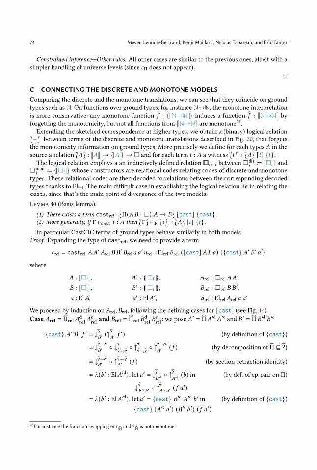
74 Meven Lennon-Bertrand, Kenji Maillard, Nicolas Tabareau, and Éric Tanter
Constrained inference—Other rules. All other cases are similar to the previous ones, albeit with a
simpler handling of universe levels (since 𝑐Π does not appear).
□
C CONNECTING THE DISCRETE AND MONOTONE MODELSComparing the discrete and the monotone translations, we can see that they coincide on ground
types such as N. On functions over ground types, for instance N→N, the monotone interpretation
is more conservative: any monotone function 𝑓 : {| N→N |} induces a function˜𝑓 : JN→NK by
forgetting the monotonicity, but not all functions from JN→NK are monotone25.
Extending the sketched correspondence at higher types, we obtain a (binary) logical relation
*−+ between terms of the discrete and monotone translations described in Fig. 20, that forgets
the monotonicity information on ground types. More precisely we define for each types 𝐴 in the
source a relation H𝐴I : J𝐴K → {|𝐴 |} → □ and for each term 𝑡 : 𝐴 a witness *𝑡 + : H𝐴I [𝑡] {𝑡} .The logical relation employs a an inductively defined relation □□rel,𝑖 between □□dis
𝑖 := J□𝑖K and□□mon
𝑖 := {|□𝑖 |} whose constructors are relational codes relating codes of discrete and monotone
types. These relational codes are then decoded to relations between the corresponding decoded
types thanks to Elrel. The main difficult case in establishing the logical relation lie in relating the
casts, since that’s the main point of divergence of the two models.
Lemma 40 (Basis lemma).
(1) There exists a term castrel : HΠ(𝐴𝐵 : □□).𝐴 → 𝐵I [cast] {cast} .(2) More generally, if Γ ⊢cast 𝑡 : 𝐴 then HΓI ⊢IR *𝑡 + : H𝐴I [𝑡] {𝑡} .In particular CastCIC terms of ground types behave similarly in both models.
Proof. Expanding the type of castrel, we need to provide a term
𝑐rel = castrel 𝐴𝐴′𝐴rel 𝐵 𝐵′ 𝐵rel 𝑎 𝑎′ 𝑎rel : Elrel 𝐵rel ( [cast]𝐴𝐵 𝑎) ({cast} 𝐴′ 𝐵′ 𝑎′)
where
𝐴 : J□𝑖K, 𝐴′: {|□𝑖 |}, 𝐴rel : □□rel𝐴𝐴′,
𝐵 : J□𝑖K, 𝐵′: {|□𝑖 |}, 𝐵rel : □□rel 𝐵 𝐵′,
𝑎 : El𝐴, 𝑎′ : El𝐴′, 𝑎rel : Elrel𝐴rel 𝑎 𝑎′
We proceed by induction on 𝐴rel, 𝐵rel, following the defining cases for [cast] (see Fig. 14).Case 𝐴rel = Πrel𝐴
drel𝐴
crel and 𝐵rel = Πrel 𝐵
drel 𝐵
crel: we pose 𝐴
′ = Π𝐴′d𝐴′cand 𝐵′ = Π 𝐵′d 𝐵′c
{cast} 𝐴′ 𝐵′ 𝑓 ′ = ↓?𝐵′ (↑?𝐴′ 𝑓
′) (by definition of {cast})
= ↓?→?𝐵′ ◦ ↓?
?→?◦ ↑?
?→?◦ ↑?→?
𝐴′ (𝑓 ) (by decomposition of Π ⊑ ?)
= ↓?→?𝐵′ ◦ ↑?→?
𝐴′ (𝑓 ) (by section-retraction identity)
= _(𝑏 ′ : El𝐴′d). let𝑎′ = ↓?𝐵′d ◦ ↑?
𝐴′d (𝑏) in (by def. of ep-pair on Π)
↓?𝐵′c 𝑏′ ◦ ↑?
𝐴′c 𝑎′ (𝑓 𝑎′)
= _(𝑏 ′ : El𝐴′d). let𝑎′ = {cast} 𝐵′d 𝐴′d 𝑏 ′ in (by definition of {cast}){cast} (𝐴′c 𝑎′) (𝐵′c 𝑏 ′) (𝑓 𝑎′)
25For instance the function swapping err ¥N and ? ¥N is not monotone.

Gradualizing the Calculus of Inductive Constructions 75
Translation of contexts
H·I := · HΓ, 𝑥 : 𝐴I := HΓI, 𝑥dis : J𝐴K, 𝑥mon : {|𝐴 |}, 𝑥rel : H𝐴I 𝑥dis 𝑥mon
Logical relation on terms and types
H𝐴I := Elrel *𝐴+
*𝑥 + := 𝑥rel
*□𝑖 + := □□rel,𝑖
*𝑡 𝑢+ := *𝑡 + [𝑢] {𝑢} * 𝑢+*_ 𝑥 : 𝐴.𝑡 + := _(𝑥dis : J𝐴K) (𝑥mon : {|𝐴 |}) (𝑥rel : H𝐴I 𝑥dis 𝑥mon) . * 𝑡 +*Π𝑥 : 𝐴.𝐵+ := Πrel *𝐴+ (_(𝑥dis : J𝐴K) (𝑥mon : {|𝐴 |}) (𝑥rel : H𝐴I 𝑥dis 𝑥mon).H𝐵I)*N+ := Nrel
*?𝐴+ := ?H𝐴I : H𝐴I ?J𝐴K ?{𝐴}*err𝐴+ := errH𝐴I : H𝐴I errJ𝐴K err{𝐴}*cast+ := castrel
Inductive-recursive relational universe □□rel : □□dis→□□mon→□
𝐴rel ∈ □□rel,𝑖 𝐴 𝐴′ 𝐵 ∈ Π(𝑎 : 𝐴) (𝑎′ : 𝐴′).Elrel𝐴rel 𝑎 𝑎′ → □□rel, 𝑗 (𝐵 𝑎) (𝐵′ 𝑎′)
Πrel 𝐴rel 𝐵rel ∈ □□rel,𝑠Π (𝑖, 𝑗) (Π𝐴𝐵) (Π𝐴′ 𝐵′)
𝑗 < 𝑖
□□rel, 𝑗 ∈ □□rel,𝑖 □□𝑗 □□𝑗
Nrel ∈ □□rel,𝑖 N N ?rel ∈ □□rel,𝑖 ? ? ✠rel ∈ □□rel,𝑖 ✠ ✠
Decoding function Elrel : □□rel𝐴𝐴′→El𝐴→El𝐴′→□
Elrel □□rel, 𝑗 𝐴 𝐴′:= □□rel, 𝑗 𝐴 𝐴′
Elrel Nrel 𝑛 𝑚 := 𝑛 =𝑚
Elrel✠rel () () := unit
Elrel ?rel (𝑐;𝑥) 𝑦 := Elrel (germrel
𝑐) 𝑥 (downcast?,germ 𝑐𝑦)
Elrel (Πrel 𝐴rel 𝐵rel) 𝑓 𝑓 ′ := Π(𝑎 : El𝐴) (𝑎′ : El𝐴′) (𝑎rel : Elrel𝐴rel 𝑎 𝑎′).
Elrel (𝐵rel 𝑎 𝑎′ 𝑎rel) (𝑓 𝑎) (𝑓 ′ 𝑎′)
Fig. 20. Logical relation between the discrete and monotone models
For any 𝑏 : El𝐵dand 𝑏 ′ : El𝐵′d
, 𝑏rel : Elrel 𝐵d
rel𝑏 𝑏 ′, we have by inductive hypothesis
𝑎rel := *cast+ 𝐵d
rel𝐴d
rel𝑏rel : Elrel 𝐴rel ( [cast] 𝐵d𝐴d 𝑏) ({cast} 𝐵′d𝐴′d 𝑏 ′)
so that, posing 𝑎 = [cast] 𝐵d𝐴d 𝑏 and 𝑎′ = {cast} 𝐵′d𝐴′d 𝑏 ′,
𝑓rel 𝑎 𝑎′ 𝑎rel : Elrel (𝐴c
rel𝑎 𝑎′ 𝑎rel) (𝑓 𝑎) (𝑓 ′ 𝑎′)

76 Meven Lennon-Bertrand, Kenji Maillard, Nicolas Tabareau, and Éric Tanter
and by another application of the inductive hypothesis
*cast+ (𝐵c
rel𝑏 𝑏 ′𝑏rel) (𝐴c
rel𝑎 𝑎′ 𝑎rel) (𝑓rel 𝑎 𝑎′ 𝑎rel) : H𝐵c
rel𝑏 𝑏 ′𝑏relI ( [cast]𝐴𝐵 𝑓 𝑎) ({cast} 𝐴′ 𝐵′ 𝑓 ′ 𝑎′)
Packing these together, we obtain a term
*cast+ 𝐴rel 𝐵rel 𝑓rel : Elrel (Π 𝐵d
rel𝐵c
rel) ( [cast] 𝐴 𝐵 𝑓 ) ({cast} 𝐴′ 𝐵′ 𝑓 ′).
Case 𝐴rel = Πrel𝐴drel𝐴
crel and 𝐵rel = ?rel: By definition of the logical relation at ?rel, we need to
build a witness of type
Elrel (?𝑐Π (𝑖) → ?
𝑐Π (𝑖) ) ( [cast] 𝐴 (? → ?) 𝑓 ) (↓??→?
({cast} 𝐴′ ? 𝑓 ′))
We compute that
↓??→?
({cast} 𝐴′ ? 𝑓 ′) = ↓??→?
◦ ↓??◦ ↑?
𝐴′ 𝑓′ = ↓?
?→?◦ ↑?
𝐴′ 𝑓′ = {cast} 𝐴′ (? → ?) 𝑓 ′
So the result holds by induction hypothesis.
Other cases with 𝐴rel = Πrel𝐴drel𝐴
crel: It is enough to show that {cast} 𝐴′ 𝐵′ 𝑓 ′ = ✠𝐵′ when
𝐵′ = ✠ (trivial) or head 𝐵′ ≠ pi. The latter case holds because ↓?germ 𝑐 ↑?germ 𝑐′ 𝑥 = ✠El
Head𝑐 whenever
𝑐 ≠ 𝑐 ′ and downcasts preserve ✠.
Case𝐴rel = ?rel, 𝐵rel = Πrel 𝐵drel 𝐵
crel and𝑎 = (pi; 𝑓 ): By hypothesis,𝑎rel : Elrel (? → ?) 𝑓 (↓?
?→?𝑎′)
and {cast} ? 𝐵′ 𝑎′ = {cast} (? → ?) 𝐵′ (↓??→?
𝑎′) so by induction hypothesis
*cast+ (?rel →rel ?rel) 𝐵rel 𝑓 (↓??→?
𝑎′) 𝑎rel : Elrel 𝐵rel ( [cast] ? 𝐵 (pi; 𝑓 )) ({cast} ? 𝐵′ 𝑎′)
The others cases with 𝐴rel = ?rel proceed in a similarly fashion. All cases with 𝐴rel = ✠rel are
immediate since ✠dis
and ✠mon
are related at any related types. Finally, the cases with 𝐴rel = Nrel
follow the same pattern as for Πrel. □
D DIVERGING TERMS DENOTE AS ERRORS IN 𝜔-CPOSIn this section we define a logical relation between CastCIC
Gand CIC
IR
QITand prove a fundamental
lemma, obtaining Lemma 33 as a corollary. The logical relation is presented in Figs. 21 to 23 and
relates types 𝐴 in CastCICGwith sub-𝜔-cpos of ¥?, following the description of El in that model.
A type 𝐴 related to an 𝜔-cpo 𝐴′by the logical relation, noted 𝐴 ∼ 𝐴′
, induces a relation between
terms of type 𝐴 and elements of 𝐴′. We use variables with Y subscript to name proof witnesses of
relatedness between two objects, for instance 𝐴Y : 𝐴 ∼ 𝐴′, and bold variables such as Γ,∆ for the
corresponding double contexts consisting of variable bindings 𝑎 ∼ 𝑎′ : 𝐴Y . The projections Γ1 and
Γ2 are then respectively contexts in CastCICGand CIC
IR
QIT.
The logical relation uses weak head reduction to characterize divergence. We note 𝑡 ↠wh 𝑢
when a CastCIC term 𝑡 reduces to a weak head normal form, that is a term 𝑢 such that canonical𝑢
hold (see Fig. 7), using only weak head reduction steps. We note 𝑡 ↠wh when weak head reduction
paths from 𝑡 never reach a weak head normal form, that is 𝑡 is unsolvable.
We first state a lemma making explicit how divergence is accounted for by the logical relation.
Lemma 41 (Diverging terms relate to errors).
(1) If Γ1 ⊢ 𝑡 : 𝑇 , 𝑇Y : Γ ⊩ 𝑇 ∼ 𝑇 ′and 𝑡 ↠wh then Γ ⊩ 𝑡 ∼ err𝑇 ′ : 𝑇Y .
(2) Conversely, if Γ ⊢ 𝑡 : 𝑇 , 𝑇Y : Γ ⊩ 𝑇 ∼ 𝑇 ′, Γ ⊩ 𝑡 ∼ 𝑡 ′ : 𝑇Y and 𝑡 ↠wh then 𝑡 ′ = err𝑇 ′ .
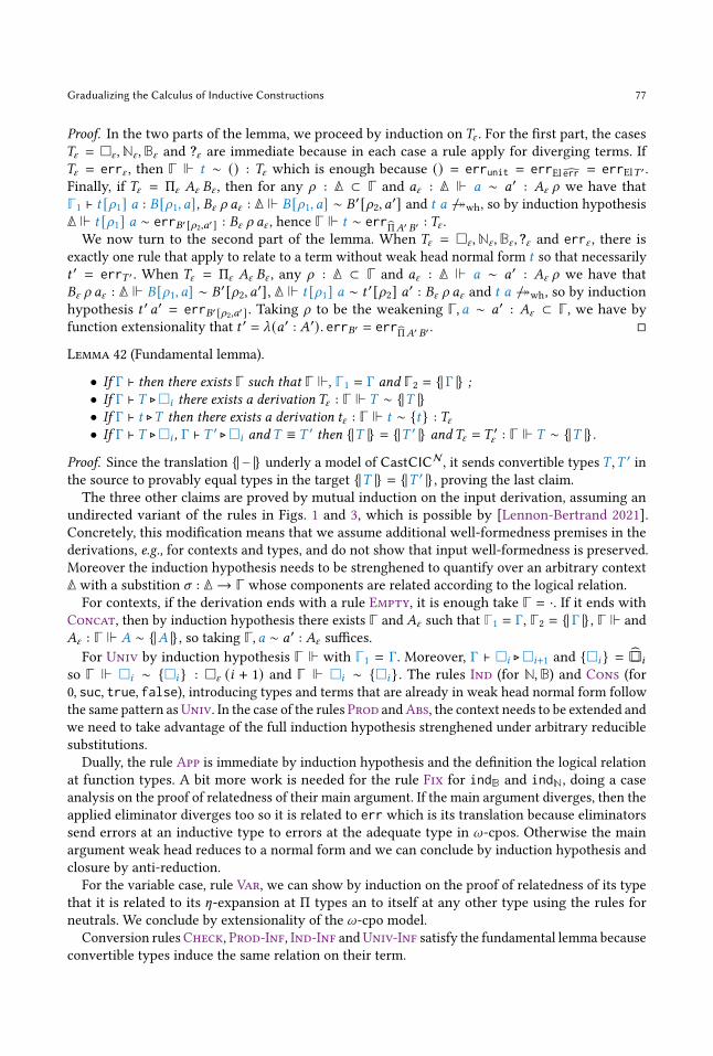
Gradualizing the Calculus of Inductive Constructions 77
Proof. In the two parts of the lemma, we proceed by induction on 𝑇Y . For the first part, the cases
𝑇Y = □Y ,NY ,BY and ?Y are immediate because in each case a rule apply for diverging terms. If
𝑇Y = errY , then Γ ⊩ 𝑡 ∼ () : 𝑇Y which is enough because () = errunit = errEl err = errEl𝑇 ′ .
Finally, if 𝑇Y = ΠY 𝐴Y 𝐵Y , then for any 𝜌 : ∆ ⊂ Γ and 𝑎Y : ∆ ⊩ 𝑎 ∼ 𝑎′ : 𝐴Y 𝜌 we have that
Γ1 ⊢ 𝑡 [𝜌1] 𝑎 : 𝐵 [𝜌1, 𝑎], 𝐵Y 𝜌 𝑎Y : ∆ ⊩ 𝐵 [𝜌1, 𝑎] ∼ 𝐵′[𝜌2, 𝑎′] and 𝑡 𝑎 ↠wh, so by induction hypothesis
∆ ⊩ 𝑡 [𝜌1] 𝑎 ∼ err𝐵′ [𝜌2,𝑎′ ] : 𝐵Y 𝜌 𝑎Y , hence Γ ⊩ 𝑡 ∼ errΠ𝐴′ 𝐵′ : 𝑇Y .
We now turn to the second part of the lemma. When 𝑇Y = □Y ,NY ,BY , ?Y and errY , there is
exactly one rule that apply to relate to a term without weak head normal form 𝑡 so that necessarily
𝑡 ′ = err𝑇 ′ . When 𝑇Y = ΠY 𝐴Y 𝐵Y , any 𝜌 : ∆ ⊂ Γ and 𝑎Y : ∆ ⊩ 𝑎 ∼ 𝑎′ : 𝐴Y 𝜌 we have that
𝐵Y 𝜌 𝑎Y : ∆ ⊩ 𝐵 [𝜌1, 𝑎] ∼ 𝐵′[𝜌2, 𝑎′], ∆ ⊩ 𝑡 [𝜌1] 𝑎 ∼ 𝑡 ′[𝜌2] 𝑎′ : 𝐵Y 𝜌 𝑎Y and 𝑡 𝑎 ↠wh, so by induction
hypothesis 𝑡 ′ 𝑎′ = err𝐵′ [𝜌2,𝑎′ ] . Taking 𝜌 to be the weakening Γ, 𝑎 ∼ 𝑎′ : 𝐴Y ⊂ Γ, we have by
function extensionality that 𝑡 ′ = _(𝑎′ : 𝐴′). err𝐵′ = errΠ𝐴′ 𝐵′ . □
Lemma 42 (Fundamental lemma).
• If Γ ⊢ then there exists Γ such that Γ ⊩, Γ1 = Γ and Γ2 = {| Γ |} ;• If Γ ⊢ 𝑇 ⊲□𝑖 there exists a derivation 𝑇Y : Γ ⊩ 𝑇 ∼ {|𝑇 |}• If Γ ⊢ 𝑡 ⊲𝑇 then there exists a derivation 𝑡Y : Γ ⊩ 𝑡 ∼ {𝑡} : 𝑇Y• If Γ ⊢ 𝑇 ⊲□𝑖 , Γ ⊢ 𝑇 ′ ⊲□𝑖 and 𝑇 ≡ 𝑇 ′
then {|𝑇 |} = {|𝑇 ′ |} and 𝑇Y = 𝑇 ′Y : Γ ⊩ 𝑇 ∼ {|𝑇 |} .
Proof. Since the translation {| − |} underly a model of CastCICN, it sends convertible types 𝑇,𝑇 ′
in
the source to provably equal types in the target {|𝑇 |} = {|𝑇 ′ |} , proving the last claim.
The three other claims are proved by mutual induction on the input derivation, assuming an
undirected variant of the rules in Figs. 1 and 3, which is possible by [Lennon-Bertrand 2021].
Concretely, this modification means that we assume additional well-formedness premises in the
derivations, e.g., for contexts and types, and do not show that input well-formedness is preserved.
Moreover the induction hypothesis needs to be strenghened to quantify over an arbitrary context
∆ with a substition 𝜎 : ∆ → Γ whose components are related according to the logical relation.
For contexts, if the derivation ends with a rule Empty, it is enough take Γ = ·. If it ends withConcat, then by induction hypothesis there exists Γ and 𝐴Y such that Γ1 = Γ, Γ2 = {| Γ |} , Γ ⊩ and
𝐴Y : Γ ⊩ 𝐴 ∼ {|𝐴 |} , so taking Γ, 𝑎 ∼ 𝑎′ : 𝐴Y suffices.
For Univ by induction hypothesis Γ ⊩ with Γ1 = Γ. Moreover, Γ ⊢ □𝑖 ⊲□𝑖+1 and {□𝑖 } = □□𝑖
so Γ ⊩ □𝑖 ∼ {□𝑖 } : □Y (𝑖 + 1) and Γ ⊩ □𝑖 ∼ {□𝑖 } . The rules Ind (for N,B) and Cons (for
0, suc, true, false), introducing types and terms that are already in weak head normal form follow
the same pattern asUniv. In the case of the rules Prod andAbs, the context needs to be extended and
we need to take advantage of the full induction hypothesis strenghened under arbitrary reducible
substitutions.
Dually, the rule App is immediate by induction hypothesis and the definition the logical relation
at function types. A bit more work is needed for the rule Fix for indB and indN, doing a case
analysis on the proof of relatedness of their main argument. If the main argument diverges, then the
applied eliminator diverges too so it is related to err which is its translation because eliminators
send errors at an inductive type to errors at the adequate type in 𝜔-cpos. Otherwise the main
argument weak head reduces to a normal form and we can conclude by induction hypothesis and
closure by anti-reduction.
For the variable case, rule Var, we can show by induction on the proof of relatedness of its type
that it is related to its [-expansion at Π types an to itself at any other type using the rules for
neutrals. We conclude by extensionality of the 𝜔-cpo model.
Conversion rulesCheck, Prod-Inf, Ind-Inf andUniv-Inf satisfy the fundamental lemma because
convertible types induce the same relation on their term.
78 Meven Lennon-Bertrand, Kenji Maillard, Nicolas Tabareau, and Éric Tanter
For Err, we have by induction hypothesis that 𝑇Y : Γ ⊩ 𝑇 ∼ {𝑇 } : □Y . By case analysis, 𝑇Yis necessarily one of errY ,ΠY , ?Y ,BY ,NY or □Y . If 𝑇Y = errY 𝑇 then Γ ⊩ err𝑇 ∼ () : errY 𝑇 since
Γ1 ⊢ err𝑇 ⊲𝑇 , and we can conclude using extensionality of unit = {|𝑇 |} , that is {err𝑇 } = (). If𝑇Y = ΠY 𝐴Y 𝐵Y , then for any 𝜌 : ∆ ⊂ Γ and 𝑎Y : ∆ ⊩ 𝑎 ∼ 𝑎′ : 𝐴Y 𝜌 we have that𝑇 [𝜌1] ↠wh Π(𝑎 : 𝐴)𝐵and err𝑇 𝑎 ↠wh err𝐵 [𝑎] , so we conclude this case by induction hypothesis ∆ ⊩ err𝐵 [𝑎] ∼{err𝐵 [𝑎]} : 𝐵Y 𝑎Y , closure by anti-reduction and the fact that {err𝐵 [𝑎]} = err{𝐵 [𝑎] } = err{𝐵 } [𝑎′ ] .In all the other cases 𝑇 weak head reduces to a type in weak head normal form ?□,□𝑖 ,N or B,
and a corresponding rule is present in the logical relation to conclude directly. A similar proof
apply for the rule Unk.
Finally, for the rule Cast with conclusion Γ ⊢ ⟨𝐵 ⇐ 𝐴⟩ 𝑡 ⊲𝐵, we have by induction hypothesis
we have that Γ ⊩, 𝐴Y : Γ ⊩ 𝐴 ∼ {|𝐴 |}, 𝐵Y : Γ ⊩ 𝐵 ∼ {| 𝐵 |} and Γ ⊩ 𝑡 ∼ {𝑡} : 𝐴Y . By analysing all
possible weak head reduction paths from ⟨𝐵 ⇐ 𝐴⟩ 𝑡 , either:(a) ⟨𝐵 ⇐ 𝐴⟩ 𝑡 ↠wh 𝑢 such that Γ ⊩ 𝑢 ∼ {𝑢} : 𝐵Y using inversions on 𝐴Y , 𝐵Y and 𝑡Y , or
(b) one of 𝐴, 𝐵 or 𝑡 never reduces to a weak head normal form.
In case (a), we conclude that Γ ⊩ ⟨𝐵 ⇐ 𝐴⟩ 𝑡 ∼ {⟨𝐵 ⇐ 𝐴⟩ 𝑡} : 𝐵Y by closure under anti-reduction
and using the fact that {⟨𝐵 ⇐ 𝐴⟩ 𝑡} = {𝑢} (because {−} maps convertible terms to equal terms in
the model). In case (b), we have that Γ ⊩ ⟨𝐵 ⇐ 𝐴⟩ 𝑡 ∼ err{𝐵 } : 𝐵Y by the first part of Lemma 41
and the second part of that lemma ensures that one of {𝐴} , {𝐵} or {𝑡} is an error at the adequate
type so that {⟨𝐵 ⇐ 𝐴⟩ 𝑡} =↓?{𝐵 } ↑?{𝐴} {𝑡} = err{𝐵 } . □
Corollary 43. If Γ ⊢ 𝑡 ⊲𝑇 and 𝑡 ↠wh then {𝑡} = err{𝑇 } .
Proof. By the fundamental lemma, Γ ⊩ 𝑡 ∼ {𝑡} : 𝑇Y with 𝑇Y : Γ ⊩ 𝑇 ∼ {𝑇 } : □Y and by the second
part of Lemma 41, {𝑡} = err{𝑇 } . □
E A DIRECT PRESENTATION OF VECTORSVectors have two new normal forms, corresponding to cast of nil and cons to vec𝐴 ?N. The differ-
encewith the treatment of the universe is that the corresponding term, for instance ⟨vec 𝐴 ?N ⇐ vec 𝐴 𝑛⟩ 𝑡for the case of nil, can not be considered as canonical form because they involve a non-linear
occurrence of𝐴. To remedy to this issue, we add two new canonical forms (nil? 𝐴 and cons? 𝐴 𝑎 𝑛 𝑣)
to vectors with introduction typing rules defined in Appendix E.
Regarding cast on vectors, it does not only compute in the argument of the cast as it is the case
for inductive types without indices, but it also computes on the indices. That is, a cast on vectors is
neutral when either one of the indices is neutral or the argument is neutral (see Appendix E). Other
kind of neutral can be derived from the one of inductive types without indices and are omitted
here.
Similarly, we do not detail the other typing rules for vectors as they are similar to the one for
inductive types wihtout indices, and focus on explaining the new reduction rules, presented also in
Appendix E.
The two first reduction rules v-rect-nil and v-rect-cons are standard reduction rules in CIC
for the recursor vect_rect on vectors. The rules v-rect-err and v-rect-unk are the standard
rules dealing with exceptions. Additionally, there are two computation rules for the eliminator on
the two new constructors v-rect-nilu and v-rect-consu which basically consist in the underlying
non-exceptional constructor to the eliminator and cast the result back to 𝑃 ?N. This rule somehow
transfers the cast on vectors to a cast on the returned type of the predicate.
Finally, there are rules to conduct casts between vectors in canonical forms. The last three rules
(V-unk, V-err and V-to-err) are simply propogation of errors. Then, there remains 12 rules, 3 by
constructors of vectors. We just explain the one on cons. Rule V-cons applies when both indices

Gradualizing the Calculus of Inductive Constructions 79
of the form 𝑆 of somthing and progates the cast of the arguments, as does the standard rule for
casting a constructor. Rule V-cons-nil detects that the indices do not match and raise an error.
Finally, Rule V-cons-? propagates the cast on the arguments, but this time applied to cons?, thusconverting precise information to a less precise information.

80 Meven Lennon-Bertrand, Kenji Maillard, Nicolas Tabareau, and Éric Tanter
Γ ⊩ logical relation between CastCICNcontexts and 𝜔-cpos.
· ⊩Γ ⊩ 𝐴Y : Γ ⊩ 𝐴 ∼ 𝐴′
Γ, 𝑎 ∼ 𝑎′ : 𝐴Y ⊩
·1 = ·(Γ, 𝑎 ∼ 𝑎′ : 𝐴Y)1 = Γ1, 𝑎 : 𝐴
Γ ⊩ 𝐴 ∼ 𝐵 logical relation between CastCICGtypes 𝐴 and 𝜔-cpos 𝐵 ⊂ ¥?.
Γ ⊩ 𝑇 ∼ 𝑈 : □Y
Γ ⊩ 𝑇 ∼ El𝑈
Γ ⊩ 𝑡 ∼ 𝑢 : BY logical relation between CastCICGterms of type B and elements of
¥B.
Γ1 ⊢ 𝑡 ⊲B 𝑡 ↠wh true Γ ⊩
Γ ⊩ 𝑡 ∼ true : BY
Γ1 ⊢ 𝑡 ⊲B 𝑡 ↠wh false Γ ⊩
Γ ⊩ 𝑡 ∼ false : BY
Γ1 ⊢ 𝑡 ⊲B 𝑡 ↠wh ?B Γ ⊩
Γ ⊩ 𝑡 ∼ ⊤ ¥B : BY
Γ1 ⊢ 𝑡 ⊲B 𝑡 ↠wh errB ∨𝑡 ↠wh Γ ⊩
Γ ⊩ 𝑡 ∼ ⊥ ¥B : BY
Γ1 ⊢ 𝑡 ⊲B 𝑡 ↠wh 𝑡 ′ Γ ⊩ 𝑡 ′ ∼ne 𝑢 : BY
Γ ⊩ 𝑡 ∼ 𝑢 : BY
Γ ⊩ 𝑡 ∼ 𝑢 : NY logical relation between CastCICGterms of type N and elements of
¥N.
Γ1 ⊢ 𝑡 ⊲N 𝑡 ↠wh 0 Γ ⊩
Γ ⊩ 𝑡 ∼ 0 : NY
Γ1 ⊢ 𝑡 ⊲N 𝑡 ↠wh suc 𝑡 ′ Γ ⊩ 𝑡 ′ ∼ 𝑢 ′: NY
Γ ⊩ 𝑡 ∼ suc𝑢 ′: NY
Γ1 ⊢ 𝑡 ⊲N 𝑡 ↠wh ?N Γ ⊩
Γ ⊩ 𝑡 ∼ ⊤ ¥N : NY
Γ1 ⊢ 𝑡 ⊲N 𝑡 ↠wh errN ∨𝑡 ↠wh Γ ⊩
Γ ⊩ 𝑡 ∼ ⊥ ¥N : NY
Γ1 ⊢ 𝑡 ⊲N 𝑡 ↠wh 𝑡 ′ Γ ⊩ 𝑡 ′ ∼ne 𝑢 : NY
Γ ⊩ 𝑡 ∼ 𝑢 : NY
Γ ⊩ 𝑡 ∼ 𝑢 : ?Y 𝑖 logical relation between CastCICGterms of type ?□𝑖
and elements of ¥?𝑖 .
Γ1 ⊢ 𝑡 ⊲ ?□ 𝑡 ↠wh ??□𝑖Γ ⊩
Γ ⊩ 𝑡 ∼ ⊤¥?𝑖 : ?Y 𝑖
Γ1 ⊢ 𝑡 ⊲ ?□ 𝑡 ↠wh err?□𝑖∨𝑡 ↠wh Γ ⊩
Γ ⊩ 𝑡 ∼ ⊥¥?𝑖 : ?Y 𝑖
Γ1 ⊢ 𝑡 ⊲ ?□ 𝑡 ↠wh ⟨?⇐ 𝐴⟩ 𝑡 ′ Γ ⊩ 𝑡 ′ ∼ 𝑢 ′: 𝐴Y
Γ ⊩ 𝑡 ∼↑?𝐴′ 𝑢
′: ?Y 𝑖
Γ1 ⊢ 𝑡 ⊲ ?□ 𝑡 ↠wh 𝑡 ′ Γ ⊩ 𝑡 ′ ∼ne 𝑢 : ?Y 𝑖
Γ ⊩ 𝑡 ∼ 𝑢 : ?Y 𝑖
Fig. 21. Logical relation between CastCICGand 𝜔-cpos

Gradualizing the Calculus of Inductive Constructions 81
Γ ⊩ 𝑡 ∼ 𝑢 : errY 𝐴 logical relation between CastCICGterms of type 𝐴 and elements of unit.
Γ1 ⊢ 𝑡 ⊲𝐴Γ ⊩ 𝑡 ∼ () : errY 𝐴
Γ ⊩ 𝑡 ∼ 𝑢 : □Y 𝑖 logical relation between CastCICGterms of type □𝑖 and elements of □□𝑖 .
NY
Γ1 ⊢ 𝑇 ⊲□𝑖 𝑇 ↠wh N Γ ⊩
Γ ⊩ 𝑇 ∼ N : □Y 𝑖
?YΓ1 ⊢ 𝑇 ⊲□𝑖 𝑇 ↠wh ?□𝑖
Γ ⊩
Γ ⊩ 𝑇 ∼ ?𝑖 : □Y 𝑖
errYΓ1 ⊢ 𝑇 ⊲□𝑖 𝑇 ↠wh err□𝑖
∨𝑇 ↠wh Γ ⊩
Γ ⊩ 𝑇 ∼ err : □Y 𝑖
□YΓ1 ⊢ 𝑇 ⊲□𝑖 𝑇 ↠wh □𝑗 Γ ⊩
Γ ⊩ 𝑇 ∼ □□𝑗 : □Y 𝑖
ΠY
Γ1 ⊢ 𝑇 ⊲□𝑖 𝑇 ↠wh Π(𝑎 : 𝐴) 𝐵 𝐴Y : ∀𝜌 : ∆ ⊆ Γ,∆ ⊩ 𝐴[𝜌1] ∼ 𝐴′[𝜌2] : □Y 𝑖
∀𝜌 : ∆ ⊆ Γ,∆ ⊩ 𝑎 ∼ 𝑎′ : 𝐴Y 𝜌 =⇒ Γ ⊩ 𝐵 [𝑎] ∼ 𝐵′[𝑎′] : □Y 𝑖
Γ ⊩ 𝑇 ∼ Π𝐴′ (_(𝑎′ : 𝐴′).𝐵′) : □Y 𝑖
neYΓ1 ⊢ 𝑡 ⊲□𝑖 𝑡 ↠wh 𝑡 ′ Γ ⊩ 𝑡 ′ ∼ne 𝑢 : □Y 𝑖
Γ ⊩ 𝑡 ∼ 𝑢 : □Y 𝑖
Γ ⊩ 𝑡 ∼ 𝑢 : ΠY 𝐴Y 𝐵Y logical relation between CastCICGterms of Π type.
∀(𝜌 : ∆ ⊆ Γ) (𝑎Y : ∆ ⊩ 𝑎 ∼ 𝑎′ : 𝐴Y 𝜌), ∆ ⊩ 𝑡 [𝜌1] 𝑎 ∼ 𝑢 [𝜌2] 𝑎′ : 𝐵Y 𝜌 𝑎Y
Γ ⊩ 𝑡 ∼ 𝑢 : ΠY 𝐴Y 𝐵Y
where
• Γ1 ⊢ 𝑡 ⊲Π (𝑎 : 𝐴) 𝐵,• Γ2 ⊢IR 𝑢 : Π𝜔 (𝑎′ : 𝐴′) 𝐵′
,
• 𝐴Y : ∀𝜌 : ∆ ⊆ Γ,∆ ⊩ 𝐴[𝜌1] ∼ 𝐴′[𝜌2] : □Y 𝑖
• 𝐵Y : ∀𝜌 : ∆ ⊆ Γ,∆ ⊩ 𝑎 ∼ 𝑎′ : 𝐴Y 𝜌 =⇒ ∆ ⊩ 𝐵 [𝑎] ∼ 𝐵′[𝑎′] : □Y 𝑖
Fig. 22. Logical relation between CastCICGand 𝜔-cpos

82 Meven Lennon-Bertrand, Kenji Maillard, Nicolas Tabareau, and Éric Tanter
Γ ⊩ 𝑡 ∼ 𝑢 : neY 𝐴Y logical relation on CastCICGterms of a neutral type 𝐴 (𝐴Y : Γ ⊩ 𝐴 ∼ 𝐴′
).
Γ ⊩ 𝑡 ∼ne 𝑡′
: neY 𝐴Y
Γ ⊩ 𝑡 ∼ () : neY 𝐴Y
Γ ⊩ 𝑡 ∼ne 𝑢 : 𝐴Y logical relation on neutral CastCICGterms (excerpt).
Γ ⊩ 𝑎 ∼ 𝑎′ : 𝐴Y ∈ Γ
Γ ⊩ 𝑎 ∼ne 𝑎′
: 𝐴Y
Γ ⊩ 𝑓 ∼ne 𝑓 ′ : ΠY 𝐴Y 𝐵Y 𝑡Y : Γ ⊩ 𝑡 ∼ 𝑡 ′ : 𝐴Y
Γ ⊩ 𝑓 𝑡 ∼ne 𝑔 𝑢 : 𝐵Y 𝑡Y
𝑏Y : Γ ⊩ 𝑏 ∼ne 𝑏′
: BY 𝑃Y : Γ, 𝑧 ∼ 𝑧 ′ : BY ⊩ 𝑃 ∼ 𝑃 ′
Γ ⊩ 𝑡true ∼ 𝑡 ′true : 𝑃Y [true ∼ true] Γ ⊩ 𝑡false ∼ 𝑡 ′false : 𝑃Y [false ∼ false]Γ ⊩ indB (𝑏, 𝑧.𝑃, (𝑡true, 𝑡false)) ∼ne indB (𝑏 ′, 𝑧 ′.𝑃 ′, (𝑡 ′true, 𝑡 ′false)) : 𝑃Y [𝑏Y]
𝐴Y : Γ ⊩ 𝐴 ∼ne 𝐴′
: □Y
Γ ⊩ ?𝐴 ∼ne ?𝐴′ : 𝐴Y
𝐴Y : Γ ⊩ 𝐴 ∼ne 𝐴′
: □Y
Γ ⊩ err𝐴 ∼ne err𝐴′ : 𝐴Y
𝐴Y : Γ ⊩ 𝐴 ∼ne 𝐴′
: □Y 𝐵Y : Γ ⊩ 𝐵 ∼ 𝐵′: □Y Γ ⊩ 𝑡 ∼ 𝑡 ′ : 𝐴Y
Γ ⊩ ⟨𝐵 ⇐ 𝐴⟩ 𝑡 ∼ne↓?𝐵′↑?𝐴′ 𝑡′
: 𝐵Y
Fig. 23. Logical relation between CastCICGand 𝜔-cpos

Gradualizing the Calculus of Inductive Constructions 83
canonical nil 𝐴 canonical(cons 𝐴 𝑎 𝑛 𝑣) canonical nil? 𝐴 canonical(cons? 𝐴 𝑎 𝑛 𝑣)
neutral 𝑣 ∨ neutral𝑛 ∨ neutral𝑚
neutral(⟨vec 𝐵 𝑚 ⇐ vec 𝐴 𝑛⟩ 𝑣)neutral 𝑣
neutral(vec_rect 𝑃 𝑃𝑛𝑖𝑙 𝑃𝑐𝑜𝑛𝑠 𝑣)
Γ ⊢ 𝐴 ⊳□𝑖
Γ ⊢ nil?@{i} 𝐴 ⊲ vec 𝐴 ?Nnilu
Γ ⊢ 𝐴 ⊳□𝑖 Γ ⊢ 𝑎 ⊳𝐴 Γ ⊢ 𝑛 ⊳N Γ ⊢ 𝑣 ⊳ vec 𝐴 𝑛
Γ ⊢ cons?@{i} 𝐴 𝑎 𝑛 𝑣 ⊲ vec 𝐴 ?Nconsu
v-rect-nil : vec_rect 𝑃 𝑃𝑛𝑖𝑙 𝑃𝑐𝑜𝑛𝑠 nil 𝐴 { 𝑃𝑛𝑖𝑙
v-rect-cons : vec_rect 𝑃 𝑃𝑛𝑖𝑙 𝑃𝑐𝑜𝑛𝑠 (cons 𝐴 𝑎 𝑛 𝑣) { 𝑃𝑐𝑜𝑛𝑠 𝑎 𝑛 (vec_rect 𝑃 𝑃𝑛𝑖𝑙 𝑃𝑐𝑜𝑛𝑠 𝑣)
v-rect-err : vec_rect 𝑃 𝑃𝑛𝑖𝑙 𝑃𝑐𝑜𝑛𝑠 errvec 𝐴 𝑛 { err𝑃 errvec 𝐴 𝑛
v-rect-unk : vec_rect 𝑃 𝑃𝑛𝑖𝑙 𝑃𝑐𝑜𝑛𝑠 ?vec 𝐴 𝑛 { ?𝑃 ?vec 𝐴 𝑛
v-rect-nilu : vec_rect 𝑃 𝑃𝑛𝑖𝑙 𝑃𝑐𝑜𝑛𝑠 nil? 𝐴 { ⟨𝑃 ?N ⇐ 𝑃 0⟩ (vec_rect 𝑃 𝑃𝑛𝑖𝑙 𝑃𝑐𝑜𝑛𝑠 nil 𝐴)
v-rect-consu : vec_rect 𝑃 𝑃𝑛𝑖𝑙 𝑃𝑐𝑜𝑛𝑠 (cons? 𝐴 𝑎 𝑛 𝑣) {
⟨𝑃 ?N ⇐ 𝑃 (𝑆 𝑛)⟩ (vec_rect 𝑃 𝑃𝑛𝑖𝑙 𝑃𝑐𝑜𝑛𝑠 (cons 𝐴 𝑎 𝑛 𝑣))
V-nil : ⟨vec 𝐵 0 ⇐ vec 𝐴 0⟩ nil 𝐴 { nil 𝐵
V-nil-cons : ⟨vec 𝐵 (𝑆 𝑛) ⇐ vec 𝐴 0⟩ nil 𝐴 { errvec 𝐵 (𝑆 𝑛)
V-nil-? : ⟨vec 𝐵 ?N ⇐ vec 𝐴 0⟩ nil 𝐴 { nil? 𝐵
V-cons : ⟨vec 𝐵 (𝑆 𝑚) ⇐ vec 𝐴 (𝑆 𝑛)⟩ (cons 𝐴 𝑎 𝑘 𝑣) { cons 𝐵 (⟨𝐵 ⇐ 𝐴⟩ 𝑎) 𝑚 (⟨vec 𝐵 𝑚 ⇐ vec 𝐴 𝑘⟩ 𝑣)
V-cons-nil : ⟨vec 𝐵 0 ⇐ vec 𝐴 (𝑆 𝑛)⟩ (cons 𝐴 𝑎 𝑘 𝑣) { errvec 𝐵 0
V-cons-? : ⟨vec 𝐵 ?N ⇐ vec 𝐴 (𝑆 𝑛)⟩ (cons 𝐴 𝑎 𝑘 𝑣) { cons? 𝐵 (⟨𝐵 ⇐ 𝐴⟩ 𝑎) 𝑛 (⟨vec 𝐵 𝑛 ⇐ vec 𝐴 𝑘⟩ 𝑣)
V-nilu : ⟨vec 𝐵 ?N ⇐ vec 𝐴 ?N⟩ nil? 𝐴 { nil? 𝐵
V-nilu-nil : ⟨vec 𝐵 0 ⇐ vec 𝐴 ?N⟩ nil? 𝐴 { nil 𝐵
V-nilu-cons : ⟨vec 𝐵 (𝑆 𝑛) ⇐ vec 𝐴 ?N⟩ nil? 𝐴 { errvec 𝐵 (𝑆 𝑛)
V-consu : ⟨vec 𝐵 ?N ⇐ vec 𝐴 ?N⟩ (cons? 𝐴 𝑎 𝑘 𝑣) { cons? 𝐵 (⟨𝐵 ⇐ 𝐴⟩ 𝑎) 𝑘 (⟨vec 𝐵 𝑘 ⇐ vec 𝐴 𝑘⟩ 𝑣)
V-consu-nil : ⟨vec 𝐵 0 ⇐ vec 𝐴 ?N⟩ (cons? 𝐴 𝑎 𝑘 𝑣) { errvec 𝐵 0
V-consu-cons : ⟨vec 𝐵 (𝑆 𝑛) ⇐ vec 𝐴 ?N⟩ (cons? 𝐴 𝑎 𝑘 𝑣) {
cons 𝐵 (⟨𝐵 ⇐ 𝐴⟩ 𝑎) 𝑛 (⟨vec 𝐵 𝑛 ⇐ vec 𝐴 𝑘⟩ 𝑣)
V-unk : ⟨vec 𝐵 𝑚 ⇐ vec 𝐴 𝑛⟩ ?vec 𝐴 𝑛 { ?vec 𝐵 𝑚 𝑚,𝑛 ∈ {0, 𝑆 𝑚, ?N, errN}
V-err : ⟨vec 𝐵 𝑚 ⇐ vec 𝐴 𝑛⟩ errvec 𝐴 𝑛 { errvec 𝐵 𝑚 𝑚,𝑛 ∈ {0, 𝑆 𝑚, ?N, errN}
V-to-err : ⟨vec 𝐵 errN ⇐ vec 𝐴 𝑛⟩ 𝑣 { errvec 𝐵 errN 𝑛 ∈ {0, 𝑆 𝑚, ?N, errN} and 𝑣 ≠ ?vec 𝐴 𝑛
Fig. 24. Canonical forms and reduction rule for vectors.