Robust smooth magneto tell uric transfer functions

Geophys. J. lnt. (1996) 124,801-819

Robust smooth magnetotelluric transfer functions

Jimmy C. Larsen,’ Randall L. Mackie,2 Adele Man~e l l a ,~ Adolfo Fiordelisi4 and Shirley Rieven2 ‘Pacific Marine Environmental Laboratory, National Oceanic and Atmospheric Administration, 7600 Sand Point Way NE, Seattle WA 981 15-0070 USA ’ Wassachusetts Institute of Technology, 42 Carleton Street, Cambridge, M A 02142, USA CNR-International Institute for Geothermal Research, Piazza Soljerino 2, Pisa 56126, Italy ENEL, Esplorazione Mineraria, Via Andrea Pisano, 120 Pisa 56122, Italy

Accepted 1995 October 2. Received 1995 September 19; in original form 1994 October 26

SUMMARY Robust estimates of the magnetotelluric (MT) transfer function are found using an iterative reweighted method on time series data corrected for outliers and gaps. The MT transfer function, composed of several analytic functions smoothly varying in frequency, is used to represent the frequency-domain relationship between electric and magnetic time series. The smoothly varying transfer function facilitates identification and removal of electric and magnetic outliers (spikes), construction of the frequency- and time-domain weights used for obtaining robust smooth and band-averaged estimates, and separation of the time series into MT and correlated noise signals if a remote site exists that is free of the correlated noise. Errors in the transfer function are calculated using jackknife estimates of the solution covariance. The method is tested on: time series from a relatively clean MT site in central California; a test time series based on Tucson magnetic time series plus synthetic noise for a given transfer function; and time series from the Larderello geothermal region in central Italy where there are strong signals from d.c. electrified railways.

Key words: electromagnetic methods.

1 INTRODUCTION

Magnetotelluric (MT) transfer functions, representing the frequency-domain relationship between observed electric and magnetic time series, are used to construct earth conductivity models. This requires accurate estimates of the transfer functions. We have therefore developed a robust method using a smoothly varying transfer function to facilitate the identification and removal of outliers (spikes) and the construction of frequency- and time-domain weights needed for robust estimates. Smoothness is consistent with transfer functions generated from models of the Earth, including those having large conductivity changes, because the electromagnetic induction problem is diffusive and therefore sensitive only to the spatially averaged conductivity. Our method also facilitates the separation of time series into MT and correlated noise signals if a remote site exists that is free of the correlated noise. Correlated noise can be caused, for example, by active cathodic protection of pipelines or d.c. electrified railways.

Previous robust methods have concentrated on the Fourier transformation of variable-length data sections and have dealt with noisy time series by downweighting or rejecting noisy data sections (Chave & Thomson 1989; Chave, Thomson & Ander 1987; Egbert & Booker 1986; Egbert, Booker & Schultz

1992; Jones & Jodicke 1984; Sutarno & Vozoff 1991). Jones & Jodicke (1984), for example, obtained improved estimates using section weights based on coherence. Egbert & Booker (1986) showed that residuals for geomagnetic depth-sounding (GDS) time series often become larger when the intensity of the magnetic variations increases; they therefore used section weights inversely proportional to the intensity of the magnetic variations. These authors used a variant of this method in Egbert et al. (1992) for the 1932 to 1942 Tucson MT time series where, prior to the application of their method, short gaps and large electric outliers had been replaced by values predicted from the magnetic time series using an impulse response function; they did not consider magnetic outliers. Chave & Thomson (1989) and Thomson & Chave (1991) advanced the robust methods by introducing the use of jackknife estimates of error. Chave & Thomson (1989) also showed the importance of identifying and removing magnetic outliers. Chave & Thomson (1992) presented a new method based on the ‘hat matrix’ to control bias due to noise in the magnetic data sections even when it does not produce noise in the residuals. This ‘controlled leverage’ method is not considered here. Although these section-weighting methods overcome the inherent sensitivity to some noisy data sections, they may encounter difficulties if there are outliers or strong correlated noise signals in most data sections.

0 1996 RAS 801

802 J. C . Larsen et al.

The robust smooth method developed here uses an iterative procedure that is similar to reweighted least-squares for robust regression analysis (Rousseeuw & Leroy 1987) and improves on Larsen (1980, 1989) by using: (1) time series subdivided into data sections; ( 2 ) Chebyshev polynomials to represent the two- or three-dimensional (2-D or 3-D) part of the transfer function; (3) errors in the transfer function based on jackknife estimates of the solution covariance; (4) a procedure for identifying electric and magnetic outliers and replacing gaps and outliers; ( 5 ) a procedure for stabilizing the smooth estimates of the correction function using a damping factor based on matching the smooth errors to the undamped band- averaged errors; (6) magnetic components rotated into major and minor coherent components to minimize magnetic collinearity; and (7) section weights for downweighting those sections with numerous gaps and outliers and for rejecting those sections with coherence much smaller than the median value.

This paper first describes the frequency-domain relationship between electric and magnetic time series for MT induced variations and for situations where the MT variations are contaminated by correlated noise signals. The paper then describes the least-squares and remote-reference methods and discusses the smooth representation of the transfer function and the central issue of how to correct the time series for outliers, how to obtain robust smooth estimates objectively damped, and how to obtain realistic error estimates. The method is illustrated for time series from a relatively clean MT site in central California; a test time series based on the Tucson magnetic time series plus synthetic noise for a given transfer function; and time series from the Larderello geothermal area in central Italy where there are strong d.c. electric train-induced signals.

2 TRANSFER FUNCTIONS

The basic observations are the discrete electric time series e , ( t ) , the local magnetic time series b,(t), and the remote magnetic time series bF(t) for k = 1, ... , K horizontal components, t = 1, . . . , 2 J time values, and I data sections. The Fourier transforms of the time series are Ek(w), Bk(w) and BF(w) for j = 1, . . . , J angular frequencies w j = nj /J . We use lower-case letters for time series and upper-case letters for Fourier transforms of the time series. We assume an exp(-iwt) frequency dependence.

The observed electric and magnetic time series in the most general case contain MT variations EMT(w) and BMT(w) produced by small- or zero-wavenumber ionospheric sources, correlated noise signals Ec(w) and Bc(u) produced by cultural (man-made) sources or large-wavenumber ionospheric events, and uncorrelated noise EU(w) and B"(w) produced by environmental sources such as ground motion or electrochemical reactions at the electrodes. For the scalar case, the MT relationship is

EMT(w) = ZMT(o)BMT(w),

and the correIated noise relationship is

EC(w) = ZC(u)Bc(w) ,

where the transfer functions ZMT(o>) and Zc(w) are generally not equal. The relationship for the combined MT and correlated noise is given by the two-source form

E(w) = ZMT(w)BM'(~) + ZC(w)Bc(w)

(Madden, personal communication) where

E(w) = EMT(w) + EC(w) .

2.1 MT signals

If the noise is uncorrelated, we can use the standard single- source form given by

for estimating the MT transfer functions Zk(w) and the residuals R(w) due to uncorrelated noise in the electric and magnetic time series. The residuals are used to locate the outliers, the spectral lines in the residuals, and the frequency- and time-domain weights. We define a spectral line as a spike in the amplitude spectrum that has a bandwidth of 1/T or less for a record length T.

For the remote-reference method we assert that the MT induced magnetic variations are consistent over large distances and can therefore be used to approximate the local magnetic variations (thus the term 'remote-reference'). Remote-reference estimates of the residuals RR(w) are calculated using the following relationship:

2.2 MT signals contaminated by correlated noise sources

If the time series contain both MT and correlated noise signals, we use the two-source form given by

K K

E(w) = c ZYT(w)BYT(w) + 1 Zf (w)B f (w) + R(w) (3) k = l k = l

for simultaneously estimating the MT transfer functions ZPT(w), the correlated noise transfer functions Z f ( w ) and the uncorrelated noise R(w). The transfer functions ZFT(o) and Zf(w) will generally be different.

To estimate BpT(w) and B f ( w ) we need a remote magnetic time series bF(t) free of the correlated noise signals. We then use the following relationship between the local and remote magnetic variations Bk(w) and BF(w),

(4)

to derive the magnetic transfer functions T,, where B f ( w ) is treated as part of the uncorrelated residuals. The magnetic transfer functions may, in some circumstances, be approximately real and equal to unity, but generally they are complex-valued and different from unity.

Having determined the magnetic transfer functions, the MT magnetic variations at the contaminated site are estimated from the remote magnetic variations by

Then the MT-induced magnetic time series bFT( t ) is the inverse Fourier transform of ByT(w) and the correlated noise magnetic time series is b:( t ) = b k ( t ) - bpT( t ) .

0 1996 RAS, GJI 124, 801-819

M T transfer functions 803

Method

2.3 Methods for estimating transfer functions

There are two statistical methods for estimating transfer functions. The method of least-squares minimizes the variance of the residuals, that is (IRI’), or (IBcI2) for the magnetic transfer functions, whereas the remote-reference method minimizes the modulus of the covariance between the locally estimated residuals R(w) and the remotely estimated residuals RR(w), that is I ( R R * R ) I (Sims, Bostick & Smith 1971; Gamble, Goubau & Clarke 1979; Larsen 1989), where ( ) indicates an average over all data sections and frequencies and * represents the complex conjugate.

The method for obtaining unbiased estimates of the transfer function will depend on the type of noise present in the various time series. The various possibilities are listed in Table 1. The robust least-squares single-source method can be used when there is uncorrelated electric noise but requires noise-free magnetic time series, or vice versa. The robust remote-reference method should be used when there is uncorrelated noise in both the electric and the magnetic time series.

If there is correlated noise at the local site then the single- source method yields an estimate of the MT transfer function that combines ZMT(w) and Zc(ot) and is therefore wrong in both amplitude and phase. It is therefore important to use the two-source relationship whenever the correlated noise is large. If the remote magnetic site is noise-free then the robust least- squares two-source method can be used. However, if the remote site contains uncorrelated noise then the robust remote-reference two-source method should be used, but this requires two remote magnetic sites. The remote-reference two-source method will not be discussed further because time series from two remote sites have not been collected. If the correlated noise is intermittent and therefore removable by the robust method, then the robust remote-reference single-source method should be used because these estimates will not be biased by any uncorrelated noise in the remote magnetic series.

One can show (Egbert, personal communication) that we obtain the same non-robust estimates of ZMT(w) by both the remote-reference single-source method and the least-squares two-source method if the magnetic transfer functions are derived by non-robust least squares. However, the robust methods can yield substantially different estimates of the transfer functions and the errors (see Section 5) .

Noise 1 E B I BR 1

3 SMOOTH TRANSFER FUNCTION REPRESENTATION

least-squares single-source

We represent the smooth

Z ( 0 ) = U(w)D(w)Z’-”(o)

U NF

0 1996 RAS, GJI 124, 801

MT transfer function by

(6)

where Z’-”(w) is the transfer function for a one-dimensional (1-D) model, D(w) is the non-dimensional smooth distortion function, and U(w) is the non-dimensional smooth correction function. The subscript k, representing the various magnetic components, is ignored to simplify the expressions. We have experimented with ignoring D(w), but found that using D(o) works better.

The method proposed here builds on a 1-D transfer function Z1-”(w) generated using a best-fitting 1-D earth conductivity model based on the previously estimated transfer function Z(w). The 1-D transfer function is then modified by a smoothly varying distortion function D(w), where D(w) is used to distort the 1-D transfer function to higher dimensions, 2-D or 3-D, if necessary, so that D(w)Z’-D(w) approximates the previously estimated transfer function. The smoothly varying correction function U(w) is then derived by the next iteration to correct the transfer function D(w)Z1-D(w) and to estimate the errors. We make no assumption that the actual transfer function is 1-D, causal, or minimum-phase.

We represent the magnetic transfer function by

T(w) = U(w)D(o) > (7) without using a 1-D transfer function, which will be approximately unity for most magnetic time series and thus is unnecess- ary. Details of the transfer function representation are described in the following sections.

3.1 One-dimensional transfer function Z’-D(o)

The previously estimated transfer function Z(w) and its errors &(a) are used to compute the best-fitting 1-D transfer function Z‘-D(w) by the D+ routine (Parker 1980). The routine yields real positive coefficients a,, and An for n = 1, ... , L, and these are used to generate the 1-D causal minimum-phase transfer function by

1 L - 1

Z y w ) = - iw [ a,/(A, - iw) + U L ,

where i = m. This is an expansion in partial fractions with singularities at 1, (Weidelt 1972).

3.2 Distortion function D(w)

We represent the distortion function D(w) by N Chebyshev polynomials IT;, as

N

D(w) = c d, T,cx(w)l> (8) n = 1

where d, are the complex-valued distortion coefficients. The frequency dependence is given by x(wj ) = 1 - 2 log(j/J)/

least-squares two-source 1 U & C 1 U C C I NF remote-reference two-source I U & C I U & C I U

119

804 J. C. Larsen et al.

log( l/J) for j = 1, .. . , J frequencies so that - 1 I x(wj) I 1. Then the Chebyshev polynomials are uniformly spaced in log frequency. Chebyshev polynomials are obviously not the only choice of polynomials but they are found to yield an accurate representation of a known transfer function, provided that N is large enough (see Section 5.2). After experimenting with fits to artificial transfer functions, we found that N 2 10 yielded excellent results for 2.5 decades of frequency. This suggests that N should be about four times the number of decades of frequency, that is, N > 4 logl,Jw,,,ax/~min) but the actual size of N will depend, of course, on the amount of variability in the true transfer function.

3.3 Correction function U(w)

We also represent the correction function U ( o ) by N Chebyshev polynomials T, as

(9)

where u, are the complex-valued correction coefficients. The expansion of the correction function U in terms of polynomials is necessary so that we can apply the time-domain weights without distorting the MT transfer function relationships ( 1) and (2) (see Section 4.5).

The standard error &‘(a) in U(w) is given by

where cov(u,u~) is the real part of the estimated covariance between u, and um. Note that representation (10) allows for correlations between frequencies and permits the error E ~ ( W )

to be computed as a smoothly varying function of frequency. The covariance is estimated by the jackknife method

(Thomson & Chave 1991), yielding I

cov(u ,u~)=( l - I - I ) a L c ( u n ~ - G “ ) ( u : ~ - U : ) (11) i = l

for I independent data sections where indicates the real part, u,; is the ith estimate based on all data sections excluding the ith section, and the mean value is U , =I- ’ cf=, u,,~. We have not jackknifed the entire robust process because of computational time limitations, and therefore the present jackknife estimates are only approximations. We conclude that these approximations are valid, however, because we obtain errors that are comparable in size to the jackknife estimates of the errors by the Chave section-weighting methods (Chave & Thomson 1989, 1992) when applied to a fairly clean time series (see Section 5.1).

The error E ( W ) in Z(o) is derived from the error ~ ‘ ( w ) in U ( 4 by

&(W) = ID(w)Z’-”(W)I&’(W), (12)

where D(w) and Z’-”(o) merely act as rescaling factors. The 95 per cent confidence limits on the estimated transfer function are given by Z(w)+j ’ ,~(w), where & is derived from the Student’s t distribution for n = I - 1 degrees of freedom, assuming I independent data sections (Thomson & Chave 1991). If I > 10, then PI z 1.96. The jackknife estimates for the remote-reference method are derived in a similar way, using the covariance between the correction coefficients.

3.4 Transfer function relationship

The single-source MT relationship (1) in terms of the correction coefficients u,k becomes

N X

E(w) = c c U , k K I X ( W ) I D k ( w ) Z : - D ( W ) B k ( W ) + R(w). (l3) n = l k = l

We simplify this equation by collecting the known function T,[x(w)], the observed Bk(w), and the previously computed Dk(w) and Z:-”(w) into one term given by

E n k ( w ) = r,[X(w)lDk(o)Z:-D(w)Bk(w). (14)

E(w)= 1 u n k E n k ( w ) $ - R ( w ) . (15)

Then the MT relationship (13) becomes N X

n = l k = l

We will show (Section 4.5) that the MT relationship (15) for the correction coefficients enables us to apply the time- domain weights and data window to the time series without distorting the basic MT relationship (1).

4 ROBUST ITERATIVE PROCEDURE

Estimation of the transfer function proceeds by successive iterations (see flow diagram Fig. 1). Here we ignore the subscript k, representing the different magnetic components, to simplify the expressions. We start with Z’-”(w), which is either a generic 1-D transfer function, a 1-D transfer function from a suitable site, or a 1-D transfer function derived from a GDS transfer function (Larsen 1980; Schultz & Larsen 1987), and with a distortion function D(o) = 1, no magnetic rotation, whitening W(w) = 1, frequency-domain weights F(w) = 1 except for known spectral lines where F(w) = 0, time-domain weights g( t ) = 1 except for time series gaps where g( t ) = 0, and section weights vi = 1 for i = 1, . . . , I sections. The smooth correction function U(w) is computed by least squares or remote reference and the new estimate of the transfer function is Z(w)= U(w)Z’-”(w). The new Z(w) and time series are then used to compute the frequency residuals R(w) and time residuals r( t ) [the inverse Fourier transform of R(w)]. These are used to determine the electric and magnetic outliers, the spectral lines, the whitening W(w), the frequency-domain weights F(w), the time-domain weights g ( t ) , and the section weights vi. The estimated Z(o)s for each magnetic component are then used to compute the magnetic rotation 0 (Appendix A), the 1-D transfer function Z’-”(w), and the smooth distortion function D(w) so that D(o)Z’-”(w) approximates the estimated transfer function. The process is repeated by recomputing the correction function U ( w ) using the time series corrected for outliers and gaps and weighted by the whitening, the frequency-domain weights, the time-domain weights and the section weights. The process is stopped when the number of new outliers is less than 0.5 per cent of the total number of data and V ( w ) is approximately unity. This usually occurs within six iterations.

Robust estimates of the transfer functions proceed in five stages. For the first stage, the time series are prewhitened, corrected for gaps and instrumental filters, detrended and rotated. For the second stage, outliers and spectral lines are identified and the time series corrected for these outliers and spectral lines. For the third stage, the whitening and time- and frequency-domain weights are constructed to make the residual noise approximately Rayleigh-distributed in the frequency

0 1996 RAS, G J f 124, 801-819

MTtrnnsfer functions 805

time series (zl- time series initialization preparation (section length,

window, weights)

E rotation I

I

- I

t m- Yes

I

I I I 1 I 1 I I I I I i 1 1 I I I I I 1 I 1 1 I I I

no I

I

magnetic transfer function T I I

I 1

I yes - _ " - - - _ _ - - - _ - - - - - - - - - -,I 1 I

I I I 1 I I I I I I I I I I I I I 1 I I I I I I I I 1 I I I I I I

I I I I I I I I 1 I I I I I I 1 I I I I 1 I I I I I 1 1 I I I I 1 1

distortion D (4.5) I T=;D I - t

I MT transfer fU_":tio_"_Z- - ~

1

1- - _ . . .__- - - - weights (4.3)

I 1 I I I I 1 I I I I I I I I 1 I 1 I I I I I I

weighted corrected i - l time series

-1 1 I 8 i I D I I I I 1 I I I I I I t I I 1 I I I I I f

I I I I I 1 I 1 I 1 I I 1 I

c

Z l D (3.1) distortion D (4.5)

time series

1 T = U D

I BR-polarization

correction U (4.5) Z = U D ZID

weights (4.3) 1 I I 1 I I I I I I I I I I

h I

I I

Figure 1. Flow diagram for the basic steps used to compute robust smooth estimates of the MT and magnetic transfer functions. Relevant sections are noted in parentheses

domain, approximately Gaussian-distributed in the time domain, and approximately stationary, and the section weights are constructed to downweight noisy data sections and to reject sections with low coherence. For the fourth stage, the magnetic components are rotated to reduce collinearity. For the final stage, the whitening, weights and rotated corrected time series are used to compute robust estimates of the correction functions.

periods relative to the 95 per cent confidence level. The length of the data sections is then fixed. We want to have at least 10 data sections, but often have time series consisting of 50 to 100 sections. Linear trends are then removed from all data sections, and the time series are prewhitened by a single term (Appendix B) to reduce any long-period drift. The gaps are then filled (see Section 4.2) and the time series are corrected for instrumental filters.

4.1 Stage one: time series pre-processing 4.1.2

The electric time series, if it consists of two components, can be rotated so that one component, labelled major, has the maximum amplitude variations (e.g. Kaufman & Keller 1981); the other component is labelled minor. If there is no local distortion this orientation gives electric time series

Rotation of electric time series

4.1 .I Time series preparation

If the time series are long and continuous, we subdivide them into overlapping data sections and shorten the length of the sections until there is significant coherence at the longest

0 1996 RAS, GJI 124, 801-819


approximately normal and parallel to the structure of the geology.

4.2 Stage two: correction for outliers

4.2.1 Electric outliers

Outliers in the electric time series are identified among the residuals r( t ) = e ( t ) - p( t ) - /( t ) , where p( t ) is the predicted electric time series using the magnetic time series and the estimated transfer functions, and L( t ) is the time series due to the spectral lines. Each residual value is compared to the robust error scale aMAD, the median absolute deviation (MAD), which is equal to 1.48 times the median of Ir(t) - pI where ,u is the median of r ( t ) . The factor 1.48 converts the error scale into the usual standard deviation if the residuals have a Gaussian distribution. Here, of course, the rescaled residuals will not be Gaussian, so aMAD is just used to help set a threshold level for detecting outliers in the residuals. Electric outliers are identified for those times t where Ir(t) - pl > 5.0aMAD. First differences of the residuals are also used to locate outliers.

4.2.2 Magnetic outliers

Outliers in the magnetic time series are found by constructing forward differences bf( t ) = b( t ) - b( t - 1 ) and backward differences bb(t) = b( t ) - b(t + 1) of the magnetic time series. These are compared to the robust error scale crMAD, which is equal to 1.48 times the median of Ib‘(t)l. The magnetic outliers are identified by Ibf(t)l > 4.50MAD and Ibb(t)l > 4.5aMAD for those times t corresponding to large outliers in the residuals.

Locating magnetic outliers using outliers in the residuals can be tricky (see Rousseeuw & Leroy 1987; Chave & Thomson 1989) because magnetic outliers can cause such a severe distortion in the transfer function that outliers in the residuals may not correspond to magnetic outliers. We guard against this by temporarily replacing all possible magnetic outliers when computing the initial estimate of the transfer function. There may also be magnetic outliers that do not produce outliers in the residuals. These ‘leverage values’ are not considered here.

4.2.3 Spectral lines

Spectral lines in the residuals are removed to eliminate their influence on the transfer function estimates. To identify spectral lines, we whiten the time series by a single term and then form frequency-band averages, excluding any previously identified lines. These frequency bands are then summed over all data sections and used to compute a piecewise linear trend. The amplitude spectrum, averaged over all data sections, is then divided by the pidcewise linear trend to form a detrended mean amplitude spectrum. The spectral lines are then identified where the detrended amplitudes are greater than 1.2 standard deviations.

4.2.4 Replacement values

It is important to replace gaps and outliers by values typifying the time series so that the replacements do not cause values near the replacements to become outliers for the next iteration.

Otherwise, the replacement region could grow progressively wider for each subsequent iteration. The replacements should also include the time series due to spectral lines so that the replacements do not distort or smear the spectral lines.

The replacement values for the electric time series are given by e( t ) = p( t ) + L( t ) + z( t ) , where p ( t ) is the predicted electric time series, L( t ) is the time series due to spectral lines, and z ( t ) is the local linear trend.

The replacement values for the magnetic data are b( t ) = !(t) + r ( t ) , where L(t) is the time series due to spectral lines in the magnetic time series and z( t ) is the local linear trend.

4.3 time-domain weighting

The whitening W(o), frequency-domain weights F(w), time- domain weights g ( t ) and section weights v i are computed from the residuals based on the electric and magnetic time series corrected for outliers and gaps. The weights are chosen to make these residuals approximately Rayleigh-distributed in the frequency domain, Gaussian-distributed in the time domain, and approximately stationary. Here the discussion assumes that the residuals have been corrected for outliers and spectral lines.

We apply the whitening W(w) and frequency-domain weights F(w) in the frequency domain as R W F ( u ) = F(w)W(w)R(w), and apply the time-domain weights g ( t ) in the time domain as rWFg( t ) = g ( t ) r W F ( t ) . The latter operation is accomplished by taking the Fourier inverse of R W R ( w ) , applying the time- domain weights g( t ) , and then taking the Fourier transform of rwFg( t ) to yield RWFg(w) . We call i ( t ) = rWFg( t ) the weighted residual time series.

Stage three: whitening and frequency- and

4.3.1 Whitening W(o)

Whitening is necessary so that all frequencies make approximately the same contribution to the least-squares or remote- reference estimates. Whitening is applied in two steps. We first estimate a single whitening term for each residual data section (Appendix B). This allows us to partially whiten the residual time series to reduce end effects and any long-period trends before applying the Fourier transform. The residuals, weighted by the previously derived W(w), F(w), and g( t ) , are then used to refine the whitening in the frequency domain (Appendix B). Finally, the whitening for each data section is divided by (/ I?(CLJ)~~)~’~, where < ) indicates an average over all frequencies, so that the weighted time series for each data section have approximately the same variance. This is basically an attempt to make the weighted residuals approximately stationary and was found experimentally to be necessary before computing the frequency- and time-domain weights. The rescaled complex-valued whitening function is labelled W(w).

4.3.2 Frequency-domain weights F(w)

Frequency-domain weights, 0 2 F(w) 2 1, are used to make the weighted residuals approximately Rayleigh-distributed and to reject non-Rayleigh distributed residuals. The weights are taken to be real to avoid introducing spurious phase shifts. Refinements to the weights are derived using the distribution of the residuals &a) weighted by the previously derived W(w), F(w), and g(t) . The distribution is found by dividing R(w) by

0 1996 RAS, GJI 124, 801-819


log apparent resistivity

phase 2 0 1

-90 i

-3.0 -2.0 -1 .o 0.0 1 .o 2.0 3.0

log second

Figure 2. Central California MT transfer function for N45"E estimated by the robust smooth least-squares single-source method (dots) and the Chave robust method (large open circles). The transfer function is plotted as common log (log,,) apparent resistivity (top panel) and phase (bottom panel) versus common log period. The errors are k5 standard deviations. Estimates of the transfer function and error are in excellent agreement.

the robust error scale aMAD, which is equal to 1.48 times the median of 19&fi(co)l and I$iR(o)\ for all frequencies, excluding spectral lines, where 928 is the real part and .$m is the imaginary part. The rescaled modulus Ifi(w)l/aMAD are then sorted into bins to form a histogram of their distribution with bin widths equal to five divided by the square root of the number of values. A Rayleigh curve is fit to 50 per cent of the values located near the peak of the distribution and this curve is compared to the observed distribution. (This assumes that at least 50 per cent of the frequencies have weights of unity, which was found experimentally to give reasonable results.) The weights are thus unity near the peak and are adjusted downwards along the tails until the number of values per bin is approximately Rayleigh-distributed, as described in Larsen (1989). We set the weights to zero for those frequencies where Ifi(w)l > 3oMAD to reject the non-Rayleigh-distributed weighted residuals.

distribution is found by dividing F(t) by the robust error scale ,,MAD , which is equal to 1.48 times the median of lF(t)-pl, with replacement values excluded and with p equal to the median of rwF( t ) . The rescaled residuals r^(t)/oMAD are then sorted into bins in order to form a histogram of their distribution. Bin widths are again set equal to five divided by the square root of the number of values. A Gaussian curve is fit to 50 per cent of the values located near the peak of the distribution and compared to the observed distribution. (This assumes that at least 50 per cent of the time series have time weights of unity, which was found experimentally to give reasonable results.) The weights are thus unity near the peak and are adjusted downwards along the tails until the number of values per bin is approximately Gaussian-distributed, as described in Larsen (1989). We set the weights to zero for those times where Ir^(t)l > 3oMAD to reject the non-Gaussian distributed weighted residuals.

4.3.3 Time-domain weights g ( t ) 4.3.4 Data window h ( t )

Time-domain weights, 0 I g( t ) 5 1, are used to make the weighted residuals approximately Gaussian-distributed and to reject non-Gaussian-distributed residuals. Refinements to the weights are derived using the distribution of the residuals i ( t ) weighted by the previously derived W(w), F(o) and g(t). The

Each weighted data section is multiplied by a data window h( t ) to reduce bias in the spectral estimates due to smearing of energy from high values to low values. For independent data sections we use a cosine data window consisting of a cosine taper of five per cent of the end values. We use this

0 1996 RAS, GJI 124, 801-819

808 J . C. Larsen et al.

4 -

3 - E i c 0

B 2 -

window rather than a window with more bias control in order to retain the long-period information. For overlapping data sections the length of the data sections can be increased, and we therefore use a 4n prolate data window to give more bias control and nearly independent data sections if the overlap is less than 37 per cent.

4.3.5 Section weights v i

Finally, section weights, 0 I v i 5 1, are used to downweight those sections with numerous gaps and outliers and to reject sections with low coherence. The ith data section weight v i is defined by the reduction in degrees of freedom due to outliers, gaps and spectral lines, and is approximated by

where h( t ) is the data window, f ( w ) = 1 for F(o) >0 , p(w) = 0 for F(w) = 0, g( t ) = 1 for g( t ) > 0, and g(t) = 0 for g ( t ) = 0. We also set v i = 0 in order to reject those sections where the coherence between electric and magnetic variations is much smaller than the median value or, for correlated noise signals, where the coherence between electric and correlated magnetic noise signals is much larger than the median value.


1 I phase Z

-30

I -90 I

log second

3.5 4.5 5.5 '6.5

The section weights are applied when estimating the correction function U(o).

4.4 Stage four: rotation of magnetic time series

Unstable estimates of the transfer functions can occur if the horizontal magnetic components are correlated. This is the collinearity problem, and it is minimized by rotating the magnetic components so that one component accounts for most of the coherence with the electric component. The other component then has minor influence. For example, Mackie et al. (1988) found difficulty in obtaining reliable estimates of the transfer functions until they rotated their time series into principal coordinates and calculated the scalar transfer functions. The rotation is taken to be independent of frequency and is found to be different, in general, for each electric component.

The magnetic rotations are found (Appendix A) by rotating the magnetic components until there is maximum coherence between one magnetic component and the electric component. This magnetic component is labelled major and the other component labelled minor. This rotation reduces the correlation between the magnetic components, and this reduces the collinearity problem. Another benefit of the magnetic rotation is that it reduces the correlation of the transfer errors between magnetic components, which simplifies the rotation of the transfer function errors into any rectangular coordinate system


phase Z

1

3.5 4.5 5.5 6.5

log second

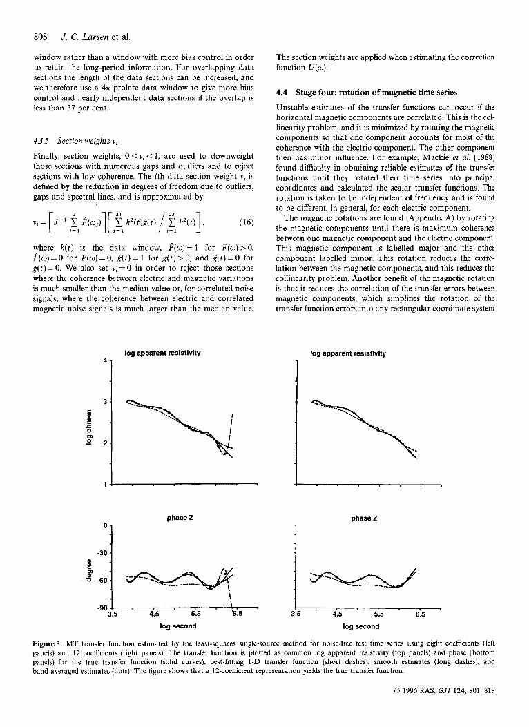
Figure 3. MT transfer function estimated by the least-squares single-source method for noise-free test time series using eight coefficients (left panels) and 12 coefficients (right panels). The transfer function is plotted as common log apparent resistivity (top panels) and phase (bottom panels) for the true transfer function (solid curves), best-fitting 1-D transfer function (short dashes), smooth estimates (long dashes), and hand-averaged estimates (dots). The figure shows that a 12-coefficient representation yields the true transfer function.

0 1996 RAS, GJI 124, 801-819


4 -

3 -

2 -

because the error covariance between components can be ignored (Appendix A).

0 -

-30 -

3 i!! m -60

-90

4.5 Stage five: robust estimation of smooth transfer function

Robust estimates of the correction function U(w) are constructed using the weighted corrected time series, the section weights, and rotated magnetic components. The Fourier transform of the weighted corrected electric time series is given by

E(o) = G*(w)* [F(w)W(o)E(w)] , (17)

where * represents a convolution summation in frequency, E(o) is the Fourier transform of the corrected electric time series, and GH(w) is the Fourier transform of the windowed time weights h( t )g( t ) . The Fourier transform of the weighted corrected magnetic time series for the nth correction coefficient and kth rotated magnetic component is given by

E,k(w) = GH(w)*[F(o)W(o)Tn(w)Dk(w)Z'-o(o)Bk(w)l 9 (18)

where Ek(w) is the Fourier transform of the corrected kth rotated magnetic time series.

The above weighted corrected time series are constructed by first whitening the corrected time series by a single term

4; 7 1


\

and applying the Fourier transform, which is then multiplied by the whitening W(w) and the frequency-domain weights F(w) and, for the kth magnetic time series, by T,(w), D k ( o ) and Z'-'(w). The convolution summation is then carried out in the time domain by converting the frequency terms within the brackets [ ] of (17) and (18) into a time series using the inverse Fourier transform, applying the time-domain weights h( t)g( t ) , and then returning to the frequency-domain using the Fourier transform.

The MT relationship (1) in terms of the weighted corrected electric and magnetic time series becomes

N K

E(w) = 1 c UnkE'nk(W) $. f i ( w ) ,

B(0) = c c UfkEfk(w) + f i R ( W ) .

(19) n = l k = l

and the MT remote-reference relationship (2) becomes N K

(20) n = 1 k = l

The important feature of eqs (19) and (20) is that the MT frequency relationships (1) and (2) have not been changed by the time-domain weights or data window because the correction coefficients unk can be moved outside the convolution summation when applying the time-domain weights g( 1) and data window h( t ) . The only limitations on representations (19)


I 1

phase Z phase Z

log second log second

Figure 4. MT transfer function estimated by the least-squares single-source method for test time series with synthetic outliers and uncorrelated noise (see text). The transfer function is plotted as common log apparent resistivity (top panels) and phase (bottom panels) for the true transfer function (solid curves), 95 per cent confidence limits on robust smooth estimates (pair of dashed curves in left panels), robust band-averaged estimates (dots with vertical bars in left panels), band-averaged estimates without weights (dots with vertical bars in right panels) and Chave robust estimates (open circles with vertical bars in right panels). The figure shows that the robust smooth and band-averaged estimates approximate the true transfer function, while the Chave estimates are biased downwards for the short periods.

0 1996 RAS, GJI 124, 801-819


and (20) are the finite number of coefficients N and the damping needed to prevent instabilities in the solution.

4.5.1

The smooth corrected function is then found by least squares or remote reference. The robust least-squares solution with damping (second term on right) is given by

Estimation of smooth correction function U ( w )

N K

(E:$E> = c [ ( E L i B n k > + (B;$Blk)6mn10rklUnk, (21) n = l k = l

and the robust remote-reference solution with damping is given by

for m = 1, . . . , N coefficients and l = 1, . . . , K magnetic components, where ( ) indicates an average over all frequencies and data sections weighted by the section weights. The two-source solution has a form similar to (21), but with K = 4 to include the MT and correlated noise sources.

The damping coefficients 6,, and damping factor tk are used to prevent instabilities in the matrix inversion due to the size of the matrix, which is equal to the number of coefficients N

times the number of magnetic inputs K . The coefficients are 6,, = (n - 1)2("-') for n = 2, ... , N, and 6," = 0 otherwise, and are based on the leading term in the Chebyshev polynomial representation for dUldX.

The correction coefficients uflk are found by a QR decompo- sitional method (Press et al. 1992, pp. 91-94) applied to a real, two-index matrix based on rearranging the complex-valued, multi-indexed matrices in (21) or (22). The minimum amount of damping is found by increasing the damping factor g in small steps of 0.02 from the undamped case, having the small value 5 = -8 until the smooth errors E" are slightly smaller than the largest band-averaged errors E~ for five band-averages per decade of frequency. If 5 = 8, the correction function U is over-damped and gives a constant value.

The smooth robust estimate of the transfer function for the minimum necessary amount of damping is given by Z(w) = U(w)D(w)Z'-"(w), where U(w) is computed using eq. (9), and the error is E(W) = lD(w)Z"D(w)leU(o), where &"(a) is computed using eq. (10) and the jackknife estimate of cov(u,u~) is computed using eq. (1 1).

The band-averages UB and eB are found by solving eqs (1) and (2) by least-squares or remote-reference using the weighted corrected time series. This yields equations similar in form to eqs (21) and (22) without damping, where ( ) now indicates

159 T magnetic

outliers 34

E -34

outliers missed 34 T

-34 1

22 44 66 88 110 132 1951

Figure 5. Test time series with synthetic outliers and uncorrelated noise for the first data section. Top curve, Tucson north magnetic time series plus noise; 2nd curve from top, 2.3 per cent estimated magnetic outliers; 3rd curve from top, magnetic outliers remaining after removing estimated magnetic outliers; 4th curve from top, test electric time series; 5th curve from top, 3.2 per cent estimated electric outliers; and bottom curve, electric outliers remaining after removing estimated outliers. The figure shows that most outliers have been removed.

0 1996 RAS, GJI 124, 801-819

M T transfer functions 81 1

s c 0 0) E E 2 - 3 :

1 1

an average over a band of frequencies and all data sections weighted by section weights. The band-averaged estimates are ZB = UBDZ'-D and provide an alternative estimate of the transfer function.

-1

4.5.2

The distortion D(w) for each magnetic component is found by a least-squares fit of D ( ~ ) z ' - ~ ( w ) to the previously estimated Z(o), using the errors E(W) as weights. This yields

Estimation ofsmooth distortion function D(w)

20 -

-20 i t

-60-

-100 'I

N (&-2ZZ'-D'T,) = c [(&-21z'-"12TmT,)

n = l

+ (&-21Z'-D12)6,,lOq a, (23) for N coefficients, where ( ) indicates an average over all frequencies, 6,, are the same damping coefficients as in eq. (21 ) , and 5 are the damping factors used to smooth the solutions. The solutions are found by the QR decomposition method of eq. ( 2 3 ) . The estimates of d, are found by decreasing the damping factor from (= 8 (the over-damped case) until D ( ~ ) z ' - ~ ( w ) lies just within the 95 per cent confidence

-

W bb;;v#p/f

M' 1

4 1

3.5 5.0 6.5 3.5 5.0 6.5

limits of Z(w) i &z(w), where /Im is based on the Student's t distribution for n = I - 1 degrees of freedom.

5 EXAMPLES

We tested the robust smooth method on numerous time series: Hawaii and Midway Island MT time series having strong tidal signals; California MT time series, some having strong correlated noise signals due to oil-production equipment and some having little noise; Indonesian MT time series having numerous lightning events; Carty Lake, Canada MT time series having many high-wavenumber events; Tucson MT time series having numerous outliers; Straits of Florida MT time series having strong tidal and Florida Current signals; various Larderello, Italy MT time series contaminated by d.c. electrified railways; Czech Republic MT time series highly contaminated by correlated noise signals; and Hawaii, Tucson, Fresno, Fredericksburg and San Juan GDS time series.

We present results for three different data sets: a California MT time series that is nearly noise-free for comparing the smooth robust method with the Chave robust method (Chave


1 T

0 1996 RAS, GJI 124, 801-819

812 J. C . L a w n et al.

& Thomson 1989, 1992); a time series based on the Tucson north magnetic time series plus Gaussian noise and random outliers and a given transfer function for evaluating the effectiveness of the robust smooth and Chave methods in removing noise and estimating the known transfer function; and Larderello time series for evaluating the effectiveness of the robust smooth and Chave methods in estimating the MT transfer functions from time series contaminated by d.c. electrified railways.

5.1

A clean time series from an MT site 100 km west of Bakersfield in central California was used to verify that the robust smooth method converges to the same solution as the Chave robust method and gives errors of similar magnitude. The time series consists of four overlapping bands of frequencies. Both methods yield band-averaged estimates of the transfer functions and its error that are in agreement. For example, Fig. 2 shows that the estimates of the transfer function in the direction of N45"E and the errors are in excellent agreement between both methods. A value of N = 10 was used.

Central California MT time series

5.2 Test time series

To test the robust smooth method, we use a magnetic time series based on the hourly Tucson north magnetic time series. The electric time series is generated from the magnetic time series using a 1-D transfer function previously estimated for

Capraia rn

Tucson and multiplied by an arbitrary distortion function D to make the transfer function distinctly non-1-D in order to verify that the robust estimate converges to this non-1-D transfer function. The time series are subdivided into 50 sections with 3456 values per section. A 4.n data window is used, giving 37 per cent overlapping data sections.

To test the sensitivity of the smooth estimates to the number of coefficients N, we use noise-free electric and magnetic time series. The misfit between smooth estimates and the true transfer function is 17.5 per cent for N = 8 (Fig. 3). It decreases to 0.8 per cent for N = 10 and to 0.4 per cent for N = 12 (Fig. 3). The percentage misfit is equal to 100 times the rms value of (log(Zt,ue/Zestimate)I over all estimates. These misfits indicate that the number of coefficients should be N210, which corresponds to 3.9 coefficients per decade of frequency. We chose N = 12.

To test the robust least-squares method, we add Gaussian electric noise with variance equal to 11 per cent of the spectral level for the electric time series, but keep the magnetic time series noise-free. This gives a theoretical coherence square of 0.90. Gaussian noise is not added to the magnetic time series to prevent biasing the estimates, because this would obscure our evaluation of the effectiveness of the robust least-squares method in identifying and removing electric and magnetic outliers. To simulate uncorrelated outliers, we contaminate 4 per cent of the first half of the electric and magnetic time series with spikes at random times with random amplitudes between +5 times the standard deviation of the time series. This means that only 1.2 per cent of the time series have been contaminated by outliers greater than 2 standard deviations.

4 50 km

I......I MT sites

Italian State Railroads

Figure 7. Larderello MT survey sites in central Italy. The two east-west MT survey lines (34 small dots) are within the rectangular box containing the town Larderello. The remote magnetic site is located on the island of Capraia. Electrified railways are marked by heavy lines.

0 1996 RAS, GJI 124, 801-819


The misfits between the robust least-squares estimates and the true transfer function (Fig. 4) are: 2.2 per cent for the smooth and 3.4 per cent for the band-averaged estimates using time series corrected for outliers and weighted by the frequency- and time-domain weights; 4.0 per cent for the band-averaged estimates using time series corrected for outliers but ignoring frequency- and time-domain weights; and 44 per cent for the band-averaged estimates using time series uncorrected for outliers and ignoring frequency- and time-domain weights. The latter is the non-robust estimate. The coherence squared for the robust smooth estimates is 0.89, which is close to the 0.90 theoretical limit. The robust method identifies 1.7 per cent electric outliers and 1.4 per cent magnetic outliers. The remaining outliers are mostly small (Fig 5). Thus the robust least- squares method performs quite well in identifying and replacing outliers and producing smooth and band-averaged estimates that approximate the true transfer function (Fig. 4). The non- robust method, however, gives quite inferior estimates. The Chave robust least-squares method yields comparable estimates for the longer periods but not for the shorter periods (Fig. 4), where the estimates are biased downwards, probably due to undetected magnetic outliers. In fact, the Chave estimates are similar to the non-robust band-averaged estimates.

To test the robust least-squares two-source method and to compare it to the robust least-squares single-source and remote-reference single-source methods, we use the same noisy electric and magnetic time series as in the least-squares single- source test, but add a large correlated random signal equal to

log modulus T log modulus T

'1 1

-1 I I

-1 .0 0.0 1.0 -f.0 0.0 1 .0 -90


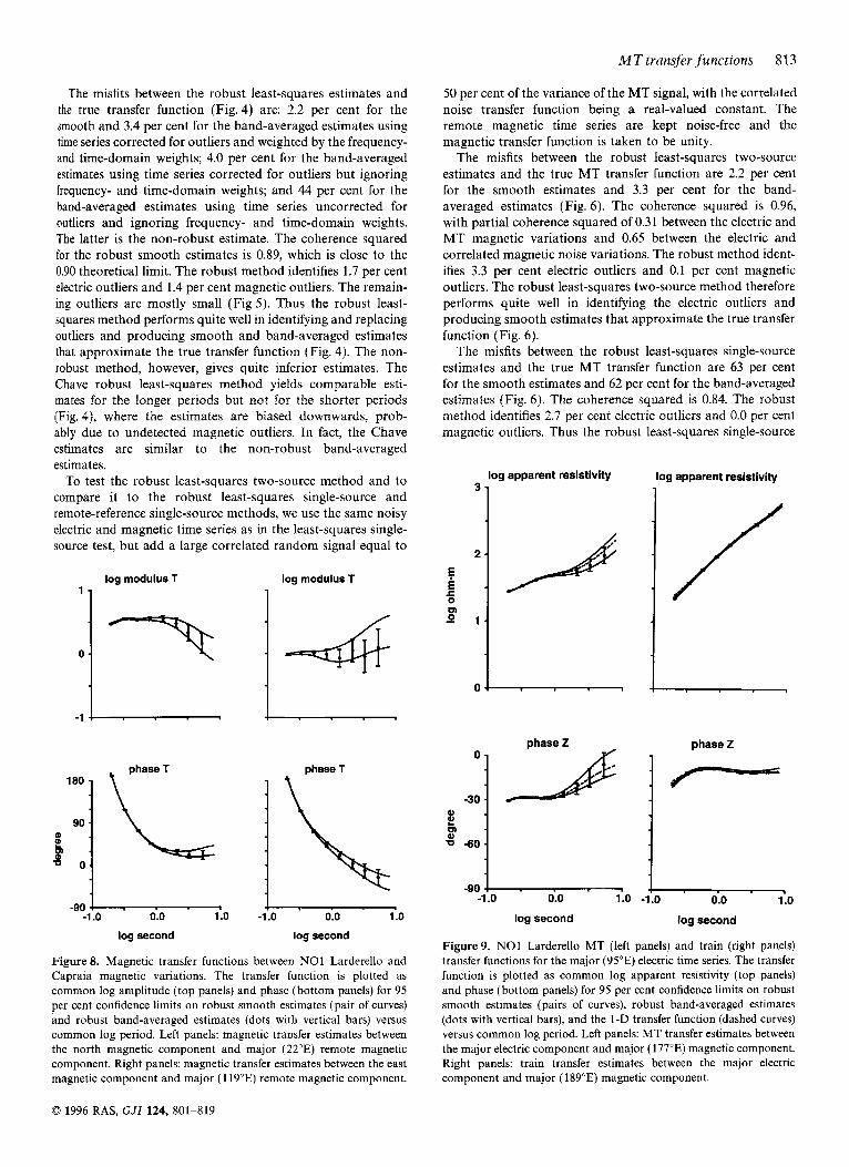
Figure 8. Magnetic transfer functions between NO1 Larderello and Capraia magnetic variations. The transfer function is plotted as common log amplitude (top panels) and phase (bottom panels) for 95 per cent confidence limits on robust smooth estimates (pair of curves) and robust band-averaged estimates (dots with vertical bars) versus common log period. Left panels: magnetic transfer estimates between the north magnetic component and major (22"E) remote magnetic component. Right panels: magnetic transfer estimates between the east magnetic component and major (119"E) remote magnetic component.

50 per cent of the variance of the MT signal, with the correlated noise transfer function being a real-valued constant. The remote magnetic time series are kept noise-free and the magnetic transfer function is taken to be unity.

The misfits between the robust least-squares two-source estimates and the true MT transfer function are 2.2 per cent for the smooth estimates and 3.3 per cent for the band- averaged estimates (Fig. 6). The coherence squared is 0.96, with partial coherence squared of 0.31 between the electric and MT magnetic variations and 0.65 between the electric and correlated magnetic noise variations. The robust method identifies 3.3 per cent electric outliers and 0.1 per cent magnetic outliers. The robust least-squares two-source method therefore performs quite well in identifying the electric outliers and producing smooth estimates that approximate the true transfer function (Fig. 6).

The misfits between the robust least-squares single-source estimates and the true MT transfer function are 63 per cent for the smooth estimates and 62 per cent for the band-averaged estimates (Fig. 6). The coherence squared is 0.84. The robust method identifies 2.7 per cent electric outliers and 0.0 per cent magnetic outliers. Thus the robust least-squares single-source

3

2

E i

0 1

r 0 m

0

lag apparent resistivity log apparent resistivity

phase 2

-30 o / J t m a,

-60-

phase 2

-1 .o 0.0 1.0 -1.0 0.0 1.0


Figure9. NO1 Larderello MT (left panels) and train (right panels) transfer functions for the major (95"E) electric time series. The transfer function is plotted as common log apparent resistivity (top panels) and phase (bottom panels) for 95 per cent confidence limits on robust smooth estimates (pairs of curves), robust band-averaged estimates (dots with vertical bars), and the 1-D transfer function (dashed curves) versus common log period. Left panels: MT transfer estimates between the major electric component and major (177"E) magnetic component. Right panels: train transfer estimates between the major electric component and major (189"E) magnetic component.

0 1996 RAS, GJI 124, 801-819


0.5 -

method estimates are clearly wrong due to the presence of the correlated noise signal. However, the results are quite mislead- ing, because the errors are relatively small and the coherence is high. This seems to indicate that the MT transfer function has been accurately estimated. What is happening is that the estimated transfer function is a combination of the MT and correlated noise signal transfer functions. The Chave robust least-squares method also gives wrong estimates and errors which are comparable to those of the robust smooth single-source method.

The misfits between the robust remote-reference single- source estimates and the true MT transfer function are 9.2 per cent for the smooth estimates and 10.1 per cent for the band- averaged estimates (Fig. 6). The coherence squared is 0.52. The robust method ideptifies 0.1 per cent electric outliers and 0.0 per cent magnetic Outliers. The robust remote-reference single- source method performs much better than the robust least- squares single-source method, but still performs poorly compared with the robust least-squares two-source method (Fig. 6). The Chave robust remote-reference method gives estimates comparable to the robust remote-reference single-source method but with some much larger errors.

log apparent resistivity 31

I

1 0 I

phase 2

-30

6 4 -60-

-90 I -1 .o 0.0 1 .o

log second


5.3 Larderello NO1 MT time series

The Larderello MT survey was carried out in central Italy and consisted of two east-west survey lines with 34 MT sites (Fig. 7). The survey area is surrounded by several electrified railways, the closest one being along the west coast of Italy to the west and south of the survey area. The trains run as frequently as every 30 minutes. The remote site is located on the island of Capraia, some 55 km from the coast (Fig. 7) and is free of electric trains.

Electric trains in Italy are powered by an overhead 3000 d.c. voltage line generated by a series of substations approximately either 10 or 20 km apart and supplying currents of up to 1500A (Linington 1974). The current flows through the overhead contact wire (5 m above the tracks), then through the electric train motors via the pantograph touching the contact wire, into the train tracks via the wheels, and then back to the substations via the train tracks, which are grounded for safety reasons. Each pair of substations spanning a particu- lar train supplies a current proportional to the distance of the train from the substation (Linington 1974). The amount of current through the motor is controlled by switches and a chopper-controlled switch. This avoids the use of rheostats and the resulting heat loss. The train-induced signals vary in intensity and frequency with the position and number of the trains, amount of current used by the trains and harmonics of the basic 50Hz power grid supplying the rectified 3000 d.c. volts. The electric current is therefore highly variable.

There are two modes by which electrified railways contaminate the natural MT signals. One mode is due to electric

0.0 phase Z

I 0.0 1 .o log second

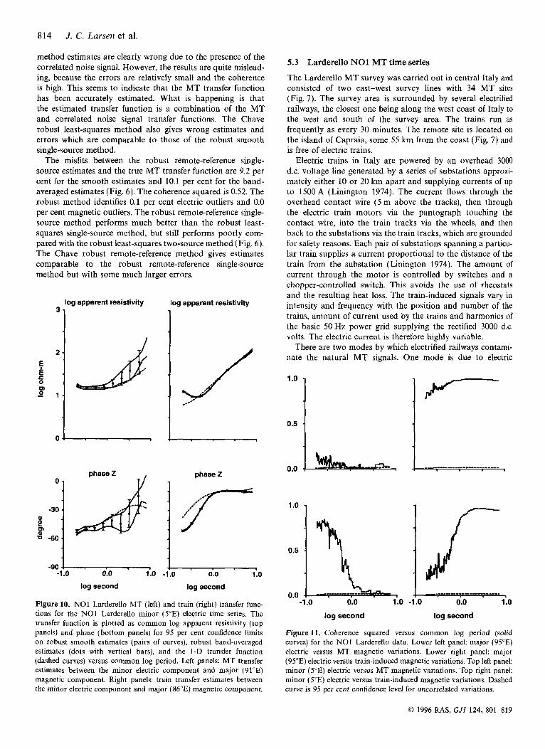
Figure 10. NO1 Larderello MT (left) and train (right) transfer functions for the NO1 Larderello minor (YE) electric time series. The transfer function is plotted as common log apparent resistivity (top panels) and phase (bottom panels) for 95 per cent confidence limits on robust smooth estimates (pairs of curves), robust band-averaged estimates (dots with vertical bars), and the 1-D transfer function (dashed curves) versus common log period. Left panels: MT transfer estimates between the minor electric component and major (91"E) magnetic component. Right panels: train transfer estimates between the minor electric component and major (86"E) magnetic component.

'.O 1

0.0 . log second

-1 .o 0.0 1 .o --I----------------- ,

0 0.0 1 .o log second

Figure 11. Coherence squared versus common log period (solid curves) for the NO1 Larderello data. Lower left panel major (95"E) electric versus MT magnetic variations. Lower right panel: major (95"E) electric versus train-induced magnetic variations. Top left panel minor (YE) electric versus MT magnetic variations. Top right panel: minor (YE) electric versus train-induced magnetic variations. Dashed curve is 95 per cent confidence level for uncorrelated variations.

0 1996 RAS, G J I 124, 801-819

MTtransfer functions 815

0.- -

currents leaking into the Earth via the grounded train tracks. This causes some of the current to return to the substations via the Earth. The other mode is due to a magnetic dipole zffect caused by currents flowing through the overhead voltage line and returning through the tracks. A simple calculation shows that this latter mode rapidly decays with distance (Linington 1974), so sites more than 1 km from the tracks are unlikely to be affected by the magnetic dipole effect. Leakage currents are therefore the dominant mode and this is probably the case for most cultural sources. A review of the extensive literature on cultural electromagnetic signals including electric train-induced signals is given in Szarka (1988).

We chose site N01, at the western end of the northern survey line, because it is closest to a north-south train track and therefore has the strongest train-induced signals. The NO1 time series should therefore provide a rigorous test of the robust smooth method for extracting the MT transfer functions from highly contaminated time series. We use 100 data sections with 256 values per section and N = 10 coefficients, and concentrate on the period range 0.17 to 7.1 s.

The magnetic transfer functions for the north and east magnetic time series are given in Fig. 8. For the north magnetic time series, the coherence squared is 0.92 between the local and remote magnetic time series and there are 7.5 per cent local magnetic outliers and 0.4 per cent remote magnetic outliers. For the east

%

E

E 5

E

E

x . >

E

E 5

E s > E

magnetic time series, the coherence

squared is 0.75 and there are 12.0 per cent local magnetic outliers and 0.5 per cent remote magnetic outliers. The train- induced magnetic signals account for 87 per cent of the variations for the north component and 98 per cent for the east magnetic component. The magnetic transfer functions are approximately flat for the shortest periods, while the phase goes through a change of about 180" from the shortest to the longest periods. This corresponds to a sign reversal in the time series that could be related to timing problems (Egbert, personal communication). This is immaterial, however, for estimating the MT time series at the NO1 site.

The MT and train transfer functions for the major (95"E) electric time series are well determined (Fig. 9). The coherence squared is 0.99 between the electric and magnetic variations, with a partial coherence squared of 0.57 between the electric and MT magnetic variations and a partial coherence squared of 0.38 between the electric and train-induced variations. There are 5.4 per cent electric outliers and 2.9 per cent magnetic outliers.

The MT transfer function for the minor (5"E) electric time series (approximately parallel to the nearest train track) (Fig. 10) is less well determined. Although the coherence squared is 0.99 between the electric and magnetic variations, the partial coherence squared is only 0.03 between the electric and MT magnetic variations, while the partial coherence squared is 0.94 between the electric and train-induced magnetic

major mt magnetic 17 -

0 .

-17 * maior cultural magnetic

-17 1 39 T

mt electric

0 .

-39 - cultural electric

-39 I 1 39 77 114 152 190 228

data points

Figure 12. Time derivative of the NO1 Larderello time series from first data section for major (95"E) electric time series. The time increment is 0.086 s. Vertical scales are k3.9 mV km-' and i0 .17 nT. Top curve: major (177"E) MT magnetic time series. Second curve from top: major ( 189"E) train-induced magnetic time series. Third curve from top: MT electric time series. Fourth curve from top: train-induced electric time series. Fifth curve from top: residual time series. Bottom curve: residual time series minus 2.3 per cent electric outliers and 1.6 per cent magnetic outliers.

0 1996 RAS, G J I 124, 801-819

816 J. C . Lumen et al.

variations. There are 0.8 per cent electric outliers and 0.2 per cent magnetic outliers.

For the major (95"E) electric time series, the train-induced signals account for most of the coherence for periods longer than 1 s, while the MT variations account for most of the coherence for periods shorter than 1 s (Fig. 11). For the minor (5"E) electric time series, the train-induced signals account for most of the coherence over the entire period range 0.17 to 7.1 s (Fig 11). This shows that the largest train-induced electric currents are on the whole parallel to the nearby north-south train tracks.

Time derivatives of the MT and train-induced variations for the major (95"E) electric direction are shown in Fig. 12 for the first data section. They show that the train-induced electric and magnetic variations are at times much larger than the MT electric and magnetic variations. Furthermore, the train- induced electric and magnetic variations have very similar appearances, which indicates that the train transfer function is approximately a constant with zero phase. This is consistent with our estimates of the train transfer functions in Figs 9 and 10.

The MT transfer functions for both electric components are found to be minimum-phase (Figs 9 and 10). In addition, the MT transfer function for the major (95"E) electric time series (approximately normal to the coast line) shows a linear rise towards long periods for log apparent resistivity and a small

phase (Fig. 9) similar to the observed TM mode (electric currents normal to coastline) at continental sites near oceans (Park et al. 1991). These features in the TM mode are due to an excess of electric currents in the surface continental layer near the coast, caused by the concentration of ocean electric currents into the surface continental layer. The train transfer functions for each component also show a similar linear rise towards long periods in the log apparent resistivity and a constant small phase. They approximate the transfer function for a high-wavenumber source and indicate that the train- induced electric currents occur mainly in the surface layer. Hence, the train transfer functions and the TM mode of the MT transfer functions for this site have similar frequency characteristics, at least for the longer periods. On the other hand, the transfer function for the minor (5"E) electric time series (Fig. 10) is similar to the TE mode (electric currents parallel to the coastline) because it has a much larger phase than the TM mode. Although we don't know the true transfer function, this interpretation of the MT transfer function and the train transfer functions by the TM and TE modes suggests that the robust smooth estimates are realistic.

We also estimate the MT transfer function by robust least- squares single-source and remote-reference single-source methods for comparison with the robust least-squares two- source estimates and the Chave robust least-squares and remote-reference estimates. The estimates of 2 (basically the

I log apparent resistivity

phase Z

30 1

-60 1 -90 1

-1 .o 0.2 1.4 !I 1.4

I log second log second log second

Figure 13. The Larderello NO1 MT transfer function for the major (95"E) electric time series by the robust least-squares single-source method (left panels), the robust remote-reference single-source method (middle panels), and the robust least-squares two-source method (right panels). The transfer function is plotted as common log apparent resistivity (top panels) and phase (bottom panels) for 95 per cent confidence limits on robust band-averaged estimates (dots with vertical bars) and Chave robust estimates (open circles with vertical bars).

0 1996 RAS, GJI 124, 801-819

MTtransfer functions 817

TM model) in Fig. 13 show that the robust least-squares single-source estimates are similar to the train transfer functions (Fig. 9) that have a nearly constant slope and small phase. Clearly, the least-squares single-source estimates are dominated by the train-induced signals and therefore give wrong estimates of the MT transfer function. The robust remote-reference single-source method also performs poorly compared with the robust least-squares two-source method for periods greater than 1 s where the train-induced signals are large. For periods less than 1 s, however, the remote-reference estimates are similar to the MT transfer function estimated by the robust least-squares two-source method. The Chave robust least-squares and remote-reference methods give results similar to the robust smooth method but with some much larger errors.

6 CONCLUSIONS

The robust smooth method provides two different estimates of the transfer function: smooth estimates, which are valuable for identifying individual outliers and examining the residual time series, and band-averaged estimates, which are independent of the damping needed to stabilize the smooth estimates. The two estimates are usually similar.

A comparison between estimates of the transfer function by the robust smooth method and by the Chave robust method shows that the two methods give similar results for clean time series. Tests with synthetic outliers and uncorrelated noise confirm that the robust smooth method is able to identify and remove electric and magnetic outliers and to provide realistic estimates of the true transfer functions. However, the Chave robust estimates are biased downwards for the shorter periods.

The MT transfer functions can be extracted from time series highly contaminated by correlated noise signals by using a remote magnetic site free of correlated noise and utilizing the robust least-squares two-source method. If the correlated noise is large, the robust least-squares single-source estimates give erroneous results, whereas the robust remote-reference single- source estimates tend to track the MT transfer function but give much larger errors than the robust least-squares two- source estimates.

We conclude that the robust smooth method is effective in removing individual outliers, but the robust methods cannot remove continuous correlated noise. This type of noise requires use of the two-source form of the MT relationship or the remote-reference single-source method if the correlated noise is not too large. However, the least-squares single-source method should be avoided if there is correlated noise.

ACKNOWLEDGMENTS

We thank Jack Richer, owner of his own PCC (Presidents Conference Committee) electric red car no. 3072 retired from the Los Angeles transit system, for many delightful discussions concerning engineering details about electric trolleys, Gaston Fisher for helpful discussion about electric trains and supplying us with references, Ted Madden, who saw the need for simultaneously solving for train and MT transfer functions, Dean Livelybrooks, Alan Chave and an anonymous reviewer for fine-comb reviews and many helpful suggestions, and Martha Jackson for careful editing of the manuscript. This work was

funded by a research grant by ENEL, Italy, MIT, and NOAA. It is PMEL contribution 1596.

REFERENCES

Chave, A.D., Thomson, D.J. & Ander, M.E., 1987. On the robust estimation of power spectra, coherences, and transfer functions, J. geophys. Res., 92, 633-648.

Chave, A.D. & Thomson, D.J., 1989. Some comments on magnetotelluric response function estimation, J. geophys. Res., 94,

Chave, A.D. & Thomson, D.J., 1992. Robust, controlled leverage estimation of magnetotelluric response functions, Proc 11th Workshop on Electromagnetic Induction in the Earth, Abstract 8.13, Victoria University of Wellington, New Zealand.

Egbert, G.D. & Booker, J.R., 1986. Robust estimation of geomagnetic transfer functions, Geophys. J . R . astr. Soc., 87, 173-194.

Egbert, G.D., Booker, J.R. & Schultz, A,, 1992. Very long period magnetotellurics at Tucson Observatory: Estimation of impedances, J. geophys. Res., 97, 15 113-15 128.

Gamble, T.D., Goubau, W.M. & Clarke, J., 1979. Magnetotellurics with a remote reference, Geophysics, 44, 53-68.

Jones, A.G. & Jodicke, H., 1984. Magnetotelluric transfer function estimation improvement by a coherence-based rejection technique, paper EM1.5, 271, presented at 54th Annl. Int. Mtg, SOC. Excl. Geophys., Atlanta, Georgia.

Kaufman, A.A. & Keller, G.V., 1981. The Magnetotelluric Sounding Method, Elsevier, New York, NY.

Larsen, J.C., 1980. Electromagnetic response functions from interrupted and noisy time series, J. Geomag. Geoelectr., 32, 89-103.

Larsen, J.C., 1989. Transfer functions: smooth robust estimates by least-squares and remote reference methods, Geophys. J., 99,

Linington, R.E., 1974. The magnetic disturbances caused by DC electric railways, Prospezioni Archeologiche, 9, 9-20.

Mackie, R.L., Bennett, B.R. & Madden, T.R., 1988. Long-period magnetotelluric measurements near the central California coast: a land-locked view of the conductivity structure under the Pacific Ocean, Geophys. J., 95, 181-194.

Park, S.K., Biasi, G.P., Mackie, R.L. & Madden, T.R., 1991. Magnetotelluric evidence for crustal suture zones bounding the southern Great Valley, California, J. geophys. Res., 96, 353-376.

Parker, R.L., 1980. The inverse problem of electromagnetic induction: existence and construction of solutions based on incomplete time series, J. geophys. Res., 85, 4421-4428.

Press, W.H., Teukolsky, S.A., Vetterling, W.T. & Flannery, B.P., 1992. Numerical Recipes in Fortran, 2nd edn, Cambridge University Press, New York, NY.

Rousseeuw, P.J. & Leroy, A.M., 1987. Robust Regression and Outlier Detection, John Wiley & Sons, New York, NY.

Schultz, A. & Larsen, J.C., 1987. On the electrical conductivity of the mid-mantle: I. Calculation of equivalent scalar magnetotelluric response functions, Geophys. J. R . astr. SOC., 88, 773-761.

Sims, W.E., Bostick, Jr, F.X. & Smith, H.W., 1971. The estimation of magnetotelluric impedance tensor elements from measured time series, Geophysics, 36, 938-942.

Sutarno, D. & Vozoff, K., 1991. Phase-smoothed robust M-estimation of magnetotelluric impedance functions, Geophysics, 56, 1999-2007.

Szarka, L., 1988. Geophysical aspects of man-made electromagnetic noise in the Earth-A review, Surveys in Geophysics, 9, 287-318.

Thomson, D.J. & Chave, A.D., 1991. Jackknifed error estimates for spectra, coherences, and transfer functions, in Aduances in Spectrum Analysis and Array Processing, Vol. 1, pp. 58-113, ed. Haykin, S., Prentice Hall, Englewood Cliffs.

Weidelt, P., 1972. The inverse problem of geomagnetic induction, Z . Geophysic, 38, 257-289.

14 215-14 225.

645-663.

0 1996 RAS, GJI 124, 801-819


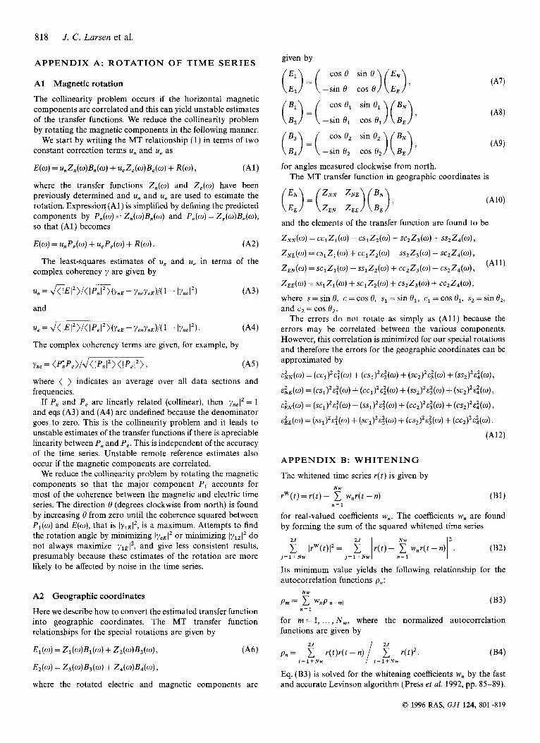
APPENDIX A: ROTATION OF TIME SERIES given by

A1 Magnetic rotation

The collinearity problem occurs if the horizontal magnetic components are correlated and this can yield unstable estimates of the transfer functions. We reduce the collinearity problem by rotating the magnetic components in the following manner.

We start by writing the MT relationship (1) in terms of two constant correction terms u, and ue as

E(w) = unZn(w)B,(w) + ueZe(w)Be(w) + R(w) > (Al l

where the transfer functions ZJo) and Z,(w) have been previously determined and u, and u, are used to estimate the rotation. Expression ( A l ) is simplified by defining the predicted components by P,(w) = Z,(w)B,(w) and P,(w) = Z,(w)B,(w), so that (Al) becomes

E(w) = u,P,(w) + u,P,(w) + R(w) . ('42)

The least-squares estimates of u, and u, in terms of the complex coherency y are given by

and

u e = & IEI2 >/( I P e l Z X Y e E - Y e n Y n E ) / ( 1 - IYnelZ). ('44)

The complex coherency terms are given, for example, by

where ( ) indicates an average over all data sections and frequencies.

If P, and P , are linearly related (collinear), then lynelZ = 1 and eqs (A3) and (A4) are undefined because the denominator goes to zero. This is the collinearity problem and it leads to unstable estimates of the transfer functions if there is apreciable linearity between P, and P,. This is independent of the accuracy of the time series. Unstable remote reference estimates also occur if the magnetic components are correlated.

We reduce the collinearity problem by rotating the magnetic components so that the major component Pl accounts for most of the coherence between the magnetic and electric time series. The direction 8 (degrees clockwise from north) is found by increasing 8 from zero until the coherence squared between Pl(w) and E(w), that is IylEIZ, is a maximum. Attempts to find the rotation angle by minimizing JyeEIZ or minimizing ly1z12 do not always maximize lylE 1 2 , and give less consistent results, presumably because these estimates of the rotation are more likely to be affected by noise in the time series.

A2 Geographic coordinates

Here we describe how to convert the estimated transfer function into geographic coordinates. The MT transfer function relationships for the special rotations are given by

E l ( 4 = Z,(w)B,(w) + Zz(w)B,(w),

EZ(4 = Z, (w)B3(4 + Z , ( W , ( w ) ,

('46)

where the rotated electric and magnetic components are

cos e sin 8 ) (&) cos el sin el ) (&) cos e2 sin O2 ) (;j

(z:) = (-sin 8 cos 6

(::) = (-sin el cos o1

(::) = (-sin o2 cos e, for angles measured clockwise from north.

The MT transfer function in geographic coordinates is

and the elements of the transfer function are found to be

Z"(O) = cCiZl(w) - csiZz(w) - SCZZ,(W) + SSZZ,(W),

zNE(w)=Cs1zl(O)+ c ~ ~ ~ ~ ( ~ ) - ~ ~ ~ z ~ ( ~ ) - ~ c ~ z ~ ( ~ ) ~ ( A l l ) Z , N ( W ) = ~ ~ ~ Z ~ ( W ) - - S S ~ Z Z ( O ) + C C ~ Z ~ ( W ) - csZZ,(w),

ZEE(O) = ss,Z,(w) + sc,zz(o) + cszZ,(w) + cczZ,(w),

where s = sin 8, c = cos 8, s1 = sin el, c1 = cos el, s2 = sin Oz, and c2 = cos 8,.

The errors do not rotate as simply as ( A l l ) because the errors may be correlated between the various components. However, this correlation is minimized for our special rotations and therefore the errors for the geographic coordinates can be approximated by

E ~ N ( W ) = (CC1)zE:(W) + (CS1)'E;(W) + (SCZ)~E:(O) + (SSz) 'Ei (W),

E i ~ ( 0 . l ) = (CS1)'E:(w) + ( C C 1 ) 2 E ; ( 0 ) + (SSZ)~E:(U) + (SCZ)~E~(U),

E ~ N ( W ) = ( S C 1 ) z E : ( 0 ) + ( S S 1 ) z E i ( 0 ) + (CCz)'E:(O) + ( C S Z ) ~ E ~ ( W ) ,

E ~ E ( W ) = (SS,)'E:(W) + (SCi)2E$(W) + (CSz)'E:(W) + ( C C Z ) ~ E ~ ( W ) .

('412)

APPENDIX B: WHITENING

The whitened time series r( t ) is given by

r w ( t ) = r ( t ) - 1 w , r ( t - n ) Nw

n = 1

for real-valued coefficients w,. The coefficients w, are found by forming the sum of the squared whitened time series

Its minimum value yields the following relationship for the autocorrelation functions p n :

for rn = 1, . . . , Nw, where the normalized autocorrelation functions are given by

Eq. (B3) is solved for the whitening coefficients w, by the fast and accurate Levinson algorithm (Press et al. 1992, pp. 85-89).

0 1996 RAS, GJI 124, 801-819


The value of Nw is chosen so that lpn12 for n > Nw are less than the 95 per cent confidence limit for the coherence squared between r( t ) and r( t - n), assuming Gaussian noise.

An alternative method for determining the whitening coefficients is to take the Fourier transform of (B1 ), yielding

R W ( 0 ) = W(w)R(w), (B5)

which has complex-valued whitening function

Nw W(w) = 1 - C w, e-inw.

n = 1

The coefficients can be found by forming the sum of the squared whitened Fourier transform

Its minimum value yields expression (B3), where the normalized autocorrelation functions are now given by

3

(B8) i” j=1 P n == 1 IR(wj)12 cOs(nwj) c IR(wj)12.

j=1

These are computed using the cosine transform of IR(w)l’.

0 1996 RAS, G J I 124, 801-819

Robust smooth magneto tell uric transfer functions

Documents

Transcript of Robust smooth magneto tell uric transfer functions