Magneto-Dielectric Wire Antennas

Theory and Design

by

Tom Sebastian

A Dissertation Presented in Partial Fulfillment

of the Requirements for the Degree

Doctor of Philosophy

Approved May 2013 by the

Graduate Supervisory Committee:

Rodolfo Diaz, Chair

George Pan

James Aberle

Michael Kozicki

ARIZONA STATE UNIVERSITY

August 2013

i

ABSTRACT

There is a pervasive need in the defense industry for conformal, low-profile,

efficient and broadband (HF-UHF) antennas. Broadband capabilities enable shared

aperture multi-function radiators, while conformal antenna profiles minimize physical

damage in army applications, reduce drag and weight penalties in airborne applications

and reduce the visual and RF signatures of the communication node. This dissertation is

concerned with a new class of antennas called Magneto-Dielectric wire antennas

(MDWA) that provide an ideal solution to this ever-present and growing need.

Magneto-dielectric structures ( ) can partially guide

electromagnetic waves and radiate them by leaking off the structure or by scattering

from any discontinuities, much like a metal antenna of the same shape. They are

attractive alternatives to conventional whip and blade antennas because they can be

placed conformal to a metallic ground plane without any performance penalty.

A two pronged approach is taken to analyze MDWAs. In the first, antenna circuit

models are derived for the prototypical dipole and loop elements that include the effects

of realistic dispersive magneto-dielectric materials of construction. A material selection

law results, showing that: (a) The maximum attainable efficiency is determined by a

single magnetic material parameter that we term the hesitivity: Closely related to Snoek’s

product, it measures the maximum magnetic conductivity of the material. (b) The

maximum bandwidth is obtained by placing the highest amount of loss in the

frequency range of operation. As a result, high radiation efficiency antennas can be

ii

obtained not only from the conventional low loss (low ) materials but also with highly

lossy materials ( ( ) ).

The second approach used to analyze MDWAs is through solving the Green

function problem of the infinite magneto-dielectric cylinder fed by a current loop. This

solution sheds light on the leaky and guided waves supported by the magneto-dielectric

structure and leads to useful design rules connecting the permeability of the material to

the cross sectional area of the antenna in relation to the desired frequency of operation.

The Green function problem of the permeable prolate spheroidal antenna is also solved as

a good approximation to a finite cylinder.

iii

To my teachers and my family

iv

Ring the bells that still can ring.

Forget your perfect offering.

There is a crack in everything.

That is how the light gets in.

- Leonard Cohen

v

TABLE OF CONTENTS

Page

LIST OF TABLES ................................................................................................................... ix

LIST OF FIGURES .................................................................................................................. x

CHAPTER

1. INTRODUCTION ....................................................................................................... 1

2. DIELECTRIC DIPOLE ANTENNA: CIRCUIT MODEL AND

RADIATION EFFICIENCY .................................................................................. 12

2.1 Introduction .............................................................................................. 12

2.2 Capacitor/ Condenser Antenna ................................................................ 16

2.3 Dielectric Monopole (Capacitive Feed) .................................................. 19

2.4 Radiation Efficiency of a Lossy Dielectric Dipole ................................. 24

3. MAGNETO-DIELECTRIC DIPOLE ANTENNA: CIRCUIT MODEL

AND RADIATION EFFICIENCY ........................................................................ 35

3.2 Historical Development of Permeable Antennas .................................... 37

3.3 Radiation Efficiency of an Electrically Small Magneto-

dielectric Dipole Antenna .............................................................................. 40

3.4 Full-wave Simulations of the Magneto-dielectric Dipole

Antenna .......................................................................................................... 50

3.5 Magneto-dielectric Dipole Prototype ...................................................... 55

3.6 A Note on the Duality between Material Dipoles ................................... 58

3.7 Summary, Conclusions and Future Work ............................................... 60

vi

4. MAGNETO-DIELECTRIC LOOP ANTENNA: CIRCUIT MODEL AND

RADIATION EFFICIENCY .................................................................................. 62

4.1 Introduction .............................................................................................. 62

4.2 Circuit model ........................................................................................... 63

4.3 Full-wave Simulations of the Magneto-dielectric Loop

Antenna .......................................................................................................... 69

4.4 Practical Application of the Circuit Model: Body Wearable

Belt Antenna ................................................................................................... 73

4.5 Summary, Conclusions and Future Work .............................................. 82

5. MATERIAL SELECTION RULEFOR MAGNETO-DIELECTRIC

ANTENNA DESIGNS ........................................................................................... 84

5.1 Introduction .............................................................................................. 84

5.2 Classification of Magnetic Materials: Dia, Para, Ferro, Ferri

and Anti-Ferro ................................................................................................ 86

5.3 Fundamental Physical Limits in Designing Low Profile &

Conformal Electrically Small Magneto-dielectric Material

Antennas ......................................................................................................... 91

5.4 Hesitivity and Magneto-Dielectric Antenna Radiation

Efficiency ..................................................................................................... 100

5.5 Material Selection Law in the design of magneto-dielectric

antennas ........................................................................................................ 106

5.6 Some Realistic and Almost Realistic Magneto-dielectric

materials Evaluated using the Material Selection Law ............................... 109

vii

5.7 Conclusions and Future Work ............................................................... 114

6. MAGNETO-DIELECTRIC DIPOLE ANTENNA: CIRCUIT MODEL

USING POLARIZABILITY ................................................................................ 115

6.1 Introduction ............................................................................................ 115

6.2 Polarizability and Antenna Capacitance .............................................. 117

6.3 Factor Relating Polarizability and Antenna Capacitance of a

Permable Prolate Spheroid Antenna ............................................................ 120

6.4 Circuit Model Comparison with Full-Wave Simulations ..................... 128

6.5 Summary and Conclusions ................................................................... 131

7. INFINITELY LONG MAGNETO_DIELECTRIC CYLINDER AS A

MAGNETIC RADIATOR .................................................................................... 132

7.1 Introduction ............................................................................................ 132

7.2 Infinite Magneto-Dielectric Cylinder Wave Equation

Solution ........................................................................................................ 134

7.3 Effective Length for a Finite Magneto-dielectric Dipole

Based on the Radiated Power of an Infinite Magneto-dielectric

cylinder ......................................................................................................... 147

7.4. Summary, Conclusions and Future Work ............................................ 156

8. FINITE MAGNETO-DIELECTRIC PROLATE SPHEROIDAL

ANTENNA ANALYSIS ...................................................................................... 159

8.1 Introduction ........................................................................................... 159

8.2 Prolate Spheroidal Antenna Problem Statement ................................... 161

8.3 Solution of the Wave Equation .............................................................. 162

viii

8.4 Comparison with Full-Wave Simulations ............................................ 173

8.5 Summary and Future Work ................................................................... 177

REFERENCES ................................................................................................................... 178

APPENDIX

A. DERIVATION OF THE INTERNAL FIELD SHAPE CORRECTION

FACTOR TO ACCOUNT FOR THE EFFECT OF SKIN DEPTH ................. 182

B. DERIVATION OF EFFICIENCY OF A PERMEABLE DIPOLE

FOLLOWING THE APPROACH BY DeVORE et. al. (Ref. 15) ................... 185

C. HELMHOLTZ VECTOR WAVE EQUATION IN PROLATE

SPHEROIDAL COORDINATES UNDER CIRCULAR ( )

SYMMETRY ........................................................................................................ 189

ix

LIST OF TABLES

Table Page

2-1 TM01 onset/cutoff frequency for a 1cm radius dielectric cylinder for different . ..20

4-1 TE01 onset/cutoff frequency for a 0.5” wire radius magneto-dielectric cylinder

for different and . .............................................................................................70

5-1 Typical Hesitivities of Microwave materials ............................................................100

5-2 Hesitivity of the materials being evaluated using the material selection rule ..........111

7-1 values for different .....................................................................................150

x

LIST OF FIGURES

Figure Page

1-1 Off- the-shelf Whip and Blade Antennas on Military platforms. ............................... 3

1-2 Image effects of (a) Horizontal metallic antenna placed on a metallic ground-

plane at height ‘ ’(b) Vertical metallic antenna on a metallic ground

plane. ........................................................................................................................... 4

1-3 Image effects of a (a) metallic antenna on a metallic ground plane covered with a

high impedance material (b) Magneto-dielectric antenna on a metallic ground

plane. ............................................................................................................................5

1-4 (a) E and H field structure around a PMC wire (b)HE11 mode in a magneto-

dielectric material (c) TE01 mode in a magneto-dielectric material. .......................... 6

1-5 Outline of the dissertation............................................................................................ 7

2-1 a) Schelkunoff’s dielectrically loaded antenna [1] (b) Wheeler’s capacitor

antenna [2] [3] (c) Dielectric Dipole antenna ............................................................ 12

2-2 (a) Simulation geometry of the capacitor antenna. (b) Ampere’s loop in the

simulator to measure the conduction current in the center conductor and the total

radiation current of the monopole. ............................................................................ 16

2-3 The ratio of the total radiated current (Itotal) to the conduction current (Ic) in the

center conductor @ 100MHz plotted along the length of the loaded monopole for

different values of . ................................................................................................ 17

2-4 (a) Real and (b) Imaginary part of input impedance of the capacitor antenna for

different values of εr. ................................................................................................. 17

xi

2-5 (a) Antenna Q calculated from input impedance using (1) and (b) Ratio of the

Antenna Q of the dielectric capacitor to the Q of the metallic monopole. The

dielectric Q is higher than the metallic monopole throughout the band. .................. 19

2-6 Simulation geometry of the dielectric monopole. ..................................................... 19

2-7 (a) & (b) are plots of along a line in the XY plane (@ z=4cm) indicating TM

Mode structure inside the dielectric material at 100MHz and 500MHz

respectively (c) Plot of displacement current density ‘ ’ plotted along the axis

of the dielectric cylinder. ........................................................................................... 21

2-8 The ratio of the total radiated current (Itotal) to the average conduction current

(Ic) in the center conductor of the feed capacitor@ 100MHz plotted along the

length of the dielectric monopole for different values of . .................................... 22

2-9 (a) Real and (b) Imaginary part of input impedance of the dielectric monopole for

different values of εr. (c) Antenna Q calculated from input impedance. ................... 23

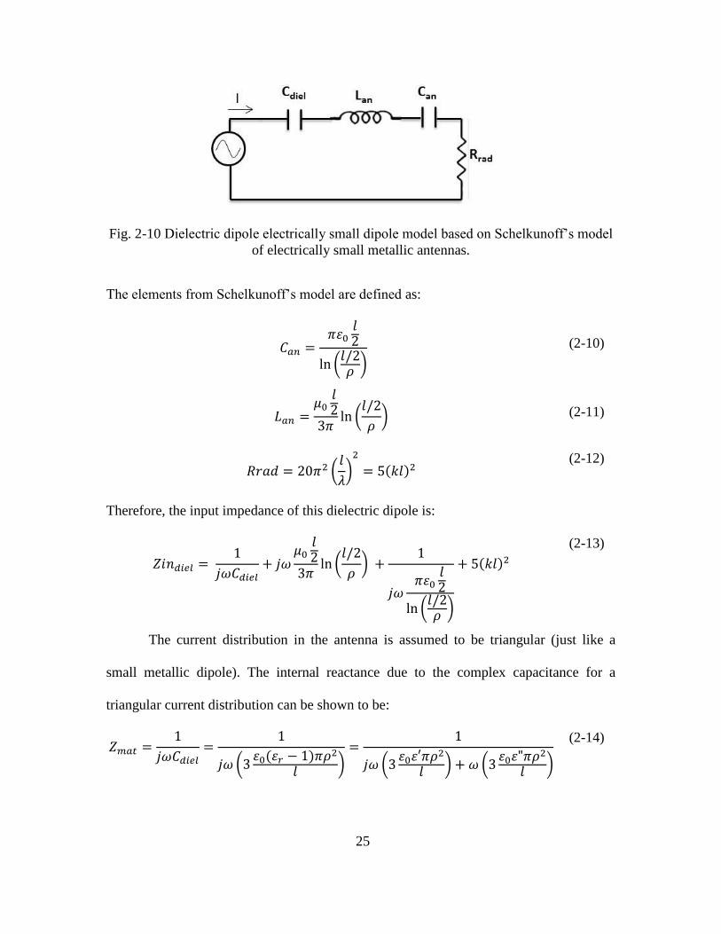
2-10 Dielectric dipole electrically small dipole model based on Schelkunoff’s model

of electrically small metallic antennas. ..................................................................... 25

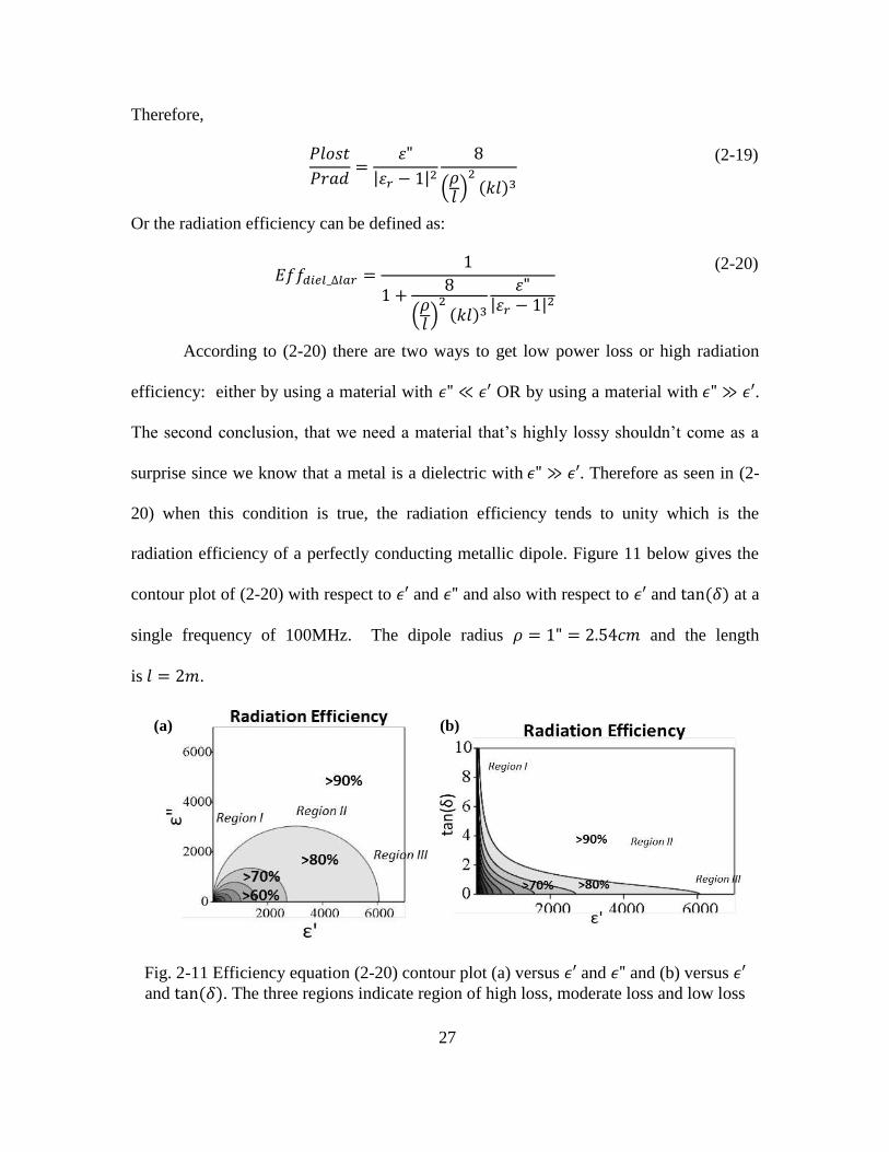
2-11 Efficiency equation (2-20) contour plot (a) versus and and (b) versus

and ( ). The three regions indicate region of high loss, moderate loss and low

loss ............................................................................................................................. 27

2-12 Comparison of simulated results and analytical equation (2-20) of the Radiation

Efficiency (dB) of a lossy dielectric dipole. .............................................................. 30

2-13 Assumed and Simulated current distribution in the lossy dielectric monopole ...... 31

2-14 Dielectric dipole antenna with multiple capacitive feeds simulated using lumped

ports ........................................................................................................................... 31

xii

2-15 (a) Current distribution of the multiple feed 1m long dielectric dipoles using

dielectrics with . (b) Radiation Efficiency as compared to (2-23). ....... 32

2-16 Radiation Efficiency as compared to (2-23) of the multiple capacitive feed 1m

long dipole using dielectrics with tan(δ)=1. .............................................................. 33

3-1 Dielectric dipole model based on Schelkunoff’s model of electrically small

metallic antennas. The permeability of the dielectric material is also included. ....... 41

3-2 (a) Skin depth in a cylindrical dipole (b) The transverse field shape for 0<δ<ρ of

the TM mode dielectric dipole. The solid line is the actual field shape and the

dashed line is the closest approximation ................................................................... 43

3-3 (a) A dielectric dipole carrying an electric current ‘Ie’ fed with an electric

voltage source ‘Ve’ and PEC feed lines (solid lines) such that

(b) Dual magnetic dipole carrying magnetic current ‘Im’ fed with a

magnetic voltage source ‘Vm’ and PMC feed lines (dashed lines) such that

(c) Permeable or magnetic dipole carrying

magnetic current ‘Im’ fed with an electric loop. ....................................................... 44

3-4 Cross-section of the permeable material dipole of 3-3(c) at the electric feed loop.

The mode of operation is TE like with the B-field along the axis of the dipole. ...... 45

3-5 Electrically small magnetic dipole antenna circuit model. ........................................ 47

3-6 (a) Efficiency equation (3-29) contour plot (a) versus μ’ and μ” and (b) versus μ’

and tan(δ). The three regions indicate region of high loss, moderate loss and low

loss. ............................................................................................................................ 49

3-7(a) Simulation geometry of a magneto-dielectric dipole fed by a single electric

feed loop and (b) eight feed loops ............................................................................. 51

xiii

3-8(a) Magnetic current distribution along the length of the dipole at two frequencies

(a) 100MHz ( ) (b) 200MHz ( ) ........................................ 51

3-9 Simulated Radiation Efficiency (symbols) comparison with (3-28) (solid curves)

for a single loop fed magneto-dielectric dipole. ........................................................ 52

3-10 Uniform magnetic current distribution along the length of the dipole at two

frequencies (a) 100MHz ( ) (b) 200MHz ( ) ..................... 53

3-11 Radiation Efficiency comparison of (3-28) with full-wave simulations of a

multi-loop fed magnetic dipole made of (a) low loss ( ( ) ( )

), (b) high magnetic but low electric loss ( ( ) ( ) )

(c) high loss( ( ) ( ) ) (d) extremely high loss ( ( )

( ) ) and (e) extremely high loss materials but neglecting skin depth

effects in the efficiency calculation. .......................................................................... 54

3-12 Magneto-dielectric dipole constructed using the NiZn ferrite tiles. ........................ 55

3-13 (a) NiZn FairRite tile material permeability. Permittivity of the ferrite is

. (b)Comparison of simulated Radiation Efficiency of the magneto-

dielectric dipole with two closed form equations. ..................................................... 56

3-14 (a) Magneto-dielectric dipole antenna mounted in the anechoic chamber (b)

Comparison of simulated realized gain & antenna gain measured in the chamber... 57

3-15 (a) Conformity of a Magneto-dielectric dipole as compared to a conventional

Whip antenna (b) Magneto-dielectric dipole raw measured gain comparison with

the standard whip antenna on a Humvee. .................................................................. 57

3-16 (a) Magnetic dipole with 8 electric feed loops. (b) Dielectric Dipole with 8

lumped port feeds. ..................................................................................................... 59

xiv

3-17 Radiation Efficiency comparison of a dielectric and magnetic dipole of the

same length and cross-section but with dual material properties. ............................. 60

4-1 Electrically small dielectric loop antenna model. ...................................................... 64

4-2 Electrically small magneto-dielectric loop antenna circuit model. ........................... 65

4-3 (a) Efficiency equation (4-12) plot versus ( )for (a) electrically small

antenna (b) small antenna and (c) electrically large

antenna . The radiation efficiency is the lowest at for any . .... 68

4-4 Magneto-dielectric loop HFSS simulation geometry ................................................ 69

4-5 Uniform magnetic current distribution along the length of the loop at two

frequencies (a) 100MHz ( ) (b) 200MHz ( ) ........................... 70

4-6 Radiation Efficiency comparison of (4-11) with full-wave simulations of a multi-

loop fed magnetic dipole made of (a) low loss ( ( ) ( ) ),

(b) high loss( ( ) ( ) ) (c) extremely high loss ( ( )

( ) ) and (d) extremely high loss materials but neglecting skin depth

effects in the efficiency calculation. .......................................................................... 72

4-7 Body Wearable Belt Antenna designed to replace tall whip antennas carried by

foot soldiers for interpersonal communication .......................................................... 73

4-8 (a) Human body cylinder fed with an ideal lumped port at the same location as

the eventual position of the BWA belt. (b) Frequency dependent permittivity of

the human body. ........................................................................................................ 75

4-9 Simulation results of the geometry in 4-8(a) where (a) Radiated power and

Power loss, (b) Feed Voltage and (c) Input impedance. ........................................... 75

xv

4-10 (a) Radiation resistance and loss resistance calculated from the simulation data

(b) the sum of which equals the real part of input impedance. (c) Radiation

Efficiency of the dielectric human body cylinder fed with an ideal lumped

capacitive port feed ................................................................................................... 76

4-11 Circuit model of the dielectric human body cylinder fed with a capacitive feed. ... 77

4-12 The circuit model of the BWA system that takes into account the ground plane. .. 77

4-13 Simulation geometry of the body wearable antenna system with quarter plane ..... 78

4-14 Radiation Efficiency comparison of the BWA system circuit model and full-

wave simulations for different values of permeability of the belt with (a),(b)

having a loss tangent of tan(δ)=0.1 and (c)(d) with high tan(δ)=1............................ 79

4-15 Radiation efficiency comparison for different permeability values for a toroid

minor radius of 3cm. ................................................................................................. 80

4-16 Radiation efficiency comparison for different permeability values for a toroid

minor radius of 6cm. ................................................................................................. 80

4-17 (a) Magneto-dielectric material permeability used in the belt(b) Radiation

efficiency of the BWA using the circuit model for different radii of the loop belt. .. 81

4-18 Contribution to the total radiation from the two sources of radiation: the human

body and the permeable toroid. ................................................................................. 82

5-1 Two sources of atomic magnetic dipole moments a) an orbiting electron and (b)a

spinning electron ....................................................................................................... 86

5-2 Intrinsic magnetic dipole moments in (a) Paramagnetic material (b)

Ferromagnetic material (c) Anti-ferromagnetic material and (d) Ferrimagnetic

materials .................................................................................................................... 87

xvi

5-3 Possible solutions to negate eddy current effects in ferromagnetic materials (a)

Lamination of thin films of material with an insulator in between and (b) Micro-

particles/ Flakes of ferromagnetic materials mixed in with an insulating resin ........ 89

5-4 Complex permeability of the NiZn family from [31] ................................................ 95

5-5 (a) A single Debye susceptibility function (b) A single Lorentz susceptibility

function ...................................................................................................................... 96

5-6 (a) Single Debye equivalent RC circuit and (b) Single Lorentz equivalent RLC

circuit ......................................................................................................................... 97

5-7 Magnetic conductivity of the (a) Debye and (b) Lorentz examples in 5-5 ............... 99

5-8 Magneto-dielectric dipole antenna geometry used to test the radiation efficiency

equations in terms of hesitivity ............................................................................... 104

5-9 Different (a) Debye and (b) Lorentz materials permeability and magnetic

conductivity plots, used in the verification of the radiation efficiency equation (5-

31). The hesitivity of the three seemingly different Debye materials is the same

and the same is true for the four Lorentz materials ................................................. 105

5-10 The Radiation Efficiency of (a) single Debye materials and (b) single Lorentz

materials shown in 5-9. The solid curve is using (5-31). ....................................... 105

5-11 (a) Loss tangent of the simulated Debye materials and (b) Efficiency Bandwith

Product (EBWP) curves for the same. ..................................................................... 107

5-12 (a) Loss tangent of the simulated Lorentz materials and (b) Efficiency

Bandwidth Product (EBWP) curves for the same. .................................................. 108

5-13 Frequency dispersive permeability (Solid: Real and Dashed: Imaginary) of

different magnetic materials that were considered for evaluation. ......................... 110

xvii

5-14 a) Radiation Efficiency (b) Fractional Bandwidth (c) Efficiency Bandwidth

product for different materials for a 1m long, 0.5” radius dipole. .......................... 112

6-1 ESA circuit model of (a) PEC dipole (b) the proposed model for a Magneto-

dielectric Dipole ...................................................................................................... 116

6-2 (a) PEC sphere with external flux lines and a (b) Dielectric sphere with internal

and external flux lines created in the presence of a uniform ambient E field(E). ... 117

6-3 PEC spherical antenna excited by a magnetic ring current ..................................... 118

6-4 Prolate Spheroidal Magneto-Dielectric Antenna fed by an electric loop

(Approximates a Cylinder) ...................................................................................... 119

6-5 Simulation model of a Prolate Spheroidal Antenna of different aspect ratios (AR)

in the full wave simulator (Ansoft HFSS). .............................................................. 120

6-6 Inductance of feed loop vs Frequency for different loop radii ................................ 122

6-7 Magnetic Capacitance of the ESA magneto-dielectric dipole Simulated and

Calculated from Polarizability for (a) (b) .................................. 123

6-8 Magnetic Capacitance and Polarizability proportionality factor (a) vs Aspect

Ratio and (b) vs Permeability .................................................................................. 124

6-9 Single pole Debye factor function (6-11) compared to fullwave simulation

extraction from polarizability for cross sectional radius (a) 1cm and (b)

1inch=2.54cm. ......................................................................................................... 125

6-10 a) Plot of factor for PMC dipole ‘facPMC’ and factor at the diaphanous limit

‘facDia’ versus invers of the aspect ratio. (b) Plot of the poles of (6-11). .............. 126

6-11 Simulated and Calculated complex magnetic capacitance for AR=30(a) &

AR=50(b), (c) List of complex used (numbered 1-10 => x-axis) ...................... 127

xviii

6-12 Input impedance comparison of circuit model and simulation of a 21” long, 1”

radius antenna (a) Real part (b) Imaginary part of input impedance. ...................... 129

6-13 The magnetic current ‘Im’ (in volts) plotted along the length of the antenna (a)

30MHz (b) 100MHz and (c) 500MHz. (d) List of permeability simulated. ...... 130

7-1 Infinite Magneto-Dielectric cylinder of radius ‘a’ .................................................. 134

7-2 Amplitude (a),Phase (b) as a function of distance from the feed for a 2” radius

, rod from 30MHz to 170MHz (c) Mode Structure ( ) .............. 143

7-3 Amplitude (a),Phase (b) as a function of distance from the feed for a 2” radius

, rod from 190MHz to 330MHz (c) Mode Structure ( ) ............ 144

7-4 Amplitude (a),Phase (b) as a function of distance from the feed for a 2” radius

, rod from 350MHz to 490MHz (c) Mode Structure ( ) ............ 146

7-5 Radiated Power (Prad) vs Frequency(MHz) for a 2” radius , rod . 147

7-6 Magnetic current (Im) of a semi-infinite cylindrical magento-dielectric antenna

(a = 3cm) vs antenna length measured from the feed loop. .................................... 148

7-7 Magnetic current ( ) of a semi-infinite magneto-dielectric antenna fit to an

exponential (dashed black curves). ......................................................................... 149

7-8 ‘Im’ and ‘Im – exp(fit)’ current curves for different µr vs antenna length. ............... 149

7-9 Finite cylindrical magneto-dielectric rod with circular feed loop. ......................... 151

7-10 Electric Current ‘Ie’ in the feed loop vs angular position for different µr. ............ 151

7-11 Radiated Power vs µr (Analytic: Infinite rod versus Simulated Finite cylindrical

rod) .......................................................................................................................... 152

7-12 a) Radiated power, (b) Effective (Half) Length of Finite 3cm radius magneto-

dielecric cylinder vs Frequency for µr = 60 ............................................................. 153

xix

7-13 a) Radiated power, (b) Effective (Half) Length of finite 0.75cm radius magneto-

dielectric cylinder vs Frequency and (c) Radiated power, (d) Effective (Half)

Length of finite 6cm radius magneto-dielectric cylinder vs Frequency. ................. 154

7-14 (a) Radiated power, (b) Effective (Half) Length (c) Effective (Half) Length /

Radius of a magneto-dielectric Antenna vs k0*a for a permeability µr = 60 (d)

Average of the three curves in (c) ........................................................................... 155

8-1 Prolate spheroidal coordinate system ( ) ........................................................ 161

8-2 Magneto-Dielectric finite prolate spheroidal antenna fed by anate spheroidal

antenna fed by a circular electric current loop at ................ 162

8-3 Prolate spheroidal antenna with a=8” and b=0.5” showing the line ξ=1.1. ............. 174

8-4 (a)The electric feed loop used in the full-wave simulator. Note that the outer

conductor was extended to the center to maintain symmetry w.r.t to the ground

plane. (b) Measured feed current ‘Ie’ for different frequencies for case(A) ......... 174

8-5 Comparison of of the analytical equation and the simulated result for case

(A) at (a) path in the near field and (b) path which is in the far

field. ......................................................................................................................... 175

8-6 Measured electric feed current at different frequencies vs. angle ‘ ’ for case (B) . 175

8-7 Comparison of of the analytical equation and the simulated result for case

(B) at (a) and (b) . ............................................................................. 176

8-8 Comparison between analytic and simulated radiated power Prad for the (A)

a=8” & b=0.5” and (B) a=12” and b=1.5”. ............................................................. 176

8-9 (a) Non-uniform Electric feed current for higher frequencies computed in HFSS

(b) Radiated power at those frequencies indicated by the circle markers. .............. 177

1

Chapter 1

INTRODUCTION

An antenna or an “aerial” (term deprecated in 1983 from IEEE Antenna Std.

Definitions) has traditionally been considered as a metallic object that radiates energy and

is used to send and receive radio signals over large distances. With the increasing use of

non-metals in antenna design, the traditional definition of an antenna has been changed

to: “that part” of a transmitting or receiving system that is designed to radiate or to

receive electromagnetic waves. In the transmitting mode, a conventional metal antenna

binds the electromagnetic wave and allows it to propagate close to the speed of light of

the external medium. The principal sources of radiation are then the discontinuities at the

ends of the antenna. In contrast, a dipole constructed from a penetrable material does not

necessarily bind the electromagnetic wave but instead partially guides it, letting it leak off

along the length of the structure. Whatever energy is carried to the ends of the antenna

radiates at these discontinuities just like a metal antenna. Thus, such antennas make use

of two distinct radiation mechanisms. In this report, we examine antennas made up of

dielectric ( , ~1), permeable ( , ) or magneto-dielectric ( and

with ) materials.

The fundamental sources of radiation in antennas are the electric and magnetic

currents supported by the antenna structure. The ‘source’ of any problem in

electromagnetic theory or antenna theory is contained within Maxwell’s equations.

Maxwells’ original “Treatise on Electricity and Magnetism” contained 20 equations with

2

20 unknowns represented using quaternions. Twelve of the original twenty were reduced

to the set of the now conventional four by Oliver Heaviside. The two curl equations or

circuital current equations in its simplest form as stated by Heaviside are:

(1-1)

(1-2)

where, is the electric current density and is the magnetic current density. To maintain

the symmetry of the curl equations, Heaviside defined these current densities as:

(1-3)

(1-4)

where dD/dt and dB/dt are the electric and magnetic displacement current densities

respectively and and are the electric and magnetic conduction current densities

respectively. By introducing material properties, namely permittivity ( ) and

permeability ( ) through the constitutive relations, and , the

current density equations can be further expanded as:

( )

(1-5)

( )

(1-6)

where, ( ) is the electric polarization current density and

( ) is magnetic polarization current density. In the case of

metallic antennas, the antenna radiation source is the electric current due to . In the case

of the most general dielectric antenna, the source of radiation is the electric current due to

both and . In the case of magneto-dielectric antennas with the source

3

of radiation is the the magnetic polarization current density , since magnetic

monopoles don’t exist ( ).

The motivation for the analysis of magneto-dielectric antennas comes from the

fact that magneto-dielectric materials can be used as wire elements to make efficient

conformal antennas over a metal ground plane. The IEEE Standard definition of terms for

antennas defines a conformal antenna as an antenna that conforms to a surface whose

shape is determined by considerations other than electromagnetic; for example

aerodynamic or hydrodynamic. The surface or platform in this case can be part of an

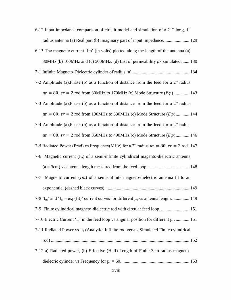
aircraft, truck, jeep or any other vehicle. Whip or Blade Antennas are commonly used as

VHF/UHF antennas in military vehicles. These off-the-shelf antennas operate over a

narrow band of frequency. Therefore, military vehicles often have many such antennas

protruding from the body for use in navigation, communication, radars, etc. (Fig. 1-1).

Fig. 1-1Off- the-shelf Whip and Blade Antennas on Military platforms.

Such antennas are usually attached as an afterthought and routinely in locations and

orientations that can damage them and expose them to the enemy. In other words, they

are not low profile and are conspicuous. They cause considerable drag and increase fuel

consumption. The ideal solution would be to replace several such antennas on a military

platform with a “Single Conformal Wideband Antenna”. An antenna with wideband

4

capabilities enables shared aperture multi-function radiators, while conformal profiles

minimize physical damage of the antenna in Army applications, drag and weight

penalties in Airborne applications and reduce the visual and RF signatures associated

with the communication and RADAR systems.

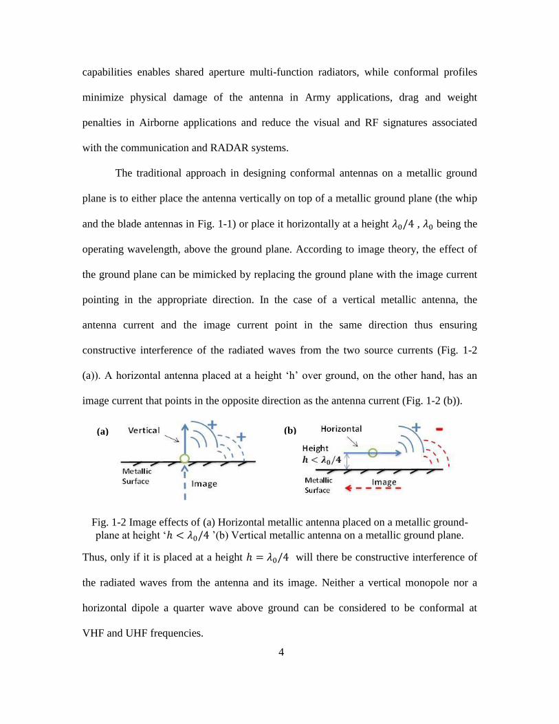
The traditional approach in designing conformal antennas on a metallic ground

plane is to either place the antenna vertically on top of a metallic ground plane (the whip

and the blade antennas in Fig. 1-1) or place it horizontally at a height , being the

operating wavelength, above the ground plane. According to image theory, the effect of

the ground plane can be mimicked by replacing the ground plane with the image current

pointing in the appropriate direction. In the case of a vertical metallic antenna, the

antenna current and the image current point in the same direction thus ensuring

constructive interference of the radiated waves from the two source currents (Fig. 1-2

(a)). A horizontal antenna placed at a height ‘h’ over ground, on the other hand, has an

image current that points in the opposite direction as the antenna current (Fig. 1-2 (b)).

Fig. 1-2 Image effects of (a) Horizontal metallic antenna placed on a metallic ground-

plane at height ‘ ’(b) Vertical metallic antenna on a metallic ground plane.

Thus, only if it is placed at a height will there be constructive interference of

the radiated waves from the antenna and its image. Neither a vertical monopole nor a

horizontal dipole a quarter wave above ground can be considered to be conformal at

VHF and UHF frequencies.

(a) (b)

5

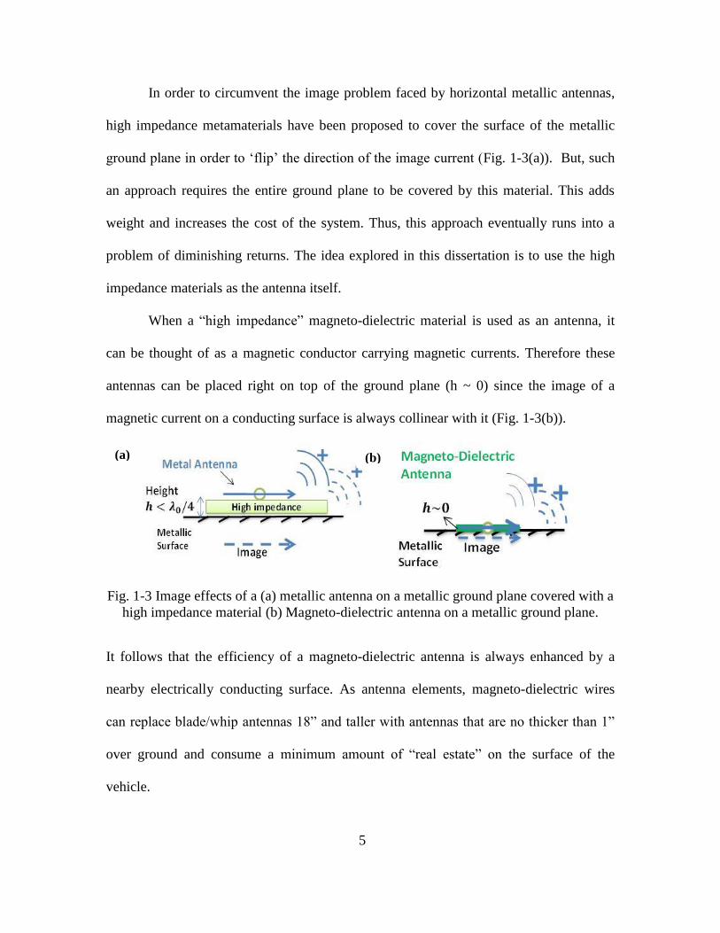
In order to circumvent the image problem faced by horizontal metallic antennas,

high impedance metamaterials have been proposed to cover the surface of the metallic

ground plane in order to ‘flip’ the direction of the image current (Fig. 1-3(a)). But, such

an approach requires the entire ground plane to be covered by this material. This adds

weight and increases the cost of the system. Thus, this approach eventually runs into a

problem of diminishing returns. The idea explored in this dissertation is to use the high

impedance materials as the antenna itself.

When a “high impedance” magneto-dielectric material is used as an antenna, it

can be thought of as a magnetic conductor carrying magnetic currents. Therefore these

antennas can be placed right on top of the ground plane (h ~ 0) since the image of a

magnetic current on a conducting surface is always collinear with it (Fig. 1-3(b)).

Fig. 1-3 Image effects of a (a) metallic antenna on a metallic ground plane covered with a

high impedance material (b) Magneto-dielectric antenna on a metallic ground plane.

It follows that the efficiency of a magneto-dielectric antenna is always enhanced by a

nearby electrically conducting surface. As antenna elements, magneto-dielectric wires

can replace blade/whip antennas 18” and taller with antennas that are no thicker than 1”

over ground and consume a minimum amount of “real estate” on the surface of the

vehicle.

(a) (b)

6

The lowest order modes that a magneto-dielectric wire can carry are the HE11

mode and the TE01 mode. The field structure of these modes along with that of a PMC

(perfect magnetic conductor) wire are shown in Fig. 1-4.

Fig. 1-4 (a) E and H field structure around a PMC wire (b)HE11 mode in a magneto-

dielectric material (c) TE01 mode in a magneto-dielectric material.

The HE11 mode shown in Fig. 1-4(b) has no cut-off or onset frequency. That is,

the HE11 mode is well guided by the magneto-dielectric wire from dc to daylight.

Although it is well supported by the structure, the HE11 mode looks like a two-wire PMC

transmission line which we know is a poor radiator. The TE01 mode has a cut-off or

onset frequency ( ) given by:

√

(1-7)

where is the speed of light in free space and ‘ ’ is the radius of the wire. Below the

TE01 onset frequency, the wave is loosely guided by the magneto-dielectric wire. The

field shape of the TE01 wave outside the wire in this case looks like that of a PMC wire

and hence is will radiate off of any discontinuities in the structure. This favorable TE01

Im

Two PMC wire line

HE11 modePMC wire

Single PMC wire

TE01 mode

(a) (b)

(c)

7

mode can be injected into the magneto-dielectric material using an electric current loop

with the material place along its axis. This is the feeding mechanism utilized throughout

this dissertation.

The outline of the dissertation is shown as flow- chart in Fig. 1-5. Each section in

the flow chart is covered in subsequent chapters as labeled.

Fig. 1-5 Outline of the dissertation

In Chapter 2, the dielectric capacitor/condenser antenna is re-examined and we

point out the efficacy of putting the dielectric material outside the capacitor plates instead

of within them as in a condenser. This structure is referred to as a dielectric dipole and its

comparison with conventional metallic antennas of the same size is shown. It is

demonstrated through simulations that the performance of an electrically small dielectric

8

dipole can approach but never surpass a metallic dipole of the same dimension. A closed

form expression of the radiation efficiency of this dielectric dipole using realistic

materials is also derived which includes the often omitted loss tangent (tan (δ)) or

imaginary part of permittivity i.e. ε” loss. The accuracy of this equation is tested through

rigorous full-wave simulations. The results show that high radiation efficiency in

dielectric dipoles can be obtained with both low loss and high loss materials which is a

deviation from contemporary notion of requiring only low loss materials to achieve the

same.

In Chapter 3, the properties of an electrically small dipole antenna constructed

from magneto-dielectric media ( ) are derived in closed form by following

Schelkunoff’s original development for electrically small metallic antennas and

exploiting duality. Such dipoles are attractive alternatives to vertical monopoles because

they can be placed conformal to a metallic ground plane without performance

degradation. The closed form expression of the radiation efficiency derived includes the

often neglected imaginary part of permeability i.e. loss. This analysis shows that it is

possible to construct high radiation efficiency antennas out of not only the traditional or

conventional low loss (low ) materials but also with highly lossy materials

( ( ) ). This is a noteworthy conclusion given the fact that most magnetic

materials exhibit loss beyond VHF or sometimes even beyond the HF range. A magneto-

dielectric dipole using commercially available NiZn ferrite absorber tile material was

constructed and tested in an anechoic chamber demonstrating significant efficiency .

Finally, the duality between a magneto-dielectric dipole and the dielectric dipole of

Chapter 2 is explored analytically and numerically.

9

In Chapter 4, the properties of a magneto-dielectric electrically small loop antenna

are derived in closed form using the same approach as that followed for the magneto-

dielectric dipole in Chapter 3. A magneto-dielectric loop is an ideal alternative to vertical

monopoles because they have same radiation pattern as the monopole and yet can be

placed conformal to a metallic ground plane without performance degradation. Similar to

Chapter 3, the results here also show that it is possible to construct high efficiency loops

using lossy materials. An application to the case of a body wearable antenna is also

discussed.

In Chapter 5, a material selection law for selecting the most appropriate

permeable material to design magneto-dielectric antennas is postulated. This selection

law is derived within the bounds of three fundamental physical limits, namely, 1) the

Gain-Bandwidth product limit, 2) Snoek’s product limit for magnetically permeable

materials and 3) the restrictions imposed on the permeability function by the Kramers-

Krönig relations. Within these constraints it is shown that one dominant parameter with

the units of magnetic conductivity characterizes the performance of the material. The

validity and applicability of the selection law is demonstrated by full-wave simulations of

conformal magneto-dielectric dipoles using both fictitious and realistic magneto-

dielectric materials.

In Chapter 6, a simpler three element RLC circuit model for a magneto-dielectric

dipole is postulated where the capacitance ‘C’ is proportional to the polarizabilty of the

object. The proportionality factor that relates the two accounts for the morphology of the

magnetic field structure and is found to be a single pole Debye function in the

morphology variable ( ( )). The inductance and the radiation resistance are

10

then derived by duality from the case of the electric dipole. Although this approach

extends the magneto-dielectric dipole model beyond the regime of the electrically small

circuit models of Chapter 3, it implicitly assumes that the magnetic current distribution

on the antenna is triangular. As is shown in Chapter 7 this is only true for a narrow range

of frequencies and values of permeability that result in operation close to the onset of

guided mode propagation.

In Chapter 7, the Green function problem of a cylindrical magneto-dielectric rod

of infinite length excited by an electric current loop current is solved. The magnetic

current wave excited in a magneto-dielectric infinite rod is shown to go through a

succession of fast wave-slow wave transitions as a function of frequency. Below the first

mode and in between modes the fast wave regions exhibit leaky wave behavior with

decaying amplitude and phase velocities faster than the speed of light. Every time we

approach the onset of guidance of a mode, there is a band of frequencies over which the

magneto-dielectric rod behaves very much like a PMC metal rod. Given the

predominantly leaky wave behavior exhibited by these antennas in their most common

application (low frequencies, electrically small elements) it is possible to calculate the

minimum length of material required to get the same amount of radiated power as that of

an infinite magneto-dielectric cylinder of the same cross-section.

In Chapter 8, the Green function problem of a finite prolate spheroidal magneto-

dielectric antenna fed by a current loop is solved. The electric and magnetic fields

calculated are shown to agree well with full-wave simulations. An expression for the

total radiated power from this finite dipole is also derived and compared to simulations.

11

At the end of every chapter, suggestions are given for follow-on work that could

extend the results presented. Three Appendices are included covering the impact to the

model of the skin effect in magneto-dielectric cylinders, an alternative derivation of the

efficiency of a permeable dipole, and details of the solution of the Helmholtz wave

equation in Prolate spheroidal coordinates.

12

Chapter 2

DIELECTRIC DIPOLE ANTENNA

2.1 Introduction

Ever since the idea of accelerated charges radiating energy was first conceived,

scientists and engineers have extensively used conductors or metals as antenna elements

due to the abundance of free charges available in them. It was also known that dielectric

materials can guide waves in them. But, it was an accepted fact that since dielectric

materials guide waves, they have the tendency to trap these waves and hence do not

promote radiation. Nevertheless, one of the first variants from the conventional metallic

antennas was the capacitor/condenser antenna. Such a design employing dielectric

materials was implemented but was immediately disregarded by prominent engineers like

S. Schelkunoff [1] and H. A. Wheeler [2] [3] (Fig. 2-1(a) & Fig. 2-1(b)).

Fig. 2-1 a) Schelkunoff’s dielectrically loaded antenna [1] (b) Wheeler’s capacitor

antenna [2] [3] (c) Dielectric Dipole antenna

13

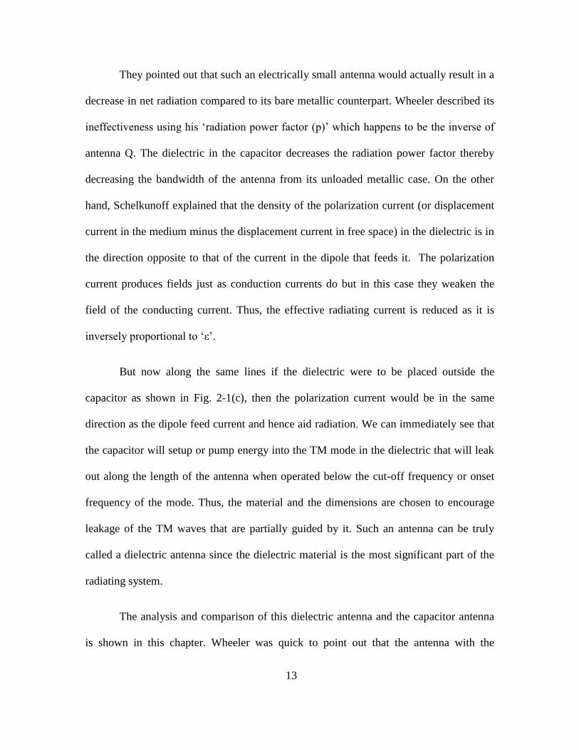
They pointed out that such an electrically small antenna would actually result in a

decrease in net radiation compared to its bare metallic counterpart. Wheeler described its

ineffectiveness using his ‘radiation power factor (p)’ which happens to be the inverse of

antenna Q. The dielectric in the capacitor decreases the radiation power factor thereby

decreasing the bandwidth of the antenna from its unloaded metallic case. On the other

hand, Schelkunoff explained that the density of the polarization current (or displacement

current in the medium minus the displacement current in free space) in the dielectric is in

the direction opposite to that of the current in the dipole that feeds it. The polarization

current produces fields just as conduction currents do but in this case they weaken the

field of the conducting current. Thus, the effective radiating current is reduced as it is

inversely proportional to ‘ε’.

But now along the same lines if the dielectric were to be placed outside the

capacitor as shown in Fig. 2-1(c), then the polarization current would be in the same

direction as the dipole feed current and hence aid radiation. We can immediately see that

the capacitor will setup or pump energy into the TM mode in the dielectric that will leak

out along the length of the antenna when operated below the cut-off frequency or onset

frequency of the mode. Thus, the material and the dimensions are chosen to encourage

leakage of the TM waves that are partially guided by it. Such an antenna can be truly

called a dielectric antenna since the dielectric material is the most significant part of the

radiating system.

The analysis and comparison of this dielectric antenna and the capacitor antenna

is shown in this chapter. Wheeler was quick to point out that the antenna with the

14

dielectric outside will be considerable larger in size. Hence in order to evaluate the

performance of the “dielectric dipole”, comparison is done with a metallic dipole of the

same length and cross-section. We show that in the electrically small limit we can never

do better than a metallic small antenna with dielectric materials.

A comprehensive summary of theoretical analysis and experimental data on

electrically small and moderate dielectric loaded antennas done up to 1977 was presented

by Smith [4]. Three distinct cases were considered and it was shown that i) a

dielectrically loaded electrically small antenna always led to reduction in efficiency and

bandwidth. ii) Metal monopoles are superior to antennas of moderate lengths with a thin

dielectric coating and iii) dipole with thick dielectric coatings are intrinsically

narrowband.

Since the 1980s the focus of design of antennas that use dielectric materials

shifted to another class of such antennas called ‘dielectric resonator antennas’. The term

was first coined by Richtmyer [5] in 1939, however such antennas were first analyzed in

detail in the eighties starting with Long et al. [6]. A detailed summary of research on this

subject is given in [7]. These antennas have found widespread use in mobile phone

handsets. These can also be called dielectric antennas but because they operate at

frequencies past or around the resonance of the dielectric object, they are intrinsically

narrowband. Their usual operating frequency range is anywhere between 1GHz-40GHz

with the antenna length being greater than . In this chapter, we shall concentrate on

dielectric antennas operated in the electrically small regime (length ).

Another sub-class of antennas employing dielectric materials is the dielectric rod

antenna or polyrod antenna [8-10]. These are typically fed from a dielectric filled metallic

15

waveguide that launches the lowest order surface wave into the dielectric rod several

wavelengths long. Such antennas also rely on leakage along the length of the structure.

As they are many wavelength’s long, these antennas also do not fall under the category

that we are interested in.

Although there are many variations of the dielectric dipole as listed above, we are

going to restrict our analysis to the most fundamental case: a monopole over a ground

plane. We start our analysis in Section 2.2 with the classic capacitor antenna and prove

via simulations, Wheeler and Schelkunoff’s heuristic reasoning as to why they are not

beneficial. This is followed by the dielectric dipole antenna analysis in Section 2.3 which

showing how a dielectric material can aid the radiation process. In Section 2.4, the

radiation efficiency of a realistic dielectric antenna with lossy material is derived based

on the electrically small antenna circuit model. The result shows that unlike the classical

notion that all materials ought to have very low loss for high radiation efficiency, an

extremely lossy dielectric can also give high radiation efficiency. Section 2.5 contains the

summary of the chapter, some notable conclusions and possible future work on this

subject.

The purpose of this chapter is to explain why and how small dielectric dipoles

work the way they do and derive some simple expressions and antenna models that agree

with simulations. It serves as an introduction to a much more useful and practical

antenna: the magneto-dielectric dipole antenna.

16

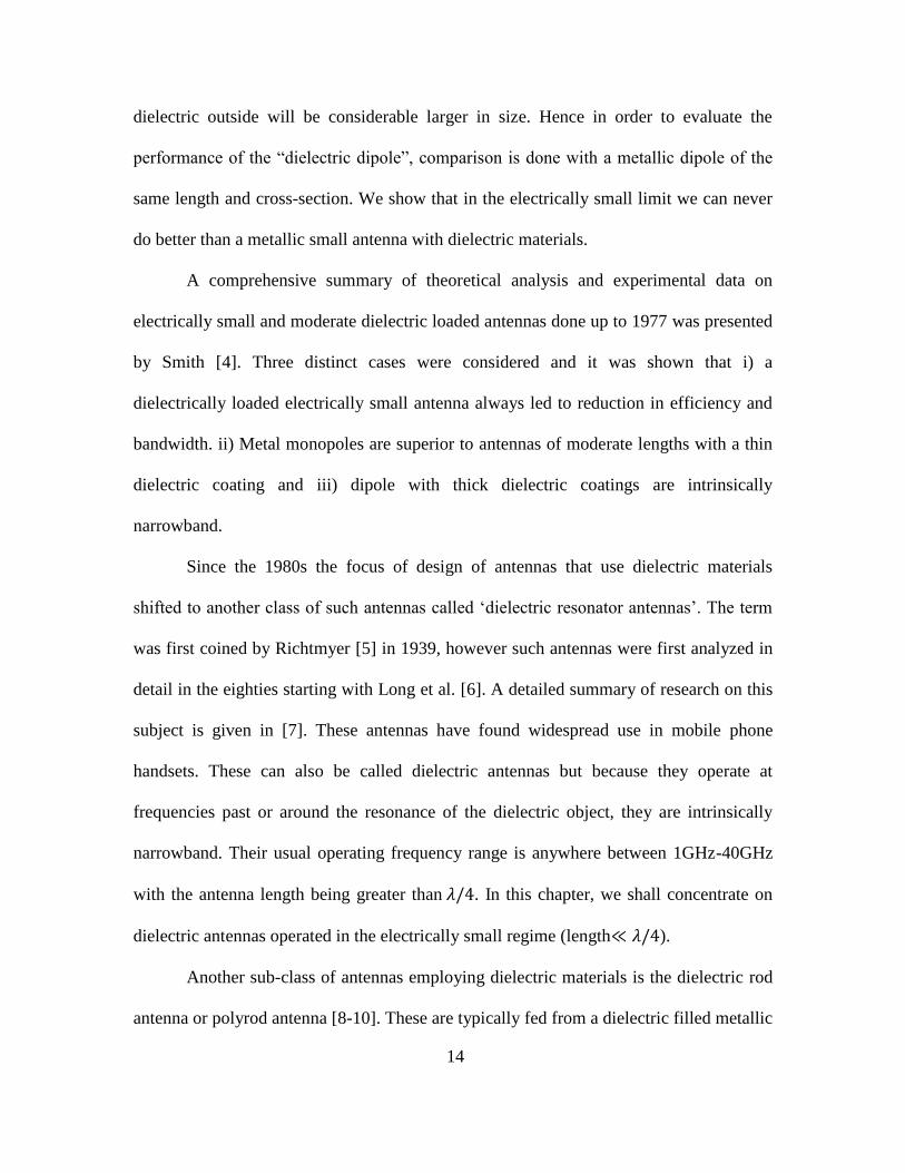
2.2 Capacitor/ Condenser Antenna

The HFSS simulation geometry for the capacitor antenna of Fig. 2-1(a) is shown

below in Fig. 2-2(a). It’s a 10cm tall and 2cm diameter monopole over ground terminated

in a top plate filled with a dielectric εr, with the center conductor extending all the way to

the top plate. In order to prove Schelkunoff’s assessment, the conduction current ‘Ic’ in

the center conductor and the total radiation current ‘Itotal’ (sum of conduction current in

the center conductor and the displacement current in the dielectric) in the monopole are

measured using two Amperean loops shown in Fig. 2-2(b).

Fig. 2-2 (a) Simulation geometry of the capacitor antenna. (b) Ampere’s loop in the

simulator to measure the conduction current in the center conductor and the total

radiation current of the monopole.

The dielectric constant εr of the material is swept from unity which is the basic

metallic monopole over ground to εr=1000. The ratio of the total radiating current to the

conduction current at 100MHz is shown in Fig. 2-3.

(a)

(b)

17

Fig. 2-3 The ratio of the total radiated current (Itotal) to the conduction current (Ic) in the

center conductor @ 100MHz plotted along the length of the loaded monopole for

different values of .

For the metallic monopole, this ratio should be unity. The slight drop seen around

the origin and around 10cm is due to the turbulence near the feed and the end

discontinuity respectively. Clearly, as Schelkunoff envisioned the net current that

accounts for radiation drops as the dielectric constant of the material increases. The input

impedance of the capacitor antenna is shown in Fig. 2-4.

Fig. 2-4 (a) Real and (b) Imaginary part of input impedance of the capacitor antenna for

different values of εr.

(a) (b)

18

Loading the dipole with a dielectric material has resulted in a drop in the real part

of input impedance indicating a drop in radiation resistance due to the reduction in net

radiating current as seen in Fig. 2-3. The added dielectric has also clearly shifted the

dipole resonance to a much lower value. The resonance frequency decreases with

increasing εr due to an increase in capacitance. The antenna Q can be now calculated

using the equation below given by Best et al. [11].

( ) (2-8)

The antenna Q calculated from the input impedance of the antenna is a convenient

approximation and can have errors in cases where there are closely spaced resonances.

For all the dielectrically loaded cases, the antenna Q is higher than that of the metal

monopole (as seen in Fig. 2-5. It is not that significant but it still is higher than the metal

for this particular geometry) and therefore the bandwidth is reduced. Also, the radiation

efficiency of a capacitor antenna will always be lower than that of a pure metallic dipole

assuming negligible conductor losses. Therefore the efficiency bandwidth product which

is sometimes used as a figure of merit for antennas will always decrease when the

capacitor antenna is loaded with a dielectric. Hence we can see that dielectrically loading

a monopole is not useful in the electrically small regime.

19

Fig. 2-5(a) Antenna Q calculated from input impedance using (1) and (b) Ratio of the

Antenna Q of the dielectric capacitor to the Q of the metallic monopole. The dielectric Q

is higher than the metallic monopole throughout the band.

2.3 Dielectric Monopole (Capacitive Feed)

Now, consider a dielectric monopole postulated before, with the dielectric placed

outside the capacitor similar to Fig. 2-1(c). The simulation geometry is shown below in

Fig. 2-6.

Fig. 2-6 Simulation geometry of the dielectric monopole.

The dielectric constant of the material is swept from unity which is the

capacitive feed gap (a short monopole) by itself all the way to . In order to

(a) (b)

20

make a fair comparison with its metallic counterpart, a metallic monopole is also

simulated of the same dimensions (i.e. height =10cm and 2cm diameter). The capacitive

feed injects TM like modes (circulating and longitudinal ) into the dielectric

material supported by it which when below the onset of guidance (i.e. below the cutoff

frequency) will leak out of the material. The cutoff frequency of the TM modes depends

on the antenna cross-section and the dielectric constant. For this geometry and set of

dielectric constants the lowest order TM01 mode onset/cutoff frequencies are given

below in Table 2-1.

Dielectric Constant

(εr)

TM01 Onset

Frequency (MHZ)

20 2632.5

80 1291

300 663.6

1000 363

Table 2-1 TM01 onset/cutoff frequency for a 1cm radius dielectric cylinder for

different .

The simulation frequency range is 30MHz-500MHz. Note that in this range,

εr=1000 is the only case where the onset frequency is crossed. Figure 7 below gives the

shape of the mode inside the dielectric material for different dielectrics at two different

frequencies (100MHz and 500MHz). Figure 7(a) and (b) show the strength of the

circulating magnetic field , at a height above the feed as a function of

tranverse position (‘x’ in cm). The black vertical lines at indicate the

boundary of the rod. At 100MHz (Fig. 2-7(a)) the TM mode launched into the dielectric

is strongly cutoff. At 500MHz (Fig. 2-7(b)) we see evidence of the onset of guided waves

21

particularly in the case of where we can clearly see more than one transverse

wavelength fit inside the dielectric. Outside the cylinder, the field drops exponentially as

expected. As the wave becomes more and more trapped due to guidance, its energy

migrates to the interior of the rod i.e increases inside the cylinder and the next higher

order mode(TM02) starts to appear.

Fig. 2-7 (a) & (b) are plots of along a line in the XY plane (@ z=4cm) indicating TM

Mode structure inside the dielectric material at 100MHz and 500MHz respectively (c)

Plot of displacement current density ‘ ’ plotted along the axis of the dielectric cylinder.

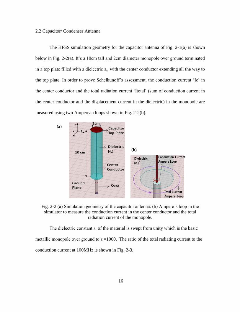
In Fig. 2-8, the ratio of the total radiating current to the conduction current is

plotted. The conduction current in this case is the current at the coaxial feed. As expected

in a clear contrast with the capacitor antenna, the net radiating current in the dielectric

increases with increasing values of the dielectric constant .

(a) (b)

22

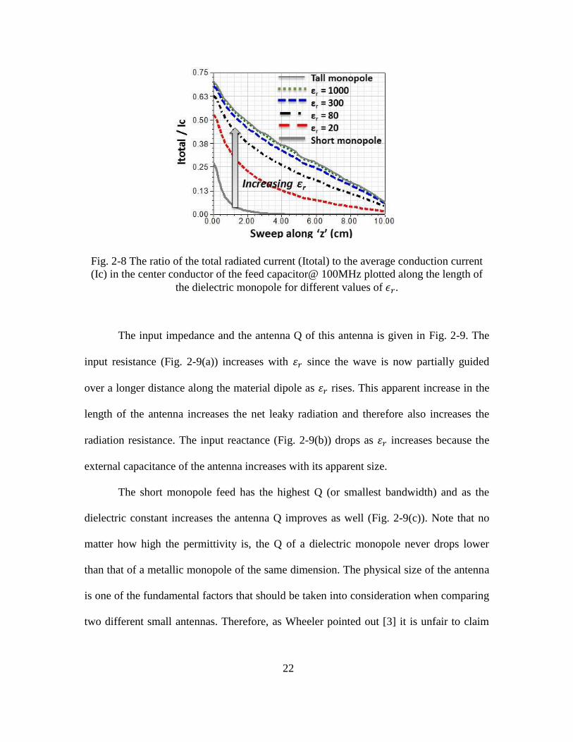
Fig. 2-8 The ratio of the total radiated current (Itotal) to the average conduction current

(Ic) in the center conductor of the feed capacitor@ 100MHz plotted along the length of

the dielectric monopole for different values of .

The input impedance and the antenna Q of this antenna is given in Fig. 2-9. The

input resistance (Fig. 2-9(a)) increases with since the wave is now partially guided

over a longer distance along the material dipole as rises. This apparent increase in the

length of the antenna increases the net leaky radiation and therefore also increases the

radiation resistance. The input reactance (Fig. 2-9(b)) drops as increases because the

external capacitance of the antenna increases with its apparent size.

The short monopole feed has the highest Q (or smallest bandwidth) and as the

dielectric constant increases the antenna Q improves as well (Fig. 2-9(c)). Note that no

matter how high the permittivity is, the Q of a dielectric monopole never drops lower

than that of a metallic monopole of the same dimension. The physical size of the antenna

is one of the fundamental factors that should be taken into consideration when comparing

two different small antennas. Therefore, as Wheeler pointed out [3] it is unfair to claim

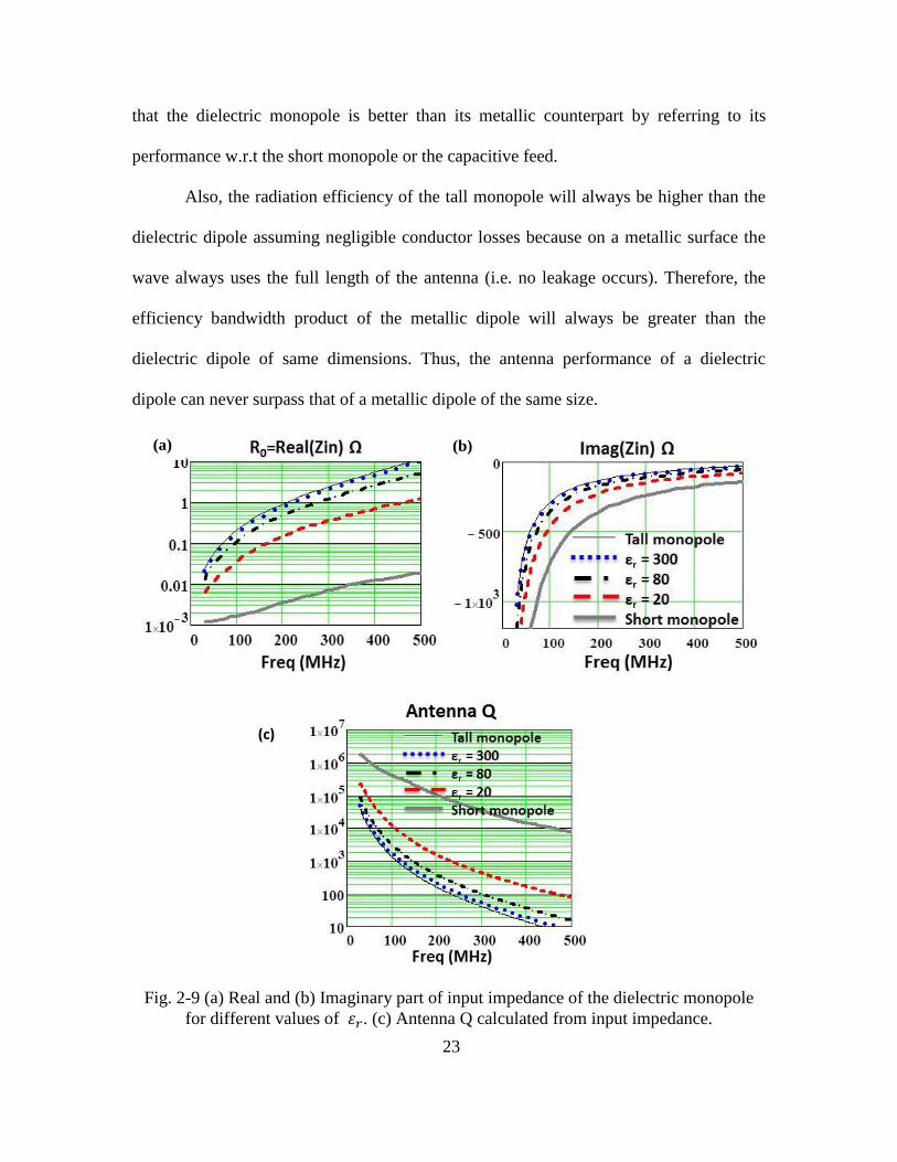
23

that the dielectric monopole is better than its metallic counterpart by referring to its

performance w.r.t the short monopole or the capacitive feed.

Also, the radiation efficiency of the tall monopole will always be higher than the

dielectric dipole assuming negligible conductor losses because on a metallic surface the

wave always uses the full length of the antenna (i.e. no leakage occurs). Therefore, the

efficiency bandwidth product of the metallic dipole will always be greater than the

dielectric dipole of same dimensions. Thus, the antenna performance of a dielectric

dipole can never surpass that of a metallic dipole of the same size.

Fig. 2-9 (a) Real and (b) Imaginary part of input impedance of the dielectric monopole

for different values of . (c) Antenna Q calculated from input impedance.

(a) (b)

(c)

24

2.4 Radiation Efficiency of a Lossy Dielectric Dipole

The goal of this section is to determine in closed form an equation for the

radiation efficiency of a dielectric dipole antenna. There are two definitions of efficiency

for antennas: the radiation efficiency and the antenna efficiency. The radiation efficiency

computes efficiency of radiation in the presence of antenna material losses (conductor

losses or dielectric losses). The antenna efficiency is the total efficiency of the system

which includes the feed mismatch loss. Since all realistic materials have some amount of

loss in them (i.e. or ( ( )) where or loss tangent ( )

signifies the loss), we will start our analysis with the radiation efficiency. The radiation

efficiency is defined as

(2-9)

where, ‘Prad’ is the power radiated by the antenna and ‘Plost’ is the power lost in the

antenna material.

Starting from Schelkunoff’s circuit model for electrically small metallic antennas

[2]; a dielectric dipole antenna can be modeled by including the material properties in

series with it i.e. with a series internal complex capacitance (due to complex

permittivity ). This term accounts for the internal energy in the material. The

circuit model is shown in Fig. 2-10.

25

Fig. 2-10 Dielectric dipole electrically small dipole model based on Schelkunoff’s model

of electrically small metallic antennas.

The elements from Schelkunoff’s model are defined as:

( )

(2-10)

(

)

(2-11)

(

)

( ) (2-12)

Therefore, the input impedance of this dielectric dipole is:

(

)

( )

( )

(2-13)

The current distribution in the antenna is assumed to be triangular (just like a

small metallic dipole). The internal reactance due to the complex capacitance for a

triangular current distribution can be shown to be:

( ( )

)

(

) (

)

(2-14)

26

where, ( ( )

). The factor of ‘3’ shows up due the triangular distribution.

This factor is unity for uniform current distribution which would be a simple capacitor

equation. is derived by equating the electric energy integral to the circuital capacitor

energy equation Free space is subtracted from the internal capacitance (i.e. dielectric

constant ( )) since when we must be left with just the feed. This internal

reactance can be further expanded as,

(

) (

( )

)

( ( ( )

))

( (

))

(2-15)

The loss in the antenna comes from the frequency dependent “loss resistance” or the

terms with . Therefore, the power lost in the antenna carrying a current ‘I’ can be

defined as,

(

)

(2-16)

Now the radiated power ‘Prad’ is defined as

( )

(2-17)

From (2-16) and (2-17),

(

)

( )

(2-18)

We know that k=ω/c0 , √ and √ . Also,

.

27

Therefore,

( ) ( )

(2-19)

Or the radiation efficiency can be defined as:

( ) ( )

(2-20)

According to (2-20) there are two ways to get low power loss or high radiation

efficiency: either by using a material with OR by using a material with .

The second conclusion, that we need a material that’s highly lossy shouldn’t come as a

surprise since we know that a metal is a dielectric with . Therefore as seen in (2-

20) when this condition is true, the radiation efficiency tends to unity which is the

radiation efficiency of a perfectly conducting metallic dipole. Figure 11 below gives the

contour plot of (2-20) with respect to and and also with respect to and ( ) at a

single frequency of 100MHz. The dipole radius and the length

is .

Fig. 2-11 Efficiency equation (2-20) contour plot (a) versus and and (b) versus and ( ). The three regions indicate region of high loss, moderate loss and low loss

(a) (b)

28

Fig. 2-11 is in greyscale with the efficiency going from highest to lowest as the

shade goes from light to dark. The contours are divided in tens i.e the lightest region has

efficiency greater than 90%, the next, greater than 80% and so on. Region I, II and III

stands for regions of high loss ( ) or metal-like materials, moderate loss (where

is comparable to ) and low loss ( ) or what researchers call good dielectrics,

respectively. The figure reiterates the comment made before that there are different ways

to get low power loss-to-power radiated ratios. The figure also shows a third region of

high efficiency where both and are sufficiently high and comparable to each other. It

is obvious that the ‘good dielectrics’ of Region I will have high radiation efficiency due

to low dielectric loss. In the metal-like Region I and Region II, the material skin-depth is

very small compared to the antenna cross-section and hence all the fields are pushed out

to the surface of the antenna. Therefore, the dielectric dipole tends to act more like the

conventional metal dipole and therefore exhibit high radiation efficiency.

Now if the assumed current distribution is uniform then,

( )

(2-21)

(

)

( ) (2-22)

Therefore, the radiation efficiency assuming a uniform current distribution can be derived

the same way as before to be:

( ) ( )

(2-23)

29

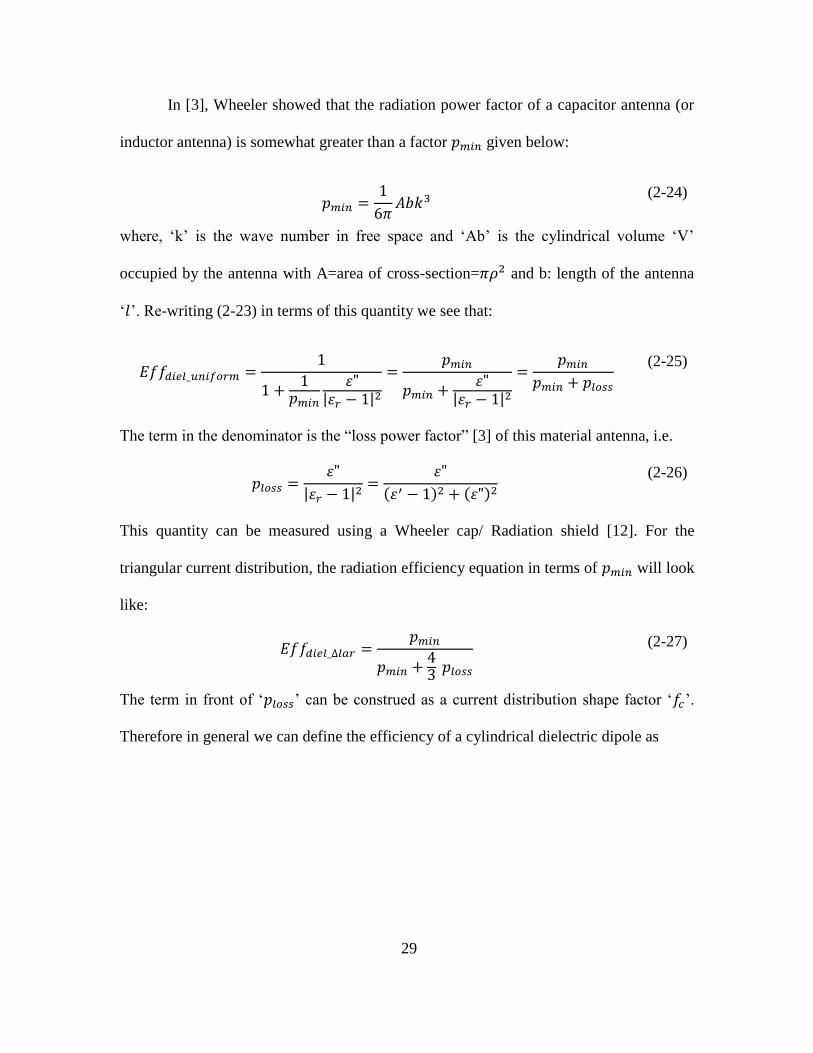
In [3], Wheeler showed that the radiation power factor of a capacitor antenna (or

inductor antenna) is somewhat greater than a factor given below:

(2-24)

where, ‘k’ is the wave number in free space and ‘Ab’ is the cylindrical volume ‘V’

occupied by the antenna with A=area of cross-section= and b: length of the antenna

‘ ’. Re-writing (2-23) in terms of this quantity we see that:

(2-25)

The term in the denominator is the “loss power factor” [3] of this material antenna, i.e.

( ) ( )

(2-26)

This quantity can be measured using a Wheeler cap/ Radiation shield [12]. For the

triangular current distribution, the radiation efficiency equation in terms of will look

like:

(2-27)

The term in front of ‘ ’ can be construed as a current distribution shape factor ‘ ’.

Therefore in general we can define the efficiency of a cylindrical dielectric dipole as

30

{

(2-28)

Simulations were run for the same set of dielectric constants as the lossless

case but now with a loss tangent of 0.05. The comparison between the simulation and the

analytical equation (2-20) is shown below in Fig. 2-12.

Fig. 2-12 Comparison of simulated results and analytical equation (2-20) of the Radiation

Efficiency (dB) of a lossy dielectric dipole.

The agreement between the simulated result and (2-20) is very good at the low

end (upto ) for all . As in the lossless case, it is clear that increasing the

permittivity of a low loss dielectric dipole results in higher radiation efficiency. The

appropriateness of the assumption made regarding the current distribution is verified in

Fig. 2-13. The assumption has limited validity but the effects of it are not drastic in this

case.

31

Fig. 2-13 Assumed and Simulated current distribution in the lossy dielectric monopole

Because of the leaky nature of these antennas, the shape of the current distribution

is a decaying exponential away from the TM01 mode onset frequency and eventually

becomes more and more triangular as the onset is approached. Therefore, along with the

physical size of the antenna, the current distribution is a function of both frequency and

permittivity. To prove unequivocally the accuracy of the radiation efficiency equation (2-

23) (and therefore also (2-20)) a dielectric dipole antenna with multiple capacitive feeds

was simulated as shown in Fig. 2-14.

Fig. 2-14 Dielectric dipole antenna with multiple capacitive feeds simulated using

lumped ports

32

The multiple capacitive feed forces the dipole current distribution to be more

uniform. The multiple feeds were implemented using lumped ports in the fullwave

simulator. The resulting current distribution and the radiation efficiency comparison with

(2-25) are shown in Fig. 2-15.

Fig. 2-15 (a) Current distribution of the multiple feed 1m long dielectric dipoles using

dielectrics with ( ) . (b) Radiation Efficiency as compared to (2-23).

The ‘ ’ notches in Fig. 2-15(a) for all the cases are due to the calculation of the

Amperean current at the lumped ports where there is no dielectric material. These notches

are therefore non-radiating and can be ignored. The current distribution is significantly

uniform and the comparison between simulated and calculated radiation efficiency shows

better agreement as expected. These simulations were repeated for highly lossy materials

i.e. with loss tangent ( ) . The radiation efficiency for this case is shown in Fig.

2-16.

(a) (b)

33

Fig. 2-16 Radiation Efficiency as compared to (2-23) of the multiple capacitive feed 1m

long dipole using dielectrics with tan(δ)=1.

The current distribution is also uniform and the match between simulated

efficiency and the analytical equation is still excellent. Thus the equation for radiation

efficiency of (2-28) for a dielectric dipole is valid for all realistic materials.

2.5 Summary, Conclusions and Future Work

At the beginning of this chapter, the capacitor antenna conceived in the early part

of last century was re-examined. It was shown through full-wave simulations that it is

indeed true that adding a dielectric material is detrimental to radiation as envisioned by

Wheeler and Schelkunoff. It was also shown that if the same dielectric material is placed

outside the capacitor plates i.e. if the air capacitor is made to excite TM modes into a

dielectric placed outside it, then we see an improvement in antenna Q and efficiency with

increasing permittivity. But such a dipole can never surpass the performance of a metallic

dipole of the same dimension. A closed form expression for radiation efficiency of a

34

dielectric dipole with complex permittivity was derived (2-20),(2-23) and shown to be

accurate using full-wave simulations. The equation shows that there are three possible

ways to get maximum radiation efficiency out of a material dipole: (a) use a material with

very low loss (b) use a material with very high loss but low real part of permittivity and

(c) using a dielectric with both high loss and high real part of permittivity. The efficiency

equation was also written in terms of the radiation power factor described by Wheeler

explicitly showing the radiation power factor and the loss power factor for the antenna.

Based on the analysis in this chapter, it is seen that the electrically small dielectric

dipole or monopole is an ineffectual antenna when compared to the metal alternative.

That is, for electrically small monopoles we have access to materials with extraordinarily

high , namely metals, and the high efficiency that it entails. This is true at microwave

frequencies but at optical frequencies, metals no longer have high [13]. They behave

more or less like a low loss dielectric material. Thus, the concepts learned in this chapter

can be directly applied in design of optical dielectric antennas.

However at microwave frequencies, when we consider low profile conformal

antennas tangent to a ground plane, metallic antennas are not the answer and neither

would be dielectric dipoles. In these antennas the primary radiating current is always

fighting the opposing image current. Thus for conformal applications we require

magnetic current radiators. Since magnetic conductors do not exist this leads us to the

pragmatic choice of the permeable dipole, the electromagnetic dual of the dielectric

dipole considered in this chapter. Such an antenna can be analyzed in the same way as the

dielectric dipole by invoking duality.

35

Chapter 3

MAGNETO-DIELECTRIC DIPOLE ANTENNA: CIRCUIT MODEL & RADIATION

EFFICIENCY

3.1 Introduction

In Chapter 1, we developed an electrically small circuit model for a realistic

dielectric dipole antenna where the primary radiator is a pure dielectric material of

complex permittivity . We concluded that as long as we have materials with

extraordinarily high , namely metals, the dielectric dipole will be inferior in

performance to a metallic dipole of the same size in the microwave regime. However,

when it comes to low profile conformal antennas, both metallic & dielectric dipoles are

not the answer. In this chapter we develop an electrically small circuit model for a

magneto-dielectric dipole that is suited for such conformal applications. Such an antenna

is analyzed the same way as the dielectric dipole in Chapter 1 by invoking duality.

Antennas made up of ideal magnetic conductors can be placed on a metallic

ground plane without any adverse effect on their impedance or radiation efficiency

because, unlike conventional metallic antennas, their primary radiating magnetic current

is aided by the image current due to the ground plane. Since magnetic conductors do not

exist, the more practical choice is to use permeable materials (with permeability:

). Given that both natural and engineered permeable materials are often accompanied

with a permittivity ( ) greater than 1, realistic magnetic materials are magneto-

36

dielectrics i.e. they are materials with . In this chapter we analyze a dipole

antenna constructed from magneto- dielectric materials with . A unique

feature of these magneto-dielectric dipole antennas is that the main radiating current is

the displacement current in the material rather than the conduction current used in

conventional metallic antennas. Such an antenna is the ideal candidate for practical low

profile conformal antenna applications.

The permeable dipole antenna is the electromagnetic dual of the dielectric dipole

antenna described in Chapter 1 and hence radiates in the same two ways: end

discontinuity and wave leakage along the structure. The desired magnetic dipole mode,

the TE mode, is generated using an electric feed loop. In Section 3.2, we briefly review

the classic and recent work on permeable and permeable core augmented radiators. In

Section 3.3, starting with the electrically small circuit model of a dielectric dipole, we use

the principle of duality to develop the model for the magneto-dielectric dipole and obtain

a radiation efficiency equation that incorporates the material constitutive properties

(complex and ). This analysis encompasses the classic work on ferrite rod antennas

and extends it to the development of efficient low frequency conformal radiators. In

Section 3.4, full-wave simulations are used to verify the correctness of the results. And in

Section 3.5, experimental results of a magneto-dielectric dipole constructed out of NiZn

ferrite tiles are shown that confirm the value of the closed-form formulation. In Section

3.6, the duality between the magnetic dielectric dipole is shown via simulation and

equations. Section 3.7 contains the summary of the chapter, some notable conclusions

and possible future work on this subject.

37

3.2 Historical Development of Permeable Antennas

Throughout most of the 20th

century, the most common kind of permeable dipole

antenna that was investigated was the ferrite rod antenna [1-2], [14-16]. It is an

electrically small loop antenna (usually a multi-turn loop or solenoid) with a ferrite core.

They were generally used in AM broadcast receivers due to its high Signal to Noise Ratio

(SNR) and compact size as opposed to a metallic monopole. Schelkunoff [1] showed that

for a given current in the winding, the field, hence the radiated power and therefore the

radiation resistance, is increased by the ferrite core. Wheeler [2] also showed that the

radiation power factor ‘p’ (which is the inverse of Quality factor ‘Q’) of such an inductor

antenna is increased by the addition of the core thereby increasing the bandwidth of the

antenna as well. The radiation efficiency of an electrically small ferrite loaded multi-turn

loop antenna was first derived by Rumsey et al. [14] using the reaction concept [16].

Apart from ignoring permittivity they assumed that the ferrite had low loss i.e. .

The derived efficiency in [14] is:

( )

( )

(3-1)

where, is the length of the ferrite rod, is the radius of the rod/solenoid,

is the complex permeability of the ferrite, is the wavelength in free space and is

the demagnetization factor. Using the same low loss ferrite assumption and ignoring

permittivity, DeVore et al. [15] derived the radiation resistance and loss resistance

of a multi-turn magnetically loaded loop antenna. Using and the radiation

efficiency hence reads,

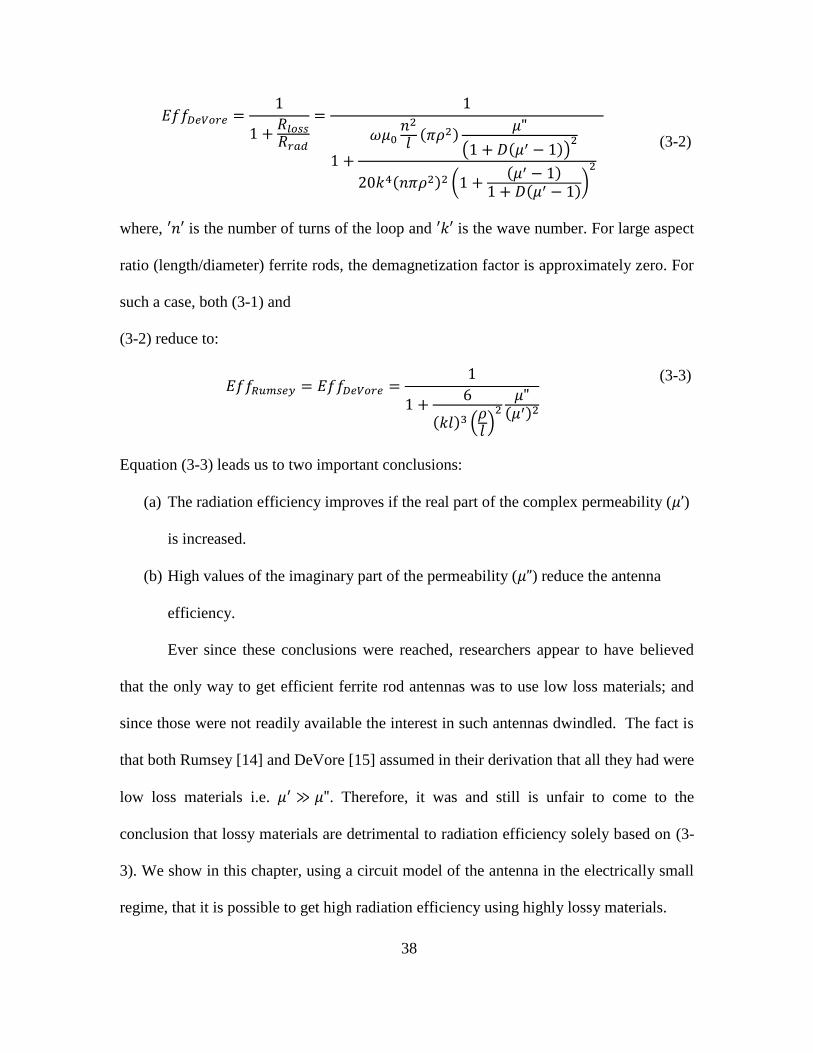
38

( )

( ( ))

( ) ( ( )

( ))

(3-2)

where, is the number of turns of the loop and is the wave number. For large aspect

ratio (length/diameter) ferrite rods, the demagnetization factor is approximately zero. For

such a case, both (3-1) and

(3-2) reduce to:

( ) ( )

( )

(3-3)

Equation (3-3) leads us to two important conclusions:

(a) The radiation efficiency improves if the real part of the complex permeability ( )

is increased.

(b) High values of the imaginary part of the permeability ( ) reduce the antenna

efficiency.

Ever since these conclusions were reached, researchers appear to have believed

that the only way to get efficient ferrite rod antennas was to use low loss materials; and

since those were not readily available the interest in such antennas dwindled. The fact is

that both Rumsey [14] and DeVore [15] assumed in their derivation that all they had were

low loss materials i.e. . Therefore, it was and still is unfair to come to the

conclusion that lossy materials are detrimental to radiation efficiency solely based on (3-

3). We show in this chapter, using a circuit model of the antenna in the electrically small

regime, that it is possible to get high radiation efficiency using highly lossy materials.

39

Lately there has been a renewed interest in antennas that utilize magneto-

dielectric materials, due to the availability of considerably lower loss materials than what

was available a decade or two ago. Stuart et al. [17] designed an electrically small electric

dipole antenna surrounded by a high permeability material that has very low antenna Q

(quality factor). Another example is the use of magneto-dielectric materials as the core in

a spherical TE mode wire antenna [18], to reduce its Q [19-21]. The high permeability

core excludes the magnetic field from within the spherical antenna thereby reducing the

stored internal magnetic energy and reducing Q. This fact is true only when there are no

internal resonances within the sphere since resonances would increase the internal stored

energy and therefore would reduce Q. Thus the onset of internal resonances imposes a

restriction on the size and value of permeability that can be used.

Since all materials have some loss, the case of a lossy magneto-dielectric core was

analyzed numerically in [22] and analytically in [23]. In [23], the authors showed that it

is possible to get high radiation efficiency in a spherical wire antenna with a highly lossy

magneto-dielectric core which goes against the conventional notion of requiring only low

loss materials to get high efficiency. The magnetically loaded spherical antenna although

attractive owing to its low Q is not a low-profile or conformal structure. In this chapter,

we restrict the analysis to linear magneto-dielectric dipoles that can be placed tangential

to a metallic ground plane. A purely numerical analysis of an array of lossy magneto-

dielectric dipoles was shown in [24] in which the radiation efficiency was seen to

increase as the loss tangent was increased beyond unity. We prove this observation

analytically for a single magneto-dielectric dipole.

40

3.3 Radiation Efficiency of an Electrically Small Magneto-dielectric Dipole Antenna

The radiation efficiency of an antenna is defined as:

(3-4)

where, ‘ ’ is the power radiated by the antenna and ‘Plost’ is the power lost in the

antenna material.

In this section, the radiation efficiency of a magneto-dielectric dipole is derived

starting from Schelkunoff’s circuit model for electrically small antennas. The ultimate

goal is to estimate the material properties required to build a conformal magneto-

dielectric antenna that can meet a given target efficiency requirement. We will use the

concept of duality to derive the equations for the magnetic dipole antenna starting from

the circuit model of a dielectric antenna from Chapter 1.

In the dielectric dipole model, the material properties are represented by a series

internal impedance term which is composed of a complex internal capacitance

to represent permittivity and a complex internal inductance to represent

permeability . This term accounts for the internal energy in the material. For a

rod of radius, , the internal capacitance is defined by assuming a uniform E-field (TM

like fundamental mode) in the material thus yielding a simple capacitor of area

and separation which is the length on the dipole. The internal inductance is the

inductance of a wire with uniform current . The current distribution is assumed

uniform. The circuit model is shown in Fig. 3-1.

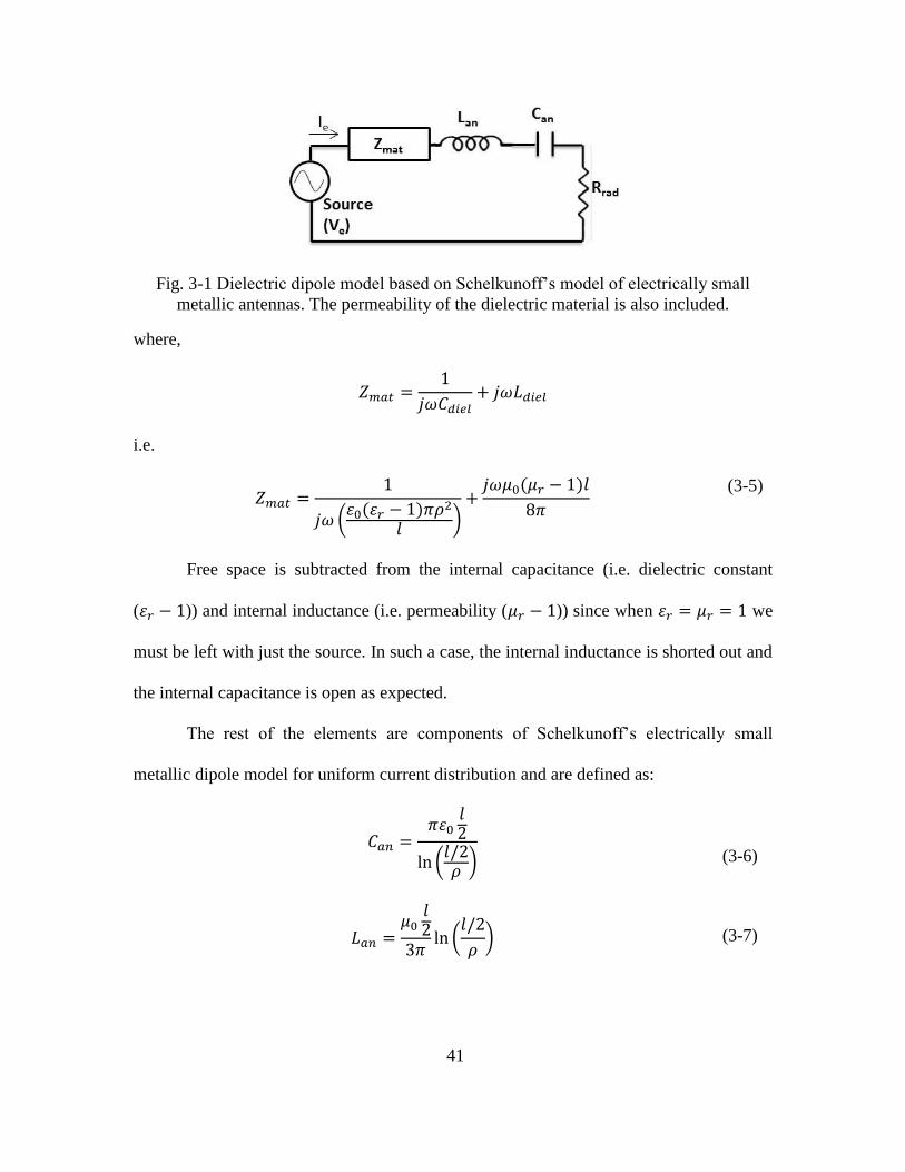
41

Fig. 3-1 Dielectric dipole model based on Schelkunoff’s model of electrically small

metallic antennas. The permeability of the dielectric material is also included.

where,

i.e.

( ( )

) ( )

(3-5)

Free space is subtracted from the internal capacitance (i.e. dielectric constant

( )) and internal inductance (i.e. permeability ( )) since when we

must be left with just the source. In such a case, the internal inductance is shorted out and

the internal capacitance is open as expected.

The rest of the elements are components of Schelkunoff’s electrically small

metallic dipole model for uniform current distribution and are defined as:

( )

(3-6)

(

)

(3-7)

42

(

)

( ) (3-8)

In Chapter 1, we did not include the effect of skin depth ‘ ’ since the majority of

dielectric materials have ( was ignored). This is not true about the relative

permittivity of realistic magnetic materials i.e. can be much greater than unity. For a

plane wave, the skin depth can be calculated as:

( √ )

(3-9)

where, is the wave number in free space. For small , the calculated skin depth is

usually larger than the radius ‘ ’ of the material i.e. a very significant amount of the field

pervades the entire material. For such cases ‘ ’ is set equal to ‘ ’. In magnetic materials

with large , the electromagnetic skin depth of the material will force the magnetic flux

to flow closer to the surface and therefore has the effect of decreasing the internal

capacitance and internal inductance.

Since we are concerned with TM like modes in the dielectric dipole, the internal

complex capacitance as seen in the first term of (3-5) can be corrected to account for skin

depth (due to the permeability in this case) with an Area Factor (AF) in front of it. This

factor is given by

( )

(3-10)

The correction to the inductance term is ambiguous since the shape of the φ-

directed H-field in the transverse ‘r’ direction is a function of frequency, size of the

cross-section and the material properties and . A simple and good approximation to

43

this rapidly changing field structure and the corresponding equation of the Hφ-field due to

a current ‘ ’ in the electrically small regime is shown below in Fig. 3-2.

Fig. 3-2 (a) Skin depth in a cylindrical dipole (b) The transverse field shape for 0<δ<ρ of

the TM mode dielectric dipole. The solid line is the actual field shape and the dashed line

is the closest approximation

The resulting internal Field Shape Factor (FSF) correction term to the complex internal

inductance term is given below:

( )

[

(

) (

)

(

)

] (3-11)

This factor is derived by equating the magnetic energy integral to the circuital inductor

energy equation and is shown in Appendix A. The input impedance of the dielectric

dipole is therefore:

( ( )

)

( )

(

)

( )

( )

(3-12)

(a) (b)

44

Using the concept of duality, we can obtain the magnetic input impedance (in mhos) of

the dual antenna by:

( )

( )

(3-13)

where, the superscript ‘m’ and ‘e’ represent magnetic and electric impedances,

respectively. However, this dual problem maps a dielectric dipole with PEC feed lines

and electric voltage source (Ve) to a permeable dipole with PMC feed line and magnetic

voltage source (Vm) as shown in Fig. 3-3(a) and (b). Since we don’t have PMC wires and

a magnetic voltage source, the simplest way to feed a permeable dipole is to use an

electric loop as shown in Fig. 3-3(c). The cross section of this electric loop fed permeable

dipole at the feed loop is shown in Fig. 3-4.

Fig. 3-3 (a) A dielectric dipole carrying an electric current ‘Ie’ fed with an electric

voltage source ‘Ve’ and PEC feed lines (solid lines) such that (b)

Dual magnetic dipole carrying magnetic current ‘Im’ fed with a magnetic voltage source

‘Vm’ and PMC feed lines (dashed lines) such that (c)

Permeable or magnetic dipole carrying magnetic current ‘Im’ fed with an electric loop.

(a) (b)

duality

e

e

Ve

Ie m

m

Vm

Im

Ie

m

m

Ve

Im

(c)

45

Fig. 3-4 Cross-section of the permeable material dipole of Fig. 3-3(c) at the electric feed

loop. The mode of operation is TE like with the B-field along the axis of the dipole.

The magnetic current (Im) is defined as the surface integral of dB/dt or jωB

passing through the surface ‘S’ and the magnetic voltage (Vm) is the line integral of the

H-field around the closed contour of the surface. Now, according to Faraday’s law, the

surface integral of jωB is equal to the line integral of the E-field along the closed contour

of the surface ‘S’ (c(S)), which by definition is the electric voltage ‘Ve’. In other words,

∫

∮

( )

(3-14)

Also according to Ampere’s circuit law, the line integral of the H field along the

closed contour formed by surface ‘S’ (c(S)), is the electric current Ie or in the dual world

the magnetic voltage Vm. In other words,

∮

( )

(3-15)

Therefore,

( )

( )

(3-16)

Surface SIe

Ve

B flux lines

µ

46

From (3-13) and (3-16) the input admittance of a permeable dipole antenna fed by an

electric loop is given by:

|

(3-17)

Since we are interested in a magneto-dielectric dipole and not just a permeable one, we

will call the input admittance of the magneto-dielectric circuit . Therefore

from

(3-12) and (3-17), the input admittance of the magneto-dielectric dipole can be written as

(

)

( )

( )

(3-18)

where,

( )

( )

(3-19)

is the admittance of the following circuit shown in Fig. 3-5.

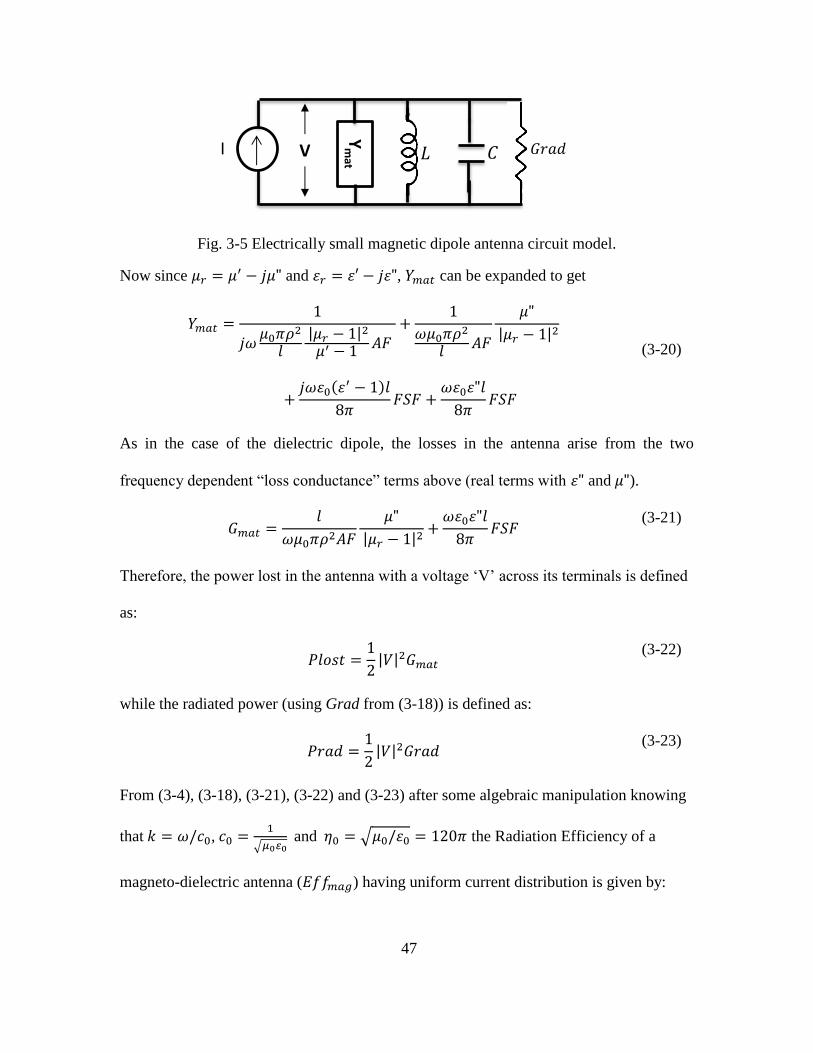
47

Fig. 3-5 Electrically small magnetic dipole antenna circuit model.

Now since and , can be expanded to get

(

)

(3-20)

As in the case of the dielectric dipole, the losses in the antenna arise from the two

frequency dependent “loss conductance” terms above (real terms with and ).

(3-21)

Therefore, the power lost in the antenna with a voltage ‘V’ across its terminals is defined

as:

(3-22)

while the radiated power (using Grad from (3-18)) is defined as:

(3-23)

From (3-4), (3-18), (3-21), (3-22) and (3-23) after some algebraic manipulation knowing

that ,

√ and √ the Radiation Efficiency of a

magneto-dielectric antenna ( ) having uniform current distribution is given by:

Ym

at

I V

48

( ) ( )

( )

(3-24)

Now if the assumed current distribution is triangular and not uniform then,

(

)

(3-25)

(

)

(3-26)

(

)

( ) (3-27)

Therefore, the radiation efficiency assuming a triangular current distribution can be

derived in the same way as before to be:

( ) ( )

( )

(3-28)

Now for a purely magnetic material i.e. , for which implies AF = FSF =

1, (3-24) simplifies to

( ) ( )

(3-29)

This equation is the exact dual of the radiation efficiency of a dielectric dipole in Chapter

1. Equation (3-29) can be re-written in terms of Wheeler’s loss power factor and

minimum power factor as

(3-30)

where,

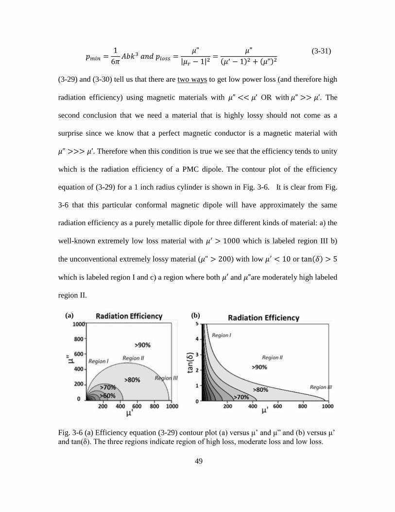
49

( ) ( )

(3-31)

(3-29) and (3-30) tell us that there are two ways to get low power loss (and therefore high

radiation efficiency) using magnetic materials with OR with . The

second conclusion that we need a material that is highly lossy should not come as a

surprise since we know that a perfect magnetic conductor is a magnetic material with

. Therefore when this condition is true we see that the efficiency tends to unity

which is the radiation efficiency of a PMC dipole. The contour plot of the efficiency

equation of (3-29) for a 1 inch radius cylinder is shown in Fig. 3-6. It is clear from Fig.

3-6 that this particular conformal magnetic dipole will have approximately the same

radiation efficiency as a purely metallic dipole for three different kinds of material: a) the

well-known extremely low loss material with which is labeled region III b)

the unconventional extremely lossy material ( ) with low or ( )

which is labeled region I and c) a region where both and are moderately high labeled

region II.

Fig. 3-6 (a) Efficiency equation (3-29) contour plot (a) versus μ’ and μ” and (b) versus μ’

and tan(δ). The three regions indicate region of high loss, moderate loss and low loss.

(a) (b)

50

In Region I and Region II, the material skin-depth is so small that all the fields are

pushed out of the antenna. Therefore, the material dipole tends to act more like the

conventional metal dipole and therefore exhibit high radiation efficiency. The same

conclusions were obtained for the dielectric dipole.

3.4 Full-wave Simulations of the Magneto-dielectric Dipole Antenna

Full wave simulations of the magneto-dielectric dipole were carried out using a

variety of magneto-dielectric material parameters in order to ascertain the accuracy of (3-

24) and (3-28). Two simulation cases are shown in Fig. 3-7. In Fig. 3-7(a) a magnetic

dipole is fed with a single current loop and in Fig. 3-7(b) a magnetic dipole is fed with

eight current loops. The single loop simulation results will be compared with (3-28) in

which the magnetic current distribution was assumed to be triangular. However, due to

the leaky nature of radiation from a material antenna, this assumption will be true only

for a small range of frequencies. The current distribution for a material dipole is not only

a function of the antenna size but also of the material properties. Also, this leaky behavior

implies that the entire length of the antenna will not contribute to radiation at all

frequencies. The energy will leak out sooner when operated well below the TE01

guidance frequency.

51

Fig. 3-7(a) Simulation geometry of a magneto-dielectric dipole fed by a single electric

feed loop and (b) eight feed loops

One way to ensure that all the material available contributes to radiation is to

employ multiple feed loops. By doing so, we force the magnetic current distribution to be

more uniform for which we have derived (3-24). The magneto-dielectric dipole simulated

is 1m long (extending from -50cm to 50cm on the simulation axis) with a radius of

1cm.The magnetic current distribution (volts) along the dipole length for the single

feed loop case is shown in Fig. 3-8.

Fig. 3-8(a) Magnetic current distribution along the length of the dipole at two frequencies

(a) 100MHz ( ) (b) 200MHz ( )

(a) (b)

(a) (b)

52

The radiation efficiency comparison with the triangular current distribution

equation (3-28) is shown in Fig. 3-9. As expected from Fig. 3-8(a) the agreement is

excellent throughout the electrically small regime for the high permeability case (

) and degrades from there as the current becomes more exponentially

damped.

Fig. 3-9 Simulated Radiation Efficiency (symbols) comparison with (3-28) (solid curves)

for a single loop fed magneto-dielectric dipole.

As mentioned before, one way to obviate the problem of the exponentially

damped (leaky) current is to employ multiple feed loops along the length of the antenna.

This is tantamount to using a solenoid feed ensuring that the B-field or the magnetic

current is uniform throughout the length of the dipole. A solenoid would work fine in the

electrically small limit but, as the antenna becomes electrically large, there would be a

considerable phase difference in the electric current along the length of the solenoid

which can cause destructive interference in radiation. Therefore in order to minimize this

effect, it is better to use multiple individual feed loops each fed in phase as shown in Fig.

3-7(b).

53

The magnetic current distribution plots of a multi-loop fed 1m long (extending

from -50cm to 50cm on the simulation axis) magnetic dipole are shown in Fig. 3-10. The

current distribution is nearly uniform except for the spikes seen in the figure. These

spikes/notches result from the calculation of the current as the closed line integral of the

electric field when we get too close to the feed loops. Very close to the loops we capture

in the integral near field flux lines (higher order modes) that are not part of the assumed

magnetic current in the material.

Fig. 3-10 Uniform magnetic current distribution along the length of the dipole at two

frequencies (a) 100MHz ( ) (b) 200MHz ( )

The simulated results for radiation efficiency and the comparison with equation

(3-28) are shown in Fig. 3-11. The cases studied vary from low permeability to high

permeability cases where the permittivity is also varied as to validate the

calculation of skin depth in equation (3-28). Even though the above model was derived

assuming the dipole is electrically small, it behaves properly all the way to the half-wave

resonance ( ). For low loss materials the validity extends further as seen in Fig.

3-11(a).

(a) (b)

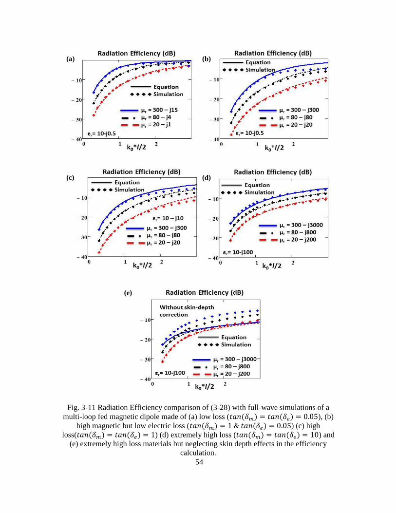
54

Fig. 3-11 Radiation Efficiency comparison of (3-28) with full-wave simulations of a

multi-loop fed magnetic dipole made of (a) low loss ( ( ) ( ) ), (b)

high magnetic but low electric loss ( ( ) ( ) ) (c) high

loss( ( ) ( ) ) (d) extremely high loss ( ( ) ( ) ) and

(e) extremely high loss materials but neglecting skin depth effects in the efficiency

calculation.

(a) (b)

(c) (d)

(e)

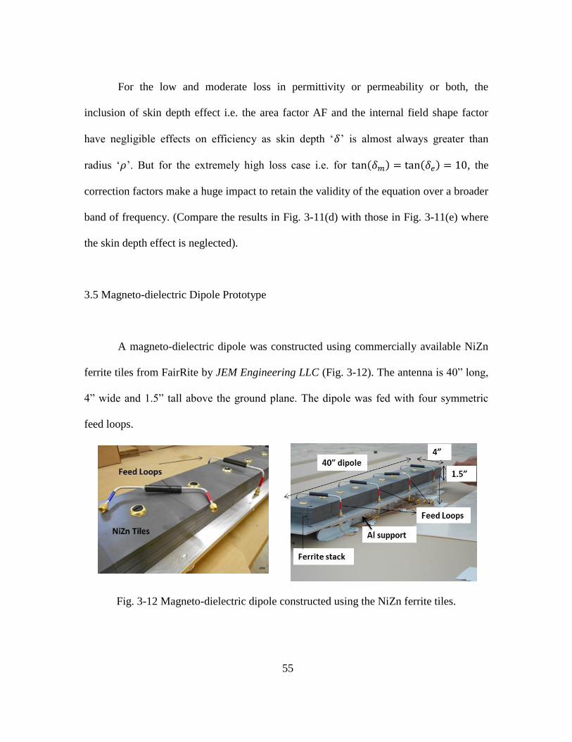
55

For the low and moderate loss in permittivity or permeability or both, the

inclusion of skin depth effect i.e. the area factor AF and the internal field shape factor

have negligible effects on efficiency as skin depth ‘ ’ is almost always greater than

radius ‘ ’. But for the extremely high loss case i.e. for ( ) ( ) , the

correction factors make a huge impact to retain the validity of the equation over a broader

band of frequency. (Compare the results in Fig. 3-11(d) with those in Fig. 3-11(e) where

the skin depth effect is neglected).

3.5 Magneto-dielectric Dipole Prototype

A magneto-dielectric dipole was constructed using commercially available NiZn

ferrite tiles from FairRite by JEM Engineering LLC (Fig. 3-12). The antenna is 40” long,

4” wide and 1.5” tall above the ground plane. The dipole was fed with four symmetric

feed loops.

Fig. 3-12 Magneto-dielectric dipole constructed using the NiZn ferrite tiles.

56

Fig. 3-13(a) shows the material properties of the FairRite tiles used in the

design. Note that in the frequency range of interest (VHF) the material is lossy with the

magnetic loss tangent tan(δm) > 2. Fig. 3-13(b) shows the comparison between full-wave

simulation radiation efficiency and the two closed form equations: (3-24) and the one

derived by Rumsey et al. ignoring permittivity and assuming low material loss (3-3). As

expected, since Rumsey’s equation was for only low loss materials (tan(δm)<<1) the

curve deviates significantly from simulation results whereas, equation (3-24)’s agreement

is excellent up to that is well beyond the electrically small antenna assumption.

Fig. 3-13 (a) NiZn FairRite tile material permeability. Permittivity of the ferrite is . (b)Comparison of simulated Radiation Efficiency of the magneto-dielectric

dipole with two closed form equations.

The magneto-dielectric antenna gain was measured in JEM’s anechoic chamber.

The comparison between measured and simulated gain is shown in Fig. 3-14(b). Since

the model assumes an infinite ground plane the measurement is compared to full wave

simulations. Their gains agree well over the entire range of measured frequencies. This

suggests that the circuit model works well in the electrically small limit since the

0 0.25 0.5 0.75 130

20

10

dB

Radiation Efficiency

SimulationEquation (5)

Rumsey’s Eqn

200 400 6000

20

40

60

80

0.1 10 1 103

0

1 103

2 103

3 103

Frequency (MHz)

μ‘μ"

Freq. (MHz)0.1 10 1 10

3

0

1 103

2 103

3 103

Permeability(a) (b)

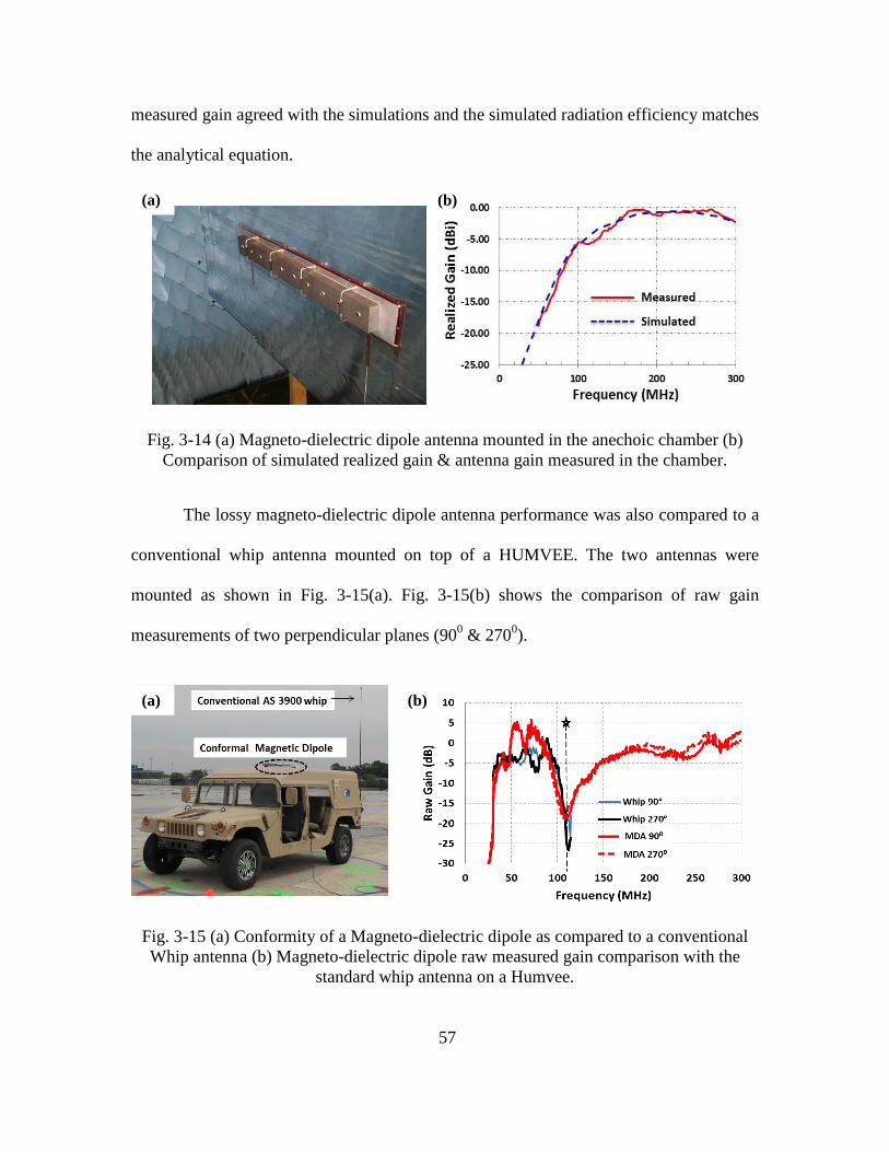
57

measured gain agreed with the simulations and the simulated radiation efficiency matches

the analytical equation.

Fig. 3-14 (a) Magneto-dielectric dipole antenna mounted in the anechoic chamber (b)

Comparison of simulated realized gain & antenna gain measured in the chamber.

The lossy magneto-dielectric dipole antenna performance was also compared to a

conventional whip antenna mounted on top of a HUMVEE. The two antennas were

mounted as shown in Fig. 3-15(a). Fig. 3-15(b) shows the comparison of raw gain

measurements of two perpendicular planes (900 & 270

0).

Fig. 3-15 (a) Conformity of a Magneto-dielectric dipole as compared to a conventional

Whip antenna (b) Magneto-dielectric dipole raw measured gain comparison with the

standard whip antenna on a Humvee.

(a) (b)

(a) (b)

58

In the operational frequency range of the whip, the lossy MD antenna excels in

performance compared to the standard whip between 30-88MHz. Any variations in gain

in this range are due to structural resonances being setup in the HUMVEE by the antenna

under test. The star marker (110MHz) indicates the whip antenna’s roll-off above

88MHz. At the same frequency the conformal antenna is half wavelength away from the

ground causing a null in the gain.

3.6 A Note on the Duality between Material Dipoles

We have always known that a PMC dipole fed by a magnetic voltage generator is

the dual of a PEC dipole fed with an electric voltage generator. In the same way, a

material dipole made up of a dielectric material fed using an electric voltage source must

be the dual of dipole made up of magnetic material fed with magnetic voltage source. We

used this principle while deriving the equation of radiation efficiency of a magneto-

dielectric dipole in the preceding section. We pointed out in that section that the analytic

efficiency equations of a dielectric and magnetic dipole are perfectly dual. In this section,

we prove this conjecture via simulations. Consider the two cases shown in Fig. 3-16. Fig.

3-16(a) is a dielectric dipole fed with eight voltage ports to ensure uniform current

distribution and (b) is the magnetic dipole of the previous section with eight metallic

loops as feeds. The two dipoles are of the same length (1 m) and have the same cross-

section (radius =1”).

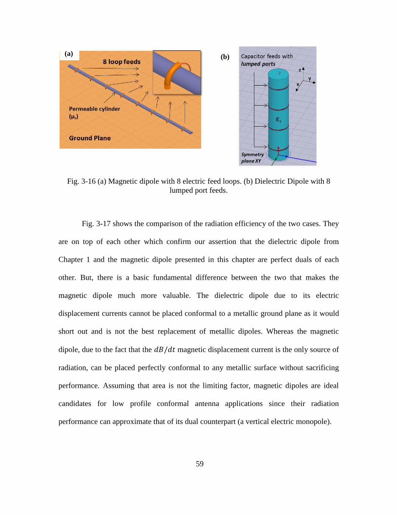
59

Fig. 3-16 (a) Magnetic dipole with 8 electric feed loops. (b) Dielectric Dipole with 8

lumped port feeds.

Fig. 3-17 shows the comparison of the radiation efficiency of the two cases. They

are on top of each other which confirm our assertion that the dielectric dipole from

Chapter 1 and the magnetic dipole presented in this chapter are perfect duals of each

other. But, there is a basic fundamental difference between the two that makes the

magnetic dipole much more valuable. The dielectric dipole due to its electric

displacement currents cannot be placed conformal to a metallic ground plane as it would

short out and is not the best replacement of metallic dipoles. Whereas the magnetic

dipole, due to the fact that the magnetic displacement current is the only source of

radiation, can be placed perfectly conformal to any metallic surface without sacrificing

performance. Assuming that area is not the limiting factor, magnetic dipoles are ideal

candidates for low profile conformal antenna applications since their radiation

performance can approximate that of its dual counterpart (a vertical electric monopole).

(a) (b)

60

Fig. 3-17 Radiation Efficiency comparison of a dielectric and magnetic dipole of the

same length and cross-section but with dual material properties.

3.7 Summary, Conclusions and Future Work

A closed form equation for the radiation efficiency equation was developed for a

small magneto-dielectric dipole. The equation is derived from the electrically small

circuit model of a conventional metallic dipole by adding additional elements (L for

permeability and C for permittivity) to take into account the material properties. The

equation shows that maximum radiation efficiency of a material dipole can be obtained

not only by using a material with very low loss but also with a material that has very high

loss.

Two equations were derived, one for uniform magnetic current distribution

generated by using multiple feed loops and the other for a triangular current distribution

assumed with a single feed loop. It is hard to maintain a triangular current distribution

across the length of a magneto-dielectric dipole due to the leaky nature of radiation

61

mechanism and hence the validity of the radiation equation for this case is limited. On the

other hand, fairly uniform current distribution can be maintained with multiple loops and

hence the radiation efficiency equation for uniform current distribution matches the full-

wave simulations accurately.

The circuit model presented here does not include the details of the feed structure.

Once the feed is included we would have a complete model that can be used to calculate

the input impedance of the antenna. This will enable us to calculate the Antenna Q and

hence the bandwidth of the antenna; thus yielding in one formulation the radiation

efficiency and antenna bandwidth, the two parameters that completely characterize a

given material dipole antenna.

The next logical extension to this development is to analyze a loop or a toroid

made up of a magneto-dielectric material. Although such an antenna would occupy more

area over ground than the linear dipole it would offer unequivocal vertical polarization

for all azimuth directions which can therefore replace a vertical metallic dipole antenna.

Since there is a closed form model for the electrically small metallic loop antenna with

uniform current distribution, we can use the same steps used in this chapter to arrive at

the radiation efficiency equation of a magneto-dielectric toroid. This is the subject of the

next chapter.

62

Chapter 4

MAGNETO-DIELECTRIC LOOP/TOROID ANTENNA: CIRCUIT MODEL &

RADIATION EFFICIENCY

4.1 Introduction

The magneto-dielectric dipole in Chapter 3 has a broadside ‘figure of 8’ pattern

just like a metallic dipole. However, often conformal low-profile antenna applications

demand omnidirectional antenna coverage. In fact this is one of the reasons why a

vertical metallic monopole is preferred over a horizontal metallic dipole, apart from the

obvious problem of destructive image effect in the horizontal dipole. A magneto-

dielectric loop antenna has a radiation pattern that is identical to a vertical electric dipole.

It has an omnidirectional pattern in the azimuth plane and it comes with the added

advantage of being low profile and conformal without any adverse effects due to a

conventional metallic ground plane. Therefore, it is quintessential to model the magneto-

dielectric loop antenna.

The steps followed in the derivation of the model and the radiation efficiency

equation is identical to that of the magneto-dielectric dipole. In Section 4.2, we will start

with the electrically small circuit model of a metallic loop and introduce the material

properties as a series impedance to come up with a model for a dielectric loop antenna.

Then, similar to the derivation in Chapter 3, we will use the principle of duality and

obtain an admittance circuit model of the magneto-dielectric loop which will then be used

to derive the radiation efficiency. In Section 4.3, we will examine design trade-offs based

63

on the radiation efficiency equation between a magneto-dielectric loop and a magneto-

dielectric dipole. In Section 4.4, a practical application of the admittance circuit model of

the loop: design of a Body Wearable Belt Antenna will be discussed. Section 4.5 contains

the summary of the chapter, some notable conclusions and possible future work on this

subject.

4.2 Circuit model

In this section, the radiation efficiency of a magneto-dielectric loop is derived

starting from the circuit model for an electrically small metallic loop antenna. The

ultimate goal is to estimate the material properties required to build a conformal

magneto-dielectric antenna that can meet a given target efficiency requirement. As in

Chapter 2, the material properties are introduced by a series internal impedance

term which is composed of a complex internal capacitance to represent

permittivity and a complex internal inductance to represent permeability .

This term accounts for the internal energy in the material. For a loop of radius

and wire radius, , the internal capacitance is defined by assuming a uniform E-field

(TM like fundamental mode) in the material thus yielding a simple capacitor of area

and separation which is the circumference of the loop. The internal

inductance is the inductance of a wire of length equal to the circumference of the loop

with a uniform current . The current distribution is assumed uniform. The circuit model

is shown in Fig. 4-1.

64

Fig. 4-1 Electrically small dielectric loop antenna model.

where,

i.e.

( ( )

) ( )( )

(4-1)

Free space is subtracted from the internal capacitance (i.e. dielectric constant ( ))

and internal inductance (i.e. permeability ( )) since when we must be

left with just the source. In such a case, the internal inductance is shorted out and the

internal capacitance is open as expected.

The rest of the elements are components of the electrically small metallic loop model for

uniform current distribution and are defined as:

( (

) )

(4-2)

(

)

( ) (4-3)

To account for skin depth, the same correction factors as in Chapter 3 can be used. The

internal complex capacitance is corrected by the area factor ‘AF’ (3-10).

IeLan

Rrad

Zmat

Source (Ve)

65

( )

The internal complex inductance is corrected by the Field Shape Factor ‘FSF’ (3-11).

( )

[

(

) (

)

(

)

]

The input impedance of the dielectric loop is therefore:

( ( )

)

( )

( (

) ) ( )

(4-4)

Using the concept of duality as explained in Chapter 3, using (3-13),(3-16) and (3-17),

the input admittance of the magneto-dielectric loop ( ) can be written as,

( (

) )

( )

(4-5)

where,

( )

( )( )

(4-6)

is the admittance of the following circuit shown in Fig. 3-52.

Fig. 4-2 Electrically small magneto-dielectric loop antenna circuit model.

Ym

at

I V

66

Now since and , can be expanded to get

(

)( )

(4-7)

As in the case of the magneto-dielectric dipole, the losses in the antenna arise from the

two frequency dependent “loss conductance” terms in (4-7) above (real terms with

and ).

( )

(4-8)

Therefore, the power lost in the antenna with a voltage ‘V’ across its terminals is defined

as:

(4-9)

while the radiated power (using Grad from (3-18)) is defined as:

(4-10)

From (3-4), (4-5), (4-8),(4-9) and (4-10) after some algebraic manipulation knowing

that ,

√ and √ the Radiation Efficiency of a

magneto-dielectric antenna ( ) having uniform current distribution is given by:

( )

( )

( )

(4-11)

67

Now for a purely magnetic material i.e. , for which imp lies AF = FSF = 1,

(4-11) simplifies to

( )

( )

(4-12)

(4-11)and (4-12) tell us that there are two ways to get low power loss (and therefore high

radiation efficiency) using magnetic materials with μ”<<μ’ OR with μ”>>μ’. The second

conclusion that we need a material that is highly lossy should not come as a surprise since

we know that a perfect magnetic conductor is a magnetic material with μ”>>>μ’.

Therefore when this condition is true we see that the efficiency tends to unity which is the

radiation efficiency of a PMC loop. This conclusion was corroborated in Chapter 3 by the

contour plot of the radiation efficiency equation of the magneto-dielectric dipole versus

and . Here, let us plot the radiation efficiency of the magneto-dielectric loop as a

function of the loss tangent ( ( ) ) for different fixed ranging from 5 to

5000 (Fig. 4-3) and different electrical size of the antenna by varying from 0.1 to 1.

(a) (b)

68

Fig. 4-3 (a) Efficiency equation (4-12) plot versus ( )for (a) electrically small

antenna (b) small antenna and (c) electrically large antenna

. The radiation efficiency is the lowest at ( ) for any .

Fig. 4-3 shows that for low loss materials i.e. ( ) , the radiation efficiency is high

as expected from the conventional notion of highly efficient antennas. The radiation

efficiency then drops as ( ) is increased till it reaches a minimum at ( ) .

Beyond unity loss tangent, the radiation efficiency starts to rise back up again for all the

three cases. In this region, the material skin-depth is so small that all the fields are pushed

out of the antenna. Hence, the magneto-dielectric antenna tends to act more like the

conventional metal loop and therefore exhibit high radiation efficiency.

(c)

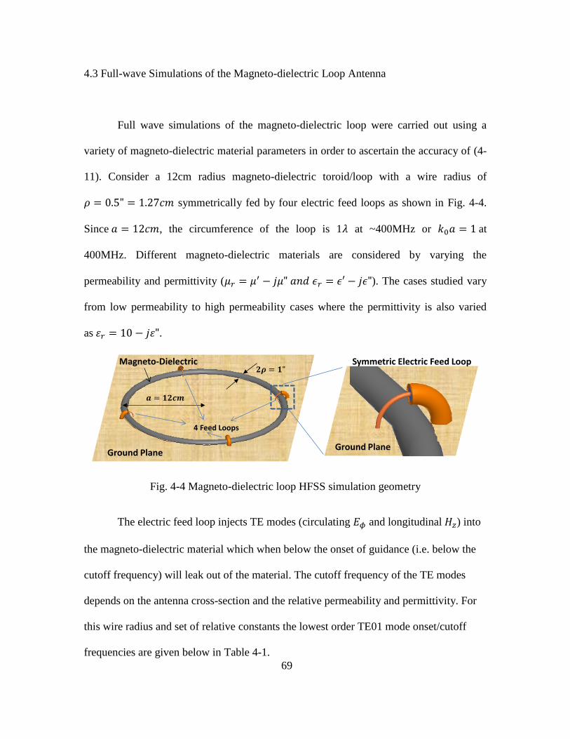
69

4.3 Full-wave Simulations of the Magneto-dielectric Loop Antenna

Full wave simulations of the magneto-dielectric loop were carried out using a

variety of magneto-dielectric material parameters in order to ascertain the accuracy of (4-

11). Consider a 12cm radius magneto-dielectric toroid/loop with a wire radius of

symmetrically fed by four electric feed loops as shown in Fig. 4-4.

Since , the circumference of the loop is 1 at ~400MHz or at

400MHz. Different magneto-dielectric materials are considered by varying the

permeability and permittivity ( ). The cases studied vary

from low permeability to high permeability cases where the permittivity is also varied

as .

Fig. 4-4 Magneto-dielectric loop HFSS simulation geometry

The electric feed loop injects TE modes (circulating and longitudinal ) into

the magneto-dielectric material which when below the onset of guidance (i.e. below the

cutoff frequency) will leak out of the material. The cutoff frequency of the TE modes

depends on the antenna cross-section and the relative permeability and permittivity. For

this wire radius and set of relative constants the lowest order TE01 mode onset/cutoff

frequencies are given below in Table 4-1.

4 Feed Loops

Ground PlaneGround Plane

Symmetric Electric Feed LoopMagneto-Dielectric

70

Real

Permeability (μ’)

Real

Permittivity (ε’)

TE01 Onset

Frequency (MHz)

value at

the TE01

Onset

20 10 640 1.61

80 10 320 0.8

300 10 165 0.42

Table 4-1 TE01 onset/cutoff frequency for a 0.5” wire radius magneto-dielectric cylinder

for different and .

The magnetic current distribution plots at two different frequencies (100MHz and

200MHz) of the multi-loop fed magneto-dielectric loop for different materials are shown

in Fig. 4-5. The current distribution is nearly uniform except for the spikes seen in the

figure. These spikes/notches result from the calculation of the current as the closed line

integral of the electric field when we get too close to the feed loops. Very close to the

loops we capture in the integral the near field flux lines (higher order modes) that are not

part of the assumed magnetic current in the material.

Fig. 4-5 Uniform magnetic current distribution along the length of the loop at two

frequencies (a) 100MHz ( ) (b) 200MHz ( )

(a) (b)

71

The simulated results for radiation efficiency and the comparison with equation

(4-11) are shown in Fig. 4-6. Even though the above model was derived assuming the

dipole is electrically small, it behaves properly all the way to the loop resonance (

). Note that in Fig. 4-6(a), which is the low loss case, near the onset frequency of the

TE01 guidance ( for (black curve) and for (blue

curve)), the simulated efficiency curve starts to plateau and deviate from the curve that is

generated using (4-11). There reaches a point beyond the onset frequency where the

efficiency drops to a minimum (at for (black curve)) and then it

rises again. This phenomenon occurs because once the onset frequency is crossed

majority of the wave that the magneto-dielectric loop supports is trapped inside the loop

and very little extends outside it. Therefore, it becomes progressively difficult to ‘leak

off’ the structure due to just the curvature discontinuity of the toroid and you reach a

minima in the efficiency curve. However beyond that point, the electric feed loop starts to

favor the excitation of the next higher order TE mode which is the TE02 inside the

magneto-dielectric loop. Hence, the radiation efficiency starts to climb up again due to

TE02 mode radiation. As we keep going higher in frequency, this phenomenon keeps

repeating and successive higher order TE modes appear and fade away just like the TE01

mode. A detailed analysis of this phenomenon is done in Chapter 6. This effect is not

seen in the lossy material cases, because the supported electromagnetic wave is never

truly guided in the lossy structure, the wave always leaks off the structure.

72

Fig. 4-6 Radiation Efficiency comparison of (4-11) with full-wave simulations of a multi-

loop fed magnetic dipole made of (a) low loss ( ( ) ( ) ), (b) high

loss( ( ) ( ) ) (c) extremely high loss ( ( ) ( ) ) and

(d) extremely high loss materials but neglecting skin depth effects in the efficiency

calculation.

For the low and moderate loss in permittivity or permeability or both, the

inclusion of skin depth effect i.e. the area factor AF and the internal field shape factor

have negligible effects on efficiency as skin depth ‘ ’ is almost always greater than

radius ‘ ’. But for the extremely high loss case i.e. for ( ) ( ) , the

correction factors has a huge effect in retaining the validity of the equation over a broader

band of frequency. (Compare the results in Fig. 4-6(c) with those in Fig. 4-6 (d) where

the skin depth effect is neglected).

(a) (b)

(c) (d)

73

4.4 Practical Application of the Circuit Model: Body Wearable Belt Antenna

In this section, we will discuss a practical application of the circuit model of the

magneto-dielectric loop antenna described in Section 3.3. The circuit model will be used

to evaluate the radiation efficiency of a Body Wearable Belt Antenna (BWBA) shown in

Fig. 4-7. The antenna design is targeted towards use by the communication personnel in a

battlefield. The goal is to replace the tall whip antennas carried around by these soldiers

with a low observable body wearable antenna (Fig. 4-7). The performance of the new

antenna must be better or at least the same as the standard antennas currently used for this

purpose.

Fig. 4-7 Body Wearable Belt Antenna designed to replace tall whip antennas carried by

foot soldiers for interpersonal communication

74

The operational frequency band for the antenna design is from 30MHz to

500MHz. But in particular, we want to maximize the efficiency of the antenna in the

30MHz to 100MHz band in order to beat the conventional whip antennas, used in this

range, convincingly. At the same time we want to minimize the manufacturing cost of

these antennas so that they can be mass produced and distributed. Also, this antenna will

be worn by the soldier, therefore we also want minimize the overall weight of the antenna

as well. Therefore, the most appropriate approach to tackle this problem is to find an

analytic circuit model of the system and then play ‘what if’ games with the volume of

material used.

The BW antenna system not only consists of the body wearable antenna made up

of some magneto-dielectric material but also the “dielectric” human body. These are the

two primary sources of radiation. Therefore, to model the system, we first simulate a

dielectric cylinder representing the human body fed with an ideal lumped port source in

the full-wave simulator. The human body is then ‘modeled’ as circuit impedance in the

frequency range of interest. Next, the source is replaced by the body wearable belt

antenna circuit model to complete the complete antenna model.

Consider a dielectric cylinder having the frequency dependent permittivity of a

human torso fed by a capacitive feed (lumped port in the simulator) over a ground plane

(Fig. 4-8). A foot soldier does not stay stationary and moves his arms and legs during

combat or in other words the shape of the dielectric human body radiator is constantly

changing. A cylinder is a good statistical average for the shape of the human body. The

dimensions of the cylinder soldier are 6 feet height and 32” waist.

75

Fig. 4-8 (a) Human body cylinder fed with an ideal lumped port at the same location as

the eventual position of the BWA belt. (b) Frequency dependent permittivity of the

human body.

Full-wave simulation of the geometry above yields the curves in Fig. 4-9(a) for

radiated power (Pradb) and power loss (Plossb). The input voltage (Vfeed) measured at

the lumped port is shown in Fig. 4-9(b). Fig. 4-9(c) shows the real and imaginary part of

the input impedance.

Fig. 4-9 Simulation results of the geometry in Fig. 4-8(a) where (a) Radiated power and

Power loss, (b) Feed Voltage and (c) Input impedance.

Given these simulation data we can calculate the radiation resistance (Rradb) and

loss resistance (Rlossb) the following way:

(a) (b)

(a) (b) (c)

76

(

)

(4-13)

(

)

(4-14)

The resulting radiation resistance and loss resistance is shown in Fig. 4-10(a). Fig.

4-10(b) show that the sum of Rradb and Rlossb is equal to the real part of the input

impedance as expected. The radiation efficiency of this dielectric cylinder fed with the

ideal capacitive lumped port feed is shown in Fig. 4-10(c). This is the maximum radiation

efficiency that can be achieved by this antenna system. Any addition of lossy materials to

the system by replacing the ideal feed with a permeable material feed will bring down the

radiation efficiency below this maximum value.

Fig. 4-10 (a) Radiation resistance and loss resistance calculated from the simulation data

(b) the sum of which equals the real part of input impedance. (c) Radiation Efficiency of

the dielectric human body cylinder fed with an ideal lumped capacitive port feed

(a) (b)

(c)

77

Therefore, the circuit model for the human body is now reduced to the one shown

in Fig. X+4. The imaginary part of input impedance is left as it is and the real part has

been separated into radiation and loss resistance.

Fig. 4-11 Circuit model of the dielectric human body cylinder fed with a capacitive feed.

The next step is to replace the ‘Vfeed’ with the magneto-dielectric loop circuit

model from Fig. 4-2. The resulting model is shown in Fig. 4-12.

Fig. 4-12 The circuit model of the BWA system that takes into account the ground plane.

Now let us compare the model to full-wave simulations. The simulation geometry

is shown in Fig. 4-13 where the lumped port of Fig. 4-8(a) has been replaced by the body

wearable toroid belt of minor radius of 4cm (ρ=4cm). It also has its own finite metallic

78

ground plane. We will use quarter symmetry to simplify the simulations. The circuit

element equations for the permeable toroid are the same as before except that we

observed thorough simulation of the toroid by itself that we need to add a correction

factor (2/5) to the Glossm. This factor comes from the fact that the model was developed

for a toroid in free space. The problem at hand has a finite ground plane and a dielectric

core. This factor accounts for this change in geometry. Since the ground plane and the

core properties are fixed the factor will always be the same 2/5. The same factor is also

applied to the radiation resistance. Thus,

( )

( ) ( )

( )

( )

(4-15)

Fig. 4-13 Simulation geometry of the body wearable antenna system with quarter plane

The permittivity of the human body is the same as in Fig. 4-8(b). To start with,

different dispersion-less permeability was simulated and the comparison to the model is

shown in Fig. 4-14.

79

Fig. 4-14 Radiation Efficiency comparison of the BWA system circuit model and full-

wave simulations for different values of permeability of the belt with (a),(b) having a loss

tangent of tan(δ)=0.1 and (c)(d) with high tan(δ)=1.

As seen in Fig. 4-14(c) and (d) the model works well for extremely lossy μr values

as well. Next let us test the validity for different volume of the permeable material i.e. for

different toroid radii ‘ρ’. Fig. 4-15 is for ρ=3cm and Fig. 4-16 is for ρ=6cm.

(a) (b)

(c) (d)

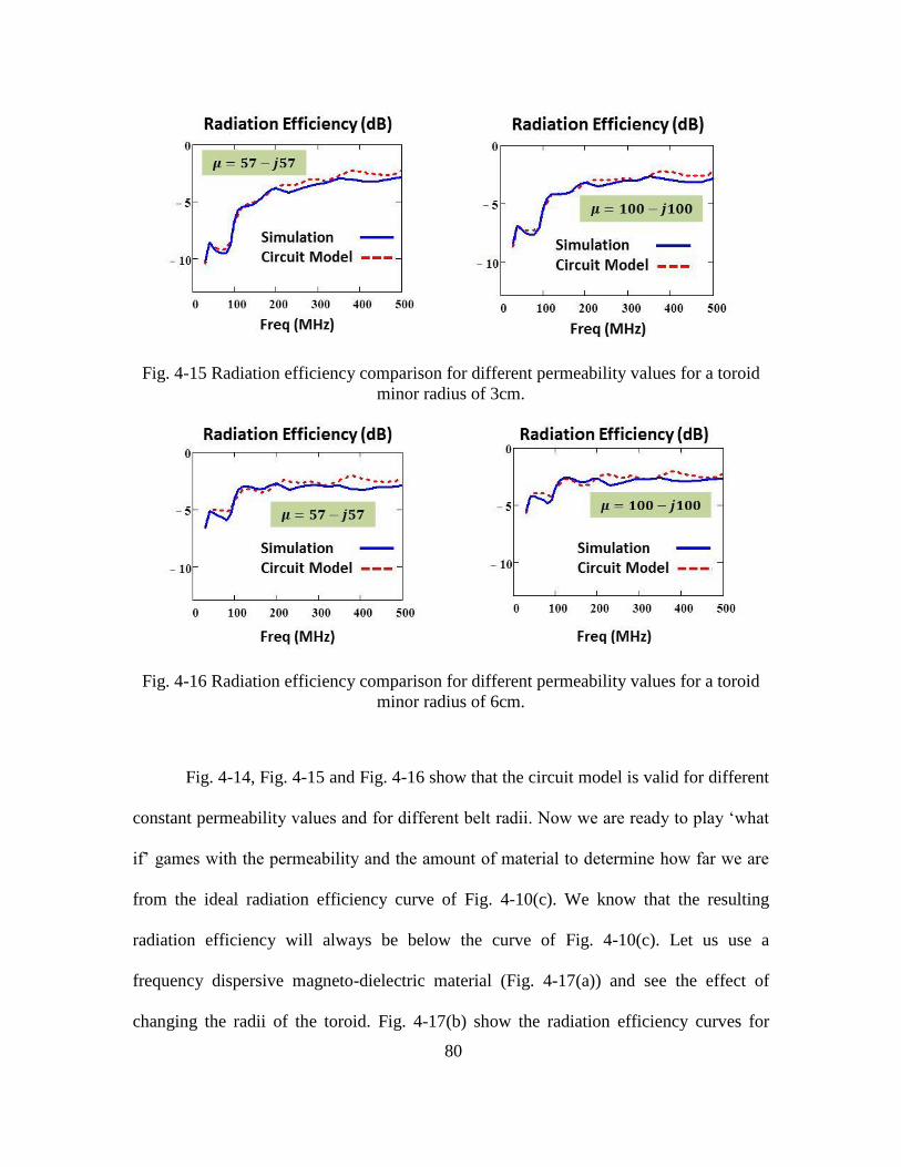
80

Fig. 4-15 Radiation efficiency comparison for different permeability values for a toroid

minor radius of 3cm.

Fig. 4-16 Radiation efficiency comparison for different permeability values for a toroid

minor radius of 6cm.

Fig. 4-14, Fig. 4-15 and Fig. 4-16 show that the circuit model is valid for different

constant permeability values and for different belt radii. Now we are ready to play ‘what

if’ games with the permeability and the amount of material to determine how far we are

from the ideal radiation efficiency curve of Fig. 4-10(c). We know that the resulting

radiation efficiency will always be below the curve of Fig. 4-10(c). Let us use a

frequency dispersive magneto-dielectric material (Fig. 4-17(a)) and see the effect of

changing the radii of the toroid. Fig. 4-17(b) show the radiation efficiency curves for

81

different ‘ρ’. Clearly as the radii of the belt increases, the radiation efficiency of the

BWA system increases as well, but the price we pay is the increase in the amount of

material required which corresponds to the increase in the overall cost of the belt. Table

next to Fig. 4-17(b) also gives the volume of material used in cubic centimeters. Also

beyond a certain radii (8cm in this case), any additional increase of the radius doesn’t

show any appreciable increase in radiation efficiency.

Fig. 4-17 (a) Magneto-dielectric material permeability used in the belt(b) Radiation

efficiency of the BWA using the circuit model for different radii of the loop belt.

Another consequence of the circuit model for this body wearable antenna system

is that we can clearly isolate the contribution towards radiation from the two sources, the

human body and the permeable toroid. From the circuit model in Fig. 4-12, we can see

100 1 103

1 104

10

0

10

20

30

40

Freq (MHz)

μ’μ "

Permeability(a)

(b)

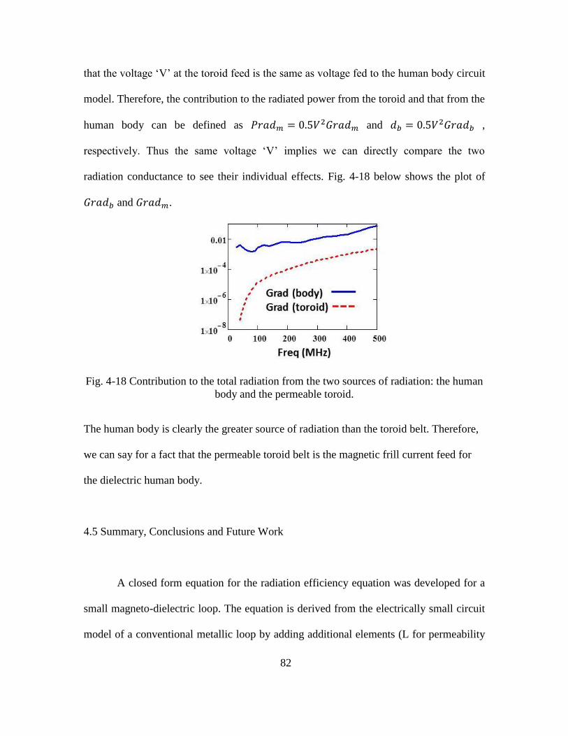
82

that the voltage ‘V’ at the toroid feed is the same as voltage fed to the human body circuit

model. Therefore, the contribution to the radiated power from the toroid and that from the

human body can be defined as and ,

respectively. Thus the same voltage ‘V’ implies we can directly compare the two

radiation conductance to see their individual effects. Fig. 4-18 below shows the plot of

and .

Fig. 4-18 Contribution to the total radiation from the two sources of radiation: the human

body and the permeable toroid.

The human body is clearly the greater source of radiation than the toroid belt. Therefore,

we can say for a fact that the permeable toroid belt is the magnetic frill current feed for

the dielectric human body.

4.5 Summary, Conclusions and Future Work

A closed form equation for the radiation efficiency equation was developed for a

small magneto-dielectric loop. The equation is derived from the electrically small circuit

model of a conventional metallic loop by adding additional elements (L for permeability

83

and C for permittivity) to take into account the material properties. The equation shows

that maximum radiation efficiency of a material loop can be obtained not only by using a

material with very low loss but also with a material that has very high loss.

The main reason behind analyzing the Magneto-dielectric Loop antenna geometry

is the fact that it has an omnidirectional pattern unlike the Magneto-dielectric Dipole. Just

by examining the radiation efficiency equations of the two ((3-24) and (4-11)) the dipole

is superior in the electrically small limit because the efficiency drops as a factor of ( )

in its case as opposed to the ( ) in the loop.

The circuit model presented here does not include the details of the feed structure.

Once the feed is included we would have a complete model that can be used to calculate

the input impedance of the antenna. This will enable us to calculate the Antenna Q and

hence the bandwidth of the antenna; thus yielding in one formulation the radiation

efficiency and antenna bandwidth, the two parameters that completely characterize a

given material dipole antenna.

84

Chapter 5

MATERIAL SELECTION RULE FOR MAGNETO-DIELECTRIC ANTENNA

DESIGNS

5.1 Introduction

In Chapter 3 and 4, the two fundamental magneto-dielectric antenna designs, the

magneto-dielectric dipole and the magneto-dielectric loop was analyzed. A simple small

antenna equivalent circuit model was postulated using which the radiation efficiency

equation for such antennas was derived and validated in the small antenna limit using

full-wave simulations. The radiation efficiency equation is a function of the antenna

geometry and the material properties ( ). Purely based on antenna geometry and

operational frequency range, i.e. for the same magneto-dielectric material, the magneto-

dielectric dipole has higher radiation efficiency than the magneto-dielectric loop in the

small antenna limit. In this chapter, it is shown that for either of the two fundamental

geometries, for a given size constraints of the antenna, the desired operation frequency

range and the desired efficiency in this range we can unequivocally identify the magneto-

dielectric material that can meet the required specifications. The analysis that follows is

under the assumption that the frequency range of operation is below the onset frequency

of the principal wave mode supported by the material antenna structure, theTE01 mode.

There are numerous books written and countless papers published on magnetic

materials each with its unique characteristics. The most basic classification of such

materials based on its magnetic properties is quite literally done based on whether a

85

material is “magnetic” or not in the presence or absence of an external magnetic field.

Materials are broadly classified as being diamagnetic, paramagnetic, ferromagnetic,

ferrimagnetic or anti-ferromagnetic. This classification is briefly described in Section 5.2.

Of these, ferromagnetic and ferromagnetic materials are most useful for antenna

applications as they have sufficiently high frequency dispersive permeability in the

frequencies of interest for antenna designs. In Section 5.3 we show three fundamental

physical limits that dictate the eventual choice of magneto-dielectric material. These are:

1) Gain Bandwidth Product limit 2) Snoek’s Product limit and 3) Kramers Krönig

relation restriction on the permeability dispersion. Within these constraints it is shown

that one single parameter which we call ‘hesitivity’ ( ) with the units of magnetic

conductivity ( ) characterizes the performance of the material. In Section 5.4, the

relationship between Hesitivity and antenna radiation efficiency is derived. The

relationship shows that materials that have the same hesitivity will have the same antenna

radiation efficiency. Hence, the parameter hesitivity is used to identify a family of

materials that satisfy the design requirements. It is shown that, higher the hesitivity of the

material family, the higher is the radiation efficiency over the frequency range of

operation. In Section 5.5, we narrow down the choice of material from the family with a

unique hesitivity to a single material based on the Gain-Bandwidth Product limit. We

show that any loss in the material ( ) improves the bandwidth of the antenna. Therefore

we state the material selection law based on hesitivity ( ) and the magneto-dielectric

material loss ( ). In Section 5.6, the material selection law is applied to realistic

magneto-dielectric materials obtained from the literature. Section 5.7 contains the

summary of the chapter, some notable conclusions and possible future work.

86

5.2 Classification of Magnetic Materials: Dia, Para, Ferro, Ferri and Anti-Ferro

The origin of magnetism is directly related to the motion of electrons in an atom.

Without delving deep into quantum physics, the two most significant sources of an

electron’s magnetic properties are the orbital motion of the electron around the atom’s

nucleus and the electron spinning around its own axis (Fig. 5-1). The electron orbiting the

nucleus can be thought of as a small current loop generating a small magnetic field with a

magnetic moment along its axis of rotation. The electron spinning on its axis has a spin

magnetic moment associated with it whose vector direction depends on the direction of

spin (up for right spin and down for left spin based on the right hand rule). Each atom

therefore acts like a tiny magnet carrying an intrinsic or net magnetic dipole moment

which is a superposition of the moments from these two sources. The type of magnetism

is determined by how these elementary dipole moments are ordered and are broadly

classified into diamagnetic, paramagnetic, ferromagnetic, ferrimagnetic or anti-

ferromagnetic.

Fig. 5-1 Two sources of atomic magnetic dipole moments a) an orbiting electron and (b)a

spinning electron

Most of the materials that exist on earth fall under the category of Diamagnetic

materials. They do not have a net dipole moment i.e. the orbital and spin magnetic

(a) (b)

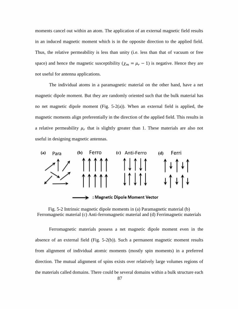
87

moments cancel out within an atom. The application of an external magnetic field results

in an induced magnetic moment which is in the opposite direction to the applied field.

Thus, the relative permeability is less than unity (i.e. less than that of vacuum or free

space) and hence the magnetic susceptibility ( ) is negative. Hence they are

not useful for antenna applications.

The individual atoms in a paramagnetic material on the other hand, have a net

magnetic dipole moment. But they are randomly oriented such that the bulk material has

no net magnetic dipole moment (Fig. 5-2(a)). When an external field is applied, the

magnetic moments align preferentially in the direction of the applied field. This results in

a relative permeability that is slightly greater than 1. These materials are also not

useful in designing magnetic antennas.

Fig. 5-2 Intrinsic magnetic dipole moments in (a) Paramagnetic material (b)

Ferromagnetic material (c) Anti-ferromagnetic material and (d) Ferrimagnetic materials

Ferromagnetic materials possess a net magnetic dipole moment even in the

absence of an external field (Fig. 5-2(b)). Such a permanent magnetic moment results

from alignment of individual atomic moments (mostly spin moments) in a preferred

direction. The mutual alignment of spins exists over relatively large volumes regions of

the materials called domains. There could be several domains within a bulk structure each

(a) (b) (c) (d)

88

with a magnetic moment vector that point in some random direction. This phenomenon in

which the magnetic moments within a domain are bound to a preferred direction is said to

be caused by an internal effective anisotropy field ( ). On the application of an external

d.c field, the domains most closely oriented with the direction of the applied field grows

at the expense of other domains, eventually occupying the material’s whole volume.

When this happens, the material is said to be saturated with a saturation magnetization

‘ ’ (units: Gauss in CGS) which is equal to the maximum magnetic flux density within

the material. Any further increase in the strength of the external field will not result in an

increase in the magnetic flux density in the material. Also, on the application of an

external field ‘H’, the spinning electron starts to precess about the direction of H at a

frequency ‘ ’ or ‘ ’. This frequency is called the Larmor frequency or ferromagnetic

resonance frequency.

Some examples of ferromagnetic materials are iron, nickel, cobalt, rare earth

metals, etc. They have a large relative permeability and are hence one of the candidate

material category in antenna applications. The only drawback with ferromagnetic

materials is that they have very high electrical conductivity (therefore high ). Apart

from the obvious disadvantage seen just from the radiation efficiency equations ((3-24)

and (4-11)), on the application of an external high frequency magnetic field, the high

electrical conductivity results in creation of eddy currents in the material, which in turn

creates a field in opposition to the external applied field. The opposition to the applied

field results in the fields being pushed out from within the material. Thus,

electromagnetic waves only penetrate to a certain depth, called the skin depth (seen in

Chapter 3, Section 3.3), within the material. Therefore, only a fraction of the volume of

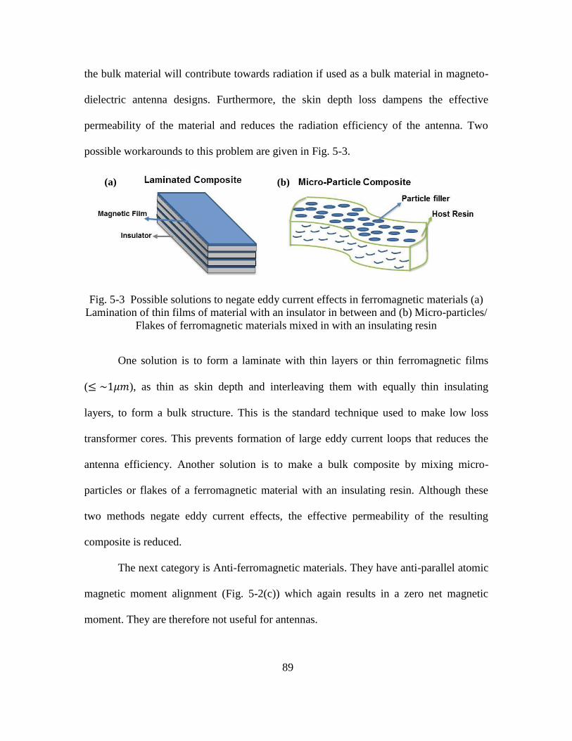
89

the bulk material will contribute towards radiation if used as a bulk material in magneto-

dielectric antenna designs. Furthermore, the skin depth loss dampens the effective

permeability of the material and reduces the radiation efficiency of the antenna. Two

possible workarounds to this problem are given in Fig. 5-3.

Fig. 5-3 Possible solutions to negate eddy current effects in ferromagnetic materials (a)

Lamination of thin films of material with an insulator in between and (b) Micro-particles/

Flakes of ferromagnetic materials mixed in with an insulating resin

One solution is to form a laminate with thin layers or thin ferromagnetic films

( ), as thin as skin depth and interleaving them with equally thin insulating

layers, to form a bulk structure. This is the standard technique used to make low loss

transformer cores. This prevents formation of large eddy current loops that reduces the

antenna efficiency. Another solution is to make a bulk composite by mixing micro-

particles or flakes of a ferromagnetic material with an insulating resin. Although these

two methods negate eddy current effects, the effective permeability of the resulting

composite is reduced.

The next category is Anti-ferromagnetic materials. They have anti-parallel atomic

magnetic moment alignment (Fig. 5-2(c)) which again results in a zero net magnetic

moment. They are therefore not useful for antennas.

(a) (b)

90

Ferrimagnetic materials or Ferrites have anti-parallel atomic magnetic moments

as well, but they are not of equal strengths and hence do not cancel out in the bulk

structure (Fig. 5-2(d)).They are generally oxides of iron combined with one or more

mixtures of bivalent transition metals ’Me’ of the form “ ”. The prototypical

ferrite, with just iron in it, is magnetite ( ), most commonly known as lodestone.

Other examples are NiZn ferrite, MnZn ferrite, NiZnCo, CoZ Hexaferrites, etc. Their

permeability spectra is similar to ferromagnetic materials i.e. they have a relatively high

relative permeability (usually lower than ferromagnetic materials) but they come with an

added advantage of high electrical resistivity due to the presence of insulating oxides.

Therefore, eddy current or skin depth losses are not an issue unlike ferromagnetic metals

and hence, it is also a candidate material category for antenna applications.

To summarize this section, the two candidate magnetic material categories for use

in magneto-dielectric antenna designs are ferromagnetic materials and ferrimagnetic

materials or ferrites. The next criterion for narrowing down the candidate magneto-

dielectric material is the frequency dispersion of the relative permeability, both its real

and imaginary components. The selection will depend on the three fundamental limits in

the design of magneto-dielectric material antennas described in the next section.

91

5.3 Fundamental Physical Limits in Designing Low Profile & Conformal Electrically

Small Magneto-dielectric Material Antennas

Electrically small antennas constitute the primary component of the physical layer

in a large percentage of wireless communication systems. Whether the application is

commercial or scientific the benefits afforded by miniaturization of these systems

continually drives the size of the antenna down. Frequently absent from many of these

intriguing proposals is an examination of the fundamental limits of performance to which

electromagnetic radiators are subjected.

5.3.1 Gain-Bandwidth or Efficiency-Bandwidth Product Limit

The first of these limits is the Gain-bandwidth Product(GBWP) limit. It is a

known fact that an antenna performance is best described by the product of gain and

bandwidth. Since the antenna Q is inversely proportional to the bandwidth (BW) of the

antenna ( ), some researchers and authors prefer to state the Gain/Antenna Q

limit [25] [26]. To reduce it a step further, since we are concerned with electrically small

antenna whose directive gain is constant (approximately 1.5), we prefer to fix the

Directive gain to unity (or ignore it in other words) and call it the Efficiency Bandwidth

Product (EBWP) limit. Now, traditionally since a vast majority of radiators were metallic

with unity radiation efficiency, the main concern was to estimate the minimum Q limit.

The antenna Q is defined as the ratio of the energy stored per unit cycle in the near field

of the antenna ( ) to the power radiated by the antenna ( ). The minimum Q

equation for a resonant electrically small radiator that is completely enclosed in a sphere

92

of radius ‘a’ was first given by Chu in 1948 [25]. Since then, there have been numerous

modifications and re-derivations to this equation but the most simple and accepted

equation for the minimum Q ( ) of the lowest order mode (TE or TM) for an

electrically small antenna is the one derived my McLean [27].

( )

( )

(5-1)

Here, is the propagation constant, is the free space wavelength and ‘ ’ is

the radius of the enclosing sphere. The limiting equation (5-1) gives us the maximum

limit of the Efficiency bandwidth Product of an electrically small metallic antenna. This

limit is extremely stringent and difficult to achieve with realistic metallic antennas as

only fields outside the sphere ‘ ’ were considered in deriving the equation. By including

the fields inside the sphere, Thal [28] showed that the lowest achievable Q is about three

times the value given by (5-1).

Now, for magneto-dielectric antennas, Wheeler [2] showed that it is possible to

come close to (5-1) limit using an infinitesimally small spherical permeable ( ) antenna.

Hansen [29], Kim et al [23] have given equations for a spherical antenna with a lossless

and lossy magneto-dielectric core for any size of the sphere. They showed that even with

magneto-dielectric materials, the minimum Q that could be achieved is always greater

than the equation given in (5-1). Since the radiation efficiency of realistic magneto-

dielectric antennas will always be less than unity, it is safe to assume that the maximum

unassailable EBWP is given by .

The actual Antenna Q for any given antenna (metallic or magneto-dielectric) can

be calculated from its input impedance ( ( )) in closed form using the equation given by

93

Best et al [11] ((2-8) given in Chapter 2). In the same paper, a better and more accurate

expression for the Fractional bandwidth (FBW) of the antenna, than the 1/Q

approximation, is given which depends on the allowable amount of reflection coefficient

( ).

( ) ( )

( )

√

( )

(5-2)

where, ( ) ( ( )). The equation assumes that the antenna is perfectly matched at

every frequency at which the FBW is calculated. That is, at every matched frequency, the

reflection coefficient, and antenna efficiency (Ant Eff.) is equal to the radiation

efficiency (Radn Eff.) since, ( ). Therefore, using (3-24),

(4-11) and (5-2) we can calculate the EBWP of a small magneto-dielectric antenna dipole

or loop.

The most important consequence of the antenna Q and EBWP calculation is the

following:

The magneto-dielectric antenna will radiate with the highest possible radiation efficiency

given by (3-24) and (4-11) only if it operates within the FBW given by (5-2). This is also

true for metallic radiators in the sense that the theoretical close to 100% radiation

efficiency can only be attained if operated in the FBW given by (5-2). The only way to

increase the bandwidth in either case is to sacrifice antenna efficiency by adding loss in

the system. This trade-off between efficiency (or gain) and bandwidth does not affect or

change the EBWP curve (or GBWP curve).

94

5.3.2 Snoek’s Law Limit

The second limiting factor in the design of antennas using magnetic materials is

the limit imposed by Snoek’s Law which was first postulated by J.L. Snoek in 1948 [30].

He observed a general trend in ferrites; the higher the dc permeability ( or ) the

lower the ferromagnetic resonance frequency. He made the theoretical connection

between the two by realizing that, while the ferromagnetic resonance frequency is

proportional to the internal anisotropy field ‘ ’, the initial dc permeability (or initial

susceptibility ) is inversely proportional to ‘ ’, and therefore, the

product of these two quantities, which is now called Snoek Product (SP), is a constant

that is dependent only on the saturation magnetization ( ) of the material. The Snoek’s

Law for a bulk polycrystalline ferrite is:

( ) (

)

𝛾

(5-3)

→ ( ) 𝛾

(5-4)

All the members in a particular family of magnetic materials have roughly the same

Snoek product value. An example is the ferrite family given in Smit and

Wijn [31] (Page 269) Fig. 5-4. The Snoek Product for all the members in this family is

~30,000.

95

Fig. 5-4 Complex permeability of the NiZn family from [31]

Since the Snoek product is constant for members of the same family and since it

is only a function of ‘ ’, we can say that chemical composition of such materials

primarily alters the anisotropy field ‘ ’. Therefore, Snoek’s law implies that to increase

the resonance frequency of a member of a material family, the price paid is a drop in

initial susceptibility. This has been an important limit in the development of magnetic

materials for radiofrequency applications over the last half century because most

designers look for materials with low loss ( ) at ever increasing frequencies. From

Snoek’s law this means pushing the resonance frequency up past the desired operating

frequency range and accepting a lower permeability.

96

5.3.3 Limit imposed by the Kramer’s Krönig relations

The third limit is the recognition that the requirements of causality, linearity,

passivity and energy conservation force the frequency dependent permeability and

permittivity of all materials to be an analytic function of a very precise nature that obeys

the Kramers-Krönig relations [32]. Two classic examples of analytic functions that obey

these relations are a Debye function and a Lorentz function.

𝑦 𝑦

(5-5)

𝑦

( )

(5-6)

where, ‘ ’ is the DC susceptibility, ‘ ’ is the relaxation frequency (or resonance

frequency) and ‘ ’ in the Lorentz function is the damping factor.

An example of these two susceptibility functions is given in Fig. 5-5 with

, ( ) and for the Lorentz function.

Fig. 5-5 (a) A single Debye susceptibility function (b) A single Lorentz susceptibility

function

0.01 0.1 1 10 10050

0

50

100

Single Debye Single Lorentz

0.01 0.1 1 10 10050

0

50

100

(a) (b)

97

Almost all material frequency dependent permittivity and permeability functions

are either Debye or Lorentz or a linear combination of many single Debye and/or Lorentz

functions. In the case of the dispersive permittivity function it can be shown these

analytic functions can always be reduced to the form of an electric circuit consisting of a

parallel sum of series Inductor- Capacitor-Resistor (LCR) circuits [33] [34]. Given the

duality of Maxwell’s equations, the LCR circuit model also holds for the magnetic

permeability function. Thus, the typical spin resonance of a single Debye permeable

material and a single Lorentz material is represented by the LCR circuit of Fig. 5-6 (a)

and (b) respectively, resulting in the dispersive permeability with a ferromagnetic

resonance frequency . In this representation, the complex permeability ( )

( ) ( ) is the magnetic capacitance of the RLC circuits. Any physically

realizable magnetic material must, at the very least, be described by a single Debye

relaxation or a single Lorentz resonance circuit.

Fig. 5-6 (a) Single Debye equivalent RC circuit and (b) Single Lorentz equivalent RLC

circuit

(5-7)

(5-8)

(a) (b)

98

Here, , ( ) and ( ). The two resistors are given by,

( )

(5-9)

( )

(5-10)

A little algebra recovers the usual form of the Debye and Lorentz permeability

dispersion given by,

{

}

(5-11)

{

( ) }

(5-12)

Now, a closer look at (5-9) and (5-10), reveals that the units of the inverse of this

Debye and Lorentz circuit resistance is that of magnetic conductivity ( ). Heaviside

first introduced the concept of magnetic conductivity when he postulated a completely

symmetric form of Maxwell’s curl equations which some call Heaviside’s duplex

equations [35]. By introducing the complex permittivity and permeability functions into

his equations, Heaviside’s version of Maxwell’s equations is reduced to:

( )

(5-13)

( )

(5-14)

From (5-14), Heaviside’s magnetic conductivity is defined as . The plot of

the magnetic conductivity for the two susceptibility examples given in Fig. 5-5 is shown

in Fig. 5-7.

99

Fig. 5-7 Magnetic conductivity of the (a) Debye and (b) Lorentz examples in Fig. 5-5

The star marker represents the ‘maximum magnetic conductivity’ in both the

Debye and Lorentz curve. For a Debye equation, this maximum value is twice the

magnetic conductivity at the resonance frequency i.e. ( ) and for the Lorentz

function, this value is equal to the magnetic conductivity at resonance i.e. ( ).We

have given the term “hesitivity” ( ) to this maximum conductivity. In the Debye and

Lorentz circuit equivalent (Fig. 5-6), the hesitivity is equal to the inverse of the circuit

resistor (R). Therefore,

( 𝑦 )

( ) ( )

(5-15)

( )

( )

( )

(5-16)

As will be shown momentarily, this quantity determines the radiation

efficiency of a magnetic antenna constructed from a permeable material. We should point

out immediately that the hesitivity is proportional to the Snoek’s Product (5-4) and

therefore is also a fundamental quantity that characterizes families of magnetic materials.

Materials that belong to the same family have the same Hesitivity. For Debye materials,

(a) (b) Debye Magnetic Conductivity

0.01 0.1 1 10 1000

5 105

1 106

1.5 106

0.01 0.1 1 10 1000

5 105

1 106

1.5 106

Lorentz Magnetic Conductivity

0.01 0.1 1 10 1000

5 105

1 106

1.5 106

0.01 0.1 1 10 1000

5 105

1 106

1.5 106

100

hesitivity and Snoek Product is identical. Table 5-1shows typical hesitivities of some

magnetic material families.

Material Hesitivity

( )

Air 0

Bulk NiZn ferrite 30,000

Co2Z Hexaferrite(aligned) 280,000

CoFeSiNoB ferromagnetic metal alloy 2,175,000

CoZrNb ferromagnetic metal alloy 5,000,000

Table 5-1 Typical Hesitivities of Microwave materials

5.4 Hesitivity and Magneto-Dielectric Antenna Radiation Efficiency

In this section, we derive the radiation efficiency equations of a magneto-

dielectric dipole and the magneto-dielectric loop antenna in terms of hesitivity, the new

term that we coined in Section 5.3 for maximum magnetic conductivity. We will show

that the radiation efficiency equation is identical for both a single Debye permeability

material and a single Lorentz permeability material in terms of hesitivity. The radiation

efficiency of a magneto-dielectric dipole and magneto-dielectric loop was derived in

Chapters 3, (3-24), and Chapter 4, (4-11), respectively. The terms that contain

permeability components ( and ) which are common to both these efficiency

equations can be written together as ( ):

101

( )

( ) ( )

(5-17)

Let, and 𝑦. Therefore,

( ) 𝑦

𝑦

(5-18)

(𝑦

( ))

(

( ))

(5-19)

which is the equation of a circle with center at (

( )) and radius ‘

( )’.

Now for the Debye susceptibility function in (5-5), the real and imaginary parts of

the function can be separated as

( )

𝑦 (

)

( )

(5-20)

Therefore,

𝑦 (

)

(5-21)

Substituting (5-21) in (5-19), we get

(

)

( ) (

)

Therefore, or

( )

( )

( )

(5-22)

Comparing (5-22) and (5-20) we get

( )(

)

( )

(5-23)

102

Now, the Hesitivity of a single Debye material is defined in (5-15) as:

( 𝑦 )

Substituting in (5-23) we get:

( )

( 𝑦 )

(5-24)

Now, let us consider the single Lorentz material, the real and imaginary parts of

susceptibility can be separated as

( ( )

)

( ( )

)

(

)

𝑦

( )

( ( )

)

(

)

(5-25)

Therefore,

𝑦 ( )

( )

(5-26)

Substituting (5-21) in (5-19), we get

(( )

( ) )

( )

( )

( )

Therefore, or

( )

( ) ( (

)

)

( ( )

)

(

)

(5-27)

Comparing (5-22) and (5-20) we get

103

( ) (

)

( )

(5-28)

Now, the Hesitivity of a single Lorentz material is defined in (5-15) as:

( )

Substituting in (5-23) we get:

( )

( )

(5-29)

From (5-23) and (5-23), we see that for both a single Debye and a single Lorentz, the

relationship between the function ( ) and is the same, i.e.

( )

( 𝑦 )

( )

(5-30)

Substituting (5-23) back into the equations of the radiation efficiency of the magneto-

dielectric dipole and the loop antenna we get the following two equations:

( ) ( )

(5-31)

( )

( )

( )

(5-32)

where, is the volume of the cylindrical dipole and ( )( ) is

the volume of the loop.

Therefore, the efficiency of a cylindrical magneto-dielectric dipole and a

magneto-dielectric loop carrying a uniform current is uniquely determined by a single

parameter for the material, its hesitivity, which is only a function of the d.c.

104

susceptibility, the resonance frequency and the damping constant (for the Lorentz). These

results are readily shown to be true using a full-wave simulator like Ansoft HFSS.

Fig. 5-8 shows a 1 meter long dipole of 0.5” radius fed with eight electric feed

loops, placed directly on a conducting surface. The eight feed loops are used to strictly

enforce the uniform current distribution assumption.

Fig. 5-8 Magneto-dielectric dipole antenna geometry used to test the radiation efficiency

equations in terms of hesitivity

Fig. 5-9(a) and (b) shows three different Debye materials and four different

Lorentz materials, respectively, considered in the numerical experiment. All the Debye

materials and the all the Lorentz materials have exactly the same hesitivity but with

relaxation frequencies ranging from 300 MHz to 2 GHz as seen in the magnetic

conductivity plots.

1 10 100 1 103

1 104

0

50

100

150

200

Debye Permeability

RealImag.

Frequency (MHz)

(a)

10 100 1 103

1 104

1 105

0

1 105

2 105

3 105

hs

Magnetic Conductivity (σm)

Frequency (MHz)

Same Hesitivity

( )

105

Fig. 5-9 Different (a) Debye and (b) Lorentz materials permeability and magnetic

conductivity plots, used in the verification of the radiation efficiency equation (5-31). The

hesitivity of the three seemingly different Debye materials is the same and the same is

true for the four Lorentz materials.

They clearly exhibit very different loss tangents across the frequency range that

was simulated: 30MHz to 300MHz. Nevertheless as Fig. 5-10 shows that the efficiency

computed by the full-wave solver is the same for all three Debye materials and also for

the four Lorentz materials, and lies right on top of the result of equation (5-31) in the

entire small antenna range.

Fig. 5-10 The Radiation Efficiency of (a) single Debye materials and (b) single Lorentz

materials shown in Fig. 5-9. The solid curve is using (5-31).

0 0.2 0.4 0.6 0.8 1

10

5

0

10 100 1 103

1 104

500

0

500

1 103

10 100 1 103

1 104

2

1

0

1

2

Lorentz Permeability

RealImag.

Frequency (MHz)

(b)

10 100 1 103

1 104

0

5 105

1 106

1.5 106

hs

Magnetic Conductivity (σm)

Frequency (MHz)

Same Hesitivity( )

(a) (b)

0 0.2 0.4 0.6 0.8 120

15

10

5

0

Eqn.Sim. (3 curves)

Rad

n.

Eff

(dB

)

Debye materials

0 0.2 0.4 0.6 0.8 120

15

10

5

0

Rad

n.

Eff

(dB

)

Lorentz materials

Eqn.Sim. (4 curves)

106

Therefore, using (5-31) and (5-31), given the real estate available and a minimum

efficiency requirement to design a low profile conformal magneto-dielectric material

antenna, we can determine to which family of magnetic materials the candidate antenna

material will belong to. That is, we can estimate the hesitivity of the family of the

candidate magneto-dielectric material.

In a different scenario, in antenna designs where we know beforehand the

material that we intend to use, we can estimate the radiation efficiency at any frequency

within the small antenna limit without having to measure the permeability of the material

at the said frequencies because we would know the hesitivity of the material.

The next obvious question is whether we can narrow down the choice of material

further, by picking an optimum one within the family of same hesitivity materials. The

answer lies within the first fundamental physical limit EBWP that was described in

section 5.3 of this chapter: Antenna Bandwidth.

5.5 Material Selection Law in the design of magneto-dielectric antennas

The radiation efficiency equations of (5-31) and (5-32) show that higher the

hesitivity of the material used in the design of magneto-dielectric antennas, higher will be

the radiation efficiency. But it is always possible to have more than one material with the

same hesitivity, which is true of materials that belong to the same family, an example

being the NiZn family in Fig. 5-4. The parameter that can aid us in the final choice of

material is the antenna bandwidth. We have already described in Section 5.3 how the

product of Efficiency and Bandwidth, EBWP, is a fundamental physical limit in antenna

107

designs. Let us calculate the bandwidth for the Debye and Lorentz materials that were

simulated in Section 5.4 (Fig. 5-9) using the fractional bandwidth equations given by

Best et al. [11] (5-2). In order to use this equation, the input impedance of the antenna

( ) is calculated by using ideal power splitters/dividers to form a single feed line. Since

the efficiency for these materials is the same, the EBWP is essentially a plot of the

antenna bandwidth.

The Efficiency Bandwidth Product along with the loss tangent of the Debye

materials shown in Fig. 5-9(a), is shown in Fig. 5-11. The material with the highest in

the frequency band that was simulated gives the highest Efficiency Bandwidth Product.

This is not a surprising result. We know that adding any kind of loss to the antenna

system improves the bandwidth of the antenna. In contrast to some traditional methods to

increase bandwidth like additional elements like a resistor in series to the input of the

antenna, etc. the loss in the magneto-dielectric material itself is performing the function

of raising antenna bandwidth.

Fig. 5-11 (a) Loss tangent of the simulated Debye materials and (b) Efficiency Bandwidth

Product (EBWP) curves for the same.

(a) (b)

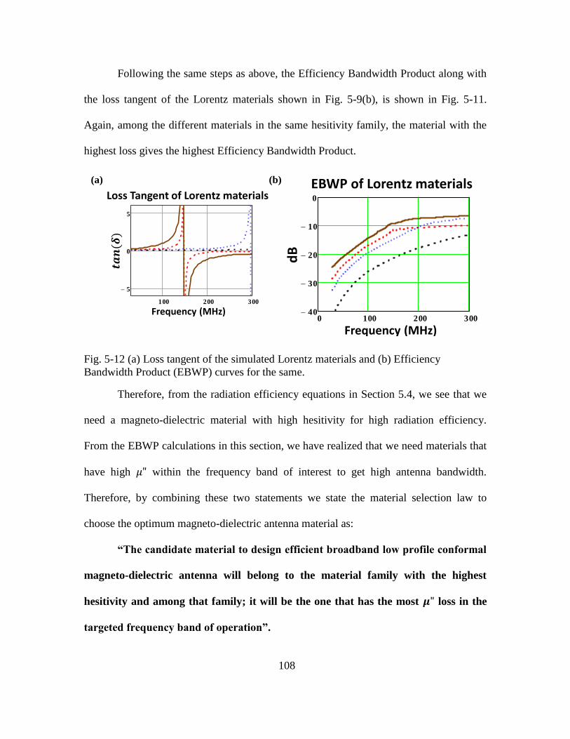
108

Following the same steps as above, the Efficiency Bandwidth Product along with

the loss tangent of the Lorentz materials shown in Fig. 5-9(b), is shown in Fig. 5-11.

Again, among the different materials in the same hesitivity family, the material with the

highest loss gives the highest Efficiency Bandwidth Product.

Fig. 5-12 (a) Loss tangent of the simulated Lorentz materials and (b) Efficiency

Bandwidth Product (EBWP) curves for the same.

Therefore, from the radiation efficiency equations in Section 5.4, we see that we

need a magneto-dielectric material with high hesitivity for high radiation efficiency.

From the EBWP calculations in this section, we have realized that we need materials that

have high within the frequency band of interest to get high antenna bandwidth.

Therefore, by combining these two statements we state the material selection law to

choose the optimum magneto-dielectric antenna material as:

“The candidate material to design efficient broadband low profile conformal

magneto-dielectric antenna will belong to the material family with the highest

hesitivity and among that family; it will be the one that has the most loss in the

targeted frequency band of operation”.

(a) (b)

Frequency (MHz)

dB

EBWP of Lorentz materials

0 100 200 30040

30

20

10

0

100 200 300

5

0

5

Frequency (MHz)

Loss Tangent of Lorentz materials

109

Since the loss or the imaginary part of permeability ( ) peaks at the

ferromagnetic resonance frequency ( ), a useful rule of thumb or extension to the

material selection law is to ensure that the ferromagnetic resonance frequency of the

material that is selected is within band of interest.

5.6 Some Realistic and Almost Realistic Magneto-dielectric materials Evaluated using

the Material Selection Law

In this section, the material selection law that was postulated in the previous

section will be used to evaluate some of the existing magneto-dielectric material found in

the literature. The permeability data obtained from these sources was fit to an analytic

function (Debye or Lorentz) whenever it was possible to do so. The following materials

were considered:

a) NiZn: Bulk NiZn ferrite produced by FairRite [36]. The permeability data was

obtained from the same reference.

b) Co2Z: Unaligned Cobalt Hexaferrite (permeability data from the book by Smit

and Wijn [31]. This material is also produced by Transtech Inc.)

c) Bek12: Bekaert CZN film sheets (12 Kapton substrate thin film) laminated to

form a bulk composite (as in Fig. 5-3). The data sheet was provided by the

manufacturer Bekaert Specialty Films.

d) Bek7p5: Bekaert CZN assuming that it is deposited on insulating

substrate; many such thin films are then assumed to be laminated to form the bulk

structure.

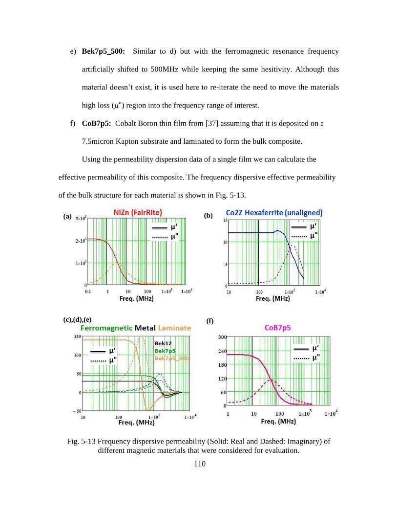
110

e) Bek7p5_500: Similar to d) but with the ferromagnetic resonance frequency

artificially shifted to 500MHz while keeping the same hesitivity. Although this

material doesn’t exist, it is used here to re-iterate the need to move the materials

high loss ( ) region into the frequency range of interest.

f) CoB7p5: Cobalt Boron thin film from [37] assuming that it is deposited on a

7.5micron Kapton substrate and laminated to form the bulk composite.

Using the permeability dispersion data of a single film we can calculate the

effective permeability of this composite. The frequency dispersive effective permeability

of the bulk structure for each material is shown in Fig. 5-13.

Fig. 5-13 Frequency dispersive permeability (Solid: Real and Dashed: Imaginary) of

different magnetic materials that were considered for evaluation.

(a) (b)

(f) (c),(d),(e)

111

The hesitivity of the individual thin films and the hesitivity of the bulk sample are

tabulated in Table 5-2.

Magnetic

Material

Hesitivity ( )

(Single Film)

Hesitivity ( )

(Bulk Sample)

NiZn na 5.524*104

Co2Z na 1.042*105

Bek12 6.511 * 106 3.951*10

5

Bek7p5 6.511 * 106 5.01*10

5

Bek7p5_500 6.511 * 106 5.01*10

5

CoB7p5 2.720 * 106 8.646*10

4

Table 5-2 Hesitivity of the materials being evaluated using the material selection rule

As expected, upon lamination the permeability of the single film gets diluted and

the hesitivity drops. Notice that the hesitivity of the CoB drops significantly after

lamination because the individual film found in the literature has a thickness of 300nm

which is significantly thinner than the assumed dielectric substrate. Therefore, if it is

possible to deposit thicker films while maintaining the same permeability dispersion, then

the bulk hesitivity of this material will approach that of the Bekaert’s films.

The materials arranged in the ascending order of hesitivity is therefore,

𝑦

Also, among the two high hesitivity materials, Bek7p5 and Bek7p5_500, Bek7p5_500

has the highest amount of loss ( ) in the frequency range of interest. Therefore,

according to the Material Selection Law, the optimum choice among the materials above

must be Bek7p5_500. This conclusion is easily validated by using a full-wave simulator.

112

Full-wave simulations of a 1m long cylindrical dipole of 0.5” radius fed with four

feed loops were performed using these materials. This geometry was fixed for all the

materials listed above for direct comparison. The frequency range of simulation was

30MHz to 300MHz. The impedance seen at each feed port was combined using an ideal

power divider netwrok as in Section 5.6, to find the total input impedance . The

bandwidth (BW) was again calculated using (5-2). The radiation efficiency, bandwidth

(for Γ = -10dB) and Efficiency-Bandwidth Product (EBWP)’ for all these cases are

shown in Fig. 5-14.

Fig. 5-14 a) Radiation Efficiency (b) Fractional Bandwidth (c) Efficiency Bandwidth

product for different materials for a 1m long, 0.5” radius dipole.

(a) (b)

(c)

113

From Fig. 5-14(a), it is clear that the radiation efficiency of the magneto-dielectric

dipole increases with hesitivity. And also as expected, two different materials with

different permeability dispersion but with the same hesitivity, have the same radiation

efficiency (Orange: Bek7p5_500 curve is on top of the Green: Bek7p5 curve).

The fractional bandwidth (FBW) curve, on the other hand (Fig. 5-14(b)), has a

different trend. As we saw in Section 5.6, the highest FBW is obtained using the NiZn

and CoB materials that are extremely lossy at these frequencies.

Fig. 5-14(c) shows that at low frequencies, for this structure, the NiZn ferrite has

the highest EBWP. The loss in this material makes it very easy to match the antenna and

hence the boost in bandwidth overcomes the drop in efficiency as seen in Fig. 5-14(a)

and Fig. 5-14(b). A similar result is observed in the case of CoB7p5 material. But, as

frequency goes up, we see that the Bek7p5_500 material has the highest EBWP. The high

hesitivity of this material results in high efficiency and as the ferromagnetic resonance of

this material is close to the band of operation (ferromagnetic resonance f0=500MHz), the

high μ” loss gives it higher FBW. The difference is clearly seen when compared to

Bek7p5 which is a material from the same ‘family’ (same hesitivity). Although

Bek7p5_500 and Bek7p5 have the same radiation efficiency, Bek7p5 has a lower

bandwidth (and therefore lower EBWP) as it has low μ” in the frequency range of operation.

These results validate the material selection law that was stated in Section 5.6.

The laminated Bek7p5_500 material has the highest EBWP throughout the band of

interest. Therefore, it is the right choice of material as predicted by the Material Selection

Law.

114

5.7 Conclusions and Future Work

Using a closed form model of an electrically small magneto-dielectric antenna

that satisfies automatically the Fano-Chu Gain bandwidth Product limit, and including in

that model a dispersive permeability consistent with the Kramers Kronig relations, we

obtain a material selection rule that states that given a fixed volume of material,

maximum efficiency is obtained by choosing the material to have the largest possible

hesitivity, a quantity commensurate with Snoek’s Product, and which has the largest

amount of loss in the desired frequency range of operation. This material selection rule

enables the rapid design of magneto dielectric antennas for conformal applications.

Future work on this subject will include extending the material selection law to

multi-Debye and multi-Lorentz materials.

115

Chapter 6

MAGNETO-DIELECTRIC DIPOLE ANTENNA CIRCUIT MODEL USING

POLARIZABILITY

6.1 Introduction

In Chapters 3 and 4, we developed an electrically small magneto-dielectric

antenna model by adding circuit elements (L & C) that are functions of the magneto-

dielectric material constitutes (permeability ( ) and permittivity ( ) respectively) to the

electrically small RLC circuit model of a conventional metallic antenna. The additional

elements accounted for the penetration of fields into the material. The external field

structure were assumed to be the same as that of a metallic (or PEC) electrically small

antenna and hence they were modeled by Schelkunoff’s electrically small antenna circuit

elements. In this chapter, we take a different approach in modeling a magneto-dielectric

dipole antenna in which we use only three basic elements (R, L and C) to come up with a

much simpler (less circuit elements) equivalent magnetic circuit model, with the

magnetic capacitor being a function of permeability. The permeability is incorporated

into the antenna capacitance using polarizability (α) of the object. The polarizability

equation enables us to model both the external and internal magnetic field morphology

using a single magnetic capacitor. The analysis is done for a purely magnetic material

before extending it to a more general realistic lossy magneto-dielectric material.

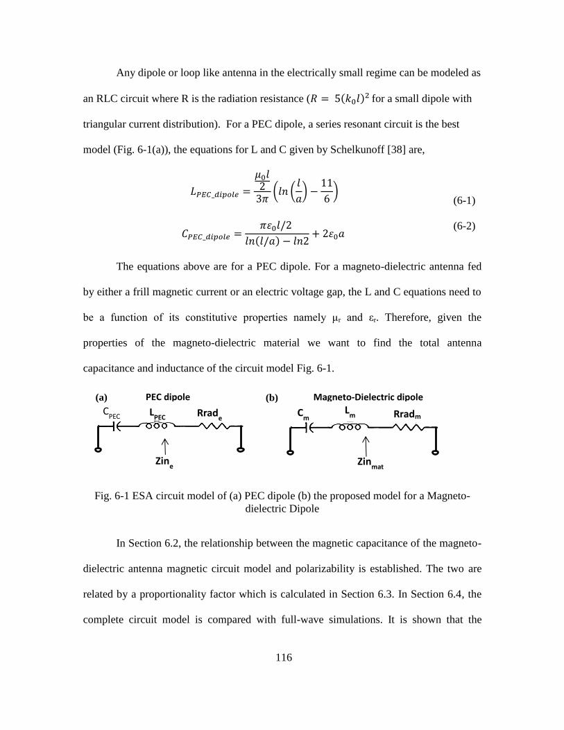
116

Any dipole or loop like antenna in the electrically small regime can be modeled as

an RLC circuit where R is the radiation resistance ( ( )

for a small dipole with

triangular current distribution). For a PEC dipole, a series resonant circuit is the best

model (Fig. 6-1(a)), the equations for L and C given by Schelkunoff [38] are,

( (

)

)

(6-1)

( )

(6-2)

The equations above are for a PEC dipole. For a magneto-dielectric antenna fed

by either a frill magnetic current or an electric voltage gap, the L and C equations need to

be a function of its constitutive properties namely μr and εr. Therefore, given the

properties of the magneto-dielectric material we want to find the total antenna

capacitance and inductance of the circuit model Fig. 6-1.

Fig. 6-1 ESA circuit model of (a) PEC dipole (b) the proposed model for a Magneto-

dielectric Dipole

In Section 6.2, the relationship between the magnetic capacitance of the magneto-

dielectric antenna magnetic circuit model and polarizability is established. The two are

related by a proportionality factor which is calculated in Section 6.3. In Section 6.4, the

complete circuit model is compared with full-wave simulations. It is shown that the

LPEC

Rrade

Zine

Cm

Lm

Rradm

Zinmat

PEC dipole Magneto-Dielectric dipole

CPEC

(a) (b)

117

agreement between the circuit model and the full wave simulations is good only in the

electrically small limit. The summary and some notable conclusions of the chapter are

outlined in Section 6.5.

6.2 Polarizability and Antenna Capacitance

Let us complete the magnetic circuit model by starting with the antenna

capacitance. Now we need a parameter that connects capacitance to its constituents. One

such quantity is Polarizability ( ). Suppose a uniform electric field (E) is impressed on a

conducting sphere of radius ‘a’ (Fig. 6-2(a)).The induced dipole moment (p) of the sphere

in the presence of this uniform E-field is given by

𝑦 (6-3)

Fig. 6-2 (a) PEC sphere with external flux lines and a (b) Dielectric sphere with internal

and external flux lines created in the presence of a uniform ambient E field(E).

Now suppose, the sphere is not made up of PEC but a material say of finite

dielectric constant ( ) (Fig. 6-2(b)), then the Polarizability, αmaterial, is that of a PEC

E E

PEC Sphere Dielectric Sphere (εr<<∞)

p=α(εr)*E

(a) (b)

118

sphere de-rated by the factor, ( ) ( ). The dipole moment is still p= αmaterial E.

Note that the PEC sphere has only external flux lines while the material object has both

internal and external flux lines. Now, if we consider a PEC sphere and wrap it with a

magnetic ring current and make a spherical antenna (Fig. 6-3) we know that its near field

looks like the field of a dipole and we can calculate its dipole moment. Therefore, is there

a relation between the antenna capacitance (from the flux lines) and Polarizability? Let us

assume that

(6-4)

Fig. 6-3 PEC spherical antenna excited by a magnetic ring current

The antenna susceptance of different spherical modes of the metallic sphere is

given by [38]:

( ) (

{[ ] }

)

Since we are interested in the electrically small domain; for the lowest order mode or

principal wave (TM01), n=1,

PEC Spherical

Antenna

119

(6-5)

From (6-3), (6-4) & (6-5) :

or

(6-6)

Thus, (6-6) relates Polarizability to capacitance of a PEC sphere. This can be extended to

a magneto-dielectric sphere by using its polarizability αmaterial from above. But here we

are interested in linear cylindrical objects as antennas that can be placed conformal to

ground. We can always approximate a cylinder by a prolate spheroid of large aspect ratio

(Fig. 6-4). The reason for considering a prolate spheroid is that unlike a cylinder, we

know the Polarizability of a prolate spheroid in closed form [39].

Fig. 6-4 Prolate Spheroidal Magneto-Dielectric Antenna fed by an electric loop

(Approximates a Cylinder)

If ‘k1’ and ‘k2’ represent the constitutive properties of the external and the

internal medium and k0 = ε0 or µ0 (depending on the type of material):

(

)

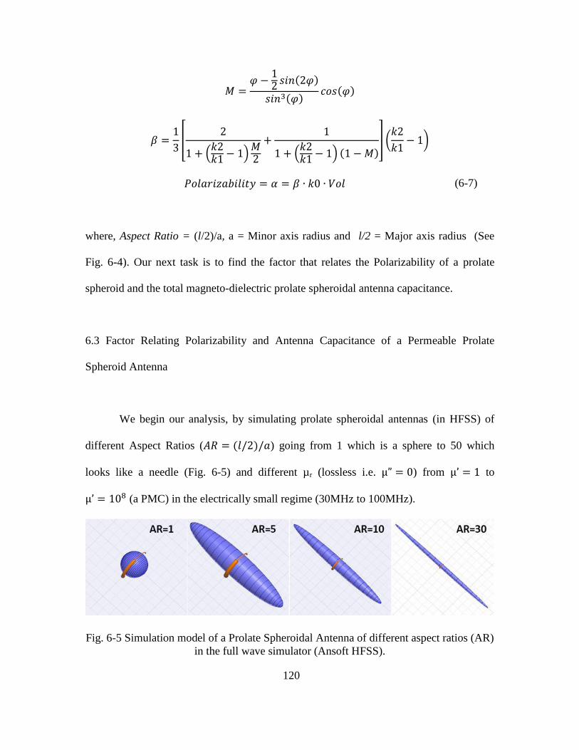
120

( )

( ) ( )

[

(

)

(

) ( )] (

)

𝑦 (6-7)

where, Aspect Ratio = (l/2)/a, a = Minor axis radius and l/2 = Major axis radius (See

Fig. 6-4). Our next task is to find the factor that relates the Polarizability of a prolate

spheroid and the total magneto-dielectric prolate spheroidal antenna capacitance.

6.3 Factor Relating Polarizability and Antenna Capacitance of a Permeable Prolate

Spheroid Antenna

We begin our analysis, by simulating prolate spheroidal antennas (in HFSS) of

different Aspect Ratios ( ( ) ) going from 1 which is a sphere to 50 which

looks like a needle (Fig. 6-5) and different µr (lossless i.e. ) from to

(a PMC) in the electrically small regime (30MHz to 100MHz).

Fig. 6-5 Simulation model of a Prolate Spheroidal Antenna of different aspect ratios (AR)

in the full wave simulator (Ansoft HFSS).

121

The circuit model assumed is shown in Fig. 6-1(b), but since we are working in

the electrically small regime, we will ignore the inductance ( ) for now. In HFSS we

measure the input impedance of the loop which is electric impedance Zine. We want the

dual impedance . We saw in Chapter 3 that the magnetic input impedance is

equivalent to the electric input admittance. Thus, we can find the magnetic input

impedance of the ESA equivalent circuit model by taking the inverse of the input

impedance measured in the full wave simulator.

Note, that although we said that the inductance of the equivalent circuit will be

ignored, what we were talking about was the internal inductance. The antenna would

always see the inductance of the feed loop itself. Hence, this extra inductance should be

subtracted out of our antenna capacitance calculation. Therefore, before we analyze the

magneto-dielectric case, let us analyze the electric feed loop by itself (µ’=1) in order to

find out its self-inductance. Jeffimenko [40] gives us the static solution of the self-

inductance of a thin circular wire ring (circle radius ‘R’ and wire radius ‘ρ’):

( (

)

)

(6-8)

On the other hand, Schelkunoff [41] also gives us the inductance of a small loop by

integrating around the loop the inductance per unit length of the principal wave:

( (

))

(6-9)

Surprisingly, the two equations are different. The comparison of the two

equations along with the HFSS result for different loop radii is shown in Fig. 6-6. We can

clearly see that Schelkunoff’s Loop equation agrees well with simulation for all the cases

122

considered keeping in mind that the simulation curves can go lower as we go deeper into

the electrically small domain. Therefore, we will use his equation to subtract out the

inductance of the loop in our antenna capacitance calculation.

Fig. 6-6 Inductance of feed loop vs Frequency for different loop radii

Therefore, the antenna capacitance calculated from HFSS is given by

( )

(

)

(

)

(6-10)

The factor of ‘2’ is to account for the fact that the antenna was placed on top of a PEC

ground plane. Fig. 6-7 below shows this HFSS magnetic capacitance compared with the

magnetic capacitance calculated from the polarizability for two different values of µr.

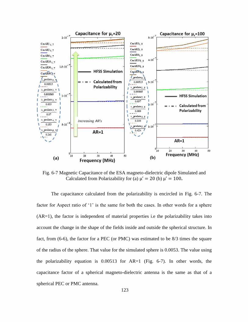
123

Fig. 6-7 Magnetic Capacitance of the ESA magneto-dielectric dipole Simulated and

Calculated from Polarizability for (a) (b) .

The capacitance calculated from the polarizability is encircled in Fig. 6-7. The

factor for Aspect ratio of ‘1’ is the same for both the cases. In other words for a sphere

(AR=1), the factor is independent of material properties i.e the polarizability takes into

account the change in the shape of the fields inside and outside the spherical structure. In

fact, from (6-6), the factor for a PEC (or PMC) was estimated to be 8/3 times the square

of the radius of the sphere. That value for the simulated sphere is 0.0053. The value using

the polarizability equation is 0.00513 for AR=1 (Fig. 6-7). In other words, the

capacitance factor of a spherical magneto-dielectric antenna is the same as that of a

spherical PEC or PMC antenna.

(a) (b)

124

Also note that the in each plot the factor is different for different aspect ratio’s

and at the same time the factor in Fig. 6-7(a) and (b) are different for a fixed aspect ratio

except AR=1. This implies that the factor that relates polarizability and magnetic

capacitance for a prolate spheroidal antenna is a function of both the Aspect ratio (AR)

and the material property of the magneto-dielectric (µ’). The proportionality factor is

plotted versus the Aspect ratio for different µ’s and vice versa in Fig. 6-8 below.

Fig. 6-8 Magnetic Capacitance and Polarizability proportionality factor (a) versus Aspect

Ratio and (b) versus Permeability

The constant curve in Fig. 6-8(b) is for the sphere (AR=1) which as mentioned

before is a constant w.r.t . Fig. 6-8 clearly shows the variation of the proportionality

factor with aspect ratio and . Therefore, we are left with the task of finding a function

for the factor which is a function of AR and . Based on Diaz et. al. [42], since the

problem at hand is that of finding the capacitance factor in the electrically small regime,

Laplace’s equation must be satisfied. Thus, the equation of this capacitance factor that

accounts for the morphology of the field structure as a function of will be of a Debye

equation form:

(a) (b)

125

(

)

(6-11)

where, ‘facPMC’ is the factor for PMC, ‘facDia’ is the factor at the diaphanous limit

(assuming μ=1.1 since μ=1 makes the polarizability zero), ( ) and ‘upoles’

are the estimated poles of this function. Thus we have in effect separated the two possible

sources of variation of the factor function into ‘facPMC’, ‘facDia’ and upoles that vary

only with aspect ratio and ‘u’ that is a function of just the permeability . The

comparison between simulated factor and equation (6-11) for two different cross-

sectional radius of the prolate spheroid is shown in Fig. 6-9.

Fig. 6-9 Single pole Debye factor function (6-11) compared to full-wave simulation

extraction from polarizability for cross sectional radius (a) 1cm and (b) 1inch=2.54cm.

(a) (b)

126

The plot of the terms of the factor function that depend on the aspect ratio is shown in

Fig. 6-10.

Fig. 6-10 a) Plot of factor for PMC dipole ‘facPMC’ and factor at the diaphanous limit

‘facDia’ versus invers of the aspect ratio. (b) Plot of the poles of (6-11).

As this function (6-11) is analytic; although it was derived for purely real μr, its

validity extrapolates to the entire complex plane of permeability. For a few complex

values of µr, HFSS simulations were run to find the magnetic capacitance as before. Note

that since we have a complex µr, the Polarizability calculated from (6-4) and (6-11) will

be complex and therefore we end up with a Complex magnetic capacitance with the

imaginary part corresponding to the magnetic loss resistance. In order to preserve the

complex data from our HFSS ‘Zin’ measurement, we have to subtract out the Radiation

resistance due to the magnetic current flowing in the magneto-dielectric dipole. Since we

are operating in the electrically small regime it is safe to assume a triangular current

distribution due to the leaky nature of the wave in this structure. Therefore, the magnetic

radiation resistance of this dipole using duality is given by:

( )

(6-12)

where η0 is the impedance of free space, i.e. 377Ω.

(a) (b)

127

Fig. 6-11shows the resulting calculated and HFSS simulated magnetic capacitance

for different cases. There is an excellent agreement between simulation and the calculated

magnetic capacitance from polarizability using the factor calculated before. The

agreement is good not only in the real part of capacitance but also the imaginary term,

which goes to show that the polarizability can also accurately account for the magnetic

loss resistance incurred due to the complex permeability. Therefore we have determined a

closed form expression for the magnetic capacitance in the circuit model of Fig.

6-1(b). Now all that is left is the inductance.

Fig. 6-11 Simulated and Calculated complex magnetic capacitance for AR=30(a) &

AR=50(b), (c) List of complex used (numbered 1-10 => x-axis)

0 2 4 6 8 100

2 108

4 108

6 108

0

1 108

2 108

3 108

4 108

AR = 30

Im(Cm) Re(Cm)

HFSS Simulation Cm Calculated

0 2 4 6 8 100

1 108

2 108

3 108

0

1 108

2 108

3 108

4 108

AR = 50

Re(Cm) Im(Cm)

HFSS Simulation Cm Calculated

(a)

(b)

(c)

128

The antenna magnetic inductance, to first order, is the dual of (6-2). Therefore the

zeroth order equations for the electrically small magnetic circuit model of a permeable

prolate spheroidal dipole (Fig. 6-1 (b)) fed by a single electric loop are summarized as

follows:

From (6-12), ( )

From (6-4), (6-7) and (6-11),

Using duality on (6-2)

( (

)

)

6.4 Circuit Model Comparison with Full-Wave Simulations

Consider a 21 inch long and 2inch cross-section prolate spheroid permeable

antenna. Note that the TE01 mode onset frequency for a cylinder of this cross section for

the different permeability values simulated are: => 4.5GHz; => 1.5GHz;

=> 645MHz and => 202MHz which corresponds to of 8, 2.7,

1.15 and 0.36 respectively. The comparison of input impedance and the proposed circuit

model is shown in Fig. 6-12.

129

Fig. 6-12 Input impedance comparison of circuit model and simulation of a 21” long, 1”

radius antenna (a) Real part (b) Imaginary part of input impedance.

The imaginary part of the input impedance matches well in the electrically small

limit (antenna long). The real part does not agree well even at the low end. All

signs point towards the fact that our assumption of triangular current distribution is not

accurate for all the values of . Let us take a closer look at the magnitude of current

distribution on the antenna (Fig. 6-13).

(a) (b)

(a) (b)

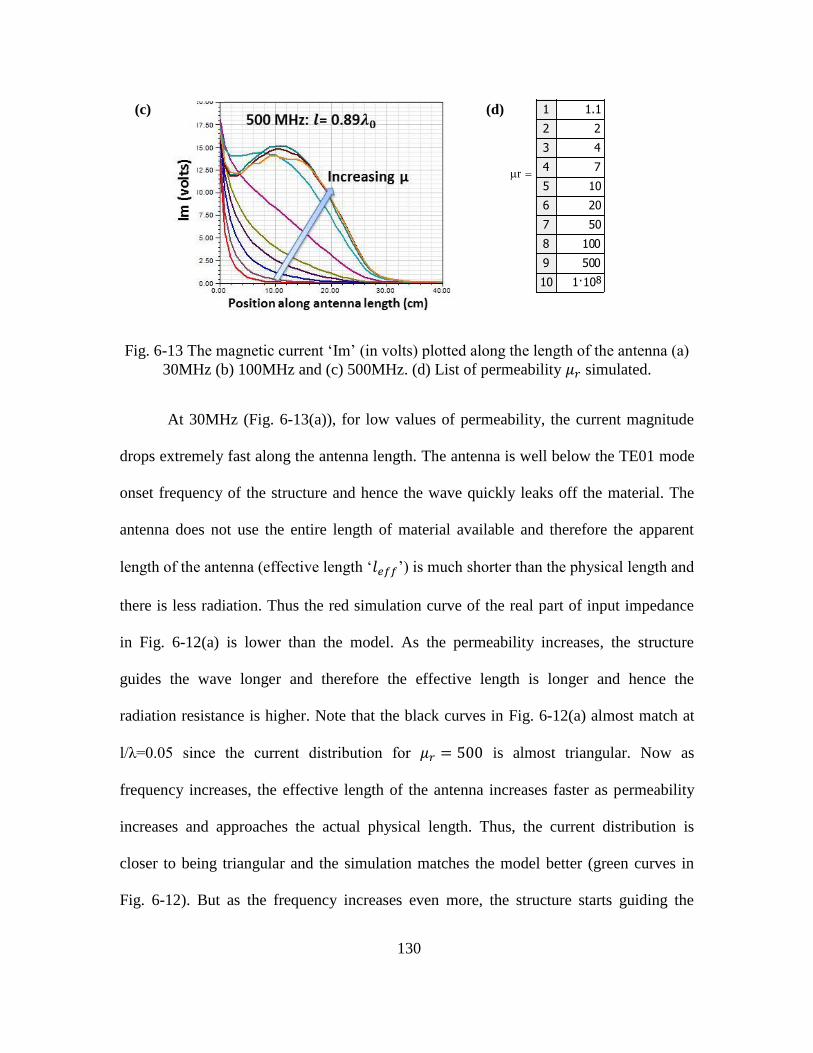
130

Fig. 6-13 The magnetic current ‘Im’ (in volts) plotted along the length of the antenna (a)

30MHz (b) 100MHz and (c) 500MHz. (d) List of permeability simulated.

At 30MHz (Fig. 6-13(a)), for low values of permeability, the current magnitude

drops extremely fast along the antenna length. The antenna is well below the TE01 mode

onset frequency of the structure and hence the wave quickly leaks off the material. The

antenna does not use the entire length of material available and therefore the apparent

length of the antenna (effective length ‘ ’) is much shorter than the physical length and

there is less radiation. Thus the red simulation curve of the real part of input impedance

in Fig. 6-12(a) is lower than the model. As the permeability increases, the structure

guides the wave longer and therefore the effective length is longer and hence the

radiation resistance is higher. Note that the black curves in Fig. 6-12(a) almost match at

l/λ=0.05 since the current distribution for is almost triangular. Now as

frequency increases, the effective length of the antenna increases faster as permeability

increases and approaches the actual physical length. Thus, the current distribution is

closer to being triangular and the simulation matches the model better (green curves in

Fig. 6-12). But as the frequency increases even more, the structure starts guiding the

mr

0

0

1

2

3

4

5

6

7

8

9

10

0

1.1

2

4

7

10

20

50

100

500

81·10

(c) (d)

131

wave all the way to the ends of the antenna and hence deviates further away from the

triangular distribution assumption (Fig. 6-13(c)). Hence the circuit model devised in this

chapter is valid for only a narrow range of combination of frequency and permeability

where the distribution is close to being triangular.

6.5 Summary and Conclusions

In this chapter, we tried to come up with a simple three element (R,L and C)

circuit model for an electrically small magneto-dielectric antenna. We were successful in

calculating one of the three elements accurately, namely the magnetic capacitance Cm , by

relating polarizability and antenna capacitance through a proportionality factor. This

factor for a prolate spheroid antenna magneto-dielectric is a function of both the aspect

ratio and the permeability of the material used. The prolate spheroid was analyzed as

opposed a more conventional cylindrical geometry as we have a closed form equation of

the polarizability of prolate spheroid. A high aspect ratio prolate spheroid is a good

approximation for a cylinder. The inductance and the radiation resistance were assumed

to be the dual of the electric dipole. By doing so, the current distribution on the antenna

was fixed to triangular which on hindsight resulted in the final circuit model to be valid

only for a narrow range of frequencies and value of permeability.

132

Chapter 7

INFINITELY LONG MAGNETO-DIELECTRIC CYLINDER AS A MAGNETIC

RADIATOR

7.1 Introduction

In Chapters 3, 4, 5 & 6 we developed an electrically small magneto-dielectric

antenna circuit model. The individual circuit elements were functions of the geometry

and the magneto-dielectric material constitutes (permeability (μr) and permittivity (εr) ) .

We determined the radiation efficiency of the antenna and the input impedance sans the

feed circuit. But the circuit model did not and cannot tell us anything about the electric

and magnetic field structure inside and around the antenna object, nor did it give us any

insight on the kind of wave guided by this structure. The conventional approach to tackle

this problem is to solve the wave equation for the antenna structure and apply the

appropriate boundary conditions. However, it is difficult to obtain the wave equation

solution for a finite cylinder because of the complexities involved in matching the

boundary conditions at the finite ends of the cylinder. Therefore, we will start with the

‘slightly easier’ problem of solving the wave equation for an infinite magneto-dielectric

cylinder placed on the axis of a single electric feed loop source which will inject the

desired TE-like modes into the cylinder. Depending on the frequency of operation and the

radius of the cylinder, the injected TE waves either ‘leaks’ off the structure or is guided

by it. Although such a structure is physically not realizable, the analysis gives us insight

into how magneto-dielectric materials guide or partially guide the TE modes.

133

A material with a high enough real constitutive can provide a wave-guiding

boundary, similar to conductors, as long as the modes excited in the structure is of the

form of the TE (for magnetic structures) or TM (for dielectric structures) modes. If the

frequency of operation is below the cut-off (or onset) frequency of the modes, the

electromagnetic wave excited in the material is loosely (or poorly) guided and radiates by

leaving the antenna structure or if the structure is finite, by scattering off the ends of the

antenna structure in a way similar to a wave guided by a metal antenna of the same shape.

The magneto-dielectric antenna, being penetrable, exhibits intrinsic frequency dependent

behavior. As frequency increases the wave on the penetrable rod becomes more and more

tightly bound until the onset of the TE01 and TM01 modes, when it is formally a guided

wave. Clearly, once the mode is well above this onset frequency, and trapped by the

material, it will not be available to be radiated by scattering off the ends of the antenna.

The purpose of this chapter is to elucidate partially guided or leaky wave and

guided wave propagation in magneto-dielectric cylinders or wires. In Section 7.2, the

equations for electric and magnetic fields everywhere in space is derived starting from

Helmholtz vector wave equation and applying appropriate boundary conditions to arrive

at the particular solution. The magnetic current (‘ ’ in Volts) along the length of the

structure is calculated by performing the circulation integral of the E-field around the rod.

The magnetic current amplitude and phase plots versus length along the antenna clearly

show us whether the wave is guided or is leaky at a particular frequency. Using the

electric and magnetic field equations, the power radiated by this structure is calculated by

integrating the complex Poynting vector over a cylindrical surface enclosing the antenna.

Using this equation, in Section 7.3, given the predominantly leaky wave behavior

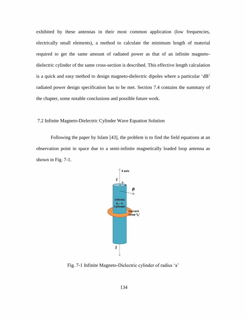
134

exhibited by these antennas in their most common application (low frequencies,

electrically small elements), a method to calculate the minimum length of material

required to get the same amount of radiated power as that of an infinite magneto-

dielectric cylinder of the same cross-section is described. This effective length calculation

is a quick and easy method to design magneto-dielectric dipoles where a particular ‘dB’

radiated power design specification has to be met. Section 7.4 contains the summary of

the chapter, some notable conclusions and possible future work.

7.2 Infinite Magneto-Dielectric Cylinder Wave Equation Solution

Following the paper by Islam [43], the problem is to find the field equations at an

observation point in space due to a semi-infinite magnetically loaded loop antenna as

shown in Fig. 7-1.

Fig. 7-1 Infinite Magneto-Dielectric cylinder of radius ‘a’

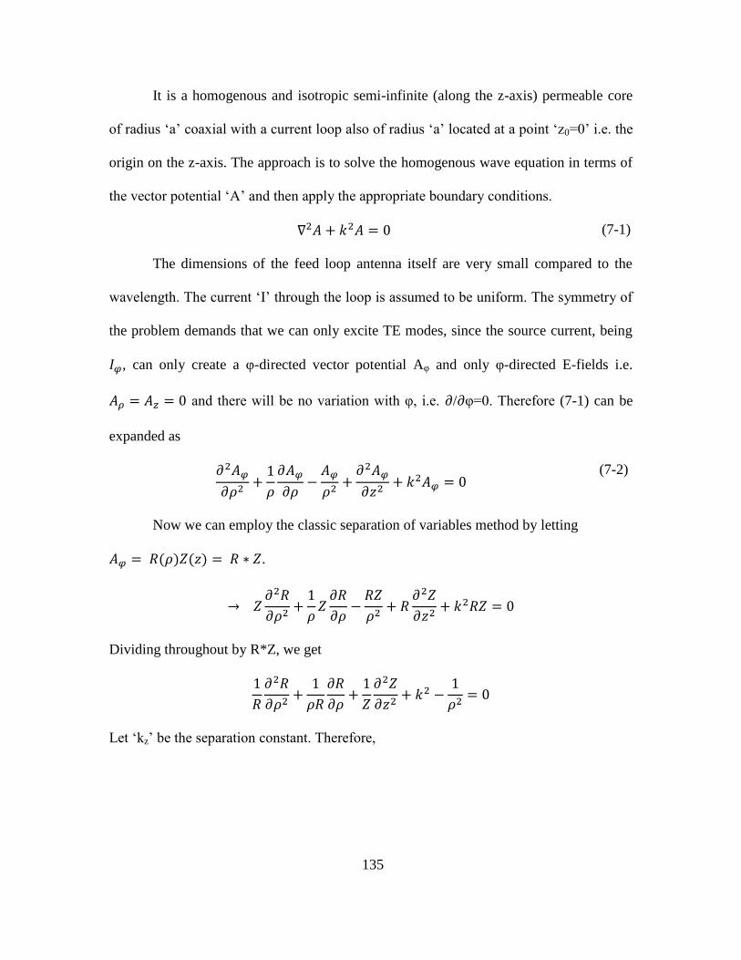
135

It is a homogenous and isotropic semi-infinite (along the z-axis) permeable core

of radius ‘a’ coaxial with a current loop also of radius ‘a’ located at a point ‘z0=0’ i.e. the

origin on the z-axis. The approach is to solve the homogenous wave equation in terms of

the vector potential ‘A’ and then apply the appropriate boundary conditions.

(7-1)

The dimensions of the feed loop antenna itself are very small compared to the

wavelength. The current ‘I’ through the loop is assumed to be uniform. The symmetry of

the problem demands that we can only excite TE modes, since the source current, being

, can only create a φ-directed vector potential Aφ and only φ-directed E-fields i.e.

and there will be no variation with φ, i.e. / φ=0. Therefore (7-1) can be

expanded as

(7-2)

Now we can employ the classic separation of variables method by letting

( ) ( ) .

→

Dividing throughout by R*Z, we get

Let ‘kz’ be the separation constant. Therefore,

136

{(

) }

(7-3)

And

(7-4)

Since there are two regions, inside the magneto-dielectric i.e. and outside i.e. ,

the solution can be written as

[ ] ( )

(7-5)

[ ]

( )( ) (7-6)

Where, √ and √

. The term implies a wave travelling

along the +ve z-axis with a propagation constant .

Here, C and D are unknown constants to be determined by applying the boundary

conditions, ( ) is the Bessel function of the first kind and ( )( ) is the Hankel

function of the second kind.

Since the solution extends to infinity radially i.e. there are no cylindrical

boundaries that might impose restrictions on ( ), there are correspondingly no

restrictions on and the solution involves integral over all . Therefore,

[ ]

∫ ( ) ( )

(7-7)

[ ] ∫ ( )

( )( )

(7-8)

137

Now, the two boundary conditions to be enforced at the boundary of the two

regions I and II are

( )

( ) 𝑦

These two equations can be rewritten in terms of the vector potential A ( ) as

[ ]

[ ]

(7-9)

(

[ ])

(

[ ]) 𝑦

(7-10)

Substituting (7-5) and (7-6) in (7-9) at we get,

( ) ( )( )

Or

( )

( )( )

(7-11)

Now, since the only surface current is at the feed loop located at the origin, the

current can be represented by the Dirac Delta function ( ). This Delta function can

be expanded into an infinite set of current waves travelling along the z-axis each using

the Fourier Integral theorem:

( )

∫

(7-12)

Substituting (7-7), (7-8) and (7-12) in (7-10) and keeping in mind that the integrands

alone should satisfy this condition we get,

(

( )( ))

( ( ))|

(7-13)

The derivative of the Bessel or the Hankel function (let’s call it Y1(px)) is given by

138

( ) ( )

( )

Also

( ( ))

( ) ( ) ( )

( ) ( )

( ( )) ( )

Substituting in (7-13) we get,

( )( )

( )

(7-14)

Substituting (11) in (14) we get

( )

( )( )

( )( )

( )

Therefore, C(kz) is given by

( )

( )( )

( ) ( )( ) ( )

( )( )

Or

( )

( )( )

( ) ( ) ( )( ) ( ) ( )

( )( )

(7-15)

And

( )

( )

( ) ( ) ( )( ) ( ) ( )

( )( )

(7-16)

Substituting (7-15)and (7-16)in (7-7) and (7-8) we get

139

[ ]

∫

( )( ) ( )

( ) ( ) ( )( ) ( ) ( )

( )( )

(7-17)

[ ]

∫

( ) ( )( )

( ) ( ) ( )( ) ( ) ( )

( )( )

(7-18)

Now the individual field components can be derived using and

. Therefore, using the two equations above we get the E and H fields in the

two regions as:

For (inside the magneto-dielectric)

[ ]

∫

( )( ) ( )

( ) ( ) ( )( ) ( ) ( )

( )( )

(7-19)

And

[ ]

∫

( )( ) ( )

( ) ( ) ( )( ) ( ) ( )

( )( )

(7-20)

And

[ ]

∫

( )( ) ( )

( ) ( ) ( )( ) ( ) ( )

( )( )

(7-21)

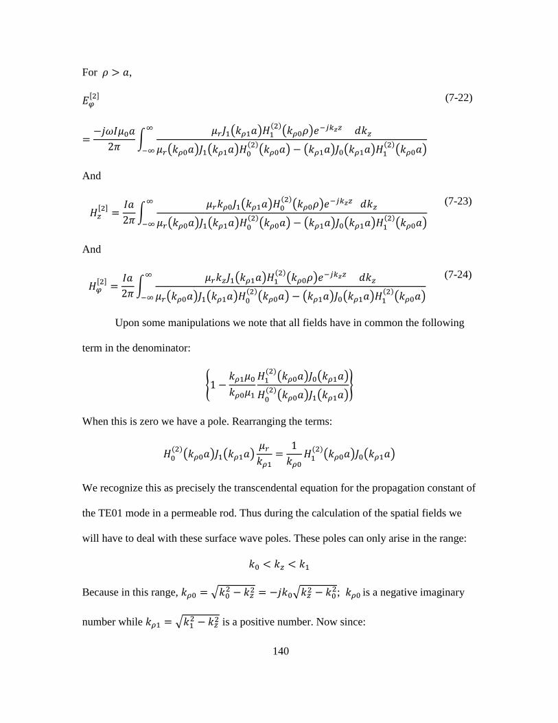
140

For ,

[ ]

∫

( ) ( )( )

( ) ( ) ( )( ) ( ) ( )

( )( )

(7-22)

And

[ ]

∫

( ) ( )( )

( ) ( ) ( )( ) ( ) ( )

( )( )

(7-23)

And

[ ]

∫

( ) ( )( )

( ) ( ) ( )( ) ( ) ( )

( )( )

(7-24)

Upon some manipulations we note that all fields have in common the following

term in the denominator:

{

( )( ) ( )

( )( ) ( )

}

When this is zero we have a pole. Rearranging the terms:

( )( ) ( )

( )( ) ( )

We recognize this as precisely the transcendental equation for the propagation constant of

the TE01 mode in a permeable rod. Thus during the calculation of the spatial fields we

will have to deal with these surface wave poles. These poles can only arise in the range:

Because in this range, √ √

; is a negative imaginary

number while √ is a positive number. Now since:

141

( )

( )( ) ( )

( )( )

The quantity

( )( )

( )( )

( )

( )

is known as the logarithmic derivative of ( ) and is well behaved. In fact, the quantity

( )

( )( )

( )( )

is purely real and negative while in the same range the quantity

{( ) ( )

( )}

is also purely real, so only in this range can the denominator vanish. Said another way:

we know guided slow waves travel slower than free space but no slower than the rod

medium, therefore it is only in this range between and that the spectrum waves

can match in speed the slow wave modes and it is then that they can couple strongly to

them.

When we are concerned with the onset of surface waves as a function of

frequency in the source-less solution of the penetrable rod, this onset is controlled by the

argument of the Bessel functions . In the case of the spectrum excited by the current

band, this onset is a function of in the rod medium; and is at its largest, namely

equal to , at the horizon when kz approaches k0:

√

142

Therefore, if the rod is internally electrically large enough to trap the wave, this pole will

first appear in the spectrum at the horizon.

Now we are interested in the current wave (guided displacement current dB/dt

wave). We obtain this by integrating the circulating E-field at the surface of the rod:

∮ ∫

[ ]

( )

∫

( ) ( )( )

( ) ( ) ( )( ) ( ) ( )

( )( )

(7-25)

the magnetic current is in Volts.

To perform the integration numerically, we deform the integration path in the

vicinity of the surface wave poles. Fig. 7-2 shows the amplitude (a) and phase(b) of the

current wave from 30MHz to 170MHz every 20MHz versus distance in wavelengths for

a permeable rod of , and radius a = 2 inches. Fig. 7-2(c) shows the

structure of the mode inside the permeable rod (Plot of the field). In Fig. 7-2(a), it is

clear that for frequencies far below cutoff the current is not guided at all and we see a

precipitous drop in amplitude. Therefore, far below cutoff the noise in the calculation

makes determination of the phase velocity ambiguous for the black and gray curves in

Fig. 7-2 (b) (30MHz and 50MHz). Nevertheless it is clear that they start below the light

line and then all we see above one wavelength is noise. Above 70MHz the phase plots

are well behaved and we clearly see fast wave behavior with phase velocities that

approach the light line (31.4c over 5 wavelengths) at 170MHz.The amplitude and phase

plots show that as 170MHz is approached, the approaching surface wave onset tends to

143

flatten the amplitude of the current wave and brings its speed close to light, thus the

magneto-dielectric rod behaves more and more like a Perfect Magnetic Conductor

antenna.

Fig. 7-2 Amplitude (a),Phase (b) as a function of distance from the feed for a 2” radius

, rod from 30MHz to 170MHz (c) Mode Structure ( )

Fig. 7-3show the results from 190MHz to 330MHz every 20MHz again plotted versus

distance from the feed in wavelengths. We are now in the region of the guided TE01

mode.

(a) (b)

(c)

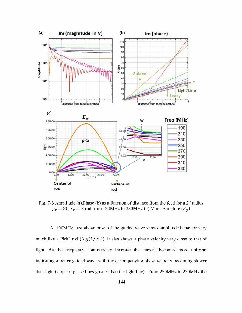
144

Fig. 7-3 Amplitude (a),Phase (b) as a function of distance from the feed for a 2” radius

, rod from 190MHz to 330MHz (c) Mode Structure ( )

At 190MHz, just above onset of the guided wave shows amplitude behavior very

much like a PMC rod ( ( )). It also shows a phase velocity very close to that of

light. As the frequency continues to increase the current becomes more uniform

indicating a better guided wave with the accompanying phase velocity becoming slower

than light (slope of phase lines greater than the light line). From 250MHz to 270MHz the

(a) (b)

(c)

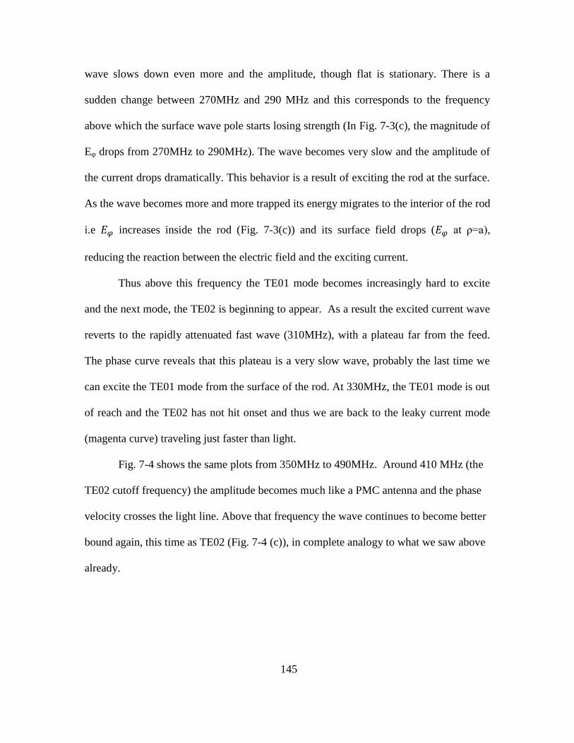
145

wave slows down even more and the amplitude, though flat is stationary. There is a

sudden change between 270MHz and 290 MHz and this corresponds to the frequency

above which the surface wave pole starts losing strength (In Fig. 7-3(c), the magnitude of

Eφ drops from 270MHz to 290MHz). The wave becomes very slow and the amplitude of

the current drops dramatically. This behavior is a result of exciting the rod at the surface.

As the wave becomes more and more trapped its energy migrates to the interior of the rod

i.e increases inside the rod (Fig. 7-3(c)) and its surface field drops ( at ρ=a),

reducing the reaction between the electric field and the exciting current.

Thus above this frequency the TE01 mode becomes increasingly hard to excite

and the next mode, the TE02 is beginning to appear. As a result the excited current wave

reverts to the rapidly attenuated fast wave (310MHz), with a plateau far from the feed.

The phase curve reveals that this plateau is a very slow wave, probably the last time we

can excite the TE01 mode from the surface of the rod. At 330MHz, the TE01 mode is out

of reach and the TE02 has not hit onset and thus we are back to the leaky current mode

(magenta curve) traveling just faster than light.

Fig. 7-4 shows the same plots from 350MHz to 490MHz. Around 410 MHz (the

TE02 cutoff frequency) the amplitude becomes much like a PMC antenna and the phase

velocity crosses the light line. Above that frequency the wave continues to become better

bound again, this time as TE02 (Fig. 7-4 (c)), in complete analogy to what we saw above

already.

146

Fig. 7-4 Amplitude (a),Phase (b) as a function of distance from the feed for a 2” radius

, rod from 350MHz to 490MHz (c) Mode Structure ( )

Fig. 7-5 below shows the Radiated power (Prad) versus frequency. Prad is

calculated by integrating the complex Poynting vector over a cylindrical surface

enclosing the antenna. The red lines indicate the cut-off frequencies of the TE0n modes.

(a) (b)

(c)

147

Fig. 7-5 Radiated Power (Prad) vs Frequency(MHz) for a 2” radius , rod

The Radiated power and hence the Radiation Resistance drops right after every TE0n

cutoff as the mode is well guided. Prad continues to drop until the loop feed starts

exciting the next higher order mode.

7.3 Effective Length for a Finite Magneto-dielectric Dipole Based on the Radiated Power

of an Infinite Magneto-dielectric cylinder

We know that the magneto-dielectric antenna radiates by leaking off energy off its

structure. In Section 7.3, we calculated the magnetic current distribution of an infinite

cylindrical antenna. Since we can’t make an infinite structure can we design a realistic

finite magneto-dielectric antenna using what we have learned so far?

Let us start by looking at the current distribution at a fixed frequency for different

values of permeability . A fixed radius (a=3cm) infinite magneto-dielectric rod was

148

simulated and the permeability varied from to 160 (permittivity ). The

frequency was fixed to 100MHz which is well below the TE01 mode cut-off frequency

for even the highest µr considered ( , ). The magnetic

current is shown below in Fig. 7-6.

Fig. 7-6 Magnetic current (Im) of a semi-infinite cylindrical magento-dielectric antenna

(a = 3cm) vs antenna length measured from the feed loop.

The ripples seen in the results are due to the numerical noise when solving the

equations from Section 7.2. The magnetic current shows an exponential tail (leaky wave

behavior) away from the feed, however, close to it we can clearly see a logarithmic drop

in magnitude (ln(1/L)).

Now, a closer look at the current curves shows that it is possible to fit the

exponential tail of the magnetic current with a single exponential term (dashed black

curves in Fig. 7-7).

149

Fig. 7-7 Magnetic current ( ) of a semi-infinite magneto-dielectric antenna fit to an

exponential (dashed black curves).

If we now subtract these exponential fits from the magnetic current, , we get the

following curves for different values of (Fig. 7-8).

Fig. 7-8 ‘Im’ and ‘Im – exp(fit)’ current curves for different µr vs antenna length.

150

Fig. 7-8 shows that the magnetic current of a semi-infinite magneto-dielectric

antenna is the sum of a constant perturbation current (Im-exp(fit) curves in Fig. 7-8) and

an exponential leaky wave current of the TE01 mode below its cutoff. The constant

perturbation current is due to all the higher order modes that are extremely leaky that can

get coupled into the magneto-dielectric material.

Now if we ask the question at what length should we truncate the antenna so that

we can get as much radiated power as possible? For an exponential current distribution it

is natural to choose the 1/e point as my effective length ( ). Table 7-1 lists for

different .

Leff (in) Leff (cm)

40 17.02 43.18

60 21.29 54.07

80 25.55 64.9

100 30.46 77.36

120 38.32 97.33

140 47.57 120.84

Table 7-1 values for different

Now let us see how well did we do in choosing the length by comparing the

radiated power of the finite dipole of length = (Fig. 7-9) with that of an infinite

dipole of same cross-section and permeability.

151

Fig. 7-9 Finite cylindrical magneto-dielectric rod with circular feed loop.

As shown in Fig. 7-9, the outer conductor of the coaxial feed of the circular loop

is extended out of the ground plane all the way to the center of the loop. This removes the

asymmetry of the loop and maintains the unidirectional electric current flow. Fig. 7-10

shows the electric current in the feed loop for this new configuration.

Fig. 7-10 Electric Current ‘Ie’ in the feed loop vs angular position for different µr.

0

0.02

0.04

0.06

0.08

0.1

0.12

0 45 90 135 180

40

60

80

100

120

140

160

Current Ie in the feed loop vs angular position

Ie

Angle in deg. (measured from the coax w.r.t loop center)

μ

152

The circular loop has a uniform constant current distribution. Now we compare

the analytical Prad of an infinite magneto-dielectric cylinder with the simulated Prad of a

finite magneto-dielectric cylindrical dipole over ground vs µr (Fig. 7-11).

Fig. 7-11 Radiated Power vs µr (Analytic: Infinite rod versus Simulated Finite cylindrical

rod)

The simulated was calculated from f=100MHz magnetic current curves. The

length was kept the same for the other two frequencies. If we consider just the f=100MHz

case, the analytic and simulation results match fairly well for small ‘ ’. As the value of

‘ ’ goes up, we keep getting closer and closer to the guided domain i.e. the waves are

better guided by the PC rod. Hence, we can see that there is a deviation between analytic

and simulated results for higher µr due to the fact that in the case of the finite rod there is

an additional radiation effect from the end discontinuities. Therefore, we get a higher

Prad in our finite rod simulations. In the 50MHz case, Prad is higher because we have

started with a longer Leff than what would be required, as the 100MHz Leff was chosen.

50 100 1500.01

0.1

1

10

100

1 103

Radiated Power vs μ

Pra

d

50MHz

100MHz

150MHz

μr

Infinite rod (Analytic)Finite rod (Simulation)

153

So far, a finite magneto-dielectric antenna with different permeability at a fixed

frequency was analyzed. In Fig. 7-11, the simulation and calculations at 50MHz and

150MHz were done using the effective length values obtained from the 100MHz case.

Therefore, in order to prove the validity of the method conclusively, the above approach

was now repeated for a single value of (=60) analyzed at different frequencies. Since

we are interested in the leaky domain operation of these antennas; for 3cm magneto-

dielectric cylinder as before, 50MHz to 400MHz is the frequency range considered as the

TE01 mode cutoff frequency for these values is 500MHz. Fig. 7-12 shows the Prad

curves obtained analytically and from simulation along with the plot of the effective

length calculated from the procedure outlined above w.r.t frequency.

Fig. 7-12 a) Radiated power, (b) Effective (Half) Length of Finite 3cm radius magneto-

dielecric cylinder vs Frequency for µr = 60

Fig. 7-12(a) shows that the Prad curves has the same behavior as the case where

different µ’s were analyzed. At low frequency, the analytic and simulated curves are on

top of each other. As the frequency increases, the magneto-dielctric cylinder starts

guiding the wave longer along its axis resulting in a stronger radiation from the two end

(a) (b)

154

discontinuities. Thus, we see around a factor of two increase in radiated power at higher

frequencies close to cut-off.

Similar analysis was done for two other magneto-dielectric cross-sections. The

results are shown below in Fig. 7-13. For a 0.75cm radius magneto-dielectric cylinder,

the TE01 cut-off frequency for is 2GHz and for a 6cm radius magneto-

dielectric cylinder, the TE01 cut-off frequency is 249MHz.

Fig. 7-13 a) Radiated power, (b) Effective (Half) Length of finite 0.75cm radius magneto-

dielectric cylinder vs Frequency and (c) Radiated power, (d) Effective (Half) Length of

finite 6cm radius magneto-dielectric cylinder vs Frequency.

(a) (b)

(c) (d)

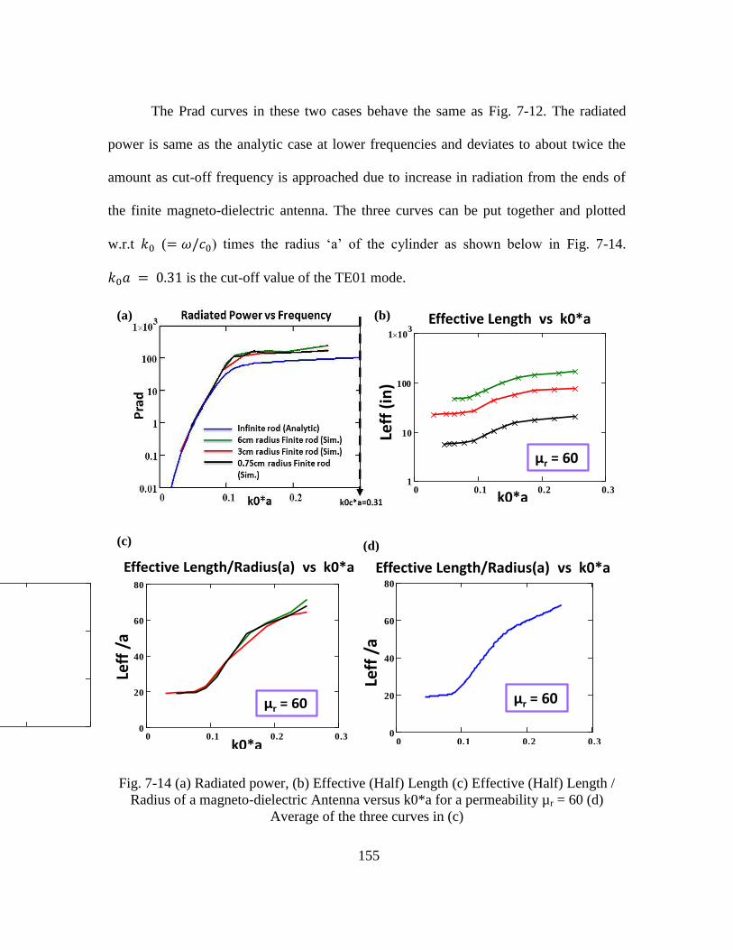
155

The Prad curves in these two cases behave the same as Fig. 7-12. The radiated

power is same as the analytic case at lower frequencies and deviates to about twice the

amount as cut-off frequency is approached due to increase in radiation from the ends of

the finite magneto-dielectric antenna. The three curves can be put together and plotted

w.r.t ( ) times the radius ‘a’ of the cylinder as shown below in Fig. 7-14.

is the cut-off value of the TE01 mode.

Fig. 7-14 (a) Radiated power, (b) Effective (Half) Length (c) Effective (Half) Length /

Radius of a magneto-dielectric Antenna versus k0*a for a permeability µr = 60 (d)

Average of the three curves in (c)

0 0.1 0.2 0.31

10

100

1 103

Effective Length vs k0*a

Leff

(in

)

k0*a 0 0.1 0.2 0.30

20

40

60

80

k0*a

Leff

/a

Effective Length/Radius(a) vs k0*a

(b) (c)

µr = 60 µr = 60

(a) (b)

0 0.1 0.2 0.31

10

100

1 103

Effective Length vs k0*a

Leff

(in

)

k0*a 0 0.1 0.2 0.30

20

40

60

80

k0*a

Leff

/a

Effective Length/Radius(a) vs k0*a

(b) (c)

µr = 60 µr = 60 µr = 60

k0*a

Leff

/a

Effective Length/Radius(a) vs k0*a

0 0.1 0.2 0.30

20

40

60

80

(c) (d)

156

Fig. 7-14 (a) shows that the three Simulated ‘Prad’ curves lie on top of each other

when plotted w.r.t . Similarly, the effective length curves of the finite magneto-

dielectric antenna when normalized by the cross-section of the antennas lie on top of each

other. Therefore, we have reduced our complete analysis to a single curve (Fig. 7-14(c)),

i.e. given a magneto-dielectric materials permeability we can find the effective length of

a finite magneto-dielectric antenna for any cross-section that gives the same amount of

radiated power as an infinite magneto-dielectric rod at low frequency ( for

) and about twice the amount of power as we approach the TE01 cut-off

frequency ( ).

7.4. Summary, Conclusions and Future Work

The green function problem of the cylindrical permeable rod excited by a electric

current loop was presented in this chapter. The current wave in a magneto-dielectric

infinite rod is shown to go through a succession of fast wave-slow wave transitions.

Below the first mode and in between modes the fast wave regions exhibit leaky wave

behavior with decaying amplitude and waves travelling faster than speed of light. Every

time we approach the onset of guidance of a mode, there is a band of frequencies over

which the magneto-dielectric rod behaves very much like a PMC metal rod. Then as the

mode gets more trapped the magnetic current and the radiated power eventually drop

because this magnetic current cannot be excited from the surface. Eventually, as

157

frequency increases, the mode reverts to a fast wave leaky mode that corresponds to the

next higher order mode.

The exponential decay of the current during the leaky wave periods reduces the

effective electrical length of the antenna. This reduced aperture size contributes to the

lower gain bandwidth product when compared to a similarly sized metal dipole in free

space.

We also established a method to estimate the minimum length required for a magneto-

dielectric antenna to give the same (or slightly greater) radiated power than an infinite

length magneto-dielectric rod of the same cross-section and permeability when operating

in the leaky domain. It is first shown that this length is directly proportional to the value

of permeability of the rod for a fixed frequency and radius of the rod. When analyzed

w.r.t frequency for a single permeability of µr = 60, it was observed that the effective

length is a function of frequency as well. Finally, the complete analysis versus frequency

was reduced to a single curve of ‘Effective length/a versus ’ (Figure 2.14) from which

it is possible to determine the effective length required to radiate more power than an

infinite µr=60 magneto-dielectric rod for a given cross-section. In the future, this analysis

can be repeated for different µ’s to obtain a family of effective length curves.

So far we have discussed the case of loading a loop antenna with a cylinder of

infinite length. Since an infinite cylinder is never realizable in reality, the next step in our

effort to understand a pragmatic antenna is to obtain a rigorous model of a finite

magneto-dielectric antenna. Because of the complexities involved in the analysis of the

ends of a finite cylindrical magneto-dielectric rod we will assume a prolate spheroidal

shape antenna. A long and thin prolate spheroid is a good approximation to a finite

158

cylinder. We propose to solve this problem in a similar way as the infinite case, by

solving the inhomogeneous wave equation using the appropriate boundary condition,

however, this time due to the spheroidal geometry, a spheroidal coordinate system will be

used. This analysis is done in Chapter 5.

The most useful application of magneto-dielectric dipoles is in conformal antenna

applications where it is placed tangential to a metallic ground plane. There are cases,

where even this might be unacceptable for example on a UAV where any protrusion

would increase the drag force and increase fuel consumption. Thus ideally we want to an

antenna which can be buried in the ground plane. The use of permeable materials does

enable us to do so. The magneto-dielectric antenna can be buried inside a metallic trough

in the ground plane and thus be truly conformal. The analysis of such a trough structure is

planned for the future.

159

Chapter 8

FINITE MAGNETO-DIELECTRIC PROLATE SPHEROIDAL ANTENNA

ANALYSIS

8.1 Introduction

In Chapter 7, we analyzed an infinite magneto-dielectric cylinder and saw

the guided and partially guided (leaky) wave propagation along the structure as a function

of frequency and material properties. The infinite magneto-dielectric cylinder antenna

problem was first tackled because the solution of the wave equation for a finite cylinder

is not trivial due of the finite ends of the cylinder. Another workaround for that problem

is to assume that the finite magneto-dielectric cylinder wire antenna to be analyzed is thin

enough and long enough to be approximated by a large aspect prolate spheroid. The same

argument was used in Chapter 6, where the cylindrical magneto-dielectric dipole was

assumed to be a prolate spheroid since the polarizability has a closed form solution.

Therefore, in this chapter we examine a finite magneto-dielectric prolate spheroid

antenna which is analyzed by solving the wave equation and applying the appropriate

boundary conditions in the prolate spheroidal coordinate system.

A large aspect ratio (AR=major axis/minor axis) prolate mimics a long slender

cylindrical dipole. Under quasi-static assumptions, the wave equation solution of a

magneto-dielectric prolate spheroidal antenna fed by a single loop was analyzed by Islam

[44]. In the last decade, using similar quasi-static assumptions, Simpson et al. analyzed

solenoid fed prolate spheroidal [45] and hollow prolate spheroidal material antennas [46].

160

The quasi-static assumptions ensured that the solution of the wave equation is a sum of

Legendre polynomials which are orthogonal functions. Hence the algebra involved in

matching boundary conditions to find the coefficients of the wave function solution was

simplified. But , clearly the quasi-static analysis in [44] [45] [46] is applicable only for

low frequencies. In [45], the validity is shown from 1MHz to 10MHz.

In this chapter, the wave equation is solved in the prolate spheroidal coordinate

system (ξ, η, φ). The derivation of the wave equation in this system is shown in Appendix

C. The solution takes the form of a sum of angular spheroidal functions ( ) and

radial spheroidal functions ( ) and ( ) where, √ and ‘f’ is

the focus of the spheroid. The angular spheroidal functions are related to associated

Legendre functions and the radial spheroidal functions are related to the spherical Bessel

and Hankel functions.

In Section 8.2, a brief description of the prolate spheroidal coordinate system is

given along with the statement of the problem at hand. In Section 8.3, the solution of the

wave equation is derived, the coefficients of which are found by applying appropriate

boundary conditions. Section 8.4 contains the comparison with full-wave solutions and

finally Section 8.5 contains a summary and a look at future work.

161

8.2 Prolate Spheroidal Antenna Problem Statement

A set of prolate spheroids is obtained by revolution about the major axis of a

family of confocal ellipses. Let ‘a’ be the major radius, ‘b’ the minor radius of the ellipse

and ‘f’ the focus √ . If x,y, and ‘z’ are Cartesian coordinates with

√ 𝑦 , then the prolate spheroidal coordinates (ξ, η, φ) are obtained by applying a

hyperbolic cosine conformal transformation as shown below:

( ) (8-1)

( ) , ( ) and (𝑦 ) (8-2)

The range of each coordinate are → ; and . The coordinate

system is shown in Fig. 8-1.

Fig. 8-1 Prolate spheroidal coordinate system ( )

The goal is to find the electric and magnetic fields at a point in space ( ) in

the prolate spheroidal coordinate system in the presence of a finite magneto-dielectric

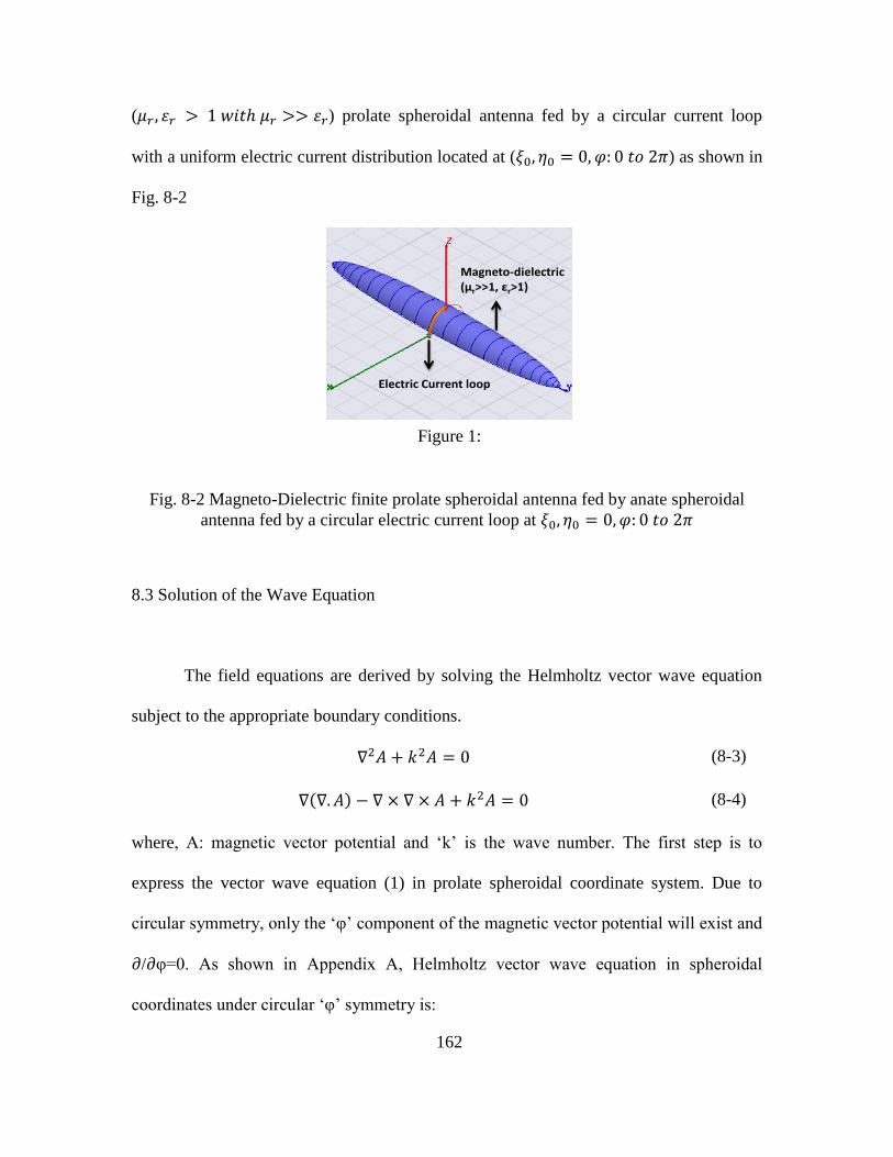
162

( ) prolate spheroidal antenna fed by a circular current loop

with a uniform electric current distribution located at ( ) as shown in

Fig. 8-2

Fig. 8-2 Magneto-Dielectric finite prolate spheroidal antenna fed by anate spheroidal

antenna fed by a circular electric current loop at

8.3 Solution of the Wave Equation

The field equations are derived by solving the Helmholtz vector wave equation

subject to the appropriate boundary conditions.

(8-3)

( ) (8-4)

where, A: magnetic vector potential and ‘k’ is the wave number. The first step is to

express the vector wave equation (1) in prolate spheroidal coordinate system. Due to

circular symmetry, only the ‘φ’ component of the magnetic vector potential will exist and

/ φ=0. As shown in Appendix A, Helmholtz vector wave equation in spheroidal

coordinates under circular ‘φ’ symmetry is:

Magneto-dielectric(μr>>1, εr>1)

Electric Current loop

Figure 1:

163

[( )

]

[( )

]

( )

(8-5)

Now let us separate the variables by assuming ( ) ( )

Then,

[( )

( )

]

( )

[( )

( )

]

( )

( )( )

(8-6)

[( )

( )

]

( )

[( )

( )

]

( )

( )( )

(8-7)

Diving throughout by UV we get,

[( )

( )

]

[( )

( )

]

( )

Let ,

[( )

( )

]

[( )

( )

]

(8-8)

Since the left side of the above equation is a function of ξ only, the right side of

the equation is a function of η only and that the equation must be valid for the left and the

right hand side can be equated to a constant say -B. Therefore the left hand side is:

[( )

( )

]

164

[( )

( )

]

(8-9)

Similarly the right hand side,

[( )

( )

]

(8-10)

The solution for U involves its behavior in the range: 1 to ∞ and the solution for V

involves behavior between singular points -1 & +1. The current source as mentioned

before is at ξ=ξ0 .

The solution of (A) and (B) is of the form:

[ ] ∑ ( ) ( ) (8-11)

[ ] ∑ ( ) ( ) ; (8-12)

where, √ and and are constants to be determined by

applying the proper boundary conditions, ( ) are angular spheroidal functions and

( ) and ( ) are radial spheroidal functions.

Now at the boundary between the two regions I and II ( ), the boundary

condition on the E-field is:-

( ) => [ ]

[ ]

Therefore,

∑ ( ) ( ) ∑ ( ) ( )

(8-13)

The boundary condition on the H-field is

( )

165

The “true surface current” which in this case is the loop current I at can

be represented as

( )

(8-14)

Therefore, the boundary condition on the H-field can be written as

[

( [ ])

( [ ])

]|

( )

(8-15)

are the scale factors of the prolate spheroidal system defined as

√

√

√ √

(8-16)

Substituting (8-16) in (8-15), the boundary condition on the H-field can be expanded as,

√

√ √

[

( √ √ [ ])

( √ √ [ ])

]|

|

√

( )

√ [

( √ √ ∑ ( ) ( ) )

( √ √ ∑ ( ) ( ) )

]|

√ ( )

166

√ [ √

∑ ( )

(√ ( ))

√

∑ ( )

(√ ( ))

]|

√ ( )

[

∑ ( ) [

√ ( ) √

( )]

∑ ( )

[

√ ( )

√

( )]]|

√ ( )

∑ ( )√

[

( ) ( )]

∑ ( )√

[

( )

( )] √ ( )

(8-17)

The Dirac delta function can be expanded as,

( ) ∑

( ) ( ) ( )

(8-18)

where, ( ) ∫

Substituting (8-18) in (8-17) we get,

167

∑ ( )√

[

( ) ( )]

∑ ( )√

[

( )

( )] √

∑

( ) ( ) ( )

(8-19)

(Note that RHS=0 for all ). Therefore, the term √ can be replaced by

√ .

In (8-13) and (8-19), ( )and ( )are two different terms that are not

orthogonal to each other. Therefore strictly speaking we cannot compare terms. But, we

can represent ( )as:

( ) ∑ ( )

( )

(8-20)

( ) ∑ ( )

( )

(8-21)

where the coefficients ( ) are non-zero when r is even (odd) and n is odd (even).

( ) is the associated Legendre function. Since

( ) exists on both sides of the

equations now, it is possible to make use of the orthogonality of Legendre polynomials or

to compare both sides of the equations using the coefficients of ( ). Therefore, (8-

13) can be rewritten as;

∑ ∑ ( )

( )

( )

∑ ∑ ( )

( )

( )

(8-22)

168

And (8-19) can be rewritten as:

∑ ∑ ( )

( )

√

[

( ) ( )]

∑ ∑ ( )

( )

√

[

( )

( )]

∑ √

( )∑

( ) ( )

( )

(8-23)

Since these two equations are valid for each ‘r’ sufficient equations can be

generated depending on the number of coefficients required. Since

is non-zero only

when n is odd(even) and r is even(odd), the equations involving the odd ordered

functions are completely decoupled from those of even order. This implies that the

problem can be broken into two parts: solving for even ordered coefficients and solving

for the odd ordered coefficients.

Equations (8-22) and (8-23) can be re-written as

∑ ( )

∑ ( )

(8-24)

∑ ( )

∑ ( )

∑ ( )

(8-25)

where,

( ) ( ) ( ) (8-26)

( ) ( ) ( ) (8-27)

169

( ) ( )

√

[

( ) ( )]

(8-28)

( ) ( )

√

[

( ) ( )]

(8-29)

( ) ( )

√

( ) ( )

(8-30)

Therefore, (8-24) and (8-25) are system of equations that can be solved for Cn and Dn. In

the matrix form

[( )

( )

( )

( )] [( )

( )] [

( )

] (8-31)

where, E,F,G and H can be written as (X), (the first subscript is for ‘r’ and the second

subscript for ‘n’)

( )

{

(

)

(

)

(8-32)

And C or D can be represented as (Y):

( )

{

(

)

(

)

(8-33)

170

And (K) can be written as

( )

{

(

∑

∑

∑

)

(

∑

∑

∑

)

(8-34)

Note that the function ( ) when i.e when the feed loop is at the

center of the spheroid. Hence and coefficients are equal to zero when ‘n’ is even.

Therefore in summary, given the coefficients we can find the magnetic vector potential

Aφ at an point ( ) in space using (8-11) and (8-12).

The individual field components can be determined as follows: Under circular

symmetry,

(8-35)

The H-field components can be obtained by taking the curl of the vector potential as

(8-36)

171

In the far field, in the prolate spheroidal coordinate system,

[

{

(

[ ])}

{

(

[ ])}]

(8-37)

Therefore,

[ ]

[

{ ∑

( ) ( )

∑ ( ) ( )

}]

(8-38)

Now equation (8-38) can be further simplified by first finding the derivative of the

scaling factor,

( √ √ )

√

√

√ √

( )

Substituting in (8-38),

[ ]

[

{ ∑

( ) ( )

∑ ( ) ( )

}]

[ ]

[∑

( ) ( )

∑ ( ) ( )

]

[ ]

[∑ ( )

( ( )

( ))]

(8-39)

172

Similarly from (8-37),

[ ]

[

{ ∑ ( )

( )

∑ ( ) ( )

}]

(8-40)

Equation (8-40) can be further simplified as,

( √ √ )

√

√ √ √

[ ]

[

{ ∑ ( )

( )

∑ ( ) ( )

}]

[ ]

[∑ ( )

( )

∑ ( ) ( )

]

[ ]

[∑ ( )

(

( )

( ) )] (8-41)

The complex Poynting vector is then,

{ (

)}

{ (

)} (8-42)

The radiated power ‘Prad’ can be calculated by integrating the complex Poynting vector

over a closed surface enclosing the antenna for a large ξ>ξ0. That is,

173

∯ ( ) ∯ ( ) ( )

∯

{ (

)}( )

∯ {

} ∫ { }

(8-43)

All the field components outside the antenna (region 2) and the radiated power equation

are summarized below:

[ ]

∑ ( ) ( )

[ ]

[∑ ( )

( ( )

( ))]

[ ]

[∑ ( )

(

( )

( ) )]

∯ {

} ∫ { }

8.4 Comparison with Full-Wave Simulations

In this section, the closed form equations derived in Section 8.4 are compared

with full-wave HFSS simulations. The simulation geometry is shown in Fig. 8-2. The

magneto-dielectric material used was and . The feed loop radius is same

as the minor radius ‘b’ of the spheroid (It is slightly greater than ‘b’ to account for the

finite wire thickness). The antenna is placed above a ground plane. Two cases were

considered (A) a=8” and b=0.5” i.e. a 16 inch long antenna of 0.5” inch cross-sectional

174

radius & (B) a=12” and b=1.5” i.e. a 24 inch long antenna with a radius of cross-section

of 1.5”. The first set of comparisons was done for (8-35) versus η for a fixed value of

ξ as shown in Fig. 8-3.

Fig. 8-3 Prolate spheroidal antenna with a=8” and b=0.5” showing the line ξ=1.1.

The electric feed current was first measured in the full-wave simulator. The plot

of feed electric current versus angle (alpha ‘ ’) on the feed loop is shown in Fig. 8-4.

Fig. 8-4 (a)The electric feed loop used in the full-wave simulator. Note that the outer

conductor was extended to the center to maintain symmetry w.r.t to the ground plane.

(b) Measured feed current ‘Ie’ for different frequencies for case(A)

ξ=1.1

(a)

100 MHz200 MHz500 MHz

(b)

175

The average of the feed current in Fig. 8-4(b) was used for feed current ‘I0’ in the

analytical equation (8-35). The comparison between the simulated and the calculated

Eφ for three different frequencies for ξ=1.1 and ξ=5 for case (A) is shown in Fig. 8-5.

Fig. 8-5 Comparison of of the analytical equation and the simulated result for case

(A) at (a) path in the near field and (b) path which is in the far field.

The agreement between the analytical equation and the simulation is excellent for

near field (ξ=1.1) and far-field (ξ=5) at these frequencies. Note that as frequency

increases the feed current starts becoming less and less uniform in the simulation. The

feed loop becomes large w.r.t to the wavelength at these frequencies. This effect is more

pronounced for a fatter dipole (and therefore a bigger feed loop since rad=b) as seen in

Fig. 8-6 which shows the feed current for case (B) with a=12” and b=1.5”.

Fig. 8-6 Measured electric feed current at different frequencies vs. angle ‘ ’ for case (B)

100 MHz200 MHz500 MHz

(a) (b)

176

As seen in Fig. 8-6, the feed current at 500MHz can no longer be called uniform

throughout the loop which is one of the first assumptions made in deriving the analytical

equations. Nevertheless is compared to simulation for the fat prolate spheroid case (B)

in Fig. 8-7 by taking the average of the electric feed current versus ‘ ’ in Fig. 8-6.

Fig. 8-7 Comparison of of the analytical equation and the simulated result for case

(B) at (a) and (b) .

The agreement between the simulation and analytical equation is excellent at low

frequencies and starts deviating slightly at higher frequencies due to the non-uniform

electric feed current. Next, the radiated power calculated analytically in (8-43) is

compared with full-wave simulations for both case (A) and case (B) versus frequency in

Fig. 8-8.

Fig. 8-8 Comparison between analytic and simulated radiated power ‘Prad’ for the (A)

a=8” & b=0.5” and (B) a=12” and b=1.5”.

(a) (b)

(a) (b)

177

Again, the agreement is excellent at low frequencies but it starts to deviate at

higher frequencies and again the reason being that the electric feed current is no longer

uniform due to the large size of the feed loop. This is clearly seen in the measured electric

feed current in the HFSS simulator (Fig. 8-9).

Fig. 8-9 (a) Non-uniform Electric feed current for higher frequencies computed in HFSS

(b) Radiated power at those frequencies indicated by the circle markers.

8.5 Summary and Future Work

The closed form equations for the electric and magnetic fields in the near and far

field of a finite prolate spheroidal magneto-dielectric antenna are derived in this chapter.

The analytical equations agreed well with simulations. The power radiated by the antenna

was also calculated. The equations are shown to be accurate as long as the electric feed

current distribution is uniform.

The magneto-dielectric material in this chapter was assumed to be lossless. Thus,

a possible future work in this topic will be to derive the field equations for lossy

magneto-dielectric prolate spheroidal dipole antenna.

(a) (b)

178

REFERENCES

[1] S. Schelkunoff and H. Friis, Antenna theory and practice, Wiley, 1952.

[2] H. Wheeler, "Fundamental limitations of small antennas," Proc. IRE, vol. 35, pp.

1479-1484, Jul. 1947.

[3] H. Wheeler, "Small Antennas," IEEE Trans. Antennas Propag., vol. 23, no. 4, pp.

462-469, Jul.1975.

[4] M. Smith, "Properties of dielecrically loaded antennas," Proc. IEE Electronics, vol.

124, no. 10, pp. 837-839, Oct. 1977.

[5] R. Richtmeyer, "Dielectric Resonators," J. Appl. Phys., vol. 10, pp. 391-398, Jun.

1939.

[6] S. Long, M. McAllister and L. Shen, "The resonant cylindrical dielectric cavity

antenna," IEEE Trans. on Antennas Propag., vol. 31, pp. 406-412, Mar. 1983.

[7] Petosa, "Dielectric reosnator antennas: A historical review and the current state of

the art," IEEE Trans. Antennas Propag., vol. 52, no. 5, pp. 91-116, Oct. 2010.

[8] S. R. Best and A. D. Yaghjian, "Impedance, bandwidth and Q of antennas," IEEE

Trans. Antennas Propag., vol. 44, no. 5, pp. 672-676, May 1996.

[9] H. A. Wheeler, "The radian sphere around a small antenna," Proc. IRE, vol. 47, pp.

1325-1331, Aug. 1959.

[10] E. D. Palik, Handbook of Optical Constants of Solids, Elsevier, 1998.

[11] V. Rumsey and W. Weeks, "Electrically small ferrite loaded loop antennas," IRE

Nat. Conv. Rec., vol. 4, no. 1, pp. 165-170, 1956.

[12] V. Rumsey, "Reaction concept in electromagnetic theory," Phys. Rev., vol. 94, no. 6,

pp. 1483-1491, Jun. 1954.

[13] R. DeVore and P. Bohley, "The electrically small magnetically loaded multiturn

loop antenna," IEEE Trans. Antennas Propag., vol. 25, pp. 496-505, 1977.

179

[14] H. Stuart and A. Yaghjian, "Approaching the lower bounds on Q for electrically

small electric dipole antennas using high permeability shells," IEEE Trans. Antennas

Propag., vol. 58, no. 12, pp. 3865-3872, Dec. 2010.

[15] S. Best, "A low Q electrically small magnetic (TE mode) dipole," IEEE Antennas

Wireless Propag. Lett., vol. 8, pp. 572-575, 2009.

[16] J. McLean, H. Foltz and R. Sutton, "Electrically small TE01 mode spherical wire

antennas employing lossy magnetodielectric materials," in International Workshop

on Antenna Technology Proceedings, Lisbon, Portugal, Mar. 2010.

[17] T. Hansen, O. Kim and O. Breinbjerg, "Electrical properties of spherical dipole

antennas with lossy material cores," in 6th European conference on Antennas and

Propag., Prague, Czech Republic, Mar. 2012.

[18] J. McLean and R. Sutton, "An efficienct low profile antenna employing lossy

magneto-dielectric materials," in IEEE International worskshop on antenna

technology, Tucson,AZ., 2012.

[19] L. J. Chu, "Physical limitations of omni-directional antennas," J. Appl. Phys., vol.

35, pp. 1479-1484, 1948.

[20] W. Geyi, "Optimization of the Ratio of Gain to Q," IEEE Trans. Antennas Propag.,

vol. 61, no. 4, pp. 1916-1922, 2013.

[21] J. S. McLean, "A Re-examination of the Fundamental Limits on the Radiation Q of

Electrically Small Antennas," IEEE Trans. Antennas Propag., vol. 44, no. 5, pp.

672-676, May, 1996.

[22] H. L. Thal, "New Radiation Q Limits for Spherical Wire Antennas," IEEE Trans.

Antennas Propag., vol. 54, no. 10, pp. 2757-2763, Oct. 2006.

[23] R. Hansen, "Q and Mu," in IEEE Sym. Antennas Propag. (APSURI), Spokane,WA,

July 2011.

[24] J. L. Snoek, "Dispersion and Absorption in Magnetic Ferrites at Frequencies Above

1 Mc/s," Physica, vol. 14, no. 4, pp. 207-217, 1948.

[25] J. Smit and H. Wijn, Ferrites, New York: Wiley, 1959.

180

[26] J. Toll, "Causality and the Dispersion Relation: Logical Foundations," Phys. Rev.,

vol. 104, pp. 1760-1770, 1956.

[27] F. Grant, "Use of Complex Conductivity in the Representation of Dielectric

Phenomena," J. Appl. Phys., vol. 29, pp. 76-80, 1958.

[28] R. Diaz and N. Alexopoulos, "An Analytic Contiuation Method for the Analysis and

Design of Dispersive Materials," IEEE Trans. Antennas Propag., vol. 45, no. 11, pp.

602-610, Nov. 1997.

[29] H. J. Josephs, "The Heaviside Papers Found at Paignton in 1957," IEE Monograph,

vol. 319, pp. 70-76, 1959.

[30] Fair-Rite Products Corp, [Online]. Available: http://www.fair-

rite.com/cgibin/catalog.pgm#select:freq1.

[31] E. Louis, I. Jeong and R. Walser, "Magnetization distribution in nearly isotropic

ultra-soft magnetic CoB amorphous thin films," IEEE Trans. Magn, vol. 25, no. 5,

pp. 3366-3368, 1989.

[32] W. Weeks, Electromagnetic Theory for Engineering Applications, Wiley, 1964.

[33] H. Fricke, "A mathematical treatment of the electric conductivity and capacity of

disperse systems: I. The electric conductivity of a suspension of homogenous

spheroids," Phys. Rev., vol. 24, no. 5, pp. 575-587, 1924.

[34] O. Jeffimenko, Electricity and Magnetism, Start city, WVa: Meredith, 1989.

[35] S. A. Schelkunoff and H. Friis, Antenna theory and practice, Wiley, 1952.

[36] R. Diaz, W. Merrill and N. Alexopoulos, "Analytic framework for the modeling of

effective media," Journal of Appl. Phys., vol. 84, no. 12, pp. 6815-6826, 1998.

[37] M. Islam, "A theoretical treatment of low frequency loop antennas with ferrite

cores," IEEE Trans. Antennas Propag., vol. 11, no. 3, pp. 162-169, Mar. 1963.

[38] M. Islam, "Mathematical Analysis on the Effect of a Prolate Spheroidal Core in a

Magnetic Dipole field," J. Math Phys., vol. 4, no. 9, pp. 1205-1212, 1963.

[39] T. Simpson and Y. Zhu, "The electrically small multi-turn loop antenna with a

spheroidal core," IEEE Antennas Propag. Mag., vol. 48, no. 5, pp. 54-66, Oct. 2006.

181

[40] T. Simpson, "Electrically Small Spheroidal loops wound on a hollow ferrite core,"

IEEE Antennas Propag. Mag., vol. 50, no. 3, pp. 88-94, Jun 2008.

[41] D. Halliday and D. Kiely, "Dielectric rod aerials," Proc. IEE Part IIIA: Radio

Comm., vol. 94, no. 16, pp. 610-618, Mar. 1947.

[42] J. James, "Theoretical investigation of cylindrical dielectric rod antennas," Proc.

IEE, vol. 114, no. 3, pp. 672-676, May 1996.

[43] G. Mueller and W. Tyrell, "Polyrod Antennas," Bell Sys. Tech. J., vol. 26, pp. 837-

851, 1947.

[44] O. Kim and O. Breinbjerg, "Lower bound for the radiation Q of electrically small

magnetic dipole antenna with solid magnetodielectric core," IEEE Trans. Antennas

Propag., vol. 59, no. 2, pp. 679-681, 2011.

[45] O. Kim, O. Breinbjerg and A. Yaghjian, "Electrically small magnetic dipole

antennas with quality factors approaching the Chu lower bound," IEEE Antennas

Propag., vol. 58, no. 6, pp. 1898-1906, 2010.

[46] R. Hansen and M. Burke, "Antennas with magneto-dielectrics," Microwave Opt.

Tech. Lett., vol. 26, no. 2, pp. 75-78, 2000.

[47] D. V. Giri, "Electrically small loop antenna loaded by a homogenous and isotropic

ferrite cylinder-part I," Harvard University, Cambridge, Mass., Jul. 1973.

[48] A. Karilainen, P. Ikonen, C. Simovski and S. Tretyakov, "Choosing dielectric or

magnetic material to optimize the bandwidth of miniaturized resoannt antennas,"

IEEE Trans. Antennas Propag., vol. 59, no. 11, pp. 3991-3998, Nov. 2011.

[49] P. Ikonen, K. Rozanov, A. Osipov, P. Alitalo and S. Tretyakov, "Magnetodielectric

substrates in antenna miniaturization: potential and limitations," IEEE Trans.

Antennas Propag., vol. 54, no. 11, pp. 3391-3998, Nov. 2006.

[50] J. McLean and R. S. a. H. Foltz, "Broadband, electrically small spherical wire and

generalized loop antennas exploting inhomogenous magnetic cores," in 20th

International Conference on applied electromagnetics and communications

proceedings, Dubrovnik, Croatia, Sept. 2010.

[51] T. Sebastian, S. Clavijo and R. Diaz, "Small Material Dipole Antenna Analysis: I.

Dielectric Dipole," IEEE Trans. on Antennas Propag., submitted for publication.

182

APPENDIX A

DERIVATION OF THE INTERNAL FIELD SHAPE CORRECTION FACTOR TO

ACCOUNT FOR THE EFFECT OF SKIN DEPTH

183

The energy stored by an inductor ‘L’ is the amount of work done to establish a

current ‘I’ through the inductor. That is,

𝑦

(A-1)

Now, the assumed TM internal magnetic field ( ) of a magneto-dielectric cylinder

( & ) of radius ‘ρ’ with the skin depth ‘δ’ < ρ as shown in Fig. 3-2 is:

( )

(A-2)

The internal magnetic energy (IME) of this magneto-dielectric cylinder assuming a

uniform field along the length ‘l’ of the cylinder is therefore given by

∭

∫ ∫ ∫

(A-3)

(A-1) and (A-3) must be identical. Therefore

∫ ∫ (

( )

)

(A-4)

(

)∫ ( ( ) ( ))

(A-5)

where,

( )

[

(

) (

)

(

)

] (A-6)

When skin depth can be neglected i.e. when δ>ρ, then δ is set equal to ρ and therefore

FSF is unity which gives us

184

(A-7)

This is the internal inductance of a wire of length ‘ ’. Now if the current distribution and

therefore the magnetic field across the length of the wire is not uniform but triangular,

then the current ‘I’ for a wire should be replaced by

(

)

(A-8)

where, is the maximum value of current seen at the origin(or feed point) with the wire

extending from – to . Therefore on solving the integral in (A-4) with the current in

(A-4) we get

(A-9)

which is the same as (3-26).

185

APPENDIX B

DERIVATION OF EFFICIENCY OF A PERMEABLE DIPOLE FOLLOWING THE

APPROACH BY DEVORE ET. AL. [15]

186

Consider a multi-turn loop antenna of ‘n’ turns radius ‘ρ’ of total length ‘l’

carrying a constant current ‘I0’. Let it be loaded by an ellipsoidal permeable material (μr)

of length ‘l’. The internal magnetic field of an ellipsoidal core in terms of the an

unperturbed static field ‘H0’ is given by

( )

(B-1)

where, D: is the demagnetization factor. The uniform field of the ellipsoidal winding is

equated to the unperturbed field:

( )

(B-2)

If is the cross-sectional area and is the self-inductance of the ith winding then the

self-inductance of the ith winding is given by

(B-3)

Therefore, the total inductance of the loaded multi-turn loop antenna by superposition

over ‘n’ turns is given by

( )

( )

( )( )

(B-4)

Since the permeability is complex ( ), to account for the energy lost in

the permeable material we introduce a loss resistance .

( ) (B-5)

From (B-4),

( )( ) [

( ) ]

(B-6)

From (B-4), the imaginary part of the inductance ‘L’ can be expanded as

187

( )

( )( )

{ ( )} { }

(B-7)

From (B-4) and (B-4), the loss resistance is given by:

( )( )

{ ( )} { }

(B-8)

Now, the radiation resistance of an electrically small loop antenna is given by

(B-9)

where, ‘m’ is the magnetic dipole moment. The magnetic dipole moment of the antenna

is the magnetic moment of the core is given by

( ) ( ) (B-10)

The magnetic moment of the winding is given by

( ) (B-11)

Substituting (B-4) and (B-4) into (B-4) and we get,

|

( ) ( )

{ ( )} |

(B-12)

Assuming that the flux is well contained that there is no demagnetization i.e. D~0. Now

from (B-4)

( )

(B-13)

And (B-4) becomes

( ) (B-14)

Dividing (B-4) by (B-4) and expanding we get

188

( ) ( )

(B-15)

Therefore the radiation efficiency upon not assuming that is given by

( ) ( )

(B-16)

189

APPENDIX C

HELMHOLTZ VECTOR WAVE EQUATION IN PROLATE SPHEROIDAL

COORDINATES UNDER CIRCULAR ( ) SYMMETRY.

190

The electric and magnetic field equations of a finite prolate spheroid magneto-

dielectric antenna are derived by solving the Helmholtz vector wave equation subject to

the appropriate boundary conditions.

(C-1)

( ) (C-2)

The first step is to express the vector wave equation (C-1) in prolate spheroidal

coordinate system. Due to circular symmetry, only the ‘ ’ component of the magnetic

vector potential will exist and . Under these conditions, and

can be expanded as

( ) [

{

( )}

{

( )}]

[ ]

(C-3)

where, and are the scale factors of the prolate spheroidal system defined as

√

√

√ √

(C-4)

And,

{

( )}

{

( )}

Now,

{

( )}

{

(

)}

{

(

)

(

)

}

191

{

(

(

)

)

(

)

}

(

)

(

)

(C-5)

Now,

( √ √ )

√

√

(C-6)

And

( )

(C-7)

Substituting (C-7) and (C-6) in (C-5) we get,

(( )

)

(

√ √ )

(( )

)

√

(

√

√

)

(( )

)

√ (

( )√ )

(( )

)

( )

(C-8)

Now, similarly from (C-3)

{

}

192

{

(

)

(

)

}

{

(

)

(

)}

(C-9)

Now,

( √ √ )

√

√

(C-10)

And

( )

(C-11)

Substituting (C-11) and (C-10) in (C-9) we get,

(( )

)

(

√ √ )

(( )

)

√

(

√

√

)

(( )

)

√ (

( )√ )

(( )

)

( )

(C-12)

From (C-8) and (C-12)

[

(( )

)

(( )

)

( )

( )]

193

Now,

( )

Therefore,

( )[

(( )

)

(( )

)

( )

( )]

(C-13)

Substituting (C-13) in (C-3) and then in (C-2), under circular symmetry,

( )[

(( )

)

(( )

)

( )

( )]

(( )

)

(( )

)

( )

( )

( )

(C-14)

Equation (C-14) is the Helmholtz vector wave equation in spheroidal coordinates under

circular ‘ ’ symmetry.