GRAPE: Using graph grammars to implement shape grammars

Thomas Grasl1, and Athanassios Economou2

1SWAP [+] Lange Gasse 16/12,

1080 Vienna, Austria tg@swap-zt.com

2Georgia Institute of Technology 245 4th St. NW,

Atlanta, GA, U.S.A., 30332 economou@coa.gatech.edu

Keywords: Shape, graph, grammar, implementation.

Abstract An implementation of a shape grammar interpreter is

described. The underlying graph-theoretic framework is briefly discussed to show how alternative representations from graph theory including graphs, overcomplete graphs and hyperedge graphs can support some of the intuitions handled in shape grammars by direct visual computations with shapes. The resulting plugin implemented in Rhino, code-named GRAPE, is briefly described in the end.

1. INTRODUCTION Shape grammars provide a powerful generative

approach for the description, interpretation and evaluation of existing designs as well as new designs (Stiny and Gips 1972; Stiny 2006). A nice account of various applications of shape grammars for the study of existing and new languages of design can be found in Knight (2003).

Still, while the shape grammar formalism has produced a long and excellent series of formal studies the corresponding efforts for automation of the tasks the shape grammars accomplish have not met the same success. Recent summaries of such approaches are given in various sources (Gips 1999; Chau et al. 2004). Typically these efforts have been concentrated in shapes of specific geometry, for example, straight lines (Krisnamurti, 1981), polygonal shapes (Tapia, 1999) or parametric curves (Jowers and Earl, 2010).

One of the challenges for a computer implementation of a shape grammar is the design of an underlying formalism that will allow for symbol-based substitutions of any part of a shape that may be of use in a design setting. The specific

formalism used here to support such computations has been built upon graph theory. Our efforts have been focused on the possibility of mapping shape grammars into graph grammars, the advantage being that graph grammars are more amenable to computer implementation. Moreover existing graph grammar packages can be used to develop tailor-made software. Much of the more complicated computation, such as subshape recognition, is thereby taken care of.

Graphs are a popular choice for representing the structure of shape (Heisserman, 1994; Kelles et al., 2009), and graph grammars have been used to implement specific grammars by also mapping the rule set from shapes to graphs (Grasl and Economou, 2010). Typically graphs are seen as multidimensional data structures that with an appropriate embedding formally structure and visually resemble the shapes they represent. Still, the encoding of shapes in terms of these alternative graph representations is not straightforward. Various approaches to representing shapes as graphs are described here and one of them is selected as the most useful for a shape grammar interpreter. The resulting formalism uses two parallel representations, a graph theoretic which is used for the computation, and a visual one that illustrates the shape and which can be queried for geometric properties such as angles, lengths and intersections. Since all computation is done on the graph representation, the shape rules are mapped into graph rules and all the matching subgraphs are mapped back into shapes in order to display to the user. The formalism has been implement in Rhino and it is code-named Grape to affectionately recall the parallel representations of GRAphs and shAPEs.

45

2. TWO PUZZLES IN VISUAL COMPUTATION The two key features that distinguish shape grammars

from other generative models for the description of designs - and in fact the two characteristics that make shape grammars so deeply grounded in design discourse are: a) recursion; and b) embedding (Stiny 2006). Recursion allows a design to be described in terms of successive states that each of them has to be constructed to allow for the construction of the next one; in this sense, recursion picks up wonderfully the notion of process in a design setting where the making of a design is understood and modeled as an active talk -or back-talk if we take Schön’s words (Schön 1983) between the designer and the design she makes. This characteristic is akin to the recursive definition of formulas in mathematics whereas any term in a sequence is defined in terms of the term preceding it – a process that requires a starting point and a set of rules to apply to generate the terms of the sequence. This mindset is quite distinct from the definition of the so-called closed or explicit formulas that are applied to give direct results; for example, to compute the fiftieth member of the Fibonacci sequence using a closed formula, the only thing that is needed is a substitution of the corresponding numbers in the explicit formula. The corresponding solution of the problem using the recursive formula requires fifty calculations starting from the first member and proceeding to the last. Still, this delay, so to speak, has clear advantages in a spatial setting because it clearly shows in steps the construction of a design and brings to the foreground the rules and conventions used to make this design. In this sense the challenge for the implementation of a shape grammar has clearly to do with the design of a program to support this recursive visual construction of a design; the typical contemporary discourse of the writing of a script (in text format) in some modeling environment, and then executing to see the visual results, creates a non-visual setting for making designs, requires an alienated setting for visual discourse and hides entirely from design inquiry the opportunities that arise in a seamless visual computation.

The second characteristic of a shape grammar, embedding, is paramount in visual composition and completely absent from computer aided design systems. Embedding is the relation that explains the wild, so to speak, nature of shapes, and their ability to constantly fuse and make new shapes too. But there is no miracle behind this, nor a suspense of natural laws; in symbolic computation any combination of discrete symbols such as

letters, notes or numbers will be always and unambiguously reproduced, read, performed or computed; in visual computation any combination of shapes, produce an incredible complexity of additional, diverse, emergent, of different topologies and shapes that were not used in the original combination. In this sense the challenge for the implementation of a shape grammar has clearly to do with the design of a program to support spatial computation and visual continuity while using the limitations of symbolic media to capture this continuity; the typical contemporary discourse of simulating rule-based design in some modeling environment is extremely limited, fosters blindness to designers, and creates a procrustean world view entirely antithetical to the design inquiry.

The key idea to address both these two challenges is the notion of an evolving, reconfigurable structure; a structure (parts and relations) is required for any shape to be retrieved, illustrated and computed upon. Still if and when the opportunity arises, this structure has to be reconfigured to account for the new opportunity at hand (Stiny 1991).

There are many examples that can do – a useful one is depicted in Figure 1a – a full account of the emergence of this specific paradigm and its role in shape grammar scholarship is given elsewhere (Stiny, 1991).

Figure 1: (a) A shape. (b) The same shape seen as two overlapping squares; (c) an emergent smaller third square.

The questions that arise looking at this shape quickly supersede the apparent simplicity of the argument. The careful observer – as well as the one familiar with the complexities, novelties and insights resulting from computations involving shapes, will immediately concede to the complexity that is hidden behind this – and many other, in fact all, pictorial settings. If the shape is seen as the intersection of two squares (Figure 1b) then the emergent smaller inner square is unaccounted (Figure 1c). And the Pandora’s Box is opened: L-shapes, 8-shapes, +- shapes, parallel lines, quotation marks (<<) , and many more, all point to the wonderful unsettling nature of shapes and their resistance to be modeled in terms of discrete, atomic parts.

46

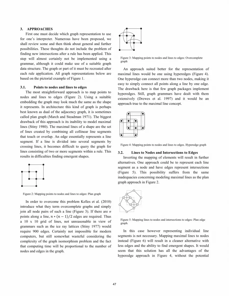
3. APPROACHES First one must decide which graph representation to use

for one’s interpreter. Numerous have been proposed, we shall review some and then think about general and further possibilities. These thoughts do not include the problem of finding new intersections after a rule has been applied. This step will almost certainly not be implemented using a grammar, although it could make use of a suitable graph data structure. The graph or part of it must be recreated after each rule application. All graph representations below are based on the pictorial example of Figure 1.

3.1. Points to nodes and lines to edges The most straightforward approach is to map points to

nodes and lines to edges (Figure 2). Using a suitable embedding the graph may look much the same as the shape it represents. In architecture this kind of graph is perhaps best known as dual of the adjacency graph, it is sometimes called plan graph (March and Steadman 1971). The biggest drawback of this approach is its inability to model maximal lines (Stiny 1980). The maximal lines of a shape are the set of lines created by combining all collinear line segments that touch or overlap. An edge essentially represents a line segment. If a line is divided into several segments by crossing lines, it becomes difficult to query the graph for lines consisting of two or more segments within a rule. This results in difficulties finding emergent shapes.

Figure 2: Mapping points to nodes and lines to edges: Plan graph

In order to overcome this problem Kelles et al. (2010) introduce what they term overcomplete graphs and simply join all node pairs of such a line (Figure 3). If there are n points along a line, �𝑛� ∗ (𝑛 − 1) 2⁄ edges are required. Thus a 10 x 10 grid of lines, not unreasonable in view of grammars such as the ice ray lattices (Stiny 1977) would require 900 edges. Certainly not impossible for modern computers, but still somewhat wasteful considering the complexity of the graph isomorphism problem and the fact that computing time will be proportional to the number of nodes and edges in the graph.

Figure 3: Mapping points to nodes and lines to edges: Overcomplete graph

An approach suited better for the representation of maximal lines would be one using hyperedges (Figure 4). One hyperedge can connect more than two nodes, making it easy to simply connect all points along a line by one edge. The drawback here is that few graph packages implement hyperedges. Still, graph grammars have dealt with them extensively (Drewes et al. 1997) and it would be an approach true to the maximal line concept.

Figure 4: Mapping points to nodes and lines to edges. Hyperedge graph

3.2. Lines to Nodes and Intersections to Edges Inverting the mapping of elements will result in further

alternatives. One approach could be to represent each line segment as a node and have edges represent intersections (Figure 5). This possibility suffers from the same inadequacies concerning modeling maximal lines as the plan graph approach in Figure 2.

Figure 5: Mapping lines to nodes and intersections to edges: Plan edge graph.

In this case however representing individual line segments is not necessary. Mapping maximal lines to nodes instead (Figure 6) will result in a cleaner alternative with less edges and the ability to find emergent shapes. It would seem that this solution has all the advantages of the hyperedge approach in Figure 4, without the potential

47

drawback of having to use hyperedges. However, problems arise as soon as more than two lines intersect in one point, hence it can only be used on a very limited set of grammars, such as orthogonal grammars.

Figure 6: Mapping lines to nodes and intersections to edges: Hyperedge edge graph.

Again the only possibility to satisfy all needs is the introduction of hyperedges (Figure 7) with all the above mentioned reservations.

Figure 7: Mapping lines to nodes and intersections to edges: Overcomplete edge graph.

3.3. Points and Lines to Nodes Finally both points and line segments could be

represented as nodes (Figure 8). Again this approach lacks support for maximal lines, since line segments rather than lines are represented.

Figure 8: Mapping points and lines to nodes: Planar node-edge graph.

Using maximal lines instead of line segments (Figure 9) can easily improve upon the situation without having to use hyperedges. The necessity to introduce hyperedges can be traced back to the fact, that in a general shape both maximal lines and points can be related to more than two entities of the other class. That is to say there may be more than two points on a maximal line and more than two maximal lines may meet in a point. If both classes are represented by

nodes and edges are used for various kinds of relations, this restriction does not apply.

Figure 9: Mapping points and lines to nodes: Planar edge-edge graph.

Mapping several classes to nodes increases the total number of elements needed to represent a shape, but it also adds flexibility because additional classes could be added (Figure 10). Depending on the grammar at hand classes of interest could be labels, faces, solids, colors, infinite lines and more. Heisserman (1994) uses such a graph-based boundary representation for boundary solid grammars.

Figure 10: Graph representation of the shape in Figure 1a using three layers of objects: points (black), lines (white) and faces (grey).

3.4. Discussion The approach chosen by the authors and used for the

remainder of this paper is based on representing points and lines as nodes (Figure 9). It is a good compromise between few elements and an efficient and flexible data-structure.

4. CONSTRAINED TOPOLOGY PATTERNS The graph as described above contains only topological

information and as such would not be of much use for a shape grammar interpreter. Metric information can be added to the model by adding attributes to nodes and/or edges. It would suffice to add the coordinates of the points as attributes to the respective nodes as all other information such as lengths and angles could be derived. Depending on the nature of the implementation and the capabilities of the graph package it could make sense to store some additional information where appropriate. GRAPE stores the slopes of the maximal lines as attributes of the line nodes, in addition to the point coordinates.

48

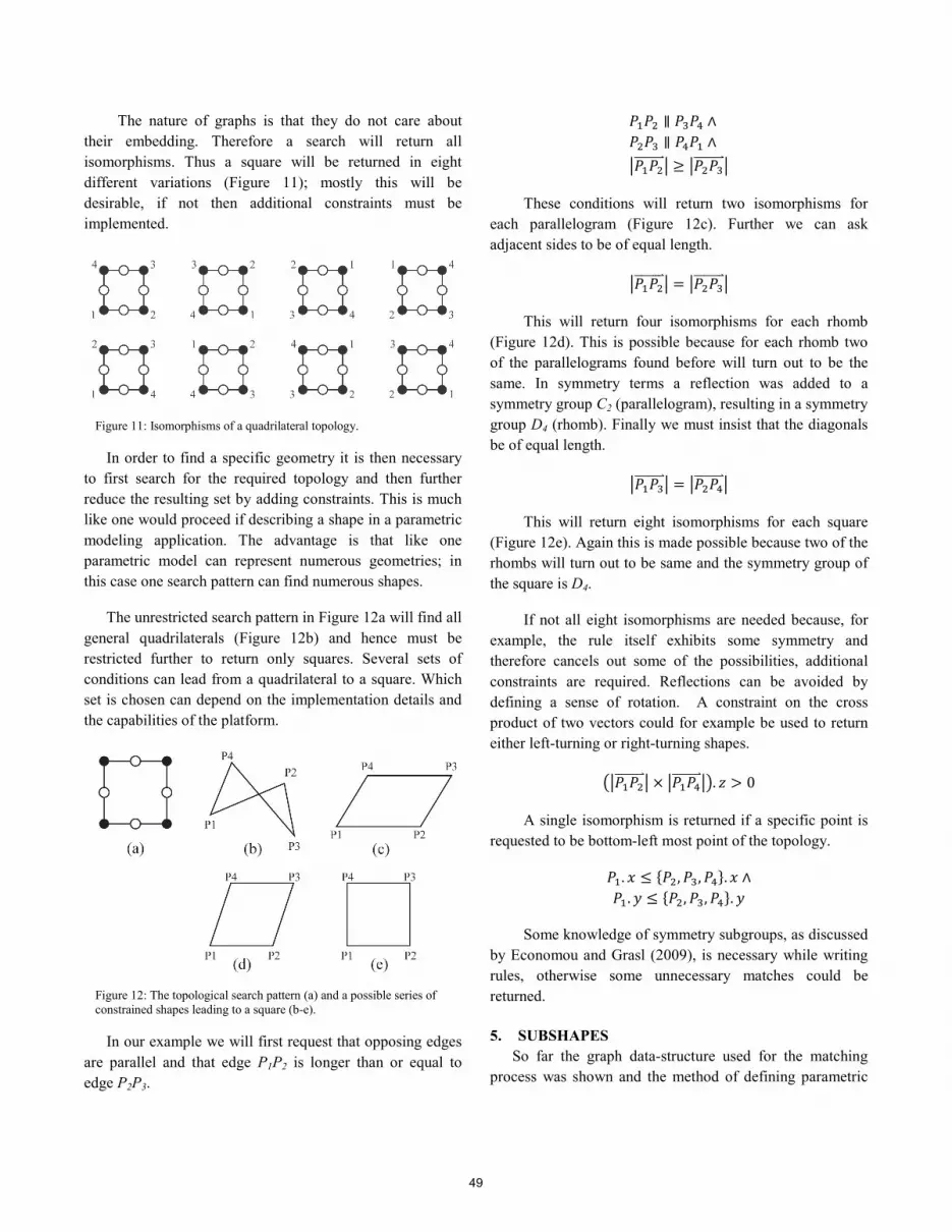
The nature of graphs is that they do not care about their embedding. Therefore a search will return all isomorphisms. Thus a square will be returned in eight different variations (Figure 11); mostly this will be desirable, if not then additional constraints must be implemented.

Figure 11: Isomorphisms of a quadrilateral topology.

In order to find a specific geometry it is then necessary to first search for the required topology and then further reduce the resulting set by adding constraints. This is much like one would proceed if describing a shape in a parametric modeling application. The advantage is that like one parametric model can represent numerous geometries; in this case one search pattern can find numerous shapes.

The unrestricted search pattern in Figure 12a will find all general quadrilaterals (Figure 12b) and hence must be restricted further to return only squares. Several sets of conditions can lead from a quadrilateral to a square. Which set is chosen can depend on the implementation details and the capabilities of the platform.

Figure 12: The topological search pattern (a) and a possible series of constrained shapes leading to a square (b-e).

In our example we will first request that opposing edges are parallel and that edge P1P2 is longer than or equal to edge P2P3.

𝑃1𝑃2 ∥ 𝑃3𝑃4 ∧ 𝑃2𝑃3 ∥ 𝑃4𝑃1 ∧ �𝑃1𝑃2��������⃑ � ≥ �𝑃2𝑃3��������⃑ �

These conditions will return two isomorphisms for each parallelogram (Figure 12c). Further we can ask adjacent sides to be of equal length.

��𝑃1𝑃2��������⃑ �� = ��𝑃2𝑃3��������⃑ ��

This will return four isomorphisms for each rhomb (Figure 12d). This is possible because for each rhomb two of the parallelograms found before will turn out to be the same. In symmetry terms a reflection was added to a symmetry group C2 (parallelogram), resulting in a symmetry group D4 (rhomb). Finally we must insist that the diagonals be of equal length.

��𝑃1𝑃3��������⃑ �� = ��𝑃2𝑃4��������⃑ ��

This will return eight isomorphisms for each square (Figure 12e). Again this is made possible because two of the rhombs will turn out to be same and the symmetry group of the square is D4.

If not all eight isomorphisms are needed because, for example, the rule itself exhibits some symmetry and therefore cancels out some of the possibilities, additional constraints are required. Reflections can be avoided by defining a sense of rotation. A constraint on the cross product of two vectors could for example be used to return either left-turning or right-turning shapes.

���𝑃1𝑃2��������⃑ �� × ��𝑃1𝑃4��������⃑ ���. 𝑧 > 0

A single isomorphism is returned if a specific point is requested to be bottom-left most point of the topology.

𝑃1. 𝑥 ≤ {𝑃2,𝑃3,𝑃4}.𝑥 ∧ 𝑃1.𝑦 ≤ {𝑃2,𝑃3,𝑃4}.𝑦

Some knowledge of symmetry subgroups, as discussed by Economou and Grasl (2009), is necessary while writing rules, otherwise some unnecessary matches could be returned.

5. SUBSHAPES So far the graph data-structure used for the matching

process was shown and the method of defining parametric

49

rules has been explained. However, once a rule is applied to the graph, the connection between the graph representation and the shape representation deteriorates. If new subshapes have emerged during the rule application, they will go undetected by the graph. .

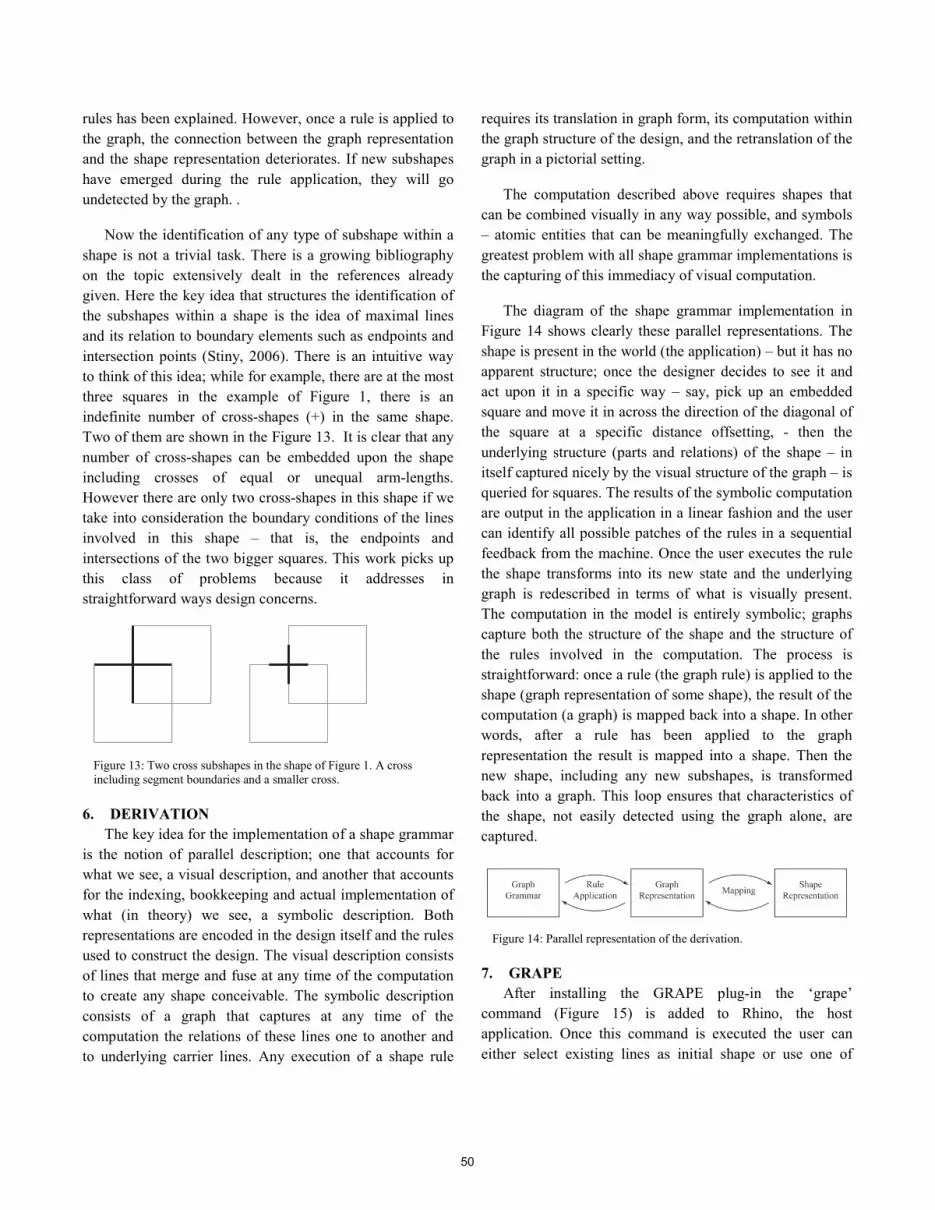
Now the identification of any type of subshape within a shape is not a trivial task. There is a growing bibliography on the topic extensively dealt in the references already given. Here the key idea that structures the identification of the subshapes within a shape is the idea of maximal lines and its relation to boundary elements such as endpoints and intersection points (Stiny, 2006). There is an intuitive way to think of this idea; while for example, there are at the most three squares in the example of Figure 1, there is an indefinite number of cross-shapes (+) in the same shape. Two of them are shown in the Figure 13. It is clear that any number of cross-shapes can be embedded upon the shape including crosses of equal or unequal arm-lengths. However there are only two cross-shapes in this shape if we take into consideration the boundary conditions of the lines involved in this shape – that is, the endpoints and intersections of the two bigger squares. This work picks up this class of problems because it addresses in straightforward ways design concerns.

Figure 13: Two cross subshapes in the shape of Figure 1. A cross including segment boundaries and a smaller cross.

6. DERIVATION The key idea for the implementation of a shape grammar

is the notion of parallel description; one that accounts for what we see, a visual description, and another that accounts for the indexing, bookkeeping and actual implementation of what (in theory) we see, a symbolic description. Both representations are encoded in the design itself and the rules used to construct the design. The visual description consists of lines that merge and fuse at any time of the computation to create any shape conceivable. The symbolic description consists of a graph that captures at any time of the computation the relations of these lines one to another and to underlying carrier lines. Any execution of a shape rule

requires its translation in graph form, its computation within the graph structure of the design, and the retranslation of the graph in a pictorial setting.

The computation described above requires shapes that can be combined visually in any way possible, and symbols – atomic entities that can be meaningfully exchanged. The greatest problem with all shape grammar implementations is the capturing of this immediacy of visual computation.

The diagram of the shape grammar implementation in Figure 14 shows clearly these parallel representations. The shape is present in the world (the application) – but it has no apparent structure; once the designer decides to see it and act upon it in a specific way – say, pick up an embedded square and move it in across the direction of the diagonal of the square at a specific distance offsetting, - then the underlying structure (parts and relations) of the shape – in itself captured nicely by the visual structure of the graph – is queried for squares. The results of the symbolic computation are output in the application in a linear fashion and the user can identify all possible patches of the rules in a sequential feedback from the machine. Once the user executes the rule the shape transforms into its new state and the underlying graph is redescribed in terms of what is visually present. The computation in the model is entirely symbolic; graphs capture both the structure of the shape and the structure of the rules involved in the computation. The process is straightforward: once a rule (the graph rule) is applied to the shape (graph representation of some shape), the result of the computation (a graph) is mapped back into a shape. In other words, after a rule has been applied to the graph representation the result is mapped into a shape. Then the new shape, including any new subshapes, is transformed back into a graph. This loop ensures that characteristics of the shape, not easily detected using the graph alone, are captured.

Figure 14: Parallel representation of the derivation.

7. GRAPE After installing the GRAPE plug-in the ‘grape’

command (Figure 15) is added to Rhino, the host application. Once this command is executed the user can either select existing lines as initial shape or use one of

50

several pre-defined shapes. The chosen shape is mapped to a graph representation.

Figure 15: Diagram of the commands structure

The user can then select a rule from the catalog or exit the command. If a rule is selected the matching isomorphisms are returned and the user can cycle through the respective shapes until the desired match is shown. Finally the rule can be applied and the command returns to the catalog of rules for the selection of the next rule.

An example of a shape computation in Grape is given in Figure 16. Here the rules used for the computation are taken from classic examples in the field of shape grammars to relate to the existing discourse. Obviously any other shapes and rules would do. The three rules used in the computation are given at the top of Figure 16; the first moves an L-shape along its diagonal axis; the second rule moves a square along its diagonal axis and the third rules moves a copy of a square along its diagonal axis. The cross label to the side of each rule is used to fix the origin of transformation. The dotted lines visualize the effect of the application of the rule. The computation itself is shown in the lower half of Figure 16. The initial shape of Figure 1 (the double square) is used as an initial shape.

Figure 16: Example of a derivation using the initial shape of Figure 1 and three shape rules.

8. CONCLUSION Grape simulates nicely some of the visual calculations that designers do effortlessly with a pencil and a paper – visual calculations that shape grammars capture nicely in their algebras of shapes and rules in schemas defined in these algebras. These visual calculations here have remained sufficiently abstract to foreground the two most important characteristics of shape grammars; recursion and embedding; recursion as the means to construct a shape in terms of the previous one in the calculation and embedding as the means to construct a shape in terms of an appropriate matching and application of a rule within the shape. The key mechanism that was used to present these two ideas was the notion of maximal lines and the description of any shape

51

and their subshapes in terms of such maximal lines. There are many more devices of the formidable armature of shape grammars - and visual computation at large, that would be useful to be automated, and this is one step towards this direction. Several directions present themselves readily.

Most shape grammars applications have been modeled after Stiny’s two studies in formal composition (1976) and their foundational inquiry upon the significance and usage of the notion of rule. The rules in the first type of studies are defined in terms of parts and relations observed or found in some existing corpus while in the second are constructed from scratch and they do not have a specific existing corpus as a target for definition (or generative reconstruction). Grape has been designed to address these later exercises; in a sense it allows for a free definition of rules and a formal experimentation with these rules. A specific application designed to address the highly complex grammars that address specific architectural languages using graph grammars is given elsewhere (Grasl and Economou, 2010). And still more work needs to be done to provide a seamless platform between such efforts for computation.

Currently GRAPE handles grammars in U12. Since the method described above can also handle additional dimensions and object types expanding the software to other classes of algebras is possible including the algebras of shapes, labels and weights. The task is not trivial and a major effort is required for its successful implementation.

Currently GRAPE handles rules entirely symbolically. Visual editing capabilities are absent and all rules are defined symbolically. It is trivial to allow the creation and alteration of rules directly via the graph grammar, however this does not greatly increase usability and really only poses an option for interested CAAD professionals. A graphical editor, much along the lines described by Tapia (1999), would of course be more appealing. This also constitutes a major effort and is being considered for future research.

Acknowledgements GRAPE (GRaph shAPE) is a plug-in written for C# for

Rhino 5. The graph grammars were implemented using GrGen.NET.

References CHAU H. H., CHEN X., MCKAY A. AND DE PENNINGTON A. 2004.

Evaluation of a 3D shape grammar implementation, In J.S. Gero (Ed.) Design computing and cognition '04. Kluwer. Boston. pp 357-376.

DREWES F., KREOWSKI H.-J., AND HABLE A. 1997. Hyperedge Replacement Graph Grammars. In G. Rozenberg (Ed.) Handbook of Graph Grammars, Volume 1.

ECONOMOU A. AND GRASL T. 2009. Point Worlds. Computation: The New Realm of Architectural Design [27th eCAADe Conference Proceedings]. 221 – 228.

GIPS J. 1999. Computer Implementation of Shape Grammars. NSF/MIT Workshop on Shape Computation.

GRASL T. AND ECONOMOU A. 2010. Palladian Graphs: Using a graph grammar to automate the Palladian grammar. F [28th eCAADe Conference Proceedings]. 275 – 283.

HEISSERMAN J. 1994. Generative Geometric Design. IEEE Computer Graphics and Applications. 14(2). 37 – 45.

JOWERS I. AND EARL C. 2010. The construction of curved shapes. Environment and Planning B. 37(1). 42 – 58.

KELES H. Y., ÖZKAR M., AND TARI S. 2010. Embedding shapes without predefined parts. Environment and Planning B: Planning and Design. 37(4). 664 – 681.

KNIGHT T. 2003. Computing with emergence. Environment and Planning B. 30(1). 125 – 155.

KRISHNAMURTI R. 1981. The construction of shapes. Environment and Planning B. 8. 5-40.

SCHÖN D. 1983. The Reflective Practitioner. Temple Smith.

STINY G. 1977. Ice-ray: a note on the generation of Chinese lattice designs. Environment and Planning B. 4(1). 89 – 98.

STINY G. 1980. Introduction to shape and shape grammars. Environment and Planning B. 7(3). 343 – 351.

STINY G. 1982. Spatial relations and grammars. Environment and Planning B. 9(1). 113 – 114.

STINY G. 1991. The algebras of design. Research in Engineering Design. 2(3). 171-181.

STINY G. 1992. Weights. Environment and Planning B. 19. 413-430.

STINY G. 2006. Shape: Talking about Seeing and Doing. MIT Press.

STINY G. AND GIPS J. 1972. Shape Grammars and the Generative Specification of Painting and Sculpture. In C. V. Freiman (Ed.) Information Processing 71.

TAPIA M. 1999. A visual implementation of a shape grammar system. Environment and Planning B. 26(1). 59 – 73.

52