ARCHITECTURE AND ALGORITHMS FOR A FULLY PROGRAMMABLE ULTRASOUND

SYSTEM

George W. P. York

A dissertation submitted in partial fulfillment of the requirements for the degree of

Doctor of Philosophy

University of Washington

1999

Program Authorized to Offer Degree: Electrical Engineering Department

OTIC QUALITY INSPECTED 4 19991108 1

REPORT DOCUMENTATION PAGE Form Approved

OMB No. 0704-0188

Public reporting burden for this collection of information is estimated to average 1 hour per response, including the time for reviewing instructions, searching existing data sources, gathering and maintaining the data needed, and completing and reviewing the collection of information. Send comments regarding this burden estimate or any other aspect of this collection of information, including suggestions for reducing this burden, to Washington Headquarters Services, Directorate for Information Operations and Reports, 1215 Jefferson Davis Highway, Suite 1204, Arlington, VA 22202-4302, and to the Office of Management and Budget, Paperwork Reduction Project (0704-0188), Washington, DC 20503,

2. REPORT DATE | 3. REPORT TYPE AND DATES COVERED 1. AGENCY USE ONLY (Leave blank)

15.Oct.99 DISSERTATION 4. TITLE AND SUBTITLE

ARCHITECTURE AND ALGORITHMS FOR A FULLY PROGRAMMABLE ULTRASOUND SYSTEM

6. AUTHOR(S)

MAJ YORK GEORGE W

7. PERFORMING ORGANIZATION NAME(S) AND ADDRESS(ES)

UNIVERSITY OF WASHINGTON

9. SPONSORING/MONITORING AGENCY NAME(S) AND ADDRESS(ES)

THE DEPARTMENT OF THE AIR FORCE AFIT/CIA, BLDG 125 2950 P STREET WPAFB OH 45433

5. FUNDING NUMBERS

8. PERFORMING ORGANIZATION REPORT NUMBER

10. SPONSORING/MONITORING AGENCY REPORT NUMBER

FY99-314

11. SUPPLEMENTARY NOTES

12a. DISTRIBUTION AVAILABILITY STATEMENT

Unlimited distribution In Accordance With AFI 35-205/AFIT Sup 1 DISTRIBUTION STATEMENT A

Approved for Public Release Distribution Unlimited

12b. DISTRIBUTION CODE

13. ABSTRACT (Maximum 200 words)

14. SUBJECT TERMS

17. SECURITY CLASSIFICATION OF REPORT

18. SECURITY CLASSIFICATION OF THIS PAGE

19. SECURITY CLASSIFICATION OF ABSTRACT

15. NUMBER OF PAGES

125 16. PRICE CODE

20. LIMITATION OF ABSTRACT

Standard Form 298 (Rev. 2-89) (EG) Prescribed by ANSI Std. 239.18 Designed using Perform Pro, WHS/DIOR, Oct 94

University of Washington Graduate School

This is to certify that I have examined this copy of a doctoral dissertation by

George W.P. York

and have found that it is complete and satisfactory in all respects, and that any and all revisions required by the final

examining committee have been made.

Chair of Supervisory Committee:

Yongmin

Reading Committee:

■lu. L3<^ C-.

Donglok Kim

Date: Auwt It, IW

Doctoral Dissertation

In presenting this dissertation in partial fulfillment of the requirements for the Doctoral degree at the University of Washington, I agree that the Library shall make its copies freely available for inspection. I further agree that extensive copying of the dissertation is allowable only for scholarly purposes, consistent with "fair use" as prescribed in the U.S. Copyright Law. Requests for copying or reproduction of this dissertation may be referred to University Microfilms, 300 North Zeeb Road, Ann Arbor, MI 48106-1346, to whom the author has granted "the right to reproduce and sell (a) copies of the manuscript in microform and/or (b) printed copies of the manuscript made from microform."

Signature J&Hto t^PUt^L.

Date A^ 20J [999

University of Washington

Abstract

ARCHITECTURE AND ALGORITHMS FOR A FULLY PROGRAMMABLE ULTRASOUND

SYSTEM

George W. P. York

Chairperson of the Supervisory Committee: Professor Yongmin Kim Departments of Bioengineering and Electrical Engineering

Diagnostic ultrasound has become a popular imaging modality because it is safe, non-

invasive, relatively inexpensive, easy to use, and capable of real-time imaging. In order

to meet the high computation and throughput requirements, ultrasound machines have

been designed using algorithm-specific fixed-function hardware with limited

reprogrammability. As a result, improvements to the various ultrasound algorithms and

additions of new ultrasound applications have been quite expensive, requiring redesigns

ranging from hardware chips and boards up to the complete machine. On the other hand,

a fully programmable ultrasound machine could be reprogrammed to quickly adapt to

new tasks and offer advantages, such as reducing costs and the time-to-market of new

ideas.

Despite these advantages, an embedded programmable multiprocessor system capable

of meeting all the processing requirements of a modern ultrasound machine has not yet

emerged. Limitations of previous programmable approaches include insufficient

compute power, inadequate data flow bandwidth or topology, and algorithms not

optimized for the architecture. This study has addressed these issues by developing not

only an architecture capable of handling the computation and data flow requirements, but

also designing efficient ultrasound algorithms, tightly integrated with the architecture,

and demonstrating the requirements being met through a unique simulation method.

First, we designed a low-cost, high performance multi-mediaprocessor architecture,

capable of meeting the demanding processing requirements of current hardwired

ultrasound machines. Second, we efficiently mapped the ultrasound algorithms,

including B-mode processing, color-flow processing, scan conversion, and raster/image

processing, to the multi-mediaprocessor architecture, emphasizing not only efficient

subword computation, but data flow as well. In the process, we developed a

methodology for mapping algorithms to mediaprocessors, along with several unique

ultrasound algorithm implementations. Third, to demonstrate this multiprocessor

architecture and algorithms meet the processing and data flow requirements, we

developed a multiprocessor simulation environment, combining the accuracy of a cycle-

accurate processor simulator, with a board-level VHDL (VHSIC Hardware Description

Language) simulator. Due to the large scale of the multiprocessor system simulation,

several methods were developed to reduce component complexity and reduce the address

trace file size, in order to make the simulation size and time reasonable while still

preserving the accuracy of the simulation.

Table of Contents

List of Figures iy

List of Tables vii

Chapter 1: Introduction • • 1

1.1 Motivation • 1

1.1.1 Review of Ultrasound Processing ........2

1.1.2 Advantages of a Fully Programmable Ultrasound System 7

1.1.3 Previous Research in Programmable Ultrasound 8

1.2 Research Goals and Contributions '. 12

1.3 Overview of Thesis • 14

Chapter 2: System Requirements 16

Chapter 3: Mediaprocessors and Methods for Efficient Algorithm Mapping 19

3.1 Introduction • • 19

3.2 Methods 19

3.2.1 Mediaprocessor Selection 19

3.2.2 Algorithm Mapping Methods ......24

3.2.3 Method to Determine Efficiency of Algorithms 33

3.3 Conclusions 34

Chapter 4: Mapping Ultrasound Algorithms to Mediaprocessors 36

4.1 Efficient Echo Processing 36

4.1.1 Introduction .....36

4.1.2 Methods 38

4.1.3 Results ...43

4.2 Efficient Color-Flow 44

4.2.1 Introduction .-44

4.2.2 Results . 46

i

4.3 Efficient Scan Conversion for B-mode 47

4.3.1 Introduction 47

4.3.2 Methods 49

4.3.3 Results & Discussion 56

4.4 Efficient Scan Conversion for Color-flow Data 57

4.4.1 Introduction , • —-57

4.4.2 Methods »-60

4.4.3 Results & Discussion... -63

4.5 Efficient Frame Interpolation & Tissue/Flow 64

4.5.1 Introduction -64

4.5.2 Methods —65

4.5.3 Results & Discussion 67

4.6 Overall Results of Ultrasound Algorithm Mapping 68

4.7 Discussion —69

Chapter 5: Multi-mediaprocessor Architecture for Ultrasound ; .....71

5.1 Introduction —71

5.2 Methods •• 74

5.2.1 UWGSP10 Architecture 74

5.2.2 Multiprocessor Simulation Environment. 86

5.3 Results • 94

5.3.1 B-mode 95

5.3.2 Color Mode 97

5.3.3 Refined Specification Analysis 97

5.3.4 Single MAP1000 Ultrasound Demonstration ....99

5.4 Discussion 100

Chapter 6: Conclusions and Future Directions 104

6.1 Conclusions 104

6.2 Contributions 105

6.3 Future Directions 108

ii

6.3.1 Advanced Ultrasound Applications 108

6.3.2 Graphical User Interface and Run-Time Executive 109

6.3.3 Processor Selection • 109

Bibliography HO

VITA • • 123

in

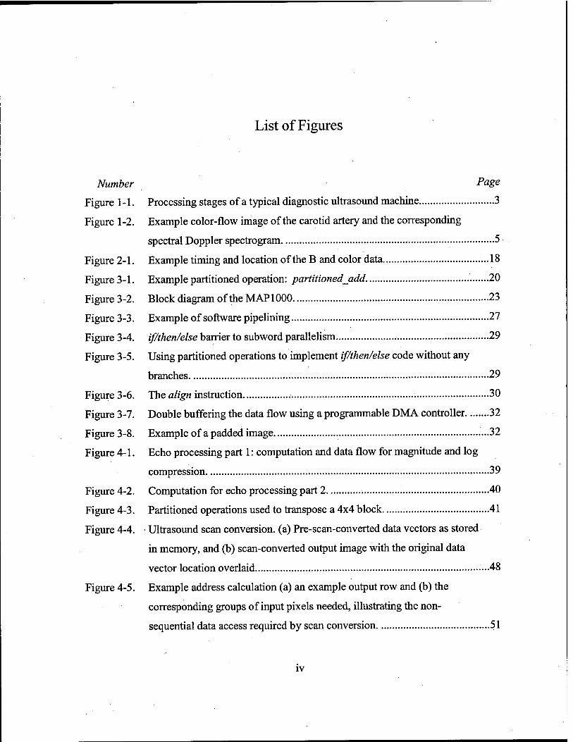
List of Figures

Number Page

Figure 1-1. Processing stages of a typical diagnostic ultrasound machine 3

Figure 1-2. Example color-flow image of the carotid artery and the corresponding

spectral Doppler spectrogram 5

Figure 2-1. Example timing and location of the B and color data ....18

Figure 3-1. Example partitioned operation: partitioned_add 20

Figure 3-2. Block diagram of the MAP1000 23

Figure 3-3. Example of software pipelining 27

Figure 3-4. if/then/else barrier to subword parallelism ...29

Figure 3-5. Using partitioned operations to implement if/then/else code without any

branches 29

Figure 3-6. The align instruction • -—30

Figure 3-7. Double buffering the data flow using a programmable DMA controller. ......32

Figure 3-8. Example of a padded image —.32

Figure 4-1. Echo processing part 1: computation and data flow for magnitude and log

compression 39

Figure 4-2. Computation for echo processing part 2 40

Figure 4-3. Partitioned operations used to transpose a 4x4 block ....41

Figure 4-4. Ultrasound scan conversion, (a) Pre-scan-converted data vectors as stored

in memory, and (b) scan-converted output image with the original data

vector location overlaid —.48

Figure 4-5. Example address calculation (a) an example output row and (b) the

corresponding groups of input pixels needed, illustrating the non-

sequential data access required by scan conversion 51

IV

Figure 4-6. Computing an output pixel value via a 4x2 interpolation with the polar

input data -—52

Figure 4-7. Extracting the filter coefficients for the lateral interpolation based on the

single VOB index -53

Figure 4-8. Example of run-length encoded output lines ...54

Figure 4-9. 2D block transfers. Spatial relationship between the output image blocks

and the corresponding 2D input data blocks 55

Figure 4-10. Interpolating color-flow data: RZ.<j> versus D+jN 58

Figure 4-11. Extra transforms are needed to use the linear scan converter on color-flow

data versus using a special scan converter implementing circular

interpolation 59

Figure 4-12. Example of shortest arc math, simplified for 4-bit data. The long arc of

"13" is too large for signed 4-bit data, resulting in the short arc of "3" ..61

Figure 4-13. 4-tap circular interpolation using shortest arc distance and partitioned

operations 62

Figure 4-14. Frame interpolation 64

Figure 4-15. Partitioned operations used to implement the combined frame

interpolation and tissue/flow tight loop .66

Figure 5-1. Parallel processing topologies —.73

Figure 5-2. UWGSP10 architecture utilizing 2 PCI ports per MAP 1000 processor. 75

Figure 5-3. UWGSP10 architecture utilizing 1 PCI port per MAP1000 processor 76

Figure 5-4. Hierarchical architecture with five processors per board 77

Figure 5-5. 2D array architecture 77

Figure 5-6. Example of division of a sector between four processors, showing the

overlapping vectors for a sub-sector #2 80

Figure 5-7. B-mode algorithm assignments (for one of 2 boards) 80

Figure 5-8. Color-mode algorithm assignments (for one of 2 boards) 81

Figure 5-9. Detailed PCI Bus Signals, showing an example of 4 processors requesting

the bus (PCIREQ1-4; active low signal), and the round robin arbitrator's v

corresponding bus grants (PCI_GNTl-4; active low signal). The address,

data, and spin cycles are labeled on the P_PCI_ADDR (multiplexed

address and data) signal • 82

Figure 5-10. Simulation process 88

Figure 5-11. When the simulation has reached steady state, the PCI arbitrator VHDL

model counts each cycle by type {address, data, un-hidden arbitration,

spin, and idle) to be used to determine the bus load statistics 91

Figure 5-12. MAP1000 VHDL model ,' 92

Figure 5-13. Timeline of B-mode simulation (dual-PCI architecture on board #1)

illustrating the pipelining of computations on the processors and

overlapping of data flow on the PCI bus for 3 frames 95

VI

List of Tables

Number

Table 1-1

Table 2-1

Table 3-1

Table 4-1

Table 4-2

Table 4-3

Table 4-4

Table 4-5

Table 4-6.

Table 4-7.

Table 4-8.

Table 5-1.

Table 5-2.

Table 5-3.

Table 5-4.

Page

Performance and number of processors required for basic ultrasound

functions • 9

Worst case scenarios for various processing modes. 17

Comparison of processors considered 22

Performance estimates for EP part 2 42

EP part 1 results 43

EP part 2 results • -.43

Color flow simulation results when E=6 47

Comparison of the performance of the three scan conversion data

flow methods for 16-bit 800x600 output image, a 90-degree sector,

and 340x1024 input vector data. 56

Simulation results for color scan conversion, comparing processing <f>

and R in separate routines versus in one combined routine 63

Ideal performance for frame interpolation and tissue flow,

implemented individually and combined 67

Estimated number of MAP 1000 processors needed for various

scenarios 68

Load balancing of color-mode 81

Estimated bandwidth required versus effective bandwidth available

for various buses for the worst case scenarios for the dual-PCI bus

architecture 83

Memory requirement per processor 84

Number of CINE frames and CINE time supported by the local

SDRAM memory in various scenarios 85

vii

Table 5-5. Validation results, comparing the accuracy of the VHDL models to

that of the CASIM simulator 93

Table 5-6. Performance of the CASIM simulator versus the real MAP 1000

processor in executing ultrasound algorithms 94

Table 5-7. B-mode multiprocessor simulation results 96

Table 5-8. Color-mode Multiprocessor Simulation Results 97

Table 5-9. Impact of reducing the number of samples per vector 99

Table 5-10. Performance of a single MAP 1000 (actual chip) executing the

ultrasound algorithms with reduced specifications 100

vin

Acknowledgments

First and foremost, I would like to thank my advisor, Professor Yongmin Kim, for

providing me this research opportunity and his expertise, guidance, and encouragement to

see it successfully completed. His dedication to perfection and professionalism will

continue to be a lasting example and inspiration for me. I am also indebted to my

supervisory committee, Donglok Kim, John Sahr, Roy Martin, and Greg Miller, who

provided their insight and experience throughout this project. I am extremely grateful to

my research partner, Ravi Managuli, whose many thought-provoking conversations

greatly contributed to our research and whose kindness, generosity, and sense-of-humor

made this a memorable and pleasurable experience. I would also like to thank the rest of

the Image Computing Systems Laboratory (ICSL) for their support and fellowship.

Credit is also due to Siemens Medical Systems Ultrasound Group for funding our

research and providing their technical expertise. Finally, I would like to thank Chris

Basoglu of Equator Technologies who helped pioneer this research effort and served as a

mentor throughout the project.

IX

Dedication

I dedicate this dissertation to my wife, Diane, for her love, support, understanding,

patience, and enthusiasm; to my sons, Rees and Henry, who maintained my sanity

through their insanity at home; and to my parents, Drs. Guy and Virginia York, and my

sister, Dr. Timmerly Richman, who led by example. Without them this dissertation could

not have been possible.

Chapter 1: Introduction

1.1 Motivation

Since the introduction of medical ultrasound in the 1950s, modern diagnostic

ultrasound has progressed to see many diagnostic tools come into widespread clinical

use, such as B-mode imaging, color-flow imaging and spectral Doppler. New

applications, such as panoramic imaging, three-dimensional imaging and quantitative

imaging, are now beginning to be offered on some commercial ultrasound machines, and

are expected to grow in popularity.

Today's ultrasound machines achieve the necessary real-time performance byusing a

hardwired approach (e.g., application-specific integrated circuits, (ASIC), and custom

boards) throughout the machine. While the hardwired approach offers a high amount of

computation capacity tailored for a specific algorithm, disadvantages include being

expensive to modify, having a long design cycle, and requiring many engineers for their

design, manufacture, and testing. The high cost of ASIC and board development can

hinder new algorithms and applications from being implemented in real systems, as

companies are conservative about making modifications.

While the older, mature B and color-flow modes are implemented using hardwired

components and boards, new applications, such as three-dimensional imaging and image

feature extraction, are being implemented more using programmable processors. This

trend toward programmable ultrasound machines will continue in the future, as the

programmable approach offers the advantages of quick implementation of new

applications without any additional hardware and the flexibility to adapt to the changing

requirements of these dynamic new applications.

While a programmable approach offers more flexibility than the hardwired approach,

an embedded programmable multiprocessor system capable of meeting all the

computational requirements of an ultrasound machine currently has not been

implemented. Limitations of earlier programmable systems include not having enough

computation power, due to either designs scoped for only single functions (versus the

entire ultrasound processing in general) or inefficient large-grained parallel architectures

combined with algorithms not tightly-coupled with the architecture.

This research addresses the above issues by first designing our architecture based

upon new advanced digital signal processors (DSP), known as mediaprocessors.

Mediaprocessors offer a fine-grained parallelism at the instruction level, which we have

found necessary for efficient implementation of ultrasound algorithms. Next, we

carefully mapped the various ultrasound algorithms to the mediaprocessor architecture,

creating new efficient algorithm implementations in the process. In addition, this

provided thorough understanding of the number of processors and data flow required to

implement the entire system, leading to the final design of our multi-mediaprocessor

architecture. Finally, to demonstrate that the system could meet the requirements, we

developed a multiprocessor simulation environment, with reduced simulation complexity

and time, while preserving accuracy. Our simulation results show that a cost-effective,

programmable architecture utilizing eight mediaprocessors is feasible for ultrasound

processing.

The remainder of the chapter reviews the basic ultrasound processing requirements

and previous programmable ultrasound systems, motivating the need for a fully

programmable ultrasound system, and summarizes the contributions of this research.

1.1.1 Review of Ultrasound Processing

Figure 1-1 illustrates the processing stages of a typical ultrasound system. The

ultrasound acoustic signals are generated by converting pulses of an electrical signal

ranging from 2 to 20 MHz (known as the carrier frequency, coc) from the transmitter into

a mechanical vibration using a piezoelectric transducer. As the acoustic wave pulse

travels through the tissue, a portion of the pulse is reflected at the interface of material

with different acoustical impedance, creating a return signal that highlights features, such

as tissue boundaries along a fairly well-defined beam line. The reflected pulses are

sensed by the transducer and converted back into radio frequency (RF) electrical signals.

Transducer

Tissue/Flow Decision

Echo Pixels

Color Pixels ^~

Figure 1-1. Processing stages of a typical diagnostic ultrasound machine.

The transducer emits the acoustic pulses at a pulse repetition frequency (PRF),

typically ranging from 0.5 to 20 kHz, based on the time for the pulse to travel to the

maximum target depth (d) and return to the transducer. The PRF is

PRF=-^T~ (i-i) c setup

where tsetup is the transducer setup time between each received and transmitted pulse and

speed of sound, c, is assumed to be a constant 1540 m/s, although it actually varies

depending on tissue type.

As the acoustic wave travels through the tissue, its amplitude is attenuated. Therefore,

the receiver first amplifies the returned signal in proportion to depth or the time required

for the signal to return (i.e., time-gain compensation, TGC). The signal's attenuation also

increases as ©c is increased, limiting the typical ultrasound system to depths of 10-30 cm.

After the RF analog signal is received and conditioned through TGC, it is typically

sampled at a conservatively high rate (e.g., 36 MHz for a transducer with coc = 7.5 MHz).

The demodulator then removes the carrier frequency using techniques, such as quadrature

demodulation, to recover the return (echo) signal. In quadrature demodulation, the

received signal is multiplied with cos(coct) and sin(coct), which after lowpass filtering,

results in the baseband signal of complex samples, I(t) + jQ(t). The complex samples

contain both the magnitude and phase information of the signal and are needed to detect

moving objects, such as blood.

The samples of the signal obtained from one acoustic pulse (i.e., one beam) are called

a vector. Today's phased-array transducers can change the focal point of the beam as

well as steer the beam by changing the timing of the firing of the piezoelectric elements

that comprise the array. By steering these beams and obtaining multiple vectors in

different directions along a plane (e.g., V1-V5 in Figure 1), a two-dimensional (2D) image

can be formed. Depending on how the vectors are processed, the image can be simply a

gray-scale image of the tissue boundaries (known as echo imaging or B-mode) or also

have a pseudo-color image overlaid, in which the color represents the speed and direction

of blood flow (known as color mode) as shown in Figure 1-2. In addition, the spectrum

of the blood velocity at a single location over time can be tracked (known as gated

Doppler spectral estimation) and plotted in a spectrogram as shown in the bottom of

Figure 1-2. By combining multiple slices of these 2D images, 3D imaging is also

possible.

Figure 1-2. Example color-flow image of the carotid artery and the corresponding spectral Doppler spectrogram.

To create the final output images for these modes, several digital signal processing

stages are needed following demodulation, including the echo processor, the color-flow

processor, the scan converter, and additional raster processing (such as tissue/flow

decision), which are the main stages for this study. For B-mode imaging, the echo

processor (EP) obtains the tissue boundary information by taking the magnitude

(envelope detection) of the quadrature signal, Ba(t) = i]l2(t)+Q2(t). The EP men

logarithmically compresses the signalBb(t}=log(Ba(t)), to reduce the dynamic range from

the sampled range (around 12 bits) to that of the output display (8 bits) and to nonlinearly

map the dynamic range to enhance the darker-gray levels at the expense of the brighter-

gray levels (Dutt, 1995). The vectors are then spatially and temporally filtered to

enhance the edges while reducing the speckle noise.

For color-flow imaging, the color-flow processor (CF) estimates the velocity of

moving particles (e.g., blood) by taking advantage of the Doppler shift of the acoustic

signal due to motion. In pulsed ultrasound systems, the velocity is estimated from:

c-PRF <b

lfccos0 lit K }

where c is the velocity of sound in blood, 6 is the Doppler angle, (j> is the phase difference

between two consecutive pulses (Kasai et al., 1985). To improve the accuracy of the

velocity estimate, multiple vectors are shot along the same beam over time, known as

ensembles. A small number of ensembles (6 to 16) are used by color flow in order to

reduce the amount of data needed to be collected and allow real-time frame rates. The

color-flow processor first filters out any low velocity motion not due to blood (like the

vessel wall) using the wall filter. Then, the velocity is typically estimated by calculating

the average change in phase using an autocorrelation technique (Barber et al., 1985):

<j){f) = arctan (1-3) E!:0

2(ge(o^(o-^(oa+1(0) X^o2(/ew/e+1(o+awa+,(0)/

where the denominator and numerator are respectively the real and imaginary part of the

first lag of autocorrelation, and E is the ensemble size. In addition to the velocity, the

variance of the velocity and power of the flow are often calculated and imaged.

Similarly, the spectral Doppler processor is used to get a more accurate estimate of the

spectrum of velocities by collecting a large number of ensembles (e.g., 256) at one

location, then doing a ID Fast Fourier Transform (FFT).

When the vectors are obtained by sweeping the beams in an arc (sector scan), the

scan converter (SC) geometrically transforms the data vectors from the polar coordinate

space into the Cartesian coordinate space needed for the output display. This transform

can also zoom, translate, and rotate the image if needed. Then, the raster/image processor

performs tissue/flow (TF) decision, which determines if an output pixel should be a gray-

scale tissue value or a color-flow value. It also performs frame interpolation to increase

the apparent frame rate. Depending on the application, typical frame rates can range from

5 to 30 frames per second (rps) for 2D color-flow imaging to over 50 fps for 2D B-mode

imaging.

A large amount of computing power is required to support all the processing in B-

mode imaging, color-flow imaging, and image processing/display. The ultrasound

systems are typically implemented in a hardwired fashion by using application specific

integrated circuits (ASIC) and custom boards to meet the real-time requirements. In our

recent article (Basoglu et al., 1998), we estimated the total computation required for a

modern ultrasound machine to range from 31 to 55 billion operations per second (BOPS),

depending on if certain functions are implemented in lookup tables or calculated on the

fly. To incorporate new features, such as advanced image processing applications,

panoramic imaging or 3D imaging, will require even more computing power in future

machines. These new applications are currently not well defined and are continually

evolving. These dynamic applications will require the flexibility to adapt to changing

requirements offered by programmable processors, which the hardwired ASIC approach

cannot support easily.

1.1.2 Advantages of a Fully Programmable Ultrasound System

Benefits of an ultrasound processing system based on multi-mediaprocessors are:

• Adaptable. Easy to add new algorithms or modify existing algorithms by just modifying the software. With the hardwired approach, often a simple change could cause the costly redesign of specialized chips or an entire board.

• Hardware Reuse. Depending on the mode of operation of an ultrasound machine, much of the hardwired components can sit idle or are needlessly computing results never to be used. With the programmable system, the idle processors can be reconfigured to do useful tasks. For example, when switching from various modes, e.g., B-mode, color mode, power mode, spectral Doppler, 3D imaging, panoramic imaging, quantitative imaging, etc., the same processors can be reprogrammed to do different tasks.

• Scalable. By adding or removing multiprocessor boards, the system will be able to scale from a low to high-end system.

• Reduced R&D Cost. Less engineering manpower will be needed not only for the design, testing, and manufacturing of ASICs and boards, but also for their redesigns.

• Reduced System Cost. The programmable approach may not be cost-effective compared to the hardwired approach for low-end systems that use well-define, non- changing algorithms. However, for high-end systems the fully programmable system maybe more cost-effective because of the hardware reuse advantage and developing only one standardized multiprocessor board repeated throughout the system, where the board is composed of low-cost processors, standardized memory, and a simple bus structure.

• Faster Clinical Use of New Features. The ease of adaptability and reduced cost of system modifications compared to a hardwired system should decrease the time and increase the probability of new, innovative algorithms actually making the leap from R&D into a product routinely used by the customer.

• Software Upgrades. The cost of field upgrades will be reduced by providing new features to the users in the field through software upgrades without any hardware changes needed.

1.1.3 Previous Research in Programmable Ultrasound.

Table 1-1 lists several programmable systems developed for various ultrasound

functions. This table shows how the performance has improved and the number of

processors required decreased as processor technology has improved, particularly with

the introduction of mediaprocessors (e.g., TMS320C80 and MAP1000). Many of these

systems were designed to implement specific experimental functions without an

architecture that could handle the full computation load and/or be generalized for the full

processing requirements of modern ultrasound machines. For example, Cowan et al.

(1995) developed a system to perform gated Doppler spectral estimation using the

INMOS T800 transputer processor. With this early 90's technology, it required 2

hardwired FFT chips (Al 00) along with a T800 transputer to achieve real-time

performance.

Color-flow imaging requires much more computing power than these spectral

Doppler systems. Thus, using early 90's technology, Costa et al. (1993) developed a

parallel architecture with 64 Analog Devices ADSP2105 programmable DSPs running

for a real-time (10 fps with 8 ensembles) narrowband color-flow estimation system based

on an autoregressive method. Using mid 90's technology, Jensen et al. (1996) developed

a programmable system with 16 Analog Devices ADSP21060 processors and were

planning to implement color flow on this system, but were "disappointed with the

performance of the 21060," finding that the system could not achieve its expected

performance. This is often the case when dealing with algorithm mapping and data flow

issues of implementing real applications on parallel processing systems.

Table 1-1. Performance and number of processors required for basic ultrasound functions.

Number of Function Processor Data size Processors (MHz) Performance

Color-flow ADADSP2105 256x512x8 64 40 10fps (Costa, 93) ADADSP21060 16 40 (Jensen, 96) Tl TMS320C80 256x512x16 4 50 10fps (Basoglu, 98) Equator MAPI 000 256x512x16 2 200 10 fps*

SDectral doDDler INMOST800&A100 889 3 20 40 ms (Cowan, 95) Tl TMS320C25 1024 1 40 30 ms (Christman, 90) Tl TMS320C80 512 1 50 0.073 ms (Basoglu, 97) Equator MAPI 000 512 1 200 0.012 ms *

Scan conversion SUN SPARC 512x512 1 25 630 ms (Berkhoff, 94) Tl TMS320C80 512x512 1 50 17 ms (Basoglu, 96) Equator MAP 1000 512x512 1 200 4 ms (York, 98)

Tissue/Flow Tl TMS320C30 17x48 2 20 24 fps (Bohs, 93) Tl TMS320C80 304x498 1 50 60 fps (Basoglu, 97)

* Our estimate includes similar assumptions as the above implementations, but excludes several filters and the adaptive wall filter. The specifications for the complete ultrasound system in this thesis includes all filters, requiring a much larger processing load than indicated by this table.

Bohs et al. (1993) developed a unique system to experiment with a velocity

estimation technique based on the sum of absolute difference method. The velocity

estimate was performed with a hardwired board, but the tissue/flow decision and final

image processing were implemented on 2 Texas Instruments TMS320C30 DSPs and one

TMS34020 graphics processor. For scan conversion, various algorithms have been

explored on an off-line workstation, taking an excessive 630 ms on a 512x512 image, as

no effort was made to optimally map the algorithm to the architecture. None of these

systems are flexible or powerful enough to implement a full ultrasound processing

system.

10

In addition to these systems, many researchers who developed their own "add-on"

programmable systems (typically external to existing ultrasound machines) to take

advantage of the flexibility of the programmable approach when developing new

algorithms or applications. These systems often have difficulty achieving real-time

performance as they are not integrated with the machine and process the digitized data

off-line. The external implementations typically do not have access to the original vector

data or scan-converted data inside the machine, thus suffer from poor image quality from

digitizing the analog video out from the ultrasound machine. Examples include off-line

external systems for speckle reduction (Czerwinski et al., 1995), intravascular ultrasound

image subtraction (Pasterkamp et al., 1995), and 3D reconstruction (Rosenfield et al.,

1992). Others have been used for real-time experiments with limited functionality, such

as for left ventricular endocardial contour detection (Bosch et al., 1994), speckle

reduction (Loupas et al., 1994), and contour tracing (Jensch & Ameling, 1988).

Noting the limitations of the above architectures, the Image Computing Systems

Laboratory at the University of Washington started the UWGSP8 project to demonstrate

the feasibility of using a programmable approach in an ultrasound machine (Basoglu,

1997). A programmable ultrasound image processor (PUIP) board, composed of two

TMS320C80 mediaprocessors, was integrated with the other hardwired boards inside a

Siemens' ultrasound machine. The PUIP has access to both the pre-scan-converted data

and post-scan-converted data. Therefore, several experiments could be done testing

various algorithms on the mediaprocessors, such as the TMS320C80 results in Table 1-1.

Basoglu experimented with implementing efficient algorithms for scan conversion, color

flow (frequency estimation and wall filter only), tissue/flow decision, and the FFT

required by spectral Doppler. His results indicated the performance of mediaprocessors is

sufficient to support several of the primary functions of an ultrasound machine.

The PUIP board could not implement the entire backend processing. Still, the

ultrasound machine with the PUIP board relies on the hardwired boards for many

functions. However, the PUIP board clearly demonstrated several advantages of the

11

programmable approach. A new application (not initially intended for the PUIP) called

panoramic imaging was quickly developed on the mediaprocessors (Weng et al., 1997).

Panoramic imaging allows the user to see organs larger than the field of view of the

standard B-mode sector by blending multiple images into a larger panoramic image as the

multiple images are acquired. The mediaprocessors were capable of handling panoramic

imaging's dynamic processing requirements of registration, warping, and interpolation in

real time. Since the exact algorithms for panoramic imaging were initially undefined, the

ability to modify the programs and iterate the design was crucial to quickly prototype,

test and finalize the application. A hardwired design approach could not have adapted

this quickly, and there would have difficulty creating a working prototype in a reasonable

time and cost. This programmable system also has successfully proven the advantage of

hardware reuse. The same hardware has been reprogrammed to offer other features in

addition to panoramic imaging, such as automatic fetal head measurement (Pathak et al.,

1996), fetal abdomen and femur measurement, harmonic imaging, color panoramic

imaging, and 3D imaging (Edwards et al., 1998).

The programmable approach has also recently emerged in other commercial

ultrasound machines. The ATL HDI-1000 is a mid-range ultrasound machine in which

programmable processors replace 50% of the previous hardware components (ATL,

1997). This system uses a Motorola 68060 (113 MIPS) for B-mode and scan conversion

and two ATT DSP3210 (33 MFLOPS) for Doppler processing, thus cannot handle the

computation load of a 30 BOPs ultrasound machine. There are also some low-end PC-

based ultrasound machines emerging supporting only B and M mode, such as the Fukuda

Denshi UF-4500 that uses 7 programmable processors (Fukuda, 1999) and the Medison

SA-5500 that uses Pentium processors combined with a hardwired ASIC (Medison,

1999).

12

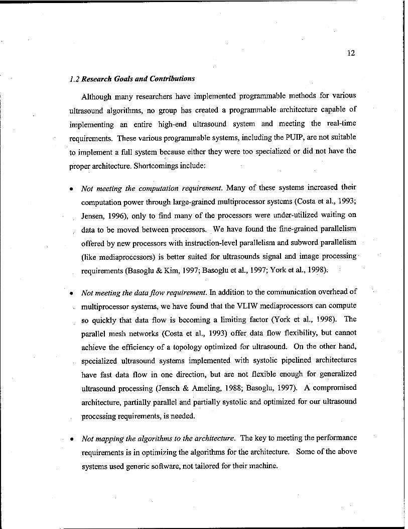
1.2 Research Goals and Contributions

Although many researchers have implemented programmable methods for various

ultrasound algorithms, no group has created a programmable architecture capable of

implementing an entire high-end ultrasound system and meeting the real-time

requirements. These various programmable systems, including the PUIP, are not suitable

to implement a full system because either they were too specialized or did not have the

proper architecture. Shortcomings include:

• Not meeting the computation requirement. Many of these systems increased their

computation power through large-grained multiprocessor systems (Costa et al., 1993;

Jensen, 1996), only to find many of the processors were under-utilized waiting on

data to be moved between processors. We have found the fine-grained parallelism

offered by new processors with instruction-level parallelism and subword parallelism

(like mediaprocessors) is better suited for ultrasounds signal and image processing

requirements (Basoglu & Kim, 1997; Basoglu et al., 1997; York et al., 1998).

Not meeting the dataflow requirement. In addition to the communication overhead of

multiprocessor systems, we have found that the VLIW mediaprocessors can compute

so quickly that data flow is becoming a limiting factor (York et al., 1998). The

parallel mesh networks (Costa et al., 1993) offer data flow flexibility, but cannot

achieve the efficiency of a topology optimized for ultrasound. On the other hand,

specialized ultrasound systems implemented with systolic pipelined architectures

have fast data flow in one direction, but are not flexible enough for generalized

ultrasound processing (Jensch & Ameling, 1988; Basoglu, 1997). A compromised

architecture, partially parallel and partially systolic and optimized for our ultrasound

processing requirements, is needed.

Not mapping the algorithms to the architecture. The key to meeting the performance

requirements is in optimizing the algorithms for the architecture. Some of the above

systems used generic software, not tailored for their machine.

13

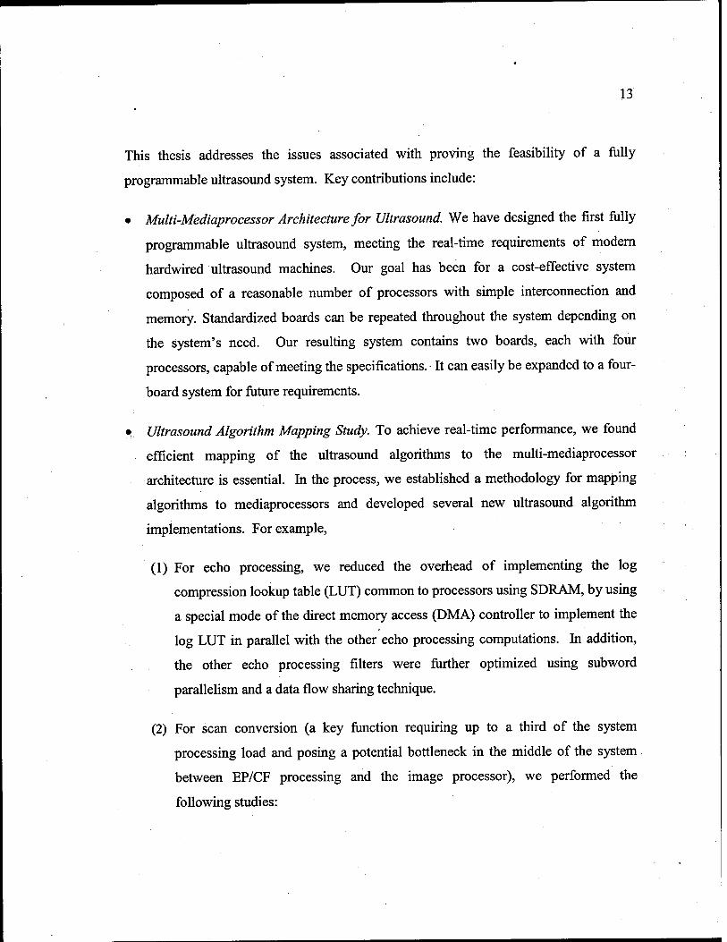
This thesis addresses the issues associated with proving the feasibility of a fully

programmable ultrasound system. Key contributions include:

• Multi-Mediaprocessor Architecture for Ultrasound. We have designed the first fully

programmable ultrasound system, meeting the real-time requirements of modern

hardwired ultrasound machines. Our goal has been for a cost-effective system

composed of a reasonable number of processors with simple interconnection and

memory. Standardized boards can be repeated throughout the system depending on

the system's need. Our resulting system contains two boards, each with four

processors, capable of meeting the specifications. It can easily be expanded to a four-

board system for future requirements.

• Ultrasound Algorithm Mapping Study. To achieve real-time performance, we found

efficient mapping of the ultrasound algorithms to the multi-mediaprocessor

architecture is essential. In the process, we established a methodology for mapping

algorithms to mediaprocessors and developed several new ultrasound algorithm

implementations. For example,

(1) For echo processing, we reduced the overhead of implementing the log

compression lookup table (LUT) common to processors using SDRAM, by using

a special mode of the direct memory access (DMA) controller to implement the

log LUT in parallel with the other echo processing computations. In addition,

the other echo processing filters were further optimized using subword

parallelism and a data flow sharing technique.

(2) For scan conversion (a key function requiring up to a third of the system

processing load and posing a potential bottleneck in the middle of the system

between EP/CF processing and the image processor), we performed the

following studies:

14

(a) A trade-off study of the various data flow approaches for scan conversion

available to mediaprocessors, such as cache-based versus DMA-based

(including 2D block transfers and guided transfers). Our study shows that

carefully managing data flow is the key to efficient scan conversion.

(b) A different scan conversion algorithm for the color-flow data on

mediaprocessors was developed, called circular interpolation, improving the

performance by removing the need for two image transformations.

(3) For the final frame interpolation and tissue/flow processing, a combined

algorithm was used to reduce the I/O overhead. Also we removed the if/then/else

barrier to subword parallelism, which improved the algorithm's efficiency.

• Multiprocessor Simulation Environment. To demonstrate that the system

requirements are met, we developed a unique multiprocessor simulation environment

using VHDL models of the system components to simulate various processing modes

on our ultrasound processing system. To prevent these simulations with complex

components and large programs from becoming intractable (and unable to run) as the

scale of the multiprocessor system is increased, we developed a method to reduce the

simulation time of our system while still remaining reasonably accurate. This includes

techniques to reduce the size of the address trace files as well as control the

component complexity by combining the accuracy of a commercial cycle-accurate

simulator for a single mediaprocessor along with our multiprocessor VHDL

simulation environment.

1.3 Overview of Thesis

Chapter 2 specifies the requirements that our architecture must support for both B-

mode and color-flow ultrasound modes.

15

In Chapter 3, we first discuss how we selected the mediaprocessor upon which the

architecture is based. We then discuss a methodology for optimally mapping algorithms

to mediaprocessors.

In Chapter 4, we discuss the mapping of various ultrasound algorithms to the

mediaprocessor architecture, the new algorithm implementations created, and how we

estimated the number of processors and data flow required for the final architecture

through cycle-accurate simulations on a single processor.

Chapter 5 discusses the design of our multi-mediaprocessor architecture, the

simulation tools and techniques we developed, and the results of our multiprocessor

VHDL simulations for both B-mode and color mode.

Finally in Chapter 6, we summarize our conclusions and contributions of this thesis

and discuss future directions.

16

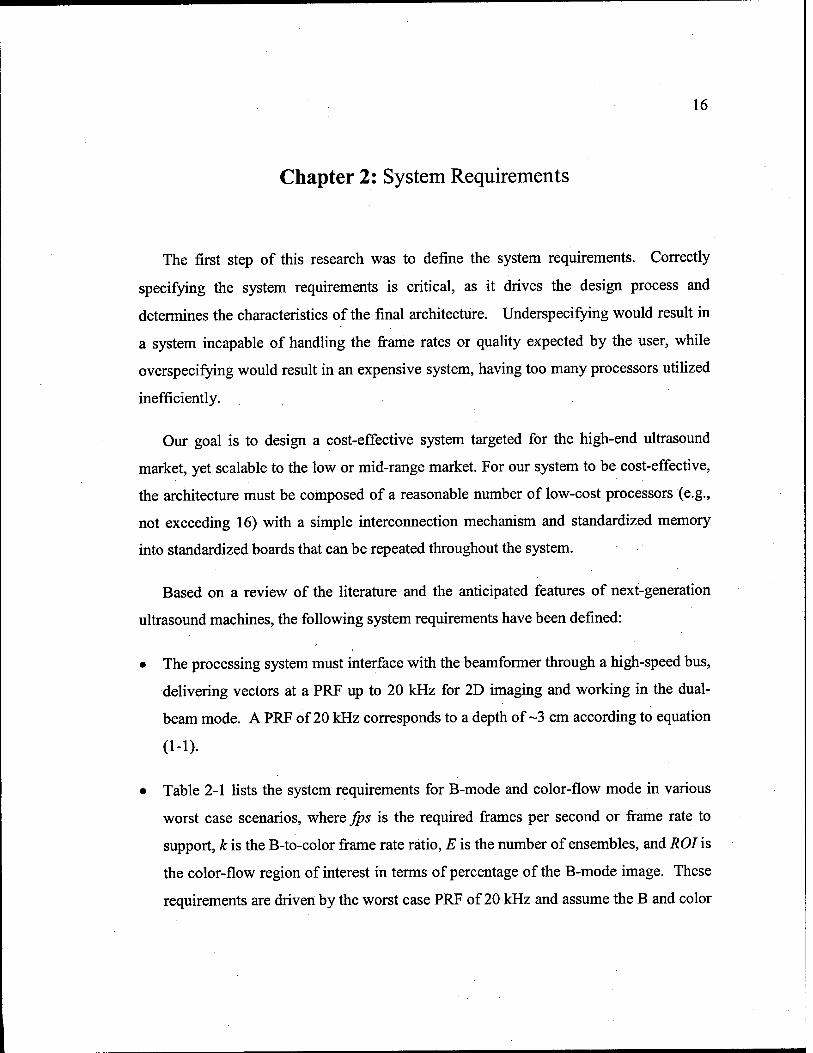
Chapter 2: System Requirements

The first step of this research was to define the system requirements. Correctly

specifying the system requirements is critical, as it drives the design process and

determines the characteristics of the final architecture. Underspecifying would result in

a system incapable of handling the frame rates or quality expected by the user, while

overspecifying would result in an expensive system, having too many processors utilized

inefficiently.

Our goal is to design a cost-effective system targeted for the high-end ultrasound

market, yet scalable to the low or mid-range market. For our system to be cost-effective,

the architecture must be composed of a reasonable number of low-cost processors (e.g.,

not exceeding 16) with a simple interconnection mechanism and standardized memory

into standardized boards that can be repeated throughout the system.

Based on a review of the literature and the anticipated features of next-generation

ultrasound machines, the following system requirements have been defined:

• The processing system must interface with the beamformer through a high-speed bus,

delivering vectors at a PRF up to 20 kHz for 2D imaging and working in the dual-

beam mode. A PRF of 20 kHz corresponds to a depth of ~3 cm according to equation

(1-1).

• Table 2-1 lists the system requirements for B-mode and color-flow mode in various

worst case scenarios, where fps is the required frames per second or frame rate to

support, k is the B-to-color frame rate ratio, E is the number of ensembles, and ROI is

the color-flow region of interest in terms of percentage of the B-mode image. These

requirements are driven by the worst case PRF of 20 kHz and assume the B and color

17

image have the same depth, thus same PRF. The color mode frame rate is determined

by:

Color fps = PRF • beams

•" ' ^vectors ' vectors (2-1)

where beams is 2 for a dual-beam system. In addition, the frame rate is limited to the

maximum display update rate of 68 fps. The sector angle is based on a maximum

lateral resolution for 2D imaging of 3.8 vectors/degree.

Table 2-1. Worst case scenarios for various processing modes.

Mode k Color fps

B fps

# Color vectors

#B vectors E ROI

Output Image

sector angle

B — — 68.0 — 512 — — 800x600 136 — 68.0 — 340 — 800x600 90

Color 1 9.0 9.0 256 340 16 100% 800x600 90 2 8.4 16.8 3 7.8 23.5 4 7.3 29.3 5 6.9 34.5

Color 1 22.3 22.3 256 256 6 100% 800x600 90 2 19.5 39.1 3 17.4 52.1 4 15.6 62.5

Color 1 68.0 68.0 52 256 6 20% 800x600 90

The largest number of samples per vector is assumed to be 1024 for B-mode and 512

for color mode, with 16 bits per sample. Current hardwired ultrasound machines

process the maximum number of samples, regardless of whether all the samples

contain meaningful data. For example, for the 3 cm depth, 1024 data samples led to

many more axial samples than can be resolved by a 7.5 MHz transducer. This can

lead to an overspecified system. A programmable system has the flexibility to adapt

the processing to the actual data size/resolution required, as discussed more in section

5.3.3 .

18

In color mode, the timing of the acquisition of the B and color vectors are as shown in

Figure 3-2 for the K = 4 and E =6 scenario.

K=4 spatially adjacent B beams T= 1/PRF, including fse(up

r ^

Bi B2 B3 B4 C1.1 C1,2 C1,3 C1,4 C1,5 C1,6 B5 B6 B7 B8 C2,1

^ J Y

E=6 Color beams, spatially coincident with B1

Figure 2-1. Example timing and location of the B and color data.

• The processing system must interface with the host processor through the system PCI

bus (either 32 bits or 64 bits @ 33 MHz).

Finally, when designing embedded computer systems it is prudent to allow room for

future growth as requirements often change after the system has been developed. Our

rule-of-thumb is the system should be designed with enough capacity that only 50% of

the processing power, memory, and bus bandwidth are utilized.

19

Chapter 3: Mediaprocessors and Methods for Efficient Algorithm

Mapping

3.1 Introduction

In this chapter, we discuss rationale behind selecting the mediaprocessor for our

architecture. We then discuss the key techniques we have developed to achieve efficient

mapping of algorithms to the highly parallel architectures of mediaprocessors.

3.2 Methods

3.2.1 Mediaprocessor Selection

To meet the ultrasound processing requirement of 31 to 55 BOPS (Basoglu et al.,

1998) is challenging for systems based on programmable processors. Fortunately, a new

class of advanced DSPs, known as mediaprocessors, have rapidly evolved recently to

handle the high computation requirements of multimedia applications, which are similar

to those of ultrasound processing. To avoid the high cost of developing huge

multiprocessor systems with large-grained parallelism, mediaprocessors increase

performance through fine-grained on-chip parallelism, known as instruction-level

parallelism (ILP) (Gwennap, 1994). ILP allows multiple operations (e.g., load/stores,

adds, multiplies, etc.) to be initiated each clock cycle on multiple execution units. The

two primary methods of implementing ILP are known as superscalar and very long

instruction word (VLIW) architectures (Patterson & Hennessey, 1996). For VLIW

architectures, the programmer (or compiler) uses the long instruction word to uniquely

control each execution unit each cycle, while for superscalar architectures, special on-

chip hardware looks ahead through a serial instruction stream to find independent

operations that can be executed in parallel on the various execution units each cycle.

20

Thus, the superscalar architectures are easier to program at the expense of this additional

hardware to find the parallelism on the fly. On the other hand, VLIW architectures

require the programmer to understand the architecture intimately to efficiently maximize

the parallelism of a given algorithm. The VLIW programmer usually can outperform the

superscalar scheduling hardware, which can only search a limited number of future

instructions. Much research has been conducted to ease the VLIW programming burden

thought smart compilers (Lowney et al., 1993), as discussed in section 3.2.2.2.

Instruction-level parallelism can be extended further by execution units that support

partitioned operations (subword parallelism, e.g., allowing a 64-bit execution unit to be

divided into eight 8-bit execution units, as shown for the partitioned add instruction in

Figure 3-1). This single instruction multiple data (SIMD) style architecture can usually

be partitioned on different subword sizes (i.e., 32, 16, or 8 bits), increasing the

performance by 2x, 4x, or 8x for carefully-mapped algorithms such as the vector and

image processing required in ultrasound machines. In some instances, these partitioned

operations require multiple cycles to complete, thus the execution units are fully

pipelined, providing an effective throughput of a complete partitioned operation each

cycle.

8-bit partition

A7 A6 A5 A4 A3 A2 A A0 |

■ + + + + + + + +

By B6 B5 B4 B3 B2 Bi B0

A7+B7 A6+B6 A5

+B5 A4+B4 A3

+B3 A2+B2 A+Bi A0

+B0

64-bit registers

Figure 3-1. Example partitioned operation: partitioned add.

21

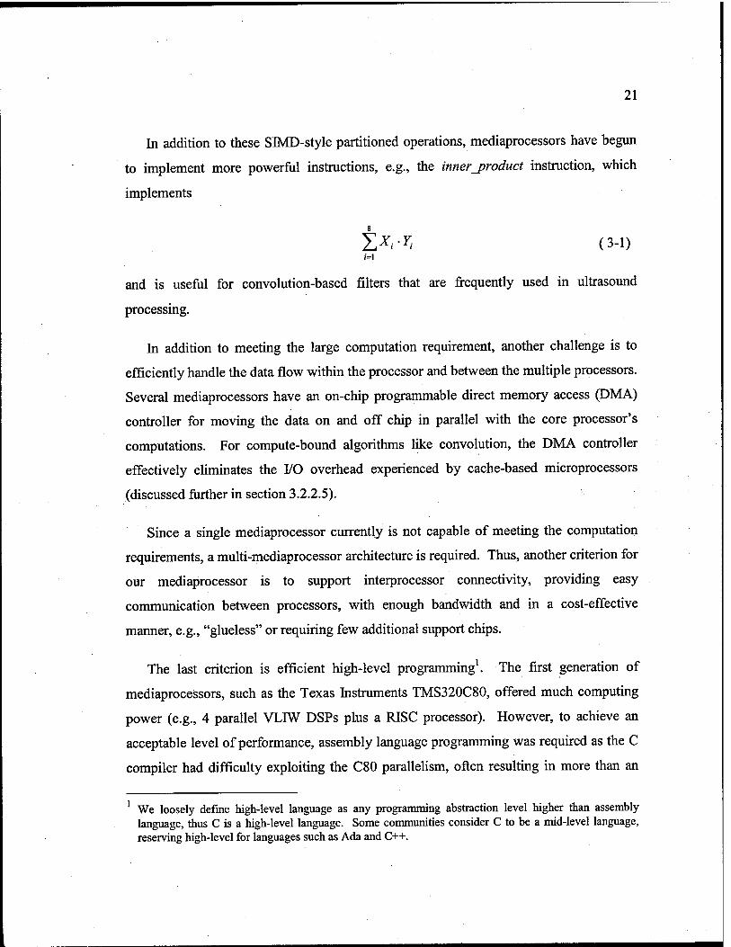
In addition to these SEVLD-style partitioned operations, mediaprocessors have begun

to implement more powerful instructions, e.g., the innerjproduct instruction, which

implements

JLXi'Yi (3-1) 1=1

and is useful for convolution-based filters that are frequently used in ultrasound

processing.

In addition to meeting the large computation requirement, another challenge is to

efficiently handle the data flow within the processor and between the multiple processors.

Several mediaprocessors have an on-chip programmable direct memory access (DMA)

controller for moving the data on and off chip in parallel with the core processor's

computations. For compute-bound algorithms like convolution, the DMA controller

effectively eliminates the I/O overhead experienced by cache-based microprocessors

(discussed further in section 3.2.2.5).

Since a single mediaprocessor currently is not capable of meeting the computation

requirements, a multi-mediaprocessor architecture is required. Thus, another criterion for

our mediaprocessor is to support interprocessor connectivity, providing easy

communication between processors, with enough bandwidth and in a cost-effective

manner, e.g., "glueless" or requiring few additional support chips.

The last criterion is efficient high-level programming1. The first generation of

mediaprocessors, such as the Texas Instruments TMS320C80, offered much computing

power (e.g., 4 parallel VLIW DSPs plus a RISC processor). However, to achieve an

acceptable level of performance, assembly language programming was required as the C

compiler had difficulty exploiting the C80 parallelism, often resulting in more than an

1 We loosely define high-level language as any programming abstraction level higher than assembly language, thus C is a high-level language. Some communities consider C to be a mid-level language, reserving high-level for languages such as Ada and C++.

22

order of magnitude performance difference (Stotland et al., 1999). For ease of

maintenance, portability, and reduced development time, it would be preferred to use a

high-level language, such as C. The next-generation mediaprocessors have been

developed with the C compiler in mind. For example, the Phillips TM1100 and Equator

MAP 1000 for some algorithms like morphology achieve a 3 to 2 performance difference

between C and assembly language implementations (York et al., 1999).

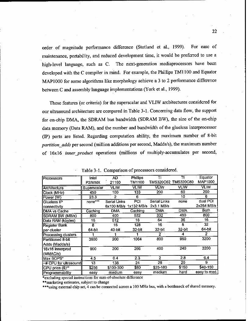
These features (or criteria) for the superscalar and VLIW architectures considered for

our ultrasound architecture are compared in Table 3-1. Concerning data flow, the support

for on-chip DMA, the SDRAM bus bandwidth (SDRAM BW), the size of the on-chip

data memory (Data RAM), and the number and bandwidth of the glueless interprocessor

(IP) ports are listed. Regarding computation ability, the maximum number of 8-bit

partition adds per second (million additions per second, Madds/s), the maximum number

of 16x16 innerjproduct operations (millions of multiply-accumulates per second,

Table 3-1. Comparison i of processors considered

Processors Intel P2/MMX

AD 21160

Phillips TM1100

Tl Tl TMS320C62 TMS320C80

Equator MAPI 000

Architecture Superscalar VLIW VLIW VLIW VLIW VLIW

Clock (MHz) 450 100 133 200 60 200

Power (W) 23.3 2 6 10 6

Glueless IP connectivity

none*** Serial Links 6x100 MB/s

PCI 1x132 MB/s

Serial Links 2x3.1 MB/s

none dual PCI 2x264 MB/s

DMA vs Cache Caching DMA Caching DMA DMA Both

SDRAM BW (MB/s) 800 400 532 332 480 800

Data RAM (kbytes) 16 512 16 64 36 16

Register Bank per cluster

8 64-bit

16 40-bit

128 32-bit

16 32-bit

8 32-bit

32 64-bit

Processing clusters 1 1 1 2 4 2

Partitioned 8-bit Adds (Madds/s)

3600 200 1064 800 960 3200

16x16 Innerprod (MMAC/s)

900 200 266 400 240 3200

Max BOPS* 4.5 0.4 2.3 2 2.8 6.4

~# CPU for ultrasound 13 138 24 28 20 9

CPU price ($)** $256 $100-300 $80 $25-180 $150 $40-150

Programmability easy medium easy medium hard easy to med.

♦excluding special instructions for sum-of-absolute difference """marketing estimates, subject to change ***using external chip set, 4 can be connected across a 100 MHz bus, with a bottleneck of shared memory.

23

MMAC/s), and the maximum BOPS ratings are shown for various processors. The

number of partitioned registers available per processing cluster is also listed, as a large

number of registers are needed for many applications to approach their ideal performance

on a processor, particularly when using techniques, such as software pipelining discussed

in section 3.2.2.2. The power drawn by each chip is also a consideration, as several

processors will be needed to implement the system. Finally, the cost of a system will be

influenced not only by the CPU price listed, but also by the support for glueless

interprocessor connectivity and the total number of processors required. The number of

processors required to implement a 55-BOPS ultrasound machine is roughly estimated in

Table 3-1 based solely on the ideal BOPS number of each processor. Estimates based on

the ideal BOPS are rarely achieved, but serve as an initial estimate.

The MAP1000 was selected for our system, as it leads most of the categories in Table

3-1. As shown in Figure 3-2, the MAPI000 is a single-chip VIJW mediaprocessor with a

highly parallel internal architecture optimized for signal and image processing. The

processing core is divided into two clusters, each of which has two execution units, an

IALU and an IFGALU, allowing four different operations to be issued per clock cycle.

MAPI 000

Core Processor Cluster 0

registers

IALU IFGALU

Cluster 1

registers

IALU IFGALU

Cache

16KB Data

16KB Instruction

Video Graphics

Coprocessor

9KB SRAM

64 bits @ 100 MHz

SDRAM

Other Media Ports

PCI Ports

32 bits @ 66 MHz

*-^+

Figure 3-2. Block diagram of the MAP 1000.

24

The IALU can perform either a 32-bit fixed-point arithmetic operation or a 64-bit

load/store operation while the IFGALU can perform either a 64-bit partitioned arithmetic

operation, a 8-tap, 16x8 inner_product, or a floating-point operation (e.g., division and

square root operations). Each cluster has 32 64-bit general registers, 16 predicate

registers, and a pair of 128-bit registers used for special instructions like inner_product.

In addition, the MAP 1000 has a 16-kbyte data cache, a 16-kbyte instruction cache, an on-

chip programmable DMA controller called the Data Streamer (DS), and two PCI ports.

The MAPlOOO's dual PCI ports will provide a good basis for interconnecting the

multiple processors gluelessly, with only the ADSP21160 in Table 3-1 providing a better

connectivity (6 serial links). The MAP 1000 is the only processor offering both the

caching mechanism and DMA controller, leads in SDRAM bus bandwidth, is fairly

inexpensive, and in general is the best computation engine. The MAPlOOO's primary

weakness is that it has the smallest data cache in Table 3-1, which requires careful data

flow management for efficient ultrasound processing. In addition, developing a system

based on the MAP 1000 carries a risk in that it is a new chip under development from a

new company.

3.2.2 Algorithm Mapping Methods

Even with these new powerful mediaprocessors, carefully designing algorithms by

making efficient use of this newly available parallelism will be necessary to implement

the ultrasound processing in a reasonable number of processors. Through our extensive

experience in developing algorithms (both ultrasound processing and an imaging library)

for the TMS320C80 and MAP 1000 mediaprocessors, we found several keys to efficiently

mapping algorithms. Performance is gained by:

(1) Mapping the algorithms to the mediaprocessor's multiple processing units and subword parallelism.

(2) Utilizing the full capacity of the multiple processing units using software pipelining.

25

(3) Removing barriers to subword parallelism, such as if/then/else code and memory alignment problems.

(4) Avoiding redundant computations by using lookup tables (LUT).

(5) Carefully managing the data flow using the programmable DMA controller and minimizing the I/O overhead.

(6) Optimize from a system-level perspective, reducing unnecessary transforms, sharing the data flow between algorithms, and balancing the processing load throughout the system.

The following sections describe these techniques in more detail. Also, the method used

to determine the efficiency of our algorithm mapping is presented as well.

3.2.2.1 Mapping the algorithms to the parallel processing units

Most of the ultrasound algorithms are vector-based or image-based with the

computations for each data point or pixel the same, but independent from its neighbors.

These computations readily map to the subword parallelism of the IFGALU units, which

can implement all the typical computations (e.g., or, and, min, max, add, subtract,

multiply, compare, etc.). Most of the ultrasound computations are on 16-bit data,

allowing 8 data to be computed in parallel using both IFGALU units. Some algorithms

use special instructions, e.g., innerjproduct, which due to special 128-bit registers can

compute an 8-tap FIR with 16-bit coefficients in a single instruction. While the IFGALU

is performing the primary computations, the IALUs are generally used to load and store

the data from the cache and to handle loop control and branching. Examples are

discussed in the following sections.

3.2.2.2 Loop unrolling and software pipelining

For VLIW mediaprocessors to achieve their peak performance, all the execution units

need to be kept busy, starting a new instruction each cycle. However, different classes of

instructions have different latencies (cycles to complete), sometimes making it difficult to

achieve peak performance. For example, a load instruction has a 5-cycle latency while

26

partitioned operations have a 3-cycle latency for the MAP 1000. Let us consider the gray-

scale morphology dilation computation :

(* © S)(m,n) = MAX^iX^j, +S(iJ)] (3-2)

where X is the input image, S is the structuring element (similar to the kernel used in

convolution), and m, n, i, j are the spatial coordinates. Figure 3-3(a) illustrates a

simplified version of the gray-scale morphology computation loop before pipelining. For

simplicity, loop branching instructions are ignored and only one cluster is shown. In this

loop, LDX and LDS represent loading the input pixels and structuring element pixels.

After a 5-cycle latency, the partitioned_add (ADD) is issued, and then after 3 cycles, the

partitioned_max (MAX) is issued. Finally, after iterating for each active structuring

element pixel (i), the results are stored (ST) after another latency of 3. This results in

only 4 instruction slots used out of 20 possible slots for the IALU and IFGALU in the

loop.

For better performance, loop unrolling and software pipelining can be used to more

efficiently utilize the execution units by working on multiple sets of data and overlapping

their execution in the loop (Lam, 1988). In loop unrolling, multiple sets of data are

computed inside the loop, illustrated by Figure 3-3(b), in which we dilate five sets of data

(indexed 1 through 5). We then software pipeline the five sets of operations, overlapping

their execution wherever possible to make the IALU and IFGALU execution units

initiating a new instruction each cycle. Using these techniques result in all possible slots

used in the inner loop in Figure 3-3(b), processing five times more data in approximately

the same number of cycles. This is an ideal example in that there are equal numbers of

IALU and IFGALU instructions, allowing all the slots to be filled.

Morphology is not a mainstream ultrasound function. However, it has been used as a nonlinear filter for speckle reduction (Harvey et al., 1993) and it has been found useful in ultrasound feature extraction, e.g., segmenting ventricular endocardial borders (Klinger et al., 1988) and fetal head segmentation and measurement (Matsopoulos et al., 1994)

27

cycle

1 2

3 4 5 6 7 8 9 10

11 12 13

IALU IFGALU

LD_S(i)

LD_X(i)

ADD(i)

MAX(i)

ST,

For i in 0 to Elements Loop

End Loop

IALU IFGALU

LD_S,(0)

LD_X,(0)

LD_S2(0)

LD_X2(0)

LD_S3(0)

LD_X3(0)

LD_S4(0) ADD,(0) LD_X4(0)

LD_S5(i) ADD2(i)

LDX5(i) MAX,(i)

LD_S,(i+l) ADD3(i)

LD_X,(i+l) MAX2(i)

LD_S2(i+l) ADD4(i)

LD_X2(i+l) MAX3(i)

LD_S3(i+l) ADD5(i)

LD_X3(i+l) MAX4(i)

LD_S4(i+l) ADD,(i+l) LD_X4(i+l) MAX5(i)

LD_S5(i) ADD2(i)

LD_X5(i) MAX,(i)

ADD3(i)

MAX2(i)

ST, ADD4(i)

MAX3(i)

ST2 ADD5(i)

MAX4(i)

ST3

MAX5(i)

ST4

ST5

Prolog

For i in 0 to Elements-1 Loop

End Loop

Epilog

(a) Before Pipelining (b) After Pipelining

Figure 3-3. Example of software pipelining

Pipelining code in assembly language is a tedious process and creates code that is

difficult to modify and maintain. The MAP 1000 C compiler has the capability to

automatically unroll and software pipeline the code for the programmer. For functions

like morphology, we found that the compiler is only 50% slower than an optimized

assembly code implementation (York et al., 1999).

28

3.2.2.3 Avoiding barriers to subword parallelism

To utilize the full computation capability of the IFGALU's subword parallelism, an

ideal situation in algorithm mapping is to continuously compute useful partitioned

instructions on the IFGALUs without interruptions, as was achieved in the simple

example in Figure 3-3(b). More complex algorithms often have barriers to continually

computing in the pipeline, which need to be overcome, e.g., if/then/else code and memory

alignment problems.

if/then/else code (i.e., conditional branching) in executing the inner loop can severely

degrade the performance of a VLIW processor, as the multiple paths of the branches are

usually short (only a few instructions) and make software pipelining difficult, if not

impossible. Thus, the execution units incur many idle cycles, as the latencies between

instructions are difficult to overlap. In addition, the if test can only operate on a single

data value, and it cannot take advantage of subword parallelism. For example, if we

directly implement the algorithm in Figure 3-4(a), where X, S, and Y are image pixels, the

direct implementation would be Figure 3-4(b), where the branch-if-gredter-than (BGT)

and jump (JMP) instructions have a 3-cycle latency. Due to these idle instruction slots, it

takes either 6 or 9 cycles (depending on the path taken), and since the IFGALU's

partitioned units are not used, only one pixel is processed per loop. To take better

advantage of the subword parallelism, this if/then/else algorithm could be remapped to

use partitioned compares as illustrated in Figure 3-5, comparing each subword in two

partitioned registers and storing the result of the test (e.g., TRUE or FALSE) in the

respective subword in another partitioned register. This partitioned register can be used

as a mask register (M) for the bitselect instruction, bitselect selects between each

respective subword in two partition registers, based on the a TRUE or FALSE in the mask

register. The implementation in Figure 3-5 requires three IFGALU and three IALU

instructions. As there are no branches to interfere with software pipelining, it only

requires 3 cycles per loop compared to 6 or 9 cycles above. More importantly, since the

subword parallelism of the IFGALU is used, performance is increased by a factor of 8 for

29

16-bit subwords or 16 for 8-bit subwords. For our ultrasound algorithms, these

techniques were useful for the color-flow data scan conversion, discussed in section 4.4

and in tissue/flow decision, discussed in section 4.5.

ifX> Ythen S = S+X;

else S = S+Y;

Label LI L2 L3 L4 L5 L6 L7 L8 L9

L10

IALU IFGALU

CMP(X,Y)

BGTL9

JMPL10 ADD(S,Y)

ADD(S,X)

(a) if/then/else algorithm (b) Direct implementation

Figure 3-4. if/then/else barrier to subword parallelism

23 89 24 52 53 43 36 50

49 49 49 49 49 49 49 49

False True False True True False False True

49 89 49 52 53 49 49 50

10 10 10 10 10 10 10 10

59 99 59 62 63 59 59 60

Figure 3-5. Using partitioned operations to implement if/then/else code without any branches.

Another barrier to efficient subword parallelism is not having the data in the proper

format or alignment to take advantage of the partitioned operations. Before subword

parallelism, alignment was not a problem, as just the data value of interest was directly

30

loaded and then operated on. Now, when the IALU loads 64 bits into a partitioned

register containing several subwords, each subword's location in the partitioned register

is determined by its respective offset from a 64-bit-aligned address. This is not a problem

for simple functions (e.g., inverting an image) where each output pixel is computed

independent of its neighboring pixels. However, for functions that compute an output

value based on a window of neighboring pixels, such as convolution, FIR filters, median

filters, morphology filters, etc., extra overhead is incurred for loading, shifting, and

masking the neighboring subwords into the proper positions for the partitioned

computations. To reduce this overhead, special mediaprocessor instructions are used to

extract the proper subwords from a neighboring pair of partitioned registers, as shown for

the align instruction below, in which a shift_amount of 3 is given to fetch the subwords 3

taps away.

source 1 (64-bit) | I source 0 (64- bit)

*« x14 X13 X12 X„ X10 *B x8 k x6 x5 x4 x3 x2 *i X0

shift amount - 3 X10 x9 x8 x7 x6 x5 x4 x3 ^

destination (64-bit)

Figure 3-6. The align instruction.

3.2.2.4 Use Lookup Tables (LUT) to Avoid Redundant Computations

LUTs are often used throughout an ultrasound machine to avoid redundant

calculations that can be predetermined ahead of time, such as for transcendental functions

(sin, cos, atan, sqrt, log, etc.) and for nonlinear mapping between input and output data,

such as the output color map for color-flow data. For scan conversion, we use several

LUTs to prevent recomputing the relative addresses between the output image and input

data vectors, which could not be computed in real time, as discussed in section 4.3.

While LUTs can greatly improve performance in general, the LUT approach can also

become a bottleneck when implemented on mediaprocessors (as oppose to the hardwired

31

ASIC systems). If a LUT is too large to fit in the fast on-chip memory and the data

access pattern to the LUT is random (i.e., not sequential), a large I/O penalty can occur,

stalling the processor. Cache line miss and SDRAM row miss penalties occur due to

randomly-accessed data. An example of this is the large, randomly-accessed logarithm

LUT used in echo processing. In section 4.1, we discuss a method to minimize this

penalty by using the DMA controller to implement the LUT in parallel with other

computations on the core processor. LUTs also can be a barrier to efficient subword

parallelism. As discussed in section 4.1, the adaptive persistence algorithm must incur a

cost of unpacking (extracting) each individual subword from a partitioned register, then

individually performing a LUT access for each subword, and then repack the LUT results

into a partitioned register before continuing with the computations.

3.2.2.5 Data Flow Management with Programmable DMA Controller

The programmable DMA controller is used to carefully manage the data flow with a

goal of minimizing the I/O overhead. Since the on-chip memory is limited (16 kbytes for

the MAP 1000) and cannot hold the entire image or vector set for a frame, we process

either smaller 2D image blocks or individual vectors at a time. To keep the processor

from waiting on data I/O from external memory to on-chip memory, an on-chip

programmable DMA controller is used to move the data on and off chip concurrent with

the processor's computations. This technique is commonly known as double buffering,

illustrated in Figure 3-7. To double buffer, we allocate four buffers in on-chip memory,

two for input blocks (pingjnbuffer and pong in buffer) and two for output blocks

(pingoutjbuffer and pongoutjbuffer). While the core processor processes a current

image block (e.g., block #2) from ponginjbuffer and stores the result in

pongoutbuffer, the DMA controller stores the previously-calculated output block (e.g.,

block #1) in pingoutbuffer to external memory and brings the next input block (e.g.,

block #3) from external memory into pingjnbuffer. Then, the core processor and DMA

controller switch buffers, with the core processor now working on the ping buffers and

the DMA controller working on the pong buffers.

32

CD O) CO

E "3 Q. C

CD O) CO

E «♦-»

Q. ■4-"

o

External Memory

: 1 !2 ,3 i

> t

i

t

t

&' • .' 1 84--

1 |

1 1 1

1 I

I t

DMA Controller loading #3

while storing #1

On-Chip Memory

Ping_ln_Buffer block #3

Ping_Out_Buffer block #1

Pong_ln_Buffer block #2

Pong_Out_Buffer block #2

Core Processor processing

V block #2

Figure 3-7. Double buffering the data flow using a programmable DMA controller.

The DMA controller can also be programmed to perform other tasks, such as image

padding (or vector padding) needed for filters like convolution to prevent edge artifacts

from occurring. We have developed a method to perform this padding with little

additional overhead. As Figure 3-8 shows, since the interior blocks are not on the

boundary, they require no padding. Therefore, the processor computes these blocks first

while the DMA controller concurrently pads the outside exterior blocks. By the time the

core processor finishes processing the inner blocks, the DMA controller has completed

M'ttX'K^KWIMI'M'J'KWI'MW^^^^

|

2 itisspfp

i|

:■:¥:■: W:W;W;

Padded region

Outer blocks

Inner blocks

Figure 3-8. Example of a padded image.

33

this padding, and the processor can begin processing the exterior blocks with no

additional overhead.

An alternative to using the DMA controller to bring the data on and off chip is to rely

on the natural caching mechanism of the MAPlOOO's data cache. If the needed data do

not already reside in the cache, a cache miss occurs, in which the cache must first evict a

cache line (32 bytes) to external memory if it has been modified, then load the requested

data (another 32 bytes) into the cache line. The core processor must stall when the

necessary data are not ready. When comparing using the DMA versus the caching

mechanism, we found using the DMA to be between 66% faster for morphology (York et

al., 1999) and 300% slower for convolution (Managuli et al., in press).

3.2.2.6 System-Level Optimizations

In our algorithm mapping study, some optimizations were made from a system-level

perspective. In section 4.4, we discuss how using a different approach to the color-flow

data scan conversion can reduce unnecessary transforms before and after scan

conversion. In section 4.1, we show how sharing data flow between algorithms can

decrease the overall I/O overhead, and in section 5.2.1.5 the importance of balancing the

processing load throughout the multiprocessor system is presented.

3.2.3 Method to Determine Efficiency of Algorithms

In developing the software for the ultrasound algorithms, using a high-level language

like C is preferred for ease of programming and maintenance. However, coding in

assembly language is often required to achieve good performance. To determine if the C

compiler's ability to software pipeline is efficient enough for a given algorithm or if

assembly programming is required, we used the following method. We first break down

our computation loop into the IALU and IFGALU operations required, thus determining

if the loop is IALU-bound or IFGALU-bound. The maximum of the two determines the

optimum number of cycles (assuming the instruction latencies can be overcome by ideal

34

software pipelining) required to compute the number of subword pixels across two

clusters. For example, in Figure 3-3 there are two IALU instructions and two IFGALU

instructions in the loop. If the subword size is 8 bits, then ideally every two cycles we

should be able to compute sixteen pixels or 0.125 cycles/pixel. By multiplying the total

number of pixels in the image and dividing by the clock rate (200 MHz), can estimate the

computing time required on the core processor (tcompute).

We then implement the algorithms in the C language. After coding and simulations,

we can determine how well the C compiler did compared to our ideal time (tcompute). Our

rule-of-thumb is that if an algorithm is more than 2 times slower in C, then we implement

the computing loop in assembly language. For example, the C implementation for

morphology was only 1.7 times slower than the ideal performance, while the C

implementation for convolution was 3.6 times slower, thus convolution was implemented

again in assembly language, resulting in only 1.17 times slower than the ideal

performance (Stotland et al., 1999).

We also estimate the I/O time (ti/o) required to move the input and output images on

and off chip assuming the ideal bandwidth on the SDRAM bus is achieved (800

Mbytes/s). From these two numbers, we have an estimate as to if our algorithm is

compute-bound (i.e., tcompule > ti/o) or I/O-bound (i.e., ti/o > tcompute)- If an algorithm is I/O-

bound, it becomes a candidate for data flow sharing, as discussed in section 4.1.

3.3 Conclusions

Using these algorithms mapping techniques, we have obtained good performance for

a variety of image processing algorithms. For example, in mapping morphology to the

TMS320C80 (assembly language) and MAP 1000 (C language) for a 515x512 image and

a 3x3 structuring element, gray-scale dilation took 32.7 ms and 7.0 ms, and binary

dilation took 9.2 ms and 0.8 ms, respectively (York et al., 1999). These results offer

comparable performance to ASIC-based approaches proposed in the literature, e.g., a

35

gray-scale dilation ASIC takes 8.8 ms* at 30 MHz (Andreadis et al., 1996) and improved

performance over previously reported programmable approaches, e.g., binary dilation

took 43.2 ms* on Sun IPX SparcStation (Boomgaard & Balen, 1992). In mapping

convolution to the TMS320C80 (assembly language), TM1000 (C language), and

MAP 1000 (assembly Language) for a 512x512 image and a 7x7 kernel, convolution took

71.3 ms, 68.3 ms, and 8.2 ms (Managuli et al., in press). This MAP1000 performance is

also comparable to some ASIC hardware implementations, e.g., LSI logic's L64240 takes

13.4 ms (LSI, 1989) and Plessey's PDSP 16488 takes 6.7 ms (Mitel, 1997).

These comparable performance numbers to hardwired chips makes the programmable

MAP 1000 attractive for use in a fully programmable ultrasound system. In the next

section, we discuss how we applied these techniques to the ultrasound processing

algorithms.

* Times scaled for equivalent image and structuring element sizes and assuming no I/O overhead.

36

Chapter 4: Mapping Ultrasound Algorithms to Mediaprocessors

In this chapter, we look at each major ultrasound processing stage (echo processing,

color-flow processing, scan conversion, and image processing) and discuss the unique

mapping techniques and algorithms we have implemented. Besides providing highly-

tuned algorithms for each stage, these algorithm mapping studies have not only provided

results that can be used to more accurately estimate the number of processors required in

the complete ultrasound system, but also aided in understanding the data flow and

architectural requirements needed for designing the multi-mediaprocessor architecture.

4.1 Efficient Echo Processing

4.1.1 Introduction

Real-time B-mode scanning has been in use for the last two decades and is still the

most frequently-used ultrasound mode by clinicians, allowing them to image in real time

the various tissue structures throughout the body. The B-mode image is created by first

taking the magnitude (envelope detection) of the quadrature signal, Ba(t) = ^I2(t) + Q2(t).

Then, the signal is logarithmically compressed, Bb(t) = log(Ba(t)), to reduce the dynamic

range from the sampled range (around 16 bits) to that of the output display (8 bits) and to

nonlinearly map the dynamic range to enhance the darker-gray levels at the expense of

the brighter-gray levels (Dutt, 1995).

Several techniques are used to improve the quality of the image. Edge-enhancing

filters are used to sharpen the tissue boundaries. A finite impulse response (FIR) can be

used:

M-l N-l

^(^^ZZ^"'™)-^*-"'^-™) (4-1) m=0 w=0

37

with the proper highpass filter coefficients, h(n,m). These filters also enhance the noise

in the image, which is typically dominated by speckle. Due to the transmitted acoustic

pulse having a finite size as it travels through the body, different scatterers that are

closely spaced may reflect parts of the same beam. When these reflected parts arrive

back at the transducer, they may be in phase or out of phase. The combined reflected

acoustic energy will show both constructive and destructive interference, resulting in a

granular pattern called speckle. Even though B-mode imaging is very mature,

suppressing speckle noise without degrading the image signal is still a challenge. This is

further complicated by the fact that some speckle patterns are used by clinicians to

distinguish different tissue regions, such as fat versus muscle (Kremkau & Taylor, 1986).

The following discusses various speckle filtering techniques, which usually can be turned

on or off as needed by the clinician.

Temporal, Spatial, And Frequency Compounding. Compounding averages

multiple images of the same target obtained under different imaging conditions designed

to have uncorrelated speckle patterns. This averaging enhances the stationary signal

(e.g., tissue boundaries) while reducing the varying speckle noise. Temporal

compounding assumes that the frame rate is low enough to ensure uncorrelated speckle.

It averages the current unfiltered image Bin with the previous filtered output image Bout,

i.e., Boul{k) = a ■ Bout(k-1) + (1 -a)Bin(Jc) where k is the frame number and a is the weight,

also known as the persistence coefficient (Evans & Nixon, 1993). This averaging can

cause streaking of fast moving objects (Kalivas & Sawchuck, 1990). To avoid this, a can

be made to adapt to quick changes, e.g., let a = f[\./\Bln (k) - Bout (k -1)|).

In spatial compounding, the uncorrelated speckle patterns are generated by varying

the spatial orientation of the aperture relative to the target (Trayhey & Allison, 1987),

while in frequency compounding, the acoustic frequency is varied to create the

uncorrelated speckle patterns (Magnin et al., 1982). Spatial compounding is more

complicated as the images must be spatially registered with respect to each other before

38

they are interpolated. Both of these techniques require multiple images to be acquired to

produce an averaged output frame, which decreases the frame rate.

Other Filters. Linear filters tend to introduce severe blurring and loss of

diagnostically significant information (Loupas et al., 1994), thus several nonlinear filters

have been attempted, such as simple three-tap median filters (Novakov, 1991) that are

known for preserving edges while reducing the noise. However, the statistical

characteristics of the speckle throughout ultrasound images are not consistent. Some

regions behave as fully-formed speckle (i.e., high density of random scatterers with small

spacing compared to wavelength of ultrasound), which can be modeled as a Rayleigh

distribution and filtered accordingly, and other regions behave as partially-formed

speckle, requiring higher-order statistics to model (e.g., Rician and homodyned-K

distributions) (Dutt, 1995). Adaptive techniques have been developed to adjust the

amount of filtering pixel-by-pixel based on the speckle texture in a local window. For

example, Loupas et al. (1994) used an adaptive algorithm that measures the local

homogeneity (i.e., weighted median) in a 9x9 window and adapted the smoothing for

each pixel, while Bamber (1986) used an unsharp masking filter where the amount of

smoothing is controlled by the local mean and variance in a 7x7 window. These

nonlinear filters require a large amount of computation and present a challenge to

implement in real time.

4.1.2 Methods

We divide these echo processing (EP) algorithms into two stages. In the first stage,

the magnitude of the complex signal is taken, followed by log compressing the signal.

The second stage is primarily the filters to enhance the image: an edge enhancing FIR

filter, a speckle reduction filter, a corner turn (transposing the data for the later scan

conversion), and a persistence (temporal compounding) filter.

39

The computation and data flow for EP part 1 (EP1) is shown in Figure 4-1. For the

magnitude computation (Ba(t) = jl\t)+Q2(t)), the floating-point hardware of the

MAPlOOO's IFGALU is used, which allows four square-root operations to be computed

in parallel. Some overhead is required to convert from fixed-point to floating-point and

back, and the floating-point hardware is not fully pipelined, resulting in the ideal

computing time tcompMe of 4 cycles/pixel or 10.5 ms.

«3

Q

"DMA Controller' loading l3 & Q3

while ^ storing logfB^ y

External Memory On-Chip Memory

\ —► Ping_ln_Buffer

2 -► ! 1, ► h ( T-D transfer^^ -Qr ►

"•"' 1 Z^ Q. JE

n Ping_Out_Buffer Qj ^

o2 1 Bi ► U3 ./ \ I

£? : Pong In Buffer ;

^ /

I k ( Core 4oa<B.->--- -► d I Q.I

u2 ► Processor *-* :

o , )<^öuided transf?r^ > Pong Out Buffer

-B2- ► [fi2=V/2

2+e22

log_LUT x$ V

Figure 4-1. Echo processing part 1: computation and data flow for magnitude and log compression.

However, the challenge of this stage is not the magnitude computation, but instead

the implementation of logarithmic compression. The log function, £6(0 = log(5a(0),

could be estimated using a Taylor series expansion. However, using a LUT is faster, and

it allows other nonlinear transforms to be implemented, e.g., allowing the clinician to

select different dynamic range transforms depending on the tissue being imaged (Wells &

Ziskin, 1980). The challenge in implementing the log LUT is that it is too large to fit in

on-chip memory (128 kbytes) and the B-mode data frequently change due to speckle

noise. If the core processor directly implements the log LUT after calculating the

magnitude for a data point B by loading log_LUT[B], the probability that the correct data

40

already reside in the cache is low. Thus, with the randomly-changing data, a large

number of cache misses will occur causing many SDRAM row misses, which results in

high overhead.

Our approach to minimize this overhead is to have the core processor perform the

magnitude computation concurrently with the DMA controller implementing the

log_LUT as shown in Figure 4-1. The DMA uses a special mode called guided transfer,

in which the output values of the magnitude computation (B) are used as relative

addresses, telling the DMA controller where to fetch the proper values in the logLUT.

This method still has the overhead of the SDRAM row access penalties, but minimizes

the penalty of the cache misses.

Edge Enhance FIR filter:

B0U,(x,y)='^Ydc(n,m)-Bl„(x-n,y-m)

Speckle Reduction 3 tap median:

B^rmedianßjx-l.y), BJx.y), BJx+l,y)]

Bla,erarmedian[BJ*-y-1)- fio*,W BJx,y+l)]

Corner Turn Transpose Block:

B0Jy*)=Btn(x,y)

Adaptive Persistence

Bmi,(k) = a-B0Ul(k-\) + (l-a)Bl„(k)

where k = frame number

« = /(#.„(*)-*»„,(*-1)|)

Figure 4-2. Computation for echo processing part 2.

41

The main computations for EP part 2 (EP2) are shown in Figure 4-2. A 3xl6-tap FIR

filter is used for edge enhancement (3 taps in the sparser lateral direction) and utilizes the

MAPlOOO's inner product instruction. For speckle reduction, the following algorithm

implements 3-tap axial and lateral median filters without the branching overhead of a

sorting algorithm:

BaJiai= mini max{ Bin(x-l,y), min( Bin(x,y), Bin(x+l,y))}, max( Bin(x,y), Bin(x+l,y)) ] Biaemi = min[ max{Bin(x,y-l),min(B^, Bin(x,y+1))}, max(B^a, Bin(x,y+1))]

where the partitioned min and max instructions are utilized, processing eight 16-bit

subwords in parallel. The data are then corner turned (transposed) for the proper format

needed for scan conversion. For an efficient transpose, both the DMA controller and core

processor are used. The DMA brings in 2D data blocks similar to Figure 3-7 and then

outputs the 2D blocks in a transposed order. Meanwhile, the core processor uses special

partitioned operations to shuffle and combine the subwords between the partitioned

registers, such that the 2D block is transposed, as shown for a 4x4 block in Figure 4-3.

An alternative transpose method would be to use the DMA controller to read in a

complete vector row, then write out the data in its transposed column. However, this has

a high I/O penalty compared to our 2D block method, as writing to each image row in a

column causes the maximum number of SDRAM row misses and each write is fine-

grained (i.e., only 16 bits).

a b c d

e f 9 h

i j k 1

m n 0 P

a e b f (^shuffle}

c 9 d h

'(Jrtü^Xj i m j n

k 0 1 P

combine^ a e i m

b f j n

combini£[~ c 9 k 0

d h 1 P Original 4x4 block Transposed 4x4 block

Figure 4-3. Partitioned operations used to transpose a 4x4 block.

42

Finally, the persistence filter is computed with the adaptive term a, which is

determined using a small (1024 bytes) on-chip LUT. We first compute eight indexes to

the a LUT in parallel using the partitioned_absolute_value instruction, \Bin(k) - BoM(k-l)\.

Each resulting subword must be individually unpacked (extracted) from the partitioned

register, individually passed through the LUT, and repacked into a partitioned register

before continue the remaining computations {partitioned multiply add).

Table 4-1. Performance estimates for EP part 2.

512x1024 Ideal Performance (time in ms) ' compute ti/o Max

Edge enhance Median filters Corner turn Persistence EP2 individual i/o

9.3 6.8 9.3 2.6 6.8 6.8 1.3 6.4 6.4 5.9 12.8 12.8

19.1 32.8 35.3 EP2 shared i/o 19.1 13.2 19.1

Table 4-1 lists the ideal tcompute and ti/o for each algorithm, showing that all the

algorithms are I/O-bound except the FIR filter. If each algorithm is implemented

individually, requiring the data to be copying on and off chip for each algorithm, the total

time can be estimated by:

t = ^max(tcomputej,ti/0j) (4-2) j

for each algorithm j, resulting in a total time for EP part 2 of 35.3 ms. Since many of

these algorithms are I/O-bound, the performance can be improved by sharing the data

flow between algorithms. In data sharing, once a 2D block is brought on-chip for the first

algorithm, it is continually processed by the other algorithms before storing the final

results for the block off-chip. The total time using data sharing can be estimated from:

f \ (4-3) ? = max V / • compute j /' «/. lo-shared

\ J

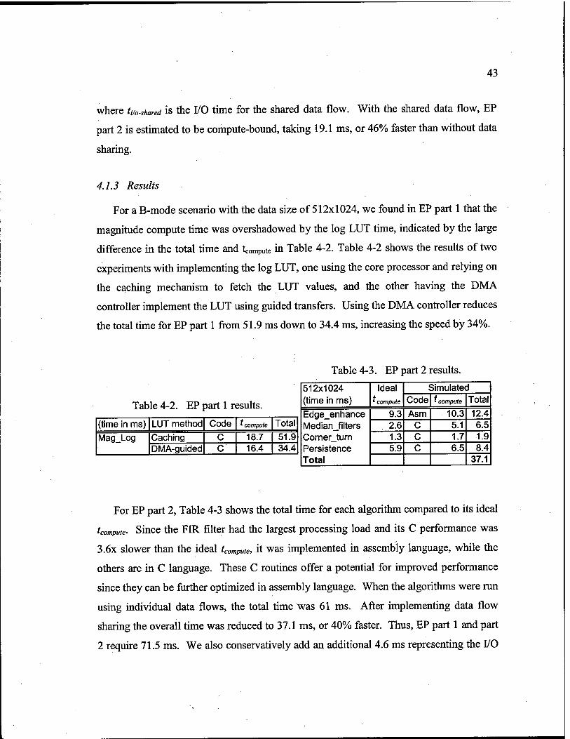
43

where ti/0.shared is the I/O time for the shared data flow. With the shared data flow, EP

part 2 is estimated to be compute-bound, taking 19.1 ms, or 46% faster than without data

sharing.

4.1.3 Results

For a B-mode scenario with the data size of 512x1024, we found in EP part 1 that the

magnitude compute time was overshadowed by the log LUT time, indicated by the large

difference in the total time and Ungute in Table 4-2. Table 4-2 shows the results of two

experiments with implementing the log LUT, one using the core processor and relying on

the caching mechanism to fetch the LUT values, and the other having the DMA

controller implement the LUT using guided transfers. Using the DMA controller reduces

the total time for EP part 1 from 51.9 ms down to 34.4 ms, increasing the speed by 34%.

Table 4-2. EP part 1 results.

Table 4-3. EP part 2 results.

(time in ms) LUT method Code ' compute Total

Mag_Log Caching C 18.7 51.9 DMA-guided C 16.4 34.4

512x1024 Ideal * compute

Simulated (time in ms) Code 'compute Total

Edge enhance 9.3 Asm 10.3 12.4 Median filters 2.6 C 5.1 6.5 Corner turn 1.3 C 1.7 1.9 Persistence 5.9 C 6.5 8.4 Total 37.1

t,

For EP part 2, Table 4-3 shows the total time for each algorithm compared to its ideal

Since the FIR filter had the largest processing load and its C performance was compute-

3.6x slower than the ideal tcompute, it was implemented in assembly language, while the

others are in C language. These C routines offer a potential for improved performance

since they can be further optimized in assembly language. When the algorithms were run

using individual data flows, the total time was 61 ms. After implementing data flow

sharing the overall time was reduced to 37.1 ms, or 40% faster. Thus, EP part 1 and part

2 require 71.5 ms. We also conservatively add an additional 4.6 ms representing the I/O

44

overhead of the next / and Q data frame from the beamformer, which will be arriving

while the current frame is being processed. In total, echo processing stage takes around

76.1 ms, which at 68 fps would require 5.17 MAP 1000s.

4.2 Efficient Color-Flow

4.2.1 Introduction

Although B-mode imaging is useful for observing the spatial relationship between

tissue layers in the body and for monitoring moving structures, such as the heart and

fetus, it cannot be used for visualizing faster motion, such as blood flow. The ability to

visualize and measure the velocity of moving blood cells in the body is important for

many clinical situations, such as detecting the degree of stenosis in a vessel, monitoring

the cardiac cycle, and assessing the blood flow to the fetus. In continuous-wave

ultrasound systems, the velocity can be estimated from the Doppler shift of the

continuously transmitted signal. In pulsed ultrasound systems, the velocity of a sample

volume is estimated from:

^ c-PRF j>_ (4-4)

~2/ccos<9 2K

where c is the velocity of sound in blood, 6 is the Doppler angle, and <f> is the phase

difference between two consecutive pulses (Kasai et al., 1985).

In order to visualize the distribution of flow, the velocity of the blood flow for a

specified region is mapped to a pseudo-color image and overlaid on top of a 2D B-mode

image in real time as shown in Figure 1-2. The magnitude and direction of the velocity

toward and away from the transducer (i.e., axial direction) are displayed as the brightness

of colors, typically red and blue, respectively. This is known as color-flow imaging. Its

main processing steps are wall filtering and velocity estimation.

45

4.2.1.1 Clutter Filtering (Wall Filter)

In addition to the desired signal from the blood scatterers, the received signal contains

clutter noise returned from the surrounding tissue and slowly-moving vessel walls. The

frequency components due to wall motion are low, e.g., < 1 kHz, while the blood motion

frequency is typically around 15 kHz (Ferrara & DeAngelis, 1997). Due to the smooth

structures of the walls, the clutter signal can be much stronger than the scattered signal

from the blood by about 40 dB (Routh, 1996). Many highpass filters have been

developed to remove the unwanted clutter signal. These techniques include stationary

echo canceling, finite impulse response (FIR), infinite impulse response (IIR), and

regression filters (Jensen, 1996). Of these techniques, regression filters have shown to

have better performance compared to other techniques (Kadi & Loupas, 1995). These

filters are designed to filter the clutter adaptively by first estimating the clutter frequency

and then using this estimated frequency to filter clutter noise.

Regression wall filters treat their inputs as polynomial functions in time domain and

operate on the assumption that the slowly-varying clutter component in the Doppler

signal can be approximated by a polynomial of a given order (Hoeks et al., 1991). Once

approximated, this component can then be subtracted from the original signal so that the

contribution from the blood flow can be retrieved and analyzed. Mathematically, it can be

described by

D+l

y(k) = x(k) - Y,aAd k=l,2, ... E ( 4-5 )

where x(k) and y(k) are input and output signals at ensemble k, ad are the regression

model coefficients, D is the regression order. Accurately determining aa requires a

computationally-intensive Vandermonde matrix multiplication (Kadi & Loupas, 1995).

Basoglu (1997) developed a wavelet-based method reducing these computations by 22%

with accuracy similar to normal regression and better than the FIR and IIR techniques.

i_

46

4.2.1.2 Color-Flow Velocity Estimate

The most common method to detect the velocity is to measure the change in phase A^

(equation 4-4) by (a) acquiring multiple vectors along a single scan line with the

transducer stationary and (b) calculate the average change in phase at each range bin

along the scan line (Kasai et al., 1985). Barber et-al. (1985) showed that computing the

first lag of autocorrelation is sufficient to correctly estimate the change in phase </> for

each range bin t:

0(/) = aretanW (4-6)

where

E-\ E-\

and the N and D are respectively the real and imaginary part of the first lag of

autocorrelation, and E is the ensemble size, varying from 6 to 16. In addition, the flow

magnitude, R = ^N2 +D2 , is computed for use later in tissue/flow decision. Color-flow

processing ends similar to echo processing with several filters to reduce noise and add

persistence.

4.2.2 Results

Another graduate student in our laboratory, Ravi Managuli, has been researching the

color-flow processing for this project, and obtained the following results for the scenario

with 6 ensembles, 256 vectors, and 512 samples/vector.

47

Table 4-4. Color flow simulation results when E=6.

256x512x6 (time in ms)

Simulated Code ' compute Total

Corner turn Adaptive wall filter Autocorrelation FIR filter Rect-to-polar Median filters Key hole filters Persistence Total

C 8.4 10.5 Asm/C 51.2 56.3

C 25.9 30.8 C 10.5 12.4 C 8.6 9.2 C 4.5 5.1 C 0.5 0.6 C 3.5 5.1

130.8

4.3 Efficient Scan Conversion for B-mode

In this section, we present an ultrasound scan conversion algorithm that can be

efficiently implemented on mediaprocessors. Efficient implementation of scan

conversion is important as this function utilizes 1/3 of our system's processing load.

Since scan conversion lies in the critical path between the echo/color-flow processing

stage and the image processing stage, it can become a system bottleneck if not

implemented efficiently. We have discovered that when using today's mediaprocessors,

the performance of scan conversion is not limited by their computational ability, but

rather in how the data flow is handled. Therefore, we performed a scan conversion data

flow study comparing using the caching mechanism versus two DMA transfer methods

(2D block transfers versus guided transfers).

4.3.1 Introduction

After the B-mode vector data are acquired and processed, the polar coordinate data

must then be spatially transformed to the geometry and scale of the sector scan on the

Cartesian raster output image through a process known as digital scan conversion (Ophir

& Mackland, 1979). As Figure 4-4 shows, when a sector scan is made using a curvilinear

transducer, each Cartesian raster pixel value P(x,y) must be interpolated from its

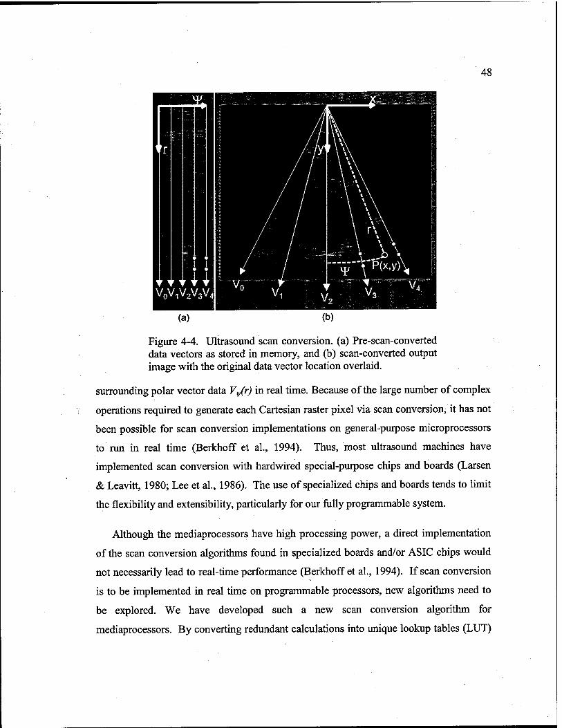
48

Figure 4-4. Ultrasound scan conversion, (a) Pre-scan-converted data vectors as stored in memory, and (b) scan-converted output image with the original data vector location overlaid.

surrounding polar vector data Vy/r) in real time. Because of the large number of complex

operations required to generate each Cartesian raster pixel via scan conversion, it has not

been possible for scan conversion implementations on general-purpose microprocessors

to run in real time (Berkhoff et al., 1994). Thus, most ultrasound machines have

implemented scan conversion with hardwired special-purpose chips and boards (Larsen

& Leavitt, 1980; Lee et al., 1986). The use of specialized chips and boards tends to limit

the flexibility and extensibility, particularly for our fully programmable system.

Although the mediaprocessors have high processing power, a direct implementation

of the scan conversion algorithms found in specialized boards and/or ASIC chips would

not necessarily lead to real-time performance (Berkhoff et al., 1994). If scan conversion

is to be implemented in real time on programmable processors, new algorithms need to

be explored. We have developed such a new scan conversion algorithm for

mediaprocessors. By converting redundant calculations into unique lookup tables (LUT)

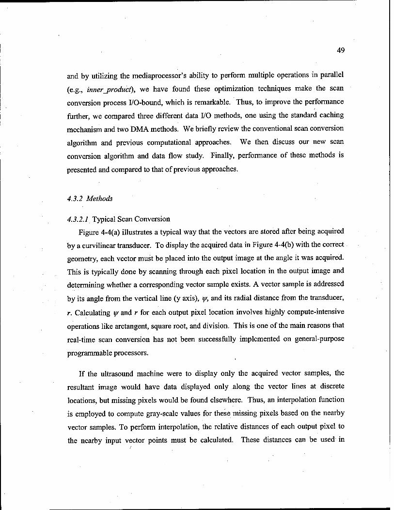
49

and by utilizing the mediaprocessor's ability to perform multiple operations in parallel

(e.g., inner_product), we have found these optimization techniques make the scan

conversion process I/O-bound, which is remarkable. Thus, to improve the performance

further, we compared three different data I/O methods, one using the standard caching

mechanism and two DMA methods. We briefly review the conventional scan conversion

algorithm and previous computational approaches. We then discuss our new scan

conversion algorithm and data flow study. Finally, performance of these methods is

presented and compared to that of previous approaches.

4.3.2 Methods

4.3.2.1 Typical Scan Conversion

Figure 4-4(a) illustrates a typical way that the vectors are stored after being acquired

by a curvilinear transducer. To display the acquired data in Figure 4-4(b) with the correct

geometry, each vector must be placed into the output image at the angle it was acquired.

This is typically done by scanning through each pixel location in the output image and

determining whether a corresponding vector sample exists. A vector sample is addressed

by its angle from the vertical line (y axis), y/, and its radial distance from the transducer,

r. Calculating y/ and r for each output pixel location involves highly compute-intensive

operations like arctangent, square root, and division. This is one of the main reasons that

real-time scan conversion has not been successfully implemented on general-purpose

programmable processors.

If the ultrasound machine were to display only the acquired vector samples, the

resultant image would have data displayed only along the vector lines at discrete

locations, but missing pixels would be found elsewhere. Thus, an interpolation function

is employed to compute gray-scale values for these missing pixels based on the nearby

vector samples. To perform interpolation, the relative distances of each output pixel to

the nearby input vector points must be calculated. These distances can be used in

50

computing a weighted average of the vector samples. Various interpolation functions and

window sizes have been applied in ultrasonic scan conversion (Berkhoff et al., 1994),

such as linear interpolation, cubic spline, sine, or Bessel functions (Parker & Troxel,

1983).

Not every pixel in the output image needs to be interpolated, e.g., the image pixels

that lie outside the sector scan region do not have to be processed. The pixels at such

locations can be set to a background value (blanking) instead of going through the

interpolation process (Zar & Richard, 1993). However, the costly computation of ^and r

must be made for all the pixel locations in the output image including the background

pixels. Furthermore, ^and r must be checked to see if they lie outside their bounds in the

vector space for each output pixel including those active pixels where interpolation is

going to be performed.

4.3.2.2 Our Approach

The key tasks for scan conversion are (a) to calculate the address of the input data

(i.e., a polar conversion, requiring arctan(yfx) and yx2 + y2 ) and the interpolation

coefficient weights for each output pixel P(x, v); (b) to fetch the 8 respective input data

values; and (c) compute the interpolation.

Address Calculation. Basoglu et al. (1996) demonstrated that steps (b) and (c) can

be done in real time on mediaprocessors (TMS320C80), if the computations of step (a)

are precomputed and stored in lookup tables. Figure 4-5(a) shows an example output

image row containing five pixels, and in Figure 4-5(b) the corresponding input data in the

vector storage needed for the interpolation are highlighted. We implement a 4x2

interpolation, thus eight vector samples must be retrieved. However, only one address

must be stored in the input-address LUT per group of eight input pixels. In addition, the

relative offset in the axial direction (ROB=±) and lateral direction (VOB = B+c+D+E)

between the output pixel and its neighboring input vector samples (see Figure 4-6) are

51

also precomputed and stored in a rob-vob LUT for each output pixel. To avoid the

overhead of checking for and interpolating the blank pixels (those outside the sector

scan), an output-address LUT is also used to guide the processor to only compute the

active pixels in the sector. By using these LUTs, the core processor is freed from these

time-consuming computations as well as testing for the blank pixels. Using the double-

buffering techniques discussed in section 3.2.2 , this LUT data are moved on and off chip

in parallel with the core processor performing the interpolation.

Midpoint of Display w, >n v-i

v-i r~ © cs »/"» r— ._ *n v-i -f^^H-o«?^™. Ohm I I I I I I o c;— Nnnt II II II II II II II || II II II II II

/■=11

r=4 M r= 5 is* Bl r=6 .U7 ^

'=8 __| Lv|r

r=io TT Zn r= 11 ■ :» Ml r= 12i r=U

(a) (b)

Figure 4-5. Example address calculation (a) an example output row and (b) the corresponding groups of input pixels needed, illustrating the non- sequential data access required by scan conversion.

Interpolation. Although precalculating the address and offset LUTs reduces the

overall computation significantly, the interpolation is still compute-intensive. However,

it can be efficiently handled using the powerful inner_product instruction on new

mediaprocessors. We implement the interpolation using three inner_product instructions,

by decomposing the 4x2 interpolation into lateral interpolation (two 4x1),

4

Po=yZLiV^'-^ (4-7) /=i

1=1

(4-8)

52

followed by a bilinear axial interpolation (one 1x2),

P{xt y) = (l- ROB)Po + (RQB)Pl (4-9)

where U = f(VOB) are the respective weighting coefficients, such as the Barlett

interpolation filter (Oppenheim & Shaffer, 1989) in Figure 4-7. These filter coefficients

(Li) are stored in a small on-chip LUT (256 bytes), so they can be quickly accessed.

Since this LUT is programmable, other lowpass filters could also be used for the

interpolation. This approach allows us to only store the small 8-bit VOB index in the off-

chip LUTs for each output pixel, which is more efficient than the alternative of storing

the four 16-bit weighting coefficients (Lh L2, L3, L4) for each output pixel (Zar &

Richard, 1993), which is 8 times larger, significantly increasing ti/o.

Figure 4-6. Computing an output pixel value via a 4x2 interpolation with the polar input data.

An alternative interpolation approach is to perform the axial interpolations before the

lateral interpolations (Basoglu et al., 1996), but this requires more multiplications. Also,

since the MAP 1000 can perform a complete 8-tap, 16-bit inner_product instruction, it is

capable of doing the complete 4x2 interpolation in one instruction. However, this would

either require precomputing eight 16-bit coefficients, increasing the off-chip LUTs by 16

and greatly increasing ti/o to load the 8 coefficients, or requires computing in real time the

53

8 coefficients from ROB and Lh which overshadows the advantage of this powerful

inner_product instruction.

>" '*"-*

;/

* ** >. Ixwpass intapdaticn fiter ooeffioenls

0 v» L-l L+\*B-1 2L-1 2L+\CB-1 3L-1 3L+VCB-1 4L-1

Figure 4-7. Extracting the filter coefficients for the lateral interpolation based on the single VOB index.

Fetching the Input Data. The main bottleneck to scan conversion is the step (b)

(fetching the input data) due to the nonlinear relationship between the input and output

pixels. For example, to calculate one row with five output pixels shown in Figure 4-5(a),

the sets of input data needed are stored non-sequentially along an arc in memory as

shown in Figure 4-5(b). Today's SDRAM memory and cache-based architectures are

optimized for sequential memory access, not the random access as needed in Figure

4-5(b), resulting in I/O limiting the overall speed of scan conversion on mediaprocessors.

Hardwired scan conversion boards using expensive SRAM memory do not have this

random access penalty. However, given the constraints of today's SDRAM-based

processors, we had to perform a data flow study to find the most efficient approach to

address this I/O bottleneck, experimenting with the following three methods:

(1) Cache-based: In this method, the core processor uses the precomputed input-

address LUT and directly "loads" the input vector data, which causes the caching

mechanism to bring the data into on-chip memory. Advantages of the cache-based

approach are that it is easy to program and very efficient if the data can be reused

while in the cache before being flushed. However, for large images, the non-

sequential memory access can cause a large number of cache misses.

54

Output pixel group 1

Output pixel group N

Figure 4-8. Example of run-length encoded output lines.

(2) DMA-based guided transfers: Following a method proposed by Basoglu et al.

(1996), the DMA controller is used in the guided transfer mode (see section 4.1.2 ),

such that the DMA controller uses the input-address LUT to directly bring into the

on-chip memory the exact 4x2 group of input pixels for each output pixel, properly

aligned for the inner_product instruction. Since the data are already aligned, this

method has the most efficient computing time tcompute of the three methods, and

double buffering is again used so the core processor works concurrently with the

DMA controller. A disadvantage to using the DMA guided transfers is that memory

is accessed with a small grain size (four 16-bits values) and the data are never reused

after being brought on-chip (e.g., if two neighboring output pixels share the same

group of input vector data, the data will not be shared, but instead brought on-chip

twice). However, when the input data are sparse relative to the output pixels, the

DMA approach does not bring on-chip unused data as the cached-based method

would. For the output-address LUT, a run-length encoded LUT is used to reduce the

LUT size, as shown in Figure 4-8. The output pixels are processed in groups of lines

at a time with each line represented in the LUT by a start address followed by its run-

length (i.e., the number of sequential active pixels in the line), which greatly reduces

the size of the LUT (e.g., 6.1 kbytes), particularly for the longer lines.

55

Input Data Output Image

Figure 4-9. 2D block transfers. Spatial relationship between the output image blocks and the corresponding 2D input data blocks.

(3) DMA-based 2D block transfers: In an attempt to get the advantages of data

reuse of the caching mechanism and the double-buffering advantage of a DMA

approach, a 2D block transfer method can be used, in which the DMA controller is

programmed to bring 2D data blocks on and off chip. The output image is divided

into a series of 2D blocks as shown in Figure 4-9 each containing about 300 pixels.

The output-address LUT is fairly small (7.5 kbytes) and contains the upper-left

corner pixel's address, the block width, and block height for each block. Similarly,

the same information is stored in the input-address LUT for the input data blocks.

The size of the input data blocks will vary greatly due to the polar transformation, as

illustrated in Figure 4-9. Towards the top of the sector scan, the blocks are too large

to fit in the on-chip memory, thus the algorithm adapts in these few cases to use the

simple caching-mechanism instead of the DMA 2D transfers. One advantage of the

DMA-based 2D block transfer method is the data can be reused within the 2D block,

and these 2D blocks allow a larger memory grain size to be used, transferring the

sequential rows of the block efficiently. A disadvantage is that more input data are

brought on-chip than is needed to calculate the output blocks, due to the polar

transform, as shown by the overlapping blocks in Figure 4-9 and by the sparseness of

the data used in Figure 4-5(b). Another disadvantage is that the core processor has a

56

larger processing load as some "blank" pixels are needlessly computed along the

edge of the sector, as shown in the top and bottom block of Figure 4-9, and extra

instructions are needed to properly align the input data for the inner_product

instructions as the data can reside anywhere in the 2D block, unlike in the DMA-

guided method where the input data are automatically aligned.

4.3.3 Results & Discussion

Table 4-5 compares the results of the three scan conversion data flow methods on the

MAP 1000, using the large input and output image sizes proposed for the ultrasound

system. As expected, the DMA-guided transfer method has the best compute time

tcompute- However, the DMA 2D block transfer method (with the worst tcompute) has the

best overall time, 52% faster than the Cache-based method and 36% faster than the

guided method. The DMA 2D block transfer method for handling data flow offers a

good balance of grain-size, data reuse, and double-buffering, combining the benefits of

the other two methods. A lesson we learned is that even though our processor supports

exciting hardware features, such as DMA-guided transfers, we should be careful in

accepting that using these new features is the best approach. We need to take into

account the entire system during algorithm mapping. In this case, using simpler 2D block

transfers that are common to many on-chip DMA controllers provides the best result

Table 4-5. Comparison of the performance of the three scan conversion data flow methods for 16-bit 800x600 output image, a 90-degree sector, and 340x 1024 input vector data.

(time in ms) ^compute Total Time

Cache-Based Transfers 11.8 49.6 DMA Guided Transfers 7.8 37.1 DMA 2D Transfers 12.9 23.8

When a smaller input data set of 40x512 was used on the MAP 1000 to create a 16-bit

512x512, 60-degree sector scan, tcompute was 1.9 ms, and the total time was 4.4 ms (York

57

et al., 1998). Using the same data and image size, Basoglu et al. (1996) used the DMA-

guided transfer on a 50 MHz TMS320C80 getting a total time ranging from 16 ms to 24

ms depending on external memory speed. Berkhoff et al. (1994) implemented several

scan conversion interpolation methods on a programmable SPARC IPX workstation,

finding a computer graphics line drawing algorithm achieved the fastest time of 630 ms

for a 512x512 image. Today's mediaprocessors are clearly faster than general-purpose

processors and fast enough to support real-time video-rate ultrasound scan conversion.

Similar to the log LUT in echo processing, scan conversion is I/O-bound and poses a

challenge for programmable processors using inexpensive SDRAM memory. As a result

of our data flow study and algorithm mapping techniques, we have created an algorithm

on mediaprocessors efficient enough for a real-time ultrasound machine. This DMA 2D

block technique also applies to color-flow scan conversion with a different interpolation

method used for the color data.

4.4 Efficient Scan Conversion for Color-flow Data

In this study, we created a new algorithm for scan converting color-flow data on

mediaprocessors using circular interpolation. Using this different approach, we can

remove the need for 2 transforms, i.e., a polar (RZ(f>) to rectangular (D + jN) and a

rectangular to polar conversion, improving the performance of the system.

4.4.1 Introduction

In color-flow imaging, our velocity estimate is proportional to a change in phase, <j).

Phase is angular data and naturally periodic, as opposed to the scalar B-mode data, thus

the scan converter interpolation must be different. Our color-flow data are in the form of

a complex vector, which can be represented in a rectangular form (D +jN) or polar form

(i?Z^), as shown for vectors Vt and Vi+i in Figure 4-10. Vectors Vt and Vi+] could be

two velocity estimates we are trying to interpolate where Vi+i has aliased over the color

58

boundary (e.g., passing TC from the positive color, red, of V{ to the negative color, blue).

Aliasing often occurs in color-flow imaging (Routh, 1996). The speed of blood is

typically a few centimeters per second, but it can increase to as high as 10 m/s in a

stenotic area (Beach, 1992). For the phase-shift technique, the maximum velocity that can

be measured without aliasing depends on the PRF and center frequency of the transducer,

cPRF v = max

4 fc

(4-10)

While the clinician can increase the PRF (thus the maximum measurable velocity) by

decreasing the imaging depth, aliasing can still occur in the color-flow image. An

example of aliasing can be seen in Figure 1-2 in the carotid artery where it is

predominantly blue-green, then transitions from white to yellow to red. This red is not

reversed blood flow, but instead faster blood flow in the same direction as the blue-green,

but it has aliased over the pseudo-color range.

Figure 4-10. Interpolating color-flow data: RZ(f> versus D +jN

In Figure 4-10, we assume the shortest distance angle between the two vectors is their

correct relationship, which is more probable. However, with extreme turbulent flow the

flow could reverse direction between Vt and Vi+i, making the longer obtuse angle a

possibility (as well as other multiples of 2n due to aliasing). Interpolating Vt and Vi+i in

rectangular form by averaging the N and D components produces the "correct" vector,

59

VCOrrect- However, interpolating in polar form by simply linearly averaging $ and R would

use the longest distance arc and give rise to the "incorrect vector", Vincorrect-

Interpolating in rectangular form (D +jN) uses the same interpolation computation as

in the B-mode scan converter. Thus, a company designing a hardwired ultrasound

machine would be encouraged to reuse any hardwired B-mode scan conversion board

and/or ASICs for color-flow scan conversion in order to save in non-recurring

engineering cost. The cost of reusing this scan converter for color flow is shown in

Figure 4-11(a). The output of the color-flow processing stage is in the polar form (RZfi)

and the input to the final tissue/flow stage also requires the polar form (RZ0). Thus,

extra polar-to-rectangular and rectangular-to-polar conversions are required (taking 17.9

ms for our data size). These image transforms can be avoided if scan conversion can be

done directly in the polar form (RZ<f>), which requires circular interpolation. Circular

interpolation assumes the shortest distance arc between vectors, resulting in the "correct"

vector.

-R-

Polar->Rect

(a) System with linear interpolation

N

D = R cos((/>) N = R sin(<f>)

N-

h-D-

Scan Conversion

Scan Conversion

Rect->Polar

^ = atanl (£) R = ^N2+D2

M- R-

(b) System with circular interpolation

—R-

Scan Conversion

H- R-

Figure 4-11. Extra transforms are needed to use the linear scan converter on color-flow data versus using a special scan converter implementing circular interpolation.

60

In this section, we present an efficient method to implement circular interpolation on

mediaprocessors, reducing the number of transforms required in the system. The

flexibility of programming regular interpolation for the B-mode while programming

circular interpolation for the <|> data is one advantage of a programmable ultrasound

system, which hardwired systems often do not have due to cost considerations.

4.4.2 Methods

One method to compute the circular interpolation for two vectors is to use the

following pseudo-code:

If\<ßi- <th+i\ > x then Iffy < 0 then $ = fa + 2n If<lH+i < 0 then fi+i = ipi+i + 2n

0out = (1-ROB)<IH + (ROB)<IH+,

If(f>0ut > it then

<t>out = faut - 2K

As discussed in section 3.2.2.3, directly implementing this code faces the if/then/else

barrier to efficient processing on mediaprocessors, making it difficult to harness the

power of the partitioned operations and software pipelining due to the individual pixel

tests and branching. In addition, extending this algorithm from 2-tap interpolation to 4x2

interpolation would increase the complexity of this if/then/else style algorithm.

Another approach is based on finding the shortest arc distance. In developing an

angular (circular) median filter, Nikolaidas & Pitas (1998) proposed one method to

calculate the shortest arc distance:

Arcshort =n-\n-\fa -(j>MI (4-11)

However, we greatly reduce this computation using fixed-point arithmetic:

Arcshort=^-<ßM (4-12)

and taking advantage of 2's complement arithmetic's ability to overflow (or wrap around)

the number range (Morris, 1984). This assumes that our measurements for the <|> data are

61

scaled to the full dynamic range of our signed 2's complement number (e.g., with 8-bit

data, maximum red n = Olli 1111 and maximum blue -n = 1000 0000). Then, if we

compute the signed subtraction of two vectors, $ - $+;, ignoring the overflow flag and

use the 8-bit result, we are guaranteed to have the shortest arc distance between the two

vectors (illustrated in Figure 4-12 for 4-bit data). This method produces a signed result

where the sign bit indicates the relative direction of the arc distance. On the other hand,

equation (4-11) produces an unsigned result.

Figure 4-12. Example of shortest arc math, simplified for 4-bit data. The long arc of "13" is too large for signed 4-bit data, resulting in the short arc of "3".

"-6" = 1010

+7 -(-6)

+13

-6 • (7)

-13

0111 0110

lllOl -> -3

t overflow

1010 1001

i|ooii -> 3

t overflow

To utilize the signed shortest arc distance, we need to modify our interpolation

computation. The scalar B-mode 4-tap lateral interpolation has the form:

tout = LA + Liti + A& + LA ( 4-13 )

where the filter coefficients sum to one, i.e., U + L2 + L3 + L4 = 1. The above equation

can be manipulated into the following equivalent form for 4-tap circular interpolation:

where the new filter coefficients are computed from the old coefficients:

Lc~ L4 LB — L3 + L4

(4-14)

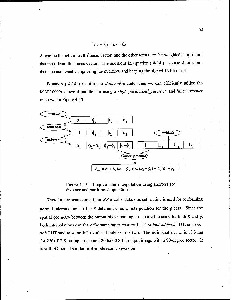
62

LA —L2 + L3 + L4

fa can be thought of as the basis vector, and the other terms are the weighted shortest arc

distances from this basis vector. The additions in equation ( 4-14 ) also use shortest arc

distance mathematics, ignoring the overflow and keeping the signed 16-bit result.

Equation ( 4-14 ) requires no if/then/else code, thus we can efficiently utilize the

MAPlOOO's subword parallelism using a shift, partitionedjsubtract, and inner_product

as shown in Figure 4-13.

^ ♦, <|>2 <t>3 <f>4 C shift »8~~^>

J^ 0 (J), (|>2 ()>3

(^subtract "*}

^ *1 «Mv ^-$2 V"^ T r

1 LA LB Lc

(1nner_produrt^>

ku, = fa + LA(4>2 ~ A) + LB(01 ~ <t>2)+Lc(<f>4 ~ A)

Figure 4-13. 4-tap circular interpolation using shortest arc distance and partitioned operations.

Therefore, to scan convert the RZ.(f> color-data, one subroutine is used for performing

normal interpolation for the R data and circular interpolation for the ^ data. Since the

spatial geometry between the output pixels and input data are the same for both R and $,

both interpolations can share the same input-address LUT, output-address LUT, and rob-

vob LUT saving some I/O overhead between the two. The estimated tcompute is 18.3 ms

for 256x512 8-bit input data and 800x600 8-bit output image with a 90-degree sector. It

is still I/O-bound similar to B-mode scan conversion.

63

4.4.3 Results & Discussion

Table 4-6 compares the results for implementing color scan conversion (</> with

circular interpolation and R with regular interpolation) using the DMA 2D block transfer

method for two different implementations: one with (/> and R processed in separate

subroutines and the other with ^ and R combined into one subroutine tight loop. The

combined tight-loop implementation reduces the total scan conversion time from 47.6 ms

to 36.4 ms as the two could share several LUTs and some data flow.

By using this efficient circular interpolation method and eliminating the external

polar-to-rectangular and rectangular-to-polar transforms, we saved an extra 17.9 ms, or

49% of the scan conversion time.

Table 4-6. Simulation results for color scan conversion, comparing processing ^ and R in separate routines versus in one combined routine.

Color SC (time in ms)

Ideal ' compute

Simulated Code ' compute Total

Seperate 0 and R 19.5 C 26.6 47.6 Combined <j> and R 18.3 C 24.2 36.4

In addition, this circular interpolation method using shortest arc distance can also be

applied to similar filters, such as circular FIR, circular convolution, circular edge

detection and segmentation, etc. These techniques apply not only to our color-flow

application, but to other applications based on angular (circular) data, such as radar and

seismic signal processing, color image processing (e.g., hue data), and estimating wind

direction or moving target direction.

64

4.5 Efficient Frame Interpolation & Tissue/Flow ,

In this section, we present our unique approach of combining frame interpolation and

tissue/flow into one algorithm to reduce the processing time and efficiently implementing

this algorithm on mediaprocessors.

4.5.1 Introduction

Following the creation of the B-mode and color-flow image frames after scan

conversion is the final image processing stage containing the frame interpolation (FI) and

tissue/flow decision (TF) algorithms. If the B-mode and color-flow image frames are

obtained at different frame rates, then frame interpolation can be used to increase the

apparent frame rate of the slower mode. Then, the tissue/flow decision creates the final

output image by properly overlaying the color-flow image on the B-mode image at the

frame rate of the faster mode.

Frame interpolation is illustrated in Figure 4-14 where the slower color frames, C0u

and Cnew, are used to temporally interpolate synthetic frames, Cy to d, in synchronization

with the B-mode frames, Bj to B3. Bilinear interpolation can be used with the weighting

ColdC1

f\

C3 Cnew

Figure 4-14. Frame interpolation.

65

coefficient a = %, where Att is the change in time from C0id to C, and Tc is the period

between the original C frames. The color frame data are in the RZ<f> format, and similar

to scan conversion, the R data require linear interpolation:

Ri=(\-a)RcU+aRmw (4-15)

and the ^ data require circular interpolation:

After frame interpolation, the color-flow and B-mode data are at the same frame rate,

and they can be combined into one output image. The tissue/flow decision algorithm

determines whether a gray-scale B-mode pixel, B(x,y), or a color-flow pixel, <tfx,y),

should be output for each pixel in the color-flow region of interest (ROI). The decision is

based on predetermined thresholds for parameters, such as the B-mode value, the

magnitude and phase of the velocity vector (Boh et al., 1993) and other statistics, such as

the variance or power of the flow (Shariatti et al., 1993). The algorithm we implement is:

IfB(x,y)>Bthreshoidthen

Out(x,y) = B(x,y) Else if\(j)(x,y)\ > threshold andR(x,y) > RthreshoU then

Out(x,y) = <f>(x,y) Else

Out(x,y) = B(x,y)

4.5.2 Methods

Frame interpolation of equations (4-15) and (4-16) can directly utilize the subword

parallelism of the MAP 1000, using the partitioned multiply, add, and subtract

instructions. However, the tissue/flow algorithm above is classically if/then/else-based,

which must be remapped using techniques discussed in 3.2.2.3 to avoid the if/then/else

barrier to efficient subword parallelism. The resulting partitioned algorithm for the

combined frame interpolation and tissue/flow tight loop is shown in Figure 4-15 with the

ideal performance shown in Table 4-7. Since all the if/then/else statements have been

66

removed and all operations implemented using partitioned operations, the algorithm can

be easily software pipelined.

™new

♦old/

♦nl *n2 *n3 *n4

'♦.1 4>o2 *o3 ♦o4

a a a a

B, B2 B3 B4 R- R, R3 R4 w I w I w I w

"thresh Bfhresh Bthresh B(hresh

' ' True False False True

1

elecT>< ♦

♦1 B2 B3 *4

Figure 4-15. Partitioned operations used to implement the combined frame interpolation and tissue/flow tight loop.

A double-buffered data flow (Figure 3-7) using 2D block transfers similar to scan

conversion is used. The respective LUTs are preprogrammed to only move the data

needed within the color-flow ROI, avoiding computation for blank pixels and the B-mode

only regions. As shown in Table 4-7, both frame interpolation and tissue/flow are highly

67

I/O-bound due to the large number of images ($,w, fa*» R0id, Rnew, B, Out) involved with

relatively low processing load. Combining the two algorithms into one function reduces

the I/O load around 33%. However, the function is still I/O-bound.

Table 4-7. Ideal performance for frame interpolation and tissue flow, implemented individually and combined.

800x600 Ideal Performance (time in ms) ' compute tj/0 Max

Frame interpolation Tissue flow Total

0.63 4.58 4.58 1.09 4.58 4.58 1.72 9.16 9.16

Fl & TF combined 2.97 6.10 6.10

4.5.3 Results & Discussion

Frame interpolation and tissue/flow (FI/TF) were implemented in C language.

Simulation results for our scenario with an 800x600 output image with a 90-degree

sector, having approximately 250,000 active pixels in the color-flow ROI, show that the

total time for frame interpolation and tissue implemented individually were 14.1 ms,

while the combined algorithm took 7.96 ms. The combined function is I/O-bound with

the actual tcompute of 3.3 ms or 11% slower than ideal, indicating that the compiler

performs well in software pipelining. •

The Pentium II with MMX supports similar partitioned operations needed for FI/TF

in Figure 4-15. Using a standard C compiler (gcc) with optimizations turned on, we

achieved a performance of 60 ms, which is 7.5 times slower than the MAP1000.' Basoglu

& Kim (1997) implemented tissue/flow decision combined with the velocity computation

(i.e., a rectangular-to-polar conversion instead of frame interpolation) targeted to a 50-

MHz TMS320C80 mediaprocessor. They achieved a total execution time of 16 ms for

304x498 12-bit images (N, D, and B). However, direct comparison of these two

approaches is inappropriate, as rectangular-to-polar conversion (atari and square root)

requires more computation while frame interpolation requires more I/O.

68

4.6 Overall Results of Ultrasound Algorithm Mapping

The results of mapping and simulating the various ultrasound algorithm stages (echo

processing, EP; color flow, CF; scan conversion, SC; frame interpolation, FI and

tissue/flow, TF) for all the specified scenarios from Chapter 2 are shown in Table 4-8.

The estimated number of MAP 1000 processors required for a scenario was calculated by

multiplying the total execution time for a processing stage on a single MAP 1000 (units of

processor*seconds/frame) with the frame rate requirement (frames/second). The total

execution time includes not only the execution time for each stage, but an additional I/O

time (ti/o) due to incoming data frames from the previous processing stage. These

incoming frames are double-buffered. Thus, some of this ti/o may be hidden behind the

computation of the respective stage. However, to be conservative we assume it is not

hidden, slightly inflating the number of processors estimated. On the other hand, the

estimate in Table 4-8 does not account for any overhead that would be experienced in

typical multiprocessor architectures, which includes interprocessor communication

delays, bus traffic and contention between processors. In addition, division of the

processing load across parallel processors can incur additional load if the processing load

can not be evenly balanced between stages (due to different grain size of the procesing

Table 4-8. Estimated number of MAP 1000 processors needed for various scenarios. c

Mode k fps B

fps #C #B

vectors vectors E ROI sector angle

Number of Map1000s EP CF SC/FI/TF Total

B B

color 1 9.0 2 8.4 3 7.8 4 7.3 5 6.9

color 1 22.3 2 19.5 3 17.4 4 15.6

color 68.0

68.0 68.0 9.0 16.8 23.5 29.3 34.5 22.3 39.1 52.1 62.5 68.0

256

256

52

512 340 340

256

256

16

6

6

100%

100%

20%

136 90 90

90

90

5.17 1.42 6.74 3.44 1.73 5.16 0.46 2.42 0.66 3.54 0.85 2.25 0.89 3.99 1.19 2.10 1.10 4.38 1.48 1.97 1.27 4.73 1.74 1.85 1.43 5.03 0.85 2.62 1.61 5.08 1.49 2.29 2.07 5.85 1.98 2.04 2.42 6.44 2.38 1.83 2.70 6.91 2.59 1.62 2.23 6.44

69

tacks) and due to overlapping data between parallel processors being recomputed. The

internal overhead of each MAP 1000 processor can also increase in the multi-processor

architecture as its internal data flow interacts with external data flow, possibly requiring

more internal bus arbitration and SDRAM row miss cycles. The actual loading due to

these effects will be determined during the multiprocessor simulations in section 5.3.

4.7 Discussion

Of the above scenarios, the worst case B-mode and color-mode simulations require

about seven MAP 1000s, with 6.74 and 6.91, respectively. Based on these initial results,

in Chapter 5 we designed our architecture based on eight MAP 1000s, but expandable to

sixteen MAP 1000s. As these simulations were based on our stringent specifications and

most of the functions were implemented in C language, leaving more room for assembly

optimizations, an eight-processor system appears feasible. This will require the

algorithm's processing load to be well-balanced across the multiprocessor system and

sufficient bus bandwidth. The multiprocessor simulations in Chapter 5 will determine

whether the overhead incurred in the multiprocessor environment requires more than

eight processors.

By sharing the data flow between processing stages, we were able to reduce the

overall execution time of echo processing and color-flow processing, making the overall

implementation primarily compute-bound. However, the unique requirements of scan

conversion, frame interpolation, and tissue flow make them I/O-bound. Using our

algorithm mapping techniques from section 3.2.2 , we have created new algorithms and

implementations for:

• Magnitude/log compression: implementing magnitude on the core processor while the DMA performs log LUT using guided transfers

70

Edge enhancement/speckle reduction/persistence: used powerful partitioned operations and inner_product instructions, removing barriers like if/then/else to fully utilize mediaprocessor subword parallelism.

B-mode scan conversion: performed the data flow study to find the optimum data flow approach and reducing redundant computations using a LUT method.

Color scan conversion: developed an efficient circular scan conversion algorithm to eliminate the need for two transformations.

Frame interpolation/tissue flow: combining multiple algorithms reduces some I/O overhead, and removal of the if/then/else barrier efficiently utilizes subword parallelism.

71

Chapter 5: Multi-mediaprocessor Architecture for Ultrasound

Through the algorithm mapping study of Chapter 4, we gained a good understanding

of the processing and data flow requirements for the various ultrasound algorithms.

Based on these results, we present our multi-mediaprocessor architecture for ultrasound

processing in this chapter. To evaluate the performance of this architecture, we

developed a simulation method and models, attempting to preserve accuracy with a

reasonable simulation time. This chapter concludes with the results of our B-mode and

color-mode simulations on this architecture, demonstrating that a fully programmable

ultrasound machine with mediaprocessors is feasible.

5.1 Introduction

While the fine-grained parallelism of VLIW mediaprocessors incorporating

instruction-level parallelism and subword parallelism can efficiently compute our

ultrasound algorithms, we still need multi-mediaprocessors to meet our system

requirements. Designing an efficient parallel architecture depends on two key issues:

(1) Balanced Processing Load. Ideally, the application should be inherently parallel,

such that the processing load can be divided across the system with an equal

processing load for each processor and no idle time. Load balancing is easier for

fine-grained tasks like low-level image processing, but more challenging for our

large-grained ultrasound processing stages of EP, CF, SC, and FI/TF.

(2) Minimizing I/O Overhead. Properly managing the data flow into and out of the

parallel processors is very important. If not, the processors can be underutilized

while waiting for data. In a multiprocessor system, as the number of processors is

increased to decrease tcompute, the I/O overhead typically increases to a point that

72

adding an additional processor can increase the overall execution time (York,

1992).

The parallel processing load can be divided spatially (i.e., each processor does the

same task on different data) or temporally (i.e., each processor is responsible for a J

different processing stage on the same data stream, also known as pipelining). Both

pipelining and spatial parallelism achieve an overall throughput based on the slowest

processing node, thus the need for a balanced system (Patterson & Hennessey, 1994).

Pipelining has the disadvantage of latency or a delay between when the input data are

acquired and when the data are output, which equals to the sum of the processing time for

each pipeline stage. Spatial parallelism has the disadvantage that the processors must

often share overlapping data. Thus, these overlapping data can be processed once by one

processor, then shared with the neighboring processors (increasing tuo) or processed

multiple times by each processor (increasing tcompute)-

Since the advent of microprocessors, parallel processing systems have become more

practical allowing several high performance, low-cost processing nodes to be integrated

on a single board (also known as a cluster) (Patterson & Hennessey, 1994). The short

distance between microprocessors on the boards has allowed higher bandwidth

communications. A variety of multiprocessor systems have been implemented, and they

can be classified by their connection schemes, both between clusters and within the

cluster, as shown in Figure 5-1. The fully-connected topology can offer the most

flexibility, least I/O latency, and highest system bandwidth. This comes at an expensive

cost, increasing by a factor of N*(N-1) where N is the number of processors, requiring

either dedicated ports between processors, as in the symbolic processing array by Weems

et al. (1989) or crossbar switches, such as the Raceway™ architecture (Kuszmaul, 1999).

Other topologies offer a varying trade-off between data flow flexibility and cost, such as

hypercubes (e.g., Proteus System by Haralick et al., 1992), 2D arrays (Weems et al.,

1989) and ring topologies (Duncan, 1990).

73

üüüü D4>M 4 i i 6 Fully connected Cube 2D Array Ring Pipeline Shared Bus

Figure 5-1. Parallel processing topologies.

These large parallel processing systems are not cost-effective for embedded

applications like ultrasound, which do not require the data flow flexibility of these

topologies. For example, for ultrasound tomography, Wiegand & Hoyle (1991) used a

system of 12 transputers connected by serial links to form a flexible 2D array

architecture, but found after algorithm mapping that a parallel architecture with systolic

pipelines was required. Due to difficulty in balancing the processing load, a few

transputers were overloaded, while most of the other transputers were underutilized (I/O

bound) waiting on data from other transputers. For most ultrasound applications, the

ultrasound data flow originates with the transducer on one end and usually terminates at

the output display on the other end with sequential processing stages in between, the

clusters for ultrasound systems tend to be systolic pipelines (Jensch & Ameling, 1988;

Kim et al., 1997). Another practical approach with more flexibility than the pipeline is to

connect the clusters across a shared bus. However, adequate bus bandwidth is required to

prevent bottlenecks and idle processors. For example, Costa et al (1993) developed a

color-flow system by connecting 64 AD2105 DSPs across a shared bus. Even with the

computing power of 64 processors, real-time performance was limited as the processing

time took longer than the acquisition time of the data from the transducer. Combinations

of connection schemes are common, such as a system by Jensen et al. (1996) with 16

AD21060s using a combination of shared bus and direct links between 4 boards where

each board has 4 processors fully connected by both shared memory and communication

links. While data flow was not a problem for this system, they found the AD21060 lacks

the computation power for their ultrasound application.

74

In general, these previous architectures (summarized in Table 1-1 in Chapter 1) were

not designed to handle either the full computing or data flow requirements of ultrasound

processing, which we have to consider in designing a fully programmable ultrasound

architecture. In Chapter 4, eight MAP 1000s were estimated to provide enough

computation power, provided that our architecture can support the proper data flow and

bandwidth and the algorithms are well balanced throughout the system.

5.2 Methods

Our goal in designing the ultrasound architecture is to develop a high performance,

flexible, cost-effective system targeted for the high-end ultrasound market. We define

high performance as meeting the specifications in Chapter 2. We define flexible as ä

reprogrammable system, capable of adapting dynamically to the changing requirements

of different ultrasound modes. To be cost-effective for the high-end ultrasound market,

the architecture must be composed of a reasonable number of processors with a simple

interconnection mechanism, low-cost standardized memory (e.g., SDRAM), and

standardized boards repeated throughout the system.

5.2.1 UWGSP10 Architecture

In this section, we discuss the primary and alternative architectures considered. Also,

various architectural issues are discussed, such as interprocessor communication, system

data flow, bus bandwidth, memory size, and remapping the algorithms to a

multiprocessor architecture.

5.2.1.1 Primary Architectures

Taking advantage of the MAPlOOO's dual PCI buses, our baseline architecture uses

clusters of four MAPlOOOs per board, connected by shared buses, as shown in Figure 5-2.

Similar to systolic architectures, the data flow in from one end (Vector bus) and after

processing flow out the other end (Top/System PCI buses). Thus, this architecture has

75

the flexibility to implement both spatial and pipelined parallel processing, provided that

the shared buses have enough bandwidth.

Bridge (optional level)

.-, board #1 T

Bridge

Host (pentium)

System PCI bus

Top PCI bus additional boards ->

! board #2 T

Bridge

Middle PCI bus t ji Middle PCI bust

MAP1000 #1

MAP1000 #2

MAP1000 #3

MAP1000 #4

MAP1000 #1

MAP1000 #2

MAP1000 #3

MAP1000 #4

1 r^~t f Bottom PCI bus f

Bridge

T_n_TZE__T Bottom PCI bus I

i r i r;

T iL 3 Bridge

(data from beamformer) Vector bus

Figure 5-2. UWGSP10 architecture utilizing 2 PCI ports per MAP 1000 processor.

The host processor (Pentium) is located at the top level. It handles the graphical user

interface and controls up to four standardized boards. The results from Chapter 4

indicate a 2-board system with eight MAP 1000s is feasible for our ultrasound machine.

However, this architecture can be expanded 100% to a four-board system with a total of

16 processors. Each MAP 1000 block in Figure 5-2 includes a MAP 1000 and its local 64

Mbytes of SDRAM. Data vectors flow in from the beamformer through a proprietary

bus. They are relayed by a bridge to the appropriate processor through the bottom PCI

76

bus. The middle PCI bus is used to share data between processors. Through another

bridge, we can transfer the output to either the host processor on the top (or system) PCI

bus. The top PCI bus can interface with the system PCI bus through a bridge to relieve

the fan-out limitation on the system PCI bus or the boards can directly connect to the

system PCI bus (eliminating the need for the top bus and bridge). The system and/or top

PCI buses between the boards are at 33 MHz with either 32-bit or 64-bit width, while the

middle and bottom on-board PCI buses run at 66 MHz at 32 bits.

In case we can use only a single PCI port on the MAP1000, Figure 5-3 shows the

architecture using MAP 1000s utilizing one PCI port. Both the single and dual-PCI port

architectures were simulated in this study.

Top (or System) PCI bus

Vector bus

t board #1 ± 1

Bridge Bridge

Middle PCI Bus

MAP1000 MAP1000 MAP1000 MAP1000"

board #2

additional boards ->

Bridge Bridge

MAP1000

/ii>- "iflv,

MAP1000 MAP1000 MAP1000

Figure 5-3. UWGSP10 architecture utilizing 1 PCI port per MAP 1000 processor.

5.2.1.2 Alternative Architectures

As an alternative to the four-processor board, the top bridge could instead be

implemented by a fifth MAP 1000 as shown in Figure 5-4, adding more computing power

to each board. This would require a trade-off of slowing the top bus by reducing its

width from 64 bits to 32 bits. In addition, this fifth processor would be handicapped in

computing due to the added responsibility of transferring data between the other

processors and the system bus.

77

4 Top (or System) PCI bus "">"= boards ->

board«!

MAP 1000

Middle PCI bus t

* * ♦ * { \ MAP1000

■

MAP10OO

■

MAP 1000 MAP1OO0

+ ♦ t t Bottom PCI bus |

Bridge :, y/ : ':'.■:.:; >y ;\

::~

Vector bus

Bridge \ I * * MAP1000 MAP1000 MAP1000 MAP1000 o

Bridge \ °

I 1 I «< MAP1000 MAP1000 MAP1QO0 MAP1000 3

Bridge \ o

I 1 I O"

MAP1000 MAP1000 MAP1000 MAP1000 c 0)

( \ Bridge

___ i I i

MAP1000 MAP1000 MAP1000 MAP1000

Bridge Bridge Bridge Bridge

t t t t Vector bus

Figure 5-4. Hierarchical architecture with five processors per board.

Figure 5-5. 2D array architecture.

Another alternative is to arrange 16 of the dual-PCI port MAP 1000s in a 2D array as

shown in Figure 5-5. 2D arrays would allow more flexible data transfer between

processors, particularly those from opposite ends of the system (Patterson & Hennessey,

1994). However, the flow of our ultrasound algorithms is more tightly-coupled, and we

do not anticipate needing this flexibility. Furthermore, manufacturing the 2D array in a

scalable fashion is difficult, while still supporting the 66-MHz PCI bus speed. In

addition, 2D arrays technically violate the PCI specification (PCI, 1993) by allowing

multiple paths between processors, creating an ambiguous address map.

5.2.1.3 Interprocessor Communication

For our primary architectures of Figure 5-2 and Figure 5-3, the interprocessor

communication is based on a simple message passing paradigm (Patterson & Hennessey,

1994), in which the destination processor is assumed to be polling certain predefined

memory addresses (either continually or at regular intervals) waiting on a message (32

bytes) from the source. The source processor then sends the message (using a normal

PCI write) to the destination processor's memory. The destination processor then returns

an acknowledge message. In addition, a hardware interrupt mechanism is also available

for more urgent cases, e.g., allowing the host processor to put every processor in a known

78

state during events, such as "booting up" the system and restarting the processing when

the machine switches operating modes. For example, after a processor has been

configured via interrupt for a certain processing stage, e.g., echo processing, it will then

go into a polling mode, checking for a message from the beamformer whether a frame of

vectors has arrived. After the processor receives the message, it responds with an

acknowledgment, and proceeds with processing the vectors.

5.2.1.4 Data Flow between Processors

The incoming data vectors from the beamformer are written from a programmable

DMA controller vector-by-vector onto the vector bus, with a target address for the proper

processor in the system. For those overlapping vectors that are shared between

processors and/or boards, either the beamformer board's DMA controller can rebroadcast

the shared vectors to the second processor/board or the shared vectors can be broadcast

once while the bridges on the processor board detect the proper "window" of vectors for

each processor on the board. The demodulator board's DMA controller is also assumed

to transmit a special 32-byte "end of transfer" message to signal the end of each frame for

each processor's portion of the frame data.

The processing stages (e.g., EP and SC during B-mode) are pipelined and use double-

buffering techniques between stages to increase the throughput, similar to the double

buffering internal to each processor as discussed in section 3.2.2.5. For example, while

the processor is computing the current frame in one memory buffer in its SDRAM, the

next frame is being loaded in another buffer by the earlier processing stage in the

pipeline. Thus, the external frame I/O and the internal processing occur in parallel with

the maximum of the two determining the overall throughput for the stage. The stage with

the slowest throughput determines the frame rate that the system can support.

Pipelining incurs a latency of time between data acquisition and when the first frame

is displayed. B-mode's two stages result in a latency of two frame periods plus the time

to acquire the frame subsection needed for an EP processor. Color mode has an

79

additional latency when frame interpolation is enabled, as several B-mode frames (e.g., k

in equation 2-2) and the old color frame C0u must be buffered until the next color frame

C„ew arrives.

After the final processing stages (scan conversion and tissue/flow decision), the

output images are sent to the host processor, which performs color map lookup during

color mode and overlays other graphics, such as text, logos, etc.

5.2.1.5 Remapping Algorithms to Multiple Processor Architecture

The ultrasound algorithms mapped to the architecture of an individual MAP 1000 in

Chapter 4 were then mapped to the multiple processor architecture. Since the

performance of parallel processors and systolic pipelines depend on the speed of the

slowest processing stage, balancing the processing load equally across all the processors

in the system is essential for maximum performance. For our system, we need to map a

processing load estimated for about 6.91 processors to an 8-processor system.

We mapped the ultrasound functions across the system in both a spatial-parallel and

temporal-pipelined fashion. The spatial-parallel mapping has an advantage of less latency

than pipelining, while the pipeline has an advantage of not requiring the duplicate

processing of overlapping data as the parallel approach requires. For example, in color

mode we divide the image into four subsections as shown in Figure 5-6 to be processed in

parallel. Due to the lateral 4-tap window of scan conversion and the 3-tap window of

other filters, overlapping vectors must be shared with the other subsections. One option

is to process the overlapping vectors once and then copy the processed vectors to the

neighboring processors. However, this can slow down the neighboring processor,

making it wait on the shared vector. Instead we choose to increase the computation

burden by recomputing the shared vectors, making the pipeline control and data flow

easier.

80

Figure 5-6. Example of division of a sector between four processors, showing the overlapping vectors for a sub-sector #2.

For B-mode, we map the 5.17 processing load for EP to 6 processors (-86%

load/processor) and the 1.42 load for SC to 2 processors (-71% load/processor), which is

fairly well balanced. Thus, the sector data are divided into 6 subsections for EP and only

2 subsections for SC. Figure 5-7 shows the processing assignments per processor on one

board, processing half the image. The gray arrows indicate the data flow pattern. For

example, while the scan converter is processing the first frame (#1) and outputting the

^f Top (or System) PCI bus additional boards ->

board #1

Bridge

MAP 1000 (EP)

MAP1000

(EP)

^rw MAP1000

(EP) MAP 1000

(SC)

^s».*?!/ Bottom PCI bus

Bridge

I Vector bus

Figure 5-7. B-mode algorithm assignments (for one of 2 boards).

81

results across the middle PCI bus to the system bus, the echo processors are processing

the second frame (#2), sending these results to the scan converter also across the middle

bus. Meanwhile, the third frame (#3) is being transmitted across the bottom PCI bus to

the echo processors. The timing of this pipeline is illustrated in the results in Figure 5-13.

For color mode, the initial grouping combining EP/CF (~5 processors) and SC/FI/TF

(~3 processors) functions is not well balanced across the two board architecture, as

shown in Table 5-1. Therefore, the functions are remapped, moving EP2 to the second

stage, implementing EP1/CF and EP2/SC/FI/TF in two pipelined stages. This results in a

well-balanced system, dividing the processing across four image subsections. Table 5-1

also shows the additional overhead due to the overlapping vectors, after mapping to the

8-processor system. The processor assignments for one board (half the image) are shown

in Figure 5-8 with the EP1/CF processors 88% loaded and the EP2/SC/FI/TF processors

90.5% loaded.

Table 5-1. Load balancing of color-mode.

Color-Flow Number of MAPI 000s EP/CF SC/FI/TF total

unbalanced 4.21 2.7 6.91

EP1/CF EP2/SC/FI/TF total balanced with overlap

3.44 3.53 6.97 3.53 3.62 7.15

Top (or System) PCI bus additional boards ->

Bridge

Middle PCI bus t

T~L MAP 1000 (EP1/CF)

MAP iooo (EP1/CF)

•MAP1000' (EP2/SC/ LfJ/TFjJ

Bottom PCI bus f

1VIAP1000' (EP2/SC/ I FI/TR J

Bridge

f Vector bus

Figure 5-8. Color-mode algorithm assignments (for one of 2 boards).

5.2.1.6 Bus Bandwidth

In addition to ensuring that our system can meet the processing requirements, it must

have adequate bus bandwidth to handle the high amount of data flow in ultrasound

82

processing. At first look, the 64-bit PCI bus at 33 MHz and the 32-bit PCI bus at 66

MHz appear to have the same maximum bandwidth (BWmax) of 264 Mbytes/s (MBps).

However, not all of this bandwidth can be used to transfer data, as some bandwidth is

used in overhead cycles. For example, the PCI bus is set to transfer 32 bytes for one

processor before switching to another processor. Each transfer includes one clock cycle

to send address information followed by the cycles needed to send the 32 data bytes (i.e.,

4 cycles for a 64-bit bus and 8 cycles for a 32-bit bus) followed by the spin cycle, needed

between transfers to allow one processor to release the bus (unload signals) while the

next processor begins to load the bus (PCI, 1993) as shown in Figure 5-9. The effective

bandwidth available for data can be estimated from:

BW. data cycles

eff address cycles + data cycles + spin cycles BWm

(5-1)

This estimate does not include any overhead due to bus arbitration, which for the PCI

bus is often hidden. While one processor has been granted the bus and is transferring 32

File View Edit Change Signal Axis Select

Figure 5-9. Detailed PCI Bus Signals, showing an example of 4 processors requesting the bus (PCI_REQl-4; active low signal), and the round robin arbitrator's corresponding bus grants (PCI_GNTl-4; active low signal). The address, data, and spin cycles are labeled on the PPCIADDR (multiplexed address and data) signal.

83

bytes of data, the other processors arbitrate for the next transfer as shown in Figure 5-9.

This estimate also does not factor in back-to-back transfers on the PCI bus, in which the

current processor can send back-to-back transfers avoiding the overhead of the spin

cycles when there is no second processor arbitrating for the bus.

Table 5-2 estimates the amount of bus loading based on the BWej? and the estimated

data bandwidth required (BWreq) for the worst ease B-mode and color-mode scenarios on

the various buses in the dual-PCI bus system. All the buses are expected to have less

Table 5-2. Estimated bandwidth required versus effective bandwidth available for various buses for the worst case scenarios for the dual-PCI bus architecture.

PCI Bus B-mode Color-mode

Clock (MHz)

Width (bits)

BWeff (MBps)

BWreq

(MBps) load BWreq

(MBps) load

Top/System bus 33 32 106 34 31.9% 34 31.9% Top/System bus 33 64 176 34 19.2% 34 19.2% Middle bus 66 32 211 53 24.9% 36 17.3% Bottom bus 66 32 211 73 34.6% 61 29.1%

than a 35% load, indicating that our system sufficient bus throughput (which needs to be

verified during the multiple processor simulations). For the single-PCI architecture, the

load on the middle and bottom buses is to be placed on one bus, resulting in an expected

loading for B-mode of 59.5% and color mode of 46.4%.

5.2.1.7 Memory Map and CINE data

Each MAP 1000 processor can support up to 64 Mbytes of local SDRAM memory for

a total of 512 Mbytes for a 2-board (8-processor) system. Table 5-3 lists the memory

requirement per processor based on the algorithm mapping of B-mode and color mode in

section 5.2.1.5. The frame buffers are double-buffered between processing stages, the

internal buffers are for temporary storage between algorithms, and the cache buffers are

the double buffers used to internally bring data to and from the cache memory.

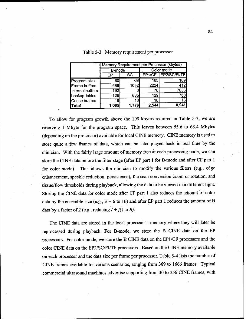
84

Table 5-3. Memory requirement per processor.

Memory Requirement per Processor (kbytes) B-mode Color mode

EP sc EP1/CF EP2/SC/FI/TF

Program size Frame buffers Internal buffers Lookup-tables Cache buffers Total

60 63 105 109 688 1032 2224 412 192 0 70 7636 129 665 129 768

16 16 16 16 1,085 1,776 2,544 8,941

To allow for program growth above the 109 kbytes required in Table 5-3, we are

reserving 1 Mbyte for the program space. This leaves between 55.6 to 63.4 Mbytes

(depending on the processor) available for local CINE memory. CINE memory is used to

store quite a few frames of data, which can be later played back in real time by the

clinician. With the fairly large amount of memory free at each processing node, we can

store the CINE data before the filter stage (after EP part 1 for B-mode and after CF part 1

for color-mode). This allows the clinician to modify the various filters (e.g., edge

enhancement, speckle reduction, persistence), the scan conversion zoom or rotation, and

tissue/flow thresholds during playback, allowing the data to be viewed in a different light.

Storing the CINE data for color mode after CF part 1 also reduces the amount of color

data by the ensemble size (e.g., E = 6 to 16) and after EP part 1 reduces the amount of B

data by a factor of 2 (e.g., reducing / +jQ to B).

The CINE data are stored in the local processor's memory where they will later be

reprocessed during playback. For B-mode, we store the B CINE data on the EP

processors. For color mode, we store the B CINE data on the EP1/CF processors and the

color CINE data on the EP2/SC/FI/TF processors. Based on the CINE memory available

on each processor and the data size per frame per processor, Table 5-4 lists the number of

CINE frames available for various scenarios, ranging from 369 to 1666 frames. Typical

commercial ultrasound machines advertise supporting from 30 to 256 CINE frames, with

85

one high-end machine supporting up to 1024 frames (Siemens, 1997). The number of

CINE frames can be translated into the CINE time (TONE) by

TCINE = min

B C frames ^frames (5-2)

The B-mode CINE ranges from 5.4 to 8.2 seconds for our two scenarios. In

comparison, a high-end commercial ultrasound machine is advertised to support from 2.1

to 30.5 seconds of CINE running at 30 fps for 256 vectors/frame, depending on the

amount of CINE memory purchased (Siemens, 1997). Scaling this to our specification of

68 fps and 512 vectors reduces their CINE range to 0.5 to 6.7 seconds. For color mode,

our CINE time ranges from 6.6 to 38.1 seconds while the commercial ultrasound machine

supports from 2.2 to 17.4 seconds of CINE running at 30 fps for 128 color vectors and

256 B vectors. Scaling this to our specification of 22.3 fps (k = 1) and 256 color vectors

results in a CINE time ranging from 4.4 to 25.6 seconds, compared to our 19.8 seconds

for this scenario. This hardwired commercial machine stores pre-scan-converted CINE

data, thus it can only allow the clinician to modify the scan conversion and tissue/flow

during playback, but not to modify the various filters of EP2 and CF2. The ability of our

programmable system to randomly select the location (relative to the processing stages)

of our CINE data illustrates the flexibility of programmable system, allowing additional

Table 5-4. Number of CINE frames and CINE time supported by the local SDRAM memory in various scenarios.

C B #C #B Mode k fps fps vectors vectors

C frames

B frames

time (s)

B 68.0 512 B 68.0 340

369 5.4 559 8.2

color 1 9.0 9.0 256 340 2 8.4 16.8 3 7.8 23.5 4 7.3 29.3 5 6.9 34.5

421 343 38.1 421 322 19.1 421 316 13.5 421 311 10.6 421 306 8.9

color 1 22.3 22.3 256 256 2 19.5 39.1 3 17.4 52.1 4 15.6 62.5

442 450 19.8 442 422 10.8 442 415 8.0 442 408 6.5

color 1 68.0 68.0 52 256 1666 451 6.6

86

features to be offered to the clinician.

5.2.2 Multiprocessor Simulation Environment

Based on this multi-processor architecture and the mapped ultrasound algorithms, we

developed a simulation method and tools to test whether our system could meet the

design specifications. While the individual function's performance was already assessed

by running single processor simulations, the goal of the multiprocessor simulation is to

evaluate if there is enough bus bandwidth between the processors and what the impact of

the interprocessor communication and bus traffic is on the overall processing

performance.

5.2.2.1 Introduction

The timing of the data flow between processors is key to determining multiprocessor

performance. A common approach is to record the bus level events when running the

application algorithms for each processor in the system (e.g., the detailed timing of all the

reads and writes across the bus, known as address traces). Stunkel et al. (1991) classified

the primary methods of collecting address traces into hardware-captured traces, interrupt-

based traces, instrumented program-based traces, and simulation-based traces. One

challenge for these techniques is not to modify the data flow timing while collecting the

address traces, causing the dilation artifact, i.e., increasing the number of cycles required

for a task due to adding additional instructions to monitor the task (Koldinger et al.,

1991). Hardware-based traces are collected by monitoring the real hardware bus in real

time, which is very accurate. However, the hardware monitors have limited memory,

only allowing a short fragment of execution to be monitored. In interrupt-based traces,

interrupts are programmed to occur after every instruction to store the address trace

information. However, this can cause a severe dilation (lOOx to lOOOx). In the

instrumented program approach, the executable program is modified to store the major

87

events of the basic program blocks, e.g., address parameters for each iteration of the tight

loop, which also leads to dilation.

The above techniques allow fast collection of address traces by running the

application program on real hardware. Since the MAP 1000 chip did not exist for the

majority of this project, we used the simulation-based trace approach, in which the

hardware is modeled in software. Ideally, a simulator capable of simulating the entire

multiprocessor system, including running the actual executable code on each processor in

the simulation, would not require the address trace. However, a software simulator of

this level of complexity is difficult to design and would require an excessively long time

to run the simulation. Instead, using the address traces can significantly reduce the

complexity of the processor model and reduce the simulation time. However, the address

trace files for long simulation times can be extremely large (much larger than the original

executable code), thus methods are needed to reduce the address trace file size within the

memory limits of the simulation workstation.

The software simulation models can be classified by their temporal resolution, e.g.,

sub-nanosecond accurate models, cycle-accurate models, and instruction-accurate models

(Rowson, 94), and by their abstraction level, e.g., behavioral or structural (Kim, 1995).

Structural models mimic the internal logic gates and electrical timing of a device and tend

to be very accurate. This accuracy is necessary for ensuring signal integrity before

fabricating chips and/or manufacturing a circuit board, but it would take too long to

simulate complete applications like an ultrasound system. The behavioral-level models

tend to be cycle-accurate, modeling the device behavior at a higher abstraction via high-

level programming languages or hardware description languages like VHDL. For

multiprocessor simulations, the behavioral model approach combined with address

tracing can lead to reasonable accuracy with a manageable simulation time.

88

5.2.2.2 Simulation Process

In developing our simulation process, our goal is to achieve a cycle-accurate

simulation with reasonable simulation time and manageable address trace file size. In

Chapter 4, we simulated the ultrasound algorithms targeted to a single processor using

Equator's MAP1000 cycle-accurate simulator, CASIM. CASIM is designed to model the

complex interaction between the core processor, the 4-way set-associative data cache

with 4 banks, 2 way set-associative instruction cache, DMA controller, and SDRAM.

CASIM's accuracy is advertised to be +/- 5% of the real hardware, similar to the results

we found in section 5.2.2.4. For our multiprocessor simulation, ideally we would like to

run multiple CASIM simulations for each processor, having the programs dynamically

interact cycle by cycle. However, we cannot use CASIM directly for the multiprocessor

simulation, as it produces static address traces (debug files) instead of allowing dynamic

interaction. In addition, CASIM does not simulate the PCI ports needed for the

multiprocessor simulation. The alternative of creating a complete dynamic simulator of

the MAP 1000 on our own would have been challenging. Furthermore, there is no

guarantee it could be as accurate as CASIM since we do not have access to all the

internal technical design details of the MAP 1000.

Algorithm —► Compiler & Assembler

—* Single

Processor Simulator

fr-

' Debug F ies

Parser

1 Address Trace

VHDL Models

—►

Multi- Processor Simulator

►

Single Processor

Performance

Multiple Processor

Performance

Figure 5-10. Simulation process.

89

Instead, we created a simulation process combining the accuracy of CASIM with the

flexibility of a VHDL simulation environment for multiprocessor architectures. Our

simulation process is shown in Figure 5-10 with the following features to maintain

accuracy while reducing the simulation complexity and time.

(1) The simulation process starts with using the "real" ultrasound algorithms coded

in C and/or assembly language, which are then compiled to generate accurate

MAP 1000 executable code.

(2) The MAPI000's cycle-accurate simulator (CASIM) is then used to generate

detailed instruction and data flow timing information called debug files for each

processor. These debug files have the necessary information for accurate address

trace files (ATF) needed to drive a multiprocessor simulation. CASIM generates

extreme details of data access patterns, as shown in Appendix B, creating a large file.

For example, a simple convolution of a 512x512 image with a 3x3 kernel with 4.5 ms

of execution time creates a 420-Mbyte debug file. If these files are created statically

for our full ultrasound system, they will far exceed our workstation's memory

capacity.

(3) To prevent CASIM's debug files from overflowing our workstation's memory,

we developed sparser program to extract only critical information from the debug

file as it is created during the CASIM simulation before being stored, resulting in a

1200-to-l reduction in the final ATF file size. For example, the convolution final

ATF is around 350 kbytes.

(4) The size of the ATF files is further reduced by limiting data flow we monitor to

the transfers external to the processor/cache model in Figure 3-2, e.g., data flow

between the cache and SDRAM and between the DMA controller and SDRAM

and/or cache, rather than the highly detailed data flow activities between the core

processor and cache. The. data accesses between the core processor and cache (every

90

load and store operation) occur much more frequently and in small grain sizes, which

would lead to creating extremely large ATF files. The corresponding cache read and

write bursts to SDRAM occur less frequently, and can be recorded in a compressed

format (e.g., start address and sequential burst size). An example ATF file for our

processor/cache model is shown below:

an 14 -- no address operation, anop <cycles> rb 80000 4 -- read burst <addressxburst size> wb 90000 4 -- write burst <addressxburst size> is 1 -- issue DMA transfer on <channel #> an 467 -- anop <cycles> wt 1 -- wait on DMA transfer on <channel #>

(5) In addition, the data transfers for the DMA controller can be compressed into a

descriptor with 2D block parameters, such as start address, width, length, etc.,

compared to having an ATF entry for each individual transfer. An example of a

DMA ATF entry for a DMA transfer is shown below:

wl 80000 64 16 448 -- write <address><widthxcountxpitch>

(6) We rely on the accuracy of CASIM to simulate the timing of data accesses

between the core processor and cache, while our VHDL models (discussed in the

next section) have the flexibility to model the cache, DMA, SDRAM, and PCI port

data flow dynamically.

(7) We use a standard simulation environment (by Viewlogic) for simulating VHDL

behavioral models, providing the accuracy and security of a well-established

simulation tool.

(8) The multiprocessor performance is obtained by tracking key signals in the output

timing diagrams. The computation load of each processor is known by the start and

stop times of main computation loops and when the issues and waits on the DMA

occur. In addition, special VHDL models track the PCI bus statistics needed to

determine bus loading, as shown in Figure 5-11.

91

fMlABLE""^.,;" fyi»e. Value

/ADDRESS_C0UNT NATURAL

/ARBITRATE_COI | NATURAL

/DATA_COUNT NATURAL

/DATA_FLAG_BOO BOOLEAN

/GO_BOO BOOLEAN

/IDLE^COUNT NATURAL

/SPIN_COUNT NATURAL

j- 142049

132773

13Q73S7

[TRUE

"%;v,'.;.|lKÖE ■.:.;>/■

1277S516

|11686

Figure 5-11. When the simulation has reached steady state, the PCI arbitrator VHDL model counts each cycle by type (address, data, un-hidden arbitration, spin, and idle) to be used to determine the bus load statistics.

5.2.2.3 VHDL Models

A block diagram of our MAP 1000 VHDL model is shown in Figure 5-12. The model

is composed of a processor core/cache model, DMA channel models, an SDRAM buffer

and controller model, PCI port models, an internal 1MB (I/O-memory bus) bus arbitrator,

and an external PCI bus arbitrator model.

The processor core/cache model runs an ATF file implementing five operations:

read burst (rb), write burst (wb), no-address-operation (an), issue DMA transfer (is), and

wait on DMA transfer (wt). With these five instructions, timing of the data flow with

respect to the processor/cache and the control of the DMA channels can be simulated.

The processor/cache data transfers are loaded into a 4-entry buffer to wait for access to

the 1MB bus.

The MAPlOOO's DMA controller supports 64 independently programmable channels.

In our ultrasound algorithm mapping, we utilize only six channels and simulate these six

channels in our VHDL model to reduce complexity. Channels 0 and 1 are combined for

input data flow from the SDRAM to the processor/cache; channels 2 and 3 are combined

for output data flow from the processor/cache to either the SDRAM or PCI ports; and

92

channels 4 and 5 are used for memory to memory transfers, such as when implementing

the log LUT with guided transfers.

v \ (issues & waits)

PMB i 64 bits @ 200 MHz

I • '" DMA \ (Data Streamer)

Buffer Buffer

Channel 4

IL I Channel 1 5

SDRAM Buffer

SDRAM Controller

64 bits® 100 MHz ^

Figure 5-12. MAP1000 VHDL model.

The SDRAM models follow the specifications assumed by CASIM. The SDRAM

buffer stores up to four data transfers while the SDRAM controller simulates controlling a

2 bank, 2 kbytes per row SDRAM (64 bits at 100 MHz) and refreshes a row in each bank

every 16 microseconds. The dual PCI ports (32 bits at 66 MHz) are modeled with each

port having an 8 entry buffer for input and a 4 entry buffer for output. The PCI Port

models act as agents to talk on PCI bus, while PCI channel models act as agents to talk

on the internal 1MB bus. The PCI arbitrator uses round-robin arbitration, allowing a

fixed 32-byte burst between bus masters. On the 1MB internal bus, the 1MB arbitrator

uses a prioritized round-robin arbitration after 32-byte bursts, giving the highest priority

to the processor/cache model, the next to the PCI channel, and the lowest priority to the

DMA channels.

93

Maintaining the accuracy of the VHDL simulation relative to the original CASM

simulation depends on the timing of the data flow on the MB bus. When the parser

creates the ATF, it guarantees the core processor on the VHDL simulator will repeat (as a

minimum) the number of cycles as the original CASM simulation. Any DMA and cache

data transfers executed out of order in the VHDL simulator compared to the CASIM

simulator can cause additional overhead in terms of extra arbitration cycles and SDRAM

row miss penalties, causing dilation of the original time line. The dilation occurs as the

core processor must stall during read operations to wait on the delayed data, as we do not

know the true data dependencies of the instructions in the ATF, so we must stall,

assuming they are dependent on incoming data. Fortunately, the 1MB arbitrator's

prioritized arbitration scheme reduces some of the dilation by giving the processor/cache

highest priority. The dilation error is always conservative, increasing the estimated

execution time, thus our final estimates for processing load for the system should be

larger than that of the actual hardware.

5.2.2.4 Validation

To validate the accuracy of the VHDL model and parser, we compared their accuracy

to that of CASIM in executing various ultrasound algorithms with the dilation artifact in

% shown in Table 5-5, indicating the VHDL simulator dilates the CASIM simulation by

0.55 to 2.46% for the ultrasound functions.

Table 5-5. Validation results, comparing the accuracy of the VHDL models to that of the CASIM simulator.

Program % error EP SC CF EP1/CF EP2/SC/FIHT

1.24 1.99 0.55 2.46 1.85

The accuracy of our multiprocessor VHDL simulation is highly dependent on the

accuracy of the CASM simulator to generate the proper address trace files. To verify the

94

accuracy of CASIM, we compared its performance to the real MAP 1000 hardware, as

shown in Table 5-6. A positive error indicates when CASIM is conservative (dilation),

while a negative error indicates when CASIM is optimistic. For B-mode and color mode,

the CASIM simulator adds an additional 4.5 to 5.7% dilation (Table 5-6) to the 0.55 to

2.46% dilation of the VHDL simulation in Table 5-5. Thus, we can expect the processing

load in our final simulation results will be conservative.

Table 5-6. Performance of the CASIM simulator versus the real MAP 1000 processor in executing ultrasound algorithms.

Input Output time in ms

simulator hardware % error

EP part 1 EP part 2 CF part 1 CF part 2 B-mode SC B-mode SC Color SC TF+color map

100x1024 100x1024 40x576x6

40x576 40x512

100x1024 40x576 240x320

100x1024 100x1024 40x576 40x576 120x320 320x400 240x320 240x320

7.81 8.51 -8.2% 14.15 13.12 7.9% 24.64 22.03 11.8% 19.66 19.06 3.1% 3.15 2.85 10.5%

19.26 17.83 8.0% 13.20 12.04 9.6% 3.46 4.05 -14.6%

B-mode Total 40x512 100x1024 40x576x6

120x320 320x400 320x400

7.54 7.18 5.1% B-mode Total 41.22 39.46 4.5% Color-mode Total 102.18 96.64 5.7%

The above validation is for the single MAP 1000s, not the complete multi-processor

environment, which can only be verified after the multi-processor hardware is

prototyped. Since CASIM does not simulate the PCI ports, the above simulations do not

verify the accuracy of the VHDL PCI ports and PCI arbitrator. The PCI model was

verified by comparing the output waveforms of the PCI bus with those of the PCI

standard specification (PCI, 1993) as shown in Figure 5-9.

5.3 Results

In this section, we present the multiprocessor simulation results for our worst case B-

mode and color-mode scenarios. We are very interested in determining whether bus

95

bandwidth is adequate for both single and dual-PCI MAP 1000 designs and understanding

the impact on computation load per processor due to bus traffic and interprocessor

communication.

5.3.1 B-mode

Figure 5-13 shows an example timing diagram illustrating the pipelining of the EP

computations on three processors and the SC computations on the fourth processor for

three B-mode frames for board #1. The overlap of the middle PCI bus data flow (PCI

out) for each subframe is also illustrated. Figure 5-13 was derived from Figure A- 1,

which is a plot of the actual simulator display showing the signals used to measure the

beginning and end of the processing for each frame, tcompute, and the time the processor is

waiting for the next frame, twait. Although at times all four processors appear to have

conflicting transfers on the middle PCI bus in Figure 5-13, a "zoomed-in" plot in Figure

A- 2 shows that the actual PCI data transfers are relatively sparse, thus bus conflicts do

not occur as often as Figure 5-13 may imply. Figure A- 3 is a more detailed timing

diagram of the other signals tracked for each processor, such as the data flow for each

channel, showing the transition from EP1 to EP2 and 2D versus guided transfers on the

Bottom PCI Bus|1-1h-2M':=3|-

EP CPU #1

EP CPU #2

2-1 2-2 2-3 3-1 3-2 3-3 i wt compute 1-1

i wt compute 2-1 wt compute 3-1

wt compute 1-2 wt compute 2-2

wt compute 3-2

EP CPU #3 h

SCCPU h

EP PCI OUT #1 h

EPPCIOUT#2l-

EP PCI OUT #3h

wait (wt)

SC PCI OUT h

compute 1-3 wt

wt

out 1-1

out 1-2

out 1-3

compute 2-3 wt

compute 1 wt

out 2-1

out 2-2

out 2-3

outl

compute 3-3

compute 2 wt

out 3-1

out 3-2

out 3-3

out 2

compute 3

out 3

Figure 5-13. Timeline of B-mode simulation (dual-PCI architecture on board #1) illustrating the pipelining of computations on the processors and overlapping of data flow on the PCI bus for 3 frames.

96

EP.

From the timing diagrams, we calculate the processing load for each processor as

follows:

r, • T J compute Processing Load = —-f— /fPS

(5-3)

where the tcompute we measure includes computation time plus any extra overhead due to

incoming data flow from other processors during the processing of one frame. Table 5-7

shows the simulation results for B-mode on for both the architectures (dual-PCI port and

single-PCI port) for the worst case scenario (512x1024 at 68 fps). The processing load is

fairly well-balanced with the EP processors slightly more loaded than the SC processors.

The processing load is about the same for the two architectures, indicating that the single-

PCI port architecture has sufficient bandwidth. The bus load results in Table 5-7 are

defined as

busload — overhead cycles + data cycles

idle cycles + overhead cycles + data cycles (5-4)

where the overhead cycles consist of the spin, address, and any un-hidden arbitration

cycles (defined in section 5.2.1.6), and they are tracked by the VHDL PCI arbitrator over

one complete frame, when all processors are computing and the pipeline has reached

steady-state. In the dual-PCI port architecture, there is sufficient bandwidth available

Table 5-7. B-mode multiprocessor simulation results.

B-Mode Clock (MHz)

Bus width

Dual-PCI bus board

Single-PCI bus board

PROCESSING LOAD EP SC

BUS LOAD System bus System bus Middle bus Bottom bus

200 200

33 33 66 66

32 bits 64 bits 32 bits 32 bits

85.6% 85.7% 76.6% 77.1%

30.2% 30.2% 17.2% 17.2% 29.9% 64.1% 32.4%

97

(-1/3 utilized). In the single-PCI port system, the middle bus is heavily utilized (64%

loaded) and offers less room for growth, but can support the system specifications.

5.3.2 Color Mode ,

Similar timing diagrams for the color-mode simulations are shown in Figure A- 4 and

Figure A- 5, and the performance results are tabulated in Table 5-8 for the worst case

scenario (i.e., B = 62.5 fps and color = 15.6 fps, 256x512 E=6 color data). For color

mode, the PCI buses are even less loaded than B-mode, with sufficient bandwidth for

both the dual-PCI port and single-PCI port architectures. However, the processors are

heavily loaded to about 94% for the worst case. While this is within limits, this would

become risky due to very little room available for error and growth, unless additional

boards are added or the stringent specifications are reduced as discussed in the next

section.

Table 5-8. Color-mode Multiprocessor Simulation Results

Color Mode clock Bus (MHz) Width

Dual-PCI bus board

One PCI bus board

PROCESSING LOAD EP1/CF

EP2/SC/FI/TF BUS LOAD

System bus System bus Middle bus Bottom bus

200 200

33 32 bits 33 64 bits 66 32 bits 66 32 bits

93.2% 93.7% 91.0% 91.1%

30.1% 30.1% 17.3% 17.3% 18.6% 46.1% 27.8%

5.3.3 Refined Specification Analysis

In Chapter 2, our specifications were conservatively estimated based on a dual-beam

system, 20 kHz PRF, and a large vector size with 1024 samples in B-mode and 512

samples in color mode. The vector size was fixed similar to a commercial hardwired

ultrasound machine, always processing the maximum number of samples per vector

98

regardless of whether all the samples contain meaningful data or are sampled more than

the actual axial resolution. At the high 20 kHz PRF specified, the fixed vector size is

overspecified. For example, the axial resolution can be approximated from

Axialresolution = (5-5)

where f0 is the center frequency of the transducer and Q is its quality factor (Christensen,

1996). For B-mode imaging, a broadband signal is used with a typical Q of 2, while for

color imaging using the time-shift velocity estimation technique, a narrow-band signal is

used with a typical Q of 8 (Jensen, 1996). Assuming a 7.5-MHz transducer is used, the

minimum axial resolution for B and color data is 0.1 mm and 0.4 mm, respectively. For

the 20 kHz PRF, the vector depth is ~3 cm, from equation (1-1 ). Thus, if we take one

sample per axial resolution bin, we would need 300 samples per vector for B data and 75

samples per vector for color data, which are much less than our specification of 1024 and

512, respectively.

Table 5-9 shows the impact on processor loading comparing the current oversampled

specification, to two times oversampled axially (2x) and one time oversampled (lx) for

both B-mode and color mode. For the lx case, the processing load reduces down to

-27% for the EP and CF stages, which is directly dependent on the number of data

samples per vector. For the SC processors, the loading is not reduced much since SC is

more dependent on the output image size than the varying input data size. Thus, simply

reducing the number of samples per vector results in an unbalanced processing load. A

more balanced processing load can be achieved as shown in the last entry of Table 5-9.

B-mode can be balanced by dedicating 4 processors for EP (versus 6) and 4 processors

for SC (versus 2), while color mode can be balanced by keeping the same number of

processors for each stage, but moving EP2 and color scan conversion (SCC) from the

second stage to the first. This results in a well-balanced system. The processing load in

99

this case is about 38% for B-mode and 50% for color mode, which are well within our

design goals.

Table 5-9. Impact of reducing the number of 'samples pei ■ vector.

sampling

B samples

per vector

Color samples

per vector

Processor Loading B-mode Color-mode

EP SC EP1/CF EP2/SC/FI/TF

current 1024 512 85.6% 76.6% 93.2% 91.0% 2x 600 150 50.2% 70.2% 54.6% 77.9% 1x 300 75 25.1% 66.8% 27.3% 69.0%

number of processors 6 2 4 4

Balanced Processing Load EP SC 75 | 37.6% | 33.4%~T 1x 300

EP/CF/SCC SCB/FI/TF 46.3% 1 50.0%

number of processors

In addition, reducing the samples per vector to lx increases the number of CINE

frames that can be stored in memory in Table 5-4. For the worst B-mode case, the

maximum CINE time increases from 5.43 seconds to 18.7 seconds, and the worst color-

mode case increases from 6.5 seconds to 22.3 seconds.

5.3.4 Single MAP 1000 Ultrasound Demonstration

Recently, the first MAP 1000 chips have been produced and we have access to a

development board with one MAP 1000. To create a real-time ultrasound demonstration

with only one MAP 1000, a smaller data size was used as shown in Table 5-10. B-mode

on a single MAP 1000 with 100x1024 input data can achieve 25 fps, while adding the

additional color-flow load of 40x576 with E=6 reduces the frame rate to 10 fps. This

data set was taken from a diagnostic ultrasound machine under typical operating

conditions (not worst case). The ability of one MAP 1000 with efficient algorithm

mapping to handle the complete ultrasound processing for these conditions illustrates the

power of today's programmable processors, which has not been possible before.

However, the frame rates achieved for the data sizes in Table 5-10 can keep up with the

beamformer's acquisition frame rate only when the depth is greater than 22 cm or PRF <

100

3500 Hz. This is not fast enough for a high-end ultrasound machine, but one MAP1000

could serve as the ultrasound processor for a low-end machine or specialized device.

Table 5-10. Performance of a single MAP 1000 (actual chip) executing the ultrasound algorithms with reduced specifications.

Input Output time (ms) fps

EP part 1 EP part 2 CF part 1 CF part 2 B-mode SC B-mode SC Color SC TF+color map

100x1024 100x1024 40x576x6 40x576 40x512

100x1024 40x576 240x320

100x1024 100x1024 40x576 40x576 120x320 320x400 240x320 240x320

8.51 13.12 22.03 19.06 2.85

17.83 12.04 4.05

B-mode total 40x512 100x1024 40x576x6

120x320 320x400 320x400

7.18 139.4 25.3 10.3

B-mode total 39.46 Color-mode total 96.64

5.4 Discussion

The simulation results demonstrate a two-board system is capable of supporting both

B-mode and color mode for a high-end ultrasound machine with two remaining board

slots available for future expansion. Simulations of both modes show that there is

adequate bandwidth on the PCI buses and that the single-PCI bus architecture is also

feasible, even though the dual-PCI bus architecture offers more room to grow. The

processing load is our main concern. With our original scenarios, the processors were

between 77% (B-mode) to 94% (color mode) loaded. When the data sampling was

reduced to meet the axial resolution, the load was reduced to 38% (B-mode) to 50%

(color mode). Thus, a reasonable system load lies somewhere between 38 % and 86% for

B-mode and 50% to 94% for color mode, providing a safe margin for the system design.

Even though this proposes reducing the number of samples/vector specification, the

overall system still has challenging specifications, requiring supporting dual beams

(doubling the fps requirement) and a high maximum frame rate of 68 fps, while early

systems supported a display refresh rate of 30 to 50 fps. Furthermore, the load per

101

processor can be further reduced by adding additional boards or by optimizing our C

language functions in assembly language. In addition, the ability of our programmable

system to adapt the samples/vector in the processing stages depending on the situation,

offers an advantage over the hardwired system around which our specifications were

developed, where all subsystems process at the maximum samples/vector regardless of

whether the situation requires this or not.

The impact on one specification, such as samples per vector, highlights an important

lesson learned. Correctly specifying the system requirements is critical, as it determines

the performance of the final system. Incorrect assumptions can lead to an overdesigned

system (e.g., twice the number of boards and processors with higher cost) possibly

making the system noncompetitive on the market or to an underdesigned system failing

to meet the worst case requirements.

For a low-end ultrasound machine, the single MAP 1000 demonstrated surprisingly

good performance in Table 5-10. This indicates a single MAP 1000 can handle the

computation of low-end ultrasound machines supporting only B and M mode, such as the

Medison SA-5500 that uses Pentium processors combined with a hardwired ASIC

(Medison, 1999). For a mid-range ultrasound machine, the processing load values for the

balanced lx specs in Table 5-9 are less than 50% and the bus loading is less than 33 %

for our two board system. Thus, a single board system (i.e., 4 MAPlOOOs) would be too

risky for a high-end ultrasound system, but a one-board system could handle the

requirements of a mid-range ultrasound system. For example, this four MAP 1000 board

has more computing power than the mid-range ATL HDI-1000 ultrasound machine,

which uses a Motorola 68060 (113 MIPS) for scan conversion and two ATT DSP3210

(33 MFLOPS) for Doppler processing (ATL, 1997), thus can handle its reduced

processing requirements.

Regarding CINE loop memory, the 64 Mbytes of SDRAM per MAP 1000 supports

reasonable CINE times between 5.4 to 38.1 seconds (or over 369 CINE frames). In

102

addition, the flexibility of the programmable approach allows additional CINE features

not offered by the hardwired ultrasound machine. Since we can store the CINE loop data

after any stage of processing, we choose to store after EP1 and CF1, allowing all the

filters to be modified by the user during CINE playback, e.g., changing persistence, the

degree of speckle reduction or edge enhancement, zoom or rotation of scan conversion,

and the thresholds for tissue/flow decision.

Regarding bus bandwidth, although we prefer the comfort and extra bandwidth

offered by the dual-PCI port architecture, the single-PCI port architecture can adequately

support the bandwidth. Having only one PCI port would decrease the expense of the

MAP 1000 chip and board, reducing the pin count by at least 52 pins and the number of

high speed (66 MHz) lines needed to be routed on the board.

There are other issues involved in manufacturing this architecture. PCI specifications

limit each PCI board to 25W of power consumption. The MAP 1000 is currently

estimated to consume 6W. With four processors, each with 64 M-Byte SDRAM, plus 2

PCI bridges on the board, the board will require more than 25W. Thus, an additional

power source (and cooling) might be required. The standard PCI long card is 4.2" x

12.3" which may be challenging to fit all the components. Thus, a nonstandard PCI rack

with larger boards may be required. More challenging will be designing the board layout

with four MAP 1000s plus two arbitrators connected across an on-board PCI bus running

at 66 MHz. Systems designed with these high-speed buses must be carefully designed,

modeling the bus as a transmission line, ensuring the bus signals are properly loaded, the

noise between the bus signal's are minimized, and the maximum length between nodes is

short enough for the signals to propagate within this short clock period. Failure to

consider these factors resulted in several early systems targeted for 66 MHz PCI bus only

achieving 40-50 MHz (Needham, 1995).

The estimated cost for this 4-processor board is around $1400, or $2800 for a two-

board system. This programmable system replaces 9 uniquely designed boards totaling

103

over $10,000 in a commercial ultrasound machine. Thus, the programmable approach

not only greatly reduces the system cost, but also can potentially reduce the non-recurring

engineering cost by developing only on one board (repeated throughout the system)

instead of 9 custom boards.

104

Chapter 6: Conclusions and Future Directions

6.1 Conclusions

Modern diagnostic ultrasound machines require over 30 billion operations per second

(BOPS) and have been designed using hardwired boards to achieve the necessary real-

time performance. Though the real-time processing requirements have been met, these

hardwired boards have many disadvantages, such as being inflexible to adapt to new

algorithms. The expense and long lead-time required to modify the hardware can hinder

new innovative ideas from making the transition from the research lab to clinical use.

On the other hand, programmable systems have the flexibility to adapt to changing

requirements. A programmable ultrasound system would ideally require developing one

multiprocessor board and consist of several copies of this board, instead of incurring the

cost of developing many unique single-function boards as in the current systems. In the

current hardwired systems, when a machine is used in B-mode, the color-flow boards sit

idle. In a fully-programmable system, the processors can be reused as a machine

switches modes. For example, the many processors needed to process color-flow image

sequences during scanning can be easily switched to performing 3D rendering during the

visualization phase of 3D imaging. Additionally, the programmable system would

provide a real-time platform to experiment many new ideas, features, and applications.

For example, it may be possible with a fully-programmable architecture to radically

convert an ultrasound system from using phase-shift (autocorrelation) to time-shift

(cross-correlation) velocity estimation without requiring any modifications to the signal

processing hardware. The ease of adapting new algorithms to the programmable system

should not only encourage the research and development of new applications or better

algorithms, but also reduce the time required to bring innovative ideas from the research

105

laboratory into clinical use, providing the clinicians a fast and effective means to enhance

the quality of patient care.

Despite these advantages, an embedded programmable multiprocessor system capable

of meeting all the processing requirements of a modern ultrasound machine has not

emerged yet. Limitations of previous programmable approaches include limited

computing power (Costa et al., 1993; Jensen et al. 1996; Basolgu, 1997; ATL, 1997),

inadequate data flow bandwidth or topology (Jensch & Ameling, 1988), or algorithms not

optimized for the architecture (Berkhoff et al., 1994). This study has addressed the issues

associated with proving the feasibility of a fully programmable ultrasound system not

only by developing the architecture capable of handling the computation and data flow

requirements, but also designing tightly integrated ultrasound algorithms, efficiently

mapping them to the architecture, and demonstrating that the requirements are met

through a unique simulation method.

6.2 Contributions

The major contributions of this research are to the fields of medical ultrasound

imaging and embedded computer architecture design. Overall, the feasibility of a cost-

effective, fully programmable ultrasound machine capable of handling the real-time

processing requirements of a high-end ultrasound machine was demonstrated. To

achieve this, we had to tackle several challenges.

(1) Multiprocessor Architecture for Ultrasound: We designed and demonstrated the

feasibility of a low-cost, high performance multi-mediaprocessor architecture,

targeted for a high-end ultrasound machine. Simulation results showed that both the

computation load and bus load were adequate for both B-mode and color mode for a

2-board system composed of 8 mediaprocessors. We found that the single-PCI port

architecture has adequate bandwidth, allowing the possibility for a less expensive

system than the dual-PCI port architecture. In addition, this multi-processor

106

architecture has demonstrated some of the advantages of a programmable system,

including: (a) hardware reuse: allowing the same processors to be reused in different

ultrasound modes, (b) flexibility and adaptability: allowing CINE loop data to be

stored at an early stage, so that the clinician can change many filter parameters during

CINE playback; allowing different scan conversion algorithms with reduced

computation for B and color data; and allowing algorithms to be quickly swapped,

such as changing the speckle reduction from a proprietary algorithm to a median

filter, (c) scalability: allowing the system to scale from a low to high-end system by

removing or adding boards, (d) cost-effective: using a common board repeated

through the system with low-cost mediaprocessors, standard SDRAM memory and a

standard bus.

(2) Algorithm Mapping Techniques: To achieve ultrasound's high computation

requirement of 31 to 55 BOPS, efficient algorithms that are tightly coupled to the

mediaprocessor architecture are needed to implement the entire system with a

reasonable number of processors. We developed a systematic methodology toward

algorithm mapping including the steps of (a) mapping the algorithm to utilize

subword parallelism, (b) remove barriers to subword parallelism, such as if/then/else

algorithms, (c) utilize software pipelining, (d) avoid redundant computations using

lookup tables, and (e) minimizing I/O via utilizing the DMA controller. These

techniques were developed in collaboration with the UW Image Computing Library

(UWICL) algorithm development team (Stotland et al., 1999; Managuli et al., in

press; York et al., 1999). Following our method of determining the efficiency of

algorithms, we used tcompute and ty0 estimates to optimize the algorithms from a

system perspective, sharing data flow between I/O-bound algorithms and balancing

the load throughout the system.

(3) Ultrasound Algorithm Mapping Studies: Using these algorithm mapping techniques,

several new algorithms and optimized mappings to mediaprocessors have been

developed for ultrasound processing. For echo processing, we found a method to

107

minimize the log lookup table (LUT) bottleneck by implementing the magnitude

computation on the core processor concurrently with the DMA controller performing

the log LUT, increasing the speed by 34% over cache-based methods. For the echo

processing filters (e.g., edge enhancement, speckle reduction, corner turn, and

persistence) we utilized subword parallelism combined with sharing the data flow

between functions, increasing the speed by 40% versus individual functions. For B-

mode scan conversion, we performed a study to find the optimum data flow approach

and used a new 2D block DMA transfer method increasing the speed by 36% over a

DMA guided method (Basoglu et al., 1997), and by 52% over cache-based methods.

For color scan conversion, we developed an efficient circular interpolation using

shortest distance math to eliminate the need for two image transforms, increasing the

speed by 49%. Finally, we combined the frame interpolation and tissue/flow

algorithms and removed barriers to subword parallelism to increase the speed by

another 44%. This work was done in collaboration with Ravi Managuli, a Ph.D.

candidate in EE at the University of Washington, who developed the color-flow

processing and convolution algorithms.

(4) Multiprocessor Simulation Method: To demonstrate that the ultrasound architecture

meets the processing load and bus bandwidth requirements, we developed a unique

multiprocessor simulation environment with a goal of maintaining accuracy while

reducing the simulation time and size of address trace files. This method uses the

accuracy of a cycle-accurate simulator running compiled ultrasound algorithms to

generate address trace files (ATF) for each processor in the system. These ATF files

are used to drive the VHDL mediaprocessor models in our multiprocessor simulation

board. This work was done in collaboration with Ravi Managuli who developed a

key component known as the parser tool.

108

6.3 Future Directions

Having designed and simulated the fully programmable ultrasound architecture and

demonstrated in detail its feasibility, the next step is transitioning the design to an

ultrasound company for implementation inside a commercial ultrasound machine. Areas

of future work include mapping advanced ultrasound applications, developing a graphical

user interface, and staying current with mediaprocessor advances.

6.3.1 Advanced Ultrasound Applications

In this study, our goal was to support the main stream modes (B-mode and color

mode) of a typical high-end diagnostic ultrasound machine. High-end machines are now

beginning to offer more advanced features. For example, the programmable ultrasound

image processor (PUIP) board with two TMS320C80 mediaprocessors is integrated along

with its other hardwired boards in a Siemen's Elegra™ (Kim et al., 1997). These two

processors have been adapted to implement several advanced features, e.g., panoramic

imaging (Weng et al., 1997), segmentation and quantitative imaging (Pathak et al., 1996),

and 3D imaging (Edwards et al., 1998). Our architecture with eight MAPlOOOs has much

more computing power than two TMS320C80s, particularly for algorithms and

applications that usually process after image acquisition when all 8 processors are free,

such as segmentation and 3D volume rendering. Thus, further studies are needed to map

implement these advanced features, as well as develop new features/applications.

For example, 3D reconstruction is often done while acquiring images, thus we need to

determine if 8 processors can handle this extra computation or if another board needs to

be added. Another challenge is to share the 3D volume memory across multiple

processors. Current 3D implementations use smaller volumes, e.g., 128 =2 Mbytes or

2563 = 16 Mbytes (Edwards et al., 1998), which can easily fit in the SDRAM available to

one MAP 1000. However, future volumes of 5123 or 128 Mbytes will not only require the

memory space and processing power of multiple MAPlOOOs, but new algorithms to share

109

volume reconstruction and rendering computations and 3D data across multiple

processors.

6.3.2 Graphical User Interface and Run-Time Executive

To create the final product, a graphical user interface (GUI) needs to be developed for

the host computer, and a real-time operating system is needed for the multiprocessor

architecture. A multi-tasking scheduler is needed to automatically reconfigure and

balance processor load for the system when the clinician changes the mode of operation,

the transducers, or other settings. Our estimates for tcompu,e and ty0 for the various

algorithms can be used as guides for this load balancing routine as they are a function of

the changing data sizes and frame rates.

6.3.3ProcessorSelection

Processor technology advances rapidly. As the MAP 1000 is currently replacing older

mediaprocessors like the TMS320C80, the MAP1000 could soon be replaced by new

mediaprocessors offering better architectures and higher clock speeds. Since the future

mediaprocessors seem to be continuing the trend toward supporting subword parallelism

and DMA controllers, our algorithm mapping techniques and ultrasound algorithm

implementations should be readily remapped to newer processors. A future 500 MHz

mediaprocessor would enable us to reduce our 8-processor system to a single board 4-

processor system. However, processor memory bandwidth usually does not scale with

the increase in computing power with clock speed. As many ultrasound stages are VO-

bound, such as log compression, scan conversion and frame interpolation/tissue-flow, this

4-processor system could fail to meet requirements. Thus, a systematic methodology is

needed to estimate the number of processors required to implement the architecture

composed of new mediaprocessors.

110

Bibliography

Andreadis I, Gasteratos A, Tsalides P. 1996. An ASIC for fast grey-scale dilation.

Microprocessors and Microsystems 20: 89-95.

ATL. 1997. ATL Announces New Breakthrough Product. Advanced Technology

Laboratories, Bothell, WA. http://www.atl.com/news/55_pr_022097.html.

Bamber JC. 1986. Adaptive filters for reduction of speckle in ultrasonic pulse echo

images, Ultrasonics 24:41-4.

Barber WD, Eberhard JW, Karr SG. 1985. A new time domain technique for velocity

measurements using Doppler ultrasound. IEEE Trans. Biomed. Engineering 32:213-

29.

Basoglu C. 1997. A generalized programmable system and efficient algorithms for

ultrasound backend processing. Ph.D. dissertation. University of Washington.

Basoglu C, Gove R, Kojima K, O'Donnell J. 1999. A single-chip processor for media

applications: The MAP 1000. International! Imaging Systems & Technology 10:96-

106.

Basoglu C, Kim Y. 1997. A real-time algorithm for generating color Doppler ultrasound

images. SPIE Medical Imaging 3031:385-96.

Basoglu C, Kim Y, Chalana V. 1996. A real-time scan conversion algorithm on

commercially-available microprocessors. Ultrasonic Imaging 18:241-60.

Basoglu C, Lee W, Kim Y. 1997. An efficient FFT algorithm for superscalar and VLIW

processor architectures. Real-Time Imaging 3:441-53.

Ill

Basoglu C, Managuli R, York G, Kim Y. 1998. Computing requirements of modern

medical diagnostic ultrasound machines. Parallel Computing 24:1407-31.

Beach KW. 1992. 1975-2000: A quarter century of ultrasound technology. Ultrasound

Med.Biol. 18:377-88.

Berkhoff AP, Huisman HJ, Thyssen JM, Jacobs EMG, Homan RJF. 1994. Fast scan

conversion algorithms for displaying ultrasound sector images. Ultrasonic Imaging

16:87-108.

Bohs LN, Friemel BH, McDermott BA, Trahey GE. 1993. A real time system for

quantifying and displaying two-dimensional velocities using ultrasound Ultrasound

Med.Biol 19:751-61.

Boomgaard RV, Baien RV. 1992. Methods for fast morphological image transforms

using bitmapped binary images. Graphical Models and Image Processing 54:252-8.

Bosch JG, van Burken G, Schukking SS, Wolff R, van de Goor AJ, et al.. 1994. Real-

time frame-to-frame automatic contour detection on echocardiograms. Computers in

Cardiology 29-32.

Christensen DA. 1996. Ultrasonic Bioinstrumentation. New York: Wiley.

Christman HA, Smith DR, Weaver BL, Betten WR. 1990. Real-time DSP system for

ultrasonic blood flow measurement. IEEE International Symposium Circuits and

Systems 2045-8.

Costa A, De-Gloria A, Faraboschi P, Olivieri M. 1993. A parallel architecture for the

color Doppler flow technique in ultrasound imaging. Microprocessing and

Microprogramming 38:545-51.

112

Cowan DM, Deane ERI, Robinson TM, Lee JW, Roberts VC. 1995. A transputer based

physiological signal processing system. Part 1—System design. Medical

Engineering and Physics 17: 403 -9.

Czerwinski RN, Jones DL, O'Brien WD. 1995. Ultrasound speckle reduction by

directional median filtering. Proceedings of International Conference on Image

Processing, Los Alamitos, CA, 1:358-61.

Duncan R. 1990. A survey of parallel computer architectures. IEEE Computer Feb., 5-

16.

Dutt V. 1995. Statistical analysis of ultrasound echo envelope, Ph.D. dissertation, The

Mayo Graduate School, Rochester, MN.

Edwards WS, Deforge C, Kim Y. 1998. Interactive three-dimensional ultrasound using

a programmable multimedia processor. International J. Imaging Systems &

Technology 9:442-54.

Evans AN, Nixon MS. 1993. Temporal methods for ultrasound speckle reduction. IEE

Texture Analysis in Radar and Sonar 1:1-6.

Ferrara KW, DeAngelis G. 1997. Color flow mapping. UltrasoundMed. Biol. 23:321-

45.

Fukuda Denshi. 1999. UF-4500. http://www.scantechmedical.com/ultrasou.htm.

Gwennap L. 1994. Architects debate VLIW, single-chip MP. Microprocess. Rep.,

8.12:20-3.

Haralick RM, Somani AK, Wittenbrink C, Johnson R, Cooper K. et al.. 1992. Proteus: a

reconfigurable computational network for computer vision. SPIE Image Processing

and Interchange 1659:554-76.

113

Harvey NR, Marshall S, Matsopoulos G. 1993. Adaptive stack filters towards a design

methodology for morphological filters. IEE Colloqium on Morphological and

Nonlinear Image Processing Techniques, 6:1-4.

Hoeks APG, van de Vorst JJW, Dabekaussen A. 1991. An efficient algorithm to remove

low frequency Doppler signals in digital Doppler systems. Ultrasonic Imaging

13:135-44.

Jensch P, Ameling W. 1988. Analysis of ultrasound image sequences by a data-flow

architecture supporting concurrent processing. SPIE Hybrid Image and Signal

Processing 939:229-36.

Jensen JA. 1996. Estimation of Blood Velocities Using Ultrasound. Cambridge:

Cambridge University Press.

Jensen JL, Jensen JA, Stetson PF, Antonius P. 1996. Multi-processor system for real-

time deconvolution and flow estimation in medical ultrasound. IEEE Ultrason.

Symposium Proc, San Antonio, 2:1197-200.

Kalivas DS, Sawchuck AA. 1990. Motion compensated enhancement of noisy image

sequences./«?. Conf. Acoustics, Speech, and Signal Processing, Albuquerque,

4:2121-4.

Kadi AP, Loupas T. 1995. On the performance of regression and step initialized IIR

clutter filters for color Doppler systems in diagnostical medical ultrasound IEEE

Trans. Ultrason. Ferroelect. Freq. Control 42:927-37.

Kasai C, Namekawa K, Koyano A, Omoto R. 1985. Real-time two-dimensional blood

flow imaging using an autocorrelation technique. IEEE Trans. Sonics and

Ultrasonics 32:458-64.

114

Kim JH. 1995. Towards More Efficient Domain-Specific Image Computing. Ph.D.

Dissertation, University of Washington, Seattle.

Kim Y, Kim JH, Basoglu C, Winter TC. 1997. Programmable ultrasound imaging using

multimedia technologies: A next-generation ultrasound machine. IEEE Trans.

Information Tech. Biomed. 1:19-29.

Klinger JW, Vaughan CL, Fraker TD, Andrews LT. 1988. Segmentation of

echocardiographic images using mathematical morphology. IEEE Trans. Biomedical

Eng. 35:925-34.

Koldinger EJ, Eggers SJ, Levy HM. 1991. On the validity of trace-driven simulation for

multiprocessors, Computer Architecture News 19:244-53.

Kremkau FW, Taylor KJW. 1986. Artifacts in ultrasound imaging. J. Ultrasound Med.

5:227-37.

Kuszmaul, BC. 1999. The RACE Network Architecture. Mercury Computer Systems

Inc., http://www.mc.com/whitepaper_folder/academic.pdf.

Lam M. 1988. Software pipelining: an effective scheduling technique for VLIW

machines. SIGPLAN Conference on Programming Language Design and

Implementation, 318-328.

Larson HG, Leavitt SC. 1980. An image display algorithm for use in real time sector

scanners with digital scan converters. IEEE Ultrasonics Symposium, 763-5.

Lee MH, Kim JH, Park SB. 1986. Analysis of a scan conversion algorithm for algorithm

for a real-time sector scanner. IEEE Trans. Med. Imag. 5:96-105.

Lockwood GR, Turnbull DH, Christopher DA, Foster FS. 1996. Beyond 30 MHz:

Applications of high-frequency ultrasound imaging. IEEE Eng. Med. Biol. 15.6:60-

71.

115

Loupas T, McDicken WN, Anderson T, Allan PL. 1994. Development of an advanced

digital image processor for real-time speckle suppression in routine ultrasonic

scanning. Ultrasound Med. Biol. 20:239-49.

Lowney PG, Freudenberger SM, Karzes TJ, Lichtenstein WD, Nix RP, et al.. 1993. The

multiflow trace scheduling compiler. J. Supercomput. 7:51-142.

LSI. 1989. L64240 Multibit Filter (MFIR). LSI Logic Corporation, Milpitas CA.

Magnin PA, Von Ramm OT, Thurstone FL. 1982. Frequency compounding for speckle

contrast reduction in phased array images. Ultrasonic Imaging 4:267-81.

Managuli R, York G, Stotland I, Kim D, Kim Y. 1999. Mapping of 2D convolution on

VLrW mediaprocessors for real-time performance, Journal of Electronic Imaging,

submitted.

Managuli R, York G, Kim Y. 1999. An efficient convolution algorithm for VLIW

mediaprocessors," SPIE Electronic Imaging, 3655:65-75.

Matsopoulos GK, Marshall S. 1994. Use of morphological image processing techniques

for the measurement of a fetal head from ultrasound images. Pattern Recognition

27.10:1317-24.

Medison. 1999. World's First B/WOnly Digital Ultrasound.

http://www.medison.co.kr/news/news_week_k4.htm.

Mitel Semiconductor. 1997. PDSP16488 single chip convolver with integral line delays,

http: i'/www.mitelsemi. com/products/htm_view. cgi/PDSPl 6488/.

Morris, MM. 1984. Digital Design. Prentice Hall, Englewood Cliffs NJ.

116

Needham HM. 1995. Peripheral component interconnect (PCI) bus for ASIC designers.

Texas Instruments Application's Notes SRGA013, http://www.ti.com/sc/docs/asic

/srga013/sl.htm.

Nikolaidis N, Pitas I. 1998. Nonlinear processing and analysis of angular signals. IEEE

Trans. Signal Processing. 46:3181-94.

Novakov EP. 1991. Online median filter for ultrasound signal processing. Med. & Biol.

Eng. & Comp. 29:222-4.

Ophir J, Makland NF. 1979. Digital scan converters in diagnostic ultrasound imaging.

Proceedings of the IEEE 67:654-64.

Oppenheim AV, Schaffer RW. 1989. Discrete-Time Signal Processing. Prentice-Hall,

Englewood Cliffs, NJ.

Parker JA, Troxel DE. 1983. Comparison of interpolating methods for image resampling.

IEEE Trans. Med. Imag. 2:31-9.

Pasterkamp G, Borst C, Moulaert ASR, Bouma CJ, VanDijk D, et al.. 1995.

Intravascular ultrasound image subtraction: a constrast enhancing technique to

facilitate automatic three-dimensional visualization of the arterial lumen. Ultrasound

Med Biol. 21:913-8.

Pathak SD, Chalana V, Kim Y. 1996. Interactive automatic fetal head measurements

from ultrasound images using multimedia computer technology Ultrasound Med.

Biol. 23:665-73.

Patterson DA, Hennessey JL. 1996. Computer Architecture: A Quantitative Approach.

Morgan Kaufman, San Francisco, CA.

PCI Special Interest Group. 1993. PCI Local Bus Specification, Revision 2.0. Hillsboro,

Oregon.

117

Rosenfield K, Kaufman J, Peiczek M, Langevin RE, Palefski E, et al. 1992. Human

coronary and peripheral arteries: On-line three-dimensional reconstruction from two-

dimensional intravascular US scans. Radiology 184:823-32.

RouthHF. 1996. Doppler ultrasound. IEEE Eng. Med. Bio. 15.6:31-40.

RowsonJ. 1994. Hardware/software co-simulation. Proc. 31st ACM/IEEE Design

Automation Conference 439-40.

Shariati MA, Dripss JH, McDicken WN. 1993. Comparison of color flow imaging

algorithms. Physics in Med. Biol. 38:1589-1600.

Siemens. 1997. SONOLINE? Elegra Ultrasound Imaging System Operating

Instructions. Siemens Medical Systems, Inc., Issaquah, WA.

Stotland I, Kim D, Kim Y. 1999. Image computing library for a VLIW multimedia

processor. SPIE Electronic Imaging 3655: 47-58.

Stunkel CB, Janssens B, Fuchs WK. 1991. Address Tracing for Parallel Machines.

IEEE Computer, 24.1:31-8.

Trahey GE, Allison JW. 1987. Speckle reduction achievable by spatial compounding and

frequency compounding: experimental results and implications for target

detectability. SPIE Pattern Recognition and Acoustical Imaging 768:185-92.

Wells PNT, Ziskin MC. 1980. New techniques and instrumentation in ultrasonography.

Clinics in Diagnostic Ultrasound, Churchill Livingstone, New York, 5:40-68.

Weems CC, Levitan SP, Hanson AR, Riseman EM, SHU DB, et al.. 1989. The image

understanding architecture. Intern. J. Computer Vision 2:251-282.

Weng L, Tirumalia AP, Lowery CM, Nock LF, Gustafson DE, et al.. 1997. Ultrasound

extended-field-of-view imaging technology. Radiology 203 :S77-SO.

118

Wiegand F, Hoyle BS. 1991. Development and implementation of real-time ultrasound

process tomography using a transputer network. Parallel Computing 17:791-807.

York G. 1992. Architecture/Environment Evaluation. Air Force Research Laboratory,

Eglin AFB, FL, DTIC# ADA257849,1992.

York G, Basoglu C, Kim Y. 1998. Real-time ultrasound scan conversion algorithm on

programmable mediaprocessors. SPIE Medical Imaging 3335:252-62.

York G, Kim Y. 1999. Ultrasound processing and computing: Review and future

directions. Chapter in Annual Review ofBiomedical Engineering, in press.

York G, Managuli R, Kim Y. 1999. Fast binary and gray-scale mathematical

morphology on VLIW mediaprocessors. SPIE Electronic Imaging 3645:45-55.

Zar DM, Richard WD. 1993. A scan conversion engine for standard B-mode ultrasonic

imaging. ASEE Annual Conference Proceedings 686-90.

119

APPENDIX A: Timing Diagrams from Multiprocessor

Simulations.

T2 DefaultActSJii

Key "Meltdown' Is unbound

Figure A- 1. Processing load and PCI bus load for the middle bus, for 3 frames of B- mode simulation of the single PCI-port architecture. Signals POPER* show processing on the core processor (indicated by color bars) versus the wait periods (indicated by "08"), as does PFRAMEx with odd numbers indicating the processing time and even numbers indicating the wait periods. On signals P_PCI_OPx, solid bars and "05" indicate the time period a processor or bridge is trying to transfer a frame sub-section on the PCI bus. x = 0 for the bridge (sending vectors); x= 1, 2, or 3 for the EP processors; and x = 4 for the SC processor.

120

P_PC!_OP2

Figure A- 2. Zoomed-in PCI bus load for the middle bus, illustrating the bus conflicts during steady state of the B-mode simulation when all four processors are using the bus. "05" indicates a processor is trying to transfer data a large block of data (e.g., -1024 kbytes). Fortunately, each processor needs to use the bus relatively sparsely, having plenty of time to finish one transfer, before the next one begins.

Figure A- 3. Example signals tracked for EP #3 (x=3) and the SC processors (x=4) during B-mode simulation of 3 frames. POPERJC shows processing on the core processor (indicated by the color bar) versus the waits (indicated by "08"), as does PFRAMEx with odd numbers indicating processing time and even numbers indicating wait periods. P_CH01_OPx indicates the DMA input data flow, while P_CH23_OPx indicates the DMA output data flow. P_CH4_OP3 and P_CH5_OP3 show the DMA guided transfer to implement the LogLUT in EP part 1, while PCH230P3 shows the normal output transfers for EP part 2.

121

If Select 12 DefaultAction OTäSPolirt mptjtip

Figure A- 4. Color-mode simulation signals showing steady-state processing load (P_OPERx and P_FRAMEx) and bus load (P_PCI_OPx), with K=4 (or 4 B frames for every color frame). x= 1 or 2 for EP1/CF processors; x= 3 or 4 for the EP2/SC/FI/TF processors; and x= UB for the bridge on the bottom PCI bus.

L2 DefaultAction

Figure A- 5. Detailed signals for EP1/CF processor #1 and EP2/SC/FI/TF processor #3 during steady-state of color mode simulation with 4 EP frames to every one CF frame.

122

APPENDIX B: Example CASIM Debug File

Example entries from a CASIM debug file

The details of the events tracked cause excessively large files. For example, the total debug file size when simulating convolution of 512x512 image with 3x3 kernel is 420Mbytes. Below are selected entries from an example CASIM debug file, showing key processor, data streamer, and SDRAM events, such as when the processor kicked a DS data transfer (cycle 12931), when the DS receives the transfer parameters (cycle 12947), the SDRAM row miss for the first data (cycle 12991), the RAS and CAS signals (cycles 12994 and 13001), and the data transfers for the first 32 bytes (cycles 13001- 13009). Our parser tool creates the ATF files for our multiple processor simulations by extracting the key information from the CASIM debug file, greatly reducing the file size in the process.

cycle:12931: DS: DSHandle_Kick: #13348 channel 0 kicked off with Descriptor address 0x007fee60

cycle:12947: DS: DSReceiveDesc: descriptor got for channel 0, nextDescAddr 0x7fee60, dataAddr 0xb500, count 0x8, controlWord 0x38, pitch 0x0, width 0x200 PA:0x7fee60

cycle:12991: MB: SDRAMStateMachine: #13414 moving entry from pStage3Mess to pPrecharge ROW_MISS, setting SDRAMBusUsed=TRUE, no other request in SDRAM BA: 0xb500

cycle:12 994: MB: SDRAMStateMachine: #6 moving entry from pP2 to pRAS, setting SDRAMBusUsed=TRUE BA: 0x100

cycle:13001: MB: firstCASCycle: #13414 moving LOAD to CAS, cyclesToGo 3, cyclesToEarlyWarning 5 BA: 0xb500

cycle:13003: MB: dataToFromMemory: #13414 LOADING Data[0]=Oxffffffffffffffff from CasimMemory[0x0000b500]

cycle:13005: MB: dataToFromMemory: #13414 LOADING Data[l]=Oxffffffffffffffff from CasimMemory[0x0000b508]

cycle:13007: MB: dataToFromMemory: #13414 LOADING Data[2]=0xffffffffffffffff from CasimMemory[0x0000b510]

cycle:13009: MB: dataToFromMemory: #13414 LOADING Data[3]=0xffffffffffffffff from CasimMemory[0x0000b518]

123

VITA

George W. P. York

Academic Degrees Ph.D. in Electrical Engineering, University of Washington, 1999

Dissertation: Architecture and Algorithms for a Fully Programmable Ultrasound Machine.

MS in Electrical Engineering, University of Washington, 1988 Thesis: Recognition of Unconstrained Isolated Handwritten Numerals

BS in Electrical Engineering, US Air Force Academy, 1986 r-

Books G. York and Y. Kim, "Ultrasound Processing and Computing: Review and Future

Directions," in Annual Review ofBiomedical Engineering, in press, Fall of 1999.

Journal Papers

R. Managuli, I. Scotland, G. York, D. Kim, and Y. Kim, "Mapping of 2D Convolution on VUW Mediaprocessors for Real-time Performance", SPIE Journal of Electronic Imaging, submitted.

S. F. Barrett, D. J. Pack, G. W. P. York, P. J. Neal, R. D. Fogg, E. Doskocz, S. A. Stefanov, P. C. Neal, C. H. G. Wright, and A. R. Klayton, "Student-centered Educational Tools for the Digital Systems Curriculum," ASEE Computers in Education Journal, Vol. 1, Mar 99.

C. Bosoglu, R. Managuli, G. York, and Y. Kim, "Computing Requirements of Modern Medical Diagnostic Ultrasound Machines," Parallel Computing, Vol. 24, 1998, pp 1407-1431.

D. Pack, S. Stefanov, G. W. P. York, and P. J. Neal, "Constructing a Wall-Follower

J

124

Robot for a Senior Design Project," ASEE Computers in Education Journal, Vol. VII, No. 1,1997.

Conference Papers G. York, R. Managuli, and Y. Kim, "Fast Binary and Gray-scale Mathematical

Morphology on VLIW Mediaprocessors," SPIE Electronic Imaging, Vol. 3645, Jan 1999, pp 45-55.

R. Managuli, G. York, and Y. Kim, "An Efficient Convolution Algorithm for VLIW Mediaprocessors," SPIE Electronic Imaging, Vol. 3655, Jan 1999.

S. F. Barrett, D. J. Pack, G. W. P. York, P. J. Neal, R. D. Fogg, E. Doskocz, S. A. Stefanov, P. C. Neal, C. H. G. Wright, and A. R. Klayton, "Student-centered Educational Tools for the Digital Systems Curriculum," Proceedings of the 1998 ASEE Annual Conference and Exposition, Seattle, WA., June 1998.

G. York, C. Basoglu, and Y. Kim, "Real-Time Ultrasound Scan Conversion on Programmable Mediaprocessors", SPIE Medical Imaging, Vol. 3335, 1998, pp. 252- 262.

P. J. Neal and G. W. P. York, "MC68HC11 Portable Lab Unit - A Flexible Tool for Teaching Microprocessor Concepts," Proceedings of the 1996 ASEE Annual Conference and Exposition, Washington D.C., June 1996.

D. Pack, G W. P. York, P. J. Neal, and S. Stefanov, "Constructing a Wall-Follower Robot for a Senior Design Project," Proceedings of the 1996 ASEE Annual Conference and Exposition, Washington D.C., June 1996.

G. W. P. York and R. D. Fogg, "VISICOMP: The Visible Computer," Proceedings of the 1996 ASEE Annual Conference and Exposition, Washington D.C., June 1996.

G. W. P. York and Jong M. Rhee, "Commercial Implementation of X.400 MHS in a Military Messaging System," Proceedings of the Winter Computer Communication Workshop, Pohang, Korea, 1993.

Technical Reports G. W. P. York, "Military Multimedia Messaging System," Agency for Defense

Development, Taejon, Korea, Jun 1994.

G. W. P. York, "Architecture/Environment Evaluation (RISC)," Air Force Research Laboratory, Eglin AFB, FL, DTIC# ADA257849,1992.

J

125

Professional Experience 1994-96 Instructor, Department of Electrical Engineering, United States Air Force

Academy, Colorado Springs, CO.

1992-94 Researcher, selected for the USAF Engineer/Scientist Exchange Program at the Agency for Defense Development in Taejon, Korea.

1988-92 Program Manager and Project Engineer, designing embedded computer systems for missile systems, USAF Wright Lab, Armament Directorate, Eglin AFB, FL.

Teaching Experience 1995 Microprocessor Interface Design U.S. Air Force Academy 1995-96 Senior Design Project U.S. Air Force Academy 1995-96 Engineering Systems Design U.S. Air Force Academy 1995-96 Introductory Microprocessor Design U.S. Air Force Academy 1994 Electrical Signals and Systems U.S. Air Force Academy 1992-93 Ada Programming Korean Agency for Def. Development 1990 Advanced Microprocessors University of West Florida 1986 Introduction to Digital U.S. Air Force Academy

Professional Society Activities 1997 Tau Beta Pi. Served in MathCounts, a high school math contest, Seattle, WA.

1996 Rocky Mountain Bioengineering Society (RMBS). In charge of local publicity for the 33rd Annual Rocky Mountain Bioengineering Symposium, USAF A, CO, April 1996.

1995 Armed Forces Communications and Electronics Association (AFCEA). In charge of Protocol for the AFCEA Space C4I Conference, USAF A, CO, July 1995.

Academic Awards 1997 17th Annual National VLSI Design Contest, 2nd Place. 1997 Invited to join Tau Beta Pi. 1986-88 Boeing Endowment for Excellence Scholarship. 1986 Distinguished Graduate, USAF A. Graduated 20 out of 962.