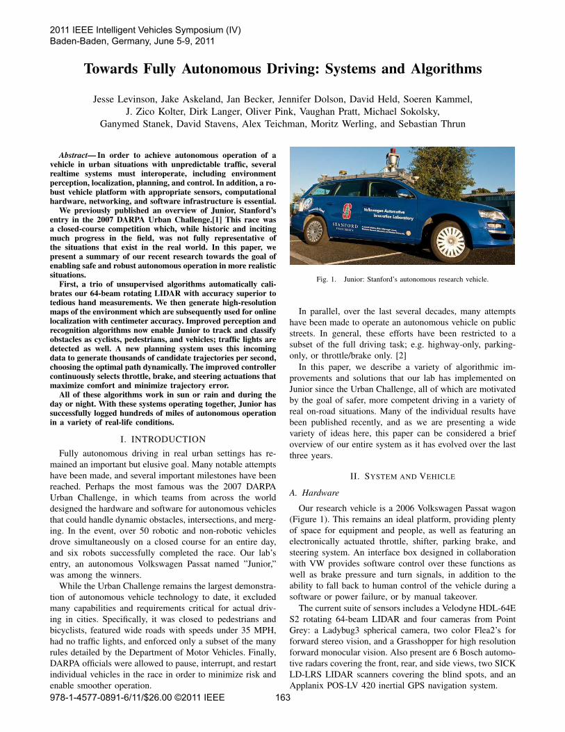
Towards Fully Autonomous Driving: Systems and Algorithms

Jesse Levinson, Jake Askeland, Jan Becker, Jennifer Dolson, David Held, Soeren Kammel,

J. Zico Kolter, Dirk Langer, Oliver Pink, Vaughan Pratt, Michael Sokolsky,

Ganymed Stanek, David Stavens, Alex Teichman, Moritz Werling, and Sebastian Thrun

Abstract— In order to achieve autonomous operation of avehicle in urban situations with unpredictable traffic, severalrealtime systems must interoperate, including environmentperception, localization, planning, and control. In addition, a ro-bust vehicle platform with appropriate sensors, computationalhardware, networking, and software infrastructure is essential.

We previously published an overview of Junior, Stanford’sentry in the 2007 DARPA Urban Challenge.[1] This race wasa closed-course competition which, while historic and incitingmuch progress in the field, was not fully representative ofthe situations that exist in the real world. In this paper, wepresent a summary of our recent research towards the goal ofenabling safe and robust autonomous operation in more realisticsituations.

First, a trio of unsupervised algorithms automatically cali-brates our 64-beam rotating LIDAR with accuracy superior totedious hand measurements. We then generate high-resolutionmaps of the environment which are subsequently used for onlinelocalization with centimeter accuracy. Improved perception andrecognition algorithms now enable Junior to track and classifyobstacles as cyclists, pedestrians, and vehicles; traffic lights aredetected as well. A new planning system uses this incomingdata to generate thousands of candidate trajectories per second,choosing the optimal path dynamically. The improved controllercontinuously selects throttle, brake, and steering actuations thatmaximize comfort and minimize trajectory error.

All of these algorithms work in sun or rain and during theday or night. With these systems operating together, Junior hassuccessfully logged hundreds of miles of autonomous operationin a variety of real-life conditions.

I. INTRODUCTION

Fully autonomous driving in real urban settings has re-

mained an important but elusive goal. Many notable attempts

have been made, and several important milestones have been

reached. Perhaps the most famous was the 2007 DARPA

Urban Challenge, in which teams from across the world

designed the hardware and software for autonomous vehicles

that could handle dynamic obstacles, intersections, and merg-

ing. In the event, over 50 robotic and non-robotic vehicles

drove simultaneously on a closed course for an entire day,

and six robots successfully completed the race. Our lab’s

entry, an autonomous Volkswagen Passat named ”Junior,”

was among the winners.

While the Urban Challenge remains the largest demonstra-

tion of autonomous vehicle technology to date, it excluded

many capabilities and requirements critical for actual driv-

ing in cities. Specifically, it was closed to pedestrians and

bicyclists, featured wide roads with speeds under 35 MPH,

had no traffic lights, and enforced only a subset of the many

rules detailed by the Department of Motor Vehicles. Finally,

DARPA officials were allowed to pause, interrupt, and restart

individual vehicles in the race in order to minimize risk and

enable smoother operation.

Fig. 1. Junior: Stanford’s autonomous research vehicle.

In parallel, over the last several decades, many attempts

have been made to operate an autonomous vehicle on public

streets. In general, these efforts have been restricted to a

subset of the full driving task; e.g. highway-only, parking-

only, or throttle/brake only. [2]

In this paper, we describe a variety of algorithmic im-

provements and solutions that our lab has implemented on

Junior since the Urban Challenge, all of which are motivated

by the goal of safer, more competent driving in a variety of

real on-road situations. Many of the individual results have

been published recently, and as we are presenting a wide

variety of ideas here, this paper can be considered a brief

overview of our entire system as it has evolved over the last

three years.

II. SYSTEM AND VEHICLE

A. Hardware

Our research vehicle is a 2006 Volkswagen Passat wagon

(Figure 1). This remains an ideal platform, providing plenty

of space for equipment and people, as well as featuring an

electronically actuated throttle, shifter, parking brake, and

steering system. An interface box designed in collaboration

with VW provides software control over these functions as

well as brake pressure and turn signals, in addition to the

ability to fall back to human control of the vehicle during a

software or power failure, or by manual takeover.

The current suite of sensors includes a Velodyne HDL-64E

S2 rotating 64-beam LIDAR and four cameras from Point

Grey: a Ladybug3 spherical camera, two color Flea2’s for

forward stereo vision, and a Grasshopper for high resolution

forward monocular vision. Also present are 6 Bosch automo-

tive radars covering the front, rear, and side views, two SICK

LD-LRS LIDAR scanners covering the blind spots, and an

Applanix POS-LV 420 inertial GPS navigation system.

2011 IEEE Intelligent Vehicles Symposium (IV)Baden-Baden, Germany, June 5-9, 2011

978-1-4577-0891-6/11/$26.00 ©2011 IEEE 163

Fig. 2. Unsupervised intrinsic calibration using 10 seconds of data (allscans depicted above). Points colored by surface normal. Even starting withan unrealistically inaccurrate calibration (a) we are still able to achieve avery accurate calibration after optimization (b).

Two on-board Xeon computers running Linux provide

more than enough processing power; a 12-core server runs

our vision and laser algorithms while a 6-core server takes

care of planning, control, and low-level communication.

B. Software

The low-level software system is a modified version of that

used in the 2005 DARPA Grand Challenge and the 2007

Urban Challenge. Individual input, output, and processing

modules run asynchronously, communicating over network

sockets and shared memory. This paper focuses on modules

developed since the Urban Challenge; for a more in-depth

treatment of the initial system, see [1].

Significant changes have been made, primarily to enable

a shift in focus from competition-mode to research. Unlike

in a competition, in which software is expected to recover or

restart no matter what, in a research vehicle deployed in real-

world environments, safety is the primary concern. Thus, a

safety driver is always present behind the wheel, taking over

whenever there is a software issue or unexpected event.

In the sections that follow, we will discuss the various

algorithms and modules that have changed significantly since

our previous report.

III. UNSUPERVISED LASER CALIBRATION

Whereas single-beam sensors can often be calibrated

without great difficulty, deriving an accurate calibration for

lasers with many simultaneous beams has been a tedious and

significantly harder challenge. We have developed a fully

unsupervised approach to multi-beam laser calibration [3],

recovering optimal parameters for each beam’s orientation

and distance response function. Our method allows simulta-

neous calibration of tens or hundreds of beams, each with its

own parameters. In addition, we recover the sensor’s extrinsic

pose relative to the robot’s coordinate frame.

Crucially, our approach requires no specific calibration tar-

get, instead relying only on the weak assumption that points

in space tend to lie on contiguous surfaces. Specifically, we

define an energy function on point clouds which penalizes

points that are far away from surfaces defined by points from

other beams:

J =

B∑

bi=1

bi+N∑

bj=bi−N

∑

k

wk‖ηk · (pk −mk)‖2

where B is the total number of beams and N is the number

of neighboring beams we align each beam to, k iterates over

Fig. 3. The two channels of our probabilistic maps. On the left we seethe average infrared reflectivity, or brightness, of each cell. Our approachis novel in also considering the extent to which the brightness of each cellvaries, as shown on the right.

the points seen by beam bj , pk is the kth point projected

according to the current transform, mk is the closest point

to pk seen by beam bi, ηk is the surface normal at point mk

and wk is 1 or 0 based on whether ‖pk −mk‖ < dmax

For the intrinsic calibration, we aggregate points acquired

across a series of poses, and take derivatives of the energy

function across pairs of beams with respect to individual

parameters. Using an iterative optimization method we arrive

a globally consistent calibration that is more accurate than

the factory calibration, even with an unrealistically bad

initialization (see Figure 2).

For the extrinsic calibration of the LIDAR’s mounting

location on the vehicle, the same energy function is used,

but in this case an iterative application of grid search is

used to discover the optimal 6-DOF sensor pose. Here, we

can recover the position within 1 cm, and the orientation

to within a much finer granularity than can be measured by

hand.

Finally, we also calibrate the intensity remittance return

values for each beam by using Expectation Maximization

to enforce the constraint that beams should roughly agree on

the (unknown) brightness of surfaces in the environment. The

resulting remittance maps are significantly more consistent

after calibration.

IV. MAPPING AND LOCALIZATION

Autonomous vehicle navigation in dynamic urban environ-

ments requires localization accuracy exceeding that available

from GPS-based inertial guidance systems. Although the

Urban Challenge prohibited pre-driving the course, no such

limitation exists in the real world; thus, we use GPS, IMU,

and Velodyne LIDAR data to generate a high-resolution

infrared remittance ground map that can be subsequently

used for localization. [4] For algorithmic and computational

simplicity, our maps are orthographic grid-based projections

of LIDAR remittance returns onto the ground plane.

Our approach yields substantial improvements over pre-

vious work in vehicle localization, including higher preci-

sion, the ability to learn and improve maps over time, and

increased robustness to environment changes and dynamic

obstacles. Specifically, we model the environment, instead

of as a spatial grid of fixed infrared remittance values, as a

probabilistic grid whereby every cell is represented as its own

gaussian distribution over remittance values; see Figure 3.

Subsequently, Bayesian inference is able to preferentially

weight parts of the map most likely to be stationary and of

164

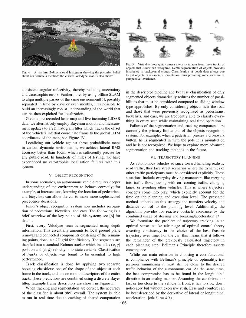
Fig. 4. A realtime 2-dimensional histogram showing the posterior beliefabout our vehicle’s location; the current Velodyne scan is also shown.

consistent angular reflectivity, thereby reducing uncertainty

and catastrophic errors. Furthermore, by using offline SLAM

to align multiple passes of the same environment[5], possibly

separated in time by days or even months, it is possible to

build an increasingly robust understanding of the world that

can be then exploited for localization.

Given a pre-recorded laser map and live incoming LIDAR

data, we alternatively employ Bayesian motion and measure-

ment updates to a 2D histogram filter which tracks the offset

of the vehicle’s intertial coordinate frame to the global UTM

coordinates of the map; see Figure IV.

Localizing our vehicle against these probabilistic maps

in various dynamic environments, we achieve lateral RMS

accuracy better than 10cm, which is sufficiently precise for

any public road. In hundreds of miles of testing, we have

experienced no catostrophic localization failures with this

system.

V. OBJECT RECOGNITION

In some scenarios, an autonomous vehicle requires deeper

understanding of the environment to behave correctly; for

example, at intersections, knowing the location of pedestrians

and bicyclists can allow the car to make more sophisticated

precedence decisions.

Junior’s object recognition system now includes recogni-

tion of pedestrians, bicyclists, and cars. The following is a

brief overview of the key points of this system; see [6] for

details.

First, every Velodyne scan is segmented using depth

information. This essentially amounts to local ground plane

removal and connected components clustering of the remain-

ing points, done in a 2D grid for efficiency. The segments are

then fed into a standard Kalman tracker which includes (x, y)position and (x, y) velocity in its state variable. Classification

of tracks of objects was found to be essential to high

performance.

Track classification is done by applying two separate

boosting classifiers: one of the shape of the object at each

frame in the track, and one on motion descriptors of the entire

track. These predictions are combined using a discrete Bayes

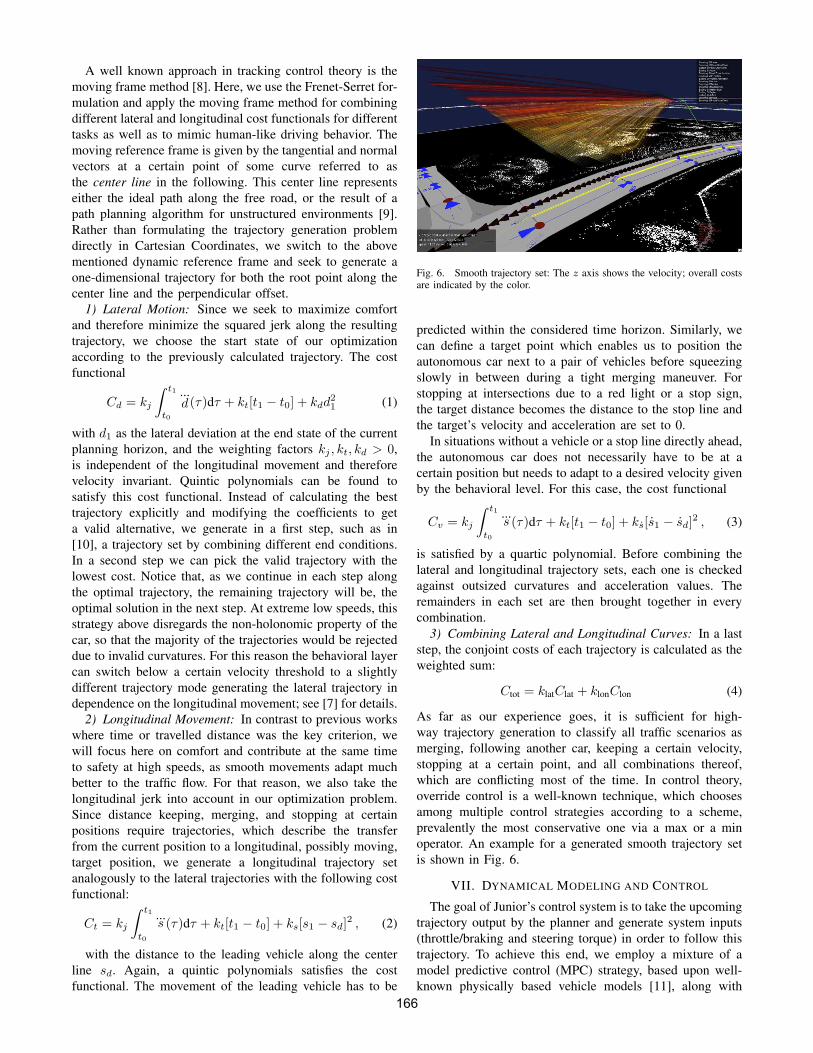
filter. Example frame descriptors are shown in Figure 5.

When tracking and segmentation are correct, the accuracy

of the classifier is about 98% overall. The system is able

to run in real time due to caching of shared computation

Fig. 5. Virtual orthographic camera intensity images from three tracks ofobjects that Junior can recognize. Depth segmentation of objects providesinvariance to background clutter. Classification of depth data allows oneto put objects in a canonical orientation, thus providing some measure ofperspective invariance.

in the descriptor pipeline and because classification of only

segmented objects dramatically reduces the number of possi-

bilities that must be considered compared to sliding window

type approaches. By only considering objects near the road

and those that were previously recognized as pedestrians,

bicyclists, and cars, we are frequently able to classify every-

thing in every scan while maintaining real time operation.

Failures of the segmentation and tracking components are

currently the primary limitations of the objects recognition

system. For example, when a pedestrian presses a crosswalk

button, he is segmented in with the pole it is mounted on

and he is not recognized. We hope to explore more advanced

segmentation and tracking methods in the future.

VI. TRAJECTORY PLANNING

As autonomous vehicles advance toward handling realistic

road traffic, they face street scenarios where the dynamics of

other traffic participants must be considered explicitly. These

situations include everyday driving maneuvers like merging

into traffic flow, passing with on- coming traffic, changing

lanes, or avoiding other vehicles. This is where trajectory

concepts come into play, which explicitly account for the

time on the planning and execution level. The presented

method embarks on this strategy and transfers velocity and

distance control to the planning level. Additionally, the

algorithm provides for reactive obstacle avoidance by the

combined usage of steering and breaking/acceleration [7].

We formulate the problem of trajectory tracking in an

optimal sense to take advantage of optimal control theory

asserting consistency in the choice of the best feasible

trajectory over time. For the car, this means that it follows

the remainder of the previously calculated trajectory in

each planning step. Bellman’s Principle therefore asserts

convergence.

While our main criterion in choosing a cost functional

is compliance with Bellman’s principle of optimality, tra-

jectories minimizing it must still be close to the desired

traffic behavior of the autonomous car. At the same time,

the best compromise has to be found in the longitudinal

direction in an analog manner. Assuming the car drives too

fast or too close to the vehicle in front, it has to slow down

noticeably but without excessive rush. Ease and comfort can

be best described by the derivative of lateral or longitudinal

acceleration: jerk(t) := a(t).

165

A well known approach in tracking control theory is the

moving frame method [8]. Here, we use the Frenet-Serret for-

mulation and apply the moving frame method for combining

different lateral and longitudinal cost functionals for different

tasks as well as to mimic human-like driving behavior. The

moving reference frame is given by the tangential and normal

vectors at a certain point of some curve referred to as

the center line in the following. This center line represents

either the ideal path along the free road, or the result of a

path planning algorithm for unstructured environments [9].

Rather than formulating the trajectory generation problem

directly in Cartesian Coordinates, we switch to the above

mentioned dynamic reference frame and seek to generate a

one-dimensional trajectory for both the root point along the

center line and the perpendicular offset.

1) Lateral Motion: Since we seek to maximize comfort

and therefore minimize the squared jerk along the resulting

trajectory, we choose the start state of our optimization

according to the previously calculated trajectory. The cost

functional

Cd = kj

∫ t1

t0

...d(τ)dτ + kt[t1 − t0] + kdd

21 (1)

with d1 as the lateral deviation at the end state of the current

planning horizon, and the weighting factors kj , kt, kd > 0,

is independent of the longitudinal movement and therefore

velocity invariant. Quintic polynomials can be found to

satisfy this cost functional. Instead of calculating the best

trajectory explicitly and modifying the coefficients to get

a valid alternative, we generate in a first step, such as in

[10], a trajectory set by combining different end conditions.

In a second step we can pick the valid trajectory with the

lowest cost. Notice that, as we continue in each step along

the optimal trajectory, the remaining trajectory will be, the

optimal solution in the next step. At extreme low speeds, this

strategy above disregards the non-holonomic property of the

car, so that the majority of the trajectories would be rejected

due to invalid curvatures. For this reason the behavioral layer

can switch below a certain velocity threshold to a slightly

different trajectory mode generating the lateral trajectory in

dependence on the longitudinal movement; see [7] for details.

2) Longitudinal Movement: In contrast to previous works

where time or travelled distance was the key criterion, we

will focus here on comfort and contribute at the same time

to safety at high speeds, as smooth movements adapt much

better to the traffic flow. For that reason, we also take the

longitudinal jerk into account in our optimization problem.

Since distance keeping, merging, and stopping at certain

positions require trajectories, which describe the transfer

from the current position to a longitudinal, possibly moving,

target position, we generate a longitudinal trajectory set

analogously to the lateral trajectories with the following cost

functional:

Ct = kj

∫ t1

t0

...s (τ)dτ + kt[t1 − t0] + ks[s1 − sd]

2 , (2)

with the distance to the leading vehicle along the center

line sd. Again, a quintic polynomials satisfies the cost

functional. The movement of the leading vehicle has to be

Fig. 6. Smooth trajectory set: The z axis shows the velocity; overall costsare indicated by the color.

predicted within the considered time horizon. Similarly, we

can define a target point which enables us to position the

autonomous car next to a pair of vehicles before squeezing

slowly in between during a tight merging maneuver. For

stopping at intersections due to a red light or a stop sign,

the target distance becomes the distance to the stop line and

the target’s velocity and acceleration are set to 0.

In situations without a vehicle or a stop line directly ahead,

the autonomous car does not necessarily have to be at a

certain position but needs to adapt to a desired velocity given

by the behavioral level. For this case, the cost functional

Cv = kj

∫ t1

t0

...s (τ)dτ + kt[t1 − t0] + ks[s1 − sd]

2 , (3)

is satisfied by a quartic polynomial. Before combining the

lateral and longitudinal trajectory sets, each one is checked

against outsized curvatures and acceleration values. The

remainders in each set are then brought together in every

combination.

3) Combining Lateral and Longitudinal Curves: In a last

step, the conjoint costs of each trajectory is calculated as the

weighted sum:

Ctot = klatClat + klonClon (4)

As far as our experience goes, it is sufficient for high-

way trajectory generation to classify all traffic scenarios as

merging, following another car, keeping a certain velocity,

stopping at a certain point, and all combinations thereof,

which are conflicting most of the time. In control theory,

override control is a well-known technique, which chooses

among multiple control strategies according to a scheme,

prevalently the most conservative one via a max or a min

operator. An example for a generated smooth trajectory set

is shown in Fig. 6.

VII. DYNAMICAL MODELING AND CONTROL

The goal of Junior’s control system is to take the upcoming

trajectory output by the planner and generate system inputs

(throttle/braking and steering torque) in order to follow this

trajectory. To achieve this end, we employ a mixture of a

model predictive control (MPC) strategy, based upon well-

known physically based vehicle models [11], along with

166

feedforward proportional integral derivative (PID) control

for the lower-level feedback control tasks such as applying

torque to achieve a desired wheel angle.

At the higher of these two levels, the car’s state and control

input are described by the vectors x ∈ R7 and u ∈ R

2

x = [x, y, θ, u, v, θ, δ], u = [u, δ] (5)

where x, y, and θ denote the 2D state and orientation, u and

v denote the longitudinal and lateral velocities (aligned with

the car frame), δ denotes the wheel angle, and the dotted

variables represent the corresponding time derivatives. The

equations of motion are given by a bicycle model1

v = tan δ(u− θv) + (Fyf/ cos δ + Fyr)/m− θu

Iθ = ma tan δ(u− θv) + aFyf/ cos δ − bFyr

(6)

where m denotes the car’s mass a and b denote the distancefrom the center of gravity to the front and rear axlesrespectively, I is the moment of inertia, and the lateral tireforces are given via a linear tire model with stiffness C,

Fyf = C

(

tan−1

(

v + θa

u

)

− δ

)

, Fyf = C tan−1

(

v − θb

u

)

.

(7)

Given this system, we interpret a trajectory output by the

planner as a sequence of desired states x⋆1:H for some time

horizon H , and minimize the quadratic cost function

J(u1:H) =

H∑

t=1

(

(xt − x⋆t )

TQ(xt − x⋆t ) + u

Tt Rut

)

(8)

subject to the system dynamics, where Q and R are cost

matrices (chosen to be diagonal, in our case), that specify the

trade-off in errors between the different state components.

We minimize this objective by linearizing the dynamics

around the target trajectory, and applying an algorithm

known as the Linear Quadratic Regulator (LQR) [13] to the

resulting linearized system; this optimization is done in an

online fashion, each time we send a new control command.

Finally, after obtaining controls that approximately mini-

mize this cost function, we integrate the dynamics forward,

leading to a sequence of desired steering angles and veloci-

ties δd1:H , ud1:H (and similarly for their velocities). To achieve

these states we use feedforward PID control, for instance

applying steering torque

τ = kp(δt − δdt ) + kd(δ − δd) + kfff(δdt ) (9)

where kp, kd and kff are the feedback gains, and f(δ) is a

feedforward control tuned for the car.

VIII. TRAFFIC LIGHT DETECTION

Detection of traffic light state is essential for autonomous

driving in urban environments. We have developed a passive

camera-based pipeline for traffic light state detection, using

vehicle localization and assuming prior knowledge of traffic

light location [14]. In order to achieve robust real-time

detection results in a variety of lighting conditions, we

combine several probabilistic stages that explicitly account

1Although not usually written in this form, this is simply the model frome.g. [12] for a front wheel drive car and with the longitudinal forces set towhatever value necessary to achieve u acceleration.

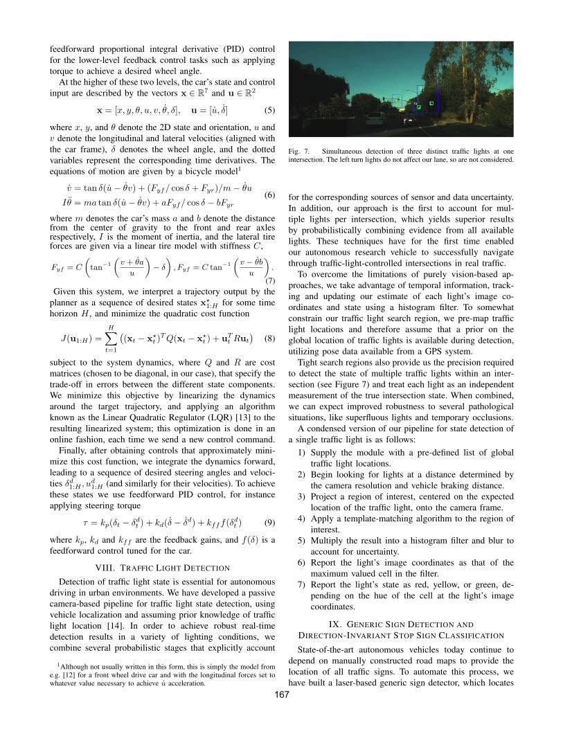
Fig. 7. Simultaneous detection of three distinct traffic lights at oneintersection. The left turn lights do not affect our lane, so are not considered.

for the corresponding sources of sensor and data uncertainty.

In addition, our approach is the first to account for mul-

tiple lights per intersection, which yields superior results

by probabilistically combining evidence from all available

lights. These techniques have for the first time enabled

our autonomous research vehicle to successfully navigate

through traffic-light-controlled intersections in real traffic.

To overcome the limitations of purely vision-based ap-

proaches, we take advantage of temporal information, track-

ing and updating our estimate of each light’s image co-

ordinates and state using a histogram filter. To somewhat

constrain our traffic light search region, we pre-map traffic

light locations and therefore assume that a prior on the

global location of traffic lights is available during detection,

utilizing pose data available from a GPS system.

Tight search regions also provide us the precision required

to detect the state of multiple traffic lights within an inter-

section (see Figure 7) and treat each light as an independent

measurement of the true intersection state. When combined,

we can expect improved robustness to several pathological

situations, like superfluous lights and temporary occlusions.

A condensed version of our pipeline for state detection of

a single traffic light is as follows:

1) Supply the module with a pre-defined list of global

traffic light locations.

2) Begin looking for lights at a distance determined by

the camera resolution and vehicle braking distance.

3) Project a region of interest, centered on the expected

location of the traffic light, onto the camera frame.

4) Apply a template-matching algorithm to the region of

interest.

5) Multiply the result into a histogram filter and blur to

account for uncertainty.

6) Report the light’s image coordinates as that of the

maximum valued cell in the filter.

7) Report the light’s state as red, yellow, or green, de-

pending on the hue of the cell at the light’s image

coordinates.

IX. GENERIC SIGN DETECTION AND

DIRECTION-INVARIANT STOP SIGN CLASSIFICATION

State-of-the-art autonomous vehicles today continue to

depend on manually constructed road maps to provide the

location of all traffic signs. To automate this process, we

have built a laser-based generic sign detector, which locates

167

Fig. 8. Left: Multiple detections for a single sign, before non-maximalsuppression. Center: a single detection for a single sign, after non-maximalsuppression. Right: A single sign detection, re-centered using the weightedaverage of the classification values.

the position and orientation of all signs surrounding the

autonomous vehicle. We have also implemented a direction-

invariant classifier that can distinguish stop signs from non-

stop signs, even when viewed from the back or side, which

can help an autonomous car differentiate from a 2-way stop

vs a 4-way stop.

Given a 3d point cloud, an SVM is trained to detect all

signs of all types around the car. Negative examples are

obtained using feedback retraining in a similar manner to

that in [15]. To compute the features for the SVM, the points

within each square are divided into 0.5 m sections based

on height, referenced by the lowest point in each square.

Features are computed both overall for the square, as well

as separately for each height section. Sign detections are per-

formed using a sliding window detector with a fixed square

size of 1m x 1m, with overlapping grids shifted in 0.25

m increments in all directions. Points from 30 consecutive

frames are accumualated for each classification, to obtain a

fuller representation of each object being classified. After the

signs are classified, a non-maximal suppression algorithm is

run to cluster the sign predictions, using an alternative to

mean shift [16] (see Figure 8). Finally, a weighted voting

method is used to combine classification scores across time

frames to produce a single classification score per location.

We then attempt to determine whether a given sign is a

stop sign in a direction-invariant manner. To do this, we

accumulate points and project them onto a RANSAC plane.

We use Haar-type filters with a sliding window to determine

the differential along the edges of the target sign. Because the

absolute size of the object is known, scaling is not necessary.

Currently we detect signs at 89% precision, which sig-

nificantly reduces the amount of manual effort required to

annotate a map. In related ongoing work, we are exploring

the algorithmic discovery of traffic lights, lane markers,

crosswalks, and street signs so that the manual annotation of

these features in drivable maps may eventually be replaced

automated methods.

X. CONCLUSION

With the previously described realtime algorithms operat-

ing in concert, Junior has been able to drive autonomously

for hundreds of miles in a variety of lighting, weather,

and traffic conditions. Challenges including narrow roads,

crosswalks, and intersections governed by traffic lights are

now manageable. However, it remains necessary for a safety

driver to be present at all times, and we are not yet able

to drive for hours on end without occasionally switching to

manual control due to unexpected events.

As an academic research lab, we have been focusing our

efforts on scientifically interesting challenges with important

practical implications. We consider tasks such as object de-

tection and classification, precision localization and planning

under uncertainty, and automatic calibration and environmen-

tal feature discovery, to be among the most algorithmically

demanding topics that were not fully solved by any Urban

Challenge entry or published work. Towards that end, in this

paper we have presented several successful techniques that

conquer these tasks.

Nevertheless, much work remains to be done before self-

driving cars become a reality for commuters. Significant

engineering effort, beyond that appropriate for a research

lab, must go into a system to ensure maximal reliability and

safety in all conditions. Sensors, of which several hundred

thousand US dollars worth are used on our vehicle, are still

prohibitively expensive for a consumer vehicle. Finally, the

hardest perception and reasoning tasks still remain unsolved

to date, as no autonomous vehicle has yet demonstrated

an ability to understand and navigate construction zones,

accident areas, and other unexpected scenarios at nearly the

proficiency of a human driver.

REFERENCES

[1] M. Montemerlo, J. Becker, S. Bhat, H. Dahlkamp, D. Dolgov, S. Et-tinger, D. Haehnel, et al., “Junior: The Stanford Entry in the UrbanChallenge,” Journal of Field Robotics, vol. 25(9), pp. 569–597, 2008.

[2] E. Dickmanns, “Vision for ground vehicles: history and prospects.”IJVAS, vol. 1(1), 2002.

[3] J. Levinson and S. Thrun, “Unsupervised Calibration for Multi-beamLasers,” in International Symposium on Experimental Robotics, 2010.

[4] ——, “Robust Vehicle Localization in Urban Environments UsingProbabilistic Maps,” in International Conference on Robotics and

Automation, 2010.[5] J. Levinson, M. Montemerlo, and S. Thrun, “Map-Based Precision

Vehicle Localization in Urban Environments,” in Robotics Science and

Systems, 2007.[6] A. Teichman, J. Levinson, and S. Thrun, “Towards 3D Object Recog-

nition via Classification of Arbitrary Object Tracks,” in International

Conference on Robotics and Automation, 2011.[7] M. Werling, J. Ziegler, S. Kammel, and S. Thrun, “Optimal trajectory

generation for dynamic street scenarios in a frenet frame,” in ICRA,2010, pp. 987–993.

[8] P. Martin, P. Rouchon, and J. Rudolph, “Invariant tracking,” ESAIM:

Control, Optimisation and Calculus of Variations, vol. 10, no. 1, pp.1–13, 2004.

[9] J. Ziegler, M. Werling, and J. Schroder, “Navigating car-like robots inunstructured environments using an obstacle sensitive cost function,”in 2008 IEEE Intelligent Vehicles Symposium, 2008, pp. 787–791.

[10] C. Urmson, J. Anhalt, D. Bagnell, C. Baker, D. Ferguson, et al.,“Autonomous driving in urban environments: Boss and the urbanchallenge,” Journal of Field Robotics, vol. 25, pp. 425–466, 2008.

[11] T. D. Gillespie, Fundamentals of Vehicle Dynamics. SAE Interational,1992.

[12] J. C. Gerdes and E. J. Rosseter, “A unified approach to driverassistance systems based on artificial potential fields,” in Proceedings

of the ASME International Mechanical Engineering Congress and

Exposition, 1999.[13] B. D. O. Anderson and J. B. Moore, Optimal Control: Linear

Quadratic Methods. Prentice-Hall, 1989.[14] J. Levinson, J. Askeland, J. Dolson, and S. Thrun, “Traffic Light

Localization and State Detection,” in International Conference on

Robotics and Automation, 2011.[15] N. Dalal and B. Triggs, “Histograms of oriented gradients for human

detection,” in Computer Vision and Pattern Recognition, 2005. CVPR

2005. IEEE Computer Society Conference on, vol. 1, 2005, pp. 886–893 vol. 1.

[16] D. Comaniciu and P. Meer, “Mean shift: a robust approach towardfeature space analysis,” Pattern Analysis and Machine Intelligence,

IEEE Transactions on, vol. 24, no. 5, pp. 603 –619, May 2002.

168