Radar Sensors for Autonomous Driving: Modulation Schemes and InterferenceMitigation

Fabian Roos, Jonathan Bechter, Christina Knill, Benedikt Schweizer, and Christian Waldschmidt

c© 2019 IEEE. Personal use of this material is permitted. Permission from IEEE must be obtained for all other uses, inany current or future media, including reprinting/republishing this material for advertising or promotional purposes,creating new collective works, for resale or redistribution to servers or lists, or reuse of any copyrighted component of

this work in other works.

DOI: 10.1109/MMM.2019.2922120

Radar Sensors for Autonomous Driving:Modulation Schemes and Interference Mit-igationFabian Roos, Jonathan Bechter, Christina Knill, Benedikt Schweizer, and Christian

Waldschmidt

1 Introduction

The topic of autonomous driving currently draws much media attention, and automobile

manufacturers and component suppliers are working on the realisation of autonomous

vehicles. On the way to a fully autonomously driving vehicle, different levels of au-

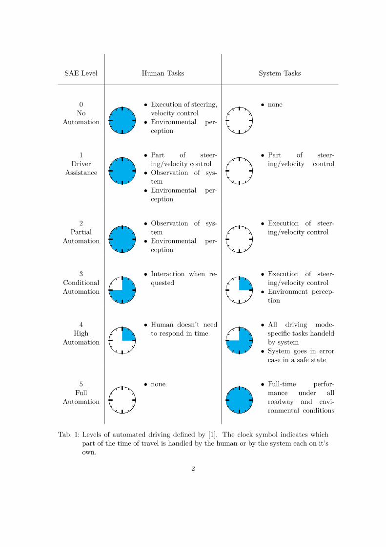
tomated driving have to be mastered as depicted in Tab. 1 and defined, for example,

by [1]. With an increasing automation level, the execution, monitoring, and fallback

performance are increasingly handled by the system and not by the human driver, in-

creasing the requirements for the sensor system. As shown e.g. in [2] radar sensors are

a key technology to enable Level 5 full automation. In contrast to video cameras and

laser scanners, a radar sensor is nearly independent of severe weather and light condi-

tions and even remains operational in complete darkness and snowfall. By exploiting

the reflections of the electromagnetic waves between road surfaces and the underbody

of vehicles it is even possible to detect hidden targets behind other vehicles.

1.1 Some Key Tasks towards Autonomous Driving

High-Resolution Capabilities: Enabling Advanced Driver Assistance Functions

With a radar sensor the radial distance, velocity, and angle of targets can be measured.

Key parameters are the accuracy of the measurement and the resolution, i.e. the abil-

ity to distinguish close targets. For certain driver assistance functions, typically SAE

Level 1 cf. Tab. 1, it was sufficient that a radar sensor can distinguish different objects

1

SAE Level Human Tasks System Tasks

0No

Automation

• Execution of steering,velocity control

• Environmental per-ception

• none

1Driver

Assistance

• Part of steer-ing/velocity control

• Observation of sys-tem

• Environmental per-ception

• Part of steer-ing/velocity control

2Partial

Automation

• Observation of sys-tem

• Environmental per-ception

• Execution of steer-ing/velocity control

3ConditionalAutomation

• Interaction when re-quested

• Execution of steer-ing/velocity control

• Environment percep-tion

4High

Automation

• Human doesn’t needto respond in time

• All driving mode-specific tasks handeldby system

• System goes in errorcase in a safe state

5Full

Automation

• none • Full-time perfor-mance under allroadway and envi-ronmental conditions

Tab. 1: Levels of automated driving defined by [1]. The clock symbol indicates whichpart of the time of travel is handled by the human or by the system each on it’sown.

2

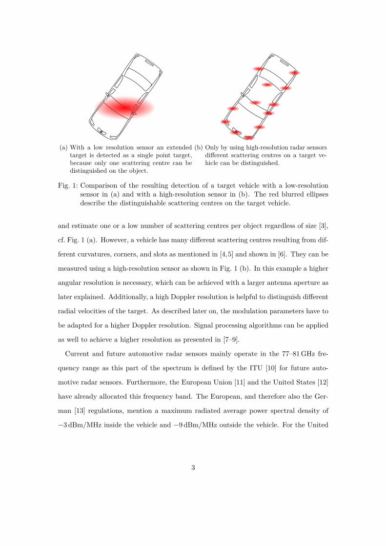
(a) With a low resolution sensor an extendedtarget is detected as a single point target,because only one scattering centre can bedistinguished on the object.

(b) Only by using high-resolution radar sensorsdifferent scattering centres on a target ve-hicle can be distinguished.

Fig. 1: Comparison of the resulting detection of a target vehicle with a low-resolutionsensor in (a) and with a high-resolution sensor in (b). The red blurred ellipsesdescribe the distinguishable scattering centres on the target vehicle.

and estimate one or a low number of scattering centres per object regardless of size [3],

cf. Fig. 1 (a). However, a vehicle has many different scattering centres resulting from dif-

ferent curvatures, corners, and slots as mentioned in [4,5] and shown in [6]. They can be

measured using a high-resolution sensor as shown in Fig. 1 (b). In this example a higher

angular resolution is necessary, which can be achieved with a larger antenna aperture as

later explained. Additionally, a high Doppler resolution is helpful to distinguish different

radial velocities of the target. As described later on, the modulation parameters have to

be adapted for a higher Doppler resolution. Signal processing algorithms can be applied

as well to achieve a higher resolution as presented in [7–9].

Current and future automotive radar sensors mainly operate in the 77–81GHz fre-

quency range as this part of the spectrum is defined by the ITU [10] for future auto-

motive radar sensors. Furthermore, the European Union [11] and the United States [12]

have already allocated this frequency band. The European, and therefore also the Ger-

man [13] regulations, mention a maximum radiated average power spectral density of

−3 dBm/MHz inside the vehicle and −9 dBm/MHz outside the vehicle. For the United

3

States the limitation is given by a maximum equivalent isotropically radiated power

(EIRP) of 50 dBm within this frequency band. Additionally, the European as well as

the American regulation specify a maximum peak power of 55 dBm (EIRP). A second

frequency band around 24GHz that is currently being used will not be available world-

wide in the future as new vehicles using this frequency range will not be permitted after

2018 for example in Germany [14].

An example of an urban scenario, where a target vehicle is measured with an exper-

imental radar sensor, is depicted in Fig. 2. In the range-Doppler evaluation in (a) the

velocity distribution of the moving object can be seen. Applying an angle estimation the

contour becomes visible in (b). The video image in (c) is used for validation purposes

and shows the measured scene. It can be seen that the moving object is detected with

several reflections.

Vehicle Manoeuvre Planning: Dimension, Orientation, and Motion State

Estimation of Target Vehicles

The dimension, orientation, and motion state of target vehicles can be used by an

autonomous vehicle to plan its driving manoeuvres. High-resolution radar sensors can

extract the dimension and orientation of target vehicles [15,16], cf. Fig. 2 (b). Using the

orientation it is possible to detect lane changes faster than with a conventional tracking

filter, as the filter usually needs several steps to predict the motion correctly. With two

radar sensors it is even possible to estimate the complete motion state, for example the

orientation and the movement vector including the yaw rate of a target vehicle [17].

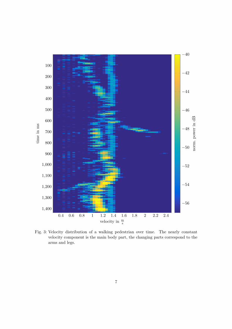
Vulnerable Road User Detection and Classification: Micro-Doppler Analysis

For the operation in urban areas, vulnerable road users, such as pedestrians or cyclists,

must be detected and classified [18]. As the reflected power from those road users is much

lower than from vehicles, the radar sensor must be sensitive for weak targets [19]. Due to

the movement of pedestrians various different Doppler velocities can be measured using

the micro-Doppler effect [20], cf. Fig. 3. In [21] the authors provide measurement results

4

−2−10120

2

4

6

8

10

velocity in ms

rang

ein

m

(a) The range-Doppler evaluation of the targetvehicle.

−4 −2 0 2 40

2

4

6

8

10

x in m

yin

m

(b) The x-y representation of the target vehi-cle with estimated orientation ( ) as de-scribed in [15,16].

(c) Camera image of the measured scenario.

Fig. 2: Measurement of a target vehicle with an experimental radar sensor. The shownmeasurements are top view, while the camera image is a side view.

5

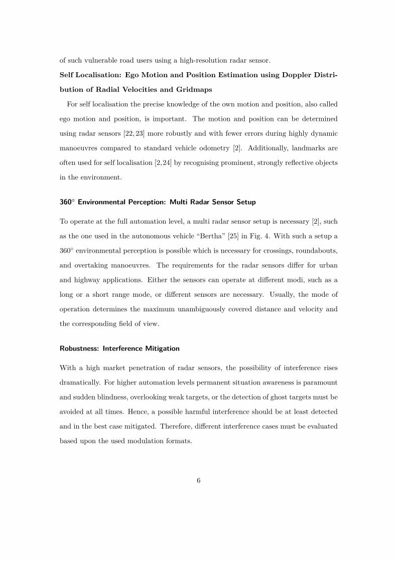
of such vulnerable road users using a high-resolution radar sensor.

Self Localisation: Ego Motion and Position Estimation using Doppler Distri-

bution of Radial Velocities and Gridmaps

For self localisation the precise knowledge of the own motion and position, also called

ego motion and position, is important. The motion and position can be determined

using radar sensors [22, 23] more robustly and with fewer errors during highly dynamic

manoeuvres compared to standard vehicle odometry [2]. Additionally, landmarks are

often used for self localisation [2,24] by recognising prominent, strongly reflective objects

in the environment.

360◦ Environmental Perception: Multi Radar Sensor Setup

To operate at the full automation level, a multi radar sensor setup is necessary [2], such

as the one used in the autonomous vehicle “Bertha” [25] in Fig. 4. With such a setup a

360◦ environmental perception is possible which is necessary for crossings, roundabouts,

and overtaking manoeuvres. The requirements for the radar sensors differ for urban

and highway applications. Either the sensors can operate at different modi, such as a

long or a short range mode, or different sensors are necessary. Usually, the mode of

operation determines the maximum unambiguously covered distance and velocity and

the corresponding field of view.

Robustness: Interference Mitigation

With a high market penetration of radar sensors, the possibility of interference rises

dramatically. For higher automation levels permanent situation awareness is paramount

and sudden blindness, overlooking weak targets, or the detection of ghost targets must be

avoided at all times. Hence, a possible harmful interference should be at least detected

and in the best case mitigated. Therefore, different interference cases must be evaluated

based upon the used modulation formats.

6

0.4 0.6 0.8 1 1.2 1.4 1.6 1.8 2 2.2 2.4

100

200

300

400

500

600

700

800

900

1,000

1,100

1,200

1,300

1,400

velocity in ms

time

inm

s

−56

−54

−52

−50

−48

−46

−44

−42

−40

norm

.pow

erin

dB

Fig. 3: Velocity distribution of a walking pedestrian over time. The nearly constantvelocity component is the main body part, the changing parts correspond to thearms and legs.

7

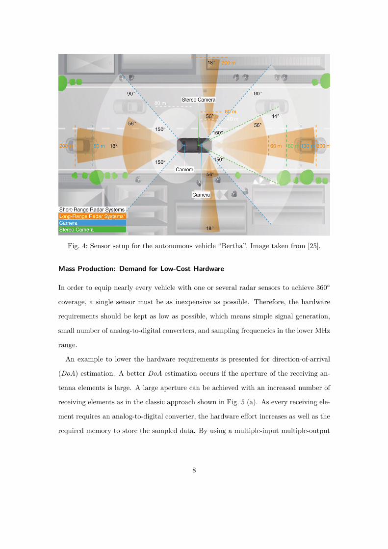
Fig. 4: Sensor setup for the autonomous vehicle “Bertha”. Image taken from [25].

Mass Production: Demand for Low-Cost Hardware

In order to equip nearly every vehicle with one or several radar sensors to achieve 360◦

coverage, a single sensor must be as inexpensive as possible. Therefore, the hardware

requirements should be kept as low as possible, which means simple signal generation,

small number of analog-to-digital converters, and sampling frequencies in the lower MHz

range.

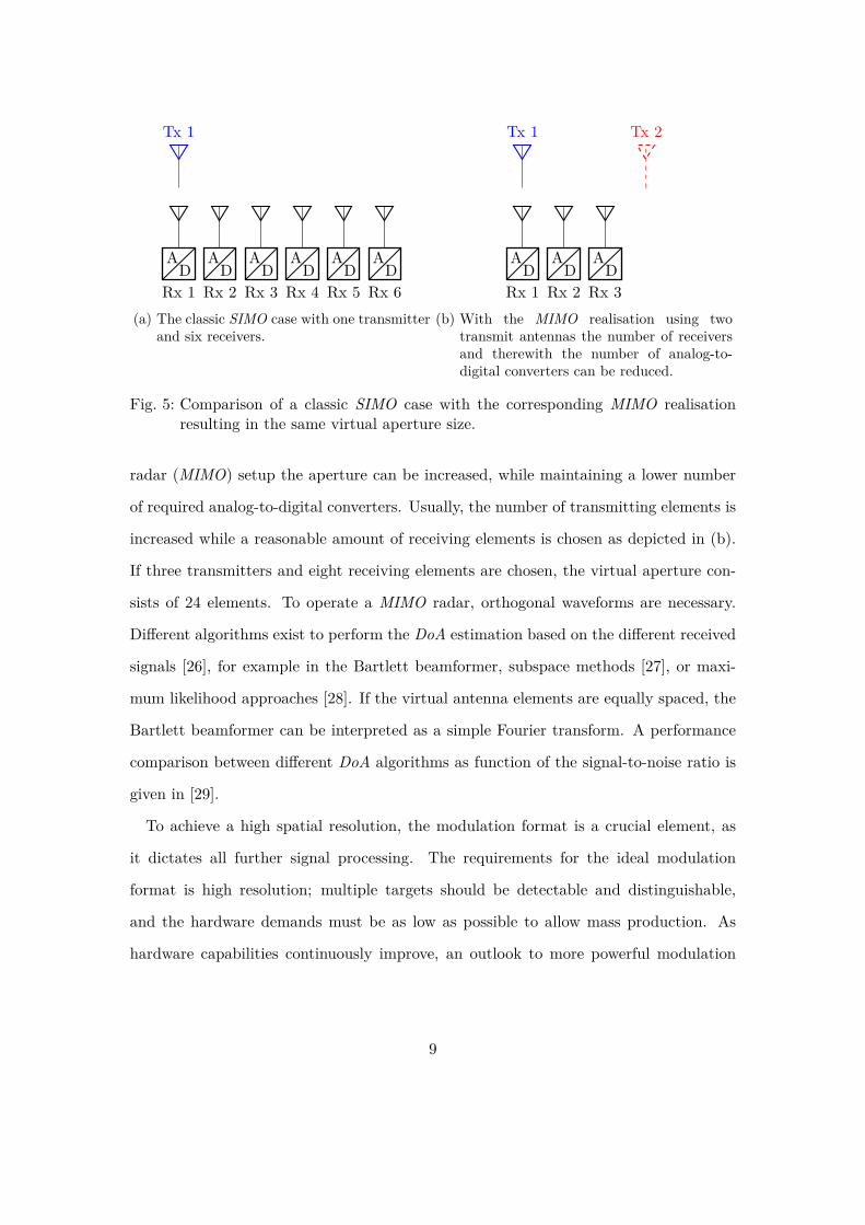
An example to lower the hardware requirements is presented for direction-of-arrival

(DoA) estimation. A better DoA estimation occurs if the aperture of the receiving an-

tenna elements is large. A large aperture can be achieved with an increased number of

receiving elements as in the classic approach shown in Fig. 5 (a). As every receiving ele-

ment requires an analog-to-digital converter, the hardware effort increases as well as the

required memory to store the sampled data. By using a multiple-input multiple-output

8

Rx 1D

A

Rx 2D

A

Rx 3D

A

Rx 4D

A

Rx 5D

A

Rx 6D

A

Tx 1

(a) The classic SIMO case with one transmitterand six receivers.

Rx 1D

A

Rx 2D

A

Rx 3D

A

Tx 1 Tx 2

(b) With the MIMO realisation using twotransmit antennas the number of receiversand therewith the number of analog-to-digital converters can be reduced.

Fig. 5: Comparison of a classic SIMO case with the corresponding MIMO realisationresulting in the same virtual aperture size.

radar (MIMO) setup the aperture can be increased, while maintaining a lower number

of required analog-to-digital converters. Usually, the number of transmitting elements is

increased while a reasonable amount of receiving elements is chosen as depicted in (b).

If three transmitters and eight receiving elements are chosen, the virtual aperture con-

sists of 24 elements. To operate a MIMO radar, orthogonal waveforms are necessary.

Different algorithms exist to perform the DoA estimation based on the different received

signals [26], for example in the Bartlett beamformer, subspace methods [27], or maxi-

mum likelihood approaches [28]. If the virtual antenna elements are equally spaced, the

Bartlett beamformer can be interpreted as a simple Fourier transform. A performance

comparison between different DoA algorithms as function of the signal-to-noise ratio is

given in [29].

To achieve a high spatial resolution, the modulation format is a crucial element, as

it dictates all further signal processing. The requirements for the ideal modulation

format is high resolution; multiple targets should be detectable and distinguishable,

and the hardware demands must be as low as possible to allow mass production. As

hardware capabilities continuously improve, an outlook to more powerful modulation

9

formats is given in the following. Smart signal processing of the modulation formats can

additionally decrease the required hardware effort.

This article is organised as follows. In the next section different modulation formats

are discussed. Section 3 explains reasons for interference and Section 4 presents possible

interference mitigation schemes. Afterwards, in Section 5, a summary and conclusion

are given.

10

2 Automotive Radar Modulation Schemes

In most radars sensors, e.g. [30], the state-of-the-art chirp-sequence modulation format

is applied, which is the successor of the well-known frequency modulated continuous

wave (FMCW ) modulation format. With the ongoing development of faster analog-to-

digital converters (ADC ), the application of digital modulation formats such as code

modulation or orthogonal frequency division multiplexing (OFDM ) becomes feasible.

Therefore, these modulation formats are discussed in the following.

2.1 Often Used: FMCW with Slow Ramps

The key idea of the classic FMCW modulation scheme is to transmit linear frequency

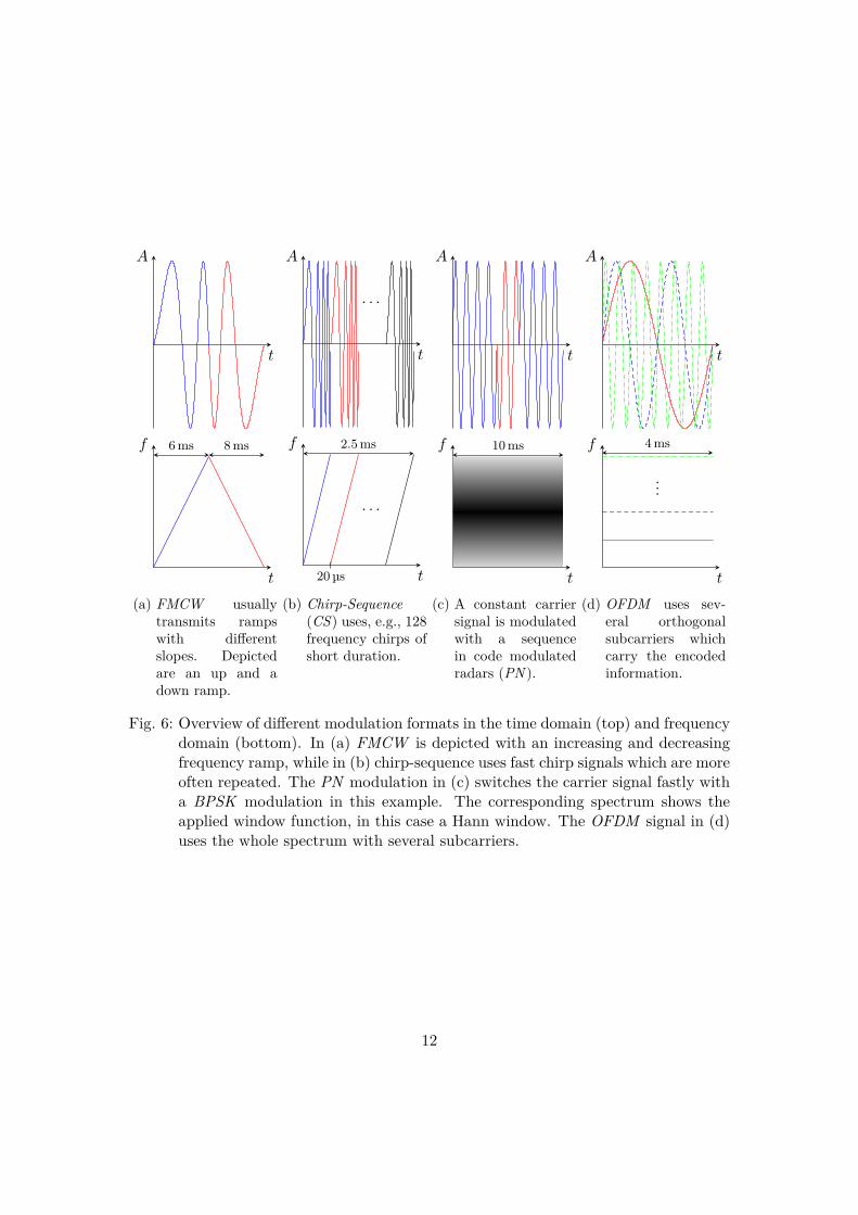
ramps with different slopes as depicted in Fig. 6 (a). The transmit time is usually in

the range of a couple of milliseconds and the number of transmitted ramps is limited.

This realisation is also called slow ramp modulation. The transmit signal is reflected

by a target and the received signal is mixed with the transmit signal [31, 32]. After the

down-conversion each reflection from a target results in a sinusoidal signal component

after mixing, which depends on the range to the target and the Doppler shift. If the

bandwidth of the transmit signal typically is within the range of a GHz, the resulting

baseband signal is in the range of several hundred kHz. Hence, the baseband signal can

be sampled after an anti-aliasing low-pass filter with a slow low-cost analog-to-digital

converter.

The baseband signal, also called the beat signal, consists of the range and Doppler

velocity of the target. In order to distinguish the two components, different ramp slopes

are required. To resolve multiple targets the number of different ramp slopes must be

increased accordingly [32].

11

A

t

f

t

6 ms 8 ms

(a) FMCW usuallytransmits rampswith differentslopes. Depictedare an up and adown ramp.

A

t

f

t

· · ·

· · ·

20 µs

2.5 ms

(b) Chirp-Sequence(CS) uses, e.g., 128frequency chirps ofshort duration.

A

t

f

t

10 ms

(c) A constant carriersignal is modulatedwith a sequencein code modulatedradars (PN ).

A

t

f

t

...

4 ms

(d) OFDM uses sev-eral orthogonalsubcarriers whichcarry the encodedinformation.

Fig. 6: Overview of different modulation formats in the time domain (top) and frequencydomain (bottom). In (a) FMCW is depicted with an increasing and decreasingfrequency ramp, while in (b) chirp-sequence uses fast chirp signals which are moreoften repeated. The PN modulation in (c) switches the carrier signal fastly witha BPSK modulation in this example. The corresponding spectrum shows theapplied window function, in this case a Hann window. The OFDM signal in (d)uses the whole spectrum with several subcarriers.

12

Challenging Task in Automotive Environments: Multi Target Scenarios

The typical automotive environment consists of multiple targets, which must be dis-

criminated. With the classic FMCW and a reasonable number of different ramp slopes,

only a limited number of different targets can be distinguished in a single measurement.

Usually, there are more targets present than can be detected unambiguously. This can

be either solved by tracking targets over time or with the following fast ramp modulation

scheme.

2.2 State-of-the-Art: Fast Ramps / Chirp-Sequence Modulation

In the slow ramp procedure the baseband signal depends on the range and the Doppler.

If a single frequency ramp is steep, cf. Fig. 6 (b), the range dependent part dominates the

baseband signal and the Doppler dependency can be neglected for a single ramp [32,33].

Thus, the Doppler estimation requires a sequence of frequency chirps, which motivates

the name of this modulation format as fast ramps or chirp-sequence modulation. As the

range and Doppler information is separated, a two-dimensional Fourier transform can

be used for evaluation.

The advantage compared to the slow ramp procedure is that fast ramp modulation

is capable of distinguishing multiple targets in a single measurement. As a drawback

of the steeper ramps, the resulting baseband frequencies are typically in the range of

several MHz which increases the sampling effort.

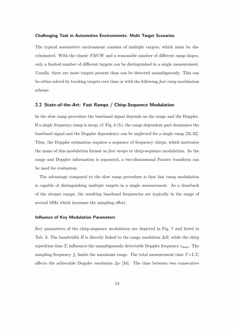
Influence of Key Modulation Parameters

Key parameters of the chirp-sequence modulation are depicted in Fig. 7 and listed in

Tab. 3. The bandwidth B is directly linked to the range resolution ∆R, while the chirp

repetition time Tr influences the unambiguously detectable Doppler frequency vmax. The

sampling frequency fs limits the maximum range. The total measurement time T=LTr

affects the achievable Doppler resolution ∆v [34]. The time between two consecutive

13

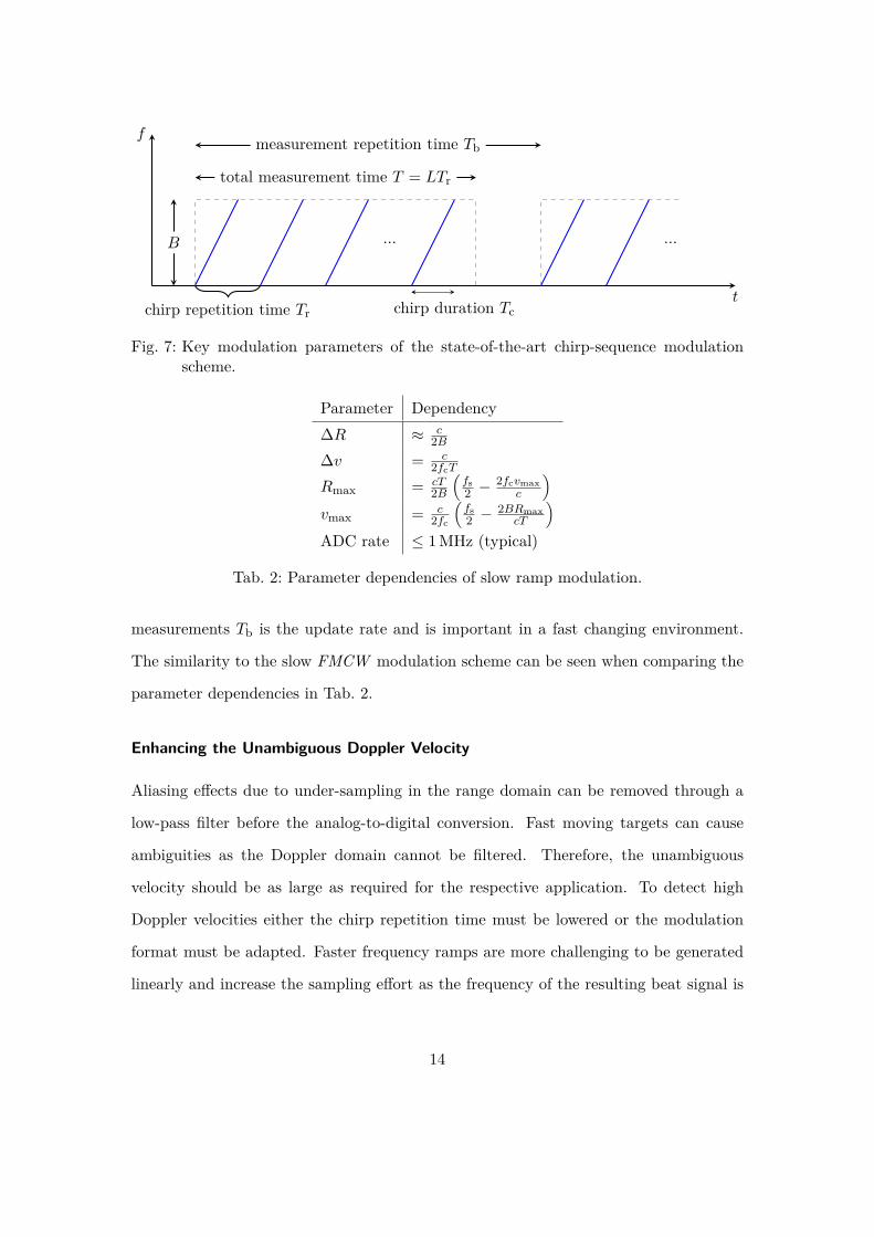
t

f

B ...

chirp repetition time Tr chirp duration Tc

total measurement time T = LTr

measurement repetition time Tb

...

Fig. 7: Key modulation parameters of the state-of-the-art chirp-sequence modulationscheme.

Parameter Dependency∆R ≈ c

2B

∆v = c2fcT

Rmax = cT2B

(fs2 − 2fcvmax

c

)vmax = c

2fc

(fs2 − 2BRmax

cT

)ADC rate ≤ 1 MHz (typical)

Tab. 2: Parameter dependencies of slow ramp modulation.

measurements Tb is the update rate and is important in a fast changing environment.

The similarity to the slow FMCW modulation scheme can be seen when comparing the

parameter dependencies in Tab. 2.

Enhancing the Unambiguous Doppler Velocity

Aliasing effects due to under-sampling in the range domain can be removed through a

low-pass filter before the analog-to-digital conversion. Fast moving targets can cause

ambiguities as the Doppler domain cannot be filtered. Therefore, the unambiguous

velocity should be as large as required for the respective application. To detect high

Doppler velocities either the chirp repetition time must be lowered or the modulation

format must be adapted. Faster frequency ramps are more challenging to be generated

linearly and increase the sampling effort as the frequency of the resulting beat signal is

14

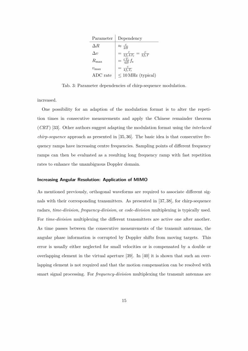
Parameter Dependency∆R ≈ c

2B

∆v = c2fcLTr

= c2fcT

Rmax = c Tc4B fs

vmax = c4fcTr

ADC rate ≤ 10 MHz (typical)

Tab. 3: Parameter dependencies of chirp-sequence modulation.

increased.

One possibility for an adaption of the modulation format is to alter the repeti-

tion times in consecutive measurements and apply the Chinese remainder theorem

(CRT ) [33]. Other authors suggest adapting the modulation format using the interlaced

chirp-sequence approach as presented in [35, 36]. The basic idea is that consecutive fre-

quency ramps have increasing centre frequencies. Sampling points of different frequency

ramps can then be evaluated as a resulting long frequency ramp with fast repetition

rates to enhance the unambiguous Doppler domain.

Increasing Angular Resolution: Application of MIMO

As mentioned previously, orthogonal waveforms are required to associate different sig-

nals with their corresponding transmitters. As presented in [37, 38], for chirp-sequence

radars, time-division, frequency-division, or code-division multiplexing is typically used.

For time-division multiplexing the different transmitters are active one after another.

As time passes between the consecutive measurements of the transmit antennas, the

angular phase information is corrupted by Doppler shifts from moving targets. This

error is usually either neglected for small velocities or is compensated by a double or

overlapping element in the virtual aperture [39]. In [40] it is shown that such an over-

lapping element is not required and that the motion compensation can be resolved with

smart signal processing. For frequency-division multiplexing the transmit antennas are

15

active at the same time but at different centre frequencies. Each target is therefore

detected at different beat frequencies. Code-division multiplexing exploits orthogonal

codes. Each transmit signal is encoded by an unique orthogonal code and recovered at

the receiver [41].

2.3 A Code Division Modulated Approach: Phase-Modulated Continuous

Wave Radar

Code-modulated radars (spread spectrum, pseudo-noise (PN ), phase modulated con-

tinuous wave (PMCW )) transmit a wide-band code sequence that is modulated on a

high-frequency continuous wave (CW ) carrier signal, cf. the schematic in Fig. 6 (c). On

the receiver side, the signals are down-converted and correlated with the transmitted

code sequence as depicted in Fig. 8. The codes have a short duration Ts2s such that the

Doppler effect does not influence the correlation. Peaks in the correlation yield the time

of flight and thus the object distance. A PN radar transmits a series of code sequences

for Doppler extraction, as the phase of the continuous-wave carrier changes between the

transmitted sequences. A Fourier transform across all transmitted sequences yields the

velocity information; however, in contrast to chirp-sequence, PN radars require an I-Q

receiver in order to distinguish positive and negative velocities. A proper selection of

the code offers low range side lobes or a low cross-correlation with other codes [42]. The

parameter dependencies are summarized in Tab. 4 and are very similar to the parameter

dependencies of chirp-sequence radars.

An important aspect of PN radars is the realization of the correlation of the receive

signal. A correlation is possible in the digital domain after sampling the receive sig-

nal [44]; however, this requires a very high sampling rate, as the baseband bandwidth

is equal to the RF modulation bandwidth. Consequently, high data rates have to be

handled. Such systems for the 79GHz band with bandwidths up to 2GHz and a fo-

cus on automotive applications have been discussed in [45–47]. The high sampling rate

16

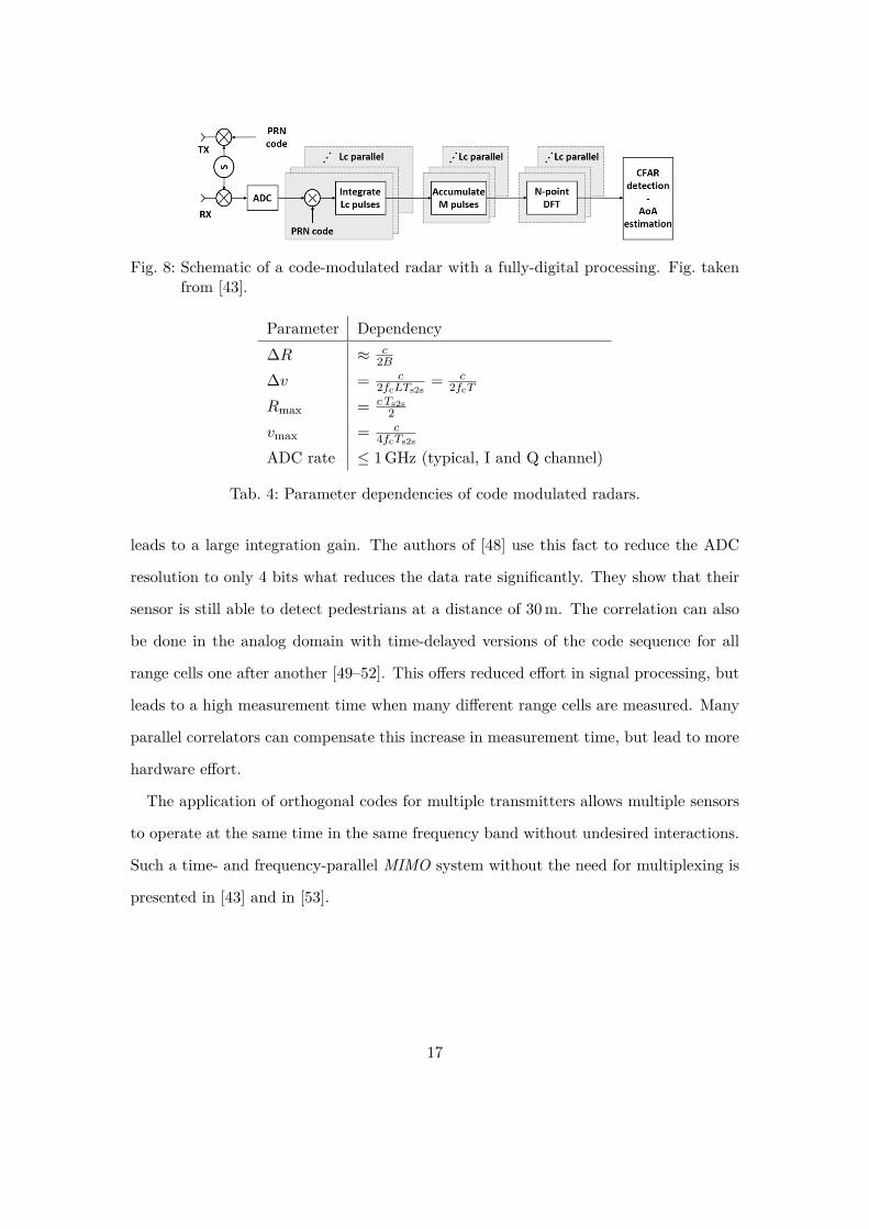
Fig. 8: Schematic of a code-modulated radar with a fully-digital processing. Fig. takenfrom [43].

Parameter Dependency∆R ≈ c

2B

∆v = c2fcLTs2s

= c2fcT

Rmax = c Ts2s2

vmax = c4fcTs2s

ADC rate ≤ 1 GHz (typical, I and Q channel)

Tab. 4: Parameter dependencies of code modulated radars.

leads to a large integration gain. The authors of [48] use this fact to reduce the ADC

resolution to only 4 bits what reduces the data rate significantly. They show that their

sensor is still able to detect pedestrians at a distance of 30m. The correlation can also

be done in the analog domain with time-delayed versions of the code sequence for all

range cells one after another [49–52]. This offers reduced effort in signal processing, but

leads to a high measurement time when many different range cells are measured. Many

parallel correlators can compensate this increase in measurement time, but lead to more

hardware effort.

The application of orthogonal codes for multiple transmitters allows multiple sensors

to operate at the same time in the same frequency band without undesired interactions.

Such a time- and frequency-parallel MIMO system without the need for multiplexing is

presented in [43] and in [53].

17

2.4 A Digital Modulation Format: Orthogonal Frequency Division

Multiplexing

Due to the progress in digital technology in the past few years, approaches that shift the

major effort of radar systems to the digital domain have become more favorable. Such a

system can be seen as a software defined radio (SDR) that provides capabilities that are

hard to match with common single-carrier radars. This includes unmatched flexibility,

adaptivity, robustness, calibration opportunities, and efficient channel usage.

A multi-carrier modulation scheme suitable for an SDR and radar detection is orthogo-

nal frequency division multiplexing (OFDM ) which is also widely used in communication

technology [54].

OFDM dates back to the 1960’s [55,56] but did not attract attention for radar appli-

cations until the last decade. The idea of a multi-carrier radar scheme was first brought

up by Levanon [57] in 2000. Driven by the idea to combine radar and communica-

tions [58–60], various signal processing improvements [61–63] have been presented since

then.

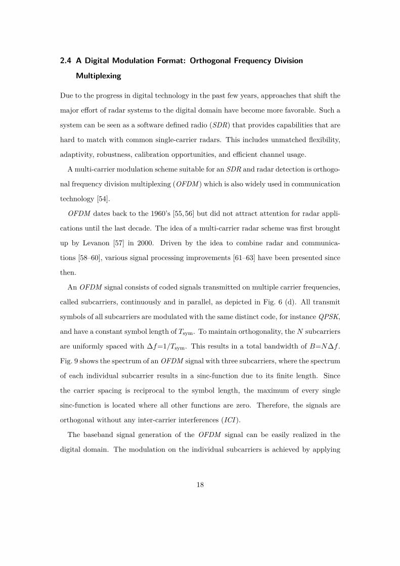
An OFDM signal consists of coded signals transmitted on multiple carrier frequencies,

called subcarriers, continuously and in parallel, as depicted in Fig. 6 (d). All transmit

symbols of all subcarriers are modulated with the same distinct code, for instance QPSK,

and have a constant symbol length of Tsym. To maintain orthogonality, the N subcarriers

are uniformly spaced with ∆f=1/Tsym. This results in a total bandwidth of B=N∆f .

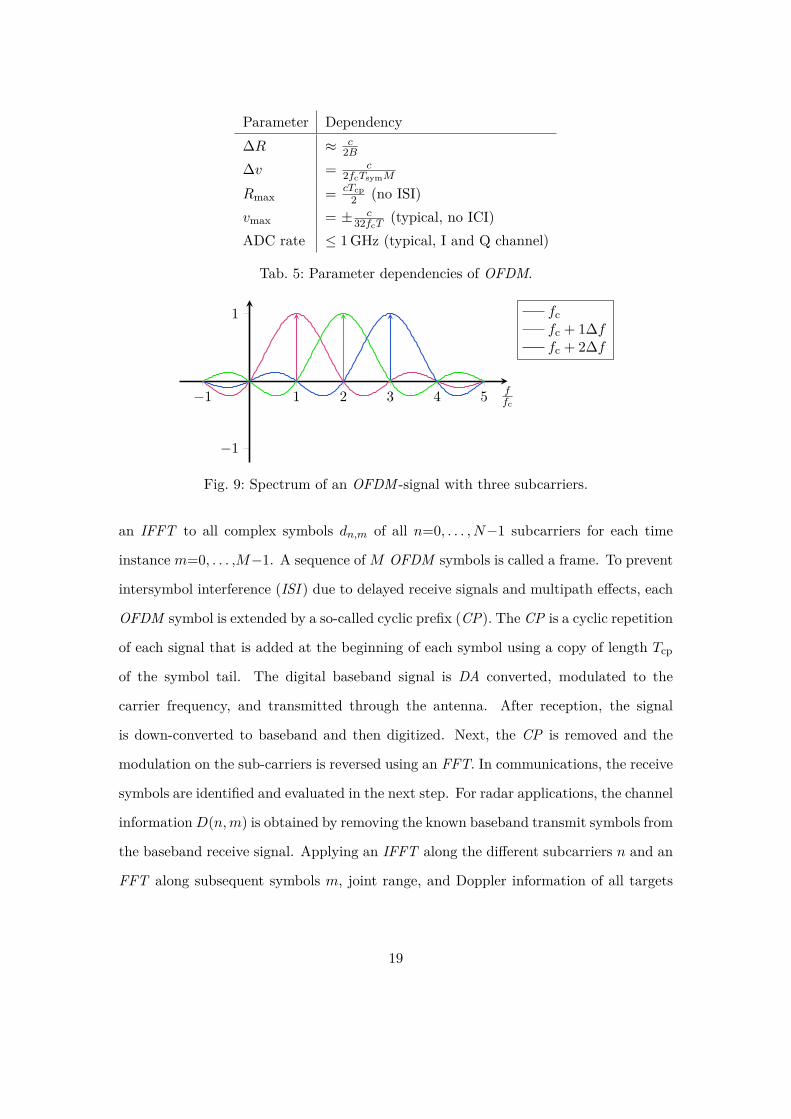
Fig. 9 shows the spectrum of an OFDM signal with three subcarriers, where the spectrum

of each individual subcarrier results in a sinc-function due to its finite length. Since

the carrier spacing is reciprocal to the symbol length, the maximum of every single

sinc-function is located where all other functions are zero. Therefore, the signals are

orthogonal without any inter-carrier interferences (ICI ).

The baseband signal generation of the OFDM signal can be easily realized in the

digital domain. The modulation on the individual subcarriers is achieved by applying

18

Parameter Dependency∆R ≈ c

2B

∆v = c2fcTsymM

Rmax = cTcp2 (no ISI)

vmax = ± c32fcT (typical, no ICI)

ADC rate ≤ 1 GHz (typical, I and Q channel)

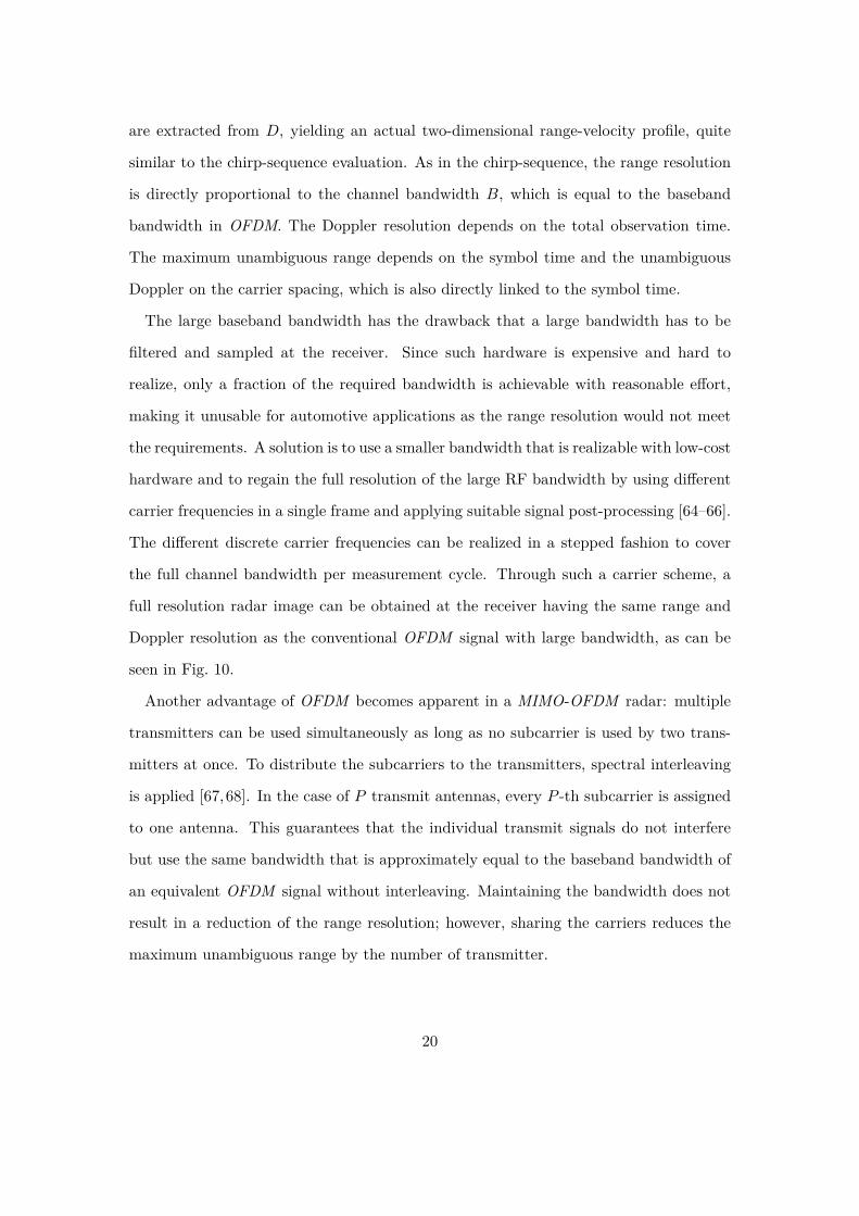
Tab. 5: Parameter dependencies of OFDM.

−1 1 2 3 4 5

−1

1

ffc

fcfc + 1∆ffc + 2∆f

Fig. 9: Spectrum of an OFDM -signal with three subcarriers.

an IFFT to all complex symbols dn,m of all n=0, . . . , N−1 subcarriers for each time

instance m=0, . . . ,M−1. A sequence ofM OFDM symbols is called a frame. To prevent

intersymbol interference (ISI ) due to delayed receive signals and multipath effects, each

OFDM symbol is extended by a so-called cyclic prefix (CP). The CP is a cyclic repetition

of each signal that is added at the beginning of each symbol using a copy of length Tcp

of the symbol tail. The digital baseband signal is DA converted, modulated to the

carrier frequency, and transmitted through the antenna. After reception, the signal

is down-converted to baseband and then digitized. Next, the CP is removed and the

modulation on the sub-carriers is reversed using an FFT. In communications, the receive

symbols are identified and evaluated in the next step. For radar applications, the channel

informationD(n,m) is obtained by removing the known baseband transmit symbols from

the baseband receive signal. Applying an IFFT along the different subcarriers n and an

FFT along subsequent symbols m, joint range, and Doppler information of all targets

19

are extracted from D, yielding an actual two-dimensional range-velocity profile, quite

similar to the chirp-sequence evaluation. As in the chirp-sequence, the range resolution

is directly proportional to the channel bandwidth B, which is equal to the baseband

bandwidth in OFDM. The Doppler resolution depends on the total observation time.

The maximum unambiguous range depends on the symbol time and the unambiguous

Doppler on the carrier spacing, which is also directly linked to the symbol time.

The large baseband bandwidth has the drawback that a large bandwidth has to be

filtered and sampled at the receiver. Since such hardware is expensive and hard to

realize, only a fraction of the required bandwidth is achievable with reasonable effort,

making it unusable for automotive applications as the range resolution would not meet

the requirements. A solution is to use a smaller bandwidth that is realizable with low-cost

hardware and to regain the full resolution of the large RF bandwidth by using different

carrier frequencies in a single frame and applying suitable signal post-processing [64–66].

The different discrete carrier frequencies can be realized in a stepped fashion to cover

the full channel bandwidth per measurement cycle. Through such a carrier scheme, a

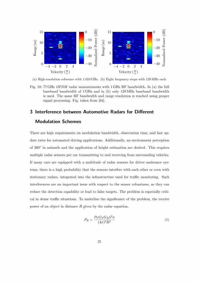
full resolution radar image can be obtained at the receiver having the same range and

Doppler resolution as the conventional OFDM signal with large bandwidth, as can be

seen in Fig. 10.

Another advantage of OFDM becomes apparent in a MIMO-OFDM radar: multiple

transmitters can be used simultaneously as long as no subcarrier is used by two trans-

mitters at once. To distribute the subcarriers to the transmitters, spectral interleaving

is applied [67,68]. In the case of P transmit antennas, every P -th subcarrier is assigned

to one antenna. This guarantees that the individual transmit signals do not interfere

but use the same bandwidth that is approximately equal to the baseband bandwidth of

an equivalent OFDM signal without interleaving. Maintaining the bandwidth does not

result in a reduction of the range resolution; however, sharing the carriers reduces the

maximum unambiguous range by the number of transmitter.

20

−4 −2 0 2 40

5

10

15

Velocity (ms )

Ran

ge(m

)

−40

−30

−20

−10

0

Nor

mal

ized

Powe

r(d

B)

(a) High-resolution reference with 1.024GHz.

−4 −2 0 2 40

5

10

15

Velocity (ms )

Ran

ge(m

)

−40

−30

−20

−10

0

Nor

mal

ized

Powe

r(d

B)

(b) Eight frequency steps with 128MHz each.

Fig. 10: 77GHz OFDM radar measurements with 1GHz RF bandwidth. In (a) the fullbaseband bandwidth of 1GHz and in (b) only 128MHz baseband bandwidthis used. The same RF bandwidth and range resolution is reached using propersignal processing. Fig. taken from [64].

3 Interference between Automotive Radars for Different

Modulation Schemes

There are high requirements on modulation bandwidth, observation time, and fast up-

date rates for automated driving applications. Additionally, an environment perception

of 360◦ in azimuth and the application of height estimation are desired. This requires

multiple radar sensors per car transmitting to and receiving from surrounding vehicles.

If many cars are equipped with a multitude of radar sensors for driver assistance sys-

tems, there is a high probability that the sensors interfere with each other or even with

stationary radars, integrated into the infrastructure used for traffic monitoring. Such

interferences are an important issue with respect to the sensor robustness, as they can

reduce the detection capability or lead to false targets. The problem is especially criti-

cal in dense traffic situations. To underline the significance of the problem, the receive

power of an object in distance R given by the radar equation,

PR = PTGTGRλ2σ

(4π)3R4 (1)

21

is compared with the Friis equation for an interference source in the same distance,

Pint = PTGTGRλ2

(4π)2R2 . (2)

It is assumed that the transmit power PT , the antenna gain GT , and the wavelength λ of

the interfered and the interfering sensor are in the same order of magnitude. The receive

antenna gain GR is in both equations related to the interfered sensor. When comparing

the equations it can be noticed that the receive power of targets decreases with R4,

while the interference power decreases only proportional to R2. Thus, the problem is

even more critical for distant objects. Based on the above equations, [69] shows that

the power level of a target with a radar cross section (RCS) of 1m2 in 200m distance is

about 56 dB below the interference power received from the same distance.

Because of the interference problem, sensors need sufficient countermeasures for re-

liable functionality in interference situations. The effects and the probability of in-

terference strongly depend on the modulation format. The occurrence of interference

between two FMCW radars depends on multiple factors: the transmit frequencies, the

transmission times, the ramp slopes determining the duration, and how frequent the

interference occurs. While short spikes affecting a few samples in the time signal will

be the most common effect in such a setup, leading to wide-band noise increase in the

spectrum [69–71], the probability for frequent and long-acting interferences is small —

for identical modulation parameters it is below 10−3 [70] for a single measurement.

When interference between chirp-sequence-, PN -, or OFDM -modulated radars are

considered, the problem is much more critical. The latter modulation formats have

a larger occupancy of the available spectrum during a measurement cycle and have

higher receiver bandwidths, especially the OFDM and PN modulations. When even

more sensors operate at the same time in the 76–77GHz or 77–81GHz frequency band,

it is unavoidable that interferences occur. Interference generation between automotive

22

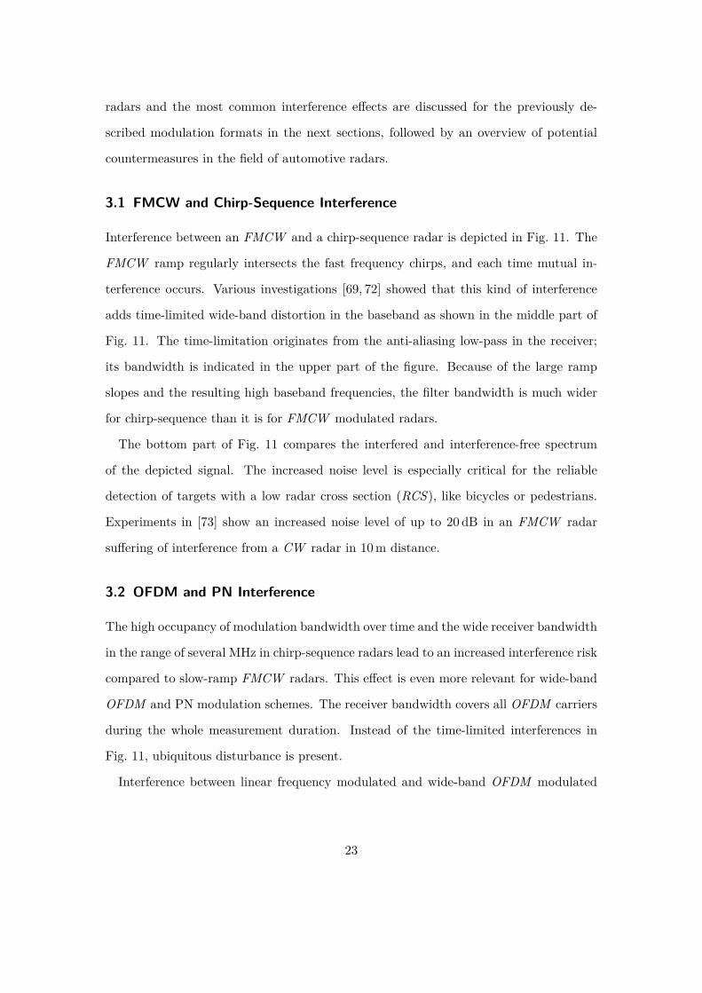
radars and the most common interference effects are discussed for the previously de-

scribed modulation formats in the next sections, followed by an overview of potential

countermeasures in the field of automotive radars.

3.1 FMCW and Chirp-Sequence Interference

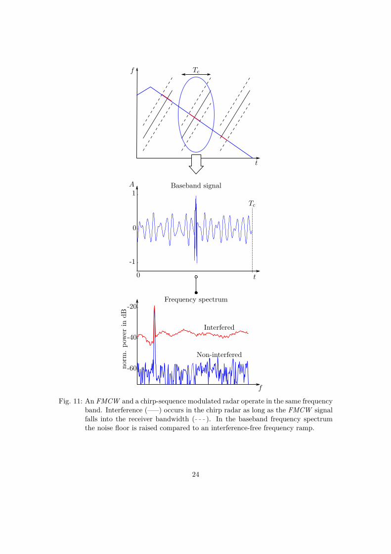
Interference between an FMCW and a chirp-sequence radar is depicted in Fig. 11. The

FMCW ramp regularly intersects the fast frequency chirps, and each time mutual in-

terference occurs. Various investigations [69, 72] showed that this kind of interference

adds time-limited wide-band distortion in the baseband as shown in the middle part of

Fig. 11. The time-limitation originates from the anti-aliasing low-pass in the receiver;

its bandwidth is indicated in the upper part of the figure. Because of the large ramp

slopes and the resulting high baseband frequencies, the filter bandwidth is much wider

for chirp-sequence than it is for FMCW modulated radars.

The bottom part of Fig. 11 compares the interfered and interference-free spectrum

of the depicted signal. The increased noise level is especially critical for the reliable

detection of targets with a low radar cross section (RCS), like bicycles or pedestrians.

Experiments in [73] show an increased noise level of up to 20 dB in an FMCW radar

suffering of interference from a CW radar in 10m distance.

3.2 OFDM and PN Interference

The high occupancy of modulation bandwidth over time and the wide receiver bandwidth

in the range of several MHz in chirp-sequence radars lead to an increased interference risk

compared to slow-ramp FMCW radars. This effect is even more relevant for wide-band

OFDM and PN modulation schemes. The receiver bandwidth covers all OFDM carriers

during the whole measurement duration. Instead of the time-limited interferences in

Fig. 11, ubiquitous disturbance is present.

Interference between linear frequency modulated and wide-band OFDM modulated

23

f

t

-60

-40

-20

Tc

-1

0

1

norm

.po

werin

dB

f

t

A

Interfered

Non-interfered

Frequency spectrum

Baseband signal

Tc

0

Fig. 11: An FMCW and a chirp-sequence modulated radar operate in the same frequencyband. Interference ( ) occurs in the chirp radar as long as the FMCW signalfalls into the receiver bandwidth ( ). In the baseband frequency spectrumthe noise floor is raised compared to an interference-free frequency ramp.

24

BRx

t

f

OFDM carriersChirp ramps

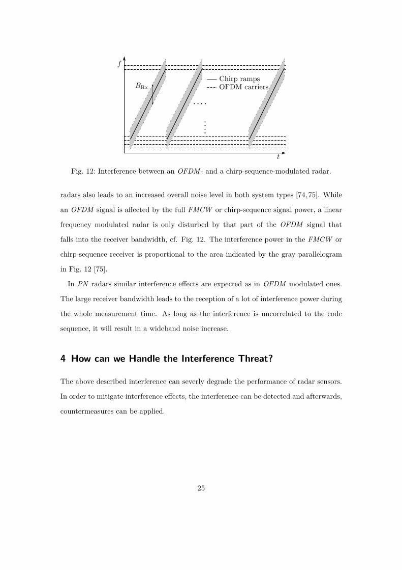
Fig. 12: Interference between an OFDM - and a chirp-sequence-modulated radar.

radars also leads to an increased overall noise level in both system types [74,75]. While

an OFDM signal is affected by the full FMCW or chirp-sequence signal power, a linear

frequency modulated radar is only disturbed by that part of the OFDM signal that

falls into the receiver bandwidth, cf. Fig. 12. The interference power in the FMCW or

chirp-sequence receiver is proportional to the area indicated by the gray parallelogram

in Fig. 12 [75].

In PN radars similar interference effects are expected as in OFDM modulated ones.

The large receiver bandwidth leads to the reception of a lot of interference power during

the whole measurement time. As long as the interference is uncorrelated to the code

sequence, it will result in a wideband noise increase.

4 How can we Handle the Interference Threat?

The above described interference can severly degrade the performance of radar sensors.

In order to mitigate interference effects, the interference can be detected and afterwards,

countermeasures can be applied.

25

4.1 Interference Detection

For interference between FMCW or chirp-sequence radars several detection algorithms

have been developed for the time domain signals. This is done based on the high power

and the short duration of the interference in [76]. Other approaches apply matched signal

transforms [77] or image processing methods [78] to detect interference. It was shown

that OFDM interference is very difficult to distinguish from thermal noise in the spec-

trum of FMCW receivers, making a detection more problematic [79]. For OFDM radars

a detection algorithm similar to the above-mentioned power detectors in combination

with an ordered statistic approach is demonstrated in [80].

4.2 Time-Domain Approaches

After the detection of the interfered samples in the time domain data of chirp-sequence

signals, those samples can be set to zero to prevent an increase of the noise level in

the frequency spectrum [69]. However, zeroing requires a robust detection and raises

additional frequency components; these artifacts can be reduced by introducing a win-

dow function at the time domain discontinuities [78] or a prediction of the missing data

with autoregressive models [81]. It is also possible to estimate and afterwards cancel the

interference component [82] from the time signals. This does not suppress the interfer-

ence completely, but it does not introduce artifacts in the spectrum. These time-domain

approaches are well-suited for time-limited interference between linear frequency modu-

lated radars; however, they are not yet tested for interference from and between Code-

and OFDM -modulated radars. Code and OFDM modulations occupy a wide bandwidth

during the whole duration of a measurement and therefore cause and suffer from long

interference durations. Nevertheless, it is shown in [80] that the interfered data can be

removed and subsequently reconstructed through compressed sensing algorithms when

interference between multiple OFDM radars occurs.

26

f

t76GHz

77GHz

Window Suppression

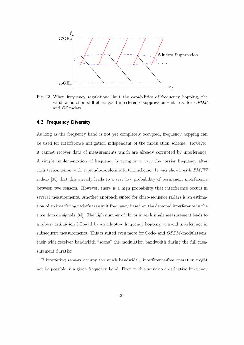
Fig. 13: When frequency regulations limit the capabilities of frequency hopping, thewindow function still offers good interference suppression – at least for OFDMand CS radars.

4.3 Frequency Diversity

As long as the frequency band is not yet completely occupied, frequency hopping can

be used for interference mitigation independent of the modulation scheme. However,

it cannot recover data of measurements which are already corrupted by interference.

A simple implementation of frequency hopping is to vary the carrier frequency after

each transmission with a pseudo-random selection scheme. It was shown with FMCW

radars [83] that this already leads to a very low probability of permanent interference

between two sensors. However, there is a high probability that interference occurs in

several measurements. Another approach suited for chirp-sequence radars is an estima-

tion of an interfering radar’s transmit frequency based on the detected interference in the

time domain signals [84]. The high number of chirps in each single measurement leads to

a robust estimation followed by an adaptive frequency hopping to avoid interference in

subsequent measurements. This is suited even more for Code- and OFDM -modulations:

their wide receiver bandwidth “scans” the modulation bandwidth during the full mea-

surement duration.

If interfering sensors occupy too much bandwidth, interference-free operation might

not be possible in a given frequency band. Even in this scenario an adaptive frequency

27

hopping can align the sensors’ bandwidths with the smallest possible overlap, cf. Fig. 13.

In this case the window function applied in signal processing of linear frequency modu-

lated radars leads to a good interference suppression, cf. [72]. The same way of windowing

is also valid for OFDM radars.

4.4 Spatial Masking of Interference Sources

In radar systems with multiple receive channels it is possible to apply a receiver-sided

digital beamforming (DBF) to suppress signals from an interferer’s direction. This

direction can be estimated based on the interfered samples of the time signals [77, 85].

With this knowledge the interference is removed from the field of view as depicted in

Fig. 14, and desired directions of arrival can be amplified. The opportunities of DBF

increase with an increasing aperture size and number of receive channels. Although

MIMO radars offer a large virtual aperture size, this virtual aperture cannot be used

for interference suppression. The interference affects only the physical receive array and

not the whole virtual aperture. Therefore, interference can only be canceled within the

physical receive aperture [86].

Interference suppression by DBF is very promising because it is independent of the

modulation format of the interfered and the interfering sensor. It is also not required to

detect all interfered samples in the time signals, as long as the direction of the interfering

signals can be determined. However, desired signals in the direction of the interference

cannot be detected anymore. Experimental results for a chirp-sequence system with only

four receive channels already show an interference suppression of up to 15 dB [85].

There is one special issue concerning DBF in linear frequency modulated radars. As

these systems typically do not have an I-Q receiver, the interference energy is spread over

multiple directions of arrival because of the image frequency of the interfering signal [86].

In this case a beamformer must take into account multiple directions when forming its

beams.

28

Fig. 14: The beamformer removes the interfering sensor from the field of view.

5 Summary

The key tasks which enable autonomous driving explained in the introduction are used

to compare the different presented modulation schemes.

5.1 High-Resolution Capabilities

To enable the detection and classification of vulnerable road users in automotive envi-

ronments high-resolution and separability of close targets is a key requirement. The lack

of real multi-target capability of the slow FMCW modulation format is a disadvantage.

The enhancement of the FMCW scheme, the so-called chirp-sequence modulation, has

higher but manageable hardware demands and is therefore the current state-of-the-art

approach. To enhance the angular resolution MIMO schemes are used which could be

realised easier with the digital modulation formats.

29

5.2 Demand for Low-cost Hardware and Efficient Usage of Resources

Considering the signal generation and sampling of the resulting baseband signal, slow

FMCW has the lowest hardware demands. Transmitting faster frequency chirps and

sampling the higher baseband signals is possible at low cost. Hence, the chirp-sequence

modulation format is the current state-of-the-art modulation format and has manageable

hardware demands.

Both digital modulation formats, PN and OFDM, require in the basic scheme a digital-

to-analog converter for the signal generation as well as an analog-to-digital converter with

the full modulation bandwidth. The advantage of mixing the transmit with the receive

signal to gain a low frequent baseband signal is not possible as in FMCW or CS. As

this bandwidth is mostly in the range of a couple of GHz such converters are either

not available or the hardware costs are too high for automotive applications. Solutions

might be stepped OFDM modulations.

5.3 Robustness against Interference

The sensor requirements for automated and autonomous driving make interference an

important topic. For FMCW and chirp-sequence modulation, interference will not occur

during the whole measurement duration, as the baseband bandwidth is much smaller

compared to the transmitted bandwidth. This clearly reduces the chance to collect

interference power from other sensors compared to both digital modulation formats

where the full transmit bandwidth is sampled during the whole measurement duration.

It also reduces the chance to transmit interfering power into other sensors.

There exists a multitude of ways to counteract interference effects. Time domain ap-

proaches span from the calculation power intensive interpolation of corrupted data to the

simple zeroing of interfered samples. They are most effective for short-duration interfer-

ence, require reliable detection algorithms, and their specific realization depends on the

modulation format. Frequency hopping is very cost-effective in terms of implementation

30

and calculation effort and can offer good performance for interference mitigation. It is,

however, limited by the available bandwidth, especially in dense traffic situations when

many sensors operate simultaneously. Digital beamforming is effective for all modulation

schemes, and it does not require a detection of all interfered samples. While suppress-

ing interferences DBF can also amplify directions of interest. On the other hand, the

sensor will always be blind towards the direction of the interferer. Furthermore, the

performance is limited by the available aperture.

It is not yet clear, what kind of interference countermeasures or mitigation approaches

are suited best for the different modulation schemes. It seems reasonable that time do-

main approaches are helpful in case of short interference durations, for example between

linear frequency modulated sensors. However, time domain approaches will suffer in case

of long interference durations caused by PN - or OFDM -modulated radars. Currently,

there are not many automotive interference evaluations available for PN - and OFDM -

modulated radars. Further investigations are required to examine which additional ef-

fects might have to be taken into account and which approach handles interference best.

6 Conclusion

Enabling autonomous driving has a huge influence on the requirements of radar sensors.

Different common modulation formats are introduced and compared regarding the new

requirements. To establish a 360◦ coverage of the environment, a single radar sensor is

not sufficient. Together with an increasing number of vehicles equipped with multiple

sensors the probability of interference increases. The overview of interference mitigation

schemes shows that there are many approaches towards reliable radar operation in multi-

sensor scenarios. Once a large number of sensors are operating at the same time, one

single approach will not be sufficient. In order to guarantee reliable operation for all

scenarios multiple interference countermeasures must be combined.

31

References[1] SAE International, “Taxonomy and Definitions for Terms Related to Driving

Automation Systems for On-Road Motor Vehicles,” 2016. [Online]. Available:http://standards.sae.org/j3016_201609/

[2] J. Dickmann et al., “"Automotive Radar the Key Technology for Autonomous Driv-ing: From Detection and Ranging to Environmental Understanding",” in IEEERadar Conference (RadarConf), May 2016, pp. 1–6.

[3] J. Dickmann et al., “Radar contribution to highly automated driving,” in EuropeanRadar Conference, Oct. 2014, pp. 412–415.

[4] H. Buddendick and T. F. Eibert, “Incoherent Scattering-Center Representations andParameterizations for Automobiles,” IEEE Antennas and Propagation Magazine,vol. 54, no. 1, pp. 140–148, Feb. 2012.

[5] M. Bühren and B. Yang, “Automotive Radar Target List Simulation based on Re-flection Center Representation of Objects,” in Workshop on Intelligent Transporta-tion (WIT), Hamburg, Germany, Mar. 2006, pp. 161–166.

[6] M. Andres, P. Feil, and W. Menzel, “3D-Scattering Center Detection of AutomotiveTargets Using 77GHz UWB Radar Sensors,” in European Conference on Antennasand Propagation (EUCAP), Mar. 2012, pp. 3690–3693.

[7] M. Andres, W. Menzel, H.-L. Bloecher, and J. Dickmann, “Detection of Slow Mov-ing Targets using Automotive Radar Sensors,” in German Microwave Conference(GeMiC), Mar. 2012, pp. 1–4.

[8] C. Fischer et al., “Adaptive Super-Resolution with a Synthetic Aperture Antenna,”in Proceedings of the 9th European Radar Conference (EuRAD), Oct. 2012, pp.250–253.

[9] S. Olbrich and C. Waldschmidt, “New pre-estimation Algorithm for FMCW RadarSystems using the Matrix Pencil Method,” in European Radar Conference (Eu-RAD), Sep. 2015, pp. 177–180.

[10] ITU, “Final Acts WRC-15 – World Radiocommunication Conference,” 2015.

[11] ETSI, “Short Range Devices; Transport and Traffic Telematics (TTT); Short RangeRadar equipment operating in the 77 GHz to 81 GHz band; Harmonised Standardcovering the essential requirements of article 3.2 of Directive 2014/53/EU,” 2017.

[12] Federal Communications Commission, “FCC-CIRC1707-07,” 2017.

[13] Bundesnetzagentur, “Allgemeinzuteilung von Frequenzen für Kraftfahrzeug -Kurzstreckenradare im Frequenzbereich 77–81GHz,” 2014.

32

[14] Bundesnetzagentur, “Allgemeinzuteilung von Frequenzen für Kraftfahrzeug-Kurzstreckenradare im Frequenzbereich 21,65–26,65GHz,” 2012.

[15] F. Roos et al., “Estimation of the Orientation of Vehicles in High-Resolution RadarImages,” in IEEE MTT-S International Conference on Microwaves for IntelligentMobility (ICMIM), Apr. 2015, pp. 1–4.

[16] F. Roos, D. Kellner, J. Dickmann, and C. Waldschmidt, “Reliable Orientation Es-timation of Vehicles in High-Resolution Radar Images,” IEEE Transactions on Mi-crowave Theory and Techniques, vol. 64, no. 9, pp. 2986–2993, Sep. 2016.

[17] D. Kellner et al., “Tracking of Extended Objects with High-Resolution DopplerRadar,” IEEE Transactions on Intelligent Transportation Systems, vol. 17, no. 5,pp. 1341–1353, Dec. 2016.

[18] J. Dickmann et al., “Making Bertha See Even More: Radar Contribution,” IEEEAccess, vol. 3, pp. 1233–1247, 2015.

[19] D. Belgiovane and C.-C. Chen, “Bicycles and Human Riders Backscattering at77GHz for Automotive Radar,” in European Conference on Antennas and Propa-gation (EuCAP), Apr. 2016, pp. 1–5.

[20] V. C. Chen, F. Li, S.-S. Ho, and H. Wechsler, “Micro-Doppler Effect in Radar:Phenomenon, Model, and Simulation Study,” IEEE Transactions on Aerospace andElectronic Systems, vol. 42, no. 1, pp. 2–21, Jan. 2006.

[21] E. Schubert, F. Meinl, M. Kunert, and W. Menzel, “High Resolution AutomotiveRadar Measurements of Vulnerable Road Users – Pedestrians & Cyclists,” in IEEEMTT-S International Conference on Microwaves for Intelligent Mobility (ICMIM),Apr. 2015, pp. 1–4.

[22] D. Kellner et al., “Instantaneous Ego-Motion Estimation using Doppler Radar,” inInternational IEEE Conference on Intelligent Transportation Systems (ITSC), Oct.2013, pp. 869–874.

[23] D. Kellner et al., “Instantaneous Ego-Motion Estimation using Multiple DopplerRadars,” in IEEE International Conference on Robotics and Automation (ICRA),May 2014, pp. 1592–1597.

[24] K. Werber, J. Klappstein, J. Dickmann, and C. Waldschmidt, “Interesting Areasin Radar Gridmaps for Vehicle Self-Localization,” in IEEE MTT-S InternationalConference on Microwaves for Intelligent Mobility (ICMIM), May 2016, pp. 1–4.

[25] J. Ziegler et al., “Making Bertha Drive - An Autonomous Journey on a HistoricRoute,” IEEE Intelligent Transportation Systems Magazine, vol. 6, no. 2, pp. 8–20,Summer 2014.

33

[26] P. Häcker and B. Yang, “Single snapshot DOA estimation,” Advances in RadioScience, vol. 8, pp. 251–256, 2010. [Online]. Available: http://www.adv-radio-sci.net/8/251/2010/

[27] R. O. Schmidt, “Multiple Emitter Location and Signal Parameter Estimation,”IEEE Transactions on Antennas and Propagation, vol. 34, no. 3, pp. 276–280, Mar.1986.

[28] P. Stoica and K. C. Sharman, “Maximum Likelihood Methods for Direction-of-Arrival Estimation,” IEEE Transactions on Acoustics, Speech, and Signal Process-ing, vol. 38, no. 7, pp. 1132–1143, Jul. 1990.

[29] M. Schoor and B. Yang, “High-Resolution Angle Estimation for an AutomotiveFMCW Radar Sensor,” in International Radar Symposium (IRS), 2007.

[30] Robert Bosch GmbH, LRR3: 3rd generation Long-Range Radar Sensor,2009. [Online]. Available: http://products.bosch-mobility-solutions.com/media/db_application/downloads/pdf/safety_1/en_4/lrr3_datenblatt_de_2009.pdf

[31] A. Stove, “Linear FMCW radar techniques,” IEE Proceedings-F on Radar and Sig-nal Processing, vol. 139, no. 5, pp. 343–350, Oct. 1992.

[32] V. Winkler, “Range Doppler Detection for automotive FMCW Radars,” in Proceed-ings of the 4th European Radar Conference (EuRAD), Oct. 2007, pp. 166–169.

[33] C. Schroeder and H. Rohling, “X-Band FMCW Radar System with Variable ChirpDuration,” in IEEE Radar Conference, May 2010, pp. 1255–1259.

[34] F. Roos et al., “Enhancement of Doppler Resolution for Chirp-Sequence ModulatedRadars,” in European Radar Conference (EuRAD), Oct. 2016, pp. 237–240.

[35] K. Thurn et al., “A Novel Interlaced Chirp Sequence Radar Concept with Range-Doppler Processing for Automotive Applications,” in IEEE MTT-S InternationalMicrowave Symposium (IMS), May 2015, pp. 1–4.

[36] K. Thurn et al., “Concept and Implementation of a PLL-Controlled Interlaced ChirpSequence Radar for Optimized Range-Doppler Measurements,” IEEE Transactionson Microwave Theory and Techniques, vol. 64, no. 10, pp. 3280–3289, Oct. 2016.

[37] J. J. M. de Wit, W. L. van Rossum, and A. J. de Jong, “Orthogonal Waveforms forFMCW MIMO Radar,” in IEEE RadarCon (RADAR), May 2011, pp. 686–691.

[38] H. Sun, F. Brigui, and M. Lesturgie, “Analysis and Comparison of MIMO RadarWaveforms,” in International Radar Conference, Oct. 2014, pp. 1–6.

[39] C. M. Schmid, R. Feger, C. Pfeffer, and A. Stelzer, “Motion Compensation andEfficient Array Design for TDMA FMCW MIMO Radar Systems,” in 6th EuropeanConference on Antennas and Propagation (EUCAP), Mar. 2012, pp. 1746–1750.

34

[40] J. Bechter, F. Roos, and C. Waldschmidt, “Compensation of Motion-Induced PhaseErrors in TDMMIMORadars,” IEEE Microwave and Wireless Components Letters,vol. 27, no. 12, pp. 1164–1166, Dec. 2017.

[41] R. Feger, H. Haderer, and A. Stelzer, “Optimization of Codes and Weighting Func-tions for Binary Phase-Coded FMCW MIMO Radars,” in IEEE MTT-S Interna-tional Conference on Microwaves for Intelligent Mobility (ICMIM), May 2016, pp.1–4.

[42] W. V. Thillo et al., “Almost perfect auto-correlation sequences for binary phase-modulated continuous wave radar,” in European Radar Conference, Oct. 2013, pp.491–494.

[43] A. Bourdoux et al., “PMCW Waveform and MIMO Technique for a 79GHz CMOSAutomotive Radar,” in IEEE Radar Conference (RadarConf), May 2016, pp. 1–5.

[44] A. Vazquez, M. G. Sanchez, I. Cuinas, and M. Dawood, Wideband Noise Radarbased in Phase Coded Sequences, Radar Technology, G. Kouemou, Ed. InTech,2010.

[45] V. Giannini et al., “A 79GHz Phase-Modulated 4GHz GHz-BW CW Radar Trans-mitter in 28 nm CMOS,” IEEE Journal of Solid-State Circuits, vol. 49, no. 12, pp.2925–2937, Dec. 2014.

[46] D. Guermandi et al., “A 79GHz Binary Phase-Modulated Continuous-Wave RadarTransceiver with TX-to-RX Spillover Cancellation in 28 nm CMOS,” in IEEE In-ternational Solid-State Circuits Conference, Feb. 2015, pp. 1–3.

[47] K. Kobayashi et al., “79GHz-band Coded Pulse Compression Radar System Perfor-mance in Outdoor for Pedestrian Detection,” in European Radar Conference, Oct.2013, pp. 327–330.

[48] W. V. Thillo et al., “Impact of ADC clipping and quantization on phase-modulated79GHz CMOS radar,” in 11th European Radar Conference, Oct. 2014, pp. 285–288.

[49] W. Menzel, J. Buechler, and J. Taech, “An Experimental 24GHz Radar using PhaseModulation Spread Spectrum Techniques,” in 28th European Microwave Confer-ence, vol. 2, Oct. 1998, pp. 56–60.

[50] V. Filimon and J. Buechler, “A pre-crash radar sensor system based on pseudo-noisecoding,” in IEEE MTT-S International Microwave Symposium Digest, vol. 3, Jun.2000, pp. 1415–1418 vol.3.

[51] H. J. Ng, R. Feger, and A. Stelzer, “A Fully-Integrated 77-GHz Pseudo-RandomNoise Coded Doppler Radar Sensor with Programmable Sequence Generators inSiGe Technology,” in IEEE MTT-S International Microwave Symposium, Jun. 2014,pp. 1–4.

35

[52] R. Feger, H. Haderer, H. J. Ng, and A. Stelzer, “Realization of a Sliding-Correlator-Based Continuous-Wave Pseudorandom Binary Phase-Coded Radar Operating inW-Band,” IEEE Transactions on Microwave Theory and Techniques, vol. 64, no. 10,pp. 3302–3318, Oct. 2016.

[53] H. Haderer, R. Feger, C. Pfeffer, and A. Stelzer, “Millimeter-Wave Phase-CodedCW MIMO Radar Using Zero- and Low-Correlation-Zone Sequence Sets,” IEEETransactions on Microwave Theory and Techniques, vol. 64, no. 12, pp. 4312–4323,Dec. 2016.

[54] T. Hwang et al., “OFDM and Its Wireless Applications: A Survey,” IEEE Trans-actions on Vehicular Technology, vol. 58, no. 4, pp. 1673–1694, May 2009.

[55] R. W. Chang, “Synthesis of Band-Limited Orthogonal Signals for MultichannelData Transmission,” Bell Syst. Tech. Journal,, vol. 45, no. 10, pp. 1775–1796, 1966.

[56] S. B. Weinstein and P. M. Ebert, “Data Transmission by Frequency-Division Mul-tiplexing Using the Discrete Fourier Transform,” IEEE Transactions on Communi-cation Technology, vol. 19, no. 5, pp. 628–634, 1971.

[57] N. Levanon, “Multifrequency complementary phase-coded radar signal,” IEE Pro-ceedings - Radar, Sonar and Navigation, vol. 147, no. 6, pp. 276–284, Dec. 2000.

[58] B. J. Donnet and I. D. Longstaff, “Combining MIMO Radar with OFDM Commu-nications,” Proceedings of the 3rd European Radar Conference, pp. 37–40, 2007.

[59] D. Garmatyuk, J. Schuerger, and K. Kauffman, “Multifunctional Software-DefinedRadar Sensor and Data Communication System,” IEEE Sensors Journal, vol. 11,no. 1, pp. 99–106, Jan. 2011.

[60] C. Sturm and W. Wiesbeck, “Waveform Design and Signal Processing Aspects forFusion of Wireless Communications and Radar Sensing,” Proceedings of the IEEE,vol. 99, no. 7, pp. 1236–1259, 2011.

[61] R. F. Tigrek, W. J. A. De Heij, and P. Van Genderen, “Multi-Carrier Radar Wave-form Schemes for Range and Doppler Processing,” IEEE National Radar Conference- Proceedings, pp. 2–6, 2009.

[62] C. R. Berger et al., “Signal Processing for Passive Radar Using OFDM Waveforms,”IEEE Journal of Selected Topics in Signal Processing, vol. 4, no. 1, pp. 226–238,Feb. 2010.

[63] C. Sturm, E. Pancera, T. Zwick, and W. Wiesbeck, “A Novel Approach to OFDMRadar Processing,” in IEEE National Radar Conference, Proceedings, no. 3, 2009,pp. 9–12.

[64] B. Schweizer, C. Knill, D. Schindler, and C. Waldschmidt, “Stepped-Carrier OFDM-Radar Processing Scheme to Retrieve High-Resolution Range-Velocity Profile at

36

Low Sampling Rate,” IEEE Transactions on Microwave Theory and Techniques,vol. 66, no. 3, pp. 1610–1618, 2017.

[65] G. Lellouch, A. K. Mishra, and M. Inggs, “Stepped OFDM Radar Technique toResolve Range and Doppler Simultaneously,” IEEE Transactions on Aerospace andElectronic Systems, vol. 51, no. 2, pp. 937–950, 2015.

[66] C. Pfeffer, R. Feger, and A. Stelzer, “A Stepped-Carrier 77-GHz OFDM MIMORadar System with 4GHz Bandwidth,” in 2015 European Radar Conference (Eu-RAD), Sep. 2015, pp. 97–100.

[67] Z. Wang et al., “Interleaved OFDM Radar Signals for Simultaneous PolarimetricMeasurements,” IEEE Transactions on Aerospace and Electronic Systems, vol. 48,no. 3, pp. 2085–2099, 2012.

[68] C. Sturm, Y. L. Sit, M. Braun, and T. Zwick, “Spectrally interleaved multi-carriersignals for radar network applications and multi-input multi-output radar,” IETRadar, Sonar & Navigation, vol. 7, no. 3, pp. 261–269, 2013.

[69] G. M. Brooker, “Mutual Interference of Millimeter-Wave Radar Systems,” IEEETransactions on Electromagnetic Compatibility, vol. 49, no. 1, pp. 170–181, Feb.2007.

[70] D. Oprisan and H. Rohling, “Analysis of Mutual Interference between AutomotiveRadar Systems,” in International Radar Symposium (IRS), 2005, Berlin.

[71] M. Goppelt, H.-L. Blöcher, and W. Menzel, “Automotive radar - investigation ofmutual interference mechanisms,” Advances in Radio Science, vol. 8, pp. 55–60,2010.

[72] T. Schipper et al., “Discussion of the operating range of frequency modulated radarsin the presence of interference,” International Journal of Microwave and WirelessTechnologies, vol. 6, pp. 371–378, Jun. 2014.

[73] T. Schipper et al., “An estimation of the operating range for frequency modulatedradars in the presence of interference,” in European Radar Conference (EuRAD),Oct. 2013, pp. 227–230.

[74] G. Hakobyan and B. Yang, “A Novel Narrowband Interference Suppression Methodfor OFDM Radar,” in 24th European Signal Processing Conference (EUSIPCO),Aug. 2016, pp. 2230–2234.

[75] C. Knill, J. Bechter, and C. Waldschmidt, “Interference of Chirp Sequence Radarsby OFDM Radars at 77GHz,” in IEEE MTT-S International Conference on Mi-crowaves for Intelligent Mobility (ICMIM), Mar. 2017, pp. 147–150.

[76] C. Fischer, M. Goppelt, H.-L. Blöcher, and J. Dickmann, “Minimizing interferencein automotive radar using digital beamforming,” Advances in Radio Science, vol. 9,pp. 45–48, 2011.

37

[77] C. Fischer, H.-L. Blöcher, J. Dickmann, and W. Menzel, “Robust Detection andMitigation of Mutual Interference in Automotive Radar,” in 16th InternationalRadar Symposium (IRS), Jun. 2015, pp. 143–148.

[78] M. Barjenbruch et al., “A Method for Interference Cancellation in AutomotiveRadar,” in IEEE MTT-S International Conference on Microwaves for IntelligentMobility (ICMIM), Apr. 2015, pp. 1–4.

[79] S. Heuel, “Automotive Radar Interference Test,” in 18th International Radar Sym-posium (IRS), Jun. 2017, pp. 1–7.

[80] B. Nuss, L. Sit, and T. Zwick, “A Novel Technique for Interference Mitigation inOFDM Radar Using Compressed Sensing,” in IEEE MTT-S International Confer-ence on Microwaves for Intelligent Mobility (ICMIM), Mar. 2017, pp. 143–146.

[81] B. E. Tullsson, “Topics in fmcw radar disturbance suppression,” in Radar 97, Oct.1997, pp. 1–5.

[82] J. Bechter, K. D. Biswas, and C. Waldschmidt, “Estimation and Cancellation ofInterferences in Automotive Radar Signals,” in 18th International Radar Symposium(IRS), Jun. 2017, pp. 1–10.

[83] L. Mu, T. Xiangqian, S. Ming, and Y. Jun, “Research on Key Technologies forCollision Avoidance Automotive Radar,” in Intelligent Vehicles Symposium, Jun.2009, pp. 233–236.

[84] J. Bechter, C. Sippel, and C. Waldschmidt, “Bats-inspired Frequency Hopping forMitigation of Interference between Automotive Radars,” in IEEE MTT-S Interna-tional Conference on Microwaves for Intelligent Mobility (ICMIM), May 2016, pp.1–4.

[85] J. Bechter, K. Eid, F. Roos, and C. Waldschmidt, “Digital Beamforming to Mit-igate Automotive Radar Interference,” in IEEE MTT-S International Conferenceon Microwaves for Intelligent Mobility (ICMIM), May 2016, pp. 1–4.

[86] J. Bechter, M. Rameez, and C. Waldschmidt, “Analytical and Experimental Inves-tigations on Mitigation of Interference in a DBF MIMO Radar,” IEEE Transactionson Microwave Theory and Techniques, vol. 65, no. 5, pp. 1727–1734, May 2017.

38