13

Innovative Numerical Modelling in Geomechanics – Ribeiro e Sousa et al. (eds)© 2012 Taylor & Francis Group, London, ISBN 978-0-415-61661-4

CHAPTER 2

Underground hydroelectric power schemes

Xia-Ting Feng & Jiang QuanInstitute of Rock and Soil Mechanics, Chinese Academy of Sciences, Wuhan, China

Luís Ribeiro e SousaState Key Laboratory for GeoMechanics and Deep Underground Engineering, Beijing, China University of Porto, Porto, Portugal

Tiago MirandaUniversity of Minho, Guimarães, Portugal

ABSTRACT: The purpose of this Chapter is to analyze the behavior of underground works associated to hydroelectric schemes with particular emphasis to the development of numerical models for predicting their structural behavior. The present work starts with a brief introduction to the different types of under-ground hydroelectric schemes with an illustration to the specific works related to the hydraulic circuit, the powerhouse complex and surge chambers. Sections concerning the methodologies followed by numerical modeling of the underground structures and for risk analysis are presented. Also the numerical use of inverse methodologies for the identification of parameters is evaluated. Two examples of application of numerical modeling are presented. The first case is related to the application of numerical modeling to the Venda Nova II hydroelectric scheme in Portugal, where innovative numerical methodologies were developed and validated using real testing and monitoring data. An optimization algorithm was used with a 3D model for the power caverns. The second case regards to numerical studies performed to Jinping II hydroelectric scheme in China. The project involves infrastructures planning and developed on a large scale. Results and studies performed by numerical models are presented. Finally, considerations about numerical modeling of large underground structures from hydroelectric schemes are presented.

a hydroelectric scheme whose performance is dependent on their suitable location, conception and on the adequate design of supports in order to ensure the safety of the overall underground complex (Sousa et al., 1994). Surge chambers are also important underground structures that may be located in the hydraulic circuit depending on its arrangement and particularly its length. Surge chambers are in general concentrated structures in which tridimensional equilibriums develop with similar problems caused by the caverns of the pow-erhouse complex. The pressure tunnels and shafts that form the hydraulic circuit of hydroelectric schemes can be of considerable importance due to the internal and external high water pressures that may be present, to the length they can have and to the variety of geotechnical conditions that may occur.

Examples of large underground schemes are illustrated in Figures 1 and 2 regarding, respec-tively the Jinping I and Alto Lindoso schemes where different types of underground structures occurred (Sousa et al., 1994; Wu et al., 2010).

1 GENERAL

Amongst the hydraulic projects that make use of the underground space, the hydroelectric power schemes are the most important ones. They are composed mainly by the dam, the hydraulic circuit with the inclusion of surge chambers and the pow-erhouse complex. The use of underground space has been widely implemented because of the safety and environmental advantages that it brings when compared with other surface solutions. The costs of excavations and supports are usually balanced by the costs of the foundation and superstruc-ture of surface infrastructures. In good rock mass conditions the supports for tunnels caverns and shafts can be considerably reduced and economi-cal and environmental impacts are always miti-gated. On the other hand significant advances in rock engineering and computers allowed a rational approach to the conception and design of these underground structures.

The underground works associated with the powerhouses form a fundamental part of

14

2 DIFFERENT TYPES OF SCHEMES

2.1 Conventional hydroelectric schemes

In these undertakings, we can distinguish differ-ent types of works, being generally formed by the powerhouse underground complex, high pres-sure shafts, high and low pressure tunnels, access tunnels and shafts, upstream and downstream surge chambers, water intakes and tunnel portals. Figure 2 illustrates the complex scheme of Alto Lindoso where the mentioned underground struc-tures were built.

For the hydraulic circuits, there are several alter-native schemes that have been evolving over time, as we intend to illustrate in Figure 3. The choice among them has to take into account the local con-ditions, in order to select the position of shafts, the high and low pressure tunnels, as well the location of the powerhouse complex and surge chambers (Martins, 1985; Sousa et al., 1994).

The hydraulic circuits were originally con-structed partly in underground, namely the high pressure tunnels, comprising a structure located on the hillside, which worked as surge chamber, after the high pressure tunnel, followed by a penstock at the ground surface, which led the water to the powerhouse, near the foot of the hill. In the fol-lowing schemes that emerged after the 1950s, the entire hydraulic circuit was moved to an under-ground location and the surge chamber was located upstream of the powerhouse. The hydraulic circuit is then constituted by a concrete shaft with or with-out a steel lining until the powerhouse, with the water to be restored through a low pressure tunnel. In areas of low resistance or very permeable rock masses, it is necessary to carry out a treatment for strengthening the rock mass. The last scheme of Figure 3 corresponds to a stage where surge cham-bers are used with smaller size and partially filled with compressed air.

Among the presented schemes, there are sev-eral possible arrangements, mainly related to the development of the high and low pressure tunnels,

Figure 1. Jinping-I project layout (www.chincold.org.cn/news-/li080321–12-Jinping–1.pdf).

Figure 2. Alto Lindoso hydroelectric power scheme (Sousa et al., 1994).

Figure 3. Alternative schemes of hydraulic circuits.

Figure 4. Different arrangements for hydraulic circuits.

which could be classified, as shown in Figure 4, in Swedish arrangements with an upstream power-house; in Alpine arrangements with a downstream powerhouse, and intermediate arrangements.

15

2.2 Reversible hydroelectric schemes

Many of the hydroelectric schemes are revers-ible, they accumulate water in an upper reservoir by pumping, using the energy during lower con-sumption periods in order to take advantage of the accumulated water to produce energy during peri-ods of highest demand. This energy storage system has been assuming a prominent role in the electric power load diagram, helping to support the peak demand of the electricity consumption (Martins, 1985; Schleiss, 2000).

The design of the elements associated with the hydraulic circuit and the powerhouse of a revers-ible hydroelectric scheme does not differ too much from a conventional scheme, unless the necessity of the existence of two reservoirs and of electro-mechanical equipments. These projects use a lower and an upper reservoir. The upper reservoir can be created by a dam or by an artificial basin on top of a hill as a result of excavations and construction of circular dikes (Figure 5a). There have also been proposed reversible hydroelectric projects with deep underground reservoirs designated by UPHS systems (Underground Pumped Storage Hydro-electric), as shown in Figure 5b.

The first UPHS scheme with both reservoirs in underground was implemented at Socorridos plant in Madeira Island that is integrated in a multiple purpose scheme with the same name (Figure 6). The hydroelectric complex is equipped with revers-ible units with a differential elevation of about 450 m between the Covão upper tunnel and the lower storage tunnel. The rock mass involved is predominantly basaltic.

The repowering included the following sequence of underground works: a 5.2 km tunnel located at an upper level (Figure 7); galleries for storage of water as a lower reservoir with a total capacity of 40000 m3 (Figure 8); and a cavern pumpage sta-tion, where the pumpage equipments are located. The Covão tunnel allows, besides the purpose of water supply and irrigation, an upper pressure gallery for the Socorridos hydroelectric power-

Figure 5. Reversible hydraulic schemes.

Figure 6. UPHS Socorridos hydroelectric scheme (Cafofo et al., 2007).

Figure 7. Plan and longitudinal cross section of Covão tunnel (Cafofo et al., 2007).

Figure 8. Plan of the lower tunnel reservoir (Cafofo et al., 2007).

house. The initial length of 100 m was excavated by the drill and blasting method with a section of 4.20 × 3.60 m2, through the Campanário side. The remaining 5144 m were excavated by a TBM with a diameter of 3.016 m being the cross section of the tunnel circular with a 3 m diameter. The distur-bance introduced by the TBM was reduced when compared with the drill-and-blast techniques.

16

An empiric approach was followed in order to obtain the parameters regarding deformability and strength of the volcanic formations. Preference was done to the work of Bieniawski (1989) and to the suggestions developed by Romana (2003), adding the important local experience about these forma-tions (Cafofo et al., 2007).

2.3 Hydraulic circuit

The pressure tunnels and shafts that form the hydraulic circuit of the hydroelectric schemes have in general a considerable importance due to high water pressures that may exist, the considerable length they have in some schemes and to the vari-ety of geotechnical conditions occurring (Sousa et al., 1994).

An example of an ambitious project is Jinping II hydroelectric project being in construc-tion in China, developed on a large scale, and requir-ing four high pressure tunnels, 16.67 km long, with 60 m spacing between them, a drainage tunnel, two access tunnels, and a large underground power-house structure (Wu et al., 2010; Feng and Hudson, 2011). Two of the high pressure tunnels are 13 m in span, excavated using drilling and blasting (D&B), and the other two are 12.4 m in diameter, excavated using TBMs. They are being excavated in marble, sandstone and slate strata. Figure 9 illustrates the hydraulic circuit of Jinping II.

A hypothetic hydraulic circuit is illustrated in Figure 10. It can be formed by a large variety of works. Normally, after the water intake at the upper reservoir starts a tunnel that ends at a vertical or inclined shaft as indicated in Figure 3, followed by a high pressure tunnel that conducts water to the

powerhouse complex. After the turbines, the water in conducted to the lower reservoir by a low pres-sure tunnel. Different arrangements for the hydrau-lic circuit are possible as indicated by Figure 4. An excellent example of all the different types of tun-nels is the hydraulic circuit of Alto Lindoso illus-trated at Figure 2.

The choice of the adequate location and the alignment of the hydraulic circuit depends on several economical and technical factors, namely water heads and internal pressures, surface topog-raphy, in situ stresses and prevention of hydraulic jacking, the needs of supports and final linings, and of course requirements for access, ventilation and drainage (Lamas, 1993; Schleiss, 2000). The design of supports for pressure tunnels and shafts should be done on the basis of a detailed geo-technical study. In the case of high pressure tun-nels in order to quantify the actions and to design the underground structures it is necessary to take into account the possibility of the permeability of the support and the hydromechanical behavior of the rock mass. Figure 11 illustrates a sketch of the most important actions in the rock mass for both situations of impermeable and permeably lin-ings. Numerical models are very useful in order to define correctly the supports (Lamas, 1993).

2.4 Powerhouse complex

The underground works for the powerhouse are in general an essential part of a hydroelectric scheme which depends of a suitable location and an ade-quate conception and design of the shapes and sup-ports taking into consideration the location of the electromechanical equipments and the nature of the surrounding rock mass. In addition to the pow-erhouse cavern other important cavities can exist such as transformer room, spherical and butterfly valve chambers and sometimes surge chambers. Linear type structures such as shafts and tunnels and connection tunnels can also exist.

The project needs a good geological and geo-technical study of the rock mass. The design of these works involves the definition of the main

Figure 9. Jinping-II project layout (Wu et al., 2010).

Figure 10. Profile of an hypothetic hydraulic circuit (Schleiss, 2000).

Figure 11. Action in the rock mass in the case of permeable and impermeable lining (Schleiss, 2000).

17

orientation axes of the caverns, the definition of the shapes and associated shafts and tunnels, tak-ing into account factors related to the mechani-cal properties of the rock mass, the discontinuity sets and other lower strength surfaces and the in situ state of stress installed in the rock mass. Risk evaluation of the stability of large cavities is an important issue to be considered. The adequate design of the different parts of the underground powerhouse complex should be a process that pro-vides an optimum solution from the safety, func-tionality and economical point of view. The use of numerical models is fundamental and in general the development of huge 3D numerical models is required.

For the shape of the powerhouse cavern, in gen-eral the most important cavity, different possible solutions exist as shown in Figure 12. The most common cross-section used is a mushroom type with vertical walls and concrete arch as it is the case for Miranda I hydroelectric scheme (Sousa et al., 2000). For large projects, like in Waldeck II (Sousa et al., 1994), oval or egg-shaped sections are recommended in order to avoid high vertical walls. Other shapes with nearly circular ceilings are used as referred in Figure 12. At small depths it can be more convenient to locate the powerhouse in a shaft due to the poor quality of the rock mass that may exist as it is the case of Miranda II project (Sousa et al., 2000).

For large schemes multiple cavity systems can exist. In these situations it is important to study the influence of the excavation of each cavity in the others due to the occurrence of high stress concentration zones that can affect the excavation procedure and the supports. There are different rules that should be followed based on empiri-cal and numerical simulations (Martins, 1985; Geoguide 4, 1992).

Several construction sequences are considered and recommendations are made relatively to the span of the powerhouse cavity (Figure 13). The sequences of excavation largely affect the behavior of the cavities associated to the powerhouse com-plex during the construction regarding the final stresses and strains in the rock mass and installed supports.

As an example of a large underground power-house complex, Figure 14 illustrates the power-house complex of Jinping II where four upstream surge chambers are also associated with consider-able dimensions.

2.5 Surge chambers

Surge chambers are planned to limit the effects of the water hammer and to supply turbines with necessary volume of water when sudden loading variations happen. They may be located upstream or lowstream of the powerhouse and also in the powerhouse complex or near the hydraulic circuit. Depending on the number of power units one or more surge chambers can be adopted.

Figure 12. Shapes of underground powerhouses (Sousa et al., 1994).

Figure 13. Excavation sequence (Geoguide 4, 1992).

Figure 14. Jinping II underground powerhouse (Feng & Hudson, 2011).

18

There are several types of surge chambers (Figure 15). Smaller surge chambers have also been constructed with an air pressure cushion that permits to reduce the inertia aspect of the water mass in the plant. Special mention should be made to the importance of design supports required for ensuring the stability of these very important underground structures. Surge chambers are in general concentrated type structures and therefore tridimensional equilibrium should be considered. Problems and phenomena involved in construction and structural design are in general similar to the powerhouse complex.

Examples of large surge chambers are illus-trated in Figure 2 (Alto Lindoso, Portugal) and 16 (Cahora Bassa, Wu et al., 2010).

3 MODELING OF UNDERGROUND STRUCTURES

3.1 Methodologies for rock mass modeling

The determination of geomechanical parameters of rock masses for underground structures is still subject to high uncertainties which are related to geotechnical and construction conditions. An accurate determination of the geomechani-cal parameters is a key factor for an efficient and economic design of the underground excavation support and for the definition of a suite excava-tion method. The methodologies used to obtain the parameters are based on laboratory and in situ tests and on the application of empirical

methodologies. They intend to provide an overall description of the rock mass and to determine key parameters that can be related to strength, deform-ability and permeability of the ground (Miranda et al., 2009).

In the construction of underground works, and in a first step, geomechanical parameters are deter-mined and included in engineering models. Then, based on their results, decisions are made with a given uncertainty degree. After new information is gathered the knowledge about the problem can be updated and reused in the models to obtain new results and perform decisions based on less uncer-tain data.

As stated the calculation of the parameters is mainly carried out through in situ and labora-tory tests and also by the application of empiri-cal methodologies such as RMR, Q and GSI. The in situ tests for deformability characterization are normally carried out by applying a load in a cer-tain way and measuring the corresponding defor-mations in the rock mass. The tests for strength characterization are not fully satisfactory and are normally performed as shear or sliding tests in low strength surfaces. However the strength evalu-ation is usually carried out by the Hoek-Brown criterion associated to the GSI system. Laboratory tests interest a relatively small volume and conse-quently it is necessary to perform a considerable number in order to contemplate the variability in the obtained geomechanical parameters. Labora-tory tests such as the determination of uniaxial compressive strength (UCS), point-load and dis-continuities tests are also very important for the empirical methodologies.

The evaluation of geomechanical param-eters has been influenced due to several developments, such as new instruments and equipments for the tests allowing a higher accu-racy; development of more powerful numerical tools and particularly in performing back analy-sis in identification problems; development of innovative tools based in Artificial Intelligence techniques for development of new models; and new probabilistic methodologies for rock mass characterization based on Bayes theory (Feng & Hudson, 2011).

In the initial stages, the available information about the rock masses is limited. However, the con-struction of geotechnical models is a dynamic proc-ess and, as the project advances, it can be updated as new data is gathered. Data can have different sources each with its own precision and accuracy. Nowadays, a methodology to consistently treat the problem of geomechanical parameters updat-ing is needed in order to reduce the uncertainties related to this subject. In this context, a method-ology for the deformability modulus updating

Figure 16. Cahora Bassa surge chambers.

Figure 15. Types of surge chambers.

19

in underground structures based on a Bayesian framework was already developed (Miranda et al., 2009).

Also, Data Mining (DM) techniques can be applied in order to discover new geotechnical mod-els that are consistent with existent knowledge. The models developed using these techniques, which allow analyzing large databases of complex data, are expected to have higher or similar accuracy than existing ones. They can also use only a part of the information required to apply the traditional models but still maintaining a high predictive accu-racy (Miranda et al., 2011). The process of discov-ering new knowledge from databases consists of the following steps: data selection; pre-processing, where irrelevant information is removed; data transformation in suitable forms for application of DM algorithms; application of DM intelligent methods consisting of search and inference of pat-terns or models such as BN, (Sousa, 2011); and interpretation of results from previous steps.

3.2 Numerical modeling for large cavities

Calculation methods of underground structures implies, not including experimental physical mod-els, the application of models that result from an idealization of reality with simplifications inher-ent to the situations in structural design (Feng & Hudson, 2011). In order to choose the computa-tional methodologies for representation of phe-nomena and processes, scientific and pragmatic criteria must be taken into account. For technical and scientific criteria models present sometimes great complexity the most appropriate model is the one that best fits to the available results and information. For a pragmatic approach simplified models are adopted resulting from selection crite-ria based essentially on empirical considerations.

In this section the modeling of large under-ground structures are distinguished from the linear underground structures (tunnels and shafts) due to their complexity, existence of multiple and of dif-ferent types of cavities.

Numerical models provide an important con-tribution for the structural analysis of these underground structures in spite of the numerous uncertainties regarding the rock mass characteri-zation. They are based on continuous mechanics, essentially using differential methods (finite ele-ment and difference methods) and integral methods (boundary element method), or on the mechanics of discontinua media, namely by discrete element method. Also the use of limit equilibrium methods is very relevant in the study and design of supports. The supports are analyzed for loads determined under the assumption that limit equilibrium have been established. The shape and dimensions

depend on the depth of the underground structures and on the procedures followed by different soft-ware or approach. Once load has been defined the support is designed and studied without con-sidering its compability with rock mass. Later on other numerical procedures are adopted for global calculations. Particular reference should be made to the methods using Discontinuous Deforma-tion Analysis (DDA) for funding key blocks of the underground caverns and tunnel systems as devel-oped by Shi (2009). In Figure 17 is shown the key blocks as well as the rock mass of an underground powerhouse and connected surge chamber tunnels after the excavation.

For large cavities at great depth and good qual-ity rock masses it is not expected a considerable difference in relation to the elastic behavior of the rock mass, and therefore continuum equiva-lent models are appropriate for a global analysis. In complement, local stability problems can be analyzed by other numerical methods referred above. In the continuum models the anisotropy of the rock mass can be considered and the occur-rence of non-linear behaviors can be taken into consideration using elasto-plastic, multilaminated or damage models (Lemos, 2010).

The existing software allows a detailed modeling of all the construction process. The building of 3D models is appropriate due to the importance of involved underground works. These models obliges a large computational effort due to the consider-able number of degrees of freedom, sometimes with more than a million, and therefore 2D simpli-fied models are still of great importance during the design stage.

Figure 17. Key blocks and rock masses of an under-ground powerhouse and connected surge chambers tun-nels after excavation (Shi, 2009).

20

An interesting example is the case of Laxiwa hydroelectric scheme at Yellow river in China (Figure 18). In 18a) is indicated the fault distribu-tion at unit section 2 and in 18b) the fault distribu-tion at Section 5. The Laxiwa hydroelectric scheme consists of a large powerhouse scheme, an auxiliary powerhouse and a transformer chamber, and other galleries. The main powerhouse is 312 × 30 × 75 m3 in length, width and height. The auxiliary power-house is 32 × 27.8 × 42 m3 in excavation size. The transformer chamber has an excavation size of 232.6 × 29 × 53 m3.

There are granite formations in the area of the underground powerhouse complex. The gran-ite rock mass is hard, brittle and compact and the complex is located in a high stress region with a maximum principal stress of 22 to 29 MPa dip-ping to the gorge of the river; an intermediate prin-cipal stress of about 15 MPa and dipping to the mountain; and a minimum principal stress almost vertical with a magnitude of 10 MPa (Feng & Hudson, 2011). Figure 19 illustrates the 3D model used for the numerical analysis in a) and the cal-culation model for the excavation of the cavern complex in b).

The behavior of the powerhouse complex for a set of identified mechanical parameters was used to analyze the stability of the caverns after excavation at lower level, as shown in Figure 20. The Figure shows: at a) the distribution of maxi-mum principal stresses at the engine 5 section; at b) the strain distribution at the section of the cavern-right 0 + 96 of the main powerhouse cavern

Figure 18. Laxiwa hydroelectric scheme. Faults distribu-tions at a powerhouse section (Feng & Hudson, 2011).

Figure 19. Laxiwa hydroelectric scheme. a) 3D model for numerical analysis; b) calculation model for excava-tion of the cavern group (Feng & Hudson, 2011).

Figure 20. Laxiwa hydroelectric scheme. Distribution of stresses and strains (Feng & Hudson, 2011).

21

after complete excavation: and at c) the strain distribution at the section of the cavern + right 0 + 95 of the transformer chamber after complete excavation. Large tensile strains occurred at the roof of both caverns.

At small depths the powerhouse can be located in a shaft as in the case of Miranda II project (Sousa et al., 2000). The 3D numerical model used is illustrated in Figure 21, as well as displace-ments obtained for the last stage of excavation (Figure 22).

In discontinuous models using the discrete element method, the rock mass is modeled as a discontinuous media formed by a system of polie-dric blocks. The mechanical interaction between blocks follows a constitutive model that repre-sents the mechanical behavior of the discontinu-ity. An application to an underground complex of Nathpa Jhakri Hydroelectric project (analyzed

by B. Dasgupta, Hoek, 2000) is illustrated in Figure 23. Other models with circular shape, the designated particle DE models, initially intended for the study of the mechanical behavior of granular media (Cundall & Strack, 1979), can be used following the Synthetic Rock Mass concept (Pierce & Fairhurst, 2011).

3.3 Numerical modeling for high pressure tunnels and shafts

For the high pressure tunnels and shafts multil-aminated can be used for the mechanical behav-ior models that simulate in a homogeneous way the presence of several joint sets. For each joint set a model is established and the rheological model consists of several units in series (Lamas, 1993; Sousa et al., 1994). When a discontinuous media approach is to be used, the discontinuity or group of discontinuities is individualized and their mechanical behavior is required.

These models can be used for low pressure tun-nels or shafts or when is analyzed a steel lined tun-nel (or shaft). This is the case of an application to the Alto Lindoso high pressure hydraulic circuit (Figure 2). For simulation of a section a finite ele-ment model was built (Lamas, 1993). Figure 24

Figure 21. 3D numerical model of Miranda II hydro-electric scheme (Sousa et al., 2000).

F LAC3D 2.00

LNEC - DB

Step 93150 Model Perspective

11:30:55 Tue Jul 13 1999

Center:

X: 0.000e+000

Y: 6.803e+000

Z: 4.839e+002

Rotation:

X: 20.000

Y: 0.000

Z: 0.000

Dist: 6.104e+002Mag.: 2.44

Ang.: 22.500

Plane Origin:

X: 0.000e+000

Y: 0.000e+000

Z: 0.000e+000

Plane Normal:

X: -2.921e-001

Y: 9.564e-001

Z: 0.000e+000

Contour of Displacement Mag.

Plane: on behind

0.0000e+000 to 5.0000e-003

5.0000e-003 to 1.0000e-002

1.0000e-002 to 1.5000e-002

1.5000e-002 to 2.0000e-002

2.0000e-002 to 2.5000e-002

2.5000e-002 to 3.0000e-002

3.0000e-002 to 3.5000e-002

3.5000e-002 to 3.8443e-002

Interval = 5.0e-003

Figure 22. 3D numerical model of Miranda II. Total displacements for phase 7 (Sousa et al., 2000).

Figure 23. An application of a discontinuous model to an underground hydroelectric complex (Hoek, 2000).

Figure 24. Detail view of the finite element mesh for the steel lined section of a high pressure tunnel (Lamas, 1993).

22

presents details of the mesh in the central zone. It is a quasi 3D equilibrium. The steel lining is represented by Lagrangean elements. Between steel and concrete, as well as between concrete and rock mass, joint elements are provided in order to simulate the interface surfaces. It is important in these models to consider the gaps between the steel liner and the concrete and between concrete and the rock mass. Table 1 shows radial displacements along two radii in the steel lining (ra), in both sides of the concrete (rb

i and rbe) and in the surface of

rock mass (rr). More details about the results are presented in Lamas (1993).

In the underground hydraulic circuit the pres-ence of water has to be taken into consideration due to several effects, influence in the definition of actions, changes created by the excavations and also the effect of the circulation of water inside the pressure tunnels and shafts. A correct analysis of the involved phenomena can only be done by models simulating the hydromechanical behavior of the rock mass (Schleiss, A. 2000). An example of application is illustrated in Figure 25

for a concrete lined section of Alto Lindoso, representing velocities radial displacements and radial and tangential stresses due to an internal pressure for coupled analyses (Lamas, 1993).

A more recent application was performed for the Venda Nova II hydroelectric scheme using a multilaminated model with an anisotropic conduc-tivity tensor representing the major discontinuity sets (Figure 26).

3.4 Use of inverse numerical methodologies

Nowadays, with computational methods and observational techniques, the input data (like the geomechanical parameters) can be updated allow-ing a deeper understanding of the rock mass-underground structure behavior and providing a sound basis for the adaptation of the initial design and construction method. The procedure of using field measurements in order to obtain input mate-rial parameters is called back analysis in opposi-tion to the conventional forward approach. In the back analysis approach, field measurements are used together with the models to calibrate their parameters matching, under a defined tolerance, predicted with observed measures.

Two basic types of problems can be solved using back analysis techniques (Castro et al., 2002): inverse problems of the first kind—determination of external loads based on the structural properties and corresponding observed effects; inverse prob-lems of the second kind—determination of struc-tural properties as a function of the external loads and corresponding observed effects. Modeling soft-wares are not prepared to compute geomechanical parameters from measurement input data. Hence, an iterative procedure has to be adopted in order to obtain the required output. Depending on the way the identification problem is solved, the avail-able back analysis methodologies can be divided in two main categories: the inverse and the direct approach.

Table 1. Radial displacements due to internal pressure (in μm) (adapted from Lamas, 1993).

Gap

Radius 0°

ra rbi rb

e rr

30 μm 958 927 808 256

130 μm 1037 906 792 20

1020 μm 1772 751 674 128

Gap

Radius 90°ra rb

i rbe rr

30 μm 1082 1050 936 874

130 μm 1153 1022 913 362

1020 μm 1838 818 745 199

Figure 25. Concrete lined section of Alto Lindoso (Lamas, 1993).

Figure 26. Hydromechanical model for the Venda Nova II hydroelectric scheme (Leitão and Lamas, 2006).

23

The main components necessary to perform back analysis through the direct approach are the following (Oreste, 2005): a representative calcula-tion model that can determine the stress/strain field of the rock mass; an error function; and an optimization algorithm to reduce the difference between the computed results and the observed values. The error function can take several forms. The most used error functions in geotechnical inverse analysis are the least-square method and maximum likelihood approach. The fundaments of the different optimization procedures are pre-sented in the publication of Miranda (2007).

In the next paragraphs two different inverse analyses will be presented. One is related to the identification of the in situ state of stress and the deformability of the rock mass in Alto Lin-doso powerhouse complex (Figure 2). The other is related to the recognition of mechanical param-eters used in the numerical models for Laxiwa hydroelectric scheme (Feng and Hudson, 2011).

The excavation of the Alto Lindoso power-house complex was accomplished in a sequential way (Sousa et al., 1997), (Figure 27). An inverse methodology was formulated for geomechanical parameter estimation, as an inverse problem of the second kind, function of the external loads and observed responses (Castro et al., 2002). In the analysis, two components of the initial state of stress (σx and σxy) and the deformability of the rock mass (E) near the underground structures were determined. The vertical component of the initial state of stress was assumed equal to the dead weight. The considered monitoring results were the convergence measurements and the displacements in the rod-extensometers EB1.2, EB4.2 and EB8.2 of section S2, measured in stages 3 and 6, and the in situ stresses obtained by SFJ tests at the end of stage 6 (Castro et al., 2002).

The study involved some significant particularities. In one hand, two different types of parameters (in situ stresses and elasticity modu-lus) were determined based in two different types of measurements (displacements and stresses); in the other hand, the computation procedure was developed in ns different stages. The responses were obtained, in each stage j, using the displacement vector uj resulting from the quilibrium of the stress field after the stress relaxation in the rock due to the excavation in the previous stage. As the structure to be analyzed has n different elasticity modulus zones and s different initial state of stress zones, the problem to be solved is the identification of the n elasticity modulus and the s groups of the initial stress components. The numerical formulation is presented in the publication of Castro et al. (2002).

A 2D numerical model was used developed on FLAC2D. In Table 2, the in situ test results and the corresponding identified values are pre-sented. In Figure 28 the observed and the calcu-lated responses with the identified parameters are presented.

For the Laxiwa scheme a particle swarm optimization (PSO) algorithm (Kennedy & Eberhart, 1995) was used to recognize the parame-ters εp

c and εpf of the proposed models for cohesion

weakening and frictional strengthening for brittle

Figure 27. Alto Lindoso monitoring scheme of section S2 and excavations stages.

Table 2. Comparison between observed and calculated parameters (Castro et al., 2002).

Parameter Test results Inverse analysis results

σx (MPa) 10.7 (STT & SFJ) 10.3

σxy (MPa) 2.9 (STT) 0.2

E (GPa) 63 (GSI) 65.0

σy (MPa) 7.6 (STT & SFJ) 9.0+

+ Assumed parameter in the inverse analysis.

Figure 28. Comparison between observed and calcu-lated responses (Castro et al., 2002).

24

rocks to predict the depth and extent of failed rock in the deep underground openings in hard rocks (Feng & Hudson, 2011), (Figure 29). The method-ology followed for parameter recognition is pre-sented in Figure 30.

The PSO method is based on simulating the social behavior of a bird flock or a school of fish. The key idea is that the flock, any agent of the group can profit from the discoveries and previ-ous experiences of all members of the group in the search for food. The main idea in the model is to generate particles randomly and assign to them a motion law (Elegbede, 2005). In the PSO algorithm, the birds are abstractly represented as particles which are mass-less and extended to D dimensional space. The position of the particle I in the D dimensional space are represented by a vec-tor Xi = Xij ( j = 1, 2, … D), and the flying velocity is represented by a vector Vi = Vij ( j = 1, 2, … D). The vectors Pi = Pij ( j = 1, 2, … D) and Pg = Pgj ( j = 1, 2, … D) are the optimal position of the of the particle i recognized so far and the optimal

position of the entire particle swarm recognized so far, respectively. The position of each particle in D dimensional space Xi is a tentative solution in the problem space. The fitness of the model can be obtained by substituting Xi to the target func-tion. Therefore the search procedure of the PSO algorithm depends on interaction between parti-cles. The position and velocity of particle I can be updated by the equations (Kennedy & Eberhart, 1995; Feng & Hudson, 2011):

Vid = wVid + c1r1(Pid − Xid) + c2r2(Pgd − Xid) (1)

Xid = Xid + Vid (2)

in which w is inertia weight; c1 and c2 are constants for learning, c1 > 0, c2 > 0; r1 and r2 are random numbers in [0, 1]; d = 1, 2, … D.

The PSO algorithm is used to recognize parame-ters for the given structure of the model, in searching for the global optimal parameters. The details of the numerical analysis and steps followed are described in the publication of Feng & Hudson (2011).

The algorithm proposed enabled the recogni-tion of the peak cohesion of the Laxiwa granite rock mass and the two parameters ε p

c and ε pf of

the model. The measured depths of the failed zone at the exploration tunnel section (Figure 31a) were used to perform back analysis. The estab-lished results were cmax = 12 MPa, ε p

c = 0.2% and ε p

f = 0.5%. Recognized parameters were input to a FLAC model (Figures 31b and 31c).

Figure 29. Relations among cohesion, frictional strength and plastic strain in the models used at Laxiwa.

Figure 30. Intelligent recognition of a constitutive model and its parameters for the hard rock and brittle rock mass under high stress conditions.

Figure 31. Comparison of the observed failed zone a) of an exploration tunnel at Laxiwa hydroelectric project with simulated results by using b) the recognized parameters and c) the Mohr-Coulomb model.

25

The results indicated that the model with recog-nized parameters has a better performance than that of the Mohr-Coulomb model.

4 RISK ANALYSIS AND RISK ASSESSMENT

4.1 Introduction

Most accidents and other associated problems occur during the construction works of the under-ground structures and are very often related to uncertainties concerning the ground conditions. To help eliminate or at least reduce these accidents, it is necessary to systematically assess and manage the risks associated with underground construc-tion (Einstein, 2002; Sousa, 2006; Sousa, 2010).

Underground construction works impose risks on all parties involved as well as on those not directly involved in the project. Due to the inher-ent uncertainties, mainly related to ground and groundwater conditions, there might be significant cost overrun and delay as well as environmen-tal risks. Traditionally, risks have been managed indirectly through the engineering decisions taken during the project development. However, the guidelines from ITA (Eskesen et al., 2004) consider that present risk management processes can be sig-nificantly improved by using systematic risk man-agement techniques throughout the underground project development. By the use of these tech-niques potential problems can be clearly identified such that appropriate risk mitigation measures can be implemented in a timely manner.

These guidelines provide a description of risk management activities that may be used for tunnels and underground works. Risk management may be used throughout the project from the early planning stage through to start of operation (Figure 32): Phase 1—Early Design Stage (Feasibility and Conceptual Design); Phase 2—Tendering and

Figure 32. Guidelines for tunneling risk management (ITA Working Group no. 2).

Contract Negotiation; and Phase 3—Construction Phase.

Risk assessment is developed with the goal of avoiding major problems that can occur in the underground structures of hydroelectric schemes. There are many definitions for risk assessment. More generally for an undesirable event E with dif-ferent consequences, vulnerability levels are associ-ated and the risk can be defined as (Einstein, 2002; Sousa, 2010; He et al., 2011):

R P P E u C⎢⎣⎢⎢ ⎥⎦[ ]E [ ]C (3)

where R is the risk, P[E] is the hazard, i.e., the probability of the event, P[C/E] is vulnerability of event E, and u[C] is the utility of consequences C.

More generally, for different modes with differ-ent consequences and hence associated vulnerabil-ity levels, expected risk can be defined in a more general way (Sousa, 2010).

For risk evaluation it is necessary to identify the models to be used to represent the existing knowledge and perform risk and decision analy-sis. Risk assessment and management requires an evaluation of the hazard and the assessment of the likelihood of the harmful effects. Risk assessment starts with the hazard identification, focusing on the likelihood of damage extend. After hazard identification, risk characterization is followed, which involves a detailed assessment of each haz-ard in order to evaluate the risk associated to each one of them (Sousa, 2010).

Based on studies presented in several publica-tions (Lamas, 1993; Sousa, 2006; Sousa, 2010), several hazard situations are characterized for the underground works during the different stages as identified in Table 3.

Table 3. Hazard identification scenarios for the under-ground structures.

Stage Hazard Description

Constru-ction H1 Rock fall

H2 Rockburst

H3 Water inflow and leakage

H4 Collapse

H5 Large deformations

First filling & normal operation

H3 Water inflow and leakage

H5 Large deformations

H6 Inadequate confinement

H7 Deterioration of rock mass

H8 Buckling of steel linings

H9 Dynamic fluctuations of water pressure

H10 Landslides

26

Hazard H1 may occur due to block falls, planar or wedge failures and the use of inadequate sup-ports. The existence of discontinuities with clay fillings is a situation to be taken into account into the failure process. Case history situations in which accidents have occurred for underground hydro-electric schemes are referred in Sousa (2006).

A case that had significant consequences, reported by Rocha (1977) is an accident that occurred during the construction of one of the surge chambers of the Cahora Bassa hydroelec-tric scheme in Mozambique (Figure 16). Figure 33 illustrates the occurred accident. It consisted of a wedge failure, with a volume of about 2000 m3, which is schematically represented in Figure 34.

In the rock mass some faults of reduced importance and three major discontinuity sets, one sub-horizontal and two inclined occurred. The sub-horizontal lamprophyre dykes that intercept the surge chamber are accompanied in the ceiling and walls by gneiss formations. For the lamprophyre, based in in situ and laboratory tests, the follow-ing average strength was considered: φ = 20.3° and c = 0.22 MPa. The accident was due to a wedge failure that took place along the interception line of two inclined discontinuities plans due to occur-rence of a low strength surface with a very low friction angle.

This hazard is very common in the construction of underground hydroelectric schemes. Rock falls are difficult to predict with instrumentation, since they are normally localized incidents. The best way to try to predict is with careful mapping of the tunnels and caverns during construction. Poten-tial unstable wedges or blocks should be stabilized by means of rockbolts and shotcrete/wire mesh. At each step of the excavation these evaluations of potential unstable wedges must be reassessed as new information becomes available. In the case of particularly large wedges detailed calculations of the factor of safety and support requirements must be carried out. To assess the risk, the potential unstable wedges, should be mapped out along with information on their weight, their possible failure mode(s) and factor of safety (Sousa, 2010). The establishment of the influence diagram containing the factors that affect the likelihood of a rockfall as well as its consequences is very important in terms of risk analysis (Figure 35).

Figure 33. Accident occurred in a surge chamber of Cahora Bassa (Rocha, 1977).

Figure 34. Scheme of the accident in the surge chamber of Cahora Bassa (Adapted from Rocha, 1977). Figure 35. Influence diagram for rock fall (Sousa, 2010).

27

Hazard H2 is an event that is caused by the high stresses that occur in intact brittle rocks, located generally at great depths, during the excavation of an underground work (Kaiser, 2009). There are several mechanisms by which the rock fails, origi-nating the rockburst. The main source mechanisms are according to Ortlepp and Stacey (1994): strain bursting, buckling, face crushing, virgin shear in the rock mass and reactivated shear on existing faults and/or shear rupture on existing disconti-nuities. Rockbursts are not easy to predict. Inves-tigations using acoustic emission monitoring are sometimes recommended. Acoustic emissions allow one to monitor the accumulation of crack-ing and evaluate the tendency for the rock to suf-fer rockburst (Tang, 2010). Influence diagrams can also be built (Sousa, 2010). A database with 62 cases was organized of selected cases of rockburst with great presence of hydroelectric schemes case studies. The used classification for rockburst was the same of Jinping II (Wu et al., 2010). The distri-bution by accident type is indicated in Figure 36, where about 91% represents hydroelectric schemes (He et al., 2012).

Hazard H3 concerns to water inflow and leakage and can occur during construction and operation. The impact during construction can be considera-ble. It will influence the design, the choice of con-struction methods and the construction process itself. In addition to this, excessive water inflow can lead and has led to serious problems dur-ing construction, requiring substantial changes in design and causing considerable delays, as well as financial loss (Sousa, 2010). This hazard occurred for instance with great severity at Jin-ping II. The strategy for controlling water inflow during construction was analyzed for this scheme by Qian (2009). During operation, deterioration of the rock mass, namely due to erosion of seams or faults, can lead to excessive leakage (Lamas, 1993). For H4 (collapse), the main reported cause of collapse is unpredicted geology, i.e., geology that has not been predicted during the design

phase. In most of the cases this corresponded to weak zones and fault zones, or karstic features. They can also be a consequence of excessive deformation and excessive water inflow. For H5 (large deformations), One of the main causes of excessive deformation is crossing fault zones composed by squeezing and weak strata (Sousa, 2010). During operation this hazard corresponds to a class of deterioration due to deformable rock mass with inefficient grouting that can cause failure of the lining namely due to high internal water pressures (Lamas, 1993).

Finally, hazards H5 to H10 concerns to the first filling and normal operation. They correspond to different classes of deterioration in pressure tun-nels and shafts of the hydraulic circuit and also to the occurrence of landslides. The majority of dete-riorations occurred in tunnels and shafts with con-crete supports or without any support. The first filing or the load preliminary tests were responsible for about 20% of the cases. However, most of them occurred during operation. According to a study performed by Lamas (1993), Figure 37 shows the distribution of the deterioration cases for dif-ferent situations of pressure tunnels and shafts

A – light rockburst (15%) C – strong rockburst (19%)

A

B

C

D

B – moderate rockburst (6%) D – excess of loads (60%)

Figure 36. Distribution of cases by accident type.Figure 37. Distribution of cases of deterioration for pressure tunnels and shafts.

28

considering the different classes indicated in Table 3. The analysis of the Figure makes it pos-sible to identify the most important mechanisms responsible for the deterioration of these types of underground structures (Sousa, 2006).

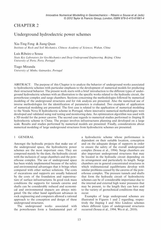
In the case of pressure tunnels located in slopes, severe accidents may occur, as in the case of Wahl—each hydroelectric scheme, Canada (Figure 38). A break in the steel lining of the scheme occurred and it is though this break was caused by a slow gravitational movement caused by block rotations

within a near-surface zone (Hoek, 2000). The generation of cavities by dissolution in tunnels of hydroelectric schemes is also a situation that can lead to serious cases of deterioration, as is the case in Guatemala and in Switzerland (Sousa, 2006).

4.2 Risk analysis and management

Risk analysis should follow the guidelines estab-lished by ITA with a description of the risk man-agement activities that may be used for all the cavities (Eskesen et al., 2004). A process established by Golder Associates for DUSEL underground laboratory is followed in this section (Popielak & Weinig, 2010). The process consists in the activi-ties: i) ranking the risk factors; ii) system to be modeled; iii) conceptual models of the system; iv) numerical analysis to study potential impacts of risk factors; and v) risk management plan to man-age risk factors.

The first activity is related to the rank the risk factors according to their impact in the matrix of risks, and should include project cost, construction sequence, safety, operations and the environment.

The second activity regards the system to be modeled combining the constructing facilities and the existing rock mass where the underground structures will be performed. The rock mass, includes the rock formations, their arrangements, the discontinuities sets and the existing faults and other low strength surfaces, the groundwater fac-tors and the hydromechanical and thermomechan-ical properties. Other factors with impact in the schedule and project costs should also be included. The underground facilities includes: the works for the powerhouse complex, that in general form an essential part of all the scheme from the risk analysis point of view; the hydraulic circuit some-times with considerable extension involving a large variety of geotechnical conditions and high pres-sures in the upper circuit, and considers the intakes with eventual instabilities at the surface; the surge chambers that can involved large concentrated excavations with high risk situations; and finally the access works that comprise access tunnels and shafts that can reach a considerable development and also connecting galleries and shafts for the major underground works. In the system other infrastructures should be included like the electro-mechanical equipments, transportation facilities, ventilation during construction, power supply, lightning and other equipments.

In the context of risk analysis, the system is entirely dynamic involving the knowledge of all components that will be updated as works progresses, which happens with the ongoing geo-technical studies and investigations and with excavations. The conception and design of the

Table 4. Classes of deterioration in pressure tunnels and shafts (Lamas, 1993).

Class Description of deterioration

A Inadequate confinement, leading to excessive rates of flow, hydraulic jacking or instabil-ity of the rock mass, including landslides or uplifts.

B Specific geologic features of high hydraulic con-ductivity, leading to leakage, hydraulic jacking or instability of the rock mass, including land-slides or uplifts.

C Deterioration of the rock mass namely due to erosion of seams, dissolution and swelling, leading to excessive leakage, rockfalls or rock mass instabilities.

D Excessive water pressure as regards impermeable barriers, such as seams or clay filled faults, leading to movements and instability including landslides.

E Deformable rock mass, inefficient grouting or deficient construction, leading to failure of the lining, namely due to high internal pressures.

F Buckling of steel linings, caused by external pres-sure of the water or grouting.

G Dynamic fluctuations of water pressure.

Figure 38. Cross section of a high pressure tunnel of the Wahleach hydroelectric scheme (Hoek, 2000).

29

underground structures will change and this will affect the system and of course future risk analyses (Popielak & Weinig, 2010).

The conceptual models of the system should consider a description of the process to a success-ful construction and operation of all the under-ground structures with particular emphasis to the large cavities like caverns and a list of uncertainties that could influence the cost; and the sequence of the excavations. The system model should con-sider the most relevant activities and also include the relationship between them. The diagrams of the system may be subdivided in sub-processes according to the different types of underground structures, like the powerhouse complex, hydrau-lic circuit, surge chambers included or not in the hydraulic circuit and for the access works.

The numerical analysis regarding the conception and design of the underground structures is a very important issue in order to ensure the safety of the works and it is an integrated process including the study of the potential impact of the risk factors in the safety of the structures. For the conception of the works, the process consists of (Geoguide 4, 1992; Sousa et al., 1994): choice of the site with optimum conditions from the safety point of view; definition of the alignment of the hydraulic cir-cuit and of the cavern main axes of orientation minimizing the stability problems; definition of the shapes for the different types of cavities tak-ing into consideration mechanical and geometrical properties of the rock mass and particularly of the discontinuity sets and faults and the in situ state of stress; dimensioning of the different parts of the underground structures in order to achieve an opti-mum solution from economic point of view; choice of the construction process for the different cavi-ties, equipments and topographic and geological conditions, and monitoring of the works.

The design stage of the underground structures is based on numerical analysis of the different hazard scenarios already defined on Table 3. The analysis started with the hazard ranking highlight-ing their relative importance. The ranking hazard for the large cavities is H1 (rock fall) combining wedge failure with stress induced failure, isolated or with mutual influence. It is therefore important to evaluate the existing discontinuity sets. To ana-lyze the risk for wedge failure and to determine the corresponding support requirements various types of numerical calculations should be carried out, as illustrated in Figure 39 using the software Unwedge (Popielak & Weinig, 2010).

Other important hazard analysis is for instant H4 (collapse) due to the interception of the cavities by low strength surfaces as happened at Cahora Bassa (Figure 33). It is necessary to develop large numerical models using different techniques, like

FEM, FDM or DEM in order to predict stability of the large cavities and their deformations. Nowa-days the use of complex 3D numerical models is possible considering different type of underground structures and can be combined with 2D simpli-fied models (Miranda, 2007). For the high pressure tunnels and shafts of the hydraulic circuit, hydro-mechanical models need to be applied in order to simulate the real behavior of the rock mass (Lamas, 1993; Scheleiss, 2000).

To model the range of expected deformations and taking into consideration the existing uncer-tainties, a series of sensitivity calculations can be carried out (Fellner & Hobson, 2008). The detail of the construction sequence of the cavities must be analyzed. Numerical calculations should be car-ried out in order to determine the deformations and state of stresses for the different underground structures and for the final stage.

Also and for better evaluation of the risk involved it is relevant to combine the results of these numer-ical models with probabilistic simulations using Monte Carlo method or BN approaches. Nowa-days due to the importance of the BN, next section is dedicated to the analysis of this approach. The results of the probabilistic numerical simulations determine the probability distribution of schedule impact and the sensitivity of the project to model input parameters risk factors and to take decisions about the appropriate measures to be taken during the several stages of the works (Popielak & Weinig, 2010; Sousa, 2010).

The final activity regarding risk management is to review the probabilistic analysis and identify a list of the potential problems. The prioritized list of significant risks represents an important step in the risk mitigation plan. A recommended risk management plan should be presented and their strategies (Popielak & Weinig, 2010).

Figure 39. Roof wedge at a large cavern (Popielak and Weinig, 2010).

30

In the context of rock engineering design methodology it is beneficial to be able to audit the content of rock mechanics modeling and design in order to ensure that all the necessary factors are included (Feng & Hudson, 2011).

4.3 Application of Bayesian networks (BN)

The risk related to the underground hydroelectric structures can be analyzed by using BN. A BN, also known as belief network, is a graphical representa-tion of knowledge for reasoning under uncertainty (Sousa, 2010). Over the last decade, BN have become a popular model for encoding uncertain expert knowledge in expert systems (Heckerman, 1995). BN provide a good tool for decision analy-sis, including prior analysis, posterior analysis and pre-posterior analysis. Furthermore, they can be extended to influence diagrams, including decision and utility nodes in order to explicitly model a deci-sion problem. A BN is a concise graphical represen-tation of the joint probability of the domain that is being represented by the random variables, consist-ing of (Russell & Norvig, 1995; Sousa, 2011):

− A set of random variables that make up the nodes of the network.

− A set of directed links between nodes. (These links reflect cause-effect relations within the domain.)

− Each variable has a finite set of mutually exclu-sive states.

− The variables together with the directed links form a directed acyclic graph (DAG).

− Attached to each random variable A with par-ents B1, …, Bn there is a conditional probability table, except for the variables in the root nodes. The root nodes have prior probabilities.

Figure 40 is an illustration of a BN for the risk analysis due to CO2 injection in carboniferous for-mations (Sousa & Sousa, 2011). In the Figure, the arrows going from one variable to another reflect the relations between variables.

There are several advantages that BN have over other methods, such as event and fault trees, and this technique can be chosen to model the haz-ards that happen during construction and opera-tion stages of underground hydroelectric projects (Sousa, 2010).

An example of application was developed by Smith (2006) for dam risk analysis using BN. Risk analysis using BN can be performed taking into account the complexity and the uncertain-ties related to potential failure mechanisms. A BN was developed for the analysis of a 25 m high and 860 m long clay embankment without internal drainage and founded on untreated soil founda-tion. The failure of the dam is analyzed by con-sidering internal erosion and overtopping. These failures mechanisms are affected by the reservoir level, which depends on the precipitations and spillway operation and risk of overtopping. The use of BN has contributed to solve a risk analysis problem for this project involving irrigation and flood protection works. It was possible to compare according to the probability of failure being used as a common denominator, the geotechnical and hydrogeological risks related to the embankment dam as well as the risk related to the reliability of the electrical/mechanical components of the spill-way (Smith, 2006).

A methodology for risk assessment and decision making using BN was proposed by Sousa (2010) for risk assessment and decision making for tun-nel projects during design and construction phases. During the design phase, different strategies can be defined that is wanted to evaluate. The tunnel alignment will be divided into different sections of more or less homogeneous conditions. Each section is treated independently. For each sec-tion the following information is needed: i) prior probability of geological states; ii) vulnerability, i.e., the probability of failure mode k, in geology i with construction strategy j; iii) the consequences of failure mode k, expressed in utilities; iv) cost of changing (where relevant) construction strate-gies. Figure 41 gives a BN for a hypothetical tunnel with three sections. The goal of the analysis was

Figure 41. Influence diagram for design phase (Sousa, 2010).Figure 40. BN for risk analysis of storage of CO2 (He et al., 2011).

31

to determine the optimal sequence of construction strategies for the tunnel based on the available information.

The influence diagram for the design phase, pre-sented in Figure 41, was solved using the Policy Evaluation algorithm. This algorithm computes the maximum expected utility for the whole tun-nel and corresponding optimal construction strat-egy sequence. The total maximum expected utility for the tunnel is E (Utility) = −34.76 and the cor-responding optimal construction strategy sequence is to use construction strategy CS2 in section 1 (E (U) = −13.81), switch to construction strategy CS1 in section 2 (E (U) = −13.75) and then switch back to construction strategy CS2 in section 3 (E (U) = −7.20) (Sousa, 2010).

When tunnel construction starts, new informa-tion is available as the excavation progresses. This information can and should be used to update the prior probability distribution of the geological states within each section. The proposed method consists of dividing each section into subsec-tions as shown in Figure 42. Once the excavation progresses in section x and information is available regarding the geological state, data can be used to update the geological states in the remainder of the unexcavated section x. For this one needs a transi-tion model, in this case, the probabilities of chang-ing from one ground type to another ground type.

This methodology was used and applied with success to the Porto Metro where three collapses occurred between 2000 and 2001 (Geodata, 2001). Based on the analysis of Porto metro case study, the decision support framework for determin-ing the “optimal” (minimum risk) construction method for a given tunnel alignment, was further developed for the specific case of the Porto metro line C tunnel. The decision support framework

consists of two models: one geologic prediction model and a decision model (Figure 43).

This methodology can be developed for the dif-ferent hazards defined in Table 3 for underground hydroelectric schemes, during construction and first filling or normal operation. For instance for the scenario H2 that corresponds to the occurrence of rockburst during construction, which happen in the case of Jinping II (Wu et al., 2010), a BN applied for the rockburst is illustrated in Figure 44. A methodology for rockburst evaluation during construction can be established.

5 STUDY OF VENDA NOVA II POWERHOUSE COMPLEX

5.1 Introduction

EDP—Electricity of Portugal decided to repower the Venda Nova hydroelectric scheme, located in the North of Portugal, by building a new power station, named Venda Nova II, that took advan-tage of the high existing head, about 420 m, between the reservoirs of Venda Nova and Salam-onde dams (Lima et al., 2002) (Figure 45).

The scheme is almost fully composed by under-ground facilities, including caverns and several tun-nels and shafts with total lengths of about 7.5 km and 750 m, respectively (Figure 46). The project involved the construction of important geotechni-cal underground works of which the following can be mentioned: i) the access tunnel to the caverns, with about 1.5 km, and 58 m2 cross-section; ii) the hydraulic circuit with a 2.8 km headrace tunnel with 14.8% slope and a 1.4 km tailrace tunnel and 2.1% slope, with a 6.3 m diameter modified circu-lar section; iii) the powerhouse complex located at about 350 m depth with two caverns, for the pow-erhouse and transforming units, connected by two galleries; iv) an upper surge chamber with a 5.0 m diameter and 415 m height shaft and a lower surge chamber with the same diameter and 60 m height. The arrangement of the cavities for the powerhouse complex is illustrated in Figure 47. A cross-section of the powerhouse complex caverns is presented in Figure 48.

Figure 42. Division of Section 1 into subsections (Sousa, 2010).

Figure 43. Decision support framework for the design and construction phases (Sousa, 2010).

32

The scheme was built in a granite rock mass with overall good quality. In order to have an insight of the main geomechanical characteristics of the rock formation, in the following section some of infor-mation gathered during the geotechnical surveys carried out to characterize the rock mass interest-ing the hydraulic circuit is concisely analyzed.

Afterwards, the main characteristics of the powerhouse complex are presented together with the geotechnical survey performed to character-ize the rock mass near the caverns and the defined monitoring plan. The main results of the numeri-cal models are analyzed and compared with the monitored data in terms of displacements. Finally, back analysis techniques are applied in order to identify some geomechanical parameters. Two dif-ferent techniques are used, namely an optimiza-tion software called SiDolo which is based on a hybrid technique which combines two traditional optimization algorithms and an evolution strategy algorithm. Due to the rock mass characteristics the most important parameters in the behavior of the

Figure 44. BN for rockburst prediction.

Figure 45. General perspective of the power reinforce-ment scheme (Adapted from Plasencia 2003).

Figure 46. Scheme of the underground works com-posing the Venda Nova II complex (adapted from Lima et al., 2002).

Figure 47. Arrange of Venda Nova II powerhouse complex (provided by EDP).

Figure 48. Cross-section of the Venda Nova II power-house complex caverns.

33

powerhouse complex are K0 and E (deformability modulus). Therefore, these parameters were the ones object of the back analysis process (Miranda, 2007).

5.2 Geotechnical information

A succinct analysis of the deformability and strength properties determined by means of in situ and laboratory tests was carried out (LNEC, 1983, 2003). The results of the following tests are analyzed: dilatometers, LFJ tests, seismic waves propagation by ultrasounds, uniaxial compres-sive strength in rock samples and shear tests on discontinuities.

In the dilatometer test, the deformations are applied in four diametral directions and in three load cycles. In the analysis of the results, the read-ings produced by the first cycle were not consid-ered. The number of tests was 436. The mean and standard deviation obtained were equal to 16.1 and 12.0 GPa, respectively. The percen-tiles correspondent to 5% and 95% were 2.2 and 41.9 GPa, respectively. The Shapiro-Wilk and the Kolmogorov-Smirnov tests were performed to the results of the dilatometers. The distribution can-not be considered normal or lognormal for a 95% confidence degree. However, the second one con-stitutes a better fit (Miranda, 2007).

The LFJ tests were carried out in a relatively undisturbed rock mass which was fairly representa-tive of the expected overall behavior of the granite formation. To perform these tests, co-planar con-tiguous slots were cut into the rock with a disc saw. In each flat jack, four deformeters are installed which allow to measure the displacements of the rock perpendicular to the slot. These deformeters allow applying several loading/unloading cycles testing the rock formation under different condi-tions of loading. In the case of the LFJ tests car-ried out in the scope of the Venda Nova II project, they allowed to measure, and excluding the values obtained in the first loading cycles, a total of 160 E values. Table 5 resumes some statistical data con-cerning the LFJ tests results.

This information was used to update the prior distribution of E, considered a random vari-able, set using empirical formulations based on

correlations through a Bayesian framework developed with this goal (Miranda et al., 2009). The geomechanical data obtained in this formation was well adjusted to the normal and lognormal dis-tributions. Both distributions were considered to evaluate the impact of prior assumptions on the final results.

The mean values of E, calculated and measured by the LFJ tests, are very similar. The main differ-ence is the higher variation in the calculated values. This fact can be considered normal since the LFJ tests are much more accurate than the empirically based expressions. Considering this initial informa-tion and the additional one provided by the results of the LFJ test the application of the Bayesian methodology allowed us to obtain the prior distri-butions and correspondent updated posteriors.

Figure 49 shows the prior and posterior prob-ability density functions of the mean value of E considering the mean value of its standard devia-tion. The uncertainty reduction from the prior to the posterior can be clearly observed. Using simu-lation it was possible to infer mean and 95% CI for the population. In relation to the mean value, the updating process only changed significantly the mean of the lognormal distribution which was reduced in about 11%. For the normal distribution case this value remained almost unchanged.

The mean value of the dilatometer tests is sub-stantially lower than the results obtained by LFJ tests. The dilatometers tests were performed in all types of rock masses which are translated by the high variability of the results and wide interval between the 5% and 95% percentile. In the other hand, the LFJ was performed in a very good qual-ity rock mass. The highest values obtained by the dilatometer tests are close to the mean value obtained with the LFJ.

Table 5. Statistical results of the performed LFJ tests (GPa).

Number of tests Mean

95% CI for the mean

Standard deviation

160 36.9 35.9–37.8 6.1

CI—confidence interval.Figure 49. Prior and posterior probability density func-tions for the mean value of E.

34

To complement the previous analysis, the results from ultrasound tests, which allow obtaining the seismic waves velocity (Vp and Vs) also related with deformability properties, were analyzed.

In situ tests were performed in order to estimate the in situ state of stress existent in the rock mass. A total of nine SFJ tests were performed. From these, only three were considered to be representa-tive of the rock mass with a low disturbance (frac-turing) degree caused by the excavation process. The results of E ranged from 46 to 51 GPa. A value of 1.63 was found for K0 perpendicular to the cavern axis. Six overcoring STT tests were performed in two different locations. The tests, in spite of being carried out in relatively distant test sites, present very similar results. In fact, values of 2.2 and 2.6 were found for K0 in the same direction as stated for the SFJ tests. The vertical stress corresponds approximately to the overburden gravitic load.

Concerning the laboratory tests, compression tests were made permitting to obtain unconfined compressive strength (σc) and the elasticity modu-lus of the intact rock (Ei). Laboratory shear tests on discontinuities were only performed in samples collected in best geotechnical zone. Besides the Mohr-Coulomb strength parameters and also the dilation angle and the stiffness in the normal (KN) and tangent (KT) were obtained on 40 samples. The discontinuities present good strength characteris-tics. In fact, the mean value of the residual φ ′ is high (around 39°) and they also exhibit, most of the times, some internal cohesion. This parameter is characterized by a high variability which is much less pronounced in what concerns φ ′. It is interest-ing to observe the dilatant behavior of the discon-tinuities in almost every test.

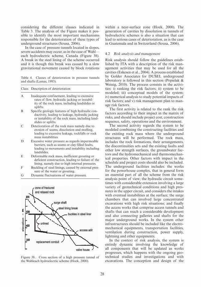
5.3 Numerical modeling of the powerhouse

5.3.1 Description of the developed modelsThe 3D model was carried out using the soft-ware FLAC3D to simulate the complex geometry of the powerhouse complex and its construction sequence (Figure 50). A 2D numerical model, developed using Phases2 software, was performed in a middle cross-section.

Figure 50. 3D mesh developed for the powerhouse complex.

For the 3D numerical modeling, the construction sequence was simplified relatively to the one defined in design. Five excavation stages were con-sidered (Table 6). Due to the good geomechanical quality of the rock mass its behavior during tun-neling was almost elastic. Hence, the simplifica-tions considered for the excavation stages had minor impact on the computed displacements. The construction sequence adopted for the 2D model was very similar.

Due to the high depth of the underground com-plex, a constant stress field was considered and its magnitude was set based on the results of the in situ tests. The vertical stress was computed considering the overburden dead load of the rock mass. The same stress value was considered in the horizontal direction parallel to the cavern axis. In the perpen-dicular direction the performed tests pointed out for a K0 between 2 and 3. Some preliminary calcu-lations allowed concluding that lower values of this coefficient led to more realistic results. Therefore, in the analysis, an initial value of 2 was adopted.

5.3.2 Analysis of the resultsThe results of the models are analyzed and com-pared particularly for the last excavation stage. Emphasis is given to the results in terms of dis-placements since they can be compared with the real behavior of the structure observed by the extensometers, allowing the validation of the models.

Due to the high K0 and the span of the main cavern vertical wall, the higher displacements were expected to take place in that area. Figure 51 presents the displacement contours computed with the 3D model for the last excavation stage. In fact, the highest displacements are observed in the wall of the main cavern, particularly, between the two interconnecting galleries.

Table 6. Adopted construction stages for the 3D numerical model.

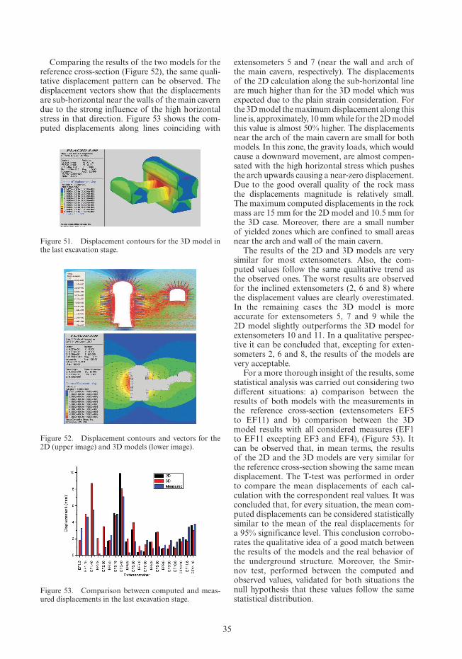
35

Comparing the results of the two models for the reference cross-section (Figure 52), the same quali-tative displacement pattern can be observed. The displacement vectors show that the displacements are sub-horizontal near the walls of the main cavern due to the strong influence of the high horizontal stress in that direction. Figure 53 shows the com-puted displacements along lines coinciding with

extensometers 5 and 7 (near the wall and arch of the main cavern, respectively). The displacements of the 2D calculation along the sub-horizontal line are much higher than for the 3D model which was expected due to the plain strain consideration. For the 3D model the maximum displacement along this line is, approximately, 10 mm while for the 2D model this value is almost 50% higher. The displacements near the arch of the main cavern are small for both models. In this zone, the gravity loads, which would cause a downward movement, are almost compen-sated with the high horizontal stress which pushes the arch upwards causing a near-zero displacement. Due to the good overall quality of the rock mass the displacements magnitude is relatively small. The maximum computed displacements in the rock mass are 15 mm for the 2D model and 10.5 mm for the 3D case. Moreover, there are a small number of yielded zones which are confined to small areas near the arch and wall of the main cavern.

The results of the 2D and 3D models are very similar for most extensometers. Also, the com-puted values follow the same qualitative trend as the observed ones. The worst results are observed for the inclined extensometers (2, 6 and 8) where the displacement values are clearly overestimated. In the remaining cases the 3D model is more accurate for extensometers 5, 7 and 9 while the 2D model slightly outperforms the 3D model for extensometers 10 and 11. In a qualitative perspec-tive it can be concluded that, excepting for exten-someters 2, 6 and 8, the results of the models are very acceptable.

For a more thorough insight of the results, some statistical analysis was carried out considering two different situations: a) comparison between the results of both models with the measurements in the reference cross-section (extensometers EF5 to EF11) and b) comparison between the 3D model results with all considered measures (EF1 to EF11 excepting EF3 and EF4), (Figure 53). It can be observed that, in mean terms, the results of the 2D and the 3D models are very similar for the reference cross-section showing the same mean displacement. The T-test was performed in order to compare the mean displacements of each cal-culation with the correspondent real values. It was concluded that, for every situation, the mean com-puted displacements can be considered statistically similar to the mean of the real displacements for a 95% significance level. This conclusion corrobo-rates the qualitative idea of a good match between the results of the models and the real behavior of the underground structure. Moreover, the Smir-nov test, performed between the computed and observed values, validated for both situations the null hypothesis that these values follow the same statistical distribution.

Figure 51. Displacement contours for the 3D model in the last excavation stage.

Figure 52. Displacement contours and vectors for the 2D (upper image) and 3D models (lower image).

Figure 53. Comparison between computed and meas-ured displacements in the last excavation stage.

36

In terms of stresses, the rock mass surrounding the caverns is mainly under compression. The maximum compression stress, about 35 MPa, is observed in the upper zone of the main cavern arch (Figure 54). Tension stresses only happen near the main cavern wall due to its span and in situ state of stress. However, the maximum tension stresses are below 1 MPa. Considering the strength properties of the rock mass it is expected that only a few plas-tic zones occur and the rock mass behaves almost in elasticity. Figure 55 shows the zones in plastic-ity and, in fact, only a few sheared zones can be observed in the surroundings of the underground structure. This almost elastic behavior of the struc-ture and surrounding rock mass mean that the adopted construction sequence in the models has a low impact on the final results.

Figure 56 presents the maximum and minimum principal stresses in the sprayed concrete for the last excavation stage. It can be observed, and in agreement with a previous statement, that the most compressed zone is located near the arch of the main cavern, mainly between the interconnecting galleries. In this area, the computed compression stresses range between 4 and 5 MPa. These values are still far from the limit compression strength of a current sprayed concrete so crushing of the mate-rial is not expected to happen. The computed ten-sion stresses are generally low (<2 MPa). However, in the beginnings of the main cavern arch, tension stresses can reach values up to 11 MPa. This is caused by a stress concentration effect in this area and may cause cracking to the concrete.

For the 3D model a calculation of the factor of safety (FOS) was carried out. FLAC3D uses the method defined by Dawson (1999) in which the strength parameters are consecutively reduced until significant plastic flow appears in some zone of the structure. The computed FOS was 4.63 which can be considered satisfactory in terms of security level. Figure 57 shows an image of the last

Figure 54. Computed minimum stresses (negative values translate compression).

Figure 55. Plastic zones at the last excavation stage.

Figure 56. Stresses in the fiber sprayed concrete.

Figure 57. 3D visualization of the shear strain contours for the last non-equilibrium state.

37

non-equilibrium state produced by the methodology of strength reduction applied to calculate FOS.

5.4 Back-analysis of geomechanical parameters

5.4.1 Used optimization techniquesAs it was concluded by the structural analysis of the models, the parameters with more influence on the behavior of the powerhouse complex are E and K0. Different techniques were applied in order to back-analyze these parameters based on the monitored displacements. Two optimization algorithms, a deterministic and a probabilistic, were applied together with the 3D model. These algorithms were coupled with FLAC3D in order to perform the identification process in a more efficient way.

The deterministic method was the one provided by the software SiDolo (SiDolo, 2005). It uses a hybrid algorithm that combines two traditional opti-mization techniques, namely, a gradient based algo-rithm and a variant of the Levenberg-Marquardt method to accelerate convergence when the proc-ess is close to the solution (Eclaircy-Caudron et al., 2007). The error function (L(A)) used by SiDolo is translated by Equation 7.1:

LM

T Z Z D Z ZnM

sZ sZ n s sZi

MnMM

( )A D Zn sD ZZsZ *D Z Z*= ( )A tiA tit ( )i(ttit⎡⎣⎡⎡ ⎤⎦ ( )A tit,AA ( )ti⎡⎣⎡⎡ ⎤⎦⎤⎤

=

1

1

⋅D∑∑∑=n

N

1 (4)

where a represent the model parameters, N is the number of experimental results, [Zs(A, ti)−Z*

s (ti)] is the difference between numerical and experi-mental results of the Mn observation at timestep ti and Dn is the weighting matrix of the nth test. Dn is a diagonal matrix and these coefficients cor-respond, normally, to the square of the inverse measurement error or of its estimation. In this study, these errors were assumed to be equal for all measurements which reduced Equation (4) to a least square error function. In SiDolo, the proc-ess is stopped if one of two conditions is verified: a maximum pre-defined number of iterations is reached or when the relative difference between the error function value obtained at a certain step and the best one obtained during the process is lower than a defined threshold. In this study, a rate of 10−15 was adopted.

The other used optimization algorithm was the (μ/ρ + λ) evolution strategy (ES) (Miranda, 2007). The same error function used by SiDolo was consid-ered together with this algorithm. For the stopping criteria, the error values ε1 and ε2 were initially con-sidered equal to 10−5. In a more advanced stage, a value of 10−7 was also tested in order to analyze the influence of this parameter in the obtained results and in the algorithm efficiency.

5.4.2 Validation studiesIn order to determine the possibility to identify E and K0 using the described techniques together with the observed displacements in the exten-someters, validation studies were carried out. An experimental response of the 24 displace-ments measured by the extensometers was artifi-cially created using the 3D model and the set of geomechanical parameters initially defined for the structural analysis. Then, the strength param-eters, as well as the Poisson coefficient, were fixed while E and K0 (perpendicular to the caverns axis) were supposed unknown. Both methods need a definition of boundary values for the parameters to identify. This way, the interval values were set between 1 GPa and 100 GPa for E and between 0.5 and 2.5 for K0. Moreover, as SiDolo is based on traditional optimization algorithms, it also needs an initial approximation to the parameters. In this context, values of 60 GPa (+44.4% deviation) and 1.0 (−50% deviation) were adopted for E and K0, respectively.

Two identification processes were carried out using SiDolo. In a first approach, just the displace-ments obtained after the first excavation stage were considered. Afterwards, the displacements meas-ured at every stage were used in the process. With the ES algorithm only the first of the described calculations was carried out. Table 7 resumes the obtained results.

It is possible to observe that SiDolo allows obtaining the correct parameter values in both situations. The main difference is the efficiency of each calculation. When the displacements of all excavation phases are considered, the iteration number, and consequently the computation time, is much higher than in the case where the results of a single stage are used. It is once again proved that the rock mass behavior during the caverns excava-tion is nearly elastic and the construction sequence has minor impact on the identification process. The ES algorithm, which used the measurements of only one stage, reached convergence within a single generation of solutions, i.e., in ten iterations. The identified parameters are close to the correct ones with an error of approximately 4% which is due to the relatively high values adopted for ε1 and ε2 (10−5). A more restrict stopping criteria would enhance the quality of the results but increase the

Table 7. Results of the validation studies.

Case E (GPa) K0 Error value Iterarions

SiDolo (1 phase) 45.0 2.0 8.9 × 10−13 2

SiDolo (all phases) 45.0 2.0 1.0 × 10−8 50

ES (1 phase) 43.3 1.9 1.3 × 10−7 10 (1 gen.)

38

computation time. Nevertheless, it was concluded that, also with this technique, it would be possible to proceed to the back analysis of the interested parameters considering only the measurements made after one excavation stage.

Figure 58 presents the error function topology for the referred case. In spite of being somewhat irregu-lar, the error function presents a clear and singular minimum. This characteristic enables the param-eters identification using both algorithms without convergence problems. Hence, it was decided that in the back analysis calculations, only the displace-ments observed after the last excavation stage would be used. This option lead to a very important decrease of the computation time with almost insig-nificant precision loss, in comparison to the option of using the data of all construction stages.

5.4.3 ResultsConcerning the back analysis using the 3D model, two different methodologies were used. The soft-ware SiDolo based on traditional algorithms and an ES were coupled with the model to perform the identification process. The interval range adopted for the parameters was the same used for the valida-tion studies. They seem sufficiently large to contain the optimal solution and to correctly test the algo-rithms in this real application. In the calculations performed using SiDolo, the initial approximation for the parameters were the values given by the soft-ware GEOPAT (Miranda, 2003), i.e. 45 GPa for E and 2.0 for K0. In the first identification attempt the 20 measurements were considered and convergence was reached. In order to evaluate the process stabil-ity and consistency on the results it was decided to

perform another calculation in different conditions. It was verified that the difference between the com-puted and observed measurements was always of the same sign before and after optimization exclud-ing for the values of EF1.15 and EF5.40. This way, a second process was carried out considering as a starting point the optimized values of the first calculation and without the cited measurements. Table 8 presents the results of the two identification attempts using SiDolo and compares them with the results obtained with the initial guess provided by GEOPAT (Miranda, 2003).

Concerning the first identification attempt, con-vergence is attained in a total of 25 iterations. The optimized set of parameters is not significantly dif-ferent to the initial guesses especially in what con-cerns K0. The optimized value of E is 22% higher than the initial one. The error function value under-went a 29% decrease and the mean displacement differs only 0.12 mm from the measured values.

Figure 59 presents a comparison between the measured displacements with the ones computed with the initial and optimized set of parameters. It is interesting to notice that the results obtained with the optimized parameters only outperform the fit of the initial calculations in nine out of twenty measures. However, the errors plot shows a more smooth distribution of the errors in the differ-ent extensometers for the optimized parameters calculation.

For the second attempt, additional 12 iterations were necessary to achieve convergence. In spite a higher variation in relation to the initial val-ues given by GEOPAT, the final obtained set of parameters is close to the first attempt. The error function value was reduced in a similar percent-age as in the previous calculation. The mean value of the displacement is only 0.18 mm less than the observed values. The results of this calculation point out to more rigid rock mass and less impor-tant horizontal loads translated by the lower value of K0 in relation to the first calculation.

In the identifications carried out with the ES, only 18 displacement measurements were considered

a)

b)

Figure 58. Topology of the error function on the iden-tification of E and K0 for the validation study using only the displacements measured after the first stage. (a) 3D view (b) Plan view.

Table 8. Results of the identification processes using SiDolo.

CaseE (GPa) K0

Error value (×10−6)

Mean disp. (mm)* Iterations

Initial values 45.0 2.00 1.76 2.91 –

Results (1) 55.0 1.98 1.26 2.36 25

Initial values 45.0 2.00 1.90 2.51 –

Results (2) 56.7 1.90 1.34 1.93 12

* Displacements are 2.48 and 2.11 mm for the first and second calculations, respectively

39

In the first calculation, and due to the relatively high value for the stopping criteria (10−5), con-vergence was reached in only one generation (10 iterations). The probabilistically created group of solutions by the algorithm allowed obtaining results which reduced the error function value. The optimized set of parameters varied the same relative magnitude in relation to the initial values. In particular, the optimized value of E is 14% higher and K0 14% lower. The adoption of a more restrict stopping criteria (10−7), allowed to improve the results in relation to the observed measure-ments. With this new set of optimized parameters, every evaluation criteria was improved. In fact, the value of the error function was decreased and the mean displacement is closer to the observed value. This improvement was obviously translated with an increased computational effort. In this case, 6 generations (60 iterations) were needed in order to reach convergence. In comparison with the set of parameters obtained with SiDolo, the error func-tion value is similar but the mean displacement is slightly closer to the observed values in the solu-tion found by the ES. Figure 60 presents a com-parison between the observed displacements and

Figure 59. Comparison between the observed meas-urements and the computed values with the initial and optimized set of parameters obtained by SiDolo in the first identification attempt. (a) Absolute values; (b) Error values.

in order to check, under different circumstances, if the obtained results could be improved.

A total of three back analysis processes were performed using the ES algorithm. In the first identification attempt, a value of 10−5 was consid-ered for ε1 and ε2. To evaluate the influence of the stopping criteria, a second process was carried out using a value of 10−7 for these parameters. Finally, in the third attempt, an elastic constitutive model was adopted for the rock mass. Table 9 resumes the obtained results of these calculations.

Table 9. Results of the identification processes using ES algorithm.

CaseE (GPa) K0

Error value (×10−6)

Mean disp. (mm)* Generations

Initial values 45.0 2.00 1.90 2.51 –

ES (10−5) 52.1 1.72 1.37 1.91 1

ES (10−7) 58.0 1.98 1.34 1.97 6

ES (10−7) elast 58.5 2.02 1.36 1.91 7

* The mean measured displacement is 2.11 mm

Figure 60. Comparison between the observed meas-urements and the computed values with the initial and optimized set of parameters obtained by the evolution strategy considering ε1 and ε2 equal to 10−7. (a) Absolute values (b) Error values.

40

the ones computed with the initial and optimized set of parameters. The results are similar to those reported with the set of parameters identified with SiDolo namely in relation to the more smooth distribution of errors obtained with the opti-mized parameters. However, in this case, the fit is improved in 9 out of 18 cases while for the previous case, that value was 8.

In conclusion, the results obtained by the set of parameters identified by the ES algorithm slightly outperforms the ones obtained by SiDolo. The rea-son could be one of the following: i) the traditional algorithm based software SiDolo was kept in a local minimum; ii) the stopping criteria of the ES was more restrict. Figure 61 presents the topology of the error function for this case and the location of the identified values by both methodologies. In the plan view, it is possible to observe that the solution given by SiDolo and the ES using the more restrict stopping criteria, lay near the same isoline. The other solution given by this algorithm corresponds to a higher value of the error function caused not by a local minimum but because of the higher error value to stop the process. This way, it is possible to conclude that the correct hypothesis is the one raised in ii), i.e. the slight differences in the solutions provided by the two methodologies is related with the stopping criteria.

However, it is also possible to observe a local minimum in the error function near the region corresponding to E and K0 values of 45 GPa and

1.5, respectively. Both methodologies were able to avoid this local minimum and converge to the global solution but probably for different reasons: the ES because of its intrinsic characteristics of global optimization that allows it to avoid local minima; SiDolo because of the characteristics of the error function topology but mostly because the initial guess for the identification with SiDolo was already close to the global optimum.

Finally, the optimization procedure was carried out considering an elastic model for the rock mass. The identified set of parameters is rather close to ones obtained with the plastic model. The error function value is only slightly increased.

6 STUDY OF JINPING II HYDROELECTRIC SCHEME

6.1 The underground powerhouse

The Jinping II hydroelectric project, being con-structed presently in China, involves infrastruc-tures planning developed on a large scale, requiring four high pressure tunnels, 16.67 km long, with 60 m spacing between them, a drainage tunnel, two access tunnels, and a large underground power-house structure (Wu et al., 2010; Feng & Hudson, 2011). Two of the high pressure tunnels are 13 m in span, excavated using drilling and blasting (D&B), and the other two are 12.4 m in diameter, excavated using TBMs.

Jinping II is an ambitious project for the owner, Ertan Hydropower Development Co. Ltd. It is located in Yalong River, and Jinping site is unique in that it will utilize a natural 180 degree bend in the Yalong River (Figure 62). Jinping II has a large underground complex for the powerhouse with 8 units and a total installed capacity of 4800 MW, to produce a multi-year average annual output

Figure 61. Topology of the error function for the plas-tic model of Venda Nova II powerhouse complex. (a) 3D view (b) Plan view.

Figure 62. Location of the Jinping II hydropower sta-tion underground powerhouse.

41

of 24.23 TWh. Figures 63 and 64 illustrate the underground power station complex. Construc-tion started in August 2008 and will be finished in 2012.

This section is only dedicated to the study of the underground powerhouse complex. The com-plex mainly includes main powerhouse, auxiliary powerhouse, transformer chamber, draft tube gate chamber, pressure adjustment shaft, draft tube tunnels, erection bay, tailrace tunnels, and bus tun-nels. According to the water ahead and hydraulic process, the underground powerhouse has different layouts, e.g., shown in Figure 14. Usually, there is one penstock, bus tunnel, and draft tube tunnel for one generator. Sometimes, there may have one tail-race tunnel for three generators. There may have one headrace tunnel for two generators. Jinping II powerhouse has been designed with sizes shown in Figure 63.

6.2 Features and constraints of the Jinping II powerhouse

6.2.1 Geological conditions at the siteRegional tectonic characters: the site is located at South-east region of Songfan-ganzi fold system; it underwent the Yinzhi and Yanshan movement, especially Himalaya movement, since the Mesozoic era and formed a series of thrust faults, overturn

of strata, ‘A’ type recumbent fold, and mountain peak, as seen in Figure 64.

Topography and geomorphology: North side of the site has high and steep slope. The slope has an angle of about 50 −70° at altitude of 1330–1600 m, due to intersection of steep bed-parallel joints and NWW steep and gent joints. The slope has its angle about 35–45° at altitude of 1600 m—about 1700 m and steep bank at altitude of 1700 m. After altitude of 1700 m, slope angle is changed to about 35°, as seen in Figure 65.

Stratum lithology: It is the middle Triassic Yan-tang formation (T2y) and quaternary system (Q). T2y

4: greyish-green stripped micaceous marble with thickness of about 400 m (Figure 66b). T2y

5-(1): ash black fine marble with white coarse-grain marble (Figure 66c). T2y

5-(2): gray—white coarse-grain mar-ble including H2S) with thickness of about 400 m (Figure 66d). T2y

6: ash—ash black moderate—thin layered argillaceous limestone (Figure 66e), at alti-tude 1870 m or above, thickness of 350 m. Qua-ternary system (Q): slope wash, accumulation and wash locally.

1. Main powerhouse (352.4 × 72.2 × 28.5m3)2. Transformer chamber (374.6 × 35.1 × 19.8m3)3. Draft tube gate chamber

( 351 × 63.7 × 13m3) 7. Access tunnel 8. Access tunnel to draft tube Gate chamber 9. Ventilation tunnel to transformer chamber 10. GIL electric wire outlet passway 11. Ventilation and safe tunnel 12. Passing wind tunnel for trans for-mer chamber

14. Shaft for ventilation and the pas-sage of smoke 15. Pump cavern 16. Bus tunnel 17. Transportation tunnel for trans-former chamber 18.Transportation electric wire passway 19.Transportation walls G1–G8. High pressure head con-duits nos. 1–8 P1–P4. 1–4# water drainagegalleriesW1–W8. Tailrace tunnels Nos.1–8 Z1–Z2. Wind tunnels nos. 1–2 for draft tube gate chamber S1–S8. Construction galleries nos. 1–8.

Figure 63. Structure of underground powerhouse of Jinping II hydropower station.

3550

3300

3050

2800

2550

2300

2050

1800

1550

1300

1050

0 500 1000 1500 2000 2500

T2y5 6

2yT42yT

52yT

42yT

52yT

52yT

62yT

Depth (m)

Underground

powerhouse

Yalong river

Altitud

e (

m)

Syncline

Syncline Anticline Anticline

Scale: 1:25000

N64°E

Figure 64. Geological section of folds at the site.

Figure 65. Topography and geomorphology of the site.

42

The strata strike is about NNE. Meanwhile, it is also subject to second in situ stress field (Feng & Hudson, 2011). Five set of fractures exist such as: (1) N10°W–N30°E, NE-NW∠73–85°, (2) N60–80°W, SW∠20–40°, ∠70–90°, (3) N40–60°E SE∠20–40°, (4) EW, S∠20–40°, (5) N70–85°E SE∠60–80°.

Hydrogeology: It belongs to eastern solution crack-fracture broken stream hydrogeology ele-ment (III) with width 2.5–4.5 km and occurred in middle Triassic Yantang formation. Shallow layer underground water comes from raining with large flow at rain season. Deep underground water is mainly structure-fissure water or karst water, has a large overburden of about 200–250 m, with a small change with season.

6.2.2 Current in situ stress fieldSome of the measured in situ results indicated that Jinping II underground powerhouse is located at high tectonics stress region (Table 10). The meas-ured results show that the maximum principal stress is about 10.1–22.9 MPa and mainly vertical to slope with average S43.1–47.4°E, which agrees with direction of the maximum principal stress in the region.

The technical auditing was firstly performed on the measured in situ stress data using ISRM Sug-gested Methods (Ulusay & Hudson, 2007). Also, the location and depth of the measured points for the in situ stress estimation and their relation to the Jinping II underground power station cav-erns needed to be considered for this selection. The measured data of total six measured points were finally selected for this purpose (Figure 67), (Jiang et al., 2009).

The regional tectonics and the measured in situ stress data show that the in situ stress field in Jin-ping II hydropower station result from not only the ancient stress field, but also deep valley stress field. Therefore, the influence of tectonics sequence and formation of current topography shall be consid-ered in the recognition of the in situ stress field at the Jinping II underground powerhouse region. The evolution of the stress path on the in situ stress field can be simulated using elastic-plastic calcula-tion, which uses the step-loading on deformation boundary to simulate sequence of tectonics and the calculation of excavation from top to down to simulate process of strata erosion. The calculation model of three dimensional stress field is shown in Figure 68, considering seven control faults such as F7, F17, F16, F32 etc. In Figure 68 they are included.

The main factors considered, affecting the in situ stress field in Jinping II underground power-house region, are gravity, extrusion at direction X,

T2y5-

(1)

Qcol+d

l4

T2y5-

(2)

T2y6

Qcol+d

l4

T2y4

(a)

(b) T2y4 (c) T2y

5-(1)

(d) T2y5-(2) (e) T2y

6

Figure 66. Stratum lithology of the site.

2y

6

2y

4

2y5- 1

5- 2

2y

F8

F7

F14

F33

F63

F62

F61 F60

F65

F59

F29

F27

F32

F37

F21

F17

F47

F49

F35

F16

F51

F24

6

2y

2y

5- 2 5- 12y

4

2y

T

T

T

T

T

T

T

T

Cz3-183.11

Cz1-304.9

Cz2-285.6

Cz2-250

PD4-1-215.8

PD4-1-52.4

Yalong river

σ2

σ3

σ 2

σ3

σ2

σ1

σ3

σ2

σ1 σ3

σ2 σ1

σ3

σ2

σ1

σ

σ3

Figure 67. Distribution of fault and position of in situ stress measurement points for the stress field recognition in Jinping II hydropower station region.

Geological structure in the region: The geological structure at the site almost agreed with the regional structure, which is subject to NWW—SEE in situ stress filed and developed NNE structures.

43

Table 10. The measured in situ stresses in the underground powerhouse site (from Chen et al., 2007).

Location Depth (m) Method Principal stresses

PD1 463 HF σ1 (value-MPa; strike°; dip angle°)

14.4 47 −6

σ2 (value-MPa; strike°; dip angle°)

10.0 152 −66

σ3 (value-MPa; strike°; dip angle°)

5.7 135 23

PD2 425 HF σ1 (value-MPa; strike°; dip angle°)

22.0 161 41

σ2 (value-MPa; strike°; dip angle°)

15.5 7 12

σ3 (value-MPa; strike°; dip angle°)

13.5 84 −46

PD4–1 152.4 HF σ1 (value-MPa; strike°; Dip angle°)

11.7 126 56

σ2 (value-MPa; strike°; dip angle°)

6.4 42 −4

σ3 (value-MPa; strike°; dip angle°)

4.9 134 −33

CR1 439.6 HF σ1 (value-MPa; strike°; dip angle°)

10.1 9 −35

σ2 (value-MPa; strike°; dip angle°)

6.8 129 −36

σ3 (value-MPa; strike°; dip angle°)

6.5 70 35

CR2 250.4 HF σ1 (value-MPa; strike°; dip angle°)

16.8 74 −11

σ2 (value-MPa; strike°; dip angle°)

10.9 170 −28

σ3 (value-MPa; strike°; dip angle°)

8.9 144 160

CR3 183.1 OV σ1 (value-MPa; strike°; dip angle°)

11.2 148 −5

σ2 (value-MPa; strike°; dip angle°)

8.9 65 50

σ3 (value-MPa; strike°; dip angle°)

7.2 234 39

HF—Hydraulic fracturing; OV—Overcoring.

44

extrusion at direction Y, shear at the horizontal direction X, and shear at horizontal direction Y. The value ranges of these factors shown in Table 11, are used to construct a set of factor data sets for the back analysis of the in situ stress field. (Length at X direction and Y direction are 860 and 840 m, respectively. Z is from altitude of 800 m to top of the mountain. The original point starts at cross point of axis of main powerhouse and the central line of generator No. 8).

The tectonic process such as gravity action→ extrusion at direction Y and shear at the horizon-tal direction X → extrusion at direction X and shear at horizontal direction Y was added to the displacement boundary to perform balance calcu-lation, shown in Figure 69a. And then, the ero-sion process of strata is simulated as Figure 69b→ 69c to format the current topography shown in Figure 69d. Each set of factors, shown in Table 11 is input to the model to calculate in situ stress val-ues. The calculated six stress components for each measured points shown in Figure 67 and the five factors shown in Table 11 are used to input and output of the neural network respectively. Thus, there are total 30 samples to train neural networks with the topology of 36–45–9–5 to obtain the connection weights. Other ten samples shown in Table 11 were used to test the obtained neural net-works. The neural network, giving good outputs both for the training and testing samples shown in Table 11, can be used to back analysis. With input of the measured stress data to the obtained neural networks, the actual value for five factors are recognized and shown at last line of Table 11. The recognized factors are input to the model

Main powerhouse

Transformer chambe

Draft tube gate chambe

Figure 68. Sketch map of calculation coordinate and range in back analysis of in situ stress field.

Table 11. Range of values for the factors relating to the in situ stress field for uniform design of samples.

FactorsG m⋅s−2

Tyy 10−2 m

Txx 10−2 m

Txy 10−2 m

Tyx 10−2 m

Value ranges 9.0- 1.5- 3.5- 3.0- 2.0-

Samples for ANN

11.0 3.5 5.5 5.0 4.0

1 10 3.0 3.5 5.0 3.5

2 11 2.5 4.0 5.0 3.0

3 10 2.0 4.5 5.0 2.0

.

.

.

.

.

.

.

.

.

.

.

.

.

.

.

.

.

.

30 10 2.0 5.5 3.0 2.5

Samples for testing ANN

31 10.5 2.5 3.5 4.5 4.0

.

.

.

.

.

.

.

.

.

.

.

.

.

.

.

.

.

.

40 9.5 2.5 5.5 3.5 2.0

Established results

4.32 1.84 17.10 12.28 9.9

Figure 69. Sketch maps of ground surface abrasion and forming of valley in numerical simulation. (a) ancient topography, (b) strata erosion → , (c) strata erosion → , (d) current topography.

45

to calculate the three dimensional in situ stress field. The recognized results for the measured points are good agreement with the measurement (Table 12).

It can be seen from the back analysis results that three dimensional in situ stress field has the follow-ing typical features, shown in Figure 70:

1) At the region of the underground powerhouse, the three principal stresses are −14 – −17 MPa −9 – −11 MPa, and −5 – −8 MPa, respectively. At the altitude of underground powerhouse, normal stresses for directions X, Y, Z are about −10 – −14 MPa, −9 – −10 MPa, and −9 – −11 MPa, respectively.

2) Orientation of in situ stress of underground powerhouse region: dip angle of maximum prin-cipal stress at shallow strata is almost consistent with ground slope angle and then increase with overburden. At the altitude of underground pow-erhouse, three maximum principal stresses have dip angle about 30–55° with S50−75°E, about 20–30° with about N20–40°E, about 40−55° with about N25−40°E.

3) The coefficient of horizontal stress (λx = σx/σz and λy = σy/σz): λx is in the range 0.60–1.12 and λy varies from 0.57 in the deeper area to 1.50 in the shallow area (Figure 71).

The features of the in situ stress field in the region of the underground powerhouse were veri-fied by the failure that occurred in the explora-tion tunnels and after the excavation of the first layer of the underground powerhouse (Feng & Hudson, 2011).

Table 12. Comparison between measured and numeri-cally determined magnitudes of the in situ normal stress components.

Measured points σx (MPa) σy (MPa) σz (MPa)

PD4–1(152.4)

MC

−6.91 −6.41

−6.56 −8.55

−9.53 −8.00

PD4–1(215.8)

MC

−11.48 −8.46

−6.00 −9.35

−7.12 −9.55

CR1(304.9)

MC

−9.64 −9.43

−10.15 −9.55

−12.12 −9.36

CR2(250.4)

MC

−11.25−10.24

−15.66 −9.74

−9.69−10.36

CR2(285.6)

MC

−11.89−11.10

−9.47 −9.99

−11.04 −8.95

CR3(183.11)

MC

−10.69 −9.16

−9.67 −8.99

−6.94 −8.33

M—Measured; C—Calculated; compressed negative.

Lateral pressure coefficient

0.4 0.7 1.0 1.3 1.6

1800

1600

1400

1200

1000

800

Altitu

de

(m

)

λx λy

Figure 71. The coefficient of horizontal stress with depth at the position of the hydropower caverns.

Figure 70. General characters of geo-stress distribution in hydropower station region. (a) Maximum principal stress, (b) moderate principal stress, and (c) minimum principal stress.

46

6.3 The approach used in the design and stability analysis of underground powerhouse of Jinping II

A methodology was developed to carry out initial and dynamic design of excavation procedure of large underground powerhouses (Feng & Hudson, 2011). Figure 72 shows the approaches to rock mechanics modeling of rock engineering design and in Table 13 are shown the main tasks.

The principles followed for the initial design, the optimization of the excavation procedure and bench height for the powerhouse complex and the deter-mination of support parameters are illustrated in detail in the publication of Feng & Hudson (2011).

For the analysis of the deformation and fail-ure characteristics of the surrounding rock, a 3D numerical analysis was performed. The 3D model of the cavern group includes the main powerhouse, auxiliary powerhouse, clipping room, transformer chamber, bus tunnels, tailrace tunnels, draft tube gate chamber, high-pressure tube (Figure 73). Main faults such as F16, F21, F24, F25, F36, F65, and F68 and strata such as T2y

4, T2y5–1, and T2y

5–2 are all included in the model. The support design is simulated by using cable and shell elements.

The excavation sequences listed in Table 14 were simulated using the mechanical parameters in Table 15 (the meaning of the parameters can be seen at Feng & Hudson (2011). The results for the underground powerhouse indicated that:

1) When the excavation of the entire power-house and transformer chamber is complete, the displacements at key locations of powerhouse are about 20–40 mm at arch crown, about 75–80 mm at rock anchorage beam at upper stream, about 60–80 mm at EL1320 of downstream sidewall. There is larger displacement at the projecting part at upper of machine stable at downstream of pow-erhouse (as seen in typical cases in Table 16 and

Objective

Method A

Lab a

nd fie

ld tests

Use of

pre-existing

Standard

methods

Construction and monitoring

Design based on forward analysis Design based on back analysis

Precedent

type analyses and

modifications

Analytical methods,

stress-based

Integrated

systems approaches,

internet-

based

Site investigation

Level 2 Not

1:1 mapping

Level 1 1:1

mapping

Method B Method C Method D

Basic numerical methods,

FEM, BEM, DEM, hybrid

Extended numerical methods,

fully-coupled models

Rock mass

classification

RMR, Q,

GSI, BQ*

Database expert

systems,& other

systems approaches

Figure 72. Approaches of rock mechanics modelling and rock engineering design used in the feedback analysis and final design of large underground powerhouse.

Table 13. Main tasks and their determination methods used for the initial and dynamic design of the power-house complex.

Tasks Determination methods

Recognition of geological conditions

Geophysics, geological investigation

Recognition of 3D stress field

Back analysis of measured results considering tectonics

Classification of rock mass

RMR, Q, and BQ

Recognition of mechanical model and parameters of rock mass

Site investigation, lab and field tests, back analysis

Selection of axis location of powerhouse

Empirical analogy from existing powerhouses

Optimization of excavation procedure and bench height of powerhouse

Global optimization algorithms such as genetic algorithm, particle swam optimiza-tion; Intelligent modeling such as neural networks, support vector machines Numerical analysis

Optimization of support parameters of powerhouse

Global optimization algorithms such as genetic algorithm, particle swam optimiza-tion; Intelligent modeling such as neural networks, support vector machines Numerical analysis

Estimation of rock mechanical behaviors

Expert systems, neural networks, numerical analysis

Estimation of entire safety of powerhouse

Over-loading method, numerical analysis

Recognition of potential failure modes

Empirical analogy, numerical analysis

Determination of deformation management classification

Empirical analogy, laboratory and field tests, and numerical analysis

Prediction of deformation and mechanical behavior of surrounding rocks

Numerical analysis based on plastic zone, failure approach index, local energy release rate, neural networks based

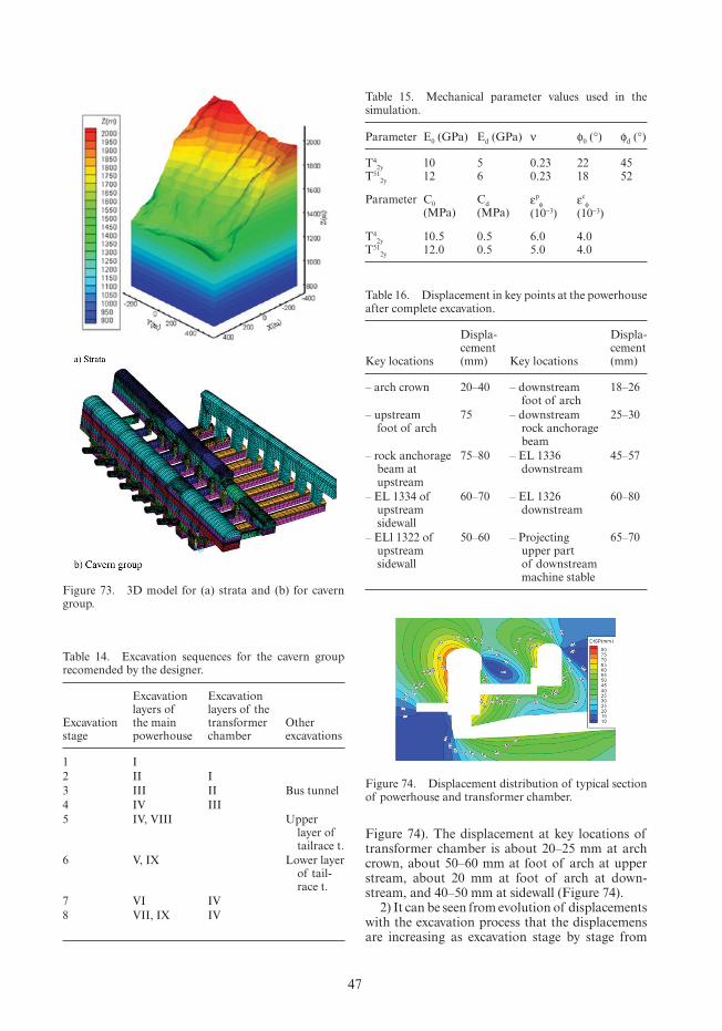
47

Figure 73. 3D model for (a) strata and (b) for cavern group.

Table 14. Excavation sequences for the cavern group recomended by the designer.

Excavation stage

Excavation layers of the main powerhouse

Excavation layers of the transformer chamber

Other excavations

1 I

2 II I

3 III II Bus tunnel

4 IV III

5 IV, VIII Upper layer of tailrace t.

6 V, IX Lower layer of tail-race t.

7 VI IV

8 VII, IX IV

Table 15. Mechanical parameter values used in the simulation.

Parameter E0 (GPa) Ed (GPa) ν φ0 (°) φd (°)

T42y

T512y

1012

56

0.230.23

2218

4552

Parameter C0 (MPa)

Cd (MPa)

εp

φ (10−3)

εc

φ (10−3)

T42y

T512y

10.512.0

0.50.5

6.05.0

4.04.0

Figure 74). The displacement at key locations of transformer chamber is about 20–25 mm at arch crown, about 50–60 mm at foot of arch at upper stream, about 20 mm at foot of arch at down-stream, and 40–50 mm at sidewall (Figure 74).

2) It can be seen from evolution of displacements with the excavation process that the displacemens are increasing as excavation stage by stage from

Table 16. Displacement in key points at the powerhouse after complete excavation.

Key locations

Displa-cement (mm) Key locations

Displa-cement (mm)

– arch crown 20–40 – downstream foot of arch

18–26

– upstream foot of arch

75 – downstream rock anchorage beam

25–30

– rock anchorage beam at upstream

75–80 – EL 1336 downstream

45–57

– EL 1334 of upstream sidewall

60–70 – EL 1326 downstream

60–80

– ELl 1322 of upstream sidewall

50–60 – Projecting upper part of downstream machine stable

65–70

Figure 74. Displacement distribution of typical section of powerhouse and transformer chamber.

48

top to down. The excavation progress at current layer has large influence on displacement of sur-rounding rock nearby. The excavation at stages 7 and 8, near to bottom of powerhouse, has small influence on deformation of arch crown and rock anchorage beam of powerhouse and transformer chamber. But the excavation of stages 4–6, middle part of high sidewall, has large influence on the cavern deformation.

3) After complete excavation of the cavern, there is an obvious change of the stress field. It is due to influence of faults that there is large stress con-centration at arch at downstream of powerhouse with about −30– –35 MPa, stress relaxation at arch of upper stream of powerhouse with about −2–0 MPa. There is also a large stress concentra-tion at machine stable of powerhouse with about −30 MPa. There has obvious stress relaxation at the isolated rock mass between powerhouse and transformer chamber, cross location of powerhouse

Figure 75. Distribution of (a) maximum principal stress, (b) minimum principal stress, and (c) plastic zone for typical section of powerhouse.

and bus tunnels, the connection of head conduit and powerhouse, the projecting part at upper of machine stable. There is high stress concentration at side arch of downstream of transformer cham-ber, with maximum of about −36 MPa, and large stress relaxation at sidewall of transformer cham-ber (Figures 75a and b).

4) After complete excavation of the cavern, the plastic zone is generally about 2–3 m in depth, but 2–4 m depth at arch at down stream of powerhouse and the machine stable, 3–5 m depth at upper stream sidewall, bus tunnels near powerhouse, pro-jecting part at upper of machine stable (Figure 75c). These locations having high stress concentration, high stress relaxation, and deeper plastic zone shall be paid more attention for the stability during the construction. There is generally about 2 m depth of plastic zone at transformer chamber, larger shear-ing plastic zone of about 3–4 m depth at side arch of down stream at transformer chamber, and ten-sile plastic zone at sidewalls and side arch of upper stream of transformer chamber.

Different numerical models were used during the design and monitoring of the complex of the Jinping II powerhouse scheme as it can be seen in the book of Feng & Hudson (2011). For their com-plexity mention for 3D numerical model as shown in Figure 76 performed for the re-evaluation of the cavern group stability after excavation of stage 3,

Figure 76. 3D calculation model of current excavation layer.

49

Castro, A.T., Leitão, N.S., Sousa, L.R., Desheng D. & Nguyen-Mind, D. 2002. ISRM News, Vol. 7, no. 2, pp. 24–32.

Chen, X.R., Hou, J. & Chen, J.L. 2007. Stability analysis and support design of Jinping II hydropower station. HydroChina Huadong Engineering Corporation.

Cundall, P.A. & Strack, O.D.L. 1979. A discrete numeri-cal model for granular assemblies. Geotechnique, 29(1): 47–65.

Dawson 1999. Slope stability analysis with finite element and finite difference methods. Geotechnique, 49(6): 835–840.

Eclaircy-Caudron, S., Dias, D., Kastner, R., Miranda, T., Correia, A.G. & Sousa, L.R. 2007. Inverse analysis of two geotechnical works: a tunnel and a cavern. 5th Int. Workshop on Applications of Computational Mechanics in Geotechnical Engineering, Francis & Taylor, Sousa, Fernandes, Vargas & Azevedo (eds), London, pp. 125–142.

Einstein, H. 2002. Risk assessment and management in geotechnical engineering. 8th Portuguese Geotechni-cal Congress, Lisbon, pp. 2237–2262.

Elegbede, C. 2005. Structural reliability assessment based on Particles Swarm Optimization. Structural Safety, 27, pp. 171–186.

Eskesen, S., Tengborg, P., Kampmann, J. & Veicherts, T. 2004. Guidelines for tunnelling risk management: Inter-national Tunnelling Association, Working Group No. 2. Tunnelling and Underground Space Technology 19 (2004) 217–237.

Fellner, D. & Hobson, D. 2008. HPP Glendoe—Rock Mechanical aspects for large span underground powerhouse. Journal Geomechanik und Tunnelbau, 5, October 2008, pp. 374–382.

Feng, X. & Hudson, J. 2011. Rock engineering design. Taylor & Francis, London, 468p.

Geodata 2001. New guidelines for tunneling works. April 2001.

Geoguide 4 1992. Guide to cavern engineering. Geotech-nical Engineering Office, Hong Kong, 147p.

He M., Sousa, L.R., Sousa, R.L., Gomes, A., Vargas, E. & Zhang, N. 2011. Risk Assessment of CO2 injection processes and storage in carboniferous formations: a review. Journal of Rock Mechanics and Geotechnical Engineering, 3 (1): 39–56.

He M., Jia X., Peixoto, A., Sousa, L.R., Sousa, R.L. & Miranda, T. 2012. Prediction of Rockburst Based on Experimental Systems and Artificial Intelligence Tech-niques. Brazilian Congress for Tunnels, São Paulo, p. 8 (to be published).

Heckerman, D. 1997. A Tutorial on Learning with Baye-sian Networks. Data Mining and Knowledge Discov-ery, 1:79–119.

Hoek, E. 2000. Rock engineering, Course notes, Roc-science, www.rocscience.com.

Kaiser, P. (1999). “Lessons learned for deep tunnelling from rockburts in Mining”. GEAT’99 Switzerland.

Kennedy, J. & Eberhart, R.C. 1995. Particle swarm opti-mization. IEEE Int. Conference on Neural Networks, Piscataway, NJ. IEEE Press, pp. 1942–1948.

Jiang, Q., Feng, X.T., Xiang T.B. & Wan X.B. 2009. Geos-tress study of Jinping II hydropower station region considering historical tectonic process. ISRM Sympo-sium on Rock Characterization, Modeling and Engi-neering Design Methods, Hong-Kong, pp. 436–440.

Table 17. Established mechanical parameters for various monitoring sections.

Monitoring sectionE0 51

(GPa)E0 51

(GPa)E0 51

(GPa)E0 51

(GPa)

S1 8.2 7.1 5.1 4.6

S2 8.7 7.3 5.5 4.4

S3 8.5 8.1 6.3 5.1

S4 7.7 5.5

Monitoring sectionC0 51

(MPa)C0 4

(MPa)φ0 51

(°)φ0 4

(°)

S1 7.7 7.4 18.4 22.4

S2 7.4 7.3 22.2 17.5

S3 7.6 7.5 20.0 23.0

S4 7.5 20.8

using the established mechanical parameters of the surrounded rock, as listed in Table 17.

7 FINAL CONSIDERATIONS

This Chapter was developed by the authors taking into consideration their experience mainly in their countries, China and Portugal, particularly in the Jinping II and Venda Nova II hydroelectric schemes. The purpose was to analyze the behavior of under-ground works associated to hydroelectric schemes with emphasis to the development of numerical models for predicting the behavior and the risk associated. Special emphasis was given to the sec-tion devoted to risk analysis and management. Also, it is recognized in the context of an optimal engineering design, the benefits of auditing the rock mechanics modeling and design in order to ensure that all factors are included.

ACKNOWLEDGEMENTS

The authors are especially grateful to Ertan Com-pany, EDP—Electricity of Portugal and Professor He Manchao, from State Key Laboratory of Geo-Mechanics and Deep Underground Engineering for the given support to prepare this document.

Also the authors would like to thank CRC Press, Taylor & Francis Group for allowing to include information from the book entitled Rock Engineering Design, from Xia-Ting Feng & John A. Hudson.

REFERENCES

Bieniawski, Z. 1989. Engineering rock mass classifica-tions. John Wiley & Sons.

Cafofo, P., Sousa, L.R., & Moura, F. 2007. Innovative underground works at Madeira Island, Portugal. 11th ACUUS Conference on Underground Space: Expand-ing the Frontiers, Athens, pp. 137–143.

50

Lamas, L.N. 1993. Contributions to understanding the hydromechanical behavior of pressure tunnels. PhD Thesis. Imperial College, London, p. 419.

Leitão, N. & Lamas, L.N. 2006. Modeling of the high pressure circuit of the Venda Nova II hydroelectric scheme. 4th FLAC Symposium (Eds., R. Hart and P. Varona), Madrid, Paper No. 03–03.

Lemos, J.V. 2010. Modeling rock masses in large under-ground works (in Portuguese). Int. Conference on Hydroelectric Schemes in Portugal. A New Cycle, Porto, p. 13.

Lima, C., Resende, M., Plasencia, N. & Esteves, C. 2002. Venda Nova II hydroelectric scheme powerhouse geo-technics and design. ISRM News Journal, 7(2): 37–41.

LNEC 1983. LNEC collaboration in the geological and geotechnical studies concerning the hydraulic circuit of Venda Nova II (in Portuguese). LNEC Report 47/1/7084, Lisbon.

LNEC 2003. Venda Nova II scheme. determination of the state of stress (in Portuguese). LNEC Report 371/03, Lisbon.

Martins, C.S. 1985. Contribution to the study of under-ground structures associated with hydroelectric devel-opments (in Portuguese). LNEC Thesis, Lisbon, p. 471

Miranda, T. 2003. Contribution to the calculation of geomechanical parameters for underground structures modeling in granite formations (in Portuguese). MSc thesis, University of Minho, Guimarães p. 186.

Miranda, T. 2007. Geomechanical parameters evalua-tion in underground structures. Artificial intelligence, Bayesian probabilities and inverse methods. PhD the-sis, University of Minho. p. 317.

Miranda, T., Correia, A.G. & Sousa, L.R. 2009. Bayesian methodology for updating geomechanical parameters and uncertainty quantification. Int. J. Rock Mechan-ics Min. Science, Vol. 46, Issue 7, pp. 1144–1153.

Miranda, T., Correia, A., Santos. M., Sousa, L.R. & Cortez, P. 2011. New models for strength and deform-ability parameter calculation in rock masses using data-mining techniques. Int. Journal of Geomechan-ics, ASCE, Jan-Feb, pp. 44–58.

Oreste, P. 2005. Back-analysis techniques for the improve-ment of the understanding of rock in underground constructions. Tunnelling and Underground Space Technology, 20: 7–21.

Ortlepp, W.D. & Stacey, T.R. 1994. Rockburst Mechanisms in Tunnels and Shafts. Tunnelling and Underground Space Technology, Vol. 9, No. 1, pp. 59–65, 1994.

Pierce, M.; Fairhurst, C. 2011. Synthetic rock mass appli-cations in mass mining. 12th ISRM Congress, Beijing, pp. 109–114.

Plasencia, N. 2003. Underground works—aspects of the engineering geology contribution and design (in Por-tuguese), MSc thesis, Technical University of Lisbon, Lisbon.

Popielak, R. & Weining, W. 2010. Engineering and design services for excavation—DUSEL. Preliminary Design, Preliminary Report #2, Contract D10–04, Lakewood, Colorado, 104.

Qian Q. 2009. The strategy for controlling water inflow. Int. Consulting Report for the Key Technology of Safe and Rapid Construction for Jinping II Hydro-power Station High Overburden and Long Tunnels, Jinping II, pp. 15–18.

Rocha, M. 1977. Some problems related to the Rock Mechanics of low strength materials (in Portuguese). Journal Geotecnia, no. 18, pp. 3–17.

Romana, M. 2003. DMR, a new geomechanics classi-fication fou use in dams foundations, adapted from RMR. 4th International Symposium on Roller Com-pacted Concrete (RCC) Dams, Madrid.

Russell, S. & Norvig, P. 1995. Artificial Intelligence. A Modern approach. Second Edition, Prentice Hall Series in Artificial Intelligence.

Schleiss, A. 2000. Hydraulic schemes (in French). EFPL, Lausanne, p. 482.

Shi, G. 2009. Application of three dimensional discon-tinuous deformation analysis (3D DDA). Int. Con-ference on Rock Joints and Jointed Rock Masses, Tucson, p. 11.

SiDolo 2005. Manual of utilization (in French). Version 2.4495, Laboratoire Génie Mecanique et Matériaux de l’Université de Bretagne-Sud, Lorient, France.

Smith, M. 2006. Dam risk analysis using Bayesian net-works. ECI Conference on Geohazards, Lillehammer, Paper 10, p. 10.

Sousa, L.R. 2006. Learning with accidents and damage associated to underground works. Geotechnical Risks in Rock Tunnels, Francis & Taylor, Matos, Sousa, Kleberger & Pinto (eds), London, pp. 7–39.

Sousa, L.R., Lamas, L.N. & Martins, C.S. 1994. Appli-cations of computational mechanics to underground structures in hydraukic projects. 1st Int. Workshop on Applications of Computaional Mechanics in Geo-technical Engineering. Balkema, Vargas, Azevedo, Sousa & Fernandes (eds.), Rio de Janeiro, pp. 15–88.

Sousa, L.R., Leitão, N.S. & Monteiro, G. 2000. Observed behavior of the structures for the power increase of Miranda hydroelectric Project. 9th ISRM Congress, Paris.

Sousa, L.R. & Sousa, R.L. 2011. Risk associated to stor-age of CO2 in carboniferous formations. Application of Bayesian networks. CO2 Storage in Carboniferous For-mations and Abandoned Coal Mines, Ed. He, Sousa, Elsworth & Vargas, CRC Press/Balkema, pp. 153–178.

Sousa, R.L. 2010. Risk analysis for tunneling projects. MIT, Cambridge, p. 589.

Sousa, R.L. 2011. Methodologies for risk analysis and decision making. CO2 Storage in Carboniferous For-mations and Abandoned Coal Mines, Ed. He, Sousa, Elsworth & Vargas, CRC Press/Balkema, pp. 125–152.

Sousa, R.L. 2012. Risk analysis for tunnels using Baye-sian networks. In Innovative Numerical Modeling in Geomechanics, Ed. Sousa, Vargas, Fernandes & Azevedo (to be published).

Tang, C. 2010. Preliminary engineering application of microseismic monitoring technique to rockburst pre-diction in tunnelling of Jinping II project. J. of Rock Mechanics and Geotechnical Engineering, Vol. 2, no. 3, 193–208.

Ulusay, R. & Hudson, J. 2007. The complete ISRM sug-gested methods for rock characterization, testing and monitoring: 1974–2006. The compilation prepared by the ISRM Turkish National Group on behalf of ISRM.

Wu, S.Y., Feng, X. & Sousa, L.R. 2010. Jinping II mega hy-dropower project, China. Int. Conference on Hydroelectric Schemes in Portugal. A New Cycle, Porto, pp. 223–231.