Autonomous Air HockeySSYX02-16-82

Bachelor thesis at the Department of Signals and Systems

Christofer Berntsson, Lars Brown, Simon Fitz,Albin Hallberg, David Sondell, Kim Svensson

Department of Signals and SystemsCHALMERS UNIVERSITY OF TECHNOLOGYGothenburg, Sweden 2016

AbstractThe purpose of this bachelor project was to develop a robot that is capable of play-ing air hockey against either another robot or a human. First, by using a camera,a program controlling the robot tracks the puck and calculates a trajectory. Thecalculations are made on an external computer running a program written in C++.The program continuously sends information to a micro controller which controls amechatronic system. The mechatronic system consists of two stepper motors andtwo stepper drivers together with a combination of linear rails, linear bearings andcustom 3D printed parts. This system moves the mallet based on the informationsent from the computer to emulate a human player and thereby defeat the opponent.

The system uses different strategy algorithms to decide how to move the malletdepending on the speed and direction of the puck and is capable of both defendingagainst incoming pucks and attacking if the puck moves below a certain speed. Theproject has been completed with the implementation being successful although thereare definitely some points of improvement.

SammanfattningSyftet med detta kandidatarbete var att utveckla en robot som kan spela air hockeymot antingen en annan robot eller en människa. Genom att använda en kameraföljer programmet som styr roboten puckens rörelse och beräknar en förutsägelseav hur den kommer att röra sig. Beräkningarna sker på en extern dator som körett program skrivet i C++. Programmet skickar kontinuerligt information till enmikrokontroller som styr det mekatroniska systemet. Det mekatroniska systemetbestår av två stegmotorer och två stegmotordrivare som driver den mekaniska delensom är byggd av kombination av axlar, linjärlager och 3D utskrivna delar. Dettasystem förflyttar klubban för att efterlikna en människas spelsätt och förhoppn-ingsvis vinna över motståndaren.

Systemet använder olika strategialgoritmer för at avgöra hur klubban ska flyttasberoende på puckens hastighet och riktning. Roboten är kapabel att både försvaramot inkommande puckar samt attackera om pucken rör sig långsammare än en speci-ficerad hastighet. Slutsatsen är att projektet överlag är lyckat även om förbättringarkan göras.

ii

Acknowledgements

The whole team would like to thank the other air hockey project for support andmotivation.

Hakan Köroğlu for feedback and support throughout the project.

The department of Signals and Systems at Chalmers University of Technology.

iii

Contents

1 Introduction 11.1 Background . . . . . . . . . . . . . . . . . . . . . . . . . . . . . . . . 11.2 Purpose . . . . . . . . . . . . . . . . . . . . . . . . . . . . . . . . . . 11.3 Problems and Tasks . . . . . . . . . . . . . . . . . . . . . . . . . . . . 2

1.3.1 Tracking the Puck . . . . . . . . . . . . . . . . . . . . . . . . 21.3.2 Predicting the Future Trajectory of the Puck . . . . . . . . . . 31.3.3 Controlling the Movement of the Mallet . . . . . . . . . . . . 31.3.4 Programming a Game Strategy . . . . . . . . . . . . . . . . . 3

1.4 System Requirements . . . . . . . . . . . . . . . . . . . . . . . . . . . 41.5 Delimitations . . . . . . . . . . . . . . . . . . . . . . . . . . . . . . . 51.6 Thesis Outline . . . . . . . . . . . . . . . . . . . . . . . . . . . . . . . 5

2 Overall System Description 6

3 Vision System 73.1 Camera Hardware . . . . . . . . . . . . . . . . . . . . . . . . . . . . . 73.2 Image Analysis and Puck Detection . . . . . . . . . . . . . . . . . . . 8

3.2.1 Color Representation: RGB and HSV . . . . . . . . . . . . . . 93.2.2 Mathematical Morphology . . . . . . . . . . . . . . . . . . . . 10

3.3 Position and Distortion . . . . . . . . . . . . . . . . . . . . . . . . . . 15

4 Mechanical Design 184.1 CoreXY . . . . . . . . . . . . . . . . . . . . . . . . . . . . . . . . . . 184.2 Choice of Design . . . . . . . . . . . . . . . . . . . . . . . . . . . . . 20

4.2.1 One Layer Belt Design . . . . . . . . . . . . . . . . . . . . . . 204.2.2 Two Layer Belt Design . . . . . . . . . . . . . . . . . . . . . . 20

4.3 Choice of Mechanical Components . . . . . . . . . . . . . . . . . . . . 214.3.1 Linear Shafts . . . . . . . . . . . . . . . . . . . . . . . . . . . 214.3.2 Linear Bearings . . . . . . . . . . . . . . . . . . . . . . . . . . 214.3.3 Belts . . . . . . . . . . . . . . . . . . . . . . . . . . . . . . . . 224.3.4 Dimensioning of the Belt Pulleys . . . . . . . . . . . . . . . . 224.3.5 Camera Stand . . . . . . . . . . . . . . . . . . . . . . . . . . . 24

5 Electrical Design 265.1 Choice of Components . . . . . . . . . . . . . . . . . . . . . . . . . . 265.2 Programming of the MCU . . . . . . . . . . . . . . . . . . . . . . . . 27

iv

Contents

6 Game Strategy and Algorithms 306.1 Predicting the Trajectory of the Puck . . . . . . . . . . . . . . . . . . 306.2 Strategy . . . . . . . . . . . . . . . . . . . . . . . . . . . . . . . . . . 31

7 Validation 33

8 Discussion 368.1 Prototype Performance . . . . . . . . . . . . . . . . . . . . . . . . . . 368.2 Possible Improvements and Future Project . . . . . . . . . . . . . . . 388.3 Environmental Aspects . . . . . . . . . . . . . . . . . . . . . . . . . . 38

9 Conclusion 39

Bibliography 40

Appendices 42

Appendix A System Requirements 42

Appendix B MatLab Script - Deflection 43

Appendix C Drawing of the Prototype 44

v

1Introduction

1.1 BackgroundMechatronic systems are introduced to solve a growing number of every day tasks.If a system is to perform well, it is crucial that it is fast, accurate and reliable.Detecting and reacting to quickly moving objects are challenges that are found fre-quently in manufacturing and other applications. The developments in mechatronicsystems technology have made it possible to introduce robotic units to various gameplatforms like table-tennis [1], football [2] and baseball [3]. This project is based onthe development of such a system for an air hockey table.

Traditionally, air hockey is a game played by two opposing players on a rectangularfield as represented in Figure 1.1. The winner of the game is decided based on thenumber of goals scored by each player. Each player has a slot on his or her side ofthe table and a goal is scored when the puck enters the opponent’s slot. Aroundthe whole field there is a rail which prevents the puck from falling off the side of thetable. The puck bounces easily against the rail without losing a significant amountof its momentum. The puck floats on an airbed with negligible friction, which leadsto a fast game play. Due to the fast game play, the reaction time of each player andthe estimation of the path of the puck is vital for the outcome of the game. A videofrom the world championship final 2010 [4] displays the game play.

To imitate a human playing air hockey, the robot must be able to perform the sameactions as a human during the game. These actions include tracking the puck, mov-ing the mallet and having an understanding of the game mechanics and followingthe rules.

There are many different kinds of robots that are able to play air hockey: robotarms, combinations with linear rails and more complex solutions. To protect thegoal, the robot only needs to move along the short side of the table, but if an attackmode is desired, the mallet will have to be able to move in two dimensions, thusmaking the system more complex.

1.2 PurposeThe purpose of our project is to develop and build an air hockey robot that operatessemi-autonomously. The robot is supposed be fully autonomous when the game is

1

1. Introduction

Figure 1.1: Illustration of an air hockey table and gaming accessories (two malletsand a puck). The vertical blue line is referred to as the middle line and seperatesthe two players’ sides.

on, but will need human interaction to place the puck back on the table when eitherthe robot or the opponent has scored a goal. The robot should be able to playagainst either a robot or a human. A second group is also assigned to develop asimilar, separate robotic unit to be mounted to the other side of the same table. Asa common project goal, the different robots are supposed to play against each otherto compare their performances.

During the project, members expect to gain more knowledge and improve theirskills in the analysis and design of vision-based control systems (with all the relatedmechanical and electronic units) as well as project management.

1.3 Problems and Tasks

With this project, multiple challenges were faced because of the diversity of thetasks to be performed. To cope with these challenges, the project work was dividedinto several separate tasks.

1.3.1 Tracking the Puck

Air hockey is a fast-paced game, which means that the puck must be located asearly as possible. Since a green puck is used, a vision system that is able to trackthe puck on the field based on color is hence needed. Sampling rate is crucial since itsets the limitations for calculating the trajectory of the puck. Accuracy in acquiringthe position of the puck is also very important, since the error from locating thepuck can not be compensated for when controlling the motion of the mallet.

2

1. Introduction

1.3.2 Predicting the Future Trajectory of the PuckOnce at least two measured positions of the puck and the time between them havebeen determined, both the speed and direction of the puck can be calculated. Whenthese two parameters have been calculated, a trajectory can be estimated easilysince the physics of the game is very simple with linear motion under very lowfriction. From this point a vector representation of the expected trajectory will givethe system an indication of where to move the mallet before the puck reaches theforeseen position.

1.3.2.1 Multiple Measurement Points

With two measured locations of the puck, a very basic estimation of the puck’strajectory can be made. However, with only two measured points the contingencyis high and the predicted trajectory might not be accurate enough. If there aremore than two measured locations, the accuracy of the predicted trajectory will beimproved, but the method to calculate a vector that fits the trajectory becomesmore complex.

1.3.2.2 Bounce Against the Rail

The bouncing against the rails adds to the complexity of the mathematical modeland makes the estimation of the trajectory more difficult. The law of reflection[5] will not perfectly apply to this system and thus a new mathematical model ofreflection might have to be used. The bouncing itself might alter the velocity of thepuck and thus the mathematical model of the trajectory will have to take this intoaccount. If only two samples from the vision system are used and a bounce occursin between the samples, the bounce might not be recognised and a false trajectorymight be calculated as illustrated in Figure 1.2.

1.3.3 Controlling the Movement of the MalletAfter the puck has been located and a first trajectory has been calculated, the mallethas to be moved by a mechatronic system. The system has to be fast enough todefend the goal against the incoming puck and to shoot the puck towards the goalof the opponent. The system will have to be able to move the mallet simultaneouslyin two directions, along and across the table. This means that there will have to bea mechanical system that holds the mallet and that is able move it with high speedand accuracy. An essential goal will hence be to keep the weight of the movingparts low and design a smooth, robust, low-friction rail system without exceedingthe available budget.

1.3.4 Programming a Game StrategyThe last step is to program a strategy which the robot will use to defend the goaland attack the opponent. It should be able to use different modes, which could bedefense, attack or a combination of the two.

3

1. Introduction

Figure 1.2: Representation of a potential error when a bounce occurs. When abounce occurs between two samples, shown as the green pucks, the data suggestthat the puck traveled straight as shown in red. However, the puck could also havetraveled as the green line suggests.

1.4 System Requirements

Listed below are the overall requirements and specifications for developed the pro-totype system. A full list of requirements which have been evaluated can be foundin Appendix A.

• The prototype should be able to block a moving puck from the middle line at3 m/s towards the goal.

• The prototype must not protrude over the middle line into the opponent’s half.

• The prototype should be able to strike the puck, sending it towards the oppo-nent at a speed of 8 m/s.

• The camera system should be able to locate a still puck at an accuracy of ±5mm.

• When moving the mallet 400 mm with the actuators and without feedbackcontrol, the actual distance moved should not exceed a fault of ±10 mm.

• The prototype should be constructed with materials which leads to a sustain-able design.

4

1. Introduction

1.5 DelimitationsThe delimitations are as follows:

• The system will require human interaction when starting the game and/or ifa player scores a goal. This is due to the limited time and budget of the project.

• The system might need help with software calibration when operating from acold start, thus making the robot require human interaction.

• Only one prototype will be constructed as the robot opponent will be designedand constructed by another development group. This decision was made to-gether with the other group to further promote competition and thus createmotivation for better designs.

• The airspace above the middle line will be shared due to complications withinterfering with the camera’s field of view.

• The robot will not be required to be able to operate in an arbitrary envi-ronment. Limited lightening might cause the vision system to be unable toperform its task. Due to the limited project budget and duration, only onevision system will be implemented and the environment has to be adjusted tothe requirements of the chosen system.

• The system will be designed to function on a specific air hockey table withdimensions 198 x 106.5 cm and will therefore not be operational on a tablewith other dimensions without reprogramming and changing the mechanicalconstruction.

1.6 Thesis OutlineThe outline of this bachelor thesis is as follows. Chapter 2 presents an overview ofthe system with its most essential subsystems described briefly. This chapter aims tofacilitate an understanding of the overall system before getting into a more detaileddescription of each subsystem in the chapters that follows. Chapter 3 describesthe vision system by explaining how the puck is detected and what methods areused. Chapter 4 presents the mechanical design that has been chosen and builtin order to move the mallet. In Chapter 5 a description of the electrical design ispresented which connects the vision system with the mechanical system. In orderto calculate the trajectory of the puck and make an appropriate move according tothese calculations, Chapter 6 explains the game strategies and algorithms behindthe decision making of the robot. Chapter 7 then sets up different tests to checkif the system requirements in the introduction have been met. The next chapterof the report discusses the results of the project work and possible improvements.Latsl follows a conclusion about the project as a whole.

5

2Overall System Description

This chapter will give a brief description of the system as a whole, introduce themain concepts of the following chapters and explain the interaction of the subsys-tems. The main subsystems of this project are the vision, mechanical and electricalsystems. After this follows a description of the strategy and prediction algorithms.Each subsystem will be explained in further detail in the following chapters.

An overall description of the whole system is provided in Figure 2.1. Basically, acamera will send information to a computer which will perform the image analy-sis. The image analysis is done in a self-developed program written in C++, whichimplements an open source library called OpenCV. The OpenCV library simpli-fies several aspects of the programing, for which there would not be enough timeto do otherwise. The program tracks the puck using the camera and calculates aprediction of the trajectory and uses the strategy algorithms to decide what infor-mation to send. The program then sends information to the micro controller unit(MCU) about where the mallet should move. The communication with the MCUis performed through serial communication. The MCU will control the steppermotors through the motor drivers, which is power by a power supply unit (PSU),and thereby move the mechanical system. The mechanical system consists of steelshafts, linear bearings and custom 3D-printed parts. The belt system used is calledCoreXY, and eliminates the need to move one of the motors, which significantlyreduces the weight of the moving parts.

Figure 2.1: Flowchart of the system where the input signals flow through thesystem and end up as motions in of the mallet.

6

3Vision System

This chapter addresses the main source of input data for the air hockey robot, whichis the camera. The main point of the vision system is to filter out the position ofthe puck and the mallet by using their distinctive color. In this chapter more detailsabout the camera hardware and image analysis software will be described.

Information about the hardware will be presented first in this chapter followed by abrief description of the image analysis libraries that were used in this project. Afterthe library has been introduced, the filtering algorithms and calculation algorithmsregarding image analysis are described with some mathematical background.

3.1 Camera Hardware

The problem of locating the puck was addressed with a vision system. A camerasolution was best suited for this project and a couple of different camera solutionshave been examined. There are a couple of features which were especially importantfor this project. The camera had to capture images at a high frame rate so thatan accurate trajectory could be predicted at an early stage. The images also hadto be clear enough to be analysed with suitable image processing algorithms [6] foraccurate positioning of the puck and the mallet.

The project used a camera from ELP which captures images at a frame rate of 120frames per second (fps) with a resolution of 640 x 480 pixels. This camera doesnot have integrated image analysis algorithms and thus these algorithms had to bedeveloped and run on a separate computer.

The camera was placed above the table as low as possible, but still covering thewhole table in its field of view. The game field is 200 cm long and the ELP cameracame with a 70◦ angle of view lens. The required height was calculated to be 143cm by using equation 3.1 where Θ is the camera’s angle of view. The height wasmeasured from the game field surface to the camera lens.

Height = Length/2tan(Θ/2) = 100cm

tan(35◦) ≈ 143cm (3.1)

7

3. Vision System

3.2 Image Analysis and Puck Detection

OpenCV [7] is a library used for image processing with features which were partic-ularly useful in this project. The OpenCV library was used in this project and thefunctions used will be described in this section. In Table 3.1 some of the features ofOpenCV used in this project are listed and briefly explained.

Table 3.1: Selection of most important features from OpenCV used in this project.

Feature Description

VideoCapture Object that listens and reads the input from a camera or video file.

Mat Class used to create an object that can store an image as a matrixrepresentation.

cvtColor Convert an image from one representation to another.Example RBG to HSV.

inRange Function to analyse an image. Returns a mask where pixels withthe right properties are given a high value and other pixels aregiven a low value.

Moments Creates an object that gives each pixel a weight equal to itsintensity. Borrowing formulas from physics the centroid or centerof mass can be calculated.

erode Morphological operation that erodes the source image based onits structures with a specified pixel neighborhood.

dilate Morphological operation that dilates the source image based onits structures with a specified pixel neighborhood.

VideoCapture is an object that handles input from the camera. With a VideoCap-ture object a single frame from a video feed could be retrieved and converted to aMat object which is an image container using matrix representation.

The Mat object used in this project is a three dimensional matrix where the firstdimension represents the height of the frame in pixels. The second dimension rep-resents the width of the frame and the third dimension represents the color of thepixel. The third dimension contains three integer values and these values set thecolor of the pixel.

8

3. Vision System

3.2.1 Color Representation: RGB and HSVWhen representing a color with three integers, the most common way is called RGB(Red Green Blue). In this representation, the first integer represents the amountof red in the pixel as a value between 0 and 255. The other two integers workin the same way but for green and blue. The concept of RGB is shown in Fig-ure 3.1. In OpenCV the order of the colors are different and a BGR (Blue GreenRed) representation is used, but it works in the same way as the RGB representation.

Figure 3.1: A 3 x 3 matrix where each cell represents a pixel and the backgroundof the cell corresponds to the RGB numbers written inside it.

RGB or BGR representation is not ideal for filtering out an object based on color.The problem with using RGB when tracking a color is that a certain value of anyone of the three integers does not correspond to a color. The color of a pixel isdepending on all three parameters, which makes defining the desired color moredifficult than with another representation. This is displayed in Figure 3.2. For colorfiltering in this project, the BGR frame was converted to an HSV (Hue SaturationValue) representation. The conversion was done using a function from OpenCVcalled cvtColor, which converts a Mat object to another representation.

Hue in HSV is a value between 0 and 180 which represents a color spectrum wherevalues around 70 correspond to green and by testing different values, the interval of60 to 75 was found to work best for detecting the green puck. Saturation determineshow intense the color green has to be in order to be considered green. Without thisparameter a gray pixel with slightly green tendencies would be considered green.Value corresponds to light intensity, for example, the sun is considered yellow butwhen looking directly at it, a human can not determine the color due to the highintensity of the light. By leaving this parameter untouched, the light environment

9

3. Vision System

Figure 3.2: Shows two different types of green with RGB representation where thevalues differ significantly. This illustrates the difficulties of using RGB representationin color tracking. The numbers in the image represent the color of the background.

has very little effect to the system’s ability to track the puck.

The HSV image and the parameters for hue, saturation and value were then used tocreate a binary image mask with the OpenCV function inRange, which gave everypixel that was considered as green the value of 1 (white) and every pixel that wasnot considered green the value of 0 (black).

3.2.2 Mathematical MorphologyIn the binary image created by the inRange function, shown in Figure 3.3, thecenter of the puck could clearly be identified by a human. However, some noisebleed through the previous filter which decreases the accuracy of the algorithmthat calculates the center of the puck (center of mass algorithm is described inSection 3.3). This is because it uses every pixel in the image with the value 1 (whitepixels in Figure 3.3) and weigh them together. Note that this also means that theshape of the puck affects the algorithm’s accuracy.

Figure 3.3: Binary image of air hockey table after filtering by threshold levels overHSV values. The large white circle in the lower right corner is the puck.

10

3. Vision System

To get around this problem mathematical morphology was used to eradicate thenoise. Mathematical morphology literally means "using mathematical principals todo things to shapes" [8]. Two different but similar operations was used to spread theblack pixels, making them cover the white noise. The erosion also covers some partsof the puck. In order to restore it a white spreading operation is used to restorethe circular puck. The darkness spreading operation is called erosion, and the whiterestoring operation is called dilation.

A more detailed description of the operations is found in the following sections:3.2.2.1, 3.2.2.2 and 3.2.2.3. These sections are not essential for an overview of thesystem so a jump to section 3.3 from here can be made.

The binary image can be viewed as a set and the notations shown in Table 3.2 willbe used to describe two binary operations.

Table 3.2: Mathematical notations used to describe dilation and erosion.

A the imageB the structuring elementA ∪B the union of the sets A and BA ∩B the intersection of the sets A and B⊕ dilation sign erosion sign◦ opening sign• closing sign

An introduction to the notion of an translated image set will also be needed. Amovement vector t describes a translated image A in equation 3.2.

At = {c|c = a+ t for some a ∈ A} (3.2)

3.2.2.1 Morphological Dilation

Dilation is a translation-invariant operation where an image, represented as the setA is manipulated using a structuring element B [8]. The mathematical definition ofdilation can be seem below in equation 3.3.

A⊕B = {c|c = a+ b for some a ∈ A and b ∈ B} (3.3)

By taking copies of A and translating them with help of the movement vectors de-fined by all the pixels in B and then by a union of these superimposed sets together,it can be written as in equation 3.4.

11

3. Vision System

A⊕B =⋃t∈B

At (3.4)

Just as A can translate over B, B can translate over A. This can be interpreted asusing the structuring element B as a stamp and making copies of B over every pixelof A. Similarly the union B ⊕ A is created as in equation 3.5.

A⊕B =⋃t∈A

Bt (3.5)

To further illustrate dilation, consider that A is the following 11 x 10 matrix andthe structuring element B is represented by a 3 x 3 matrix given in Figure 3.4.

Figure 3.4: Matrix A is to be dilated by using the structuring element B.

The dilation of A by B would then be executed by first moving the center of B overeach pixel in A. With a copy of the structuring element over a specific pixel in A,then if the field created by the structuring element contains a 1, then the specificpixel in A also becomes a 1 in the output image. The result can be seen in Figure 3.5where the ones has spread out.

3.2.2.2 Morphological Erosion

Erosion is a translation-invariant operation where an image, represented as the setA is manipulated using an structuring element B [8]. The mathematical definitionof erosion can be seen below in equation 3.6.

AB = {x|x = x+ b ∈ A for every b ∈ B} (3.6)

12

3. Vision System

Figure 3.5: Result after dilation using matrices found in figure 3.4.

Just like with dilation, by taking copies of A and translating them with help of the bymovement vectors defined by all the pixels in B. However, this time the copies are in-tersected together and in the opposite direction. It can be written as in equation 3.7.

AB =⋂t∈B

A−t (3.7)

By using the same image to illustrate erosion, consider that A is the following 11x 10 matrix and the structuring element B represented by a 3 x 3 matrix, seen inFigure 3.6.

Figure 3.6: Matrix A is to be erosion by using the structuring element B.

The erosion of A by B would then be executed by first moving the center of Bover each pixel in A. With a copy of the structuring element over a specific pixelin A, then if the field created by the structuring element only contains 1’s then the

13

3. Vision System

specific pixel in A also becomes a 1 in the output image. The result would look likein Figure 3.7 where the zeroes have spread over the ones.

Figure 3.7: Result after erosion using matrices found in Figure 3.6.

3.2.2.3 Morphological Opening and Closing

When translating ones and zeroes to black and white, it becomes clear that theeffect of dilation expands white parts while erosion expands black. Because of this,one can think that they are the opposite to each other and can cancel out the other,just as in simple arithmetic with addition and subtraction. But in fact, this is notthe case, see equation 3.8.

(AB)⊕B 6= (A⊕B)B (3.8)

One needs to keep in mind that erosion requires the structuring element to fit insidethe image, thus eliminating objects smaller than the structuring element. Whenan erosion is followed up by a dilation, the objects that remain will be somewhatrestored, but the smaller objects would have been completely removed. The restora-tion from the dilation will also have trouble with filling in details. This combinationof operations is known as an opening [9] and is illustrated in Figure 3.8. Openingscan be very useful when trying to remove small objects, smoothing out edges orremoving thin protrusions from objects.An opening is written as in equation 3.9, which is nothing but the first part of 3.8:

A ◦B = (AB)⊕B (3.9)

14

3. Vision System

The same tale is told about the second half of equation 3.8. But now it is a dilationfollowed up by an erosion. This is known as a closing [9] and works in the oppositemanner. Whereas opening removes all the pixels that the structuring element willnot fit, closing on the other hand will fill in all places where the structuring elementwill not fit in the image background.An closing is written as the second half of equation 3.8 or as in 3.10.

A •B = (A⊕B)B (3.10)

Again, one needs to keep in mind that this duality of the functions does not meanthat an inverse operation is possible (i.e. an opening followed by an closing will notrestore the image). An example of how an opening followed by a closing can be seenin Figure 3.8.

3.3 Position and Distortion

The mask image of ones and zeroes described in the previous section from Figure 3.8was used to calculate the center of the puck. Each pixel was handled as a physicalpart with a mass, either 1 or 0. Using the laws of physics about center of mass,the location of the puck could be found. The coordinates for the center of mass inthe mask are the same as the coordinates of the center of the puck [10]. The puck’slocation was handled as a point in its center.

The position could not be used directly due to the barrel distortion caused by thewide angle lens. This effect leads to that the position point from the camera does notcorrespond to the actual position on the air hockey table. OpenCV has a methodfor correcting the distortion based on the parameters of the lens. Figure 3.9 showsthe distorted image to the left and the calculated correction image to the right.However, this method requires a lot processing power, thus taking a long time toperform. Testing this method showed that only 5 fps could be reached which isbelow what was required. Therefore another method had to be used.

For this project, a method that decreases the distortion of a single point was neededso that only the necessary calculations were made. This in order to transform onlythe relevant information from the curved (i.e. distorted) image to the flat (i.e.undistorted) game field, thus minimizing the required processing time. The methodfound to work best was based on the formulas provided by Imatest [11] that wasproved to work well in the project from the previous year[12]. The following stepswere taken to transform a curved position to a flat. The first step was to find thedistance (marked Rcurv in Figure 3.10) from the curved position to the center of theimage, which is where the camera is located (marked Camera in figure 3.10), usingequation 3.11.

15

3. Vision System

Figure 3.8: Illustrating of each step through a morphological filtering process.By eroding, dilating, dilating and eroding in that specific order; shortly known asopening and closing.

Rcurv =√x2

curv + y2curv (3.11)

xcurv and ycurv are the distances from the camera to the position of the puck in Xand Y directions. Rcurv was then transformed to Rflat using equation 3.12 where a,b, c, and d are parameters that were changed in order to counteract the distortioncaused by the camera lens.

Rflat = a ·R4curv + b ·R3

curv + c ·R2curv + d ·Rcurv (3.12)

16

3. Vision System

Figure 3.9: Original image (left) from the 70◦ angle of view lens compared to theundistorted image (right) generated by the built in OpenCV method.

Figure 3.10: Figure shows the difference in position from the image taken by thecamera compared to the flat position used in strategy algorithms. The camera isrepresented by a white dot, the light green represent the flat position and the darkgreen represent the actual puck.

The flat position (xflat, yflat) corresponding to xcurv and ycurv was then calculatedusing the ratio between Rcurv and Rflat as given in equations 3.13 and 3.14,.

xflat = xcurv ·Rcurv

Rflat

(3.13)

yflat = ycurv ·Rcurv

Rflat

(3.14)

The flat position xflat and yflat was used in game strategy algorithms. To developa strategy the vision system process had to be done for both the puck and malletpositions. Further information about the strategy can be found in Chapter 6 of thisreport.

17

4Mechanical Design

The system needs some mechanical construction to move the mallet to the desiredposition. The chosen mechanical design was based on a system called CoreXY.CoreXY is a principle that has been proven to work well for various CNC (Com-puter Numerical Control) projects [13]. The group did not develop the CoreXYprinciple; it was merely implemented for the purpose of this project. In this section,CoreXY is further explained and the construction of the system is presented.

Most of the design was made in CATIA [14] CAD-program. The robot was madeof various components, such as steel shafts, aluminum brackets and distance MDF-blocks (Medium Density Fiberboard), but most parts were made by 3D-printing inPLA plastic. This was a fast, easy and precise manufacturing method.

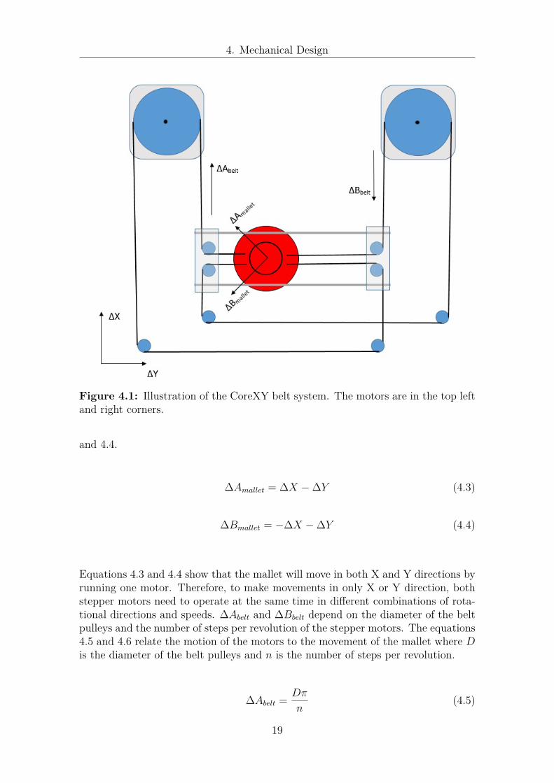
4.1 CoreXYThe mechanical design CoreXY, shown in Figure 4.1, consists of two motors andtwo belts which control the mallet. The belts were structured in a way that onemotor with its corresponding belt moves the mallet diagonally. Therefore, in orderto move the mallet along the table, both motors have to run simultaneously. TheCoreXY system has the advantage that both motors are stationary, meaning thatthere is less mass to be moved, compared to last year’s design[12] and it is possibleto use larger, heavier motors without affecting the mass of the moving parts.

Since the CoreXY system uses a different coordinate system than the vision system,equations for converting coordinates between the two systems had to be developed,and the result can be seen in equation 4.1 and 4.2.

∆X = 12(∆Abelt −∆Bbelt) (4.1)

∆Y = 12(−∆Abelt −∆Bbelt) (4.2)

These equations describe the motion in X and Y direction in terms of the displace-ment of the belts moved with the two motors. The desired belt displacements fora certain amount of motion in X and Y directions are obtained with equations 4.3

18

4. Mechanical Design

Figure 4.1: Illustration of the CoreXY belt system. The motors are in the top leftand right corners.

and 4.4.

∆Amallet = ∆X −∆Y (4.3)

∆Bmallet = −∆X −∆Y (4.4)

Equations 4.3 and 4.4 show that the mallet will move in both X and Y directions byrunning one motor. Therefore, to make movements in only X or Y direction, bothstepper motors need to operate at the same time in different combinations of rota-tional directions and speeds. ∆Abelt and ∆Bbelt depend on the diameter of the beltpulleys and the number of steps per revolution of the stepper motors. The equations4.5 and 4.6 relate the motion of the motors to the movement of the mallet where Dis the diameter of the belt pulleys and n is the number of steps per revolution.

∆Abelt = Dπ

n(4.5)

19

4. Mechanical Design

∆Bbelt = Dπ

n(4.6)

The prototype built in this project used belt pulleys with a diameter of 50 mm andstepper motors with 400 steps per revolution which resulted in the mallet movingapproximately 0.4 mm/step. This made it possible to convert between mm and stepswhich was important for the program in the MCU since it only handles steps. Amore detailed description of the program in the MCU is found in Chapter 5.

4.2 Choice of Design

The CoreXY system can be designed in a variety of different ways, but for thisproject, only two different design concepts were created: a one layer belt design anda two layer belt design.

4.2.1 One Layer Belt Design

The one layer belt design (OLBD) has the two belts at the same height, thereforethe design is lower and slimmer than the two level belt design. One downside ofthe OLBD is that the belts need to cross each other at one point, which makesthis design more of a challenge. The corner pieces (seen in Appendix C) will notbe symmetrical and the belts and the linear shafts are on the same level. Anotherdownside is that the OLBD leaves less space and freedom to change and modify thefinished design and the mallet will not be able to move as far along the table aswith the two layer belt design. This design was eventually chosen and constructedbecause of its slimmer and lower profile design and lighter moving parts.

4.2.2 Two Layer Belt Design

The two layer belt design (TLBD) differs from the OLBD mainly in the fact thatthe belts are stacked in two layers. The construction of the corner pieces would beeasier, with the left and right mountings being almost identical, only mirrored. Thebelts would be mounted at different heights, which would eliminate the problem withcrossing belts. However, a problem with this design might have been that the cornermountings would be higher and possibly more unstable. This design was consideredinferior compared to the OLBD because of the risk that the moving parts would beheavier and that the system might have been less rigid than the OLBD.

20

4. Mechanical Design

4.3 Choice of Mechanical Components

4.3.1 Linear ShaftsThe choice of material for the shafts was between steel, aluminum and carbon fibre.Steel was chosen due to low price, availability and robustness. Carbon fibre andaluminium are lighter but the surfaces might not have been strong enough for thelinear bearings.

Dimensioning of the steel shafts was made with respect to the deflection. The max-imum deflection of the shafts will occur when the mallet is in the middle of therobot’s area of operation. The shafts are simply supported beams with the loadpositioned in the centre and a spread load from the weight of the shafts. The de-flection was calculated by using equation 4.7 [15].

p = PL3

48EI + 5WL4

384EI (4.7)

The variables used in this equation are identified as follows:

• p is the deflection.• P is the weight of the mallet holder (and the Y-shafts’ weights when calculating

X-shaft deflection).• E is the elastic modulus of steel.• L is the length of the shaft.• W is the load per length unit (weight of shaft).• I is the second moment of area for a circular cross-section.

The weight of the mallet holder and linear bearings were approximated to 0.1 kg andthe shafts for the Y-axis has a diameter of 8 mm. The deflection for the shafts alongthe Y-axis was 2.15 mm. The shafts for the X-axis were at first chosen to be 8 mmin diameter but due to the weight of the Y-axis shafts as well as the length of theX-axis, the deflection was 9.5 mm. This was considered too high and thus, the X-axis shafts were changed to be 10 mm in diameter, which made the total maximumdeflection 3.7 mm. Details about the calculation can be found in a MatLab scriptin Appendix B.

4.3.2 Linear BearingsThe bearings which were bought from the same distributor [16] as the belts hada low price and was advertised as high quality bearings. The model type of thebearings is LM10UU and they were manufactured by Fushi. The bearings have aninner diameter of 10 mm, an outer diameter of 19 mm and a length of 29 mm. Thespacing between the lock track for the retaining rings are 23 mm. The sledge houses(see Appendix C for explanation) had to be designed so that the bearings would be

21

4. Mechanical Design

able to fit inside and lock in place with the retaining rings. The linear bearings forthe 8 mm X-axis shafts were reused from last year’s project [12]. The linear bearingswere tested and compared to a set of 3D-printed plastic bearings. The ball bearingswere chosen since their friction was significantly lower compared to the plastic ones.Specific data and dimensions of these linear bearings are found in the data sheet [17].

4.3.3 BeltsThere were two different types of belts commonly available: GT2 and T2.5 (seeFigure 4.2 for a comparison of the profiles). These belts differ in the tooth spacingand profile. The GT2 belt has a rounder profile to minimize skidding and was thuspreferred but due to it being out of stock at the reseller at the time, the T2.5 beltwas chosen [18]. The distributor [16] was only able to deliver a width of 6 or 9 mmof T2.5 belt. The belt chosen was the 6 mm belt to keep the design slimmer. Thestrength of the belt was specified at 36 N/mm, for a 6 mm belt that results in 216N. The 6 mm belt was able to carry the weight the entire construction and wastherefore considered sufficient.

Figure 4.2: Difference between the GT2 (left) and T2.5 (right) belt profiles.

4.3.4 Dimensioning of the Belt PulleysDesigning and dimensioning of the belt pulleys were made with inspiration from lastyear’s project. Since the motors and load forces were mostly the same on this system,last year’s construction was used as a rule of thumb. The equations presented laterin this chapter were used to verify that the chosen dimensions were correct.When dimensioning the belt pulleys, things to consider were the rated torque thatthe stepper motors could deliver, the stepper motor’s maximum angular velocity andthe maximum final speed of the mallet. The belt pulleys had to be large enoughdiameter so that the speed of the mallet would reach the requirements yet not toolarge so that the torque required to accelerate the mallet would exceed the torquethat the motors were capable of delivering.

There are three different load cases for the stepper motors. One case where onlyone motor is active and the mallet is moving diagonally, and two cases when bothof the motors are active and the mallet is moving forward (X-direction) or across

22

4. Mechanical Design

the table (Y-direction). When the robot is moving in the Y-direction, the two steelshafts across the table do not move and will not need to be accelerated, unlike thecase when moving in X-direction. The load case when moving in the X-directionwas the most demanding because of the need to accelerate the steel shafts acrossthe table. Due to this, the X-direction movement with both stepper motors activewas the movement calculated for when dimensioning the belt pulleys.

Figure 4.3: The masses and inertia of the system that affects the equation ofmotion and calculations for the belt pulley dimensioning.

The following notation are used in equation 4.8 based on which the calculation wasperformed. Also see Figure 4.3 for a visual representation.

• Jsteppermotor is the inertia of the stepper motor, from the stepper motor datasheet [19].

• Jbeltpulley is the inertia of the belt pulleys.• Jwheels is the total inertia of the small belt wheels.• mload is the total mass of the mallet, mallet holder, bearings, steel shafts for

the y axis and belt wheels.• Tsteppermotor is the stepper motors’ rated torque, and this is multiplied with

two in the equation, since both motors are active.• nwheels is the number of rotating belt wheels (4 in this case).• Dbeltpulley is the diameter of the belt pulley.• Dwheel is the diameter of the belt wheels. See Figure 4.3.

The relation between the torque and acceleration is expressed in equation 4.8. Nofriction or losses were considered in the calculations since they were very uncertain

23

4. Mechanical Design

and hard to calculate. The friction is still a prominent factor of loss in the system.

Tsteppermotor · 2 =(Jsteppermotor + Jbeltpulley) · ω̇ +mload · ω̇ ·Dbeltpulley

2+ nwheels · Jwheels · ω̇ ·

Dbeltpulley

Dwheels

(4.8)

ω̇ is the angular acceleration of the stepper motor axis, which was determined fromthe desired acceleration time and acceleration distance and requested maximum ve-locity of the mallet in equation 4.9.

Vmax,mallet = V0,mallet +amallet · t = {V0,mallet = 0}+amallet · t = ·ω̇beltpulley ·Dbeltpulley

2 · t(4.9)

The belt pulley is approximated as a thin disc Jbeltpulleys and calculated in equation4.10.

Jbeltpulleys = 18 · nwheels ·mbeltpulley ·Dbeltpulleys (4.10)

The stepper motors were the same as the ones used in last year’s project. The ratedtorque was found in the data sheet for the stepper motors [19]. The calculationvalidated the rule of thumb from the last year’s project and the decided diameterof the belt pulley was 50 mm. The height of the belt pulleys was designed to fitthe 6 mm T2.5 belt. The CAD-drawing of the belt pulleys was made in MakerbotCustomizer [20] and then 3D-printed in PLA plastic.

4.3.5 Camera StandThe camera needed to be mounted at a height of 143 cm over the playing surfaceaccording to the calculations for the camera lens in equation 3.1. The exact distancewas uncertain before the camera was mounted as it was a decision made togetherwith the other air hockey project group, since the stand was to be used by bothgroups. The cameras of both groups needed to be at the same height to avoidthe other team’s camera to interfere and hide parts of the game field. Since thegroups used different cameras with different lenses, the groups had different preferredheights for the cameras. Therefore was an agreement made on a height that workedfor both groups. The camera mounting was designed and built in square steel tubing,and then adjusted to fit both groups’ demands as well as possible, which turned out

24

4. Mechanical Design

to be at 122 cm over the game field surface. It was of important that the mountingwould be stable and not connected to the table to avoid vibrations from the robotswhich would increase the risk of bad image capturing.

25

5Electrical Design

This chapter provides more information about the choice of electrical componentsand the programming of the MCU in order to control the mechanical design. Whendeciding which electrical components to use, there were several different aspects toconsider. It was very important that the motors were strong enough to control themechanical construction and that the MCU was capable of controlling the stepperdrivers. The stepper drivers needed to be able to provide a sufficient amount of cur-rent to the motors so that there was less chance that the motors would skip steps.In Figure 5.1 the electronic components are shown as mounted on the side of thetable.

Figure 5.1: The electronic components are mounted on the side of the air hockeytable. Furthest to the left is the power supply. There are two drivers, one on eachside of the table. In the middle is the Arduino board (MCU).

5.1 Choice of ComponentsThe first choice concerning the electrical components was deciding about which mo-tors to use. Since there was a group with the same project the year before, the groupchose to reuse the same stepper motors to save money. The main reason for usingstepper motors was that they are very exact in their positioning, but they also have adisadvantage since they are not supposed to run fast. Normally, stepper motors areused to control CNC machines with high precision at low speeds and high torque,

26

5. Electrical Design

but in this application there was a need for higher speeds. This has been takeninto consideration when designing the mechanical system, especially concerning thediameter of the belt pulleys.

The motors required a maximum current of 2.8A which led us to choose driverscapable of delivering this current. The drivers that were chosen and bought weremicro-stepping drivers called M542T [21]. They are capable of delivering a currentbetween 1.5-4.5A which covered the requirements of the motors. When driving themotors in full step mode, the motors started to resonate at a certain speed, whichwould have become a problem. Instead the drivers were configured to run in halfstep mode, so that the resolution is 400 steps per revolution instead of 200. Thisremoved the problem with resonance but the disadvantage was that the torque wasreduced by approximately 15% [22] compared to full step mode. Controlling thestepper drivers was simple: 3 pins were used for each motor, one for stepping andone to choose which direction it should move. The third one was optional but gavethe possibility to turn off the current to the motors so that they did not draw un-necessary power and overheat.

To supply the motor drivers with current, a Power Supply Unit (PSU) was usedwhich could supply enough current at a suitable voltage. The PSU that was chosen[23] is capable of delivering 7.3A at a voltage of 48V. The reason this voltage waschosen is that the higher the voltage is, the faster the motor will be able to run [24].

The MCU which was used was an Arduino Mega [25], which was handed over fromprevious year’s project [12]. The Arduino MCUs are easy to program and the Megaversion had enough processing power and memory for the application in this project.Since there was an external computer running software for object tracking and strat-egy algorithms, which is described in Chapters 3 and 6, information needs to be sentfrom the computer to the MCU. This was done through serial communication.

5.2 Programming of the MCUThe main assignment for the MCU was to control the stepper motors based on thetarget position given from the external computer. Hence the MCU only set the direc-tion and speed of the motors. The direction was set by either giving high or low onthe driver direction pin and the speed of the motors was set by sending pulses withdesired frequency to the step pin. These pulses were created in the program by theusage of the built-in hardware timer functions on the MCU. These timers providedthe basic function of being able to pulse different output ports without interrupt-ing the rest of the program. This solved many problems and removed the need tomanually pulse the outputs, which was hard to complete without losing performance.

The target position given from the external computer was based on the coordinatesystem used by the vision system which had the X-coordinate in direction of thelong side of the table and the Y-coordinate perpendicular to X. The MCU used the

27

5. Electrical Design

CoreXY coordinate system which meant that the coordinates had to be convertedand that was done with equations 5.1 and 5.2. The origin of the CoreXY coordi-nate system was set to be in X = 0 and Y = width

2 . The coordinates were given inmillimeters which were converted into steps with equation 4.5 and 4.6 described inChapter 4. This is represented with the constant Ψ in the equations (5.1) and 5.2shown below, which is in steps/mm in order for the result to be in steps.

m1target = (X − Y + width

2 ) ·Ψ (5.1)

m2target = (−X − Y + width

2 ) ·Ψ (5.2)

When the target positions had been calculated, it was sent to move_steps, whichbasically was the main function of the program and other functions like accelerationwas called from there. The move_steps function first calculated what speed the twomotors should run at. The maximum speed was given as a parameter to the functionand the motor which had to travel furthest was given that speed. The speed of theother motor was calculated from the quotient of both distances, and this was tomake sure that motors stopped at the same time. The program also kept track ofthe current speed and direction of the motors, which the function used to determinehow the acceleration or deceleration should be performed. If a motor was running inthe opposite direction, it would first have to decelerate before the change of direction.

In order for the stepper motors to perform well, they had to start and stop smoothly.To achieve this, a linear change of speed was programmed. This was done with ac-celeration and deceleration functions which took the difference between the currentspeed and the target speed and divided it into a certain amount of steps. Sincethe timers have time period as input and frequency had to be used for the calcula-tions, the frequency was calculated by inverting the time period. If the period justdecreases linearly, the acceleration would not be constant. An array with evenlyspaced increasing or decreasing frequencies was calculated and then the frequencyvalues are traversed through and inverted then sent to the timers, starting fromcurrent frequency and making its way up or down to the target frequency, whichtranslates to the target speed.

When the target speed had been reached after the acceleration, the move_stepsfunction would have entered a while-loop waiting for new instructions, since thetimer functions ran in the background constantly running the motors. When therequired steps for the deceleration function to start was reached, the program ex-ited the while-loop and started to decelerate so the mallet would end up at thecorrect location. A flowchart of the program is presented in Figure 5.2 and thebasic procedure described so far is basically shown in the top loop. There is also acondition in the while-loop waiting for new information from the external computer.

28

5. Electrical Design

Figure 5.2: Flowchart over the stepperprogram in the Arduino. The program readsthe serial information and converts it into steps. Then runs the stepper motors tothe target position with the step control as reference.

The program always had to know how many steps it had sent to the motors, inorder to start decelerating at the right time. The bottom half of the flowchart inFigure 5.2 shows how step control, which basically is position control, was managedby counting steps. A function in the timers called attachInterrupt made it possibleto run a short function each time a pulse was given to the stepper drivers. Thisfunction was used for two tasks: to count steps and trigger a deceleration when themotors had run far enough.

If new information from the external computer made the counted steps equal to thetarget position without a deceleration having been made, the program would checkthe current speed and stop the motors if the speed was low enough for a smoothstop. Otherwise it would start to decelerate at that position, making the malletovershoot a little. This was not an issue since the program still counts steps andgoes to the right position when new information is acquired next time.

However, since it was possible for the stepper motors to skip steps, the system couldnot rely only on the position calculated from the timers. The plan was to solve thisby using feedback control from the external computer which would tell the MCUwhere the mallet was located. If the difference between the calculated position andthe position given from the camera was too large, the step count would calibrateusing the position given by the camera. However, it was not implemented and there-fore a calibration done manually had to be made regularly by placing the mallet atthe centre of the coordinate system.

29

6Game Strategy and Algorithms

This chapter is about how the robot acts based on the information about the positionof the puck and the mallet. The first part is predicting the trajectory of the puckbased on the position information and later deciding what to do.

6.1 Predicting the Trajectory of the PuckThe algorithm which calculates the trajectory of the puck does this without takingthe speed into consideration. A function takes an X coordinate as input and calcu-lates the Y position of the puck at the given X coordinate. The function does thisby using the equation 6.1.

YC = ∆Xm

∆X ∆Y + Y (6.1)

The variables used in equation 6.1 are illustrated in Figure 6.1.

Figure 6.1: Illustration of the algorithm which calculates the trajectory

30

6. Game Strategy and Algorithms

If the calculated Y position lies outside the field of the game as seen above, thedistance E from the edge is multiplied by -1. If the Y position would still be outsidethe game field, this is repeated until the calculated position is within the edges.The algorithm results in a Y-position regardless of where along table it needs to beknown.

Figure 6.2: Illustration of attacking algorithm. The first move is to place themallet at an intersection between the trajectory and the default defense axis (1).The second and last move is to the mallet along the trajectory of the puck (2).

6.2 StrategyThere are four basic modes used to decide what the robot should do. The decisionabout which mode to use is based on the speed, position and direction of the puck.The speed basically translates to the difference in position between the last and thecurrent frame, assuming that the frame rate is constant.

• If the puck is moving towards us faster than a certain threshold speed set bythe user, the robot enters a defensive mode and only moves the mallet withinthe edges of the goal with the only intention to defend. This motion in theY-axis is done at a certain distance in the X-axis from the goal.

• If the puck is moving slower than the threshold speed towards us, the robotenters an attack mode. In this mode, the vision system calculates the intersec-tion between the puck’s trajectory and the default X-axis of the defense mode.The mallet is first moved to the resulting intersection and when the mallet is

31

6. Game Strategy and Algorithms

in place, it moves along the trajectory of the puck to make an attack. SeeFigure 6.2. In this way, the timing of the attack is less important since therobot will hit the puck regardless of when it starts the attack if the trajectoryis correct.

• If the puck is laying still on our side of the game field the robot just hits thepuck to prevent the need of human interaction.

• If the the puck does not move towards our side, the robot returns to the de-fault position, the middle in front of the goal.

When using the prediction algorithm, there is always a small error in the calculationbecause the vision system’s algorithm returns data which is fluctuating. To decreasethis error, a mean value is calculated. The mean value calculation puts more weighton the latest value which makes the algorithm work better since the prediction getsbetter when the puck is closer to the final position.

32

7Validation

Testing and evaluation have been done to verify whether the requirements and spec-ifications in Appendix A have been reached. The validation of the system require-ments will all be tested separately from each other and listed in separate sections.

R1.1 Block puck at low speedWhen the defensive capabilities of the robot was tested, it was concluded that itwas capable of protecting the goal from pucks moving at 3 m/s towards the robot.The requirement was fulfilled.

R1.2 & R1.3 Pinpoint a still puck and malletThe puck was placed on our half of the game field and the correct X and Y coor-dinates were measured with a measuring rod. This point was compared with thevalue given by the detection system, see Figure 7.1. The mallet was tested in thesame way as the puck.

The result for the puck gave a maximum deviation from the real position by 29 mmwhich does not fulfill the requirement of ±5 mm.The result for the mallet gave a maximum deviation from the real position by 31mm which does not fulfill the requirement of ±5 mm.

R1.4 Actuator motion accuracyWhen the mallet was programmed to move 400 mm at maximum speed, the traveleddistance was 399 mm which was in the error range of ±10 mm. This meant thatthis requirement was fulfilled.

R1.5 Construction and table spaceA simple visual conformation gave the result for this requirement. See Figure 7.2.The construction requirement was fulfilled.

R1.6 Striking the puckA special program for the Arduino was created to be able to hit the puck repeat-edly at an optimal angle to give the puck maximum speed. The same acceleration

33

7. Validation

Figure 7.1: Plot over our half of the game field with points showing where thepuck actually are and where the camera system think it is.

and speed of the stepper motors as in the game mode were used and the puck wascompletely still. The speed of the puck was measured by recording a video with acamera that uses a known frame rate. By counting how many frames it takes forthe puck to travel a certain distance, the speed is acquired.

The mean value from the results was : 1.44 m/s which does not fulfill the require-ment of 8 m/s.

R1.7 Materials used in the process

The prototype is constructed with materials that leads to a sustainable design.The requirement on the materials was fulfilled.

34

7. Validation

Figure 7.2: Picture of the motormounts and the puck on the opponents side of thetable.

R1.8 Dismantling the prototypeWhen dismantling the prototype, only handheld tools is required. 24 Pozidriv screwshold the prototype in place.The construction requirement was fulfilled.

D1.1 Calculation powerThe calculations made on the computer does not become a bottle neck in the systemwhich makes the desire fulfilled.

D1.2 Block puck at high speedWhen the defensive capabilities of the robot was tested, it was concluded that itwasn’t able to protect the goal from pucks moving at 6 m/s towards the robot.The desire was not fulfilled.

D1.3 Actuator motion accuracyWhen the mallet was programmed to move 400 mm at maximum speed, the traveleddistance was 399 mm which was in the error range of ±5 mm. This meant that thisdesire was fulfilled.

35

8Discussion

This chapter discusses the results of the project. Discussion will focus on whether theprototype fulfilled the requirements or not and the reason behind the result. It willgo into further detail about the performance of each subsystem and discuss possibleimprovements of the systems. Lastly a short section about what environmentalaspects that have been taken into consideration will be described.

8.1 Prototype PerformanceThe construction of all the subsystems has been finished in time and the subsystemsare working together as intended. However there are some minor issues within eachsubsystem. All the functionality of the robot is working but the overall performancedoes not reach all the requirements and desires set up in the system requirements,as discussed in Chapter 7.

Requirement R1.6, where the system should be able to strike a puck towards theopponent with a speed of 8 m/s, is not met. A strike from the system on a pucklaying still sends the puck moving towards the opponent at about 1.4 m/s which isbelow the desired speed. Calculating the speed of the mallet based on the data sentto the motor drivers results in a speed of about 1.57 m/s. The problem with thelow speed of the puck could be addressed by moving the mallet faster. To move themallet faster there are a couple of solutions. One is to increase the radius of the beltpulleys so that one revolution of the motors correspond to a larger movement of themallet. Another solution is to decrease the time between each step command beingsent to the motor drivers, but this would cause the stepper motors to miss some ofthe commands, thus leading to imprecise positioning. In hindsight, the requirementR1.6 was set too high as it was based on the speed of the previous year’s system [12],which was able to defend against an incoming puck moving at 8 m/s. Striking is amore complex maneuver compared to defending and outperforming the last year’sdefending maneuver with just raw speed is not possible with the prototype built inthis project.

Pinpointing a puck laying still and a mallet as described in requirement R1.2 andR1.3 with an accepted margin for error at ±5 mm is not achieved with the prototypein this project. The maximum error when testing the puck location was 29 mm asdescribed in the system requirements chapter. The requirement is not met but themaximum errors found are located far out to the sides of the game field (shown in

36

8. Discussion

Figure 7.1) where the robot would rarely (or never) have to hit the puck and theproblem with low accuracy in pinpointing is not a problem in practice. The lowaccuracy can be fixed by further tuning the parameters in the method for removingthe distortion for point described in the vision system chapter. Since this error inpinpointing does not affect the performance of the system there should be little tono advantage gained by further fine tuning the parameters.

There is however a problem with the vision system that affects the performanceof the prototype. That is the error in hardware settings for the camera used. Thecamera specification states that is should be able to generate 120 fps and it is able toreach 100 fps using a special webcam software. When accessing the camera troughOpenCV, there is no option to set the frame rate and the camera uses its defaultframe rate of 30 fps. Capturing frames at 30 fps is a considerable decrease in framerate compared to the stated frame rate of 120 fps. This causes the system to iden-tify puck movement slower and it generates fewer points measured. Identifying thepuck slower is a problem as it decreases the time left for the prototype to take anappropriate counter action to whatever is happening on the game field. A coupleof actions to fix the problem with the low frame rate has been taken. The manu-facturer was contacted and a development kit was provided but it was written inMandarin Chinese. Due to lack of knowledge in Mandarin within the group as wellas the manufacturer’s lack of knowledge in English, communication was hard andno solution was found. Some other ways of accessing the camera settings were alsoattempted including Matlab and Python scripts, but these methods did not grantus access to the required settings and no solution to the frame rate problem couldbe found.

The frame rate problem is the most significant problem but there are some otherperformance issues with the vision system. The processing time for the vision sys-tem is a factor that is affecting the overall system. This project uses the OpenCVlibrary which is free and open source with a large community which is very helpfulbut some of the methods in the library are not properly optimized. This causes theprocessing time to increase, which adds to the already slow data gathering causedby the low frame rate.

Directly depending on the data gathering is the game strategy algorithms. Thealgorithms described in the chapter called Game Strategy and Algorithms whichmakes the prediction about where the puck will be located in the future is flickering.The methods described to stabilize the prediction works well enough for the systemto play a game of air hockey. Adding a Kalman filter to the prediction would leadto a more stable prediction, but the calculations would take additional computingtime, which caused this option to be left unexplored. It was decided not to take thepossible loss of momentum from the bounces in consideration, as it was observed tobe negligible.

37

8. Discussion

8.2 Possible Improvements and Future ProjectIf the problem with the camera is not resolved, there are a few different options ofwhat to do. One possibility is to use it at 30 fps with high resolution or anothercamera could be purchased. If another camera is purchased, it could be a PS3 Eyecamera, which can be used at 60 fps at a resolution of 640x480 pixels [26].

The Pixy CMUcam5 [27] is a promising alternative since it has integrated imageanalysis algorithms. With the use of such a camera, which means that an externalcomputer would not be needed. However, this integrated analysis can also become aproblem as it is not flexible. Another drawback of the Pixy CMUcam5 is that it onlytakes pictures at 50 fps, which might cause some problems since some interactioncan happen between the two pictures, especially when the puck is moving at a highspeed.

Another possibility might be to use a mobile phone with a high frame rate cameraas web cam.

The corner mountings were designed with some extra space for larger belt pulleysif it would show that the stepper motors had more torque than anticipated. If thiswould be the case, then larger belt pulleys could be manufactured for increasedspeed and acceleration.

When the problems discussed above have been solved, a lot of time could be spenton developing well-performing game strategy algorithms.

8.3 Environmental AspectsThe following considerations have been made concerning the environmental aspects:

• The parts are printed in a material called Polylactide (PLA) which is biodegrad-able and made from corn starch.

• The robot has electrical motors which have high efficiency and no emissions,and since the electrical production in Sweden has low emissions, the totalemission will be low.

• All parts in the construction are easily removable.

38

9Conclusion

The purpose of this project was to develop a robot which is capable of replacing ahuman playing air hockey. This goal is considered to be achieved to some degree inour project, although not at the same level as a human player. The finished robotconsists of two stepper motors moving the mallet using a CoreXY system, a cameramade by ELP, a computer processing the camera data and an MCU which receivesdata from the computer and controls the stepper drivers which drive the motors.

Since the prototype fulfills most of the specified requirements and desires, the projectis considered as successfully completed. The prototype is capable of playing againsteither a human or a robot even though human interaction will be needed during thegame. Even though it works as intended for the most part, there is definitely roomfor improvement. The biggest area of improvement is within the software that wasdeveloped. The software on the computer could be optimised for faster filtration,better game strategies and the communication between the computer and the MCUcould definitely be improved.

39

Bibliography

[1] K. Mülling, J. Kober, and J. Peters, A Biomimetic Approach to Robot TableTennis. Technische Universität Darmstadt Germany, Max Planck InstituteTübingen Germany, 2011.

[2] L. Jodensvi, V. Johansson, C. Lanfelt, and S. Löfström, ONE ROBOT TOROLL THEM ALL. Construction of a self-balancing, two-wheeled, football play-ing robot. Chalmers University of Technology, Gothenburg, 2015.

[3] T. Senoo, A. Namiki, and M. Ishikawa, High-Speed Batting Using a Multi-Jointed Manipulator. New Orleans, USA, 4.28: 2004 IEEE International Con-ference on Robotics and Automation, 2004.

[4] Video of air hockey world championship finals 2010. [Online]. Available:https://www.youtube.com/watch?v=iArc6FTLISA [Accessed: 17.05.2016].

[5] R. Fitzpatrick. Professor of physics at the university of texas describes the lawof reflection in a lecture note. [Online]. Available: http://farside.ph.utexas.edu/teaching/302l/lectures/node127.html [Accessed: 17.05.2016].

[6] D. Eugster, High-Speed Motion Tracking for Robot Control. EidgenössischeTechnische Hochschule Zürich, 2012.

[7] D. Rubino. Documentation for open source library opencv. [Online]. Available:http://docs.opencv.org/master [Accessed: 17.05.2016].

[8] B. Morse. Lecture notes about binary morphology. [Online].Available: http://homepages.inf.ed.ac.uk/rbf/CVonline/LOCAL_COPIES/MORSE/morph1.pdf [Accessed: 17.05.2016].

[9] N. Efford, Digital Image Processing: A Practical Introduction Using Java,P. Education, Ed., 2000.

[10] J. Flusser and T. Suk. Rotation moment invariantsfor recognition of symmetric objects. [Online]. Available:http://library.utia.cas.cz/separaty/historie/flusser-rotation%20moment%20invariants%20for%20recognition%20of%20symmetric%20objects.pdf [Ac-cessed: 17.05.2016].

[11] Imatest llc, distortion. [Online]. Available: http://www.imatest.com/docs/distortion/ [Accessed: 17.05.2016].

[12] E. Bergendal, M. Ganelius, J. Gustafsson, N. Hellberg, J. Hasselgren, andJ. Karlsson, “Självspelande air-hocketspel,” [Accessed: 17.05.2016].

[13] I. Moyer. Corexy, principle of operation. [Online]. Available: http://corexy.com/theory.html [Accessed: 17.05.2016].

[14] Dassault systèmes, catia. [Online]. Available: http://www.3ds.com/se/produkter-och-tjaenster/catia/ [Accessed: 17.05.2016].

40

Bibliography

[15] B. Sundström, Handbok och formelsamling i hållfasthetslära. Institutionen förhållfasthetslära KTH, 1998.

[16] 3D-Grottan. Parts distrubitor. [Online]. Available: http://3d-grottan.se/[Accessed: 17.05.2016].

[17] F. Bearings. Lm10uu datasheet. [Online]. Available: http://www.euro-bearings.com/eurocatonline.pdf [Accessed: 17.05.2016].

[18] D. Grottan. Corexy, principle of operation. [Online]. Available: http://3d-grottan.se/T2.5-Timing-Belt?search=T2.5 [Accessed: 17.05.2016].

[19] R. Components. 57mm 1.8’ high torque stepper. [Online]. Available: http://uk.rs-online.com/web/p/stepper-motors/5350423/ [Accessed: 17.05.2016].

[20] droftarts. Parametric pulley - lots of tooth profiles. [Online]. Available:http://www.thingiverse.com/thing:16627 [Accessed: 17.05.2016].

[21] StepperOnline. High performance microstepping driver. [Online]. Avail-able: http://eu.stepperonline.com/download/pdf/M542T.pdf [Accessed:17.05.2016].

[22] Minebea. Microstepping, full step & half step. [Online]. Available: http://www.nmbtc.com/step-motors/engineering/full-half-and-microstepping/ [Accessed:17.05.2016].

[23] StepperOnline. 350w power supply s-350-48. [Online]. Available: http://eu.stepperonline.com/download/pdf/S-350-48.pdf [Accessed: 17.05.2016].

[24] Ericsson. Drive circuit basics. [Online]. Available: http://users.ece.utexas.edu/~valvano/Datasheets/StepperDriveBasic.pdf [Accessed: 17.05.2016].

[25] Arduino. Arduino mega. [Online]. Available: https://www.arduino.cc/en/Main/arduinoBoardMega [Accessed: 17.05.2016].

[26] Sony computer entertainment europe, playstation eye. [Online]. Avail-able: http://uk.playstation.com/media/247868/7010571%20PS3%20Eye%20Web_GB.pdf [Accessed: 17.05.2016].

[27] CMUcam, “Cmucam5 pixy.” [Online]. Available: http://cmucam.org/projects/cmucam5 [Accessed: 17.05.2016].

41

ASystem Requirements

42

BMatLab Script - Deflection

43

CDrawing of the Prototype

1 X-Shaft2 Back right corner pieces3 Back left corner pieces4 Front right motor mount5 Front left motor mount6 Mallet holder7 Stepper motor8 Y-Shaft9 Sledge house

44