COUPLED FULLY THREE-DIMENSIONAL HYDRO ...
200
COUPLED FULLY THREE-DIMENSIONAL HYDRO-MORPHODYNAMIC MODELLING OF BRIDGE PIER SCOUR IN AN ALLUVIAL BED by Jeanine Karen Vonkeman Dissertation presented for the degree of Doctor of Philosophy in Civil Engineering in the Faculty of Engineering at Stellenbosch University Supervisor: Prof. GR Basson Co-Supervisor: Prof. GJF Smit December 2019 The financial assistance of the National Research Foundation (NRF) towards this research is hereby acknowledged. Opinions expressed and conclusions arrived at, are those of the author and are not necessarily to be attributed to the NRF.
-
Upload
khangminh22 -
Category
Documents
-
view
0 -
download
0
Transcript of COUPLED FULLY THREE-DIMENSIONAL HYDRO ...

COUPLED FULLY THREE-DIMENSIONAL HYDRO-MORPHODYNAMIC MODELLING
OF BRIDGE PIER SCOUR IN AN ALLUVIAL BED
by Jeanine Karen Vonkeman
Dissertation presented for the degree of
Doctor of Philosophy in Civil Engineering
in the Faculty of Engineering
at Stellenbosch University
Supervisor: Prof. GR Basson Co-Supervisor: Prof. GJF Smit
December 2019
The financial assistance of the National Research Foundation (NRF) towards this research is hereby acknowledged. Opinions expressed and conclusions arrived at, are those of the author and are not
necessarily to be attributed to the NRF.

i
Declaration
By submitting this dissertation, I declare that the entirety of the work contained therein is my own, that I am the sole author thereof (unless to the extent explicitly otherwise stated), that reproduction and publication thereof will not infringe any third party rights, and that I have not previously in its entirety or in part submitted it for obtaining any other qualification.
December 2019
Copyright © 2019 Stellenbosch University All rights reserved
Stellenbosch University https://scholar.sun.ac.za

ii
Abstract
Local scour at piers has been cited as the main mechanism responsible for the collapse of bridges founded in alluvial beds and yet there is no universally agreed upon design procedure to accurately predict the equilibrium scour depth.
The scour process was investigated by a 1:15 scale physical model for a combination of different flows, pier shapes and sediment beds, from which the scour patterns and flow velocities were measured. The experimental data was used to evaluate thirty empirical equations for bridge pier scour, which were found to produce a wide range of unreliable results. No single equation is conclusively superior but the HEC-18 equation is proposed, as well as equations that rely on the pier Reynolds number, a parameter which has been shown to be significant in the horseshoe vortex formation. Subsequently, an improved dimensionless shape factor and armouring factor based on the particle Reynolds number were developed for the HEC-18 equation from field data measurements.
Although extensive research has been published on bridge pier scour for more than six decades, comparatively few studies have been presented on the detailed 3D numerical modelling of such processes. The key aim of this study was to develop an improved coupled fully three-dimensional hydro-morphodynamic model with the Immersed Boundary method and Reynolds Stress Model to simulate pier scour. The proposed numerical model computes bed shear stresses from implicit wall functions and adopts an Eulerian multi-fluid model to account for rolling and saltating particles. Numerical instabilities were addressed in the sediment transport submodels which were ascribed to the fine mesh resolution required to resolve the crucial horseshoe vortex and the diffusion resulting from the discretization of the Immersed Boundary method. The Reynolds Stress Model was compared with the 𝑘𝑘-ε turbulence model but it was found that the results from the numerical model are more sensitive to the computational grid than to the choice of turbulence model to resolve the horseshoe vortex and to obtain stability. Despite the perceived limitations of the proposed hydro-morphodynamic model, the model demonstrated that the velocity flow field, the horseshoe vortex and the subsequent maximum bridge pier scour upstream of the pier nose can be modelled successfully to simulate the results from the experimental work.
The simplicity of conservative empirical equations may be feasible for the conceptual design of bridges. However, advanced numerical models have the ability to better account for the interaction of several interrelated parameters and the intricate vortex systems responsible for the scour process at bridge piers. It is proposed that the primary subject of future studies for bridge pier scour should be on the comparison of numerical models with one another.
Stellenbosch University https://scholar.sun.ac.za

iii
Opsomming
Lokale uitskuring by brugpylers is die belangrikste meganisme wat verantwoordelik is vir die faling van brûe wat in alluviale riviere gebou is, maar daar is nog geen universele metode om die ewewiguitskuurdiepte te voorspel nie.
Die uitskuurproses is ondersoek deur laboratoriumtoetse met ‘n 1:15 skaal vir verskillende deurstromings, pylervorms en sedimentbeddings, waarvoor die uitskuurpatrone en die snelheidsvloeiveld gemeet is.
Die eksperimentele data is gebruik om dertig empiriese vergelykings vir brugpyleruitskuring te toets. Soos in al die voorafgaande studies, het die vergelykings se voorspellings 'n reeks van onbetroubare resultate gelewer. Geen enkele vergelyking is by uitstek die beste nie, maar die HEC-18 vergelyking word voorgestel, asook vergelykings wat op die pyler Reynolds-getal staatmaak, 'n parameter wat beduidend is in die hoefyster werwel. 'n Verbeterde pylervormfaktor en sedimentfaktor gebaseer op die deeltjie Reynoldsgetal is daarom vir die HEC-18-vergelyking met velddata ontwikkel.
Alhoewel daar meer as ses dekades lank uitgebreide navorsing oor brugpyleruitskuring gedoen is, is daar relatief min studies gepubliseer oor die 3D numeriese modellering van sulke prosesse. Die hoofdoel van hierdie studie was om ‘n verbeterde gekoppelde en volledig drie-dimensionele hidro-morfodinamiese model met die Immersed Boundary metode en die Reynolds Stress Model te ontwikkel om pyleruitskuring te simuleer. Die voorgestelde numeriese model bereken die skuifspanning deur implisiete muurfunksies en neem ‘n Euleriese meervoudige model aan vir deeltjies wat rol en spring. Numeriese onstabiliteite is in die submodelle van die sedimentvervoer aangespreek, wat toegeskryf is aan die fyn maas wat nodig is om die kritieke hoefyster werwel op te los en aan die diffusie wat voortspruit uit die diskretisasie van die Immersed Boundary metode. Die Reynolds Stress Model is met die 𝑘𝑘-ε turbulensiemodel vergelyk, maar die resultate van die numeriese modellering is meer sensitief vir die maas as vir die keuse van ‘n turbulensiemodel om die hoefyster werwel op te los en om stabiliteit te verkry.
Ten spyte van die waargenome beperkings van die voorgestelde hidro-morfodinamiese model, het die model gedemonstreer dat die snelheidsvloeiveld, die hoefyster draaikolk en die maksimum brugpyleruitskuring voor die pylerneus suksesvol gemodelleer kan word vergeleke met die resultate van die eksperimentele werk.
Die eenvoud van konserwatiewe empiriese vergelykings kan haalbaar wees vir die konseptuele ontwerp van brûe. Gevorderde numeriese modelle het egter die vermoë om die interaksie van verskillende interwante parameters en ingewikkelde draaikolkstelsels beter te verantwoord. Dit word voorgestel dat die primêre onderwerp van toekomstige studies vir brugpyleruitskuring op die vergelyking van numeriese modelle met mekaar moet wees.
Stellenbosch University https://scholar.sun.ac.za

iv
Preface
The research from the proposed dissertation has been disseminated at the following academic conferences, workshops and journals to date:
• Vonkeman, J.K. 2015. Bridge pier scour modelling. Stellenbosch University ShortCourse: Stormwater, River & Estuary Hydraulics, October 2015, Franschhoek.
• Vonkeman, J.K., Basson, G.R. and Smit, G.J.F. 2017. Hydro-morphodynamicmodelling of local bridge pier scour in alluvial beds, 18th International Conference onTransport & Sedimentation of Solid Particles, September 2017, Prague, pp. 377-384.(ISSN 0867-7964).
• Vonkeman, J.K. 2018. Immersed Boundary & Arbitrary Lagrangian Eulerian methodsfor modeling a packed bed at a bridge pier. Engineering Simulation Conference,September 2018, Stellenbosch.
• Vonkeman, J.K. and Basson, G.R. 2019. Evaluation of empirical equations to predictbridge pier scour in a noncohesive bed under clear-water conditions, South AfricanInstitution of Civil Engineering, 61(2), pp. 2-20 (ISSN 1021-2019).
Stellenbosch University https://scholar.sun.ac.za

v
Acknowledgements
I would like to express my appreciation to the following parties for their support and pivotal roles in my postgraduate studies:
• First and foremost, I would like to acknowledge and thank my supervisor, Prof. GR Basson, for his support and guidance, for his continual mentorship and for enabling me.
• I am equally grateful to my co-supervisor Prof. GJF Smit for introducing me to CFD and for sharing his insightful knowledge, advice and positive reassurance.
• I further extend my appreciation to Dr Ousmane Sawadogo for his patience and modelling assistance, whose research and knowledge guided me and provided me with the foundation for my studies.
• I am also thankful to Dr Simon Schneiderbauer, from the Johannes Kepler University, for sharing his modelling research and knowledge with me.
• I acknowledge QFINSOFT for supplying the ANSYS software as well as software training. I am grateful to Evan Smuts and his team for their programming assistance and numerical modelling advice.
• I acknowledge the Centre for High Performance Computing, South Africa, for providing invaluable computational resources to this research project and for dramatically reducing the time required to run and investigate simulations. In particular, I thank Charles Crosby for his patience and advice.
• I extend my gratitude to Christiaan Visser and his team, Johann Nieuwoudt, Iliyaaz Williams and Marvin Lindoor, for their positive spirits, hard work and assistance in the hydraulics laboratory. I equally acknowledge Amanda de Wet for her enthusiasm and professional facilitation of the administration of the postgraduate course.
• I am grateful for the opportunity to have worked with my peer, Jaco Koen, for his motivation and for his help in the office and laboratory.
• I am grateful to the National Research Foundation, as well as the Division of Water and Environmental Engineering of Stellenbosch University, ASP TECH and Golder Associates, for their financial support and for providing me with the opportunity to pursue my postgraduate studies fulltime in Stellenbosch.
• To my parents, Ab and Inka Vonkeman, loved ones and friends, thank you for your confidence in me, for reviewing my work and for your continued encouragement in achieving my goals. Finally, I honour God for my mental and physical gifts, and for the lesson of perseverance.
“I called the Lord and He answered me.” ~ Psalm 34:4
Stellenbosch University https://scholar.sun.ac.za

vi
Table of Contents 1. Introduction ............................................................................................................................ 1
1.1 Background ....................................................................................................................... 1
1.2 Problem Statement ........................................................................................................... 2
1.3 Objectives ......................................................................................................................... 3
1.4 Scope ................................................................................................................................ 4
1.5 Methodology ..................................................................................................................... 5
2. Literature Review ................................................................................................................... 7
2.1 Introduction ....................................................................................................................... 7
2.2 Classification of Scouring ................................................................................................. 7
2.3 The Relevance of Bridge Pier Scour ................................................................................ 8
2.4 Countermeasures ........................................................................................................... 10
2.5 The Scour Process ......................................................................................................... 10
2.5.1 The Boundary Layer ................................................................................................ 11
2.5.2 The Horseshoe Vortex ............................................................................................ 12
2.5.3 The Lee-Wake Vortex ............................................................................................. 13
2.5.4 The Trailing Vortex .................................................................................................. 15
2.5.5 Scour Hole Formation ............................................................................................. 15
2.6 Sediment Transport in Rivers ......................................................................................... 16
2.6.1 The Threshold of Movement ................................................................................... 16
2.6.2 Modes of Sediment Transport ................................................................................. 21
2.6.3 Bed Load Transport ................................................................................................ 23
2.6.4 Clear-Water Scouring .............................................................................................. 24
2.7 Scour Parameters ........................................................................................................... 25
2.7.1 Fluid Properties ....................................................................................................... 25
2.7.2 Sediment Properties ................................................................................................ 25
2.7.3 Flow Properties ....................................................................................................... 29
2.7.4 Pier Properties ........................................................................................................ 31
2.7.5 Time to Reach Equilibrium Scour ........................................................................... 34
2.8 Predicting the Equilibrium Bridge Pier Scour Depth....................................................... 35
2.8.1 Empirical Equations ................................................................................................ 36
2.8.2 Machine Learning and Artificial Neural Networks ................................................... 39
2.8.3 Collection of In-Situ Scour Data .............................................................................. 40
2.8.4 Physical Modelling and Scale Effects ..................................................................... 42
2.8.5 The Transition towards Numerical Models ............................................................. 43
2.9 Numerical Modelling of Bridge Pier Scour ...................................................................... 44
Stellenbosch University https://scholar.sun.ac.za

vii
2.9.1 Review of Numerical Models .................................................................................. 44
2.9.2 Hydrodynamic Modelling ......................................................................................... 51
2.9.3 Sediment Transport Modelling ................................................................................ 56
2.10 Summary ......................................................................................................................... 58
3. Theory for the Proposed Model ......................................................................................... 59
3.1 Introduction ..................................................................................................................... 59
3.2 Computational Fluid Dynamics Modelling ...................................................................... 59
3.2.1 Governing Equations ............................................................................................... 59
3.2.2 Two-Equation Turbulence Model ............................................................................ 60
3.3 Sediment Transport Modelling ........................................................................................ 61
3.3.1 Sediment Erosion and Deposition Model ................................................................ 61
3.3.2 Immersed Boundary Method ................................................................................... 65
3.4 Variations to the Proposed Model Code ......................................................................... 67
3.4.1 Reynolds Stress Turbulence Model ........................................................................ 67
3.4.2 Arbitrary Lagrangian Euerian Method ..................................................................... 69
3.4.3 Alternative Shear Stress Formulations ................................................................... 72
3.5 Summary ......................................................................................................................... 73
4. Experimental Work .............................................................................................................. 74
4.1 Introduction ..................................................................................................................... 74
4.2 Outline of Approach ........................................................................................................ 74
4.2.1 Model-to-Prototype Scaling of Sediment Material .................................................. 75
4.2.2 Incipient Motion and Appropriate Flow Rates ......................................................... 77
4.2.3 Time to Reach Equilibrium Scour ........................................................................... 79
4.3 Physical Model Setup ..................................................................................................... 80
4.4 Velocity Measurement .................................................................................................... 83
4.5 Testing Procedure .......................................................................................................... 84
4.6 Summary ......................................................................................................................... 85
5. Numerical Model Setup ....................................................................................................... 86
5.1 Introduction ..................................................................................................................... 86
5.2 Computational Fluid Dynamics Software ....................................................................... 86
5.3 Geometry of Model Domain ............................................................................................ 87
5.1 Model Computational Grid .............................................................................................. 87
5.2 Boundary Conditions ...................................................................................................... 92
5.3 Numerical Solution Technique and Procedure ............................................................... 92
5.4 Parallelization.................................................................................................................. 94
5.5 Summary ......................................................................................................................... 97
Stellenbosch University https://scholar.sun.ac.za

viii
6. Analysis of Empirical Results ............................................................................................ 98
6.1 Introduction ..................................................................................................................... 98
6.2 Bed Deformation Observations from Experimental Work .............................................. 98
6.2.1 Repeatability............................................................................................................ 99
6.3 Effect of Parameters on Equilibrium Scour .................................................................. 102
6.3.1 Approach Velocity ................................................................................................. 102
6.3.2 Relative Sediment Size ......................................................................................... 104
6.3.3 Pier Shape ............................................................................................................. 105
6.4 Evaluation of Empirical Equations ................................................................................ 106
6.5 An Improved Equation Based on Field Data ................................................................ 110
6.6 Summary ....................................................................................................................... 115
7. Evaluation of the Numerical Model .................................................................................. 116
7.1 Introduction ................................................................................................................... 116
7.2 Numerical Modelling of the Velocity Flow Field ............................................................ 116
7.2.1 Comparison of Velocity Flow Fields ...................................................................... 116
7.2.2 Vertical Velocity Profiles ....................................................................................... 118
7.2.3 Resolving the Vortex Systems .............................................................................. 121
7.3 Numerical Modelling of the Sediment Bed ................................................................... 128
7.3.1 Model Calibration .................................................................................................. 128
7.3.2 Validation of the Proposed Model ......................................................................... 131
7.3.3 Model Variations ................................................................................................... 136
7.3.4 Parameter Sensitivity ............................................................................................ 142
7.4 Summary ....................................................................................................................... 146
8. Conclusions and Recommendations .............................................................................. 147
8.1 Summary of Findings .................................................................................................... 147
8.2 Suggestions for Further Research................................................................................ 153
References ................................................................................................................................... 155 Appendix A: List of Empirical Equations ...................................................................................... 166 Appendix B: Velocity Profiles ....................................................................................................... 169 Appendix C: Scour Profiles .......................................................................................................... 175
Stellenbosch University https://scholar.sun.ac.za

ix
List of Figures
Figure 2-1: Different scour mechanisms in a river at a bridge (Idaho Field Manual, 2004) .......................... 7 Figure 2-2: Scour at the I-90 Bridge pier on the Schoharie Creek, New York (Garver, 2012) ..................... 8 Figure 2-3: Vortex formation at a cylindrical pier (Garde & Ranga, 2000).................................................. 11 Figure 2-4: Flow separation at a cylindrical pier (Chadwick et al., 2013). .................................................. 12 Figure 2-5: Smoke-flow visualization of the horseshoe vortex structure from the side .............................. 13 Figure 2-6: Diagrammatic flow pattern for the lee-wake vortex (Raudkivi, 1986) ....................................... 14 Figure 2-7: Flow transitions around a cylinder (Mills, 1998) ....................................................................... 14 Figure 2-8: Lee-Wake vortex shedding from alternating sides (Siqueira, 2005) ........................................ 15 Figure 2-9: Bed shear stress amplification for the (a) initial plane bed and (b) scoured bed (Roulund
et al., 2005) .............................................................................................................................. 15 Figure 2-10: Shields diagram for a particle relative density of 2.65 (Graf, 1971) ....................................... 18 Figure 2-11: Hjulström’s diagram (Conrad, 2004) ...................................................................................... 19 Figure 2-12: Modified Lui Diagram (Rooseboom, 2013) ............................................................................ 20 Figure 2-13: Different modes of sediment transport (Sullivan, 2015) ......................................................... 21 Figure 2-14: Bedform criteria (Graf, 1971) ................................................................................................. 22 Figure 2-15: The effect of relative sediment size on relative scour depth (Lee and Sturm, 2009) ............. 26 Figure 2-16: Relationship between CD and Re for spherical particles (Wu, 2008) .................................... 28 Figure 2-17: The effect of relative flow depth on relative scour depth ........................................................ 30 Figure 2-18: Influence of Reynolds number on separation distance for δ/D = 8 (Roulund et al., 2005) ..... 31 Figure 2-19: Shear stress amplification for (a) streamlined and (b) blunt nosed pier (Tseng et al.,
2000) ........................................................................................................................................ 32 Figure 2-20: Commonly used pier shapes .................................................................................................. 32 Figure 2-21: Alignment factors for piers not aligned with flow (Melville & Sutherland, 1988) ..................... 33 Figure 2-22: Effect of relative lateral pier spacing on relative scour depth (Beg, 2010) ............................. 34 Figure 2-23: Scour depth versus time for live-bed and clear-water scouring (Chiew, 1984) ...................... 35 Figure 2-24: Development of relative scour depth with time by (a) Roulund et al. (2005) and
(b) Mohamed et al. (2013) ....................................................................................................... 35 Figure 2-25: Comparison of empirical equations relative to flow depth (Richardson & Davis, 2001) ......... 37 Figure 2-26: Boxplot representing the distribution of scour depth prediction errors over a test set
for different empirical equations (Toth, 2015) .......................................................................... 39 Figure 2-27: Example of the structure of an ANN model for equilibrium scour depth (Bateni et al.,
2007a) ...................................................................................................................................... 40 Figure 2-28: DPIV generated images showing time-averaged streamwise velocity for different
Reynolds numbers (Apsilidis et al., 2010) ............................................................................... 42 Figure 2-29: Intermediate scour hole contour map by Olsen & Kjellesvig (1998) ...................................... 48 Figure 2-30: Equilibrium scour hole contour map by Khosronejad et al. (2012)......................................... 49 Figure 2-31: Equilibrium scour hole computed by (a) Roulund et al. (2005) and by (b) Baykal et al.
(2015) in a follow-up study ....................................................................................................... 49 Figure 2-32: Bridge pier scour as simulated by (a) Fox & Feurich (2019) with FLOW-3D and
(b) Afzul (2013) with REEF3D ................................................................................................. 50 Figure 2-33: Velocity vectors for the symmetrical model setup by Ali & Karim (2002) ............................... 52 Figure 2-34: a) Nonorthogonal cartesian grid (Olsen & Kjellesvig, 1998) b) Unstructured grid with
orthogonal centre (Huang et al., 2009) c) Multiblock structured grid with nonorthogonal centre (Tseng et al., 2000) ....................................................................................................... 56
Figure 3-1: Immersed Boundary Method (Sawadogo, 2015) ..................................................................... 65 Figure 3-2: Arbitrary Lagrangian Eulerian Method (Schneiderbauer & Pirker, 2014) ................................. 69 Figure 3-3: Example of mesh distortion within first cell layer adjacent to the riverbed boundary ............... 70 Figure 3-4: Irregularities in the displacement of the cell nodes on the packed bed boundary at a
bridge pier ................................................................................................................................ 71 Figure 4-1: Overview of experimental work ................................................................................................ 74 Figure 4-2: The different pier shapes with dimensions ............................................................................... 75 Figure 4-3: Photographs of the round nosed, sharp nosed and cylindrical pier models............................. 75 Figure 4-4: Particle size distribution curves for the fine sand and the crushed peach pips ........................ 76
Stellenbosch University https://scholar.sun.ac.za

x
Figure 4-5: Modified Lui Diagram to scale peach pips ............................................................................... 77 Figure 4-6: Development of relative scour depth with time in the laboratory.............................................. 79 Figure 4-7: Profile of the experimental flume layout ................................................................................... 81 Figure 4-8: Photographs illustrating the laboratory flume setup ................................................................. 82 Figure 4-9: Photograph of the ADV instrumentation for velocity measurement ......................................... 83 Figure 4-10: Position of vertical velocity measurements relative to the cylindrical, the round nosed
and the sharp nosed piers ....................................................................................................... 84 Figure 5-1: Geometry of computational fluid domain for (a) the cylindrical pier (b) the round nosed
pier and (c) the sharp nosed pier ............................................................................................. 88 Figure 5-2: Multi-block grid around a cylinder using (a) an unstructured (b) a nonorthogonal
curvilinear grid and (c) an orthogonal approach ...................................................................... 89 Figure 5-3: Profile of computational grids for (a) the cylindrical pier (b) the round nosed pier and
(c) the sharp nosed pier, as well as (d) a side view of the computational grids ....................... 91 Figure 5-4: Flow chart for the proposed numerical solution technique and procedure ............................... 94 Figure 5-5: Decomposition of the computational domain across multiple compute nodes ........................ 95 Figure 5-6: ANSYS Fluent’s parallel architecture ....................................................................................... 96 Figure 5-7: Efficiency of scaling the number of processors used by the proposed numerical model ......... 97 Figure 6-1: Photographs of scour holes formed in the laboratory ............................................................ 100 Figure 6-2: Scour profiles for 3 tests repeated for a 40 l/s flow and cylindrical pier ................................. 101 Figure 6-3: Relative scour depth for 3 duplicated tests to evaluate repeatability ..................................... 101 Figure 6-4: Relative scour length and width for 3 duplicated tests to evaluate repeatability .................... 101 Figure 6-5: The effect of relative velocity on relative scour depth from experimental work ...................... 102 Figure 6-6: The effect of relative velocity on the relative length and width of the scour hole ................... 103 Figure 6-7: The effect of the Rouse number on relative scour depth from experimental work ................. 103 Figure 6-8: The effect of the pier Reynolds number and the Froude number on the relative scour
depth ...................................................................................................................................... 104 Figure 6-9: Evaluation of shape factors for the prediction of maximum scour depth ................................ 105 Figure 6-10: Boxplot showing the distribution of scour depth residuals for the different lab tests ............ 106 Figure 6-11: Boxplot showing the distribution of scour depth as a percentage error for the different
empirical equations from the experimental work ................................................................... 108 Figure 6-12: Comparison of relative scour depths observed from the experimental work and
calculated by the different empirical equations ...................................................................... 109 Figure 6-13: Relationship between the idealized factor Ka and Rep ......................................................... 110 Figure 6-14: Contour plot for the observed bridge pier scour depth in m relative to Ks and Rep .............. 111 Figure 6-15: Modified Liu Diagram for bridge pier scour depth in m ........................................................ 113 Figure 6-16: Comparison of the sum of squared residuals for the different equations for lab data
and field data ......................................................................................................................... 114 Figure 7-1: Vertical velocity profiles for the round nosed pier (a) upstream of the pier and (b) beside
the pier for a flat rigid bed ...................................................................................................... 118 Figure 7-2: Photograph of the bow wave forming in front of the cylindrical pier in the laboratory ............ 119 Figure 7-3: Vertical velocity profiles measured for the round nosed pier with fine sand (a) upstream
and (b) beside the pier from the physical model .................................................................... 120 Figure 7-4: Vertical velocity profiles measured for the cylindrical pier with crushed peach pips
(a) upstream of the pier and (b) beside the pier for three repeat tests .................................. 121 Figure 7-5: Photographs of coloured dye wands to illustrate the flow pattern around the
cylindrical pier ........................................................................................................................ 122 Figure 7-6: Elevation of the velocities simulated for a 28 l/s flow directly upstream of (a) the
cylindrical pier, (b) the round nosed pier and (c) the sharp nosed pier .................................. 122 Figure 7-7: Elevation of the vertical velocity component simulated for a 28 l/s flow directly upstream
of (a) the cylindrical pier, (b) the round nosed pier and (c) the sharp nosed pier .................. 123 Figure 7-8: Turbulent kinetic energy and turbulent intensity for the different pier shapes compared
0.15 m beside the pier nose from the physical model and numerical model for a 28 l/s flow ............................................................................................................................... 123
Figure 7-9: Velocity vectors showing the horseshoe vortex formation simulated directly upstream of (a) the cylindrical pier, (b) the round nosed pier and (c) the sharp nosed pier .................. 125
Stellenbosch University https://scholar.sun.ac.za

xi
Figure 7-10: Velocity vectors showing the horseshoe vortex formation simulated directly upstream of the cylindrical pier for (a) 2nd order k-ε model, (b) 1st order SST model and (c) 1st order RSM model ............................................................................................................................ 126
Figure 7-11: Photographs of the lee-wake vortex forming behind the cylindrical pier .............................. 127 Figure 7-12: Velocity profiles for a cylindrical pier with a 28 l/s flow for (a) 2nd order k-ε turbulence
model, (b) 1st order SST model and (c) 1st order RSM model ............................................... 127 Figure 7-13: Longitudinal section and contour plot in plan of irregular bed deformation pattern at a
bridge pier for a fine mesh with a large diffusion coefficient for a flow of 34 l/s ..................... 129 Figure 7-14: 3D isometric contour plots of the bridge pier scour for a flow of 34 l/s (a) from
experimental work (b) from improved numerical model and (c) with numerical instability for a fine mesh ....................................................................................................................... 131
Figure 7-15: Comparison of scour sections from the numerical and physical modelling for the cylindrical pier with 56 l/s and 64 l/s flows ............................................................................. 132
Figure 7-16: Comparison of relative scour depths observed from the experimental work and simulated by the proposed numerical model ......................................................................... 133
Figure 7-17: The sum of squared residuals for the proposed numerical model compared to different bridge pier scour prediction equations for the laboratory data on a prototype scale ............. 134
Figure 7-18: Comparison of relative scour depth, length and width observed from the experimental work and simulated by the proposed numerical model .......................................................... 135
Figure 7-19: Development of relative scour depth with time simulated by the numerical model .............. 136 Figure 7-20: Wall shear stress distribution for a cylindrical pier with a 28 l/s flow and the
corresponding scour hole initiated at the sides of a pier after 1 minute physical time ........... 136 Figure 7-21: Comparison of scour sections for different turbulence models for a 46 l/s flow ................... 137 Figure 7-22: Velocity vectors showing the horseshoe vortex formation in the scour hole directly
upstream of the cylindrical pier for (a) the 2nd order k-ε model and (c) the RSM turbulence model ................................................................................................................... 137
Figure 7-23: Comparison of the bed elevation in plan (m) for a bridge pier scour hole simulated by (a) the IB method and (b) the ALE method before crashing after 6.8 minutes for a flow of 34 l/s .................................................................................................................................. 138
Figure 7-24: Longitudinal section of the scour hole directly upstream of the cylindrical pier for different bed shear stress relaxation coefficients for a flow of 68 l/s ..................................... 140
Figure 7-25: Comparison of scour sections for different shear stress parameters for a flow of 68 l/s ...... 141 Figure 7-26: Comparison of scour sections for different angles of repose for a flow of 68 l/s .................. 141 Figure 7-27: Comparison of scour sections for different creep parameters for a flow of 68 l/s ................ 142 Figure 7-28: Comparison of scour sections for different entrainment coefficients for a flow of 68 l/s ...... 143 Figure 7-29: Comparison of scour sections for different diffusion coefficients for a flow of 68 l/s ............ 143 Figure 7-30: Comparison of scour sections for different mesh resolutions for a flow of 68 l/s ................. 144 Figure 7-31: Scour profiles simulated at a cylindrical pier for (a) a coarser mesh, (b) a finer mesh
and (c) a finer mesh with a smaller diffusion coefficient of 0.001 for a flow of 68 l/s ............. 144 Figure 7-32: Comparison of scour sections for different scale factors for a flow of 68 l/s ........................ 145 Figure 8-1: Relative maximum bridge pier scour predicted by the different numerical model studies
to date .................................................................................................................................... 152
Stellenbosch University https://scholar.sun.ac.za

xii
List of Tables
Table 2-1: Coefficients for the impact of pier shape on scour depth relative to a cylindrical pier ............... 37 Table 4-1: Sediment characteristics measured for the fine sand and crushed peach pips ........................ 76 Table 4-2: Critical velocities (m/s) determined analytically and experimentally .......................................... 78 Table 4-3: Flow rates and associated flow properties selected for the two sediment beds........................ 78 Table 5-1: Detailed information on generated grids ................................................................................... 90 Table 6-1: Maximum bridge pier scour depth and extent from experimental work (m) .............................. 99 Table 6-2: Comparison of sediment characteristics ................................................................................. 105 Table 6-3: New equation parameters proposed for different confidence intervals ................................... 112 Table 7-1: Quantitative comparison of velocities in m/s measured 0.15 m upstream of the pier and
0.15 m beside the pier at a nondimensional flow depth of 0.5............................................... 117 Table 7-2: Comparison of physical and calibration parameters used by different model studies ............. 129 Table 7-3: Maximum bridge pier scour depth from numerical and physical modelling (m) ...................... 133 Table 7-4: Summary of numerical model studies for bridge pier scour at a cylinder in an alluvial bed .... 139 Table 7-5: Evaluation of scale factor to simulate the physical time of 120 minutes ................................. 145
Stellenbosch University https://scholar.sun.ac.za

xiii
Nomenclature
Symbol Description
∆ℎ Vertical displacement of arbitrary grid node for ALE method
∆𝑙𝑙 Mesh cell size
∆𝑡𝑡 Time step size
∆ℎ𝑖𝑖 Mean displacement of neighbouring nodes of mesh for ALE method
𝜙𝜙𝑖𝑖𝑖𝑖 Linear pressure-strain term
Γ𝑆𝑆𝑆𝑆 Diffusion coefficient for suspended sediment transport
Γ𝑏𝑏 , λ𝑏𝑏 Diffusion coefficient for the packed bed
Γ Ratio of maximum to mean drag and lift on the particle
Ω Stream power
𝛺𝛺𝑖𝑖𝑖𝑖 Rotation term
Ψ Percent tolerance limit for mesh deformation in ALE method
𝛼𝛼 Angle of flow alignment
𝛼𝛼𝑏𝑏 Volume fraction for the packed bed
𝛼𝛼𝑐𝑐 Calibration coefficient to dampen the effect of the centripetal force
𝑎𝑎𝑓𝑓 Shear stress amplification
𝛼𝛼𝑜𝑜 Opening ratio
𝛼𝛼𝑞𝑞 Volume fraction for phase 𝑞𝑞
𝛼𝛼𝑟𝑟 Volume fraction for rolling particulate phase
𝛼𝛼𝑠𝑠 Volume fraction for saltating particulate phase
𝛼𝛼𝑤𝑤 Volume fraction for water phase
𝛽𝛽 Angle of the bed slope to the horizontal
𝛽𝛽𝑑𝑑 Mean drag level
𝛿𝛿 Length of a discrete shearing slide
𝛿𝛿𝑖𝑖𝑖𝑖 Kronecker delta
ε Turbulent dissipation rate
𝜺𝜺(𝒉𝒉) Strain tensor of the mesh displacement vector
𝜖𝜖𝑖𝑖𝑖𝑖 Dissipation term
𝜀𝜀𝑝𝑝 Turbulent dissipation rate at the first fluid cells
φ Transport ratio
η Ratio of mean drag and lift per unit area on whole bed to mean drag and lift on the top
grain
𝜑𝜑 Angle of repose
κ von Kármán constant
λ Lame’s first parameter
𝜇𝜇 Shear modulus
Stellenbosch University https://scholar.sun.ac.za

xiv
𝜇𝜇𝑞𝑞 Shear viscosity of phase 𝑞𝑞
𝜇𝜇𝑠𝑠 Static friction coefficient
𝜇𝜇𝑡𝑡 Turbulent or eddy viscosity
𝜇𝜇𝑤𝑤 Molecular viscosity of water
𝜃𝜃 Slope angle with respect to the flow direction
𝜃𝜃𝑆𝑆 Shields parameter
𝜃𝜃𝑆𝑆,𝑐𝑐 Critical Shields parameter
𝜃𝜃𝑡𝑡 Angle of the transverse bed slope normal to the flow
𝜌𝜌 Fluid density
𝜌𝜌𝑏𝑏 Bulk density of the packed bed
𝜌𝜌𝑝𝑝 Density of particle
𝜌𝜌𝑞𝑞 Density of phase 𝑞𝑞
𝜌𝜌𝑠𝑠 Sediment density
𝜌𝜌𝑤𝑤 Density of water
𝝈𝝈(𝒉𝒉) Stress tensor of mesh displacement
𝜎𝜎𝑐𝑐 Turbulent Schmidt number
𝜎𝜎𝑔𝑔 Particle size distribution or deviation
𝜎𝜎𝑘𝑘 ,𝜎𝜎𝜀𝜀 Turbulence model coefficients
𝜏𝜏 Total bed shear stress
𝜏𝜏0 Bed shear stress
𝜏𝜏𝑡𝑡 Critical shear stress or shear stress threshold for particle entrainment
𝜏𝜏𝑤𝑤 Wall shear stress exerted by the mixture onto the surface of the packed bed
υ Kinematic viscosity
ύ Poisson’s ratio
ω Specific turbulent dissipation
𝜔𝜔𝑘𝑘 Rotation or vorticity magnitude
ζ𝑟𝑟 Restitution parameter of particle-bed collision
𝐴𝐴 Area of a grid cell adjacent to the packed bed
𝐴𝐴𝑝𝑝 Number of prominent particles in a given surface
𝐵𝐵 Channel width
𝐶𝐶 Suspended sediment concentration
𝐶𝐶η′ Dimensionless hydrodynamic entrainment coefficient
𝐶𝐶𝜇𝜇 ,𝐶𝐶1𝜀𝜀 ,𝐶𝐶2𝜀𝜀 Turbulence model coefficients
𝐶𝐶𝐷𝐷 Drag coefficient
𝐶𝐶𝑏𝑏 Reference concentration (for suspended material)
𝐶𝐶𝑑𝑑 Discharge coefficient
𝐶𝐶𝑖𝑖𝑖𝑖 Convection term
𝐶𝐶𝐶𝐶 Courant number
𝐷𝐷 Pier diameter or width
Stellenbosch University https://scholar.sun.ac.za

xv
𝐷𝐷/𝑑𝑑50 Relative sediment size
𝐷𝐷ℎ Hydraulic diameter
𝐷𝐷𝑆𝑆𝑆𝑆 Deposition term in suspended sediment model
𝐷𝐷𝑖𝑖𝑖𝑖 Turbulent diffusion term
𝐸𝐸𝑆𝑆𝑆𝑆 Erosion term in suspended sediment model
𝐹𝐹𝑐𝑐 Centripetal force
𝐹𝐹𝐹𝐹 Froude number
𝐺𝐺𝑘𝑘 Production of turbulent kinetic energy
𝑰𝑰 Unity tensor
𝐾𝐾𝑎𝑎 Armouring factor
𝐾𝐾𝜃𝜃 Alignment factor
𝐾𝐾𝜎𝜎 Gradation factor
𝐾𝐾𝐺𝐺 Channel geometry factor
𝐾𝐾𝐼𝐼 Flow intensity factor
𝐾𝐾𝑏𝑏 Bed condition factor
𝐾𝐾𝑑𝑑 Sediment size factor
𝐾𝐾𝑡𝑡 Time factor
𝐾𝐾𝑠𝑠 ,𝐾𝐾1 Pier shape factor
𝐾𝐾𝑦𝑦 ,𝐾𝐾𝑦𝑦1 Depth size factor
𝐿𝐿 Pier length
𝐿𝐿/𝐷𝐷 Relative pier length
𝑁𝑁𝐴𝐴 Number of particles entrained due to hydrodynamic shear stress
𝑁𝑁𝐸𝐸𝑝𝑝𝐼𝐼 Number of ejected particles per impact
𝑁𝑁𝐼𝐼𝐼𝐼 Number of impacts with the packed bed per unit time
𝑃𝑃 Rouse number
𝑃𝑃𝑃𝑃 Probability of particle movement
𝑃𝑃𝑖𝑖𝑖𝑖 Rate of stress production term
𝑄𝑄 Flow rate
𝑅𝑅 Hydraulic radius
𝑅𝑅𝑅𝑅 Reynolds number
𝑅𝑅𝑅𝑅𝐷𝐷 Pier Reynolds number
𝑅𝑅𝑅𝑅𝑃𝑃 Particle Reynolds number
𝑅𝑅𝑖𝑖𝑖𝑖 Reynolds stresses
𝑅𝑅𝑝𝑝𝑞𝑞 Interphase momentum exchange term for fluid-solid interaction
𝑅𝑅𝑋𝑋 Fixed RSM values at packed bed boundary
𝑆𝑆 Energy slope of the channel
𝑆𝑆𝑃𝑃 Particle shape factor
𝑆𝑆𝑅𝑅𝑆𝑆𝑅𝑅 Source term for RSM forcing scheme
𝑆𝑆𝑑𝑑𝑑𝑑𝑠𝑠𝑠𝑠 Total mass of deposition caused by shearing slides
Stellenbosch University https://scholar.sun.ac.za

xvi
𝑆𝑆𝑑𝑑𝑟𝑟𝑠𝑠𝑠𝑠 Total mass of erosion caused by shearing slides
𝑆𝑆𝑖𝑖𝑖𝑖 Strain rate
𝑆𝑆𝑘𝑘 Source term for turbulent kinetic energy
𝑆𝑆𝑞𝑞 Mass source term for phase 𝑞𝑞
𝑆𝑆𝑟𝑟𝑜𝑜𝑠𝑠 Mass source term for rolling particles
𝑆𝑆𝑟𝑟𝑜𝑜𝑠𝑠𝑑𝑑𝑑𝑑 Total mass of deposition of rolling particles
𝑆𝑆𝑟𝑟𝑜𝑜𝑠𝑠𝑑𝑑 Total mass of particles entrained into surface rolling
𝑆𝑆𝑟𝑟𝑜𝑜𝑠𝑠𝑑𝑑𝑖𝑖 Total mass of ejected particles due to impacting particles
𝑆𝑆𝑠𝑠𝑎𝑎𝑠𝑠 Mass source term for saltating particles
𝑆𝑆𝑠𝑠𝑎𝑎𝑠𝑠𝑑𝑑𝑑𝑑 Total mass of deposition of saltating particles
𝑆𝑆𝑠𝑠𝑎𝑎𝑠𝑠𝑑𝑑 Total mass of particles entrained into saltation
𝑆𝑆𝑠𝑠𝑑𝑑 Source term for the amount of erosion and deposition
𝑆𝑆𝑡𝑡 Time scaling factor
𝑆𝑆𝜀𝜀 Source term for turbulent dissipation rate
𝑇𝑇𝑇𝑇 Turbulent intensity
𝑇𝑇2 Second invariant of the rate of strain tensor for the mixture
𝑻𝑻𝑞𝑞 Pressure-strain tensor of phase 𝑞𝑞
𝑈𝑈+ Nondimensional velocity
𝑈𝑈𝐼𝐼𝐼𝐼 Speed of impacting particles
𝑉𝑉 Volume of a grid cell adjacent to the packed bed
𝑉𝑉0 Voltage reading
𝑌𝑌+ Nondimensional wall distance
𝑋𝑋 Large arbitrary value for RSM forcing scheme
𝑎𝑎, 𝑏𝑏 Coefficients for empirical bridge pier scour equation confidence intervals
𝑐𝑐𝐼𝐼 Dimensionless impact velocity coefficient
𝑐𝑐𝑎𝑎 , 𝑐𝑐ℎ Empirical coefficients for impacting particles
𝑐𝑐𝑠𝑠 Fraction of energy not converted to heat after impact
𝑑𝑑 Representative particle size, usually taken as 𝑑𝑑50
𝑑𝑑∞ Equilibrium scour depth
𝑑𝑑50 Median sediment particle size
𝑑𝑑90 Sediment size for which 90% of the sample is finer
𝑑𝑑𝑎𝑎 Median armour size
𝑑𝑑𝐼𝐼𝑎𝑎𝑚𝑚 Maximum sediment particle size
𝑑𝑑𝑝𝑝 Diameter of particulate phase 𝑞𝑞
𝑑𝑑𝑠𝑠 Local scour depth at pier
𝑑𝑑𝑠𝑠/𝐷𝐷 Relative scour depth
𝒇𝒇𝑞𝑞 Additional volumetric forces of phase 𝑞𝑞
𝑓𝑓𝑟𝑟 Roughness function
𝑔𝑔 Gravitational acceleration
Stellenbosch University https://scholar.sun.ac.za

xvii
𝒉𝒉 Mesh displacement vector for ALE method
ℎ𝑠𝑠𝑎𝑎 Ratio of initial ejection velocity to shear velocity
ℎ𝑉𝑉 Head of water above V-notch weir
𝑘𝑘 Turbulent kinetic energy
𝑘𝑘𝛽𝛽 Correction factor for critical shear stress for a transverse bed
𝑘𝑘𝜃𝜃 Correction factor for critical shear stress for a longitudinally sloped bed
𝑘𝑘𝑐𝑐 Stiffness or spring constant factor
𝑘𝑘𝑝𝑝 Turbulent kinetic energy at the first fluid cells
𝑘𝑘𝑠𝑠 Equivalent wall surface roughness
𝑙𝑙𝑠𝑠 Local scour length at pier
𝑚𝑚𝑝𝑝 Particle mass
𝑚𝑚𝑝𝑝𝑞𝑞 Mass transfer from phase 𝑝𝑝 to phase 𝑞𝑞
𝑚𝑚𝑞𝑞𝑝𝑝 Mass transfer from phase 𝑞𝑞 to phase 𝑝𝑝
𝑛𝑛𝑝𝑝 Bed porosity
𝑝𝑝 Pressure for all phases
𝑝𝑝𝑟𝑟 Creeping parameter defining probability of particle entrainment into surface rolling
𝑝𝑝𝑟𝑟𝑑𝑑 Probability of a particle rebound
𝑝𝑝𝑟𝑟𝑑𝑑𝐼𝐼𝑎𝑎𝑚𝑚 Probability of impacting particle with a high velocity
𝑝𝑝𝑡𝑡𝑟𝑟 Probability of a particle being trapped
𝑞𝑞𝑏𝑏𝑑𝑑𝑑𝑑 Rate of bed load transport
𝐹𝐹 Physical roughness height
𝑠𝑠 Relative sediment density
𝑡𝑡 Time
𝑡𝑡𝑟𝑟′ Mean travel time for rolling particles
𝑡𝑡𝑠𝑠′ Mean travel time for saltating particles
𝑡𝑡𝑐𝑐 Critical time to reach equilibrium scour depth
𝑡𝑡𝑓𝑓 Time scale of the fluid
𝑡𝑡ℎ Time scale of the surface deformation
𝐶𝐶∗ Friction or shear velocity
𝐶𝐶∗/𝑤𝑤 Movability number
𝐶𝐶𝑖𝑖,𝑖𝑖 Component of local time-averaged flow velocities
𝐶𝐶𝑖𝑖,0 Initial ejection velocity of entrained particle
𝐶𝐶𝑝𝑝 Mean velocity at the first fluid cells
𝐶𝐶𝑡𝑡∗ Shear velocity threshold
𝒗𝒗 Velocity vector of mixture
𝑣𝑣1 Approach flow velocity
𝑣𝑣1/𝑣𝑣𝑐𝑐 Relative velocity or flow intensity
𝑣𝑣1𝑆𝑆/𝑤𝑤 Unit stream power
𝑣𝑣𝑐𝑐 Critical velocity
Stellenbosch University https://scholar.sun.ac.za

xviii
𝑣𝑣𝑝𝑝 Velocity magnitude of the particulate phases
𝒗𝒗𝑞𝑞 Velocity vector of phase 𝑞𝑞
𝑤𝑤 Settling velocity
𝑤𝑤𝑠𝑠 Local scour width at pier
𝑦𝑦0 Roughness length
𝑦𝑦/𝑦𝑦1 Nondimensional flow depth
𝑦𝑦1 Approach flow depth
𝑦𝑦1/𝐷𝐷 Relative flow depth
𝑦𝑦𝑝𝑝 Cell-wall distance
Stellenbosch University https://scholar.sun.ac.za

xix
Abbreviations and Acronyms
1D One-Dimensional
2D Two-Dimensional
3D Three-Dimensional
ADV Acoustic Doppler Velocimeter
ADCP Acoustic Doppler Current Profiler
ALE Arbitrary Lagrangian Eulerian Method
ANN Artificial Neural Network
BSDMS Bridge Scour Data Management Systems
CFD Computational Fluid Dynamics
CHPC Centre for High Performance Computing
CPU Central Processing Unit
CSU Colorado State University
CSRP Continuous Seismic Reflection Profiling
DPIV Digital Particle Image Velocimetry
FHWA Federal Highway Association
GPR Ground Penetrating Radar
GUI Graphical User Interface
IB Immersed Boundary Method
LES Large Eddy Simulations
MTRD Maximum Theoretical Relative Density
PE Percentage Error
RANS Reynolds Averaged Navier-Stokes
RNG Renormalization Group
RSM Reynolds Stress Model
SSR Sum of Squared Residuals
SST Shear Stress Transport
SNR Signal-to-noise ratio
UDF User Defined Function
UDS User Defined Scalar
URF Under-Relaxation Factor
URANS Unsteady Reynolds Averaged Navier-Stokes
VOF Volume of Fluid
Stellenbosch University https://scholar.sun.ac.za

Section 1. Introduction
1
1. Introduction
1.1 Background
Rivers are active agents of sediment transport, erosion and deposition, and thus pose challenges for the design of structures embedded in a river. In particular, the placement of a bridge pier in a hydraulic environment changes the flow field, yielding it susceptible to local scour whereby the surrounding sediment is washed away by swiftly moving water. As a result, the bridge foundation may be undermined and the structural stability compromised.
Local scour at piers has been cited as the main mechanism responsible for the collapse of bridges founded in alluvial beds (Deshmukh & Raikar, 2014; Rooseboom, 2013; Constantinescu et al., 2004;). Furthermore, Huber (1991) and Sumer (2007) estimate that 60% of all structural bridge failures in the United States can be attributed to scouring and not to overloading. Designing for bridge pier scour is important because the failure of bridges can result in devastating consequences such as human fatalities, large economic costs, disruption of transportation networks, damage to the environment and the loss of historical or cultural landmarks. Briaud et al. (1999) reports that more than 1 000 of the approximate 600 000 bridges in the United States have failed during the last 30 years, incurring costs of approximately $30 million per annum (Xiong et al., 2014). The relevance of local scour damage in South Africa can be demonstrated by the 200 bridges in the Limpopo Province that were damaged by the floods in the year 2000 and cost approximately R1.3 billion to repair (Hugo, 2007). Thus, the study of bridge pier scour is of fundamental importance to the civil engineering practice.
Scour is difficult to detect and to measure owing to the unpredictability and complexity of the river system. Sediment transport, erosion and deposition are complex processes, involving the interaction of several interrelated flow, pier and sediment parameters that limit the extent to which a mathematical analysis can be made (Chiew, 1984). Furthermore, simplifying assumptions are required to address the three-dimensional (3D) turbulence and intricate vortex systems (Guo, 2012). Extensive research has been conducted on the prediction of bridge pier scour since the 1950s. However, a wide range of varying results have been produced, even under controlled laboratory conditions (Johnson, 1995; Olsen & Kjellesvig, 1998). Consequently, there is no universally agreed upon design procedure to accurately predict the scour depth (Ali & Karim, 2002; Rooseboom, 2013). Most sediment studies are still based on empirical formulas derived and calibrated by laboratory and field data despite the availability of sophisticated computers. The simplicity of conservative empirical equations may be appealing but they often overestimate the anticipated scour depth leading to uneconomical designs with unnecessarily expensive foundations and countermeasures.
More weight should be attached to relationships that are fundamentally sound and based on first principles, which computer software is capable of solving (Olsen & Malaaen, 1993; Dey, 1996). Numerical models using Computational Fluid Dynamics (CFD) has become increasingly popular to compute fluid flow as technology is advancing and the cost of computational time is decreasing.
Hydrodynamic models coupled with sediment transport algorithms have the ability to predict not only scour depth but also scour geometry (Nagata et al., 2005). Furthermore, they are
Stellenbosch University https://scholar.sun.ac.za
Section 1. Introduction
2
not limited in terms of scale restrictions (Sawadogo, 2015) and allow parametric studies of conditions that are otherwise impossible, difficult or tedious to investigate in the laboratory (Sumer, 2007). By using numerical models, changes to the riverbed can be forestalled or accommodated in the design of hydraulic structures such as piers.
Although extensive research has been conducted on bridge pier scour for more than six decades, comparatively few studies have been presented involving detailed 3D numerical modelling of such processes (Baykal et al., 2015). These studies can principally be differentiated by their approaches towards meshing, boundary conditions, turbulence models and sediment transport calculations. The accuracy of their solutions relies heavily on the numerical model’s ability to resolve the horseshoe vortex structure as well as the underlying assumptions of the selected sediment transport model (Ahmed & Rajaratnam, 1998; Salaheldin et al., 2004; Abbasnia & Ghiassi, 2011). Consequently, the majority of the studies have attempted to resolve the flow for a flat rigid bed and not to model sediment transport.
Commercial software exists to model sediment transport although they are not fully coupled (Afzul, 2013). In other words, the same time step is used for the turbulent flow simulation as for the scouring component despite their discrepancy in temporal scales, which is in the order of seconds and of hours respectively (Lui & Garcia, 2008). The interaction between fluid and sediment is described as a coupled problem because the sediment transport modifies the flow but also the bed in terms of elevation, slope and roughness (Sawadogo, 2015). Furthermore, most existing commercial and open-source numerical models are not fully three-dimensional as they use a layer-averaged approach in conjunction with Saint-Venant equations (Sawadogo, 2015). Bridge pier scour is classified as a fully three-dimensional, turbulent unsteady problem due to the intricate vortex systems that drive the scour process. Existing numerical models also do not adopt an Eulerian multi-fluid model approach whereby sediment transport is modelled by the continuity as well as the Navier-Stokes equations.
1.2 Problem Statement
A coupled fully three-dimensional hydro-morphodynamic model was developed by Sawadogo (2015) to investigate the scour pattern caused by bottom outlet sediment flushing. He adopted the same approach that was modelled by Schneiderbauer & Pirker (2014) for aeolian snow-transport. The hydrodynamic model could potentially be applied to other fields of sediment transport, such as bridge pier scouring.
The coupled fully 3D model is distinguished from other bridge pier scour models by its particle transport algorithms. Unlike most existing CFD software, it does not employ only one bed load function whereby bed shear stresses are computed from a simplified law-of-the-wall assuming equilibrium conditions. The particulate phase is considered as a continuum and is modelled by the Eulerian multi-fluid model while turbulence is modelled by a two-equation Unsteady Reynolds Averaged Navier-Stokes (URANS) model in conjunction with implicit wall functions. The Eulerian multiphase model differentiates between saltating and rolling modes of particle entrainment and considers sand shear slides when the bed slope exceeds the angle of repose. This allows for the modelling of multiple separate yet interacting phases and thereby account for fluid momentum loss due to entrained particles. While the Arbitrary Lagrangian Eulerian (ALE) method is prevalent in bridge pier scour studies, the Immersed Boundary (IB) method is used to model the changing topography of
Stellenbosch University https://scholar.sun.ac.za

Section 1. Introduction
3
the sediment bed. The IB method is generally considered superior (Schneiderbauer & Pirker, 2014) in the case of complicated topologies of massive erosions, such as bridge pier scour. However, there is little evidence of successful application of the IB method in the instance where vortices at the packed bed need to be resolved. According to Schneiderbauer & Pirker (2014), the IB method under-predicts the velocity magnitude in the cells adjacent to the surface of the packed bed which leads to minor inconsistencies in the turbulent kinetic energy in that area.
The flow field and scour process associated with bridge pier scour are distinctly different from that of bottom outlet sediment flushing (unobstructed straight channel flow) owing to the separated flow and complex vortices, which are crucial mechanisms in the formation of a scour hole. In order to resolve the complex flow structures, a very fine computational mesh with an advanced turbulence model is required. However, the sediment transport submodels of the proposed numerical model are very sensitive to the mesh resolution and a finer mesh could result in instability at the surface of the bed causing an irregular shape of the scour hole according to Sawadogo (2015). Uhlmann (2005) noted that the IB method shows a strong grid dependency and according to Lee (2003), the numerical instabilities of the IB method are not well understood. The IB method is inherently unstable and only has a 1st or 2nd order accuracy (Newren, 2007) which could presumably affect the accuracy of the scour solution near the fluid interface.
The capability of a numerical model to predict bridge pier scour relies not only on the numerical model’s ability to resolve the horseshoe vortex but is also restricted by the underlying assumptions of the sediment transport functions. Therefore, an improved formulation for incipient motion or bed shear stress that apply the vorticity or flow curvature effect at bridge piers may be required (Abbasnia & Ghiassi, 2011). An alternative algorithm for shear stress threshold could be considered if it is less sensitive to parameters such as the angle of repose responsible for destabilizing the surface of the packed bed. A more advanced turbulence model to resolve the horseshoe vortex, which is also less sensitive to the geometric mesh representation, may be coded. While Large Eddy Simulations (LES) and the Reynolds Stress Model (RSM) have previously been used to simulate the flow for a pier with a flat rigid bed, no previous studies have been found for these turbulence models implemented in conjunction with sediment transport models. Typically, robust two-equation Reynolds Averaged Navier-Stokes (RANS) turbulence models are used.
If the proposed numerical model were to be improved to accurately predict bridge pier scour, it could serve as a predictive tool to help protect the structural integrity of a bridge within economic means and thereby help prevent imminent collapse. Furthermore, the proposed model could contribute towards an improved understanding of certain numerical modelling methods as well as the complex flow and sediment transport processes involved in bridge pier scour, and ultimately find its application in other sediment transport problems.
1.3 Objectives
The aim of the research was thus to investigate improved prediction methods for bridge pier scouring by means of empirical equations, physical modelling and numerical modelling. The key objective was to develop an improved hydro-morphodynamic model to simulate bridge pier scour in an alluvial bed, based on the modelling approach adopted by Schneiderbauer & Pirker (2014) and Sawadogo (2015). This entailed the following:
Stellenbosch University https://scholar.sun.ac.za

Section 1. Introduction
4
• Determining whether the proposed model is applicable to the field of bridge pier scour by resolving the complex flow field and vortices associated with bridge piers, and by simulating the temporal bed surface deformation around piers;
• Investigating shortcomings associated with the numerical model and improving it by addressing these limitations; and
• Calibrating and validating the new numerical model against experimental data.
The objectives of the study are further outlined below.
1) Experimental work: To simulate channel flow and scouring around a scaled pier in a flume in the laboratory, from which the scour pattern could be surveyed and the flow pattern could be visualized by velocity measurements;
2) Parameterization: To briefly investigate the effect of parameters such as approach velocity, sediment type, pier shape and time on equilibrium scour depth, and to confirm these with literature;
3) Empirical equations: To demonstrate the shortcomings of empirical equations by obtaining a range of predictions from thirty empirical equations for equilibrium scour depth simulated in the laboratory and by developing a new empirical equation from field data to predict bridge pier scour;
4) Resolving the flow: a. To accentuate that the relationship between the flow and sediment transport
is coupled by comparing the velocity profile of a fixed bed with that of a sediment bed;
b. To optimize the model setup with fully developed flow that is capable of resolving the horseshoe vortex and junction flow associated with a bridge pier by numerical simulations;
c. To compare the flow field from the numerical model with that of the physical model;
d. To briefly evaluate the vortices resolved by the proposed model closed with different turbulence models;
5) Simulating sediment transport: a. To obtain a numerically stable solution capable of simulating bridge pier
scour, by calibrating nonphysical numerical parameters to eliminate mesh sensitivity;
b. To develop, improve and calibrate the numerical model to more accurately simulate bridge pier scour and to limit the time required to reach equilibrium;
c. To validate the proposed coupled fully 3D hydro-morphodynamic model against data generated in the laboratory;
d. To compare the proposed Immersed Boundary (IB) method with the Arbitrary Lagrangian Eulerian (ALE) method;
6) Sensitivity analysis: To investigate the reliability of the data generated by the numerical model and physical model by examining repeatability and parameter sensitivities.
1.4 Scope
Bridge pier scour is an extensive field of study; therefore, the scope of the present study was limited to the following aspects:
Stellenbosch University https://scholar.sun.ac.za

Section 1. Introduction
5
• The scour mechanism is fundamentally different in a non-cohesive alluvial bed as opposed to that of cohesive materials which are dominated by their physiochemical properties. Consideration was only given to local scour in a non-cohesive alluvial bed.
• The scope was limited to the simpler case of clear-water scour to warrant control of the conservation of mass in the laboratory. The local scour component determined from clear-water conditions may also be considered more conservative than that from live-bed scour conditions.
• The study focus was on a hydraulic bridge pier subjected to a steady approach flow, in contrast to currents and waves associated with a marine environment.
• Mathematical modelling of scour can be extended to structures other than piers, such as abutments, pipelines and groins, but fall beyond the scope of the present study.
• The local scour process is affected by countless different, yet interrelated parameters. However, only four flow rates, two different types of sediment material and three common simple pier shapes were investigated due to time constraints.
• Owing to time constraints, it was assumed that the simulated scoured holes were sufficiently developed and had achieved equilibrium conditions after approximately 2 hours. This assumption was validated by experimental work but only the final equilibrium scour holes and not the temporal development of the scouring process was surveyed and evaluated for all the laboratory tests.
• The aim of the proposed study was to simulate bridge pier scouring. Although resolving the horseshoe vortex is an important element in such a study, it was not the intention to measure the vortices in the laboratory or to perform a detailed study of the coherent structures by numerical modelling.
• The experimental work was conducted in an allocated flume at the Civil Engineering Hydraulics Laboratory, Stellenbosch University. The experimental instrumentation for scour and velocity measurements were supplied by the university.
• In 2016, the Centre for High Performance Computing (CHPC), South Africa, unveiled Africa’s fastest supercomputer. The Lengau cluster consists of Intel 5th generation Central Processing Units (CPUs), 1368 compute nodes with 24 cores and 128 GB memory. Access to the cluster was obtained in February 2017 which dramatically accelerated the numerical modelling investigations and provided the computing power required by the simulations. However, the numerical model is still constrained by its ability to compute across multiple parallel processors and additional coding was required to exchange information between the nodes. Previously, a Dell Precision T5600 Duel Xeon 3.3GHz with 16 GB RAM was used to run simulations on 15 processors but analysis of the simulations was severely constrained by the computer’s computational power.
1.5 Methodology
A brief overview of the sections is summarized below to explain the organization of the report relative to the research process that was followed.
Section 1 serves as an introduction to the study, outlining the purpose of the project.
Section 2 provides a literature study on the complex flow field and scouring process associated with bridge piers, as well as the several interrelated parameters and scour
Stellenbosch University https://scholar.sun.ac.za

Section 1. Introduction
6
prediction methods. The aim was to gain an understanding of the scour process, as well as the typical approach adopted by existing numerical models, which could be applied to the proposed model. Important sediment transport concepts were also introduced as context for the morphodynamic algorithms.
Section 3 presents the theory for the coupled fully three-dimensional hydro-morphodynamic model proposed for the prediction of bridge pier scour in an alluvial bed.
Section 4 describes the methodology followed to conduct the laboratory tests and to generate data in a controlled environment for the validation of the proposed model. It elaborates on the physical model setup, instrumentation and testing procedures.
Section 5 describes the model setup for the numerical simulation on ANSYS Fluent. The setup process with regards to the domain geometry, meshing, boundary conditions and solution technique are given in detail.
Section 6 discusses results from the physical modelling and evaluation of empirical equations.
Section 7 discusses the results from the numerical simulation in comparison to that of the experimental work. The abilities and limitations for the proposed model are evaluated and the analysis is supplemented with observations on the scour process from the laboratory. The section is divided into two parts that address the results for (a) the flow field and (b) the sediment bed.
Section 8 summarizes the conclusions regarding the experimental work and numerical simulations as well as recommendations for future studies.
Stellenbosch University https://scholar.sun.ac.za
Section 2. Literature Review
7
2. Literature Review
2.1 Introduction
The purpose of the literature review is to provide background on the hydraulic flow around a bridge pier and the effect thereof on local scouring. Various parameters relevant to the scouring process are discussed, as well as different scour prediction models, in particular numerical modelling. The theory of sediment transport is also introduced.
2.2 Classification of Scouring
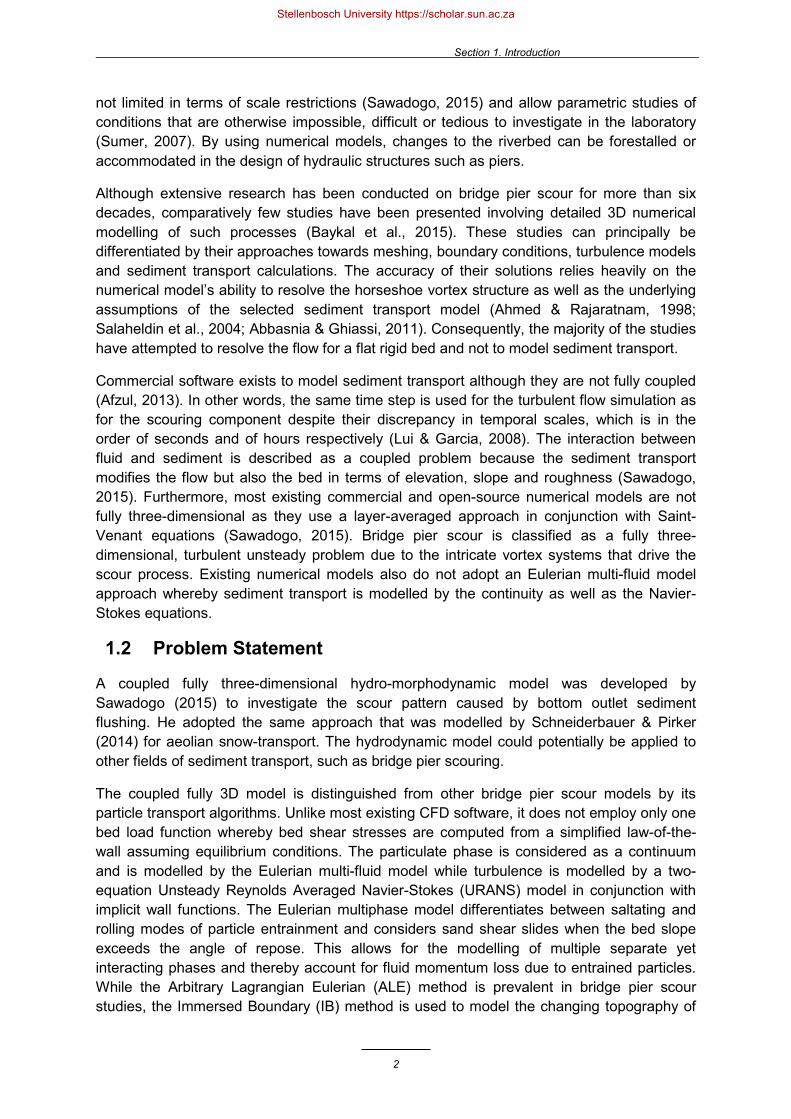
Bridge pier scour is defined as the washing away of river bed material in the vicinity of a bridge pier during flood events. Scouring results from the erosive action of water that excavates the sediment material. The total depth of scour that occurs at a bridge is the sum of the depths of three different categories of scour, as illustrated in Figure 2-1 and discussed below.
1. General scour is the natural washing away or morphing of a river bed, whereby the entire river bed is in motion, that would occur irrespective of the presence of the bridge.
2. Contraction scour occurs when the abutments and piers of a bridge constrict the flow along a river channel and consequently increase the flow velocity and erosive potential.
3. Local scour is caused by the 3D turbulent flow around an obstruction, such as an abutment or pier, which alters the local flow field of a river. It is the most significant and least understood component of total scouring owing to the large number of parameters that influence local scour (Ettema, 1980). Rooseboom (2013) reiterates that local scour is responsible for the majority of bridge failures.
Figure 2-1: Different scour mechanisms in a river at a bridge (adapted from Idaho Field Manual, 2004)
Local scour can further be classified as either bridge pier scour or abutment scour. It can take place in either cohesive or alluvial beds, and in either clear-water or live-bed scour conditions. Live-bed scour is characterized by the simultaneous action of local scour with contraction scour or general scour. Otherwise, the isolated event of local scour is known as clear-water scouring.
PIER
ABUTMENT
BRIDGE DECK
CHANNEL BED WATER SURFACE
LONG TERM DEGRADATION CONTRACTION SCOUR LOCAL SCOUR
Stellenbosch University https://scholar.sun.ac.za

Section 2. Literature Review
8
2.3 The Relevance of Bridge Pier Scour
Designing for bridge pier scour is important because the undermining action exposes the bridge’s foundation, reduces the soil’s bearing capacity and compromises the structural integrity. Hugo (2007) reports that scour holes can be as deep as 20 to 30 m. Figure 2-2 shows the exposed pile cap of the I-90 Bridge on the Schoharie Creek to place these numbers into perspective. The photograph illustrates the several metres of scour in front of the west pier that resulted from a 500-year flood of 3625 m3/s after the 2011 Irene hurricane.
Figure 2-2: Scour at the I-90 Bridge pier on the Schoharie Creek, New York (permissions by Garver, 2012)
Local scour at piers and abutments has been cited as the main mechanism responsible for the collapse of bridges founded in alluvial beds (Deshmukh & Raikar, 2014; Rooseboom, 2013; Constantinescu et al., 2004). Briaud et al. (1999) reports that more than 1 000 of the approximate 600 000 bridges in the United States have failed during the last 30 years. Furthermore, Huber (1991) and Sumer (2007) estimate that 60% of all structural bridge failures in the United States can be attributed to scouring and not to overloading, incurring costs of approximately $30 million per annum (Xiong et al., 2014). In New Zealand, 70% of the NZ$36 million annual scour related costs are attributed to bridge repairs rather than preventative maintenance (Brandimarte et al., 2012). The percentage of collapsed bridges has increased in the past decade due to the aging of structures and lack of maintenance.
Stellenbosch University https://scholar.sun.ac.za

Section 2. Literature Review
9
Changes in the boundaries of a river must be either forestalled or accommodated in the design of such structures, or run the risk of the eventual structural failure. Serious implications of such failures include human fatalities, large economic costs to repair, disruption of transportation networks, damage to the environment and the loss of historical or cultural landmarks. Smith (1976) cites examples since 1961 of which 56% are directly attributable to scour. Recent cases of bridge failures include:
• Plaka Bridge in Greece, 2015: The 148 year old bridge endured the great world wars and yet flash floods ripped its stone foundations from the river bed.
• Bonnybrook Bridge in Canada, 2013: Six train cars were derailed that were transporting a highly explosive and toxic liquid that could have caused serious damage to the environment if they had leaked. This example stresses the importance of improved inspection methods and scour prediction models because the bridge was inspected 18 times after the flood before its collapse.
• Malahide Viaduct in Ireland, 2009: A 20 m section of the bridge collapsed after an inspection missed the scour damage due to impaired visibility.
• I5 Bridge in California, 1995: Seven people were killed and a major transportation link between Seattle and Vancouver was severed.
• Schoharie Creek Thruway Bridge in New York, 1987: The collapse is one of the better known incidents that instigated funding and research into bridge pier scour. The 1st pier dropped 1.2 m into the scour hole after which a 2nd pier and three 20 m spans collapsed. Ten motorists were killed. A discharge of approximately 2 410 m3/s washed the protective riprap away; hence, the bridge was rebuilt with deeper piles, as seen from Figure 2-2.
• Glanrhyd Bridge in Wales, 1987: Four people drowned due to the collapse of the railway bridge.
With regards to the local South African context, local scour has been observed at 60% of the bridges while contraction scour has been observed at 44% (Hugo, 2007). South Africa is seeing an escalation in flood incidents with extreme weather patterns and should prepare for increased erosion and scouring processes of river beds. The relevance of local scour damage in South Africa can be demonstrated by the following bridge failures:
• Queen’s Bridge, Umgeni River in KwaZulu-Natal, 1868: Local scour caused the failure of the iron plate girder.
• Lovu River in KwaZulu-Natal, 1959: A pier dropped into a 2.74 m scour hole after which three bridge spans collapsed.
• Pondoland Bridge, Mzimvubu River in Eastern Cape, 1978: Scouring resulted in the collapse of one pier and two spans.
• Domoina Cyclone, 1984: More than 100 bridges were destroyed by the tropical storm floods throughout Madagascar, Mozambique, Swaziland and South Africa, with a total cost estimated at R360 million.
• The Limpopo Province, 2000: Approximately 200 bridges were severely damaged by floods with a total cost estimated at R1.3 billion.
Stellenbosch University https://scholar.sun.ac.za

Section 2. Literature Review
10
2.4 Countermeasures
Existing guidelines for the bridge design recommend a combination of the following three methods to address scour (Rooseboom, 2013):
1) Hydraulic countermeasures: a. River training structures such as check dams, spurs, dykes, berms, barbs,
groynes and vanes are used to alter the stream hydraulics and to deflect the flow.
b. Bed armouring with riprap, gabions, grout filled mattresses, concrete armour unit and soil cement are used to fix the river bed sediment in place. Of these, riprap is the most common employed countermeasure. However, regular inspections and maintenance is required to ensure they are not washed away by floods.
2) Structural countermeasures: Foundation strengthening could potentially be the safest and most economic option if piles are extended to levels well below the estimated scour depth and preferably to the bedrock level. Furthermore, optimization of the pier shape and other structural modifications allows the bridge design to control and reduce the flow processes responsible for scouring.
3) Maintenance: Maintenance is required to ensure the river sections remain formalised through regular inspections. Expensive sonar and laser technologies exist to address the shortcomings associated with visual inspections. However, scour is difficult to detect and the maximum scour, which occurs under peak flow conditions, is difficult to measure. This is owing to the unpredictability and complexity of the river system.
However, there is no universally agreed upon design procedure for bridge scour and the calculation thereof is not common practice in many countries (Ali & Karim, 2002). Lack of practical knowledge on the scouring process has left hydraulic experts claiming that the collapse of large bridges caused by foundation erosion is inevitable. Therefore, there is a need to understand and predict scour more accurately.
2.5 The Scour Process
The construction of a bridge pier in a hydraulic environment will alter the flow pattern in the vicinity of the pier, resulting in the generation of turbulence, the separation of flow and the formation of a horseshoe vortex in front of the structure as well as lee-wake vortices behind the structure (with or without vortex shedding). It has been established by extensive research studies that these vortices are the basic mechanisms responsible for causing the scour initiation and development. Due to the varying interaction between these vortices, the junction flow is characterised as three-dimensional, turbulent and unsteady. The key features of the flow pattern are illustrated in Figure 2-3.
Stellenbosch University https://scholar.sun.ac.za

Section 2. Literature Review
11
Figure 2-3: Vortex formation at a cylindrical pier (Garde & Ranga, 2000)
2.5.1 The Boundary Layer
The velocity profile of water approaching a bridge pier is characterised by a logarithmic shape whereby the maximum velocity occurs at the water surface and a zero velocity at the channel bed. This is because water is a viscous fluid that experiences a shearing action when it comes into contact with a solid surface such as the channel bed or the pier wall. A thin layer of water adjacent to the surface decelerates. Once the layer comes to rest, a shearing action ensues between the static layer and the next layer. This layer is then forced to decelerate somewhat less and the process continues until a boundary layer zone is formed (Chadwick et al., 2013). The flow outside the boundary layer is free of shear and the velocity remains unaffected. This principle is important because the incoming boundary layers at the pier, as well as the pressure gradient, are responsible for the vortex formation.
As the flow reaches the pier, the velocity decreases abruptly and the flow is deflected away from the pier as illustrated in Figure 2-4. The flow accelerates where the streamlines converge and a boundary layer forms. Once the fluid within the boundary layer surpasses the Y-axis, it decelerates to a velocity comparatively lower than that of the fluid in the free stream. Eventually negative velocities and low pressures arise. A separation layer (indicated by the dashed line) divides the regions into those with positive and negative velocities. Consequently, flow from outside the boundary layer is drawn into the low pressure region. Eddies are produced and drawn downstream to form the turbulent wake (Chadwick et al., 2013).
Stellenbosch University https://scholar.sun.ac.za

Section 2. Literature Review
12
Figure 2-4: Flow separation at a cylindrical pier (Chadwick et al., 2013).
2.5.2 The Horseshoe Vortex
The horseshoe vortex upstream of the bridge pier is primarily responsible for the scouring action. Since the flow velocity is at a maximum at the free surface and decreases to zero at the bed, the stagnation pressure decreases in the same direction. A downflow is driven by the strong pressure gradient and vertical velocity component which rolls and curls up when it comes into contact with the channel bed, as illustrated in Figure 2-3. The resulting circulation and 3D separation of flow forms the vortex, which acts like an impinging jet on the bed, digging up the sediment material (Williams, 2014). The vortex sinks into the ring of scoured material where it is trapped and stabilized, causing rapid sediment erosion until equilibrium is reached. The ends of the vortex system are then swept downstream around the pier by the flow, forming the characteristic U horseshoe shape.
A surface roller, or bow wave, is formed at the free surface on the upstream side of the pier (refer to Figure 2-3). An upward flow circulating in a direction opposite to that of the horseshoe vortex causes the flow depth to increase. In shallow flow depths, the bow wave has the ability to counteract and weaken the horseshoe vortex (Melville, 1975).
Baker (1980a) was one of the first to observe that the horseshoe vortex structure consists of a system of different vortices, as demonstrated by Figure 2-5a. The vortices are caused by different separation boundary layers on the pier face (A), on the channel bed (B) or smaller ones below other more prominent vortices (C). While Baker (1980a) observed two primary vortices, Dargahi (1989) observed three rotating in the same direction and Chen et al. (2000) only observed one large primary vortex that oscillated chaotically around a mean position. However, recent research has shown that the vortex system is highly dependent on the Reynolds number, causing the structure, location, size and intensity of these vortices to be highly variable in time (Constandinescu & Koken, 2005).
Stellenbosch University https://scholar.sun.ac.za

Section 2. Literature Review
13
Figure 2-5: (a) Smoke-flow visualization of the horseshoe vortex structure from the side (b) Oil-flow visualisation of the horseshoe eddies from above (adapted from Baker, 1980a)
Figure 2-5b shows the horseshoe vortex destabilizing into 3D eddies that do not wrap uniformly around the pier. These eddies extend over variable distances in a polar direction around the upstream side of the pier, and are continuously and randomly created and destroyed. The largest shear stress values are situated beneath these eddies, as well as the detached shear layers, which occur at polar angles larger than 30° around the pier (Kirkil & Constantinescu, 2005).
2.5.3 The Lee-Wake Vortex
The lee-wake vortex forms behind the pier and is induced by the pier itself, characterised by an upflow, contrary to the horseshoe vortex (as illustrated by Figure 2-6). Furthermore, the horseshoe vortex is characterised by a horizontal axis of rotation while the axes of the lee-wake vortices are almost vertical that create a suction and suspend the sediment into the main flow field, similar to a vacuum cleaner (Breusers et al., 1977). Consequently, these vortices largely affect not only the horizontal but also the vertical velocity component at a bridge pier (Breusers et al., 1977). These vortices are generally weaker and remove less sediment than the horseshoe vortices (Williams, 2014).
The lee-wake vortices are caused by the rotation of fluid past the boundary layer over the surface of the pier. Near the sediment bed, stagnation pressures cause unstable shear layers to form at the pier surface, which then roll up and detach from either side of the pier at the separation layer (the dashed line in Figure 2-6). The unstable vortices are shed from alternating sides of the pier as the flow sweeps them downstream. They can be recognized from the eddies at the water surface behind the pier that dissipate as they move downstream.
C A C B
Stellenbosch University https://scholar.sun.ac.za

Section 2. Literature Review
14
Figure 2-6: Diagrammatic flow pattern for the lee-wake vortex (adapted from Raudkivi, 1986)
However, at low pier Reynolds numbers between 5 and 50, the vortices are able to form stable standing systems, as illustrated in Figure 2-7. The flow starts to separate at 𝑅𝑅𝑅𝑅𝐷𝐷 = 5 and oscillations first appear at 𝑅𝑅𝑅𝑅𝐷𝐷 = 50. The shedding frequency of the wake vortex was found to be proportional to the flow velocity of the main stream and inversely proportional to the pier diameter (Melville, 1975). The regularity of vortex shedding ranges between a stable von Kármán state, with Reynolds numbers less than 300, and a chaotic state, with Reynolds numbers greater than 3.5×10⁶ (Breusers et al., 1977). Figure 2-8 illustrates an example of a lee-wake vortex in a von Kármán state.
𝑅𝑅𝑅𝑅𝐷𝐷 < 5 5 < 𝑅𝑅𝑅𝑅𝐷𝐷 < 50 50 < 𝑅𝑅𝑅𝑅𝐷𝐷 < 3.5×10⁶ 3.5×10⁶ < 𝑅𝑅𝑅𝑅𝐷𝐷
Figure 2-7: Flow transitions around a cylinder (Mills, 1998)
Propagation of deposition mound
Logarithmic velocity profile
Angle of repose
“U” shape
Vortex trench
Stellenbosch University https://scholar.sun.ac.za

Section 2. Literature Review
15
Figure 2-8: Lee-Wake vortex shedding from alternating sides (Siqueira, 2005)
2.5.4 The Trailing Vortex
In the case of submerged piers, a third trailing vortex system will form at the top of the pier. The discrete vortices extend downstream from the top edge of the pier where the vortices are generated by a difference in pressure. The investigation of these vortices is beyond the scope of the study as it does not contribute towards the scouring process.
2.5.5 Scour Hole Formation
The horseshoe vortex system has the effect of amplifying the local bed shear stress, turbulent kinetic energy and pressure fluctuation levels near the bed (Roulund et al., 2005). The heightened velocities and associated shear stresses in front of and adjacent to the pier are responsible for scouring the loose bed. Figure 2-9 shows the shear stress amplification (𝜏𝜏/𝜏𝜏0) for the initial rigid plane bed and for the quasi-equilibrium scoured bed.
Consequently, the development of the scour hole is initiated at the sides of the pier with both holes swiftly propagating upstream around the pier to meet on the centreline. A U-shaped hole, with the open ends facing downstream toward the wake, is formed concentric with the pier (Dey, 1996). According to Hoffmans & Verhij (1997), the slope of a scour hole can be divided into different regions whereby the deepest part of the scour hole in front of the pier sees a concave shape. The upstream portion of the scour hole is characterised by a frustum shape of an inverted cone with slopes equal to the angle of repose of the bed material (Ali & Karim, 2002). In the early stages of the scour development, the lip of the hole is very sharp with a near vertical face (refer to Figure 2-6).
Figure 2-9: Bed shear stress amplification for the (a) initial plane bed and (b) scoured bed (Roulund et al., 2005)
Stellenbosch University https://scholar.sun.ac.za
Section 2. Literature Review
16
Excavation of the scour hole by the horseshoe vortex undermines the slope which collapses in local avalanches of bed material such that the angle of repose is maintained (Ali & Karim, 2002). The collapsed material is removed in an upward direction by the lee-wake vortex and transported downstream by the eddies. Once the eddies begin to dissipate, the removed sediment deposits to form a dune in the low pressure zone. The dune migrates further downstream as time passes until it eventually disappears.
As the scour hole grows, the horseshoe vortex rapidly increases in size and in circulation while the vertical velocity component near the bed decreases. Consequently, the shear stress and agitation on the channel bed decrease until a point where the downflow can no longer entrain sediment and an equilibrium scour hole is formed (Breusers et al, 1977).
Backfilling of the scour hole is caused by shear slides of sediment on the slopes of scour hole. It is considered part of the natural scouring process until the scour hole profile reaches an equilibrium. However, the backfilling process in a continuously changing flow climate makes it difficult to measure the maximum scour depth once a flood has subsided. Backfill of the scour hole is a complicated process and limited literature on the topic is presently available.
2.6 Sediment Transport in Rivers
Turbulence and vortices in the vicinity of a pier are responsible for the heightened velocities and shear stresses that drive the scouring process. The study of sediment transport is thus of fundamental importance to quantify the initiation and rate of erosion or scouring. Sediment transport occurs when an interface between a moving fluid and an erodible boundary is present. This activity at the interface is complex because the flow is no longer a simple fluid flow but multiphase flow in a boundary layer (Chadwick, 2013). While this study deals with the interrelationship between flowing water and sediment particles, the principles are fundamentally similar whether the mechanisms may be fluvial, aeolian or glacial. The basic concepts of sediment transport, erosion and deposition are introduced as a context for scouring.
2.6.1 The Threshold of Movement
Various relationships exist that define the boundary conditions under which a river will begin to entrain the bed material. A sediment particle will only become unstable and be put into motion once the fluid applies drag and lift forces by oscillating eddy currents sufficient to overcome the particle’s natural resistance to motion, which is caused by a gravitational force holding it in place. A mathematical description of the complex eddy currents is almost impossible and instead hydraulic parameters in the vicinity of the packed bed are considered (Langmaak, 2013). Incipient motion is typically defined by a critical or threshold shear stress or velocity.
2.6.1.1 Shear Stress Sediment transport as a function of shear stress is the measure of the frictional force caused by a fluid flowing over an erodible bed. The sediment transport process is initiated when the average shear stress on an alluvial bed τ0 exceeds the critical tractive stress of the sediment material τ𝑡𝑡. Thus, at the threshold of movement for alluvial sediment τ0 = τ𝑡𝑡 the drag force is proportional to the submerged weight of a spherical particle
Stellenbosch University https://scholar.sun.ac.za

Section 2. Literature Review
17
where 𝜌𝜌𝑠𝑠 and 𝜌𝜌 are the densities of the sediment and fluid, respectively, 𝑑𝑑 is the grain diameter, 𝜑𝜑 is the angle of repose, and 𝑔𝑔 is the gravitational acceleration. The number of prominent grains in a given surface area 𝐴𝐴𝑝𝑝 is described as the area of the grains divided by the total area (Chadwick et al., 2013). The relationship is rearranged to give the dimensionless ratio of shear force to gravity force, known as the entrainment function or the critical Shields parameter
which is one of the most widely used parameters in engineering to define incipient motion. The derivation of the Shields parameter does not account for the effect of a sloping bed or scour hole whereby incipient motion is a function of gravity and traction as well as hydrodynamic forces. A correction factor can be applied to reduce the critical shear stress derived for a flat bed. For example, CIRIA et al. (2007) proposed the correction factors for a longitudinally sloped bed and a transverse slope, respectively
where 𝜑𝜑 is the angle of repose, 𝜃𝜃 is the angle of the bed slope with respect to the flow direction and 𝜃𝜃𝑡𝑡 is the angle of the transverse bed slope normal to the flow.
Due to the difficulty of measuring shear stress in the field, the Chézy Formula is the simplest and most commonly used approach to establish the average bed shear stress
where 𝑅𝑅 is the hydraulic radius and 𝑆𝑆 is the energy slope of the channel. The formula assumes that the flow is steady and uniform in its derivation from momentum considerations whereby the gravity force component in the flow direction equals the friction force. However, not all flows can be simplified using a single representative slope and cross section.
Several other equations exist to empirically define the critical shear stress as well as the local bed shear stress, for example, the quadratic stress law, friction-based method or the wall function. The wall function is the most widely used method and it allows the bed shear stress to be written in units of velocity, known as the shear or friction velocity 𝐶𝐶∗. Turbulent shear velocity is also often used as a function for particle entrainment because it is a representative scaling parameter for the fluctuating component of velocity in turbulent flows, given as
For unsteady flow, the bed shear stress is established locally by applying the Saint-Venant equations for continuity which takes acceleration into consideration. Furthermore, numerical
𝜏𝜏𝑡𝑡𝑑𝑑2
𝐴𝐴𝑝𝑝∝ (𝜌𝜌𝑠𝑠 − 𝜌𝜌)𝑔𝑔
𝜋𝜋𝑑𝑑3
6tan𝜑𝜑 , (2-1)
𝜃𝜃𝑠𝑠,𝑐𝑐 =𝜏𝜏𝑡𝑡
(𝜌𝜌𝑠𝑠 − 𝜌𝜌)𝑔𝑔𝑑𝑑 , (2-2)
𝑘𝑘𝜃𝜃 =sin(𝜑𝜑 − 𝜃𝜃)
sin(𝜑𝜑) , (2-3)
𝑘𝑘𝜃𝜃𝑡𝑡 = cos𝜃𝜃1 − tan𝜃𝜃tan𝜑𝜑
2
, (2-4)
𝜏𝜏0 = 𝜌𝜌𝑔𝑔𝑅𝑅𝑆𝑆 , (2-5)
𝐶𝐶∗ = 𝜏𝜏0/𝜌𝜌 = 𝑔𝑔𝑦𝑦1𝑆𝑆 = 𝑅𝑅𝑖𝑖𝑖𝑖 . (2-6)
Stellenbosch University https://scholar.sun.ac.za

Section 2. Literature Review
18
models have the ability to establish the bed shear stress from the Reynolds stress 𝑅𝑅𝑖𝑖𝑖𝑖, the turbulent kinetic energy 𝑘𝑘 or the turbulent viscosity 𝜇𝜇𝑡𝑡 used in turbulence models (Afzul, 2013)
which are explained in more detail in subsequent sections. The Reynolds stress is defined as 𝑅𝑅𝑖𝑖𝑖𝑖 = 𝐶𝐶𝚤𝚤′𝐶𝐶𝚥𝚥′ where 𝐶𝐶𝑖𝑖,𝑖𝑖 is the component of local time-averaged velocities.
2.6.1.2 Particle Reynolds Number The Shields parameter suggests that the entrainment function should be a constant based on relative roughness (the ratio of the particle size to the flow depth). However, Shields (1936) showed that particle entrainment was not only related to the bed form and the immersed weight of the particle, but also to a form of the Reynolds number 𝑅𝑅𝑅𝑅𝑝𝑝 for a particle. The ratio of the shear force to the gravity force is defined as
where υ is the kinematic viscosity and 𝐶𝐶∗ is the average particle velocity or shear velocity. Subsequently, many variations of the Shields threshold line, illustrated in Figure 2-10, have commonly been used to determine the critical shear stress.
Figure 2-10: Shields diagram for a particle relative density of 2.65 (Graf, 1971)
Only one particle size is taken into account in the equation even though riverbeds typically contain a mixture of different sediment sizes. In the case of partial motion, only the finer fractions of the sediment bed are washed away, exposing a layer of gravel which is less easily eroded (Chadwick et al., 2013). The finer sediment underneath this layer is then protected, or armoured, against further sediment transport.
𝜏𝜏0 = 𝜌𝜌𝑅𝑅𝑖𝑖𝑖𝑖 = 𝜌𝜌𝑘𝑘𝐶𝐶𝜇𝜇 = 𝜌𝜌𝜇𝜇𝑡𝑡𝜕𝜕𝑣𝑣𝜕𝜕𝜕𝜕
, (2-7)
𝑅𝑅𝑅𝑅𝑝𝑝 =𝐶𝐶∗𝑑𝑑
υ , (2-8)
Stellenbosch University https://scholar.sun.ac.za

Section 2. Literature Review
19
2.6.1.3 Critical Velocity Incipient motion can also be described in terms of a critical velocity 𝑣𝑣𝑐𝑐 whereby sediment transport commences once the approach flow velocity exceeds the critical velocity required for general sediment entrainment. Several equations for critical velocity derived empirically are presented in Section 2.8.1, but the equation derived classically from the Shields diagram and Manning equation is given which assumes a shear stress limit for incipient motion of 𝜃𝜃𝑠𝑠,𝑐𝑐 = 0.056 for the condition 𝑅𝑅𝑅𝑅 > 400 (Graf, 1971):
Hjulström’s diagram in Figure 2-11 shows the logarithmic relationship between the sediment size and critical velocity required to entrain it. The diagram was later modified to show separate curves for the threshold of movement for different water depths because velocity is used instead of boundary shear stress to represent the flow strength (as in the Shields diagram).
The simplicity of the critical velocity parameter is attractive but it is criticized for not differentiating between deceleration and acceleration in the description of deposition and erosion respectively. The stability of particles is characterised by the impulsive force of turbulent eddies and high velocity gradients in the vicinity of the particle, not of the average stream approach velocity, which are difficult if not impossible to determine analytically (Langmaak, 2013).
Figure 2-11: Hjulström’s diagram (Conrad, 2004)
𝑣𝑣𝑐𝑐𝑔𝑔𝑑𝑑
= 1.9𝜌𝜌𝑠𝑠 − 𝜌𝜌𝜌𝜌
𝑅𝑅𝑑𝑑16
. (2-9)
Stellenbosch University https://scholar.sun.ac.za

Section 2. Literature Review
20
2.6.1.4 Stream Power The Shields approach has been criticized for only considering the tangential drag force and for disregarding the vertical lift force, specifically at high particle Reynolds numbers (Langmaak, 2013). Lui (1956) instead described incipient motion by relating the particle Reynolds number with a movability number defined as the ratio of shear velocity and settling velocity (𝐶𝐶∗/𝑤𝑤). This ratio represents the ratio of the stream power applied and the power required to entrain particles. Stream power is the rate of potential energy dissipated as friction or work done against a riverbed per unit downstream length, given by the equation
where 𝑄𝑄 is the discharge or flow rate. Rooseboom et al. (1983) argue that particle size poorly represents the transportability of sediment and instead recommends the use of settling velocity of particles in alluvial beds. Unit stream power can be rewritten as 𝑣𝑣1𝑆𝑆/𝑤𝑤 and Rooseboom (1992) showed that the power required per unit volume to suspend a particle is given by (𝜌𝜌𝑠𝑠 − 𝜌𝜌)𝑔𝑔𝑤𝑤. Sediment entrainment will occur once the power for suspension exceeds the power required for to maintain motion in turbulent flow, that is
or
The movability number required for incipient motion becomes a constant for turbulent flow based on certain flow conditions as well as sediment size. The analysis of incipient motion in terms of stream power led to development of the Modified Lui Diagram in Figure 2-12.
Figure 2-12: Modified Lui Diagram (Rooseboom, 2013)
Ω = 𝜌𝜌𝑔𝑔𝑄𝑄𝑆𝑆 , (2-10)
(𝜌𝜌𝑠𝑠 − 𝜌𝜌)𝑔𝑔𝑤𝑤 >𝑝𝑝𝑔𝑔𝑆𝑆𝑦𝑦1𝐶𝐶∗
𝑑𝑑 , (2-11)
(𝜌𝜌𝑠𝑠 − 𝜌𝜌)𝑑𝑑𝜌𝜌𝑆𝑆𝑦𝑦1
𝑤𝑤 > 𝐶𝐶∗ . (2-12)
Stellenbosch University https://scholar.sun.ac.za

Section 2. Literature Review
21
Other work pertaining to the fluid threshold includes Meyer-Peter & Müller (1948), Chepil (1959), Bagnold (1966), Engelund-Hansen (1967), Schmidt (1980) Lefort (1991) and Belleudy (2012). The best known of these relationships is probably the dimensionless Shields diagram which is currently widely used and accepted (Chadwick, 2013). Dey (1999) gave a mathematical solution for the diagram to use in mathematical modelling.
2.6.2 Modes of Sediment Transport
The total sediment load is the sum of the following modes of sediment transport and is illustrated in Figure 2-13:
• Bed load transport occurs at a relatively lower shear stress whereby moving particles remain in contact with the stationary bed. Bed load particles are either transported by surface creeping, rolling or saltation. Saltation occurs when a grain obtains an upward impulse from a particle dropping out of suspension (Chiew, 1984).
• Suspended load transport occurs when finer particles lose contact with the bed due to a high velocity flow or shear stress. The particles are carried downstream in the flow while being held in suspension against gravity by an upward diffusion of turbulence.
• Wash / colloidal / dissolved load transport consists of very fine clay and silt particles or disassociated ions that were washed overland into streams. Wash load can also derive from the abrasion of sediment grains in transport and are too fine to be present in the bed load. Unlike the suspended load, the particles remain in suspension by Brownian motion, even in still water, as they are not dependent on the hydraulic parameters of stream flow (Raudkivi, 1998). The total sediment load is primarily constituted of wash load (Sawadogo, 2015).
Furthermore, according to Sawadogo (2015), landslide-like shear slides of a whole layer of grains could also be considered as a particle transport mode. This is particularly important to the formation of a scour hole because as the side slopes develop, the sediment becomes very unstable and slide on the upper slope such that the bed angle of repose is maintained (Dargahi, 1990).
Figure 2-13: Different modes of sediment transport (adapted from Sullivan, 2015)
Stellenbosch University https://scholar.sun.ac.za

Section 2. Literature Review
22
In general, the mode of sediment transport can be determined by the Rouse number which is given by the settling velocity 𝑤𝑤, the von Kármán constant κ = 0.407, and the shear velocity 𝐶𝐶∗:
In summary, the mode of sediment transport can be established by the following conditions: • Threshold of sediment movement as bed load: 𝜃𝜃𝐶𝐶 ≤ 𝜃𝜃 or 𝑃𝑃 ≤ 7.5 or 𝑣𝑣𝐶𝐶 ≤ 𝑣𝑣 • Initiation of suspended load: 𝐶𝐶∗ ≤ 𝑤𝑤 or 𝑃𝑃 ≤ 2.5 • Transport dominated by 100% suspended load: 𝑃𝑃 ≤ 1.2 • Transport in the lower regime as ripples and dunes: 𝜃𝜃𝐶𝐶 ≤ 𝜃𝜃 ≤ 0.8 • Transport in the upper regime as sheet flow over a flatbed: 𝜃𝜃 > 0.8 or 𝑃𝑃 ≤ 0.8
Sediment particles do not move independently once the threshold of movement is reached. During general sediment transport (or general scouring), features such as dunes are formed that migrate downstream as the sand is driven from the dune crests to the lee side. The different bedform mechanics can be classified based on Froude numbers as either lower, transition or upper regime. The lower regime involves subcritical flow with ripples and dunes that move in discrete steps. Conversely, the upper regime features chutes, antidunes, pools or a flatbed in continuous motion for supercritical flow. Once the flow has a suspended load, major changes occur at the bed as the dunes wash out. Bedforms have also been described by Shields relative to shear stress and by Lui relative to the movability number. Figure 2-14 shows the Lui Diagram as a criterion for bedforms.
Figure 2-14: Bedform criteria (Graf, 1971)
𝑃𝑃 =𝑤𝑤
κ𝐶𝐶∗ . (2-13)
Stellenbosch University https://scholar.sun.ac.za

Section 2. Literature Review
23
2.6.3 Bed Load Transport
Numerous sediment transport relationships exist to quantify the rate of bed load transport by weight or volume for a given cross section and time. These have all been verified against experimental data and yet there is no unanimity on the best quality method to compute bed shear stresses (Raudkivi, 1998). The different equations, similar to equations for the threshold of movement, can be grouped according to their derivation. It should be noted that sediment transport is a field of study in its own right and only an introduction has been presented for background to Sections 2.9.3 and 3.3.1.
• Bed load transport equations are commonly a function of shear stress excess (𝜏𝜏 − 𝜏𝜏𝑡𝑡) or the transport ratio φ = 𝜏𝜏/𝜏𝜏𝑡𝑡 which are measures of the threshold of motion. The transport equations are normally nonlinear whereby the shear stress excess or transport ratio is raised to a power. Many notable bed load transport formulae have been derived from that of Meyer-Peter & Müller (1948) for well graded fine gravel
Another well-known example is that of van Rijn (1987) for bed load concentration
where 𝑦𝑦1 is the water depth reference level and υ is the viscosity of water. Similarly, Dey (1999) proposed an equation in terms of the relative sediment density 𝑠𝑠
More recently, Kuhnle et al. (2013) developed a formula for bed load transport of sand fractions where an additional roughness geometry function 𝑓𝑓 is required to adjust the bed shear stress for an immobile gravel bed
• Similar to Section 2.6.1.4, sediment transport may be equated to work done or stream power Ω = 𝜏𝜏𝑣𝑣 such as that of Bagnold (1966; 1980)
𝑞𝑞𝑏𝑏𝑑𝑑𝑑𝑑 = φ𝑑𝑑 𝜌𝜌𝑠𝑠 − 𝜌𝜌𝜌𝜌
𝑔𝑔𝑑𝑑0.5
𝜏𝜏(𝜌𝜌𝑠𝑠 − 𝜌𝜌)𝑔𝑔𝑑𝑑
− 𝜏𝜏𝑡𝑡1.5
. (2-14)
𝑞𝑞𝑏𝑏𝑑𝑑𝑑𝑑 = 0.015𝑣𝑣𝑑𝑑0.7
𝑦𝑦1
𝜏𝜏 − 𝜏𝜏𝑡𝑡𝜏𝜏𝑡𝑡
1.5
(𝜌𝜌𝑠𝑠 − 𝜌𝜌)𝑔𝑔 υ2
0.1 , (2-15)
𝑞𝑞𝑏𝑏𝑑𝑑𝑑𝑑 = 0.053(𝑠𝑠 − 1)𝑓𝑓𝑑𝑑50𝜏𝜏 − 𝜏𝜏𝑡𝑡
𝜏𝜏𝑡𝑡2.1
(𝜌𝜌𝑠𝑠 − 𝜌𝜌)𝑔𝑔 υ2
0.1 . (2-16)
𝑞𝑞𝑏𝑏𝑑𝑑𝑑𝑑 = [(𝑠𝑠 − 1)𝑔𝑔𝑑𝑑]0.5𝑝𝑝𝑠𝑠𝑑𝑑𝑓𝑓2.14 𝜏𝜏𝜏𝜏𝑡𝑡3.49
. (2-17)
𝑞𝑞𝑏𝑏𝑑𝑑𝑑𝑑 = Ω𝐶𝐶∗ − 𝐶𝐶𝑡𝑡∗
𝐶𝐶∗𝑡𝑡𝑎𝑎𝑛𝑛𝜑𝜑1 −
5.75𝐶𝐶∗ log 0.37𝑦𝑦1𝑛𝑛𝑑𝑑 + 𝑤𝑤
𝑣𝑣 . (2-18)
Stellenbosch University https://scholar.sun.ac.za

Section 2. Literature Review
24
• Furthermore, a probabilistic, statistical or numerical analysis may be used to establish bed load. Most approaches follow that of Einstein (1950) who deviated from the concept for mean tractive forces (Raudkivi, 1998). The argument is that in turbulent flow, the fluid forces acting on a particle vary with time and space, and subsequently, particle movement depends on the probability that applied forces exceed resisting forces at a certain time and position.
In turbulent flow, both lift and drag forces fluctuate in magnitude, position and direction. The drag component causes energy dissipation or increased turbulence near the bed. This leads to strong and rapid pressure fluctuations on the bed surface which have the ability to entrain sediment. Thus, effective bed shear stress is not only a function of grain roughness but also of turbulent intensity (Sumer et al., 2003). The principle is probabilistic because the applied stresses in turbulent flow and the response of a particle to its position are governed by chance. Engelund & Fredsøe (1976) proposed different variations of the following equation
where 𝑣𝑣𝑝𝑝 is the mean particle velocity and 𝑃𝑃𝑃𝑃 is the probability of particle movement given by
2.6.4 Clear-Water Scouring
According to Bagnold (1966), the particles entrained from a mobile bed occur by surface creeping, saltation and suspension. However, clear-water scouring (defined for the approach velocity to the critical velocity ratio 𝑣𝑣/𝑣𝑣𝑐𝑐 < 1) is not subjected to suspended loads, thus bed load is the main component of sediment transport (Baker, 1986).
Furthermore, as opposed to live-bed scouring whereby the entire riverbed is in motion, clear-water scouring occurs when the general riverbed is stable but the bed shear stress only in the vicinity of the bridge pier exceeds the critical shear stress. Thus, the study of bridge pier scour under clear-water conditions is only concerned with sediment transport in the vicinity of the structure because (1) the average bed shear stress is increased and (2) the degree of turbulence is increased. The increase in bed shear stress is expressed by the amplification factor given by
where 𝜏𝜏0 defines the bed shear stress for undisturbed flow. This is illustrated in Figure 2-9 whereby the local increase in 𝑎𝑎𝑓𝑓 > 1 implies the sediment transport capacity will increase and presumably scour the bed.
𝑞𝑞𝑏𝑏𝑑𝑑𝑑𝑑 = 9.3𝜋𝜋𝑑𝑑6𝑣𝑣𝑝𝑝 Pp 1 − 0.7
𝜃𝜃𝑆𝑆,𝑐𝑐
𝜃𝜃𝑆𝑆0.5
, (2-19)
𝑃𝑃𝑃𝑃 = 1 + 0.51𝜋𝜋/6𝜃𝜃𝑆𝑆 − 𝜃𝜃𝑆𝑆,𝑐𝑐
4
−0.25
. (2-20)
𝑎𝑎𝑓𝑓 =𝜏𝜏𝜏𝜏0
, (2-21)
Stellenbosch University https://scholar.sun.ac.za

Section 2. Literature Review
25
2.7 Scour Parameters
The local scour process is affected by several different yet interrelated parameters which are discussed below. Because the parameters are interrelated, they are often described as quantities relative to one another. In an attempt to simplify the various parameters, the following quantities have repeatedly been identified as the most significant in literature (Williams, 2014):
1. Flow intensity or relative velocity (𝑣𝑣1/𝑣𝑣𝑐𝑐), the distinguishing factor between clear-water and live-bed scouring, and the driving force behind shear stresses.
2. Relative flow depth (𝑦𝑦1/𝐷𝐷), the factor representing the flow’s ability to suppress vortices.
3. Pier Reynolds number (𝑣𝑣1𝐷𝐷/υ), the factor accounting for turbulence. 4. Relative sediment size or roughness (𝐷𝐷/𝑑𝑑50), the primary differentiating factor
between laboratory and field tests. 5. Time to reach equilibrium scour (𝑡𝑡/𝑇𝑇𝑑𝑑), an important factor in the case of clear-water
scouring.
In essence, the scour parameters can be classified as either a property of the fluid, the flow, the sediment, the pier or time. While the flow properties describe the fluid’s capacity to shear or entrain, the sediment properties describe its resistance to these forces. The aim is to introduce common terminology used in literature and to explain the parameters used in scour prediction models.
2.7.1 Fluid Properties
The influence of the fluid properties on the scour process is generally considered less important compared to the other properties (Hoffmans & Verheij, 1997). A fluid is defined in terms of its density 𝜌𝜌 and kinematic viscosity υ, which are both dependent on temperature. However, there is no existing data to determine the effect of temperature on scouring (Chiew, 1984). At a temperature of 20°C, water has a density of 998.2 kg/m3 and a kinematic viscosity of 1.004×10⁻⁶ m2/s. Kinematic viscosity or momentum diffusivity represents a fluid’s resistance to shearing flows as a ratio of its dynamic viscosity to its density. It is an important concept when analysing the shearing potential of the fluid, as well as its Reynolds number or turbulence. Recall that the Reynolds number is given by 𝑅𝑅𝑅𝑅 = 𝑣𝑣𝐷𝐷ℎ υ⁄ where 𝑣𝑣 is the fluid velocity and 𝐷𝐷ℎ is the hydraulic diameter (4 x Area / Perimeter for the channel).
2.7.2 Sediment Properties
The properties of sediment can be classified as either individual or bulk properties, whereby the sediment acts as individual particles or as a group. Individual properties include the sediment size, relative density, shape and settling velocity, while bulk properties include particle size distribution, specific weight, cohesion, porosity and angle of repose.
2.7.2.1 Size and Particle Size Distribution Size is the most basic, descriptive and readily measurable physical property of sediment particles. The size can be determined by sieve or visual-accumulation tube analyses. There are several different definitions, generally defined for spheres. However, accepted practice is to use the nominal diameter approximated as the median diameter 𝑑𝑑50 from sieve tests. The median diameter is the size of sediment for which 50% of the sample is finer.
Stellenbosch University https://scholar.sun.ac.za

Section 2. Literature Review
26
The influence of sediment size on the scour depth is best understood by considering a relative sediment size, i.e. the ratio of the pier size to the median grain size (𝐷𝐷/𝑑𝑑50). From the Shields parameter it is evident that larger and denser sediment particles are more difficult to entrain. However, Figure 2-15 illustrates that the relative scour depth decreases for a relative sediment size greater than 50 (Lee and Sturm, 2009). While sediment size determines the erodibility of the riverbed, the bed roughness has no effect on the strength of the vortices (Roulund et al., 2005).
Figure 2-15: The effect of relative sediment size on relative scour depth (Lee and Sturm, 2009)
Although the behaviour of individual sediment particles is of fundamental concern (Sawadogo, 2015), the particle size distribution describes the non-uniformity of the sediment particles. The particle size distribution can be determined from direct measurement of large particles, the sifting method and the sedimentation method. The sifting method is appropriate to sand and small gravel particles whereby the sediment sample is passed through a series of sieves with different mesh openings. The weight fractions for each sieve are used to generate a cumulative frequency curve. The most common terms used to describe particle size distribution are the geometric mean size, geometric standard deviation and gradation deviation. The geometric standard deviation 𝜎𝜎𝑔𝑔 and geometric mean size 𝑑𝑑𝑔𝑔 are determined by the sizes corresponding to the 84.1% and 15.9% finer, and are given by
According to Chiew (1984), sediment is classified as uniformly graded for a standard particle size deviation of less than 2, whereas a well-mixed and graded sample has a large range of sizes larger than 4. On the other hand, Melville and Sutherland (1988) classify a sediment as uniformly graded for 𝜎𝜎𝑔𝑔 < 1.3, and Ettema (1980) for 𝜎𝜎𝑔𝑔 < 1.5. For natural river sand, 𝜎𝜎𝑔𝑔 is about 1.8. (Hoffmans & Verheij, 1997). Graded particles with higher values for 𝜎𝜎𝑔𝑔 are less easily entrained owing to the sheltering or armouring ability of larger neighbouring particles. However, limited field data is available to establish the decrease in scour depth as a result of coarser particles.
𝜎𝜎𝑔𝑔 = 𝑑𝑑84.1 𝑑𝑑15.9⁄ and 𝑑𝑑𝑔𝑔 = 𝑑𝑑84.1𝑑𝑑15.9 . (2-22)
Stellenbosch University https://scholar.sun.ac.za

Section 2. Literature Review
27
2.7.2.2 Relative Density and Specific Weight The density of a sediment particle refers to its mineral composition and is defined as the ratio of the weight of a single particle to its volume. Relative density, or specific gravity, is used as an indicator of density and is defined as the ratio of the density of the sediment to that of water. Typically, a relative density of 2.65 is used for non-cohesive quartz particles found in natural rivers (Chadwick et al., 2013). Conversely, specific weight is a volumetric unit which describes the space occupied by deposits of sediment relative to its void ratios. It is also an indication of density but depends on the extent of consolidation and compaction of the sediment bed.
2.7.2.3 Porosity and Void Ratio Porosity is the measure of the volume of voids filled with air or water per unit volume of the sediment mixture, typically about 0.4 for a sand bed. It is an essential parameter in sediment deposition and in the conversion between sediment volume and sediment discharge. Similarly, void ratio is defined as the volume of voids per volume of solids.
2.7.2.4 Cohesion In scour research, riverbed sediment is usually classified as either cohesive or alluvial as the scour mechanism is fundamentally different; although, most riverbeds contain both. Cohesive clay and silt sediments are generally very fine (< 2 µm) negatively charged clay minerals that are characterised by their plasticity due to surface physio-chemical forces (Basson & Rooseboom, 2008). Their interparticle forces influence important sediment transport parameters such as the rate of sedimentation and compaction, erosion resistance, flocculation and the angle of repose. Once eroded, cohesive materials remain in suspension and they are capable of forming steeper scour hole slopes, up to 90° (Chen, 2002). Conversely, the particle properties for non-cohesive or alluvial sediments, such as settling velocity, incipient motion and erosion rate, are affected by gravitational forces which are normally a function of sediment size. However, the boundary between cohesive and noncohesive sediment is not yet clearly defined and changes with the type of sediment (Basson & Rooseboom, 2008). The sediment cohesion is affected by clay content, bed shear strength and sediment water content. Generally, the effect of interparticle cohesion over gravitational forces increases with a decreasing particle size. Williams (2014) concluded that the maximum scour depth occurs in rivers where the bed is solely composed of clay or sand. However, in mixed beds, a higher clay content has the effect of minimising the scour depth. Beck and Basson (2003) found that if the riverbed contains as little as 7% clay and silt, it will effectively behave as a cohesive material.
2.7.2.5 Angle of Repose According to Baker (1980b), the slopes of the scoured hole approximate the sediment’s angle of repose except for the portion directly below the horseshoe vortex. The angle of repose 𝜑𝜑 is the limiting slope angle formed with the horizontal at the critical condition of incipient rolling or sliding. It increases with a decrease in sediment size, sorting and shape factor, varying from nearly 90° to less than 20°. In the case of cohesive sediments, steeper slopes can be achieved as the angle is a function of concentration. The angle of repose for river sand is typically 32° in air which reduces to approximately 28° if it is fully saturated with water (Chadwick et al., 2013). However, particles that are only partially saturated achieve a much higher angle of repose owing to increased shear strengths. The behaviour of particles immersed in a river can be approximated as a single grain on a fixed rough bed. Miller and
Stellenbosch University https://scholar.sun.ac.za
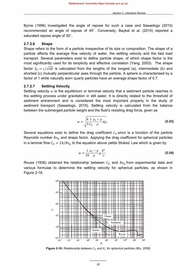
Section 2. Literature Review
28
Byrne (1996) investigated the angle of repose for such a case and Sawadogo (2015) recommended an angle of repose of 45°. Conversely, Baykal et al. (2015) reported a saturated repose angle of 30°.
2.7.2.6 Shape Shape refers to the form of a particle irrespective of its size or composition. The shape of a particle affects the average flow velocity of water, the settling velocity and the bed load transport. Several parameters exist to define particle shape, of which shape factor is the most significantly used for its simplicity and effective correlation (Yang, 2003). The shape factor 𝑆𝑆𝑃𝑃 = 𝑐𝑐 √𝑎𝑎𝑏𝑏⁄ is calculated from the lengths of the longest (a), intermediate (b) and shortest (c) mutually perpendicular axes through the particle. A sphere is characterised by a factor of 1 while naturally worn quartz particles have an average shape factor of 0.7.
2.7.2.7 Settling Velocity Settling velocity 𝑤𝑤 is the equilibrium or terminal velocity that a sediment particle reaches in the settling process under gravitation in still water. It is directly related to the threshold of sediment entrainment and is considered the most important property in the study of sediment transport (Sawadogo, 2015). Settling velocity is calculated from the balance between the submerged particle weight and the fluid’s resisting drag force, given as
Several equations exist to define the drag coefficient 𝐶𝐶𝐷𝐷 which is a function of the particle Reynolds number 𝑅𝑅𝑅𝑅𝑝𝑝 and shape factor. Applying the drag coefficient for spherical particles in a laminar flow 𝐶𝐶𝐷𝐷 = 24/𝑅𝑅𝑅𝑅𝑝𝑝 to the equation above yields Stokes’ Law which is given by
Rouse (1936) obtained the relationship between 𝐶𝐶𝐷𝐷 and 𝑅𝑅𝑅𝑅𝑝𝑝 from experimental data and various formulas to determine the settling velocity for spherical particles, as shown in Figure 2-16.
Figure 2-16: Relationship between 𝐶𝐶𝐷𝐷 and 𝑅𝑅𝑑𝑑 for spherical particles (Wu, 2008)
𝑤𝑤 = 43
1𝐶𝐶𝐷𝐷
𝜌𝜌𝑠𝑠 − 𝜌𝜌𝜌𝜌
𝑑𝑑𝑔𝑔 . (2-23)
𝑤𝑤 =1
18𝜌𝜌𝑠𝑠 − 𝜌𝜌𝜌𝜌
𝑔𝑔𝑑𝑑2
υ . (2-24)
Stellenbosch University https://scholar.sun.ac.za
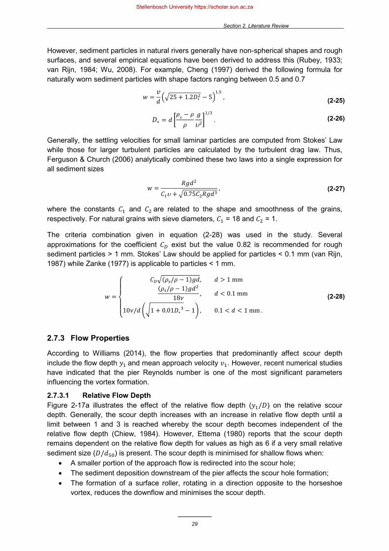
Section 2. Literature Review
29
However, sediment particles in natural rivers generally have non-spherical shapes and rough surfaces, and several empirical equations have been derived to address this (Rubey, 1933; van Rijn, 1984; Wu, 2008). For example, Cheng (1997) derived the following formula for naturally worn sediment particles with shape factors ranging between 0.5 and 0.7
Generally, the settling velocities for small laminar particles are computed from Stokes’ Law while those for larger turbulent particles are calculated by the turbulent drag law. Thus, Ferguson & Church (2006) analytically combined these two laws into a single expression for all sediment sizes
where the constants 𝐶𝐶1 and 𝐶𝐶2 are related to the shape and smoothness of the grains, respectively. For natural grains with sieve diameters, 𝐶𝐶1 = 18 and 𝐶𝐶2 = 1.
The criteria combination given in equation (2-28) was used in the study. Several approximations for the coefficient 𝐶𝐶𝐷𝐷 exist but the value 0.82 is recommended for rough sediment particles > 1 mm. Stokes’ Law should be applied for particles < 0.1 mm (van Rijn, 1987) while Zanke (1977) is applicable to particles < 1 mm.
2.7.3 Flow Properties
According to Williams (2014), the flow properties that predominantly affect scour depth include the flow depth 𝑦𝑦1 and mean approach velocity 𝑣𝑣1. However, recent numerical studies have indicated that the pier Reynolds number is one of the most significant parameters influencing the vortex formation.
2.7.3.1 Relative Flow Depth Figure 2-17a illustrates the effect of the relative flow depth (𝑦𝑦1/𝐷𝐷) on the relative scour depth. Generally, the scour depth increases with an increase in relative flow depth until a limit between 1 and 3 is reached whereby the scour depth becomes independent of the relative flow depth (Chiew, 1984). However, Ettema (1980) reports that the scour depth remains dependent on the relative flow depth for values as high as 6 if a very small relative sediment size (𝐷𝐷/𝑑𝑑50) is present. The scour depth is minimised for shallow flows when:
• A smaller portion of the approach flow is redirected into the scour hole; • The sediment deposition downstream of the pier affects the scour hole formation; • The formation of a surface roller, rotating in a direction opposite to the horseshoe
vortex, reduces the downflow and minimises the scour depth.
𝑤𝑤 =𝑣𝑣𝑑𝑑25 + 1.2𝐷𝐷∗2 − 5
1.5 ,
𝐷𝐷∗ = 𝑑𝑑 𝜌𝜌𝑠𝑠 − 𝜌𝜌𝜌𝜌
𝑔𝑔υ2
1/3 .
(2-25)
(2-26)
𝑤𝑤 =𝑅𝑅𝑔𝑔𝑑𝑑2
𝐶𝐶1υ + 0.75𝐶𝐶2𝑅𝑅𝑔𝑔𝑑𝑑3 , (2-27)
𝑤𝑤 =
⎩⎪⎨
⎪⎧ 𝐶𝐶𝐷𝐷(𝜌𝜌𝑠𝑠/𝜌𝜌 − 1)𝑔𝑔𝑑𝑑, 𝑑𝑑 > 1 mm
(𝜌𝜌𝑠𝑠/𝜌𝜌 − 1)𝑔𝑔𝑑𝑑2
18𝜈𝜈, 𝑑𝑑 < 0.1 mm
10𝜈𝜈/𝑑𝑑 1 + 0.01𝐷𝐷∗3 − 1 , 0.1 < 𝑑𝑑 < 1 mm .
(2-28)
Stellenbosch University https://scholar.sun.ac.za

Section 2. Literature Review
30
Note that once the flow depth is greatly escalated by a flood that submerges a bridge, pressure flow (or orifice flow) results which greatly increases the scour potential by 200 to 300% compared to free surface flow (Richardson & Davis, 2001). Pressure flow scour is classified as vertical contraction scour that is additional to the conventional local pier scour component.
2.7.3.2 Mean Approach Velocity The undisturbed approach flow velocity has the direct effect of strengthening the vortices and increasing the local scour depth. Figure 2-17b illustrates that the relative scour depth (𝑑𝑑𝑠𝑠/𝐷𝐷) almost increases linearly with the relative velocity ratio or flow intensity (𝑣𝑣1/𝑣𝑣𝑐𝑐) under clear-water scouring. Interestingly, there is a dispute in literature as to whether the no scour condition exists for the flow intensity 𝑣𝑣1/𝑣𝑣𝑐𝑐 < ~0.5 (Johnson, 1995).
Figure 2-17: (a) The effect of relative flow depth on relative scour depth (b) The effect of relative velocity on relative scour depth (Ettema, 1980)
2.7.3.3 Turbulence A distinction should be made between 𝑅𝑅𝑅𝑅 and 𝑅𝑅𝑅𝑅𝐷𝐷 whereby 𝑅𝑅𝑅𝑅𝐷𝐷 describes the turbulence induced by the pier diameter 𝐷𝐷 and not by the channel dimensions or flow depth. The pier Reynolds number is a useful parameter because it describes the combined effect of the pier size and approach velocity on the vortex formation and scour depth. Furthermore, the relative boundary layer thickness δ/𝐷𝐷 may be used to describe the size of the horseshoe vortex. A stronger and larger vortex causes the boundary layer to move upstream and to scour a larger hole. For small values of δ/𝐷𝐷, the boundary layer may not separate and no horseshoe vortex would form (Sumer & Fredsøe, 2002).
The structure, location, size and intensity of the horseshoe vortex system with time are highly affected by the characteristics of the approaching boundary layer and by the pier Reynolds number (Constandinescu & Koken, 2005). Roulund et al. (2005) observed that a critical pier Reynolds number 𝑅𝑅𝑅𝑅𝑐𝑐 exists, corresponding to a certain relative flow depth, whereby the primary oscillations in the horseshoe vortex first emerge. This number defines a laminar boundary layer for 𝑅𝑅𝑅𝑅𝐷𝐷 < 𝑅𝑅𝑅𝑅𝑐𝑐 and a turbulent boundary layer for 𝑅𝑅𝑅𝑅𝐷𝐷 > 𝑅𝑅𝑅𝑅𝑐𝑐. Figure 2-18 shows that the size of the horseshoe vortex as well as the subsequent bed shear stresses decrease with an increasing pier Reynolds number, while the converse is true for laminar flow.
Stellenbosch University https://scholar.sun.ac.za
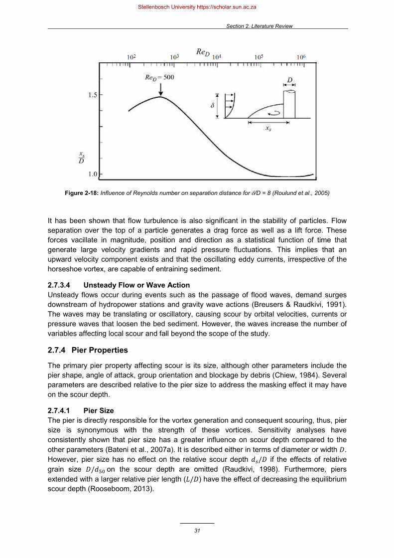
Section 2. Literature Review
31
Figure 2-18: Influence of Reynolds number on separation distance for δ/D = 8 (Roulund et al., 2005)
It has been shown that flow turbulence is also significant in the stability of particles. Flow separation over the top of a particle generates a drag force as well as a lift force. These forces vacillate in magnitude, position and direction as a statistical function of time that generate large velocity gradients and rapid pressure fluctuations. This implies that an upward velocity component exists and that the oscillating eddy currents, irrespective of the horseshoe vortex, are capable of entraining sediment.
2.7.3.4 Unsteady Flow or Wave Action Unsteady flows occur during events such as the passage of flood waves, demand surges downstream of hydropower stations and gravity wave actions (Breusers & Raudkivi, 1991). The waves may be translating or oscillatory, causing scour by orbital velocities, currents or pressure waves that loosen the bed sediment. However, the waves increase the number of variables affecting local scour and fall beyond the scope of the study.
2.7.4 Pier Properties
The primary pier property affecting scour is its size, although other parameters include the pier shape, angle of attack, group orientation and blockage by debris (Chiew, 1984). Several parameters are described relative to the pier size to address the masking effect it may have on the scour depth.
2.7.4.1 Pier Size The pier is directly responsible for the vortex generation and consequent scouring, thus, pier size is synonymous with the strength of these vortices. Sensitivity analyses have consistently shown that pier size has a greater influence on scour depth compared to the other parameters (Bateni et al., 2007a). It is described either in terms of diameter or width 𝐷𝐷. However, pier size has no effect on the relative scour depth 𝑑𝑑𝑠𝑠/𝐷𝐷 if the effects of relative grain size 𝐷𝐷/𝑑𝑑50 on the scour depth are omitted (Raudkivi, 1998). Furthermore, piers extended with a larger relative pier length (𝐿𝐿/𝐷𝐷) have the effect of decreasing the equilibrium scour depth (Rooseboom, 2013).
Stellenbosch University https://scholar.sun.ac.za

Section 2. Literature Review
32
2.7.4.2 Pier Shape The pier geometry also has a direct effect on the strength of the vortices and the shape of the nose can influence up to 20% of the total pier scour depth (Arneson et al., 2012). A stronger vortex (or pressure gradient) causes the boundary layer to move upstream and to scour a larger hole. As illustrated in Figure 2-19, blunt nosed piers produce relatively stronger vortices compared to streamlined piers. In fact, practically no vorticity is generated at the nose of a sharp nosed pier (Tseng et al., 2000).
Figure 2-19: Shear stress amplification for (a) streamlined and (b) blunt nosed pier (Tseng et al., 2000)
Figure 2-20 shows the commonly used pier shapes, including some of the more complex ones. The case of a single cylindrical pier has principally been investigated and is commonly used as a reference to other cases by employing shape factors (Hoffmans & Verhij, 1997). However, there is a dispute in literature as to whether pier shape has a significant impact on the local scour depth (Brandimarte et al., 2012; Mueller & Wagner, 2005) particularly in the field where pier shapes vary with depth and are concealed by submerged debris.
Figure 2-20: Commonly used pier shapes
Rectangular
Round Nosed
Sharp Nosed
Lenticular
Cylindrical
Group of Cylinders
Jakowski Profile
Elevation of Pile Cap
Flow direction
Stellenbosch University https://scholar.sun.ac.za

Section 2. Literature Review
33
2.7.4.3 Alignment and Angle of Attack Skewed flow approaching at an angle of up to 90° has the ability to dramatically amplify the depth of a scour hole. The effect of the angle of attack of flow can further be magnified by a large relative pier length, defined as the ratio of the pier length and width (𝐿𝐿/𝐷𝐷). This is best demonstrated in Figure 2-21 whereby alignment factors, used in empirical equations, can describe the effect of skewed flow on bridge pier scour because they are directly proportional (𝐾𝐾𝛼𝛼 ∝ 𝑑𝑑𝑠𝑠).
Figure 2-21: Alignment factors for piers not aligned with flow (Melville & Sutherland, 1988)
2.7.4.4 Group Orientation and Spacing Extensive information is available on the local scour process at a single isolated pier; however, limited research has been completed with a focus on piers constructed in close proximity. According to Hoffmans & Verheij (1997), two piers in line parallel with the flow have the effect of increasing the scour depth at the front pier up to 15% for a spacing less than three times the pier diameter 𝐷𝐷, and decreasing the scour depth at the back pier up to 20%. Furthermore, these effects disappear if the pier spacing is greater than 15𝐷𝐷.
Beg (2010) investigated the effect of placing two piers in a direction transverse to the flow and established that a complex interaction in the flow profiles generated a very different scour process. The lateral spacing between the two piers affects (1) the interaction between the horseshoe vortices, and (2) the accelerated flow caused by contraction (Elliott & Baker, 1985). A closer lateral arrangement of piers causes compressed horseshoe vortices to generate increased velocities and scour depths. Beg (2010) observed that both piers scoured to the same depth. Furthermore, contraction scour occurs owing to the sudden decrease in the flow width. The outcome is an increased scour depth (Rooseboom, 2013) although researchers cannot distinguish between the individual contributions of each process in the case of laterally spaced piers.
Figure 2-22 illustrates the effect of the relative lateral pier spacing on the relative scour depth. A 95% increase is observed for two adjacent piers with no lateral spacing which is in agreement with scouring affected by the combined width of the piers. As the spacing increases, the compression effect of the horseshoe vortex is diminished until a relative lateral pier spacing of 8 is reached whereby the two piers scour individually.
Stellenbosch University https://scholar.sun.ac.za

Section 2. Literature Review
34
Figure 2-22: Effect of relative lateral pier spacing on relative scour depth (Beg, 2010)
2.7.4.5 Debris Accumulation Waterborne debris, such as tree branches and ice, often accumulate in front of bridges during floods. The debris can potentially increase the effective pier width and length, change the shape or cause the flow to plunge downward onto the riverbed. The effect is that the local scour depth may increase. Furthermore, contraction scour could result if the debris constricts the flow. This effect is highly variable and still undetermined, despite equations attempting to predict and quantify blockage as a constriction or an increase in width, based on an idealized rectangular or triangular debris shape and size. The greatest amount of pier scour occurs when the debris floats at the surface of a flood with a length in the flow direction upstream of the pier that is equal to the approach flow depth.
2.7.5 Time to Reach Equilibrium Scour
Local scour is a time dependent process whereby equilibrium between the flow’s erosive ability and the sediment’s resistance to motion is progressively achieved. As the scour hole grows, the velocity component near the bed gradually decreases. Once the bed shear stresses fall below the critical shear stress required to initiate scour, an equilibrium scour hole is formed (Roulund et al., 2005). This scour process can be divided into the initial, development, stabilisation and equilibrium phases (Hoffmans & Verheij, 1997). Figure 2-23a shows that clear-water scour equilibrium is achieved much slower than for live-bed scouring. Furthermore, the clear-water scour equilibrium is approached asymptotically while the live-bed scour equilibrium oscillates as the bed features move through the scour hole as backfill (Chiew, 1984). The equilibrium scour depth in live-bed scouring is achieved once the sediment supply equals the outflow in the scour hole (Baker, 1980b).
Melville & Chiew (1999) proposed the chart in Figure 2-23b to estimate the time required for equilibrium scour, as a function of flow intensity. While they believe that the equilibrium depth takes several days or months to develop, some researchers such as Breusers et al. (1977) claim that the time to reach equilibrium depth may be infinite. However, flood peaks often do not last long enough to develop an equilibrium scour depth (Mia & Nago, 2003) and it is impractical to run an experiment for several days. Therefore, it is important to model a smaller scour depth to a known time-to-peak value for a design flood rather than the equilibrium scour depth.
Stellenbosch University https://scholar.sun.ac.za

Section 2. Literature Review
35
Figure 2-23: (a) Scour depth versus time for live-bed and clear-water scouring (Chiew, 1984)
(b) Design chart to estimate time required to reach equilibrium scour depth (Melville & Chiew, 1999)
It is well known that scour development is rapid in the beginning; 50-80% of the equilibrium scour depth develops within 10% of the time required for equilibrium (Melville & Chiew, 1999). Thus, it is justifiable to measure scour once the rate of increase does not exceed a certain percentage, relative to the bridge pier size. For example, Melville (1975) observed that the scour hole was almost fully developed after only 2.5 hours in the laboratory. Xiong et al. (2014) used this to justify their 30 minute simulation of the scour hole. Figure 2-24a illustrates that the scour hole stabilized after 2 hours in the laboratory and after 10 minutes in the numerical simulation by Roulund et al. (2005). Figure 2-24b shows that 90% of the maximum scour depth was reached after 2 hours in Mohamed et al.’s (2013) experiment.
Figure 2-24: Development of relative scour depth with time by (a) Roulund et al. (2005) and
(b) Mohamed et al. (2013)
2.8 Predicting the Equilibrium Bridge Pier Scour Depth
An overwhelming amount of research has been conducted on bridge pier scouring since the 1950s. Comprehensive reviews of the subject can be found in Breusers at al. (1977), Ettema (1980), Raudkivi & Ettema (1983), Raudkivi (1986), Melville & Sutherland (1988), Melville (1988), Breusers & Raudkivi (1991), Richardson & Davis (1995), Melville (1997), Dey (1997), Hoffmans & Verheij (1997), Raudkivi (1998), Melville & Coleman (2002), Sumer & Fredsøe (2002), and the list continues. The long list of researchers clearly indicates the significance of scouring problems.
Hours
Numerical simulation
Stellenbosch University https://scholar.sun.ac.za

Section 2. Literature Review
36
The studies attempt to better understand the turbulent flow field, to capture the important scouring parameters and to develop improved scour prediction models. Until the 1990s, most of the work on bridge pier scour was based on physical modelling in the laboratory followed by empirical modelling. However, the focus of the work has slowly shifted towards numerical modelling on computers owing to the recent technological advancements.
In spite of the extensive research into bridge pier scouring, a unifying theory for the prediction of equilibrium scour depth at piers is still in an embryonic stage.
2.8.1 Empirical Equations
Most scour depth equations traditionally used in bridge designs have been developed on the basis of experimentation, dimensional analyses and simplified theoretical models (Chadwick, 2013). The equations have been derived by assuming dominant parameters, reducing them to simplified relationships and then calibrating them by means of a coefficient from laboratory and field data. Of all the relationships developed to date, Appendix A lists 30 of the better known prediction formulas for clear-water bridge pier scour in an alluvial bed. Only equations which are dimensionally correct and in SI units are presented.
In short, the formulas describe the resulting equilibrium scour depth 𝑑𝑑𝑠𝑠 as a function of a combination of one or more of the following parameters:
𝜌𝜌 = Fluid density 𝜌𝜌𝑠𝑠 = Sediment density 𝑠𝑠 = Relative density υ = Kinematic viscosity 𝑡𝑡 = Time 𝐷𝐷 = Pier diameter or width 𝐿𝐿 = Pier length 𝑑𝑑 = Median sediment size 𝜎𝜎𝑔𝑔 = Particle size distribution 𝐵𝐵 = Channel width
𝑆𝑆 = Energy slope 𝑣𝑣1 = Approach flow velocity 𝑦𝑦1 = Approach flow depth 𝑔𝑔 = Gravitational acceleration 𝑣𝑣𝑐𝑐 = Sediment critical velocity 𝐶𝐶𝑡𝑡∗ = Shear velocity threshold 𝑅𝑅𝑅𝑅 = Reynolds number 𝐹𝐹𝐹𝐹 = Froude number 𝛼𝛼 = Angle of flow in radians 𝐾𝐾𝑠𝑠 = Shape factor
Some interesting remarks on the given equations are briefly discussed:
• The simplest expression is that of Breuers (1965) which assumes that the maximum bridge pier scour can be estimated as 1.4 times the pier size.
• Pier size is by far the most predominant parameter appearing in all the formulas except Chitale (1962) which is based on the Froude number. The HEC-18 equations also depend on the Froude number, which describes the gravity effect at the free water surface, thus it is only valid for low flow depths (Guo, 2012).
• Simplified expressions have been proposed to represent debris accumulation and complex pier geometries in terms of a single equivalent or effective pier width to allow them to be incorporated into equations such as Melville & Coleman (2000) and Amini et al. (2011). Arneson et al. (2012) recommends that complex pier configurations are divided into three substructural elements namely the pier stem, pile cap / footing and pile group, and that the scour for each component that obstructs flow is superimposed. While this falls beyond the scope of the study, it has potential for further investigation in numerical modelling.
Stellenbosch University https://scholar.sun.ac.za
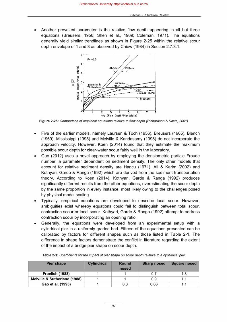
Section 2. Literature Review
37
• Another prevalent parameter is the relative flow depth appearing in all but three equations (Breusers, 1956; Shen et al., 1969; Coleman, 1971). The equations generally yield similar trendlines as shown in Figure 2-25 within the relative scour depth envelope of 1 and 3 as observed by Chiew (1984) in Section 2.7.3.1.
Figure 2-25: Comparison of empirical equations relative to flow depth (Richardson & Davis, 2001)
• Five of the earlier models, namely Laursen & Toch (1956), Breusers (1965), Blench
(1969), Mississippi (1995) and Melville & Kandasamy (1998) do not incorporate the approach velocity. However, Koen (2014) found that they estimate the maximum possible scour depth for clear-water scour fairly well in the laboratory.
• Guo (2012) uses a novel approach by employing the densiometric particle Froude number, a parameter dependent on sediment density. The only other models that account for relative sediment density are Hancu (1971), Ali & Karim (2002) and Kothyari, Garde & Ranga (1992) which are derived from the sediment transportation theory. According to Koen (2014), Kothyari, Garde & Ranga (1992) produces significantly different results from the other equations, overestimating the scour depth by the same proportion in every instance, most likely owing to the challenges posed by physical model scaling.
• Typically, empirical equations are developed to describe local scour. However, ambiguities exist whereby equations could fail to distinguish between total scour, contraction scour or local scour. Kothyari, Garde & Ranga (1992) attempt to address contraction scour by incorporating an opening ratio.
• Generally, the equations were developed from an experimental setup with a cylindrical pier in a uniformly graded bed. Fifteen of the equations presented can be calibrated by factors for different shapes such as those listed in Table 2-1. The difference in shape factors demonstrate the conflict in literature regarding the extent of the impact of a bridge pier shape on scour depth.
Table 2-1: Coefficients for the impact of pier shape on scour depth relative to a cylindrical pier
Pier shape Cylindrical Round nosed
Sharp nosed Square nosed
Froelich (1988) 1 1 0.7 1.3 Melville & Sutherland (1988) 1 1 0.9 1.1
Gao et al. (1993) 1 0.8 0.66 1.1
Stellenbosch University https://scholar.sun.ac.za
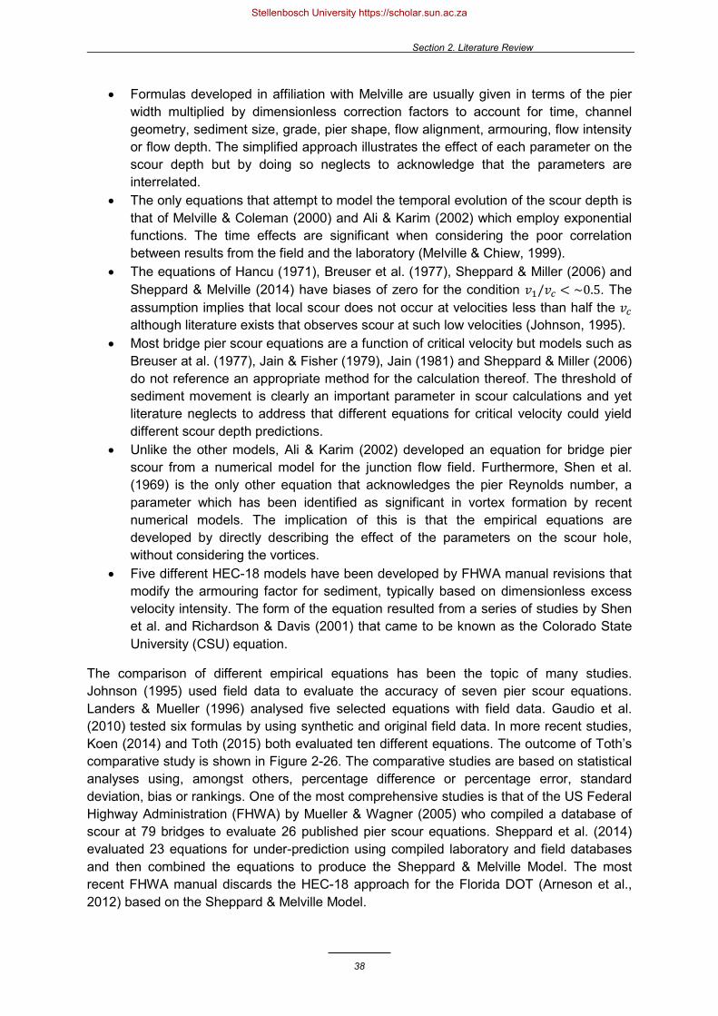
Section 2. Literature Review
38
• Formulas developed in affiliation with Melville are usually given in terms of the pier width multiplied by dimensionless correction factors to account for time, channel geometry, sediment size, grade, pier shape, flow alignment, armouring, flow intensity or flow depth. The simplified approach illustrates the effect of each parameter on the scour depth but by doing so neglects to acknowledge that the parameters are interrelated.
• The only equations that attempt to model the temporal evolution of the scour depth is that of Melville & Coleman (2000) and Ali & Karim (2002) which employ exponential functions. The time effects are significant when considering the poor correlation between results from the field and the laboratory (Melville & Chiew, 1999).
• The equations of Hancu (1971), Breuser et al. (1977), Sheppard & Miller (2006) and Sheppard & Melville (2014) have biases of zero for the condition 𝑣𝑣1/𝑣𝑣𝑐𝑐 < ~0.5. The assumption implies that local scour does not occur at velocities less than half the 𝑣𝑣𝑐𝑐 although literature exists that observes scour at such low velocities (Johnson, 1995).
• Most bridge pier scour equations are a function of critical velocity but models such as Breuser at al. (1977), Jain & Fisher (1979), Jain (1981) and Sheppard & Miller (2006) do not reference an appropriate method for the calculation thereof. The threshold of sediment movement is clearly an important parameter in scour calculations and yet literature neglects to address that different equations for critical velocity could yield different scour depth predictions.
• Unlike the other models, Ali & Karim (2002) developed an equation for bridge pier scour from a numerical model for the junction flow field. Furthermore, Shen et al. (1969) is the only other equation that acknowledges the pier Reynolds number, a parameter which has been identified as significant in vortex formation by recent numerical models. The implication of this is that the empirical equations are developed by directly describing the effect of the parameters on the scour hole, without considering the vortices.
• Five different HEC-18 models have been developed by FHWA manual revisions that modify the armouring factor for sediment, typically based on dimensionless excess velocity intensity. The form of the equation resulted from a series of studies by Shen et al. and Richardson & Davis (2001) that came to be known as the Colorado State University (CSU) equation.
The comparison of different empirical equations has been the topic of many studies. Johnson (1995) used field data to evaluate the accuracy of seven pier scour equations. Landers & Mueller (1996) analysed five selected equations with field data. Gaudio et al. (2010) tested six formulas by using synthetic and original field data. In more recent studies, Koen (2014) and Toth (2015) both evaluated ten different equations. The outcome of Toth’s comparative study is shown in Figure 2-26. The comparative studies are based on statistical analyses using, amongst others, percentage difference or percentage error, standard deviation, bias or rankings. One of the most comprehensive studies is that of the US Federal Highway Administration (FHWA) by Mueller & Wagner (2005) who compiled a database of scour at 79 bridges to evaluate 26 published pier scour equations. Sheppard et al. (2014) evaluated 23 equations for under-prediction using compiled laboratory and field databases and then combined the equations to produce the Sheppard & Melville Model. The most recent FHWA manual discards the HEC-18 approach for the Florida DOT (Arneson et al., 2012) based on the Sheppard & Melville Model.
Stellenbosch University https://scholar.sun.ac.za

Section 2. Literature Review
39
Figure 2-26: Boxplot representing the distribution of scour depth prediction errors over a test set for different
empirical equations (Toth, 2015)
Throughout the research, the following conclusions are recurring:
• Different formulas produce significantly different predictions from the field. • Furthermore, they are in weak agreement with one another. The equations are not
universal and only yield good results under conditions similar to those from which they were derived.
• Most of the equations overestimate observed scour depths and may perform better in conservative designs. However, this may lead to uneconomical designs of unnecessarily expensive foundations or countermeasures.
• On the other hand, some of the formulas are not fit for pier design due to underpredictions, for example Froelich (1988). As a result, the Froelich Design equation came about, which adds the upstream flow depth to the predicted scour depth as a precautionary.
• No single equation is conclusively superior. Ranking the performance of equations is difficult due to the tradeoff between accuracy and underpredictions.
• Nevertheless, the HEC-18 design equations are commonly favoured for results that most closely resemble the field and rarely underpredict, as illustrated in Figure 2-26. Interestingly, the Shen et al. (1969) model, which relies on the pier Reynolds number, also performed well.
• Further research and improved prediction models are recommended.
2.8.2 Machine Learning and Artificial Neural Networks
In recent years a different approach towards empirical equations has been developed: the application of Artificial Neural Networks (ANNs) to estimate bridge pier scour (Firat & Gungor, 2009). ANNs are predictive mathematical models inspired by biological neural networks (i.e. the brain), which are used to approximate functions that depend on several unknown variables. ANNs have been applied to many other branches of science. Examples in the field of water engineering include the prediction of rainfall intensity, river floods, tides and earthquake induced liquefaction (Lee et al., 2007).
Overprediction
Underprediction
Stellenbosch University https://scholar.sun.ac.za
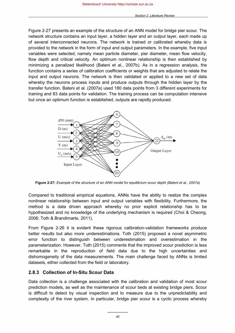
Section 2. Literature Review
40
Figure 2-27 presents an example of the structure of an ANN model for bridge pier scour. The network structure contains an input layer, a hidden layer and an output layer, each made up of several interconnected neurons. The network is trained or calibrated whereby data is provided to the network in the form of input and output parameters. In the example, five input variables were selected, namely mean particle diameter, pier diameter, mean flow velocity, flow depth and critical velocity. An optimum nonlinear relationship is then established by minimizing a penalized likelihood (Bateni et al., 2007b). As in a regression analysis, the function contains a series of calibration coefficients or weights that are adjusted to relate the input and output neurons. The network is then validated or applied to a new set of data whereby the neurons process inputs and produce outputs through the hidden layer by the transfer function. Bateni et al. (2007a) used 180 data points from 3 different experiments for training and 83 data points for validation. The training process can be computation intensive but once an optimum function is established, outputs are rapidly produced.
Figure 2-27: Example of the structure of an ANN model for equilibrium scour depth (Bateni et al., 2007a)
Compared to traditional empirical equations, ANNs have the ability to realize the complex nonlinear relationship between input and output variables with flexibility. Furthermore, the method is a data driven approach whereby no prior explicit relationship has to be hypothesized and no knowledge of the underlying mechanism is required (Choi & Cheong, 2006; Toth & Brandimarte, 2011).
From Figure 2-26 it is evident these rigorous calibration-validation frameworks produce better results but also more underestimations. Toth (2015) proposed a novel asymmetric error function to distinguish between underestimation and overestimation in the parameterization. However, Toth (2015) comments that the improved scour prediction is less remarkable in the reproduction of field data due to the high uncertainties and dishomogeneity of the data measurements. The main challenge faced by ANNs is limited datasets, either collected from the field or laboratory.
2.8.3 Collection of In-Situ Scour Data
Data collection is a challenge associated with the calibration and validation of most scour prediction models, as well as the maintenance of scour beds at existing bridge piers. Scour is difficult to detect by visual inspection and to measure due to the unpredictability and complexity of the river system. In particular, bridge pier scour is a cyclic process whereby
Stellenbosch University https://scholar.sun.ac.za

Section 2. Literature Review
41
erosion and backfilling occur several times during the life of a structure and during the hydrograph of a flood event. The measurement of real time scour (particularly in the case of live-bed scour) is necessary to capture the maximum scour depth. Different methods for scour measurement are summarized.
Direct scour measurement: • The simplest direct method of scour measurement is by a steel rod manned from a
boat or a fixed steel sliding ring that captures the difference in depth mechanically by a rod that drops inside a PVC pipe. While the method is quick, easy and affordable, it is only applicable to piers without aprons or armouring in wadable rivers.
• Topographic mapping of cross-sections upstream and downstream of bridges can be done by surveying equipment, such as a total station, but the method is limited by the calibration precision of the instruments and accessibility to the submerged riverbed.
• Discharge survey methods involve a current meter mounted to a crane that is lowered during floods to profile the riverbed sub-bottom in discrete locations while measuring depth-integrated discharge. Inspection by diving is dangerous especially during floods, requires clear waters and is only considered semi-quantitate (Brandimarte et al., 2012).
• Drilling the riverbed is an expensive but standard technique that allows vertical profiles of sub-bottom filling materials to be captured if the log sample is undisturbed. The selection of the drilling location is imperative and a large floating platform is required.
Indirect scour measurement: • Expensive geophysical (indirect) technologies are capable of overcoming the
shortcomings associated with direct scour inspections, particularly because they do not interfere with the scour process. The most common methods use electromagnetic impulses with radar, acoustic/sonar or elastic (seismic) wave frequencies. The instruments require careful calibration by skilled personal. They require a strong differential wave conductivity between the water and sediment bed, cannot be used in shallow waters with high salinity or turbidity, and they could be affected by the flow disturbances due to the pier.
• Examples of indirect scour measurement include: o Acoustic Doppler Velocimeter (ADV) and Acoustic Doppler Current Profiler
(ADCP) o Fathometer/echosounder o Ground Penetrating Radar (GPR) and Continuous Seismic Reflection Profiling
(CSRP) are the most reliable sub-bottom profiling methods capable of generating 3D images for flow depths of up to 10 m with CSRP even capable of profiling bedrock.
One of the most comprehensive databases of scour at bridges was measured and compiled by the US Geological Survey and the FHWA (Mueller & Wagner, 2005). The Bridge Scour Data Management Systems (BSDMS) has a collection of 493 local pier scour measurements sampled over six years at 79 sites across 17 states. An array of measuring techniques was used to generate cross-sections upstream and downstream of the bridge piers, including discharge surveys and echo-sounding by ADCPs.
Stellenbosch University https://scholar.sun.ac.za

Section 2. Literature Review
42
While laboratory derived equations oversimplify or ignore complexities in the field, the process of in-situ scour data collection at existing bridge piers is a possible source of error propagating through scour prediction models calibrated against field data. Brandimarte et al. (2006) attempt to quantify the uncertainty or evaluate risk associated with bridge pier scour in a cohesive riverbed by applying a stochastic model with a Monte Carlo probabilistic procedure, commonly used in hydrological studies. The different sources of uncertainty in scour measurement can be classified as: 1. Observation uncertainty related to the approximation of hydraulic variables such as flow
regime and time to reach equilibrium scour. 2. Parameter uncertainty related to the imperfect parameterization of prediction methods
such as pier shape and sediment material. 3. Structural uncertainty caused by the inability of prediction models to schematize
physical processes, which is typically addressed by using safety factors. 4. Aleatory uncertainty caused by natural variability and randomness. 5. Epistemic uncertainty caused by an incomplete knowledge or understanding.
2.8.4 Physical Modelling and Scale Effects
According to Breusers & Raudkivi (1991), field data on bridge pier scour is difficult to collect and rare. Thus, most bridge pier scour studies are furnished with extensive laboratory experiments, particularly for physical model studies of costly and complex bridge developments. While it may be preferable to calibrate models with field data, such as those from Breusers et al. (1977) and Melville (1975), small scale laboratory studies allow control over the masking effects of interrelated parameters. This offers determination not only of the scour hole but also visualisation of the flow field by measurement of pressure, velocity, turbulence and bed shear stress.
In order to obtain flow visualizations of the horseshoe vortex system, Baker (1980a) conducted experiments with smoke and oil, Dargahi (1989) used hydrogen-bubbles and hot film anemometry while Chen et al. (2000) used dye. According to Ali & Karim (2002), not all relevant quantities can be measured in a physical model, such as the vorticity. Salaheldin et al. (2004) claim that local velocities are difficult to determine in experimental studies owing to the strong circulation. Nevertheless, with recent advances in flow visualisation techniques supplemented by numerical modelling, measurement of such quantities is coming into reach. The Acoustic Doppler Velocimeter (ADV) and Digital Particle Image Velocimetry (DPIV) have dramatically bettered the understanding of the intricate vortex structure, as demonstrated by Figure 2-28.
Figure 2-28: DPIV generated images showing time-averaged streamwise velocity for different Reynolds numbers
(Apsilidis et al., 2010)
Stellenbosch University https://scholar.sun.ac.za
Section 2. Literature Review
43
One of the main challenges associated with scaled laboratory tests is translating the scour depth, established in the laboratory, to prototype field depths. These scaled predictions often overestimate the actual scour field depths (Lee & Sturm, 2009). To address this problem, kinematic and dynamic similarity must be present between the model and field prototype (Williams, 2014). Sediment transport problems are normally modelled by applying Froude similarity and the median grain size is scaled according to the Shields criterion (Heller, 2011). This may result in a very small model sediment size that exhibits cohesive interparticle forces not present in sand bed rivers (Lee & Sturm, 2009). According to the FHWA (Arneson et al., 2012), it is not possible to scale the bed material size and that bed material with a critical velocity just less than the model velocity could be tested. Heller (2011) recommends that the sediment density should be reduced and that a larger grain diameter should be employed to reach the same flow–sediment interaction behaviour.
2.8.5 The Transition towards Numerical Models
Presently available equations, such as those listed in Appendix A, produce a wide range of varying results for the same case, even under controlled laboratory conditions (Johnson, 1995; Olsen & Kjellesvig, 1998; Rooseboom, 2013). And although extensive research has been conducted on bridge pier scour for more than six decades, there is still no universally agreed upon accurate design procedure that can predict the scour depth. This is because traditional methods of estimating the maximum depth of scour near bridge piers rely on simplistic formulas, each with its own assumptions and limitations, which often yield unreliable results (Richardson & Panchang, 1998; Landers & Mueller, 1996).
Evidently, the scouring process at the river bed interface is complex and affected by numerous interrelated parameters (Chadwick, 2013). According to the Rooseboom (2013), the complexity of bridge pier scour can be attributed to the following factors:
• Nonhomogeneous mixture of sediment and water; • Three-dimensional flow patterns at bridges during floods; • Difficulties in determining the actual geometrical properties of rivers during floods; • Difficulties in observing actual sour depths and processes; and • Highly variable properties of in-situ bed materials.
Furthermore, the complexity of the 3D flow field separation and multiple vortices is amplified by the dynamic interaction between the flow and movable bed. The flow field initiates and controls the progress of the scour pattern, which in turn alters the flow profile by continuous interaction (Raudkivi, 1986). While the simplicity of conservative empirical equations may be appealing, overestimating the anticipated scour depth leads to uneconomical designs with unnecessarily expensive foundations and countermeasures.
Various attempts have been made to address the complexity by assuming dominant variables and reducing them to simplified relationships to describe scour. However, it is difficult to generalize the scour process because there are so many variables that may conceal the influence of one another on scouring. Furthermore, simplifying assumptions are required to quantify the three-dimensional flow patterns, complicated vortex and turbulence structures. These limit the extent to which a mathematical analysis can be made to model scour (Chiew, 1984; Tseng, 2000; Guo, 2012). When faced with such uncertainty in bridge design, hydraulic engineers are compelled to pursue costly, labour intensive and time consuming physical model studies, with their own flow visualisation and scaling challenges
Stellenbosch University https://scholar.sun.ac.za

Section 2. Literature Review
44
(Xiong et al., 2014). Most sediment studies are still based on empirical formulas derived and calibrated by means of a coefficient from small scale laboratory experiments, and occasionally field data, despite the availability of sophisticated computers. More weight should be attached to relationships that are fundamentally sound and based on first principles, which computer software is capable of solving (Olsen & Malaaen, 1993; Dey, 1996). A recently studied alternative is the use of 3D numerical models to better predict equilibrium scour depth.
Numerical solutions by Computation Fluid Dynamics (CFD) are becoming increasingly popular to compute fluid flow as technology advances and the cost of computational time decreases. According to Baykal et al. (2015), comparatively little research has been presented on numerical modelling of bridge pier scour.
Numerical models are not limited in terms of scale restrictions (Sawadogo, 2013) and have the ability to predict not only scour depth but also scour geometry (Nagata et al., 2005). Furthermore, they allow parametric studies to obtain results for conditions that are otherwise impossible, difficult or tedious to accomplish in the laboratory.
However, numerical models are not without their own limitations such as computer constraints in terms of memory capacity and processors as well as the computational effort (Sawadogo, 2013). The accuracy of the solution relies on the underlying assumptions of governing equations, and in particular, the model’s ability to resolve the vortices. Furthermore, according to Abbasnia & Ghiassi (2011), the ability of numerical models to predict bridge pier scour is restricted by the sediment transport formula.
2.9 Numerical Modelling of Bridge Pier Scour
The aim is to provide an overview of existing numerical models as a context for the proposed model. While the review is by no means complete, it demonstrates the development of and the general approach adopted in numerical simulations of bridge pier scouring.
There is no standard procedure to validate or evaluate numerical models. However, Sumer (2007) recommends that once a model is calibrated into good agreement with experimental data, it should be further validated by additional experimentation and field data. Models give good comparisons when all the processes are reflected and discrepancies are analysed on a case-by-case basis.
2.9.1 Review of Numerical Models
A review is presented on existing studies of the numerical modelling of bridge pier scour. Mathematical models that aim to resolve the flow processes and subsequent scouring can be divided into two categories, namely simple models and advanced models (Sumer, 2007).
2.9.1.1 Simple Models Simple models resolve the flow field by idealizing characteristic parts of the complete flow field and thereby mathematically modelling these parts separately from first principles. According to Sumer (2007), the following simple models are noteworthy as they provide reasonably accurate predictions for scouring and are useful to engineering calculations.
Stellenbosch University https://scholar.sun.ac.za

Section 2. Literature Review
45
• Dey & Bose (1994) presented a model to compute the bed shear stress in an equilibrium scour hole. The simulation was performed using a cylindrical pier in a loose bed under the clear-water regime. The model used a turbulent boundary analysis that integrates the Navier-Stokes equations, which are solved using 1/7th power law distribution for velocity.
• Dey et al. (1995), in another study, presented a semi-empirical 3D kinematic model for the vortex flow around a circular pier in a quasi-equilibrium scour hole using velocity distribution patterns obtained from laboratory measurements. The results showed good agreement with the velocity distribution of Melville’s (1975) experiment.
• In a follow up study, Dey (1996) developed a model to estimate the temporal variation of sediment pick-up or entrainment in an evolving scour holes for the same scour regime.
• Finally, Dey (1999) developed a model to estimate the time variation of scour depth under both clear-water and live-bed scour regimes.
• Tsujimoto (1986) had previously also given a model for bridge pier scour using the sediment pick-up concept.
• Miller & Sheppard (2002) presented a model for the time variation of local scour depth at a circular pier, based on a flatbed sediment transport function for shear stress. The model was developed for clear-water conditions but could be extended to the live-bed regime.
2.9.1.2 Advanced Models Advanced models involve flow modelling by means of a CFD code coupled with sediment transport algorithms to predict bridge pier scour. Generally, the hydrodynamic component computes the bed shear stress which is used by the sediment transport component to establish entrainment. The accurate prediction of bridge pier scour highly depends on resolving the flow structure and the mechanism of sediment transport (Ahmed & Rajaratnam, 1998; Salaheldin et al., 2004). However, many researchers believe that a clear understanding of the horseshoe vortex and scour mechanism is still lacking. Consequently, most of the numerical models focus on resolving the flow, particularly for a flat rigid bed, and not on modelling scour.
The models below are presented chronologically to illustrate the development thereof with time while the models that simulated the bed deformation of bridge pier scour are highlighted in bold.
• Olsen & Malaaen (1993) were one of the first to simulate scour around a cylindrical pier with the use of a coupled fully 3D steady state numerical model. However, the flow field’s transient effects were not reproduced and the scour hole did not reach its maximum magnitude owing to the steady state model and large computational costs.
• Mendoza & Cabrales (1993) used the standard 𝑘𝑘-ε turbulence model to solve the 3D flow in the vicinity of a cylindrical pier and the associated shear stresses. A large discrepancy was found in comparison with the experimental data of Melville (1975) which was attributed to the inadequacy of the 𝑘𝑘-ε turbulence model for vertical 3D flow.
• Olsen & Kjellesvig (1998), in a follow up study, used a transient 3D numerical model closed by the 𝑘𝑘-ε turbulence equations to resolve the horseshoe vortex. They managed to simulate clear-water scour by employing convection-diffusion and bed
Stellenbosch University https://scholar.sun.ac.za

Section 2. Literature Review
46
load equations for the sediment concentration. The flow field and sediment calculations were solved simultaneously and an adaptive grid was used to track the changes in bed and free surface elevations. The results compared well with four empirical formulas despite being 1st order accurate. The simulation took 9 weeks to solve 78 400 cells.
• Richardson & Panchang (1998), inspired by Olsen & Malaaen (1993), further explored the numerical modelling approach to simulate the flow field around a cylindrical pier. The model was based on the 3D transient Reynolds Averaged Navier-Stokes (RANS) equations closed by the Renormalization Group (RNG) 𝑘𝑘-ε turbulence model and solved by the commercial software FLOW-3D. The multiphase Volume of Fluid (VOF) method was used for the free surface flow. Three scenarios were represented: the initial flat bed, the intermediate scour hole and the equilibrium scour hole. The scour holes, however, were assumed to be sections of a cone. They managed to resolve the horseshoe vortex and the results compared well to that of Melville & Raudkivi’s (1997) laboratory tests. The results were supplemented by Lagrangian particle tracking. The simulation took 168 hours to solve 7 000 cells.
• Tseng et al. (2000) developed a transient 3D numerical model closed with Smahorinsky Large Eddy Simulations (LES) for a rigid plane bed. The numerical model employed a finite volume method based on MacCormack’s explicit predictor-corrector scheme to solve weak compressible hydrodynamic equations for turbulent flow. Furthermore, the free surface was modelled as a rigid-lid surface to save Central Processing Unit (CPU) time. They managed to resolve the horseshoe vortex and vortex shedding for circular and square piers. Good agreement was found when the model was validated against Dargahi’s experiments. Instead of computing the scour depth, they inferred some conclusions for the scour pattern based on the mean velocity field and shear stress ratio τ/τ𝑐𝑐.
• Nurtjahyo et al. (2002) also resolved the horseshoe vortex and obtained time-domain flow solutions for a rectangular pier. The RANS method was employed in conjunction with the chimera domain decomposition technique for the maximum shear stress on a rigid bed.
• Chen (2002) also employed the chimera RANS method in conjunction with a scour rate equation for cohesive soils, a relatively simpler case to alluvial soils. He achieved flow calculations and scour simulations for an array of circular and rectangular bridge piers.
• Ali & Karim (2002) used the commercial 3D numerical code ANSYS Fluent and two 𝑘𝑘-ε turbulence models to predict the 3D flow field around a circular pier for scour holes from different time-durations. The bed shear stress obtained by the model was used in a sediment continuity equation to obtain an empirical expression for the variation of scour depth with time. The model compared fairly well with a range of field data and new experimental data.
• Salaheldin et al. (2004) obtained flow solutions from ANSYS Fluent by the VOF method. They examined the performance of the Reynolds Stress Model (RSM) and variants of the 𝑘𝑘-ε model in simulating the flow field around a cylinder. The velocity field and shear stresses were computed for a rigid bed and equilibrium scour hole, and compared well with experiments by Melville (1975), Dargahi (1987) and Ahmed & Rajaratnam (1998).
Stellenbosch University https://scholar.sun.ac.za

Section 2. Literature Review
47
• Constantinescu et al. (2004) made LES for a cylindrical pier, resolving the horseshoe vortex and vortex shedding in time on a flat rigid bed. Constandinescu & Koken (2005), in a follow-up study, extended their work to cover relatively larger Reynolds numbers. The same model setup was used by Kirkil & Constantinescu (2005) for a flat bed and by Kirkil et al. (2005; 2008) for an equilibrium scoured bed. Constantinescu et al. (2004) had 1.2 million cells while Kirkil & Constantinescu (2005) had 4 million cells. The objective was to capture the fine coherent turbulent structures and to illustrate the time-space evolution of primary and secondary vortices inside the horseshoe vortex system.
• Ge & Sotiropoulos (2005) solved the 3D unsteady URANS equations with the 𝑘𝑘-ε turbulence closure. They managed to capture 2nd order accurate vortex shedding at high Reynolds numbers for complex pier structures.
• Roulund et al. (2002, 2005) is the most referenced numerical model in literature. They used a 3D hydrodynamic model, EllipSys3D, closed with the Shear Stress Transport (SST) model to simulate the flow around a circular pier. The horseshoe vortex and vortex shedding was resolved in transient solutions to investigate different parameters. The model was then coupled with a morphologic model which included a description for 2D bed load transport and for surface layer sand slides for bed slopes exceeding the angle of repose. Scour calculations were successfully achieved in alluvial soils with the steady solution to avoid prohibitively large computational times. New experimental data, as well as data from other researchers, were used to validate the model. The live-bed scouring and the ripples were also resolved. However, the scour downstream of the pile was underpredicted which is attributed to the steady state flow model whereby the transient effects (i.e. the fluctuating vortices) were not accounted for. Sumer (2007) suggested that the effect of turbulence on scouring can be incorporated in empirical sediment transport equations to limit CPU time. The simulation took 2.5 months to solve 800 000 cells for a time step of 0.02 s.
• Nagata et al. (2005) solved fully 3D RANS equations, closed with a nonlinear 𝑘𝑘-ε turbulence model and a moving bed boundary system, to simulate the flow and bed deformation with time. The temporal change in the bed topography was computed by coupled stochastic equations for sediment pickup and deposition by employing the momentum equation for sediment particles. Instead of employing the usual combination of the sediment continuity and bed load transport equations, they accounted for nonequilibrium sediment transport. The model was validated for a cylindrical bridge pier, as well as a spur dyke, against experimental data and Melville’s (1975) results within sufficient accuracy. Figure 2-29 shows the well computed equilibrium scour hole relative to that of the intermediate scour hole computed by Olsen & Kjellesvig (1998).
• Lui & Garcia (2008) used the open source CFD code OpenFOAM to model local scouring under waves with a free surface by the VOF scheme and automatic mesh deformation by the Lagrangian approach. The 𝑘𝑘-ε model was used for turbulence closure and the flow field was coupled with sediment transport equations for bed load and suspended load using a quasi-steady approach. A similar approach to Roulund et al. (2005) was used to model the bed load whereby the Engelund & Fredsøe (1976) formula was employed. The results were similar to those from laboratory experiments.
Stellenbosch University https://scholar.sun.ac.za

Section 2. Literature Review
48
Figure 2-29: (a) Intermediate scour hole contour map by Olsen & Kjellesvig (1998) (b) Computed equilibrium scour hole contour map by Nagata et al. (2005)
• Abbasnia & Ghiassi (2011) developed an improved bed-shear stress formulation to incorporate flow curvature or vortices instead of straight flow parameters. The numerical model solved 3D RANS 𝑘𝑘-ε equations with a sediment transport module for suspended load as well as nonequilibrium bed load. A 2nd order upwind scheme was used and the results were compared to that of Olsen & Malaaen (1993).
• Escauriaza & Sotiropoulus (2011) used Detached Eddy Simulations (DES) to model local scour around a cylindrical pier to compare with results from Dargahi (1990). The coupled hydro-morphodynamic model used the dynamic mesh updating technique to simulate the bed deformation. The model employed a novel transport equation to calculate sediment velocity in the bed load layer. However, simulations were only reported for the initial stages of the scouring process due to the long computational times.
• Apsilidis et al. (2012) conducted LES for a fixed initial scour hole. The emphasis was placed on resolving the horseshoe vortex using numerical simulations and DPIVs. Similarly, present research aiming to resolve and study the horseshoe vortices are made by highly accurate commercial LES turbulence models.
• Khosronejad et al. (2012) modelled the temporal evolution and equilibrium clear-water scour around circular, square and diamond piers. URANS equations, closed with the k-ω model, were solved using a 2nd order step method. The curvilinear IB method was employed to track the movable bed. The nonequilibrium sediment continuity equation (so called Exner-Polyna) was solved in the bed load layer with a sand-slide slope-limiting algorithm. The results were compared to experimental data. However, the scour pattern for the circular and square piers were significantly underpredicted at the pier nose, as illustrated in Figure 2-30a, where the maximum scour depth should occur. The authors claimed that the horseshoe vortex was not properly resolved by the turbulence model.
• Xiong et al. (2014) used ANSYS Fluent to conduct CFD simulations for a single, twin and flared cylindrical pier. Bed deformation was established by the dynamic mesh updating technique coupled with equations for incipient motion and bed load transport. Convergence was forced by ensuring that the generalized denominators never approached zero. The results were compared to Melville (1975); however, the scour pattern was also significantly underpredicted at the pier nose, as illustrated in
Stellenbosch University https://scholar.sun.ac.za

Section 2. Literature Review
49
Figure 2-30b. The authors also claimed that the horseshoe vortex was not properly resolved by the 𝑘𝑘-ε turbulence model. Furthermore, they criticized the IB method used by Khosronejad et al. (2012) for following an assumed pattern that does not conform to actual practice (in contradiction with Section 2.9.3).
Figure 2-30: (a) Equilibrium scour hole contour map by Khosronejad et al. (2012) (b) Equilibrium scour hole computed by Xiong et al. (2014)
• Baykal et al. (2015), in a follow-up study of Roulund et al. (2005), additionally incorporated the transient effects of the lee-wake vortices, as well as suspended sediment transport by a turbulent-diffusion equation. The 3D RANS equations closed with the 𝑘𝑘-ω turbulence model were solved by OpenFOAM. They found that the equilibrium scour depth decreased by 50% when suspended sediment transport was not accounted for. Furthermore, they emphasized that the effects of vortex shedding on the downstream scour pattern was prevalent in the early stage of the scouring process. Figure 2-31 shows the computed equilibrium scour hole relative to that of Roulund et al. (2005).
Figure 2-31: Equilibrium scour hole computed by (a) Roulund et al. (2005) and by (b) Baykal et al. (2015) in a follow-up study
2.9.1.3 Commercial and Open-Source CFD Software Currently there are several commercial and open source numerical models available to simulate fluid flow and sediment transport in one-, two- and three-dimensions. However, 1D and 2D models are not suitable to model flow separation and vortices because they can only simulate depth-averaged fields. Nevertheless, most of the available numerical models are not fully three-dimensional as they use a layer-averaged approach in conjunction with Saint-Venant equations (Sawadogo, 2015).
Calculated
Measured
Stellenbosch University https://scholar.sun.ac.za

Section 2. Literature Review
50
Examples of widely used 3D commercial and open-source software for fluid flow include EllipSys3D, OpenFoam and ANSYS Fluent, while software commonly used to model sediment transport include SSIM, MIKE3, Delft3D, REEF3D and FLOW-3D. SSIM (Sediment Simulation Intakes with Multiblock Option) simulates noncohesive sediment transport in rivers and estuaries following the approach by Olsen & Kjellesvig (1998). Both MIKE3 by the Danish Hydraulic Institute and DELFT3D by Deltares are able to simulate water quality, and cohesive and noncohesive sediment processes for free surface flows with waves and currents. However, they were developed for the general morphology of complex river and coastal bathymetries and the grid system restricts the modelling of 3D structures. FLOW-3D by Flow Science Inc. and REEF3D by the Norwegian University of Science and Technology are the most advanced commercial models available to date for noncohesive sediment transport. FLOW-3D uses the standard wall function for bed shear stress and the Meyer-Peter and Muller (1948) bed load function. REEF3D offers 3 different bed load transport equations and 4 different bed shear stress formulations. Nevertheless, Figure 2-32 shows the bed morphology simulated at bridge piers by the software companies whereby scour in front of the pier nose has been underpredicted.
Existing commercial numerical models use a semi-coupled or fully decoupled approach because a fully coupled approach for bed evolution is complex and computationally expensive (Afzul, 2013). In other words, the existing programs assume the same large time step for the flow simulation as for the sediment component. However, the time scale of scour to approach equilibrium is in the order of hours or days and requires a much smaller time step than that of turbulence fluctuations, which has a time scale in the order of seconds or smaller. The discrepancy in the temporal scales makes hydro-morphodynamic simulations stiff and unstable (Lui & Garcia, 2008).
Numerical models that are not fully coupled in terms of the hydrodynamic flow and sediment transport components first simulate the velocity field and then the concentration and bed change. However, the interaction between fluid and sediment is described as a coupled problem because the sediment transport modifies the flow but also the bed in terms of elevation, slope and roughness (Sawadogo, 2015). According to Basson & Rooseboom (2008), the interrelationship between bed forms, associated roughness, hydraulic and sediment transport capacities, as well as the velocity profile change caused by sediment transport, have not been modelled adequately.
Figure 2-32: Bridge pier scour as simulated by (a) Fox & Feurich (2019) with FLOW-3D and (b) Afzul (2013) with REEF3D
Stellenbosch University https://scholar.sun.ac.za
Section 2. Literature Review
51
2.9.2 Hydrodynamic Modelling
The CFD or hydrodynamic models solve the partial differential continuity and Navier-Stokes equations in an iterative manner to obtain a numerical description for the flow field. The fluid flow is described within a computational grid, defined by boundary conditions and closed by turbulence models, which are all elements that differentiate the various advanced numerical models presented in Section 2.9.1.2. The models can also be differentiated by their sediment transport calculations, which are studied in subsequent sections.
2.9.2.1 Boundary Conditions Computational Fluid Dynamics are defined under the limits of the computational domain boundaries. It is important to correctly describe the conditions at these boundaries because they have a direct impact on the quality of the results. The common boundary conditions include inlet and outlet conditions, symmetry conditions, physical boundary conditions and pressure conditions.
• Inlet and Outlet Boundaries The upstream inlet boundary must be placed at a distance sufficiently far from the pier to ensure that the flow becomes fully developed, normally 10 to 15 times the hydraulic diameter of the channel (Versteeg & Malalasekera, 2007). Furthermore, a distance of approximately 12 times the pier diameter is required downstream of the pier to ensure that the outflow remains undisturbed (Salhaldin et al., 2004; Kirkil & Constantinescu, 2005). Typically, an inflow inlet boundary and a pressure outlet boundary are applied. To reduce the computational domain required for fully developed flow, a logarithmic velocity profile may be prescribed at the inlet (Tseng et al., 2002; Olsen & Kjellesvig, 1998; Lui & Garcia, 2008). Conversely, Olsen & Kjellesvig (1998) prescribed a symmetry outlet condition to ensure the outflow remained undisturbed.
• Wall Treatment While a no-slip boundary condition at the walls is more accurate, a slip condition is excusable where viscous effects are negligible or if the mesh size is bigger than the boundary layer thickness. Defining the side boundaries as smooth walls or with symmetry conditions has no effect on the flow field around the pier (Salhaldin et al., 2004).
However, Richardson & Panchang (1998) demonstrated the importance of a no-slip condition at the pier surface for the downflow to form. The no-slip wall condition and the treatment of the incoming boundary layer at a wall surface are equally important to the adverse pressure gradient to resolve the horseshoe vortex (Sumer & Fredsøe, 2002). Generally, the wall function or law-of-the-wall for the mean velocity is employed to establish the shear stress for the boundary layer formation. The general form for the law-of-the-wall is given by
where 𝐶𝐶+ is a constant, κ is the von Kármán constant, 𝑌𝑌+ is the nondimensional wall distance in terms of the shear velocity 𝑦𝑦1𝐶𝐶∗/υ and u+ is the nondimensional velocity 𝑣𝑣 𝐶𝐶∗⁄ . Furthermore, the riverbed should be treated as a rough wall. Salhaldin et al. (2004) defined a roughness equivalent to the 𝑑𝑑50 of the bed material while Tseng et al. (2000) applied a partial slip condition.
𝑈𝑈+ =1κ
ln𝑌𝑌+ + 𝐶𝐶+ , (2-29)
Stellenbosch University https://scholar.sun.ac.za
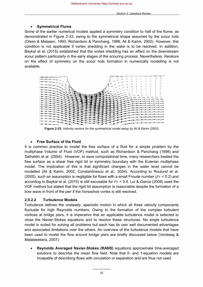
Section 2. Literature Review
52
• Symmetrical Flume Some of the earlier numerical models applied a symmetry condition to half of the flume, as demonstrated in Figure 2-33, owing to the symmetrical shape assumed by the scour hole (Olsen & Malaaen, 1993; Richardson & Panchang, 1988; Ali & Karim, 2002). However, this condition is not applicable if vortex shedding in the wake is to be resolved. In addition, Baykal et al. (2015) established that the vortex shedding has an effect on the downstream scour pattern particularly in the early stages of the scouring process. Nevertheless, literature on the effect of symmetry on the scour hole formation in numerically modelling is not available.
Figure 2-33: Velocity vectors for the symmetrical model setup by Ali & Karim (2002)
• Free Surface of the Fluid It is common practice to model the free surface of a fluid for a simple problem by the multiphase Volume of Fluid (VOF) method, such as Richardson & Panchang (1998) and Salhaldin et al. (2004). However, to save computational time, many researchers treated the free surface as a shear free rigid lid or symmetry boundary with the Eulerian multiphase model. The implication of this is that significant changes in the water level cannot be modelled (Ali & Karim, 2002; Constantinescu et al., 2004). According to Roulund et al. (2005), such an assumption is negligible for flows with a small Froude number (𝐹𝐹𝐹𝐹 < 0.2) and according to Baykal et al. (2015) is still excusable for 𝐹𝐹𝐹𝐹 < 0.4. Lui & Garcia (2008) used the VOF method but stated that the rigid lid assumption is reasonable despite the formation of a bow wave in front of the pier if the horseshoe vortex is still resolved.
2.9.2.2 Turbulence Models Turbulence defines the unsteady, aperiodic motion in which all three velocity components fluctuate for high Reynolds numbers. Owing to the formation of the complex turbulent vortices at bridge piers, it is imperative that an applicable turbulence model is selected to close the Navier-Stokes equations and to resolve these structures. No single turbulence model is suited for solving all problems but each has its own well documented advantages and associated limitations over the others. An overview of the turbulence models that have been used to model the flow around bridge piers are briefly discussed below (Versteeg & Malalasekera, 2007):
• Reynolds Averaged Navier-Stokes (RANS) equations approximate time-averaged solutions to describe the mean flow field. Note that 0- and 1-equation models are incapable of describing flows with circulation or separation and are thus not used.
Stellenbosch University https://scholar.sun.ac.za

Section 2. Literature Review
53
o The 𝒌𝒌-ε model is the most widely used for its simplicity, stability and reasonable accuracy. However, it generally predicts circulating or separated flows with less accuracy. The 2-equation model allows for the turbulent kinetic energy (𝑘𝑘) and the turbulent dissipation (ε) to be determined independently. Three variants exist which differ in the way that the turbulent viscosity, Prandtl number and the generation and dissipation terms of ε are calculated. The standard 𝒌𝒌-ε is robust and economical, giving mediocre results
for complex flows with severe pressure gradients and strong streamline curvature. Furthermore, it is only applicable to fully turbulent flows.
The Renormalization Group (RNG) 𝒌𝒌-ε gives improved results for streamline curvature and transitional flows.
The realizable 𝒌𝒌-ε further improves complex secondary and separated flows with strong recirculation.
o The 𝒌𝒌-ω model is another 2-equation model based on the 𝑘𝑘-ε model whereby the specific dissipation (ω) is determined directly. The model suffers from the same drawbacks with the exception that adverse pressure gradients are better modelled.
o The Shear Stress Transport (SST) model performs well for adverse pressure gradients and separated flow. The model applies the 𝑘𝑘-ω approach in boundary layers near walls and a 𝑘𝑘-ε approach in free streams, making it more robust.
o The Reynolds Stress Model (RSM) requires 7 differential equations to be solved making it more efficient for flows with streamline curvature, circulation, separation or rapid changes in high strain rates. It is described as the most physically complete and superior model for complex flows but requires 2-3 times more CPU effort and time.
• The Large Eddy Simulation (LES) model is based on space filtered, time-dependent equations. Large eddies are explicitly solved while smaller eddies are accounted for by subgrids. While the model is highly accurate, it is often described as uneconomic.
• The Detached Eddy Simulation (DES) is a hybrid combination of the RANS and LES turbulence models that attempts to alleviate the uneconomic near-wall meshing requirements imposed by LES by switching to RANS where the turbulent length scale is less than the prescribed maximum grid size.
Evidently, the simplest and most used turbulence model used to simulate bridge pier scour is the 𝑘𝑘-ε model. Many numerical studies have evaluated these different turbulence models on their applicability to the junction flow of a bridge pier. Richardson & Panchang (1998) and Ali et al. (1997) recommended the RNG model above the standard 𝑘𝑘-ε model because it requires less reliance on the empirical constants and produces improved results in high shear stress problems. On the other hand, Ali & Karim (2002) suggested that both give similar results for the velocity profile.
Salaheldin et al. (2004) agreed, despite the commonly perceived weakness of the k-ε model, it performs satisfactorily in reproducing the velocity profile near the bed, albeit it slightly underestimated. However, the 𝑘𝑘-ε models show some discrepancy with the measured bed shear stress and generally overestimate the area of scour initiation. Furthermore, even
Stellenbosch University https://scholar.sun.ac.za

Section 2. Literature Review
54
though the realizable 𝑘𝑘-ε model is considered superior among the 𝑘𝑘-ε models, it performs the most poorly and substantially overestimates the flow velocity. Salaheldin et al. (2004) recommended that the realizable 𝑘𝑘-ε model should not be used in bridge pier scour modelling.
Salaheldin et al. (2004) concluded that the RSM is the most accurate model in simulating the velocity distribution and shear stress on flat beds and in scour holes. However, the computation of more reliable results is generally time intensive and risks instability. The selection of an optimum turbulence model requires some degree of compromise between accuracy and economy. Thus, the two equation models are favoured above the RSM model.
Menter (1993) evaluated the standard 𝑘𝑘-ε model, 𝑘𝑘-ω model and the SST model and established that the 𝑘𝑘-ε model did not yield as accurate results as the others. Furthermore, he recommended the SST model for its ability to handle adverse pressure gradient flows. Mendoza & Cabrales (1993), Khosronejad et al. (2012) and Xiong et al. (2014) could not resolve the horseshoe vortex which they attributed to the inadequacy of the k-ε model.
Alternatively, Constantinescu et al. (2004), and their literary successors, believe that RANS models are not suitable for the prediction of junction flows if a detailed study of the coherent structures and frequency spectra inside the horseshoe vortex system is of interest. Khosronejad (2012) acknowledged that the 2-equation turbulence models tend to underpredict the intensity of the horseshoe vortex. To overcome the limitations associated with URANS, they propose the LES model which has been shown to accurately reproduce vortices at bridge piers. Furthermore, LES does not employ wall functions or adjustable constants, and are capable of resolving very fine mesh sizes.
LES models have led to an improved understanding of the flow field around bridge piers. However, their application to coupled hydrodynamic and sediment transport models is challenging due to the excessive computational resources required. Owing to the discrepancy in temporal scales, hydro-morphodynamic simulations using LES or DES are impractical for engineering applications (Khosronejad, 2012). Only RANS models have thus far been used to simulate bridge pier scour because they are generally capable of resolving the primary horseshoe vortex structure. The influence of the secondary horseshoe vortices (captured by LES) on the maximum scour depth is still largely undetermined. Consequently, the less CPU intensive RANS models are considered sufficient.
In spite of this, Richardson & Panchang (1998) state that contrary to expectation, the results from numerical modelling are less sensitive to the choice of turbulence model than to the geometric mesh representation.
2.9.2.3 Computational Grid One of the challenges faced in numerical modelling is establishing a mesh with an optimum balance between computation time, stability, solution accuracy and grid independence. A good quality mesh structure is defined by a high orthogonal quality (> 0.1), low skewness (< 0.95), smoothness (< 2.5) and a low aspect ratio (< 90). These metrics are particularly important where strong transverse gradients are anticipated (Fluent, 2011).
Furthermore, a fairly dense mesh is required in the horseshoe vortex region to resolve the boundary layer and vortex formation at the pier, particularly at the bed surface where entrainment occurs (Kirkil & Constantinescu, 2005). According to Ali & Karim (2002), shear
Stellenbosch University https://scholar.sun.ac.za

Section 2. Literature Review
55
stress results computed by ANSYS Fluent depend on the absolute size of the cells. Thus, if the cells are too big, the results become grid dependent. Olsen & Kjellesvig (1998) stated that a coarse grid results in a smaller scour hole, produces false diffusion and fails to simulate small eddies. The law-of-the-wall may be used as a guideline to establish the required mesh resolution (Salaheldin et al., 2004).
Ideally, fluid flow is best described by a structured grid with hexagon cells aligned with the streamlines. Mesh cells that deviate from the ideal shape may cause interpolation errors, slowing down the solver and risking divergence. Figure 2-34 illustrates the different ways in which a circular pier may be accommodated in a hex-dominant fluid domain by employing a Cartesian grid, an unstructured grid or a multi-block grid. The different types of grids are discussed below.
• Unstructured grids have an irregular connectivity and are space inefficient, deviating from the ideal shape. However, they are widely accepted for more complex geometries, thereby reducing the time required for meshing. According to Lui & Garcia (2008), unstructured grids complicate the grid tracking process invalidating the grid at the scour hole and causing instability. Unstructured grids have been employed by Salaheldin et al. (2004), Constantinescu et al. (2004), Kirkil et al. (2005) and Lui & Garcia (2008).
• Structured curvilinear grids result in a higher resolution and improved convergence because fewer resources are required to distribute functions across cells.
o Cartesian grids waste cells in dealing with objects outside the fluid domain and are not recommended (see Figure 2-34a). These have been implemented by Olsen & Kjellesvig (1998), Richardson & Panchang (1998) and Khosronejad et al. (2012).
o Orthogonal grids are defined by perpendicular gridlines at intersections. However, they are inflexible and do not adapt well to complex geometries unless aided by unstructured cells as seen in Figure 2-34b (Huang et al., 2009).
o Nonorthogonal grids accommodating streamlined flow around piers, such as that in Figure 2-34c, have commonly been used by Olsen & Malaaen (1993), Ali & Karim (2002) and Nagata et al. (2005).
• Multi-block grids divide the domain into different regions with different grid types. This method of meshing is easy to generate, can accommodate curved boundaries and regions requiring different degrees of fineness, and can discretize equations more easily. Examples include those from Tseng et al. (2000), Roulund et al. (2005) and Xiong et al. (2014).
In addition, the computational grid constrains the time step size permissible for a stable transient numerical model. In other words, denser grids not only require additional computational effort at each grid point but also require a reduced time step size, thereby further increasing the computational time. The Courant number is a spatial-time condition necessary for convergence which is given by the equation below for a 3D domain
𝐶𝐶𝐶𝐶 =𝑣𝑣∆𝑡𝑡∆𝑙𝑙𝐼𝐼𝑖𝑖𝑚𝑚
=𝑣𝑣𝑚𝑚∆𝑡𝑡∆𝑙𝑙𝑚𝑚
+𝑣𝑣𝑦𝑦∆𝑡𝑡∆𝑙𝑙𝑦𝑦
+𝑣𝑣𝑦𝑦∆𝑡𝑡∆𝑙𝑙𝑧𝑧
, (2-30)
Stellenbosch University https://scholar.sun.ac.za

Section 2. Literature Review
56
where ∆𝑡𝑡 is the time step size, ∆𝑙𝑙 is the cell size and 𝑣𝑣 is the velocity defined for the 𝑥𝑥-, 𝑦𝑦- and 𝜕𝜕-axis components. For explicit solvers, the Courant number must be less than 1, while implicit solvers tolerate larger values as they are less sensitive to numerical instability (Versteeg & Malalasekera, 2007). However, the Courant number should also be used as a guideline to avoid unnecessarily small values which may lead to vacillating residuals and divergence.
Figure 2-34: a) Nonorthogonal cartesian grid (Olsen & Kjellesvig, 1998) b) Unstructured grid with orthogonal centre (Huang et al., 2009) c) Multiblock structured grid with nonorthogonal centre (Tseng et al., 2000)
2.9.3 Sediment Transport Modelling
The behaviour of the particles in motion can be modelled by either taking the surface of the packed bed as a continuous phase with wall shear stresses or by tracking particle trajectories (Shao & Li, 1999). Richardson & Panchang (1998) supplemented their flow simulations by Lagrangian particle tracking for prospective scour depth estimations. However, the widespread method has been to approximate the sediment bed as a continuum. Typically, the approach adopted in the sediment transport modelling has four main elements, namely the bed load equation, sand slide considerations, sediment continuity and bed surface deformation tracking.
Different formulas for the rate of bed load transport or concentration were implemented by the different numerical models. The transition from empirical bridge pier scour equations towards numerical modelling has also redirected the attention towards the evaluation of sediment transport expressions that best reflect reality. Bed load functions such as those presented in Section 2.6.3 were used by the models to quantify the sediment transport.
(a) (b)
(c)
Stellenbosch University https://scholar.sun.ac.za

Section 2. Literature Review
57
Olsen & Kjellesvig (1998) applied equation (2-10) for bed load concentration by van Rijn (1987) while Khosronejad et al. (2012) and Abbasnia & Ghiassi (2011) used a similar equation by van Rijn (1993) that allows for the computation of nonequilibrium bed concentration. Similarly, Xiong et al. (2014) used equation (2-11) by Dey (1999). Roulund et al. (2005), Lui & Garcia (2008) and Baykal et al. (2015) all used variations of the Engelund & Fredsøe (1976) formula given in equation (2-14). These bed load calculations are usually based on the bed shear stress computed by the hydrodynamic model at each grid point.
However, in order to prevent the bed slope from exceeding the angle of repose and scouring indefinitely beyond equilibrium conditions, sand slides were typically imposed. Bridge pier scour results in a sloping bed cells, thereby reducing the critical shear stress and increasing erosion. Sand slide algorithms act as a limiter for the critical shear stress reduction by correcting the slope when it exceeds the angle of repose. The models simply enforce a constant angle of repose which gave bed cells the same slope and made the scour holes appear smooth and uniform.
The sediment continuity equation was widely used to establish the bed elevation change h by employing the bed load transport rate 𝑞𝑞𝑏𝑏𝑑𝑑𝑑𝑑 at each grid point. Also known as the Exner equation, the general form can be given by
where 𝑛𝑛𝑝𝑝 is the bed porosity. In contrast, Nagata et al. (2005) used the momentum equation and the volume of sediment pickup and deposition. From the equation above, 𝐷𝐷𝑆𝑆𝑆𝑆 and 𝐸𝐸𝑆𝑆𝑆𝑆 are the deposition and erosion terms stemming from a suspended sediment model. Olsen & Kjellesvig (1998), Lui & Garcia (2008) and Baykal et al. (2015) made allowances for suspended sediment transport which is normally determined by the convection-diffusion equation given in the form of
where 𝑤𝑤 is the settling velocity, 𝐶𝐶 is the suspended sediment concentration and Γ𝑆𝑆𝑆𝑆 is the diffusion coefficient calculated from the eddy viscosity divided by the turbulent Schmidt number (𝜇𝜇𝑡𝑡/𝜎𝜎𝑐𝑐). The Schmidt number is usually in the order of 0.5 to 1, which is calculated from the settling velocity and the shear velocity following van Rijn (1981)
Finally, the change in bed elevation or the deformation of the bed surface was tracked by: 1. The Arbitrary Lagrangian Eulerian (ALE) method links the grid for the fluid domain
boundary to the changing topography of the packed bed. The method is also known as Dynamic Mesh Updating whereby each node on the riverbed is updated during each time step, deforming the grid in the same way that the surface elevation of the packed bed would change due to erosion and deposition.
2. The Immersed Boundary (IB) method includes the entire packed bed inside the computational domain with a fixed grid system and tracks the bed’s surface by employing a volume fraction. The method is also known as the Fictitious Domain or
𝜕𝜕ℎ𝜕𝜕𝑡𝑡
=1
1 − 𝑛𝑛𝑝𝑝[−∇ ∙ 𝒒𝒒𝑏𝑏𝑑𝑑𝑑𝑑 + 𝐷𝐷𝑆𝑆𝑆𝑆 − 𝐸𝐸𝑆𝑆𝑆𝑆] , (2-31)
𝜕𝜕𝐶𝐶𝜕𝜕𝑡𝑡
+ 𝑣𝑣𝑖𝑖𝜕𝜕𝐶𝐶𝜕𝜕𝑥𝑥𝑖𝑖
+ 𝑤𝑤𝜕𝜕𝐶𝐶𝜕𝜕𝜕𝜕
=𝜕𝜕𝜕𝜕𝑥𝑥𝑖𝑖
Γ𝑆𝑆𝑆𝑆𝜕𝜕𝐶𝐶𝜕𝜕𝑥𝑥𝑖𝑖
, (2-32)
𝜎𝜎𝑐𝑐 =1
1 + 2𝑤𝑤𝐶𝐶∗
2 . (2-33)
Stellenbosch University https://scholar.sun.ac.za

Section 2. Literature Review
58
Virtual Boundary Method because a direct forcing scheme is required to apply boundary conditions to the specified virtual surface of the packed bed and to apply a rigid body condition to the fluid inside the packed bed. The method was originally developed for flows around flexible membranes such as the human heart, which was extended to Stokes flow around suspended particles (Peskin, 2002).
The ALE method with the adaptive grid is evidently prevalent, with the exception of Khosronejad & Sotiropoulus (2012) which was the only model found to implement the IB method. According to Schneiderbauer & Pirker (2014), the ALE method is more economic because no modifications to the turbulence model are required and less computational cells are modelled. However, frequent remeshing and artificial smoothing is required (Uhlmann, 2005) because large boundary movements distort the mesh and deteriorate the mesh quality, causing the computation to become unstable and diverge (Lui & Garcia, 2008). The IB method is superior in the case of complicated topologies, particularly those involving massive erosions.
2.10 Summary
Local scour at piers has been cited as the main mechanism responsible for the collapse of bridges, not overloading. In spite of the highly advanced scientific basis for the structural design of bridges, there is still no universally agreed upon design procedure to accurately predict and counter bridge pier scour. Evidently, the scouring process is complex owing to the formation of boundary layers and intricate 3D vortex structures, which are the basic mechanisms responsible for scouring. Furthermore, the local scour process is affected by several different yet interrelated parameters that are often described as quantities relative to one another. While the flow and pier properties describe the fluid’s capacity to shear, the sediment properties describe its resistance to these forces. The study of sediment transport is thus of fundamental importance to quantify the initiation and rate of entrainment.
Traditional methods of predicting the equilibrium scour depth near bridge piers rely on overly simplified formulas that have been calibrated by small scale laboratory experiments. These methods yield a wide range of varying and unreliable results. However, advanced hydro-morphodynamic models using CFD codes are becoming increasingly popular owing to recent technological advancements. Existing studies of these numerical models are principally differentiated by their approaches towards meshing, boundary conditions, turbulence models and sediment transport calculations. The accuracy of their solutions relies heavily on the numerical model’s ability to resolve the vortex structures as well as the underlying assumptions of the selected sediment transport model.
The literature study presented a detailed discussion on the complex flow field and scouring process associated with bridge piers, as well as the several interrelated parameters and scour prediction methods. The aim was to gain an understanding of the scour process, as well as the typical approach adopted by existing numerical models, which could be applied to the proposed model. Important sediment transport concepts were introduced as a context for the subsequent section.
Stellenbosch University https://scholar.sun.ac.za

Section 3. Theory for the Proposed Model
59
3. Theory for the Proposed Model
3.1 Introduction
The section describes the theory for the coupled fully 3D numerical model proposed for the prediction of the bridge pier scour in an alluvial bed. The model solves the URANS equations, which includes both sediment transport and hydrodynamic parameters. The first part of the section addresses the basics of the fluid dynamics while the second part discusses the sediment transport model and focuses on the flow-particle interaction.
The model proposed in the study was developed by Sawadogo (2015) to investigate the scour pattern caused by bottom outlet sediment flushing. He adopted the same approach that was modelled by Schneiderbauer (2010) and Schneiderbauer & Pirker (2014) to study the erosion and sedimentation processes of snow in a wind tunnel. These studies dealt with aeolian particle transport, while Sawadogo (2015) refined and applied the mathematics to hydrodynamic particle transport for dam bottom outlet flushing. It is recommended that these studies are consulted for a more detailed understanding of the model development.
3.2 Computational Fluid Dynamics Modelling
3.2.1 Governing Equations
The governing equations used to model the flow field, namely the conservation of mass and that of momentum, are presented.
Unlike the 2D single-phase flow equations, the proposed 3D numerical model follows the Eulerian multiphase approach. This allows for the modelling of multiple separate, yet interacting, phases and thereby account for fluid momentum loss due to entrained particles. Three phases are considered, namely water (𝛼𝛼𝑤𝑤), rolling particles (𝛼𝛼𝑟𝑟) and saltating particles (𝛼𝛼𝑠𝑠). Section 3.3 describes the classification of these particles into saltating and rolling particles.
The continuity equation for phase 𝑞𝑞 ∈ 𝐹𝐹 = w, r, s in the model is given by
where 𝛼𝛼𝑞𝑞 is defined as the volume fraction, 𝐯𝐯𝑞𝑞 is the velocity of phase 𝑞𝑞, 𝜌𝜌𝑞𝑞 is the density of phase 𝑞𝑞, 𝑚𝑚𝑝𝑝𝑞𝑞 denotes the mass transfer from phase 𝑝𝑝 to phase 𝑞𝑞, and 𝑚𝑚𝑞𝑞𝑝𝑝 the mass transfer from phase 𝑞𝑞 to phase 𝑝𝑝. A constant density is assumed and the mass transfer between phases is neglected, i.e. 𝑚𝑚𝑝𝑝𝑞𝑞 = −𝑚𝑚𝑞𝑞𝑝𝑝 = 0. The mass source term (𝑆𝑆𝑞𝑞) accounts for sediment deposition and erosion submodels, discussed in Section 3.3.1.
The momentum equation for phase 𝑞𝑞 is given by
𝜕𝜕𝛼𝛼𝑞𝑞𝜕𝜕𝑡𝑡
+ 𝛁𝛁 ∙ 𝛼𝛼𝑞𝑞𝐯𝐯𝑞𝑞 = 1𝜌𝜌𝑞𝑞 𝑚𝑚𝑝𝑝𝑞𝑞 − 𝑚𝑚𝑞𝑞𝑝𝑝
𝑚𝑚
𝑝𝑝=1 + 𝑆𝑆𝑞𝑞 , (3-1)
𝜕𝜕𝛼𝛼𝑞𝑞𝐯𝐯𝑞𝑞𝜕𝜕𝑡𝑡
+ ∇ ∙ 𝛼𝛼𝑞𝑞𝐯𝐯𝑞𝑞𝐯𝐯𝑞𝑞 = 1𝜌𝜌𝑞𝑞−∝𝑞𝑞 𝛁𝛁𝑝𝑝 + 𝛁𝛁 ∙ 𝐓𝐓𝑞𝑞 +∝𝑞𝑞 𝜌𝜌𝑞𝑞𝐠𝐠 + 𝑅𝑅𝑝𝑝𝑞𝑞
𝑝𝑝∈𝐹𝐹𝐯𝐯𝑝𝑝 − 𝐯𝐯𝑞𝑞 + 𝐟𝐟𝑞𝑞 , (3-2)
Stellenbosch University https://scholar.sun.ac.za

Section 3. Theory for the Proposed Model
60
where 𝑝𝑝 is the pressure shared by all the phases, 𝐓𝐓𝑞𝑞 is the stress tensor of phase 𝑞𝑞, 𝐠𝐠 is the gravitational acceleration, 𝑅𝑅𝑝𝑝𝑞𝑞 is the interphase momentum exchange term for fluid-solid interaction and 𝐟𝐟𝑞𝑞 accounts for the momentum transfer of phase 𝑞𝑞 (refer to Section 3.3.2.1).
The stress tensor of phase 𝑞𝑞 is obtained from
where 𝜇𝜇𝑞𝑞 is the constant shear viscosity of phase 𝑞𝑞 and 𝐈𝐈 denotes the unity tensor. The equation is only valid for Newtonian fluids as is the case in this study. It is assumed that 𝜇𝜇𝑞𝑞 approximates the shear viscosity of water because the solids volume fractions are very small (< 10-3) and the fluid stresses are dominant.
The interphase momentum exchange or drag term is computed from a Wen & Yu (1996) model
where
and the Reynolds number, based on 𝑑𝑑𝑝𝑝 or the diameter of the particulate phase p, is given by
3.2.2 Two-Equation Turbulence Model
The proposed model employs the standard (or realizable) 𝑘𝑘-ε turbulent model, which is defined as an eddy viscosity model, whereby Reynolds stresses are computed by the Boussinesq hypothesis. The two-equation model is widely used for its robust and reasonably accurate solutions over a spread of turbulent flows. The two transport equations for turbulent kinetic energy (𝑘𝑘) and its dissipation rate (𝜀𝜀) are given by
and
where 𝜌𝜌 is the density of the mixture, 𝐯𝐯 is the velocity of the mixture, 𝜇𝜇𝑡𝑡 is the turbulent or eddy viscosity and 𝐺𝐺𝑘𝑘 represents the production of turbulent kinetic energy due to the mean velocity gradients. Additional user-defined source terms, 𝑆𝑆𝑘𝑘 and 𝑆𝑆𝜀𝜀, are termed for 𝑘𝑘 and 𝜀𝜀 respectively, and are explained in Section 3.3.2.2.
The following default values (Fluent, 2011) were used for the model constants: 𝐶𝐶1𝜀𝜀 = 1.44, 𝐶𝐶2𝜀𝜀 = 1.92, 𝐶𝐶𝜇𝜇 = 0.09, 𝜎𝜎𝑘𝑘 = 1.00 and 𝜎𝜎𝜀𝜀 = 1.30.
𝐓𝐓𝑞𝑞 = 𝛼𝛼𝑞𝑞𝜇𝜇𝑞𝑞 𝛁𝛁𝐯𝐯𝑞𝑞 + 𝛁𝛁𝐯𝐯𝑞𝑞𝑇𝑇 −23𝛁𝛁 ∙ 𝐯𝐯𝑞𝑞𝐈𝐈 , (3-3)
𝑅𝑅𝑝𝑝𝑞𝑞 = 34𝐶𝐶𝐷𝐷
𝛼𝛼𝑝𝑝𝛼𝛼𝑞𝑞𝜌𝜌𝑞𝑞𝐯𝐯𝑝𝑝 − 𝐯𝐯𝑞𝑞𝑑𝑑𝑝𝑝
∝𝑞𝑞−2.65 , (3-4)
𝐶𝐶𝐷𝐷 =24
𝛼𝛼𝑞𝑞𝑅𝑅𝑅𝑅𝑝𝑝1 + 0.15𝛼𝛼𝑞𝑞𝑅𝑅𝑅𝑅𝑝𝑝
0.687 , (3-5)
𝑅𝑅𝑅𝑅𝑝𝑝 =𝜌𝜌𝑞𝑞𝑑𝑑𝑝𝑝𝐯𝐯𝑝𝑝 − 𝐯𝐯𝑞𝑞
𝜇𝜇𝑞𝑞 . (3-6)
𝜕𝜕𝜌𝜌𝑘𝑘𝜕𝜕𝑡𝑡
+ 𝛁𝛁 ∙ (𝜌𝜌𝑘𝑘𝐯𝐯) = 𝛁𝛁 ∙ 𝜇𝜇𝑡𝑡𝜎𝜎𝑘𝑘𝛁𝛁𝑘𝑘 + 𝐺𝐺𝑘𝑘 − 𝜌𝜌𝜀𝜀 + 𝑆𝑆𝑘𝑘 , (3-7)
𝜕𝜕𝜌𝜌𝜀𝜀𝜕𝜕𝑡𝑡
+ 𝛁𝛁 ∙ (𝜌𝜌𝜀𝜀𝐯𝐯) = 𝛁𝛁 ∙ 𝜇𝜇𝑡𝑡𝜎𝜎𝜀𝜀𝛁𝛁𝜀𝜀 +
𝜀𝜀𝑘𝑘
(𝐶𝐶1𝜀𝜀𝐺𝐺𝑘𝑘 − 𝐶𝐶2𝜀𝜀𝜌𝜌𝜀𝜀) + 𝑆𝑆𝜀𝜀 . (3-8)
Stellenbosch University https://scholar.sun.ac.za

Section 3. Theory for the Proposed Model
61
The density and velocity for the mixture are obtained from the expressions
while the turbulent viscosity is given by
Finally, the turbulence production 𝐺𝐺𝑘𝑘 can be computed from the expression simplified by the Boussinesq concept
where 𝑇𝑇2 denotes the second invariant of the tensor for the mixture’s strain rate 𝑆𝑆𝑖𝑖𝑖𝑖 expressed as
3.3 Sediment Transport Modelling
3.3.1 Sediment Erosion and Deposition Model
In order to model the local erosion and deposition, the fully resolved modelling approach is confined to very small geometries and focuses only on the behaviour of the particles and fluid above the packed bed. Instead of tracking individual particle trajectories, the particulate phase is considered as a continuum. The packed bed is seen as a rough wall and therefore the quantity of entrained particles is determined from the wall shear forces of the fluid.
The mass source term from the continuity equation (3-1) accounts for the sediment erosion and deposition of the two phases, namely saltating particles (𝑆𝑆𝑠𝑠𝑎𝑎𝑠𝑠) and rolling particles (𝑆𝑆𝑟𝑟𝑜𝑜𝑠𝑠). The mass source terms per unit volume and per unit time (kg/m3/s) are determined by the following
where particles eroded, ejected or deposited are denoted by their superscripts. The erosion and deposition processes were modelled by considering the following particle transport modes for non-cohesive sediment:
• Particle entrainment due to shear stresses; • Particles rolling due to hydrodynamic shearing; • The erosion or ejection of saltating particles due to impacting particles; • Particles rebound or trapped after impact; • Particle deposition and accumulation; and • Landside shearing.
𝜌𝜌 = 𝛼𝛼𝑞𝑞𝜌𝜌𝑞𝑞𝑞𝑞∈𝐹𝐹
and 𝐯𝐯 = 1𝜌𝜌𝛼𝛼𝑞𝑞𝜌𝜌𝑞𝑞𝐯𝐯𝑞𝑞𝑞𝑞∈𝐹𝐹
, (3-9)
𝜇𝜇𝑡𝑡 = 𝜌𝜌𝐶𝐶𝜇𝜇𝑘𝑘2
𝜀𝜀 . (3-10)
𝐺𝐺𝑘𝑘 = 𝜇𝜇𝑡𝑡𝑇𝑇22 , (3-11)
𝑇𝑇2 = 2𝑆𝑆𝑖𝑖𝑖𝑖𝑆𝑆𝑖𝑖𝑖𝑖 . (3-12)
𝑆𝑆𝑠𝑠𝑎𝑎𝑠𝑠 = 𝑆𝑆𝑠𝑠𝑎𝑎𝑠𝑠𝑑𝑑 − 𝑆𝑆𝑠𝑠𝑎𝑎𝑠𝑠𝑑𝑑𝑑𝑑 , (3-13)
𝑆𝑆𝑟𝑟𝑜𝑜𝑠𝑠 = 𝑆𝑆𝑟𝑟𝑜𝑜𝑠𝑠𝑑𝑑 + 𝑆𝑆𝑟𝑟𝑜𝑜𝑠𝑠𝑑𝑑𝑖𝑖 − 𝑆𝑆𝑟𝑟𝑜𝑜𝑠𝑠𝑑𝑑𝑑𝑑 , (3-14)
Stellenbosch University https://scholar.sun.ac.za

Section 3. Theory for the Proposed Model
62
3.3.1.1 Hydrodynamic Entrainment The number of particles entrained by the packed bed due to hydrodynamic shear stress is calculated by the equation given by Shao & Li (1999)
where 𝐶𝐶∗ and 𝐶𝐶𝑡𝑡∗ are the shear velocity and shear velocity threshold respectively, 𝑑𝑑𝑝𝑝 is the particle diameter and the dimensionless entrainment coefficient 𝐶𝐶η
′ is considered a calibration parameter for the hydrodynamic transport of sand particles. This approach is fundamentally based on the estimation of Anderson & Haff (1991) where the number of entrained particles depends linearly on the difference between the shear stress at the surface and shear stress threshold.
The total number of particles entrained due to the shear forces of water flow is the sum of the rolling particles and the saltating particles at the bed surface. From equation (3-15) for the number of entrained particles, the total mass of particles entrained into surface rolling and into saltation are given by
and
where 𝑚𝑚𝑝𝑝 is the particle mass, 𝜌𝜌𝑝𝑝 is the particle density, 𝐴𝐴 and 𝑉𝑉 are the area and volume, respectively, of a grid cell adjacent to the packed bed, and 𝑝𝑝𝑟𝑟 defines the probability that a particle with no initial velocity is entrained into the surface rolling transport mode.
The entrained particles are classified as either surface rolling or saltating based on their initial ejection velocity 𝐶𝐶𝑖𝑖,0, which is approximated as half the shear velocity (Shao and Li, 1999). A relationship between shear velocity 𝐶𝐶∗ and probability 𝑝𝑝𝑟𝑟 was assumed whereby 𝑝𝑝𝑟𝑟 ≈ 0.5 corresponds to 𝐶𝐶∗ < 1 and decreases as the shear stress increases at the surface of the bed.
To determine the critical shear stress 𝜏𝜏𝑡𝑡 (or fluid threshold) and subsequently the shear velocity threshold 𝐶𝐶𝑡𝑡∗, the calculation from Schmidt (1980) can be applied to account for a change in slope relative to the flow direction
where 𝛽𝛽𝑑𝑑 is the mean drag level, η is the ratio of mean drag and lift per unit area on the whole bed to mean drag and lift on the top grain entrained by the fluid, Γ is the ratio of maximum to mean drag and lift on the particle, 𝜃𝜃 is the slope angle with respect to the flow direction, and 𝜑𝜑 is the angle of repose. The following values, taken from Chepil (1959), were selected: η = 0.21, Γ = 2.5 and 𝛽𝛽 = 24°.
𝑁𝑁𝐴𝐴 =𝐶𝐶η′
𝑑𝑑𝑝𝑝3𝐶𝐶𝑠𝑠∗𝐶𝐶∗2 − 𝐶𝐶𝑡𝑡∗
2 , (3-15)
𝑆𝑆𝑟𝑟𝑜𝑜𝑠𝑠𝑑𝑑 = 𝑝𝑝𝑟𝑟𝑚𝑚𝑝𝑝𝐴𝐴𝑉𝑉𝑁𝑁𝐴𝐴 = 𝑝𝑝𝑟𝑟
𝜋𝜋𝜌𝜌𝑝𝑝𝑑𝑑𝑝𝑝3
6𝐴𝐴𝑉𝑉𝑁𝑁𝐴𝐴 , (3-16)
𝑆𝑆𝑠𝑠𝑎𝑎𝑠𝑠𝑑𝑑 = (1 − 𝑝𝑝𝑟𝑟)𝑚𝑚𝑝𝑝𝐴𝐴𝑉𝑉𝑁𝑁𝐴𝐴 = (1 − 𝑝𝑝𝑟𝑟)
𝜋𝜋𝜌𝜌𝑝𝑝𝑑𝑑𝑝𝑝3
6𝐴𝐴𝑉𝑉𝑁𝑁𝐴𝐴 , (3-17)
𝜏𝜏𝑡𝑡 = 𝜌𝜌𝐶𝐶𝑡𝑡∗2 =
23
ηΓ𝜌𝜌𝑝𝑝 − 𝜌𝜌𝑔𝑔𝑑𝑑𝑝𝑝(cos 𝜃𝜃 − sin𝜃𝜃 / tan𝜑𝜑) tan𝛽𝛽𝑑𝑑
1 + 0.85 tan𝛽𝛽𝑑𝑑 , (3-18)
Stellenbosch University https://scholar.sun.ac.za

Section 3. Theory for the Proposed Model
63
The shear velocity 𝐶𝐶∗ exerted by the water flow onto the surface of the packed bed is referred to as the most sensitive parameter for the submodel (Schneiderbauer & Pirker, 2014). To determine the shear velocity 𝐶𝐶∗, Newton’s method is used to solve the implicit equations proposed by Prandtl (Fluent, 2011) for the logarithmic law-of-the-wall which is given by
where κ is the von Kármán constant 0.407 and 𝐸𝐸 is an empirical constant of 9.793. The dimensionless distance from the wall 𝑌𝑌+ and the roughness function 𝑓𝑓𝑟𝑟 can be obtained from
and
where 𝜌𝜌𝑤𝑤 is the water density, 𝜇𝜇𝑤𝑤 is the dynamic viscosity of water, 𝑦𝑦𝑝𝑝 is the cell-wall distance and 𝐹𝐹 is the physical roughness height.
3.3.1.2 Ejection The ejection of particles due to impacting particles at the packed bed surface is considered because the collision of saltating particles impacting the packed bed surface may cause the ejection of other particles (erosion). Furthermore, the impacting particles may be rebound or trapped at the surface (deposition). It was assumed that the energy from a rolling particle is not enough to eject particles from the packed bed. The number of ejected particles per impact depends mainly on the kinetic energy of impacting particles and is given by the equation (Andreotti, 2004)
where 𝑈𝑈𝐼𝐼𝐼𝐼 is the speed of impacting particles and 𝑐𝑐𝐼𝐼 ≈ 10 is a dimensionless coefficient that defines a velocity scale. The initial speed of impacting particles, with an impacting angle of 45°, is given by Andreotti (2002)
where ζ𝑟𝑟 = 0.5 is the restitution parameter of particle-bed collision, which is the velocity ratio of the rebounding particle to the impacting particle. A theoretical limitation for the maximum number of ejected particles per impact was proposed by Shao & Li (1999)
where the following values, based on previous studies, were used for the empirical coefficients: 𝑐𝑐𝑠𝑠 = 0.5, 𝑐𝑐𝑎𝑎 = 0.5 and 𝑐𝑐ℎ = 0.25. The limitation is based on the energy balance between particles whereby the empirical coefficients represent the fraction of energy not converted into heat after the impact.
𝐶𝐶𝑠𝑠𝐶𝐶∗
=1κ
ln𝐸𝐸𝑌𝑌+
𝑓𝑓𝑟𝑟 , (3-19)
𝑌𝑌+ =𝜌𝜌𝑤𝑤𝑦𝑦𝑝𝑝𝐶𝐶∗
𝜇𝜇𝑤𝑤 , (3-20)
𝑓𝑓𝑟𝑟 = 1 + 0.5𝜌𝜌𝑤𝑤𝐹𝐹𝐶𝐶∗
𝜇𝜇𝑤𝑤 , (3-21)
𝑁𝑁𝐸𝐸𝑝𝑝𝐼𝐼 = 0.3𝑈𝑈𝐼𝐼𝐼𝐼
𝑐𝑐𝐼𝐼𝑔𝑔𝑑𝑑𝑝𝑝2
, (3-22)
𝑈𝑈𝐼𝐼𝐼𝐼,0 = ζ𝑟𝑟𝑐𝑐𝑖𝑖𝑔𝑔𝑑𝑑𝑝𝑝 , (3-23)
𝑁𝑁𝐸𝐸𝑝𝑝𝐼𝐼𝐼𝐼𝑎𝑎𝑚𝑚 =𝑐𝑐𝑠𝑠 − 1.9𝑐𝑐𝑎𝑎2 1 − 𝑅𝑅𝑈𝑈𝑖𝑖𝑖𝑖/𝑐𝑐𝑖𝑖𝑔𝑔𝑑𝑑𝑝𝑝
2𝑐𝑐ℎ2 , (3-24)
Stellenbosch University https://scholar.sun.ac.za
Section 3. Theory for the Proposed Model
64
The total mass of ejected particles due to particle impact at the packed bed surface is given by the equation (Schneiderbauer & Pirker, 2014)
where 𝑁𝑁𝐼𝐼𝐼𝐼 denotes the number of impacts with the packed bed per unit time given by 𝛼𝛼𝑠𝑠/𝑡𝑡𝑠𝑠′ . The total mass of ejected particles 𝑆𝑆𝑟𝑟𝑜𝑜𝑠𝑠
𝑑𝑑𝑖𝑖 is included in the rolling particulate phase because relatively little kinetic energy is generated by the ejected grain.
3.3.1.3 Particle Deposition Particle deposition was modelled by assuming that during the particle-bed collision some particles remain trapped at each rebound event. A probabilistic approach was used to quantify the amount of particles trapped, which were initially part of impacting particles. The probability of a particle rebound 𝑝𝑝𝑟𝑟𝑑𝑑 is calculated by the equation given by Anderson & Haff (1991)
where 𝑝𝑝𝑟𝑟𝑑𝑑𝐼𝐼𝑎𝑎𝑚𝑚 defines the rebound probability for a high velocity impacting particle, approximated as 0.95 by Andreotti (2004). The term 𝑐𝑐𝐼𝐼𝑔𝑔𝑑𝑑𝑝𝑝 represents the velocity threshold required by impacting particles to escape potential trapping below which 𝑝𝑝𝑟𝑟𝑑𝑑 is small, in the range of 0 to 1. Given the probability of a particle rebound, the probability of a particle being trapped is
Given the trapping probability of a particle, the total mass of deposition of saltating particles and rolling particles are determined by
and
where 𝑡𝑡𝑠𝑠′ and 𝑡𝑡𝑟𝑟′ are mean travel times for saltating and rolling particles respectively, approximated as
3.3.1.4 Shearing Slides The shearing slide mode of transport describes the sliding motion of sediment particles inside the scoured hole. The particles involved in shearing slides are not classified as rolling or saltating particles, however, they contribute towards the computation of the bed deformation in Section 3.3.2. Shear slides are imposed to prevent the bed slope from exceeding the angle of repose by redistributing the sediment mass to neighbouring cells until the angle of repose is achieved.
𝑆𝑆𝑟𝑟𝑜𝑜𝑠𝑠𝑑𝑑𝑖𝑖 = 𝜌𝜌𝑝𝑝𝑁𝑁𝐼𝐼𝐼𝐼 min𝑁𝑁𝐸𝐸𝑝𝑝𝐼𝐼 ,𝑁𝑁𝐸𝐸𝑝𝑝𝐼𝐼𝐼𝐼𝑎𝑎𝑚𝑚, (3-25)
𝑝𝑝𝑟𝑟𝑑𝑑 = 𝑝𝑝𝑟𝑟𝑑𝑑𝐼𝐼𝑎𝑎𝑚𝑚 1 − 𝑅𝑅−𝑈𝑈𝐼𝐼𝑖𝑖/(𝑐𝑐𝐼𝐼𝑔𝑔𝑑𝑑𝑝𝑝) , (3-26)
𝑝𝑝𝑡𝑡𝑟𝑟 = 1 − 𝑝𝑝𝑟𝑟𝑑𝑑 = 1 − 𝑝𝑝𝑟𝑟𝑑𝑑𝐼𝐼𝑎𝑎𝑚𝑚 1 − 𝑅𝑅−𝑈𝑈𝐼𝐼𝑖𝑖/(𝑐𝑐𝐼𝐼𝑔𝑔𝑑𝑑𝑝𝑝) . (3-27)
𝑆𝑆𝑠𝑠𝑎𝑎𝑠𝑠𝑑𝑑𝑑𝑑 = 𝜌𝜌𝑝𝑝𝛼𝛼𝑠𝑠𝑡𝑡𝑠𝑠′𝑝𝑝𝑡𝑡𝑟𝑟 , (3-28)
𝑆𝑆𝑟𝑟𝑜𝑜𝑠𝑠𝑑𝑑𝑑𝑑 = 𝜌𝜌𝑝𝑝𝛼𝛼𝑟𝑟𝑡𝑡𝑟𝑟′𝑝𝑝𝑡𝑡𝑟𝑟 , (3-29)
𝑡𝑡𝑠𝑠′ = 2𝐶𝐶𝑖𝑖,0𝑔𝑔
and 𝑡𝑡𝑟𝑟′ = 22𝑑𝑑𝑝𝑝/𝑔𝑔 . (3-30)
Stellenbosch University https://scholar.sun.ac.za

Section 3. Theory for the Proposed Model
65
Particle erosion and deposition caused by shearing slides are only applicable if the slope angle 𝜃𝜃 is greater than the angle of repose 𝜑𝜑. The total mass of erosion caused by shearing slides is calculated by the equation given by (Schneiderbauer & Pirker, 2014)
where 𝛿𝛿 is the length of a discrete shearing slide, ∆𝑡𝑡 is the time step and 𝜌𝜌𝑏𝑏 is the bulk density of the bed taken as the product of the packing ratio and particle density. The maximum size of a shearing slide released during a single time step is limited by the smallest cell size divided by the scaling factor. The total mass of deposition caused by shearing slides is given by
where the set 𝐶𝐶𝑖𝑖 consists of all cells for which the cell 𝑗𝑗 is the nearest neighbour cell located along the steepest descent. In other words, the particles released by shearing slides are transferred to the nearest neighbour cell along the steepest descent.
3.3.2 Immersed Boundary Method
The described erosion and deposition processes deform or alter the topography of the packed bed. The elevation of the packed bed increases in areas of deposition, and conversely decreases in areas of erosion. Consequently, the local velocity field is affected by the change in elevation of the packed bed. Furthermore, the change in the local fluid flow causes a time-dependent deformation.
The Immersed Boundary (IB) method was used to model the packed bed surface deformation. The flow equations are solved on a fixed grid while the sediment bed is imposed by the source terms added to the Navier-Stokes equations. The immersed body or packed bed was considered flexible and included in the computational domain whereby a volume fraction 𝛼𝛼𝑏𝑏 was used track the packed bed surface. Figure 3-1 describes the IB method where the surface of the packed bed, or the interface between the fluid and the packed bed, is defined by 𝛼𝛼𝑏𝑏 = 0.5 (as indicated by the sinuous line). Cells with a volume fraction 𝛼𝛼𝑏𝑏 < 1 are the first fluid cells (the light grey cells) whereas cells with 𝛼𝛼𝑏𝑏 ≥ 1 are located within the packed bed (the dark grey cells).
Figure 3-1: Immersed Boundary Method (Sawadogo, 2015)
𝑆𝑆𝑑𝑑𝑟𝑟𝑠𝑠𝑠𝑠 = 𝜌𝜌𝑏𝑏𝛿𝛿𝐴𝐴∆𝑡𝑡𝑉𝑉
, 𝜃𝜃 > 𝜑𝜑
0, 𝜃𝜃 ≤ 𝜑𝜑 , (3-31)
𝑆𝑆𝑑𝑑𝑑𝑑𝑠𝑠𝑠𝑠 = 𝑆𝑆𝑑𝑑𝑟𝑟,𝑖𝑖𝑠𝑠𝑠𝑠
𝑠𝑠∈𝐶𝐶𝑗𝑗
, (3-32)
Stellenbosch University https://scholar.sun.ac.za

Section 3. Theory for the Proposed Model
66
The transport diffusion equation for the volume fraction 𝛼𝛼𝑏𝑏 of the packed bed is given by
where 𝜌𝜌𝑏𝑏 is the bulk density of the packed bed, 𝑆𝑆𝑡𝑡 is the time scaling factor, 𝑆𝑆𝑠𝑠𝑑𝑑 is the source term accounting for the amount of erosion and deposition, and Γ𝑏𝑏 is the diffusion coefficient given by the following condition
where a diffusion coefficient λ𝑏𝑏 of 10 was selected by Sawadogo (2015) and 0.01 by Schneiderbauer & Pirker (2014). The scaling factor 𝑆𝑆𝑡𝑡 = 𝑡𝑡𝑓𝑓/𝑡𝑡ℎ = 60 is introduced to limit the required computational time where 𝑡𝑡𝑓𝑓 is the time scale of the fluid, from equations (3-1) and (3-2), and 𝑡𝑡ℎ is the time scale of the surface deformation, from equation (3-33). Thus, for the physical time scale 𝑡𝑡ℎ, the flow is considered steady for the duration of 𝑆𝑆𝑡𝑡𝑡𝑡ℎ. The source term 𝑆𝑆𝑠𝑠𝑑𝑑 is calculated by the sum of erosion and deposition, including that caused by sliding slides from Section 3.3.1, and is given as
where the positive sign describes mass contribution from deposition and conversely, the negative sign denotes erosion at the surface of the packed bed.
3.3.2.1 Direct Forcing Approach to Momentum Equation A forcing scheme was applied to the momentum equations to prescribe the desired velocity values at selected cells. The direct forcing approach is given by (Uhlmann, 2005)
where 𝐟𝐟𝑞𝑞 defines any additional volumetric forces of phase 𝑞𝑞 from equation (3-2). The equation is applied to cells inside the packed bed such that the velocity within the packed bed is set to zero. In other words, a rigid body is given to the fluid and particulate phases within the packed bed.
3.3.2.2 Additional Turbulence Model Considerations The erosion and deposition processes take place within a turbulent flow regime at the surface of the packed bed. Thus, boundary conditions for the turbulent kinetic energy 𝑘𝑘 and the turbulent dissipation rate 𝜀𝜀 are fixed at the first fluid cells (Pope, 2000). The turbulent production, from equation (3-7), at the first fluid cells is calculated as
where 𝜏𝜏𝑤𝑤 is the wall shear stress exerted by the mixture phase onto the surface of the packed bed, 𝑦𝑦𝑝𝑝 is the cell-wall distance and 𝑘𝑘𝑝𝑝 is the turbulent kinetic energy at the first fluid cells. Sawadogo (2015) selected a model constant of 𝐶𝐶𝜇𝜇 = 0.09. The turbulent dissipation rate 𝜀𝜀𝑝𝑝 at the first fluid cells was applied to equation (3-8) by direct forcing
𝜌𝜌𝑏𝑏𝜕𝜕𝛼𝛼𝑏𝑏𝜕𝜕𝑡𝑡
= 𝑆𝑆𝑡𝑡(𝛁𝛁 ∙ Γ𝑏𝑏𝛁𝛁𝛼𝛼𝑏𝑏 + 𝑆𝑆𝑠𝑠𝑑𝑑) , (3-33)
Γ𝑏𝑏 = 0, 0 ≤ 𝛼𝛼𝑏𝑏 < 1λ𝑏𝑏 , 𝛼𝛼𝑏𝑏 ≥ 1 , (3-34)
𝑆𝑆𝑠𝑠𝑑𝑑 = −𝑆𝑆𝑠𝑠𝑎𝑎𝑠𝑠 − 𝑆𝑆𝑟𝑟𝑜𝑜𝑠𝑠 + 𝑆𝑆𝑑𝑑𝑑𝑑𝑠𝑠𝑠𝑠 − 𝑆𝑆𝑑𝑑𝑟𝑟𝑠𝑠𝑠𝑠 , (3-35)
𝐟𝐟𝑞𝑞 = −𝛼𝛼𝑞𝑞𝜌𝜌𝑞𝑞𝐯𝐯𝑝𝑝 − 𝐯𝐯𝑞𝑞
∆𝑡𝑡 for 𝛼𝛼𝑏𝑏 ≥ 1 , (3-36)
𝐺𝐺𝑘𝑘 =𝜏𝜏𝑤𝑤2
κ𝜌𝜌𝑦𝑦𝑝𝑝𝐶𝐶𝜇𝜇1/2𝑘𝑘𝑝𝑝
for 0 ≤ 𝛼𝛼𝑏𝑏 < 1, (3-37)
Stellenbosch University https://scholar.sun.ac.za

Section 3. Theory for the Proposed Model
67
where
Additionally, the production of turbulent kinetic energy 𝐺𝐺𝑘𝑘, as well as the production of the turbulent dissipation rate 𝜀𝜀, disappear inside the packed bed, that is 𝐺𝐺𝑘𝑘 = 0 and 𝐶𝐶1𝜀𝜀𝐺𝐺𝑘𝑘 −𝐶𝐶2𝜀𝜀𝜌𝜌𝜀𝜀 = 0 for 𝛼𝛼𝑏𝑏 ≥ 1.
Furthermore, the diffusion of the turbulent quantities within the packed bed are suppressed by defining the turbulent viscosity as a small value close to zero (𝜇𝜇𝑡𝑡 = 0 for 𝛼𝛼𝑏𝑏 ≥ 1).
Finally, the wall shear stress 𝜏𝜏𝑤𝑤 exerted by the mixture onto the packed bed surface is determined by applying the standard logarithmic law-of-the-wall, similar to equation (3-19), given by
where
where 𝑈𝑈+ is the dimensionless velocity, 𝐶𝐶𝑝𝑝 is the mean velocity at the first fluid cells and 𝐶𝐶∗ is the wall shear velocity. The dimensionless distance from the wall 𝑌𝑌+ and the roughness function 𝑓𝑓𝑟𝑟 can be obtained from the following equations
and
3.4 Variations to the Proposed Model Code
3.4.1 Reynolds Stress Turbulence Model
The proposed hydro-morphodynamic model was originally developed with the standard 𝑘𝑘-ε turbulence model which was revised with additional code to incorporate the more advanced turbulence model. The Reynolds Stress Model (RSM) is described as the most complete RANS turbulence model whereby the isotropic eddy-viscosity hypothesis is abandoned and the Reynolds stresses are directly computed from six transport equations, along with another equation for the dissipation rate. Because the RSM model accounts for directional effects such as streamline curvature (Versteeg & Malalasekera, 2007), it could yield more accurate
𝑆𝑆𝜀𝜀 = −𝜌𝜌𝜀𝜀 − 𝜀𝜀𝑝𝑝∆𝑡𝑡
for 0 ≤ 𝛼𝛼𝑏𝑏 < 1, (3-38)
𝜀𝜀𝑝𝑝 =𝐶𝐶𝜇𝜇
3/2𝑘𝑘𝑝𝑝3
κ𝑦𝑦𝑝𝑝 . (3-39)
𝜏𝜏𝑤𝑤 =𝜌𝜌𝐶𝐶𝑝𝑝𝐶𝐶𝜇𝜇
1/2𝑘𝑘𝑝𝑝𝑈𝑈+ ,
(3-40)
𝑈𝑈+ =𝐶𝐶𝑝𝑝𝐶𝐶∗
= 1κ
ln𝐸𝐸𝑌𝑌+
𝑓𝑓𝑟𝑟 , 𝑌𝑌+ ≥ 11.225
𝑌𝑌+, 𝑌𝑌+ < 11.225 , (3-41)
𝑌𝑌+ =𝜌𝜌𝑦𝑦𝑝𝑝𝐶𝐶𝜇𝜇
1/2𝑘𝑘𝑝𝑝𝜇𝜇
, (3-42)
𝑓𝑓𝑟𝑟 = 1 + 0.5𝜌𝜌𝐹𝐹𝐶𝐶𝜇𝜇
1/2𝑘𝑘𝑝𝑝𝜇𝜇
. (3-43)
Stellenbosch University https://scholar.sun.ac.za

Section 3. Theory for the Proposed Model
68
predictions to resolve the horseshoe vortex associated with bridge pier scouring. However, the RSM model may not always offer superior results compared to the simpler turbulence models to warrant the additional computational effort, but it is still far cheaper than Large Eddy Simulations (LES).
The differential transport equations for the Reynolds stresses take the following form for each of the six independent Reynolds stresses (𝑖𝑖 and 𝑗𝑗 are defined for 𝑥𝑥-, 𝑦𝑦- and 𝜕𝜕-axis components)
where the local time derivative and the convection term are the sum of turbulent diffusion, rate of stress production, linear pressure-strain, rotation, dissipation and a user-defined source term 𝑆𝑆𝑅𝑅𝑆𝑆𝑅𝑅. Each of these terms are given below
where turbulent viscosity 𝜇𝜇𝑡𝑡 is as defined in equation (3-10) but now values 𝐶𝐶𝜇𝜇 = 0.09 and 𝜎𝜎𝑘𝑘 = 0.82, the Kronecker delta 𝛿𝛿𝑖𝑖𝑖𝑖 is 1 if 𝑖𝑖 = 𝑗𝑗 and 0 if 𝑖𝑖 ≠ 𝑗𝑗, 𝜔𝜔𝑘𝑘 is the rotation or vorticity, 𝐶𝐶1 = 1.8 and 𝐶𝐶2 = 0.6. Turbulent kinetic energy is obtained from the three normal Reynolds stresses
The 7th equation for the RSM model defines the scalar dissipation rate 𝜀𝜀 as was previously in equation (3-8) but with 𝜎𝜎𝜀𝜀 = 1 (Fluent, 2011).
3.4.1.1 Forcing Scheme to Packed Bed Because the Immersed Boundary Method is used to track the bed surface deformation, a forcing scheme is required to suppress the velocities and turbulent quantities in the packed bed. The boundary conditions for the Reynolds stresses are prescribed from wall functions at the first fluid cells at the surface of the packed bed, i.e. 0 ≤ 𝛼𝛼𝑏𝑏 < 1 . For the coordinate system where 𝑥𝑥 is in the flow direction, 𝑦𝑦 in the transverse direction and 𝜕𝜕 in the vertical direction, the Reynolds stresses are fixed using the values calculated as (Fluent, 2011)
𝜕𝜕𝑅𝑅𝑖𝑖𝑖𝑖𝜕𝜕𝑡𝑡
+ 𝐶𝐶𝑖𝑖𝑖𝑖 = − 𝐷𝐷𝑖𝑖𝑖𝑖 − 𝑃𝑃𝑖𝑖𝑖𝑖 + 𝜙𝜙𝑖𝑖𝑖𝑖 − 𝛺𝛺𝑖𝑖𝑖𝑖 − 𝜖𝜖𝑖𝑖𝑖𝑖 + 𝑆𝑆𝑅𝑅𝑆𝑆𝑅𝑅 , (3-44)
𝐶𝐶𝑖𝑖𝑖𝑖 = 𝛁𝛁 ∙ 𝜌𝜌𝑅𝑅𝑖𝑖𝑖𝑖𝐯𝐯 , (3-44a)
𝐷𝐷𝑖𝑖𝑖𝑖 = 𝛁𝛁 ∙ 𝜇𝜇𝑡𝑡𝜎𝜎𝑘𝑘𝛁𝛁𝑅𝑅𝑖𝑖𝑖𝑖 , (3-44b)
𝑃𝑃𝑖𝑖𝑖𝑖 = 𝑅𝑅𝑖𝑖𝑘𝑘𝜕𝜕𝑣𝑣𝑖𝑖𝜕𝜕𝑥𝑥𝑘𝑘
+ 𝑅𝑅𝑗𝑗𝑘𝑘𝜕𝜕𝑣𝑣𝑖𝑖𝜕𝜕𝑥𝑥𝑘𝑘
, (3-44c)
𝜙𝜙𝑖𝑖𝑖𝑖 = 𝐶𝐶1𝜀𝜀𝑘𝑘𝑅𝑅𝑖𝑖𝑖𝑖 −
23𝑘𝑘𝛿𝛿𝑖𝑖𝑖𝑖 + 𝐶𝐶2 𝑃𝑃𝑖𝑖𝑖𝑖 −
23𝑃𝑃𝛿𝛿𝑖𝑖𝑖𝑖 , (3-44d)
𝛺𝛺𝑖𝑖𝑖𝑖 = 2𝜔𝜔𝑘𝑘𝐶𝐶𝚥𝚥′𝐶𝐶𝐼𝐼′𝜖𝜖𝑖𝑖𝑘𝑘𝐼𝐼 + 𝐶𝐶𝚤𝚤′𝐶𝐶𝐼𝐼′𝜖𝜖𝑖𝑖𝑘𝑘𝐼𝐼 , (3-44e)
𝜖𝜖𝑖𝑖𝑖𝑖 =23𝜀𝜀𝛿𝛿𝑖𝑖𝑖𝑖 , (3-44f)
𝑘𝑘 =12𝑅𝑅𝑖𝑖𝑖𝑖 =
12𝑅𝑅𝑚𝑚𝑚𝑚 + 𝑅𝑅𝑦𝑦𝑦𝑦 + 𝑅𝑅𝑧𝑧𝑧𝑧 . (3-45)
Stellenbosch University https://scholar.sun.ac.za

Section 3. Theory for the Proposed Model
69
In addition, a rigid body is prescribed to the packed bed by suppressing the turbulent quantities within it. The Reynolds stresses are fixed as a value close to zero for 𝛼𝛼𝑏𝑏 ≥ 1.
The approach from Patankar (1980) was adopted to impose a fixed value 𝑅𝑅𝑋𝑋 from equations (3-46) to (3-49) to the Reynolds stresses via a source term
where 𝑋𝑋 is very large arbitrary value ~O(1030) to negate the influence of the other terms in the RSM equations. In other words, if the source term is large enough to make the other RSM terms negligible, the discretization equation reduces to 𝑋𝑋 𝑅𝑅𝑋𝑋 − 𝑋𝑋 𝑅𝑅𝑖𝑖𝑖𝑖 ≈ 0 and will impose the desired value 𝑅𝑅𝑖𝑖𝑖𝑖 = 𝑅𝑅𝑋𝑋.
3.4.2 Arbitrary Lagrangian Euerian Method
In contrast to the IB method, the Arbitrary Lagrangian Eulerian (ALE) approach does not include the packed bed in the computational domain and instead uses a Dynamic Mesh to track the changing topography of the riverbed boundary. Figure 3-2 describes the ALE method whereby each node on the bottom fluid domain boundary is updated during each time step in the same way that the riverbed deformed due to erosion and deposition. The vertical displacement of an arbitrary node at the bed is determined by
where the set 𝐹𝐹 contains all the node’s neighbouring faces and ‖𝐹𝐹‖ denotes the number of neighbour faces. Note that decoupling by 𝑆𝑆𝑡𝑡 is only applicable if
Figure 3-2: Arbitrary Lagrangian Eulerian Method (Schneiderbauer & Pirker, 2014)
3.4.2.1 Smoothing of the Internal Mesh When the dynamic mesh approach is used, the quality of the mesh can decrease significantly and cause numerical instabilities. The displaced nodes on the bed can overstretch the cells, increase the cell skewness and even cause negative cell volumes to occur (as demonstrated by Figure 3-3). Furthermore, the deformations may cause the law-
𝑅𝑅𝑚𝑚𝑚𝑚 = 1.098 𝑘𝑘 = 5.1 𝜏𝜏𝑤𝑤 𝜌𝜌⁄ , (3-46)
𝑅𝑅𝑦𝑦𝑦𝑦 = 0.655 𝑘𝑘 = 2.3 𝜏𝜏𝑤𝑤 𝜌𝜌⁄ , (3-47)
𝑅𝑅𝑧𝑧𝑧𝑧 = 0.247 𝑘𝑘 = 𝜏𝜏𝑤𝑤 𝜌𝜌⁄ , (3-48)
𝑅𝑅𝑚𝑚𝑦𝑦 = 𝑅𝑅𝑦𝑦𝑧𝑧 = 𝑅𝑅𝑚𝑚𝑧𝑧 = −0.255 𝑘𝑘 = −𝜏𝜏𝑤𝑤 𝜌𝜌⁄ . (3-49)
𝑆𝑆𝑅𝑅𝑆𝑆𝑅𝑅 = 𝑋𝑋 𝑅𝑅𝑋𝑋 − 𝑋𝑋 𝑅𝑅𝑖𝑖𝑖𝑖 , (3-50)
∆ℎ =𝑆𝑆𝑡𝑡 ∆𝑡𝑡𝜌𝜌𝑏𝑏 ‖𝐹𝐹‖
𝑉𝑉𝑠𝑠𝐴𝐴𝑠𝑠𝑆𝑆𝑠𝑠𝑑𝑑,𝑠𝑠
𝑠𝑠∈𝐹𝐹
, (3-51)
𝑣𝑣𝐼𝐼𝑖𝑖𝑚𝑚 ≫ ∆ℎ𝐼𝐼𝑎𝑎𝑚𝑚 𝑆𝑆𝑡𝑡 /∆𝑡𝑡 . (3-52)
Stellenbosch University https://scholar.sun.ac.za

Section 3. Theory for the Proposed Model
70
of-the-wall distance 𝑌𝑌+ condition necessary for the formation of a boundary layer or horseshoe vortex to be violated. In order to absorb the movement of the bed deformation, the interior mesh needs to be distorted along with the surface of the packed bed. Smoothing methods can be applied to adjust the interior nodes of the mesh while maintaining the number of nodes and their connectivity. In this instance, either the linearly-elastic-solid-based smoothing or boundary-layer-based smoothing methods are recommended. These methods are more computationally expensive but are better at preserving the mesh quality and required wall distance compared to other simpler methods such as the Laplacian smoothing method.
Figure 3-3: Example of mesh distortion within first cell layer adjacent to the riverbed boundary
With linearly-elastic-solid based smoothing, the motion of the interior mesh is treated as an elastic solid subjected to a vertical mesh displacement of ∆ℎ (or mesh displacement vector 𝐡𝐡). The motion of the interior mesh is governed by the following equations
where 𝛔𝛔(𝐡𝐡) is the stress tensor and 𝛆𝛆(𝐡𝐡) is the strain tensor of the mesh displacement vector 𝐡𝐡, 𝜇𝜇 is the shear modulus, λ is Lame’s first parameter and ύ is Poisson’s ratio taken as a default of 0.45.
With boundary-layer-based smoothing, the nodes of each cell in the boundary layer are given the same displacement as that of the bed boundary, in order to preserve the quality and height of the boundary layer cells adjacent to the deformed boundary. Spring-based smoothing is then applied to the rest of the interior mesh using Hooke’s Law and a stiffness or spring constant factor 𝑘𝑘𝑐𝑐. The displacement ∆ℎ𝑖𝑖 for node 𝑖𝑖 with 𝑛𝑛 number of neighbouring cells is solved iteratively from the following equation using a Jacobi sweep
∇ ∙ 𝛔𝛔(𝐡𝐡) = 0 , (3-53)
𝛔𝛔(𝐡𝐡) = λ𝑡𝑡𝐹𝐹𝛆𝛆(𝐡𝐡)𝐈𝐈 + 2𝜇𝜇𝛆𝛆(𝐡𝐡) , (3-54)
𝛆𝛆(𝐡𝐡) =12
(𝛁𝛁𝐡𝐡 + (𝛁𝛁𝐡𝐡)𝑇𝑇) , (3-55)
ύ = 121 + 𝜇𝜇
λ−1
, (3-56)
Stellenbosch University https://scholar.sun.ac.za
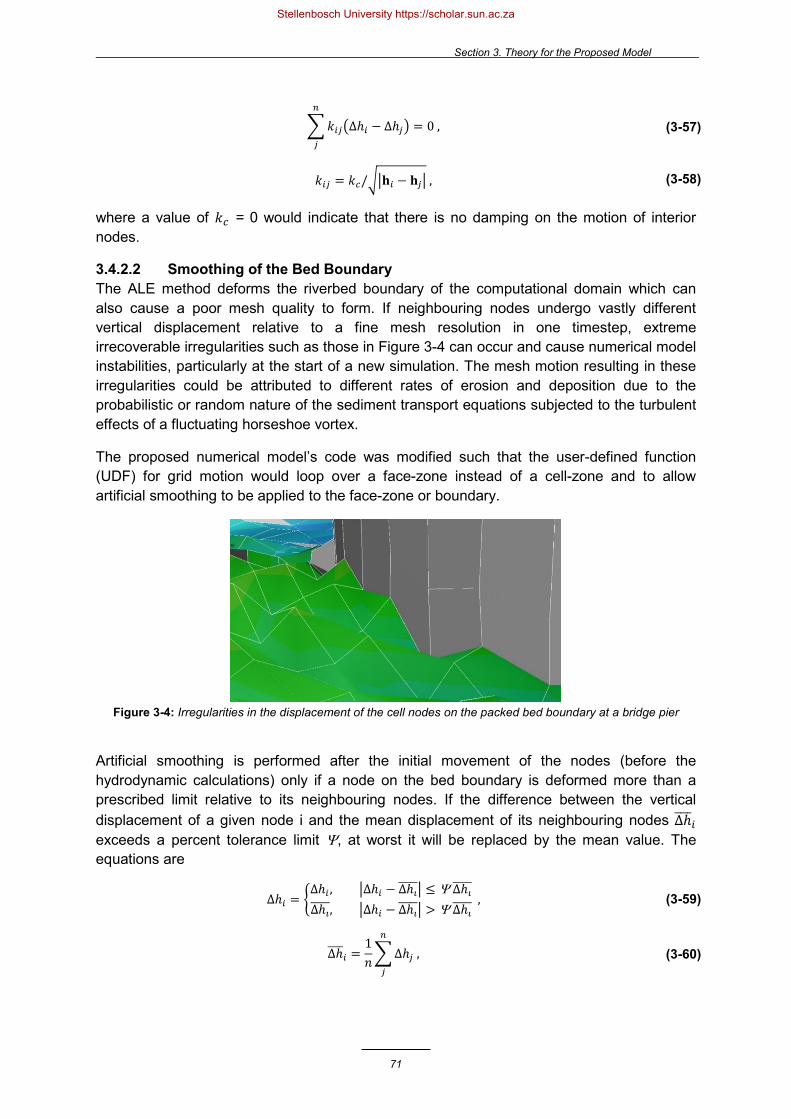
Section 3. Theory for the Proposed Model
71
where a value of 𝑘𝑘𝑐𝑐 = 0 would indicate that there is no damping on the motion of interior nodes.
3.4.2.2 Smoothing of the Bed Boundary The ALE method deforms the riverbed boundary of the computational domain which can also cause a poor mesh quality to form. If neighbouring nodes undergo vastly different vertical displacement relative to a fine mesh resolution in one timestep, extreme irrecoverable irregularities such as those in Figure 3-4 can occur and cause numerical model instabilities, particularly at the start of a new simulation. The mesh motion resulting in these irregularities could be attributed to different rates of erosion and deposition due to the probabilistic or random nature of the sediment transport equations subjected to the turbulent effects of a fluctuating horseshoe vortex.
The proposed numerical model’s code was modified such that the user-defined function (UDF) for grid motion would loop over a face-zone instead of a cell-zone and to allow artificial smoothing to be applied to the face-zone or boundary.
Figure 3-4: Irregularities in the displacement of the cell nodes on the packed bed boundary at a bridge pier
Artificial smoothing is performed after the initial movement of the nodes (before the hydrodynamic calculations) only if a node on the bed boundary is deformed more than a prescribed limit relative to its neighbouring nodes. If the difference between the vertical displacement of a given node i and the mean displacement of its neighbouring nodes ∆ℎ𝑖𝑖 exceeds a percent tolerance limit Ψ, at worst it will be replaced by the mean value. The equations are
𝑘𝑘𝑖𝑖𝑖𝑖∆ℎ𝑖𝑖 − ∆ℎ𝑖𝑖𝑚𝑚
𝑖𝑖
= 0 , (3-57)
𝑘𝑘𝑖𝑖𝑖𝑖 = 𝑘𝑘𝑐𝑐/𝐡𝐡𝑖𝑖 − 𝐡𝐡𝑖𝑖 , (3-58)
∆ℎ𝑖𝑖 = ∆ℎ𝑖𝑖 , ∆ℎ𝑖𝑖 − ∆ℎ𝚤𝚤 ≤ Ψ ∆ℎ𝚤𝚤 ∆ℎ𝚤𝚤, ∆ℎ𝑖𝑖 − ∆ℎ𝚤𝚤 > Ψ ∆ℎ𝚤𝚤 , (3-59)
∆ℎ𝑖𝑖 =1𝑛𝑛∆ℎ𝑖𝑖
𝑚𝑚
𝑖𝑖
, (3-60)
Stellenbosch University https://scholar.sun.ac.za

Section 3. Theory for the Proposed Model
72
where the proposed tolerance limit of 0.1% controls the degree of natural erosion permitted per time-step. Enforcing an artificially smooth profile for numerical stability may reduce the solution accuracy. Therefore, a new variable Σ𝐻𝐻𝑖𝑖 that sums the difference ∆ℎ𝑖𝑖 − ∆ℎ𝚤𝚤 lost to smoothing with time at each node is defined and can be used to monitor the location and quantity of smoothing required.
3.4.3 Alternative Shear Stress Formulations
3.4.3.1 Bed Shear Stress The capability of a numerical model to predict bridge pier scour relies heavily on its ability to resolve the horseshoe vortex as well as the underlying assumptions of the sediment transport functions. Because the difference between the bed shear stress and shear stress threshold is the main parameter governing particle entrainment, an improved formulation for bed shear stress by Abbasnia & Ghiassi (2011) is considered. Traditional sediment transport equations are based on straight unobstructed flow but cannot accurately predict bed shear stress when streamlines are curved. The new formula accounts for the vorticity or flow curvature effect at bridge piers by adding a term for centripetal force into the classic bed shear stress equation. The centripetal force is calculated as
where 𝑣𝑣𝑝𝑝 is the velocity magnitude of the particulate phases and 𝜔𝜔 is the vorticity magnitude derived from the curl of the fluid velocity 𝛚𝛚 = 𝛁𝛁 × 𝐯𝐯𝑞𝑞. Since the centripetal force acts perpendicular to shear force, the new total bed shear stress 𝜏𝜏 is given by
where 𝜏𝜏𝑤𝑤 is the bed shear stress and 𝛼𝛼𝑐𝑐 is a calibration coefficient ranging in value from zero to one used to dampen the effect of the centripetal force. The sensitivity analysis by Abbasnia & Ghiassi (2011) shows that a value of 0.4 to 0.7 yields the most accurate results.
3.4.3.2 Shear Stress Threshold Schneiderbauer & Pirker (2014) and Sawadogo (2015) observed that the angle of repose is a sensitive parameter that can be responsible for destabilizing the surface of the packed bed. As an alternative to equation (3-18), the expression for the shear stress threshold that was successfully implemented by Roulund et al. (2005) for bridge pier scour could be used. The well-known transport equation of Engelund & Fredsøe (1976) was generalized to account for 3D effects and changes in the bed slope. The equation is based on the critical Shields parameter calculated by
where 𝛽𝛽 is the angle of the bed slope to the horizontal and 𝜃𝜃 is the angle of the bed slope to the flow. The static friction coefficient was selected as 𝜇𝜇𝑠𝑠 = 0.63 for sand and the critical Shields parameter as 𝜃𝜃𝑠𝑠,𝑐𝑐 = 0.015 for a horizontal bed.
𝐹𝐹𝑐𝑐 = 𝜌𝜌𝑝𝑝43𝜋𝜋 𝑑𝑑𝑝𝑝2
3
𝑣𝑣𝑝𝑝𝜔𝜔2
, (3-61)
𝜏𝜏 = 𝜏𝜏𝑤𝑤2 + 𝛼𝛼𝑐𝑐𝐹𝐹𝑐𝑐𝐴𝐴2
, (3-62)
𝜏𝜏𝑡𝑡𝜌𝜌𝑝𝑝 − 𝜌𝜌𝑔𝑔𝑑𝑑𝑝𝑝
= 𝜃𝜃𝑠𝑠,𝑐𝑐 𝑐𝑐𝑐𝑐𝑠𝑠𝛽𝛽1 −sin2 𝜃𝜃 tan2𝛽𝛽
𝜇𝜇𝑠𝑠2−
cos𝜃𝜃 sin𝛽𝛽𝜇𝜇𝑠𝑠
, (3-63)
Stellenbosch University https://scholar.sun.ac.za

Section 3. Theory for the Proposed Model
73
3.5 Summary
The focus of the section was to present the coupled fully 3D hydrodynamic model developed by Sawadogo (2015). The first part of the section addressed the Navier-Stokes equations and the 𝑘𝑘-ε turbulent model, while the second part described the sediment transport equations and the IB method used to track the surface of the sediment bed.
Finally, variations to the proposed model code were discussed, namely, the RSM turbulence model, the ALE method and improved shear stress formulations. Additional forcing to the IB method was also coded by enforcing the following condition to the volume fraction of equation (3-33) at neighbouring cells 𝑖𝑖 and 𝑗𝑗 with co-ordinates (𝑥𝑥,𝑦𝑦,𝜕𝜕)
to ensure a fluid cavity is not formed below the sediment bed (or vice versa).
𝛼𝛼𝑏𝑏,𝑖𝑖 ≤ 𝛼𝛼𝑏𝑏,𝑖𝑖 if 𝜕𝜕𝑖𝑖 ≥ 𝜕𝜕𝑖𝑖 , (3-64)
Stellenbosch University https://scholar.sun.ac.za

Section 4. Experimental Work
74
4. Experimental Work
4.1 Introduction
Bridge pier scouring was investigated by physical modelling to generate data in a controlled environment for the validation of the proposed model. Furthermore, observations of bridge pier scour in a laboratory provided invaluable insight on the vortex formation and scour process.
The experimental work was conducted at the Department of Civil Engineering Hydraulics Laboratory, Stellenbosch University, in a rectangular flume with the dimensions of a 40 m length, 1 m width and 1.24 m depth. A sediment bed was packed in the flume around a scaled pier model and water was released to emulate channel flow and local scouring. A model-to-prototype scale of 1:15 was used based on Froude similarity. More detail on the experimental setup and testing procedure is discussed in the subsequent sections.
4.2 Outline of Approach
A total of 48 different tests were conducted whereby 4 different flows, 3 pier shapes and 2 sediment beds were used. The equilibrium scour hole that formed in the vicinity of the scaled pier model was surveyed, along with velocity measurements to visualize the flow field. Furthermore, the flow field was measured for the flume setup without sediment, i.e. a fixed bed, to simulate a rigid plane-bed flow. Note that the range of flows under which local scour was observed was different for the two sediment materials. Figure 4-1 outlines the variables for the different experiments. Fifteen percent of these experiments were duplicated 3 times to ensure repeatability of the results.
Figure 4-1: Overview of experimental work
The 3 different pier shapes selected for the physical modelling are shown in Figure 4-2 and Figure 4-3. The first pier model has a standard cylindrical shape with a diameter of 110 mm, which is based on a scale of 1:15. The round nosed and sharp nosed piers were designed for the same pier width but with a length of 770 mm to represent a small 2 lane bridge cross-section with an 𝐿𝐿/𝐷𝐷 ratio of 7. PVC pipe offcuts were used to construct the piers which were capable of resisting flow induced deflections.
Constant flow depth with 4 different flows
Model 1: Cylindrical pier
Repeat 15% of experiments
Model 2: Round nosed pier
Model 3:Sharp nosed pier
Fixed bed Sediment bed
Two different sediments
Stellenbosch University https://scholar.sun.ac.za
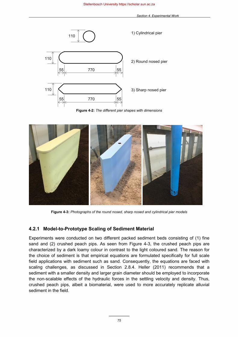
Section 4. Experimental Work
75
Figure 4-2: The different pier shapes with dimensions
Figure 4-3: Photographs of the round nosed, sharp nosed and cylindrical pier models
4.2.1 Model-to-Prototype Scaling of Sediment Material
Experiments were conducted on two different packed sediment beds consisting of (1) fine sand and (2) crushed peach pips. As seen from Figure 4-3, the crushed peach pips are characterized by a dark loamy colour in contrast to the light coloured sand. The reason for the choice of sediment is that empirical equations are formulated specifically for full scale field applications with sediment such as sand. Consequently, the equations are faced with scaling challenges, as discussed in Section 2.8.4. Heller (2011) recommends that a sediment with a smaller density and larger grain diameter should be employed to incorporate the non-scalable effects of the hydraulic forces in the settling velocity and density. Thus, crushed peach pips, albeit a biomaterial, were used to more accurately replicate alluvial sediment in the field.
1) Cylindrical pier
2) Round nosed pier
3) Sharp nosed pier
110
55 770 55
55 770 55
110
110
Stellenbosch University https://scholar.sun.ac.za

Section 4. Experimental Work
76
Table 4-1 summarizes the defining material properties for the two different “sediments” which were measured directly in the laboratory.
• A standard sieve analysis was performed to determine the particle size distributions, shown in Figure 4-4, from which the particle sizes 𝑑𝑑50, 𝑑𝑑90 and 𝑑𝑑𝐼𝐼𝑎𝑎𝑚𝑚, as well as the particle size deviation 𝜎𝜎𝑔𝑔, were determined. According to Chiew (1984), both sediment beds may be classified as uniformly graded for the condition 𝜎𝜎𝑔𝑔 < 2.
• The Maximum Theoretical Relative Density (MTRD) was established by a Rice Density Test. Sawadogo (2015) used a similar sample of crushed peach pips and that the associated properties (𝑑𝑑50 = 0.74 mm, MTRD = 1.35 and 𝜎𝜎𝑔𝑔 = 1.65) compare favourably with those in Table 4-1. Furthermore, the MTRD for the fine sand is almost identical to the typical value of 2.65 for alluvial sand found in natural rivers (Section 2.7.2.2).
• The angle of repose φ was roughly established by the fixed funnel method for saturated and dry material and is in agreement with typical values quoted in Section 2.7.2.5, i.e. 45° for saturated material and 30 to 35° for dry sand.
• Finally, the settling velocity was measured in a settling column. With 𝑤𝑤50 for sand being the exception, the measured settling velocities compare well with theoretical settling velocities determined analytically by equation (2-23) (sand: 𝑤𝑤50 = 0.048, 𝑤𝑤90 = 0.057, peach pips: 𝑤𝑤50 = 0.036, 𝑤𝑤90 = 0.051).
Figure 4-4: Particle size distribution curves for the fine sand and the crushed peach pips
Table 4-1: Sediment characteristics measured for the fine sand and crushed peach pips
0.0
20.0
40.0
60.0
80.0
100.0
0.01 0.1 1 10
Perc
enta
ge P
sasi
ng (%
)
Sieve Size (mm)
Fine Sand
Peach Pips
Properties 𝒅𝒅𝟓𝟓𝟓𝟓 (mm)
𝒅𝒅𝟗𝟗𝟓𝟓 (mm)
𝒅𝒅𝒎𝒎𝒎𝒎𝒎𝒎 (mm) 𝝈𝝈𝒈𝒈 𝒅𝒅𝒈𝒈
(mm) MTRD 𝛗𝛗𝐬𝐬𝐬𝐬𝐬𝐬 𝛗𝛗𝐝𝐝𝐝𝐝𝐝𝐝 𝒘𝒘𝟓𝟓𝟓𝟓
(m/s) 𝒘𝒘𝟗𝟗𝟓𝟓
(m/s)
1. Fine sand 0.214 0.308 1.180 1.360 0.209 2.630 45° 28° 0.036 0.059
2. Peach pips 0.740 1.457 2.360 1.570 0.766 1.280 44° 32° 0.032 0.053
Stellenbosch University https://scholar.sun.ac.za

Section 4. Experimental Work
77
Instead of the median or geometric mean particle sizes, the particle size corresponding to the average settling velocity for the sediment material may be used as a representative for the particle grading. From equation (2-23), particle sizes 0.225 mm and 0.928 mm are calculated for the fine sand and peach pips respectively based on the average settling velocities of 0.049 m/s and 0.041 m/s.
Rooseboom et al. (1983) recommended that settling velocity better represents the transportability of sediment as opposed to particle size. Therefore, the Modified Lui Diagram in Figure 4-6 was generated to obtain an identical movability number (𝐶𝐶∗/𝑤𝑤) and thereby scale the density and particle sizes for the peach pips to that of a representative in-situ alluvial sediment. Recall from Section 2.6.1.4 that the movability number (or stream power) and particle Reynolds number are defined respectively as
where 𝑆𝑆 is the energy slope and equation (2-23) was used to relate the particle density and size with settling velocity. The final scaled prototype particle sizes would be 3.21 mm and 1.87 mm respectively for the sand and peach pip materials.
Figure 4-5: Modified Lui Diagram to scale peach pips
4.2.2 Incipient Motion and Appropriate Flow Rates
Appropriate flow rates were selected for testing within the limit 0.5 𝑣𝑣𝐶𝐶 < 𝑣𝑣1 ≤ 𝑣𝑣𝐶𝐶 for clear-water scouring. Since numerous equations exist to define incipient motion or critical velocity 𝑣𝑣𝐶𝐶 of the packed bed (refer to Table 4-2), it was determined by an experimental procedure whereby the flow rate was increased incrementally until incipient motion of particles was observed. No local scour pattern was observed for the condition 𝑣𝑣1 < ~0.5 𝑣𝑣𝐶𝐶 as noted by Sheppard & Miller (2006) and Sheppard & Melville (2014), so clear-water scouring was only present over a small range of velocities. The equations used in Table 4-2 are given in Appendix A.
0
0.2
0.4
0.6
0.8
1
1.2
1.4
1.6
1.8
2
1 10 100 1000
Mov
abili
ty N
umbe
r
Particle Reynolds Number
Pipsd50
Pipsdmax
Pipsd90
Scaledd50
Scaledd90 Scaled
dmax
Boundary laminar flow region
Turbulent flow region
NO SEDIMENTMOVEMENT
SEDIMENT MOVEMENT
𝐶𝐶∗
𝑤𝑤=𝑔𝑔𝑦𝑦1𝑆𝑆𝑤𝑤
, (4-1)
𝑅𝑅𝑅𝑅𝑝𝑝 =𝑔𝑔𝑦𝑦1𝑆𝑆𝑑𝑑
υ , (4-2)
Stellenbosch University https://scholar.sun.ac.za
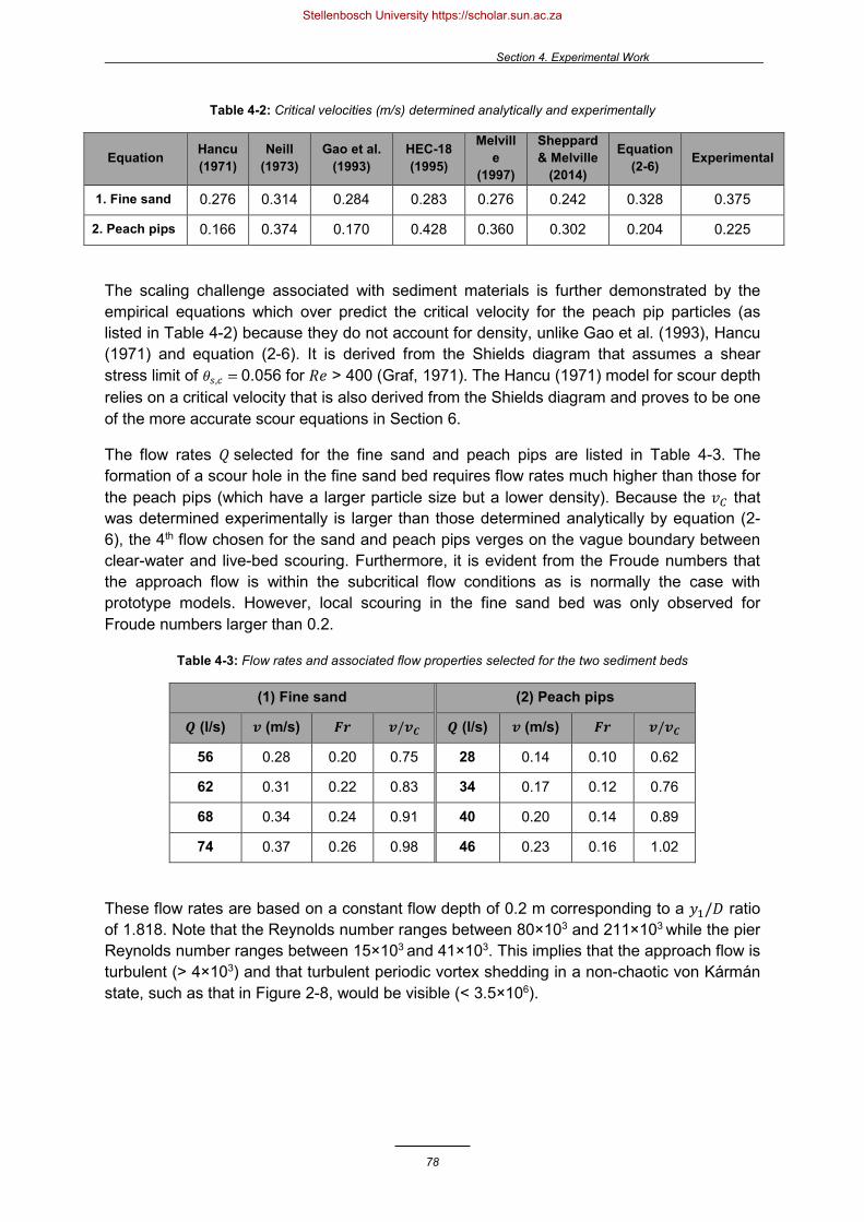
Section 4. Experimental Work
78
Table 4-2: Critical velocities (m/s) determined analytically and experimentally
Equation Hancu (1971)
Neill (1973)
Gao et al. (1993)
HEC-18 (1995)
Melville
(1997)
Sheppard & Melville
(2014)
Equation (2-6) Experimental
1. Fine sand 0.276 0.314 0.284 0.283 0.276 0.242 0.328 0.375
2. Peach pips 0.166 0.374 0.170 0.428 0.360 0.302 0.204 0.225
The scaling challenge associated with sediment materials is further demonstrated by the empirical equations which over predict the critical velocity for the peach pip particles (as listed in Table 4-2) because they do not account for density, unlike Gao et al. (1993), Hancu (1971) and equation (2-6). It is derived from the Shields diagram that assumes a shear stress limit of 𝜃𝜃𝑠𝑠,𝑐𝑐 = 0.056 for 𝑅𝑅𝑅𝑅 > 400 (Graf, 1971). The Hancu (1971) model for scour depth relies on a critical velocity that is also derived from the Shields diagram and proves to be one of the more accurate scour equations in Section 6.
The flow rates 𝑄𝑄 selected for the fine sand and peach pips are listed in Table 4-3. The formation of a scour hole in the fine sand bed requires flow rates much higher than those for the peach pips (which have a larger particle size but a lower density). Because the 𝑣𝑣𝐶𝐶 that was determined experimentally is larger than those determined analytically by equation (2-6), the 4th flow chosen for the sand and peach pips verges on the vague boundary between clear-water and live-bed scouring. Furthermore, it is evident from the Froude numbers that the approach flow is within the subcritical flow conditions as is normally the case with prototype models. However, local scouring in the fine sand bed was only observed for Froude numbers larger than 0.2.
Table 4-3: Flow rates and associated flow properties selected for the two sediment beds
(1) Fine sand (2) Peach pips
𝑸𝑸 (l/s) 𝒗𝒗 (m/s) 𝑭𝑭𝑭𝑭 𝒗𝒗/𝒗𝒗𝑪𝑪 𝑸𝑸 (l/s) 𝒗𝒗 (m/s) 𝑭𝑭𝑭𝑭 𝒗𝒗/𝒗𝒗𝑪𝑪
56 0.28 0.20 0.75 28 0.14 0.10 0.62
62 0.31 0.22 0.83 34 0.17 0.12 0.76
68 0.34 0.24 0.91 40 0.20 0.14 0.89
74 0.37 0.26 0.98 46 0.23 0.16 1.02
These flow rates are based on a constant flow depth of 0.2 m corresponding to a 𝑦𝑦1/𝐷𝐷 ratio of 1.818. Note that the Reynolds number ranges between 80×103 and 211×103 while the pier Reynolds number ranges between 15×103 and 41×103. This implies that the approach flow is turbulent (> 4×10³) and that turbulent periodic vortex shedding in a non-chaotic von Kármán state, such as that in Figure 2-8, would be visible (< 3.5×10⁶).
Stellenbosch University https://scholar.sun.ac.za
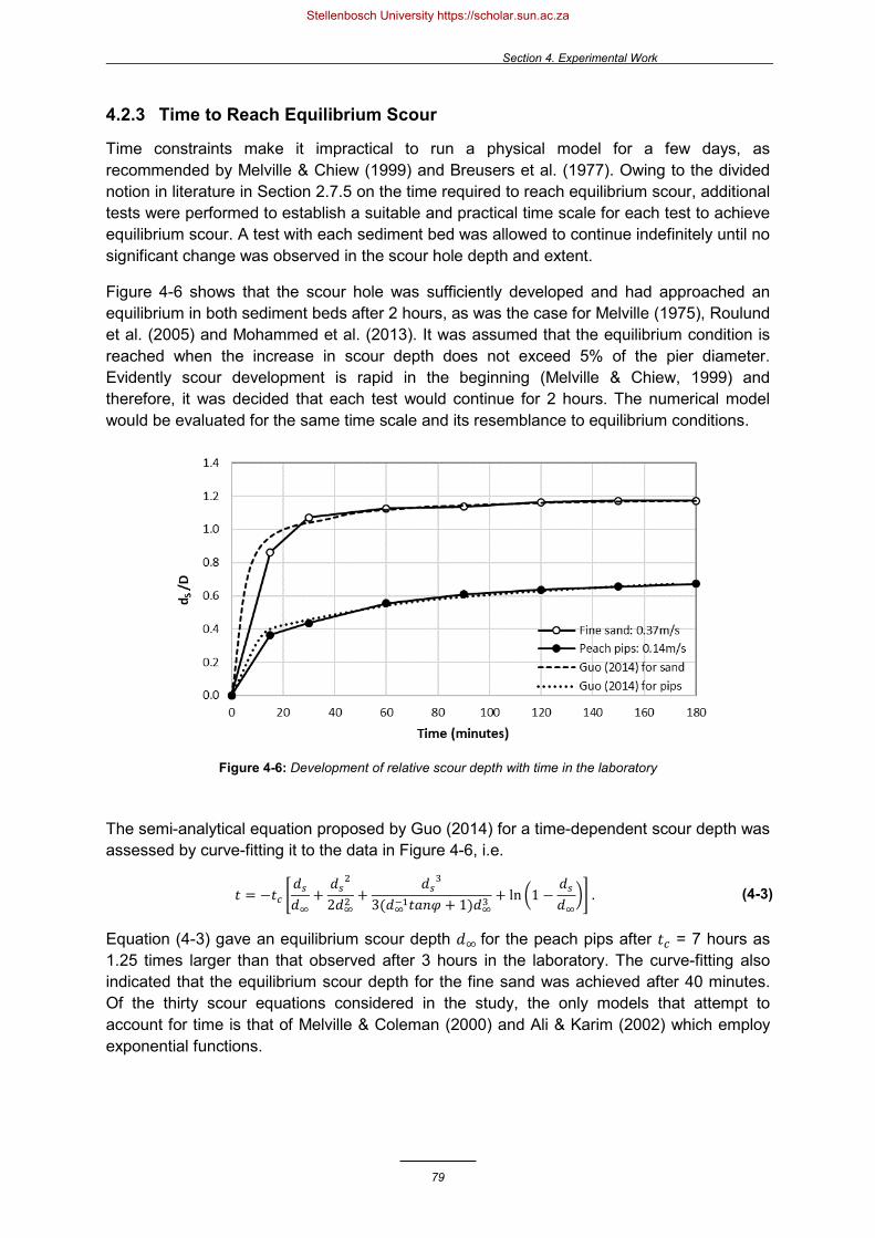
Section 4. Experimental Work
79
4.2.3 Time to Reach Equilibrium Scour
Time constraints make it impractical to run a physical model for a few days, as recommended by Melville & Chiew (1999) and Breusers et al. (1977). Owing to the divided notion in literature in Section 2.7.5 on the time required to reach equilibrium scour, additional tests were performed to establish a suitable and practical time scale for each test to achieve equilibrium scour. A test with each sediment bed was allowed to continue indefinitely until no significant change was observed in the scour hole depth and extent.
Figure 4-6 shows that the scour hole was sufficiently developed and had approached an equilibrium in both sediment beds after 2 hours, as was the case for Melville (1975), Roulund et al. (2005) and Mohammed et al. (2013). It was assumed that the equilibrium condition is reached when the increase in scour depth does not exceed 5% of the pier diameter. Evidently scour development is rapid in the beginning (Melville & Chiew, 1999) and therefore, it was decided that each test would continue for 2 hours. The numerical model would be evaluated for the same time scale and its resemblance to equilibrium conditions.
Figure 4-6: Development of relative scour depth with time in the laboratory
The semi-analytical equation proposed by Guo (2014) for a time-dependent scour depth was assessed by curve-fitting it to the data in Figure 4-6, i.e.
Equation (4-3) gave an equilibrium scour depth 𝑑𝑑∞ for the peach pips after 𝑡𝑡𝑐𝑐 = 7 hours as 1.25 times larger than that observed after 3 hours in the laboratory. The curve-fitting also indicated that the equilibrium scour depth for the fine sand was achieved after 40 minutes. Of the thirty scour equations considered in the study, the only models that attempt to account for time is that of Melville & Coleman (2000) and Ali & Karim (2002) which employ exponential functions.
𝑡𝑡 = −𝑡𝑡𝑐𝑐 𝑑𝑑𝑠𝑠𝑑𝑑∞
+𝑑𝑑𝑠𝑠
2
2𝑑𝑑∞2+
𝑑𝑑𝑠𝑠3
3(𝑑𝑑∞−1𝑡𝑡𝑎𝑎𝑛𝑛𝜑𝜑 + 1)𝑑𝑑∞3+ ln 1 −
𝑑𝑑𝑠𝑠𝑑𝑑∞
. (4-3)
Stellenbosch University https://scholar.sun.ac.za

Section 4. Experimental Work
80
4.3 Physical Model Setup
The physical model consisted of an elevated rectangular flume, with a 40 m length, 1 m width and 1.24 m depth, and a pier secured to the base of the flume with silicone adhesive. The pier was fixed in the centre of the flume to ensure that the fully developed flow would remain unaffected by conditions upstream or downstream of the pier. As a rule of thumb, the entrance length required for flow to become fully developed is 10 to 15 times the hydraulic diameter of the flume (Versteeg & Malalasekera, 2007). Therefore, the entrance length condition > ~5 to 9 m was satisfied based on a hydraulic diameter of 0.571 m.
Limited sediment material was available so the sediment bed was only placed in the vicinity of the pier, extending 5 m upstream and 2 m downstream of the pier. The bed was packed to a depth of 0.3 m to ensure that the scour hole remained unrestricted by the bed boundary. The bed boundary upstream of the sediment bed was constructed with a slope of 1:5 to limit disruption of the flow profile.
A constant flow depth was selected based on the 0.333 m limiting flow depth which is taken as a third of the flume width to minimize shearing or boundary layer effects of the side walls on the junction flow at the pier. Thus, a constant flow depth of 0.2 m above the sediment bed was maintained throughout the tests by manually adjusting a sluice gate downstream of the pier. A flowmeter and manual valve were used to adjust and control the flow rates for each test. In addition, a V-notch weir was installed upstream of the pier to monitor and measure the flow with improved accuracy. The turbulence created by the weir was then smoothed by a plunge pool with tubes to realign the streamlines. Needle gauges were used to monitor the water levels upstream of the sluice gate and weir at a distance much greater than the drawdown length of 4 times ℎ𝑉𝑉 or the head over the weir (Chadwick et al., 2013). The flow rate in m3/s corresponding to the water levels upstream of the V-notch weir was determined by the equation below for a 90° vee
with a 𝐶𝐶𝑑𝑑 value of 0.59. The flow rate corresponding to the voltage reading 𝑉𝑉0 on the flowmeter was determined by the calibration equation for 𝐿𝐿 = 0.3 m given by
Figure 4-7 shows a schematic representation of the flume setup and Figure 4-8 shows photographs of the flume setup with the pier, sediment bed, trolley and needle gauge, as well as the sluice gate, V-notch weir and plunge pool.
𝑄𝑄 =8
15𝐶𝐶𝑑𝑑2𝑔𝑔 tan
90°2
ℎ𝑉𝑉52 , (4-4)
𝑄𝑄 = (𝑉𝑉0 0.262𝐿𝐿⁄ ) 𝜋𝜋/4 𝐿𝐿2. (4-5)
Stellenbosch University https://scholar.sun.ac.za

Section 4. Experimental Work
81
Figu
re 4
-7: P
rofil
e of
the
expe
rimen
tal f
lum
e la
yout
Stellenbosch University https://scholar.sun.ac.za
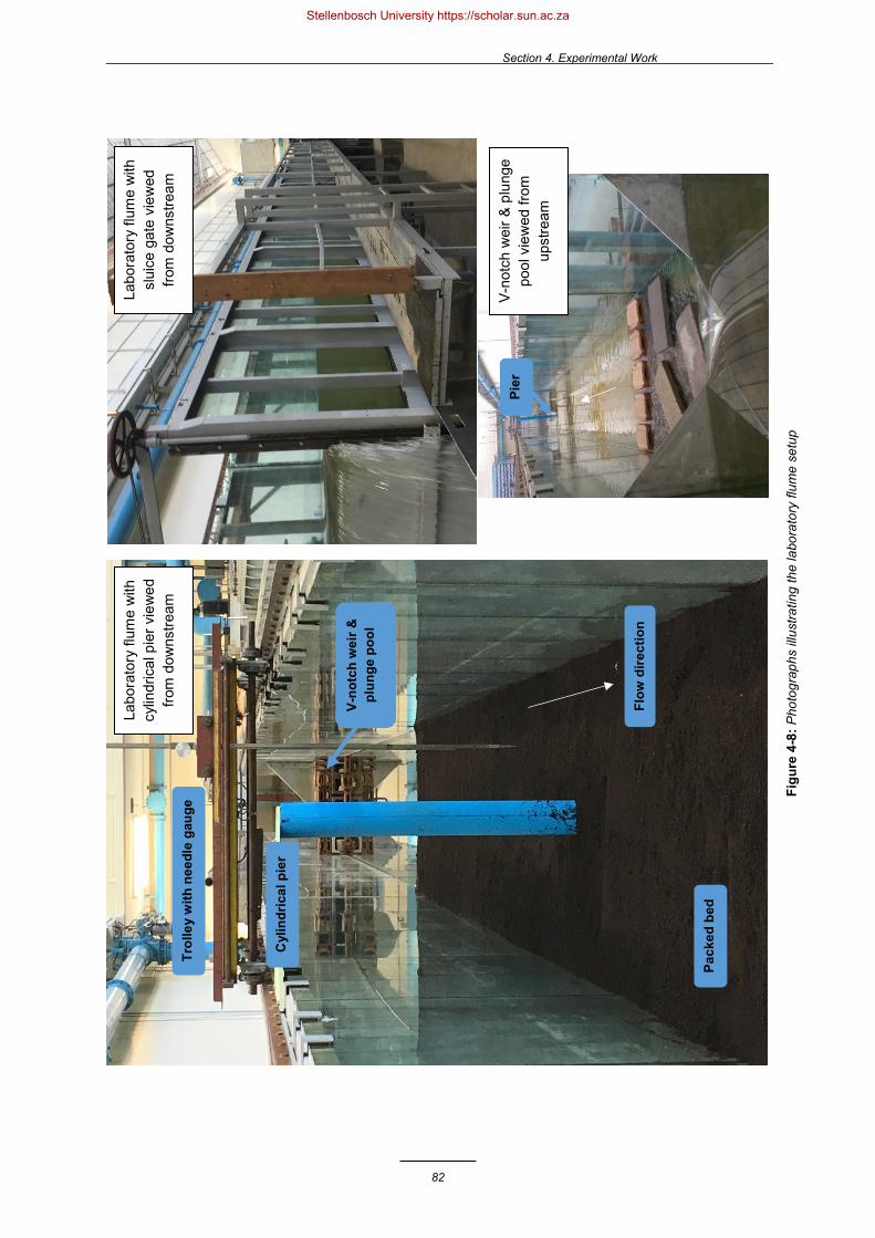
Section 4. Experimental Work
82
Labo
rato
ry fl
ume
with
sl
uice
gat
e vi
ewed
fro
m d
owns
tream
V-no
tch
wei
r & p
lung
e po
ol v
iew
ed fr
om
upst
ream
Labo
rato
ry fl
ume
with
cy
lindr
ical
pie
r vie
wed
fro
m d
owns
tream
Pack
ed b
ed
Trol
ley
with
nee
dle
gaug
e
Cyl
indr
ical
pie
r
V-no
tch
wei
r &
plun
ge p
ool
Pier
Flow
dire
ctio
n
Figu
re 4
-8: P
hoto
grap
hs il
lust
ratin
g th
e la
bora
tory
flum
e se
tup
Stellenbosch University https://scholar.sun.ac.za
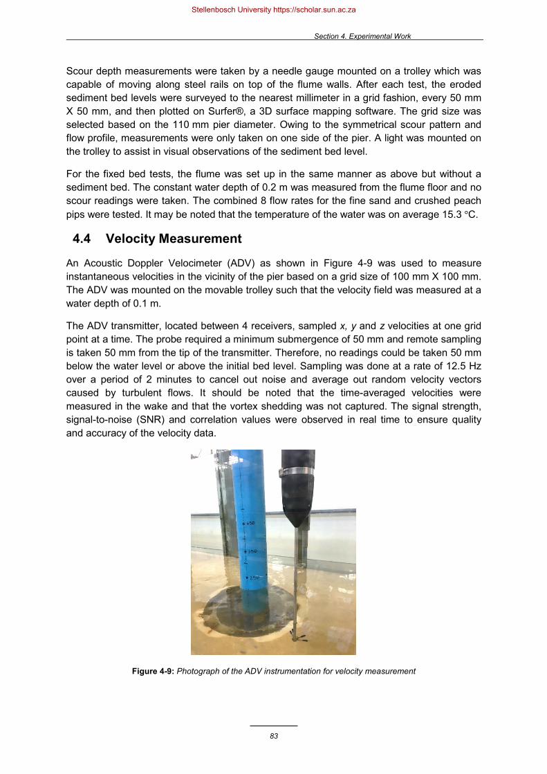
Section 4. Experimental Work
83
Scour depth measurements were taken by a needle gauge mounted on a trolley which was capable of moving along steel rails on top of the flume walls. After each test, the eroded sediment bed levels were surveyed to the nearest millimeter in a grid fashion, every 50 mm X 50 mm, and then plotted on Surfer®, a 3D surface mapping software. The grid size was selected based on the 110 mm pier diameter. Owing to the symmetrical scour pattern and flow profile, measurements were only taken on one side of the pier. A light was mounted on the trolley to assist in visual observations of the sediment bed level.
For the fixed bed tests, the flume was set up in the same manner as above but without a sediment bed. The constant water depth of 0.2 m was measured from the flume floor and no scour readings were taken. The combined 8 flow rates for the fine sand and crushed peach pips were tested. It may be noted that the temperature of the water was on average 15.3 °C.
4.4 Velocity Measurement
An Acoustic Doppler Velocimeter (ADV) as shown in Figure 4-9 was used to measure instantaneous velocities in the vicinity of the pier based on a grid size of 100 mm X 100 mm. The ADV was mounted on the movable trolley such that the velocity field was measured at a water depth of 0.1 m.
The ADV transmitter, located between 4 receivers, sampled x, y and z velocities at one grid point at a time. The probe required a minimum submergence of 50 mm and remote sampling is taken 50 mm from the tip of the transmitter. Therefore, no readings could be taken 50 mm below the water level or above the initial bed level. Sampling was done at a rate of 12.5 Hz over a period of 2 minutes to cancel out noise and average out random velocity vectors caused by turbulent flows. It should be noted that the time-averaged velocities were measured in the wake and that the vortex shedding was not captured. The signal strength, signal-to-noise (SNR) and correlation values were observed in real time to ensure quality and accuracy of the velocity data.
Figure 4-9: Photograph of the ADV instrumentation for velocity measurement
Stellenbosch University https://scholar.sun.ac.za

Section 4. Experimental Work
84
Vertical velocity profiles were also measured at five points in the vicinity of the scour hole, 0.15 m upstream of the pier and 0.15 m beside the pier, where the separated flow and horseshoe vortex formation were anticipated. Figure 4-10 indicates the position of the vertical velocity measurements relative to the different piers and to the centrelines of the scour holes. Note that the ADV measurements were limited to only one grid point at a specific elevation at a time.
Figure 4-10: Position of vertical velocity measurements relative to the cylindrical, the round nosed and the sharp nosed piers
4.5 Testing Procedure
Before commencing the physical model test, the surface of the sediment bed was uniformly levelled to an elevation of 0.3 m above the flume floor. The upstream and downstream sections of the flume were then slowly filled with water at a rate < 2 l/s. This was done over a period of 2 hours to avoid disturbing the surface of the sediment bed or causing an initial scour hole prior to commencing the actual test. As the water depth reached the top of the bed, the bed was levelled as required to ensure the water flowed uniformly over the bed. After the flume was filled with water and the sediment bed was consolidated and saturated, the initial bed level was surveyed under water.
The actual test began once the valve and sluice gate had been manually adjusted to obtain the desired flow rate and to maintain the constant water depth of 0.2 m (above the sediment bed). The ADV was manually moved between grid points every 2 minutes. Once the scour process had reached equilibrium after approximately 2 hours, the valve was closed and the scour hole was surveyed under water. The flow rate was then increased and the process was repeated for a new test. Each test would take 2.5 to 3 hours while the process of gradually filling the flume would take 2 hours.
A limitation of the movable tests is that the scour holes could not be surveyed under flowing water because the trailing vortex that formed around the needle gauge impaired visibility. The consequence of this is that the scour hole may have been subjected to an unknown quantity of backfilling while reducing the flow.
X
X
X
X
X
X
y (m
)
x (m)
Flow
Dire
ctio
n
Stellenbosch University https://scholar.sun.ac.za
Section 4. Experimental Work
85
The fixed bed test was simpler as the flume did not have to be gradually filled with water and no scour hole had to be surveyed. The flume was simply filled with water, and the valve and sluice gate were then manually adjusted and the test would begin. Velocity readings were taken before repeating the process for a new test. The process would take approximately 1.5 hours per test.
4.6 Summary
Laboratory tests were conducted in a flume with a sediment bed packed around a scaled pier model in order to investigate the bridge pier scouring process. A total of 48 different tests were conducted whereby 4 different flows, 3 different pier shapes and 2 different sediment beds were used. Additional tests were performed to select appropriate flow rates from verified critical velocities, to determine the time required to reach equilibrium scouring and to ensure repeatability of the results. A movable trolley with a needle gauge was used to survey the equilibrium scour hole in a grid fashion and to visualize the flow field, an ADV measured velocities. Furthermore, the flow field was measured for the flume set up with a fixed bed. Measurements were only taken on the one side of the pier, owing to symmetry, and were plotted on Surfer®.
Stellenbosch University https://scholar.sun.ac.za
Section 5. Numerical Model Setup
86
5. Numerical Model Setup
5.1 Introduction
This section describes the model setup for the numerical simulation of the proposed coupled fully 3D hydrodynamic model. In order to validate the proposed numerical model against the experimental data, the goal of the model setup was to replicate the physical model setup while optimizing computational effort and accuracy. This was accomplished by ensuring the mesh is fine enough to accurately resolve the fluid flow while limiting the domain size and the number of cells. Because the accuracy of a numerical model relies on the underlying assumptions of the sediment transport algorithms as well as its ability to resolve the vortex structures, the model setup was an imperative step to resolve the fluid flow and vortex structures.
The setup process was based on the different approaches adopted by Sawadogo (2015), Schneiderbauer & Pirker (2014), and the other bridge pier scour models in Section 2.9. The ANSYS computer package was used to set up and solve the bridge pier model by adopting the following steps, which are discussed in detail in subsequent sections:
1) Define the model geometry for the computational domain in ANSYS DesignModeler; 2) Generate the mesh by discretising the flow domain into small grid cells in ANSYS
Meshing; 3) Set up the boundary conditions for the model; 4) Adopt a numerical solution technique and procedure; 5) Solve the governing equations and submodels at each cell using ANSYS Fluent; and 6) Visualize and analyse the results on Surfer® in concurrence with the experimental
work.
5.2 Computational Fluid Dynamics Software
The flow equations for the Eulerian multiphase and turbulence models, presented in Section 3.2, were solved by ANSYS Fluent software. The computer program is extensively used to model fluid flow using the finite volume method. Ali & Karim (2002), Salaheldin et al. (2004) and Xiong et al. (2014) also used ANSYS Fluent to perform hydro-morphodynamic calculations.
The sediment transport submodels proposed in Section 3.3, namely the erosion and deposition model, as well as the modelling of the deformation of the packed bed’s surface cannot be implemented in the standard version of ANSYS Fluent. The software offers a special feature called User Defined Functions (UDFs) which allow the user to specify customised model parameters and to define additional functions or code in C++ programming language. The customised UDFs were compiled and dynamically linked with the ANSYS Fluent solver. Throughout the study, newer versions of the ANSYS Fluent software were regularly released and upgraded from v16.0 to v19.3 to remain current. While the syntax for the UDFs were generally unaffected, it should be noted that the differing interfaces can cause the coupling of certain submodels to be concealed.
Stellenbosch University https://scholar.sun.ac.za

Section 5. Numerical Model Setup
87
5.3 Geometry of Model Domain
The fluid domain was set up by applying pier and flume dimensions taken from the physical model setup (1 m width and 0.2 m water depth). However, the full 40 m length of the laboratory flume was not modelled in order to significantly reduce the number of grid cells generated and subsequently, to decrease the computational time. The experimental work showed that the extent of the scour length was no more than 0.4 m upstream of the pier and the deposition length 0.8 m downstream of the pier for a scour depth less than 0.2 m. Thus, the sediment bed was only modelled for this domain. Only the flow field above the sediment bed was modelled, as well as a distance of approximately 12 times the pier width (~1.4 m) was modelled downstream of the pier to ensure the outflow remained undisturbed (Salhaldin et al., 2004; Kirkil & Constantinescu, 2005). The entrance length condition for fully developed flow (~5 to 9 m) was not satisfied because this generated an unfeasible number of cells (up to 10 times more cells) and was instead incorporated by the inlet boundary. Figure 5-1 shows the domain geometries for the 3 pier shapes that were modelled in ANSYS DesignModeler as a simplified representation of the laboratory setup. The dimensions for the model setup are given in terms of the pier diameter and are similar to those used by other numerical models for bridge pier scour. Note that the preferred orientation of the model geometry relative to the axes is important – the flow direction should be in the positive 𝑥𝑥-axis direction with scouring in the 𝜕𝜕-direction.
5.1 Model Computational Grid
Ideally, fluid flow is best described by a structured grid of hexagon cells aligned with the streamlines to achieve higher quality, more robust solutions and to limit false diffusion for a 2nd order solution. However, bridge piers with curved surfaces present an additional challenge in terms of meshing. A multi-block grid was used to accommodate the circular pier in a hex-dominant fluid domain. Several different grids were constructed to establish the approach that offered the best mesh quality. A high orthogonal quality, a low skewness and a low aspect ratio are particularly important in regions where strong transverse gradients exist (Fluent, 2011). Figure 5-2 illustrates three of the primary approaches used to model the computational grid:
• The unstructured grid dramatically reduces the time required for meshing but offers limited control over the shape and quality of the grid. False diffusion is generated which is highlighted by the fact that a symmetrical grid cannot be generated in this instance.
• The nonorthogonal curvilinear grid was generated by using a spline to accommodate the streamlined flow around the piers. However, ANSYS Meshing is not capable of smoothing the poor quality and highly skewed cells that appear upstream and downstream of the pier.
• The orthogonal grid was generated by modelling a cylindrical block at the centre of a cross multi-block. Strictly defined and calculated edge sizings ensure the entire grid remains structured. This approach is favoured because it offers control over the cell resolution at the pier and allows poor-quality cells to be removed at the area of interest.
Stellenbosch University https://scholar.sun.ac.za

Section 5. Numerical Model Setup
88
Figure 5-1: Geometry of computational fluid domain for (a) the cylindrical pier (b) the round nosed pier and
(c) the sharp nosed pier
Inlet
Outlet
1.8D = 200
1.8D = 200
a) Cylindrical pier
b) Round nosed pier
c) Sharp nosed pier
Origin
Stellenbosch University https://scholar.sun.ac.za
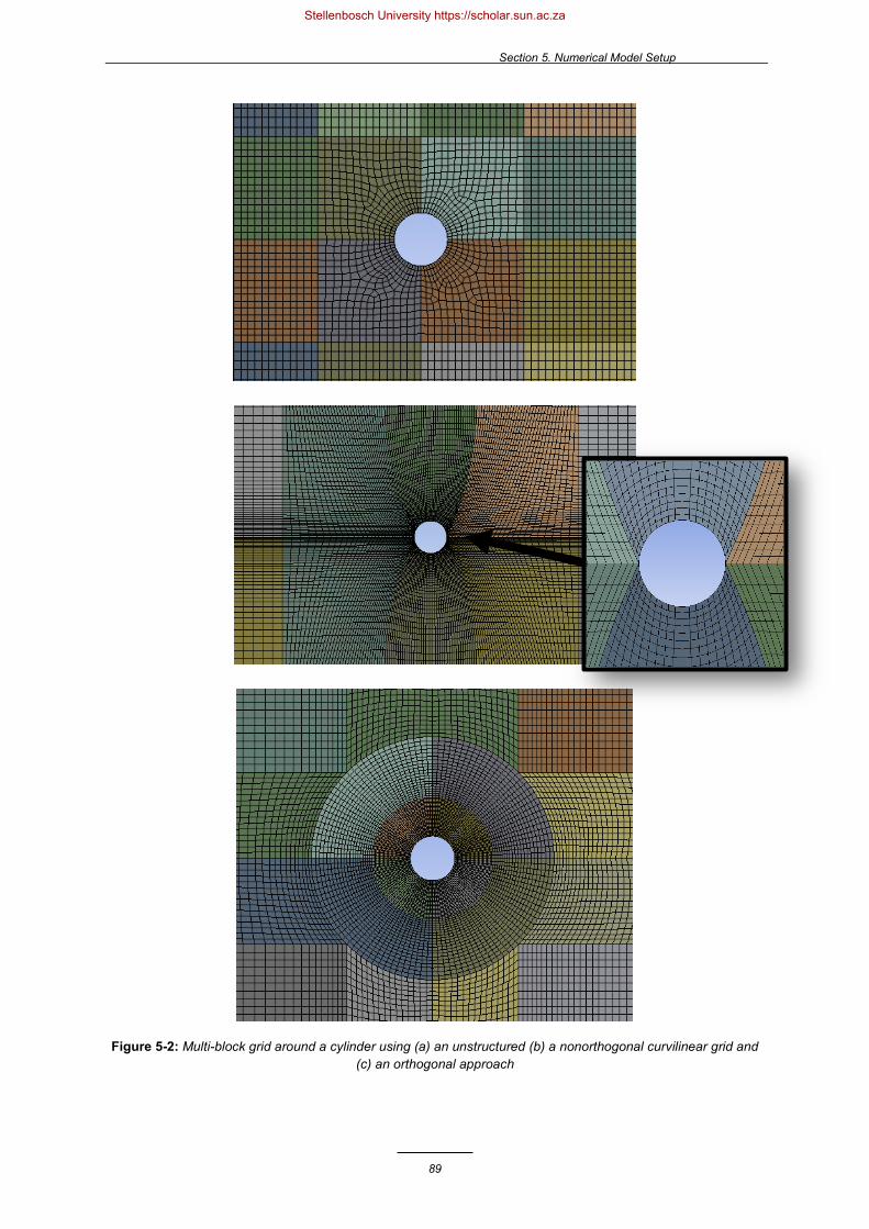
Section 5. Numerical Model Setup
89
Figure 5-2: Multi-block grid around a cylinder using (a) an unstructured (b) a nonorthogonal curvilinear grid and (c) an orthogonal approach
Stellenbosch University https://scholar.sun.ac.za
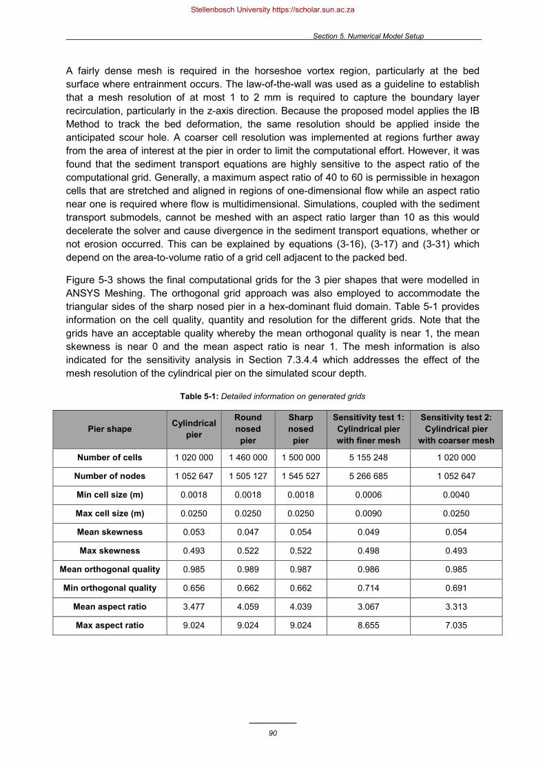
Section 5. Numerical Model Setup
90
A fairly dense mesh is required in the horseshoe vortex region, particularly at the bed surface where entrainment occurs. The law-of-the-wall was used as a guideline to establish that a mesh resolution of at most 1 to 2 mm is required to capture the boundary layer recirculation, particularly in the z-axis direction. Because the proposed model applies the IB Method to track the bed deformation, the same resolution should be applied inside the anticipated scour hole. A coarser cell resolution was implemented at regions further away from the area of interest at the pier in order to limit the computational effort. However, it was found that the sediment transport equations are highly sensitive to the aspect ratio of the computational grid. Generally, a maximum aspect ratio of 40 to 60 is permissible in hexagon cells that are stretched and aligned in regions of one-dimensional flow while an aspect ratio near one is required where flow is multidimensional. Simulations, coupled with the sediment transport submodels, cannot be meshed with an aspect ratio larger than 10 as this would decelerate the solver and cause divergence in the sediment transport equations, whether or not erosion occurred. This can be explained by equations (3-16), (3-17) and (3-31) which depend on the area-to-volume ratio of a grid cell adjacent to the packed bed.
Figure 5-3 shows the final computational grids for the 3 pier shapes that were modelled in ANSYS Meshing. The orthogonal grid approach was also employed to accommodate the triangular sides of the sharp nosed pier in a hex-dominant fluid domain. Table 5-1 provides information on the cell quality, quantity and resolution for the different grids. Note that the grids have an acceptable quality whereby the mean orthogonal quality is near 1, the mean skewness is near 0 and the mean aspect ratio is near 1. The mesh information is also indicated for the sensitivity analysis in Section 7.3.4.4 which addresses the effect of the mesh resolution of the cylindrical pier on the simulated scour depth.
Table 5-1: Detailed information on generated grids
Pier shape Cylindrical pier
Round nosed
pier
Sharp nosed pier
Sensitivity test 1: Cylindrical pier with finer mesh
Sensitivity test 2: Cylindrical pier
with coarser mesh
Number of cells 1 020 000 1 460 000 1 500 000 5 155 248 1 020 000
Number of nodes 1 052 647 1 505 127 1 545 527 5 266 685 1 052 647
Min cell size (m) 0.0018 0.0018 0.0018 0.0006 0.0040
Max cell size (m) 0.0250 0.0250 0.0250 0.0090 0.0250
Mean skewness 0.053 0.047 0.054 0.049 0.054
Max skewness 0.493 0.522 0.522 0.498 0.493
Mean orthogonal quality 0.985 0.989 0.987 0.986 0.985
Min orthogonal quality 0.656 0.662 0.662 0.714 0.691
Mean aspect ratio 3.477 4.059 4.039 3.067 3.313
Max aspect ratio 9.024 9.024 9.024 8.655 7.035
Stellenbosch University https://scholar.sun.ac.za

Section 5. Numerical Model Setup
91
Figure 5-3: Profile of computational grids for (a) the cylindrical pier (b) the round nosed pier and (c) the sharp
nosed pier, as well as (d) a side view of the computational grids
Stellenbosch University https://scholar.sun.ac.za

Section 5. Numerical Model Setup
92
5.2 Boundary Conditions
The standard combination of a velocity inlet boundary and a pressure outlet boundary was used for its numerical robustness which were based on the flow information available. The flow rates and approach velocities at the inlet were measured during the laboratory tests and a gauge pressure of 0 Pa relative to the atmosphere was defined at the outlet. Furthermore, the velocity inlet was defined by a fully developed logarithmic velocity profile (which are compared to the velocity profiles measured in the laboratory in Section 0). The hydraulic diameter of 0.571 m was specified and a turbulent intensity of 5% was assumed (similar to Lui & Garcia, 2008).
The proposed numerical model was developed for a constant water level as the fourth phase of air is not modelled for numerical simplicity. Instead, the free surface of the fluid is defined by a symmetry boundary. This type of boundary sets the approach velocity at the water surface as maximum and defines the velocity component normal to the free surface as zero. This approach is widely adopted in modelling of bridge pier scouring and other sediment transport problems. However, this implies that significant changes in the water level and the formation of the bow wave at the pier in the present study cannot be modelled. According to Roulund et al. (2005), such an assumption is excusable for flows with a small Froude number (𝐹𝐹𝐹𝐹 < 0.2) but local scouring in the fine sand bed for this study was only observed for Froude numbers ranging between 0.2 and 0.26. Even though the Froude numbers are still relatively small, it is recommended that this limitation is addressed by future studies of the proposed model.
The sidewalls, the floor of the flume and the surface of the pier were set as wall boundaries whereby a no-slip condition was defined. According to Richardson & Panchang (1998), the no-slip condition is imperative for the boundary layer and the associated downflow to form the horseshoe vortex. Furthermore, the proposed coupled fully 3D model automatically defines the surface of the sediment bed as a rough wall by applying the law-of-the-wall.
To further reduce the number of cells, the domain could have been halved about the perceived axis of symmetry. However, the model would subsequently not be able to resolve the transient non-symmetrical vortex shedding and could contribute towards the instability of the model. Although the symmetrical horseshoe vortex is primarily responsible for the scouring process and the effect of a symmetry boundary on the scour hole could be a topic for future studies.
5.3 Numerical Solution Technique and Procedure
The settings required for the numerical model were selected through ANSYS Fluent’s Graphical User Interface (GUI) by launching it as a standalone double precision platform for 3D geometries. The previously generated mesh file was loaded in the GUI and the UDF header and code files were compiled and loaded. The standard 𝑘𝑘-ε turbulence model or Reynolds Stress model was specified in conjunction with standard wall functions and a customised UDF for the 𝑘𝑘-ε turbulence model was coupled to the turbulent viscosity. The Eulerian multiphase model was activated for 3 phases namely water, saltating and rolling particles. Density and particle size were specified for the sediment particles while the other standard material properties were taken from ANSYS Fluent’s database. UDFs for the mass and momentum source terms were coupled to each phase for ANSYS Fluent to implement
Stellenbosch University https://scholar.sun.ac.za
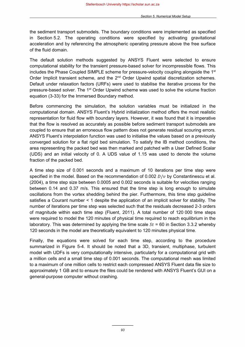
Section 5. Numerical Model Setup
93
the sediment transport submodels. The boundary conditions were implemented as specified in Section 5.2. The operating conditions were specified by activating gravitational acceleration and by referencing the atmospheric operating pressure above the free surface of the fluid domain.
The default solution methods suggested by ANSYS Fluent were selected to ensure computational stability for the transient pressure-based solver for incompressible flows. This includes the Phase Coupled SIMPLE scheme for pressure-velocity coupling alongside the 1st Order Implicit transient scheme, and the 2nd Order Upwind spatial discretization schemes. Default under relaxation factors (URFs) were used to stabilise the iterative process for the pressure-based solver. The 1st Order Upwind scheme was used to solve the volume fraction equation (3-33) for the Immersed Boundary method.
Before commencing the simulation, the solution variables must be initialized in the computational domain. ANSYS Fluent’s Hybrid initialization method offers the most realistic representation for fluid flow with boundary layers. However, it was found that it is imperative that the flow is resolved as accurately as possible before sediment transport submodels are coupled to ensure that an erroneous flow pattern does not generate residual scouring errors. ANSYS Fluent’s interpolation function was used to initialise the values based on a previously converged solution for a flat rigid bed simulation. To satisfy the IB method conditions, the area representing the packed bed was then marked and patched with a User Defined Scalar (UDS) and an initial velocity of 0. A UDS value of 1.15 was used to denote the volume fraction of the packed bed.
A time step size of 0.001 seconds and a maximum of 10 iterations per time step were specified in the model. Based on the recommendation of 0.002 𝐷𝐷/𝑣𝑣 by Constantinescu et al. (2004), a time step size between 0.0005 and 0.002 seconds is suitable for velocities ranging between 0.14 and 0.37 m/s. This ensured that the time step is long enough to simulate oscillations from the vortex shedding behind the pier. Furthermore, this time step guideline satisfies a Courant number < 1 despite the application of an implicit solver for stability. The number of iterations per time step was selected such that the residuals decreased 2-3 orders of magnitude within each time step (Fluent, 2011). A total number of 120 000 time steps were required to model the 120 minutes of physical time required to reach equilibrium in the laboratory. This was determined by applying the time scale 𝑆𝑆𝑡𝑡 = 60 in Section 3.3.2 whereby 120 seconds in the model are theoretically equivalent to 120 minutes physical time.
Finally, the equations were solved for each time step, according to the procedure summarized in Figure 5-4. It should be noted that a 3D, transient, multiphase, turbulent model with UDFs is very computationally intensive, particularly for a computational grid with a million cells and a small time step of 0.001 seconds. The computational mesh was limited to a maximum of one million cells to restrict each compressed ANSYS Fluent data file size to approximately 1 GB and to ensure the files could be rendered with ANSYS Fluent’s GUI on a general-purpose computer without crashing.
Stellenbosch University https://scholar.sun.ac.za
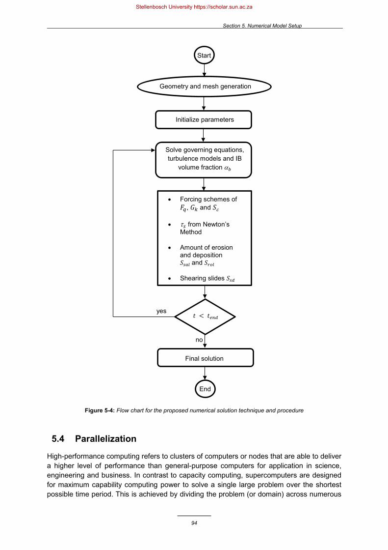
Section 5. Numerical Model Setup
94
Figure 5-4: Flow chart for the proposed numerical solution technique and procedure
5.4 Parallelization
High-performance computing refers to clusters of computers or nodes that are able to deliver a higher level of performance than general-purpose computers for application in science, engineering and business. In contrast to capacity computing, supercomputers are designed for maximum capability computing power to solve a single large problem over the shortest possible time period. This is achieved by dividing the problem (or domain) across numerous
Start
Geometry and mesh generation
Final solution
yes
no
𝑡𝑡 < 𝑡𝑡𝑑𝑑𝑚𝑚𝑑𝑑
Initialize parameters
Solve governing equations, turbulence models and IB
volume fraction α𝑏𝑏
• Forcing schemes of 𝐹𝐹𝑞𝑞, 𝐺𝐺𝑘𝑘 and 𝑆𝑆ε
• τ𝑠𝑠 from Newton’s Method
• Amount of erosion and deposition 𝑆𝑆𝑠𝑠𝑎𝑎𝑠𝑠 and 𝑆𝑆𝑟𝑟𝑜𝑜𝑠𝑠
• Shearing slides 𝑆𝑆𝑠𝑠𝑑𝑑
End
Stellenbosch University https://scholar.sun.ac.za
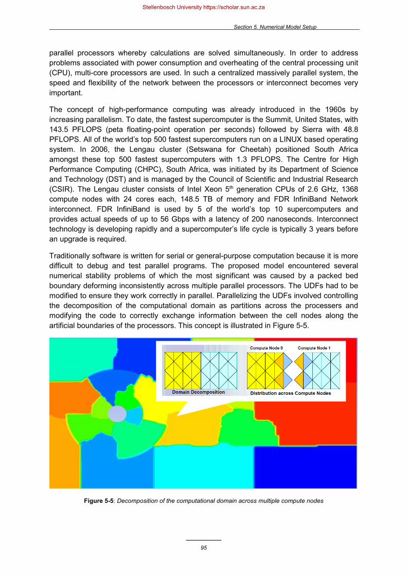
Section 5. Numerical Model Setup
95
parallel processors whereby calculations are solved simultaneously. In order to address problems associated with power consumption and overheating of the central processing unit (CPU), multi-core processors are used. In such a centralized massively parallel system, the speed and flexibility of the network between the processors or interconnect becomes very important.
The concept of high-performance computing was already introduced in the 1960s by increasing parallelism. To date, the fastest supercomputer is the Summit, United States, with 143.5 PFLOPS (peta floating-point operation per seconds) followed by Sierra with 48.8 PFLOPS. All of the world’s top 500 fastest supercomputers run on a LINUX based operating system. In 2006, the Lengau cluster (Setswana for Cheetah) positioned South Africa amongst these top 500 fastest supercomputers with 1.3 PFLOPS. The Centre for High Performance Computing (CHPC), South Africa, was initiated by its Department of Science and Technology (DST) and is managed by the Council of Scientific and Industrial Research (CSIR). The Lengau cluster consists of Intel Xeon 5th generation CPUs of 2.6 GHz, 1368 compute nodes with 24 cores each, 148.5 TB of memory and FDR InfiniBand Network interconnect. FDR InfiniBand is used by 5 of the world’s top 10 supercomputers and provides actual speeds of up to 56 Gbps with a latency of 200 nanoseconds. Interconnect technology is developing rapidly and a supercomputer’s life cycle is typically 3 years before an upgrade is required.
Traditionally software is written for serial or general-purpose computation because it is more difficult to debug and test parallel programs. The proposed model encountered several numerical stability problems of which the most significant was caused by a packed bed boundary deforming inconsistently across multiple parallel processors. The UDFs had to be modified to ensure they work correctly in parallel. Parallelizing the UDFs involved controlling the decomposition of the computational domain as partitions across the processers and modifying the code to correctly exchange information between the cell nodes along the artificial boundaries of the processors. This concept is illustrated in Figure 5-5.
Figure 5-5: Decomposition of the computational domain across multiple compute nodes
Stellenbosch University https://scholar.sun.ac.za
Section 5. Numerical Model Setup
96
ANSYS Fluent’s parallel architecture involves a host process that communicates commands and results between the cortex and compute nodes via a master compute node (see Figure 5-6). Compiler directories in the UDF (such as “#if !PARALLEL” and “#if !RP_HOST”) assign certain commands to be executed only on the host or the node processes. Grid cells and solution data are distributed and stored on the different compute nodes while copies of the neighbouring partition’s cells are also kept on each compute node, designated as exterior cells. However, this approach is not applicable in the case where the cell nodes on the riverbed surface are worked and the same UDF variables can have different values on different compute nodes. The “EXCHANGE_SVAR” macro should be used to exchange data or storage variables (SVAR) between the compute nodes which are virtually synchronized; receiving compute nodes wait for data to be sent before continuing the packed bed deformation calculations.
Figure 5-6: ANSYS Fluent’s parallel architecture
The efficiency of parallelizing the numerical model can be evaluated by the speed-up plot in Figure 5-7. Using an increased number of processors almost linearly increases the number of iterations performed by the model per hour of physical simulation time until a limit of 240 processors (10 nodes) is reached. Beyond this limit, the scaling of the numerical model becomes erratic and unpredictable on the Lengau cluster. This could be ascribed to a very full cluster and some contention on the Inifniband network, especially when nodes used are not on the same rack. Alternatively, the proposed numerical model’s ability to compute across multiple parallel processors could be constrained by bottlenecking on the master node (i.e. Compute-Node-0 in Figure 5-6).
Nevertheless, the simulation runs 10 times faster with 240 processors compared to the 15 processors previously used on a general-purpose Dell Precision T5600 Duel Xeon 3.3GHz with 16 GB RAM and a Solid State hard drive. The processing time required to run each simulation on the CHPC is 4 to 6 days, to reach equilibrium after 120 seconds model time X 0.001 seconds time step size X 10 iterations per time step.
Cortex Host Compute-Node-0
Compute-Node-1 Compute-Node-2 Compute-Node-3
Stellenbosch University https://scholar.sun.ac.za
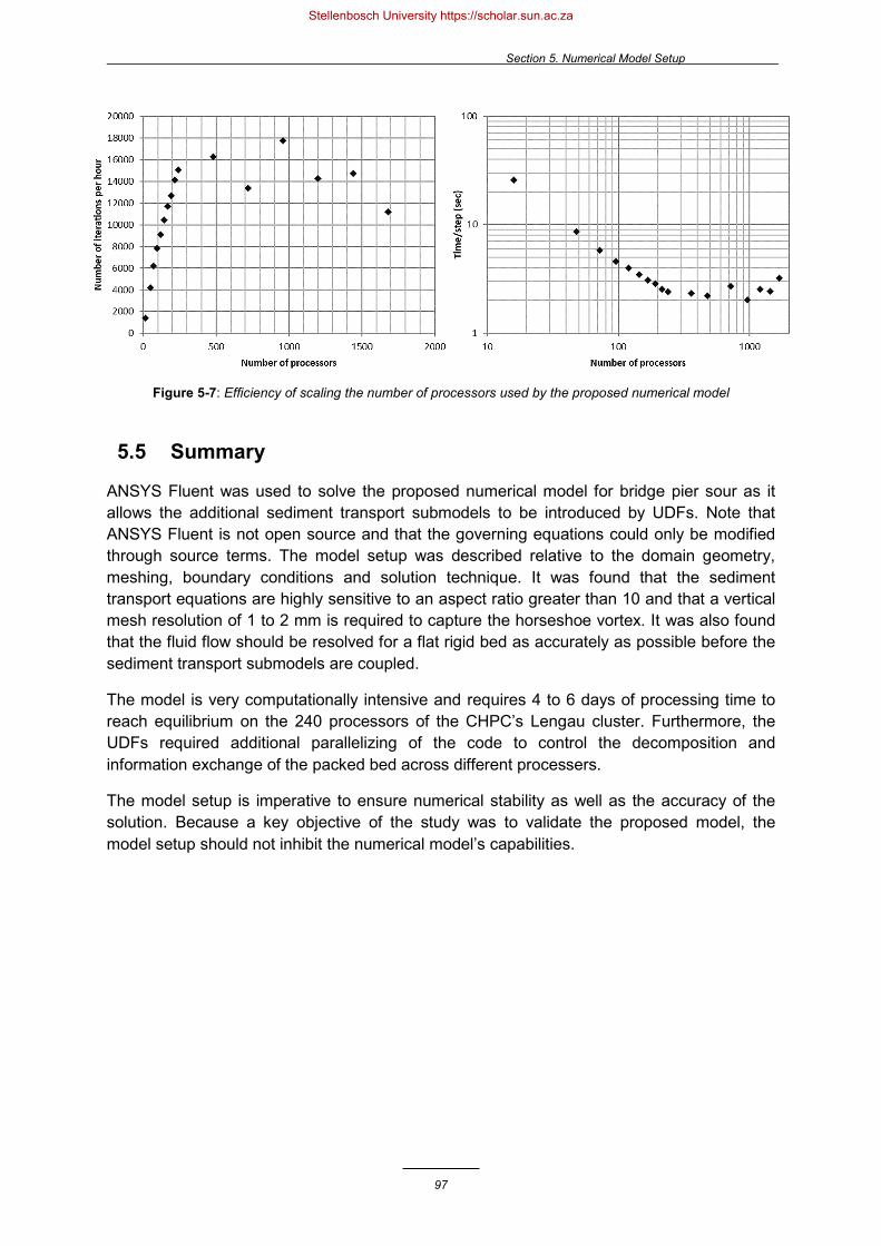
Section 5. Numerical Model Setup
97
Figure 5-7: Efficiency of scaling the number of processors used by the proposed numerical model
5.5 Summary
ANSYS Fluent was used to solve the proposed numerical model for bridge pier sour as it allows the additional sediment transport submodels to be introduced by UDFs. Note that ANSYS Fluent is not open source and that the governing equations could only be modified through source terms. The model setup was described relative to the domain geometry, meshing, boundary conditions and solution technique. It was found that the sediment transport equations are highly sensitive to an aspect ratio greater than 10 and that a vertical mesh resolution of 1 to 2 mm is required to capture the horseshoe vortex. It was also found that the fluid flow should be resolved for a flat rigid bed as accurately as possible before the sediment transport submodels are coupled.
The model is very computationally intensive and requires 4 to 6 days of processing time to reach equilibrium on the 240 processors of the CHPC’s Lengau cluster. Furthermore, the UDFs required additional parallelizing of the code to control the decomposition and information exchange of the packed bed across different processers.
The model setup is imperative to ensure numerical stability as well as the accuracy of the solution. Because a key objective of the study was to validate the proposed model, the model setup should not inhibit the numerical model’s capabilities.
Stellenbosch University https://scholar.sun.ac.za

Section 6. Analysis of Empirical Results
98
6. Analysis of Empirical Results
6.1 Introduction
This section discusses the results from the experimental work and the evaluation of empirical equations. The data generated by the physical modelling was assessed with reference to literature and was then applied to evaluate different methods for predicting the equilibrium scour depth. The objective was to demonstrate the shortcomings of thirty of the better-known empirical equations and to emphasize the need for improved prediction methods to pave the way for future research on numerical modelling. A summary of the different methods is given in Appendix A. Finally, field data was analysed to develop a new equation for the prediction of bridge pier scour.
6.2 Bed Deformation Observations from Experimental Work
Once the scour hole had reached equilibrium in the laboratory, the sediment bed levels were surveyed. Appendix C shows the bed deformation for each experiment by means of a scour profile with contours plotted on Surfer. These scour profiles are plotted relative to an initial bed level at the datum 0 m whereby negative values represent erosion (warmer red and orange colours) and positive values represent deposition (cooler blue and green colours).
The characteristic U-shaped scour holes can be observed by the red sections in the scour profiles whereby the ends of the vortex system were swept downstream around the pier (Dey, 1996). The scoured sediment then deposited downstream of the pier forming a longitudinal bar or dune (Breusers et al, 1977), identified by the blue sections in the scour profiles. As the flow and velocities increase, not only does the scour hole increase in size but the dune migrates further downstream. Generally, research has not been concerned with quantifying the dune size or the scour hole extent because the safety of a bridge design is related to the maximum scour depth.
From the scour profiles and sections, it is evident that the maximum scour depth occurs at the upstream face of the pier where the horseshoe vortex circulates (see Section 2.5.5). However, the sharp nosed piers see an increased scour depth on the sides of the pier, because the horseshoe vortex was not fully developed (Tseng et al., 2000). The maximum scour depths 𝑑𝑑𝑆𝑆 obtained from the experimental work, as well as the approximate lengths 𝑙𝑙𝑆𝑆 and widths 𝑤𝑤𝑆𝑆 of the scour hole extent, are summarized in Table 6-1. Notice that negligible scouring of only 9 mm took place for the 28 l/s flow for the sharp nosed pier. From Table 6-1 it is clear that the width and length of the scour hole are dependent on the scour depth, increasing in size as the depth increases, because the slope stability is controlled by the sediment’s angle of repose (Ali & Karim, 2002). The slope angles for the surveyed scour holes ranged between 28 to 58° but had an average angle of repose of 40° for the fine sand and 42° for the peach pips. These values compare well with the 45° and 44° saturated repose angles measured experimentally in Section 4.2.1.
Stellenbosch University https://scholar.sun.ac.za

Section 6. Analysis of Empirical Results
99
Table 6-1: Maximum bridge pier scour depth and extent from experimental work (m)
Figure 6-1 presents 6 photographs of the submerged equilibrium scour holes developed in the laboratory for the 3 pier shapes and 2 sediment materials. According to Hoffmans & Verhij (1997) the slope of a scour hole can be divided into different regions, as demonstrated quite well by Figure 6-1a. The primary area is driven by the vortex and bed shear stress, while the secondary area is driven by the slope stability or shear slides (Sawadogo, 2015).
The presence of dunes on the sand bed suggest that the largest flow chosen for the sand results in live-bed scouring as these are bed features associated with the lower subcritical regime for general scouring (Chadwick, 2013). However, this allows the proposed numerical model’s potential for live-bed scour simulations to be assessed. In addition, some armouring of the coarser factions of material in the scour hole can be observed in Figure 6-1, which the numerical model and empirical equations would not be able to simulate if they do not account for more than one sediment size. It is recommended that the proposed numerical model could be upgraded to accommodate more than one sediment fraction size by future studies.
6.2.1 Repeatability
Fifteen percent of the experimental work, i.e. 4 tests with the cylindrical pier and crushed peach pips, were duplicated 3 times to examine the repeatability or reliability of the results. Figure 6-2 shows the bed deformation results from the tests repeated for the 40 l/s flow. The 3 profiles are not completely identical whereby the U-shaped scour hole is most dominant in Test 3 while the deposition mound is most visible in Test 1. Nevertheless, identical maximum scour depths were obtained by the 3 tests. In fact, Figure 6-3 shows that near identical maximum scour depths were obtained by the 3 tests for all 4 flows with a maximum deviation of 9% for the 34 l/s flow or 𝑣𝑣1/𝑣𝑣𝑐𝑐 = 0.75. This could partly be attributed to the human error involved in manually surveying the scour hole, deviating within a few millimeters or 1 to 2%. Such errors may be considered negligible in light of the errors from the empirical equations evaluated in Section 6.4, which are on the scale of 150% or larger. Therefore, it may be deduced that the scour results are within an acceptable range of accuracy.
Cylindrical pier Round nosed pier Sharp nosed pier 𝑸𝑸 (l/s) 𝒗𝒗 (m/s) 𝒅𝒅𝑺𝑺 𝒍𝒍𝑺𝑺 𝒘𝒘𝑺𝑺 𝒅𝒅𝑺𝑺 𝒍𝒍𝑺𝑺 𝒘𝒘𝑺𝑺 𝒅𝒅𝑺𝑺 𝒍𝒍𝑺𝑺 𝒘𝒘𝑺𝑺
Peac
h pi
ps 28 0.14 0.063 0.13 0.13 0.037 0.12 0.13 0.009 0.06 0.01
34 0.17 0.116 0.21 0.22 0.077 0.17 0.18 0.050 0.13 0.14 40 0.20 0.127 0.24 0.28 0.095 0.23 0.25 0.072 0.15 0.20 46 0.23 0.135 0.24 0.30 0.111 0.25 0.28 0.106 0.17 0.24
Fine
san
d
56 0.28 0.099 0.15 0.20 0.056 0.16 0.19 0.060 0.17 0.22 62 0.31 0.111 0.19 0.24 0.080 0.18 0.22 0.065 0.18 0.25 68 0.34 0.114 0.19 0.24 0.094 0.23 0.24 0.084 0.20 0.25 74 0.37 0.121 0.25 0.26 0.102 0.25 0.25 0.090 0.20 0.27
Stellenbosch University https://scholar.sun.ac.za
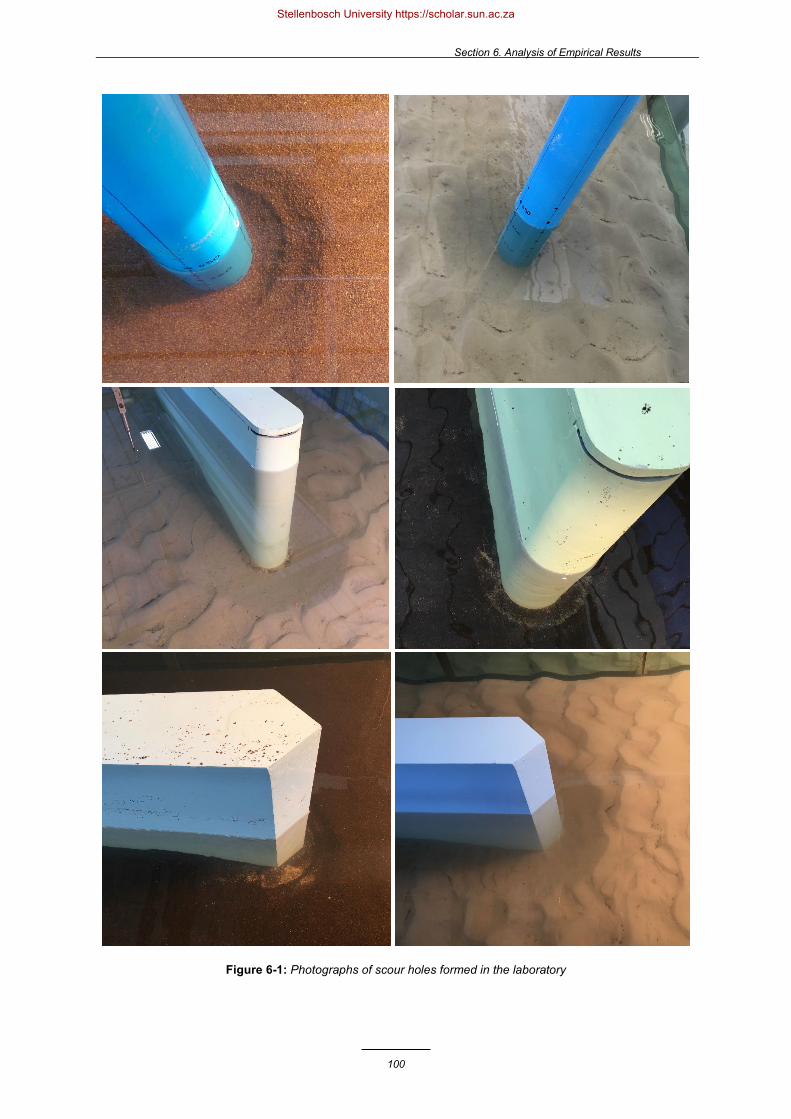
Section 6. Analysis of Empirical Results
100
Figure 6-1: Photographs of scour holes formed in the laboratory
Stellenbosch University https://scholar.sun.ac.za

Section 6. Analysis of Empirical Results
101
Figure 6-2: Scour profiles for 3 tests repeated for a 40 l/s flow and cylindrical pier
Figure 6-3: Relative scour depth for 3 duplicated tests to evaluate repeatability
Similarly, the scour geometry was evaluated for repeatability as shown in Figure 6-4. The relative scour length and width are slightly smaller for Test 1, as shown in Figure 6-11, while the relative scour width is slightly larger for Test 3. The values are far more variable than that of the relative scour depth and the scour geometry is not as accurate with a maximum deviation of 21%. Note that the scour extents in Table 6-1 are also only estimates (to the nearest cm) interpolated from the sections in Appendix C to enable a quantitative comparison of the scour geometries.
Figure 6-4: Relative scour length and width for 3 duplicated tests to evaluate repeatability
0.0
0.2
0.4
0.6
0.8
1.0
1.2
1.4
0.5 0.6 0.7 0.8 0.9 1.0 1.1
d s /D
v/vc
Test 1Test 2Test 3
0.0
0.5
1.0
1.5
2.0
2.5
0.5 0.6 0.7 0.8 0.9 1.0 1.1
l s /D
v/vc
Test 1Test 2Test 3
0.0
0.5
1.0
1.5
2.0
2.5
3.0
0.5 0.6 0.7 0.8 0.9 1.0 1.1
ws /
D
v/vc
Test 1Test 2
∆z (m)
y (m
)
x (m)
Flow
Dire
ctio
n
Test 1 Test 2 Test 3
Stellenbosch University https://scholar.sun.ac.za

Section 6. Analysis of Empirical Results
102
6.3 Effect of Parameters on Equilibrium Scour
The local scour process is affected by several different yet interrelated parameters of which the relative velocity, relative sediment size, relative flow depth and time to reach equilibrium scour, have been identified as the most significant (Williams, 2014). The effect of three variable parameters (i.e. the approach velocity, sediment type and pier shape) on equilibrium scour depth were briefly examined, but flow depth and pier width were fixed in the experimental work due to time constraints.
6.3.1 Approach Velocity
As shown by the scour profiles in Appendix C, the scour hole increases in size as the approach velocity or flow increases. To quantify this relationship, Figure 6-5 plots the relative velocity against the relative scour depth. The relative scour depth increases almost linearly with the relative velocity, in accordance with Chiew (1984) and Ettema (1980), albeit a smaller scour depth and milder gradient. The differences can be attributed to other parameters such as the sediment material, pier shape or time, which reaffirms that the scour process involves several interrelated parameters that cannot be simplified to a single expression. Despite the dispute in literature, no local scour pattern was observed below the relative velocity condition of 0.5 in accordance with research such as those by Hancu (1971), Breuser et al. (1977), Sheppard & Miller (2006) and Sheppard & Melville (2014). Similarly, the relative velocity was plotted against the relative scour length or width in Figure 6-6 to display an analogous trend. However, graphs plotted in terms of scour extent instead of depth have not previously been published, because scour length and width are the less critical dimensions in bridge design. The negligible scouring noted for the 28 l/s flow for the sharp nosed pier appears to deviate from the general observed trend and could invalidate its reliability.
Figure 6-5: The effect of relative velocity on relative scour depth from experimental work
0.0
0.5
1.0
1.5
2.0
2.5
3.0
0.4 0.5 0.6 0.7 0.8 0.9 1 1.1
d s /D
v/vc
Ettema (1980)Cylinder, pipsCylinder, sandRound nosed, pipsRound nosed, sandSharp nosed, pipsSharp nosed, sand
Stellenbosch University https://scholar.sun.ac.za

Section 6. Analysis of Empirical Results
103
Figure 6-6: The effect of relative velocity on the relative length and width of the scour hole
The threshold for sediment movement can also be described in terms of the Rouse number 𝑃𝑃 (as defined in Section 2.6.2) which is related to the shear velocity (or shear stress) for the approach channel and the settling velocity for the sediment. While the upper limit of the relative velocity ratio in Figure 6-5 approaches the condition 𝑣𝑣/𝑣𝑣𝐶𝐶 ≥ 1, the lower limit of the Rouse number in Figure 6-7 exceeds the condition 𝑃𝑃 ≤ 7.5 required for live-bed scour to initiate. An indirect relationship with the same gradient exists for all the laboratory data sets; as the local scour hole increases in size, the Rouse number decreases.
Figure 6-7: The effect of the Rouse number on relative scour depth from experimental work
The effect of the increased velocity on the scour depth can also be evaluated by plotting the pier Reynolds number and Froude number against the relative scour depth, as shown in Figure 6-8, because the pier size and flow depth is fixed. The pier Reynolds number may be considered the chief parameter affecting the strength of the horseshoe vortex, alongside the approaching boundary layer (Constandinescu & Koken, 2005). It has rarely been described relative to scour depth even though the horseshoe vortex is directly responsible for causing
0.0
0.5
1.0
1.5
2.0
2.5
0.5 0.6 0.7 0.8 0.9 1.0 1.1
l s /D
v/vc
Cylindrical, pipsCylindrical, sandRound nosed, pipsRound nosed, sandSharp nosed, pipsSharp nosed, sand
0.0
0.5
1.0
1.5
2.0
2.5
3.0
0.5 0.6 0.7 0.8 0.9 1.0 1.1
ws /
D
v/vc
Cylinder, pipsCylinder, sandRound nosed, pipsRound nosed, sandSharp nosed, pips
0.0
0.2
0.4
0.6
0.8
1.0
1.2
1.4
7.5 9.5 11.5 13.5 15.5 17.5
d s /D
Rouse number P
Cylinder, pipsCylinder, sandRound nosed, pipsRound nosed, sandSharp nosed, pipsSharp nosed, sand
Stellenbosch University https://scholar.sun.ac.za

Section 6. Analysis of Empirical Results
104
scour. The pier Reynolds number should be considered a more significant scour parameter because it describes the combined effect of the pier size and approach velocity on the vortex strength. Evidently, a similar trend exists whereby an increased Reynolds number scours a larger hole. However, unlike the relative velocity, the Reynolds number and Froude number do not incorporate parameters representative of the scour bed and the difference between the two different sediment materials are more discernible.
Figure 6-8: The effect of the pier Reynolds number and the Froude number on the relative scour depth
6.3.2 Relative Sediment Size
From Figure 6-8, it is evident that the peach pips requires a smaller Reynolds number (or velocity) to scour the same sized hole as that for the fine sand and is therefore, the more easily erodible material. On the other hand, similarly sized scour holes are formed for the same relative velocity or flow intensity for both materials in Figure 6-5. This is in accordance with Lee & Strum (2009) who suggest that a similar scour depth should be obtained for the scaled 𝐷𝐷/𝑑𝑑 of 882 for the peach pips and 514 for the sand (refer to Figure 2-15). It is difficult to directly compare the two materials to explain this behaviour in terms of the interrelated sediment parameters because both the model median particle size and density are different. The peach pips have a larger particle size which implies that the material is less easily entrained, and yet it has a lower relative density which infers the opposite. The crushed peach pips are the more easily erodible material because they have a lower critical velocity and movability number. These parameters are representative of the material because they are based on both the particle size and density. In addition, when the two materials are scaled (in Section 4.2.1) to an equivalent density, the sand has a prototype particle size larger than that for the peach pips. Therefore, the scaled relative sediment size is no longer masked by the effect of the density and the larger scaled 𝐷𝐷/𝑑𝑑50 affirms that the peach pips are less resistant to entrainment.
0.0
0.2
0.4
0.6
0.8
1.0
1.2
1.4
10 000 100 000
d s /D
ReD
Cylinder, pipsCylinder, sandRound nosed, pipsRound nosed, sandSharp nosed, pipsSharp nosed, sand
2 3 4 5 6 7 8 9
Fr 0.06 0.13 0.19 0.26 0.32 0.39 0.52 0.65
Stellenbosch University https://scholar.sun.ac.za

Section 6. Analysis of Empirical Results
105
Table 6-2: Comparison of sediment characteristics
Model Prototype
Properties 𝒅𝒅𝟓𝟓𝟓𝟓 (mm) MTRD 𝒘𝒘𝟓𝟓𝟓𝟓
(m/s) 𝒗𝒗𝑪𝑪
(m/s) Scaled Density
(kg/m3) Scaled 𝒅𝒅𝟓𝟓𝟓𝟓 (mm)
Scaled 𝑫𝑫/𝒅𝒅𝟓𝟓𝟓𝟓
1. Fine sand 0.214 2.63 0.036 0.375 2629 3.21 514
2. Peach pips 0.740 1.28 0.032 0.225 2629 1.87 882
6.3.3 Pier Shape
With reference to Figure 6-5 and Figure 6-8, a cylindrical pier yields the largest scour hole while the sharp nosed pier has the least amount of scour because practically no vorticity is generated at the nose of streamlined piers (Tseng et al., 2000). The round nosed pier causes less scour than the cylindrical pier due to its increased relative pier length 𝐿𝐿/𝐷𝐷. It is important to understand the effect of pier shape on scour depth because it allows for the optimum pier design to control and reduce the flow processes responsible for scouring. However, it is difficult to mathematically describe the effect of pier shape on the scour depth. Empirical equations account for pier shape by incorporating constants as a shape factor 𝐾𝐾𝑠𝑠 calibrated against scour depths for cylindrical piers. Figure 6-9 shows the anticipated scour generated for the round and sharp nosed piers by applying shape factors to the curve of the cylindrical pier. Evidently, the use of a single factor cannot describe the effect of pier shape on scour depth because different gradients exist for the near linear relationships. Furthermore, the shape factors recommended by the empirical equations overestimate the scour depth. A numerical model has the ability to overcome this shortcoming.
Figure 6-9: Evaluation of shape factors for the prediction of maximum scour depth
0.0
0.2
0.4
0.6
0.8
1.0
1.2
1.4
0.6 0.7 0.8 0.9 1.0 1.1
d s /D
v/vc
Cylinder, pipsRound nosed, pipsSharp nosed, pips
KS0.90.860.80.7
0.0
0.2
0.4
0.6
0.8
1.0
1.2
0.7 0.8 0.9 1.0 1.1
d s /D
v/vc
Cylinder, sandRound nosed, sandSharp nosed, sand
KS0.90.860.80.7
Stellenbosch University https://scholar.sun.ac.za

Section 6. Analysis of Empirical Results
106
6.4 Evaluation of Empirical Equations
In order to demonstrate the shortcomings of empirical equations and to promote the use of numerical models for scour prediction, thirty of the better-known equations (listed in Appendix A) were evaluated for clear-water conditions in an alluvial bed. The results from the equations were compared to that of the experimental work for the small sample size of 24 tests. Because the empirical equations were developed for full-scale applications, the input parameters (other than sediment properties) and scour depth results were scaled by applying Froude similarity to the 1: 15 model (𝑛𝑛𝑦𝑦 = 15 and 𝑛𝑛𝑣𝑣 = √15).
Furthermore, critical velocities determined experimentally were used in the analysis (unless specified otherwise) to ensure the relative velocity ratio was maintained for both model and prototype scales. Several equations exist to determine critical velocity and most of the equations for bridge pier scour in this study fail to reference an appropriate method to calculate it. The threshold of sediment movement is an important parameter and yet literature neglects to address that different equations for critical velocity could produce different scour depth predictions.
The comparison of different empirical equations has been the topic of many studies and without exception, the conclusion is the same each time: empirical equations for bridge pier scour yield a wide range of varying and unreliable results (Johnson, 1995; Rooseboom, 2013). From Figure 6-10, it is evident that a wide range of scour depths were also produced in this study for each test or boxplot (each boxplot represents the range of scour depths predicted by 30 empirical equations for one test). The scour depth was predominantly overpredicted, as safe design equations intend to be conservative when they fail to be accurate. Nevertheless, the empirical equations are discordant and still predict scour depths varying up to 3 m from one another for the same test.
Since the equations are generally developed from a standard experimental setup with a cylindrical pier in a uniformly graded bed, the most accurate scour depths were predicted for the tests with the cylindrical pier as well as the crushed peach pips. It can be deduced that the scaling of the peach pips is a better representative of in-situ sediment than that of the sand. Moreover, larger flows yield larger scour depths, and consequently the equations yield less conservative predictions.
Figure 6-10: Boxplot showing the distribution of scour depth residuals for the different lab tests
Stellenbosch University https://scholar.sun.ac.za

Section 6. Analysis of Empirical Results
107
The statistical spread for each empirical equation is indicated by each boxplot in Figure 6-11 which can be evaluated in conjunction with the more detailed relative scour depth dataset in Figure 6-12 where the percentage error is taken as
Evidently, the equations are in weak agreement with one another and generally overestimate the observed scour depths with an average error of 78%. Hancu (1971) and Melville & Kandasamy (1998) are the most accurate methods while the safest equations for bridge pier design are Blench (1969), Shen et al. (1969) and Ali & Karim (2002), followed by the FDOT and HEC-18 equations. However, some of these equations tend away from the line of equality in Figure 6-12 and do not properly capture the processes responsible for local scour. This is in agreement with the literature study whereby the HEC-18 and Shen et al. (1969) equations are known to better resemble scour in the field. In addition, Shen et al. (1969) and Ali & Karim (2002) most likely performed better because they rely on the pier Reynolds number, a parameter which is significant in the formation of the horseshoe vortex (Roulund et al., 2005). The implication of this is that models taking the vortex formation into consideration could offer better scour depth predictions.
The simpler and older models of Breusers (1965), Laursen & Toch (1956), Blench (1969) and Melville & Kandasamy (1998) appear to be more accurate but they do not incorporate approach velocity or particle size. The equations are not considered applicable because they predicted the same scour depth for all the tests; only Melville & Kandasamy (1998) and Laursen & Toch (1956) differentiated between shapes. The simplest expression is that of Breusers which assumes that the maximum bridge pier scour can be taken as 1.4 times the pier size. Pier size is the most prevalent parameter emerging in all the equations except in Chitale (1962). Consequently, Chitale also performed deceptively well because only one pier size was tested. Instead, Chitale (as well as the HEC-18 equations) depend on the Froude number, which is related to the mode of sediment transport of the different bedforms (Graf, 1971). The relative flow depth is also prevalent in the HEC-18 models, which is related to the boundary layer thickness (Roulund et al., 2005).
𝑃𝑃𝐸𝐸 =(𝑑𝑑𝑠𝑠𝑜𝑜𝑏𝑏𝑠𝑠𝑑𝑑𝑟𝑟𝑣𝑣𝑑𝑑𝑑𝑑 – 𝑑𝑑𝑠𝑠𝑐𝑐𝑎𝑎𝑠𝑠𝑐𝑐𝑐𝑐𝑠𝑠𝑎𝑎𝑡𝑡𝑑𝑑𝑑𝑑)
𝑑𝑑𝑠𝑠𝑜𝑜𝑏𝑏𝑠𝑠𝑑𝑑𝑟𝑟𝑣𝑣𝑑𝑑𝑑𝑑 × 100 . (6-1)
Stellenbosch University https://scholar.sun.ac.za
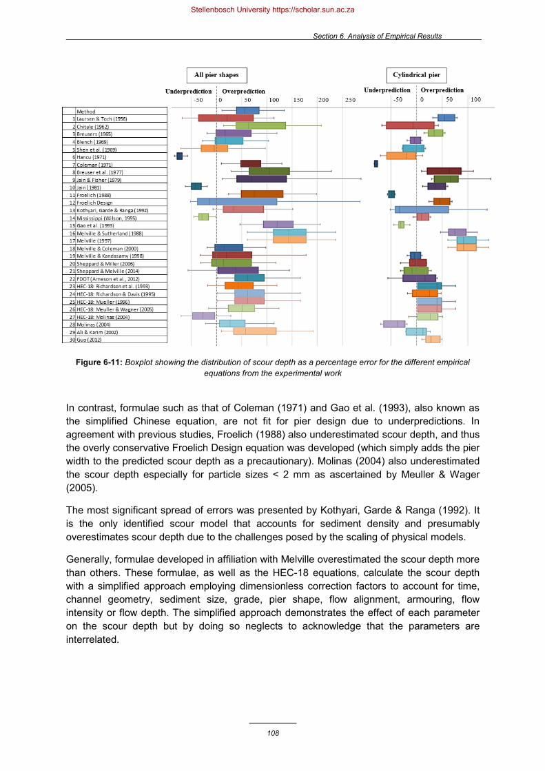
Section 6. Analysis of Empirical Results
108
Figure 6-11: Boxplot showing the distribution of scour depth as a percentage error for the different empirical equations from the experimental work
In contrast, formulae such as that of Coleman (1971) and Gao et al. (1993), also known as the simplified Chinese equation, are not fit for pier design due to underpredictions. In agreement with previous studies, Froelich (1988) also underestimated scour depth, and thus the overly conservative Froelich Design equation was developed (which simply adds the pier width to the predicted scour depth as a precautionary). Molinas (2004) also underestimated the scour depth especially for particle sizes < 2 mm as ascertained by Meuller & Wager (2005).
The most significant spread of errors was presented by Kothyari, Garde & Ranga (1992). It is the only identified scour model that accounts for sediment density and presumably overestimates scour depth due to the challenges posed by the scaling of physical models.
Generally, formulae developed in affiliation with Melville overestimated the scour depth more than others. These formulae, as well as the HEC-18 equations, calculate the scour depth with a simplified approach employing dimensionless correction factors to account for time, channel geometry, sediment size, grade, pier shape, flow alignment, armouring, flow intensity or flow depth. The simplified approach demonstrates the effect of each parameter on the scour depth but by doing so neglects to acknowledge that the parameters are interrelated.
Stellenbosch University https://scholar.sun.ac.za

Section 6. Analysis of Empirical Results
109
As illustrated in Section 6.3.3, it is difficult to mathematically describe the effect of pier shape on the horseshoe vortex and the scour depth with simply a constant shape factor. Half of the 30 empirical equations evaluated in this study account for pier shape by using different factors. Subsequently, the scour depths for the round nosed and sharp nosed were largely overestimated (refer to Figure 6-10). Figure 6-11 is supplemented with boxplots for the empirical equations applied only to the 8 tests with a cylindrical pier. The scour depths are better predicted but the average error of 50% is still fairly large. The HEC-18 equations consistently performed the best with the least underpredictions while the other equations were less inclined to overpredict the scour depth for a cylindrical pier.
Five different HEC-18 have been developed by the different FHWA manual revisions for scour at bridges by improving the armouring factor Ka, which is intended to be representative of the sediment material. With the exception of Mueller & Wagner (2005), Ka is determined by a dimensionless excess velocity intensity based on the critical velocity formulation introduced by Gao et al. (1993). The most recent FHWA manual discards the CSU’s HEC-18 approach for the Florida DOT (Arneson et al., 2012) which is based on the approach by Sheppard & Miller (2006) and Sheppard & Melville (2014) for wide piers with a new critical velocity calculation. While this method has a mean error percentage closer to zero, it also has a larger range of residuals (or higher SSR) with more underpredictions.
Figure 6-12: Comparison of relative scour depths observed from the experimental work and calculated by the
different empirical equations
Stellenbosch University https://scholar.sun.ac.za

Section 6. Analysis of Empirical Results
110
6.5 An Improved Equation Based on Field Data
Because the HEC-18 equations are generally preferred to the other empirical equations for better resembling scour in the field, they were improved by developing new dimensionless factors for armouring and pier shape. According to Guo (2012), the HEC-18 equations are well established with regards to the flow-structure interaction but they are limited in terms of the flow-sediment interaction.
Extensive field data from the Bridge Scour Data Management System (BSDMS) was obtained from Mueller & Wagner (2005) to perform the regression analysis. The 493 pier scour measurements were reduced to a sample size of 207 measurements to satisfy the criteria for noncohesive sediment, limited debris effects, aligned flow and upstream scour at single piers. The scour depth measurements were filtered further to ensure a < 0.3 m accuracy in an attempt to eradicate the variability typically observed in field data.
A new approach to bridge pier scouring was adopted to evaluate the entrainment potential of the riverbed whereby the critical velocity was discarded for another parameter, the particle Reynolds number 𝑅𝑅𝑅𝑅𝑝𝑝. Several other parameters were also considered, such as the movability number based on settling velocity, unit stream power and the rate of energy dissipation, but it was found from a regression analysis that Rep correlated best with the relative scour depth from the field data as shown in Figure 6-13 (𝑅𝑅2 = 0.84, 𝑃𝑃-value = 10 to 11, Significance 𝐹𝐹 = 10 to 61). The correlation is given for the 50%, 95% and 99% confidence intervals respectively that were determined statistically from the field data for the different pier shapes (laboratory data is plotted for context).
Figure 6-13: Relationship between the idealized factor Ka and Rep
Stellenbosch University https://scholar.sun.ac.za

Section 6. Analysis of Empirical Results
111
Representative particle sizes other than the median 𝑑𝑑50 were also investigated for their ability to account for the grading of the sediment bed but the best correlation was observed for the traditional particle size 𝑑𝑑 = 𝑑𝑑50. The particle Reynolds number has an additional advantage that it depends on the channel shape and bed form roughness. However, limited information was captured by the field data and the energy slope 𝑆𝑆 was determined from the Chézy equation by assuming that the hydraulic radius 𝑅𝑅 → 𝑦𝑦 for a wide channel. Equation (2-3) for bed shear stress is also based on the slope and shape of a channel but these parameters have not been previously used by empirical equations to describe their effect on scour depth. Despite the criterion for the ±0.3 m accuracy limit, the field data still displays a broad scatter of data for the observed scour, even for one given site or pier where the structure and sediment parameters are fixed, that the captured flow parameters (velocity and flow depth) cannot explain.
A new approach to the pier shape factor was also adopted by accounting for the relative pier lengths 𝐿𝐿/𝐷𝐷 and by employing an empirical equation whereby the effect of the pier shape on the scour depth is amplified by greater velocities, or equivalently, greater pier Reynolds numbers associated with a stronger horseshoe vortex. Figure 6-14 shows that an increased shape factor correlates with the increased scour depths observed for a particle Reynolds number between 100 and 1 000.
Figure 6-14: Contour plot for the observed bridge pier scour depth in m relative to Ks and Rep
The standard HEC-18 equation with the new proposed factors for armouring and pier shape are presented. The standard factors should be used for the bed condition with clear-water scouring 𝐾𝐾𝑏𝑏 = 1.1 and for alignment 𝐾𝐾𝜃𝜃 = (cos𝜃𝜃 + 𝐿𝐿/𝐷𝐷 sin𝜃𝜃) 0.65. The 𝑎𝑎 and 𝑏𝑏 coefficients in Table 6-3 were determined for different confidence intervals for while a good design equation with a higher confidence interval may guarantee fewer underpredictions, an empirical equation with a lower confidence interval may yield more accurate predictions. Adopting a new approach with confidence intervals can quantify the trade-off between accuracy and unsafe underpredictions, offering flexibility to the bridge designer.
Stellenbosch University https://scholar.sun.ac.za

Section 6. Analysis of Empirical Results
112
Table 6-3: New equation parameters proposed for different confidence intervals
Confidence Interval 𝒎𝒎 𝒃𝒃 99% -0.065 -0.03 95% -0.095 -0.08 50% -0.130 -0.09
The HEC-18 equation with the new proposed factors for armouring and pier shape are given:
In addition to the new proposed empirical equations, the contour plot in Figure 6-15, based on the Modified Liu Diagram for incipient motion, is capable of predicting bridge pier scour from the particle Reynolds number and movability number. Even though these two parameters account for all the flow and sediment parameters except for the pier structure, the observed pier scour depth in Figure 6-15 (not relative scour depth 𝑑𝑑𝑠𝑠/𝐷𝐷) is comparable to the calculated pier scour depth with limited scatter. The scour depth calculated by the new equations (6-2), (6-3) and (6-4) for a 99% confidence produce a smoother contour plot similar to the one observed from the field data but with deeper scour holes in the far corner of the turbulent movement region. This new diagram relating 𝑅𝑅𝑅𝑅𝑝𝑝, 𝑣𝑣∗/𝑤𝑤 and 𝑑𝑑𝑠𝑠 has the potential to accurately predict bridge pier scour should it be supplemented and validated by additional scour data, and should the assumptions for energy slope, channel shape and settling velocity be supported.
Furthermore, in accordance with the Modified Lui Diagram of Figure 2-12 in Section 2.6.1.4, sediment movement is observed for a particle Reynolds number greater than 13 and a movability number greater than 0.2 in the turbulent flow region (Rooseboom et al., 1983). The scour depth dramatically increases for a smaller particle Reynolds number between 100 and 1000 and for a larger movability number above 3.
𝑑𝑑𝑠𝑠 = 2𝐷𝐷𝐾𝐾𝑠𝑠𝐾𝐾𝜃𝜃𝐾𝐾𝑏𝑏𝐾𝐾𝑎𝑎(𝑦𝑦1/𝐷𝐷)0.35𝐹𝐹𝐹𝐹0.43 , (6-2)
𝐾𝐾𝑎𝑎 = 𝑔𝑔𝑦𝑦1𝑆𝑆𝑑𝑑
υ𝑎𝑎
, (6-3)
if 100 < 𝑅𝑅𝑅𝑅𝐷𝐷 < 1000
𝐾𝐾𝑠𝑠 =
⎩⎪⎨
⎪⎧ [1.1 + 1.6𝐸𝐸−8(𝑅𝑅𝑅𝑅𝐷𝐷)](𝐿𝐿/𝐷𝐷)𝑏𝑏 , for square nosed piers
[0.9 + 3.6𝐸𝐸−8(𝑅𝑅𝑅𝑅𝐷𝐷)](𝐿𝐿/𝐷𝐷)𝑏𝑏 , for sharp nosed piers(𝐿𝐿/𝐷𝐷)𝑏𝑏 , for round nosed piers
1, for cylindrical piers
else 𝐾𝐾𝑠𝑠 = 1 .
(6-4)
Stellenbosch University https://scholar.sun.ac.za

Section 6. Analysis of Empirical Results
113
Figure 6-15: Modified Liu Diagram for bridge pier scour depth in m
Finally, Figure 6-15 compared the sum of squared residuals against the thirty empirical equations evaluated in Section 6.4, for both the field and laboratory data. Note that the equation was developed from field data and validated against the laboratory data. The equations are ranked according to the least overall error as well as the least underpredictions without any weighting. The new proposed equation ranks the highest, followed by HEC-18 Mueller (1996), Shen et al. (1969) and Mueller & Wagner (2005). Note that these equations are based on the parameters 𝑣𝑣𝑐𝑐, 𝑅𝑅𝑅𝑅𝐷𝐷 and 𝑑𝑑/𝐷𝐷 respectively. The sum of squared residuals is given by
𝑆𝑆𝑆𝑆𝑅𝑅 = (𝑑𝑑𝑠𝑠𝑐𝑐𝑜𝑜𝐼𝐼𝑝𝑝𝑐𝑐𝑡𝑡𝑑𝑑𝑑𝑑 − 𝑑𝑑𝑠𝑠
𝑜𝑜𝑏𝑏𝑠𝑠𝑑𝑑𝑟𝑟𝑣𝑣𝑑𝑑𝑑𝑑)2 . (6-5)
Stellenbosch University https://scholar.sun.ac.za
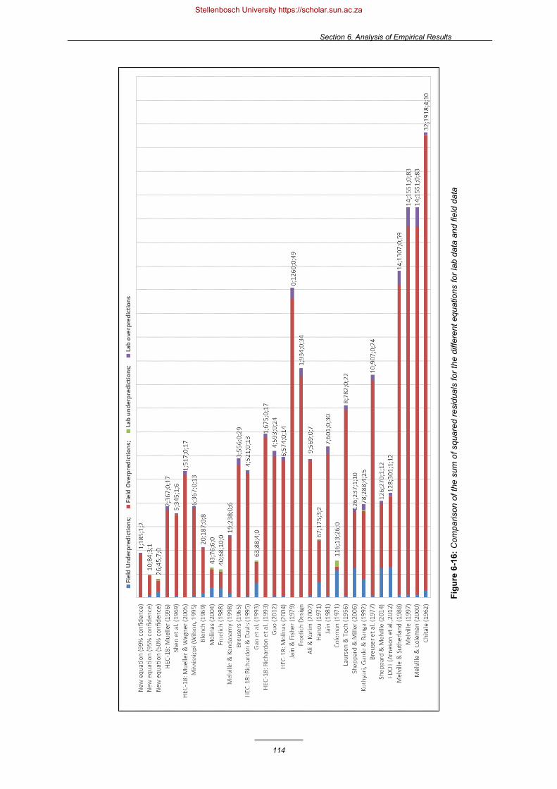
Section 6. Analysis of Empirical Results
114
Figu
re 6
-16:
Com
paris
on o
f the
sum
of s
quar
ed re
sidu
als
for t
he d
iffer
ent e
quat
ions
for l
ab d
ata
and
field
dat
a
Stellenbosch University https://scholar.sun.ac.za

Section 6. Analysis of Empirical Results
115
The new equation (99% confidence) ranked the highest with the least total SSR 186;3 and least underpredictions 1;1 for the field data and lab data combined, followed by the new equation with the 95% and 50% confidence intervals for the combined data. It also had the least total SSR 3 and the 2nd least underpredictions of SSR 1 for the lab data. The new equation (50% confidence) yielded the least total SSR 71 followed by 94 for the new equation (95% confidence) for just the field data (ranking 11th and 15th in underpredictions). For the lab data, the new equation (95% confidence) ranked 2nd and 3rd and the new equation (50% confidence) ranked 4th and 6th in the least total SSR and underpredictions respectively.
If the ±0.3 m accuracy of the pier scour measurements is considered, the SSR for the field data is 12 and for the lab data is 0. The new equation (95% confidence) is therefore also adequately reliable as a design equation (with an SSR for underpredictions of 10 which is less than the 12 representing the accuracy of the data).
The new proposed equation performs comparably better to the field data than to the lab data. The new equations have achieved considerably less scatter about the line of equality despite underpredictions for the cylindrical piers. The new equation (50% confidence) would not be fit for pier design due to underpredictions but the new equation (99% confidence) is the most accurate method that has a compact boxplot range of error and a mean percentage error closest to but greater than zero (10%) and a minimum of only -28% (acceptable compared to the laboratory error of 9%).
6.6 Summary
The simplicity of conservative empirical equations may be appealing but overestimating the anticipated scour depth leads to uneconomical designs with unnecessarily expensive foundations and countermeasures. Thirty empirical equations traditionally employed to predict bridge pier scour were evaluated against the results from the laboratory for a full-scale prototype. And as in all preceding studies, the equations were found to yield a wide range of varying and mostly unreliable results for the same case, even under controlled laboratory conditions. An improved equation was proposed but advanced CFD numerical models for scour prediction should be the primary subject of any future studies.
The results of Section 6 were published as an adapted version of the journal article: Vonkeman, J.K. and Basson, G.R. 2019. Evaluation of empirical equations to predict bridge pier scour in a noncohesive bed under clear-water
conditions, South African Institution of Civil Engineering, 61(2), pp. 2-20 (ISSN 1021-2019).
Stellenbosch University https://scholar.sun.ac.za

Section 7. Evaluation of the Numerical Model
116
7. Evaluation of the Numerical Model
7.1 Introduction
The ability of the proposed coupled fully 3D hydro-morphodynamic model to simulate the complex flow field and the subsequent bridge pier scour was evaluated and validated by the experimental work. Section 7 is divided into two parts that discuss the outcomes from the numerical modelling relative to the objectives outlined in Section 1 for the (a) flow field and (b) sediment bed, respectively.
7.2 Numerical Modelling of the Velocity Flow Field
Before the proposed numerical model’s ability to simulate bridge pier scour can be evaluated, the flow field must be resolved. The accurate prediction of bridge pier scour depends on a numerical model’s ability to resolve the flow structure (Ahmed & Rajaratnam, 1998; Salaheldin et al., 2004) and consequently, most of the numerical models reviewed in Section 2.9.1.2 focused on resolving the flow, and not on modelling scour. The flow field from the experimental work was therefore visualized by velocity readings and was first compared to the numerical model for a flat rigid bed (without sediment).
7.2.1 Comparison of Velocity Flow Fields
Appendix B records the flow field in plan for each test from the experimental work and numerical model by means of a time-averaged velocity profile with contours plotted on Surfer. The velocity profiles are compared at the central water depth of 0.1 m (equivalently a nondimensional flow depth of 0.5) whereby warmer red and orange colours represent increased velocities. The key discrepancy between the experimental work and numerical model is that the velocities measured in the laboratory are generally higher. While the velocity profiles from the laboratory and the model do not have identical contour patterns, both capture the dominant flow elements in a similar manner. These elements include the separated flow beside the pier, the abrupt decrease in velocities directly upstream of the pier, and the low-pressure zone downstream of the pier. The general increase in approach velocity is equally evident in the physical and numerical modelling.
The velocity profiles from the numerical modelling have smoother contours while those from the laboratory are rougher and more irregular. This is attributed to the coarser resolution of the grid for experimental data collection and interpolation. The computational grid for the numerical model is in the order of 2 to 25 mm while the grid employed in the laboratory was based on a grid size of 100 mm. The Kriging gridding method was implemented by Surfer to interpolate values between the grid nodes which, according to the Surfer software, expresses trends well and has been proven to be effective in many fields. Interpolation of the physical model’s coarse grid resolution has caused the boundary layer at the pier surface to be exaggerated in certain velocity profiles, in particular those for the sharp nosed pier (28 to 46 l/s) and the cylindrical pier (46 and 68 l/s). The low-pressure zones downstream of the sharp and round nosed piers have also been misrepresented as they do not emerge directly behind the pier.
Stellenbosch University https://scholar.sun.ac.za

Section 7. Evaluation of the Numerical Model
117
Table 7-1 is a quantitative comparison of the velocities at two points from the experimental work and numerical modelling, implemented initially with the standard 𝑘𝑘-ε turbulence model and then with the more advanced RSM turbulence model. The velocities are compared 0.15 m upstream of the pier and 0.15 m beside the pier as indicated in Figure 4-10 of Section 4.4. Note the larger velocity values (relative to the approach velocity) that are present beside the pier in the region of separated flow.
The 𝑘𝑘-ε model underestimates the velocities by an average of 0.026 m/s which is considered a 9% difference between the results from the numerical model and the laboratory. The RSM model is capable of replicating near identical results to the laboratory, particularly for the velocities less than 0.34 m/s, which are on average 0.004 m/s lower than those measured in the laboratory. This 1% error is considered negligible in light of the 6% maximum margin of error present in the experimental work (Section 7.2.1.3). This is concurrent with the findings of Salaheldin et al. (2004) who attribute the slight underestimations of numerical modelling to the 𝑘𝑘-ε turbulence model. Nevertheless, they also claim that the 𝑘𝑘-ε turbulence model performs satisfactorily in reproducing the velocity profile and that the RSM model is the most accurate model for simulating velocity distributions and bed shear stresses.
Table 7-1: Quantitative comparison of velocities in m/s measured 0.15 m upstream of the pier and 0.15 m beside the pier at a nondimensional flow depth of 0.5
Velocities upstream of the pier (m/s) Test 1 2 3 4 5 6 7 8 Pier shape Approach velocity 0.14 0.17 0.20 0.23 0.28 0.31 0.34 0.37
Cylindrical pier
Laboratory 0.133 0.166 0.194 0.220 0.269 0.317 0.356 0.374 RSM model 0.140 0.169 0.199 0.228 0.277 0.306 0.335 0.364 𝑘𝑘-ε model 0.125 0.152 0.179 0.205 0.250 0.277 0.303 0.330
Round nosed pier
Laboratory 0.132 0.157 0.196 0.216 0.263 0.308 0.352 0.396 RSM model 0.137 0.166 0.195 0.224 0.271 0.300 0.329 0.357 𝑘𝑘-ε model 0.123 0.149 0.176 0.202 0.246 0.272 0.298 0.325
Sharp nosed pier
Laboratory 0.135 0.156 0.195 0.225 0.278 0.315 0.345 0.392 RSM model 0.141 0.170 0.196 0.229 0.278 0.307 0.336 0.366 𝑘𝑘-ε model 0.127 0.154 0.181 0.208 0.253 0.280 0.307 0.334
Velocities beside the pier (m/s) Test 1 2 3 4 5 6 7 8 Pier shape Approach velocity 0.14 0.17 0.20 0.23 0.28 0.31 0.34 0.37
Cylindrical pier
Laboratory 0.175 0.215 0.245 0.297 0.341 0.407 0.435 - RSM model 0.177 0.214 0.251 0.288 0.349 0.386 0.423 0.460 𝑘𝑘-ε model 0.165 0.201 0.236 0.271 0.329 0.364 0.400 0.435
Round nosed pier
Laboratory 0.172 0.208 0.247 0.285 0.345 0.379 0.437 0.494 RSM model 0.175 0.212 0.249 0.286 0.348 0.385 0.422 0.458 𝑘𝑘-ε model 0.166 0.202 0.237 0.272 0.331 0.366 0.402 0.437
Sharp nosed pier
Laboratory 0.173 0.203 0.249 0.303 0.361 0.393 0.439 0.478 RSM model 0.175 0.212 0.249 0.286 0.348 0.385 0.422 0.458 𝑘𝑘-ε model 0.166 0.201 0.236 0.272 0.330 0.366 0.401 0.436
Stellenbosch University https://scholar.sun.ac.za

Section 7. Evaluation of the Numerical Model
118
7.2.2 Vertical Velocity Profiles
7.2.2.1 Fully Developed Velocity Profile The vertical velocity profiles from the experimental work and the numerical model with the RSM model were also compared 0.15 m upstream of the pier and 0.15 m beside the pier. Figure 7-1 shows that the vertical velocity profiles for the tests with the round nosed pier exemplify the well-recognised logarithmic relationship, as discussed in Section 2.5.1 and illustrated in Figure 2-6. They also illustrate the difference between the physical and numerical modelling more plainly and confirm the previous observation that the velocities calculated by the numerical model are underestimated, particularly as the flow intensity increases. As observed in Section 7.2.1, the velocities beside the pier are slightly larger than those upstream of the pier on account of the separated flow, and an equal increment in velocity distribution is observed for each flow.
A prominent dissimilarity is the shape of the logarithmic velocity profile. The numerical model yields a velocity profile that is distinctly underpredicted near the water surface with the maximum velocity simulated at a nondimensional flow depth of 0.55. This behaviour could be attributed to a numerical overchute of the fully developed profile due to the boundary condition of the proposed numerical model. The free surface has been treated as a shear free rigid lid by a symmetry boundary while the law-of-the-wall was employed to establish the shear stress for the boundary layer formation at the surface of the packed bed. Conversely, the entrance length condition for fully developed flow (in the order of 5 to 9 m) may not have been satisfied in the physical model, particularly for larger flow velocities, whereby the sediment bed was only placed in the flume for a distance of 5 m upstream of the pier with a 1:5 slope to facilitate a gradual transition of the velocity profile. Nevertheless, the hydrodynamic model performs reasonably well in reproducing the velocity profile from the laboratory closer to the bed.
Figure 7-1: Vertical velocity profiles for the round nosed pier (a) upstream of the pier and (b) beside the pier for a
flat rigid bed
0.00 0.10 0.20 0.30 0.40 0.50
Non
dim
ensi
onal
flow
dep
th
v (m/s)
Physical model - 56 L/s
Physical model - 62 L/s
Physical model - 68 L/s
Physical model - 74 L/s
∀ Water level
∀ Fixed bed level
1.00
0.75
0.50
0.25
0.00
(a)
0.00 0.10 0.20 0.30 0.40 0.50 0.60v (m/s)
Numerical model - 56 L/s
Numerical model - 62 L/s
Numerical model - 68 L/s
Numerical model - 74 L/s
∀ Water level
∀ Fixed bed level
(b)
Stellenbosch University https://scholar.sun.ac.za

Section 7. Evaluation of the Numerical Model
119
The approach for modelling the free surface as a rigid lid is widely adopted to limit computational costs and is considered acceptable for flows with a small Froude number because modelling the free surface would not affect the morphodynamic results for small Froude numbers typically less than 0.2 or even 0.4 (Roulund et al., 2005; Lui & Garcia, 2008; Baykal et al, 2015). The maximum Froude number that was investigated in this study was 0.26, and even though the bow wave at the pier, shown in Figure 7-2, cannot be modelled, it only counteracts the horseshoe vortex in shallow waves (Melville, 1975). Once the morphodynamic model is resolved, future studies could investigate the feasibility of modelling air as an additional phase to capture the free surface of floods with high Froude numbers, for example with the VOF multiphase model.
Figure 7-2: Photograph of the bow wave forming in front of the cylindrical pier in the laboratory
For hydraulically rough and fully developed flow, the logarithmic velocity distribution in Figure 2-6 can be fitted by the wall function in Equation 2-29 where 𝐶𝐶+ = 0. Curve-fitting the vertical velocity profiles gives the nondimensional wall distance 𝑌𝑌+ = (𝑦𝑦 − 𝑦𝑦1)/𝑦𝑦0 and the roughness length 𝑦𝑦0 = 0.05𝑑𝑑 where 𝑦𝑦1 is the flow depth of 0.2 m and 𝑑𝑑 is the particle diameter. In other words, 𝑦𝑦0 is 0.01 m for sand, 0.04 m for the crushed pips and 1×10⁻⁵ m for the fixed bed in the laboratory. This is similar to the roughness length described by Mohammed et al. (2016) as 𝑦𝑦0 = 𝑘𝑘𝑠𝑠/30 where the roughness 𝑘𝑘𝑠𝑠 can be approximated as 3𝑑𝑑. Curve-fitting of the wall function also produces shear velocity values of 0.03 to 0.22 m/s for the fine sand, and 0.01 to 0.12 m/s for the crushed pips (in the same order as experimental values from Bagnold, 1941). In comparison, the numerical model simulates shear velocities as large as 0.31 and 0.21 m/s for the fine sand and the crushed peach pips, respectively. From curve-fitting to the numerical model, it is also evident that the roughness length is typically double to that from the physical modelling. The increased roughness and shear velocities simulated at the surface of the bed could justify the underestimated velocity profile by the numerical model.
Salaheldin et al. (2004) also observed that the 𝑘𝑘-ε turbulence model generally overestimates the bed shear stress and potentially the area of scour initiation. Numerical models with the 𝑘𝑘-ε turbulence model have been criticised for being constrained by the 𝑘𝑘-ε model because the velocities, particularly the 𝜕𝜕-velocities, are underestimated. However, the proposed RSM model also underestimated the velocity profiles, albeit less, and produced slightly higher shear velocities and bed shear stresses.
Wake
Eddies from detached shear layers
Bow wave
Stellenbosch University https://scholar.sun.ac.za

Section 7. Evaluation of the Numerical Model
120
7.2.2.2 Coupled Behaviour of Sediment Transport in a Flow Field The vertical velocity profiles between a fixed bed and a sediment bed for different approach flows are compared in Figure 7-3 0.15 m upstream of the pier and 0.15 m beside the pier (see Figure 4-10). The reduced and formalized cross-sections of the flat rigid bed generally have increased and more uniform velocities than the movable sediment bed which trap and stabilize the vortices (Williams, 2014). Note that no velocity measurements were possible in the vicinity of the boundary layer by the ADV in the laboratory. Although commercial software exists to model sediment transport, they are not fully coupled. The interaction between fluid and sediment is coupled because sediment transport modifies the local flow patterns but also the bed in terms of elevation, slope and roughness, which in turn alters the local velocities and flow field in the vicinity of the pier, over different time scales. The presence of saltating particles in particular modifies the velocity profile inside the moving layer (Schneiderbauer & Pirker, 2013).
Figure 7-3: Vertical velocity profiles measured for the round nosed pier with fine sand (a) upstream and
(b) beside the pier from the physical model
7.2.2.3 Repeatability As discussed in Section 6.2.1, the 4 tests involving the cylindrical pier and crushed peach pips were duplicated 3 times to evaluate the repeatability and reliability of the results. Figure 7-4 shows the vertical velocity profiles measured upstream and beside the pier during the 3 tests that were repeated for 4 flows. Test 3 for the 40 l/s flow yielded underpredicted and unreliable results for both points, indicating that an incorrect flow less than the 40 l/s was tested, emphasizing the importance of repeat tests and monitoring the flow during the laboratory tests.
0.00 0.10 0.20 0.30 0.40 0.50
Non
dim
ensi
onal
flow
dep
th
v (m/s)
Movable bed - 56 L/s
Movable bed - 62 L/s
Movable bed - 68 L/s
Movable bed - 74 L/s
∀ Water level
∀ Initial bed level
(a)
0.00 0.10 0.20 0.30 0.40 0.50 0.60v (m/s)
Fixed bed - 56 L/s
Fixed bed - 62 L/s
Fixed bed - 68 L/s
Fixed bed - 74 L/s
∀ Water level
∀ Initial bed level
(b)1.00
0.75
0.50
0.25
0.00
Stellenbosch University https://scholar.sun.ac.za

Section 7. Evaluation of the Numerical Model
121
Erroneous values that deviate from the repeat tests and logarithmic velocity profile are easily identified and discarded. For example, upstream of the pier, the 34 l/s Test 2 obtained a velocity 0.035 m/s lower (17% error) than the other tests at 0.15 m below the water level. However, the rest of the results are near identical, only deviating within a range of 0.009 m/s (a maximum error of 6%). This error could be attributed to small fluctuations in the flow rates that could have been caused occasionally by vacillating pumps or the ADV probe oscillated indistinctly with the flow and could not resolve the erratic vectors, particularly near the packed bed or water surface. Alternatively, the increased velocities measured in the laboratory could be caused by electrical noise evident in the ADV even under no flow conditions.
Figure 7-4: Vertical velocity profiles measured for the cylindrical pier with crushed peach pips (a) upstream of the pier and (b) beside the pier for three repeat tests
7.2.3 Resolving the Vortex Systems
In the previous section, the flow field from the numerical model was evaluated. However, the flow field should be more specifically examined for its ability to resolve the horseshoe vortex because it governs the ability of a numerical model to simulate bridge pier scour accurately.
7.2.3.1 The Horseshoe Vortex Coloured dye wands were used to visualize the flow pattern around the pier in the laboratory. The photographs in Figure 7-5 show the accelerated velocities in the region of the separated flow, as well as dye captured by the downward flow component of the horseshoe vortex in front of the cylindrical pier.
0.00 0.05 0.10 0.15 0.20 0.25 0.30
Non
dim
ensi
onal
flow
dep
th
v (m/s)28 L/s Test 128 L/s Test 228 L/s Test 334 L/s Test 134 L/s Test 234 L/s Test 3
∀ Water level
∀ Initial bed level
1.00
0.75
0.50
0.25
0.00
(a)
0.00 0.05 0.10 0.15 0.20 0.25 0.30 0.35
v (m/s)40 L/s Test 140 L/s Test 240 L/s Test 346 L/s Test 146 L/s Test 246 L/s Test 3
∀ Water level
∀ Initial bed level
(b)
Stellenbosch University https://scholar.sun.ac.za
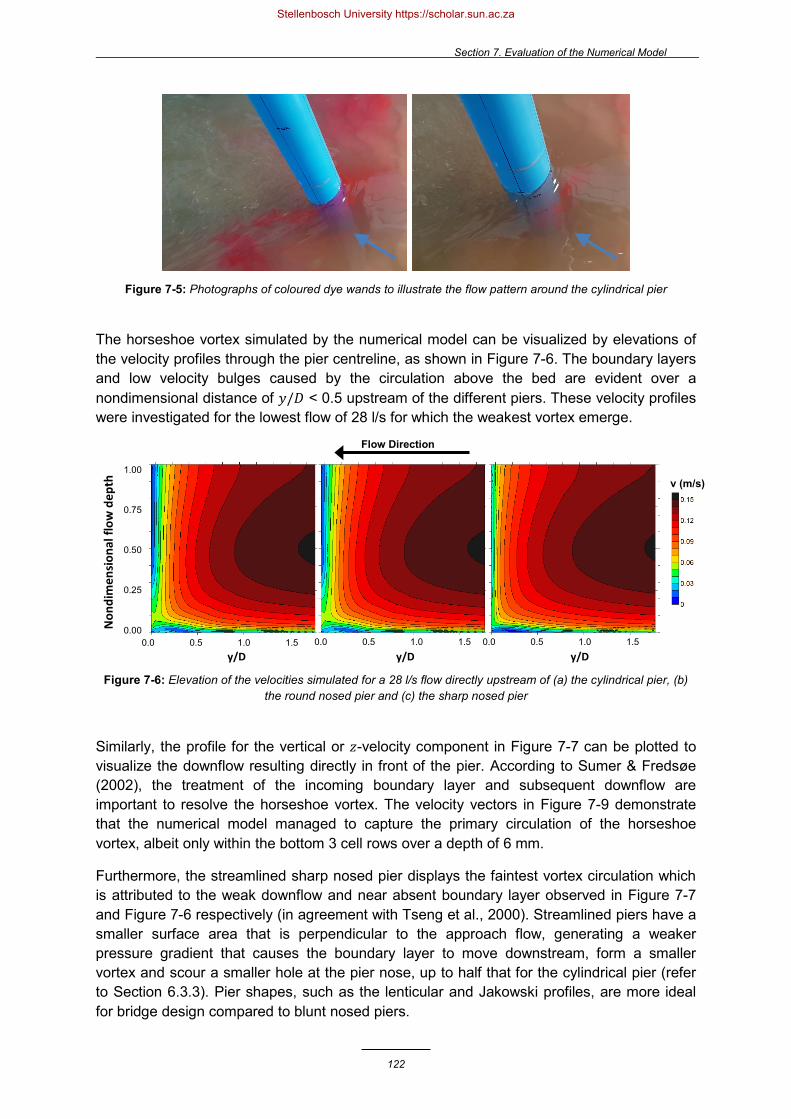
Section 7. Evaluation of the Numerical Model
122
Figure 7-5: Photographs of coloured dye wands to illustrate the flow pattern around the cylindrical pier
The horseshoe vortex simulated by the numerical model can be visualized by elevations of the velocity profiles through the pier centreline, as shown in Figure 7-6. The boundary layers and low velocity bulges caused by the circulation above the bed are evident over a nondimensional distance of 𝑦𝑦/𝐷𝐷 < 0.5 upstream of the different piers. These velocity profiles were investigated for the lowest flow of 28 l/s for which the weakest vortex emerge.
Figure 7-6: Elevation of the velocities simulated for a 28 l/s flow directly upstream of (a) the cylindrical pier, (b) the round nosed pier and (c) the sharp nosed pier
Similarly, the profile for the vertical or 𝜕𝜕-velocity component in Figure 7-7 can be plotted to visualize the downflow resulting directly in front of the pier. According to Sumer & Fredsøe (2002), the treatment of the incoming boundary layer and subsequent downflow are important to resolve the horseshoe vortex. The velocity vectors in Figure 7-9 demonstrate that the numerical model managed to capture the primary circulation of the horseshoe vortex, albeit only within the bottom 3 cell rows over a depth of 6 mm.
Furthermore, the streamlined sharp nosed pier displays the faintest vortex circulation which is attributed to the weak downflow and near absent boundary layer observed in Figure 7-7 and Figure 7-6 respectively (in agreement with Tseng et al., 2000). Streamlined piers have a smaller surface area that is perpendicular to the approach flow, generating a weaker pressure gradient that causes the boundary layer to move downstream, form a smaller vortex and scour a smaller hole at the pier nose, up to half that for the cylindrical pier (refer to Section 6.3.3). Pier shapes, such as the lenticular and Jakowski profiles, are more ideal for bridge design compared to blunt nosed piers.
v (m/s)
Flow Direction
1.00
0.75
0.50
0.25
0.00 0.0 0.5 1.0 1.5
Non
dim
ensi
onal
flow
dep
th
y/D y/D y/D 0.0 0.5 1.0 1.5 0.0 0.5 1.0 1.5
Stellenbosch University https://scholar.sun.ac.za

Section 7. Evaluation of the Numerical Model
123
Figure 7-7: Elevation of the vertical velocity component simulated for a 28 l/s flow directly upstream of (a) the cylindrical pier, (b) the round nosed pier and (c) the sharp nosed pier
A further comparison of the pier shapes is shown in Figure 7-8 by the turbulent kinetic energy (𝑘𝑘) and turbulent intensity (𝑇𝑇𝑇𝑇) profiles beside the pier nose. The turbulence for the approach flow (0.15 m upstream of the piers) is identical for the different pier shapes but has different boundary layer curves near the bed beside the pier because the pier shapes deflect the flow sideways in different proportions. An average 𝑘𝑘 = 7.6×10⁻⁵ m2/s2 and 𝑇𝑇𝑇𝑇 = 7% is modelled for the 28 l/s flow comparable to the 𝑇𝑇𝑇𝑇 = 5% assumed for the inflow boundary.
Figure 7-8: Turbulent kinetic energy and turbulent intensity for the different pier shapes compared 0.15 m beside the pier nose from the physical model and numerical model for a 28 l/s flow
v (m/s)
Flow Direction
1.00
0.75
0.50
0.25
0.00 0.0 0.5 1.0 1.5
Non
dim
ensi
onal
flow
dep
th
y/D y/D y/D 0.0 0.5 1.0 1.5 0.0 0.5 1.0 1.5
Non
dim
ensi
onal
flow
dep
th
Stellenbosch University https://scholar.sun.ac.za
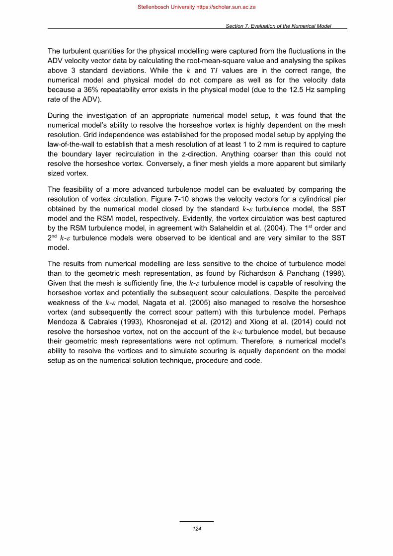
Section 7. Evaluation of the Numerical Model
124
The turbulent quantities for the physical modelling were captured from the fluctuations in the ADV velocity vector data by calculating the root-mean-square value and analysing the spikes above 3 standard deviations. While the 𝑘𝑘 and 𝑇𝑇𝑇𝑇 values are in the correct range, the numerical model and physical model do not compare as well as for the velocity data because a 36% repeatability error exists in the physical model (due to the 12.5 Hz sampling rate of the ADV).
During the investigation of an appropriate numerical model setup, it was found that the numerical model’s ability to resolve the horseshoe vortex is highly dependent on the mesh resolution. Grid independence was established for the proposed model setup by applying the law-of-the-wall to establish that a mesh resolution of at least 1 to 2 mm is required to capture the boundary layer recirculation in the z-direction. Anything coarser than this could not resolve the horseshoe vortex. Conversely, a finer mesh yields a more apparent but similarly sized vortex.
The feasibility of a more advanced turbulence model can be evaluated by comparing the resolution of vortex circulation. Figure 7-10 shows the velocity vectors for a cylindrical pier obtained by the numerical model closed by the standard 𝑘𝑘-ε turbulence model, the SST model and the RSM model, respectively. Evidently, the vortex circulation was best captured by the RSM turbulence model, in agreement with Salaheldin et al. (2004). The 1st order and 2nd 𝑘𝑘-ε turbulence models were observed to be identical and are very similar to the SST model.
The results from numerical modelling are less sensitive to the choice of turbulence model than to the geometric mesh representation, as found by Richardson & Panchang (1998). Given that the mesh is sufficiently fine, the 𝑘𝑘-ε turbulence model is capable of resolving the horseshoe vortex and potentially the subsequent scour calculations. Despite the perceived weakness of the 𝑘𝑘-ε model, Nagata et al. (2005) also managed to resolve the horseshoe vortex (and subsequently the correct scour pattern) with this turbulence model. Perhaps Mendoza & Cabrales (1993), Khosronejad et al. (2012) and Xiong et al. (2014) could not resolve the horseshoe vortex, not on the account of the 𝑘𝑘-ε turbulence model, but because their geometric mesh representations were not optimum. Therefore, a numerical model’s ability to resolve the vortices and to simulate scouring is equally dependent on the model setup as on the numerical solution technique, procedure and code.
Stellenbosch University https://scholar.sun.ac.za

Section 7. Evaluation of the Numerical Model
125
Figure 7-9: Velocity vectors showing the horseshoe vortex formation simulated directly upstream of (a) the cylindrical pier, (b) the round nosed pier and (c) the sharp nosed pier
Stellenbosch University https://scholar.sun.ac.za
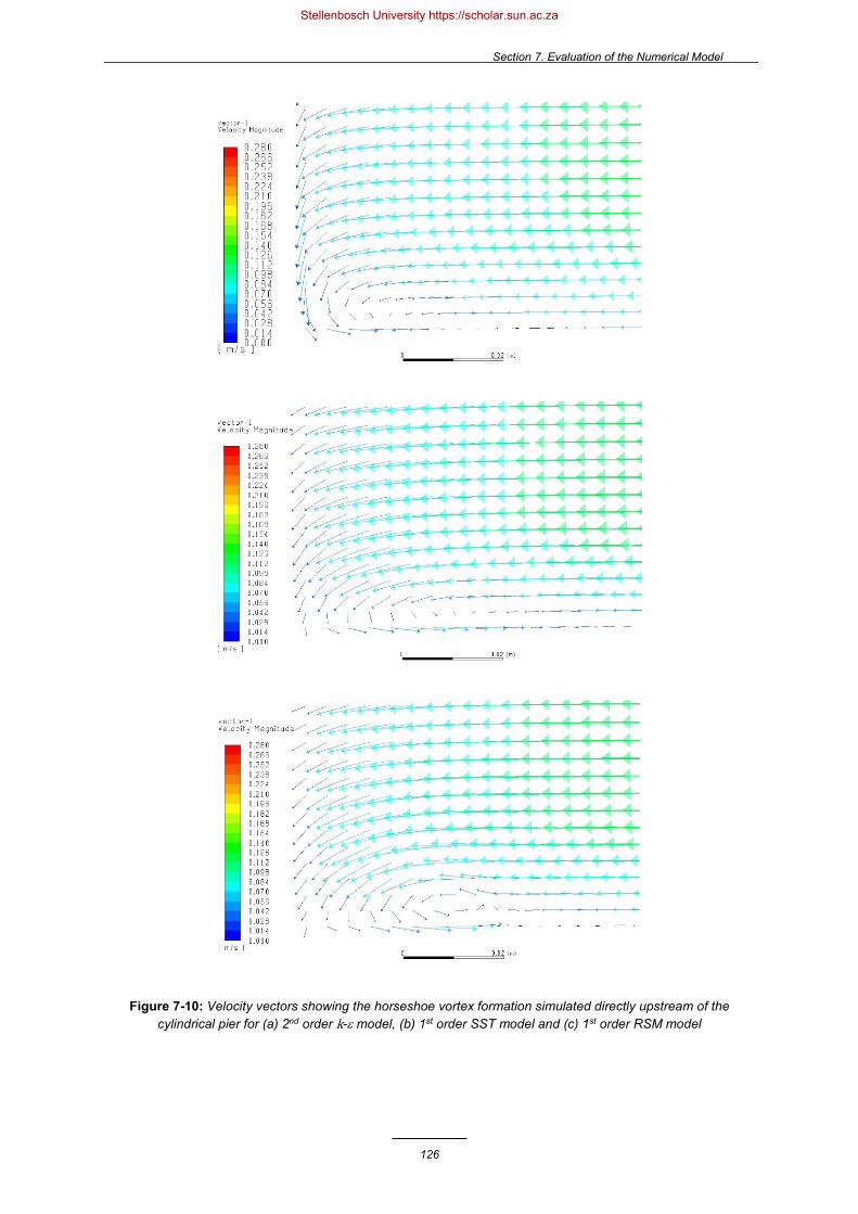
Section 7. Evaluation of the Numerical Model
126
Figure 7-10: Velocity vectors showing the horseshoe vortex formation simulated directly upstream of the cylindrical pier for (a) 2nd order k-ε model, (b) 1st order SST model and (c) 1st order RSM model
Stellenbosch University https://scholar.sun.ac.za

Section 7. Evaluation of the Numerical Model
127
7.2.3.2 The Lee-Wake Vortex The photographs in Figure 7-11 illustrate the lee-wake vortex shedding downstream of the pier in the laboratory. These vortices are easy to visualize because they occur on the water surface. The test with the 28 l/s flow had a cycle time 1/𝑓𝑓 of approximately 4 seconds which holds true for the Strouhal number 𝑆𝑆𝐹𝐹 = 𝑓𝑓𝐷𝐷/𝑣𝑣1 of 0.2 for a cylindrical pier. Note that the comparison of the velocity flow field in Appendix B does not show the lee-wake vortex because the ADV in the laboratory could only capture time-averaged velocities. In order to simulate the vortex shedding, a transient numerical simulation with a more advanced turbulence model is required. Figure 7-12 shows the velocity profiles for a cylindrical pier obtained by different URANS turbulence models. The 1st order 𝑘𝑘-ε turbulence model in Figure 7-9a is very similar to that of the 2nd order 𝑘𝑘-ε model and 1st order SST model. However, the lee-wake vortex has only been resolved by the RSM turbulence model for the time step of 0.001 seconds. The impact of the lee-wake vortex on the maximum scour depth is negligible and only affects the downstream scour pattern in the early stages of the scouring process (Baykal et al., 2015).
Figure 7-11: Photographs of the lee-wake vortex forming behind the cylindrical pier
Figure 7-12: Velocity profiles for a cylindrical pier with a 28 l/s flow for (a) 2nd order k-ε turbulence model,
(b) 1st order SST model and (c) 1st order RSM model
v (m/s)
y (m
)
x (m)
Flow
Dire
ctio
n
Stellenbosch University https://scholar.sun.ac.za

Section 7. Evaluation of the Numerical Model
128
7.3 Numerical Modelling of the Sediment Bed
The proposed numerical model has demonstrated that the model setup is optimized and capable of simulating the crucial horseshoe vortex and flow field observed in the laboratory. The final objective of the study was to develop an improved hydro-morphodynamic model and to evaluate its ability to simulate bridge pier scour. Before the numerical model could be validated against experimental data for its correctness, the model limitations had to be investigated and addressed.
The proposed model is exceedingly sensitive and several numerical instabilities were encountered by the sediment transport submodels because there are so many nonphysical numerical parameters and because the proposed hydro-morphodynamic model algorithms are coupled by the source terms in the governing fluid equations. Divergence in the model frequently occurred in the Eulerian multiphase model that were made unstable by the loss in the fluid momentum term caused by the entrained particles or by the implicit wall functions. Schneiderbauer & Pirker (2014) referred to the implicit wall functions for the shear stress velocity as the most sensitive element in the model. Since the processing time for each simulation on a supercomputer took several days, the numerical study was a time intensive process of trial-and-error.
7.3.1 Model Calibration
The proposed hydro-morphodynamic model was examined for parameter instabilities and sensitivities, and was calibrated to accommodate the sediment material as well as the mesh resolution, to obtain a numerically stable and accurate solution. It was established that a very fine computational mesh in the order of 1 to 2 mm is required to resolve the horseshoe vortex that is crucial for bridge pier scour. However, the sediment transport submodels of the proposed numerical model are very sensitive to the mesh resolution and result in an instability of the packed bed with an unrealistic and irregularly shaped scour hole as shown by Figure 7-13 (Vonkeman et al., 2017). The scour hole was simulated by a model setup with parameters identical to those of Sawadogo (2015) for hydrodynamic entrainment but with a minimum mesh size of 1.8 mm. In spite of the scour instability, the model demonstrated that it had the potential to predict bridge pier scour as a maximum scour depth of 0.125 m was simulated which is of the same order as the 0.116 m measured in the laboratory for a cylindrical pier with a 34 l/s flow.
In a sensitivity analysis for dam bottom outlet flushing, Sawadogo (2015) also recognized that the choice of the mesh size is crucial for the proposed hydro-morphodynamic model and that a finer mesh can cause an irregularly shaped scour hole. Schneidernauer & Pirker (2014) also used a fine mesh with a minimum size of 2.5 mm. Consequently, the parameters that were different in the model study by Schneidernauer & Pirker (2014) and Sawadogo (2015) were compared in Table 7-2. The parameters used by Shao & Li (1999) are also compared because most of the sediment transport algorithms were based on their model study. However, Shao & Li (1999) adopted a different approach whereby the motion of individual saltating particles were tracked as opposed to the proposed hydro-morphodynamic model that modelled the deformation of the particulate bed.
Stellenbosch University https://scholar.sun.ac.za
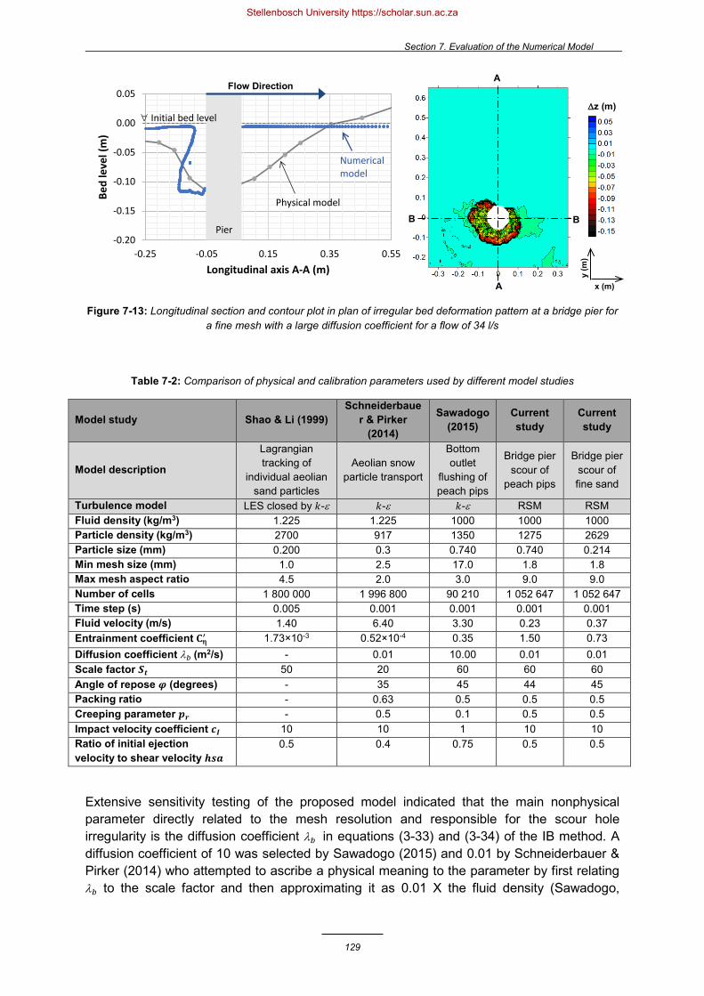
Section 7. Evaluation of the Numerical Model
129
Figure 7-13: Longitudinal section and contour plot in plan of irregular bed deformation pattern at a bridge pier for a fine mesh with a large diffusion coefficient for a flow of 34 l/s
Table 7-2: Comparison of physical and calibration parameters used by different model studies
Model study Shao & Li (1999) Schneiderbaue
r & Pirker (2014)
Sawadogo (2015)
Current study
Current study
Model description
Lagrangian tracking of
individual aeolian sand particles
Aeolian snow particle transport
Bottom outlet
flushing of peach pips
Bridge pier scour of
peach pips
Bridge pier scour of fine sand
Turbulence model LES closed by 𝑘𝑘-ε 𝑘𝑘-ε 𝑘𝑘-ε RSM RSM Fluid density (kg/m3) 1.225 1.225 1000 1000 1000 Particle density (kg/m3) 2700 917 1350 1275 2629 Particle size (mm) 0.200 0.3 0.740 0.740 0.214 Min mesh size (mm) 1.0 2.5 17.0 1.8 1.8 Max mesh aspect ratio 4.5 2.0 3.0 9.0 9.0 Number of cells 1 800 000 1 996 800 90 210 1 052 647 1 052 647 Time step (s) 0.005 0.001 0.001 0.001 0.001 Fluid velocity (m/s) 1.40 6.40 3.30 0.23 0.37 Entrainment coefficient 𝐂𝐂η
′ 1.73×10⁻³ 0.52×10⁻⁴ 0.35 1.50 0.73 Diffusion coefficient λ𝑏𝑏 (m2/s) - 0.01 10.00 0.01 0.01 Scale factor 𝑺𝑺𝒕𝒕 50 20 60 60 60 Angle of repose 𝝋𝝋 (degrees) - 35 45 44 45 Packing ratio - 0.63 0.5 0.5 0.5 Creeping parameter 𝒑𝒑𝑭𝑭 - 0.5 0.1 0.5 0.5 Impact velocity coefficient 𝒄𝒄𝑰𝑰 10 10 1 10 10 Ratio of initial ejection velocity to shear velocity 𝒉𝒉𝒉𝒉𝒎𝒎
0.5 0.4 0.75 0.5 0.5
Extensive sensitivity testing of the proposed model indicated that the main nonphysical parameter directly related to the mesh resolution and responsible for the scour hole irregularity is the diffusion coefficient λ𝑏𝑏 in equations (3-33) and (3-34) of the IB method. A diffusion coefficient of 10 was selected by Sawadogo (2015) and 0.01 by Schneiderbauer & Pirker (2014) who attempted to ascribe a physical meaning to the parameter by first relating λ𝑏𝑏 to the scale factor and then approximating it as 0.01 X the fluid density (Sawadogo,
-0.20
-0.15
-0.10
-0.05
0.00
0.05
-0.25 -0.05 0.15 0.35 0.55
Bed
leve
l (m
)
Longitudinal axis A-A (m)
∀ Initial bed level
Physical model
Pier
Numericalmodel
y (m
)
x (m)
∆z (m)
Flow Direction
A
B B
A
Stellenbosch University https://scholar.sun.ac.za

Section 7. Evaluation of the Numerical Model
130
2015). However, a diffusion coefficient of 10 yielded erratic scour results and it was found that a value ≤ 0.01 should be implemented instead. This is in accord with Schneiderbauer & Pirker (2014) who implemented the same diffusion coefficient for a 2.5 mm minimum mesh size similar to that of the proposed study. Because the dimension for the diffusion coefficient is area per unit time, it is recommended that future studies of the proposed hydro-morphodynamic model select a diffusion coefficient with an order of magnitude based on the guideline
which relates the volume fraction of the IB method to the mesh resolution or grid cell volume 𝑉𝑉. A reduction of the diffusion coefficient value dramatically reduces the erosion of the sediment bed and should be compensated by an increase in the dimensionless entrainment coefficient 𝐶𝐶η
′ which is considered the chief calibration parameter. Shao & Li (1999) used 1.73×10⁻³ for the aerodynamic entrainment of sand particles, Schneiderbauer & Pirker (2014) used 0.52×10⁻⁴ for the aerodynamic entrainment of snow particles, while Sawadogo (2015) selected 0.35 for the hydrodynamic entrainment of peach pips. The entrainment coefficient for the hydrodynamic transport of particles is much larger than that for the aerodynamic transport of particles because it is related to the fluid and particulate densities. No experimental investigations have been conducted to explain the different values presented for the nonphysical proportionality factor but it is proposed that the following approximation, based on Shao & Li (1999), should be used to establish the order of magnitude for the entrainment coefficient in equation (3-15)
where 𝑠𝑠 is the particle density relative to the fluid. Based on the relative density of sand (𝑠𝑠 = 2.63) or peach pips (𝑠𝑠 = 1.28), the value of 𝐶𝐶η
′ was selected as 0.73 and 1.5 for the fine sand and crushed peach pips, respectively. Furthermore, a saturated angle of repose of 45° and 44° was selected from Table 4-1 for the sand and peach pips. The angle of repose is an extremely sensitive parameter causing numerical instabilities with unrealistic scour patterns.
Second to the entrainment coefficient, the creeping parameter 𝑝𝑝𝑟𝑟 of equations (3-16) and (3-17) should be considered a principal calibration parameter. It defines the probability (between 0 and 1) that a particle with no initial velocity is entrained into the surface rolling or saltating transport mode. For simplicity, a median value of 0.5 for the creeping parameter was found to be the best at replicating the scour results from the laboratory.
The packing ratio in the shear slides equation (3-31) and the IB method equation (3-33) also dramatically destabilized the model. A value of 0.5 as well as an impact velocity coefficient of 10 and a velocity ratio ℎ𝑠𝑠𝑎𝑎 of 0.5 were selected from the original study by Shao and Li (1999) because they offered improved numerical stability while the observed effect of the latter two parameters on the scour hole were negligible. Finally, a scaling factor of 60 was selected because the time scale of scour to approach equilibrium is in the order of minutes or hours, and the time scale of turbulence fluctuations is within the order of seconds. According to Lui & Garcia (2008), the time scale disparity makes coupled hydro-morphodynamic simulations stiff, possibly leading to numerical instabilities.
𝑂𝑂(λ𝑏𝑏) = 𝑉𝑉𝐼𝐼𝑖𝑖𝑚𝑚 𝑑𝑑∆𝑡𝑡 , (7-1)
𝑂𝑂(𝐶𝐶η′) = 6 πs , (7-2)
Stellenbosch University https://scholar.sun.ac.za

Section 7. Evaluation of the Numerical Model
131
The final scour depth results obtained from the improved and calibrated hydro-morphodynamic model are shown in Figure 7-14 relative to the experimental work for a cylindrical pier with a flow of 34 l/s and an initial bed level of 0 m.
Figure 7-14: 3D isometric contour plots of the bridge pier scour for a flow of 34 l/s (a) from experimental work,
(b) from improved numerical model and (c) with numerical instability for a fine mesh
7.3.2 Validation of the Proposed Model
7.3.2.1 Scour Bed Profiles Appendix C records the bed deformation in plan for each test from the experimental work and numerical model, whereby negative values represent erosion (warmer red and orange colours) and positive values represent deposition (cooler blue and green colours). The local scour hole simulated by the proposed numerical model compares well with that of the experimental work for the 24 tests. While the scour profiles from the laboratory and the model are not identical, the proposed hydro-morphodynamic model has successfully captured the characteristic U-shaped scour hole and is capable of simulating the maximum scour depth at the upstream face of the pier where the horseshoe vortex circulates. The numerical model is equally capable of resolving the variation in the scour hole size for different pier shapes and approach velocities or flows.
(a) (b)
(c)
Eros
ion
I Dep
ositi
on
Stellenbosch University https://scholar.sun.ac.za
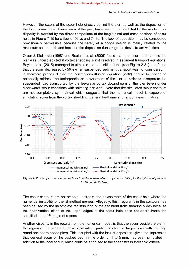
Section 7. Evaluation of the Numerical Model
132
However, the extent of the scour hole directly behind the pier, as well as the deposition of the longitudinal dune downstream of the pier, have been underpredicted by the model. This disparity is clarified by the direct comparison of the longitudinal and cross sections of scour holes in Figure 7-15 for a flow of 56 l/s and 74 l/s. The lack of deposition may be considered provisionally permissible because the safety of a bridge design is mainly related to the maximum scour depth and because the deposition dune migrates downstream with time.
Olsen & Kjellesvig (1998) and Roulund et al. (2005) found that the scour depth behind the pier was underpredicted if vortex shedding is not resolved in sediment transport equations. Baykal et al. (2015) managed to simulate the deposition dune (see Figure 2-31) and found that the scour decreased by 50% when suspended sediment transport was not considered. It is therefore proposed that the convection-diffusion equation (2-32) should be coded to potentially address the underprediction downstream of the pier, in order to incorporate the suspended load transported by the lee-wake vortex downstream of the pier (even under clear-water scour conditions with saltating particles). Note that the simulated scour contours are not completely symmetrical which suggests that the numerical model is capable of simulating scour from the vortex shedding, general bedforms and randomness in nature.
Figure 7-15: Comparison of scour sections from the numerical and physical modelling for the cylindrical pier with
56 l/s and 64 l/s flows
The scour contours are not smooth upstream and downstream of the scour hole where the numerical instability of the IB method merges. Allegedly, this irregularity in the contours has been caused by the incomplete redistribution of the sediment from shearing slides because the near vertical slope of the upper edges of the scour hole does not approximate the specified 44 to 45° angle of repose.
Another disparity in the results from the numerical model, is that the scour beside the pier in the region of the separated flow is prevalent, particularly for the larger flows with the long round and sharp-nosed piers. This, coupled with the lack of deposition, gives the impression that general scour of the packed bed, in the order of 1 to 5 mm, has been simulated in addition to the local scour, which could be attributed to the shear stress threshold criteria.
-0.20
-0.15
-0.10
-0.05
0.00
0.05
-0.35 -0.15 0.05 0.25
Cross sectional axis (m)Numerical model: 0.28 m/sNumerical model: 0.37 m/s
∀ Initial bed level
-0.25 -0.05 0.15 0.35 0.55
Longitudinal axis (m)Physical model: 0.28 m/sPhysical model: 0.37 m/s
Flow Direction
Bed
leve
l (m
)
Stellenbosch University https://scholar.sun.ac.za
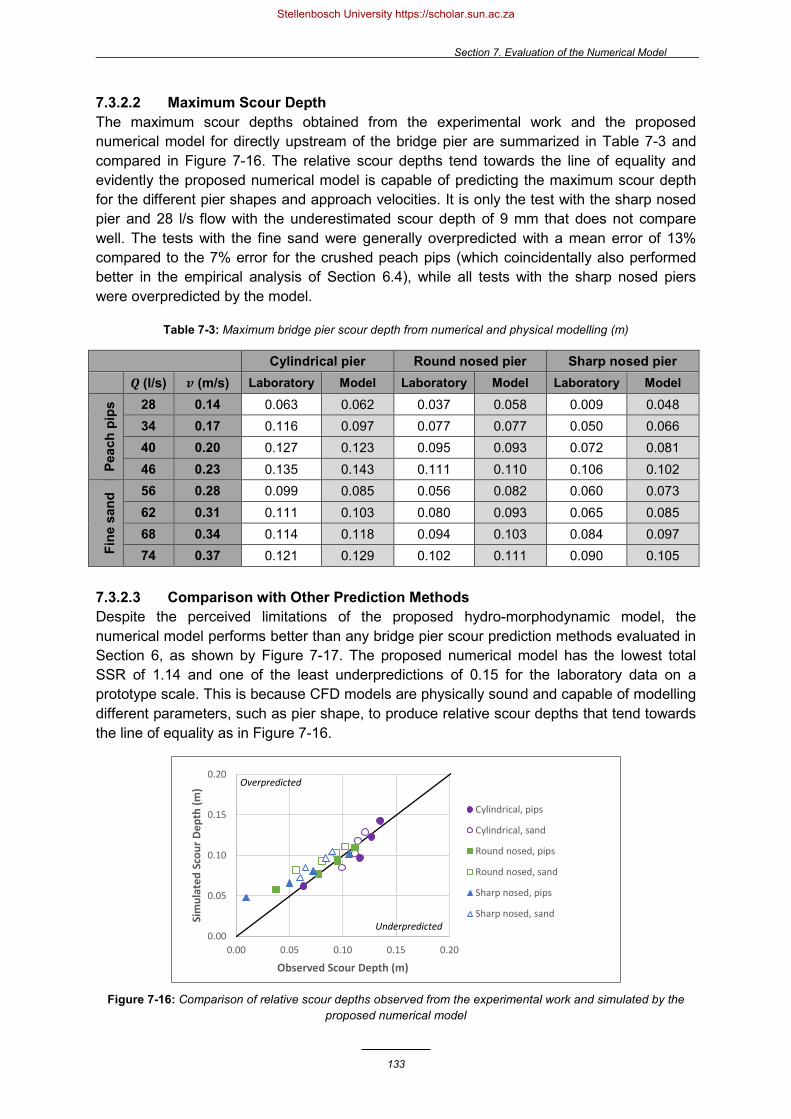
Section 7. Evaluation of the Numerical Model
133
7.3.2.2 Maximum Scour Depth The maximum scour depths obtained from the experimental work and the proposed numerical model for directly upstream of the bridge pier are summarized in Table 7-3 and compared in Figure 7-16. The relative scour depths tend towards the line of equality and evidently the proposed numerical model is capable of predicting the maximum scour depth for the different pier shapes and approach velocities. It is only the test with the sharp nosed pier and 28 l/s flow with the underestimated scour depth of 9 mm that does not compare well. The tests with the fine sand were generally overpredicted with a mean error of 13% compared to the 7% error for the crushed peach pips (which coincidentally also performed better in the empirical analysis of Section 6.4), while all tests with the sharp nosed piers were overpredicted by the model.
Table 7-3: Maximum bridge pier scour depth from numerical and physical modelling (m)
Cylindrical pier Round nosed pier Sharp nosed pier 𝑸𝑸 (l/s) 𝒗𝒗 (m/s) Laboratory Model Laboratory Model Laboratory Model
Peac
h pi
ps 28 0.14 0.063 0.062 0.037 0.058 0.009 0.048
34 0.17 0.116 0.097 0.077 0.077 0.050 0.066 40 0.20 0.127 0.123 0.095 0.093 0.072 0.081 46 0.23 0.135 0.143 0.111 0.110 0.106 0.102
Fine
san
d 56 0.28 0.099 0.085 0.056 0.082 0.060 0.073 62 0.31 0.111 0.103 0.080 0.093 0.065 0.085 68 0.34 0.114 0.118 0.094 0.103 0.084 0.097 74 0.37 0.121 0.129 0.102 0.111 0.090 0.105
7.3.2.3 Comparison with Other Prediction Methods Despite the perceived limitations of the proposed hydro-morphodynamic model, the numerical model performs better than any bridge pier scour prediction methods evaluated in Section 6, as shown by Figure 7-17. The proposed numerical model has the lowest total SSR of 1.14 and one of the least underpredictions of 0.15 for the laboratory data on a prototype scale. This is because CFD models are physically sound and capable of modelling different parameters, such as pier shape, to produce relative scour depths that tend towards the line of equality as in Figure 7-16.
Figure 7-16: Comparison of relative scour depths observed from the experimental work and simulated by the
proposed numerical model
0.00
0.05
0.10
0.15
0.20
0.00 0.05 0.10 0.15 0.20
Sim
ulat
ed S
cour
Dep
th (m
)
Observed Scour Depth (m)
Cylindrical, pips
Cylindrical, sand
Round nosed, pips
Round nosed, sand
Sharp nosed, pips
Sharp nosed, sand
Overpredicted
Underpredicted
Stellenbosch University https://scholar.sun.ac.za

Section 7. Evaluation of the Numerical Model
134
Figure 7-17: The sum of squared residuals for the proposed numerical model compared to different bridge pier
scour prediction equations for the laboratory data on a prototype scale
The proposed numerical model would be considered safe for bridge design because when it fails to be accurate, it predominantly overpredicts the maximum bridge pier scour depth with a mean error of 10% (comparable to the maximum laboratory error of 9%). However, it is proposed that further research is done to evaluate the ability of the model to simulate field data, i.e. a full prototype scale bridge pier calibrated to accommodate the in-situ sediment material and the required mesh resolution. The performance of the proposed model should also be compared with the ability of other numerical models, such as FLOW-3D and REEF3D, to simulate bridge pier scour. Furthermore, it is proposed that the primary subject of future studies should be on the comparison of advanced CFD numerical models with one another. The prediction methods should be calibrated or validated with scour data and not with empirical equations.
Stellenbosch University https://scholar.sun.ac.za

Section 7. Evaluation of the Numerical Model
135
7.3.2.4 Scour Extent Figure 7-18 shows a comparison of the extent of the local scour hole (length and width) simulated by the proposed numerical model with the experimental work. Even though the model is capable of correctly predicting the maximum scour depth at the pier nose, the extent of the scour is predicted with less accuracy, as indicated by the high SSR values in the figure. The scour extent, particularly the length of the scour hole in the flow direction, is mainly underpredicted which could be attributed to the contour irregularity and incomplete redistribution of the sediment from shearing slides identified in Section 7.3.2.1. Nevertheless, the scour extent values tend about the line of equality and demonstrate an average error of 15%, comparable to the 21% repeatability error observed for the scour extent from the laboratory data. The laboratory error for the extent of the local scour holes is greater than the 9% error observed for the maximum scour depths because the scour extent values are only estimates interpolated from the laboratory data to the nearest cm (refer to Section 6.2.1).
Figure 7-18: Comparison of relative scour depth, length and width observed from the experimental work and
simulated by the proposed numerical model
7.3.2.5 Temporal Development of Scour Depth A comparison of the maximum scour bed deformation with time is shown in Figure 7-19. While the proposed numerical model is capable of simulating the temporal bed surface deformation for the 0.14 m/s test with the peach pips, the rate of scour for the 0.37 m/s test with the fine sand is incorrect. The scour development should be more rapid in the beginning and approach equilibrium asymptotically, instead of scouring indefinitely. This could be attributed to the implicit wall functions or the numerical instability and contour irregularity, allegedly caused by incomplete shearing slides, that become increasingly evident with time and with increased approach velocities. Because the critical shear stress is reduced on a sloping bed, sand slides are imposed to prevent the bed slope from exceeding the angle of repose and scouring indefinitely beyond equilibrium conditions (Afzul, 2013). Instead of comparing equilibrium scour depths for different time scales, the maximum simulated scour depths were compared with the experimental work for the same time of 2 hours.
Even though the scouring rate was not modelled properly, the proposed numerical model is capable of capturing the scour process, as shown by the scour hole simulated after 1 minute in Figure 7-20.
0.00
0.05
0.10
0.15
0.20
0.25
0.30
0.00 0.10 0.20 0.30
Sim
ulat
ed L
ocal
Sco
ur (m
)
Observed Local Scour(m)
Scour depth
Scour length
Scour width
Overpredicted
Underpredicted
Sum
of S
quar
e Re
sidua
ls
Tota
l
Und
erpr
edic
tions
1.1 0.1
12.5 10.4
5.1 3.4
Stellenbosch University https://scholar.sun.ac.za
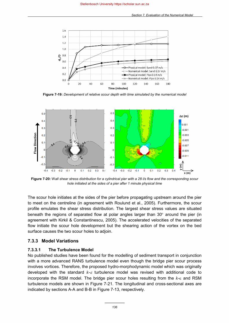
Section 7. Evaluation of the Numerical Model
136
Figure 7-19: Development of relative scour depth with time simulated by the numerical model
Figure 7-20: Wall shear stress distribution for a cylindrical pier with a 28 l/s flow and the corresponding scour hole initiated at the sides of a pier after 1 minute physical time
The scour hole initiates at the sides of the pier before propagating upstream around the pier to meet on the centreline (in agreement with Roulund et al., 2005). Furthermore, the scour profile emulates the shear stress distribution. The largest shear stress values are situated beneath the regions of separated flow at polar angles larger than 30° around the pier (in agreement with Kirkil & Constantinescu, 2005). The accelerated velocities of the separated flow initiate the scour hole development but the shearing action of the vortex on the bed surface causes the two scour holes to adjoin.
7.3.3 Model Variations
7.3.3.1 The Turbulence Model No published studies have been found for the modelling of sediment transport in conjunction with a more advanced RANS turbulence model even though the bridge pier scour process involves vortices. Therefore, the proposed hydro-morphodynamic model which was originally developed with the standard 𝑘𝑘-ε turbulence model was revised with additional code to incorporate the RSM model. The bridge pier scour holes resulting from the 𝑘𝑘-ε and RSM turbulence models are shown in Figure 7-21. The longitudinal and cross-sectional axes are indicated by sections A-A and B-B in Figure 7-13, respectively.
y (m
)
x (m)
Flow
Dire
ctio
n
∆z (m)
Stellenbosch University https://scholar.sun.ac.za

Section 7. Evaluation of the Numerical Model
137
The 𝑘𝑘-ε turbulence models overpredict the maximum scour depth by 9% or 0.012 m more than that of the RSM model because 𝑘𝑘-ε models typically overestimate the bed shear stress (Salaheldin et al., 2004). The RSM model is the most accurate model for simulating the flow field and subsequently, for replicating the scour hole in the laboratory. However, the simulation for the RSM model is more time intensive and less robust. The processing time required to run one second of model time was 0.9 hours for the 𝑘𝑘-ε model and 1.3 hours for the RSM model. Furthermore, the RSM model is responsible for generating more numerical instabilities and contour irregularities upstream and downstream of the bridge pier scour hole. Figure 7-22 shows that both turbulence models are equally capable of resolving the horseshoe vortex circulation with better resolution for a scoured bed, where it is stabilized by the scour hole (Williams, 2014), than for the flat rigid bed in Section 7.2.3.1.
Figure 7-21: Comparison of scour sections for different turbulence models for a 46 l/s flow
Figure 7-22: Velocity vectors showing the horseshoe vortex formation in the scour hole directly upstream of the cylindrical pier for (a) the 2nd order k-ε model and (c) the RSM turbulence model
-0.20
-0.15
-0.10
-0.05
0.00
0.05
-0.35 -0.15 0.05 0.25Cross sectional axis (m)
∀ Initial bed level
-0.25 -0.05 0.15 0.35 0.55Longitudinal axis (m)
RSM (Ref)1st order k-e2nd order k-e
Physical model
Bed
leve
l (m
)
Flow Direction
Stellenbosch University https://scholar.sun.ac.za

Section 7. Evaluation of the Numerical Model
138
7.3.3.2 Evaluation of the IB Method The IB method was used by the proposed hydro-morphodynamic model to track the changing topography of the sediment bed. In contrast, the ALE method was commonly used by the numerical model studies of bridge pier scouring in Section 2.9.1, to deform the grid or sediment bed boundary physically, in conjunction with either the 𝑘𝑘-ε or 𝑘𝑘-𝜔𝜔 turbulence models (refer to Section 2.9.3). The only other identified bridge pier scour model that implemented the IB method was that of Khosronejad et al. (2012) who did not manage to resolve the horseshoe vortex. According to Lee (2003), the stability of the IB method is not well understood but the fictitious domain method works well for 3D turbulent flows of a very short timescale motion. Newren (2007) attributes the numerical instabilities of the IB method to the time step restriction for explicit transient schemes and to the loss of volume at the IB interface for closed pressurized systems; neither of which are relevant to the present study.
One of the major drawbacks of the IB method is that it only has a 1st order accuracy and that the surface of the sediment bed tends to get smeared over two to three cells due to the numerical instability or diffusion resulting from the discretization of the volume fraction equation (3-33). The numerical diffusion of the IB method is shown by the velocity vectors in Figure 7-22 for a scour hole with no physical boundary. The packed bed surface is tracked as a virtual boundary by the volume fraction 𝛼𝛼𝑏𝑏 = 0.5 in equation (3-33). However, velocity vectors of the vortex, albeit near zero, are evident within the boundary for 0 < 𝛼𝛼𝑏𝑏 < 1. The resolution of this boundary is improved by defining a smaller diffusion coefficient.
The ALE method and artificial smoothing of the mesh was investigated as an alternative to the IB method for the proposed numerical model, as shown in Figure 7-23. However, it was impossible to obtain a final equilibrium solution of the bridge pier scour hole because the ALE method greatly deformed the computational mesh into poor quality cells, causing the URANS equations to diverge and crash. Schneiderbauer & Pirker (2014) could also not obtain a converged solution with the ALE method due to the distortion of the mesh within the first cell layer above the snow boundary. While the IB method requires calibration of the diffusion coefficient to accommodate the mesh resolution, it is considered robust and superior in the case of complicated topologies of massive erosion (Vonkeman, 2018).
Figure 7-23: Comparison of the bed elevation in plan (m) for a bridge pier scour hole simulated by (a) the IB method and (b) the ALE method before crashing after 6.8 minutes for a flow of 34 l/s
Flow Direction
Stellenbosch University https://scholar.sun.ac.za
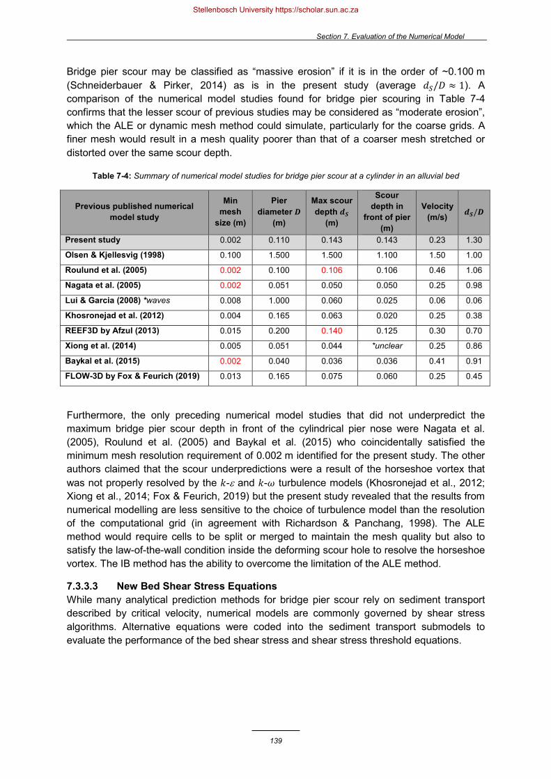
Section 7. Evaluation of the Numerical Model
139
Bridge pier scour may be classified as “massive erosion” if it is in the order of ~0.100 m (Schneiderbauer & Pirker, 2014) as is in the present study (average 𝑑𝑑𝑆𝑆/𝐷𝐷 ≈ 1). A comparison of the numerical model studies found for bridge pier scouring in Table 7-4 confirms that the lesser scour of previous studies may be considered as “moderate erosion”, which the ALE or dynamic mesh method could simulate, particularly for the coarse grids. A finer mesh would result in a mesh quality poorer than that of a coarser mesh stretched or distorted over the same scour depth.
Table 7-4: Summary of numerical model studies for bridge pier scour at a cylinder in an alluvial bed
Previous published numerical model study
Min mesh
size (m)
Pier diameter 𝑫𝑫
(m)
Max scour depth 𝒅𝒅𝑺𝑺
(m)
Scour depth in
front of pier (m)
Velocity (m/s) 𝒅𝒅𝑺𝑺/𝑫𝑫
Present study 0.002 0.110 0.143 0.143 0.23 1.30
Olsen & Kjellesvig (1998) 0.100 1.500 1.500 1.100 1.50 1.00
Roulund et al. (2005) 0.002 0.100 0.106 0.106 0.46 1.06
Nagata et al. (2005) 0.002 0.051 0.050 0.050 0.25 0.98
Lui & Garcia (2008) *waves 0.008 1.000 0.060 0.025 0.06 0.06
Khosronejad et al. (2012) 0.004 0.165 0.063 0.020 0.25 0.38
REEF3D by Afzul (2013) 0.015 0.200 0.140 0.125 0.30 0.70
Xiong et al. (2014) 0.005 0.051 0.044 *unclear 0.25 0.86
Baykal et al. (2015) 0.002 0.040 0.036 0.036 0.41 0.91
FLOW-3D by Fox & Feurich (2019) 0.013 0.165 0.075 0.060 0.25 0.45
Furthermore, the only preceding numerical model studies that did not underpredict the maximum bridge pier scour depth in front of the cylindrical pier nose were Nagata et al. (2005), Roulund et al. (2005) and Baykal et al. (2015) who coincidentally satisfied the minimum mesh resolution requirement of 0.002 m identified for the present study. The other authors claimed that the scour underpredictions were a result of the horseshoe vortex that was not properly resolved by the 𝑘𝑘-ε and 𝑘𝑘-𝜔𝜔 turbulence models (Khosronejad et al., 2012; Xiong et al., 2014; Fox & Feurich, 2019) but the present study revealed that the results from numerical modelling are less sensitive to the choice of turbulence model than the resolution of the computational grid (in agreement with Richardson & Panchang, 1998). The ALE method would require cells to be split or merged to maintain the mesh quality but also to satisfy the law-of-the-wall condition inside the deforming scour hole to resolve the horseshoe vortex. The IB method has the ability to overcome the limitation of the ALE method.
7.3.3.3 New Bed Shear Stress Equations While many analytical prediction methods for bridge pier scour rely on sediment transport described by critical velocity, numerical models are commonly governed by shear stress algorithms. Alternative equations were coded into the sediment transport submodels to evaluate the performance of the bed shear stress and shear stress threshold equations.
Stellenbosch University https://scholar.sun.ac.za

Section 7. Evaluation of the Numerical Model
140
Equations (3-61) and (3-62) for bed shear stress by Abbasnia & Ghiassi (2011) were modelled to account for the centripetal force of the horseshoe vortex. The proposed numerical model was simulated with a relaxation coefficient 𝛼𝛼𝑐𝑐 of 0.7, 0.5 and 0, respectively, whereby 0 suppresses the effect of the centripetal force. Figure 7-24 shows that almost identical sections for the relaxation coefficients were modelled (0.119, 0.118 and 0.118 m, respectively) which indicates the implicit wall functions for the bed shear stress are capable of modelling the effect of the horseshoe vortex without Abbasnia & Ghiassi’s (2011) formulation.
Figure 7-24: Longitudinal section of the scour hole directly upstream of the cylindrical pier for different bed shear stress relaxation coefficients for a flow of 68 l/s
Equation (3-63) by Engelund & Fredsøe (1976) was coded as an alternative to the shear stress threshold of equation (3-18) by Schmidt (1980). While Engelund & Fredsøe (1976) is commonly modelled for hydrodynamic entrainment and Schmidt (1980) was developed for aeolian snow particles, the latter accounts for lift as well as drag forces. Both algorithms account for the effect of the change in slope of the scour bed. Figure 7-25 shows that both algorithms are equally capable of simulating the bridge pier scour hole (equation 3-18 yielded a slightly underpredicted scour depth of 0.108 mm) and are more sensitive to their choice of calibration parameters such as the critical Shields parameter. Equation (3-63) by Engelund & Fredsøe (1976) was also effectively implemented by Roulund et al. (2005), and in a follow-up study by Baykal et al. (2015), which could be considered the most successful numerical model studies of bridge pier scour to date. Their runtime for one simulation was 2.5 months on an Alpha 21264 workstation.
-0.15
-0.13
-0.11
-0.09
-0.07
-0.05
-0.03
-0.01
-0.25 -0.2 -0.15 -0.1 -0.05 0Longitudinal axis (m)
Bed αc 0.5 (Ref)Bed αc 0.0Bed αc 0.7
Physical model
∀ Initial bed level
Bed
leve
l (m
)
Flow Direction
Stellenbosch University https://scholar.sun.ac.za

Section 7. Evaluation of the Numerical Model
141
Figure 7-25: Comparison of scour sections for different shear stress parameters for a flow of 68 l/s Schneiderbauer & Pirker (2014) and Sawadogo (2015) observed that the angle of repose is a sensitive parameter in the shear stress threshold equation that can be responsible for destabilizing the surface of the packed bed. Figure 7-26 shows that the relationship between the scour depth and angle of repose is inversely proportionally. A saturated angle of repose in the range of 40 to 45° yields better results than a dry angle of repose of 28 to 35°. Furthermore, equation (3-63) by Engelund & Fredsøe (1976) is slightly less sensitive to the angle of repose than the original shear stress threshold equation (3-18) by Schmidt (1980) because the scour depth by equation (3-63) is increased by 0.013 m for an angle of repose of 40° while that of equation (3-18) is increased by 0.017 mm. It could be that the angle of repose is associated with the numerical instability associated with the shearing slides because the scour slopes in Figure 7-26 do not approximate the specified angle of repose.
Figure 7-26: Comparison of scour sections for different angles of repose for a flow of 68 l/s
-0.20
-0.15
-0.10
-0.05
0.00
0.05
-0.35 -0.15 0.05 0.25Cross sectional axis (m)
∀ Initial bed level
-0.25 -0.05 0.15 0.35 0.55Longitudinal axis (m)
Eq 3-63, Shields 0.015 (Ref)Eq 3-18Eq 3-63, Shields 0.050Eq 3-63, Shields 0.010
Physical model
-0.20
-0.15
-0.10
-0.05
0.00
0.05
-0.35 -0.15 0.05 0.25Cross sectional axis (m)
∀ Initial bed level
-0.25 -0.05 0.15 0.35 0.55Longitudinal axis (m)
Repose45 (Ref)Repose32Repose40Repose40 (Eq 3-18)
Physical model
Bed
leve
l (m
) Flow Direction
Bed
leve
l (m
)
Flow Direction
Stellenbosch University https://scholar.sun.ac.za

Section 7. Evaluation of the Numerical Model
142
7.3.4 Parameter Sensitivity
A sensitivity analysis is presented for the main parameters that were used to calibrate the proposed numerical model. Note that the model is also sensitive to the sediment size and density but these parameters are fixed to correlate with the experimental work.
7.3.4.1 Creeping vs Saltating The creeping parameter 𝑝𝑝𝑟𝑟 is a robust calibration parameter that affects the bed surface deformation without affecting the stability of the numerical model. It defines the dominant mode of transport as salting (𝑝𝑝𝑟𝑟 = 0) or creeping (𝑝𝑝𝑟𝑟 = 1). As the creeping parameter increases, the rolling transport mode dominates, resulting in an increased scour depth as demonstrated by Figure 7-27 because creeping particles require less energy or streampower to be entrained compared to saltating particles. While a constant value was used in the study, it is recommended that future studies investigate the relationship between the creeping parameter and bed form related parameters such as the Froude number.
Figure 7-27: Comparison of scour sections for different creep parameters for a flow of 68 l/s
7.3.4.2 Entrainment Coefficient Figure 7-28 shows a comparison of the scour depth which increases exponentially with an increase in the dimensionless entrainment coefficient 𝑅𝑅𝑑𝑑𝑠𝑠 ∝ Cη
′ . The entrainment coefficient in equation (3-15) should be considered the chief calibration parameter for entrainment of the sediment bed, which is based on the fluid and particulate densities. While the equation is based on the shear stress excess derived by Anderson & Haff (1991) for the aerodynamic entrainment of sand, which is an approach for bed load transport that is fundamentally the same for hydrodynamic and aerodynamic entrainment, there is no experimental data available to validate calibration for hydrodynamic entrainment. Future research could consider comparing the approach with an alternative bed load transport equation widespread in the field of water engineering, such as the Engelund & Fredsøe (1976) formula given in equation (2-14), particularly because the shear stress threshold given by equation (3-18) compared well with that of Engelund & Fredsøe (1976) in Section 7.3.3.2.
-0.20
-0.15
-0.10
-0.05
0.00
0.05
-0.35 -0.15 0.05 0.25Cross sectional axis (m)
∀ Initial bed level
-0.25 -0.05 0.15 0.35 0.55Longitudinal axis (m)
Creep 05 (Ref)Creep 01Creep 09
Physical model
Bed
leve
l (m
)
Flow Direction
Stellenbosch University https://scholar.sun.ac.za

Section 7. Evaluation of the Numerical Model
143
Figure 7-28: Comparison of scour sections for different entrainment coefficients for a flow of 68 l/s
7.3.4.3 Diffusion The diffusion coefficient λ𝑏𝑏 is related to the fictitious volume fraction of the packed bed in equations (3-33) and (3-34) of the IB method. Extensive sensitivity testing of the proposed model indicated that the diffusion coefficient is the main nonphysical parameter directly related to the mesh resolution and responsible for the scour hole irregularity. Figure 7-29 shows that an increase in the diffusion coefficient value dramatically increases the erosion of the sediment bed. While the scour can be restricted by reducing the entrainment coefficient (from 0.73 to 0.17 to obtain the same scour depth for a diffusion coefficient of 0.1), the numerical stability that causes the irregularity in the scour hole shape becomes more apparent for an increase in λ𝑏𝑏.
Figure 7-29: Comparison of scour sections for different diffusion coefficients for a flow of 68 l/s
-0.20
-0.15
-0.10
-0.05
0.00
0.05
-0.35 -0.15 0.05 0.25Cross sectional axis (m)
∀ Initial bed level
-0.25 -0.05 0.15 0.35 0.55Longitudinal axis (m)
C'n 0.73 (Ref)C'n 1.45C'n 0.37
Physical model
-0.20
-0.15
-0.10
-0.05
0.00
0.05
-0.35 -0.15 0.05 0.25Cross sectional axis (m)
∀ Initial bed level
-0.25 -0.05 0.15 0.35 0.55Longitudinal axis (m)
Dif 0.01 (Ref)Dif 0.1 & C'n 0.17Dif 0.001Dif 0.1
Physical model
Bed
leve
l (m
)
Flow Direction
Bed
leve
l (m
) Flow Direction
Stellenbosch University https://scholar.sun.ac.za

Section 7. Evaluation of the Numerical Model
144
7.3.4.4 Mesh Resolution Section 7.2.3 acknowledged that a finer mesh would yield a more apparent vortex but the coarsest mesh that could resolve the primary vortex circulation was selected to limit the computational time. Therefore, sensitivity testing was done for the finer and coarser mesh described in Table 5-1. The processing time required to run one second of model time was 1.0 hour for the coarser mesh and nearly double that for the finer mesh (2.1 hours). Figure 7-30 and Figure 7-31 show the simulated bridge pier scour resulting for the finer and coarser mesh. Evidently, the proposed numerical model is very sensitive to the mesh resolution as the finer mesh largely overpredicts the scour depth (𝑑𝑑𝑆𝑆 = 0.166 m) while the coarser mesh does not resolve the horseshoe vortex. This is in agreement with the findings of Sawadogo (2015) whereby a coarser mesh underestimated the scour caused by dam bottom outlet flushing and a finer mesh resulted in an irregularly shaped scour hole. Schneiderbauer & Pirker (2013) also defined a lower limit for their mesh resolution because their final snow erosion pattern showed considerable dependence on the grid resolution. Figure 7-31 demonstrates that the numerical instability of the packed bed for the finer mesh can be addressed by implementing a smaller diffusion coefficient based on the proposed guideline of equation (7-1).
Figure 7-30: Comparison of scour sections for different mesh resolutions for a flow of 68 l/s
Figure 7-31: Scour profiles simulated at a cylindrical pier for (a) a coarser mesh, (b) a finer mesh and (c) a finer mesh with a smaller diffusion coefficient of 0.001 for a flow of 68 l/s
-0.20
-0.15
-0.10
-0.05
0.00
0.05
-0.35 -0.15 0.05 0.25Cross sectional axis (m)
∀ Initial bed level
-0.25 -0.05 0.15 0.35 0.55Longitudinal axis (m)
Mesh (Ref)CoarserFiner
Physical model
Bed
leve
l (m
)
Flow Direction
y (m
)
x (m)
Flow
Dire
ctio
n
∆z (m)
Stellenbosch University https://scholar.sun.ac.za
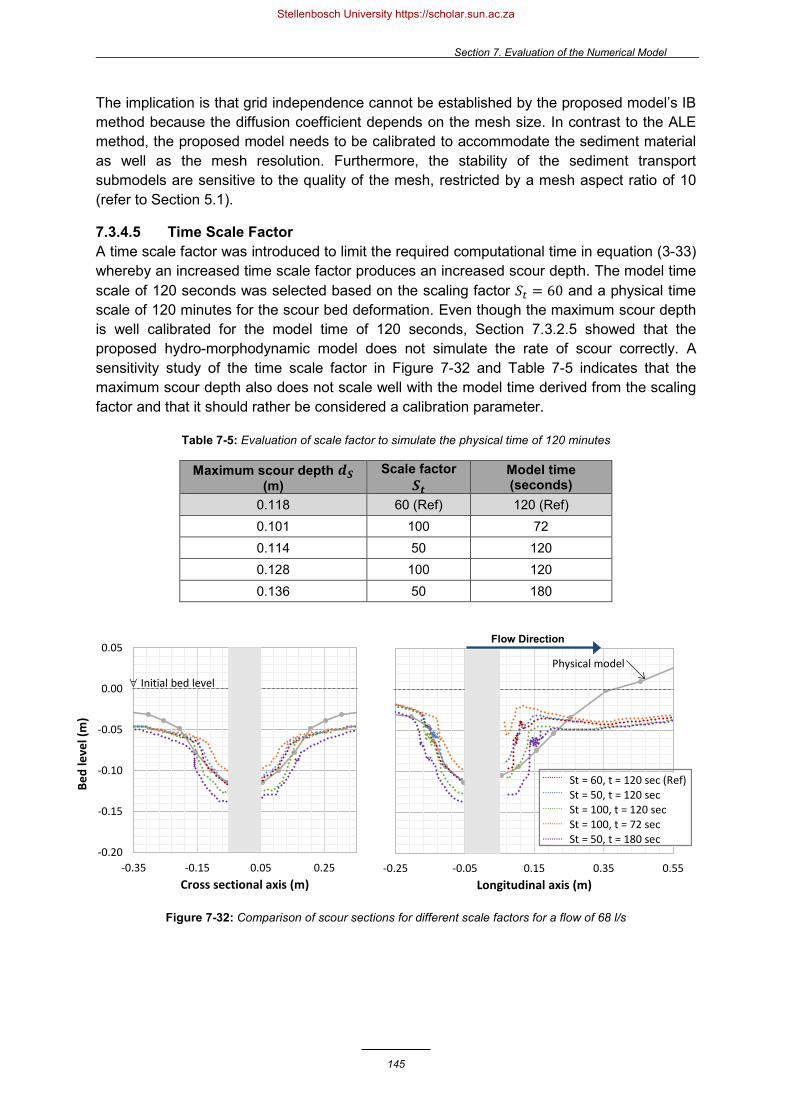
Section 7. Evaluation of the Numerical Model
145
The implication is that grid independence cannot be established by the proposed model’s IB method because the diffusion coefficient depends on the mesh size. In contrast to the ALE method, the proposed model needs to be calibrated to accommodate the sediment material as well as the mesh resolution. Furthermore, the stability of the sediment transport submodels are sensitive to the quality of the mesh, restricted by a mesh aspect ratio of 10 (refer to Section 5.1).
7.3.4.5 Time Scale Factor A time scale factor was introduced to limit the required computational time in equation (3-33) whereby an increased time scale factor produces an increased scour depth. The model time scale of 120 seconds was selected based on the scaling factor 𝑆𝑆𝑡𝑡 = 60 and a physical time scale of 120 minutes for the scour bed deformation. Even though the maximum scour depth is well calibrated for the model time of 120 seconds, Section 7.3.2.5 showed that the proposed hydro-morphodynamic model does not simulate the rate of scour correctly. A sensitivity study of the time scale factor in Figure 7-32 and Table 7-5 indicates that the maximum scour depth also does not scale well with the model time derived from the scaling factor and that it should rather be considered a calibration parameter.
Table 7-5: Evaluation of scale factor to simulate the physical time of 120 minutes
Maximum scour depth 𝒅𝒅𝑺𝑺 (m)
Scale factor 𝑺𝑺𝒕𝒕
Model time (seconds)
0.118 60 (Ref) 120 (Ref) 0.101 100 72 0.114 50 120 0.128 100 120 0.136 50 180
Figure 7-32: Comparison of scour sections for different scale factors for a flow of 68 l/s
-0.20
-0.15
-0.10
-0.05
0.00
0.05
-0.35 -0.15 0.05 0.25Cross sectional axis (m)
∀ Initial bed level
-0.25 -0.05 0.15 0.35 0.55Longitudinal axis (m)
St = 60, t = 120 sec (Ref)St = 50, t = 120 secSt = 100, t = 120 secSt = 100, t = 72 secSt = 50, t = 180 sec
Physical model
Bed
leve
l (m
)
Flow Direction
Stellenbosch University https://scholar.sun.ac.za
Section 7. Evaluation of the Numerical Model
146
7.4 Summary
The proposed coupled fully 3D hydro-morphodynamic model demonstrated that the velocity flow field, the horseshoe vortex and the subsequent maximum bridge pier scour can be modelled successfully to simulate the results from the experimental work. The sediment transport submodels were calibrated, validated and tested for numerical and parameter sensitivities which are ascribed to the fine mesh resolution required to resolve the horseshoe vortex, the diffusion coefficient associated with the IB method and incomplete shear slides. Despite the perceived limitations of the proposed coupled fully 3D hydro-morphodynamic model, the numerical model performs better than any of the bridge pier scour prediction methods evaluated in Section 6. Furthermore, no other published studies have been found for the numerical modelling of bridge pier scour in conjunction with the more advanced RSM turbulence model nor with the successful implementation of the IB method. The proposed numerical model was capable of resolving the horseshoe vortex with the RSM model and predicting the maximum scour depth directly in front of the pier nose with the IB method.
Stellenbosch University https://scholar.sun.ac.za

Section 8. Conclusions and Recommendations
147
8. Conclusions and Recommendations
8.1 Summary of Findings
The aim of the research was to investigate improved prediction methods for bridge pier scour by means of empirical equations, physical modelling and numerical modelling. The conclusions of the study are presented below with reference to the research objectives of Section 1.3.
In short, an improved bridge pier scour equation based on the particle Reynolds number as well as an improved hydro-morphodynamic model to simulate bridge pier scour in an alluvial bed were developed. The proposed coupled fully 3D hydro-morphodynamic model demonstrated that the velocity flow field, the horseshoe vortex and the subsequent maximum bridge pier scour can be modelled successfully to simulate results from the experimental work.
Experimental work:
Bridge pier scour was successfully simulated by 48 laboratory tests with a 1:15 scale for a combination of different flows, pier shapes and sediment beds, from which the scour patterns in Appendix C and the velocity profiles in Appendix B were obtained. In addition, the material properties for the two different sediments were measured in the laboratory and compared well with values quoted by different literature sources. Fifteen percent of the experimental work was duplicated 3 times and quantified the maximum percentage repeatability error as 9% for the manual scour survey and 6% for the ADV measurements. The characteristic U-shaped scour holes were observed with the maximum scour depth occurring at the upstream nose of the pier where the horseshoe vortex circulates.
Parameterization:
The experimental work facilitated a simplified study of the bridge pier scour process as well as the effect of different interrelated parameters such as approach velocity, sediment type, pier shape and time on the equilibrium scour depth.
• Despite the divided notion in literature on the time required to reach equilibrium, experimentation indicated that two hours was sufficient time for the scour hole to reach equilibrium because the scour process is rapid in the beginning and develops asymptotically; 60-75% of the equilibrium scour depth developed within 10% of the time required for equilibrium (in agreement with Melville, 1975; Mohammed et al., 2013; Roulund et al., 2005).
• In accordance with Chiew (1984) and Ettema (1980), the relative scour depth increases almost linearly with the relative velocity while no local scour pattern was observed below a relative velocity condition of 0.5. Similarly, the relative scour length or width was plotted to display an analogous trend but these parameters have not been published in previous studies because they are less critical to bridge design. The relative scour depth also increases linearly with the pier Reynolds number and Froude number.
• The same amount of relative scouring occurs in both materials for the same relative velocity. Even though the peach pips have a larger particle diameter, they are the
Stellenbosch University https://scholar.sun.ac.za
Section 8. Conclusions and Recommendations
148
more easily erodible material because the protype relative sediment size 𝐷𝐷/𝑑𝑑 (scaled for its density) is larger than that for the fine sand. This is in accordance with Lee & Strum (2009) who predicted a similar scour depth relationship for the scaled 𝐷𝐷/𝑑𝑑 of 882 for the peach pips and 514 for the sand.
• The cylindrical pier yielded the largest scour hole while the sharp nosed pier caused the least amount of scouring in front of the pier nose because practically no horseshoe vortex was generated. Few empirical equations account for pier shapes but its effect on scouring cannot simply be described by a constant dimensionless shape factor.
Empirical equations:
Thirty of the better-known empirical equations for bridge pier scour were evaluated against the experimental work for a full-scale prototype. The equations were found to be in weak agreement with one another, producing a wide range of unreliable results (errors in the order of 95%). No single equation is conclusively superior but the HEC-18 equations are recommended, as well as Shen et al. (1969) and Ali & Karim (2002), because they rely on the pier Reynolds number. It may be considered the chief parameter affecting the horseshoe vortex formation and yet, it has rarely been described relative to scour depth. Models that account for the vortex could offer better scour depth predictions.
Because the HEC-18 equations generally performed better and have been revised in five different FHWA manuals, 207 BSDMS field data measurements from Mueller & Wagner (2005) were used to improve the HEC-18 equation with new dimensionless factors for the pier shape and armouring given by equations (6-3) and (6-4). A new approach for the shape factor was adopted by a linear relationship that amplified the impact of the pier shape and length on the scour depth for greater pier Reynolds numbers (which are associated with stronger horseshoe vortices). A new approach was adopted for the armouring factor whereby the critical velocity was discarded for the particle Reynolds number as it achieves considerably less scatter about the line of equality. In addition, the particle Reynolds number is capable of accounting for the channel shape and bed form roughness. Finally, a new approach with confidence intervals was also adopted to quantify the trade-off between accuracy and underpredictions, offering flexibility to the bridge designer.
The contour plot in Figure 6-15, based on the Modified Liu Diagram for incipient motion, is also recommended as a potential prediction method for bridge pier scour. Even though stream power and the particle Reynolds number account for all the flow and sediment parameters except for the pier structure, the relationship given for the pier scour depth from the field shows limited scatter. This new diagram has the potential to accurately predict bridge pier scour should it be supplemented and validated by additional scour data, and should the assumptions for energy slope, channel shape and settling velocity be supported.
The new equation (99% confidence) ranked the best with the least total SSR and least underpredictions for the scour depths, followed by HEC-18 Mueller (1996) and Shen et al. (1969). The new proposed equation has the lowest mean error percentage compared to the other methods of 10% for the physical modelling which is acceptable compared to the lab repeatability error of 9%. The new equation (95% confidence) also performed well but the new equation (50% confidence) would not be fit for bridge design due to underpredictions.
Stellenbosch University https://scholar.sun.ac.za
Section 8. Conclusions and Recommendations
149
Furthermore, the prototype scour depths were better predicted by the empirical equations for the tests with the standard cylindrical pier and the crushed peach pips than for the fine sand bed. Therefore, it may be presumed that the scaling of the peach pips by the movability number was more representative of alluvial sediment in the field, as recommended by Heller (2011). The non-scalable effects of the hydraulic forces in the density and settling velocity can be overcome by using a sediment with a larger particle size and smaller density. The scaling challenge associated with sediment was further demonstrated by the empirical equations that overpredicted the critical velocity for the peach pip particles because they do not account for density, unlike equation (2-6). Equations for critical velocity based on particle size as well as density should be given preference. While shear stress algorithms are implemented by numerical models, empirical equations for bridge pier scour are typically dependent on the critical velocity parameter but fail to reference an appropriate calculation method. In addition, the comparison of the average stream approach velocity with the critical velocity is limited by its inability to represent the local velocity gradients in the vicinity of the sediment.
Traditional bridge pier scour studies are still based on empirical formulas derived and calibrated by laboratory and field data despite the availability of sophisticated computers. The simplicity of conservative empirical equations may be appealing but they often overestimate the anticipated scour depth leading to uneconomical designs. Although extensive research has been done on bridge pier scour for more than six decades, comparatively few studies have been presented involving detailed 3D numerical modelling of such processes and even fewer have attempted to model a movable bed at the bridge pier. While an improved equation was proposed, numerical modelling has the potential to overcome the shortcomings associated with empirical equations as well as experimental work, and should subsequently be the primary subject of future studies for bridge pier scour.
Resolving the flow:
Most of the preceding numerical model studies focussed on resolving the horseshoe vortex because it governs the ability of a numerical model to accurately simulate bridge pier scour. The proposed hydrodynamic model demonstrated that it is capable of reproducing the time-averaged velocity field from the laboratory. The hydrodynamic model closed with the 𝑘𝑘-ε turbulence model underestimated the velocities with a 9% error, which is concurrent with the findings of Salaheldin et al. (2004). Alternatively, the RSM turbulence model was capable of replicating the laboratory results with only a 1% error which is considered negligible in light of the 6% maximum margin of error that was present in the experimental work.
The velocity vectors verified that the proposed numerical model is also capable of resolving the primary circulation of the horseshoe vortex, whether the model was closed by the standard 𝑘𝑘-ε turbulence model, the SST model or the RSM model because the law-of-the-wall indicated that a minimum cell size of at least 1 to 2 mm is required to capture the boundary layer recirculation. The results from numerical modelling are less sensitive to the choice of turbulence model than to the geometric mesh representation, in accordance with Richardson & Panchang (1998). Given that the mesh is sufficiently fine, even the 𝑘𝑘-ε turbulence model is capable of resolving the horseshoe vortex and the subsequent scour calculations.
Stellenbosch University https://scholar.sun.ac.za
Section 8. Conclusions and Recommendations
150
Furthermore, the flow field for a fixed bed and a sediment bed were compared to demonstrate that the interaction between fluid and sediment may be described as a coupled problem, and would best be simulated by a coupled numerical model. The reduced and formalized cross-sections of the flat rigid bed generally have increased and more uniform velocities than the movable sediment bed which trap and stabilize the vortices. Thus, the change in the sediment bed altered the local velocities and flow field in the vicinity of the pier.
Simulating sediment transport:
The key objective was to develop an improved hydro-morphodynamic model to simulate bridge pier scour in an alluvial bed, based on the modelling approach adopted by Schneiderbauer & Pirker (2014) and Sawadogo (2015). The proposed sediment transport submodels are exceedingly sensitive and according to Newren (2007), the IB method is inherently unstable. The following challenges and improvements to the hydro-morphodynamic code and model setup were addressed to achieve a numerically stable and more accurate solution:
• It was established that a very fine computational mesh is required to resolve the horseshoe vortex that is crucial for the development of bridge pier scour. However, the proposed sediment transport submodels are very sensitive to the mesh resolution and result in an instability of the packed bed with an unrealistic and irregularly shaped scour hole (in agreement with Sawadogo, 2015 and Scneiderbauer & Pirker, 2014). Extensive sensitivity testing of the proposed model indicated that the main nonphysical parameter directly related to the mesh resolution and responsible for the scour hole irregularity is the diffusion coefficient λ𝑏𝑏 of the IB method. It is recommended that future studies of the proposed hydro-morphodynamic model select a diffusion coefficient with an order of magnitude based on equation (7-1) which relates the volume fraction of the IB method to the minimum grid cell volume, the sediment particle size and timestep. The implication is that grid independence cannot be established by the proposed model’s IB method because the diffusion coefficient needs to be calibrated for the mesh resolution.
• A reduction of the diffusion coefficient value dramatically reduces the erosion of the sediment bed and should be compensated by an increase in the dimensionless entrainment coefficient 𝐶𝐶η
′ which is considered the chief calibration parameter for entrainment based on the fluid and particulate densities. No experimental investigations have been conducted to validate the calibration of the entrainment coefficient but it is proposed that equation (7-2) based on Shao & Li (1999) should be used to approximate an appropriate value.
• Furthermore, it was found that the stability of the sediment transport submodels are sensitive to the quality of the computational grid, restricted by a mesh aspect ratio of 10.
• The aspect ratio limitation placed additional strain on the computational cost of the simulation due to the exceedingly large number of cells generated. The 3D, transient, multiphase, turbulent, numerical model coupled with UDFs required a supercomputer to run and evaluate simulations. An efficiency analysis of parallelizing the numerical model indicated that the optimum limit of 240 processors on the Lengau cluster could run the simulations 10x faster than on a general-purpose computer with 15
Stellenbosch University https://scholar.sun.ac.za

Section 8. Conclusions and Recommendations
151
processors. However, the proposed numerical model was constrained by its ability to compute across multiple parallel processors and additional coding was required to control the decomposition of the computational domain across the 240 processors and to correctly exchange information between them, particularly at the surface of the sediment bed.
• Alternative equations were coded into the sediment transport submodels to evaluate the performance of the shear stress equations. However, the implicit wall functions for the bed shear stress are capable of modelling the effect of the horseshoe vortex without Abbasnia & Ghiassi’s (2011) formulation for the centripetal force of the horseshoe vortex. Equation (3-63) by Engelund & Fredsøe (1976) was coded as an alternative to the shear stress threshold of equation (3-18) by Schmidt (1980) because it is commonly modelled in the engineering industry for hydrodynamic entrainment and was effectively implemented by Roulund et al. (2005). Both algorithms are equally capable of simulating the bridge pier scour hole and are more sensitive to their choice of calibration parameters such as the critical Shields parameter. Equation (3-63) is also slightly less sensitive to the angle of repose; a parameter that destabilizes the bed and is related to allegedly incomplete shearing slides as the scour hole slopes do not approximate the specified angle of repose.
• In order to accurately replicate the bridge pier scour, it was established that the flow must be initialized as accurately as possible (including a fully developed velocity profile at the inflow boundary) before the sediment transport submodels are coupled and run, to ensure an erroneous flow pattern from the first few time steps does not generate residual scouring errors and instabilities.
• The more advanced RSM turbulence model was coded to resolve the horseshoe vortex with a better resolution. Because the IB method is used to track the bed surface deformation, a forcing scheme with source terms had to be coded for the RSM model to suppress the velocities and turbulent quantities in the packed bed. While the RSM model is reproached for making numerical models more susceptible to divergence, it is the most accurate model for simulating the flow field and subsequently, for replicating the scour hole in the laboratory. The 𝑘𝑘-ε turbulence model overpredicted the maximum scour depth more than the proposed RSM model because the turbulence models, particularly the 𝑘𝑘-ε model, typically overestimate the shear velocity and bed shear stress, as confirmed by Salaheldin et al. (2004). No previous studies have been found for RSM turbulence models implemented in conjunction with hydro-morphodynamic models for bridge pier scour.
• Finally, the proposed hydro-morphodynamic model was examined for other parameter instabilities and sensitivities. The packing ratio in the shear slides equation (3-31) and the IB method equation (3-33) also dramatically destabilized the model. A value of 0.5 as well as an impact velocity coefficient of 10 and a velocity ratio of 0.5 were used because they offered improved numerical stability while the observed effect of the latter two parameters on the scour hole were negligible.
• While the ALE method is prevalent in bridge pier scour studies, the IB method is used by the proposed model to simulate the changing topography of the sediment bed. The only other identified bridge pier scour model that implemented the IB method was that of Khosronejad et al. (2012) who did not manage to resolve the horseshoe vortex. The ALE method and artificial smoothing of the mesh was investigated as an alternative to the IB method for the proposed numerical model.
Stellenbosch University https://scholar.sun.ac.za
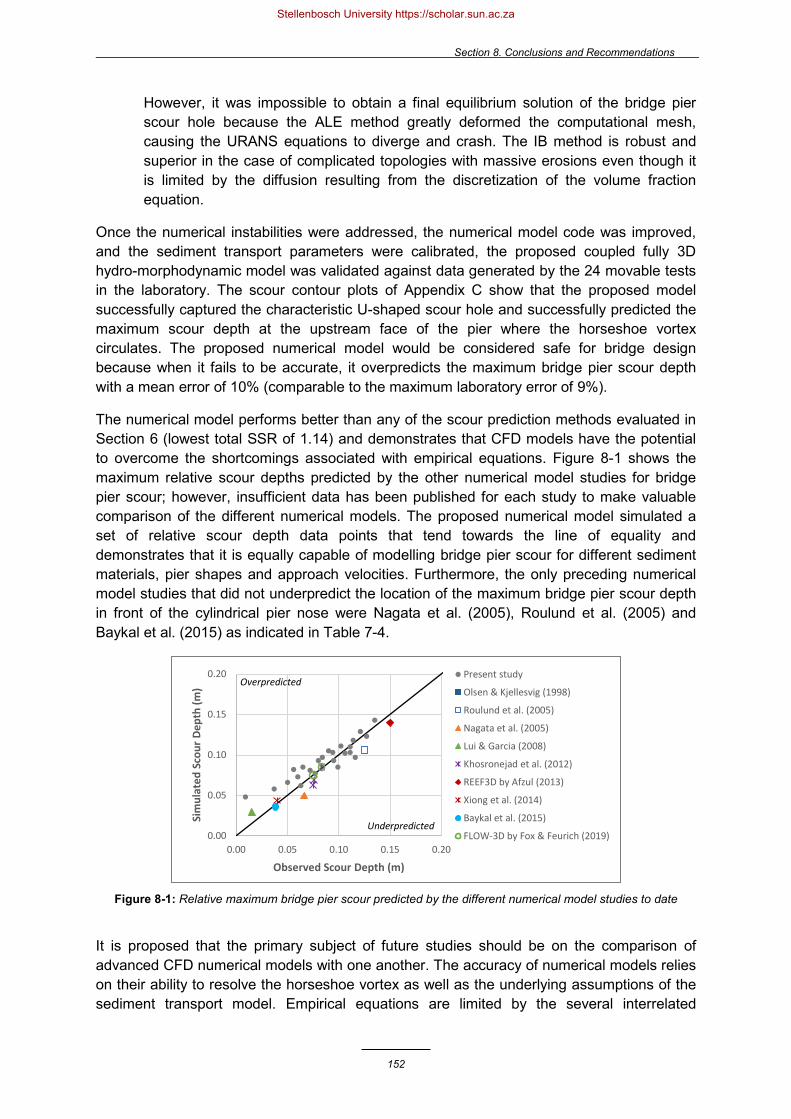
Section 8. Conclusions and Recommendations
152
However, it was impossible to obtain a final equilibrium solution of the bridge pier scour hole because the ALE method greatly deformed the computational mesh, causing the URANS equations to diverge and crash. The IB method is robust and superior in the case of complicated topologies with massive erosions even though it is limited by the diffusion resulting from the discretization of the volume fraction equation.
Once the numerical instabilities were addressed, the numerical model code was improved, and the sediment transport parameters were calibrated, the proposed coupled fully 3D hydro-morphodynamic model was validated against data generated by the 24 movable tests in the laboratory. The scour contour plots of Appendix C show that the proposed model successfully captured the characteristic U-shaped scour hole and successfully predicted the maximum scour depth at the upstream face of the pier where the horseshoe vortex circulates. The proposed numerical model would be considered safe for bridge design because when it fails to be accurate, it overpredicts the maximum bridge pier scour depth with a mean error of 10% (comparable to the maximum laboratory error of 9%).
The numerical model performs better than any of the scour prediction methods evaluated in Section 6 (lowest total SSR of 1.14) and demonstrates that CFD models have the potential to overcome the shortcomings associated with empirical equations. Figure 8-1 shows the maximum relative scour depths predicted by the other numerical model studies for bridge pier scour; however, insufficient data has been published for each study to make valuable comparison of the different numerical models. The proposed numerical model simulated a set of relative scour depth data points that tend towards the line of equality and demonstrates that it is equally capable of modelling bridge pier scour for different sediment materials, pier shapes and approach velocities. Furthermore, the only preceding numerical model studies that did not underpredict the location of the maximum bridge pier scour depth in front of the cylindrical pier nose were Nagata et al. (2005), Roulund et al. (2005) and Baykal et al. (2015) as indicated in Table 7-4.
Figure 8-1: Relative maximum bridge pier scour predicted by the different numerical model studies to date
It is proposed that the primary subject of future studies should be on the comparison of advanced CFD numerical models with one another. The accuracy of numerical models relies on their ability to resolve the horseshoe vortex as well as the underlying assumptions of the sediment transport model. Empirical equations are limited by the several interrelated
0.00
0.05
0.10
0.15
0.20
0.00 0.05 0.10 0.15 0.20
Sim
ulat
ed S
cour
Dep
th (m
)
Observed Scour Depth (m)
Present study
Olsen & Kjellesvig (1998)
Roulund et al. (2005)
Nagata et al. (2005)
Lui & Garcia (2008)
Khosronejad et al. (2012)
REEF3D by Afzul (2013)
Xiong et al. (2014)
Baykal et al. (2015)
FLOW-3D by Fox & Feurich (2019)
Overpredicted
Underpredicted
Stellenbosch University https://scholar.sun.ac.za

Section 8. Conclusions and Recommendations
153
parameters involved in bridge pier scour, but the parameters for morphodynamic modelling are also interrelated, which need to be accurately resolved and calibrated. The transition from empirical bridge pier scour equations towards numerical modelling should redirect the assessment of bridge pier scour prediction methods towards resolving better sediment transport algorithms for bed load, suspended load and incipient motion which are fundamentally sound.
Sensitivity analysis:
A sensitivity analysis was performed for the main parameters that were used to calibrate the proposed numerical model, i.e. Shields’ parameter, the angle of repose, the creeping parameter, the entrainment coefficient, the diffusion coefficient, the scale factor and the mesh resolution. The creeping parameter is a robust calibration parameter that affects the bed surface deformation without affecting the stability of the numerical model. As the creeping parameter increases, the rolling transport mode dominates, resulting in an increased scour depth. The maximum scour depth also does not scale well with the model time derived from the scaling factor and that it should rather be considered as a proportional calibration parameter.
As concluded previously, grid independence cannot be established by the proposed model’s IB method. A finer mesh would yield a more apparent vortex but the coarsest mesh that could resolve the primary vortex circulation was selected to limit the computational time. A finer mesh was shown to largely overpredict the scour depth and should be stabilized with a smaller diffusion coefficient. However, a decrease in the diffusion coefficient dramatically decreases the erosion of the sediment bed and could be compensated by an increase in the entrainment coefficient.
8.2 Suggestions for Further Research
Recommendations are given to improve the reliability of the experimental work, because they were used as the basis of validation for the empirical equations and numerical models. It is proposed that human error is eliminated in future studies by using a laser scanner for the scour bed survey. Using an ADV capable of measuring velocity at multiple elevations at once would improve vertical velocity profile measurements. A different probe for the ADV would be required with a higher sampling rate to capture the horseshoe vortex and boundary layers near the packed bed or pier, and a grid with a finer resolution for data collection would improve the velocity contour plots in Appendix B. Finally, pressure measurements may also be used to facilitate visualization of the flow field.
While the maximum bridge pier scour depths simulated at the pier nose by the proposed coupled fully 3D hydro-morphodynamic model were validated by the experimental work, additional improvements to the numerical model are recommended.
• The numerical model underpredicted the extent of the scour hole directly behind the pier, as well as the deposition downstream of the pier. The lack of deposition may be considered provisionally permissible because the safety of a bridge design is mainly related to the maximum scour depth. However, it is proposed that the numerical model is improved to incorporate suspended sediment transport of fluctuating vortex shedding by coding the convection-diffusion equation (2-32) to address the
Stellenbosch University https://scholar.sun.ac.za

Section 8. Conclusions and Recommendations
154
underprediction downstream of the pier. This would also extend the model validity to live-bed scour conditions. The role of the lee-wake vortex in bridge pier scour could be investigated and whether a symmetry boundary across the longitudinal centreline of the pier would be feasible to decrease the computational cost.
• The incomplete redistribution of the sediment from the shear slides algorithms require additional investigation because the near vertical slope of the upper edges of the scour holes do not approximate the specified 44 to 45° angle of repose. It is anticipated that this study would address the incorrect rate of scour as well as the irregularity in the contours directly upstream and downstream of the scour hole. The time scale and the temporal variation of scouring by the numerical model must be addressed because this is not a limitation that has been encountered by the preceding numerical model studies for bridge pier scour.
• Modelling the free surface as a shear free rigid lid is a widely adopted approach that is considered acceptable for flows with small Froude numbers. However, the logarithmic velocity profile was underpredicted near the water surface and while bridge pier scour may not be affected, future studies could investigate the feasibility of modelling air an additional phase to allow modelling of the free surface and the bow wave at the pier for supercritical floods.
• It is recommended that future studies investigate the relationship between the creeping parameter and bed form related parameters such as the Froude number.
• There is no experimental data available to validate the calibration of the entrainment coefficient for hydrodynamic entrainment. Future research should compare equation (3-15) with an alternative bed load transport equation, such as the Engelund & Fredsøe (1976) formula given in equation (2-14), particularly because the shear stress threshold given by equation (3-18) compared well with that of Engelund & Fredsøe (1976).
• Finally, the performance of the proposed numerical model should be compared with the ability of other numerical models, such as FLOW-3D and REEF3D, to simulate bridge pier scour for the same model setups and case studies. Future research should evaluate the ability of the model to simulate field data, i.e. a full prototype scale bridge pier calibrated to accommodate the in-situ sediment material and the required mesh resolution. The study could be extended to include complex pier shapes such a pile cap or pier group, to accommodate more than one sediment fraction (particularly to simulate armouring) and to simulate live-bed scour.
The proposed numerical model has demonstrated that it is capable of predicting bridge pier scour and overcoming the shortcomings of empirical equations. Nevertheless, numerical modelling is faced with its own set of challenges that need to be addressed, such as calibrating for stability and computational effort. The simplicity of conservative empirical equations may be feasible for the conceptual design phase of a standard bridge. However, hydro-morphodynamic models need to be refined and calibrated to manage the uncertainty of scour predictions for more complex bridge scenarios, such as pile caps subjected to skewed flow and debris accumulation.
Stellenbosch University https://scholar.sun.ac.za

155
References
Abbasnia, A.H. and Ghiassi, R. 2011. Improvements on bed-shear stress formulation for pier scour computation. International Journal for Numerical Methods in Fluids, 67, pp. 383-402.
Afzul, M.S. 2013. 3D Numerical modelling of sediment transport under current and waves. MSc Thesis, Department of Civil and Transport Engineering, Norwegian University of Science and Technology.
Ahmed, F. and Rajaratnam, N. 1998. Flow around bridge piers. Journal of Hydraulic Engineering, 124(3), pp. 288-300.
Ali, K.H.M. and Karim, O.A. 2002. Simulation of flow around piers. Journal of Hydraulic Research, 40(2), pp. 161-174.
Ali, K.H.M., Karim, O.A. and Connor, B.A. 1997. Flow patterns around bridge piers and offshore structures. Proceedings of ASCE Water Resources Engineering Conference, August 10-15, San Francisco, pp. 208-213.
Amini, A., Mohammed, T.A., Aziz, A.A, Ghazali, A.H. and Huat, B.B.K. 2011. A local scour prediction method for pile caps in complex piers. Water Management, In proceedings of Institute of Civil Engineers, 164, pp. 1-8.
Anderson, R. and Haff, P. 1991. Wind modification and bed response during saltation of sand in air. Aeolian Grain Transport, 1, pp. 21-51.
Andreotti, B. 2002. Selection of dune shapes and velocities: Part 1. The European Physical Journal N – Condensed Matter and Complex Systems, 28(3), pp. 321-339.
Andreotti, B. 2004. A two-species model of aeolian sand transport. Journal of Fluid Mechanics, Volume 510, pp. 47-70.
Apsilidis, N., Khosronejad, A., Sotiropoulos, F., Dancey, C.L. and Diplas, P. 2012. Physical and numerical modelling of the turbulent flow field upstream of a bridge pier. Proceedings of the Sixth International Conference on Scour and Erosion, 27-31 August 2012, Paris, pp. 181-188.
Apsilidis, N., Diplas, P., Dancey, C., Vlachos, P. and Raben, S. 2010. Local scour at bridge pier: The role of Reynolds number on horseshoe vortex dynamics. Proceedings of the Fifth International Conference on Scour and Erosion, 7-10 November 2010, California, pp. 86-94.
Arneborg, L., Hansen, E.A. and Juhl, J. 1995. Numerical modelling of local scour at vertical structures. Final Proceedings of the Project Monolithic (Vertical) Coastal Structures. Commission of the European Communities, Directorate General for Science, Research and Development, MAST contract No. MAS2-CT92-0042, Paper 3.2.
Arneson, L.A., Zevenbergen, L.W., Lagasse, P.F. and Clopper, P.E. 2012. Evaluating Scour at Bridges. Publication no. FHWA-HIF-12-003, US Department of Transportation, Federal Highway Administration, Washington DC, USA.
Bagnold, R.A. 1941. The Physics of Blown Sand and Desert Dunes. Chapman and Hall, New York.
Bagnold, R.A. 1966. An approach to the sediment transport problem from general physics. U.S. Geological Survey Professional Paper, 422(1).
Stellenbosch University https://scholar.sun.ac.za

156
Baker, C.J. 1980a. The turbulent horseshoe vortex. Journal of Wind Engineering and Industrial Aerodynamics, 6(1-2), pp. 9-23.
Baker, C.J. 1980b. Theoretical approach to the prediction of local scour around bridge piers. Journal of Hydraulic Research, 18(1), pp. 1-12.
Baker, R.A. 1986. Local Scour at Bridge Piers in Non-Uniform Sediment. PhD Thesis, Department of Civil Engineering, University of Auckland.
Basson, G.R. and Rooseboom, A. 2008. Mathematically modelling of sediment transport and deposition in reservoirs. Bulletin 140, ICOLD.
Bateni, S.M., Borghei, S.M. and Jeng, D.S. 2007a. Neural network and neuro-fuzzy assessments for scour depth around bridge piers. Engineering Applications of Artificial Intelligence, 20(3), pp. 401–414.
Bateni, S.M., Jeng, D.S. and Melville, B.W. 2007b. Bayesian neural networks for prediction of equilibrium and time-dependent scour depth around bridge piers. Advances in Engineering Software, 38(2), pp. 102-111.
Baykal, C., Sumer, B.M., Fuhrman, D.R., Jacobsen, N.G. and Fredsøe, J. 2015. Numerical investigation of flow and scour around a vertical circular cylindrical pier. Philosophical Transactions of the Royal Society A, 373(2033).
Beck, J.S. and Basson, G.R. 2003. The hydraulics of the impacts of dam development on the river morphology, WRC Report No. 1102/1/03, Water Research Commission, Department of Environmental Affairs, Pretoria.
Beg, M. 2010. Characteristics of developing scour holes around two piers placed in transverse arrangement. Proceedings of the Fifth International Conference on Scour and Erosion, 7-10 November 2010, California, pp. 76-85.
Blench, T. 1969. Mobile-bed fluviology. University of Alberta Press, Edmonton, Canada.
Brandimarte, L., Montanari, A., Briaud J.L. and D’Odorico, P. 2006. Stochastic flow analysis for predicting river scour of cohesive soils. Journal of Hydraulic Engineering, 132, pp. 493-500.
Brandimarte, L., Paron, P. and Di Baldassarre, G. 2012. Bridge pier scour: A review of processes, measurements and estimates. Environmental Engineering and Management Journal, 11(5), pp. 975-989.
Breusers, H.N.C. 1965. Scour around drilling platforms. Bulletin of Hydraulic Research, 19, pp. 276.
Breusers, H.N.C. and Raudkivi, A.J. 1991. Scouring. A.A. Balkema: Rotterdam.
Breusers, H.N.C., Nicollet, G. and Shen, H.W. 1977. Local scour around cylindrical pier. Journal of Hydraulic Research, 15(3), pp. 211-252.
Briaud, L., Ting, K., Chen, C., Gudavalli, R., Perugu, S. and Wei, G. 1999. SRICOS: prediction of scour rate in cohesive soils at bridge piers. Journal of Geotechnical and Geoenvironmental Engineering., ASCE 125, pp. 237-246.
Bruce, D.A. and Juran, I. 1996. Testing Report, Publication no. FHWA-RD-96-018, FHWA, US Department of Administration.
Chadwick, A., Morfett, J. and Borthwick, M. 2013. Hydraulics in Civil and Environmental Engineering. 5th Edition. CRC Press.
Stellenbosch University https://scholar.sun.ac.za

157
Chen, G., Du, X.D. and Wei, Q.D. 2000. The effects of cylinder shape on the primary horseshoe vortex of the juncture flow, 9th Symposium of Flow Visualization, 54, pp. 1-9.
Chen. H.C. 2002. Numerical simulation of scour around complex piers in cohesive soil. Proceedings of the First International Conference on Scour of Foundations, 17-20 November 2002, Texas A&M University, College Station, USA. 1, pp. 11-33.
Cheng, N.S. 1997. Simplified settling velocity formula for sediment particle. Journal of Hydraulic Engineering. ASCE, 123(2), pp. 149-152.
Chepil, W.S. 1959. Equilibrium of soil grains at the threshold of movement by wind. Soil Science Society of America Proceedings, 23(6), pp. 422-428.
Chiew, Y.M. 1984. Local scour at bridge piers. PhD Thesis, Department of Civil Engineering, University of Auckland.
Chitale, S.V. 1962, Scour at bridge crossings. Transactions of the American Society of Civil Engineers, 127(1), pp. 191–196.
Choi, S. and Cheong, S. 2006. Prediction of local scour around bridge piers using artificial neural networks. Journal of the American Water Resources Association, 42(2), pp. 487-494.
Choi, S. U. and Yang, W. 2002 Numerical simulation of 3D flows around bridge piers. Proceedings of the First International Conference on Scour of Foundations, 17-20 November 2002, Texas A&M University, College Station, USA.
CIRIA, CUR and CETMEF. 2007. The Rock Manual: The use of rock in hydraulic engineering (2nd edition). London: CIRIA.
Coleman, N. L. 1971. Analysing laboratory measurements of scour at cylindrical piers in sand beds. Proceedings of 14th International Association for Hydraulic Research (IAHR) Congress, Paris, 3, pp. 307-313.
Conrad, C. 2004. Hydrology. IGCSE Geography Class Notes, Kinabalu International School, Malaysia.
Constantinescu, S.G. and Koken, M. 2005. Time-dependent and time-averaged structure of the flow past a surface mounted cylindrical pier. Fourth International Conference on Computation Heat and Mass Transfer, Cachan, France, May 2005.
Constantinescu, S.G., Ettema, R. and Koken, M. 2004. An eddy-resolving technique to predict the unsteady horseshoe vortex and wake of a cylindrical pier. Proceedings of Second International Conference on Scour and Erosion, 14-17 November 2004, Stallion Press, Singapore, 2, pp. 202-211.
Dargahi, B. 1989. The turbulent flow field around a circular cylinder. Experiments in Fluids, 8, pp. 1-12.
Department of Transport. 1986. TMH1 Standard Methods for Testing Road Construction Materials. 2nd Edition. Pretoria: SA Department of Transport.
Department of Water Affairs and Forestry. 1992. Historical flood documentation series no.1 Natal and Transkei, pp. 1848-1989. Technical Report TR147, Compiled by D van Bladeren.
Deshmukh, A.R. and Raikar, R.V. 2014. A clear-water scour around a circular bridge pier under steady flow for different opening ratios. International Journal of Research in Engineering and Technology, 3(1), pp. 158-162, January 2014.
Stellenbosch University https://scholar.sun.ac.za

158
Dey, S. 1996. Sediment pick-up for evolving scour near circular cylindrical piers. Applied Maths Modelling, 20, pp. 534-539.
Dey, S. 1997. Local scour at piers, part 1: A review of developments of research. International Journal of Sediment Research. 12, pp. 23–46.
Dey, S. 1999. Sediment Threshold. Applied Mathematical Modelling, 23(5), pp. 399-417.
Dey, S. and Bose, S.K. 1994. Bed shear in equilibrium scour around a circular cylindrical pier embedded in a loose bed. Applied Maths Modelling, 18, pp. 265-273.
Dey, S., Bose, S.K. and Sastry, G.L.N. 1995. Clear-water scour at circular piers: a model. Journal of Hydraulic Engineering, ASCE, 121(12), pp. 869-876.
Einstein, H.A. 1950. The bed load function for sediment transportation in open channel flows. US Department of Agriculture, Washington D.C., Technical Bulletin No. 1026.
Elliott, K.R. and Baker, C.J. 1985. Effect of pier spacing on scour around bridge piers. Journal of Hydraulic Engineering, 111(7), pp. 1105-1109.
Engelund, F. and Fredsøe, J. 1976. A sediment transport model for straight alluvial channels. Nordic Hydrology, 7(5), 293-306.
Escauriaza, C. and Sotiropoulos, F. 2011. Initial stages of erosion and bed-form development in turbulent flow past a bridge pier. Journal of Geophysical Research, 116.
Escauriaza, C. and Sotiropoulos, F. 2011. Lagrangian model of bed-load transport in turbulent flows. Journal of Fluid Mechanics, 666, pp. 36-76.
Ettema, R. 1980. Scour at Bridge Piers. Report, Department of Civil Engineering, University of Auckland.
Ferguson, R.I. and M. Church. 2006. A simple universal equation for grain settling velocity. Journal of Sedimentary Research, 74(6), pp. 933-937.
Firat, M. and Gungor, M. 2009. Generalized regression neural networks and feed forward neural networks for prediction of scour depth around bridge piers. Advances in Engineering Software, 40(8), pp. 731-737.
Fluent. 2011, ANSYS Fluent Theory Guide. USA, ANSYS Inc.
Fluent. 2013, ANSYS Fluent UDF Manual. USA, ANSYS Inc.
Fox, B. and Feurich, R. 2019. CFD analysis of local scour at bridge piers. Proceedings of Federal Interagency Sedimentation and Hydrologic Modeling SEDHYD Conference. June 24-28, Nevada.
Froehlich, D.C. 1988. Analysis of onsite measurements of scour at piers. In ASCE National Conference on Hydraulic Engineering, Colorado Springs, CO, ASCE, pp. 534–539.
Gao, D., Posada, G. L. and Nordin, C. F. 1993. Pier scour equations used in the People’s Republic of China, Publication no. FHWA-SA-93-076, FHWA, US Department of Administration.
Garde, R.J. and Ranga Raju, K.G. 2000. Mechanics of Sediment Transportation and Alluvial Streams Problems. The New Age Publisher: New Delhi.
Garver, J.I. 2012. Deep scour and downstream deposition, I-90 bridge (Schoharie) [Photographs]. 2012 Mohawk Watershed Symposium, Department of Geology, Union College, Schenectady NY.
Stellenbosch University https://scholar.sun.ac.za

159
Garver, J.I. and Rodbell, D.T. 2011. South Trip: Surficial geology and geomorphic evolution of the Plotterkill preserve, Schoharie Creek, and the Mohawk lowlands (New York). In Hollocher, K.T. (ed). 24th Keck Symposium, Field Trip Guidebook, Union College, Schenectady NY, pp. 1-21.
Gaudio, R., Grimaldi, C., Tafarojnoruz, A. and Calomino, F. 2010. Comparison of formula for the prediction of scour depth at piers, Proceedings of the 1st IAHR European Division Congress 2010, Heriot-Watt University of Edinburgh, UK.
Ge, L. and Sotiropoulos, F. 2005. 3D Unsteady RANS modelling of complex hydraulic engineering flows. Journal of Hydraulic Engineering, 131, pp. 800-808.
Graf, W.H. 1971. Hydraulics of Sediment Transport. Series in Water Resources and Environmental Engineering. McGraw-Hill Inc, New York, USA.
Guo, J. 2012. Pier scour in clear water for sediment mixtures. Journal of Hydraulic Research, 50(1), pp. 18-27.
Guo, J. 2014. Semi-analytical model for temporal clear water scour at prototype piers. Journal of Hydraulic Research, 52(3), pp. 366-374.
Hancu, S. 1971. On the estimation of local scour in the bridge piers zone. Proceedings of 14th International Association for Hydraulic Research (IAHR) Congress, Delft, Netherlands, 3, pp. 299-313.
Hannah, C. 1978. Scour at Pile Groups. Report. Civil Engineering Department, University of Canterbury.
Hatton, K.A., Foster, D.L., Traykovski, P. and Smith, H.D. 2006. Numerical simulations of the flow and sediment transport regimes surrounding a short cylindrical pier. IEEE J. Oceanic Engineering.
Heller, V. 2011. Scale effects in physical hydraulic engineering models. Journal of Hydraulic Research, 49(3), pp. 293-306.
Hoffmans, G.J.C.M. and Verheij, H.J. 1997. Scour Manual. A.A. Balkema: Rotterdam.
Hong, J., Goyal, M.K., Chiew, Y. and Chua, L.H.C. 2012. Predicting time-dependent pier scour depth with support vector regression, Journal of Hydrology, 468-469, pp. 241-248.
Huang, W., Yang, Q. and Xiao, H. 2009. CFD modelling of scale effects on turbulence flow and scour around bridge piers. Computers and Fluids, 38, pp. 1050-158.
Huber, F. 1991. Update: Bridge Scour. American Society of Civil Engineers, 61(9), pp. 62-63.
Hugo, T. 2007. Bridging scour knowledge through research. The Water Wheel. September/October, pp. 12.
Idaho Transportation Department. 2004. Field Manual, Scour Critical Bridges: High-Flow Monitoring and Emergency Procedures, Ayers Associates: Colorado, USA.
Jain, S.C. 1981. Maximum clear-water scour around circular piers. Journal of the Hydraulics Division, 107(HY5), pp. 611-626.
Jain, S.C. and Fischer, E.E. 1979. Scour around bridge piers at high Froude numbers, Publication no. FHWA-RD-79-104, FHWA, US Department of Transportation.
Johnson, P.A. 1995. Comparison of pier-scour equations using field data. Journal of Hydraulic Engineering, ASCE, 121(8), pp. 626-629.
Stellenbosch University https://scholar.sun.ac.za
160
Kandasamy, J. and Melville, B. 1998. Maximum local scour depth at bridge piers and abutments. Journal of Hydraulic Research, 36(2), pp. 183-109.
Khadra, K., Angot, P., Parneix, S. and Caltagirone, J.P. 2000. Fictitious domain approach for numerical modelling of Navier-Stokes equations. International Journal for Numreical Methods in Fluids, 34(8), pp. 651-684.
Khosronejad A, Kang S, Borazjani I, Sotiropoulos F. 2011. Curvilinear Immersed Boundary Method for simulating coupled flow and bed morphodynamic interactions due to sediment transport phenomena. Advances in Water Resources, 34(7), pp. 829–843.
Khosronejad, A., Kang, S. and Sotiropoulos, F. 2012. Experimental and computational investigation of local scour around bridge piers. Advances in Water Resources, 37, pp. 73–85.
Kim, H.S., Nabi, M., Kimura, I. and Shimizu, Y. 2014. Numerical investigation of local scour at two adjacent cylinders. Advances in Water Resources, 70, pp. 131-147.
Kirkil, G. and Constantinescu, S.G. 2005. The Horseshoe vortex system around a circular bridge pier on a flat bed. XXXI International Association Hydraulic Research Congress, September 2005, Seoul, Korea.
Kirkil, G., Constantinescu, S.G. and Ettema, R. 2008. Coherent structures in the flow field around a circular cylinder with scour hole. Journal of Hydraulic Engineering, 134, pp. 572-587.
Kobayashi, T. 1992. Three-dimensional analysis of the flow around a vertical cylindrical pier on a scoured seabed. Proceedings of the 23rd International Conference on Coastal Engineering, Venice, Italy, 3(99), pp. 3482-3495.
Koen, J. 2014. Bridge Pier Local Scour Investigation. Report, Department of Civil Engineering, Stellenbosch University.
Kothyari, U.C., Garde, R.C.J. and Ranga Raju, K.G. 1992. Temporal variation of scour around circular bridge piers. Journal of Hydraulic Engineering, 118(8), pp. 1091-1106.
Kuhnle, R.A., Wren, D.G., Langendoen, E.J. and Rigby, J.R. 2013. Sand transport over an immobile gravel substrate. Journal of Hydraulic Engineering. 139(2).
Kumar, A. and Kothyari, U.C. 2012. Three-dimensional flow characteristics within the scour hole around circular uniform and compound piers. Journal of Hydraulic Engineering, 138(5), pp. 420-429.
Landers, M.N. and Mueller, D.S. 1996. Evaluation of selected pier-scour equations using field data. Transportation Research Record, 1523, pp. 186-195.
Langmaak, K. 2013. Incipient Motion of Riprap on Steep Slopes. PhD thesis, Department of Water Engineering, Stellenbosch University.
Laursen, E.M. and Toch, A. 1956. Scour around bridge piers and abutments. Bulletin No. 4, Iowa Highway Research Board, Ames, IA.
Lee, C. 2003. Stability characteristics of the virtual boundary method in three-dimensional applications. Journal of Computational Physicals, 183, pp. 559-591.
Lee, S.O. and Strum, T.W. 2009. Effect of sediment size scaling on physical modelling of bridge pier scour. Journal of Hydraulic Engineering, 135(10), pp. 793-802.
Lee, T.L., Jeng, D.S., Zhang, G.H. and Hong, J.H. 2007. Neural network modelling for estimation of scour depth around bridge piers. Journal of Hydrodynamics, 19(3), pp. 378-386.
Stellenbosch University https://scholar.sun.ac.za

161
Leeuwenstein, W. and Wind, H.G. 1984. The computations of bed shear in a numerical model. Proceedings of the 19th International Conference on Coastal Engineering, Houston, TX, 2(114), pp. 1685-1702.
Liu, X. and García, M.H. 2008. Three-dimensional numerical model with free water surface and mesh deformation for local sediment scour. Journal of Waterway, Port, Coastal and Ocean Engineering, 134, pp. 203-217.
Melville, B.W. 1975. Local scour at bridge site. Report No. 117, School of Engineering, The University of Auckland, New Zealand.
Melville, B.W. 1997. Pier and abutment scour: Integrated approach. Journal of Hydraulic Engineering, 123(2), pp. 125-136.
Melville, B.W. and Chiew, Y.M. 1999. Time scale for local scour at bridge piers, Journal of Hydraulic Engineering, 125(1), pp. 59-65.
Melville, B.W. and Coleman, S.E. 2000. Bridge Scour. Water Resources Publications, Highlands Ranch, CO.
Melville, B.W. and Kandasamy, J.K. 1998. Maximum local scour depth at bridge piers and abutments. Journal of Hydraulic Research. 26(2), pp. 183-198.
Melville, B.W. and Sutherland, A.J. 1988. Design methods for local scour at bridge piers. Journal of Hydraulic Engineering, ASCE, 114(10), pp. 1210-1226.
Mendoza-Cabrales, C. 1993. Computation of flow past a pier mounted on a flat plate. Proceedings of ASCE Water Resources Engineering Conference, July 25-30, San Francisco, pp. 889-904.
Menter, F.R. 1993. Zonal Two Equation k-turbulence Models for Aerodynamic Flows. AIAA 24th Fluid Dynamic Conference, 6-9 July, Orlanda, Florida.
Meyer-Peter, E. and Muller, R. 1948. Formulas for bed-load transport. Proceedings of 2nd Meeting International Association Hydraulic Resources, Stockholm, pp. 39-64.
Mia, F. and Nago, H. 2013. Design method of time-dependent local scour at circular bridge pier. Journal of Hydraulic Engineering, 129, pp. 420-427.
Miller, R.L. and Byrne, R.J. 1996. The angle of repose for a single grain on a fixed rough bed. Sedimentology, 6(4), pp. 303-314.
Miller, W. and Sheppard, D.M. 2002. Time rate of local scour at a circular pile. Proceedings of the First International Conference on Scour Foundations, 17-20 November, Texas A&M University, College Station, USA. 2, pp. 827-841.
Mills, A.F. 1998. Heat Transfer. 2nd Edition. Prentice Hall: London.
Mohammed, Y.A., Abdel-Aal, G.M., Nasr-Allah, T.H. and Shawky, A.A. 2016. Experimental and theoretical investigations of scour at bridge abutment. Journal of King Saud University-Engineering Sciences, 28(1), pp.32-40.
Molinas, A. 2004. Bridge scour in nonuniform sediment mixtures and in cohesive materials. Publication no. FHWA-RD-03-083, US Department of Transportation, Federal Highway Administration, Washington DC, USA.
Mueller, D.S. 1996. Local scour at bridge piers in nonuniform sediment under dynamic conditions. PhD thesis, Colorado State University, Fort Collins.
Stellenbosch University https://scholar.sun.ac.za
162
Mueller, D.S. and Wagner, C.R. 2005. Field observations and evaluations of streambed scour at bridges. Publication no. FHWA-RD-03-052, US Department of Transportation, Federal Highway Administration, Washington DC, USA.
Nagata, N., Hosoda, T., Nakato, T. and Muramoto, Y. 2005. Three-dimensional numerical model for flow and bed deformation around river hydraulic structures, Journal of Hydraulic Engineering, 131, pp. 1074-1087.
Neill, C.R. 1973. Guide to bridge hydraulics. University of Toronto Press, Canada.
Newren, E.P. 2007. Enhancing the Immersed Boundary Method: Stability, Volume Conservation and Implicit Solvers. PhD Thesis, Department of Mathematics, The University of Utah.
Nikora, V.I. and Goring, D.G. 1998. ADV measurements of turbulence: Can we improve their interpretation?. Journal of Hydraulic Engineering, 124(6), pp. 630-634.
Nurtjahyo, P., Chen, H.C. Briau, J.L., Li, Y. and Wang, J. 2002. Bed shear stress around rectangular pier: Numerical approach. Proceedings of the First International Conference on Scour Foundations, 17-20 November, Texas A&M University, College Station, USA. 1, pp. 242-256.
Olsen, N.R.B. and Kjellesvig, H.M. 1998. Three-dimensional numerical flow modelling for estimation of maximum local scour depth. Journal of Hydraulic Resources, 36(4), pp. 579-590.
Olsen, N.R.B. and Melaaen, M.C. 1993. Three-dimensional calculation of scour around cylindrical piers. Journal of Hydraulic Engineering, ASCE, 119(9), pp. 1048-1054.
Ouriemi, M., Aussillous, P. and Guazzelli, E. 2009. Sediment Dynamics Part 1. Journal of Fluid Mechanics, 638, pp. 295-319.
Patankar, S. V. 1980. Numerical Heat Transfer and Fluid Flow. McGraw-Hill: New York.
Peskin, C. 2002. The immersed boundary method. Acta Numerica, 11, pp. 1-39.
Pope, S.B. 2000. Turbulent Flows. Cambridge University Press: United Kingdom.
Raudkivi, A. J. 1998. Loose Boundary Hydraulics. A.A. Balkema: Rotterdam.
Richardson, E.V. and Davis, S.R. 2001. Evaluating Scour at Bridges. 3rd Edition. Publication no. FHWA-IP-90-017, US Department of Transportation, Federal Highway Administration, Washington DC, USA.
Richardson, E.V., Harrison, L.J., Richardson, J.R., and Davis, S.R. 1993. Evaluating scour at bridges. 2nd Edition. Publication no. FHWA-IP-90-017, US Department of Transportation, Federal Highway Administration, Washington DC, USA.
Richardson, E.V. and Davis, S.R. 1995. Evaluating Scour at Bridges. 1st Edition. Publication no. FHWA-IP-90-017, US Department of Transportation, Federal Highway Administration, Washington DC, USA.
Richardson, J.E. and Panchang, V.G. 1998. Three-dimensional simulation of scour-inducing flow at bridge piers. Journal of Hydraulic Engineering, ASCE, 124(5), pp. 530-540.
Rooseboom, A. 1992. Sediment Transport in Rivers and Reservoirs - A Southern African Perspective. WRC Report No. 297/1/92, Water Research Commission, Department of Environmental Affairs, Pretoria.
Rooseboom, A. 2013. Drainage Manual, 6th Edition, Section 8.
Stellenbosch University https://scholar.sun.ac.za

163
Rooseboom, A., Basson, M.S., Loots, C.H., Wiggett, J.H. and Bosman, J. 1983. National Transport Commission Road Drainage Manual. 2nd Edition. Pretoria: Director-General: Transport. Chief Directorate: National Roads.
Roulund, A., Sumer, B.M., Fredsøe, J. and Michelsen, J. 2002. 3D Numerical modelling of flow and scour around a pile. Proceedings of the First International Conference on Scour of Foundations, 17-20 November, Texas A&M University, College Station, USA. 2, pp. 795-809.
Roulund, A., Sumer, B.M., Fredsøe, J. and Michelsen, J. 2005. Numerical and experimental invesstigation of flow and scour around a circular pile. Journal of Fluid Mechanics, 524, pp. 351-401.
Rouse, H. 1936. Fluid Mechanics for Hydraulic Engineers. McGraw Hill, New York.
Salaheldin, T.M., Irman, J. and Chaudhry, M.H. 2004. Numerical modelling of three-dimensional flow field around circular piers. Journal of Hydraulic Engineering, ASCE, 130(2), pp. 91-100.
Sawadogo, O. 2015. Coupled Fully Three-Dimensional Mathematical Modelling of Sediment Deposition and Erosion in Reservoirs. PhD thesis, Department of Water Engineering, Stellenbosch University.
Sawadogo, O. 2015. Local Scour Modelling at Dam Bottom Outlets for Sediment Control. Design of Hydraulic Structures, Stellenbosch University.
Sawadogo, O., Basson., G.R. and Schneiderbauer. S. 2019. Physical and coupled fully three-dimensional numerical modeling of pressurized bottom outlet flushing processes in reservoirs. International Journal of Sediment Research. 34. Pp. 461-474.
Schmidt, R. 1980. Threshold wind speeds and elastic impact in snow transport. Journal of Glaciology. 26, pp. 453-467.
Schneiderbauer, S. and Pirker, S. 2010. Modelling erosion and sedimentation of a packed bed by Immersed Boundary (IB) and Arbitrary Lagrangian Eulerian (ALE) methods. In Curtis JS, & Balachandar S, editors. Proceedings of the International Conference on Multiphase Flow, pp 6, Tampa, Florida.
Schneiderbauer, S. and Pirker, S. 2014. IB and ALE methods for modelling erosion and sedimentation of a packed bed in the vicinity of an obstacle. Johannes Kepler University, Austria.
Schneiderbauer, S. and Prokop, A. 2011. The atmospheric snow-transport model: SnowDrift3D. Journal of Glaciology, 57(203), pp 526-542.
Shao, Y. and Li, A. 1999. Numerical modelling of saltation in the atmospheric surface layer. Boundary-Layer. Meteorology, 91(2), pp 199-225.
Shen, H.W., Schneider, V.R. and Karaki, S. 1969. Local scour around bridge piers. Journal of the Hydraulics Division, 95(6), pp. 1919-1940.
Sheppard, D.M. and Miller, W. 2006. Live-bed local pier scour experiments. Journal of Hydraulic Engineering, 132(7), pp. 635–642.
Sheppard, D.M., Melville, B. and Demir, H. 2014. Evaluation of existing equations for local scour at bridge piers. Journal of Hydraulic Engineering, 140(1), pp. 14-23.
Siqueira, C. 2005. Vortex-Street Animation, 22 March 2005 [Video Clip].
Smit, G.J.F. 2015. Turbulence Modelling. Introduction to CFD Class Notes. Department of Applied Mathematics, Stellenbosch University.
Stellenbosch University https://scholar.sun.ac.za
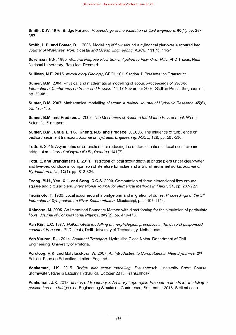
164
Smith, D.W. 1976. Bridge Failures, Proceedings of the Institution of Civil Engineers. 60(1), pp. 367-383.
Smith, H.D. and Foster, D.L. 2005. Modelling of flow around a cylindrical pier over a scoured bed. Journal of Waterway, Port, Coastal and Ocean Engineering, ASCE, 131(1), 14-24.
Sørensen, N.N. 1995. General Purpose Flow Solver Applied to Flow Over Hills. PhD Thesis, Riso National Laboratory, Roskilde, Denmark.
Sullivan, N.E. 2015. Introductory Geology, GEOL 101, Section 1, Presentation Transcript.
Sumer, B.M. 2004. Physical and mathematical modelling of scour. Proceedings of Second International Conference on Scour and Erosion, 14-17 November 2004, Stallion Press, Singapore, 1, pp. 29-46.
Sumer, B.M. 2007. Mathematical modelling of scour: A review. Journal of Hydraulic Research, 45(6), pp. 723-735.
Sumer, B.M. and Fredsøe, J. 2002. The Mechanics of Scour in the Marine Environment. World Scientific: Singapore.
Sumer, B.M., Chua, L.H.C., Cheng, N.S. and Fredsøe, J. 2003. The influence of turbulence on bedload sediment transport. Journal of Hydraulic Engineering, ASCE, 129, pp. 585-596.
Toth, E. 2015. Asymmetric error functions for reducing the underestimation of local scour around bridge piers. Journal of Hydraulic Engineering, 141(7).
Toth, E. and Brandimarte L. 2011. Prediction of local scour depth at bridge piers under clear-water and live-bed conditions: comparison of literature formulae and artificial neural networks. Journal of Hydroinformatics, 13(4), pp. 812-824.
Tseng, M.H., Yen, C.L. and Song, C.C.S. 2000. Computation of three-dimensional flow around square and circular piers. International Journal for Numerical Methods in Fluids, 34, pp. 207-227.
Tsujimoto, T. 1986. Local scour around a bridge pier and migration of dunes. Proceedings of the 3rd International Symposium on River Sedimentation, Mississippi, pp. 1105-1114.
Uhlmann, M. 2005. An Immersed Boundary Method with direct forcing for the simulation of particulate flows. Journal of Computational Physics, 209(2), pp. 448-476.
Van Rijn, L.C. 1987. Mathematical modelling of morphological processes in the case of suspended sediment transport. PhD thesis, Delft University of Technology, Netherlands.
Van Vuuren, S.J. 2014. Sediment Transport. Hydraulics Class Notes. Department of Civil Engineering, University of Pretoria.
Versteeg, H.K. and Malalasekera, W. 2007. An Introduction to Computational Fluid Dynamics, 2nd Edition. Pearson Education Limited: England.
Vonkeman, J.K. 2015. Bridge pier scour modelling. Stellenbosch University Short Course: Stormwater, River & Estuary Hydraulics, October 2015, Franschhoek.
Vonkeman, J.K. 2018. Immersed Boundary & Arbitrary Lagrangian Eulerian methods for modeling a packed bed at a bridge pier. Engineering Simulation Conference, September 2018, Stellenbosch.
Stellenbosch University https://scholar.sun.ac.za

165
Vonkeman, J.K. and Basson, G.R. 2019. Evaluation of empirical equations to predict bridge pier scour in a noncohesive bed under clear-water conditions, South African Institution of Civil Engineering, 61(2), pp. 2-20.
Vonkeman, J.K., Basson, G.R. and Smit, G.J.F. 2017. Hydro-morphodynamic modelling of local bridge pier scour in alluvial beds, 18th International Conference on Transport & Sedimentation of Solid Particles, September 2017, Prague, pp. 377-384.
Wilcox, D.C. 1993. Turbulence Modelling for CFD. DCW Industries Inc: Canada.
Williams, P.D. 2014. Scale Effects on Design Estimation of Scour Depths at Piers. Thesis. Department of Civil Engineering, Stellenbosch University.
Wilson, K.V. 1995. Scour at selected bridge sites in Mississippi: Reston, VA, U.S. Geological Survey Water-Resources Investigations Report 94–4241.
Wu, W. 2008. Computational River Dynamics. Taylor & Francis/Balkema, National Center of Computational Hydroscience and Engineering, University of Mississippi.
Xiong, W., Cai, C.S., Kong, B. and Kong, X. 2014. CFD simulations and analyses for bridge scour development using a dynamic mesh updating technique. Journal of Computing in Civil Engineering, 30(1), pp. 1-11.
Yang, C.T. 2003. Sediment Transport: Theory and Practice. Krieger Publishing Company, Florida.
Yuhi, M., Ishida, H. and Umeda, S. 2000. A numerical study of three-dimensional flow fields around a vertical cylindrical pier mounted on a bed. Proceedings of Coastal Structures ’99, Santander, Spain, 2, pp. 783-792.
Zanke, U. 1977. Calculation of the settling velocity of sediment. Proceedings of the Franzius-Institute for Hydraulic Engineering. Technical University of Hannover, Germany, 46(243), pp. 231-245.
Stellenbosch University https://scholar.sun.ac.za

166
Appendix A
Appendix A1: List of Empirical Equations
1.
Laursen & Toch (1956) 𝑑𝑑𝑠𝑠 = 1.35𝐷𝐷0.7𝑦𝑦10.3𝐾𝐾𝑠𝑠 Square 𝐾𝐾𝑠𝑠=1.1; Circular 𝐾𝐾𝑠𝑠=1; Round 𝐾𝐾𝑠𝑠=0.8; Sharp 𝐾𝐾𝑠𝑠=0.66
2. Chitale (1962) 𝑑𝑑𝑠𝑠 = 𝑦𝑦1(6.65𝐹𝐹𝐹𝐹 − 0.51 − 5.49𝐹𝐹𝐹𝐹2) 3. Breusers (1965) 𝑑𝑑𝑠𝑠 = 1.4𝐷𝐷 4. Blench (1969) 𝑑𝑑𝑠𝑠 = 1.8𝑦𝑦10.75𝐷𝐷0.25 − 𝑦𝑦1 5. Shen et al. (1969) 𝑑𝑑𝑠𝑠 = 0.00023(𝑣𝑣1𝐷𝐷/υ)0.619 6. Hancu (1971)
𝑑𝑑𝑠𝑠 = 2.42𝐷𝐷 2𝑣𝑣1𝑣𝑣𝑐𝑐
− 1 𝑣𝑣𝑐𝑐2
𝑔𝑔𝐷𝐷1/3
𝑓𝑓𝑐𝑐𝐹𝐹 0.5 <𝑣𝑣1𝑣𝑣𝑐𝑐
< 1
𝑣𝑣𝑐𝑐 = 1.2𝑔𝑔𝑑𝑑(𝑠𝑠 − 1)(𝑦𝑦1/𝑑𝑑)0.2 7. Coleman (1971) 𝑣𝑣1
2𝑔𝑔𝑑𝑑𝑠𝑠= 0.6
𝑣𝑣1𝐷𝐷0.9
8. Breuser et al. (1977)
𝑑𝑑𝑠𝑠 = 𝐷𝐷(2𝑣𝑣1/𝑣𝑣𝑐𝑐 − 1)[2 𝑡𝑡𝑎𝑎𝑛𝑛ℎ(𝑦𝑦1/𝐷𝐷)]𝐾𝐾𝑠𝑠𝐾𝐾𝜃𝜃 𝑓𝑓𝑐𝑐𝐹𝐹 0.5 < 𝑣𝑣1/𝑣𝑣𝑐𝑐 < 1 Square 𝐾𝐾𝑠𝑠=1.1; Circular 𝐾𝐾𝑠𝑠=1; Round 𝐾𝐾𝑠𝑠=0.8; Sharp 𝐾𝐾𝑠𝑠=0.66
Assume 𝑣𝑣𝑐𝑐 from Neill’s formulation (1973) 9. Jain & Fisher (1979)
𝑑𝑑𝑠𝑠1 = 2𝐷𝐷(𝐹𝐹𝐹𝐹1 − 𝐹𝐹𝐹𝐹𝑐𝑐)0.25(𝑦𝑦1/𝐷𝐷)0.5 𝑓𝑓𝑐𝑐𝐹𝐹 (𝐹𝐹𝐹𝐹 − 𝐹𝐹𝐹𝐹𝑐𝑐) > 0.2
𝑑𝑑𝑠𝑠2 = 1.85𝐷𝐷𝐹𝐹𝐹𝐹10.25(𝑦𝑦1/𝐷𝐷)0.5 𝑓𝑓𝑐𝑐𝐹𝐹 (𝐹𝐹𝐹𝐹 − 𝐹𝐹𝐹𝐹𝑐𝑐) < 0 𝑑𝑑𝑠𝑠 = 𝑚𝑚𝑎𝑎𝑥𝑥(𝑑𝑑𝑠𝑠1 , 𝑑𝑑𝑠𝑠2) 𝑓𝑓𝑐𝑐𝐹𝐹 0 < (𝐹𝐹𝐹𝐹 − 𝐹𝐹𝐹𝐹𝑐𝑐) < 0.2
𝐹𝐹𝐹𝐹𝑐𝑐 =𝑣𝑣𝑐𝑐
𝑔𝑔𝑦𝑦1
Assume 𝑣𝑣𝑐𝑐 from Neill’s formulation (1973) 10. Jain (1981)
𝑑𝑑𝑠𝑠 = 1.84𝑦𝑦1𝐹𝐹𝐹𝐹𝑐𝑐0.25(𝐷𝐷/𝑦𝑦1)0.7
Assume 𝑣𝑣𝑐𝑐 from Neill’s formulation (1973) 11a. Froelich (1988) 𝑑𝑑𝑠𝑠 = 0.32𝐾𝐾𝑠𝑠𝐷𝐷0.62𝑦𝑦10.47𝐹𝐹𝐹𝐹0.22𝑑𝑑−0.09
Square 𝐾𝐾𝑠𝑠=1.3; Circular 𝐾𝐾𝑠𝑠=1; Round 𝐾𝐾𝑠𝑠=1; Sharp 𝐾𝐾𝑠𝑠=0.7 11b. Froelich Design (1988) 𝑑𝑑𝑠𝑠 = 0.32𝐾𝐾𝑠𝑠𝐷𝐷0.62𝑦𝑦10.47𝐹𝐹𝐹𝐹0.22𝑑𝑑−0.09 + 𝐷𝐷 12. Kothyari, Garde & Ranga
(1992) 𝑑𝑑𝑠𝑠 = 𝐷𝐷 𝐷𝐷𝑑𝑑−0.25
𝑦𝑦1𝑑𝑑0.16
𝑣𝑣12 − 𝑣𝑣𝑐𝑐2
(𝑠𝑠 − 1)𝑔𝑔𝑑𝑑0.4
𝑓𝑓𝑐𝑐𝐹𝐹 𝑣𝑣1𝑣𝑣𝑐𝑐
< 1
𝑣𝑣𝑐𝑐2 = 1.2[(𝑠𝑠 − 1)𝑔𝑔𝑑𝑑](𝐷𝐷/𝑑𝑑)−0.11(𝑦𝑦1/𝑑𝑑)0.16 13. Mississippi (Wilson, 1995) 𝑑𝑑𝑠𝑠 = 0.9𝐷𝐷0.6𝑦𝑦10.4 14. Simplified Chinese
Gao et al. (1993)
𝑑𝑑𝑠𝑠 = 0.46𝐾𝐾𝑠𝑠𝐷𝐷0.6𝑦𝑦10.15𝑑𝑑−0.07 𝑣𝑣1 − 𝑣𝑣𝑖𝑖𝑣𝑣𝑐𝑐 − 𝑣𝑣𝑖𝑖
η
η = (𝑣𝑣𝑐𝑐/𝑣𝑣1)9.35+2.23𝑠𝑠𝑜𝑜𝑔𝑔 (𝑑𝑑)
𝑣𝑣𝑐𝑐 = 𝑦𝑦1𝑑𝑑0.14
17.6(𝑠𝑠 − 1)𝑑𝑑 + 6.05𝐸𝐸−7 10 + 0.3048𝑦𝑦1(0.3048𝑑𝑑)0.72
0.5
𝑣𝑣𝑖𝑖 = 0.645𝑣𝑣𝑐𝑐(𝑑𝑑/𝐷𝐷)0.053 Square 𝐾𝐾𝑠𝑠=1.1; Circular 𝐾𝐾𝑠𝑠=1; Round 𝐾𝐾𝑠𝑠=0.8; Sharp=0.66
15. Melville & Sutherland (1988) 𝑑𝑑𝑠𝑠 = 𝐾𝐾𝜃𝜃𝐾𝐾𝜎𝜎𝐾𝐾𝑠𝑠𝐾𝐾𝑦𝑦1(2.4𝐾𝐾𝐼𝐼)𝐾𝐾𝑑𝑑 Gradation factor 𝐾𝐾𝜎𝜎 = 1
Alignment factor 𝐾𝐾𝜃𝜃 = (𝑐𝑐𝑐𝑐𝑠𝑠𝜃𝜃 + 𝐿𝐿/𝐷𝐷𝑠𝑠𝑖𝑖𝑛𝑛𝜃𝜃)0.65 General shape factor Square 𝐾𝐾𝑠𝑠=1.1; Circular 𝐾𝐾𝑠𝑠=1; Round 𝐾𝐾𝑠𝑠=1; Sharp 𝐾𝐾𝑠𝑠=0.9 Flow intensity factor
𝐾𝐾𝐼𝐼 =𝑣𝑣1 − (𝑣𝑣𝑎𝑎 − 𝑣𝑣𝑐𝑐)
𝑣𝑣𝑐𝑐 𝑓𝑓𝑐𝑐𝐹𝐹
𝑣𝑣1 − (𝑣𝑣𝑎𝑎 − 𝑣𝑣𝑐𝑐)𝑣𝑣𝑐𝑐
< 1
𝐾𝐾𝐼𝐼 = 1 𝑓𝑓𝑐𝑐𝐹𝐹 𝑣𝑣1 − (𝑣𝑣𝑎𝑎 − 𝑣𝑣𝑐𝑐)
𝑣𝑣𝑐𝑐 ≥ 1
𝐶𝐶𝑐𝑐∗ = 0.0115 + 0.0125𝑑𝑑1.4 𝑓𝑓𝑐𝑐𝐹𝐹 0.1 𝑚𝑚𝑚𝑚 < 𝑑𝑑 < 1 𝑚𝑚𝑚𝑚 𝐶𝐶𝑐𝑐∗ = 0.0305𝑑𝑑0.5 − 0.0065𝑑𝑑−1 𝑓𝑓𝑐𝑐𝐹𝐹 1 𝑚𝑚𝑚𝑚 < 𝑑𝑑 < 100 𝑚𝑚𝑚𝑚
Stellenbosch University https://scholar.sun.ac.za

167
Median armour size 𝑑𝑑𝑎𝑎 = 𝑑𝑑𝑖𝑖𝑚𝑚𝑚𝑚
1.8 for 𝑣𝑣𝑎𝑎 = 0.8𝑣𝑣𝑐𝑐𝑎𝑎
𝑣𝑣𝑐𝑐𝑎𝑎 = 5.75𝐶𝐶𝑐𝑐𝑎𝑎∗ 𝑙𝑙𝑐𝑐𝑔𝑔 5.53𝑦𝑦1𝑑𝑑𝑎𝑎
𝑣𝑣𝑐𝑐 = 5.75𝐶𝐶𝑐𝑐∗ 𝑙𝑙𝑐𝑐𝑔𝑔 5.53𝑦𝑦1𝑑𝑑
Sediment factor 𝐾𝐾𝑑𝑑 = 0.57 𝑙𝑙𝑐𝑐𝑔𝑔(2.24𝐷𝐷/𝑑𝑑) 𝑓𝑓𝑐𝑐𝐹𝐹 𝐷𝐷/𝑑𝑑 ≤ 25 𝐾𝐾𝑑𝑑 = 1 𝑓𝑓𝑐𝑐𝐹𝐹 𝐷𝐷/𝑑𝑑 > 25
Depth size factor 𝐾𝐾𝑦𝑦1 = 𝐷𝐷 𝑓𝑓𝑐𝑐𝐹𝐹 𝑦𝑦1/𝐷𝐷 > 2.6 𝐾𝐾𝑦𝑦1 = 0.78𝐷𝐷(𝑦𝑦1/𝐷𝐷)0.255 𝑓𝑓𝑐𝑐𝐹𝐹 𝑦𝑦1/𝐷𝐷 < 2.6
16. Melville (1997) 𝑑𝑑𝑠𝑠 = 𝐾𝐾𝜃𝜃𝐾𝐾𝐺𝐺𝐾𝐾𝑠𝑠𝐾𝐾𝑦𝑦𝐾𝐾𝐼𝐼𝐾𝐾𝑑𝑑 Channel geometry 𝐾𝐾𝐺𝐺 = 1 for a bridge pier
Revised depth size factor 𝐾𝐾𝑦𝑦 = 2.4𝐷𝐷 𝑓𝑓𝑐𝑐𝐹𝐹 𝐷𝐷/𝑦𝑦1 < 0.7 𝐾𝐾𝑦𝑦 = 2𝑦𝑦1𝐷𝐷 𝑓𝑓𝑐𝑐𝐹𝐹 0.7 < 𝐷𝐷/𝑦𝑦1 < 5
𝐾𝐾𝑦𝑦 = 4.5𝑦𝑦1 𝑓𝑓𝑐𝑐𝐹𝐹 𝐷𝐷/𝑦𝑦1 > 5 17. Melville & Coleman (2000) 𝑑𝑑𝑠𝑠 = 𝐾𝐾𝜃𝜃𝐾𝐾𝐺𝐺𝐾𝐾𝑠𝑠𝐾𝐾𝑦𝑦𝐾𝐾𝐼𝐼𝐾𝐾𝑑𝑑𝐾𝐾𝑡𝑡
Time factor 𝐾𝐾𝑡𝑡 = 𝑅𝑅𝑥𝑥𝑝𝑝 −0.07 𝑣𝑣𝑐𝑐𝑣𝑣1𝑙𝑙𝑛𝑛 𝑡𝑡
𝑡𝑡𝑒𝑒1.5 𝑓𝑓𝑐𝑐𝐹𝐹 𝑣𝑣1
𝑣𝑣𝑐𝑐< 1
where 𝑡𝑡𝑑𝑑 = total time to reach equilibrium profile 18. Melville & Kandasamy (1998) 𝑑𝑑𝑠𝑠 = 𝐾𝐾𝑠𝑠𝐾𝐾𝑦𝑦1𝑚𝑚𝐷𝐷1−𝑚𝑚
𝐾𝐾 = 5,𝑛𝑛 = 1 𝑓𝑓𝑐𝑐𝐹𝐹 0.04 ≥ 𝑦𝑦1/𝐷𝐷 𝐾𝐾 = 1,𝑛𝑛 = 0.5 𝑓𝑓𝑐𝑐𝐹𝐹 0.04 < 𝑦𝑦1/𝐷𝐷 < 1
𝐾𝐾 = 1,𝑛𝑛 = 0 𝑓𝑓𝑐𝑐𝐹𝐹 𝑦𝑦1/𝐷𝐷 ≥ 1 19. Sheppard & Miller (2006) 𝑑𝑑𝑠𝑠 = 2.5𝐷𝐷𝑓𝑓1𝑓𝑓2𝑓𝑓3 𝑓𝑓𝑐𝑐𝐹𝐹 0.47 < 𝑣𝑣1/𝑣𝑣𝑐𝑐 < 1
𝑓𝑓1 = 𝑡𝑡𝑎𝑎𝑛𝑛ℎ([𝑦𝑦1/𝐷𝐷]0.4) 𝑓𝑓2 = 1 − 1.75[𝑙𝑙𝑛𝑛(𝑣𝑣1/𝑣𝑣𝑐𝑐)]2
Assume 𝑣𝑣𝑐𝑐 from Neill’s formulation (1973)
𝑓𝑓3 =𝐷𝐷/𝑑𝑑
0.4(𝐷𝐷/𝑑𝑑)1.2 + 10.6(𝐷𝐷/𝑑𝑑)−0.13
20. Sheppard & Melville (2014) 𝑑𝑑𝑠𝑠 = 2.5𝑓𝑓1𝑓𝑓2𝑓𝑓3𝐾𝐾1𝐷𝐷 𝑓𝑓𝑐𝑐𝐹𝐹 0.4 ≤𝑣𝑣1𝑣𝑣𝑐𝑐
< 1.0
𝑓𝑓1 = 𝑡𝑡𝑎𝑎𝑛𝑛ℎ 𝑦𝑦1𝐾𝐾1𝐷𝐷
0.4
𝑓𝑓2 = 1 − 1.2 𝑙𝑙𝑛𝑛 𝑣𝑣1𝑣𝑣𝑐𝑐
2
𝑓𝑓3 = 𝐾𝐾1𝐷𝐷𝑑𝑑 0.4
𝐾𝐾1𝐷𝐷𝑑𝑑1,2
+ 10.6 𝐾𝐾1𝐷𝐷𝑑𝑑−0.13
−1
𝐾𝐾1 = 1 for cylindrical piers
𝐾𝐾1 = 0.86 + 0.97 𝛼𝛼 − 𝜋𝜋44 for rectangular piers
𝐶𝐶𝑐𝑐∗ = 16.2𝑑𝑑 9.09 × 10⁻⁶
𝑑𝑑− 𝑑𝑑[38.76 + 9.6 𝑙𝑙𝑛𝑛(𝑑𝑑)]− 0.005
12
𝑅𝑅𝑅𝑅 =𝐶𝐶𝑐𝑐∗𝑑𝑑
υ 𝑓𝑓𝑐𝑐𝐹𝐹 5 ≤ 𝑅𝑅𝑅𝑅 ≤ 70
𝑣𝑣𝑐𝑐 = 2.5𝐶𝐶𝑐𝑐∗ 𝑙𝑙𝑛𝑛 73.5𝑦𝑦1𝑑𝑑𝑅𝑅𝑅𝑅[2.85 − 0.58 𝑙𝑙𝑛𝑛(𝑅𝑅𝑅𝑅) + 0.002𝑅𝑅𝑅𝑅] +
111𝑅𝑅𝑅𝑅
− 6−1 𝑓𝑓𝑐𝑐𝐹𝐹 𝑅𝑅𝑅𝑅 > 70
𝑣𝑣𝑐𝑐 = 2.5𝐶𝐶𝑐𝑐∗ 𝑙𝑙𝑛𝑛 2.21𝑦𝑦1𝑑𝑑
𝑓𝑓𝑐𝑐𝐹𝐹 𝑅𝑅𝑅𝑅 < 7
Stellenbosch University https://scholar.sun.ac.za

168
21. FDOT (Arneson et al., 2012)
𝑑𝑑𝑠𝑠 = 2.5𝑓𝑓1𝑓𝑓2𝑓𝑓3𝐾𝐾1𝐷𝐷 𝑓𝑓𝑐𝑐𝐹𝐹 0.4 ≤𝑣𝑣1𝑣𝑣𝑐𝑐
< 1.0
𝑣𝑣𝑐𝑐 = 2.5𝐶𝐶𝑐𝑐∗ log(5.53𝑦𝑦1/𝑑𝑑) 𝐶𝐶𝑐𝑐∗ = 0.0377 + 0.041𝑑𝑑1.4 𝑓𝑓𝑐𝑐𝐹𝐹 0.1 𝑚𝑚𝑚𝑚 < 𝑑𝑑 < 1 𝑚𝑚𝑚𝑚 𝐶𝐶𝑐𝑐∗ = 0.1𝑑𝑑0.5 − 0.0213/𝑑𝑑 𝑓𝑓𝑐𝑐𝐹𝐹 1 𝑚𝑚𝑚𝑚 < 𝑑𝑑 < 100 𝑚𝑚𝑚𝑚
22. HEC-18 or CSU equations 𝑑𝑑𝑠𝑠 = 2𝐷𝐷𝐾𝐾𝑠𝑠𝐾𝐾𝜃𝜃𝐾𝐾𝑏𝑏𝐾𝐾𝑎𝑎(𝑦𝑦1/𝐷𝐷)0.35𝐹𝐹𝐹𝐹0.43 Bed condition factor 𝐾𝐾𝑏𝑏 = 1.1 for clear-water scouring
22a. Richardson et al. (1993) Armouring factor 𝐾𝐾𝑎𝑎 = 1 22b. Richardson & Davis (1995) 𝐾𝐾𝑎𝑎 = [1 − 0.89(1 − 𝑉𝑉𝑅𝑅)2]0.5
Dimensionless excess velocity intensity
𝑉𝑉𝑅𝑅 =𝑣𝑣1 − 𝑣𝑣𝑖𝑖𝑣𝑣𝑐𝑐90 − 𝑣𝑣𝑖𝑖
𝑣𝑣𝑖𝑖 = 0.645𝑣𝑣𝑐𝑐(𝑑𝑑/𝐷𝐷)0.053 𝑣𝑣𝑐𝑐90 = 6.19𝑦𝑦1
1/6𝑑𝑑901/3where 𝑑𝑑90 = 𝑑𝑑𝜎𝜎𝑔𝑔1.282
22c. Mueller (1996) 𝐾𝐾𝑎𝑎 = 0.4𝑉𝑉𝑅𝑅0.15
𝑉𝑉𝑅𝑅 =𝑣𝑣1 − 𝑣𝑣𝑖𝑖𝑣𝑣𝑐𝑐 − 𝑣𝑣𝑖𝑖95
𝑣𝑣𝑖𝑖 = 0.645𝑣𝑣𝑐𝑐(𝑑𝑑/𝐷𝐷)0.053 𝑣𝑣𝑖𝑖95 = 0.645𝑣𝑣𝑐𝑐95(𝑑𝑑95/𝐷𝐷)0.053where 𝑑𝑑95 = 𝑑𝑑𝜎𝜎𝑔𝑔1.645
Critical velocity (Neill, 1973) 𝑣𝑣𝑐𝑐 = 𝜃𝜃𝑠𝑠0.531.08𝑦𝑦11/6𝑑𝑑1/3 using Shields parameter 𝜃𝜃𝑠𝑠 = 0.0019𝑑𝑑−0.384 𝑖𝑖𝑓𝑓 𝑑𝑑 < 0.0009 𝑚𝑚
𝜃𝜃𝑠𝑠 = 0.0942𝑑𝑑0.175 𝑖𝑖𝑓𝑓 0.0009 𝑚𝑚 < 𝑑𝑑 < 0.020 𝑚𝑚 𝜃𝜃𝑠𝑠 = 0.047 𝑖𝑖𝑓𝑓 𝑑𝑑 > 0.020 𝑚𝑚
22d. Mueller & Wagner (2005) 𝐾𝐾𝑎𝑎 = 0.35(𝐷𝐷/𝑑𝑑)0.19 22e. Molinas (2004) 𝐾𝐾𝑎𝑎 = 1.25 + 3𝑑𝑑𝑐𝑐𝑓𝑓𝐼𝐼/𝑑𝑑𝑉𝑉𝑅𝑅0.6𝑙𝑙𝑛𝑛 (𝑉𝑉𝑅𝑅 + 0.5)
𝑉𝑉𝑅𝑅 =𝑣𝑣1 − 𝑣𝑣𝑖𝑖𝑣𝑣𝑐𝑐𝐼𝐼 − 𝑣𝑣𝑖𝑖
𝑣𝑣𝑖𝑖 = 2.65𝑦𝑦11/6𝑑𝑑35
1/3 𝑣𝑣𝑐𝑐𝐼𝐼 = 6.625𝑦𝑦1
1/6𝑑𝑑𝑐𝑐𝑓𝑓𝐼𝐼1/3
𝑑𝑑𝑐𝑐𝑓𝑓𝐼𝐼 = (𝑑𝑑85 + 2𝑑𝑑90 + 2𝑑𝑑95 + 𝑑𝑑99)/6 23. Molinas (2004) 𝑑𝑑𝑠𝑠 = 0.99𝐾𝐾𝑖𝑖𝐾𝐾𝑠𝑠𝐾𝐾𝜃𝜃𝐾𝐾𝑏𝑏𝐾𝐾𝑎𝑎𝑉𝑉𝑅𝑅0.55𝐷𝐷0.66𝑦𝑦0.17
Scour initiation 𝐾𝐾𝑖𝑖 = (1 − 𝑣𝑣𝑖𝑖/𝑣𝑣1)0.45
𝐾𝐾𝑎𝑎 = 1.25 + 3𝑑𝑑𝑐𝑐𝑓𝑓𝐼𝐼/𝑑𝑑𝑉𝑉𝑅𝑅0.6𝑙𝑙𝑛𝑛 (𝑉𝑉𝑅𝑅 + 0.5)
24. Ali & Karim (2002) 𝑑𝑑𝑠𝑠 =
𝐾𝐾1𝐷𝐷∗1.2𝑦𝑦1𝑣𝑣1𝐷𝐷 υ
1 − 𝐸𝐸𝑥𝑥𝑝𝑝(−5.32𝐸𝐸−4𝑣𝑣1𝑡𝑡𝑦𝑦1
)
𝐾𝐾1 = 0.1(𝑠𝑠 − 1)𝑔𝑔𝑑𝑑3/2𝐷𝐷∗−0.3 𝐷𝐷∗ = [(𝑠𝑠 − 1)𝑔𝑔υ−2]1/3
25. Guo (2012) 𝑑𝑑𝑠𝑠 = 𝐷𝐷𝑦𝑦1 𝑡𝑡𝑎𝑎𝑛𝑛ℎ
𝐻𝐻2
3.75𝜎𝜎𝑔𝑔 𝑤𝑤ℎ𝑅𝑅𝐹𝐹𝑅𝑅 𝜎𝜎𝑔𝑔 = 𝑑𝑑84 𝑑𝑑16⁄
Densiometric particle Froude number
𝐻𝐻 =𝑣𝑣1
(𝑠𝑠 − 1)𝑔𝑔𝑑𝑑
Stellenbosch University https://scholar.sun.ac.za
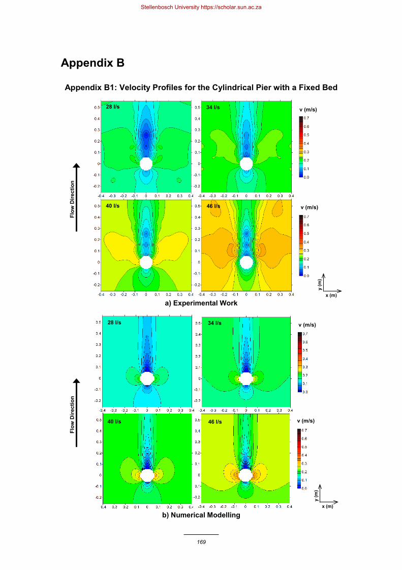
169
Appendix B
Appendix B1: Velocity Profiles for the Cylindrical Pier with a Fixed Bed
a) Experimental Work
b) Numerical Modelling
v (m/s)
y (m
)
x (m)
v (m/s)
v (m/s)
Flow
Dire
ctio
n
28 l/s 34 l/s
40 l/s 46 l/s
Flow
Dire
ctio
n
28 l/s 34 l/s
40 l/s 46 l/s
y (m
)
x (m)
v (m/s)
Stellenbosch University https://scholar.sun.ac.za
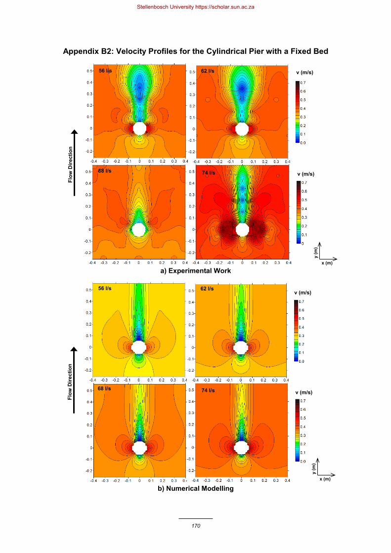
170
Appendix B2: Velocity Profiles for the Cylindrical Pier with a Fixed Bed
a) Experimental Work
b) Numerical Modelling
56 l/s 62 l/s
68 l/s 74 l/s
v (m/s) Fl
ow D
irect
ion
56 l/s 62 l/s
68 l/s 74 l/s
v (m/s)
Flow
Dire
ctio
n
y (m
)
x (m)
v (m/s)
y (m
)
x (m)
v (m/s)
Stellenbosch University https://scholar.sun.ac.za

171
Appendix B3: Velocity Profiles for the Round Nosed Pier with a Fixed Bed
a) Experimental Work
b) Numerical Modelling
v (m/s)
y (m
)
x (m)
v (m/s)
y (m
)
x (m)
Flow
Dire
ctio
n
28 l/s 34 l/s 40 l/s 46 l/s
Flow
Dire
ctio
n
28 l/s 34 l/s 40 l/s 46 l/s
Stellenbosch University https://scholar.sun.ac.za

172
Appendix B4: Velocity Profiles for the Round Nosed Pier with a Fixed Bed
a) Experimental Work
b) Numerical Modelling
v (m/s)
y (m
)
x (m)
Flow
Dire
ctio
n
56 l/s 62 l/s 68 l/s 74 l/s
v (m/s)
y (m
)
x (m)
Flow
Dire
ctio
n
56 l/s 62 l/s 68 l/s 74 l/s
Stellenbosch University https://scholar.sun.ac.za
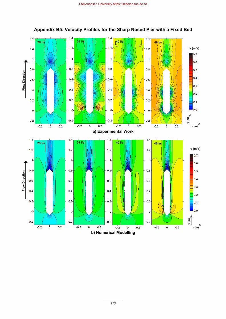
173
Appendix B5: Velocity Profiles for the Sharp Nosed Pier with a Fixed Bed
a) Experimental Work
b) Numerical Modelling
v (m/s)
y (m
)
x (m)
v (m/s)
y (m
)
x (m)
Flow
Dire
ctio
n
28 l/s 34 l/s 40 l/s 46 l/s
Flow
Dire
ctio
n
28 l/s 34 l/s 40 l/s 46 l/s
Stellenbosch University https://scholar.sun.ac.za

174
Appendix B6: Velocity Profiles for the Sharp Nosed Pier with a Fixed Bed
a) Experimental Work
b) Numerical Modelling
v (m/s)
y (m
)
x (m)
Flow
Dire
ctio
n
56 l/s 62 l/s 68 l/s 74 l/s
v (m/s)
y (m
)
x (m)
Flow
Dire
ctio
n
56 l/s 62 l/s 68 l/s 74 l/s
Stellenbosch University https://scholar.sun.ac.za

175
Appendix C Appendix C1: Scour Profiles for the Cylindrical Pier with Peach Pips
a) Experimental Work
b) Numerical Modelling
∆z (m)
∆z (m)
y (m
)
x (m)
Flow
Dire
ctio
n 28 l/s 34 l/s
40 l/s 46 l/s
∆z (m)
∆z (m)
y (m
)
x (m)
Flow
Dire
ctio
n
28 l/s 34 l/s
40 l/s 46 l/s
Stellenbosch University https://scholar.sun.ac.za

176
Appendix C2: Scour Profiles for the Cylindrical Pier with Fine Sand
a) Experimental Work
b) Numerical Modelling
∆z (m)
∆z (m)
y (m
)
x (m)
Flow
Dire
ctio
n
56 l/s 62 l/s
68 l/s 74 l/s
∆z (m)
∆z (m)
y (m
)
x (m)
Flow
Dire
ctio
n
56 l/s 62 l/s
68 l/s 74 l/s
Stellenbosch University https://scholar.sun.ac.za

177
Appendix C3: Scour Profiles for the Round Nosed Pier with Peach Pips
a) Experimental Work
b) Numerical Modelling
∆z (m)
y (m
)
x (m)
Flow
Dire
ctio
n
28 l/s 34 l/s 40 l/s 46 l/s
∆z (m)
y (m
)
x (m)
Flow
Dire
ctio
n
28 l/s 34 l/s 40 l/s 46 l/s
Stellenbosch University https://scholar.sun.ac.za

178
Appendix C4: Scour Profiles for the Round Nosed Pier with Fine Sand
a) Experimental Work
b) Numerical Modelling
y (m
)
x (m)
Flow
Dire
ctio
n
56 l/s 62 l/s 68 l/s 74 l/s
∆z (m)
y (m
)
x (m)
Flow
Dire
ctio
n
56 l/s 62 l/s 68 l/s 74 l/s ∆z (m)
Stellenbosch University https://scholar.sun.ac.za
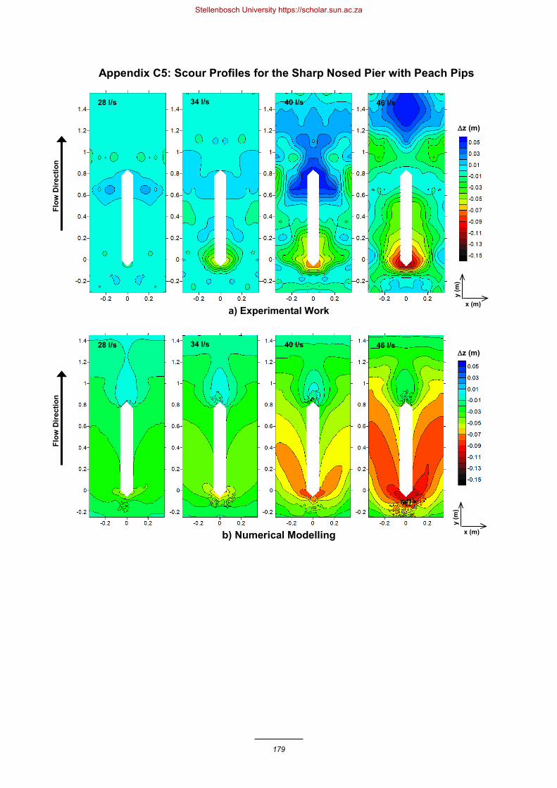
179
Appendix C5: Scour Profiles for the Sharp Nosed Pier with Peach Pips
a) Experimental Work
b) Numerical Modelling
∆z (m)
y (m
)
x (m)
Flow
Dire
ctio
n
28 l/s 34 l/s 40 l/s 46 l/s
∆z (m)
y (m
)
x (m)
Flow
Dire
ctio
n
28 l/s 34 l/s 40 l/s 46 l/s
Stellenbosch University https://scholar.sun.ac.za

180
Appendix C6: Scour Profiles for the Sharp Nosed Pier with Fine Sand
a) Experimental Work
b) Numerical Modelling
y (m
)
x (m)
Flow
Dire
ctio
n
56 l/s 62 l/s 68 l/s 74 l/s
∆z (m)
y (m
)
x (m)
Flow
Dire
ctio
n
56 l/s 62 l/s 68 l/s 74 l/s
∆z (m)
Stellenbosch University https://scholar.sun.ac.za