Environmental Geotechnics

A coupled thermal-hydro-mechanical simulation for carbon dioxide sequestrationBao, Xu and Fang

Environmental Geotechnicshttp://dx.doi.org/10.1680/envgeo.14.00002Paper 14.00002Received 20/01/2014; accepted 31/07/2014Keywords: numerical methods/waste containment and disposal system

ICE Publishing: All rights reserved

1

Herein, the authors present a coupled thermal-hydro-mechanical model, as an improvement of the isotherm hydro-

mechanical model in their previous work, for geological sequestration of carbon dioxide followed by stress, deformation,

and shear-slip failure analyses. This fully coupled model considers the geomechanical response, fluid flow and thermal

transport relevant to geological sequestration. Both analytical solutions and numerical approach by way of finite

element model are introduced for solving the thermal-hydro-mechanical model. Analytical solutions for pressure,

temperature, deformation and stress field were obtained for a simplified typical geological sequestration scenario by

assuming a simplified temperature profile in an aquifer. The finite element model is more general and can be used for

arbitrary geometry. It was built on an open-source finite element solver, Elmer, and was designed to simulate the entire

period of carbon dioxide injection both stably and accurately – even for large time steps. The shear-slip failure analysis

was implemented based on the numerical results from the finite element model. The analysis reveals the potential

failure zone caused by the fluid injection and thermal effect. From the simulation results, the thermal effect is shown

to reduce the potential failure zone, especially at the early time of the injection.

3 Yilin Fang PhD Scientist, Hydrology Technical Group, Energy and Environment

Directorate, Pacific Northwest National Laboratory, Richland, WA, USA

1 Jie Bao PhD Engineer, Experimental and Computational Engineering Group,

Energy and Environment Directorate, Pacific Northwest National Laboratory, Richland, WA, USA

2 Zhijie Xu PhD Scientist, Computational Mathematics Group, Fundamental and

Computational Sciences Directorate, Pacific Northwest National Laboratory, Richland, WA, USA

A coupled thermal-hydro-mechanical simulation for carbon dioxide sequestration

NotationCl fluid specific heat ((J/kg)/°C)Cs rock specific heat ((J/kg)/°C)

D dimensionless number, µθβ λ

=+ +

/1/( 2 )k

DG

Es rock volumetric thermal expansion (°C–1)F(l) integration of an exponential functionG shear modulus (Pa)g gravity acceleration (m/s2)Kl fluid thermal conductivity ((W/m)/°C))Ks rock thermal conductivity ((W/m)/°C))k permeability (m2)Ms rock bulk modulus (GPa)p pressure (Pa)pp pore pressure (Pa)�p scaling factor,

ψ µπ ρ

′=� 1

4p

k�( , )R r z position of point A

¢ ¢�

0( , )R r z position of centre of dilation′′ ′−�

0( , )R r z position of image of centre of dilationr horizontal distance from injection well (m)T temperature (°C)t injection time (s)�u mechanical displacement vector (m)uz vertical displacement (m)ur horizontal/radial displacement (m)z depth (m)b fluid compressibility (Pa−1)dij the Kronecker deltaeij strain componentg azimuthal anglel Lame’s constant (Pa)l dimensionless number, l = r2/(4Dt)m viscosity (Pa·s)q porosity

1 2 3

1

2

3

4

5

6

7

8

9

10

11

12

13

14

15

16

17

18

19

20

21

22

23

24

25

26

27

28

29

30

31

32

33

34

35

36

37

38

39

40

41

42

43

44

45

46

47

48

49

50

51

52

53

54

55

envgeo1400002.indd 1 Manila Typesetting Company 08/26/2014 03:26PM

Environmental Geotechnics A coupled thermal-hydro-mechanical simulation for carbon dioxide sequestrationBao, Xu and Fang

2

r1 density of liquid (kg/m3)rs rock of liquid (kg/m3)rs density of the soil/rock (kg/m3)

r¢(r,z) distance between point A [ ( , )]R r z�

and centre of dilation 0[ ( , )]R r z¢ ¢

� as shown in Figure 4 (m)

r¢¢(r,z) distance between point A and the image of centre of dilation 0[ ( , )]R r z-¢¢ ¢

� as shown in Figure 4 (m)

σ� total stress tensor (Pa)

sh horizontal remote stress (Pa)ijσ ¢ effective stress component (Pa)

sv vertical remote stress (Pa)σ ′1 maximum principal effective stress (Pa)σ ′3 minimum principal effective stress (Pa)y external source term stands for the carbon dioxide

injection rate ((kg/m3)/s)y ¢ line injection rate (kg/m/s)

IntroductionIt is well known that carbon dioxide sequestration in deep saline

aquifers could be a promising mitigation method for reducing the

amount of carbon dioxide emitted into the atmosphere (Vilarrasa

et al., 2011). It is widely accepted that geothermal energy offers

clean, renewable, reliable electric power with no need for grid-

scale energy storage (Atrens et al., 2009, 2010). Recent research

has presented a novel approach of combining geothermal energy

capture with geologic carbon dioxide sequestration (Randolph and

Saar, 2011a, 2011b). Still, even without combining a geothermal

energy capture system, the temperature of injected carbon dioxide

is lower than the environment temperature in deep ground,

especially in areas with great amounts of geothermal resources.

Injection of carbon dioxide into a site often lasts a few decades,

and carbon dioxide is expected to be retained underground until

well past the end of the fossil fuel era; it could easily last several

hundreds of years or even longer than 1000 years (Holloway, 2005;

Wilson, 1992). Hence, geological injection and sequestration of

supercritical carbon dioxide intrinsically involve a number of

complicated physical and chemical processes that occur within

large spatial domains and extremely long periods of time.

Mathematical models and numerical simulation tools will play

an important role in evaluating and predicting the feasibility of

carbon dioxide storage in subsurface reservoirs, designing and

analysing field tests and designing and operating geologic carbon

dioxide disposal and geothermal extraction systems (Pruess et

al., 2004). In recent years, various thermal-hydro-mechanical

models and simulation tools (Gor et al., 2013; Preisig and Prévost,

2011; Simone et al., 2013; Vilarrasa et al., 2013) have been

applied to the study of geological carbon dioxide sequestration.

However, although a fully coupled 3D multiphase, multiphysics,

multicomponent computational model provides a relatively more

complete description of the problem, it is sometimes fragile because

of various computational challenges, such as the difficulties

in model parameter identification, process coupling, severe

heterogeneity and non-linearity (Xu et al., 2012). An analytical

solution to a simplified model of carbon dioxide sequestration

based on reasonable assumptions is much more efficient and can

uncover the critical relationship between injection conditions

and geomechanical response, which can help us understand

the mechanism and physical effects and provide guidance to

applications on the actual sites where the detailed parameters are

not yet well identified. The purpose of this paper is to present an

efficient model for understanding geomechanical response when a

deep geological formation is subjected to injection of substantial

supercritical carbon dioxide with thermal effects.

In this article, the authors first introduce a thermal-hydro-mechanical

model in ‘Thermal-hydro-mechanical model for carbon dioxide

geological sequestration’. The corresponding analytical solutions

of fluid pressure, temperature, deformation and stress fields for a

typical injection scenario are introduced in ‘Analytical solution for

the thermal-hydro-mechanical model’. A finite element solution,

based on an open-source solver, Elmer, is introduced in ‘Finite

element model for the thermal-hydro-mechanical model’, and

comparisons between analytical and numerical methods are shown

in ‘Comparison of finite element results with analytical solutions’.

‘Failure analysis and thermal effects’ describes the application of

geomechanical shear-slip failure analysis based on the coupled

thermal-hydro-mechanical model to estimate the potential damage

zone during carbon dioxide injection.

Thermal-hydro-mechanical model for carbon dioxide geological sequestrationThe authors’ previous works (Bao et al., 2013a; Xu et al., 2012)

introduced the isothermal hydro-mechanical model companion

with both analytical and numerical solutions for carbon dioxide

geological sequestration. To make the model analytically solvable

and more computationally efficient in numerical simulation,

the flow was assumed as single phase, although carbon dioxide

injection is a multiphase system. Therefore, a carbon dioxide–brine

multiphase subsurface flow simulation, subsurface transport over

multiple phases (STOMP) (White and Oostrom, 2006), was used to

validate the proposed single-phase model in the authors’ previous

works (Bao et al., 2013a, 2013b, 2014), and it was shown that the

single-phase model can capture the characteristics of the pressure

evolution of the carbon dioxide–brine multiphase system in an

aquifer layer, because the pressure evolves more rapidly than flow

transport. In addition, the capillary pressure for supercritical carbon

dioxide and brine is on the order of 103–10

4 Pa (Tokunaga et al.,

2013), while the injection pressure is often higher than 106 Pa; so

the capillary pressure is negligible for the carbon dioxide injection

system, and therefore, the single-phase model is an appropriate

approximation of the carbon dioxide–brine flow system for

estimating the pressure evolution in the aquifer layer. Based on

the single-phase isothermal model in the authors’ previous work

(Bao et al., 2013a; Xu et al., 2012), the thermal effect is involved,

which makes the thermal-hydro-mechanical model include fluid

flow, heat transfer and linear elasticity equations that describe the

geomechanical reaction to fluid injection flow. The coupled hydro-

mechanical model (Biot, 1935, 1941, 1955, 1956, 1962; Terzaghi,

1923; Yin et al., 2010, 2011) reads

1

2

3

4

5

6

7

8

9

10

11

12

13

14

15

16

17

18

19

20

21

22

23

24

25

26

27

28

29

30

31

32

33

34

35

36

37

38

39

40

41

42

43

44

45

46

47

48

49

50

51

52

53

54

55

envgeo1400002.indd 2 Manila Typesetting Company 08/26/2014 03:26PM envgeo1400002.indd 3 Manila Typesetting Company 08/26/2014 03:26PM

Environmental Geotechnics A coupled thermal-hydro-mechanical simulation for carbon dioxide sequestrationBao, Xu and Fang

3

1.

2

1

1 ( ) ψθβ θµβ θρ β

∂ ∂ ∇ ⋅+ = ∇ +∂ ∂

�p u k

p

t t

2.

1 1 1

2

1

[(1 ) ]

[(1 ) ]

θ ρ θρ ρ

θ θ

1¶- + + Ѷ

= - + Ñ

�s s

s

TC C C v T

t

K K T

3. 2

( ) ( )λ + ∇ ∇⋅ + ∇ = ∇ + ∇� �

s sG u G u p M E T

Equation 1 is a fluid flow continuity equation in terms of the pore

pressure p in Pascals, and the units for all parameters are listed in

Table 1 and in Notation. In Equation 1, t is the injection time, u

�

is the mechanical displacement vector in metres, q is the porosity,

b is the compressibility, m is the viscosity, k is the permeability,

r1 is the density of liquid and y is the external source term that

stands for the carbon dioxide bulk injection rate in kilograms per

cubic metre per second. Equation 2 is a heat transfer equation

for temperature field T in degree Celsius. In Equation 2, C1 and

Cs are the heat capacity for liquid and solid parts, respectively.

K1 and Ks are the thermal conductivity for liquid and solid parts,

respectively. rs is the density of solid soil/rock.

�v is the Darcy flux

and is calculated by

4. .

µ= − ∇� kv p

Because the single-phase model is assumed, there is no vertical

gradient of injection-induced pressure in an aquifer, and therefore,

the effects of gravity are neglected. Equation 3 is a Navier-type

elasticity equation in terms of the displacement vector

�u. In

Equation 3, for solid rock or soil, G is the shear modulus, l is

Lamé’s constant, Es is the volumetric thermal expansion coefficient

and Ms is the bulk modulus. Equations 1–3 are valid for arbitrary

geometry and boundary conditions. In the following sections, an

analytical and a numerical solution using finite element method are

introduced.

Methodology

Analytical solution for the thermal-hydro-mechanical modelFor arbitrary geometry and boundary conditions, it is difficult to

get a general analytical solution for Equations 1–3. However, based

on the analytical solution for pressure introduced in the authors’

previous work (Bao et al., 2013a; Xu et al., 2012), Equation 1 can

be solved analytically by ignoring the effects of the thermal stress

term (MsEsÑT) on the pressure-equivalent diffusion coefficient. The

numerical simulation results show that the effects of the thermal

stress term on pressure evolution are very limited; ignoring it in

order to make the system analytically solvable is reasonable, and

the details are shown in ‘Comparison of finite element results

with analytical solutions’. In a simplified practical carbon dioxide

geological sequestration in an axisymmetric coordinate system, as

shown in Figure 1, r is the radial axis, and z is the vertical axis. The

carbon dioxide injection well is located at r = 0 m, and the ground

surface is at z = 0 m. Carbon dioxide is injected into a confined

aquifer formation to a depth between z1 and z2. The permeability

of the caprock and the base rock is assumed to be small enough to

confine the fluid flow. The analytical solution of pressure field is

5. ( )λ= �p pF ,

Lamé’s constant, l: GPa 14Shear modulus, G: GPa 14Permeability of aquifer layer, k: m2 10−13

Permeability of caprock and base rock, k: m2 0Line injection rate, y : (kg/m)/s 0·7, 2·0 and 3·5Porosity, q: dimensionless 0·1CO2 thermal conductivity, Kl: (W/m)/°C 0·087Rock thermal conductivity, Ks: (W/m)/°C 2·1CO2 specific heat, Cl: (J/kg)/°C 2200Rock specific heat, Cs: (J/kg)/°C 1000Fluid density, rl: kg/m3 1000Rock density, rs: kg/m3 2600Fluid viscosity, μ: Pa·s 10−3

Fluid compressibility, b: Pa−1 10−9

Rock volumetric thermal expansion, Es: °C−1 3·6 × 10−5

Rock bulk modulus, Ms: GPa 23

Table 1. Material properties

Z

γ

r

CO2

Z1

Z2 Injection zone Base

Caprock

Injection well

Figure 1. Sketch of the geometry configuration for carbon dioxide injection

envgeo1400002.indd 2 Manila Typesetting Company 08/26/2014 03:26PM

1

2

3

4

5

6

7

8

9

10

11

12

13

14

15

16

17

18

19

20

21

22

23

24

25

26

27

28

29

30

31

32

33

34

35

36

37

38

39

40

41

42

43

44

45

46

47

48

49

50

51

52

53

54

55

envgeo1400002.indd 3 Manila Typesetting Company 08/26/2014 03:26PM

Environmental Geotechnics A coupled thermal-hydro-mechanical simulation for carbon dioxide sequestrationBao, Xu and Fang

4

where the dimensionless number λ = r2/(4Dt), and the equivalent

diffusion coefficient /

1/( 2 )

µθβ λ

=+ +

kD

G

. This equivalent diffusion

coefficient ignores the effects of thermal stress as mentioned above.

F(λ) is the integration of an exponential function, defined as

6. ( ) / .

λλ

¥ - ¢= ¢ ¢ò t

F e t dt

The scaling factor �p is defined as

7.

1,

4

p

k

ψ µπ ρ

¢=�

where ψʹ is a line injection rate in kilograms per metre per second.

Details of the analytical solution were introduced in the authors’

previous works (Bao et al., 2013a; Xu et al., 2012).

With the solution for the pressure field, the Darcy flux can be calculated

from Equation 4, which is facilitated by solving Equation 2 for the

temperature-change field T. It is difficult to achieve an analytical

solution for Equation 2 with a time- and space-dependent Darcy

flux distribution, even in the axisymmetric system. The temperature

variation along the vertical axis z is quite small, so the temperature

profile is assumed to be a function of radial r and time t. Figure 2

shows the finite element method simulation results for the proposed

coupled system (Equations 1–3) in an axisymmetric geometry after

10 years of injection with the injection rate of 3×5 (kg/m)/s. Because

the single-phase model slightly overestimates the pressure near the

injection well (Bao et al., 2013b), the Darcy flux is overestimated

as well near the injection well. Therefore, the contribution of the

convection term (1 1C vρ�ÑT ) is also slightly overestimated compared

with the results in Randolph and Saar’s work (Randolph and Saar,

2011a). The geothermal gradient is 25–30°C per kilometre depth

(Fridleifsson et al., 2008), so the temperature of the brine and the

rock in an aquifer (around 2500 m deep) is around 90°C, and the

injected supercritical carbon dioxide is around 15°C. The proposed

model neglects the phase change of supercritical carbon dioxide in an

aquifer with temperature variation. It is assumed that the temperature

of injected carbon dioxide is 75°C lower than the environment

temperature in an aquifer at the injection point, so T = −75°C at the

injection well and T = 0°C in the rest of the investigated domain at the

beginning of injection. Compared with the length scale of the carbon

dioxide geological sequestration problem, the gradual temperature

transition, from T = − 75°C to T = 0°C is negligible as shown in

the simplified solution in Figure 2. Hence, the analytical solution for

Equation 2 in the aquifer layer (z2 ≤ z ≤ z1) is assumed to be

8. 75 C 0 , and 0 C for ,T for r L T r L= - ° £ £ = ° >

where L represents the area that temperature is cooled by the

injected cold carbon dioxide. The authors call this ‘progression

distance’ of the temperature difference (shown in Figure 2), and it

can be expressed as

9. 0

( , ) .

t

L v L t dt= ò�

Figure 3 shows the numerical integration of Equation 9 compared

with the finite element method simulation results for the fully

coupled system (Equations 1–3) at different injection rates (0·7

and 3·5 (kg/m)/s). The distance, L, calculated from Equation 9, can

match the finite element simulation result fairly well, which means

that the simplified solution can represent the temperature evolution

in the aquifer layer accurately. With the solution for the pressure

and temperature field, the displacement field can be solved from

Equation 3 with displacement boundary conditions

10. r r 0 r r z r r z z z| 0, | 0, | 0, | 0, | 0u u u u u= =¥ =¥ =-¥ =-¥= = = = =

Solving Equation 3 requires finding the elastic field of a centre

of dilation 0( , )′ ′�R r z (due to the pressure and thermal stress at the

centre) (Davies, 2003; Mindlin and Cheng, 1950a, 1950b; Sen,

1951) in a semi-infinite solid (Figure 4). The vertical displacement

solution uz is

11.

2

1

0 s s 0

0 0

2

0 03 3 5

1[ ( , ) ( , )]

2 ( 2 )

(1 4 ) (3 4 ) 6 ( ),

z

z

z

u p r t M E T r t

G

z z v z v z z z zr dz d dr

π

π λ

γρ ρ ρ

¥= +

+

é ù- - + - +¢ ¢ ¢- - ¢ê ú¢ ¢¢ ¢¢ë û

ò ò ò

and the radial displacement ur is

12.

2

1

r 0 s s 0 0

0 0

0 03 3 5

1[ ( , ) ( , )]( cos )

2 ( 2 )

1 (3 4 ) 6 ( ),

z

z

u p r t M E T r t r r

G

v z z zr dz d dr

πγ

π λ

γρ ρ ρ

¥= + -

+

é ù- + ¢- - ¢ê ú¢ ¢¢ ¢¢ë û

ò ò ò

Temperature distribution in aquifer layer

FEM simulation result

Simplified solution

0–80

–70

–60

–50

–40

Tem

pera

ture

: °C

–30

–20

–10

0

200

L

400 600r: m

800 1000 1200 1400

Figure 2. Temperature distribution in an aquifer layer for finite element simulation results and simplified solution

1

2

3

4

5

6

7

8

9

10

11

12

13

14

15

16

17

18

19

20

21

22

23

24

25

26

27

28

29

30

31

32

33

34

35

36

37

38

39

40

41

42

43

44

45

46

47

48

49

50

51

52

53

54

55

envgeo1400002.indd 4 Manila Typesetting Company 08/26/2014 03:26PM envgeo1400002.indd 5 Manila Typesetting Company 08/26/2014 03:26PM

Environmental Geotechnics A coupled thermal-hydro-mechanical simulation for carbon dioxide sequestrationBao, Xu and Fang

5

where, as shown in Figure 4,

13. 2 2 2

0 0( , ) ( ) 2 cosρ γ′ ′ ′= − = − + + −

� �r z R R z z r r rr

is the distance between point A [ ( , )

�R r z ] and centre of dilation

[ 0( , )R r z¢ ¢�

]. g is the difference of the azimuthal angle between point

A and the dilation centre.

14. 2 2 2

0 0( , ) ( ) 2 cosρ γ′′ ′′ ′= − = − + + −

� �r z R R z z r r rr

is the distance between point A and the image of centre of dilation

image [ 0( , )′′ ′−�R r z ]. With known displacement, the strain component

eij is related to the displacement vector u

� through the geometry

relationship for small deformation elasticity, where

15. ij i j j i( )/2u uε = ¶ + ¶ .

For a homogeneous, isotropic, linear elastic solid, effective stress

component σ ′ij is related to the strain component eij through

16. ij kk ij ij2 ,Gσ λε δ ε= +¢

where dij is Kronecker’s delta and ekk follows the standard Einstein

summation. In geomechanics, the stress is positive in compression,

so the effective stress tensor is defined as

17. σ σ′ = −�� �

pI ,

where σ� is the total stress tensor.

Finite element model for the thermal-hydro-mechanical modelThe analytical solution for displacements and stresses near the

aquifer layer is not available because of singularity problem for

′−� �R R close to 0 (as shown in Equations 12 and 13). In addition,

the analytical solution is only available for simplified cases with

axisymmetric geometry, completely impermeable caprock and

base rock and homogeneous aquifer and rock properties. To solve

the coupled thermal-hydro-mechanical model (Equations 1–3) for

more general and practical cases, the authors used the open-source

multiphysics finite element solver, Elmer, to compute the pressure,

temperature, deformation and stress field for the proposed coupled

0 2 4

Time: year

6 8 10

0

100

Dis

tanc

e, L

: m

200

300

400

500

600

Progression distance of temperature

3·5 (kg/m)/s analytical

3·5 (kg/m)/s FEM

0·7 (kg/m)/s analytical

0·7 (kg/m)/s FEM

Figure 3. Comparison of progression distance of temperature between finite element solution and analytical solution

Z

r

A

Centre of dilation

Image of centre of dilation

R¢ (r0,z ¢)

R¢¢ (r0,–z¢)

R (r,z)

ρ¢

ρ¢¢

γ

Figure 4. Sketch of the centre of dilation and its image in the cylindrical coordinate system

envgeo1400002.indd 4 Manila Typesetting Company 08/26/2014 03:26PM

1

2

3

4

5

6

7

8

9

10

11

12

13

14

15

16

17

18

19

20

21

22

23

24

25

26

27

28

29

30

31

32

33

34

35

36

37

38

39

40

41

42

43

44

45

46

47

48

49

50

51

52

53

54

55

envgeo1400002.indd 5 Manila Typesetting Company 08/26/2014 03:26PM

Environmental Geotechnics A coupled thermal-hydro-mechanical simulation for carbon dioxide sequestrationBao, Xu and Fang

6

system. Elmer applies standard Galerkin finite element method

and residual square method for stabilisation (CSC – IT Centre for

Science, 2011; Franca and Frey, 1992; Franca et al., 1992). For this

study, the advection–diffusion equation solver, flux/gradient solver

and linear-elastic solver are used; a few user-defined codes are

developed to couple the different solvers together (CSC – IT Centre

for Science, 2011), and the detailed simulation steps are as follows.

(a) Use an advection–diffusion equation solver to solve the

pressure-change field p from Equation 1.

(b) Use a flux/gradient solver to solve the pressure gradient Ñp

and calculate the Darcy flux from Equation 4.

(c) Use a user-modified advection–diffusion equation solver to

solve the temperature-change field T from Equation 2 with

Darcy flux as advection effect.

(d) Apply the pressure gradient and thermal stress into Equation 3

as a source term.

(e) Use a linear-elastic solver to get the displacement field,

�u.

(f ) Use a divergence solver to get the transient of displacement’s

divergence term ( )∂ ∇ ⋅∂

�u

t

.

(g) Apply the term ( )∂ ∇ ⋅∂

�u

t

into Equation 1 as an additional

negative source term.

For an explicit coupled transient problem, Elmer can iterate (a)–(g)

substeps within each time step for convergence. Because of this

feature, a relatively large-size time step can be applied in this case,

such as over 1 year. For comparison against analytical solutions,

the geometry of a typical injection (Figure 1) was used in the

finite element study with horizontal bottom boundary and vertical

boundary, which is far away from the asymmetric axis, set at

−164 816 and 80 000 m, respectively, to mimic the semi-infinite

domain boundary conditions (Equation 10). Figure 5 shows a

typical 2D planar mesh with mesh refinement close to the injection

well and aquifer layer for solving the axisymmetric problem. The

actual model contains approximately 150 000 quadratic elements

after the mesh convergence study to achieve balance between

efficiency and accuracy. The aquifer layer is from z1 = −2242 m

to z2 = −2742 m, which is simplified from the sample structure in

Illinois Basin – Decatur (Gollakota and McDonald, 2012).

Results

Comparison of finite element results with analytical solutionsAs introduced in ‘Analytical solution for the thermal-hydro-

mechanical model’, the equivalent diffusion coefficient does not

include the effects of thermal stress, so the pressure distribution

is examined in both analytical and finite element results. The

line injection rate is 0·7 (kg/m)/s, and the material properties and

parameters are listed in Table 1, which is summarised from the

samples in Illinois Basin – Decatur (Gollakota and McDonald,

2012). The fluid density in the aquifer layer varies from about

600 kg/m3 (supercritical carbon dioxide) to approximately 1000 kg/

m3 (water) in the multiphase system. The 1000-kg/m

3 water density

was used in the proposed single-phase model because the water

still occupies the major part of the aquifer layer after 10 years of

injection. Similarly, the viscosity (10−3

Pa×s) and compressibility

(10−9

Pa–1

) of water are used for the fluid in the aquifer. The

analytical solutions of displacements (Equations 11 and 12)

require homogeneous mechanical properties, and the effects of the

variation in mechanical properties on geomechanical response are

very limited (Bao et al., 2013b, 2013c), so the same values are used

for the whole calculation domain. For comparison, the permeability

of caprock and base rock is set to 0. Figure 6 shows the comparison

of the pressure distribution after 10 years of injections along the

centreline of the aquifer layer (z = −2492 m). The size of the time

step is set to 1 year, and the coupled system is iterated 5 to 10 times

in each time step to converge. The pressure distribution can match

the numerical simulation result very well, which solves the fully

coupled system. It means that the impact of the thermal stress on

hydraulic pressure evolution can be neglected. Ground surface

displacements are critical parameters that can be used to monitor the

potential hazard caused by carbon dioxide sequestration activities.

Colesanti and Wasowski’s (2004) work shows that a ground surface

movement velocity of about 10 mm/year has a high probability of

80 km

Z

rCO2 injection

Base: –2742 to –164 816 m

Aquifer: –2242 to –2742 mCaprock: –2044 to –2242 m

Upper: 0 to –2044 m

Figure 5. Sketch of the mesh for Elmer finite element simulation

1

2

3

4

5

6

7

8

9

10

11

12

13

14

15

16

17

18

19

20

21

22

23

24

25

26

27

28

29

30

31

32

33

34

35

36

37

38

39

40

41

42

43

44

45

46

47

48

49

50

51

52

53

54

55

envgeo1400002.indd 6 Manila Typesetting Company 08/26/2014 03:26PM envgeo1400002.indd 7 Manila Typesetting Company 08/26/2014 03:26PM

Environmental Geotechnics A coupled thermal-hydro-mechanical simulation for carbon dioxide sequestrationBao, Xu and Fang

7

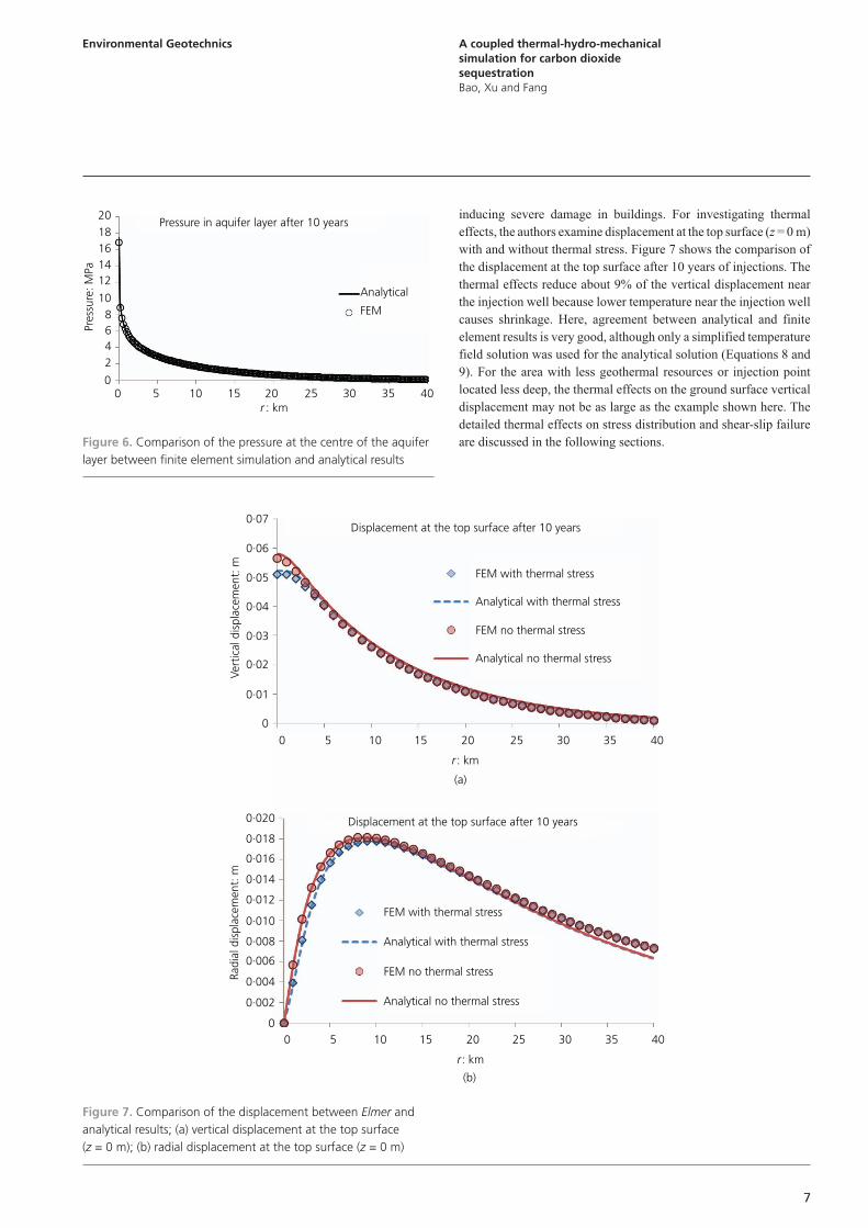
inducing severe damage in buildings. For investigating thermal

effects, the authors examine displacement at the top surface (z = 0 m)

with and without thermal stress. Figure 7 shows the comparison of

the displacement at the top surface after 10 years of injections. The

thermal effects reduce about 9% of the vertical displacement near

the injection well because lower temperature near the injection well

causes shrinkage. Here, agreement between analytical and finite

element results is very good, although only a simplified temperature

field solution was used for the analytical solution (Equations 8 and

9). For the area with less geothermal resources or injection point

located less deep, the thermal effects on the ground surface vertical

displacement may not be as large as the example shown here. The

detailed thermal effects on stress distribution and shear-slip failure

are discussed in the following sections.

r : km0

0

2

468

10

12

Pres

sure

: MPa 14

1618

20

5 10 15 20 25

FEM

Analytical

Pressure in aquifer layer after 10 years

30 35 40

Figure 6. Comparison of the pressure at the centre of the aquifer layer between finite element simulation and analytical results

00

0·002

0·004

0·006

0·008

0·010

0·012

0·014

0·016

Radi

al d

ispl

acem

ent:

m

0·018

0·020

0·01

0·02

0·03

0·04

Vert

ical

dis

plac

emen

t: m

0·05

0·06

0·07

(a)

5

Analytical no thermal stress

Analytical with thermal stress

FEM no thermal stress

FEM with thermal stress

Analytical no thermal stress

Analytical with thermal stress

FEM no thermal stress

FEM with thermal stress

Displacement at the top surface after 10 years

Displacement at the top surface after 10 years

10 15

(b)

r: km

20 25 30 35 40

0

0

5 10 15

r : km

20 25 30 35 40

Figure 7. Comparison of the displacement between Elmer and analytical results; (a) vertical displacement at the top surface (z = 0 m); (b) radial displacement at the top surface (z = 0 m)

envgeo1400002.indd 6 Manila Typesetting Company 08/26/2014 03:26PM

1

2

3

4

5

6

7

8

9

10

11

12

13

14

15

16

17

18

19

20

21

22

23

24

25

26

27

28

29

30

31

32

33

34

35

36

37

38

39

40

41

42

43

44

45

46

47

48

49

50

51

52

53

54

55

envgeo1400002.indd 7 Manila Typesetting Company 08/26/2014 03:26PM

Environmental Geotechnics A coupled thermal-hydro-mechanical simulation for carbon dioxide sequestrationBao, Xu and Fang

8

Failure analysis and thermal effectsSome shear-slip analysis is conducted using principal stress

magnitudes and orientations with respect to pre-existing fault

planes and fluid pressure within the fault plane (Morris et al., 1996;

Streit and Hillis, 2004; Wiprut and Zodack, 2000). Because the

location and orientation of pre-existing faults underground may

not be well known, the shear-slip failure analysis discussed in this

article assumed that a fault could exist at any point with an arbitrary

orientation, which might be useful as a precaution (Rutqvist et

al., 2007). In this analysis, the authors assume that cohesion is 0

and friction angle is 30° (Rutqvist et al., 2007). The null cohesion

assumption of the pre-existing faults may cause overestimation of

the risk of failure, which is usually favourable when the cohesion

situation is not clear. Thus, the criterion for shear slip is BC BC³¢

in the Mohr circle (shown in Figure 8), and the criterion for the

stress is

18. 1 3 1 3

3 1 3sin 30 3

2 2

σ σ σ σσ σ σ′ ′ ′ ′+ +′ ′ ′− ≥ ° ⋅ → ≥ ,

where σ1́ is the maximum principal effective stress and σ3́ is the

minimum principal effective stress. As shown in Figure 9, remote

stresses are applied to the entire simulation area. The vertical

remote stress is the lithostatic stress sv = rsg|z|, where g is gravity

and |z| is depth. Horizontal remote stress (sh) varies with different

subsurface formations and locations. Generally, a small sh is more

likely to cause tensile failure than shear-slip failure. Thus, in all

the simulations described here, a relatively large horizontal remote

stress sh = 1·5sv (Rutqvist et al., 2007) was used to lead more

easily to shear-slip failure. Because the proposed model (Equation

3) and the failure criterion (Equation 18) are based on elastic theory,

no fracture is actually initiated, and there was no redistribution of

stresses due to failure. It means that once a considerable failure

zone appears in the simulation domain, fractures are highly possibly

initiated, and the continuum material model may not be accurate

enough, so the simulations in this study are all limited to 3 years.

The applied shear-slip failure criterion offers an easy and efficient

way to estimate the potential risk of the injection well under desired

operation conditions. Figures 10, 11 and 12 show the contour of

σ1́–3σ3 MPa after 1 and 3 years of carbon dioxide injection with

a line injection rate ψʹ = 0·7, 2·0, 3·5 (kg/m)/s. The area marked

by a black line is the zone where σ1́ > 3σ3́, namely, where shear-

slip failure can possibility occur if a pre-existing fault is located

in that zone. The injected cold carbon dioxide causes shrinkage

and reduces pressure in the aquifer layer near the injection well

(Yin et al., 2011), so the thermal effects significantly change the

distribution of the failure zone as well as reduce the failure zone

in the aquifer layer for the high injection rate cases (2·0 and 3·5

(kg/m)/s shown in Figures 11 and 12. It was believed that failure in

the aquifer can enhance the injectivity because the fault increases

the porosity and permeability of the aquifer formation (Flekkøy et

al., 2002). However, frequent or continuous failure possibly causes

considerable seismic activity, which may lead to ground building

or facility damage. Therefore, necessary attention should be paid

to the failure zone in the aquifer to avoid considerable ground

surface damage, although it probability enhances the injectivity.

From this point, the thermal stress can possibly reduce the risk of

injection. However, thermal stress also causes small failure zones

in the caprock and the base rock near the aquifer layer, because the

shrinkage in the aquifer layer may reduce the compression stress

in the caprock and the base rock. In addition, for the low injection

rate case (0·7 (kg/m)/s), the hydraulic pressure does not cause any

failure zone, while the thermal effect causes small failure zones in

the caprock and the base rock (Figure 10). Generally, the possible

failure zone in the caprock means the fracture may be activated in

the caprock, which may lead to carbon dioxide leakage, and this

definitely impacts the injectivity. It is unavoidable that the thermal

effects influence stress distribution during carbon dioxide injection

in both the geological sequestration geothermal capture combined

system and the solo carbon dioxide storage system. Coupling the

thermal effect into the hydro-mechanical model can more closely

predict the displacement, stress distribution and possible failure

Effective normal stress

Shea

r st

ress

A

30˚

B

C

C¢

σ ¢3 σ ¢1

Shear-slip failure

Figure 8. Stress state represented by Mohr circles for failure analysis

Remote stress

Local stress

σhσh

σv

σz

σr

σz

σr

Figure 9. Sketch of remote stress

1

2

3

4

5

6

7

8

9

10

11

12

13

14

15

16

17

18

19

20

21

22

23

24

25

26

27

28

29

30

31

32

33

34

35

36

37

38

39

40

41

42

43

44

45

46

47

48

49

50

51

52

53

54

55

envgeo1400002.indd 8 Manila Typesetting Company 08/26/2014 03:26PM envgeo1400002.indd 9 Manila Typesetting Company 08/26/2014 03:26PM

Environmental Geotechnics A coupled thermal-hydro-mechanical simulation for carbon dioxide sequestrationBao, Xu and Fang

9

0

–2742

–2242

–120·0σ ¢1–3σ ¢3: MPa

–87·50

–55·00

–22·50

10·00

1 year

with thermal stress

Line injection rate: 0·7 kg/m.s

Dep

th, z

: m

500 1000

(a)

1500r: m

2000 2500 0

–2742

–2242

1 year

10·00

–22·50

–55·00

–87·50

–120·0

no thermal stress

Line injection rate: 0·7 kg/m.s

Dep

th, z

: m

500 1000

(b)r: m

1500 2000 2500

σ ¢1–3σ ¢3: MPa

–2742

0 500 1000

(c)

r: m1500 2000 2500

–2242

3 years

with thermal stress

Line injection rate: 0·7 kg/m.s

Dep

th, z

: m

10·00

–22·50

–55·00

–87·50

–120·0

σ ¢1–3σ ¢3: MPa

0

–2742

–2242

Dep

th, z

: m

500 1000

(d)

r: m1500 2000 2500

10·00

–22·50

–55·00

–87·50

–120·0

σ ¢1–3σ ¢3: MPa

3 years

no thermal stress

Line injection rate: 0·7 kg/m.s

Figure 10. Contour of σ ¢1–3σ ¢3 MPa for injection rate y ¢ = 0·7 (kg/m)/s. The area marked by the black line is the zone σ ¢1 > 3σ ¢3, which means the shear-slip failure would occur in high potential.

envgeo1400002.indd 8 Manila Typesetting Company 08/26/2014 03:26PM

1

2

3

4

5

6

7

8

9

10

11

12

13

14

15

16

17

18

19

20

21

22

23

24

25

26

27

28

29

30

31

32

33

34

35

36

37

38

39

40

41

42

43

44

45

46

47

48

49

50

51

52

53

54

55

envgeo1400002.indd 9 Manila Typesetting Company 08/26/2014 03:26PM

Environmental Geotechnics A coupled thermal-hydro-mechanical simulation for carbon dioxide sequestrationBao, Xu and Fang

10

−2242

−2742

0 500 1000

(a)

1500 2000 2500r: m

Dep

th, z

: m

Line injection rate: 2·0 kg/m.s

with thermal stress

1 year

10·00

−22·50

−55·00

−87·50

−120·0σ ¢1–3σ ¢3: MPa

−2242

−2742

0 500 1000

(b)

1500 2000 2500r: m

Dep

th, z

: m

Line injection rate: 2·0 kg/m.s

no thermal stress

1 year

10·00

−22·50

−55·00

−87·50

−120·0σ ¢1–3σ ¢3: MPa

−2242

−2742

0 500 1000

(c)

1500 2000 2500r: m

Dep

th, z

: m

Line injection rate: 2·0 kg/m.s

with thermal stress

3 years

10·00

−22·50

−55·00

−87·50

−120·0σ ¢1–3σ ¢3: MPa

−2242

−2742

0 500 1000

(d)

1500 2000 2500r: m

Dep

th, z

: m

Line injection rate: 2·0 kg/m.s

no thermal stress

3 years

10·00

−22·50

−55·00

−87·50

−120·0σ ¢1–3σ ¢3: MPa

Figure 11. Contour of σ ¢1–3σ ¢3 MPa for injection rate y ¢ = 2·0 (kg/m)/s

1

2

3

4

5

6

7

8

9

10

11

12

13

14

15

16

17

18

19

20

21

22

23

24

25

26

27

28

29

30

31

32

33

34

35

36

37

38

39

40

41

42

43

44

45

46

47

48

49

50

51

52

53

54

55

envgeo1400002.indd 10 Manila Typesetting Company 08/26/2014 03:26PM envgeo1400002.indd 11 Manila Typesetting Company 08/26/2014 03:26PM

Environmental Geotechnics A coupled thermal-hydro-mechanical simulation for carbon dioxide sequestrationBao, Xu and Fang

11

−2242

−2742

0 500 1000

(a)

1500 2000 2500r: m

Dep

th, z

: m

Line injection rate: 3·5 kg/m.s

with thermal stress

1 year

10·00

−22·50

−55·00

−87·50

−120·0σ ¢1–3σ ¢3: MPa

−2242

−2742

0 500 1000

(b)

1500 2000 2500r: m

Dep

th, z

: m

Line injection rate: 3·5 kg/m.s

no thermal stress

1 year

10·00

−22·50

−55·00

−87·50

−120·0σ ¢1–3σ ¢3: MPa

−2242

−2742

0 500 1000

(c)

1500 2000 2500r: m

Dep

th, z

: m

Line injection rate: 3·5 kg/m.s

with thermal stress

3 years

10·00

−22·50

−55·00

−87·50

−120·0σ ¢1–3σ ¢3: MPa

−2242

−2742

0 500 1000

(d)

1500 2000 2500r: m

Dep

th, z

: m

Line injection rate: 3·5 kg/m.s

no thermal stress

3 years

10·00

−22·50

−55·00

−87·50

−120·0σ ¢1–3σ ¢3: MPa

Figure 12. Contour of σ ¢1–3σ ¢3 MPa for injection rate y ¢ = 3·5 (kg/m)/s

envgeo1400002.indd 10 Manila Typesetting Company 08/26/2014 03:26PM

1

2

3

4

5

6

7

8

9

10

11

12

13

14

15

16

17

18

19

20

21

22

23

24

25

26

27

28

29

30

31

32

33

34

35

36

37

38

39

40

41

42

43

44

45

46

47

48

49

50

51

52

53

54

55

envgeo1400002.indd 11 Manila Typesetting Company 08/26/2014 03:26PM

Environmental Geotechnics A coupled thermal-hydro-mechanical simulation for carbon dioxide sequestrationBao, Xu and Fang

12

zone to the practical cases than models that neglect non-isothermal

effects, especially in areas that contain high geothermal resources.

The proposed model can efficiently predict the sustainability of

the injection site and can uncover the critical relationship between

injection conditions and geomechanical response when the detailed

properties and parameters are not yet well identified.

Discussions and conclusionsBased on an isothermal hydro-mechanical model in the authors’

previous works (Bao et al., 2013a; Xu et al., 2012), a thermal-

hydro-mechanical model was developed. The companion analytical

solution and a finite element approach were introduced for solving

the proposed model and were compared against each other. By

neglecting the thermal stress impacts on pressure evolution and

assuming a simplified temperature profile in an aquifer, the model

was analytically solved for a simplified carbon dioxide injection

case, and the assumptions were shown to be reasonable by

comparing with finite element numerical simulation results. The

analytical solution can be used to quantitatively evaluate the typical

sequestration problem instantly, while the finite element model

can be applied in more practical cases and can offer more detailed

results. A shear-slip failure analysis was conducted based on

numerical results. The analysis provides the potential failure zone

and can be used to estimate the maximum sustainable injection

rate and temperature. Thermal effects on deformation and potential

shear-slip failure were quantitatively investigated. Generally,

shrinkage caused by the cooling effects near the injection well

helps on delaying reactivation of pre-existing fault in an aquifer

layer, especially during early well life. However, it will cause small

fractures in the caprock and the base rock near the aquifer layer.

Using the authors’ thermal-hydro-mechanical model instead of

neglecting thermal effects can predict the deformation and fracture

more closely when compared with real applications.

AcknowledgementThis research was funded and conducted through the Pacific

Northwest National Laboratory (PNNL) Carbon Sequestration

Initiative, which is part of the Laboratory Directed Research and

Development Program. PNNL is operated by Battelle for the U.S.

Department of Energy under Contract DE-AC05-76RL01830.

REFEREnCEs

Atrens AD, Gurgenci H and Rudolph V (2009) CO2 thermosiphon

for competitive geothermal power generation. Energy & Fuels

23: 553–557.

Atrens AD, Gurgenci H and Rudolph V (2010) Electricity

generation using a carbon-dioxide thermosiphon. Geothermics

39: 161–169.

Bao J, Xu Z and Fang Y (2013a) A finite element model for

simulation of carbon dioxide sequestration. Environmental

Geotechnics 1(3): 152–160.

Bao J, Xu Z, Lin G and Fang Y (2013b) Evaluating the impact of

aquifer layer properties on geo-mechanical response during

CO2 geological sequestration. Computers & Geoscience 54:

28–37.

Bao J, Hou Z, Fang Y, Ren H and Lin G (2013c) Uncertainty

quantification for evaluating impacts of caprock and

reservoir properties on pressure buildup and ground

surface displacement during geological CO2 sequestration.

Greenhouse Gases: Science and Technology 3: 338–358.

Bao J, Chu Y, Xu Z, Tartakovsky AM and Fang Y (2014)

Uncertainty quantification for the impact of injection rate

fluctuation on the geomechnical response of geological carbon

sequestration. International Journal of Greenhouse Gas

Control 20: 160–167.

Biot MA (1935) Le problème de la consolidation des matières

argileuses sous une charge. Annales de la Société Scientifique

de Bruxelles Serie B 55: 110–113.

Biot MA (1941) General theory of three-dimensional

consolidation. Journal of Applied Physics 12: 155–164.

Biot MA (1955) Theory of elasticity and consolidation for a porous

anisotropic solid. Journal of Applied Physics, 26: 182–185.

Biot MA (1956) Thermoelasticity and irreversible

thermodynamics. Journal of Applied Physics 27: 240–253.

Biot MA (1962) Mechanics of deformation and acoustic

propagation in porous media. Journal of Applied Physics 33:

1482–1498.

Colesanti C and Wasowski J (2004) Satellite SAR interferometry

for wide-area slope hazard detection and site-specific

monitoring of slow landslides. International Landslide

Symposium, Rio de Janeiro, Brasil.

CSC – IT Centre for Science (2011) Elmer Solver Manual. CSC,

Espoo, Finland.

Davies JH (2003) Elastic field in a semi-infinite solid due to

thermal expansion or a coherently misfitting inclusion.

Journal of Applied Mechanics 70: 655–661.

Flekkøy EG, Sørenssen AM and Jamtveit B (2002) Modeling

hydrofracture. Journal of Geophysical Research 107:

2151–2162.

Franca LP and Frey SL (1992) Stabilized finite element methods:

II. The incompressible Navier-Stokes equations. Computer

Methods in Applied Mechanics and Engineering 99: 209–233.

Franca LP, Frey SL and Hughes TJR (1992) Stabilized finite

element methods: I. Application to the advective-diffusive

model. Computer Methods in Applied Mechanics and

Engineering 95: 253–276.

Fridleifsson IB, Bertani R, Huenges B, Lund JW and Rybach L

(2008) The possible role and contribution of geothermal

energy to the mitigation of climate change. In IPCC Scoping

Meeting on Renewable Energy Sources (Hohmeyer O and

Trittin T (eds.)). IPCC, Luebeck, Germany, pp. 59–80.

Gollakota S and McDonald S (2012) Industrial CO2 storage in Mt.

Simon Sandstone Saline Reservoir – A large-scale demonstration

project in Illinois. Eleventh Annual Carbon Capture, Utilization

& Sequestration Conference. Pittsburgh, PA, USA.

Gor GY, Elliot TR and Prévost JH (2013) Effects of thermal stresses

on caprock integrity during CO2 storage. International Journal

of Greenhouse Gas Control 12: 300–309.

1

2

3

4

5

6

7

8

9

10

11

12

13

14

15

16

17

18

19

20

21

22

23

24

25

26

27

28

29

30

31

32

33

34

35

36

37

38

39

40

41

42

43

44

45

46

47

48

49

50

51

52

53

54

55

envgeo1400002.indd 12 Manila Typesetting Company 08/26/2014 03:26PM envgeo1400002.indd 13 Manila Typesetting Company 08/26/2014 03:26PM

13

Environmental Geotechnics A coupled thermal-hydro-mechanical simulation for carbon dioxide sequestrationBao, Xu and Fang

WHAT DO YOU THINK?

To discuss this paper, please submit up to 500 words to the editor at journals@ice.org.uk. Your contribution will be forwarded to the author(s) for a reply and, if considered appropriate by the editorial panel, will be published as a discussion in a future issue of the journal.

Holloway S (2005) Underground sequestration of carbon

dioxide – a viable greenhouse gas mitigation option. Energy

30: 2318–2333.

Mindlin RD and Cheng DH (1950a) Nuclei of strain in the semi-

infinite solid. Journal of Applied Physics 21: 926–930.

Mindlin RD and Cheng DH (1950b) Thermoelastic stress in the

semi-infinite solid. Journal of Applied Physics 21: 931–933.

Morris A, Ferril DA and Henderson DB (1996) Slip tendency

analysis and fault reactivation. Geology 24: 275–278.

Preisig M and Prévost JH (2011) Coupled multi-phase thermo-

poromechanical effects. Case study: CO2 injection at In Salah,

Algeria. International Journal of Greenhouse Gas Control 5:

1055–1064.

Pruess K, Garcia J, Kovscek T et al. (2004) Code intercomparison

builds confidence in numerical simulation models for geologic

disposal of CO2. Energy 29: 1431–1444.

Randolph JB and Saar MO (2011a) Combining geothermal

energy capture with geologic carbon dioxide sequestration.

Geophysical Research Letter 38: L10401.

Randolph JB and Saar MO (2011b) Coupling carbon dioxide

sequstration with geothermal energy capture in naturally

permeable, porous geologic formations: implications for CO2

sequestration. Energy Procedia 4: 2206–2213.

Rutqvist J, Birkholzer J, Cappa F and Tsang CF (2007)

Estimating maximum sustainable injection pressure during

geological sequestration of CO2 using coupled fluid flow and

geomechanical fault-slip analysis. Energy Conversion and

Management 48: 1798–1807.

Sen B (1951) Note on the stresses produced by nuclei of

thermoelastic strain in a semi-infinite elastic solid. Quarterly

of Applied Mathematics 8: 365–369.

Simone SD, Vilarrasa V, Carrera J, Alcolea A and Meier P (2013)

Thermal coupling may control mechanical stability of

geothermal reservoirs during cold water injection. Physics and

Chemistry of the Earth 64: 117–126.

Streit JE and Hillis RR (2004) Estimating fault stability and

sustainable fluid pressures for underground storage of CO2 in

porous rock. Energy 29: 1445–1456.

Terzaghi K (1923) Die Berechnung der Durchlassigkeitsziffer

des Tones aus dem Verlauf der hydrodynamischen

Spannungserscheinungen. Mathematisch

Naturwissenschaftliche 132: 125–138.

Tokunaga TK, Wan J, Jung JW et al. (2013) Capillary pressure and

satuation relations for supercritical CO2 and brine in sand: High-

pressure Pc(Sw) controller/meter measurements and capillary

scaling predictions. Water Resources Research 49: 4566–4579.

Vilarrasa V, Olivella S and Carrera J (2011) Geomechanical

stability of the caprock during CO2 sequestration in deep

saline aquifers. Energy Procedia 4: 5306–5313.

Vilarrasa V, Silva O, Carrera J and Olivella S (2013) Liquid

CO2 injection for geological storage in deep saline aquifers.

International Journal of Greenhouse Gas Control 14: 84–96.

White MD and Oostrom M (2006) STOMP subsurface transport

over multiple phases version 4.0. Pacific Northwest National

Laboratory, Richland, Washington, PNNL-15782.

Wilson TRS (1992) The deep ocean disposal of carbon dioxide.

Energy Conversion and Management 33: 627–633.

Wiprut D and Zodack MD (2000) Fault reactivation and fluid flow

along a previously dormant normal fault in the northern North

Sea. Geology 28: 595–598.

Xu Z, Fang Y, Scheibe TD and Bonneville A (2012) A fluid

pressure and deformation analysis for geological sequestration

of carbon dioxide. Computers and Geoscience 46: 31–37.

Yin S, Dusseault MB and Rothenburg L (2011) Coupled THMC

modeling of CO2 injection by finite element methods. Journal

of Petroleum Science and Engineering 80: 53–60.

Yin S, Towler BF, Dusseault MB and Rothenburg L (2010) Fully

coupled THMC modeling of wellbore stability with thermal

and solute convection considered. Transport in Porous Media

84: 773–798.

envgeo1400002.indd 12 Manila Typesetting Company 08/26/2014 03:26PM

1

2

3

4

5

6

7

8

9

10

11

12

13

14

15

16

17

18

19

20

21

22

23

24

25

26

27

28

29

30

31

32

33

34

35

36

37

38

39

40

41

42

43

44

45

46

47

48

49

50

51

52

53

54

55

envgeo1400002.indd 13 Manila Typesetting Company 08/26/2014 03:26PM