Trajectory-Tracking Scheme in Lagrangian Form for Solving Linear Advection Problems: Interface...

Trajectory-Tracking Scheme in Lagrangian Form for Solving Linear AdvectionProblems: Interface Spatial Discretization

LI DONG

LASG, Institute of Atmospheric Physics, Chinese Academy of Sciences, Beijing, China

BIN WANG

LASG, Institute of Atmospheric Physics, Chinese Academy of Sciences, and Ministry of Education Key Laboratory

for Earth System Modeling, and Center for Earth System Science, Tsinghua University, Beijing, China

(Manuscript received 23 February 2012, in final form 25 July 2012)

ABSTRACT

A previous Lagrangian linear advection scheme (trajectory-tracking scheme) is modified to achieve

local mass conservation in this paper, which is more favorable to climate modeling. The discretized tracer

parcels are volumes with interfaces instead of centroids. In 2D problems, the parcels are polygons and

the interfaces are described by polygonal edges with a finite number. Because polygons will deform under

the background wind field, a curvature-guard algorithm (CGA) is devised to retain accurate represen-

tation of the deformed interfaces among parcels. The tracer mass carried by parcels is mapped onto the

regular latitude–longitude mesh by a first-order conservative remapping algorithm that can handle

concave polygons. Several standard test cases have been carried out to show the effectiveness of the

new scheme.

1. Introduction

Advection is a fundamental process in climate mod-

eling, and the number of transported tracers is steadily

increasing to accommodatemodernmicrophysics schemes

and more advanced chemistry. Hence, the numerical

scheme for solving it becomes a vital component of the

general circulation models (e.g., atmospheric model, or

AGCM); see Rood (1987) for a basic review. Despite

the apparent simplicity of the continuous advection

equation it remains a challenge to solve it numerically,

and research on the numerical schemes is still active

(Lauritzen et al. 2011, 185–187). The current main-

stream schemes are based on the Eulerian form or semi-

Lagrangian form, which discretize the continuous tracer

on a fixed mesh, such as the two-step shape-preserving

advection scheme (TSPAS; Yu 1994), flux-form semi-

Lagrangian scheme (FFSL; Lin and Rood 1996), con-

servative semi-Lagrangian multitracer transport scheme

(CSLAM; Lauritzen et al. 2010), etc.

Among desirable properties for the development of

transport scheme are the following:

1) Numerical diffusion error: If a scheme is excessively

diffusive, the large gradients or discontinuities in the

tracer distribution will be smoothed out spuriously

(Rood 1987; Stenke et al. 2008).

2) Filament preservation: Fine structures exist, in partic-

ular, for long-lived stratospheric tracers, and havewide

spatial scales (McKenna et al. 2002a,b; Wohltmann

and Rex 2009).

3) Tracer correlations preservation: For chemistry

and chemistry–climate applications, it is impor-

tant that preexisting functional relations between

tracers are not spuriously perturbed. Constant and

linear relations that can be maintained by careful

scheme design are preservation of uniform mixing

ratios as well as linear relations between tracers

(Lin and Rood 1996; Thuburn and McIntyre 1997).

Preserving nonlinear relations is much more chal-

lenging in traditional Eulerian and semi-Lagrangian

discretizations (if not impossible); however, fully

Lagrangian schemes, in the absence of numerical

mixing processes, can maintain any relation between

tracers.

Corresponding author address: Li Dong, LASG, Institute of At-

mospheric Physics, Chinese Academy of Sciences, 40 Hua Yan Li,

Qi Jia Huo Zi, Chao Yang District, Beijing 100029, China.

E-mail: [email protected]

324 MONTHLY WEATHER REV IEW VOLUME 141

DOI: 10.1175/MWR-D-12-00058.1

� 2013 American Meteorological Society

4) Multitracer efficiency: With the increase of tracer

number, the computational efficiency problem will

emerge. In semi-Lagrangian schemes that track

area and fully Lagrangian schemes, the movement

of Lagrangian parcels and computation of overlap

areas only has to be done once per time step and can

be reused for each additional tracer.

The motivation of the Lagrangian advection scheme

development by this study is to address these topics. The

first two topics are interconnected, since one scheme

with large numerical diffusion error will certainly not

preserve thin filament well. In the physical sense, the nu-

merical diffusion error is caused by the nonadaptivity

of the spatial discretization to the tracer distribution. In

the Eulerian schemes and semi-Lagrangian schemes, the

advection process is described as the movement of trac-

ers among mesh cells, and excessive mixing can occur

during the movement when the mesh is fixed. This makes

Eulerian schemes and semi-Lagrangian schemes able to

handle large deformational flow, but with the expense of

precise interface definition (i.e., numerical diffusion), as

stated inDonea et al. (2004). This error can be reduced by

increasing spatial resolution, but this approach also in-

creases the computational cost simultaneously. The spa-

tial discretization of Lagrangian schemes is based on

tracking a finite number of parcels moving with the flow.

The adaptivity to the tracer distribution is inherent in

such schemes. Several Lagrangian schemes have been

developed—for example, the GRANTOUR model

(Walton et al. 1988), Chemical Lagrangian Model of

the Stratosphere (CLaMS; McKenna et al. 2002a), At-

mospheric Tracer Transport In a Lagrangian model

(ATTILA; Reithmeier and Sausen 2002), and also the

trajectory-tracking scheme (noted as TTS-C, where ‘‘C’’

means centroid) developed by the authors (Dong and

Wang 2012). Stenke et al. (2008) compared the perfor-

mances of a semi-Lagrangian scheme and ATTILA,

where ATTILA showed positive effects on the reduc-

tion of cold bias in ECHAM4 GCM. All of these La-

grangian schemes adopt centroids as the form of parcels.

Each parcel is a centroid that has no definite spatial

boundary. InGRANTOUR,CLaMS, andATTILA, each

parcel carries constant mass, but in TTS-C, the tracer

density is carried. Thus, parcels in TTS-C behave like

sample points rather than particles in the aforemen-

tioned three schemes. Several test cases in Dong and

Wang (2012) showed the ability of TTS-C to significantly

reduce the numerical diffusion error, but there is a weak

point (i.e., the unphysical renormalization technique

adopted to conserve the total mass). This will hamper

the preservation of tracer correlation and also bring

some arbitrariness (Nair and Machenhauer 2002).

In this study, this unphysical renormalization tech-

nique is replaced. To conserve the mass locally and

physically, the tracer is discretized as parcel polygons in

2D problems with specific interfaces. These polygons do

not overlap and each carries some amount of tracers, so

the total mass is conserved locally and inherently. The

new TTS is denoted as TTS-I, where ‘‘I’’ stands for in-

terface that needs to be tracked. In the literature, there

are several numerical methods working on tracking in-

terfaces (Tryggvason et al. 2001; Aulisa et al. 2004).

Typical methods are volume of fluid method (VOF) and

level set method (LS). VOF was first presented in Hirt

and Nichols (1981). The main idea of it is to define a

function F that is the fraction of fluid within a cell, ad-

vect it by some numerical advection scheme, and re-

construct fluid interface from F (Noh and Woodward

1976; Rudman 1997; Ubbink and Issa 1999). The quan-

tity LS defines an implicit surface function u that is the

distance from the interface; u is advected as F in VOF.

For details of LS see Osher and Fedkiw (2003). In

Enright et al. (2002), Hieber and Koumoutsakos (2005),

and Enright et al. (2005), the authors pointed out that LS

has difficulties controlling the numerical diffusion, es-

pecially in areas of high curvature and long and thin

filamentary regions, and proposed a hybrid method that

combines LS and Lagrangian particles, called particle

level set method. Both of these two types of methods are

constructed under the Eulerian framework, and they

have rare applications in meteorology. Contrary to them,

TTS-I tracks the interface of each parcel in fully La-

grangian way, which is considered as a nontrivial task

(Hirt and Nichols 1981).

The major effort in TTS-I is to construct a set of al-

gorithms that will make the polygonal edges adapt to

the change of the interface curvature, and devise a first-

order conservative remapping algorithm that can handle

concave polygons. The details of TTS-I will be described

in section 2. Three numerical test cases are carried out to

verify TTS-I, and the results are shown in section 3. The

conclusions are cast in section 4.

2. Details of TTS-I

In the Lagrangian framework, there are two types of

spatial discretization. One is the parcel centroids, which

have no definite spatial boundary. The other one is the

parcels with interfaces, which cover the whole compu-

tational domain without gaps or overlaps. Several La-

grangian schemes have chosen the first type, such as

CLaMS and ATTILA, including TTS-C. The lack of con-

serving mass in a physical way will emerge when the

carried mass or density needs to be mapped onto the

backgroundmesh, since centroids haveno spatial boundary.

JANUARY 2013 DONG AND WANG 325

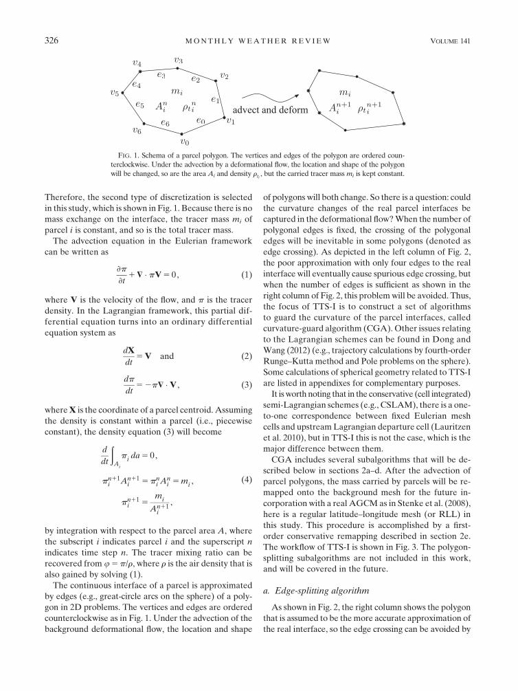
Therefore, the second type of discretization is selected

in this study, which is shown in Fig. 1. Because there is no

mass exchange on the interface, the tracer mass mi of

parcel i is constant, and so is the total tracer mass.

The advection equation in the Eulerian framework

can be written as

›p

›t1$ � pV5 0, (1)

where V is the velocity of the flow, and p is the tracer

density. In the Lagrangian framework, this partial dif-

ferential equation turns into an ordinary differential

equation system as

dX

dt5V and (2)

dp

dt52p$ �V , (3)

whereX is the coordinate of a parcel centroid. Assuming

the density is constant within a parcel (i.e., piecewise

constant), the density equation (3) will become

d

dt

ðA

i

pi da5 0,

pn11i An11

i 5pni A

ni 5mi ,

pn11i 5

mi

An11i

,

(4)

by integration with respect to the parcel area A, where

the subscript i indicates parcel i and the superscript n

indicates time step n. The tracer mixing ratio can be

recovered from u5p/r, where r is the air density that is

also gained by solving (1).

The continuous interface of a parcel is approximated

by edges (e.g., great-circle arcs on the sphere) of a poly-

gon in 2D problems. The vertices and edges are ordered

counterclockwise as in Fig. 1. Under the advection of the

background deformational flow, the location and shape

of polygons will both change. So there is a question: could

the curvature changes of the real parcel interfaces be

captured in the deformational flow?When the number of

polygonal edges is fixed, the crossing of the polygonal

edges will be inevitable in some polygons (denoted as

edge crossing). As depicted in the left column of Fig. 2,

the poor approximation with only four edges to the real

interface will eventually cause spurious edge crossing, but

when the number of edges is sufficient as shown in the

right column of Fig. 2, this problemwill be avoided. Thus,

the focus of TTS-I is to construct a set of algorithms

to guard the curvature of the parcel interfaces, called

curvature-guard algorithm (CGA). Other issues relating

to the Lagrangian schemes can be found in Dong and

Wang (2012) (e.g., trajectory calculations by fourth-order

Runge–Kutta method and Pole problems on the sphere).

Some calculations of spherical geometry related to TTS-I

are listed in appendixes for complementary purposes.

It isworth noting that in the conservative (cell integrated)

semi-Lagrangian schemes (e.g., CSLAM), there is a one-

to-one correspondence between fixed Eulerian mesh

cells and upstreamLagrangian departure cell (Lauritzen

et al. 2010), but in TTS-I this is not the case, which is the

major difference between them.

CGA includes several subalgorithms that will be de-

scribed below in sections 2a–d. After the advection of

parcel polygons, the mass carried by parcels will be re-

mapped onto the background mesh for the future in-

corporation with a real AGCMas in Stenke et al. (2008),

here is a regular latitude–longitude mesh (or RLL) in

this study. This procedure is accomplished by a first-

order conservative remapping described in section 2e.

The workflow of TTS-I is shown in Fig. 3. The polygon-

splitting subalgorithms are not included in this work,

and will be covered in the future.

a. Edge-splitting algorithm

As shown in Fig. 2, the right column shows the polygon

that is assumed to be themore accurate approximation of

the real interface, so the edge crossing can be avoided by

FIG. 1. Schema of a parcel polygon. The vertices and edges of the polygon are ordered coun-

terclockwise. Under the advection by a deformational flow, the location and shape of the polygon

will be changed, so are the area Ai and density rti , but the carried tracer mass mi is kept constant.


inserting more edges. Then the key question is when and

where should more edges be inserted. The basic idea is

depicted in Fig. 4a. EdgeAB is equipped with a test point

O, which is initially at the middle of the edge, and ad-

vected with A and B. Because of the deformation of the

flow,:AOB (see appendix B for the calculation details)

will deviate from 1808. After it exceeds some threshold,

edge AB will be split into two new edges AO and OB.

Obviously, this threshold is a key parameter to control

the accuracy of the approximation of the real interfaces.

During the experiments, this threshold is set as a function

of the edge length to make longer edge more easily split.

The following function, which is modified from a smooth-

ing function in Liu and Liu (2003), is chosen:

a(l)5

8>><>>:

A0 l#L0 ,

(A12A0)(42 3t)t31A0 L0, l#L1 ,

A1 l.L1 ,

(5)

whereA0 andA1 are the angle threshold bounds,L0 and

L1 are the edge length range, and t5 (l2L0)/(L1 2L0).

In Fig. 4b, two such functions with different parameters

are stitched together to gain more control on the length

scales of edges.

b. Edge-merging algorithm

With the insertion of more edges, the computational

complexity will increase significantly. On the other hand,

not all the curvature change is genuine, because of the

temporal discretization error and the discrete velocity

field. Thus, the merging of edges needs to be included

to remove the neighboring edges that are nearly straight

or short in some sense. The angle threshold that con-

trols when to merge two neighboring edges is the same

as the one for edge splitting but with a relax factor R

[i.e., multiply (5) by R] to avoid merging the newly split

edges. This relax factor has the same form of (5) boun-

ded by R0 and R1. The edge merging can be considered

as the inversion of edge splitting and also a filtering

procedure. The similar idea is found in Dritschel (1988)

(contour surgery) with the name of ‘‘cutoff scale,’’ which

is used to remove the vorticity features thinner than

that scale.

c. Vertex–edge-approaching detection algorithm

Under the advection of the deforming flow, the rela-

tive position of vertices will change largely. Especially as

the filaments, where edges are very close, any splitting or

merging of edges may affect the calculation by causing

FIG. 2. Schema of edge crossing. (left) The result without CGA and (right) with CGA.


potential edge crossings. Therefore, the orientation and

the projection of the vertex on the edge are calculated

(see appendixes A and D for calculation details) and re-

corded to provide the following potential crossing

detection algorithm the basic geometric information.

Figure 5 shows the relative movement of a vertex to

another edge, including its projection on that edge. Ad-

ditionally, one vertex may have projections on several

edges, so each vertex will have a list of those edges. On

the other hand, each edge will also have a list of vertices

that have projection on it. In the algorithm, the vertex

will be paired with the edge on which it has projection.

Each polygon will be detected to update these orienta-

tions and projections after both edge-splitting and edge-

merging operations as shown in Fig. 3.

d. Potential crossing detection algorithm

Since the edge-splitting and edge-merging operations

will change the geometric structure of the polygon to

capture the curvature change and reduce the computa-

tional complexity, respectively, the edge crossing may

be caused in the regions with high density of vertices and

edges. Thus, some detections of the potential edge crossing

should be conducted. The possible edge-crossing pat-

terns are listed in Fig. 6.

For edge splitting, a new vertex will be inserted.When

edges are very close, itmay cross some edges. So for those

paired vertices of the old edge, the orientation of them to

the two new edges will be calculated and compared with

the old one. If those orientations are not consistent as

shown in Fig. 6a1, the edges linked with the crossing

paired vertex will have intersection with the new edges.

Figure 6a2 indicates that the paired edges of the old edge’s

end vertices may have intersection too. Test points of

edgesmay also cross as shown in Fig. 6a3. The crossing test

points will be reset to the middle point of their host edges

to avoid potential problems. For edge merging, the effects

of removing the common vertex of two neighboring

edges will be detected; see Fig. 6b. In detail, check the

potential wrong orientation and intersection of the

paired vertices of the two old edges relative to the new

edge as in the edge-splitting cases. If any of the patterns

happen, the edge-splitting or edge-merging operation

will not be conducted.

FIG. 3. Workflow of TTS-I. FIG. 4. Schema of edge splitting. (a) An edge-splitting operation

and (b) an angle threshold function to judge whether to split an

edge.

FIG. 5. Schema of the approaching detection algorithm. The

orientation and projection of the vertex C on the edge AB are

calculated for detecting approaching events.


e. First-order conservative remapping

Conservative remapping is an important topic for cou-

pling different components in coupled climate system

modeling. Jones (1999) proposed a general first- and

second-order algorithm called the Spherical Coordinate

Remapping and Interpolation Package (SCRIP). SCRIP

has large geometric error when the mesh cell sides are

not straight lines in latitude–longitude space, which was

noted in Lauritzen and Nair (2008), and the cell must be

convex. Lauritzen and Nair (2008) developed a Cascade

Remapping between Spherical Grids (CaRS), which is

based on cascade interpolation (Purser and Leslie 1991).

CaRS splits the two-dimensional interpolation into two

one-dimensional interpolations. Ullrich et al. (2009)

constructed a Geometrically Exact Conservative Re-

mapping (GECoRe) between RLL and cubed–sphere

grids, which is designed to reduce the geometric error in

SCRIP and CaRS. GECoRe uses fully two-dimensional

high-order remapping and converts area integrals to line

integrals.

Conservative remapping is also an essential part in the

conservative semi-Lagrangian schemes, such as incre-

mental remapping scheme (Dukowicz and Baumgardner

2000) and CSLAM (Lauritzen et al. 2010). These

schemes track Lagrangian cells forward or backward,

and remap the tracers to or from deformed mesh cells.

Because the Lagrangian cells start from a regular cell

at each time step, the deformation is not that large,

whereas the parcel polygons in TTS-I will be tracked all

the time, and so the remapping in TTS-I will be more

complicated.

In TTS-I, the polygonal edges are great-circle arcs,1

and the polygons will turn to be arbitrarily shaped (e.g.,

concave) under the advection of deformational flow, so

SCRIP cannot be used. The tracer density is assumed

constant within a polygon, so the remapping from poly-

gons to mesh cells will be first order. Higher-order re-

mapping is not trivial, because the shape of polygon is

arbitrary. But it is worth noting that because of the La-

grangian nature of TTS-I, the results are not diffusive as

in other first-order schemes. Thus the basic idea of first-

order conservative remapping in SCRIP (i.e., finding the

overlaps between different mesh cells) is applied in this

study, but with the handling of concave polygons, which

will be described in details below. In the future, the re-

versed remapping (i.e., frommesh cells to parcel polygons)

FIG. 6. Schemas of the potential crossing patterns. (a) Is for

splitting edge AB and (b) is for merging edges AB and BC.

FIG. 7. Schema for the remapping of a concave polygon. The

filled circles are the calculated intersections between polygonal

edges and grid lines. The numbers in the cells compose the mark

matrix C with a meaning of 0 for no overlap, 1 for crossing, 2 for

fully covering, and 21 also for no overlap in this case. The eight

ellipses indicate the searching order for a cell.

1 High-order edge approximations are considered in Ullrich

et al. (2012).


will be also needed to map tendencies from the physical

parameterization suite back to the tracer grid. For this,

higher-order mapping such as GECoRe technology

could be used.

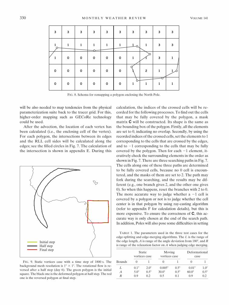
After the advection, the location of each vertex has

been calculated (i.e., the enclosing cell of the vertex).

For each polygon, the intersections between its edges

and the RLL cell sides will be calculated along the

edges; see the filled circles in Fig. 7. The calculation of

the intersection is shown in appendix E. During this

calculation, the indices of the crossed cells will be re-

corded for the following processes. To find out the cells

that may be fully covered by the polygon, a mask

matrix C will be constructed. Its shape is the same as

the bounding box of the polygon. Firstly, all the elements

are set to 0, indicating no overlap. Secondly, by using the

recorded indices of the crossed cells, set the elements to 1

corresponding to the cells that are crossed by the edges,

and to 21 corresponding to the cells that may be fully

covered by the polygon. Then for each 21 element, it-

eratively check the surrounding elements in the order as

shown in Fig. 7. There are three searching paths in Fig. 7.

The cells along one of these three paths are determined

to be fully covered cells, because no 0 cell is encoun-

tered, and the masks of them are set to 2. The path may

fork during the searching, and the results may be dif-

ferent (e.g., one branch gives 2, and the other one gives

0). So when this happens, reset the branches with 2 to 0.

The more accurate way to judge whether a 21 cell is

covered by a polygon or not is to judge whether the cell

center is in that polygon by using ray-casting algorithm

(refer to appendix F for calculation details), but this is

more expensive. To ensure the correctness of C, this ac-

curate way is only chosen at the end of the search path.

In addition, Poles will also pose some difficulties in setting

FIG. 8. Schema for remapping a polygon enclosing the North Pole.

FIG. 9. Static vortices case with a time step of 1800 s. The

background mesh resolution is 18 3 18. The rotational flow is re-

versed after a half step (day 6). The green polygon is the initial

square. The black one is the deformed polygon at half step. The red

one is the reversed polygon at final step.

TABLE 1. The parameters used in the three test cases for the

edge-splitting and edge-merging algorithms. The L is the range of

the edge length,A is range of the angle deviation from 1808, and R

is range of the relaxation factor on A when judging edge merging.

Static

vortices case

Moving

vortices case

Deformational

case

Bounds 0 1 0 1 0 1

L 0.18 2.08 0.0058 0.58 0.018 1.08A 5.08 0.58 30.08 0.58 60.08 0.58R 0.9 0.2 0.5 0.1 0.9 0.2


C. When a polygon encloses a Pole (judged by ray-

casting algorithm), C will span the whole zonal region

as shown in Fig. 8. The cells between the edges and the

Pole will be set to 3.

With the intersections and C, the overlap area be-

tween the polygons and the RLL cells can be calculated.

The tracer mass of the polygon remapped onto the mesh

is calculated as

FIG. 10. Tracer density inmoving vortices case. The backgroundmesh resolution is 18 3 18 and the polygon number

is 40 962. (a) The initial condition is a contour level set varying from 0.5 to 1.5. The solutions at the (b) half and (c) full

revolution with time step 1800 s and vortices crossing Poles. (d) The relative error is depicted at the full revolution.

(e) The solution at full revolution with time step 900 s and vortices crossing Poles. (f) The solution at full revolution

with time step 1800 s and vortices along equator.


mi,j 5 �k2S

i,j

Aki,j

Ak

mk , (6)

whereAk is the area of polygon k, andAki,j is the overlap

area between cell (i, j) and polygon k. Set Si,j is the

polygons that overlap with the cell (i, j). The inverse

remapping can use the overlap area too as

mk 5 �i,j2S

k

Aki,j

Ai,j

mi,j , (7)

where Ai,j is the area of cell (i, j), and set Sk is the cells

that overlap with polygon k. Theoretically, the overlap

areas have the following relations with the polygon and

cell area:

Ak 5 �i,j2S

k

Aki,j, and

Ai,j 5 �k2S

i,j

Aki,j ,

but because of the floating-point error of the numerical

computing, the above equations are approximated

within the order of 10213. So Ak and Ai,j in (6) and (7)

should be replaced by the right-hand side in the above

equations to ensure the sum of the area weights will be

exactly 1 (i.e., partition of unity).

3. Numerical results

In the following sections, the test results of TTS-I are

presented on the sphere with RLL background mesh.

Since deformational flow is more challenging in TTS-I,

we choose two cases relating to vortex and one case that

are highly deformational.

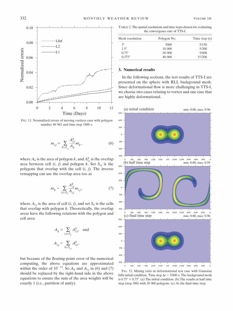
FIG. 11. Normalized errors of moving vortices case with polygon

number 40 962 and time step 1800 s.

TABLE 2. The spatial resolutions and time steps chosen for evaluating

the convergence rate of TTS-I.

Mesh resolution Polygon No. Time step (s)

38 5000 5/150

1.58 10 000 5/300

0.758 20 000 5/600

0.3758 40 000 5/1200

FIG. 12. Mixing ratio in deformational test case with Gaussian

hills initial condition. Time step Dt5 5/600 s. The backgroundmesh

is 0.758 3 0.758. (a) The initial condition. (b) The results at half time

step (step 300) with 20 000 polygons. (c) At the final time step.


a. Static vortices test case

In Nair and Jablonowski (2008), a moving vortices test

case has been established that has been widely adopted

(Putman and Lin 2007; Flyer and Lehto 2010; Lauritzen

et al. 2010). To demonstrate the effects of the splitting

and merging of edges on a simple but clear platform, the

moving vortices are modified to be stationary, and the

moving case will be used next. The two vortices are lo-

cated at (08, 08) and (1808, 08), and an initial square

polygon (the green one) is placed at (158, 08) with four

vertices and edge length 108 as shown in Fig. 9. The

background mesh is an equidistant regular latitude–

longitude mesh with resolution 18 3 18. The parameters

in the edge-splitting and edge-merging algorithms are

listed in Table 1. It is worth noting that these parameters

for CGA are adjustable. There may be more objective

and optimal ways to set them, and this needs further

research. When the time advances with the time step

1800 s, more edges are inserted as expected so that the

curved interface of the parcel is captured by the edge-

splitting algorithm; see the black deformed polygon at

half step in Fig. 9. To clearly show the effect of the edge-

merging algorithm, the flow is reversed after some time

(6 days in this case), and the polygon will be restored to

its original position. Because of the discretization error,

TTS-I exhibits some small error [i.e., the final polygon

(the red one) does not coincide with the initial polygon

exactly, and the vertex number is more than four]. The

remapping procedure is not included in this test in order

to focus on the interface calculation part of TTS-I.

Overall, CGA can capture the changes of the parcel in-

terface under the deformational flow.

b. Moving vortices test case

In this test, the moving vortices test case (Nair and

Jablonowski 2008) is adopted as in Dong and Wang

(2012) to verify the performance of TTS-I near the

vortex, where the parcel polygons are stirred to form very

thin filaments. Some other schemes with the adaptive

mesh refinement (AMR; see Behrens 2006, Flyer and

Lehto 2010, and also Nair and Jablonowski 2008) show

promising results by adding more resolution near the

two vortices under the Eulerian framework. The basic

setup of this test case is omitted here to avoid duplicates

(a5 908); for details refer toNair and Jablonowski (2008)

and Dong and Wang (2012). The initial polygon distri-

bution of TTS-I is set by the geodesic or icosahedral grids

for uniform coverage of the sphere with 40 962 poly-

gons. The key parameters are tabulated in Table 1. The

results of tracer density at half (6 days) and full (12 days)

revolution are depicted in Figs. 10b and c, respectively,

with Dt 5 1800 s. To remove the bias caused by the

polygon distribution, the true solution is evaluated at

the background mesh, remapped onto the polygons and

then remapped back again at each step. The difference

between the true solution and TTS-I at day 12 is shown in

Fig. 10d and the normalized errors are shown in Fig. 11.

Compared with the results in Dong and Wang (2012)

and the references there, the simulated filaments at the

vortex center are poorer than the ones in TTS-C. This is

caused by the Poles, where a polar stereographic (PS)

plane is introduced for velocity interpolation and tra-

jectory calculation. In TTS-I, the tracer density is affected

by the polygon area directly—see (4)—and the area is

affected by the vertex trajectories. Thus, the transition

between latitude–longitude space and PS plane when

calculating trajectories will cause some unphysical distur-

bance, whichwill have adverse effects on the calculation of

polygon area. Whereas in TTS-C, the density is calculated

by solving (3) and is affected by velocity divergence.When

decreasing the time step to 900 s in the original test setup

(Fig. 10e) or making the vortices rotate along the equator

by setting a 5 08 (Fig. 10f), the results of TTS-I become

FIG. 13. Convergence plots for (a) l2 and (b) l‘, computed with Gaussian hills initial conditions by TTS-I. The CFL

is chosen as about 2.0, and the spatial resolutions and time steps are listed in Table 2. The upper and lower heavy lines

on each plot correspond to the slopes of first- and second-order convergence rates, respectively.


better. Nevertheless, TTS-I conserves the mass physically.

In future research, other meshes without Pole problems

could be used to improve the accuracy of TTS-I.

c. Deformational test case

There is an undertaking effort to construct a more

standard test case suite for comparing transport or ad-

vection schemes (refer to Lauritzen et al. 2012)—not only

testing single tracer, but also diagnosing the preservation

of the predefined correlations amongmultiple tracers. The

basic test cases are proposed in Nair and Lauritzen (2010)

as a class of deformational test cases to provide more re-

alistic flow. The chosen test flow is the case 4 of Nair and

Lauritzen (2010) with three types of initial conditions in

this study. The background air and tracer are both ad-

vected, and the tracermixing ratio is calculated asu5p/r.

The convergence rate of TTS-I is studied by using an

initial condition of Gaussian hills. The resolution of RLL

mesh, the number of polygons, and the time steps are

tabulated in Table 2 with CFL (in the sense of RLL

mesh) about 2.0. The results of 20 000 polygons are

shown in Fig. 12, and the convergence rate is plotted in

Fig. 13. From the figure, it can be seen that TTS-I has

first-order convergence rate. Although the rate is rel-

atively low compared with other high-order schemes,

the performance of TTS-I is not low as other first-order

schemes, especially for the discontinuous tracers as

shown in Fig. 14.

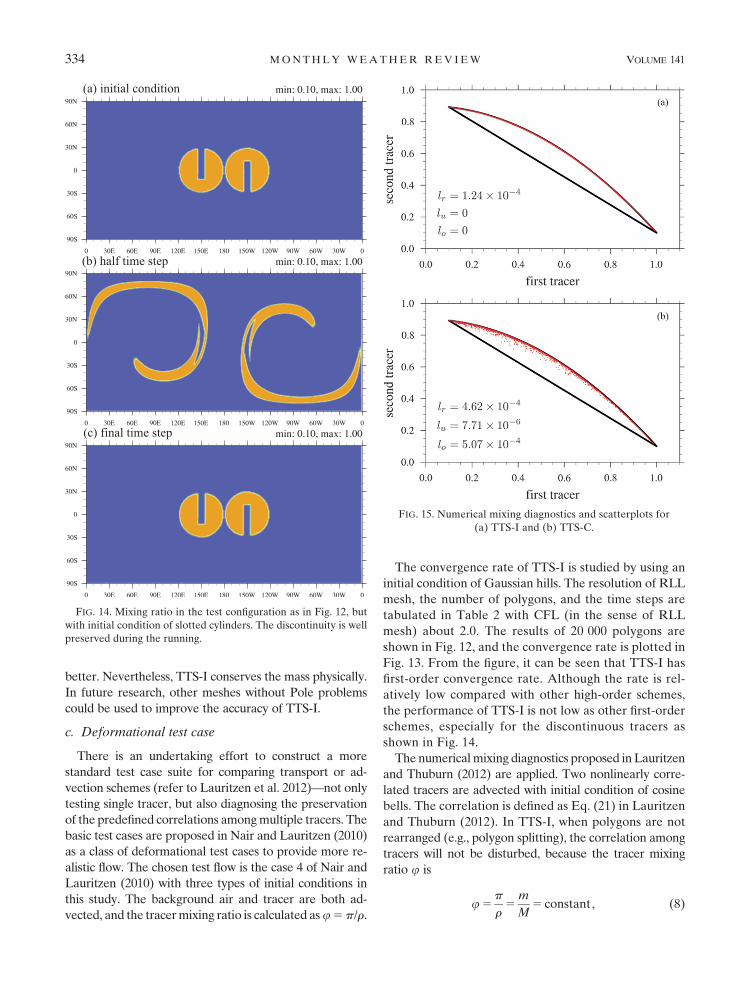
The numericalmixing diagnostics proposed inLauritzen

and Thuburn (2012) are applied. Two nonlinearly corre-

lated tracers are advected with initial condition of cosine

bells. The correlation is defined as Eq. (21) in Lauritzen

and Thuburn (2012). In TTS-I, when polygons are not

rearranged (e.g., polygon splitting), the correlation among

tracers will not be disturbed, because the tracer mixing

ratio u is

u5p

r5

m

M5 constant, (8)

FIG. 14. Mixing ratio in the test configuration as in Fig. 12, but

with initial condition of slotted cylinders. The discontinuity is well

preserved during the running.

FIG. 15. Numerical mixing diagnostics and scatterplots for

(a) TTS-I and (b) TTS-C.


where m is the tracer mass in the polygon, M is the air

mass. Whereas in TTS-C, this correlation will not be

preserved. Figure 15 shows the numerical mixing di-

agnostics (lr, lu, lo) and scatterplots at half time step. The

polygon number in TTS-I is 40 962, and the centroid

number in TTS-C is 115 200. Themesh resolution is 18 318 and the time step is 5/600 in both of them. It is obvious

that TTS-I preserves the correlation accurately with

only small mixing caused by the remapping procedure.

The highlight of TTS-C–I is the well preserving of

discontinuity, so the slotted cylinder’s initial condition is

also used with the results in Fig. 14. Compare it with

Dong and Wang (2012), their Fig. 13, which used parcel

centroid spatial discretization, where the filamented slot-

ted cylinders showed some sawtooth in TTS-C, which

can be attributed to the inverse distance weighted in-

terpolation. This problem is avoided in TTS-I by de-

scribing the interfaces of each parcel explicitly, and this

will give more accurate region that a parcel will influ-

ence. Thus, TTS-I has better performance when advect-

ing discontinuous tracers.

4. Conclusions

This study is a proof of concept, where the previous

parcel centroid spatial discretization in Dong and Wang

(2012) (TTS-C) is replaced by parcel interface (TTS-I).

This type of spatial discretization can eliminate the un-

physical global renormalization for conserving total mass.

The curvature changes of parcel polygon interfaces are

captured by a novel proposed curvature-guard algorithm

(CGA), including edge-splitting and edge-merging sub-

algorithms, etc. To avoid potential edge-crossing problems,

vertex–edge-approaching detection and potential cross-

ing detection subalgorithms are also devised to make

CGA capable to deal with extreme cases in the region of

large deformation. It should be noted that the parame-

ters in edge-splitting and edge-merging algorithms are

vital to successful simulations. For the time being, they are

only the functions of edge length, which will make longer

edge split more easily. Further research must be carried

out to formulate a more objective and optimal form of

them. For example, the deformation of the flow should be

taken into consideration to make CGA more effective.

Another major effort in this study is constructing a

first-order conservative remapping algorithm that can

deal with polygons with arbitrary shape (may be concave),

which is not covered by the previous popular similar

package: the Spherical Coordinate Remapping and

Interpolation Package. The existing higher-order remap-

ping (e.g., Geometrically Exact Conservative Remapping)

could be incorporated to improve accuracy when remap-

ping from background mesh cells to parcel polygons.

The polar stereographic plane introduced to tackle

Pole problems in TTS-C degenerates the accuracy of

TTS-I. In future research, a more effective solution

should be sought or other mesh without Pole problems

could be used. Although the convergence rate of TTS-I

is only first order in the current research, the perfor-

mance of it is not as low as other first-order schemes,

especially in the discontinuous test cases.

The polygon-splitting subalgorithms, which are im-

portant for the real application of TTS-I, will be em-

phasized in the future works, and real flows outputted

by an atmospheric model or from a reanalysis data will

be used to verify the practicability of TTS-I. In addi-

tion, the parallel implementation of TTS-I is not

achieved for the time being. It will be quite different

from the static Eulerian counterparts, and may be not

trivial.

Acknowledgments. The authors acknowledge the Min-

istry of Science and Technology of China for the Na-

tional Basic Research Program of China (973 Program:

Grant 2011CB309704) and the National High-tech R&D

Program (863 Program: Grant 2010AA012304).

APPENDIX A

Calculation of Orientation

During the running of TTS-I, the orientation of the

vertex relative to the edge is important geometric in-

formation as shown in Fig. A1a. Assume the spherical

and Cartesian coordinates of vertices A, B, and C are

(lA,uA), xA5 (xA, yA, zA) ,

(lB,uB), xB 5 (xB, yB, zB), and

(lC,uC), xC 5 (xC, yC, zC) ,

then the orientation can be judged from the sign of the

determinant of a matrix

det5

��xC yC zCxA yA zAxB yB zB

�� .

Because of the floating-point error, a small criteria � (here,

10216) is adopted as

8<:

det. � , left side,

det, 2� , right side,

otherwise, on the edge.


APPENDIX B

Calculation of Angle

When calculating spherical polygon area and calling

curvature-guard algorithm, the angles between edges as

shown in Fig. A1bmust be calculated first. The spherical

andCartesian coordinates of vertices of edgeAB and edge

BC are assumed as above. The normal vectors of the two

edges are

nAB 5 xA 3 xB and

nBC 5 xB3 xC ,

respectively. Then the angle u is

u5

�arccos(2nAB � nBC) xB � (nAB 3 nBC)$ 0,

2p2 arccos(2nAB � nBC) xB � (nAB 3 nBC), 0.

(B1)

The conditional branches are for handling the angles that

are greater than 1808.

APPENDIX C

Calculation of Spherical Polygon Area

The formula of the spherical polygon area is very simple,

which is known as Girard’s theorem, as follows:

S5R2eE , (C1)

FIG. A1. Schemas of spherical calculations. (a) Calculate the orientation of point C to edge

AB. (b) Calculate the angle between edge AB and BC. (c) Calculate the projection of point C

onto edge AB. (d) Calculate the intersections of AB–CD and EF–GH. (e) Ray-casting algo-

rithm for judging a point in a polygon or not. (f) Ray-casting algorithm on the sphere.


where S is the area, Re the radius of the sphere, and E is

the spherical excess of the polygon defined as

E5 �N

i51

ui2 (N2 2)p ,

where N is the edge number of the polygon. Angle ui is

calculated from (9).

APPENDIX D

Calculation of Projection

The projection of a vertex onto an edge is an impor-

tant geometric information for approaching detection

algorithm (section 2c). Assume the edge AB and the

vertex C with the coordinates as above (see Fig. A1c).

First get the rotating North Pole P, (lP, uP), which

makes the edge AB on the equator in the rotated co-

ordinate system. This can be achieved by rotating B

with A as the North Pole to get (l0B, l0B), set a tempo-

rary coordinate (l0B 2 (p/2), 0), and rotate it reversely

to the original coordinate system to get point P. Then

rotate A, B, and C with P as the North Pole to get

(l0A, l0A), (l

0B, l

0B), and (l0C, l

0C). The projection in this

rotated coordinate system is just (l0C, 0), and judge

whether the projection is on the edge considering

zonal periodic boundary condition. The rotation for-

mula is

8>><>>:

l0(l,u)5 arctan

"cosu sin(l2 lp)

cosu sinup cos(l2 lp)2 cosup sinu

#,

u0(l,u)5 arcsin[sinu sinup1 cosu cosup cos(l2 lp)] ,

and the inverse rotation formula is8>><>>:

l(l0,u0) 5 lp 1 arctan

cosu0 sinl0

sinu0 cosup 1 cosu0 cosl0 sinup

!,

u(l0,u0) 5 arcsin(sinu0 sinup 2 cosu0 cosup cosl0) .

APPENDIX E

Calculation of Intersection

a. Intersection between two great-circle arcs

Calculate the intersection between arc AB and CD as

shown in Fig. A1d. Firstly, compute the normal vectors

of the two planes defined by AB–CD and sphere center,

respectively, as

nAB5 xA3 xB and

nCD 5 xC 3 xD .

Secondly, compute the cross product

v5nAB 3nCDjnABjjnCDj

.

Note that when the denominator is less than a small

criteria � (here, 10212 because of the floating-point er-

ror), there would be no intersection. Then the intersection

is one of the end points of the dashed line 1 in Fig.A1d and

is chosen by the following judgment:

(xA3 x) � (xB 3 x), 0 and (xC 3 x) � (xD 3 x), 0,

where x is one of the end points. If the judgment is true,

that end point will be the intersection.

b. Intersection between great-circle arcand latitude segment

In Fig. A1d, calculate the intersection between great-

circle arc EF and the latitude segment GH with latitude

u. The planes where they reside are defined as

ax1 by1 cz5 0,

z5R sin(u) ,

where a, b, and c are the components of the normal

vector of the plane where EF resides; R is the radius of

the sphere. Eliminate x from the above two equations to

get

y21 2bcz

a21 b2y1

(a21 c2)z22 a2R2

a21 b25 0.


Solve this quadratic equation to get

y52d6 e ,

where d5 bcz/(a2 1 b2), and e5ffiffiffiffiffiffiffiffiffiffiffiffiffiffiffiffiffiffiffiffiffiffiffiffiffiffiffiffiffiffiffiffiffiffiffiffiffiffiffiffiffiffiffiffiffiffiffiffiffiffiffiffiffiffiffiffiffiffiffiffiffiffiffiffiffiffiffiffiffiffiffid2 2 [(a2 1 c2)z2 2 a2R2]/(a2 1 b2)

p. Then x5 (2by2

cz)/a. The intersection is one of the end points of the

dashed line 2 in Fig. 15c and is chosen by the following

judgment

lG # l# lH and (xE3 x) � (xF 3 x), 0,

where x is one of the end points and l is the longitude.

Similar calculation has also been given inNair et al. (1999).

In some cases, the floating-point error is so large that no

or wrong intersection is produced by the above formulas,

and this will affect the next calculations. Thus, when this

happens, higher precision floating-point computations

are adopted [e.g., the Multiple Precision Floating-Point

Reliably (MPFR; see http://www.mpfr.org and http://

www.holoborodko.com/pavel/mpfr) library can be used

in C11].

APPENDIX F

Ray-Casting Algorithm

To judge whether a point is located in a polygon on the

sphere, the ray-casting algorithm (RCA; see http://en.

wikipedia.org/wiki/Point_in_polygon) can be used. The

original RCA handles only polygons in Cartesian space

as shown in Fig. A1e. The hollow circle is the point for

judgment. First, cast a ray from the point to infinity along

the x or y axis. Second, calculate the number of inter-

sections between the ray and polygonal edges. If the

number is odd, the point is inside the polygon; other-

wise, it is outside the polygon. For application on the

sphere, rotate the spherical coordinate system with

the point as the North Pole, and project the point and

the polygon onto the equatorial plane as shown in Fig.

A1f; then the original RCA can be used.

REFERENCES

Aulisa, E., S. Manservisi, and R. Scardovelli, 2004: A surface

marker algorithm coupled to an area-preserving marker redis-

tribution method for three-dimensional interface tracking.

J. Comput. Phys., 197, 555–584.Behrens, J., 2006: Adaptive Atmospheric Modeling: Key Tech-

niques in Grid Generation, Data Structures, and Numerical

Operations with Applications. Lecture Notes in Computational

Science and Engineering, Vol. 54, Springer, 233 pp.

Donea, J., A. Huerta, J.-P. Ponthot, and A. Rodrıguez-Ferran,

2004: Arbitrary Lagrangian–Eulerian methods. Funda-

mentals, E. Stein, R. de Borst, and T. J. R. Hughes, Eds.,

Vol. 1, Encyclopedia of Computational Mechanics, Wiley,

413–437.

Dong, L., and B. Wang, 2012: Trajectory-tracking scheme in La-

grangian form for solving linear advection problems: Pre-

liminary tests. Mon. Wea. Rev., 140, 650–663.Dritschel, D. G., 1988: Contour surgery: A topological reconnection

scheme for extended integrations using contour dynamics.

J. Comput. Phys., 77, 240–266.

Dukowicz, J. K., and J. R. Baumgardner, 2000: Incremental re-

mapping as a transport/advection algorithm. J. Comput. Phys.,

160, 318–335.

Enright, D., R. Fedkiw, J. Ferziger, and I. Mitchell, 2002: A hybrid

particle level set method for improved interface capturing.

J. Comput. Phys., 183, 83–116.

——, F. Losasso, and R. Fedkiw, 2005: A fast and accurate semi-

Lagrangian particle level set method.Comput. Struct., 83, 479–

490.

Flyer, N., and E. Lehto, 2010: Rotational transport on a sphere:

Local node refinement with radial basis functions. J. Comput.

Phys., 229, 1954–1969.

Hieber, S. E., and P. Koumoutsakos, 2005: A Lagrangian particle

level set method. J. Comput. Phys., 210, 324–367.Hirt, C.W., and B. D. Nichols, 1981: Volume of fluid (VOF)method

for the dynamics of free boundaries. J. Comput. Phys., 39,

201–225.

Jones, P.W., 1999: First- and second-order conservative remapping

schemes for grids in spherical coordinates. Mon. Wea. Rev.,

127, 2204–2210.

Lauritzen, P. H., and R. D. Nair, 2008: Monotone and conservative

cascade remapping between spherical grids (CaRS): Regular

latitude–longitude and cubed-sphere grids. Mon. Wea. Rev.,

136, 1416–1432.

——, and J. Thuburn, 2012: Evaluating advection/transport

schemes using interrelated tracers, scatter plots and numerical

mixing diagnostics. Quart. J. Roy. Meteor. Soc., 138, 906–918.

——, R. D. Nair, and P. A. Ullrich, 2010: A conservative semi-

Lagrangian multi-tracer transport scheme (CSLAM) on the

cubed-sphere grid. J. Comput. Phys., 229, 1401–1424.——, C. Jablonowski, M. A. Taylor, and R. D. Nair, Eds., 2011:

Numerical Techniques for Global Atmospheric Models. 1st ed.

Lecture Notes in Computational Science and Engineering,

Vol. 80, Springer, 580 pp.

——, W. C. Skamarock, M. J. Prather, and M. A. Taylor, 2012: A

standard test case suite for two-dimensional linear transport

on the sphere. Geosci. Model Dev. Discuss., 5, 887–901.

Lin, S.-J., and R. B. Rood, 1996: Multidimensional flux-form semi-

Lagrangian transport schemes.Mon. Wea. Rev., 124, 2046–2070.Liu, G. R., andM. B. Liu, 2003: Smoothed Particle Hydrodynamics:

A Meshfree Particle Method. World Scientific Publishing

Company, 449 pp.

McKenna, D. S., P. Konopka, J.-U. Groofl, G. Gunther, R. Muller,

R. Spang, D. Offermann, and Y. Orsolini, 2002a: A new

Chemical Lagrangian Model of the Stratosphere (CLaMS) 1.

Formulation of advection and mixing. J. Geophys. Res., 107,

4309, doi:10.1029/2000JD000114.

——, J.-U. Groofl, G. Gunther, P. Konopka, R. Muller, G. Carver,

and Y. Sasano, 2002b: A new Chemical Lagrangian Model

of the Stratosphere (CLaMS) 2. Formulation of chemistry

scheme and initialization. J. Geophys. Res., 107, 4256,

doi:10.1029/2000JD000113.

Nair, R. D., and B. Machenhauer, 2002: The mass-conservative

cell-integrated semi-Lagrangian advection schemeon the sphere.

Mon. Wea. Rev., 130, 649–667.


——, and C. Jablonowski, 2008: Moving vortices on the sphere: A

test case for horizontal advection problems. Mon. Wea. Rev.,

136, 699–711.

——, and P. H. Lauritzen, 2010: A class of deformational flow test

cases for linear transport problems on the sphere. J. Comput.

Phys., 229, 8868–8887.

——, J. Cote, and A. Staniforth, 1999: Cascade interpolation for

semi-Lagrangian advection over the sphere. Quart. J. Roy.

Meteor. Soc., 125, 1445–1468.

Noh, W., and P. Woodward, 1976: SLIC (simple line interface

calculation). Proc. Fifth Int. Conf. on Numerical Methods in

FluidDynamics,Enschede, Netherlands, University of Twente,

330–340.

Osher, S. J., and R. P. Fedkiw, 2003: Level Set Methods and Dy-

namic Implicit Surfaces.Applied Mathematical Sciences, Vol.

153, Springer, 296 pp.

Purser, R. J., and L. M. Leslie, 1991: An efficient interpolation

procedure for high-order three-dimensional semi-Lagrangian

models. Mon. Wea. Rev., 119, 2492–2498.Putman, W. M., and S.-J. Lin, 2007: Finite-volume transport on

various cubed-sphere grids. J. Comput. Phys., 227, 55–78.

Reithmeier, C., andR. Sausen, 2002:ATTILA:Atmospheric tracer

transport in a Lagrangian model. Tellus, 54B, 278–299.Rood, R. B., 1987: Numerical advection algorithms and their role

in atmospheric transport and chemistry models. Rev. Geo-

phys., 25, 71–100.Rudman, M., 1997: Volume-tracking methods for interfacial flow

calculations. Int. J. Numer. Methods Fluids, 24, 671–691.

Stenke, A., V. Grewe, and M. Ponater, 2008: Lagrangian transport

of water vapor and cloud water in the ECHAM4GCM and its

impact on the cold bias. Climate Dyn., 31, 491–506.

Thuburn, J., and M. E. McIntyre, 1997: Numerical advection

schemes, cross-isentropic random walks, and correlations be-

tween chemical species. J. Geophys. Res., 102 (D6), 6775–6797.

Tryggvason, G., and Coauthors, 2001: A front tracking method for

the computations of multiphase flow. J. Comput. Phys., 169,708–759.

Ubbink, O., and R. I. Issa, 1999: Amethod for capturing sharp fluid

interfaces on arbitrary meshes. J. Comput. Phys., 153, 26–50.

Ullrich, P. A., P. H. Lauritzen, and C. Jablonowski, 2009: Geo-

metrically Exact Conservative Remapping (GECoRe): Reg-

ular latitude–longitude and cubed-sphere grids. Mon. Wea.

Rev., 137, 1721–1741.——, ——, and ——, 2012: Some considerations for high-order

‘incremental remap’-based transport schemes: Edges, re-

constructions, and area integration. Int. J. Numer. Methods

Fluids, doi:10.1002/fld.3703, in press.

Walton, J. J., M. C. MacCracken, and S. J. Ghan, 1988: A global-

scale Lagrangian trace species model of transport, trans-

formation, and removal processes. J. Geophys. Res., 93 (D7),

8339–8354.

Wohltmann, I., and M. Rex, 2009: The Lagrangian chemistry and

transport model ATLAS: Validation of advective transport

and mixing. Geosci. Model Dev., 2, 153–173.Yu, R., 1994: A two-step shape-preserving advection scheme.Adv.

Atmos. Sci., 11, 479–490.


Trajectory-Tracking Scheme in Lagrangian Form for Solving Linear Advection Problems: Interface...

Documents

Transcript of Trajectory-Tracking Scheme in Lagrangian Form for Solving Linear Advection Problems: Interface...