Article

Volume 11, Number 8

21 August 2010

Q08020, doi:10.1029/2010GC003081

ISSN: 1525‐2027

Modeling advection in geophysical flows with particlelevel sets

H. SamuelBayerisches Geoinstitut, Universität Bayreuth, D‐95440 Bayreuth, Germany

M. EvonukDepartment of Theoretical Physics I, Universität Bayreuth, D‐95440 Bayreuth, Germany

[1] We have applied, for the first time in geodynamical flows, the Particle Level Set method for advectingcompositional fields with sharp discontinuities. This robust and efficient Eulerian‐Lagrangian technique isbased on the concept of Implicit Surfaces, which allows the use of high order accurate numerical schemesin the vicinity of discontinuities. We have tested the Particle Level Set method against the robust and pop-ular Tracer‐in‐Cell method on well‐known 2D thermochemical benchmarks and typical 3D convectiveflows. The use of Lagrangian tracers in the Particle Level Set method yields accurate solutions of purelyadvective transport, where sub‐grid scale features can be resolved. In every case we ran we found that theParticle Level Set method accuracy equals or is better than the popular Tracer‐in‐Cell method, and can leadto significantly smaller computational cost, in particular in three‐dimensional flows, where the reduction ofcomputational time for modeling advection processes is most needed.

Components: 12,700 words, 21 figures, 1 table.

Keywords: advection; level set method; numerical modeling; interface tracking; geophysical flows; particle‐in‐cell method.

Index Terms: 0545 Computational Geophysics: Modeling (1952, 4255); 8120 Tectonophysics: Dynamics of lithosphere andmantle: general (1213); 1956 Informatics: Numerical algorithms.

Received 15 February 2010; Revised 4 June 2010; Accepted 10 June 2010; Published 21 August 2010.

Samuel, H., and M. Evonuk (2010), Modeling advection in geophysical flows with particle level sets, Geochem. Geophys.Geosyst., 11, Q08020, doi:10.1029/2010GC003081.

1. Introduction

[2] Advection is one of the major processes thatcommonly occurs on various scales in Geody-namics. When diffusion is negligible this transportmode, in its simplest form, can be described by thefollowing differential equation:

@C

@tþ U:rC ¼ 0; ð1Þ

where t is the time, and C is a scalar quantity (e.g.,temperature or a chemical component) being ad-vected by a given velocity field U. Various geody-namic scenarios of current interest involve thepresence of sharp discontinuities in C (e.g., coreformation processes [Hoïnk et al., 2006; Samuel etal., 2010; Lin et al., 2009; Monteux et al., 2009;Ichikawa et al., 2010], subduction dynamics[Schmeling et al., 2008; van Hunen et al., 2004],lithospheric dynamics [Muehlhaus et al., 2002],

Copyright 2010 by the American Geophysical Union 1 of 22

mantle convective stirring [Manga, 1996; Schmalzlet al., 1996; Tackley, 2002; Samuel and Farnetani,2003; van Keken et al., 2003; Farnetani andSamuel, 2003], thermochemical plume dynamics[Farnetani and Samuel, 2005; Lin and van Keken,2005, 2006; Samuel and Bercovici, 2006], multiphase flows in magma chambers [Verhoeven andSchmalzl, 2009], salt diapirism [Weinberg andSchmeling, 1992; Chemia et al., 2008] or bubbledynamics in magma flows [Manga and Stone,1994]). Unfortunately in such cases, solving forequation (1) can be very challenging becausesharp discontinuities lead to numerical instabilities,which prevent the local use of high order numericalschemes.

[3] Several approaches have been used in compu-tational geodynamics in order to overcome thisdifficulty with variable amounts of success. Despitethe use of correcting filters or non‐oscillatory, shock‐preserving schemes, Eulerian (fixed grid) techniquesgenerally suffer from artificial numerical diffusionand dispersion. Lagrangian approaches (dynamicgrids or particles) tend to be more popular in com-putational geodynamics because they are not proneto excessive numerical diffusion. However, theseapproaches are generally computationally expen-sive, especially in 3D, and can suffer from spuriousstatistical noise.

[4] As an alternative to these aforementionedapproaches, a powerful hybrid Eulerian‐LagrangianParticle Level Set method for modeling advection ofsharply varying quantities, has become increasinglypopular in the field of computer graphics [Enright etal., 2002]. This Particle Level Set method is anextension of the Level Set method [Osher andSethian, 1988], which is based on the concept ofimplicit surfaces that mark the boundary betweensharply varying scalar fields.

[5] This paper aims to apply this recent method thatcombines the best of Eulerian and Lagrangianapproaches, to geodynamic flows. In the first partof the paper the Particle Level Set methodologyis described. In the second part of the paper themethod is tested against well known benchmarksand classical two‐ and three‐dimensional Geo-dynamic flows.

2. Numerical Strategies for Advectinga Scalar Field

[6] In this section we first briefly review thenumerical methods that have been developed and

commonly used inGeodynamics to solve equation (1).Next we will introduce two relatively recent meth-ods that have proven to be accurate and efficient foradvecting sharp material surfaces: the EulerianLevel Set method [Osher and Sethian, 1988] and theParticle Level Set method, a Lagrangian extensionof the Level Set approach [Enright et al., 2002].The pure Eulerian Level Set method is becomingincreasingly common in Geodynamics [Gross et al.,2007; Suckale et al., 2010], and the Particle LevelSet is a popular method in hydrodynamics andcomputer graphics [Osher and Fedkiw, 2003].However, to our knowledge, the Particle Level Setmethod has not been applied to geodynamic flows.

2.1. Popular Advection Methodsin Geodynamics

[7] Numerical methods for modeling advectivetransport can generally be cast into either Eulerian(i.e., fixed grid), Lagrangian (i.e., mobile grid orparticles) approaches, or a combination of the two.

2.1.1. Eulerian Methods

[8] The advection equation (1) can be straightfor-wardly discretized onto a fixed grid. The advan-tage, in computational geodynamics, is that oftenthe discretization of equation (1) is similar to thatof other conservation equations, such as the con-servation of energy, which are also discretized onEulerian grids. Sharp variations in C require specialcare in discretizing equation (1). For instance, it iswell known that discretizing the advective terms inequation (1) with a second order centered finitedifference scheme can lead to the appearance ofunphysical spurious oscillations in C [Press et al.,1992; Fletcher, 1991]. Low order schemes, suchas upwinding, provide a way to solve equation (1)without producing oscillations in C, but are gen-erally prone to significant numerical diffusion. Analternative approach is to add a small diffusion termin equation (1) [Farnetani and Richards, 1995; vanKeken et al., 1997] which artificially smoothes C.Further significant reduction of numerical diffusioncan also be achieved with the use of correcting filters[Lenardic and Kaula, 1993; Tackley and King,2003] and the use of anti‐diffusive corrections[Smolakiewicz, 1984].

[9] More sophisticated Eulerian advection schemeshave been developed in the past decades. In par-ticular the use of Total Variation Diminishingschemes with flux limiters [Harten, 1984; Sweby,

GeochemistryGeophysicsGeosystems G3G3 SAMUEL AND EVONUK: ADVECTION METHOD 10.1029/2010GC003081

2 of 22

1984; Roe, 1986] allow a high order discretization ofadvection in regions where C varies smoothly andlow order monotone discretization of advection inregions where C varies sharply. Providing that theresolution is sufficient, TVD schemes with fluxlimiters such as Superbee or Sweby [Roe, 1986],yield significant reduction in numerical diffusion[Ricard et al., 2009; Monteux et al., 2009].

[10] Another approach, popular in hydrodynamicmodeling, is to discretize equation (1) using Essen-tially Non Oscillatory (ENO) and Weighted Essen-tially Non Oscillatory (WENO) schemes [Harten etal., 1987; Liu et al., 1994]. Such schemes usepolynomial interpolation of the discrete values of C,which upon differentiation yield stencils for theapproximation of numerical fluxes. The mainidea behind these schemes is the use of either thesmoothest local stencil (for ENO schemes) or aweighted combination of local stencils (for WENOschemes), leading to monotonicity even in thevicinity of discontinuities, and high accuracy wher-ever C is smooth.

[11] Despite all these improvements, due to thefixed nature of the grid, numerical diffusion anddispersion in Eulerian grids cannot be completelyremoved [e.g., van Keken et al., 1997; Tackley andKing, 2003] and are always significantly larger inregions where C varies sharply.

[12] Finally, considering a total number of Degreesof Freedom (grid cells/points) N, and assumingoptimum solvers (e.g., multigrid) or explicit schemesare used for solving and discretizing equation (1),the computational cost associated with the use ofEulerian methods goes as ∼N.

2.1.2. Lagrangian (Tracer) Methods

[13] A fundamentally different approach to solveequation (1) can be adopted using Lagrangianmethods that involve either the use of deformablemeshes or tracer particles that are advected in a givenvelocity field U [Christensen and Hofmann, 1994;vanKeken et al., 1997; Samuel and Farnetani, 2003;Tackley and King, 2003]. In this case the Lagrangianversion of equation (1) is a set of ordinary differ-ential equations for each component of the particleposition vector xp

dxpdt

¼ U; ð2Þ

which can be integrated using classical methods, e.g.,Runge‐Kutta of second order or higher. The tracers

locations xp are then converted into a continuumfield C at each time step by weighted averaging[Tackley and King, 2003; Gerya and Yuen, 2003;Deubelbeiss and Kaus, 2008]. The major advantageof Tracer‐in‐Cell methods (also named tracer ratiomethods) is the fact that numerical diffusion isnegligible. In addition they allow sub grid scaleresolution. On the other hand, these methods sufferfrom spurious statistical noise because the number ofparticles is finite. Reducing this noise to an accept-able level requires the use of at least 3n tracers percell, where n is the number of spatial dimensions.This makes these methods computationally expen-sive, particularly in 3D. Indeed, for the least favor-able case (tracers particles located everywhere in thecomputational domain), the cost associated with theuse of Lagrangian methods goes as N × Ntracer/cell,where the minimum number of tracers per cellNtracer/cell is typically 9 in 2D and 27 in 3Dgeometry. This leads to an extra cost that canbe one or two orders of magnitude larger than thecomputational cost associated with Eulerian advec-tion methods. In addition, the advection of tracerparticles may lead to incorrect results when char-acteristics are merging [Enright et al., 2002].Finally, the use of tracer particles is not suitablefor numerically determining geometrical quantitiessuch as normal vectors to interfaces or the interfacecurvature, even in the case of a continuous interfacewith a smooth curvature.

[14] Other Lagrangianmethods focus on tracking onlythe interfaceW that marks changes/discontinuities inthe scalar field C. For instance 2D marker chainshave been proven to track accurately the evolution of2D surfaces [van Keken et al., 1997; Lin and vanKeken, 2005; Samuel and Bercovici, 2006], andsubdivision surfaces have been successfully appliedto 3D geodynamic flows [Schmalzl and Loddoch,2003]. However, these methods can become pro-hibitively expensive, even in 2D, because theirassociated computational cost increases with thearea of the interface tracked. Contrary to Tracer‐in‐Cell methods for which the number of tracersremains constant during the calculation, the area ofthe interface tracked can grow without bounds. Thiscan lead to a significant increase in computationalcost, sometimes exceeding by far the cost associatedwith advection using Tracer‐in‐Cell methods [vanKeken et al., 1997]. For instance, in chaotic con-vective flows, the repeated action of stretching andfolding leads to efficient convective stirringwhere thearea of the interface W and consequently the com-putational cost will grow exponentially with time.

GeochemistryGeophysicsGeosystems G3G3 SAMUEL AND EVONUK: ADVECTION METHOD 10.1029/2010GC003081

3 of 22

2.2. Dynamic Implicit Surfaces forAdvecting Sharply Varying Quantities

[15] In the following sections, the Level Set andParticle Level Set methods will be summarized. Formore details the reader is referred to Osher andSethian [1988], Sethian [1999], Enright et al.[2002], Osher and Fedkiw [2003] and referencestherein.

2.2.1. Level Set Method

[16] In order to track the location of an interface thatmarks sharp discontinuities in an advected field C,Osher and Sethian [1988] have developed anEulerianmethod whose basic principle consists in the use ofan implicit surface, as part of a smooth Level Setfunction � of higher dimension, which replaces C inequation (1):

@�

@tþ U:r� ¼ 0: ð3Þ

[17] The choice of the Level Set function is free aslong as � remains continuous. However, it is con-venient to maintain the Level Set as a signed dis-tance function to the interface W. This guaranteesthat � remains smooth and it enables a straight-forward reconstruction of the interface W as itcorresponds exactly to the location of the zero levelset W ≡ � = 0. A major advantage of the LevelSet method over other Eulerian methods lies inthe smoothness of �, for which high order accurateschemes can be efficiently applied, thus significantlyreducing numerical errors.

[18] When solving equation (3) with physicalvelocities U (i.e., obtained by solving the Navier‐Stokes equations) to advect �, the Level Set will bedistorted by the flow, therefore, in general, �will notremain a signed distance function to the interface W.In order to remain a signed distance function, theLevel Set function must be reinitialized to meet thefollowing Eikonal requirement at each time step:

jr�j ¼ 1: ð4Þ

[19] However, as proposed by Sussman et al.[1994], the Level Set reinitialization step can alsobe achieved by solving the following non‐linearhyperbolic equation to steady state:

@�

@�¼ Sð�0Þð1� jr�jÞ; ð5Þ

where�0 is the Level Set determinedwith equation (3)prior to reinitialization, t represents a fictitious timeand S(�0) is a smoothed signed distance function:

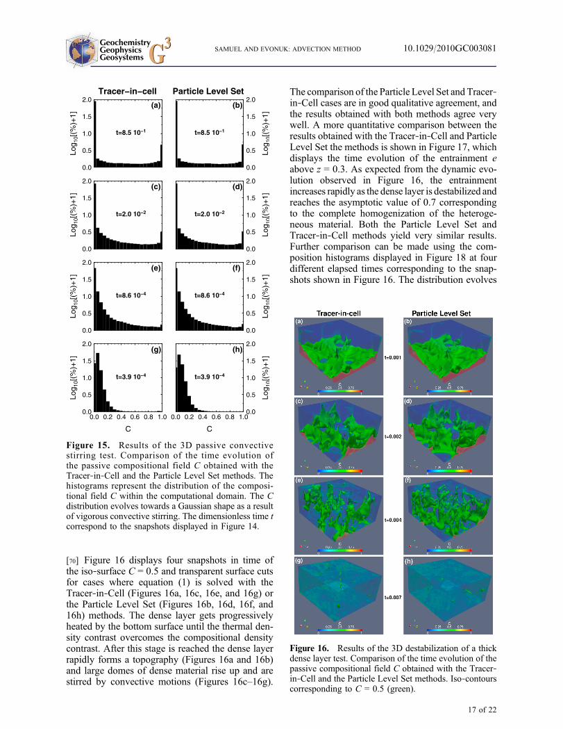
Sð�0Þ ¼ �0ffiffiffiffiffiffiffiffiffiffiffiffiffiffiffi�20 þ "2

p ; ð6Þ

where " is taken as the grid spacingDh (assuminga constant grid spacing). Note that solving forequation (5) is not computationally prohibitive asthe steady state is generally reached within 1 to 2fictitious time iterations, with a time stepDt = 0.1Dh [Sussman et al., 1994]. Similarly to Sussmanet al. [1994] and Min and Gibou [2007], the spa-tial derivatives in equation (5) can be approximatedwith a monotone second order Godunov‐Hamilto-nian scheme. The time discretization of equation (5)is performed via a second order TVD Runge‐Kutta(predictor‐corrector) scheme [Shu and Osher, 1988;Min and Gibou, 2007].

[20] As noted by Sussman et al. [1994] such areinitialization step tends to produce artificial dis-placement of the zero Level Set, which leads even-tually to weak mass conservation of the LevelSet method. In fact the reinitialization step couldbe avoided by constructing extension velocities[Adalsteinsson and Sethian, 1999; Sethian, 1999] foradvecting the Level Set when solving equation (3).This has the advantage that the Level Set is not dis-torted and therefore no reinitialization is necessary.However, the use of tracers in the Particle Level Setmethod prevents the artificial displacement of thezero Level Set during the reinitialization step. Thus,for simplicity we do not construct extension veloc-ities and maintain the Level Set as a signed distancefunction by solving equation (5).

[21] Finally, in cases where the velocity field isaffected by C, the Level Set needs to be convertedinto a compositional field C as follows:

C ¼1 if � > þ l0 if � < � lCi if j�j � l

8<: ð7Þ

where l represents the half grid cell diagonallength (e.g., in 3D Cartesian geometry l =0.5

ffiffiffiffiffiffiffiffiffiffiffiffiffiffiffiffiffiffiffiffiffiffiffiffiffiffiffiffiffiffiffiffiffiffiffiffiDx2 þDy2 þDz2

p). Ci corresponds to the

value of the compositional field in cells that arecrossed by the zero Level Set. This quantity canbe calculated as the volume fraction of positive �to negative � contained in the cell following, forinstance, the approach described by Sussman andPuckett [2000] or Ménard et al. [2007].

[22] Overall, despite the additional computationalcost involved in the reinitialization or the con-

GeochemistryGeophysicsGeosystems G3G3 SAMUEL AND EVONUK: ADVECTION METHOD 10.1029/2010GC003081

4 of 22

struction of extension velocities, the Level Setmethod is computationally efficient. Indeed, similarto the other Eulerian methods listed in section 2.1.1,the computational cost is O(N). However, this limitis an upper bound as equations (1), (4) or (5) onlyneed to be solved in the vicinity of the zero Level Setfunction, instead of in the whole domain. Thereforethe effective computational cost of the method willvary with time and with the problem considered, butwill always be bounded by N. Moreover, the LevelSet method has proven to be particularly efficient intracking interfaces of a sharply varying advectedfield, even in the presence of strong topologicalchanges [Sethian, 1999, and references therein].

[23] In addition, this formulation allows a straight-forward calculation of critical geometric quantitiessuch as the unit normal vector to the interface:

n ¼ r�

jr�j ð8Þ

and the mean curvature:

G ¼ r:n; ð9Þ

which are required in order to evaluate surface ten-sion acting on the interface W [Brackbill et al.,1992]. This can be relevant to several geodynamicscenarios such as metal diapir fragmentation in amagma ocean during the earliest stages of terrestrialplanet evolution [Rubie et al., 2003; Ichikawa et al., 2010]or gas bubble dynamics in magma flows [Manga

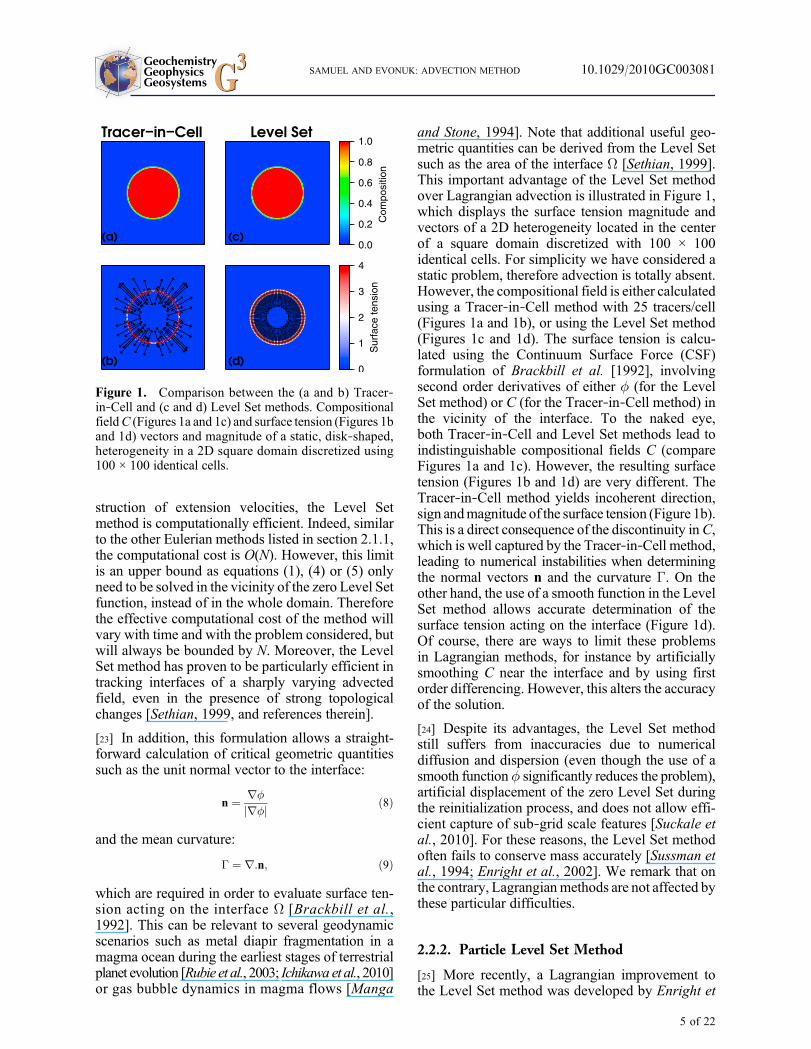
and Stone, 1994]. Note that additional useful geo-metric quantities can be derived from the Level Setsuch as the area of the interface W [Sethian, 1999].This important advantage of the Level Set methodover Lagrangian advection is illustrated in Figure 1,which displays the surface tension magnitude andvectors of a 2D heterogeneity located in the centerof a square domain discretized with 100 × 100identical cells. For simplicity we have considered astatic problem, therefore advection is totally absent.However, the compositional field is either calculatedusing a Tracer‐in‐Cell method with 25 tracers/cell(Figures 1a and 1b), or using the Level Set method(Figures 1c and 1d). The surface tension is calcu-lated using the Continuum Surface Force (CSF)formulation of Brackbill et al. [1992], involvingsecond order derivatives of either � (for the LevelSet method) or C (for the Tracer‐in‐Cell method) inthe vicinity of the interface. To the naked eye,both Tracer‐in‐Cell and Level Set methods lead toindistinguishable compositional fields C (compareFigures 1a and 1c). However, the resulting surfacetension (Figures 1b and 1d) are very different. TheTracer‐in‐Cell method yields incoherent direction,sign andmagnitude of the surface tension (Figure 1b).This is a direct consequence of the discontinuity inC,which is well captured by the Tracer‐in‐Cell method,leading to numerical instabilities when determiningthe normal vectors n and the curvature G. On theother hand, the use of a smooth function in the LevelSet method allows accurate determination of thesurface tension acting on the interface (Figure 1d).Of course, there are ways to limit these problemsin Lagrangian methods, for instance by artificiallysmoothing C near the interface and by using firstorder differencing. However, this alters the accuracyof the solution.

[24] Despite its advantages, the Level Set methodstill suffers from inaccuracies due to numericaldiffusion and dispersion (even though the use of asmooth function � significantly reduces the problem),artificial displacement of the zero Level Set duringthe reinitialization process, and does not allow effi-cient capture of sub‐grid scale features [Suckale etal., 2010]. For these reasons, the Level Set methodoften fails to conserve mass accurately [Sussman etal., 1994; Enright et al., 2002]. We remark that onthe contrary, Lagrangianmethods are not affected bythese particular difficulties.

2.2.2. Particle Level Set Method

[25] More recently, a Lagrangian improvement tothe Level Set method was developed by Enright et

Figure 1. Comparison between the (a and b) Tracer‐in‐Cell and (c and d) Level Set methods. CompositionalfieldC (Figures 1a and 1c) and surface tension (Figures 1band 1d) vectors and magnitude of a static, disk‐shaped,heterogeneity in a 2D square domain discretized using100 × 100 identical cells.

GeochemistryGeophysicsGeosystems G3G3 SAMUEL AND EVONUK: ADVECTION METHOD 10.1029/2010GC003081

5 of 22

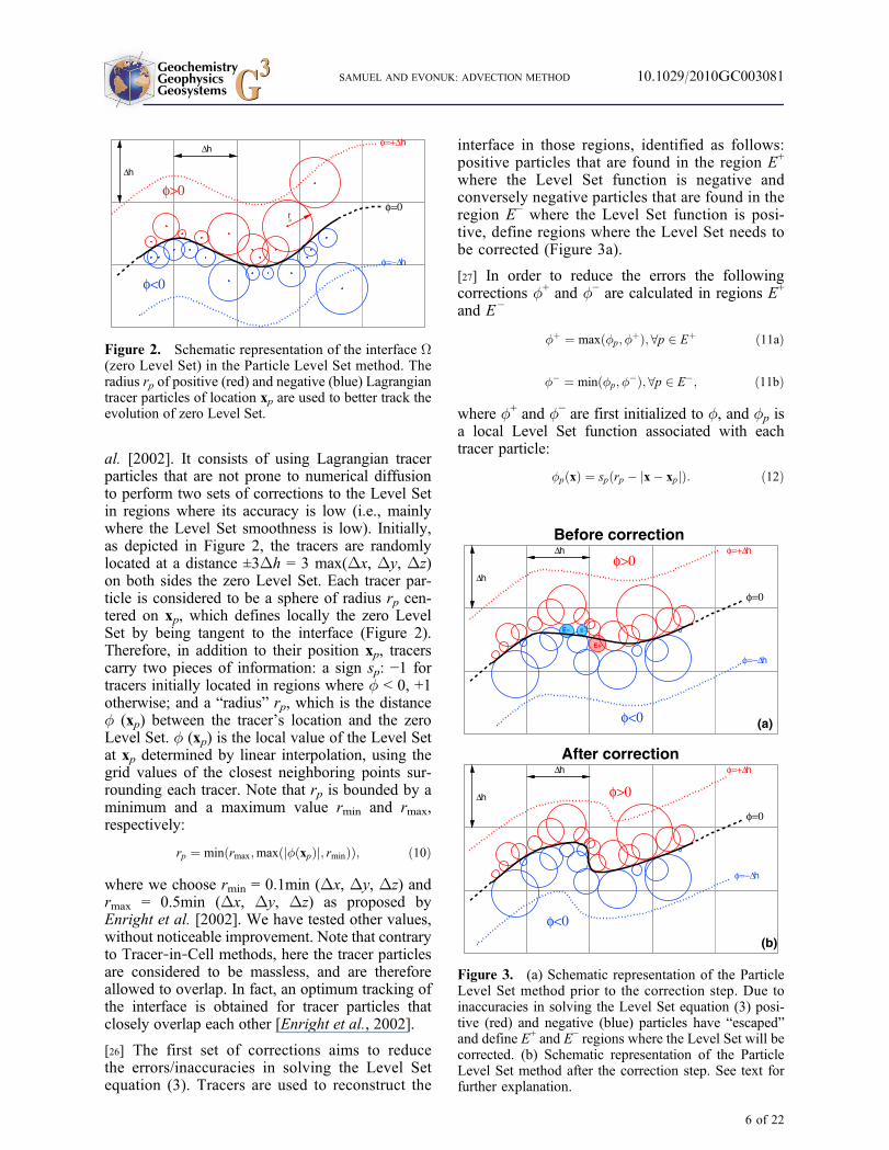
al. [2002]. It consists of using Lagrangian tracerparticles that are not prone to numerical diffusionto perform two sets of corrections to the Level Setin regions where its accuracy is low (i.e., mainlywhere the Level Set smoothness is low). Initially,as depicted in Figure 2, the tracers are randomlylocated at a distance ±3Dh = 3 max(Dx, Dy, Dz)on both sides the zero Level Set. Each tracer par-ticle is considered to be a sphere of radius rp cen-tered on xp, which defines locally the zero LevelSet by being tangent to the interface (Figure 2).Therefore, in addition to their position xp, tracerscarry two pieces of information: a sign sp: −1 fortracers initially located in regions where � < 0, +1otherwise; and a “radius” rp, which is the distance� (xp) between the tracer’s location and the zeroLevel Set. � (xp) is the local value of the Level Setat xp determined by linear interpolation, using thegrid values of the closest neighboring points sur-rounding each tracer. Note that rp is bounded by aminimum and a maximum value rmin and rmax,respectively:

rp ¼ minðrmax;maxðj�ðxpÞj; rminÞÞ; ð10Þ

where we choose rmin = 0.1min (Dx, Dy, Dz) andrmax = 0.5min (Dx, Dy, Dz) as proposed byEnright et al. [2002]. We have tested other values,without noticeable improvement. Note that contraryto Tracer‐in‐Cell methods, here the tracer particlesare considered to be massless, and are thereforeallowed to overlap. In fact, an optimum tracking ofthe interface is obtained for tracer particles thatclosely overlap each other [Enright et al., 2002].

[26] The first set of corrections aims to reducethe errors/inaccuracies in solving the Level Setequation (3). Tracers are used to reconstruct the

interface in those regions, identified as follows:positive particles that are found in the region E+

where the Level Set function is negative andconversely negative particles that are found in theregion E− where the Level Set function is posi-tive, define regions where the Level Set needs tobe corrected (Figure 3a).

[27] In order to reduce the errors the followingcorrections �+ and �− are calculated in regions E+

and E −

�þ ¼ maxð�p; �þÞ; 8p 2 Eþ ð11aÞ

�� ¼ minð�p; ��Þ; 8p 2 E�; ð11bÞ

where �+ and �− are first initialized to �, and �p isa local Level Set function associated with eachtracer particle:

�pðxÞ ¼ spðrp � jx� xpjÞ: ð12Þ

Figure 2. Schematic representation of the interface W(zero Level Set) in the Particle Level Set method. Theradius rp of positive (red) and negative (blue) Lagrangiantracer particles of location xp are used to better track theevolution of zero Level Set.

Figure 3. (a) Schematic representation of the ParticleLevel Set method prior to the correction step. Due toinaccuracies in solving the Level Set equation (3) posi-tive (red) and negative (blue) particles have “escaped”and define E+ and E− regions where the Level Set will becorrected. (b) Schematic representation of the ParticleLevel Set method after the correction step. See text forfurther explanation.

GeochemistryGeophysicsGeosystems G3G3 SAMUEL AND EVONUK: ADVECTION METHOD 10.1029/2010GC003081

6 of 22

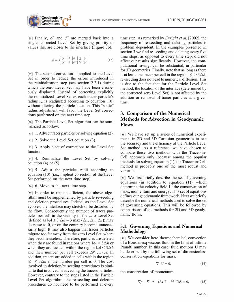
[28] Finally, �+ and �− are merged back into asingle, corrected Level Set by giving priority tovalues that are closer to the interface (Figure 3b):

� ¼ �þ if j�þj � j��j�� if j�þj > j��j

�ð13Þ

[29] The second correction is applied to the LevelSet in order to reduce the errors introduced inthe reinitialization step (see section 2.2.1) duringwhich the zero Level Set may have been errone-ously displaced. Instead of correcting explicitlythe reinitialized Level Set �, each tracer particle’sradius rp is readjusted according to equation (10)without altering the particle location. This “static”radius adjustment will favor the Level Set correc-tions performed on the next time step.

[30] The Particle Level Set algorithm can be sum-marized as follow:

[31] 1. Advect tracer particles by solving equation (2).

[32] 2. Solve the Level Set equation (3).

[33] 3. Apply a set of corrections to the Level Setfunction.

[34] 4. Reinitialize the Level Set by solvingequation (4) or (5).

[35] 5. Adjust the particles radii according toequation (10) (i.e., implicit correction of the LevelSet performed on the next time step).

[36] 6. Move to the next time step.

[37] In order to remain efficient, the above algo-rithm must be supplemented by particle re‐seedingand deletion procedures. Indeed, as the Level Setevolves, the interface may stretch or be distorted bythe flow. Consequently the number of tracer par-ticles per cell in the vicinity of the zero Level Set(defined as ∣�∣ ≤ 3 Dh = 3 max (Dx, Dy, Dz)) maydecrease to 0, or on the contrary become unneces-sarily high. It may also happen that tracer particlesmigrate too far away from the zero Level Set, wherethey become useless. Therefore, particles are deletedwhen they are found in regions where ∣�∣ > 3Dh orwhen they are located within the region ∣�∣ ≤ 3Dhand their number per cell exceeds 2Ntracer/cell. Inaddition, tracers are added in cells within the region∣�∣ ≤ 3Dh if the number per cell is 0. The costinvolved in deletion/re‐seeding procedures is simi-lar to that involved in advecting the tracers particles.However, contrary to the steps listed in the ParticleLevel Set algorithm, the re‐seeding and deletionprocedures do not need to be performed at every

time step. As remarked by Enright et al. [2002], thefrequency of re‐seeding and deleting particles isproblem dependent. In the examples presented insection 3 we find re‐seeding and deleting every fivetime steps, as opposed to every time step, did notaffect our results significantly. However, the com-putational savings can be substantial, in particularfor 3D geometries. Finally, note that as long as thereis at least one tracer per cell in the region ∣�∣ > 3Dh,re‐seeding does not lead to numerical diffusion. Thisis due to the fact that for the Particle Level Setmethod, the location of the interface (determined bythe corrected zero Level Set) is not affected by theaddition or removal of tracer particles at a giventime.

3. Comparison of the NumericalMethods for Advection in GeodynamicFlows

[38] We have set up a series of numerical experi-ments in 2D and 3D Cartesian geometries to testthe accuracy and the efficiency of the Particle LevelSet method. As a reference, we have chosen tocompare these two methods with the Tracer‐in‐Cell approach only, because among the popularmethods for solving equation (1), the Tracer‐in‐Cellmethod is probably one of the most robust andversatile.

[39] We first briefly describe the set of governingequations (in addition to equation (1)), whichdetermine the velocity field U: the conservation ofmass, momentum and energy. This set of equationsdefines our geodynamic framework. Next we brieflydescribe the numerical methods used to solve the setof governing equations. This will be followed bycomparisons of the methods for 2D and 3D geody-namic flows.

3.1. Governing Equations and NumericalMethodology

[40] We consider here thermochemical convectionof a Boussinesq viscous fluid in the limit of infinitePrandtl number. In this case, fluid motions U maybe described by the following set of dimensionlessconservation equations for mass:

r � U ¼ 0; ð14Þ

the conservation of momentum:

rp�r � �þ ðRa T � Rb CÞ~ez ¼ 0; ð15Þ

GeochemistryGeophysicsGeosystems G3G3 SAMUEL AND EVONUK: ADVECTION METHOD 10.1029/2010GC003081

7 of 22

and the conservation of energy:

@T

@tþ U:rT ¼ r2T ; ð16Þ

where p is the dynamic pressure, T is the potentialtemperature, t is the time, � is the deviatoric viscousstress tensor, and~ez is a unit vector along the verticalz axis. These equations are non‐dimensionalizedusing the following characteristic scales: the thick-ness of the convective domain H for distances, thesuper‐adiabatic temperature difference between thetop and bottom surfaces DT for temperature, andH2/� for time, where � is the thermal diffusivity.The equation of state for the dimensionless density is:r = r0 (1 − aT + CDrc/r0), where r0 is the referencedensity,a is the thermal expansion, andDrc = r (C =1) − r (C = 0) is the compositional density contrast.

[41] The first non‐dimensional number that appearsin the conservation of momentum is a thermalRayleigh number, Ra = r0aDTgH3/(h0�), where gis the gravitational acceleration and h0 is the ref-erence viscosity. The second is a compositionalRayleigh number, Rb = DrcgH

3/(h0�).

[42] The whole set of conservation equations issolved using a finite volume code StreamV3D. Twodifferent approaches are used to solve the Stokes(mass and momentum) equations. In 2D, a purestream function formulation is adopted [Samuel,2009]. This reduces the set of Stokes equations toone biharmonic equation for the stream function thatautomatically satisfies the conservation of mass[e.g., Christensen, 1989; van Keken et al., 1997].The stream function is calculated at nodal points,leading to a natural finite volume configurationwhere the velocity components are located at thecenter of each cell surface.

[43] For 3D cases, the mass and momentum equa-tions are solved using a primitive variable formula-tion on a staggered grid with a SIMPLER algorithm[Patankar, 1980; Albers, 2000].

[44] The set of discretized Stokes equations is solvedin 2D with a fast sparse direct solver (superLU[Demmel et al., 1999]) or with a robust iterativeconjugate gradient method [Press et al., 1992] forcases with a large number of points.

[45] A finite volume formulation is used to dis-cretize the energy equation (16) on a staggered grid[e.g., Patankar, 1980; Albers, 2000]. Two approachesare available for treating the advection term inequation (16) in StreamV3D: a pure Eulerianapproach where a Total Variation Diminishingscheme with various flux limiters is used [Sweby,

1984; Roe, 1986], or the Tracer‐in‐Cell method[Gerya and Yuen, 2003; Samuel and Tackley,2008]. However, in this paper the spatial deriva-tives in equation (16) are discretized using a pureEulerian TVD scheme with Sweby a flux limiter[Sweby, 1984]. Time derivatives are approximatedby explicit, first order finite differences subject to aCourant‐Friedrich‐Lewy stability criteria.

[46] Finally, equation (1) is either solved using theParticle‐in‐Cell or the Particle Level Set method.Unless specified otherwise, for tests with the ParticleLevel Set method, the Level Set equation (3) isdiscretized with the same finite volume TVD schemewith a Sweby flux limiter, as for the energy equation.

[47] The code has been successfully benchmarkedagainst analytical solutions (see appendix A),purely thermal and thermo‐chemical benchmarks[Blankenbach et al., 1989; van Keken et al., 1997]including strongly variable viscosity cases (seealso section 3.2 and Appendix A).

3.2. Two‐Dimensional Flows

[48] We consider the well‐known thermochemicalbenchmarks presented by van Keken et al. [1997]in a 2D Cartesian box of aspect ratio l, with dif-ferent velocities and temperature boundary condi-tions and different values for Ra and Rb. The initialcondition for the composition corresponds to a hori-zontally layered structure of thickness db. The timeevolution of several quantities is monitored, in par-ticular the Root Mean Square velocity:

Vrms ¼ffiffiffiffiffiffiffiffiffiffiffiffiffiffiffiffiffiffiffiffiffiffiffiffiffiffiffiffi1

V

ZkUk2 dV

s; ð17Þ

and the entrainment e above a given dimensionlessheight de:

e ¼ 1

�n�1db

Z z¼1

z¼de

CdV ; ð18Þ

where n is the number of spatial dimensions. Inaddition, the mass error [Tackley and King, 2003]was monitored for each run:

DM ¼ ðR CdV Þt � ðR CdV Þt¼0

ðR CdV Þt¼0

: ð19Þ

3.2.1. Rayleigh‐Taylor Benchmarks

[49] The first set of numerical experiments corre-sponds to a gravitational destabilization of a lightlayer of initial thickness db = 0.2 in a 2D Cartesian

GeochemistryGeophysicsGeosystems G3G3 SAMUEL AND EVONUK: ADVECTION METHOD 10.1029/2010GC003081

8 of 22

box of aspect ratio l = 0.9142. In this case Ra isset to 0 and Rb to 1. Rigid, isothermal boundaryconditions are applied on horizontal surfaces whilethe vertical surfaces are reflective. The layer isinitially deflected by w = 0.02cos(px/l). Threecases are considered for which Dh, the ratio of theviscosity in the dense layer hr to the referenceviscosity h0, is 1, 10 and 100.

[50] Before comparing the results obtained usingthe Tracer‐in‐Cell and the Particle Level Set

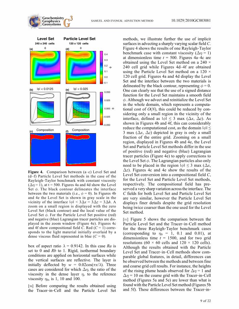
methods, we illustrate further the use of implicitsurfaces in advecting a sharply varying scalar fieldC.Figure 4 shows the results of one Rayleigh‐Taylorbenchmark case with constant viscosity (Dh = 1)at dimensionless time t = 500. Figures 4a–4c areobtained using the Level Set method on a 240 ×240 cell grid while Figures 4d–4f are obtainedusing the Particle Level Set method on a 120 ×120 cell grid. Figures 4a and 4d display the LevelSet and the interface between the two materials isdelineated by the black contour, representing � = 0.One can clearly see that the use of a signed distancefunction for the Level Set maintains a smooth field�. Although we advect and reinitialize the Level Setin the whole domain, which represents a computa-tional cost of O(N), this could be reduced by con-sidering only a small region in the vicinity of theinterface, defined as ∣�∣ ≤ 3 max (Dx, Dz). Asshown in Figures 4b and 4f, this can considerablyreduce the computational cost, as the domain ∣�∣ ≤3 max (Dx, Dz) depicted in gray is only a smallfraction of the entire grid. Zooming on a smallregion, displayed in Figures 4b and 4e, the LevelSet and Particle Level Set methods differ in the useof positive (red) and negative (blue) Lagrangiantracer particles (Figure 4e) to apply corrections tothe Level Set �. The Lagrangian particles also onlyneed to be placed in the region ∣�∣ ≤ 3 max (Dx,Dz). Figures 4c and 4e show the results of theLevel Set conversion into a compositional field C,for the Level Set and Particle Level Set methods,respectively. The compositional field has pre-served a very sharp variation across the interface. TheC fields for both Level Set and Particle Level Setare very similar, however the Particle Level Setdisplays finer details despite the grid resolutionbeing twice coarser than the one used for the LevelSet method.

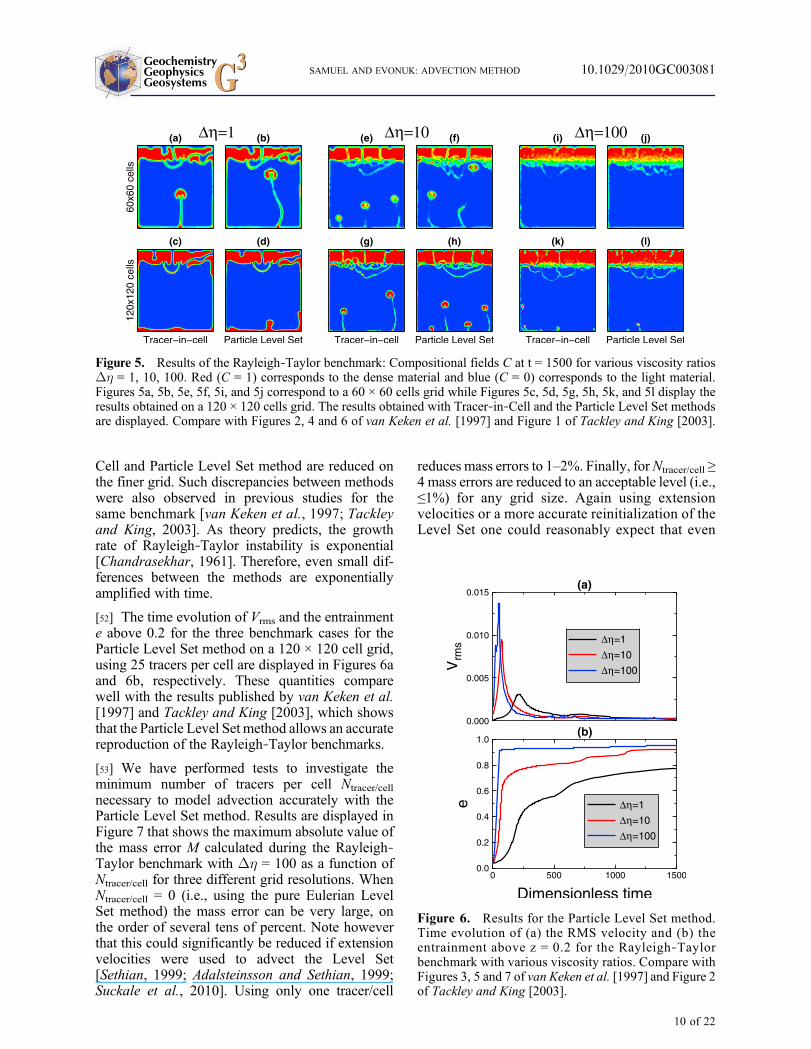
[51] Figure 5 shows the comparison between theParticle Level Set and the Tracer‐in‐Cell methodfor the three Rayleigh‐Taylor benchmark cases(corresponding to h0 = 1, 0.1 and 0.01), atdimensionless time t = 1500, and for two gridresolutions (60 × 60 cells and 120 × 120 cells).Although the results obtained with the ParticleLevel Set and Tracer‐in‐Cell methods show com-parable global features, in detail, differences canbe observed between the methods and between fineand coarse grid cell results. For instance, the heightsof the rising plume heads observed for Dh = 1 andDh = 10 on the coarse grid with the Tracer‐in‐Cellmethod (Figures 5a and 5e) are lower than what isfoundwith the Particle Level Set method (Figures 5band 5f). These differences between the Tracer‐in‐

Figure 4. Comparison between (a–c) Level Set and(d–f) Particle Level Set methods in the case of theRayleigh‐Taylor benchmark with constant viscosity(Dh = 1), at t = 500. Figures 4a and 4d show the LevelSet �. The black contour delineates the interfacebetween the two materials (i.e., � = 0). In Figures 4band 4e the Level Set is shown in gray scale in thevicinity of the interface ∣�∣ < 3Dx = 3Dz = 3Dh. Azoom on a small region is displayed with the zeroLevel Set (black contour) and the local value of theLevel Set �. For the Particle Level Set positive (red)and negative (blue) Lagrangian tracer particles are dis-played in the zoom window (Figure 4e). Figures 4cand 4f show compositional field C. Red (C = 1) corre-sponds to the light material initially overlaid by adense viscous fluid represented in blue (C = 0).

GeochemistryGeophysicsGeosystems G3G3 SAMUEL AND EVONUK: ADVECTION METHOD 10.1029/2010GC003081

9 of 22

Cell and Particle Level Set method are reduced onthe finer grid. Such discrepancies between methodswere also observed in previous studies for thesame benchmark [van Keken et al., 1997; Tackleyand King, 2003]. As theory predicts, the growthrate of Rayleigh‐Taylor instability is exponential[Chandrasekhar, 1961]. Therefore, even small dif-ferences between the methods are exponentiallyamplified with time.

[52] The time evolution of Vrms and the entrainmente above 0.2 for the three benchmark cases for theParticle Level Set method on a 120 × 120 cell grid,using 25 tracers per cell are displayed in Figures 6aand 6b, respectively. These quantities comparewell with the results published by van Keken et al.[1997] and Tackley and King [2003], which showsthat the Particle Level Set method allows an accuratereproduction of the Rayleigh‐Taylor benchmarks.

[53] We have performed tests to investigate theminimum number of tracers per cell Ntracer/cell

necessary to model advection accurately with theParticle Level Set method. Results are displayed inFigure 7 that shows the maximum absolute value ofthe mass error M calculated during the Rayleigh‐Taylor benchmark with Dh = 100 as a function ofNtracer/cell for three different grid resolutions. WhenNtracer/cell = 0 (i.e., using the pure Eulerian LevelSet method) the mass error can be very large, onthe order of several tens of percent. Note howeverthat this could significantly be reduced if extensionvelocities were used to advect the Level Set[Sethian, 1999; Adalsteinsson and Sethian, 1999;Suckale et al., 2010]. Using only one tracer/cell

reduces mass errors to 1–2%. Finally, forNtracer/cell ≥4 mass errors are reduced to an acceptable level (i.e.,≤1%) for any grid size. Again using extensionvelocities or a more accurate reinitialization of theLevel Set one could reasonably expect that even

Figure 5. Results of the Rayleigh‐Taylor benchmark: Compositional fields C at t = 1500 for various viscosity ratiosDh = 1, 10, 100. Red (C = 1) corresponds to the dense material and blue (C = 0) corresponds to the light material.Figures 5a, 5b, 5e, 5f, 5i, and 5j correspond to a 60 × 60 cells grid while Figures 5c, 5d, 5g, 5h, 5k, and 5l display theresults obtained on a 120 × 120 cells grid. The results obtained with Tracer‐in‐Cell and the Particle Level Set methodsare displayed. Compare with Figures 2, 4 and 6 of van Keken et al. [1997] and Figure 1 of Tackley and King [2003].

Figure 6. Results for the Particle Level Set method.Time evolution of (a) the RMS velocity and (b) theentrainment above z = 0.2 for the Rayleigh‐Taylorbenchmark with various viscosity ratios. Compare withFigures 3, 5 and 7 of van Keken et al. [1997] and Figure 2of Tackley and King [2003].

GeochemistryGeophysicsGeosystems G3G3 SAMUEL AND EVONUK: ADVECTION METHOD 10.1029/2010GC003081

10 of 22

smaller values of Ntracer/cell necessary to modeladvection accurately with the Particle Level Setmethod. This should be investigated in the future.For comparison we have displayed in Figure 7similar curves obtained with the Tracer‐in‐Cellmethod. Larger values of Ntracer/cell (i.e., 9) are nec-essary to reduce mass errors below 1%. Overall, we

verified with all the 2D and 3D cases presented inthis paper the following rules of thumb for theminimum value of Ntracer/cell required in order toconserve mass accurately in a domain with n spatialdimensions:

Particle Level Set : Ntracer=cell � 2n ð20aÞ

Tracer � in� Cell : Ntracer=cell � 3n: ð20bÞ

The above rules are compatible with previous stud-ies using the Tracer‐in‐Cell method [van Keken etal., 1997; Tackley and King, 2003; Gerya andYuen, 2003] and Particle Level Set method[Enright et al., 2002, 2005].

[54] Additional selected quantities for these caseswith various grid resolutions are listed in Table 1.The values obtained with the Particle Level Set orthe Tracer‐in‐Cell method compare well with thoselisted in van Keken et al. [1997] and Tackley andKing [2003]. In addition, both methods conservemass within less than 1% for any grid size. Forreference we have included in Table 1 several casescalculated with the Level Set method, which illus-trates that mass conservation for the pure EulerianLevel Set method is more problematic and requireshigher grid resolution.

[55] Figure 8 shows the computational time spentfor advecting the compositional field tadv normal-

Figure 7. Results for the Rayleigh‐Taylor benchmarkwith a viscosity ratio Dh = 100. Maximum value ofthe mass error for various grid resolutions as a functionof the number of tracer particles per cell, for both theTracer‐in‐Cell (dashed line and circles) and the ParticleLevel Set (solid lines and triangles) methods. The grayarea represents the domain where the mass is reasonablywell conserved (i.e., max ∣M∣ < 1%).

Table 1. Selected Quantities for the Rayleigh‐Taylor Benchmark Problemsa

Method Grid Growth Rate g t (max Vrms) max Vrms max ∣DM∣(%) mean ∣DM∣(%)

Dh = 1Level Set 60 × 60 0.006607 228.88 0.002925 4.51 2.29Level Set 120 × 120 0.011066 215.87 0.003051 1.68 0.66Level Set 240 × 240 0.011519 211.52 0.003093 0.04 0.02Particle Level Set 60 × 60 0.010643 215.57 0.003087 0.56 0.12Particle Level Set 120 × 120 0.011549 212.22 0.003109 0.18 0.04Tracer‐in‐Cell 60 × 60 0.011143 213.72 0.003135 0.14 0.05Tracer‐in‐Cell 120 × 120 0.011953 214.04 0.003129 0.07 0.03

Dh = 10Level Set 60 × 60 0.040860 78.48 0.009087 3.03 1.14Level Set 120 × 120 0.044414 75.89 0.009269 1.72 0.59Level Set 240 × 240 0.046040 73.45 0.009480 0.18 0.07Particle Level Set 60 × 60 0.046090 71.98 0.009375 0.83 0.24Particle Level Set 120 × 120 0.046034 74.07 0.009414 0.63 0.10Tracer‐in‐Cell 60 × 60 0.043853 75.86 0.009193 0.34 0.10Tracer‐in‐Cell 120 × 120 0.046188 72.54 0.009185 0.31 0.59

Dh = 100Level Set 60 × 60 0.09787 55.81 0.01212 3.67 1.37Level Set 120 × 120 0.10309 51.33 0.01414 0.64 0.20Level Set 240 × 240 0.10359 50.65 0.01445 0.27 0.09Particle Level Set 60 × 60 0.10477 51.06 0.01360 0.98 0.44Particle Level Set 120 × 120 0.10354 51.09 0.01405 0.84 0.23Tracer‐in‐Cell 60 × 60 0.10343 52.90 0.01292 0.52 0.30Tracer‐in‐Cell 120 × 120 0.10138 51.23 0.01392 0.33 0.16

aFor the cases calculated with the Particle Level Set and Tracer‐in‐Cell method, 25 tracers per cell are used.

GeochemistryGeophysicsGeosystems G3G3 SAMUEL AND EVONUK: ADVECTION METHOD 10.1029/2010GC003081

11 of 22

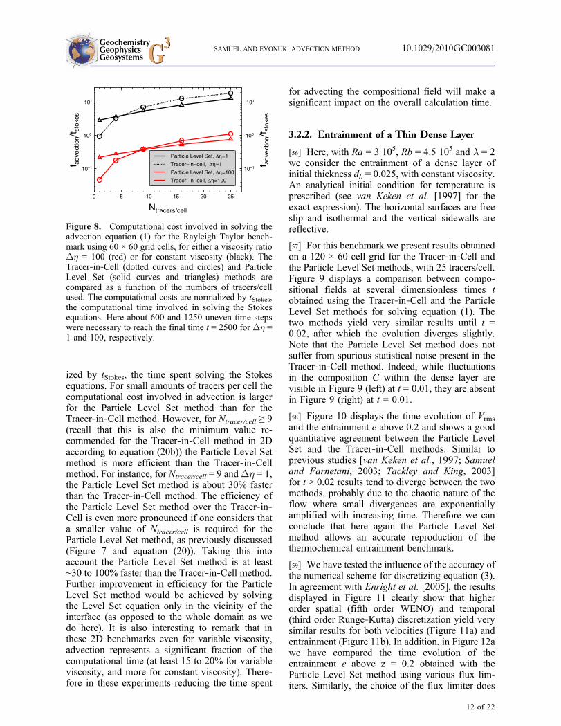
ized by tStokes, the time spent solving the Stokesequations. For small amounts of tracers per cell thecomputational cost involved in advection is largerfor the Particle Level Set method than for theTracer‐in‐Cell method. However, for Ntracer/cell ≥ 9(recall that this is also the minimum value re-commended for the Tracer‐in‐Cell method in 2Daccording to equation (20b)) the Particle Level Setmethod is more efficient than the Tracer‐in‐Cellmethod. For instance, for Ntracer/cell = 9 andDh = 1,the Particle Level Set method is about 30% fasterthan the Tracer‐in‐Cell method. The efficiency ofthe Particle Level Set method over the Tracer‐in‐Cell is even more pronounced if one considers thata smaller value of Ntracer/cell is required for theParticle Level Set method, as previously discussed(Figure 7 and equation (20)). Taking this intoaccount the Particle Level Set method is at least∼30 to 100% faster than the Tracer‐in‐Cell method.Further improvement in efficiency for the ParticleLevel Set method would be achieved by solvingthe Level Set equation only in the vicinity of theinterface (as opposed to the whole domain as wedo here). It is also interesting to remark that inthese 2D benchmarks even for variable viscosity,advection represents a significant fraction of thecomputational time (at least 15 to 20% for variableviscosity, and more for constant viscosity). There-fore in these experiments reducing the time spent

for advecting the compositional field will make asignificant impact on the overall calculation time.

3.2.2. Entrainment of a Thin Dense Layer

[56] Here, with Ra = 3 105, Rb = 4.5 105 and l = 2we consider the entrainment of a dense layer ofinitial thickness db = 0.025, with constant viscosity.An analytical initial condition for temperature isprescribed (see van Keken et al. [1997] for theexact expression). The horizontal surfaces are freeslip and isothermal and the vertical sidewalls arereflective.

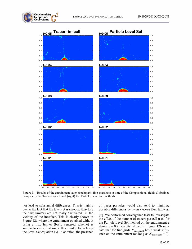
[57] For this benchmark we present results obtainedon a 120 × 60 cell grid for the Tracer‐in‐Cell andthe Particle Level Set methods, with 25 tracers/cell.Figure 9 displays a comparison between compo-sitional fields at several dimensionless times tobtained using the Tracer‐in‐Cell and the ParticleLevel Set methods for solving equation (1). Thetwo methods yield very similar results until t =0.02, after which the evolution diverges slightly.Note that the Particle Level Set method does notsuffer from spurious statistical noise present in theTracer‐in‐Cell method. Indeed, while fluctuationsin the composition C within the dense layer arevisible in Figure 9 (left) at t = 0.01, they are absentin Figure 9 (right) at t = 0.01.

[58] Figure 10 displays the time evolution of Vrms

and the entrainment e above 0.2 and shows a goodquantitative agreement between the Particle LevelSet and the Tracer‐in‐Cell methods. Similar toprevious studies [van Keken et al., 1997; Samueland Farnetani, 2003; Tackley and King, 2003]for t > 0.02 results tend to diverge between the twomethods, probably due to the chaotic nature of theflow where small divergences are exponentiallyamplified with increasing time. Therefore we canconclude that here again the Particle Level Setmethod allows an accurate reproduction of thethermochemical entrainment benchmark.

[59] We have tested the influence of the accuracy ofthe numerical scheme for discretizing equation (3).In agreement with Enright et al. [2005], the resultsdisplayed in Figure 11 clearly show that higherorder spatial (fifth order WENO) and temporal(third order Runge‐Kutta) discretization yield verysimilar results for both velocities (Figure 11a) andentrainment (Figure 11b). In addition, in Figure 12awe have compared the time evolution of theentrainment e above z = 0.2 obtained with theParticle Level Set method using various flux lim-iters. Similarly, the choice of the flux limiter does

Figure 8. Computational cost involved in solving theadvection equation (1) for the Rayleigh‐Taylor bench-mark using 60 × 60 grid cells, for either a viscosity ratioDh = 100 (red) or for constant viscosity (black). TheTracer‐in‐Cell (dotted curves and circles) and ParticleLevel Set (solid curves and triangles) methods arecompared as a function of the numbers of tracers/cellused. The computational costs are normalized by tStokes,the computational time involved in solving the Stokesequations. Here about 600 and 1250 uneven time stepswere necessary to reach the final time t = 2500 for Dh =1 and 100, respectively.

GeochemistryGeophysicsGeosystems G3G3 SAMUEL AND EVONUK: ADVECTION METHOD 10.1029/2010GC003081

12 of 22

not lead to substantial differences. This is mainlydue to the fact that the level set is smooth, thereforethe flux limiters are not really “activated” in thevicinity of the interface. This is clearly shown inFigure 12a where the entrainment obtained withoutusing a flux limiter (basic centered scheme) issimilar to cases that use a flux limiter for solvingthe Level Set equation (3). In addition, the presence

of tracer particles would also tend to minimizepossible differences between various flux limiters.

[60] We performed convergence tests to investigatethe effect of the number of tracers per cell used forthe Particle Level Set method on the entrainment eabove z = 0.2. Results, shown in Figure 12b indi-cate that for fine grids Ntracer/cell has a weak influ-ence on the entrainment (as long as Ntracer/cell > 0).

Figure 9. Results of the entrainment layer benchmark: five snapshots in time of the Compositional fields C obtainedusing (left) the Tracer‐in‐Cell and (right) the Particle Level Set methods.

GeochemistryGeophysicsGeosystems G3G3 SAMUEL AND EVONUK: ADVECTION METHOD 10.1029/2010GC003081

13 of 22

This means that only one tracer per cell is sufficientto resolve accurately sub‐grid scale features withthe Particle Level Set method. However, this is nota sufficient condition since, as pointed out insection 3.2.1 and in Figure 7, at least 4 tracers percell are needed to reduce mass errors to less than1% in 2D.

[61] Note that with such a small initial layerthickness db, sub‐grid scale resolution is critical forthis benchmark problem. This is partly the reasonwhy Eulerian approaches fail to reproduce thisbenchmark [van Keken et al., 1997] (in addition todiffusion and dispersion errors). To illustrate thisfurther, we have performed experiments with thepure Eulerian Level Set method (i.e., no tracers) andfind that even on a 240 × 120 grid the entrainment eabove z = 0.2 is almost zero, throughout the wholecalculation. This underestimation of the entrainmentis a direct consequence of the fact that pure EulerianLevel Set fails to capture sub‐grid scale features,as shown by Suckale et al. [2010]. The ability toresolve sub‐grid scales represents certainly one ofthe most attractive advantages of the Particle LevelSet method compared to other Eulerian approaches,including the pure Eulerian Level Set method itself.

[62] In summary, the comparisons performedbetween implicit surfaces and Tracer‐in‐Cell meth-ods for 2D flows have shown that the Particle LevelSet method can yield similar results to the Tracer‐in‐Cell method at the same grid resolution. Thisincludes cases where sub‐grid scale resolution iscritical.

3.3. Three‐Dimensional Flows

[63] Advection in three‐dimensional flows is com-putationally expensive, in particular when usingLagrangian methods. Therefore we have conducted3D experiments to compare the accuracy and thecomputational efficiency of the Tracer‐in‐Cell andthe Particle Level Set methods.

[64] We have selected three geodynamic problems,the first two involving strong topological changesin C and sub‐scale flow that are particularly diffi-cult to model accurately. In these problems, pureEulerian methods solving equation (1) would auto-

Figure 10. Results of the entrainment layer bench-mark. Time evolution of (a) the RMS velocity and(b) the entrainment above z = 0.2 obtained using theTracer‐in‐Cell and the Particle Level Set methods. Com-pare with Figure 12 of van Keken et al. [1997] and withFigure 4 of Tackley and King [2003].

Figure 11. Results of the entrainment layer benchmarkwith the Particle Level Set method on a 120 × 60 cellwith 25 tracers/cell. Comparison between the resultsobtained using high order time and space discretization(third order TVD Rung Kutta and fifth order WENOscheme for spatial derivatives, red dashed curves) andresults obtained with a lower accuracy (black curves)for both time (first order explicit) and space (secondorder TVD with Sweby flux limiter). Time evolutionof (a) the RMS velocity and (b) the entrainment abovez = 0.2.

GeochemistryGeophysicsGeosystems G3G3 SAMUEL AND EVONUK: ADVECTION METHOD 10.1029/2010GC003081

14 of 22

matically fail to compare well with the more robustLagrangian (e.g., Tracer‐in‐Cell) methods. For allcases presented in this section, we use 27 tracers/cellfor both the Tracer‐in‐Cell and Particle Level Setmethods.

3.3.1. Convective Stirring of a PassiveHeterogeneity

[65] We consider the homogenization via convectivestirring of a passive heterogeneity in a 1 × 1 × 1domain discretized using 60 × 60 × 60 grid cells. Thehorizontal surfaces are free‐slip and isothermal andthe vertical walls are reflective. The values of thegoverning parameters are Ra = 107 and Rb = 0. Theinitial temperature condition, shown in Figure 13awas obtained after reaching a statistical steadystate. At t = 0 a spherical passive heterogeneity(C = 1) of dimensionless radius 0.25 is placed in thecenter of the domain, while the composition in thesurrounding fluid is initialized toC = 0 (Figure 13b).The calculation is run for several thousand timesteps, which would scale for the Earth to a fewbillion years.

[66] Figure 14 displays snapshots in time of the iso‐surface C = 0.5 and of a horizontal cut at mid‐depthobtained by solving equation (1) with the Tracer‐in‐Cell (left) or the Particle Level Set (right)methods. Despite the strong topological changesdue to the repeated action of convective stretchingand folding, the results obtained with both methodsagree very well. This remains true even in the latestages, where the compositional field becomesmore homogeneous.

[67] The time evolution of the composition is alsomonitored via histograms that show the distributionof C at dimensionless time corresponding to thesnapshots displayed in Figure 15. The histogramsobtained with the Tracer‐in‐Cell and Particle Level

Figure 12. Results of the entrainment layer benchmarkwith the Particle Level Set method. Time evolution ofthe entrainment above z = 0.2. (a) Influence of the fluxlimiters applied for solving equation (3) on a 120 ×60 cell with 16 tracers/cell. (b) Convergence test withtwo grid resolutions and various numbers of tracers/cell.

Figure 13. Initial condition for the 3D passive convective stirring test. (a) Dimensionless temperature T. (b) Dimen-sionless velocity field (arrows) and iso‐contour displaying the interface between the passive heterogeneity and thesurrounding mantle.

GeochemistryGeophysicsGeosystems G3G3 SAMUEL AND EVONUK: ADVECTION METHOD 10.1029/2010GC003081

15 of 22

Set method also agree very well. They both showthat the C distribution evolves towards a Gaussianshape as a result of vigorous convective stirring.

[68] This first 3D test demonstrates the abilityof the Particle Level Set method to compete withrobust Tracer‐in‐Cell advection. Moreover, theParticle Level Set method allows a significantreduction in computational time because only tra-cers near the interface are involved, contrary to theTracer‐in‐Cell method where tracers are locatedeverywhere in the computational domain. Never-theless, in this particular example the computa-tional gain of using the Particle Level Set methoddecreases with time because the area occupied bythe zero Level Set increases exponentially withtime as a result of convective stirring. Consequently,the number of tracers particles used to correctthe Level Set increases. However, this increase isbounded by the total number of grid cells, and sta-bilizes around an asymptotic value Ntrmax ∼ N ×

Ntracer/cell, corresponding ultimately to a fullyhomogenized state.

3.3.2. Destabilization of a Dense Layer

[69] We consider the homogenization via convectivestirring of a passive heterogeneity in a 2 × 2 × 1domain discretized using 60 × 60 × 30 grid cells. Thehorizontal surfaces are free‐slip and isothermal andthe vertical walls are reflective. The values of thegoverning parameters are Ra = 107 and Rb = 2 106.Similar to the previous case, the initial temperaturecondition was obtained after running a convectioncalculation until reaching a statistical steady state.At t = 0 a dense layer of dimensionless thickness0.3 (C = 1) is placed in the bottom of the domain,while the composition in the overlying fluid is ini-tialized to C = 0. The calculation is run until com-plete destabilization and homogenization of thedense layer is achieved.

Figure 14. Results of the 3D passive convective stirring test. Comparison of the time evolution of the passive com-positional field C obtained with the Tracer‐in‐Cell and the Particle Level Set methods. Iso‐contours corresponding toC = 0.5 (green) and a mid‐depth surface cut are shown.

GeochemistryGeophysicsGeosystems G3G3 SAMUEL AND EVONUK: ADVECTION METHOD 10.1029/2010GC003081

16 of 22

[70] Figure 16 displays four snapshots in time ofthe iso‐surface C = 0.5 and transparent surface cutsfor cases where equation (1) is solved with theTracer‐in‐Cell (Figures 16a, 16c, 16e, and 16g) orthe Particle Level Set (Figures 16b, 16d, 16f, and16h) methods. The dense layer gets progressivelyheated by the bottom surface until the thermal den-sity contrast overcomes the compositional densitycontrast. After this stage is reached the dense layerrapidly forms a topography (Figures 16a and 16b)and large domes of dense material rise up and arestirred by convective motions (Figures 16c–16g).

The comparison of the Particle Level Set and Tracer‐in‐Cell cases are in good qualitative agreement, andthe results obtained with both methods agree verywell. A more quantitative comparison between theresults obtained with the Tracer‐in‐Cell and ParticleLevel Set the methods is shown in Figure 17, whichdisplays the time evolution of the entrainment eabove z = 0.3. As expected from the dynamic evo-lution observed in Figure 16, the entrainmentincreases rapidly as the dense layer is destabilized andreaches the asymptotic value of 0.7 correspondingto the complete homogenization of the heteroge-neous material. Both the Particle Level Set andTracer‐in‐Cell methods yield very similar results.Further comparison can be made using the com-position histograms displayed in Figure 18 at fourdifferent elapsed times corresponding to the snap-shots shown in Figure 16. The distribution evolves

Figure 15. Results of the 3D passive convectivestirring test. Comparison of the time evolution ofthe passive compositional field C obtained with theTracer‐in‐Cell and the Particle Level Set methods. Thehistograms represent the distribution of the composi-tional field C within the computational domain. The Cdistribution evolves towards a Gaussian shape as a resultof vigorous convective stirring. The dimensionless time tcorrespond to the snapshots displayed in Figure 14.

Figure 16. Results of the 3D destabilization of a thickdense layer test. Comparison of the time evolution of thepassive compositional field C obtained with the Tracer‐in‐Cell and the Particle Level Set methods. Iso‐contourscorresponding to C = 0.5 (green).

GeochemistryGeophysicsGeosystems G3G3 SAMUEL AND EVONUK: ADVECTION METHOD 10.1029/2010GC003081

17 of 22

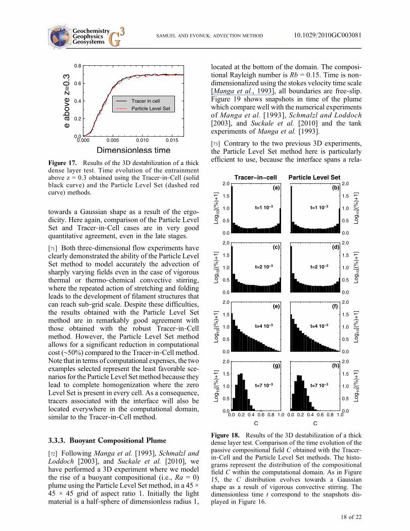
towards a Gaussian shape as a result of the ergo-dicity. Here again, comparison of the Particle LevelSet and Tracer‐in‐Cell cases are in very goodquantitative agreement, even in the late stages.

[71] Both three‐dimensional flow experiments haveclearly demonstrated the ability of the Particle LevelSet method to model accurately the advection ofsharply varying fields even in the case of vigorousthermal or thermo‐chemical convective stirring,where the repeated action of stretching and foldingleads to the development of filament structures thatcan reach sub‐grid scale. Despite these difficulties,the results obtained with the Particle Level Setmethod are in remarkably good agreement withthose obtained with the robust Tracer‐in‐Cellmethod. However, the Particle Level Set methodallows for a significant reduction in computationalcost (∼50%) compared to the Tracer‐in‐Cell method.Note that in terms of computational expenses, the twoexamples selected represent the least favorable sce-narios for the Particle Level Set method because theylead to complete homogenization where the zeroLevel Set is present in every cell. As a consequence,tracers associated with the interface will also belocated everywhere in the computational domain,similar to the Tracer‐in‐Cell method.

3.3.3. Buoyant Compositional Plume

[72] Following Manga et al. [1993], Schmalzl andLoddoch [2003], and Suckale et al. [2010], wehave performed a 3D experiment where we modelthe rise of a buoyant compositional (i.e., Ra = 0)plume using the Particle Level Set method, in a 45 ×45 × 45 grid of aspect ratio 1. Initially the lightmaterial is a half‐sphere of dimensionless radius 1,

located at the bottom of the domain. The composi-tional Rayleigh number is Rb = 0.15. Time is non‐dimensionalized using the stokes velocity time scale[Manga et al., 1993], all boundaries are free‐slip.Figure 19 shows snapshots in time of the plumewhich compare well with the numerical experimentsof Manga et al. [1993], Schmalzl and Loddoch[2003], and Suckale et al. [2010] and the tankexperiments of Manga et al. [1993].

[73] Contrary to the two previous 3D experiments,the Particle Level Set method here is particularlyefficient to use, because the interface spans a rela-

Figure 17. Results of the 3D destabilization of a thickdense layer test. Time evolution of the entrainmentabove z = 0.3 obtained using the Tracer‐in‐Cell (solidblack curve) and the Particle Level Set (dashed redcurve) methods.

Figure 18. Results of the 3D destabilization of a thickdense layer test. Comparison of the time evolution of thepassive compositional field C obtained with the Tracer‐in‐Cell and the Particle Level Set methods. The histo-grams represent the distribution of the compositionalfield C within the computational domain. As in Figure15, the C distribution evolves towards a Gaussianshape as a result of vigorous convective stirring. Thedimensionless time t correspond to the snapshots dis-played in Figure 16.

GeochemistryGeophysicsGeosystems G3G3 SAMUEL AND EVONUK: ADVECTION METHOD 10.1029/2010GC003081

18 of 22

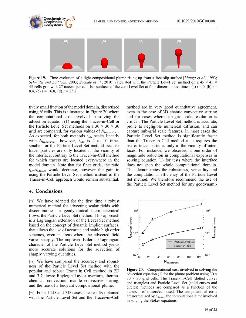
tively small fraction of themodel domain, discretizedusing N cells. This is illustrated in Figure 20 wherethe computational cost involved in solving theadvection equation (1) using the Tracer‐in‐Cell orthe Particle Level Set methods on a 30 × 30 × 30grid are compared, for various values of Ntracers/cell.As expected, for both methods tadv scales linearlywith Ntracers/cell, however, tadv is 4 to 10 timessmaller for the Particle Level Set method becausetracer particles are only located in the vicinity ofthe interface, contrary to the Tracer‐in‐Cell methodfor which tracers are located everywhere in themodel domain. Note that for finer grids, the ratiotadv/tStokes would decrease, however the gain inusing the Particle Level Set method instead of theTracer‐in‐Cell approach would remain substantial.

4. Conclusions

[74] We have adapted for the first time a robustnumerical method for advecting scalar fields withdiscontinuities in geodynamical thermochemicalflows: the Particle Level Set method. This approachis a Lagrangian extension of the Level Set methodbased on the concept of dynamic implicit surfaces,that allows the use of accurate and stable high orderschemes, even in areas where the advected fieldvaries sharply. The improved Eulerian‐Lagrangiancharacter of the Particle Level Set method yieldsmore accurate solutions for the advection ofsharply varying quantities.

[75] We have compared the accuracy and robust-ness of the Particle Level Set method with thepopular and robust Tracer‐in‐Cell method in 2Dand 3D flows: Rayleigh‐Taylor overturn, thermo-chemical convection, mantle convective stirring,and the rise of a buoyant compositional plume.

[76] For all 2D and 3D cases, the results obtainedwith the Particle Level Set and the Tracer‐in‐Cell

method are in very good quantitative agreement,even in the case of 3D chaotic convective stirringand for cases where sub‐grid scale resolution iscritical. The Particle Level Set method is accurate,prone to negligible numerical diffusion, and cancapture sub‐grid scale features. In most cases theParticle Level Set method is significantly fasterthan the Tracer‐in‐Cell method as it requires theuse of tracer particles only in the vicinity of inter-faces. For instance, we observed a one order ofmagnitude reduction in computational expenses insolving equation (1) for tests where the interfacedoes not span the whole computational domain.This demonstrates the robustness, versatility andthe computational efficiency of the Particle LevelSet method. We therefore recommend the use ofthe Particle Level Set method for any geodynami-

Figure 19. Time evolution of a light compositional plume rising up from a free‐slip surface [Manga et al., 1993;Schmalzl and Loddoch, 2003; Suckale et al., 2010] calculated with the Particle Level Set method on a 45 × 45 ×45 cells grid with 27 tracers per cell. Iso‐surfaces of the zero Level Set at four dimensionless times: (a) t = 0, (b) t =8.4, (c) t = 16.8, (d) t = 25.2.

Figure 20. Computational cost involved in solving theadvection equation (1) for the plume problem using 30 ×30 × 30 grid cells. The Tracer‐in‐Cell (dotted curvesand triangles) and Particle Level Set (solid curves andcircles) methods are compared as a function of thenumbers of tracers/cell used. The computational costsare normalized by tStokes, the computational time involvedin solving the Stokes equations.

GeochemistryGeophysicsGeosystems G3G3 SAMUEL AND EVONUK: ADVECTION METHOD 10.1029/2010GC003081

19 of 22

cal problem that involves the pure advection ofsharply varying quantities.

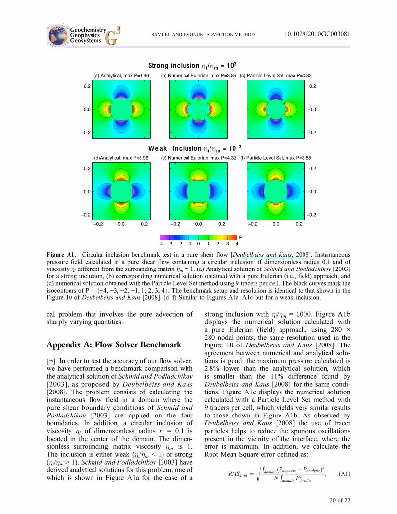
Appendix A: Flow Solver Benchmark

[77] In order to test the accuracy of our flow solver,we have performed a benchmark comparison withthe analytical solution of Schmid and Podladchikov[2003], as proposed by Deubelbeiss and Kaus[2008]. The problem consists of calculating theinstantaneous flow field in a domain where thepure shear boundary conditions of Schmid andPodladchikov [2003] are applied on the fourboundaries. In addition, a circular inclusion ofviscosity hi of dimensionless radius ri = 0.1 islocated in the center of the domain. The dimen-sionless surrounding matrix viscosity hm is 1.The inclusion is either weak (hi/hm < 1) or strong(hi/hm > 1). Schmid and Podladchikov [2003] havederived analytical solutions for this problem, one ofwhich is shown in Figure A1a for the case of a

strong inclusion with hi/hm = 1000. Figure A1bdisplays the numerical solution calculated witha pure Eulerian (field) approach, using 280 ×280 nodal points, the same resolution used in theFigure 10 of Deubelbeiss and Kaus [2008]. Theagreement between numerical and analytical solu-tions is good: the maximum pressure calculated is2.8% lower than the analytical solution, whichis smaller than the 11% difference found byDeubelbeiss and Kaus [2008] for the same condi-tions. Figure A1c displays the numerical solutioncalculated with a Particle Level Set method with9 tracers per cell, which yields very similar resultsto those shown in Figure A1b. As observed byDeubelbeiss and Kaus [2008] the use of tracerparticles helps to reduce the spurious oscillationspresent in the vicinity of the interface, where theerror is maximum. In addition, we calculate theRoot Mean Square error defined as:

RMSerror ¼ffiffiffiffiffiffiffiffiffiffiffiffiffiffiffiffiffiffiffiffiffiffiffiffiffiffiffiffiffiffiffiffiffiffiffiffiffiffiffiffiffiffiffiffiffiffiffiffiffiffiffiffiffiRdomainðPnumeric � PanalyticÞ2

NRdomain P

2analitic

s; ðA1Þ

Figure A1. Circular inclusion benchmark test in a pure shear flow [Deubelbeiss and Kaus, 2008]. Instantaneouspressure field calculated in a pure shear flow containing a circular inclusion of dimensionless radius 0.1 and ofviscosity hi different from the surrounding matrix hm = 1. (a) Analytical solution of Schmid and Podladchikov [2003]for a strong inclusion, (b) corresponding numerical solution obtained with a pure Eulerian (i.e., field) approach, and(c) numerical solution obtained with the Particle Level Set method using 9 tracers per cell. The black curves mark theisocontours of P = {−4, −3, −2, −1, 1, 2, 3, 4}. The benchmark setup and resolution is identical to that shown in theFigure 10 of Deubelbeiss and Kaus [2008]. (d–f) Similar to Figures A1a–A1c but for a weak inclusion.

GeochemistryGeophysicsGeosystems G3G3 SAMUEL AND EVONUK: ADVECTION METHOD 10.1029/2010GC003081

20 of 22

where N is the total number of grid points used. Wefind that RMSerror = 0.13% and 0.18% for theresults displayed in Figures A1e and A1f, respec-tively. These values also compare well with theresults of Deubelbeiss and Kaus [2008].

[78] Such a comparison has also been carried out inSuckale et al. [2010], except that they considered aweak inclusion with hi/hm = 10−3. We have there-fore performed the same tests. The analytical andnumerical solutions are displayed in Figures A1d,A1e and A1f). We find a larger error (yet accept-able) for the maximum pressure than in the stronginclusion test, and comparable rms error values:RMSerror = 0.15% and 0.12% for the results dis-played in Figures A1e and A1f, respectively.

[79] As noted by Deubelbeiss and Kaus [2008], thegood agreement between numerical and analyticalsolutions is mainly due to the combination ofstaggered grid and harmonic averaging of viscosi-ties from cell centers to nodal points. Indeed, wefind that geometric or arithmetic averaging of vis-cosities systematically yields larger differencesbetween numerical and analytical solutions.

[80] These tests demonstrate the robustness of ourStokes solver for large viscosity contrasts.

Acknowledgments

[81] The authors are grateful to Peter van Keken and an anon-ymous reviewer for their thoughtful suggestions, which signif-icantly improved the manuscript. Henri Samuel acknowledgesthe funds from the Stifterverband für die Deutsche Wissenchaft.2D figures were made with the Generic Mapping Tools[Wessel and Smith, 1995]. 3D figures were drawn with Para-View software.

References

Adalsteinsson, D., and J. A. Sethian (1999), The fast construc-tion of extension velocities in level set methods, J. Comput.Phys., 148, 2–22.

Albers, M. (2000), A local mesh refinement multigrid methodfor 3‐D convection problems with strongly variable viscosity,J. Comput. Phys., 160(1), 126–150.

Blankenbach, B., et al. (1989), A benchmark comparison formantle convection codes, Geophys. J. Int., 98(1), 23–38.

Brackbill, J. U., D. B. Kothe, and C. Zemach (1992), A con-tinuum method for modeling surface tension, J. Comput.Phys., 100, 335–354.

Chandrasekhar, S. (1961), Hydrodynamic and HydromagneticStability, 643 pp., Dover, New York.

Chemia, Z., H. Koyi, and H. Schmeling (2008), Numericalmodelling of rise and fall of a dense layer in salt diapirs,Geophys. J. Int., 172, 798–816.

Christensen, U. R. (1989), Mixing by time‐dependent convec-tion, Earth Planet. Sci. Lett., 95, 382–394.

Christensen, U. R., and A. W. Hofmann (1994), Segregation ofsubducted oceanic crust in the convecting mantle, J. Geo-phys. Res., 99, 19,867–19,884.

Demmel, J. W., S. C. Eisenstat, J. R. Gilbert, X. S. Li, andJ. W. Liu (1999), A supernodal approach to sparse partialpivoting, SIAM J. Matrix Anal. Appl., 20, 720–755.

Deubelbeiss, Y., and B. J. Kaus (2008), Comparison of Eulerianand Lagrangian numerical techniques for the Stokes equationsin the presence of strongly varying viscosity, Phys. EarthPlanet. Inter., 171, 92–111.

Enright, D., R. Fedkiw, J. Ferziger, and I. Mitchell (2002),A hybrid particle level set method for improved interfacecapturing, J. Comput. Phys., 183(1), 83–116.

Enright, D., F. Lossaso, and R. Fedkiw (2005), A fast andaccurate semi‐Lagrangian particle level set method, Comput.Surf., 83, 479–490.

Farnetani, C. G., and M. A. Richards (1995), Thermal entrain-ment and melting in mantle plumes, Earth Planet. Sci. Lett.,136, 251–267.

Farnetani, C. G., and H. Samuel (2003), Lagrangian structuresand stirring in the Earth’s mantle, Earth Planet. Sci. Lett.,206, 335–348.

Farnetani, C. G., and H. Samuel (2005), Beyond the thermalplume paradigm, Geophys. Res. Lett. , 32 , L07311,doi:10.1029/2005GL022360.

Fletcher, C. A. J. (1991), Computational Techniques for FluidDynamics, 401 pp., Springer, New York.

Gerya, T. V., and D. A. Yuen (2003), Characteristics‐basedmarker‐in‐cell method with conservative finite‐differencesschemes for modeling geological flows with strongly variabletransport properties, Phys. Earth Planet. Inter., 140, 293–318.

Gross, L., L. Bourgouin, A. J. Hale, and H.‐B. Muhlhaus(2007), Interface modeling in incompressible media usinglevel sets in Escript, Phys. Earth Planet. Inter., 163, 23–34.

Harten, A. (1984), On a class of high resolution total‐variation‐stable finite‐difference schemes, SIAM J. Numer. Anal., 21,1–23.

Harten, A., B. Engquist, S. Osher, and S. R. Chakravarthy(1987), Uniformly high order accurate essentially non‐oscillatory schemes, III, J. Comput. Phys., 71, 231–303.

Hoïnk, T., J. Schmalzl, and U. Hansen (2006), Dynamicsof metal‐silicate separation in a terrestrial magma ocean,Geochem. Geophys. Geosyst., 7, Q09008, doi:10.1029/2006GC001268.

Ichikawa, H., S. Labrosse, and K. Kurita (2010), Directnumerical simulation of an iron rain in the magma ocean,J. Geophys. Res., 115, B01404, doi:10.1029/2009JB006427.

Lenardic, A., and W. M. Kaula (1993), Numerical treatment ofgeodynamic viscous‐flow problems involving the advectionof material interfaces, J. Geophys. Res., 98, 8243–8260.

Lin, J.‐R., T. V. Gerya, P. J. Tackley, D. A. Yuen, and G. J.Golabek (2009), Numerical modeling of protocore destabili-zation during planetary accretion: Methodology and results,204, 732–748.

Lin, S.‐C., and P. E. van Keken (2005), Multiple volcanic epi-sodes of flood basalts caused by thermochemical mantleplumes, Nature, 436, 250–252.

Lin, S.‐C., and P. E. van Keken (2006), Deformation, stirringand material transport in thermochemical plumes, Geophys.Res. Lett., 33, L20306, doi:10.1029/2006GL027037.

Liu, X.‐D., S. Osher, and T. Chan (1994), Weighted essen-tially non‐oscillatory schemes, J. Comput. Phys., 115,200–212.

GeochemistryGeophysicsGeosystems G3G3 SAMUEL AND EVONUK: ADVECTION METHOD 10.1029/2010GC003081

21 of 22

Manga, M. (1996), Mixing of chemical heterogeneities in themantle: Effect of viscosity differences, Geophys. Res. Lett,23, 403–406.

Manga, M., and H. Stone (1994), Interactions between bubblesin magmas and lavas: Effects of bubble deformation, J. Vol-canol. Geotherm. Res., 63, 267–279.

Manga, M., H. Stone, and R. O’Connell (1993), The interac-tion of plume heads with compositional discontinuities inthe Earth’s mantle, J. Geophys. Res., 98, 19,979–19,990.

Ménard, T., S. Tanguy, and A. Berlemont (2007), Couplinglevel set/VOF/ghost fluid methods: Validation and applica-tion to 3D simulation of the primary break‐up of a liquidjet, Int. J. Multiphase Flow, 33, 510–524.

Min, C., and F. Gibou (2007), A second order accurate levelset method on non‐graded adaptive cartesian grids, J. Comput.Phys., 225, 300–321.

Monteux, J., Y. Ricard, N. Coltice, F. Dubuffet, andM. Ulvrova(2009), A model of metal‐silicate separation on growing pla-nets, Earth Planet. Sci. Lett., 287, 353–362.

Muehlhaus, H.‐B., L. Moresi, B. Hobbs, and D. F. (2002),Large amplitude folding in finely layered viscoelastic rockstructures, Pure Appl. Geophys., 159, 2311–2333.

Osher, S., and R. Fedkiw (2003), Level Set Methods andDynamic Implicit Surfaces, 273 pp., Springer, New York.

Osher, S., and J. A. Sethian (1988), Fronts propagating withcurvature‐dependent speed: Algorithms based on Hamilton‐Jacobi formulations, J. Comput. Phys., 79, 12–49.

Patankar, S. V. (1980), Numerical Heat Transfer and FluidFlow, 197 pp., Hemisphere, New York.

Press,W. H., S. A. Teukolsky,W.Vetterling, and B. P. Flannery(1992), Numerical Recipes, 933 pp., Cambridge Univ. Press,Cambrige, U. K.

Ricard, Y., O. Sramek, and F. Dubuffet (2009), A multi‐phasemodel of runaway core‐mantle segregation in planetaryembryos, Earth Planet. Sci. Lett., 284, 144–150.

Roe, P. L. (1986), Characteristic‐based schemes for the Eulerequations, Annu. Rev. Fluid Mech., 18, 337–365.

Rubie, D. C., H. J. Melosh, J. E. Reid, C. Liebske, andK. Righter (2003), Mechanisms of metal‐silicate equilibrationin the terrestrial magma ocean, Earth Planet. Sci. Lett., 205,239–255.

Samuel, H. (2009), STREAMV: A fast, robust and modularnumerical code for modeling various 2D geodynamic sce-narios, annual report, pp. 203–205, Bayerisches Geoinst.,Bayreuth, Germany.

Samuel, H., and D. Bercovici (2006), Oscillating and stagnat-ing plumes in the Earth’s lower mantle, Earth Planet. Sci.Lett., 248, 90–105.

Samuel, H., and C. G. Farnetani (2003), Thermochemical con-vection and helium concentrations in mantle plumes, EarthPlanet. Sci. Lett., 207, 39–56.

Samuel, H., and P. J. Tackley (2008), Dynamics of core for-mation and equilibration by negative diapirism, Geochem.Geophys. Geosyst., 9, Q06011, doi:10.1029/2007GC001896.

Samuel, H., P. J. Tackley, and M. Evonuk (2010), Heat parti-tioning during core formation by negative diapirism in terres-trial planets, Earth Planet. Sci. Lett., 290, 13–19.

Schmalzl, J., and A. Loddoch (2003), Using subdivision sur-faces and adaptive surface simplification algorithms formodeling chemical heterogeneities in geophysical flows,Geochem. Geophys. Geosyst., 4(9), 8303, doi:10.1029/2003GC000578.

Schmalzl, J., G. A. Houseman, and U. Hansen (1996), Mixingin vigorous, time‐dependent three‐dimensional convectionand application to Earth’s mantle, J. Geophys. Res., 101,21,847–21,858.

Schmeling, H., et al. (2008), A benchmark comparison ofspontaneous subduction models—Towards a free surface,Phys. Earth. Planet. Inter., 171, 198–223.

Schmid, D. W., and Y. Y. Podladchikov (2003), Analyticalsolutions for deformable elliptical inclusions in generalshear, Geophys. J. Int., 155, 269–288.

Sethian, J. A. (1999), Level Set Methods and Fast MarchingMethods, Cambridge Univ. Press, Cambridge, U. K.

Shu, C.‐W., and S. Osher (1988), Efficient implementationof essentially non‐oscillatory shock‐capturing schemes,J. Comput. Phys., 77, 439–471.

Smolakiewicz, P. K. (1984), A fully multidimensional positivedefinite advection algorithm with small implicit diffusion,J. Comput. Phys., 54, 325–362.

Suckale, J., J.‐C. Nave, and B. H. Hager (2010), It takes threeto tango: 1. Simulating buoyancy‐driven flow in the presenceof large viscosity contrasts, J. Geophys. Res., 115, B07409,doi:10.1029/2009JB006916.

Sussman, M., and E. Puckett (2000), A coupled level set andvolume‐of‐fluid method for computing 3D and axisymmetricincompressible two‐phase flows, J. Comput. Phys., 162,301–337.

Sussman, M., P. Smereka, and S. Osher (1994), A level setapproach for computing solutions to incompressible two‐phase flow, J. Comput. Phys., 114, 146–159.

Sweby, P. K. (1984), High resolution schemes using flux limit-ers for hyperbolic conservation laws, SIAM J. Numer. Anal.,21, 995–1011.

Tackley, P. J. (2002), Strong heterogeneity caused by deepmantle layering, Geochem. Geophys. Geosyst., 3(4), 1024,doi:10.1029/2001GC000167.

Tackley, P. J., and S. D. King (2003), Testing the tracer ratiomethod for modeling active compositional fields in mantleconvection simulations, Geochem. Geophys. Geosyst., 4(4),8302, doi:10.1029/2001GC000214.

van Hunen, J., A. P. van den Berg, and N. J. Vlaar (2004),Various mechanisms to induce present‐day shallow flat sub-duction and implications for the younger Earth: A numericalparameter study, Phys. Earth. Planet. Inter., 146, 179–174.

van Keken, P. E., S. D. King, H. Schmeling, U. R. Christensen,D. Neumeister, and M.‐P. Doin (1997), A comparison ofmethods for the modeling of thermochemical convection,J. Geophys. Res., 102, 22,477–22,495.

van Keken, P. E., C. J. Ballentine, and E. Hauri (2003), Con-vective mixing in the Earth’s mantle, in Geochemistry ofthe Mantle and Core, edited by K. K. Turekian and H. D.Holland, pp. 471–491, Elsevier, New York.

Verhoeven, J., and J. Schmalzl (2009), A numerical methodfor investigating crystal settling in convecting magmachambers, Geochem. Geophys. Geosyst., 10, Q12007,doi:10.1029/2009GC002509.

Weinberg, R. F., and H. Schmeling (1992), Polydiapirs:Multiwavelength gravity structures, J. Struct. Geol., 4,425–436.

Wessel, P., and W. H. F. Smith (1995), Eos Trans. AGU, 76,329.

GeochemistryGeophysicsGeosystems G3G3 SAMUEL AND EVONUK: ADVECTION METHOD 10.1029/2010GC003081

22 of 22