Hardware-Accelerated Lagrangian-EulerianTexture Advection for 2D Flow Visualization

Daniel Weiskopf1 Gordon Erlebacher2 Matthias Hopf1 Thomas Ertl1

1Visualization and Interactive Systems Group,University of Stuttgart, Germany

� 2School of Computational Science and InformationTechnology, Florida State University, USA†

Abstract

A hardware-based approach for visualizing un-steady flow fields by means of Lagrangian-Eulerianadvection is presented. Both noise-based and dye-based texture advection is supported. The imple-mentation allows the advection of each texture tobe performed completely on the graphics hardwarein a single-pass rendering. We discuss experienceswith the interactive visualization of unsteady flowfields that become possible due to the high visual-ization speed of the hardware-based approach.

1 Introduction

Traditionally, flow fields are visualized as a col-lection of streamlines, pathlines, or streaklines thatoriginate from user-specified seed points. The prob-lem of placing seed points for particle tracing atappropriate positions is approached, e.g., by em-ploying spot noise [14], LIC (line integral convolu-tion) [1], texture splats [2], texture advection [10],equally spaced streamlines [13], or flow-guidedstreamline seeding [15].

In this paper, we present and discuss a hardware-based approach for visualizing unsteady flow fieldsby means of Lagrangian-Eulerian advection [8, 9].This approach combines the advantages of the La-grangian and Eulerian formalisms: A dense collec-tion of particles is integrated backward in time (La-grangian step), while the color distribution of theimage pixels are updated in place (Eulerian step). Acommon problem of dense representations of vec-tor fields is that they are computationally expensive,especially when a high-resolution domain is used.We demonstrate that texture advection maps ratherwell to the programmable features of modern con-

���weiskopf,hopf,ertl � @informatik.uni-stuttgart.de

†erlebach@mailer.csit.fsu.edu

sumer graphics hardware: Noise and dye advectioncan be done in single pass rendering, respectively;therefore, a speed-up of one to two orders of mag-nitudes compared to an optimized CPU-based ap-proach can be achieved. We discuss how our inter-active visualization tool facilitates the understand-ing of unsteady flows in the context of numericalfluid dynamics.

The hardware approach of this paper is influ-enced by previous work on hardware-based LIC [5]and texture advection [7]. These early implementa-tions were based on pixel shaders exclusively avail-able on SGI MXE graphics and were limited byquite restrictive sets of operations. Therefore, mul-tiple rendering passes were necessary and accuracywas limited by the resolution of the frame buffer.In [16], we presented a GeForce 3-based textureadvection approach that is particularly well-suitedfor dye advection; a similar approach was indepen-dently developed for a fluid visualization demo [11]by Nvidia.

2 Lagrangian-Eulerian Advection

In this section, a brief survey of Lagrangian-Eulerian advection of 2D textures is presented. Amore detailed description can be found in [9]. Notethat the description in this section partly differsfrom the algorithm [9] to allow a better mappingto graphics hardware.

In the traditional Lagrangian approach to particletracing, each single particle can be identified indi-vidually and the trajectory of each particle is com-puted separately according to the ordinary differen-tial equation

d �r � t �dt � �v ��r � t �� t �� (1)

where �r � t � describes the path of the particle and�v � �r t � represents the vector field to be visualized.

VMV 2002 Erlangen, Germany, November 20–22, 2002

In the Eulerian approach, particles loose their iden-tity and particle properties (such as color) are ratherstored in a property field. Positions are only givenimplicitly as the coordinates of a property field.

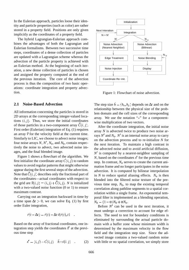
The hybrid Lagrangian-Eulerian approach com-bines the advantages of both the Lagrangian andEulerian formalisms. Between two successive timesteps, coordinates of a dense collection of particlesare updated with a Lagrangian scheme whereas theadvection of the particle property is achieved withan Eulerian method. At the beginning of each iter-ation, a new dense collection of particles is chosenand assigned the property computed at the end ofthe previous iteration. The core of the advectionprocess is thus the composition of two basic oper-ations: coordinate integration and property advec-tion.

2.1 Noise-Based Advection

All information concerning the particles is stored in2D arrays at the corresponding integer-valued loca-tions � i j � . Thus, we store the initial coordinatesof those particles in a two-component array �C � i j � .First order (Eulerian) integration of Eq. (1) requiresan array �v for the velocity field at the current time.Similarly to LIC, we choose to advect noise images;four noise arrays N, N

�, Na, and Nb, contain respec-

tively the noise to advect, two advected noise im-ages, and the final blended image.

Figure 1 shows a flowchart of the algorithm. Wefirst initialize the coordinate array �C � i j � to randomvalues to avoid regular patterns that might otherwiseappear during the first several steps of the advection.Note that �C � i j � describes only the fractional part ofthe coordinates—actual coordinates with respect tothe grid are �x � i j � � � i j � � �C � i j � . N is initializedwith a two-valued noise function (0 or 1) to ensuremaximum contrast.

Carrying out an integration backward in time bya time span ∆t � 0, we can solve Eq. (1) by firstorder Euler integration,

�r � t � ∆t � � �r � t ��� ∆t �v ��r � t �� t ���

Based on the array of fractional coordinates, one in-tegration step yields the coordinates �x � at the previ-ous time step

�x � � � i j � � �C � i j ��� �h � �v � i j ��� (2)

Noise Advection(Nearest Neighbor)

Integration

Initialization

N a

Noise Advection(Bilinear)

Noise Injection

Edge Treatment

Coordinate Re−init.

Noise Blending

Display

Next Interation

N = N’

N’

N b

Figure 1: Flowchart of noise advection.

The step size �h � � hx hy � depends on ∆t and on therelationship between the physical size of the prob-lem domain and the cell sizes of the correspondingarray. We use the notation “ � ” for a component-wise multiplication of two vectors.

After the coordinate integration, the initial noisearray N is advected twice to produce two noise ar-rays N

�and Na. N

�is an internal noise array to carry

on the advection process and to re-initialize N forthe next iteration. To maintain a high contrast inthe advected noise and to avoid artificial diffusion,N�

is computed by a nearest-neighbor sampling ofN, based on the coordinates �x � for the previous timestep. In contrast, Na serves to create the current ani-mation frame and no longer participates in the noiseadvection. It is computed by bilinear interpolationin N to reduce spatial aliasing effects. Na is thenblended into the filtered noise texture of the pre-vious time step, Nb, to map the existing temporalcorrelation along pathline segments to a spatial cor-relation within a single frame. An exponential tem-poral filter is implemented as a blending operation,Nb � � 1 � α � Nb

� αNa.Before N

�can be used in the next iteration, it

must undergo a correction to account for edge ef-fects. The need to test for boundary conditions iseliminated by surrounding the actual particle do-main with a buffer zone whose minimum width isdetermined by the maximum velocity in the flowfield and the integration step size. Since the ad-vected image contains a two-valued random noisewith little or no spatial correlation, we simply store

666

new random noise in the buffer zone as the new in-formation potentially flowing into the physical do-main. At the next iteration, N will contain thesevalues and some of them will be advected to the in-terior of the physical domain by Eq. (2). Since ran-dom noise has no spatial correlation, the advectionof the surrounding buffer values into the interior re-gion produces no visible artifacts.

Another correction step counteracts a duplicationeffect that occurs during the computation of Eq. (2).Effectively, if particles in neighboring cells of N

�

retrieve their property value from within the samecell of N, this value will be duplicated in the cor-responding cells of N

�. This effect is undesirable

since lower noise frequency reduces the spatial res-olution of the features that can be represented. Thisduplication effect is caused by the discrete natureof our texture sampling and is further reinforced inregions where the flow has a strong positive diver-gence. To break the undesirable formation of uni-form blocks and to maintain a high frequency ran-dom noise, we inject a user-specified percentage ofnoise into N

�. Random cells are chosen in N

�and

their value is inverted. From experience, a fixed per-centage of two to three percent of randomly invertedcells provides adequate results over a wide range offlows.

Finally, the array �C � i j � of fractional coordinatesis re-initialized to prepare a new collection of parti-cles to be integrated backward in time for the nextiteration. Nearest-neighbor sampling implies that aproperty value can only change if it originates froma different cell. If fractional coordinates were ne-glected in the next iteration, subcell displacementswould be ignored and the flow would be frozenwhere the velocity magnitude or the integration stepsize is too small. Therefore, the array �C � i j � is set tothe fractional part of the coordinates �x � originatingfrom Eq. (2).

2.2 Dye-Based Advection

The process of dye advection can be emulated by re-placing the advected noise texture by a texture witha smooth pattern. A dye is released into the flow andadvected with the fluid, giving results analogouslyto traditional experimental flow dynamics. Thenoise texture is simply replaced by a texture of uni-form background color upon which the dye is de-posed. As the high frequency nature of the texture isremoved, many of the above correction steps are no

longer required and the implementation is greatlysimplified: Particle injection into the edge buffer,random particle injection, constant interpolation ofthe noise texture, coordinate re-initialization, andnoise blending can be neglected.

The point of injection can be freely chosen by theuser by “painting” into the fluid. Points of finite di-ameter or lines are possible shapes of dye sources.The dye can be released once and tracked (whichapproximates the path of a particle), released con-tinuously at a single point (generates a streakline),or pulsated (the dye is turned on intermittently, cre-ating time surfaces). Colored dye is used of distin-guish different injection points or times in the re-sulting patterns.

Dye advection is exclusively based on bilinearlookup in the particle texture of the previous timestep. In contrast to noise advection, no nearest-neighbor sampling is needed because dye has amuch smaller spatial frequency than noise. Bilinearinterpolation computes the true position of particleswithin a cell and therefore overcomes the problemthat subcell displacements are ignored and the flowis frozen where the velocity magnitude or the inte-gration step size is too small. Thus, fractional co-ordinates can be neglected. As a disadvantage ofbilinear interpolation, the dye gradually smears outdue to an implicit, artificial “diffusion” process.

3 Advection on Graphics Hardware

The above advection algorithm was originally de-signed for an optimized CPU-based implementa-tion. For a mapping to the GPU, advection speedand an appropriate accuracy are the two main is-sues. To achieve the first goal, the number of ren-dering passes and the number of texture lookups ineach pass should be minimized. Therefore, we min-imize the number of textures necessary to representthe arrays in the advection process.

Limited accuracy on the GPU is a major issue formost hardware-based algorithms. The main prob-lem is the extremely low resolution of only 8 bitsper channel in the frame buffer or texture on con-sumer market GPUs. This can only be overcomeby computing crucial operations with higher reso-lution, e.g., in the fragment shader unit.

666

3.1 Noise Advection on the GPU

In what follows, we demonstrate single pass noiseadvection on the ATI Radeon 8500. The Radeonprovides two phases in a single rendering pass, withup to six texture lookups and eight numerical op-erations in each phase. The two-component array�C � i j � and the single-component arrays N and Nbare combined in a single RGBα texture referred toas a particle texture. The intermediate arrays N

�and

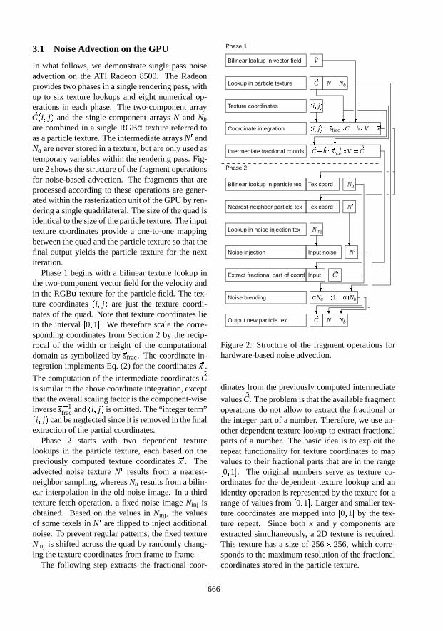
Na are never stored in a texture, but are only used astemporary variables within the rendering pass. Fig-ure 2 shows the structure of the fragment operationsfor noise-based advection. The fragments that areprocessed according to these operations are gener-ated within the rasterization unit of the GPU by ren-dering a single quadrilateral. The size of the quad isidentical to the size of the particle texture. The inputtexture coordinates provide a one-to-one mappingbetween the quad and the particle texture so that thefinal output yields the particle texture for the nextiteration.

Phase 1 begins with a bilinear texture lookup inthe two-component vector field for the velocity andin the RGBα texture for the particle field. The tex-ture coordinates � i j � are just the texture coordi-nates of the quad. Note that texture coordinates liein the interval

�0 1 � . We therefore scale the corre-

sponding coordinates from Section 2 by the recip-rocal of the width or height of the computationaldomain as symbolized by �sfrac. The coordinate in-tegration implements Eq. (2) for the coordinates �x � .The computation of the intermediate coordinates ˜�Cis similar to the above coordinate integration, exceptthat the overall scaling factor is the component-wiseinverse �s � 1

frac and � i j � is omitted. The “integer term”� i j � can be neglected since it is removed in the finalextraction of the partial coordinates.

Phase 2 starts with two dependent texturelookups in the particle texture, each based on thepreviously computed texture coordinates �x � . Theadvected noise texture N

�results from a nearest-

neighbor sampling, whereas Na results from a bilin-ear interpolation in the old noise image. In a thirdtexture fetch operation, a fixed noise image Ninj isobtained. Based on the values in Ninj, the valuesof some texels in N

�are flipped to inject additional

noise. To prevent regular patterns, the fixed textureNinj is shifted across the quad by randomly chang-ing the texture coordinates from frame to frame.

The following step extracts the fractional coor-

�

�C N Nb

�� �

�

� �

�

�

� ��

�

�

�

αNa ��� 1 � α Nb

Ninj

�V

�C N Nb

� i j

� i j � �sfrac � �C � �h � �V � �x �C � �h � �s � 1

frac ��V � ˜�C

Tex coord Na

Tex coord N

Input noise N

Input�C Extract fractional part of coord

Noise injection

Lookup in noise injection tex

Nearest-neighbor particle tex

Bilinear lookup in particle tex

Noise blending

Intermediate fractional coords

Coordinate integration

Texture coordinates

Lookup in particle texture

Bilinear lookup in vector field

Output new particle tex

Phase 2

Phase 1

Figure 2: Structure of the fragment operations forhardware-based noise advection.

dinates from the previously computed intermediate

values ˜�C. The problem is that the available fragmentoperations do not allow to extract the fractional orthe integer part of a number. Therefore, we use an-other dependent texture lookup to extract fractionalparts of a number. The basic idea is to exploit therepeat functionality for texture coordinates to mapvalues to their fractional parts that are in the range�0 1 � . The original numbers serve as texture co-

ordinates for the dependent texture lookup and anidentity operation is represented by the texture for arange of values from

�0 1 � . Larger and smaller tex-

ture coordinates are mapped into�0 1 � by the tex-

ture repeat. Since both x and y components areextracted simultaneously, a 2D texture is required.This texture has a size of 256 � 256, which corre-sponds to the maximum resolution of the fractionalcoordinates stored in the particle texture.

666

After the fractional coordinates are extracted, theadvected noise Na is blended with Nb, the filterednoise of the previous iteration. Finally, edge cor-rection is implemented in a separate step by render-ing randomly shifted noise textures into the bufferzones. Note that some of the numerical opera-tions within a single box in the flowchart have tobe split into several consecutive operations in theactual fragment shader implementation (e.g, a sumof three terms has to be split into two summations).

3.2 Dye Advection on the GPU

As another application of texture advection, the pro-cess of dye advection can be emulated by replacingthe advected noise texture by a smooth dye texture.In Section 2.2, we described that many of the abovecorrection steps are no longer required and that theimplementation is greatly simplified: Particle injec-tion into the edge buffer, random particle injection,nearest-neighbor lookup in the noise texture, frac-tional coordinates, and noise blending can be ne-glected. Only the core advection step with bilinearinterpolation is required. User-specified dye injec-tion is implemented by rendering the dye sourcesinto the texture, after the actual advection part wasperformed.

3.3 Complete Visualization Process

The complete visualization process is as follows.First, the noise and the dye textures are advected,each in a single rendering pass. Here, we renderdirectly into a texture. Second, the just updated tex-tures serve as input to the actual rendering pass:The α channel of the noise texture is replicated toRGB colors (giving a gray-scale noise image) andblended with the colored dye texture. For an un-steady flow, the vector field is transferred from mainmemory to texture memory before each iteration.Otherwise, there is no difference between the im-plementation of unsteady and steady flows.

Since the blending of noise and dye textures re-quires only a simple fragment blending operation,more advanced postprocessing steps can also be in-cluded in the final rendering part. A useful postpro-cessing operation modulates the pixel intensity withthe magnitude of the velocity. In this way, ratheruninteresting regions of the flow that exhibit onlyslow motions are faded out in the noise texture byreducing their brightness; the important parts of the

flow are emphasized. This velocity mask is imple-mented by introducing a third texture lookup whichretrieves the vector field texture. The red and greenchannels of the flow texture hold the vx and vy com-ponents of the velocity. We assume that the bluechannel stores a weighting factor that depends onthe magnitude of the velocity; this weight has to becomputed by the CPU before the flow field is down-loaded to the GPU. In the final rendering pass, thebrightness of the noise texture can be scaled by thisweighting factor.

As another postprocessing operation, the repre-sentation of the flow can be superimposed over abackground image that provides additional context.For the implementation, another texture that repre-sents the background has to be fetched and blendedwith the noise and dye textures.

4 Implementation

We chose DirectX 8.1 [3] for our implementa-tion. One of the advantages of DirectX is that ad-vanced fragment operations are configured in theform of so-called pixel shader programs. Pixelshaders target a vendor-independent programmingenvironment (instead of vendor-specific OpenGLextensions). Another advantage is a rather sim-ple, assembler-like nature of pixel shader programs,as opposed to more difficult and complex OpenGLextensions. Moreover, the DirectX SDK providesan interactive environment for testing pixel shadercode, which facilitates debugging of fragment code.A very important advantage of DirectX is its bet-ter support by some vendors’ graphics drivers, bothwith respect to stability and performance. The mainreason for this is the much bigger market for Di-rectX products than for OpenGL products. Thetransfer between frame buffer and texture memoryis indispensable for the advection algorithm and isan example of better support by DirectX. On theATI Radeon 8500, only DirectX allows direct ren-dering into a texture and thus makes a transfer oftexture data completely superfluous.

A major problem with DirectX is the restrictionto Windows because many visualization environ-ments are based on Unix/Linux. OpenGL (with-out vendor-specific extensions) promotes platform-independent software development and very oftenthe resulting code can be included into existing vi-sualization tools.

666

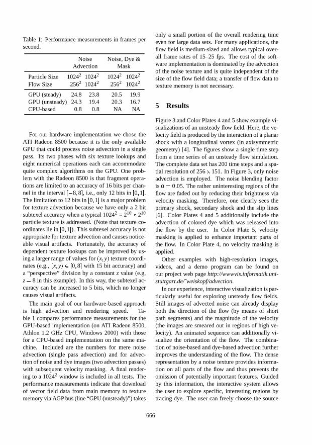
Table 1: Performance measurements in frames persecond.

Noise Noise, Dye &Advection Mask

Particle Size 10242 10242 10242 10242

Flow Size 2562 10242 2562 10242

GPU (steady) 24.8 23.8 20.5 19.9GPU (unsteady) 24.3 19.4 20.3 16.7CPU-based 0.8 0.8 NA NA

For our hardware implementation we chose theATI Radeon 8500 because it is the only availableGPU that could process noise advection in a singlepass. Its two phases with six texture lookups andeight numerical operations each can accommodatequite complex algorithms on the GPU. One prob-lem with the Radeon 8500 is that fragment opera-tions are limited to an accuracy of 16 bits per chan-nel in the interval

�� 8 8 � , i.e., only 12 bits in

�0 1 � .

The limitation to 12 bits in�0 1 � is a major problem

for texture advection because we have only a 2 bitsubtexel accuracy when a typical 10242 = 210 � 210

particle texture is addressed. (Note that texture co-ordinates lie in

�0 1 � ). This subtexel accuracy is not

appropriate for texture advection and causes notice-able visual artifacts. Fortunately, the accuracy ofdependent texture lookups can be improved by us-ing a larger range of values for � x y � texture coordi-nates (e.g., � x y � � �

0 8 � with 15 bit accuracy) anda “perspective” division by a constant z value (e.g,z � 8 in this example). In this way, the subtexel ac-curacy can be increased to 5 bits, which no longercauses visual artifacts.

The main goal of our hardware-based approachis high advection and rendering speed. Ta-ble 1 compares performance measurements for theGPU-based implementation (on ATI Radeon 8500,Athlon 1.2 GHz CPU, Windows 2000) with thosefor a CPU-based implementation on the same ma-chine. Included are the numbers for mere noiseadvection (single pass advection) and for advec-tion of noise and dye images (two advection passes)with subsequent velocity masking. A final render-ing to a 10242 window is included in all tests. Theperformance measurements indicate that downloadof vector field data from main memory to texturememory via AGP bus (line “GPU (unsteady)”) takes

only a small portion of the overall rendering timeeven for large data sets. For many applications, theflow field is medium-sized and allows typical over-all frame rates of 15–25 fps. The cost of the soft-ware implementation is dominated by the advectionof the noise texture and is quite independent of thesize of the flow field data; a transfer of flow data totexture memory is not necessary.

5 Results

Figure 3 and Color Plates 4 and 5 show example vi-sualizations of an unsteady flow field. Here, the ve-locity field is produced by the interaction of a planarshock with a longitudinal vortex (in axisymmetricgeometry) [4]. The figures show a single time stepfrom a time series of an unsteady flow simulation.The complete data set has 200 time steps and a spa-tial resolution of 256 � 151. In Figure 3, only noiseadvection is employed. The noise blending factoris α � 0 � 05. The rather uninteresting regions of theflow are faded out by reducing their brightness viavelocity masking. Therefore, one clearly sees theprimary shock, secondary shock and the slip lines[6]. Color Plates 4 and 5 additionally include theadvection of colored dye which was released intothe flow by the user. In Color Plate 5, velocitymasking is applied to enhance important parts ofthe flow. In Color Plate 4, no velocity masking isapplied.

Other examples with high-resolution images,videos, and a demo program can be found onour project web page http://wwwvis.informatik.uni-stuttgart.de/˜weiskopf/advection.

In our experience, interactive visualization is par-ticularly useful for exploring unsteady flow fields.Still images of advected noise can already displayboth the direction of the flow (by means of shortpath segments) and the magnitude of the velocity(the images are smeared out in regions of high ve-locity). An animated sequence can additionally vi-sualize the orientation of the flow. The combina-tion of noise-based and dye-based advection furtherimproves the understanding of the flow. The denserepresentation by a noise texture provides informa-tion on all parts of the flow and thus prevents theomission of potentially important features. Guidedby this information, the interactive system allowsthe user to explore specific, interesting regions bytracing dye. The user can freely choose the source

666

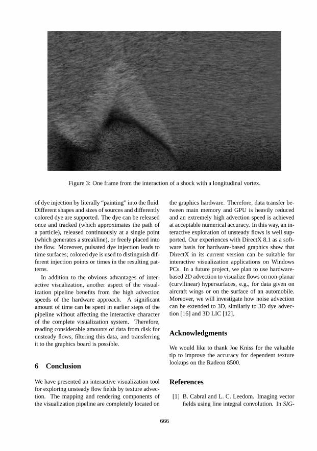
Figure 3: One frame from the interaction of a shock with a longitudinal vortex.

of dye injection by literally “painting” into the fluid.Different shapes and sizes of sources and differentlycolored dye are supported. The dye can be releasedonce and tracked (which approximates the path ofa particle), released continuously at a single point(which generates a streakline), or freely placed intothe flow. Moreover, pulsated dye injection leads totime surfaces; colored dye is used to distinguish dif-ferent injection points or times in the resulting pat-terns.

In addition to the obvious advantages of inter-active visualization, another aspect of the visual-ization pipeline benefits from the high advectionspeeds of the hardware approach. A significantamount of time can be spent in earlier steps of thepipeline without affecting the interactive characterof the complete visualization system. Therefore,reading considerable amounts of data from disk forunsteady flows, filtering this data, and transferringit to the graphics board is possible.

6 Conclusion

We have presented an interactive visualization toolfor exploring unsteady flow fields by texture advec-tion. The mapping and rendering components ofthe visualization pipeline are completely located on

the graphics hardware. Therefore, data transfer be-tween main memory and GPU is heavily reducedand an extremely high advection speed is achievedat acceptable numerical accuracy. In this way, an in-teractive exploration of unsteady flows is well sup-ported. Our experiences with DirectX 8.1 as a soft-ware basis for hardware-based graphics show thatDirectX in its current version can be suitable forinteractive visualization applications on WindowsPCs. In a future project, we plan to use hardware-based 2D advection to visualize flows on non-planar(curvilinear) hypersurfaces, e.g., for data given onaircraft wings or on the surface of an automobile.Moreover, we will investigate how noise advectioncan be extended to 3D, similarly to 3D dye advec-tion [16] and 3D LIC [12].

Acknowledgments

We would like to thank Joe Kniss for the valuabletip to improve the accuracy for dependent texturelookups on the Radeon 8500.

References

[1] B. Cabral and L. C. Leedom. Imaging vectorfields using line integral convolution. In SIG-

666

GRAPH 1993 Conference Proceedings, pages263–272, 1993.

[2] R. A. Crawfis and N. Max. Texture splatsfor 3D scalar and vector field visualization.In IEEE Visualization ’93 Proceedings, pages261–267, 1993.

[3] DirectX. Web Site: http://www.microsoft.com/directx.

[4] G. Erlebacher, M. Y. Hussaini, and C.-W. Shu.Interaction of a shock with a longitudinal vor-tex. J. Fluid Mech., 337:129–153, 1997.

[5] W. Heidrich, R. Westermann, H.-P. Seidel, andT. Ertl. Application of pixel textures in visual-ization and realistic image synthesis. In ACMSymposium on Interactive 3D Graphics, pages127–134, 1999.

[6] M. Y. Hussaini, G. Erlebacher, and B. Jo-bard. Real-time visualization of unsteady vec-tor fields. In 40th AIAA Aerospace SciencesMeeting, 2002.

[7] B. Jobard, G. Erlebacher, and M. Y. Hus-saini. Hardware-accelerated texture advectionfor unsteady flow visualization. In IEEE Visu-alization 2000 Proceedings, pages 155–162,2000.

[8] B. Jobard, G. Erlebacher, and M. Y. Hussaini.Lagrangian-Eulerian advection for unsteadyflow visualization. In IEEE Visualization 2001Proceedings, pages 53–60, 2001.

[9] B. Jobard, G. Erlebacher, and M. Y. Hussaini.Lagrangian-Eulerian advection of noise anddye textures for unsteady flow visualization.IEEE Transactions on Visualization and Com-puter Graphics, 8(3):211–222, 2002.

[10] N. Max, R. Crawfis, and D. Williams. Visual-izing wind velocities by advecting cloud tex-tures. In IEEE Visualization ’92 Proceedings,pages 171–178, 1992.

[11] Nvidia. OpenGL fluid visualization.Web Site: http://developer.nvidia.com/view.asp?IO=ogl fluid viz.

[12] C. Rezk-Salama, P. Hastreiter, C. Teitzel, andT. Ertl. Interactive exploration of volume lineintegral convolution based on 3D-texture map-ping. In IEEE Visualization ’99 Proceedings,pages 233–240, 1999.

[13] G. Turk and D. Banks. Image-guided stream-line placement. In SIGGRAPH 1996 Confer-ence Proceedings, pages 453–460, 1996.

[14] J. J. van Wijk. Spot noise-texture synthesis for

data visualization. In SIGGRPAPH 1991 Con-ference Proceedings, pages 309–318, 1991.

[15] V. Verma, D. Kao, and A. Pang. A flow-guidedstreamline seeding strategy. In IEEE Visu-alization 2000 Proceedings, pages 163–170,2000.

[16] D. Weiskopf, M. Hopf, and T. Ertl. Hardware-accelerated visualization of time-varying 2Dand 3D vector fields by texture advection viaprogrammable per-pixel operations. In VMV’01 Proceedings, pages 439–446. infix, 2001.

666

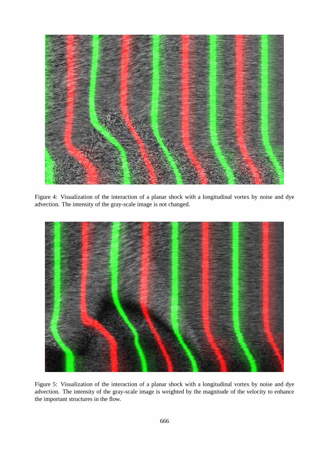
Figure 4: Visualization of the interaction of a planar shock with a longitudinal vortex by noise and dyeadvection. The intensity of the gray-scale image is not changed.

Figure 5: Visualization of the interaction of a planar shock with a longitudinal vortex by noise and dyeadvection. The intensity of the gray-scale image is weighted by the magnitude of the velocity to enhancethe important structures in the flow.

666