Comparison between Lagrangian and Eulerian

mesoscopic modelling approaches for inertial

particles suspended in decaying isotropic

turbulence

A. Kaufmann a,1 M. Moreau b O. Simonin b J. Helie b,2

aCERFACS, 42 Av. G. Coriolis, 31057 Toulouse, France, kaufmann@cerfacs.fr

bIMFT,UMR 5502 CNRS/INPT/UPS, Toulouse, France, simonin@imft.fr

Abstract

The purpose of this paper is to evaluate an unsteady Eulerian approach from a

direct comparison with a Lagrangian approach for the simulation of an ensemble

of non-colliding particles interacting with a decaying homogeneous isotropic turbu-

lence given by DNS. Comparison between both approaches is is carried out for two

different particle inertia from global instantaneous quantities such as particle kinetic

energy, local instantaneous Eulerian quantities such as particle number density and

spectral quantities such as spectral particle kinetic energy. The proposed Eulerian

approach yields instantaneous three dimensional velocity and number density fields

which are in very good agreement, at large scales, with the discrete particle simu-

lation results. However, appreciable discrepancies between the two approaches are

measured at small scales for the particles with larger inertia. Indeed, for Stokes

number value close to unity, segregation effects are very important and due to the

stiff gradients in number density the Eulerian method is limited by spatial grid res-

Preprint submitted to J. Comp. Physics 15 May 2006

olution. To overcome this numerical difficulty, a simulation approach using a bulk

viscosity is proposed.

Key words: particle laden flows, eulerian methods, preferential concentration,

compressibility

1 Introduction

A true direct numerical simulation (DNS) of dispersed two phase flows includes

the simulation of the carrier phase around each single particle (or droplet),

taking into account its deformation, to compute exactly the forces of the car-

rier phase acting upon it. Unfortunately such true DNS are today limited to

few particles [1,2]. When studying collective physical phenomena such as par-

ticle segregation or turbulence modulation occurring in industrial applications

or environmental flows, the full particle number cannot be accounted for and

requires approximations to limit the numerical cost. For very small particle

sizes compared to the typical energy containing scales, the momentum trans-

fer with the carrier phase can be modeled by some semi-empirical interaction

force expression that reduces to a drag law in the case of large density ra-

tio. The characteristics of the particles can be described by several means.

One possibility is the discrete particle simulation (DPS) approach in which

every particle is treated in an Lagrangian framework. An alternative method

is to consider only some collective characteristics of the particles in an Eule-

rian framework such as particle number density and mean particle velocity.

1 Present address : Siemens VDO, Regensburg Germany, An-

dre.Kaufmann@siemens.com2 Present address : Siemens VDO, Toulouse France, Jerome.Helie@siemens.com

2

Equilibrium Eulerian approaches [3,4] consider a transport equation for the

particle number density and compute the particle velocity using the carrier

phase velocity and a Taylor expansion for the equation of particle motion.

The expansion parameter is written in terms of the particle relaxation time to

carrier phase characteristic time ratio and such approaches are well suited for

small Stokes number values but lead to increasing error with increasing Stokes

number. Computation of particle laden flow for particle relaxation time larger

than the Kolmogorov time scale requires a transport equation for the particle

velocity in order to account accurately for inertia effects.

The purpose of the present paper is to compare predictions using an Eulerian

approach, with a transport equation for the particle velocity, to the reference

results obtained from discrete particle simulation (DPS) in a homogeneous

isotropic decaying gaseous turbulence given by DNS. Following Fevrier et

al. [5], a probability density function (PDF) f (1)p (cp;xp, t|Hf ) depending on

the particle velocity cp, the particle location xp at time t may be defined for a

given carrier flow realization Hf . This function gives the local instantaneous

probable number of particles with the given translation velocity up = cp and

obeys a Boltzmann-type kinetic equation, which may account for momentum

exchange with the carrier fluid and inter-particle collisions. Alternatively, in

analogy with the derivation of the Navier-Stokes equations in the frame of

kinetic theory [6], transport equations of the first order moments (such as

particle number density, mean velocity and fluctuant kinetic energy) may be

derived directly by averaging from the PDF kinetic equation [7]. Such an ap-

proach has been evaluated in previous a priori test from DPS coupled with

DNS or LES of forced homogeneous isotropic turbulence [8] and fully devel-

oped channel flow [9].

This study is the first attempt to solve the set of equations of the mesoscopic

3

Eulerian approach allowing ”a posteriori” comparison of the model predictions

with DPS results. In the present study, interaction forces are limited to Stokes

drag and two-way coupling effects are neglected, that is the carrier phase is

considered as uninfluenced by the presence of the dispersed phase. Particles

are of identical size and the gravity force is not considered. However, the ex-

tension to evaporating droplets, gravity force, modelling non-linear effect in

the drag force and other interaction forces is not in conflict with the derivation

methodology of the Eulerian field equations. Also the introduction of inter-

particle collisions is without major difficulties [10]. The drastic assumptions

are chosen in order not to obscure the effects related to particle turbulence

dynamic interaction.

Comparisons between Eulerian an Lagrangian simulation results are performed

for three levels. First the integral properties of the dispersed phase such as vol-

ume averaged particle kinetic energy and particle-fluid velocity correlation are

investigated. The second comparison concerns the local instantaneous field

properties such as particle number density np, correlated velocity up,i and

random uncorrelated kinetic energy δθp. The third comparison concerns the

spectral properties such as the particle kinetic energy spectrum Ep(k) and

the fluid-particle correlation spectrum Efp(k) computed from the correlated

particle velocity field.

To allow these comparisons a spatial filtering procedure is used to project

Lagrangian quantities on a grid and thus to obtain continuous fields from

the DPS results. To validate such a procedure, several projection methods

are tested on a one-dimensional synthetic case. In the case of non-interacting

particles, the number of particles per cell for a given carrier phase realization

is not limited, a gaussian projector is then validated using DPS results with

different simulated particle numbers at the kinetic energy spectrum level. The

4

ˆEp(k) ˆEfp(k) Ep(k) Efp(k)

Eulerian Field Variables

np up,i δθp

Mesoscopic Field Variables

np up,i δθp

DPSEulerian

Simulation

q2p qfp q2

p qfp δq2p⇐⇒(1)

⇐⇒(2)

⇐⇒(3)

⇓Volume Filtering m

⇑ ⇑

⇓ ⇓

Fig. 1. Methodology for comparison of DPS to Eulerian Simulation Approaches

particle number densities np and the correlated velocity up obtained by the

volume filtering procedure can then be compared to it’s counterpart from the

mesoscopic Eulerian Simulation (fig. 1).

The paper is organised as follow : the mesoscopic eulerian approach is pre-

sented in section 2, then the projection procedure to obtain Eulerian field

from Lagrangian results is described and validated (section 3), the section 4

concerns the numerical test case, finally Eulerian simulation predictions are

discused and compared with DPS results in section 5.

2 The mesoscopic Eulerian approach

In turbulent particle laden flow the dispersed phase cannot be regarded as

independent of the carrier phase turbulence [11]. Therefore several statistical

5

approaches rely on joint carrier-phase, dispersed-phase probability functions.

In particular, the joint fluid-particle PDF equations may be used to establish

transport equations for carrier phase and dispersed phase quantities such as

number densities, momentum and energies as well as fluid-particle correla-

tions [7,12]. Since the interaction of particles and turbulence is rather com-

plicated, modelling of the unclosed terms is a difficult and challenging issue.

Due to the statistical character of such approaches, three dimensional un-

steady effects, as they can also be found in single phase turbulent flow, cannot

be represented. One important example among others are segregation effects

which need a two-point PDF approach [13].

To derive local instantaneous Eulerian equations in dilute flows (without tur-

bulence modification by the particles), Fevrier et al. [5,8,10] introduce an

ensemble average over dispersed-phase realizations conditioned by one carrier-

phase realization. Such an averaging procedure leads to a conditional velocity

PDF for the dispersed phase,

f (1)p (cp,x, t; Hf ) =

⟨W (1)

p (cp,x, t) |Hf

⟩. (1)

W (1)p is the fine grid PDF of the realizations of position and velocity in time

of any given particle [14] and Hf is the given carrier flow realization. Ignoring

particle collisions, the conditional PDF equation takes the form :

∂

∂tfp +

∂

∂xj

cp,j fp +∂

∂cp,j

[Fp,j

mp

fp

]= 0 (2)

This PDF equation can be used to derive transport equations for the moments

(number density np, mesoscopic velocity up,...) of the dispersed phase following

kinetic theory methodology [6].

6

2.1 Transport equations for particle properties

Instead of resolving directly the Boltzman-type kinetic equation (2) one may

solve the first order moments as done in kinetic theory of dilute gases when

deriving the Navier Stokes equations [6]. Integration over the particle velocity

phase space yields statistical “mesoscopic” properties of the dispersed phase.

The “mesoscopic” particle number density is written

np =∫

f (1)p (cp,x, t; Hf ) dcp (3)

Other averaged properties of the dispersed phase are obtained by integration

of the product of the quantity with the conditional PDF.

Φ = 〈Φ|Hf〉p =1

np

∫Φ (cp) f (1)

p (cp,x, t; Hf ) dcp (4)

With this definition one may define a local instantaneous particulate veloc-

ity field, which is here named “mesoscopic” or “correlated” Eulerian particle

velocity field.

up (x, t; Hf ) =1

np

∫cpf

(1)p (cp,x, t; Hf ) dcp. (5)

For simplicity, the dependence of the above variables on the single carrier

phase realization Hf is not shown explicitly. The velocity of every individual

particle V(k)i can be decomposed into its correlated up,i and uncorrelated δv

(k)i

components :

V(k)i = up,i + δv

(k)i (6)

7

This uncorrelated part of the particle velocity is here referred to as Random

spatially Uncorrelated Velocity component (RUV) 3 . By construction, δv(k)i

is spatially uncorrelated. Indeed the two point correlation

δRp,ij(x,x′) =∫ ∫

[cp,i − up,i(x, t)][c′p,j − up,j(x

′, t)]f (2)

p

(cp, c

′p,x,x′, t; Hf

)dcpdc

′p(7)

is zero when |x−x′| > 0. This uncorrelated velocity distribution has similarity

with the peculiar velocity distribution in the framework of kinetic theory of

dilute gases which obeys the molecular chaos assumption. Nevertheless it has

to be pointed out that the particle position distribution is not as random due

to the segregation mechanism and the uncorrelated velocity distribution is not

gaussian.

Application of the conditional-averaging procedure to the kinetic equation

(eq. (2)) governing the particle PDF leads directly to the transport equations

for the first order moments consisting of number density and mesoscopic Eu-

lerian velocity,

∂

∂tnp +

∂

∂xi

npup,i = 0 (8)

np∂

∂tup,i + npup,j

∂

∂xj

up,i =− np

τp

[up,i − ui] +∂

∂xj

npδσp,ij (9)

The first term on the right hand side of eq. (9) represents the drag force,

where ui is the carrier phase velocity at the particle position. τp is the particle

3 Random spatially Uncorrelated Velocity (RUV) has been referred to as Quasi

Brownian Motion (QBM) in previous publications. We agree that the expression

Quasi Brownian is misleading since the physical interpretation of the uncorrelated

motion is not of Brownian nature.

8

relaxation time modeled by Stokes drag :

τp =ρpd

2

18µf

(10)

Here ρp is the density of the particle, d is the particle diameter and µf is the

dynamic viscosity of the carrier phase. The stress term in eq. (9) arises from

the averaging of the convective term in the PDF transport equation :

npδσp,ij =−∫

(cp,i − up,i) (cp,j − up,j) f (1)p (cp,x, t; Hf ) dcp (11)

=−np〈δup,iδup,j|Hf〉p. (12)

This term account for the transport of mesoscopic momentum due to the un-

correlated part of the particle velocity. The time dependant fields of the parti-

cle number density and mesoscopic velocity can be predicted using eqs (8) and

(9). Concerning the momentum conservation equation it is however necessary

to specify an expression for the RUV stress tensor δσp,ij. One possibility is

to use transport equations for the components of the velocity variance tensor.

This shifts the difficulty however in finding an expression for the third order

tensor appearing in the transport equation and increases the numerical cost

because of six additional transport equations. Alternatively, one can model

directly the velocity variances using the computed moments as done in the

Navier-Stokes equations when deriving the viscosity assumption in the frame

of kinetic theory.

2.2 The uncorrelated velocity variance tensor δσp,ij

When the Euler or Navier-Stokes equations are derived from kinetic gas the-

ory, the trace of 〈δup,iδup,j〉p is interpreted as temperature (ignoring the Boltz-

9

mann constant and molecular mass) and defined as the uncorrelated part of

the molecular kinetic energy. By analogy, the Random Uncorrelated particle

kinetic Energy (RUE) is defined as half the trace of δσp,ij :

δθp =1

2〈δup,iδup,i|Hf〉p. (13)

In the frame of kinetic theory of dilute gas, pressure is linked to density and

temperature by an equation of state. In the same manner, a Random Uncor-

related Pressure (RUP) may be defined by the product of uncorrelated kinetic

energy and particle number density :

Pp = np2

3δθp (14)

With such a definition, the velocity stress tensor may be separated into an

isotropic part corresponding to the RUP and a deviatoric trace-free term δτp,ij,

npδσp,ij = −Ppδij + δτp,ij (15)

Then, the momentum transport eq. (9) is written,

np∂

∂tup,i + npup,j

∂

∂xj

up,i = − np

τp

[up,i − ui]−∂

∂xi

Pp +∂

∂xj

δτp,ij (16)

and, in first approximation, the deviatoric stress tensor is written in terms of

the mesoscopic rate-of-strain tensor and a dynamic viscosity,

δτp,ij = µp

(∂up,i

∂xj

+∂up,j

∂xi

− 2

3

∂up,k

∂xk

δij

)(17)

In such an approach the particle dynamic viscosity is written µp = 1/3npτpδθp

[10] where τp is the particle relaxation time. This expression can be obtained

using the transport equation for the deviatoric part of the velocity variance

10

tensor 〈δup,iδup,j〉 and supposing weak shear [7]. This closure model for the

dynamic viscosity corresponds to a characteristic mixing length proportional

to λp ∝ τp

√2/3δθp which is the stopping distance due to drag of a particle with

relative instantaneous velocity δup =√

2/3δθp. The closure model (eq. (17))

and the dynamic viscosity µp require the knowledge of the RUE δθp. Modelling

approaches for this quantity are developed in the next section.

2.3 Models for Random Uncorrelated kinetic Energy (RUE)

From the PDF equation (eq. 2) a general transport equation for RUE can be

obtained in the same way than temperature equation in the frame of kinetic

theory [6].

∂

∂tnpδθp +

∂

∂xj

npup,jδθp =−2np

τp

δθp + npδσp,ij∂up,i

∂xj

− ∂

∂xj

np

2〈δup,iδup,iδup,j|Hf〉p (18)

The first rhs. term account for the RUE dissipation by drag force, the second

is the production due to shear, the last term is the diffusion by RUV.

In a first approach, transport of RUE and production of RUE by divergence of

the mesoscopic velocity field are assumed to be dominant and the other contri-

butions being negligible. In a second approach it is attempted to solve directly

the transport eq.(18) with a closure model for the triple velocity correlations.

2.3.1 Isentropic Approach for δθp

The first approach is assuming a quasi isentropic behavior of the dispersed

phase leading to an algebraic expression for δθp depending on the particle

11

number density 4 :

δθp = 〈A〉 n2/3p (19)

In homogeneous turbulence 〈A〉 is only dependent on time and can be deter-

mined from the spatial average of δθp to insure the correct value for the mean

RUE.

The spatial average (over the computational domain) is defined by {φ} =

1/V∫V φdV . The particle weighted averages is defined by {φ}p = {npφ} / {np}.

This allows to define A = {np} δq2p/{n5/3

p

}. The mean uncorrelated particle

kinetic energy is defined as δq2p =

{δθp

}p.

DPS performed by P. Fevrier [8] in stationary homogeneous isotropic turbu-

lence suggest that the mean uncorrelated kinetic energy δq2p depends on the

resolved dispersed phase kinetic energy q2p = 1/2 {up,kup,k}p, the fluid-particle

correlation qfp = {ukup,k}p where uk is the carrier phase velocity, and the car-

rier phase kinetic energy weighted by the particle presence q2f@p = 1/2 {ukuk}p.

This equilibrium expression is written,

δq2p = q2

p

(4q2

pq2f@p

q2fp

− 1

)(20)

2.3.2 Transport equation for δθp

The second approach uses the full transport equation for random uncorre-

lated kinetic energy [10] and requires the closure of the triple correlation. The

equation is written,

∂

∂tnpδθp +

∂

∂xj

npup,jδθp = −2np

τp

δθp (21)

4 This quantity can be obtained by first order analysis [6,15]

12

+

[−Ppδij + µp

(∂up,i

∂xj

+∂up,j

∂xi

− 2

3

∂up,k

∂xk

δij

)]∂up,i

∂xj

+∂

∂xj

[κp

∂

∂xj

δθp

]

In this equation, the stress tensor δσp,ij from eq. (18) has been replaced by

the approach already presented for the momentum equation (eq. (15)). The

interpretation of the triple correlation as a diffusive flux motivates the gradient

law approximation :

np

2〈δup,iδup,iδup,j|Hf〉p = −κp

∂

∂xj

δθp (22)

The diffusivity coefficient is modelled assuming κp = 5/3npτpδθp. This closure

is equivalent to the Fick’s law for the heat flux in the Navier-Stokes equations.

3 Computation of Eulerian mesoscopic fields from Discrete Parti-

cle Simulation results

In DPS approach every single k-particle follows its individual trajectory X(k)i (t)

and has its proper particle velocity V(k)i (t). Discrete particle position and ve-

locity are given by the simple set of differential equations.

d

dtX

(k)i = V

(k)i (t) (23)

d

dtV

(k)i =

1

τp

[ui(X

(k)(t), t)− V(k)i (t)

](24)

Special care has to be taken when evaluating the carrier phase velocity u(X(k), t)

at the particle location for the computation of Stokes drag law. In the present

study high order interpolation methods (fourth order Lagrange polynomes)

are used to ensure a minimal numerical error [16].

13

Table 1

Projection procedure definitions in 3D

Control volume Weight function Characteristic length

Projection Vc w(X(k) − x) 2σ

Box (∆x)3 1 ∆x

Large box (2∆x)3 1 2∆x

Volumic (∆x)3 Π3i=1(2− 2 |X(k)

i −xi|∆x/2 )

∆x√2

Large volumic (2∆x)3 123 Π3

i=1(1−|X(k)

i −xi|∆x )

√2∆x

Gaussian (2∆x)3 (2∆x)3

erf(√

6)3( 6

π∆x2 )32 exp(−6|X(k)−x|2

∆x2 ) (1− 2√

6e−6√

πerf(√

6))∆x ≈ ∆x

The Eulerian model presented above is based, in theory, on an ensemble av-

erage over all particle flow realizations for a given fluid flow realization. But,

without inter-particle influences (directly by collisions, or through a modi-

fication of the fluid flow due to particles), an average over the Lagrangian

quantities of a large number of particle is equivalent to the statistical condi-

tional average on several particle realizations of a few number of particles. In

addition, interpretation of Lagrangian results in term of Eulerian mesoscopic

fields such as particle number density, correlated velocity or RUE require the

use of a projection procedure based on volume filtering method.

In this study, the DPS is performed with a large number of particles and

field properties are obtained by projection on a regular grid with a given cell

size ∆x. Such projection procedure from Lagrangian to Eulerian quantities

are widely used to handle the two-way coupling in DPS approach [11,17–

19]. The salient feature of the configuration is the discontinuous distribution

of the Lagrangian velocities due to the particle RUV. A control volume Vc

14

around a computational node at the location x is defined. Vc should be chosen

small enough with respect to the characteristic length scale of variation of

the mesoscopic variables but large enough to have sufficiently particles for the

averaging. Mesoscopic fields such as particle number density np, correlated

velocity up and random uncorrelated energy δθp are measured in DPS as :

np(x, t) =1

Vc

∑k

w(X(k)(t)− x) (25)

np(x, t)up,i(x, t) =1

Vc

∑k

w(X(k)(t)− x)V(k)i (t) (26)

np(x, t)δθp(x, t) =1

2

1

Vc

∑k

w(X(k)(t)− x)[V(k)i (t)]2

−1

2np(x, t)u2

p,i(x, t) (27)

where w(X(k)(t)−x) is a weight function. Definitions of several different projec-

tions are presented in Table 1. The top-hat and volumic (based on Schoenberg

M2 spline) projectors are written for two different widths, a gaussian projector

is also presented. We restrict our attention to second order space accurate pro-

jectors for two reasons. Firstly, higher order projector weight function should

have negative loops leading for unphysical negative particle number when few

particles are present. Secondly, the corresponding convergence rate in terms

of the particle number is slower [19]. Integral of the different projector kernels

over the control volume is unity to ensure the globaly (ie. for infinite par-

ticle number) quantity mean conservation by projection. It must be noticed

that the box, large box and large volumic projector are also locally mean-

conservative for finite particle number densities [17]. The characteristic length

scale of the projector is evaluated by twice the standard deviation of the weigth

function σ :

15

Fig. 2. Weight function of the different projection in 1D

σ2 =1

Vc

∫Vc

|X− x|2w(X− x)dX1dX2dX3 (28)

Leading to the characteristic length scale classification of the retained projec-

tors :

Large box > Large volumic > Box ≈ Gaussian > Volumic (29)

3.1 Validation on 1D synthetic case

Tests of these projection procedures have been performed on one-dimensional

synthetic case. The box, volumic and gaussian 1D projection kernels are pre-

sented on fig. 2. Np particles are randomly distributed on a one dimensional

grid with an equidistant node spacing ∆x of N nodes. The mean particle

number per cell is Np/N = 〈np〉∆x in 1D. The particle distribution is pro-

jected on the grid (eq. 25) to obtain the mesoscopic particle number density.

The conservation of mean quantities by gaussian and volumic projection is

16

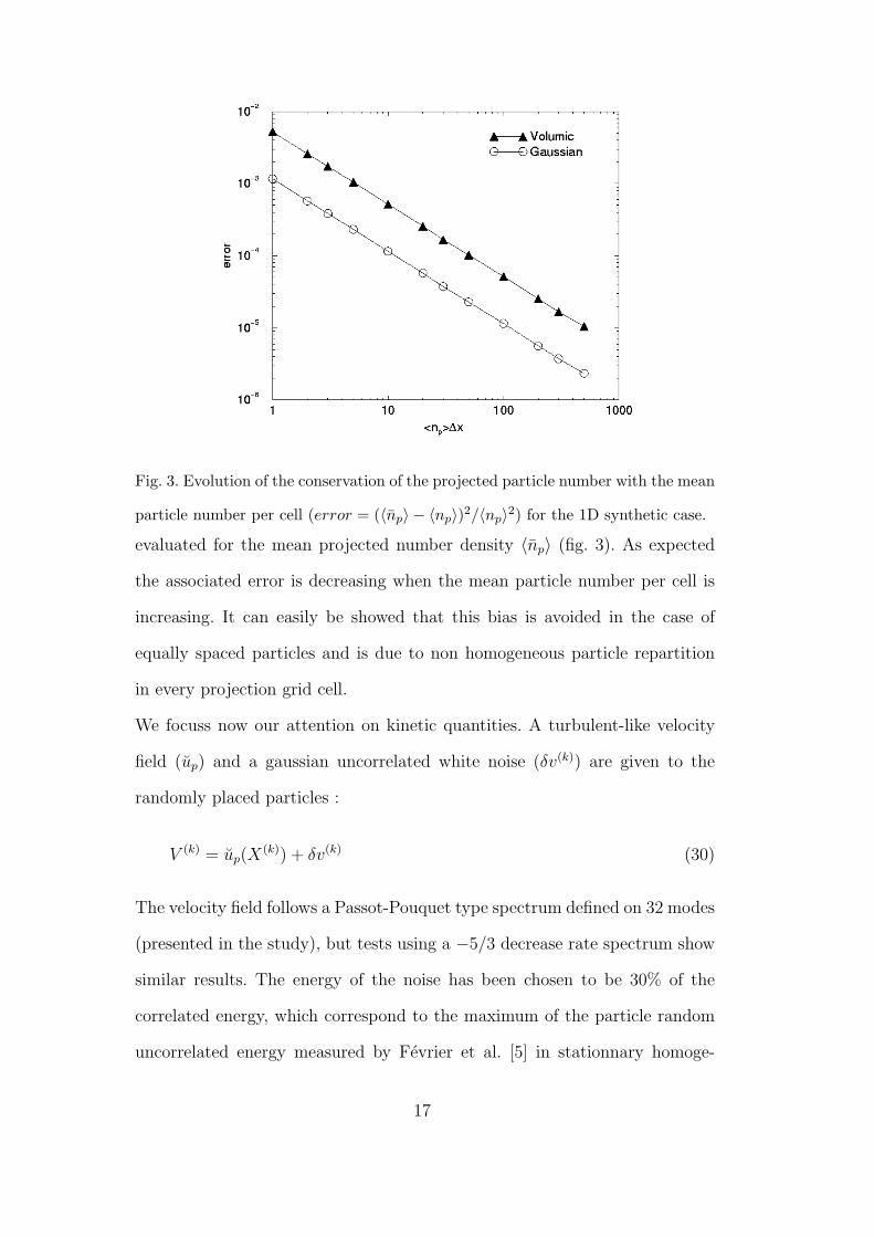
Fig. 3. Evolution of the conservation of the projected particle number with the mean

particle number per cell (error = (〈np〉 − 〈np〉)2/〈np〉2) for the 1D synthetic case.

evaluated for the mean projected number density 〈np〉 (fig. 3). As expected

the associated error is decreasing when the mean particle number per cell is

increasing. It can easily be showed that this bias is avoided in the case of

equally spaced particles and is due to non homogeneous particle repartition

in every projection grid cell.

We focuss now our attention on kinetic quantities. A turbulent-like velocity

field (up) and a gaussian uncorrelated white noise (δv(k)) are given to the

randomly placed particles :

V (k) = up(X(k)) + δv(k) (30)

The velocity field follows a Passot-Pouquet type spectrum defined on 32 modes

(presented in the study), but tests using a −5/3 decrease rate spectrum show

similar results. The energy of the noise has been chosen to be 30% of the

correlated energy, which correspond to the maximum of the particle random

uncorrelated energy measured by Fevrier et al. [5] in stationnary homoge-

17

neous isotropic turbulence. Particle properties are then projected on a one-

dimensional 64 node grid of length 2π. Substituting eq. 30 in eq. 26 leads

to :

npup =1

Vc

∑k

w(X(k) − x)up(X(k)) +

1

Vc

∑k

w(X(k) − x)δv(k) (31)

npup = npup + npδv (32)

To identified the projected velocity up to the correlated velocity up, the pro-

jection procedure must be able to supprim the noise δv and must not affect

the correlated velocity field. The difference between the projected velocity

fields and the non projected correlated velocity distribution is evaluated by

the quadratic error :

Error(φ) =〈(φ(x)− up(x))2〉

〈up(x)2〉(33)

where φ is the projected velocity with added noise up or without noise up. The

same Lagrangian field is projected with the different projections. To obtain

statistical convergence, average is performed on 5000 different realizations of

the velocity field. This procedure is repeated for several values of the particle

number per cell of the projection grid, from one to thousand. Fig. 4 shows

the dependence of the velocity projection error (computed from eq. 33) on

the particle number per cell for the different projection procedures. The error

decreases when increasing the particle number, but a systematic error occurs

even for a large particle number density. For more than 10 particles per cell,

the related error arises in decreasing order from the large box projector, the

large volumetric filter, the box filter and the volumetric filter. In the noisy case

(fig. 5) more than 100 particles per cell are needed to reach the systematic pro-

jector error level, but the projector efficiency classification remains the same.

18

Fig. 4. Dependence of velocity quadratic error (given by eq. 33) due to the pro-

jection procedure on the particle number per cell for 1D synthetic case. Particle

velocity distribution is given from the interpolation of a continuous turbulent field

on the particle position. Upper figure : comparison between between box, large box,

volumic, large volumic projections. Lower figure : comparison between box, volumic

and gaussian projections at the bottom.

19

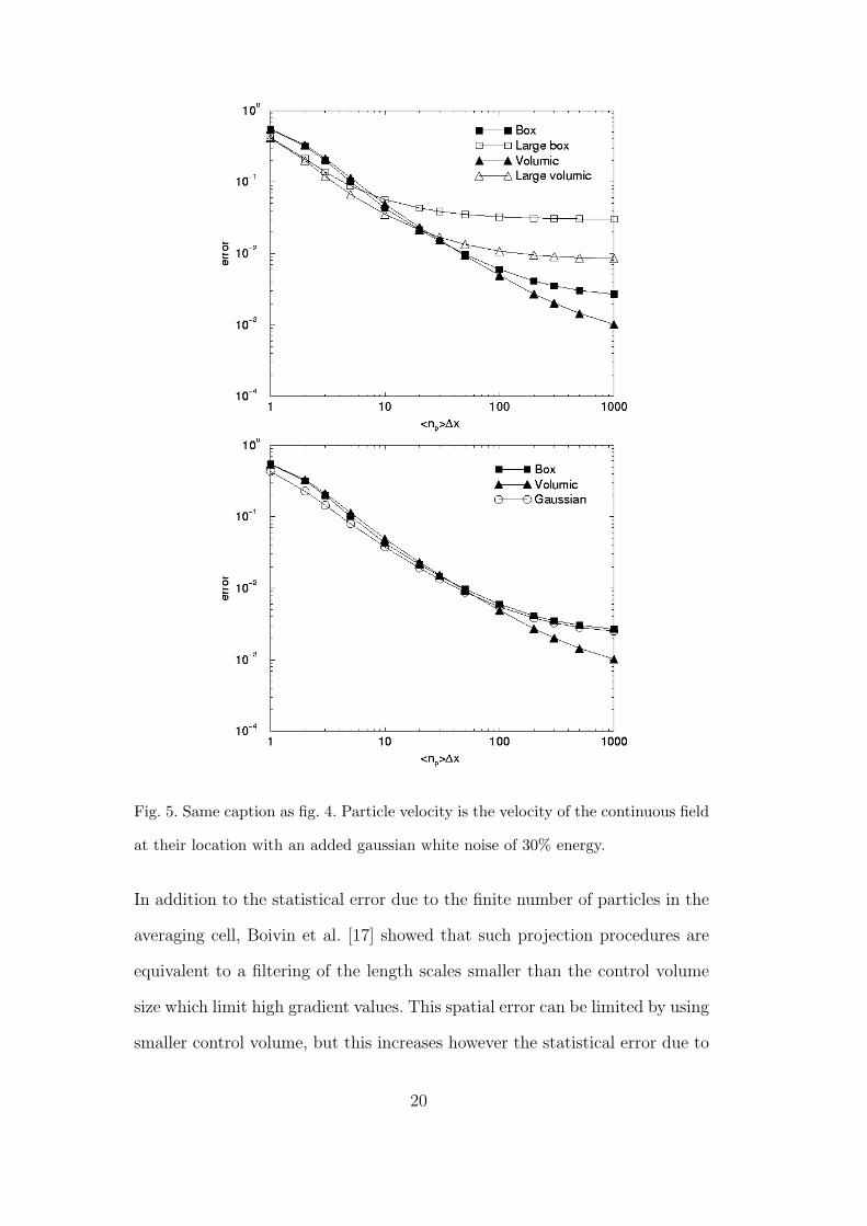
Fig. 5. Same caption as fig. 4. Particle velocity is the velocity of the continuous field

at their location with an added gaussian white noise of 30% energy.

In addition to the statistical error due to the finite number of particles in the

averaging cell, Boivin et al. [17] showed that such projection procedures are

equivalent to a filtering of the length scales smaller than the control volume

size which limit high gradient values. This spatial error can be limited by using

smaller control volume, but this increases however the statistical error due to

20

Fig. 6. Dependence of the projected correlated energy spectra using the gaussian

projector on the mean number of particles per cell. 1D synthetic case. The line is

the correlated energy spectra.

particle number. A different alternative would be to use a projection kernel

with a smaller characteristic length scale. It can be noticed that volumic-type

projectors returns better results than box-type projectors. A compromise be-

tween small systematic error and accuracy for small particle number density

is to use the gaussian projector on a large control volume (see Table 1) but

having the box projection characteristic length scale. The Gaussian projector

error is comparable to the box projection error for high particle numbers and

to the large box for small particle number.

To analyse more in details the projection error, the energy spectra of up, up,

δv, and up are presented on fig. 6-8 with the gaussian projector for 2, 20 and

200 mean particle number per cell of the projection grid. For all the cases the

projected correlated velocity energy (fig. 6) spectra follow the one of the cor-

related velocity at large scales. The projected correlated velocity (up) energy

spectra for the 200 mean particle number per cell case underestimates the

21

Fig. 7. Dependence of the projected noise energy spectra using the gaussian pro-

jector on the mean number of particles per cell. 1D synthetic case. The continuous

line is the correlated energy spectra. The horizontal dashed lines correspond to the

noise spectrum models (Eq. 35).

energy at small scales comparing to the up energy spectra. This behaviour is

the mark of the spatial error detailled before. In the case of 2 particles per cell

case, the spectrum presents an unphysical overestimation of the small scale

energy. This effect is avoided by increasing the mean particle number density,

np so that the spectra for 20 and 200 particles per cell are nearly identical for

all waves numbers. For equally spaced particles, the error is removed, even for

the case with the lowest particle number per cell (not presented here) proving

that the overestimation of the velocity spectrum induced by the projection

procedure is due to the random repartition of the particles.

Fig. 7 presents the energy spectra of the projected noise (δv). These spectra

are mainly flat and their level quasi-linearly decrease by increasing the parti-

cle number density. The noise spectra level are comparable to the correlated

energy ones. More precisely, this level can be evaluated. The energy spectrum

22

Fig. 8. Dependence of the projected correlated energy spectra with added noise

using the gaussian projector on the mean number of particles per cell. 1D synthetic

case. The continuous line is the correlated energy spectra. The horizontal dashed

lines correspond to the noise spectrum models (Eq. 35).

of a discret white noise on Np equaly spaced particles is constant up to the

Nyquist frequency (Np/2 = 〈np〉N∆x/2). Considering that the spectrum in-

tegral gives the Random Uncorrelated Energy, the energy spectrum of the

discret noise is :

Eδv(k) =N∆x

2π(Np

2− 1)−1δq2

p (34)

Eδv(k)≈ 1

π〈np〉δq2

p (35)

For non homogeneous particle distribution, eq. 35 can be used as a noise

spectrum level estimation. Comparing the projected noise spectra level with

the non projected noise model level, the particle density effect is recovered and

the mean level too (about 2% error). The projection procedure is just filtering

the noise and cut off all the components with wave numbers bigger than N/2.

23

We now consider the projection of correlated velocity with added noise (fig. 8).

At small scales the energy spectrum of up obtained with 2 or 20 mean particle

number per cell follows the one of the noise. A statistical error occurs and

the projection is not able to eliminate noise of the discret velocity field. By

increasing the number of particle the energy of the projected noise becomes

negligeable against the correlated energy at all length scales. An a-posteriory

validity criteria in the computation of the correlated energy spectra with added

noise is introduced :

Eup(k) >1

π〈np〉δq2

p for all k (36)

To resume, when obtaining continuous eulerian fields from discret Lagrangian

quantities by projection, errors are mainly due to a statistical error and to

an intrisic filtering (or spatial error) at small scales. By using a well chosen

projector (e.g. gaussian projection) with enough of particles (more than 10

particles per cell), it is possible to circumvent the problem in a satisfactory

manner.

3.2 Validation on DPS results

Finally to validate the gaussian projection, two DPS have been performed with

10 and 80 millions Lagrangian particles. Particles are randomly placed in the

computational domain of length 2π with the fluid velocity at their position.

Initial Lagrangian quantities are then projected with a gaussian filter on a 643

and 1283 node grids. For the coarser case, 10 millions of particles projected on

a 643 grid cell (about 38 particles by cell) with a ∆x equal to the computing

mesh size, the projected spectrum is identical to the fluid one for k smaller than

24

Fig. 9. Comparison of correlated energy spectra of DPS results at the initialisation

with V(k)(t = 0) = u(X(k)(t = 0), (t = 0)). DPS with 107 or 8. 107 particles

projected on a 643 or 1283 grid with the gaussian projector.

18 (fig. 9). For larger value of k, the energy spectrum of the projected velocity

shows an unphysical increase but remains 104 smaller than the effective values

measured in the energetic region. As expected, fig. 9 shows that this effect can

be diminished by increasing the particle number and decreasing the projection

cell size but leading to very expansive simulation costs.

Both DPS are performed and the same analyse is realised on a case with RUE

(≈ 16% of the correlated energy is measured) and particle segregation. The

energy spectra of mesoscopic velocities obtained by projection on a 643 (fig. 10)

are nearly identical for the two DPS results, no statistical bias is observed

so that 10 million particles (≈ 38 particles per cell) is sufficient to analyse

mesoscopic velocity fields in term of energy spectra. Indeed, these spectra

follow the one obtained by projection on a finer grid (1283) up to the higher

wave number (fig. 10). The one-dimensional noise spectrum model (eq. 35) is

extended for the three-dimensional spectrum by replacing the total number of

25

Fig. 10. Comparison of correlated energy spectra of DPS results. DPS with 107 or

8. 107 particles projected on a 643 or 1283 grid with the gaussian projector. Case

St = 0.53 at time t = 10.8. Horizontal dashed lines are the lower limit of spectrum

validity given by Eq. 37 (upper line is for cases 107 particles projected on 643 and

8. 107 particles projected on 1283 grid; lower line is for case 8. 107 particles projected

on 643 grid).

particle by the number of particles in only one direction (〈np〉∆x3N) :

Eup(k) >1

π〈np〉∆x2δq2

p for all k (37)

We notice on fig. 10 that the correlated energy spectrum validity criterion

(eq. 37) is satisfied. This criterion is of course questionable because particle

distribution is far from homogeneous and RUE is not uniform, but it could be

considered as a spectrum validity indicator. The gaussian projector is really

able to limit the intrinsic error of the projection procedure and is used to

obtain mesoscopic fields from DPS results with 10 million particles for 643

projection cells (about 38 particles per cell) in the rest of the paper.

26

4 Homogeneous isotropic decaying turbulence test case

Homogeneous isotropic turbulence is one of the classical cases where dynam-

ics and dispersion of particle laden flows can be studied. This has been done

extensively using the DPS formalism and encouraging results and insight are

obtained by such methods. Comparison of DPS in decreasing homogeneous

isotropic turbulence [20] with experimental measurements of particle disper-

sion in grid generated turbulence [21] shows that essential features of the

particle dynamics can be captured. Preliminary computations with a simpli-

fied Eulerian formalism of this test case gave encouraging results [22]. In the

case of tracer particles (small Stokes number limit) Eulerian methods are well

suited to describe the dynamics [3,4]. With increasing inertia, the particle

velocities become de-correlated from the gaseous carrier phase velocity and

segregation occurs for particle relaxation times comparable or larger than the

Kolmogorov time scale [23].

For the sake of simplicity, the case of decaying homogeneous isotropic tur-

bulence is studied. The carrier phase is initially supposed to have uniform

density, the velocity field to be divergence free and the kinetic energy to fol-

low a Passot-Pouquet spectrum [24]. After roughly one turn over time of the

energy containing eddies, the velocity field is supposed to represent a realis-

tic turbulent flow and the dispersed phase is added. At the particle injection

time, the Reynolds number is ReL = 13.6. For DPS initial conditions, par-

ticles are randomly and homogeneously distributed in space and the initial

particle velocities are given equal to the carrier phase velocity at the location

of the particle. For the Eulerian computation, these conditions correspond

to a uniform particle number density fieldand a mesocopic particle velocity

27

field identical to the carrier phase velocity field and zero uncorrelated velocity

variances. So the initial uncorrelated kinetic energy (RUE) is zero at initial-

ization and should develop during the simulation. The spatial resolution of the

gaseous phase computation is 643 and a total of 10 million individual particles

are traced in the computational domain. This corresponds to 38.1 particles

per gaseous node.

4.1 Numerical Method

The Eulerian simulation is performed using a different code (AVBP [25]) then

the DPS reference solution (NTMIX [18]). AVBP offers several spatial and

temporal schemes. In the present study a central second order spatial scheme

with a second order temporal correction (Lax Wendroff) was used. Comparison

to third order Runge Kutta time stepping showed no significant improvement

of the numerical accuracy. NTMIX uses a high-order spectral like scheme [26]

on cartesian grids and Runge Kutta time stepping. Both numerical tools use

domain decomposition and MPI for parallel computation. For the test cases

carrier phase solutions are identical and velocity spectra superpose.

To ensure the accuracy of the DNS of the carrier phase a necessary condition

is to satisfy the balance of the volume averaged kinetic energy (q2f ) with the

dissipation rate (ε) computed directly form the viscous stress tensor (τij) on

the computational grid.

∂

∂tq2f = −ε (38)

This verification that dissipation of carrier phase kinetic energy results from

laminar viscous effects and not from the numerical diffusion in AVBP code

28

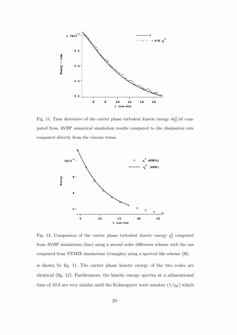
Fig. 11. Time derivative of the carrier phase turbulent kinetic energy dq2f/dt com-

puted from AVBP numerical simulation results compared to the dissipation rate

computed directly from the viscous terms.

Fig. 12. Comparison of the carrier phase turbulent kinetic energy q2f computed

from AVBP simulations (line) using a second order difference scheme with the one

computed from NTMIX simulations (triangles) using a spectral like scheme [26].

is shown by fig. 11. The carrier phase kinetic energy of the two codes are

identical (fig. 12). Furthermore, the kinetic energy spectra at a adimentional

time of 10.8 are very similar until the Kolmogorov wave number (1/ηK) which

29

Fig. 13. Kinetic energy spectra of the carrier phase from simulations with the two

numerical codes used in this study at time t = 10.8.

is 7.7 in non-dimensional units.

In the Eulerian simulation, the dispersed phase is computed using the same

numerical method as the carrier phase, imposing an additional limit on the

time step due to particle relaxation time (τp).

The Eulerian results are compared to DPS results at different levels : average

quantities over the compational domain, kinetic energy spectra and snapshot

of instantaneous local fields.

4.2 Integral Properties

The integral properties of particle kinetic energy q2p and fluid-particle correla-

tion qfp should be identical in the two simulations and therefore constitute a

first step of comparison. In the present test case of decreasing homogeneous

isotropic turbulence those quantities vary in time. The properties are averaged

over the computational volume and defined for the Eulerian simulation by

30

q2f =

1

2{uiui} (39)

qfp = {uiup,i}p (40)

q2p =

1

2{up,iup,i}p (41)

and for the DPS by

qfp =1

N

∑k

V(k)i ui(X

(k)) (42)

q2p =

1

N

∑k

1

2V

(k)i V

(k)i (43)

The volume averaged uncorrelated kinetic energy (RUE) from DPS is given

by

δq2p =

{δθp

}p

(44)

with the local RUE δθp measured by eq. 27.

4.3 Spectral treatment

Using the Fourier transformed velocities of the carrier phase ui(k) = F(ui(x))

and dispersed phase up,i(k) = F(up,i(x)) one can construct three dimensional

fluid and particle energy spectra and a fluid-particle correlation spectrum.

Ef (k) =1

2ui(k)ui(k) (45)

Ep(k) =1

2up,i(k)up,i(k) (46)

Efp(k) = ui(k)up,i(k) (47)

For established turbulent flow the undisturbed carrier phase kinetic energy fol-

lows the standard Kolmogorov spectrum. Here the interest lies on the behavior

of the spectrum of the correlated particle kinetic energy and the fluid-particle

31

correlation. Whereas the carrier phase is considered incompressible, segrega-

tion effects measured in DPS show that there must be a compressible part

in the correlated dispersed phase velocity spectrum. With the definition of

Kraichnan [27] operators in the spectral velocity can be divided into a com-

pressible and an incompressible (solenoidal) component.

ucp,i =

κiκj

κ2up,j (48)

usp,i =

(1− κiκj

κ2

)up,j (49)

This orthogonal decomposition allows to construct a compressible and a solenoidal

spectral energy such that the sum equals to the total spectral energy.

Ecp(k) =

1

2uc

p,i(k)ucp,i(k) (50)

Esp(k) =

1

2us

p,i(k)usp,i(k) (51)

5 Simulations results and discussion

Eulerian methods are well suited to describe the particle dynamics [3] for

particle relaxation times small compared to the Kolmogorov time scale. It

is therefore interesting to study how the Eulerian description behaves out-

side this range. Preliminary tests with the decaying homogeneous turbulence

described above, showed that the numerical simulation with any of the two

models proposed for the RUE is possible up to a Stokes number (St = τp/τ+)

of St = 0.042 based on the macroscopic dissipative time scale τ+(= k/ε) at

the particle injection time. This corresponds to a Stokes number of StK = 0.17

based on the Kolmogorov time scale. In contrast, mesoscopic Eulerian Simu-

lations with larger Stokes numbers failed. Detailed analysis revealed that, due

32

Fig. 14. Comparison of correlated particle kinetic energy and fluid particle correla-

tion from DPS and Eulerian simulation for the test case of St = 0.042.

to segregation effects, the particle number density field has very stiff local gra-

dients that caused dispersion errors in the numerical scheme. Increasing grid

resolution for the Eulerian simulation up to (1283, 1923, 2563) only allowed a

small increase in attainable Stokes number. Therefore in a first step the results

of DPS and the Eulerian model are compared for the limiting Stokes number

of St = 0.042. In a second step an heuristic extension of the proposed model

overcoming the numerical difficulties encountered due to massive segregation

is presented and results are compared for a Stokes number based on the macro-

scopic dissipative time scale of St = 0.53 according to a Stokes number value,

based on the Kolmogorov time scale, StK = 2.2. Eulerian results presented

here are obtained with the RUE transport equation (eq. 21).

33

Fig. 15. Comparison of volume filtered DPS and Eulerian number density PDF for

the test case with St = 0.042 at t=10.8.

5.1 Comparison at St = 0.042

At Stokes numbers as small as St = 0.042 based on the dissipative time scale

τ+(= k/ε) the particles are expected to follow closely the carrier phase veloc-

ity and the uncorrelated velocity contribution to the particle dynamics is very

small. In fig. 14 the integral quantities of correlated particle kinetic energy q2p,

fluid-particle correlation qfp of the Eulerian simulation are compared to the

DPS results. Temporal evolution of particle kinetic energy and fluid-particle

correlation are well predicted by the Eulerian Simulation.

RUE measured in DPS (≈ 10−2q2p) is of the same order of numerical error.

Then the predicted RUE is of two orders of magnitude lower than the corre-

lated kinetic energy, the contribution of RUE can be neglected in this case.

Fig. 15 shows the probability to find a computational cell with a given value

for the number density in the Eulerian prediction and the DPS reference re-

sult at t=10.8. The distribution of the Eulerian number density is less wide

than the DPS distribution. If the correlated velocity is well predicted in the

34

Eulerian simulation, a possible cause of the non-matching number density

distributions may be the numerical scheme dispersion leading to a more ho-

mogeneous droplet number density.

35

Fig. 16. Comparison of the normalized droplet number n/〈n〉 from the Lagrangian

simulation (upper graph, resolution 643) with the one from the Eulerian simulation

(lower graph, resolution 643) at the non-dimensional time t=10.8, case St = 0.042.

The drawing plane is parallel to the x-y reference plane and crosses the computa-

tional domain center.

36

Fig. 17. Comparison of total and compressible kinetic energy spectra from DPS and

Eulerian Simulation for the test case with St = 0.042 at t=10.8.

As an instantaneous local quantity the normalized droplet number density is

shown in fig. 16 for the x-y plane crossing the computational domain center at

the simulation time t=10.8. This corresponds to roughly 18 particle relaxation

times (τp) and two dissipative times scales (τ+) of the carrier phase. It shows

that the Eulerian number density prediction is quantitatively close to the DPS

result. Regions with high and low particle number densities are well correlated

in the two approaches.

Fig. 17 shows the total particle kinetic energy spectra and the compressible

kinetic energy spectra computed from Lagrangian and Eulerian simulation

results. The correlated particle kinetic energy spectrum follows closely the

spectrum of the carrier phase at large scales. Up to the kink in the DPS

energy spectra, the spectra computed from the Eulerian Simulation match well

those from the DPS. As shown in section 3, this kink is probably unphysical

and is due to a numerical error induced by the non-homogeneous particle

distribution.

37

In case of small Stokes number, the mesoscopic simulation is able to predict

integral quantities such as particle energy and also local quantities such as

segragation. Results with Eulerian mesoscopic approach are very similar to

the ones obtained using the Eulerian equilibrium approach propose by Rani

and Balachandar [4,28].

5.2 Comparison at St = 0.53

Preliminary tests with Stokes numbers larger than St = 0.042 failed since

large segregation effects imply shock like in the number density distribution

that could not be handled by the numeric scheme [15]. Supposing that the

numerical resolution of the model is insufficient, several possibilities exist to

circumvent this difficulty : a different numerical scheme using up-winding or

flux limiters are clearly able to capture those strong gradients but imply some

type of numerical diffusion. For the computation of the number density in

the equilibrium Eulerian approach with a limited Stokes number range Rani

and Balachandar [4,28] use a spectral viscosity to overcome this difficulty.

Increasing spatial resolution increases strongly numerical cost. The origin of

the preferential concentration is due to the compressibility of the particle

number density field. A pure diffusivity added to the evolution of the number

density field would bias the conservative transport of the particle velocity. The

origin of the compressibility is the compressible component of the mesoscopic

particle velocity field.

At this point it was found preferable to act on the compressible component of

the correlated velocity field to circumvent the measured difficulties associated

with steep gradients. This leads to compute for a modified correlated velocity

38

˜up,i transport equation and consequently a modified droplet number density

field ¯np. The compressible component of the correlated velocity is modified by

introducing a subgrid bulk viscosity, ξsgs.

∂

∂t¯np

˜up,i +∂

∂xj

¯np˜up,i

˜up,j =− ∂

∂xi

PQB +∂

∂xj

τij −¯np

τp

(˜up,i − uf,i

)(52)

+∂

∂xi

ξsgs∂

∂xk

˜up,k

The subgrid model has the form of a bulk viscous term ξsgs∂ ˜uk/∂xkδij which

is added to the shear viscosity term δτp,ij in eq. 17. The subgrid bulk viscosity

is mesh-size dependent (ξsgs ∝ ¯np(∆x)2|∂ ˜uk/∂xk|). The proportionality coeffi-

cient for the bulk viscosity used for all simulations with St > 0.042 is 50. The

RUE transport equation (eq. 21) is not modified.

In homogeneous turbulence, the spatial average of this bulk viscous term is

zero, still it acts locally and leads to a more homogeneous number density

field. Simulations have been carried out for several particle relaxation times.

The following computation with a Stokes number of St = 0.53 is performed

with this heuristically introduced bulk viscosity and compared to the DPS

reference results.

5.2.1 Integral quantities

Figure 18 shows the temporal evolution of carrier phase kinetic energy, par-

ticle kinetic energy and fluid-particle correlation. The carrier phase kinetic

energy decreases due to viscous dissipation. Particle kinetic energy follows the

carrier phase kinetic energy with a delay of the order of the particle relaxation

time. Due to particle inertia, the particle velocities become partially uncorre-

lated in space and the RUE begins to increase. The behavior of the integral

39

Fig. 18. Temporal evolution of the fluid, particle and fluid-particle velocity corre-

lations for DPS (symbols) and Eulerian simulations (lines). For Eulerian approach

the total particle kinetic energy q2p is computed as the sum of the kinetic energy

due to correlated motion q2p and the random uncorrelated energy δq2

p.

quantities of correlated and uncorrelated particle kinetic energy as well as the

fluid-particle correlation are well predicted by the Eulerian simulation using

the transport equation for RUE. Simulations using the isentropic approxima-

tion show results of similar quality.

Comparison of particle number density PDF is provided on fig. 19. As ex-

pected, the Eulerian approach underestimates particle segregation.

5.2.2 Instantaneous local fields

Fig 20 shows a snapshot of number density in DPS and the Eulerian simulation

in the upper and the lower graph. The number density field shows the same

kind of structures for both the Lagrangian and Eulerian simulations. But the

instantaneous distribution is less heterogeneouss for the Eulerian simulation

due to the heuristic bulk viscosity which reduces compressibility effects.

40

Fig. 19. Comparison of DPS and Eulerian number density PDF for the test case St

=0.53 at t=10.8.

The heuristically introduced bulk viscous term tends to render the spatial par-

ticle number density more uniform. Without this bulk viscous term, Eulerian

simulations can currently not be carried out : the physical particle segregation

is too large as it could be resolved by the numerical scheme. Since the spatial

average of the volume viscosity is however zero, it does not effect the tempo-

ral evolution of the averaged kinetic energy of Random Uncorrelated Motion

of the particles δq2p. In contrast, local instantaneous values of δθp may differ

notably from the values obtained in the DPS (fig. 21).

41

Fig. 20. Comparison of the normalized droplet number np/〈np〉 from the Lagrangian

simulation (upper graph, resolution 643) with the one from the Eulerian simulation

(lower graph, resolution 1283) (St = 0.53) at time (t=10.8). Same cut-plane as

fig. 16.

42

Fig. 21. Comparison of RUE (δθp) in the DPS (upper graph,resolution 643) and the

Eulerian computation (lower graph,resolution 1283) after one particle relaxation (St

= 0.53) time (t=10.8) . Same cut-plane as fig. 16.

43

5.3 Transition filter between DPS and Eulerian simulation results

The number density of the Eulerian simulation with subgrid bulk viscosity

can be interpreted as a filtered Eulerian number density. Formally the filtered

number density field is obtained by the following convolution with the filter

kernel :

¯np(x) =∫

np(x′)F (x′ − x) dx’ (53)

The actually predicted Eulerian number density without bulk viscosity is not

known. Since the DPS number density should be equal to the Eulerian number

density field in question, the particle number density from DPS np is used in

its place. Using the Fourier transform property the convolution becomes a

product in spectral space :

ˆnp(κ) = ˆnp(κ)F (κ) (54)

This allows to obtain the filtering kernel associated to the difference between

the number density field predicted in the Eulerian computation with bulk

viscosity and the DPS result that should be achieved. Finally, the space filter

kernel can be obtained by backward Fourier transform :

F (x) = F−1

ˆnp(κ)ˆnp(κ)

(55)

The filtering kernel allows a qualitative comparison of the particle number den-

sity field obtained by the grid filtering of the DPS and the Eulerian prediction

of the particle number density field. Using the number density weighted filter

it is possible to obtain from DPS the filtered particle number density that cor-

44

respond to the Eulerian prediction with subgrid bulk viscosity operator (fig.

22). These two snapshot are very comparable.

5.4 Filtering Kernel

The filter kernel is displayed in fig. 23. Since the filter is considered isotropic in

space, averaging over the different directions was performed and only the one

dimensional kernel is retained. The figure shows that the convolution kernel

averages the DPS number density field a little more than the neighboring grid

cells. When interpreting this graph, one has to keep in mind that the DPS

number density was already volume filtered to obtain a continuous field.

5.5 Spectral kinetic energies

Fig. 24 shows spectra of the total kinetic energies of the dispersed phase as

well as the compressible kinetic energies measured from the DPS and Eule-

rian simulation. First, one remarks the high compressible component of the

kinetic energy compared to the gaseous carrier phase kinetic energy. This

causes structures similar to those known as eddy shocklets in compressible

turbulence [29]. In addition, the compressible part of the energy spectrum is

of the same order than the solenoidal part at small scales or large wavenum-

ber values. The kinetic energy spectrum of the Eulerian simulation does not

reflect this behaviour to the same extend at small scales in contrast with the

one measured at large scales or small wave number values. This discrepancy

between both approaches is probably due to the bulk viscosity operator which

reduces drastically the compressible effects at small scales.

45

Fig. 22. Comparison of the normalized droplet number np/〈np〉 with filtered DPS

(upper graph, resolution 643) and with the Eulerian computation (lower graph,

resolution 1283) after one particle relaxation (St = 0.53) at time (t=10.8). Same

cut-plane as fig. 16.

46

Fig. 23. Filtering Kernel obtained by backward convolution between the DPS num-

ber density field and the Eulerian number density field. Case St = 0.53 at time

t = 10.8. The upper graph shows the spatial filter and the lower graph shows the

spectral filter.

47

Fig. 24. Comparison of DPS and Eulerian kinetic energy spectra for the Stokes

number St = 0.53 at t = 10.8.

48

6 Conclusion and perspectives

This study presents the potentials of a new Eulerian approach for particle

ensemble in gas turbulent flows that differs from standard approaches by it’s

ability to account for instantaneous local phenomena. The proposed meso-

scopic Eulerian approach allows to simulate the dynamics of particles sus-

pended in homogeneous isotropic decaying turbulence at large scales even in

the vicinity of unity Stokes numbers based on the turbulent time macroscale.

The role of the uncorrelated velocity variances in the momentum equation

is identified and a modeling approach in terms of pressure and viscosity is

presented and evaluated. Simulations were performed at very small turbulent

Reynolds numbers because simulations

with higher Reynolds numbers of the carrier phase show deficiencies for the

spatial accuracy of the dispersed numerical prediction. Therefore tests have

to be extended to higher Reynolds numbers and for colliding particles. Con-

currently such an approach is being adapted to a LES formalism [30], which

are very interesting for the unsteady computations of industrial applications

with a very large number of particles or droplets.

Eventually it is necessary to quantify the capacity of such an approach in real

geometries other than the synthetic case of boxes with periodic boundary con-

ditions. Possible configurations are particle laden jets or particle laden channel

flow with and without collisions.

49

Acknowledgements

Numerical computation of the Eulerian simulations were performed on the

COMPAQ supercomputers of CEA and CERFACS. Numerical solutions on

large grids (1923, 2563) were performed on SGI ORIGIN 3800 at CINES in

the framework of the Extreme Computing for Turbulent Combustion program

using up to 128 processors. The DPS reference solution was obtained with

numerical simulations performed at computing center IDRIS using the DPS

version of NTMIX in the Ecoulements Reactifs Diphasiques : Simulations Di-

rectes et aux Grandes Echelles project.

Financial support for this work was received from the European Community

via the STOPP research training network.

References

[1] A. Ten Cate, J. J. Derksen, L. M. Portela, H. E. A. Van den Akker, Fully

resolved simulations of colliding monodisperse spheres in forced isotropic

turbulence, Journal of Fluid Mechanics 519 (2004) 233–271.

[2] T. M. Burton, J. K. Eaton, Fully resolved simulations of particle-turbulence

interaction, J. Fluid Mech. 545 (2005) 67–111.

[3] O. Druzhinin, S. Elghobashi, On the decay rate of isotropic turbulence laden

with microparticles, Physics of Fluids 11(3) (1999) 602–610.

[4] S. L. Rani, S. Balachandar, Evaluation of the equilibrium eulerian approach for

the evolution of particle concentration in isotropic turbulence, Int. Journal of

Multiphase Flow 29 (2003) 1793–1816.

50

[5] P. Fevrier, O. Simonin, K. D. Squires, Partitioning of particle velocities in gas-

solid turbulent flows into a continuous field and a spatially uncorrelated random

distribution: theoretical formalism and numerical study, J. Fluid Mech. 533

(2005) 1–46.

[6] S. Chapman, T. Cowling, The Mathematical Theory of Non-Uniform Gases,

Cambridge Mathematical Library Edition, Cambridge University Press, 1939

(digital reprint 1999).

[7] O. Simonin, Combustion and turbulence in two phase flows, Lecture Series

1996-02, von Karman Institute for Fluid Dynamics (1996).

[8] P. Fevrier, Etude numerique des effets de concentration preferentielle et de

correlation spatiale entre vitesses des particules solides en turbulence homogene

isotrope stationaire, PhD Thesis, INP Toulouse,France 2000 (2000).

[9] M. Vance, K. Squires, O. Simonin, Properties of the particle field in gas-solid

turbulent channel flow, Physics of Fluids in press.

[10] O. Simonin, P. Fevrier, J. Lavieville, On the spatial distribution of heavy

particle velocities in turbulent flow: from continuous field to particulate chaos,

Journal of Turbulence 3 (2002) 040.

[11] S. Elghobashi, G. Truesdell, On the two-way interaction between homogeneous

turbulence and dispersed solid particles. I: Turbulence modification, Physics of

Fluids A 5(7) (1993) 1790–1801.

[12] J. Minier, E. Peirano, The pdf approach to turbulent polydispersed two-phase

flows, Physics Reports 352 (2001) 1–214.

[13] L. Zaichik, O. Simonin, V. Alipchenkov, Two statistical models for predicting

collision rates of inertial particles in homogeneous isotropic turbulence, Physics

of Fluids 15(10) (2003) 2995–3005.

51

[14] M. Reeks, On a kinetic equation for the transport of particles in turbulent flows,

Physics of Fluids A 3(3) (1991) 446–456.

[15] A. Kaufmann, Towards eulerian-eulerian large eddy simulation of reactive two-

phase flows, PhD Thesis, INP Toulouse, France 2004 (2004).

[16] S. B. Pope, Lagrangian pdf methods for turbulent flows, Annu. Rev. Phys.

Mech. 26 (1994) 23–63.

[17] M. Boivin, O. Simonin, K. D. Squires, On the prediction of gas-solid flows with

two-way coupling using large eddy simulation, Phys. Fluids 12 (2000) 2080–

2090.

[18] O. Vermorel, B. Bedat, O. Simonin, T. Poinsot, Numerical study and modelling

of turbulence modulation in a particle laden slap flow, Journal of Turbulence

335 (2003) 75–109.

[19] D. Schmidt, Theoretical analysis for achieving high-order spacial accuracy in

Lagrangian/Eulerian source terms, Int. J. Numer. Meth. Fluids.

[20] S. Elghobashi, G. Truesdell, Direct simulation of particle dispersion in a

decaying isotropic turbulence, J. of Fluid Mech. 242 (1992) 655–700.

[21] W. Snyder, J. Lumley, Some measurements of particle velocity autocorrelation

functions in a turbulent flow, Journal of Fluid Mechanics 48, part 1 (1970)

41–71.

[22] A. Kaufmann, O. Simonin, T. Poinsot, J. Helie, Dynamics and dispersion in

Eulerian-Eulerian DNS of two-phase flows, in: Proceedings of the Summer

Program 2002, Studying Turbulence Using Numerical Simulation Databases

IX, Center for Turbulence Research Stanford,Ca, 2002, pp. 381–392.

[23] K. D. Squires, J. K. Eaton, Preferential concentration of particles by turbulence,

Physics of Fluids A: Fluid Dynamics 3 (1991) 1169–1178.

52

[24] T. Passot, A. Pouquet, Numerical simulation of compressible homogeneous flow

in the turbulent regime, Journal of Fluid Mechanics 181 (1987) 441–466.

[25] T. Schonfeld, M. Rudgyard, Steady and unsteady flows simulations using the

hybrid flow solver AVBP, AIAA Journal 37 (11) (1999) 1378–1385.

[26] S. Lele, Compact finite difference schemes with spectral like resolution, J.

Computational Physics 103 (1992) 16–42.

[27] R. Kraichnan, An almost-Markovian Galilean-invariant turbulence model,

Journal of Fluid Mechanics 47 (1971) 513.

[28] S. L. Rani, S. Balachandar, Preferential concentration of particles in isotropic

turbulence: a comparison of the Lagrangian and equilibrium Eulerian approach,

Powder Technology 141 (2004) 109–118.

[29] G. Erlebacher, M.Y.Hussaini, C. S. T. Zang, Toward the large eddy simulation

of compressible turbulent flows, ICASE 90-76 (1990) 1–43.

[30] M. Moreau, B. Bedat, O. Simonin, A priori testing of subgrid stress models

for euler-euler two-phase LES from euler-lagrange simulations of gas-particle

turbulent flow, in: 18th Ann. Conf. on Liquid Atomization and Spray Systems,

ILASS Americas, 2005.

53