Calhoun: The NPS Institutional Archive

Theses and Dissertations Thesis and Dissertation Collection

1992-06

Optimum design of isotropic monocoque and

ring-stiffened circular cylindrical shells subject to

external hydrostatic pressure

Castillo, Henry A., Jr.

Monterey, California. Naval Postgraduate School

http://hdl.handle.net/10945/26142

10L

SECURITY CLASSIFICATION OF THIS PAGE

REPORT DOCUMENTATION PAGE

1a. REPORT SECURITY CLASSIFICATION

UNCLASSIFIEDlb RESTRICTIVE MARKINGS

2a SECURITY CLASSIFICATION AUTHORITY

2b. DECLASSIFICATION/DOWNGRADING SCHEDULE

3 DISTRIBUTION/AVAILABILITY OF REPORT

Approved for public release; distribution is unlimited.

4. PERFORMING ORGANIZATION REPORT NUMBER(S) 5. MONITORING ORGANIZATION REPORT NUMBER(S)

6a. NAME OF PERFORMING ORGANIZATIONNaval Postgraduate School

6b. OFFICE SYMBOL(If applicable)

ME

7a. NAME OF MONITORING ORGANIZATION

Naval Postgraduate School

6c. ADDRESS (Crty, State, and ZIP Code)

Monterey, CA 93943-5000

7b ADDRESS (City, State, and ZIP Code)

Monterey, CA 93943-5000

8a. NAME OF FUNDING/SPONSORING

ORGANIZATION8b OFFICE SYMBOL

(If applicable)

9 PROCUREMENT INSTRUMENT IDENTIFICATION NUMBER

8c. ADDRESS {City. State, and ZIP Code) 10. SOURCE OF FUNDING NUMBERS

Program Element No Work Unit Accession

Number

1 1 . TITLE (Include Security Classification)

OPTIMUM DESIGN OF ISOTROPIC MONOCOQUE AND RING-STIFFENED CIRCULAR CYLINDRICAL SHELLSSUBJECT TO EXTERNAL HYDROSTATIC PRESSURE

12. PERSONAL AUTHOR(S) HENRY A. CASTILLO, JR.

13a. TYPE OF REPORTMaster's Thesis

13b. TIME COVERED

From To

14 DATE OF REPORT (year, month, day)

JUNE 1992

15. PAGE COUNT

13416. SUPPLEMENTARY NOTATION

The views expressed in this thesis are those of the author and do not reflect the official policy or position of the Department of Defense or the U.S.

Government.

I7.COSATI CODES 18 SUBJECT TERMS (continue on reverse if necessary and identify by block number)

OPTIMIZATION, CYLINDRICAL SHELLS, SHELL DESIGN

1 9 . ABSTRACT (continue on reverse if necessary and identify by block number)

The objective of this research is to create a flexible code which is to be used in the investigation ofoptimum (minimum weight) shell designs.

A shell analysis/design program (DAPS3) and a general purpose numerical optimization program (ADS) are incorporated into a single code

(THESIS). This code provides the user great flexibility in changing the design variables and constraints which model the optimization

problem. The optimum designs produced by this code are compared to DAPS3 optimum designs in order to identify any improvements madeby the numerical optimization technique.

20. DISTRIBUTION/AVAILABILITY OF ABSTRACT

El UNCLASSIFIED/UNLIMITED l**l SAME AS REPORT

21 ABSTRACT SECURITY CLASSIFICATION

UNCLASSIFIED

22a. NAME OF RESPONSIBLE INDIVIDUAL

DAVID SAUNAS22b TELEPHONE (Include Area code)

(408)646-3426

22c. OFFICE SYMBOLME/Sa

DD FORM 1473. 84 MAR 83 APR edition may be used until exhausted

All other editions are obsolete

SECURITY CLASSIFICATION OF THIS PAGE

UNCLASSIFIED

T257757

Approved for public release; distribution is unlimited.

OPTIMUM DESIGN OF ISOTROPICMONOCOQUE AND RING-STIFFENEDCIRCULAR CYLINDRICAL SHELLS

SUBJECT TO EXTERNAL HYDROSTATIC PRESSURE

by

Henry A. Castillo, Jr.

Lieutenant, United States Navy

B.S., United States Naval Academy, 1985

Submitted in partial fulfillment

of the requirements for the degree of

MASTER OF SCIENCE IN MECHANICAL ENGINEERING

from the

ABSTRACT

The objective of this research is to create a flexible code which is to be used

in the investigation of optimum (minimum weight) shell designs. A shell

analysis/design program (DAPS3) and a general purpose numerical optimization

program (ADS) are incorporated into a single code (THESIS). This code provides

the user great flexibility in changing the design variables and constraints which model

the optimization problem. The optimum designs produced by this code are

compared to DAPS3 optimum designs in order to identify any improvements made

by the numerical optimization technique.

TABLE OF CONTENTS

I. INTRODUCTION 1

A. DEVELOPING A MATHEMATICAL MODEL FOR

OPTIMIZATION 1

B. MODELING A CYLINDRICAL SHELL FOR MINIMUM

WEIGHT DESIGN 2

C. THESIS OBJECTIVES 4

II. SHELL BUCKLING AND STRENGTH 5

A. BUCKLING EQUATIONS 5

1. Axisymmetric Collapse Pressure (PC) 7

2. Elastic Interbay Instability Pressure (PIB) 11

3. Elastic Genera] Instability Pressure (PGEN) 16

B. STRENGTH (STRESS) EQUATIONS 20

1. Middle Fiber Shell Stress at Mid-bay (STR) 22

2. Outer Fiber Shell Stress at a Ring Junction (SIGVOF) 24

3. Inner Fiber Shell Stress at a Ring Junction (SIGVIF) 25

4. Center Fiber Ring Stress (SRF) 26

III. OPTIMIZATION PROBLEM 28

A. OBJECTIVE FUNCTION 28

B. CONSTRAINT FUNCTIONS 30

1. Monocoque Shell Constraints 30

2. Ring-stiffened Shell Constraints 31

C. SIDE CONSTRAINTS 32

D. SUMMARY 34

1. Monocoque Shell 34

2. Ring-Stiffened Shell 35

E. OPTIMIZATION TECHNIQUE 35

IV. RESULTS 40

A. MONOCOQUE SHELL 40

1. Objective: DAPS3 vs. THESIS 40

2. Design Variables: DAPS3 vs. THESIS 42

3. Constraints: DAPS3 vs. THESIS 44

B. RING-STIFFENED SHELL 52

1. Objective: DAPS3 vs. THESIS 52

2. Design Variables: DAPS3 vs. THESIS 54

3. Constraints: DAPS3 vs. THESIS 58

V. CONCLUSIONS 69

VI. RECOMMENDATIONS 72

APPENDIX A: THESIS CODE LISTING 73

APPENDIX B: THESIS CODE INPUT FILE 120

APPENDIX C: THESIS CODE FLOW CHART LOGIC 122

LIST OF REFERENCES 124

INITIAL DISTRIBUTION LIST 125

ACKNOWLEDGEEMENT

The author must acknowledge Professor Philip Y. Shin, the original advisor of

this thesis. Without his guidance a majority of this research would not have been

possible. Also due much gratitude is Professor David Salinas, who enthusiastically

assumed the duties of thesis advisor upon Professor Shin's departure from the Naval

Postgraduate School. Their support is greatly appreciated.

vn

I. INTRODUCTION

A. DEVELOPING A MATHEMATICAL MODEL FOR OPTIMIZATION

Design optimization is a powerful tool available to the design engineer. While

it is not a new concept, only recently has numerical design optimization become a

technique which is routinely applied by practicing engineers to the myriad of design

tasks. This trend can be attributed to recent technological advances in high-speed

digital computers, which are necessary to solve the multitude of equations modeling

the optimization problem.

One area particularly suited for design optimization applications is structural

design. The design of a structure requires a great deal of forethought by the design

engineer. Several restrictions (constraints) on the design, such as environmental

effects, geometry, and material selection, must first be determined. Then, these

restrictions are applied to the design process to produce a specific output (objective),

such as maximum structural response or minimum cost. The goal of the design

engineer is to design the best possible structure, in terms of a specific desired output,

while adhering to several expected constraints on the final design. That is, the final

structure must be the optimum design for anticipated conditions.

In order to achieve this optimum design, the design optimization process

requires that the design task be defined as a mathematical model. This model

consists of an objective function, constraint functions, and side constraint functions.

These three functions are mathematical equations expressed in terms of design

variables and state variables. State variables are fixed quantities in the mathematical

equations. Design variables are those quantities which are allowed to vary during

the optimization process. The objective function, which contains every design

variable, is a single equation representing the quantity to be optimized (such as

weight, displacement, cost, etc.). Constraint functions are one or more equations

which restrict the design variables; one or more design variables are contained in

each constraint function. Side constraint functions are equations which limit the

upper and lower bound ranges of each design variable. Simply stated, the model

describes, mathematically, what is to be optimized (objective) and the limitations

(constraints and side constraints) on design variables.

Having converted the design task into a mathematical model, the design

engineer can program the model. Using his own optimization code, or, more likely,

available software, the design engineer may now execute the process of optimizing

the objective function and the associated design variables.

B. MODELING A CYLINDRICAL SHELL FOR MINIMUM WEIGHT DESIGN

The design optimization task is to design a minimum weight thin cylindrical

shell subjected to external hydrostatic pressure. The shell can be either monocoque

or ring-stiffened (by internal rectangular cross-section rings placed at equidistant

intervals within the shell). A single isotropic shell and ring material will be used in

either case. A more complex orthotropic material or a hybrid construction material

could have been used (and supported by the DAPS3 analysis mode). However, due

to time limitations, only an isotropic material will be investigated. This simpler

material should still credibly serve the purpose of demonstrating the application of

numerical optimization techniques to a minimum weight shell design. The optimized

design is also constrained by buckling, strength, and geometry considerations. This

design task is applicable to the design of submerged cylindrical structures under a

static pressure load. Examples might include submarine pressure hulls and torpedo

cases.

In order to model the above design task, a shell analysis program, DAPS3

(Design and Analysis of Plastic Shells version 3), was used to evaluate the buckling

and strength constraint functions of a thin shell under external hydrostatic pressure.

Development of these constraint functions is discussed in Chapter II (Shell Buckling

and Strength). The optimization problem was evaluated by the general purpose

numerical optimization program ADS (Automated Design Synthesis version 1.10).

Development of the mathematical model for optimization is discussed in Chapter III

(Optimization Problem). Both programs, which are written in the FORTRAN

language, are incorporated into a single FORTRAN code named THESIS.

The THESIS code produces a minimum weight shell design, and it indicates the

shell dimension design variables (thickness, ring height, and ring width) associated

with that optimum design. Therefore, the design task is modeled and optimized

within the THESIS code.

C. THESIS OBJECTIVES

DAPS3 uses an iterative technique to optimize the shell design variables. The

variables are manipulated (in a "DO" loop sense) until a design is produced which

does not buckle under the input hydrostatic pressure. When all possible buckling

loads are greater than the hydrostatic pressure, DAPS3 terminates the iterations.

The DAPS3 generated optimum design is produced from the last design iteration.

It was felt that incorporation of the more sophisticated numerical optimization

technique should improve upon the DAPS3 iterative design technique.

In pursuit of the above hypothesis, this thesis will investigate optimum designs

generated by the THESIS code over a wide range of geometry configurations (L/OD

ratios) and loads (external hydrostatic pressures). These designs will then be

compared to the optimum designs generated by DAPS3 (when used in the "design"

mode). Specifically, the following design elements will be compared: 1) objective

(shell weight), 2) design variables (thickness, ring height, and ring width), and 3)

constraints (buckling, strength, and geometry). Any design improvements made by

use of the numerical optimization technique will be identified. Results are presented

in Chapter IV. Conclusions as to the advantages and disadvantages of incorporating

a numerical optimization technique are presented in Chapter V.

II. SHELL BUCKLING AND STRENGTH

The purpose of this chapter is to explain the formulation of the buckling and

strength (or stress) terms used by the THESIS code. A detailed derivation of the

buckling equations is provided by Renzi [Refs. 1,2].

A. BUCKLING EQUATIONS

Structural failure by buckling is associated with an "unstable" design. Material,

geometry, and load factors contribute to this instability. The THESIS code designs

the geometry of a "stable" cylindrical shell based on material and load factors which

are input by the user. Within the THESIS code, DAPS3 is used as a subroutine

analysis program to calculate the buckling loads on either a monocoque or ring-

stiffened shell. These buckling loads are then returned to the numerical optimization

program (ADS), which is incorporated in the THESIS code, to be considered in

buckling constraints on the optimum shell design. Of course, other constraints

(strength and geometry) are also considered before the THESIS code produces the

optimum shell design.

The three types of shell buckling loads considered are:

1. Axisymmetric Collapse Pressure (PC)

2. Elastic Monocoque Shell Instability Pressure or Elastic Interbay Instability

Pressure (PIB)

3. Elastic General Instability Pressure (PGEN)

Note that the above buckling terms are expressed in terms of pressure rather than

in terms of force. The specific unit of pressure used in the THESIS code is (lb/in2).

The use of buckling pressures, rather than buckling forces, allows easy comparison

of the buckling loads to the applied load, which is the external hydrostatic pressure

(PSTR), also in (lbf/in

2). The comparison of buckling load to applied load will

quickly reveal whether the shell will buckle under the specified applied load. From

herein, any use of the term "load" will mean pressure in units of (lbf/in

2).

Since this thesis examines both monocoque and ring-stiffened shells, the type

of shell also determines which particular buckling loads are present. For the

monocoque shell and ring-stiffened shells, two buckling loads are present:

axisymmetric collapse pressure (PC) and elastic shell monocoque shell instability

pressure (PIB). When the shell is ring-stiffened, a third buckling load, elastic general

instability pressure (PGEN), is also present.

Note that the buckling term PIB is associated with two different names. If the

shell is monocoque, then PIB is called the elastic shell monocoque instability

pressure. Otherwise, the same term is called the elastic interbay instability pressure

if the shell is ring-stiffened. This distinction is discussed in the subsection concerning

development of the PIB term.

1. Axisymmetric Collapse Pressure (PC)

This buckling load is present in both monocoque and ring-stiffened shells.

It describes local axisymmetric buckling of the shell in between two ring-stiffeners

(or in between the end frames for a monocoque shell). An example of axisymmetric

buckling between two rings is illustrated in Figure 1.

Figure 1. Local Axisymmetric Buckling of a Ring-Stiffened Shell Between

Adjacent Rings.

To find an explicit expression for the axisymmetric collapse pressure (PC),

first consider the differential element of a thin cylindrical shell shown in Figure 2.

After establishing equilibrium of forces and moments on the element, it is found that

the governing differential equation of the isotropic shell is:

ETdx4

(PSTR)(R)a :

12(l-v z).

where:

T = Thickness of Shell

d2w

dx2

ET w = -(PSTR)(l--^-)

a = —-; R = -(Outside Diameter), R = Ro

- -(7)a 2 2

v = Poisson Ratio

E = Elastic Modulus

w = Radial Displacement

r , wQ x + dQ x N x + dN x

U x, uMx + dMx ^ A ^ U^^~^~ \ :

'"

< /\ ..--- a/ ""^X^/ T^ R0, V/-^ ,/- PSTR /// T

N ^^2^-~ --'' --"

N^fe? *^;\NX ,7 My

Ox X

d0 //

R

Figure 2. Differential Element of an Isotropic Thin Shell

Subjected to External Hydrostatic Pressure (PSTR).

The coefficient of the second order term, in this fourth order ordinary

differential equation, renders the solution w(x) to be nonlinear with respect to the

external hydrostatic pressure (PSTR). This same coefficient also makes it possible

to extract the axisymmetric collapse pressure (PC) from the solution w(x).

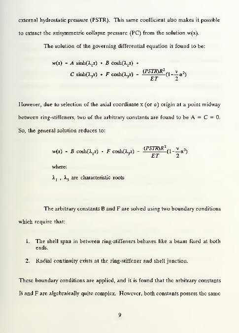
The solution of the governing differential equation is found to be:

w(x) = A sinhCXjJc) + B cosh^*) +

C smhCX^) + F cosha^) - (psm>R (1-^-a 2)ET 2

However, due to selection of the axial coordinate x (or u) origin at a point midway

between ring-stiffen ers, two of the arbitrary constants are found to be A = C = 0.

So, the general solution reduces to:

w(x) = B cosh(XjX) + F cosh(X^) - (PSTK>R (l--a 2)

where:

Aj

, A3are characteristic roots

The arbitrary constants B and F are solved using two boundary conditions

which require that:

1. The shell span in between ring-stiffeners behaves like a beam fixed at both

ends.

2. Radial continuity exists at the ring-stiffener and shell junction.

These boundary conditions are applied, and it is found that the arbitrary constants

B and F are algebraically quite complex. However, both constants possess the same

denominator quantity.1This denominator quantity is found to be a function of shell

material variables, shell geometry variables, and the characteristic roots. Since the

variables of shell material and geometry are independent of the PC term, the

axisymmetric collapse pressure (PC) must be extracted from the characteristic roots.

The PC term may be extracted from the solution w(x) by requiring that,

upon collapse, the radial displacement of the shell tend to infinity. That is, the

common denominator (which is a function of the characteristic roots) of the arbitrary

constants B and F is equal to zero when the external hydrostatic pressure (PSTR)

exceeds the axisymmetric collapse pressure (PC). Thus:

The characteristic roots A,1and X

3correspond to:

PSTR

PC> 1.0

Then, it is found that the characteristic roots are pure imaginary numbers:

K = iV3(l-v

2)

s/RT

PSTR

\ PC \ PC

k3

= i

..V^rv)

RT

PSTR

PSTR

\ PC \ PCPSTR

+ 1

1 For brevity, the algebraically complex expression of this common denominator

is omitted. See [Ref. 2: p. A-ll] for details.

10

When these characteristic roots are placed into the common denominator,

which is then set equal to zero, a transcendental equation results. This equation is

a function of PC and can be solved for the same.

The DAPS3 subroutine, in the THESIS code, calculates the PC term for

each change in the shell geometry design variables (thickness, T, for monocoque

shells; thickness, T, ring height, HEIGHT, and ring width, WIDTH, for ring-stiffened

shells). Recall that the other terms (shell material and geometry properties and

external hydrostatic pressure) used to extract the PC term are user-specified and

remain constant throughout the process. The PC term is then returned to the ADS

optimization program, incorporated in the THESIS code, to be evaluated as a

buckling constraint term.

2. Elastic Interbay Instability Pressure (PIB)

Recall that the PIB term is associated with two different names:

• Elastic Monocoque Shell Instability Pressure (for the monocoque shell).

• Elastic Interbay Instability Pressure (for the ring-stiffened shell).

This buckling load describes local non-symmetric collapse of a ring-stiffened shell in

between any two rings. Similarly, this describes non-symmetric collapse of a

monocoque shell in between its two rigid bulkheads (end-rings). An example of

interbay buckling is illustrated in Figure 3. Regardless of shell type, from hereon,

the PIB term will be called Elastic Interbay Instability Pressure, which describes the

more general case of a ring-stiffened shell.

11

Figure 3. Local Non-symmetric Buckling of a Ring-Stiffened Shell Between

Adjacent Rings.

Interbay buckling differs from the type of buckling described by the PC

term in subsection (a) in that inward and outward lobes are formed alternately

around the circumference. That is, the collapse is not axisymmetric. The number

of circumferential waves formed by these lobes is known as the buckling mode, which

is designated by the variable (n). This buckling mode term will be discussed in more

detail during development of the equations necessary to find the elastic interbay

instability pressure (PIB).

The first step in finding PIB is to establish the equilibrium equations for

a thin shell differential element, as shown in Figure 4. The differential equilibrium

equations ~ in terms of forces (N), moments (M), and radial displacement (w) — in

the x, <f>, and r directions are, respectively:

12

Figure 4. Differential Element of an Isotropic Thin Shell

&n a2^,* _

dx2 d<S>dx

#N„ dN± &M*<?> _ A

dx:

dtf d<\>dx Rd$i

i *+ - R2 * + + M = (/>/fl)(w+— +——

)

dx2 dxdb dx2dtf

*d<\>

2 2 dx 2

Next, a solution for the displacement terms — u (axial), v(circumferential),

and w(radial) — is assumed: 2

2In [Ref. 1, p.2-7], Renzi notes that this is the same displacement pattern used

by Von Mises for isotropic shells. It is a well accepted solution which is

somewhat conservative.

13

u = A sin(/i<b)sin—R

v = B cos(n(J))cos—

w> = sin(n<J))cosfix

where:

_ n

P = ; Ls

= Unsupported shell length between rings

These assumed displacements account for the sinusoidal nature of the

circumferential waves which form upon collapse. As noted earlier, the buckling

mode (n) is the number of waves formed.

UNDEFORMEDSHELL

DEFORMEDSHELL

Buckling Mod*

Figure 5. Buckling Mode (n) under Elastic Interbay Instability Pressure.

Next, strain and curvature expressions are generated in terms of the

assumed displacements. Then, the forces (N) and moments (M) are expressed in

14

terms of the generated strain and curvature expressions. Subsequently, the force and

moment expressions in the established differential equilibrium equations are now in

terms of the assumed displacements. That is, the three equilibrium equations are

now in terms of known shell material properties, known shell geometry properties,

unknown arbitrary constants A and B, and the unknown term PIB. The following

system of equations results:

ai

at

aMPlB*.

Note that the above at

terms are expressions in terms of known shell geometry

properties, known shell material properties, and buckling mode (n). To insure that

the last equation in the above system is a consistent linear combination of the other

two, the determinant of the following augmented matrix must equal zero:

det

a,

"4 "5 "6

a7

a%

a9+(PIB)a

l0

=

Thus, the elastic interbay instability pressure (PIB) is given by the

following explicit expression:

15

PIB = —

The only remaining unknown in the expression is the buckling mode (n). The

DAPS3 subroutine in the THESIS code iterates the variable n over an integer range

from 2 to 20. The minimum PIB calculated within this range is the elastic interbay

instability pressure, and the corresponding n is the number of circumferential waves

in which the shell will buckle. The value of PIB is returned to the ADS optimization

program, which is incorporated into the THESIS code, for evaluation as a buckling

constraint term.

3. Elastic General Instability Pressure (PGEN)

The third buckling load considered describes the overall or general

instability of a ring-stiffened shell, whereas the previously described PC and PIB

buckling loads described local instabilities (in between any two ring-stiffeners) for

both monocoque and ring-stiffened shells. Collapse under elastic general instability

pressure (PGEN) is somewhat similar to collapse under elastic interbay instability

pressure (PIB) in that the shell does not collapse axisymmetrically. That is, the shell

collapses in inward and outward lobes around the circumference as was seen in

Figure 5. However, the buckling effect is not isolated between any two ring-

stiffeners. Instead, the entire length of the shell (between its rigid bulkheads)

collapses with a discernible buckling mode (n), as seen in Figure 6.

16

Figure 6. General Non-symmetric Buckling of a Ring-Stiffened Shell

In deriving the previous local buckling loads, PC and PIB, differential

equations were used to find a closed form exact solution. However, use of a

differential equation method in deriving PGEN would be quite difficult without

making simplistic, perhaps unrealistic, assumptions. So, an alternative method is

needed to obtain an expression for PGEN.

The approach used is the Ritz energy method. Consider a system

consisting of a ring-stiffened shell under external hydrostatic pressure (PSTR). Pre-

buckling displacements and post-buckling (collapse) displacements (in the shell and

in the rings) contribute strain energy to the system. In addition, work is done by the

applied load (PSTR) to cause these displacements. Thus, the system possesses some

total potential energy, which is the sum of these strain potential energies and the

work done by external pressure:

17

", v„ * usb + ure

+ urJb

+ w^where:

C/f

= Total Potential Energy

l/je= Shell Extensional Strain Potential Energy

Usb = Shell Bending Strain Potential Energy

Ur

= Ring Extensional Strain Potential Energy

Urb = Ring Bending Strain Potential Energy

wpstr= Work of the External PressureCPSrfl)

Under the Ritz energy method, this total potential energy must be a minimum. This

requirement ultimately leads to a solution for the elastic general instability pressure

(PGEN), which is the critical PSTR at which the ring-stiffened shell buckles.

After a long series of derivations, it can be shown that the potential

energy, Ut,

is a function of: known shell/ring material and geometry properties; the

unknown elastic general instability pressure (PGEN); and the variable displacements

u,v, and w. The displacements due to buckling are assumed to be of the form:

u = ^jCOSC

v = B,sin(/i(J))s

w = CjCos(

n(J))cosj-y

nil— + £2sin(n(J>)

n4>)sin[^

1-cos( 2nx)

KLf)

+ Cxos(n4>) 1-cos2tt*

7 )

18

By substituting the above displacements into the U, expression, the total

potential energy becomes a function of the five arbitrary constants:

Ut= U

t(Av Bv Cv B

2, C2)

Recall that the total potential energy must be a minimum to satisfy equilibrium

requirements, thus:

BUt _ dU

t _ dUt _ dU

t _ dUt _

dA. dB, dC. dB~ dC2

The result is five symmetrical linear homogeneous equations in the unknown

arbitrary constants. These equations can be expressed in form [A-jjx,} = 0, or:

A2l

A22

A23

Au A25

^31 ^32 ^33 ^34 A35

^41 ^42 ^43 ^44 ^45

^51 ^52 AS3

AS4

AS5

=

The terms in the above 5X5 coefficient matrix are given by:

AV

au

- (PGEMby ; ij = 1,5

where:

aJb» expressions in terms of known material

and geometry properties and the

buckling mode variable(w)

19

Provided that the 5X5 coefficient matrix is symmetric and positive

definite, it has five positive eigenvalues, (PGEN)i5

and five corresponding

eigenvectors, {x};. The minimum eigenvalue is the external pressure (PGEN) at

which the ring-stiffened shell will buckle.

However, the buckling mode (n) still remains a variable quantity to

consider when establishing the minimum eigenvalue. The DAPS3 subroutine iterates

(n) in the integer range from 2 to 12, and it saves the minimum eigenvalue (of the

five possible eigenvalues) for each corresponding mode. The array of these

eigenvalues is examined, and the absolute minimum is chosen as the elastic general

instability pressure (PGEN). This is the value which is returned to the ADS

optimization program to be considered as a buckling constraint term for a ring-

stiffened shell.

B. STRENGTH (STRESS) EQUATIONS

Another type of failure to consider is that of strength limitation. By this, it is

meant that the shell fails when resultant Von Mises stresses, at specific locations,

exceed the yield strength of the shell/ring material. Since material properties (such

as elastic modulus, Poisson's ratio, yield strength, etc.) are input by the THESIS code

user and remain fixed, some constraints must be placed on the optimum design to

20

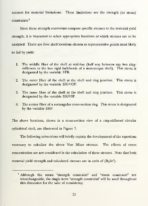
account for material limitations. These limitations are the strength (or stress)

constraints.3

Since these strength constraints compare specific stresses to the material yield

strength, it is important to select appropriate locations at which stresses are to be

analyzed. There are four shell locations chosen as representative points most likely

to fail by yield:

1. The middle fiber of the shell at mid-bay (half way between any two ring-

stiffeners or the two rigid bulkheads of a monocoque shell). This stress is

designated by the variable STR.

2. The outer fiber of the shell at the shell and ring junction. This stress is

designated by the variable SIGVOF.

3. The inner fiber of the shell at the shell and ring junction. This stress is

designated by the variable SIGVIF.

4. The center fiber of a rectangular cross-section ring. This stress is designated

by the variable SRF.

The above locations, shown in a cross-section view of a ring-stiffened circular

cylindrical shell, are illustrated in Figure 7.

The following subsections will briefly explain the development of the equations

necessary to calculate the above Von Mises stresses. The effects of stress

concentration are not considered in the calculation of these stresses. Note that both

material yield strength and calculated stresses are in units of (lbf/in

2).

3 Although the terms "strength constraint" and "stress constraint" are

interchangeable, the single term "strength constraint" will be used throughout

this discussion for the sake of consistency.

21

SIGVOF

-^STR SIGVIF

SRF

—

™

SHELL /RING END-RING RO

V v

Figure 7. Locations of Stress Values STR, SIGVOF, SIGVIF, and SRFShown in a Shell Cross-section View.

1. Middle Fiber Shell Stress at Mid-bay (STR)

The effects of the radial stress component are ignored in the calculation

of this Von Mises stress. In fact, the radial component is ignored in the calculation

of the Von Mises stress at all four locations since the shell is assumed to be thin.

(A side constraint is included in the THESIS code to insure that the thickness, T, is

less than or equal to 20 percent of the mean radius, R. This insures that the

optimum design has negligible radial stress components.)

22

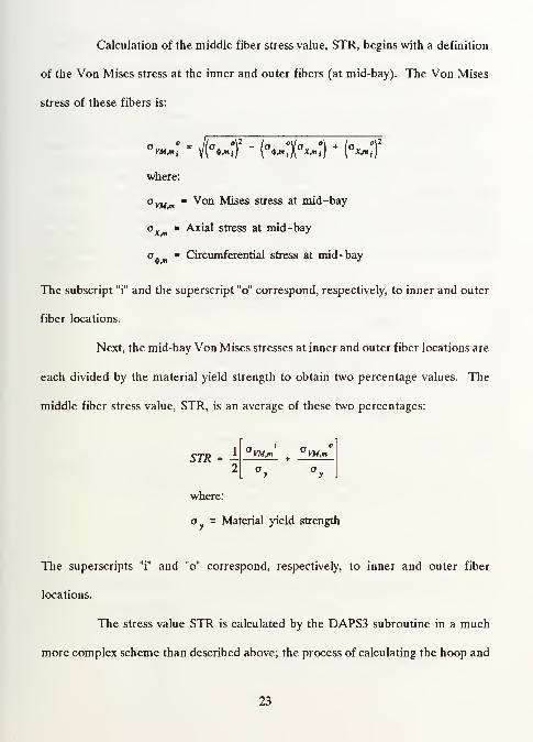
Calculation of the middle fiber stress value, STR, begins with a definition

of the Von Mises stress at the inner and outer fibers (at mid-bay). The Von Mises

stress of these fibers is:

•«-; - fZtf -MM + K;fwhere:

a vMjnm ^on Mis^ stress at mid-bay

ax - Axial stress at mid-bay

o^ = Circumferential stress at mid-bay

The subscript "i" and the superscript "o" correspond, respectively, to inner and outer

fiber locations.

Next, the mid-bay Von Mises stresses at inner and outer fiber locations are

each divided by the material yield strength to obtain two percentage values. The

middle fiber stress value, STR, is an average of these two percentages:

STR2

where:

o Material yield strength

The superscripts "i" and "o" correspond, respectively, to inner and outer fiber

locations.

The stress value STR is calculated by the DAPS3 subroutine in a much

more complex scheme than described above; the process of calculating the hoop and

23

axial stresses is quite involved.4 The STR value is returned to the ADS optimization

program to be considered as the first of four strength constraints on the optimum

design.

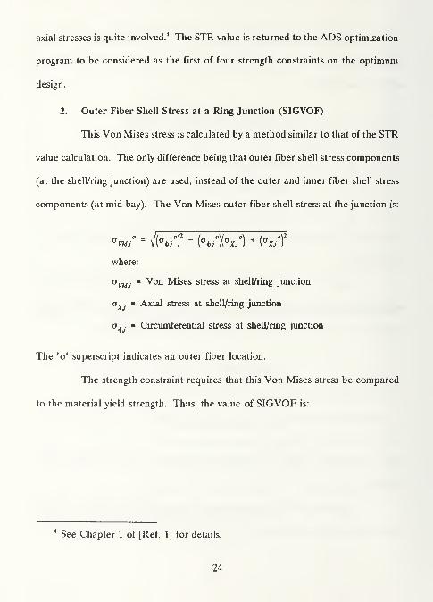
2. Outer Fiber Shell Stress at a Ring Junction (SIGVOF)

This Von Mises stress is calculated by a method similar to that of the STR

value calculation. The only difference being that outer fiber shell stress components

(at the shell/ring junction) are used, instead of the outer and inner fiber shell stress

components (at mid-bay). The Von Mises outer fiber shell stress at the junction is:

<W vK/)2

-MM + (V)2

where:

°vmj ~ ^on Mises stress at shell/ring junction

oXJ

- Axial stress at shell/ring junction

o . - Circumferential stress at shell/ring junction

The "o" superscript indicates an outer fiber location.

The strength constraint requires that this Von Mises stress be compared

to the material yield strength. Thus, the value of SIGVOF is:

4See Chapter 1 of [Ref. 1] for details.

24

SIGVOF = -^L

This is the value returned to the optimization program for consideration as the

second of four strength constraints.

3. Inner Fiber Shell Stress at a Ring Junction (SIGVIF)

The development of this value is identical to that of the SIGVOF value

except that inner fiber shell stress components are used. The Von Mises inner fiber

shell stress is defined as:

<W \/K/f - K/K1 + K/)2

where:

°vmj " V°n Mises stress at shell/ring junction

oXJ

- Axial stress at shell/ring junction

o^j Circumferential stress at shell/ring junction

Then, this Von Mises stress is compared to the material yield strength:

SIGVIF = -^-

This is the value returned to the optimization program for consideration as the third

of four strength constraints.

25

4. Center Fiber Ring Stress (SRF)

The last of the four strength constraints is the Von Mises stress at the

centroid of a ring-stiffener. Note that this is not a shell stress, but rather a stress

inside the internally located rectangular cross-section ring. Since the ring-stiffener

does not bear an axial load, the Von Mises stress inside the ring reduces to the

circumferential stress, which is defined as:

m*v*,r A

eff+ (WIDTH)(T)[rR)

where:

Q* = Total load on ring per unit circumference length

Aeff

= (HEIGHT)(WIDTH)(—

)

RR = Radius from shell centerline to ring centroid

HEIGHT = Height of rectangular ring-stiffener

WIDTH = Width of rectangular ring-stiffener

The "c" superscript indicates a center fiber location, which is the centroid of the ring.

Perhaps, the above shell geometry terms are best illustrated by Figure 8.

26

Figure 8. Illustration of Various Shell Geometry Terms.

27

III. OPTIMIZATION PROBLEM

Now that the buckling and strength terms have been defined, a mathematical

model of the optimization problem can be defined. The model consists of an

objective function (F), constraint functions (gj), and side constraint functions. These

functions will be defined in subsequent subsections of this chapter. A description of

the Sequential Linear Programming (SLP) technique used to optimize the model

follows those subsections.

A. OBJECTIVE FUNCTION

Recall that the objective of the optimization is to design a minimum weight

circular cylindrical shell. The objective function (F), then, is a mathematical

expression of the shell weight. For the general case of a ring-stiffened shell, the

objective function is:

24ti

L(R)(T)(L)(p) + (RO-YR)(AR)(±-lXPf)

where:

p - Specific weight [lbf/ft

3]of the shell(skin)

p/= Specific weight flbf

/ft3l of the ring(s)

Figure 8 best illustrates the above variable terms. The first quantity represents the

shell(skin) weight, while the second quantity represents the ring(s) weight. Note that

28

the weight is expressed on a (lb/ft) basis. The above expression is also valid for the

more specific case of a monocoque shell. In that case, the AR (ring cross-section

area) term would just be zero.

The objective function contains aU the design variables of the optimization

problem. Recall that the single design variable for the monocoque shell is:

1. Thickness (T)

In contrast, the ring-stiffened shell has three design variables, which are:

1. Thickness (T)

2. Ring height (HEIGHT)

3. Ring width (WIDTH)

The design variable T is explicitly expressed in the objective function. The objective

function (F) also contains indirect expressions which incorporate the design variables.

These expressions are:

R = RO - -2

yn _ rp HEIGHT+

2

AR = (HEIGHT)(WIDTH)

Now that the objective has been defined in terms of the design variable(s), the first

step in defining the optimization model is complete. Next, constraints on the design

variables will be defined.

29

B. CONSTRAINT FUNCTIONS

The constraints on the design variables are divided into three groups: 1)

buckling, 2) strength, 3) geometry. As noted in Chapter II, the number and type of

constraints placed on the design variables depends upon the particular shell being

designed: monocoque or ring-stiffened. The next two subsections define the specific

constraints placed on monocoque and ring-stiffened shell designs.

1. Monocoque Shell Constraints

The monocoque shell is subject to two buckling loads (PC,PIB); four stress

loads (STR,SIGVOF,SIGVIF,SRF); and no geometry constraints.5Accordingly, the

six constraints on the monocoque shell design are:

g l

= l-(PC/PSTR) <l

g2= l-(PIB/PSTR) z

g3= (STR/100) -1 s

gA= (SIGVOF/100) $

g5= (57GV7F/100)-1 s;

g6= (SRF/\00)-l z

In the above expressions, gj(j=l,2) represent the buckling constraints and

gj(j= 3,4,5,6) represent the strength constraints on the monocoque shell design.

5Actually, the monocoque shell is subject to a type of geometry constraint which

limits the range of the design variable, thickness (T), between an upper and

lower bound. However, it will be seen that this is actually a side constraint on

the design variable.

30

2. Ring-stiffened Shell Constraints

The ring-stiffened shell is subject to three buckling loads (PC, PIB,

PGEN), four stress loads (STR, SIGVOF, SIGVIF, SRF), and one geometry

constraint which limits the ring aspect ratio (HEIGHT/WIDTH) to be less than 4:1.6

This geometry constraint is necessary to ensure that the resultant ring

design is not "flimsy", that is, unstable. The predominate mode of instability for

rectangular ring-stiffeners is the tendency to rotate about the ring-stiffener base [Ref.

3: pp. 23-24]. This rotation causes the ring-stiffener to deform in a sinusoidal pattern

which crosses in and out of the ring's vertical plane of symmetry. Since DAPS3 does

not check for this instability when designing a ring-stiffened shell, this particular

constraint keeps the ring aspect ratio low enough that the ring instability mode is

adequately addressed (by the THESIS produced shell design).7

Inclusion of this

constraint may result in a weight penalty since a "flimsy" ring may weigh less than a

short and thick, but inherently stable, ring.

The resulting eight constraints on the ring-stiffened shell design are given

by the following g- expressions:

6 As explained in the previous footnote, side constraints on the design variables

(T, HEIGHT, WIDTH) also apply for the ring-stiffened shell.

7 DAPS3 does attempt to prevent a "flimsy" ring. If intermediate designs have

an aspect ratio greater than 4:1 and a ring width less than 0.125 inch, a

minimum ring width of 0.125 inch is then forced. However, this does not

necessarily prevent the aspect ratio from increasing to an unreasonable number

(» 4:1).

31

g x= 1-(PC/PSTR) ±

g2= l-(PIB/PSTR) z

g3= 1-(PGEN/PSTR) <l

g4 = (STRJ100)- 1 <;

g5= (SIGVOF/100) <;

g6= (SIGV7F/100)-1 z

g7= (5i^F/100)-l ^

g8= [(HEIGHT/WIDTH)/^]-^ *

In the above expressions, gj(j= 1,2,3) represent the buckling constraints, gj(j=4,5,6,7)

represent the strength constraints, and gj(j= 8) represents the geometry constraint.

C. SIDE CONSTRAINTS

Side constraints directly impose bounds on the design variables. The ADS

optimization program incorporated into the THESIS code requires that the user

specify lower and upper bounds on all declared design variables. The optimization

search will then only occur in that portion of the design space delineated by the side

constraints.

The monocoque shell has only one design variable, T, and it is directly

constrained by the following bounds:

0.10 IN s T z 1.818 IN

The lower bound was chosen as an arbitrarily low number to permit a broad design

space, knowing that the lower bound would not be approached at the higher external

hydrostatic pressure shell loads. The upper bound was chosen such that the shell

thickness (T) would not exceed the ratio:

32

- s 0.20R

where:

1 TR = - (Shell Outside Diameter) - —

2 2

T= RO - -

2

Since the shell outside diameter is fixed input (OD = 20 IN), the outside radius

remained fixed (RO = 10 in). Thus, the value of T = 1.818 IN was calculated such

that the shell thickness never exceeded 20% of the mean radius. Recalling that the

objective is to design a thin circular cylindrical shell, a T/R value less than 20%

assures that the shell remains "thin". That is, radial stress is much smaller than axial

or circumferential stresses and can be ignored.

The design variables of a ring-stiffened shell are assigned the following side

constraints:

0.10 IN * T z 1.818 IN

0.05 IN <; HEIGHT <l 10.0 IN

0.05 IN <; WIDTH <l 5.0 IN

Again, the lower bounds are chosen to be arbitrarily low. The upper bounds are

chosen such that: HEIGHT does not exceed the physical dimension of the shell

outside diameter, and WIDTH does not become so wide that the resulting HEIGHT

is negligible (in other words, the ring would be virtually flat, and a monocoque shell

would probably be more appropriate).

33

D. SUMMARY

The mathematical models of the monocoque and the ring-stiffened shell are

summarized below. These are the models programmed into the THESIS code to

solve the optimization problem.

1. Monocoque Shell

Minimize:

F =24ti

(R)(T)(L)(p) + (RO-YR)(AR)&-'h

Subject to:

Side constraints:

g l= l-(PC/PSTR) <;

g2 = l-(PIB/PSTR) <;

g3= (STRJ100)-1 £

g4 = (SIGVOF/lOO) z

g5= (5/GWF/100)-l ^

g6= (SKF/100)-! <;

0.10 IN s 7 <; 1.818 IN

34

2. Ring-Stiffened Shell

Minimize:

24ti

L(R)(T)(L)(p) * (RO-YR)(AR)Uj-l\p

Subject to:

g l= \-(PC/PSTR) z

g2= \-(PIBIPSTR) z

g3= l-(PGENIPSTR) 4

gA= (STtylOO)-l z

g5= (SIGVOF/100) z

g6= (SIGVIF/lOO)-\ <l

gn= (SRF/100)-1 <;

gs= [(HEIGHT/WIDTH)/4]-l <l

Side constraints:

0.10 IN ^ T ^ 1.818 IN

0.05 IN * HEIGHT <l 10.0 IN

0.05 IN ^ W7Z>777 ^ 5.0 IN

E. OPTIMIZATION TECHNIQUE

The mathematical models are now structured for application of an optimization

technique. The general purpose numerical optimization program, Automated Design

35

Synthesis (ADS), is used in conjunction with the analysis mode of the DAPS3 to

produce optimum shell designs. An excellent reference on numerical optimization

techniques is found in [Ref. 4].

The procedure to obtain the optimum shell design involves a mathematical

search from an initial design, X°, to the optimum design, X*. A gradient method is

used to search for X* within the design space specified by the side constraints.

Search limitations within this design space are imposed by the constraint functions.

The objective function, F, when evaluated at the optimum design, X*, is the

minimized objective: shell weight.

The above optimization procedure is described in more detail by the following

general steps [Ref. 5: p. 15]:

1. User inputs an initial design, X°, for the qlh

iteration; q = 0.

2. Iteration number, q, is updated to q = q + 1.

3. Objective function, F(X), and the constraint functions, gj(X), are evaluated at

the design Xql.

4. Active constraints, J, are identified. These are the gj constraints which are

very close to zero, within a specified tolerance, say « 0.003.

5. The objective function gradient, V F(Xql) is evaluated, and critical constraint

function gradients, V gj(Xql

) are evaluated for j e J.

6. Search direction, Sq, is determined from the evaluations in step 5.

7. A one-dimensional search is performed to find the step length a.

8. The design, Xql, is updated by: Xq = Xql + a*Sq

.

36

9. Convergence criteria are examined. If design has converged, then X* has

been found. Otherwise, the procedure is reiterated from step 2.

Execution of the above general procedure may be accomplished by a variety of

methods, especially at steps 3, 6, and 7. Step 3 is termed the "strategy" (ISTRAT);

step 6 is termed the "optimizer"(IOPT); and step 7 is termed the "one-dimensional

search"(IONED). These are the three basic levels at which the ADS numerical

optimization program can be controlled to produce an optimum design.

ADS offers a great number of combinations of these basic levels. In fact,

version 1.10 offers nine strategies, five optimizers, and eight one-dimensional search

methods [Ref. 6]. Selecting an appropriate combination of ISTRAT, IOPT, and

IONED is a matter of experience, since not all possible combinations are suitable

to particular kinds of optimization problems.

The specific combination chosen for this study is:

• ISTRAT = 6: Sequential Linear Programming

• IOPT = 5: Modified Method of Feasible Directions

• IONED = 6: Golden Section + Polynomial 1-D Search

The Sequential Linear Programming (SLP) method is an optimization strategy that

approximates a nonlinear problem as a linear problem. This is done by creating a

first order Taylor Series approximation of the objective and constraint functions.

Now that the problem is linear, an evaluation of the objective and constraint

functions are easily and inexpensively calculated, in terms of computer time. Then,

37

the Modified Method of Feasible Directions is used to determine a search direction

Sq. This is also easily obtained since the gradients of the objective and constraint

functions are directly available from the Taylor Series expression. Next, the Golden

Section + Polynomial one-dimensional search method is used to find the step length,

a. This step length is how far the search direction vector, Sq, will traverse from

design point Xql. An optimum design, Xq

, to this linear approximation is then

obtained. The original nonlinear problem is again linearized about this design. The

process is repeated until an optimum solution is obtained, as determined by specific

convergence criteria.

This combination using the SLP method is a very fast optimization technique

since the original nonlinear problem is approximated as a linear problem. Speed

represents the major advantage in using this method. Possible disadvantages include:

1) the optimum design may be infeasible and 2) the method may perform poorly for

an underconstrained problem [Ref. 4: pp. 156-157]. The first disadvantage means

that X*, though very close to the true optimum, may have a small degree of

constraint violation. The second disadvantage means that if there are fewer active

constraints at the optimum than there are design variables, the method may not

rapidly or accurately converge to the true optimum. ADS deals with this difficulty

by imposing finite move limits on the linear approximation so that the true optimum

will be approached within the tolerance of the move limits. These possible

disadvantages are not considered severe enough to preclude use of the SLP method

for this optimization problem. In fact, all methods within the ADS program have

38

certain advantages and disadvantages which must be accepted when that method is

applied to a particular optimization problem.

The optimization combination chosen for this study was compared against other

direct and indirect methods.8It was found that the array of optimum designs

produced by the SLP method were almost identical to the other strategies. The

speed advantage offered by the SLP method was the principal reason that this

particular optimization combination was chosen. The next chapter presents the

results of applying SLP to the mathematical models defined in this chapter.

8 An "indirect" method involves converting a constrained problem into an

unconstrained problem; the constraints are accounted for by a penalty function

method, and the objective function is converted into a pseudo-objective

function which includes the penalty function. By contrast, a "direct" method

involves dealing with the objective and constraint functions individually during

the optimization process.[Ref. 4: pp.54-58]

39

IV. RESULTS

A. MONOCOQUE SHELL

The elements of an optimum design are derived from the optimization model.

Accordingly, the results are presented in three parts:

1. Objective: DAPS3 vs. THESIS

2. Design Variables: DAPS3 vs. THESIS

3. Constraints: DAPS3 vs. THESIS

The first part will compare the optimum shell weights achieved by each program

(DAPS3 and THESIS). The second part then compares the optimum shell thickness'

(T) which correspond to these optimum shell weights. The last part will compare

constraint activity (buckling and strength violations) of the two optimum designs.

1. Objective: DAPS3 vs. THESIS

A graphical comparison of the optimum weights achieved by DAPS3 and

THESIS is shown in Figures 9 and 10. The graphs are set up such that the optimum

monocoque shell weights are shown over a range of external hydrostatic pressure

(PSTR) loads and over a range of shell geometries (L/OD ratios, which were varied

from 9:1 to 1:1). It can be seen that the weight curves (of each L/OD ratio) is

essentially the same for both programs. The one noticeable difference is seen in the

1:1 (L/OD ratio) weight curves. The THESIS objective (weight) is somewhat higher

40

90

80

^70H^ 60CQ

ri 50

£: 40

S2 30

£= 20

10

DAPS3 OPTIMUM WEIGHTMONOCOQUE SHELL

1000 2000 3000 4000 5000

PSTR [PSI]

L/OD

^^ 9:1

7:1

5:1

3:1

1:1

6000

Figure 9. DAPS3 Optimum Shell Weight

90

80

i—i 70

^ 60CQ

id 50

t: 40

S5 30

^ 20

10

THESIS OPTIMUM WEIGHTMONOCOQUE SHELL

1000 2000 3000 4000

PSTR [PSI]

5000

L/OD

-m-===^^™ 9:1

^^^^^^^Z^^' —i

—

^^^^^^^^ 7:1

^^z^^^^ 5:1

Jf^ ^J2!^^^^^^^^^ >^^ 3:1

// ^^^ /^^ ->«-

~-{y^ 1:1

^6000

Figure 10. THESIS Optimum Shell Weight

41

than the DAPS3 objective after PSTR = 1000 psi. This will be accounted for in part

three of these results. It will be seen that the increase in weight was necessary due

to an increase in thickness to compensate for a constraint violation.

At this point, the results of an optimum shell weight comparison do not

indicate the advantage of using a numerical optimization technique. The next

optimum design element to be examined is the single design variable of the

monocoque shell: shell thickness (T).

2. Design Variables: DAPS3 vs. THESIS

The design variable, shell thickness (T), is a monotonically increasing

variable. That is, as the external hydrostatic pressure (PSTR) increases, the

thickness also increases. This results in the shell weight being directly proportional

to the shell thickness, as would be expected. Accordingly, the optimum thickness

curves look like the optimum weight curves. This can be seen in Figures 11 and 12.

Since the monocoque shell only has one design variable, the design space

is quite simple. There is only one design variable which corresponds to the global

optimum in this design space. Even the simple iterative technique employed by

DAPS3 will converge quite close to the unique design variable which corresponds to

the global optimum (minimum weight). Thus, the advantage of using a numerical

optimization technique to find the optimum design variable is not realized. The last

part of these results will indicate the advantage of using numerical optimization in

even a simple one variable design space.

42

DAPS3 OPTIMUM THICKNESSMONOCOQUE SHELL i/od

0.8-

^L 0.6-

0.4-

0.2-i0^9:1

7:1

—SK

—

5:1

3:1

X1:1

C 1000 2000 3000 4000 5000 6000

PSTR [PSI]

Figure 11. DAPS3 Optimum Shell Thickness (T)

1.2

0.8

!ZL 0.6

0.4

0.2

THESIS OPTIMUM THICKNESSMONOCOQUE SHELL

1000 2000 3000 4000

PSTR [PSI]

L/OD

==^L#^"__

^-^^^^^^^^ 9:1

^^^^^^^ 7:1

^^^^ ^^Ja ^^ -^—

m^^^ ^^^^^^^ 5:1

y^ ^^^ ^^/TJ*^^/^^

3:1

{f 1:1

5000 6000

Figure 12. THESIS Optimum Shell Thickness (T)

43

3. Constraints: DAPS3 vs. THESIS

The six constraints imposed on a monocoque shell design are shown in

Figures 13 through 18. The graphs are set up such that a violated constraint is a

positive gj(j= 1,6) value; a satisfied constraint is represented by a negative value;

and an active constraint is a zero value. If the constraint is violated, this is an

indication of an infeasible design. A feasible design is indicated by an active

constraint or a satisfied constraint.

The purpose of showing graphs of each constraint is to identify, at a

glance, any violations which the "optimum" design may have. The optimum designs

produced by DAPS3 and THESIS may be a minimum weight shell design for the

input load (PSTR) and geometry (L/OD). However, the code user must be able to

verify that the produced optimum, in fact, satisfies the original constraints imposed

upon the design. If there are violations, the design produced is not a valid design.

That is, the design is infeasible: the objective may have been minimized, but at the

expense of violated constraints.

In comparing DAPS3 and THESIS objective values, one program's design

may weigh less than the other (when load and geometry are the same for each

program). Before accepting the lesser weight design as the true optimum, constraint

activity must be verified as outlined above. An example of this was seen in

monocoque shell designs of 1:1 L/OD ratios. DAPS3 appears to produce lesser

weight designs above PSTR = 1000 psi than THESIS, however, these DAPS3 designs

violate the strength (stress) constraints g3(STR) and g5(SIGVIF).

44

DAPS3 G(l) CONSTRAINTMONOCOQUE SHELL L/OD

2

-2

-4

CJ -8

-10

-12

-14

-16

9:1

7:1

5:1

3:1

'1 1:1

-JSYMMETRIC

LOCAL BUCKLING

2000 3000 4000

PSTR [PS1]

5000

Figure 13. DAPS3 Constraint: Symmetric Local Buckling (PC)

THESIS G(l) CONSTRAINT

2

-2

-4

Cf -8

-10

-12

-14

-16

MONOCOQUE SHELL L/OD

9:1

r^^^^^s=======*

/f^r* 7:1

- / kf >K

* //5:1

11

- II 3:1

a/1 X- I 1:1

- 1 SYMMETRIC

-£ LOCAL BUCKLING

1000 2000 3000 4000

PSTR [PSI]

5000 6000

Figure 14. THESIS Constraint: Symmetric Local Buckling (PC)

45

DAPS3 G(2) CONSTRAINTMONOCOQUE SHELL L/OD

o-

-0.5-

S -1.5-O

-2-

-2.5-

-3-

9:1

7:1

—sk—5:1

O3:1

X1:1

"\NON-SYMMETRICLOCAL BUCKLING

C 1000 2000 3000 4000 5000

PSTR [PSI]

6000

Figure 15. DAPS3 Constraint: Non-Symmetric Local Buckling (PIB)

THESIS G(2) CONSTRAINTMONOCOQUE SHELL L/OD

o-

-0.5-

-1 -

S -1.5-O

-2-

-2.5-

-3-

9:1

—*

—

7:1

5:1

3:1

X1:1

NON-SYMMETRICLOCAL BUCKLING

( ) 1000 2000 3000 4000 5000 60

PSTR [PSI]

)0

Figure 16. THESIS Constraint: Non-Symmetric Local Buckling (PIB)

46

DAPS3 G(3) CONSTRAINTMONOCOQUE SHELL

STRESS:

1000 2000 3000 4000

PSTR [PSI]

5000

L/OD

6000

Figure 17. DAPS3 Constraint: Stress (STR)

o.i

o

-0.1

-0.2

-0.3

^"0.4"O -0.5

-0.6

-0.7

-0.8

-0.9

-1

THESIS G(3) CONSTRAINTMONOCOQUE SHELL

[000 2000 3000 4000

PSTR [PSI]

5000

L/OD

9:1

7:1

^^^*^ ^^L^**1**^5:1

/ ^^ j^**1*^

3:1

X1:1

STRESS:STR

Figure 18. THESIS Constraint: Stress (STR)

47

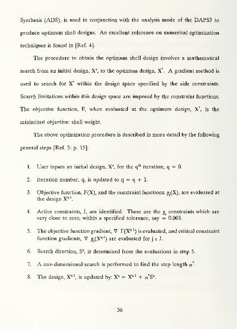
o-

-0.2-

^ -0.4-

O-0.6-

-0.8-

C

DAPS3 G(4) CONSTRAINTMONOCOQUE SHELL L/OD

9:1

—t

—

7:1

5:1

—B—3:1

X1:1^^^^ STRESS:

SIGVOF

1000 2000 3000 4000 5000

PSTR [PSI]

6000

Figure 19. DAPS3 Constraint: Stress (SIGVOF)

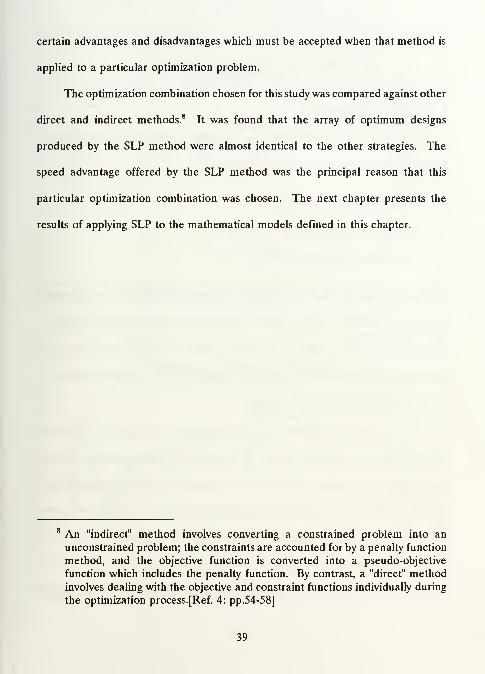
On

-0.2-

-0.4-

O-0.6-

-0.8-

-1 -

(

THESIS G(4) CONSTRAINTMONOCOQUE SHELL L/OD

9:1

7:1

—*k—5:1

3:1

X1:1Z' ^^^^{^^ STRESS:

SIGVOF

) 1000 2000 3000 4000 5000

PSTR [PSI]

60 30

Figure 20. THESIS Constraint: Stress (SIGVOF)

48

0.4-

0.2-

o-

^ -0.2-

^ -0.4-

-0.6-

-0.8-

-1 -

C

DAPS3 G(5) CONSTRAINTMONOCOQUE SHELL L/OD

9:1

4

7:1

5:1

3:1

X1:1

STRESS:SIGVIF

1000 2000 3000 4000 5000

PSTR [PSI]

6000

Figure 21. DAPS3 Constraint: Stress (SIGVIF)

0.4-

0.2-

o-

^ -0.2-

° -0.4-

-0.6-

-0.8-

(

THESIS G(5) CONSTRAINTMONOCOQUE SHELL L/OD

9:1

7:1

5:1

3:1

1:1f/^^<^r STRESS:

SIGVIF

I 1000 2000 3000 4000 5000

PSTR [PSI]

60 30

Figure 22. THESIS Constraint Stress (SIGVIF)

49

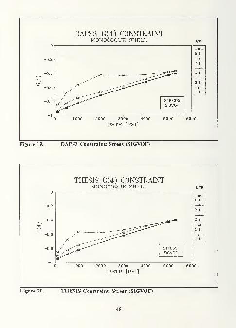
DAPS3 G(6) CONSTRAINTMONOCOQUE SHELL

-0.6-

-0.8

1000 2000 3000 4000

PSTR [PSI]

L/OD

Figure 23. DAPS3 Constraint: Stress (SRF)

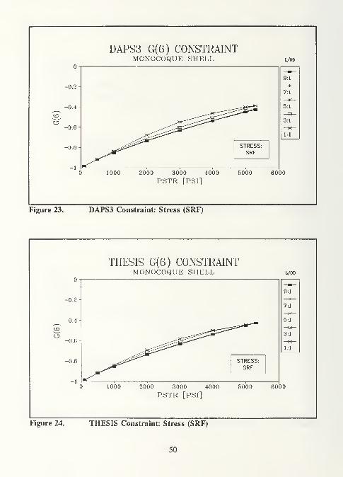
THESIS G(6) CONSTRAINTMONOCOQUE SHELL

-0.2

-0.4

-0.8

L/OD

9:1

7:1

—m—5:1

3:1

X1:1

J^^^^ STRESS:SRF

1000 2000 3000 4000

PSTR [PSI]

5000 6000

Figure 24. THESIS Constraint: Stress (SRF)

50

The DAPS3 strength constraint violations are seen in Figures 17 and 21.

This is especially noticeable in Figure 21. The g5strength constraint (SIGVIF)

remains violated at all pressures above 1000 psi (for 1:1 L/OD) and above 4000 psi

(for 3:1 L/OD). Thus, all 1:1 and 3:1 (L/OD) DAPS3 designs above the

aforementioned pressures are infeasible due to material failure by yield. By contrast,

the THESIS designs, which include strength constraints, designs monocoque shells

which satisfy all strength constraints. This can be seen in Figures 18, 20, 22, and 24.

The DAPS3 iterative technique is only constrained by buckling

considerations. As seen in Figures 13 and 15, the DAPS3 designs do not violate

either monocoque shell buckling constraint throughout the range of applied loads.

DAPS3 designs a minimum weight shell with the consideration being that a shell

which just exceeds buckling loads will be the absolute minimum design required to

withstand the external hydrostatic pressure. All monocoque designs thicker than this

absolute minimum will also not buckle. These designs will also withstand greater

structural stresses due to the added thickness, but an additional weight penalty is

imposed upon these stronger designs. Because DAPS3 does not consider strength

constraints, the smaller L/OD ratio DAPS3 designed shells are limited by stresses

which exceed the material yield strength. In contrast, the THESIS code considers

both strength and buckling constraints. As can be seen in Figures 14, 16, 18, 20, 22,

and 24, both types of constraints remain satisfied throughout the range of pressures

for all L/OD ratios. The THESIS shell weight may be heavier, but the design is

feasible throughout the range of pressures.

51

B. RING-STIFFENED SHELL

The results for the ring-stiffened shell are presented in the same format as the

monocoque shell: objective, design variables, and constraints. There are now three

design variables (instead of one) and eight constraints (instead of six). This results

in a more complex optimization problem since the design space is now three-

dimensional (due to three design variables). The simple iterative technique

employed by DAPS3 produced nearly the same objective (shell weight) as the

THESIS program, which used a numerical optimization technique. However, the

optimum design variables for DAPS3 and THESIS differed. Specifically, the

HEIGHT and WIDTH of the ring-stiffener varied considerably. A graphical

summary of the results are seen in Figures 25 through 48.

1. Objective: DAPS3 vs. THESIS

The first optimum design element examined is the objective: optimum shell

weight. Inspection of Figures 25 and 26 show that essentially the same objective was

achieved by DAPS3 and THESIS. Some slight weight reduction is seen in the 1:1

and 3:1 THESIS weight curves, which can be attributed to a lesser weight ring design

(that is, design variables of HEIGHT and WIDTH). This will be discussed in the

design variable results. In general, it can be concluded that the iterative design

technique essentially achieves the same objective as the numerical optimization

technique. The other design elements (design variables and constraints) must be

examined to reveal if numerical optimization provides any advantage.

52

90-

80-

i—i70-

E-"

\ 60-

CE

Z± 50 ~

E^ 40-JU

E5 30-

^ 20-

10-

0-C

DAPS3 OPTIMUM WEIGHTONE RING SHELL L/OD

-0^"9:1

—*

—

7:1

—*<=

—

5:1

3:1

1:1

1000 2000 3000 4000 5000

PSTR [PSI]

6000

Figure 25. DAPS3 Optimum Weight (Ring-Stiffened Shell)

90-

80-

^70-^ 60-PQ

££, 50 "

S5 30-

^ 20-

10-

o-(

THESIS OPTIMUM WEIGHTONE RING SHELL L/OD0^ 9:1

7:1

5:1

D3:1

X1:1

) 1000 2000 3000 4000 5000

PSTR [PSI]

60 30

Figure 26. THESIS Optimum Weight (Ring-Stiffened Shell)

53

2. Design Variables: DAPS3 vs. THESIS

The three optimum design variables produced by DAPS3 and THESIS are

seen in Figures 27 through 32. The first design variable, T, is compared in Figures

27 and 28. There is not an apparent difference between the two programs. Shell

thickness, T, remains a monotonically increasing variable with increasing external

hydrostatic pressure. Since shell thickness is the primary source of shell weight, the

optimum thickness curves look very similar to the weight curves, as was seen in the

monocoque shell case.

The addition of a single ring-stiffener also contributes to the weight curves,

although not very noticeably. Within the surveyed pressure range (500 psi to 5800

psi), both DAPS3 and THESIS design a relatively small single ring-stiffener into the

shell design. The small size of this ring-stiffener, in relation to the entire shell, is the

reason that the weight curves resemble only the shell thickness curves. However, this

small ring-stiffener increases the allowable external hydrostatic pressure by about 500

psi. That is, compared to a similar L/OD ratio monocoque shell, the ring-stiffened

shell design can withstand a load of 5800 psi (instead of 5300 psi for the monocoque

shell) before the material fails by yield.

The design of this ring-stiffener consists of optimizing the variables

HEIGHT and WIDTH such that the shell weight, which includes the weight of the

ring, is minimized and all constraints are satisfied. As seen in Figures 29 through 32,

the optimized variables of ring HEIGHT and ring WIDTH are quite different

between the DAPS3 and THESIS codes.

54

DAPS3 OPTIMUM THICKNESSONE RING SHELL L/OD

m

1-9:1

7:1

0.8-

^L 0.6-

5:1

3:1

><

0.4- 1:1

0.2-

C 1000 2000 3000 4000 5000

PSTR [PSI]

6000

Figure 27. DAPS3 Optimum Shell Thickness (T)

1.2-

1-

0.8-

£1 0.6-

E-«

0.4-

0.2-

o-(

THESIS OPTIMUM THICKNESSONE RING SHELL L/OD

0^ 9:1

7:1

5:1

3:1

1:1

) 1000 2000 3000 4000 5000

PSTR [PSI]

60 30

Figure 28. THESIS Optimum Shell Thickness (T)

55

DAPS3 OPTIMUM RING HEIGHT

1000 2000 3000

PSTR

2.5-

9:1

2-7:1

^1 1.5- 5:1

GHT

^^^^L3:1

Ed1:1

0.5-

o -1i . i i i

4000 5000 6000

Figure 29. DAPS3 Optimum Ring Height (HEIGHT)

THESIS OPTIMUM RING HEIGHTONE RING SHELL l/od

2-

LL 1.5-

tn

S5 i-

S0.5-

Z?\9:1

7:1

—^k—5:1

D3:1

1:1

-

() 1000 2000 3000 4000 5000 601

PSTR)0

Figure 30. THESIS Optimum Ring Height (HEIGHT)

56

DAPS3 OPTIMUM RING WIDTHONE RING SHELL L/OD

10

EC 5E-

S *

2

1000 2000 3000 4000 5000 6000

PSTR

Figure 31. DAPS3 Optimum Ring Width (WIDTH)

THESIS OPTIMUM RING WIDTHONE RING SHELL

, ,7

rc 5

Q 4

L/OD

9:1

7:1

5:1

—B-3:1

1000 2000 3000 4000 5000 6000

PSTR

Figure 32. THESIS Optimum Ring Width (WIDTH)

57

Because the design variables HEIGHT and WIDTH are non-linear in the

objective function, neither variable is monotonically increasing or decreasing with

respect to the external hydrostatic pressure load. This accounts for the wide array

of ring heights and widths for each L/OD ratio, as designed by the THESIS code

(see Figures 30 and 32). By contrast, the ring heights for each L/OD ratio, as

designed by the DAPS3 code, are generally increasing with increasing pressure (see

Figure 29), and the ring widths for each L/OD ratio are generally decreasing (see

Figure 31). Thus, a noticeable difference exists in the way that the two programs

optimize non-linear design variables.

At this point, it is seen that the same objective may be achieved by

different design variables. The selection of these optimum design variables depends

on the particular technique employed: iterative (DAPS3) or numerical optimization

(THESIS). As in the case of monocoque shell design, an examination of constraint

activity by the two different programs may reveal if the numerical optimization

technique yields any advantages.

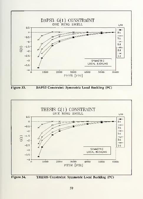
3. Constraints: DAPS3 vs. THESIS

The ring-stiffened shell, as designed by THESIS, has eight design

constraints: three for buckling, four for strength, and one for geometry. Recall that

DAPS3 designs are only constrained by buckling considerations. This difference

results in noticeable strength constraint violations by DAPS3 designs. A graphical

comparison of all eight constraints is shown in Figures 33 through 48.

58

0.5

-0.5

-1

eT -2

-2.5

-3

-3.5

-4

DAPS3 G(l) CONSTRAINTONE RING SHELL L/OD

—9:1

7:1

//j^ 5:1

df/yD

3:1

J

1:1

SYMMETRICLOCAL BUCKLING

1000 2000 3000 4000

PSTR [PSI]

5000 6000

Figure 33. DAPS3 Constraint: Symmetric Local Buckling (PC)

0.5-

o-

-0.5-

-1 -

cT -2-

-2.5-

-3-

-3.5-

-4 -

(

THESIS G(l) CONSTRAINTONE RING SHELL L/0D

9:1

7:1

5:1

3:1

X1:1w^

SYMMETRICLOCAL BUCKLING

1 1000 2000 3000 4000 5000

PSTR [PSI]

60 )0

Figure 34. THESIS Constraint: Symmetric Local Buckling (PC)

59

DAPS3 G(2) CONSTRAINTONE RING SHELL

^ -4C\2

-10

-12

9:1

7:1-

lAl^r D-—_ ~*

5:1

o3:1

1:1

.

NON-SYMMETRICLOCAL BUCKLING

1000 2000 3000 4000

PSTR [PSI]

5000 6000

Figure 35. DAPS3 Constraint: Non-Symmetric Local Buckling (P1B)

THESIS G(2) CONSTRAINTONE RING SHELL L/0D

9:1

~~^\ "-==*==;;----_: —i

—

7:1

5:1

3:1

-X—1:1

NON-SYMMETRICLOCAL BUCKLING

1000 2000 3000 4000

PSTR [PSI]

5000 6000

Figure 36. THESIS Constraint: Non-Symmetric Local Buckling (PIB)

60

0.5

-0.5

-1

S -1.5O

-2

-2.5

-3

-3.5

DAPS3 G(3) CONSTRAINTONE RING SHELL

1000 2000 3000

PSTR4000 5000

L/OD

! m —9:1

—*

—

7:1

\ -~^=^-

—**—5:1

-

3:1

- X1:1

NON-SYMMETRICGENERAL BUCKLING

6000

Figure 37. DAPS3 Constraint: Non-Symmetric General Buckling (PGEN)

THESIS G(3) CONSTRAINTONE RING SHELL L/0D

0.5-

o-

-0.5-

£2-O -1.5-

-2-

-2.5-

-3-

9:1

7:1

5:1

3:1

X1:1

NON-SYMMETRICGENERAL BUCKLING

(I 1000 2000 3000 4000 5000 60

PSTR [PSI]

)0

Figure 38. THESIS Constraint: Non-Symmetric General Buckling (PGEN)

61

-0

-0

2~°O -0

-0

-0

-0

-0

DAPS3 G(4) CONSTRAINTONE RING SHELL

1000 2000 3000

PSTR4000 5000

L/OD

Figure 39. DAPS3 Constraint: Stress (STR)

o.i

-0

-0

2~°CJ -0

-0

-0

-0

-0

.5-

THESIS G(4) CONSTRAINTONE RING SHELL

1000

L/OD

6000

Figure 40. THESIS Constraint: Stress (STR)

62

DAPS3 G(5) CONSTRAINTONE RING SHELL

STRESS:SIGVOF

L/OD

7:1

5:1

—B-3:1

1:1

6000

Figure 41. DAPS3 Constraint: Stress (SIGVOF)

THESIS G(5) CONSTRAINTONE RING SHELL L/0D—

-0.1 -

^^x x *—' x 9:1

-H

—

-0.2- y*~ ^^^--—-^^^ 7:1

-0.3- / ^^ r^y^ ^<^^^ 5:1

3 -0.4-

-0.5- f /^^^^^ 3:1

X

-0.6-

-0.7-

i ^^^<^:::::^ 1:1

<*^<j#^^ STRESS:

-0.8-

-0.9-(

SIGVOF

) 1000 2000 3000 4000 5000 60 )0

PSTR

Figure 42. THESIS Constraint- Stress (SIGVOF)

63

0.2

o.i H

-0.1

^ -0.2 H

3 -0.3o

-0.4

-0.5

-0.6

-0.7

-0.8

DAPS3 G(6) CONSTRAINTONE RING SHELL

STRESS:SIGVIF

1000 4000 6000

Figure 43. DAPS3 Constraint: Stress (SIGVIF)

0.2

0.1

-0.1

<£, -0.3o

-0.4

-0.5

-0.6

-0.7

-0.8

THESIS G(6) CONSTRAINTONE RING SHELL

1000 2000 3000

PSTR4000 5000

L/OD

9:1

7:1

5:1

*: / *c ^'^^3:1

/l//^^ ^^^ 1:1

* /^^ STRESS:SIGVIF

6000

Figure 44. THESIS Constraint: Stress (SIGVIF)

64

0.1

-0.1

-0.2

^ -0.3

£. -0.4O

-0.5

-0.6

-0.7

-0.8

-0.9

DAPS3 G(7) CONSTRAINTONE RING SHELL

1000 3000 4000

PSTR

STRESS:SRF

L/OD

6000

Figure 45. DAPS3 Constraint: Stress (SRF)

0.1 -

o-

-0.1 -

-0.2-

-0.3-

£. -0.4 -

O-0.5-

-0.6-

-0.7-

-0.8-

-0.9-(

THESIS G(7) CONSTRAINTONE RING SHELL L/OD

9:1

7:1

5:1

3:1

X1:1

(j^~STRESS:SRF

*r^) 1000 2000 3000 4000 5000

PSTR60 30

Figure 46. THESIS Constraint: Stress (SRF)

65

-0

-0

-0

o -o

-0

-0

-0

-0

DAPS3 G(8) CONSTRAINTONE RING SHELL

1000 3000

PSTR

91RING

ASPECT RATIO- 7:1

-

5:1- o- 3:1

/1:1

W=Wr a -sa m-

Figure 47. DAPS3 Constraint: Ring Aspect Ratio

THESIS G(8) CONSTRAINTONE RING SHELL L/OD

Figure 48. THESIS Constraint: Ring Aspect Ratio

66

An inspection of Figures 33 through 38 shows that both DAPS3 and

THESIS generally satisfy all three buckling constraints. A visible improvement is

seen in the g3constraint, non-symmetric general buckling. A comparison of Figure

37 with Figure 38 shows that this constraint is better adhered to by the THESIS

code. In Figure 37, the DAPS3 g3constraint shows slight violations (just above the

zero line) but is generally active or satisfied. In contrast, Figure 38 shows that the

THESIS g3 constraint is always active or satisfied. Some improvement is realized by

using the numerical optimization technique.

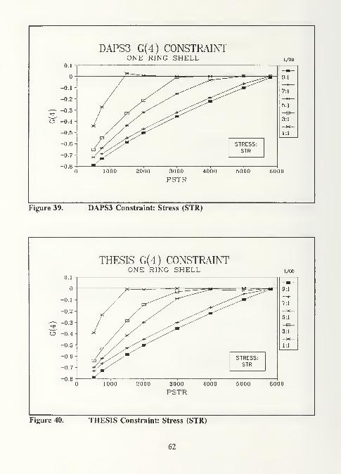
Strength constraints are considered next. These are shown in Figures 39

through 46. Notice that the THESIS gj(j= 4,5,6,7) constraints do not show any

violations: all designs insure that stresses do not exceed the material yield strength.

In contrast, the same DAPS3 constraints show violations in two cases. The first

violation is seen in Figure 39, which is the g4constraint (stress at mid-bay). This

constraint is rather small in comparison with the g6 constraint (stress at the shell and

ring junction inner fiber) seen in Figure 43. This constraint was identified as the

limiting stress location, which means that it is the first location where the shell would

fail by yield. At higher pressures, the g6 constraint is always active in the THESIS

designs, but some large violations occur in DAPS3 designs at these same pressures

(see Figure 43). Thus, use of a numerical optimization technique, which easily

incorporates strength constraints, has shown an advantage over the DAPS3 technique

which does not concurrently consider strength constraints and buckling constraints.

67

By considering both strength and buckling constraints, the THESIS codes

sometimes designs a thicker (and heavier) shell than the DAPS3 code. The result

is that the strength constraints become more active (since, at higher pressures, the

material yield strength is the limiting design factor) and some buckling constraints

become less active. An example of this is seen in Figures 36 and 38, which show the

g2 and g3 constraints falling below the zero line (becoming less active). The

corresponding pressures where the g2 and g3 constraints become less active are also

the pressures where all the strength constraints, gj(j= 4,5,6,7), approach the zero

line (become more active). This is seen in Figures 40, 42, 44, and 46. Thus, the

THESIS code may design a slightly heavier shell, but this shell design does not

violate any buckling or strength constraints.

Geometry is the last type of constraint considered. The g8 constraint limits the

maximum aspect ratio of the ring-stiffener to 4:1. This was done to prevent design

of a "flimsy" ring. This constraint is shown in Figures 47 and 48. Except for a few

of the smaller L/OD ratio designs, this constraint was generally not active. Initial

ring-stiffened shell designs by the THESIS code showed this constraint to be active

at higher pressures, however these earlier designs were made with a different

material (AISI 1060 steel, instead of the Al alloy 6061-T6 used in this study). In

summary, this constraint was not active, and all ring-stiffeners could be considered

"stable".

68

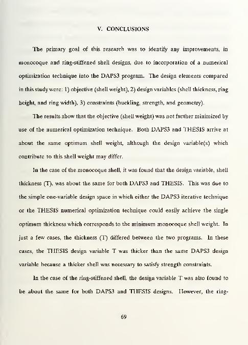
V. CONCLUSIONS

The primary goal of this research was to identify any improvements, in

monocoque and ring-stiffened shell designs, due to incorporation of a numerical

optimization technique into the DAPS3 program. The design elements compared

in this study were: 1) objective (shell weight), 2) design variables (shell thickness, ring

height, and ring width), 3) constraints (buckling, strength, and geometry).

The results show that the objective (shell weight) was not further minimized by

use of the numerical optimization technique. Both DAPS3 and THESIS arrive at

about the same optimum shell weight, although the design variable(s) which

contribute to this shell weight may differ.

In the case of the monocoque shell, it was found that the design variable, shell

thickness (T), was about the same for both DAPS3 and THESIS. This was due to

the simple one-variable design space in which either the DAPS3 iterative technique

or the THESIS numerical optimization technique could easily achieve the single

optimum thickness which corresponds to the minimum monocoque shell weight. In

just a few cases, the thickness (T) differed between the two programs. In these

cases, the THESIS design variable T was thicker than the same DAPS3 design

variable because a thicker shell was necessary to satisfy strength constraints.

In the case of the ring-stiffened shell, the design variable T was also found to

be about the same for both DAPS3 and THESIS designs. However, the ring-

69

stiffener designed by the two programs differed in ring HEIGHT and ring WIDTH.

This difference in design variables is not significant with respect to minimizing the

shell weight. That is, the optimum design variables produced by DAPS3 and

THESIS, although different, still result in the same shell weights. In the more

complex three-variable design space of this optimization problem, it was found that

HEIGHT and WIDTH are nonlinear variables in the objective function. This

accounted for the "up and down" range of values, seen in Figures 30 and 32, for

HEIGHT and WIDTH. Although HEIGHT and WIDTH do not significantly

contribute to shell weight (due to the relatively small size of the ring-stiffen er), these

design variables made a difference in complying with the design constraints.

The primary advantage of using a numerical optimization technique for shell

design was realized by an examination of the constraints. In general, both DAPS3

and THESIS satisfied the buckling constraints for both monocoque and ring-stiffened

shells. However, a significant difference was seen in the strength constraints.

In the monocoque shell case, it was found that some DAPS3 strength

constraints (especially at the ring and shell junction inner fiber location) are violated

(see Figure 21). In contrast, the same THESIS strength constraints were satisfied

due to an increase in shell thickness, as discussed above.

In the ring-stiffened shell case, it was found that similar strength constraint

violations occurred in DAPS3 designs. These constraint violations were absent from

THESIS designs. Since THESIS shell designs consider strength constraints, while

DAPS3 designs do not, the THESIS code was able to optimize the design variables

70

(especially ring HEIGHT and ring WIDTH) such that there were no strength

constraint violations.

In summary, incorporation of a numerical optimization technique into DAPS3

proved to be a worthwhile venture. The primary advantage realized is that

constraints can easily be added and tailored to fit a more constrained shell design

problem. This is simply done by adding a mathematical constraint function, gj, to the

optimization model. DAPS3 is an excellent shell design program, but it somewhat

lacks user flexibility in specifying additional constraints (such as strength constraints).

Another advantage realized is that additional design variables, such as shell length

(L) and shell outside diameter (OD), may be optimized when the flexible numerical

optimization technique is used.

The THESIS code was not written to refine the solutions produced by DAPS3,

but rather to supplement the number of solutions available. In this age of high-

speed digital computer technology, the ease of employing numerical optimization

techniques could be the key to discovering alternative, possibly more effective,

solutions to traditional problems.

71

VI. RECOMMENDATIONS

The THESIS code was a first endeavor into incorporating numerical

optimization with the DAPS3 program. Several possibilities exist for more

sophisticated optimization research. The following are suggested for any successive

research:

1. New design variables. Investigate optimum: number of rings, shell diameter,

or shell length.

2. New constraints. One example is maximum allowable shell deflection.

3. New materials. Composite (orthotropic) materials and/or hybrid construction

materials. Dramatic shell weight reductions may be realized by use of these

materials. The DAPS3 "analysis" and "design" modes fully supports research

of these materials.

4. New optimization strategies. Several optimization strategies exist in the ADSprogram which may improve upon the SLP strategy used in this study.

Additionally, a parametric optimization technique such as the homotopymethod using an envelope function may be investigated [Ref. 7].

72

APPENDIX A: THESIS CODE LISTING

This appendix provides a complete listing of the THESIS code. It is written

in FORTRAN to be compatible with the DAPS3 code, which is also written in

FORTRAN. Also included is the modified DAPS3 code, which is used as a

subroutine (DAPS3 SUB) by THESIS.

73

r-> *****************************************************************

C THESISC (AN INTEGRATED FORTRAN CODE FOR OPTIMUM DESIGN OF ISOTROPICC MONOCOQUE AND RING-STIFFENED CIRCULAR CYLINDRICAL SHELLSC SUBJECT TO EXTERNAL HYDROSTATIC PRESSURE USING A NUMERICALC OPTIMIZATION TECHNIQUE)/

'

*****************************************************************

CC THIS FORTRAN CODE INTEGRATES THE PROGRAMS:C 1) DESIGN AND ANALYSIS OF PLASTIC SHELLS, VERSION 3 (DAPS3)C BY J.R. RENZIC 2) AUTOMATED DESIGN SYNTHESIS, VERSION 1.10 (ADS)C BY G.N. VANDERPLAATSC PROGRAM (1) IS A SHELL ANALYSIS/DESIGN PROGRAM WHICH IS USED TOC CALCULATE THE BUCKLING AND STRENGTH TERMS CONTAINED IN THEC DESIGN CONSTRAINTS, G(I).

C PROGRAM (2) RECEIVES THE TERMS EVALUATED BY PROGRAM (1) ANDC EVALUATES THE DESIGN CONSTRAINTS AS PART OF THE OVERALLC NUMERICAL OPTIMIZATION PROCESS.C THE OBJECTIVE OF THIS NUMERICAL OPTIMIZATION PROCESS IS TOC DESIGN AN OPTIMUM (MINIMUM WEIGHT) RING-STIFFENED ORC MONOCOQUE SHELL.

PROGRAM THESIS

INTEGER NPLOT,NCURVE,NDESIGN,ORTHO,IPRINT,ISTRAT,IOPT,IONEDREAL ITHICK,IHEIGHT,rWIDTH

OPEN (20,FILE=7DAPS3 INP Al'.STATUS^OLD')

READ (20/(4(15))') NPLOT,NCURVE,NDESIGN,ORTHOIF((NPLOT.EQ.0).AND.(NDESIGN.EQ.-l))

: READ (20/(//////F10.3)') ARIF((NPLOTEQ.0).AND.(NDESIGN.NE.-l))

: READ (20,'(/////F10.3)') ARIF((NPLOTNE.0).AND.(NDESIGN.EQ.-l))

: READ (20/(/////F10.3)') ARIF((NPLOT.NE.0).AND.(NDESIGN.NE.-l))

: READ (20/(////F10.3)') AR

CLOSE(20,STATUS='KEEF)

INPUT ADS OPTIMIZATION PARAMETERS:IPRINT = 2020

ISTRAT = 6

IOPT = 5

IONED = 6

74

INPUT INITIAL DESIGN FOR OPTIMIZATION SEARCH:IF (AR.LE.O) THENITHICK = 1.1589

CALL MONO (IPRINT,ISTRAT,IOPT,IONED,rTHICK)ELSEITHICK = 0.191

IHEIGHT = 0.191

IWIDTH = 1.730

CALL RING (IPRINT,ISTRAT,IOPT,IONED,rTHICK,IHEIGHT,IWIDTH)ENDIF

END

SUBROUTINE MONO (IPRINT,ISTRAT,IOPT,IONED,ITHICK)

REAL L,ODXPC,PIB,R )RO,RHO,RHOF,AR

)YR,LF,MOSl,MOS2,MOS

REAL MSSl,MSS2,MSS3,MSS4,MSS,LS,IR,rTHICKINTEGER NPLOT,NCURVE,NDESIGN,ORTHO,NSAVE,ISEC,NXPNT,NYPNT,NFPNTINTEGER IPRINT,ISTRAT,IOPT,IONEDCHARACTER*70 TITLEPARAMETER (PI = 3.141593)

DIMENSION X(21), VLB(21), VUB(21), G(100), IDG(IOO), IC(30),

: DF(100), A(21,30), WK( 10000), IWK(5000)

COMMON AR)IR,YR,LF,LS,ARM,L,RO,T,GXY,EX,EY,EF

)VXY,VYX,VPLAS,R,

:PSTR,STR,SIGX,SIGY,SIGXl,SIGYl,HEIGHT,WIDTH,OD

COMMON /COUNT/ rrERAT,INDIC,INDIC2,INDIC3,

: INDICS.NDESIGN.ORTHCNOKG.NCURVE^IdTERAM.OKMJTERAG.OKCISEC,: NPLOT,NOKM,NRINGS,NEGLAM,INDIC7

COMMON /EMOD/ STRESX(10),STRINX(10),STRESY(10),STRINY(10),

:STRESF(10),STRINF(10),RATIOX,RATIOY,NXPNT,NYPNT,NFPNT

COMMON /GRAPH/ET(28),SIG(28),PB(28),PS(28),ES(28)AAA(6),

:BBB(6),CCC(8),DDD(6),EEE(5),FFF(7),GGG(4),HHH(7),000(8),ER(28),

:SIGF(28),SHAPEG(5),SHAPEI(3),WX(101)

COMMON /LAYER/ A11,A22,D11,D22

COMMON /STRESS/ STRX,STRY,PIB,NSAVEI,PGEN,NSAVEG

COMMON /HENRY/ SRF,WM,WF

OPEN (8,FILE=yTHESIS OUT Al',STATUS='OLD')

75

C COMMENCE READING INPUT VARIABLES FROM (20,FILE='/DAPS3 INP Al'):

OPEN (20,FILE=7DAPS3 INP Al\STATUS='OLD')

READ (20,500) NPLOT,NCURVE,NDESIGN,ORTHOREAD (20,50) TrTLEWRrrE(6,'(A/A)*) 'COMMENCING OPTIMIZATION OF:', TTTLEIF (NPLOT.EQ.O)

: READ (20,50) HHHIF (NDESIGN.EQ.-l)

: READ (20,51) A11,A22,D11,D22

READ (20,51) EX,VYX,VPLAS,SIGX,GXY,EY,EFREAD (20,53) PSTR,SIGY,SIGX1,SIGY1,PEL,STRX,STRY,NSAVEREAD (20,51) L,OD,T,RHO,RHOFIF (PEL.LE.0.)

: READ (20,51) AR,IR,YR,LF,LS,ARMIF (NDESIGN.GTO)

: READ (20,53) RINGS,SECDEP,DW,DASP,RINGSI,RINGSF,DRINGS,ISECIF (NCURVE.EQ.4) GOTO 2

READ (20,52) SIGXNOM,SIGYNOM,NXPNT,NYPNT,NFPNTREAD (20,55) (STRESX(I), I = 1,NXPNT)READ (20,55) (STRINX(I), I = 1,NXPNT)IF (NCURVE.EQ.l) GOTO 2

READ (20,55) (STRESY(I), I = 1,NYPNT)READ (20,55) (STRINY(I), I = 1,NYPNT)IF (NCURVE.EQ.2) GOTO 2

READ (20,55) (STRESF(I), I = l.NFPNT)READ (20,55) (STRINF(I), I = l.NFPNT)

500 FORMAT (BZ,10I5)

50 FORMAT (BZ,A)

51 FORMAT (BZ,8F10.3)

52 FORMAT (BZ,2F10.3,3I5)

53 FORMAT (BZ,7F10.3,I5)

55 FORMAT (BZ,10F8.0)

2 CONTINUE

CLOSE(20,STATUS='KEEP')

NRA = 21

NCOLA = 30

NRWK = 10000

NRrWK = 5000

IGRAD =NDV = 1

NCON = 6

C THE LOWER BOUND IS THE MIN ALLOWED SHELL THICKNESS (INCHES)VLB(l) = 0.10

76

C THE UPPER BOUND IS SET TO 1.818 IN. SO THAT THE MAX ALLOWEDC T/R RATIO IS 20%. (THIS VALUE IS VALID FOR THE FIXED VALUEC 10 IN. OUTSIDE SHELL DIAMETER USED IN THIS STUDY.)

VUB(l) = 1.818

DO 3 I = 1,6

IDG(I) =3 CONTINUE

WRITE (8,'(A)') ''

WRITE (8,,(5XAI1,T20AH,T32AI1)')

: 'ISTRAT = \ISTRAT,'IOPT = \IOPT,'IONED = \IONEDWRITE (8,'(A)') '

'

X(l) = ITHICK

WRITE (8,,

(/lXAT20AF7.3,T50,A/)') 'INITIALIZED AT:',

: 'THICKNESS(IN) = \X(1),'(DESIGN VARIABLE #1)'

WRITE (8,'(1XAT30AF7.2,2XAF7.2/)'): 'BOUNDARY CONSTRAINTS —-',

: 'VARIABLE #1:', VLB(l), 'TO', VUB(l)

INFO = -2

CALL ADS (INFO,ISTRAT,IOPT,IONED,IPRINT,IGRAD,NDV,NCON,X,VLB,: VUB,OBJ,G,IDG,NGT,IC,DFANRANC01AWK,NRWK,IWK,NRIWK)IWK(2) =

10 CALL ADS (INFO,ISTRAT,IOPT,IONED,IPRINT,IGRAD,NDV,NCON,X,VLB,: VUB,OBJ,G,IDG,NGT,IC,DFANRANCOIAWK,NRWK,IWK,NRIWK)IF (INFO .EQ. 0) GOTO 20

T = X(l)

RO = OD/2.

R = RO - T/2.

CALL DAPS3 (PC,RHO,RHOF,TITLE,SIGVOF,SIGVIF,USEVOL,CL)

OBJ = (24/PI/L) * (R*T*L*RHO + (RO-YR)*AR*(L/LF-l.)*RHOF)

C THE G(l) CONSTRAINT INSURES AXISYMMETRIC COLLAPSE PRESSURE IS

C LESS THAN ANALYSIS PRESSUREG(l) = 1. - (PC/PSTR)

C THE G(2) CONSTRAINT INSURES ELASTIC MONOCOQUE INSTABILITYC OR INTER-BAY INSTABILITY PRESSURE IS LESS THAN ANALYSIS PRESSURE

G(2) = 1. - (PIB/PSTR)

C THE G(3) CONSTRAINT INSURES MID-BAY MEMBRANE STRESS LEVELC (VON MISES STRESS, FROM SIGXM AND SIGTM, PER YIELD) IS LESSC THAN 100% (OF MATERIAL YIELD STRENGTH SIGX)

G(3) = (STR/100.) - 1.

77

C THE G(4) CONSTRAINT INSURES VON MISES STRESS IN MEMBER ATC OUTSIDE FRAME IS LESS THAN 100% OF MATERIAL YIELD STRENGTH

G(4) = (SIGVOF/100.) - 1.

C THE G(5) CONSTRAINT INSURES VON MISES STRESS IN MEMBER ATC INSIDE FRAME IS LESS THAN 100% OF MATERIAL YIELD STRENGTH

G(5) = (SIGVIF/100.) - 1.

C THE G(6) CONSTRAINT INSURES THAT HOOP STRESS IN THE FRAME (RING)

C IS LESS THAN MATERIAL YIELD STRENGTHIF (ORTHO.EQ.0) THEN

G(6) = ABS(SRF/SIGX) - 1.

ELSEIF ((ORTHO.EQ.l)AND.(SRF.LT.O)) THENG(6) = ABS(SRF/SIGY) - 1.

ELSEIF ((ORTHO.EQ.l)AND.(SRF.GT.O)) THENG(6) = (SRF/SIGY1) - 1.

ENDIFGOTO 10

20 CONTINUE

C DEFINE LIMITING MARGIN OF STABILITY (MOS)MOS1 = PC/PSTRMOS2 = PIB/PSTRMOS = MIN(MOSl,MOS2)

C DEFINE LIMITING MARGIN OF STRENGTH (MSS)

MSS1 = STR/100.

MSS2 = SIGVOF/100.

MSS3 = SIGVIF/100.

IF (ORTHO.EQ.0) THENMSS4 = ABS(SRF/SIGX)

ELSEIF ((ORTHO.EQ.l)AND.(SRF.LT.O)) THENMSS4 - ABS(SRF/SIGY)

ELSEIF ((ORTHO.EQ.l).AND.(SRF.GT.O)) THENMSS4 = SRF/SIGY1

ENDIFMSS = MAX(MSS1,MSS2,MSS3,MSS4)

WRITE (8,'(1X,20H*** OPTIMIZATION OF:/lX,A)') TITLEWRITE (8 )'(T6,AF7.0,1X,A/)') *@ ANALYSIS PRESSURE = \PSTR,'PS1'

IF (ORTHO.EQ.0) THENWRITE (8,'(T6,A)') 'ISOTROPIC MATERIAL PROPERTIES:'

ELSEWRITE (8,'(T6,A)') 'ORTHOTROPIC MATERIAL PROPERTIES:'

ENDIFWRITE (8,'(T11A)') '>>> SHELL:'IF (ORTHO.EQ.0) THENWRrTE (8,'(T14A2PE9.2,1X,A)')

: 'EX = \EX,'PSI'

ELSEWRTO(8,'(2(T14A2PE9.2

) 1XA/),T14AE9.2,1X,A)')

78

'EX = \EX,TSI\

'EY = \EY,TSI',

*EF = ',EF,'PSI'

ENDIFWRITE (8,'(T14A1PE9.2,1X,A)')

'GXY = ',GXY,'PSI'

IF (ORTHO.EQ.O) THENWRrrE (8,'(T14AF8.0,1XA)')

'YIELD = \SIGX,'PSI'

ELSEWRrrE(8,'(T14A3(T14,A,F8.0,lX,A/),T14AF8.0,lXA)')

'YIELD:',

'AXIAL(C)= \SIGX,'PSI\

'AXIAL(T)= ',SIGX1,'PSI\

'HOOP (C)= ',SIGY,'PSI',

'HOOP (T)= \SIGYl,'PSr

ENDIFWRITE (8,'(T14AF5.3,1XA)')

'DENSITY = \RHO,'LB/CU.IN.'

WRITE (8,'(T14AF6.1,1XA')= ',RHO*(12**3),'LB/CU.FT.'

WRrTE (8,'(3(T14AF6.3/))')

'VXY = \VXY,'VYX = ',VYX,

'VPLAS = \VPLASWRITE (8,'(3(1XAF9.4/),1XAF9.4,T50A2(1XAF9.4/))')

'CRITICAL LENGTH(IN) = ', CL,

'LENGTH(IN) = ', L,

'OUTDIAMETER(IN) = ', OD,'THICKNESS(IN) = ', X(l),'(OPTIMIZED VARIABLE #1)',

'RING SPACING(IN) = ', LF,

'INTERBAY WIDTH(IN) = ', LSWRrTE (8,'(2(1XAF6.4,1X,A/))')

'SHELL RADIAL DEFLECTION @ MIDBAY = ', WM, 'IN',

@ FRAME = ', WF, 'IN'

IF (MOS.EQ.MOS1) THENWRrTE (8,'(1XAF6.4)')

'LIMITING MARGIN OF STABILITY (PC/PSTR) = ', MOSELSEIF (MOS.EQ.MOS2) THENWRITE (8,'(1XAF6.4)')

'LIMLTING MARGIN OF STABILnY (PIB/PSTR) = ', MOSENDIFIF (MSS.EQ.MSS1) THENWRITE (8,'(1XAF6.4/)')

'LIMITING MARGIN OF STRENGTH (STR/YIELD) = ', MSSELSEIF (MSS.EQ.MSS2) THENWRrTE (8,'(1X,A,F6.4/)')

'LIMITING MARGIN OF STRENGTH (SIGVOF/YIELD) = ', MSSELSEIF (MSS.EQ.MSS3) THENWRITE (8,'(1XAF6.4/)')

79

'LIMITING MARGIN OF STRENGTH (SIGVIF/YIELD) = ', MSSELSEIF ((MSS.EQ.MSS4).AND.(ORTHO.EQ.O)) THENWRITE (8,'(1XAF6.4/)')

'LIMITING MARGIN OF STRENGTH (SRF/SIGX) = ', MSSELSEIF ((MSS.EQ.MSS4).AND.(ORTHO.EQ.1).AND.(SRF.LT.O)) THENWRITE (8,'(1XAF6.4/)')

'LIMITING MARGIN OF STRENGTH (SRF/SIGY) = ', MSSELSEIF ((MSS.EQ.MSS4).AND.(ORTHO.EQ.l).AND.(SRF.GT0)) THENWRITE (8,'(1XAF6.4/)')

'LIMmNG MARGIN OF STRENGTH (SRF/SIGY1) = ', MSSENDIF

WRrTE (8,'(6(1XA1PE103,T25AO)')'G(l) = \G(1),'AXISYMMETRIC COLLAPSE PRESSURE : PC',

•G(2) = \G(2),'MONOCOQUE/INTERBAY INSTABILITY PRESURE : PB3',

*G(3) = \G(3),'VON MISES MIDBAY MEMBRANE STRESS : STR\'G(4) = ',G(4),'VON MISES OUTSIDE FRAME MEMBRANE STRESS: SIGVOF,'G(5) = ',G(5),'VON MISES INSIDE FRAME MEMBRANE STRESS : SIGVIF,'G(6) = ',G(6),'HOOP STRESS IN THE FRAME : SRF'

WRrTE(8,'(2(lXAF10.3/),lXAF10.3,T50AlXAF10.3//lXAI6//)')'INTERNAL VOLUME(CU.FT./FT.) = ', USEVOL,'INTERNAL VOLUME(CU.FT) = ', USEVOL*L/12.,'WEIGHT(LB/FT) = ', OBJ,'(OPTIMIZED OBJECTIVE)','WEIGHT(LB) = ', ORPL/12.,

'ADS ITERATIONS = ', IWK(28)

IF (L.LT.CL) THENWRITE (8,'(3(1X,A/))')

'NOTE: SHELL LENGTH IS LESS THAN MINIMUM CRmCAL LENGTH.','END PLATE EFFECTS MAY AFFECT REPRESENTATIVE STATES OF STRESS',

'AT MID-SPAN OF THE SHELL.'

ENDIF

CLOSE (8,STATUS='KEEF)

END

SUBROUTINE RING (IPRINT,ISTRAT,IOPT,IONED,rTHICK,IHEIGHT,IWIDTH)

REAL L,OD,T,PC,PIB,R,RO,RHO,RHOFAR,YR,LF,MOSl,MOS2,MOS3,MOSREAL MSS1,MSS2,MSS3,MSS4,MSS,LS,IR,ITHICK,IHEIGHT,IWIDTHINTEGER NPLOT,NCURVE,NDESIGN,ORTHO,NSAVE,ISEC,NXPNT,NYPNT,NFPNTINTEGER NOR,IPRINT,ISTRAT,IOPT,IONEDCHARACTER*70 TTILEPARAMETER (PI = 3.141593)

DIMENSION X(21), VLB(21), VUB(21), G(100), IDG(IOO), IC(30),

80

: DF(IOO), A(21,30), WK(IOOOO), IWK(5000)

COMMON AR,IR,YR,LF,LS,ARM,LRO,T,GXY,EX,EY,EF,VXY,VYX,VPLAS,R,:PSTR,STR,SIGX,SIGY,SIGXl,SIGYl,HEIGHT,WIDTH,OD

COMMON /COUNT/ ITERAT,INDIC,INDIC2,INDIC3,: INDIC5,NDESIGN,ORTHO,NOKG,NCURVE,OK,rTERAM,OKM,ITERAG,OKG,ISEC,: NPLOT,NOKM,NRINGS,NEGLAM,INDIC7

COMMON /EMOD/ STRESX(10),STRINX(10),STRESY(10),STRINY(10),

:STRESF(10),STRINF(10),RATIOX,RATIOY,NXPNT,NYPNT,NFPNT

COMMON /GRAPH/ET(28),SIG(28),PB(28),PS(28),ES(28),AAA(6),

:BBB(6),CCC(8),DDD(6),EEE(5),FFF(7),GGG(4),HHH(7),000(8),ER(28),

:SIGF(28),SHAPEG(5),SHAPEI(3),WX(101)

COMMON /LAYER/ A11,A22,D11,D22

COMMON /STRESS/ STRX,STRY,PIB,NSAVEI,PGEN,NSAVEG

COMMON /HENRY/ SRF.WM.WF

OPEN (8,FILE=yTHESIS OUT Ar,STATUS='OLD')

C COMMENCE READING INPUT VARIABLES FROM (20,FILE='/DAPS3 INP Al'):

OPEN (20,FILE='/DAPS3 INP Al\STATUS='OLD')

READ (20,500) NPLOT,NCURVE,NDESIGN,ORTHOREAD (20,50) TITLEWRrrE(6,'(A/A)') 'COMMENCING OPTIMIZATION OF:', TITLEIF (NPLOT.EQ.0)

: READ (20,50) HHHIF (NDESIGN.EQ.-l)

: READ (20,51) All ,A22,D11,D22READ (20,51) EX,VYX,VPLAS,SIGX,GXY,EY,EFREAD (20,53) PSTR,SIGY,SIGX1,SIGY1,PEL,STRX,STRY,NSAVEREAD (20,51) L,OD,T,RHO,RHOFIF (PEL.LE.0.)

: READ (20,51) AR,IR,YR,LF,LS,ARMIF (NDESIGN.GT.O)

: READ (20,53) RINGS,SECDEP,DW,DASP,RINGSI,RINGSF,DRINGS,ISECIF (NCURVE.EQ.4) GOTO 2

READ (20,52) SIGXNOM,SIGYNOM,NXPNT,NYPNT,NFPNTREAD (20,55) (STRESX(I), I = 1,NXPNT)READ (20,55) (STRINX(I), I = 1,NXPNT)IF (NCURVE.EQ.l) GOTO 2

READ (20,55) (STRESY(I), I = 1,NYPNT)READ (20,55) (STRINY(I), I = 1,NYPNT)IF (NCURVE.EQ.2) GOTO 2

READ (20,55) (STRESF(I), I = 1,NFPNT)

81

READ (20,55) (STRINF(I), I = 1,NFPNT)

500 FORMAT (BZ, 1015)

50 FORMAT (BZ,A)

51 FORMAT (BZ,8F10.3)

52 FORMAT (BZ,2F10.3,3I5)

53 FORMAT (BZ,7F103,I5)

55 FORMAT (BZ,10F8.0)

2 CONTINUE

CLOSE(20,STATUS='KEEP')

NRA = 21

NCOLA = 30

NRWK = 10000

NRIWK = 5000

IGRAD =NDV = 3

NCON = 8

C THE LOWER BOUNDS ON (1) THICKNESS, (2) RING HEIGHT, ANDC (3) RING WIDTH ARE ESTABLISHED (INCHES)

VLB(l) = 0.10

VLB(2) = 0.05

VLB(3) = 0.125

C THE UPPER BOUNDS ON (1) THICKNESS, (2) RING HEIGHT, ANDC (3) RING WIDTH ARE ESTABLISHED (INCHES)

VUB(l) = 1.818

VUB(2) = 10.

VUB(3) = 5.

DO 3 I = 1,8

IDG(I) =3 CONTINUE

WRITE (8,'(A)') ''

WRITE (8,'(5X,A,I1,T20,A,I1,T32,A,I1)')

: 'ISTRAT = ',ISTRAT,'IOPT = ',IOPT,'IONED = \IONEDWRITE (8,'(A)') '

'

X(l) = ITHICKX(2) « IHEIGHTX(3) = IWIDTH

WRITE (8,'(/lXA3(T20AF7.3,T50AO)') 'INITIALIZED AT:',

: 'THICKNESS(IN) = ',X(1),'(DESIGN VARIABLE #1)',

: 'RING HEIGHT(IN) = \X(2),'(DESIGN VARIABLE #2)',

82

'RING WIDTH(IN) = \X(3),'(DESIGN VARIABLE #3)'

WRITE (8,'(1XA3(T30AF7.2,2XAF7.2/))')

'BOUNDARY CONSTRAINTS'VARIABLE #1:', VLB(l), 'TO', VUB(l),

'VARIABLE #2:', VLB(2), 'TO', VUB(2),

'VARIABLE #3:', VLB(3), 'TO', VUB(3)

INFO = -2

CALL ADS (INFO,ISTRAT,IOPT,IONED,IPRINT,IGRAD,NDV,NCON,X,VLB,: VUB,OBJ,G,IDG,NGT,IC,DFANRA,NCOLAWK,NRWK,IWK,NRIWK)IWK(2) =

10 CALL ADS (INFO,ISTRAT,IOPT,IONED,IPRINT,IGRAD,NDV,NCON,X,VLB,: VUB,OBJ,G,IDG,NGT,IC,DFANRANCOIAWK,NRWK,IWK,NRIWK)IF (INFO .EQ. 0) GOTO 20

T = X(l)

HEIGHT = X(2)

WIDTH = X(3)

RO = OD/2.

R = RO - T/2.

YR = T + HEIGHT/2.AR = HEIGHT * WIDTH

CALL DAPS3 (PC,RHO,RHOF,TITLE,SIGVOF,SIGVIF,USEVOL,CL)

OBJ = (24.*PI/L) * (R*T*L*RHO + (RO-YR)*AR*(L/LF-l.)*RHOF)

C THE G(l) CONSTRAINT INSURES AXISYMMETRIC COLLAPSE PRESSURE IS

C LESS THAN ANALYSIS PRESSUREG(l) = 1. - (PC/PSTR)

C THE G(2) CONSTRAINT INSURES ELASTIC MONOCOQUE INSTABILITYC OR INTER-BAY INSTABILITY PRESSURE IS LESS THAN ANALYSIS PRESSURE

G(2) = 1. - (PIB/PSTR)

C THE G(3) CONSTRAINT INSURES THAT EGI PRESSURE (RING-STIFFENEDC SHELL) IS LESS THAN ANALYSIS PRESSURE

G(3) = 1. - (PGEN/PSTR)

C THE G(4) CONSTRAINT INSURES MID-BAY MEMBRANE STRESS LEVELC (VON MISES STRESS, FROM SIGXM AND SIGTM, PER SIGX) IS LESSC THAN 100% (OF MATERIAL YIELD STRENGTH SIGX)

G(4) = (STR/100.) - 1.

C THE G(5) CONSTRAINT INSURES VON MISES STRESS IN MEMBER ATC OUTSIDE FRAME IS LESS THAN 100% OF MATERIAL YIELD STRENGTH

G(5) = (SIGVOF/100.) - 1.

C THE G(6) CONSTRAINT INSURES VON MISES STRESS IN MEMBER ATC INSIDE FRAME IS LESS THAN 100% OF MATERIAL YIELD STRENGTH

83

G(6) = (SIGVIF/100.) - 1.

C THE G(7) CONSTRAINT INSURES THAT HOOP STRESS IN THE FRAME (RING)C IS LESS THAN MATERIAL YIELD STRENGTH

IF (ORTHO.EQ.O) THENG(7) = ABS(SRF/SIGX) - 1.

ELSEIF ((ORTHO.EQ.l)AND.(SRF.LT.O)) THENG(7) = ABS(SRF/SIGY) - 1.

ELSEIF ((ORTHO.EQ.l)AND.(SRF.GT.O)) THENG(7) = (SRF/SIGY1) - 1.

ENDIF

C THE G(8) CONSTRAINT LIMrTS RING ASPECT TO 4:1 HEIGHT/WIDTH RATIOG(8) = (HEIGHT/WIDTH)/4. - 1.

GOTO 10

20 CONTINUE

C DEFINE LIMITING MARGIN OF STABILITY (MOS)MOS1 = PC/PSTRMOS2 = PIB/PSTRMOS3 = PGEN/PSTRMOS = MIN(MOSl,MOS2,MOS3)

C DEFINE LIMITING MARGIN OF STRENGTH (MSS)MSS1 = STR/100.

MSS2 = SIGVOF/100.

MSS3 = SIGVIF/100.

IF (ORTHO.EQ.O) THENMSS4 = ABS(SRF/SIGX)

ELSEIF ((ORTHO.EQ.l)AND.(SRF.LT.O)) THENMSS4 = ABS(SRF/SIGY)

ELSEIF ((ORTHO.EQ.1).AND.(SRF.GT.O)) THENMSS4 = SRF/SIGY1

ENDIFMSS = MAX(MSS1,MSS2,MSS3,MSS4)

C DEFINE NUMBER OF RINGS (NOR)NOR = INT((L/LF)-1.)

WRITE (8,'(1X,20H*** OPTIMIZATION OF:/lX,A)') TITLEWRITE (8,'(T6AF7.0,1X,A/)') "@ ANALYSIS PRESSURE = \PSTR,'PSI'

IF (ORTHO.EQ.O) THENWRITE (8,'(T6,A)') 'ISOTROPIC MATERIAL PROPERTIES:'

ELSEWRITE (8,'(T6,A)') 'ORTHOTROPIC MATERIAL PROPERTIES:'

ENDIFWRrTE (8,'(T11AT43A)') '>>>SHELL:','>>>RING:'WRITE (8,'(T14A2PE9.2,1X,AT46AE9.2,1X,A)')

: 'EX = ',EX,'PSI', 'EF = \EF,'PSI'

IF (ORTHO.EQ.l):WRrTE (8,'(T14A2PE9.2,1XA)') 'EY = ',EY,'PSI'

84

WRITE (8,'(T1 4A 1 PE9.2, 1 X,A,T46,A,E9.2, IX,A)')

: 'GXY = ',GXY,'PSF, 'GXY = \GXY,'PSI'

IF (ORTHO.EQ.O) THENWRITE (8,'(T14AF8.0,1XAT46AF8.0,1XA)')

: 'YIELD = \SIGX,TSI7YIELD = ',SIGX,'PST

ELSEWRrTE (8,'(T14AT46A)')

: 'YIELD:','YIELD:'

WRrTE (8,*(T14AF8.0,1XAT46AF8.0,1XAT14AF8.0, 1 X,A,T46AF8.0, 1XA)')

'HOOP(C) = \SIGY,'PSI','HOOP(C) =',SIGY,'PSr,

'HOOP(T) =',SIGYl,'PSI','HOOP(T) =',SIGY1,'PST

WRrTE (8,'(T14AF8.0,1XAT14AF8.0,1XA)'): 'AXIAL(C)= \SIGX,'PSI','AXIAL(T)= \SIGX1 ,'PST

ENDIFWRITE (8,'(T14AF5.3,1XAT46AF5.3,1XA)')

: 'DENSITY = \RHO,'LB/CU.IN.\

: 'DENSITY = \RHOF,'LB/CU.IN.'

WRITE (8,'(T14AF6.1,1XAT46AF6.1,1X,A)'):

' = ',RHO*(12**3),'LB/CU.FT.\

:' = ',RHOF*(12**3),'LB/CU.FT.*

WRITE (8,'(3(T14AF6.3,T46AF6.3/))')

'VXY = \VXY, 'VXY = ',VXY,

'VYX = \VYX, 'VYX = ',VYX,

'VPLAS = \VPLAS, 'VPLAS = ',VPLAS

WRITE (8,'(3(1XAF9.4/),3(1XAF9.4,T50A)>

IXAF9.4, 1 X, 1 H(,I2, 1X,6HRINGS)/1XAF9.4/)')'CRITICAL LENGTH(IN) = ', CL'LENGTH(IN) = ', L,

'OUTDIAMETER(IN) = ', OD,'THICKNESS(IN) = ',X(l),'(OPTIMIZED VARIABLE #1)',

'RING HEIGHT(IN) = ',X(2),'(OPTIMIZED VARIABLE #2)',

'RING WIDTH(IN) = ',X(3),'(OPTIMIZED VARIABLE #3)',

'RING SPACING(IN) = ',LF,NOR,

'INTERBAY WIDTH(IN) = ',LF - X(3)

C NOTE: INTERBAY WIDTH (LS) HAS BEEN REDEFINED AS LS = LF - X(3)

C SO THAT THE ORIGINAL DAPS3 INP VALUE OF LS IS NOT USED.WRITE (8,'(2(1XAF6.4,1X,A/))')

: 'SHELL RADIAL DEFLECTION @ MIDBAY = ', WM, 'IN',

:

'

@ FRAME = ', WF, 'IN'

IF (MOS.EQ.MOS1) THENWRITE (8,'(1XAF6.4)')

: 'LIMITING MARGIN OF STABILITY (PC/PSTR) = ', MOSELSEIF (MOS.EQ.MOS2) THENWRITE (8,'(1X,A,F6.4)')

: 'LIMITING MARGIN OF STABILITY (PIB/PSTR) = ', MOSELSEIF (MOS.EQ.MOS3) THENWRITE (8,'(1XAF6.4)')

: 'LIMITING MARGIN OF STABILITY (PGEN/PSTR) = ', MOSENDIF

85

IF (MSS.EQ.MSS1) THENWRITE (8,'(1XAF6.4/)')

'LIMITING MARGIN OF STRENGTH (STR/YIELD) = ', MSSELSEIF (MSS.EQ.MSS2) THENWRITE (8,'(1XAF6.4/)')

'LIMITING MARGIN OF STRENGTH (SIGVOF/YIELD) = ', MSSELSEIF (MSS.EQ.MSS3) THENWRITE (8,'(1XAF6.4/)')

'LIMITING MARGIN OF STRENGTH (SIGVIF/YIELD) = ', MSSELSEIF ((MSS.EQ.MSS4)AND.(ORTHO.EQ.O)) THENWRITE (8,'(1XAF6.4/)')

'LIMITING MARGIN OF STRENGTH (SRF/YIELD) = ', MSSELSEIF ((MSS.EQ.MSS4)AND.(ORTHO.EQ.1).AND.(SRF.LT.O)) THENWRITE (8,'(1XAF6.4/)')

'LIMITING MARGIN OF STRENGTH (SRF/SIGY) = ', MSSELSEIF ((MSS.EQ.MSS4)AND.(ORTHO.EQ.1).AND.(SRF.GT.O)) THENWRLTE (8,'(1XAF6.4/)')

'LIMITING MARGIN OF STRENGTH (SRF/SIGY1) = ', MSSENDIFWRITE (8,'(8(1XA1PE10.3,T25AO)')

'G(l) = \G(1),'AXISYMMETRIC COLLAPSE PRESSURE : PC,'G(2) = ',G(2),'MONOCOQUE/INTERBAY INSTABILITY PRESURE : PIB',

'G(3) = ',G(3),'ELASTIC GENERAL INSTABILITY PRESSURE : PGEN',

'G(4) = \G(4),'VON MISES MIDBAY MEMBRANE STRESS : STR',

'G(5) = ',G(5),'VON MISES OUTSIDE FRAME MEMBRANE STRESS: SIGVOF,'G(6) = ',G(6),'VON MISES INSIDE FRAME MEMBRANE STRESS : SIGVIF,

'G(7) = ',G(7),'HOOP STRESS IN THE FRAME : SRF\'G(8) = ',G(8),'RING ASPECT RATIO(HT/WDT) .LE. 4:1'

WRITE(8,'(2(1XAF10.3/),1XAF10.3,T50A1XAF10.3//1XAI6//)')'INTERNAL VOLUME(CU.FT./FT.) = ', USEVOL,'INTERNAL VOLUME(CU.FT) = ', USEVOL*L/12.,

'WEIGHT(LB/FT) = ', OBJ,'(OPTIMIZED OBJECTIVE)',

'WEIGHT(LB) = ', OBJ*L/12.,

'ADS ITERATIONS = ', rWK(28)

IF (L.LT.CL) THENWRITE (8,'(3(1X,A/))')

'NOTE: SHELL LENGTH IS LESS THAN MINIMUM CRITICAL LENGTH.','END PLATE EFFECTS MAY AFFECT REPRESENTATIVE STATES OF STRESS''AT MID-SPAN OF THE SHELL.'ENDIF

CLOSE (8,STATUS='KEEF)

END

86

c *****************************************************************

SUBROUTINE DAPS3 (PC,RHO,RHOF,TTTLE,SIGVOF,SIGVIF,USEVOL,CL)*****************************************************************C

C (THIS SUBROUTINE IS ESSENTIALLY THE SAME AS THE ORIGINAL DAPS3C PROGRAM. SOME MODIFICATIONS WERE NECESSARY TO INTEGRATE THISC CODE WITH THE THESIS CODE. SUCH MODIFICATIONS ARE NOTED IN

C COMMENT LINES.)

DIMENSION RSAVE(99),WSAVE(99)INTEGER OK,OKM,OKG,ORTHO,RCOUNT,OKRREAL IR,L,LS,LF

CHARACTER*70 TnLE(l)COMMON AR,IR,YR,LF,LS,ARM,L,RO,T,GXY,EX,EY,EF,VXY,VYX,VPLAS,R,:PSTR,STR,SIGX,SIGY,SIGXl,SIGYl,HEIGHT,WIDTH,ODCOMMON /COUNT/ rrERAT,INDIC,INDIC2,INDIC3,

: INDIC5,NDESIGN,ORTHO,NOKG,NCURVE,OK,ITERAM,OKM,ITERAG,OKG,ISEC,: NPLOT,NOKM,NRINGS,NEGLAM,INDIC7COMMON /EMOD/ STRESX(10),STRINX(10),STRESY(10),STRINY(10),

:STRESF(10),STRINF(10),RATIOX,RATIOY,NXPNT)NYPNT,NFPNT

COMMON /GRAPH/ET(28),SIG(28),PB(28),PS(28),ES(28),AAA(6),

:BBB(6),CCC(8),DDD(6),EEE(5),FFF(7),GGG(4),HHH(7),000(8),ER(28),

: SIGF(28),SHAPEG(5),SHAPEI(3),WX(101)

COMMON /LAYER/ A11,A22,D11,D22

COMMON /STRESS/ STRX,STRY,PIB,NSAVEI,PGEN,NSAVEGCOMMON /HENRY/ SRF,WM,WF

PI = 4.*ATAN(1.)

rrERAT = o

RINGSI = 0.

RINGSF = 0.

DRINGS = 0.

3 IF (RINGSI.GT.O.) GO TO 4

C UNIT= 6, FILE =ATHESIS DAPSOUT Tl: IS DEFINED BY THE THESIS EXECC UPON EXECUTION OF THE MAIN PROGRAM (THESIS FORTRAN Al)

100 CONTINUE10000 CONTINUE

4 IF (NDESIGN.EQ.2) GO TO 5

WRITE (6,60) TITLE(l)

IF (NDESIGN.EQ.l) WRITE (6,64)

5 IF (NDESIGN.EQ.2) WRITE (6,60) TITLE(l)

IF (NDESIGN.EQ.2) WRrTE (6,645)

OK= -1

rTERAM=0ITERAG=OKM=OKG=RCOUNT=

87

NOKM=NOKG =NEGLAM =

PEL = 0.

IF (RINGSI.GT.O.) GO TO 6

NXPNT =NYPNT=NFPNT=DO 7 I = 1,10

STRESX(I)= 0.

STRINX(I)= 0.

STRESY(I)= 0.

STRINY(I)= 0.

STRESF(I)= 0.

STRINF(I)= 0.

7 CONTINUEC AR IS COMMENTED OUT TO PREVENT CHANGING INPUT VALUE FM DAPS3 INP

C AR = 0.

RINGS = 0.

10007 IF (NCURVE.EQ.4) GO TO 6

10014 IF (NCURVE.GT.l .AND. NYPNT.EQ.O) WRITE (6,6100)

IF (NCURVE.EQ.3 .AND. NFPNT.EQ.0) WRITE (6,6110)

6 CONTINUE

IF (PEL.GT.0..AND.NDESIGN.NE.0) WRITE (6,6000)

IF (PEL.GT.0..AND.NDESIGN.NE.0) GO TO 999

IF (NDESIGN.EQ.2) WRITE (6,646) PSTREFSAVE = EFIF (NCURVE.EQ.2) EF = EYIF (ORTHO.EQ.l) GO TO 8

EY = EXEF = EXSIGY1 = SIGXSIGX1 = SIGXSIGY = SIGXSTRY = STRXSIGYNOM = SIGXNOMGXY = EX/(2.*(1.+VYX))

IF (VPLAS.GT. 0.5) VPLAS = 0.5

8 CONTINUEIF (ORTHO.EQ.O .AND. NCURVE.EQ.3) EF = EFSAVEIF (ORTHO.EQ.O .AND. NCURVE.LT3) RHOF = RHOSTRY = ABS(STRY)STRX = ABS(STRX)

C IF PEL .GT. 0., THEN AT THIS POINT BOTH STRX AND STRY MUST BEC GREATER THAN ZERO.

IF (EX.LT.10.) EX = 10.

88

IF (EY.LT.10.) EY = 10.

VXY = VYX*EX/EYIF (NDESIGN.EQ.-l) VXY = VYX*A22/A11IF (NDESIGN.EQ.-l) GO TO 14

IF (VXY.GT.SQRT(EX/EY)/2.) VXY = SQRT(EX/EY)/2.VYX = VXY*EY/EXIF (VYX.GT.SQRT(EY/EX)/2.) VYX = SQRT(EY/EX)/2.VXY = VYX*EX/EY

14 CONTINUEIF (NDESIGN.GT.-l) GO TO 16

IF (VXY.GT.SQRT(A22/All)/2.) VXY = SQRT(A22/All)/2.

VYX = VXY*A11/A22IF (VYX.GT.SQRT(All/A22)/2.) VYX = SQRT(All/A22)/2.

VXY = VYX*A22/A1116 CONTINUE

IF (VPLAS.LE.O.) VPLAS = VYXIF (SIGXNOM.LE.0.) SIGXNOM = SIGXIF (SIGYNOM.LE.0.) SIGYNOM = SIGYRATIOX = SIGX/SIGXNOMRATIOY = SIGY/SIGYNOMDO 9 I = 1,40

WSAVE(I) = 0.

9 RSAVE(I) = 0.

IF (NDESIGN.GT.O .AND. PSTR.LE.O.) WRrTE (6,6300)

IF (NDESIGN.GT.O .AND. PSTR.LE.O.) GO TO 997

RINGS = AINT(RINGS)IF (NDESIGN.LT.2) GO TO 10

C REMEMBER, IN NDESIGN = 2 OPTION, NDESIGN IS RESET FROM 2 TO 1

C AFTER SEARCHING. RMAX IS THE MAXIMUM NUMBER OF RINGS CONSIDERED.IRING =IF (RINGSI.GT.0. .AND.RINGSF.GT.O. .AND.(RINGSF-RINGSI).GT.O.)

: IRING = 1

RINGS = RINGSIRMAX = RINGSFIF (IRING.EQ.l) GO TO 17

RINGS = 1.

RINGSI = 1.

RMAX = AINT(L/1.5)

IF (RMAX.GT.66.) RMAX = 66.

RINGSF = RMAX17 CONTINUE

DRINGS = AINT(RMAX/15.)IF (DRINGS.LT.3.) DRINGS = 3.

IF ((RINGSF-RINGSI).LT3. .AND.IRING.EQ.l) DRINGS = 1.

10 CONTINUEC IF (NDESIGN.GT.O) PRINT *, " CALL RIBBIT FROM DAPS3 NEAR LABEL 10"

IF (NDESIGN.GT.O) CALL RIBBIT(RINGS,SECDEP,DW,DASP)1 OK = OK + 1

IF (NCURVE.EQ.4) OK = 1

INDIC =

89

INDIC3 =INDIC5 =INDIC7 =RO = OD/2.

R = RO - T/2.

RR = RO - YRIF (NDESIGN.EQ.-l) EXOEY = A22/A11

IF (NDESIGN.GT.-l) EXOEY = EX/EYCL = PI*(R**2 * T**2 /(3.*(1. - VXY*VYX))*EXOEY)*\25IF (AR.LE.O.) THENLS = LLF = LEND IF

IF (LF.GT.O. .AND. NDESIGN.LE.O) RINGS = L/LF - 1.

IF (RINGS.GT.O. .AND. (RINGS-AINT(RINGS)).GT..5) RINGS = RINGS +1.

RINGS = AINT(RINGS)NRINGS = RINGSIF (PSTR.LE.O.) OK = 1

IF (NDESIGN.GT.O .AND. OK.EQ.O) INDIC5 = 1

IF (INDIC5.EQ.1) GO TO 15

INDIC7 = 1

C SETTING INDIC7 = 1 ALLOWS THE FULL FIFTH ORDER SET OF EQUATIONS TOC BE USED IN GENERL IN THE FINAL SET OF CALCULATIONS AFTER THEC DESIGN ITERATIONS.

IF (NDESIGN.NE.-l) WRITE (6,61) EX,EY,EF,GXY,VXY,VYX,VPLASIF (NDESIGN.EQ.-l) WRITE (6,612) A11,A22,D11,D22,GXY,EF,VXY,VYXIF (PEL.GT.0.) GO TO 11

VOLF = 0.

IF (YR.GT.O.) VOLF = 2.*PI*(RO-YR)*AR*(L/LF-l.)

VOLS = 2.*PI*R*T*L

WEIGHT = 24.*PI/L * (R*T*L*RHO + (RO-YR)*AR*(L/LF-l.)*RHOF)USEVOL = (L*PI*OD**2/4. - (VOLF+VOLS))/(L*144.)

WRITE (6,615) WEIGHT,USEVOL,RHO,RHOF11 IF (PEL.GT.0.) WRITE (6,605)

IF (PEL.GT.0.) GO TO 12

IF (AR.GT.O.) WRITE (6,62) OD,L,CL,T,LF

IF (AR.LE.O.) WRITE (6,67) OD,L,CL,TIF (AR.GT.O.) WRITE (6,625) LSIF (AR.GT.O.) WRITE (6,63) IR,AR,RR

12 CONTINUEIF (RINGS.GT.0..AND.NDESIGN.GT.0) WRITE (6,65) HEIGHT,WIDTH,NRINGSSECTION = T + HEIGHTIF (WIDTH .GT.O.) ASPECT = HEIGHT/WIDTHIF (RINGS.GT.O. .AND. NDESIGN.GT.O) WRITE (6,66) SECTION,ASPECTIF (PEL.LE.0.) GO TO 13

WRITE (6,672) OD,L,CL,T,PELWRnE (6,673) STRY,STRX,PSTRGO TO 40

13 CALL RENSALP(PC,0,SIGVOF,SIGVIF)IF (PSTR.LE.O.) GO TO 997

90

15 CONTINUEINDIC = 1

C PROGRAM CONTROL (GENERAL, INTERBAY, AND AXISYMMETRIC BUCKLING.)IF(AR.LE.O.) GO TO 70

INDIC3 = 1

C PRINT *, " CALL RENKEN FROM DAPS3 NEAR LABEL 70"

CALL RENKEN(PINELG)IF (NCURVE.EQ.4) WRITE (6,655) PGEN,NSAVEGIF (NCURVE .EQ. 4) WRITE (6,662) SHAPEGIF (NCURVE.EQ.4 .AND. NEGLAM.EQ.l) WRITE (6,663)

70 CONTINUEC PRINT *, " CALL RENVON FROM DAPS3 NEAR LABEL 70

"

CALL RENVON(PINELB)IF (NCURVE.EQ.4.AND.AR.GT.0.) WRITE (6,692) PIB.NSAVEIIF (NCURVE.EQ.4.AND.AR.LE.0.) WRITE (6,693) PIB.NSAVEIIF (NCURVE .EQ. 4) WRITE (6,694) SHAPEI

C IF (NCURVE.EQ.4) GO TO 100

40 CONTINUEIF (INDIC3.EQ.0) OKG = 1

I =IF (INDICEQ.O) CALL REDUCE(PEL,NSAVE,I)IF (INDICEQ.O) GO TO 997

IF (INDIC5.NE.1) GO TO 90

C FROM HERE TO 90 IS ONLY SEEN IN A DESIGN OPTION.OKR = 1

CALL RENSALP(PC,l,SIGVOF,SIGVIF)PDUM = AMINl(PQPINELB)CALL ITERM(PDUM)IF (OKM.EQ.l .AND. INDIC3.EQ.0) GO TO 90

IF (INDIC3.EQ.1) CALL ITERG(PINELG,SECDEP,DW,DASP)OKM =

OKG =IF (INDIC3.EQ.0) OKG = 1

75 ITERAT = ITERAT + 1

CALL RENSALP(PC,l,SIGVIF,SIGVOF)C PRINT *, " CALL RENVON FROM DAPS3 NEAR LABEL 75

"

CALL RENVON(PINELB)PDUM = AMIN1(PC,PINELB)CALL ITERM(PDUM)IF (NOKM.EQ.2) WRITE (6,6200)

IF (NOKM.EQ.2) THENOKM = 1

OKG = 1

END IF

IF (OKM.EQ.0) GO TO 75

IF (INDIC3.EQ.0) GO TO 90

76 ITERAT = ITERAT + 1

C PRINT *," CALL RENKEN FROM DAPS3 NEAR LABEL 76"

CALL RENKEN(PINELG)CALL ITERG(PINELG,SECDEP,DW,DASP)

91

IF (NOKG.EQ. 2) WRITE (6,6200)

IF (NOKG.EQ. 2) THENOKM = 1

OKG = 1

END IF

IF (OKG.EQ.O) THENOKM =

ITERAM =

END IF

IF (OKG.EQ.O) GO TO 76

IF (OKM.EQ.0) THENOKG =

ITERAG =

END IF

IF (OKM.EQ.0) GO TO 75

C WHEN NDESIGN = 1 (WHICH INCLUDES THE FINAL DESIGN OF NDESIGN = 2

C WHERE NDESIGN WAS RESET TO 1), INDIC7 SERVES THE SOLE PURPOSE OFC CAUSING FIRST THE SHELL TO BE DESIGNED USING CUBIC AND THENC REFINED FURTHER TO THE FINAL OPTIMUM DIMENSIONS USING EIGZF (SEEC GENERL). THEREFORE ALL FINAL DESIGNS USE EIGZF.

INDIC7 = INDIC7 + 1

IF (INDIC7.EQ.1 .AND. NOKG.LT.2 .AND. NOKM.LT.2) THENOKM =OKG =

ITERAM =

ITERAG =

END IF

IF (OKM.EQ.0 .AND. NDESIGN.EQ.l) GO TO 75

C INDIC7 DOES NOTHING WHILE NDESIGN IS STILL 2 .

C PRINT *," DAPS3 ",RO,T,AR,YR,HEIGHT,WIDTH,LSIF (NDESIGN.EQ.l) GO TO 90

C SEARCH FOR OPTIMUM WEIGHT (NDESIGN = 2) IS CONTROLLED HERE.OKM=ITERAM =OKG=ITERAG=NOKM=NOKG =RCOUNT = RCOUNT + 1

IF (RCOUNT.EQ.99) GO TO 997

WEIGHT = 24.*PI/L * (R*T*L*RHO + (RO-YR)*AR*(L/LF-l.)*RHOF)RSAVE(RCOUNT) = RINGSWSAVE(RCOUNT) = WEIGHT

C A=SECOND() — CALCULATES CPU SECONDSWRITE (6,666) RINGS,WEIGHT,ITERAT,A

84 RINGS = RINGS + DRINGSNRINGS = RINGSIF (RINGS.GTRMAX) GO TO 85

CALL RIBBIT(RINGS,SECDEP,DW,DASP)GO TO 75

92

85 CONTINUECALL RCLOSE(RSAVE,WSAVE,RINGS,WEIGI IT,RINGSI,DRINGS,RMAX,1 RCOUNT.OKR)IF (OKR.EQ.l) GO TO 84

ITERAT =NDESIGN = 1

RINGSI = RINGSRINGSF = RINGSDRINGS = 1.

NRINGS = RINGSWRITE (6,6400) NRINGSGO TO 3

90 CONTINUENOKM =

NOKG =C FOR AN ANALYSIS OF A MONOCOQUE SHELL, OKG = 1 HERE SINCE INDIC3 =

C (ABOVE AFTER 40) AND OK = (FIRST TIME THRU) BUT OKM .NE. 1 SOC THE PROGRAM STILL DOES NOT GO TO 1 .

IF (OKM.EQ.1.AND.OKG.EQ.1.AND.OKEQ.0) GO TO 1

60 FORMAT (//5H*****,A70)

605 FORMAT (1H0)

61 FORMAT ( /5X,'ELASTIC MODULI ',/ 7X,'EX = *,2PE10.3,3X,'EY = ',

: E10.3, 3X,'EF = \E10.3, 3X,'GXY = \1PE10.3 / 5X/POISSON RATIO:S' ,3X,'VXY = ', 0PF5.3, 3X,'VYX = \F5.3,3X,'VPLAS = \F5.3)

612 FORMAT ( /5X/A11 = \1PE10.3,3X,'A22 = \E10.3,3X,'D11 = \E10.3,

: 3X/D22 = \E10.3/ 5X,'GXY = \1PE10.3,3X,'EF = ',E10.3,3X,

: 'VXY = ',0PF5.3,3X,'VYX = ',F5.3)

615 FORMAT (5X/SHELL WEIGHT = ',F7.2,' LB/FT , INTERNAL VOLUME = ',

: F8.4,' CU.FT./FT.75X,'(SKIN DENSITY = \F6.3,7X,

: 'RING DENSITY = ' ,F6.3,,

)7

)

62 FORMAT(5X,'OUTSIDE DIAMETER = ',F7.3,' LENGTH = \F8.3,' CRITI:CAL LENGTH = \F5.2/5X,'BAY THICKNESS = ',F5.3,' RING SPACING =

:\F6.3)

625 FORMAT (5X/UNSUPPORTED BAY WIDTH = \F6.3,2X,'(USED FOR INTERBAY:BUCKLING)'/)

63 FORMAT (5X/RING PROPERTIES' /8X,'IX = \1PE10.3,3X, 'AREA = ',

: E10.3.3X, 'RADIUS TO C.G. = \0PF7.3)

64 FORMAT(/21X,'THIS SHELL IS DESIGNED BY THE PROGRAM. ')

645 FORMAT (/4X,THE DAPS3 SEARCH OPTION FOR THE OPTIMUM NUMBER OF RIN:GS GOES AS FOLLOWS.')

646 FORMAT ( 25X,'(DESIGN PRESSURE = ',F6.0,' PSI)'/// 8X,

: 'NUMBER OF RINGS',5X,'WEIGHT (LB/FT)',5X,'ITERATIONS',5X,

: 'CP SECONDS'/

)

65 FORMAT (8X/RING HEIGHT = ',F7.3,' RING WIDTH = \F7.3,4X,'(',

: 13,' RINGS)')

655 FORMAT ( / 5X/ELASTIC GENERAL INSTABILITY PRESSURE = \1PE10.3,

:3X,'MODE = ',12)

66 FORMAT(8X,'SECTION DEPTH = ',F7.3,' ASPECT RATIO = \F7.3)

662 FORMAT ( 5X,'A1=\1PE10.3,' B1 = ',E10.3,' C1=',E10.3,' B2=\: E10.3,' C2=',E10.3)

93

663 FORMAT ( 5X,'(A NEGATIVE EIGENVALUE WAS IGNORED.)'

)

666 FORMAT (13X,F4.0,13X,F8.3,10X,I7,6X,F10.3)

67 FORMAT(5X,'OUTSIDE DIAMETER = \F7.3,' LENGTH = \F8.3,' CRITI:CAL LENGTH = \F5.2/5X,'SKIN THICKNESS = \F5.3/5X,'(ANALYSIS IS F:OR A MONOCOQUE SHELL.)')

672 FORMAT(5X,'OUTSIDE DIAMETER = ',F6.3,' LENGTH = \F8.3,' CRITI:CAL LENGTH = \F5.2/5X,'SKIN THICKNESS = ',F5.3//5X,'THE ELASTIC B:UCKLING PRESSURE (PRECALCULATED) = \1PE10.3,' PSI.')

673 FORMAT (/5X,'THE PRECALCULATED STRESS LEVELS IN THE SHELL = \1PE1:0.3,' PSI (HOOP) AND V5X,1PE10.3,' PSI (AXIAL) FOR AN APPLIED PR:ESSURE OF \E10.3,' PSI. '/)

692 FORMAT( /5X/ELASTIC INTER-BAY INSTABILITY PRESSURE = \1PE10.3,

:3X,'MODE = ',12)

693 FORMAT ( /5X/ELASTIC MONOCOQUE SHELL INSTABILITY PRESSURE = ',

: 1PE10.3,2X,'MODE = ',12)

694 FORMAT (5X/BUCKLED SHAPE ... ',2X,'A = ',1PE10.3,2X,' B = ',

: E10.3.2X,' C = \0PF5.3)

699 FORMAT (/5X,'(THIS SHELL REQUIRED ',17,' NUMERICAL ITERATIONS.)')6000 FORMAT (/5X,'USER WARNING -- YOU CANNOT USE THE DESIGN OPTION WHEN

: PEL IS GREATER THAN 0. '/)

6100 FORMAT ( 5X,'NOTE -- NO POINTS ON THE Y-CURVE WERE READ IN SINCE N:YPNT = .')

6110 FORMAT ( 5X/NOTE -- NO POINTS ON THE F-CURVE WERE READ IN SINCE N:FPNT = .')

6200 FORMAT ( 5X,'* ATTEMPTS AT CONVERGENCE FOR THIS DESIGN ARE DISCON:TINUED.

')

6300 FORMAT (/5X,'USER MESSAGE -- NDESIGN MUST BE OR -1 WHEN PSTR IS

rNEGATIVE.')6400 FORMAT ( // 8X,'ALTHOUGH ',13,' RINGS GIVES THE MINIMUM WEIGHT DES

:IGN, THIS TABLE MAY 7 5X/SHOW THAT FROM A PRACTICAL DESIGN STAND:POINT CONSIDERABLY FEWER RINGS 7 5X/WILL RESULT IN ONLY A SLIGHT: WEIGHT PENALTY. ')

IF (DRINGS.LT.l.) DRINGS = 1.

IF (RINGSI.GT.O.) RINGSI = RINGSI + DRINGSRINGS = RINGSINRINGS = RINGSWRITE (6,699) ITERATITERAT =

p ********************** MQ'Fpl ************************************

C THE NEXT LINE IS USED TO FORCE RETURN TO MAIN PROGRAM.IF (ITERAT.GE.O) GO TO 999

C OTHERWISE, AN INFINITE LOOP RESULTS AND FILE =ATHESIS DAPSOUT TlC IS FILLED TO CAPACITY WITHOUT EVER RETURNING TO MAIN THE PROGRAM.Q ********************** MQTTTI ************************************

IF (RINGSILE.RINGSF) GO TO 3

997 RINGSI = 0.

GO TO 100

999 CONTINUE

94

C CLOSE (UNIT=5,STATUS='KEEF)C CLOSE (UNIT=6,STATUS='KEEF)

END

SUBROUTINE CUBIC(P,A11,B11,A12,B12,A13)B13,A22 >B22,A23 )

B23,

1 A33,B33)

PI = 4.*ATAN(1.)

El = -B11*B22*B33 + B23**2*B11 + B33*B12**2 - 2.*B12*B13*B23

1 + B13**2*B22

Fl = A11*B22*B33 + A22*B11*B33 + A33*B11*B22 - 2.*A23*B23*B11

1 - A11*B23**2 - 2.*A12*B12*B33 - A33*B12**2 + 2.*(A12*B13*B23

2 + A13*B12*B23 + A23*B12*B13) - 2.*A13*B22*B13 - A22*B13**2

Gl = -A22*A33*B11 - A11*A33*B22 - A11*A22*B33 + A23**2*B11

1 + 2.*A23*A11*B23 + A12**2*B33 + 2.*A12*A33*B12 - 2.*(A12

2 *A13*B23 + A12*A23*B13 + A23*A13*B12) + A13**2*B22 + 2.*A13

3 *A22*B13

HI = A11*A22*A33 - A11*A23**2 - A12**2*A33 + 2.*A12*A13*A23

1 - A13**2*A22

Bl = Fl/El

CI = Gl/El

Rl = SQRT(ABS(C1 - Bl**2/3.)**3/27.)

TH1 = ACOS((Bl*Cl/3.-2.*Bl**3/27.-Hl/El)/2./Rl)

XI = 2.*Rr*(l./3.)*COS(THl/3.) - Bl/3.

X2 = 2.*Rl**(l./3.)*COS((THl + 2.*PI)/3.) - Bl/3.

X3 = 2.*Rl**(l./3.)*COS((THl + 4.*PI)/3.) - Bl/3.

P = AMIN1(ABS(X1),ABS(X2),ABS(X3))RETURNENDSUBROUTINE CURVE(STRESS,STRAIN,NPNTS,Y,DYDX,E)

C THIS SUBROUTINE CALCULATES THE TANGENT MODULUS FOR ANYC VALUE OF STRESS ON A CURVE AS REQUESTED BY SUBROUTINE MODULI.

DIMENSION STRESS(NPNTS),STRAIN(NPNTS)COMMON /COUNT/ ITERAT,INDIC,INDIC2,INDIC3,

1 INDICS.NDESIGN.ORTHO.NOKG^CURVE.OICITERAM.OKMJTERACOKGJSEC,2 NPLOT,NOKM,NRINGS,NEGLAM,INDIC7ISAVE = NPNTSDO 100 I = LNPNTSITERAT = ITERAT + 1

IF (Y.LE.STRESS(I)) ISAVE = I

IF (ISAVE.EQ.I) GO TO 150

100 CONTINUE150 CONTINUE

IF (ISAVE.GT.l) GO TO 200

DYDX = ERETURN

200 CONTINUEC AT THIS POINT, ISAVE IS AT LEAST 2 AND AT MOST 10 .

ERIGHT = (STRESS(ISAVE) - STRESS(ISAVE-l)) / (STRAIN(ISAVE)1 - STRAIN(ISAVE-l))IF (ISAVE.EQ.NPNTS .AND. Y.GE.STRESS(NPNTS))DYDX=AMAX1(ERIGHT,10.)

95

IF (ISAVE.EQ.NPNTS .AND. Y.GE.STRESS(NPNTS)) RETURNC AT THIS POINT, DYDX HAS BEEN CALCULATED AND RETURNED FOR ANYC STRESS VALUE .LT. THE FIRST POINT OR .GT. THE LAST POINT ON THEC INPUT STRESS-STRAIN CURVE.

IF (ISAVE.EQ.2) ELEFT = EIF (ISAVE.GT.2) ELEFT = (ERIGHT + (STRESS(ISAVE-l) - STRESS(ISAVE-

1 2)) / (STRAIN(ISAVE-l) - STRAIN(ISAVE-2))) / 2.

IF (ISAVE.LT.NPNTS) ERIGHT = (ERIGHT + (STRESS(ISAVE+1) -

1 STRESS(ISAVE)) / (STRAIN(ISAVE-H) - STRAIN(ISAVE))) / 2.

IF (ERIGHT.GTELEFT) GO TO 300

C ELEFT AND ERIGHT DEFINE A STRAIGHT LINE WITH DYDX ON THIS LINE.

SLOPE = (ERIGHT - ELEFT) / (STRESS(ISAVE) - STRESS(ISAVE-l))

DYDX = ERIGHT -I- SLOPE*(Y - STRESS(ISAVE))IF (DYDX.LT.10.) DYDX = 10.

RETURN300 CONTINUEWRITE (6,60) STRESS(1),STRAIN(1)

60 FORMAT ( //// 7X/DAPS3 USER FATAL ERROR MESSAGE ...' // 7X,

1 'THE SLOPE OF THE STRESS-STRAIN CURVE BEGINNING '// 7X,

2 'WITH THE POINT ( \1PE10.3, ' , ',E10.3, ' ) IS '// 7X,

3 'NOT MONOTONICALLY DECREASING EVERYWHERE. '

)

STOP 1000

ENDSUBROUTINE GENERL(ETX,ETY,EF,VLT,VTL,PGEN,NSAVEP)

C THIS SUBROUTINE USES THE RENKEN (RENZI-KENDRICK) EQUATIONS TOC CALCULATE THE GENERAL INSTABILITY PRESSURE.C FOR THE DERIVATION, SEE RENZI, JOHN R., "AXISYMMETRIC STRESSESC AND DEFLECTIONS, INTERBAY BUCKLING, AND GENERAL INSTABILITY OFC ORTHOTROPIC, HYBRID, RING-STIFFENED CYLINDRICAL SHELLS UNDERC EXTERNAL HYDROSTATIC PRESSURE," NAVAL SURFACE WEAPONSC CENTER,NSWCC TR 80-269, 19 APRIL 1981.

C EFE, VXY, AND VYX ARE ALWAYS ELASTIC VALUES HERE. EF, VLT, ANDC VTL ARE PLASTIC VALUES HERE UNLESS THIS ROUTINE IS CALLED DIRECTLYC BY RENKEN.

REALL,IR,K1,K2,K3 )KPRIME,N,N2,L2,LF,LF2,LS >A(5,5),B(5,5),

1 BETA(5),WK(50),RALFA(10),RZ(50),RLAM(10),PLAM(11),VRZ(55),JAY

COMMON AR,IR,YR,LF,LS,ARM,L,RO,T,GLT,EX,EY,EFE,VXY,VYX,VPLAS,RCOMMON /COUNT/ ITERAT,INDIC,INDIC2,INDIC3,1 INDIC5,NDESIGN,ORTHO,NOKG,NCURVE,OK,ITERAM,OKM,ITERAG,OKG,ISEC,2 NPLOT,NOKM,NRINGS,NEGLAM,INDIC7COMMON /GRAPH/ET(28),SIG(28),PB(28),PS(28),ES(28),AAA(6),

1 BBB(6),CCC(8),DDD(6),EEE(5),FFF(7),GGG(4),HHH(7),000(8),ER(28),

2SIGF(28),SHAPEG(5),SHAPEI(3),WX(101)COMMON /LAYER/ A11,A22,D11,D22

COMPLEX ALFA(5),Z(5,5),LAMBDA(5)EQUIVALENCE (ALFA(1),RALFA(1)),(Z(1,1),RZ(1)),(LAMBDA(1),RLAM(1))double precision da(5,5), db(5,5), dbeta(5)

complex* 16 dz(5,5), dalfa(5)

PI = 4.*ATAN(1.)

96

PI2 = PI**2

PI3 = PI**3

R = RO - T/2.

R2 = R**2R3 = R**3ALPHA = RO/RAL2 = ALPHA* *2

T2 = T**2

T3 = T**3

ECC = YR - T/2.

RN = NRINGSKl = 4.*(RN + l.)**2/((2.*RN + 3.)*(2.*RN + 1.))

K2 = 1. + T2/(12.*R2)

K3 = 2. - K2V2 = VXY*VYXIF (NDESIGN.EQ.-l) GO TO 200

CYE = EY*T/(1.-V2)

DXE = EX*T3/(12.*(1.-V2))

VT2 = VLT*VTLCX = ETX*T/(1.-VT2)

CY = ETY*T/(1.-VT2)

DX = ETX*T3/(12.*(1.-VT2))

DY = ETY*T3/(12.*(1.-VT2))

200 CONTINUEIF (NDESIGN.NE.-l) GO TO 210

CX = A22CYE = AllCY = AllDXE = D22DX = D22DY = Dll

210 CONTINUEC PRINT *, " GENERL ".ETX.ETY.EF.VLT.VTUGLT/rC PRINT *,

"

",EX,EY,EFE,VXY,VYX,RO,LC PRINT *,

"

".AR.IR.YR.LF.LS.RN

L2 = L**2

LF2 = LF**2

BB = LF - LSC FROM HERE THRU GAMFE, ELASTIC PROPERTIES MUST ALWAYS BE USED.C REMEMBER THAT V2 IS ELASTIC.

THETA = SQRT(SQRT(CYE*(1.- V2)/(4.*DXE*R2)))*LS

RR = RO - YRAEFF = AR*(R/RR)**2KPRIME = EFE/R2*(AEFF + BB*T)APRIME = KPRIME*R2/(CYE*(1.- V2))*(l. - VYX*AL2/2.) -

1 BB*(1. - VXY*ALPHA/2.)DPRIME = SINH(THETA) + SIN(THETA)FPRIM1 = 2./(THETA*DPRIME)*(COSH(THETA) - COS(THETA))GAMSE = CYE*(1.- V2)*APRIME/(R*(KPRIME/FPRIM1 +1 4.*THETA**4*DXE/LS**3))

97

BET = EFE*(AEFF + BB*T)*(1.- VYX*AL2/2.)/CYE/(L- V2) -

1 BB*(1. - VXY*ALPHA/2.)GAMFE = -T/CYE/(1.- V2)*((VYX*AL2/2. - 1.) +

1 BET/(EFE*(AEFF + BB*T)/CYE/(L- V2) + LS'FPRIMl))

EOR = ECC/RNODICE =

IF (NSAVEP.EQ.-100 .OR. (INDIC7.EQ.0 .AND. NDESIGN.GT.O))1 NODICE = 1

NSAVEP = 2

DO 81 K = 2,12

ITERAT = ITERAT + 1

N = KN2 = N**2

C SETTING JAY = 0. IS THE SAME AS ELIMINATING THE EIGHTH INTEGRAL IN

C EQUATION (3-56) ON P. 3-23 OF NSWC TR 80-269 BY RENZI. KENDRICK"SC ISOTROPIC SOLUTION DID NOT HAVE THIS ANALOGOUS INTEGRAL. NOR DIDC HE HAVE THE EXACT DEFINITIONS FOR GAMSE AND GAMFE DEFINED ABOVEC AND BY EQUATIONS (3-30) AND (3-44). IN ADDITION, THIS IS THE MOSTC EXACT CLOSED FORM ORTHOTROPIC SOLUTION PRESENTLY KNOWN.

JAY = 1.

A(l,l) = CX*PI3*R/4./L + GLT*PI*T*L*N2*K2/4./R

B(l,l) = PI*L*N2/4.*(1. - GAMSE/R) + EF*PI*AR*GAMFE*(RN -

1 l.)*N2/4./T*(l. + EOR)A(l,2) = -PI2*N/4.*(GLT*T*K3 + VTL*CX)A(2,l) = A(l,2)

B(l,2) = PI2*R*N/8.

B(2,l) = B(l,2)

A(l,3) = PI2/4.*(VTL*CX - GLT*T3*N2/6./R2)

A(3,l) = A(l,3)

B(l,3) = -PI2*R/4.

B(3,l) = B(l,3)

A(2,2) = CY*PI*L*N2/4./R + GLT*PI3*T*R*K2/4./L +1 EF*PI*AR*(RN + l.)*N2/4./R

B(2,2) = PI3*R2*AL2/8./L + EF*PI*AR*GAMFE*(RN + l.)*N2/2./T*JAY

A(2,3) = -PI*N/4./R*(CY*L + GLT*PI2*T3/6./L +1 EF*AR*(RN + l.)*(l. + EOR*(l. - N2)))

A(3,2) = A(2,3)

B(2,3) = PI*N/4./RAT*(L*T*GAMSE +1 EF*AR*R*GAMFE*(RN + l.)*(JAY*(EOR*(N2-l.)-l.)-l.-EOR))

B(3,2) = B(2,3)

A(3,3) = PPL/4./R*(CY + DY/R2*(N2 - l.)**2 + DX*PI2/L2*(PI2*R2/L2

1 + 2.*VTL*(N2 - 1.))) -I- GLT*PI3*T3*N2/12./R/L + EF*PI*AR*(RN + 1.)

2 /4./R*(l.+EOR*(EOR*(N2 - l.)**2 + 2.*(1. - N2))) + EF*PI*IR*(RN +3 l.)*(N2 - l.)**2/4./R3

B(3,3) = PI*L/4.*(EF*AR*GAMFE*N2/T/L*(1. + EOR)*(RN + 1.) - 1.

1+ PI2*R2*AL2/2./L2 + N2/R*(R - GAMSE))IF (NDESIGN.EQ.2.0R.NODICE.EQ.1) GO TO 10

C ALWAYS USES THE CUBIC WHEN NDESIGN = 2.

A(l,4) = -PPN'Kr(GLT*T*K3 + VTL*CX)A(4,l) = A(l,4)

98

B(l,4) = PI*R*N*Kl/2.

B(4,l) = B(l,4)

A(l,5) = PI*K1*(VYX*CX - GLT* T3*N2/6./R2)

A(5,l) = A(l,5)

B(l,5) = -PI*R*K1

B(5,l) = B(l,5)

A(2,4) = CY*L*N2*K1/R + GLT*PI2*T*R*K1*K2/LA(4,2) = A(2,4)

B(2,4) = Kl*PI2*R2*AL2/2./L

B(4,2) = B(2,4)

A(2,5) = -CY*L*N*K1/R -

1 GLT*PI2*T3*N*Kl/6./R/L

A(5,2) = A(2,5)

A(3,4) = A(2,5)

A(4,3) = A(2,5)

B(2,5) = L*N*K1*GAMSE/RB(5,2) = B(2,5)

B(3,4) = B(2,5)

B(4,3) = B(2,5)

A(3,5) = PI2*K1/1VR*(VTL*DX*(N2 - 1.) + DX*PI2*R2/L2 +1 GLT*T3*N2/3.) + K1*L/R*(CY + DY*(N2 - l.)*((N2 - l.)/R2 +2 VLT*PI2/L2))

A(5,3) = A(3,5)

B(3,5) = Kl*PI2*R2*AL2/2./L + K1*L*(N2*(1. - GAMSE/R)-1.)

B(5,3) = B(3,5)

A(4,4) = GLT*PI3*T*R*L*K2/LF2 + 0.75*CY*PI*L*N2/R

B(4,4) = PI3*L/2.*R2*AL2/LF2

A(4,5) = -PrL*N/2./R*(1.5*CY + GLT*PI2*T3/3./LF2)

A(5,4) = A(4,5)

B(4,5) = 0.75*PI*L*N/R*GAMSEB(5,4) = B(4,5)

A(5,5) = PrL/2./R*(1.5*CY + 4.*DX*PI2/LF2*(2.*PI2*R2/LF2 + VTL*(1 N2 - 1.)) + 1.5*DY/R2*(N2 - l.)**2) + GLT*PI3*T3*L*N2/3./R/LF2

B(5,5) = PI3*L*R2*AL2/2./LF2 - 0.75*PI*L*(1. + N2*(GAMSE/R - 1.))

C DATA LDA,LDB,IN,LDEVEC/5,5,5,5/ NEW IMSL NAMESDATA lA,IB,IN,IZ/5,5,5,5/

CC * * * THE IMSL ROUTINE GVCRG (EIGZF) IS REQUIRED HERE.

do 8833 i = 1, 5

DO 8833 J = 1, 5

DA(U) = A(I,J)

DB(I,J) = B(I,J)

8833 continue

CALLdGVCRG(IN,dAIAdB,IB,dALFAdBETAdZ,IZ)

do 8834 i = 1, 5

ALFA(I) = DALFA(I)BETA(I) = DBETA(I)DO 8834 J = 1, 5

99

8834 z(i,j) = dz(i,j)

C * * * ******* , * *

cDO 48 I = 1,IN

ITERAT = ITERAT + 1

LAMBDA(I) = (0.,0.)

48 IF (BETA(I) .NE. 0.) LAMBDA(I) = ALFA(I)/BETA(I)

C PICK OUT THE MINIMUM EIGENVALUE FOR EACH MODE 2 THRU 12 .

ISAVE = 1

IF (RLAM(l).LTO.) NEGLAM = 1

IF (RLAM(l).LTO.) RLAM(l) = 500000.

P = RLAM(l)DO 80 I = 1,9,2

ITERAT = ITERAT + 1

IF (RLAM(I).LTO.) NEGLAM = 1

IF (RLAM(I).LT.O.) RLAM(I) = 500000.

IF (P.GT.RLAM(I)) ISAVE = I

IF (ISAVE.EQ.I) P = RLAM(I)80 CONTINUEPLAM(K-l) = P

C IN A BIG VECTOR, SAVE ALL THE MODE SHAPES CORRESPONDING TO THEC MINIMUM EIGENVALUES OF EACH MODE.

DO 82 I = 1,5

ITERAT = ITERAT + 1

VRZ(I + (K-2)*5) = RZ((ISAVE-1)*5 + 1*2 - 1)

82 CONTINUEIF (NODICE.EQ.0) GO TO 49

10 CALL CUBIC (P,A(1,1),B(1,1),A(1,2),B(1,2),A(1,3),B(1,3),A(2,2)

1,B(2,2),A(2,3),B(2,3),A(3,3),B(3,3))

PLAM(K-l) = P

49 CONTINUEIF(K.LT.3) GO TO 50

IF (P.LT.PLAM(K-2)) NSAVEP = KIF (P.GT.PLAM(K-2)) GO TO 83

50 CONTINUE81 CONTINUE83 CONTINUEPGEN = PLAM(NSAVEP- 1)

IF (NDESIGN.EQ.2.0R.NODICE.EQ.1) RETURNC SAVE THE MODE SHAPE CORRESPONDING TO THE ABSOLUTE MINIMUMC EIGENVALUE.

DO 95 I = 1,5

ITERAT = ITERAT + 1

SHAPEG(I) = VRZ((NSAVEP - 1)*5 - 5 + I)

95 CONTINUERETURNENDSUBROUTINE IECAL(IE)

C THIS SUBROUTINE CALCULATES THE RING-SHELL INERTIA AS CALLED FROM

100

C SUBROUTINES RIBDW, RIBAR, AND RIBH. (HERE, AR = AREA.)COMMON AR,IR,YR,LF,LS,DUM 1 (3),T,GXY,EX,EY,EF,VXY,VYX,VPLAS,

1 DUM2(7),H,W,ODCOMMON /COUNT/ ITERAT,INDIC,INDIC2,INDIC3,1 INDIC5,NDESIGN,ORTHO,NOKG,NCURVE,OK,ITERAM,OKM,ITERAG,OKG,ISEC,2 NPLOT,NOKM,NRINGS,NEGLAM,INDIC7REAL IR,IE,LF,LE,IS,LS

AR = W * HIR = AR/12.*H**2

YR = T + H/2.

LS = LF - WRO = OD/2.

R = ROT/2.C IF (T.LE.O.) PRINT *, " IECAL ",H,W,LF,LS,T,ITERAT,RO,R

B = SQRT(SQRT(3.*(1.-VXY*VYX)*EY/EX)/(R*T))*LFLE = (2.*(LF/B)*(COSH(B)-COS(B)))/(SINH(B) + SIN(B))

AS=LE*TIS=(AS/12.)*T**2

YBAR=(T/2.*AS+YR*AR)/(AS+AR)RCG=RO-YBARRR=RO-YRIE = EY/EF*(IS + AS*(R - RCG)**2) + IR + AR*(RR - RCG)**2RETURNENDSUBROUTINE ITERG(PIN,SECDEP,DW,DASP)

C THIS SUBROUTINE PERFORMS THE DESIGN ITERATIONS ON THE RINGC HEIGHT, WIDTH, ASPECT RATIO, AND SECTION DEPTH AS REQUIRED.

COMMON AREAIR,YR,LF,LS,DUM1(3),T,DUM2(8),P,DUM3(5),HEIGHT,WIDTHCOMMON /COUNT/ ITERAT,INDIC,INDIC2,INDIC3,1 INDire,NDESIGN,ORTHO,NOKG,N<^RVE,OKJTERAM,OKM,ITERAG,OKG,ISEC,2 NPLOT,NOKM,NRINGS,NEGLAM,INDIC7INTEGER OKGREAL IR,LF,LS

ITERAT = ITERAT + 1

C PRINT V ITERG1 ",DUM1(3),T,AREAYR,HEIGHT,WIDTH,LSQ = (P-PIN)/AMAX1(P,PIN)

IF (ABS(Q).LT.OOl) OKG = 1

C PRINT V ITERGQ ",P,PIN,Q,OKG

IF (OKG.EQ.l) RETURNITERAG = ITERAG + 1

HEIGHT = HEIGHT/(1. - Q/3.)

C IF (T.LE.O.) PRINT *, " ITERG ",HEIGHT,WIDTH,LF,LS,T,ITERAT,Q,C 1 ITERAG

IF (ISEC.EQ.l) CALL RIBH(SECDEP)C PRINT •," RIBH O ",DUM1(3),T,AREAYR,HEIGHT,WIDTH,LS

IF (ISEC.EQ.O .AND. DW.GT.O. .AND. WIDTH.GT.DW) CALL RIBDW(DW)AR = HEIGHT/WIDTHIF (AR.LT.DASP) CALL RIBAR(DASP)

C PRINT V RIBARO ",DUM1(3),T,AREAYR,HEIGHT,WIDTH,LSAR = HEIGHT/WIDTH

101

IF (AR.GT.4..AND.WIDTH.LT..125)CALL RIBDW(0.125)

IF (ITERAG.EQ.100) OKG = 1

IF (ITERAG.EQ.100) NOKG = NOKG + 1

AREA = WIDTH * HEIGHTIR = AREA/12.*HEIGHT**2YR = T + HEIGHT/2.LS = LF - WIDTH

C PRINT V ITERG2 ",DUM1(3),T,AREA,YR,HEIGHT,WIDTH,LSRETURNENDSUBROUTINE ITERM(PIN)

C THIS SUBROUTINE PERFORMS THE DESIGN ITERATIONS ON THE SKINC THICKNESS AS CALLED FROM THE MAIN PROGRAM.

COMMON AREA,IR,YR,DUM 1 (4),RO,T,DUM2(7),R,P,DUM3(5),HEIGHT,WIDTHCOMMON /COUNT/ ITERAT,INDIC,INDIC2(INDIC3,

1 INDire,NDESIGN,ORTHO,NOKG,NCURVE,OKITERAM,OKM,ITERAG,OKG,ISEC,2 NPLOT,NOKM,NRINGS,NEGLAM,INDIC7INTEGER OKMREALIR

C PRINT V ITERM1 ")RO,T,AREA,YR,HEIGHT,WIDTH,DUMl(2)

ITERAT = ITERAT + 1

Q = (P-PIN)/AMAX1(P,PIN)

IF (ABS(Q).LT.0008) OKM = 1

C PRINT V ITERMQ ",P,PIN,Q,OKM

IF (OKM.EQ.l) RETURNITERAM = ITERAM + 1

HI = TT = T/(l. - Q/3.)

R = RO - T/2.

C IF (T.LE.O.) PRINT *, " ITERM ",HEIGHT,WIDTH,DUM1(1),DUM1(2),C 1 T,ITERAT,Q,ITERAM

IF (ITERAM.EO.100) OKM = 1

IF (ITERAM.EQ.100) NOKM = NOKM + 1

IF (AREA.LE.O.) RETURNHEIGHT = HEIGHT + HI - TAREA = WIDTH*HEIGHTIR = AREA/12.*HEIGHT**2YR = T + HEIGHT/2.

C PRINT V ITERM2 ",RO,T,AREAYR,HEIGHT,WIDTH,DUM 1 (2)

RETURNENDSUBROUTINE LOCAL(ETX,ETY,VXY,VYX,PREN,NSAVE)

C THIS SUBROUTINE USES THE RENVON (RENZI-VON MISES) EQUATIONS TOC CALCULATE THE INTERBAY OR MONOCOQUE SHELL INSTABILITY PRESSURE.C THE DERIVATION OF THE EQUATIONS CAN BE FOUND IN NSWC TR 80-269.

C (SEE THE REFERENCE IN SUBROUTINE GENERL.) VXY AND VYX ARE PLASTICC VALUES HERE UNLESS THIS ROUTINE IS CALLED DIRECTLY BY RENVON.

COMMON DUMl(4),LS,DUM2(2),RO,T,GXY,DUM3(6),RCOMMON /COUNT/ ITERAT,INDIC,INDIC2,INDIC3,

1 INDIC5,NDESIGN,ORTHO,NOKG,NCURVE,OK,ITERAM,OKM,ITERAG,OKG,ISEC,

102

2 NPLOT,NOKM,NRINGS,NEGLAM,INDIC7COMMON /GRAPH/ET(28),SIG(28),PB(28),PS(28),ES(28),AAA(6),

1 BBB(6),CCC(8) >DDD(6) (

EEE(5),FFF(7),GGG(4) )HMH(7),000(8),ER(28),

2SIGF(28),SHAPEG(5),SHAPEI(3),WX(101)

COMMON /LAYER/ A11,A22,D11,D22

REAL N,N2,N3,N4,LS

PI = 4.*ATAN(1.)

PSAVE = 1000000.

R = RO - T/2.

R2 = R**2AA = PPR/LSAA2 = AA**2T3 = T**3

V2 = VXY*VYXIF (NDESIGN.EQ.-l) GO TO 200

CX = ETX*T/(1.-V2)

CY = ETY*T/(1.-V2)

DX = ETX*T3/(12.*(1.-V2))

DY = ETY*T3/(12.*(1.-V2))

200 CONTINUEIF (NDESIGN.GT-1) GO TO 210

CX= A22CY = All

DX = D22DY = Dll

210 CONTINUEA3 = VYX*CX*AADO 80 NN = 2,20

ITERAT = ITERAT + 1

N = NNN2 = N**2N3 = N**3

N4 = N**4Al = CX*AA2 + GXY*T*N2A2 = -VYX*CX*AA*N - GXY*T*AA*NA4 = CX*AA*(AA2 - VYX*N2)A5 = CY*N3 - VYX*CX*AA2*N + GXY/6./R2*AA2*T3*N + DY/R2*N3A6 = CY*(VXY*AA2 - N2) - GXY/6./R2*AA2*T3*N2 - DY/R2*N4A7 = CX*AA*(VYX*(N2 - 1.) - AA2)A8 = VYX*DX/R2*AA2*N + GXY/6./R2*AA2*T3*N + CY*N*(VXY*AA2 - N2+1.)

A9 = CY*(N2-VXY*AA2-l.)-DX/R2*AA2*(AA2+VYX*N2)-GXY/6./R2*AA2*T3*N2A10 = R*(AA2/2. + N2 - 1.)

PREN = ((A7*(A3*A5-A2*A6)+A8*(A1*A6-A3*A4))/(A1*A5-A2*A4)-A9)/A10IF (PREN.GT.PSAVE) GO TO 81

PSAVE = PRENNSAVE = NNDEN = A1*A5 - A2*A4SHAPEI(l) = (A3*A5 - A2*A6)/DENSHAPEI(2) = (A1*A6 - A3*A4)/DEN

80 CONTINUE

103

81 CONTINUEPREN = PSAVESHAPEI(3) = 1.

RETURNENDSUBROUTINE MIDBAY(PSTR,SIGXM,SIGTM,SIGHOT)

C THIS SUBROUTINE USES SOME OF THE RENSALP EQUATIONS TO CALCU-C LATE THE MIDBAY MIDPLANE STRESSES DUE TO A PRESSURE PSTR, ASC CALLED FROM REDUCE.

REAL IR,LF,LS,NETA1,NETA2,N1,N2,L

COMMON AR,IR,YR,LF,LS,ARM)L,RO,T,GXY

)EX,EY )EF )VXY

)VYX,VPLAS,R

COMMON /COUNT/ ITERAT,INDIC,INDIC2,INDIC3,

1 INDICS.NDESIGN.ORTHO.NOKG.NCURVE^I^ITERAM.OKMJTERAaOKG.ISEC,2 NPLOT,NOKM,NRINGS,NEGLAM,INDIC7COMMON /LAYER/ A11A22,D11,D22T3 = T**3

V2 = VXY*VYXR2 = R**2IF (NDESIGN.EQ.-l) GO TO 200

CY = EY*T/(1.-V2)

DX = EX*T3/(12.*(1.-V2))

200 CONTINUEIF (NDESIGN.GT-1) GO TO 210

CY = AllDX = D22

210 CONTINUEB = LF - LSRR = RO - YRRATIO = RO/RIF (PSTR.LT.0.) RATIO = (RO-T)/R

THETA = LS*(CY*(1.-V2)/(4.*DX*R2))**.25

GAMMA = PSTR*R2*RATIO**2/(4.*SQRT(DX*CY*(l.-V2)))

IF (GAMMA.GE.l.) GAMMA = .999

NETA1 = .5*SQRT(1. - GAMMA)NETA2 = .5*SQRT(1. + GAMMA)AEFF=AR*(R/RR)**2IF (AR.LE.0.) AEFF = ARMBETA = EF*(AEFF + B*T)*(l.-VYX/2.*RATIO**2)/(CY*(l.-V2)) -

1 B*(l.-VXY/2.*RATIO)

SIGMAU = -PSTR* RATNl = NETA1*THETAN2 = NETA2*THETADEN = COSH(Nl)*SINH(Nl) /NETA1 + COS(N2)*SIN(N2) /NETA2Fl = (COSH(Nl)**2 - COS(N2)**2)*4.ATHETA/DENF2 = (COSH(Nl)*SIN(N2)/NETA2 + SINH(Nl)*COS(N2)/NETAl)/DENF4 = (+COSH(Nl)*SIN(N2)/NETA2 - SINH(Nl)*COS(N2)/NETAl)/DENDELTA = EF*(AEFF + B*T) + CY*(1.-V2)*LS*F1

SIGXBM = 6.*SIGMAU*BETA*F4/(T*DELTA)*SQRT(DX*CY*(1.-V2))SIGTMF = SIGMAU*BETA/DELTA*CY*(1.-V2)SIGXO = .5*SIGMAU*RATIO**2 + SIGXBM

104

SIGXI = .5*SIGMAU*RATIO**2 - SIGXBMSIGTO = SIGMAU - SIGTMF*F2 + VYX*SIGXBMSIGTI = SIGMAU - SIGTMF*F2 - VYX*SIGXBMSIGXM = ABS((SIGXO + SIGXI)/2.)

SIGTM = ABS((SIGTO + SIGTI)/2.)

QSTAR = -PSTR*B*(l.-VXY/2.* RATIO) + SIGTMF*T*LS*F1/RSIGHOT = ABS(QSTAR*R/(AEFF + B*T)*(R/RR))

RETURNENDSUBROUTINE MODULI(X,Y,F,ETX,ETY,ETF,VLT,VTL,NCURVE)

C THIS SUBROUTINE, WITH THE HELP OF CURVE, CALCULATES THE TANGENTC MODULI AS REQUIRED BY SUBROUTINE REDUCE. THE PLASTIC POISSONC RATIOS ARE ALSO CALCULATED HERE FOR USE IN THE STABILITY ROUTINES.

COMMON DUM1(10),EX,EY,EF,VXY,VYX,VPLAS,DUM2(4),SIGYCOMMON /EMOD/ STRESX(10),STRINX(10),STRESY(10),STRINY(10),

1STRESF(10),STRINF(10),RATIOX,RATIOY,NXPNT,NYPNT,NFPNTETX = EXETY = EYETF = EFX = X/RATIOXYSAVE = XIF (X.LT.STRESX(l)) GO TO 10

CALLCURVE(STRESX,STRINX,NXPNT,X,ETX,EX)10 X = X'RATIOX

IF (NCURVE.EQ.l) ETY = ETXIF (NCURVE.EQ.l .AND. F.GT.STRESX(l)) CALL CURVE(STRESX,

1 STRINX,NXPNT,F,ETF,EX)IF (NCURVE.EQ.l) GO TO 30

Y = Y/RATIOYYSAVE = YIF (Y.LT.STRESY(l)) GO TO 20

IF (NCURVE.GT.l) CALL CURVE(STRESY,STRINY,NYPNT,Y,ETY,EY)20 Y = Y*RATIO

Y

IF (NCURVE.EQ.2 .AND. F.GT.STRESY(l)) CALL CURVE(STRESY,1 STRINY,NYPNT,F,ETF,EY)IF (NCURVE.EQ.2) GO TO 30

IF (F.LT.STRESF(l)) GO TO 30

IF (NCURVE.EQ.3) CALL CURVE(STRESF,STRINF,NFPNT,F,ETF,EF)30 CONTINUE

IF (ETX.GT.EX) ETX = EXIF (ETY.GT.EY) ETY = EYIF (ETF.GT.EF) ETF = EF

C Yl IS THE PROPORTIONAL LIMIT STRESS IN THE HOOP DIRECTION.Yl = 0.

IF (NCURVE.EQ.l) Yl = STRESX(l)IF (NCURVE.GT.l) Yl = STRESY(l)SLOPEV = 0.

IF (Yl.LT.SIGY) SLOPEV = (VPLAS - VYX)/(SIGY - Yl)

B = VYX - SLOPEVY1C LINEAR VARIATION OF VTL FROM Yl TO SIGY.

105

VTL = SLOPEVYSAVE + BIF (YSAVE.LT.Y1) VTL = VYX

C BEYOND YIELD, VTL IS HELD CONSTANT AT VPLAS.

IF (YSAVE.GT.SIGY) VTL = VPLASVLT = VTL*ETX/ETY

C WORDS OF WISDOM ... THE PRODUCT OF A STRESS COMPONENT AND THEC CORRESPONDING STRAIN COMPONENT REPRESENTS WORK DONE BY THE

STRESS.C THE SUM OF THE WORK DONE BY ALL STRESS COMPONENTS MUST BE POSITIVEC IN ORDER TO AVOID THE CREATION OF ENERGY. ... (P. 42, JONES)

IF (VLT.GT.SQRT(ETX/ETY)/2.) VLT = SQRT(ETX/ETY)/2.VTL = VLT*ETY/ETXIF (VTL.GT.SQRT(ETY/ETX)/2.) VTL = SQRT(ETY/ETX)/2.VLT = VTL*ETX/ETY

C PRINT *, " MODULI n,X,Y,F,ETX,ETY,ETF,VLT,VTLRETURNENDSUBROUTINE RCLOSE(RSAVE,WSAVE,RINGS,WEIGHT,RINGSI,DRINGS,RMAX,1 RCOUNT,OKR)

C THIS SUBROUTINE AIDS IN CLOSING IN ON THE OPTIMUM NUMBER OFC RINGS IN THE NDESIGN = 2 OPTION.

COMMON /COUNT/ ITERAT,INDIC,INDIC2,INDIC3,1 INDIC5,NDESIGN,ORTHO,NOKG,NCURVE,OK,ITERAM,OKM,ITERAG,OKG,ISEC,2 NPLOT,NOKM,NRINGS,NEGLAM,INDIC7INTEGER RCOUNT,OKRDIMENSION RSAVE(RCOUNT),WSAVE(RCOUNT)IMIN =

RMIN = 50000.

WMIN = 50000.

DO 100 I = l,RCOUNTITERAT = ITERAT + 1

IF (WSAVE(I) .GE. WMIN) GO TO 100

IMIN = I

RMIN = RSAVE(I)WMIN = WSAVE(I)

100 CONTINUERINGS = RMINWEIGHT = WMINIF (DRINGS.LE. 1.) GO TO 300

IF (RMIN .LE. RINGSI) GO TO 200

RINGS = RMIN - DRINGSRSAVE(l) = RINGSWEIGHT = WSAVE(IMIN-l)WSAVE(l) = WEIGHT

200 RMAX = RINGS + 2.*DRINGS - 1.

IF (RMIN .LE. RINGSI) RMAX = RINGS + DRINGS - 1.

DRINGS = AINT(DRINGS/2.)IF (DRINGS XT. 1.) DRINGS = 1.

RCOUNT = 1

RETURN

106

300 OKR = 2

RETURNENDSUBROUTINE REDUCE(PINEL,NSAVErI)

C THIS SUBROUTINE CALCULATES A REDUCED BUCKLING PRESSURE BASED ONC THE STRESS LEVEL EXISTING IN THE SHELL AT THE SAME PRESSURE.

INTEGER OK,OKM,OKG,ORTHOREAL L,N,LF,IR,LS

COMMON AR.IR.YR.LF.LSARM.LRO.TGXY^X^Y.EF.VXY.VYX.VPLA^R,1 PSTR.STR.SIGX^IGY.SIGXl.SIGYLDUM^.ODCOMMON /COUNT/ ITERAT,INDIC,INDIC2,INDIC3,

1 INDICS.NDESIGN.ORTHO.NOKG.NCURVE.OKITERAM^KM.ITERACOKG.ISEC,2 NPLOT.NOKM.NRINGS.NEGLAMJNDIC?COMMON /GRAPH/ET(28),SIG(28),PB(28),PS(28),ES(28),AAA(6),

1 BBB(6),CCC(8),DDD(6),EEE(5),FFF(7),GGG(4),HHH(7),000(8),ER(28),

2SIGF(28),SHAPEG(5),SHAPEI(3),WX(101)COMMON /STRESS/ STRX,STRY,PIB,NSAVEI,PGEN,NSAVEGCOMMON /HENRY/ SRF,WM,WF

PI = 4.*ATAN(1.)

INDIC6 =IF (NCURVE .EQ. 4 .AND. NPLOT .EQ. -2) INDIC6 = 1

C PRINT V REDUCE ",RO)T,AR,YR,DUM(l)

)DUM(2) >LS

C IF(INDIC6.EQ.l)GOTO93PSI = 0.

SLOPES = 0.

SLOPEF = 0.

PBI = 0.

PB(1) = 0.

IF (J.EQ.0) PEL = PINELIF (J.EQ.0) J = 1

C FOR PROGRAM OPTION LB, RESORT TO THE FOLLOWING EFFECTIVE MODULUSC MUST BE USED. (IN OPTION LA, EX = EY = E.)

E = SQRT(EX*EY)IF (INDIC.EQ.l) CALL MIDBAY(PSTR,STRX,STRY,SF)

C SF HAS AN INFLUENCE ON THE REDUCTION OF BOTH ISOTROPIC AND ORTHO-C TROPIC RING STIFFENED SHELLS SINCE ETF IS USED IN THE RING TERMS.

IF (NDESIGN.GT.O .AND. OK.EQ.0) INDIC5 = 1

IF (ORTHO.EQ.0) THENSTRX = SQRT(STRX**2 + STRY**2 - STRX*STRY)STRY = STRXEND IF

IF (ORTHO.EQ.0) THENYIELDX = SIGYYIELDY = SIGYSIGX = SIGYEND IF

IF (ORTHO.EQ.0) GO TO 47

C ALPHA IS A MEASURE OF PERCENT YIELD CAUSED BY STRESSES STRX ANDC STRY. YIELDX AND YIELDY ARE THE STRESSES WHICH WILL CAUSE YIELD.

107

51 = STRX/SIGX52 = STRY/SIGYALPHA = AMAX1(S1,S2)YIELDX = STRX/ALPHAYIELDY = STRY/ALPHA

47 CONTINUEC (THE NEXT EQUATION COULD EQUALLY BE SLOPES = PSTR*YIELDX/STRX .)

IF(INDIC.EQ.0.OR. INDIC5.EQ.1 ) SLOPES = 2.*PSTR/(STRX/YIELDX +1 STRY/YIELDY)

C (INDIC CANNOT = IF INDIC5 = 1 .)

IF (INDIC5.EQ.1) SLOPEF = SF*YIELDX/STRXN = 0.

DS = 0.04

S = -0.04

DO 90 I = 1,28

ITERAT = ITERAT + 1

S = S + DSSIG(I) = S*100.

C THE VALUES AS CALCULATED IN THE NEXT THREE LINES WILL BE RETAINEDC IF (INDIC .EQ. .OR. INDIC5 .EQ. 1) .

PS(I) = SLOPES*SSX = S'YIELDXSY = S*YIELDYSF = S*SLOPEFIF(INDIC.EQ.O .OR. INDIC5.EQ.1) GO TO 957

C PI IS AN ESTIMATE OF THE PRESSURE REQUIRED TO PRODUCE S PERCENTC YIELD.

PI = 2.*T/R/SQRT(3.)*S*SQRT(YIELDX**2 + YIELDY**2 - YIELDX*YIELDY)IF (S.EQ.0.) GO TO 956

955 IF (P1.LE.0.) PI = PB(I)

ITERAT = ITERAT + 1

CALL MIDBAY(P1,SX,SY,SF)XI = SQRT(SX**2 + SY**2 - SX*SY)/SIGX51 = SX/SIGX52 = SY/SIGYIF (ORTHO.EQ.l) XI = AMAX1(S1,S2)ERO = (S-X1)/AMAX1(S,X1)

PI = Pl/(l.-ERO/2.)

IF (ABS(ERO).GT.OOl) GO TO 955

C PI IS NOW EXACTLY (WITHIN .1 PERCENT) THE PRESSURE REQUIRED TOC PRODUCE S PERCENT YIELD AT MIDBAY, MID-PLANE OF THE SHELL. SF IS

C THE STRESS IN THE FRAME AT PI.

956 CONTINUEPS(I) = PI

SIGF(I) = SF957 CONTINUE

IF (ORTHO.EQ.0) THENSX = SQRT(SX**2 + SY**2 - SX*SY)SY = SXEND IF

108

CALLMODULI(SX,SY,SF,ETX,ETY,ETF,VLT,VTL,NCURVE)C ARRAY ET(I) IS AXIAL MODULUS. ARRAY ES(I) IS HOOP MODULUS.C ER(I) IS RING MODULUS.

ET(I) = ETXES(I) = ETYER(I) = ETF

C THE EFFECTIVE MODULUS IS ONLY USED FOR OPTION LB .

ETI = SQRT(ETX*ETY)IF (INDIC.EQ.O) PB(I) = PEL*ETI/EINDICM =

INDICG =

IF (I.EQ.l) GO TO 30

IF (ET(I).EQ.ET(I-l) .AND. ES(I).EQ.ES(I-1)) INDICM = 1

IF (INDICM.EQ.l .AND. ER(I).EQ.ER(I-1)) INDICG = 1

30 CONTINUEIF (INDIC.EQ.l .AND. J.EQ.l .AND. INDICM.EQ.O)1 CALL LOCAL(ETX,ETY,VLT,VTL,PB(I),NSAVE)IF (INDICEQ.l .AND. J.EQ.l .AND. INDICM.EQ.l) PB(I) = PB(I-l)

IF (J.EQ.2 .AND. INDICG.EQ.O)

1 CALL GENERL(ETX,ETY,ETF,VLT,VTL,PB(I),NSAVE)IF (J.EQ.2 .AND. INDICG.EQ.l) PB(I) = PB(I-l)

IF (I.EQ.28) PB(I) = 0.

C PRINT *, " REDUCEP "T^TX.ETY.ETF.VLTVTLPSWT'BW.NSAVE.JIF (N.EQ.L.OR.PB(I).GT.PS(I)) GO TO 90

N = 1.

SSAVE = SIG(I-1)/100.

IF (INDIC5.EQ.1) GO TO 95

90 CONTINUE95 CONTINUE

IF (INDIC.EQ.O) THENETSAVE = EESSAVE = EEND IF

DS = 0.004

S = SSAVE - 2.*DS

N = 0.

DO 89 1=1,13

ITERAT = ITERAT + 1

IF (N.EQ.l.) GO TO 86

S = S + DSPSI = SLOPES* S

SX = S*YIELDXSY = S*YIELDYSF = S'SLOPEFIF (INDIC.EQ.O .OR. INDIC5.EQ.1) GO TO 857

PI = 2.*T/R/SQRT(3.)*S*SQRT(YIELDX**2 + YIELDY**2 - YIELDX*YIELDY)855 IF (P1.LE.0.) PI = PBI

ITERAT = ITERAT + 1

CALL MIDBAY(P1,SX,SY,SF)XI = SQRT(SX**2 + SY**2 - SX*SY)/SIGX

109

51 = SX/SIGX52 = SY/SIGYIF (ORTHO.EQ.l) XI = AMAX1(S1,S2)

ERO = (S-X1)/AMAX1(S,X1)

PI = Pl/(1. - ERO/2.)

IF (ABS(ERO).GT..001) GO TO 855

PSI = PI

857 CONTINUEIF (ORTHO.EQ.O) THENSX = SQRT(SX**2 + SY**2 - SX*SY)SY = SXEND IF

C PRINT *,M CALL MODULI FROM REDUCE NEAR LABEL 857'

CALLMODULI(SX,SY,SF,ETX,ETY,ETF,VLT,VTL,NCURVE)C THE EFFECTIVE MODULUS IS ONLY USED FOR OPTION l.B .

ETI = SQRT(ETX*ETY)ETSAVE = ETXESSAVE = ETYEFSAVE = ETFIF (INDIC.EQ.O) PBI = PEL*ETI/EINDICM =INDICG =IF (I.EQ.l) GO TO 40

IF (ETX.EQ.ETSAVE .AND. ETY.EQ.ESSAVE) INDICM = 1

IF (INDICM.EQ.l .AND. ETF.EQ.EFSAVE) INDICG = 1

40 CONTINUEIF (INDIC.EQ.l .AND. J.EQ.l .AND. INDICM.EQ.O)

1 CALL LOCAL(ETX,ETY,VLT,VTL,PBI,NSAVE)IF (J.EQ.2 .AND. INDICG.EQ.O)

1 CALL GENERL(ETX,ETY,ETF,VLT,VTLPBI,NSAVE)IF (I.EQ.13) PBI = 0.

IF (N.EQ.L.OR.PBI.GT.PSI) GO TO 87

N = 1.

SLOPEB = (PBI - PSAVE)/DSSSLOPE = (PSI - SSAVE)/DSBINTER = PBI - SLOPEB*

S

SINTER = PSI - SSLOPE*

S

SIGMA = (SINTER - BINTER)/(SLOPEB - SSLOPE)PINEL = SSLOPE*SIGMA + SINTER

87 PSAVE = PBI

SSAVE = PSI

89 CONTINUE86 CONTINUE

C IF (T.LE.O.) PRINT *, " REDUCE ",T,ITERAT,PINEL,ITERAM,ITERAGIF (INDIC5.EQ.1) GO TO 99

IF (INDIC.EQ.1.AND.AR.GT.0..AND.J.EQ.1)WRITE (6,692) PIB,NSAVEIIF (INDIC.EQ.l.AND.ARLE.0..ANDJ.EQ.l) WRITE (6,693) PIB.NSAVEIIF (J.EQ.2) WRITE (6,655) PGEN,NSAVEGSIGMA = SIGMA* 100.

WRITE (6,698) PINEL,NSAVE,SIGMA

110

IF (INDIC.EQ.l .AND. J.EQ.l) WRITE (6,694) SHAPEIIF (J.EQ.2) WRITE (6,662) SHAPEGIF (J.EQ.2 .AND. NEGLAM.EQ.l) WRITE (6,663)

C ***** PLOTOUTPUTREMOVEDIF (NPLOT.GT.O) GO TO 99

655 FORMAT ( / 5X/ELASTIC GENERAL INSTABILITY PRESSURE = \1PE10.3,

15X/MODE = ',12)

662 FORMAT ( 5X,*A1 = \1PE10.3,' B1 = ',E10.3,' C1 = ',E10.3,' B2=',

1 E10.3,' C2=',E10.3)

663 FORMAT ( 5X,*(A NEGATIVE EIGENVALUE WAS IGNORED.)' )

692 FORMAT( /5X/ELASTIC INTER-BAY INSTABILITY PRESSURE = \1PE10.3,

13X/MODE = ',12)

693 FORMAT ( /5X,'ELASTIC MONOCOQUE SHELL INSTABILITY PRESSURE = ',

1 1PE10.3,2X,'MODE = ',12)

694 FORMAT (5X/BUCKLED SHAPE ... \2X,'A = ',1PE10.3,2X,' B = ',

1 E10.3.2X,' C = \0PF5.3)

698 FORMAT ( 5X,'*** INELASTIC BUCKLING PRESSURE = ',1PE10.3,1X,'PSI

l.',4X,'MODE = ',12/ 5X/THE STRESS LEVEL IN THE SHELL = ',

2 0PF10.4,' PERCENT YIELD.')

801 FORMAT(' INELASTIC BUCKLING PRESSURE = '.1PE10.3,' PSI, MODE = ',

112)

802 FORMAT(' THE REPRESENTATIVE STRESS LEVEL = \F10.4,' PERCENT YIELD1')

803 FORMATf YIELD STRESSES LC = \F7.0,\ LT = \F7.0,', HC = ',

1 F7.0,', HT = ',F7.0,' PSI ')

804 FORMAT(' SHELL LENGTH = ',F8.3,' IN, OD = \F7.3,', T = ',F5.3)

805 FORMATf ELASTIC BUCKLING PRESSURE = ',1PE10.3,' PSI')

806 FORMAT(' MIDBAY, MIDPLANE STRESSES = MPE10.3,' (HOOP) AND ',

1 E10.3,' (AXIAL) ')

807 FORMAT(' UNDER A PRESSURE OF \1PE10.3,' PSI.')

808 FORMAT( 'YIELD STRESSES LC = ',F7.0,', LT = ',F7.0,', HC = ',

1 F7.0,', HT = \F7.0,' PSI ')

99 CONTINUERETURNENDSUBROUTINE RENKEN(PINELG)

C THIS SUBROUTINE DIRECTLY CALLS GENERL TO CALCULATE THE ELASTICC GENERAL INSTABILITY PRESSURE WHEN INDIC5 = . WHEN NCURVE .NE. 4

C REDUCE IS CALLED WHICH CALLS GENERL TO CALCULATE THE INELASTICC VALUE BY USING TANGENT MODULI.

COMMON DUM(10),EX,EY,EF,VXY,VYXCOMMON /COUNT/ ITERAT,INDIC,INDIC2,INDIC3,1 INDIC5,NDESIGN,ORTHO,NOKG,NCURVE,OKITERAM,OKM,ITERAG,OKG,ISEC,2 NPLOT,NOKM,NRINGS,NEGLAM,INDIC7COMMON /STRESS/ STRX,STRY,PIB,NSAVEI,PGEN,NSAVEGJ = 2

IF (INDIC5.EQ.0) CALL GENERL(EX,EY,EF,VXY,VYX,PGEN,NSAVEG)IF (NCURVE.EQ.4 .AND. NPLOT.EQ.-2) CALL REDUCE(PINEL,NSAVE,J)

C PINEL AND NSAVE IN THE ABOVE CALL IS DUMMY SINCE PGEN AND NSAVEGC IS IN COMMON WITH REDUCE.

Ill

IF (NCURVE.EQ.4) RETURNC PRINT *, " CALL REDUCE FROM RENKEN"

CALL REDUCE(PINEL,NSAVE,J)PINELG = PINELRETURNENDSUBROUTINE RENSALP(PC,OKT,SIGVOF,SIGVIF)

C THIS SUBROUTINE USES NONLINEAR STRESS EQUATIONS (WHICH INCLUDEC THE BEAM-COLUMN NONLINEARITY PRODUCED BY AXIAL COMPRESSION WITHC AXIAL BENDING) TO CALCULATE THE AXISYMMETRIC ELASTIC DEFORMATIONSC AND STRESSES IN A RING-STIFFENED CIRCULAR CYLINDRICAL SHELL UNDERC HYDROSTATIC PRESSURE. THESE SAME EQUATIONS ARE USED TO CALCULATEC THE AXISYMMETRIC COLLAPSE PRESSURE. THE RENSALP (RENZI-SALERNO-C PULOS) EQUATIONS ARE GOOD FOR ORTHOTROPIC HYBRID SHELLS AS WELLC AS ISOTROPIC SHELLS.C FOR THE DERIVATION, SEE RENZI, JOHN R., "OPTIMIZATION OFC ORTHOTROPIC, NON-LINEAR, RING-STIFFENED CYLINDRICAL SHELLS UNDERC EXTERNAL HYDROSTATIC PRESSURE AS APPLIED TO MMC MATERIALS", NSWCC TR 79-305, 30 SEPTEMBER 1979. SEE ALSO RENZI, NSWC TR 80-269.

INTEGER OKT.ORTHOREALIR,LF,LS,NETA1,NETA2,N1,N2,LKSI(10)COMMON AR,IR,YR,LF,LS,ARM,LRO,T,GXY,EX,EY,EF,VXY,VYX,VPLAS,R,

: PSAV,STR,SIGX,SIGY,SIGX1,SIGY1

COMMON /COUNT/ ITERAT,INDIC,INDIC2,INDIC3,: INDIC5,NDESIGN,ORTHO,NOKG,NCURVE,OK,ITERAM,OKM,ITERAG,OKG,ISEC,: NPLOT,NOKM,NRINGS,NEGLAM,INDIC7COMMON /EMOD/ STRESX(10),STRINX(10),STRESY(10),STRINY(10),

:STRESF(10),STRINF(10),RATIOX,RATIOY,NXPNT,NYPNT,NFPNTCOMMON /LAYER/ A11,A22,D11,D22

COMMON /HENRY/ SRF,WM,WFC WHEN OKT = 1, RENSALP IS EXPRESSLY USED TO QUICKLY CALCULATE THEC AXISYMMETRIC COLLAPSE PRESSURE.C PRINT •," RENSALP ",RO,T,AR,YR,LS

T3 = T**3

V2 = VXY'VYXIF (NDESIGN.EQ.-l) GO TO 470

CY = EY*T/(1.-V2)

DX = EX*T3/(12.*(1.-V2))

IF (NDESIGN.GT.-l) GO TO 480

470 CONTINUECY = AllDX = D22

480 CONTINUEPSTR = PSAVB = LF - LSRR = RO - YRR = RO - T/2.

R2 = R**2RATIO = RO/RINDIC2 =

112

IF (OKT.EQ.l) GO TO 490

IF (PSAV.LT.O.) RATIO = (RO-T)/R

IF (NDESIGN.LT 1) WRITE (6,60) PSAVIF (NDESIGN.EQ.l) WRITE (6,61) PSAV

490 CONTINUETHETA = LS*(CY*(1.-V2)/(4.*DX*R2))**.25

AEFF=AR*(R/RR)**2IF (AR.LE.O.) AEFF = ARMBETA = EF*(AEFF + B*T)*(l.-VYX/2.*RATIO**2)/(CY*(l.-V2)) -

1 B*(l.-VXY/2.* RATIO)600 GAMMA = PSTR*R2*RATIO**2/(4.*SQRT(DX*CY*(l.-V2)))

ITERAT = ITERAT + 1

IF (GAMMA.GE.l.) GAMMA = .999

NETA1 = .5*SQRT(1. - GAMMA)NETA2 = .5*SQRT(1. + GAMMA)SIGMAU = -PSTR*RATNl = NETA1*THETAN2 = NETA2*THETADEN = COSH(Nl)*SINH(Nl) /NETA1 + COS(N2)*SIN(N2) /NETA2Fl = (COSH(Nl)**2 - COS(N2)**2)*4/THETA/DENF2 = (COSH(Nl)*SIN(N2)/NETA2 + SINH(Nl)*COS(N2)/NETAl)/DENF4 = (+COSH(Nl)*SIN(N2)/NETA2 - SINH(Nl)*COS(N2)/NETAl)/DENDELTA = EF*(AEFF + B*T) + CY*(1.-V2)*LS*F1

IF (OKT.EQ.l .OR. INDIC2.EQ.1) GO TO 700

F3 = (-COSH(Nl)*SINH(Nl)/NETAl + COS(N2)*SIN(N2)/NETA2)/DENF5 = (COSH(Nl)*SIN(N2)/NETAl - SINH(Nl)*COS(N2)/NETA2)/DENFAC4 = F2*COSH(Nl)*COS(N2) + F5*SINH(N1)*SIN(N2)

SIGXBM = 6.*S1GMAU*BETA*F4/(T*DELTA)*SQRT(DX*CY*(1.-V2))SIGTMF = SIGMAU*BETA/DELTA* CY*(1.-V2)

FAC2 = 6.*SIGTMF*F3*SORT(DX/(CY*(l.-V2)))/T

S1GXO = .5*SIGMAU*RATIO**2 + SIGXBMSIGXI = .5*SIGMAU*RATIO**2 - SIGXBMSIGTO = SIGMAU - SIGTMF*F2 + VYX*SIGXBMSIGTI = SIGMAU - SIGTMF*F2 - VYX*SIGXBMSIGXM = (SIGXO+SIGXI)/2.

SIGTM = (SIGTO + SIGTI)/2.

SXI = ABS(SIGX1/SIGX)SXO = ABS(SIGXO/SIGX)STI = ABS(SIGTI/SIGY)STO = ABS(SIGTO/SIGY)IF (SIGXI.GTO.) SXI = SIGXI/SIGX1

IF (SIGXO.GT.O.) SXO = SIGXO/SIGX1IF (SIGTI.GT.0.) STI = SIGTI/SIGY1

IF (SIGTO.GT.0.) STO = SIGTO/SIGY1: KEEP IN MIND THAT FOR ORTHO = 0, SIGX = SIGY = SIGXI = SIGY1.

IF (ORTHO.EQ.0) SIGVO=SQRT(SIGTO**2+SIGXO**2-SIGTO*SIGXO)/1SIGXM00.IF (ORTHO.EQ.0) SIGVI = SQRT(SIGTT*2+SIGXr*2-SIGTI*SIGXI) /

1SIGXM00.IF(ORTHO.EQ.l) SIGVO = AMAX1(SXO,STO)*100.

113

IF(ORTHO.EQ.l) SIGVI = AMAX1(SXI,STI)*100.

SIGXOF = .5*SIGMAU*RATIO* *2 + FAC2SIGXIF = .5*SIGMAU*RATIO**2 - FAC2SIGTOF = SIGMAU - SIGTMF + VYX*FAC2SIGTIF = SIGMAU - SIGTMF - VYX*FAC2SXI = ABS(SIGXIF/SIGX)SXO = ABS(SIGXOF/SIGX)STI = ABS(SIGTIF/SIGY)

STO = ABS(SIGTOF/SIGY)IF (SIGXIF.GTO.) SXI = SIGXIF/SIGX1

IF (SIGXOF.GT.O.) SXO = SIGXOF/SIGX1IF (SIGTIF.GT.O.) STI = SIGTIF/SIGY1

IF (SIGTOF.GTO.) STO = SIGTOF/SIGY1IF (ORTHO.EQ.O) SIGVOF = SQRT(SIGTOF**2+SIGXOF**2-SIGTOF*SIGXOF) /

1SIGX*100.

IF (ORTHO.EQ.O) SIGVIF = SQRT(SIGTIF**2+ SIGXIF* *2-SIGTIF*SIGXIF) /

1SIGX*100.

IF(ORTHO.EQ.l) SIGVOF = AMAX1(SXO,STO)*100.IF(ORTHO.EQ.l) SIGVIF = AMAX1(SXI,STI)*100.

QSTAR = -PSTR*B*(l.-VXY/2.*RATIO) + SIGTMF*T*LS*F1/RSIGHOT = QSTAR*R/(AEFF + B*T)*(R/RR)

SRF = SIGHOTWINF = -PSTR*R2*(1. - VYX/2.*RATIO**2)/(CY*(l.-V2))

WM = WINF + PSTR*R2*BETA*F2/DELTAWF = WINF + PSTR*R2*BETA*FAC4/DELTASXI = ABS(SIGXM/SIGX)STI = ABS(SIGTM/SIGY)IF (SIGXM.GT.O.) SXI = SIGXM/SIGX1IF (SIGTM.GT.O.) STI = SIGTM/SIGY1IF (ORTHO.EQ.O) STR = SQRT(SIGXM**2+SIGTM**2

1 - SIGXM*SIGTM)/SIGX*100.IF(ORTHO.EQ.l) STR = AMAX1(SXI,STI)*100.

WRITE(6,100)

WRITE(6,200) SIGXO,SIGXI,SIGTO,SIGTl,SIGVO,SIGVI,WMWRITE(6,50)STRWRITE(6,250)

WRITE(6,200) SIGXOF,SIGXIF,SIGTOF,SIGTIF,SIGVOF,SIGVIF,WFWRITE(6,300)SIGHOTIF (ORTHO.EQ.O) WRITE (6,320)

IF (ORTHO.EQ.l) WRITE (6,322)

WRITE (6,325) SIGY,SIGX,SIGY1,SIGX1IF (NCURVE.EQ.4) GO TO 80

WRITE (6,310)

DO 70 I=1,NXPNT70 KSI(I) = STRESX(I)/1000.

WRITE (6,311) (KSI(I),I=1,NXPNT)

WRITE (6,314) (STRINX(I),I=1,NXPNT)IF (NCURVE.EQ.l) GO TO 80

DO 71 I = l.NYPNT71 KSI(I) = STRESY(I)/1000.

114

WRITE (6,312) (KSI(I),I = 1,NYPNT)WRITE (6,314) (STRINY(I),I=1,NYPNT)

IF (NCURVE.EQ.2) GO TO 80

DO 72 I = l.NFPNT72 KSI(I) = STRESF(I)/1000.

WRITE (6,313) (KSI(I),I=1,NFPNT)

WRITE (6,314) (STRINF(I),I = 1,NFPNT)80 CONTINUEINDIC2 = 1

IF (PSAV.LE.O.) RETURN700 A = 6.*BETA*F4/(T*DELTA)*SQRT(DX*CY*(1.-V2))

R5 = -1. + BETA/DELTA*CY*(1.-V2)*F2- VYX*AR6 = -0.5*RATIO**2-

A

IF (ORTHO.EQ.0) PC = SIGX*T/R/SQRT(R5**2+R6**2-R5*R6)IF (ORTHO.EQ.0) GO TO 701

PCX = ABS(SIGX*T/R/R6)PCY = ABS(SIGY*T/R/R5)PC = AMIN1(PCX,PCY)

701 CONTINUEER = (PSTR-PC)/AMAX1(PSTR,PC)PSTR=PC/(l.-ER/2.)

IF(ABS(ER).GT.001) GO TO 600

IF (OKT.EQ.l) RETURNWRITE (6,350) PCRETURN

50 FORMAT( /5X,'CALCULATED MIDBAY MEMBRANE STRESS LEVEL IS \F10.4,'

1PERCENT YIELD.')

60 FORMAT ( /5X/ANALYSIS PRESSURE IS \F7.0,' PSI.')

61 FORMAT ( /5X,'DESIGN PRESSURE IS \F6.0,' PSI.*)

100 FORMAT( /5X,'SHELL STRESSES AT MIDBAY)200 FORMAT( 35X,'OUTSIDEM2X,'INSIDEV,10X,'LONGITUDINAL(PSI)',4X,

1F10.0,8X,F10.0/,10X,'CIRCUMFERENTIAL (PSI)',1X, F10.0,8X,F10.0/,

210X,'PERCENT YIELD *',6X,F10.4,8X,F10.4, /,10X,

3'RADIAL DEFLECTION (IN.)',6X,F7.4)

250 FORMAT( /5X,'SHELL STRESSES AT THE FRAME')300 FORMAT(10X,'HOOP STRESS IN FRAME (PSI)',F10.0)

310 FORMAT ( 5X/STRESS-STRAIN DATA ECHO ... (STRESS IS IN KSI FOR EC1HO ONLY.)')

311 FORMAT ( 5X,'X',10(1X,F6.2))

312 FORMAT ( 5X,'Y',10(1X,F6.2))

313 FORMAT ( 5X,'F',10(1X,F6.2))

314 FORMAT ( 6X,10(1X,F6.5))

320 FORMAT (/5X,** YIELD STRESSES (USED WITH VON MISES YIELD CRITERIION) ')

322 FORMAT (/5X,'* YIELD STRESSES (USED WITH MAXIMUM STRESS YIELD CR1ITERION) ')

325 FORMAT ( 24X,'HOOP (C) = ',F7.0,' PSI',8X,'AXIAL (C) = ',F7.0,

1 ' PSI '/24X,'HOOP (T) = ',F7.0,' PSI',8X,'AXIAL (T) = ',F7.0,

2 ' PSI ')

350 FORMAT( /5X/AXISYMMETRIC COLLAPSE PRESSURE = ',F6.0 ,' PSI, BASED

115

1 ON OUTER FIBER V6X,'STRESSES AT MID-BAY.')

ENDSUBROUTINE RENVON(PINELB)

C THIS SUBROUTINE DIRECTLY CALLS LOCAL TO CALCULATE THE ELASTICC INTERBAY OR MONOCOQUE SHELL INSTABILITY PRESSURE WHEN INDIC5 =

C WHEN NCURVE .NE. 4, REDUCE IS CALLED WHICH CALLS LOCAL TO CALCU-C LATE THE INELASTIC VALUE BY USING TANGENT MODULI.

COMMON DUM(10),EX,EY,EF,VXY,VYXCOMMON /COUNT/ ITERAT,INDIC,INDIC2,INDIC3,

1 INDIC5)NDESIGN

)ORTHO

)NOKG,NCURVE,OK,ITERAM,OKM,ITERAG,OKG,ISEC

)

2 NPLOT,NOKM,NRINGS,NEGLAM,INDIC7COMMON /STRESS/ STRX,STRY,PIB,NSAVEI,PGEN,NSAVEGIF (INDIC5.EQ.0) CALL LOCAL(EX,EY,VXY,VYX,PIB,NSAVEI)IF (NCURVE.EQ.4) RETURNJ = 1

C PRINT *, CALL REDUCE FROM RENVON"CALL REDUCE(PINEL,NSAVE,J)PINELB = PINELRETURNENDSUBROUTINE RIBAR(DASP)

C THIS SUBROUTINE MODIFIES EXISTING RIB DIMENSIONS TO GIVE AC DESIRED ASPECT RATIO WITHOUT AFFECTING SHELL INERTIA.C H = RIB HEIGHT, W = RIB WIDTH, DASP = DESIRED ASPECT RATIO.

COMMON DUM(23),H,WCOMMON /COUNT/ ITERAT,INDIC,INDIC2,INDIC3,1 INDIC5,NDESIGN,ORTHO,NOKG,NCURVE,OK,rTERAM,OKM,ITERAG,OKG,ISEC,2 NPLOT,NOKM,NRINGS,NEGLAM,INDIC7REAL IE.IE1

CALL IECAL(IE)C PRINT •," RIBARI ",DUM(8),DUM(9),DUM(1),DUM(3),H,W,DUM(5)

DO 50 I = 1,300

ITERAT = ITERAT + 1

W = H/DASPCALL IECAL(IEl)

Q = (IE-IE1)/AMAX1(IE,IE1)

IF (ABS(Q).LT.OOOl) RETURNH = H/(l.-Q/2.)

50 CONTINUECALL IECAL(IE)RETURNENDSUBROUTINE RIBBIT(RINGS,SECDEP,DW,DASP)

C THIS SUBROUTINE WHIPS UP A GOOD INITIAL DESIGN OF A MONOCOQUEC OR RING STIFFENED SHELL FROM WHICH THE MANY REFINEMENTS ARE MADEC THROUGHOUT THE PROGRAM IN THE DESIGN OPTION.

COMMON AREA,IR,YR,LF,LS,ARM,L,RO,T,GXY,EX,EY,EF,VXY,VYX,VPLAS,R,1 P,STR,SIGX,SIGY,DUMl(2),H,W,ODCOMMON /COUNT/ ITERAT,INDIC,INDIC2,INDIC3,

116

1 INDIC5,NDESIGN,ORTHO,NOKG,NCURVE,OK,ITERAM,OKM,ITERAG,OKG,ISEC,2 NPLOT,NOKM,NRINGS,NEGLAM,INDIC7INTEGER ORTHOREAL IR,K,L,LF,LS

: PRINT V RIBBITr,RO,T,AREA,YR,H,W,LSSIGMAY = SQRT(SIGX**2 + SIGY**2 - SIGX'SIGY)ETX = EXETY = EYETF= EFVLT = VXYVTL= VYXIF (NCURVE.EQ.4) GO TO 10

: ASSUME 80 PERCENT YIELD AND A STRESS RATIO OF 2.

S = .8

K = .5

SF = S*SIGMAYSY = SFSX = K*SYIF (ORTHO.EQ.0) THENSX = SQRT(SX**2 + SY**2 - SX*SY)SY = SXEND IF

: PRINT *, " CALL MODULI FROM RIBBIT*CALLMODULI(SX,SY,SF,ETX,ETY,ETF,VLT,VTLNCURVE)

10 CONTINUERO = OD/2.

NRINGS = RINGSLS = L/(RINGS + 1.)

LF = LST = P*RO/(2./SQRT(3.)*SIGMAY + P/2.)

DO 100 ITERAL = 1,100

: PRINT *, " RIBBIT1 ",RO,R,T,LF,VLT,VTL

CALL LOCAL(ETX,ETY,VLT,VTL,PCRrrLNCRITL): PRINT \ " RIBBIT2 ",RO,R,T, LF,PCRITL,NCRITL,ETX,ETY

IF(ITERAL.EQ.1.AND.PCRITL.GE.P) GO TO 115

F = (P-PCRITL)/AMAX1(P,PCRITL)IF (ABS(F).LT.OOl) GO TO 115

T = T/(l. - F/3.)

100 CONTINUE115 IF (NRINGS.GT.O) GO TO 116

W= 0.

H= 0.

AREA= 0.

IR= 0.

YR= 0.

DW= 0.

DASP= 0.

SECDEP=0.RETURN

116 CONTINUE

117

H = ABS(SECDEP - T)

IF (H.LT.T) H = TW= H/2.

NCRITL = -100

YR = T + H/2.

ITERAG =200 ITERAT = ITERAT + 1

AREA = W*HIR = AREA*H**2/12.LS = LF - WITERAG = ITERAG + 1

IF (ITERAG .EQ. 150) GO TO 207

IF (W.LE.LS) GO TO 205

LS = LF/2.

CALL RIBDW(LS)205 NCRITL = -100

CALLGENERL(ETX,ETY,ETF,VLT,VTL,PCRITG,NCRITL)G= (P-PCRITG)/AMAX1(P,PCRITG)IF (ABS(G).LT.Ol) GO TO 207

W= W/(l.-G)

GO TO 200

207 CONTINUEIF (DW.GT.0. .AND. W.GT.DW) CALL RIBDW(DW)IF (ISEC.EQ.1) CALL RIBH(SECDEP)AR = H/WIF (AR.LT.DASP) CALL RIBAR(DASP)AR = H/WIF (AR.GT.4..AND.W.LT..125) CALL RIBDW(0.125)

AREA = W*HIR = AREA/12.*H**2YR = T + H/2.

LS = LF - WC PRINT •," RIBBITA

)RO,T,AREA,YR,H

)W,LS

IF (W.LE.LS) RETURNLS = LF/2.

CALL RIBDW(LS)LS = LF - W

C PRINT •," RIBBITB",RO,T,AREA,YR,H,W,LSRETURNENDSUBROUTINE RIBDW(DW)

C THIS SUBROUTINE MODIFIES EXISTING RIB DIMENSIONS TO GIVE A DESIREDC RIB WIDTH WITHOUT AFFECTING SHELL INERTIA.C H = RIB HEIGHT, W = RIB WIDTH, DW = DESIRED WIDTH.

COMMON DUM(23),H,WCOMMON /COUNT/ ITERAT,INDIC,INDIC2,INDIC3,1 INDIC5,NDESIGN,ORTHO,NOKG,NCURVE,OK,ITERAM,OKM,ITERAG,OKG,ISEC,2 NPLOT,NOKM,NRINGS,NEGLAM,INDIC7REAL IE,IE1

CALL IECAL(IE)

118

C PRINT *," RIBDWI ",DUM(8),DUM(9),DUM(1),DUM(3),H,W,DUM(5),DWW = DWDO 50 I = 1,300

ITERAT = ITERAT + 1

CALL IECAL(IE1)

Q = (IE-IE 1)/AMAX1(IE,IE1)

IF (ABS(Q).LT..0001) RETURNH = H/( 1.-Q/2.)

50 CONTINUECALL IECAL(IE)RETURNENDSUBROUTINE RIBH(SECDEP)

C THIS SUBROUTINE MODIFIES EXISTING RIB DIMENSIONS TO GIVE AC DESIRED SHELL SECTION DEPTH WITHOUT AFFECTING SHELL INERTIA.C T = SHELL THICKNESS, H = RIB HEIGHT, W = RIB WIDTH.C SECDEP = H + T = SECTION DEPTH.

COMMON DUM1(3),LF,LS,DUM2(3),T,DUM3(14),H,WCOMMON /COUNT/ ITERAT,INDIC,INDIC2,INDIC3,1 INDIC5,NDESIGN,ORTHO,NOKG,NCURVE,OK,ITERAM,OKM,ITERAG,OKG,ISEC,2 NPLOT,NOKM,NRINGS,NEGLAM,INDIC7REAL IE,IE1,LF,LS

WW = WHH = H

C IF (T.LE.0.) PRINT *," RIBH ",H,W,LF,LS,T,ITERAT

CALL IECAL(IE)

C PRINT V RIBH I ",DUM2(3),T,DUM1(1),DUM1(3),H,W,LS

H = ABS(SECDEP - T)

DO 50 I = 1,300

ITERAT = ITERAT + 1

CALL IECAL(IE1)

O = (IE-IE1)/AMAX1(IE,IE1)

C IF(H.LT.0.) PRINT *," RIBHIE ",H,W,LS,LF,IE,IE1,Q,I

IF (ABS(Q).LT..0001) RETURNW = W/(l.-Q/2.)

LS = LF - WIF (LS.LT.W) GO TO 70

50 CONTINUECALL IECAL(IE)

RETURN70 CONTINUEH = HHW = WWCALL IECAL(IE)LS = LF/2.

CALL RIBDW(LS)LS = LF - W

C PRINT *," RIBH B ",DUM2(3),T,DUM1(1),DUM1(3),H,W,LSRETURNEND

119

APPENDIX B: THESIS CODE INPUT FILE

The program input file allows the user to generally describe fixed shell

geometry variables (such as L and OD), properties of the shell and ring material(s),

and the applied load: external hydrostatic pressure (PSTR). This appendix shows the

input file to be read by the THESIS code. The input file is named DAPS3 INP.

This is the same input file read by the DAPS3 code when used as a "stand alone"

shell design program (in both "design" and "analysis" modes). Adherence to the

character spacing is mandatory to insure that the input parameters are read properly.

120

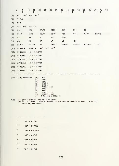
5

| |

10

|

5 20 25 30 35I I

40 451 I

50 551 I

60 651 1

70 751 I

(1) N19 N2 ,o N3" N4'

2

(2) TITLE

(3) HHH

(4) A1 1 A22 D11 D22

(5) EX VYX VPLAS SIGX GXY EY EF

(6) PSTR SIGY SIGX1 SIGY1 PEL STRX STRY NSAVE

(7) L OD T RHO RHOF

(8) AR IR YR LF LS ARM

(9) RINGS SECDEP DW DASP RINGSI RINGSF DRINGS ISEC

(10) SIGXNOM SIGYNOM NX'3

NY'4

NF'5

(11) STRESX(I) , I = 1 ,NXPNT

(12) STRINX(I) , I =1 ,NXPNT

(13) STRESY(I) , I =1 ,NYPNT

(14) STRINY(I) , I =1 ,NYPNT

(15) STRESF(I) , I =1 ,NFPNT

(16) STRINF(I) , I =1 ,NFPNT

INPU1 LINE FORMATS: (1)(2)(3)(4)(5)(6)(7)(8)(9)(10

4157A107A108F10.38F10.37F10.3,8F10.38F10.37F10.3,

: 2F10.3,

15

15315

(11) THRU (16) : 10F8.0

NOTE: (1) BLANK ENTRIES ARE READ AS ZERO(2) NOT ALL INPUT LINES REQUIRED, DEPENDING ON VALUES OF NPLOT, NCURVE

,

NDESIGN, AND ORTHO

"N1

"

= NPLOT

"N2" = NCURVE

"N3" = NDESIGN

"N4" = ORTHO

"NX" = NXPNT

"NY" = NYPNT

"NF" = NFPNT

121

APPENDIX C: THESIS CODE FLOW CHART LOGIC

This appendix shows the flow chart logic of the interaction between the

THESIS and DAPS3 codes.

122

USFJ WPUTS PAPAktTLRS

I

DAPS3 NP DAPS3 FORTRAN 0APS3 OUT

THESIS FORTRAN

USER WPUTS HfTIAL SEARCH PONT

USER hPUTS ADS OPTMZEF

MONOCOQUE TYPE OT SHELL RWG-STFTENED

rin:

fe.

ADS

w'

DAPS3 THESE DAPSOUT^^

NO

^

YES

\

OBICM

yhMZED? ^ THESE OUTW

123

LIST OF REFERENCES

1. Naval Surface Weapons Center Technical Report 80-269, Axisymmetric

Stresses and Deflections, Interbay Buckling, and General Instability of

Orthotropic Hybrid, Ring-Stiffened Cylindrical Shells Under External Hydrostatic

Pressure, by J.R. Renzi, 19 April 1981.

2. Naval Surface Weapons Center Technical Report 79-305, Optimization of

Orthotropic, Non-Linear Ring-Stiffened Cylindrical Shells Under External

Hydrostatic Pressure asApplied toMMC Materials', by J.R. Renzi, 30 September

1979.

3. David Taylor Research Center Ship Structures and Protection Department

Research and Development Report, Preliminary Considerations for Developing

Designs of Composite, Ring-Stiffened Cylindrical Cylinders Under Hydro-Static

Loading, by J.S. Mayes, pp. 23-24, April 1991.

4. Vanderplaats, G.N., Numerical Optimization TechniquesforEngineeringDesign:

With Applications, McGraw-Hill, Inc., 1984.

5. Achenbach, M.R., Design Optimization ofBlade Stiffened Laminated Composite

Plates for Maximum Buckling Load, Master's Thesis, Naval Postgraduate

School, Monterey, California, December 1990.

6. Vanderplaats, G.N., "ADS - A FORTRAN Program for Automated Design

Synthesis Version 1.10," a user's manual for the ADS numerical optimization

program, May 1985.

7. Shin, P.Y., and Castillo, H.A., "A Homotopy Method for Optimal Design

Using an Envelope Function," paper presented at the 33rd Structures,

Structural Dynamics, and Materials (SDM) Conference, Dallas, Texas, 13

April 1992.

124

INITIAL DISTRIBUTION LIST

Defense Technical Information Center

Cameron Station

Alexandria, VA 22304-6145

Library, Code 52

Naval Postgraduate School

Monterey, CA 93943-5002

Superintendent

Naval Postgraduate School

Attn: Professor AJ. Healy, Code ME/HyDepartment of Mechanical Engineering

Monterey, CA 93932-5004

Superintendent

Naval Postgraduate School

Attn: Professor David Salinas, Code ME/SaDepartment of Mechanical Engineering

Monterey, CA 93932-5004

Superintendent

Naval Postgraduate School

Attn: Curricular Officer, Code 34

Monterey, CA 93932-5004

LT Henry A. Castillo, Jr.

c/o Ronda Beagle

1330 Skyline Drive #4Monterey, CA 93940

125

:

ThesisC315

c.lCastillo

Optimum design of iso-tropic monocoque andring-stiffened circularcylindrical shells sub-ject to external hydro-static pressure.

Thesis

C315

c.l

Castillo

Optimum design of iso-

tropic monocoque and

r1v.fr-r,*-r.fcene'3. circular

cylindrical shells sub-

ject to external hydro-static pressure.