arX

iv:1

504.

0556

5v1

[ph

ysic

s.fl

u-dy

n] 2

0 A

pr 2

015

Rotation Rate of Particle Pairs in Homogeneous Isotropic Turbulence

Abdallah Daddi-Moussa-Idera,b, Ali Ghaemib

aInstitut de Recherche sur les Phenomenes Hors-Equilibre49, Rue F. Joliot-Curie 146, 13384 Marseille, Franceb Physikalisches Institut an der Universitat BayreuthUniversitatsstraße 30, 95447 Bayreuth, Germany

Abstract

Understanding the dynamics of particles in turbulent flow is important in many environmental

and industrial applications. In this paper, the statistics of particle pair orientation is numerically

studied in homogeneous isotropic turbulent flow, with Taylor microscale Rynolds number of

300. It is shown that the Kolmogorov scaling fails to predict the observed probability density

functions (PDFs) of the pair rotation rate and the higher order moments accurately. Therefore,

a multifractal formalism is derived in order to include the intermittent behavior that is neglected

in the Kolmogorov picture. The PDFs of finding the pairs at a given angular velocity for

small relative separations, reveals extreme events with stretched tails and high kurtosis values.

Additionally, The PDFs are found to be less intermittent and follow a complementary error

function distribution for larger separations.

Keywords: Turbulence, particle dispersion, rotation rate, multifractal model

1. Introduction

Understanding how particles are advected by fluids is of major interest in many applications,

including the environmental and the geophysical flows [1]. One outstanding example is the erup-

tion of volcanoes, where particles with different sizes and inertia are released into the atmosphere

[2] and then transported with turbulent currents [3, 4]. In addition to the environmental impor-

tance of understanding the influence of turbulence on particle dispersion, this problem is also of

practical interest in the industrial flows, where the advection of particles is involved [5, 6].

The theoretical studies of the relative separation between two particles are based on stochastic

models. Many experiments [7, 8] and numerical simulations [9, 10] have been performed over the

last few decades in order to accurately evaluate these theories. Richardson, in his pioneering work

[11], has examined the relative motion of particle pairs in turbulent flows. He has estimated the

scale dependency of the eddy-diffusivity coefficient through the observation of dispersed plumes.

This scale dependency is claimed to be the origin of the accelerated nature of turbulent dispersion

[12]. In the inertial range of motion (for η ≪ r ≪ L and τη ≪ t ≪ TL, where η is the Kolmogorov

∗Corresponding authorEmail address: abdallah.ider@stmail.uni-bayreuth.de (Abdallah Daddi-Moussa-Ider)

Preprint submitted to European Journal of Mechanics - B/Fluids April 22, 2015

dissipative scale, L is the energy injection length scale of the flow, τη is the local-eddy-turn-over-

time and TL is the large time scale), Richardson has suggested that the process of relative

dispersion is governed by a diffusion-like equation. Solving this equation gives the probability of

finding a pair of particles at a specific separation, at any time [13]. Nevertheless, recent studies

[14, 15] on the dynamics of tracer pairs that are released from many point sources have reported

severe deviations from the Richardson theory. Additionally, this theory does not account for the

rotational behavior of particle pairs.

The orientation dynamics of a single rigid ellipsoid particle under Stokes flow has been de-

scribed by Jeffery [16], where inertia and the thermal fluctuations are neglected. The same

equation can be used to describe the motion of any axisymmetric particle, provided that its

aspect ratio is known [17]. In the presence of weak inertia, Einarsson et al. [18, 19] studied

the rotation of small and neutrally buoyant axisymmetric particles in a viscous shear flow, by

perturbatively solving the coupled particle-flow equations. Shin and Kock [20] presented the re-

sults of direct numerical simulations (DNS) of the translational and rotational motions of fibers

in a fully developed isotropic turbulent flow, for a range of Reynolds numbers. They concluded

that the fibers whose lengths are much smaller than the Kolmogorov length scale η translate like

fluid particles and rotate like material lines. With increasing fiber length, the translational and

rotational motions of the fibers slow down as they become insensitive to the smaller-scale eddies.

Using computer simulations, Pumir and Wilkinson [21] studied the temporal evolution of

the orientation vector of microscopic rod-like particles. They showed that rod-like particles

are more strongly aligned with vorticity than with the principal strain axis. An interesting

component of turbulence, which is named the pirouette effect, has been reported by Xu et al.

[22]. It has been shown that the axis of rotation of tetrahedra tracers aligns with the initially

strongest stretching direction. A phenomena which can be justified by the conservation of the

angular momentum. Using video particle tracking technique, Parsa et al. [23] made accurate

simultaneous measurements of the motion and the orientation of the rods in the presence of

a bi-dimensional chaotic velocity field. The first three-dimensional experimental measurements

of the orientation dynamics of rod-like particles was also reported by Parsa et al. [24]. In

this work, a good agreement with the previous numerical simulations was reported. Moreover,

Parsa and colleagues [25] studied the rotation rate of the rods with lengths in the inertial range

of turbulence. They presented the experimental measurements of the rotational statistics of

neutrally buoyant rods, and derived a scaling law for the mean-squared rotation rate. The latter

showed a good agreement with the Kolmogorov classical scaling.

It is noteworthy that, to the best of our knowledge, the orientation of the tracer pairs has not

been studied so far. Therefore, this question will be addressed here, by computing the probability

of finding a pair of particles at a specific rotation rate, given the relative separation between them.

By considering a particle pair with a specific separation, one can study the orientation statistics

of an imaginary tracer rod that is delimited by these two particles. Furthermore, for the first

time, the pair rotation rate PDFs at later times will be presented in this work.

2

This paper is organized as it follows. The next section describes the numerical data, and the

approach that is used to derive the rotation rate of the tracer pairs. Afterward, the intermittency

behavior that is observed at the small scales of motion is discussed in details. In Sec. 3, the

multifractal (MF) formalism to intercept the probability density function (PDF) distributions

is presented. Thereafter, the higher-order moments of the rotation rate are evaluated and com-

pared to the multifractal prediction together with the Kolmogorov (K41) picture. Finally, the

concluding remarks, and the outlooks are stated in Sec. 4.

2. Methods

2.1. Particle pair orientation

The rotational dynamics of particle pairs in turbulent flow can be addressed by solving the

dimensionless incompressible Navier-Stokes equations for a Newtonian fluid, i.e.

∂u

∂t+ u.∇u = −∇p+

1

Re∇

2u+ f , (2.1)

∇.u = 0, (2.2)

using Direct Numerical Simulations (DNS). In these equations, u denotes the tri-dimensional

velocity field, p is the pressure and Re is the flow Reynolds number, Re ≡ Lu′/ν. Re measures

the ratio between the nonlinear inertial forces, and the linear viscous forces, where u′ is the

root-mean-squared velocity and ν is the fluid kinematic viscosity which is defined as the ratio

between the dynamic molecular viscosity µ and, the fluid density ρ. In order to avoid energy

dissipation, the flow was forced by keeping the total energy constant in the first wavenumber

shells, by applying a large-scale forcing term f . This force injects energy at a mean rate of

ǫ = 〈f .u〉, where ǫ is the mean turbulent kinetic energy dissipation rate [26]. The integration

of the equations of motion is performed on 1, 0243 regular cubic lattice with Taylor microscale

Reynolds number of 300, and periodic boundary conditions. The simulation parameters are

shown in Tab. 1. With the present choice of parameters, the dissipative range of length scales

is well resolved because the grid size ∆x is in the range of Kolmogorov length scale η (as it

is reported in more details by Biferale et al. [14]). A fully-de-aliased parallel pseudospectral

code, with a second-order Adams-Bashforth temporal scheme, for 3D homogeneous isotropic

turbulence, assuming constant fluid viscosity and density, is used in order to solve Eqs. (2.1)

and (2.2).

The fluid is seeded with bunches of tracers emitted within a small region which has a size

comparable to the Kolmogorov dissipative scale η. The emission is carried out in puffs of 2,000

particles that are followed during a maximum time of 160 τη. The tracer particles take on the

fluid velocity immediately, and adapt the rapid fluid velocity fluctuations [27]. Therefore, the

velocity of each tracer is related to the instantaneous fluid velocity by the following equation

vp ≡ dxp

dt= u(xp(t), t). (2.3)

3

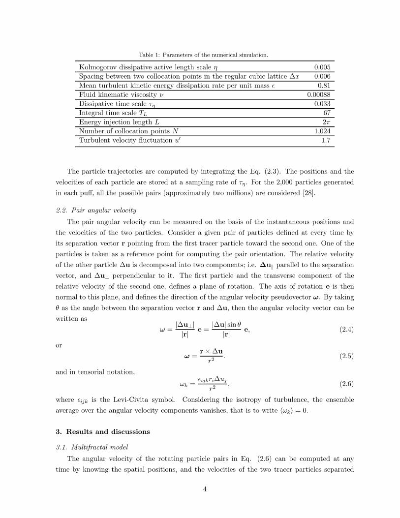
Table 1: Parameters of the numerical simulation.

Kolmogorov dissipative active length scale η 0.005

Spacing between two collocation points in the regular cubic lattice ∆x 0.006

Mean turbulent kinetic energy dissipation rate per unit mass ǫ 0.81

Fluid kinematic viscosity ν 0.00088

Dissipative time scale τη 0.033

Integral time scale TL 67

Energy injection length L 2π

Number of collocation points N 1,024

Turbulent velocity fluctuation u′ 1.7

The particle trajectories are computed by integrating the Eq. (2.3). The positions and the

velocities of each particle are stored at a sampling rate of τη. For the 2,000 particles generated

in each puff, all the possible pairs (approximately two millions) are considered [28].

2.2. Pair angular velocity

The pair angular velocity can be measured on the basis of the instantaneous positions and

the velocities of the two particles. Consider a given pair of particles defined at every time by

its separation vector r pointing from the first tracer particle toward the second one. One of the

particles is taken as a reference point for computing the pair orientation. The relative velocity

of the other particle ∆u is decomposed into two components; i.e. ∆u‖ parallel to the separation

vector, and ∆u⊥ perpendicular to it. The first particle and the transverse component of the

relative velocity of the second one, defines a plane of rotation. The axis of rotation e is then

normal to this plane, and defines the direction of the angular velocity pseudovector ω. By taking

θ as the angle between the separation vector r and ∆u, then the angular velocity vector can be

written as

ω =|∆u⊥||r| e =

|∆u| sin θ|r| e, (2.4)

or

ω =r×∆u

r2. (2.5)

and in tensorial notation,

ωk =ǫijkri∆uj

r2, (2.6)

where ǫijk is the Levi-Civita symbol. Considering the isotropy of turbulence, the ensemble

average over the angular velocity components vanishes, that is to write 〈ωk〉 = 0.

3. Results and discussions

3.1. Multifractal model

The angular velocity of the rotating particle pairs in Eq. (2.6) can be computed at any

time by knowing the spatial positions, and the velocities of the two tracer particles separated

4

by a vector r. In the case of inertialess particles, the angular velocity can be viewed as the

ratio between the Eulerian transverse velocity increment δru⊥ ≡ u⊥(r + δr) − u⊥(r), and the

instantaneous distance r. The mean-squared angular velocity 〈ω2〉 for a fixed separation r, is

thus the ratio between the second order Eulerian transverse velocity structure function, and r2.

For the purpose of computing the higher-order moment of angular velocity that is parametrized

by r, a series of computations over the whole number of bunches at different times, and for dif-

ferent constant separations are performed. In the inertial range of motion, the size of the eddies

that move the pairs apart varies with the separation distance. The eddies with the scales in the

order of r are the most effective in the dispersion process [29]. Intuitively, in this intermediate

range, the further the separation between the two particles is, the slower the pair will rotate.

This happens because in the Kolmogorov phenomenology, the angular velocity modulus scales as

r−2/3. According to the Kolmogorov second similarity hypothesis [30], all statistically averaged

quantities at scale r in the intermediate range are uniquely determined by ǫ and r. The pth

order moment angular velocity should then scale in the inertial range as

〈ωp〉 ≃ r−2p/3. (3.1)

However, in the dissipative range of turbulence (i.e. for r ≪ η), the higher order moments

are independent of the scale r. A suitable expression is therefore needed in order to fulfill the

requirements of both ranges. In Kolmogorov phenomenology, the higher order moments are

expressed with respect to separation r via the Batchelor parametrization [31], which satisfies

both the dissipative range and the inertial range. Then 〈ωp〉 is expected to be scaled as [32]

〈ωp〉 ≃(

rL

)−2p/3

(

1 +(

rη

)−2)p/3

, (3.2)

For separations in the inertial dissipative range (i.e. r > η and r ≪ L), these moments

undergo a quadratic decay.

Kolmogorov theory fails to accurately predict the intermittency behavior, because it neglects

the presence of fluctuations in the energy transfer from the large scales towards the small ones

[33]. In order to include the intermittency effect in the energy cascade, a multifractal formalism

is used together with a generalization of the Batchelor parametrization, to describe the higher

order moments of the angular velocity for both the inertial dissipative range and the inertial range

[34]. The multifractal approach to turbulence is based on the assumption that the statistical

properties of turbulent flows do exhibit scaling properties even if there is intermittency [35].

Under these assumptions, the transverse velocity increment reads [32]

δru⊥ = v0

(

rL

)h

(

1 +(

rη(h)

)−2)(1−h)/2

, (3.3)

5

where v0 denotes the large scale transverse velocity fluctuation and h is the singularity in the

MF phenomenology. In this picture, the viscous scale is not a fixed homogeneous quantity, but

it fluctuates wildly due to intermittency [36]. The Kolmogorov length scale η is a function of the

singularity h, and it is related to the Reynolds number by η/L ∝ Re−1/(1+h).

Following the Eqs. (2.6) and (3.3), the angular velocity component at a distance r is estimated

in the MF model as

ω ≡ δru⊥r

∼ v0L

(

rL

)h−1

(

1 +(

rη(h)

)−2)(1−h)/2

, (3.4)

A generalization of the probability to observe an Eulerian velocity fluctuation at scale r with

a local Holder exponent h, is given by [32]

Ph(r) ∝(

rL

)3−D(h)

(

1 +(

rη(h)

)−2)(D(h)−3)/2

, (3.5)

where D(h) is the spectrum of the fractal dimension.

3.2. Probability density function distribution

In this study, there are many particle pairs which are embedded in the turbulent flow. The

most comprehensive and accurate description of the orientation state can be achieved by evalu-

ating the PDFs of the orientation of the pairs. The non-Gaussianity is one of the fundamental

features of 3D turbulence with a non-zero skewness, and a very large kurtosis of the PDF distri-

butions [37]. A superposition of stretched exponentials corresponding to the various singularity

exponents are usually observed at small scales. In the following, we shall be interested in the

PDF of finding a pair of tracers at a given angular velocity component ω when it reaches a given

separation r.

The MF phenomenology is capable of predicting the PDFs of the velocity increment and

the accelerations in both the Eulerian and Lagrangian frames [38, 39]. The MF model can also

successfully intercept the numerically observed angular velocity PDFs. In this section, an MF

model is employed for the PDFs of the angular velocity components. The PDFs are allowed

to take values in all the axis of reals. Since the flow is isotropic, i.e. the pair properties are

distributed independently of orientation, the distributions are symmetric. Furthermore, the

PDFs that correspond to each of the components all collapse on a single curve.

By assuming that the large scale velocity field v0 is Gaussian with d components, its magni-

tude has the following PDF distribution [40]

P (v0)dv0 = vd−10 exp

(

−v202

)

, (3.6)

where the normalization constant has been omitted here. The transverse velocity modulus cor-

6

10−6

10−5

10−4

10−3

10−2

10−1

100

-30 -25 -20 -15 -10 -5 0 5 10 15

PDF

ω/ωrms

02468

10

0 400 800K

r/η

r/η = 1r/η = 40

r/η = 200erfc

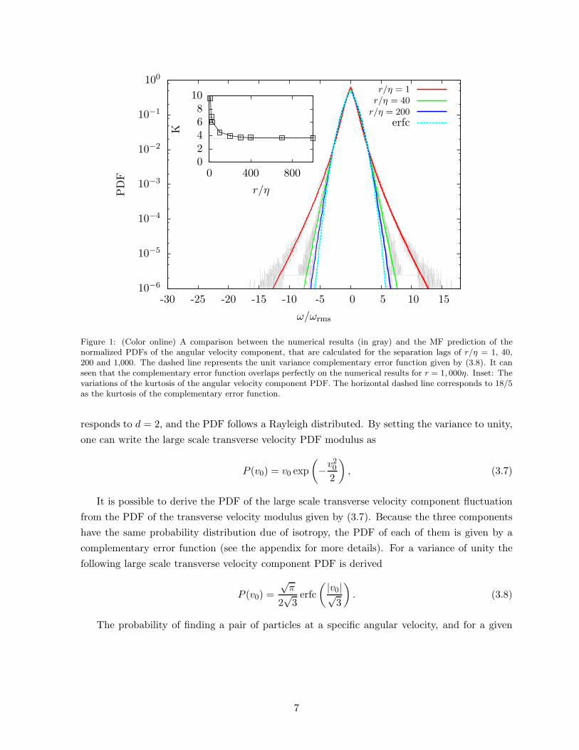
Figure 1: (Color online) A comparison between the numerical results (in gray) and the MF prediction of thenormalized PDFs of the angular velocity component, that are calculated for the separation lags of r/η = 1, 40,200 and 1,000. The dashed line represents the unit variance complementary error function given by (3.8). It canseen that the complementary error function overlaps perfectly on the numerical results for r = 1, 000η. Inset: Thevariations of the kurtosis of the angular velocity component PDF. The horizontal dashed line corresponds to 18/5as the kurtosis of the complementary error function.

responds to d = 2, and the PDF follows a Rayleigh distributed. By setting the variance to unity,

one can write the large scale transverse velocity PDF modulus as

P (v0) = v0 exp

(

−v202

)

, (3.7)

It is possible to derive the PDF of the large scale transverse velocity component fluctuation

from the PDF of the transverse velocity modulus given by (3.7). Because the three components

have the same probability distribution due of isotropy, the PDF of each of them is given by a

complementary error function (see the appendix for more details). For a variance of unity the

following large scale transverse velocity component PDF is derived

P (v0) =

√π

2√3erfc

( |v0|√3

)

. (3.8)

The probability of finding a pair of particles at a specific angular velocity, and for a given

7

separation r is obtained from

P (ω|r) =∫

h∈I

P (ω|h)Ph(r) dh. (3.9)

By Plugging the Eqs. (3.8) and (3.5) into (3.9), and using the probability conservation law

for the equation (3.4), one can write

P (ω|r) ∝∫

h∈I

(

( r

L

)2+

(

η(h)

L

)2)2−D(h)+h

2

erfc

L|ω|√3

(

( r

L

)2+

(

η(h)

L

)2)

1−h2

. (3.10)

The fractal dimension has the following form in a log-Poisson process [41, 42]

D(h) =3(h− h0)

ln β

[

ln

(

3(h0 − h)

d0 ln β

)

− 1

]

+ 3− d0, (3.11)

where β = 0.6, h0 = 1/9 and d0 = (1− 3h0)/(1− β) = 5/3. The lowest singularity hmin = 1/9 is

obtained by considering limh→hminD(h) = 0. The fractal dimension attains its maximum which

is D = 3, for hmax = hpeak ≃ 0.38 [36].

In Kolmogorov theory, the singularity h takes only the value of 1/3, and the fractal dimension

is restricted to D = 3. It is possible to derive the PDF distribution in this particular case from

Eq. (3.10). After computation, it is found that the angular velocity component PDF is given by

P (ω|r) = 1

ωrms

√π

2√3erfc

(

1√3

|ω|ωrms

)

, (3.12)

where ωrms is the root-mean-squared angular velocity, expressed in Eq. (3.2) for p = 2. The com-

plementary error function distribution given by (3.8), is therefore recovered for the normalized

PDF.

3.2.1. Comparison with numerical results

In Fig. 1, a comparison between our numerical results and the MF prediction given by (3.10)

is presented. The agreement between these two shows the robustness of the MF approach in

reproducing the DNS results accurately. The PDF of the angular velocity component for the

smallest separations i.e. of the order of the Kolmogorov length scale η, is highly intermittent and

the PDF has stretched tails that extend beyond thirty times the standard deviation of angular

velocity (for the sake of convenience, in Fig. 1 tails are not shown in full lengths). This indicates

that when the separation length r is of the order of the smallest scale of the flow, the probability

of high rotation rate events are much higher than those predicted by a complementary error

function distribution. An increasingly large number of particles is needed in order to ensure a

sufficient statistical convergence of the data, and therefore to describe the long tails accurately.

The inset of the Fig. 1 illustrates this by showing the variations of the PDF kurtosis as a

8

10−15

10−10

10−5

100

32 64 128 256

〈ωp〉τ

p η

r/η

p = 2p = 4p = 6p = 8

p = 10p = 12

MFK41

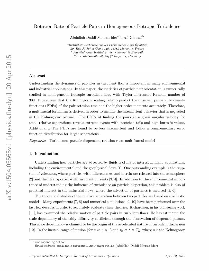
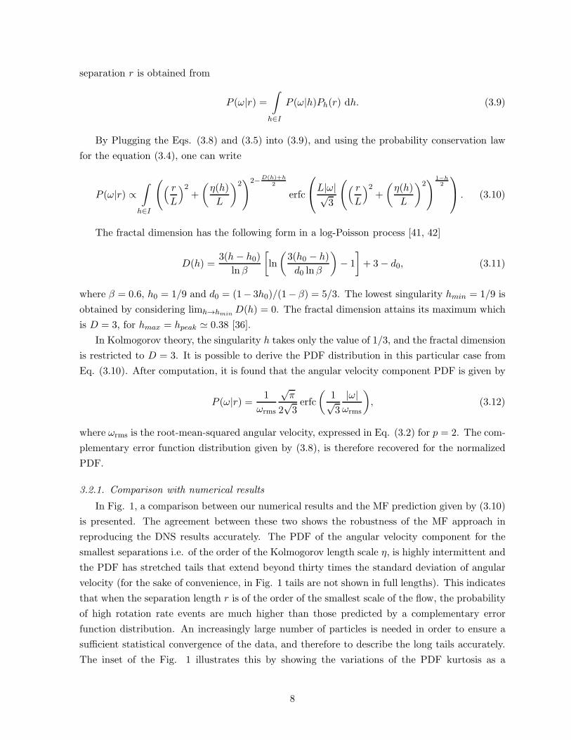
Figure 2: (Color online) Comparison between the Kolmogorov scaling and the multifractal model. The scaledhigher order moments of the angular velocity component is depicted versus the scaled separations in the inertialrange. For p = 2, 4, the MF model and the K41 scaling given by r−2p/3 are almost indistinguishable. Themultifractal prediction shows a better agreement with the numerical results for the higher order moments p =6, 8, 10, 12.

function of r. The kurtosis is a measure of the distribution pickedness. And for symmetrical

distributions, it is defined as the ratio between the forth order moment, and the square of the

distribution variance. That is to write,

K ≡ 〈ω4〉〈ω2〉2 . (3.13)

For small separations, the kurtosis is very large and it reaches a value of 10 for a separation

of the order of the Kolmogorov scale. The larger the separation is, the smaller the kurtosis will

be, and it finally converges towards 18/5. This is the kurtosis of the large scale angular velocity

component PDF given by (3.8) (see the appendix for more details about the computation of this

kurtosis).

3.3. Higher order moments

The pth order moment of the angular velocity can be computed from the PDF distributions

as

〈ωp〉 =∫

ω∈R

ωpP (ω|r)dω. (3.14)

By plugging the Eqs. (3.10) into (3.14), and integrating ω over the whole axis of reals, the

9

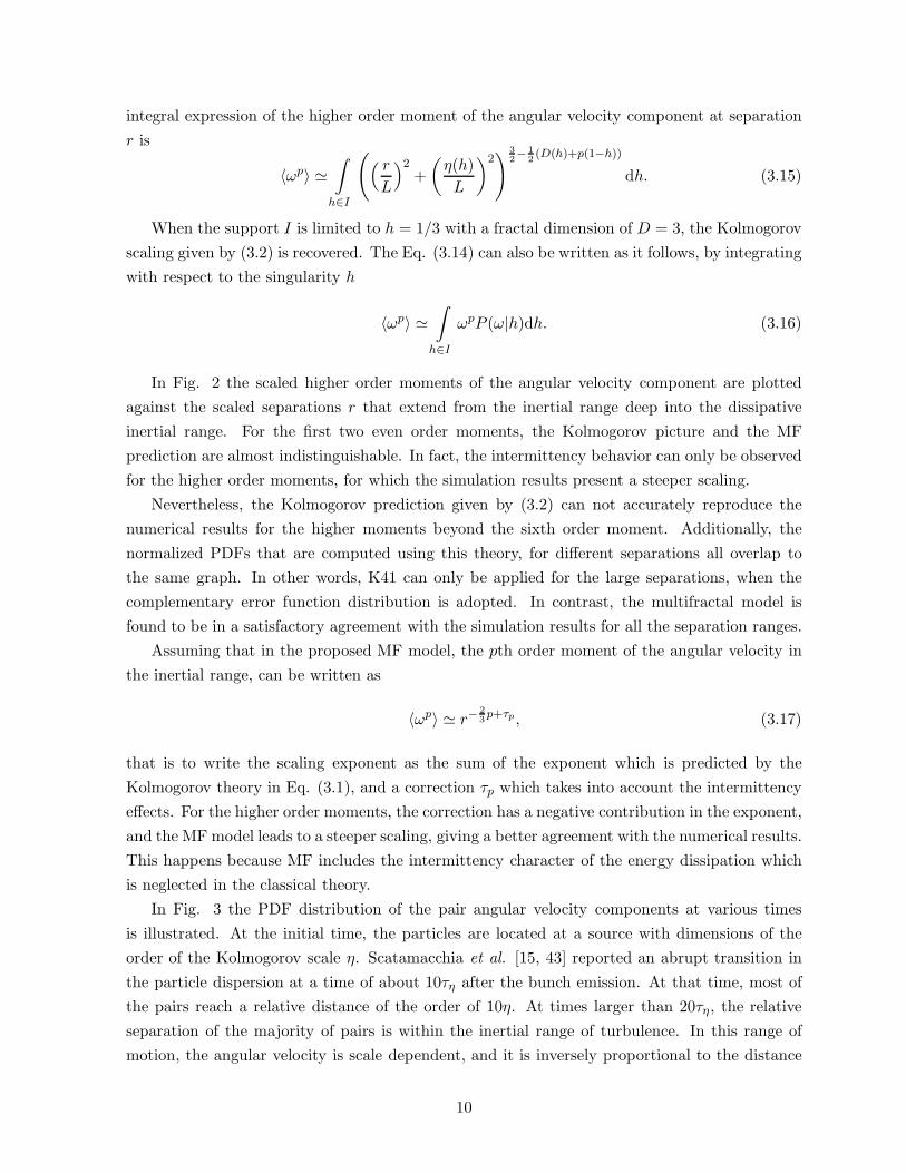
integral expression of the higher order moment of the angular velocity component at separation

r is

〈ωp〉 ≃∫

h∈I

(

( r

L

)2+

(

η(h)

L

)2)

32− 1

2(D(h)+p(1−h))

dh. (3.15)

When the support I is limited to h = 1/3 with a fractal dimension of D = 3, the Kolmogorov

scaling given by (3.2) is recovered. The Eq. (3.14) can also be written as it follows, by integrating

with respect to the singularity h

〈ωp〉 ≃∫

h∈I

ωpP (ω|h)dh. (3.16)

In Fig. 2 the scaled higher order moments of the angular velocity component are plotted

against the scaled separations r that extend from the inertial range deep into the dissipative

inertial range. For the first two even order moments, the Kolmogorov picture and the MF

prediction are almost indistinguishable. In fact, the intermittency behavior can only be observed

for the higher order moments, for which the simulation results present a steeper scaling.

Nevertheless, the Kolmogorov prediction given by (3.2) can not accurately reproduce the

numerical results for the higher moments beyond the sixth order moment. Additionally, the

normalized PDFs that are computed using this theory, for different separations all overlap to

the same graph. In other words, K41 can only be applied for the large separations, when the

complementary error function distribution is adopted. In contrast, the multifractal model is

found to be in a satisfactory agreement with the simulation results for all the separation ranges.

Assuming that in the proposed MF model, the pth order moment of the angular velocity in

the inertial range, can be written as

〈ωp〉 ≃ r−23p+τp , (3.17)

that is to write the scaling exponent as the sum of the exponent which is predicted by the

Kolmogorov theory in Eq. (3.1), and a correction τp which takes into account the intermittency

effects. For the higher order moments, the correction has a negative contribution in the exponent,

and the MF model leads to a steeper scaling, giving a better agreement with the numerical results.

This happens because MF includes the intermittency character of the energy dissipation which

is neglected in the classical theory.

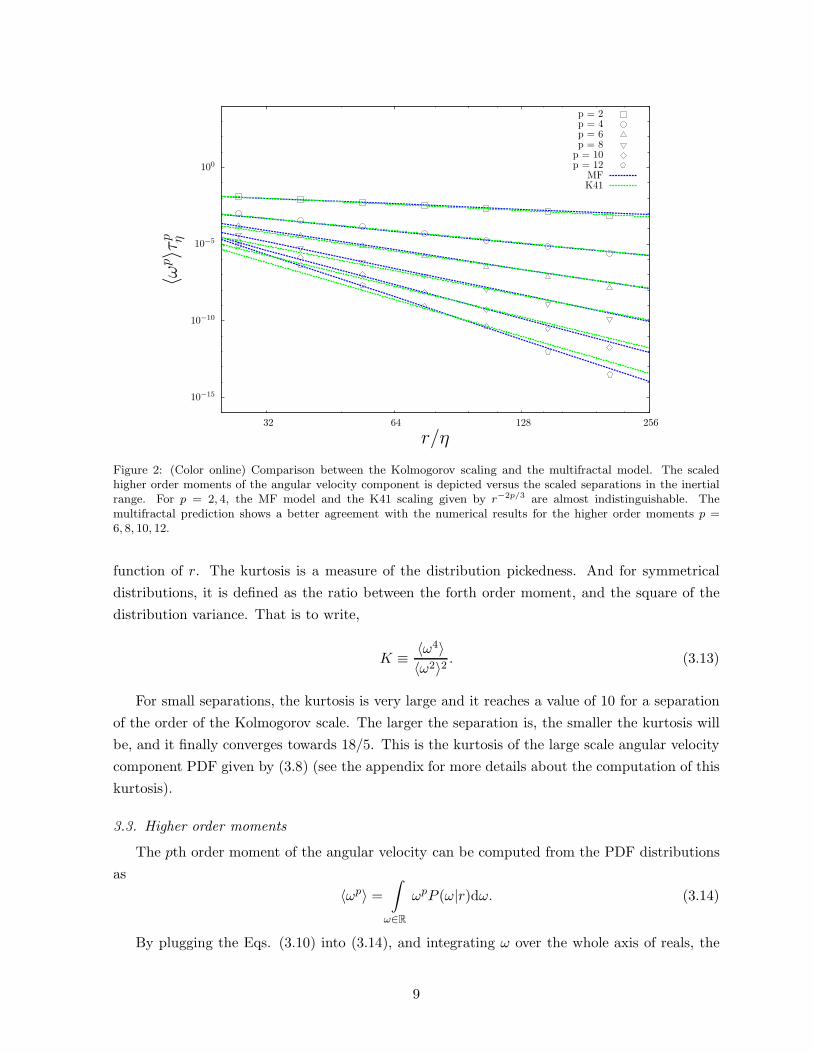
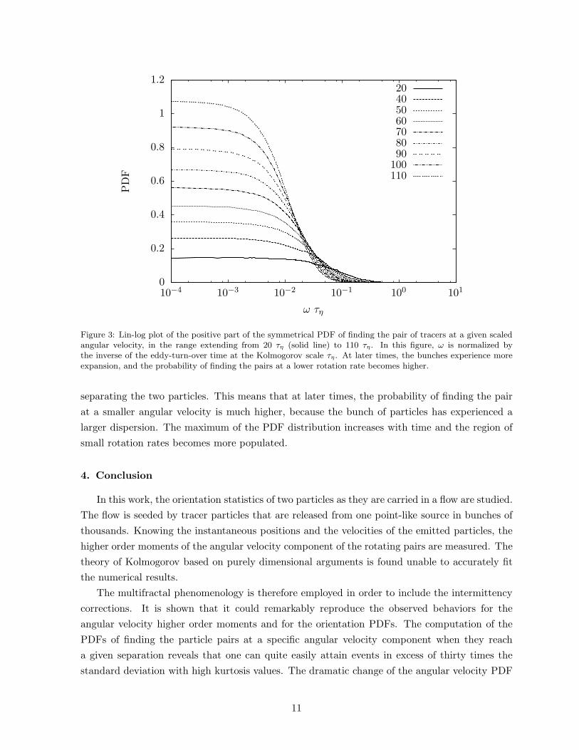
In Fig. 3 the PDF distribution of the pair angular velocity components at various times

is illustrated. At the initial time, the particles are located at a source with dimensions of the

order of the Kolmogorov scale η. Scatamacchia et al. [15, 43] reported an abrupt transition in

the particle dispersion at a time of about 10τη after the bunch emission. At that time, most of

the pairs reach a relative distance of the order of 10η. At times larger than 20τη , the relative

separation of the majority of pairs is within the inertial range of turbulence. In this range of

motion, the angular velocity is scale dependent, and it is inversely proportional to the distance

10

0

0.2

0.4

0.6

0.8

1

1.2

10−4 10−3 10−2 10−1 100 101

PDF

ω τη

20405060708090100110

Figure 3: Lin-log plot of the positive part of the symmetrical PDF of finding the pair of tracers at a given scaledangular velocity, in the range extending from 20 τη (solid line) to 110 τη. In this figure, ω is normalized bythe inverse of the eddy-turn-over time at the Kolmogorov scale τη. At later times, the bunches experience moreexpansion, and the probability of finding the pairs at a lower rotation rate becomes higher.

separating the two particles. This means that at later times, the probability of finding the pair

at a smaller angular velocity is much higher, because the bunch of particles has experienced a

larger dispersion. The maximum of the PDF distribution increases with time and the region of

small rotation rates becomes more populated.

4. Conclusion

In this work, the orientation statistics of two particles as they are carried in a flow are studied.

The flow is seeded by tracer particles that are released from one point-like source in bunches of

thousands. Knowing the instantaneous positions and the velocities of the emitted particles, the

higher order moments of the angular velocity component of the rotating pairs are measured. The

theory of Kolmogorov based on purely dimensional arguments is found unable to accurately fit

the numerical results.

The multifractal phenomenology is therefore employed in order to include the intermittency

corrections. It is shown that it could remarkably reproduce the observed behaviors for the

angular velocity higher order moments and for the orientation PDFs. The computation of the

PDFs of finding the particle pairs at a specific angular velocity component when they reach

a given separation reveals that one can quite easily attain events in excess of thirty times the

standard deviation with high kurtosis values. The dramatic change of the angular velocity PDF

11

shape provides with immediate impression of how strongly intermittent rotation events are at

small scales of motion. By increasing the separations, the PDFs become less intermittent and

converge towards the complementary error function distribution.

Here, the main attention is restricted to the neutrally buoyant particles which are passively

transported by the turbulent flow. The role of particle inertia on pair orientation should be

explored in the future. It is important to note that the measurements in the database are not

completely unbiased, because only the particles that are emitted from a single point source are

considered. In order to reduce the spatial correlation, it is worth considering the pairs which

are formed from various point-like sources. For reliable statistics, a large number of particles

will be required. It is worth mentioning that an ideal framework for the study of the orientation

statistics is a 2D turbulence, because of the absence of intermittency. Similar measurements and

quantitative investigations can be carried out as well in this particular case, where the angular

velocity vector has a unique component along the axis normal to the computational domain.

5. Acknowledgment

The first author would like to thank Prof. Federico Toschi, Prof. Luca Biferale, and Dr. Ric-

cardo Scatamacchia for supervising his thesis and for providing the numerical data, in addition to

their useful discussions and helpful comments on the manuscript during its preparation. Further-

more, he gratefully acknowledges the support from Eurasmus mobility program. He also thanks

Dr. Behnam Farid and Dr. Renaldas Urniezius for the online discussions via ResearchGate.

Author contributions: A.D.M.I. performed research and analyzed data; and A.D.M.I. and

A.G. wrote the paper. The authors declare no conflict of interest.

Appendix

Here, the PDF of the components are derived for a given vectorial quantity, by knowing the

PDF of the modulus when the isotropy is guaranteed. In the following, x, y and z represent the

vector components. LetN(r) be the distribution function of the variable r where r2 = x2+y2+z2.

N(r) is normalized to unity, that is to write

∫

R3

N(

(x2 + y2 + z2)1/2)

dxdydz = 1, (5.1)

Using the spherical coordinates, Eq. (5.1) can be written as,

∫ ∞

04πr2N(r)dr = 1. (5.2)

The PDF for the modulus Q(r) = 4πr2N(r) has a total weight of unity. Because of isotropy,

the PDFs are all the same along all the three axis. Then only P (z) will be calculated here.

P (z) =

∫

R2

N(

(x2 + y2 + z2)1/2)

dxdy, (5.3)

12

P (z) can be written as a function of Q(r),

P (z) =1

4π

∫

R2

Q(

(x2 + y2 + z2)1/2)

x2 + y2 + z2dxdy, (5.4)

If the two-dimensional vector whose Cartesian coordinates are x and y are described in the

cylindrical coordinates (u, φ, z), where u varies over [0,∞[ and φ over [0, 2π], then u2 = x2+ y2,

and

P (z) =1

2

∫ ∞

0

Q(

(u2 + z2)1/2)

u2 + z2udu, (5.5)

By considering the change of variables t2 = u2 + z2, then tdt = udu, the following PDF for

the positive values of z will be obtained,

P (z) =1

2

∫ ∞

z

Q(t)

tdt. (5.6)

The resulting equation (5.6) can be illustrated in one well-known examples of turbulence. It

is known that the large scale velocity has the following distribution,

Q(t) =4√πt2e−t2 . (5.7)

Using Eq. (5.6) one finds that the component PDF has a Gaussian distribution,

P (z) =1√πe−z2 , (5.8)

which has a total weight of unity.

as it is discussed is 3.2 , the large scale transverse velocity fluctuation has a Rayleigh distri-

bution given by Eq. (3.7), then the PDF of each component has a complementary error function

distribution after integrating Eq. (5.6),

P (z) =

√2π

4erfc

( |z|√2

)

. (5.9)

which has also a total weight of unity.

Moreover, using Eq. (3.13) the kurtosis of the above distribution is calculated as

K =1

π

∫ ∞

0z4 erfc

(

z√2

)

/

(∫ ∞

0z2 erfc

(

z√2

))2

=18

5. (5.10)

References

[1] R. A. Shaw. Particle-turbulence interaction in atmospheric clouds. Ann. Rev. Fluid Mech.,

35:183–227, 2003.

13

[2] J. M. Oberhuber, M. Herzog, H.-F. Graf, and K. Schwanke. Volcanic plume simulation on

large scales. Journal of Volcanology and Geothermal Research, 87(14):29 – 53, 1998.

[3] R. Mehaddi, F. Candelier, and O. Vauquelin. Naturally bounded plumes. Journal of Fluid

Mechanics, 717:472–483, 2013.

[4] A. Daddi-Moussa-Ider, B. Benkoussas, R. Mehaddi, O. Vauquelin, and F. Candelier.

Panaches horizontaux non-boussinesq en milieu homogene. arXiv:1412.2297, 2013.

[5] F. Lundell, L. D. Soderberg, and P. H. Alfredsson. Fluid mechanics of papermaking. Ann.

Rev. of Fluid Mech., 43(1):195–217, 2011.

[6] J. Klinkenberg, G. Sardina, H. C. de Lange, and L. Brandt. Numerical study of laminar-

turbulent transition in particle-laden channel flow. Phys. Rev. E, 87:043011, 2013.

[7] M. Bourgoin, N. Ouellette, Haitao Xu, J. Berg, and E. Bodenschatz. The role of pair

dispersion in turbulent flow. Science, 10:835–838., 2006.

[8] N. T. Ouellette, H. Xu, M. Bourgoin, and E. Bodenschatz. An experimental study of

turbulent relative dispersion models. New Journal of Physics, 8(6):109, 2006.

[9] T. Ishihara and Y. Kaneda. Relative diffusion of a pair of fluid particles in the inertial

subrangeof turbulence. Physics of Fluids, 14:L69–L72, 2002.

[10] L. Biferale, G. Boffetta, M. Celani, B. Devenish, A. Lanotte, and F. Toschi. Lagrangian

statistics of particle pairs in homogeneous isotropic turbulence. Phys. Fluids, 17:094501,

2005.

[11] L. F. Richardson. Atmospheric diffusion shown on a distance-neighbour graph. Proceedings

of the Royal Society of London. Series A, 110(756):709–737, 1926.

[12] G. Boffetta and I. Sokolov. Relative dispersion in fully developed turbulence: The richard-

son’s law and intermittency corrections. Phys. Rev. Lett., 88:094501, 2002.

[13] J. P.L.C. Salazar and L. R. Collins. Two-particle dispersion in isotropic turbulent flows.

Ann. Rev. of Fluid Mech., 41(1):405–432, 2009.

[14] L. Biferale, A. S. Lanotte, R. Scatamacchia, and F. Toschi. Intermittency in the relative

separations of tracers and of heavy particles in turbulent flows. arXiv:1411.3985, 2014.

[15] R. Scatamacchia, L. Biferale, and F. Toschi. Extreme events in the dispersions of two

neighboring particles under the influence of fluid turbulence. Phys. Rev. Lett., 109:144501,

2012.

[16] G. Jeffery. The motion of ellipsoidal particles immersed in a viscous fluid. Proceedings of

the Royal Society of London. Series A, 102(715):161–179, 1922.

14

[17] F. P. Bretherton. The motion of rigid particles in a shear flow at low reynolds number. J.

of Fluid Mech., 14:284–304, 1962.

[18] J. Einarsson, F. Candelier, F. Lundell, J. R. Angilella, and B. Mehlig. Rotation of a spheroid

in a simple shear at small reynolds number. arXiv:1504.02309, 2015.

[19] J. Einarsson, F. Candelier, F. Lundell, J. R. Angilella, and B. Mehlig. Effect of weak fluid

inertia upon jeffery orbits. arXiv:1504.02849, 2015.

[20] M. Shin and D. L. Koch. Rotational and translational dispersion of fibres in isotropic

turbulent flows. J. of Fluid Mech., 540:143–173, 2005.

[21] A. Pumir and M. Wilkinson. Orientation statistics of small particles in turbulence. New

Journal of Physics, 13(9):093030, 2011.

[22] H. Xu, A. Pumir, and E. Bodenschatz. The pirouette effect in turbulent flows. Nature

Physics, 7:709–712, 2011.

[23] S. Parsa, J. S. Guasto, M. Kishore, N. T. Ouellette, J. P. Gollub, and G. A. Voth. Rotation

and alignment of rods in two-dimensional chaotic flow. Physics of Fluids, 23(4), 2011.

[24] S. Parsa, E. Calzavarini, F. Toschi, and G. A. Voth. Rotation rate of rods in turbulent fluid

flow. Phys. Rev. Lett., 109:134501, 2012.

[25] S. Parsa and G. A. Voth. Inertial range scaling in rotations of long rods in turbulence. Phys.

Rev. Lett., 112:024501, 2014.

[26] A. Daddi-Moussa-Ider. Review of particle pair dispersion in turbulence. Technical report,

Eindhoven University of Technology, 2014.

[27] S. Klein. Dynamics of large particles in turbulence. PhD thesis, Max-Planck-Institut fur

Dynamik und Selbstorganisation, 2012.

[28] A. Daddi-Moussa-Ider. Orientation of particles in 3d homogeneous isotropic turbulence.

Master’s thesis, IRPHE, Aix-Marseille University, 2014.

[29] S. Corrsin. Theories of turbulent dispersion. Int. Colloq. Turb., pages 27–52, 1962.

[30] A. N. Kolmogorov. The Local Structure of Turbulence in Incompressible Viscous Fluid for

Very Large Reynolds’ Numbers. In Dokl. Akad. Nauk SSSR, volume 30, pages 301–305,

1941.

[31] G.K. Batchelor. Pressure fluctuations in isotropic turbulence. Proc. Cambridge Philos. Soc.,

47:359, 1951.

15

[32] L. Chevillard, B. Castaing, E. Leveque, and A. Arneodo. Unified multifractal description

of velocity increments statistics in turbulence: Intermittency and skewness. Physica D:

Nonlinear Phenomena, 218(1):77–82, 2006.

[33] G. Parisi and U. Frisch. Turbulence and Predictability in Geophysical Fluid Dynamics.,

pages 84–87, 1985.

[34] C. Meneveau. Transition between viscous and inertial-range scaling of turbulence structure

functions. Phys. Rev. E, 54:3657–3663, 1996.

[35] R. Benzi and L. Biferale. Fully developed turbulence and the multifractal conjecture. Journal

of Statistical Physics, 135(5-6):977–990, 2009.

[36] R. Benzi, L. Biferale, R. Fisher, D. Q. Lamb, and F. Toschi. Inertial range eulerian and

lagrangian statistics from numerical simulations of isotropic turbulence. J. of Fluid Mech.,

653:221–244, 2010.

[37] R. Benzi, L. Biferale, G. Paladin, A. Vulpiani, and M. Vergassola. Multifractality in the

statistics of the velocity gradients in turbulence. Phys. Rev. Lett., 67:2299–2302, 1991.

[38] F. Toschi, L. Biferale, G. Boffetta, A. Celani, B. J. Devenish, and A. S. Lanotte. Acceleration

and vortex filaments in turbulence. J. of Turb., 6:15, 2005.

[39] F. Toschi and E. Bodenschatz. Lagrangian properties of particles in turbulence. Ann. Rev.

of Fluid Mech., 41(1):375–404, 2009.

[40] L. Biferale. A note on the fluctuation of dissipative scale in turbulence. Physics of Fluids,

20(3):–, 2008.

[41] Z. S. She and E. Leveque. Universal scaling laws in fully developed turbulence. Phys. Rev.

Lett., 72:336–339, 1994.

[42] B. Dubrulle. Intermittency in fully developed turbulence: Log-poisson statistics and gener-

alized scale covariance. Phys. Rev. Lett., 73:959–962, 1994.

[43] L. Biferale, A. S. Lanotte, R. Scatamacchia, and F. Toschi. Extreme events for two-particles

separations in turbulent flows. In Progress in Turbulence V, volume 149 of Springer Pro-

ceedings in Physics, pages 9–16. Springer International Publishing, 2014.

16