Statistical Arbitrage using High Frequency Pairs Trading

This thesis is written as a part of the Master of Science in Business Administration at Oslo Metropolitan University.

We would like to thank our supervisor Einar Bakke for guidance and discussions.

Kirkestuen, Fredrik

Thomassen, Christian

________________________________

Statistical Arbitrage using High

Frequency Pairs Trading An algorithmic trading strategy in the US equity market

Abstract

Using three-month minute-by-minute data from S&P 500 constituents we examine and report

the return of a high frequency trading strategy by creating an algorithm based on pairs trading.

The algorithm is created based on two different approaches and is implemented using a broad

set of portfolio configurations to compare the effect on trading profits. We show that high

frequency pairs trading generates large positive excess returns before accounting for transaction

costs and find that the returns express no significant traditional risk factors. Furthermore, testing

of certain portfolios to estimate break-even points in respect of transaction cost and return is

conducted. Finally, we implement an approach based on implied volatility to test pairs trading

under different market conditions.

Master thesis, MSc in Business Administration Oslo Business School at Oslo Metropolitan University

2018

1

1. Introduction

Pairs trading is a quantitative trading strategy where the goal is to achieve statistical arbitrage

profits by quantifying, measuring, and predicting the relationship between pairs and trading on

the relative mispricing between securities. The strategy identifies and match a pair of assets

whose co-movement can be observed in their historical price. If prices diverge, the relative

overvalued (undervalued) security is short sold (bought) with an expectation of convergence of

the price relationship. The profitability of pairs trading using daily data is well documented by

Gatev, Goetzmann and Rouwenhorst. (1999; 2006). The development of available data and

processing tools has led to high frequency pairs trading. Since Bowen, Hutchinson, and

O’Sullivan (2010) examined pairs trading on an intraday basis this has evolved to the new norm

in this area. Research provided by Gatev et al. (1999; 2006) and Do and Faff (2010) suggest a

declining trend in the profitability using pairs trading strategy to achieve risk adjusted returns.

Moreover, Do and Faff (2012) suggest that pairs trading using daily data is highly unprofitable

after 2002 when controlling for transaction cost.

In this study, we investigate the profitability from a pairs trading strategy when implementing

pair formation restrictions and trading thresholds based on implied market volatility.

Furthermore, we examine our top performing portfolio returns robustness to transaction costs.

Back-testing high frequency pairs trading strategies using minute-by-minute data from the S&P

500 constituents. We show that transaction costs on a general basis eradicate portfolio returns

confirming results from Stübinger and Bredthauer (2017). On the other hand, we report

annualized returns of up to 17.33% and obtaining a Sharpe ratio of 3.33, after controlling for

medium transaction cost.

Finally, we examine a specific portfolio return to traditional risk exposure factors using

regression, and find no significant exposure to traditional risks with low explanatory power.

Additionally, we test top six performing portfolios to find an estimated break-even point for

additional transaction costs and find the sustainable transaction costs to vary from 1.096 basis-

points to 7.015 basis-points per trade depending on the number of transactions. To optimize our

algorithm, we test the best performing portfolio with an additional market volatility measure

and restrict the algorithm to trade under certain market conditions finding high average return

with low standard deviations.

2

This thesis is structured as follows. First, we introduce existing literature on pairs trading in

section 2. Section 3 discuss a thorough review of pairs trading and the two most cited

approaches related to pairs trading. Section 4 presents the dataset, the predefined formation

period, the trading rules in the algorithm, and we discuss the implication of transaction costs

and return computation. Section 5 provides the empirical results generated from back-testing

our dataset. Moreover, we review specific portfolio risk and measures, demonstrate the break-

even point for the top performing portfolios and introduce a volatility measure. Section 6

concludes with key findings and provide suggestions for future research.

3

2. Literature review

In this section we provide a brief overview of selected academic research papers related to pairs

trading. The first two articles deal with pairs trading using daily return data, in contrast to the

rest of the articles that back-test data of higher frequency.

Viewed as the pioneers of academic pairs trading research, Gatev et al. (1999; 2006) published

the first paper that back-tested the strategy using daily data from the S&P 500 over the period

from 1962 to 2002. To match pairs, they applied the minimum-distance criterion to measure

co-movement with normalized historical prices. The study implements a two-stage

methodology where the formation period over 12 months are followed by a trading period of 6

months. This methodology of two-to-one relationship for formation and trading is viewed as

the standard of matching and trading pairs, although this number is chosen arbitrarily. They

apply a simple trading rule where a position is opened when the price diverges more than two

standard deviations in the formation period. Their portfolio of pairs yields average annualized

returns up to 11%. The authors argue that their return is due to an unidentified market risk factor

and back this up with high correlation between the return of portfolios consisting of non-

overlapping pairs. The correlation is still present after controlling for Fama-French-

Momentum-Reversal factors. Gatev et al. (1999; 2006) further discuss the decline in

profitability using the pairs trading strategy in recent times. Moreover, the article dismisses that

decline in profit is due to competition in the hedge fund sector. Alternatively, they argue that

abnormal returns are a compensation to arbitrageurs for enforcing the “Law of One Price”.

The study from Gatev et al. (1999; 2006) is replicated by Do and Faff (2010) with near equal

results and confirm a downward trend in the profitability of the trading strategy. Results from

the study suggest that after controlling for commission, market impact and short selling fees,

pairs trading proves profitable at a modest level before 2002. By extending the dataset from

Gatev et al. (1999; 2006), they find that pairs trading performs better under periods of

turbulence such as the financial crisis in 2007-2008. In line with the replicated article Do and

Faff (2010) claims that hedge fund competition is only a part of the decline in profitability of

the pairs trading strategy. Their study finds that worsening arbitrage risk accounts for 70 percent

of the decline, while the rest is due to increased efficiency.

4

Bowen et al. (2010) is one of the first studies conducted on pairs trading using high frequency

data. The authors examine returns from pairs trading strategy using the FTSE 100 constituent

stocks intraday data from January to December 2007. They find that profits from pairs trading

are highly sensitive to both transaction costs and the speed of execution. When implementing a

wait-one-period method, excess returns are eliminated. Interestingly, the majority of profits

occurred in the first hour of trading. Bowen et al. (2010), also finds that the return made from

their trades are not related to traditional risk factors but stating that risk is related to market and

reversal risk factors. This illustrates that the spread diverges further after entering a position in

a pair.

Gundersen (2014) use high frequency intraday data from OBX in the first quarter of 2014. The

study concludes that using unrestricted pairs, i.e. not including any fundamental factor

restrictions, is a highly unprofitable strategy. On the other hand, when restricting the possible

formation of pairs, allowing only assets from the same industry sector to be paired, significant

returns are reported. The abnormal returns are also robust to moderate transaction costs and are

uncorrelated with market returns.

Kishore (2012) examines two oil stocks using a co-integration approach. He finds that the

preferable entry thresholds is dynamic when using high frequency data. Moreover, Kishore

(2012) suggest that the open and closing thresholds should be unequal as opposed to the most

cited methods. Similar to recent research, Kishore (2012) provides data which expresses high

sensitivity to transaction costs. Finally, the article concludes that the algorithm is unable to take

advantage of co-integration.

Stübinger and Bredthauer (2017) study pairs trading with high frequency strategy using minute-

by-minute data of the S&P 500 constituent stocks from 1998 to 2015. Their best performing

trading approach yields a significant return of 50.5% per annum after transaction costs. The

study also confirms the declining trend in profitability using the pairs trading strategy.

Interestingly, they find that the threshold formerly used on daily data is too aggressive when

applied to minute-by-minute data. They conclude that the trading thresholds should not only be

broader, but also suggest the use of dynamic trading signals.

5

3. Pairs Trading

The concept of pairs trading is credited a group of unconventional Wall Street traders consisting

of mathematicians, physicists and computer scientists. Among other strategies the group

developed the quantitative arbitrage strategy with advanced algorithms in the mid 1980’s. Since

its establishment it has become a popular trading strategy for hedge funds, proprietary trading

desks and institutional investors (Vidyamurthy, 2004).

In pairs trading the investor exploit relative mispricing between two securities who share

similarities in their return pattern. The basic idea of pairs trading is to identify and match pairs

of securities that have moved together historically. When the relative prices diverge, the

investor buy the relative undervalued stock, and simultaneously the relatively overvalued stock

is sold short. It is important to note that the actual prices of the stocks in a formed pair are

irrelevant. The price of one stock relative to the other is what we want to study. If the spread

between the prices of a pair expands it indicates a mispricing between the assets, thus giving a

buy- and sell signal. Accordingly, if the pairs follow an equilibrium relationship, the deviation

from this equilibrium will correct itself and profits are made upon the convergence of relative

prices.

While the basic idea of pairs trading is straightforward, an important question is how to identify

pairs of securities that have an equilibrium relationship. Due to the strategy’s proprietary nature,

hedge funds and other investors practicing pairs trading are typically reluctant to share their

approach. However, the years after Gatev et al.'s (1999) we have seen extensive research on

pairs trading. This has resulted in various approaches for the formation of pairs, where the

distance approach and co-integration approach are notably the most cited in empiric research.

The availability of technology and research has increased due to the popularity of statistical

arbitrage and pairs trading in particular. It is a reasonable theory that the profitability decline is

due to the competition amongst arbitrageurs. This is what Do and Faff (2010) identify as the

"market efficiency effect". However, their findings indicate that the primary reason for the

decline in profitability is due to a higher arbitrage risk for investors and not because of more

competitive traders and hedge funds. While Do and Faff's (2010) study investigate pairs trading

using daily data, articles in recent years have found pairs trading using high frequency data to

be profitable. In these papers it is presented that arbitrageurs are inclined to encounter arbitrage

6

risks as fundamental risk, noise-trader risk and synchronization risk. First, fundamental risk is

due to a possible disruptive event causing the equilibrium relationship amidst a pair to vanish.

Second, noise-trader risk is explained by traders who act irrationally in the market, making the

spread between two securities to diverge further. Finally, synchronization risk refers to the

timing of exploitation relative to other arbitrageurs which in effect close the difference between

two similar assets at a different time, leading to exiting positions on time rather than

convergence (Engleberg, Gao, Jagannathan, 2009).

3.1 The distance approach

The Euclidean distance approach was first introduced by Gatev et al. (1999) who constructed

this approach based on their interpretation and descriptions of pairs trading given by trading

professionals. This approach has two stages, the formation period and the trading period.

Primarily, an estimation to find securities that historically have moved together is carried out

during the formation period. This co-movement is measured by estimating the Euclidean

distance between two securities which is measured by a straight line in a Euclidean space. Thus,

pairs are identified by the sum of squared differences between their normalized price series.

The normalized price series is set from the start of the formation period where a cumulative

total return index is constructed at the end of the formation period for each stock.

𝑁𝑜𝑟𝑚𝑎𝑙𝑖𝑧𝑒𝑑 𝑝𝑟𝑖𝑐𝑒 𝑠𝑒𝑟𝑖𝑒𝑠𝑡 = 𝑁𝑃𝑡 = ∏(1 + 𝑟𝑡)

𝑇

𝑡=1

, 𝑤ℎ𝑒𝑟𝑒 𝑟𝑡 =𝑃𝑡 − 𝑃𝑡−1

𝑃𝑡−1

𝐷𝑖𝑠𝑡𝑎𝑛𝑐𝑒 = ∑(𝑁𝑃𝑡𝑆𝑡𝑜𝑐𝑘 𝐴 − 𝑁𝑃𝑡

𝑆𝑡𝑜𝑐𝑘 𝐵)2

𝑇

𝑡=1

Second, the pairs are ranked based on the distance with a smaller distance being preferable.

Gatev et al. (1999) chose to study the top 5 and 20 pairs, and although this was chosen arbitrarily

it has become the standard procedure when using the distance approach. The distance between

the pairs are monitored and positions are opened when the distance reaches a pre-determined

threshold. Gatev et al. (1999; 2006) use a two-standard deviation metric to trigger their trades.

However, this threshold is proven too aggressive when using high frequency data according to

Stübinger and Bredthauer (2017), who also suggest using a dynamic time-varying threshold.

When the spread deviates from its mean and reaches this threshold as estimated during the

7

formation period, a long- and short-position are opened in the pair. This position is maintained

until a stop-loss threshold is triggered in case of further divergence, a given trading period is

reached, one company is delisted, or when the prices converges to its mean.

The long and short trading signals are given when the spread reaches the trading threshold

computed as simply subtracting the normalized price of one stock by the other.

𝑖) 𝑁𝑃𝑡

𝐴𝐵 > 𝜇𝐴𝐵 + 𝑘 × 𝜎𝐴𝐵 → 𝑆ℎ𝑜𝑟𝑡 𝑠𝑡𝑜𝑐𝑘 𝐴, 𝑏𝑢𝑦 𝑠𝑡𝑜𝑐𝑘 𝐵

𝑖𝑖) 𝑁𝑃𝑡𝐴𝐵 < 𝜇𝐴𝐵 − 𝑘 × 𝜎𝐴𝐵 → 𝐵𝑢𝑦 𝑠𝑡𝑜𝑐𝑘 𝐴, 𝑠ℎ𝑜𝑟𝑡 𝑠𝑡𝑜𝑐𝑘 𝐵

Where 𝑁𝑃𝑡𝐴𝐵 = 𝑁𝑃𝑡

𝐴 − 𝑁𝑃𝑡𝐵 is the normalized spread between the paired stocks, 𝜇𝐴𝐵 and

𝜎𝐴𝐵is the respective mean and standard deviation of the spread from the formation period. The

parameter 𝑘 determines the aggressiveness of the entry thresholds, with Gatev et al. (1999;

2006) applying a k of 2.

The distance approach has been a popular in the literature of pairs trading. There are two main

reasons for this, the first being its simplicity and the second being because empiric results have

shown pairs trading to be profitable across several markets, asset classes and periods of time.

Krauss (2017) explains that basing pairing choices on the squared distance between securities

is suboptimal for the profit maximizing investor. A profit maximizing investor using pairs

trading would want to achieve the highest profit she can per pair, which can be calculated as

profit per trade multiplied with trades per pair. Therefore, a profit maximizing investor would

want their pairs to exhibit high spread variance with prices that reverts to the mean of the pair.

However, a perfect pair with the distance approach would have the distance of zero. Thus, they

generate no profits even though it is expected that the lowest ranking pair would be the most

profitable.

Therefore, the approach of forming pairs based on the distance-criterion between them may be

of disadvantage given that low distance leads to lower spread variance. Do, Faff and Hamza

(2006) argues that a fundamental problem with the distance-criterion in pairs trading is the

assumption of static relationship throughout the time period, or that the return of pairs of

securities are in parity. This may be the case for short periods of time, but most likely to be so

for pairs whose risk-return profiles are close to identical. However, the authors also argue that

8

the approach has an advantage given it is economic model-free and are therefore not prone to

misestimations and misspecifications. On the other hand, being non-parametric means that the

strategy lacks forecasting abilities regarding the convergence time or expected holding period.

3.2 The co-integration approach

The co-integration approach was first introduced by Vidyamurthy (2004), who created this

approach based on the framework provided by Engle and Granger (1987). Along with the

distance approach of Gatev et al. (1999; 2006), the co-integration approach is the most widely

applied in the pairs trading literature. Important academic research applying this approach

includes Lin, McCrae, and Gulati (2006), Kishore (2012), Rad, Low, and Faff (2015), as well

as Do et al. (2006) and Krauss (2017). Before explaining how co-integration is achieved, we

find it necessary to introduce the terms of stationarity and nonstationarity. In conclusion, we

elaborate cointegration in a pairs trading perspective.

For a times series to be weakly stationary1 the first two moments must be time-invariant. In

other words, the mean and variance of a given time series, 𝑥𝑡, is constant over time as well as

the autocovariance (Tsay, 2010). This can be denoted as:

𝐸(𝑥𝑡) = 𝜇

𝑉𝑎𝑟(𝑥𝑡) = 𝐸(𝑥𝑡 − 𝜇)2 = 𝛾0

𝐶𝑜𝑣(𝑥𝑡 , 𝑥𝑡−ℓ) = 𝐸{(𝑥𝑡 − 𝜇)(𝑥𝑡−ℓ − 𝜇)} = 𝛾ℓ

where the constants 𝜇 and 𝛾0 represents the mean and variance of a weak stationary time series

𝑥𝑡. The covariance, 𝛾ℓ, between 𝑥𝑡 and 𝑥𝑡−ℓ is only dependent of ℓ and measures how values

of 𝑥𝑡 are related to its past values 𝑥𝑡−ℓ. These properties provide a simple framework for future

observations and can be exploited in mean reverting strategies. As a stationary series would

fluctuate around the mean, with constant variance over time, the investor can enter positions

when the value of 𝑥𝑡 differs from the mean value.

1 Tsay (2010) splits stationarity into strict or weak, where strictly stationary conditions are so rigid that it is hard

to verify empirically. Therefore, in time series analysis we have apply a more practical version in the weakly

stationarity.

9

Unfortunately, prices and time series are likely to be nonstationary. This is understandable when

observing companies share prices as it never has a set price level. Such nonstationary series are

more commonly named unit-root nonstationary, where the most renowned model is the random

walk model (Tsay, 2013). Inherently, nonstationary series has infinite variance as time goes to

infinity.

The expected time between crossings of mean value is also infinite, meaning a nonstationary

series would wander away from the mean and rarely, if ever, cross the mean value. Under such

a model it is not possible to forecast future stock price movements. Thus, we are unable to take

advantageous trading positions. It is further possible to transfer a time series that is unit-root

nonstationary to stationarity by differencing. Differencing involves the use of the changed

series of a time series. In finance one often uses the logarithmic return series;

𝑥𝑡 = ln(𝑃𝑡) − ln (𝑃𝑡−1)

When a nonstationary series can be differenced 𝑑 times before it becomes stationary, it is said

to be integrated of order 𝑑 or 𝑥𝑡~𝐼(𝑑) (Engle and Granger, 1987). Thus, a stationary time series

𝑑 will be equal to zero. For 𝑑 equal to one, the change will be stationary after one differencing,

and if the series was integrated by order 2, one would have to take the difference of the first

difference to make a stationary series.

The combination of a stationary time series with constant variance and a nonstationary series

will always be integrated of order 1. Generally, the sum of two 𝐼(𝑑) series is also 𝐼(𝑑). This

combination can be noted as

𝑧𝑡 = 𝑥𝑡 − 𝑎𝑦𝑡

Where 𝑥𝑡 and 𝑦𝑡 are time series and where 𝑎 is a constant. There is a possible case where the

linear combination equals a series integrated by order 𝐼(𝑑 − 𝑏), where 𝑏 > 0. The simplest

case being two nonstationary series, 𝑥𝑡~𝐼(𝑑) and 𝑦𝑡~𝐼(𝑑), where both 𝑑 and 𝑏 are equal to

one and their combination equals, 𝑧𝑡~𝐼(𝑑 − 𝑏) = 𝐼(0), a stationary series.

10

In this case, the constant 𝑎 provides the scaling for which long parts of the series 𝑥𝑡 and 𝑦𝑡 are

cancelled out. That is, the infinite variance condition of nonstationary series is nullified.

Admittedly, there is not a consistent 𝑎 which makes 𝑧𝑡 stationary. When it occurs, the term co-

integration is used to describe this. An important notion of co-integration series is that it can be

represented and modelled as error correction models.

This is proposed and proved in the Granger Representation Theorem (Engle and Granger,

1987). In an error correction model, there exists a long-run equilibrium and whenever there is

a deviation from this equilibrium in one period, it is corrected in the following period.

Combined with a co-integrated time series, the two series will be stationary and a long-run

equilibrium would exist. Also, when a deviation occurs, the pairs’ time series revert and restore

the long-run equilibrium (Vidyamurthy, 2004). To create a way to test the relationship for co-

integration Engle and Granger (1987) constructed the Engle-Granger two-step approach.

One of the proposed ways for co-integrated pairs to emerge is in the commodity- and interest-

rate markets. If prices of gold on different exchanges drifted too far apart from one another,

there would be opportunities for an arbitrageur (Granger, 1981). Vidyamurthy (2004)

contributed to pairs trading literature by creating an approach to find pairs of stocks that are co-

integrated and where anomalies occurred. The profit would hence be made with a correction of

their relative prices.

The co-integration model is represented as an error correction model and applied to the

logarithm of prices to two co-integrated stocks. This is denoted as

𝑖) log(𝑝𝑡𝐴) − log(𝑝𝑡−1

𝐴 ) = 𝛼𝐴 log(𝑝𝑡−1𝐴 ) − 𝛾 log(𝑝𝑡−1

𝐵 ) + 𝜀𝐴

𝑖𝑖) log(𝑝𝑡𝐵) − log(𝑝𝑡−1

𝐵 ) = 𝛼𝐵 log(𝑝𝑡−1𝐴 ) − 𝛾 log(𝑝𝑡−1

𝐵 ) + 𝜀𝐵

The left-hand side of the equation is the return of the respective shares, A and B. With the

spread, log(𝑝𝑡−1𝐴 ) − 𝛾 log(𝑝𝑡−1

𝐵 ), in both equations expressing the long-run equilibrium

between stock A and B. As both price series of stock A and B are nonstationary, the spread will

be stationary if the shares are cointegrated. The error correction parameters, 𝛼𝐴 and 𝛼𝐵, as well

as the cointegration coefficient 𝛾, are what really determines the model and when estimating it

their values are crucial.

11

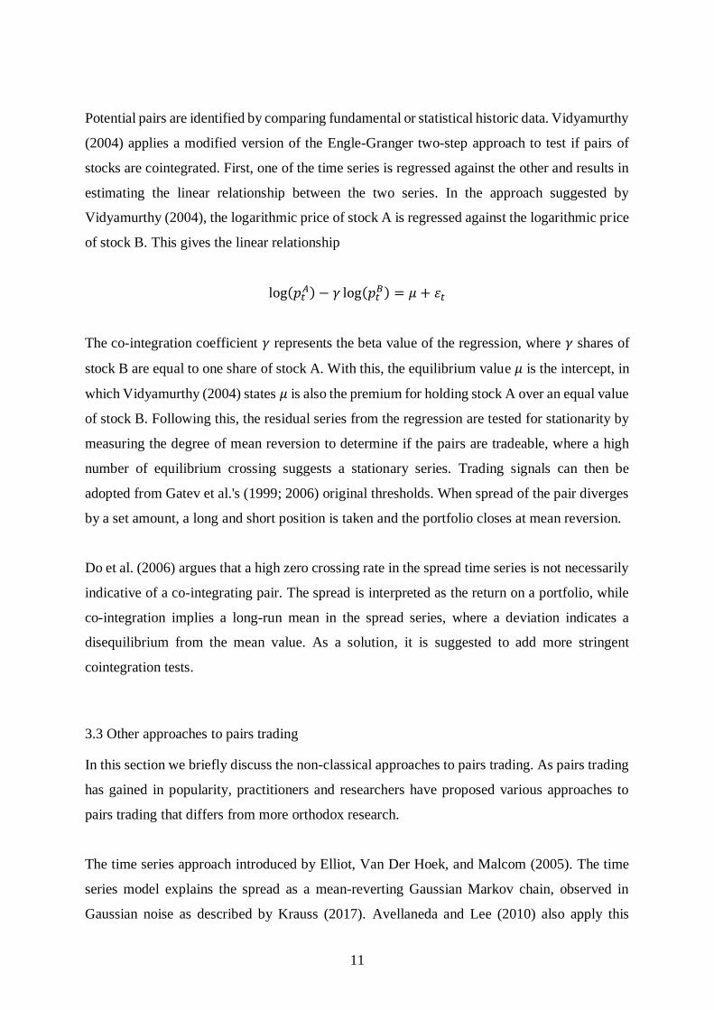
Potential pairs are identified by comparing fundamental or statistical historic data. Vidyamurthy

(2004) applies a modified version of the Engle-Granger two-step approach to test if pairs of

stocks are cointegrated. First, one of the time series is regressed against the other and results in

estimating the linear relationship between the two series. In the approach suggested by

Vidyamurthy (2004), the logarithmic price of stock A is regressed against the logarithmic price

of stock B. This gives the linear relationship

log(𝑝𝑡𝐴) − 𝛾 log(𝑝𝑡

𝐵) = 𝜇 + 𝜀𝑡

The co-integration coefficient 𝛾 represents the beta value of the regression, where 𝛾 shares of

stock B are equal to one share of stock A. With this, the equilibrium value 𝜇 is the intercept, in

which Vidyamurthy (2004) states 𝜇 is also the premium for holding stock A over an equal value

of stock B. Following this, the residual series from the regression are tested for stationarity by

measuring the degree of mean reversion to determine if the pairs are tradeable, where a high

number of equilibrium crossing suggests a stationary series. Trading signals can then be

adopted from Gatev et al.'s (1999; 2006) original thresholds. When spread of the pair diverges

by a set amount, a long and short position is taken and the portfolio closes at mean reversion.

Do et al. (2006) argues that a high zero crossing rate in the spread time series is not necessarily

indicative of a co-integrating pair. The spread is interpreted as the return on a portfolio, while

co-integration implies a long-run mean in the spread series, where a deviation indicates a

disequilibrium from the mean value. As a solution, it is suggested to add more stringent

cointegration tests.

3.3 Other approaches to pairs trading

In this section we briefly discuss the non-classical approaches to pairs trading. As pairs trading

has gained in popularity, practitioners and researchers have proposed various approaches to

pairs trading that differs from more orthodox research.

The time series approach introduced by Elliot, Van Der Hoek, and Malcom (2005). The time

series model explains the spread as a mean-reverting Gaussian Markov chain, observed in

Gaussian noise as described by Krauss (2017). Avellaneda and Lee (2010) also apply this

12

method with mean reverting portfolios creating trading signals using Principal Component

Analysis. This time series approach shows some promising results but fails to address the

problem of matching optimal pairs, according to Krauss (2017).

Do et al. (2006) suggests modeling the spread in a continuous time setting to quantify the mean

reversion of the spread using theoretical pricing methods. These approaches' main contributions

are the forecast and quantitative ability that, in case of mean reverting properties and the

presence of theoretical assets pricing, suggest more accurate trading thresholds to open and

unwind positions. Similar to the time series, the stochastic approach model fails to address the

problem of matching pairs. These methods are rarely used in empirical studies, and therefore

not given further consideration in this paper.

13

4. Data

For the empirical part of the study we use high frequency minute-by-minute data from the

constituents of the S&P 500 index in the period of December 13, 2017 to March 12, 2018. The

dataset is adjusted for dividends and splits. In the event of no trades in a given minute, the

dataset lack price information. We solve this by creating an index for all the trading minutes of

the day from 09:30 to 16:00. For the time intervals lacking price information we use the closing

price from the previous time point. To ensure that the starting price at each day is correct, we

use the first closing price in each respective day. With this we achieve a comparable index

containing 391 data points for each stock per day for 60 trading days. This generates a dataset

containing 11 730 000 stock prices.

The S&P 500 index consists of the 500 largest companies by market capitalization listed on the

NYSE and NASDAQ. The index captures roughly 80% of the US stock market capitalization2.

These stocks are highly liquid which in turn reduce the arbitrage risks and is favorable for pairs

trading strategy. Five companies on the S&P 500 are listed with two different share classes,

making the total number of stocks in the index 505. In line with Do and Faff (2010) we observe

that these stocks are often repeated as pairs when included in the pair formation algorithm.

When we test a sample for the effect of excluding these securities, we note that a higher number

of pairs are being traded and there is a greater volume of roundtrips in total. The percentage of

positions closed on time are far less, resulting in a lower average holding time per roundtrip.

Therefore, we have chosen to keep the class A stocks of companies with two different share

classes, even though this may eliminate some potential payoff from intra-company arbitrage

opportunities.

4.1 Pairs formation

Before identifying and constructing preferable pairs, we need to define the length of the historic

co-movement and the length of the trading period that we want to investigate. The most

common framework is to apply formation periods twice the length of trading periods. Another

common feature is to overlap the periods by shifting them by one day as demonstrated in Figure

1. We follow Gundersen (2014) and apply two separate frameworks for formation and trading

periods. The first framework being two days of formation and one trading day, and second with

2 https://eu.spindices.com/indices/equity/sp-500 (08.05.2017)

https://eu.spindices.com/indices/equity/sp-500

14

four days of formation followed by two days of trading. Given that formation periods do not

use any future data and the separation of different trading periods, we exclude looking-ahead

bias. As a result of this, the dataset is divided into 58 periods (2:1 framework) and 55 periods

(4:2 framework).

Following Gatev et al. (1999; 2006) and Stübinger and Bredthauer (2017) we identify pairs by

applying the original distance approach. This is the approach that Stübinger and Bredthauer

(2017) reports as the best performing approach. Hence, we first construct a cumulative total

return index for each security and normalize it to the first day for each period. Secondly, we

calculate the Euclidean squared distance between every stock. With no restrictions on pair

formation, it is possible to create 124 750 unique pairs. However, we only choose the top 5 and

top 20 pairs with the lowest distances for each period. These top pairs are then traded in their

respective trading periods.

Figure 1: Demonstration of formation and trading periods with two days formation and one day of trading.

4.2 Trading rules

Pairs are traded with predetermined rules during the trading period. As the formation and

trading subsets are independent from each other, it is unproblematic to create combinations of

multiple pairs trading strategies. Static thresholds are the original trading thresholds used by

Gatev et al. (1999; 2006), as described in section 3. Recent papers suggest that the most

favorable risk and return is achieved by implementing the Euclidean distance method with

varying trading thresholds (Kishore, 2012 and Stübinger and Bredthauer, 2017).

15

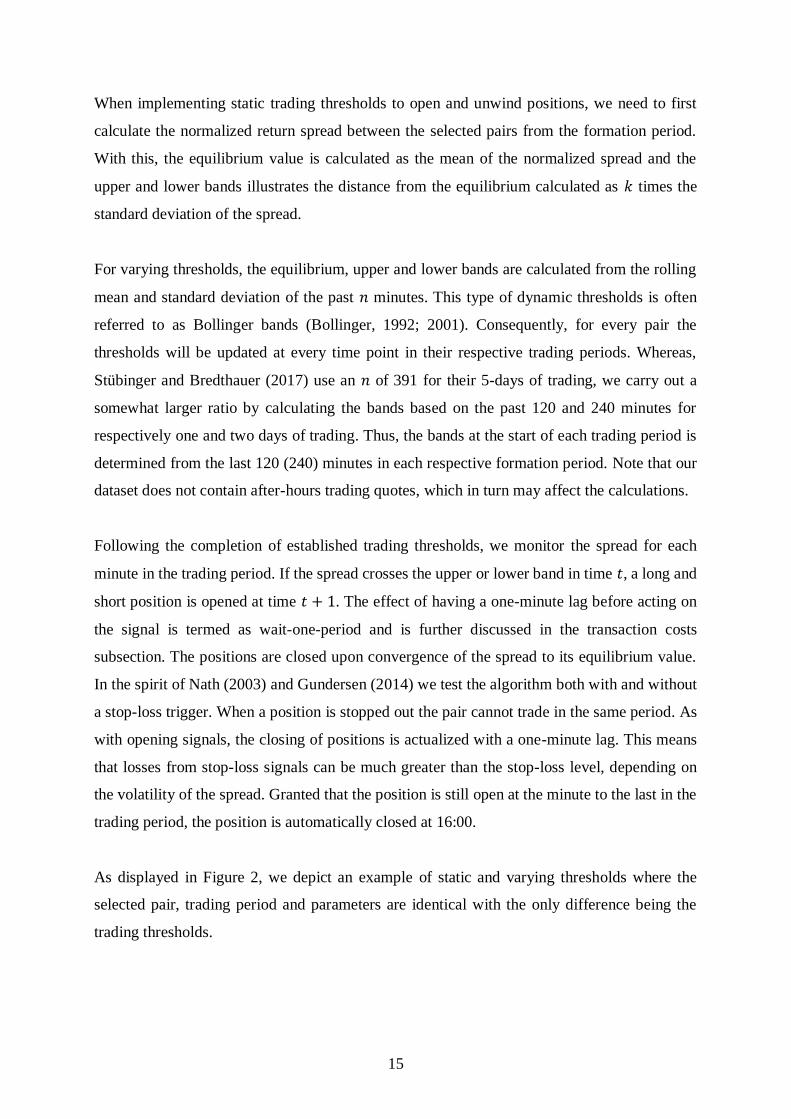
When implementing static trading thresholds to open and unwind positions, we need to first

calculate the normalized return spread between the selected pairs from the formation period.

With this, the equilibrium value is calculated as the mean of the normalized spread and the

upper and lower bands illustrates the distance from the equilibrium calculated as 𝑘 times the

standard deviation of the spread.

For varying thresholds, the equilibrium, upper and lower bands are calculated from the rolling

mean and standard deviation of the past 𝑛 minutes. This type of dynamic thresholds is often

referred to as Bollinger bands (Bollinger, 1992; 2001). Consequently, for every pair the

thresholds will be updated at every time point in their respective trading periods. Whereas,

Stübinger and Bredthauer (2017) use an 𝑛 of 391 for their 5-days of trading, we carry out a

somewhat larger ratio by calculating the bands based on the past 120 and 240 minutes for

respectively one and two days of trading. Thus, the bands at the start of each trading period is

determined from the last 120 (240) minutes in each respective formation period. Note that our

dataset does not contain after-hours trading quotes, which in turn may affect the calculations.

Following the completion of established trading thresholds, we monitor the spread for each

minute in the trading period. If the spread crosses the upper or lower band in time 𝑡, a long and

short position is opened at time 𝑡 + 1. The effect of having a one-minute lag before acting on

the signal is termed as wait-one-period and is further discussed in the transaction costs

subsection. The positions are closed upon convergence of the spread to its equilibrium value.

In the spirit of Nath (2003) and Gundersen (2014) we test the algorithm both with and without

a stop-loss trigger. When a position is stopped out the pair cannot trade in the same period. As

with opening signals, the closing of positions is actualized with a one-minute lag. This means

that losses from stop-loss signals can be much greater than the stop-loss level, depending on

the volatility of the spread. Granted that the position is still open at the minute to the last in the

trading period, the position is automatically closed at 16:00.

As displayed in Figure 2, we depict an example of static and varying thresholds where the

selected pair, trading period and parameters are identical with the only difference being the

trading thresholds.

16

Figure 2: Demonstration of static and varying upper and lower thresholds and calculated mean, trading period 37, one day

of trading, and the normalized spread between company Consolidated Edison Inc. and Western Digital Corp.

4.3 Return computation

As pairs trading is a strategy with zero net initial investment, return calculations may differ

between market operators. Firstly, the possibility of financing the long position with the short

proceeds creates a possible leverage effect that may influence the return calculation. As follows,

it is uncertain how much cash is needed to implement the strategy. Our return calculation

follows Gatev et al. (1999; 2006) where a $1-long, $1-short position requires a $1 deposit. This

is a conservative approach as opposed to Avellaneda and Lee (2010) and Liu, Chang, Geman

(2017) which respectively require $ 0.5 and $ 0.4 deposit for every $2 gross market exposure.

Secondly, we need to consider if the daily profit and loss is divided by how much capital you

commit to the strategy, or how much capital the strategy requires per trade. These two methods

are the most cited return calculations. Return on committed capital refers to when cashflows

are divided by the number of possible traded pairs. Return on employed capital refers to when

cashflows are divided by each active traded pair (Gatev et al. 1999; 2006). They also claim that

return on committed capital is obviously much more conservative when it considers the

17

opportunity cost of having to commit capital to a trading strategy even if the capital is not

employed. On the other hand, they suggest as hedge funds are flexible in their capital allocation,

return on employed capital may give a more realistic measure of profits. In this paper we report

the return on committed capital if not stated otherwise, as this is the most conservative

approach.

4.4 Transaction costs

Exploiting relative mispricing between assets often yield a low and modest return. Therefore, a

certain number of trades is critical to achieve feasible annualized returns. Thus, transaction

costs are not negligible. Do and Faff (2012) prove that almost all return provided from the

simple model of Gatev et al. (1999; 2006) disappear after controlling for various transaction

costs.

Transaction costs mainly consist of commissions, bid-ask spread, and short selling costs and

the magnitude of these cannot be determined definitively (Do and Faff, 2012). These vary in

time, with liquidity and between different market participants (Liu et al., 2017). There are many

ways to control for transaction costs both directly and indirectly. Bid-ask spread, also referred

to as bid-ask bounce or slippage, for example, is often controlled for as either using a fixed

basis-point (bps) cost or use a time-lag as a proxy. Gatev et al. (1999; 2006) use a wait-one-

period as a proxy for transaction costs.

In a contrarian strategy, price divergence may be a potential spread in the bid-ask price. The

winners price is more likely to be an ask quote and the losers price is more likely to be a bid

quote (Gatev et al., 1999; 2006). To cope with this problem, we implement a lag when testing

our strategy. We restrict our algorithms to open or unwind a position in a pair the minute after

a signal is given. This wait-one-period proxy is estimated by Liu et al. (2017) as 10 bps per

roundtrip when testing the strategy return for both fixed bps as transaction costs, and a signal-

lag as a proxy. In addition, following Avellaneda and Lee (2010), Krauss (2017) and Stübinger

and Bredthauer (2017), we choose to test our strategy for 5 basis-points per trade per stock, as

transaction costs. Additionally, we test for 2.5 bps and no fixed transaction costs. This

combined with a wait-one-period lag in our algorithm will represent our transaction costs.

18

5. Results

In this section we present our results from the different strategies. First, Table 1 through 4

depicts all 288 portfolios. Second, we discuss the top and worst performing portfolios. Third,

we present risk and return characteristics from 8 conservative portfolios. Fourth, we present

some holding statistics for specific portfolios. In addition, we test a portfolio to traditional risk

exposure. Thereafter, we test our algorithm to find the break-even point for different top

performing portfolios. Finally, we add a volatility timing measure restricting our algorithm

trading rules to optimize point of entry.

To find our optimal portfolios we test various parameters of 𝑘, stop-loss and transaction costs.

Stübinger and Bredthauer's (2017) optimal 𝑘 parameter proved to be 2.5 and they conclude a 𝑘

of 2 as used by Gatev et al. (1999; 2006), is too aggressive when handling high frequency data.

Nevertheless, we implement 𝑘′𝑠 equal to 2, 2.5 and 5. With a 𝑘 equal to 5, the spread would

have to diverge five times the standard deviation from the equilibrium before taking a position.

We acknowledge with this parameter the pair may already diverge beyond convergence, as

there may no longer be an equilibrium relationship. However, as transaction costs are

predominately important in pairs trading, a high 𝑘 could lead to fewer transactions with higher

profits per trade.

Stop-loss triggers are differentiated by applying stop-loss at 2%-level and without stop-loss

signals. For transaction costs, we perform the back-test using transaction costs of 2.5 basis-

points per transaction, 5 basis-points and without any transaction costs.

5.1 Unrestricted case

In our unrestricted case we allow all our stocks to be paired with each other in all formation

periods. We create a 500 x 500 matrix which translate to 124 750 possible pairs. We then choose

the top 5 and 20 pairs of stocks based on the minimum-distance criterion and construct a

portfolio to test in the subsequent trading period.

In the spirit of Gundersen (2014) we report our results in tables illustrating the relationship

between different configuration and returns. As shown in the table below transaction costs

totally deteriorate the returns. The table is read from left to right arranged by number of

formation and trading days, transaction costs per trade, number of standard deviation from its

19

calculated mean before a position in a pair is entered, and a stop-loss configuration. The returns,

standard deviations, and Sharpe ratios are reported on an annualized basis. Lastly, number of

roundtrips for the whole period is reported where one roundtrip equals four trades, i.e. buying

and selling a stock for both the long and the short position. When discussing results from the

following tables we refer to the different portfolio configurations in numbers.

Configuration Format TC k SL Return SD SR Roundtrips Return SD SR Roundtrips

1 2:1 5 bps 2 2 % -48,30 % 4,59 % -10,91 562 -62,29 % 4,43 % -14,44 751

2 2:1 5 bps 2 NA -48,75 % 4,67 % -10,81 562 -62,79 % 4,45 % -14,50 751

3 2:1 5 bps 2,5 2 % -38,96 % 4,91 % -8,28 455 -54,16 % 4,61 % -12,13 615

4 2:1 5 bps 2,5 NA -39,48 % 4,98 % -8,26 455 -54,78 % 4,65 % -12,14 615

5 2:1 5 bps 5 2 % -20,35 % 3,96 % -5,57 188 -27,06 % 3,67 % -7,84 246

6 2:1 5 bps 5 NA -21,36 % 4,10 % -5,62 188 -28,04 % 3,76 % -7,91 246

7 2:1 2,5 bps 2 2 % -15,66 % 4,89 % -3,55 562 -27,51 % 4,62 % -6,33 751

8 2:1 2,5 bps 2 NA -16,38 % 4,97 % -3,64 562 -28,48 % 4,64 % -6,50 751

9 2:1 2,5 bps 2,5 2 % -9,29 % 5,14 % -2,14 455 -21,72 % 4,72 % -4,97 615

10 2:1 2,5 bps 2,5 NA -10,07 % 5,20 % -2,26 455 -22,77 % 4,76 % -5,14 615

11 2:1 2,5 bps 5 2 % -6,19 % 3,78 % -2,09 188 -9,66 % 3,61 % -3,15 246

12 2:1 2,5 bps 5 NA -7,38 % 3,93 % -2,31 188 -10,87 % 3,68 % -3,41 246

13 2:1 0 bps 2 2 % 37,58 % 5,31 % 6,75 562 39,31 % 5,18 % 7,26 751

14 2:1 0 bps 2 NA 36,39 % 5,39 % 6,43 562 37,45 % 5,21 % 6,87 751

15 2:1 0 bps 2,5 2 % 34,78 % 5,44 % 6,08 455 33,64 % 4,98 % 6,40 615

16 2:1 0 bps 2,5 NA 33,62 % 5,50 % 5,80 455 31,85 % 5,02 % 6,00 615

17 2:1 0 bps 5 2 % 10,47 % 3,64 % 2,40 188 11,89 % 3,60 % 2,82 246

18 2:1 0 bps 5 NA 9,07 % 3,80 % 1,94 188 10,38 % 3,67 % 2,37 246

19 4:2 5 bps 2 2 % -25,72 % 4,85 % -5,66 564 -31,93 % 3,22 % -10,43 546

20 4:2 5 bps 2 NA -20,31 % 4,53 % -4,86 566 -31,64 % 3,21 % -10,40 548

21 4:2 5 bps 2,5 2 % -21,64 % 4,50 % -5,20 434 -25,46 % 3,13 % -8,69 456

22 4:2 5 bps 2,5 NA -15,75 % 4,03 % -4,34 436 -25,29 % 3,09 % -8,75 456

23 4:2 5 bps 5 2 % 2,25 % 4,36 % 0,12 193 -10,11 % 2,19 % -5,40 174

24 4:2 5 bps 5 NA 7,39 % 4,51 % 1,26 193 -10,09 % 2,19 % -5,40 174

25 4:2 2,5 bps 2 2 % -3,75 % 5,11 % -1,07 564 -12,55 % 3,34 % -4,27 546

26 4:2 2,5 bps 2 NA 3,34 % 4,87 % 0,34 566 -12,10 % 3,32 % -4,16 548

27 4:2 2,5 bps 2,5 2 % -4,36 % 4,59 % -1,32 434 -8,12 % 3,22 % -3,05 456

28 4:2 2,5 bps 2,5 NA 2,91 % 4,20 % 0,29 436 -7,90 % 3,18 % -3,02 456

29 4:2 2,5 bps 5 2 % 11,71 % 4,52 % 2,21 193 -2,64 % 2,19 % -1,99 174

30 4:2 2,5 bps 5 NA 17,33 % 4,68 % 3,33 193 -2,62 % 2,19 % -1,98 174

31 4:2 0 bps 2 2 % 24,71 % 5,43 % 4,23 564 12,34 % 3,53 % 3,01 546

32 4:2 0 bps 2 NA 34,01 % 5,28 % 6,12 566 13,02 % 3,50 % 3,24 548

33 4:2 0 bps 2,5 2 % 16,72 % 4,72 % 3,18 434 13,25 % 3,37 % 3,42 456

34 4:2 0 bps 2,5 NA 25,70 % 4,42 % 5,43 436 13,51 % 3,33 % 3,55 456

35 4:2 0 bps 5 2 % 22,04 % 4,71 % 4,32 193 5,44 % 2,22 % 1,68 174

36 4:2 0 bps 5 NA 28,18 % 4,89 % 5,41 193 5,46 % 2,21 % 1,69 174

Configuration: Portfolio configuration number

Format: Formation and trading period in days

TC: Transaction cost per trade in basis points

k: Upper and lower band for opening a position in standard deviations

SL: Stop-loss (NA equals no stop-loss)

Return: Annualized return

SD: Annualized standard deviation for returns

SR: Annualized Sharpe ratio

Roundtrips: Number of total roundtrips

Static Thresholds Varying Thresholds

Table 1: Annualized risk and returns measures for top 5 pairs in the no restriction case using static and varying entry

thresholdsParameters

20

5.2 Top 5 pairs unrestricted case

The highest return generated from our top 5 pairs in the unrestricted case is portfolio

configuration 13. Using varying thresholds and generating annualized return of 39.31% with a

standard deviation of 5.18%, we obtain a Sharpe ratio of 7.26. This is achieved through 751

roundtrips. The worst performing portfolio is, not surprisingly, the portfolio with the same

configuration when adding transaction costs of 5 bps and with no stop-loss, generating an

annualized return of -62.29% and a standard deviation of 4.43%.

When k decreases, more positions are opened. As these trades are profitable by themselves they

do not generate sustainable returns to justify the transaction costs added. When we stretch the

trading bands outwards, using higher k, the number of total roundtrips naturally decreases.

Moreover, we achieve positive annualized returns of 7.39% with a standard deviation of 4.51%

for portfolio configuration 24 (5 bps), with no stop-loss using static entry-thresholds, resulting

in an annualized Sharpe ratio of 1.26. The same portfolio with added stop-loss, returns 2.25%

and a standard deviation of 4.36%. In this case, the stop-loss exits profitable trades prematurely.

Both these portfolios achieved 193 roundtrips in the 55-day period.

Something we find peculiar with our results are the impact of the stop-loss limit. There are

several occasions like the scenario above, where only one stop-loss is triggered in the same

period. Making the total roundtrips equal in both cases. When these pairs are stopped out, a

common outcome is that the pair would have converged, making the total profit greater, or

potential loss smaller. This makes the stop-loss trigger arbitrary. Furthermore, the results

suggest a negative effect of restricting pairs that are stopped out, not being able to open new

positions. As a result of this, we assume a stop-loss threshold of 2% to be too strict, as it does

not provide enough room for pairs to converge. This assumption is mainly for frameworks with

two trading days, as these stand out with the negative effect of our stop-loss trigger. A possible

solution could be higher stop-loss thresholds to ensure the pair actually have diverged sufficient

enough where we could assume there are no longer an equilibrium relationship. With higher

stop-loss thresholds we are unsure if restriction of new positions in closed pairs should be

applied. However, if the pair converges to equilibrium, there is likely that profits can be made

on new roundtrips.

21

As shown in Table 1 the highest number of roundtrips in the top 5 unrestricted case is 751 as

opposed to the lowest number of roundtrips of 174, with varying thresholds of k equal to 2 and

k equal to 5. When the number of roundtrips increases, the impact of transaction costs on returns

rise. This is discussed more thoroughly in the following sub-section discussing break-even

points for the return and transaction cost relationship of specific portfolios.

5.3 Top 20 pairs unrestricted case

The following Table 2 shows the portfolios of top 20 pairs in the unrestricted case. The table is

read in the same fashion as Table 1. Note that increasing the number of pairs in our portfolios

decreases the standard deviations, giving a diversification effect in our portfolios and yielding

better Sharpe ratios. The portfolio yielding the highest return now shifts to static thresholds

yielding an annualized return of 35.01% with a standard deviation of 3.57%, with portfolio

configuration 13. However, the same portfolio using varying thresholds return 33.50% with a

standard deviation of 2.91%, achieving a Sharpe ratio of 10.94 making this the preferred

portfolio of all portfolios.

As in the top 5 no restriction case, returns diminish as we add a fixed transaction cost. In fact,

only four portfolios yield annualized returns above zero, as opposed to six in the top 5 pairs

with added transaction costs. These four portfolios all have the same configuration, 29 and 30,

using both static and varying entry-thresholds. The highest annualized return is 5.77% with a

Sharpe ratio of 1.23 using static thresholds and no stop-loss.

The worst performing portfolio is with varying thresholds, k equal to 2, one trading day, and 5

bps added transaction costs are applied. These portfolio configurations generate large losses,

making them unfit for trading. Naturally, as the number of pairs in our portfolio increases, the

number of roundtrips simultaneously increases. The portfolio with the highest number of total

roundtrips is 3 733 roundtrips, which translates to 14 932 individual trades in the 55-day period.

22

5.4 Restricted case

The matching of pairs in the unrestricted case is purely based on the minimum-distance

criterion. Thus, we may find stocks from different sectors being matched and paired together.

While this is not necessarily problematic, we may see that stocks that are exposed to common

factors express similar return patterns and makes them more likely to fit in a pairs trading

strategy (Gatev et al. 1999; 2006). To find suitable pairs within the same sector we use the

Global Industry Classification Standard (GICS), which classify companies both quantitatively

and qualitatively into four tiers. The standard sorts securities in 11 sectors, 24 industry groups,


1 2:1 5 bps 2 2 % -49,23 % 3,21 % -15,85 2245 -64,26 % 2,61 % -25,32 3028

2 2:1 5 bps 2 NA -49,55 % 3,29 % -15,60 2245 -64,79 % 2,71 % -24,53 3048

3 2:1 5 bps 2,5 2 % -40,44 % 3,35 % -12,57 1806 -54,55 % 2,47 % -22,79 2415

4 2:1 5 bps 2,5 NA -40,96 % 3,38 % -12,63 1806 -55,12 % 2,59 % -21,97 2430

5 2:1 5 bps 5 2 % -21,91 % 2,64 % -8,94 746 -27,20 % 1,69 % -17,09 954

6 2:1 5 bps 5 NA -22,23 % 2,72 % -8,80 746 -27,99 % 1,73 % -17,15 954

7 2:1 2,5 bps 2 2 % -17,20 % 3,36 % -5,64 2245 -30,92 % 2,69 % -12,13 3028

8 2:1 2,5 bps 2 NA -17,73 % 3,42 % -5,69 2245 -31,65 % 2,76 % -12,08 3048

9 2:1 2,5 bps 2,5 2 % -11,74 % 3,46 % -3,89 1806 -23,13 % 2,58 % -9,64 2415

10 2:1 2,5 bps 2,5 NA -12,51 % 3,48 % -4,09 1806 -23,85 % 2,67 % -9,57 2430

11 2:1 2,5 bps 5 2 % -8,16 % 2,57 % -3,83 746 -10,42 % 1,74 % -6,99 954

12 2:1 2,5 bps 5 NA -8,52 % 2,65 % -3,87 746 -11,39 % 1,79 % -7,32 954

13 2:1 0 bps 2 2 % 35,01 % 3,57 % 9,33 2245 33,50 % 2,91 % 10,94 3028

14 2:1 0 bps 2 NA 34,16 % 3,62 % 8,96 2245 32,66 % 2,94 % 10,52 3048

15 2:1 0 bps 2,5 2 % 30,77 % 3,60 % 8,07 1806 29,97 % 2,74 % 10,31 2415

16 2:1 0 bps 2,5 NA 29,62 % 3,62 % 7,70 1806 29,18 % 2,81 % 9,78 2430

17 2:1 0 bps 5 2 % 8,02 % 2,55 % 2,48 746 10,21 % 1,81 % 4,70 954

18 2:1 0 bps 5 NA 7,59 % 2,61 % 2,25 746 9,03 % 1,87 % 3,90 954

19 4:2 5 bps 2 2 % -28,42 % 3,81 % -7,91 2173 -44,08 % 3,37 % -13,57 3655

20 4:2 5 bps 2 NA -24,02 % 3,44 % -7,47 2196 -43,15 % 3,37 % -13,30 3733

21 4:2 5 bps 2,5 2 % -25,33 % 3,48 % -7,78 1701 -34,45 % 3,32 % -10,88 2914

22 4:2 5 bps 2,5 NA -20,77 % 3,31 % -6,78 1718 -33,39 % 3,29 % -10,67 2962

23 4:2 5 bps 5 2 % -6,89 % 3,19 % -2,70 759 -10,79 % 2,81 % -4,44 1086

24 4:2 5 bps 5 NA -3,08 % 3,26 % -1,47 761 -7,84 % 2,73 % -3,49 1088

25 4:2 2,5 bps 2 2 % -8,08 % 3,86 % -2,54 2173 -14,92 % 3,46 % -4,81 3655

26 4:2 2,5 bps 2 NA -2,17 % 3,50 % -1,11 2196 -12,73 % 3,40 % -4,25 3733

27 4:2 2,5 bps 2,5 2 % -9,19 % 3,45 % -3,16 1701 -8,40 % 3,41 % -2,97 2914

28 4:2 2,5 bps 2,5 NA -3,46 % 3,34 % -1,55 1718 -6,42 % 3,36 % -2,42 2962

29 4:2 2,5 bps 5 2 % 1,59 % 3,19 % -0,04 759 1,05 % 2,87 % -0,23 1086

30 4:2 2,5 bps 5 NA 5,77 % 3,30 % 1,23 761 4,41 % 2,81 % 0,96 1088

31 4:2 0 bps 2 2 % 18,03 % 3,96 % 4,13 2173 29,46 % 3,63 % 7,65 2655

32 4:2 0 bps 2 NA 25,94 % 3,62 % 6,69 2196 33,95 % 3,52 % 9,15 3733

33 4:2 0 bps 2,5 2 % 10,43 % 3,46 % 2,52 1701 27,99 % 3,53 % 7,43 2914

34 4:2 0 bps 2,5 NA 17,62 % 3,41 % 4,67 1718 31,45 % 3,48 % 8,55 2962

35 4:2 0 bps 5 2 % 10,83 % 3,22 % 2,83 759 14,45 % 2,95 % 4,32 1086

36 4:2 0 bps 5 NA 15,42 % 3,36 % 4,08 761 18,27 % 2,90 % 5,72 1088











Table 2: Annualized risk and returns measures for top 20 pairs in the no restriction case using static and varying entry


23

68 industries and 157 sub-industries. In this empirical study we implement GICS sector

restrictions in our pairs formation.

5.5 Top 5 restricted case

Several papers report that sector restrictions improve return from different pairs trading

strategies (Do and Faff, 2010 and Gundersen, 2014). Table 3 shows top 5 pairs where formation

and trading between stocks are restricted by the 11 sectors Consumer Discretionary, Consumer

staples, Energy, Financials, Health care, Industrials, Information technology, Materials, Real

estate, Telecommunication services, and Utilities. The table is set up in the same manner as

Table 1 and 2.

In Table 3 we see that configuration 32 yields the highest return and most favorable Sharpe

ratio with portfolio using varying thresholds. The annualized return is 40.63% with a Sharpe

ratio of 8.37. Comparing this result with the top performer from the top 5 unrestricted case, we

see that the return is only slightly higher from the restricted case while the standard deviation

has dropped 0.53%-points. Overall, the difference between the results are not considerable,

although the number of portfolios yielding a positive return rise from six to eight. Many of the

companies match in the unrestricted case as well as in the restricted case. These companies are

exposed to low cross-differences and variances are likely to be formed in both cases (Gatev et

al., 1999; 2006)

Interestingly, it is worth noting that portfolio configuration 24 still yield positive returns using

static thresholds, but with a lower annualized return of 2.59% and a standard deviation of

3.64%. This is also the case for the other portfolios with added transaction costs. However, two

of the portfolios applying varying threshold also yields return above zero.

24

5.6 Top 20 Restricted case

Table 4 is interpreted in the same way as the previous tables. The top performing portfolio now

use static thresholds with portfolio configuration 32. This portfolio yields an annualized return

of 33.78%, with a standard deviation of 3.26%, and obtains a Sharpe ratio of 9.84. The total

number of portfolios yielding a positive return with added transaction costs is still eight,

although the configuration has shifted. The portfolio using static thresholds with portfolio

configuration 27, yields a return 0.06% per annum, standard deviation of 2.84%, through 1 606

roundtrips. The same portfolio without stop-loss returns 5.09% with almost the same standard

deviation of 2.89% and 13 more roundtrips.


1 2:1 5 bps 2 2 % -46,43 % 4,51 % -10,68 526 -64,63 % 4,35 % -15,25 747

2 2:1 5 bps 2 NA -46,74 % 4,58 % -10,59 526 -65,24 % 4,33 % -15,46 748

3 2:1 5 bps 2,5 2 % -36,47 % 4,58 % -8,34 429 -56,48 % 4,23 % -13,76 625

4 2:1 5 bps 2,5 NA -37,33 % 4,64 % -8,41 429 -57,16 % 4,20 % -14,01 626

5 2:1 5 bps 5 2 % -14,21 % 4,04 % -3,94 178 -29,73 % 3,54 % -8,87 244

6 2:1 5 bps 5 NA -15,29 % 4,11 % -4,14 178 -30,68 % 3,62 % -8,95 244

7 2:1 2,5 bps 2 2 % -15,32 % 4,80 % -3,55 526 -32,24 % 4,39 % -7,72 747

8 2:1 2,5 bps 2 NA -15,81 % 4,87 % -3,60 526 -33,35 % 4,37 % -8,02 748

9 2:1 2,5 bps 2,5 2 % -7,71 % 4,69 % -2,01 429 -25,03 % 4,37 % -6,12 625

10 2:1 2,5 bps 2,5 NA -8,96 % 4,74 % -2,25 429 -26,13 % 4,34 % -6,42 626

11 2:1 2,5 bps 5 2 % 0,16 % 3,94 % -0,39 178 -13,12 % 3,48 % -4,26 244

12 2:1 2,5 bps 5 NA -1,11 % 4,00 % -0,70 178 -14,29 % 3,54 % -4,51 244

13 2:1 0 bps 2 2 % 33,83 % 5,19 % 6,19 526 29,80 % 4,72 % 5,95 747

14 2:1 0 bps 2 NA 33,05 % 5,26 % 5,96 526 27,78 % 4,69 % 5,55 748

15 2:1 0 bps 2,5 2 % 34,03 % 4,88 % 6,63 429 29,11 % 4,65 % 5,89 625

16 2:1 0 bps 2,5 NA 32,23 % 4,92 % 6,21 429 27,33 % 4,61 % 5,56 626

17 2:1 0 bps 5 2 % 16,91 % 3,88 % 3,92 178 7,41 % 3,46 % 1,65 244

18 2:1 0 bps 5 NA 15,44 % 3,94 % 3,48 178 5,97 % 3,52 % 1,21 244

19 4:2 5 bps 2 2 % -24,66 % 4,56 % -5,78 556 -42,44 % 4,52 % -9,76 918

20 4:2 5 bps 2 NA -20,33 % 4,40 % -5,01 557 -39,85 % 4,11 % -10,10 926

21 4:2 5 bps 2,5 2 % -20,61 % 4,25 % -5,26 416 -32,62 % 4,28 % -8,03 732

22 4:2 5 bps 2,5 NA -15,67 % 3,92 % -4,43 417 -29,86 % 3,79 % -8,32 737

23 4:2 5 bps 5 2 % -1,41 % 3,46 % -0,90 172 -9,53 % 2,91 % -3,86 272

24 4:2 5 bps 5 NA 2,59 % 3,64 % 0,24 172 -7,60 % 2,63 % -3,54 272

25 4:2 2,5 bps 2 2 % -2,73 % 4,91 % -0,90 556 -12,31 % 4,75 % -2,95 918

26 4:2 2,5 bps 2 NA 2,89 % 4,84 % 0,24 557 -8,02 % 4,28 % -2,28 926

27 4:2 2,5 bps 2,5 2 % -3,90 % 4,43 % -1,27 416 -5,73 % 4,47 % -1,67 732

28 4:2 2,5 bps 2,5 NA 2,12 % 4,19 % 0,10 417 -1,65 % 3,96 % -0,85 737

29 4:2 2,5 bps 5 2 % 6,69 % 3,53 % 1,41 172 2,49 % 2,98 % 0,26 272

30 4:2 2,5 bps 5 NA 11,00 % 3,75 % 2,48 172 4,67 % 2,72 % 1,09 272

31 4:2 0 bps 2 2 % 25,55 % 5,34 % 4,47 556 33,60 % 5,17 % 6,17 918

32 4:2 0 bps 2 NA 32,87 % 5,34 % 5,83 557 40,63 % 4,65 % 8,37 926

33 4:2 0 bps 2,5 2 % 16,30 % 4,66 % 3,13 416 31,87 % 4,76 % 6,34 732

34 4:2 0 bps 2,5 NA 23,64 % 4,50 % 4,87 417 37,88 % 4,23 % 8,56 737

35 4:2 0 bps 5 2 % 15,44 % 3,63 % 3,79 172 16,09 % 3,10 % 4,64 272

36 4:2 0 bps 5 NA 20,11 % 3,90 % 4,72 172 18,56 % 2,88 % 5,86 272











Table 3: Annualized risk and returns measures for top 5 pairs in the restricted case using static and varying entry


25

First, we note that all portfolio configurations with transaction cost and 2:1 formation-trading

period consistently yields negative returns, except for portfolio configuration 11 using static

thresholds in the unrestricted top 5 case, which yield an annualized return of 0.16% and a

standard deviation of close to four. This shows that two days is not enough time to measure and

quantify the distance, i.e. the co-movement of stocks, or that one day is not enough time to

allow the prices to adjust in the market. Thus, profitable positions will be unwound at the close

of the trading day prematurely of convergence. However, Bowen et al. (2010) shows that most

of the return from high frequency pairs trading arise from the first hour of trading.


1 2:1 5 bps 2 2 % -45,89 % 2,77 % -17,21 2062 -65,89 % 2,79 % -24,22 3055

2 2:1 5 bps 2 NA -46,42 % 2,88 % -16,74 2062 -66,36 % 2,81 % -24,23 3069

3 2:1 5 bps 2,5 2 % -35,94 % 2,91 % -12,96 1542 -55,99 % 2,68 % -21,57 2468

4 2:1 5 bps 2,5 NA -36,78 % 2,99 % -12,87 1652 -56,42 % 2,70 % -21,50 2478

5 2:1 5 bps 5 2 % -15,64 % 2,32 % -7,49 644 -29,22 % 1,66 % -18,66 953

6 2:1 5 bps 5 NA -17,09 % 2,42 % -7,76 644 -29,77 % 1,70 % -18,52 953

7 2:1 2,5 bps 2 2 % -15,21 % 2,96 % -5,72 2062 -33,69 % 2,86 % -12,40 3055

8 2:1 2,5 bps 2 NA -16,05 % 3,06 % -5,79 2062 -34,41 % 2,86 % -12,63 3069

9 2:1 2,5 bps 2,5 2 % -8,22 % 3,08 % -3,22 1652 -24,71 % 2,78 % -9,51 2468

10 2:1 2,5 bps 2,5 NA -9,42 % 3,17 % -3,52 1652 -25,29 % 2,79 % -9,66 2478

11 2:1 2,5 bps 5 2 % -2,95 % 2,30 % -2,03 644 -12,92 % 1,65 % -8,86 953

12 2:1 2,5 bps 5 NA -4,63 % 2,41 % -2,63 644 -13,60 % 1,69 % -9,04 953

13 2:1 0 bps 2 2 % 32,82 % 3,22 % 9,66 2062 28,89 % 3,05 % 8,90 3055

14 2:1 0 bps 2 NA 31,51 % 3,32 % 8,98 2062 27,88 % 3,04 % 8,60 3069

15 2:1 0 bps 2,5 2 % 31,48 % 3,31 % 8,99 1652 28,78 % 2,93 % 9,23 2468

16 2:1 0 bps 2,5 NA 29,75 % 3,39 % 8,27 1652 28,06 % 2,94 % 8,96 2478

17 2:1 0 bps 5 2 % 11,63 % 2,34 % 4,24 644 7,12 % 1,67 % 3,23 953

18 2:1 0 bps 5 NA 9,70 % 2,44 % 3,27 644 6,29 % 1,71 % 2,67 953

19 4:2 5 bps 2 2 % -22,82 % 2,65 % -9,26 2084 -44,93 % 2,70 % -17,28 3561

20 4:2 5 bps 2 NA -17,49 % 2,89 % -6,65 2103 -43,75 % 2,48 % -18,33 3609

21 4:2 5 bps 2,5 2 % -16,80 % 2,81 % -6,58 1606 -35,88 % 2,60 % -14,48 2860

22 4:2 5 bps 2,5 NA -12,75 % 2,78 % -5,21 1619 -34,60 % 2,41 % -15,06 2892

23 4:2 5 bps 5 2 % 0,57 % 2,43 % -0,47 649 -13,33 % 2,13 % -7,07 1110

24 4:2 5 bps 5 NA 1,96 % 2,56 % 0,10 649 -11,05 % 1,93 % -6,62 1110

25 4:2 2,5 bps 2 2 % -1,93 % 2,73 % -1,33 2084 -17,11 % 2,85 % -6,61 3561

26 4:2 2,5 bps 2 NA 5,07 % 3,04 % 1,10 2103 -14,88 % 2,59 % -6,42 3609

27 4:2 2,5 bps 2,5 2 % 0,06 % 2,84 % -0,58 1606 -10,96 % 2,74 % -4,62 2860

28 4:2 2,5 bps 2,5 NA 5,09 % 2,89 % 1,17 1619 -8,85 % 2,52 % -4,19 2892

29 4:2 2,5 bps 5 2 % 8,34 % 2,51 % 2,64 649 -1,56 % 2,20 % -1,49 1110

30 4:2 2,5 bps 5 NA 9,83 % 2,65 % 3,06 649 1,02 % 1,99 % -0,34 1110

31 4:2 0 bps 2 2 % 24,61 % 2,89 % 7,93 2084 24,76 % 3,09 % 7,47 3561

32 4:2 0 bps 2 NA 33,78 % 3,26 % 9,84 2103 28,81 % 2,79 % 9,70 3609

33 4:2 0 bps 2,5 2 % 20,32 % 2,92 % 6,37 1606 23,64 % 2,92 % 7,51 2860

34 4:2 0 bps 2,5 NA 26,55 % 3,04 % 8,17 1619 27,03 % 2,67 % 9,48 2892

35 4:2 0 bps 5 2 % 16,70 % 2,61 % 5,75 649 11,80 % 2,29 % 4,41 1110

36 4:2 0 bps 5 NA 18,32 % 2,77 % 6,00 649 14,73 % 2,08 % 6,25 1110











Table 4: Annualized risk and returns measures for top 20 pairs in the restricted case using static and varying entry


26

Moreover, if the market is strongly efficient the price history is not an estimator for the future.

In addition, there is substantial trading after the traditional close at 16:00. This is not captured

by our algorithm, making a gap in our data set when calculating the distance between pairs.

This also affects the calculation of the rolling mean and entry standard deviation calculation,

which in turn may have an impact on our formation periods, trading periods and results.

Our sector restriction does not provide more profitable results than the unrestricted case. This

indicates formation of similar pairs as suggested by Gatev et al. (1999; 2006) or that GICS

sector tier is not strict enough when optimizing pair selection approach. Suggesting more

fundamental factors should be applied when restricting formation.

In the next subsection we pick out some portfolios where we report some more thorough risk

and return measures and exposures. We also estimate the break-even point for transaction costs,

as transaction cost vary from retail to institutional investors, liquidity, timing and size of the

order, and market conditions (Liu et al., 2017). Therefore, it is interesting to find out how high

transaction costs one can have before the strategies are unsustainable. As we have shown from

our results there are obviously profits to be made from pairs trading when subtracting additional

transaction costs. Thus, making the optimal portfolio depends on what kind of transaction costs

and entry-thresholds the investor can achieve and apply.

5.7 Risk and return characteristics of specific portfolio configuration

In Table 5 we report daily return and risk measurements in the spirit of Stübinger and

Bredthauer (2017) in all trading periods. We consider a conservative portfolio configuration

opening a position when the spread deviates from its calculated mean with standard deviation

of 2.5 for both static (S) and varying (V) thresholds, adding a 10 basis-points transaction cost

per roundtrip.

The formation period consists of four days followed by a two-day trading period. The table

consists of top 5 (T5) and top 20 (T20) portfolios, where pairs both can be paired unrestricted

(NR) and restricted (R). We compare this to a buy and hold strategy in the S&P 500-index in

the same period.

27

Note: VaR and CVaR describes the daily historical value at risk and the conditional value at risk respectively, i.e. tail risk and

expected shortfall, at specific probability levels. Maximum drawdown describe max decline from peak to a through.

Portfolios using varying thresholds all yield an average daily return below zero. The top

performing portfolios in respect of return is the top 5 pairs both the restricted and unrestricted

case, along with the top 20 pairs from the restricted case. All using static thresholds to enter

trades in these specific portfolios. S&P 500 yields an average daily return of 0.07% (t-stat =

0.494) which is clearly higher than our best performing portfolio T 20 R S with an average daily

return of 0.02% (t-stat = 1.142).

Only one of the portfolios is statistically significant different from zero, T20 R V, with a t-stat

of -2,4249, indicating a return significantly different from zero. Moreover, like Gatev et al.

(1999; 2006) we note that all our returns are positively skewed in respect of the normal

distribution. Goetzmann, Ingersoll, Spiegel and Welch (2004) show that negative skewness

may bias the Sharpe ratio upwards. In these specific portfolios this imply that our Sharpe ratios

is biased downwards. The excess kurtosis in our distributions is fairly small compared to the

S&P in the same period. All tails in our sample show a leptokurtic distribution indicating long,

skinny tails.

The value at risk at different probability levels depict that our strategies have far less daily value

at risk compared to the S&P 500. The maximum drawdown which measures the decline from

a global peak in the portfolio to a through. The S&P 500 in this period have a 10.13% decline

compared to T20 R V where the maximum drawdown is 4.27%.

Measure T5 NR S T5 NR V T5 R S T5 R V T20 NR S T20 NR V T20 R S T20 R V S&P

Mean return 0,0001 -0,0003 0,0001 -0,0001 -0,0001 -0,0003 0,0002 -0,0004 0,0007

SE mean return 0,0003 0,0002 0,0003 0,0002 0,0002 0,0002 0,0002 0,0002 0,0015

t-statistic 0,4587 -1,7046 0,3373 -0,2710 -0,6908 -1,2983 1,1417 -2,4249 0,4941

Median 0,0000 -0,0003 0,0000 0,0002 -0,0002 -0,0004 0,0002 -0,0004 0,0015

Minimum -0,0047 -0,0032 -0,0047 -0,0045 -0,0037 -0,0030 -0,0026 -0,0027 -0,0408

Maximum 0,0048 0,0047 0,0047 0,0028 0,0042 0,0040 0,0047 0,0019 0,0174

Quartile 1 -0,0009 -0,0013 -0,0010 -0,0011 -0,0009 -0,0012 -0,0004 -0,0011 -0,0014

Quartile 3 0,0013 0,0003 0,0014 0,0012 0,0006 0,0004 0,0007 0,0002 0,0071

Standard deviation 0,0019 0,0014 0,0019 0,0018 0,0015 0,0015 0,0013 0,0011 0,0112

Skewness 0,0964 0,7843 0,0125 -0,5755 0,4333 0,7596 0,8197 0,1629 -1,5722

Kurtosis 0,3212 1,6971 0,1508 -0,0716 1,1501 0,6927 2,1262 -0,4926 3,8135

Historical VaR 1% -0,0042 -0,0030 -0,0043 -0,0047 -0,0034 -0,0028 -0,0023 -0,0027 -0,0379

Historical VaR 5% -0,0029 -0,0022 -0,0029 -0,0032 -0,0023 -0,0023 -0,0015 -0,0022 -0,0211

Historical Cvar 1% -0,0051 -0,0030 -0,0051 -0,0059 -0,0040 -0,0031 -0,0023 -0,0031 -0,0545

Historical Cvar 5% -0,0037 -0,0026 -0,0038 -0,0040 -0,0029 -0,0028 -0,0018 -0,0025 -0,0336

Maximum drawdown 0,0241 0,0353 0,0201 0,0277 0,0214 0,0332 0,0110 0,0427 0,1013

Table 5: Daily return characteristic and risk metrics for top 5 and top 20 pairs with static and varying entry

thresholds of k(2.5), formation and trading period of 4:2, transaction cost 2.5 bps and no stop-loss compared S&P-

long returns in the period December 12. 2017 to March 13. 2018

28

Table 6 illustrate trading and holding statistics from the portfolios mentioned above. We see

that return on employed capital increase as the number of pairs never traded increase, as

described in return computation subsection. Number of roundtrips range from 436 to 737 in the

top 5 pairs, and from 1718 to 2962 in the top 20 pairs. In the portfolio T20 R V we see that

from one single roundtrip the maximum profit is 8.57% and the maximum loss is 7.22%.

Interestingly, we see a clear pattern of average minutes of active pairs and pairs closed by force

at the end of a trading period in respect of static and varying thresholds. This indicates that

static thresholds signal convergence less often, as opposed to the dynamic threshold, leading to

higher horizon risk.

To test the excess return of the best portfolio, T20 R S, against traditional systematic risk factors

summarized in Table 7. As Stübinger and Bredthauer (2017), we use three different type of

regressions based on different factors. First, the standard three-factor model (FF3) Fama and

French (1996), where the sensitivity to the market, the difference between small-cap and large-

cap stocks (SMB) and the difference between stocks with high book-to-market ratio and low

book-to-market ratio (HML) are captured. Second, as Gatev et al. (1999; 2006), we regress the

same three factors above in addition to a momentum factor and a short-term reversal factor

(FF3+2). Finally, as described in Fama and French (2015), we extend the FF3 model (FF5) with

a factor of robust minus weak profitability stocks (RMW), and a factor of a portfolio with

companies with conservative minus aggressive investment behavior (CMA)3.

3 All data is provided and downloaded from Kenneth R. French’s website. (05.24.2018)

http://mba.tuck.dartmouth.edu/pages/faculty/ken.french/data_library.html

Feature T5 NR S T5 NR V T5 R S T5 R V T20 NR S T20 NR V T20 R S T20 R V

Period cummulative return (committed) 0,0126 -0,0353 0,0092 -0,0072 -0,0152 -0,0286 0,0219 -0,0396

Period standard deviation (commited) 0,0037 0,0028 0,0037 0,0035 0,0030 0,0030 0,0026 0,0022

Period cummulative return (employed) 0,0147 -0,0363 0,0095 -0,0072 -0,0150 -0,0286 0,0250 -0,0397

Period standard deviation (employed) 0,0041 0,0029 0,0041 0,0035 0,0031 0,0030 0,0027 0,0022

Number of roundtrips 436 456 417 737 1718 2962 1619 2892

Number of pairs never traded 14 2 19 0 52 1 78 2

Maximum roundtrip profit 0,0144 0,0301 0,0144 0,0301 0,1331 0,1331 0,0794 0,0857

Maximum roundtrip loss -0,0384 -0,0205 -0,0384 -0,0314 -0,0853 -0,0722 -0,0538 -0,0722

Pairs closed by time (percentage) 0,4771 0,4145 0,4916 0,2687 0,4936 0,2606 0,5022 0,2732

Average minutes of open pairs 327 153 321 191 329 187 329 196

Table 6: Trading and holding characteristic for top 5 and top 20 pairs with static and varying entry thresholds of k(2.5),

formation and trading period of 4:2, transaction cost 2.5 bps and no stop-loss in the period December 12. 2017 to March

13. 2018

http://mba.tuck.dartmouth.edu/pages/faculty/ken.french/data_library.html

29

***P<0.001, **P<0.01, *P<0.05

From Table 7 the returns show no significant loadings on common traditional risk factors, nor

do they yield any significant alpha. However, the excess return show some, though

insignificant, loading from the reversal, momentum and HML factor in FF3+2. Leading us to

conclude that this strategy is not significantly exposed to traditional risk factors and does not

express any significant excess return. The r-squared also depicts that the regression explain

little of the excess return variance.

5.8 Zero return transaction cost estimation

Pairs trading profitability have been in a declining trend simultaneously with the decrease of

transaction costs according to Gatev et al. (1999; 2006). It is essential that one considers

transaction costs when optimizing a pairs trading strategy. Do and Faff (2012) report

institutional commissions in recent years to be lower than 10 bps per half round trip. Comparing

this to our configurations, this is equal 5 bps per transaction. They also point out that short fees

are not included to their commission estimation. Likewise, Gatev et al. (1999; 2006) assumes

shorting costs do not change the potential profits of pairs trading strategies for hedge funds and

institutional investors as these fees are negligible. They also state that short fees are more

relevant for retail investors. According to Bogomolov’s (2013) calculations in the US equity

market common commission costs per transaction for securities on the S&P500 are less than

10 basis points.

Feature

Intercept

Market

SMB

HML

Momentum

Reversal

SMB5

HML5

RMW5

CMA5

R2

Number of observations

SMB: Small Minus Big

HML: High minus low book-to-market ratio

RMW5: Robust minus weak

CMA: Conservative minus agressive

0,0176 (0,46)

0,0830 (1,93)

FF3 FF3+2 FF5

0,1082 (1,70)

0,0752 (1,71)

Table 7: Daily returns systematic risk exposure for T20, R, S, F(4:2), TC( 2.5 bps), k(2.5) December 13.

2017 to March 12. 2018. T-statiststics is expressed in paranthesis.

0,0172 (0,93)0,0184 (1,04)

-0,0136 (-0,78)

0,0208 (0,58)

0,0010 (0,05)

55

0,1139 (1,67)

0,0738 (1,09)

-0,0967 (-1,19)

0,0799

55

0,1334

55

0,0186 (1,03)

-0,0103 (-0,61)

0,0044 (-0,12)

0,0577 (0,96)

0,0241

30

High frequency trading can constitute several thousand trades a year thus it is imperative how

much transaction costs the different strategies can tolerate before being unprofitable. For the

three best performing portfolios in the no-restriction and sector restriction case, with zero, 2.5

and 5 basis points transaction cost subtracted per trade we iterate returns to zero on a three-

decimal basis.

Table 8 demonstrate estimations for break-even point and transaction costs added additional to

our built-in proxy. We find that these specific portfolios yield close to zero annualized returns

when adding 1.096 bps up to 7.015 bps per trade. Moreover, these results again illustrate the

dependence of the number of roundtrips. This indicates, in line with Bowen et al. (2010), that

the investor should adjust the strategy to which transaction cost level the one can achieve to

find the optimal balance between transaction costs and the entry-threshold. As these levels are

varying in time and in different market conditions, this may prove challenging.

In Figure 3 below, we show the compounded return from the three top performing portfolios

with respective transaction cost level of zero, 2.5 bps, and 5 bps. Compared to the return from

S&P 500 in the same period. The portfolios show no excess return when adding transaction

costs. In line with Stübinger and Bredthauer (2017) more recent results.

TC Format Threshold k SL Return SR Roundtrips Break-even TC Return

0 bps Top 20, 2:1 Varying 2 2 % 33,50 % 10,94 3028 1,096 bps 0,01 %

2,5 bps Top 5, 4:2 Static 5 NA 17,33 % 3,33 193 7,015 bps 0,00 %

5 bps Top 5, 4:2 Static 5 NA 7,39 % 1,26 193 7,015 bps 0,00 %


2,5 bps Top 20, 4:2 Static 5 NA 9,83 % 3,06 649 5,651 bps 0,00 %



Format: Number of pair in portfolio, and formation and trading period in days






Break-even TC : The transaction costs added to the strategy per trade in basis-points closest to zero

Table 8: Break-even estimation points for top performing portfolios in relation to transaction

costs

No Restriction Case

Sector Restriction Case

31

Figure 3: Top performing portfolios in respect of transaction cost level versus the S&P 500 -index from mid-December 2017

to mid-March 2018

5.9 Volatility timing

To optimize the pairs trading strategy, we implement a volatility timing for opening positions

in co-moving pairs. Recent studies suggest pairs trading performing relatively well under

market downfalls with a higher volatility level than adjacent periods (Do and Faff, 2010 and

Stübinger and Bredthauer, 2017). Do and Faff's (2010) results suggest volatility levels do not

significantly increase the profitability of pairs trading. Huck (2015) points out that Do and

Faff’s (2010) methodology can be improved by implementing volatility as trading thresholds

for opening positions in pairs.

The Chicago Board Options Exchange (CBOE) Market Volatility Index (VIX) measures the

estimated volatility of the S&P500 for the next 30-days. The index indicates the level of

insurance hedged investors take when they expect a downfall in the market (Whaley, 2009).

Following Huck (2015) we implement volatility timing to our pairs trading. The approach

measures the percentage change of the VIX relative to a rolling mean of the index and use this

as a threshold for opening positions. Four thresholds are determined:

1) If the percentage change of the VIX is below -10% (decreasing)

2) between -10% and 10% (stable)

3) above 10% (increasing)

4) above 20% or if the VIX index closed above 30

32

Calculating a rolling mean of the VIX index for the past 14 days. If the daily VIX impact closed

at time 𝑡 − 1 within our pre-set threshold, a potential opening of positions would be possible in

the following day. We apply the volatility timing on our most profitable portfolio with an

annualized Sharp ratio of 10.94. The specific characteristics of the portfolio can be viewed in

Table 2, configuration 13. The results are presented in Table 9.

Not surprisingly the compounded return on each volatility thresholds are lower opposed to no

volatility timing. As they set limits on days of trading the total number of roundtrips decrease,

leading to lower cumulative returns when no transaction costs are involved. As a consequence

of this, it is more preferable to investigate the mean returns. Both Stable and High outperform

our best portfolio without volatility timing-thresholds with lower standard deviations. In line

with Huck (2015) there are more frequent trading signals for the Stable-threshold.

Measure None Decreasing Stable Increasing High

Annualized return 33,50 % 2,00 % 23,45 % 6,02 % 5,93 %

Annualized Sharpe ratio 10,94 0,09 8,65 1,37 1,88

Roundtrips 3028 585 1615 828 491

Pairs closed by time (percentage) 0,2962 0,3231 0,2848 0,2995 0,2811

Average minutes of open pairs 109 118 105 110 104

Mean return 0,0011 0,0004 0,0016 0,0008 0,0015

SE mean return 0,0002 0,0006 0,0003 0,0005 0,0005

t-statistic 4,7812 0,6583 5,5978 1,7063 3,1275

Median 0,0014 0,0008 0,0017 0,0006 0,0010

Minimum -0,0031 -0,0026 -0,0031 -0,0027 -0,0003

Maximum 0,0045 0,0034 0,0037 0,0045 0,0038

1. Quartile 0,0005 -0,0015 0,0012 -0,0001 0,0005

3. Quartile 0,0024 0,0018 0,0026 0,0020 0,0026

Stdev 0,0018 0,0020 0,0016 0,0020 0,0014

Skewness -0,6603 -0,2362 -1,3945 0,0844 0,3465

Kurtosis -0,0905 -1,4675 2,3873 -0,7905 -1,5506

Historical VaR 1% -0,0037 -0,0039 -0,0034 -0,0033 -0,0008

Historical VaR 5% -0,0022 -0,0030 -0,0014 -0,0023 -0,0006

Historical Cvar 1% -0,0051 -0,0047 -0,0073 -0,0040 -0,0056

Historical Cvar 5% -0,0029 -0,0033 -0,0027 -0,0029 -0,0008

Maximum drawdown 0,0031 0,0026 0,0031 0,0031 0,0003

VIX Thresholds

Table 9: Trading, holding and risk metrics for our top performing portfolio with

and without implementing volatility timing thresholds

33

The roundtrips using High-threshold are less than a third when applying the Stable-threshold.

As observed in subsection 5.8, a high volatility threshold would be more robust to transaction

costs. These results coincide with Huck (2015) who report a slight increase in performance

when implementing volatility timing as an entry-threshold.

Huck (2015) argues that a volatility timing could delay the optimal opening signal, if the

thresholds are not in the correct state when the spread diverge crossing the upper or lower band.

Our results when using volatility timing does not outperforming our best portfolio when

annualizing the returns. Therefore, it would be disadvantageous to apply this as a sole trading

threshold for opening positions. suggesting that an implementation of volatility thresholds may

be used as a signal for leveraging up forthcoming positions. Although, Stein (2009) explains

how arbitrageurs with high leverage levels may be forced to exit positions due to shock in their

portfolios. Which in turn can create upwards pressure in arbitrage possibilities create further

divergence.

34

6. Conclusion

We have tested the statistical arbitrage strategy pairs trading using high frequency data from

the S&P 500 in the period December 13, 2017 to March 12, 2018. In our algorithm we

implement a lag of one period to control for the bid-ask-bounce. Before controlling for

additional transaction costs, our best portfolio yields a positive annualized return of 33.50%,

with an annualized standard deviation of 2.91% obtaining a Sharpe ratio of 10.94. However,

when adding a transaction costs of 2.5 bps per transaction, the best performing portfolio

generate an annualized return of 17.33%, with a standard deviation of 4.68% providing a Sharpe

ratio of 3.33. Furthermore, when subtracting 5 bps per transaction, the best portfolio achieved

an annualized return of 7.39%, with a standard deviation of 4.51% providing a Sharpe ratio of

1.26.

We confirm Stübinger and Bredthauer’s (2017) evidence of varying thresholds being superior

to static thresholds. Implementation of pair formation restrictions have no effect on the

profitability when applied to our pairs trading strategy. We find that that pairs trading reduces

tail risk (VaR1% -0.27%) compared to the S&P 500 (VaR1% -3.79%) in the sample period.

When testing a conservative portfolio excess returns to systematic traditional risk loading, using

three different models, and find no significant exposure to these risk factors.

In line with Bowen et al. (2010) our findings suggest practitioners should adjust their pairs

trading strategy given the amount of transaction costs they are eligible for. With high (low)

transaction costs, higher (lower) entry-thresholds are preferable.

Further research could include a more fundamental approach finding optimal pairs.

Additionally, investigate the profitability of implementing different volatility timing-thresholds

as a signal for leveraging forthcoming positions in their trading strategy.

35

References

Avellaneda, M., Lee, J.H. (2010). Statistical arbitrage in the US equities market. Quantitative

Finance, 10(7), 761-782.

Bogomolov, T. (2013). Pairs trading based on statistical variability of the spread process.

Quantitative Finance, 13(9), 1411-1430.

Bollinger, J. (1992). Using Bollinger bands. Stocks and Commodities, 10(2), 4751.

Bollinger, J. (2001). Bollinger on Bollinger bands. New York, NY:

McGraw-Hill.

Bowen, D., Hutchinson, M.C., O’Sullivan, N. (2010). High Frequency Equity Pair Trading: Transaction Cost, Speed of Execution and Patterns in Returns. The Journal of Trading,

5(3), 31-38.

Do, B., Faff, R. (2010). Does Simple Pairs Trading Still Works? Financial Analyst Journal,

66(4), 83-95.

Do, B., Faff, R. (2012). Are Pairs Trading Profits Robust to Trading Costs? Journal of

Financial Research, 35(2), 261-287.

Do, B., Faff, R., Hamza, K. (2006), A New Approach to Modeling and Estimation for Pairs

Trading. Working Paper, Monash University.

Elliot, R.J., Van Der Hoek, J., Malcom, W.P. (2005). Pairs Trading, Quantitative Finance, 5(3),

271-276.

Engle, R.F., Granger, C.W.J. (1987). Co-Integration and Error Correction: Representation,

Estimation, and Testing. Econometrica, 55(2), 251-276.

Engleberg, J., Gao, P., Jagannathan, R., (2009). An Anatomy of Pairs Trading: the Role of Idiosyncratic News, Common Information and Liquidity, working paper, University of

North Carolina at Chapel Hill, University of Notre Dame, and Norther University.

Fama, E.F., French, K.R. (1996). Multifactor explanations of asset pricing anomalies. The

Journal of Finance, 51(1), 55-84.

Fama, E.F., French, K.R. (2015). A five-factor asset pricing model. Journal of Financial

Economics, 116(1), 1-22.

Gatev, E., Goetzmann, W.N., Rouwenhorst, K.G. (1999). Pairs Trading: Performance of a Relative-Value Arbitrage Rule. Working Paper, Yale School of Management’s

International Center for Finance.

Gatev, E., Goetzmann, W.N., Rouwenhorst, K.G. (2006). Pairs Trading: Performance of a

Relative-Value Arbitrage Rule. Review of Financial Studies, 19(3), 797- 827.

Goetzmann, W.N., Ingersoll, J., Spiegel, M., Welch, I. (2004). Sharpening Sharpe Ratios,

Working Paper (02-08), Yale School of Management.

36

Granger, C.W.J. (1981). Some Properties of Time Series Data and Their Use in Econometric

Model Specification, Journal of Econometrics, 16, North-Holland Publishing

Company, 121 -130.

Gundersen R.J. (2014). Statistical Arbitrage: High Frequency Pairs Trading, Working

Paper, Norwegian School of Economics.

Huck, N. (2015). Pairs trading: does volatility timing matter? Applied Economics, 47(57), 6239 -6256.

Kishore, V. (2012). Optimizing Pairs Trading of US equities in a High Frequency Setting.

Working Paper, University of Pennsylvania.

Krauss, C. (2017). Statistical Arbitrage Pairs Trading Strategies: review and Outlook.

Journal of Economic Surveys, 31(2), 513-545.

Lin, Y.-X., McCrae, M., Gulati, C. (2006). Loss protection in pairs trading through minimum

profit bounds: a cointegration approach. Journal of Applied Mathematics and Decision

Sciences, 1-14

Liu, B., Chang, L.B. and Geman, H. (2017). Intraday pairs trading strategies on high frequency

data: The case of oil companies. Quantitative Finance, 17(1), 87-100.

Nath, P. (2003). High Frequency Pairs Trading with U.S. Treasury Securities: Risk and

Rewards for Hedge Funds. Working Paper, London Business School.

Rad, H., Low, R.K.Y., Faff, R.W. (2015). The profitability of pairs trading strategies:

distance, Cointegration and copula methods. Working Paper, University of Queensland.

Stein, J. (2009). Sophisticated investors and market efficiency, Journal of Finance, 64, 1517-

1547

Stübinger, J., Bredthauer, J. (2017). Statistical Arbitrage Pairs Trading with High Frequency

Data. International Journal of Economics and Financial Issues, 7(4), 650-662.

Tsay, R.S. (2010). Analysis of Financial Time Series. 3rd ed..John Wiley & Sons Inc.,

Hoboken, New Jersey.

Tsay, R.S. (2013). An Introduction To Analysis of Financial Data With R. John Wiley

& Sons Inc., Hoboken, New Jersey.

Vidyamurthy, G. (2004). Pairs Trading: Quantitative Methods and Analysis. John Wiley & Sons

Inc., Hoboken, New Jersey.

Whaley, R.,E. (2009). Understanding the VIX, The Journal of Portfolio Management, 35(3),

98-105.

Statistical Arbitrage using High Frequency Pairs Trading

Documents

Transcript of Statistical Arbitrage using High Frequency Pairs Trading