C2P: Clustering based on Closest Pairs

Alexandros Nanopoulos

Dept. InformaticsAristotle Univ.

Thessaloniki, Greecealex@delab.csd.auth.gr

Yannis Theodoridis

Data & Knowl. Eng. GroupComputer Technology Inst.

Patras, Greeceytheod@cti.gr

Yannis Manolopoulos∗

Dept. Computer ScienceUniv. of CyprusNicosia, Cyprus

manolopo@ucy.ac.cy

Abstract

In this paper we present C2P, a new clus-tering algorithm for large spatial databases,which exploits spatial access methods for thedetermination of closest pairs. Several exten-sions are presented for scalable clustering inlarge databases that contain clusters of vari-ous shapes and outliers. Due to its character-istics, the proposed algorithm attains the ad-vantages of hierarchical clustering and graph-theoretic algorithms providing both efficiencyand quality of clustering result. The superior-ity of C2P is verified both with analytical andexperimental results.

1 Introduction

Clustering is the organization of a collection of datainto groups with respect to a distance or, equivalently,a similarity measure. Its objective is to assign to thesame cluster data that are more close (similar) to eachother than they are to data of different clusters. Indata mining, clustering is used for the discovery ofthe distribution of data and the detection of patterns,e.g., finding groups of customers with similar buyingbehavior.The application of clustering in spatial databases

presents important characteristics. Spatial databases

∗ On sabbatical leave from the Department of Informatics,Aristotle University, Thessaloniki, Greece, 54006.

Permission to copy without fee all or part of this material isgranted provided that the copies are not made or distributed fordirect commercial advantage, the VLDB copyright notice andthe title of the publication and its date appear, and notice isgiven that copying is by permission of the Very Large Data BaseEndowment. To copy otherwise, or to republish, requires a feeand/or special permission from the Endowment.

Proceedings of the 27th VLDB Conference,Roma, Italy, 2001

usually contain very large numbers of points. Thus,algorithms for clustering in spatial databases do notassume that the entire database can be held in mainmemory. Therefore, additionally to the good quality ofclustering, their scalability to the size of the databaseis of the same importance.

1.1 Related work

CLARANS [NH94] is a partitional clustering algo-rithm which, however, requires multiple databasescans. The efficiency of CLARANS is improved by us-ing focusing techniques proposed in [EKX95]. Rangequeries and the R∗-tree index structure are used to fo-cus only on related portions of the database. DBSCAN[EKSX96] is a density-based clustering algorithm forspatial databases. DBSCAN is based on parametersthat are difficult to determine, whereas DBCLASS[XEKS98] does not present this requirement (with thecost of a reduction in clustering performance). Sinceboth algorithms may follow a dense “bridge” of pointsthat connects different clusters, they are sensitive tothe “chaining-effect”, i.e., the incorrect merging ofclusters (left part of Figure 1). In [BBBK00] the ex-ploitation of the similarity join queries, using the R∗-tree and the X-tree index structures, is proposed toovercome the necessity for repetitive range queries re-quired by DBSCAN. The STING algorithm [WYM97]is based on a grid-like data structure and the experi-mental results in [WYM97] indicate that STING out-performs DBSCAN.The previous algorithms operate directly on the en-

tire database. On the other hand, hierarchical clus-tering algorithms for data mining in spatial databasesfollow different approaches, which are based on datapreprocessing. Algorithm BIRCH [ZRL96] is based ona pre-clustering scheme with the use of a specializedspatial index structure, the CF-tree, to determine aset of sub-clusters that are much fewer than the orig-inal data points. For the main clustering phase it re-sorts to a standard hierarchical algorithm for the setof the centers of the sub-clusters. In [GRS98], the

CURE algorithm is based on sampling and partition-ing as an initial phase of data preprocessing. For themain clustering phase it uses a variation of standardhierarchical algorithms, which is facilitated by the k-d-tree [Same90] and the nearest-neighbor query. Asdescribed in [GRS98], CURE outperforms existing hi-erarchical algorithms, including BIRCH, both with re-spect to quality of result and efficiency.OPTICS [ABKS99] is based on the concepts

of density-based clustering (DBSCAN) and identi-fies the structure of clusters. Extensions to OP-TICS are proposed in [BKS00] and, recently, in[BKKS01]. WaveCluster [SCZ99] uses the proper-ties of the wavelet transformation (low pass filtering,multi-resolution examination). Clustering is done bymerging components of the transformed space in thequantized grid. This process resembles density-basedclustering algorithms. Hence, dense narrow bands ofpoints between clusters, not consisting of just isolatedpoints and thus not removable by the low pass fil-tering at the level where clustering is done, can ren-der this procedure sensitive to the “chaining-effect”.Chameleon [KHK99] finds clusters with complicatedshapes. It is based on graph partitioning, whichpresents significant computational requirements. Itsscalability to large databases has not been exam-ined in [KHK99]. Other related work includes algo-rithms in [AY00, HK99]. However, those approachesare not directly comparable with those discussed ear-lier, due to the peculiarities of high-dimensional space[HK99, AY00].

1.2 Contribution

In this paper, we present C2P, a new clustering al-gorithm for large spatial databases. C2P is based onthe Closest Pair query (CPQ), presented in [CMTV00,HS98], and its variations [CMTV01]. The main objec-tive of C2P is efficiency and scalability. We show thatfor large inputs its time complexity is O(n logn) (n isthe number of input points). Experimental results ver-ify that C2P achieves both very good scalability andclustering quality. In summary, the main contributionsof this paper are:

• A novel clustering algorithm, C2P, which com-bines efficiency and quality of clustering result.

• The recognition of the importance of closest-pairqueries in clustering and the exploitation of thecorresponding spatial access methods for cluster-ing in spatial databases.

The rest of the paper is organized as follows. Sec-tion 2 gives necessary background information. Theoverview of the proposed method is described in Sec-tion 3, whereas the detailed algorithm is presented inSection 4. Section 5 contains the experimental results.Finally, conclusions are given in Section 6.

2 Background

Given n data points and k required clusters, hierarchi-cal agglomerative clustering algorithms start with nclusters and iteratively merge the closest pair of clus-ters until k clusters are remaining. Several differentmeasures for the distance between two clusters Ci andCj have been proposed, e.g.:

Dmin(Ci, Cj) = min∀x∈Ci,x′∈Cj ||x − x′||Dmean(Ci, Cj) = ||mi − mj ||, mx center of Cx

Dmin is used by the single-link hierarchical cluster-ing algorithm, and joins the two clusters which containthe closest pair of points. It can detect elongated orconcentric clusters, but it is sensitive to the “chaining-effect”. Each cluster is represented by all its points.Dmean is appropriate for detecting spherical and com-pact clusters. Each cluster is represented only by itscenter point. In [MSD83] different schemes are pro-posed for cluster representation, where each cluster isrepresented by a subset of distant points within thecluster. CURE [GRS98] follows this approach and usesthe Dmin distance for the set of representative points.Moreover, CURE uses a heuristic of shrinking the rep-resentative points by a factor (called shrinking factor)towards the center of the cluster to dampen the effectof outliers.In [Epps98] it is shown that a hierarchical cluster-

ing algorithm can have O(n2 log2 n) time complexityand O(n) space complexity, independently of the clus-ter distance function. In [GRS98], CURE (which usesthe Dmin cluster distance function) is shown to haveO(n2 logn) time complexity and O(n) space complex-ity (under the assumption of low dimensionality, thetime complexity is reduced to O(n2)). Hence, hierar-chical algorithms are not directly applicable for largespatial databases.Sampling can be used to reduce the size of large

databases [GRS98, PF00, J-HS98, KGKB01]. How-ever, if clusters are not of uniform size and are notwell separated, small samples may lead to incorrectresult [GRS98, BKS00], as illustrated in the exampleat the right part of Figure 1.To overcome this problem large samples have to be

used, which possibly cannot be stored entirely in mainmemory. Two general approaches are proposed for thispurpose [JMF99]: a) Incremental Clustering, whichhas been used in [Fish87] and [ZRL96] (BIRCH), butit is affected by the ordering of points. b) Divide-and-conquer Clustering, which is based on partitioningand has been used in [MK80] and [GRS98] (CURE).Quadratic time complexity is still required for eachpartition and for the final clustering [GRS98].Clustering has also been posed as a graph-theoretic

problem [AM70, RY81]. Based on the Minimal Span-ning Tree (MST), clusters can be produced as its com-ponents by removing the longest edges. This proce-dure is followed in [Zahn71]. For spatial data, the

A BA

B

Figure 1: Left: “Chaining-effect”: Clusters A and Bare connected with a “bridge” of points (circle-shaped).Right: Due to few samples in each cluster, the distanceof points inside the rectangle (dash-line) is less than thedistance from the other points of their clusters A and B,respectively. Thus, points across clusters are incorrectlymerged.

required time complexity is determined by the Eu-clidean MST construction (the equivalent of MSTfor vector spaces), which is done in O(n logn) time[PS85]. Therefore, graph-theoretic algorithms can beused for scalable clustering1. However, since all graph-theoretic algorithms that are based on MST are anal-ogous to hierarchical clustering with the Dmin dis-tance [Epps98], they are sensitive to outliers and tothe “chaining-effect”.

3 Clustering based on closest pairs

In this section we present the basic features of C2P,the proposed clustering algorithm. As it follows fromthe description of the previous section, graph-theoretic(based on MST) and hierarchical clustering algorithmsfollow two different approaches, respectively:

1. Static: Cluster distances and representations donot change during the clustering procedure. TheMST is computed once and the distances of theclusters, represented by the edges of the MST,are not updated. This is efficient with respectto time complexity (O(n log n)) but impacts theclustering quality.

2. Fully dynamic: Cluster distances and representa-tions are updated after each merging of a pair ofclusters. This is effective with respect to the clus-tering quality but the drawback is the high timecomplexity (O(n2)).

C2P consists of two main phases. The first phaseefficiently determines a number of sub-clusters. Un-like hierarchical clustering algorithms, clusters, clusterdistances and representations are not updated repeat-edly after the merging of each pair of clusters. Unlikegraph-theoretic algorithm, the representations are notstatic. The second phase performs the final clusteringby using the sub-clusters of the first phase and a dif-ferent cluster representation scheme. As a result, C2P

1Actually, the clusters of the single-link algorithm are sub-graphs of the MST [Epps98].

combines the advantages of both previous approaches,i.e., the low time complexity and the quality of clus-tering result. Since C2P is based on the determinationof closest pairs, in the following we first describe thecorresponding algorithms on this subject and then wepresent in more detail the clustering procedure.

3.1 Closest-pair queries

The Closest-Pair query (CPQ), which is proposed in[CMTV00, HS98], finds the closest pair of points fromtwo datasets indexed with two R-tree data structures.In [CMTV01], two specializations of CPQ are pro-posed. The first is the Self Closest-Pair query (Self-CPQ), which finds the closest pair of points in a sin-gle dataset. The second is the Self-Semi Closest-Pairquery (Self-Semi-CPQ), which, for one dataset, findsfor each point its nearest neighbor point (equivalentto the all-nearest-neighbor query). In [CMTV01] sev-eral algorithms are presented for the Self-CPQ and theSelf-Semi-CPQ. Here we follow the Simple Recursiveversions of the two corresponding algorithms, assum-ing that the points are indexed with one R-tree andthat the distance measure is the Euclidean.Given n points, the execution time for Self-CPQ

or Self-Semi-CPQ is the sum of time for creating theR-tree index and the time required by the correspond-ing Simple Recursive algorithm. The creation of theR-tree can be done with the bulk-loading algorithmof [KF93] in O(n log n) time (due to the sorting ofpoints). The expected search time for the nearest-neighbor query in an R-tree is O(log n), since theheight of the R-tree is O(log n) and the query searchesa limited number of paths (a similar reasoning is fol-lowed in [ABKS99] for the cost of the determinationof ε-neighborhood). A naive algorithm for the execu-tion of the aforementioned CP-queries can be based onthe application of the nearest-neighbor query for eachof the n points. The time complexity in this case isO(n log n). However, the execution time of the cor-responding Simple Recursive algorithms in [CMTV01]require less time, compared to the naive algorithm, dueto the branch-and-bound search procedure [CMTV01].Hence, an upper bound for the overall time complexityof these queries is O(n logn). The space complexity inthese cases (stemming from the R-tree) is linear to thenumber of points. It has to be noticed that differentspatial index structures, e.g., the k-d-tree, can be usedequivalently, maintaining the above bounds. We focuson the R-tree family, more particularly, on the R*-treestructure, mainly because of its popularity (R-trees arefound in commercial database systems, such as Oracleand Informix).

3.2 Overview of clustering procedure

3.2.1 First phase

The first phase of C2P has as input n points andproduces m sub-clusters, and it is iterative. Initially,

Self-Semi-CPQ finds n pairs of points (p, p′) such thatdist(p, p′) = min∀x{dist(p, x)}, for each p. The pairsform a graph, where each point corresponds to a vertexand the weight of an edge (p, p′) is equal to the dis-tance between p and p′. We store the graph with theadjacency lists representation, that maintains for eachvertex p′ all the vertices p that are adjacent to it. Morethan one vertices may be adjacent to a vertex p′, sincep′ may be the closest point of more than one points.Similarly, there may exist parallel edges, called cyclesof length two, between a pair of vertices, or cycles oflarger length (due to ties)2. Consequently, the graphmay have less than n− 1 distinct edges. A graph withfewer than n − 1 distinct edges cannot be connected,thus consisting of c > 1 connected components.The c connected components of the graph can be

found with a Depth-First Search in the graph. Eachcomponent comprises a sub-cluster. In case c is equalto m (required number of sub-clusters), the first phaseterminates. Otherwise, it proceeds to the next itera-tion. It finds the center of each sub-cluster, that formsits representation. Then, the same procedure is itera-tively applied to the set of the c center points.The connected components of the graph maintain

the proximity of points. The Minimal Spanning Tree(graph-theoretic algorithm) also connects points whichare close, but it is not allowed to contain cycles, henceclose points may not be connected if they form a cycle.For C2P, since the points if each component maintainproximity, they are merged in a single step and notin multiple, as in the case of hierarchical algorithms,where only two clusters are merged at each step. Dueto the representation of the clusters with their cen-ters, C2P uses both the Dmin (within components)and Dmean (for centers) cluster distance measures.

3.2.2 Second phase

The first phase of C2P has the objective of efficientlyproducing a number of sub-clusters which capture theshape of final clusters. Therefore, it represents clus-ters with their center points. The second phase uses adifferent cluster representation scheme to produce thefiner final clustering. Also, the second phase mergestwo clusters (not multiple as the first) at each stepin order to better control the clustering procedure.Therefore, the second phase is a specialization of thefirst, i.e., the latter can be modified in: a) finding dif-ferent points to represent the cluster instead the centerpoint, b) finding at each iteration only the closest pairof clusters that will be merged, instead of finding foreach cluster the one closest to it.When two clusters are merged, the r points (among

all their points) which are closest to the center are se-lected (modification a.) and used as representativesof the new cluster. This way, variations in the shape

2Since the graph has n edges, it always contains a cycle oflength larger than or equal to two.

and size of the clusters are captured more effectively[GRS98]3. The finding of the closest pair of clustersis done with Self-CPQ (modification b.). The originalSelf-CPQ is modified slightly to find pairs belonging todifferent clusters. The second phase terminates whenthe required number of clusters is reached and the rep-resentative points are found for each cluster (the finalassignment of original points to clusters is describedin the next section). From the above description itfollows that the second phase operates in a manneranalogous to hierarchical agglomerative clustering.An example of the two-phase procedure of C2P is

illustrated in Figure 2.

Figure 2: Left: An example dataset (4 clusters) Center:First phase. The set of center points of the sub-clusters.Right: Second phase. The set of representatives for eachcluster (depicted with different colours).

4 The C2P clustering algorithm

First, the basic version of C2P is presented, consistingof the algorithms for the two phases. The first phase isimplemented with the C2P-C algorithm(denoting therepresentation with the center point) and the secondwith the C2P-R algorithm (denoting the use of r rep-resentative points). In the sequel, extensions are givenfor the handling of outliers and for clustering very largespatial databases.

4.1 C2P-C

Figure 3 illustrates the C2P-C algorithm, based on thedescription of the previous section.

Algorithm C^2P-C(D, m) {

1) c = |D|, P=D

2) while(c > m) {3) CP = Self-Semi-CPQ(P)

4) G = AdjListsGraph (CP)

5) P = ConnectedComponents_DFS(G, m)

6) c = |P|7) }

8) return P

}

Figure 3: Basic algorithm: first phase

The inputs to C2P-C are the database of points Dand the number of required sub-clusters m. Variable cdenotes the current number of clusters (initially set to

3Representation with scattered points that are shrink to-wards the center can be easily used as in [GRS98], but it requiresthe specification of the shrinking factor.

|D|). P denotes the current set of points to be cluster(initially set to D). C2P-C iterates until the currentnumber of clusters, c, is equal to m. At each itera-tion, Self-Semi-CPQ finds the set of all closest pairs,denoted as CP (step 3). The AdjListsGraph proce-dure forms the graph G from the pairs CP (step 4).ConnectedComponents DFS finds the connected com-ponents of G (step 5). It also finds for each componentits center point. The set of all center points is returnedin variable P (the points to be clustered next). Vari-able c is updated to the current number of clusters(step 6). At the last iteration, if less than m clus-ters are going to be produced (within step 5), thenedges with the largest weights are removed and splitthe corresponding components, until exactly m clus-ters are produced. The result of C2P-C is containedin variable P , consisting of the centers of the m sub-clusters.

Proposition 1 For n points, C 2P-C has O(n log n)time complexity and O(n) space complexity.

Proof. For n points, step 3 has O(n log n) time com-plexity (Section 3.1). The formation of the adjacencylists at step 4 has O(n) time complexity, since eachpoint is appended at the end of the corresponding listand there are n edges. The DFS traversal and the de-termination of the connected components at step 5 hastime complexity O(n) for graphs that are representedwith adjacency lists [Sedg83]. Also, the centers of theclusters are found in O(n) time. It follows that thetime complexity is dominated by step 3.At the best case, the first iteration producesm clus-

ters and C2P-C terminates. Thus, in this case, thetime complexity of the algorithm is O(n logn). At theworst case, the maximum number of clusters than canoccur after step 5 for the n points is n

2 . This happenswhen only parallel edges are formed. In this case, thefollowing iteration has to cluster n

2 points and thus, thetime complexity Cn for the n points can be expressedas Cn = O(n logn) + Cn/2. This recursive equationhas solution Cn = O(n log n) [SF96]. Thus, the overalltime complexity of C2P-C is O(n log n).As mentioned in Section 3.1, the space complexity

of step 3 is O(n). The adjacency lists of the graphat step 4 have also O(n) time complexity, because thegraph has n edges. After each iteration, only the clus-ter centers are maintained. Therefore, the space com-plexity of C2P-C is O(n). ✷

4.2 C2P-R

Figure 4 illustrates C2P-R. The inputs are: SC, theset of sub-clusters produced by C2P -C (|SC| = m),and k, the required number of clusters. P denotes thepoints that are clustered at each step (initially equalto SC). Variable c denotes the number of clusters(initially is set to m). C2P-R finds the clusters, C1, C2

that contain the closest pair of representative points

(step 3). C1 and C2 are merged with procedure Mergeand the set RP of the representative points of the newcluster is found (the old ones are removed step 5). Thecurrent number of clusters is reduced by one (step 7).

Algorithm C^2P-R(SC, k) {1) c = |SC|, P=SC

2) while(c > k) {

3) Self-CPQ(P, &C1, &C2)

4) RP = Merge(C1, C2, r)5) P -= representatives of C1, C2

6) P += RP

7) c--;

8) }9) return P

}

Procedure Merge(C1, C2, r) {

1) R1 = representatives of C1

2) R2 = representatives of C23) m = Center(R1, R2)

4) RP = r-NearestNeighgbor(m)

5) return RP

}

Figure 4: Basic algorithm: second phase

C2P-R operates in a manner analogous to hierar-chical clustering algorithms, therefore, its time com-plexity is equivalent to theirs.

Corollary 1 Let m be the number of center points ofthe sub-clusters produced by the first phase. C 2P-Rhas O(m2 logm) time complexity.

Proof: The Self-CPQ at each step of C2P -R requirestime O(m logm). This determines the time complexityof the step (since only the representatives are storedfor each cluster, the complexity of the Merge procedureis constant, i.e., it does not depend on m). Each stepis executed at most m − 1 times. It follows that theoverall time complexity is O(m2 logm). ✷

The number, m, of sub-clusters produced by thefirst phase determines the “switching” point betweenthe two phases. It has to be considered that at thesecond phase each of the k clusters will be representedwith r points at most. Therefore, m can be set to r ·k(i.e., it does not depend on the number, n, of inputpoints of the first phase). The value of r depends onthe shape of clusters and can be specified following theapproaches in [GRS98, MSD83].From Proposition 1 and Corollary 1, it follows that

the overall time complexity of C2P is O(n log n +m2 logm). For large sample sizes, since m << n andm does not depend on n, it follows that the complexityof C2P is determined from the O(n logn) complexityof the first phase. Hence, C2P is scalable to inputs oflarge sizes.

4.3 Elimination of outliers

Outliers are called the points that do no belong to anyparticular cluster. They tend to belong to isolated por-

tions of the space, thus forming small neighborhoodsof points that are far apart from existing clusters.The basic version of C2P is extended by following a

simple heuristic for the elimination of outliers, whichis applied during the first phase. At step 3 of C2P-C,the mean distance D of points to their closest pointis found. Then, in step 5, points with distance largerthan a cut-off distance are considered as outliers andare removed. The cut-off distance is determined as amultiple of D (e.g., 3 · D). Additionally, if a compo-nent that is found at step 5 of C2P-C has a very smallnumber of points (e.g., 2), then it is removed. How-ever, C2P-C does not apply the latter heuristic duringits early iterations because, initially, points tend toform small clusters.

4.4 Clustering large databases

C2P uses sampling for the reduction of the databasessize (Section 2). The results of [J-HS98] indicate that:a) with an increase in the database size, the cluster-ing quality is preserved for constant sample size, b) anincrease in random sample size does not pay off be-yond a point, i.e. the quality in the result does notincrease, whereas the execution time is increased sig-nificantly. In [GRS98] it is proven that the size ofthe random sample does not dependent on the size ofthe database. This way, as verified in [GRS98], thequality of result is comparable to the case of applyingclustering on the complete database, whereas the ef-ficiency is significantly improved (sampling may alsoreduce the impact of outliers). Similar to [GRS98],and for fair comparison (c.f., Section 5), C2P uses thereservoir random sampling algorithm [Vitt85]. How-ever, [PF00, KGKB01] present algorithms for density-biased sampling for the case of skewed distribution incluster sizes. We point out the examination of density-biased sampling as a direction of future work. Forthe determination of random sample sizes we refer to[GRS98, J-HS98]. It should be mentioned that whenC2P is applied to a sample, the time complexity ofO(n log n) refers to the size of sample, n. Regardingthe total number of points, N , in the database, reser-voir sampling examines only a small fraction of them[Vitt85].

4.4.1 Divide-and-conquer method

For large random samples that cannot fit entirely inmain memory (Section 2) we next present a divide-and-conquer procedure, C2P-P (denoting partitions),as an extension to C2P-C. C2P-P (illustrated in Fig-ure 5) divides the sample into a number of partitionsand clusters them separately. In a second phase, thefinal clustering is produced. The contents of each par-tition can be stored entirely in main memory.The inputs of C2P-P are the set S of points to be

clustered (i.e., the sample), the required number ofsub-clusters m and the number of partitions p. C de-

C^2P-P(S, m, p) {

1) create partitions Pi of S, i in [1,p]

2) C = {} /*the empty set*/

3) foreach Pi {

4) C += C^2P-C(Pi, m’)5) }

6) C^2P-C(C, m)

}

Figure 5: Divide-and-conquer algorithm

notes the set of partial clusters (initially is empty).For each partition Pi, C2P-C is applied (step 4) for arequired number of clusters m′ > m. The result con-sists of the center points of the partial clusters foundin partition, and it is added to set C. Then (step 6),C2P-C is applied to the points of C (|C| = p · m′)and m clusters are produced. It is assumed that out-lier elimination is applied only during the execution ofC2P-C (steps 4 and 6). The value of m′ is set so as:a) wrong cluster merging will not occur during partialclustering, b) the |C| points can be held in main mem-ory. Section 5 will elaborate further on these issues.

4.4.2 Labeling the database contents

After having found the clusters in a given random sam-ple, C2P has to determine the cluster that each pointof the initial database belongs to. Points are assignedto the closest cluster. The distance of a point p from acluster C is equal to the minimum distance of p fromthe representative points of C. As it is illustrated inFigure 4, C2P-R returns the representative points ofthe discovered clusters. These points can be organizedin an R-tree data structure to facilitate the searchingof the nearest representative point.

5 Performance results

This section contains the experimental results on theperformance of C2P. We examine both the qualityof the clustering result and the efficiency. We com-pare C2P with CURE and graph-theoretic algorithm.Based on the experimental results of [GRS98], CUREis an efficient hierarchical agglomerative clustering al-gorithm, scalable to large databases and, at the sametime, outperforms existing algorithms (e.g., BIRCH)with respect to the clustering quality. As used in[GRS98], we derive the MST based graph-theoretic al-gorithm from CURE, by setting as representatives allthe points in a cluster and shrinking factor to 0.C2P and CURE were developed in C, using the

same components. For CURE we used the improvedprocedure for merging clusters, described in [GRS98].Since we are interested in the relative comparisonof the algorithms, we used a main-memory R-treedata structure for both algorithms and the methodin [KF93] for its bulk-loading. In [GRS98], points arestored in a k-d-tree. However, the clustering result is

Figure 6: DS1: Left: Result of C2P. Center: Result of CURE. Right: Result of graph-theoretic algorithm

not affected by the type of the data structure (see Sec-tion 3.1) and from our results it was realized that thetime performance of R-tree is not inferior to that ofk-d-tree. The experiments were run using a PentiumII computer at 500 MHz with 256 MB of RAM underWindows NT.The datasets that were used (due to space restric-

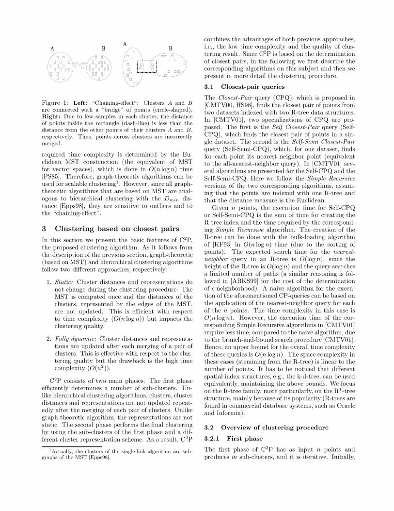
tions we present only two characteristic ones), are de-noted as DS1 (100,000 two dimensional points in 5clusters – see Figure 6) and DS2 (100,000 points in100 clusters placed on a grid – see Figure 7). DS1 wasused in [GRS98]. Its characteristics can test the qual-ity of clustering result with respect to the “chaining-effect”, the outliers and clusters with different sizesand shapes. DS2 was used both in [ZRL96, GRS98].Next, we present the results regarding the three algo-rithms on the clustering quality and in the sequel wepresent the results on efficiency. The depicted imageswere produced in color (available in [NTM01]).

Figure 7: DS2: 100 spherical clusters placed on a grid.

5.1 Clustering Quality

First, we examined the quality of the result for DS1.The random sample contained 2,500 points (the samesize that was used in [GRS98]) and no partitioning wasapplied. We used the default values for the parame-ters of CURE as given in [GRS98], i.e., 10 represen-tative points per cluster and 0.3 shrinking factor. ForC2P, the first phase produced 100 sub-clusters (i.e.,m = 100) and 20 points were used as representatives(i.e., r = 20). The outlier cut-off distance was set tothree times the average (set as default value). Fig-ure 6 presents the clustering results. As it is illus-trated, both C2P and CURE can correctly discoverthe clusters in DS1 (the different coloring is due to

the different order that clusters were identified). Thisshows that C2P is not affected by the “chaining-effect”,the differences in the cluster sizes and the existence ofoutliers. On the other hand, the graph theoretic algo-rithm is affected by the “chaining-effect” and mergesthe two elongated clusters. Also, it splits the largespherical cluster. Analogous results were obtained forDS2, and are presented in [NTM01].

5.2 Tuning the parameters of C2P

The main parameters of C2P are the number, m, ofthe sub-clusters of the first phase (the “switching”point) and the number, r, of representatives of thesecond phase. As described, the size of the randomsample can be determined following the approaches in[GRS98, J-HS98], thus we do not perform a separateexamination here. Partitioning is examined in the fol-lowing section. We use the DS1 data set that contains5 clusters (i.e., k = 5) and the size of the randomsamples was set to 5,000 points.

Number of representatives r

We set m to 100 and varied the number of represen-tatives, r, in the range from 1 (equivalent to the casewhere only the center is used for representation) to30. For values less than 20, C2P did not always pro-duce the correct result (especially for very small valuesof r). The left part of Figure 8 illustrates the repre-sentatives per cluster when r was set to 5. As it isshown, the large cluster, in the lower left corner, issplit. More precisely, the representative points wereassigned to different clusters, thus the cluster, afterthe labeling phase, is finally split (the final result isnot shown here). Additionally, the two small clus-ters on the right were merged, since the correspondingrepresentatives were assigned to the same cluster. Forlarger values of r, the correct result is produced. Theright part of Figure 8 illustrates the result when r wasset to 20. As it is shown, the representative pointswere correctly assigned to clusters and the result afterlabeling (not shown here) was correct. Generally, thevalue of r is determined by the shape of the clusters,

with larger clusters requiring more representatives tocapture their shape.

Figure 8: Number, r, of the representatives in the secondphase. Left: r = 5. Right: r = 20.

Number of sub-clusters m

Based on the previously described results, we selectedr equal to 20. Since k is 5, from the description ofSection 4.1.2, the number of sub-clusters of the firstphase has to be set to 100 (i.e., 20 · 5). We varied thevalues of m in the range from 5 to 200. The left partof Figure 9 illustrates the result for m = 10, where itcan be noticed that an incorrect clustering is produced(the large cluster was split and the two small clusters,on the right, were merged). Similar results were ob-tained for values less than 100. For larger values, C2Pproduced the correct result. The right part of Figure 9illustrates the result for m = 100. Thus, although mis much smaller than the size, n, of the sample (in thiscase n = 5, 000), the sub-clusters of the first phase caneffectively capture the shape of the final clusters.

Figure 9: Number, m, of the sub-clusters of the first phase.Left: m = 10. Right: m = 100.

5.3 Efficiency

First, we measured the execution time with respectto the sample size. We did not consider the graph-theoretic algorithm for the measurement of efficiencysince, as presented previously, it did not produce thecorrect clustering result. The result for DS1 is depictedin Figure 10. CURE used the default parameters givenin [GRS98] (10 representatives, 0.3 shrinking factor).For C2P,m was set to 100 and r to 20. No partitioning

was used. The result for DS2 is depicted in Figure 11,where for both algorithms one representative per clus-ter is used [GRS98]. As it is illustrated, C2P clearlyoutperforms CURE both for small and large samplesizes. Also, these results verify the analytical timecomplexity described in Section 4 and indicate thatC2P is scalable to inputs with large number of points,in the case of data sets that require large samples (seeSection 2).

0

20

40

60

80

100

120

140

160

2000 3000 4000 5000 6000 7000 8000 9000 10000

time

(s)

number of sample points

DS1, 100000 data points, 5 clusters

C2PCURE

Figure 10: DS1: Exec. time (in seconds) w.r.t. samplesize.

0

20

40

60

80

100

120

1000 1500 2000 2500 3000 3500 4000 4500 5000

time

(s)

number of sample points

DS2, 100000 points, 100 clusters

C2PCURE

Figure 11: DS2: Exec. time (in seconds) w.r.t. samplesize.

Next we examined the impact of the divide-and-conquer technique on the performance of both algo-rithms. More precisely, we applied C2P-P and thepartitioning algorithm described in [GRS98]. We usedDS1, with C2P and CURE having the same param-eter setting as in the previous experiment. For bothalgorithms, the clustering in each partition stoppedwhen the number of sub-clusters was 1/3 of the num-ber of points in the partition (this fraction specifiesparameter m′ of C2P-P). This criterion is indicated in[GRS98] and we use it here for the shake of fair com-parison. The left part of Figure 12 presents the ex-ecution times with respect to the sample size for fivepartitions. The right part of Figure 12 presents the ex-ecution times with respect to the number of partitions,

0

5

10

15

20

25

30

35

40

45

50

2000 4000 6000 8000 10000

time

(s)

number of sample points

DS1, 100000 data points, 5 clusters

C2PCURE

0

5

10

15

20

25

30

2 4 6 8 10

time

(s)

number of partitions

DS1, 100000 data points, 5 clusters, 5000 points sample

C2PCURE

Figure 12: Left: Execution time (in seconds) w.r.t. sample size, for 5 partitions. Right Execution time (in seconds)w.r.t. number of partitions.

for a sample size of 5,000 points. As it is illustrated,both algorithms present a performance improvement,compared to the previous case where the divide-and-conquer method was not used. However, CURE isclearly outperformed by C2P, both for small and largenumbers of partitions.

6 Conclusions

We considered the problem of scalable clustering inlarge databases, which at the same time maintains thequality of the result.We have proposed a new clustering algorithm, C2P,

which exploits index structures and the processing ofclosest pair queries in spatial databases. It combinesthe advantages of the hierarchical agglomerative andgraph-theoretic clustering algorithms. Extensions areprovided for large spatial databases and for outlierhandling. We showed that the time complexity of C2Pfor large datasets is O(n log n), thus it scales well tolarge inputs. Experimental results indicate its effi-ciency. The main findings of this paper are summa-rized as follows:

• The development of a new clustering algorithm,which is scalable to large input sizes and main-tains the quality of the clustering result.

• Extensions to the basic algorithm for handlingoutliers, clusters of various shapes and sizes, andlarge databases.

• Analytical and experimental results, which illus-trate the superiority of C2P.

In future work will consider the density-based sam-pling [PF00, KGKB01] for cluster sizes that followskew distribution.

Acknowledgments

We would like to thank Mr. Antonio Corral for hishelp on the subject of the closest pair queries.

References

[ABKS99] M. Ankerst, M. Breunig, H-P. Kriegel, J.Sander: “OPTICS: Ordering Points To Iden-tify the Clustering Structure”. Proc. ACMInt. Conf. on Management of Data (SIG-MOD’99), 1999, pp. 49-60.

[AM70] J. Augustson, J. Minker: “An Analysis ofsome Graph Theoretical Clustering Tech-niques”. Journal of the ACM, Vol.17, 4, 571-588, 1970.

[AY00] C. Aggarwal, P. Yu: “Finding General-ized Projected Clusters In High DimensionalSpaces”. Proc. ACM Int. Conf. on Manage-ment of Data (SIGMOD’00), 2000, pp. 70-81.

[BBBK00] C. Bohm, B. Braunmuller, M. Breunig, H.-P. Kriegel: “High Performance ClusteringBased on the Similarity Join”. Proc. Int. Conf.on Information and Knowledge Management(CIKM’00), 2000.

[BKKS01] M. Breunig, H.-P. Kriegel, P. Kroger, J.Sander: “Data Bubbles: Quality PreservingPerformance Boosting for Hierarchical Clus-tering”. Proc. ACM Int. Conf. on Manage-ment of Data (SIGMOD’01), 2001.

[BKS00] M. Breunig, H.-P. Kriegel, J. Sander: “FastHierarchical Clustering Based on CompressedData and OPTICS”. Proc. European Conf. onPrinciples and Practice of Knowledge Discov-ery in Databases (PKDD’00), 2000.

[CMTV00] A. Corral, Y. Manolopoulos, Y. Theodoridis,M. Vassilakopoulos: “Closest Pair Queries inSpatial Databases”. Proc. ACM Int. Conf.on Management of Data (SIGMOD’00), 2000,pp. 189-200.

[CMTV01] A. Corral, Y. Manolopoulos, Y. Theodor-idis, M. Vassilakopoulos: “Algorithms forProcessing Closest Pair Queries in SpatialDatabases”. Tech. Report (available at www-de.csd.auth.gr/publications.html), 2001.

[Epps98] D. Eppstein: “Fast Hierarchical Clusteringand Other Applications of Dynamic Closest

Pairs”. Proc. Symposium on Discrete Algo-rithms (SODA’98), 1998.

[EKSX96] M. Ester,H.-P. Kriegel, J. Sander, X. Xu:“A Density-Based Algorithm for Discover-ing Clusters in Large Spatial Databases withNoise”. Proc. Int. Conf. on Knowledge Dis-covery and Data Mining (KDD’96), 1996.

[EKX95] M. Ester, H.-P. Kriegel, X. Xu: “KnowledgeDiscovery in Large Spatial Databases: Fo-cusing Techniques for Efficient Class Identi-fication”, Proc. Int. Symp. on Large SpatialDatabases (SSD’95), 1995, pp. 67-82.

[Fish87] D. Fisher: “Knowledge Acquisition via In-cremental Conceptual Clustering”. MachineLearning, Vol.2, 139-172, 1987.

[GRS98] S. Guha, R. Rastogi, K. Shim: “CURE:An Efficient Clustering Algorithm for LargeDatabases”. Proc. ACM Int. Conf. on Man-agement of Data (SIGMOD’98), 1998, pp. 73-84.

[HK99] A. Hinneburg, D. Keim: “Optimal Grid-Clustering: Towards Breaking the Curseof Dimensionality in High-Dimensional Clus-tering”. Proc. Int. Conf. on Very LargeDatabases (VLDB’99), 1999, pp. 506-517.

[HS98] G. Hjaltason, H. Samet: “Incremental Dis-tance Join Algorithms for Spatial Databases”.Proc. ACM Int. Conf. on Management ofData (SIGMOD’98), 1998, pp. 237-248.

[J-HS98] N. Jose-Hkajavi, K. Salem: “Two-phase Clus-tering of Large Datasets”. Technical ReportCS-98-27, Department of Computer Science,University of Waterloo, 1998.

[JMF99] A. Jain, M. Murty, P. Flynn: “Data Clus-tering: A Review”. ACM Computing Surveys,Vol.31, No.3, 264-323, 1999.

[KF93] I. Kamel, C. Faloutos: “On Packing R-trees”.Proc. Int. Conf. on Information and Knowl-edge Managemenet (CIKM’93), 1993, pp. 490-499.

[KGKB01] G. Kollios, D. Gunopoulos, N. Koudas,S. Berchtold: “An Efficient ApproximationScheme for Data Mining Tasks”. Proc. IEEEInt. Conf. on Data Engineering (ICDE’01),2001, pp. 453-462.

[KHK99] G. Karypis, E. Han, V. Kumar: “Chameleon:Hierarchical Clustering Using Dynamic Mod-eling”. IEEE Computer, Vol.32, No.8, 68-75,1999.

[MK80] M. Murty, G. Krishna: “A ComputationallyEfficient Technique for Data Clustering”. Pat-tern Recognition, Vol. 12, 153-158, 1980.

[MSD83] R. Michalski, R. Stepp, E. Diday: “A RecentAdvance in Data Analysis: Clustering Ob-jects into Classes Characterized by ConjuctiveConcepts”. Progress in Pattern Recognition,Vol. 1, North-Holland Publishing, 1983.

[NH94] R. Ng, J. Han: “Efficient and Effective Clus-tering Methods for Spatial Data Mining”.Proc. Int, Conf. on Very Large Databases(VLDB’94), 1994, pp. 144-155.

[NTM01] A. Nanopoulos, Y. Theodor-idis, Y. Manolopoulos: “C2P: Cluster-ing based on Clos-est Pairs”. Tech. Report (available at www-de.csd.auth.gr/publications.html), 2001.

[PF00] C. Palmer, C. Faloutsos: “Density BiasedSampling: An Impoved Method for Data Min-ing and Clustering”, Proc. ACM Int. Conf.on Management of Data (SIGMOD’00), 2000,pp. 82-92.

[PS85] F. Preparata, M. Shamos: “ComputationalGeometry: an Introduction”. Springer-Verlag,1985.

[RY81] V. Raghavan, C. Yu: “A Comparison of theStability Characteristics of some Graph The-oretic Clustring Methods”. IEEE Trans. onPattern Analysis Machine Intelligence, Vol.3,393-402, 1981.

[Same90] H. Samet: “The Design and Analysis of Spa-tial Data Structures”. Addison Wesley, 1990.

[Sedg83] R. Sedgewick: “Algorithms”. Addison Wesley,1983.

[SCZ99] G. Sheikholeslami, S. Chatterjee, A. Zhang:“WaveCluster: A Wavelet Based ClusteringApproach for Spatial Data in Very LargeDatabases”. VLDB Journal, Vol. 8(3-4), 289-304, 1999.

[SF96] R. Sedgewick, P. Flajolet: “An Introduction tothe Analysis of Algorithms, Addison Wesley,1996.

[Vitt85] J. Vitter: “Random Sampling with a Reser-voir”. ACM Trans. on Mathematical Software,11(1), 37-57, 1985.

[WYM97] W. Wang, J. Yang, R. Muntz: “STING: AStatistical Information Grid Approach to Spa-tial Data Mining”. Proc. Int. Conf. on VeryLarge Databases (VLDB’97), 1997, pp. 186-195.

[XEKS98] X. Xu, M. Ester, H.-P. Kriegel, J. Sander:“A Nonparametric Clustering Algorithmfor Knowledge Discovery in Large SpatialDatabases”. Proc. Int. Conf. on Data Engi-neering (ICDE’98), 1998.

[Zahn71] C. Zahn: “Graph-theoretical Methods forDetecting and Describing Gestalt Clusters”.IEEE Trans. Computers C-20, 1971, pp. 68-86.

[ZRL96] T. Zhang, R. Ramakrishnan, M.Linvy:“BIRCH: An Efficient Data Clus-tering Method for Very Large Databases”.Proc. ACM Int. Conf. on Management ofData (SIGMOD’96), 1996, pp. 103-114.