
EVENT DISTORTION BASED CLUSTERING ALGORITHM ...
61
EVENT DISTORTION BASED CLUSTERING ALGORITHM FOR ENERGY HARVESTING WIRELESS SENSOR NETWORKS A thesis submitted to The Graduated School of Engineering and Science Izmir Institute of Technology In Partial Fulfillment of Requirements for a degree of MASTER OF ENGINEERING In Electrical - Electronics Engineering By ALİ MUDHEHER RAGHIB KAFI AL-QAMAJI April 2017 IZMIR
-
Upload
khangminh22 -
Category
Documents
-
view
0 -
download
0
Transcript of EVENT DISTORTION BASED CLUSTERING ALGORITHM ...

ii
EVENT DISTORTION BASED CLUSTERING
ALGORITHM FOR ENERGY HARVESTING
WIRELESS SENSOR NETWORKS
A thesis submitted to
The Graduated School of Engineering and Science
Izmir Institute of Technology
In Partial Fulfillment of Requirements for a degree of
MASTER OF ENGINEERING
In Electrical - Electronics Engineering
By
ALİ MUDHEHER RAGHIB KAFI AL-QAMAJI
April 2017
IZMIR

ii
We approve the thesis of ALİ Mudheher Raghib Kafi AL-QAMAJI
Examining Committee Members:
________________________________________
Assoc. Prof. Dr. Barış ATAKAN
Department of Electrical - Electronics Engineering
Izmir Institute of Technology
________________________________________
Assoc. Prof. Dr. Radosveta SOKULLU
Department of Electrical and Electronics Engineering
Ege University
________________________________________
Assist. Prof. Dr. Berna ÖZBEK
Department of Electrical - Electronics Engineering
Izmir Institute of Technology
21 April 2017
________________________________________
Assoc. Prof. Dr. Barış ATAKAN Supervisor, Department of Electrical - Electronics Engineering, İzmir Institute of Technology
__________________________________
Prof. Dr. Enver TATLICIOĞLU
Head of the Department of
Electrical - Electronics Engineering
_____________________________
Prof. Dr. Aysun SOFUOĞLU
Dean of the Graduate School
of Engineering and Sciences

iii
ACKNOWLEDGMENTS
First of all, I owe a huge deal of thanks to my supervisor Assoc. Prof. Dr. Barış
ATAKAN for his excellent guidance, tolerance and patience in every level of my thesis
study. Many thanks also for making reasonable amount of time whenever I asked for his
support. I would like to thank committee members for giving me contribution which helped
me a lot in revising the thesis.
I would like to express my sincere thanks to Assist. Prof. Dr. Berna ÖZBEK and
Assoc. Prof. Dr. Mustafa A. ALTINKAYA for their supports, helps and favors at first stages
of my master studies. Special thanks to the colleagues and friends from IYTE, namely Serpil
Yılmaz, Başak Esin Guzel, and Oktay Karakus for their helpful suggestions and comments
during my courses.
Last but definitely not least, I thank my mother and my father a lot for their true and
invaluable support. Very special thanks to my brother Ahmed, and my sisters Aseel and Enas
who motivated and advised me through some difficult times.
iv
ABSTRACT
EVENT DISTORTION BASED CLUSTERING ALGORITHM FOR
ENERGY HARVESTING WIRELESS SENSOR NETWORKS
Wireless Sensor Network (WSN) is a set of inexpensive densely deployed wireless
sensor nodes with limited functionalities and scarcity in energies, whose observations are
forwarded or relayed by intermediate nodes to the Base Station (BS). In the networks with
densely deployed nodes, the observations are likely to be highly correlated in the space
domain. This type of correlation is referred as spatial correlation, which produces
unfavorable redundant readings causing energy wasting.
In this thesis, the main task is to reduce these nodes that have redundant readings by
using a clustering algorithm called Event Based Clustering (EDC) algorithm. The clustering
algorithm is based on exploiting the spatial correlation that is used to cluster the sensor nodes.
Exploiting spatial correlation is proposed by using Vector Quantization (VQ) with respect to
the distortion constraints. Furthermore, this algorithm is applied for energy harvesting sensor
nodes. Also, the inessential sensor nodes that have correlated readings are reduced for
improving the Energy-Efficacy (EE) with acceptable level of event signal reconstruction
distortion at the sink node.
After applying the EDC algorithm, the communication model is changed from single-
hop model to two-hop (clustered-network) model. Hence, a theoretical framework of
distortion function, i.e., accuracy level, for both single-hop and two-hop communication
models is derived. Then, single-hop and two-hop communication models are compared in
terms of achieved distortion level, number of alive nodes, and energy consumption for
different sizes of event area. Finally, the effects of various harvested energy level on the
clustered-network is studied with respect to the same terms.

v
ÖZET
ENERJİ TOPLAYAN KABLOSUZ SENSÖR AĞLARI İÇİN OLAY
BOZULMASINA DAYALI KÜMELENME ALGORİTMASI
Kablosuz Sensör Ağı (KSA), işlevsellikleri sınırlı, enerjileri az, pahalı olmayan,
yoğun bir şekilde konuşlandırılmış kablosuz sensör düğümleri setidir. Sensör düğümlerinin
gözlemleri, ara düğümler tarafından baz istasyonuna iletilir. Yoğun bir şekilde
konuşlandırılmış düğümlerden oluşan ağlarda gözlemler büyük oranda ilintilidir. Uzaysal
ilinti olarak adlandırılan bu tür ilintiler, gereksiz algılayıcı okumalarına neden olur ve
dolayısıyla enerji israfına neden olur.
Bu tez çalışmasında enerji toplayan sensör ağları için Olay Bozulmasına Dayalı
Kümeleme (OBK) algoritması adı verilen bir kümeleme algoritması verilmektedir. OBK
algoritması sensörler arasındaki uzaysal ilintiyi kullanarak gereksiz okumalara sebep olan
düğümleri azaltmak sureti ile enerji tüketimini azaltmayı amaçlamaktadır. Uzaysal ilintinin
kullanılması bozulma kısıtlamalarına göre Vektör Nicemleme (VN) ile gerçeklenmektedir.
Sensörlerin baz istasyonuna yaptıkları iletişim için tek hop ve iki hop olmak üzere iki ayrı
iletişim modeli düşünülerek bu modellerin her biri için iki ayrı olay bozulma fonksiyonu
türetilmektedir.
Baz istasyonu OBK algoritması ile türetilen bu bozulma fonksiyonlarını kullanarak
ilintili okumalara sahip sensör düğümlerinin veri iletimini kontrol edebilmektedir. Bu kontrol
sayesinde hangi sensörün iletim yapacağına karar verilerek belli bir olay bozulma kısıtlaması
karşılanırken enerji-etkin iletişim de sağlanabilmektedir.

vi
TABLE OF CONTENTS
LIST OF FIGURES ............................................................................................................ viii
LIST OF TABLES .............................................................................................................. ...x
CHAPTER 1. INTRODUCTION .......................................................................................... 1
1.1. Wireless Sensor Network............................................................................. 1
1.2. Types And Applications .............................................................................. 2
1.3. Sensor Node Components ........................................................................... 8
1.4. Harvesting Technology ................................................................................ 9
1.5. Aim Of The Study ..................................................................................... .10
1.6. Outlines .................................................................................................... .10
CHAPTER 2. BACKGROUND AND RELATED WORKS ............................................. .11
2.1. Overview ................................................................................................... .11
2.2. Clustering In Wireless Sensor Networks .................................................. .11
2.3. Summery ................................................................................................... .14
CHAPTER 3. PROPOSED WORK.................................................................................... .15
3.1. Overview ................................................................................................... .15
3.2. Problem Formulation ................................................................................ .15
3.3. Network Model ......................................................................................... .16
3.4. Event Distortion Based Clustering (EDC) ............................................... .17
3.4.1. Optimal Distortion Phase ................................................................... .17
3.4.2. Clustering Formation Phase ............................................................... .23
3.4.3. Clustered-Network Distortion ............................................................ .27
3.5. Energy Model ........................................................................................... .34
3.5.1. Energy Consumption For Clustered-Network .................................... .35
3.5.2. Harvesting Model ............................................................................... .37

vii
3.5. Case Study ................................................................................................ .37
3.6.1. Data Rate ............................................................................................ .37
3.6.2. Number of Sensor Nodes .................................................................... .38
3.6.3. Event Distance .................................................................................... .39
3.6.2. Event Area .......................................................................................... .40
CHAPTER 4. SIMULATIONS .......................................................................................... .42
4.1. Setup Parameters ....................................................................................... .42
4.2. EDC Algorithm ......................................................................................... .43
CHAPTER 5. CONCLUSION AND FUTURE WORKS .................................................. .50
2.1. Conclusion ................................................................................................ .50
2.2. Future Works ........................................................................................... .50
BIBLIOGRAPHY ............................................................................................................... .51

viii
LIST OF FIGURES
Figure Page
Figure 1.1. Wireless Sensor Network. ................................................................................... 1
Figure 1.2. Underground Wireless Sensor Network. ............................................................. 3
Figure 1.2. Underwater Wireless Sensor Network. ............................................................... 4
Figure 1.4. Multimedia Wireless Sensor Network. ............................................................... 5
Figure 1.5. Applications of Wireless Sensor Network. ......................................................... 6
Figure 1.6. Military Applications for Wireless Sensor Network. .......................................... 7
Figure 1.7. Components of Sensor Node. .............................................................................. 8
Figure 2.1. Clustering for Wireless Sensor Network. ......................................................... .12
Figure 2.2. Exploiting Spatial Correlation. ......................................................................... .13
Figure 3.1. Wireless Sensor Network Considered in This Thesis ...................................... .16
Figure 3.2. Point-to-Point Communication Model ............................................................. .18
Figure 3.3. Clustered-Network by EDC Algorithm. ........................................................... .25
Figure 3.4. Event Distortion Based Clustering (EDC) Algorithm. ..................................... .26
Figure 3.5. Two-hop Communication Model. .................................................................... .28
Figure 3.6. First Order Radio Model. ................................................................................. .36
Figure 3.7. Distortions Vs Data Rate. ................................................................................. .38
Figure 3.8. Distortions Number of Sensor Nodes .............................................................. .39
Figure 3.9. Distortion Vs Event Distance ........................................................................... .39
Figure 3.10. Distortion Vs Event area ................................................................................ .40
Figure 4.1. Network Clustering .......................................................................................... .44
Figure 4.2. Distortion, Number of Alive nodes and Energy Consumption for 100 × 100 𝑚2
Event Area ........................................................................................................ .45
Figure 4.3. Distortion, Number of Alive nodes and Energy Consumption for 200 × 200 𝑚2
Event Area ........................................................................................................ .46
Figure 4.4. Distortion, Number of Alive nodes and Energy Consumption for 300 × 300 𝑚2
Event Area ........................................................................................................ .47
Figure 4.5. Distortion for Different Harvested Energies .................................................... .48
Figure 4.6. Energy Consumption and Number of Alive nodes for Different Harvested
Energies ............................................................................................................ .47

ix
LIST OF TABLES
Figure Page
Figure 1.1. Examples of Energy Harvesting Sources. ........................................................... 9
Figure 1.2. Simulation Parameters. ..................................................................................... .43
1
CHAPTER 1
INTRODUCTION
1.1. Wireless Sensor Network
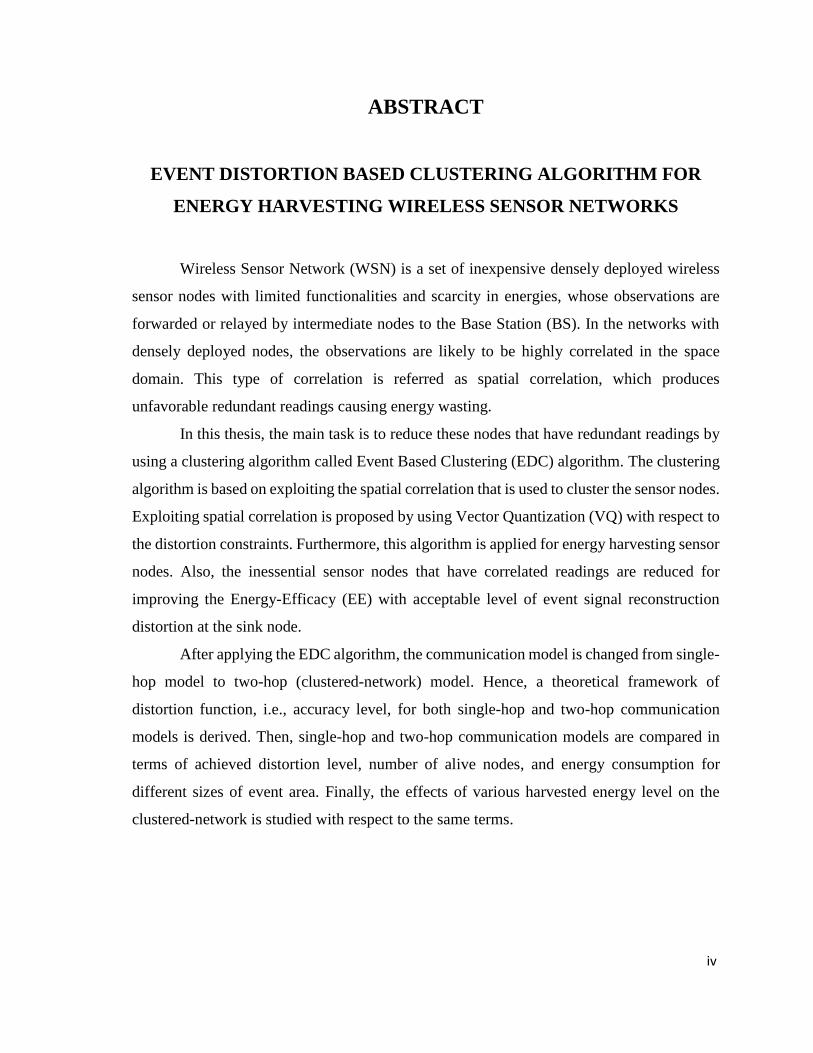
Wireless Sensor Network (WSN) is a set of sensor nodes that are connected with each
other through wireless and noisy channel. Each sensor node requires to sense for physical
phenomena (e.g., field source, fixed and random point sources). Then, each sensor node
forwards its observations to the Base Station (BS) to be processed or viewed by the end user
as in Fig 1.1. However, that’s not the whole story, there are many challenges which need to
be addressed by the developers and engineers in WSNs such as fault tolerance, scalability,
production costs, hardware constraints, communication and power consumption [1].
Figure 1.1 Wireless Sensor Network
Event area Sensor Nodes
BS

2
In WSNs, nodes’ deployment can be random or systematic (fixed topologies)
determined by the designer or application [1]. Random deployment has an advantage of being
less expensive than fixed deployment. It enables WSNs to be applied in hostile and
unreachable environment such as battlefield and under water. As a result, the random
deployment is more general case but there is a coverage problem (i.e., it’s not guaranteed that
sensors will cover the whole event area) [1]. Hence, this can be solved by increasing nodes
density in an event area, i.e., increasing the number of sensors. Since the communication
among sensor nodes is one of the main source of energy consumption, communication
protocols are devised for reducing energy consumption.
In WSNs, it is possible to exploit spatial correlation in sensor readings to improve
energy efficiency. In densely deployment case, nearby sensor nodes get similar observations
[3]. By keeping the data distortion below a predefined threshold, sensor nodes can exploit
spatial correlation to reduce amount of data forwarded to the sink node. This reduction will
improve Energy-Efficiency (EE) and preserve the distortion level, i.e., without changing the
accuracy of received data at the sink node.
One of the main challenges of communication protocols and applications in WSNs is
energy saving [1]. The battery-powered sensor nodes need to be charged regularly. Reaching
operation is expensive, on addition, some event areas are unreachable. The developers
addressed this issue by equipping energy harvesting unit to each sensor node [2]. For
harvesting sensor networks, there are various sources are available to be harvested, e.g.,
Solar, Vibration (motion), Winds, Thermal and Radio frequency (RF) Signals, etc. Each of
these harvesting sources provides a different level of harvesting energy as shown in Table
1.1. In this thesis, RF-harvesting will be used for its inexpensive implementation and
availability.
1.2. Types and Applications
In various scenarios sensor nodes are required due to their capability to observe a
different type of event sources, e.g., humidity, temperature, and lighting, etc. Based on the
applications, different types of WSNs are needed:

3
Terrestrial WSN: Typically, it consists of hundreds to larger number of low-cost
wireless sensor nodes deployed in event area, either in an ad hoc (unstructured) or in
a pre-planned (structured) manner. In ad hoc deployment, sensor nodes can be
randomly placed into the target area by being dropped from a plane. For example,
deploying a WSN on an active volcano [17]. Furthermore, some event areas may
remain uncovered (coverage issue), thus nodes density is required and thus, results
into difficulties in maintenance (e.g., recharging, communication, etc.). In pre-
planned deployment, all or some sensor nodes are deployed based on fixed planned
architecture, for example grid and optimal [25] placement models. The advantage of
pre-planned deployment is that fewer nodes can be deployed, which makes the
maintenance less cost than ad hoc deployment case.
Undergrounded WSN [26] [27] [16]: set of sensor nodes are buried underground either
in a cave or mine and are used to monitor underground conditions. Furthermore, sink nodes
are placed above ground as relays, for taking readings from underground sensor nodes to the
base station. With respect to maintenance, equipment and deployment, underground WSN
are more expensive than terrestrial WSN, where suitable equipment parts are needed to
ensure reliable communication through soil, rocks, water, and other mineral contents to
reduce the signal losses and attenuation level. Before sensor nodes deploying for
underground WSN, it requires careful planning of energy and cost considerations.
Underground sensors are powered with a limited battery power and it is difficult to recharge
or replace their batteries.
Figure 1.2 Undergrounded Wireless Sensor Network

4
Underwater WSN [28] [29]: A set of number of sensor nodes or vehicles are placed
underwater that provides great opportunity to discover oceans as to improve the
studies in environmental issues (Fig 1.3), e.g., marine life in the oceans climate,
variations of climate and population of coral reefs, etc. As compared to terrestrial
WSNs, less nodes are needed but more expensive to be sank underwater. Acoustic
waves are used for wireless communications between underwater sensor nodes.
Generally, the main challenges in underwater acoustic communication are bandwidth
limitation, propagation delay, and signal fading problems.
Figure 1.3 Underwater Wireless Sensor Network
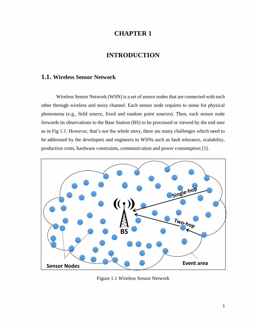
Multi-media WSN [30] [18]: A set of inexpensive sensor nodes are equipped with
cameras and microphones for monitoring multimedia events, such as videos, audios,
and images (Fig 1.4). These sensors are placed in structured manner to ensure the
coverage. Furthermore, multi-media WSN requires high bandwidth to deliver the
media content, e.g., video stream, that requires high data rate. Hence, it causes high
energy consumption rate. Besides, it is important that a certain level of Quality of
Service (QoS) is achieved for delivering data reliably.
Underwater Sensor Nodes
Wireless Acoustic links surface buoy
Base Station (BS) Internet
(Cloud Storage)
End User
5
Figure 1.4 Multimedia Wireless Sensor Network
Mobile WSN [15] [19]: A set of dynamic sensor nodes are capable to sense,
compute, and communicate like static nodes, i.e., sensor nodes with fixed locations.
However, there are two main differences with static WSN. Firstly, dynamic sensor
nodes are capable of repositioning and organize themselves. Since they are able to
move from one place to another, the higher degree of coverage and connectivity can
be achieved. Mobile sensor nodes can deliver gathered information to nearby mobile
nodes. Secondly, there is a difference in data distribution. In a static WSN, data can
be distributed using fixed routing, while mobile sensor nodes are using a dynamic
routing. As a result, the issues in mobile sensor nodes include nodes deployment,
localization, self-organization, navigation, control, coverage, energy, maintenance,
and data processing, etc.
Mainly WSNs applications (Fig 1.5) are bounded in civil applications (e.g., alarm,
medical, and home etc.) and military applications [1]: -
Environmental applications [21]: These sensor networks have many different
applications in the environment. They can be used for the wildlife tracking
Internet/ Satellite
End User
Microphone Sensor Camera
Video Camera
Gateway

6
applications, earth quack monitoring, soil observations, atmosphere context,
irrigation monitoring, natural disasters and almost agricultural issues can be
addressed by sensor nodes.
Figure 1.5 Applications of Wireless Sensor Network
Medical applications: The advances in integrated biomedical devices and smart
sensor nodes, have attracted researchers and engineers to exploit sensor networks in
biomedical field. Some of the medical applications for WSNs are provided for
diagnostics, monitoring of disabled, patient, drug administration in hospitals,
movements of insects or other animals, doctors inside hospital, and emergency
response [31].
Military applications [23]: Rapid deployment and self-organizing aspects that are
made by WSNs are very useful for sensing and observing friendly or hostile
movements in military operations (Fig 1.6). Furthermore, sensor nodes are capable
to detect chemical, nuclear, biological attacks, reconnaissance of opposing forces
WSNMilitary
Civil
Medical
Drug administration
Patient monitoring
Home
Vacuum cleaners
Refrigerators
Industrial Preventive
maintenance
Environmental
Wildlife tracking
Earth quack monitoring

7
and terrain in C4ISR systems (i.e., Command, control, communications, computers,
intelligence, surveillance, and reconnaissance), and battlefield surveillance, etc.
Home applications [20]: As the technology is developing, smart sensor nodes can
be equipped in home devices, such as vacuum cleaners, micro-wave ovens,
refrigerators, and VCRs. These nodes allow users to control home devices locally
and remotely by the capability of these nodes to be connected with each other and
with external networks by the internet or satellite.
Figure 1.6 Military Applications for Wireless Sensor Networks
Industrial applications [22]: Wired or wireless sensor networks can be used for
industrial fields, such as industrial sensing and control applications, building
automation, monitoring material fatigue, smart structures with embedded sensor
nodes and access control etc. Sensor based monitoring systems and manual
monitoring systems are usable in industrial area for preventive maintenance. Wired
sensors in such a systems require high cost for upgrading, deployment and require
personal supervision.
Satellite
Local station
Event of interest

8
1.3. Sensor Node Components
The main components [1] of any typical sensor node have been illustrated in Fig 1.7.
They are: processer, transceiver, memory, power source and sensing unit. All components of
a sensor node have different functions as defined below:
Processer (micro-controller) unit: It’s a low power consumption unit responsible for
processing data (e.g., modulation and signal processing, etc.) and controlling other
units to perform specific tasks at any given time.
Figure 1.7 Components of Sensor Node
Transceiver unit: Wireless sensors use radio frequency media for transmission and
receiving, by allocating specific frequencies with four different states; transmit,
receive, idle, and sleep. This unit is defined as the most unit consuming power than
other units because of its antenna.
Energy Harvesting
Unit
Energy
Management
Energy Storage
Low-Powered
Processing Unit
RF-Transceiver
Unit
Additional
Memory
Sensing Unit
Energy sources

9
Memory unit: Mainly it’s used for saving data before transmitting and after
receiving.
Power unit: It can be capacitor or battery (rechargeable or non-rechargeable). It is
responsible for powering other units.
Sensing unit: This unit is used for tracking or observing the physical or environment
events.
External unit: It can be another sensor node, transceiver unit, power unit or
harvesting unit.
Table 1.1. Examples of Energy Harvesting Sources [2]
1.4. Harvesting Technology
Energy gathering from surrounding environment is one of perspective solutions [2]
for powering sensor nodes. There are different kinds of sources that can be harvested as
shown in Table 1.1. RF-harvesting will be used in this thesis for its inexpensive
Source Environmental location Source Power Harvested Power
Light
Indoor 0.1 𝑚𝑊/𝑐𝑚2 10 𝜇𝑊/𝑐𝑚2
Outdoor 100 𝑚𝑊/𝑐𝑚2 10 𝑚𝑊/𝑐𝑚2
Human 0.5 𝑚 𝑎𝑡 1 𝐻𝑧
Vibration/Motion
1 𝑚/𝑠2 𝑎𝑡 50 𝐻𝑧 4 𝜇𝑊/𝑐𝑚2
Machine 1 𝑚 𝑎𝑡 5 𝐻𝑧
10 𝑚/𝑠2 𝑎𝑡 1 𝑘𝐻𝑧 100 𝜇𝑊/𝑐𝑚2
Radio Frequency GSM BSS 0.3 𝜇𝑊/𝑐𝑚2 0.1 𝜇𝑊/𝑐𝑚2
Thermal Human 20 𝑚𝑊/𝑐𝑚2 30 𝜇𝑊/𝑐𝑚2
Machine 100 𝑚𝑊/𝑐𝑚2 1 − 10 𝑚𝑊/𝑐𝑚2
10
implementation and this type of energy source is more reliable. RF-harvesting is done by
equipping a harvesting circuit to each sensor node and this type of network is called Energy
Harvesting Wireless Sensor Network (EH-WSN). RF-harvesting converting electromagnetic
energy from radio frequencies to the electrical form (DC) to be saved in the storage device.
The main components of harvesting unit are: antenna, impedance matching, voltage
multiplier and storage capacitor.
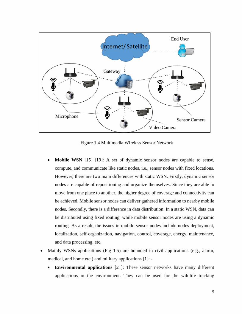
1.5. Aim of The Study
For dense nodes’ deployment, sensors have redundant readings, and hence there is a
wasting of energy and information. Consequently, the main problem is, how the number of
nodes which have similar readings can be reduced in order to select the specific nodes that
must transmit their data to the Base Station (BS) with respect to the coverage, reliability
(distortion), and Energy-Efficiency (EE).
The algorithm proposed in this thesis, addresses these problems, by exploiting spatial
correlation in densely deployment case to cluster sensor nodes and reduce their energy
consumption. Furthermore, the presented theoretical framework for point-to-point (single-
hop) communication model, to test distortion level of all sensor nodes after nodes reduction,
and for two-hop communication model to present final accuracy level of the proposed
clustering algorithm with respect to power constraints.
1.6. Outline
The remaining part of this thesis is organized as follow. Chapter 2 covers related
works. In chapter 3, the Event Distortion Based Clustering (EDC) algorithm is presented with
theoretical frameworks for both single-hop and two-hop communication models, besides, the
energy model for the resulting network (clustered-network) is discussed. EDC analysis and
simulation results are presented in chapter 4 and the conclusion in the chapter 5.

11
CHAPTER 2
BACKGROUND AND RELATED WORKS
2.1. Overview
The advantages of WSNs are more precise nowadays and in the field of
communications they cannot be neglected anymore. WSNs can provide varieties of research
works with wide range of applications in military, industry, security and environmental fields
[1] as discussed in previous chapter. But the drawback of WSN is its limited energy
constrains as it might be deployed in areas where it is not feasible for its batteries to be
replaced or recharged.
This chapter provides a brief description of the existing works related to this thesis’
study. The overview of the clustering algorithms for WSNs is described in Section 2.2. In
addition, the exploiting of spatial correlation is defined in Section 2.3. Finally, the summery
is discussed in section 2.4.
2.2. Clustering for Wireless Sensor Networks
Reliability, Energy-Efficiency (EE), channel capacity, accuracy, and communication
are crucial issues that have to be considered along with the WSN. In sensor networks, distant
nodes depend on a number of intermediate nodes to forward their observations about physical
phenomena. Consequently, the intermediate sensor nodes run out of their energy, and hence
the reliability level is lost at the sink node. These issues can be addressed by clustering the
sensor nodes. In clustering, the sensor nodes are divided into different clusters. Each cluster
is managed by a node that is referred as Cluster Head (CH) and other nodes that are referred
as Cluster Members (CMs). CMs don’t communicate directly with the sink node. They have
to pass their readings to the CH. Then, the CH aggregates their readings and transmis their

12
data to the BS or sink node. Furthermore, The CHs are responsible for coordinating with both
inter-cluster and intra-cluster communications1 as shown in Fig 2.1.
Figure 2.1 Clustering for Wireless Sensor Network
The crucial results from clustering the sensor nodes are prolonged network lifetime,
scalability for WSNs, and reduced communication overhead, etc. Hence, the clustering
algorithms can be exploited in many applications, such as earthquake monitoring and
applications that support data aggregation, such as microclimate and habitat monitoring.
As discussed in previous chapter, in a dense deployment case, nearby sensor nodes
have correlated sensing readings (due to spatial correlation) as in Fig 2.2. Hence, it may not
be essential for every sensor node to transmit its data to the sink; instead, a smaller number
of sensor nodes referred to as active nodes, might be sufficient to transfer event data to the
sink node with respect to the predefined distortion level, while the nodes that are prevented
from observing are called inactive nodes. One prevalent way [7] for conserving energy is
clustering the network into several clusters for example Low-Energy Adaptive Clustering
Hierarchy (LEACH) [8] and an Energy Efficient Clustering Scheme (EECS) [9].
1 The communications that generated inside the cluster (e.g., between CM and CH) are referred as inter-cluster communications, while the communications between two CHs that located at different clusters are referred as intra-cluster communications.
Cluster
Sink Node
Intra-cluster communication
Inter-cluster communication
Cluster Head (CH)
Cluster Member (CM)

13
Furthermore, there are several clustering algorithms that exploits spatial correlation: GAG
[10], and EAST [11], etc.
Figure 2.2 Exploiting Spatial Correlation
In [10], the authors have presented a clustering algorithm to reduce the number of
transmissions towards the sink node to reduce overhead packets and to enhance total EE of
sensor nodes. The process has been done by grouping the sensor nodes which have similar
readings into set of clusters, the size of each cluster defined by correlation range. At each
iteration, only one sensor node from each cluster is required to send its own data to the sink
node, based on fault-tolerance (accuracy level) with 10% error threshold. Finally, a reduction
of 70 % of overhead packets have been observed.
In [11], the author followed the general idea of [10], but in [11], the difference
between event sources has been investigated. For events that change at small range, the
correlated region can be decreased to keep the accuracy level, i.e., the event needs to be
informed by nearby nodes. For events that do not change at small range, the correlated region
can be increased to improve the EE. The size of the correlation region can be resized by the
sink node.
To qualify the existing algorithms in WSNs, distortion level and energy conservation
should be considered as the main issues. In WSNs, the distortion represents the similarity
level between original and estimated readings. Different distortion functions have been
derived in [3] and [4] in Minimum Mean Squared Sense (MMSE).
In [3], the author presented an algorithm called Iterative Node Selection (INS) for
selecting the representative nodes by exploiting spatial correlation through Vector
Quantization (VQ). The communication model has been considered according to the point-
Correlation range
BS
Active node
Inactive node
Densely nodes
deployment
Event area
Exploiting spatial
correlation
Communication
channel

14
to-point (single-hop) case, i.e., each sensor node transmits its reading directly to the sink
node, as shown in Fig 2.2. In addition, the author hasn’t assumed any channel noise in the
communication links. Furthermore, the spatial correlation model between sensors
observations is modeled by exponential model.
In [4], the same communication model has been used, but the sensor readings are
similar and without observation noise. Also, there is one noise in the end of network (sink
node). Hence, the distortion function is derived with respect to power constraints.
2.3. Summary
The proposed work is inspired by these above works to minimize data redundancy for
preserving node energy and prolonging the network life time. In this thesis, a new clustering
algorithm is proposed by exploiting spatial correlation through Vector Quantization (VQ). In
contrast to the previous studies (e.g., [3]), our focus is that there is a channel noise in each
communication link, besides there are observation noises for readings of sensor nodes. In
such a case, the distortion function is derived with respect to the power constraints. Then, by
clustering the sensor nodes through VQ, a different communication model is formed. Hence,
another distortion function is derived for clustered-network, i.e., two-hop communication
model, which is unlike previous studies that used fault-tolerance to define the accuracy level.

15
CHAPTER 3
EVENT DISTORTION-BASED CLUSTERING
3.1. Overview
In WSNs, clustering is one of the important techniques that is applied for enhancing
Energy-Efficiency (EE) and prolonging the lifetime of the network. In the preceding chapter,
various clustering algorithms which can exploit spatial correlation among sensor nodes and
different distortion functions to examine the reliability level of sensor network are discussed.
Those previous works have been devised for wireless sensor networks in which sensors are
assumed to be battery-powered operated nodes. However, the clustering of battery-free
sensor nodes in energy harvesting wireless sensor networks poses different challenges, such
as lack of a permanent power source to sense or enable communication process whenever it
is needed. In order to address such challenges, in this chapter, a clustering algorithm called
Event Distortion Based Clustering (EDC) algorithm is introduced for energy harvesting
wireless sensor networks.
In this chapter, the problem statement is first given in Section 3.2. Then, the network
model of WSN is introduced in Section 3.3. In Section 3.4, the EDC algorithm is introduced
and finally, the energy model that is used for the performance evaluations of the EDC
algorithm is given in Section 3.5.
3.2. Problem Statement
In this thesis, the network is considered as a set of 𝑁 homogeneous wireless sensor
nodes {𝑛}𝑁 = [𝑛1, 𝑛2, … … … , 𝑛𝑁]. The sensor nodes are assumed to be randomly and
densely deployed in an event area, and hence the sensor readings tend to be spatially
correlated and thus, redundant. Hence, due to this redundancy which may inject excessive
traffic load on the network and the lack of permanent energy source in the nodes, it is

16
important to decide which sensor nodes should transmit their readings in order to provide an
acceptable level of the event signal reconstruction distortion at the sink node. This issue is
addressed by the EDC algorithm by exploiting spatial correlation through the Vector
Quantization (VQ) in the following chapter. Next, the network model for WSN is considered
in this thesis is introduced.
3.3. Network Model
The sensor nodes are deployed in the event area for observing the physical event,
which generates an event signal, 𝑆, through a point source. Each sensor node has a fixed
location and it capable to send its data through single-hop (point-to-point) and multi-hop
communication models as illustrated in Fig 3.1. The sink node is assumed to be at the center
of the network. Furthermore, the following assumptions are considered in the thesis:
Figure 3.1 Wireless Sensor Network Considered in This Thesis
All sensor nodes are densely and randomly deployed in the event area.
All sensors are capable of adjusting their transmission power levels.
All sensor nodes are homogeneous and have the same capabilities.
Each sensor is equipped with a harvesting unit to harvest energy from ambient
electromagnetic radiation in radio frequencies.
17
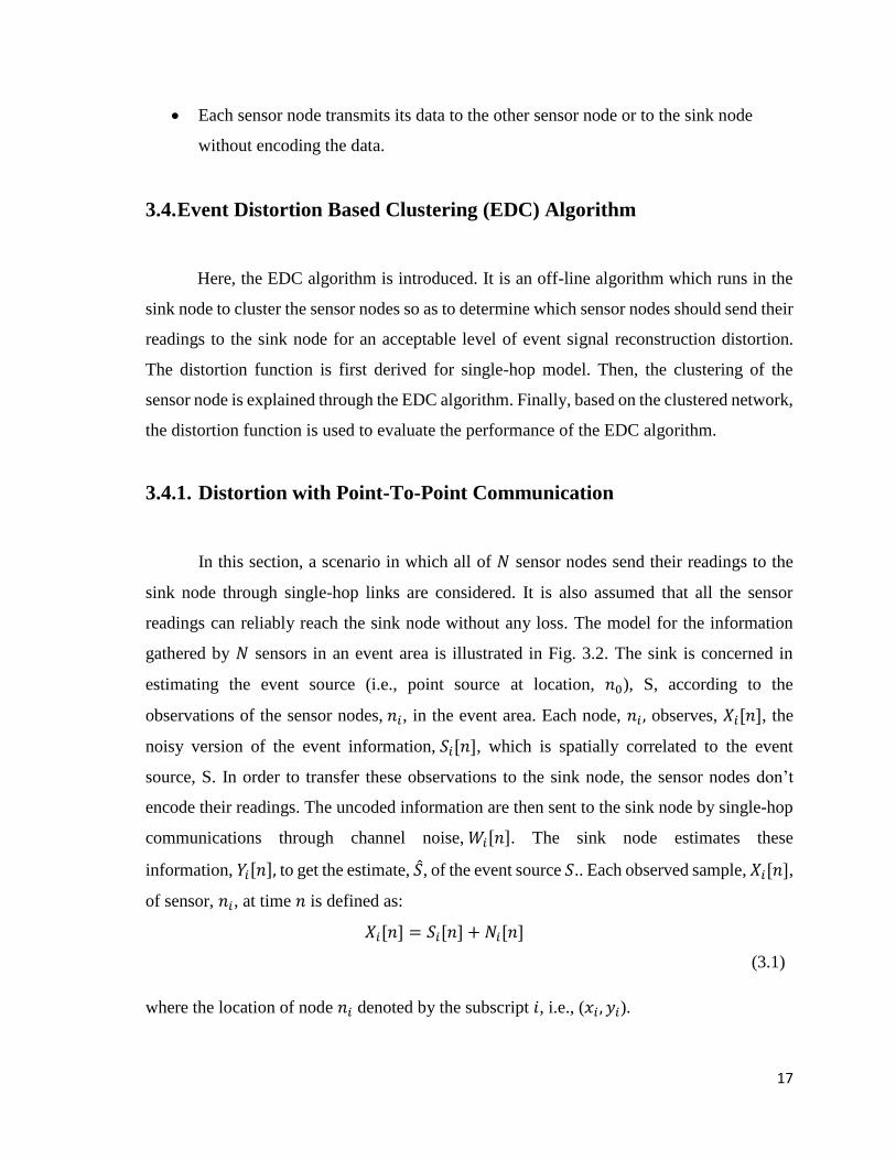
Each sensor node transmits its data to the other sensor node or to the sink node
without encoding the data.
3.4. Event Distortion Based Clustering (EDC) Algorithm
Here, the EDC algorithm is introduced. It is an off-line algorithm which runs in the
sink node to cluster the sensor nodes so as to determine which sensor nodes should send their
readings to the sink node for an acceptable level of event signal reconstruction distortion.
The distortion function is first derived for single-hop model. Then, the clustering of the
sensor node is explained through the EDC algorithm. Finally, based on the clustered network,
the distortion function is used to evaluate the performance of the EDC algorithm.
3.4.1. Distortion with Point-To-Point Communication
In this section, a scenario in which all of 𝑁 sensor nodes send their readings to the
sink node through single-hop links are considered. It is also assumed that all the sensor
readings can reliably reach the sink node without any loss. The model for the information
gathered by 𝑁 sensors in an event area is illustrated in Fig. 3.2. The sink is concerned in
estimating the event source (i.e., point source at location, 𝑛0), S, according to the
observations of the sensor nodes, 𝑛𝑖, in the event area. Each node, 𝑛𝑖 , observes, 𝑋𝑖[𝑛], the
noisy version of the event information, 𝑆𝑖[𝑛], which is spatially correlated to the event
source, S. In order to transfer these observations to the sink node, the sensor nodes don’t
encode their readings. The uncoded information are then sent to the sink node by single-hop
communications through channel noise, 𝑊𝑖[𝑛]. The sink node estimates these
information, 𝑌𝑖[𝑛], to get the estimate, �̂�, of the event source 𝑆.. Each observed sample, 𝑋𝑖[𝑛],
of sensor, 𝑛𝑖, at time 𝑛 is defined as:
𝑋𝑖[𝑛] = 𝑆𝑖[𝑛] + 𝑁𝑖[𝑛]
(3.1)
where the location of node 𝑛𝑖 denoted by the subscript 𝑖, i.e., (𝑥𝑖 , 𝑦𝑖).
18
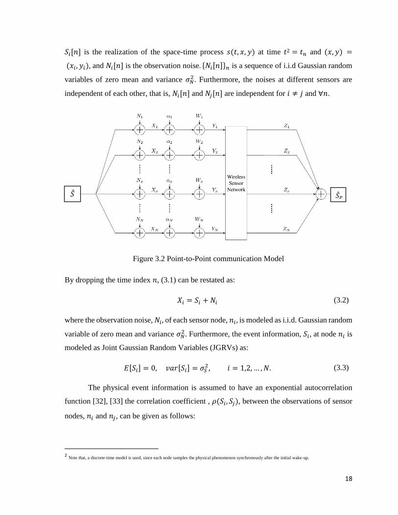
𝑆𝑖[𝑛] is the realization of the space-time process 𝑠(𝑡, 𝑥, 𝑦) at time 𝑡2 = 𝑡𝑛 and (𝑥, 𝑦) =
(𝑥𝑖, 𝑦𝑖), and 𝑁𝑖[𝑛] is the observation noise. {𝑁𝑖[𝑛]}𝑛 is a sequence of i.i.d Gaussian random
variables of zero mean and variance 𝜎𝑁2. Furthermore, the noises at different sensors are
independent of each other, that is, 𝑁𝑖[𝑛] and 𝑁𝑗[𝑛] are independent for 𝑖 ≠ 𝑗 and ∀𝑛.
Figure 3.2 Point-to-Point communication Model
By dropping the time index 𝑛, (3.1) can be restated as:
𝑋𝑖 = 𝑆𝑖 + 𝑁𝑖 (3.2)
where the observation noise, 𝑁𝑖, of each sensor node, 𝑛𝑖 , is modeled as i.i.d. Gaussian random
variable of zero mean and variance 𝜎𝑁2. Furthermore, the event information, 𝑆𝑖, at node 𝑛𝑖 is
modeled as Joint Gaussian Random Variables (JGRVs) as:
𝐸[𝑆𝑖] = 0, 𝑣𝑎𝑟[𝑆𝑖] = 𝜎𝑆2, 𝑖 = 1,2, … , 𝑁. (3.3)
The physical event information is assumed to have an exponential autocorrelation
function [32], [33] the correlation coefficient , 𝜌(𝑆𝑖, 𝑆𝑗), between the observations of sensor
nodes, 𝑛𝑖 and 𝑛𝑗 , can be given as follows:
2 Note that, a discrete-time model is used, since each node samples the physical phenomenon synchronously after the initial wake-up.
�̂�𝑃 �̂�

19
𝜌(𝑆𝑖, 𝑆𝑗) =𝐸[𝑆𝑖𝑆𝑗]
𝜎𝑆2 = 𝑒
(𝑑(𝑛𝑖,𝑛𝑗)
𝜃1⁄ )
𝜃2
.
(3.4)
Here, 𝜃2 = 1 is used in exponential model, and 𝜃1 controls the correlation range
between the observations of sensor nodes. Furthermore, 𝑑(𝑛𝑖, 𝑛𝑗) = ||𝑛𝑖 − 𝑛𝑗|| denotes the
distance between nodes 𝑛𝑖 and 𝑛𝑗 . This correlation coefficient, 𝜌(𝑆𝑖, 𝑆𝑗), is assumed to be
non-negative and decreases monotonically with the distance, 𝑑(𝑛𝑖, 𝑛𝑗), with limiting values
of 1 at 𝑑 = 0 and of 0 at 𝑑 = ∞.
The event source, S, is a JGRV and it is of special interest. Hence, the 𝜌(𝑆, 𝑆𝑖) and
𝑑(𝑛0, 𝑛𝑖), can be denoted as the correlation coefficient and the distance, between the event
source, 𝑆, at 𝑛0 and sensor node, 𝑛𝑖, respectively. As follows:
𝜌(𝑆, 𝑆𝑖) =𝐸[𝑆 𝑆𝑖]
𝜎𝑆2 = 𝑒
(𝑑(𝑛0,𝑛𝑖)
𝜃1⁄ )
𝜃2.
(3.5)
where 𝑑(𝑛0, 𝑛𝑖) = ||𝑛0 − 𝑛𝑖|| denotes the distance between event source at position 𝑛0, 𝑆,
and node, 𝑛𝑖. As each sensor node, 𝑛𝑖, observes an event information, 𝑋𝑖. This information
is then encoded to be forwarded to the sink node. It has been investigated that for sensor
networks, the uncoded transmission performs better than the coding approach with Gaussian
source [4]. Hence, uncoded transmission is adopted for the sensor readings, in this analysis.
Consequently, each node, 𝑛𝑖, sends to the sink a scaled version of the observed sample, 𝑋𝑖,
to meet its power constraint, �̂�, i.e., transmitted power for data from sensor, 𝑛𝑖, to the sink
node, which it can be defined by calculating the energy consumption for transmitting number
of bits over specific interval, it will be defined in Section 3.5. It is given as follows:
∑ 𝐸[(𝛼 𝑋𝑖)2]
𝑁
𝑖=1
≤ 𝑁�̂�.
(3.6)
By taking the upper bound, then (3.6) can be simplified with respect to (2) as:
𝐸[(𝛼 (𝑆𝑖 + 𝑁𝑖))2
] = 𝑃.̂ (3.7)

20
Since each sensor, 𝑛𝑖 , is capable to adjust its power level based on the destination,
then (�̂� = 𝑃𝑖)3. Then, the scaler, 𝛼𝑖, can be defined after taking the expectation operator as:
𝛼𝑖 = √𝑃𝑖
𝜎𝑆2 + 𝜎𝑁
2 .
(3.8)
where 𝜎𝑆2 and 𝜎𝑁
2 are the variances of the event information, 𝑆𝑖, and the observation noise,
𝑁𝑖, respectively. Then, the received signal at sink node, 𝑌𝑖, can be defined as
𝑌𝑖 = 𝛼𝑖𝑋𝑖 + 𝑊𝑖. (3.9)
where {𝑊}𝑖 is a channel noise between node, 𝑛𝑖, and sink node, which its modeled as a set
of i.i.d Gaussian random variables with zero mean and variance 𝜎𝑊2 .
The sink needs to calculate the estimation of each event information, 𝑆𝑖. Since
uncoded transmission is used, it is well known that the Minimum Mean Square Error
(MMSE) estimation is the optimum decoding technique [34]. Hence, the estimation, 𝑍𝑖, of
the event information, 𝑆𝑖, is simply the MMSE estimation of 𝑌𝑖. Then, 𝑍𝑖 can be defined
according to the linear transformation of 𝑌𝑖 as:
𝑍𝑖 = 𝑎 𝑌𝑖 . (3.10)
where 𝑎 is a constant. For optimal case, the received sample, 𝑍𝑖, in sink node is equal to the
observation, 𝑆𝑖, of node, 𝑛𝑖, as given below:
𝐸[(𝑍𝑖 − 𝑆𝑖)2] = 0. (3.11)
In order to find an optimal 𝑎, the derivative is taken with respect to 𝑎 and the
expectation is applied after (3.8) is substituted in (3.9), as follows:
𝐸 [𝑑
𝑑𝑎((𝑎2 𝑌𝑖
2) − 2(𝑎 𝑌𝑖 𝑆𝑖) + (𝑆𝑖2))] = 0.
(3.12)
Then,
3 The transmitted powers can be calculated based on sensor locations at the sink node, and hence they are assumed to be fixed.

21
𝐸[(2 𝑎 𝑌𝑖2) − 2(𝑌𝑖 𝑆𝑖)] = 0. (3.13)
Finally, 𝑎 can be written as:
𝑎 =𝐸[𝑌𝑖𝑆𝑖]
𝐸[𝑌𝑖2]
.
(3.14)
After finding 𝑎, 𝑍𝑖 can be easily expressed by substituting (3.2), (3.9) and (3.14) is
substituted in (3.10), as follows;
𝑍𝑖 =𝐸[𝑌𝑖𝑆𝑖]
𝐸[𝑌𝑖2]
𝑌𝑖 =𝐸[(𝛼𝑖 𝑋𝑖 + 𝑊𝑖 ) 𝑆𝑖]
𝐸[(𝛼𝑖 𝑋𝑖 + 𝑊𝑖)2]𝑌𝑖.
(3.15)
Since there is no correlation between 𝑆𝑖 and 𝑊𝑖, it can be written as;
𝑍𝑖 =𝐸[(𝛼𝑖 𝑋𝑖 𝑆𝑖)]
𝐸[(𝛼𝑖 𝑋𝑖)2] + 𝐸[(𝑊𝑖)2]𝑌𝑖 =
𝛼𝑖 𝐸[𝑋𝑖 𝑆𝑖]
𝑣𝑎𝑟(𝛼𝑖 𝑋𝑖) + 𝑣𝑎𝑟(𝑊𝑖)𝑌𝑖 .
(3.16)
where the means of 𝑋𝑖 and 𝑊𝑖 are zeros. Consequently, 𝑍𝑖 can be simplified as;
𝑍𝑖 =𝛼𝑖 𝐸[𝑆𝑖
2]
𝛼𝑖2(𝜎𝑆
2 + 𝜎𝑁2) + 𝜎𝑊
2 𝑌𝑖. (3.17)
Finally, 𝑍𝑖 can be stated as;
𝑍𝑖 =𝛼𝑖 𝜎𝑆
2
𝑃𝑖 + 𝜎𝑊2 𝑌𝑖.
(3.18)
The 𝑍𝑖 is decoded using (MMSE) estimator in the sink node. Hence, the estimation,
�̂�𝑃, of event source, 𝑆, can be computed by taking the average of all the received event
information, 𝑍𝑖. Then, the estimated version, �̂�𝑃, can be formed as,
�̂�𝑃 =1
𝑁∑ 𝑍𝑖
𝑁
𝑖=1
.
(3.19)
Finally, the distortion for single-hop communication model, 𝐷𝑝𝑜𝑖𝑛𝑡, can be presented
with respect to the estimated value, �̂�𝑃, as:

22
𝐷𝑝𝑜𝑖𝑛𝑡 = 𝐸 [(𝑆 − �̂�𝑃)2
] = 𝐸[𝑆2] − 2 𝐸[𝑆 �̂�] + 𝐸[�̂�2]. (3.20)
The first term, 𝐸[𝑆2], is equal to 𝜎𝑆2. The second term, 𝐸[𝑆 �̂�𝑃], is calculated by
substituting (3.19), (3.18), (3.9), and (3.2) as follows:
𝐸[𝑆 �̂�𝑃] = 𝐸 [𝑆 (1
𝑁∑
𝛼𝑖 𝜎𝑆2
𝑃𝑖 + 𝜎𝑊2 (𝛼𝑖 (𝑆𝑖 + 𝑁𝑖) + 𝑊𝑖)
𝑁
𝑖=1
)].
(3.21)
Note that, there is no correlation between (𝑆 and 𝑁𝑖), and (𝑆 and 𝑊𝑖). Hence, it can
be solved by:
𝐸[𝑆 �̂�𝑃] =1
𝑁∑
𝛼𝑖2 𝜎𝑆
4
𝑃𝑖 + 𝜎𝑊2 𝜌(𝑆, 𝑆𝑖).
𝑁
𝑖=1
(3.22)
Since mean of �̂� is zero, the third term, 𝐸[�̂�𝑃2], is equal to the variance of the estimated
version, �̂�, of 𝑆. i.e.,
𝐸[�̂�𝑃2] = 𝑣𝑎𝑟(�̂�). (3.23)
By using (3.17),
𝐸[�̂�𝑃2] = 𝑣𝑎𝑟 (
1
𝑁∑ 𝑍𝑖
𝑁
𝑖=1
) =1
𝑁2∑ 𝑣𝑎𝑟(𝑍𝑖)
𝑁
𝑖=1
+1
𝑁2∑ ∑ 𝐸[𝑍𝑖𝑍𝑗]
𝑁
𝑗=1
𝑁
𝑖=1
.
(3.24)
Substituting (3.19), (3.18), (3.9), and (3.2) in (3.24), then (3.24) can be extended as shown:
Then, it can be reduced after taking the expectation as shown:
𝐸[�̂�𝑃2] =
1
𝑁2∑
𝛼𝑖2 𝜎𝑆
4
𝑃𝑖 + 𝜎𝑊2
𝑁
𝑖=1
+𝜎𝑆
4
𝑁2∑ ∑
𝛼𝑖2
𝑃𝑖 + 𝜎𝑊2
𝛼𝑗2
𝑃𝑗 + 𝜎𝑊2
𝑁
𝑗=1
𝑁
𝑖=1
𝜌(𝑆𝑖, 𝑆𝑗).
(3.26)
Using (3.22) and (3.26) in (3.20), the result can be finalized as:
𝐸[�̂�𝑃2] =
1
𝑁2∑ (
𝛼𝑖 𝜎𝑆2
𝑃𝑖 + 𝜎𝑊2 )
2
𝑣𝑎𝑟(𝛼𝑖 𝑋𝑖 + 𝑊𝑖) +𝜎𝑆
4
𝑁2∑ ∑
𝛼𝑖
𝑃𝑖 + 𝜎𝑊2
𝛼𝑗
𝑃𝑗 + 𝜎𝑊2
𝑁
𝑗=1
𝑁
𝑖=1
𝑁
𝑖=1
× 𝐸[((𝛼𝑖(𝑆𝑖 + 𝑁𝑖) + 𝑊𝑖) (𝛼𝑗(𝑆𝑗 + 𝑁𝑗) + 𝑊𝑗)].
(3.25)
23
𝐷𝑝𝑜𝑖𝑛𝑡 = 𝜎𝑆2 −
𝜎𝑆4
𝑁2∑
𝛼𝑖2
𝑃𝑖 + 𝜎𝑊2 (2 𝑁 𝜌(𝑆, 𝑆𝑖) − 1 − ∑
𝛼𝑗2 𝜌(𝑆𝑖, 𝑆𝑗)
𝑃𝑗 + 𝜎𝑊2
𝑁
𝑗=1
) .
𝑁
𝑖=1
(3.27)
where 𝜌(𝑆, 𝑆𝑖) and 𝜌(𝑆𝑖, 𝑆𝑗) are correlation coefficients between node, 𝑛𝑖, and source event,
𝑆, and between node, 𝑛𝑖, and node, 𝑛𝑗, respectively. This distortion function represents the
accuracy level of original event 𝑆 at sink node for single-hop communication with respect to
observation and channel noises.
3.4.2. Clustering Formation
According to the results that obtained in the preceding section, the EDC algorithm is
introduced. The EDC algorithm is firstly required to select a smaller set of sensor nodes,
rather than all sensor nodes. These selected sensor nodes are defined through exploiting
spatial correlation such that the acceptable level of event signal reconstruction distortion can
be maintained at the sink node. The EDC algorithm uses VQ as a way to exploit spatial
correlation. Secondly, the sensor nodes are clustered by the sink node based on the selected
and unselected nodes that are defined by VQ. An overview about the VQ design problem is
given next.
VQ is a lossy data compression method [12], that compresses the set of pixels for
images, or the set of bits in signals (e.g., speech signals). The VQ maps k-dimensional source
vectors (i.e., pixels or bits) into the finite set of vectors called codewords. The set of all
codeword vectors is called codebook. Associated with each codeword, a nearest region is
called Voronoi region. However, this method reduces the quality of images or signals,
because VQ is nothing more than an approximation.
Generally, the samples of speech signal might be temporally correlated, and the pixels
of specific image might be spatially correlated. Therefore, the selection of correlated points
based on a distortion constraint has been investigated by exploiting VQ methods [12]. Hence,
these methods have been used by properly addressing the dense deployment issue in WSN
[3].

24
The VQ design can be described as follows [12]: Given a vector source with its
statistical properties known4, given a distortion constraint, and given the number of
codewords, the VQ algorithm tries to find a codebook and partitions (i.e., voronoi regions)
which result in the smallest possible average distortion. More specifically, the VQ algorithm
aims to represent all possible codewords in a code space by a subset of codewords, within
the distortion constraint (i.e., maximum acceptable distortion). Hence, the spatial correlation
can be exploited using VQ, where all the sensor nodes in an event area are needed to be
represented with a smaller number. If two dimensional source vector is selected, the code
space in the VQ method is applied to the network topology with the sensor nodes as the
codeword spaces. The VQ algorithm, when it is applied to the sensor nodes selection issue,
the codebook and the partitions can be determined. Since the sensor nodes are densely
deployed, it is possible to refer the closest nodes to the fixed locations of codebook as
Representative Nodes, while the other remaining nodes are referred as Unrepresentative
Nodes.
The EDC algorithm starts with selecting the length of codebook as one, to be an input
to the VQ, as well as all 𝑁 sensor nodes as a source vector. The outputs are one representative
node and set of unrepresentative nodes. Then, the EDC algorithm iteratively increases the
number of representative nodes (i.e., by increasing the length of codebook). For each
increment, the unrepresentative nodes are decreased. The EDC algorithm continues to
increase the number of representative nodes until the point distortion, defined by (27), of the
unrepresentative nodes achieves distortion constraint.
The INS algorithm [3] successfully selects the representative nodes but it does not
exploit the unselected nodes. However, the EDC algorithm consideres only the
unrepresentative nodes readings (instead of representative nodes) to be transmitted to the sink
node. Moreover, the EDC algorithm uses the representative nodes in relaying the
observations of unrepresentative sensor nodes to the sink node. In the EDC algorithm, only
the readings of unrepresentative sensor nodes are considered at the sink node. The majority
of the unrepresentative nodes and the advantage of their coverage made the distortion more
likely to be maintained at the sink node, rather than representative sensor nodes.
4 The statistical property is referred as a type of source vector distribution, or deployment approach in the WSN sense. In WSN, nodes deployment can be done through Uniform, Poisson, or Gaussian distribution.

25
.
Figure 3.3 Clustered-Network by EDC Algorithm
The EDC algorithm then forms a sample topology, as shown in Fig 3.3. The Voronoi
diagrams are referred as clusters, administered by their Cluster Heads (CHs), (i.e., 𝑐
representative nodes). All Cluster Members (CMs), (i.e., all 𝑟 unrepresentative nodes) are
located inside clusters that are assigned by K-Nearest Neighbor (KNN) [24]. Each cluster 𝑘
contains set of 𝑚𝑘5 cluster members, which are defined through KNN with respect to their
CHs. Furthermore, The distortion constraint represents the maximum acceptable distortion
level in single-hop case for unrepresentative nodes, 𝐷𝑃𝑜𝑖𝑛𝑡(𝑟) with respect to distortion
threshold, 𝐷𝑡ℎ𝑟𝑒𝑠𝑜𝑙𝑑, which it defined with respect to the application requirement.
5 Each cluster contains different numbers of 𝐶𝑀𝑠, i.e., 𝑚𝑘 ≠ 𝑚𝑙, that are calculated in the sink node based
on KNN with respect to voronoi regions, and hence they assumed to be fixed not random.
Cluster Members Cluster Heads
BS
Codebook
Inter-communication
Intra-communication
Cluster

26
Figure 3.4 Event Distortion Based Clustering (EDC) Algorithm
Calculating 𝐷𝑝𝑜𝑖𝑛𝑡(𝑁)
for all 𝑁 sensor nodes
Applying Vector Quantization
(VQ)
Unrepresentative Nodes (𝑟)-
transmission is required
Representative Nodes (𝑐)-
transmission isn’t required
IF
𝐷𝑝𝑜𝑖𝑛𝑡(𝑟) ≥ 𝐷𝑝𝑜𝑖𝑛𝑡(𝑁) + 𝐷𝑡ℎ𝑟𝑒𝑠ℎ𝑜𝑙𝑑
𝑤ℎ𝑒𝑟𝑒 𝑐 = 𝑁 − 𝑟
𝑐 = 𝑐 + 1
Representative Nodes CHs
Unrepresentative Nodes CMs
Voronoi digrams Clusters
The previous results of
representative, (𝑐 − 1), and
unrepresentatve nodes, (𝑟 + 1)
IF
𝐸𝐶𝐻(𝑖),𝐶𝑀(𝑘,𝑖) < 𝜀0
∀ 𝑘, 𝑖
𝐶𝐻(𝑘) = 𝐶𝑀(𝑘, 𝑖),
where, 𝑖 = max(𝐸𝐶𝑀𝑠(𝑘, : ))
𝐶𝑀(𝑖) = ∅
Yes
Yes
NO
No
Sensor Nodes
Initialize codebook
length, 𝑐 = 1

27
After defining a clustered-network, the EDC algorithm starts to check the energy
level of all sensor nodes (CH & CM) and changes their duties based on their remaining
energies. Since each sensor node is assumed to transmit its information about its remaining
energy level to the sink node.
In the case that the energy level of CH (or CM) is under a predefined threshold, 𝜀0, it
turns to inactive state (i.e., sensor node is prevented from observing, aggregating and
communicating etc.). Furthermore, if the energy level of cluster head 𝑘 at cluster 𝑘, 𝐸𝐶𝐻(𝑘),
is less than 𝜀0, the CM with highest energy level is elected to play CH role until CH recover
its energy. Moreover, recovering the energy is assumed to be done continuously through
energy harvesting from ambient electromagnetic radiation in radio frequencies.
During the lifetime of the network, the network topology can change due to failure or
battery drain of sensor nodes. However, since the distortion depends on the physical
phenomenon, such a change should not affect the distortion achieved at the sink, unless the
number of CMs decreases significantly (i.e., when the energy level of any cluster member 𝑖
at cluster 𝑘, 𝐸𝐶𝑀(𝑘, 𝑖), is less than 𝜀0). In such a case, the event information cannot be
captured in the sink node at the desired distortion level.
3.4.3. Distortion with Two-hop Communication
The presented EDC algorithm uses two-hop communication model for data transfer
as shown in Fig 3.3, unlike single-hop model that has been defined in Fig 3.2. The model for
the information gathered by all Cluster Members (CMs) in the event area is shown in Fig 3.5.
The sink node estimates the event source, S, i.e., point source at location 𝑛0, according to the
observations of only CMs, 𝑆𝑘,𝑖. Each cluster member 𝑖 at cluster 𝑘, 𝐶𝑀𝑘,𝑖, observes the noisy
version, 𝑋𝑘,𝑖, of the event information, 𝑆𝑘,𝑖, which is spatially correlated with the event
source, 𝑆. In order to transfer these observations to the sink node, the CMs don’t need encode
their readings. The uncoded information are then sent to the cluster head 𝑘 at cluster 𝑘, 𝐶𝐻𝑘,
by single-hop communications through channel noise, 𝑊𝑘,𝑖. Then, each 𝐶𝐻𝑘 receives and
aggregates the samples from its CMs, 𝑌𝑘,𝑖, after decoding them. Also, 𝐶𝐻𝑘 does not need to
encodes its data, and hence it only requires to receive the observations from 𝑚𝑘 cluster

28
members and then it aggregates their readings. Then, the aggregated information, 𝑆𝑘, is
relayed to the sink node through another channel noise, 𝑔𝑘. The sink is then estimates from
the information of 𝐶𝐻𝑘, 𝑌𝑘, to get the estimation, �̂�𝑅, of the event source, 𝑆. Hereafter, for
ease of illustration, the time index is dropped. Hence, each observed sample, 𝑋𝑘,𝑖, of 𝐶𝑀𝑘,𝑖
is defined as:
𝑋𝑘,𝑖 = 𝑆𝑘,𝑖 + 𝑁𝑘,𝑖. (3.28)
Figure. 3.5 Two-hop Communication Model
where {𝑁}𝑘,𝑖 is a set of i.i.d Gaussian random variables with zero mean and variance 𝜎𝑁2. The
event information, 𝑆𝑘,𝑖, at each 𝐶𝑀𝑘,𝑖 is modeled according to the Joint Gaussian Random
Variables (JGRVs) as follows:
𝐸[𝑆𝑘,𝑖] = 0, 𝑣𝑎𝑟[𝑆𝑘,𝑖] = 𝜎𝑆2, 𝑖 = 1,2, … . , 𝑚𝑘. (3.29)
where these properties are the same for different CMs and even in different clusters. The
CMs that are located in the same cluster might be correlated, as well as in different clusters.
Since, the physical event has an exponential autocorrelation function, then, the correlation
coefficient , 𝜌(𝑆𝑘,𝑖, 𝑆𝑘,𝑗), between the observations of cluster member 𝑖 and 𝑗 at cluster 𝑘, and
�̂�𝑅
�̂�
CM CH

29
𝜌(𝑆𝑘,𝑖, 𝑆𝑙,𝑗), between the observations of cluster members 𝑖 and 𝑗 at clusters 𝑘 and 𝑙,
respectively can be given as follows:
𝜌(𝑆𝑘,𝑖, 𝑆𝑘,𝑗) =𝐸[𝑆𝑘,𝑖 𝑆𝑘,𝑗]
𝜎𝑆2 = 𝑒
(𝑑(𝐶𝑀𝑘,𝑖,𝐶𝑀𝑘,𝑗)
𝜃1⁄ )
𝜃2
(3.30)
𝜌(𝑆𝑘,𝑖, 𝑆𝑙,𝑗) =𝐸[𝑆𝑘,𝑖 𝑆𝑙,𝑗]
𝜎𝑆2 = 𝑒
(𝑑(𝐶𝑀𝑘,𝑖,𝐶𝑀𝑙,𝑗)
𝜃1⁄ )
𝜃2
.
(3.31)
Similarly, the event source, S, is modeled as JGRV. The correlation coefficient,
𝜌(𝑆, 𝑆𝑘,𝑖), and the distance, 𝑑(𝑛0, 𝐶𝑀𝑘,𝑖), between the event source, 𝑆, and 𝐶𝑀𝑘,𝑖,
respectively, are given bellow:
𝜌(𝑆, 𝑆𝑘,𝑖) =𝐸[𝑆 𝑆𝑘,𝑖]
𝜎𝑆2 = 𝑒
(𝑑(𝑛0,𝐶𝑀𝑘,𝑖)
𝜃1⁄ )
𝜃2
.
(3.32)
Since uncoded transmission has been adopted in this analysis for single-hop
communication with Gaussian source, then the received sample 𝑌𝑘,𝑖 at CH can be defined as:
𝑌𝑘,𝑖 = 𝛼𝑘,𝑖𝑋𝑘,𝑖 + 𝑊𝑘,𝑖. (3.33)
where {𝑊}𝑘,𝑖 is a channel noise (between 𝐶𝑀𝑘,𝑖 and 𝐶𝐻𝑘), which is defined as a set of i.i.d
Gaussian random variables with zero mean and variance 𝜎𝑊2 . And the scalar 𝛼 is defined with
respect to its power constraints, �̂�, as:
∑ 𝐸[𝛼 𝑋𝑘,𝑖]2
𝑚𝑘
𝑖=1
≤ 𝑚𝑘 �̂�. (3.34)
Since each 𝐶𝑀𝑘,𝑖 is capable to adjust its transmitted power level, then �̂� ≜ 𝑃𝑘,𝑖, i.e.,
the transmitted power for the information from 𝐶𝑀𝑘,𝑖 to the 𝐶𝐻𝑘. Hence, by taking the upper
bound of (3.34), then the scaler 𝛼𝑘,𝑖 can be simplified as:
𝛼𝑘,𝑖 = √𝑃𝑘,𝑖
𝜎𝑆2 + 𝜎𝑁
2.
(3.35)

30
In order to estimate the received sample at CH, MMSE estimation is used. Hence,
received signal at 𝐶𝐻𝑘, 𝑍𝑘,𝑖, can be defined according to the linear transformation of 𝑌𝑘,𝑖 as
follows:
𝑍𝑘,𝑖 = 𝑎 𝑌𝑘,𝑖. (3.36)
where 𝑎 is constants. According to the MMSE estimator the optimal case the received signal,
𝑍𝑘,𝑖, is equal to the sensor observation, 𝑆𝑘,𝑖, as:
𝐸[(𝑍𝑘,𝑖 − 𝑆𝑘,𝑖)2] = 0. (3.37)
Similarly, in order to find an optimal 𝑎, the derivative is calculated with respect to 𝑎
and the expectation is applied after (36) is substituted in (37), as defined bellow:
𝐸 [𝑑
𝑑𝑎(𝑎2 𝑌𝑘,𝑖
2 − 2 𝑎 𝑌𝑘,𝑖 𝑆𝑘,𝑖 + 𝑆𝑘,𝑖2)] = 0.
(3.38)
Since the means of source 𝑆𝑘,𝑖 and noise 𝑁𝑘,𝑖 are zero, then (3.38) can be solved and
𝑎 can be given by:
𝑎 =𝐸[𝑌𝑘,𝑖 𝑆𝑘,𝑖]
𝐸[𝑌𝑘,𝑖2]
.
(3.39)
After finding 𝑎, 𝑍𝑘,𝑖 can expressed by using (3.28), (3.33), (3.39) in (3.36) as follows:
𝑍𝑘,𝑖 =𝐸[𝑌𝑘,𝑖 𝑆𝑘,𝑖]
𝐸[𝑌𝑘,𝑖2]
𝑌𝑘,𝑖 =𝐸[(𝛼𝑘,𝑖 𝑋𝑘,𝑖 + 𝑊𝑘,𝑖 ) 𝑆𝑘,𝑖]
𝐸[(𝛼𝑘,𝑖 𝑋𝑘,𝑖 + 𝑊𝑘,𝑖)2]𝑌𝑘,𝑖.
(3.40)
Since there is no correlation between 𝑆𝑘,𝑖 and 𝑊𝑘,𝑖, then it can be reduced to:
𝑍𝑘,𝑖 =𝐸[(𝛼𝑘,𝑖 𝑋𝑘,𝑖 𝑆𝑘,𝑖)]
𝐸[(𝛼𝑘,𝑖 𝑋𝑘,𝑖)2] + 𝐸[(𝑊𝑘,𝑖)2]𝑌𝑘,𝑖 =
𝛼𝑘,𝑖 𝐸[𝑋𝑘,𝑖 𝑆𝑘,𝑖]
𝛼𝑘,𝑖2𝑣𝑎𝑟( 𝑋𝑘,𝑖) + 𝑣𝑎𝑟(𝑊𝑘,𝑖)
𝑌𝑘,𝑖.
(3.41)
where the means of 𝑋𝑘,𝑖 and 𝑊𝑘,𝑖 are zero. Hence, 𝑍𝑘,𝑖 can be finally simplified as:
𝑍𝑘,𝑖 =𝛼𝑘,𝑖 𝜎𝑆
2
𝑃𝑘,𝑖 + 𝜎𝑊2 𝑌𝑘,𝑖.
(3.42)
Furthermore, since the 𝐶𝐻𝑘 decodes each 𝑌𝑘,𝑖 using the MMSE estimator, the
estimation, 𝑆𝑘, of the event information, 𝑆𝑘,𝑖 can simply be computed by taking the average
of 𝑚𝑘 readings of CMs, 𝑍𝑘,𝑖. Then, the estimation, 𝑆𝑘, is given as follows:

31
The uncoded transmission is not only optimal for single-hop communication, but also
for two-hop communication model [14]. Then, the received sample, 𝑌𝑘, at sink node, and it
can be defined as:
𝑌𝑘 = 𝛼𝑆𝑘 + 𝑔𝑘. (3.44)
where {𝑔}𝑘 is a channel noise that between 𝐶𝐻𝑘 and sink node, which it is defined as a set
of i.i.d Gaussian random variables with zero mean and variance 𝜎𝑔2. And the scalar 𝛼 is
defined with respect to its power constraint, �̂�, as shown:
∑ 𝐸[(𝛼 𝑆𝑘)2]
𝑐
𝑘=1
≤ 𝑐 �̂�.
(3.45)
where the mean of 𝑆𝑘 is zero. By substituting (3.43) in (3.45), and by taking the upper
bound then, (3.45) can be written as:
∑ 𝛼2 𝑣𝑎𝑟(1
𝑚𝑘∑ 𝑍𝑘,𝑖
𝑚𝑘
𝑖=1
)2
𝑐
𝑘=1
= 𝑐 �̂�.
(3.46)
which it can be extended to:
∑𝛼2
𝑚𝑘2
𝑐
𝑘=1
(∑ 𝑣𝑎𝑟(𝑍𝑘,𝑖)
𝑚𝑘
𝑖=1
+ ∑ ∑ 𝑐𝑜𝑣(𝑍𝑘,𝑖
𝑚𝑘
𝑗=1
, 𝑍𝑘,𝑗)
𝑚𝑘
𝑖=1
) = 𝑐 �̂�.
(3.47)
By substituting (3.28), (3.33), (3.35), and (3.42) in (3.47). Then, (3.47) can be extended as:
∑𝛼2
𝑚𝑘2
𝑐
𝑘=1
(∑ 𝑣𝑎𝑟 (𝛼𝑘,𝑖 𝜎𝑆
2
𝑃𝑘,𝑖 + 𝜎𝑊2 (𝛼𝑘,𝑖(𝑆𝑘,𝑖 + 𝑁𝑘,𝑖) + 𝑊𝑘,𝑖))
𝑚𝑘
𝑖=1
+ ∑ ∑ 𝐸 [(𝛼𝑘,𝑖 𝜎𝑆
2
𝑃𝑘,𝑖 + 𝜎𝑊2 (𝛼𝑘,𝑖(𝑆𝑘,𝑖 + 𝑁𝑘,𝑖) + 𝑊𝑘,𝑖)) (
𝛼𝑘,𝑗 𝜎𝑆2
𝑃𝑘,𝑗 + 𝜎𝑊2 (𝛼𝑘,𝑗(𝑆𝑘,𝑗 + 𝑁𝑘,𝑗) + 𝑊𝑘,𝑗))]
𝑚𝑘
𝑗=1
𝑚𝑘
𝑖=1
)
= 𝑐�̂�.
(3.48)
Since each CH is capable to adjust its transmitted power level, then �̂� ≜ 𝑃𝑘, i.e., the
transmitted power of 𝐶𝐻𝑘for data forwarding to the sink node . Hence, the scaler, 𝛼𝑘,𝑖, can
be simplified as follows:
𝑆𝑘 =1
𝑚𝑘∑
𝛼𝑘,𝑖𝜎𝑆2
𝑃𝑘,𝑖 + 𝜎𝑁2
𝑚𝑘
𝑖=1
𝑌𝑘,𝑖.
(3.43)

32
𝛼𝑘 =√
𝑃𝑘 𝑚𝑘2
∑𝛼𝑘,𝑖
2𝜎𝑆4
𝑃𝑘,𝑖 + 𝜎𝑊2
𝑚𝑘
𝑖=1 (1 + ∑𝛼𝑘,𝑗
2𝜎𝑆2
(𝑃𝑘,𝑗 + 𝜎𝑊2 )
𝜌(𝑆𝑘,𝑖𝑆𝑘,𝑗)𝑚𝑘
𝑗=1 )
.
(3.49)
where 𝜌(𝑆𝑘,𝑖, 𝑆𝑘,𝑗) is the correlation coefficient between the readings of 𝐶𝑀𝑘,𝑖 and 𝐶𝑀𝑘,𝑗.
For simplicity, the scaler, 𝛼𝑘, will be written as:
𝛼𝑘 = √𝑃𝑘
𝑣𝑎𝑟(𝑆𝑘)= √
𝑃𝑘
𝜎𝑆𝑘2 .
(3.50)
The sink node then tries to estimate the readings of each cluster, 𝑆𝑘, with MMSE
estimator in a form of linear transformation. Hence, the estimation of each cluster’s readings,
𝑍𝑘 is given as:
𝑍𝑘 = 𝑎 𝑌𝑘 . (3.51)
According to the MMSE estimator, 𝑍𝑘 has to be equal to 𝑆𝑘, which it can be written
in the form:
𝐸[(𝑍𝑘 − 𝑆𝑘)2] = 0. (3.52)
Then, the derivative with respect to 𝑎 is applied before the expectation as follows:
𝐸 [𝑑
𝑑𝑎(𝑎2 𝑌𝑘
2 − 2 𝑎 𝑌𝑘 𝑆𝑘 + 𝑆𝑘2)] = 0.
(3.53)
Since the means of source 𝑆𝑘 and noise 𝑁𝑘 are zeros, it can easily see that 𝑎 can be
written as shown:
𝑎 =𝐸[𝑌𝑘 𝑆𝑘]
𝐸[𝑌𝑘2]
.
(3.54)
By substituting (3.44) and (3.54) in (3.51), then (3.51) can be defined as:
𝑍𝑘 =𝐸[𝑌𝑘 𝑆𝑘]
𝐸[𝑌𝑘2]
𝑌𝑘 =𝐸[(𝛼𝑘 𝑆𝑘 + 𝑔𝑘)𝑆𝑘]
𝐸[(𝛼𝑘 𝑆𝑘 + 𝑔𝑘)2] 𝑌𝑘 =
𝛼𝑘 𝜎𝑆𝑘2
𝑃𝑘 + 𝜎𝑔2
𝑌𝑘. (3.55)

33
Then, the estimated version �̂�𝑅 of original event 𝑆 is defined by averaging all
information of 𝐶𝐻𝑠, 𝑍𝑘 , with number 𝑐 ,and it is demonstrated as:
Finally, the distortion of two-hop communication model is referred as relayed
distortion (𝐷𝑟𝑒𝑙𝑎𝑦). It is calculated at the sink node with respect to the estimated value �̂�𝑅
and source event, 𝑆, according to:
𝐷𝑟𝑒𝑙𝑎𝑦 = 𝐸 [(𝑆 − �̂�𝑅)2
] = 𝐸[𝑆2] − 2 𝐸[𝑆 �̂�𝑅] + 𝐸[�̂�𝑅2]. (3.57)
The first term, 𝐸[𝑆2], equal to 𝜎𝑆2, where the source mean is zero. By substituting
(3.28), (3.33), (3.43), (3.44), (3.55), and (3.56) in the second term, 𝐸[𝑆 �̂�𝑅], then it can be
defined as:
𝐸[𝑆 �̂�𝑅] = 𝐸 [𝑆1
𝑐∑
𝛼𝑘𝜎𝑆𝑘2
𝑃𝑘 + 𝜎𝑔2
(𝛼𝑘 (1
𝑚𝑘
∑𝛼𝑘,𝑖(𝜎𝑆
2 + 𝜎𝑁2)
𝑃𝑘,𝑖 + 𝜎𝑊2 (𝛼𝑘,𝑖(𝑆𝑘,𝑖 + 𝑁𝑘,𝑖) + 𝑊𝑘,𝑖)
𝑚𝑘
𝑖=1
) + 𝑔𝑘)
𝑐
𝑘=1
].
(3.58)
which it can be simplified to:
𝐸[𝑆 �̂�𝑅] =𝜎𝑆
2
𝑐∑
𝑃𝑘
𝑃𝑘 + 𝜎𝑔2
(1
𝑚𝑘∑
𝑃𝑘,𝑖
𝑃𝑘,𝑖 + 𝜎𝑊2
𝜌(𝑆 𝑆𝑘,𝑖)
𝑚𝑘
𝑖=1
)
𝑐
𝑘=1
.
(3.59)
The third term can be defined as:
𝐸[�̂�𝑅2] = 𝑣𝑎𝑟(�̂�). (3.60)
where the mean of �̂� is zero. By substituting (3.56) in (3.60), then (3.60) can be stated as
shown:
𝑣𝑎𝑟 (1
𝑐∑ 𝑍𝑘
𝑐
𝑘=1
) =1
𝑐2(∑ 𝑣𝑎𝑟(𝑍𝑘) + ∑ ∑ 𝐸[𝑍𝑘 𝑍𝑙]
𝑐
𝑙=1
𝑐
𝑘=1
𝑐
𝑘=1
).
(3.61)
By substituting (3.28), (3.33), (3.35), (3.42), and (3.44) in (3.61), then (3.61) can be
extended as:
�̂�𝑅 =1
𝑐∑ 𝑍𝑘 .
𝑐
𝑘=1
(3.56)

34
1
𝑐2(∑
𝑃𝑘𝜎𝑆𝑘2
𝑃𝑘 + 𝜎𝑔2
+ ∑ ∑𝑃𝑘
𝑃𝑘 + 𝜎𝑔2
𝑃𝑙
𝑃𝑙 + 𝜎𝑔2
1
𝑚𝑘
1
𝑚𝑙
(∑ ∑𝛼𝑘,𝑖𝜎𝑆
2
𝑃𝑘,𝑖 + 𝜎𝑊2
𝛼𝑙,𝑗 𝜎𝑆2
𝑃𝑙,𝑗 + 𝜎𝑊2 𝐸[(𝛼𝑘,𝑖 (𝑆𝑘,𝑖
𝑚𝑙
𝑗=1
𝑚𝑘
𝑖=1
𝑐
𝑙=1
𝑐
𝑘=1
𝑐
𝑘=1
+ 𝑁𝑘,𝑖) + 𝑊𝑘,𝑖) (𝛼𝑙,𝑗 (𝑆𝑙,𝑗 + 𝑁𝑙,𝑗) + 𝑊𝑙,𝑗)])).
(3.62)
Then, the last term can be simplified as:
𝐸[�̂�𝑅2] =
1
𝑐2(∑
𝑃𝑘𝜎𝑆𝑘2
𝑃𝑘 + 𝜎𝑔2 + ∑ ∑
𝑃𝑘
𝑃𝑘 + 𝜎𝑔2
𝑃𝑙
𝑃𝑙 + 𝜎𝑔2
1
𝑚𝑘
1
𝑚𝑙(∑ ∑
𝑃𝑘,𝑖
𝑃𝑘,𝑖 + 𝜎𝑊2
𝑃𝑙,𝑗
𝑃𝑙,𝑗 + 𝜎𝑊2 𝜎𝑆
2 𝜌(𝑆𝑘,𝑖𝑆𝑙,𝑗)
𝑚𝑙
𝑗=1
𝑚𝑘
𝑖=1
)
𝑐
𝑙=1
𝑐
𝑘=1
𝑐
𝑘=1
).
(3.63)
Finally, (3.57) can be simplified by using (3.59) and (3.63) as demonstrated below:
𝐷𝑟𝑒𝑎𝑙𝑦 = 𝜎𝑆2 −
1
𝑐2∑
𝑃𝑘
𝑃𝑘 + 𝜎𝑔2
1
𝑚𝑘2
∑𝛼𝑘,𝑖
2 𝜎𝑆4
𝑃𝑘,𝑖 + 𝜎𝑊2 (2 𝑐 𝑚𝑘 𝜌(𝑆, 𝑆𝑘,𝑖) − 1 − ∑
𝛼𝑘,𝑗2 𝜎𝑆
2𝜌(𝑆𝑘,𝑖 , 𝑆𝑘,𝑗)
(𝑃𝑘,𝑗 + 𝜎𝑊2 )
𝑚𝑘
𝑗=1
)
𝑚𝑘
𝑖=1
𝑐
𝑘=1
+1
𝑐2∑ ∑
𝑃𝑘𝑃𝑙𝑚𝑘𝑚𝑙
⁄
(𝑃𝑘 + 𝜎𝑔2)(𝑃𝑙 + 𝜎𝑔
2)∑ ∑
𝛼𝑘,𝑖2 𝛼𝑙,𝑗
2 𝜎𝑆6
(𝑃𝑘,𝑖 + 𝜎𝑊2 )(𝑃𝑙,𝑗 + 𝜎𝑊
2 ) 𝜌(𝑆𝑘,𝑖 , 𝑆𝑙,𝑗)
𝑚𝑙
𝑗=1
𝑚𝑘
𝑖=1
𝑐
𝑙=1
𝑐
𝑘=1
.
(3.64)
where 𝜌(𝑆, 𝑆𝑘,𝑖) and 𝜌(𝑆𝑘,𝑖, 𝑆𝑙,𝑗) are the correlation coefficients between the source event, 𝑆,
and the readings of 𝐶𝑀𝑘,𝑖, 𝑆𝑘,𝑖, and between the readings of 𝐶𝑀𝑘,𝑖, 𝑆𝑘,𝑖, and 𝐶𝑀𝑙,𝑗, 𝑆𝑘,𝑖,
respectively.
The goal of this analytical derivation is to define the accuracy level of the clustered-
network from EDC algorithm. Each sensor is required to do specific duty, but when its energy
level is less than the predetermined threshold, the sensor changes its state to inactive state
(only-harvesting) and based on that the distortion changes. The upper limit of both 𝐷𝑝𝑜𝑖𝑛𝑡
(3.27) and 𝐷𝑟𝑒𝑙𝑎𝑦 (3.64) reached when all sensor nodes triggers into inactive state. In such a
case, the distortions are equal to event variance 𝜎𝑆2 as stated below:
𝜎𝑆2 = 𝑚𝑎𝑥𝑛𝑜𝑑𝑒𝑠=∅(𝐷𝑟𝑒𝑙𝑎𝑦, 𝐷𝑝𝑜𝑖𝑛𝑡). (3.65)
3.5. Energy Model
In this section, we attempt to investigate the mechanism of energy consumption in the
sensor networks for single-hop and two-hop communication models. In both cases, a sensor
node is either in active or inactive state. An active node assists in operation of the network

35
for sensing the area or sending the data to sink. In an inactive state, sensor nodes stop sensing
and sending data until they recovered their energy by recharging their batteries or by energy
harvesting.
The energy consumption in the active nodes is composed of four components. These
components can be defined as energy consumed for packet transmitting, packet receiving,
data gathering (aggregating) and event sensing. The simplified model of energy consumption
for each part is defined in this section.
3.5.1. Energy Consumption for Clustered Network
In clustered-network model Fig 3.3, sensor nodes are assembled into clusters, where
in each cluster consists of a single CH, and several CMs with number 𝑚𝑘. Based on the EDC
algorithm, CH requires to receive the observations from its 𝐶𝑀𝑠, and aggregates their
readings to transmit towards the sink node by single-hop communication.
The required energy for transmitting and receiving 𝐿 bits over the distance 𝑑 between
the transmitter and the receiver can be modeled according to the first order radio (Fig 3.6)
model [8] defined as:
𝐸𝑇𝑥(𝐿, 𝑑) = {(𝐸𝑒𝑙𝑒𝑐 𝐿) + (𝜀𝑓𝑠 𝐿 𝑑2), 𝑑 ≤ 𝑑0
(𝐸𝑒𝑙𝑒𝑐 𝐿) + (𝜀𝑚𝑝 𝐿 𝑑4), 𝑑 > 𝑑0
𝐸𝑅𝑥(𝐿) = 𝐸𝑒𝑙𝑒𝑐 𝐿.
(3.66)
where, 𝑑0 = √𝜀𝑓𝑠
𝜀𝑚𝑝.
The 𝐸𝑒𝑙𝑒𝑐 is electronic energy. The 𝜀𝑓𝑠 and 𝜀𝑚𝑝 are coefficients in free space model
and in multi-path model, respectively. Furthermore, sensing energy for 𝐿 bits can be defined
as follows:
𝐸𝑠𝑒𝑛𝑠(𝐿) = 𝐿 𝑇𝑠𝑒𝑛𝑠 𝐼𝑠𝑒𝑛𝑠 𝑉𝑠𝑢𝑏 . (3.67)

36
Figure 3.6. First Order Radio Model
where 𝐼𝑠𝑒𝑛𝑠 is sensing current, 𝑉𝑠𝑢𝑏 is supplied voltage and 𝑇𝑠𝑒𝑛𝑠 is sensing time. The
aggregating energy form 𝑚 receiving destinations can be modeled as [8]
𝐸𝑎𝑔𝑔(𝐿, 𝑚) = 𝐿 𝑚 𝐸𝐷𝐴. (3.68)
where 𝐸𝐷𝐴 is aggregation energy. Based on the above equations, it is possible now to define
the energy consumption of 𝐶𝑀𝑘,𝑖 and 𝐶𝐻𝑘 which can be demonstrated as:
𝐸𝐶𝑀(𝑘, 𝑖) = 𝐸𝑠𝑒𝑛𝑠(𝐿) + 𝐸𝑇𝑥(𝐿, 𝑑𝑐ℎ(𝑘, 𝑖)),
𝐸𝐶𝐻(𝑘) = 𝐸𝑎𝑔𝑔(𝐿, 𝑚𝑘) + 𝑚𝑘 𝐸𝑅𝑥(𝐿) + 𝐸𝑇𝑥(𝐿, 𝑑𝐵𝑆(𝑘)).
(3.69)
(3.70)
where 𝑑𝑐ℎ(𝑘, 𝑖) and 𝑑𝐵𝑆(𝑘) are Euclidean distance between 𝐶𝑀𝑘,𝑖 and 𝐶𝐻𝑘, and between
𝐶𝐻𝑘 and sink node, respectively. Furthermore, the energy consumption for single-hop
communication case is modeled as:
𝐸𝑛𝑖(𝑖) = 𝐸𝑠𝑒𝑛𝑠(𝐿) + 𝐸𝑇𝑥(𝐿, 𝑑𝐵𝑆(𝑖)) (3.71)
where 𝑑𝐵𝑆(𝑖) is the euclidean distance between 𝑛𝑖 and sink node. The above equations in
(66) represent the energy consumption for transmitting in joules.
However, the unit of power constraints (i.e., transmitting power, that is defined in
point distortion (17) and relayed distortion (64)) is Watts. Also, the unit of above energy
consumption functions is Joules. Hence, a simple conversion method is used for finding the
power constraints by converting to Watts, which is (𝑃(𝑤𝑎𝑡𝑡𝑠) = 𝐸(𝑗𝑜𝑢𝑙𝑒𝑠)/𝑇), with respect
to the time durations (𝑇𝑠𝑒𝑛𝑠, 𝑇𝑎𝑔𝑔, and 𝑇𝑡𝑟𝑎𝑛𝑠) as shown below:

37
𝑇𝑎𝑔𝑔 = 𝐿 𝑁𝑐𝑦𝑐
𝑓𝑠𝑒𝑛, 𝑇𝑡𝑟𝑎𝑛 = 𝑇𝑟𝑒𝑐 =
𝐿
𝑅.
(3.72)
where 𝑁𝑐𝑦𝑐 is the number of processor cycles per bit, 𝑓𝑠𝑒𝑛 is sensor frequency and 𝑅 is the
data rate.
3.5.2. Harvesting Model
Energy harvesting is an interesting solution for battery recharging when nodes are
positioned in an event area covered by a cellular base station. By assuming that there is radio
frequency source such as GSM900 tower [13] with transmitted power 𝑃𝑡 and antenna gain 𝐺𝑡.
Then, it’s possible from each sensor node to harvest energy from it by equipping an additional
harvesting circuit with additional antenna of gain 𝐺𝑟. Therefore, by using Friis equation it’s
possible to model the receiving power, 𝑃𝑅, considering the free path loss model as shown:
𝑃𝑟 = 𝑃𝑡
𝐺𝑇𝐺𝑅𝜆2
(4𝜋𝑑)2.
(3.73)
where 𝜆 is wave length over 𝑑 distance. The harvested time, 𝑇ℎ𝑎𝑟, can be defined with respect
to circuit harvesting efficiency and battery charging time.
3.6. Case Study
In this section, the point (27) and relayed (64) distortion functions are studied based
on some important parameters ( data rate, number of sensor nodes, event distance, and the
size of event area for different values of 𝜃1) by means of Monte Carlo simulation ( i.e., 500
iterations).
3.6.1. Data Rate (𝑹)
The presented two distortion functions are observed by varying the data. According
to (72), increasing data rate decreases transmission time, 𝑇𝑡𝑟𝑎𝑛. It is possible to convert the

38
transmitting energy, 𝐸𝑇𝑥(𝐿, 𝑑), to transmitting powers (i.e., power constraints) by dividing
them with 𝑇𝑡𝑟𝑎𝑛. Since the power constraints of the two distortion functions are transmitting
powers (i.e., (𝑃𝑘,𝑖, 𝑃𝑘) for 𝐷𝑟𝑒𝑙𝑎𝑦 and 𝑃𝑖 for 𝐷𝑝𝑜𝑖𝑛𝑡), the distortion functions are affected also
by the transmission time, 𝑇𝑡𝑟𝑎𝑛. Hence, increasing the data rate, 𝑅, improves the distortion
functions, (𝐷𝑟𝑒𝑙𝑎𝑦 & 𝐷𝑝𝑜𝑖𝑛𝑡), i.e., the reliability or accuracy level of the entire network as
shown in Fig 3.7.
Figure 3.7 Distortion Vs Data Rate
3.6.2. Number of Sensor Nodes
Increasing the number of sensor nodes affects positively the distortion functions but
until 100 sensors. In other words, by fixing the event area (100 × 100 𝑚2), when more than
100 sensor nodes are deployed in the event area, relatively similar distortion levels are
observed in the sink node as shown in Fig 3.8. The reason for that is related to the density
property for WSN. Since the distortion isn’t changed after increasing the nodes more than
100, the 100 sensor nodes are already present a dense deployment, and the nearby sensors
create redundant readings. Hence, there is no new information about source event, even if
more sensors are deployed.

39
Figure 3.8 Distortion Vs Number of Nodes
Figure 3.9 Distortion Vs Event Distance
3.6.3. Event Distance
The correlation coefficients (𝜌(𝑆, 𝑆𝑘,𝑗) for 𝐷𝑟𝑒𝑙𝑎𝑦 and 𝜌(𝑆, 𝑆𝑖) for 𝐷𝑝𝑜𝑖𝑛𝑡) are
mainly depend on the distance between event source, 𝑆, (i.e., point source that is located at
𝑛0) and sensor nodes, 𝑛𝑖, Consequently, by setting 100 sensors, increasing the event distance,
i.e., the distance between source event and sensor nodes (in meter), effects on the distortion
40
functions negatively. In other words, if the sensor nodes are selected apart from the event
source, they observe relatively inaccurate readings, resulting higher distortion level at the
sink node for both cases, as shown in Fig 3.9.
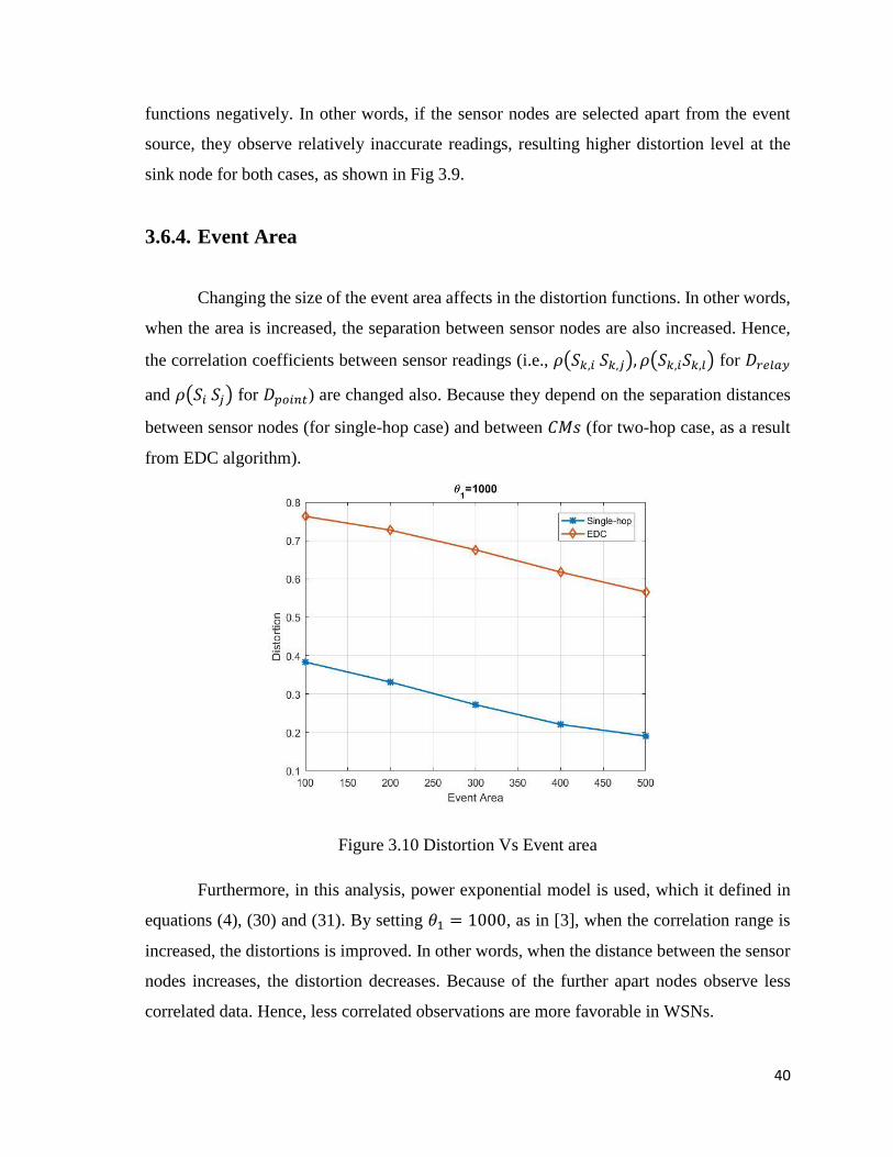
3.6.4. Event Area
Changing the size of the event area affects in the distortion functions. In other words,
when the area is increased, the separation between sensor nodes are also increased. Hence,
the correlation coefficients between sensor readings (i.e., 𝜌(𝑆𝑘,𝑖 𝑆𝑘,𝑗), 𝜌(𝑆𝑘,𝑖𝑆𝑘,𝑙) for 𝐷𝑟𝑒𝑙𝑎𝑦
and 𝜌(𝑆𝑖 𝑆𝑗) for 𝐷𝑝𝑜𝑖𝑛𝑡) are changed also. Because they depend on the separation distances
between sensor nodes (for single-hop case) and between 𝐶𝑀𝑠 (for two-hop case, as a result
from EDC algorithm).
Figure 3.10 Distortion Vs Event area
Furthermore, in this analysis, power exponential model is used, which it defined in
equations (4), (30) and (31). By setting 𝜃1 = 1000, as in [3], when the correlation range is
increased, the distortions is improved. In other words, when the distance between the sensor
nodes increases, the distortion decreases. Because of the further apart nodes observe less
correlated data. Hence, less correlated observations are more favorable in WSNs.

41
CHAPTER 4
SIMULATIONS
In this section, the proposed EDC clustering algorithm is simulated in MATLAB to
examine its detailed performance with respect to the single-hop communication model. For
this purpose, simulation results in different network scopes are reported with different
parameters to observe the performance of the proposed algorithm. The simulation is applied
in terms of distortion, energy consumption rate and network lifetime. Furthermore, the
influence of the harvesting energy on the network performance is presented with respect to
the same above terms.
4.1. Setup Parameters
In this section, some important parameters are defined. A total of 100 sensor nodes
are deployed randomly in 100×100, 200×200 and 300×300 square meters event area, based
on the uniform distribution. Changing event area, changes the density degree of nodes’
deployment. Furthermore, each sensor node requires to forward its observations to the sink
node continuously via single-hop or two-hop communication links. The sink node is assumed
to be located at the center of the event area. Furthermore, a cell tower, i.e., GSM900, can be
used as a renewable energy source. This tower is assumed to be located at the center of event
area as a harvesting source for all sensor nodes. Then each node can harvest energy, besides
its main duties.
Each sensor node has an additional circuit for energy harvesting similar to the
presented circuit in [13]. Hence, each sensor node has two antennas, one for harvesting and
the other one for communicating with others. The harvesting energy is available only if
sensor nodes are located within specific threshold distance, 𝑑0, ( due to free path loss model).
Without physical damages, sensor nodes run out from their energies with each iteration (time)
with respect to the proposed energy model in Chapter 3. The simulation parameters are
introduced in Table 4.1.

42
4.2. EDC algorithm
At the first stage of EDC algorithm, the sink node allocates all locations of sensor
nodes and estimates their receiving samples based on single-hop communication and
determines the resulted point distortion for all 𝑁 nodes, 𝐷𝑝𝑜𝑖𝑛𝑡(𝑁). After 𝐷𝑝𝑜𝑖𝑛𝑡(𝑁) is
calculated, the sink node is applied Vector Quantization (VQ). All sensor nodes are assumed
to be uniformly distributed in event area.
Table 4.1. Simulation Parameters
Hence, VQ is initiated with all sensor nodes locations as a vector source, code vector
length is one. According to EDC algorithm, the sink node starts to increase the code word
length until the remaining nodes (unrepresentative nodes) achieve distortion constraints as
shown in Fig 4.1. The maximum achievable distortion is defined according to:
Parameters Values
Area (100×100, 200×200 and 300×300) 𝑚2
Number of sensors, N 100
Sink node and GSM900 locations (50,50)
Initial energy 0.5 J
𝐸𝑒𝑙𝑒𝑐 50 nJ/bit
𝐸𝐷𝐴 5 nJ/bit
𝑑0 threshold distance 87 m
𝜀𝑓𝑠 10 PJ/bit/𝑚2
𝜀𝑚𝑝 0.0013 PJ/bit/𝑚4
L data packet size 1000 bytes
L-broadcast packet 25 bytes
Center frequency for harvesting GSM 900 950 MHZ
𝐺𝑡 , 𝐺𝑟 17 dB , 9 dB

43
𝐷𝑃𝑜𝑖𝑛𝑡(𝑁) + 𝐷𝑡ℎ𝑟𝑒𝑠𝑜𝑙𝑑 ≥ 𝐷𝑐𝑜𝑛𝑠𝑡𝑟𝑎𝑖𝑛𝑡. (4.1)
where 𝐷𝑃𝑜𝑖𝑛𝑡(𝑁) is the minimum distortion achieved when all the sensor nodes in the event
area send information to the sink [3]. And 𝐷𝑡ℎ𝑟𝑒𝑠𝑜𝑙𝑑 is threshold distortion for single-hop
case, which it is assumed to be equal to 0.001 for noiseless (𝜎𝑊2 = 0) and noisy (𝜎𝑊
2 = 0.5)
channel cases. Approximately, in both cases it produces similar results. But in noisy case, the
distortion is lifted up as shown in Fig 4.1 (a).
Figure 4.1 Network Clustering
After repeating the experiment over 100 trials (Monte Carlo), EDC approximately
selects 84 sensors nodes as unrepresentative nodes (CMs) and 16 representative nodes (CHs).
Then, the representative nodes (CHs) forms Voronoi diagrams (clusters) as shown in Fig 4.1
(b). Then, Fig 4.1 (b) represents a snapshot for the resulted network with the sink node which
is located at the center of event area. This network uses two-hop communication model, and
hence, we can use a relayed distortion function (64) to define the accuracy level. The
clustered-network is then compared with single-hop communication model. In single-hop
case, the VQ is also applied for sensor nodes and the result is unrepresentative nodes that
require to forward their observations. In 100 × 100 𝑚2 event area, the distortion for single-
hop, 𝐷𝑃𝑜𝑖𝑛𝑡(𝑐), is less than the distortion for two-hop (EDC) case, 𝐷𝑟𝑒𝑙𝑎𝑦 (64). Furthermore,
(a) (b)
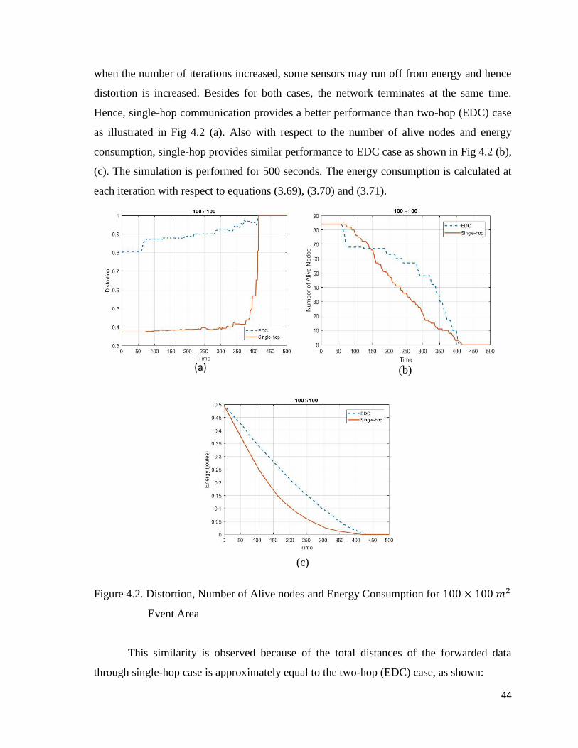
44
when the number of iterations increased, some sensors may run off from energy and hence
distortion is increased. Besides for both cases, the network terminates at the same time.
Hence, single-hop communication provides a better performance than two-hop (EDC) case
as illustrated in Fig 4.2 (a). Also with respect to the number of alive nodes and energy
consumption, single-hop provides similar performance to EDC case as shown in Fig 4.2 (b),
(c). The simulation is performed for 500 seconds. The energy consumption is calculated at
each iteration with respect to equations (3.69), (3.70) and (3.71).
Figure 4.2. Distortion, Number of Alive nodes and Energy Consumption for 100 × 100 𝑚2
Event Area
This similarity is observed because of the total distances of the forwarded data
through single-hop case is approximately equal to the two-hop (EDC) case, as shown:
(a) (b)
(c)
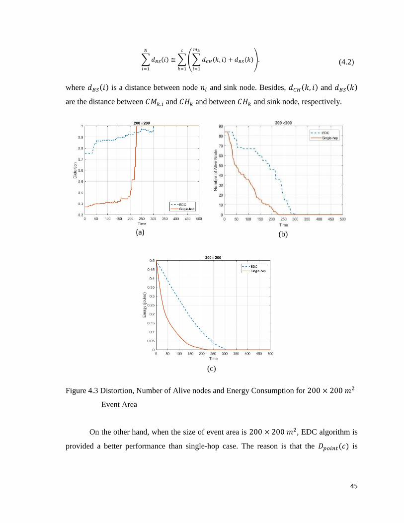
45
∑ 𝑑𝐵𝑆(𝑖)
𝑁
𝑖=1
≅ ∑ (∑ 𝑑𝐶𝐻(𝑘, 𝑖) + 𝑑𝐵𝑆(𝑘)
𝑚𝑘
𝑖=1
)
𝑐
𝑘=1
.
(4.2)
where 𝑑𝐵𝑆(𝑖) is a distance between node 𝑛𝑖 and sink node. Besides, 𝑑𝐶𝐻(𝑘, 𝑖) and 𝑑𝐵𝑆(𝑘)
are the distance between 𝐶𝑀𝑘,𝑖 and 𝐶𝐻𝑘 and between 𝐶𝐻𝑘 and sink node, respectively.
Figure 4.3 Distortion, Number of Alive nodes and Energy Consumption for 200 × 200 𝑚2
Event Area
On the other hand, when the size of event area is 200 × 200 𝑚2, EDC algorithm is
provided a better performance than single-hop case. The reason is that the 𝐷𝑝𝑜𝑖𝑛𝑡(𝑐) is
(a) (b)
(c)

46
decreasing faster that 𝐷𝑟𝑒𝑙𝑎𝑦, until all sensors expired as shown in Fig 4.3, because the total
distances to transmit data for single-hop case is greater than EDC case, as shown:
∑ 𝑑𝐵𝑆(𝑖)
𝑁
𝑖=1
> ∑ (∑ 𝑑𝐶𝐻(𝑘, 𝑖) + 𝑑𝐵𝑆(𝑘)
𝑚𝑘
𝑖=1
)
𝑐
𝑘=1
.
(4.3)
Figure 4.4 Distortion, Number of Alive nodes and Energy Consumption for 300 × 300 𝑚2
Event Area
Similarly, in case of 300 × 300 𝑚2 event area, the performance of EDC is much
better than single-hop case as in Fig 4.4. As a result, EDC is considered to be used for event
areas with sizes are greater than 100 × 100 𝑚2 and single-hop is considered to be used for
only 100 × 100 𝑚2 because of its advantage in distortion level.
(a) (b)
(c)

47
Figure 4.5 Distortion for Different Harvested Energies
Furthermore, by fixing the size of event area, another investigation is performed,
where a different harvesting energy levels (i.e., transmitted power, 𝑃𝑡, form cell tower [13])
is applied for each sensor node. Because of harvesting, an inactive sensor node can be
recharged and be active again, hence the distortion changes iteratively. Then, the distortion
level improved and made it less than the upper bound as possible as shown in Fig 4.5. The
upper bound in this simulation is set to be equal to one, i.e., it is the variance of source event
𝜎𝑆2. Furthermore, this improvement is happened because of the energy consumption rate, as
shown in Fig 4.6 (a), is reduced at each iteration and it aided the number of nodes to be alive
for longer time which is shown in Fig.4.6 (b).
(a) (b)
(c)

48
Figure 4.6 Energy Consumption and Number of Alive nodes for Different Harvested
Energies
(a) (b)

49
CHAPTER 5
CONCLUSION AND FUTURE WORKS
5.1. Conclusion
In both military and civil applications, the WSN is highly required. In most
applications, densely deployment has been used because of it is inexpensive to be deployed.
However, in densely deployment, the nearby sensors are spatially correlated, and hence their
readings are redundant, which causes wasting in energy and increasing overheading packets.
The EDC algorithm is presented to address these challenges by cluster the network based on
exploiting spatial correlations between sensor nodes through Vector Quantization. The main
contribution from exploiting spatial correlation is to ban the readings of cluster heads and
thus their duties are reduced and the network’s life time is improved. As a part of this
algorithm, a theoretical framework defining distortion for single-hop and two-hop
commutations model has been derived.
Additionally, the EDC algorithm has been presented for energy harvesting sensors.
Energy harvesting is enhancing the accuracy level. In other word, when sensor nodes harvest
energy, their life time is improved. Unlike non-harvesting case, when the network loss the
accuracy when all nodes die.
5.2. Future Works
The power constraints are not random. However, by changing this assumption and
model the power constraints randomly, another model it can be derived for distortion function
and another results are expected. Energy harvesting technology has been used in WSN and
hence it is good idea if the distortion function is connected with available harvesting power.
By developing another form for distortion for multi-hop communication model, it is possible
to compare EDC algorithm with other clustering algorithms.
50
BIBLIOGRAPHY
[1] I. F. Akyildiz, W. Su, Y. Sankarasubramaniam, and E. Cayirci, “Wireless sensor
networks: a survey” Computer Networks, vol. 38, pp. 393–422, 2002.
[2] S. Akbari, “Energy harvesting for wireless sensor networks review,” in Computer Science
and Information Systems (FedCSIS), 2014 Federated Conference on, Sept 2014, pp. 987–
992.
[3] M. C. Vuran and I. F. Akyildiz, “Spatial correlation-based collaborative medium access
control in wireless sensor networks” IEEE/ACM Transactions on Networking, vol. 14, no. 2,
pp. 316–329, April 2006.
[4] M. Gastpar and M. Vetterli, “Source-Channel Communication in Sensor Networks,”
Berlin, Heidelberg: Springer Berlin Heidelberg, 2003, pp.162–177. [Online]. Available:
http://dx.doi.org/10.1007/3-540-36978-3 11
[5] Z. Liu, W. Xing, B. Zeng, Y. Wang, and D. Lu, “Distributed spatial correlation-based
clustering for approximate data collection in wsns,” in Advanced Information Networking
and Applications (AINA), 2013 IEEE 27th International Conference on, March 2013, pp.
56–63.
[6] G. Zheng and S. Tang, “Spatial correlation-based mac protocol for event-driven wireless
sensor networks,” Journal of Networks, vol. 6, no. 2, 2011.
[7] S. K. Gupta, N. Jain, and P. Sinha, “Clustering protocols in wireless sensor networks: A
survey,” International Journal of Applied Information Systems, vol. 5, no. 2, pp. 41–50,
January 2013, published by Foundation of Computer Science, New York, USA.
[8] W. R. Heinzelman, A. Chandrakasan, and H. Balakrishnan, “Energy efficient
communication protocol for wireless microsensor networks,” in System Sciences, 2000.
Proceedings of the 33rd Annual Hawaii International Conference on, Jan 2000, pp. 10 pp.
vol.2–.
[9] M. Ye, C. Li, G. Chen, and J. Wu, “EECS: an energy efficient clustering scheme in
wireless sensor networks,” in PCCC 2005. 24th IEEE International Performance,
Computing, and Communications Conference, 2005., April 2005, pp. 535–540.
[10] S. Yoon and C. Shahabi, “Exploiting spatial correlation towards an energy efficient
clustered aggregation technique (cag) [wireless sensor network applications],” in IEEE
International Conference on Communications, 2005. ICC 2005. 2005, vol. 5, May 2005, pp.
3307–3313 Vol. 5.
[11] L. A. Villas, A. Boukerche, D. L. Guidoni, H. A. de Oliveira, R. B. de Araujo, and A.
A. Loureiro, “An energy-aware spatio-temporal correlation mechanism to perform efficient
51
data collection in wireless sensor networks,” Comput. Commun., vol. 36, no. 9, pp. 1054–
1066, May 2013. [Online]. Available: http://dx.doi.org/10.1016/j.comcom. 2012.04.007
[12] Y. Linde, A. Buzo, and R. Gray, “An algorithm for vector quantizer design,” IEEE
Transactions on Communications, vol. 28, no. 1, pp. 84– 95, Jan 1980.
[13] M. Arrawatia, M. S. Baghini, and G. Kumar, “Rf energy harvesting system from cell
towers in 900mhz band,” in Communications (NCC), 2011 National Conference on, Jan
2011, pp. 1–5.
[14] M. Gastpar and M. Vetterli, “On the capacity of large gaussian relay networks,” IEEE
Transactions on Information Theory, vol. 51, no. 3, pp. 765–779, March 2005.
[15] M. Di Francesco, S. K. Das, and G. Anastasi, “Data collection in wireless sensor
networks with mobile elements: A survey,” ACM Trans. Sen. Netw., vol. 8, no. 1, pp. 7:1–
7:31, Aug. 2011. [Online]. Available: http://doi.acm.org/10.1145/1993042.1993049
[16] I. F. Akyildiz and E. P. Stuntebeck, “Wireless underground sensor networks: research
challenges,” Ad Hoc Networks, vol. 4, no. 6, pp. 669–686, 2006.
[17] G. Werner-Allen, K. Lorincz, M. Ruiz, O. Marcillo, J. Johnson, J. Lees, and M. Welsh,
“Deploying a wireless sensor network on an active volcano,” IEEE Internet Computing, vol.
10, no. 2, pp. 18–25, March 2006.
[18] I. F. Akyildiz, T. Melodia, and K. R. Chowdhury, “A survey on wireless multimedia
sensor networks,” Computer. Network., vol. 51, no. 4, pp. 921–960, Mar. 2007. [Online].
Available: http://dx.doi.org/10.1016/ j.comnet.2006.10.002.
[19] M. Khelifi, I. Benyahia, S. Moussaoui, and F. Nat-Abdesselam, “An overview of
localization algorithms in mobile wireless sensor networks,” in 2015 International
Conference on Protocol Engineering (ICPE) and International Conference on New
Technologies of Distributed Systems (NTDS), July 2015, pp. 1–6.
[20] H. Huang, S. Xiao, X. Meng, and Y. Xiong, “A remote home security system based on
wireless sensor network and gsm technology,” in Networks Security Wireless
Communications and Trusted Computing (NSWCTC), 2010 Second International
Conference on, vol. 1, April 2010, pp. 535–538.
[21] M. T. Lazarescu, “Design of a wsn platform for long-term environmental monitoring
for iot applications,” IEEE Journal on Emerging and Selected Topics in Circuits and Systems,
vol. 3, no. 1, pp. 45–54, March 2013.
[22] E.M. Petriu, N.D. Georganas, D.C. Petriu, D. Makrakis, V.Z. Groza, “Sensor-based
information appliances,” IEEE Instrumentation and Measurement Magazine (December
2000) 31–35.

52
[23] M. P. urii, Z. Tafa, G. Dimi, and V. Milutinovi, “A survey of military applications of
wireless sensor networks,” in 2012 Mediterranean Conference on Embedded Computing
(MECO), June 2012, pp. 196–199.
[24] T. Cover and P. Hart, “Nearest neighbor pattern classification,” IEEE Transactions on
Information Theory, vol. 13, no. 1, pp. 21–27, January 1967.
[25] S. Toumpis and T. Tassiulas, “Optimal deployment of large wireless sensor networks,”
IEEE Trans. Information Theory, vol. 52, pp. 2935–2953, 2006.
[26] I. F. Akyildiz and E. P. Stuntebeck, “Wireless underground sensor networks: research
challenges,” Ad-Hoc Networks, vol. 4, pp. 669–686, 2006.
[27] M. Li, Y. Liu, “Underground structure monitoring with wireless sensor networks,” Proc.
the IPSN, Cambridge, MA, 2007.
[28] I. F. Akyildiz, D. Pompili and T. Melodia, “Challenges for efficient communication in
underwater acoustic sensor networks,” ACM Sigbed Review, vol. 1(2), pp. 3–8, 2004.
[29] J. Heidemann, Y. Li, A. Syed, J. Wills and W. Ye, “Underwater sensor networking:
research challenges and potential applications,” Proc. the Technical Report ISI-TR-2005-
603, USC/Information Sciences Institute, 2005.
[30] I. F. Akyildiz, T. Melodia, K.R. Chowdhury, “A survey on wireless multimedia sensor
networks,” Computer Networks, vol. 51, pp. 921–960, 2007.
[31] N. Bulusu, D. Estrin, L. Girod, J. Heidemann, “Scalable coordination for wireless sensor
networks: self-configuring localization systems,” Proc. Int. Symposium on Communication
Theory and Applications (ISCTA 2001), Ambleside, UK, July 2001.
[32] J. O. Berger, V. de Oliviera, and B. Sanso, “Objective Bayesian analysis of spatially
correlated data,” J. Amer. Statistical Assoc., vol. 96, no.456, pp. 1361–1374, 2001.
[33] G. L. Stuber, Principles of Mobile Communication. Norwell, MA:Kluwer, 2001.
[34] V. Poor, An Introduction to signal detection and estimation, 2𝑛𝑑 Edition, Springer-
Verlag, 1994.