Minimum-Distortion Embedding - Stanford University

Foundations and Trends® in Machine Learning

Minimum-Distortion Embedding

Suggested Citation: Akshay Agrawal, Alnur Ali and Stephen Boyd (2021), “Minimum-Distortion Embedding”, Foundations and Trends® in Machine Learning: Vol. 14, No. 3,pp 211–378. DOI: 10.1561/2200000090.

Akshay AgrawalStanford University

[email protected]

Alnur AliStanford University

[email protected]

Stephen BoydStanford [email protected]

This article may be used only for the purpose of research, teaching,and/or private study. Commercial use or systematic downloading (byrobots or other automatic processes) is prohibited without explicitPublisher approval. Boston — Delft

Contents

1 Introduction 2131.1 Contributions . . . . . . . . . . . . . . . . . . . . . . . . 2171.2 Outline . . . . . . . . . . . . . . . . . . . . . . . . . . . . 2171.3 Related work . . . . . . . . . . . . . . . . . . . . . . . . . 219

I Minimum-Distortion Embedding 224

2 Minimum-Distortion Embedding 2252.1 Embedding . . . . . . . . . . . . . . . . . . . . . . . . . . 2252.2 Distortion . . . . . . . . . . . . . . . . . . . . . . . . . . 2262.3 Minimum-distortion embedding . . . . . . . . . . . . . . . 2312.4 Constraints . . . . . . . . . . . . . . . . . . . . . . . . . . 2352.5 Simple examples . . . . . . . . . . . . . . . . . . . . . . . 2402.6 Validation . . . . . . . . . . . . . . . . . . . . . . . . . . 242

3 Quadratic MDE Problems 2473.1 Solution by eigenvector decomposition . . . . . . . . . . . 2483.2 Historical examples . . . . . . . . . . . . . . . . . . . . . 251

4 Distortion Functions 2554.1 Functions involving weights . . . . . . . . . . . . . . . . . 255

4.2 Functions involving original distances . . . . . . . . . . . . 2614.3 Preprocessing . . . . . . . . . . . . . . . . . . . . . . . . 265

II Algorithms 271

5 Stationarity Conditions 2725.1 Centered MDE problems . . . . . . . . . . . . . . . . . . 2755.2 Anchored MDE problems . . . . . . . . . . . . . . . . . . 2765.3 Standardized MDE problems . . . . . . . . . . . . . . . . 277

6 Algorithms 2806.1 A projected quasi-Newton algorithm . . . . . . . . . . . . 2816.2 A stochastic proximal algorithm . . . . . . . . . . . . . . . 287

7 Numerical Examples 2917.1 Quadratic MDE problems . . . . . . . . . . . . . . . . . . 2927.2 Other MDE problems . . . . . . . . . . . . . . . . . . . . 2957.3 A very large problem . . . . . . . . . . . . . . . . . . . . 2987.4 Implementation . . . . . . . . . . . . . . . . . . . . . . . 300

III Examples 307

8 Images 3088.1 Data . . . . . . . . . . . . . . . . . . . . . . . . . . . . . 3088.2 Preprocessing . . . . . . . . . . . . . . . . . . . . . . . . 3098.3 Embedding . . . . . . . . . . . . . . . . . . . . . . . . . . 309

9 Networks 3199.1 Data . . . . . . . . . . . . . . . . . . . . . . . . . . . . . 3199.2 Preprocessing . . . . . . . . . . . . . . . . . . . . . . . . 3229.3 Embedding . . . . . . . . . . . . . . . . . . . . . . . . . . 323

10 Counties 33110.1 Data . . . . . . . . . . . . . . . . . . . . . . . . . . . . . 33110.2 Preprocessing . . . . . . . . . . . . . . . . . . . . . . . . 33310.3 Embedding . . . . . . . . . . . . . . . . . . . . . . . . . . 333

11 Population Genetics 34011.1 Data . . . . . . . . . . . . . . . . . . . . . . . . . . . . . 34311.2 Preprocessing . . . . . . . . . . . . . . . . . . . . . . . . 34311.3 Embedding . . . . . . . . . . . . . . . . . . . . . . . . . . 344

12 Single-Cell Genomics 35012.1 Data . . . . . . . . . . . . . . . . . . . . . . . . . . . . . 35012.2 Preprocessing . . . . . . . . . . . . . . . . . . . . . . . . 35112.3 Embedding . . . . . . . . . . . . . . . . . . . . . . . . . . 351

13 Conclusions 360

Acknowledgements 363

References 364

Minimum-Distortion EmbeddingAkshay Agrawal1, Alnur Ali2 and Stephen Boyd3

1Stanford University; [email protected] University; [email protected] University; [email protected]

ABSTRACTWe consider the vector embedding problem. We are given afinite set of items, with the goal of assigning a representativevector to each one, possibly under some constraints (such asthe collection of vectors being standardized, i.e., having zeromean and unit covariance). We are given data indicatingthat some pairs of items are similar, and optionally, someother pairs are dissimilar. For pairs of similar items, we wantthe corresponding vectors to be near each other, and fordissimilar pairs, we want the vectors to not be near eachother, measured in Euclidean distance. We formalize this byintroducing distortion functions, defined for some pairs ofitems. Our goal is to choose an embedding that minimizesthe total distortion, subject to the constraints. We call thisthe minimum-distortion embedding (MDE) problem.The MDE framework is simple but general. It includes awide variety of specific embedding methods, such as spectralembedding, principal component analysis, multidimensionalscaling, Euclidean distance problems, dimensionality reduc-tion methods (like Isomap and UMAP), semi-supervisedlearning, sphere packing, force-directed layout, and others.It also includes new embeddings, and provides principledways of validating or sanity-checking historical and newembeddings alike.

Akshay Agrawal, Alnur Ali and Stephen Boyd (2021), “Minimum-Distortion Embed-ding”, Foundations and Trends® in Machine Learning: Vol. 14, No. 3, pp 211–378.DOI: 10.1561/2200000090.

212

In a few special cases, MDE problems can be solved exactly.For others, we develop a projected quasi-Newton methodthat approximately minimizes the distortion and scales tovery large data sets, while placing few assumptions on thedistortion functions and constraints. This monograph is ac-companied by an open-source Python package, PyMDE, forapproximately solving MDE problems. Users can select froma library of distortion functions and constraints or specifycustom ones, making it easy to rapidly experiment with newembeddings. Because our algorithm is scalable, and becausePyMDE can exploit GPUs, our software scales to problemswith millions of items and tens of millions of distortion func-tions. Additionally, PyMDE is competitive in runtime withspecialized implementations of specific embedding methods.To demonstrate our method, we compute embeddings forseveral real-world data sets, including images, an academicco-author network, US county demographic data, and single-cell mRNA transcriptomes.

1Introduction

An embedding of n items, labeled 1, . . . , n, is a function F mapping theset of items into Rm. We refer to xi = F (i) as the embedding vectorassociated with item i. In applications, embeddings provide concretenumerical representations of otherwise abstract items, for use in down-stream tasks. For example, a biologist might look for subfamilies ofrelated cells by clustering embedding vectors associated with individualcells, while a machine learning practitioner might use vector representa-tions of words as features for a classification task. Embeddings are alsoused for visualizing collections of items, with embedding dimension m

equal to one, two, or three.For an embedding to be useful, it should be faithful to the known

relationships between items in some way. There are many ways todefine faithfulness. A working definition of a faithful embedding is thefollowing: if items i and j are similar, their associated vectors xi andxj should be near each other, as measured by the Euclidean distance∥xi −xj∥2; if items i and j are dissimilar, xi and xj should be distant, orat least not close, in Euclidean distance. (Whether two items are similaror dissimilar depends on the application. For example two biologicalcells might be considered similar if some distance between their mRNA

1

2 Introduction

transcriptomes is small.) Many well-known embedding methods likeprincipal component analysis (PCA), spectral embedding (Chung andGraham, 1997; Belkin and Niyogi, 2002), and multidimensional scaling(Torgerson, 1952; Kruskal, 1964a) use this basic notion of faithfulness,differing in how they make it precise.

The literature on embeddings is both vast and old. PCA originatedover a century ago (Pearson, 1901), and it was further developed threedecades later in the field of psychology (Hotelling, 1933; Eckart andYoung, 1936). Multidimensional scaling, a family of methods for embed-ding items given dissimilarity scores or distances between items, wasalso developed in the field of psychology during the early-to-mid 20thcentury (Richardson, 1938; Torgerson, 1952; Kruskal, 1964a). Methodsfor embedding items that are vectors can be traced back to the early1900s (Menger, 1928; Young and Householder, 1938), and more recentlydeveloped methods use tools from convex optimization and convex anal-ysis (Biswas and Ye, 2004; Hayden et al., 1991). In spectral clustering,an embedding based on an eigenvector decomposition of the graphLaplacian is used to cluster graph vertices (Pothen et al., 1990; vonLuxburg, 2007). During this century, dozens of embedding methods havebeen developed for reducing the dimension of high-dimensional vectordata, including Laplacian eigenmaps (Belkin and Niyogi, 2002), Isomap(Tenenbaum et al., 2000), locally-linear embedding (LLE) (Roweis andSaul, 2000), stochastic neighborhood embedding (SNE) (Hinton andRoweis, 2003), t-distributed stochastic neighbor embedding (t-SNE)(Maaten and Hinton, 2008), LargeVis (Tang et al., 2016) and uniformmanifold approximation and projection (UMAP) (McInnes et al., 2018).All these methods start with either weights describing the similarity ofa pair of items, or distances describing their dissimilarity.

In this monograph we present a general framework for faithful em-bedding. The framework, which we call minimum-distortion embedding(MDE), generalizes the common cases in which similarities betweenitems are described by weights or distances. It also includes most ofthe embedding methods mentioned above as special cases. In our for-mulation, for some pairs of items, we are given distortion functionsof the Euclidean distance between the associated embedding vectors.Evaluating a distortion function at the Euclidean distance between

3

the vectors gives the distortion of the embedding for a pair of items.The goal is to find an embedding that minimizes the total or averagedistortion, possibly subject to some constraints on the embedding. Wefocus on three specific constraints: a centering constraint, which requiresthe embedding to have mean zero, an anchoring constraint, which fixesthe positions of a subset of the embedding vectors, and a standardiza-tion constraint, which requires the embedding to be centered and haveidentity covariance.

MDE problems are in general intractable, admitting efficiently com-putable (global) solutions only in a few special cases like PCA andspectral embedding. In most other cases, MDE problems can only beapproximately solved, using heuristic methods. We develop one suchheuristic, a projected quasi-Newton method. The method we describeworks well for a variety of MDE problems.

This monograph is accompanied by an open-source implementationfor specifying MDE problems and computing low-distortion embeddings.Our software package, PyMDE, makes it easy for practitioners toexperiment with different embeddings via different choices of distortionfunctions and constraint sets. Our implementation scales to very largedatasets and to embedding dimensions that are much larger than twoor three. This means that our package can be used for both visualizinglarge amounts of data and generating features for downstream tasks.PyMDE supports GPU acceleration and automatic differentiation ofdistortion functions by using PyTorch (Paszke et al., 2019) as thenumerical backend.

A preview of our framework. Here we give a brief preview of theMDE framework, along with a simple example of an MDE problem. Wediscuss the MDE problem at length in Chapter 2.

An embedding can be represented concretely by a matrix X ∈ Rn×m,whose rows xT

1 , . . . , xTn ∈ Rm are the embedding vectors. We use E to

denote the set of pairs, and fij : R+ → R to denote the distortionfunctions for (i, j) ∈ E . Our goal is to find an embedding that minimizes

4 Introduction

the average distortion

E(X) = 1|E|

∑(i,j)∈E

fij(dij),

where dij = ∥xi − xj∥2, subject to constraints on the embedding, ex-pressed as X ∈ X , where X ⊆ Rn×m is the set of allowable embeddings.Thus the MDE problem is

minimize E(X)subject to X ∈ X .

We solve this problem, sometimes approximately, to find an embedding.An important example is the quadratic MDE problem with stan-

dardization constraint. In this problem the distortion functions arequadratic fij(dij) = wijd2

ij , where wij ∈ R is a weight conveying simi-larity (when wij > 0) or dissimilarity (when wij < 0) of items i and j.We constrain the embedding X to be standardized, i.e., it must satisfy(1/n)XT X = I and XT 1 = 0, which forces the embedding vectors tospread out. While most MDE problems are intractable, the quadraticMDE problem is an exception: it admits an analytical solution viaeigenvectors of a certain matrix. Many well-known embedding methods,including PCA, spectral embedding, and classical multidimensionalscaling, are instances of quadratic MDE problems, differing only in theirchoice of pairs and weights. Quadratic MDE problems are discussed inChapter 3.

Why the Euclidean norm? A natural question is why we use theEuclidean norm as our distance measure between embedding vectors.First, when we are embedding into R2 or R3 for the purpose of vi-sualization or discovery, the Euclidean distance corresponds to actualphysical distance, making it a natural choice. Second, it is traditional,and follows a large number of known embedding methods like PCAand spectral embedding that also use Euclidean distance. Third, thestandardization constraint we consider in this monograph has a naturalinterpretation when we use the Euclidean distance, but would makelittle sense if we used another metric. Finally, we mention that thelocal optimization methods described in this monograph can be easily

1.1. Contributions 5

extended to the case where distances between embedding vectors aremeasured with a non-Euclidean metric.

1.1 Contributions

The main contributions of this monograph are the following:

1. We present a simple framework, MDE, that unifies and generalizesmany different embedding methods, both classical and modern.This framework makes it easier to interpret existing embeddingmethods and to create new ones. It also provides principled waysto validate, or at least sanity-check, embeddings.

2. We develop an algorithm for approximately solving MDE problems(i.e., for computing embeddings) that places very few assumptionson the distortion functions and constraints. This algorithm reliablyproduces good embeddings in practice and scales to large problems.

3. We provide open-source software that makes it easy for users tosolve their own MDE problems and obtain custom embeddings.Our implementation of our solution method is competitive inruntime to specialized algorithms for specific embedding methods.

1.2 Outline

This monograph is divided into three parts, I Minimum-DistortionEmbedding, II Algorithms, and III Examples.

Part I: Minimum-distortion embedding. We begin Part I by describingthe MDE problem and some of its properties in Chapter 2. We introducethe notion of anchored embeddings, in which some of the embeddingvectors are fixed, and standardized embeddings, in which the embeddingvectors are constrained to have zero mean and identity covariance.Standardized embeddings are favorably scaled for many tasks, such asfor use as features for supervised learning.

In Chapter 3 we study MDE problems with quadratic distortion,focusing on the problems with a standardization constraint. This class

6 Introduction

of problems has an analytical solution via an eigenvector decompositionof a certain matrix. We show that many existing embedding methods,including spectral embedding, PCA, Isomap, kernel PCA, and others,reduce to solving instances of the quadratic MDE problem.

In Chapter 4 we describe examples of distortion functions, showinghow different notions of faithfulness of an embedding can be captured bydifferent distortion functions. Some choices of the distortion functions(and constraints) lead to MDE problems solved by well-known methods,while others yield MDE problems that, to the best of our knowledge,have not appeared elsewhere in the literature.

Part II: Algorithms. In Part II, we describe algorithms for computingembeddings. We begin by presenting stationarity conditions for theMDE problem in Chapter 5, which are necessary but not sufficient foran embedding to be optimal. The stationarity conditions have a simpleform: the gradient of the average distortion, projected onto the set oftangents of the constraint set at the current point, is zero. This conditionguides our development of algorithms for computing embeddings.

In Chapter 6, we present a projected quasi-Newton algorithm forapproximately solving MDE problems. For very large problems, we addi-tionally develop a stochastic proximal algorithm that uses the projectedquasi-Newton algorithm to solve a sequence of smaller regularized MDEproblems. Our algorithms can be applied to MDE problems with differ-entiable average distortion, and any constraint set for which there existsan efficient projection onto the set and an efficient projection onto theset of tangents of the constraint set at the current point. This includesMDE problems with centering, anchor, or standardization constraints.

In Chapter 7, we present numerical examples demonstrating the per-formance of our algorithms. We also describe a software implementationof these methods, and briefly describe our open-source implementationPyMDE.

Part III: Examples. In Part III, we use PyMDE to approximatelysolve many MDE problems involving real datasets, including images(Chapter 8), co-authorship networks (Chapter 9), United States county

1.3. Related work 7

demographics (Chapter 10), population genetics (Chapter 11), andsingle-cell mRNA transcriptomes (Chapter 12).

1.3 Related work

Dimensionality reduction. In many applications, the original itemsare associated with high-dimensional vectors, and we can interpret theembedding into the smaller dimensional space as dimensionality reduc-tion. Dimensionality reduction can be used to reduce the computationalburden of numerical tasks, compared to carrying them out with theoriginal high-dimensional vectors. When the embedding dimension istwo or three, dimension reduction can also be used to visualize the orig-inal high-dimensional data and facilitate exploratory data analysis. Forexample, visualization is an important first step in studying single-cellmRNA transcriptomes, a relatively new type of data in which each cellis represented by a high-dimensional vector encoding gene expression(Sandberg, 2014; Kobak and Berens, 2019).

Dozens of methods have been developed for dimensionality reduc-tion. PCA, the Laplacian eigenmap (Belkin and Niyogi, 2002), Isomap(Tenenbaum et al., 2000), LLE (Roweis and Saul, 2000), maximum vari-ance unfolding (Weinberger and Saul, 2004), t-SNE (Maaten and Hinton,2008), LargeVis (Tang et al., 2016), UMAP (McInnes et al., 2018), andthe latent variable model (LVM) from (Saul, 2020) are all dimensionalityreduction methods. With the exception of t-SNE and the LVM, thesemethods can be interpreted as solving different MDE problems, as wewill see in Chapters 3 and 4. We exclude t-SNE because its objective func-tion is not separable in the embedding distances; however, methods likeLargeVis and UMAP have been observed to produce embeddings that aresimilar to t-SNE embeddings (Böhm et al., 2020). We exclude the LVMbecause it fits some additional parameters, in addition to the embedding.

Dimensionality reduction is sometimes called manifold learning inthe machine learning community, since some of these methods can bemotivated by a hypothesis that the original data lie in a low-dimensionalmanifold, which the dimensionality reduction method seeks to recover(Ma and Fu, 2011; Cayton, 2005; Lin and Zha, 2008; Wilson et al., 2014;Nickel and Kiela, 2017).

8 Introduction

Finally, we note that dimensionality reduction methods have beenstudied under general frameworks other than MDE (Ham et al., 2004;Yan et al., 2006; Kokiopoulou et al., 2011; Lawrence, 2011; Wang et al.,2020).

Metric embedding. Another well-studied class of embeddings arethose that embed one finite metric space into another one. There aremany ways to define the distortion of such an embedding. One commondefinition is the maximum fractional error between the embedding dis-tances and original distances, across all pairs of items. (This can be doneby insisting that the embedding be non-contractive, i.e., the embeddingdistances are at least the original distances, and then minimizing themaximum ratio of embedding distance to original distance.)

An important result in metric embedding is the Johnson-LindenstraussLemma, which states that a linear map can be used to reduce the dimen-sion of vector data, scaling distances by no more than (1 ± ϵ), when thetarget dimension m is O(log n/ϵ2) (Johnson and Lindenstrauss, 1984).Another important result is due to Bourgain, who showed that any finitemetric can be embedded in Euclidean space with at most a logarithmicdistortion (Bourgain, 1985). A constructive method via semidefiniteprogramming was later developed (Linial et al., 1995). Several otherresults, including impossibility results, have been discovered (Indyket al., 2017), and some recent research has focused on embedding intonon-Euclidean spaces, such as hyperbolic space (Sala et al., 2018).

In this monograph, for some of the problems we consider, all that isrequired is to place similar items near each other, and dissimilar itemsnot near each other; in such applications we may not even have origi-nal distances to preserve. In other problems we do start with originaldistances. In all cases we are interested in minimizing an average of dis-tortion functions (not maximum), which is more relevant in applications,especially since real-world data is noisy and may contain outliers.

Force-directed layout. Force-directed methods are algorithms fordrawing graphs in the plane in an aesthetically pleasing way. In aforce-directed layout problem, the vertices of the graph are considered

1.3. Related work 9

to be nodes connected by springs. Each spring exerts attractive or repul-sive forces on the two nodes it connects, with the magnitude of the forcesdepending on the Euclidean distance between the nodes. Force-directedmethods move the nodes until a static equilibrium is reached, with zeronet force on each node, yielding an embedding of the vertices into R2.Force-directed methods, which are also called spring embedders, can beconsidered as MDE problems in which the distortion functions give thepotential energy associated with the springs. Force-directed layout isa decades-old subject (Tutte, 1963; Eades, 1984; Kamada and Kawai,1989), with early applications in VLSI layout (Fisk et al., 1967; Quinnand Breuer, 1979) and continuing modern interest (Kobourov, 2012).

Low-rank models. A low-rank model approximates a matrix by oneof lower rank, typically factored as the product of a tall and a widematrix. These factors can be interpreted as embeddings of the rowsand columns of the original matrix. Well-known examples of low-rankmodels include PCA and non-negative matrix factorization (Lee andSeung, 1999); there are many others (Udell et al., 2016, §3.2). PCA (andits kernelized version) can be interpreted as solving an MDE problem,as we show in §3.2.

X2vec. Embeddings are frequently used to produce features for down-stream machine learning tasks. Embeddings for this purpose were popu-larized with the publication of word2vec in 2013, an embedding methodin which the items are words (Mikolov et al., 2013). Since then, dozensof embeddings for different types of items have been proposed, suchas doc2vec (Le and Mikolov, 2014), node2vec (Grover and Leskovec,2016) and related methods (Perozzi et al., 2014; Tang et al., 2015),graph2vec (Narayanan et al., 2017), role2vec (Ahmed et al., 2020),(batter-pitcher)2vec (Alcorn, 2016), BioVec, ProtVec, and GeneVec (As-gari and Mofrad, 2015), dna2vec (Ng, 2017), and many others. Someof these methods resemble MDE problems, but most of them do not.Nonetheless MDE problems generically can be used to produce suchX2vec-style embeddings, where X describes the type of items.

10 Introduction

Neural networks. Neural networks are commonly used to generateembeddings for use in downstream machine learning tasks. One genericneural network based embedding method is the auto-encoder, whichstarts by representing items by (usually large dimensional) input vectors,such as one-hot vectors. These vectors are fed into an encoder neuralnetwork, whose output is fed into a decoder network. The output of theencoder has low dimension, and will give our embedding. The decoderattempts to reconstruct the original input from this low-dimensionalintermediate vector. The encoder and decoder are both trained sothe decoder can, at least approximately, reproduce the original input(Goodfellow et al., 2016, §14).

More generally, a neural network may be trained to predict somerelevant quantity, and the trained network’s output (or an intermediateactivation) can be used as the input’s embedding. For example, neuralnetworks for embedding words (or sequences of words) are often trainedto predict masked words in a sentence; this is the basic principle under-lying word2vec and BERT, two well-known word embedding methods(Mikolov et al., 2013; Devlin et al., 2019). Similarly, intermediate ac-tivations of convolutional neural networks like residual networks (Heet al., 2016), trained to classify images, are often used as embeddings ofimages. Neural networks have also been used for embedding single-cellmRNA transcriptomes (Szubert et al., 2019).

Software. There are several open-source software libraries for spe-cific embedding methods. The widely used Python library sci-kit learn(Pedregosa et al., 2011) includes implementations of PCA, spectral em-bedding, Isomap, locally linear embedding, multi-dimensional scaling,and t-SNE, among others. The umap-learn package implements UMAP(McInnes, 2020b), the openTSNE package provides a more scalable vari-ant of t-SNE (Poličar et al., 2019), and GraphVite (which can exploitmultiple CPUs and GPUs) implements a number of embedding methods(Zhu et al., 2019). Embeddings for words and documents are available ingensim (Řehůřek and Sojka, 2010), Embeddings.jl (White and Ellison,2019), HuggingFace transformers (HuggingFace, 2020), and BERT (De-vlin, 2020). Force-directed layout methods are implemented in graphviz(Gansner and North, 2000), NetworkX (Hagberg et al., 2008), qgraph(Epskamp et al., 2012), and NetworkLayout.jl (NetworkLayout.jl 2020).

1.3. Related work 11

There are also several software libraries for approximately solvingoptimization problems with orthogonality constraints (which the MDEproblem with standardization constraint has). Some examples includeManopt (and its related packages PyManopt and Manopt.jl) (Boumalet al., 2014; Townsend et al., 2016; Bergmann, 2020), Geoopt (Kochurovet al., 2020), and McTorch (Meghwanshi et al., 2018). More generally,problems with differentiable objective and constraint functions can beapproximately solved using solvers for nonlinear programming, suchas SNOPT (Gill et al., 2002) (which is based on sequential quadraticprogramming) and IPOPT (Wächter and Biegler, 2006) (which is basedon an interior-point method).

Part I

Minimum-DistortionEmbedding

2Minimum-Distortion Embedding

In this chapter we introduce the minimum-distortion embedding problemand explore some of its general properties.

2.1 Embedding

We start with a finite set of items V, which we label as 1, . . . , n, soV = {1, . . . , n}. An embedding of the set of items V into Rm is a functionF : V → Rm. We denote the values of F by xi = F (i), i = 1, . . . , n, anddenote the embedding concretely by a matrix X ∈ Rn×m,

X =

xT

1xT

2...

xTn

.

The rows of X are the transposes of the vectors associated with theitems 1, . . . , n. The columns of X can be interpreted as m features orattributes of the items, with Xij = (xi)j the value of jth feature orattribute for item i; the jth column of X gives the values of the jthfeature assigned to the n items.

13

14 Minimum-Distortion Embedding

Throughout this monograph, the quality of an embedding X willonly depend on the embedding distances dij between items i and j,defined as

dij = ∥xi − xj∥2, i, j = 1, . . . , n,

i.e., dij is the Euclidean distance between the vectors xi and xj . Embed-ding distances are evidently not affected by translation of the embeddedpoints, i.e., replacing each xi by xi +a, where a ∈ Rm, or by orthogonaltransformation, i.e., replacing each xi by Qxi, where Q is an orthogonalm × m matrix. If there are no constraints on the embedding vectors,then without any loss of generality we can assume that the average ofthe xi is zero, or equivalently, XT 1 = 0, where 1 is the vector with allentries one. This means that each of the m features (columns of X) hasmean value zero across our n items.

2.2 Distortion

We express our desires about the embedding distances by distortionfunctions associated with embedding distances. These have the form

fij : R+ → R

for (i, j) ∈ E , where E ⊆ V × V is the set of item pairs for which wehave an associated function. We will assume that E is nonempty, andthat i < j for every (i, j) ∈ E .

The value fij(dij) is the distortion for the pair (i, j) ∈ E : the smallerfij(dij) is, the better the embedding captures the relationship betweenitems i and j. We can interpret these distortion functions as the weightsof a generalized graph (V, E), in which the edge weights are functions,not scalars.

We will assume that the distortion functions fij are differentiable.As in many other applications, however, we have observed that thealgorithm we propose, which assumes differentiability, works well inpractice even when the distortion functions are not differentiable.

2.2.1 Examples

The distortion functions fij we will encounter typically derive fromgiven weights (or similarities) associated with pairs of items, or from

2.2. Distortion 15

associated deviations (or distances or dissimilarities) between items,or both. Distortion functions can be also derived from one or morerelations (or undirected graphs) on the items. Below, we give simpleexamples of such distortion functions. We give many more examples inChapter 4.

Distortion functions derived from weights. We start with a set ofnonzero weights wij ∈ R, for (i, j) ∈ E . The larger wij , the more similaritems i and j are; negative weights indicate dissimilarity. We partitionthe edges into those associated with positive weights (similar items)and negative weights (dissimilar items), with

Esim = {(i, j) | wij > 0}, Edis = {(i, j) | wij < 0},

so E = Esim ∪ Edis and Esim ∩ Edis = ∅.Distortion functions derived from weights have the form

fij(dij) =

wijps(dij), (i, j) ∈ Esim

wijpd(dij), (i, j) ∈ Edis

where ps and pd are penalty functions associated with positive weights(similar items) and negative weights (dissimilar items), respectively.The penalty functions are increasing, so fij is increasing when wij

is positive and decreasing when wij is negative. Roughly speaking,the closer vectors associated with similar items are, and the farthervectors associated with dissimilar items are, the lower the distortion.The weights wij , which indicate the degree of similarity or dissimilarity,scale the penalty functions.

Perhaps the simplest distortion function derived from weights is thequadratic

fij(dij) = wijd2ij ,

for which ps(dij) = pd(dij) = d2ij . The quadratic distortion is plotted

in Figure 2.1, for weights wij = 1 and wij = −1. For wij = 1, whichmeans items i and j are similar, the distortion rises as the distancebetween xi and xj increases; for wij = −1, which means items i and j

are dissimilar, the distortion is negative and becomes more negative asthe distance between xi and xj increases. We will study the quadraticpenalty in Chapter 3.


0 1 2 3

dij

−10

−5

0

5

10

p(dij

)

wij = +1

wij = −1

Figure 2.1: Quadratic penalties, with wij = +1 or wij = −1 for (i, j) ∈ E .

Distortion functions derived from deviations. We start with nonneg-ative numbers δij for (i, j) ∈ E that represent deviations or (original)distance between items i and j, with small δij meaning the items aresimilar and large δij meaning the items are dissimilar. The smaller δij ,the more similar items i and j are. The original deviation data δij neednot be a metric.

Distortion functions derived from deviations or distances have thegeneral form

fij(dij) = ℓ(δij , dij),

where ℓ is a loss function, which is nonnegative, with ℓ(δij , δij) = 0,decreasing in dij for dij < δij and increasing for dij > δij . We caninterpret the given deviation δij as a target or desired value for theembedding distance dij ; the distortion ℓ(δij , dij) measures the differencebetween the target distance and the embedding distance.

The simplest example uses a square loss,

fij(dij) = (δij − dij)2,

the square of the difference between the given deviation and the embed-ding distance. Distortions derived from the square loss and deviationsare shown in Figure 2.2, for δij = 0.2 and δij = 1. For original deviationδij = 1, the distortion has its minimum value at dij = 1, i.e., when

2.2. Distortion 17

0 1 2 3

dij

0.0

2.5

5.0

7.5

`(dij,δij

)

δij = 1

δij = 0.2

Figure 2.2: Quadratic losses, with δij = 1 or δij = 0.2 for (i, j) ∈ E .

the distance between xi and xj is one. It rises as dij deviates from thetarget δij = 1.

Distortion functions derived from a graph. In some applications westart with an undirected graph or a relation on the items, i.e., a set ofpairs E . The associated distortion function is

fij(dij) = p(dij), (i, j) ∈ E ,

where p is a penalty function, which is increasing. Such distortionfunctions can be interpreted as deriving from weights or deviations,in the special case when there is only one value for the weights ordeviations. The simplest such distortion function is quadratic, withp(dij) = d2

ij .

Distortion functions derived from multiple graphs. As a variation, wecan have multiple original graphs or relations on the items. For examplesuppose we have Esim, a set of pairs of items that are similar, and alsoEdis, a set of pairs of items that are dissimilar, with Esim ∩ Edis = ∅.From these two graphs we can derive the distortion functions

fij(dij) =

ps(dij) (i, j) ∈ Esim

−pd(dij) (i, j) ∈ Edis,


with E = Esim ∪ Edis, where ps and pd are increasing penalty functionsfor similar and dissimilar pairs, respectively. This is a special case ofdistortion functions described by weights, when the weights take ononly two values, +1 (for similar items) and −1 (for dissimilar items).

Connections between weights, deviations, and graphs. The distinc-tion between distortion functions derived from weights, deviations, orgraphs is not sharp. As a specific example, suppose we are given someoriginal deviations δij , and we take

fij(dij) ={

d2ij δij ≤ ϵ

0 otherwise,(i, j) ∈ E ,

where ϵ is a given positive threshold. This natural distortion functionidentifies an unweighted graph of neighbors (defined by small originaldistance or deviation), and puts unit weight quadratic distortion onthose edges. (We could just as well have started with original similaritiesor weights wij and constructed the neighbor graph as wij ≥ ϵ.) Thisdistortion evidently combines the ideas of distances, weights, and graphs.

2.2.2 Average distortion

We evaluate the quality of an embedding by its average distortion,defined as

E(X) = 1|E|

∑(i,j)∈E

fij(dij).

The smaller the average distortion, the more faithful the embedding.In Chapter 4, we will see that a wide variety of notions of faithfulnessof an embedding can be captured by different choices of the distortionfunctions fij . (Our use of the symbol E to denote average distortion ismeant to vaguely hint at energy, from a mechanical interpretation wewill see later.)

The average distortion E(X) models our displeasure with the em-bedding X. With distortion functions defined by weights, small E(X)corresponds to an embedding with vectors associated with large (posi-tive) weights (i.e., similar items) typically near each other, and vectorsassociated with negative weights (i.e., dissimilar items) not near each

2.3. Minimum-distortion embedding 19

other. For distortion functions defined by deviations, small E(X) meansthat the Euclidean distances between vectors are close to the originalgiven deviations.

Evidently, (i, j) ∈ E means that E(X) does not depend on dij . Wecan interpret (i, j) ∈ E in several related ways. One interpretation isthat we are neutral about the distance dij , that is, we do not care if itis small or large. Another interpretation is that the data required tospecify the distortion fij , such as a weight wij or an original distanceδij , is not available.

2.3 Minimum-distortion embedding

We propose choosing an embedding X ∈ Rn×m that minimizes theaverage distortion, subject to X ∈ X , where X is the set of feasible orallowable embeddings. This gives the optimization problem

minimize E(X)subject to X ∈ X ,

(2.1)

with optimization variable X ∈ Rn×m. We refer to this problem as theminimum-distortion embedding (MDE) problem, and we call a solutionto this problem a minimum-distortion embedding.

In this monograph we will focus on three specific constraint sets X :the set of embeddings centered at the origin, the set of embeddings inwhich some of the embedding vectors are anchored (fixed) to specificvalues, and the set of standardized embeddings, which are centeredembeddings with unit covariance. These constraint sets are describedin §2.4.

MDE problems can be solved exactly only in a few special cases, oneof which is described in Chapter 3. In most other cases, solving an MDEproblem exactly is intractable, so in Chapter 6 we propose heuristicmethods to solve it approximately. In our experience, these methodsoften find low-distortion embeddings and scale to large datasets (Chapter7). With some abuse of language, we refer to an embedding that is anapproximate solution of the MDE problem as a minimum-distortionembedding, even if it does not globally solve (2.1).


With our assumption that the distortion functions are differentiable,the average distortion E is differentiable, provided the embeddingvectors are distinct, i.e., xi = xj for (i, j) ∈ E , i = j, which impliesdij > 0 for (i, j) ∈ E . It is differentiable even when dij = 0, providedf ′

ij(0) = 0. For example, E is differentiable (indeed, quadratic) whenthe distortion functions are quadratic.

The MDE problem (2.1) admits multiple interesting interpreta-tions. Thinking of the problem data as a generalized weighted graph, aminimum-distortion embedding can be interpreted as a representationof the vertices by vectors that respects the geometry of the graph, con-necting our problem to long lines of work on graph embeddings (Linialet al., 1995; Yan et al., 2006; Chung and Graham, 1997; Hamilton et al.,2017). The MDE problem can also be given a mechanical interpretation,connecting it to force-directed layout (Eades, 1984).

Mechanical interpretation. In the mechanical interpretation, we con-sider xi to be a point in Rm associated with item i. We imagine eachpair of points (i, j) ∈ E as connected by a spring with potential energyfunction fij , i.e., fij(dij) is the elastic stored energy in the spring whenit is extended a distance dij . The spring associated with (i, j) ∈ E has atension force versus extension given by f ′

ij . A force with this magnitudeis applied to both points i and j, each in the direction of the other.Thus the spring connecting xi and xj contributes the (vector) forces

f ′ij(dij) xj − xi

∥xi − xj∥2, −f ′

ij(dij) xj − xi

∥xi − xj∥2,

on the points xi and xj , respectively. When f ′ij is positive, the force is

attractive, i.e., it pulls the points xi and xj toward each other. Whenf ′

ij is negative, the force is repulsive, i.e., it pushes the points xi and xj

away from each other.Distortion function derived from weights are always attractive for

positive weights (pairs of similar items), and always repulsive for negativeweights (pairs of dissimilar items). Distortion functions derived fromdeviations are attractive when dij > δij and repulsive when dij < δij .For such distortion functions, we can think of δij as the natural lengthof the spring, i.e., the distance at which it applies no forces on the

2.3. Minimum-distortion embedding 21

0 1 2 3

dij

0.0

2.5

5.0

7.5fij(dij)

f ′ij(dij)

0 1 2 3

dij

−7.5

−5.0

−2.5

0.0

fij(dij)

f ′ij(dij)

Figure 2.3: Potential energy and force magnitude for quadratic distortion functions.Left. An attractive distortion function. Right. A repulsive distortion function.

points it connects. Figure 2.3 shows the potential energy and force forquadratic distortion functions, with weight +1 (left) and −1 (right).Figure 2.4 shows the potential energy and force for a function associatedwith a quadratic loss.

The MDE objective E(X) is the average elastic stored energy in allthe springs. The MDE problem is to find a minimum total potentialenergy configuration of the points, subject to the constraints. Whenthe constraint is only XT 1 = 0, such a configuration corresponds toone in which the net force on each point, from its neighbors, is zero.(Such a point corresponds to a mechanical equilibrium, not necessarilyone of minimum energy.) When there are constraints beyond XT 1 = 0,the mechanical interpretation is a bit more complicated, since theconstraints also contribute an additional force on each point, related toan optimal dual variable for the constraint.

Single-index notation. To simplify the notation, we will sometimesuse a single index k instead of a tuple of indices (i, j) to represent a pairof items. Specifically, we impose an ordering on the tuples (i, j) ∈ E ,labeling them 1, . . . , p, where p = |E| is the number of pairs for whichdistortion functions are given. For a pair k ∈ {1, . . . , p}, we write i(k)to denote its first item and j(k) to denote the second item. We use dk


0 1 2 3

dij

−2

0

2

4fij(dij)

f ′ij(dij)

Figure 2.4: Potential energy and force magnitude for a distortion function that isattractive for dij > 1 and repulsive for dij < 1.

to denote the embedding distance for the kth pair,

dk = ∥xi(k) − xj(k)∥2, k = 1, . . . , p,

with d ∈ Rp the vector of embedding distances. Similarly, we definethe vector distortion function f : Rp → Rp, whose components are thescalar distortion functions fk, k = 1, . . . , p. Using this notation, theaverage distortion is

E(X) = 1p

p∑k=1

fk(dk) = 1T f(d)/p.

We note for future reference that p ≤ n(n − 1)/2, with equalitywhen the graph is full. For a connected graph, we have p ≥ n − 1, withequality occurring when the graph is a chain. In many applications thetypical degree is small, in which case p is a small multiple of n.

Incidence matrix. Since the problem data can be interpreted as agraph, we can associate with it an incidence matrix A ∈ Rn×p (Boydand Vandenberghe, 2018, §7.3), defined as

Aij =

1 (i, j) ∈ E−1 (j, i) ∈ E0 otherwise.

(2.2)

2.4. Constraints 23

(Recall that we assume i < j for each (i, j) ∈ E .) The kth column ofA, which we denote ak, is associated with the kth pair or edge. Eachcolumn has exactly two non-zero entries, with values ±1, that give theitems connected by the edge. We can express ak as ak = ei(k) − ej(k),where el is the lth unit vector in Rn.

We can express the embedding distances compactly using the inci-dence matrix. Using single-index notation, the kth distance dk can bewritten as

dk = ∥XT ak∥2,

or equivalentlydk =

√(AT XXT A)kk.

We mention briefly that the MDE problem can be alternatively parame-trized via the Gram matrix G = XXT , since dk =

√aT

k Gak. For someconstraint sets X , the resulting rank-constrained optimization problemcan be approximately solved by methods that manipulate the squareroot of G, using techniques introduced in Burer and Monteiro (2003)and Burer and Monteiro (2005). We will not use this parametrizationin the sequel.

2.4 Constraints

2.4.1 Centered embeddings

We say that an MDE problem is centered or unconstrained when theconstraint set is X = C, where

C = {X | XT 1 = 0} (2.3)

is the set of centered embeddings. (Recall that the constraint XT 1 = 0is without loss of generality.) An unconstrained MDE problem can failto be well-posed, i.e., it might not have a solution or might admit trivialsolutions.

When an unconstrained MDE problem does have a solution, itis never unique, since both the constraint set C and the objective E

are invariant under rotations. If X⋆ is any optimal embedding, thenX = X⋆Q is also optimal, for any orthogonal m × m matrix Q.


2.4.2 Anchored embeddings

In an anchored MDE problem, some of the vectors xi are known andfixed, with

xi = xgiveni , i ∈ K, (2.4)

where K ⊆ V is the set of indices of vectors that are fixed (or anchored),and xgiven

i ∈ Rm are the given values for those vectors. We call (2.4) ananchor constraint; the items with vertices in K are anchored, and theremaining are free.

We will use A to represent a set of anchored embeddings, i.e.

A = {X | xi = xgiveni , i ∈ K}.

(The constraint set A depends on K and xgiveni , but we suppress this de-

pendence in our notation to keep it simple.) Unlike centered embeddings,the constraint set A is not closed under orthogonal transformations. Inparticular, MDE problems with this constraint are neither translationnor rotation invariant.

An anchor constraint has a natural mechanical interpretation: theanchored vertices are physically fixed to given positions (as if by nails).We will later describe the force that the nails exert on their associatedanchored points. Not surprisingly, in an optimal anchored embedding,the net force on each point (due to its neighbors and its nail, if it isanchored) is zero.

Incremental embedding. Anchor constraints can be used to buildan embedding incrementally. In an incremental embedding, we startwith an embedding of X ∈ Rn×m of a set of items V = {1, . . . , n}.We later obtain a few additional items V ′ = {n + 1, . . . , n + n′} (withn′ ≪ n), along with a set of pairs E ′ ⊆ (V ∪ V ′) × (V ∪ V ′) and theirassociated distortion functions relating old items to new items (andpossibly relating the new items to each other), i.e., (i, j) ∈ E ′ impliesi ∈ V and j ∈ V ′, or i, j ∈ V ′ (and i < j). We seek a new embeddingX ′ ∈ Rn+n′×m in which the first n embedding vectors match the originalembedding, and the last n + 1 embedding vectors correspond to thenew items. Such an embedding is readily found by anchoring the firstn embedding vectors to their original values, leaving only the last

2.4. Constraints 25

n + 1 embedding vectors free, and minimizing the average distortion.There are two approaches to handling centering or standardizationconstraints in incremental embedding. The simplest is to simply ignorethese constraints, which is justified when n′ ≪ n, so the new embeddingX ′ likely will not violate the constraints by much. It is also possibleto require that the new embedding X ′ satisfy the constraints. Thisapproach requires care; for example, suppose we are to add just onenew item, i.e., n′ = 1, and we insist that the new embedding X ′ becentered, like the original one X. In this case, the only possible choicefor the vector associated with the new item is xn+1 = 0.

Incremental embedding can be used to develop a feature map fornew (unseen) items, given some distortion functions relating the newitem to the original ones (say, the training items). In this case we haven′ = 1; we embed the new item n + 1 so as to minimize its averagedistortion with respect to the original items.

Placement problems. While MDE problems are usually nonconvex,anchored MDE problems with nondecreasing convex distortion functionsare an exception. This means that some anchored MDE problems can beefficiently and globally solved. These MDE problems can be interpretedas (convex) placement problems, which are described in Boyd andVandenberghe (2004, §8.7) and have applications to VLSI circuit design(Sherwani, 2012).

Semi-supervised learning. Anchored embeddings also arise in graph-based semi-supervised learning problems. We interpret the vectors xi,i ∈ K, as the known labels; our job is to assign labels for i ∈ K, usinga prior graph with positive weights that indicate similarity. In graph-based semi-supervised learning (Xu, 2010; El Alaoui et al., 2016), thisis done by solving an anchored MDE problem with quadratic distortionfunctions fij(dij) = wijd2

ij , which as mentioned above is convex andreadily solved.


2.4.3 Standardized embeddings

The set of standardized embeddings is

S = {X | (1/n)XT X = I, XT 1 = 0}. (2.5)

The standardization constraint X ∈ S requires that the collection ofvectors x1, . . . , xn has zero mean and unit covariance. We can expressthis in terms of the m feature columns of the embedding X ∈ S: theyhave zero mean, are uncorrelated, and have root-mean-square (RMS)value one; these properties are often desirable when the embeddingis used in downstream machine learning tasks. We refer to the MDEproblem as standardized when X = S.

Because S is a compact set, the standardized MDE problem has atleast one solution. Since S is invariant under rotations, the standardizedMDE problem has a family of solutions: if X⋆ is an optimal embedding,so is X = X⋆Q, for any m × m orthogonal matrix Q.

Natural length in a standardized embedding. We note that for X ∈ S,the sum of the squared embedding distances is constant,∑

1≤i<j≤n

d2ij = n2m. (2.6)

(Note that this is the sum over all pairs (i, j) with i < j, not just thepairs in E .) To see this, we observe that

n∑i,j=1

d2ij = 2n

n∑i=1

∥xi∥22 − 2

n∑i,j=1

xTi xj .

The first term on the right-hand side equals 2n2m, sincen∑

i=1∥xi∥2

2 = tr(XXT ) = tr(XT X) = nm,

while the second term equals 0, since XT 1 = 0. (Here tr denotes thetrace of a matrix, i.e., the sum of its diagonal entries.)

From (2.6), we can calculate the RMS value of all n(n − 1)/2 em-bedding distances. We will refer to this value as the natural length dnat

2.4. Constraints 27

of the embedding, with

dnat =√

2nm

n − 1 . (2.7)

For X ∈ S, dnat can be interpreted as the typical value of embeddingdistances. We will see later that this number is useful in choosingappropriate distortion functions.

2.4.4 Attraction, repulsion, and spreading

When all distortion functions are nondecreasing, we say the objectiveis attractive. In the mechanical interpretation, this means that thereis a positive (attractive) tension between all pairs of points (i, j) ∈ E .Roughly speaking, the distortion functions only encode similarity be-tween items, and not dissimilarity; the objective encourages neighboringembedded points to be near each other. When the only constraint is thatthe embedding is centered, i.e., X = C, a globally optimal embedding isX = 0, which is not useful. Roughly speaking, all forces between pointsare attractive, so the points collapse to a single point, which must be 0to achieve centering.

When the objective is attractive, we need a constraint to enforcespreading the points. Anchored and standardized constraints both servethis purpose, and enforce spreading of the points when the objective isattractive. When some distortion functions can be repulsive, i.e., f ′

ij(dij)can be negative, we can encounter the opposite problem, which is thatsome points might spread without bound (i.e., the MDE problem doesnot have a solution). In such situations, an anchoring or standardizedconstraint can serve the role of keeping some points from spreadingwithout bound.

The standardization constraint keeps both pathologies from happen-ing. The points are required to be spread, and also bounded. Since S iscompact, there is always a solution of the standardized MDE problem.

2.4.5 Comparing embeddings

In some cases we want to compare or evaluate a distance between twoembeddings of the same set of items, X and X. When the embeddings


are anchored, a reasonable measure of how different they are is themean-square distance between the two embeddings,

1n

∥X − X∥2F = 1

n

n∑i=1

∥xi − xi∥22.

When the embeddings are centered or standardized, the comparisonis more subtle, since in these cases any embedding can be transformedby an orthogonal matrix with no effect on the constraints or objective.As mentioned above, X and XQ, where QT Q = I, are equivalent forthe MDE problem. A reasonable measure of how different the twoembeddings are is then

∆ = inf{∥X − XQ∥2F /n | QT Q = I},

the minimum mean-square distance over all orthogonal transformationsof the second one (which is same as the minimum over transforming X,or both X and X).

We can work out the distance ∆ analytically, and also find anoptimal Q, i.e., one that achieves the minimum. This is useful forvisualization, if we are plotting X or X (presumably in the case withm two or three): we plot both X and XQ, the latter being the secondembedding, optimally orthogonally transformed with respect to the firstembedding. We refer to this as aligning the embedding X to anothertarget embedding X.

Finding the optimal Q is an instance of the orthogonal Procrustesproblem (Schönemann, 1966). We first form the m×m matrix Z = XT X,and find its (full) singular value decomposition (SVD) Z = UΣV T . Theoptimal orthogonal matrix is Q = V UT , which gives

∆ = 1n

(∥X∥2

F + ∥X∥2F − 2 tr Σ

).

For standardized embeddings we have ∥X∥2F = ∥X∥2

F = mn, so ∆ =m − 2

n tr Σ.

2.5 Simple examples

We present some simple examples of synthetic MDE problems to illus-trate some of the ideas discussed thus far. In each example, the original

2.5. Simple examples 29

−1 0 1

−1

0

1

−1 0 1

−1

0

1

Figure 2.5: Embeddings derived from a graph on 20 vertices, with 40 edges. Left.Unconstrained. Right. Anchored (orange points are anchors).

data is a graph on n = 20 vertices, and we embed into m = 2 dimensions.We will see more interesting examples, using real data, in Part III ofthis monograph.

An unconstrained embedding. In our first example, the original graphhas p = 40 edges, which were randomly selected. In constructing theMDE problem data, we take E to be all n(n − 1)/2 pairs of the n

vertices, and assign deviations δij between vertices i and j using thegraph distance (i.e., the length of the shortest path between i andj). We use quadratic distortion functions fk(dk) = (dk − δk)2, andrequire X ∈ C. The left plot in Figure 2.5 shows a minimum-distortionembedding for this problem.

An anchored embedding. We embed the same original graph as theprevious example, but in this example we impose an anchor constraintX ∈ A. Seven of the vertices are anchors, and the rest are free. Theanchors and their positions were selected randomly. The right plot inFigure 2.5 shows a minimum-distortion embedding for this problem.The anchors are colored orange.


−2 0 2

−2

0

2

−1 0 1

−1

0

1

Figure 2.6: Standardized embeddings derived from a complete graph on 20 vertices.Left. Quadratic penalty. Right Cubic penalty.

A standardized embedding. In the third example we produce stan-dardized embeddings X ∈ S of a complete graph on 20 vertices. Wecompute two embeddings: the first is obtained by solving a standardizedMDE problem with quadratic distortion functions fk(dk) = d2

k, andthe second uses cubic distortion functions fk(dk) = d3

k. (These MDEproblems can be interpreted as deriving from graphs, or from weightswith wij = 1 for all (i, j) ∈ E).

The embeddings are plotted in Figure 2.6. The embedding producedusing quadratic distortion functions is known as a spectral layout, anold and widely used method for drawing graphs (Hall, 1970; Koren,2003). With cubic penalty, we obtain the embedding on the right, withthe 20 points arranged uniformly spaced on a circle. This very simpleexample shows that the choice of distortion functions is important.With a quadratic distortion, most embedding distances are small butsome are large; with a cubic distortion, which heavily penalizes largedistances, no single embedding distance is very large.

2.6 Validation

The quality of an embedding ultimately depends on whether it is usefulfor the downstream application of interest. Nonetheless, there are simple

2.6. Validation 31

methods that can be used to sanity check an embedding, independentof the downstream task. We describe some of these methods below. (Wewill use some of these methods to sanity check embeddings involvingreal data in Part III.)

Using held-out attributes. In the original data, some or all of theitems may be tagged with attributes. For example, if the items areimages of handwritten digits, some of the images may be tagged withthe depicted digit; if the items are single-cell mRNA transcriptomescollected from several donors, the transcriptomes may be tagged withtheir donors of origin; or if the items are researchers, they may be taggedwith their field of study.

If an attribute is held-out, i.e., if the MDE problem does not dependon it, it can be used to check whether the embedding makes sense. Inparticular, we can check whether items with the same attribute valueare near each other in the embedding. When the embedding dimensionis 1, 2 or 3, this can be done visually by arranging the embedding vectorsin a scatter plot, and coloring each point by its attribute value. Whenthe dimension is greater than 3, we can check if a model can be trainedto predict the attribute, given the embedding vectors. If items taggedwith the same or similar values appear near each other in the embedding,we can take this a weak endorsement of the embedding. Of course thisrequires that the held-out attributes are related to whatever attributeswere used to create the MDE problem.

Examining high-distortion pairs. Thus far we have only been con-cerned with the average distortion of an embedding. It can also beinstructive to examine the distribution of distortions associated withan embedding.

Suppose most pairs (i, j) ∈ E have low distortion, but some havemuch higher distortion. This suggests that the high-distortion pairs maycontain anomalous items, or that the pairing itself may be anomalous(e.g., dissimilar items may have been designated as similar). If we suspectthat these outlier pairs have an outsize effect on the embedding (e.g., iftheir sum of distortions is a sizable fraction of the total distortion), we


might modify the distortion functions to be more robust, i.e., to notgrow as rapidly for large distances, or simply throw out these outliersand re-embed.

Checking for redundancy. A third method is based on the vague ideathat a good embedding should not be too sensitive to the construction ofthe MDE problem. In particular, it should not require all the distortionfunctions.

We can check whether there is some redundancy among the distortionfunctions by holding out a subset of them, constructing an embeddingwithout these functions, and then evaluating the average distortion onthe held-out functions. We partition E into training and held-out sets,

Etrain ⊆ E , Eval = E \ Etrain,

and find an embedding X using only the pairs in the training set Etrain.We then compare the average distortions on the training set and thevalidation set,

ftrain = 1|Etrain|

∑(i,j)∈Etrain

fij(dij), fval = 1|Eval|

∑(i,j)∈Eval

fij(dij).

While we would expect that fval ≥ ftrain, if fval is much larger thanftrain, it might suggest that we do not have enough edges (and that weshould obtain more).

Checking for bias. In many applications, it is important to ensurevarious groups of items are treated (in some sense) fairly and equitablyby the embedding (see, e.g., Dwork et al. (2012), Bolukbasi et al. (2016),Barocas et al. (2019), Corbett-Davies and Goel (2018), Garg et al.(2018), and Holstein et al. (2019)). For example, consider the taskof embedding English words. It has been shown that some popularembedding methods reinforce harmful stereotypes related to gender,race, and mental health; e.g., in the BERT language model (Devlin et al.,2019), words related to disabilities have been found to be associatedwith negative sentiment words (Hutchinson et al., 2020). Moreover, forembedding methods (like BERT) that are trained to model an extremely

2.6. Validation 33

large corpus of natural language documents, it is usually difficult tocorrect these biases, even if they have been identified in the embedding;Bender et al. (2021) call this the problem of unfathomable trainingdata.

The MDE framework provides a principled way of detecting andmitigating harmful bias in an embedding. In our framework, there areat least two ways in which harmful biases may manifest: the distortionfunctions may encode harmful biases, or the embedding may have lowerdistortion on the edges associated with one group than another. Alongthese lines, we propose the following three-step procedure to mitigatebias. We continue with our running example of embedding Englishwords, but the procedure applies more broadly.

1. Identify groups of interest. The first step is to identify groupsof interest. This might correspond to identifying sets of wordsrelated to gender, sex, race, disabilities, and other demographiccategories. (These sets need not be disjoint.)

2. Audit the distortion functions. The second step is to audit todistortion functions in which at least one item is a member ofan identified group, and modifying them if they encode harmfulbiases.For example, say the distortion functions are derived from weights,and the modeler is interested in words related to the female sex.The modeler should audit the functions fij for which i or j isrelated to the female sex. In particular, the modeler may wantto ensure that the weights associating these words to certainprofessions and adjectives are small, zero, or negative. The modelercan also add or modify distortion functions between words indifferent groups, to articulate whether, e.g., the vectors for “man”and “woman” should be close or not close in the embedding.This step is extremely important, since the embedding is designedto be faithful to the relationships articulated by the distortionfunctions. It is also difficult, because it requires that the modelerbe conscious of the many kinds of harmful biases that may arisein the embedding.


3. Compare distortions. The third step is to compute the embedding,and check whether it is more faithful to the stated relationshipsinvolving one group than another. This can be done by comparingthe distortions for different groups.For example, say we have two groups of interest: G1 ⊆ V andG2 ⊆ V . Let E1 be the set of pairs (i, j) in which i ∈ G1 or j ∈ G1,and let E2 be the same for G2. We can compute the averagedistortion of the embedding restricted to these two sets:

E1(X) = 1|E1|

∑(i,j)∈E1

fij(dij), E2(X) = 1|E2|

∑(i,j)∈E2

fij(dij).

Suppose E1(X) ≈ E2(X). This means that on average, the em-bedding is as faithful to the stated relationships involving groupG1 as it is to the relationships involving group G2. (Importantly,E1(X) ≈ E2(X) does not mean that the embedding is free ofharmful bias, since the distortion functions themselves may en-code harmful bias if the modeler did a poor job in step 2.)Otherwise, if E1(X) < E2(X), the embedding is on average morefaithful to the first group than the second, revealing a type ofbias. The modeler can return to step 2 and modify the distortionfunctions so that E2 contributes more to the total distortion (e.g.,by increasing some of the the weights associated with E2, ordecreasing some of the weights associated with E1).

We emphasize that ensuring an embedding is fair and free of harmfulbias is very difficult, since it requires the modelers to be aware of therelevant groups and biases. All the MDE framework does is providemodelers a procedure that can help identify and mitigate harmful biases,provided they are aware of them.

3Quadratic MDE Problems

In this chapter we consider MDE problems with quadratic distortionfunctions,

fij(dij) = wijd2ij , (i, j) ∈ E ,

where wij is a weight encoding similarities between items. Large positivewij means items i and j are very similar, small or zero wij means theyare neither similar nor dissimilar, and large negative wij means the twoitems are very dissimilar. In many cases the weights are all nonnegative,in which case the objective is attractive. We refer to an MDE problemwith quadratic distortion functions as a quadratic MDE problem.

Centered embeddings. Centered (unconstrained) quadratic MDEproblems are not interesting. In all cases, either X = 0 is a globalsolution, or the problem is unbounded below, so there is no solution.

Anchored embeddings. Anchored quadratic MDE problems with pos-itive weights are readily solved exactly by least squares. This problemis sometimes called the quadratic placement problem (Sigl et al., 1991),and has applications in circuit design. When there are negative weights,

35

36 Quadratic MDE Problems

the anchored quadratic MDE problem can be unbounded below, i.e.,not have a solution.

Standardized embeddings. For the remainder of this chapter we focuson the standardized quadratic MDE problem,

minimize (1/p)∑(i,j)∈E wijd2ij

subject to X ∈ S.(3.1)

These problems are also sometimes referred to as quadratic placementproblems, e.g., as in Hall (1970).

Standardized quadratic MDE problems are special for several reasons.First, they are tractable: we can solve (3.1) globally, via eigenvectordecomposition, as we will see in §3.1. Second, many well-known historicalembeddings can be obtained by solving instances of the quadratic MDEproblem, differing only in their choice of weights, as shown in §3.2.

3.1 Solution by eigenvector decomposition

We can re-formulate the problem (3.1) as an eigenproblem. Note that

E(X) = 1/p∑

(i,j)∈Ewijd2

ij = 1/p tr(XT LX), (3.2)

where the symmetric matrix L ∈ Sn has upper triangular entries (i.e.,i < j) given by

Lij =

−wij (i, j) ∈ E0 otherwise,

and diagonal entriesLii = −

∑j =i

Lij .

(The lower triangular entries are found from Lij = Lji.) We note thatL satisfies L1 = 0. If the weights are all nonnegative, the matrix L is aLaplacian matrix. But we do not assume here that all the weights arenonnegative.

3.1. Solution by eigenvector decomposition 37

The equality (3.2) follows from the calculation

1/p∑

(i,j)∈Ewijd2

ij = 1/p∑

(i,j)∈Ewij∥xi − xj∥2

2

= 1/p∑

(i,j)∈Ewij(∥xi∥2

2 + ∥xj∥22 − 2xT

i xj)

= 1/p

n∑i=1

Lii∥xi∥22 + 2

∑(i,j)∈E

LijxTi xj

= 1/p tr(XT LX).

The MDE problem (3.1) is therefore equivalent to the problemminimize tr(XT LX)subject to X ∈ S,

(3.3)

a solution to which can be obtained from eigenvectors of L. To see this,we first take an eigenvector decomposition of L, letting v1, v2, . . . , vn beorthonormal eigenvectors,

Lvi = λivi, i = 1, . . . , n, λ1 ≤ · · · ≤ λn.

Let x1, x2, . . . , xm ∈ Rn be the columns of X (which we recall satisfiesXT X = nI). Then

(1/p) tr(XT LX) = (1/p)n∑

i=1λi((vT

i x1)2 + (vTi x2)2 + · · · + (vT

i xm)2)

≥ (n/p)m∑

i=1λi,

where the inequality follows from

(vTi x1)2 + (vT

i x2)2 + · · · + (vTi xm)2 ≤ n

for i = 1, . . . , n, andn∑

i=1

m∑j=1

(vTi xj)2 = nm.

Let vj be the eigenvector that is a multiple of 1. If j > m, a minimum-distortion embedding is given by xi =

√nvi, i.e., by concatenating the

bottom m eigenvectors,

X =√

n[v1 · · · vm].


If j ≤ m, a solution is obtained by removing vj from the above andappending vm+1,

X =√

n[v1 · · · vj−1 vj+1 · · · vm+1].

The optimal value of the MDE problem isn

p(λ1 + · · · + λm),

for j > m, orn

p(λ1 + · · · + λm+1),

for j ≤ m.

Computing a solution. To compute X, we need to compute the bottomm + 1 eigenvectors of L. For n not too big (say, no more than 10,000),it is possible to carry out a full eigenvector decomposition of L, whichrequires O(n2) storage and O(n3) flops. This naïve method is evidentlyinefficient, since we will only use m + 1 of the n eigenvectors, andwhile storing X requires only O(nm) storage, this method requiresO(n2). For n larger than around 10,000, the cubic complexity becomesprohibitively expensive. Nonetheless, when L is dense, which happenswhen p is on the order of n2, we cannot do much better than computinga full eigenvector decomposition.

For sparse L (p ≪ n2) we can use iterative methods that only re-quire multiplication by L, taking O(p) flops per iteration; these methodscompute just the bottom m eigenvectors that we seek. One such methodis the Lanczos iteration (Lanczos, 1951), an algorithm for finding eigen-vectors corresponding to extremal eigenvalues of symmetric matrices.Depending on the spectrum of L, the Lanczos method typically reachesa suitable solution within O(n) or sometimes even O(1) iterations (Tre-fethen and Bau, 1997, §32). Another popular iterative method is thelocally optimal preconditioned conjugate gradient method (LOBPCG),which also applies to symmetric matrices (Knyazev, 2001). Lanczos iter-ation and LOBPCG belong to a family of methods involving projectionsonto Krylov subspaces; for details, see (Trefethen and Bau, 1997, §32,§36) and (Golub and Van Loan, 2013, §10).

3.2. Historical examples 39

3.2 Historical examples

In this section we show that many existing embedding methods reduceto solving a quadratic MDE problem (3.1), with different methods usingdifferent weights.

Laplacian embedding. When the weights are all nonnegative, thematrix L is a Laplacian matrix for the graph (V, E) (with edge weightswij). The bottom eigenvector v1 of L is a multiple of 1, so a solutionis X = [v2 · · · vm+1]; an embedding obtained in this way is known as aLaplacian embedding or spectral embedding. Laplacian embedding isthe key computation in spectral clustering, a technique for clustering thenodes of a graph (Pothen et al., 1990; von Luxburg, 2007). (We mentionthat spectral clustering can be extended to graphs with negative weights(Kunegis et al., 2010; Knyazev, 2017; Knyazev, 2018).) In machinelearning, Laplacian embedding is a popular tool for dimensionalityreduction, known as the Laplacian eigenmap (Belkin and Niyogi, 2002).

A variant of the Laplacian embedding uses the bottom eigenvectorsof the normalized Laplacian matrix, Lnorm = D−1/2LD−1/2, whereD ∈ Rn×n is a diagonal matrix with entries Dii = Lii. This variant canbe expressed as a quadratic MDE problem via the change of variablesY = D−1/2X.

Principal component analysis. PCA starts with data y1, . . . , yn ∈ Rq,assumed to be centered (and with q ≥ m). The data are assembled intoa matrix Y ∈ Rn×q with rows yT

i . The choice of weights

wij = yTi yj

for (i, j) ∈ E = {(i, j) | 1 ≤ i < j ≤ n} yields an MDE problem that isequivalent to PCA, in the following sense. The matrix L correspondingto this choice of weights has entries

Lij =

−yTi yj i = j∑

j:i =j yTi yj i = j.


Because the data is centered,∑j:i =j

yTi yj = −yT

i yi, i = 1, . . . , n,

so the diagonal of L has entries −yT1 y1, . . . , −yT

n yn. In particular, L =−Y Y T . Hence, the low-dimensional embedding of Y obtained by PCA,which takes X to be the m top eigenvectors of Y Y T (Udell et al., 2016,§2), is also a solution of the MDE problem.

The MDE formulation of PCA has a natural interpretation, basedon the angles between the data vectors. When the angle between yi andyj is acute, the weight wij is positive, so items i and j are consideredsimilar. When the angle is obtuse, the weight wij is negative, so items i

and j are considered dissimilar. When the data vectors are orthogonal,wij is zero, so the embedding is neutral on the pair i, j. If the datavectors each have zero mean, there is an additional interpretation: in thiscase, PCA seeks to place vectors associated with positively correlatedpairs near each other, anti-correlated pairs far from each other, and isneutral on uncorrelated pairs.

Kernel PCA. Like PCA, kernel PCA starts with vectors y1, . . . , yn, butit replaces these vectors by nonlinear transformations ϕ(y1), . . . , ϕ(yn).We define the kernel matrix K ∈ Sn of ϕ(y1), . . . , ϕ(yn) as

Kij = ϕ(yi)T ϕ(yj).

Kernel PCA applies PCA to the matrix K1/2(I − 11T /n), i.e., it com-putes the bottom eigenvectors of the matrix

L = −(I − 11T /n)K(I − 11T /n).

By construction, L is symmetric, and its rows sum to 0 (i.e., L1 = 0);therefore, the choice of weights

wij = −Lij , 1 ≤ i < j ≤ n,

yields an MDE problem equivalent to kernel PCA.

3.2. Historical examples 41

Locally linear embedding. Locally linear embedding (LLE) seeksan embedding so that each item is approximately reconstructed by alinear combination of the embedding vectors associated with its nearestneighbors (Roweis and Saul, 2000; Saul and Roweis, 2001). As in PCA,the data is a list of vectors y1, . . . , yn. A linearly-constrained leastsquares problem is solved to find a matrix W ∈ Sn that minimizes thereconstruction error

n∑i=1

∥∥∥∥∥∥yi −n∑

j=1Wijyj

∥∥∥∥∥∥2

2

,

subject to the constraints that the rows of W sum to 1 and Wij =0 if yj is not among the k-nearest neighbors of yi, judged by theEuclidean distance (k is a parameter). LLE then obtains an embeddingby computing the bottom eigenvectors of

L = (I − W )T (I − W ).

Once again, L is symmetric with rows summing to 0, so taking wij =−Lij results in an equivalent MDE problem.

Classical multidimensional scaling. Classical multidimensional scaling(MDS) is an algorithm for embedding items, given original distances ordeviations δij between all n(n − 1)/2 item pairs (Torgerson, 1952). Theoriginal distances δij are arranged into a matrix D ∈ Sn, with

Dij = δ2ij .

Classical MDS produces an embedding by computing the bottom eigen-vectors of

L = (I − 11T /n)D(I − 11T /n)/2.

This matrix is symmetric, and its rows sum to 0. Therefore, choosing

wij = −Lij , 1 ≤ i < j ≤ n,

results in an MDE equivalent to classical MDS.When the original distances are Euclidean, the weights wij are the

inner products between the (centered) points that generated the original


distances; if these points were in fact vectors in Rm, then classical MDSwill recover them up to rotation. But when the original distances arenot Euclidean, it is not clear what wij represents, or how the optimalembedding distances relate to the original distances. In §4.2, we showhow distortion functions can be chosen to preserve original distancesdirectly.

Isomap. Isomap is a well-known dimensionality reduction methodthat reduces to classical MDS (Tenenbaum et al., 2000; Bernstein et al.,2000) and therefore is also an MDE of the form (3.1). Like classicalMDS, Isomap starts with original distances δij for all pairs of items.Isomap then constructs a shortest path metric on the items, and runsclassical MDS on that metric. Specifically, it constructs a graph with n

nodes, in which an edge exists between i and j if δij < ϵ, where ϵ > 0is a parameter. If an edge between i and j exists it is weighted by δij ,and the shortest path metric is constructed from the weighted graph inthe obvious way.

Maximum variance unfolding. Maximum variance unfolding is anotherdimensionality reduction method that starts with an original datamatrix and reduces to PCA (Weinberger and Saul, 2004). For each itemi, maximum variance unfolding computes its k-nearest neighbors underthe Euclidean distance, where k is a parameter, obtaining nk originaldistances δij . Next, the method computes a (centered) Gram matrixG of maximum variance that is consistent with the δij , i.e., such thatGii − 2Gij + Gjj = δ2

ij for each δij ; this matrix can be found by solvinga semidefinite program (Weinberger and Saul, 2004, §3.2). Finally,like PCA, maximum variance unfolding takes the m top eigenvectorsof G (or the m bottom eigenvectors of L = −G) as the embedding.(When solving the semidefinite program is difficult, maximum varianceunfolding can be approximated by a method called maximum variancecorrection (Chen et al., 2013).)

4Distortion Functions

In this chapter we give examples of distortion functions. We organizethese into those that derive from given weights, and those that derivefrom given original distances or deviations between items, although thedistinction is not sharp.

4.1 Functions involving weights

In many MDE problems, the similarities between items are describedby nonzero weights wij for (i, j) ∈ E , with positive weights indicatingsimilar items and negative weights indicating dissimilar items. In thissetting, the edges are partitioned into two sets: Esim (positive weights,i.e., similar items) and Edis (negative weights, dissimilar items).

We mention some special cases. In the simplest case, all weights areequal to one. This means that the original data simply tells us whichpairs of items are similar. Another common situation is when all weightsare positive, which specifies varying levels of similarity among the items,but does not specify dissimilarity. Another common case is when theweights have only two values, +1 and −1. In this case we are specifyinga set of pairs of similar items, and a (different) set of pairs of dissimilaritems. In the most general case, the weights can be positive or negative,

43

44 Distortion Functions

indicating similar and dissimilar pairs of items, and different degrees ofsimilarity and dissimilarity.

The weights are given as, or derive from, the raw data of an applica-tion. As an example consider a social network, with (i, j) ∈ E meaningindividuals i and j are acquainted. A reasonable choice for the weightwij might be one plus the number of acquaintances individuals i andj have in common. (This provides an example of preprocessing, i.e.,deriving weights from the original data, which in this example is theunweighted acquaintance graph. We describe several other preprocessingmethods in §8.2.)

Distortion functions. For problems involving weights, distortion func-tions have the form

fij(dij) =

wijps(dij) (i, j) ∈ Esim

wijpd(dij) (i, j) ∈ Edis, (i, j) ∈ E , (4.1)

where ps : R+ → R and pd : R+ → R are increasing penalty functions.Thus for (i, j) ∈ Esim (wij ≥ 0), the distortion function fij is attractive(increasing). For (i, j) ∈ Edis (wij < 0), fij is repulsive (decreasing).When Edis is empty, the weights are all positive and the objective E

is attractive. In this case the unconstrained problem has the trivialsolution X = 0; we can use an anchor or standardization constraint toenforce spreading and avoid this pathology.

We have found that the choice of a penalty function matters muchmore than the choice of weights (in many applications, using +1 and−1 weights suffices). While there are many possible penalty functions,in practice they can be characterized by how they treat small distances,and how they treat large distances. These two vague qualities largelydetermine the characteristics of the embedding. For this reason, it sufficesto use just a few simple penalty functions (out of the many possiblechoices). In the next two subsections, we describe some attractive andrepulsive penalty functions that we have found to be useful.

4.1. Functions involving weights 45

4.1.1 Attractive distortion functions

Here we give a few examples of functions that work well as attractivepenalties. We start with powers, the simplest family of penalty functions.This family is parametrized by the exponent, which determines therelative contributions of small and large distances to the distortion.Then we describe three penalties that have gentle slopes for smalldistances, and larger (but not large) slopes for large distances; thesetypically result in embeddings in which different “classes” of items arewell-separated, but items within a single class are not too close.

Powers. The simplest family of penalty functions is the power penalty,ps(d) = dα,

where α > 0 is a parameter. The larger α is, the more heavily largedistances are penalized, and the less heavily small distances are penalized.This is illustrated in Figure 4.1, which plots linear (α = 1), quadratic(α = 2), and cubic (α = 3) penalties. For x > 1, the cubic penalty islarger than than the quadratic, which is in turn larger than the linearpenalty. For x < 1, the opposite is true.

Decreasing α increases the penalty for small distances and decreasesthe slope for large distances. So smaller values of α causes similar itemsto more closely cluster together in the embedding, while allowing forsome embedding distances to be large. In contrast when α is large, theslope of the penalty for small distances is small and the slope for largedistances is large; this results in embeddings in which the points are“spread out” so that no one embedding distance is too large.

Huber penalty. The Huber penalty is

ps(d) =

d2 d < τ

τ(2d − τ) d ≥ τ,(4.2)

where τ (the threshold) is a positive parameter. This penalty functionis quadratic for d < τ and affine for d > τ . Because the penalty isquadratic for small distances, the embedding vectors do not cluster tooclosely together; because it is linear for large distances, some embeddingdistances may be large, though most will be small.


0.0 0.5 1.0 1.5 2.0d

0

2

4

6

8

p s(d

)

linear

quadratic

cubic

Figure 4.1: Powers. A linear, quadratic, and cubic penalty.

0 1 2 3 4d

0

2

4

6

8

p s(d

)

Huber

logistic

log-one-plus

Figure 4.2: More penalties. A Huber, logistic, and log-one-plus penalty.

4.1. Functions involving weights 47

Logistic penalty. The logistic penalty has the form

ps(d) = log(1 + eα(d−τ)),

where α > 0 and τ > 0 are parameters. The logistic penalty encouragessimilar items to be smaller than the threshold τ , while charging aroughly linear cost to distances larger than τ .

Log-one-plus penalty. The log-one-plus penalty is

ps(d) = log(1 + dα), (4.3)

where α > 0 is a parameter. For small d, the log-one-plus penalty is closeto dα, a power penalty with exponent α, but for large d, log(1 + dα) ≈α log d, which is much smaller than dα.

The dimensionality reduction methods t-SNE (Maaten and Hinton,2008), LargeVis (Tang et al., 2016), and UMAP (McInnes et al., 2018)use this function (or a simple variant of it) as an attractive penalty.

4.1.2 Repulsive distortion functions

Repulsive distortion functions are used to discourage vectors associatedwith dissimilar items from being close. Useful repulsive penalties arebarrier functions, with pd(d) converging to −∞ as d → 0, and convergingto 0 as d → ∞. This means that the distortion, which has the formwijpd(dij) with wij < 0, grows to ∞ as the distance dij approaches zero,and converges to zero as dij becomes large.

We give two examples of such penalties below, and plot them inFigure 4.3.

Inverse power penalty. The inverse power penalty is

pd(d) = −1/dα,

where α > 0 is a parameter. When used in unconstrained MDE problems,this penalty sometimes results in a few embedding vectors being veryfar from the others. This pathology can be avoided by imposing astandardization constraint.


0 1 2 3 4d

0

2

4

6

8

10

−p d

(d)

1/d

1/d2

logarithmic

Figure 4.3: Repulsive penalties. Inverse power and logarithmic penalties.

Logarithmic penalty. The logarithmic penalty is

pd(d) = log(1 − exp(−dα)), (4.4)

where α > 0 is a parameter. We have found that the logarithmic penaltyis effective with or without the standardization constraint. We will seesome examples of embeddings produced using logarithmic penalties inPart III of this monograph.

Many other repulsive penalties can and have been used, includingfor example the barrier

pd(d) = log(

dα

1 + dα

),

with α > 0, used by LargeVis (Tang et al., 2016) and UMAP (McInneset al., 2018, appendix C). In fact, LargeVis and UMAP are equivalentto unconstrained MDE problems based on the log-one-plus attractivepenalty and this repulsive penalty. The dimensionality reduction methodt-SNE is almost equivalent to solving an MDE problem, except itsobjective encourages spreading via a non-separable function of theembedding distances. In practice, however, these three methods producesimilar embeddings when their hyper-parameters are suitably adjusted(Böhm et al., 2020). While there are many choices for repulsive (andattractive) penalties, in our experience, just a few simple functions, suchas the ones described above, suffice.

4.2. Functions involving original distances 49

Finally, we remark that it is possible to design distortion functionsderived from weights that combine attractive and repulsive penalties.For example, the function

fij(dij) = wijdij − log(dij − ρij),

where wij > 0 and ρij > 0, combines a linear penalty that attracts itemsi and j with a logarithmic barrier that repulses them. MDE problemsusing distortion functions like this one can be used to solve Euclideanplacement and sphere-packing problems (Boyd and Vandenberghe, 2004,§8.7).

4.2 Functions involving original distances

In another class of MDE problems, for each item pair (i, j) ∈ E , we aregiven a nonnegative number δij representing the distance, deviation, ordissimilarity between items i and j. A large value of δij means i and j

are very dissimilar, while δij = 0 means items i and j are the same, orat least, very similar. We can think of δij as the target distance for ourembedding.

If the items can be represented by vectors (e.g., images, time-seriesdata, bitstrings, and many other types of items), the original distancesmight be generated by a standard distance function, such as the Eu-clidean, Hamming, or earth-mover’s distance. But the data δij need notbe metric; for example, they can fail to satisfy the triangle inequalityδij ≤ δik + δkj , for i < k < j, (i, j), (i, k), (k, j) ∈ E . This often happenswhen the δij are scored by human experts.

Distortion functions. For problems involving distances, we considerdistortion functions of the form

fij(dij) = ℓ(δij , dij), (i, j) ∈ E ,

where ℓ : R+ × R+ → R is a loss function. The loss function isnonnegative, zero for d = δ, decreasing for d < δ, and increasing ford > δ. The embedding objective E(X) is a measure of how closely theembedding distances match the original deviations. Perfect embeddingcorresponds to E(X) = 0, which means dij = δij , i.e., the embedding


exactly preserves the original distances. This is generally impossibleto achieve, for example when the original deviations are not a metric,and also in many cases even when it is. (For example, it is impossibleto isometrically embed a four-point star graph with the shortest pathmetric into Rm, for any m.) Instead, as in all MDE problems, we seekembeddings with low average distortion.

In these problems, we do not require the standardization constraintto encourage the embedding to spread out, though we may choose toenforce it anyway, for example to obtain uncorrelated features. Whenthe standardization constraint is imposed, it is important to scale theoriginal distances δij so that their RMS value is not too far from theRMS value dnat (2.7) of the embedding distances dij .

When the original deviations δij are Euclidean distances, it is some-times possible to compute a perfect embedding (see Boyd and Van-denberghe (2004, §8.3.3) and Liberti et al. (2014) and Dokmanic et al.(2015)). In general, however, MDE problems involving original distancesare intractable. Nonetheless, the methods described in Chapter 6 oftenproduce satisfactory embeddings.

4.2.1 Examples

Quadratic loss. Perhaps the most obvious choice of loss function isthe squared loss,

ℓ(δ, d) = (δ − d)2.

The squared loss places more emphasis on preserving the distancebetween pairs with large original distances than small ones. In particular,when E contains all pairs and the feasible set is S, a simple calculationshows that the least-squares MDE is equivalent to the problem

minimize (1/p)∑(i,j)∈E −δijdij

subject to X ∈ S,

which we recognize as a linear distortion function, with coefficientthe negative of the original distance. The objective of this problemgives outsized rewards to matching large original distances with largeembedding distances.

4.2. Functions involving original distances 51

The problem of finding an embedding that minimizes the leastsquares distortion (or simple variants of it) has been discussed exten-sively in the literature. A whole family of methods called multidimen-sional scaling is almost entirely concerned with (approximately) solvingit (Kruskal, 1964a; Kruskal, 1964b; Groenen et al., 1996; Cox and Cox,2000; Borg and Groenen, 2003).

Weighted quadratic loss. A weighted quadratic loss is

ℓ(δ, d) = κ(δ)(δ − d)2,

where κ is a real function. If κ is decreasing, the weighted quadratic lossplaces less emphasis on large distances δ, compared to the quadraticloss. The choice κ(δ) = 1/δ and X = Rn×m yields a method knownas Sammon’s mapping (Sammon, 1969), while κ(δ) = 1/δ2 gives theobjective function for the Kamada-Kawai algorithm for drawing graphs(Kamada and Kawai, 1989).

Huber loss. The Huber loss is

ℓ(δ, d) =

(δ − d)2 |δ − d| ≤ τ

τ(2|δ − d| − τ) |δ − d| > τ,

where τ ∈ R is a parameter (Boyd and Vandenberghe, 2004, §6.1.2).This loss can be thought of as a robust version of the quadratic loss, inthat it is less sensitive to large residuals. This is illustrated in Figure 4.4.

Absolute loss. The absolute loss is

ℓ(δ, d) = |δ − d|. (4.5)

MDE problems with this loss function have been referred to as robustMDS and robust EDM in the literature (Cayton and Dasgupta, 2006;Zhou et al., 2019).

Logistic loss. Composing the logistic function with the absolute dis-tortion gives a soft version of the absolute distortion,

ℓ(δ, d) = log(1 + exp |δ − d|

2

).


0 1 2 3 4d

0

1

2

3

4

`(δ,d)

quadratic

weighted quadratic

Huber

absolute

Figure 4.4: Basic losses involving distances. A quadratic loss, weighted quadratic(with κ(δ) = 1/δ2), and a Huber loss (with threshold τ = 1), evaluated at δ = 2.

(Dividing the argument of the log by two has no effect on the MDEproblem, but ensures that ℓ(δ, δ) = 0.)

Fractional loss. The fractional loss is defined as

ℓ(δ, d) = max{δ/d, d/δ} − 1.

It is a barrier function: it approaches +∞ as d → 0, naturally encour-aging the embedding vectors to spread out.

Soft fractional loss. A differentiable approximation of the fractionalloss can be obtained by replacing the max function with the so-calledsoftmax function,

ℓ(δ, d) = 1γ

log(exp(γδ/d) + exp(γd/δ)

2 exp γ

),

where γ > 0 is a parameter. For large γ, this distortion function isclose to the fractional distortion; for small γ it is close to δ/d + d/δ − 2.The soft fractional distortion is compared to the fraction distortion inFigure 4.5.

4.3. Preprocessing 53

0 1 2 3 4d

0

1

2

3

4

`(δ,d)

fractional

soft fractional (γ = 10)

soft fractional (γ = 1)

Figure 4.5: Fractional loss. The fractional and soft fractional losses, with δ = 2.

4.3 Preprocessing

In this section we discuss methods that can be used to create distortionfunctions, given some raw similarity or dissimilarity data on pairs ofitems. These preprocessing methods are analogous to feature engineer-ing in machine learning, where raw features are converted to featurevectors and possibly transformed before further processing. As in featureengineering, preprocessing the raw data about items can have a strongeffect on the final result, i.e., the embedding found.

Below, we discuss two preprocessing methods. The first method,based on neighborhoods, can be used to create distortion functionsbased on weights (and to choose which pairs to include in the setsEsim and Edis). The second method, based on graph distances, is usefulin creating distortion functions based on original deviations. Thesemethods can also be combined, as explained later.

4.3.1 Neighborhoods

In some applications we have an original deviation δij or weight wij forevery pair (i, j), but we care mostly about identifying pairs that arevery similar. These correspond to pairs where the deviation is small, orthe weight is large. For raw data given as deviations, the neighborhoodof an item i is

N (i; δthresi ) = {j | δij ≤ δthres

i },


and for raw data given as weights, the neighborhood is

N (i; wthresi ) = {j | wij ≥ wthres

i },

where δthresi and wthres

i are threshold values.If item j is in the neighborhood of item i (and j = i), we say that j

is a neighbor of i. Note that this definition is not symmetric: j ∈ N (i)does not imply i ∈ N (j). The graph whose edges connect neighbors iscalled a neighborhood graph, with edges

Esim = {(i, j) | 1 ≤ i < j ≤ n, j ∈ N (i) or i ∈ N (j)}.

Building the neighborhood graph. The neighborhood graph dependson the threshold values δthres

i and wthresi . A simple option is to use the

same threshold δthres or wthres for all items, but we can also use differentthresholds for different items. An effective way to do this is based onthe nearest neighbors of each item. For original data given as deviations,we choose

δthresi = sup{δ | |N (i; δ)| ≤ k},

and analogously for weights; that is, we choose the thresholds so thateach item has k neighbors, where k is a parameter that is much smallerthan n. More sophisticated methods of building neighborhood graphsare possible, such as the one proposed by Carreira-Perpinán and Zemel(2005), but this simple choice often works very well in practice.

Computing the k-nearest neighbors of each item is expensive. Inalmost all applications, however, it suffices to carry out this computa-tion approximately. Approximate nearest neighbors can be computedcheaply using algorithms such as the one introduced by Dong et al.(2011), which has a reported empirical complexity of O(n1.14), or themethods surveyed by Andoni et al. (2018). Python libraries such aspynndescent (McInnes, 2020a) and annoy (Bernhardsson, 2020) makethese computations straightforward in practice.

Choosing dissimilar items. A natural choice for the set of dissimilaritems is

Edis = {(i, j) | (i, j) /∈ Esim},


i.e., all pairs of non-neighbors. This says that all items that are notsimilar are dissimilar. If n is large, this choice is untenable becauseEsim ∪ Edis will include all n(n − 1)/2 pairs. A practical alternative is torandomly select a subset of non-neighbors, and include only these edgesin Edis. The size of Edis affects how spread out the embedding is; in ourexperience, an effective choice is to sample |Esim| non-neighbors uni-formly at random. (If a standardization constraint or anchor constraintis imposed, we can also take Edis = ∅.) Several well-known embeddingmethods, such as word2vec, LargeVis, and UMAP, choose dissimilarpairs via random sampling (these methods call this “negative sampling”)(Mikolov et al., 2013; Tang et al., 2016; McInnes et al., 2018; Böhmet al., 2020).

Other choices are possible. Instead of including all pairs not in Esim,we can take Edis to only include pairs of items with a large originaldistance (or small original weight). This can yield embeddings in whichsimilar items are tightly clustered together, and are far away fromdissimilar items.

Choosing weights. After constructing Esim and Edis, we assign dis-tortion functions to edges. We have already discussed how to choosepenalty functions, in §4.1. Here we discuss the choice of weights wij inthe distortion functions.

The simplest choice of weights is wij = +1 for (i, j) ∈ Esim andwij = −1 for (i, j) ∈ Edis. Though exceedingly simple, this weightingoften works very well in practice. Another effective choice takes wij = +2if i ∈ N (j) and j ∈ N (i), wij = +1 if i ∈ N (j) but j ∈ N (i) (or viceversa), and wij = −1 if (i, j) ∈ Edis.

The weights can also depend on the raw weights or deviations, as in

wij = exp(−δ2ij/σ2),

where σ is a positive parameter. In this preprocessing step, the thresholdsand parameters such as σ are chosen, usually by experimentation, toget good results.

Sparsity. Preprocessing methods based on neighborhoods focus on thelocal structure in the raw data. Roughly speaking, we trust the original


data to indicate pairs of items that are similar, but less so which itemsare dissimilar. These preprocessing steps typically yield a sparse graph,with many fewer than n(n − 1)/2 edges. In many cases the averagedegree of the vertices in the graph is modest, say, on the order of 10,in which case number of edges p is a modest multiple of the number ofitems n. This makes problems with n large, say 106, tractable; it wouldnot be practical to handle all 1012 edges in a full graph, but handling107 edges is quite tractable.

4.3.2 Graph distance

The previous preprocessing step focuses on the local structure of theraw data, and generally yields a sparse graph; we can also use sparseoriginal data to create a full graph. We consider the case with originaldeviations δij , for some or possibly all pairs (i, j). We replace thesewith the graph distance δij between vertices i and j, defined as theminimum sum of deviations δij over all paths between i and j. (If theoriginal graph is complete and the original deviations satisfy the triangleinequality, then this step does nothing, and we have δij = δij .)

We mention that the graph distances can be computed efficiently,using standard algorithms for computing shortest paths (such as Dijk-stra’s algorithm, or breadth-first search for unweighted graphs): simplyrun the shortest-path algorithm for each node in the graph. Whilethe time complexity of computing all n(n − 1)/2 graph distances isO(n2 +np), the computation is embarrassingly parallel across the nodes,so in practice this step does not take too long. (For example, on astandard machine with 8 cores, 300 million graph distances can becomputed in roughly one minute.)

Sparsity. This operation yields a complete graph with n(n − 1)/2edges (assuming the original graph is connected). When n is large, thecomplete graph might be too large to fit in memory. To obtain sparsergraphs, as a variation, we can randomly sample a small fraction of then(n−1)/2 graph distances, and use only the edges associated with thesesampled graph distances. This variation can be computed efficiently,without storing all n(n − 1)/2 graph distances in memory, by iterativelysampling the graph distances for each node.


Another sparsifying variation is to limit the length of paths usedto determine the new deviations. For example, we can define δij as theminimum sum of original deviations over all paths between i and j oflength up to L. The parameter L would be chosen experimentally.

Example. As a simple example, we use this preprocessing step tocreate MDE problems for visualizing graphs (similar to the examplesin §2.5). Figure 4.6 plots standardized embeddings of a chain graph, acycle graph, a star graph, and a binary tree on n = 20 vertices, obtainedby solving MDE problems with the weighted quadratic loss and originaldistances δij given by the graph distance.

4.3.3 Other methods

Preprocessing based on shortest path distances and neighborhoods arereadily combined. As an example, we might first sparsify the originaldata, forming a neighborhood graph. Then we define distortion functionsas fij(dij) = d2

ij if (i, j) is a pair of neighbors, and fij = (1/2)d2ij if (i, j)

have distance two on the neighborhood graph.Another natural preprocessing step is based on preference data. Here,

we are given a set of comparisons between items. This kind of data isoften readily available (e.g., surveys), though we mention the literatureon preference elicitation (Schouten et al., 2013) and aggregation (Arrow,1950; Bradley and Terry, 1952; Plackett, 1975; Luce, 2012; Fligner andVerducci, 1986) is rich and goes back centuries (Easley and Kleinberg,2010), with a number of advances continuing today (Joachims, 2002;Dwork et al., 2001; Von Ahn and Dabbish, 2008). As a simple example,imagine we have a set of rankings, expressing whether item i is preferredto item j. In this case, it can make sense to set the deviations δij to anyincreasing function of the average distance between the ranks of items i

and j. As another example, we might have a set of survey responses, andsome of these responses might indicate items i and j are more similarto each other than they are to item k. There are many ways to createweights from these kinds of comparisons. A simple one is to set theweights wij to the number of times items i and j are indicated as themost similar pair, minus the number of times they are not. Thus, Esimcontains all pairs with wij ≥ 0, while Edis contains those with wij < 0.


−1 0 1

−2

−1

0

1

−1 0 1

−1

0

1

−1 0 1

−1

0

1

−1 0 1

−1

0

1

Figure 4.6: Graph layout with weighted quadratic loss. Standardized embeddings ofa chain graph, a cycle graph, a star graph, and a binary tree, using the weightedquadratic loss derived from graph distances, with κ(δ) = 1/δ2.

Evidently there are many reasonable preprocessing steps that canbe used. As in feature engineering for machine learning, there is someart in the choice of preprocessing. But also as in feature engineering, afew simple preprocessing steps, such as the ones described above, oftenwork very well.

Part II

Algorithms

5Stationarity Conditions

In this chapter we give conditions for an embedding X ∈ X ⊆ Rn×m tobe stationary for MDE problems with differentiable average distortion;these conditions are necessary, but not sufficient, for an embedding tobe optimal. The stationarity conditions presented here will guide our de-velopment of algorithms for computing minimum-distortion embeddings,as we will see in the next chapter.

The stationarity conditions can be expressed as a certain matrixG ∈ Rn×m being zero. This matrix G is the projection of the gradient∇E(X) onto the (negative) tangent cone of X at X, and it will play acrucial rule in the algorithms presented in Chapter 6. We give explicitexpressions for G for the constraint sets C (2.3), A (2.4), and S (2.5),in §5.1, §5.2. §5.3.

Below, we develop and explain this simple stationarity condition,interpreting −G as the steepest feasible descent direction for E at X

for the constraint X ∈ X . We start by giving an expression for thegradient of E.

60

61

Gradient. The gradient of the average distortion is

∇E(X) = (1/p)ACAT X, C = diag(f ′1(d1)/d1, . . . , f ′

p(dp)/dp),(5.1)

when dk > 0 for all k, i.e., xi = xj for (i, j) ∈ E ; here, A ∈ Rn×p isthe incidence matrix (2.2). The average distortion is differentiable forall embeddings if f ′

k(0) = 0 for k = 1, . . . , p. In this case we replacef ′

k(dk)/dk with f ′′k (0) in our expression for C when dk = 0. In the sequel

we will ignore these points of nondifferentiability, which do not arise inpractice with reasonable choices of distortion functions.

We observe that if the distortion functions are nondecreasing, i.e.,the objective is attractive, the matrix C has nonnegative entries, andthe matrix ACAT is a Laplacian matrix for a graph (V, E) with edgeweights given by the diagonal of C.

Tangents. A matrix V ∈ Rn×m is tangent to X at X ∈ X if for smallh,

dist(X + hV, X ) = o(h),

where dist is the Euclidean distance of its first argument to its second.We write TX(X ) to denote the set of tangents to X at X. For smoothconstraint sets, such as C, A, and S, this set is a subspace; more generally,it is a cone. In the context of optimization algorithms, a directionV ∈ TX(X ) is called a feasible direction at X, for the constraint X ∈ X .

Feasible descent directions. The first-order Taylor approximation ofE(X + V ) at X is

E(X + V ; X) = E(X) + tr(∇E(X)T V ),

where the term tr(∇E(X)T V ) is the directional derivative of E at X

in the direction V . The directional derivative gives the approximatechange in E for a small step V ; the direction V is a descent direction iftr(∇E(X)T V ) < 0, in which case E(X + V ; X) < E(X) for small V

(Boyd and Vandenberghe, 2004, §9.4). A direction V is called a feasibledescent direction if it is a feasible direction and a descent direction, i.e.,

V ∈ TX(X ), tr(∇E(X)T V ) < 0.

62 Stationarity Conditions

This defines a cone of feasible descent directions. It is empty if X ∈ X isa stationary point for the MDE problem. (We mention that the negativegradient is evidently a descent direction for E, but it is not necessarilyfeasible for the constraint.)

Steepest feasible descent direction. The steepest feasible descentdirection (with respect to the Frobenius norm) is defined as the (unique)solution of the problem

minimize tr(∇E(X)T V ) + 12∥V ∥2

F

subject to V ∈ TX(X ) (5.2)

(see Hiriart-Urruty and Lemaréchal (1993, chapter VIII, §2.3)). Whenthe solution is 0, the cone of feasible descent directions is empty, i.e., X

is a stationary point of the MDE problem. We will denote the steepestfeasible descent direction as −G. (We use the symbol G since whenX = Rn×m, it coincides with the gradient ∇E(X).)

Projected gradient. We can express the (negative) steepest feasibledescent direction as

G = ΠTX(∇E(X)),

the Euclidean projection of the gradient ∇E(X) onto the (negative)tangent cone of X at X. That is, G is the solution of

minimize 12∥∇E(X) − V ∥2

F

subject to V ∈ −TX(X ),

We will refer to G as the projected gradient of E at X ∈ X . When theset of tangents to X at X is a subspace, the constraint can be writtenmore simply as V ∈ TX(X ).

Stationarity condition. The stationarity condition for a constrainedMDE problem is simply

G = 0. (5.3)This condition is equivalent to the well-known requirement that thenegative gradient of the objective lie in the normal cone of the constraintset at X (Nocedal and Wright, 2006, §12.7).

5.1. Centered MDE problems 63

Stopping criterion. The stationarity condition (5.3) leads to a naturalstopping criterion for iterative optimization algorithms for the MDEproblem. We can interpret G as a residual for the optimality condition;algorithms should seek to make the Frobenius norm of the residual verysmall, if not exactly 0. This suggests the termination condition

∥G∥F ≤ ϵ, (5.4)

where ϵ is a given threshold or tolerance. The threshold ϵ can be a smallconstant, such as 10−5, or it may depend on problem parameters suchas n, m, or p.

We use the stopping criterion (5.4) for the algorithm we present inChapter 6. Of course, a stationary embedding need not be a global oreven local minimum, but we find that using this stopping criterion (alongwith our algorithm) consistently yields good embeddings in practice, aslong as the MDE problem is well-posed.

In the following sections we derive explicit expressions for the tangentspace TX(X ), and the projected gradient G, at a point X, for our threespecific constraint sets C, A, and S. We also derive expressions for theoptimal dual variables, though we will not use these results in the sequel.We start each section by recalling the definition of the constraint set(the definitions were given in §2.4).

5.1 Centered MDE problems

The set of centered embeddings is

C = {X | XT 1 = 0}.

The tangent space of C is the set of centered directions,

TX(C) = {V | V T 1 = 0}.

From the expression (5.1) for the gradient, it can be seen that ∇E(X) ∈TX(C) for X ∈ C. Therefore, the projection onto the tangent space isthe identity mapping, i.e.,

ΠTX(∇E(X)) = ∇E(X), (5.5)


yielding the familiar stationarity condition

G = ∇E(X) = 0. (5.6)

In the mechanical interpretation, the rows of the gradient ∇E(X) =1/p(ACAT X) are the net force on the points due to the springs, andthe stationarity condition (5.6) says that the points are at equilibrium.To see this, note that the matrix CAT X gives the forces between itemsincident to the same edge. The p rows of CAT X are

f ′k(dk)

xi(k) − xj(k)dk

, k = 1, . . . , p

i.e., xi(k) experiences a force of magnitude |f ′k(dk)| in the direction

sign(f ′k(dk))(xi(k) − xj(k))/dk, due to its connection to xj(k).

5.2 Anchored MDE problems

The set of anchored embeddings is

A = {X | xi = xgiveni , i ∈ K},

where K ⊆ V is the index set of anchored vertices. The tangent spaceof an anchor constraint set A at a point X ∈ A is the set of directionsthat preserve the values of the anchors, i.e.,

TX(A) = {V | vi = 0, i ∈ K},

where vT1 , vT

2 , . . . , vTn are the rows of V . The projection onto the tangent

space zeros out the rows corresponding to the anchors:

ΠTX(∇E(X)) = P∇E(X), P =

pT

1pT

2...

pTn

, pi =

ei i ∈ K0 otherwise,

(5.7)where P ∈ Rn×n is a masking matrix and ei ∈ Rn is the ith standardbasis vector. Therefore, the stationarity condition

G = P∇E(X) = 0 (5.8)

says that the rows of the gradient corresponding to the free verticesmust be zero.

5.3. Standardized MDE problems 65

5.2.1 Dual variables

The stationarity condition (5.8) can also be seen via Lagrange multipliers.A simple calculation shows that for a stationary embedding X ∈ A,the optimal dual variables λi ∈ Rm (associated with the constraintsxi = xgiven

i ) must satisfy

λi = −∇E(X)i.

In the mechanical interpretation of an MDE problem, the dual variablesλi are the forces on the anchored vertices due to the constraint X ∈ A.

5.3 Standardized MDE problems

The set of standardized embeddings is

S = {X | (1/n)XT X = I, XT 1 = 0}.

The tangent space to S at X ∈ S is the subspace

TX(S) = {V | V T 1 = 0, XT V + V T X = 0},

as can be seen by differentiating the constraint (1/n)XT X = I. Theprojected gradient G of E at X ∈ S is therefore the solution to thelinearly constrained least squares problem

minimize 12∥∇E(X) − V ∥2

F

subject to V T 1 = 0, V T X + XT V = 0,(5.9)

with variable V ∈ Rn×m. This problem has the simple solution

ΠTX(∇E(X)) = ∇E(X) − (1/n)X∇E(X)T X. (5.10)

This means that X ∈ S is stationary for a standardized MDE problemif

G = ∇E(X) − (1/n)X∇E(X)T X = 0. (5.11)The solution (5.10) is readily derived with Lagrange multipliers. The

Lagrangian of (5.9) is

L(V, Λ) = 12(∥∇E(X)∥2

F − 2 tr(∇E(X)T V ) + ∥V ∥2F )

+ tr(ΛT (V T X + XT V )),


where Λ ∈ Rm×m is the multiplier (we do not need a multiplier for thecentering constraint XT 1 = 0, since it can be imposed without loss ofgenerality). The optimal V and Λ must satisfy

∇V L(V, Λ) = −∇E(X) + V + X(ΛT + Λ) = 0.

Using V T X + XT V = 0 and (1/n)XT X = I, we obtain ΛT + Λ =(1/n)∇E(X)T X, from which (5.10) follows. From the expression of thegradient (5.1) and the fact that XT 1 = 0, it is easy to check that G

satisfies GT 1 = 0.

5.3.1 Dual variables

We can directly derive the stationarity condition (5.11) using Lagrangemultipliers, without appealing to the projected gradient. The Lagrangianof the MDE problem with standardization constraint is

L(X, Λ) = E(X) + (1/n) tr(ΛT (I − XT X)),

where Λ = ΛT ∈ Rm×m is the Lagrange multiplier associated withthe constraint I − (1/n)XT X = 0 (again, we omit a multiplier for thecentering constraint). The optimal multiplier Λ must satisfy

∇XL(X, Λ) = ∇E(X) − (2/n)XΛ = 0. (5.12)

Multiplying by XT on the left and using (1/n)XT X = I yields

Λ = 12∇E(X)T X = 1

2pXT ACAT X. (5.13)

Substituting this expression for Λ into (5.12), we obtain the stationaritycondition (5.11).

We can interpret the rows of −(2/n)XΛ as the forces put on thepoints by the constraint X ∈ S. The stationarity condition (5.11) isagain that the total force on each point is zero, including both thespring forces from other points, and the force due to the constraintX ∈ S.

Finally, we observe that the multiplier Λ satisfies the interestingproperty

tr(Λ) = 1p

tr(XT ACAT X)/2 = 1p

p∑k=1

f ′k(dk)dk/2.

5.3. Standardized MDE problems 67

In other words, tr(Λ) equals the average distortion of an MDE problemwith distortion functions fk(dk) = f ′

k(dk)dk/2 (and the same itemsand pairs as the original problem). When the distortion functions areweighted quadratics, this MDE problem coincides with the original one,i.e., tr(Λ) = E(X).

Quadratic problems. For quadratic MDE problems, which were stud-ied in Chapter 3, the matrix (1/2)ACAT is the matrix L, so from (5.13)the optimal dual variable satisfies

LX = (p/n)XΛ.

Substituting the optimal value of X into this equation, we see that theoptimal dual variable is diagonal, and its entries are eigenvalues of L.In particular,

Λ = (n/p) diag(λ1, . . . , λm)

for j > m, or

Λ = (n/p) diag(λ1, . . . , λj−1, λj+1, . . . , λm+1).

for j ≤ m. Notice that in both cases, tr(Λ) = E(X).

6Algorithms

MDE problems are generally intractable: there are no efficient algorithmsfor finding exact solutions, except in special cases such as when thedistortion functions are quadratic, as described in Chapter 3, or when thedistortion functions are convex and nondecreasing and the embeddingis anchored. In this chapter we describe two heuristic algorithms forapproximately solving MDE problems. The first algorithm is a projectedquasi-Newton algorithm, suitable for problems that fit in the memoryof a single machine. The second algorithm is a stochastic method thatbuilds on the first to scale to much larger problems. While we cannotguarantee that these algorithms find minimum-distortion embeddings,in practice we observe that they reliably find embeddings that are goodenough for various applications.

We make a few assumptions on the MDE problem being solved. Weassume that the average distortion is differentiable, which we have seenoccurs when the embedding vectors are distinct. In practice, this isalmost always the case. We have also found that the methods describedin this chapter work well when this assumption does not hold, evenin the case when the distortion functions themselves are nondifferen-tiable.

68

6.1. A projected quasi-Newton algorithm 69

Our access to E is mediated by a first-order oracle: we assume thatwe can efficiently evaluate the average distortion E(X) and its gradient∇E(X) at any X ∈ X . Additionally, we also assume that projectionsonto the tangent cone and constraint set exist, and that the associatedprojection operators ΠTX

(Z) and ΠX (Z) can be efficiently evaluatedfor Z ∈ Rn×m. Our algorithms can be applied to any MDE problemfor which these four operations, evaluating E, ∇E, ΠTX

, and ΠX , canbe efficiently carried out. We make no other assumptions.

We describe the projected quasi-Newton algorithm in §6.1. Thealgorithm is an iterative feasible descent method, meaning that itproduces a sequence of iterates Xk ∈ X , k = 0, 1, . . ., with E(Xk)decreasing. In §6.2 we describe a stochastic proximal method suitablefor very large MDE problems, with billions of items and edges. Thismethod uses the projected quasi-Newton algorithm to approximatelysolve a sequence of smaller, regularized MDE subproblems, constructedby sampling a subset of the edges. Unlike traditional stochastic methods,we use very large batch sizes, large enough to fill the memory of thehardware used to solve the subproblems. We will study the performanceof our algorithms when applied to a variety of MDE problems, using acustom software implementation, in the following chapter.

6.1 A projected quasi-Newton algorithm

In this section we describe a projected quasi-Newton method for ap-proximately solving the MDE problem

minimize E(X)subject to X ∈ X ,

with matrix variable X ∈ Rn×m.Each iteration involves computing the gradient ∇E(Xk) and its

projection Gk = ΠTX(∇E(Xk)) onto the tangent space (or cone) of the

constraint set at the current iterate. A small history of the projectedgradients is stored, which is used to generate a quasi-Newton searchdirection Vk. After choosing a suitable step length tk via a line search,the algorithm steps along the search direction, projecting Xk + tkVk

onto X to obtain the next iterate. We use the stopping criterion (5.4),

70 Algorithms

terminating the algorithm when the residual norm ∥Gk∥F is sufficientlysmall (or when the iteration number k exceeds a maximum iterationlimit). We emphasize that this algorithm can be applied to any MDEproblem for which we can efficiently evaluate the average distortion, itsgradient, and the operators ΠTX

and ΠX .Below, we explain the various steps of our algorithm. Recall that

we have already described the computation of the gradient ∇E(X),in (5.1); likewise, the projected gradients for these constraint sets aregiven in (5.5), (5.7), and (5.10). We first describe the computationof the quasi-Newton search direction Vk and step length tk in eachiteration. Next we describe the projections onto the constraint sets C,A, and S. In all three cases the overhead of computing the projectionsis negligible compared to the cost of computing the average distortionand its gradient. Finally we summarize the algorithm and discuss itsconvergence.

6.1.1 Search direction

In each iteration, the quasi-Newton search direction Vk is computedusing a procedure that is very similar to the one used in the limited-memory Broyden-Fletcher-Goldfarb-Shanno (L-BFGS) algorithm (No-cedal, 1980), except we use projected gradients instead of gradients. Forcompleteness, we briefly describe the algorithm here; a more detaileddiscussion (in terms of gradients) can be found in Nocedal and Wright(2006, §7.2). In what follows, for a matrix X ∈ Rn×m, we write vec X

to denote its representation as a vector in Rnm containing the entriesof X in some fixed order.

In iteration k, the search direction Vk is computed as

vec Vk = −B−1k vec Gk, (6.1)

where Bk ∈ Snm++ is a positive definite matrix. In particular, B−1

k isgiven by the recursion

B−1j+1 =

(I −

sjyTj

yTj s

)B−1

j

(I −

yjsTj

yTj sj

)+

sjsTj

yTj sj

, j = k − 1, . . . , k − M,

(6.2)


using Bk−M = γkI; the positive integer M is the memory size, and

sj = vec(Xj+1 − Xj), yj = vec(Gj+1 − Gj), γk =yT

k−1sk−1

yTk−1yk−1

.

When M ≥ k and X = Rn×m, the matrix Bk is the BFGS approxima-tion to the Hessian of E (viewed as a function from Rnm to R), whichsatisfies the secant condition Bksk−1 = yk−1 (Broyden, 1970; Fletcher,1970; Goldfarb, 1970; Shanno, 1970). More generally, Bk approximatesthe curvature of the restriction of E to X . In practice the matrices B−1

k

are not formed explicitly, since the matrix-vector product B−1k vec Gk

can be computed in O(nmM) + O(M3) time (Nocedal and Wright,2006, §7.2). (The memory M is typically small, on the order of 10, sothe second term is usually negligible.)

After computing the search direction, we form the intermediateiterate

Xk+1/2 = Xk + tkVk,

where tk > 0 is a step length. The next iterate is obtained by projectingthe intermediate iterate onto X , i.e.,

Xk+1 = ΠX (Xk+1/2).

We mention for future reference that the intermediate iterates satisfy

Xk+1/2 ∈ Xk + span{Gk, Gk−1, . . . , Gk−m, sk−1, . . . , sk−m}. (6.3)

(see Jensen and Diehl (2017, §A2)). Note in particular that if G1, G2, . . . ,

Gk and X1, X2, . . . , Xk are all centered, then Xk+1/2 is also centered(i.e., XT

k+1/21 = 0).We choose the step length tk via a line search, to satisfy the modified

strong Wolfe conditions

E(ΠX (Xk+1/2)) ≤ E(Xk) + c1tk tr(GTk Vk),

| tr(GTk+1Vk))| ≤ c2| tr(GT

k Vk)|,(6.4)

where 0 < c1 < c2 < 1 are constants (typical values are c1 = 10−4 andc2 = 0.9) (Nocedal and Wright, 2006, chapter 3). Since B−1

k is positivedefinite, tr(GT

k Vk) = tr(GTk B−1

k Gk) < 0; this guarantees the descentcondition, i.e., E(Xk+1) < E(Xk). There are many possible ways to

72 Algorithms

find a direction satisfying these conditions; for example, the line searchdescribed by Nocedal and Wright (2006, §3.5) may be used. Typically,the step length tk = 1 is tried first. After a few iterations, tk = 1 isusually accepted, which makes the line search inexpensive in practice.

Finally, we note that unlike Gk, the search direction Vk is notnecessarily a tangent to X at Xk. While algorithms similar to oursrequire the search directions to be tangents (e.g., Huang et al. (2017)and Hosseini et al. (2018)), we find that this is unnecessary in practice.

6.1.2 Projection onto constraints

The next iterate Xk+1 is obtained by projecting Xk+1/2 = Xk + tkVk

onto the constraint set X , i.e.,

Xk+1 = ΠX (Xk+1/2).

We will see below that the projections onto C and A are unnecessary,since Xk+1/2 ∈ X when X = C or X = A. We will then describe how toefficiently compute the projection ΠS .

Centered embeddings. As long as the first iterate X0 satisfies XT0 1 =

0, then the intermediate iterates Xk+1/2 also satisfy XTk+1/21 = 0. To

see this, first note that if XT 1 = 0, then ∇E(X)T 1 = 0; this can beseen from the expression (5.1) for the gradient. Since G = ∇E(X) forunconstrained embeddings, if Xk is centered, from (6.3) it follows thatXk+1/2 ∈ C. For this reason, for the constraint X ∈ C, we can simplytake

Xk+1 = Xk+1/2.

Anchored embeddings. As was the case for centered embeddings, pro-vided that Xk ∈ A, Xk+1/2 ∈ A as well, so the projection is unnecessary.This is immediate from the expression (5.7) for the projected gradientG, which is simply the gradient with rows corresponding to the anchorsreplaced with zero.

Standardized embeddings. A projection of Z ∈ Rn×m onto S is anyX ∈ S that minimizes ∥X − Z∥2

F . (Since S is nonconvex, the projection


can be non-unique; a simple example is Z = 0, where any X ∈ S is aprojection.) In the sequel, we will only need to compute a projection forZ satisfying ZT 1 = 0 and rank Z = m. For such Z, the projection ontoS is unique and can be computed from the singular value decomposition(SVD), as follows.

Let Z = UΣV T denote the SVD of Z, with U ∈ Rn×m, UT U = I,Σ ∈ Rm×m diagonal with nonnegative entries, and V ∈ Rm×m, V T V =I. The projection is given by

ΠS(Z) =√

nUV T . (6.5)

To see this, we first observe that the matrix ΠS(Z) is the projection ofZ onto the set {X ∈ Rn×m | (1/n)XT X = I}; this fact is well known(see e.g., (Fan and Hoffman, 1955), (Higham, 1989, §4) or (Absil andMalick, 2012, §3)), and it is related to the orthogonal Procrustes problem(Schönemann, 1966). To show that ΠS(Z) is in fact the projection ontoS, it suffices to show that ΠS(Z)T 1 = 0. From ZT 1 = 0, it follows thatthe vector 1 is orthogonal to the range of Z. Because rank Z = m, them columns of U form a basis for the range of Z. This means UT 1 = 0and in particular ΠS(Z)T 1 =

√nV UT 1 = 0. It is worth noting that the

projection (6.5) is inexpensive to compute, costing only O(nm2) time;in most applications, m ≪ n.

We now explain why just considering centered and full rank Z issufficient. Note from (5.10) that GT

k 1 = 0, for k = 1, 2, . . .; therefore,from (6.3), we see that Xk+1/2 is centered as long as the initial iterateis centered. Since the rank of a linear transformation is preserved undersmall perturbations and rank X = m for any X ∈ S, the intermediateiterate Xk+1/2 will be full rank provided that the step size tk is not toolarge.

From (6.5), it follows that Frobenius distance of Z to S is given by

dist(Z, S) = ∥Z − Π(Z)∥F =(

m∑i=1

(σi −√

n)2)1/2

,

where σi are the diagonal entries of Σ, i.e., the singular values of Z.

6.1.3 Algorithm summary

Algorithm 1 below summarizes our projected L-BFGS method.

74 Algorithms

Algorithm 1 Projected L-BFGS methodgiven an initial point X0 ∈ X , maximum iterations K, memory size M ,tolerance ϵ > 0.for k = 0, . . . , K

1. Projected gradient. Compute projected gradient Gk =ΠTXk

(∇E(Xk)).2. Stopping criterion. Quit if ∥Gk∥F ≤ ϵ.3. Search direction. Compute the quasi-Newton search direction Vk, as

in (6.1).4. Line search. Find step length tk satisfying the modified Wolfe condi-

tions (6.4).5. Update. Xk+1 := ΠX (Xk + tkVk).

Our method is nearly parameter-free, except for the memory sizeM , which parametrizes the computation of Vk in step 3, and possiblysome parameters in the particular line search algorithm used. We haveempirically found that a small M , specifically M = 10, works well acrossa wide variety of problems, and that the line search parameters havevery little effect. Additionally, the algorithm appears to be fairly robustto the choice of the initial iterate X0, which may be chosen randomlyor by a heuristic, such as initializing at a spectral embedding (projectedonto X ).

Practical experience with our algorithm suggests that the use ofprojected gradients Gk, instead of the gradients ∇E(Xk), is important.In our experiments, our algorithm substantially decreases the time (anditerations) to convergence compared to standard gradient and L-BFGSimplementations equipped with only ΠX (but not ΠTX

). We show anexample of this in §7.1, Figure 7.2.

Convergence. The MDE problem is in general nonconvex, so wecannot guarantee that Algorithm 1 will converge to a global solution.Nonetheless, we have found that it reliably finds good embeddings inpractice when applied to the constraint sets C, A, and S. When we have

6.2. A stochastic proximal algorithm 75

applied the method to quadratic MDE problems, it has always found aglobal solution.

There is a large body of work studying optimization with orthog-onality constraints (e.g., over the Stiefel manifold), which are closelyrelated to the standardization constraint. See, for example, Edelmanet al. (1998), Manton (2002), Absil et al. (2009), Absil and Malick(2012), Jiang and Dai (2015), Huang et al. (2015), Huang et al. (2018),Hu et al. (2019), and Chen et al. (2020). In particular, methods similarto Algorithm 1 have been shown to converge to stationary points ofnonconvex functions, when certain regularity conditions are satisfied (Ji,2007; Ring and Wirth, 2012; Huang et al., 2015; Huang et al., 2018).

Computational complexity. Each iteration of Algorithm 1 takes O(mp+nmM)+O(M3) work, plus any additional work required to compute theprojected gradient and the projection onto X . Computing the averagedistortion and its gradient contributes O(mp) work, and computingthe search direction contributes O(nmM) + O(M3). The overhead dueto the projections is typically negligible; indeed, the overhead is zerofor centered and anchored embeddings, and O(nm2) for standardizedembeddings.

In most applications, the embedding dimension m is much smallerthan n and p. Indeed, when an MDE problem is solved to produce avisualization, m is just 2 or 3; when it is used to compute features,it is usually on the order of 100. In these common cases, the costof each iteration is dominated by the cost of computing the averagedistortion and its gradient, which scales linearly in the number of pairsp. Suppressing the dependence on m and M (which we can treat asthe constant 10), the cost per iteration is just O(p). For some specialdistortion functions, this cost can be made as small as O(n log n) or O(n),even when p = n(n − 1)/2, using fast multipole methods (Greengardand Rokhlin, 1987; Beatson and Greengard, 1997).

6.2 A stochastic proximal algorithm

Building on the projected L-BFGS method described in the previoussection, here we describe a simple scheme to approximately solve MDE

76 Algorithms

problems with a number of distortion functions p too large to handleall at once. It can be considered an instance of the stochastic proximaliteration method (see, e.g., (Ryu and Boyd, 2014; Asi and Duchi, 2019)),which uses much larger batch sizes than are typically used in stochasticoptimization methods. (Stochastic proximal iteration is itself simply astochastic version of the classical proximal point algorithm (Martinet,1970; Rockafellar, 1976).) In each iteration, or round, we randomlychoose a subset of pbatch of the original p distortion functions and (afterthe first round) approximately solve a slightly modified MDE problem.

In the first round, we approximately solve the MDE problem corre-sponding to the sampled distortion functions using Algorithm 1, and wedenote the resulting embedding as X0. (We used superscripts here todenote rounds, to distinguish them from Xk, which are iterates in themethods described above.) In round k, k = 1, 2, . . ., we randomly choosea set of pbatch distortion functions, which gives us average distortion Ek,and approximately solve the MDE problem with an additional proximalterm added to the objective, i.e.

Ek(X) + ck

2 ∥X − Xk−1∥2F , (6.6)

where c is a hyper-parameter (we discuss its selection below). We denotethe new embedding as Xk. The second term in the objective, referredto as a proximal term (Parikh and Boyd, 2014), encourages the nextembedding to be close to the one found in the previous round. Incomputing Xk in round k, we can warm-start the iterative methodsdescribed above by initializing X as Xk−1. This can result in feweriterations required to compute Xk.

When the objective and constraints are convex and satisfy someadditional conditions, this algorithm can be proved to converge to asolution of the original problem. However, in an MDE problem, theobjective is generally not convex, and for the standardized problem, noris the constraint. Nevertheless we have found this method to reliablyfind good embeddings for problems with more edges than can be directlyhandled in one solve. The algorithm is outlined below.

6.2. A stochastic proximal algorithm 77

Algorithm 2 Stochastic method for MDE problems with large p.

given a batch size pbatch < p, iterations K.for k = 0, . . . , K

1. Select a batch of edges. Randomly select a batch of pbatch distortionfunctions, which defines average distortion Ek.

2. First iteration. If k = 0, solve the MDE problem with objective Ek

to get embedding X0.3. Subsequent iterations. If k > 0, solve the MDE problem using the

batch, with additional objective term as in (6.6), to get Xk.

Hyper-parameter selection. The empirical convergence rate of thealgorithm is sensitive to the choice of hyper-parameter c. If c is toobig, we place too much trust in the iterate X0 obtained by the firstround, and the algorithm can make slow progress. If c is too small, thealgorithm oscillates between minimum-distortion embeddings for eachbatch, without converging to a suitable embedding for all p distortionfunctions. For this reason, the selection of c is crucial.

The hyper-parameter can be chosen in many ways, including manualexperimentation. Here we describe a specific method for automaticallychoosing a value of c, based on properties of the MDE problem beingsolved. We find this method works well in practice. The method chooses

c = tr(∇2E0(X0))λnm

where λ ∈ R is a parameter (we find that the choice λ = 10 works well).This choice of c can be interpreted as using a diagonal approximationof the Hessian of E0 at X0, i.e.,

∇2E0(X0) ≈ cI.

In our implementation, instead of computing the exact Hessian ∇2E0(X0),which can be intractable depending on the size of n and m, we approxi-mate it using randomized linear algebra and Hessian-vector products.We specifically use the Hutch++ algorithm (Meyer et al., 2020), a recent

78 Algorithms

method based on the classical Hutchinson estimator (Hutchinson, 1989).This algorithm requires a small number q of Hessian-vector products,and additionally O(mq2) time to compute a QR decomposition of anm × q/3 matrix. Using modern systems for automatic differentiation,these Hessian-vector products can be computed efficiently, without stor-ing the Hessian matrix in memory. For our application, q = 10 suffices,making the cost of computing c negligible.

7Numerical Examples

In this chapter we present numerical results for several MDE problems.The examples are synthetic, meant only to illustrate the performanceand scaling of our algorithms. The numerical results in this chapter wereproduced using a custom implementation of our solution algorithms.We first present the numerical examples; the implementation, whichwe have packaged inside a high-level Python library for specifying andsolving MDE problems, is presented in §7.4.

In the first set of examples we apply the projected quasi-Newtonalgorithm (Algorithm 1) to quadratic MDE problems. Using a specializedsolver for eigenproblems, which can solve quadratic MDE problemsglobally, we verify that our method finds a global solution in eachexample. We also compare our algorithm to standard methods forsmooth constrained optimization, which appear to be much less effective.The problems in this section are of small to medium size, with no morethan one million items and ten million edges.

Next, in §7.2, we apply Algorithm 1 to small and medium-size (non-quadratic) MDE problems derived from weights, with constraint setsC, A, and S. We will see that the overhead incurred in handling theseconstraints is negligible.

79

80 Numerical Examples

In §7.3 we apply the stochastic proximal method (Algorithm 2)to two MDE problems, one small and one very large. We verify thatthe method finds nearly optimal embeddings for the small problem,makes progress on the very large one, and is robust across differentinitializations for both.

Experiment setup. All examples were solved with the default param-eters of our implementation. In particular, we used a memory size of10, and terminated the projected quasi-Newton algorithm when theresidual norm fell below 10−5. Experiments were run on a computerwith an Intel i7-6700K CPU (which has 8 MB of cache and four physicalcores, eight virtual, clocked at 4 GHz), an NVIDIA GeForce GTX 1070GPU (which has 8 GB of memory and 1920 cores at 1.5 GHz), and 64GB of RAM.

7.1 Quadratic MDE problems

In this first numerical example we solve quadratic MDE problems withweights wij = 1 for (i, j) ∈ E . (Recall that a quadratic MDE problem,studied in Chapter 3, has distortion functions fij(dij) = wijd2

ij , andthe constraint X ∈ S.) The edges are chosen uniformly at random bysampling p = |E| unique pairs of integers between 1 and n(n − 1)/2,and converting each integer to a pair (i, j) (1 ≤ i < j ≤ n) via a simplebijection. We solve two problem instances, a medium size one withdimensions

n = 105, p = 106, m = 2

and a large one with dimensions

n = 106, p = 107, m = 2.

The medium size problem is solved on a CPU, and the large one issolved on a GPU.

Figure 7.1 plots the residual norm ∥Gk∥F of the projected L-BFGSmethod (Algorithm 1) when applied to these problems, against bothelapsed seconds and iterations. On a CPU, it takes 55 iterations and3 seconds to reach a residual norm of 10−5 on the first problem, over

7.1. Quadratic MDE problems 81

which the average distortion is decreased from an initial value of 4.00 to0.931. On a GPU, it takes 33 iterations and 4 seconds to reach the sametolerance on the second problem, over which the average distortion isdecreased from 4.00 to 0.470.

0.5 1.0 1.5 2.0 2.5 3.0seconds

10−2

10−3

10−4

10−5

resi

du

aln

orm‖G‖ F

n = 105, p = 106, m = 2 (CPU)

0 10 20 30 40 50iteration

1.0 1.5 2.0 2.5 3.0 3.5 4.0seconds

10−2

10−3

10−4

10−5

resi

du

aln

orm‖G‖ F

n = 106, p = 107, m = 2 (GPU)

0 10 20 30iteration

Figure 7.1: Residual norm versus iterations (top horizontal axis) and time (bottomhorizontal axis) for the projected L-BFGS algorithm. Top. Medium size probleminstance. Bottom. Large problem instance.

These quadratic MDE problems can be solved globally as eigenvalueproblems, as described in Chapter 3. We solve the two problem instancesusing LOBPCG, a specialized algorithm for large-scale eigenproblems(Knyazev, 2001). We specifically used scipy.sparse.linalg.lobpcg,


initialized with a randomly selected standardized matrix, restricted tosearch in the orthogonal complement of the ones vector, and limited to amaximum iteration count of 40. For the medium size problem, LOBPCGobtained a solution with average distortion 0.932 in 2 seconds; for thelarge problem, it gives a solution with average distortion of 0.469 in17 seconds. We conclude that our algorithm found global solutions forboth problem instances. (We have not encountered a quadratic MDEproblem for which our method does not find a global solution.) We alsonote that the compute time of our method is comparable to, or betterthan, more specialized methods based on eigendecomposition.

7.1.1 Comparison to other methods

The projected L-BFGS tends to converge to approximate solutions muchfaster than simpler gradient-based methods, such as standard gradientdescent, which performs the update Xk+1 = ΠX (Xk − tk∇E(Xk)),and projected gradient descent, which performs the update Xk+1 =ΠX (Xk − tkGk). Similarly, our method is much more effective than astandard L-BFGS method that only projects iterates onto the constraintset (but does not project the gradients).

To compare these methods, we solved the medium size quadraticproblem instance on a CPU using each method, logging the residualnorm versus elapsed seconds. (We used a standard backtracking-Armijolinesearch for the gradient methods.) Figure 7.2 shows the results. Thegradient method fails to decrease the residual norm below roughly3 × 10−4, getting stuck after 66 iterations. The projected gradientmethod decreases the residual norm to just below 10−4 after about 8seconds, but makes very slow progress thereafter. The standard L-BFGSmethod performs the worst, taking nearly 30 seconds to reach a residualnorm of 10−3. The projected L-BFGS method finds a global solution,with 10−5 residual norm, in 3 seconds.

7.1.2 Scaling

To get some idea of how our implementation scales, we solved instanceswith a variety of dimensions n, m, and p. We terminated the algorithmafter K = 40 iterations for each solve, noted the solve time, and

7.2. Other MDE problems 83

0 5 10 15 20 25 30 35 40seconds

10−2

10−3

10−4

10−5

resi

du

aln

orm‖G‖ F

n = 105, p = 106, m = 2

gradient

L-BFGS

projected gradient

projected L-BFGS

Figure 7.2: Residual norm versus seconds for our algorithm (projected-LBFGS)and other algorithms, on a medium size quadratic problem instance solved on CPU.

compared the average distortion E(XK) with the average distortion ofa global solution X⋆ obtained using LOBPCG. The results are listed inTable 7.1. We can see that the scaling of our method is roughly O(mp),which agrees with our previous discussion on computational complexityin §6.1. Additionally, for sufficiently large problems, GPU-acceleratedsolves are over 10 times faster than solving on CPU. After just 40iterations, our method is nearly optimal for each problem instance, withoptimality gaps of 0.4 percent or less.

7.2 Other MDE problems

As a second example, we solve MDE problems involving both positiveand negative weights. The edges are chosen in the same way as theprevious example. We randomly partition E into Esim and Edis, andchoose weights wij = +1 for (i, j) ∈ Esim and wij = −1 for (i, j) ∈ Edis.

We use distortion functions based on penalties, of the form (4.1).We choose the log-one-plus penalty (4.3) for the attractive penalty, andthe logarithmic penalty (4.4) for the repulsive penalty.


Table 7.1: Embedding time and objective values when solving quadratic probleminstances via Algorithm 1, for K = 40 iterations.

Problem instance dimensions Embedding time (s) Objective values

n p m CPU GPU E(XK) E(X⋆)

103 104 2 0.1 0.4 1.432 1.432103 104 10 0.2 0.4 7.797 7.795103 104 100 0.8 1.5 104.5 104.5104 105 2 0.4 0.4 1.007 1.007104 105 10 0.7 0.4 6.066 6.065104 105 100 20.8 2.9 81.12 81.08105 106 2 2.5 0.6 0.935 0.931105 106 10 10.5 1.2 5.152 5.137105 106 100 334.7 15.8 63.61 63.51

As before, we solve problems of two sizes, a medium size one with

n = 105, p = 106, m = 2

and a large one with

n = 106, p = 107, m = 2.

We solve three medium problems and three large problems, with con-straints X ∈ C, X ∈ A, and X ∈ S. For the anchor constraints, a tenthof the items are made anchors, with associated values sampled from astandard normal distribution. The medium size problems are solved ona CPU, and the large problems are solved on a GPU.

Figure 7.3 plots the residual norm of the L-BFGS methods whenapplied to these problems, against both seconds elapsed and iterations;all problems are solved to a residual norm of 10−5. Note the embeddingtimes for centered and anchored embeddings are comparable, and theper-iteration overhead of computing the projections associated with thestandardization constraint is small.

7.2. Other MDE problems 85

0 10 20seconds

10−2

10−3

10−4

10−5resi

du

aln

orm‖G‖ F

0 5 10 15seconds

10−3

10−4

10−5resi

du

aln

orm‖G‖ F

0 100 200 300iteration

0 50 100iteration

0 10 20seconds

10−2

10−3

10−4

10−5resi

du

aln

orm‖G‖ F

0 5 10seconds

10−3

10−4

10−5resi

du

aln

orm‖G‖ F


0 50 100iteration

0 10 20 30seconds

10−2

10−3

10−4

10−5resi

du

aln

orm‖G‖ F

0 10 20seconds

10−3

10−4

10−5resi

du

aln

orm‖G‖ F



Figure 7.3: Residual norm versus iterations (top horizontal axis) and time (bottomhorizontal axis) for the projected L-BFGS algorithm, applied to MDE problemsderived from weights. Top. Centered. Middle. Anchored. Bottom. Standardized. Left.Medium problem instances (CPU). Right. Large problem instances (GPU).


7.3 A very large problem

In this third set of examples we use the stochastic proximal method(Algorithm 2) to approximately solve some quadratic MDE problems.To show that our method is at least reasonable, we first apply ourmethod to a small quadratic MDE problem; we solve this MDE problemexactly, and compare the quality of the approximate solution, obtainedby the stochastic method, to the global solution. Next we apply thestochastic method to a problem so large that we cannot compute aglobal solution, though we can evaluate its average distortion, whichthe stochastic method is able to steadily decrease.

In our experiments, we set the hyper-parameter c as

c ≈ tr(∇2E0(X0))10nm

,

using a randomized method to approximate the Hessian trace, as de-scribed in §6.2.

A small problem. We apply our stochastic proximal method to a smallquadratic MDE problem of size

n = 103, p = 104, m = 10,

generated in the same fashion as the other quadratic problems. We ap-proximately solve the same instance 100 times, using a different randominitialization for each run. For these experiments, we use pbatch = p/10,sample the batches by cycling through the edges in a fixed order, andrun the method for 300 rounds. This means that we passed through thefull set of edges 30 times.

Figure 7.4 shows the average distortion and residual norms versusrounds (the solid lines are the medians across all 100 runs, and the conerepresents maximum and minimum values). The mean distortion of thefinal embedding was 7.89, the standard deviation was 0.03, the max was7.97, and the min was 7.84; a global solution has an average distortionof 7.80.

7.3. A very large problem 87

8

10

12

14

16

18

20

aver

age

dis

tort

ionE

(X)

n = 103, p = 104,m = 100

0 50 100 150 200 250 300round

10−2

10−1

resi

du

aln

orm‖G‖ F

Figure 7.4: The stochastic method (Algorithm 2) applied to a small quadratic MDEproblem, with 100 different initializations. Top. Median average distortion versusrounds, optimal value plotted as a dashed horizontal line. Bottom. Median residualnorm versus rounds.

A very large problem. We approximately solve a very large quadraticMDE problem, with

n = 105, p = 107, m = 100.

This problem is too large to solve using off-the-shelf specialized solversfor eigenproblems such as scipy.sparse.linalg.lobpcg. It is also toolarge to fit on the GPU we use in our experiments, since storing the


p × m matrix of differences alone takes roughly 4 GB of memory (andforming it can take up to 8 GB of memory). While this problem does fitin our workstation’s 64 GB of RAM, evaluating the average distortionand its gradient takes 12 seconds, which makes running the full-batchprojected quasi-Newton algorithm on CPU impractical.

We solved a specific problem instance, generated in the same wayas the other quadratic MDE problems. We used pbatch = p/10, sampledthe batches by cycling through the edges in a fixed order, and ranthe stochastic proximal iteration for 40 rounds. We ran 10 trials, eachinitialized at a randomly selected iterate. Figure 7.5 shows the medianaverage distortion and residual norm at each round, across all p pairs. Onour GPU, the 40 rounds took about 10 minutes to complete. The meanaverage distortion after 40 rounds was 157.94, the standard deviationwas 0.14, the maximum was 158.21, and the min was 157.71.

7.4 Implementation

We have implemented our solution methods in PyMDE, an object-oriented Python package for specifying and approximately solvingMDE problems. In addition, PyMDE provides higher-level interfacesfor preprocessing data, visualizing embeddings, and other commontasks. PyMDE is designed to be simple to use, easily extensible, andperformant.

Our software is open-source, and available at

https://github.com/cvxgrp/pymde.

7.4.1 Design

In this section we briefly describe the design of PyMDE.

Embedding. In our package, users instantiate an MDE object by speci-fying the number of items n, the embedding dimension m, the list ofedges E , the vector distortion function f , and the constraint set (C, A,or S). Calling the embed method on this object runs the appropriatesolution method and returns an embedding, represented as a densematrix.

https://github.com/cvxgrp/pymde

7.4. Implementation 89

160

170

180

190

200

aver

age

dis

tort

ionE

(X)

n = 105, p = 107,m = 100

0 5 10 15 20 25 30 35 40round

10−2

6× 10−3

resi

du

aln

orm‖G‖ F

Figure 7.5: The stochastic method applied to a very large quadratic MDE problem,with 10 different initializations.

The distortion function may be selected from a library of functions,including the functions listed in Chapter 4, but it can also be specified bythe user. We use automatic differentiation (via PyTorch (Paszke et al.,2019)) to cheaply differentiate through distortion functions. For perfor-mance, we manually implement the gradient of the average distortion,using an efficient implementation of the analytical expression (5.1).


Extensibility. PyMDE can be easily extended, at no performance cost.Users can simply write custom distortion functions in PyTorch, withoutmodifying the internals of our package. Likewise, users can implementcustom constraint sets X by subclassing the Constraint class andimplementing (in Python) the projection operators ΠTX

and ΠX .

Performance. On modern CPUs, PyMDE can compute embeddingsfor hundreds of thousands of items and millions of edges in just a fewseconds (if the embedding dimension is not too large). On a modestGPU, in the same amount of time, PyMDE can compute embeddingswith millions of items and tens of millions of edges, as we have seen inthe previous sections.

The most expensive operation in an iteration of Algorithm 1 isevaluating the average distortion, specifically computing the differencesxi − xj for (i, j) ∈ E . On a CPU, this can become a bottleneck if p

is greater than, say, 106. A GPU can greatly accelerate this computa-tion. For cases when p is very large and a GPU is unavailable (or hasinsufficient memory), we provide an implementation of the stochasticproximal Algorithm 2.

By default we use single-precision floating point numbers, since wetypically do not need many significant figures in the fractional part of ourembedding. To minimize numerical drift, for centered and standardizedembeddings, we de-mean the iterate at the end of each iteration ofAlgorithm 1.

7.4.2 Examples

Here we demonstrate PyMDE with basic code examples.

Hello, world. The below code block shows how to construct and solvea very simple MDE problem, using distortion functions derived fromweights. This specific example embeds a complete graph on three verticesusing quadratic distortion functions, similar to the simple graph layoutexamples from §2.5.


import pymdeimport torch

n, m = 3, 2edges = torch.tensor([[0, 1], [0, 2], [1, 2]])f = pymde.penalties.Quadratic(torch.tensor([1., 2., 3.]))constraint = pymde.Standardized()

mde = pymde.MDE(n_items=n,embedding_dim=m,edges=edges,distortion_function=f,constraint=constraint)

mde.embed()

In this code block, after importing the necessary packages, wespecify the number of items n and the embedding dimension m. Thenwe construct the list edges of item pairs; in this case, there are just threeedges, (0, 1), (0, 2), and (1, 2). Next we construct the vector distortionfunction f, a quadratic penalty with weight w1 = 1 across the edge(0, 1), w2 = 2 across (0, 2), and w3 = 3 across (1, 2). Then we createa standardization constraint. In the last two lines, the MDE problemis constructed and a minimum-distortion embedding is computed viathe embed method. This method populates the attribute X on the MDEobject with the final embedding. It also writes the distortion and theresidual norm to the attributes value and residual_norm:

print('embedding matrix:\n', mde.X)print(f'distortion: {mde.value:.4f}')print(f'residual norm: {mde.residual_norm:.4g}')


embedding matrix:tensor([[ 1.4112, 0.0921],

[-0.6259, -1.2682],[-0.7853, 1.1761]])

optimal value: 12.0000residual norm: 1.583e-06

The MDE class has several other methods, such as average_distor-tion, which computes the average distortion of a candidate embedding,plot, which plots the embedding when the dimension is one, two, orthree, and play, which generates a movie showing the intermediateiterates formed by the solution method. Additionally, the embed methodtakes a few optional arguments, through which (e.g.) an initial iterate,the memory size, iteration limit, and solver tolerance can be specified.

Distortion functions. PyMDE’s library of distortion functions includesall the functions listed in §4.1 and §4.2, among others. Users simplyconstruct a vector distortion function by passing weights or originaldeviations to the appropriate constructor. Every parameter appearingin a distortion function has a sensible default value (which the user canoptionally override). PyMDE uses single-index notation for distortionfunctions, meaning the kth component of the embedding distancescorresponds to the kth row of the list of edges supplied to the MDEconstructor. For example, a quadratic penalty with fk(dk) = wkd2

k canbe constructed with pymde.penalties.Quadratic(weights), whilea quadratic loss with fk(dk) = (dk − δk)2 can be constructed withpymde.losses.Quadratic(deviations).

For functions derived from both positive and negative weights, weprovide a generic distortion function based on attractive and repulsivepenalties, of the form (4.1). As an example, a distortion function witha log-one-plus attractive penalty and a logarithmic repulsive penaltycan be constructed as


f = pymde.penalties.PushAndPull(weights,attractive_penalty=pymde.penalties.Log1p,repulsive_penalty=pymde.penalties.Log)

Users can implement their own distortion functions. These simplyneed be Python callables mapping the vector of embedding distancesto the vector of distortions via PyTorch operations. For example, aquadratic penalty can be implemented as

def f(distances):return weights * distances**2

and a quadratic loss can be implemented as

def f(distances):return (deviations - distances)**2

(note the weights and deviations are captured by lexical closure). Moregenerally, the distortion function may be any callable Python object,such as a torch.nn.Module.

Constraints. Each MDE object is parametrized by a constraint. PyMDEcurrently implements three constraint sets, which can be constructedusing

• pymde.Centered(),

• pymde.Anchored(anchors, values), and

• pymde.Standardized(),

where anchors is a torch.Tensor enumerating the anchors and valuesenumerates their values. Custom constraints can be implemented bysubclassing the Constraint class.

Preprocessors. We have implemented all the preprocessors describedin §8.2, in the module pymde.preprocess. These preprocessors can beused to transform original data and eventually obtain an MDE problem.


Several of these preprocessors take as input either a data matrixY with n rows, with each row a (possibly high dimensional) vectorrepresentation of an item, or a sparse adjacency matrix A ∈ Rn×n

of a graph (wrapped in a pymde.Graph object), with Aij equal to anoriginal deviation δij between items i and j. For example, the belowcode constructs a k-nearest neighborhood graph from a data matrix Y .

graph = pymde.preprocess.k_nearest_neighbors(Y, k=15)

The same function can be used for a graph object, with adjacencymatrix A.

graph = pymde.preprocess.k_nearest_neighbors(pymde.Graph(A), k=15)

The associated edges and weights are attributes of the returned object.

edges, weights = graph.edges, graph.weights

We have additionally implemented a preprocessor for computingsome or all of the graph distances (i.e., shortest-path lengths), givena graph. Our (custom) implementation is efficient and can exploitmultiple CPU cores: the algorithm is implemented in C, and we usemulti-processing for parallelism. As an example, computing roughly 1billion graph distances takes just 30 seconds using 6 CPUs.

Other features. PyMDE includes several other features, including astochastic solve method, high-level interfaces for constructing MDEproblems for preserving neighborhoods or distances, visualization toolsand more. The full set of features, along with code examples, is presentedin our online documentation at

https://pymde.org.

https://pymde.org

Part III

Examples

8Images

In this chapter we embed the well-known MNIST collection of images(LeCun et al., 1998), given by their grayscale vectors, into R2 or R3.Embeddings of images in general, into three or fewer dimensions, providea natural user interface for browsing a large number of images; e.g.,an interactive application might display the underlying image whenthe cursor is placed over an embedding vector. All embeddings in thischapter (and the subsequent ones) are computed using the experimentsetup detailed in Chapter 7.

8.1 Data

The MNIST dataset consists of n = 70, 000, 28-by-28 grayscale imagesof handwritten digits, represented as vectors in R784, with componentsbetween 0 and 255. Each image is tagged with the digit it depicts.The digit is a held-out attribute, i.e., we do not use the digit in ourembeddings, which are constructed using only the raw pixel data. Weuse the digit attribute to check whether the embeddings are sensible,as described in §2.6.

96


8.2 Preprocessing

We use distortion functions derived from weights. The set of similarpairs Esim holds the edges of a k-nearest neighbor graph, using k = 15;in determining neighbors, we use the Euclidean distance between imagevectors. (The Euclidean distance is in general a poor global metric onimages, but an adequate local one. Two images with large Euclideandistance might be similar e.g., if one is a translation or rotation of theother, but two images with small Euclidean distance are surely similar.)

To compute the nearest neighbors efficiently, we use the approximatenearest neighbor algorithm from Dong et al. (2011), implemented inthe Python library pynndescent (McInnes, 2020a). Computing theneighbors takes roughly 30 seconds. The resulting neighborhood graphis connected and has 774,746 edges. We sample uniformly at randoman additional |Esim| pairs not in Esim to obtain the set Edis of dissimilarimage pairs. We assign wij = +2 if i and j are both neighbors of eachother; wij = +1 if i is a neighbor of j but j is not a neighbor of i (orvice versa); and wij = −1 for (i, j) ∈ Edis.

8.3 Embedding

We consider two types of MDE problems: (quadratic) MDE problemsbased on the neighborhood graph Esim (which has 774,746 edges), andMDE problems based on the graph Esim ∪ Edis (which has 1,549,492edges).

8.3.1 Quadratic MDE problems

We solve two quadratic MDE problems on the graph Esim (i.e., MDEproblems with quadratic penalties and a standardization constraint;the resulting embeddings can be interpreted as Laplacian embeddings,since the weights are nonnegative). The first problem has embeddingdimension m = 2 and the second has dimension m = 3.

We solve these MDE problems using Algorithm 1. Using PyMDE,embedding into R2 takes 1.8 seconds on our GPU and 3.8 secondson our CPU; embedding into R3 takes 2.6 seconds on GPU and 7.5

98 Images

seconds on CPU. The solution method terminates after 98 iterationswhen m = 2 and after 179 iterations when m = 3.

The embeddings are plotted in Figures 8.1 and 8.2, with the em-bedding vectors colored by digit. In both cases, the same digits areclustered near each other in the embeddings.

Figure 8.1: Embedding based on Esim (m = 2). An embedding of MNIST, obtainedby solving a quadratic MDE problem derived from a neighborhood graph.

Outliers. The embeddings obtained by solving the quadratic MDEproblem have low average distortion, but some pairs (i, j) have muchlarger distortion fij(dij) than others. The cumulative distribution func-tions (CDFs) of distortions are shown in Figure 8.3. Figure 8.4 plots the

8.3. Embedding 99

Figure 8.2: Embedding based on Esim (m = 3). An embedding of MNIST, obtainedby solving a quadratic MDE problem derived from a neighborhood graph.

images associated with the five pairs in Esim that incurred the highestdistortion, for the embedding into R2. Each column shows a pair ofimages. Some of these pairs do not appear to be very similar, e.g., a 1is paired with a 4. Other pairs include images that are nearly illegible.

100 Images

10−4 10−3 10−2 10−1 100 101

distortion

0.0

0.5

1.0

m = 2

m = 3

Figure 8.3: Distortions. CDF of distortions for the quadratic MDE problem.

Figure 8.4: Outliers. Five pairs of images associated with item pairs with largedistortion.

8.3.2 Other embeddings

Next we solve MDE problems with distortion functions derived fromboth positive and negative weights. In each MDE problem, the distor-tion functions are based on two penalty functions, as in (4.1): ps, whichmeasures the distortion for pairs in Esim, and pd, which measures thedistortion for pairs in Edis. All the MDE problems take pd to be the log-arithmic penalty (4.4), with hyper-parameter α = 1. For each problem,we initialize the solution method at the solution to the quadratic MDEproblem from the previous section.

All embeddings plotted in the remainder of this chapter were alignedto the embedding in Figure 8.1, via orthogonal transformations, asdescribed in §2.4.5.

8.3. Embedding 101

Standardized embeddings. The first problem is derived from thegraph E = Esim ∪ Edis (with |Esim| = |Edis| = 774, 776). We impose astandardization constraint and use the log-one-plus penalty (4.3) for ps,with hyperparameter α = 1.5.

The solution method ran for 177 iterations, taking 6 seconds ona GPU and 31 seconds on a CPU. Figure 8.5 shows an embeddingobtained by solving this MDE problem. Notice that this embedding issomewhat similar to the quadratic one from Figure 8.1, but with moreseparation between different classes of digits.

Varying the number of dissimilar pairs. We solve five additional MDEproblems, using the same penalties and constraints as the previous onebut varying the number of dissimilar pairs, to show how the embeddingdepends on the ratio |Esim|/|Edis|. The results are plotted in Figure 8.6.When |Edis| is small, items belonging to similar digits are more tightlyclustered together; as |Edis| grows larger, the embedding becomes morespread out.

Varying the weights for dissimilar pairs. Finally, we solve anotherfive MDE problems of the same form, this time varying the magnitudeof the weights wij for (i, j) ∈ Edis but keeping |Edis| = |Esim| fixed. Theembeddings are plotted in Figure 8.7. Varying the weights (keeping|Edis| fixed) has a similar effect to varying |Edis| (keeping the weightsfixed).

Centered embeddings. We solve two centered MDE problems andcompare their solutions. The first MDE problem has a log-one-plusattractive penalty (4.3) (α = 1.5), and the second has a Huber attractivepenalty (4.2) (τ = 0.5). These problems were solved in about 4 secondson a GPU and 32 seconds on a CPU. The first problem was solved in170 iterations, and the second was solved in 144 iterations.

The embeddings, shown in Figure 8.8, are very similar. This suggeststhat the preprocessing (here, the choice of Esim and Edis) has a strongeffect on the embedding. The embedding produced using the Huberpenalty has more points in the negative space between classes of digits.

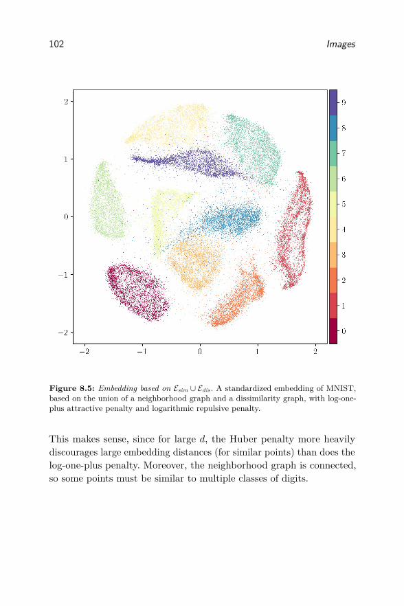
102 Images

Figure 8.5: Embedding based on Esim ∪ Edis. A standardized embedding of MNIST,based on the union of a neighborhood graph and a dissimilarity graph, with log-one-plus attractive penalty and logarithmic repulsive penalty.

This makes sense, since for large d, the Huber penalty more heavilydiscourages large embedding distances (for similar points) than does thelog-one-plus penalty. Moreover, the neighborhood graph is connected,so some points must be similar to multiple classes of digits.

8.3. Embedding 103

Figure 8.6: Varying |Edis|. Standardized embeddings of MNIST, varying |Edis|.

104 Images

Figure 8.7: Varying negative weights. Standardized embeddings of MNIST, varyingnegative weights.

8.3. Embedding 105


For comparison, we embed MNIST with UMAP (McInnes et al., 2018)and t-SNE (Hinton and Roweis, 2003), two popular embedding methods,using the umap-learn and openTSNE (Poličar et al., 2019) implemen-tations. Both methods start with neighborhood graphs on the originaldata, based on the Euclidean distance; umap-learn uses the nearest 15neighbors of each image, and openTSNE uses the nearest 90 neighborsof each image. The UMAP optimization routine takes 20 seconds onour CPU, and the openTSNE optimization routine takes roughly oneminute. (Neither implementation supports GPU acceleration.) On sim-ilar problems (the centered embeddings from §8.3.2), PyMDE takesroughly 30 seconds on CPU.

Figure 8.9 shows the embeddings. Note that the UMAP embed-ding bears a striking resemblance to the previously shown centeredembeddings (Figure 8.8). This is not surprising, since UMAP solves anunconstrained optimization problem derived from a similar graph andwith similar distortion functions.

106 Images

Figure 8.8: More embeddings. Centered embeddings of MNIST with log-one-plus(left) and Huber (right) attractive penalties, and logarithmic repulsive penalties.

Figure 8.9: UMAP (left) and t-SNE (right) embeddings of MNIST.

9Networks

The MDE problems we formulate in this chapter are derived from net-works. We start with an undirected (possibly weighted) network on n

nodes, in which the length of the shortest path between nodes i and j

encodes an original distance between them. Such networks frequentlyarise in practice: examples include social networks, collaboration net-works, road networks, web graphs, and internet networks. Our goal isto find an embedding of the nodes that preserves the network’s globalstructure.

The specific network under consideration in this chapter is a co-authorship network: each node corresponds to a unique author, and twonodes are adjacent if the corresponding authors have co-authored atleast one publication.

9.1 Data

We compiled a co-authorship network by crawling Google Scholar(Google, n.d.), an online bibliography cataloging research papers frommany different fields. Each cataloged author has a profile page, andeach page contains metadata describing the author’s body of work. Wecrawled these pages to create our network. Our network contains 590,028

107

108 Networks

authors and 3,812,943 links. We additionally collected each author’sunique identifier, affiliation, self-reported interests (such as machinelearning, renewable energy, or high energy physics), h-index (Hirsch,2005), and cumulative number of citations. Our dataset is publiclyavailable, at https://pymde.org.

We will compute two embeddings in this chapter: an embedding onthe full network, and an embedding on a network containing only high-impact authors, which we define as authors with h-indices 50 or higher.The subgraph induced by high-impact authors has 44,682 vertices and210,681 edges.

When constructing the embeddings, we use only the graph distancesbetween nodes. Later in this section we describe how we categorizeauthors into academic disciplines using their interests. An author’sacademic discipline is the held-out attribute we use to check if theembedding makes sense.

Crawling. The data was collected in November 2020 by exploringGoogle Scholar with a breadth-first search, terminating the searchafter one week. The links were obtained by crawling authors’ listedcollaborators. Google Scholar requires authors to manually add theircoauthors (though the platform automatically recommends co-authors);as a result, if two authors collaborated on a paper, but neither listedthe other as a co-author, they will not be adjacent in our network.As a point of comparison, a co-authorship network of Google Scholarfrom 2015 that determined co-authorship by analyzing publication listscontains 409,392 authors and 1,234,019 links (Chen et al., 2017).

While our co-authorship network faithfully represents Google Scholar,it deviates from reality in some instances. For example we have foundthat a small number of young researchers have listed long-deceasedresearchers such as Albert Einstein, John von Neumann, Isaac Newton,and Charles Darwin as co-authors. Compared to the size of the network,the number of such anomalies is small; e.g., there are only thirty authorswho are adjacent to Einstein but not among his true co-authors. As suchwe have made no attempt to remove erroneous links or duplicated pages(Einstein has two). For a more careful study of academic collaboration,see Chen et al. (2017).

https://pymde.org

9.1. Data 109

Some basic properties. The diameter of the full network (the lengthof the longest shortest path) is 10. The diameter of the network inducedby high-impact authors is 13.

Figure 9.1 shows the CDFs of h-indices and citation counts. Themedian h-index is 14, the 95th percentile is 58, and the maximum is 303;the median citation count is 891, the 95th percentile is 1616, and themaximum is 1,107,085. The maximum h-index and maximum citationcount both belong to the late philosopher Michel Foucault.

100 101 102 103

h-index

0.0

0.5

1.0

100 102 104 106

citation count

0.0

0.5

1.0

Figure 9.1: CDFs of author h-indices and citation counts

Figure 9.2 shows the CDF of node degrees for the full network and thesubgraph induced by high-impact authors. The number of collaboratorsan author has is moderately correlated with h-index (the Pearsoncorrelation coefficient is 0.44); citation count is strongly correlated withh-index (0.77).

100 101 102 103

degree

0.0

0.5

1.0

all

high impact

Figure 9.2: CDFs of node degree (co-author count) for the full network and thehigh-impact author network.

110 Networks

The data includes 280,819 unique interests, with 337,514 authorsinterested in at least one of the 500 most popular interests. The topfive interests are machine learning (listed by 38,220 authors), computervision (15,123), artificial intelligence (14,379), deep learning (8,984),and bioinformatics (8,496).

Academic disciplines. We assigned the high-impact authors to one offive academic disciplines, namely biology, physics, electrical engineering,computer science, and artificial intelligence, in the following ad-hocway. First, we manually labeled the 500 most popular interests with theacademic discipline to which they belonged (interests that did not belongto any of the five disciplines were left unlabeled). Then, we scannedeach author’s interests in the order they chose to display them on theirprofile, assigning the author to the discipline associated with their firstlabeled interest. For example, authors interested in machine learningfirst and bioinformatics second were assigned to artificial intelligence,while authors interested in bioinformatics first and machine learningsecond were assigned to biology. Authors that did not have at leastone labeled interest were ignored. This left us with 16,569 high-impactauthors labeled with associated academic disciplines, out of 44,682.

9.2 Preprocessing

We compute graph distances between all pairs of authors. On the fullnetwork, this yields approximately 174 billion distances, or roughly696 GB of data, too much to store in the memory of our machine.To make the embedding tractable, we sample a small fraction of thegraph distances uniformly at random, choosing to retain 0.05 percentof the distances. This results in a graph Eall on 590,028 vertices, with87,033,113 edges. Computing all 174 billion distances and randomlysubsampling them took seven hours using six CPU cores. We repeatthis preprocessing on the high-impact network, retaining 10 percent ofthe graph distances. This yields a graph Eimpact with 88,422,873 edges.Computing the graph distances with PyMDE took less than one minute,using six CPU cores.

9.3. Embedding 111

The CDFs of graph distances are shown in Figure 9.3. The values4, 5, and 6 account for around 90% of the distances in both networks.(We will see artifacts of these highly quantized values in some of ourembeddings.)

1 2 3 4 5 6 7 8 9 10graph distances

0.0

0.2

0.4

0.6

0.8

1.0

1 2 3 4 5 6 7 8 9 10graph distances

0.0

0.2

0.4

0.6

0.8

1.0

Figure 9.3: CDFs of graph distances. Top. All authors. Bottom. High-impactauthors.

9.3 Embedding

We solve two unconstrained MDE problems, based on Eall and Eimpact.The MDE problems are derived from original deviations, with δij beingthe graph distance between i and j. For both, we use the absolute loss(4.5) and embed into R2.

9.3.1 All authors

The embedding on Eall has distortion 1.58. The embedding was computedin 300 iterations by PyMDE, to a residual norm of 1.9 × 10−5. Thistook 71 seconds on our GPU.

112 Networks

Figure 9.4 shows a CDF of the the distortions. The five largestdistortions all belong to pairs whose true distance is 9, but whoseembedding distances are small (the pair with the largest distortionincludes a philosopher and an automatic control engineer). The authorsin these pairs are “unimportant” in that they have very few co-authors,and lie on the periphery of the embedding.

10−2 10−1 100 101

distortion

0.0

0.2

0.4

0.6

0.8

1.0

Figure 9.4: CDF of distortions for the embedding on all authors.

Figure 9.5 shows the embedding. (Plots of embeddings in this chapterhave black backgrounds, to make various features of the embeddingseasier to see.) Each embedding vector is colored by its author’s degree inthe co-authorship network; the brighter the color, the more co-authorsthe author has. The embedding appears sensible: highly collaborativeauthors are near the center, with the degree decreasing as one movesoutward. The diameter of the embedding is approximately 13 (measuredin Euclidean norm), compared to the original network’s 10 (measuredin graph distance).

9.3.2 High-impact authors

An embedding on the graph Eimpact has average distortion 1.45 (Fig-ure 9.6 shows a CDF of the distortions). PyMDE computed this em-bedding on a GPU in 54 seconds, in 173 iterations.

Figure 9.7 shows the embedding, colored by degree. Highly collabo-rative authors are near the center, with collaboration decreasing radiallyfrom the center. The diameter is approximately 16, compared to theoriginal network’s 13.

9.3. Embedding 113

Figure 9.5: Co-authorship network. An embedding of a co-authorship networkfrom Google Scholar, colored by degree percentile. The brighter the color, the moreco-authors the author has. The network has 590,028 authors.

The embedding has an interesting structure, with many intersectingarcs. These arcs are likely due to the original distances taking on highlyquantized values (see Figure 9.3). In Figure 9.8 we overlay a largefraction of the original high-impact network’s edges onto the embedding(i.e., edges (i, j) for which δij = 1); we show 50,000 edges, sampleduniformly at random from the original 210,681. The edges trace out thearcs, and connect adjacent communities of highly collaborative authors.

114 Networks

10−2 10−1 100 101

distortion

0.0

0.2

0.4

0.6

0.8

1.0

Figure 9.6: CDF of distortions for the embedding on high-impact authors.

Academic disciplines. Figure 9.9 shows the embedding vectors coloredby academic discipline (authors that are not tagged with a discipline areomitted). Purple represents biology, orange represents physics, greenrepresents electrical engineering, cyan represents computer science, andred represents artificial intelligence.

Authors are grouped by academic discipline, and similar disciplinesare near each other. Additionally, it turns out nearby curves in anacademic discipline roughly correspond to sub-disciplines. For example,authors in the purple curves toward the center of the embedding arelargely interested in ecology, while authors in the outer purple curvesare more interested in genomics and medicine.

Most highly-collaborative authors (authors near the center of theembedding) study computer science, artificial intelligence, or biology.This is consistent with a previous study of Google Scholar (Chen etal., 2017), which found that computer scientists and biologists aredisproportionately important in the co-authorship network, as measuredby metrics such as degree and PageRank (Page et al., 1999).


For comparison, we embed the high-impact co-authorship networksusing UMAP (McInnes et al., 2018) and t-SNE (Maaten and Hinton,2008), using the umap-learn and the scikit-learn (Pedregosa et al., 2011)implementations. We give UMAP and t-SNE the distance matricescontaining the graph distances associated with Eimpact, and we use thedefault hyper-parameters set by the software.

9.3. Embedding 115

Figure 9.7: High-impact authors. An embedding of a co-authorship network onauthors with an h-index of 50 or higher, colored by degree percentile.

The embeddings are shown in Figure 9.10, colored by degree andacademic discipline. Neither method has preserved the global structureof the network, but both have organized the embedding vectors bydiscipline. (As we have seen, embeddings emphasizing local structureover global structure are readily produced with PyMDE; in this chapter,however, we chose to emphasize global structure instead.)

116 Networks

Figure 9.8: High-impact authors, with links. High-impact author embedding, coloredby degree percentile, with links between co-authors displayed as white line segments.

9.3. Embedding 117

Figure 9.9: Academic disciplines. High-impact author embedding, colored by aca-demic discipline. The disciplines are biology (purple), physics (orange), electricalengineering (green), computer science (cyan), and artificial intelligence (red).

118 Networks

Figure 9.10: UMAP (left) and t-SNE (right) embeddings of the high-impact authornetwork, colored by degree (top) and academic discipline (bottom).

10Counties

In this example, we embed demographic data for 3,139 United Statescounties into R2. The data broadly describes the composition of thecounties, and contains information about gender, ethnicity, and income(among other things). To make sure our embeddings make sense, we willuse an additional attribute for each county to validate the embeddings,which is the fraction who voted Democratic in the 2016 election. (Wedo not use this attribute in forming the embeddings.)

10.1 Data

Our raw data comes from the 2013–2017 American Community Survey(ACS) 5-Year Estimates (United States Census Bureau, n.d.), whichis a longitudinal survey run by the United States Census Bureau thatrecords demographic information about the n = 3, 139 US counties. Wewill use 34 of the demographic features to create our embedding of UScounties.

119

120 Counties

Table 10.1: List of the features in the ACS data set, along with the initial prepro-cessing transformation we applied.

Feature Transformation

Number of people Log-transformNumber of voting age citizens Log-transformNumber of men NormalizeNumber of women NormalizeFraction Hispanic NoneFraction White NoneFraction Black NoneFraction Native American or Alaskan NoneFraction Asian NoneFraction Native Hawaiian or Pacific Islander NoneMedian household income Log-transformMedian household income standard deviation Log-transformHousehold income per capita Log-transformHousehold income per capita standard devia-tion

Log-transform

Fraction below the poverty threshold NoneFraction of children below the poverty thresh-old

None

Fraction working in management, business, sci-ence, or the arts

None

Fraction working in a service job NoneFraction working in an office or sales job NoneFraction working in natural resources, construc-tion, and maintenance

None

Fraction working in production, transportation,and material movement

None

Fraction working in the private sector NoneFraction working in the public sector NoneFraction working for themselves NoneFraction doing unpaid family work NoneNumber that have a job (are employed) NormalizeFraction unemployed NoneFraction commuting to work alone in a car,van, or truck

None

Fraction carpooling in a car, van, or truck NoneFraction commuting via public transportation NoneFraction walking to work NoneFraction commuting via other means NoneFraction working at home NoneAverage commute time in hours None


10.2 Preprocessing

We carry out some standard preprocessing of the raw features, listed inTable 10.1. For positive features that range over a very wide scale, suchas household income, we apply a log-transform, i.e., replace the rawfeature with its logarithm. We normalize raw features that are counts,i.e., divide them by the county population. (We do not transform featuresthat are given as fractions or proportions.) After these transformations,we standardize each feature to have zero mean and standard deviationone over the counties.

Using these preprocessed features, we generate a k-nearest (Eu-clidean) neighbor graph, with k = 15, which gives a graph Esim with36, 992 edges. We then sample, at random, another 36, 992 pairs ofcounties not in Esim, to obtain a graph of dissimilar counties, Edis. Ourfinal graph E = Esim ∪Edis has 73, 984 edges, corresponding to an averagedegree of around 47. We assign weight wij = 2 for (i, j) ∈ Esim whencounties i and j are both neighbors of each other. We assign weightwij = 1 for (i, j) ∈ Esim when i is a neighbor of j but j is not a neighborof i (or vice versa). We assign weight wij = −1 for (i, j) ∈ Edis.

10.3 Embedding

10.3.1 PCA embedding

We consider PCA first. The PCA embedding for m = 2 is shown inFigure 10.1, with each county shown as a colored dot, with colorsdepending on the fraction of voters who voted Democratic in 2016,from red (0%) to blue (100%). The embedding clearly captures someof the structure of the voting patterns, but we can see many instanceswhere counties with very different voting appear near each other in theembedding. (The blue counties are urban, and far more populous thanthe many rural red counties seen in the embedding. The total number ofpeople who voted Democratic exceeded those who voted Republican.)

122 Counties

−10 −5 0 5 10

−10

−5

0

5

10

0.1

0.2

0.3

0.4

0.5

0.6

0.7

0.8

0.9

Figure 10.1: PCA embedding of the election data, colored by the fraction of votersin each county who voted Democratic in the 2016 United States presidential election,from red (0%) to blue (100%).

10.3.2 Unconstrained embedding

Next we solve an unconstrained (centered) MDE problem based on thegraph E = Esim ∪ Edis. We use the log-one-plus penalty (4.3) (α = 2)for ps and the logarithmic penalty (4.4) for pd (α = 0.5). We chooseembedding dimension m = 2.

Figure 10.2 shows the results. Compared to the PCA embedding, wesee a better separation of regions corresponding to heavily Democratic,heavily Republican, and mixed voting. Figures 10.3 and 10.4 take acloser look at the upper right and bottom of the plot, labeling somerepresentative counties. We can also see a few swing counties, i.e.,

10.3. Embedding 123

counties that historically vote Democratic, but recently lean Republican(or vice versa), near the strongly Democratic (or Republican) counties;these counties are colored light red (or blue), because they have weakmajorities.

We give two alternative visualizations of the embedding in figure10.5. In these visualizations, we color each county according to its valuein each of the two embedding coordinates. In Figure 10.6, we showthe counties colored with the fraction of people who actually votedDemocratic in the 2016 election, as a point of reference.

−3 −2 −1 0 1 2 3−3

−2

−1

0

1

2

3

0.1

0.2

0.3

0.4

0.5

0.6

0.7

0.8

0.9

Figure 10.2: Embedding. A centered embedding of the election data, with log-one-plus attractive and logarithmic repulsive penalty functions.

124 Counties

1.5 2.0 2.5 3.0 3.5 4.0

1.0

1.2

1.4

1.6

1.8

2.0

2.2

2.4

San Francisco County, CA

District of Columbia, DC

New York County, NY

Philadelphia County, PA

0.1

0.2

0.3

0.4

0.5

0.6

0.7

0.8

0.9

Figure 10.3: Upper right corner. A closer look at the upper right corner of theembedding shown in Figure 10.2. Several densely populated urban counties appear.


We compare the embeddings generated by UMAP and t-SNE, shown infigure 10.7. To make it easier to compare the embeddings, we orthog-onally transformed these two embeddings with respect to the uncon-strained embedding (as described in §2.4.5), before plotting them. Theembeddings broadly resemble the unconstrained embedding, thoughthey appear to be a little bit more dispersed.

10.3. Embedding 125

−2 −1 0 1 2 3

−3.5

−3.0

−2.5

−2.0

−1.5

−1.0

Denali Borough, AK

Petroleum County, MT

Harding County, NM

Kenedy County, TX

0.1

0.2

0.3

0.4

0.5

0.6

0.7

0.8

0.9

Figure 10.4: Bottom. A closer look at the bottom of the embedding shown in Figure10.2. Several sparsely populated rural counties appear.

126 Counties

−3

−2

−1

0

1

2

3

−3

−2

−1

0

1

2

3

Figure 10.5: Embedding by coordinate. Counties colored by their first (top) andsecond (bottom) coordinate of the embedding from Figure 10.2.

10.3. Embedding 127

0.10.20.30.40.50.60.70.80.9

Figure 10.6: Election data. Counties colored by the fraction of people voting forthe Democratic candidate in the 2016 election, from red (0%) to blue (100%). (Theurban blue counties are far more densely populated than the rural red counties; intotal there were more Democratic than Republican votes.)

−10 −5−4

−2

0

2

4

6

8

−50 0 50

−50

−25

0

25

50

0.2

0.4

0.6

0.8

Figure 10.7: UMAP (left) and t-SNE (right) embeddings of the ACS data.

11Population Genetics

Our next example is from population genetics. We consider the well-known study carried out by Novembre et al. (2008) of high-dimensionalsingle nucleotide polymorphism (SNP) data associated with 3,000 indi-viduals thought to be of European ancestry. After carefully cleaning thedata in order to remove outliers, the authors embed the data into R2 viaPCA, obtaining the embedding shown in Figure 11.1. Interestingly, theembedding bears a striking resemblance to the map of Europe, shownin Figure 11.2, suggesting a close relationship between geography andgenetic variation. (In these figures we use the same color legend used inthe original Novembre et al. (2008) paper.) This resemblance does notemerge if the outliers are not first removed from the original data.

Follow-on work by Diakonikolas et al. (2017) proposed a method forrobust dimensionality reduction, showing good results on a version ofthe data from the original Novembre et al. study that was intentionallycorrupted with some bad data. After appropriately tuning a numberof parameters, they were able to recover the resemblance to a map ofEurope despite the bad data. We will explore this issue of robustnessto poor data using distortion functions that are robust, i.e., allow forsome pairs of similar items to have large distance.

128

129

−0.3 −0.2 −0.1 0.0 0.1 0.2 0.3−0.3

−0.2

−0.1

0.0

0.1

0.2

0.3

Figure 11.1: PCA embedding of population genetics data. Points are colored bycountry using the legend shown in the map of Europe in Figure 11.2.

130 Population Genetics

Figure 11.2: Map of Europe, showing the country color legend for the populationgenetics data, taken from Novembre et al.; countries with no data points are shownin gray.

11.1. Data 131

11.1 Data

We create two sets of data: one clean, and one intentionally corrupted,following Diakonikolas et al. (2017). We follow the same experimentsetup as in Novembre et al. (2008) and Diakonikolas et al. (2017), andwork with the SNP data associated with 3,000 individuals thoughtto be of European ancestry, coming from the Population ReferenceSample project (Nelson et al., 2008). Novembre et al. and Diakonikolaset al. both start off by pruning the original data set down to the 1,387individuals most likely to have European ancestry (explained in thesupplementary material of Novembre et al. (2008)), and then projectthe data onto its top 20 principal components, obtaining the (clean)samples yi ∈ R20, i = 1, . . . , 1387.

To create a corrupted set of data, we follow the method of Diakoniko-las et al., who randomly rotate the data and then inject 154 additionalpoints yi, i = 1388, . . . , 1541, where the first ten entries of the yi arei.i.d. following a discrete uniform distribution on {0, 1, 2}, and the lastten entries of the yi are i.i.d. following a discrete uniform distributionon {1/12, 1/8}. Thus the clean data is y1, . . . , y1387, and the corrupteddata is y1388, . . . , y1541.

We also have the country of origin for each of the data points, givenas one of 34 European countries. We use this attribute to check ourembeddings, but not to construct our embeddings. In plots, we colorthe synthesized (corrupted) data points black.

11.2 Preprocessing

For both the clean and corrupted raw data sets we construct a set of pairsof similar people Esim as the k-nearest (Euclidean) neighbors, with k =15. For the clean data, we have |Esim| = 16, 375, and for the corrupteddata we have |Esim| = 17, 842. We also treat the remaining pairs of peopleas dissimilar, so that |Edis| = 944, 816 for the clean data, and |Edis| =1, 168, 728 for the corrupted data. We use weights wij = 2 for (i, j) ∈ Esimwhen individuals i and j are both neighbors of each other. We use weightswij = 1 for (i, j) ∈ Esim when i is a neighbor of j but j is not a neighborof i (or vice versa). We use weights wij = −1 for (i, j) ∈ Edis.


11.3 Embedding

11.3.1 PCA embedding

We start with PCA, exactly following Novembre et al., which on theclean data results in the embedding shown in Figure 11.1. In thelanguage of this monograph, this embedding uses quadratic distortionfor (i, j) ∈ E , weights wij = yT

i yj (after centering the data), and astandardization constraint. The distribution of the weights is shown inFigure 11.4. When PCA embedding is used on the corrupted data, weobtain the embedding in Figure 11.3. In this embedding only some ofthe resemblance to the map of Europe is preserved. The synthesizedpoints are embedded on the right side. (If those points are manuallyremoved, and we PCA run again, we recover the original embedding.)

11.3.2 Unconstrained embeddings

We embed both the clean and corrupted data unconstrained (centered),based on the graph E = Esim ∪ Edis. We use a Huber attractive penalty(4.2), and a logarithmic repulsive penalty (4.4) (α = 1) to enforcespreading. The embedding of the clean data is shown in Figure 11.5, andfor the corrupted data in Figure 11.6. We can see that this embeddingis able to recover the similarity to the map of Europe, despite thecorrupted data. In fact, this embedding appears virtually identical tothe embedding of the clean data in Figure 11.5.


We show the UMAP and t-SNE embeddings on the clean and corrupteddata in figure 11.7. These embeddings were scaled and orthogonallytransformed with respect to the map given in Figure 11.2, following themethod described in §2.4.5. The embeddings with the corrupted dataare better than the PCA embedding.

11.3. Embedding 133

−0.4 −0.3 −0.2 −0.1 0.0 0.1 0.2 0.3 0.4−0.4

−0.3

−0.2

−0.1

0.0

0.1

0.2

0.3

0.4

Figure 11.3: PCA embedding of corrupted data. The resemblance to a map ofEurope is substantially reduced.


−0.1 0.0 0.1wij

0

10

20

30

40

−0.1 0.0 0.1wij

0

10

20

30

40

Figure 11.4: PCA weights. Distribution of the weights used by PCA, when expressedas an MDE problem, for the clean (left) and corrupted (right) data.

11.3. Embedding 135

−4 −3 −2 −1 0 1 2 3 4−4

−3

−2

−1

0

1

2

3

4

Figure 11.5: Embedding of clean data. The embedding resembles a map of Europe.


−6 −4 −2 0 2 4 6

−6

−4

−2

0

2

4

6

Figure 11.6: Embedding of corrupted data. The embedding is able to recover thesimilarity to the map of Europe.

11.3. Embedding 137

−15 −10 −5 0−15.0

−12.5

−10.0

−7.5

−5.0

−2.5

0.0

−40 −20 0 20 40

−40

−20

0

20

40

−10 0 10 20−10

−5

0

5

10

15

20

−50 −25 0 25 50−60

−40

−20

0

20

40

60

Figure 11.7: UMAP (left) and t-SNE (right) embeddings of clean (top) and corrupteddata (bottom).

12Single-Cell Genomics

For our last example we embed several thousand single-cell mRNA(scRNA) transcriptomes. We use data that accompanies a recent pub-lication by Wilk et al. (2020); these data are sequences of humanperipheral blood mononuclear cells (PBMCs), collected from seven pa-tients afflicted with severe COVID-19 infections and six healthy controls.We embed into R3 and visualize the embedding vectors, finding thatthe vectors are organized by donor health status and cell type.

12.1 Data

The dataset from Wilk et al. (2020) includes n = 44, 721 scRNA tran-scriptomes of PBMCs, with 16,627 cells from healthy donors and 28,094from donors infected with COVID-19. Each cell is represented by asparse vector in R26361, and each component gives the expression levelof a gene. Wilk et al. (2020) projected the data matrix onto its top50 principal components, yielding a matrix Y ∈ R44721×50 which theyfurther studied.

In constructing our embedding, we use only the reduced gene ex-pression data, i.e., the entries of Y . Each cell is tagged with manyheld-out attributes, and we use two of these to informally validate our

138


embedding. The first attribute says whether a cell came from a donorinfected with COVID-19, and the second gives a classification of thecells into (manually labeled) sub-families.

12.2 Preprocessing

We use distortion functions derived from weights. From the rows of Y

we construct a k-nearest (Euclidean) neighbor graph, with k = 15; thisgives a graph Esim with 515, 376 edges. We then sample, uniformly atrandom, an additional |Esim| pairs not in Esim to obtain a graph Edis ofdissimilar cells. The final graph E = Esim ∪ Edis has p = 1, 030, 752 edges.For the weights, we choose wij = +2 if i and j are both neighbors ofeach other; wij = +1 if i is a neighbor of j but j is not a neighbor of i

(or vice versa); and wij = −1 for (i, j) ∈ Edis.

12.3 Embedding

We form a standardized MDE problem with embedding dimensionm = 3, based on the graph E = Esim ∪ Edis. We use the log-one-pluspenalty (4.3) (α = 1.5) for ps and the logarithmic penalty (4.4) (α = 1)for pd.

We solved the MDE problem with PyMDE, initializing the solvewith a embedding obtained by solving a quadratic MDE problem on Esim.The quadratic MDE problem was solved in 7 seconds (249 iterations) onour CPU, and 2 seconds (185 iterations) on our GPU. Solving the MDEproblem took 27 seconds (300 iterations) on our CPU, and 6 seconds(300 iterations) on our GPU. The embedding has average distortion0.13; a CDF of distortions is shown in Figure 12.1. The embeddingused for initialization is shown in Figure 12.2, with embedding vectorscolored by the cell-type attribute.

The embedding is shown in Figure 12.3, colored by cell type; similarcells end up near each other in the embedding. The embedding is plottedagain in Figure 12.4, this time colored by donor health status. Cellsfrom healthy donors are nearer to each other than to cells from infecteddonors, and the analogous statement is true for cells from infecteddonors.

140 Single-Cell Genomics

10−3 10−2 10−1 100 101

distortion

0.0

0.5

1.0

Figure 12.1: CDF of distortions for the embedding of scRNA data.

As a sanity check, we partition Esim into three sets: edges betweenhealthy donors, edges between infected patients, and edges betweeninfected patients and healthy donors. The average distortion of theembedding, restricted to each of these sets, is 0.19, 0.18, and 0.21,respectively. This means pairs linking healthy donors to infected donorsare more heavily distorted on average than pairs linking donors withthe same health status.

Figure 12.5 shows the embedding with roughly 10 percent of thepairs in Esim overlaid as white line segments (the pairs were sampleduniformly at random). Cells near each other are highly connected toeach other, while distant cells are not. Finally, the 1000 pairs from Esimwith the highest distortions are shown in Figure 12.6; most of thesepairs contain different types of cells.


Figure 12.7 shows an embedding of the scRNA data produced by UMAP,which took 11 seconds, and Figure 12.8 shows an embedding made usingopenTSNE, which took 96 seconds, using the value bh for the parameternegative_gradient_method (the default value resulted in an error).The embeddings were aligned to the orientation of our embedding bysolving a Procrustes problem, as described in §2.4.5.

12.3. Embedding 141

Figure 12.2: Embedding based on Esim. An embedding of scRNA transcriptomes ofPBMCs from patients with severe COVID-19 infections and healthy controls (Wilket al., 2020), obtained by solving a quadratic MDE problem on Esim and colored bycell type.


Figure 12.3: Embedding based on Esim ∪ Edis. Embedding of scRNA transcriptomes,colored by cell type.

12.3. Embedding 143

Figure 12.4: Health status. Embedding of scRNA data, colored by health status.


Figure 12.5: With edges. Embedding of scRNA data, with edges between neighboringcells displayed as white line segments.

12.3. Embedding 145

Figure 12.6: High distortion pairs. Embedding of scRNA data, with the 1000 mostheavily distorted pairs displayed as white line segments.


Figure 12.7: UMAP. Embedding of scRNA data, produced by UMAP.

12.3. Embedding 147

Figure 12.8: t-SNE. Embedding of scRNA data, produced by t-SNE.

13Conclusions

The task of vector embedding, i.e., assigning each of a set of itemsan associated vector, is an old and well-established problem, withmany methods proposed over the past 100 years. In this monographwe have formalized the problem as one of choosing the vectors so asto minimize an average or total distortion, where distortion functionsspecified for pairs of items express our preferences about the Euclideandistance between the associated vectors. Roughly speaking, we wantvectors associated with similar items to be near each other, and vectorsassociated with dissimilar items to not be near each other.

The distortion functions, which express our prior knowledge aboutsimilarity and dissimilarity of pairs of items, can be constructed inseveral different but related ways. Weights on edges give us a measureof similarity (when positive) and dissimilarity (when negative). Alterna-tively, we can start with deviations between pairs of items, with smalldeviation meaning high similarity. Similarity and dissimilarity can alsobe expressed by one or more graphs on the items, for example onespecifying similar pairs and another specifying dissimilar pairs. Thereis some art in making the distortion functions, though we find thata few simple preprocessing steps, such as the ones described in thismonograph, work well in practice.

148

149

Our framework includes a large number of well-known previously de-veloped methods as special cases, including PCA, Laplacian embedding,UMAP, multi-dimensional scaling, and many others. Some other exist-ing embedding methods cannot be represented as MDE problems, butMDE-based methods can produce similar embeddings. Our frameworkcan also be used to create new types of embeddings, depending on thechoice of distortion functions, the constraint set, and the preprocessingof original data.

The quality of an embedding ultimately depends on whether it issuitable for the downstream application. Nonetheless we can use ourframework to validate, or at least sanity-check, embeddings. For example,we can examine pairs with abnormally high distortion. We can thensee if these pairs contain anomalous items, or whether their distortionfunctions inaccurately conveyed their similarity or lack thereof.

Our examples in Part III focused on embedding into two or threedimensions. This allowed us to plot the embeddings, which we judgedby whether they led to insight into the data, as well as by aesthetics.But we can just as well embed into dimensions larger than two or three,as might be done when developing a feature mapping on the items fordownstream machine learning tasks. When the original data recordsare high-dimensional vectors (say, several thousand dimensions), wecan embed them into five or ten dimensions and use the embeddingvectors as the features; this makes the vector representation of the datarecords much smaller, and the fitting problem more tractable. It canalso improve the machine learning, since the embedding depends onwhatever data we used to carry it out, and in some sense inherits itsstructure.

It is practical to exactly solve MDE problems only in some specialcases, such as when the distortion functions are quadratic and theembedding vectors are required to be standardized. For other cases, wehave introduced an efficient local optimization method that producesgood embeddings, while placing few assumptions on the distortionfunctions and constraint set. We have shown in particular how toreliably compute embeddings with a standardization constraint, evenwhen the objective function is not quadratic.

150 Conclusions

Our optimization method (and software) scales to very large prob-lems, with embedding dimensions much greater than two or three, andour experiments show that it is competitive in runtime to more spe-cialized algorithms for specific embedding methods. The framework ofMDE problems, coupled with our solution method and software, makesit possible for practitioners to rapidly experiment with new kinds ofembeddings in a principled way, without sacrificing performance.

Acknowledgements

We thank Amr Alexandari, Guillermo Angeris, Shane Barratt, StevenDiamond, Mihail Eric, Andrew Knyazev, Benoit Rostykus, SaberaTalukder, Jian Tang, Jonathan Tuck, Junzi Zhang, as well as severalanonymous reviewers, for their comments on the manuscript; YifanLu and Lawrence Saul, for their careful readings and many thoughtfulsuggestions; and Delenn Chin and Dmitry Kobak, for their detailedfeedback on both the manuscript and early versions of the softwarepackage.

151

References

Absil, P.-A. and J. Malick. (2012). “Projection-like retractions on matrixmanifolds”. SIAM Journal on Optimization. 22(1): 135–158.

Absil, P.-A., R. Mahony, and R. Sepulchre. (2009). Optimization Algo-rithms on Matrix Manifolds. Princeton University Press.

Ahmed, N., R. Rossi, J. Lee, T. Willke, R. Zhou, X. Kong, and H. El-dardiry. (2020). “Role-based graph embeddings”. IEEE Transactionson Knowledge and Data Engineering.

Alcorn, M. (2016). “(batter|pitcher)2vec: Statistic-free talent modelingwith neural player embeddings”. In: MIT Sloan Sports AnalyticsConference.

Andoni, A., P. Indyk, and I. Razenshteyn. (2018). “Approximate nearestneighbor search in high dimensions”. arXiv.

Arrow, K. (1950). “A difficulty in the concept of social welfare”. Journalof Political Economy. 58(4): 328–346.

Asgari, E. and M. Mofrad. (2015). “Continuous distributed represen-tation of biological sequences for deep proteomics and genomics”.PLOS One. 10(11): 1–15.

Asi, H. and J. Duchi. (2019). “Stochastic (approximate) proximal pointmethods: Convergence, optimality, and adaptivity”. SIAM Journalon Optimization. 29(3): 2257–2290.

Barocas, S., M. Hardt, and A. Narayanan. (2019). Fairness and MachineLearning. url: fairmlbook.org.

152

fairmlbook.org

References 153

Beatson, R. and L. Greengard. (1997). “A short course on fast multi-pole methods”. In: Wavelets, Multilevel Methods and Elliptic PDEs.Oxford University Press. 1–37.

Belkin, M. and P. Niyogi. (2002). “Laplacian eigenmaps and spectraltechniques for embedding and clustering”. In: Advances in NeuralInformation Processing Systems. 585–591.

Bender, E., T. Gebru, A. McMillan-Major, and S. Shmitchell. (2021).“On the dangers of stochastic parrots: Can language models be toobig?” In: Proceedings of the 2021 Conference on Fairness, Account-ability, and Transparency.

Bergmann, R. (2020). “Manopt.jl”. url: https://manoptjl.org/stable/index.html.

Bernhardsson, E. (2020). “annoy”. url: https://github.com/spotify/annoy.

Bernstein, M., V. De Silva, J. Langford, and J. Tenenbaum. (2000).“Graph approximations to geodesics on embedded manifolds”. Tech.rep. Department of Psychology, Stanford University.

Biswas, P. and Y. Ye. (2004). “Semidefinite programming for ad hocwireless sensor network localization”. In: Proceedings of the 3rd Inter-national Symposium on Information Processing in Sensor Networks.46–54.

Böhm, J. N., P. Berens, and D. Kobak. (2020). “A unifying perspectiveon neighbor embeddings along the attraction-repulsion spectrum”.arXiv.

Bolukbasi, T., K.-W. Chang, J. Zou, V. Saligrama, and A. Kalai. (2016).“Man is to computer programmer as woman is to homemaker?Debiasing word embeddings”. In: Advances in Neural InformationProcessing Systems. 4356–4364.

Borg, I. and P. Groenen. (2003). “Modern multidimensional scaling:Theory and applications”. Journal of Educational Measurement.40(3): 277–280.

Boumal, N., B. Mishra, P.-A. Absil, and R. Sepulchre. (2014). “Manopt,a Matlab toolbox for optimization on manifolds”. Journal of MachineLearning Research. 15(1): 1455–1459.

Bourgain, J. (1985). “On Lipschitz embedding of finite metric spaces inHilbert space”. Israel Journal of Mathematics. 52(1-2): 46–52.

https://manoptjl.org/stable/index.html

https://manoptjl.org/stable/index.html

https://github.com/spotify/annoy

https://github.com/spotify/annoy

154 References

Boyd, S. and L. Vandenberghe. (2004). Convex Optimization. New York,NY, USA: Cambridge University Press.

Boyd, S. and L. Vandenberghe. (2018). Introduction to Applied LinearAlgebra: Vectors, Matrices, and Least Squares. New York, NY, USA:Cambridge University Press.

Bradley, R. and M. Terry. (1952). “Rank analysis of incomplete blockdesigns: The method of paired comparisons”. Biometrika. 39(3/4):324–345.

Broyden, C. G. (1970). “The convergence of a class of double-rankminimization algorithms, general considerations”. IMA Journal ofApplied Mathematics. 6(1): 76–90.

Burer, S. and R. Monteiro. (2003). “A nonlinear programming algo-rithm for solving semidefinite programs via low-rank factorization”.Mathematical Programming. 95(2): 329–357.

Burer, S. and R. Monteiro. (2005). “Local minima and convergence inlow-rank semidefinite programming”. Mathematical Programming.103(3, Ser. A): 427–444.

Carreira-Perpinán, M. and R. Zemel. (2005). “Proximity graphs forclustering and manifold learning”. Advances in Neural InformationProcessing Systems. 17: 225–232.

Cayton, L. (2005). “Algorithms for manifold learning”. Tech. rep. De-partment of Computer Science, University of California at SanDiego.

Cayton, L. and S. Dasgupta. (2006). “Robust Euclidean embedding”.In: Proceedings of the 23rd International Conference on MachineLearning. 169–176.

Chen, S., S. Ma, A. Man-Cho So, and T. Zhang. (2020). “Proximal gra-dient method for nonsmooth optimization over the Stiefel manifold”.SIAM Journal on Optimization. 30(1): 210–239.

Chen, W., K. Weinberger, and Y. Chen. (2013). “Maximum variance cor-rection with application to A* search”. In: International Conferenceon Machine Learning. 302–310.

Chen, Y., C. Ding, J. Hu, R. Chen, P. Hui, and X. Fu. (2017). “Buildingand analyzing a global co-authorship network using Google ScholarData”. In: Proceedings of the 26th International Conference on WorldWide Web Companion. 1219–1224.

References 155

Chung, F. and F. Graham. (1997). Spectral Graph Theory. No. 92.American Mathematical Society.

Corbett-Davies, S. and S. Goel. (2018). “The measure and mismeasureof fairness: A critical review of fair machine learning”. arXiv.

Cox, T. and M. Cox. (2000). Multidimensional Scaling. CRC Press.Devlin, J. (2020). “BERT”. url: https://github.com/google-research/

bert.Devlin, J., M.-W. Chang, K. Lee, and K. Toutanova. (2019). “BERT:

Pre-training of Deep Bidirectional Transformers for Language Un-derstanding”. In: Proceedings of the 2019 Conference of the NorthAmerican Chapter of the Association for Computational Linguistics:Human Language Technologies. 4171–4186.

Diakonikolas, I., G. Kamath, D. Kane, J. Li, A. Moitra, and A. Stewart.(2017). “Being robust (in high dimensions) can be practical”. In:International Conference on Machine Learning. 999–1008.

Dokmanic, I., R. Parhizkar, J. Ranieri, and M. Vetterli. (2015). “Eu-clidean distance matrices: Essential theory, algorithms, and applica-tions”. IEEE Signal Processing Magazine. 32(6): 12–30.

Dong, W., M. Charikar, and K. Li. (2011). “Efficient k-nearest neighborgraph construction for generic similarity measures”. In: Proceedingsof the 20th International Conference on World Wide Web. 577–586.

Dwork, C., M. Hardt, T. Pitassi, O. Reingold, and R. Zemel. (2012).“Fairness through awareness”. In: Proceedings of the 3rd Innovationsin Theoretical Computer Science Conference. 214–226.

Dwork, C., R. Kumar, M. Naor, and D. Sivakumar. (2001). “Rankaggregation methods for the web”. In: Proceedings of the 10th Inter-national Conference on World Wide Web. 613–622.

Eades, P. (1984). “A heuristic for graph drawing”. In: Proceedingsof the 13th Manitoba Conference on Numerical Mathematics andComputing. Vol. 42. 149–160.

Easley, D. and J. Kleinberg. (2010). Networks, Crowds, and Markets.Vol. 8. Cambridge University Press.

Eckart, C. and G. Young. (1936). “The approximation of one matrix byanother of lower rank”. Psychometrika. 1(3): 211–218.

https://github.com/google-research/bert

https://github.com/google-research/bert

156 References

Edelman, A., T. Arias, and S. Smith. (1998). “The geometry of algo-rithms with orthogonality constraints”. SIAM Journal on MatrixAnalysis and Applications. 20(2): 303–353.

El Alaoui, A., X. Cheng, A. Ramdas, M. Wainwright, and M. Jordan.(2016). “Asymptotic behavior of ℓp-based Laplacian regularizationin semi-supervised learning”. In: Conference on Learning Theory.879–906.

Epskamp, S., A. Cramer, L. Waldorp, V. Schmittmann, and D. Bors-boom. (2012). “qgraph: Network visualizations of relationships inpsychometric data”. Journal of Statistical Software. 48(4): 1–18.

Fan, K. and A. Hoffman. (1955). “Some metric inequalities in the spaceof matrices”. Proceedings of the American Mathematical Society.6(1): 111–116.

Fisk, C., d. Caskey, and L. West. (1967). “ACCEL: Automated circuitcard etching layout”. Proceedings of the IEEE. 55(11): 1971–1982.

Fletcher, R. (1970). “A new approach to variable metric algorithms”.The Computer Journal. 13(3): 317–322.

Fligner, M. and J. Verducci. (1986). “Distance based ranking models”.Journal of the Royal Statistical Society: Series B (Methodological).48(3): 359–369.

Gansner, E. and S. North. (2000). “An open graph visualization systemand its applications to software engineering”. Software – Practiceand Experience. 30(11): 1203–1233.

Garg, N., L. Schiebinger, D. Jurafsky, and J. Zou. (2018). “Wordembeddings quantify 100 years of gender and ethnic stereotypes”.Proceedings of the National Academy of Sciences. 115(16): E3635–E3644.

Gill, P., W. Murray, and M. Saunders. (2002). “SNOPT: an SQPalgorithm for large-scale constrained optimization”. SIAM Journalon Optimization. 12(4): 979–1006.

Goldfarb, D. (1970). “A family of variable-metric methods derived byvariational means”. Mathematics of Computation. 24(109): 23–26.

Golub, G. and C. Van Loan. (2013). Matrix Computations. Fourth.Johns Hopkins Studies in the Mathematical Sciences. Johns HopkinsUniversity Press, Baltimore, MD.

References 157

Goodfellow, I., Y. Bengio, and A. Courville. (2016). Deep Learning.MIT Press.

Google. “Google Scholar”. url: https://scholar.google.com/.Greengard, L. and V. Rokhlin. (1987). “A fast algorithm for particle

simulations”. Journal of Computational Physics. 73(2): 325–348.Groenen, P., J. de Leeuw, and R. Mathar. (1996). “Least squares

multidimensional scaling with transformed distances”. In: FromData to Knowledge. Springer. 177–185.

Grover, A. and J. Leskovec. (2016). “node2vec: Scalable feature learningfor networks”. In: Proceedings of the 22nd ACM SIGKDD Interna-tional Conference on Knowledge Discovery and Data Mining. 855–864.

Hagberg, A., D. Schult, and P. Swart. (2008). “Exploring networkstructure, dynamics, and cunction using NetworkX”. In: Proceedingsof the 7th Python in Science Conference. 11–15.

Hall, K. (1970). “An r-dimensional quadratic placement algorithm”.Management Science. 17(3): 219–229.

Ham, J., D. Lee, S. Mika, and B. Schölkopf. (2004). “A kernel view of thedimensionality reduction of manifolds”. In: International Conferenceon Machine Learning. 47.

Hamilton, W., R. Ying, and J. Leskovec. (2017). “Representation learn-ing on graphs: Methods and applications”. arXiv.

Hayden, T., J. Wells, W.-M. Liu, and P. Tarazaga. (1991). “The coneof distance matrices”. Linear Algebra and its Applications. 144: 153–169.

He, K., X. Zhang, S. Ren, and J. Sun. (2016). “Deep residual learningfor image recognition”. In: Proceedings of the IEEE Conference onComputer Vision and Pattern Recognition. 770–778.

Higham, N. (1989). “Matrix nearness problems and applications”. In:Applications of Matrix Theory. Vol. 22. Oxford University Press,New York. 1–27.

Hinton, G. and S. Roweis. (2003). “Stochastic neighbor embedding”. In:Advances in Neural Information Processing Systems. 857–864.

https://scholar.google.com/

158 References

Hiriart-Urruty, J.-B. and C. Lemaréchal. (1993). Convex Analysis andMinimization Algorithms I. Fundamentals. Vol. 305. Grundlehrender Mathematischen Wissenschaften [Fundamental Principles ofMathematical Sciences]. Springer-Verlag, Berlin.

Hirsch, J. (2005). “An index to quantify an individual’s scientific researchoutput”. Proceedings of the National Academy of Sciences. 102(46):16569–16572.

Holstein, K., J. Wortman Vaughan, H. Daumé III, M. Dudik, and H.Wallach. (2019). “Improving fairness in machine learning systems:What do industry practitioners need?” In: Proceedings of the 2019CHI Conference on Human Factors in Computing Systems. 1–16.

Hosseini, S., W. Huang, and R. Yousefpour. (2018). “Line search al-gorithms for locally Lipschitz functions on Riemannian manifolds”.SIAM Journal on Optimization. 28(1): 596–619.

Hotelling, H. (1933). “Analysis of a complex of statistical variables intoprincipal components”. Journal of Educational Psychology. 24(6):417.

Hu, J., B. Jiang, L. Lin, Z. Wen, and Y. Yuan. (2019). “Structured quasi-Newton methods for optimization with orthogonality constraints”.SIAM Journal on Scientific Computing. 41(4): A2239–A2269.

Huang, W., P.-A. Absil, and K. Gallivan. (2017). “Intrinsic representa-tion of tangent vectors and vector transports on matrix manifolds”.Numerische Mathematik. 136(2): 523–543.

Huang, W., P.-A. Absil, and K. Gallivan. (2018). “A Riemannian BFGSmethod without differentiated retraction for nonconvex optimizationproblems”. SIAM Journal on Optimization. 28(1): 470–495.

Huang, W., K. Gallivan, and P.-A. Absil. (2015). “A Broyden classof quasi-Newton methods for Riemannian optimization”. SIAMJournal on Optimization. 25(3): 1660–1685.

HuggingFace. (2020). “Transformers”. url: https : / / github . com /huggingface/transformers.

Hutchinson, B., V. Prabhakaran, E. Denton, K. Webster, Y. Zhong,and S. Denuyl. (2020). “Social Biases in NLP Models as Barriersfor Persons with Disabilities”. In: Proceedings of the 58th AnnualMeeting of the Association for Computational Linguistics. 5491–5501.

https://github.com/huggingface/transformers

https://github.com/huggingface/transformers

References 159

Hutchinson, M. (1989). “A stochastic estimator of the trace of theinfluence matrix for Laplacian smoothing splines”. Communicationsin Statistics – Simulation and Computation. 18(3): 1059–1076.

Indyk, P., J. Matoušek, and A. Sidiropoulos. (2017). “Low-distortionembeddings of finite metric spaces”. In: Handbook of Discrete andComputational Geometry. Ed. by C. D. Toth, J. O’Rourke, and J. E.Goodman. Chapman and Hall/CRC. Chap. 8. 211–231.

Jensen, T. and M. Diehl. (2017). “An approach for analyzing the globalrate of convergence of quasi-Newton and truncated-Newton meth-ods”. Journal of Optimization Theory and Applications. 172(1): 206–221.

Ji, H. (2007). “Optimization approaches on smooth manifolds”. PhDthesis. Australian National University.

Jiang, B. and Y.-H. Dai. (2015). “A framework of constraint preservingupdate schemes for optimization on Stiefel manifold”. MathematicalProgramming. 153(2): 535–575.

Joachims, T. (2002). “Optimizing search engines using clickthroughdata”. In: Proceedings of the 8th ACM SIGKDD International Con-ference on Knowledge Discovery and Data Mining. 133–142.

Johnson, W. and J. Lindenstrauss. (1984). “Extensions of Lipschitzmappings into a Hilbert space”. Contemporary Mathematics. 26(189-206): 1.

Kamada, T. and S. Kawai. (1989). “An algorithm for drawing generalundirected graphs”. Information Processing Letters. 31(1): 7–15.

Knyazev, A. (2001). “Toward the optimal preconditioned eigensolver:Locally optimal block preconditioned conjugate gradient method”.SIAM Journal on Scientific Computing. 23(2): 517–541.

Knyazev, A. (2017). “Signed Laplacian for spectral clustering revisited”.arXiv.

Knyazev, A. (2018). “On spectral partitioning of signed graphs”. In:2018 Proceedings of the Seventh SIAM Workshop on CombinatorialScientific Computing. SIAM. 11–22.

Kobak, D. and P. Berens. (2019). “The art of using t-SNE for single-celltranscriptomics”. Nature Communications. 10(1): 1–14.

Kobourov, S. (2012). “Spring embedders and force directed graph draw-ing algorithms”. arXiv.

160 References

Kochurov, M., R. Karimov, and S. Kozlukov. (2020). “Geoopt: Rieman-nian optimization in PyTorch”. arXiv.

Kokiopoulou, E., J. Chen, and Y. Saad. (2011). “Trace optimization andeigenproblems in dimension reduction methods”. Numerical LinearAlgebra with Applications. 18(3): 565–602.

Koren, Y. (2003). “On spectral graph drawing”. In: International Com-puting and Combinatorics Conference. Springer. 496–508.

Kruskal, J. (1964a). “Multidimensional scaling by optimizing goodnessof fit to a nonmetric hypothesis”. Psychometrika. 29(1): 1–27.

Kruskal, J. (1964b). “Nonmetric multidimensional scaling: A numericalmethod”. Psychometrika. 29(2): 115–129.

Kunegis, J., S. Schmidt, A. Lommatzsch, J. Lerner, E. De Luca, and S.Albayrak. (2010). “Spectral analysis of signed graphs for clustering,prediction and visualization”. In: Proceedings of the 2010 SIAMInternational Conference on Data Mining. SIAM. 559–570.

Lanczos, C. (1951). “An iteration method for the solution of the eigen-value problem of linear differential and integral operators”. In: Pro-ceedings of a Second Symposium on Large-Scale Digital CalculatingMachinery. Harvard University Press. 164–206.

Lawrence, N. (2011). “Spectral dimensionality reduction via maximumentropy”. In: International Conference on Artificial Intelligence andStatistics. 51–59.

Le, Q. and T. Mikolov. (2014). “Distributed representations of sentencesand documents”. In: International Conference on Machine Learning.1188–1196.

LeCun, Y., C. Cortes, and C. Burges. (1998). The MNIST database ofhandwritten digits. url: http://yann.lecun.com/exdb/mnist/.

Lee, D. and S. Seung. (1999). “Learning the parts of objects by non-negative matrix factorization”. Nature. 401(6755): 788–791.

Liberti, L., C. Lavor, N. Maculan, and A. Mucherino. (2014). “Euclideandistance geometry and applications”. SIAM Review. 56(1): 3–69.

Lin, T. and H. Zha. (2008). “Riemannian manifold learning”. IEEETransactions on Pattern Analysis and Machine Intelligence. 30(5):796–809.

http://yann.lecun.com/exdb/mnist/

References 161

Linial, N., E. London, and Y. Rabinovich. (1995). “The geometry ofgraphs and some of its algorithmic applications”. Combinatorica.15(2): 215–245.

Luce, R. (2012). Individual choice behavior: A theoretical analysis.Courier Corporation.

Ma, Y. and Y. Fu. (2011). Manifold Learning Theory and Applications.CRC press.

Maaten, L. van der and G. Hinton. (2008). “Visualizing data usingt-SNE”. Journal of Machine Learning Research. 9: 2579–2605.

Manton, J. (2002). “Optimization algorithms exploiting unitary con-straints”. IEEE Transactions on Signal Processing. 50(3): 635–650.

Martinet, B. (1970). “Brève communication. Régularisation d’inéquationsvariationnelles par approximations successives”. Revue françaised’informatique et de recherche opérationnelle. Série rouge. 4(R3):154–158.

McInnes, L. (2020a). “pynndescent”. url: https://github.com/lmcinnes/pynndescent.

McInnes, L. (2020b). “UMAP”. url: https://github.com/lmcinnes/umap.

McInnes, L., J. Healy, and J. Melville. (2018). “UMAP: Uniform mani-fold approximation and projection for dimension reduction”. arXiv.

Meghwanshi, M., P. Jawanpuria, A. Kunchukuttan, H. Kasai, and B.Mishra. (2018). “McTorch, a manifold optimization library for deeplearning”. arXiv.

Menger, K. (1928). “Untersuchungen über allgemeine Metrik”. Mathe-matische Annalen. 100(1): 75–163.

Meyer, R., C. Musco, C. Musco, and D. Woodruff. (2020). “Hutch++:Optimal stochastic trace estimation”. arXiv.

Mikolov, T., I. Sutskever, K. Chen, G. Corrado, and J. Dean. (2013).“Distributed representations of words and phrases and their compo-sitionality”. In: Advances in Neural Information Processing Systems.3111–3119.

Narayanan, A., M. Chandramohan, L. Rajasekar Venkatesan, Y.-L.Chen, and S. Jaiswal. (2017). “graph2vec: Learning distributedrepresentations of graphs”. In: Workshop on Mining and Learningwith Graphs.

https://github.com/lmcinnes/pynndescent

https://github.com/lmcinnes/pynndescent

https://github.com/lmcinnes/umap

https://github.com/lmcinnes/umap

162 References

Nelson, M., K. Bryc, K. King, A. Indap, A. Boyko, J. Novembre, L.Briley, Y. Maruyama, D. Waterworth, G. Waeber, et al. (2008).“The Population Reference Sample, POPRES: a resource for popula-tion, disease, and pharmacological genetics research”. The AmericanJournal of Human Genetics. 83(3): 347–358.

“NetworkLayout.jl”. (2020). url: https://github.com/JuliaGraphs/NetworkLayout.jl.

Ng, P. (2017). “dna2vec: Consistent vector representations of variable-length k-mers”. arXiv.

Nickel, M. and D. Kiela. (2017). “Poincaré embeddings for learninghierarchical representations”. Advances in Neural Information Pro-cessing Systems. 30: 6338–6347.

Nocedal, J. (1980). “Updating quasi-Newton matrices with limitedstorage”. Mathematics of Computation. 35(151): 773–782.

Nocedal, J. and S. Wright. (2006). Numerical Optimization. Second.Springer Series in Operations Research and Financial Engineering.Springer, New York.

Novembre, J., T. Johnson, K. Bryc, Z. Kutalik, A. Boyko, A. Auton,A. Indap, K. King, S. Bergmann, M. Nelson, et al. (2008). “Genesmirror geography within Europe”. Nature. 456(7218): 98–101.

Page, L., S. Brin, R. Motwani, and T. Winograd. (1999). “The PageRankcitation ranking: Bringing order to the web”. Tech. rep. StanfordInfoLab.

Parikh, N. and S. Boyd. (2014). “Proximal algorithms”. Foundationsand Trends in Optimization. 1(3): 127–239.

Paszke, A., S. Gross, F. Massa, A. Lerer, J. Bradbury, G. Chanan, T.Killeen, Z. Lin, N. Gimelshein, L. Antiga, et al. (2019). “PyTorch:An imperative style, high-performance deep learning library”. In:Advances in Neural Information Processing Systems. 8024–8035.

Pearson, K. (1901). “On lines and planes of closest fit to systems ofpoints in space”. The London, Edinburgh, and Dublin PhilosophicalMagazine and Journal of Science. 2(11): 559–572.

Pedregosa, F., G. Varoquaux, A. Gramfort, V. Michel, B. Thirion,O. Grisel, M. Blondel, P. Prettenhofer, R. Weiss, V. Dubourg, etal. (2011). “Scikit-learn: Machine learning in Python”. Journal ofMachine Learning Research. 12: 2825–2830.

https://github.com/JuliaGraphs/NetworkLayout.jl

https://github.com/JuliaGraphs/NetworkLayout.jl

References 163

Perozzi, B., R. Al-Rfou, and S. Skiena. (2014). “DeepWalk: Onlinelearning of social representations”. In: Proceedings of the 20th ACMSIGKDD International Conference on Knowledge Discovery andData Mining. 701–710.

Plackett, R. (1975). “The analysis of permutations”. Journal of theRoyal Statistical Society: Series C (Applied Statistics). 24(2): 193–202.

Poličar, P., M. Stražar, and B. Zupan. (2019). “openTSNE: A modularPython library for t-SNE dimensionality reduction and embedding”.bioRxiv. doi: 10.1101/731877.

Pothen, A., H. Simon, and K.-P. Liou. (1990). “Partitioning sparsematrices with eigenvectors of graphs”. SIAM Journal on MatrixAnalysis and Applications. 11(3): 430–452.

Quinn, N. and M. Breuer. (1979). “A forced directed component place-ment procedure for printed circuit boards”. IEEE Transactions onCircuits and systems. 26(6): 377–388.

Řehůřek, R. and P. Sojka. (2010). “Software Framework for TopicModelling with Large Corpora”. In: Proceedings of the LREC 2010Workshop on New Challenges for NLP Frameworks. ELRA. 45–50.

Richardson, M. (1938). “Multidimensional psychophysics”. PsychologicalBulletin. 35: 659–660.

Ring, W. and B. Wirth. (2012). “Optimization methods on Riemannianmanifolds and their application to shape space”. SIAM Journal onOptimization. 22(2): 596–627.

Rockafellar, R. (1976). “Monotone operators and the proximal pointalgorithm”. SIAM Journal on Control and Optimization. 14(5): 877–898.

Roweis, S. and L. Saul. (2000). “Nonlinear dimensionality reduction bylocally linear embedding”. Science. 290(5500): 2323–2326.

Ryu, E. and S. Boyd. (2014). “Stochastic proximal iteration: A non-asymptotic improvement upon stochastic gradient descent”.

Sala, F., C. De Sa, A. Gu, and C. Ré. (2018). “Representation trade-offs for hyperbolic embeddings”. In: International Conference onMachine Learning. 4460–4469.

Sammon, J. (1969). “A nonlinear mapping for data structure analysis”.IEEE Transactions on Computers. 100(5): 401–409.

https://doi.org/10.1101/731877

164 References

Sandberg, R. (2014). “Entering the era of single-cell transcriptomics inbiology and medicine”. Nature Methods. 11(1): 22–24.

Saul, L. (2020). “A tractable latent variable model for nonlinear di-mensionality reduction”. Proceedings of the National Academy ofSciences. 117(27): 15403–15408.

Saul, L. and S. Roweis. (2001). “An introduction to locally linearembedding”. Tech. rep.

Schönemann, P. (1966). “A generalized solution of the orthogonal Pro-crustes problem”. Psychometrika. 31(1): 1–10.

Schouten, B., M. Calinescu, and A. Luiten. (2013). “Optimizing qualityof response through adaptive survey designs”. Survey Methodology.39(1): 29–58.

Shanno, D. (1970). “Conditioning of quasi-Newton methods for functionminimization”. Mathematics of Computation. 24(111): 647–656.

Sherwani, N. (2012). Algorithms for VLSI Physical Design Automation.Springer Science & Business Media.

Sigl, G., K. Doll, and F. Johannes. (1991). “Analytical placement: Alinear or a quadratic objective function?” In: Proceedings of the 28thACM/IEEE design automation conference. 427–432.

Szubert, B., J. Cole, C. Monaco, and I. Drozdov. (2019). “Structure-preserving visualisation of high dimensional single-cell datasets”.Scientific Reports. 9(1): 1–10.

Tang, J., J. Liu, M. Zhang, and Q. Mei. (2016). “Visualizing large-scaleand high-dimensional data”. In: Proceedings of the 25th InternationalConference on World Wide Web. 287–297.

Tang, J., M. Qu, M. Wang, M. Zhang, J. Yan, and Q. Mei. (2015).“LINE: Large-scale information network embedding”. In: Proceedingsof the 24th International Conference on World Wide Web. 1067–1077.

Tenenbaum, J., V. De Silva, and J. Langford. (2000). “A global geo-metric framework for nonlinear dimensionality reduction”. Science.290(5500): 2319–2323.

Torgerson, W. (1952). “Multidimensional scaling: I. Theory and method”.Psychometrika. 17(4): 401–419.

References 165

Townsend, J., N. Koep, and S. Weichwald. (2016). “PyManopt: Apython toolbox for optimization on manifolds using automatic dif-ferentiation”. The Journal of Machine Learning Research. 17(1):4755–4759.

Trefethen, L. and D. Bau. (1997). Numerical Linear Algebra. Societyfor Industrial and Applied Mathematics (SIAM), Philadelphia, PA.

Tutte, W. T. (1963). “How to draw a graph”. Proceedings of the LondonMathematical Society. 3(1): 743–767.

Udell, M., C. Horn, R. Zadeh, S. Boyd, et al. (2016). “Generalized lowrank models”. Foundations and Trends in Machine Learning. 9(1):1–118.

United States Census Bureau. “American Community Survey 2013–2017 5-Year Data”. url: https://www.census.gov/newsroom/press-kits/2018/acs-5year.html.

Von Ahn, L. and L. Dabbish. (2008). “Designing games with a purpose”.Communications of the ACM. 51(8): 58–67.

von Luxburg, U. (2007). “A tutorial on spectral clustering”. Statisticsand Computing. 17(4): 395–416.

Wächter, A. and L. Biegler. (2006). “On the implementation of aninterior-point filter line-search algorithm for large-scale nonlinearprogramming”. Mathematical Programming. 106(1, Series A): 25–57.

Wang, Y., H. Huang, C. Rudin, and Y. Shaposhnik. (2020). “Understand-ing how dimension deduction tools work: An empirical approachto deciphering t-SNE, UMAP, TriMAP, and PaCMAP for datavisualization”. arXiv.

Weinberger, K. and L. Saul. (2004). “Unsupervised learning of imagemanifolds by semidefinite programming”. In: Proceedings of the2004 IEEE Computer Society Conference on Computer Vision andPattern Recognition. Vol. 2.

White, L. and D. Ellison. (2019). “Embeddings.jl: Easy access to pre-trained word embeddings from Julia”. Journal of Open Source Soft-ware. 4(36): 1013.

Wilk, A., A. Rustagi, N. Zhao, J. Roque, G. Martínez-Colón, J. McK-echnie, G. Ivison, T. Ranganath, R. Vergara, T. Hollis, et al. (2020).“A single-cell atlas of the peripheral immune response in patientswith severe COVID-19”. Nature Medicine: 1–7.

https://www.census.gov/newsroom/press-kits/2018/acs-5year.html

https://www.census.gov/newsroom/press-kits/2018/acs-5year.html

166 References

Wilson, R., E. Hancock, E. Pekalska, and R. Duin. (2014). “Sphericaland hyperbolic embeddings of data”. IEEE Transactions on PatternAnalysis and Machine Intelligence. 36(11): 2255–2269.

Xu, Y. (2010). “Semi-supervised Learning on Graphs: A StatisticalApproach”. PhD thesis. Stanford University.

Yan, S., D. Xu, B. Zhang, H.-J. Zhang, Q. Yang, and S. Lin. (2006).“Graph embedding and extensions: A general framework for dimen-sionality reduction”. IEEE Transactions on Pattern Analysis andMachine Intelligence. 29(1): 40–51.

Young, G. and A. Householder. (1938). “Discussion of a set of points interms of their mutual distances”. Psychometrika. 3(1): 19–22.

Zhou, S., N. Xiu, and H.-D. Qi. (2019). “Robust Euclidean embeddingvia EDM optimization”. Mathematical Programming Computation:1–51.

Zhu, Z., S. Xu, M. Qu, and J. Tang. (2019). “GraphVite: A high-performance CPU-GPU hybrid system for node embedding”. In:Proceedings of the World Wide Web Conference. 2494–2504.

Minimum-Distortion Embedding - Stanford University

Documents

Transcript of Minimum-Distortion Embedding - Stanford University