Homology 3-spheres

Shintaro Fushida-Hardy

381B Sloan Hall, Stanford University, CA

This document contains notes on the topology of homology 3-spheres, largely followingSaveliev [Sav12]. Some solutions to exercises are also given. These notes were written aspart of a reading course with Ciprian Manolescu in Spring 2020. (These notes are notself-contained, and assume some knowledge of results from my knot theory notes also fromSpring 2020.)

Contents

1 Constructing homology spheres 21.1 Heegaard splittings and the mapping class group . . . . . . . . . . . . . . . 21.2 Lens spaces and Seifert manifolds . . . . . . . . . . . . . . . . . . . . . . . . 61.3 Dehn surgery . . . . . . . . . . . . . . . . . . . . . . . . . . . . . . . . . . . 121.4 Brieskorn homology spheres and Seifert homology spheres . . . . . . . . . . 14

2 Rokhlin invariant 212.1 The Arf invariant of a knot . . . . . . . . . . . . . . . . . . . . . . . . . . . 212.2 Rokhlin’s theorem . . . . . . . . . . . . . . . . . . . . . . . . . . . . . . . . 252.3 The Rokhlin invariant and homology cobordism group . . . . . . . . . . . . 312.4 Exercises . . . . . . . . . . . . . . . . . . . . . . . . . . . . . . . . . . . . . 33

3 The Triangulation conjecture (is false) 353.1 Simplicial triangulations vs PL structures . . . . . . . . . . . . . . . . . . . 353.2 The triangulation conjecture and related results . . . . . . . . . . . . . . . . 383.3 The connection between Θ3 and triangulations in high dimensions . . . . . 393.4 Disproving the triangulation conjecture . . . . . . . . . . . . . . . . . . . . 46

4 The Casson invariant 484.1 When does rational surgery preserve homology? . . . . . . . . . . . . . . . . 484.2 The Casson invariant: uniqueness and other properties . . . . . . . . . . . . 504.3 Construction of the Casson invariant . . . . . . . . . . . . . . . . . . . . . . 53

4.3.1 Step 1: representation spaces in general . . . . . . . . . . . . . . . . 544.3.2 Step 2: representation spaces of homology spheres . . . . . . . . . . 594.3.3 Step 3: the Casson invariant as a signed count . . . . . . . . . . . . 634.3.4 Step 4: Heegaard splitting invariance . . . . . . . . . . . . . . . . . . 66

4.4 What if we change the choices? . . . . . . . . . . . . . . . . . . . . . . . . . 674.4.1 Attempted generalisation to homology 4-spheres . . . . . . . . . . . 684.4.2 Attempted generalisation to more 3-manifolds . . . . . . . . . . . . . 694.4.3 Attempted generalisation to other gauge groups . . . . . . . . . . . . 71

1

Chapter 1

Constructing homology spheres

In this chapter we review some basic results from 3-dimensional topology, starting withHeegaard splittings. We then construct some homology spheres.

1.1 Heegaard splittings and the mapping class group

Let X,Y be manifolds with boundary, ∂X ∼= ∂Y . Let f : ∂X → ∂Y be a homeomorphism.Then X tf Y is a new manifold without boundary. A Heegaard splitting is an example ofthis procedure, where a 3-manifold X is decomposed as Hg tf H ′g for genus g handlebodiesHg, H

′g.

Definition 1.1.1. A handlebody of genus g is a 3-manifold with boundary obtained byattaching g copies of 1-handles (D2×[−1, 1]) to the 3-ball D3. (The gluing homeomorphismattaches the disks D2 × {1,−1} to disjoint disks in ∂D3 = S2.)

The boundary of a handlebody of genus g is the unique (up to homeomorphism) closedsurface of genus g, which we denote by Σg. Using this notion of handlebodies, we candefine Heegaard splittings.

Definition 1.1.2. Let M be a closed 3-manifold. A Heegaard splitting of M of genusg is a decomposition M = Hg tf H ′g, where Hg, H

′g are handlebodies of genus g, and

f : ∂Hg → ∂H ′g is a homeomorphism.

It turns out that every 3-manifold admits a Heegaard splitting of some genus! This isa big step in understanding the topology of 3-manifolds.

Theorem 1.1.3. Every closed orientable 3-manifold admits a Heegaard splitting.

This is often proven using Morse theory, but here we give a proof using triangulations.Recall that a triangulation is a decomposition of a manifold into simplices, and forms anintermediate tier of structure between smooth manifolds and topological manifolds.

2

Definition 1.1.4. A triangulation of a topological space X is a simplicial complex Ktogether with a homeomorphism K → X.

Proof. Without further ado, we prove that 3-manifolds admit Heegaard splittings. Let Mbe a closed orientable 3-manifold, and T a triangulation of M . Each vertex of T has aneighbourhood homeomorphic to 0 × D3, each edge a neighbourhood homeomorphic toD1 × D2, each face, D2 × D1, and each cell, D3 × 0. Taking appropriate intersections,M can be expressed as a union of these pieces glued along their boundaries. Let theneighbourhoods of vertices and edges define Hg, and faces and cells define H ′g. This is aHeegaard decomposition of M .

Next we discuss ways to compare Heegaard splittings of a given 3-manifold. The mostnaive equivalence is the structure of an automorphism of M which restricts to homeo-morphisms on the components Hg, H

′g. However, another natural equivalence is stable

equivalence.

Definition 1.1.5. Let M = Hg∪H ′g be a Heegaard splitting. Stabilisation is the followingprocedure:

1. Attach an additional unknotted 1-handle h to Hg, to obtain Hg+1. Since Hg is asubmanifold of M , “unkotted” is formalised by saying that the core of the 1-handlebounds an embedded disk D2 in M .

2. Let h′ denote a “thickening” of the embedded disk. Then h∪h′∪Hg is homeomorphicto Hg (since h ∪ h′ is just a boundary connected sum D3 with Hg). Therefore Mdecomposes as h ∪ h′ ∪Hg ∪H ′g.

3. By studying the boundary of h ∪ h′ ∪ Hg, we see that h′ intersects H ′g along twodisjoint disks. Therefore H ′g ∪ h′ is a handlebody of genus g+ 1, which we denote byH ′g+1.

In summary we have M = Hg+1 ∪ H ′g+1, so from our genus g Heegaard splitting we cancanonically obtain a genus g + 1 Heegaard splitting. (This process is stabilisation.)

Definition 1.1.6. Two Heegaard splittings of a 3-manifold M are said to be equivalent ifthere is an automorphism of M which restricts to homeomorphisms on the components ofthe Heegaard splittings. Two Heegaard splittings are said to be stably equivalent if theyare equivalent after stabilising each splitting some number of times.

Not all Heegaard splittings of a given 3-manifold are equivalent. For example, the 3-sphere admits a genus 0 Heegaard splitting - consider an embedded 2-sphere in the 3-sphere.By the Schonflies theorem, the 2-sphere separates the 3-sphere into two 3-balls.

On the other hand, the 3-sphere also admits a genus 1 Heegaard splitting. Take twosolid tori with meridians and longitudes µ1, µ2 and λ1, λ2 respectively. Gluing the solid

3

tori along a surface homeomorphism mapping µ1 onto λ2 and µ2 onto λ1 also results in a3-sphere.

In fact, this process is exactly stablisation! The genus 1 Heegaard splitting of the3-sphere described above is a stabilisation of the genus 0 Heegaard splitting. This is ageneral phenomenon, it turns out that all Heegaard splittings of a given manifold arestably equivalent.

Theorem 1.1.7. Any two Heegaard splittings of a closed orientable 3-manifold are stablyequivalent.

This result is due to Singer. One way that this can be proven (as is done in Saveliev)is to first show that any two Heegaard splittings induced from triangulations are stablyequivalent, and then show that any Heegaard splitting is stably equivalent to one inducedfrom a triangulation.

To study the homeomorphism classes of manifolds that can arise from gluing handle-bodies along their boundaries, we must understand surface homeomorphisms. First weobserve that any two isotopic aurface homeomorphisms necessarily give rise to the samemanifold.

Lemma 1.1.8. Suppose U, V are 3-manifolds with homeomorphic boundaries, and thath0, h1 : ∂U → ∂V are isotopic homeomorphisms. Then U th0 V and U th1 V are homeo-morphic.

Recall that homeomorphisms are said to be isotopic if they are homotopic, and thehomotopy gives a homeomorphism at every t. Thus to understand manifolds of the formU tf V , or even just U tf U , we wish to understand isotopy classes of automorphisms of∂U . This is exactly the mapping class group.

Definition 1.1.9. The mapping class group of an oriented manifold M is

Mod(M) := Aut+(M)/Aut0(M),

where Aut0(M) denotes the isotopy class of the identity.

We describe some essential properties and examples of mapping class groups here. Themost important property we use is that mapping class groups are generated from Dehntwists.

Definition 1.1.10. A Dehn twist is an automorphism of a surface F isotopic to thefollowing map T :

• Let A ⊂ F be an embedded annulus S1 × [0, 1].

• Define T : F → F to be the identity on Σ−A.

4

• Define T by T (eiθ, t) = (ei(θ−2πt), t) on A.

Theorem 1.1.11 (Dehn-Lickorish theorem). For g ≥ 0, the mapping class group Mod(Σg)is generated by 3g − 1 Dehn twists about non-separating simple closed curves.

Here Σg denotes the closed surface of genus g. Excellent exposition on the mappingclass group (and the above result) is available in Farb and Margalit [FM12]. In fact, thefollowing improvement can be made:

Theorem 1.1.12 (Wajnryb). For g ≥ 3, the mapping class group of Σg (or Σg with oneboundary component) is finitely presented by 2g + 1 generators (corresponding to Dehntwists). The relations are described in [FM12].

Theorem 1.1.13. There is an isomorphism Mod(T 2) ∼= SL(2,Z).

Proof. We give a proof outline. Every pair (p, q) ∈ Z2 determines a straight arc αp,q in R2

with endpoints at (0, 0) and (p, q). If p : R2 → T 2 is the usual universal cover, then everysuch arc descends to a closed curve on T 2. If (p, q) ∈ Z2 is primitive, i.e. if gcd(p, q) = 1,then αp,q descends to a simple closed curve.

Using the Jordan curve theorem in R2, one can show the following result:

Lemma 1.1.14. Homotopy classes of simple closed curves on T 2 are in bijective corre-spondence with primitive elements of π1(T 2) ∼= Z2.

To more closely study the relationships between simple closed curves, we use intersec-tion numbers. If α, β denote two curves on a surface in general position, their geometricintersection number denoted i(α, β) is the minimal number of intersections between repre-sentatives of free homotopy classes of α and β. The algebraic intersection number denotedi(α, β) is the signed count of intersections of two oriented simple closed curves α, β ingeneral position. Using the previous lemma together with Bezout’s identity, the followingresults can be obtained:

Lemma 1.1.15. Let α, β be simple closed curves on T 2. These correspond to primitiveelements of Z2, which we denote by (p, q) and (p′, q′). Then

i(α, β) =∣∣∣ det

(p p′

q q′

) ∣∣∣, i(α, β) = det

(p p′

q q′

).

Next we describe the isomorphism σ : Mod(T 2)→ SL(2,Z). This is induced by a map

σ : Mod(T 2)→ Aut(π1(T 2)) ∼= GL(2,Z).

The latter map is the canonical map sending f : T 2 → T 2 to f∗ : π1(T 2) → π1(T 2). Tosee that this restricts to a map into SL(2,Z), we use the algebraic intersection number.

5

Suppose α, β are simple closed curves on T 2, and ϕ an orientation preserving automorphismof T 2. Then

i(α, β) = i(ϕ ◦ α,ϕ ◦ β).

If A = σ(ϕ), one can show from the above that

det

(p p′

q q′

)= detAdet

(p p′

q q′

).

By choosing α, β with intersection number non-zero, it follows that detA = 1, so the imageof σ lies in SL(2,Z).

It is straight forward to show that σ : Mod(T 2)→ SL(2,Z) is surjective by constructinga map η : SL(2,Z) → Mod(T 2) as follows: A matrix A defines an orientation preservingautomorphism of the plane. This descends to an automorphism of T 2. Finally to see thatσ : Mod(T 2) → SL(2,Z) is injective, we show that the map η : SL(2,Z) → Mod(T 2) issurjective: lift arbitrary automorphisms ψ of T 2 to automorphisms ψ of R2, and show that

the straight line homotopy from ψ to ˜(η ◦ σ)(ψ) is equivariant under Deck transformations.Therefore the straight line homotopy descends to an isotopy between ψ and (η ◦ σ)(ψ) inMod(T 2).

This correspondence result allows us to interpret elements of the mapping class group bytheir actions on simple closed curves. In particular, an element A of SL(2,Z) is determineduniquely by the images of (1, 0) and (0, 1) under A. But these elements of Z2 correspondexactly to the meridian and longitude of the torus! In summary, any orientation preserving(or reversing) homeomorphism of Σ1 = T 2 is completely determined by where it sends themeridian and longitude of the torus.

Also observe that, Mod(T 2) is generated by the matrices(1 10 1

),

(1 01 1

).

These correspond to Dehn twists about the meridian and longitude of T 2.Note that the following result also holds (although it is not of interest for studying

Heegaard splittings).

Theorem 1.1.16. (Generalising the previous theorem), in the homotopy category, for anyn, Mod(Tn) ∼= SL(n,Z).

1.2 Lens spaces and Seifert manifolds

Here we begin classifying Heegaard splittings by Heegaard genus.

Definition 1.2.1. Let M be a closed oriented 3-manifold. The Heegaard genus of M isthe minimal genus of a component Hg of a Heegaard splitting of M .

6

The first important examples are captured in the following theorem.

Theorem 1.2.2. The unique closed 3-manifold with Heegaard genus 0 is the 3-sphere. Theunique closed 3-manifolds with Heegaard genus 1 are either S1 × S2, or lens spaces L(p, q)for p, q coprime, p ≥ 2, and 1 ≤ q ≤ p− 1.

Of course, lens spaces have yet to be defined. They will be introduced naturally whilewe give a proof outline of the theorem.

For the first part, we noted that (by Alexander’s lemma) if M and M ′ are obtainedby gluing two genus g handlebodies along homeomorphisms f and f ′ which are isotopic,then M ∼= M ′. Since Mod(S2) = 1, any two homeomorphisms of S2 are isotopic, so anymanifold with Heegaard genus 0 is homeomorphic to S3.

For the second part, suppose M = H1 tf H ′1, where f : ∂H1 → ∂H ′1 is a homeo-morphism. Then the homeomorphism class of M is determined by the isotopy class off . In fact, ∂H1 = T 2, so the homeomorphism class of M is determined by an element ofSL(2,Z) = Mod(T 2). Recall further that A ∈ SL(2,Z) is determined by where it sends(1, 0) and (0, 1), which correspond to meridians and longitudes. With these considerationsin mind, we can classify 3-manifolds of Heegaard genus 1.

We establish some notation. Let µ1, λ1 be the meridian and longitude of ∂H1, andµ2, λ2 the meridian and longitude of ∂H ′1. Let f ∈ Mod(T 2), and let A = (aij) be thematrix in SL(2,Z) representing f with respect to the bases µi, λi. By our previous remarks,

µ1 7→ a11µ2 + a21λ2, λ1 7→ a12µ2 + a22λ2

completely determines f . In fact, in the context of using f as a gluing map in a Heegaardsplitting, the homeomorphism type of the result 3-manifold depends only on the image ofµ1!

Lemma 1.2.3. Suppose M = H1tfH ′1. Then with notation as above, the homeomorphismtype of M depends only on f(µ1).

Proof. The idea is to glue H1 to H ′1 along f in two steps. First isolate a regular neigh-bourhood S1 ×D1 of µ1 in ∂H1. Since µ1 is a meridian, this extends to D2 ×D1 in H1.We can write

M = ((D2 ×D1) ∪ (H1 −D2 ×D1)) tf H ′1Then D2 × D1 is glued to H ′1 along f according to the image of µ1 (and the conventionthat gluing maps are always orientation reversing). It remains to glue H1 − D2 × D1 to(D2×D1)tf H ′1. But both pieces now have boundaries homeomorphic to 2-spheres, so bythe first argument, no more choices can be made (up to homeomorphism).

We are now ready to define lens spaces. These are exactly the spaces obtained by theabove gluing procedure.

7

Definition 1.2.4. The lens space L(p, q) is the closed orientable 3-manifold obtained froma Heegaard splitting H1 tf H ′1, where f sends µ1 to −qµ2 + pλ2.

Remark. In the previous proof, we remarked that gluing maps are conventionally ori-entation reversing. This means each element A ∈ SL(2,Z) determines a gluing map τA,where

τ =

(−1 00 1

).

This is implicitly employed from here on out without further mention.

We now attempt to classify lens spaces.The meridian of a genus 1 handlebody is fixed, but longitudes are defined modulo

meridians. Therefore one can replace λ1 by nµ1 +λ1 for any integer n. The correspondingchange of basis for A ∈ SL(2,Z) has the effect of adding n times the first column of Ato the second column. Similarly, replacing λ2 with nµ2 + λ2 corresponds to subtracting ntimes the second row from the first row.

Let A ∈ SL(2,Z) have entries

A =

(q rp s

),

in some basis {µi, λi}.

• Case 1. p = 0. Then qs = 1, so without loss of generality q = s = 1. (The ambiguityin sign corresponds to the choice of orientation of meridians and longitudes.) Thecorresponding 3-manifold is determined by

µ1 7→ −µ2.

The meridians each bound embedded disks, and restricting the gluing map to regularneighbourhoods of the disks gives S2 ×D1. Globally we obtain S2 × S1.

• Case 2. p 6= 0. Then by changing bases, the matrix A is of the form

A =

(q′ r′

p s

),

where 0 ≤ q′ ≤ p− 1.

– If p = 1, then q′ = 0. Moreover, we can also eliminate the bottom right entry,so that in some basis

A =

(0 r′′

1 0

).

This forces r′′ = 1. Therefore the gluing map exactly sends meridians to lon-gitudes and longitudes to meridians. This is the stabilisation procedure, whichfamiliarly gives us S3.

8

– If p ≥ 2, more possibilities exist.

This gives us a weak classification of lens spaces:

Theorem 1.2.5. Non-trivial Lens spaces are of the form L(p, q), for p, q coprime, p ≥ 2,and 0 ≤ q ≤ p− 1. If p = 0, then L(p, q) ∼= S1 × S2. If p = 1, then L(p, q) = S3.

This completes our classification of 3-manifolds of Heegaard genus 0 and 1. Next weimprove our classification of lens spaces, without proof (for the most part).

Theorem 1.2.6. Let L(p, q) and L(p′, q′) be lens spaces. Then

• L(p, q) and L(p′, q′) are homotopy equivalent if and only if p′ = p and qq′ = ±n2

mod p for some integer n.

• L(p, q) and L(p′, q′) are homeomorphic if and only if p′ = p and q′ = ±q±1 mod p.

We don’t prove the parts that depend on q, but determine the homology and funda-mental group of Lens spaces. This turns out to depend only on p! In particular, we candistinguish lens spaces if they have distinct values of p, as above.

Proposition 1.2.7. Let L(p, q) be a lens space. Then π1(L(p, q)) = Z/pZ. Moreover,

Hk(L(p, q)) =

Z k ∈ {0, 3}Z/pZ k = 1

0 k = 2.

Proof. To prove that π1(L(p, q)) = Z/pZ, we use the Seifert-van Kampen theorem. Ex-plicitly we have

π1(L(p, q)) = π1(H1) ∗π1(∂H1) π1(H ′1) = 〈λ1〉 ∗〈µ1,λ1〉 〈λ2〉.

But the lens space L(p, q) identifies µ1 with −qµ2 + pλ2. Therefore

〈λ1〉 ∗〈µ1,λ1〉 〈λ2〉 = 〈λ1〉 ∗〈pλ2,λ1〉 〈λ2〉 = 〈λ2〉/〈pλ2〉 = Z/pZ.

For the next claim, notice that lens spaces are orientable, so by Poincare duality, H2∼=

H1 = 0. By Hurewicz’s theorem H1 is exactly π1, and by connectedness and orientabilityH0 and H3 are both Z.

Next we introduce a generalisation of lens spaces called Seifert manifolds or Seifertfibred spaces. These provide examples of closed 3-manifolds with Heegaard genus 2.

Definition 1.2.8. A Seifert manifold is a closed orientable 3-manifold constructed asfollows:

9

• Let F be a 2-sphere with the interiors of n disjoint disks D2i removed. Then F is

homotopic to∨n−1i=1 S1, so it has fundamental group the free group on n−1 generators.

More visually, if xi represents a curve in F homotopic to ∂D2i , then

π1(F ) = 〈x1, . . . , xn | x1 · · ·xn = 1〉.

• Consider the product F×S1. This is a compact orientable 3-manifold whose boundaryis⋃i ∂D

2i × S1, i.e. a disjoint union of tori. The fundamental group is presented by

π1(F × S1) = 〈x1, . . . , xn, h | hxi = xih, x1 · · ·xn = 1〉,

where h represents the factor S1.

• To obtain a closed manifold, we “fill” the tori (boundary components) with solid tori.Consider pairs of coprime integers {(ai, bi) : ai ≥ 2, 1 ≤ i ≤ n}. As with lens spaces,we glue in solid tori by specifying that a meridian on the ith solid torus maps to acurve in ∂D2

i × S1 isotopic to aixi + bih.

The closed manifold obtained in this way is called a Seifert manifold. The image of 0×S1 ⊂D2 × S1 (under the gluing map) is called the ith singular fibre.

In particular, the above construction gives the Seifert manifold M((a1, b1), . . . , (an, bn))of genus 0 with n singular fibres. The construction generalises to arbitrary initial orientableclosed surfaces (rather than just the 2-sphere), so the genus refers to the initial surface.

We mentioned in the above construction that

π1(F × S1) = 〈x1, . . . , xn, h | hxi = xih, x1 · · ·xn = 1〉.

By gluing in additional tori, we can compute the fundamental group ofM((a1, b1), . . . , (an, bn))by the Seifert-van Kampen theorem. Specifically,

π1(M((a1, b1), . . . , (an, bn))) = π1(F × S1) ∗〈µ1,λ1〉 〈λ1〉 ∗ · · · ∗〈µn,λn〉 〈λn〉.

By the identification µi = aixi + bih, this gives

π1(M((a1, b1), . . . , (an, bn))) = 〈x1, . . . , xn, h | hxi = xih, x1 · · ·xn = 1, xaii hbi = 1〉.

In particular, for n ≥ 3, the fundamental group is generally not abelian! Therefore theSeifert fibred space cannot have Heegaard genus 0 or 1.

Example. Let M be a Seifert manifold.

• If M has one singular fibre, M is a lens space by definition.

• If M has two singular fibres, M is also a lens space! We explore this in more detailbelow.

10

• If M has at least three singular fibres, M has non-abelian fundamental group, so isnot a lens space.

In the 2000s Perelman proved the elliptisation conjecture, from which we can see whythe second point is true.

Theorem 1.2.9. Let M be a closed orientable manifold with finite fundamental group.Then M is a spherical manifold. This means M ∼= S3/Γ, where Γ is a finite subgroup ofSO(4) acting freely by rotations. Moreover, π1(M) ∼= Γ.

Proof. This result is equivalent to the Poincare conjecture (which is of course true, due toPerelman). It is clear how we can get from elliptisation to the Poincare conjecture. Forthe converse, suppose M is orientable and closed with finite fundamental group. Then ithas a universal cover

p : M →M.

Since the universal cover is orientable and connected, H1(M) = H3(M) = Z. On the

other hand, H1(M) vanishes since π1(M) = 1, and by Poincare duality, so does H2(M).

It follows that M is a simply connected homology sphere. By Whitehead’s theorem, it isthen a homotopy sphere. By the Poincare conjecture, it is homeomorphic to a sphere. Thismeans we have a covering map

p : S3 →M.

Now M ∼= S3/Aut(p), and we are done.

If M((a1, b1), (a2, b2)) is a Seifert manifold with two singular fibres, then its fundamentalgroup is

π1(M) = 〈x1, x2, h | hxi = xih, x1x2 = 1, xa11 hb1 = 1, xa22 h

b2 = 1〉.

Using Tietze transformations, this gives

π1(M) = 〈x1, h | hx1 = x1h, xa11 h

b1 = 1, x−a21 hb2 = 1〉.

This gives a finite abelian group on two generators, and using the fact that (ai, bi) are co-prime, it follows from the Chinese remainder theorem that π1(M) is finite cyclic. Thereforeby the elliptisation conjecture, M = S3/Γ where Γ is some cyclic group of rotations. Thisis exactly an alternative definition that can be used to define lens spaces.

Proposition 1.2.10. A Seifert manifold of genus g is a circle bundle over an orbifold ofgenus g.

Proof. This is more of an intuitive statement. In the construction of a Seifert manifoldM((a1, b1), . . . , (an, bn)) above, we start with F = S2− int(∪iDi) for some disjoint disks Di.These form the regular points of the orbifold, and each disk will contain a single orbifoldpoint. (More generally, a genus g Seifert surface is obtain by removing disks from #gT 2

11

instead of S2.) We then glue solid tori into the trivial bundle S1 × F . Above each disk,the torus is“ twisted” by bi/ai. This gives the degree of the orbifold point at the center ofeach disk.

Remark. A significant benefit of this interpretation is that we can declare that an ori-entable closed 3-manifold M is a Seifert manifold if M is equipped with an S1 action,and the action is free away from some number of points. These points correspond to theorbifold points of the underlying orbifold surface.

This gives further intuition regarding the fundamental group of a Seifert manifold.Rather than using Seifert-van Kampen, we can determine the fundamental group by con-sidering the orbifold fundamental group. Suppose Σ is an orbifold surface of genus 0, andorbifold points p1, . . . , pn, with degrees d1, . . . , dn. Then the fundamental group of Σ isgenerated by loops around each pi, and each of these loops must have order at most di.Moreover, any n− 1 loops determines the nth loop, so the orbifold fundamental group is

π1(Σ) = 〈x1, . . . , xn | xd11 = 1, . . . , xdnn = 1, x1 · · ·xn = 1〉.

Observe that these are generalisations of von Dyck groups! The circle bundle over thisorbifold is trivial away from the orbifold points, so we obtain a central extension

0→ Z→ π1(M)→ π1(Σ)→ 0.

1.3 Dehn surgery

Another powerful description of orientable closed 3-manifolds is that they are all obtainedfrom the sphere by Dehn surgery along links. While Heegaard splittings give representa-tions of 3-manifolds via Heegaard diagrams, surgery provides a representation via surgerydiagrams. In this section we briefly describe Dehn surgery, although more detail is givenin my notes on knot theory. We then describe lens spaces and Seifert manifolds in termsof surgery.

Theorem 1.3.1 (Lickorish-Wallace theorem). Every closed orientable 3-manifold is ob-tained by integral surgery on a link L ⊂ S3.

We now describe integral and rational surgery along knots, to understand the statementof the above theorem (which is proven in, e.g. [Lic97]).

Let K be a knot in a closed orientable manifold M , and N(K) a tubular neighbourhoodof K. The knot exterior of K in M is M − intN(K). This has boundary S1 × S1, whileN(K) itself is diffeomorphic to D2 × S1. Dehn surgery is the process of gluing D2 × S1

back into M − intN(K) along some surface homeomorphism.

12

Example. One canonical way of gluing a solid torus back into the knot exterior is toreplace D2 × S1 with S1 ×D2. This is an integral surgery along K, and exactly the typeof surgery used in the Lickorish-Wallace theorem.

From the previous sections, we know that the manifold obtained from surgery is com-pletely determined by the image of the meridian of D2 × S1 under the gluing homeomor-phism. Let M = S3, and X = M − intN(K). Then ∂X = S1 × S1 has a meridian m andlongitude ` defined as follows:

• A meridian is a generator of H1(X). This is equivalently a meridian of the solid torusN(K).

• The canonical longitude is the unique longitude of N(K) which is homologicallytrivial in X.

Then m and ` are unique up to isotopy and choice of orientation.We can fix orientations by requiring that (m, `, n) is positively oriented, where n is a

normal vector to m and ` pointing “inwards” into X from N(K). With these orientationsfixed, any meridian of a solid torus D2×S1 is mapped by the gluing surface homeomorphismto pm+ q` for some p, q. Then the reduced fraction p/q is called the surgery coefficient.

Example. Suppose q = 0, so that p/q =∞ = 1/0. Then the meridian maps to a meridian,which is the same as gluing N(K) back into X. Therefore 0-surgery returns M = S3.

Example. Suppose p/q = 0 = 0/1. Then the meridian of a solid torus is mapped to alongitude by the gluing homeomorphism. This an example of an integral surgery, as usedin the Lickorish-Wallace theorem.

Example. More generally, integral surgery is any p/q surgery with q = ±1. That is, themeridian of D2 × S1 maps to a curve with traces out one loop longitudinally, but with padditional “twists”. The value p/q = ±p is then the framing of the surgery along K. Thenotion of integral surgery is well defined for any M rather than just the 3-sphere, as we donot need a canonical choice of longitude.

With the last example, we can introduce the notion of a surgery diagram. This is alink diagram L with each component decorated by an integer. The integer specifies thesurgery gradient for Dehn surgery along the component. The corresponding oriented closed3-manifold is that obtained by integral surgeries along each component with the designatedsurgery gradient.

Example. The lens space L(p, 1) for p ≥ 2 has surgery diagram the unknot decoratedwith integer −p. To see this, observe that L(p, 1) is defined by an orientation preservingsurface homeomorphism (

1 rp s

).

13

Changing the choice of longitude λ1 (in the “domain”) corresponds to adding multiples ofthe first column to the second. Therefore without loss of generality, our surface homeo-morphism is (

1 0p 1

).

Reversing the orientation, our gluing map is defined by

µ1 7→ −µ2 + pλ2, λ1 7→ λ2.

To view our second solid torus (with meridian and longitude µ2, λ2) as a trivial knotexterior, we simply “turn it inside out”. Then µ2 7→ ` and λ2 7→ m. Therefore our gluingmap satisfies

µ1 7→ pm− `.Our surgery coefficient is p/(−1) = −p, and the knot exterior is that of a trivial knot. Ourclaim follows.

Example. More generally, the lens space L(p, q) has surgery diagram given by a chain oflinked unknots (analogous to the Audi logo) each with framing xi, where [x1, . . . , xn] is acontinued fraction of p/q.

Example. The Seifert manifold M((a1, b1), . . . , (an, bn)) has a surgery diagram consistingof n unknots each linked to a central unknot, where the central unknot is decorated with0, and the peripheral unknots are decorated with ai/bi. These fractions be replaced bychains of integers corresponding to continued fractions, as above.

1.4 Brieskorn homology spheres and Seifert homology spheres

An important class of manifolds called Brieskorn manifolds are obtained as links of Brieskornsingularities. These include the Poincare homology sphere. These also have descriptionsas Seifert manifolds.

Definition 1.4.1. A Brieskorn singularity is the zero set

Z(za11 + · · ·+ zann ) ⊂ Cn.

Provided za11 + · · ·+ zann has an isolated singularity at the origin, the link of the singularityis the intersection of the singularity with a small sphere containing it:

L = Z(za11 + · · ·+ zann ) ∩ S2n−1.

This defines a smooth manifold of real dimension

2(n− 1)− 1 = 2n− 3.

The smooth structure is independent of the radius of S2n−1, for sufficiently small radii.

14

Example. If n = 2, then the link of a Brieskorn singularity defines a link in S3 in theusual sense. If n ≥ 3, we obtain codimension 2 links in S2n−1.

Example. Suppose gcd(p, q) = 1. Then the link of the Brieskorn singularity zp1 + zq2 = 0is the torus knot Tp,q.

1-dimensional knots were extensively studied using knot polynomials, one of which wasthe Alexander polynomial. We can extend the Alexander polynomial to isolated singular-ities (see [Mur17].):

Theorem 1.4.2. Let f be an isolated singularity, and K(f) the link of the singularity.Then there is a Laurent polynomial ∆f (t) associated to K(f) generalising the Alexanderpolynomial such that

1. If K(f) is the (usual one dimensional) unknot, then ∆f (t) = 1.

2. ∆f (t) is an isotopy invariant.

3. ∆f (1) = ±1 if and only if K(f) is a homology sphere.

In fact, this has an exact formula: if

f = za11 + · · ·+ zann ,

then∆f (t) =

∏0<ik<ak

(t− ξi00 · · · ξinn ), ξk = e2πi/ak .

Example. Let f = z21 + z3

2 + z53 . By the above formula, the corresponding link of the

singularity has Alexander polynomial

∆f (t) =∏i,j

(t+ ζi3ζj5), ξk = e2πi/k, i ∈ {1, 2}, j ∈ {1, 2, 3, 4}.

But now t30 − 1 has roots ζi3ζj5 (along with others). The other roots are removed by

considering (t30− 1)/(t15− 1)(t10− 1)(t6− 1). Unfortunately this removes too many roots!In this fashion we observe that

∆f (t) =(t30 − 1)(t5 − 1)(t3 − 1)(t2 − 1)

(t15 − 1)(t10 − 1)(t6 − 1)(t− 1).

Then ∆f (1) = 1 so the link of f is a homology sphere. In fact, the link of f is the Poincarehomology sphere.

15

Example. More generally, if p, q, r are positive pairwise coprime integers, then the link ofxp + yq + zr has Alexander polynomial

∆(t) =(tpqr − 1)(tp − 1)(tq − 1)(tr − 1)

(tpq − 1)(tpr − 1)(tqr − 1)(t− 1).

If p, q, r are coprime, then ∆(1) = 1, so that p, q, r determines a homology sphere.

Definition 1.4.3. A Brieskorn 3-manifold, denoted M(p, q, r), is the link of the singularity

xp + yq + zr = 0

for p, q, r positive integers.

Proposition 1.4.4. The Brieskorn 3-manifold M(p, q, r) is a homology sphere if and onlyif p, q, r are pairwise coprime. In this case, it is denoted by Σ(p, q, r), and called a Brieskornhomology 3-sphere.

Observe that Σ(2, 3, 5) is the Poincare homology sphere.

Proposition 1.4.5. If any of p, q, r are equal to 1, then Σ(p, q, r) is homeomorphic to theusual 3-sphere.

This can be seen as a corollary of the following result, due to Milnor [Mil75].

Theorem 1.4.6. If 1/p + 1/q + 1/r 6= 1, then π1(Σ(p, q, r)) is the commutator subgroupof a central extension Γ(p, q, r) of the following von Dyck group

D(p, q, r) = 〈a, b, c | ap = bq = cr = abc = 1〉.

Specifically, the central extension is

Γ(p, q, r) = 〈a, b, c | ap = bq = cr = abc〉.

Suppose one of p, q, r = 1. (Without loss of generality, say r = 1.) Then the corre-sponding central extension is

Γ(1, q, r) = 〈a, b, c | ap = bq = c = abc〉 = 〈a, b | ap = bq, ab = 1〉 = 〈a | ap = a−q〉.

Since ap = a−q, ap+q = 1. Therefore Γ is the finite cyclic group of order p+ q. Note that1/p + 1/q + 1/r 6= 1 when one of p, q, r is equal to 1. Since the commutator subgroup ofan abelian group is trivial, it follows from the previous theorem that Σ(p, q, 1) has trivialfundamental group. Now by Whitehead’s theorem and the Poincare conjecture, Σ(p, q, r)is the 3-sphere whenever one of p, q, r is 1.

Example. Which Brieskorn homology spheres have finite non-trivial fundamental groups?We answer this question using the following lemma.

16

Lemma 1.4.7. Let G = D(p, q, r). The abelianisation G/[G,G] is finite if and only if atmost one of p, q, r is zero.

Proof. If at least two of them are zero, the von Dyck group is isomorphic to the free productof Z with a finite cyclic group. The abelianisation contains Z. Conversely, if at most oneof them is zero, then the abelianisation is generated by two commuting elements of finiteorder.

Since we only consider Σ(p, q, r) for p, q, r ≥ 1 and coprime, it follows that the abelian-isation is always finite. In particular, the derived subgroup [G,G] is finite if and only if Gis finite. But recall the following famous result:

Lemma 1.4.8. D(p, q, r) is finite if and only if 1/p+ 1/q + 1/r > 1.

This brings us to our first case: consider Σ(p, q, r) with 1/p+ 1/q + 1/r > 1. The onlyintegral solutions are

{2, 3, 3}, {2, 3, 4}, {2, 3, 5}, {2, 2, n : n ≥ 2}.

Of these, only {2, 3, 5} consists of pairwise coprime integers. Therefore this is the uniquenon-trivial Brieskorn homology sphere with finite fundamental group! We find that

Γ(2, 3, 5) = 〈a, b, c | a2 = b3 = c5 = abc〉

is the binary icosahedral group, which is exactly the fundamental group of the Poincarehomology sphere.

In the Euclidean case 1/p+ 1/q + 1/r = 1, the only integral solutions are not pairwisecoprime, and therefore we do not obtain any homology spheres. In the hyperbolic case1/p+1/q+1/r < 1, there are many pairwise coprime solutions, and they all give Brieskornspheres with infinite fundamental group or trivial fundamental group.

More generally, we can consider Brieskorn manifolds in higher dimensions. These canbe used to construct exotic spheres!

Theorem 1.4.9. Let m > 1. Then the manifold

Σ = {z ∈ C2m+1 | z30 + z5

1 + z22 + · · ·+ z2

2m = 0, |z| = 1}

is homeomorphic to S4m−1, but not diffeomorphic.

A Seifert homology sphere is a generalisation of Brieskorn homology spheres. Ratherthan just considering xp + yq + zr = 0, we add some coefficients.

Definition 1.4.10. A Seifert homology sphere is defined as follows:

17

• Let a1, . . . , an be positive integers, n ≥ 3. Let B = (bij) be an (n − 2) × n matrixwith non-zero maximal minors.

• Consider the variety

V (a1, . . . , an) := {bi1za11 + · · ·+ binzann = 0, i ∈ {1, . . . , n− 2}} ⊂ Cn.

This is non-singular except possibly at the origin.

• DefineΣ(a1, . . . , an) = V (a1, . . . , an) ∩ S2n−1,

for a small sphere S2n−1. The resulting manifold has dimension 2n−1−2(n−2) = 3.Moreover, its homeomorphism type is independent of B.

• Σ(a1, . . . , an) is a homology 3-sphere if and only if the ai are pairwise coprime. Inthis case, it is called a Seifert homology sphere.

Example. Clearly a Brieskorn homology 3-sphere is a Seifert homology sphere with n = 3.

Seifert homology spheres also admit surgery descriptions, which we give after lookingat an example.

Example. Consider the Seifert manifold M((2,−1), (3, 1), (5, 1)). This manifold has fun-damental group

π1(M) = 〈a, b, c, h | [a, h] = [b, h] = [c, h] = abc = a2h−1 = b3h = c5h = 1〉,

following the Seifert-van Kampen argument from when Seifert manifolds were first defined.Using Tietze transformations, we have

π1(M) = 〈a, b, c | a2 = b3 = c5 = abc〉.

This is exactly the binary icosahedral group! In fact, M((2,−1), (3, 1), (5, 1)) = Σ(2, 3, 5).

This correspondence is not a coincidence. Seifert homology spheres defined “alge-braically” also have surgery descriptions.

Proposition 1.4.11. The Seifert homology sphere Σ(a1, . . . , an) can be constructed asfollows:

• Consider M((a1, b1), . . . , (an, bn)). As noted earlier, this has fundamental group

〈x1, . . . , xn, h | [xi, h] = x1, . . . , xn = xaii hbi = 1〉.

18

Moreover, recall that the first homology is the abelianisation of the fundamentalgroup: it is exactly the cokernel of the map α : Zn+1 → Zn+1, which has matrix

A =

a1 0 · · · 0 b10 a2 · · · 0 b2...

. . ....

0 0 · · · an bn1 1 · · · 1 0

in the canonical basis used above.

• The first homology is trivial if and only if detA = ±1. This happens exactly when

a1 · · · ann∑i=1

bi/ai = ±1.

• Given coprime a1, . . . , an, there exists a unique Seifert manifoldM = M((a1, b1), . . . , (an, bn))up to homeomorphism, such that M is a homology sphere. Equivalently, such thatH1(M) is trivial. In this case, it is exactly a Seifert homology sphere Σ(a1, . . . , an).

Proposition 1.4.12. Seifert homology spheres obtained as “Seifert manifolds that hap-pen to be homology spheres” are exactly Seifert homology spheres obtained as links ofsingularities.

Proof. We don’t give a proof of the general case, but instead show that a Brieskorn manifoldagrees with the Seifert manifold surgery description above. To this end, we show that aBrieskorn manifold M(p, q, r) admits a circle action which acts freely at all but three orbits.The failure of freeness at these points records the degrees of the orbifold points.

Let M(p, q, r) denote

{(x, y, z) : xp + yq + zr = 0} ∩ S5.

Then a canonical circle action S1 �M(p, q, r) is defined by

eiθ(x, y, z) = (eiθbcx, eiθacy, eiθabz).

This can be verified to be well defined. Moreover, it is free on all about three orbits:suppose x = 0. Then

yq + zr = 0, |y|2 + |z|2 = ε.

This defines a circle in M(p, q, r), which is exactly an orbit of the circle action. Moreover,on this orbit, we have

eiθ(0, y, z) = (0, eiθacy, eiθabz),

19

so restricting to this orbit, the action is an a : 1 map. Similarly on y = 0 and z = 0, weobtain b : 1 and c : 1 maps.

Consider the quotient map

π : M(p, q, r)→M(p, q, r)/S1.

This descends to a manifold away from the orbits x = 0, y = 0, and z = 0. At thesepoints, the quotient descends to “orbifold points” with degrees p, q, and r. The fibre ofthe quotient map is globally S1. Therefore this quotient map realises M(p, q, r) as an S1

bundle over an orbifold, with orbifold points of degrees p, q, r, as required.

20

Chapter 2

Rokhlin invariant

In the previous chapter, we explored several examples of homology 3-spheres, togetherwith constructions of 3-manifolds in general. In this chapter we define and explore aninvariant of homology 3-spheres called the Rokhlin invariant. This is defined in terms ofthe signature of a compact smooth 4 manifold whose boundary is our given 3 manifold.Its well-definedness depends on Rokhlin’s theorem, which we state in a general form withreference to the Arf invariant.

2.1 The Arf invariant of a knot

We defined and established the well-definedness of the Arf invariant in my notes on knottheory following Lickorish. Therefore we start by listing definitions and results withoutproofs.

Definition 2.1.1. Let k be a field, and V a finite dimensional vector space over k. Aquadratic form is a map ϕ : V → k such that ϕ(ax) = a2ϕ(x) for all x ∈ V, a ∈ k, and suchthat

(x, y) 7→ ϕ(x+ y)− ϕ(x)− ϕ(y)

is a symmetric bilinear form. ϕ is said to be non-degenerate if the associated bilinear formis non-degenerate.

Remark. When k is of characteristic 2, the property ϕ(ax) = a2ϕ(x) for all x ∈ V, a ∈ k isimplied by the requirement that ϕ(x+y)−ϕ(x)−ϕ(y) be bilinear. Explicitly, by bilinearity,

0ϕ(x) = 0 = ϕ(x+ 0y)− ϕ(x)− ϕ(0y) = ϕ(0y).

On the other hand, it is immediate that 1ϕ(x) = ϕ(1x).

Definition 2.1.2. Two quadratic forms ϕ,ψ : V → k are equivalent if there exists A ∈GL(V ) such that ϕ(Ax) = ψ(x) for all x ∈ V .

21

Theorem 2.1.3. Let ϕ : V → Z/2Z be a non-degenerate quadratic form. Then ϕ belongsto one of exactly two equivalence classes:

ψ1(x1e1 + · · ·+ ynfn) = x1y1 + · · ·+ xnyn

ψ2(x1e1 + · · ·+ ynfn) = x1y1 + · · ·+ xnyn + x2n + y2

n.

If ϕ is equivalent to ψ1, ϕ is of type I. If ϕ is equivalent to ψ2, ϕ is of type II.

Definition 2.1.4. The Arf invariant of a non-degenerate quadratic form ϕ : V → Z/2Z,denoted c(ϕ), is defined by

c(ϕ) =

{0 if ϕ is of type I

1 if ϕ is of type II.

Proposition 2.1.5. Let ϕ : V → Z/2Z be a non-degenerate quadratic form. The followingvalues are equal:

1. The Arf invariant c(ϕ) of ϕ.

2. The value 0 or 1 attained more often by ϕ as it ranges over the 22n elements of V .

3. The value∑n

i=1 ϕ(ei)ϕ(fi) where {e1, f1, . . . , en, fn} is any symplectic basis.

We now define the Arf invariant of a knot. Let K ⊂ Σ be a knot embedded in anintegral homology 3-sphere Σ. K admits a Seifert surface F in Σ, and this has a Seifertform α. This bilinear form defines a non-degenerate quadratic form

q : H1(F ;Z/2Z)→ Z/2Z

by q(x) = α(x, x) mod 2.

Definition 2.1.6. The Arf invariant of a knot K is the Arf invariant of the quadraticform q defined above.

Proposition 2.1.7. The Arf invariant satisfies the following properties:

1. Arf(01) = 0.

2. Arf(K1 +K2) = Arf(K1) + Arf(K2).

3. The Arf invariant is a concordance invariant of knots (and links).

4. Arf(K) = 12∆′′K(1) mod 2, where ∆K is the Alexander polynomial of K (with the

Conway normalisation).

Proof. The proof follows the following four steps.

22

1. Let S be a Seifert matrix for K. Then for Q = S + ST , we write

a2Q = P TDP

where P is an integral matrix with odd determinant, a is an odd integer, and

D =

(2p1 c1

c1 2q1

)⊕ · · · ⊕

(2pg cgcg 2qg

)for ci odd.

2. Express the Arf invariant Arf(K) in terms of the diagonal entries of D. Explicitly,

Arf(K) =

g∑j=1

pjqj mod 2.

3. Relate the Arf invariant to the Alexander polynomial: ∆K(−1) = 1 + 4 Arf(K).

4. Observe that ∆K(−1) = 1 + 2∆′′K(1) mod 8.

1. Let S be a 2g × 2g Seifert matrix of a Seifert surface F of K. Write Q = S + ST .Modulo 2, Q is the intersection form of F . Therefore writing Q = (aij), we know thata11 = 0 mod 2, and a12 = 1 mod 2. Write

A =

(a11 a12

a12 a22

).

We further write Q as a block matrix

Q =

(A LT

L B

).

Note that A and B are symmetric, and detA = a212 = 1 mod 2, so A is invertible over Q.

Now if

R =

(I A−1LT

0 I

),

then R has determinant 1, and Q = RT (A⊕ (B − LA−1LT ))R. The matrix B − LA−1LT

is itself even with odd determinant. Therefore by induction, Q = RTDR where D has thedesired form. R is in general not integral, as it may have odd denominators in its rationalterms. Let a be the greatest common divisor of the denominators, so that

a2Q = (aR)TD(aR) = P TDP.

23

2. The expression a2Q = (aR)TD(aR) = P TDP asserts that there is a basis {aj , bj}of H1(F ;Z) for which

a2Q(ai, aj) = 2piδij , a2Q(bi, bj) = 2qiδij , a2Q(ai, bj) = ciδij .

Therefore the {aj , bj} descend to a symplectic basis of H1(F ;Z/2Z). Moreover, this basissatisfies

q(aj) =1

2Q(aj , aj) = pj mod 2, q(bj) =

1

2Q(bj , bj) = qj mod 2.

This is because q(x) = S(x, x) mod 2 = 12(S + ST )(x, x) mod 2 = 1

2Q(x, x) mod 2. Itfollows that

Arf(K) = Arf(q) =

g∑j=1

q(ai)q(bi) =

g∑j=1

piqi mod 2.

3. To relate the Arf invariant to the Alexander polynomial, recall that

∆K(t) = det(t1/2S − t−1/2ST ).

Therefore ∆K(−1) = det(iQ). On the other hand, a2Q = P TDP , so

(a2)2g det(iQ) = (detP )2 det(iD) = (detP )2g∏j=1

(c2j − 4pjqj).

Note that a2g,detP , and cj are all odd. But if t = 2k + 1 is an odd integer, then t2 =4k(k + 1) + 1, so t2 = 1 mod 8. It follows that,

∆K(−1) = det(iQ) =

g∏j=1

(1− 4pjqj) mod 8 = 1 + 4 Arf(K).

4. Finally, recall that the Alexander polynomial can be expressed as

∆K(t) = a0 + a1(t+ t−1) + a2(t2 − t−2) + · · · .

Moreover, ∆K(1) = 1. Using these two facts, we can calculate that ∆′′K(1) = 2∑

j j2aj .

Therefore1 + 2∆′′K(1) mod 8 = 1 + 4

∑j

j2aj mod 8.

On the other hand, evaluation of ∆K(−1) using the standard form above gives ∆K(−1) =1− 4

∑j odd aj . Therefore

∆K(−1) = 1 + 2∆′′K(1) mod 8.

To complete the proof, we combine the conclusions of points 3 and 4 to obtain 1 +4 Arf(K) = 1 + 2∆′′K(1) mod 8, so that in particular

Arf(K) =1

2∆′′K(1) mod 2.

24

2.2 Rokhlin’s theorem

Before discussing the Rokhlin invariant, it remains to prove Rokhlin’s theorem (which willensure that our invariant is well defined).

Theorem 2.2.1 (Rokhlin). Let M be a simply connected oriented smooth 4-manifold, andF a closed oriented surface smoothly embedded in M . If F is characteristic, then

1

8(σM − F · F ) = Arf(M,F ) mod 2.

Before proving this theorem, or even interpreting it, we give some corollaries to motivatethis section.

Corollary 2.2.2. There exist topological 4-manifolds that admit no smooth structures.

Proof. By Freedman’s theorem, there exists a unique simply connected closed topological4-manifold M whose intersection form is E8. But E8 has signature 8, so 16 does not divideσM . Therefore M cannot be smooth by Rokhlin’s theorem.

Corollary 2.2.3. Let Σ be an oriented homology 3-sphere, and M a smooth simply-connected oriented 4-manifold with even intersection form, with boundary Σ. Then theRokhlin invariant

µ(Σ) =1

8σM mod 2

is well defined.

We do not give a full proof here, as he have yet to justify the existence of an M as above.However, we can prove that µ(Σ) is independent of M . Suppose M1,M2 are two smoothsimply-connected oriented 4-manifolds with even intersection form, with boundary Σ. Thengluing M1 to M2 along an orientation reversing diffeomorphism of Σ, M = M1 tΣ −M2 isa simply connected oriented smooth 4-manifold with signature σM1 − σM2. By Rokhlin’stheorem, σM = 0 mod 16, so σM1 must agree with σM2 modulo 16. Dividing each by 8,they agree modulo 2 as required.

To understand the theorem, we now define the relevant concepts.

Definition 2.2.4. Let M be a simply connected oriented closed smooth manifold, andQM : H2(M ;Z) ⊗H2(M ;Z) → Z its intersection form. Write QM (a, b) = a · b. A closedoriented surface F smoothly embedded in M is called characteristic if

F · x = x · x mod 2

for all x ∈ H2(M ;Z).

We hereafter write a · b to mean QM (a, b) without further mention. Given a character-istic surface, we can define an Arf invariant.

25

Definition 2.2.5. Let F ⊂M be characteristic. Then Arf(M,F ) is defined as follows:

1. Let γ ∈ H1(F ;Z/2Z). This is represented by an embedded circle γ ⊂ F .

2. Observe that γ represents the trivial homology in H1(M ;Z) (since the whole firsthomology vanishes). Therefore γ bounds a connected orientable surface D embeddedin M . This can be taken to be transverse to F .

3. Let D′ be a push-off of D, deformed to ensure transversality. (In particular, ∂D′ ∩∂D = ∅.) Define

q : H1(F ;Z/2Z)→ Z/2Z, q(γ) = D ·D′ +D · F mod 2.

4. With the above definition, q is a well defined quadratic form, and Arf(q) = Arf(M,F ).

We take for granted that this is well defined, but give a key point as to why thedefinition works, and why it relies on F being characteristic. Suppose D1, D2 are twochoices of orientable surface bound by γ. Then S = D1 tγ D2 is a smoothly embeddedclosed surface, and represents some homology class. Similarly let S′ = D′1 tγ′ D′2. Since Fis characteristic, modulo two we have

D1 ·D′1 +D2 ·D′2 = S · S′ = S · S = S · F = D1 · F +D2 · F.

ThereforeD1 ·D′1 +D1 · F = D2 ·D′2 +D2 · F mod 2.

The definition also agrees the Arf invariant of a knot in the following way:

Proposition 2.2.6. Let F ⊂M be a characteristic surface. Suppose Σ ⊂M be a homol-ogy 3-sphere, separating F as F ′ tK D2, where K is the knot F ∩ Σ ⊂ Σ. Then

Arf(K) = Arf(M,F ).

Proof. We in fact prove a better result, which implies the result above. Let q : H1(F ′;Z/2Z)→Z/2Z be the form defining the Arf invariant Arf(K) = Arf(q). Let q : H1(F ;Z/2Z)→ Z/2Zbe defined as above. The natural isomorphism ι∗ : H1(F ′;Z/2Z) → H1(F ;Z/2Z) makesthe following diagram commute:

H1(F ′;Z/2Z) H1(F ;Z/2Z)

Z/2Z

i∗

q q

26

Let i : F ′ → F be the inclusion map, so that i∗ is the induced map. To see that this is anisomorphism, we use the long exact sequence of homology. Specifically, H1(F, F ′;Z/2Z) =F1(S2;Z/2Z) = 0, and the connecting map ∂ : H2(F, F ′;Z/2Z) ∼= H2(S2;Z) → H1(F ′;Z)is the zero map. Therefore i∗ : H1(F ′;Z/2Z)→ H1(F ;Z/2Z) is an isomorphism.

Therefore to understand the image of q : H1(F ;Z/2Z) → Z/2Z, it suffices to studyhomology classes represented by circles γ in F ′. Let D be a Seifert surface of γ in Σ, whichdoes not intersect D2. Then

q(γ) = D ·D′ +D · F = lk(γ, γ′) + lk(γ,K) mod 2.

Firstly we have lk(γ, γ′) = lk(γ, γ+) modulo 2, where γ+ is a positive push-off. Of coursethe latter is the definition of q, so lk(γ, γ′) agrees with q(γ) modulo 2. Secondly we havelk(γ,K) = 0, since K is homologous to ∂N(K) ∩ F ′. It follows that

lk(γ, γ′) + lk(γ,K) = q(γ) mod 2.

Therefore the above diagram commutes. In particular,

Arf(K) = Arf(M,F ).

We now give a proof outline of Rokhlin’s theorem. We first state some theorems whichare used in the proof.

Theorem 2.2.7 (Wall). Suppose M and N are simply connected closed oriented smooth4-manifolds. If their intersection forms are equivalent, then M and N are stably diffeomor-phic. That is, there exists k ≥ 0 such that M#k(S2×S2) is diffeomorphic to N#k(S2×S2).

Lemma 2.2.8. The algebraic curve x0xs−11 + xs2 = 0 in CP2 is homeomorphic to S2 and

represents the homology class s[CP1] ∈ H2(CP2).

We are now ready to prove Rokhlin’s theorem.

Theorem 2.2.9 (Rokhlin). Let M be a simply connected oriented smooth 4-manifold, andF a closed oriented surface smoothly embedded in M . If F is characteristic, then

1

8(σM − F · F ) = Arf(M,F ) mod 2.

Proof. A proof outline is as follows.

1. Observe that M#`1CP2#`2CP2 = aCP2#bCP2 for some `1, `2, a, b.

2. Show that it suffices to prove the formula for characteristic surfaces in CP2.

27

3. Within CP2, relate the Arf invariant Arf(CP2, F ) to that of a knot, Arf(K). Thelatter can be computed, and we find that it gives the desired result.

1. Consider the manifold M#CP2#CP2. This has intersection form Q1 = QM ⊕ (1)⊕(−1). This is indefinite and odd, so by the classification of unimodular forms, is equivalentto

p(1)⊕ q(−1), p = b+(M) + 1, q = b−(M) + 1.

On the other hand, the manifold N = pCP2#qCP2 has the same intersection form. ByWall’s theorem, M and N are stably diffeomorphic. But we also know that

CP2#(S2 × S2) = CP2#2CP2, CP2#(S2 × S2) = 2CP2#CP2.

Therefore for some `1, `2, and a = `1 + b+(M), b = `2 + b−(M),

M#`1CP2#`2CP2 = aCP2#bCP2.

2. We now show that Rokhlin’s theorem for CP2 implies the general theorem. Considerthe pairs (M1, F1), (M2, F2), and (M1#M2, F1 t F2). Then

• σ(M1#M2) = σM1 + σM2,

• (F1 t F2) · (F1 t F2) = F1 · F1 + F2 · F2 + 2F1 · F2 = F1 · F1 + F2 · F2.

• Observe that H1(F1tF2;Z/2Z) = H1(F1;Z/2Z)⊕H1(F2;Z/2Z). The quadratic formq : H1(F1tF2;Z/2Z)→ Z/2Z is the direct sum of the two quadratic forms associatedto F1 and F2. It follows that Arf(M1#M2, F1 t F2) = Arf(M1, F1) + Arf(M2, F2)modulo 2.

Combining these three properties, we find that the formula

1

8(σM − F · F ) = Arf(M,F ) mod 2

holds for all three of the pairs above, provided it holds for two of them.Now let F ⊂ M be characteristic, η ∈ H2(CP2) a generator of H2 respresented by

CP1 ⊂ CP2, and η ∈ H2(CP2) a generator represented by CP1. Let

F s = F + `1η + `2η2 ∈ H2(M#`1CP2#`2CP2).

We show that this is characteristic. Let

x ∈ H2(M#`1CP2#`2CP2) ∼= H2(M)⊕`1⊕i=1

H2(CP2)⊕`2⊕j=1

H2(CP2).

28

We can write x as

xM + a1ηc,1 + · · ·+ a`1ηc,`1 + b1ηc,1 + · · ·+ b`2ηc,`2 .

Since an integer is even if and only if its square is even,

a21 + · · ·+ a2

`1 = a1 + · · ·+ an mod 2, b21 + · · ·+ b2`2 = b1 + · · ·+ b`2 mod 2.

It follows that F s is characteristic, since

F s · x = (F + `1η1 + `2η2) · (xM + a1ηc,1 + · · ·+ a`1ηc,`1 + b1ηc,1 + · · ·+ b`2ηc,`2)

= F · xM + a1 + · · ·+ a`1 − b1 − · · · − b`2= xM · xM + a2

1 + · · ·+ a2`1 − b

21 − · · · − b2`2 mod 2

= x · x mod 2.

By the previous remark concerning the two-out-of-three property, to show that

1

8(σM − F · F ) = Arf(M,F ) mod 2,

it suffices to show that F s, η, and η satisfy the corresponding properties. Moreover, under

the stable diffeomorphism of M and N , F s is sent to a class in aCP2#bCP2. Therefore it

suffices to show that the above formula holds for characteristic surfaces in CP2 and CP2.The formula is invariant under orientation reversal, so we need only verify the formula forcharacteristic surfaces in CP2.

3. In summary, we must verify that

1

8(σCP2 − sη · sη) = Arf(CP2, sη) mod 2,

for all s ∈ Z is chosen such that sη is characteristic. Let k ∈ Z be arbitrary. Then, modulo2, we have

sη · kη = sk = k2 = kη · kη

if and only if s is odd. Therefore it suffices to verify the above formula for sη where s isodd. By the previous lemma, sη is represented by the algebraic curve

C = {[x0 : x1 : x2] : x0xs−11 + xs2} ⊂ CP2.

A small 3-sphere centered at [1 : 0 : 0] intersects C along the (s, s − 1) torus knot Ts,s−1.By the earlier proposition relating the Arf invariant of a surface in a four manifold to thatof a knot, we have

Arf(Ts,s−1) = Arf(CP2, sη).

29

We can in fact compute the Arf invariant of a torus knot! The Jones polynomial is givenby

VTs,s−1(t) = t(s−1)(s−2)/2 1− ts − ts+1 + t2s−1

1− t2.

Recall from Lickorish (or my notes from earlier in the quarter) that the Arf invariant isgiven by

(−1)Arf(K) = VK(i).

Therefore the Arf invariant of a torus knot Ts,s−1, for s odd, can be determined by casework. The general formula, for s = 2k + 1, is

(−1)Arf(Ts,s−1) = ik(2k−1) 1− i(−1)k + i− (−1)k+1

2.

Evaluation of this expression for the different values of k modulo 4 gives

Arf(Ts,s−1) =

{0 s ∈ {1, 7} mod 8

1 s ∈ {3, 5} mod 8.

On the other hand, we consider the expression (1− s2)/8 for odd s. If s is 1 or 7 modulo8, then (1− s2)/8 is 0 modulo 2. If s is 3 or 5 modulo 8, then (1− s2)/8 is 1 modulo 2. Itfollows that

Arf(Ts,s−1) =1− s2

8mod 2.

But observe that 1 is the signature of CP2, and s2 = sη · sη. Therefore, modulo 2, we have

1

8(σCP2 − sη · sη) =

1− s2

8= Arf(Ts,s−1) = Arf(CP2, sη)

as required. This proves Rokhlin’s theorem for CP2, so by earlier considerations we haveproven it in general.

An immediate corollary (mentioned in the motivation) is obtained by taking F to beempty. If M is an even four manifold, then x · x = 0 modulo 2 for all x ∈ H2(M ;Z).Therefore the empty surface is characteristic. This gives

Theorem 2.2.10 (Rokhlin). Let M be a closed even simply connected smooth 4-manifold.Then 16 divides the signature of M .

A generalisation of Rokhlin’s theorem to topological manifolds is the following:

Theorem 2.2.11 (Rokhlin). Let M be a simply connected oriented topological 4-manifold,and F a closed oriented surface smoothly embedded in M . If F is characteristic, then

1

8(σM − F · F ) = Arf(M,F ) + κ(M) mod 2.

Here κ(M) ∈ H4(M ;Z/2Z) is the Kirby-Siebenmann invariant.

30

The main use of this invariant is that it detects smoothability of 4-manifolds. If a closedsimply-connected topological 4-manifold M admits a smooth structure, then κ(M) mustvanish. This is clear by rearranging the above formula.

If M is even, the empty surface is characteristic, so we have

1

8σM = κ(M) mod 2.

Therefore, as we have already established, M admits a smooth structure only if 16 dividesσM .

2.3 The Rokhlin invariant and homology cobordism group

Another consequence of Rokhlin’s theorem, as mentioned at the start of the previoussection, is that the Rokhlin invariant is well defined.

Definition 2.3.1. Let Σ be a homology 3-sphere. The Rokhlin invariant of Σ is definedby

µ(Σ) =1

8σW mod 2,

where W is a simply connected even oriented smooth 4-manifold with boundary Σ.

This is well defined by Rokhlin’s theorem, since if W ′ is another simply connected evenoriented smooth 4-manifold with boundary Σ, then W tΣ (−W ′) has signature 0 mod 16by Rokhlin’s theorem.

Example. The usual 3-sphere has Rokhlin invariant

µ(S3) = 0.

This is because the 3-sphere bounds the 4-ball, which has trivial second homology andhence trivial intersection form. Thus it has signature 0.

Example. The Poincare homology sphere has Rokhlin invariant

µ(Σ(2, 3, 5)) = 1.

This is because the Poincare homology sphere bounds a compact simply-connected smooth4-manifold M with intersection form E8. This has signature 8.

For a long time the Rokhlin invariant was the only invariant that was understood inthe study of the homology cobordism group, which we now define and investigate.

31

Definition 2.3.2. Let Σ1,Σ2 be integral homology 3-spheres. Σ1 and Σ2 are said to be ho-mology cobordant, or H-cobordant, if there exists a smooth compact oriented 4-manifold Wwith boundary ∂W = −Σ1tΣ2, such that the inclusions of Σi into W induce isomorphismsin homology.

The collection of equivalence classes of oriented homology 3-spheres under homologycobordism is called the homology cobordism group, denoted by Θ3.

Proposition 2.3.3. The homology cobordism group is an abelian group, under the oper-ation of connected sums.

Proof. We do not give a proof, but simply describe the group. It is clear that, if Θ3 is agroup, then it is abelian. The identity element is the standard 3-sphere S3. Inverses aregiven by reversing orientation. This is proven in an exercise.

Proposition 2.3.4. Σ is homology cobordant to S3 if and only if there exists an orientedsmooth compact 4-manifold with boundary Σ and the homology of a point.

Proof. Suppose Σ is homology cobordant to S3. Then capping S3 gives an oriented smoothcompact 4-manifold with boundary Σ and the homology of a point. Conversely, given thelatter condition, one can cut along and embedded S3 to obtain the desired cobordism.

The Arf invariant was a cobordism invariant of knots. We find that the analogous resultholds here: the Rokhlin invariant is an invariant of homology cobordism.

Theorem 2.3.5. The Rokhlin invariant defines a surjective homomorphism Θ3 → Z/2Z.

We use the following lemma, which is a generalisation of a special case of Rokhlin’stheorem from the previous section.

Lemma 2.3.6. If M is an even smooth compact oriented 4-manifold, then 16 divides itssignature.

Using this theorem, we will show that the Rokhlin theorem is well defined.

Proof. The proof of the theorem amounts to proving three things: firstly that the Rokhlininvariant is a homology cobordism invariant, secondly that the Rokhlin invariant is non-trivial, and thirdly that it behaves correctly under connected sums. This second claim isalready understood to be true, by the earlier examples.

For the first claim, suppose Σ1 and Σ2 are homology cobordant. This is equivalent tothe requirement that Σ1#(−Σ2) bounds a compact oriented smooth 4-manifold W withH∗(W ;Z) = H∗(D

4;Z). Therefore Σ1#(−Σ2) bounds a smooth oriented even compactmanifold W . By Rokhlin’s theorem (as stated above),

µ(Σ1)− µ(Σ2) = µ(Σ1#(−Σ2)) = 0.

32

This shows that the map is well defined as a function.Finally to see that µ defines a group homomorphism, simply note that

µ(Σ1#Σ2) = µ(Σ1) + µ(Σ2)

as used above. This is because intersection form Q of a boundary connected sum M1\M2

is the direct sum of intersection forms: Q = QM1 ⊕ QM2 . (This is because boundaryconnected sums involve only 3-cells, which do not affect second homology.)

In the 70s it was conjectured that µ : Θ3 → Z/2Z was an isomorphism. However,Donaldson’s diagonalisability theorem provides a counter example.

Example. Let Σ denote the Poincare homology sphere, Σ(2, 3, 5). This bounds a smoothE8 manifold W . For each integer m, mΣ is a homology sphere which bounds the boundary-connected sum mW of m copies of W . This has intersection form mE8. Suppose mΣ ishomology cobordant to S3, for some m ≥ 1. Then there is a 4-manifold W ′ homologous toD4 with boundary mΣ. But now

mW tmΣ W′

is a smooth closed 4-manifold with intersection form mE8. This is definite and even,but any even form cannot possibly be diagonalisable, contradicting Donaldson’s theorem[Don87]. Therefore Σ has infinite order.

In fact, the homology cobordism group is not only infinite, but infinitely generated.The homology 3-spheres Σ(p, q, pqk − 1) are linearly independent over Z in Θ3.

Are there elements of finite order? It is known that there are no elements of order 2[Man13a]. In fact, surprisingly this is equivalent to a problem concerning triangulations.

Theorem 2.3.7. There are no elements of order 2 in Θ3. Equivalently, in every dimensionat least 5, there exist topological manifolds that admit no simplicial triangulations.

I wonder if it is known if there exist any finite order elements? A google search returnedno results.

2.4 Exercises

Exercise 2.4.1. (Saveliev 11.5.3) Prove that for any homology sphere Σ, Σ#(−Σ) ishomology cobordant to zero.

Solution: Σ is homology cobordant to itself, via W = Σ× [0, 1]. Consider a path γ joiningΣ to the other copy, through W . This has a regular neighbourhood N = D3 × γ, whoseboundary is S2 × γ.

33

Consider W − intN . This has boundary Σ#(S2 × γ)#(−Σ) = Σ#(−Σ). Next wecompute H∗(W − intN ;Z). By the homology long exact sequence, we have an exactsequence

· · · → Hi(W − intN ;Z)→ Hi(W ;Z)→ Hi(S3 × [0, 1];Z)→ Hi−1(W − intN ;Z)→ · · · .

This is because relative homology is just reduced homology of the quotient. It follows im-mediately that Hi(W − intN ;Z) = Hi(D

4;Z). By an earlier proposition, this is equivalentto the statement that Σ#(−Σ) is homology cobordant to S3. 4

34

Chapter 3

The Triangulation conjecture (isfalse)

The triangulation conjecture is the statement that all topological manifolds can be trian-gulated, in other words, all topological manifolds arise as the geometric realisation of asimplicial complex. This is true in dimensions 1, 2, and 3. However, it has been knownto be false in dimension 4 by the work of Casson and Freedman, and we outline the morerecent result here that it is false in all dimensions at least 5. This chapter of the notesis primarily sourced from Manolescu The Conley index, gauge theory, and triangulations[Man13b], but also borrows some definitions from Lurie [Lur09] (used in section 1) andSato [Sat72] (used in section 3).

3.1 Simplicial triangulations vs PL structures

Here we review different structures that can be equipped on manifolds and investigate howthey relate to each other. We begin with a review of the categories Man, ManPL, andMan∞.

Definition 3.1.1. Man consists of topological manifolds, with continuous maps as mor-phisms. Man∞ consists of manifolds equipped with smooth structures, with morphismssmooth maps. Finally, ManPL consists of manifolds equipped with piecewise linear struc-tures, with morphisms piecewise-linear maps.

While topological and smooth manifolds are familiar, piecewise linear manifolds are lessso. We now work through some definitions to describe piecewise linear maps and piecewiselinear manifolds.

Definition 3.1.2. A k-simplex in Rn is the convex hull of k+ 1 geometrically independentpoints in Rn. That is, whenever

∑i cixi = 0, and

∑i ci = 0, then all of the ci must vanish.

35

Given a simplex σ determined by S = {x1, . . . , xk}, a face of σ is the convex hull ofany subset of S. (This includes the empty simplex.)

A collection of K simplices is called a simplicial complex provided they glue correctly.More precisely,

1. If σ ∈ K and τ is a face of σ, then τ ∈ K.

2. Any two simplices σ, τ in K intersect along a face of σ and a face of τ .

3. K is locally finite, i.e. given any point x in a simplex in K, there is a neighbourhoodof x in Rn meeting finitely many simplices in K.

Definition 3.1.3. The underlying polyhedron of a simplicial complex K is the underlyingtopological space |K| ⊂ Rn. Explicitly,

|K| =⋃σ∈K

σ.

Conversely, K is called a (simplicial) triangulation of |K|. Any subset of Rn that admitsa triangulation is called a polyhedron.

Next we define the corresponding notion of maps between polyhedra.

Definition 3.1.4. Let P ⊂ Rn be a polyhedron. A map f : P → Rm is called linear if itis the restriction of an affine map Rn → Rm. f is called piecewise linear (or PL) if there isa triangulation K of P so that f |σ is linear for each σ ∈ K. Finally, for P,Q polyhedra, amap f : P → Q is called PL if the induced map f : P → Rm is PL.

In general a polyhedron is not a topological manifold, since there are no constraintson dimensions. To ensure that a polyhedron is a manifold, it suffices to declare that it islocally Euclidean.

Definition 3.1.5. Let P be a polyhedron. P is a PL manifold if there exists some nso that P is locally PL homeomorphic to Rn. That is, for each x ∈ P , there exists aneighbourhood of x in P which is homeomorphic to Rn, with the homeomorphism givenby a PL map.

Note that the inverse of a PL homeomorphism is also PL, so this notion of PL-homeomorphism is symmetric. We are now ready to define the category ManPL. Thesimplest definition is as follows:

Definition 3.1.6. The objects of the category ManPL are PL manifolds, and the mor-phisms are PL maps.

Equivalently, a PL manifold can be described as a topological manifold equipped witha combinatorial structure. We describe what this means, and give a proof outline of theequivalence.

36

Definition 3.1.7. Let M be an n-manifold. A combinatorial structure on M is a simplicialcomplex K such that |K| is homeomorphic to M , and the link of each vertex of K ishomeomorphic to Sn−1.

The link of a vertex is essentially the union of sub-simplices that encloses the vertex.Formally, we have the following definitions given a simplicial complex K:

• Given σ ∈ K, the star of σ is

Star(σ) = {τ ⊂ α ∈ K : σ ⊂ α}.

More generally, the star of S ⊂ K is the union of the stars of simplices in K.

• Given σ ∈ K, the link of σ is everything in the star disjoint from σ, i.e.

lk(σ) = {τ ∈ Star(σ) : τ ∩ σ = ∅}.

With this notation set up, we can prove the following:

Proposition 3.1.8. A PL manifold canonically determines a combinatorial structure onthe underlying topological manifold, and vice versa.

Proof. We take for granted the following fact: if P is a polyhedron and K is a triangulationof p, then for any vertex x ∈ K, the homeomorphism class of lk(x) is independent of thechoice of triangulation of P .

First suppose P is a topological manifold equipped with a combinatorial structure K.Let x ∈ P . If x is a vertex of K, then lk(x) is homeomorphic to Sn−1. The star of x canbe identified with the cone of lk(x), so it is a piecewise linear disk Dn. This descends toa piecewise linear homeomorphism of a neighbourhood of x in P with an open disk in Rn.If x is not a vertex of K, then K can be modified so that x is indeed a vertex and lk(x) isstill homeomorphic to Sn−1. In any case, P is locally PL homeomorphic to Rn as required.

Conversely, suppose P is a PL manifold. Then any x ∈ P has a neighbourhood whichis PL homeomorphic to Rn. The image of x under this homeomorphism can be taken to bethe origin, and then lk(x) is homeomorphic to ∂∆n ∼= Sn−1. In particular any triangulationof P gives a combinatorial structure.

It turns out that the condition of links being spheres is non-trivial. Suppose M is atopological manifold that admits a triangulation. Then for low dimensions, it is true thatany triangulation has links homeomorphic to spheres, but in high dimensions this ceasesto be true. That is, all PL manifolds admit triangulations, but not all manifolds withtriangulations are PL manifolds. In summary, we have the following inclusions:

topological manifold ⊃ triangulable manifold ⊃ PL manifold ⊃ smooth manifold.

37

3.2 The triangulation conjecture and related results

The triangulation conjecture states that all manifolds admit a triangulation. This is false,more explicitly in the following ways:

• Dimensions n ≤ 3: true (Rado, Moise).

• Dimension n = 4: false (Casson, Freedman).

• Dimension n ≥ 5: false for each such n (Manolescu).

For dimensions at most three, it is essentially a classical result. All topological manifoldsof dimension up to three admit unique smooth structures, so by “sandwiching”, they admitunique triangulations.

For dimension n = 4, we note that by Freedman’s classification of topological 4-manifolds, the E8-manifold is not smoothable. In dimension 4 PL and smooth structuresare equivalent. Moreover, the link of any triangulation of a 4-manifold is guaranteed to bea homotopy 3-sphere, so by the Poincare conjecture, triangulations are equivalent to PLstructures. Therefore the E8-manifold cannot be triangulated.

The case with n ≥ 5 will be discussed in the most detail. Before this, we mention theHauptvermutung.

Conjecture 3.2.1. Any two triangulations of a triangulable space have subdivisions thatare combinatorially equivalent. (False, Milnor.)

In fact, it is also false if we restrict to manifolds, due to Kirby and Siebenmann.

Conjecture 3.2.2. Any two combinatorial structures on a manifold have subdivisons thatare combinatorially equivalent. (False, Kirby-Siebenmann.)

Moreover, Kirby and Siebmann also disproved the “existence” statement: there existmanifolds of dimension at least 5 that admit not PL structures. The Hauptvermutung wassettled several decades ago, but the triangulation conjecture for dimensions at least fivewas more recent. This result has two parts, which we explore in each of the subsequentsections.

But one final thing to note - we have yet to establish that triangulations are genuinelydistinct from combinatorial structures! Do there exist triangulations which aren’t combi-natorial? That is, do there exist triangulations of manifolds whose links of vertices are nothomeomorphic to spheres? Yes, this indeed true, and an example exists in five dimensions.We use the double suspension theorem:

Theorem 3.2.3 (Cannon, Edwards). Let M be a homology n-sphere (for n at least 3).Then the double suspension Σ2M is homeomorphic to the standard n+ 2 sphere S2n.

38

Recall that the suspension ΣX of a topological space X is X × [0, 1], with X × {0}and X×{1} each identified to distinct points. Equivalently, ΣX is obtained by taking twocones over X. This has a simplicial version: given a simplicial complex K, the cone overK, denoted CK(x), is the simplicial complex consisting of all simplices in K, along withsimplices spanned by {x} ∪ σ for σ ∈ K. Then ΣK = CK(x) ∪ CK(y).

To see how the double suspension theorem gives an example of a simplicial complexwhich isn’t combinatorial, consider M to be the Poincare homology sphere. Then Σ2M isthe 5-sphere S5, which certainly is a manifold and admits a combinatorial triangulation.

However, we claim that if K is a triangulation of M , then Σ2K is not a combinatorialtriangulation of Σ2M . Writing

Σ2K = CΣK(x) ∪ CΣK(y),

the link of x is exactly ΣK. Therefore it suffices to show that ΣK ∼= ΣM is not a 4-sphere.This follows from Van Kampen’s theorem. If ΣM were a manifold, then (since it is

four dimensional) it follows from Van Kampen’s theorem that

π1(ΣM − {a, b}) = π1(ΣM − (B41 tB4

2))

= π1(ΣM − (B41 tB4

2)) ∗1 1

= π1(ΣM − (B41 tB4

2)) ∗π1(S31tS31) π1(B41 tB4

1) = π1(ΣM).

But taking a, b to be the cone points of the suspension ΣK, ΣK − {a, b} is homotopic toK. Since K is not simply connected, neither is M . Therefore M cannot be the 4-sphere.

3.3 The connection between Θ3 and triangulations in highdimensions

Theorem 3.3.1. Let Θ3 denote the integral homology cobordism group (of homology 3-spheres). Then the triangulation conjecture holds (in each dimension at least 5) if andonly if Θ3 has an element of order 2 with non-trivial Rokhlin invariant.

More naturally we consider the following short exact sequence:

0→ kerµ→ Θ3 µ−→ Z/2Z→ 0. (3.1)

Here µ denotes the Rokhlin invariant map, which we introduced in the previous chapter.This sequence is easily seen to split if and only if Θ3 contains an element of order two withnon-trivial Rokhlin invariant.

We now relate the above short exact sequence to a long exact sequence in cohomology:

· · · → H4(M ; kerµ)→ H4(M ; Θ3)µ∗−→ H4(M ;Z/2Z)

δ−→ H5(M ; kerµ)→ · · · .

39

To construct this long exact sequence, fix a manifold M and consider its singular complexCi(M). This a complex consisting solely of free abelian groups, i.e. free (and henceprojective Z-modules). Therefore the functor HomZ(Ci(M),−) is exact. Applying this tothe previous short exact sequence, we obtain a short exact sequence of complexes

0→ HomZ(Ci(M), kerµ)→ HomZ(Ci(M); Θ3)→ HomZ(Ci(M);Z/2Z)→ 0.

The homology long exact sequence corresponding to this short exact sequence of complexesis exactly the one claimed above. The map δ is called the Bockstein homomorphism.

To understand theorem 3.3.1, we relate the splitting of equation 3.1 to a condition on thehomology long exact sequence. The long exact sequence is then related to triangulations.To this end, we define an invariant of triangulations:

Definition 3.3.2. Let K be a triangulation of a closed n-manifold M (with n ≥ 5). LetKn−4 be the set of (n−4)-simplices of K, and Cn−4(K) the corresponding space of integralsimplicial (n− 4)-chains. A homomorphism λ : Cn−4(K)→ Θ3 is determined uniquely bythe data λ(σ) = lk(σ) for each σ ∈ Kn−4. The Sullivan-Cohen-Sato class is then thecohomology class:

c(K) = [λ] ∈ H4(M ; Θ3).

Note that if σ ∈ Kn−4, then lk(σ) is indeed a homology 3-sphere. To establish that theabove is well defined, it remains to show that λ is really a cocycle. Equivalently, (if it isreally a cocycle and M is orientable), by Poincare duality c(K) can be thought of as∑

σ∈Kn−4

[λ(σ)]σ ∈ Hn−4(M ; Θ3).

Therefore we give a proof outline that the above class is really a cycle. We must show that∑σ∈Kn−4

[λ(σ)]dσ = 0. To this end, let µ ∈ Kn−5 be an arbitrary (n − 5)-simplex. Thenµ is a face of a collection of (n − 4)-simplices σi. The link of µ is a homology 4-sphere.The links of σi are contained in lk(µ). In fact, more precisely, a cone over each link ofσi is embedded in lk(µ). Removing a cone point xi from each, lk(µ) − {xi} gives exactlythe desired cobordism of links of σi to the usual 3-sphere. Using this, one can show that∑

σ∈Kn−4[λ(σ)]dσ = 0 as required.

To relate this class to the existence (or lack-thereof) of triangulations, we use theKirby-Siebenmann invariant.

Proposition 3.3.3. Let M be a closed manifold of dimension at least 5. Then the Kirby-Siebenmann invariant κ(M) ∈ H4(M ;Z/2Z) vanishes if and only if M admits a combina-torial triangulation.

For manifolds that admit simplicial triangulations, the Sullivan-Cohen-Sato class actu-ally determines the Kirby-Siebenmann class, in the following way:

40

Proposition 3.3.4. Let M be a closed oriented manifold of dimension at least 5, with atriangulation K. Then µ∗c(K) = κ(M) ∈ H4(M ;Z/2Z).

For any such M,K, we necessarily have that δ(µ∗c(K)) = δ(κ(M)) = 0, simply be-cause the long exact sequence of cohomology is a cochain complex. In general M neednot be triangulable. In that case, we can still consider the expression δ(κ(M)). If thisexpression is non-zero, then we certainly cannot equip M with a triangulation, as it willcontradict δ(µ∗c(K)) = δ(κ(M)). Using obstruction theory, one can conversely show thatif δ(κ(M)) = 0, then M can be triangulated. In summary we have the following:

Proposition 3.3.5. Let M be a closed oriented manifold of dimension at least 5. Thenδ(κ(M)) = 0 if and only if M can be triangulated.

To relate this result back to the structure of Θ3, it remains to show that the short exactsequence 3.1 splits if and only if δ(κ(M)) = 0 for all M with dimension at least 5.

Proposition 3.3.6. If the short exact sequence 3.1 splits, then all manifolds of dimensionat least 5 are triangulable.

Proof. Suppose the short exact sequence splits, so we have

Θ3 ∼= kerµ× Z/2Z.

The Bockstein homomorphism δ : H4(M ;Z/2Z) → H5(M ; kerµ) is defined to be theconnecting homomorphism. Choose an arbitrary element [c] in H4(M ;Z/2Z). Then theconnecting homomorphism sends it to [da] = 0 in H5(M ; kerµ), by chasing the followingdiagram.

......

...

0 Ci(M, kerµ) Ci(M,Θ3) Ci(M,Z/2Z) 0

0 Ci+1(M, kerµ) Ci+1(M,Θ3) Ci+1(M,Z/2Z) 0

......

...

(a, c) c

da (da, 0) 0

δ

41

This is because Ci(M,Θ3) ∼= Ci(M, kerµ)×Ci(M,Z/2Z). But if the Bockstein homomor-phism is trivial, then δ(κ(M)) always vanishes! Therefore any M is triangulable.

The converse is also true. It turns out that if the short exact sequence 3.1 doesn’t split,then there exist manifolds of all dimension at least 5 which are not triangulable. It turnsout that it suffices to consider a 5 dimensional example. To do this, we must first learn alittle about Steenrod algebras.

Definition 3.3.7. The Steenrod algebra A2 is the algebra over Z/2Z consisting of all stablecohomology operations for mod 2 cohomology.

A cohomology operation is a natural transformation F i : Hn(−;Z/2Z)→ Hn+i(−;Z/2Z).It is said to be stable if it commutes with suspension. That is, we require the followingdiagram to commute:

Hn(X;Z/2Z) Hn+i(X;Z/2Z)

Hn+1(ΣX;Z/2Z)) Hn+i+1(ΣZ;Z/2Z)

F i

Σ Σ

F i

For example, the “cup square” S : Hn → H2n defined by x 7→ x ^ x is not stable, becausecup products on suspensions are trivial. However, we have the following:

Theorem 3.3.8. The Steenrod algebra A2 is generated by the Steenrod squares Sqn :Hm → Hm+n. These are characterised by the following axioms:

• Each Sqn is a natural transformation. More concretely, for any X,Y , any f : X → Y ,and y ∈ Hm(Y ;Z/2Z), we have

f∗(Sqn(y)) = Sqn(f∗(y)).

• Sq0 is the identity homomorphism.

• Sqn(x) = x ^ x for x ∈ Hn(X;Z/2Z).

• If n > deg(x), then Sqn(x) = 0.

• The Cartan formula. Namely, for any x, y, we have

Sqn(x ^ y) =∑i+j=n

(Sqi x) ^ (Sqj y).

Example. The Steenrod square Sq1 is the Bockstein homomorphism β of the exact se-quence

0→ Z/2Z→ Z/4Z→ Z/2Z→ 0.

42

It suffices to verify that β satisfies the axioms listed above. First we verify naturality. Letf : X → Y be arbitrary, and λ ∈ Ci(Y ;Z/2Z) a cocycle. Observe that we can write

β(λ) = d∗λ

where λ is a lift of λ ∈ Ci(Y ;Z/2Z) to Ci(Y ;Z/4Z), and d∗ is the induced map on thecocomplex C∗(Y ;Z/4Z). The equality above comes from an explicit description of theconnecting homomorphism in the long exact sequence of cohomology, i.e. the Bocksteinhomomorphism. Let fi be the induced maps Ci(X)→ Ci(Y ). This gives

f∗(β[λ]) = β([λ]) ◦ fi+1 = λ ◦ d ◦ fi+1 = λ ◦ fi ◦ d = d∗(f∗λ) = β(f∗[λ]).

This verifies naturality as required.The second condition - that Sq0 is the identity - is irrelevant (for now).The third condition requires us to verify that β(x) = x ^ x for λ ∈ H1(X;Z/2Z).

We first reduce the problem to an easier one: by Brown’s representability theorem, anyx ∈ H1(X;Z/2Z) is the pullback of some y ∈ H1(K(Z/2Z, 1);Z/2Z) = H1(RP2;Z/2Z).Therefore it suffices to verify the result for X = RP2 (since both β and cup productscommute with pullbacks). But now the cup product and Bockstein homomorphism agreetrivially (that is, they both vanish).

For the fourth condition, we must show that if deg x = 0, then βx = 0. That is, wemust show that the Bockstein homomorphism β : H0(X;Z/2Z)→ H1(X;Z/2Z) is trivial.But this is immediate from the long exact sequence of cohomology, which gives

0→ Z/2Z→ Z/4Z→ Z/2Z β−→ H1(X;Z/2Z).

Finally for the fifth condition, we require that

β(x ^ y) = x ^ β(y) + β(x) ^ y.

This again follows from an explicit formula of the Bockstein homomorphism, since

d∗(x ^ y) = d∗x ^ y + (−1)deg xx ^ d∗y.

Note that everything is mod 2, so the sign is in fact irrelevant. The result follows.

To see how this is relevant, we now prove the following result which relates the firstSteenrod square to triangulability.

Proposition 3.3.9. Suppose M is a manifold with Sq1(κ(M)) 6= 0, and suppose the shortexact sequence 3.1 doesn’t split. Then M is not triangulable.

Proof. We prove the contrapositive. Suppose the short exact sequence 3.1 doesn’t split,and M is triangulable. We will show that Sq1(κ(M)) = 0. Let K be a triangulation of M ,and L the subgroup of Θ3 generated by links of K homologous to 3-spheres. (That is, alllinks of simplices σ ∈ Kn−4, where dimM = n.) Consider the following diagram:

43

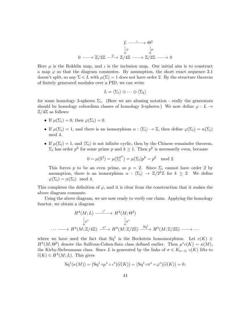
L Θ3

0 Z/2Z Z/4Z Z/2Z 0

ι

ϕ µ

2

Here µ is the Rokhlin map, and ι is the inclusion map. Our initial aim is to constructa map ϕ so that the diagram commutes. By assumption, the short exact sequence 3.1doesn’t split, so any Σ ∈ L with µ(Σ) = 1 does not have order 2. By the structure theoremof finitely generated modules over a PID, we can write

L = 〈Σ1〉 ⊕ · · · ⊕ 〈Σk〉

for some homology 3-spheres Σi. (Here we are abusing notation - really the generatorsshould be homology cobordism classes of homology 3-spheres.) We now define ϕ : L →Z/4Z as follows:

• If µ(Σi) = 0, then ϕ(Σi) = 0.

• If µ(Σi) = 1, and there is an isomorphism α : 〈Σi〉 → Z, then define ϕ(Σi) = α(Σi)mod 4.

• If µ(Σi) = 1, and 〈Σi〉 is not infinite cyclic, then by the Chinese remainder theorem,Σi has order pk for some prime p and k ≥ 1. Then pk is necessarily even, because

0 = µ(S3) = µ(Σpk

i ) = µ(Σi)pk = pk mod 2.

This forces p to be an even prime, so p = 2. Since Σi cannot have order 2 byassumption, there is an isomorphism α : 〈Σi〉 → Z/2kZ for k ≥ 2. We defineϕ(Σi) = α(Σi) mod 4.

This completes the definition of ϕ, and it is clear from the construction that it makes theabove diagram commute.

Using the above diagram, we are now ready to verify our claim. Applying the homologyfunctor, we obtain a diagram

H4(M ;L) H4(M ; Θ3)

· · · H4(M ;Z/4Z) H4(M ;Z/2Z) H5(M ;Z/2Z) · · ·

ι∗

ϕ∗ µ∗

π∗ Sq1

where we have used the fact that Sq1 is the Bockstein homomorphism. Let c(K) ∈H4(M ; Θ3) denote the Sullivan-Cohen-Sato class defined earlier. Then µ∗c(K) = κ(M),the Kirby-Siebenmann class. Since L is generated by the links of σ ∈ Kn−4, c(K) lifts toc(K) ∈ H4(M ;L). This gives

Sq1(κ(M)) = (Sq1 ◦µ∗ ◦ ι∗)(c(K)) = (Sq1 ◦π∗ ◦ ϕ∗)(c(K)) = 0,

44

because Sq1 ◦π∗ = 0 by virtue of being a complex. Therefore Sq1(κ(M)) vanishes asrequired.

In fact, the following proposition shows that we need only find a five dimensionalexample of a manifold with Sq1(κM) non-zero!

Proposition 3.3.10. Let Tm =∏m S1. If M is a 5-manifold with Sq1(κ(M)) 6= 0, then

for each n ≥ 5, N = M × Tn−5 is an n-manifold with Sq1(κ(N)) 6= 0.

Proof. Let p : M × Tn−5 → M be the projection map. Then κ(M × Tn−5) = p∗κ(M).Consider the following diagram:

H4(M ;Z/2Z) H5(M ;Z/2Z)

H4(M × Tn−5;Z/2Z)) H5(M × Tn−5;Z/2Z))

Sq1

Sq1

The vertical maps are inclusion maps by the Kunneth formula. Therefore

Sq1(κ(N)) = Sq1 p∗(κ(M)) = p∗ Sq1 κ(M) 6= 0.

Finally we construct an example of a 5-manifold M such that Sq1(κ(M)) 6= 0. Thisexample is due to Kronheimer, and uses Freedman’s classification of 4-manifolds.

Proposition 3.3.11. There exists a closed 5-manifold M such that Sq1(κ(M)) 6= 0.

Proof. Recall Freedman’s classification of 4-manifolds: For every unimodular symmetricbilinear form Q, there exists a simply connected closed topological 4-manifold X whoseintersection form is Q. If Q is even, X is unique up to homeomorphism with κ(X) = σQ/8mod 2. If Q is odd, there are exactly two homeomorphism types of such an Xi, withκ(X1) = 0 and κ(X2) = 1.

With this in mind, there exists a 4-manifold X such that QX = (1)⊕(−1) and κ(X) = 1.Since QX is isomorphic to −QX , again by Freedman’s theorem, there exists an orientationreversing homeomorphism f : X → X. Let M be the mapping torus X × [0, 1]/(x, 1) ∼(f(x), 0). This is a 5-manifold, and one can show that Sq1(κ(M)) 6= 0.

On one hand, κ(M) ∈ H4(M ;Z/2Z) is non-trivial by construction, with Poincare duala section of the bundle M → S1. By Wu’s formula, we know that

Sq1(κ(M)) = κ(M) ^ v1

where v1 is the first Wu class. This is defined implicitly by

0 + v1 = Sq1(v0) + Sq0(v1) = w1(TM).

45

Note that Sq1(v0) is trivial since deg v0 < 1. Therefore

Sq1(κ(M)) = κ(M) ^ w1(TM) = 1 6= 0.

To see that κ(M) ^ w1(TM) is non-zero, we noted earlier that κ(M) has Poincare dual asection of the bundle M → S1. On the other hand, w1(TM) has Poincare dual X. Theseintersect transversely at a point, giving the desired result.

The previous three positions combine to give the following result:

Proposition 3.3.12. If the short exact sequence 3.1 doesn’t split, then in each dimensionat least 5, there exist non-triangulable (closed) manifolds.

We already proved the converse at an earlier time. In summary, we’ve established themain theorem of this section:

Theorem 3.3.13. All manifolds of dimension at least 5 are triangulable if and only if Θ3

contains an element of order 2 with non-trivial Rokhlin invariant.

3.4 Disproving the triangulation conjecture

As mentioned earlier, the triangulation conjecture is in fact false. This is because Θ3 doesnot contain any elements of order 2 with non-trivial Rokhlin invariant. How do we showthat Θ3 contains no such elements? The proof of Manolescu uses a certain Floer homologytheory.

The strategy is as follows: we are familiar with the Rokhlin invariant map

µ : Θ3 → Z/2Z.

Suppose where was a lift µ of µ to the integers, such that µ = µ mod 2, and µ(−Σ) =−µ(Σ). Then for any homology sphere Σ of order 2,

µ(Σ) = µ(−Σ) = −µ(Σ) =⇒ µ(Σ) = 0.

Therefore µ(Σ) = 0, so there can be no order two elements of Θ3 with non-trivial Rokhlininvariant. This was exactly Manolescu’s strategy.

Proposition 3.4.1. There exists a lift of µ to a map µ : Θ3 → Z such that its reductionmod 2 is the Rokhlin map, and µ(−Σ) = −µ(Σ).

The strategy is to define a certain homology theory

Σ 7→ SWFHPin(2)∗ (Σ)

46

for each homology 3-sphere Σ. This is called the Pin(2)-equivariant Seiberg-Witten Floerhomology. It turns out that an integer associated to this homology theory gives exactlythe lift we desire. Specifically,

µ(Σ) =1

2(min{deg(middle v-tower in SWFH

Pin(2)∗ (Σ))} − 1).

The homology is equipped with a map v which changes the index by 4. This gives four”towers”, namely for each index modulo 4. The first tower consists of elements in degrees2µ(Σ) mod 4. The second, elements in degrees 2µ(Σ) + 1 mod 4, and the third, elementsin degrees 2µ(Σ) + 2 mod 4. It turns out that the fourth tower is always trivial. We callthese v-towers, so that µ(Σ) is defined to be the (B − 1)/2, where B is lowest degree thatis realised by an element of the 2nd tower.

One can show that such a homology theory really exists, that µ is a well definedinvariant of homology cobordism classes of homology 3-spheres, and that it satisfies bothof the desired properties listed above.

In summary, the proof relies on the existence of an invariant β satisfying the followingproperties:

1. β(Σ) is an invariant of integral homology 3-spheres which is also invariant underhomology cobordisms

2. β(−Σ) = −β(Σ), where −Σ is Σ with its orientation reversed.

3. β(Σ) reduces mod 2 to the Rokhlin invariant.

We note that invariants which almost satisfy these properties were constructed at earliertimes. Firstly, the Casson invariant. This satisfies properties 2 and 3 above, but not 1.Secondly, the Froyshøv invariant (which is also defined via Seiberg-Witten Floer homology)satisfies properties 1 and 3, but not 2. In the next chapter we explore the Casson invariant.

47

Chapter 4

The Casson invariant

4.1 When does rational surgery preserve homology?

The Casson invariant (which we introduce in the next section) is defined on integral ho-mology spheres. It is characterised by how it behaves under rational surgeries, so we firstexplore how homology groups behave under rational surgery, and when rational surgeryeven makes sense.

First we show that rational surgery makes sense on integral homology 3-spheres. Wewrite S to denote the set of integral homology 3-spheres. (Note that as sets Θ3 = S/ ∼.)

Proposition 4.1.1. Let Σ ∈ S, and K ∈ Σ a knot. Then K has well defined meridiansand canonical longitudes. In particular, rational surgery is well defined.

Proof. Recall that a meridian of K is a generator of H1(Σ − N), where N is a regularneighbourhood of K. A canonical longitude is the unique longitude of K in ∂N which ishomologically trivial in Σ−N . For notational brevity, we write X = Σ−N .

To establish the existence and uniqueness of these classes, we first calculate Hi(X). Wealready know that Hi(X) = 0 for i ≥ 4, while Hi(X) = Z for i = 0, 3. By Poincare duality,it remains to determine H1(X). This can be determined by the Mayer-Vietoris sequence:

· · · → H2(Σ)→ H1(∂N)→ H1(X)⊕H1(N)→ H1(Σ)→ · · · .

Since Σ is a homology sphere, H1(Σ) = H2(Σ) = 0. On the other hand, ∂N is a 2-torus,so H1(∂N) = Z2. N is a solid torus, so H1(N) = Z. Therefore we have an exact sequence

0→ Z2 → H1(X)⊕ Z→ 0.

It follows that H1(X) = Z, so it has two generators, and just one up to sign. This definesthe meridian of K.

48

Next we show that K has a canonical longitude. We consider the long exact sequenceof relative homology:

· · · → H1(∂N)→ H1(X)→ H1(X, ∂N)→ H0(∂N)→ · · · .

The pair (X, ∂N) has the same homology as (Σ,K) by retracting ∂N onto K radially.Since Σ is a homology sphere, H1(Σ,K) = H1(X, ∂N) is trivial. Therefore the above is anexact sequence

Z2 → Z→ 0→ 0,

where Z2 is generated by a meridian (1, 0) and some longitude (n, 1). The first map inthe above exact sequence maps (p, q) onto p, so there is a unique longitude (up to sign)mapping to the trivial class.

In summary this shows the existence of meridians and canonical longitudes which areunique up to sign. Fixing signs as in chapter 1, rational surgery is well defined.

This shows that rational surgery is well defined on homology spheres! But we also wantto know when a homology sphere remains a homology sphere, following rational surgery.

Example. Recall that the lens space L(p, q) is obtained via −p/q-surgery on the unknotin S3. Moreover, we calculated that

Hi(L(p, q)) =

Z i ∈ {0, 3}Z/pZ k = 1

0 k = 2.

Therefore L(p, q) is a homology sphere if and only if p = ±1.

This result can be made a little more general. The above homological results hold forrational surgery in homology spheres!

Proposition 4.1.2. Let Σ be a homology sphere, and p, q ∈ Z coprime. Then p/q-surgeryalong a knot K ⊂ Σ produces a homology sphere if and only if p = ±1. More precisely,

H1(Σ′) = Z/pZ

where Σ′ is the result of p/q-surgery along K in Σ.

Proof. As in the previous proof, it suffices to study H1(Σ′), where Σ′ is the manifoldobtained by p/q-surgery along K in Σ.

Explicitly, Σ′ = (Σ−N) tϕ D2 × S1, where ϕ is defined by sending the curve ∂D2 × 1in ∂(D2× S1) to γ = pµ+ qλ, where µ and λ are the meridian and canonical longitudes ofK.

49

The Mayer-Vietoris sequence now gives

· · · → H2(Σ′)→ H1(∂N)(i∗,j∗)−−−−→ H1(Σ−N)⊕H1(D2 × S1)

k∗−l∗−−−→ H1(Σ′)→ 0.

H1(∂N) has two generators, m and `, which are the “canonical” meridian and longitudeby considering the solid torus N which it bounds. The maps i, j, k, l are the expectedinclusions.

Under (i∗, j∗), the class [m] is mapped to [γ] + [m] = p[µ]. The other generator [`] ismapped to c + [`] for some class c which we can take to be trivial. Therefore we have asurjective map

Z⊕ Z→ H1(Σ′)

with kernel 〈p[µ], [`]〉. By the first isomorphism theorem, H1(Σ′) is isomorphic to

(Z⊕ Z)/(pZ⊕ Z) = Z/pZ.

Therefore Σ′ is a homology sphere if and only if p = ±1.

Since we are working with integers, this means that when doing surgery on homologyspheres to obtain new homology spheres, we need only consider 1/m-surgery for m ∈ Z.

Definition 4.1.3. Let Σ be a homology sphere and K ⊂ Σ a knot. We write Σ + 1mK to

denote the homology sphere resulting from 1/m-surgery along K in Σ.

We have now established the essential background to study the Casson invariant.

4.2 The Casson invariant: uniqueness and other properties

As remarked at the end of the previous chapter, the Casson invariant is an invariant ofhomology 3-spheres which lifts the Rokhlin invariant to the integers. Writing S to denotethe set of integral homology 3-spheres, the Casson invariant can be classified as follows:

Definition 4.2.1. A Casson invariant is a map λ : S → Z satisfying the following prop-erties:

(1) λ(S3) = 0.

(2) For any homology 3-sphere Σ and knot K ⊂ Σ, the difference

λ(

Σ +1

m+ 1K)− λ

(Σ +

1

mK)

is independent of m.

50

(3) For any homology 3-sphere Σ, boundary link K ∪ L ⊂ Σ, and m,n ∈ N,

λ(

Σ +1

m+ 1K +

1

n+ 1L)− λ

(Σ +

1

mK +

1

n+ 1L)

− λ(

Σ +1

m+ 1K +

1

nL)

+ λ(

Σ +1

mK +

1

nL)

= 0.

By a boundary link, we mean a link which admits a Seifert surface consisting of disjointpieces, one for each component of the link.

Remark. If K ∪ L is a boundary link in Σ, then lk(K,L) = 0. Whenever lk(K,L) = 0,the surgery Σ+(p/q)K+(r/s)L is independent of the order in which the surgery is carriedout and gives a homology sphere.

Proposition 4.2.2. The Casson invariant described above exists and is unique up to scalarmultiple.

This will be the main result that we discuss in the coming sections. Uniqueness is easierthan existence, so we start by proving uniqueness. We will also observe that the Cassoninvariant can truly be made unique by adding the following condition:

(0) λ(S) is not contained in any proper subgroup of Z.

For notational brevity, we write

λ′(K) = λ′(Σ,K) = λ(Σ +1

m+ 1K)− λ(Σ +

1

mK),

λ′′(K,L) = λ′′(Σ,K, L) = λ(

Σ +1

m+ 1K +

1

n+ 1L)− λ

(Σ +

1

mK +

1

n+ 1L)

− λ(

Σ +1

m+ 1K +

1

nL)

+ λ(

Σ +1

mK +

1

nL).

If λ′ is a well defined knot invariant (i.e. independent of m), then so is λ′′. Thereforethe three basic properties of the Casson invariant are as follows:

(1) λ(S3) = 0,

(2) λ′(Σ,K) is well defined,

(3) λ′′(Σ,K, L) = 0 for K ∪ L a boundary link.

To describe our proof of uniqueness, we introduce some additional properties of theCasson invariant:

(4) λ′(Σ, 31) = ±1 for any homology sphere Σ.

51

(5) λ′(Σ,K) = 12∆′′K(1)λ′(Σ, 31) for any K ⊂ Σ.

Uniqueness will then follow the following outline:

• Show that (0), (1), (2), and (3) imply (4) and (5).

• Show that (0), (1), (2), (4), and (5) imply uniqueness.

Note that the Casson invariant also satisfies the following useful properties:

(6) λ(−Σ) = −λ(Σ) where −Σ denotes Σ with the opposite orientation.

(7) λ(Σ1#Σ2) = λ(Σ1) + λ(Σ2).

(8) λ(Σ) = µ(Σ) mod 2, where µ is the Rokhlin invariant.

Lemma 4.2.3.(0), (1), (2), (3) =⇒ (4), (5).

Proof. We give a proof outline. First we reduce the problem to knots in S3. Specifically,for any K ⊂ Σ, we show that there exists L ⊂ S3 such that

λ′(Σ,K) = λ′(S3, L), ∆K(t) = ∆L(t).

This uses property (3) of the Casson invariant.Next we verify that λ′(−) and 1

2∆′′−(1) change by the same rule in a crossing change.More precisely, in the knot picture, any two knot diagrams are related by changing theover-under data of crossings in diagrams. In the surgery picture, let K ⊂ S3 be a knot,and D a disk intersecting K at two points. Swapping crossing data of K corresponds to±1-surgery along the boundary of D. Note that ±1-surgery along the unknot leaves theambient space diffeomorphic to S3. This operation is called a twist across D. Let c = ∂D.Then the knot obtained from the twist is denoted Kc.

Suppose we have another disk D′, with boundary c′, so that twists of K along D or D′

are disjoint. This gives knots K,Kc,Kc′ , and Kcc′ which we now consider. In the surgerypicture, it follows from property (3) that

λ′′(S3,K, c) = λ′′(S3 + c′,K, c).

In the knot theoretic picture, we have

1

2∆′′Kc

(1)− 1

2∆′′K(1) =

1

2∆′′Kcc′

(1)− 1

2∆′′Kc′

(1).

The statement with the Alexander polynomial comes from skein relations.Using the above, one can show that λ′(K) is proportional to λ′(31) for any K, so we

conclude property (4) from property (0). Finally we calculate the proportionality constantand conclude property (5).

52

Lemma 4.2.4.(1), (2), (4), (5) =⇒ uniqueness.

Proof. Let Σ be a homology sphere. Then there exist knots K1, . . . ,Kn with pairwisevanishing linking number, and εi = ±1 such that

Σ = S3 + ε1K1 + · · ·+ εnKn.

Define Σi = S3 + ε1K1 + · · ·+ εiKi, so that Σ0 = S3 and Σn = Σ. Then

λ(Σi)− λ(Σi−1) = εiλ′(Ki)

by the definition of λ′. Using property property (1), we then have

λ(Σ) =

n∑i=1

(λ(Σi)− λ(Σi−1)) + λ(Σ0) =

n∑i=1

εiλ′(Ki).

But now from properties (4) and (5), we have

λ(Σ) = ±( n∑i=1

εi2

∆′′Ki,Σi(1))

where the sign depends on λ′(31).

Combining the previous two lemmas, we have the following result:

Theorem 4.2.5. The Casson invariant is uniquely determined by properties (0), (1), (2),and (3).

4.3 Construction of the Casson invariant

We have yet to show that the Casson invariant exists! This can be constructed as acertain count of a moduli space of SU(2)-valued representations of the fundamental groupof homology spheres. Here we will construct the Casson invariant without explaining whycertain choices are being made, and in later sections explain what goes wrong if we changeour choices. The outline is as follows:

1. For any manifold M consider the space of representations

R(M) = Hom(π1M,SU(2)).

This is a topological space (equipped with the compact-open topology). SO(3) actson R(M) by conjugation, and R(M) := Rirr(M)/SO(3) is called the representationspace of M . (Note that R(M)/ SU(2) is a character variety.) Here Rirr(M) ⊂ R(M)is the subspace of irreducible representations.

53

2. For M a handlebody of genus g ≥ 1, R(M) is a smooth open manifold of dimension3g− 3 (and empty if g = 1). For F a closed oriented surface of genus g ≥ 1, R(F ) isa smooth open manifold of dimension 6g − 6.

3. For Σ a homology sphere, we can find a Heegaard decomposition Σ = M1 tF M2.Then R(Σ) = R(M1) ∩ R(M2) is a compact manifold of dimension 0 in R(F ). Byorienting R(M1) and R(M2) we obtain an algebraic count of this intersection, fromwhich we define the Casson invariant :

λ(Σ,M1,M2) =(−1)g

2#(R(M1) ∩R(M2)).

4. One can show that the invariant is independent of the choice of Heegaard splitting.

We now work through these steps in some more detail, in the corresponding subsections.

4.3.1 Step 1: representation spaces in general

Let M be a manifold. We equip R(M) = Hom(π1M,SU(2)) with the compact-open topol-ogy. Explicitly, π1M is endowed with the discrete topology, and SU(2) with the usualtopology making it homeomorphic to S3. Then the topology of R(M) is generated by theopen sets

UK,V := {f : π1M → SU(2) : f(K) ⊂ V,K ⊂ π1M compact, V ⊂ SU(2) open}.

But π1M is discrete so compact subsets are exactly finite subsets. Therefore the topologyof R(M) is generated by the sub-basis of functions

Ug,V := {f : π1M → SU(2) : f(g) ∈ V, V ⊂ SU(2) open}.

Equivalently, R(M) is equipped with the subspace topology of R(M) ⊂ SU(2)π1M , wherethe latter is equipped with the product topology. By Tychonoff’s theorem, if R(M) isclosed in SU(2)π1M , it must also be compact. Indeed R(M) is closed, so it is compact.

Definition 4.3.1. A morphism f ∈ R(M) is called a representation. The representationdetermines a corresponding C[π1M ]-module V . Explicitly, V is isomorphic to C2 as a C-vector space, but has an additional action of π1M defined by g · v = f(g)v. The module V(along with the representation f) are said to reducible if V has a non-zero proper C[π1M ]-submodule. Otherwise they are reducible.

In our context of SU(2)-valued representations, we have the following characterisationof reducible representations.

Proposition 4.3.2. For any M , f ∈ R(M) is reducible if and only if f factors throughU(1) ∼= S1.

54

Proof. By definition, we see that f is reducible if and only if there is a one dimensionalsubspace U of C2 such that f(g)U ⊂ U for all g ∈ π1M . This means that f is reducibleif and only if there is a basis {u, v} of C2 so that each f(g) maps v to λgv for some scalarλg. In this basis, for each g we have

f(g) =

(ag bg0 λg

).

But SU(2) consists of unitary matrices of determinant 1, so the above matrix is constrainedby

aλ = 1, |a|2 + |b|2 = 1, bλ = 0, |λ|2 = 1.

The third and fourth constraints give b = 0, while the first and second give a = λ, |a|2 = 1.Therefore the image of f lies in

U(1) ∼= S1 ∼={(

eiθ 00 e−iθ

): θ ∈ S1

}.

Definition 4.3.3. We write Rred(M) to denote the subset of R(M) consisting of reduciblerepresentations, and Rirr(M) to denote the irreducible representations.

By the above proposition, we see that Rred(M) ⊂ R(M) is closed and hence compact.To eventually develop the Casson invariant, we want to control the reducible representa-tions. These are of the following types:

• The trivial representation θ ∈ Rred(M); θ(g) = 1.

• The central representations f ∈ Rred(M); f(g) = {±1} (but f non-trivial). (Theseare central since the centre of SU(n) is generated by ζI for ζ an nth root of unity,which in this case is the group Z/2Z.)

• The other reducibles, which are exactly non-trivial and non-central representationsthat factor through U(1).

Observe that R(M) admits a natural group action - conjugation by SU(2). This does notact freely in general, and is particularly bad on the reducibles:

• The stabiliser of the SU(2) action on the trivial representation is all of SU(2).

• The stabiliser of the action on a central representation is also all of SU(2).

• The stabiliser of the action on any other reducible representation is U(1) ⊂ SU(2).

55

It’s natural to wonder if the conjugation action of SU(2) is free on Rirr(M). Unfortunately,this is not the case, as −A and A will always conjugate to the same element. But factoringSU(2) by {±1} gives the rotation group SO(3), and this acts freely on Rirr(M).

Definition 4.3.4. The action of SO(3) on the irreducible representations Rirr(M) is free.The quotient Rirr/SO(3), denoted by R(M), is called the representation space of M . It isequipped with the quotient topology.

In the next subsection we will establish that the representation spaces of surfaces andhandlebodies are smooth open manifolds and compute their dimensions. Before proceedingwith these special cases, we must better understand the local structure of representationspaces. Concretely, we would like to know when Rirr(M) is closed and hence compact, sowe desire a method of detecting when reducible representations are isolated. This requiresthe local theory of manifolds: tangent spaces. We will soon see that the relevant tangentspaces can be understood via group cohomology, which we now review.

Definition 4.3.5. Let G be a group, and M a G-module. (That is, an abelian group witha G action, each g ∈ G acting as an automorphism.) Then the group of inhomogeneousn-cochains is the group of set theoretic functions Cn(G,M) = MGn

. These form a cochaincomplex, with boundary map dn+1 : Cn(G,M)→ Cn+1(G,M) defined by

(dn+1ϕ)(g1, . . . , gn+1) = g1 · ϕ(g2, . . . , gn+1) +n∑i=1

(−1)iϕ(g1, . . . , gi−1, gigi+1, . . . , gn+1)

+ (−1)n+1ϕ(g1, . . . , gn).

The n-cocycles are Zn(G;M) = ker dn+1, and n-coboundaries Bn(G;M) = im dn. Thegroup cohomology of G with coefficients in M is Hn(G;M) = Zn(G;M)/Bn(G;M).

In our case, we will consider just the first cohomology of π1M with coefficients in su(2).Recall the adjoint action Ad : G → Aut(g), defined by Ad : g 7→ Adg, where Adg is thederivative (at the origin) of the conjugation automorphism of g on G. This turns the Liealgebra su(2) into an SU(2)-module. But now, given a representation f : π1M → SU(2),we can pull back the module structure by f so that su(2) is a π1M -module.

By inspecting the definition of the boundary map, we have:

Z1f (π1M ; su(2)) = {ϕ : π1M → su(2) : ϕ(xy) = ϕ(x) + Adf(x) ϕ(y)},

B1f (π1M ; su(2)) = {ϕ : π1M → su(2) : ϕ(x) = Adf(x) uϕ − uϕ, uϕ ∈ su(2)}.

The reason we are investigating group cohomology is that they turn out to encode the localstructure of spaces of representations we’re interested in.

Proposition 4.3.6. Let f ∈ R(M). The tangent space of R(M) at f is

TfR(M) ∼= Z1f (π1M ; su(2)).

56

The tangent space of the character variety χ(M) = R(M)/SO(3) at f is

Tfχ(M) ∼= H1f (π1M ; su(2)).

To understand this proposition we must define the Zariski tangent space. This is becauseR(M) is not generally a smooth manifold, so the usual notion of a tangent space does notapply.

Definition 4.3.7. Let X be an affine algebraic set over k, and α ∈ X. Then the Zariskitangent space TαX is the set of k-valued derivations D of k[X]. More explicitly,

TαX = {D : k[X]→ k | D(pq) = p(α)D(q) +D(p)q(α)}.

Each D as above is called a tangent vector.

By using the auxiliary ring of dual numbers k[ε]/(ε2), one can show that the Zariskitangent space has a more down-to-earth construction:

Proposition 4.3.8. Let X = Z(F1, . . . , Fm) ⊂ kn. Fix α ∈ X. Then TαX is the zero setof the linearisations of each Fi at α. More explicitly, write

Fi(α+ εβ) = Fi(α) + εLi(β) +Gi(εβ) = εLi(β).

Gi(εβ) vanishes since ε2 factors in it, while Fi(α) = 0 by definition of X, leaving only thelinearisation Li. Then TαX = Z(L1, . . . , Lm) ⊂ kn.

Example. Our space R(M) = Hom(π1M,SU(2)) is a real algebraic set, so we can applythe above notion of a tangent space. Explicitly, write

π1M = 〈x1, . . . , xn | r1, . . . , rm〉.

(We only concern ourselves with compact manifolds of dimension at most 3, which ad-mit finite triangulations, and hence have finite presentations.) Each map f ∈ R(M) isdetermined by the image of each xj :

f : xj 7→(aj + ibj −cj + idjcj + idj aj − ibj

)∼ (aj , bj , cj , dj) ∈ R4.

This gives an inclusion R(M) ↪→ R4n. The polynomials defining R(M) are exactly thefollowing:

• The constraint on SU(2): each matrix must have determinant 1, so a2j+b

2j+c

2j+d

2j = 1

for every j.

• The relations in π1M : each rk is a product of xjs and their inverses. These are eachrepresented by an SU(2) matrix with entries polynomials in the aj , . . . , dj . Each suchmatrix must vanish, giving four polynomial constraints for each ri.

57

This gives a description of R(M) as an algebraic set, with which we can compute thetangent space.

We are now ready to prove the earlier proposition which relates the tangent spaces ofR(M) and χ(M) to group cohomology. We’ll re-state the results and prove them one at atime.

Proposition 4.3.9. Let f ∈ R(M). Then TfR(M) = Z1f (π1M ; su(2)).

Proof. The map f : π1M → SU(2) can be perturbed to obtain f + εη, where η : x →η(x) ∈ Tf(x) SU(2). Since Tf(x) SU(2) is just the right translation of T1 SU(2) = su(2) byf(x), our perturbation can be written as

f : x 7→ f(x) + εξ(x)f(x), ξ : π1M → su(2).

Our constraint equation is that f must be the linearisation of a representation. Thereforewe must have

f(xy) = f(x)f(y)

⇔ f(xy) + εξ(xy)f(xy) = (f(x) + εξ(x)f(x))(f(y) + εξ(y)f(y))

= f(x)f(y) + εξ(x)f(x)f(y) + εf(x)ξ(y)f(y),

Where the second order term has been dropped. Subtracting f(xy) from each side, andmultiplying on the right by f(xy)−1, we have

εξ(xy) = εξ(x) + εf(x)ξ(y)f(x)−1.

The equation is now independent of ε, and can be expressed as

ξ(xy) = ξ(x) + Adf(x) ξ(y).

This is exactly a 1-cocycle! This proves the claim.

Proposition 4.3.10. Let f ∈ R(M)/ SO(3). Then Tf (R(M)/SO(3)) = H1f (π1M ; su(2)).

Proposition 4.3.11. We must show that if any two vectors are related by the SO(3)conjugation action, then their difference is a 1-coboundary. Concretely, two perturbationsf + εξ1f and f + εξ2f are related by the SO(3) action if there exists u ∈ su(2) such that

f(x) + εξ1(x)f(x) = (1 + εu)(f(x) + εξ2(x)f(x))(1 + εu)−1.

But we find that(1 + εu)(1− εu) = 1− ε2y2 = 1,

so (1 + εu)−1 = 1− εu. Making this substitution and dropping second order terms gives

f(x) + εξ1(x)f(x) = f(x) + εξ2(x)f(x) + εuf(x)− εf(x)u.

58

Rearranging the equation and multiplying on the right by f(x)−1 gives

ξ1(x)− ξ2(x) = u− f(x)uf(x)−1 = u−Adf(x) u.

Therefore ξ2 = ξ1 + ϕ where ϕ ∈ B1f (π1M, su(2)) is a 1-coboundary. But now

Tf (R(M)/ SO(3)) = Z1f (π1M, su(2))/B1

f (π1M, su(2)) = H1f (π1M, su(2))

as required.

This shows that the local structure of the character variety χ(M) can be understood viagroup cohomology. In particular, it sheds light on the representation space R(M) (whichis really a subspace of χ(M)). We will observe that in some cases the group cohomologycan be identified with singular cohomology. This completes the general theory, and we nowstudy the specifics which will lead to the Casson invariant.

4.3.2 Step 2: representation spaces of homology spheres

Our goal is to define the Casson invariant, an integral invariant of homology 3-spheres. Wewill define this by choosing a Heegaard splitting of the homology sphere;

Σ = M1 tF M2.

In the remainder of this subsection we will develop an understanding of representationspaces of Σ,Mi, and F . First we will investigate the representation space of the totalspace, Σ.

Proposition 4.3.12. R(Σ) has a unique reducible representation, namely the trivial rep-resentation.

Proof. Recall that f : π1Σ→ SU(2) is reducible if and only if f factors through U(1). ButU(1) is abelian, so the derived subgroup [π1Σ, π1Σ] must map to 1 ∈ U(1). Therefore ffactors as

f : π1Σ→ π1Σ

[π1Σ, π1Σ]→ U(1)→ SU(2).

This means f factors through H1(Σ), which is trivial since Σ is a homology sphere. There-fore f is the trivial representation.

This result will later be essential, as it gives control over the reducible representations.There is no reason to believe that R(Σ) is a manifold, but we might hope that Rirr(Σ) isa manifold. Unfortunately this turns out not to be the case, but the individual pieces of aHeegaard decomposition of Σ indeed give rise to manifolds of representations.

Proposition 4.3.13. Let M be a handlebody of genus g ≥ 1. Then Rirr(M) is a smoothopen manifold of dimension 3g, and R(M) is a smooth open manifold of dimension 3g− 3.When g = 1 the manifold is empty.

59

Proof. Since SO(3) has dimension 3 and acts freely on Rirr(M), the second claim followsimmediately provided the first claim is true.

For the first claim, observe that π1M is the free group on g generators. Therefore R(M)is diffeomorphic to

∏g SU(2) (by recalling the description of R(M) as an algebraic set).

This is a closed smooth manifold of dimension 3g. But now Rirr(M) = R(M) − Rred(M)and Rred(M) is a topologically closed subset of R(M). Therefore Rirr(M) is an opensmooth manifold of dimension 3g, as required.

When g = 1 the manifold is empty because χ(M) consists of a single point, the trivialrepresentation.

Finally, we determine the topological structure of the representation space of a surface.

Proposition 4.3.14. Let F be a closed oriented surface of genus g ≥ 1. Then Rirr(F )is a smooth open manifold of dimension 6g − 3, and R(F ) is a smooth open manifold ofdimension 6g − 6.

Proof. We give just a proof outline. Let D ⊂ F be a disk, γ = ∂D, and F0 = F − D.Define

h : R(F0)→ SU(2)

by h(f) = f(γ). Then

h−1(1) = {f ∈ R(F0) : f(γ) = 1} ∼= R(F ).

Therefore by understanding h we can understand R(F ).We consider F0 since π1F0 is free of rank 2g, with standard generators a1, . . . , ag, b1, . . . , bg.

Then γ is given by

γ =

g∏i=1

[ai, bi].

Since π1F0 is free we have an identification

R(F0) ∼= SU(2)2g, f 7→ (f(a1), f(b1), . . . , f(ag), f(bg)).

But now h can be expressed as

h : SU(2)2g → SU(2), (A1, B1, . . . , Ag, Bg) 7→g∏i=1

[Ai, Bi].

One can explicitly show that h is surjective. Moreover, by some technical calculations (car-ried out in Saveliev), one can show that h is regular exactly at irreducible representations.

It follows that Rirr(F ) (which is h−1(1) restricted to irreducible representations) is anopen submanifold of SU(2)2g with dimension 3(2g) − 3 = 6g − 3. By taking a furtherquotient by SO(3), R(F ) is a smooth open manifold of dimension 6g − 6.

60

Finally we note that if Σ = M1 tF M2, then the representation space of Σ is theintersection of the representation spaces of M1 and M2. This means that even if R(Σ)is not known to be a manifold, we can completely understand it in terms of the 3g − 3dimensional manifolds R(Mi).

Proposition 4.3.15. Let Σ = M1 tF M2 be a Heegaard splitting of a closed 3-manifoldΣ. Then R(M1)∩R(M2) = R(Σ). Moreover, it follows that Rirr(M1)∩Rirr(M2) = Rirr(Σ)and R(M1) ∩R(M2) = R(Σ).

Proof. Suppose the Heegaard splitting is of genus g. Then

π1M1 = 〈x1, . . . , xg〉, π1M2 = 〈y1, . . . , yg〉.

By the Seifert-van Kampen theorem, we have

π1Σ = 〈x1, . . . , xg | r1, . . . , rg〉 = 〈y1, . . . , yg | r′1, . . . , r′g〉,

where r1, . . . , rg are determined by y1, . . . , yg expressed in the basis x1, . . . , xg, and similarlyfor r′1, . . . , r

′g. It follows that the inclusions induce quotient maps π1M1, π1M2 → π1Σ. Now

any representation f : π1Σ→ SU(2) pulls back to representations π1Mi → SU(2).On the other hand, π1F is generated by 2g generators,

π1F = 〈x1, . . . , xg, x′1, . . . , x

′g | [xi, x′i]〉 = 〈y1, . . . , yg, y

′1, . . . , y

′g | [yi, y′i]〉.

Therefore we have quotient maps π1F → π1Mi as above, so that any representation f :π1Mi → SU(2) pulls back to a representation π1F → SU(2). In summary we have thefollowing diagram of inclusions:

R(M1)

R(Σ) R(F )

R(M2)

j1i1

i2 j2

These inclusions allow us to make sense of R(M1)∩R(M2), by considering the intersectionin R(F ). It is clear that R(Σ) ⊂ R(M1) ∩ R(M2). For the converse, we inspect thepresentations of the corresponding fundamental groups. If f ∈ R(M1) ∩ R(M2), then itis defined on both the xi and the yi. Since the yi determine the relations of π1Σ withgenerators xi, f is also well defined as map on π1Σ. Therefore R(Σ) = R(M1) ∩R(M2).

Next we restrict to irreducible representations. The lift of any irreducible representationof F is irreducible on Mi (since it cannot factor through U(1)). Conversely, reducibles liftto reducibles. Therefore

Rirr(M1) ∩Rirr(M2) = Rirr(Σ), Rred(M1) ∩Rred(M2) = Rred(Σ).

The last result is immediate.

61

This concludes our investigations of the global structures of representation spaces ofmanifolds with a view to defining the Casson invariant. Next we investigate some of thelocal structure by using tangent spaces. In the degenerate case of the trivial representation,the tangent space is in fact given by singular cohomology.

Proposition 4.3.16. If θ ∈ χ(X) = Hom(π1X,SU(2))/ SO(3) is the trivial representation,where X is any topological space with finitely presented fundamental group, then

Tθχ(X) = H1θ (π1X; su(2)) ∼= H1(X; su(2)).

(Group cohomology on the left, singular cohomology on the right.)

Proof. Recall the universal coefficient theorem: there is an exact sequence

0→ Ext1Z(H0(X;Z), su(2))→ H1(X; su(2))→ HomZ(H1(X;Z), su(2))→ 0.

But H0(X;Z) is free, so H1(X; su(2)) is isomorphic to HomZ(H1(X;Z), su(2)).Next we notice that for θ the trivial representation, the 1-cocycles Z1

1 (π1X; su(2)) areexactly su(2)-valued homomorphisms of H1(X;Z). This because the cocycle conditionbecomes

ξ(xy) = ξ(x) + Adf(x) ξ(y) = ξ(y) + ξ(y) = ξ(yx).

Therefore cocycles factor through the abelianisation of π1X (which is exactly H1(X)) andare Z-linear.

Finally we observe that the coboundaries are trivial, since the coboundary conditionreduces to

ξ(x) = Adθ(x) u− u = u− u = 0.

Therefore we have

Tθχ(X) = H1θ (π1X; su(2)) = Z1

θ (π1X; su(2)) = Hom(H1(X;Z), su(2)) = H1(X; su(2)).

In some non-degenerate cases (that is, when we restrict to irreducible representations),we have shown that the representation space is sometimes a smooth manifold. In this casethe Zariski tangent space agrees with the usual tangent space.

Example. We have established that R(F ) is a smooth manifold of dimension 6g − 6.Therefore for any f ∈ R(F ),

R6g−6 ∼= TfR(F ) = Tfχ(F ) = H1f (π1F ; su(2)).

If f is the trivial representation, then

Tfχ(F ) = H1f (π1F ; su(2)) = H1(F ; su(2)) ∼= R6g.

62

Similarly for M a handlebody of genus g, we have

Tfχ(M) =

R3g−3 f irreducible

R3g f trivial

? other reducibles.

In these two examples, the change in dimension reflects that the reducible representationsare singular points of the character variety.

4.3.3 Step 3: the Casson invariant as a signed count

We now have enough understanding of the global and local structures of representationspaces to define the Casson invariant. The definition is as follows:

Definition 4.3.17. Let M1 tF M2 be a genus g Heegaard splitting of a homology sphereΣ. Then the Casson invariant λ is defined by

λ(Σ,M1,M2) =(−1)g

2#(R(M1) ∩R(M2))

where # denotes a signed count, given orientations on R(Mi).

It is not yet immediate that this definition makes sense. We must verify the followingfacts:

1. R(M2) can be perturbed to R(M2) so that R(M1) ∩ R(M2) is a finite collectionpoints.

• R(M1) ∩R(M2) is compact.

• dimR(M1) + dimR(M2) = dimR(F ).

2. The signed count of points is independent of the perturbation.

3. The invariant is independent of choices of orientation for the Heegaard splitting.

In the next subsection we will also show that the Casson invariant does not depend on thechoice of Heegaard splitting. We now prove the first of the two bullet points above.

1. By derivations in the previous subsection, we know that dimR(M1) + dimR(M2) =(3g−3)+(3g−3) = 6g−6 = dimR(F ). Therefore by perturbingR(M2) to achieve transver-sality in R(F ), the two submanifolds intersect along a 0-manifold. For a 0-manifold, finite-ness is equivalent to compactness. Therefore it remains to show that R(M1) ∩ R(M2) iscompact.

By the previous subsection, we know that R(M1)∩R(M2) = R(Σ) ⊂ R(F ). Moreover,we know that R(Σ) is a closed subset of SU(2)π1Σ and hence compact, so χ(Σ) is compact.It remains to show that

R(Σ) = χ(Σ)−Rred(Σ)/ SO(3)

63

is closed, or equivalently that Rred(Σ) is open in R(Σ). Since Σ is a homology sphere, wehave established that it has a unique reducible representation, namely the trivial represen-tation. We will show that the trivial representation is an isolated point in R(Σ).

Recall the following result from transversality: if U, V ⊂ X are submanifolds of codi-mension n and m, and U t V in X, then U∩V is an embedded submanifold of codimensionn+m. In particular, if n+m is the dimension of X, then U ∩ V intersect along isolatedpoints. Therefore to show that the trivial representation θ is isolated in R(Σ), it sufficesto show that R(M1) and R(M2) intersect transversely at θ. This means that

TθR(M1) + TθR(M2) = TθR(F ).

But recall that the trivial representation satisfies

Tθχ(X) = TθR(X) = H1(X; su(2))

for any X (with finitely presented fundamental group). Therefore we must establish thatthe induced map

H1(M1; su(2))⊕H1(M2; su(2))→ H1(F ; su(2))

is an isomorphism, to verify transversality as above. This comes immediately from theMayer-Vietoris sequence, since Σ is a homology sphere.

Therefore R(M1) and R(M2) intersect transversely at θ, so θ is an isolated point ofR(Σ) in R(F ). But then R(Σ) − {θ} = Rirr(Σ) is topologically closed, and in particularcompact. The result follows.

2. This is a result of the general theory of differential topology.3. Formally the signed count #(R(M1) ∩R(M2)) is really #(R(M1) ∩ R(M2)), where

R(M2) is a perturbation of R(M2) so that the intersection is transverse. The signed countis then defined to be

#(R(M1) ∩R(M2)) =∑

f∈R(M1)∩R(M2)

sgn(f),

where sgn(f) is defined to be ±1 depending on whether or not the following orientationsagree:

TfR(M1)⊕ TfR(M2), TfR(F ).

We show that the signed count is independent of choices of orientation as follows:

(a) Write Σ = M1 tF M2. Choose an orientation for F , and observe how it determinesan orientation of H1(F ;R) and hence an orientation of R(F ).

(b) Use the orientation of H1(F ;R) to induce orientations on H1(Mi,R), and hence onR(Mi).

64

(c) Study how changing the orientation of F affects the signed count (we will see that itchanges sign).

(d) Study how changing the labels M1 and M2 (to reverse the order) changes the signedcount (it also changes sign).

(e) Conclude that the signed count is independent of choices of orientation for a fixedHeegaard splitting, since the orientation of F and indexing of Mi determine theorientation of Σ, which is fixed.

We now work through the above outline in a bit more detail.(a) Let F be oriented, with genus g. Then F is equipped with an intersection form,

I : H1(F ;R)×H1(F ;R)→ R, I(a, b) = (a ^ b)[F ].

In some basis of H1(F ;R), I is described by the block diagonal matrix

I =

(0 1−1 0

)⊕ · · · ⊕

(0 1−1 0

).

This is called a symplectic basis, and any two symplectic bases for which I has the same formhave the same orientation. This is the canonical orientation induced on H1(F ;R) = R2g.

Now we describe the orientation of R(F ). Choose a basis for H1(F ;R) which is con-sistent with the orientation. Define F0 = F −D for some disk in F , and recall that F0 hasfundamental group free of rank 2g. Therefore Hom(π1F0,SU(2)) ∼= SU(2)2g. But now thebasis for H1(F ;R) fixes an ordering for the generators of π1F0, and hence an identificationHom(π1F0, SU(2)) = SU(2)2g.

We have now induced an orientation on R(F0) = Hom(π1F0, SU(2)). But if h : R(F0)→SU(2) is defined by h(f) = f(∂D), then R(F ) = h−1(1) is oriented by the orientation ofSU(2). Finally by requiring that the identification su(2)⊕TR(F ) = TR(F0) is orientationpreserving, we can further induce an orientation on R(F ) as required.

All choices above were canonical, except for the choice of orientation of Σ. Suppose wechange the orientation of Σ. Then the orientation of H1(F,R) changes by (−1)g, and theorientation of R(F ) changes by (−1)g+1.

(b) The orientations on H1(Mi;R) come from the Mayer-Vietoris sequence. Specificallysince Σ is a homology sphere we have

H1(M1;R)⊕H1(M2;R) = H1(F ;R).

Therefore any choice of orientation of M1 together with the induced orientation of H1(F ;R)canonically orients H1(M2;R).

Choose a basis for H1(M1;R) which is compatible with the orientation. This defines anidentification of R(M1) with SU(2)g, and hence an orientation of R(M1) ⊂ SU(2)g/ SO(3).Similarly there is an induced orientation on R(M2).

65

(c) The orientation ofR(M1) andR(M2) both change when the orientation ofH1(M1;R)is changed, so the orientation of

TfR(M1)⊕ TfR(M2)

does not depend on the orientation of H1(M1;R).However, changing the orientation of F only changes the orientation of R(M2) and not

R(M1), so overall the orientation of TfR(M1) ⊕ TfR(M2) changes by (−1)g. We notedthat changing the orientation of F affects the orientation of R(F ) by (−1)g+1. Therefore,the sign of a given point always changes by −1.

(d) Now suppose we change the roles of M1 and M2, so that H1(M2;R) is the one whichis originally oriented. Then the orientation of TfR(M1)⊕TfR(M2) changes by (−1)g. Onthe other hand, since R(M1) has dimension 3g − 3 (which is odd exactly when g is even),changing from TfR(M1)⊕TfR(M2) to TfR(M2)⊕TfR(M1) changes the orientation exactlywhen g is even, i.e. by (−1)g+1. Therefore overall a change in labelling between M1 andM2 changes the sign of a point by −1.

(e) It follows that the signed count is independent of the choices of orientation for aHeegaard splitting, since it depends only on the orientation of F and the labelling of M1

and M2. But given a choice of orientation for F , the labelling of M1 and M2 are determinedby the choice of normal vector, which is determined by the orientation of Σ.

This completes the proof that the Casson invariant is well defined, given a choice ofHeegaard splitting. Next we show that even the Heegaard splitting need not be specified.

4.3.4 Step 4: Heegaard splitting invariance

Let Σ be a homology sphere. Then given a Heegaard splitting Σ = M1 tF M2, we haveshown that the Casson invariant λ(Σ,M1,M2) is a well defined half-integer. (It has notyet been shown that this quantity is in fact an integer.) We now show that the choice ofHeegaard splitting does not affect the Casson invariant. Recall the following classificationof Heegaard splittings:

Proposition 4.3.18. Let M be a closed 3-manifold. Any two Heegaard splittings of Mare stably equivalent.

This result was discussed at the start of the notes. Therefore to show that the Cassoninvariant is well defined independent of the Heegaard splitting, it remains to show that itis invariant under stabilisation. We give a proof outline of the following result:

Proposition 4.3.19. Let Σ = M1 tF M2 be a homology sphere. Let M ′1 tF ′ M ′2 be thestabilisation of M1 tF M2. Then

λ(Σ,M1,M2) = λ(Σ,M ′1,M′2).

66

Proof. We give a proof outline. Let F0 = F −D and F ′0 = F ′ −D, where D is some disk.We have the following fundamental groups:

π1(F0) = 〈a1, b1, . . . , ag, bg〉π1(M1) = 〈a1, . . . , ag〉π1(M2) = 〈b1, . . . , bg〉.

Then in the stabilisation, we have

π1(F ′0) = 〈a0, b0, a1, b1, . . . , ag, bg | [ai, bi]〉π1(M ′1) = 〈a0, a1, . . . , ag〉π1(M ′2) = 〈b0, b1, . . . , bg〉.

These further give identifications

R(M ′i) = SU(2)×R(Mi), R(F ′0) = SU(2)× SU(2)×R(F0).

But now we find that

R(M ′1) ∩R(M ′2) = (SU(2)× 1×R(M1)) ∩ (1× SU(2)×R(M2))

= 1× 1× (R(M1)×R(M2)).

Making appropriate quotients and perturbations, we can achieve

R(M ′1) ∩ R(M ′2) = 1× 1×R(M1) ∩ R(M2).

The Casson invariants are given by

λ(Σ,M1,M2) =(−1)g

2

∑εα, λ(Σ,M ′1,M

′2) =

(−1)g+1

2

∑ε′α.

It suffices to verify that εα = −ε′α. This is not covered here, but one can show using similararguments to the orientation invariance of the Casson invariant given a Heegaard splittingthat this indeed holds.

4.4 What if we change the choices?

In this section we explore three modifications to the Casson invariant:

• What if we try to build a Casson invariant for homology 4-spheres?

• What if we try to build a Casson invariant for 3-manifolds which aren’t homologyspheres?

• What if we change the gauge group to something else? E.g. SU(n) or SL(2,C).

67

4.4.1 Attempted generalisation to homology 4-spheres

We now attempt to repeat the construction for homology 4-spheres. Recall that closed4-manifolds have an analogue of Heegaard splittings, called trisections.

Definition 4.4.1. Let X be a closed smooth connected 4-manifold. Then for 0 ≤ k ≤ g,a (g, k)-trisection of X is a decomposition X = X1 ∪X2 ∪X3 such that

• For each i, there is a diffeomorphism ϕi : Xi → \k(S1 ×B3).

• The boundary of each Xi is #k(S1 × S2). Each of these has a Heegaard splitting

∂Xi = #k(S1 × S2) = Y −k,g tΣg Y+k,g.

• Given any i, ϕi(Xi ∩Xi+1) = Y −k,g, and ϕi(Xi ∩Xi−1) = Y +k,g.

Moreover, the diagram of inclusions of a trisection induces a diagram of surjections offundamental groups:

π1X1 π1H1

π1Σ π1X2 π1H2 π1F

π1X3 π1H3

In this diagram, each Hi is one of the handlebodies Yk,g. The above diagram induces adiagram of inclusions

R(X1) R(H1)

R(Σ) R(X2) R(H2) R(F )

R(X3) R(H3)

We would like to define some sort of Casson invariant. Each of the above spaces (exceptpossibly R(Σ)) is a manifold. Recall that trisections satisfy

2 = χ(Σ) = 2 + g − 3k,

where the Xi are \k(S1 ×B3), and F has genus g. Then

dimR(Xi) = 3k − 3 = g − 3

dimR(Hi) = 3g − 3

dimR(F ) = 6g − 6.

68

This means that, in general, R(Xi) will not be useful in an attempted transverse signedcount construction. We could attempt to count intersections of R(Hi) in R(F ). How-ever, we then come across a problem concerning induced orientations. Consider the exactsequence

· · · → H1(∂X1;R)→ H1(H1;R)⊕H1(H2;R)→ H1(F ;R)→ H2(X1;R)→ · · · .

Since ∂Xi has non-trivial homology in general, we cannot identify H1(H1;R)⊕H1(H2;R)with H1(F ;R) → H2(X1;R) to induce orientations. Therefore the foremost issue is toattempt to understand the Casson invariant for closed 3-manifolds which aren’t homologyspheres (to have any hope of generalising to homology 4-spheres).

4.4.2 Attempted generalisation to more 3-manifolds

In the definition of the Casson invariant, we consistently made use of the fact that ourunderlying manifold was a homology sphere. This manifested in the following ways: let Σbe a homology sphere, and Σ = M1 tF M2 a Heegaard splitting.

• R(Σ) has a unique reducible representation (the trivial representation). In generalthere may be more irreducible representations.

• The trivial representation is isolated. This follows from the fact that

H1(M1; su(2))⊕H1(M2; su(2))→ H1(F ; su(2))

is an isomorphism (by the Mayer-Vietoris sequence, using that Σ is a homologysphere). But for the trivial representation of π1X (for any X), we have

H1(X; su(2)) ∼= Tθχ(X).

Since R(Σ) ⊂ SU(2)π1Σ is closed and hence compact, χ(Σ) is compact. Since thetrivial representation is the unique reducible, R(Σ) is compact. In general the triv-ial representation may not be isolated, so R(Σ) may not be compact. Moreover,reducibles which are not the trivial representation may be harder to understand.

• To compute the signed count of intersections we must orient F,M1, and M2. However,we relied on the identity

H1(M1;R)⊕H1(M2;R) = H1(F ;R)

to orient H1(M2;R) given an orientation of H1(M1;R) and F . (The above equalityagain comes from Mayer-Vietoris using that Σ is a homology sphere). In general itshould be more difficult to keep track of orientations. Heegaard splitting indepen-dence cannot be considered unless orientations are made sense of.

69

To understand how things might go wrong, we consider the example Σ = S1 × S2 (ratherthan a general non-homology 3-sphere).

Example. Σ = S1 × S2 has a canonical Heegaard splitting of genus 1, M1 tF M2. Thesehave fundamental groups as follows:

π1Σ = 〈a〉, π1Mi = 〈a〉, π1F = 〈a, b | [a, b]〉.

But then Hom(π1Σ, SU(2)) ∼= SU(2), so χ(Σ) consists of a single point (corresponding tothe trivial representation). Therefore R(Σ) is empty - we can make sense of the Cassoninvariant! it must vanish. Similarly, the “Casson invariant” of Lens spaces must vanish.

These turn out to be trivial examples, so really we want to consider a three manifoldwhose fundamental group is not generated by one element. To this end, we now considerthe three torus.

Example. Let Σ = S1 × S1 × S1. This has a Heegaard splitting defined as follows: let

Γ = (S1 × {x0} × {x0}) ∪ ({x0} × S1 × {x0}) ∪ ({x0} × {x0} × S1).

Let V be a regular neighbourhood of Γ. Then V and Σ− V are handlebodies of genus 3,defining a Heegaard splitting

Σ = V t∂V (Σ− V ) = M1 tF M2.

Next we describe the relevant fundamental groups. If a1 is the curve S1×{x0}× {x0} anda2, a3 are defined analogously, then we have the following diagram of surjections:

π1M1 = 〈a1, a2, a3〉

π1F = 〈ai, bi | [ai, bi]〉 π1Σ = 〈a1, a2, a3 | [ai, aj ]〉

π1M2 = 〈a′1, a′2, a′3〉

Suppose ϕ : π1Σ → SU(2) is a reducible representation. Then ϕ factors through U(1), sowe have

Rred(π1Σ) = HomZ(Z3, U(1))

= HomZ(Z, U(1))3

= U(1)3 = T 3.

The reducible representations are homeomorphic to the 3-torus! What about the irre-ducibles? What does the space of representations look like in general?

70

This is difficult! Naively calculating the equations which describe R(Z3, SU(2)) as avariety in R12, we obtain 27 equations. 24 of these arise as the real and imaginary partsof the equations describing the relations in S3, and are homogenous of degree 4. Theremaining 3 equations specify that each matrix has determinant 1.

Overall this feels wildly intractable.

4.4.3 Attempted generalisation to other gauge groups

At this point we give up on generalising the manifold, and turn to the gauge group. In theconstruction of the Casson invariant, key facts of SU(2) were the following:

• SU(2) is compact. Therefore if we can identify R(M) as sitting inside SU(2)k forsome k, then any closed subspace in R(M) is compact. This is used to show thatRirr(Σ) is compact for Σ a homology sphere.

• To show that Rirr(Σ) is closed, we use that R(Σ) has a unique reducible represen-tation, namely the trivial representation. This result uses the fact that all reduciblerepresentations of SU(2) factor through an abelian group (U(1)).

We now look at some explicit alternatives to SU(2) and see where things go wrong. Firstwe explore SL(2,C).

Example. What does Hom(G; SL(2,C)) look like? This is not necessarily compact, sinceSL(2,C) is not compact. This already makes things a bit difficult.

What about reducible representations? As mentioned earlier, these can be classified ashaving image upper-triangular matrices. In SL(2,C), these matrices are isomorphic to thegroup

(a, b) ∈ C∗ × C, (a, b) · (a′, b′) = (aa′, ab′ + b/a′).

This is not an abelian group, so reducible representations need not factor through G/[G,G].In particular, reducible representations of π1Σ need not factor through H1(Σ) = 0. There-fore there may be non-trivial reducible representations. However, in the character variety,this is not an issue! All representations are determined by their traces in the charactervariety, so the upper triangular matrices reduce to the diagonal matrices. These are abelianas required. Therefore the main difficulty with SL(2,C) is compactness.

Example. What about SU(3) (instead of SL(2,C) or SU(2))? This is compact, which is agood start. However, reducible representations may space 1 or 2 dimensional subspaces ofC3, so there are more possibilities. If a reducible representation spans a two dimensionalsubspace, then in some basis, the image consists of matrices of the formλ1 0 x1

0 λ2 x2

0 0 x3

.

71

The special unitary condition forces the following constraints:

λ1λ2x3 = 1,

λ1 0 0

0 λ2 0x1 x2 x3

=

λ2x3 0 −λ2x1

0 λ1x3 −λ1x2

0 0 λ1λ2

.

Therefore we have x1 = x2 = 0, and λ1, λ2, x3 are complex numbers with norm 1 which allmultiply to the identity. Therefore reducibles factor through the group of matrices of theform eiθ 0 0

0 eiτ 00 0 e−iθ−iτ

.

Therefore any reducible with two-dimensional subspace must factor through U(1)× U(1).It follows that any such reducible representation of π1Σ for Σ a homology sphere must bethe trivial representation!

What about reducibles which restrict to subspaces of dimension 1? These are matriceswith determine 1 satisfyingλ1 0 0

y1 y2 y3

x1 x2 x3

=

x3y2 − x2y3 x1y3 − x3y1 x2y1 − x1y2

0 λ1x3 −λ1x2

0 −λ1y3 λ1y2

.

The constraints can be re-written as (a, b, c, d) ∈ C4 such that

|ad− bc| = 1, |a|2 = |d|2, |b|2 = |c|2, |a|2 − |c|2 = 1.

This is compact, since each parameter must surely have norm bounded by 2. (This is nota tight bound). This is a group, but not an abelian group. Therefore in general there maybe reducibles that do not factor through an abelian group, so homology spheres may havenon-trivial reducibles.

Finally we note that generalisations of the Casson invariant do in fact exist!

• The Casson-Walker invariant is a generalisation of the Casson invariant to a surjec-tive map λCW from rational homology 3-spheres to Q.

• The Casson-Walker-Lescop invariant is a further generalisation to oriented compact3-manifolds.

• By equating the Casson invariant with a gauge-theoretic invariant, one can define anSU(3)-Casson invariant.

• Finally we note that a Casson-type invariant can in fact be defined for 4-manifolds,namely homology S1×S3s. This is also accomplished using gauge-theoretic techniques(and does not use trisections etc.) See [Zen14] or [RS05] for more details.

72

References

[Don87] S. K. Donaldson. The orientation of Yang-Mills moduli spaces and 4-manifoldtopology. J. Differential Geom., 26(3):397–428, 1987.

[FM12] Benson Farb and Dan Margalit. A Primer on Mapping Class Groups. PrincetonUniversity Press, 2012.

[Lic97] W.B. Raymond Lickorish. An Introduction to Knot Theory. Graduate Texts inMathematics. Springer-Verlag New York Berlin Heidelberg, 1997.

[Lur09] Jacob Lurie. Piecewise Linear Topology (Lecture 2). http://people.math.

harvard.edu/~lurie/937notes/937Lecture2.pdf, 2009. Harvard Math 937.

[Man13a] Ciprian Manolescu. Pin(2)-Equivariant Seiberg-Witten Floer homology and theTriangulation Conjecture. Journal of the American Mathematical Society, 29,03 2013.

[Man13b] Ciprian Manolescu. The Conley index, gauge theory, and triangulations. Journalof Fixed Point Theory and Applications, 13:431–457, 2013.

[Mil75] John Milnor. On the 3-Dimensional Brieskorn Manifolds M(p, q, r). Annals ofMathematical Studies, (84):175–226, 1975.

[Mur17] Takumi Murayama. Poincare Homology Spheres and Exotic Spheres from Linksof Hypersurface Singularities. https://web.math.princeton.edu/~takumim/

LinksOfSingularities.pdf, 2017. Student Algebraic Geometry seminar, Uni-versity of Michigan.

[RS05] Daniel Ruberman and Nikolai Saveliev. Casson-type invariants in dimensionfour. pages 281–306, 12 2005.

[Sat72] Hajime Sato. Constructing manifolds by homotopy equivalences i. an obstructionto constructing pl-manifolds from homology manifolds. Annales de l’institutFourier, 22:271–286, 1972.

[Sav12] Nikolai Saveliev. Lectures on the Topology of 3-Manifolds. De Gruyter, 2012.

73

[Zen14] Raphael Zentner. A vanishing result for a casson-type instanton invariant. Pro-ceedings of the London Mathematical Society, 109(6):1507–1548, 2014.

74