Wireless Communications

Andrea Goldsmith

Draft of Second Edition

Chapters 1-16, Appendices A-C

March 3, 2020

Contents

1 Overview of Wireless Communications 1

1.1 History of Wireless Communications . . . . . . . . . . . . . . . . . . . . . . . . . . . . . . . . . 1

1.1.1 Origins of Radio Technology . . . . . . . . . . . . . . . . . . . . . . . . . . . . . . . . . 1

1.1.2 From Analog to Digital . . . . . . . . . . . . . . . . . . . . . . . . . . . . . . . . . . . . 2

1.1.3 Evolution of Wireless Systems and Standards . . . . . . . . . . . . . . . . . . . . . . . . 2

1.2 Current Systems . . . . . . . . . . . . . . . . . . . . . . . . . . . . . . . . . . . . . . . . . . . . 7

1.2.1 Wireless Local Area Networks . . . . . . . . . . . . . . . . . . . . . . . . . . . . . . . . 7

1.2.2 Cellular Systems . . . . . . . . . . . . . . . . . . . . . . . . . . . . . . . . . . . . . . . 8

1.2.3 Satellite Systems . . . . . . . . . . . . . . . . . . . . . . . . . . . . . . . . . . . . . . . 11

1.2.4 Fixed Wireless Access . . . . . . . . . . . . . . . . . . . . . . . . . . . . . . . . . . . . 12

1.2.5 Short Range Radios with Multihop Routing . . . . . . . . . . . . . . . . . . . . . . . . . 13

1.3 Wireless Spectrum . . . . . . . . . . . . . . . . . . . . . . . . . . . . . . . . . . . . . . . . . . 14

1.3.1 Regulation . . . . . . . . . . . . . . . . . . . . . . . . . . . . . . . . . . . . . . . . . . 14

1.3.2 Properties and Existing Allocations . . . . . . . . . . . . . . . . . . . . . . . . . . . . . 17

1.4 Communication Standards . . . . . . . . . . . . . . . . . . . . . . . . . . . . . . . . . . . . . . 18

1.5 Wireless Vision . . . . . . . . . . . . . . . . . . . . . . . . . . . . . . . . . . . . . . . . . . . . 19

1.6 Technical Challenges . . . . . . . . . . . . . . . . . . . . . . . . . . . . . . . . . . . . . . . . . 20

2 Path Loss, Shadowing, and Multipath 27

2.1 Radio Wave Propagation . . . . . . . . . . . . . . . . . . . . . . . . . . . . . . . . . . . . . . . 28

2.2 Transmit and Receive Signal Models . . . . . . . . . . . . . . . . . . . . . . . . . . . . . . . . . 29

2.3 Free-Space Path Loss . . . . . . . . . . . . . . . . . . . . . . . . . . . . . . . . . . . . . . . . . 31

2.4 Two-Ray Multipath Model . . . . . . . . . . . . . . . . . . . . . . . . . . . . . . . . . . . . . . 33

2.5 Path Loss Exponent Models . . . . . . . . . . . . . . . . . . . . . . . . . . . . . . . . . . . . . 36

2.5.1 Single-Slope . . . . . . . . . . . . . . . . . . . . . . . . . . . . . . . . . . . . . . . . . 36

2.5.2 Multi-Slope . . . . . . . . . . . . . . . . . . . . . . . . . . . . . . . . . . . . . . . . . . 38

2.6 Shadowing . . . . . . . . . . . . . . . . . . . . . . . . . . . . . . . . . . . . . . . . . . . . . . 39

2.7 Combined Path Loss and Shadowing . . . . . . . . . . . . . . . . . . . . . . . . . . . . . . . . . 43

2.7.1 Single-Slope Path Loss with Log-Normal Shadowing . . . . . . . . . . . . . . . . . . . . 43

2.7.2 Outage Probability . . . . . . . . . . . . . . . . . . . . . . . . . . . . . . . . . . . . . . 44

2.7.3 Cell Coverage Area and Percentage . . . . . . . . . . . . . . . . . . . . . . . . . . . . . 44

2.8 General Ray Tracing . . . . . . . . . . . . . . . . . . . . . . . . . . . . . . . . . . . . . . . . . 48

2.8.1 Multi-Ray Reflections . . . . . . . . . . . . . . . . . . . . . . . . . . . . . . . . . . . . 49

2.8.2 Diffraction . . . . . . . . . . . . . . . . . . . . . . . . . . . . . . . . . . . . . . . . . . 50

2.8.3 Scattering . . . . . . . . . . . . . . . . . . . . . . . . . . . . . . . . . . . . . . . . . . . 52

2.8.4 Multipath Model with Reflection, Diffraction, and Scattering . . . . . . . . . . . . . . . . 53

ii

2.8.5 Multi-Antenna and MIMO Systems . . . . . . . . . . . . . . . . . . . . . . . . . . . . . 53

2.8.6 Local Mean Received Power . . . . . . . . . . . . . . . . . . . . . . . . . . . . . . . . . 54

2.9 Measurement-Based Propagation Models . . . . . . . . . . . . . . . . . . . . . . . . . . . . . . 54

2.9.1 Okumura Model . . . . . . . . . . . . . . . . . . . . . . . . . . . . . . . . . . . . . . . 54

2.9.2 Hata Model . . . . . . . . . . . . . . . . . . . . . . . . . . . . . . . . . . . . . . . . . . 55

2.9.3 Cellular System Models . . . . . . . . . . . . . . . . . . . . . . . . . . . . . . . . . . . 56

2.9.4 Wi-Fi Channel Models . . . . . . . . . . . . . . . . . . . . . . . . . . . . . . . . . . . . 58

2.9.5 Millimeter Wave Models . . . . . . . . . . . . . . . . . . . . . . . . . . . . . . . . . . . 58

2.9.6 Indoor Attentuation Models . . . . . . . . . . . . . . . . . . . . . . . . . . . . . . . . . 61

3 Statistical Multipath Channel Models 75

3.1 Time-Varying Channel Impulse Response . . . . . . . . . . . . . . . . . . . . . . . . . . . . . . 76

3.2 Narrowband Fading Model . . . . . . . . . . . . . . . . . . . . . . . . . . . . . . . . . . . . . . 81

3.2.1 Autocorrelation, Cross-Correlation, and Power Spectral Density . . . . . . . . . . . . . . 82

3.2.2 Envelope and Power Distributions . . . . . . . . . . . . . . . . . . . . . . . . . . . . . . 88

3.2.3 Level Crossing Rate and Average Fade Duration . . . . . . . . . . . . . . . . . . . . . . 91

3.2.4 Block-Fading and Finite-State Markov Fading . . . . . . . . . . . . . . . . . . . . . . . 93

3.3 Wideband Fading Model . . . . . . . . . . . . . . . . . . . . . . . . . . . . . . . . . . . . . . . 94

3.3.1 Autocorrelation and Scattering Function . . . . . . . . . . . . . . . . . . . . . . . . . . . 95

3.3.2 Power Delay Profile . . . . . . . . . . . . . . . . . . . . . . . . . . . . . . . . . . . . . 96

3.3.3 Coherence Bandwidth . . . . . . . . . . . . . . . . . . . . . . . . . . . . . . . . . . . . 99

3.3.4 Doppler Power Spectrum and Channel Coherence Time . . . . . . . . . . . . . . . . . . 101

3.3.5 Transforms for Autocorrelation and Scattering Functions . . . . . . . . . . . . . . . . . . 102

3.4 Discrete-Time Model . . . . . . . . . . . . . . . . . . . . . . . . . . . . . . . . . . . . . . . . . 102

3.5 MIMO Channel Models . . . . . . . . . . . . . . . . . . . . . . . . . . . . . . . . . . . . . . . . 104

4 Capacity of Wireless Channels 113

4.1 Capacity in AWGN . . . . . . . . . . . . . . . . . . . . . . . . . . . . . . . . . . . . . . . . . . 114

4.2 Capacity of Flat Fading Channels . . . . . . . . . . . . . . . . . . . . . . . . . . . . . . . . . . . 116

4.2.1 Channel and System Model . . . . . . . . . . . . . . . . . . . . . . . . . . . . . . . . . 116

4.2.2 Channel Distribution Information Known . . . . . . . . . . . . . . . . . . . . . . . . . . 117

4.2.3 Channel Side Information at Receiver . . . . . . . . . . . . . . . . . . . . . . . . . . . . 117

4.2.4 Channel Side Information at Transmitter and Receiver . . . . . . . . . . . . . . . . . . . 120

4.2.5 Capacity with Receiver Diversity . . . . . . . . . . . . . . . . . . . . . . . . . . . . . . 126

4.2.6 Capacity Comparisons . . . . . . . . . . . . . . . . . . . . . . . . . . . . . . . . . . . . 126

4.3 Capacity of Frequency-Selective Fading Channels . . . . . . . . . . . . . . . . . . . . . . . . . . 128

4.3.1 Time-Invariant Channels . . . . . . . . . . . . . . . . . . . . . . . . . . . . . . . . . . . 129

4.3.2 Time-Varying Channels . . . . . . . . . . . . . . . . . . . . . . . . . . . . . . . . . . . 131

5 Digital Modulation and Detection 141

5.1 Signal Space Analysis . . . . . . . . . . . . . . . . . . . . . . . . . . . . . . . . . . . . . . . . . 142

5.1.1 Signal and System Model . . . . . . . . . . . . . . . . . . . . . . . . . . . . . . . . . . 142

5.1.2 Geometric Representation of Signals . . . . . . . . . . . . . . . . . . . . . . . . . . . . . 143

5.1.3 Receiver Structure and Sufficient Statistics . . . . . . . . . . . . . . . . . . . . . . . . . 147

5.1.4 Decision Regions and the Maximum Likelihood Decision Criterion . . . . . . . . . . . . 149

5.1.5 Error Probability and the Union Bound . . . . . . . . . . . . . . . . . . . . . . . . . . . 151

5.2 Passband Modulation Principles . . . . . . . . . . . . . . . . . . . . . . . . . . . . . . . . . . . 156

5.3 Amplitude and Phase Modulation . . . . . . . . . . . . . . . . . . . . . . . . . . . . . . . . . . 156

5.3.1 Pulse Amplitude Modulation (MPAM) . . . . . . . . . . . . . . . . . . . . . . . . . . . . 158

5.3.2 Phase-Shift Keying (MPSK) . . . . . . . . . . . . . . . . . . . . . . . . . . . . . . . . . 160

5.3.3 Quadrature Amplitude Modulation (MQAM) . . . . . . . . . . . . . . . . . . . . . . . . 162

5.3.4 Differential Modulation . . . . . . . . . . . . . . . . . . . . . . . . . . . . . . . . . . . 163

5.3.5 Constellation Shaping . . . . . . . . . . . . . . . . . . . . . . . . . . . . . . . . . . . . 166

5.3.6 Quadrature Offset . . . . . . . . . . . . . . . . . . . . . . . . . . . . . . . . . . . . . . . 166

5.4 Frequency Modulation . . . . . . . . . . . . . . . . . . . . . . . . . . . . . . . . . . . . . . . . 166

5.4.1 Frequency-Shift Keying (FSK) and Minimum-Shift Keying (MSK) . . . . . . . . . . . . 167

5.4.2 Continuous-Phase FSK (CPFSK) . . . . . . . . . . . . . . . . . . . . . . . . . . . . . . 168

5.4.3 Noncoherent Detection of FSK . . . . . . . . . . . . . . . . . . . . . . . . . . . . . . . . 169

5.5 Pulse Shaping . . . . . . . . . . . . . . . . . . . . . . . . . . . . . . . . . . . . . . . . . . . . . 170

5.6 Symbol Synchronization and Carrier Phase Recovery . . . . . . . . . . . . . . . . . . . . . . . . 173

5.6.1 Receiver Structure with Phase and Timing Recovery . . . . . . . . . . . . . . . . . . . . 174

5.6.2 Maximum Likelihood Phase Estimation . . . . . . . . . . . . . . . . . . . . . . . . . . . 176

5.6.3 Maximum Likelihood Timing Estimation . . . . . . . . . . . . . . . . . . . . . . . . . . 177

6 Performance of Digital Modulation over Wireless Channels 185

6.1 AWGN Channels . . . . . . . . . . . . . . . . . . . . . . . . . . . . . . . . . . . . . . . . . . . 185

6.1.1 Signal-to-Noise Power Ratio and Bit/Symbol Energy . . . . . . . . . . . . . . . . . . . . 185

6.1.2 Error Probability for BPSK and QPSK . . . . . . . . . . . . . . . . . . . . . . . . . . . . 186

6.1.3 Error Probability for MPSK . . . . . . . . . . . . . . . . . . . . . . . . . . . . . . . . . 188

6.1.4 Error Probability for MPAM and MQAM . . . . . . . . . . . . . . . . . . . . . . . . . . 189

6.1.5 Error Probability for FSK and CPFSK . . . . . . . . . . . . . . . . . . . . . . . . . . . . 191

6.1.6 Error Probability Approximation for Coherent Modulations . . . . . . . . . . . . . . . . 192

6.1.7 Error Probability for Differential Modulation . . . . . . . . . . . . . . . . . . . . . . . . 193

6.2 Alternate Q-Function Representation . . . . . . . . . . . . . . . . . . . . . . . . . . . . . . . . 194

6.3 Fading . . . . . . . . . . . . . . . . . . . . . . . . . . . . . . . . . . . . . . . . . . . . . . . . . 195

6.3.1 Outage Probability . . . . . . . . . . . . . . . . . . . . . . . . . . . . . . . . . . . . . . 195

6.3.2 Average Probability of Error . . . . . . . . . . . . . . . . . . . . . . . . . . . . . . . . . 196

6.3.3 Moment Generating Function Approach to Average Error Probability . . . . . . . . . . . 199

6.3.4 Combined Outage and Average Error Probability . . . . . . . . . . . . . . . . . . . . . . 203

6.4 Doppler Spread . . . . . . . . . . . . . . . . . . . . . . . . . . . . . . . . . . . . . . . . . . . . 204

6.5 Intersymbol Interference . . . . . . . . . . . . . . . . . . . . . . . . . . . . . . . . . . . . . . . 206

7 Diversity 217

7.1 Realization of Independent Fading Paths . . . . . . . . . . . . . . . . . . . . . . . . . . . . . . . 217

7.2 Receiver Diversity . . . . . . . . . . . . . . . . . . . . . . . . . . . . . . . . . . . . . . . . . . . 219

7.2.1 System Model . . . . . . . . . . . . . . . . . . . . . . . . . . . . . . . . . . . . . . . . 219

7.2.2 Selection Combining . . . . . . . . . . . . . . . . . . . . . . . . . . . . . . . . . . . . . 221

7.2.3 Threshold Combining . . . . . . . . . . . . . . . . . . . . . . . . . . . . . . . . . . . . 224

7.2.4 Equal-Gain Combining . . . . . . . . . . . . . . . . . . . . . . . . . . . . . . . . . . . . 226

7.2.5 Maximal-Ratio Combining . . . . . . . . . . . . . . . . . . . . . . . . . . . . . . . . . . 227

7.2.6 Generalized Combining . . . . . . . . . . . . . . . . . . . . . . . . . . . . . . . . . . . 229

7.3 Transmitter Diversity . . . . . . . . . . . . . . . . . . . . . . . . . . . . . . . . . . . . . . . . . 230

7.3.1 Channel Known at Transmitter . . . . . . . . . . . . . . . . . . . . . . . . . . . . . . . . 230

7.3.2 Channel Unknown at Transmitter – The Alamouti Scheme . . . . . . . . . . . . . . . . . 231

7.4 Moment Generating Functions in Diversity Analysis . . . . . . . . . . . . . . . . . . . . . . . . 232

7.4.1 Diversity Analysis for MRC . . . . . . . . . . . . . . . . . . . . . . . . . . . . . . . . . 233

7.4.2 Diversity Analysis for EGC, SC, and GC . . . . . . . . . . . . . . . . . . . . . . . . . . 236

7.4.3 Diversity Analysis for Noncoherent and Differentially Coherent Modulation . . . . . . . . 237

8 Coding for Wireless Channels 243

8.1 Overview of Code Design . . . . . . . . . . . . . . . . . . . . . . . . . . . . . . . . . . . . . . . 244

8.2 Linear Block Codes . . . . . . . . . . . . . . . . . . . . . . . . . . . . . . . . . . . . . . . . . . 245

8.2.1 Binary Linear Block Codes . . . . . . . . . . . . . . . . . . . . . . . . . . . . . . . . . . 245

8.2.2 Generator Matrix . . . . . . . . . . . . . . . . . . . . . . . . . . . . . . . . . . . . . . . 247

8.2.3 Parity-Check Matrix and Syndrome Testing . . . . . . . . . . . . . . . . . . . . . . . . . 249

8.2.4 Cyclic Codes . . . . . . . . . . . . . . . . . . . . . . . . . . . . . . . . . . . . . . . . . 250

8.2.5 Hard Decision Decoding (HDD) . . . . . . . . . . . . . . . . . . . . . . . . . . . . . . . 253

8.2.6 Probability of Error for HDD in AWGN . . . . . . . . . . . . . . . . . . . . . . . . . . . 254

8.2.7 Probability of Error for SDD in AWGN . . . . . . . . . . . . . . . . . . . . . . . . . . . 256

8.2.8 Common Linear Block Codes . . . . . . . . . . . . . . . . . . . . . . . . . . . . . . . . 258

8.2.9 Nonbinary Block Codes: The Reed Solomon Code . . . . . . . . . . . . . . . . . . . . . 259

8.3 Convolutional Codes . . . . . . . . . . . . . . . . . . . . . . . . . . . . . . . . . . . . . . . . . 260

8.3.1 Code Characterization: Trellis Diagrams . . . . . . . . . . . . . . . . . . . . . . . . . . 260

8.3.2 Maximum Likelihood Decoding . . . . . . . . . . . . . . . . . . . . . . . . . . . . . . . 261

8.3.3 The Viterbi Algorithm . . . . . . . . . . . . . . . . . . . . . . . . . . . . . . . . . . . . 264

8.3.4 Distance Properties . . . . . . . . . . . . . . . . . . . . . . . . . . . . . . . . . . . . . . 266

8.3.5 State Diagrams and Transfer Functions . . . . . . . . . . . . . . . . . . . . . . . . . . . 267

8.3.6 Error Probability for Convolutional Codes . . . . . . . . . . . . . . . . . . . . . . . . . . 269

8.4 Concatenated Codes . . . . . . . . . . . . . . . . . . . . . . . . . . . . . . . . . . . . . . . . . . 270

8.5 Turbo Codes . . . . . . . . . . . . . . . . . . . . . . . . . . . . . . . . . . . . . . . . . . . . . . 271

8.6 Low-Density Parity-Check Codes . . . . . . . . . . . . . . . . . . . . . . . . . . . . . . . . . . 273

8.7 Coded Modulation . . . . . . . . . . . . . . . . . . . . . . . . . . . . . . . . . . . . . . . . . . 274

8.8 Coding with Interleaving for Fading Channels . . . . . . . . . . . . . . . . . . . . . . . . . . . . 277

8.8.1 Block Coding with Interleaving . . . . . . . . . . . . . . . . . . . . . . . . . . . . . . . 278

8.8.2 Convolutional Coding with Interleaving . . . . . . . . . . . . . . . . . . . . . . . . . . . 280

8.8.3 Coded Modulation with Symbol/Bit Interleaving . . . . . . . . . . . . . . . . . . . . . . 281

8.9 Unequal Error Protection Codes . . . . . . . . . . . . . . . . . . . . . . . . . . . . . . . . . . . 281

8.10 Joint Source and Channel Coding . . . . . . . . . . . . . . . . . . . . . . . . . . . . . . . . . . . 283

9 Adaptive Modulation and Coding 293

9.1 Adaptive Transmission System . . . . . . . . . . . . . . . . . . . . . . . . . . . . . . . . . . . . 294

9.2 Adaptive Techniques . . . . . . . . . . . . . . . . . . . . . . . . . . . . . . . . . . . . . . . . . 295

9.2.1 Variable-Rate Techniques . . . . . . . . . . . . . . . . . . . . . . . . . . . . . . . . . . 295

9.2.2 Variable-Power Techniques . . . . . . . . . . . . . . . . . . . . . . . . . . . . . . . . . . 296

9.2.3 Variable Error Probability . . . . . . . . . . . . . . . . . . . . . . . . . . . . . . . . . . 297

9.2.4 Variable-Coding Techniques . . . . . . . . . . . . . . . . . . . . . . . . . . . . . . . . . 297

9.2.5 Hybrid Techniques . . . . . . . . . . . . . . . . . . . . . . . . . . . . . . . . . . . . . . 297

9.3 Variable-Rate Variable-Power MQAM . . . . . . . . . . . . . . . . . . . . . . . . . . . . . . . . 298

9.3.1 Error Probability Bounds . . . . . . . . . . . . . . . . . . . . . . . . . . . . . . . . . . . 298

9.3.2 Adaptive Rate and Power Schemes . . . . . . . . . . . . . . . . . . . . . . . . . . . . . . 299

9.3.3 Channel Inversion with Fixed Rate . . . . . . . . . . . . . . . . . . . . . . . . . . . . . . 300

9.3.4 Discrete-Rate Adaptation . . . . . . . . . . . . . . . . . . . . . . . . . . . . . . . . . . . 301

9.3.5 Average Fade Region Duration . . . . . . . . . . . . . . . . . . . . . . . . . . . . . . . . 306

9.3.6 Exact versus Approximate Bit Error Probability . . . . . . . . . . . . . . . . . . . . . . . 308

9.3.7 Channel Estimation Error and Delay . . . . . . . . . . . . . . . . . . . . . . . . . . . . . 309

9.3.8 Adaptive Coded Modulation . . . . . . . . . . . . . . . . . . . . . . . . . . . . . . . . . 312

9.4 General M -ary Modulations . . . . . . . . . . . . . . . . . . . . . . . . . . . . . . . . . . . . . 313

9.4.1 Continuous-Rate Adaptation . . . . . . . . . . . . . . . . . . . . . . . . . . . . . . . . . 313

9.4.2 Discrete-Rate Adaptation . . . . . . . . . . . . . . . . . . . . . . . . . . . . . . . . . . . 317

9.4.3 Average BER Target . . . . . . . . . . . . . . . . . . . . . . . . . . . . . . . . . . . . . 318

9.5 Adaptive Techniques in Combined Fast and Slow Fading . . . . . . . . . . . . . . . . . . . . . . 321

10 MIMO Communications 330

10.1 Narrowband MIMO Model . . . . . . . . . . . . . . . . . . . . . . . . . . . . . . . . . . . . . . 330

10.2 Parallel Decomposition of the MIMO Channel . . . . . . . . . . . . . . . . . . . . . . . . . . . . 332

10.3 MIMO Channel Capacity . . . . . . . . . . . . . . . . . . . . . . . . . . . . . . . . . . . . . . . 334

10.3.1 Static Channels . . . . . . . . . . . . . . . . . . . . . . . . . . . . . . . . . . . . . . . . 334

10.3.2 Fading Channels . . . . . . . . . . . . . . . . . . . . . . . . . . . . . . . . . . . . . . . 338

10.4 MIMO Diversity Gain: Beamforming . . . . . . . . . . . . . . . . . . . . . . . . . . . . . . . . 342

10.5 Diversity–Multiplexing Trade-offs . . . . . . . . . . . . . . . . . . . . . . . . . . . . . . . . . . 343

10.6 MIMO Receiver Detection Algorithms . . . . . . . . . . . . . . . . . . . . . . . . . . . . . . . . 345

10.6.1 Maximum Likelihood (ML) Detection . . . . . . . . . . . . . . . . . . . . . . . . . . . . 345

10.6.2 Linear Receivers: ZF and MMSE . . . . . . . . . . . . . . . . . . . . . . . . . . . . . . 345

10.6.3 Sphere Decoders (SD) . . . . . . . . . . . . . . . . . . . . . . . . . . . . . . . . . . . . 346

10.7 Space-Time Modulation and Coding . . . . . . . . . . . . . . . . . . . . . . . . . . . . . . . . . 347

10.7.1 ML Detection and Pairwise Error Probability . . . . . . . . . . . . . . . . . . . . . . . . 347

10.7.2 Rank and Determinant Criteria . . . . . . . . . . . . . . . . . . . . . . . . . . . . . . . . 348

10.7.3 Space-Time Trellis and Block Codes . . . . . . . . . . . . . . . . . . . . . . . . . . . . . 349

10.7.4 Spatial Multiplexing and BLAST Architectures . . . . . . . . . . . . . . . . . . . . . . . 349

10.8 Frequency-Selective MIMO Channels . . . . . . . . . . . . . . . . . . . . . . . . . . . . . . . . 352

10.9 Smart Antennas . . . . . . . . . . . . . . . . . . . . . . . . . . . . . . . . . . . . . . . . . . . . 352

11 Equalization 364

11.1 Equalizer Noise Enhancement . . . . . . . . . . . . . . . . . . . . . . . . . . . . . . . . . . . . 365

11.2 Equalizer Types . . . . . . . . . . . . . . . . . . . . . . . . . . . . . . . . . . . . . . . . . . . . 366

11.3 Folded Spectrum and ISI-Free Transmission . . . . . . . . . . . . . . . . . . . . . . . . . . . . . 366

11.4 Linear Equalizers . . . . . . . . . . . . . . . . . . . . . . . . . . . . . . . . . . . . . . . . . . . 370

11.4.1 Zero-Forcing (ZF) Equalizers . . . . . . . . . . . . . . . . . . . . . . . . . . . . . . . . 370

11.4.2 Minimum Mean-Square Error (MMSE) Equalizers . . . . . . . . . . . . . . . . . . . . . 372

11.5 Maximum Likelihood Sequence Estimation . . . . . . . . . . . . . . . . . . . . . . . . . . . . . 374

11.6 Decision-Feedback Equalization . . . . . . . . . . . . . . . . . . . . . . . . . . . . . . . . . . . 376

11.7 Other Equalization Methods . . . . . . . . . . . . . . . . . . . . . . . . . . . . . . . . . . . . . 377

11.8 Adaptive Equalizers: Training and Tracking . . . . . . . . . . . . . . . . . . . . . . . . . . . . . 378

12 Multicarrier Modulation 388

12.1 Data Transmission Using Multiple Carriers . . . . . . . . . . . . . . . . . . . . . . . . . . . . . 389

12.2 Multicarrier Modulation with Overlapping Subchannels . . . . . . . . . . . . . . . . . . . . . . . 391

12.3 Mitigation of Subcarrier Fading . . . . . . . . . . . . . . . . . . . . . . . . . . . . . . . . . . . 394

12.3.1 Coding with Interleaving over Time and Frequency . . . . . . . . . . . . . . . . . . . . . 394

12.3.2 Frequency Equalization . . . . . . . . . . . . . . . . . . . . . . . . . . . . . . . . . . . 394

12.3.3 Precoding . . . . . . . . . . . . . . . . . . . . . . . . . . . . . . . . . . . . . . . . . . . 395

12.3.4 Adaptive Loading . . . . . . . . . . . . . . . . . . . . . . . . . . . . . . . . . . . . . . . 395

12.4 Discrete Implementation of Multicarrier Modulation . . . . . . . . . . . . . . . . . . . . . . . . 396

12.4.1 The DFT and Its Properties . . . . . . . . . . . . . . . . . . . . . . . . . . . . . . . . . . 396

12.4.2 The Cyclic Prefix . . . . . . . . . . . . . . . . . . . . . . . . . . . . . . . . . . . . . . . 397

12.4.3 Orthogonal Frequency-Division Multiplexing (OFDM) . . . . . . . . . . . . . . . . . . . 399

12.4.4 Matrix Representation of OFDM . . . . . . . . . . . . . . . . . . . . . . . . . . . . . . . 401

12.4.5 Vector Coding . . . . . . . . . . . . . . . . . . . . . . . . . . . . . . . . . . . . . . . . 403

12.5 Challenges in Multicarrier Systems . . . . . . . . . . . . . . . . . . . . . . . . . . . . . . . . . . 405

12.5.1 Peak-to-Average Power Ratio . . . . . . . . . . . . . . . . . . . . . . . . . . . . . . . . 405

12.5.2 Frequency and Timing Offset . . . . . . . . . . . . . . . . . . . . . . . . . . . . . . . . 407

12.6 Case Study: OFDM design in the Wi-Fi Standard . . . . . . . . . . . . . . . . . . . . . . . . . . 409

12.7 General Time-Frequency Modulation . . . . . . . . . . . . . . . . . . . . . . . . . . . . . . . . . 410

13 Spread Spectrum 418

13.1 Spread-Spectrum Principles . . . . . . . . . . . . . . . . . . . . . . . . . . . . . . . . . . . . . . 418

13.2 Direct-Sequence Spread Spectrum (DSSS) . . . . . . . . . . . . . . . . . . . . . . . . . . . . . . 423

13.2.1 DSSS System Model . . . . . . . . . . . . . . . . . . . . . . . . . . . . . . . . . . . . . 423

13.2.2 Spreading Codes for ISI Rejection: Random, Pseudorandom, and m-Sequences . . . . . . 427

13.2.3 Synchronization . . . . . . . . . . . . . . . . . . . . . . . . . . . . . . . . . . . . . . . 430

13.2.4 RAKE Receivers . . . . . . . . . . . . . . . . . . . . . . . . . . . . . . . . . . . . . . . 432

13.3 Frequency-Hopping Spread Spectrum (FHSS) . . . . . . . . . . . . . . . . . . . . . . . . . . . . 434

13.4 Multiuser DSSS Systems . . . . . . . . . . . . . . . . . . . . . . . . . . . . . . . . . . . . . . . 436

13.4.1 Spreading Codes for Multiuser DSSS . . . . . . . . . . . . . . . . . . . . . . . . . . . . 437

13.4.2 Downlink Channels . . . . . . . . . . . . . . . . . . . . . . . . . . . . . . . . . . . . . . 440

13.4.3 Uplink Channels . . . . . . . . . . . . . . . . . . . . . . . . . . . . . . . . . . . . . . . 444

13.4.4 Multiuser Detection . . . . . . . . . . . . . . . . . . . . . . . . . . . . . . . . . . . . . 449

13.4.5 Multicarrier CDMA . . . . . . . . . . . . . . . . . . . . . . . . . . . . . . . . . . . . . 451

13.5 Multiuser FHSS Systems . . . . . . . . . . . . . . . . . . . . . . . . . . . . . . . . . . . . . . . 453

14 Multiuser Systems 463

14.1 Multiuser Channels: The Uplink and Downlink . . . . . . . . . . . . . . . . . . . . . . . . . . . 463

14.2 Multiple Access . . . . . . . . . . . . . . . . . . . . . . . . . . . . . . . . . . . . . . . . . . . . 465

14.2.1 Frequency-Division Multiple Access (FDMA) . . . . . . . . . . . . . . . . . . . . . . . 465

14.2.2 Time-Division Multiple Access (TDMA) . . . . . . . . . . . . . . . . . . . . . . . . . . 467

14.2.3 Code-Division Multiple Access (CDMA) . . . . . . . . . . . . . . . . . . . . . . . . . . 468

14.2.4 Space-Division Multiple Access (SDMA) . . . . . . . . . . . . . . . . . . . . . . . . . . 469

14.2.5 Hybrid Techniques . . . . . . . . . . . . . . . . . . . . . . . . . . . . . . . . . . . . . . 470

14.3 Random Access . . . . . . . . . . . . . . . . . . . . . . . . . . . . . . . . . . . . . . . . . . . . 471

14.3.1 Pure ALOHA . . . . . . . . . . . . . . . . . . . . . . . . . . . . . . . . . . . . . . . . . 472

14.3.2 Slotted ALOHA . . . . . . . . . . . . . . . . . . . . . . . . . . . . . . . . . . . . . . . 473

14.3.3 Carrier-Sense Multiple Access (CSMA) . . . . . . . . . . . . . . . . . . . . . . . . . . . 474

14.3.4 Scheduling . . . . . . . . . . . . . . . . . . . . . . . . . . . . . . . . . . . . . . . . . . 475

14.4 Power Control . . . . . . . . . . . . . . . . . . . . . . . . . . . . . . . . . . . . . . . . . . . . . 475

14.5 Downlink (Broadcast) Channel Capacity . . . . . . . . . . . . . . . . . . . . . . . . . . . . . . . 478

14.5.1 Channel Model . . . . . . . . . . . . . . . . . . . . . . . . . . . . . . . . . . . . . . . . 478

14.5.2 Capacity in AWGN . . . . . . . . . . . . . . . . . . . . . . . . . . . . . . . . . . . . . . 479

14.5.3 Common Data . . . . . . . . . . . . . . . . . . . . . . . . . . . . . . . . . . . . . . . . 485

14.5.4 Capacity in Fading . . . . . . . . . . . . . . . . . . . . . . . . . . . . . . . . . . . . . . 486

14.5.5 Capacity with Multiple Antennas . . . . . . . . . . . . . . . . . . . . . . . . . . . . . . 490

14.6 Uplink (Multiple Access) Channel Capacity . . . . . . . . . . . . . . . . . . . . . . . . . . . . . 492

14.6.1 Capacity in AWGN . . . . . . . . . . . . . . . . . . . . . . . . . . . . . . . . . . . . . . 492

14.6.2 Capacity in Fading . . . . . . . . . . . . . . . . . . . . . . . . . . . . . . . . . . . . . . 495

14.6.3 Capacity with Multiple Antennas . . . . . . . . . . . . . . . . . . . . . . . . . . . . . . 496

14.7 Uplink-Downlink Duality . . . . . . . . . . . . . . . . . . . . . . . . . . . . . . . . . . . . . . . 497

14.8 Multiuser Diversity . . . . . . . . . . . . . . . . . . . . . . . . . . . . . . . . . . . . . . . . . . 500

14.9 MIMO Multiuser Systems . . . . . . . . . . . . . . . . . . . . . . . . . . . . . . . . . . . . . . 502

15 Cellular Systems and Infrastructure-Based Wireless Networks 512

15.1 Cellular System Fundamentals . . . . . . . . . . . . . . . . . . . . . . . . . . . . . . . . . . . . 512

15.2 Channel Reuse . . . . . . . . . . . . . . . . . . . . . . . . . . . . . . . . . . . . . . . . . . . . 515

15.3 SIR and User Capacity . . . . . . . . . . . . . . . . . . . . . . . . . . . . . . . . . . . . . . . . 518

15.3.1 Orthogonal Systems (TDMA/FDMA) . . . . . . . . . . . . . . . . . . . . . . . . . . . . 519

15.3.2 Nonorthogonal Systems (CDMA) . . . . . . . . . . . . . . . . . . . . . . . . . . . . . . 522

15.4 Interference Reduction Techniques . . . . . . . . . . . . . . . . . . . . . . . . . . . . . . . . . . 524

15.5 Dynamic Resource Allocation . . . . . . . . . . . . . . . . . . . . . . . . . . . . . . . . . . . . 525

15.5.1 Scheduling . . . . . . . . . . . . . . . . . . . . . . . . . . . . . . . . . . . . . . . . . . 526

15.5.2 Dynamic Channel Assignment . . . . . . . . . . . . . . . . . . . . . . . . . . . . . . . . 526

15.5.3 Power Control . . . . . . . . . . . . . . . . . . . . . . . . . . . . . . . . . . . . . . . . 527

15.6 Fundamental Rate Limits . . . . . . . . . . . . . . . . . . . . . . . . . . . . . . . . . . . . . . . 529

15.6.1 Shannon Capacity of Cellular Systems . . . . . . . . . . . . . . . . . . . . . . . . . . . . 529

15.6.2 Area Spectral Efficiency . . . . . . . . . . . . . . . . . . . . . . . . . . . . . . . . . . . 530

16 Ad Hoc Wireless Networks 541

16.1 Applications . . . . . . . . . . . . . . . . . . . . . . . . . . . . . . . . . . . . . . . . . . . . . . 541

16.1.1 Data Networks . . . . . . . . . . . . . . . . . . . . . . . . . . . . . . . . . . . . . . . . 542

16.1.2 Home Networks . . . . . . . . . . . . . . . . . . . . . . . . . . . . . . . . . . . . . . . 543

16.1.3 Device Networks . . . . . . . . . . . . . . . . . . . . . . . . . . . . . . . . . . . . . . . 543

16.1.4 Sensor Networks . . . . . . . . . . . . . . . . . . . . . . . . . . . . . . . . . . . . . . . 544

16.1.5 Distributed Control Systems . . . . . . . . . . . . . . . . . . . . . . . . . . . . . . . . . 545

16.2 Design Principles and Challenges . . . . . . . . . . . . . . . . . . . . . . . . . . . . . . . . . . 545

16.3 Protocol Layers . . . . . . . . . . . . . . . . . . . . . . . . . . . . . . . . . . . . . . . . . . . . 547

16.3.1 Physical Layer Design . . . . . . . . . . . . . . . . . . . . . . . . . . . . . . . . . . . . 547

16.3.2 Access Layer Design . . . . . . . . . . . . . . . . . . . . . . . . . . . . . . . . . . . . . 549

16.3.3 Network Layer Design . . . . . . . . . . . . . . . . . . . . . . . . . . . . . . . . . . . . 551

16.3.4 Transport Layer Design . . . . . . . . . . . . . . . . . . . . . . . . . . . . . . . . . . . 555

16.3.5 Application Layer Design . . . . . . . . . . . . . . . . . . . . . . . . . . . . . . . . . . 556

16.4 Cross-Layer Design . . . . . . . . . . . . . . . . . . . . . . . . . . . . . . . . . . . . . . . . . . 557

16.5 Network Capacity Limits . . . . . . . . . . . . . . . . . . . . . . . . . . . . . . . . . . . . . . . 558

16.6 Energy-Constrained Networks . . . . . . . . . . . . . . . . . . . . . . . . . . . . . . . . . . . . 560

16.6.1 Modulation and Coding . . . . . . . . . . . . . . . . . . . . . . . . . . . . . . . . . . . 560

16.6.2 MIMO and Cooperative MIMO . . . . . . . . . . . . . . . . . . . . . . . . . . . . . . . 561

16.6.3 Access, Routing, and Sleeping . . . . . . . . . . . . . . . . . . . . . . . . . . . . . . . . 562

16.6.4 Cross-Layer Design under Energy Constraints . . . . . . . . . . . . . . . . . . . . . . . . 563

16.6.5 Capacity per Unit Energy . . . . . . . . . . . . . . . . . . . . . . . . . . . . . . . . . . . 563

A Representation of Bandpass Signals and Channels 576

B Probability Theory, Random Variables, and Random Processes 580

B.1 Probability Theory . . . . . . . . . . . . . . . . . . . . . . . . . . . . . . . . . . . . . . . . . . 580

B.2 Random Variables . . . . . . . . . . . . . . . . . . . . . . . . . . . . . . . . . . . . . . . . . . . 581

B.3 Random Processes . . . . . . . . . . . . . . . . . . . . . . . . . . . . . . . . . . . . . . . . . . 585

B.4 Gaussian Processes . . . . . . . . . . . . . . . . . . . . . . . . . . . . . . . . . . . . . . . . . . 588

C Matrix Definitions, Operations, and Properties 591

C.1 Matrices and Vectors . . . . . . . . . . . . . . . . . . . . . . . . . . . . . . . . . . . . . . . . . 591

C.2 Matrix and Vector Operations . . . . . . . . . . . . . . . . . . . . . . . . . . . . . . . . . . . . . 592

C.3 Matrix Decompositions . . . . . . . . . . . . . . . . . . . . . . . . . . . . . . . . . . . . . . . . 595

0

Chapter 1

Overview of Wireless Communications

Wireless communication is one of the most impactful technologies in history, drastically affecting the way we live,

work, play, and interact with people and the world. There are billions of cellphone subscribers worldwide, and

a wide range of devices in addition to phones use cellular technology for their connectivity. Wireless network

technology using the Wi-Fi standard has been incorporated into billions of devices as well, including smartphones,

computers, cars, drones, kitchen appliances, watches, and tennis shoes. Satellite communication systems support

video, voice, and data applications for receivers on earth, in the air, and in space. Revenue across all areas of

wireless technology and services is trillions of dollars annually. The insatiable demand for wireless data along

with new and compelling wireless applications indicate a bright future for wireless systems. However, many

technical challenges remain in designing wireless networks and devices that deliver the performance necessary

to support existing and emerging applications. In this introductory chapter we will briefly review the history of

wireless communications, from the smoke signals of antiquity to the rise of radio communication that underlies

the Wi-Fi, cellular, and satellite networks of today. We then discuss the most prevalent wireless communication

systems in operation today. The impact of spectrum properties and regulation as well as standards on the design

and success of wireless systems is also illuminated. We close the chapter by presenting a vision for the wireless

communication systems of the future, including the technical challenges that must be overcome to make this

vision a reality. Techniques to address many of these challenges are covered in subsequent chapters. The huge

gap between the capabilities of current systems and the vision for future systems indicates that much research and

development in wireless communications remains to be done.

1.1 History of Wireless Communications

1.1.1 Origins of Radio Technology

The first wireless networks were developed in antiquity. These systems transmitted information visually over

line-of-sight distances (later extended by telescopes) using smoke signals, torch signaling, flashing mirrors, signal

flares, or semaphore flags. An elaborate set of signal combinations was developed to convey complex messages

with these rudimentary signals. Observation stations were built on hilltops and along roads to relay these messages

over large distances. These early communication networks were replaced first by the telegraph network (invented

by Samuel Morse in 1838) and later by the telephone.

The origins of radio communications began around 1820 with experiments by Oersted demonstrating that an

electric field could move a compass needle, thereby establishing a connection between electricity and magnetism.

Work by Ampere, Gauss, Henry, Faraday, and others further advanced knowledge about electromagnetic waves,

culminating in Maxwell’s theory of electromagnetism published in 1865. The first transmission of electromagnetic

1

waves was performed by Hertz in the late 1880s, after which he famously declared to his students that these waves

would be “of no use whatsoever.” He was proved wrong in 1895 when Marconi demonstrated the first radio trans-

mission across his father’s estate in Bologna. That transmission is considered the birth of radio communications,

a term coined in the early 1900s. Marconi moved to England to continue his experiments over increasingly large

transmission ranges, culminating in the first trans-Atlantic radio transmission in 1901. In 1900 Fessenden became

the first person to send a speech signal over radio waves, and six years later he made the first public radio broad-

cast. From these early beginnings, described in more detail in [1], radio technology advanced rapidly to enable

transmissions over larger distances with better quality, less power, and smaller, cheaper devices, thereby enabling

public and private radio communications, television, and wireless networking.

1.1.2 From Analog to Digital

Radio systems designed prior to the invention of the transistor, including AM/FM radio, analog television, and

amateur radio, transmitted analog signals. Most modern radio systems transmit digital signals generated by digital

modulation of a bit stream. The bit stream may represent binary data (e.g., a computer file, digital photo, or digital

video stream) or it may be obtained by digitizing an analog signal (e.g., by sampling the analog signal and then

quantizing each sample). A digital radio can transmit a continuous bit stream or it can group the bits into packets.

The latter type of radio is called a packet radio and is characterized by bursty transmissions: the radio is idle

except when it transmits a packet. When packet radios transmit continuous data such as voice and video, the delay

between received packets must not exceed the delay constraint of the data. The first wireless network based on

packet radio, ALOHAnet, was developed at the University of Hawaii and began operation in 1971. This network

enabled computer sites at seven campuses spread out over four islands to communicate with a central computer

on Oahu via radio transmission. The network architecture used a star topology with the central computer at its

hub. Any two computers could establish a bi-directional communications link between them by going through

the central hub. ALOHAnet incorporated the first set of protocols for channel access and routing in packet radio

systems, and many of the underlying principles in these protocols are still in use today.

The U.S. military saw great potential for communication systems exploiting the combination of packet data

and broadcast radio inherent to ALOHAnet. Throughout the 70’s and early 80’s the Defense Advanced Research

Projects Agency (DARPA) invested significant resources to develop networks using packet radios for communi-

cations in the battlefield. The nodes in these packet radio networks had the ability to configure (or reconfigure)

into a network without the aid of any established infrastructure. Self-configuring wireless networks without any

infrastructure were later coined ad hoc wireless networks.

DARPA’s investment in packet radio networks peaked in the mid 1980’s, but these networks fell far short of

expectations in terms of speed and performance. This was due in part to the limited capabilities of the radios and in

part to the lack of robust and efficient access and routing protocols. Packet radio networks also found commercial

application in supporting wide-area wireless data services. These services, first introduced in the early 1990’s,

enabled wireless data access (including email, file transfer, and web browsing) at fairly low speeds, on the order

of 20 Kbps. The market for these wide-area wireless data services did not take off due mainly to their low data

rates, high cost, and lack of “killer applications”. All of these services eventually folded, spurred in part by the

introduction of wireless data in 2G cellular services [2], which marked the dawn of the wireless data revolution.

1.1.3 Evolution of Wireless Systems and Standards

The ubiquity of wireless communications has been enabled by the growth and success of Wireless Local Area Net-

works (WLANs), standardized through the family of IEEE 802.11 (Wi-Fi) protocols, as well as cellular networks.

Satellite systems also play an important role in the wireless ecosystem. The evolution of these systems and their

corresponding standards is traced out in this subsection.

2

Wi-Fi Systems

The success story of Wi-Fi systems, as illuminated in [3], began as an evolution of the Ethernet (802.3)

standard for wired local area networks (LANs). Ethernet technology, developed at Xerox Parc in the 1970s and

standardized in 1983, was widely adopted throughout the 1980s to connect computers, servers, and printers within

office buildings. WLANs were envisioned as Ethernet LANs with cables replaced by radio links. In 1985 the

Federal Communications Commission (FCC) enabled the commercial development of WLANs by authorizing for

unlicensed use three of the Industrial, Scientific, and Medical (ISM) frequency bands: the 900 MHz band spanning

902-928 MHz, the 2.4 GHz band spanning 2.4-2.4835 GHz, and the 5.8 GHz band spanning 5.725-5.875 GHz. Up

until then, these frequency bands had been reserved internationally for radio equipment associated with industrial,

scientific and medical purposes other than telecommunications. Similar rulings followed shortly thereafter from

the spectrum regulatory bodies in other countries. The new rulings allowed unlicensed use of these ISM bands by

any radio following a certain set of restrictions to avoid compromising the performance of the primary band users.

Such radios were also subject to interference from these primary users. The opening of these ISM bands to “free”

use by unlicensed wireless devices unleashed a flurry of research and commercial wireless system development,

particularly for WLANs.

The first WLAN product for the ISM band, called WaveLAN, was launched in 1988 by the NCR corporation

and cost several thousand dollars. These WLANs had data rates up to 2 Mbps and operated in the 900 MHz and

2.4 GHz ISM bands. Dozens of WLAN companies and products appeared over the ensuing few years, mostly

operating in the 900 MHz ISM band using direct-sequence spread spectrum, with data rates on the order of 1-

2 Mbps. The lack of standardization for these products led to high development costs, poor reliability, and lack

of interoperability between systems. Moreover, Ethernet’s 10 Mbps data rate and high reliability far exceeded the

capabilities of these early WLAN products. Since companies were willing to run cables within and between their

facilities to get this better performance, the WLAN market remained small for its first decade of existence. The

initial WLAN products were phased out as the 802.11 standards-based WLAN products hit the market in the late

1990s. In Europe a WLAN standard called HIPERLAN was finalized in 1996. An improved version was launched

in 2000, but HIPERLAN systems never gained much traction.

The first 802.11 standard, finalized in 1997, was born from a working group within the IEEE 802 LAN/MAN

Standards Committee that was formed in 1990. This standard, called 802.11-1997, operated in the 2.4 GHz ISM

band with data rates up to 2 Mbps. The standard used channel sensing with collision avoidance for medium access

as well as frequency hopping or direct-sequence spread spectrum to mitigate the main sources of interference in

that band which, at the time, consisted primarily of microwave ovens, cordless phones, and baby monitors. Also in

1997, the FCC authorized 200 MHz of additional unlicensed spectrum in the 5 GHz band, with certain constraints

to avoid interfering with the primary users, mostly radar systems, operating in this band. Two years later, in 1999,

the standard that would ignite the Wi-Fi revolution, 802.11b, was finalized. This standard increased data rates to 11

Mbps and eliminated the frequency-hop option of its predecessor. A plethora of 802.11b products soon appeared.

Their interoperability, coupled with dramatically lower costs relative to earlier WLAN products, led to widespread

use of this new technology. Millions of 802.11b products were shipped in 2000, just one year after the standard was

finalized, and these shipments grew tenfold by 2003. The year 1999 marked two other important milestones for

WLANs. That year the 802.11a standard for the 5GHz ISM frequency band was finalized to capitalize on the new

unlicensed spectrum in that band. This standard enabled 54 Mbps data rates in 20 MHz channels and introduced

orthogonal-frequency-division-multiplexing (OFDM) coupled with adaptive modulation as a new physical layer

design. Also in 1999 the Wireless Ethernet Compatibility Alliance was formed to facilitate interoperability and

certification of WLAN products. The name of this group was later abbreviated to the Wi-Fi Alliance, thereby

coining the widely used moniker for WLAN technology and standards today.

3

The Wi-Fi standard has evolved rapidly since its early days, with new versions developed about every five

years, as described in more detail in Appendix D.1. The 802.11g standard, introduced in 2003, is essentially the

same in its physical layer and multiple access design as 802.11a, but operates in the 2.4 GHz ISM frequency

band. Later standards provided improvements over these first OFDM Wi-Fi systems, including wider channels,

multiple transmit and receive antennas to enable multiple spatial streams and improved robustness through beam-

forming, larger signal constellations, improved error-correction codes, and coordinated multiple access. These

improvements have led to highly-reliable Wi-Fi products that are capable of 10 Gbps data rates within a building

or outdoor area. Wi-Fi has also moved into the unregulated 60 GHz frequency band through the 802.11ad standard.

Even its name has evolved; In 2018 the 802.11 standards body abandoned using letter suffixes for new generations

of the standard. Instead it coined the sixth generation of the WiFi standard, originally named 802.11ax, as Wi-Fi

6. Today Wi-Fi technology is pervasive indoors and out even in remote corners of the world. In addition to its

pervasiveness, Wi-Fi has experienced an explosion of applications beyond its original use of connecting computers

to each other and their peripheral devices. In addition to computers, smartphones, and tablets, many electronic

devices today, from medical devices to refrigerators to cars, are equipped with Wi-Fi, allowing them to download

new software, exchange data with other devices, and take advantage of cloud-based storage and computation.

Cellular Systems

Cellular systems are another exceedingly successful wireless technology. The convergence of radio and tele-

phony began in 1915, when wireless voice transmission between New York and San Francisco was first established.

The first analog mobile telephone system was deployed in St. Louis Missouri in 1946, launching AT&T’s Mobile

Telephone Service (MTS). Within two years AT&T had deployed MTS over approximately 100 cities and highway

corridors. Only six channels were allocated by the FCC for the service and, due to their close spacing in frequency,

only three were usable at any given time. Hence only three people within a city could make a call simultaneously.

The monthly service and per-call cost was very high, and the equipment bulky and heavy. Evolution of the system

was slow; while the equipment improved and spectrum to support up to 12 channels was added, the system capacity

remained extremely limited.

Ironically, about the same time MTS was first being deployed, a solution to this capacity problem had already

emerged from researchers at AT&T Bell Laboratories: the notion of cellular systems. The cellular system concept,

articulated in a 1947 Bell Laboratories Technical Memo by D. H. Ring [4], exploited the fact that the power of

a transmitted signal falls off with distance. Thus, channels using the same frequency can be allocated to users at

spatially-separate locations with minimal interference between the users. To exploit this principle of frequency

reuse, a cellular system partitions a geographical area into non-overlapping cells, as shown in Fig. 1.3 below. Sets

of channels are assigned to each cell, and cells that are assigned the same channel set are spaced far enough apart

so that interference between the users in these cells is small. In early cellular systems the distance between cells

using the same channel set was relatively large, but today sophisticated interference mitigation techniques allow

channels to be reused in every cell. As a user moves between adjacent cells, its call is handed off to a channel

associated with the new cell. Frequency reuse enables much more efficient use of spectrum as the number of

simultaneous users is no longer limited to the number of available channels. Indeed, while many aspects of cellular

system technology have changed over time, frequency reuse remains at the heart of cellular system design.

Although the cellular concept was introduced in the late 1940s, it was not implemented for several decades,

as technology was not yet ripe to realize the system in practice. In the mid-1960s engineers at Bell Laboratories

began work on a design and feasibility study for a metropolitan analog cellular system. The details of the design

and analysis, along with successful system tests in Newark and Philadelphia, formed the basis of an AT&T FCC

proposal in 1971 to approve cellular service and allocate spectrum for it [5]. The FCC approved experimental

cellular licenses to telephone companies in 1974, which led to the construction of several cellular systems. Fol-

4

lowing a long and convoluted process, in 1981 the FCC finalized its ruling for the issuance of commercial cellular

licenses, instituting a duopoly in every metropolitan area whereby one license would be granted to a traditional

phone company, and the other to a non-traditional operator. The first generation cellular system for U.S. deploy-

ment, called the advanced mobile phone system (AMPS) and described in [6], was launched in Chicago in 1983.

A similar service had been launched in Tokyo in 1979 and in Scandinavia in 1981, although those systems were

incompatible with AMPS. Cellular service in many other countries launched in the ensuing years, mostly with

incompatible standards, which precluded cellular roaming between countries. These first generation systems are

referred to as 1G systems.

Like Wi-Fi, the exponential growth of the cellular industry exceeded all expectations, increasing by at least

an order of magnitude every decade, from a modest 100,000 subscribers in 1984 to tens of millions in 1994,

hundreds of millions in 2004, and billions in 2014. To meet the growing demand for wireless data along with a

diverse requirements for different types of wireless devices, a new generation of cellular systems and standards

has emerged approximately every decade. In fact, that timeline was compressed for 1G systems, since the analog

cellular system deployed in Chicago in 1983 was already saturated by 1984. At that point the FCC increased the

cellular spectral allocation from 40 MHz to 50 MHz. As cellular systems throughout more and more cities became

saturated with demand, the development of digital cellular technology for increased capacity and better perfor-

mance became essential. These enhanced system requirements launched the process to create a second generation

(2G) cellular standard in the late 1980s with deployments in the early 1990s. In addition to voice communication,

the move to digital technology paved the way for these systems to support low-rate data as well, in particular

short texts, voice mail, and paging services. Unfortunately, the great market potential for cellular phones led to a

proliferation of 2G cellular standards, with three different standards in the U.S. alone. One of these matched the

European standard; Japan adopted a separate standard. Hence global roaming required a multi-mode phone. This

deficiency was corrected for the third generation of cellular standards (3G), for which seven telecommunications

standards bodies across Asia, Europe and the United States formed the third-generation partnership project (3GPP)

to develop a single worldwide standard. The 3G cellular systems based on the 3GPP standard, whose deployments

began in the early 2000s, provided an order of magnitude higher peak data rates than 2G systems. Indeed, it was

the capabilities of 3G systems that transitioned the “killer application” of cell phones from voice to wireless data.

The proliferation of smart phone technology in the mid-2000s, which were designed to consume vast amounts of

wireless data, greatly stressed the capacity of 3G networks. Moreover, the 3G networks had far lower data rates

than Wi-Fi, which became the access mode of choice for high-speed data. These developments paved the way for

the next-generation 4G “long term evolution (LTE)” cellular standard. These systems, deployed in the early 2010s,

supported an order-of-magnitude peak data rate increase over 3G systems. The 5G cellular standard supports

higher data rates than 4G systems, as well as lower latency and better energy efficiency. System deployments for

5G began in 2019, continuing the trend of new cellular systems and standards every decade. Starting with the 3G

systems, each generation of cellular standard has been developed to meet a set of International Mobile Telecom-

munications (IMT) requirements outlined by the International Telecommunications Union (ITU). The ITU certifies

which cellular standards meet its IMT requirements; the 3GPP standard is designed to meet these requirements, as

are alternate standards developed by specific countries or other standards organizations. More details on current

cellular technology will be given in Chapter 15, with the evolution of cellular standards described in Appendix D.2.

Satellite Systems

Satellite communication systems are another major component of today’s wireless communications infras-

tructure. Commercial satellite systems can provide broadcast services over very wide areas, fill the coverage gap

in locations without cellular service, and provide connectivity for aerial systems such as airplane Wi-Fi. Satellite

systems are typically categorized by the height of the satellites’ orbit: low-earth orbit (LEO) satellites operate at

5

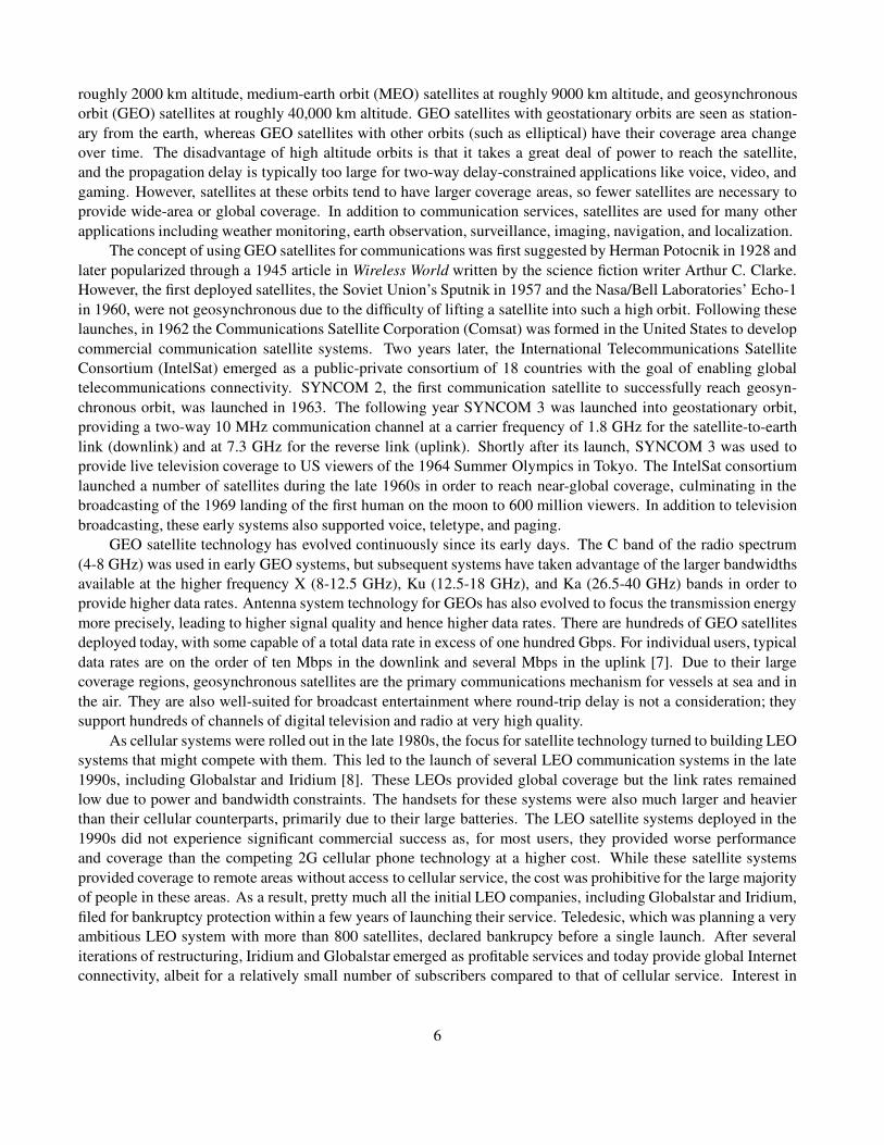
roughly 2000 km altitude, medium-earth orbit (MEO) satellites at roughly 9000 km altitude, and geosynchronous

orbit (GEO) satellites at roughly 40,000 km altitude. GEO satellites with geostationary orbits are seen as station-

ary from the earth, whereas GEO satellites with other orbits (such as elliptical) have their coverage area change

over time. The disadvantage of high altitude orbits is that it takes a great deal of power to reach the satellite,

and the propagation delay is typically too large for two-way delay-constrained applications like voice, video, and

gaming. However, satellites at these orbits tend to have larger coverage areas, so fewer satellites are necessary to

provide wide-area or global coverage. In addition to communication services, satellites are used for many other

applications including weather monitoring, earth observation, surveillance, imaging, navigation, and localization.

The concept of using GEO satellites for communications was first suggested by Herman Potocnik in 1928 and

later popularized through a 1945 article in Wireless World written by the science fiction writer Arthur C. Clarke.

However, the first deployed satellites, the Soviet Union’s Sputnik in 1957 and the Nasa/Bell Laboratories’ Echo-1

in 1960, were not geosynchronous due to the difficulty of lifting a satellite into such a high orbit. Following these

launches, in 1962 the Communications Satellite Corporation (Comsat) was formed in the United States to develop

commercial communication satellite systems. Two years later, the International Telecommunications Satellite

Consortium (IntelSat) emerged as a public-private consortium of 18 countries with the goal of enabling global

telecommunications connectivity. SYNCOM 2, the first communication satellite to successfully reach geosyn-

chronous orbit, was launched in 1963. The following year SYNCOM 3 was launched into geostationary orbit,

providing a two-way 10 MHz communication channel at a carrier frequency of 1.8 GHz for the satellite-to-earth

link (downlink) and at 7.3 GHz for the reverse link (uplink). Shortly after its launch, SYNCOM 3 was used to

provide live television coverage to US viewers of the 1964 Summer Olympics in Tokyo. The IntelSat consortium

launched a number of satellites during the late 1960s in order to reach near-global coverage, culminating in the

broadcasting of the 1969 landing of the first human on the moon to 600 million viewers. In addition to television

broadcasting, these early systems also supported voice, teletype, and paging.

GEO satellite technology has evolved continuously since its early days. The C band of the radio spectrum

(4-8 GHz) was used in early GEO systems, but subsequent systems have taken advantage of the larger bandwidths

available at the higher frequency X (8-12.5 GHz), Ku (12.5-18 GHz), and Ka (26.5-40 GHz) bands in order to

provide higher data rates. Antenna system technology for GEOs has also evolved to focus the transmission energy

more precisely, leading to higher signal quality and hence higher data rates. There are hundreds of GEO satellites

deployed today, with some capable of a total data rate in excess of one hundred Gbps. For individual users, typical

data rates are on the order of ten Mbps in the downlink and several Mbps in the uplink [7]. Due to their large

coverage regions, geosynchronous satellites are the primary communications mechanism for vessels at sea and in

the air. They are also well-suited for broadcast entertainment where round-trip delay is not a consideration; they

support hundreds of channels of digital television and radio at very high quality.

As cellular systems were rolled out in the late 1980s, the focus for satellite technology turned to building LEO

systems that might compete with them. This led to the launch of several LEO communication systems in the late

1990s, including Globalstar and Iridium [8]. These LEOs provided global coverage but the link rates remained

low due to power and bandwidth constraints. The handsets for these systems were also much larger and heavier

than their cellular counterparts, primarily due to their large batteries. The LEO satellite systems deployed in the

1990s did not experience significant commercial success as, for most users, they provided worse performance

and coverage than the competing 2G cellular phone technology at a higher cost. While these satellite systems

provided coverage to remote areas without access to cellular service, the cost was prohibitive for the large majority

of people in these areas. As a result, pretty much all the initial LEO companies, including Globalstar and Iridium,

filed for bankruptcy protection within a few years of launching their service. Teledesic, which was planning a very

ambitious LEO system with more than 800 satellites, declared bankrupcy before a single launch. After several

iterations of restructuring, Iridium and Globalstar emerged as profitable services and today provide global Internet

connectivity, albeit for a relatively small number of subscribers compared to that of cellular service. Interest in

6

LEO satellites resurfaced as 4G cellular systems rolled out due to increased demand for connectivity in remote

locations not served by cellular, better technology for both satellites and ground transceivers, and reduced launch

costs. Significant commercial development of LEO satellites emerged concurrent with 5G cellular rollouts as a

means to provide broadband Internet service to the billions of people worldwide that do not have access to high-

speed connectivity. It is anticipated that such systems will each deploy hundreds to thousands of satellites.

Today we take for granted the magic of wireless communications, which allows us and our devices to be

connected anywhere in the world. This magic has been enabled by the pioneers that contributed to advances in

wireless technology underlying the powerful systems ubiquitous today.

1.2 Current Systems

This section provides a design overview of the most prevalent wireless systems in operation today. The design

details of these systems are constantly evolving, incorporating new technologies and innovations. This section

will focus mainly on the high-level design aspects of these systems. More details on these systems and their

underlying technologies will be provided in specific sections of the book. A summary of Wi-Fi, cellular, and

short-range networking standards can be found in Appendix D with more complete treatments of recent standards

in [9, 10, 11, 12, 13].

1.2.1 Wireless Local Area Networks

WLANs support data transmissions for multiple users within a “local” coverage area whose size depends on the

radio design, operating frequency, propagation characteristics, and antenna capabilities. A WLAN consists of one

or more access points (APs) connected to the Internet that serve one or more WLAN devices, also called clients.

The basic WLAN architecture is shown in Figure 1.1. In this architecture clients within the coverage area of an

AP connect to it via single-hop radio transmission. For better performance and coverage, some WLANs use relay

nodes to enable multi-hop transmissions between clients and APs, as shown in Figure 1.2. WLANs today follow

the 802.11 Wi-Fi family of protocols. Handoff of a moving client between APs is not supported by the 802.11

protocol, however some WLAN networks, particularly corporate and campus systems, incorporate this feature into

their overall design.

Figure 1.1: Basic wireless LAN architecture

While early WLANs were exclusively indoor systems, current WLANs operate both indoors and outdoors.

Indoor WLANs are prevalent in most homes, offices, and other indoor locations where people congregate. Outdoor

systems are generally deployed in areas with a high density of users such as corporate and academic campuses,

sports stadiums, and downtown areas. The range of an indoor WLAN is typically less than 50 meters and can

7

Figure 1.2: Wireless LAN architecture with multihop transmissions

be confined to a single room for those operating at 60 GHz. Outdoor systems have a bigger range than indoor

systems due to their higher power, better antennas, and lower density of obstructions between the transmitter and

receiver. WLANs generally operate in unlicensed frequency bands, hence share these bands with other unlicensed

devices, such as cordless phones, baby monitors, security systems, and Bluetooth radios. Interference between

WLAN devices is controlled by the WLAN access protocol, whereas interference between WLAN devices and

other unlicensed devices is mitigated by a limit on the power per unit bandwidth for such devices.

WLANs use packet data transmission for better sharing of the network resources. Hence, data files are seg-

mented into packets. Sharing of the available bandwidth between different APs and, for most systems, between

clients accessing the same AP is typically controlled in a distributed manner using the carrier sense multiple access

with collision avoidance (CSMA/CA) protocol. In CSMA/CA, energy from other transmissions on a given channel

is sensed prior to a transmission and, if the energy is sensed above a given threshold, the transmitter waits a random

backoff time before again attempting a transmission. A transmitted packet is acknowledged by the receiver once

received. If a transmitted packet is not acknowledged, it is assumed lost and hence retransmitted. As discussed in

more detail in Chapter 14, the CSMA/CA access protocol is very inefficient, which leads to poor performance of

WLANs under moderate to heavy traffic loads. As a result, some WLANs use more sophisticated access protocols,

similar to those in cellular systems, that provide centralized scheduling and resource allocation either to all clients

served by a given AP or, more generally, to all APs and clients within a given system.

1.2.2 Cellular Systems

Cellular systems provide connectivity to a wide range of devices, both indoors and out, with a plethora of features

and applications including text messages, voice calls, data and video transfer, Internet access, and mobile “apps”

(application software tailored to run on mobile devices). Cellular systems typically operate in licensed frequency

bands, whereby the cellular operator must purchase or lease the spectrum in which their system operates. These

licenses typically grant the operator exclusive use of the licensed spectrum. Starting in 2017 regulators in several

countries began allowing cellular systems to operate in the 5 GHz unlicensed band in addition to within their

licensed spectrum. Given the large amount of spectrum in these unlicensed bands compared to what is available in

the licensed bands, this development has the potential to drastically increase cellular system capacity. However, it

will also increase interference in the unlicensed bands, particularly for Wi-Fi systems.

The basic premise behind cellular system design is frequency reuse, which exploits the fact that signal power

falls off with distance to reuse the same frequency spectrum at spatially separated locations. Specifically, a cellular

8

system consists of multiple cells, where each cell is assigned one or more channels to serve its users. Each channel

may be reused in another cell some distance away, and the interference between cells operating on the same

channel is called intercell interference. The spatial separation of cells that reuse the same channel set, the reuse

distance, should be as small as possible so that frequencies are reused as often as possible, thereby maximizing

spectral efficiency. However, as the reuse distance decreases, the intercell interference increases owing to the

smaller propagation distance between interfering cells. Early cellular systems had reuse distances greater than one,

but current systems typically reuse each channel in every cell while managing the resulting interference through

sophisticated mitigation techniques.

The most basic cellular system architecture consists of tessellating cells, as shown in Figure 1.3, where Cidenotes the channel set assigned to cell i. The two-dimensional cell shapes that tessellate (cover a region without

gaps or overlap) are hexagons, squares, and triangles. Of these, the hexagon best approximates an idealized omni-

directional transmitter’s circular coverage area. Early cellular systems followed this basic architecture using a

relatively small number of cells to cover an entire city or region. The cell base stations in these systems were

placed on tall buildings or mountains and transmitted at very high power with cell coverage areas of several square

miles. These large cells are called macrocells. The first few generations of macrocell base stations used single-

antenna omni-directional transmitters, so a mobile moving in a circle around these base station had approximately

constant average received power unless the signal was blocked by an attenuating object. In deployed systems cell

coverage areas overlap or have gaps as signal propagation from a set of base stations never creates tessellating

shapes in practice, even if they can be optimally placed. Optimal base station placement is also impractical, as

zoning restrictions, rooftop availability, site cost, backhaul and power availability, as well as other considerations

influence this placement.

Figure 1.3: Cellular network architecture (homogeneous cell size).

Macrocells have the benefit of wide area coverage, but they can often become overloaded when they contain

more users than channels. This phenomenon has led to hierarchical cellular system architectures, with macrocells

that provide wide area coverage and small cells embedded within these larger cells to provide high capacity, as

shown in Figure 1.4. Not only do the small cells provide increased capacity over a macrocell-only network,

but they also reduce the transmit power required at both the base station and mobile terminal, since the maximum

transmission distance within the small cell is much less than in the macrocell. Cellular systems with heterogeneous

cells sizes are referred to as Hetnets. In current cellular systems, channels are typically assigned dynamically

based on interference conditions. Another feature of many current cellular system designs is for base stations in

9

adjacent macrocells to operate on the same frequency, utilizing power control, adaptive modulation and coding, as

well as interference mitigation techniques to ensure the interference between users does not preclude acceptable

performance.

Figure 1.4: Hierarchical cellular network architecture (a Hetnet with macrocells and small cells).

All base stations in a given geographical area, both macrocells and small cells, are connected via a high-speed

communications link to a mobile telephone switching office (MTSO), as shown in Figure 1.5. The MTSO acts as a

central controller for the cellular system, allocating channels within each cell, coordinating handoffs between cells

when a mobile traverses a cell boundary, and routing calls to and from mobile users. The MTSO can route calls to

mobile users in other geographic regions via the local MTSO in that region or to landline users through the public

switched telephone network (PSTN). In addition, the MTSO can provide connectivity to the Internet.

A new user located in a given cell requests a channel by sending a call request to the cell’s base station over

a separate control channel. The request is relayed to the MTSO, which accepts the call request if a channel is

available in that cell. If no channels are available then the call request is rejected. A call handoff is initiated when

the base station or the mobile in a given cell detects that the received signal power for that call is approaching a

given minimum threshold. In this case the base station informs the MTSO that the mobile requires a handoff, and

the MTSO then queries surrounding base stations to determine if one of these stations can detect that mobile’s

signal. If so then the MTSO coordinates a handoff between the original base station and the new base station.

If no channels are available in the cell with the new base station then the handoff fails and the call is dropped.

A call will also be dropped if the signal strength between a mobile and its base station falls below the minimum

threshold needed for communication due to signal propagation effects such as path loss, blockage, or multipath

fading. These propagation characteristics are described in Chapters 2-3.

Spectral sharing in cellular systems, also called multiple access, is done by dividing the signaling dimensions

along the time, frequency, code, and/or the spatial dimensions. Current cellular standards use a combination of

time and frequency division for spectral sharing within a cell. However, there are still 2G and 3G systems in

operation that use code-division multiple access based on direct sequence spread spectrum. Channels assigned to

users within a cell may be orthogonal or non-orthogonal. In the latter case the channels of two users within a cell

will overlap in time, frequency, code or spatial dimensions, which is referred to as intracell interference. More

details on multiple access techniques and their performance analysis will be given in Chapters 13 and 14.

Efficient cellular system designs are interference limited – that is, interference from within and outside a

cell dominates the noise floor, since otherwise more users could be added to the system. As a result, any tech-

10

Figure 1.5: Cellular network architecture evolution.

nique to reduce interference in cellular systems leads directly to an increase in system capacity and performance.

Some methods for interference reduction in cellular systems include cell sectorization, power control, directional

antennas and antenna-array signal processing, multiuser detection and interference cancellation, base station co-

operation, and user scheduling. Details of these techniques will be given in Chapters 14 and 15.

1.2.3 Satellite Systems

Satellite systems are another major component of the wireless communications infrastructure [14, 15]. There is a

plethora of satellite communications services available today, including mobile service to airplanes, ships, vehicles,

and hand-held terminals, fixed satellite service to earth stations, as well as broadcast radio and television service.

Fig. 1.6 illustrates the satellite architecture supporting all such services. One of the biggest advantages of satellites

over terrestrial wireless systems is their ability to provide coverage in remote areas.

Figure 1.6: Satellite System Architecture

Satellite communication systems consist of one or more satellites communicating with stations on earth or

in the air. Communication satellites typically serve as relays between stations on the ground and in some cases

provide direct links to other satellites as well. Ground stations may be at fixed locations, in which case their

antennas may be large to maximize received signal strength. Mobile stations and indoor fixed stations have smaller

antennas, typically on the order of 1-3 meters. The coverage area or footprint of a satellite depends on its orbit. A

GEO satellite can cover one or more continents, hence only a handful are needed to provide coverage for the entire

globe. However, the transmission latency between the earth and a GEO satellite is high, on the order of 300 ms.

11

MEO satellites have a coverage area of around ten thousand square kilometers and a latency of around 80 ms. A

LEO coverage area is about a thousand square kilometers with a latency of around 10 ms.

A GEO satellite provides continuous coverage to any station within its footprint, whereas a satellite with a

different orbit will have a fixed station within its footprint for only part of a 24 hour period. GEO satellites are

heavy, sophisticated, and costly to build and launch. Portable stations or handsets for GEOs tend to be large and

bulky due to the power required to reach the satellite. In addition, the large round-trip propagation delay to a GEO

satellite is quite noticeable in two-way voice communication. The most common service offered by GEO satellites

is radio and TV broadcasting since delay is not a constraint and the satellite construction, launch, and operational

costs are amortized over the many users within the GEO footprint. GEO satellites are also commonly used as a

backbone link for terrestrial networks, for airplane and maritime communications, and for connectivity in remote

locations.

LEO satellites are much lighter and lower in cost than GEOs to manufacture, launch, and operate. In addition,

the stations and handsets in a LEO system have smaller size, transmit power, and latency than GEO systems due

to the closer proximity of LEO satellites to the earth. Hence, most mobile services use LEO satellites, typically

in a constellation of dozens to hundreds of satellites whose total footprint covers the locations around the globe

supported by the system. Continuous coverage of a given location in a LEO system requires handoff between

satellites as a fixed location on earth is within the footprint of a given LEO satellite for only 10-40 minutes. Hence,

when the footprint of a LEO satellite moves away from a given station or handset, its connection is handed off

to another LEO satellite so as to maintain continuous connectivity. Sophisticated antennas on LEO satellites can

create very small spotbeams for mobile terminals that focus that transmission energy within a small footprint.

These spotbeams allow for frequency reuse similar to that of cellular systems.

For the reasons outlined in the previous paragraph, LEOs tend to support the highest data rates, best per-

formance, and lowest cost among satellite services. As expected, MEO satellite systems provide a compromise

between the system requirements, performance, and costs compared with those of GEO and LEO systems. MEO

satellite services mainly compete with GEO systems by offering better performance at a lower cost for users in

relatively remote locations that are not well served by LEO or terrestrial systems.

1.2.4 Fixed Wireless Access

Fixed wireless access (FWA) systems support wireless communications between a fixed access point and multiple

terminals. The FWA system architecture is shown in Fig 1.7. The access point transmits to the receivers of multiple

terminals in the downlink direction, and receives signals from the transmitters of multiple terminals in the uplink

direction. Different multiple access techniques can be used to share the system spectrum between the multiple

terminals.

FWA systems provide an alternative to the wired broadband options of DSL, cable and fiber, whose availability

may be limited in rural areas. In the United States, two frequency bands were set aside for these systems in the late

1990s: part of the 28 GHz spectrum for local distributionsystems (local multipoint distribution service, LMDS) and

a band in the 2 GHz spectrum for metropolitan distribution service (multichannel multipoint distribution services,

MMDS). MMDS systems were never widely deployed, and are used today in sparsely populated rural areas,

where laying cables is not economically viable. The initial LMDS systems were expensive and performed poorly

due to the challenges of providing service at such high frequencies. As a result these systems did not succeed

commercially and were discontinued. The LMDS spectrum is just below the millimeter wave band of 30-300

GHz. Recent interest in utilizing the large amount of unregulated millimeter wave spectrum has led to advances in

system, circuit, and antenna design at these high frequencies, which in turn has renewed interest in FWA systems

using the LMDS and millimeter wave bands.

One of the main growth drivers of FWA was the IEEE 802.16 (WiMAX) standard, finalized in 2001. The

first WiMAX standard defined operation between 2 GHz and 11 GHz for non-line-of-sight links and between

12

Figure 1.7: Fixed Wireless Access System

10 GHz and 66 GHz for line-of-sight links, however WiMAX systems generally operate below 6 GHz. The first

commercial WiMAX systems followed the 802.16d standard with data rates of around 40 Mbps. A later version,

802.16e, was developed in the mid-2000s to support mobile users with a system design similar to that of cellular.

The 802.16e systems offered 15 Mbps data rates, much higher than that of 3G cellular systems. The significantly

higher data rates of 802.16e over 3G led to speculation that it would be adopted for 4G cellular. However, in the

end 4G cellular adopted the LTE standard, which ultimately pushed WiMAX systems out of most mobile service

markets. WiMAX is still used to support mobile services in areas where LTE has not been deployed, as well as in

industrial markets such as aviation, utilities, and transportation. FWA systems based on the LTE and 5G cellular

standards have been deployed to provide high-speed connectivity for homes, apartments, and office buildings.

1.2.5 Short Range Radios with Multihop Routing

As radios decrease their cost and power consumption, it becomes feasible to embed them into more types of

electronic devices, which enables applications such as smart homes, sensor networks, vehicular networks, and

other interconnected systems. The most common radio standards that have emerged to support this trend are

Bluetooth, ZigBee, and Z-Wave. All of these radios support a multihop routing protocol, whereby a given radio

can communicate with any other radio in its transmission range. If the destination radio is not within this range,

intermediate radios relay the message to this destination. Radios with multihop routing form an ad hoc wireless

network since they can reconfigure and have no established infrastructure. Such ad hoc wireless networks are

commonly used by the military as well as for emergency response. In principle a multihop routing protocol can

support hundreds or even thousands of nodes, but network performance generally degrades as the number of

nodes increases. The short range radios described in this section have not yet demonstrated that their multihop

routing protocols are feasible in practice for large numbers of nodes. In addition to Bluetooth, Zigbie, and Z-

Wave, proprietary radios have been used in a number of devices, products, and military systems to support their

communication requirements.

The Bluetooth standard is based on a small radio transceiver microchip built into digital devices.1 The standard

and device certification is managed by the Bluetooth Special Interest Group. In most applications the Bluetooth

1The Bluetooth standard is named after Harald I Bluetooth, the king of Denmark between 940 and 985 A.D. who united Denmark and

Norway. Bluetooth proposes to unite devices via radio connections, hence the inspiration for its name.

13

radio takes the place of a connecting cable for electronic devices such as cell phones, tablets, headsets, audio

equipment, cameras, watches, and smart meters. Bluetooth has also been integrated into larger devices such as

cars and medical equipment. Bluetooth is mainly for short-range communications – for example, from a laptop

to a nearby printer or from a cell phone to a wireless headset. Its normal range of operation is 10 m (at 2.5-mW

transmit power), and this range can be increased to 100 m by increasing the transmit power to 100 mW. The system

operates in the unlicensed 2.4-GHz frequency band, so it can be used worldwide without any licensing issues. The

Bluetooth standard provides one data channel at 723.2 kbps. In this mode, there is a reverse channel with a data

rate of 57.6 kbps. The specification also allows up to three additional channels each at a rate of 64 kbps, which

are primarily used for voice connections with headsets. These different modes result in an aggregate bit rate of

approximately 1 Mbps. An enhanced data rate mode provides up to 3 Mbps, while a low-energy mode significantly

reduces power consumption at the expense of range or data rate.

Bluetooth uses frequency hopping for multiple access with a carrier spacing of 1 MHz. Typically, up to eighty

different frequencies are used for a total bandwidth of 80 MHz. At any given time, the bandwidth available is

1 MHz. Bluetooth radios form small ad hoc networks of up to eight devices sharing the same logical channel (same

hop sequence), which is called a piconet. Different channels (different hopping sequences) can simultaneously

share the same 80 MHz bandwidth. Collisions will occur when devices in different piconets that are on different

logical channels happen to use the same hop frequency at the same time. As the number of piconets in an area

increases, the number of collisions increases and performance degrades. The original Bluetooth standard was

developed jointly by 3 Com, Ericsson, Intel, IBM, Lucent, Microsoft, Motorola, Nokia, and Toshiba. Many

additional manufactures have contributed to each new generation of the standard. Bluetooth is integrated into a

wide range of electronic devices with several billion Bluetooth-enabled devices shipped annually.

The ZigBee2 radio specification is designed for lower cost and power consumption than Bluetooth. It follows

the IEEE 802.15.4 standard with device certification managed by the Zigbie Alliance. The radio operates in the

same 2.4 GHz ISM band as Bluetooth. Zigbee radios support data rates of up to 250 kbps at a range of up to 30 m.

These data rates are slower than Bluetooth, but in exchange the radio consumes significantly less power with a

larger transmission range. Zigbee also operates in a “green” mode whereby the radio is powered through energy

harvesting of its environment, reducing or in some cases completely elimiating the need for battery power. The

goal of ZigBee is to provide radio operation for months or years without recharging, thereby targeting devices such

as smart tags, meters, lights, and thermostats, as well as those used for sensing and automation.

Z-Wave radios are designed primarily for smart home applications with operation in the 900 MHz ISM band.

Since power falls off more slowly in this band than at the higher 2.4 GHz spectrum, Z-Wave radios have a higher

range than standard Zigbee or Bluetooth radios, on the order of 100 m. In addition, there is no interference between

Z-Wave radios and those operating in the crowded 2.4 GHz band, including Wi-Fi as well as Bluetooth and Zigbee.

On the downside, Z-Wave has significantly lower data rates than either Bluetooth or Zigbee, ranging from 10 to

100 Kbps. The Z-Wave standard and device certification is managed by the Z-Wave Alliance.

1.3 Wireless Spectrum

1.3.1 Regulation

Most countries have government agencies responsible for allocating and controlling use of the radio spectrum.

In the United States, spectrum is allocated by the Federal Communications Commission (FCC) for commercial

use and by the Office of Spectral Management (OSM) under the auspices of the National Telecommunications

and Information Administration (NTIA) for government use. Countries throughout the world have similar regula-

2ZigBee takes its name from the dance that honey bees use to communicate information about newly found food sources to other

members of the colony.

14

tory agencies to regulate spectrum within their borders. Certain regions of the world have a common regulatory

agency for spectrum allocation, e.g. commercial spectral allocation across Europe is governed by the European

Telecommunications Standards Institute (ETSI). Satellite systems cover large areas spanning many countries and

sometimes the globe. Globally, spectrum is allocated by the International Telecommunications Union Radio Com-

munications group (ITU-R) through its World Radiocommunication Conferences (WRC). The standards arm of

this body, ITU-T, adopts telecommunication standards for global systems that must interoperate across national

boundaries. Regulatory agencies typically have many competing considerations in deciding how to allocate any

given block of spectrum, including whether to allocate it for commercial, military, or shared use. These deci-

sions are generally driven by a broad mandate to regulate spectrum “in the public interest,” as stated in the U.S.

Communications Act of 1934 establishing the FCC.

Historically government agencies allocated spectral blocks for specific uses and assigned licenses to use these

blocks to specific groups or companies. For example, in the 1980s the FCC allocated spectrum around 850 MHz

for analog cellular phone service, in particular 824-849 MHz for the downlink (base station to mobile) and 869-894

MHz in the uplink (mobile to base station). Spectral licenses were provided to two operators in each geographical

area based on a number of criteria. While this method of licensed spectral allocation is still used in some circum-

stances, a fundamental shift occurred worldwide in the early 1990s for licensed spectrum to be auctioned to the

highest bidder, with some restrictions in place to ensure fairness and competitive use of the spectrum. The basis for

the shift was the market-based reasoning that auctions provide the fairest and most efficient way for governments

to allocate the limited spectral resource and, moreover, this method provides significant revenue to the government.

However, auctions are not universally supported for spectral allocation based on the contention that they can stifle

innovation, limit competition, and hurt technology adoption. Specifically, the high cost of spectrum dictates that

only large companies or conglomerates can purchase it. Moreover, the large investment required to obtain spectrum

can delay, sometimes indefinitely, the ability to invest in infrastructure for system rollout. Finally, high spectral

cost is usually passed on to the end user. The early 3G spectral auctions, with suspected collusion between bidders,

low bids, and several auction winners that ultimately defaulted, provided ammunition to the opponents of spectral

auctions. Lessons learned from these early auctions were adopted in the design of subsequent auctions, which

generally went smoothly and raised up to tens of billions of dollars. In addition, reverse or incentive auctions were

initiated starting in 2016, whereby license holders could sell back their spectrum to regulatory bodies for future

auctioning. A comprehensive treatment of spectrum regulation and its allocation through auctions can be found in

[16].

In addition to spectral auctions, spectrum can be set aside in specific frequency bands, called unlicensed

bands, that are free to use without a license according to a specific set of rules. The rules may correspond to a spe-

cific access protocol to ensure fairness, restrictions on power levels, and so forth. The purpose of these unlicensed

bands is to encourage innovation and low-cost implementation. Wi-Fi is often associated with the unlicensed fre-

quency bands, however it is just one of the hundreds of successful unlicensed systems, which include standardized

short-range radio systems as well as proprietary radios in cordless phones, wireless home security systems, baby

monitors, medical equipment, inventory systems, smart meters, and keyless automobile entry systems. Indeed,

it is estimated that unlicensed wireless devices contribute tens of billions of dollars annually to the US economy

alone. A major difficulty of unlicensed bands is that they can be killed by their own success. If many unlicensed

devices on the same channel are used in close proximity then they interfere with each other, which can make the

band unusable. Cellular systems can also operate in the unlicensed bands by following the unlicensed spectrum

rules. However, since these systems can use their licensed bands for control, they have an advantage over systems

such as Wi-Fi that use the unlicensed bands for both control and data transmission and can crowd out Wi-Fi users

as a result [17]. Much of the spectrum above 30 GHz is unregulated or lightly regulated, and hence can be used by

unlicensed users with little to no restriction.

Underlay systems are another alternative for allocating spectrum. An underlay system operates as a secondary

15

user in a licensed frequency band simultaneous with the licensed users in a manner such that the licensed users

experience minimal interference from them. This is usually accomplished by spreading the signal over a very

wide bandwidth, typically more than 500 MHz, and restricting its power per Hertz. The first underlay standard

approved for operation was ultrawideband (UWB) communications [18]. Specifically, in 2002 the FCC approved

7500 MHz of spectrum for the use of UWB devices, with the very stringent power restriction of no more than 75

nW/MHz. This sparked regulatory activities in countries throughout Europe and Asia to also enable UWB, albeit

with different restrictions than those in the US. Indeed, regulatory approval of UWB proved to be quite contro-

versial given the complexity of characterizing how interference affects the primary band users, and the fact the

UWB transmissions span many licensed users across both commercial and government domains. The regulatory

challenges coupled with the severe power constraints on UWB systems ultimately proved insurmountable for most

commercial systems, hence the technology failed to achieve much success [19]. The interference constraint for

underlay users may alternatively be met without restricting power per Hertz by using multiple-antenna techniques

to guide the underlay signals away from the spatial dimensions occupied by licensed users [20].

Following the introduction of underlay systems, regulatory bodies began exploring other innovative technolo-

gies that could make spectrum utilization in the licensed bands more flexible and efficient. This push for innovation

was long overdue; other than spectral auctions and underlay systems, the basic mechanisms for licensed spectral

allocation had not changed much since the inception of regulatory bodies in the early to mid-1900s. Many of the

compelling ideas for exploiting technology to better utilize licensed spectrum fall under the notion of a cognitive

radio. A cognitive radio utilizes advanced radio and signal processing technology along with novel spectrum al-

location policies to support unlicensed users operating in the existing licensed spectrum, without degrading the

performance of the licensed users. In particular, a cognitive radio “learns” about coexisting licensed users within

its spectrum and then uses this information to utilize the spectrum without degrading the transmissions of these

users [21]. Based on the nature of the coexisting user information the cognitive radio can collect, as well as a priori

rules about spectrum usage, a cognitive radio seeks to overlay or interweave its signal with the transmissions of

licensed nodes. Spatial underlay systems that dynamically avoid the spatial dimensions of licensed users also fall

within the paradigm of cognitive radios. Cognitive radio techniques can also be applied in the unlicensed bands to

reduce interference between users and thus improve spectral efficiency in these bands as well.

Interweave cognitive radios utilize unused parts of the licensed spectrum. The idea of interweave radios

came about after studies conducted by the FCC and industry showed the existence of space-time-frequency voids,

referred to as spectrum holes, in both the licensed and unlicensed bands that are not in constant use. These spectrum

holes, which can change with time and geographic location, can be exploited by interweave radios to support their

communication. In some cases the spectrum holes are permanent, either because a certain block of licensed

spectrum is unused, or because “guard channels” between occupied channels are needed in the overall design to

reduce interference between the licensed users. Such guard channels, or “white spaces,” were specified in the

analog television broadcast standard. As analog television bands transitioned to digital, arguments were made that

such guard bands were no longer needed, and hence these white spaces could be freed up for other uses. Despite

resistance from the television broadcasters, unlicensed use of television white spaces was approved by regulatory

bodies in multiple countries starting in 2010. White space devices must generally consult a database of available

spectrum holes in their geographical area before using them, and such databases are relatively static. A more

sophisticated interweave radio looks for dynamic spectrum holes by periodically monitoring the radio spectrum,

detecting spectrum holes as they occur in time, space, and/or frequency, and then using such holes opportunistically

to communicate over them. Such opportunistic use of white spaces, which was the original motivation behind the

notion of cognitive radio [22], has yet to be approved for spectrum allocation.

In overlay systems the cognitive transmitter has some knowledge about the transmissions of noncognitive

users in the band. This knowledge can be exploited in two ways: to mitigate the interference caused to licensed

users and to improve the performance of licensed users by amplifying (relaying) their signals. In particular, an

16

overlay user with knowledge of the licensed user’s transmitted signal can use a special type of signal encoding to

completely cancel the interference caused by this licensed user at its own receiver. While this coded signal will

cause interference to the licensed user, by also using part of its power to amplify the licensed user’s signal, the

impact of this interference can be completely mitigated and, in fact, the licensed user might even experience better

performance than without the existence of the overlay user. The overlay cognitive radio paradigm was originally

proposed in [23] and capacity limits as well as practical implementations of overlay systems have been extensively

studied since then. However, regulatory agencies have not yet considered allowing overlay systems to operate in

the licensed spectrum.

Overlay, underlay, and interweave radio innovations could make spectrum utilization far more efficient than it

is today, in both the licensed and unlicensed bands, thereby enabling new wireless systems, products, and applica-

tions. More details on the technologies behind these cognitive radio paradigms will be discussed in Chapter 16.7.

However, even once these and other cognitive radio technologies are fully developed, changing regulatory policies

to include these novel mechanisms will likely be fraught with conflicting opinions from government, industry, and

the end users about what best serves the public interest in the allocation of spectrum.

1.3.2 Properties and Existing Allocations

Most wireless communication systems operate in the radio spectrum between 30 MHz and 30 GHz, with some

in the millimeter wave frequency band (30 GHz-300 GHz) as well. For communication systems at frequencies

below 800 MHz, antenna sizes are too large for small devices, and at frequencies above 3 GHz, signal attenuation

with distance precludes long-range transmission. Given these tradeoffs, the primary frequency bands that fueled

the extraordinary grown of cellular, Wi-Fi, and short-range radios like Bluetooth were in the 0.8-3 GHz range.

As those frequency bands became congested, these systems moved to adjacent bands (0.6-0.8 for cellular and 3-5

GHz for cellular and Wi-Fi). Cellular and Wi-Fi systems started to expand into the millimeter wave bands as well

due to the plentiful spectrum there. A similar evolution into higher frequency bands occured in satellite systems.

In particular, early satellite systems used the 4-8 GHz C band, but over time moved into the X (8-12.5 GHz), Ku

(12-18 GHz), K (18-26 GHz) and Ka (26-40 GHz) bands. The K bands were assigned to terrestrial fixed wireless

services as well, including LMDS. Note that the required antenna size for good reception is inversely proportional

to the signal frequency, so moving systems to a higher frequency allows for more compact antennas. However,

received signal power with nondirectional antennas is proportional to the inverse of frequency squared, so it is

harder to cover large distances with high-frequency signals.

As discussed previously, spectrum is allocated either in licensed bands (which regulatory bodies assign to

specific operators) or in unlicensed bands (which can be used by any system subject to certain operational re-

quirements). Often different countries try to match their frequency bands for licensed and unlicensed use so that

technology developed for that spectrum is compatible worldwide, however that isn’t possible if a country has al-

located one of these frequency bands to another use. Figure 1.8 shows the unlicensed spectrum allocations in

the United States. In most cases there are similar frequency allocations in Europe and Asia. ISM Band I at 900

MHz has limited spectrum availability as well as licensed users transmitting at high power who interfere with the

unlicensed users. Since performance in this band is somewhat poor, it is not heavily utilized by unlicensed devices.

The U-NII bands have a total of 555 MHz of spectrum in four separate bands, with different power restrictions.

In addition, some countries have imposed restrictions on parts of the U-NII bands so that unlicensed systems must

avoid interference with radar systems licensed to operate in those bands.

Figure 1.9 shows the frequency bands allocated to current and legacy cellular systems in the United States

along with their band name abbreviations3. Note from this table that 4G (LTE) systems operate in the 3.5 GHz

3Specialized Mobile Radio (SMR); Personal Communication System (PCS); Advanced Wireless Services (AWS); Digital Dividend

(DD); Wireless Communications Services (WCS); Broadband Radio Service (BRS); Citizen’s Broadband Radio Service (CBRS).

17

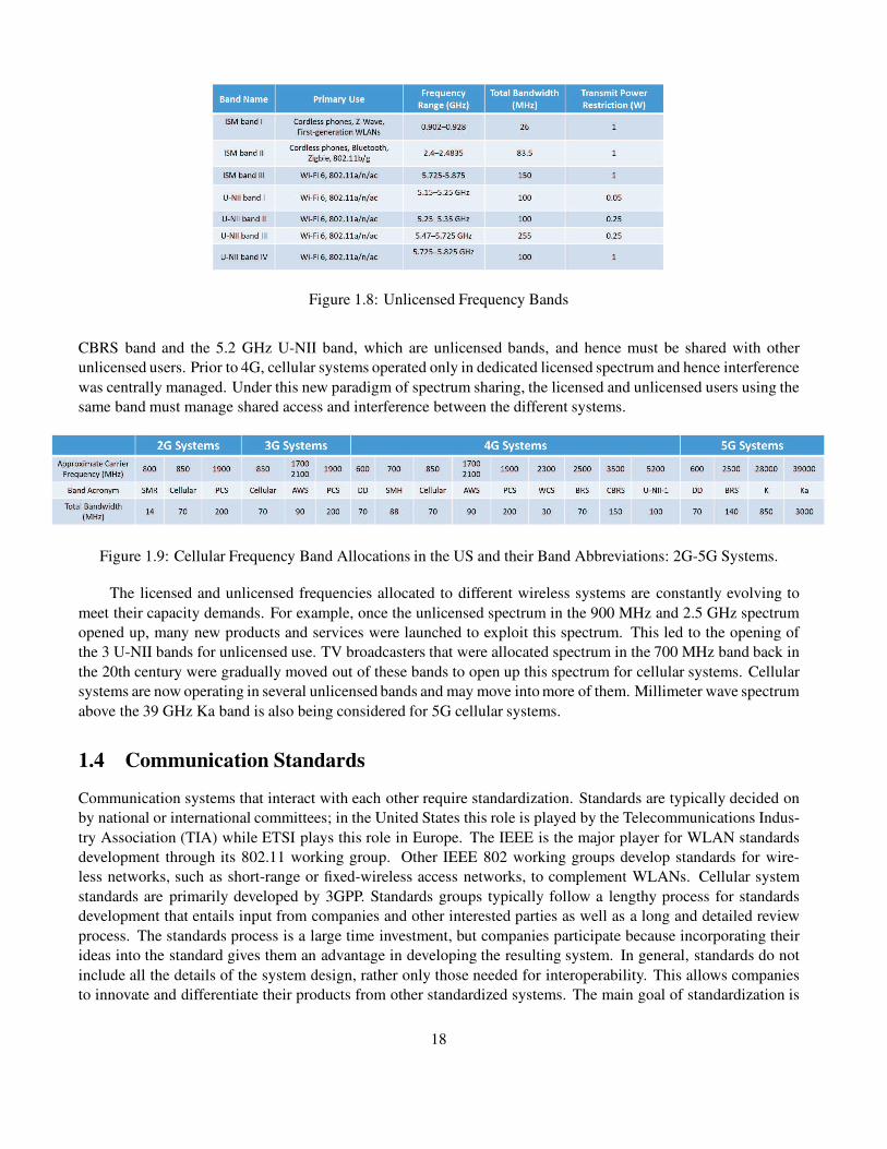
Figure 1.8: Unlicensed Frequency Bands

CBRS band and the 5.2 GHz U-NII band, which are unlicensed bands, and hence must be shared with other

unlicensed users. Prior to 4G, cellular systems operated only in dedicated licensed spectrum and hence interference

was centrally managed. Under this new paradigm of spectrum sharing, the licensed and unlicensed users using the

same band must manage shared access and interference between the different systems.

Figure 1.9: Cellular Frequency Band Allocations in the US and their Band Abbreviations: 2G-5G Systems.

The licensed and unlicensed frequencies allocated to different wireless systems are constantly evolving to

meet their capacity demands. For example, once the unlicensed spectrum in the 900 MHz and 2.5 GHz spectrum

opened up, many new products and services were launched to exploit this spectrum. This led to the opening of

the 3 U-NII bands for unlicensed use. TV broadcasters that were allocated spectrum in the 700 MHz band back in

the 20th century were gradually moved out of these bands to open up this spectrum for cellular systems. Cellular

systems are now operating in several unlicensed bands and may move into more of them. Millimeter wave spectrum

above the 39 GHz Ka band is also being considered for 5G cellular systems.

1.4 Communication Standards

Communication systems that interact with each other require standardization. Standards are typically decided on

by national or international committees; in the United States this role is played by the Telecommunications Indus-

try Association (TIA) while ETSI plays this role in Europe. The IEEE is the major player for WLAN standards

development through its 802.11 working group. Other IEEE 802 working groups develop standards for wire-

less networks, such as short-range or fixed-wireless access networks, to complement WLANs. Cellular system

standards are primarily developed by 3GPP. Standards groups typically follow a lengthy process for standards

development that entails input from companies and other interested parties as well as a long and detailed review

process. The standards process is a large time investment, but companies participate because incorporating their

ideas into the standard gives them an advantage in developing the resulting system. In general, standards do not

include all the details of the system design, rather only those needed for interoperability. This allows companies

to innovate and differentiate their products from other standardized systems. The main goal of standardization is

18

enabling systems to interoperate.

In addition to ensuring interoperability, standards also allow economies of scale and pressure prices lower. For

example, WLANs typically operate in the unlicensed spectral bands, so they are not required to follow a specific

standard. The first generation of WLANs were not standardized and so specialized components were needed for

many systems, leading to excessively high cost that, when coupled with poor performance, led to limited adoption.

This experience resulted in a strong push to standardize the next WLAN generation, which yielded the highly

successful IEEE 802.11 family of standards. Adherence of products to the 802.11 standard is certified by the

Wi-Fi Alliance.

There are, of course, disadvantages to standardization. The standards process is not perfect, as company

participants often have their own agendas, which do not always coincide with the best technology or the best

interests of consumers. In addition, the standards process must be completed at some point, after which it becomes

more difficult to add new innovations and improvements to an existing standard. Finally, the standards process

can become quite politicized. This happened in Europe with 1st generation cellular systems, where each country

had its own standard, and with the second generation of cellular phones in the United States which ultimately

adopted three different standards. The formation of the 3GPP standards body to create a single unified cellular

standard throughout much of the world was a response to these pitfalls in earlier cellular standards, and is largely

responsible for the massive growth in and success of cellular technology. Hence, despite its flaws, standardization

is often an essential component of wireless system design and operation in order to ensure its success.

1.5 Wireless Vision

“It is always wise to look ahead, but difficult to look further than you can see.” - Winston Churchill

Wireless communication is ubiquitious in the world we live in, enabling vast connectivity among people and

devices as well as rapid access to information. Wireless technology impacts every aspect of modern life: culture,

business, politics, economics, health, entertainment, and education. So what might the future bring?

Demand for higher data rates seems unending, hence future wireless systems could support peak speeds of

hundreds or perhaps thousands of Gigabits per second. There are billions of people and locations throughout the

world today without wireless (or wired) connectivity, so perhaps future systems will fill in these coverage holes

so that no person or place on the planet lacks wireless connectivity. Wireless devices might shrink to such small

sizes that they can be deployed within any object or living being. Some wireless devices may be powered from a

very small battery or even self-power through energy harvesting or wireless charging, eliminating the need to ever

plug in. Wireless technology might evolve to support the “five-nines” standard in reliability for tradition telephone

service, meaning that the service is reliable 99.999% of the time in any location, indoors and out. Finally, wireless

systems must be extremely secure against natural impairments as well as eavesdroppers, attackers and spoofers.

If this vision of wireless technology comes to pass, what will it enable? In addition to providing people

with voice, high-speed data, and broadcast entertainment, future wireless networks will also support machine-to-

machine communications for tens of billions of devices. In the home these networks will enable a new class of

intelligent electronic devices that can interact with each other and with the Internet. Such “smart” homes will

drastically improve energy efficiency, security, emergency response, as well as help the elderly and disabled with

assisted living. Other applications of these networks include sensing and data collection in the power grid to

improve robustness and efficiency, “smart cities” that provide services such as trash collection and road mainte-

nance when the need is detected, and in-body communications for medical devices, biosensors, and targeted drug

delivery. Wireless video and virtual reality will permeate the home and any place that people congregate with

entertainment, and also enable remote classrooms, remote training facilities, and remote hospitals anywhere in

the world. Wireless sensor networks will improve monitoring of and response to fire hazards, toxic waste sites,

19

stress and strain in buildings and bridges, carbon dioxide movement, and the spread of chemicals and gases at

disaster sites. Finally, wireless networks with very low latency will enable distributed control systems with remote

devices, sensors, and actuators linked together via wireless communication channels. Such systems will in turn en-

able intelligent transportation systems including self-driving vehicles, mobile robots and drones, as well as easily

reconfigurable industrial automation.

The exponential growth of smartphone use and wireless Internet access has led to great optimism about

wireless technology in general. Obviously not all wireless applications will flourish. While many wireless systems

and companies have enjoyed spectacular success, there have also been many failures along the way, including

the first generation of wireless LANs and LEO satellite systems, as well as wide area data services, and fixed

wireless access to the home. Indeed, it is impossible to predict what wireless failures and triumphs lie on the

horizon. Moreover, there must be sufficient flexibility and creativity among both engineers and regulators to allow

for accidental successes. It is clear, however, that the current and emerging wireless systems of today – coupled

with the vision of applications that wireless can enable – ensure a bright future for wireless technology.

1.6 Technical Challenges

This section provides an overview of the many technical challenges that must be addressed to make the wireless

vision a reality. These challenges extend across all aspects of the system, including hardware design, channel

characterization, physical layer and multiple access techniques as well as networking protocols and architectures.

Techniques to address many of these challenges are described in subsequent chapters of the book.

The design of wireless systems begins with a model for the underlying channel through which the signals will

propagate. In all such channels, signal power decreases with distance due to the physics of propagation as well as

attenuation from blocking objects. These signal propagation models are developed in Chapter 2. If the transmitter,

receiver, or surrounding objects are moving, the channel changes randomly with time due to changing reflections

and attenuation. These random channel variations, whose statistical models are developed in Chapter 3, make it

difficult to design reliable systems with guaranteed performance. Channel characteristics, including signal attenu-

ation, also depend on the frequency of operation. In particular, received power generally decreases with the carrier

frequency and, in the case of free space propagation with omnidirectional antennas, it is inversely proportional

to the square of this frequency. Thus, most wireless systems today operate at carrier frequencies below 5 GHz

to ensure good coverage, leading to a spectrum shortage in this range of frequencies. Moving to higher carrier

frequencies, such as millimeter wave (30-300 GHz) or terahertz (.3-3 THz), provides much more spectrum than

what is available in the lower frequency bands. However, these higher frequencies of operation reduce range unless

energy is directionally focused using multiple or directional antenna techniques. Signal propagation characteristics

at these frequencies create challenges in designing reliable communication links, as described in Chapter 2.9.5. In

addition, hardware components are expensive and power hungry.

The maximum data rate that can be reliably sent over a wireless (or wireline) channel is its Shannon capacity,

which is derived in Chapter 4. This capacity is directly proportional to the channel bandwidth, i.e. the amount of

spectrum allocated to the channel. This rate also depends on the number of antennas at the transmitter and receiver,

as multiple-input multiple-output (MIMO) techniques allow for independent data streams to be transmitted along

the independent spatial dimensions these multiple antennas create, as described in Chapter 10. Achievable data

rates for a given wireless system also depend on signal propagation and interference characteristics. Due to these

challenges, data rates for both cellular and Wi-Fi systems are several orders of magnitude lower than for a fiber

optic cable, but that could change as millimeter wave systems are deployed.

In terms of hardware challenges, as the size of wireless devices shrink, breakthroughs are needed to make

both the analog and digital circuitry significantly smaller, cheaper, and more energy efficient. Wireless systems

operating at millimeter wave and higher frequencies require cheap and reliable RF components, which remains a

20

significant challenge. The size, power consumption, and precision of analog-to-digital converters is also becoming

a bottleneck as systems move to larger bandwidths. Finally, large antenna arrays that improve signal propagation

and mitigate interference require hardware innovations, including hybrid analog and digital processing, to reduce

their footprint, power consumption, and cost.

The physical layer design of wireless systems today is quite sophisticated, with dense-constellation modula-

tion (Chapters 5-6), diversity and adaptive modulation techniques to combat random signal variations (Chapters

7 and 9), powerful error-correction coding (Chapter 8), as well as techniques to combat intersymbol interference

caused by delayed signal components that arise from channel reflections (Chapters 11-13). Systems operating in

rapidly changing environments require new modulation, coding, detection, and multi-antenna techniques that are

robust to such changes when adaptation to them is infeasible. Machine learning may play a role in improving

physical layer techniques for channel estimation, signal detection, decoding, and equalizaiton, particularly when

channels are hard to model, hard to estimate, or rapidly varying [24, 25]. In addition, algorithms that best exploit

the many spatial degrees of freedom offered by large antenna arrays are needed. For energy-constrained systems,

particularly those running off non-rechargeable batteries, communication schemes must be developed that can meet

performance requirements while minimizing total system power consumption (for signal transmission, reception,

and processing).

Multiple access techniques, developed in Chapter 14, allow users to share the same system bandwidth. This

bandwidth sharing is done either through coordinated access, as in cellular systems and current Wi-Fi standards,

or through distributed techniques, as used in early generations of Wi-Fi systems. Most wireless systems use access

schemes that assign orthogonal time and frequency slices of the total system bandwidth to different users. For

MIMO systems, independent spatial dimensions can be used as separate channels as well. Non-orthogonal access

designs improve spectral efficiency by overlapping channels in the time, frequency, code, or spatial dimensions

while managing the interference that results. Channel assignment is done by the base stations in cellular systems

and by access points in Wi-Fi systems. Wireless access techniques are ripe for innovation, in the centralized and

distributed mechanisms used to assign channels as well as in slicing up channels in a non-orthogonal manner to

increases spectral efficiency with minimal interference. Machine learning is also being applied to multiple access,

resource allocation, and scheduling [24].

The network architectures and protocols for future wireless systems must support a much wider range of

devices and applications than exist today. For infrastructure-based systems like cellular networks (Chapter 15),

this will require a more flexible architecture, with a range of cell sizes, greater densification of cells, as well as

significant data processing, dynamic optimization, and resource allocation that may be centralized, decentralized,

or centralized within a subsets of nodes (coined neighborhood or “fog-based” optimization). Rethinking cellular

system architectures to take into account novel forms of cooperation across base stations and users to exploit rather

than mitigate interference may lead to significantly higher capacity and robustness. Reduction of latency and over-

head for applications with short delay-constrained messages is also needed, as are innovations in energy-efficient

architectures, e.g. for systems whose backbone is powered by batteries, solar, other forms of energy harvesting, or

wireless power transfer. In ad hoc wireless networks (Chapter 16), advances in cooperative techniques for trans-

mission, reception, and relaying have the potential to significantly improve coverage, reliability, and data rates.

Seamless handoff between different wireless networks, such as Wi-Fi and cellular, is precluded by existing

protocols and addressing mechanisms, which must evolve to allow a device to continuously connect on any and all

available networks. How best to utilize a multiplicity of available networks for a given device or application is an

open challenge. Many wireless systems consist of predominantly wired links, with wireless as the last hop only.

Hence, challenges in wired networking, such as latency and bandwidth shortages, impact wireless networks as

well. Deployment of caching and computation capabilities in base stations and Wi-Fi access points give rise to new

design challenges; should applications utilize these edge capabilities or rely on more powerful capabilities situated

farther from the network edge, which entail more latency to access. Security is also more difficult to implement for

21

signals traveling over wireless channels, since the airwaves are susceptible to snooping and jamming by anyone

with an RF antenna.

22

Chapter 1 Problems

1. As storage capability increases, we can store larger and larger amounts of data on smaller and smaller

storage devices. Indeed, we can envision microscopic computer chips storing terraflops of data. Suppose

this data is to be transfered over some distance. Discuss the pros and cons of putting a large number of these

storage devices in a truck or drone and driving or flying them to their destination rather than sending the data

electronically.

2. Describe two technical advantages and disadvantages of wireless systems that use bursty data transmission

rather than continuous data transmission.

3. Fiber optic cable typically exhibits a probability of bit error of Pb = 10−12. A form of wireless modulation,

DPSK, has Pb = 1/2γ in some wireless channels, where γ is the average SNR. Find the average SNR

required to achieve the same Pb in the wireless channel as in the fiber optic cable. Because of this extremely

high required SNR, wireless channels typically have Pb much larger than 10−12.

4. Find the round-trip delay of data sent between a satellite and the earth for LEO, MEO, and GEO satellites

assuming the speed of light is 3 · 108 m/s. If the maximum acceptable delay for a voice system is 30 ms,

which of these satellite systems would be acceptable for two-way voice communication?

5. What applications might significantly increase the demand for wireless data?

6. This problem illustrates some of the economic issues facing service providers for mixed-media systems.

Suppose you are a service provider with 120 kHz of bandwidth that you must allocate between voice and

data users. The voice users require 20 kHz of bandwidth and the data users require 60 kHz of bandwidth. So,

for example, you could allocate all of your bandwidth to voice users, resulting in six voice channels, or you

could divide the bandwidth into one data channel and three voice channels, etc. Suppose further that this is a

time-division system with timeslots of duration T . All voice and data call requests come in at the beginning

of a timeslot, and both types of calls last T seconds. There are six independent voice users in the system:

each of these users requests a voice channel with probability .2 and pays $.20 if his call is processed. There

are two independent data users in the system: each of these users requests a data channel with probability .5

and pays $.50 if his call is processed. How should you allocate your bandwidth to maximize your expected

revenue?

7. Describe three disadvantages of using a fixed wireless access systems instead of DSL or cable. Describe

three scenarios where the disadvantages override the advantages.

8. Cellular systems have migrated to Hetnets consisting of a mix of macrocells and small cells in order to

increase system capacity and energy efficiency. Name at least three design issues that are complicated by

this trend.

9. Why does minimizing the reuse distance maximize the spectral efficiency of a cellular system?

10. This problem demonstrates the capacity increase associated with a decrease in cell size. Consider a square

city of 100 square kilometers. Suppose you design a cellular system for this city with square cells, where

every cell (regardless of cell size) has 100 channels and so can support 100 active users. (In practice, the

number of users that can be supported per cell is mostly independent of cell size as long as the propagation

model and power scale appropriately.)

(a) What is the total number of active users that your system can support for a cell size of 1 km2?

23

(b) What cell size would you use if your system had to support 250,000 active users?

Now we consider some financial implications based on the fact that users do not talk continuously. Assume

that Friday from 5–6 P.M. is the busiest hour for cell-phone users. During this time, the average user places a

single call, and this call lasts two minutes. Your system should be designed so that subscribers need tolerate

no greater than a 2% blocking probability during this peak hour. (Blocking probability is computed using

the Erlang B model: Pb = (AC/C!)/(∑c

k=0 Ak/k!

), where C is the number of channels and A = UµH

for U the number of users, µ the average number of call requests per unit time per user, and H the average

duration of a call [5, Chap. 3.6].

(c) How many total subscribers can be supported in the macrocell system (1-km2 cells) and in the microcell

system (with cell size from part (b))?

(d) If a base station costs $500,000, what are the base station costs for each system?

(e) If the monthly user fee in each system is $50, what will be the monthly revenue in each case? How long

will it take to recoup the infrastructure (base station) cost for each system?

24

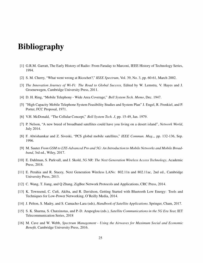
Bibliography

[1] G.R.M. Garratt, The Early History of Radio: From Faraday to Marconi, IEEE History of Technology Series,

1994.

[2] S. M. Cherry, “What went wrong at Ricochet?,” IEEE Spectrum, Vol. 39, No. 3, pp. 60-61, March 2002.

[3] The Innovation Journey of Wi-Fi: The Road to Global Success, Edited by W. Lemstra, V. Hayes and J.

Groenewegen, Cambridge University Press, 2011.

[4] D. H. Ring, “Mobile Telephony - Wide Area Coverage,” Bell System Tech. Memo, Dec. 1947.

[5] ”High Capacity Mobile Telephone System Feasibility Studies and System Plan” J. Engel, R. Frenkiel, and P.

Porter, FCC Proposal, 1971.

[6] V.H. McDonald, “The Cellular Concept,” Bell System Tech. J, pp. 15-49, Jan. 1979.

[7] P. Nelson, “A new breed of broadband satellites could have you living on a desert island”, Network World,

July 2014.

[8] F. Abrishamkar and Z. Siveski, “PCS global mobile satellites,” IEEE Commun. Mag.,, pp. 132-136, Sep.

1996.

[9] M. Sauter From GSM to LTE-Advanced Pro and 5G: An Introduction to Mobile Networks and Mobile Broad-

band, 3rd ed., Wiley, 2017.

[10] E. Dahlman, S. Parkvall, and J. Skold, 5G NR: The Next Generation Wireless Access Technology, Academic

Press, 2018.

[11] E. Perahia and R. Stacey, Next Generation Wireless LANs: 802.11n and 802.11ac, 2nd ed., Cambridge

University Press, 2013.

[12] C. Wang, T. Jiang, and Q Zhang, ZigBee Network Protocols and Applications, CRC Press, 2014.

[13] K. Townsend, C. Cufi, Akiba, and R. Davidson, Getting Started with Bluetooth Low Energy: Tools and

Techniques for Low-Power Networking, O’Reilly Media, 2014.

[14] J. Pelton, S. Madry, and S. Camacho-Lara (eds), Handbook of Satellite Applications. Springer, Cham, 2017.

[15] S. K. Sharma, S. Chatzinotas, and P.-D. Arapoglou (eds.), Satellite Communications in the 5G Era Year, IET

Telecommunication Series, 2018

[16] M. Cave and W. Webb, Spectrum Management - Using the Airwaves for Maximum Social and Economic

Benefit, Cambridge University Press, 2016.

25

[17] F. M. Abinader et al., ”Enabling the coexistence of LTE and Wi-Fi in unlicensed bands,” IEEE Commun.

Mag., vol. 52, no. 11, pp. 54-61, Nov. 2014.

[18] S. Emami, UWB Communication Systems: Conventional and 60 GHz: Principles, Design and Standards,

Springer, 2013.

[19] L. Frenzel, “What ever happened to ultrawideband wireless,” Electronic Design, Sep. 2014.

[20] R. Zhang and Y. C. Liang, Exploiting multi-antennas for opportunistic spectrum sharing in cognitive radio

networks, IEEE J. Sel. Topics Signal Proc., vol. 2, no. 1, pp. 88-102, Feb. 2008.

[21] E. Biglieri, A. J. Goldsmith, L. J. Greenstein, N. B. Mandayam, and H. V. Poor, Principles of Cognitive

Radio, Cambridge University Press, 2012.

[22] J. Mitola and G. Q. Maguire, ”Cognitive radio: making software radios more personal,” IEEE Personal

Commun., Vol. 6, No. 4, pp. 13-18, Aug. 1999.

[23] N. Devroye, P. Mitran, and V. Tarokh, Achievable Rates in Cognitive Radio Channels, Proc. 39th Annual

Conf. Info. Sci. and Sys., Mar. 2005.

[24] D. Gunduz, Paul de Kerret, Nicholas D. Sidiropoulos, David Gesbert, Chandra Murthy, Mihaela van der

Schaar, “Machine Learning in the Air,” Arxiv: https://arxiv.org/pdf/1904.12385.pdf.

[25] O. Simeone, A very brief introduction to Machine Learning with applications to communication systems,

IEEE Trans. on Cognitive Commun. and Networking, vol. 4, no. 4, pp. 648664, Dec. 2018.

26

Chapter 2

Path Loss, Shadowing, and Multipath

The wireless radio channel poses a severe challenge as a medium for reliable high-speed communication. Not only

is it susceptible to noise, interference, and other channel impediments, but these impediments change over time in

unpredictable ways as a result of user movement and environment dynamics. In this chapter we characterize the

primary phenomena that affect signal propagation: path loss and shadowing, as well as signal reflection, diffraction,

and scattering. Path loss characterizes how a signal’s received power decreases with transmit-receive distance. It

is caused by dissipation of the power radiated by the transmitter as well as by effects of the propagation channel.

Path-loss models assume that path loss is the same at a given transmit–receive distance (assuming that the path-

loss model does not include shadowing effects). Shadowing is the attenuation caused by obstacles between the

transmitter and receiver that absorb the transmitted signal. When the attenuation is strong, the signal is blocked.

The number and type of objects that cause shadowing at any given receiver location is typically unknown. Hence

attenuation due to shadowing is modeled as a random parameter. Unlike path loss, shadowing does not depend

on the transmit-receive distance itself but rather on the objects between the transmitter and receiver. Reflection,

diffraction, and scattering are caused by a transmitted signal interacting with objects in the environment around

the transmitter or receiver. The signal components that arise due to these objects are called multipath components.

Different multipath components arrive at the receiver with different time delays and phase shifts. When the phase

shifts are aligned, the multipath components add constructively; when they are not aligned, they add destructively.

This constructive and destructive addition of multipath components leads to significant variations in the received

signal power.

Received power variation due to path loss occurs over long distances (100-1000 m), whereas variation due to

shadowing occurs over distances that are proportional to the length of the obstructing object (10-100 m in outdoor

environments and less in indoor environments). Since variations in received power due to path loss and shadowing

occur over relatively large distances, these variations are sometimes referred to as large-scale propagation effects.

The received power variations due to constructive and destructive addition of multipath components occur over

very short distances, on the order of the signal wavelength, since each component’s phase rotates 360 degrees

over that distance. Hence, power variations due to multipath are sometimes referred to as small-scale propagation

effects. Figure 2.1 shows an example of the received-to-transmit power ratio in decibels1 (dB) versus log distance

for the combined effects of path loss, shadowing, and multipath. As indicated in the figure, received power due to

path loss alone is generally modeled as decreasing linearly with respect to the log of the transmit-receive distance,

with additional slow variations due to shadowing and fast variations due to multipath.

After a brief introduction to propagation and a description of our signal model, we present the simplest model

for signal propagation: free-space path loss. A signal propagating between two points with no attenuation or

reflection follows the free-space propagation law. We then describe the two-ray multipath model, which augments

1The decibel value of x is 10 log10 x.

27

Figure 2.1: Effects of path loss, shadowing, and multipath on received power as a function of distance.

the free-space model with a single reflected ray. The two-ray model introduces the notion of a variable path-loss

exponent, which gives rise to more general path loss exponent models. After introducing these models, we discuss

the commonly-used log-normal model for shadowing. General ray tracing is then introduced to model the multipath

components that arise due to signal reflections, diffraction, and scattering. These models approximate signal

propagation according to Maxwell’s equations and depend heavily on the geometry and dielectric properties of the

region through which the signal propagates. If the number of multipath components is large or if the geometry and

dielectric properties of the propagation environment are unknown, then statistical multipath models must be used

instead of ray tracing. These statistical multipath models will be described in Chapter 3. We close the chapter by

describing empirical channel models with parameters for path loss and shadowing based on measurements for both

indoor and outdoor channels.

Although this chapter gives a brief overview of channel models for path loss, shadowing, and multipath,

comprehensive coverage of channel and propagation models at different frequencies of interest merits a book in

its own right, and in fact there are many excellent references on this topic including [1, 2, 3, 4, 10, 6]. Models

specialized to multiple antenna, ultrawideband, and millimeter wave channels can be found in [7], [8], and [9],

respectively.

2.1 Radio Wave Propagation

The initial understanding of radio wave propagation goes back to the pioneering work of James Clerk Maxwell,

who in 1864 formulated a theory of electromagnetic propagation that predicted the existence of radio waves. In

1887, the physical existence of these waves was demonstrated by Heinrich Hertz. However, Hertz saw no practical

use for radio waves, reasoning that since audio frequencies were low, where propagation was poor, radio waves

could never carry voice. In 1894 Oliver Lodge used these principles to build the first wireless communication

system, though its transmission distance was limited to 150 meters. By 1897 the entrepreneur Guglielmo Marconi

had managed to send a radio signal from the Isle of Wight to a tugboat eighteen miles away, and in 1901 Marconi’s

wireless system could traverse the Atlantic ocean. These early systems used telegraph signals for communicating

information. The first transmission of voice and music was made by Reginald Fessenden in 1906 using a form of

amplitude modulation, which circumvented the propagation limitations at low frequencies observed by Hertz by

translating signals to a higher frequency, as is done in all wireless systems today.

28

Electromagnetic waves propagate through environments where they are reflected, scattered, and diffracted

by walls, terrain, buildings, and other objects. The ultimate details of this propagation can be obtained by solving

Maxwell’s equations with boundary conditions that express the physical characteristics of these obstructing objects.

This often requires the calculation of the radar cross-section (RCS) of large and complex structures. Since these

calculations are difficult and since the necessary parameters are often not available, approximations have been

developed to characterize signal propagation without resorting to Maxwell’s equations.

The most common signal propagation approximations use ray-tracing techniques based on ray-optic theory

[10]. Ray-tracing approximates the propagation of electromagnetic waves by representing the wavefronts as dis-

crete narrow beams or rays. This approximation determines the reflection and refraction effects on the wavefront

but ignores the more complex scattering phenomenon predicted by Maxwell’s coupled differential equations. The

ray-tracing model most accurately approximates Maxwell’s equations when the wavelength of the signal is much

less than the size of the objects off of which it is reflected, refracted, or scattered. The simplest ray-tracing model is

the two-ray model, which accurately describes signal propagation when there is one direct path between the trans-

mitter and receiver and one reflected path. The reflected path typically bounces off the ground, and the two-ray

model is a good approximation for propagation along highways or rural roads and over water. We will analyze the

two-ray model in detail, as well as more complex models with additional reflected, scattered, or diffracted compo-

nents. Many propagation environments are not accurately characterized by ray-tracing models. In these cases it is

common to develop analytical models based on empirical measurements, and we will discuss several of the most

common of these empirical models.

Often the complexity and variability of the radio channel make it difficult to obtain an accurate deterministic

channel model. For these cases, statistical models are often used. The attenuation caused by signal path obstruc-

tions such as buildings or other objects is typically characterized statistically, as described in Section 2.7. Statistical

models are also used to characterize the constructive and destructive interference for a large number of multipath

components, as described in Chapter 3. Indoor environments tend to be less regular than outdoor environments,

since the geometric and dielectric characteristics change dramatically depending on whether the indoor environ-

ment is an open factory, cubicled office, or metal machine shop. For these environments computer-aided modeling

tools are available to predict signal propagation characteristics [11].

2.2 Transmit and Receive Signal Models

The transmitted and received signals in any wireless system are real-valued. The channel introduces an amplitude

and phase change at each frequency of the transmitted signal so that the received signal is also real-valued. Real

modulated and demodulated signals are often represented as the real part of a complex signal in order to facilitate

analysis. This model gives rise to the equivalent lowpass representation of bandpass signals, which we use for our

transmitted and received signals. More details on the equivalent lowpass representation of bandpass signals and

systems can be found in Appendix A.

We model the transmitted signal at carrier frequency fc as

s(t) = Reu(t)ej2πfct= Reu(t) cos(2πfct) − Imu(t) sin(2πfct)

= sI (t) cos(2πfct) − sQ(t) sin(2πfct), (2.1)

where u(t) = sI(t)+jsQ(t) is a complex baseband signal with in-phase component sI(t) = Reu(t), quadrature

component sQ(t) = Imu(t), bandwidth Bu, and power Pu. The signal u(t) is called the complex envelope or

equivalent lowpass signal of s(t). We call u(t) the complex envelope of s(t) because the magnitude of u(t) is the

magnitude of s(t). The phase of u(t) includes any carrier phase offset. The equivalent lowpass representation of

29

band-pass signals with bandwidthB fc allows signal manipulation via u(t) irrespective of the carrier frequency.

The power in the transmitted signal s(t) is Pt = Pu/2.

For time-invariant channels, the received signal is the convolution of s(t) with the channel impulse response

h(t) plus an additional noise component n(t) introduced by the channel: r(t) = s(t) ∗ h(t) + n(t). It can be

written in a similar form as the transmitted signal as:

r(t) = Rev(t)ej2πfct + n(t), (2.2)

where v(t) is the equivalent lowpass signal for the received signal without the noise. This equivalent signal depends

on h(t). In particular, as discussed in Appendix A, v(t) = u(t)∗ c(t), where c(t) is the equivalent lowpass channel

impulse response for h(t). Time-varying channels will be treated in Chapter 3.

The received signal in (2.2) consists of two terms, the first term corresponding to the transmitted signal after

propagation through the channel, and the second term corresponding to the noise added by the channel. The signal-

to-noise power ratio (SNR) of the received signal is defined as the power of the first term divided by the power

of the second term. In this chapter (and in Chapter 3) we will neglect the random noise component n(t) in our

analysis, since these chapters focus on signal propagation, which is not affected by noise. However, noise will play

a prominent role in the capacity and performance of wireless systems studied in later chapters.

When the transmitter or receiver is moving, the received signal will have a Doppler shift of fD = vλ cos θ

associated with it, where θ is the arrival angle of the received signal relative to the direction of motion, v is

the receiver velocity toward the transmitter in the direction of motion, and λ = c/fc is the signal wavelength

(c = 3 · 108 m/s is the speed of light). The geometry associated with the Doppler shift is shown in Figure 2.2.

The Doppler shift results from the fact that transmitter or receiver movement over a short time interval ∆t causes

a slight change in distance ∆d = v∆t cos θ that the transmitted signal needs to travel to the receiver. The phase

change due to this path-length difference is ∆φ = 2πvλ ∆t cos θ. The Doppler frequency is then obtained from the

relationship between signal frequency and phase:

fD =1

2π

∆φ

∆t=v

λcos θ. (2.3)

If the receiver is moving toward the transmitter (i.e., if −π/2 ≤ θ ≤ π/2) , then the Doppler frequency is positive;

otherwise, it is negative. We will ignore the Doppler term in the path loss models of this chapter, since for typical

vehicle speeds (75 km/hr) and frequencies (about 10 GHz) it is small, on the order of 1 KHz [1]. However, we

will include Doppler effects in Chapter 3 on statistical fading models where it is used to characterize a random

channel’s rate of change.

Suppose a signal s(t) of power Pt is transmitted through a given channel with corresponding received signal

r(t) of power Pr, where Pr is averaged over any random variations due to shadowing. We define the linear path

loss of the channel as the ratio of transmit power to receive power:

PL =PtPr. (2.4)

We define the path loss of the channel as the value of the linear path loss in decibels or, equivalently, the difference

in dB between the transmitted and received signal power:

PL dB = 10 log10

(PtPr

)

dB. (2.5)

The dB path loss is a nonnegative number since the channel does not contain active elements, and thus it can

only attenuate the signal. The dB path gain is defined as the negative of the dB path loss: PG = −PL =10 log10(Pr/Pt) dB. Due to the laws of physics underlying signal propagation, the dB path loss generally increases

30

Figure 2.2: Geometry associated with Doppler shift.

with distance, as illustrated in Figure 2.1 (note that this figure shows a decreasing path gain or, equivalently, an

increasing path loss). The path loss generally increases with distance, which means the received power in dB

decreases with distance, as illustrated in Figure 2.1. With shadowing, also illusrated in Figure 2.1, the received

power is random owing to random blockage from objects, as we discuss in Section 2.6.

2.3 Free-Space Path Loss

Consider a signal transmitted through free space to a receiver located at distance d from the transmitter. Assume

there are no obstructions between the transmitter and receiver and that the signal propagates along a straight line

between the two. The channel model associated with this transmission is called a line-of-sight (LOS) channel, and

the corresponding received signal is called the LOS signal or ray. Under free-space path loss the received signal is

given by [2]:

r(t) = Re

[

λ√GtGru(t− τl)e

−j2πd/λ

4πd

]

ej2πfct

, (2.6)

where Gt and Gr are, respectively, the transmit and receive antenna power gains in the LOS direction relative to a

unity gain isotropic antenna, τl = d/c is the signal propagation delay of the LOS signal traveling the distance d, and

the phase shift e−j2πd/λ is due to the distance d that the wave travels2. Transmit and receive directional antennas

have gainsGt and Gr greater than unity in one or more angular directions relative to the idealized isotropic antenna

gains Gt = Gr = 1. Directional antenna gains can range from 2.15 dB for a half-wavelength dipole to tens of dB

in horn or dish antennas. More details on directional antenna designs and their gains can be found in [12].

2When the transmit and receive antennas are at the same height, the distance d equals the horizontal separation distance between the

transmitter and receiver. When the transmitter and receiver are at different heights, the distance the wave travels exceeds this separation

distance. These different distances will be characterized in the two-ray model (Section 2.4).

31

The power in the transmitted signal s(t) is Pt, so from (2.6), the linear path loss for free-space propagation, a

formula first introduced by Friis [13], is

PrPt

= GtGr

[λ

4πd

]2

. (2.7)

The Friis formula (2.7) dictates that the receive power Pr equals the transmit power per unit area under free space

propagation that is incident on the receive antenna, given by PtGt/(4πd2), multiplied by that antenna’s effective

area Ar, a quantity that determines how effectively the receive antenna captures this incident power. From (2.7)

this effective area equals

Ar =λ2Gr4π

. (2.8)

The dependence ofAr on λ2 is due to the resonance of a signal with a given wavelength on a linear conductor half

that size. Since λ = c/fc, the Friis formulae indicates that, as the carrier frequency increases, the received power

decreases as the square of the increase. Antenna arrays, discussed in Chapter 10, create a different effective area

than single-element antennas, which can mitigate or remove the dependence of received power on λ [14]. The Friis

formula also indicates that the received signal power falls off in inverse proportion to the square of the distance

d between the transmit and receive antennas. We will see in the next section that, for other signal propagation

environments, the received signal power falls off more quickly relative to this distance.

The received power can be expressed in dBm as3

Pr (dBm) = Pt (dBm) + 10 log10(GtGr) + 20 log10(λ)− 20 log10(4π)− 20 log10(d). (2.9)

Equation (2.9) is an example of a link budget equation, which expresses the received power of a signal transmitted

through a given channel (or link) as a function of the transmit power and all the losses the signal experiences on

that link. Free-space path loss is defined as the path loss of the free-space model:

PL (dB) = 10 log10

(PtPr

)

= −10 log10

(

GtGr

[λ

4πd

]2)

. (2.10)

The free-space path gain is thus

PG = −PL = 10 log10

(

GtGr

[λ

4πd

]2)

. (2.11)

Example 2.1: Consider an outdoor small cell with fc = 2.5 GHz, cells of radius 10 m, and isotropic antennas.

Under the free-space path loss model, what transmit power is required at the base station in order for all terminals

within the cell to receive a minimum power of 0.1 µW? How does this change if the system frequency is 5 GHz?

Solution: We must find a transmit power such that the terminals at the cell boundary receive the minimum required

power. We obtain a formula for the required transmit power by inverting (2.7) to obtain:

Pt = Pr

[4πd√GtGrλ

]2

.

3The dBm value of a power x is its dB value relative to a milliwatt: 10 log10(x/.001). The dBW value of a power x is its dB value

relative to a watt: 10 log10 x, so 1W corresponds to 30 dBm.

32

Substituting in Gt = Gr = 1 (isotropic antennas), λ = c/fc = 0.12 m, d = 10 m, and Pr = 0.1 µW yields

Pt = .1097 W. At 5 GHz only λ = .06 changes, so Pt = .4388 W. We see that doubling the carrier frequency

leads to a requirement for four times more transmit power, illustrating the power consumption challenges in moving

wireless systems to high-frequency spectral bands.

2.4 Two-Ray Multipath Model

The two-ray model is used when a single ground (or other) reflection dominates the multipath effect, as illustrated

in Figure 2.3. The received signal consists of two components: the LOS component or ray, which corresponds to

the transmitted signal propagating through free space, and a reflected component or ray, which is the transmitted

signal reflected off the ground. The received LOS ray is given by the free-space propagation loss formula (2.6)

with the distance the signal travels set to d0. The reflected ray shown in Figure 2.3 travels distance d1 = d11 +d12.

Since the two signal components in this model travel different distances, we use d in this model and all subsequent

propagation models in this chapter to denote the horizontal distance between the transmitter and receiver. The

distances d0 and d1 then depend on d as well as the transmitter and receiver heights ht and hr. We see from Figure

2.3 that when ht = hr, d = d0, and when d is very large relative to ht and hr, d ≈ d0 ≈ d1.

If we ignore the effect of surface wave attenuation4 then, by superposition, the received signal for the two-ray

model is

r2-ray(t) = Re

λ

4π

[√G0u(t− τ0)e

−j2πd0/λ

d0+R√G1u(t− τ1)e

−j2πd1/λ

d1

]

ej2πfct

, (2.12)

where τ0 = d0/c is the time delay of the LOS ray, τ1 = d1/c is the time delay of the ground reflection ray,√G0 =

√Gt0Gr0 is the product of the transmit and receive antenna field radiation patterns in the LOS direction,

R is the ground reflection coefficient, and√G1 =

√Gt1Gr1 is the product of the transmit and receive antenna

field radiation patterns corresponding to the ground reflection. The delay spread of the two-ray model equals the

difference between the delay of the LOS ray and that of the reflected ray: (d1 − d0)/c.If the transmitted signal is narrowband relative to the delay spread such that (τ1−τ0 B−1

u ) then u(t−τ1) ≈u(t− τ0). With this approximation, the received power of the two-ray model for narrowband transmission is

Figure 2.3: Two-ray model.

4This is a valid approximation for antennas located more than a few wavelengths from the ground.

33

Pr = Pt

[λ

4π

]2 ∣∣∣∣

√G0

d0+R√G1e

−j∆φ

d1

∣∣∣∣

2

, (2.13)

where ∆φ = 2π(d1 − d0)/λ is the phase difference between the two received signal components. Equation

(2.13) has been shown [15] to agree closely with empirical data. From the geometry of the two-ray model, d1 =√

(ht + hr)2 + d2 and d0 =√

(ht − hr)2 + d2. Hence

d1 − d0 =√

(ht + hr)2 + d2 −√

(ht − hr)2 + d2. (2.14)

When d is very large compared to ht + hr , we can use a Taylor series approximation in (2.14) to get

∆φ =2π

λ

(√

(ht + hr)2 + d2 −√

(ht − hr)2 + d2)

≈ 4πhthrλd

. (2.15)

The ground reflection coefficient is given by [1, 16]

R =sin θ − Z

sin θ + Z, (2.16)

where

Z =

√εr − cos2 θ/εr for vertical polarization,√εr − cos2 θ for horizontal polarization,

(2.17)

and εr is the dielectric constant of the ground. For earth or road surfaces this dielectric constant is approximately

that of a pure dielectric (for which εr is real with a value of about 15).

Since for asymptotically large d, d1 ≈ d0 ≈ d, G1 ≈ G0 where we denote this approximate antenna gain as

G, and θ ≈ 0 which by (2.16) then implies that R ≈ −1. Substituting these approximations into (2.13) yields

Pr ≈ Pt

[

λ√G

4πd

]2

|1− e−j∆φ|2. (2.18)

Using the approximation for ∆φ in (2.15) at large dwe get the final approximation for received power at large

distance d as

Pr ≈ Pt

[

λ√G

4πd

]2 [4πhthrλd

]2

= Pt

[√Ghthrd2

]2

, (2.19)

or, in dB,

Pr dBm = Pt dBm + 10 log10(G) + 20 log10(hthr) − 40 log10(d). (2.20)

Thus, in the limit of asymptotically large d, the received power falls off inversely with the fourth power of d and is

independent of the wavelength λ. This is in contrast to free-space propagation where power is inversely proportion

to d2 and proportional to λ2. The received signal power becomes independent of λ because directional antenna

arrays have a received power that does not necessarily decrease with λ, and combining the direct path and reflected

signal at the receiver effectively forms an antenna array.

A plot of (2.13) as a function of the transmit-receive separation distance d is shown in Figure 2.4 for fc = 900

MHz, R = −1, ht = 50 m, hr = 2 m, G0 = G1 = 1, and received power normalized to 0 dB at a reference

distance of 1 m. This plot reflects the case where the transmit antenna height ht is much larger than the receiver

34

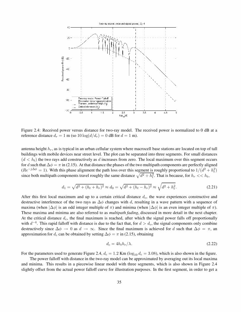
Figure 2.4: Received power versus distance for two-ray model. The received power is normalized to 0 dB at a

reference distance dr = 1 m (so 10 log(d/dr) = 0 dB for d = 1 m).

antenna height hr, as is typical in an urban cellular system where macrocell base stations are located on top of tall

buildings with mobile devices near street level. The plot can be separated into three segments. For small distances

(d < ht) the two rays add constructively as d increases from zero. The local maximum over this segment occurs

for d such that ∆φ = π in (2.15). At that distance the phases of the two multipath components are perfectly aligned

(Re−j∆φ = 1). With this phase alignment the path loss over this segment is roughly proportional to 1/(d2 + h2t )

since both multipath components travel roughly the same distance√

d2 + h2t . That is because, for hr << ht,

d1 =√

d2 + (ht + hr)2 ≈ d0 =√

d2 + (ht − hr)2 ≈√

d2 + h2t . (2.21)

After this first local maximum and up to a certain critical distance dc, the wave experiences constructive and

destructive interference of the two rays as ∆φ changes with d, resulting in a wave pattern with a sequence of

maxima (when |∆φ| is an odd integer multiple of π) and minima (when |∆φ| is an even integer multiple of π).

These maxima and minima are also referred to as multipath fading, discussed in more detail in the next chapter.

At the critical distance dc, the final maximum is reached, after which the signal power falls off proportionally

with d−4. This rapid falloff with distance is due to the fact that, for d > dc, the signal components only combine

destructively since ∆φ → 0 as d → ∞. Since the final maximum is achieved for d such that ∆φ = π, an

approximation for dc can be obtained by setting ∆φ = π in (2.15), obtaining

dc = 4hthr/λ. (2.22)

For the parameters used to generate Figure 2.4, dc = 1.2 Km (log10 dc = 3.08), which is also shown in the figure.

The power falloff with distance in the two-ray model can be approximated by averaging out its local maxima

and minima. This results in a piecewise linear model with three segments, which is also shown in Figure 2.4

slightly offset from the actual power falloff curve for illustration purposes. In the first segment, in order to get a

35

constant power falloff we assume d0 ≈ d1 ≈ ht, leading to a power falloff proportional to 1/h2t that is independent

of d; for distances between ht and dc, power falls off at −20 dB/decade; and at distances greater than dc, power

falls off at –40 dB/decade.

The critical distance dc is proportional to the transmit antenna height ht and to the carrier frequency fc = c/λ.

Thus, for small cells and indoor systems where ht is ten meters or less, for fc on the order of 1 GHz, dc is hundreds

of meters, as illustrated in Example 2.2. On the other hand, for millimeter wave systems where fc is tens of GHz,

dc typically well exceeds a kilometer. The value of dc can be used for system design. For example, if propagation

in a cellular system obeys the two-ray model then the critical distance would be a natural size for the cell radius,

since the path loss associated with interference outside the cell would be much larger than path loss for desired

signals inside the cell. However, setting the cell radius to dc could result in very large cells, as illustrated in Figure

2.4 and in the next example. Since smaller cells are more desirable – both to increase capacity and reduce transmit

power – cell radii are typically much smaller than dc. Thus, with a two-ray propagation model, power falloff within

these relatively small cells goes as distance squared. Moreover, propagation in cellular systems rarely follows a

two-ray model, since cancellation by reflected rays rarely occurs in all directions.

Example 2.2: Determine the critical distance for the two-ray model in an outdoor cell with ht = 10 m, hr = 3 m

and in an indoor cell with ht = 3 m, hr = 2 m for fc = 2 GHz.

Solution: dc = 4hthr/λ = 800 m for the outdoor cell and 160 m for the indoor cell. A cell radius of 800 m in

an outdoor cell is typical for a macrocell but a bit large for a small cell which today are on the order of 10-100 m

to maintain large capacity. However, for a macrocell with an 800 m radius under these system parameters, signal

power would fall off as d2 inside the cell, while interference from neighboring cells would fall off as d4 and thus

would be greatly reduced. Similarly, 160 m is quite large for the cell radius of an indoor system, as there would

typically be many walls the signal would have to penetrate for an indoor cell radius of that size. Hence an indoor

system would typically have a smaller cell radius: on the order of 10–20 m, the size of one room or a few adjacent

rooms in a typical building.

2.5 Path Loss Exponent Models

2.5.1 Single-Slope

The complexity of signal propagation makes it difficult to obtain a single model that characterizes path loss accu-

rately across a range of different environments and frequencies. Accurate path loss models can be obtained from

complex analytical models or empirical measurements when tight system specifications must be met or the best

locations for base stations or access-point layouts must be determined. However, for general trade-off analysis of

various system designs it is sometimes best to use a simple model that captures the essence of signal propagation

without resorting to complicated path loss models, which are only approximations to the real channel anyway.

The following single-slope model for path loss as a function of distance is a simple model that captures several

important propagation characteristics.

Pr = PtK

[drd

]γ

, (2.23)

36

Table 2.1: Typical path loss exponents

Environment γ range

Urban macrocells 3.7–6.5

Urban microcells 2.7–3.5

Office building (same floor) 1.6–3.5

Office building (multiple floors) 2–6

Store 1.8–2.2

Factory 1.6–3.3

Home 3

where dr is a reference distance for the antenna far field, γ is the path-loss exponent, and K is a unitless constant

equal to the path gain Pr/Pt at distance d = dr. The dB attenuation is thus

Pr (dBm) = Pt (dBm) +K dB − 10γ log10 (d/dr) , (2.24)

and the path loss consists of two terms, where all environment and antenna parameters are captured by the first

term, and the path loss due only to distance is captured by the second term:

PL (dB) = 10 log10 (Pt/Pr) = −10 log10K + 10γ log10(d/dr). (2.25)

The values for K, dr, and γ can be obtained to approximate either an analytical or empirical model. In

particular, the free-space path-loss model and some of the empirical models described in Section 2.7 are all of the

same form as (2.24). Because of antenna near field effects at transmit distances on the order of a signal wavelength,

the model (2.24) is generally valid only at transmission distances d > dr, where dr is typically assumed to be 1 mfor systems transmitting over distances greater than this nominal value.

When the single-slope model is used to approximate empirical measurements, the value of K < 1 is some-

times set to the free-space path gain at distance dr assuming isotropic antennas:

K dB = 20 log10

λ

4πdr, (2.26)

and this assumption is supported by empirical data for free-space path loss at a transmission distance of 100 m [17].

Alternatively,K can be determined by measurement at dr or optimized (alone or together with γ) to minimize the

mean-square error (MSE) between the model and the empirical measurements [17]. The value of γ depends on the

propagation environment: for propagation that approximately follows a free-space or two-ray model, γ is set to 2 or

4 respectively. The value of γ for more complex environments can be obtained via a minimum mean-square error

(MMSE) fit to empirical measurements, as illustrated in Example 2.3. Alternatively, γ can be obtained from an

empirically based model that takes into account frequency and antenna height [17]. Table 2.6 summarizes values

of the path loss exponent γ for different environments based on data from [11, 17, 18, 19, 20, 21, 52]. Empirical

measurements indicate that path loss exponents at higher frequencies tend to be higher [19, 23, 21, 22, 57, 59]

whereas path loss exponents at higher antenna heights tend to be lower [17, 57, 59]. The more complex empirical

models described below in Section 2.7, particularly the widely used 3GPP and WINNER II channel models [57,

59], have additional terms that explicitly capture the dependence of path loss on frequency and antenna height.

Note that the wide range of empirical path-loss exponents for indoor propagation may be due to attenuation caused

by floors, objects, and partitions (see Section 2.5.5).

Example 2.3: Consider the set of empirical measurements of Pr/Pt given in Table 2.2 for an indoor system at 900

37

MHz. Find the path loss exponent γ that minimizes the MSE between the single-slope model (2.24) and the empir-

ical dB power measurements, assuming that dr = 1 m and K is determined from the free-space path-gain formula

at this dr. Find the received power at 150 m for the single-slope path loss model with this path loss exponent and a

transmit power of 1 mW (0 dBm). Note that, since the path loss model in dB is linear, minimizing the MSE of the

empirical data in dB (versus in linear units) relative to this model is a simple linear regression.

Solution: We first set up the MMSE error equation for the dB power measurements as

F (γ) =

5∑

i=1

[Mmeasured(di) −Mmodel(di)]2,

where Mmeasured(di) is the path loss measurement in Table 2.2 at distance di and where Mmodel(di) = K −10γ log10(di) is the path loss at di based on (2.24) since dr = 1. Now using the free-space path gain formula

yields K = 20 log10(.3333/(4π)) = −31.53 dB. Thus

Table 2.2: path loss measurements

Distance from transmitter M = Pr/Pt

10 m –70 dB

20 m –75 dB

50 m –90 dB

100 m –110 dB

300 m –125 dB

F (γ) = (−70 + 31.53 + 10γ)2 + (−75 + 31.53 + 13.01γ)2

+ (−90 + 31.53 + 16.99γ)2 + (−110 + 31.53 + 20γ)2

+ (−125 + 31.53 + 24.77γ)2

= 21682.50− 11656.60γ+ 1571.47γ2. (2.27)

Differentiating F (γ) relative to γ and setting it to zero yields

∂F (γ)

∂γ= −11656.60 + 3142.94γ = 0 ⇒ γ = 3.71.

For the received power at 150 m under the single-slope path loss model with K = −31.53, γ = 3.71, and Pt = 0dBm, we have Pr = Pt +K − 10γ log10(d/dr) = 0 − 31.53 − 10 · 3.71 log10(150) = −112.26 dBm. Clearly

the measurements deviate from the single-slope path loss model; this variation can be attributed to shadow fading,

described in Section 2.7.

2.5.2 Multi-Slope

The multi-slope path loss model, which is piecewise linear in dB, generalizes the single-slope model by allowing

for different path loss exponents at different distances. Given this greater flexibility, the multi-slope model is

commonly used to analytically model empirical measurements. The multi-slope path loss model and a set of

38

measurement data on which it would be based is illustrated in Figure 2.5 for dB attenuation versus log distance,

where the dots represent hypothetical measurements and the multi-slope model is the analytical approximation to

these measurements. A multi-slope model with N segments must specify N − 1 breakpoints d1, . . . , dN−1 as

well as the slopes corresponding to each segment s1, . . . , sN . The slope of the ith segment is si = −10γi for

γi the path loss exponent on that segment. Different methods can be used to determine the number and location

of breakpoints to be used in modeling the empirical data. Once these are fixed, the slopes corresponding to each

segment can be obtained by linear regression on the data. The transition to a new slope might be instantaneous at a

given breakpoint distance or entail some smoothing. Multi-slope models capture the analytical two-ray propagation

model of Section 2.4. They also fit well to empirical measurements in propagation environments where the path

loss exponent increases with distance [52], where the LOS path loss differs from that of non-LOS path loss [98],

and in heterogeneous cellular networks where users may connect to a relatively distant macrocell base station while

experiencing interference from a nearby small cell [99].

A special case of the multi-slope model is the dual-slope model. The dual-slope model is characterized by a

constant path loss factorK and a path loss exponent γ1 above some reference distance dr and up to some breakpoint

distance dBP, after which power falls off with path loss exponent γ2. The dB path loss is thus given by:

Pr(d) (dB) =

Pt +K − 10γ1 log10(d/dr), dr ≤ d ≤ dBP,

Pt +K − 10γ1 log10(dBP/dr) − 10γ2 log10(d/dBP), d > dBP.(2.28)

The path loss exponents,K, and dBP are typically obtained via a regression fit to empirical data [17, 92]. The two-

ray model described in Section 2.4 for d > ht can be approximated by the dual-slope model, with the breakpoint

distance dBP = dc given by (2.22) and path loss exponents γ1 = 2 and γ2 = 4. Many of the measurement-based

models described in Section 2.9 use the dual-slope model for path loss.

The transition between the multiple equations in the dual-slope model (2.28) can be smoothed by the following

model [34, 93]:

Pr =PtK

L(d), (2.29)

where

L(d)∆=

(d

dr

)γ1(

1 +

(d

dBP

)(γ1−γ2)q)1/q

. (2.30)

In this expression, q is a parameter that determines the smoothness of the path loss at the transition region close to

the breakpoint distance dBP. This smoothing in this model can be extended to more than two regions [91].

2.6 Shadowing

A signal transmitted through a wireless channel will typically experience random variation due to blockage from

objects in the signal path, giving rise to random variations of the received power at a given distance. Such variations

are also caused by changes in reflecting surfaces and scattering objects. Thus, a model for the random attenuation

due to these effects is also needed. The location, size, and dielectric properties of the blocking objects – as well as

the changes in reflecting surfaces and scattering objects that cause the random attenuation – are generally unknown,

so statistical models must be used to characterize this attenuation.

39

Figure 2.5: Multi-slope model for path loss.

The most common model for this additional attenuation is log-normal shadowing; under this model the dB

value of the random attenuation is Gauss-distributed. The log-normal shadowing model has been empirically con-

firmed to model accurately the variation in received power in both outdoor and indoor radio propagation environ-

ments (see, e.g., [17, 102]). In the log-normal shadowing model, the ratio of transmit-to-receive power ψ = Pt/Pris assumed to be random with a log-normal distribution given by

p(ψ) =ξ√

2πσψdBψ

exp

[

−(10 log10 ψ − µψdB)2

2σ2ψdB

]

, ψ > 0, (2.31)

where ξ = 10/ ln10, µψdBis the mean of ψdB = 10 log10 ψ in decibels, and σψdB

is the standard deviation of

ψdB (also in dB). The mean can be based on an analytical model or empirical measurements. For empirical mea-

surements µψdBequals the empirical path loss, since average attenuation from shadowing is already incorporated

into the measurements. For analytical models, µψdBmust incorporate both the path loss (e.g., from a free-space or

ray-tracing model) as well as average attenuation from blockage. Alternatively, path loss can be treated separately

from shadowing, as described in the next section.

A random variable with a log-normal distribution is called a log-normal random variable. Note that if ψ

is log-normal then the received power and received SNR will also be log-normal, since these are just constant

multiples of ψ. For received SNR the mean and standard deviation of this log-normal random variable are also in

decibels. For log-normal received power the random variable has units of power, so its mean and standard deviation

will be in dBm or dBW instead of dB. The mean of ψ (the linear average path gain) can be obtained from (2.31) as

µψ = E[ψ] = exp

[

µψdB

ξ+σ2ψdB

2ξ2

]

. (2.32)

The conversion from the linear mean (in dB) to the log mean (in dB) is derived from (2.32) as

10 log10 µψ = µψdB+σ2ψdB

2ξ. (2.33)

40

Performance in log-normal shadowing is typically parameterized by the log mean µψdB, which is referred to

as the average dB path loss and is given in units of dB. We can compute the distribution of the dB value of ψ,

ψdB = 10 log10 ψ from the distribution ofψ given in (2.31). This computation reveals that ψdB is Gauss-distributed

with mean µψdBand standard deviation σψdB:

p(ψdB) =1√

2πσψdB

exp

[

−(ψdB − µψdB)2

2σ2ψdB

]

. (2.34)

The log-normal distribution of ψ or, equivalently, the Gaussian distribution of ψdB is defined by two parameters:

µψdBand σψdB

. Given that ψdB is based on the ratio of transmit and receive powers, it can be expressed as a

difference of these powers in either dBW or dBm, as follows:

ψdB = 10 log10(Pt/Pr) = Pt dBW − Pr dBW = Pt dBm − Pr dBm. (2.35)

Since ψdB is Gauss-distributed, by (2.35) and properties of Gaussian random variables we have that Pr dBW is

also Gauss-distributed with mean Pt dBW− µψdBand standard deviation σψdB, i.e. the same standard deviation as

ψdB. Similarly, Pr dBm is Gauss-distributed with mean Pt dBm − µψdBand standard deviation σψdB.

The log-normal distribution is an imperfect approximation to the effect of shadowing because it has a non-zero

probability that the received power exceeds the transmit power, which violates the laws of physics. In particular,

since the transmit power should always exceed the received power, ψ = Pt/Pr should always be greater than unity.

Thus shadowing models set µψdBto be greater than zero. Note, however, that the log-normal distribution (2.31)

takes values for 0 ≤ ψ ≤ ∞. Hence, for ψ < 1 we have Pr > Pt, which is physically impossible. However, this

probability will be very small when µψdBis large and positive. Thus, the log-normal model captures the underlying

physical model for shadowing most accurately when µψdB 0.

If the mean and standard deviation for the shadowing model are based on empirical measurements, then the

question arises as to whether they should be obtained by taking averages of the linear or rather the dB values of the

empirical measurements. In other words, given empirical (linear) path loss measurements piNi=1, should the mean

path loss be determined as µψ = (1/N )∑Ni=1 pi or as µψdB

= (1/N )∑N

i=1 10 log10 pi? A similar question arises

for computing the empirical variance. In practice it is more common to determine mean path loss and variance

based on averaging the dB values of the empirical measurements for several reasons. First, as we shall see, the

mathematical justification for the log-normal model is based on dB measurements. In addition, the literature

shows that obtaining empirical averages based on dB path loss measurements leads to a better approximation for

the physical channel being modeled [103]. Finally, as we saw in Section 2.5.4, power falloff with distance models

are often obtained by a piecewise linear approximation to empirical measurements of dB power versus the log of

distance [11].

Most empirical studies for outdoor channels support a standard deviation σψdBranging from 4 dB to 13 dB

[1, 34, 104, 105, 106]. Larger deviations are associated with environments that contain a high density of blocking

objects such as buildings and foliage outdoors, or walls and furniture indoors. Moreover, since attenuation by ob-

jects is more severe and more variable at high frequencies, and there is more variance in the number of attenuating

objects at large distances, σψdBgenerally increases with both frequency and distance [72].The mean power µψdB

depends on the path loss and building properties in the area under consideration. The mean power µψdBvaries with

distance; this is due to path loss and to the fact that average attenuation from objects increases with distance owing

to the potential for a larger number of attenuating objects.

The Gaussian model for the distribution of the mean received signal in dB can be justified by the following

attenuation model when shadowing is dominated by the attenuation from blocking objects. The attenuation of a

signal as it travels through an object of depth d is approximately equal to

s(d) = ce−αd, (2.36)

41

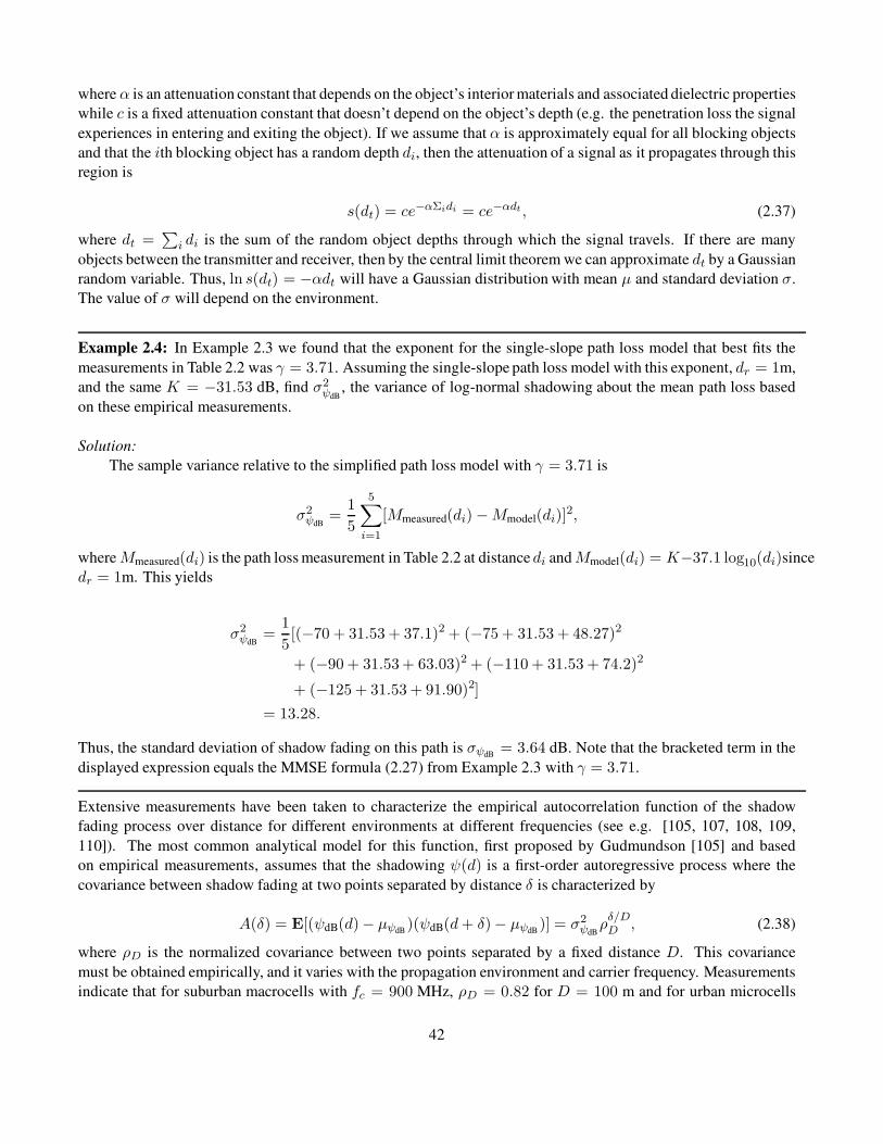
where α is an attenuation constant that depends on the object’s interior materials and associated dielectric properties

while c is a fixed attenuation constant that doesn’t depend on the object’s depth (e.g. the penetration loss the signal

experiences in entering and exiting the object). If we assume that α is approximately equal for all blocking objects

and that the ith blocking object has a random depth di, then the attenuation of a signal as it propagates through this

region is

s(dt) = ce−αΣidi = ce−αdt , (2.37)

where dt =∑

i di is the sum of the random object depths through which the signal travels. If there are many

objects between the transmitter and receiver, then by the central limit theorem we can approximate dt by a Gaussian

random variable. Thus, ln s(dt) = −αdt will have a Gaussian distribution with mean µ and standard deviation σ.

The value of σ will depend on the environment.

Example 2.4: In Example 2.3 we found that the exponent for the single-slope path loss model that best fits the

measurements in Table 2.2 was γ = 3.71. Assuming the single-slope path loss model with this exponent, dr = 1m,

and the same K = −31.53 dB, find σ2ψdB

, the variance of log-normal shadowing about the mean path loss based

on these empirical measurements.

Solution:

The sample variance relative to the simplified path loss model with γ = 3.71 is

σ2ψdB

=1

5

5∑

i=1

[Mmeasured(di) −Mmodel(di)]2,

whereMmeasured(di) is the path loss measurement in Table 2.2 at distancedi andMmodel(di) = K−37.1 log10(di)since

dr = 1m. This yields

σ2ψdB

=1

5[(−70 + 31.53 + 37.1)2 + (−75 + 31.53 + 48.27)2

+ (−90 + 31.53 + 63.03)2 + (−110 + 31.53 + 74.2)2

+ (−125 + 31.53 + 91.90)2]

= 13.28.

Thus, the standard deviation of shadow fading on this path is σψdB= 3.64 dB. Note that the bracketed term in the

displayed expression equals the MMSE formula (2.27) from Example 2.3 with γ = 3.71.

Extensive measurements have been taken to characterize the empirical autocorrelation function of the shadow

fading process over distance for different environments at different frequencies (see e.g. [105, 107, 108, 109,

110]). The most common analytical model for this function, first proposed by Gudmundson [105] and based

on empirical measurements, assumes that the shadowing ψ(d) is a first-order autoregressive process where the

covariance between shadow fading at two points separated by distance δ is characterized by

A(δ) = E[(ψdB(d)− µψdB)(ψdB(d+ δ)− µψdB

)] = σ2ψdBρδ/DD , (2.38)

where ρD is the normalized covariance between two points separated by a fixed distance D. This covariance

must be obtained empirically, and it varies with the propagation environment and carrier frequency. Measurements

indicate that for suburban macrocells with fc = 900 MHz, ρD = 0.82 for D = 100 m and for urban microcells

42

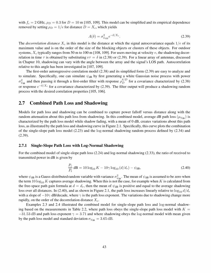
with fc = 2 GHz, ρD = 0.3 for D = 10 m [105, 109]. This model can be simplified and its empirical dependence

removed by setting ρD = 1/e for distanceD = Xc, which yields

A(δ) = σ2ψdB

e−δ/Xc . (2.39)

The decorrelation distance Xc in this model is the distance at which the signal autocovariance equals 1/e of its

maximum value and is on the order of the size of the blocking objects or clusters of these objects. For outdoor

systems,Xc typically ranges from 50 m to 100 m [108, 109]. For users moving at velocity v, the shadowing decor-

relation in time τ is obtained by substituting vτ = δ in (2.38) or (2.39). For a linear array of antennas, discussed

in Chapter 10, shadowing can vary with the angle between the array and the signal’s LOS path. Autocorrelation

relative to this angle has been investigated in [107, 109].

The first-order autoregressive correlation model (2.38) and its simplified form (2.39) are easy to analyze and

to simulate. Specifically, one can simulate ψdB by first generating a white Gaussian noise process with power

σ2ψdB

and then passing it through a first-order filter with response ρδ/DD for a covariance characterized by (2.38)

or response e−δ/Xc for a covariance characterized by (2.39). The filter output will produce a shadowing random

process with the desired correlation properties [105, 106].

2.7 Combined Path Loss and Shadowing

Models for path loss and shadowing can be combined to capture power falloff versus distance along with the

random attenuation about this path loss from shadowing. In this combined model, average dB path loss (µψdB) is

characterized by the path loss model while shadow fading, with a mean of 0 dB, creates variations about this path

loss, as illustrated by the path loss and shadowing curve in Figure 2.1. Specifically, this curve plots the combination

of the single-slope path loss model (2.23) and the log-normal shadowing random process defined by (2.34) and

(2.39).

2.7.1 Single-Slope Path Loss with Log-Normal Shadowing

For the combined model of single-slope path loss (2.24) and log-normal shadowing (2.33), the ratio of received to

transmitted power in dB is given by

PrPt

dB = 10 log10K − 10γ log10 (d/dr) − ψdB, (2.40)

where ψdB is a Gauss-distributed random variable with variance σ2ψdB

. The mean of ψdB is assumed to be zero when

the term 10 log10K captures average shadowing. When this is not the case, for example whenK is calculated from

the free-space path gain formula at d = dr, then the mean of ψdB is positive and equal to the average shadowing

loss over all distances. In (2.40), and as shown in Figure 2.1, the path loss increases linearly relative to log10 d/drwith a slope of −10γ dB/decade, where γ is the path loss exponent. The variations due to shadowing change more

rapidly, on the order of the decorrelation distanceXc.

Examples 2.3 and 2.4 illustrated the combined model for single-slope path loss and log-normal shadow-

ing based on the measurements in Table 2.2, where path loss obeys the single-slope path loss model with K =−31.53 dB and path loss exponent γ = 3.71 and where shadowing obeys the log-normal model with mean given

by the path loss model and standard deviation σψdB= 3.65 dB.

43

2.7.2 Outage Probability

The combined effects of path loss and shadowing have important implications for wireless system design. In

wireless systems there is typically a target minimum received power level Pmin or, equivalently, a minimum SNR

SNRmin = Pmin/(N0B) below which performance becomes unacceptable (e.g., the caller’s voice on a cell phone

is unintelligible). However, with shadowing the received power at any given distance from the transmitter is log-

normally distributed with some probability of falling below Pmin. We define outage probabilityPout(Pmin, d) to be

the probability that the received power at a given distance d, Pr(d), falls below Pmin: Pout(Pmin, d) = p(Pr(d) <

Pmin). For the combined path loss and shadowing model of Section 2.8 this becomes

p(Pr(d) ≤ Pmin) = 1 − Q

(Pmin − (Pt + 10 log10K − 10γ log10(d/dr))

σψdB

)

, (2.41)

where the Q-function is defined as the probability that a Gaussian random variable X with mean 0 and variance 1

is greater than z:

Q(z) , p(X > z) =

∫ ∞

z

1√2πe−y

2/2dy. (2.42)

The conversion between the Q-function and complementary error function is

Q(z) =1

2erfc

(z√2

)

. (2.43)

We will omit the arguments Pmin and d of Pout when the context is clear or in generic references to outage proba-

bility.

Example 2.5: Find the outage probability at 150 m for a channel based on the single-slope path loss and shadowing

models of Examples 2.3 and 2.4, assuming a transmit power of Pt = 10 mW and minimum power requirement of

Pmin = −110.5 dBm.

Solution: We have Pt = 10 mW = 10 dBm. Hence,

Pout(−110.5 dBm, 150 m)

= p(Pr(150 m) < −110.5 dBm)

= 1 −Q

(Pmin − (Pt + 10 log10K − 10γ log10(d/dr))

σψdB

)

= 1 −Q

(−110.5− (10 − 31.53− 37.1 log10(150))

3.65

)

= 0.0120.

An outage probability of l% is a typical target in wireless system designs.

2.7.3 Cell Coverage Area and Percentage

The coverage area of a given cell in a cellular system is defined as the area of locations within the cell where the

received power is above a given minimum. Consider a base station inside a circular cell of a given radius R. All

44

Figure 2.6: Contours of constant received power.

mobiles within the cell require some minimum received SNR for acceptable performance. Assuming a given model

for noise, the SNR requirement translates to a minimum received power Pmin throughout the cell. The transmit

power at the base station is designed for an average received power at the cell boundary of PR, averaged over the

shadowing variations. In the absence of shadowing, the coverage area of this system is πR2 since all locations

have received power above the required minimum. However, shadowing will cause some locations within the cell

to have received power below PR, and others will have received power exceeding PR. This is illustrated in Figure

2.6, where we show contours of constant received power based on a fixed transmit power at the base station for

path loss and average shadowing and for path loss and random shadowing. For path loss and average shadowing,

constant power contours form a circle around the base station because combined path loss and average shadowing

is the same at a uniform distance from the base station. For path loss and random shadowing, the contours form an

amoeba-like shape due to the random shadowing variations about the average.

The constant power contours for combined path loss and random shadowing indicate the challenge that shad-

owing poses in cellular system design. Specifically, it is not possible for all users at the cell boundary to receive the

same power level. Thus, either the base station must transmit extra power to ensure users affected by shadowing

receive their minimum required power Pmin, which causes excessive interference to neighboring cells, or some

users within the cell will find their minimum received power requirement unmet. In fact, since the Gaussian distri-

bution has infinite tails, under this model any mobile in the cell has a nonzero probability of experiencing received

power below its required minimum, even if the mobile is close to the base station. The model matches propagation

scenarios in practice since a mobile may be in a tunnel or blocked by a large building, regardless of its proximity

to the base station.

The cell coverage percentage is defined as the expected percentage of locations within a cell where received

power exceeds Pmin. The cell coverage percentage under path loss and shadowing, also referred to as the fraction

of useful service area, was derived by Reudink in [1, Chapter 2.5.3] as follows. The percentage of area within a cell

where the received power exceeds the minimum required power Pmin is obtained by taking an incremental area dA

at radius r from the base station in the cell, as shown in Figure 2.6. Let Pr(r) be the received power in dA from

combined path loss and shadowing. Then the total area within the cell where the minimum power requirement is

exceeded is obtained by integrating over all incremental areas where this minimum is exceeded:

45

C = E

[1

πR2

∫

cell area

1[Pr(r) > Pmin in dA] dA

]

=1

πR2

∫

cell area

E[1[Pr(r) > Pmin in dA]] dA, (2.44)

where 1[·] denotes the indicator function. Define PA(r) = p(Pr(r) > Pmin) in dA. Then PA(r) = E[1[Pr(r) >Pmin in dA]]. Making this substitution in (2.44) and using polar coordinates for the integration yields

C =1

πR2

∫

cell area

PA(r) dA =1

πR2

∫ 2π

0

∫ R

0PA(r)r dr dθ. (2.45)

The outage probability within the cell is defined as the percentage of area within the cell that does not meet its

minimum power requirement Pmin; that is, P cellout = 1 − C. Given the log-normal distribution for the shadowing,

we have

PA = p(Pr(r) ≥ Pmin) = Q

(Pmin − (Pt + 10 log10K − 10γ log10(r/d0))

σψdB

)

= 1 − Pout(Pmin, r), (2.46)

where Pout is the outage probability defined in (2.41) with d = r. Locations within the cell with received power

below Pmin are said to be outage locations.

Combining (2.45) and (2.46) yields5

C =2

R2

∫ R

0rQ(

a+ b lnr

R

)

dr, (2.47)

where

a =Pmin − P r(R)

σψdB

, b =10γ log10(e)

σψdB

, (2.48)

and P r(R) = Pt + 10 log10K − 10γ log10(R/d0) is the received power at the cell boundary (distance R from

the base station) due to path loss alone. Applying integration by parts to solve this integral yields a closed-form

solution for C in terms of a and b:

C = Q(a) + exp

[2 − 2ab

b2

]

Q

(2 − ab

b

)

. (2.49)

If the target minimum received power equals the average power at the cell boundary, Pmin = P r(R), then a = 0and the cell coverage percentage simplifies to

C =1

2+ exp

[2

b2

]

Q

(2

b

)

. (2.50)

5Recall that (2.46) is generally valid only for r ≥ d0, yet to simplify the analysis we have applied the model for all r. This approximation

will have little impact on cell coverage percentage, since d0 is typically very small compared to R and the outage probability for r < d0 is

negligible.

46

Note that with this simplification C depends only on the ratio γ/σψdB. Moreover, owing to the symmetry of the

Gaussian distribution, under this assumption the outage probability at the cell boundary Pout(P r(R), R) = 0.5.

Example 2.6: Find the cell coverage percentage for a cell with the combined path loss and shadowing models of

Examples 2.3 and 2.4, a cell radius of 600 m, a base station transmit power of Pt = 100 mW = 20 dBm, and a

minimum received power requirement of Pmin = −110 dBm and also one of Pmin = −120 dBm.

Solution: We first consider Pmin = −110 and check if a = 0 to see whether we should use the full formula (2.49)

or the simplified formula (2.50). We have P r(R) = Pt +K − 10γ log10(600) = 20− 31.53− 37.1 log10(600) =

−114.6 dBm 6= −110 dBm, so we use (2.49). Evaluating a and b from (2.48) yields a = (−110 + 114.6)/3.65 =1.26 and b = (37.1 · 0.434)/3.65 = 4.41. Substituting these into (2.49) yields

C = Q(1.26) + exp

[2 − 2(1.26 · 4.41)

4.412

]

Q

(2 − (1.26)(4.41)

4.41

)

= .59,

which would be a very low cell coverage percentage value for an operational cellular system (lots of unhappy

customers). Now considering the less stringent received power requirement Pmin = −120 dBm yields a =(−120 + 114.6)/3.65 = −1.479 and the same b = 4.41. Substituting these values into (2.49) yields C = .988, a

much more acceptable value for cell coverage percentage.

Example 2.7: Consider a cellular system designed so that Pmin = P r(R). That is, the received power due to path

loss and average shadowing at the cell boundary equals the minimum received power required for acceptable per-

formance. Find the cell coverage percentage for path loss values γ = 2, 4, 6 and σψdB= 4, 8, 12, and explain how

cell coverage percentage changes as γ and σψdBincrease.

Solution: For Pmin = P r(R) we have a = 0, so cell coverage percentage is given by the formula (2.50). The cell

coverage percentage thus depends only on the value for b = 10γ log10(e)/σψdB, which in turm depends only on

the ratio γ/σψdB. Table 2.3 contains cell coverage percentage evaluated from (2.50) for the different γ and σψdB

values.

Table 2.3: cell coverage percentage for different γ and σψdB

γ σψdB=4 dB σψdB

=8 dB σψdB=12 dB

2 .77 .67 .63

4 .85 .77 .71

6 .90 .83 .77

Not surprisingly, for fixed γ the cell coverage percentage increases as σψdBdecreases; this is because a smaller

σψdBmeans less variation about the mean path loss. Without shadowing we have 100% cell coverage percentage

(since Pmin = P r(R)) and so we expect that, as σψdBdecreases to zero, cell coverage percentage increases to

100%. It is a bit more puzzling that for a fixed σψdBthe cell coverage percentage increases as γ increases, since a

larger γ implies that received signal power falls off more quickly. But recall that we have set Pmin = P r(R), so the

faster power falloff is already taken into account (i.e., we need to transmit at much higher power with γ = 6 than

with γ = 2 for this equality to hold). The reason cell coverage percentage increases with path loss exponent under

this assumption is that, as γ increases, the transmit power must increase to satisfy Pmin = P r(R). This results in

higher average power throughout the cell, yielding a higher percentage of locations in the cell that have the desired

minimum power.

47

2.8 General Ray Tracing

In a typical urban or indoor environment, a radio signal transmitted from a fixed source will encounter multiple

objects in the environment, as shown in Figure 2.7. These objects produce reflected, diffracted, or scattered copies

of the transmitted signal, which are not captured by the free-space and two-ray models discussed earlier. These

additional copies of the transmitted signal, known as multipath components, can be attenuated in power, delayed

in time, and shifted in phase and/or frequency with respect to the LOS signal path at the receiver. The transmitted

signal and its multipath components are summed together at the receiver, which can produce rapid fluctuations in

received signal power due to constructive and destructive combining of the components. This multipath fading was

also exhibited in the two-ray model. If the arriving signal components have delay differences that exceed a symbol

time, this leads to distortion in the received signal relative to the transmitted signal.

Figure 2.7: Reflected, diffracted, and scattered wave components.

In ray tracing we assume a finite number of reflectors with known location and dielectric properties. The

details of the multipath propagation can then be solved using Maxwell’s equations with appropriate boundary

conditions. However, the computational complexity of this solution makes it impractical as a general modeling

tool. Ray-tracing techniques approximate the propagation of electromagnetic waves by representing the wavefronts

as simple particles. Thus, the effects of reflection, diffraction, and scattering on the wavefront are approximated

using simple geometric equations instead of Maxwell’s more complex wave equations. The error of the ray-

tracing approximation is smallest when the receiver is many wavelengths from the nearest scatterer and when all

the scatterers are large relative to a wavelength and fairly smooth. Comparison of the ray-tracing method with

certain empirical data sets shows that it can accurately model received signal power in rural areas [24], along city

streets when both the transmitter and receiver are close to the ground [24, 26, 27], and in indoor environments with

appropriately adjusted diffraction coefficients [28].

If the transmitter, receiver, and reflectors are all immobile, then the characteristics of the multiple received

signal paths are fixed. However, if the transmitter or receiver are moving then the characteristics of the multiple

paths vary with time. These time variations are deterministic when the number, location, and characteristics of the

reflectors are known over time. Otherwise, statistical models must be used. Similarly, if the number of reflectors

is large, or if the reflector surfaces are not smooth such that each reflector generates many signal paths, then we

must use statistical approximations to characterize the received signal. We will discuss statistical fading models

48

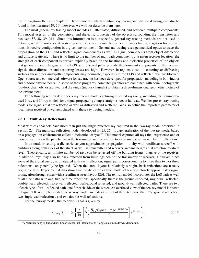
for propagation effects in Chapter 3. Hybrid models, which combine ray tracing and statistical fading, can also be

found in the literature [29, 30]; however, we will not describe them here.

The most general ray tracing model includes all attenuated, diffracted, and scattered multipath components.

This model uses all of the geometrical and dielectric properties of the objects surrounding the transmitter and

receiver [37, 38, 39, 31]. Since this information is site-specific, general ray tracing methods are not used to

obtain general theories about system performance and layout but rather for modeling propagation for a given

transmit-receive configuration in a given environment. General ray tracing uses geometrical optics to trace the

propagation of the LOS and reflected signal components as well as signal components from object diffraction

and diffuse scattering. There is no limit to the number of multipath components at a given receiver location: the

strength of each component is derived explicitly based on the locations and dielectric properties of the objects

that generate them. In general, the LOS and reflected paths provide the dominant components of the received

signal, since diffraction and scattering losses are high. However, in regions close to scattering or diffracting

surfaces these other multipath components may dominate, especially if the LOS and reflected rays are blocked.

Open source and commercial software for ray tracing has been developed for propagation modeling in both indoor

and outdoor environments. In some of these programs, computer graphics are combined with aerial photographs

(outdoor channels) or architectural drawings (indoor channels) to obtain a three-dimensional geometric picture of

the environment.

The following section describes a ray tracing model capturing reflected rays only, including the commonly-

used 6-ray and 10-ray models for a signal propagating along a straight street or hallway. We then present ray tracing

models for signals that are reflected as well as diffracted and scattered. We also define the important parameter of

local mean received power associated with these ray tracing models.

2.8.1 Multi-Ray Reflections

Most wireless channels have more than just the single reflected ray captured in the two-ray model described in

Section 2.4. The multi-ray reflection model, developed in [25, 26], is a generalization of the two-ray model based

on a propagation environment called a dielectric “canyon.” This model captures all rays that experience one or

more reflections on the path between the transmitter and receiver up to a certain maximum number of reflections.

In an outdoor setting, a dielectric canyon approximates propagation in a city with rectilinear streets6 with

buildings along both sides of the street as well as transmitter and receiver antenna heights that are close to street

level. Theoretically, an infinite number of rays can be reflected off the building fronts to arrive at the receiver;

in addition, rays may also be back-reflected from buildings behind the transmitter or receiver. However, since

some of the signal energy is dissipated with each reflection, signal paths corresponding to more than two or three

reflections can generally be ignored. When the street layout is relatively straight, back reflections are usually

negligible also. Experimental data show that the dielectric canyon model of ten rays closely approximates signal

propagation through cities with a rectilinear street layout [26]. The ten-ray model incorporates the LoS path as well

as all nine paths with one, two, or three reflections: specifically, there is the ground-reflected, single-wall reflected,

double-wall reflected, triple-wall reflected, wall-ground reflected, and ground-wall reflected paths. There are two

of each type of wall-reflected path, one for each side of the street. An overhead view of the ten-ray model is shown

in Figure 2.8. A simpler model, the six-ray model, includes a subset of these ten rays: the LOS, ground reflection,

two single-wall reflections, and two double-wall reflections.

For the ten-ray model, the received signal is given by

r10-ray(t) = Re

λ

4π

[9∑

i=0

Ri√Giu(t− τi)e

−j2πdi/λ

di

]

ej2πfct

, (2.51)

6A rectilinear city is flat and has linear streets that intersect at 90 angles, as in midtown Manhattan.

49

Figure 2.8: Overhead view of the ten-ray model. Includes the line-of-sight (LOS), ground-reflected (GR), two

single-wall (SW ) reflected, two double-wall (DW ) reflected, two triple-wall (TW ) reflected, wall-ground (WG)

reflected, and ground-wall (GW ) reflected rays

where di denotes the total distance traveled by the ith ray, τi = di/c, and Gi is the product of the transmit and

receive antenna power gains corresponding to the ith ray. The first two terms in the summation of (2.51) correspond

to the LoS and ground reflected path in the two-ray model (2.12), hence R0 = 1 since there is no reflection of

the LoS path. For the ith reflection path, i > 0, the coefficient Ri is either a single reflection coefficient given by

(2.16) or, if the path corresponds to multiple reflections, the product of the reflection coefficients corresponding

to each reflection. The dielectric constants used in (2.51) are approximately the same as the ground dielectric, so

εr = 15 is used for all the calculations ofRi. The delay spread of the 10-ray and 6-ray models equals the difference

between the delay of the LOS ray and that of the reflected ray with the largest delay: maxi τi − τ0.

If we again assume a narrowband model such that u(t − τ0) ≈ u(t − τi) for all i, then the received power

corresponding to (2.51) is

Pr = Pt

[λ

4π

]2∣∣∣∣∣

9∑

i=0

Ri√Gie

−j∆φi

di

∣∣∣∣∣

2

, (2.52)

where ∆φi = 2π(di − d0)/λ.

Power falloff with distance in both the ten-ray model (2.52) and urban empirical data [15, 32, 33] for transmit

antennas both above and below the building skyline is typically proportional to d−2, even at relatively large dis-

tances. Moreover, the falloff exponent is relatively insensitive to the transmitter height. This falloff with distance

squared is due to the dominance of the multipath rays, which decay as d−2, over the combination of the LOS and

ground-reflected rays (two-ray model), which decays as d−4. Other empirical studies [34, 35, 36] have obtained

power falloff with distance proportional to d−γ , where γ lies anywhere between 2 and 6.

2.8.2 Diffraction

The propagation model for the LOS and reflected paths was outlined in the previous section. Diffraction allows

a radio signal to “bend around” an object in its path to the receiver, as shown in Figure 2.9 for a wedge-shaped

object. This bending phenomenon can be explained using Huygen’s principle, which states that all points on

the signal wavefront can be considered as point sources for a secondary wavefront called a wavelet. When a

signal is diffracted, these wavelets combine together to produce a wavefront in the new direction of propagation

caused by the bending [29, Chapter 4.3]. Diffraction results from many phenomena, including hilly or irregular

terrain, building and rooftop edges, or obstructions blocking the LOS path between the transmitter and receiver

[2, 11, 16]. Diffraction can be accurately characterized using the geometrical theory of diffraction (GTD) [40], but

the complexity of this approach has precluded its use in wireless channel modeling. Wedge diffraction simplifies

the GTD by assuming the diffracting object is a wedge rather than a more general shape. This model has been

50

used to characterize the mechanism by which signals are diffracted around street corners, which can result in

signal attenuation exceeding 100 dB for some incident angles on the wedge [28, 39, 41, 42]. Although wedge

diffraction simplifies the GTD, it still requires a numerical solution for the resulting attenuation [40, 43] and thus

is not commonly used. Diffraction is most commonly modeled by the Fresnel knife-edge diffraction model because

of its simplicity. The geometry of this model is shown in Figure 2.9, where the diffracting object is assumed to be

asymptotically thin, which is not generally the case for hills, rough terrain, or wedge diffractors. In particular, this

model does not consider diffractor parameters such as polarization, conductivity, and surface roughness, which can

lead to inaccuracies [41].

Figure 2.9: Knife-edge diffraction.

The diffracted signal of Figure 2.9 travels a distance d∗ +d?, resulting in a phase shift of φ = 2π(d∗+d?)/λ.

For a LOS path of distance d, the geometry of Figure 2.9 indicates that, for h small relative to d∗ and d?, the signal

must travel an additional distance relative to the LOS path of approximately

∆d = d∗ + d? − d ≈ h2(d∗ + d?)

2d∗d?;

the corresponding phase shift relative to the LOS path is approximately

∆φ =2π∆d

λ≈ π

2v2, (2.53)

where

v = h

√

2(d∗ + d?)

λd∗d?(2.54)

is called the Fresnel–Kirchhoff diffraction parameter. The path loss of a signal at distance d∗ + d? experiencing

knife-edge diffraction at distance d∗ is generally a function of v. However, computing this path loss is fairly

complex, requiring the use of Huygens’s principle, Fresnel zones, and the complex Fresnel integral [2]. Moreover,

the resulting diffraction loss cannot generally be found in closed form. Approximations for the additional path loss

due to knife-edge diffraction relative to free-space path loss (in dB) as a function of v in (2.54) are given in [16, 44]

as

L(v)dB =

0, v < −1,

20 log10[.5− .62v], −0.8 ≤ v < 0,

20 log10[.5e−.95v], 0 ≤ v < 1,

20 log10[.4−√

.1184− (.38− .1v)2], 1 ≤ v ≤ 2.4,

20 log10[.225/v], v > 2.4.

(2.55)

51

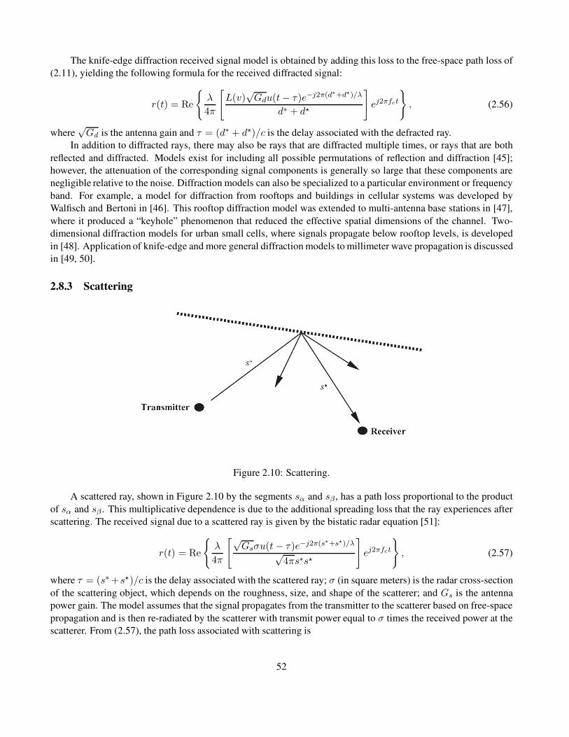
The knife-edge diffraction received signal model is obtained by adding this loss to the free-space path loss of

(2.11), yielding the following formula for the received diffracted signal:

r(t) = Re

λ

4π

[

L(v)√Gdu(t− τ)e−j2π(d∗+d?)/λ

d∗ + d?

]

ej2πfct

, (2.56)

where√Gd is the antenna gain and τ = (d∗ + d?)/c is the delay associated with the defracted ray.

In addition to diffracted rays, there may also be rays that are diffracted multiple times, or rays that are both

reflected and diffracted. Models exist for including all possible permutations of reflection and diffraction [45];

however, the attenuation of the corresponding signal components is generally so large that these components are

negligible relative to the noise. Diffraction models can also be specialized to a particular environment or frequency

band. For example, a model for diffraction from rooftops and buildings in cellular systems was developed by

Walfisch and Bertoni in [46]. This rooftop diffraction model was extended to multi-antenna base stations in [47],

where it produced a “keyhole” phenomenon that reduced the effective spatial dimensions of the channel. Two-

dimensional diffraction models for urban small cells, where signals propagate below rooftop levels, is developed

in [48]. Application of knife-edge and more general diffraction models to millimeter wave propagation is discussed

in [49, 50].

2.8.3 Scattering

Figure 2.10: Scattering.

A scattered ray, shown in Figure 2.10 by the segments sα and sβ , has a path loss proportional to the product

of sα and sβ . This multiplicative dependence is due to the additional spreading loss that the ray experiences after

scattering. The received signal due to a scattered ray is given by the bistatic radar equation [51]:

r(t) = Re

λ

4π

[√Gsσu(t− τ)e−j2π(s∗+s?)/λ

√4πs∗s?

]

ej2πfct

, (2.57)

where τ = (s∗ +s?)/c is the delay associated with the scattered ray; σ (in square meters) is the radar cross-section

of the scattering object, which depends on the roughness, size, and shape of the scatterer; and Gs is the antenna

power gain. The model assumes that the signal propagates from the transmitter to the scatterer based on free-space

propagation and is then re-radiated by the scatterer with transmit power equal to σ times the received power at the

scatterer. From (2.57), the path loss associated with scattering is

52

Pr dBm = Pt dBm + 10 log10(Gs) + 20 log10(λ) + 10 log10(σ)

−30 log(4π)− 20 log10(s∗) − 20 log10(s

?). (2.58)

Empirical values of 10 log10 σ were determined in [52] for different buildings in several cities. Results from this

study indicate that 10 log10 σ in dBm2 ranges from −4.5 dBm2 to 55.7 dBm2, where dBm2 denotes the dB value

of the σ measurement with respect to one square meter.

2.8.4 Multipath Model with Reflection, Diffraction, and Scattering

The received signal is determined from the superposition of all the components due to the multiple rays. Thus, if

we have a LOS ray, Nr reflected rays, Nd diffracted rays, and Ns scattered rays, the total received signal is

rtotal(t) = Re

λ

4π

[√G0u(t)e

−j2πd0/λ

d0+

Nr∑

i=1

Ri√Giu(t− τi)e

−j2πdi/λ

di

+

Nd∑

j=1

Lj(v)√Gdj

u(t− τj)e−j2π(d∗j +d?

j )/λ

d∗jd?j

+

Ns∑

k=1

√Gskσku(t− τk)e

−j2π(s∗k+s?k)/λ

√4πs∗ks

?k

]

ej2πfct

,

(2.59)

where τj and τk are, respectively, the time delays of the given diffracted and scattered rays, (dαj, dβj

) and

(sαk, sβk

) are, respectively, the distance pair the signal travels before and after the object causing the diffrac-

tion or scattering, and the other parameters are as defined in the model (2.51) with the LoS and reflections only.

The received power Pr of rtota1(t) and the corresponding path loss Pr/Pt are then obtained from (2.59). The delay

spread of this model equals the difference between the delay of the LOS ray and that of the reflected, diffracted, or

scattered ray that has the largest delay.

Any of these multipath components may have an additional attenuation factor if its propagation path is blocked

by objects such as buildings outdoors or walls indoors. In this case, the attenuation factor of the obstructing object

multiplies the component’s path loss term in (2.59). This attenuation loss will vary widely, depending on the

material and depth of the object [11, 53]. Models for random loss due to attenuation are described in Section 2.6.

2.8.5 Multi-Antenna and MIMO Systems

The ray tracing techniques described in Sections 2.8.1- 2.8.4 assume single antennas at the transmitter and receiver.

The same ray tracing techniques can be used for systems with multiple antennas at the transmitter and/or receiver by

superposition, whereby the single-antenna analysis is applied to each transmit-receive antenna pair and the results

are summed together. When both the transmitter and receiver have multiple antennas, the system is called multiple-

input multiple output (MIMO) system. While the application of ray tracing to MIMO systems is straightforward,

the computational complexity of this approach grows linearly with the product of the number of transmit and

receive antennas. As a result, ray tracing approximations to lower this complexity have been developed, including

clustering of rays [54] and preprocessing environmental data [56]. A summary of ray tracing methods for MIMO

systems can be found in [55].

53

2.8.6 Local Mean Received Power

The path loss computed from all ray-tracing models is associated with a fixed transmitter and receiver location. In

addition, ray tracing can be used to compute the local mean received power P r in the vicinity of a given receiver

location by adding the squared magnitude of all the received rays. This has the effect of averaging out local spatial

variations due to phase changes around the given location. Local mean received power is a good indicator of link

quality and is often used in cellular system functions like power control and handoff [83].

2.9 Measurement-Based Propagation Models

Most mobile communication systems operate in complex propagation environments that cannot be accurately

modeled by free-space path loss or ray tracing. A number of analytical path loss models have been developed over

the years by researchers as well as standards bodies to model path loss in typical wireless environments including

urban macrocells and small cells, suburban areas, rural areas, and inside buildings with different characteristics

[11, 57, 59, 74, 17]. These models are generally based on large empirical measurement campaigns that can range

over a variety of distances, frequency ranges, geographical regions for outdoor models, and building types for

indoor models. These analytical models have the highest accuracy when they are applied to propagation conditions

similar to those under which the empirical measurements that the models are based on were made. In this section

we describe the most common analytical path loss models based on empirical measurements for both indoor and

outdoor systems.

Analytical models characterize Pr/Pt as a function of distance, so path loss is well-defined. In contrast,

empirical measurements of Pr/Pt as a function of distance include the effects of path loss, shadowing, multipath,

and other site-specific factors that affect propagation. In order to remove multipath effects, empirical measurements

for path loss typically average their received power measurements and the corresponding path loss at a given

distance over several wavelengths. This average path loss is called the local mean attenuation (LMA) at distance

d, and it generally decreases with d owing to free-space path loss and signal obstructions. The LMA in a given

environment, such as a city, depends on the specific location of the transmitter and receiver corresponding to

the LMA measurement. To characterize LMA more generally, measurements are typically taken throughout the

environment and possibly in multiple environments with similar characteristics. Thus, the empirical path loss

PL(d) for a given environment (a city, suburban area, or office building) is defined as the average of the LMA

measurements at distance d averaged over all available measurements in the given environment. For example,

empirical path loss for a generic downtown area with a rectangular street grid might be obtained by averaging

LMA measurements in New York City, downtown San Francisco, and downtown Chicago. The empirical path loss

models given in this section are all obtained from average LMA measurements. Empirical path loss models can

also be developed or refined using measurement-driven learning applied to continuous LMA data collection [75].

2.9.1 Okumura Model

One of the most well-known models for signal prediction in large urban macrocells is the Okumura model [84].

This model is applicable over distances of 1–100 km and frequency ranges of 150–1500 MHz. Okumura used

extensive measurements of base station-to-mobile signal attenuation throughout Tokyo to develop a set of curves

giving median attenuation relative to free space of signal propagation in irregular terrain. The base station heights

for these measurements were 30–100 m, a range whose upper end is higher than typical base stations today. The

empirical path loss formula of Okumura at distance d parameterized by the carrier frequency fc is given by

PL(d) dB = L(fc, d) +Aµ(fc, d)−G(ht) −G(hr) −GAREA, (2.60)

54

where L(fc, d) is free-space path loss at distance d and carrier frequency fc, Aµ(fc, d) is the median attenuation in

addition to free-space path loss across all environments,G(ht) is the base station antenna height gain factor, G(hr)

is the mobile antenna height gain factor, and GAREA is the gain due to the type of environment. The values of

Aµ(fc, d) and GAREA are obtained from Okumura’s empirical plots [84, 11]. Okumura derived empirical formulas

for G(ht) and G(hr) as follows:

G(ht) = 20 log10(ht/200), 30 m < ht < 1000 m; (2.61)

G(hr) =

10 log10(hr/3), hr ≤ 3 m,

20 log10(hr/3), 3 m < hr < 10 m.(2.62)

Correction factors related to terrain are also developed in [84] that improve the model’s accuracy. Okumura’s

model has a 10–14 dB empirical standard deviation between the path loss predicted by the model and the path loss

associated with one of the measurements used to develop the model. The expected error in using Okumura’s model

for environments not based on these measurements is generally higher.

2.9.2 Hata Model

The Hata model [85] is an empirical formulation of the graphical path loss data provided by Okumura and is valid

over roughly the same range of frequencies, 150–1500 MHz. This empirical model simplifies calculation of path

loss because it is a closed-form formula and is not based on empirical curves for the different parameters. The

standard formula for empirical path loss in urban areas under the Hata model is

PL,urban(d) dB = 69.55 + 26.16 log10(fc) − 13.82 log10(ht) − a(hr)

+ (44.9− 6.55 log10(ht)) log10(d). (2.63)

The parameters in this model are the same as under the Okumura model, and a(hr) is a correction factor for the

mobile antenna height based on the size of the coverage area [85, 11]. For small to medium-sized cities, this factor

is given by

a(hr) = (1.1 log10(fc) − .7)hr − (1.56 log10(fc)− .8) dB,

and for larger cities at frequencies fc > 300 MHz by

a(hr) = 3.2(log10(11.75hr))2 − 4.97 dB.

Corrections to the urban model are made for suburban and rural propagation, so that these models are (respec-

tively)

PL,suburban(d) dB = PL,urban(d) dB − 2[log10(fc/28)]2 − 5.4 (2.64)

and

PL,rural(d) dB = PL,urban(d) dB − 4.78[log10(fc)]2 + 18.33 log10(fc) −K, (2.65)

where K ranges from 35.94 (countryside) to 40.94 (desert). Unlike the Okumura model, the Hata model does

not provide for any path-specific correction factors. The Hata model well approximates the Okumura model for

distances d > 1 km. Hence it is a good model for early-generation cellular systems operating in cities, but it

55

does not model propagation well in cellular systems with smaller cell sizes, multiple antennas, or higher frequen-

cies. Indoor environments are also not captured by the Hata model. As cellular systems evolved beyond their

early deployments, research into more complex propagation models was undertaken by multiple organizations, as

described in the next section.

2.9.3 Cellular System Models

Following the success of early cellular systems, funding agencies and standards bodies worldwide launched

projects to develop standardized cellular system channel models for the environments, carrier frequencies, cell

sizes, and multiple antenna characteristics of these evolving systems. These standardized channel models can be

used to evaluate different candidate cellular technologies in a uniform manner, and also provide guidelines for

expected system performance in typical environments and operating conditions. Cellular system channel models

span frequency ranges from .5 GHz to 100 GHz, indoor and outdoor environments with both LOS and non-LOS

propagation, small and large cells sizes, and multiple antenna transmitters and receiver of different antenna heights,

elevation angles, and polarizations. Models for all of these scenarios have been developed by 3GPP and the ITU

[57, 58], whereas other standardized models are applicable to a subset of these settings. To illustrate some basic

properties of these standardized models, in this section we provide the LOS path loss formulas for a few stan-

dardized models, which follow either the single-slope or dual-slope formulas ( (2.24) and (2.28), respectively)

with model-specific constants. Extensions of these models to more complex environments is also discussed. More

details on the unique characteristics of millimeter wave propagation are provided in Section 2.9.5.

An early project to standardize channel models for cellular systems was undertaken by the European Cooper-

ation in Science and Technology (COST). The COST 207 program, launched in 1984, brought together industry,

government, and academia under a common umbrella to develop common propagation models for the emerging

2G cellular systems. The subsequent COST 231 project was focused on extending earlier channel models to carrier

frequencies up to 2 GHz. The resulting model, referred to as the COST 231 extension to the Hata model [86], has

the following path loss expression:

PL, urban(d) dB = 46.3 + 33.9 log10(fc) − 13.82 log10(ht) − a(hr)

+ (44.9− 6.55 log10(ht)) log10(d) +CM , (2.66)

where a(hr) is the same correction factor as in the Hata model and CM = 0 dB for medium-sized cities and

suburbs while CM = 3 dB for metropolitan areas. The COST 231 extension to the Hata model is restricted to

the following range of parameters: 1.5 GHz < fc < 2 GHz, 30 m < ht < 200 m, 1 m < hr < 10 m, and

1 km < d < 20 km. Given the Okumura measurements on which it is based, this model is most accurate for

heterogeneous macrocell-only cellular system architectures with single-antenna base stations and terminals. The

COST 231 model was further extended to incorporate new features and environments of the evolving cellular

systems and standards, including diffraction and non-LOS propagation (COST-231-WI)[29], multiple base station

antennas (COST 259) [88], and multiple antennas at both the base stations and the mobile terminals (COST 273,

COST 2100) [89, 90].

The 3GPP standards body maintains a family of channel models characterizing signal propagation for the

different environments and frequencies in which their cellular systems operate [57]. These include path loss

models for both LOS and non-LOS propagation in outdoor macrocells and small cells as well as for indoor of-

fice buildings. The 3GPP outdoor propagation models follow the dual-slope path loss model (2.28); they have

a distance-dependent pathloss exponent that takes on two different values, γ1 and γ2, for distances that are, re-

spectively, smaller or greater than the breakpoint distance. The breakpoint distance is set to the critical distance

dc = 4hthr/λ given by (2.22) in the two-ray model based on the effective transmit (ht) and receive (hr) antenna

56

heights7. In particular, the 3GPP path loss for LOS propagation in outdoor macrocells and small cells is given by

PL(d) dB =

20 log10(fc) + κ+ 10γ1 log10(d), d ≤ dc,

20 log10(fc) + κ+ 10γ2 log10(d) + η log10

(d2c + (ht − hr)

2), d > dc

(2.67)

for d in meters and fc in GHz. The 3GPP indoor office model is governed by the first terms of (2.67) for all

distances (i.e., there is no breakpoint distance in the indoor model due to the shorter distances involved). At

distances below dc this model has three separate terms: the constant κ that captures environment and antenna

parameters independent of distance and frequency, the term 20 log10 fc that captures frequency-dependent path

loss, and the term 10γi log10(d) that captures distance-dependent path loss. The frequency-dependent path loss

20 log10 fc is the same as in free space (2.10), and this term along with κ are captured by the constant K in the

single-slope model (2.24). At distances above dc the macrocell and small cell models have a fourth term that

captures path loss dependence on antenna heights. The values of κ, γi, and η for the macrocell, small cell, and

indoor office models are given in Table 2.4.

Table 2.4: Parameters for 3GPP LOS Path Loss Models

Parameter Macrocell Small Cell Indoor Office

κ 28 32.4 32.4

γ γ1 = 22, γ2 = 40 γ1 = 21, γ2 = 40 γ1 = 17.3

η -9 -9.5 NA

The 3GPP family of channel models also include non-LOS propagation models that take path loss to be the

maximum of the LOS path loss model and a different non-LOS path loss model. The non-LOS path loss model

is of the same form as (2.67) but with different parameters and a fourth term that depends only on the receiver

height hr. There is also a 3GPP rural macrocell model that includes additional parameters of the environment such

as building heights and street widths. The 3GPP Spatial Channel Model (SCM) incorporates MIMO parameters.

Details can be found in [57]. The ITU channel models are similar to the 3GPP channel family and cover the same

frequency range of .5-100 GHz [58].

The European WINNER (Wireless World Initiative New Radio) I and II projects created a similar family of

channel models as 3GPP for cellular system propagation under different conditions and environments [59]. The

WINNER path loss model is similar to the single-slope model (2.24) with the constant K broken into 3 separate

terms. Specifically, the path loss in the WINNER propagation model 10 log10(Pt/Pr) is given by

PLdBm = 10γ log10(d) + κ+ β log10(.2fc) +X (2.68)

for d in meters and fc in GHz, where γ is the path loss exponent, κ is the path loss at the antenna near-field

reference distance, typically a few signal wavelengths [12], which is independent of frequency, C log10(.2fc) is

the frequency-dependence term, and X is an optional environment-specific term that may, for example, capture a

fixed attenuation at all distances. The Winner II model includes MIMO channel parameters.

The COST, 3GPP, ITU, and WINNER families of channel models are widely used by researchers and prac-

titioners for modeling path loss in cellular systems at frequencies below 6 GHz, with the 3GPP and ITU models

covering frequencies up to 100 GHz. These models also include delay spread parameters ranging from tens of

nanoseconds for indoor environments to hundreds of nanoseconds for outdoor environments. Alternative empiri-

cal channel models specifically for MIMO systems include the WIMAX 802.16 and Stanford University Interim

7In the 3GPP model the effective antennas heights are the actual heights reduced by 1m.

57

(SUI) channel models [76]. As cellular system architectures have evolved to include large and small cells, device-

to-device communications, base stations mounted on UAVs and drones, large antenna arrays, millimeter wave

frequencies, and very high speed mobile devices, there have been extensive measurement campaigns to charac-

terize propagation under these new configurations and conditions [77, 78, 79]. In addition, learning algorithms

that continually update channel models based on collected data have also been developed [80, 81, 82]. Clearly

measurement-based models for cellular systems will continue to evolve as new system architectures, frequency

bands, device requirements, and channel measurement tools are introduced.

2.9.4 Wi-Fi Channel Models

Prior to 802.11n, performance evaluation of 802.11 WLAN systems was done using channel models for 2.4 GHz

(802.11g) and 5 GHz (802.11a) that had been developed by individual researchers or companies. There was no

general consensus on which models to use for performance evaluation of these earlier systems. To address this

shortcoming, the 802.11n task group (TG) was formed to develop a standard set of models, called the TGn models,

to evaluate 802.11n systems. As per the specifications of the 802.11n standard, these models include both 20 MHz

and 40 MHz channels with up to 4 antennas at the transmitter and receiver. Six different TGn channel models

(models A-F) comprise the TGn family to characterize propagation in different size homes and offices as well

as outdoors. All six follow the dual-slope path loss model (2.28) with a path loss exponent γ1 = 2 prior to the

breakpoint distance dBP and γ2 = 3.5 above this distance. The breakpoint distance dBP = 5 m in models A, B,

and C, which correspond to LOS only, small home, and large home, respectively. This distance ranges from 10-30

m in models D-F (corresponding to small office, large office, and outdoors, respectively). The delay spread of the

multipath, normalized with respect to the LOS path, becomes the difference between the delay of the multipath

component with the largest delay and the LOS path. In these models this normalized delay spread ranges from 0ns for the A model to 150 ns for the F model. Multipath reflections are assumed to arrive in clusters based on the

indoor propagation model developed in [60]. Antenna correlation is modeled using the Kronecker model described

in [61]. Shadow fading follows the log-normal model with standard deviation σψdB= 3 for distances d < dBP.

For d > dBP, σψdB= 4 for Models A and B, σψdB

= 5 for Models C and D, and σψdB= 6 for Models E and F.

More details on the TGn models can be found in [62].

The TGac family of channels extends the TGn model to support performance evaluation of 802.11ac sys-

tems. This model increases the number of transmit and receive antennas using the same correlation model as TGn,

increases channel bandwidth up to 160 MHz, and modifies the multipath clustering models to account for simulta-

neous transmission to multiple users (multiuser MIMO). The TGax family of channel models provides additional

environmental scenarios for dense deployments both indoors and outdoors. Details of these extensions can be

found in [63, 64].

2.9.5 Millimeter Wave Models

The millimeter (mmW) frequency band, spanning the 30-300 GHz range, was not used in the first few generations

of Wi-Fi and cellular systems due to its high path loss as well as the high cost and poor performance of mmW

hardware. However, as demand for increased data rates in wireless systems continued unabated with each new

generation, utilizing the large amount of available spectrum in this band grew increasingly appealing. Moreover,

in 2005 the FCC in the US created more flexible rules for spectrum allocation in the lower part of this band to

increase its use [65]. Following this ruling, a few commercial mmW communication systems were developed for

in-home use, but the technology was not yet competitive with Wi-Fi. Interest in utilizing mmW wave spectrum

for cellular communications also started to grow, leading to outdoor channel measurement campaigns as well as

cellular system designs to overcome the propagation challenges at these high frequencies. This section provides

an overview of mmW propagation characteristics.

58

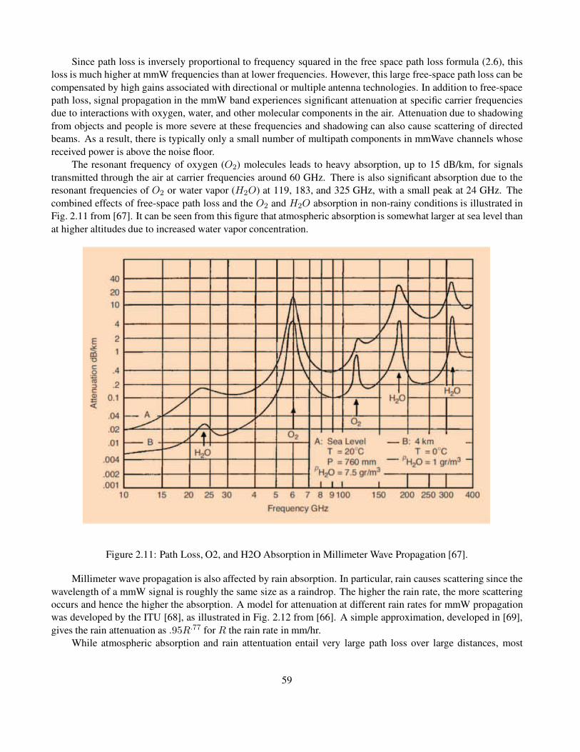
Since path loss is inversely proportional to frequency squared in the free space path loss formula (2.6), this

loss is much higher at mmW frequencies than at lower frequencies. However, this large free-space path loss can be

compensated by high gains associated with directional or multiple antenna technologies. In addition to free-space

path loss, signal propagation in the mmW band experiences significant attenuation at specific carrier frequencies

due to interactions with oxygen, water, and other molecular components in the air. Attenuation due to shadowing

from objects and people is more severe at these frequencies and shadowing can also cause scattering of directed

beams. As a result, there is typically only a small number of multipath components in mmWave channels whose

received power is above the noise floor.

The resonant frequency of oxygen (O2) molecules leads to heavy absorption, up to 15 dB/km, for signals

transmitted through the air at carrier frequencies around 60 GHz. There is also significant absorption due to the

resonant frequencies of O2 or water vapor (H2O) at 119, 183, and 325 GHz, with a small peak at 24 GHz. The

combined effects of free-space path loss and the O2 and H2O absorption in non-rainy conditions is illustrated in

Fig. 2.11 from [67]. It can be seen from this figure that atmospheric absorption is somewhat larger at sea level than

at higher altitudes due to increased water vapor concentration.

Figure 2.11: Path Loss, O2, and H2O Absorption in Millimeter Wave Propagation [67].

Millimeter wave propagation is also affected by rain absorption. In particular, rain causes scattering since the

wavelength of a mmW signal is roughly the same size as a raindrop. The higher the rain rate, the more scattering

occurs and hence the higher the absorption. A model for attenuation at different rain rates for mmW propagation

was developed by the ITU [68], as illustrated in Fig. 2.12 from [66]. A simple approximation, developed in [69],

gives the rain attenuation as .95R.77 for R the rain rate in mm/hr.

While atmospheric absorption and rain attentuation entail very large path loss over large distances, most

59

mmWave systems are designed to operate over relatively short distances, less than 500 m. The losses illustrated in

Figs. 2.11-2.12 for these short distances can be compensated through a combination of increased transmit power,

antenna techniques, modulation choice, and channel coding.

Figure 2.12: Rain Attenuation in Millimeter Wave Propagation [66].

As interest in mmW frequency utilization for cellular and Wi-Fi grew, extensive measurement campaigns

were undertaken in different indoor and outdoor environments [70], with analytical channel models developed to

approximate these empirical measurements. The most widely known of these models, summarized in [71], are

based on work done by four different organizations: the 3GPP standards body, the 5G Channel Model (5GCM)

ad hoc group, the Mobile and wireless communications Enablers for the Twentytwenty (2020) Information Soci-

ety (METIS) research project, and the Millimeter-Wave Based Mobile Radio Access Network for 5G Integrated

Communications (mmMAGIC) research project. The models for each group capture propagation for four different

categories of environments: outdoor macrocell, outdoor small cell, home, and commercial building. In addition

to models for path loss and shadowing, these mmW propagation models add a new component called LOS proba-

bility, which captures the probability that the LOS signal path between the transmitter and receiver is not blocked

or heavily attenuated. While this probability is different for the four environment categories within each family

of models, in all cases it depends on the transmit-receive distance and does not depend on the carrier frequency

[72]. Millimeter wave path loss in all these models is assumed to follow the dual-slope model (2.28), where the

breakpoint distance is different for each of the four environments. The shadowing standard deviation for each of

the four environments is a fixed constant. As expected, shadowing in these models is larger for non-LOS com-

pared to LOS environments, and ranges from about 1-8 dB. A summary of the differences between mmW and

microwave channel models can be found in [72]. The sensitivity of performance analysis to the particular channel

model adopted is demonstrated in [79]. The terahertz (THz) band (.3-3 THz) offers even more spectrum than the

mmw band, along with more challenging propagation characteristics [73].

60

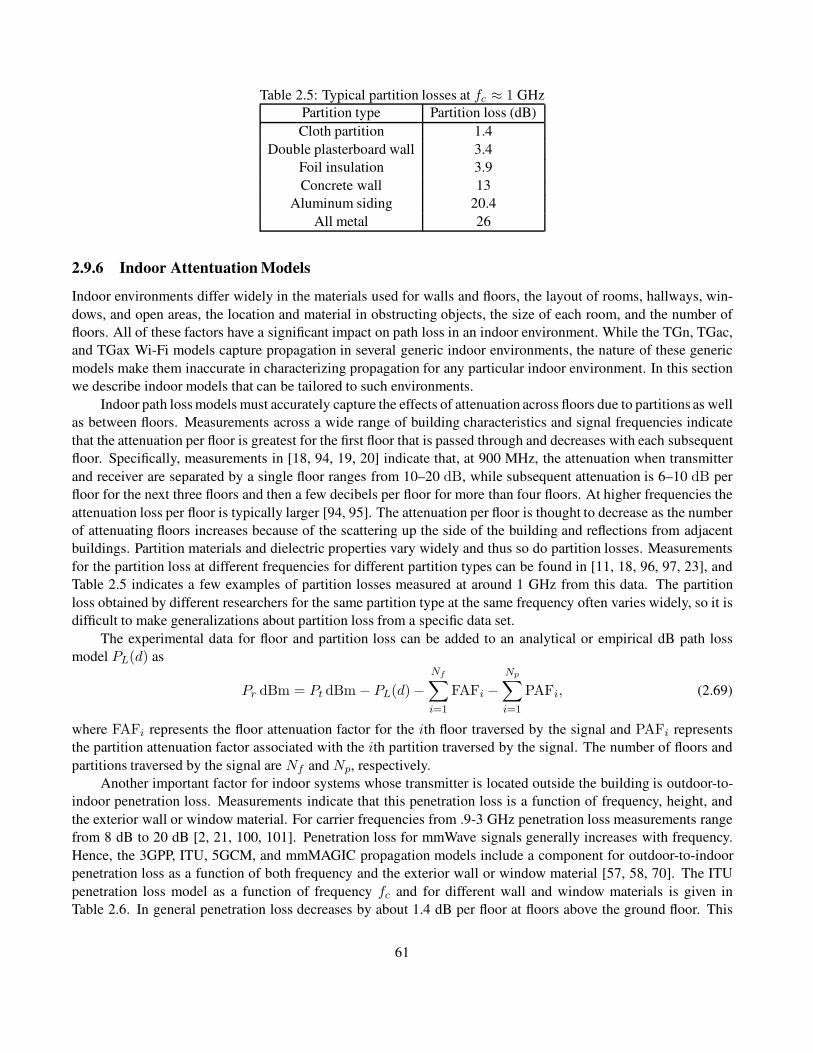
Table 2.5: Typical partition losses at fc ≈ 1 GHz

Partition type Partition loss (dB)

Cloth partition 1.4

Double plasterboard wall 3.4

Foil insulation 3.9

Concrete wall 13

Aluminum siding 20.4

All metal 26

2.9.6 Indoor Attentuation Models

Indoor environments differ widely in the materials used for walls and floors, the layout of rooms, hallways, win-

dows, and open areas, the location and material in obstructing objects, the size of each room, and the number of

floors. All of these factors have a significant impact on path loss in an indoor environment. While the TGn, TGac,

and TGax Wi-Fi models capture propagation in several generic indoor environments, the nature of these generic

models make them inaccurate in characterizing propagation for any particular indoor environment. In this section

we describe indoor models that can be tailored to such environments.

Indoor path loss models must accurately capture the effects of attenuation across floors due to partitions as well

as between floors. Measurements across a wide range of building characteristics and signal frequencies indicate

that the attenuation per floor is greatest for the first floor that is passed through and decreases with each subsequent

floor. Specifically, measurements in [18, 94, 19, 20] indicate that, at 900 MHz, the attenuation when transmitter

and receiver are separated by a single floor ranges from 10–20 dB, while subsequent attenuation is 6–10 dB per

floor for the next three floors and then a few decibels per floor for more than four floors. At higher frequencies the

attenuation loss per floor is typically larger [94, 95]. The attenuation per floor is thought to decrease as the number

of attenuating floors increases because of the scattering up the side of the building and reflections from adjacent

buildings. Partition materials and dielectric properties vary widely and thus so do partition losses. Measurements

for the partition loss at different frequencies for different partition types can be found in [11, 18, 96, 97, 23], and

Table 2.5 indicates a few examples of partition losses measured at around 1 GHz from this data. The partition

loss obtained by different researchers for the same partition type at the same frequency often varies widely, so it is

difficult to make generalizations about partition loss from a specific data set.

The experimental data for floor and partition loss can be added to an analytical or empirical dB path loss

model PL(d) as

Pr dBm = Pt dBm − PL(d)−Nf∑

i=1

FAFi −Np∑

i=1

PAFi, (2.69)

where FAFi represents the floor attenuation factor for the ith floor traversed by the signal and PAFi represents

the partition attenuation factor associated with the ith partition traversed by the signal. The number of floors and

partitions traversed by the signal are Nf and Np, respectively.

Another important factor for indoor systems whose transmitter is located outside the building is outdoor-to-

indoor penetration loss. Measurements indicate that this penetration loss is a function of frequency, height, and

the exterior wall or window material. For carrier frequencies from .9-3 GHz penetration loss measurements range

from 8 dB to 20 dB [2, 21, 100, 101]. Penetration loss for mmWave signals generally increases with frequency.

Hence, the 3GPP, ITU, 5GCM, and mmMAGIC propagation models include a component for outdoor-to-indoor

penetration loss as a function of both frequency and the exterior wall or window material [57, 58, 70]. The ITU

penetration loss model as a function of frequency fc and for different wall and window materials is given in

Table 2.6. In general penetration loss decreases by about 1.4 dB per floor at floors above the ground floor. This

61

Table 2.6: ITU penetration loss model

Material Penetration loss (dB)

Standard multi-pane glass 2 + 0.2fcInfrared reflective glass 23 + .3fc

Concrete 5 + 4fcWood 4.85 + 0.12fc

decrease is due to reduced clutter at higher floors and the higher likelihood of a LOS path.

62

Chapter 2 Problems

1. Under the free-space path loss model, find the transmit power required to obtain a received power of 1 dBm

for a wireless system with isotropic antennas (Gt = Gr = 1) and a carrier frequency fc = 5 GHz, assuming

a distance d = 10 m. Repeat for d = 100 m.

2. For the two-ray model with transmitter–receiver separation d = 100 m, ht = 10 m, and hr = 2 m, find the

delay spread between the two signals.

3. For the two-ray model, show how a Taylor series approximation applied to (2.14) results in the approximation

∆φ =2π(d1 − d0)

λ≈ 4πhthr

λd.

4. For the two-ray model, derive an approximate expression for the distance values below the critical distance

dc at which signal nulls occur.

5. Find the critical distance dc under the two-ray model for a large macrocell in a suburban area with the base

station mounted on a tower or building (ht = 20 m), the receivers at height hr = 3 m, and fc = 2 GHz. Is

this a good size for cell radius in a suburban macrocell? Why or why not?

6. Suppose that, instead of a ground reflection, a two-ray model consists of a LOS component and a signal

reflected off a building to the left (or right) of the LOS path. Where must the building be located relative to

the transmitter and receiver for this model to be the same as the two-ray model with a LOS component and

ground reflection?

7. Consider a two-ray channel with impulse response h(t) = α1δ(t) + α2δ(t − .022 µs), so for input signal

s(t) to the channel, the output is r(t) = h(t)∗s(t). Find the distance separating the transmitter and receiver,

as well as α1 and α2, assuming free-space path loss on each path with a reflection coefficient of −1. Assume

the transmitter and receiver are located 8 m above the ground and that the carrier frequency is 900 MHz.

8. Directional antennas are a powerful tool to reduce the effects of multipath as well as interference. In par-

ticular, directional antennas along the LOS path for the two-ray model can reduce the attenuation effect of

ground wave cancellation, as will be illustrated in this problem. Assume the reference distance dr = 1

m. Plot the dB power (10 log10 Pr) versus log distance (log10 d) for the two-ray model with parameters

fc = 900 MHz, R = −1, ht = 50 m, hr = 2 m, G0 = 1, and the following values for G1 : G1 = 1, .316, .1,

and .01 (i.e., G1 = 0, −5, −10, and− 20 dB, respectively). Each of the four plots should range in distance

from d = 1 m to d = 100 km. Also calculate and mark the critical distance dc = 4hthr/λ on each plot, and

normalize the plots to start at approximately 0 dB. Finally, show the piecewise linear model with flat power

falloff up to distance ht, falloff 10 log10(d−2) for ht < d < dc, and falloff 10 log10(d

−4) for d ≥ dc. (On the

power loss versus log distance plot, the piecewise linear curve becomes a set of three straight lines of slope

0, 2, and 4, respectively.) Note that at large distances it becomes increasingly difficult to have G1 G0

because this requires extremely precise angular directivity in the antennas.

9. Under what conditions is the single-slope path loss model (2.23) the same as the free-space path loss model

(2.7)?

10. Consider a receiver with noise power –160 dBm within the signal bandwidth of interest. Assume a single-

slope path loss model with d0 = 1 m, K obtained from the free-space path loss formula with isotropic

antennas and fc = 1 GHz, and γ = 4. For a transmit power of Pt = 10 mW, find the maximum distance

between the transmitter and receiver such that the received signal-to-noise power ratio is 20 dB.

63

11. For the set of empirical measurements of Pr/Pt given in Table 2.2, find the path loss exponent γ and param-

eter K that minimizes the MSE between the single-slope model (2.24) in dB and the empirical dB power

measurements, assuming that dr = 1 m. This problem differs from Example 2.5.1 in that now the two

parameters γ and K are jointly optimized to minimize MSE, rather than fixing the value of K based on

free-space path loss or the measured attenuation at the reference distance dr. Find the received power at 150

m for this single-slope path loss model with transmit power of 1 mW (0 dBm) and compare with the result in

Example 2.5.1. Does the better fitting of the data through this two-dimensional optimization lead to a larger

or smaller value for this received power? Will this always be the case for any set of empirical measurements

(why or why not)?

12. Find parameters for a multi-slope model with three segments to approximate the two-ray model path loss

(2.13) over distances between 10 and 1000 meters, assuming ht = 10 m, hr = 2 m, and G0 = G1 = 1. Plot

the path loss and the piecewise linear approximation using these parameters over this distance range.

13. This problem shows how different propagation models can lead to very different SNRs (and therefore differ-

ent link performance) for a given system design. Consider a linear cellular system using frequency division,

as might operate along a highway or rural road (see Figure 2.13). Each cell is allocated a certain band of

frequencies, and these frequencies are reused in cells spaced a distance d away. Assume the system has

square cells, 2 km per side, and that all mobiles transmit at the same power P . For the following propagation

models, determine the minimum distance that the cells operating in the same frequency band must be spaced

so that uplink SNR (the ratio of the minimum received signal-to-interference or S/I power from mobiles to

the base station) is greater than 20 dB. You can ignore all interferers except those from the two nearest cells

operating at the same frequency.

Figure 2.13: Linear cellular system for Problem 2-14.

(a) Propagation for both signal and interference follow a free-space model.

(b) Propagation for both signal and interference follow the single-slope path loss model (2.23) with d0 =100 m, K = 1, and γ = 3.

(c) Propagation for the signal follows the single-slope path loss model with d0 = 100 m, K = 1, and

γ = 2, while propagation of the interfererence follows the same model but with γ = 4.

14. Show that the log-normal distribution for ψ given in (2.31) yields the Gaussian distribution for ψdB given in

(2.34).

15. Table 2.7 lists a set of empirical path loss measurements. Assume a carrier frequency fc = 2 GHz.

(a) Find the parameters of a single-slope path loss model plus log-normal shadowing that best fit this data

assuming K is calculated from free-space path loss at the reference distance dr = 1 m.

(b) Find the path loss at 2 km based on this model.

64

Table 2.7: path loss measurements for Problem 2-14

.

Distance from transmitter Pr/Pt

5 m –60 dB

25 m –80 dB

65 m –105 dB

110 m –115 dB

400 m –135 dB

1000 m –150 dB

(c) Find the outage probability at a distance d assuming the received power at d due to path loss alone is

10 dB above the required power for non-outage.

16. Consider a cellular system operating at 900 MHz where propagation follows free-space path loss with vari-

ations about this path loss due to log-normal shadowing with standard deviation σ = 6 dB. Suppose that for

acceptable voice quality a signal-to-noise power ratio of 15 dB is required at the mobile. Assume the base

station transmits at 1 W and that its antenna has a 3 dB gain. There is no antenna gain at the mobile, and the

receiver noise in the bandwidth of interest is −60 dBm. Find the maximum cell size such that a mobile on

the cell boundary will have acceptable voice quality 90% of the time.

17. In this problem we will simulate the log-normal fading process over distance based on the autocovariance

model (2.39). As described in the text, the simulation first generates a white noise process and then passes

it through a first-order filter with a pole at e−δ/Xc . Assume Xc = 20 m and plot the resulting log-normal

fading process over a distance d ranging from 0 m to 200 m, sampling the process every meter. You should

normalize your plot about 0 dB, since the mean of the log-normal shadowing is captured by path loss.

18. In this problem we will explore the impact of different log-normal shadowing parameters on outage prob-

ability. Consider a cellular system where the received signal power in dB has a Gaussian distribution with

mean Pr dBm and standard deviation σ dB. Assume the received signal power must be above 10 dBm for

acceptable performance.

(a) What is the outage probability when Pr = 15 dBm and σ = 8 dB?

(b) For σ = 4 dB, find the value of Pr required for the outage probability to be less than l% – a typical

value for cellular systems.

(c) Repeat part (b) for σ = 12 dB.

(d) One proposed technique for reducing outage probability is to use macrodiversity, where a mobile unit’s

signal is received by multiple base stations and then combined. This can only be done if multiple base

stations are able to receive a given mobile’s signal. Explain why this might reduce outage probability.

19. Derive the formula for cell coverage percentage (2.49) by applying integration by parts to (2.47).

20. The cell coverage percentage is independent of the decorrelation distance Xc of the shadowing. Explain

why. Now suppose it is known that a particular set of cell locations near the transmitter are in outage. Will

the cell coverage percentage with this side information now depend on the decorrelation distance and, if so,

how and why?

65

21. Find the coverage area for a microcellular system where path loss follows the single-slope model (with

γ = 3, d0 = 1 and K = 0 dB) and there is also log-normal shadowing with σ = 4 dB. Assume a cell radius

of 100 m, a transmit power of 80 mW, and a minimum received power requirement of Pmin = −100 dBm.

22. Consider a cellular system where (a) path loss follows the single-slope model with γ = 6 and (b) there is

also log-normal shadowing with σ = 8 dB. If the received power at the cell boundary due to path loss is

20 dB higher than the minimum required received power for non-outage, find the cell coverage area.

23. In microcells, path loss exponents usually range from 2 to 6 and shadowing standard deviation typically

ranges from 4 to 12. Given a cellular system in which the received power due to path loss at the cell

boundary equals the desired level for non-outage, find the path loss and shadowing parameters within these

ranges that yield the best and worst coverage area. What is the coverage area when these parameters are in

the middle of their typical ranges?

Figure 2.14: System with scattering for Problem 2-11.

24. What average power falloff with distance do you expect for the ten-ray model if G0 = G1 >> Gi for

i = 2, ..., 9? Repeat for G0 = G1 = G2 >> Gi for i = 3, ..., 9. Explain your answers in both cases.

25. For the ten-ray model, assume that the transmitter and receiver are at the same height in the middle of a street

of width 20 m. The transmitter-receiver separation is 500 m. Find the delay spread for this model.

26. Consider a system with a transmitter, receiver, and scatterer as shown in Figure 2.14. Assume the transmitter

and receiver are both at heights ht = hr = 4 m and are separated by distance d, with the scatterer at distance

.5d along both dimensions in a two-dimensional grid of the ground – that is, on such a grid the transmitter

is located at (0, 0), the receiver at (0, d), and the scatterer at (.5d, .5d). Assume a radar cross-section of

20 dBm2, Gs = 1, and fc = 900 MHz. Find the path loss of the scattered signal for d = 1, 10, 100, and

1000 meters. Compare with the path loss at these distances if the signal is only reflected, with reflection

coefficient R = −1.

27. Find the median path loss under the Hata model assuming fc = 900 MHz, ht = 20 m, hr = 5 m, and

d = 100 m for a large urban city, a small urban city, a suburb, and a rural area. Explain qualitatively the path

loss differences for these four environments.

28. Consider a wireless link operating outdoors over 200m in the mmW freqency band. Assume the path loss

follows the single-slope model with a path loss exponent γ = 2 and reference distance for antenna far

field dr = 1 m. Without any additional attenuation caused by atmospheric and rain conditions, the model

attenuation factor K = 1. Assume rain attenuation follows the simple approximation Krain = .95R.77 for

R the rain rate in mm/hr. Assume the atmospheric absorption given in Fig. 2.11.

66

(a) What is the received signal power due to path loss and oxygen absorption at carrier frequencies of 60

GHz and of 80 GHz assuming a transmit power of 1W?

(b) Consider now only the 80 GHz link. Assume a day where it is dry at 8 am, there is a heavy drizzle of

2.5mm/Hr at 12 pm and a heavy downpour of 50mm/Hr at 5 pm. What is the required transmit power at

8 am, 12 pm and 5 pm if we desire a received signal power of -50dBm at each of these time instances?

29. Using the indoor attentuation model, determine the required transmit power for a desired received power of

–110 dBm for a signal transmitted over 100 m that goes through three floors with attenuation 15 dB, 10 dB,

and 6 dB (respectively) as well as two double plaster-board walls. Assume a reference distance dr = 1,

exponent γ = 4, and constant K = 0 dB.

67

Bibliography

[1] W. C. Jakes, Jr., Microwave Mobile Communications, Wiley, New York, 1974 [reprinted by IEEE Press].

[2] D. Parsons, The Mobile Radio Propagation Channel, 2nd Ed., Wiley, New York, 2000.

[3] M. Patzold, Mobile Fading Channels, 2nd Ed., Wiley, New York, 2011.

[4] H. L. Bertoni, Radio Propagation for Modern Wireless Systems, Prentice Hall, 1999.

[5] J. Cavers, Mobile Channel Characteristics, Springer 2000.

[6] IEEE J. Sel. Areas Commun., Special Issue on Channel and Propagation Modeling for Wireless Systems

Design, April 2002 and August 2002.

[7] N. Costa and S. Haykin, Multiple-input Multiple-output Channel Models: Theory and Practice, John Wiley

and Sons, 2010.

[8] IEEE J. Sel. Areas Commun., Special Issue on Ultra-Wideband Radio in Multiaccess Wireless Communica-

tions, December 2002.

[9] T. Rappaport, R. W. Heath Jr, R. C. Daniels, and J. N. Murdock. Millimeter Wave Wireless Communications.

Pearson Education, 2014.

[10] G. H. Spencer and M. V. R. K. Murty, “General Ray-Tracing Procedure”. Journal of the Optical Society of

America, Vol. 52, Issue 6, pp. 672-678, June 1962.

[11] T. S. Rappaport, Wireless Communications-Principles and Practice, 2nd ed., Prentice-Hall, Englewood

Cliffs, NJ, 2001.

[12] J. L. Volakis, Antenna Engineering Handbook, 4th Ed. McGraw-Hill, 2007.

[13] H. T. Friis, “A note on a simple transmission formula”, Proc. IRE, vol. 34, no. 5, pp. 254-256, May 1946.

[14] A. S. Y. Poon and R. W. Brodersen, “The role of multiple-antenna systems in emerging open access environ-

ments,” EE Times Commun. Design Conf., October 2003.

[15] A. J. Rustako, Jr., N. Amitay, G. J. Owens, and R. S. Roman, “Radio propagation at microwave frequencies

for line-of-sight microcellular mobile and personal communications,” IEEE Trans. Veh. Tech., pp. 203–10,

February 1991.

[16] W. C. Y. Lee, Mobile Communications Engineering, McGraw-Hill, New York, 1982.

68

[17] V. Erceg, L. J. Greenstein, S. Y. Tjandra, S. R. Parkoff, A. Gupta, B. Kulic, A. A. Julius, and R. Bianchi,

“An empirically based path loss model for wireless channels in suburban environments,” IEEE J. Sel. Areas

Commun., pp. 1205–11, July 1999.

[18] S. Y. Seidel and T. S. Rappaport, “914 MHz path loss prediction models for indoor wireless communications

in multifloored buildings,” IEEE Trans. Ant. Prop., pp. 207–17, February 1992.

[19] A. F. Toledo and A. M. D. Turkmani, “Propagation into and within buildings at 900, 1800, and 2300 MHz,”

Proc. IEEE Veh. Tech. Conf., pp. 633–6, May 1992.

[20] F. C. Owen and C. D. Pudney, “Radio propagation for digital cordless telephones at 1700 MHz and 900 MHz,”

Elec. Lett., pp. 52–3, September 1988.

[21] A. F. Toledo, A. M. D. Turkmani, and J. D. Parsons, “Estimating coverage of radio transmission into and

within buildings at 900, 1800, and 2300 MHz,” IEEE Pers. Commun. Mag., pp. 40–7, Apri1 1998.

[22] D. M. J. Devasirvathan, R. R. Murray, and D. R. Woiter, “Time delay spread measurements in a wireless local

loop test bed,” Proc. IEEE Veh. Tech. Conf., pp. 241–5, May 1995.

[23] G. Durgin, T. S. Rappaport, and H. Xu, “Partition-based path loss analysis for in-home and residential areas

at 5.85 GHz,” Proc. IEEE Globecom Conf., pp. 904–9, November 1998.

[24] T. Kurner, D. J. Cichon, and W. Wiesbeck, “Concepts and results for 3D digital terrain-based wave propaga-

tion models: An overview,” IEEE J. Sel. Areas Commun., pp. 1002–12, September 1993.

[25] A. J. Rustako, Jr., N. Amitay, G. J. Owens, and R.S. Roman, Radio propagation at microwave frequencies

for line-of-sight microcellular mobile and personal communications, IEEE Trans. Veh. Technol., vol. 40, pp.

203–210, February 1991.

[26] N. Amitay, “Modeling and computer simulation of wave propagation in lineal line-of-sight microcells,” IEEE

Trans. Veh. Tech., pp. 337–42, November 1992.

[27] J. W. McKown and R. L. Hamilton, Jr., “Ray tracing as a design tool for radio networks,” IEEE Network, pp.

27–30, November 1991.

[28] K. A. Remley, H. R. Anderson, and A. Weisshar, “Improving the accuracy of ray-tracing techniques for

indoor propagation modeling,” IEEE Trans. Veh. Tech., pp. 2350–8, November 2000.

[29] A. Domazetovic, L. J. Greenstein, N. Mandayan, and I. Seskar, “A new modeling approach for wireless

channels with predictable path geometries,” Proc. IEEE Veh. Tech. Conf., September 2002.

[30] J. H. Tarng, W.-S. Liu, Y.-F. Huang, and J.-M. Huang, “A novel and efficient hybrid model of radio multipath-

fading channels in indoor environments,” IEEE Trans. Ant. Prop., pp. 585–94, March 2003.

[31] Z. Yun and M. F. Iskander. “Ray tracing for radio propagation modeling: Principles and applications.” IEEE

Access Vol. 3, 2015, pp. 1089-1100.

[32] J.-F. Wagen, “Signal strength measurements at 881 MHz for urban microcells in downtown Tampa,” Proc.

IEEE Globecom Conf., pp. 1313–17, December 1991.

[33] R. J. C. Bultitude and G. K. Bedal, “Propagation characteristics on microcellular urban mobile radio channels

at 910 MHz,” IEEE J. Sel. Areas Commun., pp. 31–9, January 1989.

69

[34] J.-E. Berg, R. Bownds, and F. Lotse, “Path loss and fading models for microcells at 900 MHz,” Proc. IEEE

Veh. Tech. Conf., pp. 666–71, May 1992.

[35] J. H. Whitteker, “Measurements of path loss at 910 MHz for proposed microcell urban mobile systems,”

IEEE Trans. Veh. Tech., pp. 125–9, August 1988.

[36] H. Borjeson, C. Bergljung, and L. G. Olsson, “Outdoor microcell measurements at 1700 MHz,” Proc. IEEE

Veh. Tech. Conf., pp. 927–31, May 1992.

[37] K. Schaubach, N. J. Davis IV, and T. S. Rappaport, “A ray tracing method for predicting path loss and delay

spread in microcellular environments,” Proc. IEEE Veh. Tech. Conf., pp. 932–5, May 1992.

[38] F. Ikegami, S. Takeuchi, and S. Yoshida, “Theoretical prediction of mean field strength for urban mobile

radio,” IEEE Trans. Ant. Prop., pp. 299–302, March 1991.

[39] M. C. Lawton and J. P. McGeehan, “The application of GTD and ray launching techniques to channel mod-

eling for cordless radio systems,” Proc. IEEE Veh. Tech. Conf., pp. 125–30, May 1992.

[40] J. B. Keller, “Geometrical theory of diffraction,” J. Opt. Soc. Amer., 52, pp. 116–30, 1962.

[41] R. J. Luebbers, “Finite conductivity uniform GTD versus knife edge diffraction in prediction of propagation

path loss,” IEEE Trans. Ant. Prop., pp. 70–6, January 1984.

[42] C. Bergljung and L. G. Olsson, “Rigorous diffraction theory applied to street microcell propagation,” Proc.

IEEE Globecom Conf., pp. 1292–6, December 1991.

[43] R. G. Kouyoumjian and P. H. Pathak, “A uniform geomenical theory of diffraction for an edge in a perfectly

conducting surface,” Proc. IEEE, pp. 1448–61, November 1974.

[44] G. K. Chan, “Propagation and coverage prediction for cellular radio systems,” IEEE Trans. Veh. Tech., pp.

665–70, November 1991.

[45] K. C. Chamberlin and R. J. Luebbers, “An evaluation of Longley–Rice and GTD propagation models,” IEEE

Trans. Ant. Prop., pp. 1093–8, November 1982.

[46] J. Walfisch and H. L. Bertoni, “A theoretical model of UHF propagation in urban environments,” IEEE Trans.

Ant. Prop., pp. 1788–96, October 1988.

[47] D. Chizhik, G. J. Foschini, M. J. Gans and R. A. Valenzuela, “Keyholes, correlations, and capacities of

multielement transmit and receive antennas,” IEEE Transactions on Wireless Communications, vol. 1, no. 2,

pp. 361-368, April 2002.

[48] W. Zhang, “Fast two-dimensional diffraction modeling for site-specific propagation prediction in urban mi-

crocellular environments,” IEEE Trans. Veh. Techn., vol. 49, no. 2, pp. 428436, 2000.

[49] S. Deng, G. R. MacCartney and T. S. Rappaport, “Indoor and Outdoor 5G Diffraction Measurements and

Models at 10, 20, and 26 GHz,” 2016 IEEE Global Communications Conference (GLOBECOM), Washington,

DC, 2016, pp. 1-7.

[50] M. Jacob, S. Priebe, R. Dickhoff, T. Kleine-Ostmann, T. Schrader and T. Kurner, ”Diffraction in mm and

Sub-mm Wave Indoor Propagation Channels,” IEEE Transactions on Microwave Theory and Techniques,

vol. 60, no. 3, pp. 833-844, March 2012.

70

[51] M. I. Skolnik, Introduction to Radar Systems, 2nd ed., McGraw-Hill, New York, 1980.

[52] S. Y. Seidel, T. S. Rappaport, S. Jain, M. L. Lord, and R. Singh, “Path loss, scattering, and multipath delay

statistics in four European cities for digital cellular and microcellular radiotelephone,” IEEE Trans. Veh. Tech.,

pp. 721–30, November 1991.

[53] S. T. S. Chia, “1700 MHz urban microcells and their coverage into buildings,” Proc. IEEE Ant. Prop. Conf.,

pp. 504–11, York, U.K., Apri1 1991.

[54] T. Fugen, J. Maurer, W. Sorgel and W. Wiesbeck, “Characterization of multipath clusters with ray-tracing

in urban MIMO propagation environments at 2 GHz,” in 2005 IEEE Antennas and Propagation Society

International Symposium, Washington, DC, 2005, pp. 410-413.

[55] M. A. Jensen and J. W. Wallace, ”A review of antennas and propagation for MIMO wireless communications,”

IEEE Transactions on Antennas and Propagation, pp. 2810-2824, Nov. 2004.

[56] K. H. Ng, E. K. Tameh, A. Doufexi, M. Hunukumbure and A. R. Nix, ”Efficient multielement ray Trac-

ing with site-specific comparisons using measured MIMO channel data,” IEEE Transactions on Vehicular

Technology, pp. 1019-1032, May 2007.

[57] 3GPP, Study on channel model for frequencies from 0.5 to 100 GHz, 3rd Generation Partnership Project

(3GPP), Tech. Rep. TR 38.901, March 2017, Website: www.3gpp.org/DynaReport/38901.htm

[58] IMT, “Guidelines for evaluation of radio interface technologies for IMT-2020,” Tech Rep. ITU-R M.2412-0,

Oct. 2017, Website: www.itu.int/pub/R-REP-M.2412.

[59] P. Kyosti et al., WINNER II channel models, Eur. Commission, IST-4-027756-WINNER, Brussels, Belgium,

Tech. Rep. D1.1.2, Sep. 2007

[60] A. A. M. Saleh and R. Valenzuela, ”A Statistical Model for Indoor Multipath Propagation,” in IEEE Journal

on Selected Areas in Communications, vol. 5, no. 2, pp. 128-137, February 1987.

[61] L. Schumacher, K. I. Pedersen, and P.E. Mogensen, From antenna spacings to theoretical capacities guide-

lines for simulating MIMO systems, in Proc. PIMRC Conf., vol. 2, Sept. 2002, pp. 587-592.

[62] V. Erceg et al., TGn Channel Models. Doc. IEEE802.11-03/940r4.

[63] G. Breit et. al., “TGac Channel Model Addendum. IEEE 802.11-09/0308r12.

[64] J. Liu et. al., “IEEE 802.11ax Channel Model Document.” IEEE 802.11-14/0882r4.

[65] FCC Memorandum and Opinion Order 05-45 WTB Allocations and Service Rules for the 71-76 GHz, 81-86

GHz and 92-95 GHz Bands. Feb. 2005.

[66] Z. Pi and F. Khan, “An introduction to millimeter-wave mobile broadband systems, IEEE Commun. Mag.,

pp. 101107, June 2011.

[67] M. Marcus and B. Pattan, Millimeter wave propagation: Spectrum management implications, IEEE Mi-

crowave Mag., pp. 5462, June 2005.

[68] ITU-R P.838-3, Specific Model for Rain for Use in Prediction Methods, 2005.

71

[69] J. Ostrometzky and H. Messer, “Accumulated rainfall estimation using maximum attenuation of microwave

radio signal,” Proc. IEEE 8th Sensor Array and Multichannel Signal Processing Workshop (SAM), pp. 193-

196, June 2014.

[70] M. Xiao et al., “Millimeter Wave Communications for Future Mobile Networks,” IEEE Journal on Selected

Areas in Communications, vol. 35, no. 9, pp. 1909-1935, Sept. 2017.

[71] T. S. Rappaport, Y. Xing, G. R. MacCartney, A. F. Molisch, E. Mellios and J. Zhang, “Overview of Millimeter

Wave Communications for Fifth-Generation (5G) Wireless Networks With a Focus on Propagation Models,”

IEEE Transactions on Antennas and Propagation, vol. 65, no. 12, pp. 6213-6230, Dec. 2017.

[72] M. Shafi, J. Zhang, H. Tataria, A. F. Molisch, S. Sun, T. S. Rappaport, F. Tufvesson, S. Wu, K. Kitao, “Mi-

crowave vs. Millimeter-Wave Propagation Channels: Key Differences and Impact on 5G Cellular Systems,”

IEEE Communications Magazine, Vol. 56, No. 12., pp. 1420, Dec. 2018.

[73] I. F. Akyildiza, J. M. Jornet, C. Han, “Terahertz band: Next frontier for wireless communications,” Elsevier

J. Physical Commun., Volume 12, pp. 16-21, Sept. 2014.

[74] METIS. METIS Channel Model METIS2020, Deliverable D1.4 v3. [Online]. Available:

https://www.metis2020.com/wpcontent/uploads/deliverables/METIS D1.4 v1.0.pdf. July 2015.

[75] E. Ostlin, H.-J. Zepernick, and H. Suzuki, “Macrocell path-loss prediction using artificial neural networks,”

IEEE Trans. Veh. Techn., vol. 59, no. 6, pp. 27352747, 2010.

[76] P. Almers et. al., Survey of Channel and Radio Propagation Models for Wireless MIMO Systems, EURASIP

J. Wireless Commun. Net., vol. 2007.

[77] J. Medbo et al., ”Channel modelling for the fifth generation mobile communications,” The 8th European

Conference on Antennas and Propagation (EuCAP 2014), The Hague, 2014, pp. 219-223.

[78] P. Ferrand, M. Amara, S. Valentin and M. Guillaud, “Trends and challenges in wireless channel modeling for

evolving radio access,” IEEE Communications Magazine, vol. 54, no. 7, pp. 93-99, July 2016.

[79] S. Sun, T. Rappaport, M. Shafi, P. Tang, J. Zhang, and P.J. Smith, “Propagation Models and Performance

Evaluation for 5G Millimeter-Wave Bands,” IEEE Transactions on Vehicular Technology, Vol. 67 , No. 9 ,

Sept. 2018.

[80] M. Kasparick, R. L. G. Cavalcante, S. Valentin, S. Stanczak, and M. Yukawa, Kernel-based adaptive on-

line reconstruction of coverage maps with side information, IEEE Trans. Veh. Technol., vol. 65, no. 7, pp.

54615473, 2016.

[81] D. Romero, S.-J. Kim, G. B. Giannakis, and R. Lopez-Valcarce, Learning power spectrum maps from quan-

tized power measurements, IEEE Trans. Signal Process., vol. 65, no. 10, pp. 25472560, 2017.

[82] R. Nikbakht, A. Jonsson, and A. Lozano, Dual-kernel online reconstruction of power maps, IEEE Global

Commun. Conf. (GLOBECOM18), 2018.

[83] D. Wong and D. C. Cox, “Estimating local mean signal power level in a Rayleigh fading environment,” IEEE

Trans. Veh. Tech., pp. 956–9, May 1999.

[84] T. Okumura, E. Ohmori, and K. Fukuda, “Field strength and its variability in VHF and UHF land mobile

service,” Rev. Elec. Commun. Lab., pp. 825–73, September/October 1968.

72

[85] M. Hata, “Empirical formula for propagation loss in land mobile radio services,” IEEE Trans. Veh. Tech., pp.

317-325, August 1980.

[86] European Cooperative in the Field of Science and Technical Research EURO-COST 231, “Urban transmis-

sion loss models for mobile radio in the 900 and 1800 MHz bands,” rev. 2, The Hague, September 1991.

[87] Wireless Communications A. F. Molisch, John Wiley and Sons, 2nd ed. 2010.

[88] A. F. Molisch, H. Asplund, R. Heddergott, M. Steinbauer, and T. Zwick, The COST 259 directional channel

model-part I: Overview and methodology, IEEE Trans. on Wireless Communications, vol. 5, no. 12, pp. 3421

3433, Dec. 2006.

[89] N. Czink and C. Oestges, “The COST 273 MIMO Channel Model: Three Kinds of Clusters,” IEEE 10th

International Symposium on Spread Spectrum Techniques and Applications, pp. 282-286, Aug. 2008.

[90] L. Liu et al., “The COST 2100 MIMO channel model,” IEEE Wireless Communications, pp. 92-99, Dec.

2012.

[91] E. McCune and K. Feher, “Closed-form propagation model combining one or more propagation constant

segments,” Proc. IEEE Veh. Tech. Conf., pp. 1108–12, May 1997.

[92] M. Feuerstein, K. Blackard, T. Rappaport, S. Seidel, and H. Xia, “Path loss, delay spread, and outage models

as functions of antenna height for microcellular system design,” IEEE Trans. Veh. Tech., pp. 487–98, August

1994.

[93] P. Harley, “Short distance attenuation measurements at 900 MHz and 1.8 GHz using low antenna heights for

microcells,” IEEE J. Sel. Areas Commun., pp. 5–11, January 1989.

[94] A. J. Motley and J. M. P. Keenan, “Personal communication radio coverage in buildings at 900 MHz and

1700 MHz,” Elec. Lett., pp. 763–4, June 1988.

[95] S. Y. Seidel, T. S. Rappaport, M. J. Feuerstein, K. L. Blackard, and L. Grindstaff, “The impact of surrounding

buildings on propagation for wireless in-building personal communications system design,” Proc. IEEE Veh.

Tech. Conf., pp. 814–18, May 1992.

[96] C. R. Anderson, T. S. Rappaport, K. Bae, A. Verstak, N. Tamakrishnan, W. Trantor, C. Shaffer, and L. T.

Waton, “In-building wideband multipath characteristics at 2.5 and 60 GHz,” Proc. IEEE Veh. Tech. Conf., pp.

24–8, September 2002.

[97] L.-S. Poon and H.-S. Wang, “Propagation characteristic measurement and frequency reuse planning in an

office building,” Proc. IEEE Veh. Tech. Conf., pp. 1807–10, June 1994.

[98] A. Ghosh et al., Millimeter-wave enhanced local area systems: A high data-rate approach for future wireless

networks, IEEE J. Sel. Areas Commun., pp. 11521163, Jun. 2014.

[99] X. Zhang and J.G. Andrews, “Downlink cellular network analysis with multi-slope path loss models,” IEEE

Trans. Commun., pp. 1881-1894, May 2015.

[100] R. Hoppe, G. Wolfle, and F. M. Landstorfer, “Measurement of building penetration loss and propagation

models for radio transmission into buildings,” Proc. IEEE Veh. Tech. Conf., pp. 2298–2302, Apri1 1999.

[101] E. H. Walker, “Penetration of radio signals into buildings in cellular radio environments,” Bell Systems Tech.

J., pp. 2719–34, September 1983.

73

[102] S. S. Ghassemzadeh, L. J. Greenstein, A. Kavcic, T. Sveinsson, and V. Tarokh, “Indoor path loss model for

residential and commercial buildings,” Proc. IEEE Veh. Tech. Conf., pp. 3115–19, October 2003.

[103] A. J. Goldsmith, L. J. Greenstein, and G. J. Foschini, “Error statistics of real-time power measurements in

cellular channels with multipath and shadowing,” IEEE Trans. Veh. Tech., pp. 439–46, August 1994.

[104] A. J. Goldsmith and L. J. Greenstein, “A measurement-based model for predicting coverage areas of urban

microcells,” IEEE J. Sel. Areas Commun., pp. 1013–23, September 1993.

[105] M. Gudmundson, “Correlation model for shadow fading in mobile radio systems,” Elec. Lett., pp. 2145–6,

November 7, 1991.

[106] G. L. Stuber, Principles of Mobile Communications, 2nd ed., Kluwer, Dordrecht, 2001.

[107] A. Algans, K. I. Pedersen, and P. E. Mogensen, “Experimental analysis of the joint statistical properties of

azimuth spread, delay spread, and shadow fading,” IEEE J. Sel. Areas Commun., pp. 523–31, April 2002.

[108] M. Marsan and G. C. Hess, “Shadow variability in an urban land mobile radio environment,” Elec. Lett., pp.

646–8, May 1990.

[109] J. Weitzen and T. Lowe, “Measurement of angular and distance correlation properties of lognormal shadow-

ing at 1900 MHz and its application to design of PCS systems,” IEEE Trans.Veh. Tech., pp. 265–73, March

2002.

[110] W. Turin, R. Jana, S. S. Ghassemzadeh, V.W. Rice, and V. Tarokh, “Autoregressive modeling of an indoor

UWB channel,” Proc. IEEE Conf. UWB Syst. Technol., pp. 71–4, May 2002.

74

Chapter 3

Statistical Multipath Channel Models

In this chapter we examine fading models for the constructive and destructive addition of different multipath com-

ponents introduced by the channel. Although these multipath effects are captured in the ray-tracing models from

Chapter 2 for deterministic channels, we rarely have sufficiently precise knowledge about wireless propagation

environments to characterize them deterministically. Thus wireless channels are often characterized statistically.

The statistical characterization of the random multipath channel is based on its time-varying impulse response.

This chapter develops a statistical characterization of this channel model and describes its important properties.

If a single pulse is transmitted over a multipath channel then the received signal is a pulse train, with each pulse

in the train corresponding to the LOS component or a multipath component associated with a distinct reflector.

The delay spread of a multipath channel characterizes the difference in arrival times of the first received signal

component (LOS or, if blocked, the first received multipath component) and the last received signal component of

significant energy associated with a single transmitted pulse. For multi-ray reflection models such as the 10-ray

and 6-ray models of Chapter 2.8.1, the delay spread equals the delay difference between the first and last ray. The

delay spread for random channels is characterized statistically, as described in 3.3.2. If the delay spread is small

compared to the inverse of the signal bandwidth, then there is little time spreading in the received signal. However,

if the delay spread is large then there is significant time spreading of the received signal, which leads to substantial

signal distortion.

Another characteristic of the multipath channel is its time-varying nature. This time variation arises because

either the transmitter, receiver, or objects in the environment are moving. Hence the location of reflectors in the

transmission path, which gives rise to multipath, will change over time. Thus, if we repeatedly transmit pulses

from a transmitter given these changing reflector locations, we will observe changes in the amplitudes, delays,

and number of multipath components corresponding to each pulse. However, these changes occur over a much

larger time scale than the fading due to constructive and destructive addition of multipath components associated

with a fixed set of scatterer locations. We will first describe the time-varying channel impulse response that

models these changing multipath components. We then restrict this model to narrowband fading, where the channel

bandwidth is small compared to the inverse delay spread. For this narrowband model we will assume a quasi-

static environment featuring a fixed number of multipath components, each with fixed path loss and shadowing.

For this environment we then characterize the variations over short distances (small-scale variations) due to the

constructive and destructive addition of multipath components. We also characterize the statistics of wideband

multipath channels using two-dimensional transforms based on the underlying time-varying impulse response.

Discrete-time and MIMO channel models are also discussed.

75

3.1 Time-Varying Channel Impulse Response

Let the transmitted signal be as in (2.1):

s(t) = Reu(t)ej2πfct = Reu(t) cos(2πfct) − Imu(t) sin(2πfct), (3.1)

where u(t) is the equivalent lowpass signal for s(t) with bandwidth Bu and fc is its carrier frequency. Neglecting

noise, the corresponding received signal is the sum of the LOS path and all resolvable multipath components:

r(t) = Re

N(t)−1∑

i=0

αi(t)u(t− τi(t))ej(2πfc(t−τi(t))+φDi

(t))

, (3.2)

where the first term in the summation, corresponding to i = 0, is associated with the LOS path. The unknowns

in this expression are the number of resolvable signal components N (t) and, for each signal component (LOS

and multipath), its path length xi(t) and corresponding delay τi(t) = xi(t)/c, Doppler phase shift φDi(t), and

amplitude αi(t). The phase change associated with user movement and the resolvability of different signal compo-

nents will be discussed in the next two paragraphs. If at time t the LOS path is blocked or significantly attenuated

then this will be captured in the amplitude term α0(t). Similarly, the amplitude αi(t) of the ith multipath com-

ponent is determined by the path loss and shadowing along its propagation path. In addition, the amplitudes

αi(t), i = 0, . . . , N (t)− 1 may experience multipath fading due to constructive and destructive addition of nonre-

solvable multipath components.

When the transmitter or receiver is moving, the delay τi(t) in (3.2) changes over time and hence so does the

associated phase change. This change is captured in (3.2) as e−j2πfcτi(t), however τi(t) is rarely precisely known

in practice. Alternatively the phase change due to small changes in τi(t) can be captured by the signal’s Doppler

shift fDi(t) = v(t) cosθi(t)/λ for θi(t) the component’s angle of arrival (AoA) relative to the direction of motion

at velocity v(t). This Doppler frequency shift, which is generally easy to measure in practice, leads to a Doppler

phase shift of φDi(t) =

∫ t0 2πfDi

(ν)dν. Note that the phase change of the ith multipath component due to user

movement in (3.2) should either be captured in e−j2πfcτi(t) or in φDi(t), but not in both terms as then the phase shift

due to user movement is double-counted. It is generally assumed that τi(t) = xi(t)/c does not capture changes in

xi(t) of less than the signal wavelength λ, so the phase changes due to these small user movements are captured

by the Doppler term in (3.2).

We now define resolvability of multipath components. We say that two multipath components with delay τiand τj are resolvable if their delay difference significantly exceeds the inverse signal bandwidth: |τi− τj| B−1

u .

Multipath components that do not satisfy this resolvability criteria cannot be separated out at the receiver because

u(t− τi) ≈ u(t− τj), and thus these components are nonresolvable. These nonresolvable multipath components

are summed together to create a single resolvable multipath component in (3.2) corresponding to delay τi, with a

resulting amplitude and phase corresponding to the summed signal. Any multipath components with delay τj for

which |τj − τ0| < B−1u are combined with the LOS signal. The amplitudes of the LOS and resolvable multipath

components in (3.2) that include nonresolvable multipath components will typically undergo rapid multipath fading

due to the constructive and destructive combining of the different signal components. For wideband channels (Burelatively large) each term in the summation of (3.2) typically corresponds to a single (smooth or non-smooth1)

reflector, or to a cluster of closely-spaced reflectors, as shown in Figure 3.1. By contrast, narrowband channels

(Bu relatively small) are likely to have one or more of the signal components in (3.2) correspond to a summation

of nonresolvable signal components.

1A non-smooth reflector has a surface that is sufficiently rough such that it generates different multipath components with slightly

different delays.

76

Since the parameters αi(t), τi(t), and φDi(t) associated with each resolvable multipath component change

over time, they are characterized as random processes that we assume to be both stationary and ergodic. Thus,

the received signal is also a stationary and ergodic random process. For wideband channels, where each term in

(3.2) corresponds to a single reflector, these parameters change slowly as the propagation environment changes.

For narrowband channels, where each term in (3.2) results from the sum of nonresolvable multipath components,

the parameters can change quickly – on the order of a signal wavelength – owing to constructive and destructive

addition of the different components.

Figure 3.1: A single reflector and a cluster of closely-spaced reflectors. The reflector cluster generates multipath

components that are typically resolvable in wideband channels and non-resolvable in narrowband channels.

We can simplify r(t) by letting

φi(t) = 2πfcτi(t) − φDi(t). (3.3)

Then the received signal can be rewritten as

r(t) = Re

N(t)−1∑

i=0

αi(t)e−jφi(t)u(t− τi(t))

ej2πfct

. (3.4)

Since αi(t) is a function of path loss and shadowing while φi(t) depends on delay and Doppler, we typically

assume that these two random processes are independent.

We denote the equivalent lowpass time-varying impulse response of the channel at time t to an impulse at

time t− τ by c(τ, t). The received signal r(t) is obtained by convolving the equivalent lowpass input signal u(t)

with c(τ, t) and then upconverting to the carrier frequency: 2

r(t) = Re

(∫ ∞

−∞c(τ, t)u(t− τ)dτ

)

ej2πfct

. (3.5)

Note that c(τ, t) has two time parameters: the time t when the impulse response is observed at the receiver, and

the time t − τ when the impulse is launched into the channel relative to the observation time t. If at time t there

is no physical reflector in the channel with multipath delay τi(t) = τ , then c(τ, t) = 0. Although the definition of

the time-varying channel impulse response might at first seem counterintuitive, c(τ, t) must be defined in this way

2See Appendix A for discussion of the equivalent lowpass representation for bandpass signals and systems.

77

to be consistent with the special case of time-invariant channels. Specifically, for time-invariant channels we have

c(τ, t) = c(τ, t+ T ) for any T ; that is, the response at time t to an impulse at time t − τ equals the response at

time t+ T to an impulse at time t+ T − τ . Setting T = −t, we get that c(τ, t) = c(τ, t− t) = c(τ), where c(τ)is the standard time-invariant channel impulse response: the response at time τ to an impulse at time zero.3

Figure 3.2: System multipath at two different measurement times.

We see from (3.4) and (3.5) that c(τ, t) must be given by

c(τ, t) =

N(t)−1∑

i=0

αi(t)e−jφi(t)δ(τ − τi(t)). (3.6)

Substituting (3.6) back into (3.5) yields (3.4), thereby confirming that (3.6) is the channel’s equivalent lowpass

time-varying impulse response:

r(t) = Re

[∫ ∞

−∞c(τ, t)u(t− τ)dτ

]

ej2πfct

= Re

∫ ∞

−∞

N(t)−1∑

i=0

αi(t)e−jφi(t)δ(τ − τi(t))u(t− τ)dτ

ej2πfct

= Re

N(t)−1∑

i=0

αi(t)e−jφi(t)

(∫ ∞

−∞δ(τ − τi(t))u(t− τ)dτ

)

ej2πfct

= Re

N(t)−1∑

i=0

αi(t)e−jφi(t)u(t− τi(t))

ej2πfct

, (3.7)

where the last equality follows from the sifting property of delta functions:

∫ ∞

−∞δ(τ − τi(t))u(t− τ)dτ = δ(t− τi(t)) ∗ u(t) = u(t− τi(t)). (3.8)

3By definition, c(τ,0) is the response at time zero to an impulse at time −τ , but since the channel is time invariant, this equals the

response at time τ to an impulse at time zero.

78

Some channel models assume a continuum of multipath delays, in which case the sum in (3.6) becomes an integral

that simplifies to a time-varying complex amplitude associated with each multipath delay τ :

c(τ, t) =

∫ ∞

−∞α(ξ, t)e−jφ(ξ,t)δ(τ − ξ)dξ = α(τ, t)e−jφ(τ,t). (3.9)

For a concrete example of a time-varying impulse response, consider the system shown in Figure 3.2, where

each multipath component corresponds to a single reflector. At time t1 there are three multipath components

associated with the received signal, each with amplitude, phase, and delay triple (αi, φi, τi), i = 0, 1, 2. Thus,

impulses that were launched into the channel at time t1 − τi, i = 0, 1, 2, will all be received at time t1, and

impulses launched into the channel at any other time will not be received at t1 (because there is no multipath

component with the corresponding delay). The time-varying impulse response corresponding to t1 equals

c(τ, t1) =

2∑

i=0

αie−jφiδ(τ − τi), (3.10)

and the channel impulse response for t = t1 is shown in Figure 3.3. Figure 3.2 also shows the system at time t2,

where there are two multipath components associated with the received signal having amplitude, phase, and delay

triple (α′i, φ

′i, τ

′i), i = 0, 1. Thus, impulses that were launched into the channel at time t2 − τ ′i , i = 0, 1, will all

be received at time t2, and impulses launched into the channel at any other time will not be received at t2. The

time-varying impulse response at t2 equals

c(τ, t2) =

1∑

i=0

α′ie

−jφ′iδ(τ − τ ′i) (3.11)

and is also shown in Figure 3.3.

If the channel is time invariant, then its response to an impulse at time t1 is just a shifted version of its response

to an impulse at time t2 6= t1. Hence, the time-varying parameters in c(τ, t) become constant and c(τ, t) = c(τ) is

just a function of τ :

c(τ) =

N∑

i=0

αie−jφiδ(τ − τi). (3.12)

Example 3.1: Consider a wireless LAN operating in a factory near a conveyor belt. The transmitter and receiver

have a LOS path between them with gain α0, phase φ0, and delay τ0. Every T0 seconds, a metal item comes

down the conveyor belt, creating an additional reflected signal path with gain α1, phase φ1, and delay τ1. Find the

time-varying impulse response c(τ, t) of this channel.

Solution: For t 6= nT0, n = 1, 2, . . ., the channel impulse response simply corresponds to the LOS path. For

t = nT0, the channel impulse response includes both the LOS and reflected paths. Thus, c(τ, t) is given by

c(τ, t) =

α0e

jφ0δ(τ − τ0), t 6= nT0,α0e

jφ0δ(τ − τ0) + α1ejφ1δ(τ − τ1), t = nT0.

Note that, for typical carrier frequencies, the ith multipath component will have fcτi(t) 1. For example, with

fc = 1 GHz and τi = 50 ns (a typical value for an indoor system), fcτi = 50 1. Outdoor wireless systems

79

Figure 3.3: Response of time-varying channel.

have multipath delays much greater than 50 ns, so this property also holds for these systems. If fcτi(t) 1 then

a small change in the path delay τi(t) can lead to a large phase change in the ith multipath component with phase

φi(t) = 2πfcτi(t) − φDi(t) − φ0. Rapid phase changes in each multipath component give rise to constructive

and destructive addition of the multipath components constituting the received signal, which in turn causes rapid

variation in the received signal strength. This multipath fading phenomenon was exhibited in the deterministic

channel models of Chapter 2 (see, e.g., Figure 2.4 illustrating the received signal power for the two-ray multipath

model). This phenomenon for statistical multipath models will be discussed in more detail in subsequent sections.

The impact of multipath on the received signal depends on whether the spread of time delays associated

with the LOS and different multipath components is large or small relative to the inverse signal bandwidth. If

this channel delay spread is small then the LOS and all multipath components are nonresolvable, leading to the

narrowband fading model described in the next section. If the delay spread is large then some number of the LOS

and multipath components are resolvable, leading to the wideband fading model of Section 3.3. The delay spread

is typically measured relative to the received signal component to which the demodulator is synchronized. Thus,

for the time-invariant channel model of (3.12), if the demodulator synchronizes to the LOS signal component,

which has the smallest delay τ0, then the delay spread is a constant given by Tm = maxi[τi − τ0]. However,

if the demodulator synchronizes to a multipath component with delay equal to the mean delay τ , then the delay

spread is given by Tm = maxi |τi − τ |. In time-varying channels the multipath delays vary with time, so the

delay spread Tm becomes a random variable. Moreover, some received multipath components have significantly

lower power than others, so it’s not clear how the delay associated with such components should be used in the

characterization of delay spread. In particular, if the power of a multipath component is below the noise floor then

it should not significantly contribute to the delay spread. These issues are typically dealt with by characterizing

the delay spread relative to the channel power delay profile, defined in Section 3.3.2. Specifically, two common

80

characterizations of channel delay spread – average delay spread and rms (root mean square) delay spread – are

determined from the power delay profile. Other characterizations of delay spread, such as excees delay spread,

the delay window, and the delay interval, are sometimes used as well [1, Chap. 5.4.1; 2, Chap. 6.7.1]. The exact

characterization of delay spread is not that important for understanding the general impact of delay spread on

multipath channels, as long as the characterization roughly measures the delay associated with significant multipath

components. We will adopt the rms delay spread for our characterization as it is the one most widely used in the

literature. Assuming the demodulator synchronizes to a signal component at the average delay spread, the rms

delay spread is a good measure of the variation about this average. Channel delay spread is highly dependent on

the propagation environment. In indoor channels delay spread typically ranges from 10 to 1000 nanoseconds, in

urban microcells it ranges from 1–10 microseconds, and in rural macrocells is ranges from 10–100 microseconds

[1, Chap. 5].

3.2 Narrowband Fading Model

Suppose the delay spread Tm of a channel is small relative to the inverse baseband signal bandwidth Bu of the

transmitted signal; that is, suppose Tm B−1u . We refer to the fading in this scenario as narrowband fading

which is a function of both the signal bandwidth Bu and the channel delay spread Tm. As discussed previously,

the delay spread Tm for time-varying channels is usually characterized by the rms delay spread, but it can also

be characterized in other ways. Under most delay spread characterizations, Tm B−1u implies that the delay

associated with the ith multipath component τi ≤ Tm for all i, so u(t − τi) ≈ u(t) for all i. Since in the

narrowband fading model the delay associated with all multipath components results in minimal signal distortion

in time, we say the channel under this model is nondispersive. We can rewrite (3.4) as

r(t) = Re

u(t)ej2πfct

(∑

i

αi(t)e−jφi(t)

)

. (3.13)

Equation (3.13) differs from the original transmitted signal by the complex scale factor in large parentheses. This

scale factor is independent of the transmitted signal s(t) and, in particular, of the equivalent lowpass signal u(t)as long as the narrowband assumption Tm 1/Bu is satisfied. In order to characterize the random scale factor

caused by the multipath, we choose s(t) to be an unmodulated carrier with random phase offset φ0:

s(t) = Reej(2πfct+φ0) = cos(2πfct+ φ0), (3.14)

which is narrowband for any Tm.

With this assumption the received signal becomes

r(t) = Re

N(t)−1∑

i=0

αi(t)e−jφi(t)

ej2πfct

= rI(t) cos(2πfct) − rQ(t) sin(2πfct), (3.15)

where the in-phase and quadrature components are given by

rI(t) =

N(t)−1∑

i=0

αi(t) cosφi(t), (3.16)

rQ(t) =

N(t)−1∑

i=0

αi(t) sinφi(t) (3.17)

81

and where the phase term

φi(t) = 2πfcτi(t) − φDi(t) − φ0 (3.18)

now incorporates the phase offset φ0 as well as the effects of delay and Doppler.

Suppose N (t) is large and all signal (multipath as well as the LOS) components have random amplitudes

with approximately the same distribution, and similarly for the random phases of each component. Then, given

that αi(t) and φi(t) are also independent for different components, we can invoke the Central Limit Theorem

(CLT) for sums of independent identically-distributed (i.i.d.) random variables to approximate rI(t) and rQ(t) as

jointly Gaussian random processes. The Gaussian property also holds for small N (t) if the αi(t) are Rayleigh

distributed (given in (3.33) below) and the φi(t) are uniformly distributed on [−π, π]. This happens, again by

the CLT, when the ith multipath component results from a reflection cluster with a large number of nonresolvable

multipath components [3]. If the LoS or any of the multipath components has a much larger amplitude than the

average multipath component amplitude, then this component dominates the received signal; hence the Gaussian

approximation is no longer applicable as the terms in (3.15) are not i.i.d.

3.2.1 Autocorrelation, Cross-Correlation, and Power Spectral Density

We now derive the autocorrelation and cross-correlation of the in-phase and quadrature received signal components

rI(t) and rQ(t), as well as the received signal r(t). We focus on these correlations over a time period where the

transmitter or receiver moves on the order of a few signal wavelengths. As we will see, multipath can cause

the received signal to completely decorrelate over a signal wavelength due to changes in phase of the individual

multipath components such that they combine either constructively or destructively. Our derivations of these

correlations are based on some key assumptions that generally apply to propagation models without a dominant

LOS component such that all nonzero terms in (3.15) are approximately i.i.d. We will also determine the power

spectral density (PSD) of the received signal under certain assumptions that make its autocorrelation function

time-invariant. In this case the PSD is just the Fourier transform of the autocorrelation function.

A transmitter or receiver moving at velocity v tranverses a distance equal to a signal wavelenth λ over time

τ = λ/v. We will assume in this section that the LoS and multipath amplitudes αi(t), delays τi(t) = di(t)/c, and

Doppler frequencies fDi(t) = v(t) cosθi(t)/λ are changing slowly enough to be considered constant over the time

interval τ for which we compute the received signal autocorrelation and cross-correlation. This is generally true for

τ ≈ λ/v since over time τ or, equivalently, over distance λ the number of signal components N (t) = N doesn’t

change. Moreover, since the shadowing associated with αi(t) decorrelates over distance Xc which is generally

much bigger than λ, αi(t) ≈ αi for some constant αi. Similarly, the distance a given signal component travels, the

component’s AoA, and the velocity of the transmitter or receiver change little over the time interval τ , and hence

we can assume τi(t) ≈ τi for some average delay τi and fDi(t) ≈ fDi

for some average Doppler frequency fDi.

With a constant Doppler frequency, the Doppler phase shift4 is φDi(t) =

∫ t0 2πfDi

dν = 2πfDit and the phase of

the ith multipath component becomes φi(t) = 2πfcτi − 2πfDit− φ0.

We now make a key assumption; we assume that for the ith multipath component, the term 2πfcτi−2πfDit in

φi(t) changes rapidly relative to all other phase terms in the expression. This is a reasonable assumption because fcis large and hence the term 2πfcτi(t) can go through a 360 rotation for a small change in multipath delay τi(t). As

discussed earlier, this change is typically captured in the Doppler term 2πfDit for τi(t) assumed constant. Under

this assumption, φi(t) is uniformly distributed on [−π, π]. Thus

E[rI(t)] = E

[∑

i

αi cosφi(t)

]

=∑

i

E[αi]E[cosφi(t)] = 0, (3.19)

4We shall assume a Doppler phase shift at t = 0 of zero for simplicity, because this phase offset will not affect the analysis.

82

where the second equality follows from the independence of αi and φi(t) and the last equality follows from the

uniform distribution on φi(t). Similarly we can show that E[rQ(t)] = 0. Thus, the received signal also has

E[r(t)] = 0: it is a zero-mean Gaussian process. If there is a dominant LOS component in the channel then the

phase of the received signal is dominated by the phase of the LOS component, which can be determined at the

receiver, so the assumption of a random uniform phase no longer holds.

Consider now the autocorrelation ArI (t, t + τ) = E[rI(t)rI(t + τ)] of the in-phase component. Using the

independence of αi and φi(t), the independence of φi(t) and φj(t) (i 6= j), and the uniform distribution of φi(t),

we get that

ArI (t, t+ τ) = E

∑

i

αi cosφi(t)∑

j

αj cosφj(t+ τ)

=∑

i

∑

j

E[αiαj]E[cosφi(t) cosφj(t+ τ)]

=∑

i

E[α2i ]E[cosφi(t) cosφi(t+ τ)]. (3.20)

Since φi(t) = 2πfcτi − 2πfDit− φ0 and φi(t+ τ) = 2πfcτi − 2πfDi

(t+ τ) − φ0 we have

E[cosφi(t) cosφi(t+ τ)] = .5E[cos 2πfDiτ ] + .5E[cos(4πfcτi − 4πfDi

t− 2πfDiτ − 2φ0)]. (3.21)

Because 2πfcτi changes rapidly relative to all other phase terms and is uniformly distributed modulo 2π, the

second expectation term in (3.21) is zero and thus

ArI (t, t+ τ) = .5∑

i

E[α2i ]E[cos(2πfDi

τ)] = .5∑

i

E[α2i ]Eθi

[

cos

(2πvτ

λcos θi

)]

, (3.22)

since fDi= v cos(θi)/λ. The last expectation in (3.22) is with respect to the angle of arrival θi since that is the only

random parameter in the expression over which the expectation is taken. Observe that ArI (t, t+ τ) depends only

on τ and hence rI(t) is a wide-sense stationary (WSS) random process. Thus we can writeArI (t, t+ τ) = ArI (τ)as a function of τ only. Moreover, using a similar derivation as (3.22) we can show that the quadrature component

is also WSS with the same autocorrelation as ArI (τ), so ArI (τ) = ArQ(τ).

We now consider the cross-correlation between the in-phase and quadrature components. Using the same

trigonometric properties as in the derivation of (3.22) and the fact that 2πfcτi is uniformly distributed we get

ArI ,rQ(t, t+ τ) = E[rI(t)rQ(t+ τ)] = −.5∑

i

E[α2i ]Eθi

[

sin

(2πvτ

λcos θi

)]

(3.23)

and

ArQ,rI (t, t+ τ) = E[rQ(t)rI(t+ τ)] = .5∑

i

E[α2i ]Eθi

[

sin

(2πvτ

λcos θi

)]

. (3.24)

We see from (3.23) and (3.24) that these cross-corrections only depend on τ so we can write these as ArI ,rQ(t, t+τ) = ArI ,rQ(τ) and ArQ,rI (t, t + τ) = ArQ,rI (τ). Moreover, we see from these equations that ArI ,rQ(τ) =

−ArQ ,rI (τ). Finally, setting τ = 0 we see that ArI ,rQ(0) = −ArQ ,rI (0) = 0. Thus, rI(t) and rQ(t) are

uncorrelated and, since they are jointly Gaussian processes, this means they are independent.

We now consider the autocorrelation of the received signal

r(t) = rI(t) cos(2πfct) − rQ(t) sin(2πfct).

83

Figure 3.4: Dense scattering environment.

We have

Ar(t, t+ τ) = E[r(t)r(t+ τ)]

= E[(rI(t) cos(2πfct) − rQ(t) sin(2πfct))(rI(t+ τ) cos(2πfc(t+ τ)) − rQ(t+ τ) sin(2πfc(t+ τ))]

= E[rI(t)rI(t+ τ) cos(2πfct) cos(2πfc(t+ τ)) − rQ(t)rI(t+ τ) sin(2πfct) cos(2πfc(t+ τ))

− rI(t)rQ(t+ τ)) cos(2πfct) sin(2πfc(t+ τ)) + rQ(t)rQ(t+ τ) sin(2πfct) sin(2πfc(t+ τ))]

= ArI (τ) cos(2πfct) cos(2πfc(t+ τ)) +ArQ(τ) sin(2πfct) sin(2πfc(t+ τ))

− ArQ,rI (τ) sin(2πfct) cos(2πfc(t+ τ)) −ArI ,rQ(τ) cos(2πfct) sin(2πfc(t+ τ))

= ArI (τ) cos(2πfcτ) +ArI ,rQ(τ) sin(2πfcτ), (3.25)

where the last equality follows from trigonometric product formulas and that fact that ArI (τ) = ArQ(τ) and

ArI ,rQ(τ) = −ArQ,rI (τ). Since (3.25) is only a function of the time difference τ , the received signal r(t) is WSS

along with its in-phase and quadradure components.

In order to further simplify (3.22) and (3.23), we must make an additional assumption about the propagation

environment with respect to the power angle spectrum (PAS), which characterizes the received signal power as a

function of its angle of arrival. We will focus on the uniform scattering environment introduced by Clarke [4] and

further developed by Jakes [5, Chap. 1]. In this model, the channel consists of many scatterers densely packed

with respect to their angles of arrival, as shown in Figure 3.4. Note that this is a two-dimensional model, so that

the elevation angle of arrival for the signal components is ignored. In the uniform scattering model we assume N(LoS and multipath) signal components with angles of arrival θi = i4θ, i = 0, . . . , N − 1, where 4θ = 2π/N .

We also assume that each signal component has the same received power and so E[α2i ] = 2Pr/N , where Pr is the

total received power. Then (3.22) becomes

ArI (τ) =PrN

N−1∑

i=0

cos

(2πvτ

λcos (i4θ)

)

. (3.26)

Now making the substitutionN = 2π/4θ yields

84

ArI (τ) =Pr2π

N−1∑

i=0

cos

(2πvτ

λcos (i4θ)

)

4θ. (3.27)

We now take the limit as the number of scatterers grows to infinity, which corresponds to uniform scattering from

all directions. Then N → ∞,4θ → 0, and the summation in (3.27) becomes an integral:

ArI (τ) =Pr2π

∫ 2π

0cos

(2πvτ

λcos θ

)

dθ = PrJ0(2πfDτ), (3.28)

where fD = 2πv/λ and

J0(x) =1

π

∫ π

0e−jx cos θdθ

Figure 3.5: Bessel function versus fDτ .

is the Bessel function of zeroth order.5 Similarly, for this uniform scattering environment,

ArI ,rQ(τ) =Pr2π

∫

sin

(2πvτ

λcos(θ)

)

dθ = 0. (3.29)

A plot of J0(2πfDτ) is shown in Figure 3.5. There are several interesting observations to make from this plot.

First we see that the autocorrelation is zero for fDτ ≈ .4 or, equivalently, for vτ ≈ .4λ. Thus, the signal decorre-

lates over a distance of approximately one half wavelength under the uniform θi assumption. This approximation

is commonly used as a rule of thumb to determine many system parameters of interest. For example, we will see

in Chapter 7 that independent fading paths obtained from multiple antennas can be combined to remove some of

the negative effects of fading. For independent fading the antenna spacing must be .4λ based on the analysis here.

5Equation (3.28) can also be derived by assuming that 2πvτ cos θi/λ in (3.22) and (3.23) is random with θi uniformly distributed, and

then taking expectations with respect to θi . However, based on the underlying physical model, θi can be uniformly distributed only in a

dense scattering environment. So the derivations are equivalent.

85

However, combining paths that have a low correlation leads to almost the same gains as combining independent

fading paths [6, Chap. 9.6.5]. Another interesting characteristic of this plot is that the signal recorrelates after

it becomes uncorrelated. Thus, we cannot assume that the signal remains independent from its initial value at

d = 0 for separation distances greater than .4λ. Because of this recorrelation property, a Markov model is not

completely accurate for a uniform scattering environment. However, since the recorrelation once the separation

distance is greater than a half-wavelength is below .3, this is a reasonable approximation in analyses where such a

low correlation has little impact on performance.

Figure 3.6: In-phase and quadrature PSD: SrI (f) = SrQ(f).

The power spectral densities (PSDs) of rI(t) and rQ(t) – denoted by SrI (f) and SrQ(f), respectively – are

obtained by taking the Fourier transform of their respective autocorrelation functions relative to the delay parameter

τ . Since these autocorrelation functions are equal, so are the PSDs. Thus

SrI (f) = SrQ(f) = F [ArI(τ)] =

2Pr

πfD

1√1−(f/fD)2

, |f | ≤ fD ,

0, otherwise.(3.30)

This PSD is shown in Figure 3.6.

To obtain the PSD of the received signal r(t) under uniform scattering we use (3.25) with ArI ,rQ(τ) = 0,

(3.30), and properties of baseband random processes modulated by a sinusoid (discussed in Appendix B.3) to

obtain

Sr(f) = F [Ar(τ)] = .25[SrI(f − fc) + SrI (f + fc)]

=

Pr

2πfD

1√1−(|f−fc|/fD)2

, |f − fc| ≤ fD,

0, otherwise.(3.31)

Note that this PSD integrates to Pr, the total received power.

86

Since the PSD models the power density associated with multipath components as a function of their Doppler

frequency, it can be viewed as the probability density function (pdf) of the random frequency due to Doppler asso-

ciated with multipath. We see from Figure 3.6 that the PSD SrI (f) goes to infinity at f = ±fD and, consequently,

the PSD Sr(f) goes to infinity at f = ±fc ± fD. This will not be true in practice, since the uniform scattering

model is just an approximation, but for environments with dense scatterers the PSD will generally be maximized at

frequencies close to the maximum Doppler frequency. The intuition for this behavior comes from the nature of the

cosine function and the fact that (under our assumptions) the PSD corresponds to the pdf of the random Doppler

frequency fD(θ).

Figure 3.7: Cosine and PSD approximation by straight line segments.

To see this, note that the uniform scattering assumption is based on many scattered paths arriving uniformly

from all angles with the same average power. Thus, θ for a randomly selected path can be regarded as a uniform

random variable on [0, 2π]. The pdf pfD(θ)(f) of the random Doppler frequency fD(θ) can then be obtained

from the pdf of θ. By definition, pfD(θ)(f) is proportional to the density of scatterers at Doppler frequency f .

Hence, SrI (f) is also proportional to this density, and we can characterize the PSD from the pdf pfD(θ)(f). For

this characterization, in Figure 3.7 we plot fD(θ) = fD cos(θ) = vλ cos(θ) along with a (dashed) straight-line

segment approximation fD

(θ) to fD(θ). On the right in this figure we plot the PSD SrI (f) along with a dashed

straight-line segment approximation to it, SrI (f), which corresponds to the Doppler approximation fD

(θ). We

see that cos(θ) ≈ ±1 for a relatively large range of θ-values. Thus, multipath components with angles of arrival

in this range of values have Doppler frequency fD(θ) ≈ ±fD, so the power associated with all of these multipath

components will add together in the PSD at f ≈ fD. This is shown in our approximation by the fact that the

segments where fD

(θ) = ±fD on the left lead to delta functions at ±fD in the PSD approximation SrI (f) on the

right. The segments where fD

(θ) has uniform slope on the left lead to the flat part of SrI (f) on the right, since

there is one multipath component contributing power at each angular increment. This explains the shape of SrI (f)

under uniform scattering. Formulas for the autocorrelation and PSD in nonuniform scattering – corresponding to

more typical microcell and indoor environments – can be found in [5, Chap. 1; 7, Chap. 2]. Three-dimensional

channel models that incorporate elevation angle are described in [8] and the references therein.

The PSD is useful in constructing simulations for the fading process. A common method for simulating the

envelope of a narrowband fading process is to pass two independent white Gaussian noise sources with PSD N0/2

through lowpass filters with a frequency response H(f) that satisfies

SrI (f) = SrQ(f) =N0

2|H(f)|2. (3.32)

87

The filter outputs then correspond, respectively, to the in-phase and quadrature components of the narrowband

fading process with PSDs SrI (f) and SrQ(f). A similar procedure using discrete filters can be used to generate

discrete fading processes. Most communication simulation packages (e.g. the Matlab communications toolbox)

have standard modules that simulate narrowband fading based on this method. More details on this simulation

method, as well as alternative methods, can be found in [1, 7, 9, 10].

We have now completed our model for the three characteristics of power versus distance exhibited in nar-

rowband wireless channels. These characteristics are illustrated in Figure 3.8, adding narrowband fading to the

single-slope path loss and log-normal shadowing models developed in Chapter 2. In this figure we see the signal

power due to path loss decreasing at a slope of −10γ relative to log10(d/dr) for γ the path-loss exponent and drthe reference distance at which the path loss equals the constant K. The more rapid variations due to shadowing

change on the order of the decorrelation distanceXc, and the very rapid variations due to multipath fading change

on the order of half the signal wavelength. If we blow up a small segment of this figure over distances where path

loss and shadowing are constant we obtain Figure 3.9, which plots the dB value of Pr/Pt versus linear distance

d = vt (not log distance). In this figure the average value of Pr/Pt is normalized to 0 dB. A mobile receiver trav-

eling at fixed velocity v would experience stationary and ergodic received power variations over time as illustrated

in this figure.

Figure 3.8: Combined single-slope path loss, log-normal shadowing, and narrowband fading.

3.2.2 Envelope and Power Distributions

We now consider the distributionof the envelope and power for the narrowband received signal r(t) = rI(t) cos(2πfct)−rQ(t) sin(2πfct). It can be shown that, for any two Gaussian random variables X and Y , both with mean zero

and equal variance σ2, Z =√X2 + Y 2 is Rayleigh distributed and Z2 is exponentially distributed. We have

seen that, for φi(t) uniformly distributed, rI and rQ are both zero-mean Gaussian random variables. If we as-

sume a variance of σ2 = .5∑

iE[α2i ] for both in-phase and quadrature components, then the signal envelope

z(t) = |r(t)| =√

r2I (t) + r2Q(t) is Rayleigh distributed with distribution

pZ(z) =2z

Prexp

[

− z2

Pr

]

=z

σ2exp

[

− z2

2σ2

]

, z ≥ 0, (3.33)

where Pr = 2σ2 is the power of z(t) which equals the power of r(t).

We obtain the power distribution by making the change of variables z2(t) = |r(t)|2 in (3.33) to obtain

88

Figure 3.9: Narrowband fading.

pZ2(x) =1

Pre−x/Pr =

1

2σ2e−x/2σ

2, x ≥ 0, (3.34)

i.e. the power in r(t) is exponentially distributed with mean Pr = 2σ2. Thus, r(t) has a Rayleigh-distributed

amplitude and exponentially-distributed power with mean Pr = 2σ2. The equivalent lowpass signal for r(t) is

given by rLP (t) = rI(t)+jrQ(t), which has the same power as z(t) and phase θ = arctan (rQ(t)/rI(t)). For rI(t)and rQ(t) uncorrelated Gaussian random variables we can show that θ is uniformly distributed and independent of

|rLP |.

Example 3.2: Consider a channel with Rayleigh fading and average received power Pr = 20 dBm. Find the

probability that the received power is below 10 dBm.

Solution: We have Pr = 20 dBm = 100 mW. We want to find the probability that Z2 < 10 dBm = 10 mW.

Thus

p(Z2 < 10) =

∫ 10

0

1

100e−x/100dx = .095.

If the channel has a LOS component with a much larger signal power than the other multipath components, then

rI(t) and rQ(t) are not zero-mean random processes. That is because the average signal power is dominated by

the LOS component, with small fluctuations about this average due to constructive and destructive addition of

the multipath components. In this scenario the received signal equals the superposition of a complex Gaussian

component and a higher-power LOS component. The signal envelope in this case can be shown to have a Rician

distribution [11] given by

pZ(z) =z

σ2exp

[−(z2 + s2)

2σ2

]

I0

(zs

σ2

)

, z ≥ 0, (3.35)

where 2σ2 =∑

i,i6=0 E[α2i ] is the average power in the non-LOS multipath components and s2 = α2

0 is the power

in the LOS component. The function I0 is the modified Bessel function of zeroth order. The average received

power in the Rician fading is given by

89

Pr =

∫ ∞

0z2pZ(z)dz = s2 + 2σ2. (3.36)

The Rician distribution is often described in terms of a fading parameter K, defined by

K =s2

2σ2. (3.37)

Thus,K is the ratio of the power in the LOS component to the power in the other (non-LOS) multipath components,

which is typically a random variable. For K = 0 we have Rayleigh fading and for K = ∞ we have no fading

(i.e., a channel with no multipath and only a LOS component). The fading parameter K is therefore a measure of

the severity of the fading: a small K implies severe fading, a large K implies relatively mild fading. Making the

substitutions s2 = KPr/(K + 1) and 2σ2 = Pr/(K + 1), we can write the Rician distribution in terms of K and

Pr as

pZ(z) =2z(K + 1)

Prexp

[

−K − (K + 1)z2

Pr

]

I0

2z

√

K(K + 1)

Pr

, z ≥ 0. (3.38)

Both the Rayleigh and Rician distributions for the received signal envelope can be obtained by using mathe-

matics to capture the underlying physical properties of the channel models [3, 11]. However, some experimental

data does not fit well into either of these distributions. Thus, a more general fading distribution for the received

signal envelope was developed whose parameters can be adjusted to fit a variety of empirical measurements. This

distribution is called the Nakagami fading distribution and is given by

pZ(z) =2mmz2m−1

Γ(m)Pmrexp

[−mz2

Pr

]

, m ≥ .5, (3.39)

where Pr is the average received power and Γ(·) is the Gamma function. The Nakagami distribution is param-

eterized by Pr and the fading parameter m. For m = 1 the distribution in (3.39) reduces to Rayleigh fading.

For m = (K + 1)2/(2K + 1) the distribution in (3.39) is approximately Rician fading with parameter K. For

m = ∞ there is no fading: Z =√Pr is a constant. Thus, the Nakagami distribution can model both Rayleigh

and Rician distributions as well as more general ones. Note that some empirical measurements support values of

the m-parameter less than unity, in which case the Nakagami fading causes more severe performance degradation

than Rayleigh fading. The power distribution for Nakagami fading, obtained by a change of variables, is given by

pZ2(x) =

(m

Pr

)m xm−1

Γ(m)exp

[−mxPr

]

. (3.40)

While narrowband fading is often modeled using the Rayleigh, Rician, or Nakagami distribution, these distri-

butions are not accurate for many environments that arise in practice. This has led to several important extensions

of these models [6]. In particular, the Hoyt (or Nakagami-q) distribution models narrowband fading of the received

signal envelope assuming instaneous values of the in-phase and quadrature components are zero-mean Gaussian

random variables with unequal variances. The Beckman distribution generalizes the Hoyt model such that the in-

stantaneous in-phase and quadrature components are Gaussian random variables with unequal means and unequal

variances. The Weibull fading model generalizes both Rayleigh and exponential distributions, and with proper

parameterization has been shown to fit with with experimental data. The pdf formulas for the Hoyt, Beckman, and

Weibull distributions can be found in [6].

90

3.2.3 Level Crossing Rate and Average Fade Duration

In this section we derive the average fade duration of a narrowband fading signal, which equals the average length

of time the signal is continuously below a given value. To compute the average fade duration, we must first compute

the signal’s level crossing rate. The level crossing rate is a characteristic of any random process. It is defined as the

expected rate, in crossings per second, that the process crosses a particular value or level. The rate can be based

on crossing the level in either the upward or downward direction. In order to compute the average fade duration,

we consider the level crossing rate in the downward direction, since the signal is then below the desired value. We

thus define the envelope level crossing rate LZ of signal envelope z(t) = |r(t)| as the expected rate, in crossings

per second, at which the signal envelope crosses the level Z in the downward direction. ObtainingLZ requires the

joint distribution p(z, z) of the signal envelope z = |r| and its derivative with respect to time, z. We now derive

LZ based on this joint distribution.

Figure 3.10: Level crossing rate and fade duration for fading process.

Consider the fading process shown in Figure 3.10. The expected amount of time that the signal envelope

spends in the interval (Z + dz, Z) with envelope slope in the range (z + dz, z) over time duration dt is A =

p(Z, z) dz dz dt. The time required to cross from Z to Z +dz once for a given envelope slope z is B = dz/z. The

ratio A/B = zp(Z, z) dz dt is the expected number of crossings of the envelope z within the interval (Z + dz, Z)

for a given envelope slope z over time duration dt. The expected number of crossings of the envelope level Z for

slopes between z + dz and z in a time interval [0, T ] in the downward direction is thus

∫ T

0zp(Z, z)dz dt = zp(Z, z)dzT. (3.41)

Hence the expected number of crossings of the envelope level Z with negative slope over the interval [0, T ] is

NZ = T

∫ 0

−∞zp(Z, z)dz. (3.42)

Finally, the expected number of crossings of the envelope level Z per second – that is, the level crossing rate – is

LZ =NZ

T=

∫ 0

−∞zp(Z, z)dz. (3.43)

Note that this derivation of level crossing rate is a general result that applies for any random process.

The joint pdf of z and z for Rician fading was derived in [9] and can also be found in [7, Chap. 2.1]. The level

crossing rate for Rician fading is then obtained by using this pdf in (3.43), yielding

LZ =√

2π(K + 1)fDρe−K−(K+1)ρ2I0(2ρ

√

K(K + 1)), (3.44)

91

where ρ = Z/√

Pr . For Rayleigh fading (K = 0) the level crossing rate simplifies to

LZ =√

2πfDρe−ρ2 . (3.45)

We define the average signal fade duration as the average time that the signal envelope stays below a given

target level Z. This target level is often obtained from the signal amplitude or power level required for a given

performance metric such as bit error rate. If the signal amplitude or power falls below its target then we say the

system is in outage. Let ti denote the duration of the ith fade below level Z over a time interval [0, T ], as illustrated

in Figure 3.10. Thus ti equals the length of time that the signal envelope stays below Z on its ith crossing. Since

z(t) is stationary and ergodic, for T sufficiently large we have

p(z(t) < Z) =1

T

∑

i

ti. (3.46)

Thus, for T sufficiently large, the average fade duration is

tZ =1

TLZ

LZT∑

i=1

ti ≈p(z(t) < Z)

LZ. (3.47)

Using the Rayleigh distribution for p(z(t) < Z) then yields

tZ =eρ

2 − 1

ρfD√

2π(3.48)

with ρ = Z/√

Pr. Note that (3.48) is the average fade duration for the signal envelope (amplitude) level with Z

the target amplitude and√

Pr the average envelope level. By a change of variables it is easily shown that (3.48)

also yields the average fade duration for the signal power level with ρ =√

P0/Pr, where P0 is the target power

level and Pr is the average power level. The average fade duration (3.48) decreases with the Doppler frequency

fD, since as a channel changes more quickly it remains below a given fade level for a shorter period of time. The

average fade duration also generally increases with ρ for ρ 1. That is because the signal is more likely to be

below the target as the target level increases relative to the average. The average fade duration for Rician fading is

more difficult to compute; it can be found in [7, Chap. 1.4].

The average fade duration indicates the number of bits or symbols affected by a deep fade. Specifically,

consider an uncoded system with bit time Tb. Suppose the probability of bit error is high when z < Z. In this case,

if Tb ≈ tZ then the system will likely experience single error events, where bits that are received in error have the

previous and subsequent bits received correctly (since z > Z for these bits). On the other hand, if Tb tZ then

many subsequent bits are received with z < Z, so large bursts of errors are likely. Finally, if Tb tZ then, since

the fading is integrated over a bit time in the demodulator, the fading gets averaged out and so can be neglected.

These issues will be explored in more detail in Chapter 8, where we consider coding and interleaving.

Example 3.3: Consider a voice system with acceptable BER when the received signal power is at or above half

its average value. If the BER is below its acceptable level for more than 120 ms, users will turn off their phone.

Find the range of Doppler values in a Rayleigh fading channel such that the average time duration when users have

unacceptable voice quality is less than t = 60 ms.

Solution: The target received signal value is half the average, so P0 = .5Pr and thus ρ =√.5. We require

tZ =e.5 − 1

fD√π

≤ t = .060

92

and thus fD ≥ (e.5 − 1)/(.060√π) = 6.1 Hz.

3.2.4 Block-Fading and Finite-State Markov Fading

The complex mathematical characterization of the narrowband fading model described in the previous sections

can be difficult to incorporate into wireless performance analysis. Therefore, simpler models that capture the main

features of narrowband fading channels are often used for these analytical calculations. This section describes two

such models: block-fading and finite-state Markov fading channels.

In a block-fading channel, the channel SNR γ is assumed constant over some period of time T called the

block time. In this model we denote γ(i) as the channel SNR over the ith block. It is typically assumed that γ(i) is

i.i.d. between blocks although a more complex model capturing correlation of the channel gain across blocks can

also be used. Often T is set equal to an integer number of modulation symbol times Ts: T = NTs where NTsis approximately equal to the channel coherence time defined in Section 3.3.4 below. A rapidly-fading channel

might be approximated by setting N = 1 such that the fading is constant over each symbol time and changes to

a different i.i.d. value between subsequent symbols. A variation on the block-fading model allows for continuous

variation of the channel gain within a block, typically using the model of Section 3.2.1, with an abrupt transition

to an independent channel gain at each block time. This model is often used for systems where blocks of symbols

are sent intermittently and hence each block experiences a completely different propagation environment.

The finite-state Markov channel (FSMC) is a special case of block-fading where a finite set of channel SNR

values is assumed with a Markov transition probability of the fading between blocks. Specifically in the FSMC

the channel SNR is assumed to belong to a finite set of values, called channel states, and to follow a discrete-

time Markov process with time discretized to the block time T . The channel varies over its possible states at

each interval T according to a set of Markov transition probabilities. FSMCs have been used to approximate both

mathematical and experimental fading models, including satellite channels [12], indoor channels [13], Rayleigh

fading channels [14, 15], Rician fading channels [16], and Nakagami-m fading channels [17]. They have also been

used for system design and system performance analysis [15, 18]. First-order FSMC models are deficient when the

fading recorrelation affects performance analysis, in which case higher-order models are used. The FSMC models

for fading typically model amplitude variations only, although there has been some work on FSMC models for

phase in fading [19] or phase-noisy channels [20].

A detailed FSMC model for Rayleigh fading was developed in [14]. In this model the time-varying SNR γ

associated with the Rayleigh fading lies in the range 0 ≤ γ < infty. The FSMC model discretizes this fading

range into regions so that the jth region Rj is defined as Rj = γ : Aj ≤ γ < Aj+1, where the region

boundaries Aj and the total number of fade regions are parameters of the model. This model assumes that γstays within the same region over time interval T and can only transition to the same region or adjacent regions

at time T + 1. Thus, given that the channel is in state Rj at time T , at the next time interval the channel can

only transition to Rj−1, Rj, or Rj+1 – a reasonable assumption when fDT is small. Under this assumption, the

transition probabilities between regions are derived in [14] as

pj,j+1 =Lj+1T

πj, pj,j−1 =

LjT

πj, pj,j = 1 − pj,j+1 − pj,j−1, (3.49)

where Lj is the level crossing rate at Aj and πj is the steady-state distribution corresponding to the jth region:

πj = p(γ ∈ Rj) = p(Aj ≤ γ < Aj+1).

93

3.3 Wideband Fading Model

Suppose the transmitted signal is not narrowband relative to the inverse delay spread. Since the signal bandwidth

B ≈ 1/T for T the signal duration, the received signal will have duration T + Tm >> T for Tm is the delay

spread. Thus, the duration of the received signal will be significantly increased, and we refer to the channel in

this case as a dispersive channel. This phenomenon is illustrated in Figure 3.11. In the figure, a pulse of width

T is transmitted over a multipath channel. As discussed in Chapter 5, linear modulation consists of a train of

pulses where each pulse carries information in its amplitude and/or phase corresponding to a data bit or symbol.6

If the multipath delay spread Tm T then the multipath components are received roughly on top of one another,

as shown in the upper right of the figure. Hence the channel is nondispersive. The resulting constructive and

destructive interference causes narrowband fading of the pulse, but there is little time spreading of the pulse and

therefore little interference with a subsequently transmitted pulse. On the other hand, if the multipath delay spread

Tm T , then each of the different multipath components can be resolved, as shown in the lower right of the

figure. However, these multipath components interfere with subsequently transmitted pulses (dashed pulses in the

figure). This effect is called intersymbol interference (ISI).

Figure 3.11: Multipath resolution.

There are several techniques to mitigate the distortion due to multipath delay spread, including equalization,

multicarrier modulation, and spread spectrum, which are discussed in Chapters 11–13. Mitigating ISI is not nec-

essary if T Tm. However, most wireless systems require data rates R ≈ 1/T to be much greater than 1/Tm for

typical delay spreads of both indoor and outdoor channels. Multicarrier modulation and spread spectrum actually

change the characteristics of the transmitted signal to mostly avoid intersymbol interference; however, they still

experience multipath distortion due to frequency-selective fading, which is described in Section 3.3.3.

The difference between wideband and narrowband fading models is that, as the baseband signal bandwidthBuincreases so that Tm ≈ B−1

u , the approximation u(t− τi(t)) ≈ u(t) is no longer valid for all multipath component

delays τi(t). Thus, the received signal is a sum of all copies of the original signal, where each copy is delayed in

time by τi(t) and shifted in phase by φi(t). The signal copies will combine destructively when their phase terms

differ significantly and will distort the direct path signal when u(t− τi(t)) differs from u(t).

Although the approximation in (3.13) no longer applies when the signal bandwidth is large relative to the

inverse of the multipath delay spread, if the number of multipath components is large and the phase of each com-

6Linear modulation typically uses nonsquare pulse shapes for bandwidth efficiency, as discussed in Section 5.4.

94

ponent is uniformly distributed then the received signal will still be a zero-mean complex Gaussian process with a

Rayleigh-distributed envelope. However, wideband fading differs from narrowband fading in terms of the resolu-

tion of the different multipath components. Specifically, for narrowband signals, the multipath components are not

resolvable if their delay difference is less than the inverse of the signal bandwidth, so the multipath components

characterized in (3.6) combine at the receiver to yield the original transmitted signal with amplitude and phase

characterized by random processes. These random processes are in turn characterized by their autocorrelation (or

PSD) and instantaneous distributions, as discussed in Section 3.2. However, with wideband signals, the received

signal experiences distortion due to the delay spread of the different multipath components, so the received signal

can no longer be characterized by just the amplitude and phase random processes. The effect of multipath on wide-

band signals must therefore take into account both the multipath delay spread and the time variations associated

with the channel.

3.3.1 Autocorrelation and Scattering Function

The starting point for characterizing wideband channels is the equivalent lowpass time-varying channel impulse

response c(τ, t). Let us first assume that c(τ, t) is a continuous7 deterministic function of τ and t. Recall that

c(τ, t) represents the response of the channel at time t to an impulse at time t− τ . Hence, time variations of the

impulse response are captured by the parameter t. We can take the Fourier transform of c(τ, t) with respect to t as

C(τ, ρ) =

∫ ∞

−∞c(τ, t)e−j2πρtdt. (3.50)

We call C(τ, ρ) the deterministic scattering function of the equivalent lowpass channel impulse response c(τ, t).

Recall that time variations of the channel due to movement of the transmitter or receiver result in a Doppler

frequency shift fD. Since C(τ, ρ) is the Fourier transform of c(τ, t) with respect to the time variation parameter t,the deterministic scattering function C(τ, ρ) captures the Doppler characteristics of the channel via the frequency

parameter ρ. The derivation of this relationship for random channels is given in Section 3.3.4

In general, the time-varying channel impulse response c(τ, t) given by (3.6) is random instead of deterministic

because of the random amplitudes, phases, and delays of the random number of multipath components. In this case

we must characterize it statistically or via measurements. As long as the number of multipath components is large

and the LOS signal component does not dominate the received signal, we can invoke the CLT to assume that

c(τ, t) is a zero-mean complex Gaussian process and hence that its statistical characterization is fully known from

the mean, autocorrelation, and cross-correlation of its in-phase and quadrature components. As in the narrowband

case, we assume that the phase of each multipath component is uniformly distributed. Thus, the in-phase and

quadrature components of c(τ, t) are independent Gaussian processes with the same autocorrelation, a mean of

zero, and a cross-correlation of zero. The same statistics hold for the in-phase and quadrature components if the

channel contains only a small number of multipath rays – as long as each ray has a Rayleigh-distributed amplitude

and uniform phase. Note that this model does not hold when the channel has a dominant LOS component.

The statistical characterization of c(τ, t) is thus determined by its autocorrelation function, defined as

Ac(τ1, τ2; t, t+ 4t) = E[c∗(τ1; t)c(τ2; t+ 4t)]. (3.51)

Most time-varying channels associated with deployed wireless systems are WSS, so that the joint statistics of a

channel measured at two different times t and t+4t depends only on the time difference 4t. For WSS channels,

the autocorrelation of the corresponding bandpass channel h(τ, t) = Rec(τ, t)ej2πfC t can be obtained from

7The wideband channel characterizations in this section can also be made for discrete-time channels (discrete with respect to τ ) by

changing integrals to sums and Fourier transforms to discrete Fourier transforms.

95

Ac(τ1, τ2; t, t + 4t) as8 Ah(τ1, τ2; t, t + 4t) = .5 ReAc(τ1, τ2; t, t + 4t)ej2πfc4t [21]. We will assume

that our channel model is WSS, in which case the autocorrelation becomes independent of t:

Ac(τ1, τ2;4t) = E[c∗(τ1; t)c(τ2; t+ 4t)]. (3.52)

Moreover, in real environments the channel response associated with a given multipath component of delay τ1 is

uncorrelated with the response associated with a multipath component at a different delay τ2 6= τ1, since the two

components are caused by different scatterers. We say that such a channel has uncorrelated scattering (US). We

denote channels that are WSS with US as WSSUS channels. The WSSUS channel model was first introduced

by Bello in his landmark paper [21], where he also developed two-dimensional transform relationships associated

with this autocorrelation. These relationships will be discussed in Section 3.3.5. Incorporating the US property

into (3.52) yields

E[c∗(τ1; t)c(τ2; t+ 4t)] = Ac(τ1;4t)δ[τ1 − τ2]. (3.53)

Now setting τ1 = τ2 = τ we get

E[c∗(τ ; t)c(τ ; t+ 4t)] = Ac(τ ;4t), (3.54)

where Ac(τ ;4t) gives the average output power associated with the channel as a function of the multipath delay

τ = τ1 = τ2 and the difference 4t in observation time. The autocorrelation function (3.54) is based on the

approximation that τ1 = τ2 when τ1 and τ2 satisfy |τ1 − τ2| > B−1u , since otherwise the receiver can’t resolve

the multipath components with these delays. In this case the two components are modeled as a single combined

multipath component with delay τ ≈ τ1 ≈ τ2 and autocorrelationAc(τ ;4t).

The scattering function for random channels is defined as the Fourier transform of Ac(τ ;4t) with respect to

the 4t parameter:

Sc(τ, ρ) =

∫ ∞

−∞Ac(τ, 4t)e−j2πρ4td4t. (3.55)

The scattering function characterizes the average output power associated with the channel as a function of the

multipath delay τ and Doppler ρ. By constrast, for the deterministic channel, its scattering function C(τ, ρ)characterizes the complex channel gain as a function of multipath delay τ and Doppler ρ. An example scattering

function for an indoor channel with the power density and delay spread normalized by their mean values is shown

in Figure 3.12.

The most important characteristics of the wideband channel – including its power delay profile, coherence

bandwidth, Doppler power spectrum, and coherence time–are derived from the channel autocorrelationAc(τ, 4t)or the scattering function Sc(τ, ρ). These characteristics are described in subsequent sections.

3.3.2 Power Delay Profile

The power delay profile Ac(τ), also called the multipath intensity profile, is defined as the autocorrelation (3.54)

with 4t = 0 : Ac(τ) , Ac(τ, 0). The power delay profile represents the average power associated with a given

multipath delay, and it is easily measured empirically. The average and rms delay spread are typically defined in

terms of the power delay profile Ac(τ) as

µTm =

∫∞0 τAc(τ)dτ∫∞0 Ac(τ)dτ

, (3.56)

8It is easily shown that the autocorrelation of the bandpasschannel responseh(τ, t) is E[h(τ1, t)h(τ2, t+4t)] = .5 ReAc(τ1, τ2; t, t+4t)ej2πfc4t+ .5 ReAc(τ1, τ2; t, t +4t)ej2πfc(2t+4t), where Ac(τ1, τ2; t, t +4t) = E[c(τ1; t)c(τ2; t+4t)]. However, if c(τ, t)is WSS then Ac(τ1, τ2; t, t + 4t) = 0, so E[h(τ1, t)h(τ2, t + 4t)] = .5 ReAc(τ1, τ2; t, t + 4t)ej2πfc4t.

96

Figure 3.12: Scattering function with power spectral density and delay spread normalized by their mean values.

and

σTm =

√∫∞0 (τ − µTm)2Ac(τ)dτ

∫∞0 Ac(τ)dτ

. (3.57)

Note that Ac(τ) ≥ 0 for all τ , so if we define the distribution pTm of the random delay spread Tm as

pTm(τ) =Ac(τ)

∫∞0 Ac(τ)dτ

(3.58)

then µTm and σTm are (respectively) the mean and rms values of Tm, relative to this distribution. Defining the

distribution of Tm by (3.58) – or, equivalently, defining the mean and rms delay spread by (3.56) and (3.57),

respectively – weighs the delay associated with a given multipath component by its relative power, so that weak

multipath components contribute less to delay spread than strong ones. In particular, multipath components below

the noise floor will not significantly affect these delay spread characterizations.

The time delay T where Ac(τ) ≈ 0 for τ ≥ T can be used to roughly characterize the delay spread of the

channel, and this value is often taken to be a small integer multiple of the rms delay spread. For example, we

assume Ac(τ) ≈ 0 for τ > 3σTm . With this approximation, a linearly modulated signal with symbol period Tsexperiences significant ISI if Ts σTm . Conversely, when Ts σTm the system experiences negligible ISI. For

calculations one can assume that Ts σTm implies Ts < σTm/10 and that Ts σTm implies Ts > 10σTm. If Tsis within an order of magnitude of σTm then there will be some ISI, which may or may not significantly degrade

performance, depending on the specifics of the system and channel. In later chapters we will study the performance

degradation due to ISI in linearly modulated systems as well as ISI mitigation methods.

Although µTm ≈ σTm in many channels with a large number of scatterers, the exact relationship between

µTm and σTm depends on the shape of Ac(τ). For a channel with no LOS component and a small number of

97

multipath components with approximately the same large delay, µTm σTm . In this case the large value of µTm

is a misleading metric of delay spread, since in fact all copies of the transmitted signal arrive at roughly the same

time and the demodulator would synchronize to this common delay. It is typically assumed that the synchronizer

locks to the multipath component at approximately the mean delay, in which case rms delay spread characterizes

the time spreading of the channel.

Example 3.4: The power delay profile is often modeled as having a one-sided exponential distribution:

Ac(τ) =1

Tme−τ/Tm, τ ≥ 0.

Show that the average delay spread (3.56) is µTm = Tm and find the rms delay spread (3.57).

Solution: It is easily shown that Ac(τ) integrates to unity. The average delay spread is thus given by

µTm =1

Tm

∫ ∞

0τe−τ/Tmdτ = Tm,

and the rms delay spread is

σTm =

√

1

Tm

∫ ∞

0

τ2e−τ/Tmdτ − µ2Tm

= 2Tm − Tm = Tm.

Thus, the average and rms delay spread are the same for exponentially distributed power delay profiles.

Example 3.5: Consider a wideband channel with multipath intensity profile

Ac(τ) =

e−τ/.00001 0 ≤ τ ≤ 20 µs,

0 else.

Find the mean and rms delay spreads of the channel and find the maximum symbol rate such that a linearly

modulated signal transmitted through this channel does not experience ISI.

Solution: The average delay spread is

µTm =

∫ 20·10−6

0 τe−τ/.00001dτ∫ 20·10−6

0 e−τ/.00001dτ= 6.87 µs.

The rms delay spread is

σTm =

√√√√

∫ 20·10−6

0 (τ − µTm)2e−τ/.00001dτ∫ 20·10−6

0 e−τ/.00001dτ= 5.25 µs.

We see in this example that the mean delay spread is roughly equal to its rms value. To avoid ISI we require linear

modulation to have a symbol period Ts that is large relative to σTm . Taking this to mean that Ts > 10σTm yields

a symbol period of Ts = 52.5 µs or a symbol rate of Rs = 1/Ts = 19.04 kilosymbols per second. This is a

highly constrained symbol rate for many wireless systems. Specifically, for binary modulations where the symbol

98

rate equals the data rate (bits per second, or bps), voice requires on the order of 32 kbps and data has orders of

magnitude higher rates, with some systems operating at Gbps data rates.

3.3.3 Coherence Bandwidth

We can also characterize the time-varying multipath channel in the frequency domain by taking the Fourier trans-

form of c(τ, t) with respect to τ . Specifically, define the random process

C(f ; t) =

∫ ∞

−∞

c(τ ; t)e−j2πfτdτ. (3.59)

Because c(τ ; t) is a complex zero-mean Gaussian random variable in t, the Fourier transform in (3.59) represents

the sum9 of complex zero-mean Gaussian random processes; hence C(f ; t) is also a zero-mean Gaussian random

process that is completely characterized by its autocorrelation. Since c(τ ; t) is WSS, its integral C(f ; t) is also.

Thus, the autocorrelation of (3.59) is given by

AC(f1, f2;4t) = E[C∗(f1; t)C(f2; t+ 4t)]. (3.60)

We can simplify AC(f1, f2;4t) as follows:

AC(f1, f2;4t) = E

[∫ ∞

−∞c∗(τ1; t)e

j2πf1τ 1dτ1

∫ ∞

−∞c(τ2; t+ 4t)e−j2πf2τ 2dτ2

]

=

∫ ∞

−∞

∫ ∞

−∞

E[c∗(τ1; t)c(τ2; t+ 4t)]ej2πf1τ 1e−j2πf2τ 2dτ1dτ2

=

∫ ∞

−∞Ac(τ, 4t)e−j2π(f2−f1)τdτ

= AC(4f ;4t), (3.61)

where 4f = f2 − f1 and the third equality follows from the WSS and US properties of c(τ ; t). Thus, the

autocorrelation of C(f ; t) in frequency depends only on the frequency difference 4f . The function AC(4f ;4t)can be measured in practice by transmitting a pair of sinusoids through the channel that are separated in frequency

by 4f and then calculating their cross-correlation at the receiver for the time separation 4t.If we define AC(4f) , AC(4f ; 0) then, by (3.61),

AC(4f) =

∫ ∞

−∞Ac(τ)e

−j2π4fτdτ. (3.62)

Thus AC(4f) is the Fourier transform of the power delay profile. Because AC(4f) = E[C∗(f ; t)C(f +4f ; t)]

is an autocorrelation, it follows that the channel response is approximately independent at frequency separations

4f where AC(4f) ≈ 0. The frequency Bc where AC(4f) ≈ 0 for all 4f > Bc is called the coherence

bandwidth of the channel. By the Fourier transform relationship between Ac(τ) and AC(4f), if Ac(τ) ≈ 0 for

τ > T then AC(4f) ≈ 0 for 4f > 1/T . Hence, the minimum frequency separation Bc for which the channel

response is roughly independent is Bc ≈ 1/T , where T is typically taken to be the rms delay spread σTm of

Ac(τ). A more general approximation is Bc ≈ k/σTm , where k depends on the shape of Ac(τ) and the precise

specification of coherence bandwidth. For example, Lee [22] has shown that Bc ≈ .02/σTm approximates the

9We can express the integral as a limit of a discrete sum.

99

range of frequencies over which channel correlation exceeds 0.9 whereas Bc ≈ .2/σTm approximates the range of

frequencies over which this correlation exceeds 0.5.

In general, if we are transmitting a narrowband signal with bandwidth B Bc, then fading across the entire

signal bandwidth is highly correlated; that is, the fading is roughly equal across the entire signal bandwidth. This is

usually referred to as flat fading. On the other hand, if the signal bandwidth B Bc, then the channel amplitude

values at frequencies separated by more than the coherence bandwidth are roughly independent. Thus, the channel

amplitude varies widely across the signal bandwidth. In this case the fading is called frequency selective. If

B ≈ Bc then channel behavior is somewhere between flat and frequency-selective fading. Note that in linear

modulation the signal bandwidth B is inversely proportional to the symbol time Ts, so flat fading corresponds to

Ts ≈ 1/B 1/Bc ≈ σTm – that is, the case where the channel experiences negligible ISI. Frequency-selective

fading corresponds to Ts ≈ 1/B 1/Bc = σTm , the case where the linearly modulated signal experiences

significant ISI. Wideband signaling formats that reduce ISI, such as multicarrier modulation and spread spectrum,

still experience frequency-selective fading across their entire signal bandwidth; this degrades performance, as will

be discussed in Chapters 12 and 13.

We illustrate the power delay profileAc(τ) and its Fourier transformAC(4f) in Figure 3.13. This figure also

shows two signal spectra superimposed on AC(4f) : a narrowband signal with bandwidth much less than Bc, and

a wideband signal with bandwidth much greater thanBc. We see that the autocorrelationAC(4f) is flat across the

bandwidth of the narrowband signal, so this signal will experience flat fading or (equivalently) negligible ISI. The

autocorrelation AC(4f) goes to zero within the bandwidth of the wideband signal, which means that fading will

be independent across different parts of the signal bandwidth; hence fading is frequency selective, and a linearly

modulated signal transmitted through this channel will experience significant ISI.

Figure 3.13: Power delay profile, rms delay spread, and coherence bandwidth.

Example 3.6: Consider an indoor channel with σTm = 30 ns and a large macrocell channel with σTm = 300

ns. Find the maximum symbol rate Rs = 1/Ts for these environments such that a linearly modulated signal

transmitted through them experiences negligible ISI.

Solution: We assume that negligible ISI requires Ts σTm (i.e., Ts ≥ 10σTm). This translates into a symbol

rate of Rs = 1/Ts ≤ .1/σTm. For σTm = 30 ns this yields Rs ≤ 3.33 Mbps and for σTm = 300 ns this yields

Rs ≤ 333 Kbps. Note that high-performance wireless systems today can support Gbps data rates indoors and

out. To maintain these data rates for a linearly modulated signal without severe performance degradation by ISI,

some form of ISI mitigation is needed. Moreover, ISI is less severe in indoor than in outdoor systems owing to

the former’s lower delay spread values, which is why indoor systems tend to have higher data rates than outdoor

systems.

100

3.3.4 Doppler Power Spectrum and Channel Coherence Time

The time variations of the channel that arise from transmitter or receiver motion cause a Doppler shift in the

received signal. This Doppler effect can be characterized by taking the Fourier transform of AC(4f ;4t) relative

to 4t:

SC(4f ; ρ) =

∫ ∞

−∞AC(4f ;4t)e−j2πρ4td4t. (3.63)

In order to characterize Doppler at a single frequency, we set 4f to zero and then define SC(ρ)4= SC(0; ρ).

It is easily seen that

SC(ρ) =

∫ ∞

−∞AC(4t)e−j2πρ4td4t, (3.64)

where AC(4t) , AC(4f = 0;4t). Note that AC(4t) is an autocorrelation function defining how the channel

impulse response decorrelates over time. In particular,AC(4t = T ) = 0 indicates that observations of the channel

impulse response at times separated by T are uncorrelated and therefore independent, since the channel impulse

response is a Gaussian random process. We define the channel coherence time Tc to be the range of 4t values

over which AC(4t) is approximately nonzero. Thus, the time-varying channel decorrelates after approximately

Tc seconds. The function SC(ρ) is called the Doppler power spectrum of the channel. Since SC(ρ) is the Fourier

transform of an autocorrelation, it gives the PSD of the received signal as a function of Doppler ρ. The maximum

ρ-value for which |SC(ρ)| is greater than zero is called the Doppler spread of the channel, denoted by BD . By the

Fourier transform relationship between AC(4t) and SC(ρ), we have BD ≈ 1/Tc. If the transmitter and reflectors

are all stationary and the receiver is moving with velocity v, then BD ≤ v/λ = fD. Recall that in the narrowband

fading model samples became independent at time 4t = .4/fD, so in general BD ≈ k/Tc, where k depends on

the shape of Sc(ρ). We illustrate the Doppler power spectrum SC(ρ) and its inverse Fourier transform AC(4t) in

Figure 3.14.

Figure 3.14: Doppler power spectrum, Doppler spread, and coherence time.

Example 3.7: For a channel with Doppler spread BD = 80 Hz, find the time separation required in samples of the

received signal in order for the samples to be approximately independent.

101

Solution: The coherence time of the channel is Tc ≈ 1/BD = 1/80, so samples spaced 12.5 ms apart are

approximately uncorrelated. Thus, given the Gaussian properties of the underlying random process, these samples

are approximately independent.

3.3.5 Transforms for Autocorrelation and Scattering Functions

From (3.63) we see that the scattering function Sc(τ ; ρ) defined in (3.55) is the inverse Fourier transform of

SC(4f ; ρ) in the 4f variable. Furthermore Sc(τ ; ρ) and AC(4f ;4t) are related by the double Fourier transform

Sc(τ ; ρ) =

∫ ∞

−∞

∫ ∞

−∞

AC(4f ;4t)e−j2πρ4tej2πτ4fd4t d4f. (3.65)

The relationships among the four functionsAC(4f ;4t), Ac(τ ;4t), SC(4f ; ρ), and Sc(τ ; ρ) are shown in Figure

3.15.

Figure 3.15: Fourier transform relationships.

Empirical measurements of the scattering function for a given channel are often used to approximate the

channel’s delay spread, coherence bandwidth, Doppler spread, and coherence time. The delay spread for a channel

with empirical scattering function Sc(τ ; ρ) is obtained by computing the empirical power delay profileAc(τ) from

Ac(τ, 4t) = F−1ρ [Sc(τ ; ρ)] with 4t = 0 and then computing the mean and rms delay spread from this power

delay profile. The coherence bandwidth can then be approximated as Bc ≈ 1/σTm . Similarly, the Doppler spread

BD is approximated as the range of ρ values over which S(0; ρ) is roughly nonzero, with the coherence time

Tc ≈ 1/BD.

3.4 Discrete-Time Model

Often the time-varying impulse response channel model is too complex for simple analysis. In this case a discrete-

time approximation for the wideband multipath model can be used. This discrete-time model, developed by Turin

in [23], is especially useful in the study of spread-spectrum systems and RAKE receivers (covered in Chapter 13).

This discrete-time model is based on a physical propagation environment consisting of a composition of isolated

point scatterers, as shown in Figure 3.16. In this model, the multipath components are assumed to form subpath

clusters: incoming paths on a given subpath with approximate delay τi are combined, and incoming paths on

102

different subpath clusters with delays τi and τj , where |τi − τj| > 1/Bu, can be resolved. Here Bu denotes the

baseband signal bandwidth.

Figure 3.16: Point scatterer channel model.

The channel model of (3.6) is modified to include a fixed number N of these subpath clusters as

c(τ ; t) =

N−1∑

i=0

αi(t)e−jφi(t)δ(τ − τi(t)). (3.66)

The statistics of the received signal for a given t are thus given by the statistics of τiN0 , αiN0 , and φiN0 . Note

that c(τ ; t) in (3.66) has infinite bandwidth since it consists of a sum of delta functions. Since the model has infinite

bandwidth, its discrete-time approximation associated with any finite sampling rate entails sampling distortion, as

the channel’s Nyquist rate is infinite.

With this sampling distortion in mind, the model of (3.66) can be approximated in discrete-time as follows.

For a fixed t, the time axis is divided into M equal intervals of duration T such that MT ≥ σTm , where σTm

is the rms delay spread of the channel being approximated. The subpaths are restricted to lie in one of the M

time-interval bins, as shown in Figure 3.17. The multipath spread of this discrete model is MT , and the resolution

between paths is T . This resolution is based on the transmitted signal bandwidth: T ≈ 1/Bu. The statistics for the

ith bin are that ri, 1 ≤ i ≤ M, is a binary indicator of the existence of a multipath component in the ith bin: so

ri = 1 if there is a multipath component in the ith bin and 0 otherwise. If ri = 1 then (ai, θi), the amplitude and

phase corresponding to this multipath component, follow an empirically determined distribution. This distribution

is obtained by sample averages of (ai, θi) for each i at different locations in the propagation environment. The

empirical distribution of (ai, θi) and (aj, θj), i 6= j, is generally different; it may correspond to the same family of

fading but with different parameters (e.g., Rician fading with differentK factors) or to different fading distributions

altogether (e.g., Rayleigh fading for the ith bin, Nakagami fading for the jth bin).

Figure 3.17: Discrete-time approximation.

This completes our statistical model of the discrete-time approximation for a single snapshot. A sequence

of profiles will model the signal over time as the channel impulse response changes – for example, the impulse

103

response seen by a receiver moving at some nonzero velocity through a city. Thus, the model must include not only

the first-order statistics of (τi, αi, φi) for each profile (equivalently, each t) but also the temporal and spatial corre-

lations (assumed to be Markov) between them. More details on the model and the empirically derived distributions

for N and for (τi, αi, φi) can be found in [23].

3.5 MIMO Channel Models

Multiple antennas at the transmitter and/or receiver are common in wireless systems because of their diversity

and capacity benefits. These MIMO systems with multiple antennas require channel models that characterize

both spatial and temporal characteristics of the channel. For a channel with M transmit antennas and N receive

antennas, the MIMO channel can be written as a matrix

H(t, τ) =

h11(t, τ) h12(t, τ) · · · h1M (t, τ)h21(t, τ) h22(t, τ) · · · h2M (t, τ)

......

. . ....

hN1(t, τ) hN2(t, τ) · · · hNM (t, τ)

(3.67)

where hij(t, τ) is the time-varying impulse response between the jth transmit antenna and the ith receiver antenna

as given by (3.6). When the channel is narrowband and time-invariant, each of these terms reduces to a complex

channel gain hij . In this case the MIMO channel model consists of the distributions and cross correlations of these

random channel gains. The class of MIMO channel models that capture only these gains is often referred to as the

analytical MIMO channel model. The complex channel gains hij in MIMO systems are often assumed to be i.i.d.

zero mean, unit variance, circularly symmetric Gaussian random variables, meaning that a fixed phase rotation has

no impact on the distribution. This distribution for the MIMO channel gains is based on a physical environment

where there is a sufficient number of scatterers to yield independent fading over each transmit-receive signal path.

Environments with this characteristic are said to exhibit rich scattering. Models for more general environments

with antenna gains that are correlated or dependent include the Rice, Kronecker, UIU, Weichselberger, and keyhole

models [24]. For each transmit-receive antenna pair in the MIMO system, the single-antenna wideband fading

model described in Section 3.3 with channel gain hij can be used to capture the effects of time variations and delay

spread. However, this modeling approach does not capture dependencies across all three MIMO dimensions of

space, time, and frequency.

To capture dependencies across all three of these dimensions, we extend the time-varying channel impulse

response model (3.6) to take into account multiple transmit and receive antennas. As in the single-antenna case,

the propagation environment assumes multiple scatterers that generate the multipath components [24, 25]. The

locations of the scatterers at time t dictate the AoA θi(t) at the receiver array and the angle-of-departure (AoD)

ψi(t) at the transmitter array for the ith multipath component. Models can be either two-dimensional or three-

dimensional. Since knowledge of the environment via the angles of arrival and departure is used in this model, it

is sometimes referred to as the parametric MIMO channel model to contrast it with the analytical model.

The equivalent lowpass time-varying impulse response model (3.6) is extended to incorporate these angles of

arrival and departure as follows:

c(τ, t, θ, ψ) =

N(t)−1∑

i=0

αi(t)e−jφi(t)δ(τ − τi(t))δ(θ − θi)δ(ψ − ψi) (3.68)

where N (t), αi(t), φi(t) and τi(t) are defined as in (3.6). This time-varying impulse response is zero for all values

of the AoA θ that do not correspond to one of the incoming multipath components at time t associated with the

104

physical environment, and similarly for all values of the AoD ψ. In three dimensions the angles of arrival and

departure of each multipath component depends on the elevation and azimuth angles, the polarization of antenna

elements, as well as the scatterer locations. Survey papers on such 3-D channel models include [26, 27].

105

Chapter 3 Problems

1. Consider a two-ray channel consisting of a direct ray plus a ground-reflected ray where the transmitter is a

fixed base station at height h and the receiver is mounted on a truck (also at height h). The truck starts next to

the base station and moves away at velocity v. Assume signal attenuation on each path follows a free-space

path loss model. Find the time-varying channel impulse at the receiver for transmitter-receiver separation

d = vt sufficiently large for the length of the reflected path to be approximated by d11 + d12 ≈ d+ 2h2/d.

Assume a carrier frequency f = 2 GHz, unit gain antennas at the transmitter and receiver, and reflection

coefficient R = −1.

2. Find a formula for the multipath delay spread Tm for a two-ray channel model. Find a simplified formula

when the transmitter-receiver separation is relatively large. Compute Tm for ht = 10 m, hr = 4 m, and

d = 100 m.

3. Consider a time-invariant indoor wireless channel with LOS component at delay 23 nsec, a multipath com-

ponent at delay 48 ns, and another multipath component at delay 67 ns. Find the delay spread assuming the

demodulator synchronizes to the LOS component. Repeat assuming that the demodulator synchronizes to

the first multipath component.

4. Show that the minimum value of fcτi for a system at fc = 1 GHz with a fixed transmitter and a receiver

separated by more than 10 m from the transmitter is much greater than 1.

5. Prove that forX and Y independent zero-mean Gaussian random variables with variance σ2,Z =√X2 + Y 2

is Rayleigh-distributed and Z2 is exponentially-distributed.

6. Assume a Rayleigh fading channel with average signal power 2σ2 = −80 dBm. What is the power outage

probability of this channel relative to the threshold Po = −95 dBm? How about Po = −90 dBm?

7. Suppose we have an application that requires a power outage probability of .01 for the threshold Po = −80

dBm, For Rayleigh fading, what value of the average signal power is required?

8. Assume a Rician fading channel with 2σ2 = −80 dBm and a target power of Po = −80 dBm. Find the

outage probability assuming that the LOS component has average power s2 = −80 dBm.

9. This problem illustrates that the tails of the Ricean distribution can be quite different than its Nakagami

approximation. Plot the cumulative distribution function (CDF) of the Ricean distribution for K = 1, 5, 10

and the corresponding Nakagami distribution with m = (K + 1)2/(2K + 1). In general, does the Ricean

distribution or its Nakagami approximation have a larger outage probability p(γ < x) for x large?

10. The em Generalized Two Ray (GTR) fading model, proposed in [28], is a generalization of the Rayleigh and

Rician fading models. In this model there are two dominant signal components as well as many lower-power

multipath components. More precisely, the received signal Vr can be modeled as

Vr = V1ejφ1 + V2e

jφ2 +X + jY,

where V1 and V2 are non-negative constants, φi and φ2 are i.i.d. and uniformly distributed over [0, 2π], i.e.

φi ∼ U [0, 2π], i = 1, 2, and X and Y are i.i.d. Gauss-distributed random variables with mean zero and

variance σ2. The GTR model thus reduces to the Rician fading model if V1 > 0, V2 = 0 and to the Rayleigh

106

fading model if V1 = V2 = 0. The model is parameterized in terms of K and ∆ where,

K =V 2

1 + V 22

2σ2

∆ =2V1V2

V 21 + V 2

2

(a) Find the range of parameters K and ∆.

(b) Describe the channel model that corresponds to the following GTR parameters:

• K → ∞,∆ → 0

• K → ∞,∆ → 1

• K → 0

• K > 0,∆ → 0

(c) Show that the received signal given that the phase difference between the 2 dominant components is

constant,i.e., φ1 − φ2 = α for a constant α, consists of one dominant component and the multiple

diffuse lower-power multipath components. This implies that the GTR model reduces to the Rician

fading model when the phase difference between the LoS components in constant. Find the parameter

K(α,∆, K) of the equivalent Rician model as a function of α, ∆ and K.

(d) Show that α (mod 2π) ∼ U [0, 2π]. Use this to show that

pGTR(r | K,∆) =1

2π

∫ 2π

0pRice(r | K(α,∆, K))dα,

where pGTR(r | Σ) is the pdf of the received signal amplitude of the GTR channel fading model with

parameters Σ and pRice(r | Σ) is the pdf of the received signal amplitude of the GTR channel fading

model with parameters Σ.

11. In order to improve the performance of cellular systems, multiple base stations can receive the signal trans-

mitted from a given mobile unit and combine these multiple signals either by selecting the strongest one

or summing the signals together, perhaps with some optimized weights. This typically increases SNR and

reduces the effects of shadowing. Combining of signals received from multiple base stations is called macro-

diversity, and in this problem we explore the benefits of this technique. Diversity will be covered in more

detail in Chapter 7.

Consider a mobile at the midpoint between two base stations in a cellular network. The received signals (in

dBW) from the base stations are given by

Pr,1 = W + Z1,

Pr,2 = W + Z2,

where Z1,2 are N (0, σ2) random variables. We define outage with macrodiversity to be the event that both

Pr,1 and Pr,2 fall below a threshould T . The term W is the received signal power while Z1 and Z2 are

independent noise terms.

(a) If Z1 and Z2 are independent, show that the outage probability is given by

Pout = [Q(∆/σ)]2,

where ∆ = W − T is the fade margin at the mobile’s location.

107

(b) Now suppose Z1 and Z2 are correlated in the following way:

Z1 = a Y1 + b Y,

Z2 = a Y2 + b Y,

where Y, Y1, Y2 are independent N (0, σ2) random variables, and a, b are such that a2 + b2 = 1. Show

that

Pout =

∫ ∞

−∞

1√2π

[

Q

(∆ + byσ

|a|σ

)]2

e−y2/2dy.

(c) Compare the outage probabilities of (b) and (c) for the special case of a = b = 1/√

2, σ = 8 and

∆ = 5 (this will require a numerical integration).

12. The goal of this problem is to develop a Rayleigh fading simulator for a mobile communications channel

using the method based on filtering Gaussian processes based on the in-phase and quadrature PSDs described

in 3.2.1. In this problem you must do the following:

(a) Develop simulation code to generate a signal with Rayleigh fading amplitude over time. Your sample

rate should be at least 1000 samples/sec, the average received envelope should be 1, and your simulation

should be parameterized by the Doppler frequency fD . Matlab is the easiest way to generate this

simulation, but any simulation tool can be used.

(b) Write a description of your simulation that clearly explains how your code generates the fading enve-

lope using a block diagram and any necessary equations.

(c) Provide plots of received amplitude (dB) vs. time for fD = 1, 10, 100 Hz. over 2 seconds.

13. For a Rayleigh fading channel with average power P r = 30 dB and Doppler frequency fD = 10 Hz,

compute the average fade duration for target fade values P0 = 0 dB, P0 = 15 dB, and P0 = 30 dB.

14. Derive a formula for the average length of time a Rayleigh fading process with average power P r stays

above a given target fade value P0. Evaluate this average length of time for P r = 20 dB, P0 = 25 dB, and

fD = 50 Hz and compare with the average fade depth below P0 associated with the same parameters.

15. Assume a Rayleigh fading channel with average power P r = 10 dB and Doppler fD = 80 Hz. We would

like to approximate the channel using a finite state Markov model with eight states and time interval T = 10ms. The regions Rj corresponds to R1 = γ : −∞ ≤ γ ≤ −10 dB, R2 = γ : −10dB ≤ γ ≤ 0 dB,

R3 = γ : 0dB ≤ γ ≤ 5 dB, R4 = γ : 5dB ≤ γ ≤ 10 dB, R5 = γ : 10dB ≤ γ ≤ 15 dB,

R6 = γ : 15dB ≤ γ ≤ 20 dB, R7 = γ : 20dB ≤ γ ≤ 30 dB, R8 = γ : 30dB ≤ γ ≤ ∞ . Find the

transition probabilties between each region for this model.

16. Consider the following channel scattering function obtained by sending a 900 MHz sinusoidal input into the

channel:

S(τ, ρ) =

α1δ(τ) ρ = 70Hz.

α2δ(τ − .022µs) ρ = 49.5Hz.

0 else

where α1 and α2 are determined by path loss, shadowing, and multipath fading. Clearly this scattering

function corresponds to a 2-ray model. Assume the transmitter and receiver used to send and receive the

sinusoid are located eight meters above the ground.

(a) Find the distance and velocity between the transmitter and receiver.

108

(b) For the distance computed in part (a), is the path loss as a function of distance proportional to d−2 or

d−4? Hint: use the fact that the channel is based on a 2-ray model.

(c) Does a 30 KHz voice signal transmitted over this channel experience flat or frequency-selective fading?

17. In this problem we examine the narrowband approximation in the two-ray model. Consider the two-ray

model discussed in Chapter 2.4 with reflection coefficient R = −1, free space path loss for each ray and

carrier frequency 2.4 GHz. Both the transmitter and the receiver are 40 m high.

(a) For a separation distance of 20 m, find the impulse response of the equivalent baseband channel in the

time domain. What is the delay spread Tm?

(b) Repeat the computation of the impulse response and delay spread for a separation distance of 2000 m.

(c) Plot the baseband channel output in both the time and frequency domain in each of the above two

channels for channel input sinc(ft) ,sin(πft)πft and f = 20 MHz. Is there ISI in either channel?

Find the coherence bandwidth of the channel in each case and whether this bandwidth implies flat or

frequency selective fading.

18. Consider a wideband channel characterized by the autocorrelation function

Ac(τ,∆t) =

sinc(W∆t) 0 ≤ τ ≤ 10µsec.

0 else,

where W = 100Hz and sinc(x) = sin(πx)/(πx).

(a) Does this channel correspond to an indoor channel or an outdoor channel, and why?

(b) Sketch the scattering function of this channel.

(c) Compute the channel’s average delay spread, rms delay spread, and Doppler spread.

(d) Over approximately what range of data rates will a signal transmitted over this channel exhibit frequency-

selective fading?

(e) Would you expect this channel to exhibit Rayleigh or Ricean fading statistics, and why?

(f) Assuming that the channel exhibits Rayleigh fading, what is the average length of time that the signal

power is continuously below its average value.

(g) Assume a system with narrowband binary modulation sent over this channel. Your system has error

correction coding that can correct two simultaneous bit errors. Assume also that you always make an

error if the received signal power is below its average value, and never make an error if this power is

at or above its average value. If the channel is Rayleigh fading then what is the maximum data rate

that can be sent over this channel with error-free transmission, making the approximation that the fade

duration never exceeds twice its average value.

19. Let a scattering function S(τ, ρ) be nonzero over 0 ≤ τ ≤ .1 ms and −.1 ≤ ρ ≤ .1 Hz. Assume that the

power of the scattering function is approximately uniform over the range where it is nonzero.

(a) What are the multipath spread and the Doppler spread of the channel?

(b) Suppose you input to this channel two sinusoids cos(2πf1t) and cos(2πf2t) separated in frequency by

∆f = |f1−f2|. What is the minimum value of ∆f for which the channel response to the first sinusoid

is approximately independent of the channel response to the second sinusoid.

109

(c) For two sinusoidal inputs to the channel u1(t) = sin(2πft) and u2(t) = sin(2πf(t+ ∆t)), find the

minimum value of ∆t for which the channel response to u1(t) is approximately independent of the

channel response to u2(t).

(d) Will this channel exhibit flat fading or frequency-selective fading for a typical voice channel with a 3

KHz bandwidth? How about for a cellular channel with a 30 KHz bandwidth?

20. Consider a MIMO channel H with a time-invariant complex gain hij between the jth transmit antenna and

the ith receive antenna. A MIMO channel is called a keyhole channel when the channel matrix H can be

written as

H = hrh∗t

where ht is an M × 1 vector of i.i.d. zero-mean unit variance complex Gaussian random variables, and hris an N × 1 vector of i.i.d. zero-mean unit variance complex Gaussian random variables. Thus, hij is the

product of two independent complex Gaussian random variables.

(a) Show that the power of hij has a distribution p(x) = 2K0(2√x) where K0 is the modified Bessel

function of the second kind.

(b) Show that the matrix H has rank 1, i.e. show that all of its columns are linearly dependent, and the

same for its rows.

The fact that the matrix H is rank 1 is what gives rise to the name keyhole channel, since the MIMO channel’s

multiple spatial dimensions reduce to a single dimension, as if the signal between the transmit and receive

antenna arrays travels through a keyhole.

110

Bibliography

[1] T. S. Rappaport, Wireless Communications – Principles and Practice, 2nd ed., Prentice-Hall, Englewood

Cliffs, NJ, 2001.

[2] D. Parsons, The Mobile Radio Propagation Channel, Wiley, New York, 1994.

[3] R. S. Kennedy, Fading Dispersive Communication Channels, Wiley, New York, 1969.

[4] R. H. Clarke, “A statistical theory of mobile radio reception,” Bell System Tech. J., pp. 957–1000, July/August

1968.

[5] W. C. Jakes, Jr., Microwave Mobile Communications, Wiley, New York, 1974.

[6] M. K. Simon and M.-S. Alouini, Digital Communication over Fading Channels: A Unified Approach to

Performance Analysis, 2nd Ed., Wiley, New York, 2004.

[7] G. L. Stuber, Principles of Mobile Communications, 2nd ed., Kluwer, Dordrecht, 2001.

[8] J. Zhang, C. Pan, F. Pei, G. Liu, and X. Cheng, Three-dimensional fading channel models: a survey of

elevation angle research, IEEE Commun. Mag., vol. 52, no. 6, pp. 218226, 2014.

[9] M. Patzold, Mobile Fading Channels, Wiley, New York, 2002.

[10] J. Cavers, Mobile Channel Characteristics, Springer 2000.

[11] S. O. Rice, “Mathematical analysis of random noise,” Bell System Tech. J., pp. 282–333, July 1944, and pp.

46–156, January 1945.

[12] F. Babich, G. Lombardi, and E. Valentinuzzi, “Variable order Markov modeling for LEO mobile satellite

channels,” Elec. Lett., pp. 621–3, April 1999.

[13] A. M. Chen and R. R. Rao, “On tractable wireless channel models,” Proc. Intemat. Sympos. Pers., Indoor,

Mobile Radio Commun., pp. 825–30, September 1998.

[14] H. S. Wang and N. Moayeri, “Finite-state Markov channel – A useful model for radio communication chan-

nels,” IEEE Trans. Veh. Tech., pp. 163–71, February 1995.

[15] C. C. Tan and N. C. Beaulieu, “On first-order Markov modeling for the Rayleigh fading channel,” IEEE

Trans. Commun., pp. 2032–40, December 2000.

[16] C. Pimentel and I. F. Blake, “Modeling burst channels using partitioned Fritchman’s Markov models,” IEEE

Trans. Veh. Tech., pp. 885–99, August 1998.

111

[17] Y. L. Guan and L. F. Tumer, “Generalised FSMC model for radio channels with correlated fading,” IEE Proc.

Commun., pp. 133–7, April 1999.

[18] M. Chu and W. Stark, “Effect of mobile velocity on communications in fading channels,” IEEE Trans. Veh.

Tech., pp. 202–10, January 2000.

[19] C. Komninakis and R. D. Wesel, “Pilot-aided joint data and channel estimation in flat correlated fading,”

Proc. IEEE Globecom Conf., pp. 2534–9, November 1999.

[20] M. Peleg, S. Shamai (Shitz), and S. Galan, “Iterative decoding for coded noncoherent MPSK communications

over phase-noisy AWGN channels,” IEE Proc. Commun., pp. 87–95, April 2000.

[21] P. A. Bello, “Characterization of randomly time-variant linear channels,” IEEE Trans. Commun. Syst., pp.

360–93, December 1963.

[22] W. C. Y. Lee, Mobile Cellular Telecommunications Systems, McGraw-Hill, New York, 1989.

[23] G. L. Turin, “Introduction to spread spectrum antimultipath techniques and their application to urban digital

radio,” Proc. IEEE, pp. 328–53, March 1980.

[24] R. W. Heath and A. Lozano, Foundations of MIMO Communication, Cambridge University Press, 2019.

[25] R. Ertel, P. Cardieri, K. W. Sowerby, T. S. Rappaport, and J. H. Reed, “Overview of spatial channel models

for antenna array communication systems,” IEEE Personal Communications Magazine., pp. 10–22, February

1998.

[26] U. Karabulut, A. Awada, I. Viering, M. Simsek, and G. P. Fettweis, Spatial and Temporal Channel Character-

istics of 5G 3D Channel Model with Beamforming for User Mobility Investigations IEEE Communications

Magazine, Special Issue on Channel Models and Measurements for 5G, Dec. 2018.

[27] J. Zhang, C. Pan, F. Pei, G. Liu, and X. Cheng, Three-dimensional fading channel models: a survey of

elevation angle research, IEEE Communications Magazine, June 2014.

[28] G. D. Durgin, T. S. Rappaport, D. A. de Wolf, “New analytical models and probability density functions for

fading in wireless communications, IEEE Transactions on Communications, vol. 50, no. 6, pp. 1005-1015,

Jun. 2002.

112

Chapter 4

Capacity of Wireless Channels

The growing demand for wireless communication makes it important to determine the capacity limits of the under-

lying channels for these systems. These capacity limits dictate the maximum data rates that can be transmitted over

wireless channels with asymptotically small error probability, assuming no constraints on delay or complexity of

the encoder and decoder. The mathematical theory of communication underlying channel capacity was pioneered

by Claude Shannon in the late 1940s. This theory is based on the notion of mutual information between the in-

put and output of a channel [1, 2, 3]. In particular, Shannon defined channel capacity as the channel’s mutual

information maximized over all possible input distributions. The significance of this mathematical construct was

Shannon’s coding theorem and its converse. The coding theorem proved that a code did exist that could achieve

a data rate close to capacity with negligible probability of error. The converse proved that any data rate higher

than capacity could not be achieved without an error probability bounded away from zero. Shannon’s ideas were

quite revolutionary at the time: the high data rates he predicted for telephone channels, and his notion that coding

could reduce error probability without reducing data rate or causing bandwidth expansion. In time, sophisticated

modulation and coding technology validated Shannon’s theory and so, on telephone lines today, we achieve data

rates very close to Shannon capacity with very low probability of error. These sophisticated modulation and coding

strategies are treated in Chapters 5 and 8, respectively.

In this chapter we examine the capacity of a single-user wireless channel where transmitter and/or receiver

have a single antenna. The capacity of single-user MIMO systems where the transmitter and receiver both have

multiple antennas is treated in Chapter 10 and that of multiuser systems in Chapter 14. We will discuss capacity

for channels that are both time invariant and time varying. We first look at the well-known formula for capacity

of a time-invariant additive white Gaussian noise (AWGN) channel and then consider capacity of time-varying

flat fading channels. Unlike the AWGN case, here the capacity of a flat fading channel is not given by a single

formula because capacity depends on what is known about the time-varying channel at the transmitter and/or re-

ceiver. Moreover, for different channel information assumptions there are different definitions of channel capacity,

depending on whether capacity characterizes the maximum rate averaged over all fading states or the maximum

constant rate that can be maintained in all fading states (with or without some probability of outage).

We will first consider flat fading channel capacity where only the fading distribution is known at the transmitter

and receiver. Capacity under this assumption is typically difficult to determine and is only known in a few special

cases. Next we consider capacity when the channel fade level is known at the receiver only (via receiver estimation)

or when the channel fade level is known at both the transmitter and the receiver (via receiver estimation and

transmitter feedback). We will see that the fading channel capacity with channel fade level information at both

the transmitter and receiver is achieved when the transmitter adapts its power, data rate, and coding scheme to the

channel variation. The optimal power allocation in this case is a “water-filling” in time, where power and data rate

are increased when channel conditions are favorable and decreased when channel conditions are not favorable.

113

We will also treat capacity of frequency-selective fading channels. For time-invariant frequency-selective

channels the capacity is known and is achieved with an optimal power allocation that water-fills over frequency in-

stead of time. The capacity of a time-varying frequency-selective fading channel is unknown in general. However,

this channel can be approximated as a set of independent parallel flat fading channels whose capacity is the sum of

capacities on each channel with power optimally allocated among the channels. The capacity of such a channel is

known and the capacity-achieving power allocation water-fills over both time and frequency.

We will consider only discrete-time systems in this chapter. Most continuous-time systems can be converted

to discrete-time systems via sampling, and then the same capacity results hold. However, care must be taken in

choosing the appropriate sampling rate for this conversion, since time variations in the channel may increase the

sampling rate required to preserve channel capacity [4].

4.1 Capacity in AWGN

Consider a discrete-time AWGN channel with channel input/out relationship y[i] = x[i] + n[i], where x[i] is

the channel input at time i, y[i] is the corresponding channel output, and n[i] is a white Gaussian noise random

process. Assume a channel bandwidthB and received signal power P . The received signal-to-noise ratio (SNR) –

the power in x[i] divided by the power in n[i] – is constant and given by γ = P/(N0B), where N0/2 is the power

spectral density (PSD) of the noise. The capacity of this channel is given by Shannon’s well-known formula [1]:

C = B log2(1 + γ), (4.1)

where the capacity units are bits per second (bps). Shannon’s coding theorem proves that a code exists that achieves

data rates arbitrarily close to capacity with arbitrarily small probability of bit error. The converse theorem shows

that any code with rate R > C has a probability of error bounded away from zero.

Shannon capacity for AWGN channels provides interesting insights along the asymptotic regimes of band-

width and power. In particular, it is easily shown that

limB→∞

B log2

(

1 +P

N0B

)

= log2(e)P

N0. (4.2)

This regime is called the large bandwidth regime for capacity. Interestingly, in this regime the capacity no longer

depends on the bandwidth B. That is because there is not sufficient power to spread over the large amount of

bandwidth available, so as the bandwidth grows large, there is diminishing returns in capacity growth. The low

power regime captures a similar scenario, where there is not sufficient power to utilize the available bandwidth. In

particular, using the approximation that log(1 + x) ≈ x for x small yields that, for P small,

B log2

(

1 +P

N0B

)

≈ log2(e)P

N0. (4.3)

Here we also see that capacity no longer depends on the channel bandwidth. Another interesting regime for

capacity is the high power regime, where P grows large. We now consider how capacity scales with bandwidth

in this regime. Using the high-power approximation 1 + P/(N0B) ≈ P/(N0B), we get the following ratio of

AWGN channel capacity C(kB) given bandwidth kB compared with C(B) for any constant k > 1 in the limit of

asymptotically large power:

limP→∞

C(kB)

C(B)= lim

P→∞

kB log2

(

1 + PN0kB

)

B log2

(

1 + PN0B

) ≈ limP→∞

kB log2

(P

N0kB

)

B log2

(PN0B

) = limP→∞

k[

log2

(PN0B

)

+ log2(1/k)]

log2

(P

N0B

) = k.

(4.4)

114

Thus, in the high power regime, scaling the bandwidth up by a factor of k leads to the same increase in capacity.

That is because there is sufficient power to fully utilize the capacity of the additional bandwidth.

Shannon’s coding theorem and its converse are proved using the concept of mutual information between the

channel input and output. For a discrete memoryless time-invariant channel with random input x and random

output y, the channel’s mutual information is defined as

I(X ; Y ) =∑

x∈X ,y∈Y

p(x, y) log

(p(x, y)

p(x)p(y)

)

, (4.5)

where the sum is taken over all possible input and output pairs x ∈ X and y ∈ Y for X and Y the discrete

input and output alphabets. The log function is typically with respect to base 2, in which case the units of mutual

information are bits per second. Mutual information can also be written in terms of the entropy in the channel

output y and conditional output y | x as I(X ; Y ) = H(Y ) − H(Y |X), where H(Y ) = −∑y∈Y p(y) logp(y)and H(Y |X) = −∑x∈X ,y∈Y p(x, y) logp(y | x). Shannon proved that channel capacity equals the mutual

information of the channel maximized over all possible input distributions:

C = maxp(x)

I(X ; Y ) = maxp(x)

∑

x,y

p(x, y) log

(p(x, y)

p(x)p(y)

)

. (4.6)

For the AWGN channel, the sum in (4.6) becomes an integral over continuous alphabets and the maximizing input

distribution is Gaussian, which results in the channel capacity given by (4.1). For channels with memory, mutual

information and channel capacity are defined relative to input and output sequences xn and yn. More details on

channel capacity, mutual information, the coding theorem, and its converse can be found in [2, 5, 6].

The proofs of the coding theorem and its converse place no constraints on the complexity or delay of the

communication system. Indeed, the capacity-achieving strategy requires a code with an asymptotically large

blocklength to drive the error probability to zero. Such codes require asymptotically large transmission energy

and asymptotically large delay and complexity to decode. Since practical decoders are constrained in delay and

complexity, Shannon capacity is generally used as an upper bound on the data rates that can be achieved under real

system constraints. The exact capacity penalty due to finite blocklength codes was derived in [7] as a function of

blocklength, error probability, and the channel dispersion, which measures the stochastic variability of the channel

relative to a deterministic channel with the same capacity.

At the time that Shannon developed his theory of information, data rates over standard telephone lines were

on the order of 100 bps. Thus, it was believed that Shannon capacity, which predicted speeds of roughly 30 kbps

over the same telephone lines, was not a useful bound for real systems. However, by the 1990s breakthroughs

in hardware, modulation, and coding techniques brought commercial modems very close to the speeds predicted

by Shannon in the 1940s. In fact, modems can exceed this 30-kbps limit on some telephone channels, but that is

because transmission lines today are of better quality than in Shannon’s day and thus have a higher received power

than that used in his initial calculation. Advances in coding techniques over the last few decades include turbo

codes [8], LDPC codes (originally developed by Gallager in the 1960s and rediscovered in the 1990s) [9], lattice

codes [10], and polar codes [11]. All of these codes come within a fraction of a decibel of the Shannon capacity

limit using practical blocklengths. These codes and their performance will be covered in Chapter 8.

Wireless channels typically exhibit flat or frequency-selective fading. In the next two sections we consider ca-

pacity of flat fading and frequency-selective fading channels under different assumptions regarding what is known

about the channel.

Example 4.1: Consider a wireless channel where power falloff with distance follows the formula Pr(d) =

Pt(d0/d)3 for d0 = 10 m. Assume the channel has bandwidth B = 30 kHz and AWGN with noise PSD N0/2,

115

where N0 = 10−9 W/Hz. For a transmit power of 1 W, find the capacity of this channel for a transmit-receive

distance of 100 m and 1 km.

Solution: The received SNR is γ = Pr(d)/(N0B) = .13/(10−9 · 30 · 103) = 33 = 15 dB for d = 100 mand γ = .013/(10−9 · 30 · 103) = .033 = −15 dB for d = 1000 m. The corresponding capacities are C =

B log2(1 + γ) = 30000 log2(1 + 33) = 152.6 kbps for d = 100 m and C = 30000 log2(1 + .033) = 1.4 kbps

for d = 1000 m. Note the significant decrease in capacity at greater distances due to the path-loss exponent of 3,

which greatly reduces received power as distance increases.

Figure 4.1: Flat fading channel and system model.

4.2 Capacity of Flat Fading Channels

4.2.1 Channel and System Model

We assume a discrete-time channel with stationary and ergodic time-varying gain√

g[i], 0 ≤ g[i], and AWGN

n[i], as shown in Figure 4.1. The channel power gain g[i] follows a given distribution p(g); for example, with

Rayleigh fading p(g) is exponential. We assume that g[i] is independent of the channel input. The channel gain

g[i] can change at each time i, either as an independent and identically distributed (i.i.d.) process or with some

correlation over time. In a block fading channel, g[i] is constant over some blocklength T , after which time g[i]

changes to a new independent value based on the distribution p(g). Let P denote the average transmit signal

power, N0/2 the noise PSD of n[i], and B the received signal bandwidth. The instantaneous received SNR is then

γ[i] = P g[i]/(N0B), 0 ≤ γ[i] < ∞, and its expected value over all time is γ = P g/(N0B). Since P /(N0B) is

a constant, the distribution of g[i] determines the distribution of γ[i] and vice versa.

The system model is also shown in Figure 4.1, where an input message w is sent from the transmitter to the

receiver, which reconstructs an estimate w of the transmitted message w from the received signal. The message

is encoded into the codeword x, which is transmitted over the time-varying channel as x[i] at time i. The channel

gain g[i], also called the channel side information (CSI), changes during the transmission of the codeword.

The capacity of this channel depends on what is known about g[i] at the transmitter and receiver. We will

consider three different scenarios regarding this knowledge as follows.

1. Channel distribution information (CDI): The distribution of g[i] is known to the transmitter and receiver.

2. Receiver CSI : The value of g[i] is known to the receiver at time i, and both the transmitter and receiver

know the distribution of g[i].

3. Transmitter and receiver CSI: The value of g[i] is known to the transmitter and receiver at time i, and both

the transmitter and receiver know the distribution of g[i].

Transmitter and receiver CSI allow the transmitter to adapt both its power and rate to the channel gain at time

i, leading to the highest capacity of the three scenarios. Note that since the instantaneous SNR γ[i] is just g[i]

multipled by the constant P /(N0B), known CSI or CDI about g[i] yields the same information about γ[i]. Capacity

for time-varying channels under assumptions other than these three are discussed in [12, 13].

116

4.2.2 Channel Distribution Information Known

We first consider the case where the channel gain distribution p(g) or, equivalently, the distribution of SNR p(γ)is known to the transmitter and receiver. For i.i.d. fading the capacity is given by (4.6), but solving for the

capacity-achieving input distribution (i.e., the distribution achieving the maximum in that equation) can be quite

complicated depending on the nature of the fading distribution. Moreover, fading correlation introduces channel

memory, in which case the capacity-achieving input distribution is found by optimizing over input blocks, and this

makes finding the solution even more difficult. For these reasons, finding the capacity-achieving input distribu-

tion and corresponding capacity of fading channels under CDI remains an open problem for almost all channel

distributions.

The capacity-achieving input distributionand corresponding fading channel capacity under CDI are known for

two specific models of interest: i.i.d. Rayleigh fading channels and finite-state Markov channels. In i.i.d. Rayleigh

fading, the channel power gain is exponentially distributed and changes independently with each channel use. The

optimal input distribution for this channel was shown in [14] to be discrete with a finite number of mass points, one

of which is located at zero. This optimal distribution and its corresponding capacity must be found numerically.

The lack of closed-form solutions for capacity or the optimal input distribution is somewhat surprising given that

the fading follows the most common fading distribution and has no correlation structure. For flat fading channels

that are not necessarily Rayleigh or i.i.d., upper and lower bounds on capacity have been determined in [15], and

these bounds are tight at high SNRs.

Approximating Rayleigh fading channels via FSMCs was discussed in Chapter 3.2.4. This model approxi-

mates the fading correlation as a Markov process. Although the Markov nature of the fading dictates that the fading

at a given time depends only on fading at the previous time sample, it turns out that the receiver must decode all

past channel outputs jointly with the current output for optimal (i.e. capacity-achieving) decoding. This signifi-

cantly complicates capacity analysis. The capacity of FSMCs has been derived for i.i.d. inputs in [16, 17] and for

general inputs in [18]. Capacity of the FSMC depends on the limiting distribution of the channel conditioned on

all past inputs and outputs, which can be computed recursively. As with the i.i.d. Rayleigh fading channel, the

final result and complexity of the capacity analysis are high for this relatively simple fading model. This shows the

difficulty of obtaining the capacity and related design insights on channels when only CDI is available.

4.2.3 Channel Side Information at Receiver

We now consider the case where the CSI g[i] is known to the receiver at time i. Equivalently, γ[i] is known to

the receiver at time i. We also assume that both the transmitter and receiver know the distribution of g[i]. In this

case there are two channel capacity definitions that are relevant to system design: Shannon capacity, also called

ergodic capacity, and capacity with outage. As for the AWGN channel, Shannon capacity defines the maximum

data rate that can be sent over the channel with asymptotically small error probability. Note that for Shannon

capacity the rate transmitted over the channel is constant: the transmitter cannot adapt its transmission strategy

relative to the CSI. Thus, poor channel states typically reduce Shannon capacity because the transmission strategy

must incorporate the effect of these poor states. An alternate capacity definition for fading channels with receiver

CSI is capacity with outage. This is defined as the maximum rate that can be transmitted over a channel with an

outage probability corresponding to the probability that the transmission cannot be decoded with negligible error

probability. The basic premise of capacity with outage is that a high data rate can be sent over the channel and

decoded correctly except when the channel is in a slow deep fade. By allowing the system to lose some data in the

event of such deep fades, a higher data rate can be maintained than if all data must be received correctly regardless

of the fading state, as is the case for Shannon capacity. The probability of outage characterizes the probability of

data loss or, equivalently, of deep fading.

117

SHANNON (ERGODIC) CAPACITY

Shannon capacity of a fading channel with receiver CSI for an average power constraint P can be obtained from

results in [19] as

C =

∫ ∞

0B log2(1 + γ)p(γ)dγ. (4.7)

Note that this formula is a probabilistic average: the capacityC is equal to Shannon capacity for an AWGN channel

with SNR γ , given by B log2(1+ γ) and averaged over the distribution of γ . That is why Shannon capacity is also

called ergodic capacity. However, care must be taken in interpreting (4.7) as an average. In particular, it is incorrect

to interpret (4.7) to mean that this average capacity is achieved by maintaining a capacity B log2(1 + γ) when the

instantaneous SNR is γ , for only the receiver knows the instantaneous SNR γ[i] and so the data rate transmitted

over the channel is constant, regardless of γ . Note also that the capacity-achieving code must be sufficiently long

that a received codeword is affected by all possible fading states. This can result in significant delay.

By Jensen’s inequality,

E[B log2(1 + γ)] =

∫

B log2(1+γ)p(γ)dγ

≤ B log2(1 + E[γ]) = B log2(1 + γ), (4.8)

where γ is the average SNR on the channel. Thus we see that the Shannon capacity of a fading channel with

receiver CSI only is less than the Shannon capacity of an AWGN channel with the same average SNR. In other

words, fading reduces Shannon capacity when only the receiver has CSI. Moreover, without transmitter CSI, the

code design must incorporate the channel correlation statistics, and the complexity of the maximum likelihood

decoder will be proportional to the channel decorrelation time. In addition, if the receiver CSI is not perfect,

capacity can be significantly decreased [20].

Example 4.2: Consider a flat fading channel with i.i.d. channel gain√

g[i], which can take on three possible val-

ues:√g1 = .05 with probability p1 = .1,

√g2 = .5 with probability p2 = .5, and

√g3 = 1 with probability

p3 = .4. The transmit power is 10 mW, the noise power spectral density N0/2 has N0 = 10−9 W/Hz, and the

channel bandwidth is 30 kHz. Assume the receiver has knowledge of the instantaneous value of g[i] but the trans-

mitter does not. Find the Shannon capacity of this channel and compare with the capacity of an AWGN channel

with the same average SNR.

Solution: The channel has three possible received SNRs: γ1 = Ptg1/(N0B) = .01 · (.052)/(30000 · 10−9) =

.8333 = −.79 dB, γ2 = Ptg2/(N0B) = .01·(.52)/(30000·10−9) = 83.333 = 19.2 dB, and γ3 = Ptg3/(N0B) =

.01/(30000 · 10−9) = 333.33 = 25 dB. The probabilities associated with each of these SNR values are p(γ1) =

.1, p(γ2) = .5, and p(γ3) = .4. Thus, the Shannon capacity is given by

C =∑

i

B log2(1 + γi)p(γi)

= 30000(.1 log2(1.8333) + .5 log2(84.333) + .4 log2(334.33))

= 199.26 kbps.

The average SNR for this channel is γ = .1(.8333) + .5(83.33) + .4(333.33) = 175.08 = 22.43 dB. The

capacity of an AWGN channel with this SNR is C = B log2(1 + 175.08) = 223.8 kbps. Note that this

118

rate is about 25 kbps larger than that of the flat fading channel with receiver CSI and the same average SNR.

CAPACITY WITH OUTAGE

Capacity with outage applies to slowly varying channels, where the instantaneous SNR γ is constant over a large

number of transmissions (a transmission burst) and then changes to a new value based on the fading distribution.

With this model, if the channel has received SNR γ during a burst then data can be sent over the channel at rate

B log2(1 + γ) with negligible probability of error.1 Since the transmitter does not know the SNR value γ , it must

fix a transmission rate independent of the instantaneous received SNR.

Capacity with outage allows bits sent over a given transmission burst to be decoded at the end of the burst with

some probability that these bits will be decoded incorrectly. Specifically, the transmitter fixes a minimum received

SNR γmin and encodes for a data rate C = B log2(1 + γmin). The data is correctly received if the instantaneous

received SNR is greater than or equal to γmin [21, 22]. If the received SNR is below γmin then the bits received

over that transmission burst cannot be decoded correctly with probability approaching 1, and the receiver declares

an outage. The probability of outage is thus Pout = p(γ < γmin). The average rate correctly received over

many transmission bursts is Cout = (1− Pout)B log2(1 + γmin) since data is only correctly received on 1 − Pout

transmissions. The value of γmin is a design parameter based on the acceptable outage probability. Capacity with

outage is typically characterized by a plot of capacity versus outage, as shown in Figure 4.2. In this figure we plot

the normalized capacity C/B = log2(1 + γmin) as a function of outage probability Pout = p(γ < γmin) for a

Rayleigh fading channel (γ exponentially distributed) with γ = 20 dB. We see that capacity approaches zero for

small outage probability, due to the requirement that bits transmitted under severe fading must be decoded correctly,

and increases dramatically as outage probability increases. Note, however, that these high capacity values for large

outage probabilities have higher probability of incorrect data reception. The average rate correctly received can be

maximized by finding the γmin (or, equivalently, the Pout) that maximizes Cout.

Example 4.3: Assume the same channel as in the previous example, with a bandwidth of 30 kHz and three possible

received SNRs: γ1 = .8333 with p(γ1) = .1, γ2 = 83.33 with p(γ2) = .5, and γ3 = 333.33 with p(γ3) = .4. Find

the capacity versus outage for this channel, and find the average rate correctly received for outage probabilities

Pout < .1, Pout = .1, and Pout = .6.

Solution: For time-varying channels with discrete SNR values, the capacity versus outage is a staircase function.

Specifically, for Pout < .1 we must decode correctly in all channel states. The minimum received SNR for

Pout in this range of values is that of the weakest channel: γmin = γ1, and the corresponding capacity is C =

B log2(1 + γmin) = 30000 log2(1.833) = 26.23 kbps. For .1 ≤ Pout < .6 we can decode incorrectly when the

channel is in the weakest state only. Then γmin = γ2 and the corresponding capacity is C = B log2(1 + γmin) =

30000 log2(84.33) = 191.94 kbps. For .6 ≤ Pout < 1 we can decode incorrectly if the channel has received SNR

γ1 or γ2. Then γmin = γ3 and the corresponding capacity is C = B log2(1 + γmin) = 30000 log2(334.33) =

251.55 kbps. Thus, capacity versus outage has C = 26.23 kbps for Pout < .1, C = 191.94 kbps for .1 ≤ Pout <.6, and C = 251.55 kbps for .6 ≤ Pout < 1.

For Pout < .1, data transmitted at rates close to capacity C = 26.23 kbps are always correctly received

because the channel can always support this data rate. For Pout = .1 we transmit at rates close to C = 191.94

kbps, but we can correctly decode these data only when the SNR is γ2 or γ3, so the rate correctly received is

(1− .1)191940 = 172.75 kbps. For Pout = .6 we transmit at rates close to C = 251.55 kbps but we can correctly

1The assumption of constant fading over a large number of transmissions is needed because codes that achieve capacity require very

large blocklengths.

119

Figure 4.2: Normalized capacity (C/B) versus outage probability.

decode these data only when the SNR is γ3, so the rate correctly received is (1 − .6)251550 = 100.62 kbps. It

is likely that a good engineering design for this channel would send data at a rate close to 191.94 kbps, since it

would be received incorrectly at most 10% of this time and the data rate would be almost an order of magnitude

higher than sending at a rate commensurate with the worst-case channel capacity. However, 10% retransmission

probability is too high for some applications, in which case the system would be designed for the 26.23 kbps

data rate with no retransmissions. Design issues regarding acceptable retransmission probability are discussed in

Chapter 14.

Figure 4.3: System model with transmitter and receiver CSI.

4.2.4 Channel Side Information at Transmitter and Receiver

If both the transmitter and receiver have CSI then the transmitter can adapt its transmission strategy relative to this

CSI, as shown in Figure 4.3. In this case there is no notion of capacity versus outage where the transmitter sends

bits that cannot be decoded, since the transmitter knows the channel and thus will not send bits unless they can be

decoded correctly. In this section we will derive Shannon capacity assuming optimal power and rate adaptation

relative to the CSI; we also introduce alternate capacity definitions and their power and rate adaptation strategies.

SHANNON CAPACITY

We now consider the Shannon capacity when the channel power gain g[i] is known to both the transmitter and

receiver at time i. The Shannon capacity of a time-varying channel with side information about the channel state

120

at both the transmitter and receiver was originally considered by Wolfowitz for the following model. Let s[i] be

a stationary and ergodic stochastic process representing the channel state, which takes values on a finite set S of

discrete memoryless channels. Let Cs denote the capacity of a particular channel s ∈ S and let p(s) denote the

probability, or fraction of time, that the channel is in state s. The capacity of this time-varying channel is then

given by Theorem 4.6.1 of [23]:

C =∑

s∈S

Csp(s). (4.9)

We now apply this formula to the system model in Figure 4.3. We know that the capacity of an AWGN

channel with average received SNR γ is Cγ = B log2(1 + γ). Let p(γ) = p(γ[i] = γ) denote the distribution

of the received SNR. By (4.9), the capacity of the fading channel with transmitter and receiver side information is

thus2

C =

∫ ∞

0

Cγp(γ)dγ =

∫ ∞

0

B log2(1 + γ)p(γ)dγ. (4.10)

We see that, without power adaptation, (4.7) and (4.10) are the same, so transmitter side information does not

increase capacity unless power is also adapted.

Now let us allow the transmit power P (γ) to vary with γ subject to an average power constraint P :

Figure 4.4: Multiplexed coding and decoding.

∫ ∞

0P (γ)p(γ)dγ ≤ P . (4.11)

With this additional constraint, we cannot apply (4.10) directly to obtain the capacity. However, we expect that the

capacity with this average power constraint will be the average capacity given by (4.10) with the power optimally

distributed over time. This motivates our definition of the fading channel capacity with average power constraint

(4.11) as

C = maxP (γ):

R

P (γ)p(γ)dγ=P

∫ ∞

0B log2(1 +

P (γ)γ

P)p(γ)dγ. (4.12)

It is proved in [24] that the capacity given in (4.12) can be achieved and that any rate larger than this capacity

has probability of error bounded away from zero. The main idea behind the proof is a “time diversity” system with

multiplexed input and demultiplexed output, as shown in Figure 4.4. Specifically, we first quantize the range of

fading values to a finite set γj : 1 ≤ j ≤ N. For each γj , we design an encoder–decoder pair for an AWGN

channel with SNR γj . The input xj for encoder γj has average power P (γj) and data rate Rj = Cj , where Cjis the capacity of a time-invariant AWGN channel with received SNR P (γj)γj/P . These encoder–decoder pairs

2Wolfowitz’s result was for γ ranging over a finite set, but it can be extended to infinite sets [24].

121

correspond to a set of input and output ports associated with each γj . When γ[i] ≈ γj , the corresponding pair of

ports are connected through the channel. The codewords associated with each γj are thus multiplexed together for

transmission and then demultiplexed at the channel output. This effectively reduces the time-varying channel to a

set of time-invariant channels in parallel, where the jth channel operates only when γ[i] ≈ γj . The average rate on

the channel is just the sum of rates associated with each of the γj channels weighted by p(γj), the percentage of

time that the channel SNR equals γj. This yields the average capacity formula (4.12).

To find the optimal power allocation P (γ), we form the Lagrangian

J(P (γ)) =

∫ ∞

0

B log2

(

1 +γP (γ)

P

)

p(γ)dγ− λ

∫ ∞

0

P (γ)p(γ)dγ. (4.13)

Next we differentiate the Lagrangian and set the derivative equal to zero:

∂J(P (γ))

∂P (γ)=

[(B/ ln(2)

1 + γP (γ)/P

)γ

P− λ

]

p(γ) = 0. (4.14)

Solving for P (γ) with the constraint that P (γ) > 0 yields the optimal power adaptation that maximizes (4.12) as

P (γ)

P=

1/γ0 − 1/γ γ ≥ γ0,

0 γ < γ0,(4.15)

for some “cutoff” value γ0. If γ[i] is below this cutoff then no data is transmitted over the ith time interval, so the

channel is used at time i only if γ0 ≤ γ[i]<∞. Substituting (4.15) into (4.12) then yields the capacity formula:

C =

∫ ∞

γ0

B log2

(γ

γ0

)

p(γ)dγ. (4.16)

The multiplexing nature of the capacity-achieving coding strategy indicates that (4.16) is achieved with a time-

varying data rate, where the rate corresponding to the instantaneous SNR γ is B log2(γ/γ0). Since γ0 is constant,

this means that as the instantaneous SNR increases, the data rate sent over the channel for that instantaneous SNR

also increases. Note that this multiplexing strategy is not the only way to achieve capacity (4.16): it can also be

achieved by adapting the transmit power and sending at a fixed rate [25]. We will see in Section 4.2.6 that for

Rayleigh fading this capacity can exceed that of an AWGN channel with the same average SNR – in contrast to

the case of receiver CSI only, where fading always decreases capacity.

Note that the optimal power allocation policy (4.15) depends on the fading distribution p(γ) only through

the cutoff value γ0. This cutoff value is found from the power constraint. Specifically, rearranging the power

constraint (4.11) and replacing the inequality with equality (since using the maximum available power will always

be optimal) yields the power constraint

∫ ∞

0

P (γ)

Pp(γ)dγ = 1. (4.17)

If we now substitute the optimal power adaptation (4.15) into this expression then the cutoff value γ0 must satisfy

∫ ∞

γ0

(1

γ0− 1

γ

)

p(γ)dγ = 1. (4.18)

Observe that this expression depends only on the distribution p(γ). The value for γ0 must be found numerically

[26] because no closed-form solutions exist for typical continuous distributions p(γ).

Since γ is time varying, the maximizing power adaptation policy of (4.15) is a water filling formula in time,

as illustrated in Figure 4.5. This curve shows how much power is allocated to the channel for instantaneous SNR

122

Figure 4.5: Optimal power allocation: water-filling.

γ(t) = γ . The water-filling terminology refers to the fact that the line 1/γ sketches out the bottom of a bowl,

and power is poured into the bowl to a constant water level of 1/γ0. The amount of power allocated for a given γ

equals 1/γ0 − 1/γ , the amount of water between the bottom of the bowl (1/γ) and the constant water line (1/γ0).

The intuition behind water-filling is to take advantage of good channel conditions: when channel conditions are

good (γ large), more power and a higher data rate are sent over the channel. As channel quality degrades (γ small),

less power and rate are sent over the channel. If the instantaneous SNR falls below the cutoff value, the channel is

not used. Adaptive modulation and coding techniques that follow this principle were developed in [27, 28] and are

discussed in Chapter 9.

Note that the multiplexing argument sketching how capacity (4.12) is achieved applies to any power adaptation

policy. That is, for any power adaptation policy P (γ) with average power P , the capacity

C =

∫ ∞

0B log2

(

1 +P (γ)γ

P

)

p(γ)dγ (4.19)

can be achieved with arbitrarily small error probability. Of course this capacity cannot exceed (4.12), where

power adaptation is optimized to maximize capacity. However, there are scenarios where a suboptimal power

adaptation policy might have desirable properties that outweigh capacity maximization. In the next two sections

we discuss two such suboptimal policies, which result in constant data rate systems, in contrast to the variable-rate

transmission policy that achieves the capacity in (4.12).

Example 4.4: Assume the same channel as in the previous example, with a bandwidth of 30 kHz and three possible

received SNRs: γ1 = .8333 with p(γ1) = .1, γ2 = 83.33 with p(γ2) = .5, and γ3 = 333.33 with p(γ3) = .4. Find

the ergodic capacity of this channel assuming that both transmitter and receiver have instantaneous CSI. Solution:

We know the optimal power allocation is water-filling, and we need to find the cutoff value γ0 that satisfies the

discrete version of (4.18) given by

∑

γi≥γ0

(1

γ0− 1

γi

)

p(γi) = 1.

We first assume that all channel states are used to obtain γ0 (i.e., we assume γ0 ≤ mini γi) and see if the

resulting cutoff value is below that of the weakest channel. If not then we have an inconsistency, and must redo the

calculation assuming at least one of the channel states is not used. Applying the discrete power allocation formula

to our channel model yields

123

3∑

i=1

p(γi)

γ0−

3∑

i=1

p(γi)

γi= 1 ⇒ 1

γ0= 1 +

3∑

i=1

p(γi)

γi= 1 +

(.1

.8333+

.5

83.33+

.4

333.33

)

= 1.13.

Solving for γ0 yields γ0 = 1/1.13 = .89 > .8333 = γ1. Since this value of γ0 is greater than the SNR in the

weakest channel, this result is inconsistent because the channel should only be used for SNRs above the cutoff

value. Therefore, we now redo the calculation assuming that the weakest state is not used. Then the discrete power

allocation becomes

3∑

i=2

p(γi)

γ0−

3∑

i=2

p(γi)

γi= 1 ⇒ .9

γ0= 1 +

3∑

i=2

p(γi)

γi= 1 +

(.5

83.33+

.4

333.33

)

= 1.0072.

Solving for γ0 yields γ0 = .89. Hence, by assuming that the weakest channel with SNR γ1 is not used, we

obtain a consistent value for γ0 with γ1 < γ0 ≤ γ2. The capacity of the channel then becomes

C =

3∑

i=2

B log2

(γiγ0

)

p(γi)

= 30000

(

.5 log2

83.33

.89+ .4 log2

333.33

.89

)

= 200.82 kbps.

Comparing with the results of Example 4.3 we see that this rate is only slightly higher than for the case of receiver

CSI only, and it is still significantly below that of an AWGN channel with the same average SNR. This is because

the average SNR for the channel in this example is relatively high: for low-SNR channels, capacity with flat fading

can exceed that of the AWGN channel with the same average SNR if we take advantage of the rare times when the

fading channel is in a very good state.

ZERO-OUTAGE CAPACITY AND CHANNEL INVERSION

We now consider a suboptimal transmitter adaptation scheme where the transmitter uses the CSI to maintain a

constant received power; that is, it inverts the channel fading. The channel then appears to the encoder and decoder

as a time-invariant AWGN channel. This power adaptation, called channel inversion, is given by P (γ)/P = σ/γ ,

where σ equals the constant received SNR that can be maintained with the transmit power constraint (4.11). The

constant σ thus satisfies∫

(σ/γ)p(γ)dγ = 1, so σ = 1/E[1/γ].Fading channel capacity with channel inversion is just the capacity of an AWGN channel with SNR σ:

C = B log2[1 + σ] = B log2

[

1 +1

E[1/γ]

]

. (4.20)

The capacity-achieving transmission strategy for this capacity uses a fixed-rate encoder and decoder designed for

an AWGN channel with SNR σ. This has the advantage of maintaining a fixed data rate over the channel regardless

of channel conditions. For this reason the channel capacity given in (4.20) is called zero-outage capacity, since

the data rate is fixed under all channel conditions and there is no channel outage. Note that there exist practical

coding techniques that achieve near-capacity data rates on AWGN channels, so the zero-outage capacity can be

approximately achieved in practice.

124

Zero-outage capacity can exhibit a large data-rate reduction relative to Shannon capacity in extreme fading

environments. In Rayleigh fading, for example, E[1/γ] is infinite and thus the zero-outage capacity given by (4.20)

is zero. Channel inversion is common in spread-spectrum systems with near–far interference imbalances [29]. It

is also the simplest scheme to implement because the encoder and decoder are designed for an AWGN channel,

independent of the fading statistics.

Example 4.5: Assume the same channel as in the previous example, with a bandwidth of 30 kHz and three possible

received SNRs: γ1 = .8333 with p(γ1) = .1, γ2 = 83.33 with p(γ2) = .5, and γ3 = 333.33 with p(γ3) = .4.

Assuming transmitter and receiver CSI, find the zero-outage capacity of this channel. Solution: The zero-outage

capacity is C = B log2[1 + σ], where σ = 1/E[1/γ]. Since

E

[1

γ

]

=.1

.8333+

.5

83.33+

.4

333.33= .1272,

we have C = 30000 log2[1 + 1/.1272] = 94.43 kbps. Note that this is less than half of the Shannon capacity with

optimal water-filling adaptation.

OUTAGE CAPACITY AND TRUNCATED CHANNEL INVERSION

The reason that zero-outage capacity may be significantly smaller than Shannon capacity on a fading channel is the

requirement of maintaining a constant data rate in all fading states. By suspending transmission in particularly bad

fading states (outage channel states), we can maintain a higher constant data rate in the other states and thereby

significantly increase capacity. The outage capacity is defined as the maximum data rate that can be maintained

in all non-outage channel states multiplied by the probability of non-outage. Outage capacity is achieved with a

truncated channel inversion policy for power adaptation that compensates for fading only above a certain cutoff

fade depth γ0:

P (γ)

P=

σ/γ γ ≥ γ0,

0 γ < γ0,(4.21)

where γ0 is based on the outage probability: Pout = p(γ < γ0). Since the channel is only used when γ ≥ γ0, the

power constraint (4.11) yields σ = 1/Eγ0[1/γ], where

Eγ0

[1

γ

]4=

∫ ∞

γ0

1

γp(γ)dγ. (4.22)

The outage capacity associated with a given outage probability Pout and corresponding cutoff γ0 is given by

C(Pout) = B log2

(

1 +1

Eγ0 [1/γ]

)

p(γ ≥ γ0). (4.23)

We can also obtain the maximum outage capacity by maximizing outage capacity over all possible γ0:

C = maxγ0

B log2

(

1 +1

Eγ0 [1/γ]

)

p(γ ≥ γ0). (4.24)

This maximum outage capacity will still be less than Shannon capacity (4.16) because truncated channel inversion

is a suboptimal transmission strategy. However, the transmit and receive strategies associated with inversion or

125

truncated inversion may be easier to implement or have lower complexity than the water-filling schemes associated

with Shannon capacity.

Example 4.6: Assume the same channel as in the previous example, with a bandwidth of 30 kHz and three possible

received SNRs: γ1 = .8333 with p(γ1) = .1, γ2 = 83.33 with p(γ2) = .5, and γ3 = 333.33 with p(γ3) = .4. Find

the outage capacity of this channel and associated outage probabilities for cutoff values γ0 = .84 and γ0 = 83.4.

Which of these cutoff values yields a larger outage capacity?

Solution: For γ0 = .84 we use the channel when the SNR is γ2 or γ3, so Eγ0[1/γ] =∑3

i=2 p(γi)/γi = .5/83.33+.4/333.33 = .0072. The outage capacity is C = B log2(1 + 1/Eγ0[1/γ])p(γ ≥ γ0) = 30000 log2(1 + 138.88) ·.9 = 192.457 kbps. For γ0 = 83.34 we use the channel when the SNR is γ3 only, so Eγ0 [1/γ] = p(γ3)/γ3 =.4/333.33 = .0012. The capacity is C = B log2(1 + 1/Eγ0[1/γ])p(γ ≥ γ0) = 30000 log2(1 + 833.33) · .4 =

116.45 kbps. The outage capacity is larger when the channel is used for SNRs γ2 and γ3. Even though the SNR

γ3 is significantly larger than γ2, the fact that this larger SNR occurs only 40% of the time makes it inefficient to

only use the channel in this best state.

4.2.5 Capacity with Receiver Diversity

Receiver diversity is a well-known technique for improving the performance of wireless communications in fading

channels. The main advantage of receiver diversity is that it mitigates the fluctuations due to fading so that the

channel appears more like an AWGN channel. More details on receiver diversity and its performance will be given

in Chapter 7. Since receiver diversity mitigates the impact of fading, an interesting question is whether it also

increases the capacity of a fading channel. The capacity calculation under diversity combining requires first that

the distribution of the received SNR p(γ) under the given diversity combining technique be obtained. Once this

distribution is known, it can be substituted into any of the capacity formulas already given to obtain the capacity

under diversity combining. The specific capacity formula used depends on the assumptions about channel side

information; for example, in the case of perfect transmitter and receiver CSI the formula (4.16) would be used. For

different CSI assumptions, capacity (under both maximal ratio and selection combining diversity) was computed

in [26]. It was found that, as expected, the capacity with perfect transmitter and receiver CSI is greater than with

receiver CSI only, which in turn is greater than with channel inversion. The performance gap of these different

formulas decreases as the number of antenna branches increases. This trend is expected because a large number of

antenna branches makes the channel look like an AWGN channel, for which all of the different capacity formulas

have roughly the same performance.

Recently there has been much research activity on systems with multiple antennas at both the transmitter

and the receiver. The excitement in this area stems from the breakthrough results in [30, 31, 32] indicating that

the capacity of a fading channel with multiple inputs and outputs (a MIMO channel) is M times larger than the

channel capacity without multiple antennas, where M = min(Mt, Mr) for Mt the number of transmit antennas

and Mr the number of receive antennas. We will discuss capacity of MIMO channels in Chapter 10.

4.2.6 Capacity Comparisons

In this section we compare capacity with transmitter and receiver CSI for different power allocation policies along

with the capacity under receiver CSI only. Figures 4.6, 4.7, and 4.8 show plots of the different capacities (4.7),

(4.16), (4.20), and (4.24) as a function of average received SNR for log-normal fading (σ = 8 dB standard devia-

tion), Rayleigh fading, and Nakagami fading (with Nakagami parameter m = 2). Nakagami fading with m = 2is roughly equivalent to Rayleigh fading with two-antenna receiver diversity. The capacity in AWGN for the same

126

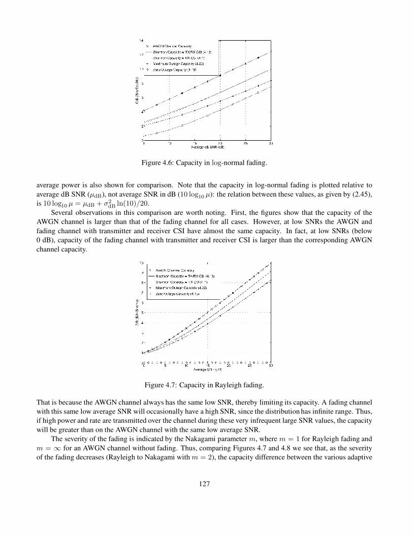
Figure 4.6: Capacity in log-normal fading.

average power is also shown for comparison. Note that the capacity in log-normal fading is plotted relative to

average dB SNR (µdB), not average SNR in dB (10 log10 µ): the relation between these values, as given by (2.45),

is 10 log10 µ = µdB + σ2dB ln(10)/20.

Several observations in this comparison are worth noting. First, the figures show that the capacity of the

AWGN channel is larger than that of the fading channel for all cases. However, at low SNRs the AWGN and

fading channel with transmitter and receiver CSI have almost the same capacity. In fact, at low SNRs (below

0 dB), capacity of the fading channel with transmitter and receiver CSI is larger than the corresponding AWGN

channel capacity.

Figure 4.7: Capacity in Rayleigh fading.

That is because the AWGN channel always has the same low SNR, thereby limiting its capacity. A fading channel

with this same low average SNR will occasionally have a high SNR, since the distribution has infinite range. Thus,

if high power and rate are transmitted over the channel during these very infrequent large SNR values, the capacity

will be greater than on the AWGN channel with the same low average SNR.

The severity of the fading is indicated by the Nakagami parameter m, where m = 1 for Rayleigh fading and

m = ∞ for an AWGN channel without fading. Thus, comparing Figures 4.7 and 4.8 we see that, as the severity

of the fading decreases (Rayleigh to Nakagami with m = 2), the capacity difference between the various adaptive

127

Figure 4.8: Capacity in Nakagami fading (m = 2).

policies also decreases, and their respective capacities approach that of the AWGN channel.

The difference between the capacity curves under transmitter and receiver CSI (4.16) and receiver CSI only

(4.7) are negligible in all cases. Recalling that capacity under receiver CSI only (4.7) and under transmitter and

receiver CSI without power adaptation (4.10) are the same, we conclude that, if the transmission rate is adapted

relative to the channel, then adapting the power as well yields a negligible capacity gain. It also indicates that

transmitter adaptation yields a negligible capacity gain relative to using only receiver side information. In severe

fading conditions (Rayleigh and log-normal fading), maximum outage capacity exhibits a 1–5-dB rate penalty

and zero-outage capacity yields a large capacity loss relative to Shannon capacity. However, under mild fading

conditions (Nakagami with m = 2) the Shannon, maximum outage, and zero-outage capacities are within 3 dB of

each other and within 4 dB of the AWGN channel capacity. These differences will further decrease as the fading

diminishes (m → ∞ for Nakagami fading).

We can view these results as a trade-off between capacity and complexity. The adaptive policy with transmitter

and receiver side information requires more complexity in the transmitter (and typically also requires a feedback

path between the receiver and transmitter to obtain the side information). However, the decoder in the receiver is

relatively simple. The nonadaptive policy has a relatively simple transmission scheme, but its code design must

use the channel correlation statistics (often unknown) and the decoder complexity is proportional to the channel

decorrelation time. The channel inversion and truncated inversion policies use codes designed for AWGN channels

and thus are the least complex to implement, but in severe fading conditions they exhibit large capacity losses

relative to the other techniques.

In general, Shannon capacity analysis does not show how to design adaptive or non-adaptive techniques for

real systems. Achievable rates for adaptive trellis-coded MQAM have been investigated in [28], where a simple

four-state trellis code combined with adaptive six-constellation MQAM modulation was shown to achieve rates

within 7 dB of the Shannon capacity (4.12) in Figures 4.6 and 4.7. More complex codes further close the gap to

the Shannon limit of fading channels with transmitter adaptation.

4.3 Capacity of Frequency-Selective Fading Channels

In this section we examine the Shannon capacity of frequency-selective fading channels. We first consider the

capacity of a time-invariant frequency-selective fading channel. This capacity analysis is like that of a flat fading

channel but with the time axis replaced by the frequency axis. Then we discuss the capacity of time-varying

frequency-selective fading channels.

128

4.3.1 Time-Invariant Channels

Consider a time-invariant channel with frequency responseH(f), as shown in Figure 4.9. Assume a total transmit

power constraint P . When the channel is time invariant it is typically assumed that H(f) is known to both

the transmitter and receiver. The capacity of time-invariant channels under different assumptions about channel

knowledge is discussed in [23, 25].

Let us first assume that H(f) is block fading, so that frequency is divided into subchannels of bandwidth Bwith H(f) = Hj constant over each subchannel, as shown in Figure 4.10.

Figure 4.9: Time-invariant frequency-selective fading channel.

Figure 4.10: Block frequency-selective fading.

The frequency-selective fading channel thus consists of a set of AWGN channels in parallel with SNR

|Hj|2Pj/(N0B) on the jth channel, where Pj is the power allocated to the jth channel in this parallel set sub-

ject to the power constraint∑

j Pj ≤ P .

The capacity of this parallel set of channels is the sum of rates on each channel with power optimally allocated

over all channels [5, 6]:

C =∑

maxPj :P

j Pj≤P

B log2

(

1 +|Hj|2PjN0B

)

. (4.25)

Note that this is similar to the capacity and optimal power allocation for a flat fading channel, with power and rate

changing over frequency in a deterministic way rather than over time in a probabilistic way. The optimal power

allocation is found via the same Lagrangian technique used in the flat-fading case, which leads to the water-filling

power allocation

PjP

=

1/γ0 − 1/γj γj ≥ γ0,

0 γj < γ0,(4.26)

for some cutoff value γ0, where γj = |Hj|2P/(N0B) is the SNR associated with the jth channel assuming it is

allocated the entire power budget P .3 This optimal power allocation is illustrated in Figure 4.11. The cutoff value

3We define γj with respect to the total power P because of the normalization by P on the left hand side of (4.26).

129

is obtained by substituting the power adaptation formula into the power constraint, so γ0 must satisfy

∑

j:γj≥γ0

(1

γ0− 1

γj

)

= 1. (4.27)

Figure 4.11: Water-filling in frequency-selective block fading.

The capacity then becomes

C =∑

j:γj≥γ0

B log2

(γjγ0

)

. (4.28)

This capacity is achieved by transmitting at different rates and powers over each subchannel. Multicarrier modu-

lation uses the same technique in adaptive loading, as discussed in more detail in Section 12.3.

When H(f) is continuous, the capacity under power constraint P is similar to the case of the block fading

channel, with some mathematical intricacies needed to show that the channel capacity is given by

C = maxP (f):

R

P (f)df≤P

∫

log2

(

1 +|H(f)|2P (f)

N0

)

df. (4.29)

The expression inside the integral can be thought of as the incremental capacity associated with given frequency fover the bandwidth df with power allocation P (f) and channel gain |H(f)|2. This result is formally proven using

a Karhunen-Loeve expansion of the channel h(t) to create an equivalent set of parallel independent channels [5,

Chap. 8.5]. An alternate proof [33] decomposes the channel into a parallel set using the discrete Fourier transform

(DFT); the same premise is used in the discrete implementation of multicarrier modulation described in Section

12.4.

The power allocation over frequency, P (f), that maximizes (4.29) is found via the Lagrangian technique. The

resulting optimal power allocation is water-filling over frequency:

P (f)

P=

1/γ0 − 1/γ(f) γ(f) ≥ γ0,

0 γ(f) < γ0,(4.30)

where γ(f) = |H(f)|2P/N0. This results in channel capacity

C =

∫

f :γ(f)≥γ0

log2

(γ(f)

γ0

)

df. (4.31)

Example 4.7: Consider a time-invariant frequency-selective block fading channel that has three subchannels of

bandwidthB = 1 MHz. The frequency responses associated with each subchannel areH1 = 1, H2 = 2, andH3 =

130

Figure 4.12: Channel division in frequency-selective fading.

3, respectively. The transmit power constraint is P = 10 mW and the noise PSD N0/2 has N0 = 10−9 W/Hz.

Find the Shannon capacity of this channel and the optimal power allocation that achieves this capacity. Solution:

We first Find γj = |Hj|2P/(N0B) for each subchannel, yielding γ1 = 10, γ2 = 40, and γ3 = 90. The cutoff γ0

must satisfy (4.27). Assuming that all subchannels are allocated power, this yields

3

γ0= 1 +

∑

j

1

γj= 1.14 ⇒ γ0 = 2.64 < γj∀j.

Since the cutoff γ0 is less than γj for all j, our assumption that all subchannels are allocated power is consistent, so

this is the correct cutoff value. The corresponding capacity isC =∑3

j=1B log2(γj/γ0) = 1000000(log2(10/2.64)+log2(40/2.64) + log2(90/2.64)) = 10.93 Mbps.

4.3.2 Time-Varying Channels

The time-varying frequency-selective fading channel is similar to the model shown in Figure 4.9 except that

H(f) = H(f, i); that is, the channel varies over both frequency and time. It is difficult to determine the capac-

ity of time-varying frequency-selective fading channels – even when the instantaneous channel H(f, i) is known

perfectly at the transmitter and receiver – because of the effects of self-interference (ISI). In the case of transmitter

and receiver side information, the optimal adaptation scheme must consider (a) the effect of the channel on the past

sequence of transmitted bits and (b) how the ISI resulting from these bits will affect future transmissions [34]. The

capacity of time-varying frequency-selective fading channels is in general unknown, but there do exist upper and

lower bounds as well as limiting formulas [34, 35].

We can approximate channel capacity in time-varying frequency-selective fading by taking the channel band-

width B of interest and then dividing it up into subchannels the size of the channel coherence bandwidth Bc, as

shown in Figure 4.12. We then assume that each of the resulting subchannels is independent, time varying, and flat

fading with H(f, i) = Hj[i] on the jth subchannel.

Under this assumption, we obtain the capacity for each of these flat fading subchannels based on the average

power Pj that we allocate to each subchannel, subject to a total power constraint P . Since the channels are

independent, the total channel capacity is just equal to the sum of capacities on the individual narrowband flat

fading channels – subject to the total average power constraint and averaged over both time and frequency:

C = maxPj:

P

j Pj≤P

∑

j

Cj(Pj), (4.32)

where Cj(Pj) is the capacity of the flat fading subchannel with average power Pj and bandwidth Bc given by

(4.16), (4.7), (4.20), or (4.24) for Shannon capacity under different side information and power allocation policies.

We can also define Cj(Pj) as a capacity versus outage if only the receiver has side information.

131

We will focus on Shannon capacity assuming perfect transmitter and receiver channel CSI, since this up-

perbounds capacity under any other side information assumptions or suboptimal power allocation strategies. We

know that if we fix the average power per subchannel then the optimal power adaptation follows a water-filling for-

mula. We expect that the optimal average power to be allocated to each subchannel will also follow a water-filling

formula, where more average power is allocated to better subchannels. Thus we expect that the optimal power allo-

cation is a two-dimensional water-filling in both time and frequency. We now obtain this optimal two-dimensional

water-filling and the corresponding Shannon capacity.

Define γj[i] = |Hj[i]|2P /(N0B) to be the instantaneous SNR on the jth subchannel at time i assuming the

total power P is allocated to that time and frequency. We allow the power Pj(γj) to vary with γj[i]. The Shannon

capacity with perfect transmitter and receiver CSI is given by optimizing power adaptation relative to both time

(represented by γj[i] = γj) and frequency (represented by the subchannel index j):

C = maxPj(γj ):

P

j

R

∞

0 Pj (γj)p(γj)dγj≤P

∑

j

∫ ∞

0Bc log2

(

1 +Pj(γj)γj

P

)

p(γj)dγj. (4.33)

To find the optimal power allocation Pj(γj), we form the Lagrangian

J(Pj(γj))

=∑

j

∫ ∞

0Bc log2

(

1 +Pj(γj)γj

P

)

p(γj)dγj − λ∑

j

∫ ∞

0Pj(γj)p(γj)dγj. (4.34)

Note that (4.34) is similar to the Lagrangian (4.13) for the flat fading channel except that the dimension of frequency

has been added by summing over the subchannels. Differentiating the Lagrangian and setting this derivative equal

to zero eliminates all terms except the given subchannel and associated SNR:

∂J(Pj(γj))

∂Pj(γj)=

[(Bc/ ln(2)

1 + γjPj(γj)/P

)γjP

− λ

]

p(γj) = 0. (4.35)

Solving for Pj(γj) yields the same water-filling as the flat-fading case:

Pj(γj)

P=

1/γ0 − 1/γj γj ≥ γ0,

0 γj < γ0,(4.36)

where the cutoff value γ0 is obtained from the total power constraint over both time and frequency:

∑

j

∫ ∞

0Pj(γj)p(γj)dγj = P . (4.37)

Thus, the optimal power allocation (4.36) is a two-dimensional water-filling with a common cutoff value γ0.

Dividing the constraint (4.37) by P and substituting into the optimal power allocation (4.36), we get that γ0 must

satisfy

∑

j

∫ ∞

γ0

(1

γ0− 1

γj

)

p(γj)dγj = 1. (4.38)

It is interesting to note that, in the two-dimensional water-filling, the cutoff value for all subchannels is the same.

This implies that even if the fading distribution or average fade power on the subchannels is different, all subchan-

nels suspend transmission when the instantaneous SNR falls below the common cutoff value γ0. Substituting the

optimal power allocation (4.37) into the capacity expression (4.33) yields

132

C =∑

j

∫ ∞

γ0

Bc log2

(γjγ0

)

p(γj)dγj. (4.39)

133

Chapter 4 Problems

1. Capacity in AWGN is given by C = B log2(1 + P/(N0B)), where P is the received signal power, B is the

signal bandwidth, and N0/2 is the noise PSD. Find capacity in the limit of infinite bandwidth B → ∞ as a

function of P .

2. Consider an AWGN channel with bandwidth 50 MHz, received signal power 10 mW, and noise PSD N0/2whereN0 = 2 · 10−9 W/Hz. How much does capacity increase by doubling the received power? How much

does capacity increase by doubling the channel bandwidth?

3. Consider two users simultaneously transmitting to a single receiver in an AWGN channel. This is a typical

scenario in a cellular system with multiple users sending signals to a base station. Assume the users have

equal received power of 10 mW and total noise at the receiver in the bandwidth of interest of 0.1 mW. The

channel bandwidth for each user is 20 MHz.

(a) Suppose that the receiver decodes user 1’s signal first. In this decoding, user 2’s signal acts as noise (as-

sume it has the same statistics as AWGN). What is the capacity of user 1’s channel with this additional

interference noise?

(b) Suppose that, after decoding user 1’s signal, the decoder re-encodes it and subtracts it out of the re-

ceived signal. Now, in the decoding of user 2’s signal, there is no interference from user 1’s signal.

What then is the Shannon capacity of user 2’s channel?

Note: We will see in Chapter 14 that the decoding strategy of successively subtracting out decoded signals

is optimal for achieving Shannon capacity of a multiuser channel with independent transmitters sending to

one receiver.

4. Consider a flat fading channel of bandwidth 20 MHz and where, for a fixed transmit power P , the received

SNR is one of six values: γ1 = 20 dB, γ2 = 15 dB, γ3 = 10 dB, γ4 = 5 dB, γ5 = 0 dB, and γ6 = −5 dB.

The probabilities associated with each state are p1 = p6 = .1, p2 = p4 = .15, and p3 = p5 = .25. Assume

that only the receiver has CSI.

(a) Find the Shannon capacity of this channel.

(b) Plot the capacity versus outage for 0 ≤ Pout < 1 and find the maximum average rate that can be

correctly received (maximum Cout).

5. Consider a flat fading channel in which, for a fixed transmit power P , the received SNR is one of four values:

γ1 = 30 dB, γ2 = 20 dB, γ3 = 10 dB, and γ4 = 0 dB. The probabilities associated with each state are

p1 = .2, p2 = .3, p3 = .3, and p4 = .2. Assume that both transmitter and receiver have CSI.

(a) Find the optimal power adaptation policy P [i]/P for this channel and its corresponding Shannon ca-

pacity per unit hertz (C/B).

(b) Find the channel inversion power adaptation policy for this channel and associated zero-outage capacity

per unit bandwidth.

(c) Find the truncated channel inversion power adaptation policy for this channel and associated outage

capacity per unit bandwidth for three different outage probabilities: Pout = .1, Pout = .25, and Pout

(and the associated cutoff γ0) equal to the value that achieves maximum outage capacity.

134

6. Consider a cellular system where the power falloff with distance follows the formula Pr(d) = Pt(d0/d)α,

where d0 = 100 m and α is a random variable. The distribution for α is p(α = 2) = .4, p(α = 2.5) =

.3, p(α = 3) = .2, and p(α = 4) = .1. Assume a receiver at a distance d = 1000 m from the transmitter,

with an average transmit power constraint of Pt = 100 mW and a receiver noise power of .1 mW. Assume

that both transmitter and receiver have CSI.

(a) Compute the distribution of the received SNR.

(b) Derive the optimal power adaptation policy for this channel and its corresponding Shannon capacity

per unit hertz (C/B).

(c) Determine the zero-outage capacity per unit bandwidth of this channel.

(d) Determine the maximum outage capacity per unit bandwidth of this channel.

7. In this problem we explore power allocation under a fixed energy constraint to maximize the number of bits

transmitted. Consider a cellular system with a mobile receiver. The receiver stops at point A (100m from

the cell phone tower) for 10 minutes and point B (500m from the cell phone tower) for 20 minutes. Assume

the signal from the cell phone tower to the receiver only experiences path loss under the simplified path loss

model with γ = 3, d0 = 1m, and K = 1 along with AWGN, that the channel bandwidth is 20MHz, and the

receiver noise PSD is N0 = 5 × 10−14mW/Hz. Also, assume a fixed transmit power of 1mW.

(a) What is the SNR received at points A and B?

(b) What is total amount of energy (in Joules) that is transmitted during the two stops.

(c) Assuming the transmitter sends data with a rate equal to the Shannon capacity of the channel at each

of the stops, what is the total number of bits received?

(d) Suppose now that the cell phone tower does not send at a fixed transmit power but fixes the total

number of Joules it will transmit to the receiver at each of the two stops. Using the total amount of

energy derived in part (b), determine the optimal allocation of this total energy at each of the stops to

maximize the number of bits received. Assume that the transmitter sends data at a rate equal to the

Shannon capacity with SNR based on your optimal energy allocation. How many bits are received

with this optimal energy allocation and how does it compare to your answer in part (c)?

8. In this problem we explore why channel inversion leads to zero capacity in Rayleigh fading. Assume a

Rayleigh fading channel with γ = 1 so the receiver power has an exponential distribution p(γ) = e−γ .

(a) Show using a first-order Taylor series expansion of e−γ around γ = 0 that p(γ) = e−γ > 1 − γ .

(b) We will now show that E[

1γ

]

is unbounded by taking the expectation for γ ∈ (0, c) for some small

constant c. Fix this small constant c and a smaller constant ε < c. Then compute the following lower

bound for E[

1γ

]

by taking the expectation over the interval (ε, c) and using the lower bound on p(γ)

from part (a):

E

[1

γ

]

>

∫ c

ε

1

γ(1 − γ)dγ.

Show that as ε → 0, the above expression becomes unbounded. This suggests that the transmit power

needed to maintain a constant received power by inverting Rayleigh fading is unbounded.

9. Assume a Rayleigh fading channel, where the transmitter and receiver have CSI and the distribution of the

fading SNR p(γ) is exponential with mean γ = 10 dB. Assume a channel bandwidth of 10 MHz.

135

Figure 4.13: Interference channel for Problem 4.8.

(a) Find the cutoff value γ0 and the corresponding power adaptation that achieves Shannon capacity on

this channel.

(b) Compute the Shannon capacity of this channel.

(c) Compare your answer in part (b) with the channel capacity in AWGN with the same average SNR.

(d) Compare your answer in part (b) with the Shannon capacity when only the receiver knows γ[i].

(e) Compare your answer in part (b) with the zero-outage capacity and outage capacity when the outage

probability is .05.

(f) Repeat parts (b), (c), and (d) – that is, obtain the Shannon capacity with perfect transmitter and receiver

side information, in AWGN for the same average power, and with just receiver side information – for

the same fading distribution but with mean γ = −5 dB. Describe the circumstances under which a

fading channel has higher capacity than an AWGN channel with the same average SNR and explain

why this behavior occurs.

10. This problem illustrates the capacity gains that can be obtained from interference estimation and also how

a malicious jammer can wreak havoc on link performance. Consider the interference channel depicted in

Figure 4.13. The channel has a combination of AWGN n[k] and interference I [k]. We model I [k] as AWGN.

The interferer is on (i.e., the switch is down) with probability .25 and off (i.e., switch up) with probability

.75. The average transmit power is 10 mW, the noise PSD has N0 = 10−8 W/Hz, the channel bandwidthBis 10 kHz (receiver noise power is N0B), and the interference power (when on) is 9 mW.

(a) What is the Shannon capacity of the channel if neither transmitter nor receiver know when the interferer

is on?

(b) What is the capacity of the channel if both transmitter and receiver know when the interferer is on?

(c) Suppose now that the interferer is a malicious jammer with perfect knowledge of x[k] (so the interferer

is no longer modeled as AWGN). Assume that neither transmitter nor receiver has knowledge of the

jammer behavior. Assume also that the jammer is always on and has an average transmit power of

10 mW. What strategy should the jammer use to minimize the SNR of the received signal?

11. Consider the malicious interferer of Problem 4.8. Suppose that the transmitter knows the interference sig-

nal perfectly. Consider two possible transmit strategies under this scenario: the transmitter can ignore the

interference and use all its power for sending its signal, or it can use some of its power to cancel out the in-

terferer (i.e., transmit the negative of the interference signal). In the first approach the interferer will degrade

capacity by increasing the noise, and in the second strategy the interferer also degrades capacity because the

transmitter sacrifices some power to cancel out the interference. Which strategy results in higher capacity?

Note: There is a third strategy, in which the encoder actually exploits the structure of the interference in its

encoding. This strategy is called dirty paper coding and is used to achieve Shannon capacity on broadcast

channels with multiple antennas, as described in Chapter 14.

136

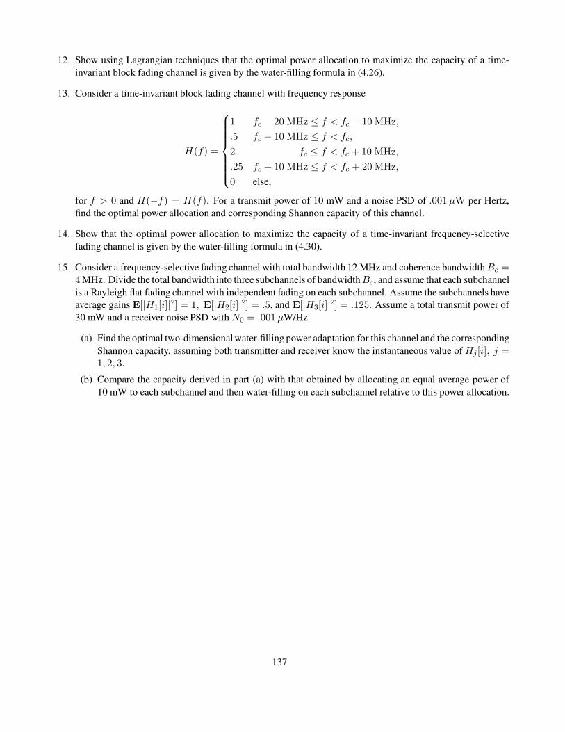
12. Show using Lagrangian techniques that the optimal power allocation to maximize the capacity of a time-

invariant block fading channel is given by the water-filling formula in (4.26).

13. Consider a time-invariant block fading channel with frequency response

H(f) =

1 fc − 20 MHz ≤ f < fc − 10 MHz,

.5 fc − 10 MHz ≤ f < fc,

2 fc ≤ f < fc + 10 MHz,

.25 fc + 10 MHz ≤ f < fc + 20 MHz,

0 else,

for f > 0 and H(−f) = H(f). For a transmit power of 10 mW and a noise PSD of .001 µW per Hertz,

find the optimal power allocation and corresponding Shannon capacity of this channel.

14. Show that the optimal power allocation to maximize the capacity of a time-invariant frequency-selective

fading channel is given by the water-filling formula in (4.30).

15. Consider a frequency-selective fading channel with total bandwidth 12 MHz and coherence bandwidthBc =4 MHz. Divide the total bandwidth into three subchannels of bandwidthBc, and assume that each subchannel

is a Rayleigh flat fading channel with independent fading on each subchannel. Assume the subchannels have

average gains E[|H1[i]|2] = 1, E[|H2[i]|2] = .5, and E[|H3[i]|2] = .125. Assume a total transmit power of

30 mW and a receiver noise PSD with N0 = .001 µW/Hz.

(a) Find the optimal two-dimensional water-filling power adaptation for this channel and the corresponding

Shannon capacity, assuming both transmitter and receiver know the instantaneous value of Hj[i], j =1, 2, 3.

(b) Compare the capacity derived in part (a) with that obtained by allocating an equal average power of

10 mW to each subchannel and then water-filling on each subchannel relative to this power allocation.

137

Bibliography

[1] C. E. Shannon, “A mathematical theory of communication,” Bell System Tech. J ., pp. 379–423, 623–56,

1948.

[2] C. E. Shannon, “Communications in the presence of noise.” Proc. IRE, pp. 10–21, 1949.

[3] C. E. Shannon and W. Weaver, The Mathematical Theory of Communication, University of Illinois Press,

Urbana, 1949.

[4] M. Medard, “The effect upon channel capacity in wireless communications of perfect and imperfect knowl-

edge of the channel,” IEEE Trans. Inform. Theory, pp. 933–46, May 2000.

[5] R. G. Gallager, Information Theory and Reliable Communication, Wiley, New York, 1968.

[6] T. Cover and J. Thomas, Elements of Information Theory, Wiley, New York, 2nd Ed, 2006.

[7] Y. Polyanskiy, H. V. Poor and S. Verdu, “Channel Coding Rate in the Finite Blocklength Regime,” IEEE

Transactions on Information Theory, vol. 56, no. 5, pp. 2307-2359, May 2010.

[8] C. Berrou, A. Glavieux, “Near optimum error correcting coding and decoding: Turbo-codes”, IEEE Trans-

actions on Commununications, vol. 44, no. 10, pp. 1261-1271, Oct. 1996.

[9] R.G. Gallager, Low-Density Parity-Check Codes. Cambridge, MA: MIT Press, 1963 (Sc.D. MIT, 1960).

[10] R. Urbanke, B. Rimoldi, “Lattice codes can achieve capacity on the AWGN channel”, IEEE Transactions on

Information Theory, vol. 44, no. 1, pp. 273-278, Jan. 1998.

[11] E. Arikan, “Channel polarization: A method for constructing capacity-achieving codes for symmetric binary-

input memoryless channels”, IEEE Transactions on Information Theory, vol. 55, no. 7, pp. 3051-3073, July

2009.

[12] I. Csiszar and J. Korner, Information Theory: Coding Theorems for Discrete Memoryless Channels, Aca-

demic Press, New York, 1981.

[13] I. Csiszar and P. Narayan, “The capacity of the arbitrarily varying channel,” IEEE Trans. Inform. Theory, pp.

18–26, January 1991.

[14] I. C. Abou-Faycal, M. D. Trott, and S. Shamai, “The capacity of discrete-time memoryless Rayleigh fading

channels,” IEEE Trans. Inform. Theory, pp. 1290–1301, May 2001.

[15] A. Lapidoth and S. M. Moser, “Capacity bounds via duality with applications to multiple-antenna systems on

flat-fading channels,” IEEE Trans. Inform. Theory, pp. 2426–67, October 2003.

138

[16] A. J. Goldsmith and P. P. Varaiya, “Capacity, mutual information, and coding for finite-state Markov chan-

nels,” IEEE Trans. Inform. Theory, pp. 868–86, May 1996.

[17] M. Mushkin and I. Bar-David, “Capacity and coding for the Gilbert-Elliot channel,” IEEE Trans. Inform.

Theory, pp. 1277–90, November 1989.

[18] T. Holliday, A. Goldsmith, and P. Glynn, “Capacity of finite state Markov channels with general inputs,”

Proc. IEEE Internat. Sympos. Inform. Theory, p. 289, July 2003.

[19] R. J. McEliece and W. E. Stark, “Channels with block interference,” IEEE Trans. Inform. Theory, pp. 44–53,

January 1984.

[20] A. Lapidoth and S. Shamai, “Fading channels: How perfect need ‘perfect side information’ be?” IEEE Trans.

Inform. Theory, pp. 1118–34, November 1997.

[21] G. J. Foschini, D. Chizhik, M. Gans, C. Papadias, and R. A. Valenzuela, “Analysis and performance of some

basic space-time architectures,” IEEE J. Sel. Areas Commun., pp. 303–20, April 2003.

[22] W. L. Root and P. P. Varaiya, “Capacity of classes of Gaussian channels,” SIAM J. Appl. Math., pp. 1350–93,

November 1968.

[23] J. Wolfowitz, Coding Theorems of Information Theory, 2nd ed., Springer-Verlag, New York, 1964.

[24] A. J. Goldsmith and P. P. Varaiya, “Capacity of fading channels with channel side information,” IEEE Trans.

Inform. Theory, pp. 1986–92, November 1997.

[25] G. Caire and S. Shamai, “On the capacity of some channels with channel state information,” IEEE Trans.

Inform. Theory, pp. 2007–19, September 1999.

[26] M.-S. Alouini and A. J. Goldsmith, “Capacity of Rayleigh fading channels under different adaptive transmis-

sion and diversity combining techniques,” IEEE Trans. Veh. Tech. pp. 1165–81, July 1999.

[27] S.-G. Chua and A. J. Goldsmith, “Variable-rate variable-power MQAM for fading channels,” IEEE Trans.

Commun., pp. 1218–30, October 1997.

[28] S.-G. Chua and A. J. Goldsmith, “Adaptive coded modulation for fading channels,” IEEE Trans. Commun.,

pp. 595–602, May 1998.

[29] K. S. Gilhousen, I. M. Jacobs, R. Padovani, A. J. Viterbi, L. A. Weaver, Jr., and C. E. Wheatley III, “On the

capacity of a cellular CDMA system,” IEEE Trans. Veh. Tech. pp. 303–12, May 1991.

[30] G. J. Foschini, “Layered space-time architecture for wireless communication in fading environments when

using multi-element antennas,” Bell System Tech. J ., pp. 41–59, Autumn 1996.

[31] E. Teletar, “Capacity of multi-antenna Gaussian channels,” AT&T Bell Labs Intemal Tech. Memo, June 1995.

[32] G. J. Foschini and M. Gans, “On limits of wireless communications in a fading environment when using

multiple antennas,” Wireless Pers. Commun., pp. 311–35, March 1998.

[33] W. Hirt and J. L. Massey, “Capacity of the discrete-time Gaussian channel with intersymbol interference,”

IEEE Trans. Inform. Theory, pp. 380–8, May 1988.

139

[34] A. Goldsmith and M. Medard, “Capacity of time-varying channels with channel side information,” IEEE

Trans. Inform. Theory Vol. 53, No. 3, pp. 881-899, March 2007.

[35] S. Diggavi, ‘Analysis of multicarrier transmission in time-varying channels,” Proc. IEEE Internat. Conf.

Commun., pp. 1191–5, June 1997.

140

Chapter 5

Digital Modulation and Detection

The advances over the last several decades in hardware and digital signal processing have made digital transceivers

much cheaper, faster, and more power efficient than analog transceivers. More importantly, digital modulation

offers a number of other advantages over analog modulation, including higher spectral efficiency, powerful error

correction techniques, resistance to channel impairments, more efficient multiple access strategies, and better secu-

rity and privacy. Specifically, high-level digital modulation techniques such as MQAM allow much more efficient

use of spectrum than is possible with analog modulation. Advances in coding and coded modulation applied to dig-

ital signaling make the signal much less susceptible to noise and fading, and equalization or multicarrier techniques

can be used to mitigate intersymbol interference (ISI). Spread-spectrum techniques applied to digital modulation

can simultaneously remove or combine multipath, resist interference, and detect multiple users. Finally, digital

modulation is much easier to encrypt, resulting in a higher level of security and privacy for digital systems. For all

these reasons, systems currently being built or proposed for wireless applications are all digital systems.

Digital modulation and detection consist of transferring information in the form of bits over a communication

channel. The bits are binary digits taking on the values of either 1 or 0. These information bits are derived

from the information source, which may be a digital source or an analog source that has been passed through

an A/D converter. Both digital and A/D-converted analog sources may be compressed to obtain the information

bit sequence. Digital modulation consists of mapping the information bits into an analog signal for transmission

over the channel. Detection consists of estimating the original bit sequence based on the signal received over the

channel. The main considerations in choosing a particular digital modulation technique are high data rate; high

spectral efficiency (minimum bandwidth occupancy); high power efficiency (minimum required transmit power);

robustness to channel impairments (minimum probability of bit error); and low power/cost implementation. Often

these are conflicting requirements, and the choice of modulation is based on finding the technique that achieves the

best trade-off between them.

There are two main categories of digital modulation: amplitude/phase modulation and frequency modulation.

Since frequency modulation typically has a constant signal envelope and is generated using nonlinear techniques,

this modulation is also called constant envelope modulation or nonlinear modulation, and amplitude/phase mod-

ulation is also called linear modulation. Linear modulation generally has better spectral properties than nonlinear

modulation, since nonlinear processing leads to spectral broadening. However, amplitude and phase modulation

embeds the information bits into the amplitude or phase of the transmitted signal, which is more susceptible to

variations from fading and interference. In addition, amplitude and phase modulation techniques typically require

linear amplifiers, which are more expensive and less power efficient than the nonlinear amplifiers that can be used

with nonlinear modulation. Thus, the trade-off between linear versus nonlinear modulation is one of better spectral

efficiency for the former technique and better power efficiency and resistance to channel impairments for the lat-

ter. Once the modulation technique is determined, the constellation size must be chosen. Modulations with large

141

constellations have higher data rates for a given signal bandwidth, but they are more susceptible to noise, fading,

and hardware imperfections. Finally, some demodulators require a coherent phase reference with respect to the

transmitted signal. Obtaining this coherent reference may be difficult or significantly increase receiver complexity.

Thus, modulation techniques that do not require a coherent phase reference in the receiver are desirable.

We begin this chapter with a general discussion of signal space concepts. These concepts greatly simplify

the design and analysis of modulation and demodulation techniques by mapping infinite-dimensional signals to

a finite-dimensional vector space. The general principles of signal space analysis will then be applied to the

analysis of amplitude and phase modulation techniques, including pulse amplitude modulation (PAM), phase-

shift keying (PSK), and quadrature amplitude modulation (QAM). We will also discuss constellation shaping

and quadrature offset techniques for these modulations, as well as differential encoding to avoid the need for

a coherent phase reference. We then describe frequency modulation techniques and their properties, including

frequency-shift keying (FSK), minimum-shift keying (MSK), and continuous-phase FSK (CPFSK). Both coherent

and noncoherent detection of these techniques will be discussed. Pulse-shaping techniques to improve the spectral

properties of the modulated signals will also be covered, along with issues associated with carrier phase recovery

and symbol synchronization.

5.1 Signal Space Analysis

Digital modulation encodes a bit stream of finite length into one of several possible transmitted signals. Intuitively,

the receiver minimizes the probability of detection error by decoding the received signal as the signal in the set of

possible transmitted signals that is “closest” to the one received. Determining the distance between the transmitted

and received signals requires a metric for the distance between signals. By representing signals as projections

onto a set of basis functions, we obtain a one-to-one correspondence between the set of transmitted signals and

their vector representations. Thus, we can analyze signals in finite-dimensional vector space instead of infinite-

dimensional function space, using classical notions of distance for vector spaces. In this section we show how

digitally modulated signals can be represented as vectors in an appropriately defined vector space and how optimal

demodulation methods can be obtained from this vector-space representation. This general analysis will then be

applied to specific modulation techniques in later sections.

Figure 5.1: Communication system model.

5.1.1 Signal and System Model

Consider the communication system model shown in Figure 5.1. Every T seconds, the system sends K = log2M

bits of information through the channel for a data rate of R = K/T bits per second (bps). There are M =2K possible sequences of K bits, and we say that each bit sequence of length K comprises a message mi =

b1, . . . , bK ∈ M, where M = m1, . . . , mM is the set of all such messages. The messages have probability

pi of being selected for transmission, where∑M

i=1 pi = 1.

Suppose messagemi is to be transmitted over the channel during the time interval [0, T ). Because the channel

is analog, the message must be embedded into an analog signal for channel transmission. Hence, each message

142

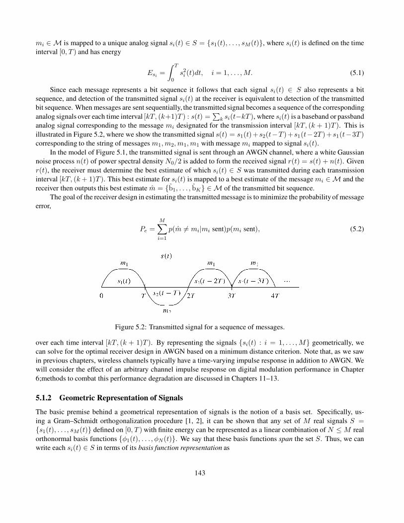
mi ∈ M is mapped to a unique analog signal si(t) ∈ S = s1(t), . . . , sM(t), where si(t) is defined on the time

interval [0, T ) and has energy

Esi =

∫ T

0s2i (t)dt, i = 1, . . . ,M. (5.1)

Since each message represents a bit sequence it follows that each signal si(t) ∈ S also represents a bit

sequence, and detection of the transmitted signal si(t) at the receiver is equivalent to detection of the transmitted

bit sequence. When messages are sent sequentially, the transmitted signal becomes a sequence of the corresponding

analog signals over each time interval [kT, (k+1)T ) : s(t) =∑

k si(t−kT ), where si(t) is a baseband or passband

analog signal corresponding to the message mi designated for the transmission interval [kT, (k + 1)T ). This is

illustrated in Figure 5.2, where we show the transmitted signal s(t) = s1(t)+s2(t−T )+s1(t−2T )+s1(t−3T )corresponding to the string of messages m1, m2, m1, m1 with message mi mapped to signal si(t).

In the model of Figure 5.1, the transmitted signal is sent through an AWGN channel, where a white Gaussian

noise process n(t) of power spectral density N0/2 is added to form the received signal r(t) = s(t) + n(t). Given

r(t), the receiver must determine the best estimate of which si(t) ∈ S was transmitted during each transmission

interval [kT, (k+ 1)T ). This best estimate for si(t) is mapped to a best estimate of the message mi ∈ M and the

receiver then outputs this best estimate m = b1, . . . , bK ∈ M of the transmitted bit sequence.

The goal of the receiver design in estimating the transmitted message is to minimize the probability of message

error,

Pe =

M∑

i=1

p(m 6= mi|mi sent)p(mi sent), (5.2)

Figure 5.2: Transmitted signal for a sequence of messages.

over each time interval [kT, (k + 1)T ). By representing the signals si(t) : i = 1, . . . ,M geometrically, we

can solve for the optimal receiver design in AWGN based on a minimum distance criterion. Note that, as we saw

in previous chapters, wireless channels typically have a time-varying impulse response in addition to AWGN. We

will consider the effect of an arbitrary channel impulse response on digital modulation performance in Chapter

6;methods to combat this performance degradation are discussed in Chapters 11–13.

5.1.2 Geometric Representation of Signals

The basic premise behind a geometrical representation of signals is the notion of a basis set. Specifically, us-

ing a Gram–Schmidt orthogonalization procedure [1, 2], it can be shown that any set of M real signals S =s1(t), . . . , sM(t) defined on [0, T ) with finite energy can be represented as a linear combination of N ≤M real

orthonormal basis functions φ1(t), . . . , φN(t). We say that these basis functions span the set S. Thus, we can

write each si(t) ∈ S in terms of its basis function representation as

143

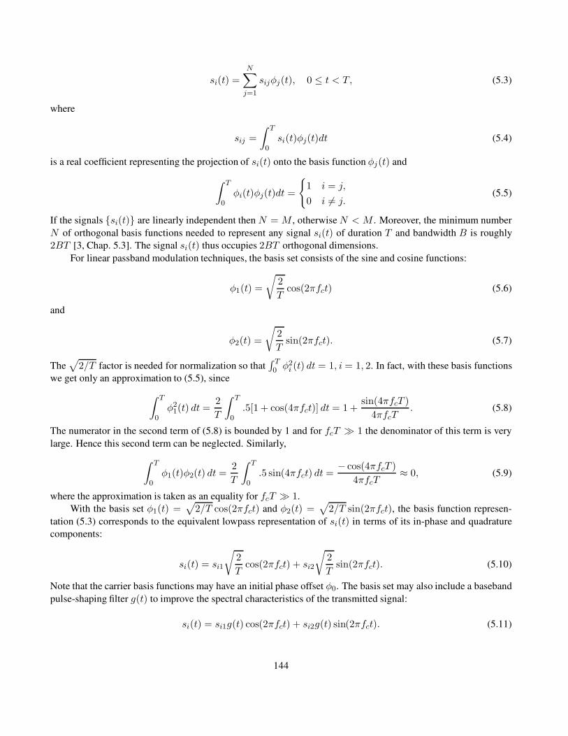
si(t) =

N∑

j=1

sijφj(t), 0 ≤ t < T, (5.3)

where

sij =

∫ T

0si(t)φj(t)dt (5.4)

is a real coefficient representing the projection of si(t) onto the basis function φj(t) and

∫ T

0φi(t)φj(t)dt =

1 i = j,

0 i 6= j.(5.5)

If the signals si(t) are linearly independent then N = M , otherwiseN < M . Moreover, the minimum number

N of orthogonal basis functions needed to represent any signal si(t) of duration T and bandwidth B is roughly

2BT [3, Chap. 5.3]. The signal si(t) thus occupies 2BT orthogonal dimensions.

For linear passband modulation techniques, the basis set consists of the sine and cosine functions:

φ1(t) =

√

2

Tcos(2πfct) (5.6)

and

φ2(t) =

√

2

Tsin(2πfct). (5.7)

The√

2/T factor is needed for normalization so that∫ T0 φ2

i (t) dt = 1, i = 1, 2. In fact, with these basis functions

we get only an approximation to (5.5), since

∫ T

0φ2

1(t) dt =2

T

∫ T

0.5[1 + cos(4πfct)] dt = 1 +

sin(4πfcT )

4πfcT. (5.8)

The numerator in the second term of (5.8) is bounded by 1 and for fcT 1 the denominator of this term is very

large. Hence this second term can be neglected. Similarly,

∫ T

0φ1(t)φ2(t) dt =

2

T

∫ T

0.5 sin(4πfct) dt =

− cos(4πfcT )

4πfcT≈ 0, (5.9)

where the approximation is taken as an equality for fcT 1.

With the basis set φ1(t) =√

2/T cos(2πfct) and φ2(t) =√

2/T sin(2πfct), the basis function represen-

tation (5.3) corresponds to the equivalent lowpass representation of si(t) in terms of its in-phase and quadrature

components:

si(t) = si1

√

2

Tcos(2πfct) + si2

√

2

Tsin(2πfct). (5.10)

Note that the carrier basis functions may have an initial phase offset φ0. The basis set may also include a baseband

pulse-shaping filter g(t) to improve the spectral characteristics of the transmitted signal:

si(t) = si1g(t) cos(2πfct) + si2g(t) sin(2πfct). (5.11)

144

In this case the pulse shape g(t) must maintain the orthonormal properties (5.5) of basis functions; that is, we must

have

∫ T

0g2(t) cos2(2πfct) dt = 1 (5.12)

and

∫ T

0g2(t) cos(2πfct) sin(2πfct) dt = 0, (5.13)

where the equalities may be approximations for fcT 1 as in (5.8) and (5.9). If the bandwidth of g(t) satisfies

B fc then g2(t) is roughly constant over Tc = 1/fc, so (5.13) is approximately true because the sine and

cosine functions are orthogonal over one period Tc. The simplest pulse shape that satisfies (5.12) and (5.13) is the

rectangular pulse shape g(t) =√

2/T, 0 ≤ t < T .

Example 5.1: Binary phase-shift keying (BPSK) modulation transmits the signal s1(t) = α cos(2πfct), 0 ≤ t ≤T , to send a 1-bit and the signal s2(t) = −α cos(2πfct), 0 ≤ t ≤ T , to send a 0-bit. Find the set of orthonormal

basis functions and coefficients sij for this modulation.

Solution: There is only one basis function for s1(t) and s2(t):

φ(t) =√

2/T cos(2πfct),

where the√

2/T is needed for normalization. The coefficients are then given by s1 = α√

T/2 and s2 =−α√

T/2.

Let si = (si1, . . . , siN ) ∈ RN be the vector of coefficients sij in the basis representation of si(t). We call si the

signal constellation point corresponding to the signal si(t). The signal constellation consists of all constellation

points s1, . . . , sM. Given the basis functions φ1(t), . . . , φN(t), there is a one-to-one correspondence between

the transmitted signal si(t) and its constellation point si. Specifically, si(t) can be obtained from si by (5.3) and

si can be obtained from si(t) by (5.4). Thus, it is equivalent to characterize the transmitted signal by si(t) or si.The representation of si(t) in terms of its constellation point si ∈ R

N is called its signal space representation,

and the vector space containing the constellation is called the signal space. A two-dimensional signal space is

illustrated in Figure 5.3, where we show si ∈ R2 with the ith axis of R

2 corresponding to the basis function φi(t),

i = 1, 2. With this signal space representation we can analyze the infinite-dimensional functions si(t) as vectors

si in finite-dimensional vector space R2. This greatly simplifies the analysis of system performance as well as the

derivation of optimal receiver design. Signal space representations for common modulation techniques like MPSK

and MQAM are two-dimensional (corresponding to the in-phase and quadrature basis functions) and will be given

later in the chapter.

In order to analyze signals via a signal space representation, we require a few definitions for vector character-

ization in the vector space RN . The length of a vector in R

N is defined as

‖si‖ 4=

√√√√

N∑

j=1

s2ij. (5.14)

The distance between two signal constellation points si and sk is thus

145

Figure 5.3: Signal space representation.

‖si − sk‖ =

√√√√

N∑

j=1

(sij − skj)2 =

√∫ T

0(si(t)− sk(t))2dt, (5.15)

where the second equality is obtained by writing si(t) and sk(t) in their basis representation (5.3) and using the

orthonormal properties of the basis functions. Finally, the inner product 〈si(t), sk(t)〉 between two real signals

si(t) and sk(t) on the interval [0, T ] is

〈si(t), sk(t)〉 =

∫ T

0

si(t)sk(t) dt. (5.16)

Similarly, the inner product 〈si, sk〉 between two constellation points is

〈si, sk〉 = sisTk =

∫ T

0

si(t)sk(t) dt = 〈si(t), sk(t)〉, (5.17)

Figure 5.4: Receiver structure for signal detection in AWGN.

where the equality between the vector inner product and the corresponding signal inner product follows from the

basis representation of the signals (5.3) and the orthonormal property of the basis functions (5.5). We say that two

146

signals are orthogonal if their inner product is zero. Thus, by (5.5), the basis functions are orthogonal functions.

5.1.3 Receiver Structure and Sufficient Statistics

Given the channel output r(t) = si(t) + n(t), 0 ≤ t < T , we now investigate the receiver structure to determine

which constellation point si (or, equivalently, which message mi) was sent over the time interval [0, T ). A similar

procedure is done for each time interval [kT, (k + 1)T ). We would like to convert the received signal r(t) over

each time interval into a vector, as this would allow us to work in finite-dimensional vector space when estimating

the transmitted signal. However, this conversion should not be allowed to compromise the estimation accuracy. We

now study a receiver that converts the received signal to a vector without compromising performance. Consider

the receiver structure shown in Figure 5.4, where

sij =

∫ T

0si(t)φj(t) dt (5.18)

and

nj =

∫ T

0n(t)φj(t) dt. (5.19)

We can rewrite r(t) as

N∑

j=1

(sij + nj)φj(t) + nr(t) =

N∑

j=1

rjφj(t) + nr(t); (5.20)

here rj = sij + nj and nr(t) = n(t) −∑Nj=1 njφj(t) denotes the “remainder” noise, which is the component

of the noise orthogonal to the signal space. If we can show that the optimal detection of the transmitted signal

constellation point si given received signal r(t) does not make use of the remainder noise nr(t), then the receiver

can make its estimate m of the transmitted message mi as a function of r = (r1, . . . , rN) alone. In other words,

r = (r1, . . . , rN) is a sufficient statistic for r(t) in the optimal detection of the transmitted messages.

It is intuitively clear that the remainder noise nr(t) should not help in detecting the transmitted signal si(t),

since its projection onto the signal space is zero. This is illustrated in Figure 5.5, where we assume the transmitted

signal lies in a space spanned by the basis set (φ1(t), φ2(t)) while the remainder noise lies in a space spanned by

the basis function φnr(t), which is orthogonal to φ1(t) and φ2(t). Specifically, the remainder noise in Figure 5.5 is

represented by nr , where nr(t) = nrφnr(t). The received signal is represented by r+nr, where r = (r1, r2) with

r(t) − nr(t) = r1φ1(t) + r2φ2(t). From the figure it appears that projecting r + nr onto r will not compromise

the detection of which constellation si was transmitted, since nr lies in a space orthogonal to the space in which silies. We now proceed to show mathematically why this intuition is correct.

Figure 5.5: Projection of received signal onto received vector r.

147

Let us first examine the distribution of r. Since n(t) is a Gaussian random process, if we condition on

the transmitted signal si(t) then the channel output r(t) = si(t) + n(t) is also a Gaussian random process and

r = (r1, . . . , rN) is a Gaussian random vector. Recall that rj = sij + nj . Thus, conditioned on a transmitted

constellation si, we have that

µrj |si= E[rj|si] = E[sij + nj|sij] = sij (5.21)

(since n(t) has zero mean) and

σrj |si= E[rj − µrj |si

]2 = E[sij + nj − sij |sij]2 = E[n2j ]. (5.22)

Moreover,

Cov[rjrk|si] = E[(rj − µrj )(rk − µrk )|si]= E[njnk]

= E

[∫ T

0n(t)φj(t) dt

∫ T

0n(τ)φk(τ) dτ

]

=

∫ T

0

∫ T

0

E[n(t)n(τ)]φj(t)φk(τ) dt dτ

=

∫ T

0

∫ T

0

N0

2δ(t− τ)φj(t)φk(τ) dt dτ

=N0

2

∫ T

0φj(t)φk(t) dt

=

N0/2 j = k,

0 j 6= k,(5.23)

where the last equality follows from the orthonormality of the basis functions. Thus, conditioned on the transmitted

constellation si, the rj are uncorrelated and, since they are Gaussian, they are also independent. Furthermore,

E[n2j ] = N0/2.

We have shown that, conditioned on the transmitted constellation si, rj is a Gauss-distributed random variable

that is independent of rk(k 6= j) with mean sij and variance N0/2. Thus, the conditional distribution of r is given

by

p(r | si sent) =

N∏

j=1

p(rj |mi) =1

(πN0)N/2exp

− 1

N0

N∑

j=1

(rj − sij)2

. (5.24)

It is also straightforward to show that E[rjnr(t) | si] = 0 for any t, 0 ≤ t < T . Thus, since rj conditioned on siand nr(t) are Gaussian and uncorrelated, they are independent. Also, since the transmitted signal is independent

of the noise, sij is independent of the process nr(t).

We now discuss the receiver design criterion and show that it is not affected by discarding nr(t). The goal of

the receiver design is to minimize the probability of error in detecting the transmitted message mi given received

signal r(t). In order to minimize Pe = p(m 6= mi | r(t)) = 1 − p(m = mi | r(t)), we maximize p(m =mi | r(t)). Therefore, the receiver output m given received signal r(t) should correspond to the message mi that

maximizes p(mi sent | r(t)). Since there is a one-to-one mapping between messages and signal constellation

148

points, this is equivalent to maximizing p(si sent | r(t)). Recalling that r(t) is completely described by r =(r1, . . . , rN) and nr(t), we have

p(si sent | r(t)) = p((si1, . . . , siN ) sent | (r1, . . . , rN), nr(t))

=p((si1, . . . , siN ) sent, (r1, . . . , rN), nr(t))

p((r1, . . . , rN), nr(t))

=p((si1, . . . , siN ) sent, (r1, . . . , rN))p(nr(t))

p(r1, . . . , rN)p(nr(t))

= p((si1, . . . , siN ) sent | (r1, . . . , rN)), (5.25)

where the third equality follows because nr(t) is independent of both (r1, . . . , rN) and (si1, . . . , siN ). This anal-

ysis shows that r = (r1, . . . , rN) is a sufficient statistic for r(t) in detecting mi – in the sense that the probability

of error is minimized by using only this sufficient statistic to estimate the transmitted signal and discarding the

remainder noise. Since r is a sufficient statistic for the received signal r(t), we call r the received vector associated

with r(t).

5.1.4 Decision Regions and the Maximum Likelihood Decision Criterion

We saw in the previous section that the optimal receiver minimizes error probability by selecting the detector output

m that maximizes 1 − Pe = p(m sent | r). In other words, given a received vector r, the optimal receiver selects

m = mi corresponding to the constellation si that satisfies p(si sent | r) ≥ p(sj sent | r) for all j 6= i. Let us

define a set of decision regions Z1, . . . , ZM that are subsets of the signal space RN by

Zi = r : p(si sent | r) > p(sj sent | r) ∀j 6= i. (5.26)

Clearly these regions do not overlap. Moreover, they partition the signal space if there is no r ∈ RN for which

p(si sent | r) = p(si sent | r). If such points exist then the signal space is partitioned into decision regions

by arbitrarily assigning such points to decision region Zi or Zj . Once the signal space has been partitioned by

decision regions, then for a received vector r ∈ Zi the optimal receiver outputs the message estimate m = mi.

Thus, the receiver processing consists of computing the received vector r from r(t), finding which decision region

Zi contains r, and outputting the corresponding message mi. This process is illustrated in Figure 5.6, where we

show a two-dimensional signal space with four decision regions Z1, . . . , Z4 corresponding to four constellations

s1, . . . , s4. The received vector r lies in region Z1, so the receiver will output the message m1 as the best message

estimate given received vector r.

We now examine the decision regions in more detail. We will abbreviate p(si sent | r received) as p(si | r)

and p(si sent) as p(si). By Bayes’ rule,

p(si | r) =p(r | si)p(si)

p(r). (5.27)

To minimize error probability, the receiver output m = mi corresponds to the constellation si that maximizes

p(si | r); that is, si must satisfy

arg maxsi

p(r | si)p(si)p(r)

= argmaxsi

p(r | si)p(si), i = 1, . . . ,M, (5.28)

where the second equality follows from the fact that p(r) is not a function of si. Assuming equally likely messages

(p(si) = 1/M), the receiver output m = mi corresponds to the constellation si that satisfies

149

Figure 5.6: Decision regions.

argmaxsi

p(r | si), i = 1, . . . ,M. (5.29)

Let us define the likelihood function associated with our receiver as

L(si) = p(r | si). (5.30)

Given a received vector r, a maximum likelihood receiver outputs m = mi corresponding to the constellation

si that maximizes L(si). Since the log function is increasing in its argument, maximizing L(si) is equivalent

to maximizing its log. Moreover, the constant factor (πN0)−N/2 in (5.24) does not affect the maximization of

L(si) relative to si. Thus, maximizing L(si) is equivalent to maximizing the log likelihood function, defined as

l(si) = ln[(πN0)N/2L(si)]. Using (5.24) for L(si) = p(r | si) then yields

Figure 5.7: Matched filter receiver structure.

l(si) = − 1

N0

N∑

j=1

(rj − sij)2 = − 1

N0‖r− si‖2. (5.31)

150

Thus, the log likelihood function l(si) depends only on the distance between the received vector r and the con-

stellation point si. Moreover, from (5.31), l(si) is maximized by the constellation point si that is closest to the

received vector r.

The maximum likelihood receiver is implemented using the structure shown in Figure 5.4. First r is computed

from r(t), and then the signal constellation closest to r is determined as the constellation point si satisfying

argminsi

N∑

j=1

(rj − sij)2 = argmin

si

‖r− si‖2. (5.32)

This si is determined from the decision region Zi that contains r, where Zi is defined by

Zi = r : ‖r − si‖ < ‖r − sj‖∀j = 1, . . . ,M, j 6= i, i = 1, . . . ,M. (5.33)

Finally, the estimated constellation si is mapped to the estimated message m, which is output from the receiver.

This result is intuitively satisfying, since the receiver decides that the transmitted constellation point is the one

closest to the received vector. This maximum likelihood receiver structure is simple to implement because the

decision criterion depends only on vector distances. This structure also minimizes the probability of message error

at the receiver output when the transmitted messages are equally likely. However, if the messages and correspond-

ing signal constellatations are not equally likely then the maximum likelihood receiver does not minimize error

probability; in order to minimize error probability, the decision regions Zi must be modified to take into account

the message probabilities, as indicated in (5.27).

An alternate receiver structure is shown in Figure 5.7. This structure makes use of a bank of filters matched

to each of the different basis functions. We call a filter with impulse response ψ(t) = φ(T − t), 0 ≤ t ≤ T , the

matched filter to the signal φ(t), so Figure 5.7 is also called a matched filter receiver. It can be shown that if a

given input signal is passed through a filter matched to that signal then the output SNR is maximized. One can also

show that the sampled matched filter outputs (r1, . . . , rn) in Figure 5.7 are the same as the (r1, . . . , rn) in Figure

5.4, so the receivers depicted in these two figures are equivalent.

Example 5.2: For BPSK modulation, find decision regions Z1 and Z2 corresponding to constellations s1 = A and

s2 = −A for A > 0. Solution: The signal space is one-dimensional, so r = r ∈ R. By (5.33) the decision region

Z1 ⊂ R is defined by

Z1 = r : ‖r −A‖ < ‖r− (−A)‖ = r : r > 0.Thus, Z1 contains all positive numbers on the real line. Similarly

Z2 = r : ‖r − (−A)‖ < ‖r −A‖ = r : r < 0.

So Z2 contains all negative numbers on the real line. For r = 0 the distance is the same to s1 = A and s2 = −A,

so we arbitrarily assign r = 0 to Z2.

5.1.5 Error Probability and the Union Bound

We now analyze the error probability associated with the maximum likelihood receiver structure. For equally likely

messages p(mi sent) = 1/M , we have

151

Pe =

M∑

i=1

p(r 6∈ Zi | mi sent)p(mi sent)

=1

M

M∑

i=1

p(r 6∈ Zi | mi sent)

= 1 − 1

M

M∑

i=1

p(r ∈ Zi | mi sent)

= 1 − 1

M

M∑

i=1

∫

Zi

p(r | mi) dr

= 1 − 1

M

M∑

i=1

∫

Zi

p(r = si + n | si) dn

= 1 − 1

M

M∑

i=1

∫

Zi−si

p(n) dn. (5.34)

The integrals in (5.34) are over theN -dimensional subset Zi ⊂ RN . We illustrate this error probability calculation

in Figure 5.8, where the constellation points s1, . . . , s8 are equally spaced around a circle with minimum separation

dmin. The probability of correct reception assuming the first symbol is sent, p(r ∈ Z1 | m1 sent), corresponds to

the probability p(r = s1 + n ∈ Z1 | s1) that, when noise is added to the transmitted constellation s1, the resulting

vector r = s1 + n remains in the Z1 region shown by the shaded area.

Figure 5.8 also indicates that the error probability is invariant to an angle rotation or axis shift of the sig-

nal constellation. The right side of the figure indicates a phase rotation of θ and axis shift of P relative to the

constellation on the left side. Thus, s′i = siejθ + P. The rotational invariance follows because the noise vector

n = (n1, . . . , nN ) has components that are i.i.d. Gaussian random variables with zero mean; hence the polar

representation n = |n|ejθ has θ uniformly distributed, so the noise statistics are invariant to a phase rotation. The

shift invariance follows from the fact that, if the constellation is shifted by some value P ∈ RN , then the decision

regions defined by (5.33) are also shifted by P. Let (si, Zi) denote a constellation point and corresponding decision

region before the shift and (s′i, Z′i) the corresponding constellation point and decision region after the shift. It is

then straightforward to show that p(r = si + n ∈ Zi | si) = p(r′ = s′i + n ∈ Z ′i | s′i). Thus, the error probability

after an axis shift of the constellation points will remain unchanged.

Although (5.34) gives an exact solution to the probability of error, we cannot solve for this error probability

in closed form. Therefore, we now investigate the union bound on error probability, which yields a closed-form

expression that is a function of the distance between signal constellation points. Let Aik denote the event that

‖r − sk‖ < ‖r − si‖ given that the constellation point si was sent. If the event Aik occurs, then the constellation

will be decoded in error because the transmitted constellation si is not the closest constellation point to the received

vector r. However, event Aik does not necessarily imply that sk will be decoded instead of si, since there may

be another constellation point sl with ‖r − sl‖ < ‖r − sk‖ < ‖r − si‖. The constellation is decoded correctly if

‖r− si‖ < ‖r− sk‖ for all k 6= i. Thus

Pe(mi sent) = p

M⋃

k=1k 6=i

Aik

≤M∑

k=1k 6=i

p(Aik), (5.35)

152

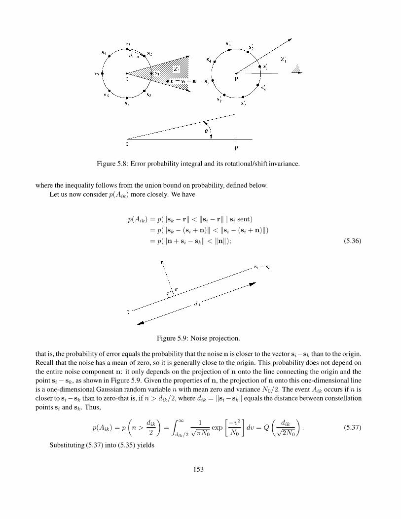
Figure 5.8: Error probability integral and its rotational/shift invariance.

where the inequality follows from the union bound on probability, defined below.

Let us now consider p(Aik) more closely. We have

p(Aik) = p(‖sk − r‖ < ‖si − r‖ | si sent)

= p(‖sk − (si + n)‖ < ‖si − (si + n)‖)= p(‖n + si − sk‖ < ‖n‖); (5.36)

Figure 5.9: Noise projection.

that is, the probability of error equals the probability that the noise n is closer to the vector si−sk than to the origin.

Recall that the noise has a mean of zero, so it is generally close to the origin. This probability does not depend on

the entire noise component n: it only depends on the projection of n onto the line connecting the origin and the

point si− sk, as shown in Figure 5.9. Given the properties of n, the projection of n onto this one-dimensional line

is a one-dimensional Gaussian random variable n with mean zero and variance N0/2. The event Aik occurs if n is

closer to si−sk than to zero-that is, if n > dik/2, where dik = ‖si−sk‖ equals the distance between constellation

points si and sk. Thus,

p(Aik) = p

(

n >dik2

)

=

∫ ∞

dik/2

1√πN0

exp

[−v2

N0

]

dv = Q

(dik√2N0

)

. (5.37)

Substituting (5.37) into (5.35) yields

153

Pe(mi sent) ≤M∑

k=1k 6=i

Q

(dik√2N0

)

, (5.38)

where the Q-function, Q(z), is defined as the probability that a Gaussian random variable X with mean 0 and

variance 1 is greater than z:

Q(z) = p(X > z) =

∫ ∞

z

1√2πe−x

2/2dx. (5.39)

Summing (5.38) over all possible messages yields the union bound

Pe =

M∑

i=1

p(mi)Pe(mi sent) ≤ 1

M

M∑

i=1

M∑

k=1k 6=i

Q

(dik√2N0

)

. (5.40)

Note that the Q-function cannot be solved for in closed form. It is related to the complementary error function as

Q(z) =1

2erfc

(z√2

)

. (5.41)

We can also place an upper bound on Q(z) with the closed-form expression

Q(z) ≤ 1

z√

2πe−z

2/2, (5.42)

and this bound is tight for z 0. A simpler upper bound can be obtained from the Chernoff bound [4] as

Q(z) ≤ e−z2/2 (5.43)

Defining the minimum distance of the constellation as dmin = mini,k dik, we can simplify (5.40) with the

looser bound

Pe ≤ (M − 1)Q

(dmin√2N0

)

. (5.44)

Using (5.42) for the Q-function yields a closed-form bound

Pe ≤M − 1

dmin

√

π/N0

exp

[−d2min

4N0

]

. (5.45)

Finally, Pe is sometimes approximated as the probability of error associated with constellations at the minimum

distance dmin multiplied by the number Mdmin of neighbors at this distance:

Pe ≈MdminQ

(dmin√2N0

)

. (5.46)

This approximation is called the nearest neighbor approximation to Pe. When different constellation points have a

different number of nearest neighbors or different minimum distances, the bound can be averaged over the bound

associated with each constellation point. Note that the nearest neighbor approximation will always be less than the

loose bound (5.44) since M ≥ Mdmin . It will also be slightly less than the union bound (5.40), since the nearest

neighbor approximation does not include the error associated with constellations farther apart than the minimum

distance. However, the nearest neighbor approximation is quite close to the exact probability of symbol error at

154

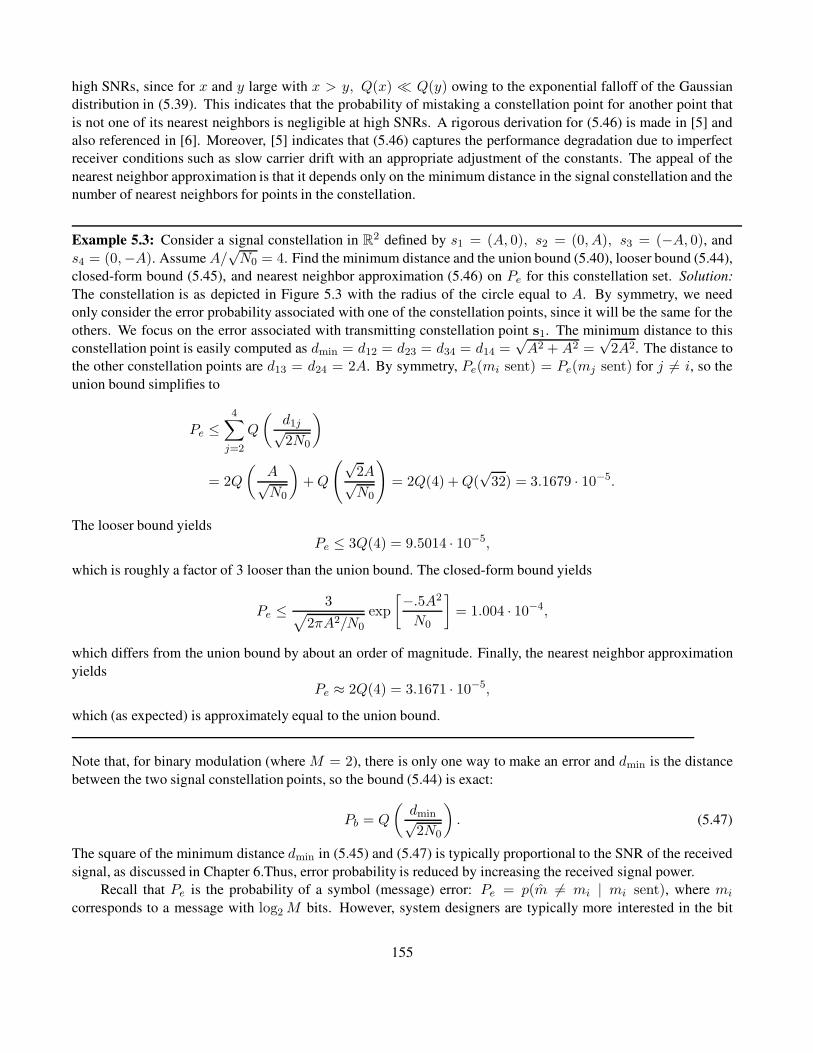
high SNRs, since for x and y large with x > y, Q(x) Q(y) owing to the exponential falloff of the Gaussian

distribution in (5.39). This indicates that the probability of mistaking a constellation point for another point that

is not one of its nearest neighbors is negligible at high SNRs. A rigorous derivation for (5.46) is made in [5] and

also referenced in [6]. Moreover, [5] indicates that (5.46) captures the performance degradation due to imperfect

receiver conditions such as slow carrier drift with an appropriate adjustment of the constants. The appeal of the

nearest neighbor approximation is that it depends only on the minimum distance in the signal constellation and the

number of nearest neighbors for points in the constellation.

Example 5.3: Consider a signal constellation in R2 defined by s1 = (A, 0), s2 = (0, A), s3 = (−A, 0), and

s4 = (0,−A). AssumeA/√N0 = 4. Find the minimum distance and the union bound (5.40), looser bound (5.44),

closed-form bound (5.45), and nearest neighbor approximation (5.46) on Pe for this constellation set. Solution:

The constellation is as depicted in Figure 5.3 with the radius of the circle equal to A. By symmetry, we need

only consider the error probability associated with one of the constellation points, since it will be the same for the

others. We focus on the error associated with transmitting constellation point s1. The minimum distance to this

constellation point is easily computed as dmin = d12 = d23 = d34 = d14 =√A2 + A2 =

√2A2. The distance to

the other constellation points are d13 = d24 = 2A. By symmetry, Pe(mi sent) = Pe(mj sent) for j 6= i, so the

union bound simplifies to

Pe ≤4∑

j=2

Q

(d1j√2N0

)

= 2Q

(A√N0

)

+Q

(√2A√N0

)

= 2Q(4) +Q(√

32) = 3.1679 · 10−5.

The looser bound yields

Pe ≤ 3Q(4) = 9.5014 · 10−5,

which is roughly a factor of 3 looser than the union bound. The closed-form bound yields

Pe ≤3

√

2πA2/N0

exp

[−.5A2

N0

]

= 1.004 · 10−4,

which differs from the union bound by about an order of magnitude. Finally, the nearest neighbor approximation

yields

Pe ≈ 2Q(4) = 3.1671 · 10−5,

which (as expected) is approximately equal to the union bound.

Note that, for binary modulation (where M = 2), there is only one way to make an error and dmin is the distance

between the two signal constellation points, so the bound (5.44) is exact:

Pb = Q

(dmin√2N0

)

. (5.47)

The square of the minimum distance dmin in (5.45) and (5.47) is typically proportional to the SNR of the received

signal, as discussed in Chapter 6.Thus, error probability is reduced by increasing the received signal power.

Recall that Pe is the probability of a symbol (message) error: Pe = p(m 6= mi | mi sent), where mi

corresponds to a message with log2 M bits. However, system designers are typically more interested in the bit

155

error probability (also called the bit error rate, BER) than in the symbol error probability, because bit errors drive

the performance of higher-layer networking protocols and end-to-end performance. Thus, we would like to design

the mapping of the M possible bit sequences to messages mi (i = 1, . . . ,M) so that a decoding error associated

with an adjacent decision region, which is the most likely way to make an error, corresponds to only one bit error.

With such a mapping – and with the assumption that mistaking a signal constellation point for a point other than

one of its nearest neighbors has a very low probability – we can make the approximation

Pb ≈Pe

log2 M. (5.48)

The most common form of mapping in which mistaking a constellation point for one of its nearest neighbors

results in a single bit error is called Gray coding. Mapping by Gray coding is discussed in more detail in Section

5.3. Signal space concepts are applicable to any modulation where bits are encoded as one of several possible

analog signals, including the amplitude, phase, and frequency modulations discussed in what follows.

5.2 Passband Modulation Principles

The basic principle of passband digital modulation is to encode an information bit stream into a carrier signal,

which is then transmitted over a communications channel. Demodulation is the process of extracting this infor-

mation bit stream from the received signal. Corruption of the transmitted signal by the channel can lead to bit

errors in the demodulation process. The goal of modulation is to send bits at a high data rate while minimizing the

probability of data corruption.

In general, modulated carrier signals encode information in the amplitude α(t), frequency f(t), or phase θ(t)of a carrier signal. Thus, the modulated signal can be represented as

s(t) = α(t) cos[2π(fc + f(t))t+ θ(t) + φ0] = α(t) cos(2πfct+ φ(t) + φ0), (5.49)

where φ(t) = 2πf(t)t+ θ(t) and φ0 is the phase offset of the carrier. This representation combines frequency and

phase modulation into angle modulation.

We can rewrite the right-hand side of (5.49) in terms of its in-phase and quadrature components as

s(t) = α(t) cos(φ(t) + φ0) cos(2πfct) − α(t) sin(φ(t) + φ0) sin(2πfct)

= sI(t) cos(2πfct) − sQ(t) sin(2πfct), (5.50)

where sI(t) = α(t)(cosφ(t) + φ0) is the in-phase component of s(t) and where sQ(t) = α(t)(sinφ(t) + φ0) is

its quadrature component. We can also write s(t) in terms of its equivalent lowpass representation as

s(t) = Reu(t)ej2πfct, (5.51)

where u(t) = sI(t) + jsQ(t). This representation, described in more detail in Appendix A, is useful because

receivers typically process the in-phase and quadrature signal components separately.

5.3 Amplitude and Phase Modulation

In amplitude and phase modulation, the information bit stream is encoded in the amplitude and/or phase of the

transmitted signal. Specifically: over a time interval of Ts, K = log2M bits are encoded into the amplitude and/or

phase of the transmitted signal s(t), 0 ≤ t < Ts. The transmitted signal over this period, s(t) = sI(t) cos(2πfct)−

156

sQ(t) sin(2πfct), can be written in terms of its signal space representation as s(t) = si1φ1(t)+si2φ2(t) with basis

functions φ1(t) = g(t) cos(2πfct + φ0) and φ2(t) = −g(t) sin(2πfct + φ0), where g(t) is a shaping pulse. For

φ0 = 0, to send the ith message over the time interval [kT, (k+ 1)T ) we set sI (t) = si1g(t) and sQ(t) = si2g(t).

These in-phase and quadrature signal components are baseband signals with spectral characteristics determined

by the pulse shape g(t). In particular, their bandwidth B equals the bandwidth of g(t), and the transmitted signal

s(t) is a passband signal with center frequency fc and passband bandwidth 2B. In practice we take B = Kg/Ts,where Kg depends on the pulse shape: for rectangular pulses Kg = .5 and for raised cosine pulses .5 ≤ Kg ≤ 1,

as discussed in Section 5.5. Thus, for rectangular pulses the bandwidth of g(t) is. 5/Ts and the bandwidth of s(t)is 1/Ts. The signal constellation for amplitude and phase modulation is defined based on the constellation points

(si1, si2) ∈ R2, i = 1, . . . ,M. The equivalent lowpass representation of s(t) is

s(t) = Rex(t)ejφ0ej2πfct, (5.52)

Figure 5.10: Amplitude/phase modulator.

where x(t) = (si1 + jsi2)g(t). The constellation point si = (si1, si2) is called the symbol associated with

the log2 M bits, and Ts is called the symbol time. The bit rate for this modulation is K bits per symbol or

R = log2M/Ts bits per second.

There are three main types of amplitude/phase modulation:

• pulse amplitude modulation (MPAM) – information encoded in amplitude only;

• phase-shift keying (MPSK) – information encoded in phase only;

• quadrature amplitude modulation (MQAM) – information encoded in both amplitude and phase.

The number of bits per symbol K = log2M , the signal constellation si, i = 1, . . . ,M, and the choice of pulse

shape g(t) determine the digital modulation design. The pulse shape g(t) is chosen to improve spectral efficiency

and combat ISI, as discussed in Section 5.5.

157

Amplitude and phase modulation over a given symbol period can be generated using the modulator structure

shown in Figure 5.10. Note that the basis functions in this figure have an arbitrary phase φ0 associated with

the transmit oscillator. Demodulation over each symbol period is performed using the demodulation structure

of Figure 5.11, which is equivalent to the structure of Figure 5.7 for φ1(t) = g(t) cos(2πfct + φ) and φ2(t) =−g(t) sin(2πfct + φ). Typically the receiver includes some additional circuitry for carrier phase recovery that

matches the carrier phase φ at the receiver to the carrier phase φ0 at the transmitter;1 this is known as coherent

detection. If φ−φ0 = 4φ 6= 0 then the in-phase branch will have an unwanted term associated with the quadrature

branch and vice versa; that is, r1 = si1 cos(4φ) + si2 sin(4φ) +n1 and r2 = −si1 sin(4φ) + si2 cos(4φ) + n2,

which can result in significant performance degradation. The receiver structure also assumes that the sampling

function every Ts seconds is synchronized to the start of the symbol period, which is called synchronization or

timing recovery. Receiver synchronization and carrier phase recovery are complex receiver operations that can be

highly challenging in wireless environments. These operations are discussed in more detail in Section 5.6. We will

assume perfect carrier recovery in our discussion of MPAM, MPSK, and MQAM and therefore set φ = φ0 = 0

for their analysis.

Figure 5.11: Amplitude/phase demodulator (coherent: φ = φ0).

5.3.1 Pulse Amplitude Modulation (MPAM)

We will start by looking at the simplest form of linear modulation, one- dimensional MPAM, which has no quadra-

ture component (si2 = 0). For MPAM, all of the information is encoded into the signal amplitude Ai. The

transmitted signal over one symbol time is given by

si(t) = ReAig(t)ej2πfct = Aig(t) cos(2πfct), 0 ≤ t ≤ Ts 1/fc, (5.53)

where Ai = (2i − 1 − M)d, i = 1, 2, . . . ,M . The signal constellation is thus Ai, i = 1, . . . ,M, which is

parameterized by the distance d. This distance is typically a function of the signal energy. The pulse shape g(t)

must satisfy (5.12) and (5.13). The minimum distance between constellation points is dmin = min i,j|Ai −Aj | =2d. The amplitude of the transmitted signal takes on M different values, which implies that each pulse conveys

log2M = K bits per symbol time Ts.

1In fact, an additional phase term of −2πfcτ will result from a propagation delay of τ in the channel. Thus, coherent detection requires

the receiver phase φ = φ0 − 2πfcτ , as discussed in more detail in Section 5.6.

158

Figure 5.12: Gray encoding for MPAM.

Over each symbol period, the MPAM signal associated with the ith constellation has energy

Esi =

∫ Ts

0

s2i (t) dt =

∫ Ts

0

A2i g

2(t) cos2(2πfct) dt = A2i , (5.54)

since the pulse shape must satisfy (5.12).2 Note that the energy is not the same for each signal si(t), i = 1, . . . ,M .

Assuming equally likely symbols, the average energy is

Es =1

M

M∑

i=1

A2i . (5.55)

The constellation mapping is usually done by Gray encoding, where the messages associated with signal

amplitudes that are adjacent to each other differ by one bit value, as illustrated in Figure 5.12. With this encoding

method, if noise causes the demodulation process to mistake one symbol for an adjacent one (the most likely type

of error), the result is only a single bit error in the sequence of K bits. Gray codes can also be designed for MPSK

and square MQAM constellations but not for rectangular MQAM.

Example 5.4: For g(t) =√

2/Ts(0 ≤ t < Ts) a rectangular pulse shape, find the average energy of 4-PAM mod-

ulation. Solution: For 4-PAM the Ai values are Ai = −3d,−d, d, 3d, so the average energy is

Es =d2

4(9 + 1 + 1 + 9) = 5d2.

The decision regions Zi, i = 1, . . . ,M , associated with pulse amplitude Ai = (2i − 1 −M)d for M = 4 and

M = 8 are shown in Figure 5.13. Mathematically, for any M these decision regions are defined by

Zi =

(−∞, Ai + d) i = 1,[Ai − d, Ai + d) 2 ≤ i ≤M − 1,

[Ai − d,∞) i = M.From (5.53) we see that MPAM has only a single basis function φ1(t) = g(t) cos(2πfct). Thus, the coherent

demodulator of Figure 5.11 for MPAM reduces to the demodulator shown in Figure 5.14, where the multithreshold

device maps r to a decision region Zi and outputs the corresponding bit sequence m = mi = b1, . . . , bK.

2Recall from (5.8) that (5.12) and hence (5.54) are not exact equalities but rather very good approximations for fcTs 1.

159

Figure 5.13: Decision regions for MPAM.

Figure 5.14: Coherent demodulator for MPAM.

5.3.2 Phase-Shift Keying (MPSK)

For MPSK, all of the information is encoded in the phase of the transmitted signal. Thus, the transmitted signal

over one symbol time Ts is given by

si(t) = ReAg(t)ej2π(i−1)/Mej2πfct

= Ag(t) cos

[

2πfct+2π(i− 1)

M

]

= Ag(t) cos

[2π(i− 1)

M

]

cos 2πfct− Ag(t) sin

[2π(i− 1)

M

]

sin 2πfct (5.56)

for 0 ≤ t ≤ Ts. Therefore, the constellation points or symbols (si1, si2) are given by si1 = A cos[2π(i− 1)/M ]

and si2 = A sin[2π(i − 1)/M ] for i = 1, . . . ,M . The pulse shape g(t) satisfies (5.12) and (5.13), and the

θi = 2π(i− 1)/M(i = 1, 2, . . . ,M = 2K) are the different phases in the signal constellation points that convey

the information bits. The minimum distance between constellation points is dmin = 2A sin(π/M), where A is

typically a function of the signal energy. Note that 2-PSK is often referred to as binary PSK or BPSK, while

4-PSK is often called quadrature phase shift keying (QPSK) and is the same as MQAM with M = 4 (defined in

Section 5.3.3).

160

Figure 5.15: Gray encoding for MPSK.

Figure 5.16: Decision regions for MPSK.

All possible transmitted signals si(t) have equal energy:

Esi =

∫ Ts

0s2i (t)dt = A2. (5.57)

Observe that for g(t) =√

2/Ts over a symbol time (i.e., a rectangular pulse) this signal has constant envelope,

unlike the other amplitude modulation techniques MPAM and MQAM. However, rectangular pulses are spectrally

inefficient, and more efficient pulse shapes give MPSK a nonconstant signal envelope. As for MPAM, constellation

mapping is usually done by Gray encoding, where the messages associated with signal phases that are adjacent to

each other differ by one bit value; see Figure 5.15. With this encoding method, mistaking a symbol for an adjacent

one causes only a single bit error.

The decision regions Zi(i = 1, . . . ,M) associated with MPSK for M = 4 and M = 8 are shown in Figure

5.16. If we represent r = r1 + jr2 = rejθ ∈ R2 in polar coordinates, then these decision regions for any M are

defined by

Zi = rejθ : 2π(i− 1.5)/M ≤ θ < 2π(i− .5)/M. (5.58)

From (5.56) we see that MPSK has both in-phase and quadrature components, and thus the coherent demodulator

is as shown in Figure 5.11. For the special case of BPSK, the decision regions as given in Example 5.2 simplify to

Z1 = (r : r > 0) and Z2 = (r : r ≤ 0). Moreover, BPSK has only a single basis function φ1(t) = g(t) cos(2πfct)and, since there is only a single bit transmitted per symbol time Ts, the bit time Tb = Ts. Thus, the coherent

demodulator of Figure 5.11 for BPSK reduces to the demodulator shown in Figure 5.17, where the threshold

device maps r to the positive or negative half of the real line and then outputs the corresponding bit value. We

have assumed in this figure that the message corresponding to a bit value of 1, m1 = 1, is mapped to constellation

161

Figure 5.17: Coherent demodulator for BPSK.

point s1 = A and that the message corresponding to a bit value of 0, m2 = 0, is mapped to the constellation point

s2 = −A.

5.3.3 Quadrature Amplitude Modulation (MQAM)

For MQAM, the information bits are encoded in both the amplitude and phase of the transmitted signal. Thus,

whereas both MPAM and MPSK have one degree of freedom in which to encode the information bits (amplitude

or phase), MQAM has two degrees of freedom. As a result, MQAM is more spectrally efficient than MPAM and

MPSK in that it can encode the most number of bits per symbol for a given average energy.

The transmitted signal is given by

si(t) = ReAiejθig(t)ej2πfct= Ai cos(θi)g(t) cos(2πfct) − Ai sin(θi)g(t) sin(2πfct), 0 ≤ t ≤ Ts, (5.59)

where the pulse shape g(t) satisfies (5.12) and (5.13). The energy in si(t) is

Esi =

∫ Ts

0

s2i (t) = A2i , (5.60)

the same as for MPAM. The distance between any pair of symbols in the signal constellation is

dij = ‖si − sj‖ =√

(si1 − sj1)2 + (si2 − sj2)2. (5.61)

For square signal constellations, where si1 and si2 take values on (2i − 1 − L)d with i = 1, 2, . . . , L, the

minimum distance between signal points reduces to dmin = 2d, the same as for MPAM. In fact, MQAM with

square constellations of size L2 is equivalent to MPAM modulation with constellations of size L on each of the

in-phase and quadrature signal components. Common square constellations are 4-QAM and 16-QAM, which are

shown in Figure 5.18. These square constellations have M = L2 = 22l constellation points, which are used to

send 2l bits/symbol or/bits per dimension, where l = .5 log2 M . It can be shown that the average power of a square

signal constellation with l bits per dimension, Pl, is proportional to 4l/3, and it follows that the average power for

one more bit per dimension Pl+1 ≈ 4Pl. Thus, for square constellations it takes approximately 6 dB more power

to send an additional 1 bit/dimension or 2 bits/symbol while maintaining the same minimum distance between

constellation points.

Good constellation mappings can be hard to find for QAM signals, especially for irregular constellation

shapes. In particular, it is hard to find a Gray code mapping where all adjacent symbols differ by a single bit.

The decision regions Zi(i = 1, . . . ,M) associated with MQAM for M = 16 are shown in Figure 5.19. From

162

4−QAM 16−QAM

Figure 5.18: 4-QAM and 16-QAM constellations.

(5.59) we see that MQAM has both in-phase and quadrature components, and thus the coherent demodulator is as

shown in Figure 5.11.

5.3.4 Differential Modulation

The information in MPSK and MQAM signals is carried in the signal phase. These modulation techniques there-

fore require coherent demodulation; that is, the phase of the transmitted signal carrier φ0 must be matched to the

phase of the receiver carrier φ. Techniques for phase recovery typically require more complexity and cost in the re-

ceiver, and they are also susceptible to phase drift of the carrier. Moreover, obtaining a coherent phase reference in

a rapidly fading channel can be difficult. Issues associated with carrier phase recovery are discussed in more detail

in Section 5.6. The difficulties as well as the cost and complexity associated with carrier phase recovery motivate

the use of differential modulation techniques, which do not require a coherent phase reference at the receiver.

Differential modulation falls in the more general class of modulation with memory, where the symbol trans-

mitted over time [kTs, (k + 1)Ts) depends on the bits associated with the current message to be transmitted and

on the bits transmitted over prior symbol times. The basic principle of differential modulation is to use the pre-

vious symbol as a phase reference for the current symbol, thus avoiding the need for a coherent phase reference

at the receiver. Specifically, the information bits are encoded as the differential phase between the current sym-

bol and the previous symbol. For example, in differential BPSK (referred to as DPSK), if the symbol over time

[(k− 1)Ts, kTs) has phase θ(k − 1) = ejθi for θi = 0, π, then to encode a 0-bit over [kTs, (k+ 1)Ts) the symbol

would have phase θ(k) = ejθi and to encode a 1-bit the symbol would have phase θ(k) = ej(θi+π). In other words:

a 0-bit is encoded by no change in phase, whereas a 1-bit is encoded as a phase change of π. Similarly, in 4-PSK

modulation with differential encoding, the symbol phase over symbol interval [kTs, (k + 1)Ts) depends on the

current information bits over this time interval and the symbol phase over the previous symbol interval. The phase

transitions for DQPSK modulation are summarized in Table 5.1.

Specifically, suppose the symbol over time [(k − 1)Ts, kTs) has phase θ(k − 1) = ejθi . Then, over symbol

time [kTs, (k + 1)Ts), if the information bits are 00 then the corresponding symbol would have phase θ(k) =ejθi ; that is, to encode the bits 00, the symbol from symbol interval [(k − 1)Ts, kTs) is repeated over the next

interval [kTs, (k + 1)Ts). If the two information bits to be sent at time interval [kTs, (k + 1)Ts) are 01, then the

corresponding symbol has phase θ(k) = ej(θi+π/2). For information bits 10 the symbol phase is θ(k) = ej(θi−π/2),

163

Figure 5.19: Decision regions for MQAM with M = 16.

Table 5.1: Mapping for DQPSK with Gray encoding

Bit sequence Phase transition

00 001 π/2

10 −π/211 π

and for information bits 11 the symbol phase is θ(n) = ej(θk+π). We see that the symbol phase over symbol interval

[kTs, (k + 1)Ts) depends on the current information bits over this time interval and on the symbol phase θi over

the previous symbol interval. Note that this mapping of bit sequences to phase transitions ensures that the most

likely detection error – that of mistaking a received symbol for one of its nearest neighbors – results in a single bit

error. For example, if the bit sequence 00 is encoded in the kth symbol then the kth symbol has the same phase as

the (k − 1)th symbol. Assume this phase is θi. The most likely detection error of the kth symbol is to decode it

as one of its nearest neighbor symbols, which have phase θi ± π/2. But decoding the received symbol with phase

θi ± π/2 would result in a decoded information sequence of either 01 or 10 – that is, it would differ by a single bit

from the original sequence 00. More generally, we can use Gray encoding for the phase transitions in differential

MPSK for any M , so that a message of all 0-bits results in no phase change, a message with a single 1-bit and

the rest 0-bits results in the minimum phase change of 2π/M , a message with two 1-bits and the rest 0-bits results

in a phase change of 4π/M , and so forth. Differential encoding is most common for MPSK signals, since the

differential mapping is relatively simple. Differential encoding can also be done for MQAM with a more complex

differential mapping. Differential encoding of MPSK is denoted by DMPSK, and for BPSK and QPSK by DPSK

and DQPSK, respectively.

164

Example 5.5: Find the sequence of symbols transmitted using DPSK for the bit sequence 101110 starting at the

kth symbol time, assuming the transmitted symbol at the (k − 1)th symbol time was s(k − 1) = Aejπ .

Solution: The first bit, a 1, results in a phase transition of π, so s(k) = A. The next bit, a 0, results in no transition,

so s(k + 1) = A. The next bit, a 1, results in another transition of π, so s(k + 1) = Aejπ , and so on. The full

symbol sequence corresponding to 101110 is A,A, Aejπ, A, Aejπ, Aejπ.

The demodulator for differential modulation is shown in Figure 5.20. Assume the transmitted constellation at time

k is s(k) = Aej(θ(k)+(φ0). Then the received vector associated with the sampler outputs is

r(k) = r1(k) + jr2(k) = Aej(θ(k)+(φ0) + n(k), (5.62)

where n(k) is complex white Gaussian noise. The received vector at the previous time sample k − 1 is thus

r(k− 1) = r1(k − 1) + jr2(k − 1) = Aej(θ(k−1)+(φ0) + n(k − 1). (5.63)

The phase difference between r(k) and r(k− 1) determines which symbol was transmitted. Consider

r(k)r∗(k − 1) =A2ej(θ(k)−θ(k−1)) +Aej(θ(k)+φ0)n∗(k − 1)

+ Ae−j(θ(k−1)+φ0)n(k) + n(k)n∗(k − 1). (5.64)

In the absence of noise (n(k) = n(k − 1) = 0) only the first term in (5.64) is nonzero, and this term yields

the desired phase difference. The phase comparator in Figure 5.20 extracts this phase difference and outputs the

corresponding symbol.

Differential modulation is less sensitive to a random drift in the carrier phase. However, if the channel has

a nonzero Doppler frequency then the signal phase can decorrelate between symbol times, making the previous

symbol a noisy phase reference. This decorrelation gives rise to an irreducible error floor for differential modulation

over wireless channels with Doppler, as we shall discuss in Chapter 6.

Figure 5.20: Differential PSK demodulator.

165

5.3.5 Constellation Shaping

Rectangular and hexagonal constellations have a better power efficiency than the square or circular constellations

associated with MQAM and MPSK, respectively. These irregular constellations can save up to 1.3 dB of power at

the expense of increased complexity in the constellation map [7]. The optimal constellation shape is a sphere in

N -dimensional space, which must be mapped to a sequence of constellations in two-dimensional space in order to

be generated by the modulator shown in Figure 5.10. The general conclusion in [7] is that, for uncoded modulation,

the increased complexity of spherical constellations is not worth their energy gains, since coding can provide much

better performance at less complexity cost. However, if a complex channel code is already being used and little

further improvement can be obtained by a more complex code, constellation shaping may obtain around 1 dB of

additional gain. An in-depth discussion of constellation shaping (and of constellations that allow a noninteger

number of bits per symbol) can be found in [7].

5.3.6 Quadrature Offset

A linearly modulated signal with symbol si = (si1, si2) will lie in one of the four quadrants of the signal space. At

each symbol time kTs the transition to a new symbol value in a different quadrant can cause a phase transition of up

to 180, which may cause the signal amplitude to transition through the zero point; these abrupt phase transitions

and large amplitude variations can be distorted by nonlinear amplifiers and filters. The abrupt transitions are

avoided by offsetting the quadrature branch pulse g(t) by half a symbol period, as shown in Figure 5.21. This

quadrature offset makes the signal less sensitive to distortion during symbol transitions.

Phase modulation with quadrature offset is usually abbreviated as OMPSK, where the O indicates the offset.

For example, QPSK modulation with quadrature offset is referred to as OQPSK. Offset QPSK has the same spectral

properties as QPSK for linear amplification, but it has higher spectral efficiency under nonlinear amplification

because the maximum phase transition of the signal is 90, corresponding to the maximum phase transition in

either the in-phase or quadrature branch but not both simultaneously. Another technique to mitigate the amplitude

fluctuations of a 180 phase shift used in the IS-136 standard for digital cellular is π/4-QPSK [8, 9]. This technique

allows for a maximum phase transition of 135 degrees, versus 90 for offset QPSK and 180 for QPSK. Thus,

π/4-QPSK has worse spectral properties than OQPSK under nonlinear amplification. However, π/4-QPSK can be

differentially encoded to eliminate the need for a coherent phase reference, which is a significant advantage. Using

differential encoding with π/4-QPSK is called π/4-DQPSK. The π/4-DQPSK modulation works as follows: the

information bits are first differentially encoded as in DQPSK, which yields one of the four QPSK constellation

points. Then, every other symbol transmission is shifted in phase by π/4. This periodic phase shift has a similar

effect as the time offset in OQPSK: it reduces the amplitude fluctuations at symbol transitions, which makes the

signal more robust against noise and fading.

5.4 Frequency Modulation

Frequency modulation encodes information bits into the frequency of the transmitted signal. Specifically: at each

symbol time, K = log2M bits are encoded into the frequency of the transmitted signal s(t), 0 ≤ t < Ts,resulting in a transmitted signal si(t) = A cos(2πfit+ φi), where i is the index of the ith message corresponding

to the log2 M bits and φi is the phase associated with the ith carrier. The signal space representation is si(t) =∑

j sijφj(t), where sij = Aδ(i − j) and φj(t) = cos(2πfjt + φj), so the basis functions correspond to carriers

at different frequencies and only one such basis function is transmitted in each symbol period. The basis functions

are orthogonal for a minimum carrier frequency separation of 4f = minij |fj − fi| = .5/Ts for φi = φj and of

4f = 1/Ts for φi 6= φj .

166

Figure 5.21: Modulator with quadrature offset.

Because frequency modulation encodes information in the signal frequency, the transmitted signal s(t) has

a constant envelope A. Since the signal is constant envelope, nonlinear amplifiers can be used with high power

efficiency and hence the modulated signal is less sensitive to amplitude distortion introduced by the channel or the

hardware. The price exacted for this robustness is a lower spectral efficiency: because the modulation technique

is nonlinear, it tends to have a higher bandwidth occupancy than the amplitude and phase modulation techniques

described in Section 5.3.

In its simplest form, frequency modulation over a given symbol period can be generated using the modulator

structure shown in Figure 5.22. Demodulation over each symbol period is performed using the demodulation

structure of Figure 5.23. Note that the demodulator of Figure 5.23 requires the jth carrier signal to be matched

in phase to the jth carrier signal at the transmitter; this is similar to the coherent phase reference requirement in

amplitude and phase modulation. An alternate receiver structure that does not require this coherent phase reference

will be discussed in Section 5.4.3. Another issue in frequency modulation is that the different carriers shown in

Figure 5.22 have different phases, φi 6= φj for i 6= j, so at each symbol time Ts there will be a phase discontinuity

in the transmitted signal. Such discontinuities can significantly increase signal bandwidth. Thus, in practice an

alternate modulator is used that generates a frequency-modulated signal with continuous phase, as will be discussed

in Section 5.4.2.

5.4.1 Frequency-Shift Keying (FSK) and Minimum-Shift Keying (MSK)

In MFSK the modulated signal is given by

si(t) = A cos[2πfct+ 2παi4fct+ φi], 0 ≤ t < Ts, (5.65)

where αi = (2i− 1 −M) for i = 1, 2, . . . ,M = 2K . The minimum frequency separation between FSK carriers

is thus 24fc. MFSK consists of M basis functions φi(t) =√

2/Ts cos[2πfct+ 2παi4fct+ φi], i = 1, . . . ,M ,

167

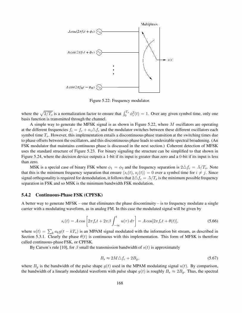
Figure 5.22: Frequency modulator.

where the√

2/Ts is a normalization factor to ensure that∫ Ts

0 φ2i (t) = 1. Over any given symbol time, only one

basis function is transmitted through the channel.

A simple way to generate the MFSK signal is as shown in Figure 5.22, where M oscillators are operating

at the different frequencies fi = fc + αi4fc and the modulator switches between these different oscillators each

symbol time Ts. However, this implementation entails a discontinuous phase transition at the switching times due

to phase offsets between the oscillators, and this discontinuous phase leads to undesirable spectral broadening. (An

FSK modulator that maintains continuous phase is discussed in the next section.) Coherent detection of MFSK

uses the standard structure of Figure 5.23. For binary signaling the structure can be simplified to that shown in

Figure 5.24, where the decision device outputs a 1-bit if its input is greater than zero and a 0-bit if its input is less

than zero.

MSK is a special case of binary FSK where φ1 = φ2 and the frequency separation is 24fc = .5/Ts. Note

that this is the minimum frequency separation that ensure 〈si(t), sj(t)〉 = 0 over a symbol time for i 6= j. Since

signal orthogonality is required for demodulation, it follows that 24fc = .5/Ts is the minimum possible frequency

separation in FSK and so MSK is the minimum bandwidth FSK modulation.

5.4.2 Continuous-Phase FSK (CPFSK)

A better way to generate MFSK – one that eliminates the phase discontinuity – is to frequency modulate a single

carrier with a modulating waveform, as in analog FM. In this case the modulated signal will be given by

si(t) = A cos

[

2πfct+ 2πβ

∫ t

−∞

u(τ) dτ

]

= A cos[2πfct+ θ(t)], (5.66)

where u(t) =∑

k akg(t − kTs) is an MPAM signal modulated with the information bit stream, as described in

Section 5.3.1. Clearly the phase θ(t) is continuous with this implementation. This form of MFSK is therefore

called continuous-phase FSK, or CPFSK.

By Carson’s rule [10], for β small the transmission bandwidth of s(t) is approximately

Bs ≈ 2M4fc + 2Bg , (5.67)

where Bg is the bandwidth of the pulse shape g(t) used in the MPAM modulating signal u(t). By comparison,

the bandwidth of a linearly modulated waveform with pulse shape g(t) is roughly Bs ≈ 2Bg. Thus, the spectral

168

Figure 5.23: Frequency demodulator (coherent).

Figure 5.24: Demodulator for binary FSK.

occupancy of a CPFSK-modulated signal is larger than that of a linearly modulated signal by M4fc ≥ .5M/Ts.The spectral efficiency penalty of CPFSK relative to linear modulation increases with data rate, in particular with

the number of bits per symbol K = log2 M and with the symbol rate Rs = 1/Ts.Coherent detection of CPFSK can be done symbol-by-symbol or over a sequence of symbols. The sequence

estimator is the optimal detector, since a given symbol depends on previously transmitted symbols and so it is

optimal to detect (or estimate) all symbols simultaneously. However, sequence estimation can be impractical

owing to the memory and computational requirements associated with making decisions based on sequences of

symbols. Details on detectors for coherent demodulation of CPFSK can be found in [11, Chap. 4.9].

5.4.3 Noncoherent Detection of FSK

The receiver requirement for a coherent phase reference associated with each FSK carrier can be difficult and

expensive to meet. The need for a coherent phase reference can be eliminated if the receiver first detects the energy

of the signal at each frequency and, if the ith branch has the highest energy of all branches, then outputs message

mi. The modified receiver is shown in Figure 5.25.

Suppose the transmitted signal corresponds to frequency fi:

169

s(t) = A cos(2πfit+ φi)

= A cos(φi) cos(2πfit) − A sin(φi) sin(2πfit), 0 ≤ t < Ts. (5.68)

Let the phase φi represent the phase offset between the transmitter and receiver oscillators at frequency fi. A

coherent receiver with carrier signal cos(2πfit) detects only the first term A cos(φi) cos(2πfit) associated with

the received signal, which can be close to zero for a phase offset φi ≈ ±π/2. To get around this problem, in Figure

5.25 the receiver splits the received signal intoM branches corresponding to each frequency fj , j = 1, . . . ,M . For

each such carrier frequency fj , the received signal is multiplied by a noncoherent in-phase and quadrature carrier

at that frequency, integrated over a symbol time, sampled, and then squared. For the jth branch the squarer output

associated with the in-phase component is denoted as AjI + njI and the corresponding output associated with the

quadrature component is denoted as AjQ + njQ, where njI and njQ are due to the noise n(t) at the receiver input.

Then, if i = j, we have AjI = A2 cos2(φi) and AjQ = A2 sin2(φi); if i 6= j then AjI = AjQ = 0. In the absence

of noise, the input to the decision device of the ith branch will beA2 cos2(φi)+A2 sin2(φi) = A2, independent of

φi, and all other branches will have an input of zero. Thus, over each symbol period, the decision device outputs

the bit sequence corresponding to frequency fj if the jth branch has the largest input to the decision device. Note

that the noncoherent receiver of Figure 5.25 still requires accurate synchronization for sampling. Synchronization

issues are discussed in Section 5.6.

Figure 5.25: Noncoherent FSK demodulator.

5.5 Pulse Shaping

For amplitude and phase modulation, the bandwidth of the baseband and passband modulated signal is a function

of the bandwidth of the pulse shape g(t). If g(t) is a rectangular pulse of width Ts, then the envelope of the signal is

constant. However, a rectangular pulse has high spectral sidelobes, which can cause adjacent channel interference.

Pulse shaping is a method for reducing sidelobe energy relative to a rectangular pulse; however, the shaping must

170

be done in such a way that intersymbol interference between pulses in the received signal is not introduced. Note

that – prior to sampling the received signal – the transmitted pulse g(t) is convolved with the channel impulse

response c(t) and the matched filter g∗(−t); hence, in order to eliminate ISI prior to sampling, we must ensure that

the effective received pulse p(t) = g(t) ∗ c(t) ∗ g∗(−t) has no ISI. Since the channel model is AWGN, we assume

c(t) = δ(t) so p(t) = g(t) ∗ g∗(−t) (in Chapter 11we will analyze ISI for more general channel impulse responses

c(t)). To avoid ISI between samples of the received pulses, the effective pulse shape p(t) must satisfy the Nyquist

criterion, which requires the pulse to equal zero at the ideal sampling point associated with past or future symbols:

p(kTs) =

p0 = p(0) k = 0,0 k 6= 0.

In the frequency domain this translates to

∞∑

l=−∞

P

(

f +l

Ts

)

= p0Ts. (5.69)

The following pulse shapes all satisfy the Nyquist criterion.

1. Rectangular pulses: g(t) =√

2/Ts(0 ≤ t ≤ Ts), which yields the triangular effective pulse shape

p(t) =

2 + 2t/Ts −Ts ≤ t < 0,2 − 2t/Ts 0 ≤ t < Ts,

0 else.

This pulse shape leads to constant envelope signals in MPSK but has poor spectral properties as a result of

its high sidelobes.

2. Cosine pulses: p(t) = sinπt/Ts, 0 ≤ t ≤ Ts. Cosine pulses are mostly used in OMPSK modulation,

where the quadrature branch of the modulation is shifted in time by Ts/2. This leads to a constant amplitude

modulation with sidelobe energy that is 10 dB lower than that of rectangular pulses.

3. Raised cosine pulses: These pulses are designed in the frequency domain according to the desired spectral

properties. Thus, the pulse p(t) is first specified relative to its Fourier transform:

P (f) =

Ts 0 ≤ |f | ≤ 1−β

2Ts,

Ts

2

[

1− sin πTs

β

(

f − 12Ts

)]1−β2Ts

≤ |f | ≤ 1+β2Ts

;

here β is defined as the rolloff factor, which determines the rate of spectral rolloff (see Figure 5.26). Setting

β = 0 yields a rectangular pulse. The pulse p(t) in the time domain corresponding to P (f) is

p(t) =sinπt/Tsπt/Ts

cosβπt/Ts1 − 4β2t2/T 2

s

.

The frequency- and time-domain properties of the raised cosine pulse are shown in Figures 5.26 and 5.27, respec-

tively. The tails of this pulse in the time domain decay as 1/t3 (faster than for the previous pulse shapes), so a

mistiming error in sampling leads to a series of inter- symbol interference components that converge. A variation

of the raised cosine pulse is the root cosine pulse, derived by taking the square root of the frequency response for

the raised cosine pulse. The root cosine pulse has better spectral properties than the raised cosine pulse but decays

171

Figure 5.26: Frequency-domain (spectral) properties of the raised cosine pulse (T = Ts).

less rapidly in the time domain, which makes performance degradation due to synchronization errors more severe.

Specifically, a mistiming error in sampling leads to a series of ISI components that may diverge.

Pulse shaping is also used with CPFSK to improve spectral efficiency, specifically in the MPAM signal that is

frequency modulated to form the FSK signal. The most common pulse shape used in CPFSK is the Gaussian pulse

shape, defined as

g(t) =

√π

αe−π

2t2/α2, (5.70)

where α is a parameter that dictates spectral efficiency. The spectrum of g(t), which dictates the spectrum of the

CPFSK signal, is given by

G(f) = e−α2f2. (5.71)

The parameter α is related to the 3-dB bandwidth of g(t), Bg, by

α =.5887

Bg. (5.72)

Clearly, increasing α results in a higher spectral efficiency.

When the Gaussian pulse shape is applied to MSK modulation, it is abbreviated as GMSK. In general, GMSK

signals have a high power efficiency (since they have a constant amplitude) and a high spectal efficiency (since

the Gaussian pulse shape has good spectral properties for large α). For these reasons, GMSK is used in the

GSM standard for digital cellular systems. Although this is a good choice for voice modulation, it is not the best

choice for data. The Gaussian pulse shape does not satisfy the Nyquist criterion and so the pulse shape introduces

ISI, which increases as α increases. Thus, improving spectral efficiency by increasing α leads to a higher ISI

level, thereby creating an irreducible error floor from this self-interference. Since the required BER for voice is a

relatively high Pb ≈ 10−3, the ISI can be fairly high and still maintain this target BER. In fact, it is generally used

as a rule of thumb thatBgTs = .5 is a tolerable amount of ISI for voice transmission with GMSK. However, a much

lower BER is required for data, which will put more stringent constraints on the maximum α and corresponding

172

Figure 5.27: Time-domain properties of the raised cosine pulse (T = Ts).

minimum Bg, thereby decreasing the spectral efficiency of GMSK for data transmission. Techniques such as

equalization can be used to mitigate the ISI in this case so that a tolerable BER is possible without significantly

compromising spectral efficiency. However, it is more common to use linear modulation for spectrally efficient

data transmission. Indeed, the data enhancements to GSM use linear modulation.

5.6 Symbol Synchronization and Carrier Phase Recovery

One of the most challenging tasks of a digital demodulator is to acquire accurate symbol timing and carrier phase

information. Timing information, obtained via synchronization, is needed to delineate the received signal asso-

ciated with a given symbol. In particular, timing information is used to drive the sampling devices associated

with the demodulators for amplitude, phase, and frequency demodulation shown in Figures 5.11 and 5.23. Carrier

phase information is needed in all coherent demodulators for both amplitude/phase and frequency modulation, as

discussed in Sections 5.3 and 5.4.

This section gives a brief overview of standard techniques for synchronization and carrier phase recovery in

AWGN channels. In this context the estimation of symbol timing and carrier phase falls under the broader category

of signal parameter estimation in noise. Estimation theory provides the theoretical framework for studying this

problem and for developing the maximum likelihood estimator of the carrier phase and symbol timing. However,

most wireless channels suffer from time-varying multipath in addition to AWGN. Synchronization and carrier

phase recovery is particularly challenging in such channels because multipath and time variations can make it

extremely difficult to estimate signal parameters prior to demodulation. Moreover, there is little theory addressing

good methods for estimation of carrier phase and symbol timing when these parameters are corrupted by time-

varying multipath in addition to noise. In most performance analysis of wireless communication systems it is

assumed that the receiver synchronizes to the multipath component with delay equal to the average delay spread;3

then the channel is treated as AWGN for recovery of timing information and carrier phase. In practice, however, the

receiver will sychronize to either the strongest multipath component or the first multipath component that exceeds

a given power threshold. The other multipath components will then compromise the receiver’s ability to acquire

3That is why delay spread is typically characterized by its rms value about its mean, as discussed in more detail in Chapter 2.

173

timing and carrier phase, especially in wideband systems like UWB. Multicarrier and spread-spectrum systems

have additional considerations related to synchronization and carrier recovery, which will be discussed in Chapters

12 and 13.

The importance of synchronization and carrier phase estimation cannot be overstated: without them, wireless

systems could not function. Moreover, as data rates increase and channels become more complex by adding

additional degrees of freedom (e.g., multiple antennas), the tasks of receiver synchronizaton and phase recovery

become even more complex and challenging. Techniques for synchronization and carrier recovery have been

developed and analyzed extensively for many years, and they are continually evolving to meet the challenges

associated with higher data rates, new system requirements, and more challenging channel characteristics. We give

only a brief introduction to synchronizaton and carrier phase recovery techniques in this section. Comprehensive

coverage of this topic and performance analysis of these techniques can be found in [12, 13]; more condensed

treatments can be found in [bib5-10, Chap. 5;bib5-13].

5.6.1 Receiver Structure with Phase and Timing Recovery

The carrier phase and timing recovery circuitry for the amplitude and phase demodulator is shown in Figure 5.28.

For BPSK only the in-phase branch of this demodulator is needed. For the coherent frequency demodulator of

Figure 5.23, a carrier phase recovery circuit is needed for each of the distinct M carriers; the resulting circuit

complexity motivates the need for noncoherent demodulators as described in Section 5.4.3. We see in Figure 5.28

that the carrier phase and timing recovery circuits operate directly on the received signal prior to demodulation.

Assuming an AWGN channel, the received signal r(t) is a delayed version of the transmitted signal s(t) plus

AWGN n(t) : r(t) = s(t − τ) + n(t), where τ is the random propagation delay. Using the equivalent lowpass

form we have s(t) = Rex(t)ejφ0ej2πfct and thus

r(t) = Re

x(t− τ)ejφej2πfct

+ n(t), (5.73)

Figure 5.28: Receiver structure with carrier and timing recovery.

where φ = φ0−2πfcτ results from the transmit carrier phase and the propagation delay. Estimation of τ is needed

for symbol timing, and estimation of φ is needed for carrier phase recovery. Let us express these two unknown

174

parameters as a vector ψ = (φ, τ). Then we can express the received signal in terms of ψ as

r(t) = s(t;ψ) + n(t). (5.74)

Parameter estimation must take place over some finite time interval T0 ≥ Ts. We call T0 the observation interval.

In practice, however, parameter estimation is initially done over this interval and is thereafter performed continually

by updating the initial estimate using tracking loops. Our development here focuses on the initial parameter

estimation over T0. Discussion of parameter tracking can be found in [12, 13].

There are two common estimation methods for signal parameters in noise: the maximum likelihood (ML)

criterion discussed in Section 5.1.4 in the context of receiver design, and the maximum a posteriori (MAP) criterion.

The ML criterion chooses the estimate ψ that maximizes p(r(t)|ψ) over the observation interval T0, whereas the

MAP criterion assumes some probability distribution p(ψ) on ψ and then chooses the estimate ψ that maximizes

p(ψ|r(t)) =p(r(t)|ψ)p(ψ)

p(r(t))

over T0. We assume that there is no prior knowledge of ψ, so that p(ψ) becomes uniform and hence the MAP and

ML criteria are equivalent.

To characterize the distribution p(r(t)|ψ), 0 ≤ t < T0, let us expand r(t) over the observation interval along

a set of orthonormal basis functions φk(t) as

r(t) =

K∑

k=1

rkφk(t), 0 ≤ t < T0.

Because n(t) is white with zero mean and power spectral density N0/2, the distribution of the vector r =(r1, . . . , rK) conditioned on the unknown parameter ψ is given by

p(r|ψ) =

(1√πN0

)K

exp

[

−K∑

k=1

(rk − sk(ψ))2

N0

]

, (5.75)

where (by the basis expansion)

rk =

∫

T0

r(t)φk(t) dt

and

sk(ψ) =

∫

T0

s(t;ψ)φk(t) dt.

From these basis expansions we can show that

K∑

k=1

[rk − sk(ψ)]2 =

∫

T0

[r(t)− s(t;ψ)]2 dt. (5.76)

Using this in (5.75) yields that maximizing p(r|ψ) is equivalent to maximizing the likelihood function

Λ(ψ) = exp

[

− 1

N0

∫

T0

[r(t)− s(t;ψ)]2]

dt. (5.77)

175

Maximizing the likelihood function (5.77) results in the joint ML estimate of the carrier phase and symbol

timing. Maximum likelihood estimation of the carrier phase and symbol timing can also be done separately, and in

subsequent sections we will discuss this separate estimation in more detail. Techniques joint estimation are more

complex; details of such techniques can be found in [10, Chap. 6.4; 11, Chaps. 8–9].

5.6.2 Maximum Likelihood Phase Estimation

In this section we derive the maximum likelihood phase estimate assuming the timing is known. The likelihood

function (5.77) with timing known reduces to

Λ(φ) = exp

[

− 1

N0

∫

T0

[r(t)− s(t; φ)]2 dt

]

= exp

[

− 1

N0

∫

T0

x2(t) dt+2

N0

∫

T0

r(t)s(t; φ) dt− 1

N0

∫

T0

s2(t; φ) dt

]

. (5.78)

We estimate the carrier phase as the value φ that maximizes this function. Note that the first term in (5.78) is

independent of φ. Moreover, we assume that the third integral, which measures the energy in s(t; φ) over the

observation interval, is relatively constant in φ. Given these assumptions, we see that the φ that maximizes (5.78)

also maximizes

Figure 5.29: Phase-locked loop for carrier phase recovery (unmodulated carrier).

Λ′(φ) =

∫

T0

r(t)s(t; φ) dt. (5.79)

We can solve directly for the maximizing φ in the simple case where the received signal is just an unmodulated

carrier plus noise: r(t) = A cos(2πfct+ φ) + n(t). Then φ must maximize

Λ′(φ) =

∫

T0

r(t) cos(2πfct+ φ) dt. (5.80)

Differentiating Λ′(φ) relative to φ and then setting it to zero yields that φ satisfies

∫

T0

r(t) sin(2πfct+ φ) dt = 0. (5.81)

Solving (5.81) for φ yields

φ = − tan−1

[ ∫

T0r(t) sin(2πfct) dt

∫

T0r(t) cos(2πfct) dt

]

. (5.82)

176

We could build a circuit to compute (5.82) from the received signal r(t); in practice, however, carrier phase

recovery is accomplished by using a phase lock loop to satisfy (5.81), as shown in Figure 5.29. In this figure, the

integrator input in the absence of noise is given by e(t) = r(t) sin(2πfct+ φ) and the integrator output is

z(t) =

∫

T0

r(t) sin(2πfct+ φ)dt,

which is precisely the left-hand side of (5.81). Thus, if z(t) = 0 then the estimate φ is the maximum likelihood

estimate for φ. If z(t) 6= 0 then the voltage-controlled oscillator (VCO) adjusts its phase estimate φ up or down

depending on the polarity of z(t): for z(t) > 0 it decreases φ to reduce z(t), and for z(t) < 0 it increases φ to

increase z(t). In practice the integrator in Figure 5.29 is replaced with a loop filter whose output .5A sin(φ−φ) ≈.5A(φ− φ) is a function of the low-frequency component of its input e(t) = A cos(2πfct+ φ) sin(2πfct+ φ) =.5A sin(φ − φ) + .5A sin(2πfct + φ + φ). This discussion of phase-locked loop (PLL) operation assumes that

φ ≈ φ because otherwise the polarity of z(t) may not indicate the correct phase adjustment; that is, we would not

necessarily have sin(φ−φ) ≈ φ−φ. The PLL typically exhibits some transient behavior in its initial estimation of

the carrier phase. The advantage of a PLL is that it continually adjusts its estimate φ to maintain z(t) ≈ 0, which

corrects for slow phase variations due to oscillator drift at the transmitter or changes in the propagation delay. In

fact, the PLL is an example of a feedback control loop. More details on the PLL and its performance can be found

in [11, 12].

The PLL derivation is for an unmodulated carrier, yet amplitude and phase modulation embed the message

bits into the amplitude and phase of the carrier. For such signals there are two common carrier phase recovery

approaches to deal with the effect of the data sequence on the received signal: the data sequence is either (a)

assumed known or (b) treated as random with the phase estimate averaged over the data statistics. The first

scenario is referred to as decision-directed parameter estimation, and this scenario typically results from sending

a known training sequence. The second scenario is referred to as non-decision directed parameter estimation.

With this technique the likelihood function (5.78) is maximized by averaging over the statistics of the data. One

decision-directed technique uses data decisions to remove the modulation of the received signal: the resulting

unmodulated carrier is then passed through a PLL. This basic structure is called a decision-feedback PLL because

data decisions are fed back into the PLL for processing. The structure of a non–decision-directed carrier phase

recovery loop depends on the underlying distribution of the data. For large constellations, most distributions

lead to highly nonlinear functions of the parameter to be estimated. In this case the symbol distribution is often

assumed to be Gaussian along each signal dimension, which greatly simplifies the recovery loop structure. An

alternate non–decision-directed structure takes the M th power of the signal (M = 2 for PAM and M for MPSK

modulation), passes it through a bandpass filter at frequency Mfc, and then uses a PLL. The nonlinear operation

removes the effect of the amplitude or phase modulation so that the PLL can operate on an unmodulated carrier at

frequency Mfc. Many other structures for both decision-directed and non–decision-directed carrier recovery can

be used, with different trade-offs in performance and complexity. A more comprehensive discussion of design and

performance of carrier phase recovery can be found in [10, Chaps. 6.2.4–6.2.5; 11].

5.6.3 Maximum Likelihood Timing Estimation

In this section we derive the maximum likelihood estimate of delay τ assuming the carrier phase is known. Since

we assume that the phase φ is known, the timing recovery will not affect the carrier phase recovery loop and

associated downconversion shown in Figure 5.28. Thus, it suffices to consider timing estimation for the in-phase

or quadrature equivalent lowpass signals of r(t) and s(t; τ). We denote the in-phase and quadrature components

for r(t) as rI(t) and rQ(t) and for s(t; τ) as sI(t; τ) and sQ(t; τ). We focus on the in-phase branch since the

timing recovered from this branch can be used for the quadrature branch. The equivalent lowpass in-phase signal

is given by

177

sI(t; τ) =∑

k

sI (k)g(t− kTs − τ), (5.83)

where g(t) is the pulse shape and sI (k) denotes the amplitude associated with the in-phase component of the

message transmitted over the kth symbol period. The in-phase equivalent lowpass received signal is rI(t) =sI(t; τ) + nI(t). As in the case of phase synchronization, there are two categories of timing estimators: those for

which the information symbols output from the demodulator are assumed known (decision-directed estimators),

and those for which this sequence is not assumed known (non–decision-directed estimators).

Figure 5.30: Decision-directed timing estimation.

The likelihood function (5.77) with known phase φ has a form similar to (5.78), the case of known delay:

Λ(τ) = exp

[

− 1

N0

∫

T0

[rI(t)− sI(t; τ)]2 dt

]

= exp

[

− 1

N0

∫

T0

r2I (t) dt+2

N0

∫

T0

rI(t)sI(t; τ) dt−1

N0

∫

T0

s2I (t; τ) dt

]

. (5.84)

Since the first and third terms in (5.84) do not change significantly with τ , the delay estimate τ that maximizes

(5.84) also maximizes

Λ′(τ) =

∫

T0

rI(t)sI(t; τ) dt

=∑

k

sI(k)

∫

T0

r(t)g(t− kTs − τ) dt =∑

k

sI (k)zk(τ), (5.85)

where

zk(τ) =

∫

T0

r(t)g(t− kTs − τ) dt. (5.86)

Differentiating (5.85) relative to τ and then setting it to zero yields that the timing estimate τ must satisfy

∑

k

sI(k)d

dτzk(τ) = 0. (5.87)

178

For decision-directed estimation, (5.87) gives rise to the estimator shown in Figure 5.30. The input to the

voltage-controlled clock (VCC) is (5.87). If this input is zero, then the timing estimate τ = τ . If not, the clock

(i.e., the timing estimate τ ) is adjusted to drive the VCC input to zero. This timing estimation loop is also an

example of a feedback control loop.

One structure for non–decision-directed timing estimation is the early–late gate synchronizer shown in Figure

5.31. This structure exploits two properties of the autocorrelation of g(t),Rg(τ) =∫ TS

0 g(t)g(t−τ) dt – namely, its

symmetry (Rg(τ) = Rg(−τ)) and the fact that its maximum value is at τ = 0. The input to the sampler in the upper

branch of Figure 5.31 is proportional to the autocorrelationRg(τ−τ+δ) =∫ TS

0 g(t−τ)g(t−τ−δ) dt, and the input

to the sampler in the lower branch is proportional to the autocorrelationRg(τ−τ−δ) =∫ TS

0 g(t−τ)g(t−τ+δ)dt.

If τ = τ then, sinceRg(δ) = Rg(−δ), the input to the loop filter will be zero and the voltage-controlled clock will

maintain its correct timing estimate. If τ > τ then Rg(τ − τ + δ) < Rg(τ − τ − δ), and this negative input to the

VCC will cause it to decrease its estimate of τ . Conversely, if τ < τ then Rg(τ − τ + δ) > Rg(τ − τ − δ), and

this positive input to the VCC will cause it to increase its estimate of τ .

Figure 5.31: Early-late gate synchronizer.

More details on these and other structures for decision-directed and non–decision-directed timing estimation–

as well as their performance trade-offs–can be found in [10, Chaps. 6.2.4–6.2.5; 11].

179

Chapter 5 Problems

1. Using properties of orthonormal basis functions, show that if si(t) and sj(t) have constellation points si and

sj (respectively) then

‖si − sj‖2 =

∫ T

0(si(t) − sj(t))

2dt.

2. Find an altemate set of orthonormal basis functions for the space spanned by cos(2πt/T ) and sin(2πt/T ).

3. Consider a set of M orthogonal signal waveforms sm(t), for 1 ≤ m ≤ M and 0 ≤ t ≤ T , where each

waveform has the same energy E . Define a new set of M waveforms as

s′m(t) = sm(t) − 1

M

M∑

i=1

si(t), 1 ≤ m ≤M, 0 ≤ t ≤ T.

Figure 5.32: Signal waveforms for Problem 5-4.

Figure 5.33: Signal waveforms for Problem 5-5.

180

Show that the M signal waveforms s′m(t) have equal energy, given by

E ′ = (M − 1)E/M.

What is the inner product between any two waveforms?

4. Consider the three signal waveforms φ1(t), φ2(t), φ3(t) shown in Figure 5.32.

(a) Show that these waveforms are orthonormal.

(b) Express the waveform x(t) as a linear combination of φi(t) and find the coefficients, where x(t) is

given as

x(t) =

2 0 ≤ t < 2,4 2 ≤ t ≤ 4.

5. Consider the four signal waveforms as shown in Figure 5.33.

(a) Determine the dimensionality of the waveforms and a set of basis functions.

(b) Use the basis functions to represent the four waveforms by vectors.

(c) Determine the minimum distance between all the vector pairs.

6. Derive a mathematical expression for decision regions Zi that minimize error probability assuming that

messages are not equally likely – that is, assuming p(mi) = pi(i = 1, . . . ,M), where pi is not necessarily

equal to 1/M . Solve for these regions in the case of QPSK modulation with s1 = (Ac, 0), s2 = (0, Ac),

s3 = (−Ac, 0), and s4 = (0, Ac), assuming p(s1) = p(s3) = .2 and p(s1) = p(s3) = .3.

7. Show that the remainder noise term nr(t) is independent of the correlator outputs ri for all i. In other

words, show that E[nr(t)ri] = 0 for all i. Thus, since rj (conditioned on si) and nr(t) are Gaussian and

uncorrelated, they are independent.

8. Show that output SNR is maximized when a given input signal is passed through a filter that is matched to

that signal.

9. Find the matched filters g(T − t), 0 ≤ t ≤ T , and Find∫ T0 g(t)g(T − t) dt for the following waveforms.

(a) Rectangular pulse: g(t) =√

2/T .

(b) Sinc pulse: g(t) = sinc(t).

(c) Gaussian pulse: g(t) = (√π/α)e−π

2t2/α2.

10. Show that the ML receiver of Figure 5.4 is equivalent to the matched filter receiver of Figure 5.7.

11. Use the Chernoff Bound to derive the upper bound (5.43).

12. Compute the three bounds (5.40), (5.44), (5.45) as well as the approximation (5.46) for an asymmetric

signal constellation s1 = (Ac, 0), s2 = (0, 2Ac), s3 = (−2Ac, 0), and s4 = (0,−Ac), assuming that

Ac/√N0 = 4.

13. Find the input to each branch of the decision device in Figure 5.11 if the transmit carrier phase φ0 differs

from the receiver carrier phase φ by 4φ.

181

14. Consider a 4-PSK constellation with dmin =√

2. What is the additional energy required to send one extra

bit (8-PSK) while keeping the same minimum distance (and thus with the same bit error probability)?

15. Show that the average power of a square signal constellation with l bits per dimension, Pl, is proportional

to 4l/3 and that the average power for one more bit per dimension, keeping the same minimum distance, is

Pl+1 ≈ 4Pl. Find Pl for l = 2 and compute the average energy of MPSK and MPAM constellations with

the same number of bits per symbol.

16. For MPSK with differential modulation, let 4φ denote the phase drift of the channel over a symbol time Ts.

In the absence of noise, how large must 4φ be in order for a detection error to occur?

17. Find the Gray encoding of bit sequences to phase transitions in differential 8-PSK. Then find the sequence

of symbols transmitted using differential 8-PSK modulation with this Gray encoding for the bit sequence

101110100101110 starting at the kth symbol time, assuming the transmitted symbol at the (k−1)th symbol

time is s(k − 1) = Aejπ/4.

18. Consider the octal signal point constellation shown in Figure 5.34.

(a) The nearest neighbor signal points in the 8-QAM signal constellation are separated by a distance of A.

Determine the radii a and b of the inner and outer circles.

(b) The adjacent signal points in the 8-PSK are separated by a distance ofA. Determine the radius r of the

circle.

Figure 5.34: Octal signal point constellation for Problem 5-17.

(c) Determine the average transmitter powers for the two signal constellations and compare the two pow-

ers. What is the relative power advantage of one constellation over the other? (Assume that all signal

points are equally probable.)

(d) Is it possible to assign three data bits to each point of the signal constellation such that nearest neighbor

(adjacent) points differ in only one bit position?

(e) Determine the symbol rate if the desired bit rate is 90 Mbps.

19. The π/4-QPSK modulation may be considered as two QPSK systems offset by π/4 radians.

(a) Sketch the signal space diagram for a π/4-QPSK signal.

182

(b) Using Gray encoding, label the signal points with the corresponding data bits.

(c) Determine the sequence of symbols transmitted via π/4-QPSK for the bit sequence 0100100111100101.

(d) Repeat part (c) for π/4-DQPSK, assuming that the last symbol transmitted on the in-phase branch had

a phase of π and that the last symbol transmitted on the quadrature branch had a phase of −3π/4.

20. Show that the minimum frequency separation for FSK such that the cos(2πfjt) and cos(2πfit) are orthog-

onal is 4f = minij |fj − fi| = .5/Ts.

21. Show that the Nyquist criterion for zero ISI pulses given by p(kTs) = p0δ(k) is equivalent to the frequency

domain condition (5.69).

22. Show that the Gaussian pulse shape does not satisfy the Nyquist criterion.

183

Bibliography

[1] S. Haykin and M. Moher, Communication Systems, 5th ed., Wiley, New York, 2009.

[2] J. Proakis and M. Salehi, Communication Systems Engineering, 2nd ed., Pearson, 2001.

[3] J. M. Wozencraft and I. M. Jacobs, Principles of Communication Engineering, Wiley, New York, 1965.

[4] H. Chernoff, “A measure of asymptotic efficiency for tests of a hypothesis based on the sum of observations,”

The Annals of Mathematical Statistics, Vol. 23, pp. 493507, 1952.

[5] M. Fitz, “Further results in the unified analysis of digital communication systems,” IEEE Trans. Commun.,

pp. 521–32, March 1992.

[6] R. Ziemer, “An overview of modulation and coding for wireless communications,” Proc. IEEE Veh. Tech.

Conf., pp. 26–30, April 1996.

[7] G. D. Forney, Jr., and L.-F. Wei, “Multidimensional constellations-Part I: Introduction, figures of merit, and

generalized cross constellations,” IEEE J. Sel. Areas Commun., pp. 877–92, August 1989.

[8] T. S. Rappaport, Wireless Communications – Principles and Practice, 2nd ed., Prentice-Hall, Englewood

Cliffs, NJ, 2001.

[9] G. L. Stuber, Principles of Mobile Communications, 4th ed., Springer, 2017.

[10] S. Haykin and M. Moher, An Introduction to Analog and Digital Communications, 2nd ed., Wiley, New York,

2006.

[11] J. G. Proakis and M. Salehi, Digital Communications, 5th ed., McGraw-Hill, New York, 2007.

[12] U. Mengali and A. N. D’Andrea, Synchronization Techniques for Digital Receivers, Plenum, New York, 1997.

[13] H. Meyr, M. Moeneclaey, and S. A. Fechtel, Digital Communication Receivers, vol. 2, Synchronization,

Channel Estimation, and Signal Processing, Wiley, New York, 1997.

[14] L. E. Franks, “Carrier and bit synchronization in data communication – A tutorial review,” IEEE Trans.

Commun., pp. 1107–21, August 1980.

184

Chapter 6

Performance of Digital Modulation over

Wireless Channels

We now consider the performance of the digital modulation techniques discussed in the previous chapter when used

over AWGN channels and channels with flat fading. There are two performance criteria of interest: the probability

of error, defined relative to either symbol or bit errors; and the outage probability, defined as the probability that

the instantaneous signal-to-noise ratio falls below a given threshold. Flat fading can cause a dramatic increase

in either the average bit error probability or the signal outage probability. Wireless channels may also exhibit

frequency-selective fading and Doppler shift. Frequency-selective fading gives rise to intersymbol interference

(ISI), which causes an irreducible error floor in the received signal. Doppler causes spectral broadening, which

leads to adjacent channel interference (small at typical user velocities) and also to an irreducible error floor in

signals with differential phase encoding (e.g. DPSK), since the phase reference of the previous symbol partially

decorrelates over a symbol time. This chapter describes the impact on digital modulation performance of noise,

flat fading, frequency-selective fading, and Doppler.

6.1 AWGN Channels

In this section we define the signal-to-noise power ratio (SNR) and its relation to energy per bit (Eb) and energy

per symbol (Es). We then examine the error probability on AWGN channels for different modulation techniques

as parameterized by these energy metrics. Our analysis uses the signal space concepts of Section 5.1.

6.1.1 Signal-to-Noise Power Ratio and Bit/Symbol Energy

In an AWGN channel the modulated signal s(t) = Reu(t)ej2πfct has noise n(t) added to it prior to reception.

The noise n(t) is a white Gaussian random process with mean zero and power spectral density (PSD) N0/2. The

received signal is thus r(t) = s(t) + n(t).

We define the received SNR as the ratio of the received signal power Pr to the power of the noise within the

bandwidth of the transmitted signal s(t). The received power Pr is determined by the transmitted power and the

path loss, shadowing, and multipath fading, as described in Chapters 2 and 3. The noise power is determined by

the bandwidth of the transmitted signal and the spectral properties of n(t). Specifically, if the bandwidth of the

complex envelope u(t) of s(t) is B then the bandwidth of the transmitted signal s(t) is 2B. Since the noise n(t)has uniform PSD N0/2, the total noise power within the bandwidth 2B is N = N0/2 · 2B = N0B. Hence the

received SNR is given by

185

SNR =PrN0B

.

In systems with interference, we often use the received signal-to-interference-plus-noise power ratio (SINR) in

place of SNR for calculating error probability. This is a reasonable approximation if the interference statistics

approximate those of Gaussian noise. The received SINR is given by

SINR =Pr

N0B + PI,

where PI is the average power of the interference.

The SNR is often expressed in terms of the signal energy per bit Eb (or per symbol, Es) as

SNR =PrN0B

=Es

N0BTs=

EbN0BTb

, (6.1)

where Ts is the symbol time and Tb is the bit time (for binary modulation Ts = Tb and Es = Eb). For pulse

shaping with Ts = 1/B (e.g., raised consine pluses with β = 1), we have SNR = Es/N0 for multilevel signaling

and SNR = Eb/N0 for binary signaling. For general pulses, Ts = k/B for some constant k, in which case

k · SNR = Es/N0.

The quantities γs = Es/N0 and γb = Eb/N0 are sometimes called the SNR per symbol and the SNR per

bit, respectively. For performance specification, we are interested in the bit error probability Pb as a function of

γb. However, with M -ary signaling (e.g., MPAM and MPSK) the bit error probability depends on both the symbol

error probability and the mapping of bits to symbols. Thus, we typically compute the symbol error probability Psas a function of γs based on the signal space concepts of Section 5.1 and then obtain Pb as a function of γb using an

exact or approximate conversion. The approximate conversion typically assumes that the symbol energy is divided

equally among all bits and that Gray encoding is used, so that (at reasonable SNRs) one symbol error corresponds

to exactly one bit error. These assumptions for M -ary signaling lead to the approximations

γb ≈γs

log2M(6.2)

and

Pb ≈Ps

log2 M. (6.3)

6.1.2 Error Probability for BPSK and QPSK

We first consider BPSK modulation with coherent detection and perfect recovery of the carrier frequency and

phase. With binary modulation each symbol corresponds to one bit, so the symbol and bit error rates are the same.

The transmitted signal is s1(t) = Ag(t) cos(2πfct) to send a 0-bit and s2(t) = −Ag(t) cos(2πfct) to send a 1-bit

for A > 0. From (5.47) we have that the probability of error is

Pb = Q

(dmin√2N0

)

. (6.4)

From Section 5.3.2, dmin = ‖s1 − s0‖ = ‖A− (−A)‖ = 2A. Let us now relate A to the energy per bit. We have

Eb =

∫ Tb

0s21(t) dt =

∫ Tb

0s22(t) dt =

∫ Tb

0A2g2(t) cos2(2πfct) dt = A2 (6.5)

186

by (5.57). Thus, the signal constellation for BPSK in terms of energy per bit is given by s0 =√Eb and s1 =

−√Eb. This yields the minimum distance dmin = 2A = 2

√Eb. Substituting this into (6.4) yields

Pb = Q

(2√Eb√

2N0

)

= Q

(√

2EbN0

)

= Q(√

2γb

)

. (6.6)

QPSK modulation consists of BPSK modulation on both the in-phase and quadrature components of the

signal. With perfect phase and carrier recovery, the received signal components corresponding to each of these

branches are orthogonal. Therefore, the bit error probability on each branch is the same as for BPSK: Pb =

Q(√

2γb). The symbol error probability equals the probability that either branch has a bit error:

Ps = 1 − [1 −Q(√

2γb)]2. (6.7)

Since the symbol energy is split between the in-phase and quadrature branches, we have γs = 2γb. Substituting

this into (6.7) yields Ps is terms of γs as

Ps = 1 − [1−Q(√γs)]

2. (6.8)

From Section 5.1.5, the union bound (5.40) on Ps for QPSK is

Ps ≤ 2Q(A/√

N0) +Q(√

2A/√

N0). (6.9)

Writing this in terms of γs = 2γb = A2/N0 yields

Ps ≤ 2Q(√γs) +Q(

√

2γs) ≤ 3Q(√γs). (6.10)

The closed-form bound (5.45) becomes

Ps ≤3√

2πγsexp[−.5γs]. (6.11)

Using the fact that the minimum distance between constellation points is dmin =√

2A2 in (5.46), we obtain the

nearest neighbor approximation

Ps ≈ 2Q(√

A2/N0) = 2Q(√γs). (6.12)

Note that with Gray encoding we can approximate Pb from Ps by Pb ≈ Ps/2, since QPSK has two bits per symbol.

Example 6.1: Find the bit error probability Pb and symbol error probability Ps of QPSK assuming γb = 7 dB.

Compare the exact Pb with the approximation Pb ≈ Ps/2 based on the assumption of Gray coding. Finally, com-

pute Ps based on the nearest neighbor bound using γs = 2γb and then compare with the exact Ps.

Solution: We have γb = 107/10 = 5.012, so

Pb = Q(√

2γb) = Q(√

10.024) = 7.726 · 10−4.

The exact symbol error probabilityPs is

Ps = 1 − [1−Q(√

2γb)]2 = 1 − [1 −Q(

√10.02)]2 = 1.545 · 10−3.

187

The bit error probability approximation assuming Gray coding yields Pb ≈ Ps/2 = 7.723 · 10−4, which is quite

close to the exact Pb. The nearest neighbor approximation to Ps yields

Ps ≈ 2Q(√γs) = 2Q(

√10.024) = 1.545 · 10−3,

which matches well with the exact Ps.

6.1.3 Error Probability for MPSK

The signal constellation for MPSK has si1 = A cos[2π(i− 1)/M ] and si2 = A sin[2π(i− 1)/M ] for A > 0 and

i = 1, . . . ,M . The symbol energy is Es = A2, so γs = A2/N0. From (5.58) it follows that, for the received vector

r = rejθ represented in polar coordinates, an error occurs if the ith signal constellation point is transmitted and

θ 6∈ (2π(i− 1 − .5)/M, 2π(i− 1 + .5)/M). The joint distribution of r and θ can be obtained through a bivariate

transformation of the noise n1 and n2 on the in-phase and quadrature branches [1, Chap. 5.2.7], which yields

p(r, θ) =r

πN0exp

[

− 1

N0(r2 − 2

√

Esr cos(θ) + Es)

]

. (6.13)

Since the error probability depends only on the distribution of θ, we can integrate out the dependence on r to obtain

p(θ) =

∫ ∞

0p(r, θ) dr =

1

2πe−γs sin2(θ)

∫ ∞

0z exp

[

−(z −√2γs cos(θ))2

2

]

dz. (6.14)

By symmetry, the probability of error is the same for each constellation point. Thus, we can derive Ps from the

probability of error assuming the constellation point s1 = (A, 0) is transmitted, which is

Ps = 1−∫ π/M

−π/Mp(θ)dθ

= 1−∫ π/M

−π/M

1

2πe−γs sin2(θ)

∫ ∞

0z exp

[

−(z −√2γs cos(θ))2

2

]

dz. (6.15)

A closed-form solution to this integral does not exist for M > 4 and so the exact value of Ps must be computed

numerically.

Each point in the MPSK constellation has two nearest neighbors at distance dmin = 2A sin(π/M). Thus, the

nearest neighbor approximation (5.46) to Ps is given by

Ps ≈ 2Q(√

2A sin(π/M)/√

N0) = 2Q(√

2γs sin(π/M)). (6.16)

This nearest neighbor approximation can differ significantly from the exact value of Ps. However, it is much

simpler to compute than the numerical integration of (6.15) that is required to obtain the exact Ps. This formula

can also be obtained by approximating p(θ) as

p(θ) ≈√

γs/π cos(θ)e−γs sin2(θ). (6.17)

Using this in the first line of (6.15) yields (6.16).

Example 6.2: Compare the probability of bit error for 8-PSK and 16-PSK assuming γb = 15 dB and using the Psapproximation given in (6.16) along with the approximations (6.3) and (6.2).

188

Solution: From (6.2) we have that, for 8-PSK, γs = (log2 8) · 1015/10 = 94.87. Substituting this into (6.16) yields

Ps ≈ 2Q(√

189.74 sin(π/8)) = 1.355 · 10−7.

Now, using (6.3), we get Pb = Ps/3 = 4.52 · 10−8. For 16-PSK we have γs = (log2 16) · 1015/10 = 126.49.

Substituting this into (6.16) yields

Ps ≈ 2Q(√

252.98 sin(π/16)) = 1.916 · 10−3,

and by using (6.3) we get Pb = Ps/4 = 4.79 · 10−4. Note that Pb is much larger for 16-PSK than for 8-PSK given

the same γb. This result is expected because 16-PSK packs more bits per symbol into a given constellation and so,

for a fixed energy per bit, the minimum distance between constellation points will be smaller.

The error probability derivation for MPSK assumes that the carrier phase is perfectly known to the receiver. Under

phase estimation error, the distribution of p(θ) used to obtain Ps must incorporate the distribution of the phase

rotation associated with carrier phase offset. This distribution is typically a function of the carrier phase estimation

technique and the SNR. The impact of phase estimation error on coherent modulation is studied in [1, Apx. C; 2,

Chap. 4.3.2; 3; 4]. These works indicate that, as expected, significant phase offset leads to an irreducible bit error

probability. Moreover, nonbinary signaling is more sensitive than BPSK to phase offset because of the resulting

cross-coupling between in-phase and quadrature signal components. The impact of phase estimation error can be

especially severe in fast fading, where the channel phase changes rapidly owing to constructive and destructive

multipath interference. Even with differential modulation, phase changes over and between symbol times can

produce irreducible errors [5]. Timing errors can also degrade performance; analysis of timing errors in MPSK

performance can be found in [2, Chap. 4.3.3; 6].

6.1.4 Error Probability for MPAM and MQAM

The constellation for MPAM is Ai = (2i − 1 −M)d, i = 1, 2, . . . ,M . Each of the M − 2 inner constellation

points of this constellation have two nearest neighbors at distance 2d. The probability of making an error when

sending one of these inner constellation points is just the probability that the noise exceeds d in either direction:

Ps(si) = p(|n| > d), i = 2, . . . ,M − 1. For the outer constellation points there is only one nearest neighbor, so

an error occurs if the noise exceeds d in one direction only: Ps(si) = p(n > d) = .5p(|n| > d), i = 1,M . The

probability of error is thus

Ps =1

M

M∑

i=1

Ps(si)

=M − 2

M2Q

√

2d2

N0

+2

MQ

√

2d2

N0

=2(M − 1)

MQ

√

2d2

N0

. (6.18)

From (5.55), the average energy per symbol for MPAM is

Es =1

M

M∑

i=1

A2i =

1

M

M∑

i=1

(2i− 1 −M)2d2 =1

3(M2 − 1)d2. (6.19)

189

Thus we can write Ps in terms of the average energy Es as

Ps =2(M − 1)

MQ

(√

6γsM2 − 1

)

. (6.20)

Consider now MQAM modulation with a square signal constellation of size M = L2. This system can be

viewed as two MPAM systems with signal constellations of size L transmitted over the in-phase and quadrature

signal components, each with half the energy of the original MQAM system. The constellation points in the in-

phase and quadrature branches take values Ai = (2i − 1 − L)d, i = 1, 2, . . . , L. The symbol error probability

for each branch of the MQAM system is thus given by (6.20) with M replaced by L =√M and γs equal to the

average energy per symbol in the MQAM constellation:

Ps, branch =2(√M − 1)√M

Q

(√

3γsM − 1

)

. (6.21)

Note that γs is multiplied by a factor of 3 in (6.21) instead of the factor of 6 in (6.20), since the MQAM constellation

splits its total average energy γs between its in-phase and quadrature branches. The probability of symbol error for

the MQAM system is then

Ps = 1 −(

1 − 2(√M − 1)√M

Q

(√

3γsM − 1

))2

. (6.22)

The nearest neighbor approximation to probability of symbol error depends on whether the constellation point is

an inner or outer point. Inner points have four nearest neighbors, while outer points have either two or three nearest

neighbors; in both cases the distance between nearest neighbors is 2d. If we take a conservative approach and set

the number of nearest neighbors to be four, we obtain the nearest neighbor approximation

Ps ≈ 4Q

(√

3γsM − 1

)

. (6.23)

For nonrectangular constellations, it is relatively straightforward to show that the probability of symbol error

is upper bounded as

Ps ≤ 1 −[

1 − 2Q

(√

3γsM − 1

)]2

≤ 4Q

(√

3γsM − 1

)

, (6.24)

which is the same as (6.23) for square constellations. The nearest neighbor approximation for nonrectangular

constellations is

Ps ≈MdminQ

(dmin√2N0

)

, (6.25)

where Mdmin is the largest number of nearest neighbors for any constellation point in the constellation and dmin is

the minimum distance in the constellation.

Example 6.3: For 16-QAM with γb = 15 dB (γs = log2M · γb), compare the exact probability of symbol error

(6.22) with (a) the nearest neighbor approximation (6.23) and (b) the symbol error probability for 16-PSK with the

same γb (which was obtained in Example 6.2).

190

Solution: The average symbol energy γs = 4 · 101.5 = 126.49. The exact Ps is then given by

Ps = 1 −(

1 − 2(4− 1)

4Q

(√

3.126.49

15

))2

= 7.37 · 10−7.

The nearest neighbor approximation is given by

Ps ≈ 4Q

(√

3 · 126.49

15

)

= 9.82 · 10−7,

which is slightly larger than the exact value owing to the conservative approximation that every constellation point

has four nearest neighbors. The symbol error probability for 16-PSK from Example 6.2 is Ps ≈ 1.916 · 10−3,

which is roughly four orders of magnitude larger than the exact Ps for 16-QAM. The larger Ps for MPSK versus

MQAM with the sameM and same γb is due to the fact that MQAM uses both amplitude and phase to encode data

whereas MPSK uses just the phase. Thus, for the same energy per symbol or bit, MQAM makes more efficient use

of energy and therefore has better performance.

The MQAM demodulator requires both amplitude and phase estimates of the channel so that the decision regions

used in detection to estimate the transmitted symbol are not skewed in amplitude or phase. The analysis of perfor-

mance degradation due to phase estimation error is similar to the case of MPSK discussed previously. The channel

amplitude is used to scale the decision regions so that they correspond to the transmitted symbol: this scaling is

called automatic gain control (AGC). If the channel gain is estimated in error then the AGC improperly scales

the received signal, which can lead to incorrect demodulation even in the absence of noise. The channel gain is

typically obtained using pilot symbols to estimate the channel gain at the receiver. However, pilot symbols do not

lead to perfect channel estimates, and the estimation error can lead to bit errors. More details on the impact of

amplitude and phase estimation errors on the performance of MQAM modulation can be found in [7, Chap. 10.3;

8].

6.1.5 Error Probability for FSK and CPFSK

Let us first consider the error probability of binary FSK with the coherent demodulator of Figure 5.24. Since

demodulation is coherent, we can neglect any phase offset in the carrier signals. The transmitted signal is defined

by

si(t) = A√

2Tb cos(2πfit), i = 1, 2. (6.26)

Hence Eb = A2 and γb = A2/N0. The input to the decision device is

z = s1 + n1 − s2 − n2. (6.27)

The device outputs a 1-bit if z > 0 or a 0-bit if z ≤ 0. Let us assume that s1(t) is transmitted; then

z|1 = A+ n1 − n2. (6.28)

An error occurs if z = A + n1 − n2 ≤ 0. On the other hand, if s2(t) is transmitted then

z|0 = n1 −A− n2, (6.29)

191

and an error occurs if z = n1 − A − n2 > 0. For n1 and n2 independent white Gaussian random variables with

mean zero and variance N0/2, their difference is a white Gaussian random variable with mean zero and variance

equal to the sum of variances N0/2 +N0/2 = N0. Then, for equally likely bit transmissions,

Pb = .5p(A+ n1 − n2 ≤ 0) + .5p(n1 −A− n2 > 0) = Q(A/√

N0) = Q(√γb). (6.30)

The derivation of Ps for coherent MFSK withM > 2 is more complex and does not lead to a closed-form solution

[2, eq. (4.92)]. The probability of symbol error for noncoherent MFSK is derived in [9, Chap. 8.1] as

Ps =

M−1∑

m=1

(−1)m+1

(M − 1

m

)1

m+ 1exp

[−mγsm+ 1

]

. (6.31)

The error probability of CPFSK depends on whether the detector is coherent or noncoherent and also on

whether it uses symbol-by-symbol detection or sequence estimation. Analysis of error probability for CPFSK is

complex because the memory in the modulation requires error probability analysis over multiple symbols. The

formulas for error probability can also become quite complicated. Detailed derivations of error probability for

these different CPFSK structures can be found in [1; Chap. 5.3]. As with linear modulations, FSK performance

degrades under frequency and timing errors. A detailed analysis of the impact of such errors on FSK performance

can be found in [2, Chap. 5.2; 10; 11].

Table 6.1: Approximate symbol and bit error probabilities for coherent modulations

Modulation Ps(γs) Pb(γb)

BFSK Pb = Q(√γb)

BPSK Pb = Q(√

2γb)QPSK, 4-QAM Ps ≈ 2Q(

√γs) Pb ≈ Q(

√2γb)

MPAM Ps =2(M − 1)

MQ

(√

6γsM2 − 1

)

Pb ≈2(M − 1)

M log2MQ

(√

6γb log2 M

M2 − 1

)

MPSK Ps ≈ 2Q(√

2γs sin( π

M

))

Pb ≈2

log2 MQ(√

2γb log2 M sin( π

M

))

Rectangular MQAM Ps ≈ 4Q

(√3γs

M−1

)

Pb ≈4

log2 MQ

(√

3γb log2M

M − 1

)

Nonrectangular MQAM Ps ≈ 4Q

(√3γs

M−1

)

Pb ≈4

log2 MQ

(√

3γb log2M

M − 1

)

6.1.6 Error Probability Approximation for Coherent Modulations

Many of the approximations or exact values for Ps derived so far for coherent modulation are in the following

form:

Ps(γs) ≈ αMQ(√

βMγs), (6.32)

where αM and βM depend on the type of approximation and the modulation type. In particular, the nearest

neighbor approximation has this form, where αM is the number of nearest neighbors to a constellation at the

minimum distance and βM is a constant that relates minimum distance to average symbol energy. In Table 6.1 we

summarize the specific values of αM and βM for common Ps expressions for PSK, QAM, and FSK modulations

based on the derivations in prior sections.

192

Performance specifications are generally more concerned with the bit error probabilityPb as a function of the

bit energy γb. To convert from Ps to Pb and from γs to γb we use the approximations (6.3) and (6.2), which assume

Gray encoding and high SNR. Using these approximations in (6.32) yields a simple formula for Pb as a function

of γb:

Pb(γb) = αMQ(

√

βMγb), (6.33)

where αM = αM/ log2M and βM = (log2M)βM for αM and βM in (6.32). This conversion is used in what

follows to obtain Pb versus γb from the general form of Ps versus γs in (6.32).

6.1.7 Error Probability for Differential Modulation

The probability of error for differential modulation is based on the phase difference associated with the phase

comparator input of Figure 5.20. Specifically, the phase comparator extracts the phase of

r(k)r∗(k − 1) =A2ej(θ(k)−θ(k−1)) +Aej(θ(k)+φ0)n∗(k − 1)

+ Ae−j(θ(k−1)+φ0)n(k) + n(k)n∗(k − 1) (6.34)

in order to determine the transmitted symbol. By symmetry we can assume a given phase difference when com-

puting the error probability. Assuming then a phase difference of zero, θ(k) − θ(k − 1) = 0, yields

r(k)r∗(k − 1) = A2 + Aej(θ(k)+φ0)n∗(k − 1) + Ae−j(θ(k−1)+φ0)n(k) + n(k)n∗(k − 1). (6.35)

Next we define new random variables

n(k) = n(k)e−j(θ(k−1)+φ0) and n(k − 1) = n(k − 1)e−j(θ(k)+φ0),

which have the same statistics as n(k) and n(k − 1). Then

r(k)r∗(k − 1) = A2 + A(n∗(k − 1) + n(k)) + n(k)n∗(k − 1). (6.36)

There are three terms in (6.36): the first term, with the desired phase difference of zero; and the second and third

terms, which contribute noise. At reasonable SNRs the third noise term is much smaller than the second, so we

neglect it. Dividing the remaining terms by A yields

z = A+ Ren∗(k − 1) + n(k)+ j Imn∗(k − 1) + n(k). (6.37)

Let us define x = Rez and y = Imz. The phase of z is then given by

θz = tan−1 y/x. (6.38)

Given that the phase difference was zero, an error occurs if |θz| ≥ π/M . Determining p(|θz| ≥ π/M) is identical

to the case of coherent PSK except that, by (6.37), we have two noise terms instead of one and so the noise power

is twice that of the coherent case. This will lead to a performance of differential modulation that is roughly 3 dB

worse than that of coherent modulation.

In DPSK modulation we need only consider the in-phase branch of Figure 5.20 when making a decision, so we

set x = Rez in our analysis. In particular, assuming a zero is transmitted, if x = A+Ren∗(k−1)+ n(k) < 0then a decision error is made. This probability can be obtained by finding the characteristic or moment generating

193

function for x, taking the inverse Laplace transform to get the distribution of x, and then integrating over the

decision region x < 0. This technique is quite general and can be applied to a wide variety of different modulation

and detection types in both AWGN and fading [9, Chap. 1.1]: we will use it later to compute the average probability

of symbol error for linear modulations in fading both with and without diversity. In DPSK the characteristic

function for x is obtained using the general quadratic form of complex Gaussian random variables [1, Apx. B; 12,

Apx. B], and the resulting bit error probability is given by

Pb =1

2e−γb . (6.39)

The error probability of DQPSK is harder to obtain than that of DPSK, since the phase difference between two

adjacent symbols depends on two information bits instead of one. An elegant analysis of the resulting error prob-

ability is obtained in [1, Apx. B] as a special case of the probability analysis for quadratic functions of complex

Gaussian random variables. This yields, under Gray coding, the bit error probability [1, Eqn. 4.5-66]

Pb = Q1(a, b)−1

2exp

[−(a2 + b2)

2

]

I0(ab), (6.40)

where Q1(a, b) is the Marcum Q function defined as

Q1(a, b)4=

∫ ∞

b

z exp

[−(a2 + z2)

2

]

I0(az)dz, (6.41)

for I0(x) the modified Bessel function of the first kind and zeroth order, a =√

2γb(1 −√.5), and b =

√

2γb(1 +√.5).

6.2 Alternate Q-Function Representation

In (6.32) we saw that Ps for many coherent modulation techniques in AWGN is approximated in terms of the

Gaussian Q-function. Recall that Q(z) is defined as the probability that a Gaussian random variable X with mean

0 and variance 1 exceeds the value z:

Q(z) = p(X ≥ z) =

∫ ∞

z

1√2πe−x

2/2dx. (6.42)

The Q-function is not that easy to work with since the argument z is in the lower limit of the integrand, the

integrand has infinite range, and the exponential function in the integral doesn’t lead to a closed-form solution.

In 1991 an alternate representation of theQ-function was obtained by Craig [13]. The alternate form is given

by

Q(z) =1

π

∫ π/2

0exp

[ −z2

2 sin2 φ

]

dφ, z > 0. (6.43)

This representation can also be deduced from the work of Weinstein [14] or Pawula et al. [5]. In this alternate

form, the integrand is over a finite range that is independent of the function argument z, and the integral is Gaussian

with respect to z. These features will prove important in using the alternate representation to derive average error

probability in fading.

Craig’s motivation for deriving the alternate representation was to simplify the probability of error calculation

for AWGN channels. In particular, we can write the probability of bit error for BPSK using the alternate form as

Pb = Q(√

2γb

)

=1

π

∫ π/2

0exp

[ −γbsin2 φ

]

dφ. (6.44)

194

Similarly, the alternate representation can be used to obtain a simple exact formula for the Ps of MPSK in AWGN

as

Ps =1

π

∫ (M−1)π/M

0

exp

[−βMγssin2 φ

]

dφ (6.45)

(see [13]), where βM = sin2(π/M). Note that this formula does not correspond to the general formαMQ(√βMγs):

the general form is an approximation, whereas (6.45) is exact. Note also that (6.45) is obtained via a finite-range

integral of simple trigonometric functions that is easily computed using a numerical computer package or calcula-

tor.

6.3 Fading

In AWGN the probability of symbol error depends on the received SNR or, equivalently, on γs. In a fading

environment the received signal power varies randomly over distance or time as a result of shadowing and/or

multipath fading. Thus, in fading, γs is a random variable with distribution pγs(γ) and so Ps(γs) is also random.

The performance metric when γs is random depends on the rate of change of the fading. There are three different

performance criteria that can be used to characterize the random variable Ps:

the outage probability,Pout, defined as the probability that γs falls below a given value γ0 corresponding to

the maximum allowable Ps;

the average error probability, Ps, averaged over the distribution of γs;

combined average error probability and outage, defined as the average error probability that can be achieved

some percentage of time or some percentage of spatial locations.

The average probability of symbol error applies when the fading coherence time is on the order of a symbol

time (Ts ≈ Tc), so that the signal fade level is roughly constant over a symbol period. Since many error correction

coding techniques can recover from a few bit errors and since end-to-end performance is typically not seriously

degraded by a few simultaneous bit errors (since the erroneous bits can be dropped or retransmitted), the average

error probability is a reasonably good figure of merit for the channel quality under these conditions.

However, if the signal fading is changing slowly (Ts Tc) then a deep fade will affect many simultaneous

symbols. Hence fading may lead to large error bursts, which cannot be corrected for with coding of reasonable

complexity. Therefore, these error bursts can seriously degrade end-to-end performance. In this case acceptable

performance cannot be guaranteed over all time – or, equivalently, throughout a cell – without drastically increasing

transmit power. Under these circumstances, an outage probability is specified so that the channel is deemed

unusable for some fraction of time or space. Outage and average error probability are often combined when

the channel is modeled as a combination of fast and slow fading (e.g., log-normal shadowing with fast Rayleigh

fading).

Note that if Tc Ts then the fading will be averaged out by the matched filter in the demodulator. Thus, for

very fast fading, performance is the same as in AWGN.

6.3.1 Outage Probability

The outage probability relative to γ0 is defined as

Pout = p(γs < γ0) =

∫ γ0

0pγs(γ)dγ, (6.46)

195

where γ0 typically specifies the minimum SNR required for acceptable performance. For example, if we consider

digitized voice, Pb = 10−3 is an acceptable error rate because it generally can’t be detected by the human ear.

Thus, for a BPSK signal in Rayleigh fading, γb < 7 dB would be declared an outage; hence we set γ0 = 7 dB.

In Rayleigh fading the outage probability becomes

Pout =

∫ γ0

0

1

γse−γs/γsdγs = 1 − e−γ0/γs . (6.47)

Inverting this formula shows that, for a given outage probability, the required average SNR γs is

γs =γ0

− ln(1 − Pout). (6.48)

In decibels this means that 10 log γs must exceed the target 10 log γ0 by

Fd = −10 log[− ln(1 − Pout)]

in order to maintain acceptable performance more than 100 · (1 − Pout) percent of the time. The quantity Fd is

typically called the dB fade margin.

Example 6.4: Determine the required γb for BPSK modulation in slow Rayleigh fading such that, for 95% of the

time (or in 95% of the locations), Pb(γb) < 10−4.

Solution: For BPSK modulation in AWGN the target BER is obtained at γb = 8.5 dB. That is, for Pb(γb) =

Q(√

2γb) we have Pb(10.85) = 10−4. Thus, γ0 = 8.5 dB. We want Pout = p(γb < γ0) = .05, so

γb =γ0

− ln(1 − Pout)=

10.85

− ln(1 − .05)= 21.4 dB.

6.3.2 Average Probability of Error

The average probability of error is used as a performance metric when Ts ≈ Tc. We can therefore assume that γsis roughly constant over a symbol time. Then the average probability of error is computed by integrating the error

probability in AWGN over the fading distribution:

Ps =

∫ ∞

0

Ps(γ)pγs(γ) dγ, (6.49)

where Ps(γ) is the probability of symbol error in AWGN with SNR γ , which can be approximated by the ex-

pressions in Table 6.1. For a given distribution of the fading amplitude r (e.g., Rayleigh, Rician, log-normal), we

compute pγs(γ) by making the change of variable

pγs(γ)dγ = p(r) dr. (6.50)

For example, in Rayleigh fading the received signal amplitude r has the Rayleigh distribution

p(r) =r

σ2e−r

2/2σ2, r ≥ 0, (6.51)

and the signal power is exponentially distributed with mean 2σ2. The SNR per symbol for a given amplitude r is

196

γ =r2Ts2σ2

n

, (6.52)

where σ2n = N0/2 is the PSD of the noise in the in-phase and quadrature branches. Differentiating both sides of

this expression yields

dγ =rTsσ2n

dr. (6.53)

Substituting (6.52) and (6.53) into (6.51) and then (6.50) yields

pγs(γ) =σ2n

σ2Tse−γσ

2n/σ

2Ts . (6.54)

Since the average SNR per symbol γs is just σ2Ts/σ2n, we can rewrite (6.54) as

pγ(γ) =1

γse−γ/γs , (6.55)

which is the exponential distribution. For binary signaling this reduces to

pγb(γ) =1

γbe−γ/γb. (6.56)

Integrating (6.6) over the distribution (6.56) yields the following average probability of error for BPSK in

Rayleigh fading:

Pb =1

2

[

1 −√

γb1 + γb

]

≈ 1

4γb(BPSK), (6.57)

where the approximation holds for large γb.A similar integration of (6.30) over (6.56) yields the average probability

of error for binary FSK in Rayleigh fading as

Pb =1

2

[

1−√

γb2 + γb

]

≈ 1

2γb(binary FSK). (6.58)

For noncoherent modulation, if we assume the channel phase is relatively constant over a symbol time then

we obtain the probability of error by again integrating the error probability in AWGN over the fading distribution.

For DPSK this yields

Pb =1

2(1 + γb)≈ 1

2γb(DPSK), (6.59)

where again the approximation holds for large γb. Thus, at high SNRs, the performance of DPSK and binary FSK

converge, and this performance is approximately 3 dB worse than that of BPSK. This was also observed in AWGN

and represents the power penalty of differential detection. In practice the power penalty is somewhat smaller, since

DPSK can correct for slow phase changes introduced in the channel or receiver, which are not taken into account

in these error calculations.

If we use the general approximation Ps ≈ αMQ(√βMγs) then the average probability of symbol error in

Rayleigh fading can be approximated as

Ps ≈∫ ∞

0αMQ(

√

βMγ) ·1

γse−γ/γs dγs =

αM2

[

1 −√

.5βM γs1 + .5βM γs

]

≈ αM2βM γs

, (6.60)

197

where the last approximation is in the limit of high SNR.

It is interesting to compare the bit error probabilities of the different modulation schemes in AWGN and

in fading. For binary PSK, FSK, and DPSK, the bit error probability in AWGN decreases exponentially with

increasing γb. However, in fading the bit error probability for all the modulation types decreases just linearly with

increasing γb. Similar behavior occurs for nonbinary modulation. Thus, the power necessary to maintain a given

Pb, particularly for small values, is much higher in fading channels than in AWGN channels. For example, in

Figure 6.1 we plot the error probability of BPSK in AWGN and in flat Rayleigh fading. We see that it requires

approximately 8-dB SNR to maintain a 10−3 bit error rate in AWGN, whereas it takes approximately 24-dB SNR

to maintain the same error rate in fading. A similar plot for the error probabilities of MQAM, based on the

approximations (6.23) and (6.60), is shown in Figure 6.2. From these figures it is clear that minimizing transmit

power requires some technique to remove the effects of fading. We will discuss some of these techniques –

including diversity combining, spread spectrum, and RAKE receivers – in later chapters.

Figure 6.1: Average Pb for BPSK in Rayleigh fading and AWGN.

Figure 6.2: Average Pb for MQAM in Rayleigh fading and AWGN.

198

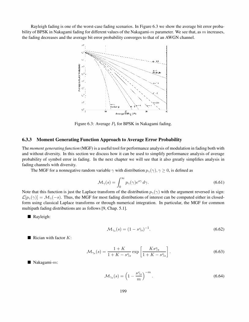
Rayleigh fading is one of the worst-case fading scenarios. In Figure 6.3 we show the average bit error proba-

bility of BPSK in Nakagami fading for different values of the Nakagami-m parameter. We see that, as m increases,

the fading decreases and the average bit error probability converges to that of an AWGN channel.

Figure 6.3: Average Pb for BPSK in Nakagami fading.

6.3.3 Moment Generating Function Approach to Average Error Probability

The moment generating function (MGF) is a useful tool for performance analysis of modulation in fading both with

and without diversity. In this section we discuss how it can be used to simplify performance analysis of average

probability of symbol error in fading. In the next chapter we will see that it also greatly simplifies analysis in

fading channels with diversity.

The MGF for a nonnegative random variable γ with distribution pγ(γ), γ ≥ 0, is defined as

Mγ(s) =

∫ ∞

0

pγ(γ)esγ dγ. (6.61)

Note that this function is just the Laplace transform of the distribution pγ(γ) with the argument reversed in sign:

L[pγ(γ)] = Mγ(−s). Thus, the MGF for most fading distributions of interest can be computed either in closed-

form using classical Laplace transforms or through numerical integration. In particular, the MGF for common

multipath fading distributions are as follows [9, Chap. 5.1].

Rayleigh:

Mγs(s) = (1− sγs)−1. (6.62)

Rician with factor K:

Mγs(s) =1 +K

1 +K − sγsexp

[Ksγs

1 +K − sγs

]

. (6.63)

Nakagami-m:

Mγs(s) =(

1 − sγsm

)−m

. (6.64)

199

As indicated by its name, the moments E[γn] of γ can be obtained from Mγ(s) as

E[γn] =∂n

∂sn[Mγs(s)]|s=0. (6.65)

The basic premise of the MGF approach for computing average error probability in fading is to express the

probability of error Ps in AWGN for the modulation of interest either as an exponential function of γs,

Ps = a exp[−bγs] (6.66)

for constants a and b, or as a finite-range integral of such an exponential function:

Ps =

∫ B

0

a exp[−b(x)γs] dx, (6.67)

where the constant b(x) may depend on the integrand but the SNR γs does not (and is not in the limits of inte-

gration). These forms allow the average probability of error to be expressed in terms of the MGF for the fading

distribution. Specifically, if Ps = a exp[−bγs], then

Ps =

∫ ∞

0

a exp[−bγ]pγs(γ)dγ = aMγs(−b). (6.68)

Since DPSK is in this form with a = 1/2 and b = 1, we see that the average probability of bit error for DPSK in

any type of fading is

Pb = 12Mγs(−1), (6.69)

where Mγs(s) is the MGF of the fading distribution. For example, using Mγs(s) for Rayleigh fading given by

(6.62) with s = −1 yields Pb = [2(1 + γb)]−1, which is the same as we obtained in (6.59). If Ps is in the integral

form of (6.67) then

Ps =

∫ ∞

0

∫ B

0a exp[−b(x)γ]dx pγs(γ) dγ

= a

∫ B

0

[∫ ∞

0exp[−b(x)γ]pγs(γ)dγ

]

dx

= a

∫ B

0Mγs(−b(x)) dx. (6.70)

In this latter case, the average probability of symbol error is a single finite-range integral of the MGF of the fading

distribution, which typically can be found in closed form or easily evaluated numerically.

Let us now apply the MGF approach to specific modulations and fading distributions. Consider any modula-

tion for which its symbol error probabilityPs in AWGN is given or approximated by an expression of the following

form:

Ps(γs) = αQ(√

βγs). (6.71)

Note that (6.32) provided an approximation to Ps in AWGN for coherent MPSK, MQAM, and MPAM in this form,

with constants α and β that depend on M .

Using the alternate Q-function representation (6.43), we get that

Ps =α

π

∫ π/2

0exp

[−.5βγsin2 φ

]

dφ, (6.72)

200

which is in the desired form (6.67). Thus, the average error probability in fading for modulations with Ps =αQ(

√βγs) in AWGN is given by

Ps =α

π

∫ ∞

0

∫ π/2

0exp

[−.5βγsin2 φ

]

dφ pγs(γ) dγdφ

=α

π

∫ π/2

0

[∫ ∞

0

exp

[−.5βγsin2 φ

]

pγs(γ)dγ

]

dφ

=α

π

∫ π/2

0Mγs

(−.5βsin2 φ

)

dφ, (6.73)

where Mγs(s) is the MGF associated with the distribution pγs(γ) as defined by (6.61). Recall that Table 6.1

approximates the error probability in AWGN for many modulations of interest as Ps ≈ αQ(√βγs), so (6.73)

gives an approximation for the average error probability of these modulations in fading. Moreover, the exact

average probability of symbol error for coherent MPSK can be obtained in a form similar to (6.73) by noting that

Craig’s formula for Ps of MPSK in AWGN given by (6.45) is in the desired form (6.67). Thus, the exact average

probability of error for MPSK becomes

Ps =

∫ ∞

0

1

π

∫ (M−1)π/M

0exp

[−βMγssin2 φ

]

dφ pγs(γ) dγ

=1

π

∫ (M−1)π/M

0

[∫ ∞

0

exp

[−βMγssin2 φ

]

pγs(γ) dγ

]

dφ

=1

π

∫ (M−1)π/M

0Mγs

(

− βM

sin2 φ

)

dφ, (6.74)

where βM = sin2(π/M) depends on the size of the MPSK constellation. The MGF Mγs(s) for Rayleigh, Ri-

cian, and Nakagami-m distributions were given by (6.62), (6.63), and (6.64), respectively. Substituting s =−βM/ sin2 φ in these expressions yields the following equations.

Rayleigh:

Mγs

(

− βM

sin2 φ

)

=

(

1 +βM γs

sin2 φ

)−1

. (6.75)

Rician with factor K:

Mγs

(

− βM

sin2 φ

)

=(1 +K) sin2 φ

(1 +K) sin2 φ+ βM γsexp

[

− KβM γs

(1 +K) sin2 φ+ βM γs

]

. (6.76)

Nakagami-m:

Mγs

(

− βM

sin2 φ

)

=

(

1 +βM γs

m sin2 φ

)−m

. (6.77)

All of these functions are simple trigonometrics and are therefore easy to integrate over the finite range in (6.73)

or (6.74).

201

Example 6.5: Use the MGF technique to find an expression for the average probability of error for BPSK modu-

lation in Nakagami fading.

Solution: We use the fact that BPSK for an AWGN channel has Pb = Q(√

2γb), so α = 1 and β = 2 in (6.71).

The moment generating function for Nakagami-m fading is given by (6.77), and substituting this into (6.73) with

α = g = 1 yields

Pb =1

π

∫ π/2

0

(

1 +γb

m sin2 φ

)−m

dφ.

From (6.22) we see that the exact probability of symbol error for MQAM in AWGN contains both the Q-

function and its square. Fortunately, an alternate form of Q2(z) allows us to apply the same techniques used here

for MPSK to MQAM modulation. Specifically, an alternate representation of Q2(z) is derived in [15] as

Q2(z) =1

π

∫ π/4

0exp

[ −z2

2 sin2 φ

]

dφ. (6.78)

Note that this is identical to the alternate representation for Q(z) given in (6.43) except that the upper limit of the

integral is π/4 instead of π/2. Thus we can write (6.22) in terms of the alternate representations for Q(z) and

Q2(z) as

Ps(γs) =4

π

(

1− 1√M

)∫ π/2

0exp

(

−βMγssin2 φ

)

dφ

− 4

π

(

1 − 1√M

)2 ∫ π/4

0exp

[

−βMγssin2 φ

]

dφ, (6.79)

where βM = 1.5/(M − 1) is a function of the MQAM constellation size. Then the average probability of symbol

error in fading becomes

Ps =

∫ ∞

0Ps(γ)pγs(γ)dγ

=4

π

(

1− 1√M

)∫ π/2

0

∫ ∞

0exp

[

− βMγ

sin2 φ

]

pγs(γ) dγ dφ

− 4

π

(

1 − 1√M

)2 ∫ π/4

0

∫ ∞

0exp

[

− βMγ

sin2 φ

]

pγs(γ) dγ dφ

=4

π

(

1− 1√M

)∫ π/2

0

Mγs

(

− βM

sin2 φ

)

dφ

− 4

π

(

1 − 1√M

)2 ∫ π/4

0

Mγs

(

− βM

sin2 φ

)

dφ. (6.80)

Thus, the exact average probability of symbol error is obtained via two finite-range integrals of the MGF over the

fading distribution, which typically can be found in closed form or easily evaluated numerically.

The MGF approach can also be applied to noncoherent and differential modulations. For example, consider

noncoherent MFSK, with Ps in AWGN given by (6.31), which is a finite sum of the desired form (6.66). Thus, in

fading, the average symbol error probability of noncoherent MFSK is given by

202

Ps =

∫ ∞

0

M∑

m=1

(−1)m+1

(M − 1

m

)1

m+ 1exp

[ −mγm+ 1

]

pγs(γ) dγ

=

M∑

m=1

(−1)m+1

(M − 1

m

)1

m+ 1

[∫ ∞

0exp

[ −mγm+ 1

]

pγs(γ) dγ

]

=

M∑

m=1

(−1)m+1

(M − 1m

)1

m+ 1Mγs

(

− m

m + 1

)

. (6.81)

Finally, for differential MPSK it can be shown [16] that the average probability of symbol error is given by

Ps =

√βM2π

∫ π/2

−π/2

exp[−γs(1 −√1 − βM cos θ)]

1 −√1− βM cos θ

dθ (6.82)

for βM = sin2(π/M) , which is in the desired form (6.67). Thus we can express the average probability of symbol

error in terms of the MGF of the fading distribution as

Ps =

√βM2π

∫ π/2

−π/2

Mγs(−(1−√1 − βM cos θ))

1 −√1 − βM cos θ

dθ. (6.83)

A more extensive discussion of the MGF technique for finding average probability of symbol error for different

modulations and fading distributions can be found in [9, Chap. 8.2].

6.3.4 Combined Outage and Average Error Probability

When the fading environment is a superposition of both fast and slow fading (e.g., log-normal shadowing and

Rayleigh fading), a common performance metric is combined outage and average error probability, where outage

occurs when the slow fading falls below some target value and the average performance in non-outage is obtained

by averaging over the fast fading. We use the following notation.

• =γs denotes the average SNR per symbol for a fixed path loss with averaging over fast fading and shadowing.

• γs denotes the (random) SNR per symbol for a fixed path loss and random shadowing but averaged over fast

fading. Its average value, averaged over the shadowing, is=γs.

• γs denotes the random SNR due to fixed path loss, shadowing, and multipath. Its average value, averaged

over multipath only, is γs. Its average value, averaged over both multipath and shadowing, is ¯γs.

With this notation we can specify an average error probability Ps with some probability 1 − Pout. An outage is

declared when the received SNR per symbol due to shadowing and path loss alone, γs, falls below a given target

value γs0 . When not in outage (γs ≥ γs0), the average probability of error is obtained by averaging over the

distribution of the fast fading conditioned on the mean SNR:

Ps =

∫ ∞

0

Ps(γs)p(γs | γs) dγs. (6.84)

The criterion used to determine the outage target γs0 is typically based on a given maximum acceptable average

probability of error Ps0 . The target γs0 must then satisfy

203

Ps0 =

∫ ∞

0Ps(γs)p(γs | γs0) dγs. (6.85)

It is clear that, whenever γs > γs0 , the average error probability Ps will be below the target maximum value Ps0 .

Example 6.6: Consider BPSK modulation in a channel with both log-normal shadowing (σψdB= 8 dB) and

Rayleigh fading. The desired maximum average error probability is Pb0 = 10−4, which requires γb0 = 34 dB.

Determine the value of=γb that will ensure Pb ≤ 10−4 with probability 1− Pout = .95.

Solution: We must find=γb, the average of γb in both the fast and slow fading, such that p(γb > γb0) = 1 − Pout.

For log-normal shadowing we compute this as

p(γb > 34) = p

(γb − ¯γbσψdB

≥ 34− ¯γbσψdB

)

= Q

(34 − ¯γbσψdB

)

= 1 − Pout, (6.86)

since, assuming units in dB, (γb − ¯γb)/σψdBis a Gauss-distributed random variable with mean 0 and standard

deviation 1. Thus, the value of ¯γb is obtained by substituting the values of Pout and σψdBin (6.86) and using a

table of Q-functions or an inversion program, which yields (34− ¯γb)/8 = −1.6 or ¯γb = 46.8 dB.

6.4 Doppler Spread

One consequence of Doppler spread is an irreducible error floor for modulation techniques using differential de-

tection. This is due to the fact that in differential modulation the signal phase associated with one symbol is used

as a phase reference for the next symbol. If the channel phase decorrelates over a symbol, then the phase refer-

ence becomes extremely noisy, leading to a high symbol error rate that is independent of received signal power.

The phase correlation between symbols and consequent degradation in performance are functions of the Doppler

frequency fD = v/λ and the symbol time Ts.The first analysis of the irreducible error floor due to Doppler was done by Bello and Nelin in [17]. In that

work, analytical expressions for the irreducible error floor of noncoherent FSK and DPSK due to Doppler are

determined for a Gaussian Doppler power spectrum. However, these expressions are not in closed form, so they

must be evaluated numerically. Closed-form expressions for the bit error probability of DPSK in fast Rician fading,

where the channel decorrelates over a bit time, can be obtained using the MGF technique, with the MGF obtained

based on the general quadratic form of complex Gaussian random variables [1, Apx. B; 12, Apx. B]. A different

approach utilizing alternate forms of the Marcum Q-function can also be used [9, Chap. 8.2.5]. The resulting

average bit error probability for DPSK is

Pb =1

2

(1 +K + γb(1 − ρC)

1 +K + γb

)

exp

[

− Kγb1 +K + γb

]

, (6.87)

where ρC is the channel correlation coefficient after a bit time Tb, K is the fading parameter of the Rician distribu-

tion, and γb is the average SNR per bit. For Rayleigh fading (K = 0) this simplifies to

Pb =1

2

(1 + γb(1− ρC)

1 + γb

)

. (6.88)

Letting γb → ∞ in (6.87) yields the irreducible error floor:

Pfloor =(1 − ρC)e−K

2(DPSK). (6.89)

204

A similar approach is used in [18] to bound the bit error probability of DQPSK in fast Rician fading as

Pb ≤1

2

(

1−√

(ρC γs/√

2)2

(γs + 1)2 − (ρC γs/√

2)2

)

exp

[

− (2−√

2)Kγs/2

(γs + 1) − (ρC γs/√

2)

]

, (6.90)

where K is as before, ρC is the channel correlation coefficient after a symbol time Ts, and γs is the average SNR

per symbol. Letting γs → ∞ yields the irreducible error floor:

Pfloor =1

2

(

1 −√

(ρC/√

2)2

1− (ρC/√

2)2

)

exp

[

−(2 −√

2)(K/2)

1− ρC/√

2

]

(DQPSK). (6.91)

As discussed in Section 3.2.1, the channel correlation AC(τ) over time τ equals the inverse Fourier transform

of the Doppler power spectrum SC(f) as a function of Doppler frequency f . The correlation coefficient is thus

ρC = AC(T )/AC(0) evaluated at T = Ts for DQPSK or at T = Tb for DPSK. Table 6.2, from [19], gives the

value of ρC for several different Doppler power spectra models, where BD is the Doppler spread of the channel.

Assuming the uniform scattering model (ρC = J0(2πfDTb)) and Rayleigh fading (K = 0) in (6.89) yields an

irreducible error for DPSK of

Table 6.2: Correlation coefficients for different Doppler power spectra models

Type Doppler power spectrum SC(f) ρC = AC(T )/AC(0)

Rectangular P0/2BD, |f | < BD sinc(2BDT )

Gaussian (P0/√πBD)e−f

2/B2D e−(πBDT )2

Uniform scattering P0/π

√

B2D − f2, |f | < BD J0(2πBDT )

1st-order Butterworth P0BD/π(f2 + B2D) e−2πBDT

Figure 6.4: Average Pb for DPSK in fast Rician fading with uniform scattering.

P floor =1 − J0(2πfDTb)

2≈ .5(πfDTb)

2, (6.92)

205

where BD = fD = v/λ is the maximum Doppler in the channel. Note that in this expression the error floor

decreases with data rate R = 1/Tb. This is true in general for irreducible error floors of differential modulation

due to Doppler, since the channel has less time to decorrelate between transmitted symbols. This phenomenon is

one of the few instances in digital communications where performance improves as data rate increases.

A plot of (6.87), the error probability of DPSK in fast Rician fading, for uniform scattering (ρC = J0(2πfDTb))

and different values of fDTb is shown in Figure 6.4. We see from this figure that the error floor starts to dominate

at γb = 15 dB in Rayleigh fading (K = 0), and as K increases the value of γb where the error floor dominates

also increases. We also see that increasing the data rate Rb = 1/Tb by an order of magnitude decreases the error

floor by roughly two orders of magnitude.

Example 6.7: Assume a Rayleigh fading channel with uniform scattering and a maximum Doppler of fD = 80

Hz. For what approximate range of data rates will the irreducible error floor of DPSK be below 10−4?

Solution: We have P floor ≈ .5(πfDTb)2 < 10−4. Solving for Tb with fD = 80 Hz, we get

Tb <

√2 · 10−4

π · 80= 5.63 · 10−5,

which yields R > 17.77 kbps.

Deriving analytical expressions for the irreducible error floor becomes intractable with more complex modulations,

in which case simulations are often used. In particular, simulations of the irreducible error floor for π/4-DQPSK

with square-root raised cosine filtering have been conducted (since this modulation is used in the IS-136 TDMA

standard) in [20, 21]. These simulation results indicate error floors between 10−3 and 10−4. As expected, in

these simulations the error floor increases with vehicle speed, since at higher vehicle speeds the channel typically

decorrelates more over a given symbol time.

6.5 Intersymbol Interference

Frequency-selective fading gives rise to intersymbol interference, where the received symbol over a given symbol

period experiences interference from other symbols that have been delayed by multipath. Since increasing signal

power also increases the power of the ISI, this interference gives rise to an irreducible error floor that is independent

of signal power. The irreducible error floor is difficult to analyze because it depends on the modulation format and

the ISI characteristics, which in turn depend on the characteristics of the channel and the sequence of transmitted

symbols.

The first extensive analysis of the degradation in symbol error probability due to ISI was done by Bello and

Nelin [22]. In that work, analytical expressions for the irreducible error floor of coherent FSK and noncoherent

DPSK are determined assuming a Gaussian delay profile for the channel. To simplify the analysis, only ISI asso-

ciated with adjacent symbols was taken into account. Even with this simplification, the expressions are complex

and must be approximated for evaluation. A more accurate analytical analysis can be found in [23, Chap. 8.2],

where the irreducible error floor is evaluated based on both the worst-case sequence of transmitted symbols and by

averaging over all possible symbol sequences. These expressions are also complex to evaluate owing to their de-

pendence on the channel and symbol sequence characteristics. A simple approximation to symbol error probability

with ISI can be obtained by treating the ISI as uncorrelated white Gaussian noise. Then the SNR becomes

γs =Pr

N0B + I, (6.93)

206

Figure 6.5: lrreducible error versus normalized rms delay spread for Gaussian power delay profile. (Reprinted by

permission from [24, Fig. 9], c© 1987 IEEE.)

where Pr is the received power associated with the line-of-sight signal component, and I is the received power

associated with the ISI. In a static channel the resulting probability of symbol error will be Ps(γs), where Ps is the

probability of symbol error in AWGN. If both the LOS signal component and the ISI experience flat fading, then

γs will be a random variable with distribution p(γs). The outage probability is then Pout = p(γs < γ0) and the

average symbol error probability is P s =∫Ps(γs)p(γs) dγs. Note that γs is the ratio of two random variables –

the LOS received power Pr and the ISI received power I – and thus the resulting distribution p(γs) may be hard to

obtain and typically is not in closed form.

Irreducible error floors due to ISI are often obtained by simulation, which can easily incorporate different

channel models, modulation formats, and symbol sequence characteristics [24, 20, 21, 25, 26, 27]. The earliest of

these works is [24]. The extensive simulations in this work determined the irreducible error floor due to ISI for

BPSK, DPSK, QPSK, OQPSK and MSK modulations with different pulse shapes and for channels with different

power delay profiles, including a Gaussian, exponential, equal-amplitude two-ray, and empirical power delay pro-

file. The results of [24] indicate that the irreducible error floor is more sensitive to the rms delay spread of the

channel than to the shape of its power delay profile. Moreover, pulse shaping can significantly impact the error

floor: for the raised cosine pulses discussed in Section 5.5, increasing β from 0 to 1 can reduce the error floor by

over an order of magnitude.

The simulation results of [24] are shown in Figure 6.5. This figure plots the irreducible bit error rate as a

function of normalized rms delay spread d = σTm/Ts for BPSK, QPSK, OQPSK, and MSK modulation assuming

a static channel with a Gaussian power delay profile. We see from the figure that, for all modulations, we can

approximately bound the irreducible error floor as

Pfloor ≤ K

(σTm

Ts

)2

(6.94)

207

for K a constant that depends on the modulation type, the transmit and receive filtering, and the power delay

profile. For the modulation types in Figure 6.5 we see thatK ranges from about 0.4 for BPSK to 1 for MSK. Other

simulation results [27, 25, 26] support this bound as well. This bound can also be derived analytically based on

group delay. Details can be found in [29, Chapter 12.3.2].

This bound imposes severe constraints on data rate even when symbol error probabilities on the order of

10−2 are acceptable, and usually this is a very high error probability even with strong error correction codes. For

example, the rms delay spread in a typical urban environment is approximately σTm = 2.5 µs. To keep σTm < .1Tsrequires that the data rate not exceed 40 kbaud, which generally isn’t enough for high-speed data applications. In

rural environments, where multipath is not attenuated to the same degree as in cities, σTm ≈ 25 µs, which reduces

the maximum data rate to 4 kbaud.

Example 6.8: Using the approximation P floor ≤ K(σTm/Ts)2 of (6.94) withK = 0.4 for BPSK and K = 0.7 for

QPSK, find the maximum data rate that can be transmitted through a channel with delay spread σTm = 3 µs, using

either BPSK or QPSK modulation, such that the probability of bit error Pb is less than 10−3.

Solution: For BPSK, we set P floor = .4(σTm/Tb)2 and so require Tb ≥ σTm/

√

P floor/.4 = 60 µs, which leads

to a data rate of R = 1/Tb = 16.67 Kbps. For QPSK, we have Ts ≥ σTm/√

P floor/.7 = 79 µs. Since there are

two bits per symbol, this leads to a data rate of R = 2/Ts = 25.2 Kbps. This indicates that, for a given data rate,

QPSK is more robust to ISI than BPSK because its symbol time is slower, even though the K value in the error

floor bound (6.94) is higher for the larger constellation size of QPSK versus BPSK. In general K increases in the

bound of (6.94) as the constellation size increases, but large constellations are still more robust to ISI than smaller

ones due to their longer symbol times.

208

Figure 6.6: BPSK demodulator for Problem 6-4.

Chapter 6 Problems

1. Consider a system in which data is transferred at a rate of 100 bits per second over the channel.

(a) Find the symbol duration if we use a sinc pulse for signaling and the channel bandwidth is 10 kHz.

(b) Suppose the received SNR is 10 dB. Find the SNR per symbol and the SNR per bit if 4-QAM is used.

(c) Find the SNR per symbol and the SNR per bit for 16-QAM, and compare with these metrics for 4-

QAM.

2. Consider BPSK modulation where the a priori probability of 0 and 1 is not the same. Specifically, p(sn =0) = 0.3 and p(sn = 1) = 0.7.

(a) Find the probability of bit error Pb in AWGN assuming we encode a 1 as s1(t) = A cos(2πfct) and a

0 as s2(t) = −A cos(2πfct) for A > 0, assuming the receiver structure is as shown in Figure 5.17.

(b) Suppose you can change the threshold value in the receiver of Figure 5.17. Find the threshold value

that yields equal error probability regardless of which bit is transmitted – that is, the threshold value

that yields p(m = 0 |m = 1)p(m = 1) = p(m = 1 |m = 0)p(m = 0).

(c) Now suppose we change the modulation so that s1(t) = A cos(2πfct) and s2(t) = −B cos(2πfct).

Find A > 0 and B > 0 so that the receiver of Figure 5.17 with threshold at zero has p(m = 0 |m =1)p(m = 1) = p(m = 1 |m = 0)p(m = 0).

(d) Compute and compare the expression for Pb in parts (a), (b), and (c) assuming Eb/N0 = 10 dB and

N0 = .1. For which system is Pb minimized?

3. Consider a BPSK receiver whose demodulator has a phase offset of φ relative to the transmitted signal, so for

a transmitted signal s(t) = ±g(t) cos(2πfct) the carrier in the demodulator of Figure 5.17 is cos(2πfct+φ).

Determine the threshold level in the threshold device of Figure 5.17 that minimizes probability of bit error,

and find this minimum error probability.

4. Assume a BPSK demodulator in which the receiver noise is added after the integrator, as shown in Figure 6.6.

The decision device outputs a 1 if its input x has Rex ≥ 0, and a 0 otherwise. Suppose the tone jammer

n(t) = 1.1ejθ, where p(θ = nπ/3) = 1/6 for n = 0, 1, 2, 3, 4, 5. What is the probability of making a

decision error in the decision device (i.e., outputting the wrong demodulated bit), assumingAc =√

2/Tb =

1 and that information bits corresponding to a 1 (s(t) = Ac cos(2πfct)) or a 0(s(t) = −Ac cos(2πfct)) are

equally likely.

5. Find an approximation to Ps for the signal constellations shown in Figure 6.7.

209

Figure 6.7: Signal constellations for Problem 6-5.

6. Plot the exact symbol error probability and the approximation from Table 6.1 of 16-QAM with 0 ≤ γs ≤30 dB. Does the error in the approximation increase or decrease with γs? Why?

7. Plot the symbol error probabilityPs for QPSK using the approximation in Table 6.1 and Craig’s exact result

for 0 ≤ γs ≤ 30 dB. Does the error in the approximation increase or decrease with γs? Why?

8. In this problem we derive an algebraic proof of the alternate representation of the Q-function (6.43) from its

original representation (6.42). We will work with the complementary error function (erfc) for simplicity and

make the conversion at the end. The erfc(x) function is traditionally defined by

erfc(x) =2√π

∫ ∞

xe−t

2dt. (6.95)

The alternate representation of this, corresponding to the alternate representation of theQ-function (6.43), is

erfc(x) =2

π

∫ π/2

0e−x

2/ sin2 θdθ. (6.96)

(a) Consider the integral

Ix(a) ,

∫ ∞

0

e−at2

x2 + t2dt, (6.97)

and show that Ix(a) satisfies the following differential equation:

x2Ix(a)−∂Ix(a)

∂a=

1

2

√π

a. (6.98)

210

(b) Solve the differential equation (6.98) and deduce that

Ix(a) ,

∫ ∞

0

e−at2

x2 + t2dt =

π

2xeax

2erfc(x

√a). (6.99)

Hint: Ix(a) is a function in two variables x and a. However, since all our manipulations deal with a

only, you can assume x to be a constant while solving the differential equation.

(c) Setting a = 1 in (6.99) and making a suitable change of variables in the left-hand side of (6.99), derive

the alternate representation of the erfc function:

erfc(x) =2

π

∫ π/2

0e−x

2/ sin2 θdθ.

(d) Convert this alternate representation of the erfc function to the alternate representation of the Q-

function.

9. Consider a communication system that uses BPSK signaling, with average signal power of 100 W and noise

power at the receiver of 4 W. Based on its error probability, can this system be used for transmission of data?

Can it be used for voice? Now consider the presence of fading with an average SNR γb = 20 dB. How do

your answers to the previous questions change?

10. Consider a cellular system at 900 MHz with a transmission rate of 64 kbps and multipath fading. Explain

which performance metric – average probability of error or outage probability – is more appropriate (and

why) for user speeds of l mph, 10 mph, and 100 mph.

11. Derive the expression for the moment generating function for SNR in Rayleigh fading.

12. This problem illustrates why satellite systems that must compensate for shadow fading are going bankrupt.

Consider an LEO satellite system orbiting 500 km above the earth. Assume that the signal follows a free-

space path-loss model with no multipath fading or shadowing. The transmitted signal has a carrier frequency

of 900 MHz and a bandwidth of 10 kHz. The handheld receivers have noise power spectral density of 10−16

mW/Hz (total noise power is N0B). Assume nondirectional antennas (0-dB gain) at both the transmitter and

receiver. Suppose the satellite must support users in a circular cell on the earth of radius 100 km at a BER

of 10−6.

(a) For DPSK modulation, find the transmit power needed for all users in the cell to meet the 10−6 BER

target.

(b) Repeat part (a) assuming that the channel also experiences log-normal shadowing with σψdB= 8 dB

and that users in a cell must have Pb = 10−6 (for each bit) with probability 0.9.

13. In this problem we explore the power penalty involved in going from BPSK to the higher-level signal mod-

ulation of 16-PSK.

(a) Find the minimum distance between constellation points in 16-PSK modulation as a function of signal

energy Es.

(b) Find αM and βM such that the symbol error probability of 16-PSK in AWGN is approximately

Ps ≈ αMQ(√

βMγs).

211

(c) Using your expression in part (b), find an approximation for the average symbol error probability of

16-PSK in Rayleigh fading in terms of γs.

(d) Convert the expressions for average symbol error probability of 16-PSK in Rayleigh fading to an ex-

pression for average bit error probability, assuming Gray coding.

(e) Find the approximate value of γb required to obtain a BER of 10−3 in Rayleigh fading for BPSK and

16-PSK. What is the power penalty in going to the higher-level signal constellation at this BER?

14. Find a closed-form expression for the average probability of error for DPSK modulation in Nakagami-mfading. Evalute for m = 4 and γb = 10 dB.

15. The Nakagami distribution is parameterized by m, which ranges from m = .5 to m = ∞. Them-parameter

measures the ratio of LOS signal power to multipath power, so m = 1 corresponds to Rayleigh fading,

m = ∞ corresponds to an AWGN channel with no fading, and m = .5 corresponds to fading that results in

performance that is worse than with a Rayleigh distribution. In this problem we explore the impact of the

parameter m on the performance of BPSK modulation in Nakagami fading.

Plot the average bit error P b of BPSK modulation in Nakagami fading with average SNR ranging from 0 dB

to 20 dB for m parameters m = 1 (Rayleigh), m = 2, and m = 4. (The moment generating function

technique of Section 6.3.3 should be used to obtain the average error probability.) At an average SNR of

10 dB, what is the difference in average BER?

16. Assume a cellular system with log-normal shadowing plus Rayleigh fading. The signal modulation is DPSK.

The service provider has determined that it can deal with an outage probability of .01 – that is, 1 in 100

customers can be unhappy at any given time. In nonoutage, the voice BER requirement is P b = 10−3.

Assume a noise PSD N0/2 with N0 = 10−16 mW/Hz, a signal bandwidth of 30 kHz, a carrier frequency of

900 MHz, free-space path-loss propagation with nondirectional antennas, and a shadowing standard devia-

tion of σψdB= 6 dB. Find the maximum cell size that can achieve this performance if the transmit power at

the mobiles is limited to 100 mW.

17. Consider a cellular system with circular cells of radius 100 meters. Assume that propagation follows the

simplified path-loss model with K = 1, d0 = 1 m, and γ = 3. Assume the signal experiences (in addition

to path loss) log-normal shadowing with σψdB= 4 as well as Rayleigh fading. The transmit power at

the base station is Pt = 100 mW, the system bandwidth is B = 30 kHz, and the noise PSD N0/2 has

N0 = 10−14W/Hz. Assuming BPSK modulation, we want to find the cell coverage area (percentage of

locations in the cell) where users have average Pb of less than 10−4.

(a) Find the received power due to path loss at the cell boundary.

(b) Find the minimum average received power (due to path loss and shadowing) such that, with Rayleigh

fading about this average, a BPSK modulated signal with this average received power at a given cell

location has P b < 10−4.

(c) Given the propagation model for this system (simplified path loss, shadowing, and Rayleigh fading),

find the percentage of locations in the cell where P b < 10−4 under BPSK modulation.

18. In this problem we derive the probability of bit error for DPSK in fast Rayleigh fading. By symmetry, the

probability of error is the same for transmitting a 0-bit or a 1-bit. Let us assume that over time kTb a 0-bit is

transmitted, so the transmitted symbol at time kTb is the same as at time k−1: s(k) = s(k−1). In fast fading,

the corresponding received symbols are r(k−1) = gk−1s(k−1)+n(k−1) and r(k) = gks(k−1)+n(k),

where gk−1 and gk are the fading channel gains associated with transmissions over times (k−1)Tb and kTb.

212

(a) Show that the decision variable that is input to the phase comparator of Figure 5.20 in order to extract

the phase difference is r(k)r∗(k − 1) = gkg∗k−1 + gks(k− 1)∗nk−1 + g∗k−1s

∗k−1nk + nkn

∗k−1.

Assuming a reasonable SNR, the last term nkn∗k−1 of this expression can be neglected. So neglecting

this term and then defining nk = s∗k−1nk and nk−1 = s∗k−1nk−1, we get a new random variable

z = gkg∗k−1 + gkn

∗k−1 + g∗k−1nk. Given that a 0-bit was transmitted over time kTb, an error is made

if x = Rez < 0, so we must determine the distribution of x. The characteristic function for x is the

two-sided Laplace transform of the distribution of x:

ΦX(s) =

∫ ∞

−∞pX(s)e−sx dx = E[e−sx].

This function will have a left-plane pole p1 and a right-plane pole p2, so it can be written as

ΦX(s) =p1p2

(s− p1)(s− p2).

The left-plane pole p1 corresponds to the distribution pX(x) for x ≥ 0, and the rightplane pole corre-

sponds to the distribution pX(x) for x < 0.

(b) Show through partial fraction expansion that ΦX(s) can be written as

ΦX(s) =p1p2

p1 − p2

1

s − p1+

p1p2

p2 − p1

1

s− p2.

An error is made if x = Rez < 0, so here we need only consider the distribution pX(x) for x < 0corresponding to the second term of ΦX(s).

(c) Show that the inverse Laplace transform of the second term of ΦX(s) from part (b) is

pX(x) =p1p2

p2 − p1ep2X , x < 0.

(d) Use part (c) to show that Pb = −p1/(p2 − p1).

In x = Rez = Regkg∗k−1 + gkn∗k−1 + g∗k−1nk, the channel gains gk, gk−1 and noises nk, nk−1

are complex Gaussian random variables. Thus, the poles p1, p2 in pX(x) are derived using the general

quadratic form of complex Gaussian random variables [1, Apx. B; 12, Apx. B] as

p1 =−1

N0(γb[1 + ρc] + 1)and p2 =

1

N0(γb[1 − ρc] + 1)

for ρC the correlation coefficient of the channel over the bit time Tb.

(e) Find a general expression for Pb in fast Rayleigh fading using these values of p1 and p2 in the Pbexpression from part (d).

(f) Show that this reduces to the average probability of error P b = 1/2(1+γb) for a slowly fading channel

that does not decorrelate over a bit time.

19. Plot the bit error probability for DPSK in fast Rayleigh fading for γb ranging from 0 dB to 60 dB and

ρC = J0(2πBDT ) with BDT = .01, .001, and .0001. For each value of BDT , at approximately what value

of γb does the error floor dominate the error probability?

20. Find the irreducible error floor due to Doppler for DQPSK modulation with a data rate of 40 kbps, assuming

a Gaussian Doppler power spectrum with BD = 80 Hz and Rician fading with K = 2.

213

21. Consider a wireless channel with an average delay spread of 100 ns and a Doppler spread of 80 Hz. Given

the error floors due to Doppler and ISI – and assuming DQPSK modulation in Rayleigh fading and uniform

scattering – approximately what range of data rates can be transmitted over this channel with a BER of less

than 10−4?

22. Using the error floors of Figure 6.5, find the maximum data rate that can be transmitted through a channel

with delay spread σTm = 3 µs (using BPSK, QPSK, or MSK modulation) such that the probability of bit

error Pb is less than 10−3.

214

Bibliography

[1] J. G. Proakis and M. Salehi, Digital Communications, 5th ed., McGraw-Hill, New York, 2008.

[2] M. K. Simon, S. M. Hinedi, and W. C. Lindsey, Digital Communication Techniques: Signal Design and

Detection, Prentice-Hall, Englewood Cliffs, NJ, 1995.

[3] S. Rhodes, “Effect of noisy phase reference on coherent detection of offset-QPSK signals,” IEEE Trans.

Commun., pp. 1046–55, August 1974.

[4] N. R. Sollenberger and J. C.-I. Chuang, “Low-overhead symbol timing and carrier recovery for portable

TDMA radio systems,” IEEE Trans. Commun., pp. 1886–92, October 1990.

[5] R. Pawula, S. Rice, and J. Roberts, “Distribution of the phase angle between two vectors perturbed by Gaus-

sian noise,” IEEE Trans. Commun., pp. 1828–41, August 1982.

[6] W. Cowley and L. Sabel, “The performance of two symbol timing recovery algorithms for PSK demodula-

tors,” IEEE Trans. Commun., pp. 2345–55, June 1994.

[7] W. T. Webb and L. Hanzo, Modern Quadrature Amplitude Modulation, IEEE/Pentech Press, London, 1994.

[8] X. Tang, M.-S. Alouini, and A. Goldsmith, “Effect of channel estimation error on M-QAM BER performance

in Rayleigh fading,” IEEE Trans. Commun., pp. 1856–64, December 1999.

[9] M. K. Simon and M.-S. Alouini, Digital Communication over Fading Channels: A Unified Approach to

Performance Analysis, 2nd Ed., Wiley, New York, 2004.

[10] S. Hinedi, M. Simon, and D. Raphaeli, “The performance of noncoherent orthogonal M-FSK in the presence

of timing and frequency errors,” IEEE Trans. Commun., pp. 922–33, February–April 1995.

[11] E. Grayver and B. Daneshrad, “A low-power all-digital FSK receiver for deep space applications,” IEEE

Trans. Commun., pp. 911–21, May 2001.

[12] M. Schwartz, W. R. Bennett, and S. Stein, Communication Systems and Techniques, McGraw-Hill, New York,

1966 [reprinted 1995 by Wiley/IEEE Press].

[13] J. Craig, “New, simple and exact result for calculating the probability of error for two-dimensional signal

constellations,” Proc. Military Commun. Conf., pp. 25.5.1–25.5.5, November 1991.

[14] F. S. Weinstein, “Simplified relationships for the probability distribution of the phase of a sine wave in narrow-

band normal noise,” IEEE Trans. Inform. Theory, pp. 658–61, September 1974.

[15] M. K. Simon and D. Divsalar, “Some new twists to problems involving the Gaussian probability integral,”

IEEE Trans. Commun., pp. 200–10, Febmary 1998.

215

[16] R. F. Pawula, “A new formula for MDPSK symbol error probability,” IEEE Commun. Lett., pp. 271–2, Octo-

ber 1998.

[17] P. A. Bello and B. D. Nelin, “The influence of fading spectrum on the bit error probabilities of incoherent and

differentially coherent matched filter receivers,” IEEE Trans. Commun. Syst., pp. 160–8, June 1962.

[18] P. Y. Kam, “Tight bounds on the bit-error probabilities of 2DPSK and 4DPSK in nonselective Rician fading,”

IEEE Trans. Commun., pp. 860–2, July 1998.

[19] P. Y. Kam, “Bit error probabilities of MDPSK over the nonselective Rayleigh fading channel with diversity

reception,” IEEE Trans. Commun., pp. 220–4, February 1991.

[20] V. Fung, R. S. Rappaport, and B. Thoma, “Bit error simulation for π/4 DQPSK mobile radio communication

using two-ray and measurement based impulse response models,” IEEE J. Sel. Areas Commun., pp. 393–405,

April 1993.

[21] S. Chennakeshu and G. J. Saulnier, “Differential detection of π/4-shifted-DQPSK for digital cellular radio,”

IEEE Trans. Veh. Tech., pp. 46–57, Febmary 1993.

[22] P. A. Bello and B. D. Nelin, “ The effects of frequency selective fading on the binary error probabilities

of incoherent and differentially coherent matched filter receivers,” IEEE Trans. Commun. Syst., pp. 170–86,

June 1963.

[23] M. B. Pursley, Introduction to Digital Communications, Prentice-Hall, Englewood Cliffs, NJ, 2005.

[24] J. C.-I. Chuang, “The effects of time delay spread on portable radio communications channels with digital

modulation,” IEEE J. Sel. Areas Commun., pp. 879–89, June 1987.

[25] N. R. Sollenberger, J. C. I. Chuang, L. F. Chang, S. Ariyavisitakul and H. Arnold, “Architecture and im-

plementation of an efficient and robust TDMA frame structure for digital portable communications,” IEEE

Transactions on Vehicular Technology, vol. 40, no. 1, pp. 250-260, Feb. 1991.

[26] J. C. I. Chuang, ”The effects of delay spread on 2-PSK, 4-PSK, 8-PSK and 16-QAM in a portable radio

environment,” IEEE Transactions on Vehicular Technology, vol. 38, no. 2, pp. 43-45, May 1989.

[27] C. Liu and K. Feher, “Bit error rate performance of π/4 DQPSK in a frequency selective fast Rayleigh fading

channel,” IEEE Trans. Veh. Tech., pp. 558–68, August 1991.

[28] S. Gumnathan and K. Feher, “Multipath simulation models for mobile radio channels,” Proc. IEEE Veh. Tech.

Conf., pp. 131–4, May 1992.

[29] Wireless Communications, 2nd Ed, A. F. Molisch, John Wiley and Sons, 2010.

216

Chapter 7

Diversity

In Chapter 6 we saw that both Rayleigh fading and log-normal shadowing exact a large power penalty on the

performance of modulation over wireless channels. One of the best techniques to mitigate the effects of fading is

diversity combining of independently fading signal paths. Diversity combining exploits the fact that independent

signal paths have a low probability of experiencing deep fades simultaneously. Thus, the idea behind diversity

is to send the same data over independent fading paths. These independent paths are combined in such a way

that the fading of the resultant signal is reduced. For example, consider a system with two antennas at either the

transmitter or receiver that experience independent fading. If the antennas are spaced sufficiently far apart, it is

unlikely that they both experience deep fades at the same time. By selecting the antenna with the strongest signal,

a technique known as selection combining, we obtain a much better signal than if we had just one antenna. This

chapter focuses on common methods used at the transmitter and receiver to achieve diversity. A more detailed

treatment of diversity combining methods and their performance, including the effects of correlated fading on the

different paths as well as channel estimation errors, can be found in [1, Chap. 9].

Diversity techniques that mitigate the effect of multipath fading are called microdiversity, and that is the focus

of this chapter. Diversity to mitigate the effects of shadowing from buildings and objects is called macrodiver-

sity. Macrodiversity is generally implemented by combining signals received by several base stations or access

points, which requires coordination among these different stations or points. Such coordination is implemented as

part of the networking protocols in infrastructure-based wireless networks. We will therefore defer discussion of

macrodiversity until Chapter 15, where we examine the design of such networks.

7.1 Realization of Independent Fading Paths

There are many ways of achieving independent fading paths in a wireless system. One method is to use multiple

transmit or receive antennas, also called an antenna array, where the elements of the array are separated in distance.

This type of diversity is referred to as space diversity. Note that with receiver space diversity, independent fading

paths are realized without an increase in transmit signal power or bandwidth. Moreover, coherent combining of

the diversity signals increases the signal-to-noise power ratio at the receiver over the SNR that would be obtained

with just a single receive antenna. This SNR increase, called array gain, can also be obtained with transmitter

space diversity by appropriately weighting the antenna transmit powers relative to the channel gains. In addition

to array gain, space diversity also provides diversity gain, defined as the change in slope of the error probabil-

ity resulting from the diversity combining. We will describe both the array gain and diversity gain for specific

diversity-combining techniques in subsequent sections.

The maximum diversity gain for either transmitter or receiver space diversity typically requires that the sep-

aration between antennas be such that the fading amplitudes corresponding to each antenna are approximately

217

independent. For example, from equation (3.28) we know that, in a uniform scattering environment with omni-

directional transmit and receive antennas, the minimum antenna separation required for independent fading on

each antenna is approximately one half-wavelength (.38λ, to be exact). If the transmit or receive antennas are

directional, the scattering is not uniform, or a dominant LOS component exists, then a larger antenna separation is

typically required to obtain independent fading samples [2, Chap. 13].

A second method of achieving diversity is by using either two transmit antennas or two receive antennas with

different polarization (e.g., vertically and horizontally polarized waves). The two transmitted waves follow the

same path. However, since the multiple random reflections distribute the power nearly equally relative to both

polarizations, the average receive power corresponding to either polarized antenna is approximately the same.

Since the scattering angle relative to each polarization is random, it is highly improbable that signals received

on the two differently polarized antennas would be simultaneously in a deep fade. There are two disadvantages

of polarization diversity. First, you can have at most two diversity branches, corresponding to the two types of

polarization. The second disadvantage is that polarization diversity loses effectively half the power (3 dB) because

the transmit or receive power is divided between the two differently polarized antennas.

Directional antennas provide angle (or directional) diversity by restricting the receive antenna beamwidth to

a given angle. In the extreme, if the angle is very small then at most one of the multipath rays will fall within the

receive beamwidth, so there is no multipath fading from multiple rays. However, this diversity technique requires

either a sufficient number of directional antennas to span all possible directions of arrival or a single antenna whose

directivity can be steered to the arrival angle of one of the multipath components (preferably the strongest one).

Note also that with this technique the SNR may decrease owing to the loss of multipath components that fall outside

the receive antenna beamwidth – unless the directional gain of the antenna is sufficiently large to compensate for

this lost power. Smart antennas are antenna arrays with adjustable phase at each antenna element: such arrays

form directional antennas that can be steered to the incoming angle of the strongest multipath component [3].

Frequency diversity is achieved by transmitting the same narrowband signal at different carrier frequencies,

where the carriers are separated by the coherence bandwidth of the channel. This technique requires additional

transmit power to send the signal over multiple frequency bands. Spread-spectrum techniques, discussed in Chapter

13, are sometimes described as providing frequency diversity in that the channel gain varies across the bandwidth

of the transmitted signal. However, this is not equivalent to sending the same information signal over independently

fading paths. As discussed in Section 13.2.4, spread spectrum with RAKE reception does provide independently

fading paths of the information signal and thus is a form of path diversity. Time diversity is achieved by transmitting

the same signal at different times, where the time difference is greater than the channel coherence time (the inverse

of the channel Doppler spread). Time diversity does not require increased transmit power but it does lower the

data rate, since data is repeated in the diversity time slots rather than sending new data in those time slots. Time

diversity can also be achieved through coding and interleaving, as will be discussed in Chapter 8. Clearly time

diversity cannot be used for stationary applications, since the channel coherence time is infinite and thus fading is

highly correlated over time.

In this chapter we focus on space diversity as a reference when describing diversity systems and the different

combining techniques, although the techniques can be applied to any type of diversity. Thus, the combining tech-

niques will be defined as operations on an antenna array. Receiver and transmitter diversity are treated separately,

since their respective system models and combining techniques have important differences.

218

7.2 Receiver Diversity

7.2.1 System Model

In receiver diversity, the independent fading paths associated with multiple receive antennas are combined to obtain

a signal that is then passed through a standard demodulator. The combining can be done in several ways, which

vary in complexity and overall performance. Most combining techniques are linear: the output of the combiner is

just a weighted sum of the different fading paths or branches, as shown in Figure 7.1 for M -branch diversity. In

this model the complex fading associated with the ith branch is riejθi . The signal on the ith branch is multiplied

by complex gain αi and then summed with the other weighted branches to form the combiner output. When all

but one of the complex αi are zero, only one path is passed to the combiner output. If more than one of the αi are

nonzero then the combiner adds together multiple paths, though each path may be weighted by a different value.

Combining more than one branch signal requires co-phasing, where the phase θi of the ith branch is removed

through multiplication by αi = aie−jθi for some real-valued ai. Without co-phasing, the branch signals would not

add up coherently in the combiner, so the resulting output could still exhibit significant fading due to constructive

and destructive addition of the signals in all the branches.

Figure 7.1: Linear combiner.

Since co-phasing requires knowledge of the branch phase prior to multiplication by αi, coherent detection to

determine this phase value is required in each branch, as shown in Figure 7.2. This coherent detection can also

determine the value of the branch signal envelope ri or SNR γi = r2i /Ni for Ni the noise power on the ith branch,1

which αi depends on in some combining techniques. A dedicated coherent detector for each branch of a diversity

system significantly increases the hardware complexity and power consumption relative to a single-branch system,

particularly for a large number of branches. When the combiner utilizes just one branch at any given time, i.e.

αi = 0 for all except one of the M branches, then the coherent detector can be placed after the combiner in

Figure 7.1, as co-phasing multiple signals is no longer needed. We will assume throughout this chapter that the

noise power in each branch Ni = N = N0B is the same. When that is not the case, the results of this chapter can

be applied by scaling the amplitude term ri by√

N/Ni for average noise power N = N0B across all branches.

The main purpose of diversity is to coherently combine the independent fading paths so that the effects of

1In practice r2i + Ni is easier to measure than SNR, since the former involves finding only the total power in the received signal.

219

Figure 7.2: Branch Coherent Detection

fading are mitigated. The signal output from the combiner equals the original transmitted signal s(t) multiplied

by a random real-valued amplitude term αΣ =∑

i airi. This amplitude term results in a random SNR γΣ at the

combiner output, where the distribution of γΣ is a function of the number of diversity paths, the fading distribution

on each path, and the combining technique, as we shall describe in more detail.

The array gain in receiver space diversity results from coherent combining of multiple receive signals. Even

in the absence of fading, this can lead to an increase in average received SNR. For example, suppose there is no

fading and that each branch has the same SNR γi = r2i /(N0B) = γ . Since both the noise and the signal are

multiplied by ai, the SNR of the combined output is

γΣ =

(∑M

i=1 airi

)2

∑Mi=1 a

2iN0B

. (7.1)

Now set ai = ri in (7.1). We will see later that setting ai = cri for any constant c is optimal for maximal-ratio

combining in fading. Then,

γΣ =

(∑M

i=1 r2i

)2

N0B∑M

i=1 r2i

=

∑Mi=1 r

2i

N0B= Mγ. (7.2)

Thus, in the absence of fading, with appropriate weighting there is an M -fold increase in SNR due to the coherent

combining of the M signals received from the different antennas. This SNR increase in the absence of fading is

referred to as the array gain. More precisely, array gainAg is defined as the increase in the average combined SNR

γΣ over the average branch SNR γ:

Ag =γΣ

γ.

Array gain occurs for all diversity combining techniques but is most pronounced in maximal-ratio combining.

The array gain allows a system with multiple transmit or receive antennas in a fading channel to achieve better

performance than a system without diversity in an AWGN channel with the same average SNR. We will see this

effect in performance curves for both maximal-ratio and equal-gain combining with a large number of antennas.

With fading, the combining of multiple independent fading paths leads to a more favorable distribution for γΣ

than would be the case with just a single path. In particular, the performance of a diversity system (whether it uses

space diversity or another form of diversity) in terms of Ps and Pout is as defined in Sections 6.3.1 and 6.3.2:

Ps =

∫ ∞

0Ps(γ)pγΣ(γ)dγ, (7.3)

220

where Ps(γ) is the probability of symbol error for demodulation of s(t) in AWGN with SNR γ; and

Pout = p(γΣ ≤ γ0) =

∫ γ0

0pγΣ(γ)dγ (7.4)

for some target SNR value γ0. The more favorable distribution for γΣ resulting from diversity combining leads to

a decrease in Ps and Pout, and the resulting performance advantage is called the diversity gain.

When Ps as a function of pγΣ(γ) has a particular form, the performance benefit of diversity combining is

defined in terms of the diversity order of the system. In particular, if the average probability of error with diversity

combining can be expressed in the form Ps = cγ−M , where c is a constant that depends on the specific modulation

and coding and γ is the average received SNR per branch, then M is defined as the diversity order of the system.

The diversity order indicates how the slope of the average probability of error as a function of average SNR changes

with diversity (Figures 7.4 and 7.7 below show these slope changes as a function of M for different combining

techniques). Recall from (6.60) that a general approximation for average error probability in Rayleigh fading with

no diversity is Ps ≈ αM/(2βM γ). This expression has a diversity order of 1, which is consistent with a single

fading path, e.g. from a single receive antenna. The maximum diversity order of a system with M fading paths,

e.g. from M antennas, is M . When the diversity order equals the number of independent fading paths that are

combined via diversity, the system is said to achieve full diversity order.

In the following sections we will describe the different combining techniques and their performance in more

detail. These techniques entail various trade-offs between performance and complexity.

7.2.2 Selection Combining

In selection combining (SC), the combiner outputs the signal on the branch with the highest SNR. Because only one

branch is used at a time, SC requires just one receiver that is switched into the active antenna branch. However,

a dedicated receiver on each antenna branch may be needed for systems that transmit continuously in order to

monitor SNR on each branch simultaneously. With SC, the path output from the combiner has an SNR equal to

the maximum SNR of all the branches. Moreover, since only one branch output is used, co-phasing of multiple

branches is not required; hence this technique can be used with either coherent or differential modulation.

For M -branch diversity, the cumulative distribution function (cdf) of γΣ is given by

PγΣ(γ) = p(γΣ < γ) = p(max[γ1, γ2, . . . , γM ] < γ) =

M∏

i=1

p(γi < γ). (7.5)

We obtain the distribution of γΣ by differentiating PγΣ(γ) relative to γ , and we obtain the outage probability by

evaluating PγΣ(γ) at γ = γ0. Assume that we have M branches with uncorrelated Rayleigh fading amplitudes riand corresponding instantaneous SNR γi = r2i /N0B. Defining the average SNR on the ith branch as γi = E[γi],

the SNR distribution will be exponential:

p(γi) =1

γie−γi/γi . (7.6)

From (6.47), the outage probability for a target γ0 on the ith branch in Rayleigh fading is

Pout(γ0) = 1 − e−γ0/γi . (7.7)

The outage probability of the selection combiner for the target γ0 is then

Pout(γ0) =

M∏

i=1

p(γi < γ0) =

M∏

i=1

[1 − e−γ0/γi ]. (7.8)

221

If the average SNR for all of the branches are the same (γi = γ for all i), then this reduces to

Pout(γ0) = p(γΣ < γ0) = [1− e−γ0/γ ]M . (7.9)

Differentiating (7.9) relative to γ0 yields the distribution for γΣ:

pγΣ(γ) =M

γ[1− e−γ/γ ]M−1e−γ/γ . (7.10)

From (7.10) we see that the average SNR of the combiner output in independent and identically distributed

Rayleigh fading is

γΣ =

∫ ∞

0

γpγΣ(γ)dγ

=

∫ ∞

0

γM

γ[1 − e−γ/γ ]M−1e−γ/γdγ

= γ

M∑

i=1

1

i, (7.11)

where (7.11) follows from the binomial expansion of [1 − e−γ/γ ]M−1 and induction to obtain the final result.

Thus, the average SNR gain and corresponding array gain increase with M , but not linearly. The biggest gain is

obtained by going from no diversity to two-branch diversity. Increasing the number of diversity branches from

two to three will give much less gain than going from one to two, and in general increasing M yields diminishing

returns in terms of the array gain. This trend is also illustrated in Figure 7.3, which shows Pout versus γ/γ0 for

different M in i.i.d. Rayleigh fading. We see that there is dramatic improvement even with two-branch selection

combining: going from M = 1 to M = 2 at 1% outage probability yields an approximate 12-dB reduction in

required SNR, and at .01% outage probability there is an approximate 20-dB reduction in required SNR. However,

at .01% outage, going from two-branch to three-branch diversity results in an additional reduction of about 7 dB,

and going from three-branch to four-branch results in an additional reduction of about 4 dB. Clearly the power

savings is most substantial when going from no diversity to two-branch diversity, with diminishing returns as the

number of branches is increased. It should be noted also that, even with Rayleigh fading on all branches, the

distribution of the combiner output SNR is no longer exponential.

Example 7.1: Find the outage probability of BPSK modulation at Pb = 10−3 for a Rayleigh fading channel with

SC diversity for M = 1 (no diversity),M = 2, and M = 3. Assume equal branch SNRs of γ = 15 dB.

Solution: A BPSK modulated signal with γb = 7 dB has Pb = 10−3. Thus, we have γ0 = 7 dB. Substituting

γ0 = 10.7 and γ = 101.5 into (7.9) yields Pout = .1466 for M = 1, Pout = .0215 for M = 2, and Pout = .0031

for M = 3. We see that each additional branch reduces outage probability by almost an order of magnitude.

The average probability of symbol error is obtained from (7.3) with Ps(γ) the probability of symbol error in

AWGN for the signal modulation and pγΣ(γ) the distribution of the combiner SNR. For most fading distributions

and coherent modulations, this result cannot be obtained in closed form and must be evaluated numerically or by

approximation. In Figure 7.4 we plot Pb versus γb in i.i.d. Rayleigh fading, obtained by a numerical evaluation

of∫Q(

√2γ)pγΣ(γ)dγ for pγΣ(γ) given by (7.10). The figure shows that the diversity system for M ≥ 8 has a

lower error probability than an AWGN channel with the same SNR, owing to the array gain of the combiner. The

same will be true for the performance of maximal-ratio and equal-gain combining. Closed-form results do exist

222

Figure 7.3: Outage probability of selection combining in Rayleigh fading.

for differential modulation under i.i.d. Rayleigh fading on each branch [1, Chap. 9.7; 4, Chap. 6.1]. For example,

it can be shown for DPSK with pγΣ(γ) given by (7.10) that the average probability of symbol error is given by

Pb =

∫ ∞

0

1

2e−γpγΣ(γ)dγ =

M

2

M−1∑

m=0

(−1)m(M−1m

)

1 +m+ γ. (7.12)

Figure 7.4: Average Pb of BPSK under selection combining with i.i.d. Rayleigh fading.

In the foregoing derivations we assume that there is no correlation between the branch amplitudes. If the

correlation is nonzero then there is a slight degradation in performance, which is almost negligible for correlations

below .5. Derivation of the exact performance degradation due to branch correlation can be found in [1, Chap. 9.7;

2].

223

7.2.3 Threshold Combining

Selection combining for systems that transmit continuously may require a dedicated receiver on each branch to

continuously monitor branch SNR. A simpler type of combining, called threshold combining, avoids the need for

a dedicated receiver on each branch by scanning each of the branches in sequential order and outputting the first

signal whose SNR is above a given threshold γT . As in SC, co-phasing is not required because only one branch

output is used at a time. Hence this technique can be used with either coherent or differential modulation.

Once a branch is chosen, the combiner outputs that signal as long as the SNR on that branch remains above

the desired threshold. If the SNR on the selected branch falls below the threshold, the combiner switches to another

branch. There are several criteria the combiner can use for determining which branch to switch to [5]. The simplest

criterion is to switch randomly to another branch. With only two-branch diversity this is equivalent to switching

to the other branch when the SNR on the active branch falls below γT . This method is called switch-and-stay

combining (SSC). The switching process and SNR associated with SSC is illustrated in Figure 7.5. Since the SSC

does not select the branch with the highest SNR, as illustrated in Figure 7.5 on the third switch, its performance is

between that of no diversity and ideal SC.

Figure 7.5: SNR of the SSC technique. Switching when the SNR falls below a threshold does not always select

the branch with the highest SNR.

Let us denote the SNR on the ith branch by γi and the SNR of the combiner output by γΣ. The cdf of γΣ will

depend on the threshold level γT and the cdf of γi. For two-branch diversity with i.i.d. branch statistics, the cdf

of the combiner output PγΣ(γ) = p(γΣ ≤ γ) can be expressed in terms of the cdf Pγi(γ) = p(γi ≤ γ) and the

distribution pγi(γ) of the individual branch SNRs as

PγΣ(γ) =

Pγ1(γT )Pγ2(γ) γ < γT ,

p(γT ≤ γ2 ≤ γ) + Pγ1(γT )Pγ2(γ) γ ≥ γT .(7.13)

For Rayleigh fading in each branch with γi = γ (i = 1, 2), this yields

PγΣ(γ) =

1 − e−γT /γ − e−γ/γ + e−(γT +γ)/γ γ < γT ,

1 − 2e−γ/γ + e−(γT +γ)/γ γ ≥ γT .(7.14)

224

The outage probabilityPout associated with a given γ0 is obtained by evaluating PγΣ(γ) at γ = γ0:

Pout(γ0) = PγΣ(γ0) =

1 − e−γT /γ − e−γ0/γ + e−(γT +γ0)/γ γ0 < γT ,

1 − 2e−γ0/γ + e−(γT +γ0)/γ γ0 ≥ γT .(7.15)

The performance of SSC under other types of fading, as well as the effects of fading correlation, is studied in [1,

Chap. 9.8; 6; 7]. In particular, it is shown in [1, Chap. 9.8] that, for any fading distribution, SSC with an optimized

threshold of γT = γ0 has the same outage probability as SC.

Example 7.2: Find the outage probability of BPSK modulation at Pb = 10−3 for two-branch SSC diversity with

i.i.d. Rayleigh fading on each branch for threshold values of γT = 5 dB, 7 dB, and 10 dB. Assume the average

branch SNR is γ = 15 dB. Discuss how the outage probability changes with γT . Also compare outage probability

under SSC with that of SC and no diversity from Example 7.1.

Solution: As in Example 7.1, γ0 = 7 dB. For γT = 5 dB we have γ0 ≥ γT , so we use the second line of (7.15) to

get

Pout = 1− 2e−10.7/101.5+ e−(10.5+10.7)/101.5

= .0654.

For γT = 7 dB we have γ0 = γT , so we again use the second line of (7.15) and obtain

Pout = 1− 2e−10.7/101.5+ e−(10.7+10.7)/101.5

= .0215.

For γT = 10 dB we have γ0 < γT , so we use the first line of (7.15) to get

Pout = 1 − e−10/101.5 − e−10.7/101.5+ e−(10+10.7)/101.5

= .0397.

We see that the outage probability is smaller for γT = 7 dB than for the other two values. At γT = 5 dB the

threshold is too low, so the active branch can be below the target γ0 for a long time before a switch is made; this

contributes to a large outage probability. At γT = 10 dB the threshold is too high: the active branch will often fall

below this threshold value, which will cause the combiner to switch to the other antenna even though that other

antenna may have a lower SNR than the active one. This example shows that the threshold γT minimizing Pout

equals γ0.

From Example 7.1, SC has Pout = .0215. Thus, γT = 7 dB is the optimal threshold where SSC performs the

same as SC. We also see that performance with an unoptimized threshold can be much worse than SC. However,

the performance of SSC under all three thresholds is better than the performance without diversity, derived as

Pout = .1466 in Example 7.1.

We obtain the distribution of γΣ by differentiating (7.13) relative to γ . Then the average probability of error

is obtained from (7.3) with Ps(γ) the probability of symbol error in AWGN and pγΣ(γ) the distribution of the SSC

output SNR. For most fading distributions and coherent modulations, this result cannot be obtained in closed form

and so must be evaluated numerically or by approximation. However, for i.i.d. Rayleigh fading we can differentiate

(7.14) to obtain

pγΣ(γ) =

(1 − e−γT /γ)(1/γ)e−γ/γ γ < γT ,

(2 − e−γT /γ)(1/γ)e−γ/γ γ ≥ γT .(7.16)

As with SC, for most fading distributions and coherent modulations the resulting average probability of error

is not in closed form and must be evaluated numerically. However, closed form results do exist for differential

225

modulation under i.i.d. Rayleigh fading on each branch. In particular, the average probability of symbol error for

DPSK is given by

Pb =

∫ ∞

0

1

2e−γpγΣ(γ) dγ =

1

2(1 + γ)(1 − e−γT /γ + e−γT e−γT /γ). (7.17)

Example 7.3: Find the average probability of error for DPSK modulation under two-branch SSC diversity with

i.i.d. Rayleigh fading on each branch for threshold values of γT = 3 dB, 7 dB, and 10 dB. Assume the average

branch SNR is γ = 15 dB. Discuss how the average proability of error changes with γT . Also compare average

error probability under SSC with that of SC and with no diversity.

Solution: Evaluating (7.17) with γ = 15 dB and γT = 3, 7, and 10 dB yields (respectively) Pb = .0029,

Pb = .0023, and Pb = .0042. As in the previous example, there is an optimal threshold that minimizes aver-

age probability of error. Setting the threshold too high or too low degrades performance. From (7.12) we have that

SC yields Pb = .5(1+101.5)−1− .5(2+101.5)−1 = 4.56 · 10−4, which is roughly an order of magnitude less than

with SSC and an optimized threshold. With no diversity we have Pb = .5(1+ 101.5)−1 = .0153, which is roughly

an order of magnitude worse than with two-branch SSC.

7.2.4 Equal-Gain Combining

Equal-gain combining (EGC) is a more complex technique than those discussed in prior sections, as it co-phases

the signals on each branch and then combines them with equal weighting, αi = e−θi . The co-phasing requires

a coherent phase detector on each branch, but the instantaneous SNR of the branch is not required, in contrast to

maximal-ratio combining. The SNR of the combiner output, assuming equal noise power N0B in each branch, is

then given by

γΣ =1

MN0B

(M∑

i=1

ri

)2

. (7.18)

The distribution and cdf of γΣ do not exist in closed form. For i.i.d. Rayleigh fading with two-branch diversity and

average branch SNR γ, an expression for the cdf in terms of theQ-function can be derived [4, Chap. 6.4; 8, Chap.

5.6] as

PγΣ (γ) = 1 − e−2γ/γ −√

πγ/γe−γ/γ(1 − 2Q(√

2γ/γ)). (7.19)

The resulting outage probability is given by

Pout(γ0) = 1− e−2γR −√πγRe

−γR(1− 2Q(√

2γR)), (7.20)

where γR = γ0/γ. Differentiating (7.19) with respect to γ yields the distribution

pγΣ(γ) =1

γe−2γ/γ +

√πe−γ/γ

(1√4γγ

− 1

γ

√γ

γ

)(

1 − 2Q

(√2γ

γ

))

. (7.21)

Substituting this into (7.3) for BPSK yields the average probability of bit error:

Pb =

∫ ∞

0Q(√

2γ)pγΣ(γ)dγ = .5

1−√

1 −(

1

1 + γ

)2

. (7.22)

226

7.2.5 Maximal-Ratio Combining

In maximal-ratio combining (MRC) the output is a weighted sum of all branches, so the αi in Figure 7.1 are all

nonzero, and the weights are determined to maximize the combiner output’s SNR. The signals are co-phased and

so αi = aie−jθi , where θi is the phase of the incoming signal on the ith branch. Thus, the envelope of the combiner

output will be r =∑M

i=1 airi. Assuming the same noise power N0B in each branch yields a total noise power at

the combiner output of∑M

i=1 a2iN0B. Thus, the output SNR of the combiner is

γΣ =1

N0B

(∑M

i=1 airi

)2

∑Mi=1 a

2i

. (7.23)

The goal of MRC is to choose the ai to maximize γΣ. Intuitively, branches with a high SNR should be

weighted more than branches with a low SNR. We find the ais that maximize γΣ by taking partial derivatives of

(7.23) or finding the weights that achieve equality in the Cauchy-Schwartz inequality2. Solving for the optimal

weights yields a2i = cγi = cr2i /(N0B) for any constant c where the constant c cancels out in the SNR calculation.

Setting ai = ri yields the combiner SNR

γΣ =

M∑

i=1

r2iN0B

=

M∑

i=1

γi. (7.24)

Thus, the SNR of the combiner output is the sum of SNRs on each branch. Hence, the average combiner SNR and

corresponding array gain increase linearly with the number of diversity branches M , in contrast to the diminishing

returns associated with the average combiner SNR in SC given by (7.11). As with SC, the distribution of the

combiner output SNR does not remain exponential even when there is Rayleigh fading on all branches.

To obtain the distribution of γΣ, we take the product of the exponential moment generating functions or

characteristic functions. Assuming i.i.d. Rayleigh fading on each branch with equal average branch SNR γ, the

distribution of γΣ is χ2 with 2M degrees of freedom, expected value γΣ = Mγ, and variance 2Mγ:

pγΣ(γ) =γM−1e−γ/γ

γM(M − 1)!, γ ≥ 0. (7.25)

The corresponding outage probability for a given threshold γ0 is given by

Pout = p(γΣ < γ0) =

∫ γ0

0

pγΣ(γ) dγ = 1 − e−γ0/γM∑

k=1

(γ0/γ)k−1

(k − 1)!. (7.26)

Figure 7.6 is a plot of Pout for maximal-ratio combining indexed by the number of diversity branches.

The average probability of symbol error is obtained from (7.3) with Ps(γ) the probability of symbol error in

AWGN for the signal modulation and pγΣ(γ) the distribution of γΣ. For BPSK modulation with i.i.d. Rayleigh

fading, where pγΣ(γ) is given by (7.25), it can be shown [4, Chap. 6.3] that

Pb =

∫ ∞

0Q(√

2γ)pγΣ(γ) dγ =

(1 − Γ

2

)M M−1∑

m=0

(M − 1 +m

m

)(1 + Γ

2

)m

, (7.27)

where Γ =√

γ/(1 + γ). This equation is plotted in Figure 7.7. Comparing the outage probability for MRC in

Figure 7.6 with that of SC in Figure 7.3, or comparing the average probability of error for MRC in Figure 7.7 with

2The Cauchy-Schwartz inequality for two vectors (x1, . . . , xn) and (y1, . . . , yn) isP

i xiyi ≤p

P

i x2i

pP

i y2i

227

Figure 7.6: Pout for maximal-ratio combining with i.i.d. Rayleigh fading.

that of SC in Figure 7.4, indicates that MRC has significantly better performance than SC. In Section 7.4 we will

use a different analysis based on moment generating functions to compute average error probability under MRC,

which can be applied to any modulation type, any number of diversity branches, and any fading distribution on the

different branches.

For modulations whose probability of error in AWGN can be approximated as Ps = αQ(√βγ) for SNR

γ , e.g. BPSK, MPSK, and MQAM, we can obtain a simple upper bound on the average probability of error by

applying the Chernoff bound Q(x) ≤ e−x2/2 from (5.43) to the Q-function. For these modulations, we have

Ps = αQ(√

βγΣ) ≤ αe−βγΣ/2 = αe−β(γ1+···+γM )/2. (7.28)

Integrating over the χ2 distribution for γΣ yields

Ps ≤ αM∏

i=1

1

1 + βγi/2. (7.29)

In the limit of high SNR and assuming that the γi are identically distributed with γi = γ, we have

Ps ≈ α

(βγ

2

)−M

. (7.30)

Thus, at high SNR, the diversity order of MRC is M (the number of antennas) and so MRC achieves full diversity

order.

MRC is the only diversity-combining technique that achieves full diversity order. However, it is shown in [8,

Chap. 5.7] that performance of EGC is quite close to that of MRC, typically exhibiting less than 1 dB of power

penalty. This is the price paid for the reduced complexity of using equal gains. A more extensive performance

comparison between SC, MRC, and EGC can be found in [1, Chap. 9].

Example 7.4: Compare the average probability of bit error with BPSK under MRC and EGC two-branch diversity,

assuming i.i.d. Rayleigh fading with an average SNR of 10 dB on each branch.

228

Figure 7.7: Average Pb for maximal-ratio combining with i.i.d. Rayleigh fading.

Solution: By (7.27), under MRC we have

Pb =

(

1 −√

10/11

2

)2

(2 +√

10/11) = 1.60 · 10−3.

By (7.22), under EGC we have

Pb = .5

1 −√

1 −(

1

11

)2

= 2.07 · 10−3.

Thus we see that the performance of MRC and EGC are almost the same.

7.2.6 Generalized Combining

The three most common diversity-combining schemes used in practice are MRC, EGC, and SC. MRC has the

best performance and achieves full diversity order. However, MRC also has the highest complexity, as it requires

coherent detection in each branch that determines the branch phase and amplitude. SC is the simplest of these

three techniques as only one coherent detector is needed. The price paid for this simplicity is in performance,

with diminishing diversity gain with each branch that is added. EGC has complexity and performance between

the extremes of MRC and SC. Generalized Combining (GC), also referred to as Generalized Selection Combining

or Hybrid Combining, utilizes SC to pick a subset of the branch signals which are then combined using MRC or

EGC. In particular, a generalized combiner has M > 2 diversity branches of which it selects the L > 1 branches,

L < M , with the highest SNR; these L branches are then combined using MRC or EGC. When MRC is used, the

performance is better than an L-branch MRC system and worse than an M -branch MRC system, and similarly for

EGC, due to the selection of the L < M highest-SNR branches among the M available branches. Performance

analysis of generalized combining under both MRC and EGC in different fading environments has been studied

extensively (see [1, Chapter 9.11] and the references therein). This performance is best analyzed via the Moment

Generating Function analysis for diversity systems, as will be explored in Section 7.4.

229

7.3 Transmitter Diversity

In transmit diversity there are multiple transmit antennas, and the transmit power is divided among these antennas.

Transmit diversity is desirable in systems where more space, power, and processing capability is available on the

transmit side than on the receive side, as best exemplified by cellular systems. Transmit diversity design depends

on whether or not the complex channel gain is known to the transmitter. When this gain is known, the system

is quite similar to receiver diversity. However, without this channel knowledge, transmit diversity gain requires a

combination of space and time diversity via a novel technique called the Alamouti scheme and its extensions. We

now discuss transmit diversity under different assumptions about channel knowledge at the transmitter, assuming

the channel gains are known at the receiver.

7.3.1 Channel Known at Transmitter

Consider a transmit diversity system with M transmit antennas and one receive antenna. We assume that the path

gain riejθi associated with the ith antenna is known at the transmitter; this is referred to as having channel side

information (CSI) at the transmitter, or CSIT. Let s(t) denote the transmitted signal with average power Pt. The

signal is multiplied by a complex gain αi = aie−jθi(0 ≤ ai ≤ 1) and then sent through the ith antenna. This

complex multiplication performs both co-phasing and weighting relative to the channel gains. Because of the

average power constraint Pt, the weights must satisfy∑M

i=1 a2i = 1. The weighted signals transmitted over all

antennas are added “in the air”, which leads to a received signal given by

r(t) =M∑

i=1

airis(t). (7.31)

Let N0B denote the noise power in the receiver and assume Nyquist pulses such that BTs = 1.

Suppose we wish to set the branch weights to maximize received SNR. Using a similar analysis as in receiver

MRC diversity, we see that the weights ai that achieve the maximum SNR are given by

ai =ri

√∑M

i=1 r2i

, (7.32)

and the resulting SNR is

γΣ =PtN0B

M∑

i=1

r2i =

M∑

i=1

γi (7.33)

for γi = r2iPt/(N0B) equal to the branch SNR between the ith transmit antenna and the receive antenna. Thus we

see that transmit diversity when the channel gains are known to the transmitter is very similar to receiver diversity

with MRC: the received SNR is the sum of SNRs on each of the individual branches. In particular, if all antennas

have the same gain ri = r then γΣ = Mr2Pt/(N0B), so there is an array gain of M corresponding to an M -fold

increase in SNR over a single antenna transmitting with full power.

We again consider modulations whose error probability in AWGN can be approximated as Ps = αQ(√βγ)

for SNR γ , such as BPSK, MPSK, and MQAM. Using the Chernoff bound as in Section 7.2.5 we see that, for such

modulations and static gains on each diversity branch,

Ps = αQ(√

βγΣ) ≤ αe−βγΣ/2 = αe−β(γ1+···+γM )/2. (7.34)

Integrating over the χ2 distribution for γΣ yields the same bound as (7.29):

Ps ≤ α

M∏

i=1

1

1 + βγi/2. (7.35)

230

In the limit of high SNR and assuming that the γi are identically distributed with γi = γ, we have

Ps ≈ α

(βγ

2

)−M

. (7.36)

Thus, at high SNR, the diversity order of transmit diversity with MRC is M , so both transmit and receive MRC

achieve full diversity order. The analysis for EGC and SC assuming transmitter channel knowledge is the same as

under receiver diversity.

The complication of transmit diversity is to obtain the channel phase and, for SC and MRC, the channel gain,

at the transmitter. These channel values can be measured at the receiver using a pilot technique and then fed back

to the transmitter. Alternatively, in cellular systems with time division, the base station can measure the channel

gain and phase on transmissions from the mobile to the base and then use these measurements when transmitting

back to the mobile, since under time division the forward and reverse links are reciprocal.

7.3.2 Channel Unknown at Transmitter – The Alamouti Scheme

We now consider the same model as in Section 7.3.1 but assume here that the transmitter no longer knows the

channel gains riejθi , so there is no CSIT. In this case it is not obvious how to obtain diversity gain. Consider, for

example, a naive strategy whereby for a two-antenna system we divide the transmit energy equally between the

two antennas. Thus, the transmit signal on antenna i will be si(t) =√.5s(t) for s(t) the transmit signal with

energy per symbol Es. Assume that each antenna has a complex Gaussian channel gain hi = riejθi(i = 1, 2) with

mean 0 and variance 1. The received signal is then

r(t) =√.5(h1 + h2)s(t). (7.37)

Note that h1 + h2 is the sum of two complex Gaussian random variables and thus is itself a complex Gaussian,

with mean equal to the sum of means (0) and variance equal to the sum of variances (2). Hence√.5(h1 + h2) is a

complex Gaussian random variable with mean 0 and variance 1, so the received signal has the same distribution as

if we had just used one antenna with the full energy per symbol. In other words, we have obtained no performance

advantage from the two antennas, since we could neither divide our energy intelligently between them nor obtain

coherent combining via co-phasing.

Transmit diversity gain can be obtained even in the absence of channel information, given an appropriate

scheme to exploit the antennas. A particularly simple and prevalent scheme for this diversity that combines both

space and time diversity was developed by Alamouti in [11]. Alamouti’s scheme is designed for a digital commu-

nication system with two-antenna transmit diversity. The scheme works over two symbol periods and it is assumed

that the channel gain is constant over this time. Over the first symbol period, two different symbols s1 and s2(each with energy Es/2) are transmitted simultaneously from antennas 1 and 2, respectively. Over the next symbol

period, symbol −s∗2 is transmitted from antenna 1 and symbol s∗1 is transmitted from antenna 2, each again with

symbol energy Es/2.

Assume complex channel gains hi = riejθi(i = 1, 2) between the ith transmit antenna and the receive

antenna. The received symbol over the first symbol period is y1 = h1s1 +h2s2 +n1 and the received symbol over

the second symbol period is y2 = −h1s∗2 + h2s

∗1 + n2, where ni(i = 1, 2) is the AWGN sample at the receiver

associated with the ith symbol transmission. We assume that the noise sample has mean 0 and power N .

The receiver uses these sequentially received symbols to form the vector y = [y1 y∗2]T given by

y =

h1 h2

h∗2 −h∗1

s1

s2

+

n1

n∗2

= HAs + n,

231

where s = [s1 s2]T ,n = [n1 n2]

T , and

HA =

h1 h2

h∗2 −h∗1

.

Let us define the new vector z = HHAy. The structure of HA implies that

HHAHA = (|h2

1| + |h22|)I2 (7.38)

is diagonal and thus

z = [z1 z2]T = (|h2

1|+ |h22|)I2s + n, (7.39)

where n = HHAn is a complex Gaussian noise vector with mean 0 and covariance matrix E[nn∗] = (|h2

1| +|h2

2|)N0I2. The diagonal nature of z effectively decouples the two symbol transmissions, so that each component

of z corresponds to one of the transmitted symbols:

zi = (|h21| + |h2

2|)si + ni, i = 1, 2. (7.40)

The received SNR thus corresponds to the SNR for zi given by

γi =(|h2

1| + |h22|)Pt

2N0B, (7.41)

where the factor of 2 comes from the fact that si is transmitted using half the total power Pt. The received SNR is

thus equal to the sum of SNRs on each branch divided by 2. By (7.40) the Alamouti scheme achieves a diversity

order of 2 – the maximum possible for a two-antenna transmit system – despite the fact that channel knowledge is

not available at the transmitter. However, by (7.41) it only achieves an array gain of 1, whereas MRC can achieve

an array gain and a diversity gain of 2. The Alamouti scheme can be generalized for M > 2; this generalization

falls into the category of orthogonal space-time block code design [10, Chap. 6.3.3; 11, Chap. 7.4].

7.4 Moment Generating Functions in Diversity Analysis

In this section we use the MGFs introduced in Section 6.3.3 to greatly simplify the analysis of average error

probability under diversity. The use of MGFs in diversity analysis arises from the difficulty in computing the

distribution pγΣ(γ) of the combiner SNR γΣ. Specifically, although the average probability of error and outage

probability associated with diversity combining are given by the simple formulas (7.3) and (7.4), these formulas

require integration over the distribution pγΣ(γ). This distribution is often not in closed form for an arbitrary num-

ber of diversity branches with different fading distributions on each branch, regardless of the combining technique

that is used. In particular, the distribution for pγΣ(γ) is often in the form of an infinite-range integral, in which

case the expressions for (7.3) and (7.4) become double integrals that can be difficult to evaluate numerically. Even

when pγΣ(γ) is in closed form, the corresponding integrals (7.3) and (7.4) may not lead to closed-form solutions

and may also be difficult to evaluate numerically. A large body of work over many decades has addressed approxi-

mations and numerical techniques for computing the integrals associated with average probability of symbol error

for different modulations, fading distributions, and combining techniques (see [14] and the references therein). Ex-

pressing the average error probability in terms of the MGF for γΣ instead of its distribution often eliminates these

integration difficulties. Specifically, when the diversity fading paths are independent but not necessarily identically

distributed, the average error probability based on the MGF of γΣ is typically in closed form or consists of a single

finite-range integral that can be easily computed numerically.

The simplest application of MGFs in diversity analysis is for coherent modulation with MRC, so this is treated

first. We then discuss the use of MGFs in the analysis of average error probability under EGC, SC, and GC.

232

7.4.1 Diversity Analysis for MRC

The simplicity of using MGFs in the analysis of maximal-ratio combining stems from the fact that, as derived in

Section 7.2.5, the combiner SNR γΣ is the sum of the γi, the branch SNRs:

γΣ =

M∑

i=1

γi. (7.42)

As in the analysis of average error probability without diversity (Section 6.3.3), let us again assume that the

probability of error in AWGN for the modulation of interest can be expressed either as an exponential function of

γs, as in (6.66), or as a finite range integral of such a function, as in (6.67).

We first consider the case where Ps = a exp[−bγ] for SNR γ as given in (6.66), e.g. for DPSK with a = .5

and b = 1. Then the average probability of symbol error under MRC is

Ps =

∫ ∞

0

a exp[−bγ]pγΣ(γ) dγ. (7.43)

We assume that the branch SNRs are independent, so that their joint distribution becomes a product of the in-

dividual distributions: pγ1,...,γM(γ1, . . . , γM) = pγ1(γ1) . . . pγM

(γM). Using this factorization and substituting

γ = γ1 + · · ·+ γM in (7.43) yields

Ps = a

∫ ∞

0

∫ ∞

0· · ·∫ ∞

0︸ ︷︷ ︸

M-fold

exp[−b(γ1 + · · ·+ γM)]pγ1(γ1) . . . pγM(γM)dγ1 . . . dγM . (7.44)

Now using the product forms exp[b(γ1 + · · ·+ γM)] =∏Mi=1 exp[bγi] and pγ1(γ1) . . . pγM

(γM) =∏Mi=1 pγi

(γi)

in (7.44) yields

Ps = a

∫ ∞

0

∫ ∞

0· · ·∫ ∞

0︸ ︷︷ ︸

M-fold

M∏

i=1

exp[−bγi]pγi(γi)dγi. (7.45)

Finally, switching the order of integration and multiplication in (7.45) yields our desired final form:

Ps = a

M∏

i=1

∫ ∞

0

exp[−bγi]pγi(γi)dγi = a

M∏

i=1

Mγi(−b), (7.46)

where Mγi(s) is the MGF of the fading distribution for the ith diversity branch as given by (6.62), (6.63), and

(6.64) for (respectively) Rayleigh, Rician, and Nakagami fading. Thus, the average probability of symbol error is

just the product of MGFs associated with the SNR on each branch.

We now consider modulations where Ps = αQ(√βγ) in AWGN for γ the SNR. Using the alternate Q-

function representation we get from (6.72) that

Ps =

∫ ∞

0

∫ π/2

0

a exp[−b(φ)γ]dφ pγΣ(γ)dγ

=

∫ ∞

0

∫ ∞

0· · ·∫ ∞

0︸ ︷︷ ︸

M-fold

∫ π/2

0a

M∏

i=1

exp[−b(φ)γi]pγi(γi) dγidφ. (7.47)

233

with a = α/π and b(φ) = .5β/ sin2 φ; Again, switching the order of integration and multiplication yields our

desired final form:

Ps =α

π

∫ π/2

0

M∏

i=1

∫ ∞

0exp

[ −.5βsin2 φ

γi

]

pγi(γi)dγidx =

α

π

∫ π/2

0

M∏

i=1

Mγi

(−.5βsin2 φ

)

dφ. (7.48)

Thus, the average probability of symbol error is just a single finite-range integral of the product of MGFs associated

with the SNR on each branch. The simplicity of (7.46) and (7.48) are quite remarkable, given that these expressions

apply for any number of diversity branches and any type of fading distributionon each branch (as long as the branch

SNRs are independent).

We now apply these general results to specific modulations and fading distributions. Let us first consider

DPSK, where Pb(γb) = .5e−γb in AWGN is in the form of (6.66) with a = 1/2 and b = 1. Then, by (7.46), the

average probability of bit error in DPSK under M -fold MRC diversity is

Pb =1

2

M∏

i=1

Mγi(−1). (7.49)

Note that this reduces to the probability of average bit error without diversity given by (6.59) for M = 1.

Example 7.5: Compute the average probability of bit error for DPSK modulation under three-branch MRC, as-

suming i.i.d. Rayleigh fading in each branch with γ1 = 15 dB and γ2 = γ3 = 5 dB. Compare with the case of no

diversity for γ = 15 dB.

Solution: From (6.62), Mγi(s) = (1 − sγi)

−1. Using this MGF in (7.49) with s = −1 yields

Pb =1

2

1

1 + 101.5

(1

1 + 10.5

)2

= 8.85 · 10−4.

With no diversity we have

Pb =1

2(1 + 101.5)= 1.53 · 10−2.

This indicates that additional diversity branches can significantly reduce average BER, even when the SNR on

these branches is somewhat low.

Example 7.6: Compute the average probability of bit error for DPSK modulation under three-branch MRC, as-

suming: Nakagami fading in the first branch withm = 2 and γ1 = 15 dB; Rician fading in the second branch with

K = 3 and γ2 = 5 dB; and Nakagami fading in the third branch with m = 4 and γ3 = 5 dB. Compare with the

results of the prior example.

Solution: From (6.63) and (6.64), for Nakagami fading Mγi(s) = (1− sγi/m)−m and for Rician fading

Mγs(s) =1 +K

1 +K − sγsexp

[Ksγs

1 +K − sγs

]

.

Using these MGFs in (7.49) with s = −1 yields

Pb =1

2

(1

1 + 101.5/2

)2 4

4 + 10.5exp

[−3 · 10.5

4 + 10.5

](1

1 + 10.5/4

)4

= 2.56 · 10−5,

234

which is more than an order of magnitude lower than the average error probability under i.i.d. Rayleigh fading

with the same branch SNRs derived in the previous problem. This indicates that Nakagami and Rician fading

are much more benign distributions than Rayleigh, especially when multiple branches are combined under MRC.

This example also illustrates the power of the MGF approach: computing average probability of error when the

branch SNRs follow different distributions simply consists of multiplying together different functions in closed

form; the result is then also in closed form. In contrast, computing the distribution of the sum of random vari-

ables from different families involves the convolution of their distributions, which rarely leads to a closed-form

distribution.

For BPSK we see from (6.44) that Pb has the same form as (6.67) with a = 1/π, and b(φ) = 1/ sin2 φ. Thus

we obtain the average bit error probability for BPSK with M -fold diversity as

Pb =1

π

∫ π/2

0

M∏

l=1

Mγi

(

− 1

sin2 φ

)

dφ. (7.50)

Similarly, if Ps = αQ(√βγs) then the average probability of error in fading with M -branch diversity is given in

(7.48) as

Ps =α

π

∫ π/2

0

M∏

i=1

Mγi

(

− .5β

sin2 φ

)

dφ. (7.51)

If the branch SNRs are i.i.d. then this expression simplifies to

Ps =α

π

∫ π/2

0

(

Mγ

(

− .5β

sin2 φ

))M

dφ, (7.52)

where Mγ(s) is the common MGF for the branch SNRs.

We can also use the MGF approach to determine the exact probability of symbol error for MPSK in fading.

For this analysis, i.e. in equations (7.55)-(7.56), we use N to denote the number of branches and M for the signal

constellation size. This analysis extends the derivation of (6.74) to multiple branches. As in that derivation, we

note that Craig’s formula for Ps of MPSK in AWGN is in the desired form (6.67) for MGF analysis. Using this

form, we get the average symbol error probability in N -branch diversity as

Ps =

∫ ∞

0

∫ (M−1)π/M

0a exp[−b(φ)γ]dφ pγΣ(γ)dγ (7.53)

=

∫ ∞

0

∫ ∞

0

· · ·∫ ∞

0︸ ︷︷ ︸

N-fold

∫ (M−1)π/M

0

aN∏

i=1

exp[−b(φ)γi]pγi(γi) dγidφ (7.54)

= Ps =1

π

∫ (M−1)π/M

0

N∏

i=1

Mγi

(

− βM

sin2 φ

)

dφ. (7.55)

for βM = sin2(π/M). For i.i.d. fading this simplifies to

Ps =1

π

∫ (M−1)π/M

0

(

Mγ

(

− βM

sin2 φ

))N

dφ. (7.56)

Example 7.7: Find an expression for the average symbol error probability for 8-PSK modulation for two-branch

235

MRC combining, where each branch is Rayleigh fading with average SNR of 20 dB.

Solution: The MGF for Rayleigh fading is Mγi(s) = (1 − sγi)

−1. Using this MGF in (7.56) with s =−(sin2 π/8)/ sin2 φ and γ = 100 yields

Ps =1

π

∫ 7π/8

0

(1

1 + (100 sin2 π/8)/ sin2 φ

)2

dφ.

This expression does not lead to a closed-form solution and so must be evaluated numerically, which results in

Ps = 1.56 · 10−3.

We can use similar techniques to extend the derivation of the exact error probability for MQAM in fading,

given by (6.80), to include MRC. As with MPSK, we let N denote the number of branches andM the constellation

size in the expression (7.57) for Ps. For this analysis we first integrate the expression for Ps in AWGN, expressed

in (6.79) using the alternate representation of Q and Q2, over the distribution of γΣ. Since γΣ =∑

i γi and

the SNRs are independent, the exponential function and distribution in the resulting expression can be written in

product form. Then we use the same reordering of integration and multiplication as in the MPSK derivation. The

resulting average probability of symbol error for MQAM modulation with MRC combining ofN branches is given

by

Ps =4

π

(

1 − 1√M

)∫ π/2

0

N∏

i=1

Mγi

(

− .5β

sin2 φ

)

dφ

− 4

π

(

1− 1√M

)2 ∫ π/4

0

N∏

i=1

Mγi

(

− .5β

sin2 φ

)

dφ. (7.57)

More details on the use of MGFs to obtain average probability of error under M -fold MRC diversity for a broad

class of modulations can be found in [1, Chap. 9.2].

7.4.2 Diversity Analysis for EGC, SC, and GC

Moment generating functions are less useful in the analysis of EGC and SC than in MRC. The reason is that, with

MRC, γΣ =∑

i γi and so exp[−bγΣ] =∏

i exp[−bγi]. This factorization leads directly to the simple formulas

whereby probability of symbol error is based on a product of MGFs associated with each of the branch SNRs.

Unfortunately, neither EGC nor SC leads to this type of factorization. However, working with the MGF of γΣ

can sometimes lead to simpler results than working directly with its distribution. This is illustrated in [1, Chap.

9.3.3]: the exact probability of symbol error for MPSK with EGC is obtained based on the characteristic function

associated with each branch SNR, where the characteristic function is just the MGF evaluated at s = j2πf (i.e., it

is the Fourier transform of the distribution). The resulting average error probability, given by [1, eq. (9.78)], is a

finite-range integral over a sum of closed-form expressions and thus is easily evaluated numerically.

In the case of GC where the L < M fading branches with the L largest SNRs are combined using MRC,

the MGF approach combined with order statistics can be used for performance analysis. Let γi, i = 1, . . . ,M ,

denote the SNR on the ith branch. We can order these random variables from smallest to largest as γ(1), . . . , γ(M ),

γ(i) ≤ γ(i+1), with γ(1) = min [γ1, γ2, . . . , γM ] and γ(M ) = max [γ1, γ2, . . . , γM ] .Note that these ordered random

variables are not i.i.d. The largest L of these values are γ(M ), γ(M−1), . . . , γ(M−L+1) where, by definition, γ(M ) ≥γ(M−1) ≥, . . . ,≥ γ(M−L+1). For GC using MRC to combine diversity branches with these L largest SNRs, its

SNR is

γΣ =

M∑

i=M−L+1

γ(i). (7.58)

236

The distribution of γΣ is difficult to obtain directly for general distributions on the branch SNRs, as is the case for

MRC of all branches (i.e. when M = L). However, as with MRC, we can obtain the distribution of γΣ through

the MGF approach as follows.

Since γi, i = 1, . . . ,M are i.i.d., the joint distribution of γ(M ), . . . , γ(M−L+1), i.e.

pγ(M),...,γ(M−L+1)(x(M ), . . . , x(M−L+1)) = p(γ(M ) = x(M ), . . . , γ(M−L+1) = x(M−L+1)) (7.59)

can be shown to equal [1, Eqn. (9.419)]

pγ(M),...,γ(M−L+1)(x(M ), . . . , x(M−L+1)) =

M !

(M − L)!

[Pγ(x(M−L+1))

]M−LL∏

i=1

pγ(x(M−L+i)), (7.60)

where pγ(x) = p(γ = x) is the pdf of the branch SNR and Pγ(x) = p(γ < x) is the cdf of the branch SNR. For

example, in i.i.d. Rayleigh fading, pγ(γ) is exponential with mean γ and Pγ(γ) = 1 − e−γ/γ .

The MGF of γΣ given by (7.58) is

MγΣ(s) = EγΣ [esγΣ ] , (7.61)

where EγΣ [·] is the expectation with respect to the distribution of γΣ as given by (7.60). A closed-form expression

forMγΣ(s) can then be obtained by writing γΣ in terms of the L−1 differences or spaces xi between theL largest

branch SNRs, given by xi = γ(M−i) − γ(M−i−1), i = 0, . . . , L − 1 . For i.i.d. Rayleigh fading on each of the

M total branches with branch SNR γ these spaces have been shown by Sukhatme [1, Theorem 9.1] to follow the

exponential distribution

pxi(x) =

1

γe−ix/γ . (7.62)

Expressing the MGF (7.58) in terms of these xis yields, after some manipulation, a closed-form result for the MGF

of GC with MRC of the L highest-SNR branches given by

MγΣ(s) = (1 − sγ)−L+1M∏

i=L

(

1 − sγL

i

)−1

. (7.63)

Differentiating this expression yields the pdf of γΣ which can then be used to obtain Pout and P s. More details

can be found in [1, Chapter 9.11.2.1].

7.4.3 Diversity Analysis for Noncoherent and Differentially Coherent Modulation

A similar MGF approach to determining the average symbol error probability of noncoherent and differentially

coherent modulations with diversity combining is presented in [1, 15]. This approach differs from that of the

coherent modulation case in that it relies on an alternate form of the Marcum Q-function instead of the Gaussian

Q-function, since the BER of noncoherent and differentially coherent modulations in AWGN are given in terms

of the Marcum Q-function. Otherwise the approach is essentially the same as in the coherent case, and it leads to

BER expressions involving a single finite-range integral that can be readily evaluated numerically. More details on

this approach are found in [1] and [15].

237

Chapter 7 Problems

1. Find the outage probability of QPSK modulation at Ps = 10−3 for a Rayleigh fading channel with SC

diversity for M = 1 (no diversity), M = 2, and M = 3. Assume branch SNRs of γ1 = 10 dB, γ2 = 15 dB,

and γ3 = 20 dB.

2. This problem explores diversity gain under both outage probability and average probability of error met-

rics, and shows they are the same for extreme SNR values. Consider an M -branch diversity system with

independent Rayleigh fading on each path. The average SNR at each branch is given by γ. Assume DPSK

transmission.

(a) Defining outage probability for M > 1 as the probability of the instantaneous SNR γ at all the receiver

antennas being less than a constant c, compute − log(outage probability)log(γ) as γ → ∞. Does it depend

on c ?

(b) Now consider an alternative definition of diversity gain based on average error probability as

− log(average probability of error with MRC)

log(γ).

For M > 1, evaluate this as γ → ∞.

(c) Now evaluate the diversity gain according to both the definitions as γ → 0. Are these definitions of

diversity gain more suitable at high or low average SNR to describe the gains from having M > 1independent fading paths?

3. This problem explores the derivation of (7.11). Show that the average SNR of the combiner output under SC

diversity in independent and identically distributed Rayleigh fading is

γΣ =

∫ ∞

0

γM

γ[1− e−γ/γ ]M−1e−γ/γdγ = γ

M∑

i=1

1

i

by expressing [1 − e−γ/γ ]M−1 using its binomial expansion, performing the integration in the resulting

expression, and applying induction to this simplified expression to get the final result.

4. This problem uses order statistics as an alternate method to derive the result of (7.11). For a set of M

identically and independently distributed random variables, X1, X2, . . . , XM , the order statistics of these

variables are given by X(1), X(2), . . . , X(M ) where

X(1) = min [X1, X2, . . . , XM ] X(M ) = max [X1, X2, . . . , XM ] .

In general, X(i) denotes the ith largest value of X1, X2, . . . , Xn, with X(1) ≤ X(2)) ≤ . . . ≤ X(M ). A well-

known result in order statistics states that ifX1, . . .XM are i.i.d random variables drawn from an exponential

distribution with mean X, then the order statistics of this collection of variables are given by

X(i) = X

i∑

j=1

Zjn − j + 1

, (7.64)

where Z1, . . . , ZM are independent exponentially distributed random variables with mean 1.

(a) For selection-combining (SC) of M i.i.d. branches under Rayleigh fading where each branch has the

same average received power γ, use the result of (7.64) to derive (7.11).

238

(b) Suppose that γ = 20 dB. Use order statistics of i.i.d. exponentially-distributed random variables to

find Pout for the cases listed below assuming BPSK modulation with Pb = 10−4.

i. M = 1 (no diversity)

ii. M = 3. Also provide an expression for Pout in terms of the cdf of X(3).

(c) Suppose that instead of an SC diversity scheme, we have a single transmitter sending to three users,

each with a single antenna. Assume BPSK modulation is sent over each user’s single-antenna channel

and these channels experience i.i.d. Rayleigh fading with SNR γ = 20 dB. A user is in outage if

Pb > 10−4. Compute the probability associated with each of the following events and express these

probabilities in terms of the cdfs of the variables X(1), X(2), and X(3):

i. No users are in outage.

ii. One or fewer users are in outage.

iii. Two or fewer users are in outage.

iv. All users are in outage.

5. Plot the distribution pγΣ(γ) given by (7.10) for the selection combiner SNR in Rayleigh fading with M -

branch diversity assuming M = 1, 2, 4, 8, and 10. Assume that each branch has an average SNR of 10 dB.

Your plot should be linear on both axes and should focus on the range of linear γ values 0 ≤ γ ≤ 60. Discuss

how the distribution changes with increasing M and why this leads to lower probability of error.

6. Derive the average probability of bit error for DPSK under SC with i.i.d. Rayleigh fading on each branch as

given by (7.12).

7. Derive a general expression for the cdf of the two-branch SSC output SNR for branch statistics that are

not i.i.d., and show that it reduces to (7.13) for i.i.d. branch statistics. Evaluate your expression assuming

Rayleigh fading in each branch with different average SNRs γ1 and γ2.

8. Derive the average probability of bit error for DPSK under SSC with i.i.d. Rayleigh fading on each branch

as given by (7.17).

9. Plot the average probability of bit error for DPSK under MRC withM = 2, 3, and 4, assuming i.i.d. Rayleigh

fading on each branch and an average branch SNR ranging from 0 dB to 20 dB.

10. Show that the weights ai maximizing γΣ under receiver diversity with MRC are a2i = r2i /N0 for N0/2 the

common noise PSD on each branch. Also show that, with these weights, γΣ =∑

i γi.

11. This problem illustrates that, because of array gain, you can get performance gains from diversity combining

even without fading. Consider an AWGN channel with N -branch diversity combining and γi = 10 dB per

branch. Assume MQAM modulation with M = 4 and use the approximation Pb = .2e−1.5γ/(M−1) for bit

error probability, where γ is the received SNR.

(a) Find Pb for N = 1.

(b) Find N so that, under MRC, Pb < 10−6.

12. Derive the average probability of bit error for BPSK under MRC with i.i.d. Rayleigh fading on each branch

as given by (7.27).

13. Derive the average probability of bit error for BPSK under EGC with i.i.d. Rayleigh fading on each branch

as given by (7.22).

239

14. Compare the average probability of bit error for BPSK modulation under no diversity, two-branch SC, two-

branch SSC with γT = γ0, two-branch EGC, and two-branch MRC. Assume i.i.d. Rayleigh fading on each

branch with equal branch SNRs of 10 dB and of 20 dB. How does the relative performance change as the

branch SNRs increase?

15. Plot the average probability of bit error for BPSK under both MRC and EGC assuming two-branch diversity

with i.i.d. Rayleigh fading on each branch and average branch SNR ranging from 0 dB to 20 dB. What is the

maximum dB penalty of EGC as compared to MRC?

16. Compare the outage probability of BPSK modulation at Pb = 10−3 under MRC versus EGC, assuming

two-branch diversity with i.i.d. Rayleigh fading on each branch and average branch SNR γ = 10 dB.

17. Compare the average probability of bit error for BPSK under MRC versus EGC, assuming two-branch

diversity with i.i.d. Rayleigh fading on each branch and average branch SNR γ = 10 dB.

18. Consider a GC diversity system with M receiver branches and L receivers, whereby the combiner chooses

the L highest SNR signals from the M branches and then combines them using MRC. Assume the SNR on

the ith branch is γi which is i.i.d. distributed uniformly between 0 and 1 in linear units. Denote the SNR for

the combiner output as γΣ; the outage probability for threshold γ0 is Pout = p(γΣ < γ0). Assume that there

are M = 3 branches and the threshold is γ0 = 1.

(a) Suppose L = 1, state the form of diversity combining for this special case and compute Pout.

(b) Repeat part (a) if L = 3.

(c) Suppose L = 2. Show that p(γmax < γ0/2) ≤ Pout = p(γΣ < γ0) ≤ p(γmin < γ0/2) for γmin =mini γi, γmax = maxi γi. Compute upper and lower bounds for Pout.

19. Compute the average BER of a channel with two-branch transmit diversity under the Alamouti scheme,

assuming the average branch SNR is 10 dB.

20. Consider a fading distribution p(γ) where∫∞0 p(γ)e−xγdγ = .01γ/

√x. Find the average Pb for a BPSK

modulated signal where (a) the receiver has two-branch diversity with MRC combining and (b) each branch

has an average SNR of 10 dB and experiences independent fading with distribution p(γ).

21. Consider a fading channel that is BPSK modulated and has three-branch diversity with MRC, where each

branch experiences independent fading with an average received SNR of 15 dB. Compute the average BER

of this channel for Rayleigh fading and for Nakagami fading with m = 2. Hint: Using the alternate Q-

function representation greatly simplifies this computation, at least for Nakagami fading.

22. Plot the average probability of error as a function of branch SNR for a two-branch MRC system with BPSK

modulation, where the first branch has Rayleigh fading and the second branch has Nakagami-m fading with

m = 2. Assume the two branches have the same average SNR; your plots should have this average branch

SNR ranging from 5 dB to 20 dB.

23. Plot the average probability of error as a function of branch SNR for an M -branch MRC system with 8-PSK

modulation for M = 1, 2, 4, 8. Assume that each branch has Rayleigh fading with the same average SNR.

Your plots should have this SNR ranging from 5 dB to 20 dB.

24. Derive the average probability of symbol error for MQAM modulation under MRC diversity given by (7.57)

from the probability of error in AWGN (6.79) by utilizing the alternate representation of Q and Q2.

240

25. Compare the average probability of symbol error for 16-PSK and 16-QAM modulation, assuming three-

branch MRC diversity with Rayleigh fading on the first branch and Rician fading on the second and third

branches with K = 2. Assume equal average branch SNRs of 10 dB.

26. Plot the average probability of error as a function of branch SNR for an M -branch MRC system with 16-

QAM modulation for M = 1, 2, 4, 8. Assume that each branch has Rayleigh fading with the same average

SNR. Your plots should have an SNR ranging from 5 dB to 20 dB.

241

Bibliography

[1] M. K. Simon and M.-S. Alouini, Digital Communication over Fading Channels: A Unified Approach to

Performance Analysis, Wiley, New York, 2nd Ed., 2004.

[2] Wireless Communications A. F. Molisch, John Wiley and Sons, 2nd ed. 2010.

[3] J. Winters, “Signal acquisition and tracking with adaptive arrays in the digital mobile radio system IS-54 with

flat fading,” IEEE Trans. Veh. Tech., pp. 1740–51, November 1993.

[4] G. L. Stuber, Principles of Mobile Communications, 2nd ed., Kluwer, Dordrecht, 2001.

[5] M. Blanco and K. Zdunek, “Performance and optimization of switched diversity systems for the detection of

signals with Rayleigh fading,” IEEE Trans. Commun., pp. 1887–95, December 1979.

[6] A. Abu-Dayya and N. Beaulieu, “Switched diversity on microcellular Ricean channels,” IEEE Trans. Veh.

Tech., pp. 970–6, November 1994.

[7] A. Abu-Dayya and N. Beaulieu, “Analysis of switched diversity systems on generalized-fading channels,”

IEEE Trans. Commun., pp. 2959–66, November 1994.

[8] M. Yacoub, Principles of Mobile Radio Engineering, CRC Press, Boca Raton, FL, 1993.

[9] T. Eng, N. Kong and L. B. Milstein, “Comparison of diversity combining techniques for Rayleigh-fading

channels,” IEEE Transactions on Communications, vol. 44, no. 9, pp. 1117-1129, Sept. 1996.

[10] GC2 M.-S. Alouini and M. K. Simon, ‘1‘An MGF-based performance analysis of generalized selection com-

bining over Rayleigh fading channels,” IEEE Transactions on Communications, vol. 48, no. 3, pp. 401-415,

March 2000.

[11] S. Alamouti, “A simple transmit diversity technique for wireless communications,” IEEE J. Sel. Areas Com-

mun., pp. 1451–8, October 1998.

[12] A. Paulraj, R. Nabar, and D. Gore, Introduction to Space-Time Wireless Communications, Cambridge Uni-

versity Press, 2003.

[13] E. G. Larsson and P. Stoica, Space-Time Block Coding for Wireless Communications, Cambridge University

Press, 2003.

[14] M. K. Simon and M.-S. Alouini, “A unified approach to the performance analysis of digital communications

over generalized fading channels,” Proc. IEEE, pp. 1860–77, September 1998.

[15] M. K. Simon and M.-S. Alouini, “A unified approach for the probability of error for noncoherent and dif-

ferentially coherent modulations over generalized fading channels,” IEEE Trans. Commun., pp. 1625–38,

December 1998.

242

Chapter 8

Coding for Wireless Channels

This chapter has not yet been updated for the 2nd edition

Coding allows bit errors introduced by transmission of a modulated signal through a wireless channel to be

either detected or corrected by a decoder in the receiver. Coding can be considered as the embedding of signal

constellation points in a higher-dimensional signaling space than is needed for communications. By going to a

higher-dimensional space, the distance between points can be increased, which provides for better error correction

and detection.

In this chapter we describe codes designed for additive white Gaussian noise channels and for fading channels.

Codes designed for AWGN channels typically do not work well on fading channels because they cannot correct

for long error bursts that occur in deep fading. Codes for fading channels are mainly based on using an AWGN

channel code combined with interleaving, but the criterion for the code design changes to provide fading diversity.

Other coding techniques to combat performance degradation due to fading include unequal error protection codes

and joint source and channel coding.

We first provide an overview of code design in both fading and AWGN, along with basic design parameters

such as minimum distance, coding gain, bandwidth expansion, and diversity order. Sections 8.2 and 8.3 provide

a basic overview of block and convolutional code designs for AWGN channels. Although these designs are not

directly applicable to fading channels, codes for fading channels and other codes used in wireless systems (e.g.,

spreading codes in CDMA) require background in these fundamental techniques. Concatenated codes and their

evolution to turbo codes – as well as low-density parity-check (LDPC) codes – for AWGN channels are also

described. These extremely powerful codes exhibit near-capacity performance with reasonable complexity levels.

Coded modulation was invented in the late 1970s as a technique to obtain error correction through a joint design

of the modulation and coding. We will discuss the basic design principles behind trellis and more general lattice

coded modulation along with their performance in AWGN.

Code designs for fading channels are covered in Section 8.8. These designs combine block or convolutional

codes designed for AWGN channels with interleaving and then modify the AWGN code design metric to incorpo-

rate maximum fading diversity. Diversity gains can also be obtained by combining coded modulation with symbol

or bit interleaving, although bit interleaving generally provides much higher diversity gain. Thus, coding combined

with interleaving provides diversity gain in the same manner as other forms of diversity, with the diversity order

built into the code design. Unequal error protection is an alternative to diversity in fading mitigation. In these codes

bits are prioritized, and high-priority bits are encoded with stronger error protection against deep fades. Since bit

priorities are part of the source code design, unequal error protection is a special case of joint source and channel

coding, which we also describe.

Coding is a very broad and deep subject, with many excellent books devoted solely to this topic. This chapter

assumes no background in coding, and thus it provides an in-depth discussion of code designs for AWGN channels

243

Figure 8.1: Coding gain in AWGN channels.

before designs for wireless systems can be treated. This in-depth discussion can be omitted for a more cursory

treatment of coding for wireless channels by focusing on Sections 8.1 and 8.8.

8.1 Overview of Code Design

The main reason to apply error correction coding in a wireless system is to reduce the probability of bit or block

error. The bit error probabilityPb for a coded system is the probability that a bit is decoded in error. The block error

probability Pbl , also called the packet error rate, is the probability that one or more bits in a block of coded bits is

decoded in error. Block error probability is useful for packet data systems where bits are encoded and transmitted

in blocks. The amount of error reduction provided by a given code is typically characterized by its coding gain in

AWGN and its diversity gain in fading.

Coding gain in AWGN is defined as the amount that the bit energy or

signal-to-noise power ratio can be reduced under the coding technique for a given Pb or Pbl. We illustrate cod-

ing gain for Pb in Figure 8.1. We see in this figure that the gain Cg1 at Pb = 10−4 is less than the gain Cg2 at

Pb = 10−6, and there is negligible coding gain at Pb = 10−2. In fact, codes designed for high-SNR channels can

have negative coding gain at low SNRs, since the extra redundancy of the code does not provide sufficient perfor-

mance gain in Pb or Pbl at low SNRs to compensate for spreading the bit energy over multiple coded bits. Thus,

unexpected fluctuations in channel SNR can significantly degrade code performance. The coding gain in AWGN is

generally a function of the minimum Euclidean distance of the code, which equals the minimum distance in signal

space between codewords or error events. Thus, codes designed for AWGN channels maximize their Euclidean

distance for good performance.

Error probability with or without coding tends to fall off with SNR as a waterfall shape at low to moderate

SNRs. Whereas this waterfall shape holds at all SNRs for uncoded systems and many coded systems, some codes

(such as turbo codes) exhibit error floors as SNR grows. The error floor, also shown in Figure 8.1, kicks in at a

threshold SNR that depends on the code design. For SNRs above this threshold, the slope of the error probability

curve decreases because minimum distance error events dominate code performance in this SNR regime.

Code performance is also commonly measured against channel capacity. The capacity curve is associated

with the SNR (Eb/N0) where Shannon capacity B log2(1 + SNR) equals the data rate of the system. At rates up

to capacity, the capacity-achieving code has a probability of error that goes to zero, as indicated by the straight line

in Figure 8.1. The capacity curve thus indicates the best possible performance that any practical code can achieve.

244

For many codes, the error correction capability of a code does not come for free. This performance enhance-

ment is paid for by increased complexity and – for block codes, convolutional codes, turbo codes, and LDPC codes

– by either a decrease in data rate or an increase in signal bandwidth. Consider a code with n coded bits for every kuncoded bits. This code effectively embeds a k-dimensional subspace into a larger n-dimensional space to provide

larger distances between coded symbols. However, if the data rate through the channel is fixed at Rb, then the

information rate for a code that uses n coded bits for every k uncoded bits is (k/n)Rb; that is, coding decreases the

data rate by the fraction k/n. We can keep the information rate constant and introduce coding gain by decreasing

the bit time by k/n. This typically results in an expanded bandwidth of the transmittted signal by n/k. Coded

modulation uses ajoint design of the code and modulation to obtain coding gain without this bandwidth expansion,

as discussed in more detail in Section 8.7.

Codes designed for AWGN channels do not generally work well in fading owing to bursts of errors that cannot

be corrected for. However, good performance in fading can be obtained by combining AWGN channel codes with

interleaving and by designing the code to optimize its inherent diversity. The interleaver spreads out bursts of

errors over time, so it provides a form of time diversity. This diversity is exploited by the inherent diversity in the

code. In fact, codes designed in this manner exhibit performance similar to MRC diversity, with diversity order

equal to the minimum Hamming distance of the code. Hamming distance is the number of coded symbols that

differ between different codewords or error events. Thus, coding and interleaving designed for fading channels

maximize their Hamming distance for good performance.

8.2 Linear Block Codes

Linear block codes are conceptually simple codes that are basically an extension of single-bit parity-check codes

for error detection. A single-bit parity-check code is one of the most common forms of detecting transmission

errors. This code uses one extra bit in a block of n data bits to indicate whether the number of l-bits in a block

is odd or even. Thus, if a single error occurs, either the parity bit is corrupted or the number of detected 1-bits in

the information bit sequence will be different from the number used to compute the parity bit; in either case the

parity bit will not correspond to the number of detected 1-bits in the information bit sequence, so the single error

is detected. Linear block codes extend this notion by using a larger number of parity bits to either detect more than

one error or correct for one or more errors. Unfortunately, linear block codes – along with convolutional codes –

trade their error detection or correction capability for either bandwidth expansion or a lower data rate, as we shall

discuss in more detail. We will restrict our attention to binary codes, where both the original information and the

corresponding code consist of bits taking a value of either 0 or 1.

8.2.1 Binary Linear Block Codes

A binary block code generates a block of n coded bits from k information bits. We call this an (n, k) binary block

code. The coded bits are also called codeword symbols. The n codeword symbols can take on 2n possible values

corresponding to all possible combinations of the n binary bits. We select 2k codewords from these 2n possibilities

to form the code, where each k bit information block is uniquely mapped to one of these 2k codewords. The rate of

the code is Rc = k/n information bits per codeword symbol. If we assume that codeword symbols are transmitted

across the channel at a rate of Rs symbols per second, then the information rate associated with an (n, k) block

code is Rb = RcRs = (k/n)Rs bits per second. Thus we see that block coding reduces the data rate compared to

what we obtain with uncoded modulation by the code rate Rc.A block code is called a linear code when the mapping of the k information bits to the n codeword symbols

is a linear mapping. In order to describe this mapping and the corresponding encoding and decoding functions in

more detail, we must first discuss properties of the vector space of binary n-tuples and its corresponding subspaces.

245

The set of all binary n-tuples Bn is a vector space over the binary field, which consists of the two elements 0 and

1. All fields have two operations, addition and multiplication: for the binary field these operations correspond

to binary addition (modulo 2 addition) and standard multiplication. A subset S of Bn is called a subspace if it

satisfies the following conditions.

1. The all-zero vector is in S.

2. The set S is closed under addition; that is, if Si ∈ S and Sj ∈ S then Si + Sj ∈ S.

An (n, k) block code is linear if the 2k length-n codewords of the code form a subspace of Bn. Thus, if Ci and

Cj are two codewords in an (n, k) linear block code, then Ci + Cj must form another codeword of the code.

Example 8.1:

The vector space B3 consists of all binary tuples of length 3:

B3 = [000], [001], [010], [011], [100], [101], [110], [111].Note that B3 is a subspace of itself, since it contains the all-zero vector and is closed under addition. Determine

which of the following subsets of B3 form a subspace:

A1 = [000], [001], [100], [101];

A2 = [000], [100], [110], [111];

A3 = [001], [100], [101].

Solution: It is easily verified thatA1 is a subspace, since it contains the all-zero vector and the sum of any two tuples

in A1 is also in A1. A2 is not a subspace because it is not closed under addition, as 110 + 111 = 001 6∈ A2. A3 is

not a subspace because it is not closed under addition (001+001 = 000 6∈ A3) and it does not contain the all-zero

vector.

Intuitively, the greater the distance between codewords in a given code, the less chance that errors introduced by

the channel will cause a transmitted codeword to be decoded as a different codeword. We define the Hamming

distance between two codewords Ci and Cj , denoted as d(Ci,Cj) or dij , as the number of elements in which they

differ:

dij =

n∑

l=1

(Ci(l) + Cj(l)), (8.1)

where Cm(l) denotes the lth bit in Cm. For example, if Ci = [00101] and Cj = [10011] then dij = 3. We define

the weight of a given codeword Ci as the number of 1-bits in the codeword, so Ci = [00101] has weight 2. The

weight of a given codeword Ci is just its Hamming distance d0i from the all-zero codeword C0 = [00 . . .0] or,

equivalently, the sum of its elements:

w(Ci) =

n∑

l=1

Ci(l). (8.2)

246

Since 0 + 0 = 1 + 1 = 0, the Hamming distance between Ci and Cj is equal to the weight of Ci + Cj . For

example, with Ci = [00101] and Cj = [10011] as given before,w(Ci) = 2, w(Cj) = 3, and dij = w(Ci+Cj) =

w([10110]) = 3. Since the Hamming distance between any two codewords equals the weight of their sum and

since this sum is also a codeword, we can determine the minimum distance between all codewords in a code by just

looking at the minimum distance between all nonzero codewords and the all-zero codeword C0. Thus, we define

the minimum distance of a code as

dmin = mini,i6=0

d0i. (8.3)

We will see in Section 8.2.6 that the minimum distance of a linear block code is a critical parameter in determining

its probability of error.

8.2.2 Generator Matrix

The generator matrix is a compact description of how codewords are generated from information bits in alinear

block code. The design goal in linear block codes is to find generator matrices such that their corresponding codes

are easy to encode and decode yet have powerful error correction/detection capabilities. Consider an (n, k) code

with k information bits, denoted as

Ui = [ui1, . . . , uik],

that are encoded into the codeword

Ci = [ci1, . . . , cin].

We represent the encoding operation as a set of n equations defined by

cij = ui1g1j + ui2g2j + · · ·+ uikgkj, j = 1, . . . , n, (8.4)

where gij is binary ( 0 or 1) and where binary (standard) multiplication is used. We can write these n equations in

matrix form as

Ci = UiG, (8.5)

where the k × n generator matrix G for the code is defined as

G =

g11 g12 · · · g1n

g21 g22 · · · g2n...

......

...

gk1 gk2 · · · gkn

. (8.6)

If we denote the lth row of G as gl = [gl1, . . . , gln], then we can write any codeword Ci as linear combinations of

these row vectors as follows:

Ci = ui1g1 + ui2g2 + · · ·+ uikgk. (8.7)

Since a linear (n, k) block code is a subspace of dimension k in the larger n-dimensional space, it follows that the

k row vectors glkl=1 of G must be linearly independent so that they span the k-dimensional subspace associated

247

with the 2k codewords. Hence, G has rank k. Since the set of basis vectors for this subspace is not unique, the

generator matrix is also not unique.

A systematic linear block code is described by a generator matrix of the form

G = [Ik|P] =

1 0 · · · 0 p11 p12 · · · p1(n−k)

0 1 · · · 0 p21 p22 · · · p2(n−k)

......

......

......

......

0 0 · · · 1 pk1 pk2 · · · pk(n−k)

, (8.8)

where Ik is the k × k identity matrix and P is a k × (n − k) matrix that determines the redundant, or parity, bits

to be used for error correction or detection. The codeword output from a systematic encoder is of the form

Ci = UiG = Ui[Ik|P] = [ui1, . . . , uik, p1, . . . , p(n−k)], (8.9)

where the first k bits of the codeword are the original information bits and the last (n−k) bits of the codeword are

the parity bits obtained from the information bits as

pj = ui1p1j + · · ·+ uikpkj , j = 1, . . . , n− k. (8.10)

Note that any generator matrix for an (n, k) linear block code can be reduced by row operations and column

permutations to a generator matrix in systematic form.

Figure 8.2: Implementation of (7,4) binary code.

Example 8.2: Systematic linear block codes are typically implemented with

n − k modulo-2 adders tied to the appropriate stages of a shift register. The resulting parity bits are appended

to the end of the information bits to form the codeword. Find the corresponding implementation for generating a

(7,4) binary code with the generator matrix

G =

1 0 0 0 1 1 0

0 1 0 0 1 0 1

0 0 1 0 0 0 1

0 0 0 1 0 1 0

. (8.11)

Solution: The matrix G is already in systematic form with

248

P =

1 1 0

1 0 1

0 0 1

0 1 0

. (8.12)

Let Plj denote the ljth element of P. By (8.10) we see that the first parity bit in the codeword is p1 = ui1P11 +ui2P21+ui3P31+ui4P41 = ui1+ui2. Similarly, the second parity bit is p2 = ui1P12+ui2P22+ui3P32+ui4P42 =

ui1 + ui4 and the third parity bit is p3 = ui1P13 + ui2P23 + ui3P33 + ui4P43 = ui2 + ui3. The shift register

implementation to generate these parity bits is shown in Figure 8.2. The codeword output is [ui1ui2ui3ui4p1p2p3],where the switch is in the down position to output the systematic bits uij(j = 1, . . . , 4) of the code or in the up

position to output the parity bits pj(j = 1, 2, 3) of the code.

8.2.3 Parity-Check Matrix and Syndrome Testing

The parity-check matrix is used to decode linear block codes with generator matrix G. The parity-check matrix H

corresponding to a generator matrix G = [Ik|P] is defined as

H = [PT |In−k]. (8.13)

It is easily verified that GHT = 0k,n−k , where 0k,n−k denotes an all-zero k× (n− k) matrix. Recall that a given

codeword Ci in the code is obtained by multiplication of the information bit sequence Ui by the generator matrix

G: Ci = UiG. Thus,

CiHT = UiGHT = 0n−k (8.14)

for any input sequence Ui, where 0n−k denotes the all-zero row vector of length n − k. Thus, multiplication of

any valid codeword with the parity-check matrix results in an all-zero vector. This property is used to determine

whether the received vector is a valid codeword or has been corrupted, based on the notion of syndrome testing,

which we now define.

Let R be the received codeword resulting from transmission of codeword C. In the absence of channel errors,

R = C. However, if the transmission is corrupted, then one or more of the codeword symbols in R will differ

from those in C. We therefore write the received codeword as

R = C + e, (8.15)

where e = [e1, e2, . . . , en] is the error pattern indicating which codeword symbols were corrupted by the channel.

We define the syndrome of R as

S = RHT . (8.16)

If R is a valid codeword (i.e., R = Ci for some i) then S = CiHT = 0n−k by (8.14). Thus, the syndrome equals

the all-zero vector if the transmitted codeword is not corrupted – or is corrupted in a manner such that the received

codeword is a valid codeword in the code but is different from the transmitted codeword. If the received codeword

R contains detectable errors, then S 6= 0n−k . If the received codeword contains correctable errors, the syndrome

identifies the error pattern corrupting the transmitted codeword, and these errors can then be corrected. Note that

the syndrome is a function only of the error pattern e and not the transmitted codeword C, since

249

S = RHT = (C + e)HT = CHT + eHT = 0n−k + eHT . (8.17)

Because S = eHT corresponds to n − k equations in n unknowns, there are 2k possible error patterns that can

produce a given syndrome S. However, since the probability of bit error is typically small and independent for

each bit, the most likely error pattern is the one with minimal weight, corresponding to the least number of errors

introduced in the channel. Thus, if an error pattern e is the most likely error associated with a given syndrome S,

the transmitted codeword is typically decoded as

C = R + e = C + e + e. (8.18)

If the most likely error pattern does occur, then e = e and C = C – that is, the corrupted codeword is correctly

decoded. The decoding process and associated error probability will be covered in Section 8.2.6

Let Cw denote a codeword in a given (n, k) code with minimum weight (excluding the all-zero codeword).

Then CwHT = 0n−k is just the sum of dmin columns of HT , since dmin equals the number of l-bits (the weight) in

the minimum weight codeword of the code. Since the rank of HT is at most n − k, this implies that the minimum

distance of an (n, k) block code is upper bounded by

dmin ≤ n − k + 1, (8.19)

which is referred to as the Singelton bound.

8.2.4 Cyclic Codes

Cyclic codes are a subclass of linear block codes in which all codewords in a given code are cyclic shifts of

one another. Specifically, if the codeword C = [c0, c1, . . . , cn−1] is a codeword in a given code, then a cyclic

shift by 1, denoted as C(1) = [cn−1, c0, . . . , cn−2], is also a codeword. More generally, any cyclic shift C(i) =[cn−i, cn−i+1, . . . , cn−i−1] is also a codeword. The cyclic nature of cyclic codes creates a nice structure that allows

their encoding and decoding functions to be of much lower complexity than the matrix multiplications associated

with encoding and decoding for general linear block codes. Thus, most linear block codes used in practice are

cyclic codes.

Cyclic codes are generated via a generator polynomial instead of a generator matrix. The generator polyno-

mial g(X) for an (n, k) cyclic code has degree n− k and is of the form

g(X) = g0 + g1X + · · ·+ gn−kXn−k, (8.20)

where gi is binary (0 or 1) and g0 = gn−k = 1. The k-bit information sequence [u0, . . . , uk−1] is also written in

polynomial form as the message polynomial

u(X) = u0 + u1X + · · ·+ uk−1Xk−1. (8.21)

The codeword associated with a given k-bit information sequence is obtained from the polynomial coefficients

of the generator polynomial multiplied by the message polynomial; thus, the codeword C = [c0, . . . , cn−1] is

obtained from

c(X) = u(X)g(X) = c0 + c1X + · · ·+ cn−1Xn−1. (8.22)

A codeword described by a polynomial c(X) is a valid codeword for a cyclic code with generator polynomial g(X)

if and only if g(X) divides c(X) with no remainder (no remainder polynomial terms) – that is, if and only if

250

c(X)

g(X)= q(X) (8.23)

for a polynomial q(X) of degree less than k.

Example 8.3: Consider a (7, 4) cyclic code with generator polynomial g(X) = 1 + X2 + X3. Determine if the

codewords described by polynomials c1(X) = 1 +X2 +X5 +X6 and c2(X) = 1 +X2 +X3 +X5 +X6 are

valid codewords for this generator polynomial.

Solution: Division of binary polynomials is similar to division of standard polynomials except that, under binary

addition, subtraction is the same as addition. Dividing c1(X) = 1 + X2 +X5 +X6 by g(X) = 1 +X2 + X3,

we have:

X3 + 1

X3 +X2 + 1)X6 +X5+ X2 + 1

X6 +X5+ X3

X3 +X2 + 1

X3 +X2 + 1

0.

Since g(X) divides c(X) with no remainder, it is a valid codeword. In fact, we have c1(X) = (1 +X3)g(X) =

u(X)g(X) and so the information bit sequence corresponding to c1(X) is U = [1001], corresponding to the

coefficients of the message polynomial u(X) = 1 +X3.

Dividing c2(X) = 1 +X2 +X3 +X5 +X6 by g(X) = 1 +X2 +X3 yields

X3 + 1

X3 +X2 + 1)X6 +X5 +X3 +X2 + 1

X6 +X5 +X3

X2 + 1,

where we note that there is a remainder of X2 + 1 in the division. Thus, c2(X) is not a valid codeword for the

code corresponding to this generator polynomial.

Recall that systematic linear block codes have the first k codeword symbols equal to the information bits and

the remaining codeword symbols equal to the parity bits. A cyclic code can be put in systematic form by first

multiplying the message polynomial u(X) by Xn−k, yielding

Xn−ku(X) = u0Xn−k + u1X

n−k+1 + · · ·+ uk−1Xn−1. (8.24)

This shifts the message bits to the k rightmost digits of the codeword polynomial. If we next divide (8.24) by

g(X), we obtain

Xn−ku(X)

g(X)= q(X) +

p(X)

g(X), (8.25)

251

where q(X) is a polynomial of degree at most k−1 and p(X) is a remainder polynomial of degree at most n−k−1.

Multiplying (8.25) through by g(X), we now have

Xn−ku(X) = q(X)g(X)+ p(X). (8.26)

Adding p(X) to both sides yields

p(X) +Xn−ku(X) = q(X)g(X). (8.27)

This implies that p(X) + Xn−ku(X) is a valid codeword, since it is divisible by g(X) with no remainder. The

codeword is described by the n coefficients of the codeword polynomial p(X) + Xn−ku(X). Note that we can

express p(X) (of degree n− k − 1) as

p(X) = p0 + p1X + · · ·+ pn−k−1Xn−k−1. (8.28)

Combining (8.24) and (8.28), we get

p(X) +Xn−ku(X)

= p0 + p1X + · · ·+ pn−k−1Xn−k−1 + u0X

n−k + u1Xn−k+1 + · · ·+ uk−1X

n−1. (8.29)

Thus, the codeword corresponding to this polynomial has the first k bits consisting of the message bits [u0, . . . , uk]

and the last n − k bits consisting of the parity bits [p0, . . . , pn−k−1], as is required for the systematic form.

Note that the systematic codeword polynomial is generated in three steps: first multiplying the message

polynomial u(X) by Xn−k; then dividing Xn−ku(X) by g(X) to obtain the remainder polynomial p(X) (along

with the quotient polynomial q(X), which is not used); and finally adding p(X) to Xn−ku(X) to get (8.29). The

polynomial multiplications are straightforward to implement, and the polynomial division is easily implemented

with a feedback shift register [1, Chap. 8.1; 2, Chap. 6.7]. Thus, codeword generation for systematic cyclic codes

has very low cost and low complexity.

Let us now consider how to characterize channel errors for cyclic codes. The codeword polynomial corre-

sponding to a transmitted codeword is of the form

c(X) = u(X)g(X). (8.30)

The received codeword can also be written in polynomial form as

r(X) = c(X) + e(X) = u(X)g(X)+ e(X), (8.31)

where e(X) is the error polynomial with coefficients equal to 1 where errors occur. For example, if the transmitted

codeword is C = [1011001] and the received codeword is R = [1111000], then e(X) = X + Xn−1. The

syndrome polynomial s(X) for the received codeword is defined as the remainder when r(X) is divided by g(X),

so s(X) has degree n− k− 1. But by (8.31), the syndrome polynomial s(X) is equivalent to the error polynomial

e(X) modulo g(X). Moreover, we obtain the syndrome through a division circuit similar to the one used for

generating the code. As stated previously, this division circuit is typically implemented using a feedback shift

register, resulting in a low-cost implementation of low complexity.

252

8.2.5 Hard Decision Decoding (HDD)

The probability of error for linear block codes depends on whether the decoder uses soft decisions or hard decisions.

In hard decision decoding (HDD), each coded bit is demodulated as a 0 or 1 – that is, the demodulator detects each

coded bit (symbol) individually. For example, in BPSK, the received symbol is decoded as a 1 if it is closer to√Eb

and as a 0 if it is closer to −√Eb. This form of demodulation removes information that can be used by the channel

decoder. In particular, for the BPSK example the distance of the received bit from√Eb and −√

Eb can be used

in the channel decoder to make better decisions about the transmitted codeword. In soft decision decoding, these

distances are used in the decoding process. Soft decision decoding of linear block codes, which is more common

in wireless systems than hard decision decoding, is treated in Section 8.2.7.

Hard decision decoding uses minimum distance decoding based on Hamming distance. In minimum distance

decoding the n bits corresponding to a codeword are first demodulated to a 0 or 1, and the demodulator output

is then passed to the decoder. The decoder compares this received codeword to the 2k possible codewords that

constitute the code and decides in favor of the codeword that is closest in Hamming distance to (differs in the least

number of bits from) the received codeword. Mathematically, for a received codeword R, the decoder uses the

formula

pick Cj s.t. d(Cj,R) ≤ d(Ci,R)∀i 6= j. (8.32)

If there is more than one codeword with the same minimum distance to R, one of these is chosen at random by the

decoder.

Figure 8.3: Maximum likelihood decoding in code space.

Maximum likelihood decoding picks the transmitted codeword that has the highest probability of having

produced the received codeword. In other words, given the received codeword R, the maximum likelihood decoder

choses the codeword Cj as

Cj = argmaxi p(R|Ci), i = 0, . . . , 2k − 1. (8.33)

Since the most probable error event in an AWGN channel is the event with the minimum number of errors needed

to produce the received codeword, the minimum distance criterion (8.32) and the maximum likelihood criterion

253

(8.33) are equivalent. Once the maximum likelihood codeword Ci is determined, it is decoded to the k bits that

produce codeword Ci.

Because maximum likelihood detection of codewords is based on a distance decoding metric, we can best

illustrate this process in code space, as shown in Figure 8.3. The minimum Hamming distance between codewords,

which are illustrated by the black dots in this figure, is dmin. Each codeword is centered inside a sphere of radius

t = b.5dminc, where bxc denotes the largest integer less than or equal to x. The shaded dots represent received

sequences where one or more bits differ from those of the transmitted codeword. The figure indicates the Hamming

distance between C1 and C2.

Minimum distance decoding can be used either to detect or to correct errors. Detected errors in a data block

cause either the data to be dropped or a retransmission of the data. Error correction allows the corruption in the

data to be reversed. For error correction the minimum distance decoding process ensures that a received codeword

lying within a Hamming distance t from the transmitted codeword will be decoded correctly. Thus, the decoder

can correct up to t errors, as can be seen from Figure 8.3: since received codewords corresponding to t or fewer

errors will lie within the sphere centered around the correct codeword, it will be decoded as that codeword using

minimum distance decoding. We see from Figure 8.3 that the decoder can detect all error patterns of dmin−1 errors.

In fact, a decoder for an (n, k) code can detect 2n − 2k possible error patterns. The reason is that there are 2k − 1

nondetectable errors, corresponding to the case where a corrupted codeword is exactly equal to a codeword in the

set of possible codewords (of size 2k) that is not equal to the transmitted codeword. Since there are 2n − 1 total

possible error patterns, this yields 2n − 2k detectable error patterns. Note that this is not hard decision decoding

because we are not correcting errors, just detecting them.

Example 8.4: A (5, 2) code has codewords C0 = [00000], C1 = [01011], C2 = [10101], and C3 = [11110].

Suppose the all-zero codeword C0 is transmitted. Find the set of error patterns corresponding to nondetectable

errors for this codeword transmission.

Solution:

The nondetectable error patterns correspond to the three nonzero code-words. That is, e1 = [01011], e2 =[10101], and e3 = [11110] are nondetectable error patterns, since adding any of these to C0 results in a valid code-

word.

8.2.6 Probability of Error for HDD in AWGN

The probability of codeword error, Pe, is defined as the probability that a transmitted codeword is decoded in error.

Under hard decision decoding a received codeword may be decoded in error if it contains more than t errors (it will

not be decoded in error if there is not an alternative codeword closer to the received codeword than the transmitted

codeword). The error probability is thus bounded above by the probability that more than t errors occur. Since the

bit errors in a codeword occur independently on an AWGN channel, this probability is given by

Pe ≤n∑

j=t+1

n

j

pj(1 − p)n−j , (8.34)

where p is the probability of error associated with transmission of the bits in the codeword. Thus, p corresponds

to the error probability associated with uncoded modulation for the given energy per codeword symbol, as treated

in Chapter 6 for AWGN channels. For example, if the codeword symbols are sent via coherent BPSK modulation

then p = Q(√

2Ec/N0), where Ec is the energy per codeword symbol and N0/2 is the noise power spectral

density. Since there are k/n information bits per codeword symbol, the relationship between the energy per bit

and the energy per symbol is Ec = kEb/n. Thus, powerful block codes with a large number of parity bits (k/n

254

small) reduce the channel energy per symbol and therefore increase the error probability in demodulating the

codeword symbols. However, the error correction capability of these codes typically more than compensates for

this reduction, especially at high SNRs. At low SNRs this may not happen, in which case the code exhibits negative

coding gain − it has a higher error probability than uncoded modulation. The bound (8.34) holds with equality

when the decoder corrects exactly t or fewer errors in a codeword and cannot correct for more than t errors in a

codeword. A code with this property is called a perfect code.

At high SNRs, the most likely way to make a codeword error is to mistake a codeword for one of its nearest

neighbors. Nearest neighbor errors yield a pair of upper and lower bounds on error probability. The lower bound

is the probability of mistaking a codeword for a given nearest neighbor at distance dmin:

Pe ≥dmin∑

j=t+1

dmin

j

pj(1 − p)dmin−j . (8.35)

The upper bound, a union bound, assumes that all of the other 2k − 1 codewords are at distance dmin from the

transmitted codeword. Thus, the union bound is just 2k − 1 times (8.35), the probability of mistaking a given

codeword for a nearest neighbor at distance dmin:

Pe ≤ (2k − 1)

dmin∑

j=t+1

dmin

j

pj(1− p)dmin−j . (8.36)

When the number of codewords is large or the SNR is low, both of these bounds are quite loose.

A tighter upper bound can be obtained by applying the Chemoff bound, P (X ≥ x) ≤ e−x2/2 for X a zero-

mean, unit-variance, Gaussian random variable, to compute codeword error probability. Using this bound, it can

be shown [3, Chap. 5.2] that the probability of decoding the all-zero codeword as the jth codeword with weightwjis upper bounded by

P (wj) ≤ [4p(1− p)]wj/2. (8.37)

Since the probability of decoding error is upper bounded by the probability of mistaking the all-zero codeword for

any of the other codewords, we obtain the upper bound

Pe ≤2k−1∑

j=1

[4p(1− p)]wj/2. (8.38)

This bound requires the weight distribution wj2k−1j=1 for all codewords (other than the all-zero codeword corre-

sponding to j = 0) in the code. A simpler, slightly looser upper bound is obtained from (8.38) by using dmin

instead of the individual codeword weights. This simplification yields the bound

Pe ≤ (2k − 1)[4p(1− p)]dmin/2. (8.39)

Note that the probability of codeword error Pe depends on p, which is a function of the Euclidean distance

between modulation points associated with the transmitted codeword symbols. In fact, the best codes for AWGN

channels should not be based on Hamming distance: they should be based on maximizing the Euclidean distance

between the codewords after modulation. However, this requires that the channel code be designed jointly with

the modulation. This is the basic concept of coded modulation, which will be discussed in Section 8.7. However,

Hamming distance is a better measure of code performance in fading when codes are combined with interleaving,

as discussed in Section 8.8.

255

The probability of bit error after decoding the received codeword depends in general on the specific code and

decoder and in particular on how bits are mapped to codewords, as in the bit mapping procedure associated with

nonbinary modulation. This bit error probability is often approximated as

Pb ≈1

n

n∑

j=t+1

j(nj

)pj(1− p)n−j (8.40)

[2, Chap. 6.5]; for t = 1, this can be simplified [2] to Pb ≈ p− p(1− p)n−1.

Example 8.5: Consider a (24, 12) linear block code with a minimum distance dmin = 8 (an extended Golay code,

discussed in Section 8.2.8, is one such code). Find Pe based on the loose bound (8.39), assuming the codeword

symbols are transmitted over the channel using BPSK modulation withEb/N0 = 10 dB. Also find Pb for this code

using the approximation Pb = Pe/k and compare with the bit error probability for uncoded modulation.

Solution: For Eb/N0 = 10 dB we have Ec/N0 = 122410 = 5. Thus, p = Q(

√10) = 7.82 · 10−4. Using

this value in (8.39) with k = 12 and dmin = 8 yields Pe ≤ 3.92 · 10−7. Using the Pb approximation we get

Pb ≈ (1/k)Pe = 3.27 · 10−8. For uncoded modulation we have Pb = Q(√

2Eb/N0) = Q(√

20) = 3.87 · 10−6.

Thus we obtain over two orders of magnitude performance gain with this code. Note that the loose bound can be

orders of magnitude away from the true error probability, so this calculation may significantly underestimate the

performance gain of the code.

8.2.7 Probability of Error for SDD in AWGN

The HDD described in the previous section discards information that can reduce probability of codeword error. For

example, in BPSK, the transmitted signal constellation is ±√Eb and the received symbol after matched filtering is

decoded as a 1 if it is closer to√Eb and as a 0 if it is closer to −√

Eb. Thus, the distance of the received symbol

from√Eb and −√

Eb is not used in decoding, yet this information can be used to make better decisions about the

transmitted codeword. When these distances are used in the channel decoder it is called soft decision decoding

(SDD), since the demodulator does not make a hard decision about whether a 0 or 1 bit was transmitted but rather

makes a soft decision corresponding to the distance between the received symbol and the symbol corresponding to

a 0-bit or a 1-bit transmission. We now describe the basic premise of SDD for BPSK modulation; these ideas are

easily extended to higher-level modulations.

Consider a codeword transmitted over a channel using BPSK. As in the case of HDD, the energy per codeword

symbol is Ec = (k/n)Eb. If the jth codeword symbol is a 1 it will be received as rj =√Ec + nj and if it is a 0 it

will be received as rj = −√Ec + nj , where nj is the AWGN sample of mean zero and variance N0/2 associated

with the receiver. In SDD, given a received codeword R = [r1, . . . , rn], the decoder forms a correlation metric

C(R, Ci) for each codeword Ci(i = 0, . . . , 2k − 1) in the code and then the decoder chooses the codeword Ci

with the highest correlation metric. The correlation metric is defined as

C(R, Ci) =

n∑

j=1

(2cij − 1)rj, (8.41)

where cij denotes the jth coded bit in the codeword Ci. If cij = 1 then 2cij − 1 = 1 and if cij = 0 then

2cij − 1 = −1. Thus the received codeword symbol is weighted by the polarity associated with the corresponding

symbol in the codeword for which the correlation metric is being computed. Hence C(R,Ci) is large when most

of the received symbols have a large magnitude and the same polarity as the corresponding symbols in Ci, is

smaller when most of the received symbols have a small magnitude and the same polarity as the corresponding

256

symbols in Ci, and is typically negative when most of the received symbols have a different polarity than the

corresponding symbols in Ci. In particular, at very high SNRs, if Ci is transmitted then C(R,Ci) ≈ n√Ec while

C(R,Cj) < n√Ec for j 6= i.

For an AWGN channel, the probability of codeword error is the same for any codeword of a linear code. Error

analysis is typically easiest when assuming transmission of the all-zero codeword. Let us therefore assume that the

all-zero codeword C0 is transmitted and the corresponding received codeword is R. To correctly decode R, we

must have thatC(R, C0) > C(R, Ci), i = 1, . . . , 2k−1. Letwi denote the Hamming weight of the ith codeword

Ci, which equals the number of 1-bits in Ci. Then, conditioned on the transmitted codeword Ci, it follows that

C(R, Ci) is Gauss distributed with mean√Ecn(1−2wi/n) and variance nN0/2. Note that the correlation metrics

are not independent, since they are all functions of R. The probability Pe(Ci) = p(C(R, C0) < C(R, Ci)can be shown to equal the probability that a Gauss-distributed random variable with variance 2wiN0 is less than

−2wi√Ec; that is,

Pe(Ci) = Q

(2wi

√Ec√

2wiN0

)

= Q(√

2wiγbRc). (8.42)

Then, by the union bound, the probability of error is upper bounded by the sum of pairwise error probabilities

relative to each Ci:

Pe ≤2k−1∑

i=1

Pe(Ci) =2k−1∑

i=1

Q(√

2wiγbRc). (8.43)

Computing (8.43) requires the weight distributionwi (i = 1, . . . , 2k−1) of the code. This bound can be simplified

by noting that wi ≥ dmin, so

Pe ≤ (2k − 1)Q(√

2γbRcdmin). (8.44)

The Chemoff bound on the Q-function is Q(√

2x) < e−x. Applying this bound to (8.43) yields

Pe ≤ (2k − 1)e−γbRcdmin < 2ke−γbRcdmin = e−γbRcdmin+k ln 2. (8.45)

Comparing this bound with that of uncoded BPSK modulation,

Pb = Q(√

2γb) < e−γb, (8.46)

we get a dB coding gain of approximately

Gc = 10 log10[(γbRcdmin − k ln 2)/γb] = 10 log10[Rcdmin − (k ln 2)/γb]. (8.47)

Note that the coding gain depends on the code rate, the number of information bits per code-word, the minimum

distance of the code, and the channel SNR. In particular, the coding gain decreases as γb decreases, and it becomes

negative at sufficiently low SNRs. In general the performance of SDD is about 2–3 dB better than HDD [1,

Chap. 8.1].

Example 8.6: Find the approximate coding gain of SDD over uncoded modulation for the (24, 12) code with dmin

= 8 considered in Example 8.5, with γb = 10 dB.

Solution: Setting γb = 10, Rc = 12/24, dmin = 8, and k = 12 in (8.47) yieldsGc = 5 dB. This significant coding

gain is a direct result of the large minimum distance of the code.

257

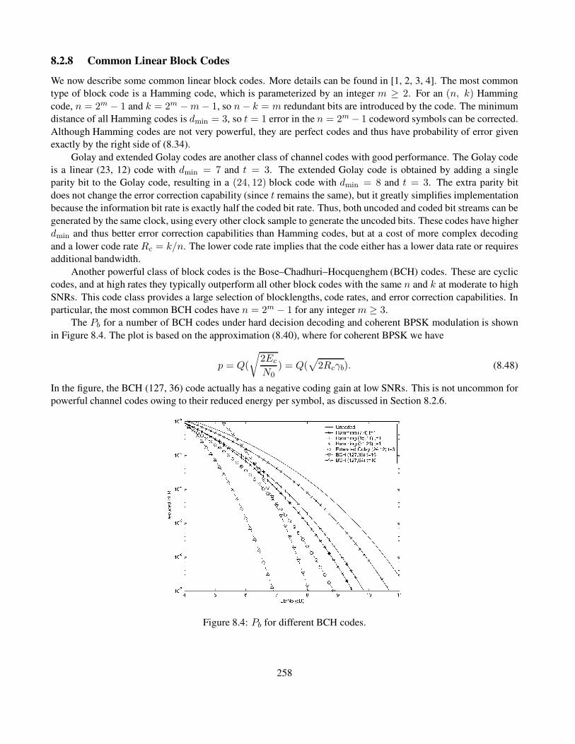
8.2.8 Common Linear Block Codes

We now describe some common linear block codes. More details can be found in [1, 2, 3, 4]. The most common

type of block code is a Hamming code, which is parameterized by an integer m ≥ 2. For an (n, k) Hamming

code, n = 2m − 1 and k = 2m −m− 1, so n − k = m redundant bits are introduced by the code. The minimum

distance of all Hamming codes is dmin = 3, so t = 1 error in the n = 2m − 1 codeword symbols can be corrected.

Although Hamming codes are not very powerful, they are perfect codes and thus have probability of error given

exactly by the right side of (8.34).

Golay and extended Golay codes are another class of channel codes with good performance. The Golay code

is a linear (23, 12) code with dmin = 7 and t = 3. The extended Golay code is obtained by adding a single

parity bit to the Golay code, resulting in a (24, 12) block code with dmin = 8 and t = 3. The extra parity bit

does not change the error correction capability (since t remains the same), but it greatly simplifies implementation

because the information bit rate is exactly half the coded bit rate. Thus, both uncoded and coded bit streams can be

generated by the same clock, using every other clock sample to generate the uncoded bits. These codes have higher

dmin and thus better error correction capabilities than Hamming codes, but at a cost of more complex decoding

and a lower code rate Rc = k/n. The lower code rate implies that the code either has a lower data rate or requires

additional bandwidth.

Another powerful class of block codes is the Bose–Chadhuri–Hocquenghem (BCH) codes. These are cyclic

codes, and at high rates they typically outperform all other block codes with the same n and k at moderate to high

SNRs. This code class provides a large selection of blocklengths, code rates, and error correction capabilities. In

particular, the most common BCH codes have n = 2m − 1 for any integer m ≥ 3.

The Pb for a number of BCH codes under hard decision decoding and coherent BPSK modulation is shown

in Figure 8.4. The plot is based on the approximation (8.40), where for coherent BPSK we have

p = Q(

√

2EcN0

) = Q(√

2Rcγb). (8.48)

In the figure, the BCH (127, 36) code actually has a negative coding gain at low SNRs. This is not uncommon for

powerful channel codes owing to their reduced energy per symbol, as discussed in Section 8.2.6.

Figure 8.4: Pb for different BCH codes.

258

8.2.9 Nonbinary Block Codes: The Reed Solomon Code

A nonbinary block code has similar properties as the binary code: it has K information symbols mapped into

codewords of length N . However, the N codeword symbols of each codeword are chosen from a nonbinary

alphabet of size q > 2. Thus the codeword symbols can take any value in 0, 1, . . . , q − 1. Usually q = 2k, so

that k bits can be mapped into one symbol.

The most common nonbinary block code is the Reed Solomon (RS) code, used in a range of applications

from magnetic recording to cellular digital packet data (CDPD). Reed Solomon codes have N = q − 1 = 2k − 1

and K = 1, 2, . . . , N − 1. The value of K dictates the error correction capability of the code. Specifically, an

RS code can correct up to t = .5bN − Kc codeword symbol errors. In nonbinary codes the minimum distance

between codewords is defined as the number of codeword symbols in which the codewords differ. Reed Solomon

codes achieve a minimum distance of dmin = N −K+1, which is the largest possible minimum distance between

codewords for any linear code with the same encoder input and output block lengths. Reed Solomon codes are

often shortened to meet the requirements of a given system [4, Chap. 5.10].

Because nonbinary codes – and RS codes in particular – generate symbols corresponding to 2k bits, they are

sometimes used with M -ary modulation where M = 2k. In particular, with 2k-ary modulation each codeword

symbol is transmitted over the channel as one of 2k possible constellation points. If the error probability associated

with the modulation (the probability of mistaking the received constellation point for a constellation point other

than the transmitted point) is PM , then the probability of codeword error associated with the non-binary code is

upper bounded by

Figure 8.5: Convolutional encoder.

Pe ≤N∑

j=t+1

N

j

PjM (1− PM )N−j, (8.49)

which is similar to the form of (8.34) for the binary code. We can then approximate the probability of information

symbol error as

Ps ≈1

N

N∑

j=t+1

j

N

j

P jM (1− PM )N−j. (8.50)

259

8.3 Convolutional Codes

A convolutional code generates coded symbols by passing the information bits through a linear finite-state shift

register, as shown in Figure 8.5. The shift register consists of K stages with k bits per stage. There are n binary

addition operators with inputs taken from all K stages: these operators produce a codeword of length n for each

k-bit input sequence. Specifically, the binary input data is shifted into each stage of the shift register k bits at a

time, and each of these shifts produces a coded sequence of length n. The rate of the code is Rc = k/n. The

maximum span of output symbols that can be influenced by a given input bit in a convolutional code is called the

constraint length of the code. It is clear from Figure 8.5 that a length-n codeword depends on kK input bits–in

contrast to a block code, which only depends on k input bits. Thus, the constraint length of the encoder is kK

bits or, equivalently, K k-bit bytes. Convolutional codes are said to have memory since the current codeword

depends on more input bits (kK) than the number input to the encoder to generate it (k). Note that in general a

convolutional encoder may not have the same number of bits per stage.

8.3.1 Code Characterization: Trellis Diagrams

When a length-n codeword is generated by the convolutional encoder of Figure 8.5, this code-word depends both on

the k bits input to the first stage of the shift register as well as the state of the encoder, defined as the contents in the

other K − 1 stages of the shift register. In order to characterize this convolutional code, we must characterize how

the codeword generation depends both on the k input bits and the encoder state, which has 2k(K−1) possible values.

There are multiple ways to characterize convolutional codes, including a tree diagram, state diagram, and trellis

diagram [1, Chap. 8.2]. The tree diagram represents the encoder in the form of a tree, where each branch represents

a different encoder state and the corresponding encoder output. A state diagram is a graph showing the different

states of the encoder and the possible state transitions and corresponding encoder outputs. A trellis diagram uses

the fact that the tree representation repeats itself once the number of stages in the tree exceeds the constraint length

of the code. The trellis diagram simplifies the tree representation by merging nodes in the tree corresponding to

the same encoder state. In this section we focus on the trellis representation of a convolutional code, since this is

the most common characterization. The details of trellis diagram representation are best described by an example.

Figure 8.6: Convolutional encoder example (n = 3, k = 1, k = 3).

Consider the convolutional encoder shown in Figure 8.6 with n = 3, k = 1, and K = 3. In this encoder,

one bit at a time is shifted into Stage 1 of the three-stage shift register. At a given time t we denote the bit in

Stage i of the shift register as Si. The three stages of the shift register are used to generate a codeword of length

3, C1C2C3; from the figure we see that C1 = S1, C2 = S1 + S2 + S3, and C3 = S1 + S3. A bit sequence

260

U shifted into the encoder generates a sequence of coded symbols, which we denote by C. Note that the coded

symbols corresponding to C1 are just the original information bits. As with block codes, when one of the coded

symbols in a convolutional code corresponds to the original information bits we say that the code is systematic.

We define the encoder state as S = S2S3 (i.e., the contents of the last two stages of the encoder), and there are

22 = 4 possible values for this encoder state. To characterize the encoder, we must show for each input bit and

each possible encoder state what the encoder output will be, and we must also show how the new input bit changes

the encoder state for the next input bit.

The trellis diagram for this code is shown in Figure 8.7. The solid lines in Figure 8.7 indicate the encoder

state transition when a 0-bit is input to Stage 1 of the encoder, and the dashed lines indicate the state transition

corresponding to a 1-bit input. For example, starting at state S = 00, if a 0-bit is input to Stage 1 then, when the

shift register transitions, the new state will remain as S = 00 (since the 0 in Stage 1 transitions to Stage 2, and

the 0 in Stage 2 transitions to Stage 3, resulting in the new state S = S2S3 = 00). On the other hand, if a 1-bit is

input to Stage 1 then, when the shift register transitions, the new state will become S = 10 (since the 1 in Stage 1

transitions to Stage 2, and the 0 in Stage 2 transitions to Stage 3, resulting in the new state S = S2S3 = 10). The

encoder output corresponding to a particular encoder state S and input S1 is written next to the transition lines in

the figure. This output is the encoder output that results from the encoder addition operations on the bits S1, S2,

and S3 in each stage of the encoder. For example, if S = 00 and S1 = 1 then the encoder output C1C2C3 has

C1 = S1 = 1, C2 = S1 + S2 + S3 = 1, and C3 = S1 + S3 = 1. This output 111 is drawn next to the dashed

line transitioning from state S = 00 to state S = 10 in Figure 8.7. Note that the encoder output for S1 = 0 and

S = 00 is always the all-zero codeword regardless of the addition operations that form the codeword C1C2C3,

since summing together any number of 0s always yields 0. The portion of the trellis between time ti and ti+1 is

called the ith branch of the trellis. Figure 8.7 indicates that the initial state at time t0 is the all-zero state. The trellis

achieves steady state, defined as the point where all states can be entered from either of two preceding states, at

time t3. After this steady state is reached, the trellis repeats itself in each time interval. Note also that, in steady

state, each state transitions to one of two possible new states. In general, trellis structures starting from the all-zero

state at time t0 achieve steady state at time tK .

For general values of k andK, the trellis diagram will have 2K−1 states, where each state has 2k paths entering

each node and 2k paths leaving each node. Thus, the number of paths through the trellis grows exponentially with

k,K, and the length of the trellis path.

Example 8.7: Consider the convolutional code represented by the trellis in Figure 8.7. For an initial state

S = S2S3 = 01, find the state sequence S and the encoder outputC for input bit sequence U = 011.

Solution: The first occurrence of S = 01 in the trellis is at time t2. We see at t2 that if the information bit S1 = 0

then we follow the solid line in the trellis from S = 01 at t2 to S = 00 at t3, and the output corresponding to this

path through the trellis is C = 011. Now at t3, starting at S = 00, for the information bit S1 = 1 we follow the

dashed line in the trellis to S = 10 at t4, and the output corresponding to this path through the trellis is C = 111.

Finally, at t4, starting at S = 10, for the information bit S1 = 1 we follow the dashed line in the trellis to S = 11at t5, and the output corresponding to this path through the trellis is C = 101.

8.3.2 Maximum Likelihood Decoding

The convolutional code generated by the finite state shift register is basically a finite-state machine. Thus, unlike an

(n, k) block code – where maximum likelihood detection entails finding the length-n codeword that is closest to

the received length-n codeword – maximum likelihood detection of a convolutional code entails finding the most

likely sequence of coded symbols C given the received sequence of coded symbols, which we denote by R. In

261

Figure 8.7: Trellis diagram.

particular, for a received sequence R, the decoder decides that coded symbol sequence C∗ was transmitted if

p(R|C∗) ≥ p(R|C) ∀C. (8.51)

Since each possible sequence C corresponds to one path through the trellis diagram of the code, maximum like-

lihood decoding corresponds to finding the maximum likelihood path through the trellis diagram. For an AWGN

channel, noise affects each coded symbol independently. Thus, for a convolutional code of rate 1/n, we can express

the likelihood (8.51) for a path of length L through the trellis as

p(R|C) =

L−1∏

i=0

p(Ri|Ci) =

L−1∏

i=0

n∏

j=1

p(Rij|Cij), (8.52)

where Ci is the portion of the code sequence C corresponding to the ith branch of the trellis,Ri is the portion of the

received code sequence R corresponding to the ith branch of the trellis,Cij is the jth coded symbol corresponding

to Ci, and Rij is the jth received coded symbol corresponding to Ri. The log likelihood function is defined as the

log of p(R|C), given as

log p(R|C) =

L−1∑

i=0

log p(Ri|Ci) =

L−1∑

i=0

n∑

j=1

log p(Rij|Cij). (8.53)

The expression

Bi =

n∑

j=1

log p(Rij|Cij) (8.54)

is called the branch metric because it indicates the component of (8.53) associated with the ith branch of the trellis.

The sequence or path that maximizes the likelihood function also maximizes the log likelihood function, since the

log is monotonically increasing. However, it is computationally more convenient for the decoder to use the loglikelihood function because it involves a summation rather than a product. The log likelihood function associated

262

with a given path through the trellis is also called the path metric, which by (8.53) is equal to the sum of branch

metrics along each branch of the path. The path through the trellis with the maximum path metric corresponds to

the maximum likelihood path.

The decoder can use either hard or soft decisions for the expressions log p(Rij|Cij) in the log likelihood

metric. For hard decision decoding, the Rij is decoded as a 1 or a 0. The probability of hard decision decoding

error depends on the modulation and is denoted as p. If R and C are N symbols long and differ in d places (i.e.,

their Hamming distance is d), then

p(R|C) = pd(1− p)N−d

and

log p(R|C) = −d log1 − p

p+N log(1 − p). (8.55)

Since p < .5, (8.55) is maximized when d is minimized. So the coded sequence C with minimum Hamming

distance to the received sequence R corresponds to the maximum likelihood sequence.

In soft decision decoding, the value of the received coded symbols (Rij) are used directly in the decoder,

rather than quantizing them to 1 or 0. For example, if the Cij are sent via BPSK over an AWGN channel with a 1

mapped to√Ec and a 0 mapped to −√

Ec, then

Rij =√

Ec(2Cij − 1) + nij , (8.56)

where Ec = kEb/n is the energy per coded symbol and nij denotes Gaussian noise of mean zero and variance

σ2 = .5N0. Thus,

p(Rij|Cij) =1√2πσ

exp

[

−(Rij −√Ec(2Cij − 1))2

2σ2

]

. (8.57)

Maximizing this likelihood function is equivalent to choosing the Cij that is closest in Euclidean distance to Rij .

In determining which sequence C maximizes the log likelihood function (8.53), any terms that are common to

two different sequences C1 and C2 can be neglected, since they contribute the same amount to the summation.

Similarly, we can scale all terms in (8.53) without changing the maximizing sequence. Thus, by neglecting scaling

factors and terms in (8.57) that are common to any Cij , we can replace∑n

j=1 log p(Rij|Cij) in (8.53) with the

equivalent branch metric

µi =

n∑

j=1

Rij(2Cij − 1) (8.58)

and obtain the same maximum likelihood output.

We now illustrate the path metric computation under both hard and soft decisions for the convolutional code of

Figure 8.6 with the trellis diagram in Figure 8.7. For simplicity, we will consider only two possible paths through

the trellis and compute their corresponding likelihoods for a given received sequence R. Assume we start at time

t0 in the all-zero state. The first path we consider is the all-zero path, corresponding to the all-zero input sequence.

The second path we consider starts in state S = 00 at time t0 and transitions to state S = 10 at time t1, then to state

S = 01 at time t2, and finally to state S = 00 at time t3, at which point this path merges with the all-zero path.

Since the paths and therefore their branch metrics at times t < t0 and t ≥ t3 are the same, the maximum likelihood

path corresponds to the path whose sum of branch metrics over the branches in which the two paths differ is smaller.

From Figure 8.7 we see that the all-zero path through the trellis generates the coded sequence C0 = 000000000

263

over the first three branches in the trellis. The second path generates the coded sequence C1 = 111010011 over

the first three branches in the trellis.

Let us first consider hard decision decoding with error probabilityp. Suppose the received sequence over these

three branches is R = 100110111. Note that the Hamming distance between R and C0 is 6 while the Hamming

distance between R and C1 is 4. As discussed previously, the most likely path therefore corresponds to C1, since

it has minimum Hamming distance to R. The path metric for the all-zero path is

M0 =

2∑

i=0

3∑

j=1

logP (Rij|Cij) = 6 logp+ 3 log(1− p), (8.59)

while the path metric for the other path is

M1 =

2∑

i=0

3∑

j=1

logP (Rij|Cij) = 4 logp+ 5 log(1− p). (8.60)

Assuming p 1, which is generally the case, this yields M0 ≈ 6 log p and M1 ≈ 4 log p. Since log p < 1, this

confirms that the second path has a larger path metric than the first.

Let us now consider soft decision decoding over time t0 to t3. Suppose the received sequence (before demod-

ulation) over these three branches, for Ec = 1, is R = (.8,−.35,−.15, 1.35, 1.22,−.62, .87, 1.08, .91). The path

metric for the all-zero path is

M0 =

2∑

i=0

µi =

2∑

i=0

3∑

j=1

Rij(2Cij − 1) =

2∑

i=0

3∑

j=1

−Rij = −5.11,

and the path metric for the second path is

M1 =

2∑

i=0

3∑

j=1

Rij(2Cij − 1) = 1.91.

Thus, the second path has a higher path metric than the first. In order to determine if the second path is the

maximum likelihood path, we must compare its path metric to that of all other paths through the trellis.

The difficulty with maximum likelihood decoding is that the complexity of computing the log likelihood

function (8.53) grows exponentially with the memory of the code, and this computation must be done for every

possible path through the trellis. The Viterbi algorithm, discussed in the next section, reduces the complexity of

maximum likelihood decoding by taking advantage of the structure of the path metric computation.

8.3.3 The Viterbi Algorithm

The Viterbi algorithm, introduced by Viterbi in 1967 [5], reduces the complexity of maximum likelihood decoding

by systematically removing paths from consideration that cannot achieve the highest path metric. The basic premise

is to look at the partial path metrics associated with all paths entering a given node (node N ) in the trellis. Since

the possible paths through the trellis leaving node N are the same for each entering path, the complete trellis path

with the highest path metric that goes through nodeN must coincide with the path that has the highest partial path

metric up to nodeN . This is illustrated in Figure 8.8, where path 1, path 2, and path 3 enter nodeN (at trellis depth

n) with partial path metrics P l =∑n−1

k=0 Blk(l = 1, 2, 3) up to this node. Assume P 1 is the largest of these partial

path metrics. The complete path with the highest metric has branch metrics Bk after node N . The maximum

likelihood path starting from node N (i.e., the path starting from node N with the largest path metric) has partial

path metric∑∞

k=n Bk. The complete path metric for path l(l = 1, 2, 3) up to nodeN and the maximum likelihood

264

Figure 8.8: Partial path metrics on maximum likelihood path.

path after nodeN is P l +∑∞

k=nBk(l = 1, 2, 3), and thus the path with the maximum partial path metric P l up to

node N (path 1 in this example) must correspond to the path with the largest path metric that goes through node

N .

The Viterbi algorithm takes advantage of this structure by discarding all paths entering a given node except

the path with the largest partial path metric up to that node. The path that is not discarded is called the survivor

path. Thus, for the example of Figure 8.8, path 1 is the survivor at node N and paths 2 and 3 are discarded from

further consideration. Hence, at every stage in the trellis there are 2K−1 surviving paths, one for each possible

encoder state. A branch for a given stage of the trellis cannot be decoded until all surviving paths at a subsequent

trellis stage overlap with that branch; see Figure 8.9, which shows the surviving paths at time tk+3. We see in the

figure that all of these surviving paths can be traced back to a common stem from time tk to tk+1. At this point

the decoder can output the codeword symbol Ci associated with this branch of the trellis. Note that there is not a

fixed decoding delay associated with how far back in the trellis a common stem occurs for a given set of surviving

paths, since this delay depends on k,K, and the specific code properties. To avoid a random decoding delay, the

Viterbi algorithm is typically modified so that, at a given stage in the trellis, the most likely branch n stages back

is decided upon based on the partial path metrics up to that point. Although this modification does not yield exact

maximum likelihood decoding, for n sufficiently large (typically n ≥ 5K) it is a good approximation.

Figure 8.9: Common stem for all survivor paths in the trellis.

The Viterbi algorithm must keep track of 2k(K−1) surviving paths and their corresponding metrics. At each

stage, in order to determine the surviving path, 2k metrics must be computed for each node corresponding to the

265

2k paths entering each node. Thus, the number of computations in decoding and the memory requirements for the

algorithm increase exponentially with k andK. This implies that practical implementations of convolutional codes

are restricted to relatively small values of k and K.

8.3.4 Distance Properties

As with block codes, the error correction capability of convolutional codes depends on the distance between code-

word sequences. Since convolutional codes are linear, the minimum distance between all codeword sequences can

be found by determining the minimum distance from any sequence or, equivalently, determining any trellis path to

the all-zero sequence/trellis path. Clearly the trellis path with minimum distance to the all-zero path will diverge

and remerge with the all-zero path, so that the two paths coincide except over some number of trellis branches. To

find this minimum distance path we must consider all paths that diverge from the all-zero state and then remerge

with this state. As an example, in Figure 8.10 we draw all paths in Figure 8.7 between times t0 and t5 that diverge

and remerge with the all-zero state. Note that path 2 is identical to path 1 – just shifted in time – and thus is not

considered as a separate path. Note also that we could look over a longer time interval, but any paths that diverge

and remerge over this longer interval would traverse the same branches (shifted in time) as one of these paths plus

some additional branches and would therefore have larger path metrics. In particular, we see that path 4 traverses

the trellis branches 00-10-01-10-01-00, whereas path 1 traverses the branches 00-10-01-00. Since path 4 traverses

the same branches as path 1 on its first, second, and last transition – and since it has additional transitions – its

path metric will be no smaller than the meteric of path 1. Thus we need not consider a longer time interval to find

the minimum distance path. For each path in Figure 8.10 we label the Hamming distance of the codeword on each

branch to the all-zero codeword in the corresponding branch of the all-zero path. By summing up the Hamming

distances on all branches of each path, we see that path 1 has a Hamming distance of 6 and that paths 3 and 4 have

Hamming distances of 8. Recalling that dashed lines indicate 1-bit inputs while solid lines indicate 0-bit inputs,

we see that path 1 corresponds to an input bit sequence from t0 to t5 of 10000, path 3 corresponds to an input bit

sequence of 11000, and path 4 corresponds to an input bit sequence of 10100. Thus, path 1 results in one bit error

relative to the all-zero squence, and paths 3 and 4 result in two bit errors.

Figure 8.10: Path distances to the all-zero path.

We define the minimum free distance df of a convolutional code, also called simply the free distance, to be

the minimum Hamming distance of all paths through the trellis to the all-zero path, which for this example is 6.

266

The error correction capability of the code is obtained in the same manner as for block codes, with dmin replaced

by df , so that the code can correct t channels errors with t = b.5dfc.

8.3.5 State Diagrams and Transfer Functions

The transfer function of a convolutional code is used to characterize paths that diverge and remerge from the all-

zero path, and it is also used to obtain probability of error bounds. The transfer function is obtained from the code’s

state diagram representing possible transitions from the all-zero state to the all-zero state. The state diagram for

the code illustrated in Figure 8.7 is shown in Figure 8.11, with the all-zero state a = 00 split into a second node

e to facilitate representing paths that begin and end in this state. Transitions between states due to a 0 input bit

are represented by solid lines, while transitions due to a 1 input bit are represented by dashed lines. The branches

of the state diagram are labeled as either D0 = 1, D1, D2, or D3, where the exponent of D corresponds to the

Hamming distance between the codeword (which is shown for each branch transition) and the all-zero codeword

in the all-zero path. The self-loop in node a can be ignored because it does not contribute to the distance proper-

ties of the code.

Figure 8.11: State diagram.

The state diagram can be represented by state equations for each state. For the example of Figure 8.11, we

obtain state equations corresponding to the four states

Xc = D3Xa +DXb, Xb = DXc +DXd, Xd = D2Xc +D2Xd, Xe = D2Xb, (8.61)

whereXa, . . . , Xe are dummy variables characterizing the partial paths. The transfer function of the code, describ-

ing the paths from state a to state e, is defined as T (D) = Xe/Xa. By solving the state equations for the code,

which can be done using standard techniques such as Mason’s formula, we obtain a transfer function of the form

T (D) =

∞∑

d=df

adDd, (8.62)

where ad is the number of paths with Hamming distance d from the all-zero path. As stated before, the minimum

Hamming distance to the all-zero path is df , and the transfer function T (D) indicates that there are adfpaths with

this minimum distance. For the example of Figure 8.11, we can solve the state equations given in (8.61) to get the

transfer function

T (D) =D6

1− 2D2= D6 + 2D8 + 4D10 + · · · . (8.63)

267

We see from the transfer function that there is one path with minimum distance df = 6 and two paths with

Hamming distance 8, which is consistent with Figure 8.10. The transfer function is a convenient shorthand for

enumerating the number and corresponding Hamming distance of all paths in a particular code that diverge and

later remerge with the all-zero path.

Figure 8.12: Extended state diagram.

Although the transfer function is sufficient to capture the number and Hamming distance of paths in the

trellis to the all-zero path, we need a more detailed characterization to compute the bit error probability of the

convolutional code. We therefore introduce two additional parameters into the transfer function, N and J , for

this additional characterization. The factor N is introduced on all branch transitions associated with a 1 input bit

(dashed lines in Figure 8.11). The factor J is introduced to every branch in the state diagram such that the exponent

of J in the transfer function equals the number of branches in any given path from node a to node e. The extended

state diagram corresponding to the trellis of Figure 8.7 is shown in Figure 8.12.

The extended state diagram can also be represented by state equations. For the example of Figure 8.12, these

are given by:

Xc = JND3Xa + JNDXb, Xb = JDXc + JDXd,

Xd = JND2Xc + JND2Xd, Xe = JD2Xb. (8.64)

Similarly to the previous transfer function definition, the transfer function associated with this extended state is

defined as T (D,N, J) = Xe/Xa, which for this example yields

T (D,N, J) =J3ND6

1− JND2(1 + J)

= J3ND6 + J4N 2D8 + J5N 2D8 + J5N 3D10 + · · · . (8.65)

The factor J is most important when we are interested in transmitting finite-length sequences; for infinite-length

sequences we typically set J = 1 to obtain the transfer function for the extended state:

T (D,N ) = T (D,N, J = 1). (8.66)

The transfer function for the extended state tells us more information about the diverging and remerging paths

than just their Hamming distance; namely, the minimum distance path with Hamming distance 6 is of length 3 and

results in a single bit error (exponent of N is unity), one path of Hamming distance 8 is of length 4 and results

in two bit errors, and the other path of Hamming distance 8 is of length 5 and results in two bit errors, consistent

268

with Figure 8.10. The extended transfer function is a convenient shorthand for representing the Hamming distance,

length, and number of bit errors that correspond to each diverging and remerging path of a code from the all-zero

path. In the next section we show that this representation is useful in characterizing the probability of error for

convolutional codes.

8.3.6 Error Probability for Convolutional Codes

Since convolutional codes are linear codes, the probability of error can be obtained by first assuming that the all-

zero sequence is transmitted and then determining the probability that the decoder decides in favor of a different

sequence. We will consider error probability for both hard decision and soft decision decoding; soft decisions are

much more common in wireless systems owing to their superior performance.

First consider soft decision decoding. We are interested in the probability that the all-zero sequence is sent

but a different sequence is decoded. If the coded symbols output from the convolutional encoder are sent over an

AWGN channel using coherent BPSK modulation with energy Ec = RcEb, then it can be shown [1] that, if the

all-zero sequence is transmitted, the probability of mistaking this sequence with a sequence Hamming distance daway is

P2(d) = Q

(√

2EcN0

d

)

= Q(√

2γbRcd). (8.67)

We call this probability the pairwise error probability, since it is the error probability associated with a pairwise

comparison of two paths that differ in d bits. The transfer function enumerates all paths that diverge and remerge

with the all zero path, so by the union bound we can upper bound the probability of mistaking the all-zero path for

another path through the trellis as

Pe ≤∞∑

d=df

adQ(√

2γbRcd), (8.68)

where ad denotes the number of paths of distance d from the all-zero path. This bound can be expressed in terms

of the transfer function itself if we use the Chemoff upper bound for the Q-function, which yields

Q(√

2γbRcd) ≤ e−γbRcd.

Using this in (8.68) we obtain the upper bound

Pe < T (D)|D=e−γbRc . (8.69)

This upper bound tells us the probability of mistaking one sequence for another, but it does not yield the more

fundamental probability of bit error. We know that the exponent in the factor N of T (D,N ) indicates the number

of information bit errors associated with selecting an incorrect path through the trellis. Specifically, we can express

T (D,N ) as

T (D,N ) =

∞∑

d=df

adDdN f(d), (8.70)

where f(d) denotes the number of bit errors associated with a path of distance d from the all-zero path. Then we

can upper bound the bit error probability for k = 1 as

269

Pb ≤∞∑

d=df

adf(d)Q(√

2γbRcd) (8.71)

[1, Chap. 8.2], which differs from (8.68) only in the weighting factor f(d) corresponding to the number of bit

errors in each incorrect path. If the Q-function is upper bounded using the Chemoff bound as before, we get the

upper bound

Pb <dT (D,N )

dN

∣∣∣∣N=1,D=e−γbRc

. (8.72)

If k > 1 then we divide (8.71) or (8.72) by k to obtain Pb.

All of these bounds assume coherent BPSK transmission (or coherent QPSK, which is equivalent to two in-

dependent BPSK transmissions). For other modulations, the pairwise error probability P2(d) must be recomputed

based on the probability of error associated with the given modulation.

Let us now consider hard decision decoding. The probability of selecting an incorrect path at distance d from

the all-zero path, for d odd, is given by

P2(d) =

d∑

k=.5(d+1)

d

k

pk(1− p)(d−k), (8.73)

where p is the probability of error on the channel. This follows because the incorrect path will be selected only

if the decoded path is closer to the incorrect path than to the all-zero path – that is, the decoder makes at least

.5(d + 1) errors. If d is even then the incorrect path is selected when the decoder makes more than .5d errors,

and the decoder makes a choice at random if the number of errors is exactly .5d. We can bound the pairwise error

probability as

P2(d) < [4p(1− p)]d/2. (8.74)

Following the same approach as in soft decision decoding, we then obtain the error probability bound as

Pe <

∞∑

d=df

ad[4p(1− p)]d/2 < T (D)|D=

√4p(1−p)

, (8.75)

and

Pb <∞∑

d=df

adf(d)P2(d) =dT (D,N )

dN

∣∣∣∣N=1, D=

√4p(1−p)

. (8.76)

8.4 Concatenated Codes

A concatenated code uses two levels of coding: an inner code and an outer code, as shown in Figure 8.13. The

inner code is typically designed to remove most of the errors introduced by the channel, and the outer code is

typically a less powerful code that further reduces error probability when the received coded bits have a relatively

low probability of error (since most errors are corrected by the inner code). Concatenated codes can be particularly

effective at correcting bursts of errors, which are common in wireless channels as a result of deep fades. In addition,

at low SNRs Viterbi decoding of a convolutional code tends to have errors that occur in bursts. To compensate

for these error bursts, an inner convolutional code is often concatenated with an outer Reed Solomon code, since

270

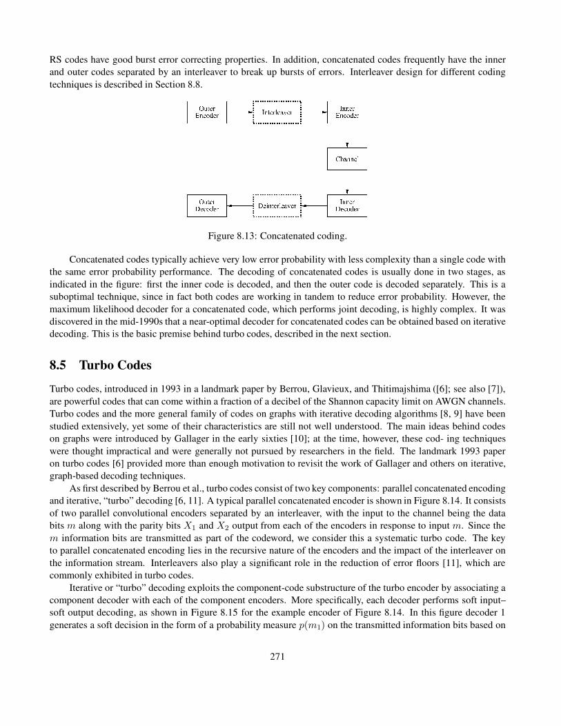
RS codes have good burst error correcting properties. In addition, concatenated codes frequently have the inner

and outer codes separated by an interleaver to break up bursts of errors. Interleaver design for different coding

techniques is described in Section 8.8.

Figure 8.13: Concatenated coding.

Concatenated codes typically achieve very low error probability with less complexity than a single code with

the same error probability performance. The decoding of concatenated codes is usually done in two stages, as

indicated in the figure: first the inner code is decoded, and then the outer code is decoded separately. This is a

suboptimal technique, since in fact both codes are working in tandem to reduce error probability. However, the

maximum likelihood decoder for a concatenated code, which performs joint decoding, is highly complex. It was

discovered in the mid-1990s that a near-optimal decoder for concatenated codes can be obtained based on iterative

decoding. This is the basic premise behind turbo codes, described in the next section.

8.5 Turbo Codes

Turbo codes, introduced in 1993 in a landmark paper by Berrou, Glavieux, and Thitimajshima ([6]; see also [7]),

are powerful codes that can come within a fraction of a decibel of the Shannon capacity limit on AWGN channels.

Turbo codes and the more general family of codes on graphs with iterative decoding algorithms [8, 9] have been

studied extensively, yet some of their characteristics are still not well understood. The main ideas behind codes

on graphs were introduced by Gallager in the early sixties [10]; at the time, however, these cod- ing techniques

were thought impractical and were generally not pursued by researchers in the field. The landmark 1993 paper

on turbo codes [6] provided more than enough motivation to revisit the work of Gallager and others on iterative,

graph-based decoding techniques.

As first described by Berrou et al., turbo codes consist of two key components: parallel concatenated encoding

and iterative, “turbo” decoding [6, 11]. A typical parallel concatenated encoder is shown in Figure 8.14. It consists

of two parallel convolutional encoders separated by an interleaver, with the input to the channel being the data

bits m along with the parity bits X1 and X2 output from each of the encoders in response to input m. Since the

m information bits are transmitted as part of the codeword, we consider this a systematic turbo code. The key

to parallel concatenated encoding lies in the recursive nature of the encoders and the impact of the interleaver on

the information stream. Interleavers also play a significant role in the reduction of error floors [11], which are

commonly exhibited in turbo codes.

Iterative or “turbo” decoding exploits the component-code substructure of the turbo encoder by associating a

component decoder with each of the component encoders. More specifically, each decoder performs soft input–

soft output decoding, as shown in Figure 8.15 for the example encoder of Figure 8.14. In this figure decoder 1

generates a soft decision in the form of a probability measure p(m1) on the transmitted information bits based on

271

Figure 8.14: Parallel concatenated (turbo) encoder.

Figure 8.15: Turbo decoder.

the received codeword (m,X1). The probability measure is generated based on either a maximum a posteriori

(MAP) probability or a soft output Viterbi algorithm (SOVA), which attaches a reliability indicator to the VA

hard decision outputs [4, Chap. 12.5]. This probability information is passed to decoder 2, which generates its

own probability measure p(m2) from its received codeword (m,X2) and the probability measure p(m1). This

reliability information is input to decoder 1, which revises its measure p(m1) based on this information and the

original received codeword. Decoder 1 sends the new reliability information to decoder 2, which revises its measure

using this new information. Turbo decoding proceeds in an iterative manner, with the two component decoders

alternately updating their probability measures. Ideally the decoders will eventually agree on probability measures

that reduce to hard decisions m = m1 = m2. However, the stopping condition for turbo decoding is not well-

defined, in part because there are many cases in which the turbo decoding algorithm does not converge: the

decoders cannot agree on the value of m. Several methods have been proposed for detecting convergence (if it

occurs), including bit estimate variance [7] and neural net–based techniques [12].

The simulated performance of turbo codes over multiple iterations of the decoder is shown in Figure 8.16 for

a code composed of two convolutional codes of rate 1/2 with constraint length K = 5 separated by an interleaver

of depth d = 216 = 65536. The decoder converges after approximately eighteen iterations. This curve indicates

several important aspects of turbo codes. First, note their exceptional performance: bit error probability of 10−6 at

an Eb/N0 of less than 1 dB. In fact, the original turbo code proposed in [6] performed within .5 dB of the Shannon

capacity limit at Pb = 10−5. The intuitive explanation for the amazing performance of turbo codes is that the

code complexity introduced by the encoding structure is similar to the codes that achieve Shannon capacity. The

272

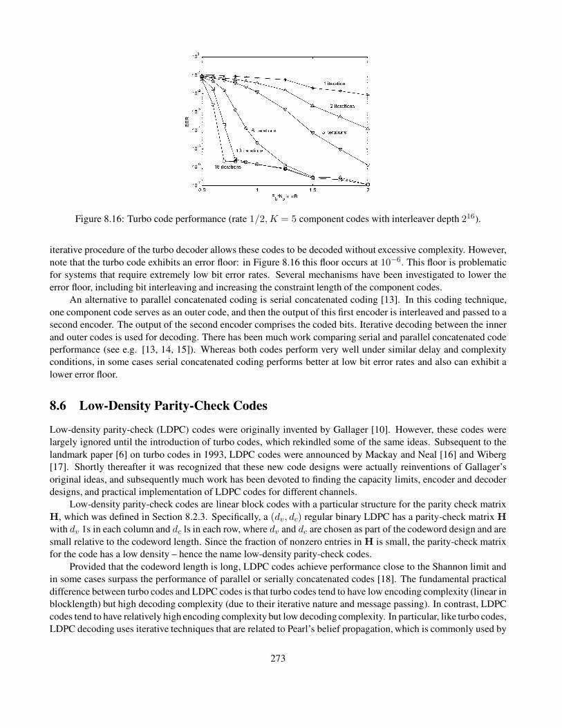
Figure 8.16: Turbo code performance (rate 1/2, K = 5 component codes with interleaver depth 216).

iterative procedure of the turbo decoder allows these codes to be decoded without excessive complexity. However,

note that the turbo code exhibits an error floor: in Figure 8.16 this floor occurs at 10−6. This floor is problematic

for systems that require extremely low bit error rates. Several mechanisms have been investigated to lower the

error floor, including bit interleaving and increasing the constraint length of the component codes.

An alternative to parallel concatenated coding is serial concatenated coding [13]. In this coding technique,

one component code serves as an outer code, and then the output of this first encoder is interleaved and passed to a

second encoder. The output of the second encoder comprises the coded bits. Iterative decoding between the inner

and outer codes is used for decoding. There has been much work comparing serial and parallel concatenated code

performance (see e.g. [13, 14, 15]). Whereas both codes perform very well under similar delay and complexity

conditions, in some cases serial concatenated coding performs better at low bit error rates and also can exhibit a

lower error floor.

8.6 Low-Density Parity-Check Codes

Low-density parity-check (LDPC) codes were originally invented by Gallager [10]. However, these codes were

largely ignored until the introduction of turbo codes, which rekindled some of the same ideas. Subsequent to the

landmark paper [6] on turbo codes in 1993, LDPC codes were announced by Mackay and Neal [16] and Wiberg

[17]. Shortly thereafter it was recognized that these new code designs were actually reinventions of Gallager’s

original ideas, and subsequently much work has been devoted to finding the capacity limits, encoder and decoder

designs, and practical implementation of LDPC codes for different channels.

Low-density parity-check codes are linear block codes with a particular structure for the parity check matrix

H, which was defined in Section 8.2.3. Specifically, a (dv, dc) regular binary LDPC has a parity-check matrix Hwith dv 1s in each column and dc ls in each row, where dv and dc are chosen as part of the codeword design and are

small relative to the codeword length. Since the fraction of nonzero entries in H is small, the parity-check matrix

for the code has a low density – hence the name low-density parity-check codes.

Provided that the codeword length is long, LDPC codes achieve performance close to the Shannon limit and

in some cases surpass the performance of parallel or serially concatenated codes [18]. The fundamental practical

difference between turbo codes and LDPC codes is that turbo codes tend to have low encoding complexity (linear in

blocklength) but high decoding complexity (due to their iterative nature and message passing). In contrast, LDPC

codes tend to have relatively high encoding complexity but low decoding complexity. In particular, like turbo codes,

LDPC decoding uses iterative techniques that are related to Pearl’s belief propagation, which is commonly used by

273

the artificial intelligence community (see [19]). However, the belief propagation corresponding to LDPC decoding

may be simpler than for turbo decoding [19, 20]. In addition, this belief propagation decoding is parallelizable and

can be closely approximated with decoders of very low complexity [21], although this may also be possible for

turbo decoding. Finally, the decoding algorithm for LDPC codes can determine when a correct codeword has been

detected, which is not necessarily the case for turbo codes. The trade-offs between turbo and LDPC codes is an

active research area, and many open questions remain regarding their relative performance.

Additional work in the area of LDPC codes includes finding capacity limits for these codes [21], determining

effective code designs [22] and efficient encoding and decoding algorithms [21, 23], and expanding the code

designs to include nonregular [18] and nonbinary LDPC codes [24] as well as coded modulation [25].

Figure 8.17: General coding scheme.

8.7 Coded Modulation

Although Shannon proved the capacity theorem for AWGN channels in the late 1940s, it wasn’t until the 1990s that

rates approaching the Shannon limit were attained – primarily for AWGN channels with binary modulation using

turbo codes. Shannon’s theorem predicted the possibility of reducing both energy and bandwidth simultaneously

through coding. However, as described in Section 8.1, traditional error correction coding schemes (e.g., block,

convolutional, and turbo codes) provide coding gain at the expense of increased bandwidth or reduced data rate.

The spectrally efficient coding breakthrough came when Ungerboeck [26] introduced a coded modulation

technique to jointly optimize both channel coding and modulation. This joint optimization results in significant

coding gains without bandwidth expansion. Ungerboeck’s trellis coded modulation, which uses multilevel/phase

signal modulation and simple convolutional coding with mapping by set partitioning, compares favorably to later

developments in coded modulation (coset and lattice codes) as well as to more complex trellis codes [27]. We

now outline the general principles of this coding technique. Comprehensive treatments of trellis, lattice, and coset

codes can be found in [26, 27, 28].

The basic scheme for trellis and lattice coding – or, more generally, for any type of coset coding – is depicted

in Figure 8.17. There are five elements required to generate the coded modulation:

1. a binary encoderE , block or convolutional, that operates on k uncoded data bits to produce k+r coded bits;

2. a subset (coset) selector, which uses the coded bits to choose one of 2k+r subsets from a partition of the

N -dimensional signal constellation;

3. a point selector, which uses n − k additional uncoded bits to choose one of the 2n−k signal points in the

selected subset;

274

4. a constellation map, which maps the selected point from N -dimensional space to a sequence of N/2 points

in two-dimensional space; and

5. an MQAM modulator (or other M -ary modulator).

The first two elements constitute the channel coding, and the remaining elements are the modulation. The receiver

essentially reverses the modulation and coding steps. After MQAM demodulation and an inverse 2/N constellation

mapping, decoding is done in essentially two stages: first, the points within each subset that are closest to the

received signal point are determined; then, the maximum likelihood subset sequence is calculated. When the

encoderE is a convolutional encoder, this scheme is referred to as trellis coded modulation; forE a block encoder,

it is called lattice coded modulation. These schemes are also referred to as trellis or lattice codes.

Steps 1–5 essentially decouple the channel coding gain from the gain associated with signal shaping in the

modulation. Specifically, the code distance properties – and thus the channel coding gain – are determined by

the encoder (E) properties and the subset partitioning, which are essentially decoupled from signal shaping. We

will discuss the channel coding gain in more detail below. Optimal shaping of the signal constellation provides

up to an additional 1.53 dB of shaping gain (for asymptotically large N ), independent of the channel coding

scheme.1 However, the performance improvement from shaping gain is offset by the corresponding complexity of

the constellation map, which grows exponentially with N . The size of the transmit constellation is determined by

the average power constraint and does not affect the shaping or coding gain.

The channel coding gain results from a selection of sequences among all possible sequences of signal points. If

we consider a sequence of N input bits as a point in N -dimensional space (the sequence space), then this selection

is used to guarantee some minimum distance dmin in the sequence space between possible input sequences. Errors

generally occur when a sequence is mistaken for its closest neighbor, and in AWGN channels this error probability

is a decreasing function of d2min. We can thus decrease the BER by increasing the separation between each point

in the sequence space by a fixed amount (“stretching” the space). However, this will result in a proportional power

increase, so no net coding gain is realized. The effective power gain of the channel code is therefore the minimum

squared distance between selected sequence points (the sequence points obtained through coding) multiplied by

the density of the selected sequence points. Specifically, if the minimum distance and density of all points in the

sequence space are denoted by d0 and 40, respectively, and if the minimum distance and density of points in

the sequence space selected through coding are denoted by dmin and 4, respectively, then maximum likelihood

sequence detection yields a channel coding gain of

Gc =

(d2

min

d20

)( 440

)

. (8.77)

The second term on the right side of this expression is also referred to as the constellation expansion factor and

equals 2−r (per N dimensions) for a redundancy of r bits in the encoder E [27].

Some of the nominal coding gain in (8.77) is lost owing to selected sequences having more than one nearest

neighbor in the sequence space, which increases the possibility of incorrect sequence detection. This loss in

coding gain is characterized by the error coefficient, which is tabulated for most common lattice and trellis coded

modulations in [27]. In general, the error coefficient is larger for lattice codes than for trellis codes with comparable

values of Gc.Channel coding is done using set partitioning of lattices. A lattice is a discrete set of vectors in real Euclidean

N -dimensional space that forms a group under ordinary vector addition, so the sum or difference of any two vectors

in the lattice is also in the lattice. A sublattice is a subset of a lattice that is itself a lattice. The sequence space for

1A square constellation has 0 dB of shaping gain; a circular constellation, which is the geometrical figure with the least average energy

for a given area, achieves the maximum shape gain for a given N [27].

275

uncoded MQAM modulation is just the N -cube,2 so the minimum distance between points is no different than in

the two-dimensional case. By restricting input sequences to lie on a lattice in N -dimensional space that is denser

than the N -cube, we can increase dmin while maintaining the same density (or, equivalently, the same average

power) in the transmit signal constellation; hence, there is no constellation expansion. The N -cube is a lattice, but

for every N > 1 there are denser lattices in N -dimensional space. Finding the densest lattice in N dimensions

is a well-known mathematical problem, and it has been solved for all N for which the decoder complexity is

manageable.3 Once the densest lattice is known, we can form partitioning subsets, or cosets, of the lattice via

translation of any sublattice. The choice of the partitioning sublattice will determine the size of the partition – that

is, the number of subsets that the subset selector in Figure 8.17 has to choose from. Data bits are then conveyed

in two ways: through the sequence of cosets from which constellation points are selected, and through the points

selected within each coset. The density of the lattice determines the distance between points within a coset, while

the distance between subset sequences is essentially determined by the binary code properties of the encoder Eand its redundancy r. If we let dp denote the minimum distance between points within a coset and ds the minimum

distance between the coset sequences, then the minimum distance code is dmin = min(dp, ds). The effective

coding gain is given by

Gc = 2−2r/Nd2min, (8.78)

where 2−2r/N is the constellation expansion factor (in two dimensions) from the r extra bits introduced by the

binary channel encoder.

Returning to Figure 8.17, suppose we want to send m = n + r bits per dimension, so that an N sequence

conveys mN bits. If we use the densest lattice in N -dimensional space that lies within an N -dimensional sphere,

where the radius of the sphere is just large enough to enclose 2mN points, then we achieve a total coding gain

that combines the coding gain (resulting from the lattice density and the encoder properties) with the shaping gain

of the N -dimensional sphere over the N -dimensional rectangle. Clearly, the coding gain is decoupled from the

shaping gain. An increase in signal power would allow us to use a largerN -dimensional sphere and hence transmit

more uncoded bits. It is possible to generate maximum-density N -dimensional lattices for N = 4, 8, 16, and 24

using a simple partition of the two-dimensional rectangular lattice combined with either conventional block or

convolutional coding. Details of this type of code construction, and the corresponding decoding

algorithms, can be found in [28] for both lattice and trellis codes. For these constructions, an effective coding gain

of approximately 1.5, 3.0, 4.5, and 6.0 dB is obtained with lattice codes for N = 4, 8, 16, and 24, respectively.

Trellis codes exhibit higher coding gains with comparable complexity.

We conclude this section with an example of coded modulation: the N = 8, 3-dB–gain lattice code proposed

in [28]. First, the two-dimensional signal constellation is partitioned into four subsets as shown in Figure 8.18,

where the subsets are represented by the points A0, A1, B0, and B1. For example, a 16-QAM constellation would

have four subsets, each consisting of four constellation points. Note that the distance between points in each subset

is twice the distance between points in the (uncoded) constellation. From this subset partition, we form an 8-

dimensional lattice by taking all sequences of four points in which (i) all points are eitherA-points orB-points and

(ii) within a four-point sequence, the point subscripts satisfy the parity check i1 + i2 + i3 + i4 = 0 (so the sequence

subscripts must be codewords in the (4, 3) parity-check code, which has a minimum Hamming distance of 2).

Thus, three data bits and one parity check bit are used to determine the lattice subset. The square of the minimum

distance resulting from this subset partition is four times that of the uncoded signal constellation, yielding a 6-dB

gain. However, the extra parity check bit expands the constellation by 1/2 bit per dimension, which by Section

5.3.3 costs an additional power factor of 4.5 = 2, or 3 dB. Thus, the net coding gain is 6−3 = 3 dB. The remaining

data bits are used to choose a point within the selected subset and so, for a data rate of m bits per symbol, the four

2The Cartesian product of two-dimensional rectangular lattices with points at odd integers.3The complexity of the maximum likelihood decoder implemented with the Viterbi algorithm is roughly proportional to N .

276

. . . A B A B A B A B A B . . .

. . . B A B A B A B A B A . . .

. . . A B A B A B A B A B . . .

. . . B A B A B A B A B A . . .

. . . A B A B A B A B A B . . .. . . A B A B A B A B A B . . .

. . . B A B A B A B A B A . . .

. . . A B A B A B A B A B . . .

. . . B A B A B A B A B A . . .

. . . A B A B A B A B A B . . .

0

1

0

1

0 0

1

0

1

0

0

1

0

1

0 0

1

0

1

0

. . .

. . .

. . .

. . .

.

.

.

.

.

.

.

.

.

.

.

.

.

.

.

.

.

.

.

.

.

.

.

.

.

.

.

.

.

.

.

.

.

.

.

.

.

.

.

.

.

.

.

.

.

.

.

.

. .

. .

.

.

. .

. .

0

1

0

1

0 0

1

0

1

0

0

1

0

1

0 0

1

0

1

0

0

1

0

1

0 0

1

0

1

0

0

1

0

1

0 0

1

0

1

0

0

1

0

1

0 0

1

0

1

0

0

1

0

1

0 0

1

0

1

0

0

1

0

1

0 0

1

0

1

0

0

1

0

1

0 0

1

0

1

0

Figure 8.18: Subset partition for an 8-dimensional lattice.

lattice subsets must each have 2m−1 points.4 For example, with a 16-QAM constellation the four subsets each have

2m−1 = 4 points, so the data rate is 3 data bits per 16-QAM symbol.

Coded modulation using turbo codes has also been investigated [29, 30, 31]. This work shows that turbo

trellis coded modulation can come very close to the Shannon limit for non-binary signaling.

8.8 Coding with Interleaving for Fading Channels

Block, convolutional, and coded modulation are designed for good performance in AWGN channels. In fading

channels, errors associated with the demodulator tend to occur in bursts, corresponding to the times when the

channel is in a deep fade. Most codes designed for AWGN channels cannot correct for the long bursts of errors

exhibited in fading channels. Hence, codes designed for AWGN channels can exhibit worse performance in fading

than an uncoded system.

To improve performance of coding in fading channels, coding is typically combined with interleaving to

mitigate the effect of error bursts. The basic premise of coding and interleaving is to spread error bursts due to

deep fades over many codewords so that each received codeword exhibits at most a few simultaneous symbol

errors, which can be corrected for. The spreading out of burst errors is accomplished by the interleaver and the

error correction is accomplished by the code. The size of the interleaver must be large enough that fading is

independent across a received codeword. Slowly fading channels require large interleavers, which in turn can lead

to large delays.

Coding and interleaving is a form of diversity, and performance of coding and interleaving is often charac-

terized by the diversity order associated with the resulting probability of error. This diversity order is typically

a function of the minimum Hamming distance of the code. Thus, designs for coding and interleaving on fading

channels must focus on maximizing the diversity order of the code rather than on metrics like Euclidean distance,

which are used as a performance criterion in AWGN channels. In the following sections we discuss coding and

interleaving for block, convolutional, and coded modulation in more detail. We will assume that the receiver has

knowledge of the channel fading, which greatly simplifies both the analysis and the decoder. Estimates of channel

fading are commonly obtained through pilot symbol transmissions [32, 33]. Maximum likelihood detection of

coded signals in fading without this channel knowledge is computationally intractable [34] and so usually requires

4This yields m − 1 bits/symbol, with the additional bit/symbol conveyed by the channel code.

277

Figure 8.19: The interleaver/deinterleaver operation.

approximations to either the ML decoding metric or the channel [34, 35, 36, 37, 38, 39]. Note that turbo codes

designed for AWGN channels, described in Section 8.5, have an interleaver inherent to the code design. However,

the interleaver design considerations for AWGN channels are different than for fading channels. A discussion of

interleaver design and performance analysis for turbo codes in fading channels can be found in [40, Chap. 8; 41;

42]. Low-density parity-check codes can also be designed for inherent diversity against fading, with performance

similar to that of turbo codes optimized for fading diversity [43].

8.8.1 Block Coding with Interleaving

Block codes are typically combined with block interleaving to spread out burst errors from fading. A block in-

terleaver is an array with d rows and n columns, as shown in Figure 8.19. For block interleavers designed for an

(n, k) block code, codewords are read into the interleaver by rows so that each row contains an (n, k) codeword.

The interleaver contents are read out by columns into the modulator for subsequent transmission over the channel.

During transmission, codeword symbols in the same codeword are separated by d− 1 other symbols, so symbols

in the same codeword experience approximately independent fading if their separation in time is greater than the

channel coherence time – that is, if dTs > Tc ≈ 1/BD, where Ts is the codeword symbol duration, Tc is the

channel coherence time, and BD is the channel Doppler spread. An interleaver is called a deep interleaver if the

condition dTs > Tc is satisfied. The deinterleaver is an array identical to the interleaver. Bits are read into the

deinterleaver from the demodulator by column so that each row of the deinterleaver contains a codeword (whose

bits may have been corrupted by the channel). The deinterleaver output is read into the decoder by rows, one

codeword at a time.

Figure 8.19 illustrates the ability of coding and interleaving to correct for bursts of errors. Suppose our coding

278

scheme is an (n, k) binary block code with error correction capability t = 2. If this codeword is transmitted through

a channel with an error burst of three symbols, then three out of four of the codeword symbols will be received

in error. Since the code can only correct two or fewer errors, the codeword will be decoded in error. However, if

the codeword is put through an interleaver then, as shown in Figure 8.19, the error burst of three symbols will be

spread out over three separate codewords. Since a single symbol error can be easily corrected by an (n, k) code

with t = 2, the original information bits can be decoded without error. Convolutional interleavers are similar in

concept to block interleavers and are better suited to convolutional codes, as will be discussed in Section 8.8.2.

Performance analysis of coding and interleaving requires pairwise error probability analysis or the application

of Chernoff or union bounds. Details of this analysis can be found in [1, Chap. 14.6]. The union bound provides

a simple approximation to performance. Assume a Rayleigh fading channel with deep interleaving such that each

coded symbol fades independently. Then the union bound for an (n, k) block code with soft decision decoding

under noncoherent FSK modulation yields a codeword error given as

Pe < (2k − 1)[4p(1− p)]dmin, (8.79)

where dmin is the minimum Hamming distance of the code and

p =1

2 +Rcγb. (8.80)

Similarly, for slowly fading channels in which a coherent phase reference can be obtained, the union bound on the

codeword error probability of an (n, k) block code with soft decision decoding and BPSK modulation yields

Pe < 2k

2dmin − 1

dmin

(1

4Rcγb

)dmin

. (8.81)

Note that both (8.79) and (8.81) are similar to the formula for error probability under MRC diversity combining

given by (7.30), with dmin providing the diversity order. Similar formulas apply for hard decoding, with diversity

order reduced by a factor of 2 relative to soft decision decoding. Thus, designs for block coding and interleaving

over fading channels optimize their performance by maximizing the Hamming distance of the code.

Coding and interleaving is a suboptimal coding technique, since the correlation of the fading that affects

subsequent bits contains information about the channel that could be used in a true maximum likelihood decoding

scheme. By essentially throwing away this information, the inherent capacity of the channel is decreased [44].

Despite this capacity loss, coding with interleaving using codes designed for AWGN channels is a common coding

technique for fading channels, since the complexity required for maximum likelihood decoding on correlated coded

symbols is prohibitive.

Example 8.8: Consider a Rayleigh fading channel with a Doppler ofBD = 80 Hz. The system uses a (5,2) Ham-

ming code with interleaving to compensate for the fading. If the codeword symbols are sent through the channel

at 30 kbps, find the required interleaver depth needed to obtain independent fading on each symbol. What is the

longest burst of codeword symbol errors that can be corrected and the total interleaver delay for this depth?

Solution: The (5, 2) Hamming code has a minimum distance of 3, so it can correct t = b.5 · 3c = 1 codeword

symbol error. The codeword symbols are sent through the channel at a rate Rs = 30 kbps, so the symbol time is

Ts = 1/Rs = 3.3 · 10−5. Assume a coherence time for the channel of Tc = 1/BD = .0125 s. The bits in the

interleaver are separated by dTs, so we require dTs ≥ Tc for independent fading on each codeword symbol. Solving

for d yields d ≥ Tc/Ts = 375. Since the interleaver spreads a burst of errors over the depth d of the interleaver,

a burst of d symbol errors in the interleaved codewords will result in just one symbol error per codeword after

279

deinterleaving, which can be corrected. The system can therefore tolerate an error burst of 375 symbols. However,

all rows of the interleaver must be filled before it can read out by columns, so the total delay of the interleaver is

ndTs = 5 · 375 · 3.3 · 10−5 = 62.5 ms. This delay can degrade quality in a voice system. We thus see that the price

paid for correcting long error bursts through coding and interleaving is significant delay.

8.8.2 Convolutional Coding with Interleaving

As with block codes, convolutional codes suffer performance degradation in fading channels because the code is

not designed to correct for bursts of errors. Thus, it is common to use an interleaver to spread out error bursts.

In block coding the interleaver spreads errors across different codewords. Since there is no similar notion of a

codeword in convolutional codes, a slightly different interleaver design is needed to mitigate the effect of burst

errors. The interleaver commonly used with convolutional codes, called a convolutional interleaver, is designed

both to spread out burst errors and to work well with the incremental nature of convolutional code generation

[45, 46].

A block diagram for a convolutional interleaver is shown in Figure 8.20. The encoder output is multiplexed

into buffers of increasing size, from no buffering to a buffer of size N − 1. The channel input is similarly mul-

tiplexed from these buffers into the channel. The reverse operation is performed at the decoder. Thus, the con-

volutional interleaver delays the transmission through the channel of the encoder output by progressively larger

amounts, and this delay schedule is reversed at the receiver. This interleaver takes sequential outputs of the encoder

and separates them by N − 1 other symbols in the channel transmission, thereby breaking up burst errors in the

channel. Note that a convolutional encoder can also be used with a block code, but it is most commonly used with

a convolutional code. The total memory associated with the convolutional interleaver is .5N (N−1) and the delay

is N (N − 1)Ts [2, Chap. 8.2.2], where Ts is the symbol time for transmitting the coded symbols over the channel.

The probability of error analysis for convolutional coding and interleaving is given in [1, Chap. 14.6] under

assumptions similar to those used in our block fading analysis. The Chernoff bound again yields a probability of

error under soft decision decoding with a diversity order based on the minimum free distance of the code. Hard

decision decoding reduces this diversity by a factor of 2.

Example 8.9: Consider a channel with coherence time Tc = 12.5 ms and a coded bit rate of Rs = 100 kilosym-

bols per second. Find the average delay of a convolutional interleaver that achieves independent fading between

subsequent coded bits.

Solution: For the convolutional interleaver, each subsequent coded bit is separated by NTs and we require NTs ≥Tc for independent fading, where Ts = 1/Rs. Thus we have N ≥ Tc/Ts = .0125/.00001 = 1250. Note that

Figure 8.20: Convolutional coding and interleaving.

this is the same as the required depth for a block interleaver to get independent fading on each coded bit. The total

delay is N (N − 1)Ts = 15 s. This is quite a high delay for either voice or data.

280

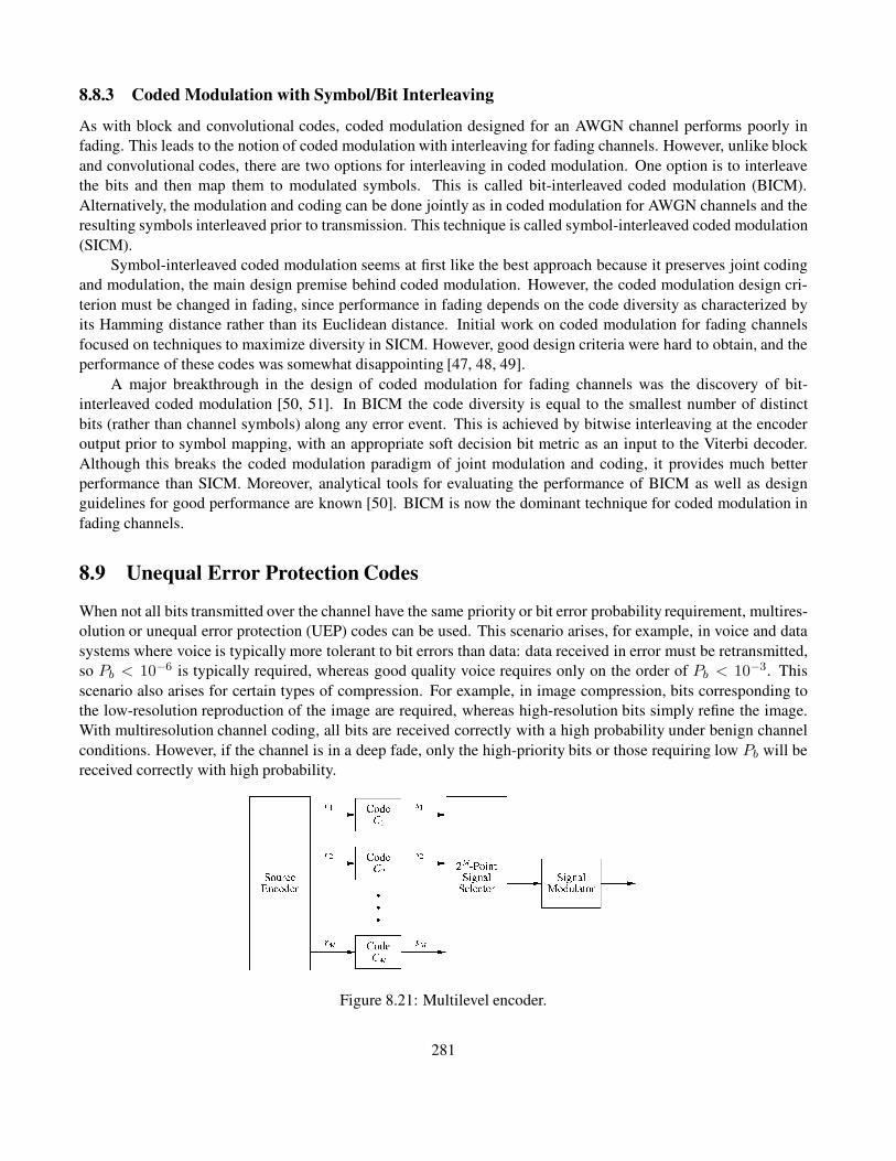
8.8.3 Coded Modulation with Symbol/Bit Interleaving

As with block and convolutional codes, coded modulation designed for an AWGN channel performs poorly in

fading. This leads to the notion of coded modulation with interleaving for fading channels. However, unlike block

and convolutional codes, there are two options for interleaving in coded modulation. One option is to interleave

the bits and then map them to modulated symbols. This is called bit-interleaved coded modulation (BICM).

Alternatively, the modulation and coding can be done jointly as in coded modulation for AWGN channels and the

resulting symbols interleaved prior to transmission. This technique is called symbol-interleaved coded modulation

(SICM).

Symbol-interleaved coded modulation seems at first like the best approach because it preserves joint coding

and modulation, the main design premise behind coded modulation. However, the coded modulation design cri-

terion must be changed in fading, since performance in fading depends on the code diversity as characterized by

its Hamming distance rather than its Euclidean distance. Initial work on coded modulation for fading channels

focused on techniques to maximize diversity in SICM. However, good design criteria were hard to obtain, and the

performance of these codes was somewhat disappointing [47, 48, 49].

A major breakthrough in the design of coded modulation for fading channels was the discovery of bit-

interleaved coded modulation [50, 51]. In BICM the code diversity is equal to the smallest number of distinct

bits (rather than channel symbols) along any error event. This is achieved by bitwise interleaving at the encoder

output prior to symbol mapping, with an appropriate soft decision bit metric as an input to the Viterbi decoder.

Although this breaks the coded modulation paradigm of joint modulation and coding, it provides much better

performance than SICM. Moreover, analytical tools for evaluating the performance of BICM as well as design

guidelines for good performance are known [50]. BICM is now the dominant technique for coded modulation in

fading channels.

8.9 Unequal Error Protection Codes

When not all bits transmitted over the channel have the same priority or bit error probability requirement, multires-

olution or unequal error protection (UEP) codes can be used. This scenario arises, for example, in voice and data

systems where voice is typically more tolerant to bit errors than data: data received in error must be retransmitted,

so Pb < 10−6 is typically required, whereas good quality voice requires only on the order of Pb < 10−3. This

scenario also arises for certain types of compression. For example, in image compression, bits corresponding to

the low-resolution reproduction of the image are required, whereas high-resolution bits simply refine the image.

With multiresolution channel coding, all bits are received correctly with a high probability under benign channel

conditions. However, if the channel is in a deep fade, only the high-priority bits or those requiring low Pb will be

received correctly with high probability.

Figure 8.21: Multilevel encoder.

281

Figure 8.22: Transceiver for time-multiplexed coded modulation.

Practical implementation of a UEP code was first studied by Imai and Hirakawa [52]. Binary UEP codes

were later considered for combined speech and channel coding [53] as well as for combined image and channel

coding [54]. These implementations use traditional (block or convolutional) error correction codes, so coding gain

is directly proportional to bandwidth expansion. Subsequently, two bandwidth-efficient implementations for UEP

codes were proposed: time multiplexing of bandwidth-efficient coded modulation [55], and coded modulation

techniques applied to both uniform and nonuniform signal constellations [56, 57]. All of these multilevel codes

can be designed for either AWGN or fading channels. We now briefly summarize these UEP coding techniques;

specifically, we describe the principles behind multilevel coding and multistate decoding as well as the more

complex bandwidth-efficient implementations.

A block diagram of a general multilevel encoder is shown in Figure 8.21. The source encoder first divides

the information sequence into M parallel bit streams of decreasing priority. The channel encoder consists of M

different binary error correcting codesC1, . . . , CM with decreasing codeword distances. The ith-priority bit stream

enters the ith encoder, which generates the coded bits si. If the 2M points in the signal constellation are numbered

from 0 to 2M − 1, then the point selector chooses the constellation point s corresponding to

s =

M∑

i=1

si · 2i−1. (8.82)

For example, if M = 3 and the signal constellation is 8-PSK, then the chosen signal point will have phase 2πs/8.

Optimal decoding of the multilevel code uses a maximum likelihood decoder, which determines the input

sequence that maximizes the received sequence probability. The ML decoder must therefore jointly decode the

code sequences s1, . . . , sm. This can entail significant complexity even if the individual codes in the mul-

tilevel code have low complexity. For example, if the component codes are convolutional codes with 2µi states,

i = 1, . . . ,M , then the number of states in the optimal decoder is 2µ1+···+µM . Because of the high complexity

of optimal decoding, the suboptimal technique of multistage decoding, introduced in [52], is used for most imple-

mentations. Multistage decoding is accomplished by decoding the component codes sequentially. First the most

powerful code, C1, is decoded, then C2, and so forth. Once the code sequence corresponding to encoder Ci is

estimated, it is assumed to be correct for code decisions on the weaker code sequences.

The binary encoders of this multilevel code require extra code bits to achieve their coding gain, so they are

not bandwidth efficient. An alternative approach proposed in [56] uses time multiplexing of the coded modulations

described in Section 8.7. In this approach, different lattice or trellis coded modulations with different coding gains

282

are used for each priority class of input data. The transmit signal constellations corresponding to each encoder may

differ in size (number of signal points), but the average power of each constellation is the same. The signal points

output by each of the individual encoders are then time-multiplexed together for transmission over the channel,

as shown in Figure 8.22 for two bit streams of different priority. Let Ri denote the bit rate of encoder Ci in this

figure for i = 1, 2. If T1 equals the fraction of time that the high-priority C1 code is transmitted and if T2 equals

the fraction of time that the C2 code is transmitted, then the total bit rate is (R1T1 + R2T2)/(T1 + T2), with the

high-priority bits constitutingR1T1/(R1T1 + R2T2) percent of this total.

The time-multiplexed coding method yields a higher gain if the constellation maps S1 and S2 of Figure 8.22

are designed jointly. This revised scheme is shown in Figure 8.23 for two encoders, where the extension to M

encoders is straightforward. In trellis and lattice coded modulation, recall that bits are encoded to select the lattice

subset and that uncoded bits choose the constellation point within the subset. The binary encoder properties reduce

the Pb for the encoded bits only; the Pb for the uncoded bits is determined by the separation of the constellation

signal points. We can easily modify this scheme to yield two levels of coding gain, where the high-priority bits are

heavily encoded and are used to choose the subset of the partitioned constellation, while the low-priority bits are

uncoded or lightly coded and are used to select the constellation signal point.

Figure 8.23: Joint optimization of signal constellation.

8.10 Joint Source and Channel Coding

The underlying premise of UEP codes is that the bit error probabilities of the channel code should be matched to

the priority or Pb requirements associated with the bits to be transmitted. These bits are often taken from the output

of a compression algorithm acting on the original data source. Hence, UEP coding can be considered as a joint

design between compression (also called source coding) and channel coding. Although Shannon determined that

the source and channel codes can be designed separately on an AWGN channel with no loss in optimality [58],

this result holds only in the limit of infinite source code dimension, infinite channel code blocklength, and infinite

complexity and delay. Thus, there has been much work on investigating the benefits of joint source and channel

coding under more realistic system assumptions.

Work in the area of joint source and channel coding falls into several broad categories: source-optimized

channel coding; channel-optimized source coding; and iterative algorithms, which combine these two code de-

signs. In source-optimized channel coding, the source code is designed for a noiseless channel. A channel code is

then designed for this source code to minimize end-to-end distortion over the given channel based on the distortion

283

associated with corruption of the different transmitted bits. Unequal error protection channel coding – where the

Pb of the different component channel codes is matched to the bit priorities associated with the source code – is

an example of this technique. Source-optimized channel coding has been applied to image compression with con-

volution channel coding and with rate-compatible punctured convolutional (RCPC) channel codes in [54, 59, 60].

A comprehensive treatment of matching RCPC channel codes or MQAM to subband and linear predictive speech

coding – in both AWGN and Rayleigh fading channels – can be found in [61]. In source-optimized modulation,

the source code is designed for a noiseless channel and then the modulation is optimized to minimize end-to-end

distortion. An example of this approach is given in [62], where compression by a vector quantizer (VQ) is followed

by multicarrier modulation, and the modulation provides unequal error protection to the different source bits by

assigning different powers to each subcarrier.

Channel-optimized source coding is another approach to joint source and channel coding. In this technique the

source code is optimized based on the error probability associated with the channel code, where the channel code

is designed independently of the source. Examples of work taking this approach include the channel-optimized

vector quantizer (COVQ) and its scalar variation [63, 64]. Source-optimized channel coding and modulation can be

combined with channel-optimized source coding via an iterative design. This approach is used for the joint design

of a COVQ and multicarrier modulation in [65] and for the joint design of a COVQ and RCPC channel code in

[66]. Combined trellis coded modulation and trellis coded quantization, a source coding strategy that borrows

from the basic premise of trellis coded modulation, is investigated in [67, 68]. All of this work on joint source and

channel code design indicates that significant performance advantages are possible when the source and channel

codes are jointly designed. Moreover, many sophisticated channel code designs, such as turbo and LDPC codes,

have not yet been combined with source codes in a joint optimization. Thus, much more work is needed in the

broad area of joint source and channel coding to optimize performance for different applications.

284

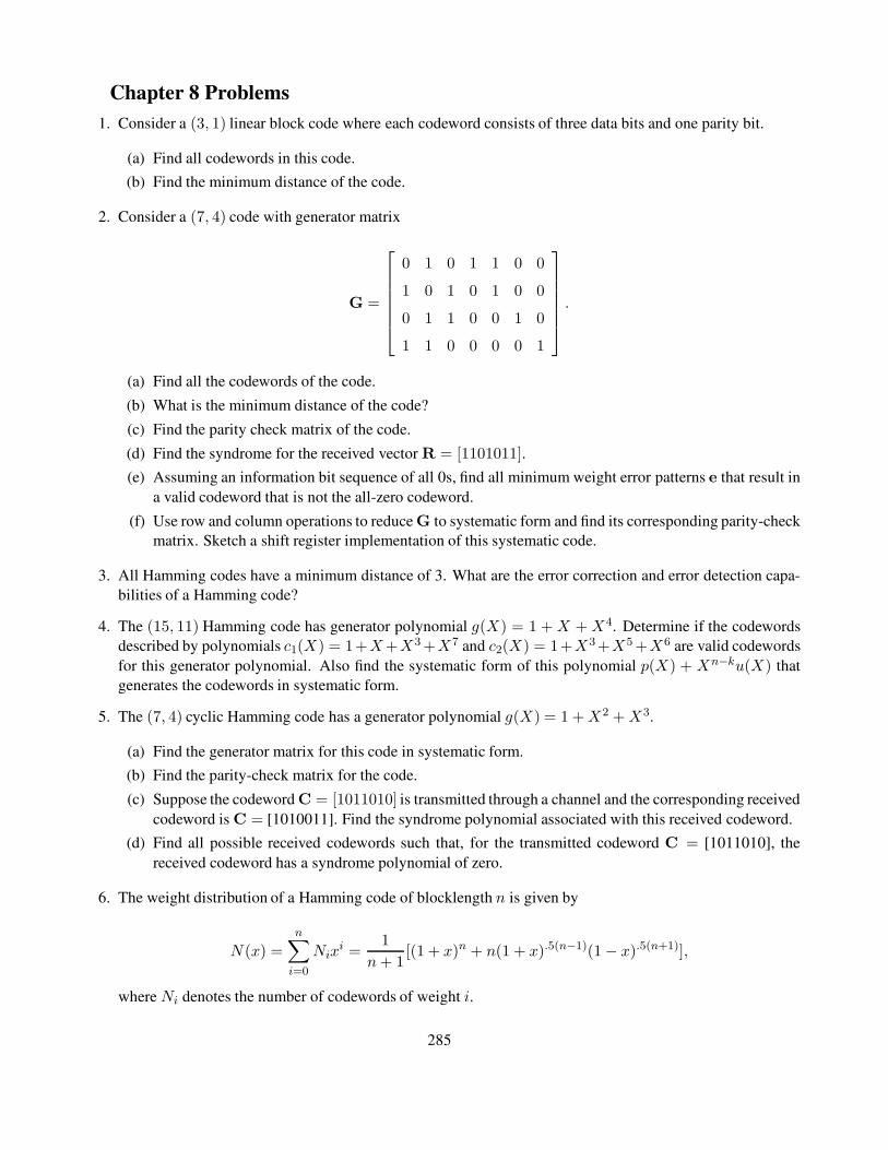
Chapter 8 Problems

1. Consider a (3, 1) linear block code where each codeword consists of three data bits and one parity bit.

(a) Find all codewords in this code.

(b) Find the minimum distance of the code.

2. Consider a (7, 4) code with generator matrix

G =

0 1 0 1 1 0 0

1 0 1 0 1 0 0

0 1 1 0 0 1 0

1 1 0 0 0 0 1

.

(a) Find all the codewords of the code.

(b) What is the minimum distance of the code?

(c) Find the parity check matrix of the code.

(d) Find the syndrome for the received vector R = [1101011].

(e) Assuming an information bit sequence of all 0s, find all minimum weight error patterns e that result in

a valid codeword that is not the all-zero codeword.

(f) Use row and column operations to reduce G to systematic form and find its corresponding parity-check

matrix. Sketch a shift register implementation of this systematic code.

3. All Hamming codes have a minimum distance of 3. What are the error correction and error detection capa-

bilities of a Hamming code?

4. The (15, 11) Hamming code has generator polynomial g(X) = 1 +X +X4. Determine if the codewords

described by polynomials c1(X) = 1+X+X3 +X7 and c2(X) = 1+X3+X5 +X6 are valid codewords

for this generator polynomial. Also find the systematic form of this polynomial p(X) + Xn−ku(X) that

generates the codewords in systematic form.

5. The (7, 4) cyclic Hamming code has a generator polynomial g(X) = 1 +X2 +X3.

(a) Find the generator matrix for this code in systematic form.

(b) Find the parity-check matrix for the code.

(c) Suppose the codeword C = [1011010] is transmitted through a channel and the corresponding received

codeword is C = [1010011]. Find the syndrome polynomial associated with this received codeword.

(d) Find all possible received codewords such that, for the transmitted codeword C = [1011010], the

received codeword has a syndrome polynomial of zero.

6. The weight distribution of a Hamming code of blocklength n is given by

N (x) =

n∑

i=0

Nixi =

1

n+ 1[(1 + x)n + n(1 + x).5(n−1)(1 − x).5(n+1)],

where Ni denotes the number of codewords of weight i.

285

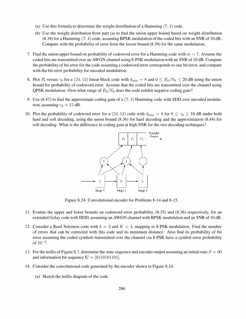
(a) Use this formula to determine the weight distribution of a Hamming (7, 4) code.

(b) Use the weight distribution from part (a) to find the union upper bound based on weight distribution

(8.38) for a Hamming (7, 4) code, assuming BPSK modulation of the coded bits with an SNR of 10 dB.

Compare with the probability of error from the looser bound (8.39) for the same modulation.

7. Find the union upper bound on probability of codeword error for a Hamming code withm = 7. Assume the

coded bits are transmitted over an AWGN channel using 8-PSK modulation with an SNR of 10 dB. Compute

the probability of bit error for the code assuming a codeword error corresponds to one bit error, and compare

with the bit error probability for uncoded modulation.

8. Plot Pb versus γb for a (24, 12) linear block code with dmin = 8 and 0 ≤ Eb/N0 ≤ 20 dB using the union

bound for probability of codeword error. Assume that the coded bits are transmitted over the channel using

QPSK modulation. Over what range of Eb/N0 does the code exhibit negative coding gain?

9. Use (8.47) to find the approximate coding gain of a (7, 4) Hamming code with SDD over uncoded modula-

tion, assuming γb = 15 dB.

10. Plot the probability of codeword error for a (24, 12) code with dmin = 8 for 0 ≤ γb ≤ 10 dB under both

hard and soft decoding, using the union bound (8.36) for hard decoding and the approximation (8.44) for

soft decoding. What is the difference in coding gain at high SNR for the two decoding techniques?

Figure 8.24: Convolutional encoder for Problems 8-14 and 8-15.

11. Evalute the upper and lower bounds on codeword error probability, (8.35) and (8.36) respectively, for an

extended Golay code with HDD, assuming an AWGN channel with BPSK modulation and an SNR of 10 dB.

12. Consider a Reed Solomon code with k = 3 and K = 4, mapping to 8-PSK modulation. Find the number

of errors that can be corrected with this code and its minimum distance. Also find its probability of bit

error assuming the coded symbols transmitted over the channel via 8-PSK have a symbol error probability

of 10−3.

13. For the trellis of Figure 8.7, determine the state sequence and encoder output assuming an initial stateS = 00and information bit sequence U = [0110101101].

14. Consider the convolutional code generated by the encoder shown in Figure 8.24.

(a) Sketch the trellis diagram of the code.

286

Figure 8.25: 16-QAM trellis encoder for Problem 8-16.

(b) For a received sequence R = [001010001], find the path metric for the all-zero path assuming proba-

bility of symbol error p = 10−3.

(c) Find one path at a minimum Hamming distance from the all-zero path and compute its path metric for

the same R and p as in part (b).

15. This problem is based on the convolutional encoder of Figure 8.24.

(a) Draw the state diagram for this convolutional encoder.

(b) Determine its transfer function T (D, N, J).

(c) Determine the minimum distance of paths through the trellis to the all-zero path.

(d) Compute the upper bound (8.72) on probability of bit error for this code assuming SDD and BPSK

modulation with γb = 10 dB.

(e) Compute the upper bound (8.76) on probability of bit error for this code assuming HDD and BPSK

modulation with γb = 10 dB. How much coding gain is achieved with soft versus hard decoding?

16. Suppose you have a 16-QAM signal constellation that is trellis encoded via the scheme of Figure 8.25.

Assume the set partitioning for 16-QAM shown in Figure 8.18.

(a) Assuming that parallel transitions–that is, transitions within a subset–dominate the error probability,

find the coding gain of this trellis code relative to uncoded 8-PSK, given that d0 for the 16-QAM is

.632 and for the 8-PSK is .765.

(b) Draw the trellis for the convolutional encoder and assign subsets to the trellis transitions according to

the following heuristic rules of Ungerboeck: (i) if k bits are to be encoded per modulation interval then

the trellis must allow for 2k possible transitions from each state to the next state; (ii) more than one

transition may occur between pairs of states; (iii) all waveforms should occur with equal frequency

287

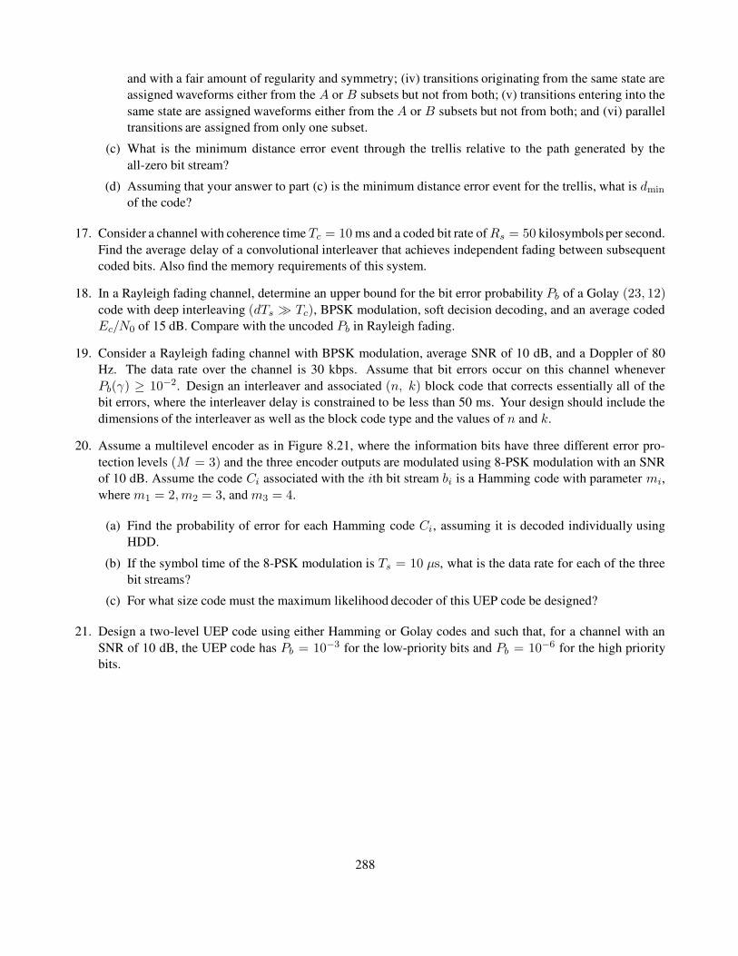
and with a fair amount of regularity and symmetry; (iv) transitions originating from the same state are

assigned waveforms either from the A or B subsets but not from both; (v) transitions entering into the

same state are assigned waveforms either from the A or B subsets but not from both; and (vi) parallel

transitions are assigned from only one subset.

(c) What is the minimum distance error event through the trellis relative to the path generated by the

all-zero bit stream?

(d) Assuming that your answer to part (c) is the minimum distance error event for the trellis, what is dmin

of the code?

17. Consider a channel with coherence time Tc = 10 ms and a coded bit rate ofRs = 50 kilosymbols per second.

Find the average delay of a convolutional interleaver that achieves independent fading between subsequent

coded bits. Also find the memory requirements of this system.

18. In a Rayleigh fading channel, determine an upper bound for the bit error probability Pb of a Golay (23, 12)

code with deep interleaving (dTs Tc), BPSK modulation, soft decision decoding, and an average coded

Ec/N0 of 15 dB. Compare with the uncoded Pb in Rayleigh fading.

19. Consider a Rayleigh fading channel with BPSK modulation, average SNR of 10 dB, and a Doppler of 80

Hz. The data rate over the channel is 30 kbps. Assume that bit errors occur on this channel whenever

Pb(γ) ≥ 10−2. Design an interleaver and associated (n, k) block code that corrects essentially all of the

bit errors, where the interleaver delay is constrained to be less than 50 ms. Your design should include the

dimensions of the interleaver as well as the block code type and the values of n and k.

20. Assume a multilevel encoder as in Figure 8.21, where the information bits have three different error pro-

tection levels (M = 3) and the three encoder outputs are modulated using 8-PSK modulation with an SNR

of 10 dB. Assume the code Ci associated with the ith bit stream bi is a Hamming code with parameter mi,

where m1 = 2, m2 = 3, and m3 = 4.

(a) Find the probability of error for each Hamming code Ci, assuming it is decoded individually using

HDD.

(b) If the symbol time of the 8-PSK modulation is Ts = 10 µs, what is the data rate for each of the three

bit streams?

(c) For what size code must the maximum likelihood decoder of this UEP code be designed?

21. Design a two-level UEP code using either Hamming or Golay codes and such that, for a channel with an

SNR of 10 dB, the UEP code has Pb = 10−3 for the low-priority bits and Pb = 10−6 for the high priority

bits.

288

Bibliography

[1] J. G. Proakis, Digital Communications, 4th ed., McGraw-Hill, New York, 2001.

[2] B. Sklar, Digital Communications–Fundamentals and Applications, Prentice-Hall, Englewood Cliffs, NJ,

1988.

[3] D. G. Wilson, Digital Modulation and Coding, Prentice-Hall, Englewood Cliffs, NJ, 1996.

[4] S. Lin and J. D. J. Costello, Error Control Coding, 2nd ed., Prentice-Hall, Englewood Cliffs, NJ, 2004.

[5] A. J. Vlterbi, “Error bounds for convolutional codes and asymptotically optimum decoding algorithm,” IEEE

Trans. Inform. Theory, pp. 260–9, April 1967.

[6] C. Berrou, A. Glavieux, and P. Thitimajshima, “Near Shannon limit error-correcting coding and decoding:

Turbo-codes,” Proc. IEEE Intemat. Conf. Commun., pp. 54–8, May 1993.

[7] C. Berrou and A. Glavieux, “Near optimum error correcting coding and decoding: Turbo-codes,” IEEE Trans.

Commun., pp. 1261–71, October 1996.

[8] IEEE Trans. Inform. Theory, Special Issue on Codes and Graphs and Iterative Algorithms, Febmary 2001.

[9] S. B. Wicker and S. Kim, Codes, Graphs, and Iterative Decoding, Kluwer, Boston, 2002.

[10] R. G. Gallager, “Low-density parity-check codes,” IRE Trans. Inform. Theory, pp. 21–8, January 1962.

[11] C. Heegard and S. B. Wicker, Turbo Coding, Kluwer, Boston, 1999.

[12] M. E. Buckley and S. B. Wicker, “The design and performance of a neural network for predicting decoder

error in turbo-coded ARQ protocols,” IEEE Trans. Commun., pp. 566–76, April 2000.

[13] S. Benedetto, D. Divsalar, G. Montorsi, and F. Pollara, “Serial concatenation ofinterleaved codes: Perfor-

mance analysis, design and iterative decoding,” IEEE Trans. Inform. Theory, pp. 909–26, May 1998.

[14] H. Jin and R. J. McEliece, “Coding theorems for turbo code ensembles,” IEEE Trans. Inform. Theory, pp.

1451–61, June 2002.

[15] I. Sasan and S. Shamai, “Improved upper bounds on the ML decoding error probability of parallel and serial

concatenated turbo codes via their ensemble distance spectrum,” IEEE Trans. Inform. Theory, pp. 24–47,

January 2000.

[16] D. J. C. MacKay and R. M. Neal, “Near Shannon limit performance of low density parity check codes,” Elec.

Lett., p. 1645, August 1996.

289

[17] N. Wiberg, N.-A. Loeliger, and R. Kotter, “Codes and iterative decoding on general graphs,” Euro. Trans.

Telecommun., pp. 513–25, June 1995.

[18] T. Richardson, A. Shokrollahi, and R. Urbanke, “Design of capacity-approaching irregular lowdensity parity-

check codes,” IEEE Trans. Inform. Theory, pp. 619–37, Febmary 2001.

[19] R. McEliece, D. J. C. MacKay, and J.-F. Cheng, “ Turbo decoding as an instance of Pearl’s‘ belief propaga-

tion’ algorithm,” IEEE J. Sel. Areas Commun., pp. 140–52, Febmary 1998.

[20] F. R. Kschischang and D. Frey, “Iterative decoding of compound codes by probability propagation in graphi-

cal models,” IEEE J. Sel. Areas Commun., pp. 219–30, Febmary 1998.

[21] T. Richardson and R. Urbanke, “ The capacity of low-density parity-check codes under message passing

decoding,” IEEE Trans. Inform. Theory, pp. 599–618, February 2001.

[22] S.-Y. Chung, G. D. Fomey, T. Richardson, and R. Urbanke, “On the design of low-density parity-check codes

within 0.0045 dB of the Shannon limit,” IEEE Commun. Lett., pp. 58–60, Febmary 2001.

[23] M. Fossorier, “Iterative reliability-based decoding of low-density parity check codes,” IEEE J. Sel. Areas

Commun., pp. 908–17, May 2001.

[24] M. C. Davey and D. MacKay, “Low density parity-check codes over GF(q),” IEEE Commun. Lett., pp. 165–7,

June 1998.

[25] J. Hou, P. Siegel, L. Milstein, and H. D. Pfister, “Capacity-approaching bandwidth efficient coded modulation

schemes based on low-density parity-check codes,” IEEE Trans. Inform. Theory, pp. 2141–55, September

2003.

[26] G. Ungerboeck, “Channel coding with multi-level/phase signals,” IEEE Trans. Inform. Theory, pp. 55–67,

January 1982.

[27] G. D. Fomey, “Coset codes, I: Introduction and geomenical classification, and II: Binary lattices and related

codes,” IEEE Trans. Inform. Theory, pp. 1123–87, September 1988.

[28] G. D. Fomey, Jr., R. G. Gallager, G. R. Lang, F. M. Longstaff, and S. U. Quereshi, “Efficient modulation for

band-limited channels,” IEEE J. Sel. Areas Commun., pp. 632–47, September 1984.

[29] S. Benedetto, D. Divsalar, G. Montorsi, and F. Pollara, “Parallel concatenated trellis coded modulation,” Proc.

IEEE Intemat. Conf. Commun., pp. 974–8, June 1996.

[30] C. Fragouli and R. D. Wesel, “Turbo-encoder design for symbol-interleaved parallel concatenated trellis-

coded modulation,” IEEE Trans. Commun., pp. 425–35, March 2001.

[31] P. Robertson and T. Worz, “Bandwidth-efficient turbo trellis-coded modulation using punctured component

codes,” IEEE J. Sel. Areas Commun., pp. 206–18, February 1998.

[32] G. T. Irvine and P. J. Mclane, “Symbol-aided plus decision-directed reception for PSK TCM modulation on

shadowed mobile satellite fading channels,” IEEE J. Sel. Areas Commun., pp. 1289–99, October 1992.

[33] D. Subasinghe-Dias and K. Feher, “A coded 16-QAM scheme for fast fading mobile radio channels,” IEEE

Trans. Commun., pp. 1906–16, February–April 1995.

290

[34] P. Y. Kam and H. M. Ching, “Sequence estimation over the slow nonselective Rayleigh fading channel with

diversity reception and its application to Vlterbi decoding,” IEEE J. Sel. Areas Commun., pp. 562–70, April

1992.

[35] D. Makrakis, P. T. Mathiopoulos, and D. P. Bouras, “Optimal decoding of coded PSK and QAM signals in

correlated fast fading channels and AWGN–A combined envelope, multiple differential and coherent detec-

tion approach,” IEEE Trans. Commun., pp. 63–75, January 1994.

[36] M. J. Gertsman and J. H. Lodge, “Symbol-by-symbol MAP demodulation of CPM and PSK signals on

Rayleigh flat-fading channels,” IEEE Trans. Commun., pp. 788–99, July 1997.

[37] H. Kong and E. Shwedyk, “Sequence detection and channel state estimation over finite state Markov chan-

nels,” IEEE Trans. Veh. Tech., pp. 833–9, May 1999.

[38] G. M. Vitetta and D. P. Taylor, “Maximum-likelihood decoding of uncoded and coded PSK signal sequences

transmitted over Rayleigh flat-fading channels,” IEEE Trans. Commun., pp. 2750–8, November 1995.

[39] L. Li and A. J. Goldsmith, “Low-complexity maximum-likelihood detection of coded signals sent over finite-

state Markov channels,” IEEE Trans. Commun., pp. 524–31, April 2002.

[40] B. Vucetic and J. Yuan, Turbo Codes: Principles and Applications, Kluwer, Dordrecht, 2000.

[41] E. K. Hall and S. G. Wilson, “Design and analysis of turbo codes on Rayleigh fading channels,” IEEE J. Sel.

Areas Commun., pp. 160–74, February 1998.

[42] C. Komninakis and R. D. Wesel, “Joint iterative channel estimation and decoding in flat correlated Rayleigh

fading,” IEEE J. Sel. Areas Commun. pp. 1706–17, September 2001.

[43] J. Hou, P. H. Siegel, and L. B. Milstein, “Performance analysis and code optimization of lowdensity parity-

check codes on Rayleigh fading channels,” IEEE J. Sel. Areas Commun., pp. 924–34, May 2001.

[44] A. J. Goldsmith and P. P. Varaiya, “Capacity, mutual information, and coding for finite-state Markov chan-

nels,” IEEE Trans. Inform. Theory, pp. 868–86, May 1996.

[45] G. D. Fomey, “Burst error correcting codes for the classic bursty channel,” IEEE Trans. Commun. Tech., pp.

772–81, October 1971.

[46] J. L. Ramsey, “Realization of optimum interleavers,” IEEE Trans. Inform. Theory, pp. 338–45, 1970.

[47] C.-E. W. Sundberg and N. Seshadri, “Coded modulation for fading channels-An overview,” Euro. Trans.

Telecommun., pp. 309–24, May/ June 1993.

[48] L.-F. Wei, “Coded M-DPSK with built-in time diversity for fading channels,” IEEE Trans. Inform. Theory,

pp. 1820–39, November 1993.

[49] S. H. Jamali and T. Le-Ngoc, Coded-Modulation Techniques for Fading Channels, Kluwer, New York, 1994.

[50] G. Caire, G. Taricco, and E. Biglieri, “Bit-interleaved coded modulation,” IEEE Trans. Inform. Theory, pp.

927–46, May 1998.

[51] E. Zehavi, “8-PSK trellis codes for a Rayleigh channel,” IEEE Trans. Commun., pp. 873–84, May 1992.

291

[52] H. Imai and S. Hirakawa, “A new multilevel coding method using error correcting codes,” IEEE Trans.

Inform. Theory, pp. 371–7, May 1977.

[53] R. V. Cox, J. Hagenauer, N. Seshadri, and C.-E. W. Sundberg, “Variable rate sub-band speech coding and

matched convolutional channel coding for mobile radio channels,” IEEE Trans. Signal Proc., pp. 1717–31,

August 1991.

[54] J. W. Modestino and D. G. Daut, “Combined source-channel coding of images,” IEEE Trans. Commun., pp.

1644–59, November 1979.

[55] A. R. Calderbank and N. Seshadri, “Multilevel codes for unequal error protection,” IEEE Trans. Inform.

Theory, pp. 1234–48, July 1993.

[56] L.-F. Wei, “Coded modulation with unequal error protection,” IEEE Trans. Commun., pp. 1439–49, October

1993.

[57] N. Seshadri and C.-E. W. Sundberg, “Multilevel trellis coded modulations for the Rayleigh fading channel,”

IEEE Trans. Commun., pp. 1300–10, September 1993.

[58] C. E. Shannon, “Coding theorems for a discrete source with a fidelity criterion,” IRE National Convention

Record, part 4, pp. 142–63, 1959.

[59] N. Tanabe and N. Farvardin, “Subband image coding using entropy-coded quantization over noisy channels,”

IEEE J. Sel. Areas Commun., pp. 926–43, June 1992.

[60] H. Jafarkhani, P. Ligdas, and N. Farvardin, “Adaptive rate allocation in ajoint source/channel coding frame-

work for wireless channels,” Proc. IEEE Veh. Tech. Conf., pp. 492–6, April 1996.

[61] W. C. Wong, R. Steele, and C.-E. W. Sundberg, Source-Matched Mobile Communications, Pentech and IEEE

Press, London and New York, 1995.

[62] K.-P. Ho and J. M. Kahn, “Transmission of analog signals using multicarrier modulation: A combined source-

channel coding approach,” IEEE Trans. Commun., pp. 1432–43, November 1996.

[63] N. Farvardin and V. Vaishampayan, “On the performance and complexity of channel-optimized vector quan-

tizers,” IEEE Trans. Inform. Theory, pp. 155–60, January 1991.

[64] N. Farvardin and V. Vaishampayan, “Optimal quantizer design for noisy channels: An approach to combined

source-channel coding,” IEEE Trans. Inform. Theory, pp. 827–38, November 1987.

[65] K.-P. Ho and J. M. Kahn, “Combined source-channel coding using channel-optimized quantizer and multi-

canier modulation,” Proc. IEEE Intemat. Conf. Commun., pp. 1323–7, June 1996.

[66] A. J. Goldsmith and M. Effros, “Joint design of fixed-rate source codes and multiresolution channel codes,”

IEEE Trans. Commun., pp. 1301–12, October 1998.

[67] E. Ayanoglu and R. M. Gray, “The design ofjoint source and channel trellis waveform coders,” IEEE Trans.

Inform. Theory, pp. 855–65, November 1987.

[68] T. R. Fischer and M. W. Marcellin, “Joint trellis coded quantization/modulation,” IEEE Trans. Commun., pp.

172–6, Febmary 1991.

292

Chapter 9

Adaptive Modulation and Coding

Adaptive modulation and coding enable robust and spectrally efficient transmission over time-varying channels.

The basic premise is to estimate the channel at the receiver and feed this estimate back to the transmitter, so that

the transmission scheme can be adapted relative to the channel characteristics. Modulation and coding techniques

that do not adapt to fading conditions require a fixed link margin to maintain acceptable performance when the

channel quality is poor. Thus, these systems are effectively designed for worst-case channel conditions. Since

Rayleigh fading can cause a signal power loss of up to 30 dB, designing for the worst-case channel conditions can

result in very inefficient utilization of the channel. Adapting to the channel fading can increase average throughput,

reduce required transmit power, or reduce average probability of bit error by taking advantage of favorable channel

conditions to send at higher data rates or lower power – and by reducing the data rate or increasing power as

the channel degrades. In Section 4.2.4 we derived the optimal adaptive transmission scheme that achieves the

Shannon capacity of a flat fading channel. In this chapter we describe more practical adaptive modulation and

coding techniques to maximize average spectral efficiency while maintaining a given average or instantaneous bit

error probability. The same basic premise can be applied to MIMO channels, frequency-selective fading channels

with equalization, OFDM or CDMA, and cellular systems. The application of adaptive techniques to these systems

will be described in subsequent chapters.

Adaptive transmission was first investigated in the late sixties and early seventies [1, 2]. Interest in these

techniques was short-lived, perhaps due to hardware constraints, lack of good channel estimation techniques, and

or systems focusing on point-to-point radio links without transmitter feedback. As technology evolved these issues

became less constraining, resulting in a revived interest in adaptive modulation methods for 3G wireless systems

[3, 4, 5, 6, 7, 8, 9, 10, 11, 12]. As a result, many wireless systems – including both GSM and CDMA cellular

systems as well as wireless LANs – use adaptive transmission techniques [13, 14, 15, 16].

There are several practical constraints that determine when adaptive modulation should be used. Adaptive

modulation requires a feedback path between the transmitter and receiver, which may not be feasible for some sys-

tems. Moreover, if the channel is changing faster than it can be reliably estimated and fed back to the transmitter,

adaptive techniques will perform poorly. Many wireless channels exhibit variations on different time scales; exam-

ples include multipath fading, which can change very quickly, and shadowing, which changes more slowly. Often

only the slow variations can be tracked and adapted to, in which case flat fading mitigation is needed to address

the effects of multipath. Hardware constraints may dictate how often the transmitter can change its rate and/or

power, and this may limit the performance gains possible with adaptive modulation. Finally, adaptive modulation

typically varies the rate of data transmission relative to channel conditions. We will see that average spectral effi-

ciency of adaptive modulation under an average power constraint is maximized by setting the data rate to be small

or zero in poor channel conditions. However, with this scheme the quality of fixed-rate applications (such as voice

or video) with hard delay constraints may be significantly compromised. Thus, in delay-constrained applications

293

the adaptive modulation should be optimized to minimize outage probability for a fixed data rate [17].

9.1 Adaptive Transmission System

In this section we describe the system associated with adaptive transmission. The model is the same as the model

of Section 4.2.1 used to determine the capacity of flat fading channels. We assume linear modulation, where

the adaptation takes place at a multiple of the symbol rate Rs = 1/Ts. We also assume the modulation uses ideal

Nyquist data pulses (sinc[t/Ts]), so the signal bandwidthB = 1/Ts. We model the flat fading channel as a discrete-

time channel in which each channel use corresponds to one symbol time Ts. The channel has stationary and ergodic

time-varying gain√

g[i] that follows a given distribution p(g) and AWGN n[i], with power spectral densityN0/2.

Let P denote the average transmit signal power, B = 1/Ts the received signal bandwidth, and g the average

channel gain. The instantaneous received signal-to-noise power ratio (SNR) is then γ[i] = P g[i]/N0B, 0 ≤γ[i] < ∞, and its expected value over all time is γ = P g/N0B. Since g[i] is stationary, the distribution of γ[i] is

independent of i, and we denote this distribution by p(γ).

In adaptive transmission we estimate the power gain or the received SNR at time i and then adapt the modu-

lation and coding parameters accordingly. The most common parameters to adapt are the data rate R[i], transmit

power P [i], and coding parameters C[i]. For M -ary modulation the data rate R[i] = log2M [i]/Ts = B log2M [i]bps. The spectral efficiency of the M -ary modulation is R[i]/B = log2M [i] bps/Hz. We denote the SNR estimate

as γ[i] = P g[i]/N0B, which is based on the power gain estimate g[i]. Suppose the transmit power is adapted

relative to γ[i]. We denote this adaptive transmit power at time i by P (γ[i]) = P [i], and the received power at time

i is then γ[i]P (γ[i])/P . Similarly, we can adapt the data rate of the modulation R(γ[i]) = R[i] and/or the coding

parameters C(γ[i]) = C[i] relative to the estimate γ[i]. When the context is clear, we will omit the time reference

i relative to γ, P (γ), R(γ), and C(γ).

The system model is illustrated in Figure 9.1. We assume that an estimate g[i] of the channel power gain g[i]at time i is available to the receiver after an estimation time delay of ie and that this same estimate is available

to the transmitter after a combined estimation and feedback path delay of id = ie + if . The availability of this

channel information at the transmitter allows it to adapt its transmission scheme relative to the channel variation.

The adaptive strategy may take into account the estimation error and delay in g[i− id] or it may treat g[i− id] as

the true gain: this issue will be discussed in more detail in Section 9.3.7. We assume that the feedback path does

not introduce any errors, which is a reasonable assumption if strong error correction and detection codes are used

on the feedback path and if packets associated with detected errors are retransmitted.

Figure 9.1: System model.

The rate of channel variation will dictate how often the transmitter must adapt its transmission parameters,

and it will also affect the estimation error of g[i]. When the channel gain consists of both fast and slow fading

components, the adaptive transmission may adapt to both if g[i] changes sufficiently slowly, or it may adapt to

294

just the slow fading. In particular, if g[i] corresponds to shadowing and multipath fading, then at low speeds the

shadowing is essentially constant, and the multipath fading is sufficiently slow that it can be estimated and fed back

to the transmitter with estimation error and delay that do not significantly degrade performance. At high speeds the

system can no longer effectively estimate and feed back the multipath fading in order to adapt to it. In this case, the

adaptive transmission responds to the shadowing variations only, and the error probability of the modulation must

be averaged over the fast fading distribution. Adaptive techniques for combined fast and slow fading are discussed

in Section 9.5.

9.2 Adaptive Techniques

There are many parameters that can be varied at the transmitter relative to the channel gain γ . In this section we

discuss adaptive techniques associated with variation of the most common parameters: data rate, power, coding,

error probability, and combinations of these adaptive techniques.

9.2.1 Variable-Rate Techniques

In variable-rate modulation the data rate R[γ] is varied relative to the channel gain γ . This can be done by fixing

the symbol rate Rs = 1/Ts of the modulation and using multiple modulation schemes or constellation sizes, or by

fixing the modulation (e.g. BPSK) and changing the symbol rate. Symbol rate variation is difficult to implement

in practice because a varying signal bandwidth is impractical and complicates bandwidth sharing. In contrast,

changing the constellation size or modulation type with a fixed symbol rate is fairly easy, and these techniques are

used in current systems. Specifically, the GSM and IS-136 EDGE system as well as 802.11a wireless LANs vary

their modulation and coding relative to channel quality [15]. In general the modulation parameters that dictate the

transmission rate are fixed over a block or frame of symbols, where the frame size is a parameter of the design.

Frames may also include pilot symbols for channel estimation and other control information.

When a discrete set of modulation types or constellation sizes are used, each value of γ must be mapped to

one of the possible modulation schemes. This is often done to maintain the bit error probability of each scheme

below a given value. These ideas are illustrated in the following example as well as in subsequent sections on

specific adaptive modulation techniques.

Example 9.1: Consider an adaptive modulation system that uses QPSK and 8-PSK for a target Pb of approximately

10−3. If the target Pb cannot be met with either scheme, then no data is transmitted. Find the range of γ-values as-

sociated with the three possible transmission schemes (no transmission, QPSK, and 8-PSK) as well as the average

spectral efficiency of the system, assuming Rayleigh fading with γ = 20 dB.

Solution: First note that the SNR γ = γs for both QPSK and 8-PSK. From Section 6.1 we have Pb ≈ Q(√γ)

for QPSK and Pb ≈ .666Q(√

2γ sin(π/8)) for 8-PSK. Since γ > 14.79 dB yields Pb < 10−3 for 8-PSK, the

adaptive modulation uses 8-PSK modulation for γ > 14.79 dB. Since γ > 10.35 dB yields Pb < 10−3 for QPSK,

the adaptive modulation uses QPSK modulation for 14.79 dB ≥ γ > 10.35 dB. The channel is not used for

γ ≤ 10.35 dB.

We determine the average rate by analyzing how often each of the different transmission schemes is used.

Since 8-PSK is used when γ > 14.79 dB = 30.1, in Rayleigh fading with γ = 20 dB the spectral efficiency

R[γ]/B = log2 8 = 3 bps/Hz is transmitted a fraction of time equal to P8 =∫∞30.1

1100e

−γ/100 dγ = .74. QPSK

is used when 10.35 < γ ≤ 14.79 dB, where 10.35 dB = 10.85 in linear units. So R[γ] = log2 4 = 2 bps/Hz is

transmitted a fraction of time equal to P4 =∫ 30.110.85

1100e

−γ/100 dγ = .157. During the remaining .103 portion of

time there is no data transmission. So the average spectral efficiency is .74 · 3+ .157 · 2+ .103 · 0 = 2.534 bps/Hz.

295

Note that if γ ≤ 10.35 dB then – rather than suspending transmission, which leads to an outage probability of

roughly .1 – either just one signaling dimension could be used (i.e., BPSK could be transmitted) or error correction

coding could be added to the QPSK to meet the Pb target. If block or convolutional codes were used then the

spectral efficiency for γ ≤ 10.35 dB would be less than 2 bps/Hz but larger than a spectral efficiency of zero

corresponding to no transmission. These variable-coding techniques are described in Section 9.2.4.

9.2.2 Variable-Power Techniques

Adapting the transmit power alone is generally used to compensate for SNR variation due to fading. The goal

is to maintain a fixed bit error probability or, equivalently, a constant received SNR. The power adaptation thus

inverts the channel fading so that the channel appears as an AWGN channel to the modulator and demodulator.1

The power adaptation for channel inversion is given by

P (γ)

P=σ

γ, (9.1)

where σ equals the constant received SNR. The average power constraint P implies that

∫P (γ)

Pp(γ) dγ =

∫σ

γp(γ) dγ = 1. (9.2)

Solving (9.2) for σ yields that σ = 1/E[1/γ], so σ is determined by p(γ), which in turn depends on the average

transmit power P through γ. Thus, for a given average power P , if the value for σ required to meet the target

bit error rate is greater than 1/E[1/γ] then this target cannot be met. Note that for Rayleigh fading, where γ is

exponentially distributed, E[1/γ] = ∞ and so no target Pb can be met using channel inversion.

The fading can also be inverted above a given cutoff γ0, which leads to a truncated channel inversion for

power adaptation. In this case the power adaptation is given by

P (γ)

P=

σ/γ γ ≥ γ0,

0 γ < γ0.(9.3)

The cutoff value γ0 can be based on a desired outage probability Pout = p(γ < γ0) or on a desired target BER

above a cutoff that is determined by the target BER and p(γ). Since the channel is only used when γ ≥ γ0, given

an average power P we have σ = 1/Eγ0 [1/γ], where

Eγ0

[1

γ

]4=

∫ ∞

γ0

1

γp(γ) dγ. (9.4)

Example 9.2: Find the power adaptation for BPSK modulation that maintains a fixed Pb = 10−3 in non-outage

for a Rayleigh fading channel with γ = 10 dB. Also find the resulting outage probability.

Solution: The power adaptation is truncated channel inversion, so we need only find σ and γ0. For BPSK modula-

tion, with a constant SNR of σ = 4.77 we get Pb = Q(√

2σ) = 10−3. Setting σ = 1/Eγ0 [1/γ] and solving for γ0,

which must be done numerically, yields γ0 = .7423. So Pout = p(γ < γ0) = 1 − e−γ0/10 = .379. Hence there is

a high outage probability, which results from requiring Pb = 10−3 in this relatively weak channel.

1Channel inversion and truncated channel inversion were discussed in Section 4.2.4 in the context of fading channel capacity.

296

9.2.3 Variable Error Probability

We can also adapt the instantaneous BER subject to an average BER constraint Pb. In Section 6.3.2 we saw that

in fading channels the instantaneous error probability varies as the received SNR γ varies, resulting in an average

BER of Pb =∫Pb(γ)p(γ) dγ. This is not considered an adaptive technique, since the transmitter does not adapt

to γ . Thus, in adaptive modulation, error probability is typically adapted along with some other form of adaptation

such as constellation size or modulation type. Adaptation based on varying both data rate and error probability to

reduce transmit energy was first proposed by Hayes in [1], where a 4-dB power savings was obtained at a target

average bit error probability of 10−4.

9.2.4 Variable-Coding Techniques

In adaptive coding, different channel codes are used to provide different amounts of coding gain to the transmitted

bits. For example, a stronger error correction code may be used when γ is small, with a weaker code or no coding

used when γ is large. Adaptive coding can be implemented by multiplexing together codes with different error

correction capabilities. However, this approach requires that the channel remain roughly constant over the block

length or constraint length of the code [7]. On such slowly varying channels, adaptive coding is particularly useful

when the modulation must remain fixed, as may be the case owing to complexity or peak-to-average power ratio

constraints.

An alternative technique to code multiplexing is rate-compatible punctured convolutional (RCPC) codes [18].

This is a family of convolutional codes at different code rates Rc = k/n. The basic premise of RCPC codes

is to have a single encoder and decoder whose error correction capability can be modified by not transmitting

certain coded bits (puncturing the code). Moreover, RCPC codes have a rate compatibility constraint so that the

coded bits associated with a high-rate (weaker) code are also used by all lower-rate (stronger) codes. Thus, to

increase the error correction capability of the code, the coded bits of the weakest code are transmitted along with

additional coded bits to achieve the desired level of error correction. The rate compatibility makes it easy to adapt

the error protection of the code, since the same encoder and decoder are used for all codes in the RCPC family,

with puncturing at the transmitter to achieve the desired error correction. Decoding is performed by a Viterbi

algorithm operating on the trellis associated with the lowest rate code, with the puncturing incorporated into the

branch metrics. Puncturing is a very effective and powerful adaptive coding technique, and it forms the basis of

adaptive coding in the GSM and IS-136 EDGE protocol for data transmission [13].

Adaptive coding through either multiplexing or puncturing can be done for fixed modulation or combined

with adaptive modulation as a hybrid technique. When the modulation is fixed, adaptive coding is often the only

practical mechanism to address the channel variations [6, 7]. The focus of this chapter is on systems where adaptive

modulation is possible, so adaptive coding on its own will not be further discussed.

9.2.5 Hybrid Techniques

Hybrid techniques can adapt multiple parameters of the transmission scheme, including rate, power, coding, and

instantaneous error probability. In this case joint optimization of the different techniques is used to meet a given

performance requirement. Rate adaptation is often combined with power adaptation to maximize spectral effi-

ciency, and we apply this joint optimization to different modulations in subsequent sections. Adaptive modulation

and coding has been widely investigated in the literature and is currently used in both cellular systems and wireless

LANs [13, 15].

297

9.3 Variable-Rate Variable-Power MQAM

In the previous section we discussed general approaches to adaptive modulation and coding. In this section we

describe a specific form of adaptive modulation where the rate and power of MQAM are varied to maximize spec-

tral efficiency while meeting a given instantaneous Pb target. We study this specific form of adaptive modulation

because it provides insight into the benefits of adaptive modulation and since, moreover, the same scheme for

power and rate adaptation that achieves capacity also optimizes this adaptive MQAM design. We will show that

there is a constant power gap between the spectral efficiency of this adaptive MQAM technique and capacity in flat

fading, and this gap can be partially closed by coded modulation using a trellis or lattice code superimposed on the

adaptive modulation.

Consider a family of MQAM signal constellations with a fixed symbol time Ts, whereM denotes the number

of points in each signal constellation. We assume Ts = 1/B based on ideal Nyquist pulse shaping. Let P , N0, γ =

P g/N0B, and γ = P /N0B be as given in our system model. Then the average Es/N0 equals the average SNR:

EsN0

=PTsN0

= γ. (9.5)

The spectral efficiency for fixed M is R/B = log2M , the number of bits per symbol. This efficiency is typically

parameterized by the average transmit power P and the BER of the modulation technique.

9.3.1 Error Probability Bounds

In [19] the BER for an AWGN channel with MQAM modulation, ideal coherent phase detection, and SNR γ is

bounded by

Pb ≤ 2e−1.5γ/(M−1). (9.6)

A tighter bound, good to within 1 dB for M ≥ 4 and 0 ≤ γ ≤ 30 dB, is

Pb ≤ .2e−1.5γ/(M−1). (9.7)

Note that these expressions are only bounds, so they don’t match the error probability expressions from Table 6.1.

We use these bounds because they are easy to invert: so we can obtain M as a function of the target Pb and the

power adaptation policy, as we will see shortly. Adaptive modulation designs can also be based on BER expressions

that are not invertible or on BER simulation results, with numerical inversion used to obtain the constellation size

and SNR associated with a given BER target.

In a fading channel with nonadaptive transmission (constant transmit power and rate), the average BER is

obtained by integrating the BER in AWGN over the fading distribution p(γ). Thus, we use the average BER

expression to find the maximum data rate that can achieve a given average BER for a given average SNR. Similarly,

if the data rate and average BER are fixed, we can find the required average SNR to achieve this target, as illustrated

in the next example.

Example 9.3: Find the average SNR required to achieve an average BER of Pb = 10−3 for nonadaptive BPSK

modulation in Rayleigh fading. What is the spectral efficiency of this scheme?

Solution: From Section 6.3.2, BPSK in Rayleigh fading has Pb ≈ 1/4γ. Thus, without transmitter adaptation,

for a target average BER of Pb = 10−3 we require γ = 1/4Pb = 250 = 24 dB. The spectral efficiency is

R/B = log2 2 = 1 bps/Hz. We will see that adaptive modulation provides a much higher spectral efficiency at

this same SNR and target BER.

298

9.3.2 Adaptive Rate and Power Schemes

We now consider adapting the transmit power P (γ) relative to γ , subject to the average power constraint P and an

instantaneous BER constraint Pb(γ) = Pb. The received SNR is then γP (γ)/P , and the Pb bound for each value

of γ , using the tight bound (9.7), becomes

Pb(γ) ≤ .2 exp

[−1.5γ

M − 1

P (γ)

P

]

. (9.8)

We adjust M and P (γ) to maintain the target Pb. Rearranging (9.8) yields the following maximum constellation

size for a given Pb:

M(γ) = 1 +1.5γ

− ln(5Pb)

P (γ)

P= 1 +Kγ

P (γ)

P, (9.9)

where

K =−1.5

ln(5Pb)< 1. (9.10)

We maximize spectral efficiency by maximizing

E[log2M(γ)] =

∫ ∞

0log2

(

1 +KγP (γ)

P

)

p(γ) dγ (9.11)

subject to the power constraint

∫ ∞

0P (γ)p(γ) dγ = P . (9.12)

The power adaptation policy that maximizes (9.11) has the same form as the optimal power adaptation policy

(4.15) that achieves capacity:

P (γ)

P=

1/γ0 − 1/(γK) γ ≥ γ0/K,

0 γ < γ0/K,(9.13)

where γ0/K is the optimized cutoff fade depth below which the channel is not used, for K given by (9.10). If we

define γK = γ0/K and multiply both sides of (9.13) by K, we obtain

KP (γ)

P=

1/γK − 1/γ γ ≥ γK ,

0 γ < γK ,(9.14)

where γK is a cutoff fade depth below which the channel is not used. This cutoff must satisfy the power constraint

(9.12):

∫ ∞

γK

(1

γK− 1

γ

)

p(γ) dγ = K. (9.15)

Substituting (9.13) or (9.14) into (9.9), we get that the instantaneous rate is given by

log2M(γ) = log2

(γ

γK

)

, (9.16)

and the corresponding average spectral efficiency (9.11) is given by

299

Figure 9.2: Average spectral efficiency in log-normal shadowing (σψdB= 8 dB).

R

B=

∫ ∞

γK

log2

(γ

γK

)

p(γ) dγ. (9.17)

Comparing the power adaptation and average spectral efficiency – (4.15) and (4.16) – associated with the

Shannon capacity of a fading channel with (9.13) and (9.17), the optimal power adaptation and average spectral

efficiency of adaptive MQAM, we see that the power and rate adaptation are the same and lead to the same average

spectral efficiency, with an effective power loss of K for adaptive MQAM as compared to the capacity-achieving

scheme. Moreover, this power loss is independent of the fading distribution. Thus, if the capacity of a fading

channel is R bps/Hz at SNR γ, then uncoded adaptive MQAM requires a received SNR of γ/K to achieve the

same rate. Equivalently,K is the maximum possible coding gain for this variable rate and power MQAM method.

We discuss superimposing a trellis or lattice code on the adaptive MQAM to obtain some of this coding gain in

Section 9.3.8.

We plot the average spectral efficiency (9.17) of adaptive MQAM at a target Pb of 10−3 and 10−6 for both

log-normal shadowing and Rayleigh fading in Figures 9.2 and 9.3, respectively. We also plot the capacity in these

figures for comparison. Note that the gap between the spectral efficiency of variable-rate variable-power MQAM

and capacity is the constant K, which from (9.10) is a simple function of the BER.

9.3.3 Channel Inversion with Fixed Rate

We can also apply channel inversion power adaptation to maintain a fixed received SNR. We then transmit a

single fixed-rate MQAM modulation that achieves the target Pb. The constellation size M that meets this target

Pb is obtained by substituting the channel inversion power adaptation P (γ)/P = σ/γ of (9.2) into (9.9) with

σ = 1/E[1/γ]. Since the resulting spectral efficiency R/B = M , this yields the spectral efficiency of the channel

inversion power adaptation as

R

B= log2

(

1 +−1.5

ln(5Pb)E[1/γ]

)

. (9.18)

This spectral efficiency is based on the tight bound (9.7); if the resulting M = R/B < 4 then the loose bound

(9.6) must be used, in which case ln(5Pb) is replaced by ln(.5Pb) in (9.18).

300

Figure 9.3: Average spectral efficiency in Rayleigh fading.

With truncated channel inversion the channel is only used when γ > γ0. Thus, the spectral efficiency with

truncated channel inversion is obtained by substitutingP (γ)/P = σ/γ(γ > γ0) into (9.9) and multiplying by the

probability that γ > γ0. The maximum value is obtained by optimizing relative to the cutoff level γ0:

R

B= max

γ0log2

(

1 +−1.5

ln(5Pb)Eγ0[1/γ]

)

p(γ > γ0). (9.19)

The spectral efficiency of adaptive MQAM (with the optimal water-filling and truncated channel inversion power

adaptation) in a Rayleigh fading channel with a target BER of 10−3 is shown in Figure 9.4, along with the capacity

under the same two power adaptation policies. We see, surprisingly, that truncated channel inversion with fixed-

rate transmission has almost the same spectral efficiency as optimal variable-rate variable-power MQAM. This

suggests that truncated channel inversion is more desirable in practice, since it achieves almost the same spectral

efficiency as variable-rate variable-power transmission but does not require that we vary the rate. However, this

assumes there is no restriction on constellation size. Specifically, the spectral efficiencies (9.17), (9.18), and (9.19)

assume that M can be any real number and that the power and rate can vary continuously with γ . Though MQAM

modulation for noninteger values of M is possible, the complexity is quite high [20]. Moreover, it is difficult in

practice to continually adapt the transmit power and constellation size to the channel fading, particularly in fast

fading environments. Thus, we now consider restricting the constellation size to just a handful of values. This will

clearly affect the spectral efficiency, though (as shown in the next section) not by very much.

9.3.4 Discrete-Rate Adaptation

We now assume the same model as in the previous section, but we restrict the adaptive MQAM to a limited set

of constellations. Specifically, we assume a set of square constellations of size M0 = 0,M1 = 2, and Mj =22(j−1), j = 2, . . . , N − 1 for some N . We assume square constellations for M > 2 since they are easier to

implement than rectangular ones [21]. We first analyze the impact of this restriction on the spectral efficiency of

the optimal adaptation policy. We then determine the effect on the channel inversion policies.

Consider a variable-rate variable-power MQAM transmission scheme subject to these constellation restric-

tions. Thus, at each symbol time we transmit a symbol from a constellation in the set Mj : j = 0, 1, . . . , N − 1;

the choice of constellation depends on the fade level γ over that symbol time. Choosing the M0 constellation

corresponds to no data transmission. For each value of γ , we must decide which constellation to transmit and what

301

Figure 9.4: Spectral efficiency with different power adaptation policies (Rayleigh fading).

the associated transmit power should be. The rate at which the transmitter must change its constellation and power

is analyzed below. Since the power adaptation is continuous while the constellation size is discrete, we call this a

continuous-power discrete-rate adaptation scheme.

We determine the constellation size associated with each γ by discretizing the range of channel fade levels.

Specifically, we divide the range of γ into N fading regions Rj = [γj−1, γj), j = 0, . . . , N − 1, where γ−1 = 0and γN−1 = ∞. We transmit constellationMj when γ ∈ Rj . The spectral efficiency for γ ∈ Rj is thus log2 Mj

bps/Hz for j > 0.

The adaptive MQAM design requires that the boundaries of the Rj regions be determined. Although these

boundaries can be optimized to maximize spectral efficiency, as derived in Section 9.4.2, the optimal boundaries

cannot be found in closed form and require an exhaustive search to obtain. Thus, we will use a suboptimal

technique to determine boundaries. These suboptimal boundaries are much easier to find than the optimal ones and

have almost the same performance. Define

M(γ) =γ

γ∗K, (9.20)

where γ∗K > 0 is a parameter that will later be optimized to maximize spectral efficiency. Note that substituting

(9.13) into (9.9) yields (9.20) with γ∗K = γK . Therefore, the appropriate choice of γ∗K in (9.20) defines the optimal

constellation size for each γ when there is no constellation restriction.

Assume now that γ∗K is fixed and define MN = ∞. To obtain the constellation size Mj(j = 0, . . . , N − 1)for a given SNR γ , we first computeM(γ) from (9.20). We then find j such that Mj ≤M(γ) < Mj+1 and assign

constellation Mj to this γ-value. Thus, for a fixed γ , we transmit the largest constellation in our set Mj : j =0, . . . , N−1 that is smaller than M(γ). For example, if the fade level γ satisfies 2 ≤ γ/γ∗K < 4 then we transmit

BPSK. The region boundaries other than γ−1 = 0 and γN−1 = ∞ are located at γj = γ∗KMj+1, j = 0, . . . , N−2.

This mapping of γ values to fading regions Rj and associated constellationsMj is shown in Figure 9.5. Clearly,

increasing the number of discrete signal constellationsN yields a better approximation to the continuous adaptation

(9.9), resulting in a higher spectral efficiency.

Once the regions and associated constellations are fixed, we must find a power adaptation policy that satisfies

the BER requirement and the power constraint. By (9.9) we can maintain a fixed BER for the constellationMj > 0

using the power adaptation policy

302

Figure 9.5: Mapping γ to Fading Regions Rj and Associated ConstellationsMj in Discrete-Rate Adaptation

Pj(γ)

P=

(Mj − 1)/(γK) Mj < γ/γ∗K ≤Mj+1,

0 Mj = 0(9.21)

for γ ∈ Rj , since this power adaptation policy leads to a fixed received Es/N0 for the constellationMj of

Es(j)

N0=γPj(γ)

P=Mj − 1

K. (9.22)

By definition of K, MQAM modulation with constellation size Mj and Es/N0 given by (9.22) results in the

desired target Pb. In Table 9.1 we tabulate the constellation size and power adaptation as a function of γ and γ∗Kfor five fading regions.

Table 9.1: Rate and power adaptation for five regions

Region (j) γ range Mj Pj(γ)/P

0 0 ≤ γ/γ?K < 2 0 0

1 2 ≤ γ/γ?K < 4 2 1/(γK)

2 4 ≤ γ/γ?K < 16 4 3/(γK)

3 16 ≤ γ/γ?K < 64 16 15/(γK)

4 64 ≤ γ/γ?K <∞ 64 63/(γK)

The spectral efficiency for this discrete-rate policy is just the sum of the data rates associated with each of the

regions multiplied by the probability that γ falls in that region:

R

B=

N−1∑

j=1

log2(Mj)p

(

Mj ≤γ

γ∗K< Mj+1

)

. (9.23)

303

Since Mj is a function of γ∗K , we can maximize (9.23) relative to γ∗K , subject to the power constraint

N−1∑

j=1

∫ γ∗KMj+1

γ∗KMj

Pj(γ)

Pp(γ) dγ = 1, (9.24)

where Pj(γ)/P is defined in (9.21). There is no closed-form solution for the optimal γ∗K: in the calculations that

follow it was found using numerical search techniques.

In Figures 9.6 and 9.7 we show the maximum of (9.23) versus the number of fading regions N for log-normal

shadowing and Rayleigh fading, respectively. We assume a BER of 10−3 for both plots. From Figure 9.6 we

see that restricting our adaptive policy to just six fading regions (Mj = 0, 2, 4, 16, 64, 256) results in a spectral

efficiency that is within 1 dB of the efficiency obtained with continuous-rate adaptation (9.17) under log-normal

shadowing. A similar result holds for Rayleigh fading using five regions (Mj = 0, 2, 4, 16, 64). Essentially this

indicates that with 5 regions, Mj ≈ M(γ) = γ/γK, j = 0, . . . , N − 1 for M(γ) the optimal rate adaptation with

no constraints on the constellation size. Both these figures also show that a smaller number of regions leads to a

lower average rate. That is because the approximation Mj ≈ M(γ) = γ/γK no longer holds, both because the

smaller number of regions implies that Mj maintains a constant value for a larger range of γ values and because

the maximum constellationMN−1 << M(γ) at high SNRs. This latter effect is evident in both figures as, for high

SNRs, the average rate levels off to that of the largest constellation in the available set of constellations (e.g. for 4

regions, the maximum constellation is M3 = 16QAM whose spectral efficiency is 4 bps/Hz).

We can simplify our discrete-rate policy even further by using a constant transmit power for each constellation

Mj . Thus, each fading region is associated with one signal constellation and one transmit power. This policy is

called discrete-power discrete-rate adaptive MQAM. Since the transmit power and constellation size are fixed in

each region, the BER will vary with γ in each region. Thus, the region boundaries and transmit power must be set

to achieve a given target average BER.

Figure 9.6: Discrete-rate efficiency in log-normal shadowing (σψdB= 8 dB).

A restriction on allowable signal constellations will also affect the total channel inversion and truncated chan-

nel inversion policies. Specifically, suppose that, with the channel inversion policies, the constellation must be

chosen from a fixed set of possible constellations M = M0 = 0, . . . , MN−1. For total channel inversion the

spectral efficiency with this restriction is thus

304

Figure 9.7: Discrete-rate efficiency in Rayleigh fading.

R

B= log2

⌊(

1 +−1.5

ln(5Pb)E[1/γ]

)⌋

M

, (9.25)

where bxcM denotes the largest number in the setM less than or equal to x. The spectral efficiency with this policy

will be restricted to values of log2M(M ∈ M), with discrete jumps at the γ-values where the spectral efficiency

without constellation restriction (9.18) equals log2M . For truncated channel inversion the spectral efficiency is

given by

R

B= max

γ0log2

⌊(

1 +−1.5

ln(5Pb)Eγ0[1/γ]

)⌋

M

p(γ > γ0). (9.26)

In Figures 9.8 and 9.9 we show the impact of constellation restriction on adaptive MQAM for the different

power adaptation policies. When the constellation is restricted we assume six fading regions, so M = M0 =

0, 2, 4, . . . , 256. The power associated with each fading region for the discrete-power discrete-rate policy was

chosen to have an average BER equal to the instantaneous BER of the discrete-rate continuous-power adaptative

policy. We see from these figures that, for variable-rate MQAM with a small set of constellations, restricting the

power to a single value for each constellation degrades spectral efficiency by about 1−2 dB relative to continuous-

power adaptation. For comparison, we also plot the maximum efficiency (9.17) for continuous-power and -rate

adaptation. All discrete-rate policies have performance that is within 3 dB of this theoretical maximum.

These figures also show the spectral efficiency of fixed-rate transmission with truncated channel inversion

(9.26). The efficiency of this scheme is quite close to that of the discrete-power discrete-rate policy. However, to

achieve this high efficiency, the optimal γ0 is quite large, with a corresponding outage probability Pout = p(γ ≤γ0) ranging from .1 to .6. Thus, this policy is similar to packet radio, with bursts of high-speed data when the

channel conditions are favorable. The efficiency of total channel inversion (9.25) is also shown for log-normal

shadowing; this efficiency equals zero in Rayleigh fading. We also plot the spectral efficiency of nonadaptive

transmission, where both the transmission rate and power are constant. As discussed in Section 9.3.1, the average

BER in this case is obtained by averaging the probability of error (9.31) over the fade distribution p(γ). The

spectral efficiency is obtained by determining the value of M that yields a 10−3 average BER for the given value

of γ, as illustrated in Example 9.3. Nonadaptive transmission clearly suffers a large spectral efficiency loss in

exchange for its simplicity. However, if the channel varies rapidly and cannot be accurately estimated, nonadaptive

305

Figure 9.8: Efficiency in log-normal shadowing (σψdB= 8 dB).

Figure 9.9: Efficiency in Rayleigh fading.

transmission may be the best alternative. Similar curves can be obtained for a target BER of 10−6, with roughly

the same spectral efficiency loss relative to a 10−3 BER as was exhibited in Figures 9.2 and 9.3.

9.3.5 Average Fade Region Duration

The choice of the number of regions to use in the adaptive policy will depend on how fast the channel is changing

as well as on the hardware constraints, which dictate how many constellations are available to the transmitter and at

what rate the transmitter can change its constellation and power. Channel estimation and feedback considerations

along with hardware constraints may dictate that the constellation remains constant over tens or even hundreds of

symbols. In addition, power-amplifier linearity requirements and out-of-band emission constraints may restrict the

rate at which power can be adapted. An in-depth discussion of hardware implementation issues can be found in

[22]. However, determining how long the SNR γ remains within a particular fading region Rj is of interest, since

it determines the trade-off between the number of regions and the rate of power and constellation adaptation. We

now investigate the time duration over which the SNR remains within a given fading region.

306

Table 9.2: Average fade region duration τj for fD = 100 Hz

Region(j) γ = 10 dB γ = 20 dB

0 2.23 ms 0.737 ms

1 0.83 ms 0.301 ms

2 3.00 ms 1.06 ms

3 2.83 ms 2.28 ms

4 1.43 ms 3.84 ms

Let τj denote the average time duration that γ stays within the jth fading region. Let Aj = γ∗KMj for γ∗Kand Mj as previously defined. The jth fading region is then defined as γ : Aj ≤ γ < Aj+1. We call τj the

jth average fade region duration (AFRD). This definition is similar to the average fade duration (AFD; see Section

3.2.3), except that the AFD measures the average time that γ stays below a single level, whereas we are interested

in the average time that γ stays between two levels. For the worst-case region (j = 0) , these two definitions

coincide.

Determining the exact value of τj requires a complex derivation based on the joint density p(γ, γ), and it

remains an open problem. However, a good approximation can be obtained using the finite-state Markov model

described in Section 3.2.4. In this model, fading is approximated as a discrete-time Markov process with time

discretized to a given interval T , typically the symbol time. It is assumed (i) that the fade value γ remains within

one region over a symbol period and (ii) that from a given region the process can only transition to the same region

or to adjacent regions. Note that this approximation can lead to longer deep fade durations than more accurate

models [23]. The transition probabilities between regions under this assumption are given as

pj,j+1 =Lj+1T

πj, pj,j−1 =

LjT

πj, pj,j = 1 − pj,j+1 − pj,j−1, (9.27)

where Lj is the level-crossing rate at Aj and πj is the steady-state distribution corresponding to the jth region:

πj = p(Aj ≤ γ < Aj+1). Since the time over which the Markov process stays in a given state is geometrically

distributed [24, Chap. 2.3], τj is given by

τj =T

pj,j+1 + pj,j−1=

πjLj+1 + Lj

. (9.28)

The value of τj is thus a simple function of the level crossing rate and the fading distribution. Whereas the

level crossing rate is known for Rayleigh fading [25, Chap. 1.3.4], it cannot be obtained for log-normal shadowing

because the joint distribution p(γ, γ) for this fading type is unknown.

In Rayleigh fading, the level crossing rate is given by (3.45) as

Lj =

√

2πAjγ

fDe−Aj/γ , (9.29)

where fD = v/λ is the Doppler frequency. Substituting (9.29) into (9.28), we easily see that τj is inversely

proportional to the Doppler frequency. Moreover, πj and Aj do not depend on fD and so, if we compute τj for a

given Doppler frequency fD , then we can compute ¯τj corresponding to another Doppler frequency fD as

¯τj =fD

fDτj . (9.30)

307

Table 9.2 shows the τj values corresponding to five regions (Mj = 0, 2, 4, 16, 64) in Rayleigh fading2 for

fD = 100 Hz and two average power levels: γ = 10 dB(γ∗K = 1.22) and γ = 20 dB(γ∗K = 1.685). The AFRD

for other Doppler frequencies is easily obtained using the table values and (9.30). This table indicates that, even at

high velocities, for rates of 100 kilosymbols/second the discrete-rate discrete-power policy will maintain the same

constellation and transmit power over tens to hundreds of symbols.

Example 9.4: Find the AFRDs for a Rayleigh fading channel with γ = 10 dB,Mj = 0, 2, 4, 16, 64, 64, and

fD = 50 Hz.

Solution: We first note that all parameters are the same as used in the calculation of Table 9.2 except that the

Doppler fD = 50 Hz is half the Doppler of fD = 100 Hz used to compute the table values. Thus, from (9.30), we

obtain the AFRDs with this new Doppler by multiplying each value in the table by fD/fD = 2.

In shadow fading we can obtain a coarse approximation of τj based on the shadowing autocorrelation function

(2.39): A(δ) = σ2ψdB

e−δ/Xc , where δ = vτ for v the mobile’s velocity. Specifically, we can approximate the AFRD

for all regions as τj ≈ .1Xc/v, since then the correlation between fade levels separated in time by τj is .9. Thus,

for a small number of regions it is likely that γ will remain within the same region over this time period.

9.3.6 Exact versus Approximate Bit Error Probability

The adaptive policies described in prior sections are based on the BER upper bounds of Section 9.3.1. Since these

are upper bounds, they will lead to a lower BER than the target. We would like to see how the BER achieved with

these policies differs from the target BER. A more accurate value for the BER achieved with these policies can be

obtained by simulation or by using a better approximation for BER than the upper bounds. From Table 6.1, the

BER of MQAM with Gray coding at high SNRs is well approximated by

Pb ≈4

log2 MQ

(√

3γ

M − 1

)

. (9.31)

Moreover, for the continuous-power discrete-rate policy, γ = Es/N0 for the jth signal constellation is

Es(j)

N0=Mj − 1

K. (9.32)

Thus, we can obtain a more accurate analytical expression for the average BER associated with our adaptive

policies by averaging over the BER (9.31) for each signal constellation as

Pb =

∑N−1j=1 4Q(

√

3/K)∫ γ∗KMj+1

γ∗KMjp(γ) dγ

∑N−1j=1 log2 Mj

∫ γ∗KMj+1

γ∗KMjp(γ) dγ

(9.33)

with MN = ∞.

We plot the analytical expression (9.33) along with the simulated BER for the variable rate and power MQAM

with a target BER of 10−3 in Figures 9.10 and 9.11 for log-normal shadowing and Rayleigh fading, respectively.

The simulated BER is slightly better than the analytical calculation of (9.33) because this equation is based on the

nearest neighbor bound for the maximum number of nearest neighbors. Both the simulated and analytical BER are

smaller than the target BER of 10−3 for γ > 10 dB. The BER bound of 10−3 breaks down at low SNRs, since

(9.7) is not applicable to BPSK, so we must use the looser bound (9.6). Since the adaptive policy often uses the

2The validity of the finite-state Markov model for Rayleigh fading channels has been investigated in [26].

308

BPSK constellation at low SNRs, the Pb will be larger than that predicted from the tight bound (9.7). That the

simulated BER is less than the target at high SNRs implies that the analytical calculations in Figures 9.6 and 9.7

are pessimistic; a slightly higher efficiency could be achieved while still maintaining the target Pb of 10−3.

9.3.7 Channel Estimation Error and Delay

In this section we examine the effects of estimation error and delay, where the estimation error ε = γ/γ 6= 1 and

the delay id = if + ie 6= 0. We first consider the estimation error. Suppose the transmitter adapts its power and

rate relative to a target BER P tb based on the channel estimate γ instead of the true value γ . By (9.8), the BER is

then bounded by

Figure 9.10: BER for log-normal shadowing (six regions).

Figure 9.11: BER for Rayleigh fading (five regions).

Pb(γ, γ) ≤ .2 exp

[ −1.5γ

M(γ) − 1

P (γ)

P

]

= .2[5P tb ]1/ε, (9.34)

309

where the right-hand equality is obtained by substituting the optimal rate (9.9) and power (9.13) policies. For

ε = 1, (9.34) reduces to the target BER P tb . For ε 6= 1 : ε > 1 yields an increase in BER above the target, and

ε < 1 yields a decrease in BER.

The average probability of bit error is given by

Pb =E[number of bits in error per transmission]

E[number of bits per transmission]. (9.35)

Given the BER bound (9.34) for constellationM(γ) with rate log2M(γ), we can bound the average probability of

error (9.35) of adaptive modulation given channel estimation error and delay as

Pb =

∫∞0

∫∞γKPb(γ, γ)M(γ)p(γ, γ) dγdγ∫∞0 M(γ)p(γ) dγ

≤∫∞0

∫∞γK.2[.5P tb ]

γ/γM(γ)p(γ, γ) dγdγ∫∞0 M(γ)p(γ) dγ

. (9.36)

Figure 9.12: Effect of estimation error on BER.

The joint distribution p(γ, γ) depends on the channel estimation technique. It has been shown [27] that, when

the channel is estimated using pilot symbols, the joint distribution of the signal envelope and its estimate is bivariate

Rayleigh. This joint distribution was used in [27] to obtain the probability of error for nonadaptive modulation with

channel estimation errors. This analysis can be extended to adaptive modulation using a similar methodology.

If the estimation error stays within some finite range then we can bound its effect using (9.34). We plot the

BER increase as a function of a constant ε in Figure 9.12. This figure shows that for a target BER of 10−3 the

estimation error should be less than 1 dB, and for a target BER of 10−6 it should be less than .5 dB. These values

are pessimistic, since they assume a constant value of estimation error. Even so, the estimation error can be kept

within this range using the pilot-symbol assisted estimation technique described in [28] with appropriate choice of

parameters. When the channel is underestimated (ε < 1) , the BER decreases but there will also be some loss in

spectral efficiency, since the mean of the channel estimate ¯γ will differ from the true mean γ. The effect of this

average power estimation error is characterized in [29].

Suppose now that the channel is estimated perfectly (ε = 1) but the delay id of the estimation and feedback

path is nonzero. Thus, at time i the transmitter will use the delayed version of the channel estimate γ[i] = γ[i− id]to adjust its power and rate. It was shown in [30] that, conditioned on the outdated channel estimates, the received

signal follows a Rician distribution, and the probability of error can then be computed by averaging over the

distribution of the estimates. Moreover, [30] develops adaptive coding designs to mitigate the effect of estimation

310

delay on the performance of adaptive modulation. Alternatively, channel prediction can be used to mitigate these

effects [31].

The increase in BER from estimation delay can also be examined in the same manner as in (9.34). Given a

target BER P tb , the exact channel SNR γ[i], and its delayed value γ[i− id], we have

Figure 9.13: Effect of normalized delay (idfD) on BER.

Pb(γ[i], γ[i− id]) ≤ .2 exp

[ −1.5γ[i]

M(γ[i− id])− 1

P (γ[i− id])

P

]

= .2[5P tb ]γ[i]/γ[i−id]. (9.37)

Define ξ[i, id] = γ[i]/γ[i− id]. Since γ[i] is stationary and ergodic, the distribution of ξ[i, id] conditioned

on γ[i] depends only on id and the value of γ = γ[i]. We denote this distribution by pid(ξ|γ). The instantaneous

data rate log2M(γ[i − id]) is based on the value of γ[i − id] but is transmitted over the channel at time i. So

the time delay id does not impact the average data rate. However, this delay impacts the instantaneous BER since

there is a mismatch between the constellation to be transmitted at time i, M(γ[i]), and associated power control to

achieve the target BER P tb , and the constellation that is transmitted at that time, M(γ[i− id]). As shown in [32],

the average BER is obtained by integrating over the distribution of this instantaneous BER which depends only on

ξ and γ:

Pb[id] =

∫ ∞

γK

[∫ ∞

0

.2[5P tb ]ξpid(ξ|γ)dξ

]

p(γ) dγ, (9.38)

where γK is the cutoff level of the optimal policy and p(γ) is the fading distribution. The outer integral is taken

from γK rather than zero since we only transmit over the channel when γ ≥ γK . The distribution pid(ξ|γ) will

depend on the autocorrelation of the fading process. A closed-form expression for pid(ξ|γ) in Nakagami fading (of

which Rayleigh fading is a special case) is derived in [32]. Using this distribution in (9.38), we obtain the average

BER in Rayleigh fading as a function of the delay parameter id. A plot of (9.38) versus the normalized time delay

idfD is shown in Figure 9.13. From this figure we see that the total estimation and feedback path delay must be

kept to within. 001/fD in order to keep the BER near its desired target.

311

9.3.8 Adaptive Coded Modulation

Additional coding gain can be achieved with adaptive modulation by superimposing trellis or lattice codes on the

adaptive modulation. Specifically, by using the subset partitioning inherent to coded modulation, trellis (or lattice)

codes designed for AWGN channels can be superimposed directly onto the adaptive modulation with the same

approximate coding gain. The basic idea of adaptive coded modulation is to exploit the separability of code and

constellation design that is characteristic of coded modulation, as described in Section 8.7.

Figure 9.14: Adaptive coded modulation scheme.

Coded modulation is a natural coding scheme to use with variable-rate variable-power MQAM, since the

channel coding gain is essentially independent of the modulation. We can therefore adjust the power and rate

(number of levels or signal points) in the transmit constellation relative to the instantaneous SNR without affecting

the channel coding gain, as we now describe in more detail.

The coded modulation scheme is shown in Figure 9.14. The coset code design is the same as it would be

for an AWGN channel; that is, the lattice structure and conventional encoder follow the trellis or lattice coded

modulation designs outlined in Section 8.7. Let Gc denote the coding gain of the coded modulation, as given by

(8.78). The modulation works as follows. The signal constellation is a square lattice with an adjustable number

of constellation points M . The size of the MQAM signal constellation from which the signal point is selected is

determined by the transmit power, which is adjusted relative to the instantaneous SNR and the desired BER, as in

the uncoded case described in Section 9.3.2.

Specifically, if the BER approximation (9.7) is adjusted for the coding gain, then for a particular SNR = γ we

have

Pb ≈ .2e−1.5(γGc/M−1), (9.39)

where M is the size of the transmit signal constellation. As in the uncoded case, using the tight bound (9.7) allows

us to adjust the number of constellation points M and signal power relative to the instantaneous SNR in order to

maintain a fixed BER:

M(γ) = 1 +1.5γGc

− ln(5Pb)

P (γ)

P. (9.40)

The number of uncoded bits required to select the coset point is

n(γ)− 2k/N = log2M(γ)− 2(k + r)/N.

Since this value varies with time, these uncoded bits must be queued until needed, as shown in Figure 9.14.

312

The bit rate per transmission is log2M(γ) , and the data rate is log2M(γ)− 2r/N . Therefore, we maximize

the data rate by maximizing E[log2M ] relative to the average power constraint. From this maximization, we obtain

the optimal power adaptation policy for this modulation scheme:

P (γ)

P=

1/γ0 − 1/γKc γ ≥ γ0/Kc,

0 γ < γ0/Kc,(9.41)

where γKc = γ0/Kc is the cutoff fade depth for Kc = KGc with K given by (9.10). This is the same as the

optimal policy for the uncoded case (9.13) with K replaced by Kc. Thus, the coded modulation increases the

effective transmit power by Gc relative to the uncoded variable-rate variable-power MQAM performance. The

adaptive data rate is obtained by substituting (9.41) into (9.40) to get

M(γ) =

(γ

γKc

)

. (9.42)

The resulting spectral efficiency is

R

B=

∫ ∞

γKC

log2

(γ

γKc

)

p(γ) dγ. (9.43)

If the constellation expansion factor is not included in the coding gainGc, then we must subtract 2r/N from (9.43)

to get the data rate. More details on this adaptive coded modulation scheme can be found in [33], along with plots

of the spectral efficiency for adaptive trellis coded modulation of varying complexity. These results indicate that

adaptive trellis coded modulation can achieve within 5 dB of Shannon capacity at reasonable complexity and that

the coding gains of superimposing a given trellis code onto uncoded adaptive modulation are roughly equal to the

coding gains of the trellis code in an AWGN channel.

9.4 General M -ary Modulations

The variable rate and power techniques already described for MQAM can be applied to otherM -ary modulations.

For any modulation, the basic premise is the same: the transmit power and constellation size are adapted to maintain

a given fixed instantaneous BER for each symbol while maximizing average data rate. In this section we will

consider optimal rate and power adaptation for both continuous-rate and discrete-rate variation of general M -ary

modulations.

9.4.1 Continuous-Rate Adaptation

We first consider the case where both rate and power can be adapted continuously. We want to find the optimal

power P (γ) and rate k(γ) = log2 M(γ) adaptation for general M -ary modulation that maximizes the average data

rate E[k(γ)] with average power P while meeting a given BER target. This optimization is simplified when the

exact or approximate probability of bit error for the modulation can be written in the following form:

Pb(γ) ≈ c1 exp

[−c2γ(P (γ)/P)

2c3k(γ) − c4

]

, (9.44)

where c1, c2, and c3 are positive fixed constants and c4 is a real constant. For example, in the BER bounds for

MQAM given by (9.6) and (9.7), c1 = 2 or .2, c2 = 1.5, c3 = 1, and c4 = 1. The probability of bit error for most

M -ary modulations can be approximated in this form with appropriate curve fitting.

The advantage of (9.44) is that, when Pb(γ) is in this form, we can invert it to express the rate k(γ) as a

function of the power adaptation P (γ) and the BER target Pb as follows:

313

k(γ) = log2M(γ) =

1c3

log2

[

c4 − c2γln(Pb/c1)

P (γ)P

]

P (γ) ≥ 0, k(γ) ≥ 0, (9.45)

0 else.(9.45)

To find the power and rate adaptation that maximize spectral efficiency E[k(γ)], we create the Lagrangian

J(P (γ)) =

∫ ∞

0k(γ)p(γ)dγ+ λ

[∫ ∞

0P (γ)p(γ)dγ− P

]

. (9.46)

The optimal adaptation policy maximizes this Lagrangian with nonnegative rate and power, so it satisfies

∂J

∂P (γ)= 0, P (γ) ≥ 0, k(γ) ≥ 0. (9.47)

Solving (9.47) for P (γ) with (9.45) for k(γ) yields the optimal power adaptation

P (γ)

P=

−1/c3(ln 2)λP − 1/(γK) P (γ) ≥ 0, k(γ) ≥ 0,

0 else,(9.48)

where

K = − c2c4 ln(Pb/c1)

. (9.49)

The power adaptation (9.48) can be written in the more simplified form

P (γ)

P=

µ− 1/(γK) P (γ) ≥ 0, k(γ) ≥ 0,

0 else.(9.50)

The constant µ in (9.50) is determined from the average power constraint (9.12).

Although the analytical expression for the optimal power adaptation (9.50) looks simple, its behavior is highly

dependent on the c4 values in the Pb approximation (9.44). For (9.44) given by the MQAM approximations (9.6)

or (9.7), the power adaptation is the water-filling formula given by (9.13). However, water-filling is not optimal in

all cases, as we now show.

Based on (6.16), with Gray coding the BER for MPSK is tightly approximated as

Pb ≈2

log2 MQ(√

2γ sin( π

M

))

. (9.51)

However, (9.51) is not in the desired form (9.44). In particular, the Q-function is not easily inverted to obtain the

optimal rate and power adaptation for a given target BER. Let us therefore consider the following three Pb bounds

for MPSK, which are valid for k(γ) ≥ 2.

Bound 1 : Pb(γ) ≈ .05 exp

[−6γ(P (γ)/P)

21.9k(γ) − 1

]

. (9.52)

Bound 2 : Pb(γ) ≈ .2 exp

[−7γ(P (γ)/P)

21.9k(γ) + 1

]

. (9.53)

Bound 3 : Pb(γ) ≈ .25 exp

[−8γ(P (γ)/P)

21.94k(γ)

]

. (9.54)

314

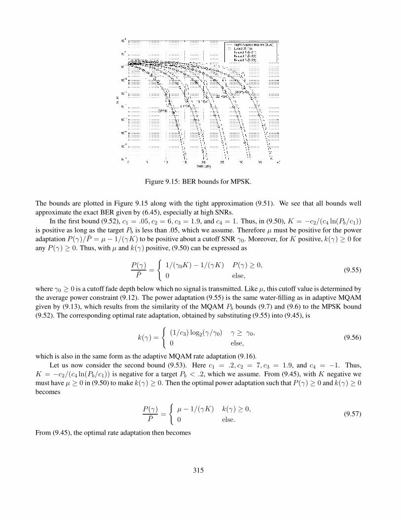
Figure 9.15: BER bounds for MPSK.

The bounds are plotted in Figure 9.15 along with the tight approximation (9.51). We see that all bounds well

approximate the exact BER given by (6.45), especially at high SNRs.

In the first bound (9.52), c1 = .05, c2 = 6, c3 = 1.9, and c4 = 1. Thus, in (9.50), K = −c2/(c4 ln(Pb/c1))

is positive as long as the target Pb is less than .05, which we assume. Therefore µ must be positive for the power

adaptation P (γ)/P = µ− 1/(γK) to be positive about a cutoff SNR γ0. Moreover, for K positive, k(γ) ≥ 0 for

any P (γ) ≥ 0. Thus, with µ and k(γ) positive, (9.50) can be expressed as

P (γ)

P=

1/(γ0K) − 1/(γK) P (γ) ≥ 0,

0 else,(9.55)

where γ0 ≥ 0 is a cutoff fade depth below which no signal is transmitted. Like µ, this cutoff value is determined by

the average power constraint (9.12). The power adaptation (9.55) is the same water-filling as in adaptive MQAM

given by (9.13), which results from the similarity of the MQAM Pb bounds (9.7) and (9.6) to the MPSK bound

(9.52). The corresponding optimal rate adaptation, obtained by substituting (9.55) into (9.45), is

k(γ) =

(1/c3) log2(γ/γ0) γ ≥ γ0,

0 else,(9.56)

which is also in the same form as the adaptive MQAM rate adaptation (9.16).

Let us now consider the second bound (9.53). Here c1 = .2, c2 = 7, c3 = 1.9, and c4 = −1. Thus,

K = −c2/(c4 ln(Pb/c1)) is negative for a target Pb < .2, which we assume. From (9.45), with K negative we

must have µ ≥ 0 in (9.50) to make k(γ) ≥ 0. Then the optimal power adaptation such that P (γ) ≥ 0 and k(γ) ≥ 0

becomes

P (γ)

P=

µ− 1/(γK) k(γ) ≥ 0,

0 else.(9.57)

From (9.45), the optimal rate adaptation then becomes

315

k(γ) =

(1/c3) log2(γ/γ0) γ ≥ γ0,

0 else,(9.58)

where γ0 = −1/(Kµ) is a cutoff fade depth below which the channel is not used. Note that for the first bound

(9.52) the positivity constraint on power (P (γ) ≥ 0) dictates the cutoff fade depth, whereas for this bound (9.53)

the positivity constraint on rate (k(γ) ≥ 0) determines the cutoff. We can rewrite (9.57) in terms of γ0 as

P (γ)

P=

−1/(γ0K)− 1/(γK) γ ≥ γ0,

0 else(9.59)

This power adaptation is an inverse water-filling: since K is negative, less power is used as the channel SNR

increases above the optimized cutoff fade depth γ0. As usual, the value of γ0 is obtained based on the average

power constraint (9.12).

Finally, for the third bound (9.54), c1 = .25, c2 = 8, c3 = 1.94, and c4 = 0. Thus,K = −c2/(c4 ln(Pb/c1)) =∞ for a target Pb < .25, which we assume. From (9.50), the optimal power adaptation becomes

P (γ)

P=

µ k(γ) ≥ 0, P (γ) ≥ 0,

0 else.(9.60)

This is on-off power transmission: power is either zero or a constant nonzero value. By (9.45), the optimal rate

adaptation k(γ) with this power adaptation is

k(γ) =

(1/c3) log2(γ/γ0) γ ≥ γ0,

0 else,(9.61)

where γ0 = − ln(Pb/c1)/c2µ is a cutoff fade depth below which the channel is not used. As for the previous

bound, it is the rate positivity constraint that determines the cutoff fade depth γ0. The optimal power adaptation as

a function of γ0 is

P (γ)

P=

K0/γ0 γ ≥ γ0,

0 else,(9.62)

where K0 = − ln(Pb/c1)/c2. The value of γ0 is determined from the average power constraint to satisfy

K0

γ0

∫ ∞

γ0

p(γ) dγ = 1. (9.63)

Thus, for all three Pb approximations in MPSK, the optimal adaptive rate schemes (9.56), (9.58), and (9.61)

have the same form whereas the optimal adaptive power schemes (9.55), (9.59), and (9.62) have different forms.

The optimal power adaptations (9.55), (9.59), and (9.62) are plotted in Figure 9.16 for Rayleigh fading with a target

BER of 10−3 and γ = 30 dB. This figure clearly shows the water-filling, inverse water-filling, and on–off behavior

of the different schemes. Note that the cutoff γ0 for all these schemes is roughly the same. We also see from this

figure that even though the power adaptation schemes are different at low SNRs, they are almost the same at high

SNRs. Specifically, we see that for γ < 10 dB, the optimal transmit power adaptations are dramatically different,

whereas for γ ≥ 10 dB they rapidly converge to the same constant value. From the cumulative distributionfunction

of γ , also shown in Figure 9.16, the probability that γ is less than 10 is 0.01. Thus, although the optimal power

adaptation corresponding to low SNRs is very different for the different techniques, this behavior has little impact

on spectral efficiency because the probability of being at those low SNRs is quite small.

316

Figure 9.16: Power adaptation for MPSK BER bounds (Rayleigh fading, Pb = 10−3, γ = 30 dB).

9.4.2 Discrete-Rate Adaptation

We now assume a given discrete set of constellations M = M0 = 0, . . . , MN−1, where M0 corresponds to

no data transmission. The rate corresponding to each of these constellations is kj = log2 Mj(j = 0, . . . , N − 1),

where k0 = 0. Each rate kj(j > 0) is assigned to a fading region of γ-values Rj = [γj−1, γj), j = 0, . . . , N − 1,

for γ − 1 = 0 and γN−1 = ∞. The boundaries γj(j = 0, . . . , N − 2) are optimized as part of the adaptive policy.

The channel is not used for γ < γ0. We again assume that Pb is approximated using the general formula (9.44).

Then the power adaptation that maintains the target BER above the cutoff γ0 is

P (γ)

P=h(kj)

γ, γj−1 ≤ γ ≤ γj, (9.64)

where

h(kj) = − ln(Pb/c1)

c2(2c3kj − c4). (9.65)

The region boundaries γ0, . . . , γN−2 that maximize spectral efficiency are found using the Lagrange equation

J(γ0, γ1, . . . , γN−2) =

N−1∑

j=1

kj

∫ γj

γj−1

p(γ) dγ+ λ

N−1∑

j=1

∫ γj

γj−1

h(kj)

γp(γ)dγ− 1

. (9.66)

The optimal rate region boundaries are obtained by solving the following equation for γj:

∂J

∂γj= 0, 0 ≤ j ≤ N − 2. (9.67)

This yields

γ0 =h(k1)

k1ρ (9.68)

317

and

γj =h(kj+1) − h(kj)

kj+1 − kjρ, 1 ≤ i ≤ N − 2, (9.69)

where ρ is determined by the average power constraint

N−1∑

j=1

∫ γj

γj−1

h(kj)

γp(γ) dγ = 1. (9.70)

9.4.3 Average BER Target

Suppose now that we relax our assumption that the Pb target must be met on every symbol transmission, requiring

instead that just the average Pb be below some target average Pb. In this case, in addition to adapting rate and

power, we can also adapt the instantaneous Pb(γ) subject to the average constraint Pb. This gives an additional

degree of freedom in adaptation that may lead to higher spectral efficiencies. The average probability of error for

adaptive modulation is given in (9.35).

When the bit rate k(γ) is continuously adapted this becomes

Pb =

∫∞0 Pb(γ)k(γ)p(γ) dγ∫∞0 k(γ)p(γ) dγ

, (9.71)

and when k(γ) takes values in a discrete set this becomes

Pb =

∑N−1j=1 kj

∫ γj

γj−1Pb(γ)p(γ) dγ

∑N−1j=1 kj

∫ γj

γj−1p(γ) dγ

. (9.72)

We now derive the optimal continuous rate, power, and BER adaptation to maximize spectral efficiency

E[k(γ)] subject to an average power constraint P and the average BER constraint (9.71). As with the instan-

taneous BER constraint, this is a standard constrained optimization problem, which we solve using the Lagrange

method. We now require two Lagrangians for the two constraints: average power and average BER. Specifically,

the Lagrange equation is

J(k(γ), P (γ)) =

∫ ∞

0k(γ)p(γ) dγ

+ λ1

[∫ ∞

0

Pb(γ)k(γ)p(γ) dγ− Pb

∫ ∞

0

k(γ)p(γ) dγ

]

+ λ2

[∫ ∞

0P (γ)p(γ) dγ− P

]

. (9.73)

The optimal rate and power adaptation must satisfy

∂J

∂k(γ)= 0 and

∂J

∂P (γ)= 0, (9.74)

with the additional constraint that k(γ) and P (γ) be nonnegative for all γ .

Assume that Pb is approximated using the general formula (9.44). Define

f(k(γ)) = 2c3k(γ) − c4. (9.75)

318

Then, using (9.44) in (9.73) and solving (9.74)), we obtain that the power and BER adaptation that maximize

spectral efficiency satisfy

P (γ)

P= max

f(k(γ))∂f(k(γ))∂k(γ)

λ2P (λ1Pb − 1)− f(k(γ))2

c2γ∂f(k(γ))∂k(γ) k(γ)

, 0

(9.76)

for nonnegative k(γ) and

Pb(γ) =λ2P f(k(γ))

λ1c2γk(γ). (9.77)

Moreover, from (9.44), (9.76), and (9.77) we get that the optimal rate adaptation k(γ) is either zero or the nonneg-

ative solution of

λ1Pb − 1∂f(k(γ))∂k(γ) λ2P

− f(k(γ))

c2γ∂f(k(γ))∂k(γ) k(γ)

=1

γc2ln

[λ1c1c2γk(γ)

λ2P f(k(γ))

]

. (9.78)

The values of k(γ) and the Lagrangians λ1 and λ2 must be found through a numerical search whereby the average

power constraint P and average BER constraint (9.71) are satisfied.

In the discrete-rate case, the rate is varied within a fixed set k0, . . . , kN−1, where k0 corresponds to no data

transmission. We must determine region boundaries γ0, . . . , γN−2 such that we assign rate kj to the rate region

[γj−1, γj), where γ−1 = 0 and γN−1 = ∞. Under this rate assignment we wish to maximize spectral efficiency

through optimal rate, power, and BER adaptation subject to an average power and BER constraint. Since the set of

possible rates and their corresponding rate region assignments are fixed, the optimal rate adaptation corresponds to

finding the optimal rate region boundaries γj, j = 0, . . . , N − 2. The Lagrangian for this constrained optimization

problem is

J(γ0, γ1, . . . , γN−2, P (γ)) =

N−1∑

j=1

kj

∫ γj

γj−1

p(γ) dγ

+ λ1

N−1∑

j=1

kj

∫ γj

γj−1

(Pb(γ)− Pb)p(γ) dγ

+ λ2

[∫ ∞

γ0

P (γ)p(γ) dγ− P

]

. (9.79)

The optimal power adaptation is obtained by solving the following equation for P (γ) :

∂J

∂P (γ)= 0. (9.80)

Similarly, the optimal rate region boundaries are obtained by solving the following set of equations for γj:

∂J

∂γj= 0, 0 ≤ j ≤ N − 2. (9.81)

From (9.80) we see that the optimal power and BER adaptation must satisfy

∂Pb(γ)

∂P (γ)=

−λ2

kjλ1, γj−1 ≤ γ ≤ γj. (9.82)

319

Substituting (9.44) into (9.82), we get that

Pb(γ) = λf(kj)

γkj, γj−1 ≤ γ ≤ γj, (9.83)

where λ = P λ2/c2λ1. This form of BER adaptation is similar to the water-filling power adaptation: the instanta-

neous BER decreases as the channel quality improves. Now, setting the BER in (9.44) equal to (9.83) and solving

for P (γ) yields

P (γ) = Pj(γ), γj−1 ≤ γ ≤ γj, (9.84)

where

Pj(γ)

P= ln

[λf(kj)

c1γkj

]f(kj)

−γc2, 1 ≤ j ≤ N − 1, (9.85)

and P (γ) = 0 for γ < γ0. We see by (9.85) that P (γ) is discontinuous at the γj boundaries.

Let us now consider the optimal region boundaries γ0, . . . , γN−2. Solving (9.81) for Pb(γj) yields

Pb(γj) = Pb −1

λ1− λ2

λ1

Pj+1(γj) − Pj(γj)

kj+1 − kj, 0 ≤ j ≤ N − 2, (9.86)

where k0 = 0 and P0(γ) = 0. Unfortunately, this set of equations can be difficult to solve for the optimal boundary

points γj. However, if we assume that P (γ) is continuous at each boundary, then (9.86) becomes

Pb(γj) = Pb −1

λ1, 0 ≤ j ≤ N − 2, (9.87)

Figure 9.17: Spectral efficiency for different adaptation constraints.

for the Lagrangian λ1. Under this assumption we can solve for the suboptimal rate region boundaries as

γj−1 =f(kj)

kjρ, 1 ≤ j ≤ N − 1, (9.88)

320

for some constant ρ. The constants λ1 and ρ are found numerically such that the average power constraint

N−1∑

j=1

∫ γj

γj−1

Pj(γ)

Pp(γ) dγ = 1 (9.89)

and the BER constraint (9.72) are satisfied. Note that the region boundaries (9.88) are suboptimal because P (γ) is

not necessarily continuous at the boundary regions, so these boundaries yield a suboptimal spectral efficiency.

In Figure 9.17 we plot average spectral efficiency for adaptive MQAM under both continuous and discrete

rate adaptation, showing both average and instantaneous BER targets for a Rayleigh fading channel. The adaptive

policies are based on the BER approximation (9.7) with a target BER of either 10−3 or 10−7. For the discrete-

rate cases we assume that six different MQAM signal constellations are available (seven fading regions), given

by M = 0, 4, 16, 64, 256, 1024, 4096. We see in this figure that the spectral efficiencies of all four policies

under the same instantaneous or average BER target are very close to each other. For discrete-rate adaptation,

the spectral efficiency with an instantaneous BER target is slightly higher than with an average BER target even

though the latter case is more constrained: that is because the efficiency with an average BER target is calculated

using suboptimal rate region boundaries, which leads to a slight efficiency degradation.

9.5 Adaptive Techniques in Combined Fast and Slow Fading

In this section we examine adaptive techniques for composite fading channels consisting of both fast and slow

fading (shadowing). We assume the fast fading changes too quickly to accurately measure and feed back to the

transmitter, so the transmitter adapts only to the slow fading. The instantaneous SNR γ has distribution p(γ|γ),

where γ is a short-term average over the fast fading. This short-term average varies slowly because of shadowing

and has a distribution p(γ), where the average SNR relative to this distribution is=γ . The transmitter adapts only

to the slow fading γ, hence its rate k(γ) and power P (γ) are functions of γ. The power adaptation is subject to a

long-term average power constraint over both the fast and slow fading:

∫ ∞

0P (γ)p(γ) dγ = P . (9.90)

As before, we approximate the instantaneous probability of bit error by the general form (9.44). Since the

power and rate are functions of γ, the conditional BER, conditioned on γ, is

Pb(γ | γ) ≈ c1 exp

[−c2γP (γ)/P

2c3k(γ)3 − c4

]

. (9.91)

Since the transmitter does not adapt to the fast fading γ , we cannot require a given instantaneous BER. However,

since the transmitter adapts to the shadowing, we can require a target average probability of bit error averaged over

the fast fading for a fixed value of the shadowing. This short-term average for a given γ is obtained by averaging

Pb(γ | γ) over the fast fading distribution p(γ | γ):

Pb(γ) =

∫ ∞

0Pb(γ | γ)p(γ | γ) dγ. (9.92)

Using (9.91) in (9.92) and assuming Rayleigh fading for the fast fading, this becomes

Pb(γ) =1

γ

∫ ∞

0c1 exp

[−c2γP (γ)/P

2c3k(γ) − c4− γ

γ

]

dγ =c1

1.5γP (γ)/P

2c3k(γ)−c4+ 1

. (9.93)

321

For example, with MQAM modulation with the tight BER bound (9.7), equation (9.93) becomes

Pb(γ) =.2

c2γP (γ)/P

2k(γ)−1+ 1

. (9.94)

We can now invert (9.93) to obtain the adaptive rate k(γ) as a function of the target average BER Pb and the

power adaptation P (γ):

k(γ) =1

c3log2

(

c4 +KγP (γ)

P

)

, (9.95)

where

K =c2

c1/Pb − 1(9.96)

depends only on the target average BER and decreases as this target decreases. We maximize spectral efficiency

by maximizing

E[k(γ)] =

∫ ∞

0

1

c3log2

(

c4 +KγP (γ)

P

)

p(γ) dγ (9.97)

subject to the average power constraint (9.90).

Let us assume that c4 > 0. Then this maximization and the power constraint are in the exact same form as

(9.11) with the fading γ replaced by the slow fading γ. Thus, the optimal power adaptation also has the same

water-filling form as (9.13) and is given by

P (γ)

P=

1/γ0 − c4/γK γ ≥ c4γ0/K,

0 γ < c4γ0/K,(9.98)

where the channel is not used when γ < c4γ0/K. The value of γ0 is determined by the average power constraint.

Substituting (9.98) into (9.95) yields the rate adaptation

k(γ) =1

c3log2

(Kγ

γ0

)

, (9.99)

and the corresponding average spectral efficiency is given by

R

B=

∫ ∞

c4γ0/Klog2(

Kγ

γ0)p(γ) dγ. (9.100)

Thus, we see that in a composite fading channel where rate and power are adapted only to the slow fading and for

c4 > 0 in (9.44), water-filling relative to the slow fading is the optimal power adaptation for maximizing spectral

efficiency subject to an average BER constraint.

Our derivation has assumed that the fast fading is Rayleigh; however, it can be shown [34] that, with c4 > 0

in (9.44), the optimal power and rate adaptation for any fast fading distribution have the same form. Since we have

assumed c4 > 0 in (9.44), the positivity constraint on power dictates the cutoff value below which the channel is

not used. As we saw in Section 9.4.1, when c4 ≤ 0 the positivity constraint on rate dictates this cutoff, and the

optimal power adaptation becomes inverse water-filling for c4 < 0 and on–off power adaptation for c4 = 0.

322

Chapter 9 Problems

1. Find the average SNR required to achieve an average BER of Pb = 10−3 for 8-PSK modulation in Rayleigh

fading. What is the spectral efficiency of this scheme, assuming a symbol time of Ts = 1/B?

2. Consider a truncated channel inversion variable-power technique for Rayleigh fading with average SNR

of 20 dB. What value of σ corresponds to an outage probability of .1? Find the maximum size MQAM

constellation that can be transmitted under this policy so that, in non-outage, Pb ≈ 10−3.

3. Find the power adaptation for QPSK modulation that maintains a fixed Pb = 10−3 in non-outage for a

Rayleigh fading channel with γ = 20 dB. What is the outage probability of this system?

4. Consider a variable-rate MQAM modulation scheme with just two constellations, M = 4 and M = 16.

Assume a target Pb of approximately 10−3. If the target cannot be met then no data is transmitted.

(a) Using the BER bound (9.7), find the range of γ-values associated with the three possible transmission

schemes (no transmission, 4-QAM, and 16-QAM) where the BER target is met. What is the cutoff γ0

below which the channel is not used?

(b) Assuming Rayleigh fading with γ = 20 dB, find the average data rate of the variable-rate scheme.

(c) Suppose that, instead of suspending transmission below γ0, BPSK is transmitted for 0 ≤ γ ≤ γ0.

Using the loose bound (9.6), find the average probability of error for this BPSK transmission.

5. Consider an adaptive modulation and coding scheme consisting of three modulations: BPSK, QPSK, and 8-

PSK, along with three block codes of rate 1/2, 1/3, and 1/4. Assume that the first code provides roughly 3 dB

of coding gain for each modulation type, the second code 4 dB, and the third code 5 dB. For each possible

value of SNR 0 ≤ γ ≤ ∞, find the combined coding and modulation with the maximum data rate for a target

BER of 10−3 (you can use any reasonable approximation for modulation BER in this calculation, with SNR

increased by the coding gain). Find the average data rate of the system for a Rayleigh fading channel with

average SNR of 20 dB, assuming no transmission if the target BER cannot be met with any combination of

modulation and coding.

6. Show that the spectral efficiency given by (9.11) with power constraint (9.12) is maximized by the water-

filling power adaptation (9.13). Do this by setting up the Lagrangian equation, differentiating it, and solving

for the maximizing power adaptation. Also show that, with this power adaptation, the rate adaptation is as

given in (9.16).

7. In this problem we compare the spectral efficiency of nonadaptive techniques with that of adaptive tech-

niques.

(a) Using the tight BER bound for MQAM modulation given by (9.7), find an expression for the average

probability of bit error in Rayleigh fading as a function of M and γ·(b) Based on the expression found in part (a), find the maximum constellation size that can be transmitted

over a Rayleigh fading channel with a target average BER of 10−3, assuming γ = 20 dB.

(c) Compare the spectral efficiency of part (b) with that of adaptive modulation shown in Figure 9.3 for

the same parameters. What is the spectral efficiency difference between the adaptive and nonadaptive

techniques?

8. Consider a Rayleigh fading channel with an average SNR of 20 dB. Assume a target BER of 10−4.

323

(a) Find the optimal rate and power adaptation for variable-rate variable-power MQAM as well as the

cutoff value γ0/K below which the channel is not used.

(b) Find the average spectral efficiency for the adaptive scheme derived in part (a).

(c) Compare your answer in part (b) to the spectral efficiency of truncated channel inversion, where γ0 is

chosen to maximize this efficiency.

9. Consider a discrete time-varying AWGN channel with four channel states. Assuming a fixed transmit power

P , the received SNR associated with each channel state is γ1 = 5 dB, γ2 = 10 dB, γ3 = 15 dB, and

γ4 = 20 dB, respectively. The probabilities associated with the channel states are p(γ1) = .4 and p(γ2) =p(γ3) = p(γ4) = .2. Assume a target BER of 10−3.

(a) Find the optimal power and rate adaptation for continous-rate adaptive MQAM on this channel.

(b) Find the average spectral efficiency with this optimal adaptation.

(c) Find the truncated channel inversion power control policy for this channel and the maximum data rate

that can be supported with this policy.

10. Consider a Rayleigh fading channel with an average received SNR of 20 dB and a required BER of 10−3.

Find the spectral efficiency of this channel using truncated channel inversion, assuming the constellation is

restricted to size 0, 2, 4, 16, 64, or 256.

11. Consider a Rayleigh fading channel with an average received SNR of 20 dB, a Doppler frequency of 80 Hz,

and a required BER of 10−3.

(a) Suppose you use adaptive MQAM modulation on this channel with constellations restricted to size

0, 2, 4, 16, and 64. Using γ∗K = .1, find the fading regions Rj associated with each of these constella-

tions. Also find the average spectral efficiency of this restricted adaptive modulation scheme and the

average time spent in each region Rj. If the symbol rate is Ts = B−1, over approximately how many

symbols is each constellation transmitted before a change in constellation size is needed?

(b) Find the exact BER of your adaptive scheme using (9.33). How does it differ from the target BER?

12. Consider a Rayleigh fading channel with an average received SNR of 20 dB, a signal bandwidth of 30 kHz,

a Doppler frequency of 80 Hz, and a required BER of 10−3.

(a) Assume the SNR estimate at the transmitter γ has the same distribution as the true channel SNR γ ,

so p(γ) = p(γ). For the optimal variable-rate variable-power MQAM scheme with no restrictions

on rate or power, suppose that the transmit power and rate is adapted relative to γ instead of γ . Will

the average transmitted data rate and average transmit power be larger, smaller, or the same as under

perfect channel estimates (γ = γ), and why? If over a given symbol time γ > γ , will the probability

of error associated with that symbol be larger or smaller than the target value and why?

(b) Suppose the estimation error ε = γ/γ in a variable-rate variable-power MQAM system with a target

BER of 10−3 is uniformly distributed between .5 and 1.5. Find the resulting average probability of bit

error for this system.

(c) Find an expression for the average probability of error in a variable-rate variable-power MQAM system

in which the SNR estimate γ available at the transmitter is both a delayed and noisy estimate of γ :γ(t) = γ(t− τ) + γε(t). What joint distribution is needed to compute this average?

324

13. In this problem, we investigate the effect of channel estimation errors and delays in system performance.

Consider a Rayleigh fading channel with mean power 1, uniform scattering and doppler of fD Hz. The

channel output y[t] is thus given by y[t] = h[t]x[t] + ν[t], where h[t] is the fading realization, x[t] is

the transmitted symbol and ν[t] is the additive noise with power 1. Symbol time Tb s. We use adaptive

modulation with no transmission, BPSK or 4-QAM; and the receiver feeds back the receiver output to the

transmitter at the end of every symbol time. The transmitter uses y[t] and x[t] to estimate h[t+ 1] and uses

this estimate to choose the constellation scheme to either have an outage or maintain a constant BER Pb for

time t+ 1. The receiver knows the instantaneous channel state information h[t] and uses that for decoding.

(a) Find the two threshold received SNRs γ0, γ1(γ0 < γ1) at which the transmitter switches modulations.

Use the exact AWGN error probability expressions wherever possible.

(b) Find out the MMSE (minimum mean squared error) estimate of h[t] given y[t] and x[t]. This is the

effect of the channel estimation error.

(c) Find out the MMSE estimate of h[t + 1] given the estimate of h[t]. This is the effect of delay in

feedback.

(d) (6 pts) Assuming that the transmitter uses the MMSE estimate h[t+ 1] to choose the transmit modula-

tion for time t+1, and the actual realization is h[t+1] known to the receiver, write down an expression

for the bit error rate Pb(|h[t+ 1]|, |h[t+ 1]|). Further, write the expression for the BER estimated over

the joint distribution of y[t] and h[t+ 1].

Note: In general the optimal transmitter would want to use past values of the feedback to refine its estimate

of h[t+ 1] but in this problem we do not consider that possibility.

14. Consider an adaptive trellis-coded MQAM system with a coding gain of 3 dB. Assume a Rayleigh fading

channel with an average received SNR of 20 dB. Find the optimal adaptive power and rate policy for this

system and the corresponding average spectral efficiency. Assume a target BER of 10−3.

15. In Chapter 6, a bound on Pb for nonrectangular MQAM was given as

Pb ≈4

log2MQ

(√

3γ

(M − 1)

)

.

Find values for c1, c2, c3, and c4 for the general BER form (9.44) to approximate this bound with M = 8.

Any curve approximation technique is acceptable. Plot both BER formulas for 0 ≤ γ ≤ 30 dB.

16. Show that the average spectral efficiency E[k(γ)] for k(γ) given by (9.45) with power constraint P is maxi-

mized by the power adaptation (9.48).

17. In this problem we investigate the optimal adaptive modulation for MPSK modulation based on the three

BER bounds (9.52), (9.53), and (9.54). We assume a Rayleigh fading channel (so that γ is exponentially

distributed with γ = 30 dB) and a target BER of Pb = 10−7.

(a) The cutoff fade depth γ0 must satisfy

∫ ∞

γ0/K

(1

γ0− 1

γK

)

p(γ) dγ ≤ 1

for K given by (9.49). Find the cutoff value γ0 corresponding to the power adaptation for each of the

three bounds.

325

(b) Plot P (γ)/P and k(γ) as a function of γ for Bounds 1, 2, and 3 for γ ranging from 0 dB to 30 dB.

Also state whether the cutoff value below which the channel is not used is based on the power or rate

positivity constraint.

(c) How does the power adaptation associated with the different bounds differ at low SNRs? What about

at high SNRs?

18. Show that, under discrete rate adaptation for general M -ary modulation, the power adaptation that maintains

a target instantaneous BER is given by (9.64). Also show that the region boundaries that maximize spectral

efficiency–obtained using the Lagrangin given in (9.66) – are given by (9.68) and (9.69).

19. Show that, for general M -ary modulation with an average target BER, the Lagrangian (9.80) implies that

the optimal power and BER adaptation must satisfy (9.82). Then show how (9.82) leads to BER adaptation

given by (9.83), which in turn leads to the power adaptation given by (9.84) and (9.85). Finally, use (9.81)

to show that the optimal rate region boundaries must satisfy (9.86).

20. Consider adaptive MPSK where the constellation is restricted to either no transmission or M = 2, 4, 8, 16.

Assume the probability of error is approximated using (9.52). Find and plot the optimal discrete-rate

continuous-power adaptation for 0 ≤ γ ≤ 30 dB assuming a Rayleigh fading channel with γ = 20 dB

and a target Pb of 10−4. What is the resulting average spectral efficiency?

21. We assume the same discrete-rate adaptive MPSK as in the previous problem, except now there is an aver-

age target Pb of 10−4 instead of an instantaneous target. Find the optimal discrete-rate continuous-power

adaptation for a Rayleigh fading channel with γ = 20 dB and the corresponding average spectral efficiency.

22. Consider a composite fading channel with fast Rayleigh fading and slow log-normal shadowing with an

average dB SNR µψdB= 20 dB (averaged over both fast and slow fading) and σψdB

= 8 dB. Assume an

adaptive MPSK modulation that adapts only to the shadowing, with a target average BER of 10−3. Using

the BER approximation (9.52), find the optimal power and rate adaptation policies as a function of the slow

fading γ that maximize average spectral efficiency while meeting the average BER target. Also determine

the average spectral efficiency that results from these policies.

23. In Section 9.5 we determined the optimal adaptive rate and power policies to maximize average spectral

efficiency while meeting a target average BER in combined Rayleigh fading and shadowing. The derivation

assumed the general bound (9.44) with c4 > 0. For the same composite channel, find the optimal adaptive

rate and power policies to maximize average spectral efficiency while meeting a target average BER assum-

ing c4 < 0. Hint: The derivation is similar to the case of continuous-rate adaptation using the second MPSK

bound and results in the same channel inversion power control.

24. As in the previous problem, we again examine the adaptative rate and power policies to maximize average

spectral efficiency while meeting a target average BER in combined Rayleigh fading and shadowing. In

this problem we assume the general bound (9.44) with c4 = 0. For the composite channel, find the optimal

adaptive rate and power policies to maximize average spectral efficiency while meeting a target average BER

assuming c4 = 0. Hint: the derivation is similar to that of Section 9.4.1 for the third MPSK bound and results

in the same on-off power control.

326

Bibliography

[1] J. F. Hayes, “Adaptive feedback communications,” IEEE Trans. Commun. Tech., pp. 29–34, February 1968.

[2] J. K. Cavers, “Variable-rate transmission for Rayleigh fading channels,” IEEE Trans. Commun., pp. 15–22,

February 1972.

[3] S. Otsuki, S. Sampei, and N. Morinaga, “Square-QAM adaptive modulation/TDMA/TDD systems using

modulation level estimation with Walsh function,” Elec. Lett., pp. 169–71, February 1995.

[4] W. T. Webb and R. Steele, “Variable rate QAM for mobile radio,” IEEE Trans. Commun., pp. 2223–30, July

1995.

[5] Y. Kamio, S. Sampei, H. Sasaoka, and N. Morinaga, “Performance of modulation-level-controlled adaptive-

modulation under limited transmission delay time for land mobile communications,” Proc. IEEE Veh. Tech.

Conf., pp. 221–5, July 1995.

[6] B. Vucetic, “An adaptive coding scheme for time-varying channels,” IEEE Trans. Commun., pp. 653–63, May

1991.

[7] M. Rice and S. B. Wicker, “Adaptive error control for slowly varying channels,” IEEE Trans. Commun., pp.

917–26, February–April 1994.

[8] S. M. Alamouti and S. Kallel, “Adaptive trellis-coded multiple-phased-shift keying for Rayleigh fading chan-

nels,” IEEE Trans. Commun., pp. 2305–14, June 1994.

[9] T. Ue, S. Sampei, and N. Morinaga, “Symbol rate and modulation level controlled adaptive modula-

tion/TDMA/TDD for personal communication systems,” Proc. IEEE Veh. Tech. Conf., pp. 306–10, July 1995.

[10] H. Matsuoka, and Y. Kamio, “Symbol rate and modulation level controlled adaptive modulation/TDMA/TDD

for personal communication systems,” Proc. IEEE Veh. Tech. Conf., pp. 487–91, April 1996.

[11] S. Sampei, N. Morinaga, and Y. Kamio, “Adaptive modulation/TDMA with a BDDFE for 2 Mbit/s multi-

media wireless communication systems,” Proc. IEEE Veh. Tech. Conf., pp. 311–15, July 1995.

[12] S. T. Chung and A. J. Goldsmith, “Degrees of freedom in adaptive modulation: A unified view,” IEEE Trans.

Commun., pp. 1561–71, September 2001.

[13] A. Furuskar, S. Mazur, F. Muller, and H. Olofsson, “EDGE: Enhanced data rates for GSM and TDMA/136

evolution,” IEEE Wireless Commun. Mag., pp. 56–66, June 1999.

[14] A. Ghosh, L. Jalloul, B. Love, M. Cudak, and B. Classon, “Air-interface for 1XTREME/lxEV-DV,” Proc.

IEEE Veh. Tech. Conf., pp. 2474–8, May 2001.

327

[15] S. Nanda, K. Balachandran, and S. Kumar, “Adaptation techniques in wireless packet data services,” IEEE

Commun. Mag., pp. 54–64, January 2000.

[16] H. Sari, “Trends and challenges in broadband wireless access,” Proc. Sympos. Commun. Veh. Tech., pp. 210–

14, October 2000.

[17] K. M. Kamath and D. L. Goeckel, “Adaptive-modulation schemes for minimum outage probability in wireless

systems,” IEEE Trans. Commun., pp. 1632–5, October 2004.

[18] J. Hagenauer, “Rate-compatible punctured convolutional codes (RCPC codes) and their applications,” IEEE

Trans. Commun., pp. 389–400, April 1988.

[19] G. J. Foschini and J. Salz, “Digital communications over fading radio channels,” Bell System Tech. J., pp.

429–56, February 1983.

[20] G. D. Forney, Jr., R. G. Gallager, G. R. Lang, F. M. Longstaff, and S. U. Quereshi, “Efficient modulation for

band-limited channels,” IEEE J. Sel. Areas Commun., pp. 632–47, September 1984.

[21] J. G. Proakis, Digital Communications, 4th ed., McGraw-Hill, New York, 2001.

[22] M. Filip and E. Vilar, “Implementation of adaptive modulation as a fade countermeasure,” Internat. J. Sat.

Commun., pp. 181–91, 1994.

[23] C. C. Tan and N. C. Beaulieu, “On first-order Markov modeling for the Rayleigh fading channel,” IEEE

Trans. Commun., pp. 2032–40, December 2000.

[24] L. Kleinrock, Queueing Systems, vol. I: Theory, Wiley, New York, 1975.

[25] W. C. Jakes, Jr., Microwave Mobile Communications, Wiley, New York, 1974.

[26] H. S. Wang and P.-C. Chang, “On verifying the first-order Markov assumption for a Rayleigh fading channel

model,” IEEE Trans.Veh.Tech., pp. 353–7, May 1996.

[27] X. Tang, M.-S. Alouini, and A. Goldsmith, “ Effect of channel estimation error on M-QAM BER performance

in Rayleigh fading,” IEEE Trans. Commun., pp. 1856–64, December 1999.

[28] J. K. Cavers, “An analysis of pilot symbol assisted modulation for Rayleigh fading channels,” IEEE

Trans.Veh.Tech., pp. 686–93, November 1991.

[29] A. J. Goldsmith and L. J. Greenstein, “Effect of average power estimation error on adaptive MQAM modu-

lation,” Proc. IEEE Internat. Conf. Commun., pp. 1105–9, June 1997.

[30] D. L. Goeckel, “Adaptive coding for time-varying channels using outdated fading estimates,” IEEE Trans.

Commun., pp. 844–55, June 1999.

[31] A. Duel-Hallen, S. Hu, and H. Hallen, “Long-range prediction of fading signals,” IEEE Signal Proc. Mag.,

pp. 62–75, May 2000.

[32] M.-S. Alouini and A. J. Goldsmith, “Adaptive modulation over Nakagami fading channels,” Kluwer J. Wire-

less Pers. Commun., pp. 119–43, May 2000.

[33] S.-G. Chua and A. J. Goldsmith, “Adaptive coded modulation for fading channels,” IEEE Trans. Commun.,

pp. 595–602, May 1998.

328

[34] S. Vishwanath, S. A. Jafar, and A. J. Goldsmith, “Adaptive resource allocation in composite fading environ-

ments,” Proc. IEEE Globecom Conf., pp. 1312–16, November 2001.

329

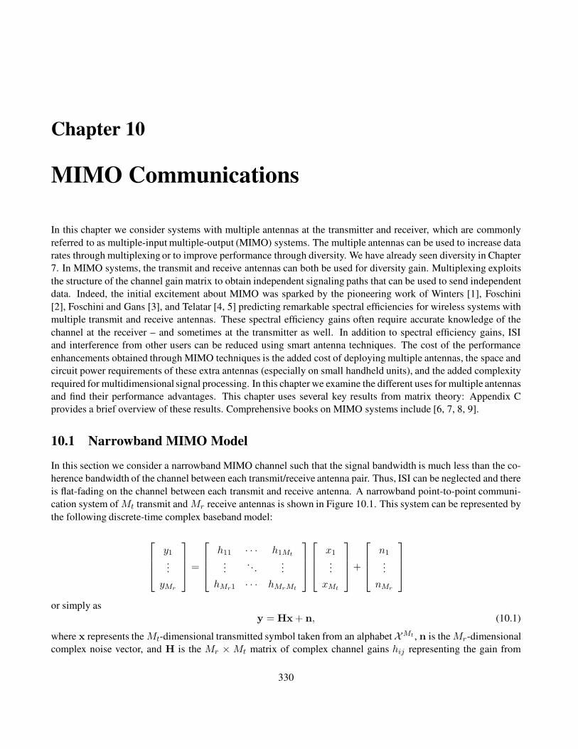
Chapter 10

MIMO Communications

In this chapter we consider systems with multiple antennas at the transmitter and receiver, which are commonly

referred to as multiple-input multiple-output (MIMO) systems. The multiple antennas can be used to increase data

rates through multiplexing or to improve performance through diversity. We have already seen diversity in Chapter

7. In MIMO systems, the transmit and receive antennas can both be used for diversity gain. Multiplexing exploits

the structure of the channel gain matrix to obtain independent signaling paths that can be used to send independent

data. Indeed, the initial excitement about MIMO was sparked by the pioneering work of Winters [1], Foschini

[2], Foschini and Gans [3], and Telatar [4, 5] predicting remarkable spectral efficiencies for wireless systems with

multiple transmit and receive antennas. These spectral efficiency gains often require accurate knowledge of the

channel at the receiver – and sometimes at the transmitter as well. In addition to spectral efficiency gains, ISI

and interference from other users can be reduced using smart antenna techniques. The cost of the performance

enhancements obtained through MIMO techniques is the added cost of deploying multiple antennas, the space and

circuit power requirements of these extra antennas (especially on small handheld units), and the added complexity

required for multidimensional signal processing. In this chapter we examine the different uses for multiple antennas

and find their performance advantages. This chapter uses several key results from matrix theory: Appendix C

provides a brief overview of these results. Comprehensive books on MIMO systems include [6, 7, 8, 9].

10.1 Narrowband MIMO Model

In this section we consider a narrowband MIMO channel such that the signal bandwidth is much less than the co-

herence bandwidth of the channel between each transmit/receive antenna pair. Thus, ISI can be neglected and there

is flat-fading on the channel between each transmit and receive antenna. A narrowband point-to-point communi-

cation system of Mt transmit and Mr receive antennas is shown in Figure 10.1. This system can be represented by

the following discrete-time complex baseband model:

y1...

yMr

=

h11 · · · h1Mt

.... . .

...

hMr1 · · · hMrMt

x1

...

xMt

+

n1

...

nMr

or simply as

y = Hx + n, (10.1)

where x represents the Mt-dimensional transmitted symbol taken from an alphabet XMt , n is theMr-dimensional

complex noise vector, and H is the Mr ×Mt matrix of complex channel gains hij representing the gain from

330

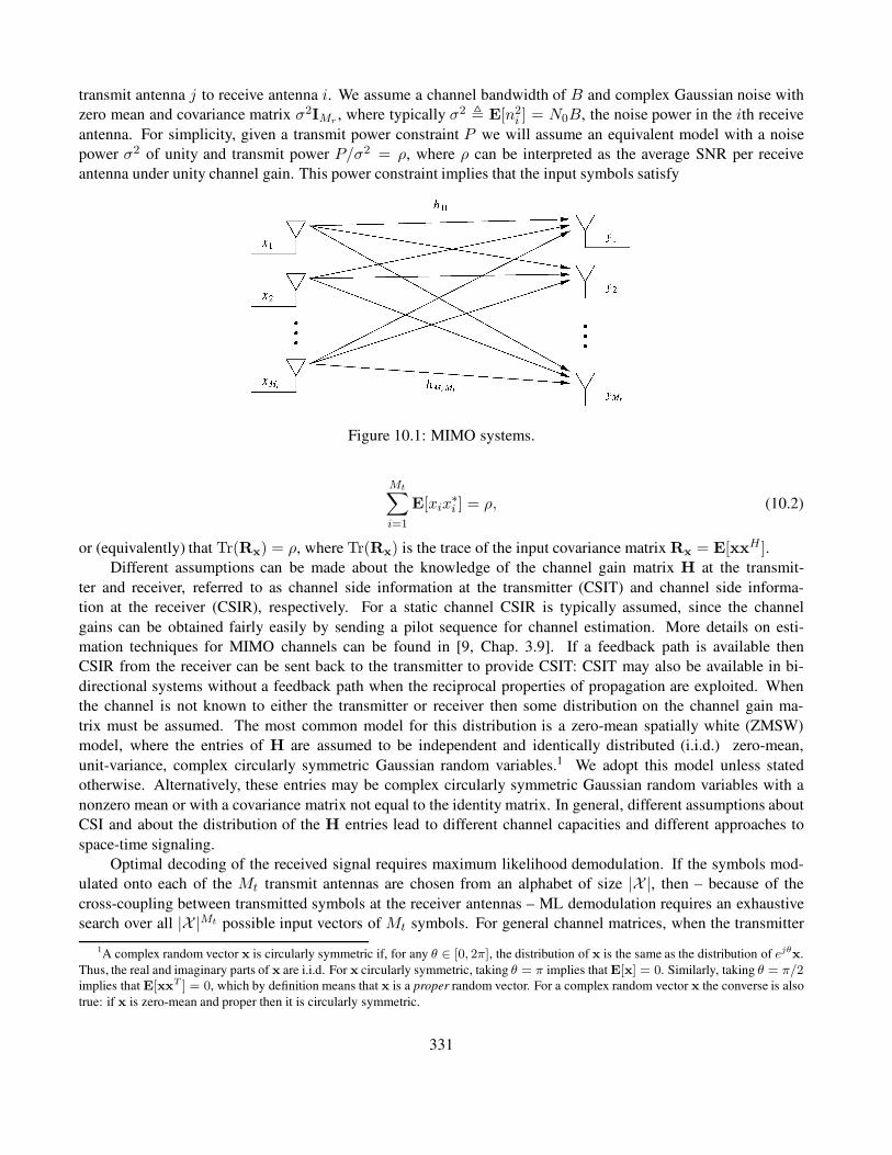
transmit antenna j to receive antenna i. We assume a channel bandwidth of B and complex Gaussian noise with

zero mean and covariance matrix σ2IMr , where typically σ2 , E[n2i ] = N0B, the noise power in the ith receive

antenna. For simplicity, given a transmit power constraint P we will assume an equivalent model with a noise

power σ2 of unity and transmit power P/σ2 = ρ, where ρ can be interpreted as the average SNR per receive

antenna under unity channel gain. This power constraint implies that the input symbols satisfy

Figure 10.1: MIMO systems.

Mt∑

i=1

E[xix∗i ] = ρ, (10.2)

or (equivalently) that Tr(Rx) = ρ, where Tr(Rx) is the trace of the input covariance matrix Rx = E[xxH ].Different assumptions can be made about the knowledge of the channel gain matrix H at the transmit-

ter and receiver, referred to as channel side information at the transmitter (CSIT) and channel side informa-

tion at the receiver (CSIR), respectively. For a static channel CSIR is typically assumed, since the channel

gains can be obtained fairly easily by sending a pilot sequence for channel estimation. More details on esti-

mation techniques for MIMO channels can be found in [9, Chap. 3.9]. If a feedback path is available then

CSIR from the receiver can be sent back to the transmitter to provide CSIT: CSIT may also be available in bi-

directional systems without a feedback path when the reciprocal properties of propagation are exploited. When

the channel is not known to either the transmitter or receiver then some distribution on the channel gain ma-

trix must be assumed. The most common model for this distribution is a zero-mean spatially white (ZMSW)

model, where the entries of H are assumed to be independent and identically distributed (i.i.d.) zero-mean,

unit-variance, complex circularly symmetric Gaussian random variables.1 We adopt this model unless stated

otherwise. Alternatively, these entries may be complex circularly symmetric Gaussian random variables with a

nonzero mean or with a covariance matrix not equal to the identity matrix. In general, different assumptions about

CSI and about the distribution of the H entries lead to different channel capacities and different approaches to

space-time signaling.

Optimal decoding of the received signal requires maximum likelihood demodulation. If the symbols mod-

ulated onto each of the Mt transmit antennas are chosen from an alphabet of size |X |, then – because of the

cross-coupling between transmitted symbols at the receiver antennas – ML demodulation requires an exhaustive

search over all |X |Mt possible input vectors of Mt symbols. For general channel matrices, when the transmitter

1A complex random vector x is circularly symmetric if, for any θ ∈ [0, 2π], the distribution of x is the same as the distribution of ejθx.

Thus, the real and imaginary parts of x are i.i.d. For x circularly symmetric, taking θ = π implies that E[x] = 0. Similarly, taking θ = π/2implies that E[xx

T ] = 0, which by definition means that x is a proper random vector. For a complex random vector x the converse is also

true: if x is zero-mean and proper then it is circularly symmetric.

331

does not know H, the complexity cannot be reduced further. This decoding complexity is typically prohibitive for

even a small number of transmit antennas. However, decoding complexity is significantly reduced if the channel is

known to the transmitter, as shown in the next section.

10.2 Parallel Decomposition of the MIMO Channel

We have seen in Chapter 7 that multiple antennas at the transmitter or receiver can be used for diversity gain.

When both the transmitter and receiver have multiple antennas, there is another mechanism for performance gain

called multiplexing gain. The multiplexing gain of a MIMO system results from the fact that a MIMO channel can

be decomposed into a number R of parallel independent channels. By multiplexing independent data onto these

independent channels, we get an R-fold increase in data rate in comparison to a system with just one antenna at

the transmitter and receiver. This increased data rate is called the multiplexing gain. In this section we describe

how to obtain independent channels from a MIMO system.

Consider a MIMO channel with Mr ×Mt channel gain matrix H that is known to both the transmitter and

the receiver. Let RH denote the rank of H. From Appendix C, for any matrix H we can obtain its singular value

decomposition (SVD) as

H = UΣVH , (10.3)

where the Mr ×Mr matrix U and the Mt ×Mt matrix V are unitary matrices2 and where Σ is an Mr ×Mt

diagonal matrix of singular values σi of H. These singular values have the property that σi =√λi for λi the

ith largest eigenvalue of HHH , and RH of these singular values are nonzero. Because RH, the rank of matrix

H, cannot exceed the number of columns or rows of H, it follows that RH ≤ min(Mt,Mr). If H is full rank,

which is referred to as a rich scattering environment, then RH = min(Mt,Mr). Other environments may lead to

a low-rank H: a channel with high correlation among the gains in H may have rank 1.

The parallel decomposition of the channel is obtained by defining a transformation on the channel input and

output x and y via transmitter and receiver shaping. In transmitter shaping the input x to the antennas is generated

by a linear transformation on input vector x as x = Vx. Receiver shaping performs a similar operation at the

receiver by multiplying the channel output y by UH , as shown in Figure 10.2.

The transmitter and receiver shaping transform the MIMO channel intoRH parallel single-input single-output

(SISO) channels with input x and output y, since from the SVD we have that

Figure 10.2: Transmitter and receiver shaping.

y = UH(Hx + n)

= UH(UΣVHx + n)

= UH(UΣVHVx + n)

= UHUΣVHVx + UHn

= Σx + n,

2U and V unitary imply that UH

U = IMrand V

HV = IMt

.

332

Figure 10.3: Parallel decomposition of the MIMO channel.

where n = UHn and where Σ is the matrix of singular values of H with σi on the ith diagonal and zeros

everywhere else. Note that multiplication by a unitary matrix does not change the distribution of the noise – that

is, n and n are identically distributed. Thus, the transmitter and receiver shaping transform the MIMO channel

into RH parallel independent channels, where the ith channel has input xi, output yi, noise ni, and channel gain

σi. Note that the σi are related because they are all functions of H, but since the resulting parallel channels do not

interfere with each other we say that the channels with these gains are independent – linked only through the total

power constraint. This parallel decomposition is shown in Figure 10.3. Since the parallel channels do not interfere

with each other, the optimal ML demodulation complexity is linear in RH, the number of independent paths that

need to be demodulated. Moreover, by sending independent data across each of the parallel channels, the MIMO

channel can support RH times the data rate of a system with just one transmit and receive antenna, leading to a

multiplexing gain ofRH. Note, however, that the performance on each one of the channels will depend on its gain

σi. The next section will more precisely characterize the multiplexing gain associated with the Shannon capacity

of the MIMO channel.

Example 10.1: Find the equivalent parallel channel model for a MIMO channel with channel gain matrix

H =

.1 .3 .7

.5 .4 .1

.2 .6 .8

. (10.4)

Solution: The SVD of H = UΣVH is given by

333

H =

−.555 .3764 −.7418

−.3338 −.9176 −.2158

−.7619 .1278 .6349

1.3333 0 0

0 .5129 0

0 0 .0965

×

−.2811 −.7713 −.5710

−.5679 −.3459 .7469

−.7736 .5342 −.3408

. (10.5)

There are three nonzero singular values and so RH = 3, leading to three parallel channels with respective channel

gains σ1 = 1.3333, σ2 = .5129, and σ3 = .0965. Note that the channels have diminishing gain, with a very

small gain on the third channel. Hence, this last channel will either have a high error probability or a low capacity.

10.3 MIMO Channel Capacity

This section focuses on the Shannon capacity of a MIMO channel, which equals the maximum data rate that can be

transmitted over the channel with arbitrarily small error probability. Capacity versus outage defines the maximum

rate that can be transmitted over the channel with some nonzero outage probability. Channel capacity depends on

what is known about the channel gain matrix or its distribution at the transmitter and/or receiver. First the static

channel capacity under different assumptions about this channel knowledge will be given, which forms the basis

for the subsequent section on capacity of fading channels.

10.3.1 Static Channels

The capacity of a MIMO channel is an extension of the mutual information formula for a SISO channel given by

equation (4.6) to a matrix channel. For static channels a good estimate of H can be obtained fairly easily at the

receiver, so we assume CSIR throughout this section. Under this assumption, the capacity is given in terms of the

mutual information between the channel input vector x and output vector y as

C = maxp(x)

I(X; Y) = maxp(x)

[H(Y)−H(Y|X)] (10.6)

for H(Y) and H(Y|X) the entropy in y and y|x, as defined in Section 4.13 The definition of entropy yields that

H(Y|X) = H(n), the entropy in the noise. Since this noise n has fixed entropy independent of the channel input,

maximizing mutual information is equivalent to maximizing the entropy in y.

Given covariance matrix Rx on the input vector x, the output covariance matrix Ry associated with MIMO

channel output y is given by

Ry = E[yyH ] = HRxHH + IMr . (10.7)

It turns out that, for all random vectors with a given covariance matrix Ry , the entropy of y is maximized when yis a zero-mean, circularly symmetric complex Gaussian (ZMCSCG) random vector [5]. But y is ZMCSCG only if

the input x is ZMCSCG, and hence this is the optimal distribution on x in (10.6), subject to the power constraint

Tr(Rx) = ρ. Thus we have H(Y) = B log2 det[πeRy] and H(n) = B log2 det[πeIMr], resulting in the mutual

information

3Entropy was defined in Section 4.1 for scalar random variables, and the definition is identical for random vectors.

334

I(X; Y) = B log2 det[IMr + HRxHH ]. (10.8)

This formula was derived in [3, 5] for the mutual information of a multiantenna system, and it also appeared in

earlier works on MIMO systems [10, 11] and matrix models for ISI channels [12, 13].

The MIMO capacity is achieved by maximizing the mutual information (10.8) over all input covariance ma-

trices Rx satisfying the power constraint:

C = maxRx:Tr(Rx)=ρ

B log2 det[IMr + HRxHH ], (10.9)

where det[A] denotes the determinant of the matrix A. Clearly the optimization relative to Rx will depend on

whether or not H is known at the transmitter. We now consider this optimization under different assumptions about

transmitter CSI.

CHANNEL KNOWN AT TRANSMITTER: WATER-FILLING

The MIMO decomposition described in Section 10.2 allows a simple characterization of the MIMO channel ca-

pacity for a fixed channel matrix H known at the transmitter and receiver. Specifically, the capacity equals the sum

of capacities on each of the independent parallel channels with the transmit power optimally allocated between

these channels. This optimization of transmit power across the independent channels results from optimizing the

input covariance matrix to maximize the capacity formula (10.9). Substituting the matrix SVD (10.3) into (10.9)

and using properties of unitary matrices, we get the MIMO capacity with CSIT and CSIR as

C = maxρi:Σiρi≤ρ

RH∑

i=1

B log2(1 + σ2i ρi), (10.10)

where RH is the number of nonzero singular values σ2i of H. Since the MIMO channel decomposes into RH

parallel channels, we say that it has RH degrees of freedom. Since ρ = P/σ2, the capacity (10.10) can also be

expressed in terms of the power allocation Pi to the ith parallel channel as

C = maxPi:ΣiPi≤P

RH∑

i=1

B log2

(

1 +σ2i Piσ2

)

= maxPi:ΣiPi≤P

RH∑

i=1

B log2

(

1 +PiγiP

)

, (10.11)

where γi = σ2i P/σ

2 is the SNR associated with the ith channel at full power. This expression indicates that, at

high SNRs, channel capacity increases linearly with the number of degrees of freedom in the channel. Conversely,

at low SNRs, all power will be allocated to the parallel channel with the largest SNR (or, equivalently, the largest

σ2i ). The capacity formula (10.11) is similar to the case of flat fading (4.12) or frequency-selective fading (4.25).

Solving the optimization leads to a water-filling power allocation for the MIMO channel:

PiP

=

1/γ0 − 1/γi γi ≥ γ0,

0 γi < γ0,(10.12)

for some cutoff value γ0. The resulting capacity is then

C =∑

i:γi≥γ0

B log

(γiγ0

)

. (10.13)

335

Example 10.2: Find the capacity and optimal power allocation for the MIMO channel given in Example 10.1, as-

suming ρ = P/σ2 = 10 dB and B = 1 Hz.

Solution: From Example 10.2, the singular values of the channel are σ1 = 1.3333, σ2 = 0.5129, and σ3 = 0.0965.

Since γi = 10σ2i , this means we have γ1 = 17.7769, γ2 = 2.6307, and γ3 = .0931. Assuming that power is

allocated to all three parallel channels, the power constraint yields

3∑

i=1

(1

γ0− 1

γi

)

= 1 =⇒ 3

γ0= 1 +

3∑

i=1

1

γi= 12.1749.

Solving for γ0 yields γ0 = .2685, which is inconsistent because γ3 = .0931 < γ0 = .2685. Thus, the third channel

is not allocated any power. Then the power constraint yields

2∑

i=1

(1

γ0− 1

γi

)

= 1 =⇒ 2

γ0= 1 +

2∑

i=1

1

γi= 1.4364.

Solving for γ0 in this case yields γ0 = 1.392 < γ2, so this is the correct cutoff value. Then Pi/P = 1/1.392−1/γi,so P1/P = .662 and P2/P = .338. The capacity is given by C = B log2(γ1/γ0) + B log2(γ2/γ0) = 4.59.

Capacity under perfect CSIT and CSIR can also be defined on channels for which there is a single antenna at

the transmitter and multiple receive antennas (single-input multiple-output, SIMO) or multiple transmit antennas

and a single receive antenna (multiple-input single-output, MISO). These channels can obtain diversity and array

gain from the multiple antennas, but no multiplexing gain. If both transmitter and receiver know the channel then

the capacity equals that of an SISO channel with the signal transmitted or received over the multiple antennas

coherently combined to maximize the channel SNR, as in MRC. This results in capacity C = B log2(1 + ρ‖h‖2)

where the channel matrix H is reduced to a vector h of channel gains, the optimal weight vector c = hH/‖h‖,

and ρ = P/σ2.

CHANNEL UNKNOWN AT TRANSMITTER: UNIFORM POWER ALLOCATION

Suppose now that the receiver knows the channel but the transmitter does not. Without channel information, the

transmitter cannot optimize its power allocation or input covariance structure across antennas. If the distribution

of H follows the ZMSW channel gain model, then there is no bias in terms of the mean or covariance of H. Thus,

it seems intuitive that the best strategy should be to allocate equal power to each transmit antenna, resulting in

an input covariance matrix equal to the scaled identity matrix: Rx = (ρ/Mt)IMt . It is shown in [4] that, under

these assumptions, this input covariance matrix indeed maximizes the mutual information of the channel. For an

Mt-transmit Mr-receive antenna system, this yields mutual information given by

I(x; y) = B log2 det

[

IMr +ρ

MtHHH

]

. (10.14)

Using the SVD of H, we can express this as

I(x; y) =

RH∑

i=1

B log2

(

1 +γiMt

)

, (10.15)

where γi = σ2i ρ = σ2

i P/σ2.

The mutual information of the MIMO channel (10.15) depends on the specific realization of the matrix H, in

particular its singular values σi. The average mutual information of a random matrix H, averaged over the matrix

336

distribution, depends on the probability distribution of the singular values of H [5, 14, 15]. In fading channels the

transmitter can transmit at a rate equal to this average mutual information and ensure correct reception of the data,

as discussed in the next section. But for a static channel, if the transmitter does not know the channel realization

(or, more precisely, the channel’s average mutual information) then it does not know at what rate to transmit such

that the data will be received correctly. In this case the appropriate capacity definition is capacity with outage. In

capacity with outage the transmitter fixes a transmission rateR, and the outage probability associated withR is the

probability that the transmitted data will not be received correctly or, equivalently, the probability that the channel

H has mutual information less than R. This probability is given by

Pout = p

(

H : B log2 det

[

IMr +ρ

MtHHH

]

< R

)

. (10.16)

This probability is determined by the distribution of the eigenvalues of HHH : these eigenvalues are the squares of

the singular values of H. The distribution of singular values for matrices is a well-studied problem and is known

for common matrices associated with the MIMO channel [15, Sec. 2.1]

As the number of transmit and receive antennas grows large, random matrix theory provides a central limit

theorem for the distribution of the singular values of H [17], resulting in a constant mutual information for all

channel realizations. These results were applied to obtain MIMO channel capacity with uncorrelated fading in

[18, 19, 20, 21] and with correlated fading in [22, 23, 24]. As an example of this limiting distribution, note that,

for fixed Mr, under the ZMSW model the law of large numbers implies that

limMt→∞

1

MtHHH = IMr . (10.17)

Substituting this into (10.14) yields that

limMt→∞

I(x; y) = limMt→∞

B log2 det

[

IMr +ρ

MtHHH

]

= B log2 det [IMr + ρIMr] = MrB log2(1 + ρ).

(10.18)

Defining M = min(Mt,Mr), this implies that as M grows large, the MIMO channel capacity in the absence of

CSIT approaches C = MB log2(1 + ρ) and hence grows linearly in M . Moreover, this linear growth of capacity

withM in the asymptotic limit of largeM is observed even for a small number of antennas [24]. A MIMO system

with a large number of transmit and receive antennas has been coined a Massive MIMO system [16]

Many MIMO systems preclude having a large number of transmit and receive antennas due to complexity or

space constraints. In such systems, we can look at capacity as SNR grows large for a fixed number of transmit

and receive antennas. It is shown in [2] that for asymptotically large SNR, capacity also grows linearly with

M = min(Mt,Mr) for any Mt and Mr. Since the ZMSW MIMO channel has RH = M = min(Mt,Mr) we see

that, for this channel, capacity in the absence of CSIT at high SNRs or with a large number of antennas increases

linearly with the number of degrees of freedom in the channel. These results are the main reason for the widespread

appeal of MIMO techniques; even if the channel realization is not known at the transmitter, the capacity of ZMSW

MIMO channels still grows linearly with the minimum number of transmit and receiver antennas – as long as the

channel can be accurately estimated at the receiver. Thus, MIMO channels can provide high data rates without

requiring increased signal power or bandwidth.

It is important to note, however, that transmit antennas are not beneficial at very low SNRs; in this regime

capacity scales only with the number of receive antennas, independent of the number of transmit antennas. The

reason is that, at these low SNRs, the MIMO system is just trying to collect energy rather than trying to exploit

all available degrees of freedom. Hence, for the ZMSW MIMO channel, energy can be spread over all transmit

antennas or concentrated in just one (or a few) of these antennas in order to achieve capacity [4]. As SNR increases,

power ceases to be a limiting factor and capacity becomes limited by the degrees of freedom in the channel.

337

Although lack of CSIT does not affect the growth rate of capacity relative to M , at least for a large number of

antennas, it does complicate demodulation. Specifically, without CSIT the transmission scheme cannot convert the

MIMO channel into noninterfering SISO channels. Recall that decoding complexity is exponential in the number

of independent symbols transmitted over the multiple transmit antennas, and this number equals the rank of the

input covariance matrix.

Our analysis here under perfect CSIR and no CSIT assumes that the channel gain matrix has a ZMSW distri-

bution; that is, it has mean zero and covariance matrix equal to the identity matrix. When the channel has nonzero

mean or a nonidentity covariance matrix, there is a spatial bias in the channel that should be exploited by the

optimal transmission strategy, so equal power allocation across antennas is no longer optimal [25, 26, 27]. Results

in [25, 28] indicate that, when the channel has a dominant mean or covariance direction, beamforming (described

in Section 10.4 can be used to achieve channel capacity. This is a fortuitous situation, given the simplicity of

beamforming.

10.3.2 Fading Channels

Suppose now that the channel gain matrix experiences flat fading, so the gains hij vary with time. As in the case of

the static channel, the capacity depends on what is known about the channel matrix at the transmitter and receiver.

With perfect CSIR and CSIT the transmitter can adapt to the channel fading, and its capacity equals the average

over all channel matrix realizations with optimal power allocation. With CSIR and no CSIT, ergodic capacity and

capacity with outage are used to characterize channel capacity. These different characterizations are described in

more detail in the following sections.

CHANNEL KNOWN AT TRANSMITTER: WATER-FILLING

With CSIT and CSIR, the transmitter optimizes its transmission strategy for each fading channel realization, as

in the case of a static channel. The capacity is then just the average of capacities associated with each channel

realization, given by (10.9), with power optimally allocated. This average capacity is called the ergodic capacity of

the channel. There are two possibilities for allocating power under ergodic capacity. A short-term power constraint

assumes that the power associated with each channel realization must equal the average power constraint P . In

this case the ergodic capacity becomes

C = EH

[

maxRx:Tr(Rx)=ρ

B log2 det[IMr + HRxHH ]

]

= EH

[

maxPi:ΣiPi≤P

∑

i

B log2

(

1 +PiγiP

)]

, (10.19)

where γi = σ2i P /σ

2. A less restrictive constraint is along-term power constraint, where we can use different

powersPH for different channel realizations H subject to the average power constraint over all channel realizations

EH[PH] ≤ P . The ergodic capacity under this assumption is given by

C = maxρH:EH[ρH]=ρ

EH

[

maxRx:Tr(Rx)=ρH

B log2 det[IMr + HRxHH ]

]

= maxPH:EH[PH]≤P

EH

[

maxPi:ΣiPi≤PH

∑

i

B log2

(

1 +PiγiPH

)]

(10.20)

338

for γi = σ2i PH/σ

2. The short-term power constraint gives rise to a water-filling in space across the antennas,

whereas the long-term power constraint allows for a two-dimensional water-filling across both space and time; this

is similar to the frequency–time water-filling associated with the capacity of a time-varying frequency-selective

fading channel. The bracketed terms in the second lines of (10.19) and (10.20) are functions of the singular values

σi of the matrix H. Thus the expectation with respect to H in these expressions will be based on the distribution

of these singular values. This distribution for H a ZMSW matrix, as well as for other types of matrices, can be

found in [15, Sec. 2.1].

CHANNEL UNKNOWN AT TRANSMITTER: ERGODIC CAPACITY AND CAPACITY WITH OUTAGE

Consider now a time-varying channel with random matrix H that is known at the receiver but not the transmitter.

The transmitter assumes a ZMSW distribution for H. The two relevant capacity definitions in this case are ergodic

capacity and capacity with outage. Ergodic capacity defines the maximum rate, averaged over all channel realiza-

tions, that can be transmitted over the channel for a transmission strategy based only on the distribution of H. This

leads to the transmitter optimization problem – that is, finding the optimum input covariance matrix to maximize

ergodic capacity subject to the transmit power constraint. Mathematically, the problem is one of characterizing the

optimum Rx to maximize

Figure 10.4: Ergodic capacity of 4 × 4 MIMO channel.

C = maxRx:Tr(Rx)=ρ

EH[B log2 det[IMr + HRxHH ]]; (10.21)

here the expectation is with respect to the distribution on the channel matrix H, which for the ZMSW model is

i.i.d. zero-mean circularly symmetric and of unit variance.

As in the case of static channels, the optimum input covariance matrix that maximizes ergodic capacity for

the ZMSW model is the scaled identity matrix Rx = (ρ/Mt)IMt; that is, the transmit power is divided equally

among all the transmit antennas, and independent symbols are sent over the different antennas. Thus the ergodic

capacity is given by

C = EH

[

B log2 det

[

IMr +ρ

MtHHH

]]

, (10.22)

339

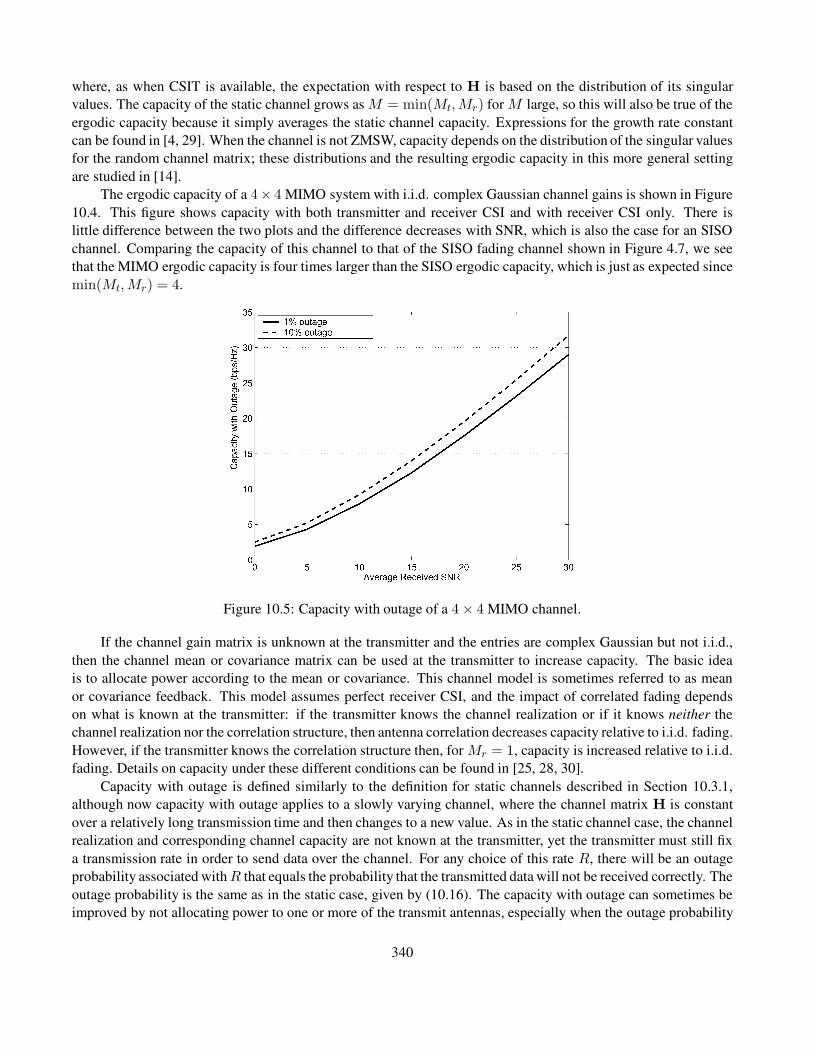
where, as when CSIT is available, the expectation with respect to H is based on the distribution of its singular

values. The capacity of the static channel grows as M = min(Mt,Mr) for M large, so this will also be true of the

ergodic capacity because it simply averages the static channel capacity. Expressions for the growth rate constant

can be found in [4, 29]. When the channel is not ZMSW, capacity depends on the distribution of the singular values

for the random channel matrix; these distributions and the resulting ergodic capacity in this more general setting

are studied in [14].

The ergodic capacity of a 4× 4 MIMO system with i.i.d. complex Gaussian channel gains is shown in Figure

10.4. This figure shows capacity with both transmitter and receiver CSI and with receiver CSI only. There is

little difference between the two plots and the difference decreases with SNR, which is also the case for an SISO

channel. Comparing the capacity of this channel to that of the SISO fading channel shown in Figure 4.7, we see

that the MIMO ergodic capacity is four times larger than the SISO ergodic capacity, which is just as expected since

min(Mt,Mr) = 4.

Figure 10.5: Capacity with outage of a 4 × 4 MIMO channel.

If the channel gain matrix is unknown at the transmitter and the entries are complex Gaussian but not i.i.d.,

then the channel mean or covariance matrix can be used at the transmitter to increase capacity. The basic idea

is to allocate power according to the mean or covariance. This channel model is sometimes referred to as mean

or covariance feedback. This model assumes perfect receiver CSI, and the impact of correlated fading depends

on what is known at the transmitter: if the transmitter knows the channel realization or if it knows neither the

channel realization nor the correlation structure, then antenna correlation decreases capacity relative to i.i.d. fading.

However, if the transmitter knows the correlation structure then, for Mr = 1, capacity is increased relative to i.i.d.

fading. Details on capacity under these different conditions can be found in [25, 28, 30].

Capacity with outage is defined similarly to the definition for static channels described in Section 10.3.1,

although now capacity with outage applies to a slowly varying channel, where the channel matrix H is constant

over a relatively long transmission time and then changes to a new value. As in the static channel case, the channel

realization and corresponding channel capacity are not known at the transmitter, yet the transmitter must still fix

a transmission rate in order to send data over the channel. For any choice of this rate R, there will be an outage

probability associated withR that equals the probability that the transmitted data will not be received correctly. The

outage probability is the same as in the static case, given by (10.16). The capacity with outage can sometimes be

improved by not allocating power to one or more of the transmit antennas, especially when the outage probability

340

is high [4]. This is because capacity with outage depends on the tail of the probability distribution. With fewer

antennas, less averaging takes place and the spread of the tail increases.

The capacity with outage of a 4 × 4 MIMO system with i.i.d. complex Gaussian channel gains is shown in

Figure 10.5 for outage of 1% and 10%. We see that the difference in capacity with outage for these two outage

probabilities increases with SNR, which can be explained by the distribution curves for capacity shown in Figure

10.6. These curves show that at low SNRs the distribution is very steep, so that the capacity with outage at 1%

is very close to that at 10% outage. At higher SNRs the curves become less steep, leading to more of a capacity

difference at different outage probabilities.

Figure 10.6: Outage probability distribution of a 4 × 4 MIMO channel.

NO CSl AT THE TRANSMITTER OR RECEIVER

When there is no CSI at either the transmitter or receiver, the linear growth in capacity as a function of the number

of transmit and receive antennas disappears, and in some cases adding additional antennas provides negligible

capacity gain. Moreover, channel capacity becomes heavily dependent on the underlying channel model, which

makes it difficult to obtain generalizations about capacity growth. For an i.i.d. ZMSW block fading channel it is

shown in [31] that increasing the number of transmit antennas by more than the duration of the block does not

increase capacity. Thus, there is no data rate increase beyond a certain number of transmit antennas. However,

when fading is correlated, additional transmit antennas do increase capacity [32]. The results of [31] were extended

in [33] to explicitly characterize capacity and the capacity-achieving transmission strategy for the i.i.d. block fading

model in the high-SNR regime. It was shown in [33] that, for i.i.d. block fading channels, capacity grows linearly

with the number of channel degrees of freedom.

The capacity of more general fading channel models without transmitter or receiver CSI was investigated

in [34, 35, 36]. These works indicate that there are three distinct regions associated with the capacity of slowly

varying flat fading channels with no CSIT or CSIR. At low SNRs capacity is limited by noise and grows linearly

with the number of channel degrees of freedom. At moderate to high SNRs capacity is limited by estimation error,

and its growth is also linear in the number of channel degrees of freedom. At very high SNRs the degrees of

freedom cease to matter and capacity grows double logarithmically with SNR. In other words, at very high SNRs

there is no multiplexing gain associated with multiple antennas for slowly varying channels without transmitter or

341

receiver CSI.

Figure 10.7: MIMO channel with beamforming.

10.4 MIMO Diversity Gain: Beamforming

The multiple antennas at the transmitter and receiver can be used to obtain array and diversity gain (defined in

Section 10.1) instead of capacity gain. In this setting the same symbol – weighted by a complex scale factor – is

sent over each transmit antenna, so that the input covariance matrix has unit rank. This scheme is also referred to

as MIMO beamforming.4 A beamforming strategy corresponds to the precoding and shaping matrices (described

in Section 10.2) being just column vectors: V = v and U = u, as shown in Figure 10.7. As indicated in the figure,

the transmit symbol x is sent over the ith antenna with weight vi. On the receive side, the signal received on the

ith antenna is weighted by u∗i . Both transmit and receive weight vectors are normalized so that ‖u‖ = ‖v‖ = 1.

The resulting received signal is given by

y = uHHvx+ uHn, (10.23)

where if n = (n1, . . . , nMr) has i.i.d. elements then the statistics of uHn are the same as the statistics for each of

these elements.

Beamforming provides diversity and array gain via coherent combining of the multiple signal paths. Channel

knowledge at the receiver is assumed, since this is required for coherent combining. The performance gain then

depends on whether or not the channel is known at the transmitter. When the channel matrix H is known, the

received SNR is optimized by choosing u and v as the principal left and right singular vectors of the channel

matrix H. That is, for σ1 = σmax the maximum singular value of H,u and v are (respectively) the first columns

of U and V. The corresponding received SNR can be shown to equal γ = σ2maxρ, where σmax is the largest

singular value of H [9, 37]. The resulting capacity is C = B log2(1 + σ2maxρ), corresponding to the capacity of

a SISO channel with channel power gain σ2max. For H a ZMSW matrix, it can be shown [9, Chap. 5.4.4] that the

array gain of beamforming diversity is between max(Mt,Mr) and MtMr and that the diversity gain is MtMr.

When the channel is not known to the transmitter, for Mt = 2 the Alamouti scheme described in Section

7.3.2 can be used to extract an array gain of Mr and the maximum diversity gain of 2 Mr [9, Chap. 5.4.3]. For

Mt > 2, full diversity gain can also be obtained using space-time block codes, as described in Section 10.7.3.

4Unfortunately, beamforming is also used in the smart antenna context of Section 10.9 to describe adjustment of the transmit or receive

antenna directivity in a given direction.

342

Although beamforming has a reduced capacity relative to the capacity-achieving transmit precoding and receiver

shaping matrices, the demodulation complexity with beamforming is on the order of |X | instead of |X |RH . An

even simpler strategy is to use MRC at either the transmitter or receiver and antenna selection on the other end:

this was analyzed in [38].

Example 10.3: Consider a MIMO channel with gain matrix

H =

.7 .9 .8

.3 .8 .2

.1 .3 .9

.

Find the capacity of this channel under beamforming, given channel knowledge at the transmitter and receiver,

B = 100 kHz, and ρ = 10 dB.

Solution: The largest singular value of H is σmax =√λmax, where λmax is the maximum eigenvalue of

HHH =

1.94 1.09 1.06

1.09 .77 .45

1.06 .45 .91

.

The largest eigenvalue of this matrix is λmax = 3.17. Thus,C = B log2(1 + λmaxρ) = 105 log2(1 + 31.7) = 503kbps.

10.5 Diversity–Multiplexing Trade-offs

The previous sections suggest two mechanisms for utilizing multiple antennas to improve wireless system per-

formance. One option is to obtain capacity gain by decomposing the MIMO channel into parallel channels and

multiplexing different data streams onto these channels. This capacity gain is also referred to as a multiplexing

gain. However, the SNR associated with each of these channels depends on the singular values of the channel

matrix. In capacity analysis this is taken into account by assigning a relatively low rate to these channels. How-

ever, practical signaling strategies for these channels will typically have poor performance unless powerful channel

coding techniques are employed. Alternatively, beamforming can be used, where the channel gains are coherently

combined to obtain a very robust channel with high diversity gain. It is not necessary to use the antennas purely

for multiplexing or diversity. Some of the space-time dimensions can be used for diversity gain and the remaining

dimensions used for multiplexing gain. This gives rise to a fundamental design question in MIMO systems: Should

the antennas be used for diversity gain, multiplexing gain, or both?

The diversity–multiplexing trade-off or, more generally, the trade-off between data rate, probability of error,

and complexity for MIMO systems has been extensively studied in the literature – both from a theoretical perspec-

tive and in terms of practical space-time code designs [39, 40, 41, 42]. This work has primarily focused on block

fading channels with receiver CSI only, since when both transmitter and receiver know the channel the trade-off is

relatively straightforward: antenna subsets can first be grouped for diversity gain, and then the multiplexing gain

corresponds to the new channel with reduced dimension due to the grouping. For the block fading model with

receiver CSI only, as the blocklength grows asymptotically large, full diversity gain and full multiplexing gain (in

terms of capacity with outage) can be obtained simultaneously with reasonable complexity by encoding diagonally

across antennas [2, 43, 44]. An example of this type of encoding is D-BLAST, described in Section 10.7.4. For

finite blocklengths it is not possible to achieve full diversity and full multiplexing gain simultaneously, in which

343

case there is a trade-off between these gains. A simple characterization of this trade-off is given in [42] for block

fading channels in the limit of asymptotically high SNR. In this analysis a transmission scheme is said to achieve

multiplexing gain r and diversity gain d if the data rate (bps) per unit hertz, R(SNR), and probability of error,

Pe(SNR), as functions of SNR satisfy

Figure 10.8: Diversity–multiplexing trade-off for high-SNR block fading.

limSNR→∞

R(SNR)

log2 SNR= r (10.24)

and

limSNR→∞

logPe(SNR)

log SNR= −d, (10.25)

where the log in (10.25) can be in any base.5 For each r, the optimal diversity gain dopt(r) is the maximum diversity

gain that can be achieved by any scheme. It is shown in [42] that if the fading blocklength T ≥Mt +Mr − 1 then

dopt(r) = (Mt − r)(Mr − r), 0 ≤ r ≤ min(Mt,Mr). (10.26)

The function (10.26) is plotted in Figure 10.8. This figure implies that (i) if we use all transmit and receive antennas

for diversity then we get full diversity gain MtMr and (ii) we can use some of these antennas to increase data rate

at the expense of diversity gain.

It is also possible to adapt the diversity and multiplexing gains relative to channel conditions. Specifically,

in poor channel states more antennas can be used for diversity gain, whereas in good states more antennas can be

used for multiplexing. Adaptive techniques that change antenna use to trade off diversity and multiplexing based

on channel conditions have been investigated in [45, 46, 47].

Example 10.4: Let the multiplexing and diversity parameters r and d be as defined in (10.24) and (10.25). Suppose

that r and d approximately satisfy the diversity–multiplexing trade-off dopt(r) = (Mt − r)(Mr − r) at any large

finite SNR. For an Mt = Mr = 8 MIMO system with an SNR of 15 dB, if we require a data rate per unit hertz of

R = 15 bps then what is the maximum diversity gain the system can provide?

Solution: With SNR = 15 dB, to get R = 15 bps we require r log2(101.5) = 15, which implies that r = 3.01.

Therefore, three of the antennas are used for multiplexing and the remaining five are used for diversity. The maxi-

mum diversity gain is then dopt(r) = (Mt−r)(Mr−r) = (8−3)(8−3) = 25.

5The base of the log cancels out of the expression because (10.25) is the ratio of two logs with the same base.

344

10.6 MIMO Receiver Detection Algorithms

In this section we describe algorithms used at a MIMO receive to detect the transmitted symbol vector. In particular,

we consider a MIMO receiver that receives vector y given by (10.1):

y = Hx + n, (10.27)

where the input vector x ∈ XMt and, for C the set of all complex numbers, the complex received vector y ∈ CMr

and H ∈ CMr×Mt . We assume a normalized power ρ such that E[xxH] = ρMt

I such that the complex noise ni has

real and imaginary part distributed as N (0, 1). The receiver estimates x(y), an estimate for the transmitted vector

x, based on its knowledge of the channel matrix H,X , and the received vector y.

We consider the following detection algorithms: maximum-likelihood (ML), the linear algorithms of zero-

forcing (ZF) and linear minimum mean-square error (L-MMSE), and an approximation to ML called sphere de-

coding (SD), where the radius of the sphere provides a tradeoff between performance and complexity. Sphere

decoding becomes ML for an asymptotically large radius, so reducing the radius reduces both complexity and

performance relative to ML.

10.6.1 Maximum Likelihood (ML) Detection

As in scalar signal detection, the ML MIMO detection algorithm minimizes the probability of symbol detection

error (assuming equiprobable x). In particular, the maximum likelihood detector with i.i.d. Gaussian noise at the

receiver antennas solves the following problem.

x(y) = argminx∈XMt‖y −Hx‖2. (10.28)

The minimization is over x ∈ XMt , i.e. over all possible transmitted vectors. Unfortunately, solving this problem

involves computing the objective function for all XMt potential values of x.Hence the ML detector has prohibitive

(exponential in Mt) complexity.

10.6.2 Linear Receivers: ZF and MMSE

The complexity of linear detectors is the same as the complexity of inverting or factorizing a matrix of dimensions

Mr ×Mt, hence the name. They work by spatially decoupling the effects of the channel by a process known as

MIMO equalization. This involves multiplying y with a MIMO equalization matrix A ∈ CMt×Mr to get x(y) ∈CMt . To get the estimate x(y) from x(y), we perform coordinatewise decoding of x(y). The coordinatewise

decoding operation is given by:

x(y)i = argmins∈X |x(y)i − s| for all i, (10.29)

i.e., it maps each coordinate to the closest constellation point.

A common way to obtain x(y) from y is through zero-forcing (ZF), which solves the following problem:

x(y) = argminx‖y −Hx‖2. (10.30)

Comparing with (10.28), we note that the constellation constraints on x have been removed. This significantly

reduces the complexity. For a square invertible matrix, the solution is given by

x(y) = H†y,

345

where H† is just H−1 if the matrix is square and invertible. If the matrix is not invertible or not square we use

the pseudo inverse instead. When Mt ≤Mr, and there are at least Mt linearly independent columns in H, which

is often the case in typical propagation environments, the pseudo inverse (sometimes called the Moore-Penrose

pseudoinverse) is given by

H† = (HHH)−1HH .

The complexity of obtaining H† from H is roughly cubic inMt for a square matrix. However obtaining x(y) from

x(y) is done in a time linear in Mt.Zero forcing can cause noise amplification if the minimum singular value of H is much smaller than its

maximum value. This may be quantified by the notion of the condition number of the matrix H. The condition

number of the matrix H is a measure of the relative magnitudes of the singular values of H. It is defined as the

ratio between the largest and the smallest singular values of H. When the condition number is unity or close to

unity, the matrix is said to be well conditioned. When the condition number is large, the matrix is ill conditioned.

When the matrix is ill-conditioned, noise is significantly amplified in the spatial channels associated with small

singular values. This problem can be compensated for using the minimum mean squared error (MMSE) detector,

which adds a regularization term to the objective function in (10.30).

x(y) = argminx‖y − Hx‖2 + λ‖x‖2,

for some λ > 0. The solution to this is given by

x(y) = (HHH + λI)−1HHy = HH(HHH + λI)−1y.

For λ = Mt

ρ , this is called the L-MMSE detector since it minimizes the mean squared error in the estimate of xamong all linear detectors, i.e., it solves the following problem:

x(y) = argmins Ex,n[‖s − x‖2],

such that s = Ay + b,

for any Mt ×Mr matrix A and vector b ∈ CMt. Note that the minimization is only over all affine functions of

y, which is parametrized by A and b. The expectation is over the randomness in x and n (the channel matrix H

is assumed to be known and non random). If x were to be Gaussian (instead of being from discrete constellation

points), this is also the MMSE detector.

Compared to the ML detector, both the ZF and MMSE linear detectors are simpler to implement, but their

BER performances are worse. A nonlinear technique that allows for better performance than a linear detector and

a simple mechanism to trade off between complexity and performance is the sphere decoder, which we describe in

the next subsection.

10.6.3 Sphere Decoders (SD)

The sphere decoder trades off performance versus complexity by controlling a parameter r. By choosing a large

enough r, the performance of SD approaches that of the ML detector. For small r, the search space (and hence

complexity) of the SD is much smaller than that of the ML detector, but it suffers a performance degradation as a

result. The sphere detector exploits the following factorization of the matrix H:

H = QR,

where Q is unitary and R is upper triangular. Since the squared-distance norm does not change under multiplica-

tion by a unitary matrix QH , we have

‖y − Hx‖2 = ‖QHy − QHQRx‖2 = ‖y −Rx‖2 =

1∑

i=Mt

|yi −Mt∑

j=i

Ri,jxj|2,

346

where y , QHy, and we use the upper triangular nature of R in the last step. The sphere decoder solves the

following problem.

x(y) = argminx∈XMt ,‖QHy−Rx‖≤r‖QHy − Rx‖2 (10.31)

Note that choosing r = ∞ gives us the ML decoder. For a smaller r, the solver can exploit the upper triangular

nature of R to “prune” many candidate solutions (using depth-first-search or breadth-first-search or a combination

of the two), thereby reducing the detection complexity significantly. One surprising property of the SD is that if it

finds a valid solution, it is the same solution that the ML detector would have returned.

10.7 Space-Time Modulation and Coding

Because a MIMO channel has input–output relationship y = Hx + n, the symbol transmitted over the channel

each symbol time is a vector rather than a scalar, as in traditional modulation for the SISO channel. Moreover,

when the signal design extends over both space (via the multiple antennas) and time (via multiple symbol times),

it is typically referred to as a space-time code.

Most space-time codes – including all codes discussed in this section – are designed for quasi-static chan-

nels, where the channel is constant over a block of T symbol times and the channel is assumed unknown at the

transmitter. Under this model, the channel input and output become matrices with dimensions corresponding to

space (antennas) and time. Let X = [x1, . . . , xT ] denote the Mt × T channel input matrix with ith column

xi equal to the vector channel input over the ith transmission time. Let Y = [y1, . . . , yT ] denote the Mr × Tchannel output matrix with ith column yi equal to the vector channel output over the ith transmission time, and let

N = [n1, . . . ,nT ] denote the Mr × T noise matrix with ith column ni equal to the receiver noise vector over the

ith transmission time. With this matrix representation, the input–output relationship over all T blocks becomes

Y = HX + N. (10.32)

10.7.1 ML Detection and Pairwise Error Probability

Assume a space-time code where the receiver has knowledge of the channel matrix H. Under maximum likelihood

detection it can be shown using similar techniques as in the scalar (Chapter 5) or vector (Chapter 8) case that, given

received matrix Y, the ML transmit matrix X satisfies

X = arg minX∈XMt×T

‖Y − HX‖2F = arg min

X∈XMt×T

T∑

i=1

‖yi −Hxi‖2, (10.33)

where ‖A‖F denotes the Frobenius norm6 of the matrix A and the minimization is taken over all possible space-

time input matrices XMt×T . The pairwise error probability for mistaking a transmit matrix X for another matrix

X, denoted as p(X → X), depends only on the distance between the two matrices after transmission through the

channel and the noise power σ2; that is,

p(X → X) = Q

√

‖H(X− X)‖2F

2σ2

. (10.34)

Let DX = X − X denote the difference matrix between X and X. Applying the Chemoff bound to (10.34), we

have

6The Frobenius norm of a matrix is the square root of the sum of the square of its elements.

347

p(X → X) ≤ exp

[

−‖HDX‖2F

4σ2

]

. (10.35)

Let hi denote the ith row of H, i = 1, . . . ,Mr. Then

‖HDX‖2F =

Mr∑

i=1

hiDXDHXhHi . (10.36)

Let H = vec(HT )T , where vec(A) is defined as the vector that results from stacking the columns of matrix A on

top of each other to form a vector.7 Hence HT is a vector of length MrMt. Also define DX = IMr ⊗ DX, where

⊗ denotes the Kronecker product. With these definitions,

‖HDX‖2F = ‖HDX‖2

F . (10.37)

Substituting (10.37) into (10.35) and taking the expectation relative to all possible channel realizations yields

p(X → X) ≤(

det

[

IMtMr +1

4σ2E[DH

XHHHDX]

])

.−1 (10.38)

Suppose that the channel matrix H is random and spatially white, so that its entries are i.i.d. zero-mean, unit-

variance, complex Gaussian random variables. Then taking the expectation in (10.38) yields

p(X → X) ≤(

1

det[IMt + .25ρ∆]

)Mr

, (10.39)

where ∆ = (1/P )DXDHX. This simplifies to

p(X → X) ≤R∆∏

k=1

(1

1 + .25γλk(∆)

)Mr

; (10.40)

here γ = P/σ2 = ρ is the SNR per input symbol and λk(∆) is the kth nonzero eigenvalue of ∆, k = 1, . . . , R∆,

where R∆ is the rank of ∆. In the high-SNR regime (i.e., for γ 1) this simplifies to

p(X → X) ≤(R∆∏

k=1

λk(∆)

)−Mr

(.25γ)−R∆Mr . (10.41)

This equation gives rise to the main criteria for design of space-time codes, described in the next section.

10.7.2 Rank and Determinant Criteria

The pairwise error probability in (10.41) indicates that the probability of error decreases as γ−d for d = R∆Mr.

Thus, R∆Mr is the diversity gain of the space-time code. The maximum diversity gain possible through coherent

combining of Mt transmit and Mr receive antennas is MtMr. Thus, to obtain this maximum diversity gain, the

space-time code must be designed such that the Mt ×Mt difference matrix ∆ between any two codewords has

full rank equal to Mt. This design criterion is referred to as the rank criterion.

The coding gain associated with the pairwise error probability in (10.41) depends on the term (∏R∆

k=1 λk(∆))Mr.

Thus, a high coding gain is achieved by maximizing the minimum of the determinant of ∆ over all input matrix

pairs X and X. This criterion is referred to as the determinant criterion.

7So for the M × N matrix A = [a1, . . . ,aN ], where ai is a vector of length M, vec(A) = [aT1 , . . . ,aT

N ]T is a vector of length MN .

348

The rank and determinant criteria were first developed in [40, 48, 49]. These criteria are based on the pairwise

error probability associated with different transmit signal matrices – rather than the binary domain of traditional

codes–and hence often require computer searches to find good codes [50, 51]. A general binary rank criterion was

developed in [52] to provide a better construction method for space-time codes.

10.7.3 Space-Time Trellis and Block Codes

The rank and determinant criteria have been primarily applied to the design of space-time trellis codes (STTCs),

which are an extension of conventional trellis codes to MIMO systems [9, 49]. They are described using a trellis

and are decoded using ML sequence estimation via the Viterbi algorithm. STTCs can extract excellent diversity and

coding gain, but the complexity of decoding increases exponentially with the diversity level and transmission rate

[53]. Space-time block codes (STBCs) are an alternative space-time code that can also extract excellent diversity

gain with linear receiver complexity. Interest in STBCs was initiated by the Alamouti code described in Section

7.3.2, which obtains full diversity order with linear receiver processing for a two-antenna transmit system. This

scheme was generalized in [54] to STBCs that achieve full diversity order with an arbitrary number of transmit

antennas. However, while these codes achieve full diversity order, they do not provide coding gain and thus have

inferior performance to STTCs, which achieve both full diversity gain as well as coding gain. Added coding gain

for STTCs as well as STBCs can be achieved by concatenating these codes either in serial or in parallel with an

outer channel code to form a turbo code [55, 56, 57]. The linear complexity of the STBC designs in [54] result

from making the codes orthogonal along each dimension of the code matrix. A similar design premise is used in

[58] to design unitary space-time modulation schemes for block fading channels when neither the transmitter nor

the receiver has CSI. More comprehensive treatments of space-time coding can be found in [9, 53, 59, 60] and the

references therein.

Figure 10.9: Spatial multiplexing with serial encoding.

10.7.4 Spatial Multiplexing and BLAST Architectures

The basic premise of spatial multiplexing is to send Mt independent symbols per symbol period using the dimen-

sions of space and time. To obtain full diversity order, an encoded bit stream must be transmitted over all Mt

transmit antennas. This can be done through a serial encoding, illustrated in Figure 10.9. With serial encoding the

bit stream is temporally encoded over the channel blocklength T to form the codeword [x1, . . . , xT ]. The codeword

is interleaved and mapped to a constellation point, then demultiplexed onto the different antennas. The first Mt

symbols are transmitted from the Mt antennas over the first symbol time, the next Mt symbols are transmitted

from the antennas over the next symbol time, and this process continues until the entire codeword has been trans-

mitted. We denote the symbol sent over the kth antenna at time i as xk[i]. If a codeword is sufficiently long, it is

349

Figure 10.10: Spatial multiplexing with parallel encoding: V-BLAST.

transmitted over all Mt transmit antennas and received by all Mr receive antennas, resulting in full diversity gain.

However, the codeword length T required to achieve this full diversity is MtMr, and decoding complexity grows

exponentially with this codeword length. This high level of complexity makes serial encoding impractical.

A simpler method to achieve spatial multiplexing, pioneered at Bell Laboratories as one of the Bell Labs

Layered Space Time (BLAST) architectures for MIMO channels [2], is parallel encoding, illustrated in Figure

10.10. With parallel encoding the data stream is demultiplexed intoMt independent streams. Each of the resulting

substreams is passed through an SISO temporal encoder with blocklength T , interleaved, mapped to a signal

constellation point, and transmitted over its corresponding transmit antenna. Specifically, the kth SISO encoder

generates the codeword xk[i], i = 1, . . . , T, which is transmitted sequentially over the kth antenna. This process

can be considered to be the encoding of the serial data into a vertical vector and hence is also referred to as

vertical encoding or V-BLAST [61]. Vertical encoding can achieve at most a diversity order of Mr, since each

coded symbol is transmitted from one antenna and received by Mr antennas. This system has a simple encoding

complexity that is linear in the number of antennas. However, optimal decoding still requires joint detection of

the codewords from each of the transmit antennas, since all transmitted symbols are received by all the receive

antennas. It was shown in [62] that the receiver complexity can be significantly reduced through the use of symbol

interference cancellation, as shown in Figure 10.11. This cancellation, which exploits the synchronicity of the

symbols transmitted from each antenna, works as follows. First the Mt transmitted symbols are ordered in terms

of their received SNR. An estimate of the received symbol with the highest SNR is made while treating all other

symbols as noise. This estimated symbol is subtracted out, and the symbol with the next highest SNR estimated

while treating the remaining symbols as noise. This process repeats until all Mt transmitted symbols have been

estimated. After cancelling out interfering symbols, the coded substream associated with each transmit antenna

can be individually decoded, resulting in a receiver complexity that is linear in the number of transmit antennas. In

fact, coding is not even needed with this architecture, and data rates of 20–40 bps/Hz with reasonable error rates

were reported in [61] using uncoded V-BLAST.

The simplicity of parallel encoding and the diversity benefits of serial encoding can be obtained by using a

creative combination of the two techniques called diagonal encoding or D-BLAST [2], illustrated in Figure 10.12.

In D-BLAST, the data stream is first parallel encoded. However, rather than transmitting each codeword with one

antenna, the codeword symbols are rotated across antennas, so that a codeword is transmitted by all Mt antennas.

The operation of the stream rotation is shown in Figure 10.13. Suppose the ith encoder generates the codeword

xi = [xi[1], . . . , xi[T ]]. The stream rotator transmits each symbol on a different antenna, so xi[1] is sent on antenna

1 over symbol time i, xi[2] is sent on antenna 2 over symbol time i + 1, and so forth. If the code blocklength Texceeds Mt then the rotation begins again on antenna 1. As a result, the codeword is spread across all spatial

350

Figure 10.11: V-BLAST receiver with linear complexity.

dimensions. Transmission schemes based on D-BLAST can achieve full MtMr diversity gain if the temporal

coding with stream rotation is capacity-achieving (Gaussian codewords of infinite blocklength T ) [9, Chap. 6.3.5].

Moreover, the D-BLAST system can achieve maximum capacity with outage if the wasted space-time dimensions

along the diagonals are neglected [9, Chap. 12.4.1]. Receiver complexity is also linear in the number of transmit

antennas, since the receiver decodes each diagonal code independently. However, this simplicity comes at a price,

as the efficiency loss of the wasted space-time dimensions (illustrated in Figure 10.13) can be large if the frame

size is not appropriately chosen.

Figure 10.12: Diagonal encoding with stream rotation.

Figure 10.13: Stream rotation.

351

10.8 Frequency-Selective MIMO Channels

When the MIMO channel bandwidth is large relative to the channel’s multipath delay spread, the channel suffers

from intersymbol interference; this is similar to the case of SISO channels. There are two approaches to dealing

with ISI in MIMO channels. A channel equalizer can be used to mitigate the effects of ISI. However, the equalizer

is much more complex in MIMO channels because the channel must be equalized over both space and time.

Moreover, when the equalizer is used in conjuction with a space-time code, the nonlinear and noncausal nature of

the code further complicates the equalizer design. In some cases the structure of the code can be used to convert

the MIMO equalization problem to a SISO problem for which well-established SISO equalizer designs can be used

[63, 64, 65].

An alternative to equalization in frequency-selective fading is multicarrier modulation or orthogonal fre-

quency division multiplexing (OFDM). OFDM techniques for SISO channels are described in Chapter 12: the

main premise is to convert the wideband channel into a set of narrowband subchannels that exhibit only flat fading.

Applying OFDM to MIMO channels results in a parallel set of narrowband MIMO channels, and the space-time

modulation and coding techniques just described for a single MIMO channel are applied to this parallel set. MIMO

frequency-selective fading channels exhibit diversity across space, time, and frequency, so ideally all three dimen-

sions should be fully exploited in the signaling scheme.

10.9 Smart Antennas

We have seen that multiple antennas at the transmitter and/or receiver can provide diversity gain as well as increased

data rates through space-time signal processing. Alternatively, sectorization or phased array techniques can be used

to provide directional antenna gain at the transmit or receive antenna array. This directionality can increase the

signaling range, reduce delay spread (ISI) and flat fading, and suppress interference between users. In particular,

interference typically arrives at the receiver from different directions. Thus, directional antennas can exploit these

differences to null or attenuate interference arriving from given directions, thereby increasing system capacity. The

reflected multipath components of the transmitted signal also arrive at the receiver from different directions and

can also be attenuated, thereby reducing ISI and flat fading. The benefits of directionality that can be obtained

with multiple antennas must be weighed against their potential diversity or multiplexing benefits, giving rise to a

multiplexing–diversity–directionality trade-off analysis. Whether it is best to use the multiple antennas to increase

data rates through multiplexing, increase robustness to fading through diversity, or reduce ISI and interference

through directionality is a complex decision that depends on the overall system design.

The most common directive antennas are sectorized or phased (directional) antenna arrays, and the gain

patterns for these antennas – along with an omnidirectional antenna gain pattern – are shown in Figure 10.14.

Sectorized antennas are designed to provide high gain across a range of signal arrival angles. Sectorization is

commonly used at cellular system base stations to cut down on interference: assuming different sectors are assigned

the same frequency band or timeslot, then with perfect sectorization only users within a sector interfere with each

other, thereby reducing the average interference by a factor equal to the number of sectors. For example, Figure

10.14 shows a sectorized antenna with a 120 beamwidth. A base station could divide its 360 angular range

into three sectors to be covered by three 120 sectorized antennas, in which case the interference in each sector is

reduced by a factor of 3 relative to an omnidirectional base station antenna. The price paid for reduced interference

in cellular systems via sectorization is the need for handoff between sectors.

Directional antennas typically use antenna arrays coupled with phased array techniques to provide directional

gain, which can be tightly contolled with sufficiently many antenna elements. Phased array techniques work by

adapting the phase of each antenna element in the array, which changes the angular locations of the antenna beams

(angles with large gain) and nulls (angles with small gain). For an antenna array with N antennas, N nulls can

352

be formed to significantly reduce the received power of N separate interferers. If there are NI < N interferers,

then theNI interferers can be nulled out usingNI antennas in a phased array, and the remaining N −NI antennas

can be used for diversity gain. Note that directional antennas must know the angular location of the desired and

interfering signals in order to provide high or low gains in the appropriate directions. Tracking of user locations can

be a significant impediment in highly mobile systems, which is why cellular base stations use sectorized instead of

directional antennas.

Figure 10.14: Antenna gains for omnidirectional, sectorized, and directive antennas.

The complexity of antenna array processing – along with the real estate required for an antenna array – make

the use of smart antennas in small, lightweight, low-power, handheld devices unlikely in the near future. However,

base stations and access points already use antenna arrays in many cases. More details on the technology behind

smart antennas and their use in wireless systems can be found in [66].

353

Chapter 10 Problems

1. Matrix identities are commonly used in the analysis of MIMO channels. Prove the following matrix identi-

ties.

(a) Given an M ×N matrix A, show that the matrix AAH is Hermitian. What does this reveal about the

eigendecomposition of AAH?

(b) Show that AAH is positive semidefinite.

(c) Show that IM + AAH is Hermitian positive definite.

(d) Show that det[IM + AAH ] = det[IN + AHA].

2. Find the SVD of the following matrix:

H =

.7 .6 .2 .4

.1 .5 .9 .2

.3 .6 .9 .1

.

3. Find a 3 × 3 channel matrix H with two nonzero singular values.

4. Consider the 4 × 4 MIMO channels given below. What is the maximum multiplexing gain of each – that is,

how many independent scalar data streams can be reliably supported?

H1 =

1 1 −1 1

1 1 −1 −1

1 1 1 1

1 1 1 −1

, H2 =

1 1 1 −1

1 1 −1 1

1 −1 1 1

1 −1 −1 −1

.

5. The capacity of a static MIMO channel with only receiver CSI is given by C =∑RH

i=1 B log2(1 + σ2i ρ/Mt).

Show that, if the sum of singular values is bounded, then this expression is maximized when all RH singular

values are equal.

6. Consider a MIMO system with the following channel matrix:

H =

.1 .3 .4

.3 .2 .2

.1 .3 .7

=

−.5196 −.0252 −.8541

−.3460 −.9077 .2372

−.7812 .4188 .4629

.9719 0 0

0 .2619 0

0 0 .0825

×

−.2406 −.8894 .3886

−.4727 −.2423 −.8472

−.8477 .3876 .3621

H

.

Note that H is written in terms of its singular value decomposition (SVD) H = UΣVH .

(a) Check if H = UΣVH . You will see that the matrices U, Σ, and VH do not have sufficiently large

precision, so that UΣVH is only approximately equal to H. This indicates the sensitivity of the SVD

– in particular, the matrix Σ – to small errors in the estimate of the channel matrix H.

354

(b) Based on the singular value decomposition H = UΣVH , find an equivalent MIMO system consisting

of three independent channels. Find the transmit precoding and the receiver shaping matrices necessary

to transform the original system into the equivalent system.

(c) Find the optimal power allocation Pi (i = 1, 2, 3) across the three channels found in part (b), and

find the corresponding total capacity of the equivalent system assuming P/σ2 = 20 dB and a system

bandwidth of B = 100 kHz.

(d) Compare the capacity in part (c) to that when the channel is unknown at the transmitter and so equal

power is allocated to each antenna.

7. Use properties of the SVD to show that, for a MIMO channel that is known to the transmitter and receiver

both, the general capacity expression

C = maxRx:Tr(Rx)=ρ

B log2 det[IMr + HRxHH ]

reduces to

C = maxρi:Σiρi≤ρ

∑

i

B log2(1 + σ2i ρi)

for singular values σi and SNR ρ.

8. For the 4× 4 MIMO channels given below, find their capacity assuming both transmitter and receiver know

the channel, whose SNR ρ = 10 dB and bandwidth B = 10 MHz:

H1 =

1 1 −1 1

1 1 −1 −1

1 1 1 1

1 1 1 −1

, H2 =

1 1 1 −1

1 1 −1 1

1 −1 1 1

1 −1 −1 −1

.

9. Assume a ZMCSCG MIMO system with channel matrix H corresponding to Mt = Mr = M transmit and

receive antennas. Using the law of large numbers, show that

limM→∞

1

MHHH = IM .

Then use this to show that

limM→∞

B log2 det[

IM +ρ

MHHH

]

= MB log2(1 + ρ).

10. Plot the ergodic capacities for a ZMCSCG MIMO channel with SNR 0 ≤ ρ ≤ 30 dB and B = 1 MHz for

the following MIMO dimensions: (a) Mt = Mr = 1; (b) Mt = 2, Mr = 1; (c) Mt = Mr = 2; (d) Mt =

2, Mr = 3; (e) Mt = Mr = 3. Verify that, at high SNRs, capacity grows linearly as M = min(Mt, Mr).

11. Plot the outage capacities for B = 1 MHz and an outage probability Pout = .01 for a ZMCSCG MIMO

channel with SNR 0 ≤ ρ ≤ 30 dB for the following MIMO dimensions: (a) Mt = Mr = 1; (b) Mt =

2, Mr = 1; (c) Mt = Mr = 2; (d)Mt = 2, Mr = 3; (e) Mt = Mr = 3. Verify that, at high SNRs, capacity

grows linearly as M = min(Mt, Mr).

355

12. Show that if the noise vector n = (n1, . . . , nMr) has i.i.d. elements then, for ‖u‖ = 1, the statistics of uHnare the same as the statistics for each of these elements.

13. Consider a MIMO system where the channel gain matrix H is known at the transmitter and receiver. Show

that if transmit and receive antennas are used for diversity then the optimal weights at the transmitter and

receiver lead to an SNR of γ = λmaxρ, where λmax is the largest eigenvalue of HHH . Also show that the

leading eigenvectors of HHH and HHH form the optimal transmit and receiver shaping vectors respec-

tively.

14. Consider a 4x4 MIMO system where the channel gain matrix H is known at the transmitter and receiver.

Assume the channel has free space signal propagation between each transmit and receive antenna (i.e. there

are no reflectors or scatterers in the environment). The antenna elements are collinear and the distance

between antenna elements l at the receiver (or transmitter) is much smaller than the distance d between the

antenna and the receiver. What is the approximate rank of the channel matrix H where singular values that

are smaller than a threshold can be approximated to zero.

15. Consider a channel with channel gain matrix

H =

.1 .5 .9

.3 .2 .6

.1 .3 .7

.

Assuming ρ = 10 dB, find the output SNR when beamforming is used on the channel with equal weights

on each transmit antenna and optimal weighting at the receiver. Compare with the SNR under beamforming

with optimal weights at both the transmitter and receiver.

16. Consider an 8 × 4 MIMO system, and assume a coding scheme that can achieve the rate–diversity trade-off

d(r) = (Mt − r)(Mr − r).

(a) Find the maximum multiplexing rate for this channel, given a requiredPe = ρ−d ≤ 10−3 and assuming

that ρ = 10 dB.

(b) Given the r derived in part (a), what is the resulting Pe?

17. Find the capacity of a SIMO channel with channel gain vector h = [.1 .4 .75 .9], optimal receiver weighting,

ρ = 10 dB, and B = 10 MHz.

18. Consider a 2 × 2 MIMO system with channel gain matrix H given by

H =

[

.3 .5

.7 .2

]

.

Assume that H is known at both transmitter and receiver and that there is a total transmit power of P =

10 mW across the two transmit antennas, AWGN with N0 = 10−9 W/Hz at each receive antenna, and

bandwidthB = 100 kHz.

(a) Find the SVD for H.

(b) Find the capacity of this channel.

356

(c) Assume that transmit precoding and receiver shaping have been used to transform this channel into two

parallel independent channels with a total power constraint P . Find the maximum data rate that can be

transmitted over this parallel set assuming MQAM modulation on each channel, with optimal power

adaptation across the channels subject to power constraint P . Assume a target BER of 10−3 on each

channel and that the BER is bounded: Pb ≤ .2e−1.5γ/(M−1); assume also that the constellation size of

the MQAM is unrestricted.

(d) Suppose now that the antennas at the transmitter and receiver are all used for diversity (with optimal

weighting at the transmitter and receiver) to maximize the SNR of the combiner output. Find the SNR

of the combiner output as well as the BER of a BPSK modulated signal transmitted over this diversity

system. Compare the data rate and BER of this BPSK signaling with diversity (assuming B = 1/Tb)to the rate and BER from part (c).

(e) Comment on the diversity–multiplexing trade-offs between the systems in parts (c) and (d).

19. Consider an M ×M MIMO channel with ZMCSCG channel gains.

(a) Plot the ergodic capacity of this channel for M = 1 and M = 4 with 0 ≤ ρ ≤ 20 dB and B = 1 MHz,

assuming that both transmitter and receiver have CSI.

(b) Repeat part (a) assuming that only the receiver has CSI.

20. Find the outage capacity for a 4 × 4 MIMO channel with ZMCSCG elements at 10% outage for ρ = 10 dB

and B = 1 MHz.

21. Plot the cdf of capacity for an M × M MIMO channel with ρ = 10 dB and B = 1 MHz, assuming no

transmitter knowledge for M = 4, 6, 8. What happens as M increases? What are the implications of this

behavior for a practical system design?

22. Assume a ZMCSCG MIMO system with channel matrix H ∈ RMr×Mt corresponding to Mt transmit and

Mr receive antennas (E[|Hi,j|2] = 1 for all i and j). Show using the law of large numbers that

limMr→∞

1

MrHHH = IMt .

Then use this to show that

limMr→∞

B log2 det

(

IMt +ρ

MrHHH

)

= MtB log2(1 + ρ).

23. An 8x8 MIMO system has a channel matrix H with singular values σ1 = 2, σ2 = 1, σ3 = 0.8, σ4 =0.3, σi = 0 where i = 5, 6, 7, 8. Assume the total transmit power is ρ = 10 dBm, the noise power at each

receive antenna is 0 dBm, and the system bandwidth is B = 10 MHz. Assume in this high-tech system that

both transmitter and receiver know the channel matrix.

(a) What is the rank of H and the SNR γi associated with each of its spatial dimensions assuming the full

transmit power is allocated to it?

(b) Find the Shannon capacity of the system assuming optimal adaptation of power and rate across spatial

dimensions.

(c) If the transmitter does not do power adaptation, it assigns equal power to all transmit antennas resulting

in Rx = ρ8 I. Show that this implies that power is equally allocated over all 8 spatial dimensions. What

is the capacity of the system in this case assuming that the rate is optimally adapted?

357

(d) What is the capacity when only the signal dimension with the largest SNR is used, i.e. all power is

allocated to the spatial dimension with the largest singular value (beamforming).

(e) Find the maximum data rate that can be sent using adaptive modulation assuming power is optimally

allocated across spatial dimensions. Compare with the maximum data rate in beamforming, where full

power is allocated to the single spatial dimension associated with beamforming. In both cases assume a

target BER of Pb = 10−3 with unrestricted modulation (i.e. M can take any value). Assume a symbol

time T = 1/B.

24. In this question we look into the diversity order of the maximum singular value σmax. Consider an m × nmatrix H with i.i.d. entries distributed as Rayleigh fading variables with power p each.

(a) Use the definition of the Frobenius norm to establish an upper bound on the square of the maximum

singular value of H in terms of the elements of H .

(b) Use the fact that the maximum singular value is greater than all the singular values to come up with a

lower bound for σmax.

Hint: This is just a scaled version of the upper bound.

(c) What is the diversity order of the Frobenius norm? Use this result and parts (a) and (b) to write down

the diversity order for the maximum singular value. For any norm ‖ · ‖, we define its diversity order to

be

limp→∞

− log(Prob(‖H‖ < 1))

log(p).

Hint: Use results from the maximal ratio combining of Rayleigh fading random variables.

25. We are given the channel matrix H, and a received vector y, seen below.

H =

0.3 0.5 0.5

0.7 0.4 0.4

0.4 0.5 0.6

0.2 0.6 0.7

, y =

0.3 + 0.2i

0.3− 0.5i

−0.7 + 0..4i

−0.3 − 0.1i

Assume that the transmitter used all the antennas for multiplexing gain, and transmitted 3 QPSK symbols,

where the constellation points for (00),(01),(11),(10) correspond to (1+i),(-1+i),(-1-i),(1- i) respectively.

Estimate the transmitted sequence assuming the following MIMO receivers:

(a) Maximum likelihood receiver

(b) Zero-forcing receiver

(c) Linear MMSE receiver (assume N0/E = 0.1)

26. Consider a MIMO channel matrix H and a sphere decoder for decoding BPSK transmissions x ∈ −1,+1non the channel

y = Hx + ν,

where ν is additive white Gaussian noise. Let the decoding radius be r, i.e., the decoder solves the following

problem

x = argminx∈−1,1n:‖y−Hx‖≤r ‖y − Hx‖2.

358

(a) For what values of rwill the performance of this decoder be the same as that of the maximum likelihood

decoder ?

(b) For a finite value r > 0, we have that the sphere decoder returns xSD. Is this the maximum likelihood

estimate ?

(c) A digital communication system with one transmit and one receive antennas has maximum- likelihood

(ML) receiver complexity equal to the constellation size since that is the number of possible symbols

that the receiver must search over. Find the complexity of an ML MIMO receiver assuming an 8x4

MIMO system with 16 QAM modulation where the matrix is full rank and all spatial dimensions

are utilized. Note that in contrast, the average complexity of sphere decoders is polynomial in the

dimension when SNR is high.

359

Bibliography

[1] J. Winters, “On the capacity of radio communication systems with diversity in a Rayleigh fading environ-

ment,” IEEE J. Sel. Areas Commun., pp. 871–8, June 1987.

[2] G. J. Foschini, “Layered space-time architecture for wireless communication in fading environments when

using multi-element antennas,” Bell System Tech. J., pp. 41–59, Autumn 1996.

[3] G. J. Foschini and M. Gans, “On limits of wireless communications in a fading environment when using

multiple antennas,” Wireless Pers. Commun., pp. 311–35, March 1998.

[4] E. Telatar, “Capacity of multi-antenna Gaussian channels,” AT&T Bell Labs Internal Tech. Memo, June 1995.

[5] E. Telatar, “Capacity of multi-antenna Gaussian channels,” Euro. Trans. Telecommun., pp. 585–96, November

1999.

[6] R. W. Heath and A. Lozano, Foundations of MIMO Communications, Cambridge University Press, 2018.

[7] J. R. Hampton, Introduction to MIMO Communications, Cambridge University Press, 2014.

[8] E. Biglieri, A. R. Calderbank, A. Constantinides, A.J. Goldsmith, A. Paulraj, H. V. Poor, MIMO Wireless

Communications, Cambridge University Press, 2007.

[9] A. Paulraj, R. Nabar, and D. Gore, Introduction to Space-Time Wireless Communications, Cambridge Uni-

versity Press, 2003.

[10] L. H. Brandenburg and A. D. Wyner, “Capacity of the Gaussian channel with memory: The multivariate

case,” Bell System Tech. J., pp. 745–78, May/June 1974.

[11] J. Salz and A. D. Wyner, “On data transmission over cross coupled multi-input, multi-output linear channels

with applications to mobile radio,” AT&T Bell Labs Internal Tech. Memo, 1990.

[12] B. Tsybakov, “The capacity of a memoryless Gaussian vector channel,” Prob. Inform. Trans., 1(1), pp. 18–29,

1965.

[13] J. L. Holsinger, “Digital communication over fixed time-continuous channels with memory, with special

application to telephone channels,” MIT Res. Lab Elec. Tech. Rep. 430, 1964.

[14] H. Shin and J. H. Lee, “Capacity of multiple-antenna fading channels: Spatial fading correlation, double

scattering, and keyhole,” IEEE Trans. Inform. Theory, pp. 2636–47, October 2003.

[15] A. M. Tulino and S. Verdu, “Random matrix theory and wireless communications,” Found. Trends Commun.

Inform. Theory, 1(1), pp. 1–182, 2004.

360

[16] T. L. Marzetta and E. G Larsson, Introductoin to Massive MIMO, Cambridge University Press, 2016.

[17] V. L. Girko, “A refinement of the central limit theorem for random determinants,” Theory Probab. Appl.,

42(1), pp. 121–9, 1998.

[18] A. Grant, “Rayleigh fading multiple-antenna channels,” J. Appl. Signal Proc., Special Issue on Space-Time

Coding (Part I), pp. 316–29, March 2002.

[19] P. J. Smith and M. Shafi, “On a Gaussian approximation to the capacity of wireless MIMO systems,” Proc.

IEEE Internat. Conf. Commun., pp. 406–10, April 2002.

[20] S. Verdu and S. Shamai (Shitz), “Spectral efficiency of CDMA with random spreading,” IEEE Trans. Inform.

Theory, pp. 622–40, March 1999.

[21] Z. Wang and G. B. Giannakis, “Outage mutual information of space-time MIMO channels,” Proc. Allerton

Conf. Commun., Control, Comput., pp. 885–94, October 2002.

[22] C.-N. Chuah, D. N. C. Tse, J. M. Kahn, and R. A. Valenzuela, “Capacity scaling in MIMO wireless systems

under correlated fading,” IEEE Trans. Inform. Theory, pp. 637–50, March 2002.

[23] A. Lozano, A. M. Tulino, and S. Verdu, “Multiple-antenna capacity in the low-power regime,” IEEE Trans.

Inform. Theory, pp. 2527–44, October 2003.

[24] A. L. Moustakas, S. H. Simon, and A. M. Sengupta, “MIMO capacity through correlated channels in the

presence of correlated interferers and noise: A (not so) large N analysis,” IEEE Trans. Inform. Theory, pp.

2545–61, October 2003.

[25] S. A. Jafar and A. J. Goldsmith, “Transmitter optimization and optimality of beamforming for multiple an-

tenna systems,” IEEE Trans. Wireless Commun., pp. 1165–75, July 2004.

[26] A. Narula, M. Lopez, M. Trott, and G. Wornell, “Efficient use of side information in multiple-antenna data

transmission over fading channels,” IEEE J. Sel. Areas Commun., pp. 1423–36, October 1998.

[27] E. Visotsky and U. Madhow, “Space-time transmit precoding with imperfect feedback,” Proc. IEEE Internat.

Sympos. Inform. Theory, pp. 357–66, June 2000.

[28] E. Jorswieck and H. Boche, “Channel capacity and capacity-range of beamforming in MIMO wireless

systems under correlated fading with covariance feedback,” IEEE Trans. Wireless Commun., pp. 1543–53,

September 2004.

[29] B. Hochwald and V. Tarokh, “Multiple-antenna channel hardening and its implications for rate feedback and

scheduling,” IEEE Trans. Inform. Theory, pp. 1893–1909, September 2004.

[30] A. J. Goldsmith, S. A. Jafar, N. Jindal, and S. Vishwanath, “Capacity limits of MIMO channels,” IEEE J. Sel.

Areas Commun., pp. 684–701, June 2003.

[31] T. Marzetta and B. Hochwald, “Capacity of a mobile multiple-antenna communication link in Rayleigh flat

fading,” IEEE Trans. Inform. Theory, pp. 139–57, January 1999.

[32] S. A. Jafar and A. J. Goldsmith, “Multiple-antenna capacity in correlated Rayleigh fading with channel co-

variance information,” IEEE Trans. Wireless Commun., pp. 990–7, May 2005.

361

[33] L. Zheng and D. N. Tse, “Communication on the Grassmann manifold: A geometric approach to the non-

coherent multi-antenna channel,” IEEE Trans. Inform. Theory, pp. 359–83, February 2002.

[34] R. Etkin and D. Tse, “Degrees of freedom in underspread MIMO fading channels,” Proc. IEEE Internat.

Sympos. Inform. Theory, p. 323, July 2003.

[35] A. Lapidoth and S. Moser, “On the fading number of multi-antenna systems over flat fading channels with

memory and incomplete side information,” Proc. IEEE Internat. Sympos. Inform. Theory, p. 478, July 2002.

[36] T. Koch and A. Lapidoth, “The fading number and degrees of freedom in non-coherent MIMO fading chan-

nels: A peace pipe,” Proc. IEEE Internat. Sympos. Inform. Theory, September 2005.

[37] G. B. Giannakis, Y. Hua, P. Stoica, and L. Tong, Signal Processing Advances in Wireless and Mobile Com-

munications: Trends in Single- and Multi-user Systems, Prentice-Hall, New York, 2001.

[38] A. Molisch, M. Win, and J. H. Winters, “Reduced-complexity transmit/receive-diversity systems,” IEEE

Trans. Signal Proc., pp. 2729–38, November 2003.

[39] H. Gamal, G. Caire, and M. Damon, “Lattice coding and decoding achieve the optimal diversity-multiplexing

trade-off of MIMO channels,” IEEE Trans. Inform. Theory, pp. 968–85, June 2004.

[40] V. Tarokh, N. Seshadri, and A. Calderbank, “Space-time codes for high data rate wireless communication:

Performance criterion and code construction,” IEEE Trans. Inform. Theory, pp. 744–65, March 1998.

[41] H. Yao and G. Wornell, “Structured space-time block codes with optimal diversity-multiplexing tradeoff and

minimum delay,” Proc. IEEE Globecom Conf., pp. 1941–5, December 2003.

[42] L. Zheng and D. N. Tse, “Diversity and multiplexing: A fundamental trade-off in multiple antenna channels,”

IEEE Trans. Inform. Theory, pp. 1073–96, May 2003.

[43] M. O. Damen, H. El Gamal, and N. C. Beaulieu, “Linear threaded algebraic space-time constellations,” IEEE

Trans. Inform. Theory, pp. 2372–88, October 2003.

[44] H. El Gamal and M. O. Damen, “Universal space-time coding,” IEEE Trans. Inform. Theory, pp. 1097–1119,

May 2003.

[45] R. W. Heath, Jr., and A. J. Paulraj, “Switching between multiplexing and diversity based on constellation

distance,” Proc. Allerton Conf. Commun., Control, Comput., pp. 212–21, October 2000.

[46] R. W. Heath, Jr., and D. J. Love, “Multi-mode antenna selection for spatial multiplexing with linear receivers,”

IEEE Trans. Signal Proc. (to appear).

[47] V. Jungnickel, T. Haustein, V. Pohl, and C. Von Helmolt, “Link adaptation in a multi-antenna system,” Proc.

IEEE Veh. Tech. Conf., pp. 862–6, April 2003.

[48] J.-C. Guey, M. P. Fitz, M. Bell, and W.-Y. Kuo, “Signal design for transmitter diversity wireless communica-

tion systems over Rayleigh fading channels,” IEEE Trans. Commun., pp. 527–37, April 1999.

[49] V. Tarokh, A. Naguib, N. Seshadri, and A. Calderbank, “Space-time codes for high data rate wireless com-

munication: Performance criteria in the presence of channel estimation errors, mobility, and multiple paths,”

IEEE Trans. Commun., pp. 199–207, February 1999.

362

[50] S. Baro, G. Bauch, and A. Hansman, “Improved codes for space-time trellis coded modulation,” IEEE Com-

mun. Lett., pp. 20–2, January 2000.

[51] J. Grimm, M. Fitz, and J. Korgmeier, “Further results in space-time coding for Rayleigh fading,” Proc.

Allerton Conf. Commun., Control, Comput., pp. 391–400, September 1998.

[52] H. Gamal and A. Hammons, “On the design of algebraic space-time codes for MIMO block-fading channels,”

IEEE Trans. Inform. Theory, pp. 151–63, January 2003.

[53] A. Naguib, N. Seshadri, and A. Calderbank, “Increasing data rate over wireless channels,” IEEE Signal Proc.

Mag., pp. 76–92, May 2000.

[54] V. Tarokh, H. Jafarkhani, and A. Calderbank, “Space-time block codes from orthogonal designs,” IEEE Trans.

Inform. Theory, pp. 1456–67, July 1999.

[55] V. Gulati and K. R. Narayanan, “Concatenated codes for fading channels based on recursive space-time trellis

codes,” IEEE Trans. Wireless Commun., pp. 118–28, January 2003.

[56] Y. Liu, M. P. Fitz, and O. Y. Takeshita, “Full-rate space-time codes,” IEEE J. Sel. Areas Commun., pp. 969–80,

May 2001.

[57] K. R. Narayanan, “Turbo decoding of concatenated space-time codes,” Proc. Allerton Conf. Commun., Con-

trol, Comput., pp. 217–26, September 1999.

[58] B. Hochwald and T. Marzetta, “Unitary space-time modulation for multiple-antenna communications in

Rayleigh flat fading,” IEEE Trans. Inform. Theory, pp. 543–64, March 2000.

[59] D. Gesbert, M. Shafi, D.-S. Shiu, P. Smith, and A. Naguib, “From theory to practice: An overview of MIMO

space-time coded wireless systems,” IEEE J. Sel. Areas Commun., pp. 281–302, April 2003.

[60] E. G. Larsson and P. Stoica, Space-Time Block Coding for Wireless Communications, Cambridge University

Press, 2003.

[61] P. Wolniansky, G. Foschini, G. Golden, and R. Valenzuela, “V-blast: An architecture for realizing very high

data rates over the rich-scattering wireless channel,” Proc. URSI Internat. Sympos. Signal Syst. Elec., pp.

295–300, October 1998.

[62] G. Foschini, G. Golden, R. Valenzuela, and P. Wolniansky, “Simplified processing for high spectral effi-

ciency wireless communication employing multi-element arrays,” IEEE J. Sel. Areas Commun., pp. 1841–52,

November 1999.

[63] G. Bauch and A. Naguib, “Map equalization of space-time coded signals over frequency selective channels,”

Proc. IEEE Wireless Commun. Network Conf., pp. 261–5, September 1999.

[64] C. Fragouli, N. Al-Dhahir, and S. Diggavi, “Pre-filtered space-time M-BCJR equalizer for frequency selective

channels,” IEEE Trans. Commun., pp. 742–53, May 2002.

[65] A. Naguib, “Equalization of transmit diversity space-time coded signals,” Proc. IEEE Globecom Conf., pp.

1077–82, December 2000.

[66] J. Winters, “Smart antennas for wireless systems,” IEEE Pers. Commun. Mag., pp. 23–7, February 1998.

363

Chapter 11

Equalization

This chapter has not yet been updated for the 2nd edition

We have seen in Chapter 6 that delay spread causes intersymbol interference (ISI), which can cause an ir-

reducible error floor when the modulation symbol time is on the same order as the channel delay spread. Signal

processing provides a powerful mechanism to counteract ISI. In a broad sense, equalization defines any signal

processing technique used at the receiver to alleviate the ISI problem caused by delay spread. Signal processing

can also be used at the transmitter to make the signal less susceptible to delay spread: spread-spectrum and mul-

ticarrier modulation fall in this category of transmitter signal processing techniques. In this chapter we focus on

equalization; multicarrier modulation and spread spectrum are the topics of Chapters 12 and 13, respectively.

Mitigation of ISI is required when the modulation symbol time Ts is on the order of the channel’s rms delay

spread σTm . For example, cordless phones typically operate indoors, where the delay spread is small. Since voice

is also a relatively low–data-rate application, equalization is generally not needed in cordless phones. However,

the IS-136 digital cellular standard is designed for outdoor use, where σTm ≈ Ts, so equalization is part of this

standard. Higher–data-rate applications are more sensitive to delay spread and generally require high-performance

equalizers or other ISI mitigation techniques. In fact, mitigating the impact of delay spread is one of the most

challenging hurdles for high-speed wireless data systems.

Equalizer design must typically balance ISI mitigation with noise enhancement, since both the signal and

the noise pass through the equalizer, which can increase the noise power. Nonlinear equalizers suffer less from

noise enhancement than linear equalizers but typically entail higher complexity, as discussed in more detail below.

Moreover, equalizers require an estimate of the channel impulse or frequency response to mitigate the resulting

ISI. Since the wireless channel varies over time, the equalizer must learn the frequency or impulse response of the

channel (training) and then update its estimate of the frequency response as the channel changes (tracking). The

process of equalizer training and tracking is often referred to as adaptive equalization, since the equalizer adapts to

the changing channel. Equalizer training and tracking can be quite difficult if the channel is changing rapidly. In

this chapter we will discuss the various issues associated with equalizer design, to include balancing ISI mitigation

with noise enhancement, linear and nonlinear equalizer design and properties, and the process of equalizer training

and tracking.

An equalizer can be implemented at baseband, the carrier frequency, or an intermediate frequency. Most

equalizers are implemented digitally after A/D conversion because such filters are small, cheap, easily tunable,

and very power efficient. This chapter mainly focuses on digital equalizer implementations, although in the next

section we will illustrate noise enhancement using an analog equalizer for simplicity.

364

Figure 11.1: Analog equalizer illustrating noise enhancement.

11.1 Equalizer Noise Enhancement

The goal of equalization is to mitigate the effects of ISI. However, this goal must be balanced so that, in the process

of removing ISI, the noise power in the received signal is not enhanced. A simple analog equalizer, shown in Figure

11.1, illustrates the pitfalls of removing ISI without considering this effect on noise. Consider a signal s(t) that

is passed through a channel with frequency response H(f). At the receiver front end, white Gaussian noise n(t)

is added to the signal and so the signal input to the receiver is Y (f) = S(f)H(f) + N (f), where N (f) is white

noise with power spectral density (PSD) N0/2. If the bandwidth of s(t) is B, then the noise power within the

signal bandwidth of interest is N0B. Suppose we wish to equalize the received signal so as to completely remove

the ISI introduced by the channel. This is easily done by introducing an analog equalizer in the receiver that is

defined by

Heq(f) = 1/H(f). (11.1)

The received signal Y (f) after passing through this equalizer becomes

[S(f)H(f) +N (f)]Heq(f) = S(f) +N ′(f),

whereN ′(f) is colored Gaussian noise with power spectral density .5N0/|H(f)|2. Thus, all ISI has been removed

from the transmitted signal S(f).

However, if H(f) has a spectral null (H(f0) = 0 for some f0) at any frequency within the bandwidth of

s(t), then the power of the noise N ′(f) is infinite. Even without a spectral null, if some frequencies in H(f) are

greatly attenuated then the equalizerHeq(f) = 1/H(f) will greatly enhance the noise power at those frequencies.

In this case, even though the ISI effects are removed, the equalized system will perform poorly because of its

greatly reduced SNR. Thus, the goal of equalization is to balance mitigation of ISI with maximizing the SNR

of the postequalization signal. In general, linear digital equalizers work by approximately inverting the channel

frequency response and thus have the most noise enhancement. Nonlinear equalizers do not invert the channel

frequency response, so they tend to suffer much less from noise enhancement. In the next section we give an

overview of the different types of linear and nonlinear equalizers, their structures, and the algorithms used for

updating their tap coefficients in equalizer training and tracking.

Example 11.1: Consider a channel with impulse response H(f) = 1/√

|f | for |f | < B, where B is the channel

bandwidth. Given noise PSD N0/2, what is the noise power for channel bandwidth B = 30 kHz with and without

an equalizer that inverts the channel?

Solution: Without equalization, the noise power is just N0B = 3N0 · 104. With equalization, the noise PSD is

.5N0|Heq(f)|2 = .5N0/|H(f)|2 = .5|f |N0 for |f | < B. So the noise power is

.5N0

∫ B

−B|f | df = .5N0B

2 = 4.5N0 · 108,

365

an increase in noise power of more than four orders of magnitude!

11.2 Equalizer Types

Equalization techniques fall into two broad categories: linear and nonlinear. The linear techniques are generally

the simplest to implement and to understand conceptually. However, linear equalization techniques typically suffer

from more noise enhancement than nonlinear equalizers and hence are not used in most wireless applications.

Among nonlinear equalization techniques, decision-feedback equalization (DFE) is the most common because it

is fairly simple to implement and usually performs well. However, on channels with low SNR, the DFE suffers

from error propagation when bits are decoded in error, leading to poor performance. The optimal equalization

technique is maximum likelihood sequence estimation (MLSE). Unfortunately, the complexity of this technique

grows exponentially with the length of the delay spread, so it is impractical on most channels of interest. However,

the performance of the MLSE is often used as an upper bound on performance for other equalization techniques.

Figure 11.2 summarizes the different equalizer types along with their corresponding structures and tap updating

algorithms.

Equalizers can also be categorized as symbol-by-symbol (SBS) or sequence estimators (SEs). SBS equalizers

remove ISI from each symbol and then detect each symbol individually. All linear equalizers in Figure 11.2 (as

well as the DFE) are SBS equalizers. Sequence estimators detect sequences of symbols, so the effect of ISI is part

of the estimation process. Maximum likelihood sequence estimation is the optimal form of sequence detection, but

it is highly complex.

Linear and nonlinear equalizers are typically implemented using a transversal or lattice structure. The transver-

sal structure is a filter with N − 1 delay elements and N taps featuring tunable complex weights. The lattice filter

uses a more complex recursive structure [1]. In exchange for this increased complexity relative to transversal struc-

tures, lattice structures often have better numerical stability and convergence properties and greater flexibility in

changing their length [2]. This chapter will focus on transversal structures; details on lattice structures and their

performance relative to transversal structures can be found in [1, 2, 3, 4].

In addition to the equalizer type and structure, adaptive equalizers require algorithms for updating the filter

tap coefficients during training and tracking. Many algorithms have been developed over the years for this purpose.

These algorithms generally incorporate trade-offs between complexity, convergence rate, and numerical stability.

In the remainder of this chapter – after discussing conditions for ISI-free transmission – we will examine the

different equalizer types, their structures, and their update algorithms in more detail. Our analysis of equalization

is based on the equivalent lowpass representation of bandpass systems, described in Appendix A.

11.3 Folded Spectrum and ISI-Free Transmission

Equalizers are typically implemented digitally. Figure 11.3 is a block diagram of an equivalent lowpass end-to-

end system with a digital equalizer. The input symbol dk is passed through a pulse-shaping filter g(t) and then

transmitted over the ISI channel with equivalent lowpass impulse response c(t). We define the combined channel

impulse response h(t) , g(t)∗c(t), and the equivalent lowpass transmitted signal is thus given by d(t)∗g(t)∗c(t)for the train d(t) =

∑

k dkδ(t−kTs) of information symbols. The pulse shape g(t) improves the spectral properties

of the transmitted signal, as described in Section 5.5. This pulse shape is under the control of the system designer,

whereas the channel c(t) is introduced by nature and thus outside the designer’s control.

At the receiver front end, equivalent lowpass white Gaussian noise n(t) with PSD N0 is added to the received

signal for a resulting signal w(t). This signal is passed through an analog matched filter g∗m(−t) to obtain the

equivalent lowpass output y(t), which is then sampled via an A/D converter. The purpose of the matched filter is

366

Figure 11.2: Equalizer types, structures, and algorithms.

to maximize the SNR of the signal before sampling and subsequent processing.1 Recall from Section 5.1 that in

AWGN the SNR of the received signal is maximized prior to sampling by using a filter that is matched to the pulse

shape. This result indicates that, for the system shown in Figure 11.3, SNR prior to sampling is maximized by

passingw(t) through a filter matched to h(t), so ideally we would have gm(t) = h(t). However, since the channel

impulse response c(t) is time varying and since analog filters are not easily tunable, it is generally not possible to

have gm(t) = h(t). Thus, part of the art of equalizer design is to chose gm(t) to get good performance. Often gm(t)is matched to the pulse shape g(t), which is the optimal pulse shape when c(t) = δ(t), but this design is clearly

suboptimal when c(t) 6= δ(t). Not matching gm(t) to h(t) can result in significant performance degradation and

also makes the receiver extremely sensitive to timing error. These problems are somewhat mitigated by sampling

y(t) at a rate much faster than the symbol rate and then designing the equalizer for this oversampled signal. This

process is called fractionally spaced equalization [4, Chap. 10.2.4].

The equalizer output provides an estimate of the transmitted symbol. This estimate is then passed through

a decision device that rounds the equalizer output to a symbol in the alphabet of possible transmitted symbols.

During training, the equalizer output is passed to the tap update algorithm to update the tap values, so that the

equalizer output closely matches the known training sequence. During tracking, the round-off error associated

with the symbol decision is used to adjust the equalizer coefficients.

Let f(t) be defined as the composite equivalent lowpass impulse response consisting of the transmitter pulse

shape, channel, and matched filter impulse responses:

f(t) , g(t) ∗ c(t) ∗ g∗m(−t). (11.2)

Then the matched filter output is given by

1Although the matched filter could be more efficiently implemented digitally, the analog implementation before the sampler allows for

a smaller dynamic range in the sampler, which significantly reduces cost.

367

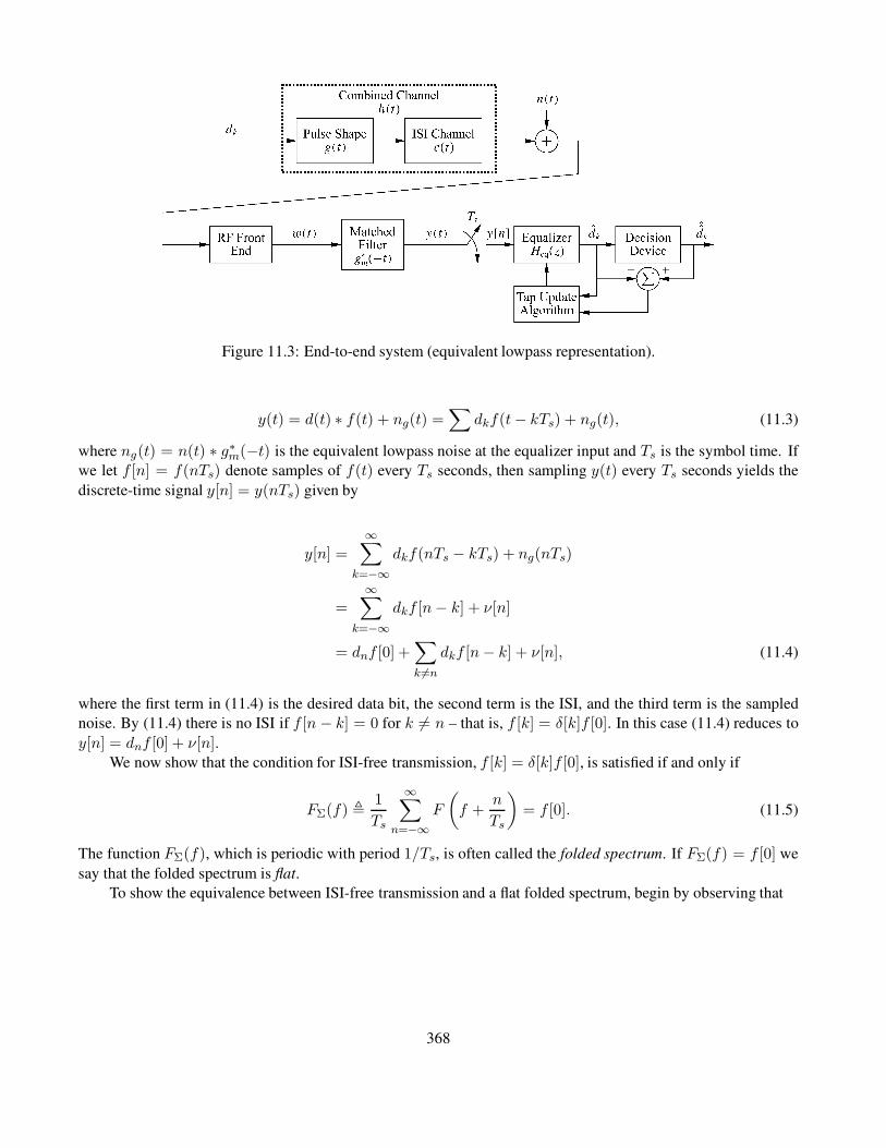
Figure 11.3: End-to-end system (equivalent lowpass representation).

y(t) = d(t) ∗ f(t) + ng(t) =∑

dkf(t− kTs) + ng(t), (11.3)

where ng(t) = n(t) ∗ g∗m(−t) is the equivalent lowpass noise at the equalizer input and Ts is the symbol time. If

we let f [n] = f(nTs) denote samples of f(t) every Ts seconds, then sampling y(t) every Ts seconds yields the

discrete-time signal y[n] = y(nTs) given by

y[n] =

∞∑

k=−∞

dkf(nTs − kTs) + ng(nTs)

=∞∑

k=−∞

dkf [n− k] + ν[n]

= dnf [0] +∑

k 6=n

dkf [n− k] + ν[n], (11.4)

where the first term in (11.4) is the desired data bit, the second term is the ISI, and the third term is the sampled

noise. By (11.4) there is no ISI if f [n − k] = 0 for k 6= n – that is, f [k] = δ[k]f [0]. In this case (11.4) reduces to

y[n] = dnf [0] + ν[n].We now show that the condition for ISI-free transmission, f [k] = δ[k]f [0], is satisfied if and only if

FΣ(f) ,1

Ts

∞∑

n=−∞

F

(

f +n

Ts

)

= f [0]. (11.5)

The function FΣ(f), which is periodic with period 1/Ts, is often called the folded spectrum. If FΣ(f) = f [0] we

say that the folded spectrum is flat.

To show the equivalence between ISI-free transmission and a flat folded spectrum, begin by observing that

368

f [k] = f(kTs) =

∫ ∞

−∞

F (f)ej2πfkTsdf

=∞∑

n=−∞

∫ .5(2n+1)/Ts

.5(2n−1)/Ts

F (f)ej2πfkTsdf

=∞∑

n=−∞

∫ .5/Ts

−.5/Ts

F

(

f ′ +n

Ts

)

ej2π(f ′+n/Ts)kTsdf ′

=

∫ .5/TS

−.5/TS

ej2πfkTs

[∞∑

n=−∞

F

(

f +n

Ts

)]

df. (11.6)

Equation (11.6) implies that the Fourier series representation of FΣ(f) is

FΣ(f) =1

Ts

∑

k

f [k]e−j2πfkTs .

We first demonstrate that a flat folded spectrum implies that f [k] = δ[k]f [0]. Suppose (11.5) is true. Then

substituting (11.5) into (11.6) yields

f [k] = Ts

∫ .5/TS

−.5/TS

ej2πfkTsf [0]df =sinπk

πkf [0] = δ[k]f [0], (11.7)

which is the desired result. We now show that f [k] = δ[k]f [0] implies a flat folded spectrum. By (11.6) and the

definition of FΣ(f),

f [k] = Ts

∫ .5/TS

−.5/TS

FΣ(f)ej2πfkTsdf. (11.8)

Hence f [k] is the inverse Fourier transform of FΣ(f)2. Therefore, if f [k] = δ[k]f [0] then FΣ(f) = f [0].

Example 11.2: Consider a channel with combined equivalent lowpass impulse response f(t) = sinc(t/Ts). Find

the folded spectrum and determine if this channel exhibits ISI.

Solution: The Fourier transform of f(t) is

F (f) = Ts rect(fTs) =

Ts |f | < .5/Ts,

.5Ts |f | = .5/Ts,

0 |f | > .5/Ts.

Therefore,

FΣ(f) =1

Ts

∞∑

n=−∞

F

(

f +n

Ts

)

= 1,

so the folded spectrum is flat and there is no ISI. We can also see this from the fact that

2This also follows from the Fourier series representation of FΣ(f).

369

f(nTs) = sinc

(nTsTs

)

= sinc(n) =

1 n = 0,

0 n 6= 0.

Thus, f [k] = δ[k], our equivalent condition for a flat folded spectrum and zero ISI.

11.4 Linear Equalizers

If FΣ(f) is not flat, we can use the equalizerHeq(z) in Figure 11.3 to reduce ISI. In this section we assume a linear

equalizer implemented via a 2L+ 1 = N -tap transversal filter:

Heq(z) =

L∑

i=−L

wiz−i. (11.9)

The length of the equalizer N is typically dictated by implementation considerations, since a large N entails more

complexity and delay. Causal linear equalizers have wi = 0 when i < 0. For a given equalizer sizeN , the equalizer

design must specify (i) the tap weights wiLi=−L for a given channel frequency response and (ii) the algorithm

for updating these tap weights as the channel varies. Recall that our performance metric in wireless systems is

probability of error (or outage probability), so for a given channel the optimal choice of equalizer coefficients

would be the coefficients that minimize probability of error. Unfortunately, it is extremely difficult to optimize

the wi with respect to this criterion. Since we cannot directly optimize for our desired performance metric, we

must instead use an indirect optimization that balances ISI mitigation with the prevention of noise enhancement,

as discussed with regard to the preceding simple analog example. We now describe two linear equalizers: the

zero-forcing (ZF) equalizer and the minimum mean-square error (MMSE) equalizer. The former equalizer cancels

all ISI but can lead to considerable noise enhancement. The latter technique minimizes the expected mean-squared

error between the transmitted symbol and the symbol detected at the equalizer output, thereby providing a better

balance between ISI mitigation and noise enhancement. Because of this more favorable balance, MMSE equalizers

tend to have better BER performance than equalizers using the ZF algorithm.

11.4.1 Zero-Forcing (ZF) Equalizers

From (11.4), the samples yn input to the equalizer can be represented based on the discretized combined equiv-

alent lowpass impulse response f(t) = h(t) ∗ g∗(−t) as

Y (z) = D(z)F (z) +Ng(z), (11.10)

where Ng(z) is the z-transform of the noise samples at the output of the matched filter G∗m(1/z∗) and

F (z) = H(z)G∗m

(1

z∗

)

=∑

n

f(nTs)z−n. (11.11)

The zero-forcing equalizer removes all ISI introduced in the composite response f(t). From (11.10) we see that

the equalizer to accomplish this is given by

HZF(z) =1

F (z). (11.12)

370

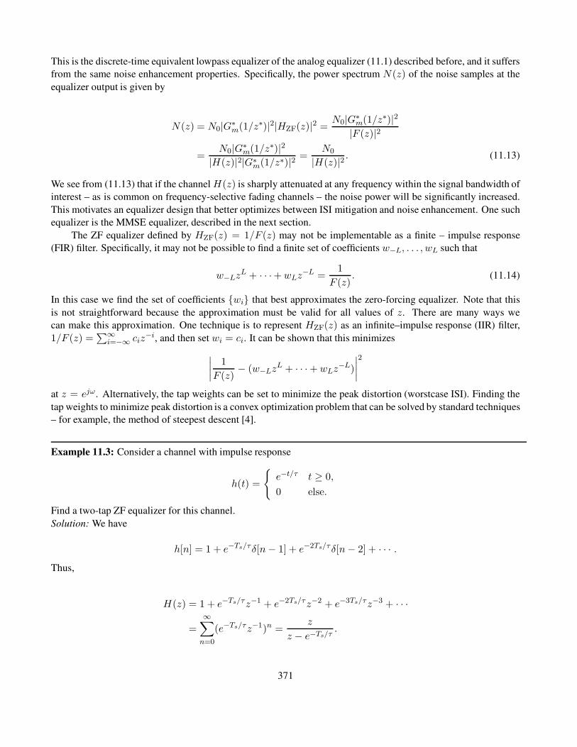
This is the discrete-time equivalent lowpass equalizer of the analog equalizer (11.1) described before, and it suffers

from the same noise enhancement properties. Specifically, the power spectrum N (z) of the noise samples at the

equalizer output is given by

N (z) = N0|G∗m(1/z∗)|2|HZF(z)|2 =

N0|G∗m(1/z∗)|2

|F (z)|2

=N0|G∗

m(1/z∗)|2|H(z)|2|G∗

m(1/z∗)|2 =N0

|H(z)|2 . (11.13)

We see from (11.13) that if the channel H(z) is sharply attenuated at any frequency within the signal bandwidth of

interest – as is common on frequency-selective fading channels – the noise power will be significantly increased.

This motivates an equalizer design that better optimizes between ISI mitigation and noise enhancement. One such

equalizer is the MMSE equalizer, described in the next section.

The ZF equalizer defined by HZF(z) = 1/F (z) may not be implementable as a finite – impulse response

(FIR) filter. Specifically, it may not be possible to find a finite set of coefficients w−L, . . . , wL such that

w−LzL + · · ·+wLz

−L =1

F (z). (11.14)

In this case we find the set of coefficients wi that best approximates the zero-forcing equalizer. Note that this

is not straightforward because the approximation must be valid for all values of z. There are many ways we

can make this approximation. One technique is to represent HZF(z) as an infinite–impulse response (IIR) filter,

1/F (z) =∑∞

i=−∞ ciz−i, and then set wi = ci. It can be shown that this minimizes

∣∣∣∣

1

F (z)− (w−Lz

L + · · ·+wLz−L)

∣∣∣∣

2

at z = ejω. Alternatively, the tap weights can be set to minimize the peak distortion (worstcase ISI). Finding the

tap weights to minimize peak distortion is a convex optimization problem that can be solved by standard techniques

– for example, the method of steepest descent [4].

Example 11.3: Consider a channel with impulse response

h(t) =

e−t/τ t ≥ 0,

0 else.

Find a two-tap ZF equalizer for this channel.

Solution: We have

h[n] = 1 + e−Ts/τδ[n− 1] + e−2Ts/τδ[n− 2] + · · · .Thus,

H(z) = 1 + e−Ts/τz−1 + e−2Ts/τz−2 + e−3Ts/τz−3 + · · ·

=

∞∑

n=0

(e−Ts/τz−1)n =z

z − e−Ts/τ.

371

Figure 11.4: MMSE equalizer with noise-whitening filter.

So Heq(z) = 1/H(z) = 1 − e−Ts/τz−1. The two-tap ZF equalizer therefore has tap weight coefficients w0 = 1and w1 = e−Ts/τ .

11.4.2 Minimum Mean-Square Error (MMSE) Equalizers

In MMSE equalization, the goal of the equalizer design is to minimize the average meansquare error (MSE)

between the transmitted symbol dk and its estimate dk at the output of the equalizer. In other words, the wi are

chosen to minimize E[dk − dk]2. Since the MMSE equalizer is linear, its output dk is a linear combination of the

input samples y[k]:

dk =L∑

i=−L

wiy[k − i]. (11.15)

As such, finding the optimal filter coefficients wi becomes a standard problem in linear estimation. In fact,

if the noise input to the equalizer is white then we have a standard Weiner filtering problem. However, because

of the matched filter g∗m(−t) at the receiver front end, the noise input to the equalizer is not white; rather, it is

colored with power spectrum N0|G∗m(1/z∗)|2. Therefore, in order to apply known techniques for optimal linear

estimation, we expand the filter Heq(z) into two components – a noise-whitening component 1/G∗m(1/z∗) and an

ISI-removal component Heq(z)− as shown in Figure 11.4.

The purpose of the noise-whitening filter (as the name indicates) is to whiten the noise so that the noise

component output from this filter has a constant power spectrum. Since the noise input to this filter has power

spectrumN0|G∗m(1/z∗)|2, the appropriate noise-whitening filter is 1/G∗

m(1/z∗). The noise power spectrum at the

output of the noise-whitening filter is then N0|G∗m(1/z∗)|2/|G∗

m(1/z∗)|2 = N0. Note that the filter 1/G∗m(1/z∗)

is not the only filter that will whiten the noise, and another noise-whitening filter with more desirable properties

(like stability) may be chosen. It might seem odd at first to introduce the matched filter g∗m(−t) at the receiver

front end only to cancel its effect in the equalizer. Recall, however, that the matched filter is meant to maximize

the SNR prior to sampling. By removing the effect of this matched filter via noise whitening after sampling, we

merely simplify the design of Heq(z) to minimize MSE. In fact, if the noise-whitening filter does not yield optimal

performance then its effect would be cancelled by the Heq(z) filter design, as we shall see in the case of IIR MMSE

equalizers.

372

We assume that the filter Heq(z), with input vn, is a linear filter with N = 2L+ 1 taps:

Heq(z) =L∑

i=−L

wiz−i. (11.16)

Our goal is to design the filter coefficients wi so as to minimize E[dk − dk]2. This is the same goal as for the

total filter Heq(z) – we just added the noise-whitening filter to make solving for these coefficients simpler. Define

vT = (v[k+L], v[k+ L− 1], . . . , v[k−L]) = (vk+L, vk+L−1, . . . , vk−L) as the row vector of inputs to the filter

Heq(z) used to obtain the filter output dk and define wT = (w−L . . . , wL) as the row vector of filter coefficients.

Then

dk = wTv = vTw. (11.17)

Thus, we want to minimize the mean-square error

J = E[dk − dk]2 = E[wTvvHw∗ − 2RevHw∗dk + |dk|2]. (11.18)

Define Mv = E[vvH ] and vd = E[vHdk]. The matrix Mv is an N ×N Hermitian matrix, and vd is a length-Nrow vector. Assume E|dk|2 = 1. Then the MSE J is

J = wTMvw∗ − 2 Revdw

∗+ 1. (11.19)

We obtain the optimal tap vector w by setting the gradient ∇wJ = 0 and solving for w. By (11.19), the

gradient is given by

∇wJ =

(∂J

∂w−L, . . . ,

∂J

∂wL

)

= 2wTMv − 2vd. (11.20)

Setting this to zero yields wTMv = vd or, equivalently, that the optimal tap weights are given by

wopt = (MTv)−1vTd . (11.21)

Note that solving for wopt requires a matrix inversion with respect to the filter inputs. Thus, the complexity of

this computation is quite high, typically on the order of N 2 to N 3 operations. Substituting in these optimal tap

weights, we obtain the minimum mean-square error as

Jmin = 1 − vdM−1v vHd . (11.22)

For an equalizer of infinite length, vT = (vn+∞, . . . , vn, . . . , vn−∞) and wT = (w−∞, . . . , w0, . . . , w∞).

Then wTMv = vd can be written as

∞∑

i=−∞

wi(f [j − i] +N0δ[j − i]) = g∗m[−j], −∞ ≤ j ≤ ∞ (11.23)

[5, Chap. 7.4]. Taking z-transforms and noting that Heq(z) is the z-transform of the filter coefficients w yields

Heq(z)(F (z) +N0) = G∗m(1/z∗). (11.24)

Solving for Heq(z), we obtain

Heq(z) =G∗m(1/z∗)

F (z) +N0. (11.25)

373

Since the MMSE equalizer consists of the noise-whitening filter 1/G∗m(1/z∗) plus the ISI removal component

Heq(z), it follows that the full MMSE equalizer (when it is not restricted to be finite length) becomes

Heq(z) =Heq(z)

G∗m(1/z∗)

=1

F (z) +N0. (11.26)

There are three interesting things to note about this result. First of all, the ideal infinitelength MMSE equalizer

cancels out the noise-whitening filter. Second, this infinite-length equalizer is identical to the ZF filter except for

the noise term N0, so in the absence of noise the two equalizers are equivalent. Finally, this ideal equalizer design

clearly shows a balance between inverting the channel and noise enhancement: if F (z) is highly attenuated at

some frequency, then the noise term N0 in the denominator prevents the noise from being significantly enhanced

by the equalizer. Yet at frequencies where the noise power spectral densityN0 is small compared to the composite

channel F (z), the equalizer effectively inverts F (z).

For the equalizer (11.26) it can be shown [5, Chap. 7.4.1] that the minimum MSE (11.22) can be expressed in

terms of the folded spectrum FΣ(f) as

Jmin = Ts

∫ .5/Ts

−.5/Ts

N0

FΣ(f) +N0df. (11.27)

This expression for MMSE has several interesting properties. First it can be shown that, as expected, 0 ≤ Jmin =

E[dk − dk]2 ≤ 1. In addition, Jmin = 0 in the absence of noise (N0 = 0) as long as FΣ(f) 6= 0 within the signal

bandwidth of interest. Also, as expected, Jmin = 1 if N0 = ∞.

Example 11.4: Find Jmin when the folded spectrum FΣ(f) is flat, FΣ(f) = f [0], in the asymptotic limit of high

and low SNR.

Solution: If FΣ = (f)[0]∆= f0 then

Jmin = Ts

∫ .5/Ts

−.5/Ts

N0

f0 +N0df =

N0

f0 +N0.

For high SNR, f0 N0 and so Jmin ≈ N0/f0 = N0/Es, where Es/N0 is the SNR per symbol. For low SNR,

N0 f0 and so Jmin = N0/(N0 + f0) ≈ N0/N0 = 1.

11.5 Maximum Likelihood Sequence Estimation

Maximum-likelihood sequence estimation avoids the problem of noise enhancement because it doesn’t use an

equalizing filter: instead it estimates the sequence of transmitted symbols. The structure of the MLSE is the same

as in Figure 11.3, except that the equalizerHeq(z) and decision device are replaced by the MLSE algorithm. Given

the combined pulse-shaping filter and channel responseh(t), the MLSE algorithm chooses the input sequence dkthat maximizes the likelihood of the received signal w(t). We now investigate this algorithm in more detail.

Using a Gram–Schmidt orthonormalization procedure, we can express w(t) on a time interval [0, LTs] as

w(t) =N∑

n=1

wnφn(t), (11.28)

where φn(t) form a complete set of orthonormal basis functions. The number N of functions in this set is a

function of the channel memory, since w(t) on [0, LTs] depends on d0, . . . , dL. With this expansion we have

374

wn =

∞∑

k=−∞

dkhnk + νn =

L∑

k=0

dkhnk + νn, (11.29)

where

hnk =

∫ LTs

0

h(t− kTs)φ∗n(t) dt (11.30)

and

νn =

∫ LTs

0

n(t)φ∗n(t) dt. (11.31)

The νn are complex Gaussian random variables with mean zero and covariance .5 E[ν∗nνm] = N0δ[n−m]. Thus,

wN = (w1, . . . , wN) has a multivariate Gaussian distribution:

p(wN |dL, h(t)) =

N∏

n=1

1

πN0exp

− 1

N0

∣∣∣∣∣wn −

L∑

k=0

dkhnk

∣∣∣∣∣

2

. (11.32)

Given a received signal w(t) or, equivalently, wN , the MLSE decodes this as the symbol sequence dL that

maximizes the likelihood function p(wN |dL, h(t)) (or the log of this function). That is, the MLSE outputs the

sequence

dL = argmax[log p(wN |dL, h(t))]

= argmax

−N∑

n=1

∣∣∣∣∣wn −

∑

k

dkhnk

∣∣∣∣∣

2

= argmax

[

−N∑

n=1

|wn|2 +

N∑

n=1

(

w∗n

∑

k

dkhnk + wn∑

k

d∗kh∗nk

)

−N∑

n=1

(∑

k

dkhnk

)(∑

m

d∗mh∗nm

)]

= argmax

[

2 Re

∑

k

d∗k

N∑

n=1

wnh∗nk

−∑

k

∑

m

dkd∗m

N∑

n=1

hnkh∗nm

]

. (11.33)

Note that

N∑

n=1

wnh∗nk =

∫ ∞

−∞w(τ)h∗(τ − kTs) dτ = y[k] (11.34)

and

N∑

n=1

hnkh∗nm =

∫ ∞

−∞h(τ − kTs)h

∗(τ −mTs) dτ = f [k −m]. (11.35)

Combining (11.33), (11.34), and (11.35), we have that

375

dL = argmax

[

2 Re

∑

k

d∗ky[k]

−∑

k

∑

m

dkd∗mu[k −m]

]

. (11.36)

We see from this equation that the MLSE output depends only on the sampler output y[k] and the channel

parameters u[n − k] = u(nTs − kTs), where u(t) = h(t) ∗ h∗(−t). Because the derivation of the MLSE is

based on the channel outputw(t) only (prior to matched filtering), our derivation implies that the receiver matched

filter in Figure 11.3 with gm(t) = h(t) is optimal for MLSE detection (typically the matched filter is optimal for

detecting signals in AWGN, but this derivation shows that it is also optimal for detecting signals in the presence of

ISI if MLSE is used).

The Viterbi algorithm can be used for MLSE to reduce complexity [4, 5, 6, 7]. However, the complexity

of this equalization technique still grows exponentially with the channel delay spread. A nonlinear equalization

technique with significantly less complexity is decision feedback equalization.

Figure 11.5: Decision-feedback equalizer structure.

11.6 Decision-Feedback Equalization

The DFE consists of a feedforward filter W (z) with the received sequence as input (similar to the linear equalizer)

followed by a feedback filter V (z) with the previously detected sequence as input. The DFE structure is shown in

Figure 11.5. In effect, the DFE determines the ISI contribution from the detected symbols ˆdk by passing them

through a feedback filter that approximates the composite channel F (z) convolved with the feedforward filter

W (z). The resulting ISI is then subtracted from the incoming symbols. Since the feedback filter V (z) in Figure

11.5 sits in a feedback loop, it must be strictly causal or else the system is unstable. The feedback filter of the

DFE does not suffer from noise enhancement because it estimates the channel frequency response rather than its

inverse. For channels with deep spectral nulls, DFEs generally perform much better than linear equalizers.

Assuming that W (z) has N1 + 1 taps and V (z) has N2 taps, we can write the DFE output as

dk =

0∑

i=−N1

wiy[k − i] −N2∑

i=1

viˆdk−i.

The typical criteria for selecting the coefficients for W (z) and V (z) are either zero-forcing (remove all ISI) or

MMSE (minimize expected MSE between the DFE output and the original symbol). We will assume that the

matched filter in the receiver is perfectly matched to the channel: gm(t) = h(t). With this assumption, in or-

der to obtain a causal filter for V (z), we require a spectral factorization of H(z)G∗m(1/z∗) = H(z)H∗(1/z∗)

[4, Chap. 10.1.2]. Specifically,H(z)H∗(1/z∗) is factorized by finding a causal filterB(z) such thatH(z)H∗(1/z∗) =

376

B(z)B∗(1/z∗) = λ2B1(z)B∗1(1/z∗), where B1(z) is normalized to have a leading coefficient of 1. With this fac-

torization, when bothW (z) and V (z) have infinite duration, it was shown by Price [8] that the optimal feedforward

and feedback filters for a zero-forcing DFE are (respectively) W (z) = 1/λ2B∗1(1/z∗) and V (z) = 1 −B1(z).

For the MMSE criterion, we wish to minimize E[dk − dk]2. Let bn = b[n] denote the inverse z-transform

of B(z) given the spectral factorization H(z)H∗(1/z∗) = B(z)B∗(1/z∗) just described. Then the MMSE mini-

mization yields that the coefficients of the feedforward filter must satisfy the following set of linear equations:

0∑

i=−N1

qliwi = b∗−l

for qli =∑0

j=−l b∗jbj+l−i +N0δ[l − i] with i = −N1, . . . , 0 [4, Chap. 10.3.1]. The coefficients of the feedback

filter are then determined from the feedforward coefficients by

vk = −0∑

i=−N1

wibk−i.

These coefficients completely eliminate ISI when there are no decision errors – that is, whenˆdk = dk. It was

shown by Salz [9] that the resulting minimum MSE is

Jmin = exp

[

Ts

∫ .5/Ts

−.5/Ts

ln

[N0

FΣ(f) +N0

]

df

]

.

In general, the MMSE associated with a DFE is much lower than that of a linear equalizer, assuming the impact of

feedback errors is ignored.

Decision-feedback equalizers exhibit feedback errors ifˆdk 6= dk, since the ISI subtracted from the feedback

path is not the true ISI corresponding to dk. Such errors therefore propagate to later bit decisions. Moreover, this

error propagation cannot be improved through channel coding, since the feedback path operates on coded channel

symbols before decoding. This is because the ISI must be subtracted immediately, which doesn’t allow for any

decoding delay. Hence the error propagation seriously degrades performance on channels with low SNR. We can

address this problem by introducing some delay in the feedback path to allow for channel decoding [10] or by

turbo equalization, described in the next section. A systematic treatment of the DFE with coding can be found in

[11, 12]. Moreover, the DFE structure can be generalized to encompass MIMO channels [13].

11.7 Other Equalization Methods

Although MLSE is the optimal form of equalization, its complexity precludes widespread use. There has been

much work on reducing the complexity of the MLSE [4, Chap. 10.4]. Most techniques either reduce the number

of surviving sequences in the Viterbi algorithm or reduce the number of symbols spanned by the ISI through

preprocessing or decision-feedback in the Viterbi detector. These reduced-complexity MLSE equalizers have better

performance-complexity trade-offs than symbol-by-symbol equalization techniques, and they achieve performance

close to that of the optimal MLSE with significantly less complexity.

The turbo decoding principle introduced in Section 8.5 can also be used in equalizer design [14, 15]. The

resulting design is called a turbo equalizer. A turbo equalizer iterates between a maximum a posteriori (MAP)

equalizer and a decoder to determine the transmitted symbol. The MAP equalizer computes the a posteriori prob-

ability (APP) of the transmitted symbol given the past channel outputs. The decoder computes the log likelihood

ratio (LLR) associated with the transmitted symbol given past channel outputs. The APP and LLR comprise

377

the soft information exchanged between the equalizer and decoder in the turbo iteration. After some number of

iterations, the turbo equalizer converges on its estimate of the transmitted symbol.

If the channel is known at the transmitter, then the transmitter can pre-equalize the transmitted signal by

passing it through a filter that effectively inverts the channel frequency response. Since the channel inversion occurs

in the transmitter rather than the receiver, there is no noise enhancement. It is difficult to pre-equalize in a time-

varying channel because the transmitter must have an accurate estimate of the channel, but this approach is practical

to implement in relatively static wireline channels. One problem is that the channel inversion often increases the

dynamic range of the transmitted signal, which can result in distortion or inefficiency from the amplifier. This

problem has been addressed through a precoding technique called Tomlinson–Harashima precoding [16, 17].

11.8 Adaptive Equalizers: Training and Tracking

All of the equalizers described so far are designed based on a known value of the combined impulse response

h(t) = g(t) ∗ c(t). Since the channel c(t) in generally not known when the receiver is designed, the equalizer

must be tunable so it can adjust to different values of c(t). Moreover, since in wireless channels c(t) = c(τ, t)

will change over time, the system must periodically estimate the channel c(t) and update the equalizer coefficients

accordingly. This process is called equalizer training or adaptive equalization [18, 19]. The equalizer can also

use the detected data to adjust the equalizer coefficients, a process known as equalizer tracking. However, blind

equalizers do not use training: they learn the channel response via the detected data only [20, 21, 22, 23].

During training, the coefficients of the equalizer are updated at time k based on a known training sequence

[dk−M , . . . , dk] that has been sent over the channel. The length M + 1 of the training sequence depends on the

number of equalizer coefficients that must be determined and the convergence speed of the training algorithm.

Note that the equalizer must be retrained when the channel decorrelates – that is, at least every Tc seconds, where

Tc is the channel coherence time. Thus, if the training algorithm is slow relative to the channel coherence time

then the channel may change before the equalizer can learn the channel. Specifically, if (M + 1)Ts > Tc then

the channel will decorrelate before the equalizer has finished training. In this case equalization is not an effective

countermeasure for ISI, and some other technique (e.g., multicarrier modulation or CDMA) is needed.

Let dk denote the bit decisions output from the equalizer given a transmitted training sequence dk. Our

goal is to update the N equalizer coefficients at time k + 1 based on the training sequence we have received up to

time k. We denote these updated coefficients as w−L(k + 1), . . . , wL(k + 1). We will use the MMSE as our

criterion to update these coefficients; that is, we will choose w−L(k+ 1), . . . , wL(k+ 1) as the coefficients that

minimize the MSE between dk and dk. Recall that dk =∑L

i=−L wi(k + 1)yk−i, where yk = y[k] is the output of

the sampler in Figure 11.3 at time k with the known training sequence as input. The w−L(k+1), . . . , wL(k+1)that minimize MSE are obtained via a Weiner filter [4, 5]. Specifically,

w(k + 1) = w−L(k + 1), . . . , wL(k + 1) = R−1p, (11.37)

where p = dk[yk+L . . . yk−L]T and

R =

|yk+L|2 yk+Ly∗k+L−1 · · · yk+Ly

∗k−L

yk+L−1y∗k+L |yk+L−1|2 · · · yk+L−1Y∗

k−L

.... . .

. . ....

yk−Ly∗k+L · · · · · · |yk−L|2

. (11.38)

Note that finding the optimal tap updates in this case requires a matrix inversion, which requires N 2 to N 3 mul-

tiply operations on each iteration (each symbol time Ts). In exchange for its complexity, the convergence of this

algorithm is very fast; it typically converges in around N symbol times forN the number of equalizer tap weights.

378

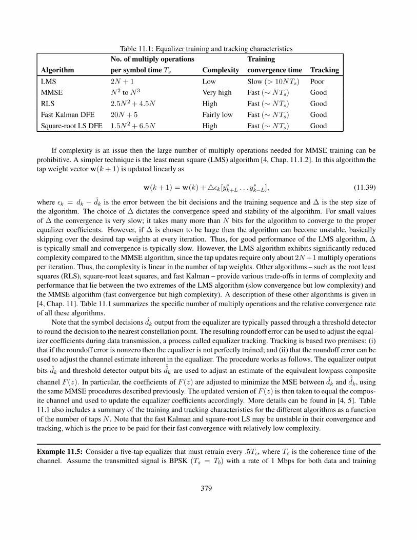
Table 11.1: Equalizer training and tracking characteristics

No. of multiply operations Training

Algorithm per symbol time Ts Complexity convergence time Tracking

LMS 2N + 1 Low Slow (> 10NTs) Poor

MMSE N 2 to N 3 Very high Fast (∼ NTs) Good

RLS 2.5N 2 + 4.5N High Fast (∼ NTs) Good

Fast Kalman DFE 20N + 5 Fairly low Fast (∼ NTs) Good

Square-root LS DFE 1.5N 2 + 6.5N High Fast (∼ NTs) Good

If complexity is an issue then the large number of multiply operations needed for MMSE training can be

prohibitive. A simpler technique is the least mean square (LMS) algorithm [4, Chap. 11.1.2]. In this algorithm the

tap weight vector w(k + 1) is updated linearly as

w(k+ 1) = w(k) + 4εk[y∗k+L . . . y∗k−L], (11.39)

where εk = dk − dk is the error between the bit decisions and the training sequence and ∆ is the step size of

the algorithm. The choice of ∆ dictates the convergence speed and stability of the algorithm. For small values

of ∆ the convergence is very slow; it takes many more than N bits for the algorithm to converge to the proper

equalizer coefficients. However, if ∆ is chosen to be large then the algorithm can become unstable, basically

skipping over the desired tap weights at every iteration. Thus, for good performance of the LMS algorithm, ∆is typically small and convergence is typically slow. However, the LMS algorithm exhibits significantly reduced

complexity compared to the MMSE algorithm, since the tap updates require only about 2N+1 multiply operations

per iteration. Thus, the complexity is linear in the number of tap weights. Other algorithms – such as the root least

squares (RLS), square-root least squares, and fast Kalman – provide various trade-offs in terms of complexity and

performance that lie between the two extremes of the LMS algorithm (slow convergence but low complexity) and

the MMSE algorithm (fast convergence but high complexity). A description of these other algorithms is given in

[4, Chap. 11]. Table 11.1 summarizes the specific number of multiply operations and the relative convergence rate

of all these algorithms.

Note that the symbol decisions dk output from the equalizer are typically passed through a threshold detector

to round the decision to the nearest constellation point. The resulting roundoff error can be used to adjust the equal-

izer coefficients during data transmission, a process called equalizer tracking. Tracking is based two premises: (i)

that if the roundoff error is nonzero then the equalizer is not perfectly trained; and (ii) that the roundoff error can be

used to adjust the channel estimate inherent in the equalizer. The procedure works as follows. The equalizer output

bits dk and threshold detector output bitsˆdk are used to adjust an estimate of the equivalent lowpass composite

channel F (z). In particular, the coefficients of F (z) are adjusted to minimize the MSE between dk andˆdk, using

the same MMSE procedures described previously. The updated version of F (z) is then taken to equal the compos-

ite channel and used to update the equalizer coefficients accordingly. More details can be found in [4, 5]. Table

11.1 also includes a summary of the training and tracking characteristics for the different algorithms as a function

of the number of taps N . Note that the fast Kalman and square-root LS may be unstable in their convergence and

tracking, which is the price to be paid for their fast convergence with relatively low complexity.

Example 11.5: Consider a five-tap equalizer that must retrain every .5Tc, where Tc is the coherence time of the

channel. Assume the transmitted signal is BPSK (Ts = Tb) with a rate of 1 Mbps for both data and training

379

sequence transmission. Compare the length of training sequence required for the LMS equalizer versus the fast

Kalman DFE. For an 80-Hz Doppler, by how much is the data rate reduced in order to enable periodic training for

each of these equalizers? How many operations do these two equalizers require for this training?

Solution: The equalizers must retrain every .5Tc = .5/Bd = .5/80 = 6.25 ms. For a data rate of Rb = 1/Tb = 1Mbps, Table 11.1 shows that the LMS algorithm requires 10NTb = 50 · 10−6 seconds for training to converge

and the fast Kalman DFE requires NTb = 50 · 10−5 seconds. If training occurs every 6.25 ms then the fraction of

time the LMS algorithm uses for training is 50 · 10−6/6.25 · 10−3 = .008. Thus, the effective data rate becomes

(1 − .008)Rb = .992 Mbps. The fraction of time used by the fast Kalman DFE for training is 50·10−5/6.25 ·10−3 = .0008, resulting in an effective data rate of (1 − .0008)Rb = .9992 Mbps. The LMS algorithm requires

approximately (2N + 1) · 10N = 550 operations for training per training period, whereas the fast Kalman DFE

requires (20N + 5) ·N = 525 operations. With processor technology today, this is not a significant difference in

terms of CPU requirements.

380

Chapter 11 Problems

1. Design a continuous-time equivalent lowpass equalizer Heq(f) to completely remove the ISI introduced by

a channel with equivalent lowpass impulse response H(f) = 1/f . Assume your transmitted signal has a

bandwidth of 100 kHz. Assuming a channel with equivalent lowpass AWGN of PSD N0, find the noise

power at the output of your equalizer within the 100-kHz bandwidth of interest. Will this equalizer improve

system performance?

2. This problem investigates the interference generated by ISI and the noise enhancement that occurs in zero-

forcing equalization. Consider two multipath channels: the first channel has impulse response

h1(t) =

1 0 ≤ t < Tm,

0 else;

the second channel has impulse response

h2(t) = e−t/Tm, 0 ≤ t <∞.

(a) Assume that the transmitted signal s(t) is an infinite sequence of impulses with amplitude A and time

separation Tb = Tm/2; that is, s(t) =∑∞

n=−∞ Aδ(t− nTb). Calculate the average ISI power over a

bit time Tb.

(b) Let Tm = 10 µs. Suppose a BPSK signal is transmitted over a channel with impulse response h1(t).

Find the maximum data rate that can be sent over the channel with zero ISI under BPSK modulation

with rectangular pulse shaping of pulse width T = 1 µs. How would this answer change if the signal

bandwidth were restricted to 100 kHz?

3. Consider a channel with equivalent lowpass impulse response

h(t) =

e−t/τ t ≥ 0,

0 else,

where τ = 6 µs. The channel also has equivalent lowpass AWGN with power spectral densityN0.

(a) What is the frequency response of the equivalent lowpass continuous-time ZF linear equalizer for this

channel? Assume no matched filter or pulse shaping.

(b) Suppose we transmit a 30-kHz signal over this channel, and assume that the frequency response of

the signal is a rectangular pulse shape. What is the ratio of SNR with equalization to SNR without

equalization in the bandwidth of our transmitted signal? Hint: Recall that a stationary random process

with power spectral density P (f) has total power∫P (f)df and that, if this process is passed through

a filter G(f), then the output process has power spectral density P (f)|G(f)|2.

(c) Approximate the equivalent lowpass MMSE equalizer for this channel using a discrete-time transversal

filter with three taps. Use any method you like as long as it reasonably approximates the time-domain

response of the MMSE equalizer.

381

4. Consider an FIR ZF equalizer with tap weights wi = ci, where ci is the inverse z-transform of 1/F (z).

Show that this choice of tap weights minimizes

∣∣∣∣

1

F (z)− (w0 +w1z

−1 + · · ·+ wNz−N )

∣∣∣∣

2

at z = ejω.

5. Consider a communication system where the modulated signal s(t) has power 10 mW, carrier frequency fc,and passband bandwidthBs = 40 MHz. The signal s(t) passes through a frequency-selective fading channel

with symmetric frequency response H(f) = H(−f), where

H(f) =

1 fc − 20 MHz ≤ f < fc − 10 MHz,

.5 fc − 10 MHz ≤ f < fc,

2 fc ≤ f < fc + 10 MHz,

.25 fc + 10 MHz ≤ f < fc + 20 MHz,

0 else.

The received signal is y(t) = s(t) ∗ h(t) + n(t), where n(t) is AWGN with PSD N0/2 = 10−12 W/Hz.

(a) Suppose y(t) is passed through a continuous-time (passband) ZF equalizer. Find the frequency re-

sponseHeq(f) for this equalizer within the bandwidth of interest (fc ± 20 MHz).

(b) For the equalizer of part (a), find the SNR at the equalizer output.

(c) Suppose the symbol time for s(t) is Ts = .5/Bs and assume no restrictions on the constellation size.

Find the maximum data rate that can be sent over the channel with the ZF equalizer of part (a) such

that Pb < 10−3.

6. Consider an ISI channel with received signal after transmission through the channel given by

y(t) =∞∑

i=−∞

xif(t− iT ),

where xi = ±1 and f(t) is the composite impulse response consisting of the pulse-shaping filter, the equiv-

alent lowpass channel, and the receiver matched filter. Assume that f(t) = sin(πt/T )/(πt/T ), which

satisfies the Nyquist criterion for zero ISI. There are two difficulties with this pulse shape: first, it has a

rectangular spectrum, which is difficult to implement in practice. Second, the tails of the pulse decay as 1/t,

so timing error leads to a sequence of ISI samples that do not converge. For parts (b) and (c) of this problem

we make the assumption that f(t) = 0 for |t| > NT , where N is a positive integer. This is not strictly

correct, since it would imply that f(t) is both time limited and bandlimited. However, it is a reasonable

approximation in practice.

(a) Show that the folded spectrum of f(t) is flat.

(b) Suppose that (because of timing error) the signal is sampled at t = kT + t0, where t0 < T . Calculate

the response yk = y(kT + t0) and separate your answer into the desired term and the ISI terms.

382

(c) Assume that the polarities of the xi are such that every term in the ISI is positive (worst-case ISI).

Under this assumption, show that the ISI term from part (b) is

ISI ≈ 2

πsin

(πt0T

) N∑

n=1

n

n2 − t20/T2

and therefore ISI → ∞ as N → ∞.

7. Let g(t) = sinc(t/Ts), |t| < Ts. Find the matched filter gm(t) for g(t). Find the noise-whitening filter

1/G∗m(1/z∗) for this system that must be used in an MMSE equalizer to whiten the noise.

8. Show that the minimum MSE (11.22) for an IIR MMSE equalizer can be expressed in terms of the folded

spectrum FΣ(f) as

Jmin = T

∫ .5/T

−.5/T

N0

FΣ(f) +N0df.

9. Show that the gradient of tap weights associated with the MMSE equalizer is given by

∇wJ =

(∂J

∂w0, . . . ,

∂J

∂wN

)

= 2wTMv − 2vd.

Set this equal to zero and solve for the optimal tap weights to obtain

wopt = (MTv )−1vHd .

10. Show that the MMSE Jmin for an IIR MMSE equalizer, given by (11.27), satisfies 0 ≤ Jmin ≤ 1.

11. Compare the value of the minimum MSE, Jmin, under both MMSE equalization and DF equalization for a

channel with three-tap discrete-time equivalent model C(z) = 1 + .5z−1 + .3z−2.

12. This problem illustrates (i) the noise enhancement of zero-forcing equalizers and (ii) how this enhancement

can be mitigated using an MMSE approach. Consider a frequency-selective fading channel with equivalent

lowpass frequency response

H(f) =

1 0 ≤ |f | < 10 kHz,

1/2 10kHz ≤ |f | < 20 kHz,

1/3 20kHz ≤ |f | < 30 kHz,

1/4 30kHz ≤ |f | < 40 kHz,

1/5 40kHz ≤ |f | < 50 kHz,

0 else.

.

The frequency response is symmetric in positive and negative frequencies. Assume an AWGN channel with

equivalent lowpass noise PSD N0 = 10−9.

(a) Find a ZF analog equalizer that completely removes the ISI introduced by H(f).

383

(b) Find the total noise power at the output of the equalizer from part (a).

(c) Assume an MMSE analog equalizer of the form Heq(f) = 1/(H(f) + α). Find the total noise power

at the output of this equalizer for an AWGN input with PSD N0 for α = .5 and for α = 1.

(d) Describe qualitatively two effects on a signal that is transmitted over channel H(f) and then passed

through the MMSE equalizerHeq(f) = 1/(H(f)+α) withα > 0. What design considerations should

go into the choice of α?

(e) What happens to the total noise power for the MMSE equalizer in part (c) as α → ∞? What is the

disadvantage of letting α→ ∞ in this equalizer design?

(f) For the equalizer design of part (c), suppose the system has a data rate of 100 kbps and that your

equalizer requires a training sequence of 1000 bits to train. What is the maximum channel Doppler

such that the equalizer coefficients converge before the channel decorrelates?

13. Why does an equalizer that tracks the channel during data transmission still need to train periodically?

Specify two benefits of tracking.

14. Assume a four-tap equalizer that must retrain every .5Tc, where Tc is the channel coherence time. If a digital

signal processing chip can perform 10 million multiplications per second and if the convergence rates for

the LMS DFE algorithm and the RLS algorithm are, respectively, 1000 iterations (symbol times) and 50

iterations, then what is the maximum data rate for both equalizers assuming BPSK modulation and Doppler

spread BD = 100 Hz? For BD = 1000 Hz? Assume that the transmitting speed is equal for training and

information sequences.

15. In this problem we seek the procedure for updating the channel estimate during tracking. Find the formula

for updating the channel coefficients corresponding to the channel H(z) based on minimizing the MSE

between dk andˆdk.

16. Ultrawideband (UWB) systems spread a data signal and its corresponding power over a very wide bandwidth

so that the power per hertz of the signal is small (typically below the noise floor). Hence such systems coexist

with other systems without causing them much interference. Consider a baseband UWB system with BPSK

modulation. The data bits are modulated with a rectangular pulse g(t), where g(t) has a very narrow time

duration T as compared to the bit time Tb. For this problem we assume T = 10−9. Thus, a UWB signal with

BPSK modulation would have the form s(t) =∑

n dng(t− nTb), where dn takes the value ±1 and Tb T

is the bit time. A sketch of s(t) with a data sequence of alternating 1-bits and 0-bits is shown in Figure 11.6.

Figure 11.6: UWB signal form for Problem 11-16.

(a) What is the approximate bandwidth of s(t) if Tb = 10−5?

(b) One of the selling points of UWB is that its signals do not experience flat fading in typical channels.

Consider a single-bit transmission s(t) = d0g(t). Suppose s(t) is transmitted through a channel that

follows a two-ray model h(t) = α0δ(t)+α1δ(t−τ). Sketch the channel output for τ T and τ T .

Which of your two sketches is more likely to depict the output of a real wireless channel? Why does

this imply that UWB signals don’t typically experience flat fading?

384

(c) Consider a channel with a multipath delay spread of Tm = 20 µs. For Figure 11.6, what is the exact

maximum data rate that can be sent over this channel with no ISI? Is the bandwidth of s(t) in the figure

less than the channel coherence bandwidth at this data rate?

(d) Let F (z) = α0 + α1z−1 + α2z

−2 denote the composite impulse response of the transmitter, channel,

and matched filter in this UWB system. Find a two-tap digital equalizer Heq(z) = w0 + w1z−1 that

approximates an IIR zero-forcing equalizer for F (z). Any reasonable approximation is fine as long as

you can justify it.

(e) For the equalizer designed in part (d), suppose the system has a data rate of 100 kbps and that your

equalizer requires a training sequence of 1000 bits to train. What is the maximum channel Doppler

such that the equalizer coefficients converge before the channel decorrelates?

385

Bibliography

[1] E. H. Satorius and S. T. Alexander, “Channel equalization using adaptive lattice algorithms,” IEEE Trans.

Commun., pp. 899–905, June 1979.

[2] F. Ling and J. Proakis, “Adaptive lattice decision feedback equalizers – Their performance and application to

time-variant multipath channels,” IEEE Trans. Commun., pp. 348–56, April 1985.

[3] J. Cioffi and T. Kailath, “Fast, recursive-least-squares transversal filters for adaptive filtering,” IEEE Trans.

Signal Proc., pp. 304–37, April 1984.

[4] J. G. Proakis, Digital Communications, 4th ed., McGraw-Hill, New York, 2001.

[5] G. L. Stuber, Principles of Mobile Communications, 2nd ed., Kluwer, Dordrecht, 2001.

[6] G. D. Forney, Jr., “Maximum-likelihood sequence estimation of digital sequences in the presence of inter-

symbol interference,” IEEE Trans. Inform. Theory, pp. 363–78, May 1972.

[7] B. Sklar, “How I learned to love the trellis,” IEEE Signal Proc. Mag., pp. 87–102, May 2003.

[8] R. Price, “Nonlinearly feedback-equalized PAM vs. capacity,” Proc. IEEE Internat. Conf. Comun., pp. 22.12–

22.17, June 1972.

[9] J. Salz, “Optimum mean-square decision feedback equalization,” Bell System Tech. J ., pp. 1341–73, October

1973.

[10] M. V. Eyuboglu, “Detection of coded modulation signals on linear, severely distorted channels using decision-

feedback noise prediction with interleaving,” IEEE Trans. Commun., pp. 401–9, April 1988.

[11] J. M. Cioffi, G. P. Dudevoir, V. Eyuboglu, and G. D. Forney, Jr., “MMSE decision-feedback equalizers and

coding. Part I: Equalization results,” IEEE Trans. Commun., pp. 2582–94, October 1995.

[12] J. M. Cioffi, G. P. Dudevoir, V. Eyuboglu, and G. D. Forney, Jr., “MMSE decision-feedback equalizers and

coding. Part II: Coding results,” IEEE Trans. Commun., pp. 2595–2604, October 1995.

[13] J. M. Cioffi and G. D. Forney, Jr., “Generalized decision-feedback equalization for packet transssion with ISI

and Gaussian noise,” in A. Paulraj, V. Roychowdhury, and C. Schaper (Eds.), Communication, Computation,

Control, and Signal Processing, pp. 79–127, Kluwer, Boston, 1997.

[14] C. Douillard, M. Jezequel, C. Berrou, A. Picart, P. Didier, and A. Glavieux, “Iterative correcon of intersymbol

interference: Turbo equalization,” Euro. Trans. Telecommun., pp. 507–11, September/October 1995.

[15] M. Tuchler, R. Koetter, and A. C. Singer, “Turbo equalization: Principles and new results,” IEEE Trans.

Commun., pp. 754–67, May 2002.

386

[16] M. Tomlinson, “A new automatic equalizer emplying modulo arithmetic,” Elec. Lett., 7, pp. 138–9, 1971.

[17] H. Harashima and H. Miyakawa, “Matched-transmission techniques for channels with intersymbol interfer-

ence,” IEEE Trans. Commun., pp. 774–80, August 1972.

[18] J. G. Proakis, “Adaptive equalization for TDMA digital mobile radio,” IEEE Trans. Veh. Tech., pp. 333–41,

May 1991.

[19] S. U. Qureshi, “Adaptive equalization,” Proc. IEEE, pp. 1349–87, September 1985.

[20] A. Benveniste and M. Goursat, “Blind equalizers,” IEEE Trans. Commun., pp. 871–83, August 1984.

[21] C. R. Johnson Jr., “Admissibility in blind adaptive channel equalization,” IEEE Control Syst. Mag., pp. 3–15,

January 1991.

[22] R. Johnson, P. Schniter, T. J. Endres, J. D. Behm, D. R. Brown, and R. A. Casas, “Blind equalation using the

constant modulus criterion: A review,” Proc. IEEE, pp. 1927–50, October 1998.

[23] L. Tong, G. Zu, and T. Kailath, “Blind identification and equalization based on second-order statistics: A

time domain approach,” IEEE Trans. Inform. Theory, pp. 340–9, March 1994.

387

Chapter 12

Multicarrier Modulation

The basic idea of multicarrier modulation is to divide the transmitted bitstream into many different substreams and

send these over many different subchannels. Typically the subchannels are orthogonal under ideal propagation

conditions. The data rate on each of the subchannels is much less than the total data rate, and the corresponding

subchannel band-width is much less than the total system bandwidth. The number of substreams is chosen to

ensure that each subchannel has a bandwidth less than the coherence bandwidth of the channel, so the subchannels

experience relatively flat fading. Thus, the intersymbol interference on each subchannel is small. The subchannels

in multicarrier modulation need not be contiguous, so a large continuous block of spectrum is not needed for high-

rate multicarrier communications. Moreover, multicarrier modulation is efficiently implemented digitally. In this

discrete implementation, called orthogonal frequency division multiplexing (OFDM), the ISI can be completely

eliminated through the use of a cyclic prefix.

Multicarrier modulation is currently used in many wireless systems. However, it is not a new technique: it

was first used for military HF radios in the late 1950s and early 1960s. Starting around 1990 [1], multicarrier

modulation has been used in many diverse wired and wireless applications, including digital audio and video

broadcasting in Europe [2], digital subscriber lines (DSL) using discrete multitone [3, 4, 5], and the most recent

generation of wireless LANs [5, 6, 7]. There are also a number of newly emerging uses for multicarrier techniques,

including fixed wireless broadband services [8, 9], mobile wireless broadband known as FLASH-OFDM [10], and

even for ultrawideband radios, where multiband OFDM is one of two competing proposals for the IEEE 802.15

ultrawideband standard. Multicarrier modulation is also a candidate for the air interface in next-generation cellular

systems [11, 12].

The multicarrier technique can be implemented in multiple ways, including vector coding [13, 14] and OFDM

[13, 15], all of which are discussed in this chapter. These techniques have subtle differences, but all are based on

the same premise of breaking a wideband channel into multiple parallel narrowband channels by means of an

orthogonal channel partition.

There is some debate as to whether multicarrier or single-carrier modulation is better for ISI channels with

delay spreads on the order of the symbol time. It is claimed in [2] that, for some mobile radio applications, single-

carrier modulation with equalization has roughly the same performance as multicarrier modulation with channel

coding, frequency-domain interleaving, and weighted maximum likelihood decoding. Adaptive loading was not

taken into account in [2], though it has the potential to significantly improve multicarrier performance [16]. But

there are other problems with multicarrier modulation that impair its performance, most significantly frequency

offset and timing jitter, which degrade the orthogonality of the subchannels. In addition, the peak-to-average

power ratio of multicarrier systems is significantly higher than that of single-carrier systems, which is a serious

problem when nonlinear amplifiers are used. Trade-offs between multicarrier and single-carrier block transmission

systems with respect to these impairments are discussed in [17].

388

Despite these challenges, multicarrier techniques are common in high–data-rate wireless systems with mod-

erate to large delay spread, as they have significant advantages over time-domain equalization. In particular, the

number of taps required for an equalizer with good performance in a high–data-rate system is typically large.

Thus, these equalizers are quite complex. Moreover, it is difficult to maintain accurate weights for a large number

of equalizer taps in a rapidly varying channel. For these reasons, most emerging high-rate wireless systems use

either multicarrier modulation or spread spectrum instead of equalization to compensate for ISI.

12.1 Data Transmission Using Multiple Carriers

The simplest form multicarrier modulation divides the data stream into multiple substreams to be transmitted over

different orthogonal subchannels centered at different subcarrier frequencies. The number of substreams is chosen

to make the symbol time on each substream much greater than the delay spread of the channel or, equivalently, to

make the substream bandwidth less than the channel coherence bandwidth. This ensures that the substreams will

not experience significant ISI.

Consider a linearly modulated system with data rate R and bandwidth B. The coherence bandwidth for the

channel is assumed to be Bc < B, so the signal experiences frequency-selective fading. The basic premise of

multicarrier modulation is to break this wideband system into N linearly modulated subsystems in parallel, each

with subchannel bandwidth BN = B/N and data rate RN ≈ R/N . For N sufficiently large, the subchannel

bandwidth BN = B/N Bc, which ensures relatively flat fading on each subchannel. This can also be seen in

the time domain: the symbol time TN of the modulated signal in each subchannel is proportional to the subchannel

bandwidth 1/BN . So BN Bc implies that TN ≈ 1/BN 1/Bc ≈ Tm, where Tm denotes the delay spread

of the channel. Thus, if N is sufficiently large, the symbol time is much greater than the delay spread, so each

subchannel experiences little ISI degradation.

Figure 12.1 illustrates a multicarrier transmitter.1 The bit stream is divided into N substreams via a serial-to-

parallel converter. The nth substream is linearly modulated (typically via QAM or PSK) relative to the subcarrier

frequency fn and occupies bandwidthBN . We assume coherent demodulation of the subcarriers so the subcarrier

phase is neglected in our analysis. If we assume raised cosine pulses for g(t) we get a symbol time TN =

(1+β)/BN for each substream, where β is the rolloff factor of the pulse shape. The modulated signals associated

with all the subchannels are summed together to form the transmitted signal, given as

s(t) =

N−1∑

i=0

si g(t) cos(2πfit+ φi), (12.1)

where si is the complex symbol associated with the ith subcarrier and φi is the phase offset of the ith carrier. For

nonoverlapping subchannels we set fi = f0 + i(BN ), i = 0, . . . , N − 1. The substreams then occupy orthogonal

subchannels with bandwidthBN , yielding a total bandwidthNBN = B and data rate NRN ≈ R. Thus, this form

of multicarrier modulation does not change the data rate or signal bandwidth relative to the original system, but it

almost completely eliminates ISI for BN Bc.The receiver for this multicarrier modulation is shown in Figure 12.2. Each substream is passed through a

narrowband filter (to remove the other substreams), demodulated, and combined via a parallel-to-serial converter

to form the original data stream. Note that the ith subchannel will be affected by flat fading corresponding to a

channel gain αi = H(fi).

1In practice, the complex symbol si would have its real part transmitted over the in-phase signaling branch and its imaginary part

transmitted over the quadrature signaling branch. For simplicity we illustrate multicarrier transmission based on sending a complex symbol

along the in-phase signaling branch.

389

Figure 12.1: Multicarrier transmitter.

Although this simple type of multicarrier modulation is easy to understand, it has several significant short-

comings. First, in a realistic implementation, subchannels will occupy a larger bandwidth than under ideal raised

cosine pulse shaping because the pulse shape must be time limited. Let ε/TN denote the additional bandwidth re-

quired due to time limiting of these pulse shapes. The subchannels must then be separated by (1+β+ ε)/TN , and

since the multicarrier system has N subchannels, the bandwidth penalty for time limiting is εN/TN . In particular,

the total required bandwidth for nonoverlapping subchannels is

B =N (1 + β + ε)

TN. (12.2)

Thus, this form of multicarrier modulation can be spectrally inefficient. Additionally, near-ideal (and hence expen-

sive) lowpass filters will be required to maintain the orthogonality of the subcarriers at the receiver. Perhaps most

importantly, this scheme requires N independent modulators and demodulators, which entails significant expense,

size, and power consumption. The next section presents a modulation method that allows subcarriers to overlap and

removes the need for tight filtering. Section 12.4 presents the discrete implementation of multicarrier modulation,

which eliminates the need for multiple modulators and demodulators.

Example 12.1: Consider a multicarrier system with a total passband bandwidth of 1 MHz. Suppose the system

operates in a city with channel delay spread Tm = 20 µs. How many subchannels are needed to obtain approxi-

mately flat fading in each subchannel?

Solution: The channel coherence bandwidth is Bc = 1/Tm = 1/.00002 = 50 kHz. To ensure flat fading on each

subchannel, we take BN = B/N = .1Bc Bc. Thus, N = B/.1Bc = 1000000/5000 = 200 subchannels

are needed to ensure flat fading on each subchannel. In discrete implementations of multicarrier modulation, Nmust be a power of 2 for the DFT (discrete Fourier transform) and IDFT (inverse DFT) operations, in which case

390

Figure 12.2: Multicarrier receiver.

N = 256 for this set of parameters.

Example 12.2: Consider a multicarrier system with TN = .2 ms: TN Tm for Tm the channel delay spread, so

each subchannel experiences minimal ISI. Assume the system has N = 128 subchannels. If time-limited raised

cosine pulses with β = 1 are used and if the additional bandwidth required (because of time limiting) to ensure

minimal power outside the signal bandwidth is ε = .1, then what is the total band-width of the system?

Solution: From (12.2),

B =N (1 + β + ε)

TN=

128(1 + 1 + .1)

.0002= 1.344 MHz.

We will see in the next section that the bandwidth requirements for this system can be substantially reduced by

overlapping subchannels.

12.2 Multicarrier Modulation with Overlapping Subchannels

We can improve on the spectral efficiency of multicarrier modulation by overlapping the subchannels. The subcar-

riers must still be orthogonal so that they can be separated out by the demodulator in the receiver. The subcarriers

cos(2π(f0 + i/TN)t + φi), i = 0, 1, 2, . . . form a set of (approximately) orthogonal basis functions on the

interval [0, TN ] for any set of subcarrier phase offsets φi, since

391

Figure 12.3: Multicarrier with overlapping subcarriers.

1

TN

∫ TN

0cos

(

2π

(

f0 +i

TN

)

t+ φi

)

cos

(

2π

(

f0 +j

TN

)

t+ φj

)

dt

=1

TN

∫ TN

0

.5 cos

(

2π(i− j)t

TN+ φi − φj

)

dt

+1

TN

∫ TN

0.5 cos

(

2π

(

2f0 +i+ j

TN

)

t+ φi + φj

)

dt

≈ 1

TN

∫ TN

0.5 cos

(

2π(i− j)t

TN+ φi − φj

)

dt

= .5δ(i− j), (12.3)

where the approximation follows because the integral in the third line of (12.3) is approximately zero for f0TN 1. Moreover, it is easily shown that no set of subcarriers with a smaller frequency separation forms an orthogonal

set on [0, TN ] for arbitrary subcarrier phase offsets. This implies that the minimum frequency separation required

for subcarriers to remain orthogonal over the symbol interval [0, TN] is 1/TN . Since the carriers are orthogonal,

by Section 5.1 the set of functions g(t) cos(2π(f0 + i/TN)t + φi), i = 0, 1, . . . , N − 1 also form a set of

(approximately) orthonormal basis functions for appropriately chosen baseband pulse shapes g(t): the family of

raised cosine pulses are a common choice for this pulse shape. Given this orthonormal basis set, even if the

subchannels overlap, the modulated signals transmitted in each subchannel can be separated out in the receiver, as

we now show.

Consider a multicarrier system where each subchannel is modulated using raised cosine pulse shapes with

rolloff factor β. The bandwidth of each subchannel is then BN = (1 + β)/TN . The ith subcarrier frequency is

set to (f0 + i/TN), i = 0, 1, . . . , N − 1, for some f0, so the subcarriers are separated by 1/TN . However, the

bandwidth of each subchannel is BN = (1 + β)/TN > 1/TN for β > 0, so the subchannels overlap. Excess

bandwidth due to time windowing will increase the subcarrier bandwidth by an additional ε/TN . However, β

and ε do not affect the total system bandwidth resulting from the subchannel overlap except in the first and last

subchannels, as illustrated in Figure 12.3. The total system bandwidth with overlapping subchannels is given by

B =N + β + ε

TN≈ N

TN, (12.4)

where the approximation holds for N large. Thus, with N large, the impact of β and ε on the total system

bandwidth is negligible, in contrast to the required bandwidth of B = N (1+β+ ε)/TN when the subchannels do

not overlap.

Example 12.3: Compare the required bandwidth of a multicarrier system with overlapping subchannels versus

392

nonoverlapping subchannels using the same parameters as in Example 12.2.

Solution: In the prior example TN = .2 ms, N = 128, β = 1, and ε = .1. With overlapping subchannels, from

(12.4) we have

B =N + β + ε

TN=

128 + 1 + .1

.0002= 645.5 kHz ≈ N/TN = 640 kHz.

By comparison, in the prior example the required bandwidth with nonoverlapping subchannels was shown to be

1.344 MHz, more than double the required bandwidth when the subchannels overlap.

Clearly, in order to separate out overlapping subcarriers, a different receiver structure is needed than the one

shown in Figure 12.2. In particular, overlapping subchannels are demodulated with the receiver structure shown

in Figure 12.4, which demodulates the appropriate symbol without interference from overlapping subchannels.

Specifically, if the effect of the channel h(t) and noise n(t) are neglected then, for received signal s(t) given by

(12.1), the input to each symbol demapper in Figure 12.4 is

sj =

∫ TN

0

N−1∑

j=0

sjg(t) cos(2πfjt+ φj)

g(t) cos(2πfit+ φi) dt

=N−1∑

j=0

sj

∫ TN

0

g2(t) cos

(

2π

(

f0 +j

TN

)

t+ φj

)

cos

(

2π

(

f0 +i

TN

)

t+ φi

)

dt

=

N−1∑

j=0

sjδ(j − i) (12.5)

= si, (12.6)

Figure 12.4: Multicarrier receiver for overlapping subcarriers.

where (12.5) follows from the fact that the functions g(t) cos(2πfjt + φj) form a set of orthonormal basis

functions on [0, TN ]. If the channel and noise effects are included, then the symbol in the ith subchannel is scaled

by the channel gain αi = H(fi) and corrupted by the noise sample, so si = αisi + ni, where ni is additive

393

white Gaussian noise with power N0BN . This multicarrier system makes much more efficient use of bandwidth

than in systems with nonoverlapping subcarriers. However, since the subcarriers overlap, their orthogonality is

compromised by timing and frequency offset. Even when relatively small, these effects can significantly degrade

performance, as they cause subchannels to interfere with each other. These effects are discussed in more detail in

Section 12.5.2.

12.3 Mitigation of Subcarrier Fading

The advantage of multicarrier modulation is that each subchannel is relatively narrowband, which mitigates the

effect of delay spread. However, each subchannel experiences flat fading, which can cause large bit error rates

on some of the subchannels. In particular, if the transmit power on subcarrier i is Pi and if the fading on that

subcarrier is αi, then the received signal-to-noise power ratio is γi = α2iPi/N0BN , where BN is the bandwidth

of each subchannel. If αi is small then the received SNR on the ith subchannel is low, which can lead to a high

BER on that subchannel. Moreover, in wireless channels αi will vary over time according to a given fading dis-

tribution, resulting in the same performance degradation as is associated with flat fading for single-carrier systems

discussed in Chapter 6. Because flat fading can seriously degrade performance in each subchannel, it is important

to compensate for flat fading in the subchannels. There are several techniques for doing this, including coding

with interleaving over time and frequency, frequency equalization, precoding, and adaptive loading, all described

in subsequent sections. Coding with interleaving is the most common, and it has been adopted as part of the Eu-

ropean standards for digital audio and video broadcasting [2, 18]. Moreover, in rapidly changing channels it is

difficult to estimate the channel at the receiver and feed this information back to the transmitter. Without channel

information at the transmitter, precoding and adaptive loading cannot be done, so only coding with interleaving is

effective at fading mitigation.

12.3.1 Coding with Interleaving over Time and Frequency

The basic idea in coding with interleaving over time and frequency is to encode data bits into codewords, interleave

the resulting coded bits over both time and frequency, and then transmit the coded bits over different subchannels

such that the coded bits within a given codeword all experience independent fading [19]. If most of the subchannels

have a high SNR, the codeword will have most coded bits received correctly, and the errors associated with the few

bad subchannels can be corrected. Coding across subchannels basically exploits the frequency diversity inherent in

a multicarrier system to correct for errors. This technique works well only if there is sufficient frequency diversity

across the total system bandwidth. If the coherence bandwidth of the channel is large, then the fading across

subchannels will be highly correlated, which will significantly reduce the benefits of coding. Most coding schemes

assume channel information in the decoder. Channel estimates are typically obtained by a two-dimensional pilot

symbol transmission over both time and frequency [20].

Note that coding with frequency/time interleaving takes advantage of the fact that the data on all the subcar-

riers are associated with the same user and can therefore be jointly processed. The other techniques for fading

mitigation discussed in subsequent sections are all basically flat fading compensation techniques, which apply

equally to multicarrier systems as well as to narrowband flat fading single-carrier systems.

12.3.2 Frequency Equalization

In frequency equalization the flat fading αi on the ith subchannel is basically inverted in the receiver [2]. Specif-

ically, the received signal is multiplied by 1/αi, which gives a resultant signal power α2iPi/α

2i = Pi. While this

removes the impact of flat fading on the signal, it enhances the noise power. Hence the incoming noise signal

is also multiplied by 1/αi, so the noise power becomes N0BN/α2i and the resultant SNR on the ith subchannel

394

after frequency equalization is the same as before equalization. Therefore, frequency equalization does not really

change the performance degradation associated with subcarrier flat fading.

12.3.3 Precoding

Precoding uses the same idea as frequency equalization, except that the fading is inverted at the transmitter instead

of at the receiver [21]. This technique requires the transmitter to have knowledge of the subchannel flat fading

gains αi(i = 0, . . . , N − 1), which must be obtained through estimation [22]. In this case, if the desired received

signal power in the ith subchannel is Pi and if the channel introduces a flat fading gain αi in the ith subchannel,

then under precoding the power transmitted in the ith subchannel is Pi/α2i . The subchannel signal is corrupted

by flat fading with gain αi, so the received signal power is Piα2i /α

2i = Pi, as desired. Note that the channel

inversion takes place at the transmitter instead of the receiver, so the noise power remains N0BN . Precoding is

quite common on wireline multicarrier systems like high–bit-rate digital subscriber lines (HDSL). There are two

main problems with precoding in a wireless setting. First, precoding is basically channel inversion, and we know

from Section 6.3.5 that inversion is not power efficient in fading channels. In particular, an infinite amount of

power is needed for channel inversion on a Rayleigh fading channel. The other problem with precoding is the need

for accurate channel estimates at the transmitter, which are difficult to obtain in a rapidly fading channel.

12.3.4 Adaptive Loading

Adaptive loading is based on the adaptive modulation techniques discussed in Chapter 9. It is commonly used

on slowly changing channels like digital subscriber lines [16], where channel estimates at the transmitter can be

obtained fairly easily. The basic idea is to vary the data rate and power assigned to each subchannel relative to

that subchannel gain. As in the case of precoding, this requires knowledge of the subchannel fading αi, i =0, . . . , N − 1 at the transmitter. In adaptive loading, power and rate on each subchannel are adapted to maximize

the total rate of the system using adaptive modulation such as variable-rate variable-power MQAM.

Before investigating adaptive modulation, let us consider the capacity of the multicarrier system with N

independent subchannels of bandwidthBN and subchannel gain αi, i = 0, . . . , N − 1. Assuming a total power

constraint P , this capacity is given by2

C = maxPi:

P

Pi=P

N−1∑

i=0

BN log2

(

1 +α2iPi

N0BN

)

. (12.7)

The power allocation Pi that maximizes this expression is a water-filling over frequency given by equation (4.26):

PiP

=

1/γc − 1/γi γi ≥ γc,

0 γi < γc,(12.8)

for some cutoff value γc, where γi = α2iP/N0BN . The cutoff value is obtained by substituting the power adapta-

tion formula into the power constraint. The capacity then becomes

C =∑

i:γi≥γc

BN log2

(γiγc

)

. (12.9)

2As discussed in Section 4.3.1, this summation is the exact capacity when the αi are independent. However, in order for the αi to be

independent, the subchannels must be separated by the coherence bandwidth of the channel, which would imply that the subchannels are

no longer flat fading. Since the subchannels are designed to be flat fading, the subchannel gains αi, i = 1, . . . , N will be correlated, in

which case the capacity obtained by summing over the capacity in each subchannel is an upper bound on the true capacity. We will take

this bound to be the actual capacity, since in practice the bound is quite tight.

395

If we now apply the variable-rate variable-power MQAM modulation scheme described in Section 9.3.2 to

the subchannels, then the total data rate is given by

R =

N−1∑

i=0

BN log2

(

1 +KγiPiP

)

, (12.10)

where K = −1.5/ ln(5Pb) for Pb the desired target BER in each subchannel. optimizing this expression relative

to the Pi yields the optimal power allocation,

KPiP

=

1/γK − 1/γi γi ≥ γK ,

0 γi < γK ,(12.11)

and corresponding data rate,

R =∑

i:γi≥γK

BN log

(γiγK

)

, (12.12)

where γK is a cutoff fade depth dictated by the power constraint P and K.

12.4 Discrete Implementation of Multicarrier Modulation

Although multicarrier modulation was invented in the 1950s, its requirement for separate modulators and demod-

ulators on each subchannel was far too complex for most system implementations at the time. However, the devel-

opment of simple and cheap implementations of the discrete Fourier transform and the inverse DFT twenty years

later – combined with the realization that multicarrier modulation could be implemented with these algorithms

– ignited its widespread use. In this section, after first reviewing the basic properties of the DFT, we illustrate

OFDM, which implements multicarrier modulation using the DFT and IDFT.

12.4.1 The DFT and Its Properties

Let x[n], 0 ≤ n ≤ N − 1, denote a discrete time sequence. The N -point DFT of x[n] is defined [23] as

DFTx[n] = X [i]4=

1√N

N−1∑

n=0

x[n]e−j2πni/N , 0 ≤ i ≤ N − 1. (12.13)

The DFT is the discrete-time equivalent to the continuous-time Fourier transform, because X [i] characterizes the

frequency content of the time samples x[n] associated with the original signal x(t). Both the continuous-time

Fourier transform and the DFT are based on the fact that complex exponentials are eigenfunctions for any linear

system. The sequence x[n] can be recovered from its DFT using the IDFT:

IDFTX [i] = x[n]4=

1√N

N−1∑

i=0

X [i]ej2πni/N , 0 ≤ n ≤ N − 1. (12.14)

The DFT and its inverse are typically performed via hardware using the fast Fourier transform (FFT) and inverse

FFT (IFFT).

When an input data stream x[n] is sent through a linear time-invariant discrete-time channel h[n], the output

y[n] is the discrete-time convolution of the input and the channel impulse response:

396

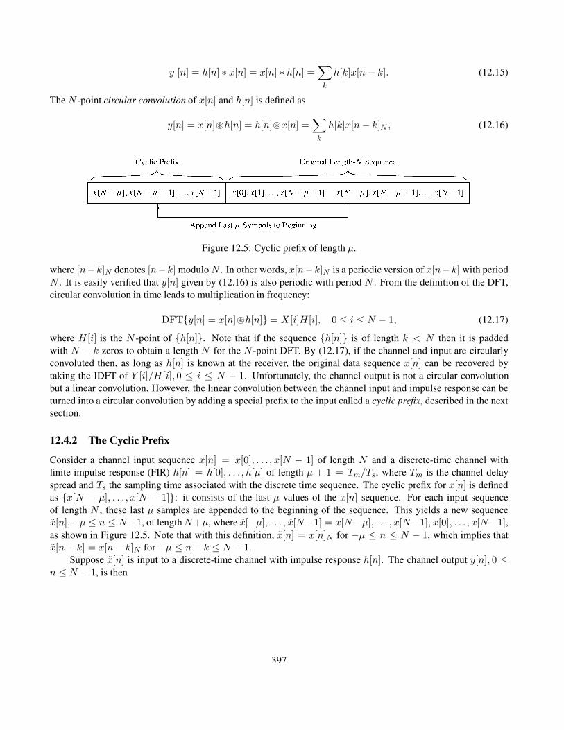
y [n] = h[n] ∗ x[n] = x[n] ∗ h[n] =∑

k

h[k]x[n− k]. (12.15)

The N -point circular convolution of x[n] and h[n] is defined as

y[n] = x[n]~h[n] = h[n]~x[n] =∑

k

h[k]x[n− k]N , (12.16)

Figure 12.5: Cyclic prefix of length µ.

where [n−k]N denotes [n−k] moduloN . In other words, x[n−k]N is a periodic version of x[n−k] with period

N . It is easily verified that y[n] given by (12.16) is also periodic with period N . From the definition of the DFT,

circular convolution in time leads to multiplication in frequency:

DFTy[n] = x[n]~h[n] = X [i]H [i], 0 ≤ i ≤ N − 1, (12.17)

where H [i] is the N -point of h[n]. Note that if the sequence h[n] is of length k < N then it is padded

with N − k zeros to obtain a length N for the N -point DFT. By (12.17), if the channel and input are circularly

convoluted then, as long as h[n] is known at the receiver, the original data sequence x[n] can be recovered by

taking the IDFT of Y [i]/H [i], 0 ≤ i ≤ N − 1. Unfortunately, the channel output is not a circular convolution

but a linear convolution. However, the linear convolution between the channel input and impulse response can be

turned into a circular convolution by adding a special prefix to the input called a cyclic prefix, described in the next

section.

12.4.2 The Cyclic Prefix

Consider a channel input sequence x[n] = x[0], . . . , x[N − 1] of length N and a discrete-time channel with

finite impulse response (FIR) h[n] = h[0], . . . , h[µ] of length µ + 1 = Tm/Ts, where Tm is the channel delay

spread and Ts the sampling time associated with the discrete time sequence. The cyclic prefix for x[n] is defined

as x[N − µ], . . . , x[N − 1]: it consists of the last µ values of the x[n] sequence. For each input sequence

of length N , these last µ samples are appended to the beginning of the sequence. This yields a new sequence

x[n],−µ ≤ n ≤ N−1, of lengthN+µ, where x[−µ], . . . , x[N−1] = x[N−µ], . . . , x[N−1], x[0], . . . , x[N−1],

as shown in Figure 12.5. Note that with this definition, x[n] = x[n]N for −µ ≤ n ≤ N − 1, which implies that

x[n− k] = x[n− k]N for −µ ≤ n− k ≤ N − 1.

Suppose x[n] is input to a discrete-time channel with impulse response h[n]. The channel output y[n], 0 ≤n ≤ N − 1, is then

397

y[n] = x[n] ∗ h[n]

=

µ∑

k=0

h[k]x[n− k]

=

µ∑

k=0

h[k]x[n− k]N

= x[n]~h[n], (12.18)

Figure 12.6: ISI between data blocks in channel output.

where the third equality follows from the fact that, for 0 ≤ k ≤ µ, x[n − k] = x[n − k]N for 0 ≤ n ≤ N − 1.

Thus, by appending a cyclic prefix to the channel input, the linear convolution associated with the channel impulse

response y[n] for 0 ≤ n ≤ N − 1 becomes a circular convolution. Taking the DFT of the channel output in the

absense of noise then yields

Y [i] = DFTy[n] = x[n]~h[n] = X [i]H [i], 0 ≤ i ≤ N − 1, (12.19)

and the input sequence x[n], 0 ≤ n ≤ N − 1, can be recovered from the channel output y[n], 0 ≤ n ≤ N − 1, for

known h[n] by

x[n] = IDFT

Y [i]

H [i]

= IDFT

DFTy[n]DFTh[n]

. (12.20)

Note that y[n],−µ ≤ n ≤ N−1, has lengthN+µ, yet from (12.20) the first µ samples y[−µ], . . . , y[−1] are

not needed to recover x[n], 0 ≤ n ≤ N − 1, owing to the redundancy associated with the cyclic prefix. Moreover,

if we assume that the input x[n] is divided into data blocks of size N with a cyclic prefix appended to each block

to form x[n], then the first µ samples of y[n] = h[n] ∗ x[n] in a given block are corrupted by ISI associated with

the last µ samples of x[n] in the prior block, as illustrated in Figure 12.6. The cyclic prefix serves to eliminate ISI

between the data blocks, because the first µ samples of the channel output affected by this ISI can be discarded

without any loss relative to the original information sequence. In continuous time this is equivalent to using a

guard band of duration Tm (the channel delay spread) after every block of N symbols of duration NTs in order to

eliminate the ISI between these data blocks.

The benefits of adding a cyclic prefix come at a cost. Since µ symbols are added to the input data blocks,

there is an overhead of µ/N and a resulting data-rate reduction of N/(µ + N ). The transmit power associated

with sending the cyclic prefix is also wasted because this prefix consists of redundant data. It is clear from Figure

12.6 that any prefix of length µ appended to input blocks of size N eliminates ISI between data blocks if the first

µ samples of the block are discarded. In particular, the prefix can consist of all zero symbols, in which case –

although the data rate is still reduced by N/(N + µ) – no power is used in transmitting the prefix. Trade-offs

associated with the cyclic prefix versus this all-zero prefix, which is a form of vector coding, are discussed in

Section 12.4.5.

398

The foregoing analysis motivates the design of OFDM. In OFDM the input data is divided into blocks of size

N , where each block is referred to as an OFDM symbol. A cyclic prefix is added to each OFDM symbol to induce

circular convolution of the input and channel impulse response. At the receiver, the output samples affected by ISI

between OFDM symbols are removed. The DFT of the remaining samples are used to recover the original input

sequence. The details of this OFDM system design are given in the next section.

Example 12.4: Consider an OFDM system with total bandwidth B = 1 MHz assuming β = ε = 0. A single-

carrier system would have symbol timeTs = 1/B = 1 µs. The channel has a maximum delay spread of Tm = 5 µs,

so with Ts = 1 µs and Tm = 5 µs there would clearly be severe ISI. Assume an OFDM system with MQAM mod-

ulation applied to each subchannel. To keep the overhead small, the OFDM system uses N = 128 subcarriers to

mitigate ISI. So TN = NTs = 128 µs. The length of the cyclic prefix is set to µ = 8 > Tm/Ts to ensure no

ISI between OFDM symbols. For these parameters, find the subchannel bandwidth, the total transmission time

associated with each OFDM symbol, the overhead of the cyclic prefix, and the data rate of the system assuming

M = 16.

Solution: The subchannel bandwidth BN = 1/TN = 7.812 kHz, so BN Bc = 1/Tm = 200 kHz, ensuring

negligible ISI. The total transmission time for each OFDM symbol is T = TN + µTS = 128 + 8 = 136 µs. The

overhead associated with the cyclic prefix is 8/128 which is 6.25%. The system transmits log2 16 = 4 bits per

subcarrier every T seconds, so the data rate is 128 · 4/136 · 10−6 = 3.76 Mbps, which is slightly less than 4B as a

result of the cyclic prefix overhead.

12.4.3 Orthogonal Frequency-Division Multiplexing (OFDM)

The OFDM implementation of multicarrier modulation is shown in Figure 12.7. The input data stream is modulated

by a QAM modulator, resulting in a complex symbol stream X [0], X[1], . . . , X [N − 1]. This symbol stream is

passed through a serial-to-parallel converter, whose output is a set ofN parallel QAM symbolsX [0], . . . , X [N−1]corresponding to the symbols transmitted over each of the subcarriers. Thus, the N symbols output from the

serial-to-parallel converter are the discrete frequency components of the OFDM modulator output s(t). In order

to generate s(t), the frequency components are converted into time samples by performing an inverse DFT on

these N symbols, which is efficiently implemented using the IFFT algorithm. The IFFT yields the OFDM symbol

consisting of the sequence x[n] = x[0], . . . , x[N − 1] of length N , where

x[n] =1√N

N−1∑

i=0

X [i]ej2πni/N , 0 ≤ n ≤ N − 1. (12.21)

This sequence corresponds to samples of the multicarrier signal: the multicarrier signal consists linearly modulated

subchannels, and the right-hand side of (12.21) corresponds to samples of a sum of QAM symbols X [i] each

modulated by the carrier ej2πit/TN , i = 0, . . . , N − 1. The cyclic prefix is then added to the OFDM symbol,

and the resulting time samples x[n] = x[−µ], . . . , x[N − 1] = x[N − µ], . . . , x[0], . . . , x[N − 1] are ordered by

the parallel-to-serial converter and passed through a D/A converter, resulting in the baseband OFDM signal x(t),

which is then upconverted to frequency f0.

The transmitted signal is filtered by the channel impulse response and corrupted by additive noise, resulting

in the received signal r(t). This signal is downconverted to baseband and filtered to remove the high-frequency

components. The A/D converter samples the resulting signal to obtain y[n] = x[n]∗h[n]+v[n],−µ≤ n ≤ N−1,

where h[n] is the discrete-time equivalent lowpass impulse response of the channel. The prefix of y[n] consisting

of the first µ samples is then removed. This results in N time samples whose DFT in the absence of noise is

Y [i] = H [i]X [i]. These time samples are serial-to-parallel converted and passed through an FFT. This results in

399

scaled versions of the original symbols H [i]X [i], where H [i] = H(fi) is the flat fading channel gain associated

with the ith subchannel. The FFT output is parallel-to-serial converted and passed through a QAM demodulator to

recover the original data.

Figure 12.7: OFDM with IFFT/FFT implementation.

The OFDM system effectively decomposes the wideband channel into a set of narrowband orthogonal sub-

channels with a different QAM symbol sent over each subchannel. Knowledge of the channel gains H [i], i =

0, . . . , N−1, is not needed for this decomposition, in the same way that a continuous-time channel with frequency

responseH(f) can be divided into orthogonal subchannels without knowledge ofH(f) by splitting the total signal

bandwidth into nonoverlapping subbands. The demodulator can use the channel gains to recover the original QAM

symbols by dividing out these gains: X [i] = Y [i]/H [i]. This process is called frequency equalization. However,

as discussed in Section 12.3.2 for continuous-time OFDM, frequency equalization leads to noise enhancement

because the noise in the ith subchannel is also scaled by 1/H [i]. Hence, while the effect of flat fading on X [i] is

removed by this equalization, its received SNR is unchanged. Precoding, adaptive loading, and coding across sub-

channels (as discussed in Section 12.3 are better approaches to mitigate the effects of flat fading across subcarriers.

An alternative to using the cyclic prefix is to use a prefix consisting of all zero symbols. In this case the OFDM

symbol consisting of x[n], 0 ≤ n ≤ N − 1, is preceded by µ null samples, as illustrated in Figure 12.8. At the

receiver the “tail” of the ISI associated with the end of a given OFDM symbol is added back in to the beginning of

the symbol, which re-creates the effect of a cyclic prefix, so the rest of the OFDM system functions as usual. This

zero prefix reduces the transmit power relative to a cyclic prefix by N/(µ+N ), since the prefix does not require

any transmit power. However, the noise from the received tail is added back into the beginning of the symbol,

which increases the noise power by (N+µ)/N . Thus, the difference in SNR is not significant for the two prefixes.

400

Figure 12.8: Creating a circular channel with an all-zero prefix.

12.4.4 Matrix Representation of OFDM

An alternate analysis for OFDM is based on a matrix representation of the system. Consider a discrete-time

equivalent lowpass channel with FIR h[n], 0 ≤ n ≤ µ, input x[n], noise v[n], and output y[n] = x[n]∗h[n]+v[n].Denote the nth element of these sequences as hn = h[n], xn = x[n], vn = v[n], and yn = y[n]. With this notation

the channel output sequence can be written in matrix form as

yN−1

yN−2

...

y0

=

h0 h1 · · · hµ 0 · · · 0

0 h0 · · · hµ−1 hµ · · · 0...

.... . .

. . .. . .

. . ....

0 · · · 0 h0 · · · hµ−1 hµ

xN−1

...

x0

x−1

...

x−µ

+

νN−1

νN−2

...

ν0

, (12.22)

which can be written more compactly as

y = Hx + ν. (12.23)

The received symbols y−1, . . . , y−µ are discarded because they are affected by ISI in the prior data block and

are not needed to recover the input. The last µ symbols of x[n] correspond to the cyclic prefix: x−1 = xN−1, x−2 =xN−2, . . . , x−µ = xN−µ. From this it can be shown that the matrix representation (12.22) is equivalent to

yN−1

yN−2

...

...

...

y0

=

h0 h1 · · · hµ 0 · · · 0

0 h0 · · · hµ−1 hµ · · · 0...

.... . .

. . .. . .

. . ....

0 · · · 0 h0 · · · hµ−1 hµ...

.... . .

. . .. . .

. . ....

h2 h3 · · · hµ−2 · · · h0 h1

h1 h2 · · · hµ−1 · · · 0 h0

xN−1

xN−2

...

...

x0

+

νN−1

νN−2

...

...

...

ν0

, (12.24)

which can be written more compactly as

y = Hx + ν. (12.25)

401

This equivalent model shows that the inserted cyclic prefix allows the channel to be modeled as a circulant convo-

lution matrix H over theN samples of interest. The matrix H is normal (HHH = HHH), so it has an eigenvalue

decomposition

H = MΛMH , (12.26)

where Λ is a diagonal matrix of eigenvalues of H and M is a unitary matrix whose columns constitute the eigen-

vectors of H.

It is straightforward to show that the DFT operation on x[n] can be represented by the matrix multiplication

X = Qx,

where X = (X [0], . . . , X [N − 1])T , x = (x[0], . . . , x[N − 1])T , and Q is an N ×N matrix given by

Q =1√N

1 1 1 · · · 1

1 WN W 2N · · · WN−1

N...

......

. . ....

1 WN−1N W

2(N−1)N · · · W

(N−1)2

N

(12.27)

for WN = e−j2π/N . Since

Q−1 = QH , (12.28)

the IDFT can be similarly represented as

x = Q−1X = QHX. (12.29)

Let v be an eigenvector of H with eigenvalue λ. Then

λv = Hv.

The unitary matrix M has columns that are the eigenvectors of H; that is, λimi = Hmi for i = 0, 1, . . . , N − 1,

where mi denotes the ith column of M. It can also be shown by induction that the columns of the DFT matrix QH

are eigenvectors of H, which implies that Q = MH and QH = M. Thus we have that

Y = Qy

= Q[Hx + ν]

= Q[HQHX + ν]

= Q[MΛMHQHX + ν] (12.30)

= QMΛMHQHX + Qν

= MHMΛMHMX + Qν

= ΛX + νQ; (12.31)

here, since Q is unitary, it follows that νQ = Qν has the same noise autocorrelation matrix as ν and hence is

generally white and Gaussian, with unchanged noise power. Thus, this matrix analysis also shows that, by adding

402

a cyclic prefix and using the IDFT/ DFT, OFDM decomposes an ISI channel into N orthogonal subchannels, and

knowledge of the channel matrix H is not needed for this decomposition.

The matrix representation is also useful in analyzing OFDM systems with multiple antennas [24]. As dis-

cussed in Chapter 10, a MIMO channel is typically represented by an Mr×Mt matrix, whereMt is the number of

transmit antennas and Mr the number of receive antennas. Thus, an MIMO-OFDM channel with N subchannels,

Mt transmit antennas,Mr receive antennas, and a channel FIR of duration µ can be represented as

y = Hx + ν, (12.32)

where y is a vector of dimension MrN × 1 corresponding to N output time samples at each of the Mr antennas,

H is a NMr × (N + µ)Mt matrix corresponding to the N flat fading subchannel gains on each transmit-receive

antenna pair, x is a vector of dimension Mt(N + µ) × 1 corresponding to N input time samples with appended

cyclic prefix of length µ at each of the Mt transmit antennas, and ν is the channel noise vector of dimension

MrN × 1. The matrix is in the same form as in the case of OFDM without multiple antennas, so the same

design and analysis applies: with MIMO-OFDM the ISI is removed by breaking the wideband channel into many

narrowband subchannels. Each subchannel experiences flat fading and so can be treated as a flat fading MIMO

channel. The capacity of this channel is obtained by applying the same matrix analysis as for standard MIMO to

the augmented channel with MIMO and OFDM [25]. In discrete implementations the input associated with each

transmit antenna is broken into blocks of size N , with a cyclic prefix appended for converting linear convolution

to circular and eliminating ISI between input blocks. More details can be found in [26].

12.4.5 Vector Coding

In OFDM the N × N circulant channel matrix H is decomposed using its eigenvalues and eigenvectors. Vector

coding (VC) is a similar technique whereby the originalN×(N+µ) channel matrix H from (12.23) is decomposed

using a singular value decomposition, which can be applied to a matrix of any dimension. The SVD does not

require a cyclic prefix to make the subchannels orthogonal, so it is more efficient than OFDM in terms of energy.

However, it is more complex and requires knowledge of the channel impulse response for the decomposition – in

contrast to OFDM, which does not require channel knowledge for its decomposition.

From Appendix C, the singular value decomposition of H can be written as

H = UΣVH , (12.33)

where U is N × N unitary, V is (N + µ) × (N + µ) unitary, and Σ is a matrix with ith diagonal element σiequal to the ith singular value of H and with zeros everywhere else. The singular values of H are related to the

eigenvalues of HHH by σi =√λi for λi the ith eigenvalue of the matrix HHH . Because H is a block-diagonal

convolutional matrix, the rank of H is N and so σi 6= 0 for all i = 1, . . . , N .

In vector coding, as in OFDM, input data symbols are grouped into vectors of N symbols. Let Xi, i =

0, . . . , N−1, denote the symbol to be transmitted over the ith subchannel and let X = (X0, . . . , XN−1, Xn, . . . , XN+µ−1)denote a vector of these symbols with µ symbolsXN , . . . , XN+µ−1 (typically zeros) appended at the end. The data

symbol Xi is multiplied by the ith column of V to form a vector, and then these vectors are added together. At the

receiver, the received vector y is multiplied by each row of UH to yieldN output symbols Yi, i = 0, 1, . . . , N−1.

This process is illustrated in Figure 12.9, where the multiplication by V and UH performs a similar function as

the transmit precoding and receiver shaping in MIMO systems.

Mathematically, it can be seen that the filtered transmit and received vectors are

x = VX

and

403

Figure 12.9: Vector coding.

Y = UHy. (12.34)

As a result, it can be shown through simple linear algebra that the filtered received vector Y is ISI-free, since

Y = UHy

= UH(Hx + ν)

= UH(UΣVH)VX + UHν

= ΣX + UHν. (12.35)

Hence, each element of X is effectively passed through a scalar channel without ISI, where the scalar gain of

subchannel i is the ith singular value of H. Additionally, the new noise vector ν = UHν has unchanged noise

variance, since U is unitary. The resulting received vector is thus

YN−1

YN−2

...

Y0

=

σ1XN−1

σ2XN−2

...

σNX0

+

νN−1

νN−2

...

ν0

. (12.36)

Figure 12.10: Guard interval (null prefix) in vector coding.

We call X, the vector obtained by appending µ extra symbols to each block of N data symbols, a vector

codeword. In contrast to OFDM, we see from (12.35) and the structure of Σ that the SVD does not require any

particular value for these extra symbols; they need not be a cyclic prefic, nor must the “tail” be added back in if

these symbols are all zeros. In practice the extra symbols are set to zero to save transmit power, thereby forming a

guard band or null prefix between the vector codeword (VC) symbols, as shown in Figure 12.10.

404

Information and estimation theory have proven that vector coding is the optimal partition of theN -dimensional

channel H [13, Chap. 4]. Thus, the capacity of any other channel partitioning scheme will be upper bounded by

vector coding. Despite its theoretical optimality and ability to create ISI-free channels with relatively small over-

head and no wasted transmit power, there are a number of important practical problems with vector coding. The

two most important problems are as follows.

1. Complexity. With vector coding, as in simple multichannel modulation, the complexity scales quickly with

N , the number of subcarriers. As seen from Figure 12.9, N transmit precoding and N receive shaping

filters are required to implement vector coding. Furthermore, the complexity of finding the singular value

decomposition of the N × (N + µ) matrix H increases rapidly with N .

2. SVD and channel knowledge. In order to orthogonally partition the channel, the SVD of the channel matrix

H must be computed. In particular, the precoding filter matrix must be known to the transmitter. This

means that, every time the channel changes, a new SVD must be computed and the results conveyed to

the transmitter. Generally, the computational complexity of the SVD and the delay incurred in getting the

channel information back to the transmitter is prohibitive in wireless systems. Since OFDM can perform

this decomposition without channel knowledge, OFDM is the method of choice for discrete multicarrier

modulation in wireless applications.

Example 12.5: Consider a simple two-tap discrete-time channel (i.e. µ = 1) described as

H(z) = 1 + .9z−1.

Since µ + 1 = Tm/Ts = 2, with N = 8 we ensure BN ≈ 1/(NTs) Bc ≈ 1/Tm. Find the system matrix

representation (12.23) and the singular values of the associated channel matrix H.

Solution: The representation (12.23) for H(z) = 1 + .9z−1 and N = 8 is given by

y7

y6...

y0

=

1 .9 0 · · · 0 · · · 0

0 1 .9 0 0 · · · 0...

.... . .

. . .. . .

. . ....

0 · · · 0 0 0 1 .9

x7

x6

...

x−1

+

ν7

ν6...

ν0

. (12.37)

The singular values of the matrix H in (12.37) can be found via a standard computer package (e.g. Matlab) as

Σ = diag[1.87, 1.78, 1.65, 1.46, 1.22, .95, .66, .34].

The precoding and shaping matrices U and V are also easily found. Given U,V, and Σ, this communication is

ISI-free, with the symbolsX0, X1, . . . , XN−1 being multiplied by the corresponding singular values as in (12.36).

12.5 Challenges in Multicarrier Systems

12.5.1 Peak-to-Average Power Ratio

The peak-to-average power ratio (PAR) is an important attribute of a communication system. A low PAR allows

the transmit power amplifier to operate efficiently, whereas a high PAR forces the transmit power amplifier to have

405

a large backoff in order to ensure linear amplification of the signal. This is demonstrated in Figure 12.11, which

shows a typical power amplifier response. Operation in the linear region of this response is generally required to

avoid signal distortion, so the peak value is constrained to be in this region. Clearly it would be desirable to have the

average and peak values be as close together as possible in order for the power amplifier to operate at maximum

efficiency. Additionally, a high PAR requires high resolution for the receiver A/D converter, since the dynamic

range of the signal is much larger for high-PAR signals. High-resolution A/D conversion places a complexity and

power burden on the receiver front end.

The PAR of a continuous-time signal is given by

PAR ,maxt |x(t)|2Et[|x(t)|2]

(12.38)

and for a discrete-time signal is given by

PAR ,maxn |x[n]|2En[|x[n]|2] . (12.39)

Any constant amplitude signal (e.g., a square wave) has PAR = 0 dB. A sine wave has PAR = 3 dB because

max[sin2(2πt/T )] = 1 and

E

[

sin2

(2πt

T

)]

=1

T

∫ T

0sin2

(2πt

T

)

dt = .5,

so PAR = 1/.5 = 2.

In general, PAR should be measured with respect to the continuous-time signal using (12.38), since the input

to the amplifier is an analog signal. The PAR given by (12.38) is sensitive to the pulse shape g(t) used in the

modulation, and it does not generally lead to simple analytical formulas [27]. For illustration we will focus on the

PAR associated with the discrete-time signal, since it lends itself to a simple characterization. However, care must

be taken when interpreting these results, since they can be quite inaccurate if the pulse shape g(t) is not taken into

account.

Figure 12.11: Typical power amplifier response.

Consider the time-domain samples that are output from the IFFT:

406

x[n] =1√N

N−1∑

i=0

X [i]ej2πin/N , 0 ≤ n ≤ N − 1. (12.40)

If N is large then the central limit theorem is applicable, and x[n] are zero-mean complex Gaussian random

variables because the real and imaginary parts are summed. The Gaussian approximation for IFFT outputs is

generally quite accurate for a reasonably large number of subcarriers (N ≥ 64). For x[n] complex Gaussian, the

envelope of the OFDM signal is Rayleigh distributed with variance σ2, and the phase of the signal is uniform.

Since the Rayleigh distribution has infinite support, the peak value of the signal will exceed any given value

with nonzero probability. It can then be shown [28] that the probability that the PAR given by (12.39) exceeds a

threshold P0 = σ20/σ

2 is given by

p(PAR ≥ P0) = 1 − (1− e−P0)N . (12.41)

Let us now investigate how PAR grows with the number of subcarriers. Consider N Gaussian independent

and identically distributed random variables xn(0 ≤ n ≤ N − 1) with zero mean and unit power. The average

signal power En[|x[n]|2] is then

E

[1√N

|x0 + x1 + · · ·+ xN−1|2]

=1

NE|x0 + x1 + · · ·+ xN−1|2

=E|x2

0|+ E|x21|+ · · ·+ E|x2

N−1|N

= 1. (12.42)

The maximum value occurs when all the xi add coherently, in which case

max

[1√N

|x0 + x1 + · · ·+ xN−1|]2

=

∣∣∣∣

N√N

∣∣∣∣

2

= N. (12.43)

Hence the maximum PAR is N for N subcarriers. In practice, full coherent addition of all N symbols is highly

improbable and so the observed PAR is typically less than N – usually by many decibels. Nevertheless, PAR

increases approximately linearly with the number of subcarriers. So even though it is desirable to have N as large

as possible in order to keep the overhead associated with the cyclic prefix down, a large PAR is an important

penalty that must be paid for large N .

There are a number of ways to reduce or tolerate the PAR of OFDM signals, including clipping the OFDM

signal above some threshold, peak cancellation with a complementary signal, allowing nonlinear distortion from

the power amplifier (and correction for it), and special coding techniques [29]. A good summary of some of these

methods can be found in [30].

12.5.2 Frequency and Timing Offset

We have seen that OFDM modulation encodes the data symbols Xi onto orthogonal subchannels, where orthogo-

nality is assured by the subcarrier separation 4f = 1/TN . The subchannels may overlap in the frequency domain,

as shown in Figure 12.12 for a rectangular pulse shape in time (sinc function in frequency). In practice, the fre-

quency separation of the subcarriers is imperfect and so 4f is not exactly equal to 1/TN . This is generally caused

by mismatched oscillators, Doppler frequency shifts, or timing synchronization errors. For example, if the carrier

frequency oscillator is accurate to 1 part per million then the frequency offset 4fε ≈ f0(.1 ·10−6). If f0 = 5 GHz,

407

Figure 12.12: OFDM overlapping subcarriers for rectangular pulses with f0 = 10 Hz and 4f = 1 Hz.

the carrier frequency for 802.11a WLANs, then 4fε = 500 Hz, which will degrade the orthogonality of the sub-

channels because now the received samples of the FFT will contain interference from adjacent subchannels. Next

we’ll analyze this intercarrier interference (ICI) more closely.

The signal corresponding to subcarrier i can be simply expressed for the case of rectangular pulse shapes

(suppressing the data symbol and the carrier frequency) as

xi(t) = ej2πit/TN . (12.44)

An interfering subchannel signal can be written as

xi+m(t) = ej2π(i+m)t/TN . (12.45)

If the signal is demodulated with a frequency offset of δ/TN , then this interference becomes

xi+m(t) = ej2π(i+m+δ)t/TN . (12.46)

The ICI between subchannel signals xi and xi+m is simply the inner product between them:

Im =

∫ TN

0xi(t)x

∗i+m(t) dt =

TN(1− e−j2π(δ+m))

j2π(m+ δ). (12.47)

It can be seen that, in (12.47), δ = 0 ⇒ Im = 0 as expected. The total ICI power on subcarrier i is then

ICIi =∑

m6=i

|Im|2 ≈ C0(TNδ)2, (12.48)

where C0 is some constant. Several important trends can be observed from this simple approximation. First, as TNincreases, the subcarriers grow narrower and hence more closely spaced, which then results in more ICI. Second,

the ICI predictably grows with the frequency offset δ, and the growth is about quadratic. Another interesting

408

observation is that (12.48) does not appear to be directly affected by N . But picking N large generally forces TNto be large also, which then causes the subcarriers to be closer together. Along with the larger PAR that comes with

large N , the increased ICI is another reason to pick N as low as possible, assuming the overhead budget can be

met. In order to further reduce the ICI for a given choice of N , nonrectangular windows can also be used [31, 32].

The effects from timing offset are generally less than those from the frequency offset [5, Chap. 5], as long as a

full N -sample OFDM symbol is used at the receiver without interference from the previous or subsequent OFDM

symbols (this is ensured by taking the cyclic prefix length µ σTm/Ts, where σTm is the channel’s rms delay

spread). It can be shown that the ICI power on subcarrier i due to a receiver timing offset τ can be approximated

as 2(τ/TN)2. Since usually τ TN , this effect is typically negligible.

12.6 Case Study: OFDM design in the Wi-Fi Standard

The IEEE 802.11 Wi-Fi family of standard, which occupies 80 MHz of bandwidth in the 2.4 GHz unlicensed band

and 300 MHz of bandwidth in the 5-GHz unlicensed band, is based on OFDM [6], except for the first standard,

802.11b, which uses spread spectrum. The IEEE 802.11b and 802.11g standards operated in the crowded 2.4-GHz

band [7] while 802.11a, 802.11n, 802.11ac, and 802.11ax (also called Wi-Fi 6) operate in the 300 MHz band. In

this section we study the properties of OFDM design in the Wi-Fi standard and discuss some of the design choices.

For simplicity we will focus on the 802.11a standard in the 300 MHz band since it does not incorporate MIMO, in

order to focus on the OFDM design choices in WiFi design.

In 802.11a, N = 64 subcarriers are generated, although only 48 are actually used for data transmission:

the outer 12 are zeroed in order to reduce adjacent channel interference, and 4 are used as pilot symbols for

channel estimation. The cyclic prefix consists of µ = 16 samples, so the total number of samples associated

with each OFDM symbol, including both data samples and the cyclic prefix, is 80. Coded bits are packetized,

and the transmitter gets periodic feedback from the receiver about the packet error rate, which it uses to pick an

appropriate error correction code and modulation technique. The same code and modulation must be used for all

the subcarriers at any given time. The error correction code is a convolutional code with one of three possible code

rates: r = 1/2, 2/3, or 3/4. The modulation types that can be used on the subchannels are BPSK, QPSK, 16-QAM,

or 64-QAM.

The total system bandwidth of 300 MHz is divided into 20-MHz channels that can be assigned to different

users. Since the channel bandwidth B (and sampling rate 1/Ts) is 20 MHz and since there are 64 subcarriers

evenly spaced over that bandwidth, the subcarrier bandwidth is:

BN =20 MHz

64= 312.5 kHz.

Since µ = 16 and 1/Ts = 20 MHz, the maximum delay spread for which ISI is removed is

Tm < µTs =16

20 MHz= 0.8 µs,

which corresponds to delay spread in an indoor environment. Including both the OFDM symbol and cyclic prefix,

there are 80 = 64 + 16 samples per OFDM symbol time, so the symbol time per subchannel is

TN = 80Ts =80

20 · 106= 4 µs.

The data rate per subchannel is log2M/TN . Thus, the minimum data rate for this system – corresponding to BPSK

(1 bit/symbol), an r = 1/2 code, and taking into account that only 48 subcarriers actually carry usable data – is

given by

409

Rmin = 48 subcarriers · 1/2 bit

1 coded bit· 1 coded bit

subcarrier symbol· 1 subcarrier symbol

4 · 10−6 seconds

= 6 Mbps. (12.49)

The maximum data rate that can be transmitted is

Rmax = 48 subcarriers · 3/4 bit

1 coded bit· 6 coded bits

subcarrier symbol· 1 subcarrier symbol

4 · 10−6 seconds

= 54 Mbps. (12.50)

Naturally, a wide range of data rates between these two extremes is possible.

Example 12.6: Find the data rate of an 802.11a system assuming 16-QAM modulation and rate-2/3 coding.

Solution: With 16-QAM modulation, each subcarrier transmits log2(16) = 4 coded bits per subcarrier symbol and

there are a total of 48 subcarriers used for data transmission. With a rate-2/3 code, each coded bit relays 2/3 of an

information bit per TN seconds. Thus, the data rate is given by

Rmax = 48 subcarriers · 2/3 bit

1 coded bit· 4 coded bits

subcarrier symbol· 1 subcarrier symbol

4 · 10−6 seconds

= 32 Mbps. (12.51)

12.7 General Time-Frequency Modulation

OFDM modulation is designed to compensate for delay spread. In channels that are constant over an OFDM

block, the rate within each subchannel can be adapted or frequency-domain equalization used to equalize the

subchannel gains. However, these techniques only work when the channel is roughly constant over an OFDM

block. For channels that experience significant time variations over an OFDM block, i.e. large doppler spread, an

accurate channel estimate over an OFDM block cannot be obtained. This typically leads to significant performance

degradation of OFDM as neither adaptive subcarrier modulation nor frequency-domain equalization can be applied.

One approach to mitigate the performance degradation caused by time-variation in OFDM is to limit the symbol

time or the OFDM block duration. Indeed, is it typical for OFDM deployments in time-varying channels to limit

the symbol time, or, equivalently, increase the subcarrier spacing, so that the product of the overall symbol duration

and the Doppler spread is small. In this regime, the time-frequency dispersive channel behaves approximately as a

static delay spread channel at the expense of an increased cyclic prefix overhead. A detailed performance analysis

of such schemes is presented in [33].

A different approach to simultaneously deal with dispersion in the time and frequency domains is via general

time-frequency signaling designed for the two-dimensional delay-Doppler channel model. Several methods for

time-frequency signalling over this two-dimensional channel have been proposed [34]. In particular, [35] estab-

lished a signal model that presents the received signal as a canonical decomposition into delay and Doppler shifted

versions of a basis signal, and proposes a delay-Doppler receiver that exploits the dispersion in both delay and

Doppler dimensions. In [36] a general framework for communication over a delay-Doppler channel based on an

410

orthogonal short-time Fourier basis consisting of time-frequency shifts of a given pulse was developed. A different

approach was taken in [37] which first demonstrates that a time-frequency receiver does not obtain full diversity

as it is not optimized on the transmit side. The work then derives optimal precoders which, in conjunction with a

jointly designed receiver, obtain the full diversity of the delay-Doppler channel. These works all design the mod-

ulation strategy in the time-frequency domain. Another work, [41], introduces Orthogonal Time-Frequency-Space

signaling (OTFS) which designs the modulation directly in the delay-Doppler domain. OTFS has been demon-

strated to have advantages over OFDM in specific high-Doppler channels. However, this performance advantage

requires complex signal processing at the transmitter to create the OTFS waveform and at the receiver to equalize

the distortion introduced by the channel.

A separate body of prior work focuses on time-frequency pulse shape design to minimize dispersion after

transmission through the channel. A special case of this body of work is pulse-shaped OFDM. Various criteria

for pulse shape optimization have been considered in earlier works including suppressing ISI and ICI [38], max-

imizing signal-to-interference-plus-noise ratio (SINR) [39], or optimizing spectral efficiency through the use of

non-rectangular lattices in the time-frequency domain [40].

Recall that OFDM utilizes time-domain multiplexing across the different subcarriers as well as a cycle prefix

in time to cancel ISI between OFDM blocks. For channels that have little delay spread and large Doppler, a

time-frequency dual of the OFDM strategy uses frequency-domain multiplexing across different timeslots with a

frequency-domain cyclic prefix to remove Doppler spread. This technique can compensate for the effect of an

arbitrary Doppler spread by performing linear equalization in the time domain, which is the dual of frequency-

domain equalization performed in OFDM. A performance analysis of this technique can be found in [42]. rather

than the delay-Doppler domain.

411

Chapter 12 Problems

1. Show that the minimum separation 4f for subcarriers cos(2πj4ft+ φj), j = 1, 2, . . . to form a set of

orthonormal basis functions on the interval [0, TN] is 4f = 1/TN for any initial phase φj . Show that if

φj = 0 for all j then this carrier separation can be reduced by half.

2. Consider an OFDM system operating in a channel with coherence bandwidthBc = 10 kHz.

(a) Find a subchannel symbol time TN = 1/BN = 10Tm, assuming Tm = 1/Bc. This should ensure flat

fading on the subchannels.

(b) Assume the system has N = 128 subchannels. If raised cosine pulses with β = 1.5 are used and

if the required additional bandwidth (from time limiting) to ensure minimal power outside the signal

bandwidth is ε = .1, then what is the total bandwidth of the system?

(c) Find the total required bandwidth of the system using overlapping carriers separated by 1/TN , and

compare with your answer in part (b).

3. Show from the definition of the DFT that circular convolution of discrete time sequences leads to multipli-

cation of their DFTs.

4. Consider a data signal with a bandwidth of .5 MHz and a data rate of .5 Mbps. The signal is transmitted over

a wireless channel with a delay spread of 10 µs.

(a) If multicarrier modulation with nonoverlapping subchannels is used to mitigate the effects of ISI, ap-

proximately how many subcarriers are needed? What is the data rate and symbol time on each subcar-

rier? (We do not need to eliminate the ISI completely, so Ts = Tm is sufficient for ISI mitigation.)

Assume for the remainder of the problem that the average received SNR (γs) on the nth subcarrier is 1000/n(linear units) and that each subcarrier experiences flat Rayleigh fading (so ISI is completely eliminated).

(b) Suppose BPSK modulation is used for each subcarrier. If a repetition code is used across all subcarriers

(i.e., if a copy of each bit is sent over each subcarrier), then what is the BER after majority decoding?

What is the data rate of the system?

(c) Suppose you use adaptive loading (i.e., different constellations on each subcarrier) such that the average

BER on each subcarrier does not exceed 10−3 (this is averaged over the fading distribution; do not

assume that the transmitter and receiver adapt power or rate to the instantaneous fade values). Find

the MQAM constellation that can be transmitted over each subcarrier while meeting this average BER

target. What is the total data rate of the system with adaptive loading?

5. Consider a multicarrier modulation transmission scheme with three nonoverlapping subchannels spaced

200 kHz apart (from carrier to carrier) and with subchannel baseband bandwidth of 100 kHz.

(a) For what values of the channel coherence bandwidth will the subchannels of your multicarrier scheme

exhibit flat fading (approximately no ISI)? For which such values will the subcarriers exhibit indepen-

dent fading? If the subcarriers exhibit correlated fading, what impact will this have on coding across

subchannels?

(b) Suppose that you have a total transmit power P = 300 mW and that the noise power in each subchannel

is 1 mW. With equal power of 100 mW transmitted on each subchannel, the received SNR on each

subchannel is γ1 = 11 dB, γ2 = 14 dB, and γ3 = 18 dB. Assume the subchannels do not experience

412

fading, so these SNRs are constant. For these received SNRs, find the maximum signal constellation

size for MQAM that can be transmitted over each subchannel for a target BER of 10−3. Assume the

MQAM constellation is restricted to be a power of 2 and use the bound BER ≤ .2e−1.5γ/(M−1) for

your calculations. Find the corresponding total data rate of the multicarrier signal assuming a symbol

rate on each subchannel of Ts = 1/B, where B is the baseband subchannel bandwidth.

(c) For the subchannel SNRs given in part (b), suppose we want to use precoding (to equalize the received

SNR in each subchannel) and then send the same signal constellation over each subchannel. What size

signal constellation is needed to achieve the same data rate as in part (b)? What transmit power would

be needed on each subchannel to achieve the required received SNR for this constellation with a 10−3

BER target? How much must the total transmit power be increased over the 300-mW transmit power

in part (b)?

6. Consider a channel with impulse response

h(t) = α0δ(t) + α1δ(t− T1) + α2δ(t− T2).

Assume that T1 = 10 µs and T2 = 20 µs. You want to design a multicarrier system for the channel with

subchannel bandwidth BN = Bc/2. If raised cosine pulses with β = 1 are used and if the subcarriers

are separated by the minimum bandwidth necessary to remain orthogonal, then what is the total bandwidth

occupied by a multicarrier system with eight subcarriers? Assuming a constant SNR on each subchannel of

20 dB, find the maximum constellation size for MQAM modulation that can be sent over each subchannel

with a target BER of 10−3, assuming also that M is restricted to be a power of 2. Find the corresponding

total data rate of the system.

7. Show the equivalence of matrix representations (12.22) and (12.24) for OFDM when a cyclic prefix is ap-

pended to each OFDM symbol.

8. Show that the DFT operation on x[n] can be represented by the matrix multiplicationX [i] = Qx[n], where

Q =1√N

1 1 1 · · · 1

1 WN W 2N · · · WN−1

N...

......

. . ....

1 WN−1N W

2(N−1)N · · · W

(N−1)2

N

(12.52)

for WN = e−j2π/N .

9. This problem shows that the rows of the DFT matrix Q are eigenvectors of H.

(a) Show that the first row of Q is an eigenvector of H with eigenvalue λ0 =∑µ

i=0 hi.

(b) Show that row 2 of Q is an eigenvector of H with eigenvalue λ1 =∑µ

i=0 hiWiN .

(c) Argue by induction that similar relations hold for all rows of Q.

10. Show that appending the all-zero prefix to an OFDM symbol and then adding in the tail of the received

sequence, as shown in Figure 12.8, results in the same received sequence as with a cyclic prefix.

11. Consider a discrete-time FIR channel with h[n] = .7 + .5δ[n− 1] + .3δ[n− 3]. Consider an OFDM system

with N = 8 subchannels.

413

(a) Find the matrix H corresponding to the matrix representation of the DMT y = Hx+v given in (12.23).

(b) Find the circulant convolution matrix H corresponding to the matrix representation in (12.25), as well

as its eigenvalue decomposition H = MAMH .

(c) What are the flat fading channel gains associated with each subchannel in the representation of part

(b)?

12. Consider a five-tap discrete-time channel

H(z) = 1 + .6z−1 + .7z−2 + .3z−3 + .2z−4.

Assume this channel model characterizes the maximum delay spread of the channel, and assume a vector

coded system is used over the channel with N = 256 carriers.

(a) What value of µ is needed for the prefix to eliminate ISI between vector codewords? What is the

overhead associated with this µ?

(b) Find the system matrix representation (12.23) and the singular values of the associated channel matrix

H.

(c) Find the transmit precoding and receiver shaping matrices, V and UH , required to orthogonalize the

subchannels.

13. Find the PAR of a raised cosine pulse with β = 0, .5, 1. Which pulse shape has the lowest PAR? Is this pulse

shape more or less sensitive to timing errors?

14. Find the constant C0 associated with intercarrier interference in (12.48).

15. Suppose the four subchannels in 802.11a used for pilot estimation could be used for data transmission by

taking advantage of blind estimation techniques. Assuming the same modulation and coding formats are

available, what maximum and minimum data rates could be achieved by including these extra subchannels?

16. Find the data rate of an 802.11a system assuming half the available 48 subchannels use BPSK with a rate-1/2

channel code and the others use 64-QAM with a rate-3/4 channel code.

414

Bibliography

[1] J. Bingham, “Multicarrier modulation for data transmission: An idea whose time has come,” IEEE Commun.

Mag., pp. 5–14, May 1990.

[2] H. Sari, G. Karam, and I. Jeanclaude, “ Transmission techniques for digital terrestrial TV broadcasting,”

IEEE Commun. Mag., pp. 100–9, February 1995.

[3] J. S. Chow, J. C. Tu, and J. M. Cioffi, “A discrete multitone transceiver system for HDSL applications,” IEEE

J. Sel. Areas Commun., pp. 895–908, August 1991.

[4] J. M. Cioffi, “A multicarrier primer,” Stanford University/Amati TIEI contribution, I1E1.4/91–157, November

1991.

[5] A. R. S. Bahai, B. R. Saltzberg, and M. Ergen, Multi-Carrier Digital Communications-Theory and Applica-

tions of OFDM, 2nd ed., Springer-Verlag, New York, 2004.

[6] IEEE 802.11a-l999: High-Speed Physical Layer in the 5 GHz Band, 1999.

[7] IEEE 802.11g-2003: Further Higher-Speed Physical Layer Extension in the 2.4 GHz Band, 2003.

[8] IEEE 802.16a-200l: IEEE Recommended Practice for Local and Metropolitan Area Networks, 2001.

[9] C. Eklund, R. B. Marks, K. L. Stanwood, and S. Wang, “IEEE Standard 802.16: A technical overview of

the WirelessMAN 326 air interface for broadband wireless access,” IEEE Commun. Mag., pp. 98–107, June

2002.

[10] M. Corson, R. Laroia, A. O’Neill, V. Park, and G. Tsirtsis, “A new paradigm for IP-based cellular networks,”

IT Professional pp. 20–9, November/December 2001.

[11] W. Lu, “4G mobile research in Asia,” IEEE Commun. Mag., pp. 104–6, March 2003.

[12] T. S. Rappaport, A. Annamalai, R. M. Buehrer, and W. H. Tranter, “Wireless communications: Past events

and a future perspective,” IEEE Commun. Mag., pp. 148–61, May 2002.

[13] J. M. Cioffi. Digital Communications, chap. 4: Multichannel Modulation, unpublished course notes, available

at 〈http://www.stanford.edu/class/ee379c/〉.

[14] S. Kasturia, J. Aslanis, and J. Cioffi, “Vector coding for partial response channels,” IEEE Trans. Inform.

Theory, pp. 741–62, July 1990.

[15] L. J. Cimini, “Analysis and simulation of a digital mobile channel using orthogonal frequency division mul-

tiplexing,” IEEE Trans. Inform. Theory, pp. 665–75, July 1985.

415

[16] P. S. Chow, J. M. Cioffi, and John A. C. Bingham, “A practical discrete multitone transceiver loading algo-

rithm for data transmission over spectrally shaped channels,” IEEE Trans. Commun., pp. 773–5, February–

April 1995.

[17] Z. Wang, X. Ma, and G. B. Giannakis, “OFDM or single-carrier block transmissions?” IEEE Trans. Com-

mun., pp. 380–94, March 2004.

[18] R. K. Jurgen, “Broadcasting with digital audio,” IEEE Spectrum, pp. 52–9, March 1996.

[19] S. Kaider, “Performance of multi-carrier CDM and COFDM in fading channels,” Proc. IEEE Globecom

Conf., pp. 847–51, December 1999.

[20] P. Hoeher, S. Kaiser, and P. Robertson, “ Two-dimensional pilot-symbol-aided channel estimation by Wiener

filtering,” Proc. IEEE Internat. Conf. Acous., Speech, Signal Proc., pp. 1845–8, April 1997.

[21] A. Scaglione, G. B. Giannakis, and S. Barbarossa, “Redundant filterbank precoders and equalizers. I: Unifi-

cation and optimal designs,” IEEE Trans. Signal Proc., pp. 1988–2006, July 1999.

[22] A. Scaglione, G. B. Giannakis, and S. Barbarossa, “Redundant filterbank precoders and equalizers. II: Blind

channel estimation, synchronization, and direct equalization,” IEEE Trans. Signal Proc., pp. 2007–22, July

1999.

[23] A. V. Oppenheim, R. W. Schafer, and J. R. Buck, Discrete-Time Signal Processing, 2nd ed., Prentice-Hall,

Englewood Cliffs, NJ, 1999.

[24] H. Sampath, S. Talwar, J. Tellado, V. Erceg, and A. Paulraj, “A fourth-generation MIMO-OFDM broadband

wireless system: Design, performance, and field trial results,” IEEE Commun. Mag., pp. 143–9, September

2002.

[25] L. H. Brandenburg and A. D. Wyner, “Capacity of the Gaussian channel with memory: The multivariate

case,” Bell System Tech. J., pp. 745–78, May/June 1974.

[26] G. L. Stuber, J. R. Barry, S. W. McLaughlin, Y. Li, M. A. Ingram, and T. G. Pratt, “Broadband MIMO-OFDM

wireless communications,” Proc. IEEE, pp. 271–94, February 2004.

[27] H. Ochiai and H. Imai, “On the distribution of the peak-to-average power ratio in OFDM signals,” IEEE

Trans. Commun., pp. 282–9, February 2001.

[28] D. J. G. Mestdagh and P. M. P. Spruyt, “A method to reduce the probability of clipping in DMT-based

transceivers,” IEEE Trans. Commun., pp. 1234–8, October 1996.

[29] K. G. Paterson and V. Tarokh, “On the existence and construction of good codes with low peak-to-average

power ratios,” IEEE Trans. Inform. Theory, pp. 1974–87, September 2000.

[30] J. Tellado, Multicarrier Modulation with Low PAR: Applications to DSL and Wireless, Kluwer, Boston, 2000.

[31] C. Muschallik, “Improving an OFDM reception using an adaptive Nyquist windowing,” IEEE Trans. Con-

sumer Elec., pp. 259–69, August 1996.

[32] A. Redfern, “Receiver window design for multicarrier communication systems,” IEEE J. Sel. Areas Commun.,

pp. 1029–36, June 2002.

416

[33] T. Wang, J. G. Proakis, E. Masry, and J. Zeidler, “Performance degradation of OFDM systems due to Doppler

spreading”, IEEE Trans. Commun., Vol. 5, No. 6, pp. 1422–1432, June 2006.

[34] G. Matz, H. Bolcskei, and F. Hlawatsch, “Time-frequency foundations of communications: Concepts and

tools”, IEEE Signal Processing Magazine, Vol. 30, No. 6, pp. 87–96, June 2013.

[35] A. Sayeed and B. Aazhang, “Joint multipath-Doppler diversity in mobile wireless communications,” IEEE

Trans. Commun., Vol. 47, No. 1, pp. 123–132, Jan. 1999.

[36] K. Liu, T. Kadous, and A.M. Sayeed, “Orthogonal time-frequency signaling over doubly dispersive channels,”

IEEE Trans. Inform. Theory, Vol. 50, No. 11, pp. 2583–2603, Nov. 2004.

[37] X. Ma and G. B. Giannakis, “Maximum-diversity transmissions Over doubly selective wireless channels,”

IEEE Trans. Inform. Theory, Vol. 49, No. 7, pp. 1832–1840, July 2003.

[38] W. Kozek and A. F. Molisch, “Nonorthogonal pulseshapes for multicarrier communications in doubly disper-

sive channels,” IEEE J. Select. Areas Commun., Vol 16, No. 8, pp. 1579–1589, Aug. 1998.

[39] S. Das and P. Schniter, “Max-SINR ISI/ICI-shaping multicarrier communication over the doubly dispersive

channel,” IEEE Trans. Signl. Proc. Vol. 55, No.12, pp. 5782-5795, Dec. 2007.

[40] T. Strohmer and S. Beaver, “Optimal OFDM design for time-frequency dispersive channels,” IEEE Trans.

Commun., Vol. 51, No. 7 pp. 1111-1122, July 2003.

[41] R. Hadani, S. Rakib, M. Tsatsanis, A. Monk, A.J. Goldsmith, A. F. Molisch, and R. Calderbank, “Orthogonal

Time Frequency Space Modulation”,

[42] T. Dean, M. Chowdhury, N. Grimwood, A. Goldsmith, “Rethinking modulation and detection for high

doppler channels,” IEEE Transactions on Wireless Communications, Jan. 2020.

417

Chapter 13

Spread Spectrum

This chapter has not yet been updated for the 2nd edition

Although bandwidth is a valuable commodity in wireless systems, increasing the transmit signal bandwidth

can sometimes improve performance. Spread

spectrum is a technique that increases signal bandwidth beyond the minimum necessary for data communica-

tion. There are many reasons for doing this. Spread-spectrum techniques can hide a signal below the noise floor,

making it difficult to detect. Spread spectrum also mitigates the performance degradation due to intersymbol and

narrowband interference. In conjunction with a RAKE receiver, spread spectrum can provide coherent combining

of different multipath components. Spread spectrum also allows multiple users to share the same signal bandwidth,

since spread signals can be superimposed on top of each other and demodulated with minimal interference between

them. Finally, the wide bandwidth of spread-spectrum signals is useful for location and timing acquisition.

Spread spectrum first achieved widespread use in military applications because of its inherent property of

hiding the spread signal below the noise floor during transmission, its resistance to narrowband jamming and

interference, and its low probability of detection and interception. For commercial applications, the narrowband

interference resistance has made spread spectrum common in cordless phones. The ISI rejection and bandwidth-

sharing capabilities of spread spectrum are very desirable in cellular systems and wireless LANs. As a result,

spread spectrum is the basis for both second- and third-generation cellular systems as well as second-generation

wireless LANs.

13.1 Spread-Spectrum Principles

Spread spectrum is a modulation method applied to digitally modulated signals that increases the transmit signal

bandwidth to a value much larger than is needed to transmit the underlying information bits. There are many

signaling techniques that increase the transmit bandwidth above the minimum required for data transmission –

for example, coding and frequency modulation. However, these techniques do not fall in the category of spread

spectrum. The following three properties are needed for a signal to be spread-spectrum modulated [1].

1. The signal occupies a bandwidth much larger than is needed for the information signal.

2. The spread-spectrum modulation is done using a spreading code, which is independent of the data in the

signal.

3. Despreading at the receiver is done by correlating the received signal with a synchronized copy of the spread-

ing code.

418

In order to make these notions precise, we return to the signal space representation of Section 5.1 to investigate

embedding an information signal of bandwidth B within a much larger transmit signal bandwidth Bs than is

needed. From (5.3), a set of linearly independent signals si(t), i = 1, . . . ,M , of bandwidth B and time duration

T can be written using a basis function representation as

si(t) =

N∑

j=1

sijφj(t), 0 ≤ t < T, (13.1)

where the basis functions φj(t) are orthonormal and span an N -dimensional space. One of these signals is trans-

mitted every T seconds to convey log2M/T bits per second. As discussed in Section 5.1.2, the minimum number

of basis functions needed to represent these signals is approximately 2BT . Since the si(t)Mi=1 are linearly inde-

pendent, this impliesM ≈ 2BT . To embed these signals into a higher-dimensional space, we choseN M . The

receiver uses an M -branch structure where the ith branch correlates the received signal with si(t). The receiver

outputs the signal corresponding to the branch with the maximum correlator output.

Suppose we generate the signals si(t) using random sequences, so that the sequence of coefficients sij are

chosen based on a random sequence generation, where each coefficient has mean zero and variance Es/N . Thus,

the signals si(t) will have their energies uniformly distributed over the signal space of dimension N . Consider an

interference or jamming signal within this signal space. The interfering signal can be represented as

I(t) =

N∑

j=1

Ijφj(t), (13.2)

with total energy over [0, T ] given by

∫ T

0I2(t) dt =

N∑

j=1

I2j = EJ . (13.3)

Suppose the signal si(t) is transmitted. Neglecting noise, the received signal is the sum of the transmitted signal

plus interference:

x(t) = si(t) + I(t). (13.4)

The output of the correlator in the ith branch of the receiver is then

xi =

∫ T

0

x(t)si(t) dt =

N∑

j=1

(s2ij + Ijsij), (13.5)

where the first term in this expression represents the signal and the second term represents the interference. It can

be shown [1] that the signal-to-interference power ratio (SIR) of this signal is

SIR =EsEj

· NM. (13.6)

This result is independent of the distribution of the interferer’s energy over theN -dimensional signal space. In

other words, by spreading the interference power over a larger dimensionN than the required signaling dimension

M , the SIR is increased by G = N/M , where G is called the processing gain or spreading factor. In practice,

spread-spectrum systems have processing gains on the order of 10–1000. Since N ≈ 2BsT and M ≈ 2BT ,

we have G ≈ Bs/B, the ratio of the spread signal bandwidth to the information signal bandwidth. Processing

gain is often defined as this bandwidth ratio or something similar, but its underlying meaning is generally related

419

to the performance improvement of a spread-spectrum system relative to a non-spread system in the presence of

interference [2, Chap. 2.1]. Note that block and convolution coding are also techniques that improve performance in

the presence of noise or interference by increasing signal bandwidth. An interesting trade-off arises as to whether,

given a specific spreading bandwidth, it is more beneficial to use coding or spread spectrum. The answer depends

on the specifics of the system design [3].

Spread spectrum is typically implemented in one of two forms: direct sequence (DS) or frequency hopping

(FH). In direct-sequence spread-spectrum (DSSS) modulation, the modulated data signal s(t) is multiplied by a

wideband spreading signal or code sc(t), where sc(t) is constant over a time duration Tc and has amplitude equal

to 1 or –1. The spreading code bits are usually referred to as chips, Tc is called the chip time, and 1/Tc is called

the chip rate. The bandwidth Bc ≈ 1/Tc of sc(t) is roughly Bc/B ≈ Ts/Tc times larger than the bandwidth

B of the modulated signal s(t), and the number of chips per bit, Ts/Tc, is an integer approximately equal to

G, the processing gain of the system. Multiplying the modulated signal by the spreading signal results in the

convolution of these two signals in the frequency domain. Thus, the transmitted signal s(t)sc(t) has frequency

response S(f) ∗ Sc(f), which has a bandwidth of roughly Bc + B. The multiplication of a spreading signal sc(t)with a modulated data signal s(t) over one symbol time Ts is illustrated in Figure 13.1.

For an AWGN (additive white Gaussian noise) channel, the received spread signal is s(t)sc(t)+n(t) for n(t)

the channel noise. If the receiver multiplies this signal by a synchronized replica of the spreading signal, the result

is s(t)s2c(t) + n(t)sc(t). Since sc(t) = ±1, we have s2c(t) = 1. Moreover, n′(t) = n(t)sc(t) has approximately

the same white Gaussian statistics as n(t) if sc(t) is zero mean and sufficiently wideband (i.e., if its autocorrelation

approximates a delta function). Thus, the received signal is s(t)s2c(t) + n(t)sc(t) = s(t) + n′(t), which indicates

that spreading and despreading have no impact on signals transmitted over AWGN channels. However, spreading

and despreading have tremendous benefits when the channel introduces narrowband interference or ISI.

We now illustrate the narrowband interference and multipath rejection properties of direct-sequence spread

spectrum (DSSS) in the frequency domain: more details will be given in later sections. We first consider narrow-

band interference rejection, as shown in Figure 13.2. Neglecting noise, we see that the receiver input consists of

the spread modulated signal S(f) ∗ Sc(f) and the narrowband interference I(f). The despreading in the receiver

recovers the data signal S(f). However, the interference signal I(t) is multiplied by the spreading signal sc(t),

resulting in their convolution I(f) ∗ Sc(f) in the frequency domain. Thus, receiver despreading has the effect

of distributing the interference power over the bandwidth of the spreading code. The demodulation of the modu-

lated signal s(t) effectively acts as a lowpass filter, removing most of the energy of the spread interference, which

reduces its power by the processing gain G ≈ Bc/B.

Figure 13.3 illustrates ISI rejection, which is based on a similar premise. Suppose the spread signal s(t)sc(t)is transmitted through a two-ray channel with impulse response h(t) = αδ(t) + βδ(t − τ). Then H(f) =

α + βe−J2πfτ

, resulting in a receiver input in the absence of noise equal to H(f)[S(f) ∗ Sc(f)] in the frequency

domain or [s(t)sc(t)] ∗ h(t) = αs(t)sc(t) + βs(t − τ)sc(t − τ) in the time domain. Suppose that the receiver

despreading process multiplies this signal by a copy of sc(t) synchronized to the first path of this two-ray model.

This results in the time-domain signal αs(t)s2c(t)+βs(t−τ)sc(t−τ)sc(t). Since the second multipath component

βs′(t) = βs(t− τ)sc(t− τ)sc(t) includes the product of asynchronized copies of sc(t), it remains spread out over

the spreading code bandwidth, and the demodulation process will remove most of its energy. More precisely,

as described in Section 13.2, the demodulation process effectively attenuates the multipath component by the

autocorrelation ρc(τ) of the spreading code at delay τ . This autocorrelation can be quite small when τ > Tc, on

the order of 1/G ≈ Tc/Ts, resulting in significant mitigation of the ISI when the modulated signal is spread over

a wide bandwidth. Since the spreading code autocorrelation determines the ISI rejection of the spread-spectrum

system, it is important to use spreading codes with good autocorrelation properties, as discussed in the next section.

420

Figure 13.1: Spreading signal multiplication.

Figure 13.2: Narrowband interference rejection in DSSS.

The basic premise of frequency-hopping spread spectrum (FHSS) is to hop the modulated data signal over a

wide bandwidth by changing its carrier frequency according to the value of a spreading code sc(t).1 This process

is illustrated in Figure 13.4. The chip time Tc of sc(t) dictates the time between hops – that is, the time duration

over which the modulated data signal is centered at a given carrier frequency fi before hopping to a new carrier

frequency. The hop time can exceed a symbol time, Tc = kTs for some integer k, which is called slow frequency

hopping (SFH); or the carrier can be changed multiple times per symbol, Tc = Ts/k for some integer k, which

is called fast frequency hopping (FFH). In FFH there is frequency diversity on every symbol, which protects each

symbol against narrowband interference and spectral nulls due to frequency-selective fading. The bandwidth of the

FH system is approximately equal to NB, where N is the number of carrier frequencies available for hopping and

B is the bandwidth of the data signal. The signal is generated using a frequency synthesizer that determines the

modulating carrier frequency from the chip sequence, typically using a form of FM modulation such as CPFSK.

In the receiver, the signal is demodulated using a similar frequency synthesizer, synchronized to the chip sequence

1The concept of frequency hopping was invented during World War II by film star Hedy Lamarr and composer George Antheil. Their

patent for a “secret communications system” used a chip sequence generated by a player piano roll to hop between 88 frequencies. The

design was intended to make radio-guided torpedos hard to detect jam.

421

Figure 13.3: ISI rejection in DSSS.

Figure 13.4: Frequency hopping.

sc(t), that generates the sequence of carrier frequencies from this chip sequence for downconversion. As with DS,

FH has no impact on performance in an AWGN channel. However, it does mitigate the effects of narrowband

interference and multipath.

Consider a narrowband interferer of bandwidthB at a carrier frequency fi corresponding to one of the carriers

used by the FH system. The interferer and FH signal occupy the same bandwidth only when carrier fi is generated

by the hop sequence. If the hop sequence spends an equal amount of time at each of the carrier frequencies,

then interference occurs a fraction 1/N of the time, and thus the interference power is reduced by roughly 1/N .

However, the nature of the interference reduction is different in FH versus DS systems. In particular, DS results

in a reduced-power interference all the time, whereas FH has a full power interferer a fraction of the time. In FFH

systems the interference affects only a fraction of a symbol time, so coding may not be required to compensate for

this interference. In SFH systems the interference affects many symbols, so typically coding with interleaving is

needed to avoid many simultaneous errors in a single codeword. Frequency hopping is commonly used in military

systems, where the interferers are assumed to be malicious jammers attempting to disrupt communications.

We now investigate the impact of multipath on an FH system. For simplicity, we consider a two-ray channel

that introduces a multipath component with delay τ . Suppose the receiver synchronizes to the hop sequence

associated with the line-of-sight signal path. Then the LOS path is demodulated at the desired carrier frequency.

However, the multipath component arrives at the receiver with a delay τ . If τ > Tc then the receiver will have

hopped to a new carrier frequency fj 6= fi for downconversion when the multipath component, centered at carrier

frequency fi, arrives at the receiver. Since the multipath occupies a different frequency band than the LOS signal

component being demodulated, it causes negligible interference to the demodulated signal. Thus, the demodulated

signal does not exhibit either flat or frequency-selective fading for τ > Tc. If τ < Tc then the impact of multipath

depends on the bandwidth B of the modulated data signal as well as on the hop rate. First consider an FFH

system where Tc Ts. Since we also assume τ < Tc, it follows that τ < Tc Ts. Since all the multipath

arrives within a symbol time, the multipath introduces a complex amplitude gain and the signal experiences flat

fading. Now consider an SFH system where Tc Ts. Since we also assume τ < Tc, all the multipath will

422

arrive while the signal is at the same carrier frequency, so the impact of multipath is the same as if there were

no frequency hopping: for B < 1/τ the signal experiences flat fading, and for B > 1/τ the signal experiences

frequency-selective fading. The fading channel also varies slowly over time, since the equivalent lowpass channel

is a function of the carrier frequency and thus changes whenever the carrier hops to a new frequency. In summary,

frequency hopping removes the impact of multipath on demodulation of the LOS component whenever τ > Tc.

For τ < Tc, an FFH system will exhibit flat fading, whereas an SFH system will exhibit slowly varying flat fading

for B < 1/τ and slowly varying frequency-selective fading for B > 1/τ . The performance analysis under time-

varying flat or frequency-selective fading is the same as for systems without hopping, as given in Sections 6.3 and

6.5, respectively.

In addition to their interference and ISI rejection capabilities, both DSSS and FHSS provide a mechanism

for multiple access, allowing many users to simultaneously share the spread bandwidth with minimal interference

between users. In these multiuser systems, the interference between users is determined by the cross-correlation

of their spreading codes. Spreading code designs typically have either good autocorrelation properties to mitigate

ISI or good cross-correlation properties to mitigate multiuser interference. However, there is usually a trade-off

between optimizing the two features. Thus, the best choice of code design depends on the number of users in

the system and the severity of the multipath and interference. Trade-offs between frequency hopping and direct

sequence in multiuser systems are discussed in Section 13.5. Frequency hopping is also used in cellular systems

to average out interference from other cells.

Example 13.1: Consider an SFH system with hop time Tc = 10 µs and symbol time Ts = 1 µs. If the FH signal

is transmitted over a multipath channel, for approximately what range of multipath delay spreads will the received

despread signal exhibit frequency-selective fading?

Solution: Based on the two-ray model analysis, the signal exhibits fading – flat or frequency-selective – only when

the delay spread τ < Tc = 10 µs. Moreover, for frequency-selective fading we require B ≈ 1/Ts = 106 > 1/τ ;

that is, we require τ > 10−6 = 1 µs. So the despread signal will exhibit frequency-selective fading for delay

spreads ranging from approximately 1 µs to 10 µs.

13.2 Direct-Sequence Spread Spectrum (DSSS)

13.2.1 DSSS System Model

An end-to-end direct-sequence spread-spectrum system is illustrated in Figure 13.5. The multiplication by sc(t)

and the carrier cos(2πfct) could be done in opposite order as well: downconverting prior to despreading allows the

code synchronization and despreading to be done digitally, but it complicates carrier phase tracking because this

must be done relative to the wideband spread signal.2 For simplicity we illustrate the receiver only for in-phase

signaling; a similar structure is used for the quadrature signal component. The data symbols sl are first linearly

2A system that performs spreading and despreading on the bandpass modulated signal works as follows. The transmitter consists of a

standard narrowband modulator that generates a passband modulated signal, followed by spreading. The receiver consists of despreading,

followed by a standard narrowband demodulator. This order of operations makes it straightforward to design a spread-spectrum system

using existing narrowband modulators and demodulators, and operations such as carrier phase recovery are not affected by spreading.

However, spread-spectrum systems today do as much of the signal processing as possible in the digital domain. Thus, spread-spectrum

systems typically modulate the data symbols and multiply by the spreading code at baseband using digital signal processing, followed by

A/D conversion and analog upconversion to the carrier frequency. In this case all functions prior to the carrier multiplication in Figure 13.5

are done digitally, with an A/D converter following the multiplication with sc(t). However, the carrier recovery loop for this system is

more difficult to design because it operates on the spread signal. In particular, any nonlinear operation (e.g. squaring) that is used to remove

either the data or the spreading sequence in carrier phase recovery can be seriously degraded by the noise associated with the spread signal.

423

modulated to form the baseband modulated signal x(t) =∑

l slg(t− lTs), where g(t) is the modulator shaping

pulse, Ts the symbol time, and sl the symbol transmitted over the lth symbol time. Linear modulation is used

because DSSS is a form of phase modulation and therefore works best in conjunction with a linearly modulated

data signal. The modulated signal is then multiplied by the spreading code sc(t) with chip time Tc, after which

it is upconverted through multiplication by the carrier cos(2πfct). The spread signal passes through the channel

h(t), which also introduces narrowband interference I(t) and zero-mean AWGN n(t) with power spectral density

N0/2.

Figure 13.5: DSSS system model.

Assume the channel introduces several multipath components: h(t) = α0δ(t− τ0) +α1δ(t− τ1) + · · · . The

received signal is first downconverted to baseband assuming perfect carrier recovery, so that the carrier cos(2πfct+φ) in the receiver has phase φmatched to the carrier phase of the incoming signal (e.g., if h(t) = δ(t) then φ = 0).

The carrier recovery loop is typically assumed to lock to the carrier associated with the LOS (or minimum delay)

multipath component. The synchronizer then uses the resulting baseband signal z(t) to align the delay τ of the

receiver’s spreading code generator with one of the multipath component delays τi. The spreading code generator

then outputs the spreading code sc(t − τ), where τ = τj if the synchronizer is perfectly aligned with the delay

associated with the ith multipath component. Ideally the synchronizer would lock to the multipath component with

the largest amplitude. However, in practice this requires a complex search procedure, so instead the synchronizer

typically locks to the first component it finds with an amplitude above a given threshold. This synchronization

procedure can be quite complex, especially for channels with severe ISI or interference, and synchronization

circuitry can make up a large part of any spread-spectrum receiver. Synchronization is discussed in more detail in

Section 13.2.3.

The multipath component at delay τ is despread via multiplication by the spreading code sc(t− τ). The other

multipath components are not despread, and most of their energy is removed, as we shortly show. After despread-

ing, the baseband signal x(t) passes through a matched filter and decision device. Thus, there are three stages

in the receiver demodulation for direct-sequence spread spectrum: downconversion, despreading, and baseband

demodulation. This demodulator is also called the single-user matched filter detector for DSSS. We now examine

the three stages of this detector in more detail.

For simplicity, assume rectangular pulses are used in the modulation (g(t) =√

2/Ts, 0 ≤ t ≤ Ts). The

matched filter g∗(−t) then simply multiplies x(t) by√

2/Ts and integrates from zero to Ts to obtain the estimate

of the transmitted symbol. Since perfect carrier recovery is assumed, the carrier phase offset φ in the receiver

matches that of the incoming signal. We also assume perfect synchronization in the receiver. The multipath and

interference rejection occurs in the data demodulation process. Specifically, the input to the matched filter is given

by

424

x(t) =([x(t)sc(t) cos(2πfct)] ∗ h(t))sc(t− τ) cos(2πfct+ φ)

+ n(t)sc(t− τ) cos(2πfct+ φ) + I(t)sc(t− τ) cos(2πfct+ φ). (13.7)

Without multipath, h(t) = δ(t), φ = 0, and the receiver ideally synchronizes with τ = 0. Then the spread-

ing/despreading process has no impact on the baseband signal x(t). Specifically, the spreading code has amplitude

±1, so multiplying sc(t) by a synchronized copy of itself yields s2c(t) = 1 for all t. Then, in the absence of

multipath and interference (i.e., for h(t) = δ(t) and I(t) = 0),

x(t) = x(t)s2c(t) cos2(2πfct) + n(t)sc(t) cos(2πfct)

= x(t) cos2(2πfct) + n(t)sc(t) cos(2πfct), (13.8)

since s2c(t) = 1. If sc(t) is sufficiently wideband then n(t)sc(t) has approximately the same statistics as n(t):

it is a zero-mean AWGN random process with PSD N0/2. The matched filter output over a symbol time for

g(t) =√

2/Ts, 0 ≤ t ≤ Ts, will thus be

sl =

∫ Ts

0x(t) ∗ g∗(−t) dt

=

√2

Ts

∫ Ts

0x(t) cos2(2πfct) dt+

√2

Ts

∫ Ts

0n(t)sc(t) cos(2πfct) dt

=2

Ts

∫ Ts

0sl cos2(2πfct) dt+

√2

Ts

∫ Ts

0n(t)sc(t) cos(2πfct) dt

≈ sl + nl, (13.9)

where sl and nl correspond to the data and noise output of a standard demodulator without spreading or despreading

and where the approximation assumes fc 1/Ts.We now consider the interference signal I(t) at the carrier frequency fc, which can be modeled as I(t) =

I ′(t) cos(2πfct) for some narrowband baseband signal I ′(t). We again assume h(t) = δ(t). Multiplication by the

spreading signal perfectly synchronized to the incoming signal yields

x(t) = x(t) cos2(2πfct) + n(t)sc(t) cos(2πfct) + I ′(t)sc(t) cos2(2πfct), (13.10)

where n(t)sc(t) is assumed to be a zero-mean AWGN process. The demodulator output is then given by

sl =2

Ts

∫ Ts

0sls

2c(t) cos2(2πfct) dt+

√2

Ts

∫ Ts

0n(t)sc(t) cos(2πfct) dt

+

√2

Ts

∫ Ts

0I ′(t)sc(t) cos2(2πfct) dt

≈ sl + nl + Il, (13.11)

where sl and nl correspond to the data and noise output of a standard demodulator without spreading or despreading

and where the approximation assumes fc 1/Ts. The narrowband interference rejection can be seen from the last

term of (13.11). In particular, the spread interference I ′(t)sc(t) is a wideband signal with bandwidth of roughly

425

1/Tc, and the integration acts as a lowpass filter with bandwidth of roughly 1/Ts 1/Tc, thereby removing most

of the interference power.

Let us now consider ISI rejection. Assume a multipath channel with one delayed component: h(t) = α0δ(t)+α1δ(t − τ1). For simplicity, assume τ1 = kTs is an integer multiple of the symbol time. Suppose that the first

multipath component is stronger than the second, α0 > α1, and that the receiver locks to the first component

(φ = 0 and τ = 0 in Figure 13.5). Then, in the absence of narrowband interference (I(t) = 0), after despreading

we have

x(t) =α0x(t)s2c(t) cos2(2πfct)

+ α1x(t− τ1)sc(t− τ1) cos(2πfc(t− τ1))sc(t) cos(2πfct)

+ n(t)sc(t) cos(2πfct). (13.12)

Since τ1 = kTs, the ISI just corresponds to the signal transmission of the (l − k)th symbol; that is, x(t − τ1) =x(t− kTs) = sl−kg(t− (l− k)Ts). The demodulator output over the lth symbol time is then given by

sl =2

Ts

∫ Ts

0α0sl cos2(2πfct) dt

+2

Ts

∫ TS

0

α1sl−ksc(t)sc(t− τ1) cos(2πfct) cos(2πfc(t− τ1)) dt

+

√2

Ts

∫ Ts

0n(t)sc(t) cos(2πfct) dt (13.13)

≈ α0sl + α1sl−k cos(2πfcτ1)ρc(τ1) + nl; (13.14)

here, as in the case interference rejection, sl and nl correspond to the data symbol and noise output of a stan-

dard demodulator without spreading or despreading, and the approximation assumes fc 1/Ts. The middle term

α1sl−k cos(2πfcτ1)

ρc(τ1) comes from the following integration:

2

Ts

∫ Ts

0sc(t)sc(t− τ1) cos(2πfct) cos(2πfc(t− τ1)) dt

=1

Ts

∫ Ts

0sc(t)sc(t− τ1)(cos(2πfcτ1) + cos(4πfct− 2πfcτ1)) dt

≈ cos(2πfcτ1)1

Ts

∫ Ts

0sc(t)sc(t− τ1) dt

= cos(2πfcτ1)ρc(t, t− τ1), (13.15)

where the approximation is based on fc T−1s and where

ρc(t, t− τ1) ,1

Ts

∫ Ts

0sc(t)sc(t− τ1) dt (13.16)

is defined as the autocorrelation of the spreading code at time t and delay τ1 over a symbol time.3 More generally,

the spreading code autocorrelation at time t (assumed to be an integer multiple of Tc) and delay τ , over a period

[0, T ], is defined as

3Note that, if τ1 is not an integer multiple of a symbol time, then the middle term in (13.14) becomes more complicated. In particular,

426

ρc(t, t− τ) ,1

T

∫ T

0

sc(t)sc(t− τ) dt =1

NT

NT∑

n=1

sc(nTc)sc(nTc − τ), (13.17)

where NT = T/Tc is the number of chips over duration T and where the second equality follows because sc(t)

is constant over a chip time Tc. It can be shown that ρc(t, t− τ) is a symmetric function with maximum value at

τ = 0. Moreover, if sc(t) is periodic with period T , then the autocorrelation depends only on the time difference

of the spreading codes; that is,

1

T

∫ T

0sc(t− τ0)sc(t− τ1) dt = ρc(τ1 − τ0), (13.18)

so that ρc(t, t− τ) , ρc(τ) in (13.17) depends only on τ .

By (13.15), if T = Ts and ρc(τ) = δ(τ) then the despreading process removes all ISI. Unfortunately, it is

not possible to have finite-length spreading codes with autocorrelation equal to a delta function. Hence there has

been much work on designing spreading codes with autocorrelation over a symbol time that approximates a delta

function. In the next section we discuss spreading codes for ISI rejection, including maximal linear codes, which

have excellent autocorrelation properties to minimize ISI effects.

13.2.2 Spreading Codes for ISI Rejection: Random, Pseudorandom, and m-Sequences

Spreading codes are generated deterministically, often using a shift register with feedback logic to create a binary

code sequence b of 1s and 0s. The binary sequence, also called a chip sequence, is used to amplitude modulate a

square pulse train with pulses of duration Tc – with amplitude 1 for a 1-bit and amplitude-l for a 0-bit-as shown

in Figure 13.6. The resulting spreading code sc(t) is a sinc function in the frequency domain, corresponding to

the Fourier transform of a square pulse. The shift register, consisting of n stages, has a cyclical output with a

maximum period of 2n − 1. To avoid a spectral spike at DC or biasing the noise in de-spreading, the spreading

code sc(t) should have no DC component, which requires that the bit sequence b have approximately the same

number of 1s and 0s. It is also desirable for the number of consecutive 1s or 0s, called a run, to be small. Runs are

undesirable because, if there is a run of k consecutive 1s or 0s, then the data signal over kTc is just multiplied by

a constant, which reduces the bandwidth spreading (and its advantages) by roughly a factor of k. Ideally the chip

values change roughly every chip time, which leads to maximal spreading. Based on (13.15), we require spreading

codes with ρc(τ) ≈ δ(τ) in order to minimize ISI effects.

Example 13.2: Find the baseband bandwidth of a spreading code sc(t) with chip time Tc = 1 µs.

Solution: The spreading code sc(t) consists of a sequence of unit-amplitude square pulses of duration Tc mod-

ulated with ±1. The Fourier transform of a unit-amplitude square pulse is S(f) = Tc sinc (fTc), with a main

lobe of bandwidth 2/Tc. Thus, the null-to-null baseband bandwidth, defined as the minimum frequency where

S(f) = 0, is 1/Tc.

Although DSSS chip sequences must be generated deterministically, properties of random sequences are useful for

assuming g(t) =p

2/Ts, if τ1 = (k+κ)Ts for 0 < κ < 1 then x(t−τ1) =p

2/Tssl−k−1 for 0 ≤ t ≤ κTs and x(t−τ1) =p

2/Tssl−k

for κTs ≤ t ≤ Ts. Thus, the middle term of (13.14) becomes

α1sl−k−1 cos(2πfcτ1)1

Ts

Z κTs

0

sc(t)sc(t − τ1) dt + α1S l−k cos(2πfcτ1)1

Ts

Z Ts

κTs

sc(t)sc(t − τ1) dt,

where each term is a function of the spreading code autocorrelation taken over a fraction of the symbol time.

427

Figure 13.6: Generation of spreading codes.

gaining insight into deterministic sequence design. A random binary chip sequence consists of independent and

identically distributed bit values with probability .5 for a l-bit or a 0-bit. A random sequence of length N can thus

be generated, for example, by flipping a fair coin N times and setting the bit to a 1 for heads and a 0 for tails.

Random sequences with lengthN asymptotically large have a number of the properties desired in spreading codes

[4]. In particular, such sequences will have an equal number of 1s and 0s, called the balanced property of a code.

Moreover, the run length in such sequences is generally short. In particular, for asymptotically large sequences,

half of all runs are of length 1, a quarter are of length 2, and so forth, so that a fraction 1/2r of all runs are of length

r for r finite. This distribution on run length is called the run-length property of a code. Random sequences also

have the property that, if they are shifted by any nonzero number of elements, the resulting sequence will have half

its elements the same as in the original sequence and half its elements different from the original sequence. This

is called the shift property of a code. Following Golomb [4], a deterministic sequence that has the balanced, run

length, and shift properties as it grows asymptotically large is referred to as a pseudorandom sequence. Because

these three properties are often the most important in system analysis, DSSS analysis is often done using random

spreading sequences instead of deterministic spreading sequences owing to the former’s analytical tractability [5,

Chap. 2.2].

Among all linear codes, spreading codes generated from maximal-length sequences, or m-sequences, have

many desirable properties. Maximal-length

sequences are a type of cyclic code (see Section 8.2.4). Thus, they are generated and characterized by a gen-

erator polynomial, and their properties can be derived using algebraic coding theory [2, Chap. 3.3; 5, Chap. 2.2].

These sequences have the maximum period N = 2n − 1 that can be generated by a shift register of length n, so

the sequence repeats every NTc seconds. Moreover, since the sequences are cyclic codes, any time shift of an

m-sequence is itself an m-sequence. These sequences also have the property that the modulo-2 addition of an

m sequence and a time shift of itself results in a different m-sequence corresponding to a different time shift of

the original sequence. This property is called the shift-and-add property of m-sequences. The m-sequences have

roughly the same number of 0s and 1s over a period: 2n−1 − 1 0-bits and 2n−1 1-bits. Thus, spreading codes

generated from m-sequences, called maximal linear codes, have a very small DC component. Moreover, maximal

linear codes have approximately the same run-length property as random binary sequences; that is, the number

of runs of length r in an n-length sequence is 1/2r for r < n and 1/2r−1 for r = n. Finally, the balanced and

shift-and-add properties of m-sequences can be used to show that m sequences have the same shift property as

random binary sequences. Therefore, since m sequences have the balanced, run-length, and shift properties of

random sequences, they belong to the class of pseudorandom (PN) sequences [5, Chap. 2.2].

The autocorrelation ρc(τ) of a maximal linear spreading code taken over a full period T = NTc is given by

ρc(τ) =

1− |τ |(1 + 1/N )/Tc |τ | ≤ Tc,

−1/N |τ | > Tc,(13.19)

for |τ | < (N−1)Tc, which is illustrated in Figure 13.7. Moreover, since the spreading code is periodic with period

428

Figure 13.7: Autocorrelation of maximal linear code (N = T/Tc).

T = NTc, the autocorrelation is also

periodic with the same period, as shown in Figure 13.8. Thus, if τ is not within a chip time of kNTc for any

integer k, then ρc(τ) = −1/N = −1/(2n − 1). By making n sufficiently large, the impact of multipath compo-

nents associated with delays that are not within a chip time of kNTc can be mostly removed. For delays τ within

a chip time of kNTc, the attenuation is determined by the autocorrelation ρc(τ), which increases linearly as τapproaches kNTc. The power spectrum of sc(t) is obtained by taking the Fourier transform of its autocorrelation

ρc(τ), yielding

Figure 13.8: Autocorrelation has period T = NTc.

Psc(f) =

∞∑

m=−∞

N + 1

N 2sinc2

(m

N

)

δ(

f − m

T

)

. (13.20)

Since ρc(τ) is periodic it follows that Psc(f) is discrete, with samples every 1/T = 1/NTc Hz.

The periodic nature of the autocorrelation ρc(τ) complicates ISI rejection. In particular, from (13.16), the

demodulator associated with the data signal in a spread-spectrum system attenuates the ISI by the autocorrelation

ρc(τ) taken over a symbol time Ts. Thus, if the code is designed with N = Ts/Tc chips per symbol, then the

demodulator computes the autocorrelation over the full period Ts = NTc and ρc(τ) is as given in (13.19). Setting

N = Ts/Tc is sometimes referred to as a short spreading code because the autocorrelation repeats every symbol

time, as shown in Figure 13.8 for T = Ts. However, short codes exhibit significant ISI from multipath components

delayed by approximately an integer multiple of a symbol time, in particular the first few symbols after the desired

429

symbol. If the period of the code is extended so that N Ts/Tc, then only multipath at very large delays are not

fully attenuated, and these multipath components typically have a low power anyway owing to path loss. Setting

N Ts/Tc is sometimes referred to as a long spreading code. With long spreading codes the autocorrelation

(13.17) performed by the demodulator is taken over a partial period T = Ts NTc instead of the full period

NTc. The autocorrelation of a maximal linear code over a partial period is no longer characterized by (13.19),

so multipath delayed by more than a chip time is no longer attenuated by −1/N . Moreover, the partial-period

autocorrelation is quite difficult to characterize analytically, since it depends on the starting point in the code over

which the partial autocorrelation is taken. By averaging over all starting points, it can be shown that the ISI

attenuation associated with the partial autocorrelation is roughly equal to 1/G for G the processing gain, where

G ≈ Ts/Tc, the number of chips per symbol [6, Chap. 9.2].

Although maximal linear codes have excellent properties for ISI rejection, they have a number of properties

that make them suboptimal for exploiting the multiuser capabilities of spread spectrum. In particular, there are

fewer maximal linear codes of a given length N than in other codes, which limits the number of users who can

share the total system band-width for multiuser DSSS based on maximal linear codes. Moreover, maximal linear

codes generally have relatively poor cross-correlation properties, at least for some sets of codes. In particular, the

normalized code cross-correlation can be as high as .37 [6, Chap. 9.2]. Hence for spread-spectrum systems with

multiple users, Gold, Kasami, or Walsh codes are used instead of maximal linear codes because they have superior

cross-correlation properties. However, these codes can be less effective at ISI rejection than maximal linear codes.

More details on these other types of spreading codes will be given in Section 13.4.1.

Example 13.3: Consider a spread-spectrum system using maximal linear codes with period T = Ts and N = 100chips per symbol. Assume the synchronizer has a delay offset of. 5Tc relative to the LOS signal component to

which it is synchronized. By how much is the power of this signal component reduced by this timing offset?

Solution: For τ = .5Tc and N = 100, the autocorrelation ρc(τ) given by (13.19) is

1 − |τ |(1 + 1/N )

Tc= 1 − .5Tc(1 + 1/100)

Tc= 1 − .5(1.01) = .495.

Since the signal component is multiplied by ρc(τ), its power is reduced by ρ2c(τ) = .4952 = .245 = −6.11 dB.

This is a significant reduction in power, indicating the importance of accurate synchronization, which is discussed

in the next section.

13.2.3 Synchronization

We now examine the operation of the synchronizer in Figure 13.5. This operation is separate from carrier phase

recovery, so we will assume that the carrier in the demodulator is coherent in phase with the received carrier.

The synchronizer must align the timing of the spreading code generator in the receiver with the spreading code

associated with one of the multipath components arriving over the channel. A common method of synchronization

uses a feed- back control loop, as shown in Figure 13.9. The basic premise of the feedback loop is to adjust the

delay τ of the spreading code generator until the function w(τ) reaches its peak value. At this point, under ideal

conditions, the spreading code is synchronized to the input, as we now illustrate.

Consider a channel with impulse response h(t) = δ(t− τ0) that introduces a delay τ0. Neglecting noise, the

signal input to the synchronizer from Figure 13.5 is z(t) = x(t− τ0)sc(t− τ0) cos(2πfc(t− τ0)) cos(2πfct+ φ),

where φ is the phase associated with the carrier recovery loop in the receiver. Assuming perfect carrier recovery,

cos(2πfc(t − τ0)) = cos(2πfct + φ), so z(t) = x(t − τ0)sc(t − τ0) cos2(2πfct + φ). The feedback loop will

achieve synchronization when τ = τ0. We will first assume that x(t) is a BPSK signal with rectangular pulse

430

shaping (so sl = ±√Eb and x(t) = ±

√

2Eb/Tb is constant over a bit time Tb) and that the spreading codes are

maximal linear codes. We will then discuss extensions to more general spreading codes and modulated signals.

Assume the spreading codes have period T = NTc = Tb, so their autocorrelation over one period is given by

(13.19) and shown in Figure 13.7. Then, setting λ =√

2/Tb, we have

w(τ) =λ

T

∫ T

0slsc(t− τ0)sc(t− τ) cos2(2πfct+ φ) dt

≈ .5λslT

∫ T

0sc(t− τ0)sc(t− τ) dt = .5λslρc(τ − τ0), (13.21)

by (13.18). Since ρc(τ − τ0) reaches its maximum at τ − τ0 = 0 and since sl = ±√Eb, the feedback control loop

will adjust τ such that |w(τ)| increases. In particular, suppose |τ−τ0| > Tc. Then, by (13.19), ρc(τ−τ0) = −1/N

and the synchronizer is operating outside the triangular region of the autocorrelation function shown in Figure

13.7. The feed-back control loop will therefore adjust τ , typically in increments of Tc, until |w(τ)| increases above

−1/N . This increase occurs when τ is sufficiently adjusted that |τ − τ0| < Tc. At this point the synchronizer

is within a chip time of perfect synchronization, which is sometimes referred to as coarse synchronization or

acquisition. In general the channel has many multipath components, in which case coarse synchronization will

synchronize to the first multipath component it finds above a given power threshold.

Figure 13.9: Synchronization loop for DSSS.

An alternative to the feedback control loop for acquisition is a parallel-search acquisition system. This system

has multiple branches that correlate the received signal against a delayed version of the spreading code, where

each branch has a different delay equal to an integer multiple of the chip time. The sychronization locks to the

branch with the maximum correlator output. A similar structure is used in a RAKE receiver, discussed in the

next section, to coherently combine multipath components at different delays. For both synchronization methods,

the coarse acquisition often uses short codes with a small period T to reduce acquisition time. If long codes are

used, the acquisition time can be shortened by performing the integration in the feedback loop over a fraction

of the entire code period. In this case, as long as the partial autocorrelation is small for delays greater than a

chip time and is above a given threshold for delays within a chip time, the acquisition loop can compare the partial

431

autocorrelation against the threshold to determine if coarse acquisition has occured. For the fine tuning that follows

coarse acquisition, long codes with integration over the full period are typically used to make the synchronization

as precise as possible.

Once coarse synchronization is achieved, the feedback control loop makes small adjustments to τ to fine-

tune its delay estimate such that τ ≈ τ0. This is called fine synchronization or tracking. Suppose through course

synchronization we obtain τ − τ0 = Tc. Referring to Figure 13.7, this implies that the synchronizer is operating

on the far right edge of the triangular correlation function. As τ is further decreased, τ − τ0 decreases toward

zero, and the synchronization “walks backwards” toward the peak of the autocorrelation at τ − τ0 = 0. Once

the peak is attained, the synchronizer locks to the delay τ0. Because of the time-varying nature of the channel

as well as interference, multipath, and noise, τ must be adjusted continuously to optimize synchronization under

these dynamic operating conditions. Spread-spectrum tracking often uses the same timing recovery techniques

discussed in Section 5.6.3 for narrowband systems.

The acquisition and tracking procedures for more general spreading codes are very similar. Since all periodic

spreading codes have an autocorrelation that peaks at zero, the course and fine synchronization will adjust their

estimate of the delay to try to maximize the autocorrelation output of the integrator. Synchronization performance

is highly dependent on the shape of the autocorrelation function. A sharp autocorrelation facilities accurate fine

tuning of the synchronization. Noise, fading, interference, and ISI will complicate both coarse and fine synchro-

nization, since the output of the integrator in Figure 13.9 will be distorted by these factors.

When s(t) is not binary and/or it has a symbol time that is less than the code period, the integrator output

will depend on the data symbol(s) over the duration of the integration. This is the same situation as in carrier

and timing recovery of narrowband systems with unknown data, discussed in Section 5.6, and similar techniques

can be applied in this setting. Note that we have also neglected carrier phase recovery in our analysis, assuming

that the receiver has a carrier recovery loop to obtain a coherent phase reference on the received signal. Carrier

recovery techniques were discussed in Section 5.6, but these techniques must be modifed for spread-spectrum

systems because the spreading codes affect the carrier recovery process [7]. Synchronization is a challenging

aspect of spread-spectrum system design, especially in time-varying wireless environments. Much work has been

devoted to developing and analyzing spread-spectrum synchronization techniques. Details on the main techniques

and their performance can be found in [2, Chaps. 4–5; 8, Chap. 6; 9, Part4:1–2; 10, Chap. 12.5].

13.2.4 RAKE Receivers

The spread-spectrum receiver shown in Figure 13.5 will synchronize to one of the multipath components in the

received signal. The multipath component to which it is synchronized is typically the first one acquired during the

coarse synchronization that is above a given threshold. This may not be the strongest multipath component; more-

over, the result is that all other multipath components are then treated as interference. A more complicated receiver

can have several branches, with each branch synchronized to a different multipath component. This structure is

called a RAKE receiver,4 and it typically assumes there is a multipath component at each integer multiple of a chip

time. Thus, the time delay of the spreading code between branches is Tc, as shown in Figure 13.10. Note that the

carrier phase offset associated with each multipath component depends on its delay: this offset is determined by

the coherent demodulator in each branch. Alternatively, each branch can be downconverted to baseband prior to

multiplication with the spreading code, in which case each branch performs carrier phase recovery prior to down-

conversion. The RAKE is essentially another form of diversity combining, since the spreading code induces a path

diversity on the transmitted signal so that independent multipath components separated by more than a chip time

4The name RAKE comes from the notion that the multibranch receiver resembles a garden rake and has the effect of raking up the

energy associated with the multipath components on each of its branches. The RAKE was invented in the 1950s to deal with the ionospheric

multipath on a spread-spectrum high-frequency transcontinental link. The name was coined by the RAKE inventors, Paul Green and Bob

Price.

432

Figure 13.10: RAKE receiver.

can be resolved. Any of the combining techniques discussed in Chapter 7 may be used, although in practice MRC

is the most common.

In order to study the behavior of RAKE receivers, assume a channel model with impulse response h(t) =∑J

j=0 αjδ(t− jTc), where αj is the gain associated with the jth multipath component. This model, described in

Section 3.4, can approximate a wide range of multipath environments by matching the statistics of the complex

gains to those of the desired environment. The statistics of the αj have been characterized empirically in [11] for

outdoor wireless channels. With this model, each branch of the RAKE receiver in Figure 13.10 synchronizes to

a different multipath component and coherently demodulates its associated signal. A larger J implies a higher

receiver complexity but also increased diversity. Then, from (13.14) and (13.15), the output of the ith branch

demodulator is

sil = αisl +

J−1∑

j=1i6=j

αjρc(iTc − jTc)slj + nil, (13.22)

where sl is the symbol transmitted over symbol time [lTs, (l + 1)Ts] (i. e., the symbol associated with the LOS

path); slj is the symbol transmitted over symbol time [lTs − jTc, (l + 1)Ts − jTc], which we assume to be

constant; and nil is the noise sample associated with the demodulator in the ith branch. If slj is not constant over

[lTs− jTc, (l+1)Ts− jTc] then the ISI term in (13.22) is more complicated and involves partial autocorrelations.

However, in all cases the ISI is reduced by roughly the autocorrelation ρc((i − j)Tc). The diversity combiner

coherently combines the demodulator outputs. In particular, with selection combining the branch output sil with the

largest path gain ai is output from the combiner, with equal gain combining all demodulator outputs are combined

with equal weighting, and with maximal ratio combining the demodulator outputs are combined with a weight

equal to the branch SNR – or to the SINR (signal-to-interference-plus-noise power ratio) if ISI interference is taken

433

into account. If ρc(τ) ≈ 0 for |τ | > Tc then we can neglect the ISI terms in each branch, and the performance of

the RAKE receiver with J branches is identical to any other J-branch diversity technique. A comprehensive study

of RAKE performance for empirically derived channel models was made by Turin in [11].

Figure 13.11: FHSS system model.

Spread spectrum is not usually used for diversity alone, since it requires significantly more bandwidth than

other diversity techniques. However, if spread-spectrum signaling is chosen for its other benefits – such as its

multiuser or interference rejection capabilities – then RAKEs provide a simple mechanism to obtain diversity

benefits.

13.3 Frequency-Hopping Spread Spectrum (FHSS)

An end-to-end frequency-hopping spread-spectrum system is illustrated in Figure 13.11. The spreading code is

input to the frequency synthesizer in order to generate the hopping carrier signal c(t) = cos(2πfit+ θj(t)), which

is then input to the modulator to upconvert the modulated signal to the carrier frequency. The modulator can be

coherent, noncoherent, or differentially coherent, although coherent modulation is not as common as noncoherent

modulation owing to the difficulties in maintaining a coherent phase reference while hopping the carrier over

a wide bandwidth [9, Part 2:2]. At the receiver, a synchronizer is used to synchronize the locally generated

spreading code to that of the incoming signal. Once synchronization is achieved, the spreading code is input to

the frequency synthesizer to generate the hopping pattern of the carrier, which is then input to the demodulator

for downconversion. For a noncoherent or differentially coherent modulator, it is not necessary to synchronize the

phase associated with the receive carrier to that of the transmit carrier.

As with DSSS, the synchronization procedure for FH systems is typically performed in two stages. First,

a coarse synchronization is done to align the receiver hop sequence to within a fraction of the hop duration Tcassociated with the transmitted FH signal. The process is similar to the coarse synchronization of DSSS: the

received FH signal plus noise is correlated with the local hopping sequence by multiplying the signals together

and computing the energy in their product. If this energy exceeds a given threshold, coarse acquisition is obtained;

otherwise, the received FH signal is shifted in time by Tc and the process is repeated. Coarse acquisition can

also be done in parallel using multiple hop sequences, each shifted in time by a different integer multiple of Tc.Once coarse acquisition is obtained, fine tuning occurs by continually adjusting the timing of the frequency hopper

to maximize the correlation between the receiver hopping sequence and the received signal. More details on FH

434

synchronization and an analysis of system performance under synchronization errors can be found in [9, Part 4].

The impact of multipath on FH systems was discussed in Section 13.1. There we saw that an FH system

does not exhibit fading if the multipath components have delay exceeding the hop time, since only one nonfading

signal component arrives during each hop. When multipath does cause flat or frequency-selective fading, the

performance analysis is the same as for a slowly time-varying non-hopping system. However, the impact of

narrowband interference on FH systems, as characterized by the probability of symbol error, is more difficult to

determine. In fact, this error probability depends on the exact structure of the interfering signal and how it affects

the specific modulation in use, as we now describe.

We will focus on symbol error probability for an SFH system without coding, where the interference, if

present, is constant over a symbol time. The analysis for fast frequency hopping is more complicated because

interference changes over a symbol time, making it more difficult to characterize its statistics and the resulting

impact on the symbol error probability. So consider an SFH system withM out of theN frequency bands occupied

by a narrowband interferer. Assuming the signal hops uniformly over the entire frequency band, the probability of

any given hop being in the same band as an interferer is then M/N . The probability of symbol error is obtained

by conditioning on the presence of an interferer over the given symbol period:

Ps = p(symbol error | no interference)p(no interference)

+ p(symbol error | interference)p(interference)

=N −M

Np(symbol error | no interference)

+M

Np(symbol error | interference). (13.23)

In the absence of interference, the probability of symbol error just equals that of the modulated data signal trans-

mitted over an AWGN channel with received SNR γs, which we will denote as PAWGNs . Note that γs is the

received SNR at the input to the demodulator in the absence of interference, so multipath components removed

in the despreading process do not affect this SNR. However, γs will be affected by the channel gain at the car-

rier frequency for the multipath components that are not removed by despreading. For most coherent modula-

tions, PAWGNs ≈ αMQ(

√βMγs) for αM and βM dependent on the modulation, as discussed in Section 6.1.6.

The PAWGNs for noncoherent or differentially coherent modulations in AWGN are generally more complex [12,

Chap. 1.1]. Given PAWGNs , it remains only to characterize the probability of error when interference is present,

p(symbol error | interference), in order to determine Ps in (13.23). If we denote this probability as P INTs , then

(13.23) becomes

Ps =N −M

NPAWGNs +

M

NP INTs . (13.24)

Let us now examine P INTs more closely. This symbol error probability will depend on the exact characteristics

of the interference signal. Consider first a narrowband interferer with the same statistics as AWGN within the

bandwidth of the modulated signal; an interferer with these characteristics is sometimes referred to as a partial

band noise jammer. For this type of interferer, P INTs is obtained by treating the interference as an additional

AWGN component with power NJ within the bandwidth of the modulated signal. The total noise power is then

N0B +NJ and so the SINR in the presence of this interference becomes

γINTs = γs

N0B

N0B +NJ,

which yields

435

P INTs = PAWGN

s (γINTs ). (13.25)

Suppose now that the interference consists of a tone at the hopped carrier frequency with some offset phase.

Then the demodulator output sl in Figure 13.11 is given by

sl = alsl + nl + Il, (13.26)

where al is the channel gain associated with the received signal after despreading, nl is the AWGN sample, and

Il =√Iejφl is the interference term with phase offset φl. Note that, since this is a wideband channel, fading is

frequency selective and so (i) the channel gain al will depend on the carrier frequency and (ii) some hops may

be associated with very poor channel gains. The impact of the additional interference term Il will depend on the

modulation. For example, with coherent MPSK and assuming ∠sl = 0,

Ps = 1 − p(|∠(alsl + nl + Il)| ≤ π/M). (13.27)

In general, computing Ps for either coherent or noncoherent modulation requires finding the distribution of the

random phase ∠(nl + Il). This distribution and the resulting Ps are derived in [9, Parts 2–3] for noncoherent,

coherent, and differentially coherent modulations for a number of different interference models. Coding or coding

with interleaving is often used in FH systems to compensate for frequency-selective fading as well as narrowband

interference jamming. Analysis of coded systems with interference can be found in [9, Part 2:2].

Figure 13.12: Downlink and uplink channels.

13.4 Multiuser DSSS Systems

Spread spectrum can also be used as a mechanism whereby many users can share the same spectrum. Using spread-

ing code properties to support multiple users within the same spread bandwidth is also called spread-spectrum

multiple access (SSMA), which is a special case of code-division multiple access (CDMA). In multiuser spread

spectrum, each user is assigned a unique spreading code or hopping pattern, which is used to modulate its data

signal. The transmitted signals for all users are superimposed in time and in frequency. The spreading codes or

hopping patterns can be orthogonal, in which case users do not interfere with each other under ideal propagation

conditions, or they can be nonorthogonal, in which case interference between users does exist but is reduced by the

spreading code properties. Thus, whereas spread spectrum for single-user systems is spectrally inefficient because

436

it uses more bandwidth than the minimum needed to convey the information signal, spread-spectrum multiuser sys-

tems can support an equal or larger number of users in a given bandwidth than other forms of spectral sharing such

as time division or frequency division. However, if the spreading mechanisms are nonorthogonal – either by design

or through channel distortion – then users interfere with each other. If there is too much interference between users,

the performance of all users degrades. Comparison of the spectral efficiency for different spectral-sharing methods

in multiuser and cellular systems will be discussed in Chapters 14 and 15.

Performance of multiuser spread spectrum also depends on whether the multiuser system is a downlink chan-

nel (one transmitter to many receivers) or an uplink channel (many transmitters to one receiver). These channel

models are illustrated in Figure 13.12: the downlink channel is also called a broadcast channel or forward link, and

the uplink channel is also called a multiple access channel or reverse link. The performance differences of DSSS

in uplink and downlink channels result from the fact that, in the downlink, all transmitted signals are typically

synchronous because they originate from the same transmitter. Moreover, both the desired signal and interference

signals pass through the same channel before reaching the desired receiver. In contrast, users in the uplink channel

are typically asynchronous, since they originate from transmitters at different locations, and the transmitted sig-

nals of the users travel through different channels before reaching the receiver. In this section we will analyze the

multiuser properties of DSSS for both downlinks and uplinks. In Section 13.5we treat multiuser FHSS systems.

13.4.1 Spreading Codes for Multiuser DSSS

Multiuser DSSS is accomplished by assigning each user a unique spreading code sequence sci(t). As described in

Section 13.2.2, the autocorrelation function of the spreading code determines its multipath rejection properties. The

cross-correlation of different spreading codes determines the amount of interference between users whose signals

are modulated by these codes. The signals of asynchronous users arrive at the receiver with arbitrary relative delay

τ , and the cross-correlation of the codes assigned to user i and user j over one symbol time with this delay is given

by

ρij(t, t− τ) =1

Ts

∫ Ts

0sci(t)scj(t− τ)dt =

1

N

N∑

n=1

sci(nTc)scj (nTc − τ), (13.28)

where N is the number of chips per symbol time. As with the autocorrelation, if sci(t) and scj (t) are periodic

with period Tsthen the cross-correlation depends only on the time difference τ , so ρij(t, t − τ) , ρij(τ). For

synchronous users, their signals arrive at the receiver aligned in time, so τ = 0 and the cross-correlation becomes

ρij(0) =1

Ts

∫ Ts

0sci(t)scj (t) dt =

1

N

N∑

n=1

sci(nTc)scj (nTc). (13.29)

Ideally, since interference between users is dictated by the cross-correlation of the spreading code, for i 6= jwe would like ρij(τ) = 0 for all τ for asynchronous users and ρij(0) = 0 for synchronous users; this would

eliminate interference between users. A set of spreading codes with this cross-correlation property is called an

orthogonal code set, and a set of spreading codes that does not satisfy this property is called a nonorthogonal code

set. It is not possible to obtain orthogonal codes for asynchronous users, and for synchronous users there is only a

finite number of spreading codes that are orthogonal within any given bandwidth. Thus, an orthogonality require-

ment restricts the number of different spreading codes (and the corresponding number of users) in a synchronous

DSSS multiuser system. We now describe the most common chip sequences and their associated spreading codes

that are used in multiuser DSSS systems.

437

GOLD CODES

Gold codes have worse autocorrelation properties than maximal-length codes but better cross-correlation properties

if properly designed. The chip sequences associated with a Gold code are produced by the binary addition of two

m-sequences each length N = 2n − 1, and they inherit the balanced, run-length, and shift properties of these

component sequences (hence they are pseudorandom sequences). Gold codes take advantage of the fact that, if

two distinct m-sequences with time shifts τ1 and τ2 are added together modulo 2, then the resulting sequence is

unique for every unique value of τ1 or τ2. Thus, a very large number of unique Gold codes can be generated,

which allows for a large number of users in a multiuser system. However, if the m-sequences that are modulo-2

added to produce a Gold code are chosen at random, then the cross-correlation of the resulting code may be quite

poor. Thus, Gold codes are generated by the chip sequences associated with the modulo-2 addition of preferred

pairs of m-sequences. These preferred pairs are chosen to obtain good cross-correlation properties in the resulting

Gold code. However, the preferred pairs of m-sequences have different autocorrelation properties than general m-

sequences. A method for choosing the preferred pairs such that the cross-correlation and autocorrelation functions

of the resulting Gold code are bounded was given by Gold in [13] and can also be found in [6, Chap. 9.2; 8,

Apx. 7; 14]. The preferred sequences are chosen so that Gold codes have a three-valued cross-correlation over a

code period with values

ρij(τ) =

−1/N,

−t(n)/N,

(t(n) − 2)/N,

(13.30)

where

t(n) =

2(n+1)/2 + 1 n odd,

2(n+2)/2 + 1 n even.(13.31)

The autocorrelation takes on the same three values.

KASAMI CODES

Kasami sequences have properties that are similar to the preferred sequences used to generate Gold codes, and they

are also derived from m-sequences. However, the Kasami codes have better cross-correlation properties than Gold

codes. There are two different sets of Kasami sequences that are used to generate Kasami codes, the large set and

the small set. To generate the small set, we begin with an m-sequence a of lengthN = 2n−1 for n even and form

a new shorter sequence a′ by sampling every 2n/2 + 1 elements of a. The resulting sequence a′ will have period

2n/2 − 1. We then generate a small set of Kasami sequences by taking the modulo-2 sum of a with all cyclic shifts

of the a′ sequence. There are 2n/2 − 2 such cyclic shifts and-by also including the original sequence a as well as

mod2(a+ a′) in the set – we obtain a set of 2n/2 binary sequences of length 2n − 1. As with the Gold codes, the

auto-correlation and cross-correlation of the Kasami spreading codes obtained from the Kasami sequences over a

code period are three-valued, taking on the values

ρij(τ) =

−1/N,

−s(n)/N,

(s(n)− 2)/N,

(13.32)

where s(n) = 2n/2 + 1. Since |s(n)| < |t(n)|, Kasami codes have better autocorrelation and cross-correlation

than Gold codes. In fact, Kasami codes achieve the Welch lower bound for autocorrelation and cross-correlation

438

for any set of 2n/2 sequences of length 2n − 1 and hence are optimal (in terms of minimizing the autocorrelation

and cross-correlation) for any such code [9, Part 1:5; 14].

The large set of Kasami sequences is formed in a similar fashion. It has a larger number of sequences than

the smaller set and thus can support more users in a multiuser system, but the autocorrelation and cross-correlation

properties across the spreading codes generated from this larger set are inferior to those generated from the smaller

set. To obtain the large set, we take an m-sequence a of lengthN = 2n−1 for n even and form two new sequences

a′ and a′′ by sampling the original sequence every 2n/2 +1 elements for a′ and every 2(n+2)/2 +1 elements for a′′.

The set is then constituted by adding a, a′, and a′′ for all cyclic shifts of a′ and a′′. The number of such sequences

is 23n/2 if n is a multiple of 4 and is 23n/2 + 2n/2 if mod4(n) = 2. The autocorrelation and cross-correlation of

the spreading codes generated from this set over a code period can take on one of five values:

ρ(τ) =

−1/N,

(−1 ± 2n/2)/N,

(−1 ± (2n/2 + 1))/N.

(13.33)

Since these values exceed those for codes generated from the small Kasami set, we see that codes generated from

the large Kasami set have inferior cross-correlation and autocorrelation properties to those generated from the

small Kasami set.

Example 13.4: Find the number of sequences and the magnitude of the worst-case cross-correlation over a code

period for spreading codes generated from the small and large Kasami sequences with n = 10.

Solution: For the small set, there are 2n/2 = 25 = 32 sequences. From (13.32), the largest-magnitude cross-

correlation of the corresponding Kasami code is

1

N[2n/2 + 1] =

1

210 − 1[25 + 1] = .032.

For the large set, mod4(10) = 2, so there are 23n/2 + 2n/2 = 215 + 210 = 33792 sequences, which is three orders

of magnitude more codes than in the small set. The largest-magnitude spreading code cross-correlation is thus

1

N[2n/2 + 2] =

1

210 − 1[25 + 2] = .033.

So there is a slightly larger cross-correlation, the price paid for the significant increase in the number of codes.

WALSH–HADAMARD CODES

Walsh–Hadamard codes of length N = Ts/Tc that are synchronized in time are orthogonal over a symbol time,

so that the cross-correlation of any two codes is zero. Thus, synchronous users modulated with Walsh–Hadamard

codes can be separated out at the receiver with no interference between them, as long as the channel does not

corrupt the orthogonality of the codes. (Delayed multipath components are not synchronous with the LOS paths,

and thus the multipath components associated with different users will cause interference between users. The loss

of orthogonality can be quantified by the orthogonality factor [15]). Although it is possible to synchronize users

on the downlink, where all signals originate from the same transmitter, it is more challenging to synchronize users

in the uplink because they are not co-located. Hence, Walsh–Hadamard codes are rarely used for DSSS uplink

channels. Walsh–Hadamard sequences of length N are obtained from the rows of an N × N Hadamard matrix

HN . For N = 2 the Hadamard matrix is

439

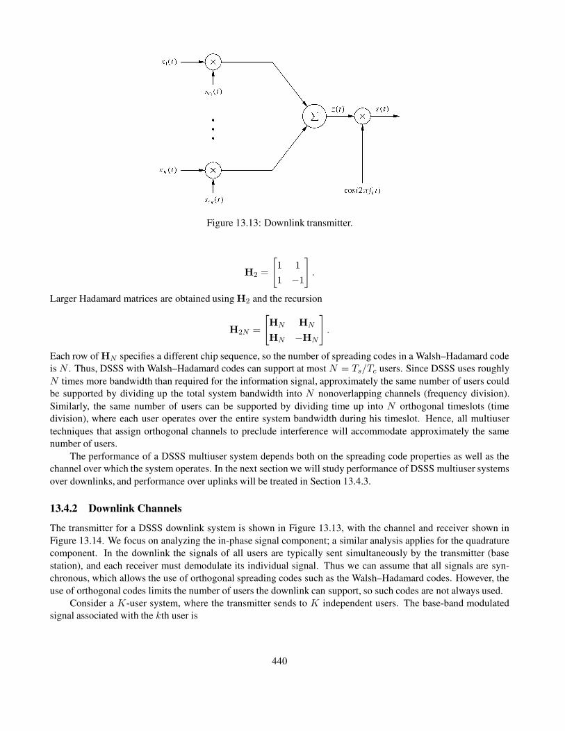
Figure 13.13: Downlink transmitter.

H2 =

[

1 1

1 −1

]

.

Larger Hadamard matrices are obtained using H2 and the recursion

H2N =

[

HN HN

HN −HN

]

.

Each row of HN specifies a different chip sequence, so the number of spreading codes in a Walsh–Hadamard code

is N . Thus, DSSS with Walsh–Hadamard codes can support at most N = Ts/Tc users. Since DSSS uses roughly

N times more bandwidth than required for the information signal, approximately the same number of users could

be supported by dividing up the total system bandwidth into N nonoverlapping channels (frequency division).

Similarly, the same number of users can be supported by dividing time up into N orthogonal timeslots (time

division), where each user operates over the entire system bandwidth during his timeslot. Hence, all multiuser

techniques that assign orthogonal channels to preclude interference will accommodate approximately the same

number of users.

The performance of a DSSS multiuser system depends both on the spreading code properties as well as the

channel over which the system operates. In the next section we will study performance of DSSS multiuser systems

over downlinks, and performance over uplinks will be treated in Section 13.4.3.

13.4.2 Downlink Channels

The transmitter for a DSSS downlink system is shown in Figure 13.13, with the channel and receiver shown in

Figure 13.14. We focus on analyzing the in-phase signal component; a similar analysis applies for the quadrature

component. In the downlink the signals of all users are typically sent simultaneously by the transmitter (base

station), and each receiver must demodulate its individual signal. Thus we can assume that all signals are syn-

chronous, which allows the use of orthogonal spreading codes such as the Walsh–Hadamard codes. However, the

use of orthogonal codes limits the number of users the downlink can support, so such codes are not always used.

Consider a K-user system, where the transmitter sends to K independent users. The base-band modulated

signal associated with the kth user is

440

Figure 13.14: Downlink channel and receiver.

xk(t) =∑

l

sklg(t− lTs), (13.34)

where g(t) =√

2/Ts is the pulse shape (assumed rectangular), Ts is the symbol time, and skl is the kth user’s

symbol over the lth symbol time. The transmitter consists of K branches, where the kth branch multiplies the kth

user’s signal xk(t) with the spreading code sck(t). The branches are summed together, resulting in the baseband

multiuser signal

z(t) =

K∑

k=1

xk(t)sck (t) =

K∑

k=1

√2

Tssklsck (t). (13.35)

this multiuser signal is multiplied by the carrier to obtain the passband signal s(t), which is transmitted over the

channel.

The signal received by user k first passes through its channel, which has impulse response hk(t) and AWGN.

Thus, the received signal at the kth user’s receiver is s(t) ∗ hk(t) + nk(t). This signal is downconverted, and we

assume perfect carrier recovery so that the phase φk of the carrier in user k’s receiver is perfectly matched to that

of its incoming signal. Thus we can normalize the delay of the kth user’s LOS (or minimum delay) path and its

associated phase shift to zero. After downconversion, the signal is then multiplied by the kth user’s spreading code

sck (t), which is assumed to be perfectly synchronized to the kth user’s spreading code in the received signal.5

The signal is then baseband demodulated via a matched filter (i.e., it is multiplied by√

2/Ts and integrated over

a symbol time). The demodulator output is sampled every Ts to obtain an estimate of the symbol transmitted by

the kth user over that symbol time. Comparing Figure 13.5 and Figure 13.14, we see that the kth user’s receiver is

5This synchronization is even more difficult than in the single-user case, since here it must be done in the presence of multiple spread

signals. In fact, some spreading code sets are obtained by shifting a single spreading code by some time period. For these systems there

must be a control channel to inform the receiver which time shift corresponds to its desired signal. More details on the synchronization for

these systems can be found in [8, Chap. 6].

441

identical to the matched filter detector in a single-user DSSS system. Thus, in the absence of multiuser interference,

the kth user has identical performance as in a single-user DSSS system. However, when multiuser interference is

taken into account, the demodulator output includes components associated with the kth user’s signal, interference

terms from other users’ signals, and noise. In particular, the demodulator output associated with the kth user over

the lth symbol time is given by

sk =

√

2

Ts

∫ Ts

0

[s(t) ∗ hk(t) + nk(t)]sck(t) cos(2πfct) dt

=

√2

Ts

∫ Ts

0[z(t) ∗ hLP

k (t)]sck(t) cos2(2πfct)dt +

√2

Ts

∫ Ts

0nk(t)sck(t) cos(2πfct) dt

=2

Ts

∫ Ts

0

K∑

j=1

sjlscj (t) ∗ hLPk (t)

sck(t) cos2(2πfct) dt

+

√2

Ts

∫ Ts

0nk(t)sck(t) cos(2πfct) dt

=2

Ts

∫ Ts

0[sklsck(t) ∗ hLP

k (t)]sck (t) cos2(2πfct) dt

+2

Ts

∫ Ts

0

K∑

j=1j 6=k

sjlscj (t) ∗ hLPk (t)

sck (t) cos2(2πfct) dt

+

√2

Ts

∫ Ts

0nk(t)sck(t) cos(2πfct) dt, (13.36)

where hLPk (t) is the in-phase component of the equivalent lowpass filter for hk(t), skl is the kth user’s transmitted

symbol over the lth symbol period that is being recovered, and sjl is the transmitted symbol of the jth user over

this symbol period, which causes interference. Note that (13.36) consists of three separate terms. The first term

corresponds to the received signal of the kth user alone, the second term represents interference from other users

in the system, and the last term is the AWGN sample, which we denote as nk. The first term and the noise sample

are characterized by the analysis in Section 13.2 for single-user systems. The second term depends on both the

channel hLPk (t) and the spreading code properties, as we now show.

To examine the characteristics of the multiuser interference, let us first assume that the kth user’s channel has

a real gain of αk and a normalized delay of zero; that is, hk(t) = αkδ(t). Then (13.36) becomes

sk =2

Ts

∫ Ts

0

αkskls2ck

(t) cos2(2πfct) dt

+2

Ts

∫ Ts

0

K∑

j=1j 6=k

αksjlscj(t)sck (t) cos2(2πfct) dt+ nk

≈ αkskl + αk

K∑

j=1j 6=k

sjlρjk(0) + nk, (13.37)

442

where ρjk(0) is the cross-correlation between sck (t) and scj (t) for a timing offset of zero, since the users are

assumed to be synchronous.6 We define

Ikl = αk

K∑

j=1j 6=k

sjlρjk(0) (13.38)

as the multiuser interference to the kth user at the demodulator output. We see from (13.37) that the kth user’s

symbol skl is attenuated by the channel gain but not affected by the spreading and despreading, exactly as in the

single-user case. The noise sample nk is also the same as in a single-user non-spread system. The interference

from other users is attenuated by the kth user’s channel gain αk and the cross-correlation of the codes ρjk(0). For

orthogonal (e.g., Walsh–Hadamard) codes, ρjk(0) = 0 so there is no interference between users. For nonorthog-

onal codes, ρjk(0) depends on the specific codes assigned to users j and k; for example, with Gold codes, ρjk(0)

can take on one of three possible values. Note that both the kth user’s signal and the interference are attenuated

by the same channel gain ak , since both signal and interference follow the same path from the transmitter to the

receiver. As we will see in the next section, this is not the case for DSSS uplink systems.

If the interference in a multiuser system has approximately Gaussian statistics then we can treat it as an

additional noise term and determine system performance based on the SINR for each user. However, the Gaussian

approximation is often inaccurate, even when the number of interferers is large [16]. Moreover, in fading the

interference terms are correlated, since they all experience the same fading αk. Thus, the interference can only

be approximated as conditionally Gaussian, conditioned on the fading. The conditionally Gaussian approximation

is most accurate when the number of interferers is large, since the sum of a large number of random variables

converges to a Gaussian random variable by the central limit theorem.7 The SINR for the kth user is defined

as the ratio of power associated with the kth user’s signal over the average power associated with the multiuser

interference and noise at the demodulator output. The kth user’s performance is then analyzed based on the bit

error rate in AWGN with SNR replaced by the SINR for this user. Moreover, if the interference power is much

greater than the system noise power, then we can neglect the noise altogether and determine performance based

on an AWGN channel analysis with SNR replaced by the signal-to-interference power ratio (SIR) for each user.

The SIR for the kth user is defined as the ratio power associated with the kth user’s signal over the average power

associated with the multiuser interference alone. Multiuser spread-spectrum systems where noise can be neglected

in the performance analysis are called interference limited, since noise is negligible relative to interference in the

performance analysis. For both SINR and SIR, obtaining the average interference power depends on the specific

spreading sequences and symbol transmissions of the interfering users, which can be highly complex to analyze.

As an alternative, average interference power is often computed assuming random spreading sequences. With this

assumption it can be shown that the SIR for a synchronousK-user system with N chips per symbol is given by

SIR =N

K − 1≈ G

K − 1, (13.39)

[17, Chap. 2.3], where G ≈ N is the processing gain of the system. Note that this matches the SIR expression

(13.6) for arbitrary interference with random signal generation. If noise is taken into account, then the SINR is

obtained from (13.39) by adding in noise scaled by the energy per symbol Es:

SINR =

(N0

Es+K − 1

G

)−1

. (13.40)

6If the users were not synchronous, which is unusual in a downlink channel, then the cross-correlation ρjk(0) in (13.37) would be

replaced by ρjk(τjk) for τjkthe relative delay between the received signal from users j and k. This assumes sjl is constant over the

integration; if not, the interference term depends on the different symbol values over the integration.7This is true even if the random variables are not i.i.d., as long as they decorrelate.

443

Now consider a more general channel hk(t) =∑M−1

m=0 αkmδ(t− τkm). We assume that m = 0 corresponds to the

LOS signal path so that, under perfect carrier recovery, we can normalize the delay τk0 and its associated phase

shift to zero. The output of the demodulator will again consist of three terms: the first corresponding to the kth

user’s signal, the second corresponding to the interference from other users, and the last an AWGN noise sample,

which is not affected by the channel. The signal component associated with the kth user is analyzed the same way

as in Section 13.2 for multipath channels: the delayed signal components are attenuated by the autocorrelation of

the kth user’s spreading code. The multiuser interference is more complicated than before. In particular, assuming

the demodulator is synchronized to the LOS component of the kth user, the demodulator output corresponding to

the multiuser interference is given by

Ikl =2

Ts

∫ Ts

0

K∑

j=1j 6=k

M−1∑

m=0

αkmsj(l−lkm)scj (i− τkm) cos(2πfc(τ − τkm))sck(t) cos(2πfct) dt

≈K∑

j=1j 6=k

M−1∑

m=0

αkmsj(l−lkm) cos(2πfcτkm)ρjk(τkm), (13.41)

where sj(l−lkm) is the symbol associated with the jth user over the (lTs−τkm)th symbol time, which we assume to

be constant for simplicity. Comparing (13.38) and (13.41), we see that the multipath channel affects the multiuser

interference in two ways. First, there are more interference terms: whereas there were K − 1 before, we now have

(K − 1)M ; so each interfering user contributesM interference terms, one for each multipath component. In addi-

tion, the cross-correlation of the codes is no longer taken at delay τ = 0, even though the users are synchronous. In

other words, the multipath destroys the synchronicity of the channel. This is significant because orthogonal codes

like the Walsh–Hadamard codes typically have zero cross-correlation only at zero delay. So if a Walsh–Hadamard

multiuser system operates in a multipath channel, the users will interfere. Equalization of the spreading codes can

be used to mitigate this interference.

Example 13.5: Consider a DSSS downlink with bandwidth expansion N = Bs/B = 100. Assume the system is

interference limited and there is no multipath on any user’s channel. Find how many users the system can support

under BPSK modulation such that each user has a BER less than 10−3.

Solution: For BPSK we have Pb = Q(√

2γb), and γb = 6.79 dB yieldsPb = 10−3. Since the system is interference

limited, we set the SIR equal to the SNR γb = 6.79 dB and solve for K, the number of users:

SIR =N

K − 1=

100

K − 1= 10.679 = 4.775.

Solving for K yields K ≤ 1 + 100/4.77 = 21.96. Since K must be an integer and we require Pb ≤ 10−3, it

follows that 21.96 must be rounded down to 21 users – although typically a designer would build the system to

support 22 users with a slight BER penalty.

13.4.3 Uplink Channels

We now consider DSSS for uplink channels. In multiuser DSSS the spreading code properties are used to separate

out the received signals from the different users. The main difference in using DSSS on the uplink versus the

downlink is that, in the downlink, both the kth user’s signal and the interfering signals from other users pass

444

through the same channel from the transmitter to the kth user’s receiver. In an uplink the signals received from

each user at the receiver travel through different channels. This gives rise to the near–far effect, where users that

are close to the uplink receiver can cause a great deal of interference to users farther away, as discussed in more

detail below.

The transmitter and channel for each individual user in a K-user uplink are shown in Figure 13.15. As in the

downlink, we will focus on in-phase signal analysis. The transmitters are typically not synchronized, since they are

not co-located. In general the asynchronous uplink is more complex to analyze than the synchronous uplink and

has worse performance. We see from Figure 13.15 that the kth user generates the baseband-modulated signal xk(t).

As in the downlink model, we assume rectangular pulses for xk(t). The kth user multiplies its baseband signal

xk(t) by its spreading code sck(t) and then upconverts to the carrier frequency to form the kth user’s transmitted

signal sk(t). (Note that the carrier signals for each user have different phase offsets.) This signal is sent over the

kth user’s channel, which has impulse response hk(t). After transmission through their respective channels, all

users’ signals are summed at the receiver front end together with AWGN n(t).

Figure 13.15: DSSS uplink system.

The uplink received signal is thus given by

r(t) =

[K∑

k=1

(xk(t)sck (t) cos(2πfct+ φk)) ∗ hk(t)]

+ n(t). (13.42)

The receiver consists ofK branches corresponding to theK received signals, as shown in Figure 13.16. We assume

(i) that the LOS path of the kth user’s channel introduces a delay of τk and (ii) that the phase offset resulting from

this delay and the transmitter carrier phase offset φk is matched by the phase offset φ′k obtained by the carrier

recovery loop in the kth branch of the receiver. For synchronous users, these delays are all equal. The kth branch

downconverts the signal to baseband and then multiplies the received signal by the kth user’s spreading code,

synchronized to the delay of the kth user’s incoming signal. The despread signal is then passed through a matched

filter and sampled to obtain an estimate of each user’s transmitted symbol over the lth symbol time. Comparing

Figures 13.5 and 13.16, we see that the kth branch of the uplink receiver is identical to the matched filter (MF)

detector in a single-user DSSS system. Thus, the uplink receiver consists of a bank ofK single-user MF detectors,

and in the absence of multiuser interference the kth user has identical performance as in a single-user system. With

multiuser interference taken into account, the demodulator output of the kth receiver branch over the lth symbol

time is given by

445

Figure 13.16: Uplink receiver.

sk =

√

2

Ts

∫ Ts

0

K∑

j=1

(xj(t)scj(t)) ∗ hLPj (t)

sck(t− τk) cos(2πfct+ φ′k) cos(2πfct+ φ′j) dt

+ nk

=2

Ts

∫ Ts

0[sklsck (t) ∗ hLP

k (t)]sck(t− τk) cos2(2πfct+ φ′k) dt

+2

Ts

∫ Ts

0

K∑

j=1j 6=k

sljkscj (t) ∗ hLPj (t)

sck(t− τk) cos(2πfct+ φ′k) cos(2πfct+ φ′j) dt

+ nk, (13.43)

where nk is the AWGN sample; hLPj (t) is the in-phase component of the equivalent lowpass filter for hj(t),

j = 1, . . . , K, with delay normalized to equal zero for the LOS path; and sljk is the symbol transmitted over the

jth user’s channel at time [lTs − τj + τk, (l + 1)Ts − τj + τk], which we assume to be constant. If this symbol

takes different values on this interval – that is, if it changes values at lTs then the ISI term is more complicated

and involves partial cross-correlations, but the ISI attenuation is roughly the same. Note that (13.43) consists of

three separate terms. The first term corresponds to the received signal of the kth user alone, and the last term is the

AWGN sample; these two terms are the same as for a single-user system. The second term represents interference

from other users in the system, and the interference of the jth user to the kth user (j 6= k) depends on the jth user’s

equivalent lowpass channel hLPj (t) and the spreading code properties, as we now show.

Assume that each user’s channel introduces only a gain αj and a delay τj , so hLPj (t) = αjδ(t− τj). Then the

demodulator output for the kth branch over the lth symbol time is

446

sk = αkskl + Ikl + nl, (13.44)

where the first and third terms are the same as for a single-user system with this channel, assuming the spreading

code in the receiver is perfectly synchronized to the delay τk . Let us now consider the interference term Ikl .Substituting hLP

j (t) = αjδ(t− τj) into (13.43) yields

Ikl =2

Ts

∫ Ts

0

K∑

j=1j 6=k

sljkscj (t) ∗ αjδ(t− τj)

sck (t− τk) cos(2πfct+ φ′k) cos(2πfct+ φ′j) dt

=1

Ts

∫ Ts

0

K∑

j=1j 6=k

αjsljkscj (t− τj)

sck (t− τk)[cos(4φkj) + cos(4πfct+ φ′k + φ′j)] dt

≈K∑

j=1j 6=k

αj cos(4φkj)sljk1

Ts

∫ Ts

0scj (t− τj)sck (t− τk) dt

=

K∑

j=1j 6=k

αj cos(4φkj)sljkρjk(τj − τk), (13.45)

where 4φkj = φ′k − φ′j and the approximation is based on fc 1/Ts. We see from (13.45) that, as with the

downlink, multiuser interference in the uplink is attenuated by the cross-correlation of the spreading codes. Since

typically τj 6= τk, users are asynchronous. It follows that orthogonal codes requiring synchronous reception (e.g.,

Walsh–Hadamard codes) are not typically used on the uplink. Another important aspect of the uplink is that the

kth user’s symbol and multiuser interference are attenuated by different channel gains. In particular, the kth user’s

signal is attenuated by the gain αk, while the interference from the jth user is attenuated by αj . If αj αkthen the interference can significantly degrade performance, even though it is reduced by the spreading code cross-

correlation.

We now consider interference-limited uplinks. Suppose initially that all users have the same received power.

Then the average SINR for asynchronous users on this channel – assuming random spreading codes with N chips

per symbol, random start times, and random carrier phases – is given [18] by

SINR =

(K − 1

3N+N0

Es

)−1

. (13.46)

For interference-limited systems we neglect the noise term and obtain the SIR as

SIR =3N

K − 1≈ 3G

K − 1, (13.47)

where G ≈ N is the processing gain of the system. The expressions (13.46) and (13.47) are referred to as the

standard Gaussian approximations for SINR and SIR. Care must be used in applying these approximations to an

arbitrary system, since the SIR and SINR for a given system is heavily dependent on the spreading code proper-

ties, timing and carrier phase assumptions, and other characteristics of the system. Modifications to the standard

Gaussian approximation have been made to improve its accuracy for practical systems, but these expressions are

447

typically more difficult to work with and don’t lead to much greater accuracy than the standard approximations [6,

Chap. 9.6]. We can modify (13.47) to approximate the SIR associated with nonrandom spreading codes as

SIR =3N

ξ(K − 1)≈ 3G

ξ(K − 1), (13.48)

where ξ is a constant characterizing the code cross-correlation that depends on the spreading code properties and

other system assumptions. Under the standard Gaussian assumption we use ξ = 1, whereas for PN sequences

ξ = 2 [19] or ξ = 3 [20], depending on the system assumptions.

Suppose now that all K − 1 interference terms have channel gain α αk. The SIR for the kth user then

becomes

SIR(k) =α2k3N

α2ξ(K − 1)≈ α2

k3G

α2ξ(K − 1) 3G

ξ(K − 1), (13.49)

so the kth user in the uplink suffers an SIR penalty of α2k/α

2 due to the different channel gains. This phenomenon

is called the near–far effect, since users far from the uplink receiver will generally have much smaller channel gains

to the receiver than those of the interferers. In fading the αk are random, which typically reduces the code cross-

correlation and hence increases the average SIR. The effect of fading can be captured by adjusting ξ in (13.48) to

reflect the average cross-correlation under the fading model. The value of ξ then depends on the spreading code

properties, the system assumptions, and the fading characteristics [21].

For multipath channels, hLPj (t) =

∑Mm=1 αjmδ(t − τjm). Substituting this into (13.45) yields multiuser

interference on the kth branch of

Ikl ≈K∑

j=1j 6=k

M∑

m=1

αjm cos(4φjkm)sljmρjk(τjm − τk), (13.50)

where we assume that the kth branch is synchronized to a channel delay of τk , that 4φjkm is the relative phase

offset, and that sljm is the symbol transmitted by the jth user over time [lTs − τk + τjm, (l+ 1)Ts − τk + τjm],

which is assumed constant. This interference also contributes to the near-far effect, since any of the multipath

components with a large gain relative to the kth user’s signal will degrade SIR.

A solution to the near–far effect in DSSS uplink systems is to use power control based on channel inversion,

where the kth user transmits signal power P/α2k so that his received signal power is P , regardless of path loss. This

will lead to an SIR given by (13.48) for each user. The disadvantage of this form of power control is that channel

inversion can require very large transmit power in some fading channels (e.g., infinite power is required in Rayleigh

fading). Moreover, channel inversion can cause significant interference to other systems or users operating on the

same frequency. In particular, channel inversion can significantly increase the interference between cells in a

cellular system. Despite these problems, channel inversion is used on the mobile-to-base station connection in the

IS-95 cellular system standard, although the inversion cannot exceed the maximum transmit power constraint.

Example 13.6: Consider a DSSS uplink system with processing gain G = Bs/B = 100. Assume the system is

interference limited and there is no multipath on any user’s channel. Suppose user k has a received power that

is 6 dB less than the other users. Find the number of users that the system can support under BPSK modulation

such that each user has a BER less than 10−3. Make the computation both for random codes under the standard

Gaussian assumption, ξ = 1, and for PN codes with ξ = 3.

Solution: As in the previous example, we require SIR = γb = 6.79 dB = 4.775 for Pb = 10−3. We again set

the SIR equal to the SNR γb = 4.775 and solve for K to find the maximum number of users that the system can

support. Since this is an asynchronous system with α2k/α

2 = .251(−6 dB), we have

448

SIR =α2k3N

α2ξ(K − 1)=.251(300)

ξ(K − 1)=

75.3

ξ(K − 1)= 4.775.

Solving for K yields K ≤ 1 + 75.3/4.77ξ = 16.78 for ξ = 1 and K ≤ 6.26 for ξ = 3, so the system can only

support between 6 and 16 users – up to a factor of 3 less than in the prior example for the downlink, which is due to

the asynchronicity of the uplink and the near–far effect. This example also illustrates the sensitivity of the system

capacity calculation to assumptions about the spreading code properties as captured by ξ. Since the SIR is roughly

proportional to 1/(ξK), the number of users the system can support for a given SIR is roughly proportional to 1/ξ.

13.4.4 Multiuser Detection

Interference signals in SSMA need not be treated as noise. If the spreading code of the interference signal is

known, then this knowledge can be used to mitigate the effects of the multiple access interference (MAI). In

particular, if all users are detected simultaneously, then interference between users can be subtracted out, which

either improves performance or, for a given performance, allows more users to share the channel. Moreover, if

all users are detected simultaneously then the near–far effect can aid in detection, since users with strong channel

gains are more easily detected (for subsequent cancellation) than if all users had the same channel gains. A

DSSS receiver that exploits the structure of multiuser interference in signal detection is called a multiuser detector

(MUD). Multiuser detectors are not typically used on downlink channels for several reasons. First, downlink

channels are typically synchronous, so they can eliminate all interference by using orthogonal codes as long as the

channel doesn’t corrupt code orthogonality. Moreover, the kth user’s receiver in a downlink is typically limited in

terms of power and/or complexity, which makes it difficult to add complex MUD functionality. Finally, the uplink

receiver must detect the signals from all users anyway, so any receiver in the uplink is by definition a multiuser

detector, albeit not necessarily a good one. By contrast, the kth user’s receiver in the downlink need only detect

the signal associated with the kth user. For these reasons, work on MUD has primarily focused on DSSS uplink

systems, and that is the focus of this section.

Multiuser detection was pioneered by Verdu in [22, 23], where the optimum joint detector for the DSSS

asynchronous uplink channel was derived. This derivation assumes an AWGN channel with different channel

gains for each user. The optimum detector for this channel chooses the symbol sequences associated with all Kusers that minimize the MSE between the received signal and the signal that would be generated by these symbol

sequences. Because the channel is asynchronous, the entire received waveform must be processed for optimal

detection over any one symbol period. The reason is that symbols from other users are not aligned in time, hence

all symbols that overlap in the given interval of interest must be considered; by applying to same reasoning to the

overlapping symbols, we see that it is not possible to process the signal over any finite interval and still preserve

optimality. The optimal MUD for the asynchronous case was shown in [23] to consist of a bank of K single-user

matched filter detectors, followed by a Viterbi sequence detection algorithm to jointly detect all users. The Viterbi

algorithm has 2K−1 states and complexity that grows as 2K , assuming binary modulation.

For synchronous users, the optimal detection becomes simpler: only one symbol interval needs to be con-

sidered in the optimal joint detection, so sequence detection is not needed. In particular, the complexity of this

detector grows as 2K/K, in contrast to the 2K growth associated with sequence detection. Consider a two-user

synchronous uplink with gain αk on channel k and binary modulation. The equivalent lowpass received signal

over one bit time is

r(t) = α1b1sc1(t) + α2b2sc2(t) + n(t), (13.51)

449

where bk is the bit transmitted by the kth user over the given bit time. The optimum (maximum likelihood) detector

outputs the pair b∗ = (b∗1, b

∗2) that satisfies

arg min(b1,b2)

[

− 1

2σ2

∫ Ts

0[r(t)− α1b1sc1(t) − α2b2sc2(t)]

2 dt

]

, (13.52)

where σ2 is the noise power. This is equivalent to finding (b∗1, b

∗2) to maximize the cost function

L(b1, b2) = α1b1r1 + α2b2r2 − α1α2b1b2ρ12, (13.53)

where

rk =

∫ Tb

0r(t)sck(t) dt (13.54)

and

ρjk =

∫ Tb

0sck (t)scj (t) dt. (13.55)

This analysis easily extends to K synchronous users. Here we can express r = (r1, . . . , rK)T in matrix form

as

r = RAb + n (13.56)

[24], where b = (b1, . . . , bK)T is the bit vector associated with theK users over the given bit time, A is a diagonal

K ×K matrix of the channel gains αk , and R is a K ×K matrix of the cross-correlations between the spreading

codes. The optimal choice of bit sequence b∗ is obtained by chosing the sequence to maximize the cost function

L(b) = 2bTAr− bTARAb. (13.57)

Unfortunately, maximizing (13.57) for K users also has complexity that grows as 2K (the same as in the asyn-

chronous case), assuming a search tree is used for the optimization. In addition to the high complexity of the

optimal detector, it has the drawback of requiring knowledge of the channel amplitudes αk.

The complexity of MUD can be decreased at the expense of optimality. Many suboptimal MUDs have been

developed with various trade-offs with respect to performance, complexity, and requirements regarding channel

knowledge. Suboptimal MUDs fall into two broad categories: linear and nonlinear. Linear MUDs apply a linear

operator or filter to the output of the matched filter bank in

Figure 13.16. These detectors have complexity that is linear in the number of users, a significant complexity

improvement over the optimal detector. The most common linear MUDs are the decorrelating detector [25] and

the minimum mean-square error (MMSE) detector. The decorrelating detector simply inverts the matrix R of

cross-correlations, resulting in

b∗ = R−1r = R−1[RAb + n] = Ab + R−1n. (13.58)

The inverse exists for most cases of interest. In the absence of noise, the resulting bit sequence equals the original

sequence, scaled by the channel gains. In addition to its simplicity, this detector has other appealing features: it

completely removes MAI, and it does not require knowledge of the channel gains. However, the decorrelating

detector can lead to noise enhancement, since the noise vector is multiplied by the matrix inverse. Thus, decorre-

lating MUD is somewhat analogous to zero-forcing equalization as described in Section 11.4.1: all MAI can be

removed, but at the expense of noise enhancement.

450

The MMSE detector finds the matrix D such that multiplication of the filter bank output by D minimizes the

expected MSE between D and the transmitted bit sequence b. In other words, the matrix D satisfies

arg minD

E[(b−Dr)T (b−Dr)]. (13.59)

The optimizing D is given [17, 24, 26] by

D = (R + .5N0I)−1. (13.60)

Note that, in the absence of noise, the MMSE detector is the same as the decorrelating detector. However, it

has better performance at low SNRs because it balances removal of the MAI with noise enhancement. This is

analogous to the MMSE equalizer design for ISI channels, described in Section 11.4.2.

Nonlinear MUDs can have much better performance than linear detectors – although not necessarily in all

cases, especially with little or no coding [27]. The most common nonlinear MUD techniques are multistage de-

tection, decision-feedback detection, and successive interference cancellation. In a multistage detector, each stage

consists of the conventional matched filter bank. The nth stage of the detector uses decisions of the (n−1)th stage

to cancel the MAI at its input. The multistage detector can be applied to either synchronous [28] or asynchronous

[29] systems. The decision-feedback detector is based on the same premise as a decision-feedback equalizer. It

consists of a feedforward and feedback filter, where the feedforward filter is the Cholesky factorization of the

correlation matrix R. The decision-feedback MUD can be designed for either synchronous [30] or asynchronous

[31] systems. These detectors require knowledge of the channel gains and can also suffer from error propagation

when decision errors are fed back through the feedback filter. In interference cancellation, an estimate of one or

more users is made and then the MAI caused to other users is subtracted out [32]. Interference cancellation can be

done in parallel, where all users are detected simultaneously and then cancelled out [33, 34], or sequentially, where

users are detected one at a time and then subtracted out from users yet to be detected [35]. Parallel cancellation

has a lower latency and is more robust to decision errors. However, its performance suffers owing to the near–

far effect, when some users have much weaker received powers than others. Under this unequal power scenario,

successive interference cancellation can outperform parallel cancellation [24]. In fact, successive cancellation the-

oretically achieves Shannon capacity of the uplink channel, as will be discussed in Chapter 14, and in practice

approaches Shannon capacity [36]. Successive interference cancellation suffers from error propagation, which can

significantly degrade performance, but this degradation can be partially offset through power control [37].

A comprehensive treatment of different MUDs and their performance can be found in [17], and shorter tutori-

als are provided in [24, 32]. Combined equalization and MUD is treated in [38]. Multiuser detection for multirate

CDMA, where different users have different data rates, is analyzed in [39]. Blind, space-time, and turbo multiuser

detectors are developed in [40]. Spectral efficiencies of the different detectors have been analyzed in [27].

13.4.5 Multicarrier CDMA

Multicarrier CDMA (MC-CDMA) is a technique that combines the advantages of OFDM and CDMA. It is very

effective both at combating ISI and as a mechanism for allowing multiple users to share the same channel. The basic

block diagram for a baseband single-user multicarrier CDMA system is shown in Figure 13.17. The data symbol

sl is sent over all N subchannels. On the ith subchannel, sl is multiplied by the ith chip cj of a spreading sequence

sc(t), where cj = ±1. This is similar to the standard spread-spectrum technique, except that multiplication with

the spreading sequence is done in the frequency domain rather than in the time domain. The frequency spread

data (slc1, slc2, . . . , slcN) is then multicarrier modulated in the standard manner: the parallel sequence is passed

through an inverse fast Fourier transform (IFFT) and a parallel-to-serial converter and then is D/A converted to

produce the modulated signal s(t), where S(f) is as shown in Figure 13.17 for subchannel carrier frequencies

(f1, . . . , fN ).

451

Assume the MC-CDMA signal is transmitted through a frequency-selective channel with a constant channel

gain of αi on the ith subchannel and with AWGN n(t). The receiver performs the reverse operations of the

transmitter – passing the received signal through an A/D converter, a serial-to-parallel converter, and an FFT – to

recover the symbol transmitted over the ith subchannel. The subchannel symbol received on the ith subchannel is

multiplied by the ith chip ci and a weighting factor βi; these terms are then summed together for the final symbol

estimate sl.In a multiuser MC-CDMA system, each user k modulates his signal as in Figure 13.17 but with a unique

spreading code sck (t). So, for a two-user system, user 1 would use the spreading code sc1(t) with chips (c11, . . . , c1N)

resulting in a transmitted signal s1(t), and user 2 would use the spreading code sc2(t) with chips (c21, . . . , c2N) re-

sulting in a transmitted signal s2(t). If the users transmit simultaneously then their signals are added “in the air”

as shown in Figure 13.18, where s1l (resp., s2l ) is the symbol corresponding to user 1 (resp., user 2) over the lth

symbol time. The interference between users in this system is reduced by the cross-correlation of the spreading

codes, as in standard spread spectrum without multicarrier. However, each user benefits from the frequency diver-

sity of spreading its signal over independently fading subchannels. This typically leads to better performance than

in standard spread spectrum.

Figure 13.17: Multicarrier CDMA system.

452

Figure 13.18: Two-user multicarrier CDMA system.

13.5 Multiuser FHSS Systems

Multiuser FHSS is accomplished by assigning each user a unique spreading code sequence sci(t) to generate its

hop pattern. If the spreading codes are orthogonal and if the users are synchronized in time, then the different users

never collide, and performance of each user is the same as in a single-user FH system. However, if the users are

asynchronous or if nonorthogonal codes are used, then multiple users will collide by occupying a given channel

simultaneously. The symbols transmitted during that time are likely to be in error, so multiuser FHSS typically

uses error correction coding to compensate for collisions.

Multiuser FHSS, also referred to as FH-CDMA or FH-SSMA, is mainly applied to uplink channels. This

access method is the preferred method for military applications because of the protection from jamming and low

probability of interception and detection characteristic of FH systems. FH-CDMA was also proposed as a candidate

for second-generation digital cellular systems [2, Chap. 9.4] but was not adopted. Trade-offs between frequency

hopping and direct sequence for multiple access are discussed in [8, Chap. 11; 41; 42]. In fact, most analyses

indicate that FH-CDMA is inferior to DS-CDMA as a multiple access method in terms of the number of users that

can share the channel simultaneously, at least under asynchronous operation. In addition, FH-CDMA systems typ-

ically cause interference at much larger distances than DS-CDMA systems, since the interference isn’t mitigated

by bandwidth spreading [8, Chap. 11]. The main benefit of FH over DS is its robustness to the near-far effect:

avoiding interference by hopping – rather than suppressing it by the processing gain – mitigates the performance

degradation caused by strong interferers. Hybrid techniques using FH along with another multiple access method

have been used to exploit the benefits of both. For example, the GSM digital cellular standard uses a combination

of time division and slow frequency hopping, where the frequency hopping is used primarily to average out inter-

ference from other cells. FH-CDMA is also used in the Bluetooth system. Bluetooth operates in the unlicensed

2.4-GHz band, and FH was chosen because it can be used with noncoherent FSK modulation, a low-cost and

energy-efficient modulation technique.

453

Chapter 13 Problems

1. In this problem we derive the SIR ratio (13.6) for a randomly spread signal with interference. The correlator

output of the ith receiver branch in this system is given by (13.5) as

xi =

∫ T

0

x(t)si(t) dt =N∑

j=1

(s2ij + Ijsij).

(a) Show that the conditional expectation of xi, conditioned on the transmitted signal si(t), is E[xi|si(t)] =Es.

(b) Assuming equiprobable signaling (p(si(t)) = 1/M), show that E[xi] = Es/M .

(c) Show that Var [xi|si(t)] = EsEJ/N .

(d) Show that (again with equiprobable signaling) Var [xi] = EsEJ/NM .

(e) The SIR is given by

SIR =E[xi]

2

Var[xi].

Show that

SIR =EsEj

· NM.

2. Sketch the transmitted DSSS signal s(t)sc(t) over two bit times [0, 2Tb] assuming that s(t) is BPSK mod-

ulated with carrier frequency 100 MHz and Ts = 1 µs. Assume the first data bit is a 1 and the second data

bit is a 0. Assume also that there are ten chips per bit and that the chips alternate between ±1, with the first

chip equal to +1.

3. Consider an FH system transmitted over a two-ray channel, where the reflected path has delay τ = 10 µsrelative to the LOS path. Assume the receiver is synchronized to the hopping of the LOS path.

(a) For what hopping rates will the system exhibit no fading?

(b) Assume an FFH system with hop time Tc = 50 µs and symbol time Ts = .5 ms. Will this system

exhibit no fading, flat fading, or frequency-selective fading?

(c) Assume a SFH system with hop time Tc = 50 µs and symbol time Ts = .5 µs. Will this system exhibit

no fading, flat fading, or frequency-selective fading?

4. In this problem we explore the statistics of the DSSS receiver noise after it is multiplied by the spreading

sequence. Let n(t) be a random noise process with autocorrelation function ρn(τ) and let sc(t) be a zero-

mean random spreading code, independent of n(t), with autocorrelation ρc(τ). Let n′(t) = n(t)sc(t).

(a) Find the autocorrelation and power spectral density of n′(t).

(b) Show that if ρc(τ) = δ(τ) then n′(t) is zero mean with autocorrelation function ρn(τ) –that is, it has

the same statistics as n(t), so the statistics of n(t) are not affected by its multiplication with sc(t).

(c) Find the autocorrelation ρn′ (τ) of n′(t) if n(t) is zero-mean AWGN and sc(t) is a maximal linear code

with autocorrelation given by (13.19). What happens to ρn′ (τ) as N → ∞ in (13.19)?

454

5. Show that, for any real periodic spreading code sc(t), its autocorrelation ρc(τ) over one period is symmetric

about τ and reaches its maximum value at τ = 0.

6. Show that, if sc(t) is periodic with period T , then the autocorrelation for time-shifted versions of the spread-

ing code depends only on the difference of their time shifts:

1

T

∫ T

0sc(t− τ0)sc(t− τ1) dt = ρc(τ1 − τ0).

7. Show that, for any periodic spreading code sc(t) with period T , its autocorrelation ρc(t) is periodic with the

same period.

8. Show that the power spectral density of sc(t) for a maximal linear spreading code with period NTc = Ts is

given by

Psc(f) =

∞∑

m=−∞

N + 1

N 2sinc2

(m

N

)

δ

(

f − m

Ts

)

.

Also plot this spectrum for N = 100 and Ts = 1 µs over the frequency range −10/Ts ≤ f ≤ 10/Ts.

9. Show that m-sequences as well as random binary spreading sequences have the balanced, run-length, and

shift properties.

10. Suppose that an unmodulated carrier s(t) is spread using a maximal linear code sc(t) with period T and

then is transmitted over a channel with an impulse response of h(t) = α0δ(t − τ0) + α1δ(t − τ1). The

corresponding received signal r(t) is input to the synchronization loop shown in Figure 13.9. Find the

functionw(τ) output from the integrator in this loop as a function of τ . What will determine which of these

two multipath components the control loop for coarse acquisition locks to?

11. Find the outage probability relative to Pb = 10−6 for a three-branch RAKE receiver with DPSK signal

modulation, independent Rayleigh fading on each branch, and a branch SNR/bit (prior to despreading) of

10 dB. Assume the code autocorrelation associated with maximal linear codes with K = N = 2n−1 = 15.

Assume also that the code in the first branch is perfectly aligned, but that the code in the second branch is

offset by Tc/4 and the code in the third branch is offset by Tc/3. Assume selection combining diversity and

neglect the interference due to other multipath components in your SNR calculations.

12. Consider a spread-spectrum signal transmitted over a multipath channel with a LOS component and a single

multipath component, where the delay of the multipath relative to the LOS is greater than the chip time

Tc. Consider a two-branch RAKE receiver, with one branch corresponding to the LOS component and the

other to the multipath component. Assume that, with perfect synchronization in both branches, the incoming

signal component at each branch (after despreading) has power that is uniformly distributed between 6 mW

and 12 mW. The total noise power in the despread signal bandwidth is 1 mW. Suppose, however, that only

the first branch is perfectly synchronized, while the second branch has a timing offset of Tc/2.366. The code

autocorrelation is that of a maximal linear code with N 1. The two branches of the RAKE are combined

using maximal-ratio combining with knowledge of the timing offset.

(a) What is the average SNR at the combiner output?

(b) What is the distribution of the combiner output SNR?

455

(c) What is the outage probability for DPSK modulation with a BER of 10−4?

13. This problem illustrates the benefits of RAKE receivers and the optimal choice of multipath components for

combining when the receiver complexity is limited. Consider a multipath channel with impulse response

h(t) = α0δ(t) + α1δ(t− τ1) + α2δ(t− τ2).

The αi are Rayleigh fading coefficients, but their expected power varies (because of shadowing) such that

E[α20] = 5 with probability .5 and 10 with probability .5, E[α2

1] = 0 with probability .5 and 20 with proba-

bility .5, and E[α22] = 5 with probability .75 and 10 with probability.25 (all units are linear). The transmit

power and noise power are such that a spread-spectrum receiver locked to the ith multipath component will

have an SNR of α2i in the absence of the other multipath components.

(a) Assuming maximal linear codes, a bit time Tb, and a spread-spectrum receiver locked to the LOS signal

component (with zero delay and gain α0), find the values of τ1 and τ2(0 ≤ τ1 ≤ τ2 < Tb) for which

their corresponding multipath components will be attenuated by − 1/N , where N is the number of

chips per bit.

For the rest of this problem, assume spreading codes with autocorrelation equal to a delta function.

(b) What is the outage probability of DPSK modulation at an instantaneousPb = 10−3 for a single-branch

spread-spectrum receiver locked to the LOS path?

(c) Find the outage probability of DPSK modulation at an instantaneous

Pb = 10−3 for a three-branch RAKE receiver, where each branch is locked to one of the multipath

components and SC is used to combine the paths.

(d) Suppose receiver complexity is limited such that only a two-branch RAKE with SC can be built. Find

which two multipath components the RAKE should lock to in order to minimize the outage probability

of DPSK modulation at Pb = 10−3, and then find this minimum outage probability.

14. This problem investigates the performance of a RAKE receiver when the multipath delays are random.

Consider a DS spreading code with chip time Tc and autocorrelation function

ρc(t) =

1 −Tc/2 < t < Tc/2,

0 else.

Suppose this spreading code is used to modulate a DPSK signal with bit time Tb = 10Tc. The spread

signal is transmitted over a multipath channel, where the channel is modeled using the discrete-time tapped

delay model described in Section 3.4, with a tap separation of Tc and a total multipath spread Tm = 5Tc.Thus, the model has five multipath “bins”, where the ith bin has at most one multipath component of delay

(i− .5)Tc. The distribution of the multipath component in each bin is independent of the components in all

the other bins. The probability of observing a multipath component in bin i is.75 and, conditioned on having

a multipath component in bin i, the amplitude of the ith multipath component after despreading is Rayleigh

distributed with average SNR/bit of Si = 20/i for i = 1, 2, . . ., 5 (in linear units). Thus, the average power

is decreasing relative to the distance that the multipath component has traveled.

At the receiving end is a five-branch SC-diversity RAKE receiver with each branch synchronized to one of

the multipath bins. Assuming a target BER of 10−3, compute the outage probability of the RAKE receiver

456

output. Compare this with the outage probability for the same BER if there is (with probability 1) a multipath

component in each bin and if each multipath component after despreading has an average SNR/bit of Si = 20

(linear units).

15. Direct-sequence spread-spectrum signals are often used to make channel measurements, since the wideband

spread-spectrum signal has good resolution of the individual multipath components in the channel. Channel

measurement with spread spectrum, also called channel sounding, is performed using a receiver with mul-

tiple branches synchronized to the different chip delays. Specifically, an unmodulated spreading sequence

sc(t) is sent through the channel h(t), as shown in Figure 13.19. The receiver has N + 1 branches synchro-

nized to different chip delays. The βi output from the ith branch approximates the channel gain associated

with that delay, so that the approximate channel model obtained by the channel sounding shown in the figure

is h(t) =∑N

i=0 βiδ(t− iTc).

Figure 13.19: Channel sounder for Problem 13-15.

Assume that the autocorrelation function for sc(t) is

ρc(τ) =1

Tb

∫ Tb

0

sc(t)sc(t− τ) dt =

1− |τ |/Tc |τ | < Tc,

0 |τ | ≥ Tc.

(a) Show that if h(t) =∑N

i=0 αiδ(t− iTc) then, in the absence of noise (n(t) = 0), the channel sounder

of Figure 13.19 will output βi = αi for all i.

(b) Again neglecting noise, if h(t) = aδ(t)+ bδ(t−1.2Tc)+ cδ(t−3.5Tc), what approximation h(t) will

be obtained by the channel sounder?

457

(c) Now assume that the channel sounder yields a perfect estimate of the channel h(t) = h(t) = β0δ(t) +β1δ(t− Tc) + β2δ(t− 2Tc), where the βi are all indepedent Rayleigh fading random variables. Con-

sider a three-branch RAKE receiver with the ith branch perfectly synchronized to the ith multipath

component of h(t) and with an average SNR/bit on each branch (after despreading) of 10 dB. Find

Pout for DPSK modulation with a target BER of 10−3 under maximal-ratio combining in the RAKE.

Do the same calculation for selection combining in the RAKE.

16. Find the values of the autocorrelation and cross-correlation for Gold codes, Kasami codes from the small

set, and Kasami codes from the large set for n = 8. Also, find the number of such Kasami codes for both

the small set and the large set.

17. Find the Hadamard matrix forN = 4 and show that the spreading codes generated by the rows of this matrix

are orthogonal, assuming synchronous users i.e., show ρij(0) = 0∀i 6= j). Also find the cross-correlation

between all pairs of users assuming a timing offset of Tc/2 between users; that is, find

ρij

(Tc2

)

=1

Ts

∫ Ts

0sci(t)scj

(

t− Tc2

)

dt =1

N

N∑

n=1

sci(nTc)scj

(

nTc −Tc2

)

for all pairs of codes.

18. Consider an asynchronous DSSS multiple access channel (MAC) system with bandwidth expansion N =Bs/B = 100 and K = 40 users. Assume the system is interference limited and there is no multipath on any

user’s channel. Find the probability of error for user k under BPSK modulation, assuming random codes

with the standard Gaussian assumption and assuming this user is in a deep fade, with received power that is

6 dB less than the other users. Would this change if the users could be synchronized?

19. Show that the vector r = (r1, . . . , rK)T for rk given by (13.54) can be expressed by the matrix equation

(13.56). What are the statistics of n in this expression?

20. Show that the maximum likelihood detector for a K-user synchronous MAC receiver choses the vector b to

maximize the cost function given by (13.57).

21. Here we illustrate the use of multiple spreading codes in single-user CDMA systems for adaptive modulation

or diversity gain. The BER for user k in a K-user DS-CDMA system, where each user transmits his BPSK

modulated bit sequence at a rate R bps along his spreading code, is given by:

BERk = Q

(√

2Pk(γk)γk1N

∑Ki=1,i6=k Pi(γi)γi + 1

)

, (13.61)

where N is the spreading factor (processing gain), γi is the ith user’s channel power gain, and Pi(γi) is i’s

transmit power when his channel gain is γi. Note that noise power has been normalized to unity and that the

receiver demodulates each spreading sequence, treating other sequences as noise (matched filter detector).

The system has a single user who can simultaneously transmit up to two spreading sequences, modulating

each with an independent BPSK bit stream at rate R bps (on each stream).

(a) Assume that the user’s channel fade is γ , and assume that he splits his total transmit powerP (γ) equally

among the transmitted sequences. Note that the user has three options: he can transmit nothing, one

BPSK modulated spreading sequence, or both spreading sequences BPSK modulated with independent

458

bits. Based on the BER expression for the multiuser case (13.61), explain why the BER for the single-

user multirate DS-CDMA system is given by

BER = Q(√

2P (γ)γ)

(13.62)

if the user transmits only one spreading sequence and by

BER = Q

(√

P (γ)γ

P (γ)γ/2N + 1

)

(13.63)

when he transmits both spreading sequences together. What are the rates achieved in both of these

cases?

(b) Assume the channel is known perfectly to the transmitter as well as the receiver, and assume that

γ is distributed according to the distribution p(γ). We want to develop an adaptive rate and power

strategy for this channel. Since we do not use error correction coding, the user needs to keep his BER

below a threshold P 0b for all transmitted bits. Assume an average transmit power constraint of unity:

∫∞0 P (γ)p(γ) dγ = 1. We have a finite discrete set of possible rates and so, as with narrowband

adaptive modulation, the optimal adaptive rate policy is to send no data when γ is below a cutoff

threshold γ0, one data stream when γ0 ≤ γ < γ1, and both data streams when γ > γ1. Find the power

adaptation strategy that exactly meets the BER target P 0b for this adaptive rate strategy as a function of

the thresholds γ0 and γ1.

(c) Given the adaptive rate and power strategy obtained in part (b), solve the Lagrangian optimization to

find γ0 and γ1 as a function of the Lagrangian λ.

22. You work for a company that wants to design a next-generation cellular system for voice plus high-speed

data. The FCC has decided to allocate 100 MHz of spectrum for this system based on whatever standard is

agreed to by the various industry players. You have been charged with designing the system and pushing your

design through the standards body. You should describe your design in as much detail as possible, paying

particular attention to how it will combat the impact of fading and ISI and to its capacity for accommodating

both voice and data. Also develop arguments explaining why your design is better than competing strategies.

459

Bibliography

[1] R. Pickholtz, D. Schilling, and L. Milstein, “Theory of spread-spectrum communications–A tutorial,” IEEE

Trans. Commun., pp. 855–84, May 1982.

[2] R. L. Peterson, R. E. Ziemer, and D. E. Borth, Introduction to Spread Spectrum Communications, Prentice-

Hall, Englewood Cliffs, NJ, 1995.

[3] V. V. Veeravalli and A. Mantravadi, “ The coding–spreading trade-off in CDMA systems,” IEEE J. Sel. Areas

Commun., pp. 396–408, February 2002.

[4] S. W. Golomb, Shlft Register Sequences, Holden-Day, San Francisco, 1967.

[5] A. J. Viterbi, CDMA Principles of Spread Spectrum Communications, Addison-Wesley, Reading, MA, 1995.

[6] G. L. Stuber, Principles of Mobile Communications, 2nd ed., Kluwer, Dordrecht, 2001.

[7] O. C. Mauss, F. Classen, and H. Meyr, “Carrier frequency recovery for a fully digital direct-sequence spread-

spectrum receiver: A comparison,” Proc. IEEE Veh. Tech. Conf., pp. 392–5, May 1993.

[8] R. C. Dixon, Spread Spectrum Systems with Commercial Applications, 3rd ed., Wiley, New York, 1994.

[9] M. K. Simon, J. K. Omura, R. A. Scholtz, and B. K. Levitt, Spread Spectrum Communications Handbook,

McGraw-Hill, New York, 1994.

[10] B. Sklar, Digital Communications–Fundamentals and Applications, Prentice-Hall, Englewood Cliffs, NJ,

1988.

[11] G. L. Turin, “Introduction to spread spectrum antimultipath techniques and their application to urban digital

radio,” Proc. IEEE, pp. 328–53, March 1980.

[12] M. K. Simon and M.-S. Alouini, Digital Communication over Fading Channels: A Unified Approach to

Performance Analysis, Wiley, New York, 2000.

[13] R. Gold, “Optimum binary sequences for spread-spectrum multiplexing,” IEEE Trans. Inform. Theory, pp.

619–21, October 1967.

[14] E. H. Dinan and B. Jabbari, “Spreading codes for direct sequence CDMA and wideband CDMA cellular

networks,” IEEE Commun. Mag., pp. 48–54, September 1998.

[15] N. B. Mehta, L. J. Greenstein, T. M. Willis, and Z. Kostic, “Analysis and results for the orthogonality factor

in WCDMA downlinks,” IEEE Trans. Wireless Commun., pp. 1138–49, November 2003.

460

[16] S. Verdu, “Demodulation in the presence of multiuser interference: Progress and misconceptions,” in D.

Docampo, A. Figueiras, and F. Perez-Gonzalez, Eds., Intelligent Methods in Signal Processing and Commu-

nications, pp. 15–46, Birkhauser, Boston, 1997.

[17] S. Verdu, Multiuser Detection, Cambridge University Press, 1998.

[18] M. Pursley, “Performance evaluation for phase-coded spread-spectrum multiple-access communication-Part

I: System analysis,” IEEE Trans. Commun., pp. 795–9, August 1977.

[19] R. Pickholtz, L. Milstein, and D. Schilling, “Spread spectrum for mobile communications,” IEEE Trans. Veh.

Tech., pp. 313–22, May 1991.

[20] K. S. Gilhousen, I. M. Jacobs, R. Padovani, A. J. Viterbi, L. A. Weaver, Jr., and C. E. Wheatley III, “On the

capacity of a cellular CDMA system,” IEEE Trans. Veh. Tech., pp. 303–12, May 1991.

[21] H. Xiang, “Binary code-division multiple-access systems operating in multipath fading, noisy channels,”

IEEE Trans. Commun., pp. 775–84, August 1985.

[22] S. Verdu, “Optimum multiuser signal detection,” Ph.D. thesis, University of Illinois, UrbanaChampaign,

August 1984.

[23] S. Verdu, “Minimum probability of error for asynchronous Gaussian multiple-access channels,” IEEE Trans.

Inform. Theory, pp. 85–96, January 1986.

[24] A. Duel-Hallen, J. Holtzman, and Z. Zvonar, “Multiuser detection for CDMA systems,” IEEE Pers. Commun.

Mag., pp. 46–58, April 1995.

[25] R. Lupas and S. Verdu, “Linear multiuser detectors for synchronous code-division multipleaccess channels,”

IEEE Trans. Inform. Theory, pp. 123–36, January 1989.

[26] M. L. Honig and H. V. Poor, “Adaptive interference suppression,” in Wireless Communications: Signal Pro-

cessing Perspectives, ch. 2, Prentice-Hall, Englewood Cliffs, NJ, 1998.

[27] S. Verdu and S. Shamai (Shitz), “Spectral efficiency of CDMA with random spreading,” IEEE Trans. Inform.

Theory, pp. 622–40, March 1999.

[28] M. K. Varanasi and B. Aazhang, “ Near-optimum detection in synchronous code division multipleaccess

communications,” IEEE Trans. Commun., pp. 725–36, May 1991.

[29] M. K. Varanasi and B. Aazhang, “Multistage detection in asynchronous code division multipleaccess com-

munications,” IEEE Trans. Commun., pp. 509–19, April 1990.

[30] A. Duel-Hallen, “Decorrelating decision-feedback multiuser detector for synchronous CDMA,” IEEE Trans.

Commun., pp. 285–90, February 1993.

[31] A. Duel-Hallen, “A family of multiuser decision-feedback detectors for asynchronous codedivision multiple-

access channels,” IEEE Trans. Commun., pp. 421–34, Febmary-April 1995.

[32] J. G. Andrews, “Interference cancellation for cellular systems: A contemporary overview,” IEEE Wireless

Commun. Mag., pp. 19–29, April 2005.

[33] D. Divsalar, M. K. Simon, and D. Raphaeli, “Improved parallel interference cancellation for CDMA,” IEEE

Trans. Commun., pp. 258–68, February 1998.

461

[34] Y. C. Yoon, R. Kohno, and H. Imai, “A spread-spectrum multiaccess system with cochannel interference

cancellation for multipath fading channels,” IEEE J. Sel. Areas Commun., pp. 1067–75, September 1993.

[35] P. Patel and J. Holtzman, “Analysis of a simple successive interference cancellation scheme in a DS/CDMA

system,” IEEE J. Sel. Areas Commun., pp. 796–807, June 1994.

[36] A. J. Viterbi, “Very low rate convolutional codes for maximum theoretical performance of spread spectrum

multiple-access channels,” IEEE J. Sel. Areas Commun., pp. 641–9, May 1990.

[37] J. G. Andrews and T. H. Meng, “Optimum power control for successive interference cancellation with imper-

fect channel estimation,” IEEE Trans. Wireless Commun., pp. 375–83, March 2003.

[38] X. Wang and H. V. Poor, “ Blind equalization and multiuser detection in dispersive CDMA channels,” IEEE

Trans. Commun., pp. 91–103, January 1998.

[39] U. Mitra, “Comparison of maximum-likelihood-based detection for two multirate access schemes for CDMA

signals,” IEEE Trans. Commun., pp. 64–77, January 1999.

[40] X. Wang and H. V. Poor, Wireless Communication Systems: Advanced Techniques for Signal Reception,

Prentice-Hall, Englewood Cliffs, NJ, 2004.

[41] R. Kohno, R. Meidan, and L. B. Milstein, “Spread spectrum access methods for wireless communications,”

IEEE Commun. Mag., pp. 58–67, January 1995.

[42] H. El Gamal and E. Geraniotis, “Comparing the capacities of FH/SSMA and DS/CDMA networks,” Proc.

Internat. Sympos. Pers., Indoor, Mobile Radio Commun., pp. 769–73, September 1998.

462

Chapter 14

Multiuser Systems

This chapter has not yet been updated for the 2nd edition

In multiuser systems the system resources must be divided among multiple users. This chapter develops

techniques to allocate resources among multiple users and examines the fundamental capacity limits of multiuser

systems. We know from Section 5.1.2 that signals of bandwidth B and time duration T occupy a signal space of

dimension 2BT . In order to support multiple users, the signal space dimensions of a multiuser system must be

allocated to the different users.1 Allocation of signaling dimensions to specific users is called multiple access.2

Multiple access methods perform differently in different multiuser channels, and we will apply these methods to

the two basic multiuser channels: downlink channels and up-link channels. Because signaling dimensions can be

allocated to different users in an infinite number of different ways, multiuser channel capacity is defined by a rate

region rather than a single number. This region describes all user rates that can be simultaneously supported by the

channel with arbitrarily small error probability. We will discuss multiuser channel capacity regions for both the

uplink and the downlink. We also consider random access techniques, whereby signaling dimensions are allocated

only to active users, as well as power control, which ensures that users maintain the SINR required for acceptable

performance. The performance benefits of multiuser diversity, which exploits the time-varying nature of the users’

channels, is also described. We conclude with a discussion of the performance gains and signaling techniques

associated with multiple antennas in multiuser systems.

14.1 Multiuser Channels: The Uplink and Downlink

A “multiuser” channel is any channel that must be shared among multiple users. There are two different types of

multiuser channels, the uplink channel and the downlink channel, which are illustrated in Figure 14.1. A downlink,

also called a broadcast channel or forward channel, has one transmitter sending to many receivers. Since the

signals transmitted to all users originate from the downlink transmitter, the transmitted signal s(t) =∑K

k=1 sk(t),

with total power P and bandwidth B, is the sum of signals transmitted to all K users. Thus, the total signaling

dimensions and power of the transmitted signal must be divided among the different users. Synchronization of the

different users is relatively easy in the downlink because all signals originate from the same transmitter, although

multipath in the channel can corrupt this synchronization. Another important characteristic of the downlink is that

both signal and interference are distorted by the same channel. In particular, user k’s signal sk(t) and all interfering

signals sj(t), j 6= k, pass through user k’s channel hk(t) to arrive at k’s receiver. This is a fundamental difference

between the uplink and the downlink, since in the uplink signals from different users are distorted by different

1Allocation of signaling dimensions through either multiple access or random access is performed by the “medium access control” layer

in the open systems interconnect (OSI) network model [1, Chap. 1.3].2The dimensions allocated to the different users need not be orthogonal, as in multiuser spread spectrum with nonorthogonal spreading

codes or the superposition coding technique discussed in Section 14.5.

463

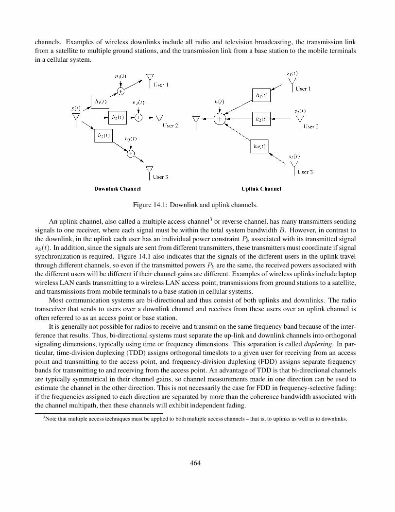
channels. Examples of wireless downlinks include all radio and television broadcasting, the transmission link

from a satellite to multiple ground stations, and the transmission link from a base station to the mobile terminals

in a cellular system.

Figure 14.1: Downlink and uplink channels.

An uplink channel, also called a multiple access channel3 or reverse channel, has many transmitters sending

signals to one receiver, where each signal must be within the total system bandwidth B. However, in contrast to

the downlink, in the uplink each user has an individual power constraint Pk associated with its transmitted signal

sk(t). In addition, since the signals are sent from different transmitters, these transmitters must coordinate if signal

synchronization is required. Figure 14.1 also indicates that the signals of the different users in the uplink travel

through different channels, so even if the transmitted powers Pk are the same, the received powers associated with

the different users will be different if their channel gains are different. Examples of wireless uplinks include laptop

wireless LAN cards transmitting to a wireless LAN access point, transmissions from ground stations to a satellite,

and transmissions from mobile terminals to a base station in cellular systems.

Most communication systems are bi-directional and thus consist of both uplinks and downlinks. The radio

transceiver that sends to users over a downlink channel and receives from these users over an uplink channel is

often referred to as an access point or base station.

It is generally not possible for radios to receive and transmit on the same frequency band because of the inter-

ference that results. Thus, bi-directional systems must separate the up-link and downlink channels into orthogonal

signaling dimensions, typically using time or frequency dimensions. This separation is called duplexing. In par-

ticular, time-division duplexing (TDD) assigns orthogonal timeslots to a given user for receiving from an access

point and transmitting to the access point, and frequency-division duplexing (FDD) assigns separate frequency

bands for transmitting to and receiving from the access point. An advantage of TDD is that bi-directional channels

are typically symmetrical in their channel gains, so channel measurements made in one direction can be used to

estimate the channel in the other direction. This is not necessarily the case for FDD in frequency-selective fading:

if the frequencies assigned to each direction are separated by more than the coherence bandwidth associated with

the channel multipath, then these channels will exhibit independent fading.

3Note that multiple access techniques must be applied to both multiple access channels – that is, to uplinks as well as to downlinks.

464

14.2 Multiple Access

Efficient allocation of signaling dimensions between users is a key design aspect of both up-link and downlink

channels, since bandwidth is usually scarce and or very expensive. When dedicated channels are allocated to

users it is often called multiple access.4 Applications with continuous transmission and delay constraints, such

as voice or video, typically require dedicated channels for good performance to ensure their transmission is not

interrupted. Dedicated channels are obtained from the system signal space using a channelization method such as

time division, frequency division, code division, or some combination of these techniques. Allocation of signaling

dimensions for users with bursty transmissions generally use some form of random channel allocation that does not

guarantee channel access. Bandwidth sharing using random channel allocation is called random multiple access or

simply random access, which will be described in Section 14.3. In general, the choice of whether to use multiple

access or random access – and which specific multiple or random access technique to apply – will depend on the

system applications, the traffic characteristics of the users in the system, the performance requirements, and the

characteristics of the channel and other interfering systems operating in the same bandwidth.

Multiple access techniques divide up the total signaling dimensions into channels and then assign these chan-

nels to different users. The most common methods to divide up the signal space are along the time, frequency,

and/or code axes. The different user channels are then created by an orthogonal or nonorthogonal division along

these axes: time-division multiple access (TDMA) and frequency-division multiple access (FDMA) are orthogonal

channelization methods, whereas code-division multiple access (CDMA) can be either orthogonal or nonorthogo-

nal, depending on the code design. Directional antennas, often obtained through antenna array processing, add an

additional angular dimension that can also be used to channelize the signal space; this technique is called space-

division multiple access (SDMA). The performance of different multiple access methods depends on whether they

are applied to an uplink or downlink as well as on their specific characteristics. The TDMA, FDMA, and orthog-

onal CDMA techniques are all equivalent in the sense that they orthogonally divide up the signaling dimensions

and hence create the same number of orthogonal channels. In particular, given a signal space of dimension 2BT , it

follows that N orthogonal channels of dimension 2BT/N can be created regardless of the channelization method.

As a result, all multiple access techniques that divide the signal space orthogonally have the same capacity when

applied to additive white Gaussian noise (AWGN) channels, as will be discussed in Sections 14.5 and 14.6. How-

ever, channel impairments such as flat and frequency-selective fading affect these techniques in different ways,

which leads to different channel capacities and different performance in typical wireless channels.

14.2.1 Frequency-Division Multiple Access (FDMA)

In FDMA the system signaling dimensions are divided along the frequency axis into nonoverlapping channels, and

each user is assign a different frequency channel; see Figure 14.2. The channels often have guard bands between

them to compensate for imperfect filters, adjacent channel interference, and spectral spreading due to Doppler.

If the channels are sufficiently narrowband, then the individual channels will not experience frequency-selective

fading even if the total system bandwidth is large. Transmission is continuous over time, which can complicate

overhead functions such as channel estimation because these functions must be performed simultaneously and

in the same bandwidth as data transmission; FDMA also requires frequency-agile radios that can tune to the

different carriers associated with the different channels. It is difficult to assign multiple channels to the same user

under FDMA, since this requires the radios to simultaneously demodulate signals received over multiple frequency

channels. Even so, FDMA is the most common multiple access option for analog communication systems, where

transmission is continuous, and serves as the basis for the AMPS and TACS analog cellular phone standards

4An uplink channel is also referred to as a multiple access channel, but multiple access techniques are needed for both uplinks and

downlinks.

465

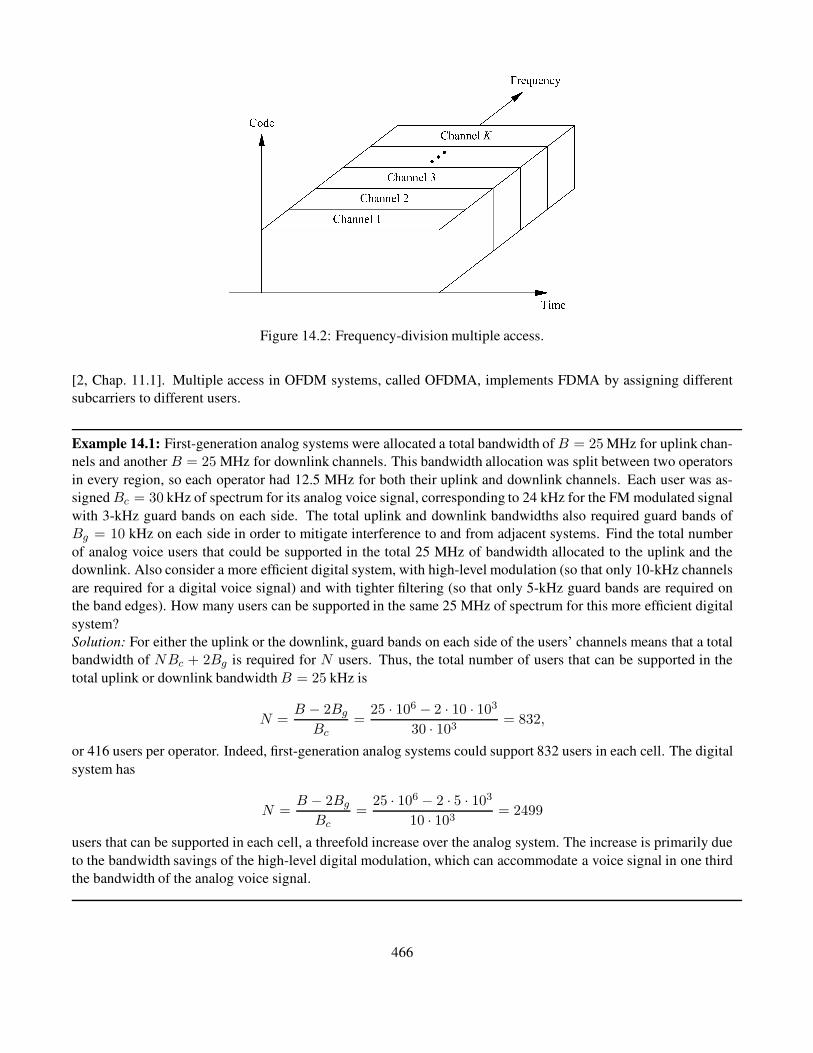
Figure 14.2: Frequency-division multiple access.

[2, Chap. 11.1]. Multiple access in OFDM systems, called OFDMA, implements FDMA by assigning different

subcarriers to different users.

Example 14.1: First-generation analog systems were allocated a total bandwidth ofB = 25 MHz for uplink chan-

nels and another B = 25 MHz for downlink channels. This bandwidth allocation was split between two operators

in every region, so each operator had 12.5 MHz for both their uplink and downlink channels. Each user was as-

signedBc = 30 kHz of spectrum for its analog voice signal, corresponding to 24 kHz for the FM modulated signal

with 3-kHz guard bands on each side. The total uplink and downlink bandwidths also required guard bands of

Bg = 10 kHz on each side in order to mitigate interference to and from adjacent systems. Find the total number

of analog voice users that could be supported in the total 25 MHz of bandwidth allocated to the uplink and the

downlink. Also consider a more efficient digital system, with high-level modulation (so that only 10-kHz channels

are required for a digital voice signal) and with tighter filtering (so that only 5-kHz guard bands are required on

the band edges). How many users can be supported in the same 25 MHz of spectrum for this more efficient digital

system?

Solution: For either the uplink or the downlink, guard bands on each side of the users’ channels means that a total

bandwidth of NBc + 2Bg is required for N users. Thus, the total number of users that can be supported in the

total uplink or downlink bandwidthB = 25 kHz is

N =B − 2BgBc

=25 · 106 − 2 · 10 · 103

30 · 103= 832,

or 416 users per operator. Indeed, first-generation analog systems could support 832 users in each cell. The digital

system has

N =B − 2BgBc

=25 · 106 − 2 · 5 · 103

10 · 103= 2499

users that can be supported in each cell, a threefold increase over the analog system. The increase is primarily due

to the bandwidth savings of the high-level digital modulation, which can accommodate a voice signal in one third

the bandwidth of the analog voice signal.

466

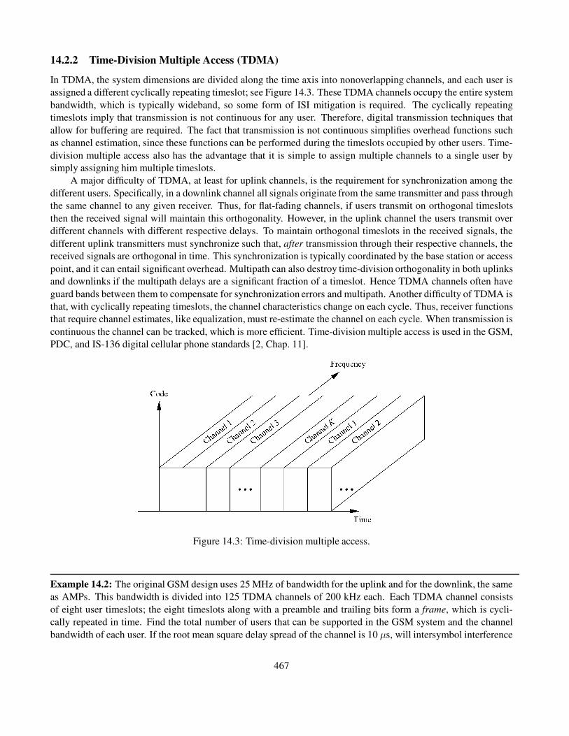
14.2.2 Time-Division Multiple Access (TDMA)

In TDMA, the system dimensions are divided along the time axis into nonoverlapping channels, and each user is

assigned a different cyclically repeating timeslot; see Figure 14.3. These TDMA channels occupy the entire system

bandwidth, which is typically wideband, so some form of ISI mitigation is required. The cyclically repeating

timeslots imply that transmission is not continuous for any user. Therefore, digital transmission techniques that

allow for buffering are required. The fact that transmission is not continuous simplifies overhead functions such

as channel estimation, since these functions can be performed during the timeslots occupied by other users. Time-

division multiple access also has the advantage that it is simple to assign multiple channels to a single user by

simply assigning him multiple timeslots.

A major difficulty of TDMA, at least for uplink channels, is the requirement for synchronization among the

different users. Specifically, in a downlink channel all signals originate from the same transmitter and pass through

the same channel to any given receiver. Thus, for flat-fading channels, if users transmit on orthogonal timeslots

then the received signal will maintain this orthogonality. However, in the uplink channel the users transmit over

different channels with different respective delays. To maintain orthogonal timeslots in the received signals, the

different uplink transmitters must synchronize such that, after transmission through their respective channels, the

received signals are orthogonal in time. This synchronization is typically coordinated by the base station or access

point, and it can entail significant overhead. Multipath can also destroy time-division orthogonality in both uplinks

and downlinks if the multipath delays are a significant fraction of a timeslot. Hence TDMA channels often have

guard bands between them to compensate for synchronization errors and multipath. Another difficulty of TDMA is

that, with cyclically repeating timeslots, the channel characteristics change on each cycle. Thus, receiver functions

that require channel estimates, like equalization, must re-estimate the channel on each cycle. When transmission is

continuous the channel can be tracked, which is more efficient. Time-division multiple access is used in the GSM,

PDC, and IS-136 digital cellular phone standards [2, Chap. 11].

Figure 14.3: Time-division multiple access.

Example 14.2: The original GSM design uses 25 MHz of bandwidth for the uplink and for the downlink, the same

as AMPs. This bandwidth is divided into 125 TDMA channels of 200 kHz each. Each TDMA channel consists

of eight user timeslots; the eight timeslots along with a preamble and trailing bits form a frame, which is cycli-

cally repeated in time. Find the total number of users that can be supported in the GSM system and the channel

bandwidth of each user. If the root mean square delay spread of the channel is 10 µs, will intersymbol interference

467

mitigation be needed in this system?

Solution: Since there are eight users per channel and 125 channels, the total number of users that can be supported

in this system is 125 · 8 = 1000 users. The bandwidth of each TDMA channel is 25 ·106/125 = 200 kHz. A delay

spread of 10 µs corresponds to a channel coherence bandwidth of Bc ≈ 100 kHz, which is less than the TDMA

channel bandwidth of 200 kHz. Thus, ISI mitigation is needed. The GSM specification includes an equalizer to

compensate for ISI, but the type of equalizer is at the discretion of the designer.

Figure 14.4: Code-division multiple access.

14.2.3 Code-Division Multiple Access (CDMA)

In CDMA the information signals of different users are modulated by orthogonal or nonorthogonal spreading

codes. The resulting spread signals simultaneously occupy the same time and bandwidth, as shown in Figure 14.4.

The receiver uses the spreading code structure to separate out the different users. The most common form of

CDMA is multiuser spread spectrum with either direct sequence or frequency hopping, which are described and

analyzed in Sections 13.4 and 13.5.

Downlinks typically use orthogonal spreading codes such as Walsh–Hadamard codes, although the orthogo-

nality can be degraded by multipath. Uplinks generally use nonorthogonal codes owing to the difficulty of user

synchronization and the complexity of maintaining code orthogonality in uplinks with multipath [3]. One of the

big advantages of nonorthogonal CDMA in uplinks is that little dynamic coordination of users in time or frequency

is required, since the users can be separated by the code properties alone. In addition, since TDMA and FDMA

carve up the signaling dimensions orthogonally, there is a hard limit on how many orthogonal channels can be

obtained. This is also true for CDMA using orthogonal codes, but if nonorthogonal codes are used then there is no

hard limit on the number of channels that can be obtained. However, because nonorthogonal codes cause mutual

interference between users, the more users that simultaneously share the system bandwidth using nonorthogonal

codes, the higher the level of interference, which degrades system performance for all users. A nonorthogonal

CDMA scheme also requires power control in the uplink to compensate for the near–far effect. The near–far effect

arises in the uplink because the channel gain between a user’s transmitter and the receiver is different for different

users. Specifically, suppose that one user is very close to his base station or access point while another user is far

468

away. If both users transmit at the same power level, then the interference from the close user will swamp the signal

from the far user. Thus, power control is used such that the received signal power of all users is roughly the same.

This form of power control, which essentially inverts any attenuation and or fading on the channel, causes each

interferer to contribute an equal amount power, thereby eliminating the near–far effect. Code-division multiple

access systems with nonorthogonal spreading codes can also use MUD to reduce interference between users. Mul-

tiuser detection provides considerable performance improvement even under perfect power control, and it works

even better when the power control is jointly optimized with the MUD technique [4]. We will see in Sections

14.5 and 14.6 that a form of CDMA with multiuser detection achieves the Shannon capacity of both the uplink

and the downlink, although the capacity-achieving transmission and reception strategies for the two channels are

quite different. Finally, it is simple to allocate multiple channels to one user with CDMA by assigning that user

multiple codes. Code-division multiple access is used for multiple access in the IS-95 digital cellular standards,

with orthgonal spreading codes on the downlink and a combination of orthogonal and nonorthogonal codes on the

uplink [2, Chap. 11.4]. It is also used in the W-CDMA and CDMA2000 digital cellular standards [5, Chap. 10.5].

Example 14.3: The signal-to-interference power ratio (SIR) for a CDMA uplink with nonorthogonal codes under

the standard Gaussian assumption was given in (13.47) as

SIR =3G

K − 1,

where K is the number of users and G ≈ 128 is the ratio of spread bandwidth to signal bandwidth. In IS-95 the

uplink channel is assigned 1.25 MHz of spectrum. Thus, the bandwidth of the information signal prior to spreading

is Bs ≈ 1.25 · 106/128 = 9.765 kHz. Neglecting noise, if the required SIR on a channel is 10 dB, how many users

can the CDMA uplink support? How many could be supported within the same total bandwidth for an FDMA

system?

Solution: To determine how many users can be supported, we invert the SIR expression to get

K ≤ 3G

SIR+ 1 =

384

10+ 1 = 39.4;

since K must be an integer, the system can support 39 users. In FDMA we have

K =1.25 · 106

9.765 · 103= 128,

so the total system bandwidth of 1.25 MHz can support 128 channels of 9.765 kHz. This calculation implies that

FDMA is three times more efficient than nonorthogonal CDMA under the standard Gaussian assumption for code

cross-correlation (FDMA is even more efficient under different assumptions about the code cross-correlation). But,

in fact, IS-95 typically supports 64 users on the uplink and downlink by allowing variable voice compression rates

depending on interference and channel quality and by taking advantage of the fact that interference is not always

present (called a voice-activity factor). Although this makes CDMA less efficient than FDMA for a single cell,

cellular systems incorporate channel reuse, which can be done more efficiently in CDMA than in FDMA (see

Section 15.2).

14.2.4 Space-Division Multiple Access (SDMA)

Space-division multiple access uses direction (angle) as another dimension in signal space, which can be chan-

nelized and assigned to different users. This is generally done with directional antennas, as shown in Figure 14.5.

Orthogonal channels can be assigned only if the angular separation between users exceeds the angular resolution of

469

the directional antenna. If directionality is obtained by using an antenna array, precise angular resolution requires a

large array, which may be impractical for the base station or access point and is certainly un-feasible in small user

terminals. In practice, SDMA is often implemented using sectorized antenna arrays, discussed in Section 10.9. In

these arrays, the 360 angular range is divided into N sectors. There is high directional gain in each sector and

little interference between sectors. Either TDMA or FDMA is used to channelize users within a sector. For mobile

users, SDMA must adapt as user angles change; or, if directionality is achieved via sectorized antennas, then a user

must be handed off to a new sector when it moves out of its original sector.

Figure 14.5: Space-division multiple access.

14.2.5 Hybrid Techniques

Many systems use a combination of different multiple access schemes to allocate signaling dimensions. OFDMA

can be combined with tone hopping to improve frequency diversity [6]. Direct-sequence spread spectrum (DSSS)

can be combined with FDMA to break the system bandwidth into subbands; in this hybrid method, different users

are assigned to different subbands with their signals spread across the subband bandwidth. Within a subband, the

processing gain is smaller than it would be over the entire system bandwidth, so interference and ISI attenuation

are reduced. In exchange for this performance loss, this hybrid technique does not require contiguous spectrum

between subbands, and it also allows more flexibility in spreading user signals over different-size subbands de-

pending on their requirements. Another hybrid method combines DS-CDMA with FH-CDMA so that the carrier

frequency of the spread signal is hopped over the available bandwidth. This reduces the near–far effect because the

interfering users change on each hop. Alternatively, TDMA and FH can be combined so that a channel with deep

fading or interference is used only on periodic hops, enabling the mitigation of fading and interference effects via

error correction coding. This idea is used in the GSM standard, which combines FH with its TDMA scheme in

order to reduce the effect of strong interferers in other cells.

There has been much discussion, debate, and analysis about the relative performance of different multiple

access techniques for current and future wireless systems (see e.g. [6, 7, 8, 9, 10, 11, 12]). Although analysis and

general conclusions can be made for simple system and channel models, it is difficult to come up with a definitive

answer as to the best technique for a complex multiuser system under a range of typical operating conditions.

Moreover, simplifying assumptions must be made in order to perform a comparative analysis or simulation study,

and these assumptions can bias the results in favor of one particular scheme. As with most engineering design

470

questions, the choice of which multiple access technique to use will depend on the system requirements and

characteristics along with cost and complexity constraints.

14.3 Random Access

Multiple access techniques are primarily for continuous applications like voice and video, where a dedicated chan-

nel facilitates good performance. However, most data applications do not require continuous transmission: data

are generated at random time instances, so dedicated channel assignment can be extremely inefficient. Moreover,

most systems have many more total users (active plus idle users) than can be accommodated simultaneously, so at

any given time channels can only be allocated to users that need them. Random access strategies are used in such

systems to efficiently assign channels to the active users.

All random access techniques are based on the premise of packetized data or packet radio. In packet radio,

user data is collected into packets ofN bits, which may include error detection/correction and control bits. Once a

packet is formed it is transmitted over the channel. Assuming a fixed channel data rate of R bps, the transmission

time of a packet is τ = N/R. The transmission rate R is assumed to require the entire signal bandwidth, and all

users transmit their packets over this bandwidth with no additional signaling to separate simultaneously transmitted

packets. Thus, if packets from different users overlap in time a collision occurs, in which case both packets may be

decoded unsuccessfully. Packets may also be decoded in error as a result of noise or other channel impairments.

The probability of a packet decoding error is called the packet error rate. Analysis of random access techniques

typically assumes that, collectively, the users accessing the channel generate packets according to a Poisson process

at a rate of λ packets per unit time; that is, λ is the average number of packets that arrive in any time interval [0, t]divided by t. Equivalently, λN is the average number of bits generated in any time inteval [0, t] divided by t. For

a Poisson process, the probability that the number of packet arrivals in a time period [0, t], denoted as X(t), is

equal to some integer k is given by

p(X(t) = k) =(λt)k

k!e−λt. (14.1)

Poisson processes are memoryless, so that the number of packet arrivals during any given time period does not

affect the distribution of packet arrivals in any other time period. Note that the Poisson model is not necessarily

a good model for all types of user traffic – especially Intemet data, where bursty data causes correlated packet

arrivals [13].

The traffic load on the channel given Poisson packet arrivals at rate λ and packet transmission duration τ

is defined as L = λτ . If the channel data rate is Rp packets per second then τ = 1/Rp = N/R for R the

channel data rate in bits per second. Note that L is unit-less: it is the ratio of the packet arrival rate divided by the

packet rate that can be transmitted over the channel at the channel’s data rate R. We assume that colliding packets

are always decoded in error. Thus, if L > 1 then on average more packets (or bits) arrive in the system over a

given time period than can be transmitted in that period, so systems with L > 1 are unstable. If the transmitter

is informed by the receiver about packets received in error and retransmits these packets, then the packet arrival

rate λ and corresponding load L = λτ is computed based on arrivals of both new packets and packets that require

retransmission. In this case L is referred to as the total offered load.

Performance of random access techniques is typically characterized by the throughput T of the system. The

throughput, which is unitless, is defined as the ratio of the average rate of packets successfully transmitted divided

by the channel packet rate Rp. The throughput thus equals the offered load multiplied by the probability of

successful packet reception, T = Lp (successful packet reception), where this probability is a function of the

random access protocol in use as well as the channel characteristics, which can cause packet errors in the absence

of collisions. Thus T ≤ L. Also, since a system with L > 1 is unstable, stable systems have T ≤ L ≤ 1.

471

Observe that the throughput is independent of the channel data rateR, since the load and corresponding throughput

are normalized with respect to this rate. This allows analysis of random access protocols to be generic to any

underlying link design or channel capacity. For a packet radio with a link data rate of R bps, the effective data

rate of the system is RT , since T is the fraction of packets or bits successfully transmitted at rate R. The goal of a

random access method is to make T as large as possible in order to fully utilize the underlying link rates. Note that

in some circumstances overlapping packets do not cause a collision. In particular, short periods of overlap between

colliding packets, different channel gains on the received packets, and/or error correction coding can allow one or

more packets to be successfully received even with a collision. This is called the capture effect [14, Chap. 4.3].

Random access techniques were pioneered by Abramson with the ALOHA protocol [15], where data is packe-

tized and users send packets whenever they have data to send. ALOHA is extremely inefficient owing to collisions

between users, which leads to very low throughput. The throughput can be doubled by slotting time and syn-

chronizing the users, but even then collisions lead to relatively low throughput values. Modifications of ALOHA

protocols to avoid collisions and thereby increase throughput include carrier sensing, collision detection, and col-

lision avoidance. Long bursts of packets can be scheduled to avoid collisions, but this typically takes additional

overhead. In this section we will describe these various techniques for random access, their performance, and their

design trade-offs.

14.3.1 Pure ALOHA

In pure or unslotted ALOHA, users transmit data packets as soon as they are formed. If we neglect the capture

effect, then packets that overlap in time are assumed to be received in error and must be retransmitted. If we also

assume packets that do not collide are successfully received (i.e., if there is no channel distortion or noise), then

the throughput equals the offered load multiplied by the probability of no collisions: T = Lp (no collisions).

Suppose a given user transmits a packet of duration τ during time [0, τ ]. Then, if any other user generates a packet

during time [−τ, τ ], that packet (of duration τ ) will overlap with the transmitted packet, causing a collision. The

probability of no collisions thus equals the probability that no packets are generated during the time [−τ, τ ]. This

probability is given by (14.1) with t = 2τ :

Figure 14.6: Throughput of pure and slotted ALOHA.

472

p(X(t) = 0) = e−2λτ = e−2L, (14.2)

with corresponding throughput

T = Le−2L. (14.3)

This throughput is plotted in Figure 14.6, where we see that throughput increases with offered load up to a max-

imum throughput of approximately .18 for L = .5, after which point it decreases. In other words, the data rate

is only 18% of what it would be with a single user transmitting continuously on the system. The reason for this

maximum is that, for small values of L, there are many idle periods when no user is transmitting, so throughput is

small. As L increases, the channel is utilized more but collisions also start to occur. At L = .5 there is the optimal

balance between users generating enough packets to utilize the channel with reasonable efficiency and these packet

generations colliding infrequently. Beyond L = .5 the collisions become more frequent, which degrades through-

put below its maximum; as L grows very large, most packets experience collisions and throughput approaches

zero.

Part of the reason for the inefficiency of pure ALOHA is the fact that users can start their packet transmissions

at any time, and any partial overlap of two or more packets destroys the successful reception of all packets. By syn-

chronizing users such that all packet transmissions are aligned in time, the partial overlap of packet transmissions

can be avoided. That is the basic premise behind slotted ALOHA.

14.3.2 Slotted ALOHA

In slotted ALOHA, time is assumed to be slotted in timeslots of duration τ , and users can only start their packet

transmissions at the beginning of the next timeslot after the packet has formed. Thus, there is no partial overlap

of transmitted packets, which increases throughput. Specifically, a packet transmitted over the time period [0, τ ]is successfully received if no other packets are transmitted during this period. This probability is obtained from

(14.1) with t = τ : p(X(t) = 0) = e−L, with corresponding throughput

T = Le−L. (14.4)

This throughput is also plotted in Figure 14.6, where we see that throughput increases with offered load up to a

maximum of approximately T = .37 for L = 1, after which point it decreases. Thus, slotted ALOHA has double

the maximum throughput as pure ALOHA, and it achieves this maximum at a higher offered load. Although

this represents a marked improvement over pure ALOHA, the effective data rate is still less than 40% of the raw

transmission rate. This is extremely wasteful of the limited wireless bandwidth, so more sophisticated techniques

are needed to increase efficiency.

Note that slotted ALOHA requires synchronization of all nodes in the network, which can entail significant

overhead. Even in a slotted system, collisions occur whenever two or more users attempt transmission in the same

slot. Error control coding can result in correct detection of a packet even after a collision, but if the error correction

is insufficient then the packet must be retransmitted. A study on design optimization between error correction and

retransmission is described in [16].

Example 14.4: Consider a slotted ALOHA system with a transmission rate of R = 10 Mbps. Suppose packets

consist of 1000 bits. For what packet arrival rate λ will the system achieve maximum throughput, and what is the

effective data rate associated with this throughput?

Solution: The throughput T is maximized for L = λτ = 1, where λ is the packet arrival rate and τ is the

packet duration. With a 10-Mbps transmission rate and 1000 bits per packet, τ = 1000/106 = .1 ms. Thus,

473

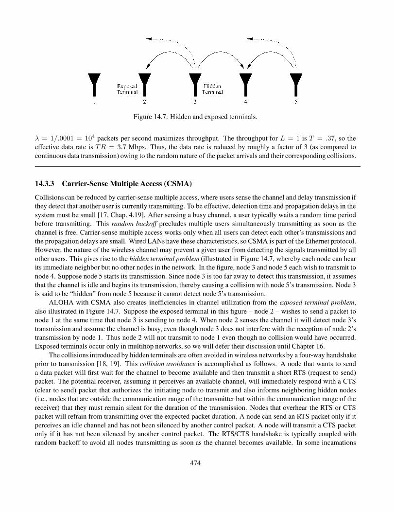
Figure 14.7: Hidden and exposed terminals.

λ = 1/.0001 = 104 packets per second maximizes throughput. The throughput for L = 1 is T = .37, so the

effective data rate is TR = 3.7 Mbps. Thus, the data rate is reduced by roughly a factor of 3 (as compared to

continuous data transmission) owing to the random nature of the packet arrivals and their corresponding collisions.

14.3.3 Carrier-Sense Multiple Access (CSMA)

Collisions can be reduced by carrier-sense multiple access, where users sense the channel and delay transmission if

they detect that another user is currently transmitting. To be effective, detection time and propagation delays in the

system must be small [17, Chap. 4.19]. After sensing a busy channel, a user typically waits a random time period

before transmitting. This random backoff precludes multiple users simultaneously transmitting as soon as the

channel is free. Carrier-sense multiple access works only when all users can detect each other’s transmissions and

the propagation delays are small. Wired LANs have these characteristics, so CSMA is part of the Ethernet protocol.

However, the nature of the wireless channel may prevent a given user from detecting the signals transmitted by all

other users. This gives rise to the hidden terminal problem (illustrated in Figure 14.7, whereby each node can hear

its immediate neighbor but no other nodes in the network. In the figure, node 3 and node 5 each wish to transmit to

node 4. Suppose node 5 starts its transmission. Since node 3 is too far away to detect this transmission, it assumes

that the channel is idle and begins its transmission, thereby causing a collision with node 5’s transmission. Node 3

is said to be “hidden” from node 5 because it cannot detect node 5’s transmission.

ALOHA with CSMA also creates inefficiencies in channel utilization from the exposed terminal problem,

also illustrated in Figure 14.7. Suppose the exposed terminal in this figure – node 2 – wishes to send a packet to

node 1 at the same time that node 3 is sending to node 4. When node 2 senses the channel it will detect node 3’s

transmission and assume the channel is busy, even though node 3 does not interfere with the reception of node 2’s

transmission by node 1. Thus node 2 will not transmit to node 1 even though no collision would have occurred.

Exposed terminals occur only in multihop networks, so we will defer their discussion until Chapter 16.

The collisions introduced by hidden terminals are often avoided in wireless networks by a four-way handshake

prior to transmission [18, 19]. This collision avoidance is accomplished as follows. A node that wants to send

a data packet will first wait for the channel to become available and then transmit a short RTS (request to send)

packet. The potential receiver, assuming it perceives an available channel, will immediately respond with a CTS

(clear to send) packet that authorizes the initiating node to transmit and also informs neighboring hidden nodes

(i.e., nodes that are outside the communication range of the transmitter but within the communication range of the

receiver) that they must remain silent for the duration of the transmission. Nodes that overhear the RTS or CTS

packet will refrain from transmitting over the expected packet duration. A node can send an RTS packet only if it

perceives an idle channel and has not been silenced by another control packet. A node will transmit a CTS packet

only if it has not been silenced by another control packet. The RTS/CTS handshake is typically coupled with

random backoff to avoid all nodes transmitting as soon as the channel becomes available. In some incamations

474

[19, 20], including the 802.11 WLAN standard [5, Chap. 14.3], the receiver sends an ACK (acknowledgement)

packet back to the transmitter to verify when it has correctly received the packet, after which the channel again

becomes available.

Another technique to avoid hidden terminals is busy-tone transmission. In this strategy, users first check to

see whether the transmit channel is busy by listening for a “busy tone” on a separate control channel [1, Chap. 4.6].

There is typically not an actual busy tone; instead, a bit is set in a predetermined field on the control channel. This

scheme works well in preventing collisions when a centralized controller can be “heard” by users throughout the

network. In a flat network without centralized control, more complicated measures are used to ensure that any

potential interferer on the first channel can hear the busy tone on the second [21, 22]. Hybrid techniques using

handshakes, busy-tone transmission, and power control can also be used [22]. Collisions can also be reduced by

combining DSSS with ALOHA. In this scheme, each user modulates his signal with the same spreading code, but

if user transmissions are separated by more than a chip time, the interference due to a collision is reduced by the

code autocorrelation [23].

14.3.4 Scheduling

Random access protocols work well with bursty traffic, where there are many more users than available channels

yet these users rarely transmit. If users have long strings of packets or continuous-stream data, then random access

works poorly because most transmissions result in collisions. In this scenario performance can be improved by

assigning channels to users in a more systematic fashion through transmission scheduling. In scheduled access,

the available bandwidth is channelized into multiple time-, frequency-, or code-division channels. Each node

schedules its transmission on different channels in such a way as to avoid conflicts with neighboring nodes while

making the most efficient use of the available signaling dimensions.

Even with a scheduling access protocol, some form of ALOHA will still be needed because a predefined

mechanism for scheduling is, by definition of random access, unavailable at startup. ALOHA provides a means

for initial contact and the establishment of some form of scheduled access for the transmission of relatively large

amounts of data. A systematic approach to this initialization that also combines the benefits of random access for

bursty data with scheduling for continuous data is packet-reservation multiple access (PRMA) [24]. This technique

assumes a slotted system with both continuous and bursty users (e.g., voice and data users). Multiple users vie for

a given time slot under a random access strategy. A successful transmission by one user in a given timeslot reserves

that timeslot for all subsequent transmissions by the same user. If the user has a continuous or long transmission

then, after successfully capturing the channel, he has a dedicated channel for the remainder of his transmission

(assuming subsequent transmissions are not corrupted by the channel; such corruption causes users to lose their

slots and they must then recontend for an unreserved slot, which can entail significant delay and packet dropping

[25]). When this user has no more packets to transmit, the slot is returned to the pool of available slots that users

attempt to capture via random access. Thus, data users with short transmissions benefit from the random access

protocol assigned to unused slots, and users with continuous transmissions get scheduled periodic transmissions

after successfully capturing an initial slot. A similar technique using a combined reservation and ALOHA policy

is described in [26].

14.4 Power Control

Power control is applied to systems where users interfere with each other. The goal of power control is to adjust

the transmit powers of all users such that the SINR of each user meets a given threshold required for acceptable

performance. This threshold may be different for different users, depending on their required performance. This

475

problem is straightforward for the downlink, where users and interferers have the same channel gains, but is more

complicated in the uplink, where the channel gains may be different. Seminal work on power control for cellular

systems and ad hoc networks was done in [27, 28, 29], and power control for the uplink is a special case for

which these results can be applied. In the uplink model, the kth transmitter has a fixed channel power gain gk to

the receiver. The quality of each link is determined by the SINR at the intended receiver. In an uplink with K

interfering users, we denote the SINR for the kth user as

γk =gkPk

n + ρ∑

j 6=k gjPj, k = 1, . . . , K, (14.5)

where Pk is the power of the kth transmitter, n is the receiver noise power, and ρ is interference reduction due to

signal processing. For example, in a CDMA uplink the interference power is reduced by the processing gain of the

code, so ρ ≈ 1/G for G the processing gain, whereas in TDMA ρ = 1.

Each link is assumed to have a minimum SINR requirement γ∗k > 0. This constraint can be represented in

matrix form with componentwise inequalities as

(I −F)P ≥ u with P > 0, (14.6)

where P = (P1, P2, . . . , PK)T is the vector of transmitter powers,

u =

(nγ∗1g1

,nγ∗2g2

, . . . ,nγ∗KgK

)T

(14.7)

is the vector of noise power scaled by the SINR constraints and channel gains, and F is a matrix with

Fkj =

0 k = j,

γ∗k gjρ/gk k 6= j,(14.8)

for k, j = 1, 2, . . . , K.

The matrix F has nonnegative elements and is irreducible. Let ρF be the Perron–Frobenius eigenvalue of

F. This is the maximum modulus eigenvalue of F, and for F irreducible this eigenvalue is simple, real, and

positive. Moreover, from the Perron–Frobenius theorem and standard matrix theory [30], the following statements

are equivalent.

1. ρF < 1.

2. There exists a vector P > 0 (i.e., Pk > 0 for all k) such that (I −F)P ≥ u.

3. (I− F)−1 exists and is positive componentwise.

Furthermore, if any of these conditions holds then we also have that P∗ = (I− F)−1u is the Pareto optimal

solution to (14.6). That is: if P is any other solution to (14.6), then P ≥ P∗ componentwise. Hence, if the SINR

requirements for all users can be met simultaneously then the best power allocation is P∗, which will minimize the

transmit power of the users.

In [28] the authors also show that the following iterative power control algorithm converges to P∗ when

ρF < 1 and diverges to infinity otherwise. This iterative Foschini–Miljanic algorithm is given by

P(i+ 1) = FP(i) + u (14.9)

for i = 1, 2, 3, . . .. Furthermore, this algorithm can be simplified to a per-user version as follows. Let

476

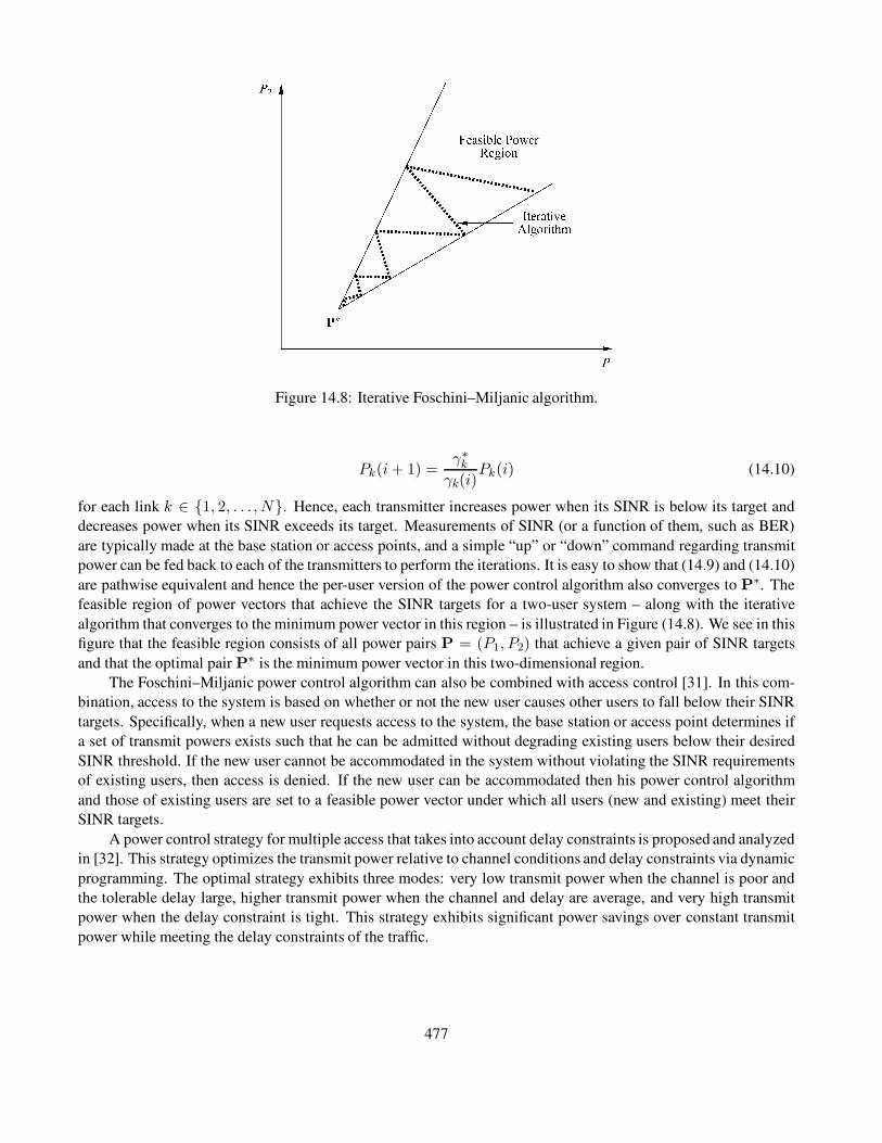
Figure 14.8: Iterative Foschini–Miljanic algorithm.

Pk(i+ 1) =γ∗kγk(i)

Pk(i) (14.10)

for each link k ∈ 1, 2, . . . , N. Hence, each transmitter increases power when its SINR is below its target and

decreases power when its SINR exceeds its target. Measurements of SINR (or a function of them, such as BER)

are typically made at the base station or access points, and a simple “up” or “down” command regarding transmit

power can be fed back to each of the transmitters to perform the iterations. It is easy to show that (14.9) and (14.10)

are pathwise equivalent and hence the per-user version of the power control algorithm also converges to P∗. The

feasible region of power vectors that achieve the SINR targets for a two-user system – along with the iterative

algorithm that converges to the minimum power vector in this region – is illustrated in Figure (14.8). We see in this

figure that the feasible region consists of all power pairs P = (P1, P2) that achieve a given pair of SINR targets

and that the optimal pair P∗ is the minimum power vector in this two-dimensional region.

The Foschini–Miljanic power control algorithm can also be combined with access control [31]. In this com-

bination, access to the system is based on whether or not the new user causes other users to fall below their SINR

targets. Specifically, when a new user requests access to the system, the base station or access point determines if

a set of transmit powers exists such that he can be admitted without degrading existing users below their desired

SINR threshold. If the new user cannot be accommodated in the system without violating the SINR requirements

of existing users, then access is denied. If the new user can be accommodated then his power control algorithm

and those of existing users are set to a feasible power vector under which all users (new and existing) meet their

SINR targets.

A power control strategy for multiple access that takes into account delay constraints is proposed and analyzed

in [32]. This strategy optimizes the transmit power relative to channel conditions and delay constraints via dynamic

programming. The optimal strategy exhibits three modes: very low transmit power when the channel is poor and

the tolerable delay large, higher transmit power when the channel and delay are average, and very high transmit

power when the delay constraint is tight. This strategy exhibits significant power savings over constant transmit

power while meeting the delay constraints of the traffic.

477

14.5 Downlink (Broadcast) Channel Capacity

When multiple users share the same channel, the channel capacity can no longer be characterized by a single

number. At the extreme, if only one user occupies all signaling dimensions in the channel then the region reduces

to the single-user capacity described in Chapter 4. However, since there is an infinite number of ways to divide the

channel between many users, the multiuser channel capacity is characterized by a rate region, where each point

in the region is a vector of achievable rates that can be maintained by all the users simultaneously with arbitrarily

small error probability. The union of achievable rate vectors under all multiuser transmission strategies is called

the capacity region of the multiuser system. The channel capacity is different for uplink channels and downlink

channels because of the fundamental differences between these channel models. However, the fact that downlink

and uplink channels seem to be mirror images implies that there might be a connection between their capacities. In

fact, there is a duality between these channels that allows the capacity region of either channel to be obtained from

the capacity region of the other. Note that, in the analysis of channel capacity, the downlink is commonly referred

to as the broadcast channel (BC) and the uplink is commonly referred to as the multiple access channel (MAC5),

and we will use this terminology in our capacity discussions. In this section we describe the capacity region of

the BC, Section 14.6 treats the MAC capacity region, and Section 14.7 characterizes the duality between these two

channels and how it can be exploited in capacity calculations.

After first describing the AWGN BC model, we will characterize its rate region using superposition code

division (CD) with successive interference cancellation, time division (TD), and frequency division (FD). We then

obtain the rate regions using DSSS for orthogonal and nonorthogonal codes. The BC and corresponding capacity

results under fading are also treated.

We will see that capacity is achieved using superposition CD with interference cancellation. In addition, DSSS

with successive interference cancellation has a capacity penalty (relative to superposition coding) that increases

with spreading gain. Finally, spread spectrum with orthogonal CD can achieve a subset of the TD and FD capacity

regions, but spread spectrum with nonorthogonal coding and no interference cancellation is inferior to all the other

spectrum-sharing techniques. The capacity regions in fading depend on what is known about the fading channel at

the transmitter and receiver, which is analogous to the case of single-user capacity in fading.

14.5.1 Channel Model

We consider a broadcast channel consisting of one transmitter sending different data streams also called inde-

pendent information or data – to different receivers. Thus, our model is not applicable to a typical radio or TV

broadcast channel, where the same data stream – also called common information or data – is received by all users.

However, the capacity results easily extend to include common data, as described in Section 14.5.3. The capacity

region of the BC characterizes the rates at which information can be conveyed to the different receivers simulta-

neously. We mainly focus on capacity regions for the two-user BC, since the general properties and the relative

performance of the different spectrum-sharing techniques are the same for any finite number of users [33].

The two-user BC has one transmitter and two distant receivers receiving data at rateRk, k = 1, 2. The channel

power gain between the transmitter and kth receiver is gk, k = 1, 2, and each receiver has AWGN of power spectral

density (PSD) N0/2. We define the effective noise on the kth channel as nk = N0/gk, k = 1, 2, and we arbitrarily

assume that n1 ≤ n2; that is, we assume the first user has a larger channel gain to its receiver than the second user.

Incorporating the channel gains into the noise PSD does not change the SINR for any user, since the signal and

interference on each user’s channel are attenuated by the same channel gain. Thus, the BC capacity with channel

gains gk is the same as the BC capacity based on the effective noises nk [34]. The fact that the channel gains

(or, equivalently, the effective noise of the users) can be ordered makes the channel model a degraded broadcast

5MAC is also used as an abbreviation for the “medium access control” layer in networks [1, Chap. 1.2].

478

channel, for which a general formula for channel capacity is known [35, Chap. 14.6]. We denote the transmitter’s

total average power and bandwidth by P and B, respectively.

If the transmitter allocates all the power and bandwidth to one of the users, then clearly the other user will

receive a rate of zero. Therefore, the set of simultaneously achievable rates (R1, R2) includes the pairs (C1, 0) and

(0, C2), where

Ck = B log2

(

1 +P

nkB

)

, k = 1, 2, (14.11)

is the single-user capacity in bits per second for an AWGN channel, as given in Section 4.1. These two points

bound the BC capacity region. We now consider rate pairs in the interior of the region that are achieved using more

equitable methods of dividing the system resources.

14.5.2 Capacity in AWGN

In this section we compute the set of achievable rate vectors of the AWGN BC under TD, FD, and the optimal

method of superposition coding, which achieves capacity. In time division, the transmit power P and bandwidth

B are allocated to user 1 for a fraction τ of the total transmission time and then to user 2 for the remainder of the

transmission. This TD scheme achieves a straight line between the points C1 and C2, corresponding to the rate

pairs

CTD =⋃

τ :0≤τ≤1

(

R1 = τB log2

(

1 +P

n1B

)

, R2 = (1 − τ)B log2

(

1 +P

n2B

))

. (14.12)

This equal-power TD achievable rate region is illustrated in Figures 14.10 and 14.11 (pp. 476–7), where n1B

and n2B differ by 3 dB and 20 dB, respectively. This dB difference, which reflects the difference in the channel

gains of the two users, is a crucial parameter in comparing the achievable rates of the different spectrum-sharing

techniques, as we discuss in more detail below.

If we also vary the transmit power of each user, subject to an average power constraint P , then we can obtain

a larger set of achievable rates. Let P1 and P2 denote the power allocated to users 1 and 2, respectively, over their

assigned time slots. The average power constraint then becomes τP1 +(1− τ)P2 = P . The achievable rate region

with TD and variable power (VP) allocation is then

CTD,VP =⋃

τ,P1,P2:0≤τ≤1;τP1+(1−τ )P2=P

(

R1 = τB log2

(

1 +P1

n1B

)

,

R2 =

(

1 − τ)B log2

(

1 +P2

n2B

))

. (14.13)

In frequency division the transmitter allocates Pk of its total power P and Bk of its total bandwidthB to user

k. The power and bandwidth constraints require that P1 + P2 = P and B1 +B2 = B. The set of achievable rates

for a fixed frequency division (B1, B2) is thus

CFFD =⋃

P1,P2:P1+P2=P

(

R1 = B1 log2

(

1 +P1

n1B1

)

, R2 = B2 log2

(

1 +P2

n2B2

))

. (14.14)

479

It was shown by Bergmans and Cover [33] that, for n1 strictly less than n2 and for any fixed frequency division

(B1, B2), there exists a range of power allocations P1, P2 : P1 +P2 = P whose corresponding rate pairs exceed

a segment of the equal-power TD line (14.12). This superiority is also illustrated in Figures 14.10 and 14.11,

where the rate regions for fixed FD under two different bandwidth divisions are plotted. The superiority is difficult

to distinguish in Figure 14.10, where the users have similar channel gains, but is much more apparent in Figure

14.11, where the users have a 20-dB difference in gain.

The FD achievable rate region is defined as the union of fixed FD rate regions (14.14) over all bandwidth

divisions:

CFD =⋃

P1,P2,B1,B2:P1+P2=P ;B1+B2=B

(

R1 = B1 log2

(

1 +P1

n1B1

)

,

R2 = B2 log2

(

1 +P2

n2B2

))

. (14.15)

It was shown in [33] that this achievable rate region exceeds the equal-power TD rate region (14.12). This supe-

riority is indicated by the closure of the fixed FD regions in Figures 14.10 and 14.11 – although it is difficult to

see in Figure 14.10, where the users have a similar received signal-to-noise ratio. In fact, when n1 = n2, (14.15)

reduces to (14.12) [33]. Thus, optimal power and/or frequency allocation is more beneficial when the users have

more disparate channel quality.

Note that the achievable rate region for TD with unequal power allocation given by (14.13) is the same as the

FD achievable rate region (14.15). This is seen by letting Bi = τiB and πi = τiPi in (14.13), where τ1 = τ and

τ2 = 1 − τ . The power constraint then becomes π1 + π2 = P . Making these substitutions in (14.13) yields

CTD,VP =⋃

π1,π2:π1+π2=P

(

R1 = B1 log2

(

1 +π1

n1B1

)

, R2 = B2 log2

(

1 +π2

n2B2

))

. (14.16)

By comparing this with (14.14) we see that, with appropriate choice of Pk and τk, any point in the FD achievable

rate region can also be achieved through TD with variable power.

Superposition coding with successive interference cancellation is a multiresolution coding technique whereby

the user with the higher channel gain can distinguish the fine resolution of the received signal constellation while

the user with the lower channel gain can only distinguish the constellation’s coarse resolution [33; 35, Chap. 14.6].

An example of a two-level superposition code constellation taken from [36] is 32-QAM with embedded 4-PSK,

as shown in Figure 14.9. In this example, the transmitted constellation point is one of the 32-QAM signal points

chosen as follows. The data stream intended for the user with the worse SNR (user 2 in our model, since n2 > n1)

provides 2 bits to select one of the 4-PSK superpoints. The data stream intended for the user with the better SNR

provides 3 bits to select one of the eight constellation points surrounding the selected superpoint. After transmission

through the channel, the user with the better SNR can easily distinguish the quadrant in which the constellation

point lies. Thus, the 4-PSK superpoint is effectively subtracted out by this user. However, the user with the

worse SNR cannot distinguish between the 32-QAM points around its 4-PSK superpoints. Hence, the 32-QAM

modulation superimposed on the 4-PSK modulation appears as noise to this user, and this user can only decode

the 4-PSK. These ideas can be easily extended to multiple users using more complex signal constellations. Since

superposition coding achieves multiple rates by expanding its signal constellation, it does not require bandwidth

expansion.

The two-user capacity region using superposition coding and successive interference cancellation was derived

in [33] to be the set of rate pairs

480

Figure 14.9: 32-QAM with embedded 4-PSK.

CBC =⋃

P1,P2:P1+P2=P

(

R1 = B log2

(

1 +P1

n1B

)

, R2 = B log2

(

1 +P2

n2B + P1

))

. (14.17)

The intuitive explanation for (14.17) is the same as for the example illustrated in Figure 14.9. Since n1 < n2, user 1

correctly receives all the data transmitted to user 2. Therefore, user 1 can decode and subtract out user 2’s message

and then decode its own message. User 2 cannot decode the message intended for user 1, since it has a worse

SNR. Thus, user 1’s message, with power P1, contributes an additional noise term to user 2’s received message.

This message can be treated as an additional AWGN term because the capacity-achieving distributions for the

signals associated with each user are Gaussian [33; 35, Chap. 14.1]. This same process is used by the successive

interference cancellation method for DSSS described in Section 13.4.4. However, although successive interference

cancellation achieves the capacity region (14.17), it is not necessarily the best method to use in practice. The

capacity analysis assumes perfect signal decoding and channel estimation, whereas real systems exhibit some

decoding and channel estimation error. This error leads to decision-feedback errors in the successive interference

cancellation scheme. Thus, multiuser detection methods that do not suffer from this type of error may work better

in practice than successive cancellation does.

The rate region defined by (14.17) was shown in [37] to exceed the regions achievable through either TD or

FD when n1 < n2. Moreover, it was also shown in [37] that this is the maximum achievable set of rate pairs for

any type of coding and spectrum sharing and thus (14.17) defines the BC capacity region; hence the notationCBC.

However, if all users have the same SNR, then this capacity region collapses to the equal-power TD line (14.12).

Thus, when n1 = n2, all the spectrum-sharing methods have the same rate region.

The ideas of superposition coding are easily extended to a K-user system for K > 2. Assume a BC with

K users, each with channel gain gk. We first order the users relative to their effective noise nk = N0/gk. Based

on this effective noise ordering, the superposition coding will now have K levels, where the coarsest level can be

detected by the user with the largest effective noise (worst SNR), the next level can be detected by the user with the

next largest effective noise, and so forth. Each user can remove the effects of the constellation points associated

with other users who have noisier channels, but the constellation points transmitted to users with better channels

481

appear as additional noise. Assuming a total power constraint P , the multiuser extension to the two-user region

(14.17) is given by

CBC =⋃

Pk:ΣKk=1Pk=P

(R1, . . . , RK) : Rk = B log2

(

1 +Pk

nkB +∑K

j=1 Pj1[nk > nj ]

)

, (14.18)

where 1[·] denotes the indicator function.

We define the sum-rate (SR) capacity of a BC as the maximum sum of rates taken over all rate vectors in the

capacity region:

CBCSR = max(R1,...,RK)∈CBC

K∑

k=1

Rk. (14.19)

Sum-rate capacity is a single number that defines the maximum throughput of the system (regardless of fairness in

the rate allocation between the users). It is therefore much easier to characterize than the K-dimensional capacity

region and often leads to important insights. In particular, it can be shown from (14.18) that sum-rate capacity is

achieved on the AWGN BC by assigning all power P to the user with the highest channel gain or, equivalently,

the lowest effective noise. Defining nmin, mink nk and gmax, maxk gk, this implies that the sum-rate capacity

CBCSR for the K-user AWGN BC is given by

CBCSR = B log2

(

1 +P

nminB

)

= B log2

(

1 +gmaxP

N0B

)

. (14.20)

The sum-rate point is therefore one of the boundary points (14.11) of the capacity region, which is the same for

superposition coding, TD, and FD because all resources are assigned to a single user.

Example 14.5: Consider an AWGN BC with total transmit power P = 10 mW, n1 = 10−9 W/Hz, n2 = 10−8

W/Hz, and B = 100 kHz. Suppose user 1 requires a data rate of 300 kbps. Find the rate that can be allocated to

user 2 under equal-power TD, equal-bandwidth FD, and superposition coding.

Solution: In equal-power TD, user 1 has a rate of R1 = τB log2(1 + P/n1B) = (6.658 · 105)τ bps. Setting R1

to the desired value R1 = (6.658 · 105)τ = 3 · 105 bps and solving for τ yields τ = 3 · 105/6.644 · 105 = .451.

Then user 2 gets a rate of R2 = (1 − τ)B log2(1 + P/n2B) = 1.89 · 105 bps. In equal-bandwidth frequency

division we require R1 = .5B log2(1 + P1/.5n1B) = 3 · 105 bps. Solving for P1 = .5n1B(2R1/(.5B) − 1) yields

P1 = 3.15 mW. SettingP2 = P−P1 = 6.85 mW, we getR2 = .5B log2(1+P2/.5n2B) = 1.94 ·105 bps. Finally,

with superposition coding we have R1 = B log2(1 + P1/n1B) = 3 · 105. Solving for P1 = n1B(2R1/B − 1)

yields P1 = .7 mW. Then

R2 = B log

(

1 +P − P1

n2B + P1

)

= 2.69 · 105 bps.

Superposition coding is clearly superior to both TD and FD, as expected, although the performance of these tech-

niques would be closer to that of superpositioncoding if we optimized the power allocation for TD or the bandwidth

allocation for FD.

Example 14.6: Find the sum-rate capacity for the system in the prior example.

482

Solution: We have P = 10 mW, n1 = 10−9 W/Hz, n2 = 10−8 W/Hz, and B = 100 kHz. The minimum noise

is associated with user 1, nmin = 10−9. Thus, CBCSR = B log2(1 + P/nminB) = 6.644 · 105 bps. This sum-rate

is achievable with TD, FD, or superposition coding, which are all equivalent for this sum-rate capacity because all

resources are allocated to the first user.

Code division for multiple users can also be implemented using DSSS, as discussed in Section 13.4. In such sys-

tems the modulated data signal for each user is modulated by a unique spreading code, which increases the transmit

signal bandwidth by approximately G, the processing gain of the spreading code. For orthogonal spreading codes,

the cross-correlation between the respective codes is zero, and these codes require a spreading gain of N to pro-

duceN orthogonal codes. For a total bandwidth constraintB, the information bandwidth of each user’s signal with

these spreading codes is thus limited to B/N . The two-user achievable rate region with these orthogonal codes

(OC) is then

CDS,OC =⋃

P1,P2:P1+P2=P

(

R1 =B

2log2

(

1 +P1

n1B/2

)

, R2 =B

2log2

(

1 +P2

n2B/2

))

. (14.21)

Comparing (14.21) with (14.14), we see that DSSS with orthogonal coding has the same capacity region as fixed

FD with the bandwidth equally divided (B1 = B2 = B/2). From (14.16), TD with unequal power allocation can

also achieve all points in this rate region. Thus, DSSS with orthogonal (e.g., Walsh–Hadamard) codes achieves a

subset of the TD and FD achievable rate regions. More general orthogonal codes are needed to achieve the same

region as these other techniques.

We now consider DSSS with nonorthogonal spreading codes. As discussed in Section 13.4.2, in these systems

interference between users is attenuated by the code crosscorrelation. Thus, if interference is treated as noise, its

power contribution to the SIR is reduced by the square of the code cross-correlation. From (13.6), we will assume

that spreading codes with a processing gain of G reduce the interference power by 1/G. This is a reasonable

approximation for random spreading codes, although (as discussed in Section 13.4.1) the exact value of the inter-

ference power reduction depends on the nature of the spreading codes and other assumptions [38, 39]. Since the

signal bandwidth is increased by G, the two-user BC rate region achievable through DSSS with nonorthogonal

codes (NC) and successive interference cancellation (IC) is given by

CDS,NC,IC

⋃

P1,P2:P1+P2=P

(

R1 =B

Glog2

(

1 +P1

n1B/G

)

,

R2 =B

Glog2

(

1 +P2

n2B/G + P1/G

))

. (14.22)

By the convexity of the log function, the rate region defined by (14.22) for G > 1 is smaller than the rate region

(14.17) obtained using superposition coding, and the degradation increases with increasing values of G. This

implies that for DSSS with nonorthogonal coding, the spreading gain should be minimized in order to maximize

capacity.

With nonorthogonal coding and no interference cancellation, the receiver treats all signals intended for other

users as noise, resulting in the achievable rate region

483

CDS, NC =⋃

P1,P2:P1+P2=P

(

R1 =B

Glog2

(

1 +P1

n1B/G+ P2/G

)

,

R2 =B

Glog2

(

1 +P2

n2B/G+ P1/G

))

. (14.23)

Again using convexity of the log function, we have that G = 1 maximizes this rate region and that the rate region

decreases as G increases. Moreover, the radius of curvature for (14.23) is given by

χ =R1R2 − R2R1

(R21 + R2

2)3/2

, (14.24)

where Ri and Ri denote (respectively) the first and second derivatives of Ri with respect to α for P1 = αP

and P2 = (1 − α)P . For G = 1, χ ≥ 0. Thus, the rate region for nonorthogonal coding without interference

cancellation (14.23)) is bounded by a convex function with end points C1 and C2, as shown in Figures 14.10 and

14.11. Therefore, the achievable rate region for DSSS with nonorthogonal coding and no interference cancellation

will lie beneath the regions for TD and FD, which are bounded by concave functions with the same endpoints.

Figure 14.10: Two-user capacity region with 3-dB SNR difference.

The achievable rate regions for equal-power TD (14.12), FD (14.14), orthogonal DSSS (14.21), and nonorthog-

onal DSSS with (14.17) and without (14.23) interference cancellation are illustrated in Figures 14.10 and 14.11,

where the SNR between the users differs by 3 dB and 20 dB, respectively. For the calculation of (14.23) we as-

sume G = 1. Direct-sequence spread spectrum with larger values of the spreading gain will result in a smaller rate

region.

484

14.5.3 Common Data

In many broadcasting applications, common data is sent to all users in the system. For example, television and

radio stations broadcast the same data to all users, and in wireless Internet applications many users may want to

download the same stock quotes and sports scores. The nature of superposition coding makes it straightforward

to develop optimal broadcasting techniques for common data and to incorporate common data into the capacity

region for the broadcast channel. In particular, for a two-user BC with superposition coding, the user with the

better channel gain always receives the data intended for the user with the worse channel gain, along with his own

data. Thus, since common data must be transmitted to both users, we can encode all common data as independent

data intended for the user with the worse SNR. Since the user with the better SNR will also receive this data, it will

be received by both users.

Under this transmission strategy, if the rate pair (R1, R2) is in the capacity region of the two-user BC with

independent data defined by (14.17), then for any R0 ≤ R2 we can achieve the rate triple (R0, R1, R2−R0) for the

BC with common and independent data, whereR0 is the rate of common data,R1 is the rate of user 1’s independent

data, andR2−R0 is the rate of user 2’s independent data. Mathematically, this gives the three-dimensional capacity

region

Figure 14.11: Two-user capacity region with 20-dB SNR difference.

CBC =⋃

P1,P2:P1+P2=P

(

R0 ≤ B log2

(

1 +P2

n2B + P1

)

, R1 = B log2

(

1 +P1

n1B

)

,

R2 = B log2

(

1 +P2

n2B + P1

)

− R0

)

. (14.25)

Example 14.7: In Example 14.5, we saw that for a broadcast channel with total transmit power P = 10 mW, n1 =10−9 W/Hz, n2 = 10−8 W/Hz, and B = 100 kHz, the rate pair (R1, R2) = (3 ·105, 2.69 ·105) is on the boundary

485

of the capacity region. Suppose that user 1 desires an independent data rate of 300 kbps and that a common data

rate of 100 kbps is required for the system. At what rate can user 2 get independent data?

Solution: In order for R1 = 300 kbps, we require the same P1 = .7 mW as in Example 14.5.2. The common

information rate R0 = 105 < 2.69 · 105, so from (14.25) it follows that the independent information rate to user 2

is just R2 − R0 = 2.69 · 105 − 1 · 105 = 1.69 · 105 bps.

14.5.4 Capacity in Fading

We now consider the capacity region of BCs with fading, where the users have independent random channel gains

that change over time. As described in Section 4.2 for single-user channels, the capacity of fading broadcast

channels depends on what is known about the channel at the transmitter and receiver. However, capacity of a BC is

only known for degraded BCs, and this model requires that the channel gains are known to both the transmitter and

receiver. Furthermore, superposition coding cannot be used without transmitter knowledge of the channel gains,

since if the transmitter does not know the relative channel gains then it does not know which user can receive

the coarse constellation point and which can receive the fine one. Thus we will only consider fading BCs where

there is perfect channel side information (CSI) about the instantaneous channel gains at the transmitter and at all

receivers. We also assume that the channel is slowly fading so that, for a given fading state, the coding strategy

that achieves any point in the capacity region for the static BC with this state has sufficient time to drive the error

probability close to zero before the channel gains change.6

As with the single-user fading channel, there are two notions of capacity for multiuser fading channels with

perfect CSI: ergodic (Shannon) capacity and outage capacity. The ergodic capacity region of a multiuser fading

channel characterizes the achievable rate vectors averaged over all fading states [34, 40] while the outage capacity

region dictates the set of fixed-rate vectors that can be maintained in all fading states subject to a given outage

probability [41, 42, 43]. Zero-outage capacity refers to outage capacity with zero outage probability [41] – that

is, the set of fixed-rate vectors that can be maintained in all fading states. The ergodic capacity region, which is

analogous to ergodic capacity for single-user systems, defines the data-rate vectors that can be maintained over

time without any constraints on delay. Hence, in some fading states the data rate may be small or zero, which can

be problematic for delay-constrained applications like voice or video. The outage capacity region – analogous to

outage capacity in single-user systems – forces a fixed-rate vector in all non-outage fading states, which is perhaps

a more appropriate capacity metric for delay-constrained applications. However, the requirement for maintain-

ing a fixed rate even in very deep fades can severely decrease the outage capacity region relative to the ergodic

capacity region. In fact, the zero-outage capacity region when all users exhibit Rayleigh fading is zero for all users.

We consider a BC with AWGN and fading where a single transmitter communicates independent information

to K users over bandwidth B with average transmit power P . The transmitter and all receivers have a single

antenna. The time-varying power gain of user k’s channel at time i is gk[i]. Each receiver has AWGN with PSD

N0/2. We define the effective time-varying noise of the kth user as7 nk[i] = N0/gk[i]. The effective noise vector

at time i is defined as

n[i] = (n1[i], . . . , nK [i]). (14.26)

We also call this the fading state at time i, since it characterizes the channel gains gk[i] associated with each user

at time i. We will denote the kth element of this vector as nk[i] or just nk when the time reference is clear. As

6More precisely, the coding strategy that achieves a point in the AWGN BC capacity region uses a block code, and the error probability

of the code goes to zero with blocklength. Our slow fading assumption presumes that the channel gains stay constant long enough for the

block code associated with these gains to drive the error probability close to zero.7Notice that the noise vector is the instantaneous power of the noise and not the instantaneous noise sample.

486

with the static channel, the capacity of the fading BC can be computed based on its time-varying channel gains or

its time-varying effective noise vector. The ergodic BC capacity region is defined as the set of all average rates

achievable in a fading channel with arbitrarily small probability of error, where the average is taken with respect

to all fading states. In [34], the ergodic capacity region and optimal power allocation scheme for the fading BC

is found by decomposing the fading channel into a parallel set of static BCs, one for every possible fading state

n = (N0/g1, . . . , N0/gK). In each fading state the channel can be viewed as a static AWGN BC, and time,

frequency, or code division can be applied to the channel in each fading state.

Since the transmitter and all receivers know n[i], superposition coding according to the ordering of the current

effective noise vector can be used by the transmitter. Each receiver can perform successive decoding in which the

users with larger effective noise are decoded and subtracted out before decoding the desired signal. Furthermore,

the power transmitted to each user Pj(n) is a function of the current fading state. Since the transmission scheme

is based on superposition coding, it remains only to determine the optimal power allocation across users and over

time.

We define a power policy P over all possible fading states as a function that maps from any fading state n to

the transmitted power Pk(n) for each user. Let FBC denote the set of all power policies satisfying average power

constraint P :

FBC4=

P : En

[K∑

k=1

Pk(n)

]

≤ P

. (14.27)

From (14.18), the capacity region assuming a constant fading state n with power allocation P(n) = Pk(n) : k =1, . . . , K is given by

CBC(P(n)) =

(R1(P(n), . . . , RK(P(n)) :

Rk(P(n)) = B log2

(

1 +Pk(n)

nkB +∑K

j=1 Pj(n)1[nk > nj]

)

. (14.28)

Let CBC(P) denote the set of achievable rates averaged over all fading states for power policy P :

CBC(P) = (R1, . . . , RK) : Rk ≤ En[Rk(P(n))],where Rk(P(n)) is as given in (14.28). From [34], the ergodic capacity region of the BC with perfect CSI and

power constraint P is:

CBC(P ) =⋃

P∈FBC

CBC(P). (14.29)

It is further shown in [34] that the region CBC(P ) is convex and that the optimal power allocation scheme is an

extension of water-filling with K different water levels for a K user system.

We can also define achievable rate vectors for TD or FD, although these will clearly lie inside the ergodic

capacity region, since superposition coding outperforms both of these techniques in every fading state. The optimal

form of TD adapts the power assigned to each user relative to the current fading state. Similarly, the optimal form

of FD adapts the bandwidth and power assigned to each user relative to the current fading state. As described

in Section 14.5.2, for each fading state, varying the power in TD yields the same rates as varying the power and

bandwidth in FD. Thus, the achievable rates for these two techniques averaged over all fading states are the same.

Focusing on the FD region, assume a power policy P ∈ FBC that assigns power Pk(n) to the kth user in fading

487

state n. By (14.27), a power policy P ∈ FBC satisfies the average power constraint. Also assume a bandwidth

policy B that assigns bandwidth Bk(n) to user k in state n, and let G denote the set of all bandwidth policies

satisfying the bandwidth constraint of the system:

G4=

B :

K∑

k=1

Bk(n) = B ∀n

.

The set of achievable rates for FD under policies P and B is

CFD(P ,B) = (R1, . . . , RK) : Rk ≤ En[Rk(P(n),B)], (14.30)

where

Rk(P (n),B) = Bk(n) log2

(

1 +Pk(n)

nkBk(n)

)

. (14.31)

The set of all achievable rates under frequency division with perfect CSI, subject to power constraint P and band-

width constraint B, is then

CFD(P , B) =⋃

P∈FBC,B∈G

CFD(P ,B). (14.32)

The sum-rate capacity for fading BCs is defined as the maximum sum of achievable rates, maximized over

all rate vectors in the ergodic BC capacity region. Since sum-rate capacity for the AWGN BC is maximized by

transmitting only to the user with the best channel, in fading the sum-rate is maximized by transmitting only to the

user with the best channel in each channel state. Clearly superposition CD, TD, and FD are all equivalent in this

setting, since all resources are assigned to a single user in each state. We can compute the sum-rate capacity and

the optimal power allocation over time from an equivalent single-user fading channel with time-varying effective

noise n[i] = mink nk[i] and average power constraint P . From Section 4.2.4 the optimal power allocation to the

user with the best channel at time i is thus a water-filling in time, with cutoff value determined from the distribution

of mink nk[i].

The ergodic capacity and achievable rate regions for fading broadcast channels under CD, TD, and FD are

computed in [34] for different fading distributions, along with the optimal adaptive resource allocation strategies

that achieve the boundaries of these regions. These adaptive transmission policies exploit multiuser diversity in

that more resources (power, bandwidth, timeslots) are allocated to the users with the best channels in any given

fading state. In particular, sum-rate capacity is achieved by allocating all resources in any given state to the user

with the best channel. Multiuser diversity will be discussed in more detail in Section 14.8.

The zero-outage BC capacity region defines the set of rates that can be simultaneously achieved for all users in

all fading states while meeting the average power constraint; it is the multiuser extension of zero-outage capacity

defined in Section 4.2.4 for single-user channels. From [42], the power required to support a rate vector R =(R1, R2, . . . , RK) in fading state n is:

Pmin(R,n) =K−1∑

k=1

[2(ΣKj=k+1Rπ(j)/B)(2Rπ(k)/B − 1)nπ(k)B] + (2Rπ(K)/B − 1)nπ(K)B, (14.33)

where π(·) is the permutation such that

nπ(1) < nπ(2) < . . . < nπ(K).

488

Therefore, the zero-outage capacity region is the union of all rate vectors that meet the average power constraint:

C0BC(P ) =

⋃

R:En[Pmin(R,n)]≤P

R = (R1, R2, . . . , RK). (14.34)

The boundary of the zero-outage capacity region is the set of all rate vectors R such that the power constraint is

met with equality. For the two-user BC with time-varying AWGN with powers n1 and n2, this boundary simplifies

to the set of all (R1, R2) that satisfy the following equation [42]:

P = p(n1 < n2)[E[n1B|n1 < n2]2R2/B(2R1/B − 1) + E[n2B|n1 < n2](2

R2/B − 1)]

+ p(n1 ≥ n2)[E[n2B|n1 ≥ n2]2R1/B(2R2/B − 1) + E[n1B|n1 ≥ n2](2

R1/B − 1)].

The boundary is determined solely by E[n1B|n1 < n2],E[n2B|n1 < n2],E[n1

B|n1 ≥ n2], and E[n2B|n1 ≥ n2]. This follows because the power required to achieve a rate vector is a lin-

ear function of the noise levels in each state, as seen in (14.33). The zero-outage capacity region depends on

the conditional expectations of the noises – as opposed to their unconditional expectations – since every different

ordering of noises leads to a different expression for the required power in each state, as can be seen from (14.33).

The outage capacity region of the BC is defined similarly as the zero-outage capacity region, except that users

may have some nonzero probability of outage so that they can suspend transmission in some outage states. This

provides additional flexibility in the system because, under severe fading conditions, maintaining a fixed rate in

all fading states can consume a great deal of power. In particular, we saw in Section 4.2.4 that, for a singleuser

fading channel, maintaining any nonzero fixed rate in Rayleigh fading requires infinite power. By allowing some

outage, power can be conserved from outage states to maintain higher rates in non-outage states. The outage

capacity region is more difficult to obtain than the zero-outage capacity region, since in any given fading state the

transmission strategy must determine which users to put into outage. Once the outage users are determined, the

power required to maintain the remaining users is given by (14.33) for the rate vector associated with the K ′ ≤ K

users that are not in outage. It is shown in [42] that this decision should be made based on a threshold policy,

and the resulting outage capacity region is then obtained implicitly based on the threshold policy and the power

allocation (14.33) for non-outage users.

The notions of ergodic capacity and outage capacity can also be combined. This combination results in the

minimum rate capacity region [44]. A rate vector in this region characterizes the set of all average rate vectors that

can be maintained, averaged over all fading states, subject to some minimum rate vector that must be maintained

in all states (possible subject to some outage probability). Minimum rate capacity is useful for systems supporting

a mix of delay-constrained and delay-unconstrained data. The minimum rates dictate the data rates available for

the constrained data that must be maintained in all fading states, while the rates above these minimums are what is

available for the unconstrained data, where these additional rates vary depending on the current fading state. The

minimum rate capacity region (with zero outage probability) lies between that of the zero-outage capacity region

and the ergodic capacity region: for minimum rates of zero it equals the ergodic capacity region; for minimum rates

on the boundary of the zero-outage capacity region, it cannot exceed these boundary points. This is illustrated in

Figure 14.12, where we plot the ergodic, zero-outage, and minimum rate capacity region for a BC with Rician

fading. We see from this figure that the ergodic capacity region is the largest, since it can adapt to the different

channel states in order to maximize its average rate (averaged over all fading states). The zero-outage capacity

region is the smallest, since it is forced to maintain a fixed rate in all states, which consumes much power when

the fading is severe. The minimum rate capacity region lies between the other two and depends on the minimum

rate requirements. As the minimum rate vector that must be maintained in all fading states increases, the minimum

rate capacity region approaches the zero-outage capacity region, and as this minimum rate vector decreases, the

minimum rate capacity region approaches the ergodic capacity region.

489

Figure 14.12: Ergodic, zero-outage, and minimum rate BC capacity regions (Rician fading with a K-factor of l,

average SNR = 10 dB).

14.5.5 Capacity with Multiple Antennas

We now investigate the capacity region for a BC with multiple antennas. We have seen in Section 10.3 that

multiple-input multiple-out (MIMO) systems can provide large capacity increases for single-user systems. The

same will be true of multiuser systems: in fact, multiple users can exploit multiple spatial dimensions even more

effectively than a single user.

Consider a K-user BC in which the transmitter has Mt antennas and each receiver has Mr antennas. The

Mr ×Mt channel matrix Hk characterizes the channel gains between each antenna at the transmitter and each

antenna at the kth receiver. The received signal for the kth user is then

yk = Hkx + nk, (14.35)

where x is the input to the transmit antennas, and we denote its covariance matrix as Qx = E[xxH ]. For simplicity,

we normalize the bandwidth to unity,8 B = 1 Hz, and assume the noise vector nk is circularly symmetric complex

Gaussian with nk ∼ N (0, I).

When the transmitter has more than one antenna, Mt > 1, the BC is no longer degraded. In other words, re-

ceivers cannot generally be ranked by their channel quality, since receivers have different channel gains associated

with the different antennas at the transmitter. The capacity region of the general nondegraded broadcast channels

is unknown. However, an achievable region for this channel was proposed in [46, 47] that was later shown [48] to

equal the capacity region. The region is based on the notion of dirty paper coding (DPC) [49]. The basic premise

of DPC is as follows. If the transmitter (but not the receiver) has perfect, noncausal knowledge of interference to

a given user, then the capacity of the channel is the same as if there were no interference or, equivalently, as if the

receiver had knowledge of the interference and could subtract it out. Dirty paper coding is a technique that allows

noncausally known interference to be “presubtracted” at the transmitter but in such a way that the transmit power

is not increased. A more practical (and more general) technique to perform this presubtraction is described in [50].

8The capacity of unity-bandwidth MIMO channels has a factor of.5 preceding the log function for real (one-dimensional) channels, with

no such factor for complex (two-dimensional) channels [45, Chap. 3.1].

490

In the MIMO broadcast channel, DPC can be applied at the transmitter when choosing codewords for different

users. The transmitter first picks a codeword x1 for user 1. The transmitter then chooses a codeword x2 for

user 2 with full (noncausal) knowledge of the codeword intended for user 1. Hence the codeword of user 1

can be presubtracted such that user 2 does not see the codeword intended for user 1 as interference. Similarly, the

codeword x3 for user 3 is chosen such that user 3 does not see the signals intended for users 1 and 2 as interference.

This process continues for allK users. The ordering of the users clearly matters in such a procedure and needs to be

optimized in the capacity calculation. Let π(·) denote a permutation of the user indices and let Q = [Q1, . . . ,QK]

denote a set of positive semidefinite covariance matrices with Tr [Q1 + · · ·+ QK ] ≤ P . Under DPC, if user π(1)is encoded first, followed by user π(2), and so forth, then the following rate vector is achievable:

R(π,Q) = (Rπ(1), . . . , Rπ(K)) :

Rπ(k) = log2

det[I + Hπ(k)(∑

j≥k Qπ(j))HHπ(k)]

det[I + Hπ(k)(∑

j>k Qπ(j))HHπ(k)

], k = 1, . . . , K. (14.36)

Figure 14.13: MIMO BC capacity region with H1 = [1 0.5],H2 = [0.5 1], and P = 10.

The capacity region C is then the convex hull of the union of all such rate vectors over all permutations and all

positive semidefinite covariance matrices satisfying the average power constraint:

CBC(P,H)4=Co

⋃

π,Q

R(π,Q)

. (14.37)

where R(π,Q) is given by (14.36). The transmitted signal is x = x1 + · · ·+xK and the input covariance matrices

are of the form Qk = E[xkxHk ]. The DPC implies that x1, . . . , xK are uncorrelated, and thus Tr [Qx] = Tr

[Q1 + · · ·+ QK ] ≤ P .

One important feature to notice about the rate equations defined by (14.36) is that these equations are neither

a concave nor a convex function of the covariance matrices. This makes finding the capacity region difficult,

491

because generally the entire space of covariance matrices that meet the power constraint must be searched [46, 47].

However, as described in Section 14.7, there is a duality between the MIMO BC and the MIMO MAC that can

be exploited to greatly simplify this calculation. Figure 14.13 shows the capacity region for a two-user channel

computed by exploiting this duality withMt = 2 andMr = 1. The region is defined by the outer boundary, and the

lines inside this boundary each correspond to the capacity region of a different dual MIMO MAC channel whose

sum power equals the power of the MIMO BC. The union of these dual regions yields the boundary of the MIMO

BC region, as will be discussed in Section 14.7.

14.6 Uplink (Multiple Access) Channel Capacity

14.6.1 Capacity in AWGN

The MAC consists ofK transmitters, each with power Pk , sending to a receiver over a channel with power gain gk.

We assume that all transmitters and the receiver have a single antenna. The received signal is corrupted by AWGN

with PSD N0/2. The two-user MAC capacity region is the closed convex hull of all vectors (R1, R2) satisfying

the following constraints [35, Chap. 14.1]:

Rk ≤ B log2

(

1 +gkPkN0B

)

, k = 1, 2, (14.38)

R1 +R2 ≤ B log2

(

1 +g1P1 + g2P2

N0B

)

. (14.39)

The first constraint (14.38) is just the capacity associated with each individual channel. The second constraint

(14.39) indicates that the sum of rates for all users cannot exceed the capacity of a “superuser” with received

power equal to the sum of received powers from all users. For K users, the region becomes

CMAC =

(R1, . . . , RK) :∑

k∈S

Rk ≤ B log2

(

1 +

∑

k∈S gkPk

N0B

)

∀S ⊂ 1, 2, . . . , K

. (14.40)

Thus, the region described by (14.40) demonstrates that the sum of rates for any subset of the K users cannot

exceed the capacity of a superuser with received power equal to the sum of received powers associated with this

user subset.

The sum-rate capacity of a MAC is the maximum sum of rates∑K

k=1 Rk, where the maximum is taken over

all rate vectors (R1, . . . , RK) in the MAC capacity region. As with the like capacity for the BC, the MAC sum-rate

also measures the maximum throughput of the system regardless of fairness and is easier to characterize than the

K-dimensional capacity region. It can be shown from (14.40) that sum-rate capacity is achieved on the AWGN

MAC by having all users transmit at their maximum power, which yields

CMACSR = B log2

(

1 +

∑Kk=1 gkPkN0B

)

. (14.41)

The intuition behind this result is that each user in the MAC has an individual power constraint, so not allowing

a user to transmit at full power wastes system power. By contrast, the AWGN BC sum-rate capacity (14.20) is

achieved by transmitting only to the user with the best channel. However, since all users share the power resource,

no power is wasted in this case.

The MAC capacity region for two users is shown in Figure 14.14, where Ck and C∗k are given by

492

Ck = B log2

(

1 +gkPkN0B

)

, k = 1, 2; (14.42)

C∗1 = B log2

(

1 +g1P1

N0B + g2P2

)

, (14.43)

C∗2 = B log2

(

1 +g2P2

N0B + g1P1

)

. (14.44)

The point (C1, 0) is the achievable rate vector when transmitter 1 is sending at its maximum rate and transmitter 2

is silent, and the opposite scenario achieves the rate vector (0, C2). The corner points (C1, C∗2 ) and (C∗

1 , C2) are

achieved using the successive interference cancellation described previously for superposition codes. Specifically,

let the first user operate at the maximum data rate C1. Then its signal will appear as noise to user 2; thus, user 2

can send data at rate C∗2 that can be decoded at the receiver with arbitrarily small error probability. If the receiver

then subtracts out user 2’s message from its received signal, the remaining message component is just user 1’s

message corrupted by noise, so rate C1 can be achieved with arbitrarily small error probability. Hence, (C1, C∗2 )

is an achievable rate vector. A similar argument with the user roles reversed yields the rate point (C∗1 , C2). Time

sharing between these two strategies yields any point on the straight line connecting (C1, C∗2 ) and (C∗

1 , C2). This

time-sharing line can also be achieved via a technique called rate splitting, whereby a given user splits his data

stream into multiple substreams and encodes these substreams as if they originated from different virtual users

[51]. Note that in the BC the user with the highest SNR must always be decoded last, whereas with MACs the

decoding can be done in either order. This is a fundamental difference between the two channels.

Figure 14.14: Two-user MAC capacity region.

A time-division strategy between two transmitters operating at their maximum rates, given by (14.42), yields

any rate vector on the straight line connectingC1 and C2. With frequency division, the rates depend on the fraction

of the total bandwidth that is allocated to each transmitter. Letting B1 and B2 denote the bandwidth allocated to

each of the two users, we obtain the achievable rate region

CFD =⋃

B1,B2:B1+B2=B

(

R1 = B1 log2

(

1 +g1P1

N0B1

)

, R2 = B2 log2

(

1 +g2P2

N0B2

))

, (14.45)

which is plotted in Figure 14.14. Clearly this region dominates TD, since settingB1 = τB and B2 = (1− τ)B in

(14.45) yieldsR1 > τC1 andR2 > (1−τ)C2. It can be shown [35, Chap. 14.3] that this curve touches the capacity

493

region boundary at one point: this point corresponds to the rate vector that maximizes the sum-rate R1 + R2. To

achieve this rate point, the bandwidths B1 and B2 must be proportional to their corresponding received powers

g1P1 and g2P2.

As with the broadcast channel, we can obtain the same achievable rate region with TD as with FD by efficient

use of the transmit power. If we take the constraints P1 and P2 to be average power constraints then it follows

that, since user k uses the channel only a fraction τk of the time, its average power over that time fraction can be

increased to Pk/τk. The rate region achievable through variable-power TD is then given by

CTD,VP =⋃

τ1,τ2:τ1+τ2=1

=

(

R1 = τ1B log2

(

1 +g1P1

N0τ1B

)

, R2 = τ2B log2

(

1 +g2P2

N0τ2B

))

, (14.46)

and substitutingBk4= τkB in (14.46) yields the same rate region as in (14.45).

Superposition codes without successive decoding can also be used. With this approach, each transmitter’s

message acts as noise to the others. Thus, the maximum achievable rate in this case cannot exceed (C∗1 , C

∗2 ),

which is clearly dominated by FD and TD for some bandwidth or time allocations – in particular, the allocation

that intersects the capacity region boundary.

Example 14.8: Consider a MAC channel in AWGN with transmit power P1 = P2 = 100 mW for both users

and with channel gains of g1 = .08 for user 1 and g2 = .001 for user 2. Assume the receiver noise has

N0 = 10−9 W/Hz and the system bandwidth is B = 100 kHz. Find the corner points of the MAC capacity

region. Also find the rate that user 1 can achieve if user 2 requires a rate of R2 = 100 kbps and of R2 = 50 kbps.

Solution: From (14.42)–(14.44) we have:

C1 = B log2

(

1 +g1P1

N0B

)

= 6.34 · 105,

C2 = B log2

(

1 +g2P2

N0B

)

= 1 · 105;

C∗1 = B log2

(

1 +g1P1

N0B + g2P2

)

= 5.36 · 105,

C∗2 = B log2

(

1 +g2P2

N0B + g1P1

)

= 1.77 · 103.

The maximum rate for user 2 is 100 kbps, so if he requires R2 = 100 kbps then this rate point is associated with

the corner point (C∗1 , C2) of the capacity region; hence user 1 can achieve a rate of R1 = C∗

1 = 536 kbps. If

user 2 requires only R2 = 50 kbps then the rate point lies on the TD portion of the capacity region. In particu-

lar, time sharing between the corner points (C1, C∗2 ) and (C2, C

∗1 ) yields, for any τ with 0 ≤ τ ≤ 1, the rate

point (R1, R2) = τ(C1, C∗2) + (1 − τ)(C∗

1 , C2). The time-share value τ that yields R2 = 50 kbps thus satisfies

τC∗2 + (1 − τ)C2 = R2. Solving for τ yields τ = (R2 − C2)/(C

∗2 − C2) = .51, about halfway between the

two comer points. Then user 1 can achieve rate R1 = τC1 + (1 − τ)C∗1 = 5.86 · 105. This example illustrates

the dramatic impact of the near–far effect in MAC channels. Even though both users have the same transmit

power, the channel gain of user 2 is much less than the gain of user 1. Hence, user 2 can achieve at most a rate of

100 kbps, whereas user 1 can achieve a rate between 536 and 634 kbps. Moreover, the interference from user 2

has little impact on user 1 owing to the weak channel gain associated with the interference: user 1 sees data rates

494

of C1 = 634 kbps without interference and C∗1 = 536 kbps with interference. However, the interference from user

1 severely limits the data rate of user 2, decreasing it by almost two orders of magnitude from C2 = 100 kbps to

C∗2 = 1.77 kbps.

14.6.2 Capacity in Fading

We now consider the capacity region of a multiple access channel with AWGN and fading, where the channel gains

for each user change over time. We assume that all transmitters and the receiver have a single antenna and that

the receiver has AWGN with PSD N0/2. Each user has an individual power constraint Pk, k = 1, . . . , K. The

time-varying power gain of user k’s channel at time i is gk[i] and is independent of the fading of other users. We

define the fading state at time i as g[i] = (g1[i], . . . , gK [i]), with the time reference dropped when the context

is clear. We assume perfect CSI about the fading state at both the transmitter and receiver; the case of receiver

CSI only is treated in [52, Chap. 6.3]. Like the broadcast and single-user channels, the fading MAC also has two

notions of capacity: the ergodic capacity region, which characterizes the achievable rate vectors averaged over all

fading states; and the outage capacity region, which characterizes the maximum rate vector that can be maintained

in all states with some nonzero probability of outage.

We first consider the ergodic capacity region as derived in [40]. Define a power policy P as a function that

maps a fading state g = (g1, . . . , gK) to a set of powers P1(g), . . . , PK(g), one for each user. Let FMAC denote

the set of all power policies satisfying the average peruser power constraint Pk:

FMAC4= P : Eg[Pk(g)] ≤ Pk, k = 1, . . . , K.

The MAC capacity region assuming a constant fading state g with power allocation P1(g), . . . , PK(g) is given by

CMAC(P1(g), . . . , PK(g))

=

(R1, . . . , RK) :∑

k∈S

Rk ≤ B log2

(

1 +

∑

k∈S gkPk(g)

N0B

)

∀S ⊂ 1, 2, . . . , K

. (14.47)

The set of achievable rates averaged over all fading states under power policy P is given by

CMAC(P)

=

(R1, . . . , RK) :∑

k∈S

Rk ≤ Eg

[

B log2

(

1 +

∑

k∈S gkPk(g)

N0B

)]

∀S ⊂ 1, 2, . . . , K

. (14.48)

The ergodic capacity region is then the union over all power policies that satisfy the individual user power con-

straints:

CMAC(P1, . . . , PK) =⋃

P∈FMAC

CMAC(P). (14.49)

From (14.41), (14.48), and (14.49), the sum-rate capacity of the MAC in fading reduces to

CMACSR = maxP∈FMAC

Eg

[

B log2(1 +

∑Kk=1 gkPk(g)

N0B)

]

. (14.50)

495

The maximization in (14.50) is solved using Lagrangian techniques, and the solution reveals that the optimal

transmission strategy to achieve sum-rate is to allow only one user to transmit in every fading state [53]. Under

this optimal policy, the user that transmits in a given fading state g is the one with the largest weighted channel

gain gk/λk, where λk is the Lagrange multiplier associated with the average power constraint of the kth user.

This Lagrangian is a function of the user’s average power constraint and fading distribution. By symmetry, if all

users have the same fading distribution and the same average power constraint, then each user has the same λkand so the optimal policy is to allow only the user with the best channel gk to transmit in fading state g. Once it

is determined which user should transmit in a given state, the power the user allocates to that state is determined

via a water-filling over time. The intuition behind allowing only one user at a time to transmit is as follows. Since

users can adapt their powers over time, system resources are best utilized by assigning them to the user with the

best channel and allowing that user to transmit at a power commensurate with his channel quality. But when users

have unequal average received power this strategy is no longer optimal: users with weak average received SNR

would rarely transmit, so their individual power resources would be underutilized.

The MAC zero-outage capacity region, derived in [41], defines the set of rates that can be simultaneously

achieved for all users in all fading states while meeting the average power constraints of each user. From (14.40),

given a power policy P that maps fading states to user powers, the MAC capacity region in state g is

CMAC(P) =

(R1, . . . , RK) :∑

k∈S

Rk ≤ B log2

(

1 +

∑

k∈S gkPk(g)

N0B

)

∀S ⊂ 1, 2, . . . , K

. (14.51)

Then, under policy P , the set of rates that can be maintained in all fading states g is

C0MAC(P) =

⋂

g

CMAC(P). (14.52)

The zero-outage capacity region is then the union of C0MAC(P) over all power policies P ∈ FMAC that satisfy the

user power constraints. Thus, the zero-outage MAC capacity region is given by

C0MAC(P1, . . . , PK) =

⋃

P∈FMAC

⋂

g

CMAC(P). (14.53)

The outage capacity region of the MAC is similar to the zero-outage capacity region, except that users can

suspend transmission in some outage states subject to a given nonzero probability of outage. As with the BC, the

MAC outage capacity region is more difficult to obtain than the zero-outage capacity region, since in any given

fading state the transmission strategy must determine which users to put into outage, the decoding order of the non-

outage users, and the power at which these non-outage users should transmit. The MAC outage capacity region

is obtained implicitly in [43] by determining whether a given rate vector R can be maintained in all fading states

– subject to a given per-user outage probability – without violating the per-user power constraints. Ergodic and

outage capacities can also be combined to obtain the minimum rate capacity region for the MAC. As with the BC,

this region characterizes the set of all average rate vectors (averaged over all fading states) that can be maintained

subject to some minimum rate vector that must be maintained in all states with some outage probability (possibly

zero). The minimum rate capacity region for the fading MAC is derived in [54] using the duality principle that

relates capacity regions of the BC and the MAC. This duality principle is described in the next section.

14.6.3 Capacity with Multiple Antennas

We now consider MAC channels with multiple antennas. As in the MIMO BC model, we normalize bandwidth to

unity, B = 1 Hz, and assume the noise vector n at the MAC receiver is circularly symmetric complex Gaussian

496

with n ∼ N (0, I). Let theMr×Mt matrix Hk characterize the MIMO MAC channel gains between each antenna

at the kth user’s transmitter and each antenna at the receiver. Define H = [H1 . . .HK ]. Then the capacity region

of the Gaussian MIMO MAC where user k has channel gain matrix Hk and power Pk is given [55, 56, 57] by

CMAC((P1 . . . , PK); H)

=⋃

Qk≥0,Tr(Qk)≤Pk∀k

(R1, . . . , RK) :

∑

k∈S

Rk ≤ log2 det

[

I +∑

k∈S

HkQkHHk

]

∀S ⊆ 1, . . . , K

. (14.54)

This region is achieved as follows. The kth user transmits a zero-mean Gaussian random vector xk with spatial co-

variance matrix Qk = E[xkxHk ]. Each set of covariance matrices (Q1, . . . ,QK) corresponds to a K-dimensional

polyhedron (i. e., (R1, . . . , RK) :∑

k∈S Rk ≤ log2 det[I +∑

k∈S HkQkHHk ]∀S ⊆ 1, . . . , K), and the

capacity region is equal to the union (over all covariance matrices satisfying the power constraints) of all such

polyhedrons. The corner points of this pentagon can be achieved by successive decoding: users’ signals are suc-

cessively decoded and subtracted out of the received signal. Note that the capacity region (14.54) has several

similarities with its single-antenna counterpart: it is defined based on the rate sum associated with subsets of users,

and the corner points of the region are obtained using successive decoding.

For the two-user case, each set of covariance matrices corresponds to a pentagon, which is similar in form to

the capacity region of the single-antenna MAC. For example, the corner point whereR1 = log2 det[I+H1Q1HH1 ]

and

R2 = log2 det[I + H1Q1HH1 + H2Q2H

H2 ]− R1

= log2 det[I + (I + H1Q1HH1 )−1H2Q2H

H2 ]

corresponds to decoding user 2 first (i.e., in the presence of interference from user 1) and decoding user 1 last

(without interference from user 2).

14.7 Uplink-Downlink Duality

The downlink and uplink channels shown in Figure 14.1 appear to be quite similar: the downlink is almost the

same as the uplink with the direction of the arrows reversed. However, there are three fundamental differences

between the two channel models. First, in the downlink there is an additive noise term associated with each

receiver, whereas in the uplink there is only one additive noise term (because there is only one receiver). A second

fundamental difference is that the downlink has a single power constraint associated with the transmitter, whereas

the uplink has different power constraints associated with each user. Finally, on the downlink both the signal and

interference associated with each user travel through the same channel, whereas on the uplink these signals travel

through different channels, which gives rise to the near–far effect. Despite extensive study of uplink and downlink

channels individually, there has been little effort to draw connections between the two models or exploit these

connections in analysis and design. In this section we describe a duality relationship between the two channels,

and we show how this relationship can be used in capacity analysis and in the design of uplink and downlink

transmission strategies.

We say that K-user downlink and uplink, as shown in Figure 14.1 for K = 3, are duals of each other if all of

the following three conditions hold.

497

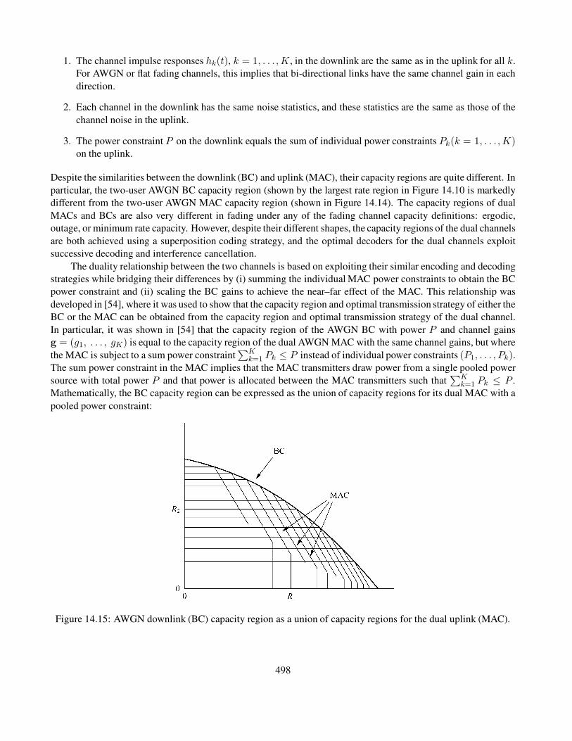
1. The channel impulse responses hk(t), k = 1, . . . , K, in the downlink are the same as in the uplink for all k.

For AWGN or flat fading channels, this implies that bi-directional links have the same channel gain in each

direction.

2. Each channel in the downlink has the same noise statistics, and these statistics are the same as those of the

channel noise in the uplink.

3. The power constraint P on the downlink equals the sum of individual power constraints Pk(k = 1, . . . , K)on the uplink.

Despite the similarities between the downlink (BC) and uplink (MAC), their capacity regions are quite different. In

particular, the two-user AWGN BC capacity region (shown by the largest rate region in Figure 14.10 is markedly

different from the two-user AWGN MAC capacity region (shown in Figure 14.14). The capacity regions of dual

MACs and BCs are also very different in fading under any of the fading channel capacity definitions: ergodic,

outage, or minimum rate capacity. However, despite their different shapes, the capacity regions of the dual channels

are both achieved using a superposition coding strategy, and the optimal decoders for the dual channels exploit

successive decoding and interference cancellation.

The duality relationship between the two channels is based on exploiting their similar encoding and decoding

strategies while bridging their differences by (i) summing the individual MAC power constraints to obtain the BC

power constraint and (ii) scaling the BC gains to achieve the near–far effect of the MAC. This relationship was

developed in [54], where it was used to show that the capacity region and optimal transmission strategy of either the

BC or the MAC can be obtained from the capacity region and optimal transmission strategy of the dual channel.

In particular, it was shown in [54] that the capacity region of the AWGN BC with power P and channel gains

g = (g1, . . . , gK) is equal to the capacity region of the dual AWGN MAC with the same channel gains, but where

the MAC is subject to a sum power constraint∑K

k=1 Pk ≤ P instead of individual power constraints (P1, . . . , Pk).

The sum power constraint in the MAC implies that the MAC transmitters draw power from a single pooled power

source with total power P and that power is allocated between the MAC transmitters such that∑K

k=1 Pk ≤ P .

Mathematically, the BC capacity region can be expressed as the union of capacity regions for its dual MAC with a

pooled power constraint:

Figure 14.15: AWGN downlink (BC) capacity region as a union of capacity regions for the dual uplink (MAC).

498

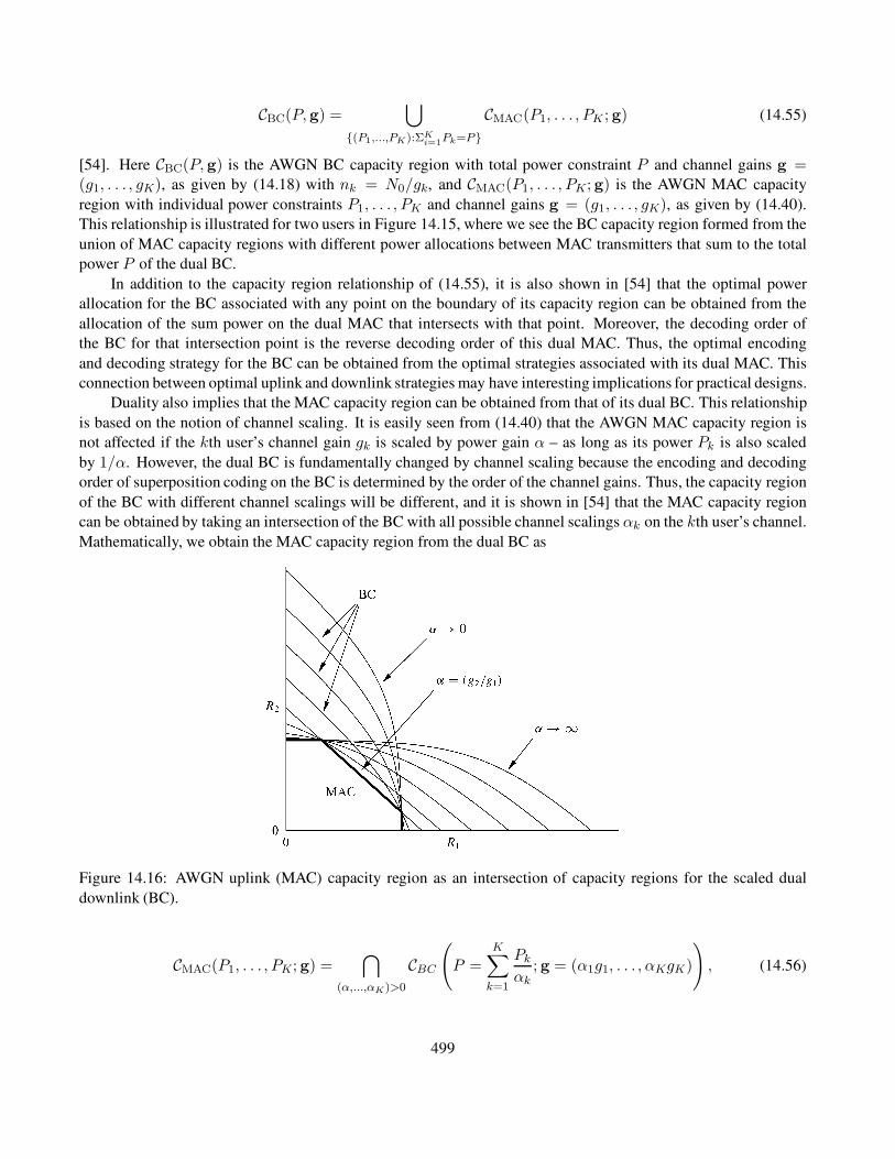
CBC(P, g) =⋃

(P1,...,PK):ΣKi=1Pk=P

CMAC(P1, . . . , PK ; g) (14.55)

[54]. Here CBC(P, g) is the AWGN BC capacity region with total power constraint P and channel gains g =(g1, . . . , gK), as given by (14.18) with nk = N0/gk, and CMAC(P1, . . . , PK; g) is the AWGN MAC capacity

region with individual power constraints P1, . . . , PK and channel gains g = (g1, . . . , gK), as given by (14.40).

This relationship is illustrated for two users in Figure 14.15, where we see the BC capacity region formed from the

union of MAC capacity regions with different power allocations between MAC transmitters that sum to the total

power P of the dual BC.

In addition to the capacity region relationship of (14.55), it is also shown in [54] that the optimal power

allocation for the BC associated with any point on the boundary of its capacity region can be obtained from the

allocation of the sum power on the dual MAC that intersects with that point. Moreover, the decoding order of

the BC for that intersection point is the reverse decoding order of this dual MAC. Thus, the optimal encoding

and decoding strategy for the BC can be obtained from the optimal strategies associated with its dual MAC. This

connection between optimal uplink and downlink strategies may have interesting implications for practical designs.

Duality also implies that the MAC capacity region can be obtained from that of its dual BC. This relationship

is based on the notion of channel scaling. It is easily seen from (14.40) that the AWGN MAC capacity region is

not affected if the kth user’s channel gain gk is scaled by power gain α – as long as its power Pk is also scaled

by 1/α. However, the dual BC is fundamentally changed by channel scaling because the encoding and decoding

order of superposition coding on the BC is determined by the order of the channel gains. Thus, the capacity region

of the BC with different channel scalings will be different, and it is shown in [54] that the MAC capacity region

can be obtained by taking an intersection of the BC with all possible channel scalings αk on the kth user’s channel.

Mathematically, we obtain the MAC capacity region from the dual BC as

Figure 14.16: AWGN uplink (MAC) capacity region as an intersection of capacity regions for the scaled dual

downlink (BC).

CMAC(P1, . . . , PK; g) =⋂

(α,...,αK)>0

CBC(

P =K∑

k=1

Pkαk

; g = (α1g1, . . . , αKgK)

)

, (14.56)

499

where CMAC(P1, . . . , PK ; g) and CBC(P, g) are defined as in (14.55). This relationship is illustrated in Figure

14.16 for two users with channel gain g = (g1, g2). The figure shows that the MAC capacity region is formed

from the intersection of BC capacity regions with different channel scalings α applied to the first user.9 As α→ 0,

the channel gain α g1 of the first user goes to zero but the total power P = P1/α+ P2 goes to infinity. Since user

2’s channel gain doesn’t change, he takes advantage of the increased power and his rate grows asymptotically large

with α. The opposite happens as α→ ∞: user 1’s channel gain grows and the total power P = P1/α+ P2 ≥ P2,

so user 1 takes advantage of his increasing channel gain to achieve an asymptotically large rate with any portion

of the total power P . All scalings between zero and infinity sketch out different BC capacity regions that intersect

to form the MAC region. In particular, when α = g2/g1, the channel gains of both users in the scaled BC are the

same, and this yields the time-sharing segment of the MAC capacity region. The optimal decoding order of the

MAC for a given point on its capacity region can also be obtained from the channel scaling associated with the

dual scaled BC whose capacity region intersects the MAC capacity region at that point.

These duality relationships are extended in [54] to many other important channel models. In particular, duality

applies to flat fading MACs and BCs, so that the ergodic, outage, and minimum rate capacity regions (along with the

optimal encoding and decoding strategies) for one channel can be obtained from the regions and strategies for the

dual channel. MAC and BC duality also holds for parallel and frequency-selective fading channels, which defines

the connection between the capacity regions of frequency-selective fading MACs and BCs [58, 59]. Another

important application of duality is to multiple antenna (MIMO) MACs and BCs [48, 60, 61]. In [60] the notion of

duality between the BC and the MAC was extended to MIMO systems such that the MIMO BC capacity region

with power constraint P and channel gain matrix H was shown to equal the union of capacity regions of the dual

MAC with channel gain matrix HH , where the union is taken over all individual power constraints that sum to P .

Mathematically, we have

CBC(P,H) =⋃

(P1,...,PK ):ΣKk=1Pk=P

CMAC((P1, . . . , PK); HH),

where CBC(P,H) is given by (14.37) and CMAC((P1, . . . , PK); HH) is given by (14.54). This duality relationship

is illustrated in Figure 14.13, where the MIMO BC capacity region is defined by the outer boundary in the fig-

ure. The regions inside this boundary are the MIMO MAC capacity region under different individual user power

constraints that sum to the total BC power P . Recall that the MIMO BC capacity region is extremely difficult

to compute directly, since it is neither concave nor convex over the covariance matrices that must be optimized.

In contrast, the optimal MIMO MAC is obtained via a standard convex optimization that is easy to solve [62].

Moreover, duality not only relates the two capacity regions but can also be used to obtain the optimal transmission

strategy for a point in the MIMO BC capacity region from a duality transformation of the optimal MIMO MAC

strategy that achieves the same point. Thus, for MIMO channels, duality can be exploited to simplify calculation

of the capacity region and also to simplify finding the corresponding optimal transmission strategy.

14.8 Multiuser Diversity

Multiuser diversity takes advantage of the fact that, in a system with many users whose channels fade indepen-

dently, at any given time some users will have better channels than others. By transmitting only to users with

the best channels at any given time, system resources are allocated to the users that can best exploit them, which

leads to improved system capacity and/or performance. Multiuser diversity was first explored in [53] as a means to

increase throughput and reduce error probability in uplink channels, and the same ideas can be applied to downlink

9It is sufficient to take the intersection for scaling overjust K−1 users, because scaling by (α1, . . . , αK−1, αK) is equivalent to scaling

by (α1/αK , . . . , αK−1/αK , 1).

500

channels. The multiuser diversity concept is an extension of the single-user diversity concepts described in Chapter

7. In single-user diversity systems, a point-to-point link consists of multiple independent channels whose signals

can be combined to improve performance. In multiuser diversity the multiple channels are associated with different

users, and the system typically uses selection diversity to select the user with the best channel in any given fading

state. The multiuser diversity gain relies on disparate channels between users and so, the larger the dynamic range

of the fading, the higher the multiuser diversity gain. In addition, as with any diversity technique, performance

improves with the number of independent channels. Thus, multiuser diversity is most effective in systems with a

large number of users.

From Section 14.5, we have seen that the total throughput (sum-rate capacity) of the fading downlink is

maximized by allocating the full system bandwidth to the user with the best channel in each fading state. As

described in Section 14.6, a similar result holds for the fading uplink if all users have the same fading distribution

and average power. If the users have different fading statistics or average powers, then the channel in any given state

is allocated to the user with the best weighted channel gain, where the weight depends on the user’s channel gain

in the given state, his fading statistics, and his average power constraint. The notion of scheduling transmissions

to users based on their channel conditions is called opportunistic scheduling, and numerical results in [34, 53]

show that opportunistic scheduling, when coupled with power control, can significantly increase both uplink and

downlink throughput as measured by sum-rate capacity.

Opportunistic scheduling can also improve BER performance [53]. Let γk[i] for k = 1, . . . , K denote the

SNR for each user’s channel at time i. By transmitting only to the user with the largest SNR, the system SNR at

time i is γ[i] = maxk γk[i]. It is shown in [63] that, in independent and identically distributed Rayleigh fading,

this maximum SNR is roughly lnK larger than the SNR of any one user as K grows asymptotically large, leading

to a multi-user diversity gain in SNR of lnK. Moreover, if Ps(γ) denotes the probability of symbol error for the

user with the best channel gain at time i, then Ps(γ) will exhibit the same diversity gains as selection combining

in a single-user system (described in Section 7.2.2) as compared to the probability of error associated with any one

user. As the number of users in the system increases, the probability of error approaches that of an AWGN channel

without fading, analogous to increasing the number of branches in single-user selection combining diversity.

Scheduling transmission to users with the best channel raises two problems in wireless systems: fairness and

delay. If user fade levels change very slowly, then one user will occupy the system for a long period of time. The

time between channel uses for any one user could be quite long, and such latency might be unacceptable for a

given application. In addition, users with poor average SNRs will rarely have the best channel and thus are rarely

allowed to transmit, which leads to unfairness in the allocation of the system resources. A solution to the fairness

and delay problems in the downlink, called proportional fair scheduling, was proposed in [63]. Suppose that, at

time i, each of the K users in the downlink system can support rate Rk[i] if allocated the full power and system

bandwidth. Let Tk[i] denote the average throughput of the kth user at time i, averaged using an exponentially

weighted low pass filter parameterized by ic, which is a parameter of the scheduler design. In the ith time slot, the

scheduler then transmits to the user with the largest ratio Rk[i]/Tk[i]. If at time i all users have experienced the

same average throughput Tk[i] = T [i], then this scheduler transmits to the user with the best channel. Suppose,

however, that one user (user j) has experienced poor throughput, so that Tj[i] Tk[i] for j 6= k. Then, at time

i, user j will likely have a high ratio of Rj[i]/Tj[i] and thus will be favored in the allocation of resources at time

i. Assuming that at time i the user k∗ has the highest ratio of Rk[i]/Tk[i], the throughput on the next times lot is

updated as

Tk[i+ 1] =

(1− 1/ic)Tk[i] + (1/ic)Rk[i] k = k∗,

(1− 1/ic)Tk[i] k 6= k∗.(14.57)

With this scheduling scheme, users with the best channels are still allocated the channel resources when throughput

between users is reasonably fair. However, if the throughput of any one user is poor, that user will be favored

501

for resource allocation until his throughput becomes reasonably balanced with that of the other users. Clearly

this scheme will have a lower throughput than allocating all resources to the user with the best channel (which

maximizes throughput), and the throughput penalty will increase as the users have more disparate average channel

qualities. The latency with this scheduling scheme is controlled via the weighting parameter ic. As this parameter

increases the latency also increases, but system throughput increases as well because the scheduler has more

flexibility in allocating resources to users. As ic grows to infinity, the proportional fair scheduler simply reduces to

allocating system resources to the user with the best channel, assuming all users have the same average SNR. The

proportional fair scheduling algorithm is part of the standard for packet data transmission in CDMA2000 cellular

systems [64]; its performance for that system is evaluated in [65]. Alternative methods for incorporating fairness

and delay constraints in opportunistic scheduling have been evaluated in [66, 67], along with their performance

under practical constraints such as imperfect channel estimates.

14.9 MIMO Multiuser Systems

Multiuser systems with multiple antennas at the transmitter(s) and/or receiver(s) are called MIMO multiuser sys-

tems. These multiple antennas can significantly enhance performance in many ways. The antennas can be used

to provide diversity gain to improve BER performance. The capacity region of the multiuser channel is increased

with multiple transmit and receive antennas, providing multiplexing gain. Finally, multiple antennas can provide

directivity gain to spatially separate users, which reduces interference. There typically are trade-offs among these

three types of performance gains in MIMO multiuser systems [68].

The multiplexing gain of a MIMO multiuser system characterizes the increase in the uplink or downlink

capacity region associated with adding multiple antennas. The capacity regions of MIMO multiuser channels

have been extensively studied, motivated by the large capacity gains associated with single-user systems. For

AWGN channels the MIMO capacity region for both the uplink and the downlink is described (respectively) in

Section 14.6.3 and Section 14.5.5. These results can be extended to find the MIMO capacity region in fading with

perfect CSI at all transmitters and receivers. Capacity results and open problems related to MIMO multiuser fading

channels under other assumptions about channel CSI are described in [69].

Beamforming was discussed in Section 10.4 as a technique to achieve full diversity in single-user systems at

the expense of some capacity loss. In multiuser systems, beamforming has less of a capacity penalty because of

the multiuser diversity effect, and in fact beamforming can achieve the sum-rate capacity of the MIMO downlink

in the asymptotic limit of a large number of users [70, 71].

Multiuser diversity is based on the idea that in multiuser channels the channel quality varies across users, so

performance can be improved by allocating system resources at any given time to the users with the best channels.

Design techniques to exploit multiuser diversity were discussed in Section 14.8 for single-antenna multiuser sys-

tems. In MIMO multiuser systems, the benefits of multiuser diversity are twofold. First, MIMO multiuser diversity

provides improved channel quality, since only users with the best channels are allocated system resources. In ad-

dition, MIMO multiuser diversity provides abundant directions where users have good channel gains, so that users

chosen for resource allocation in a given state have not only good channel quality but also good spatial separation,

thereby limiting interference between them. This twofold diversity benefit allows relatively simple, suboptimal

transmitter and receiver techniques to achieve near-optimal performance as the number of users increases [70, 72].

It also eliminates the requirement for multiple receive antennas in downlinks and multiple transmit antennas in

uplinks in order to obtain large capacity gains, which reduces complexity and power consumption in the mobile

terminal. In particular, the sum-rate capacity gain in MIMO BCs increases roughly linearly with the minimum of

the number of transmit antennas and the total number of receive antennas associated with all users [73]. Thus,

given a fixed number of transmit antennas at a base station and a large number of users, there is no capacity benefit

to having multiple antennas at the user terminals. Similarly, the sum-rate capacity gain in MIMO MACs increases

502

roughly linearly with the minimum of the number of receive antennas and the total number of transmit antennas

associated with all users. Hence, in a system with many users and a large number of receive antennas at the base

station, adding transmit antennas at the user terminals will not increase capacity. Note that multiuser diversity

increases with the dynamic range and rate of the channel fading. By modulating (in a controlled fashion) the am-

plitude and phase of multiple transmit antennas, the fading rate and dynamic range can be increased, leading to

higher multiuser diversity gains. This technique, called opportunistic beamforming, is investigated in [63].

Space-time modulation and coding techniques for MIMO multiuser systems have also been developed [74,

75, 76]. The goal of these techniques is to achieve the full range of diversity, multiplexing, and directivity trade-

offs inherent in MIMO multiuser systems. Multiuser detection techniques can also be extended to MIMO channels

and provide substantial performance gains [77, 78, 79]. In wideband channels, the multiuser MIMO techniques

must also cope with frequency-selective fading [76, 80, 81]. Advanced transmission techniques for these wideband

channels promise even more significant performance gains than in narrowband channels, since frequency-selective

fading provides yet another form of diversity. At low SNRs, however, multiple antennas are mainly used to collect

energy. The challenge for MIMO multiuser systems is to develop signaling techniques of reasonable complexity

that deliver on the promised performance gains even in practical operating environments.

503

Chapter 14 Problems

1. Consider an FDMA system for multimedia data users. The modulation format requires 10 MHz of spectrum

for each user, and guard bands of 1 MHz are required on each side of the allocated spectrum in order to

minimize out-of-band interference. What total bandwidth is required to support 100 simultaneous users in

this system?

2. GSM systems have 25 MHz of bandwidth allocated to their uplink and downlink, divided into 125 TDMA

channels with 8 user timeslots per channel. A GSM frame consists of the 8 timeslots, preceded by a set

of preamble bits and followed by a set of trail bits. Each timeslot consists of 3 start bits at the beginning,

followed by a burst of 58 data bits, then 26 equalizer training bits, another burst of 58 data bits, 3 stop bits,

and a guard time corresponding to 8.25 data bits. The transmission rate is 270.833 kbps.

(a) Sketch the structure of a GSM frame and a timeslot within the frame.

(b) Find the fraction of data bits within a timeslot as well as the information data rate for each user.

(c) Find the duration of a frame and the latency between timeslots assigned to a given user in a frame,

neglecting the duration of the preamble and trail bits.

(d) What is the maximum delay spread in the channel such that the guard band and stop bits prevent overlap

between timeslots?

3. Consider a DS CDMA system occupying 10 MHz of spectrum. Assume an interference-limited system with

a spreading gain of G = 100 and code cross-correlation of 1/G.

(a) For the MAC, find a formula for the SIR of the received signal as a function of G and the number of

users K. Assume that all users transmit at the same power and that there is perfect power control, so

all users have the same received power.

(b) Based on your SIR formula in part (a), find the maximum number of users K that can be supported

in the system, assuming BPSK modulation with a target BER of 10−3. In your BER calculation you

can treat interference as AWGN. How does this compare with the maximum number of users K that

an FDMA system with the same total bandwidth and information signal bandwidth could support?

(c) Modify your SIR formula in part (a) to include the effect of voice activity, defined as the percentage of

time that users are talking, so interference is multiplied by this percentage. Also find the voice activity

factor such that the CDMA system accommodates the same number of users as an FDMA system. Is

this a reasonable value for voice activity?

4. Consider an FH CDMA system that uses FSK modulation and the same spreading and information band-

width as the DS CDMA system in Problem 14.3. Thus, there are G = 100 frequency slots in the system,

each of bandwidth 100 kHz. The hopping codes are random and uniformly distributed, so the probability

that a given user occupies a given frequency slot on any hop is .01. As in Problem 14.3, noise is essentially

negligible, so the probability of error on a particular hop is zero if only one user occupies that hop. Also

assume perfect power control, so the received power from all users is the same.

(a) Find an expression for the probability of bit error when m users occupy the same frequency slot.

(b) Assume there is a total of K users in the system at any time. What is the probability that, on any hop,

there is more than one user occupying the same frequency?

(c) Find an expression for the average probability of bit error as a function of K, the total number of users

in the system.

504

5. Compute the maximum throughput T for a pure ALOHA and a slotted ALOHA random access system,

along with the load L that achieves the maximum in each case.

6. Consider a pure ALOHA system with a transmission rate of R = 10 Mbps. Compute the load L and

throughput T for the system assuming 1000 bit packets and a Poisson arrival rate of λ = 103 packets per

second. Also compute the effective data rate (rate of bits successfully received). What other value of load Lresults in the exact same throughput?

7. Consider a three-user uplink channel with channel power gains g1 = 1, g2 = 3, and g3 = 5 from user k to

the receiver, k = 1, 2, 3. Assume that all three users require a 10-dB SINR. The receiver noise is n = 1.

(a) Confirm that the vector equation (I −F)P ≥ u given by (14.6) is equivalent to the SINR constraints

of each user.

(b) Determine whether a feasible power vector exists for this system such that all users meet the required

SINR constraints and, if so, find the optimal power vector P∗ such that the desired SINRs are achieved

with minimum transmit power. Assume ρ = .1.

8. Find the two-user broadcast channel capacity region under superposition coding for transmit power P =10 mW, B = 100 kHz, and N0 = 10−9 W/Hz.

9. Show that the sum-rate capacity of the AWGN BC is achieved by sending all power to the user with the

highest channel gain.

10. Derive a formula for the optimal power allocation on a fading broadcast channel to maximize sum-rate.

11. Find the sum-rate capacity of a two-user fading BC, where the fading on each user’s channel is independent.

Assume that each user has (i) a received power of 10 mW and (ii) an effective noise power of l mW with

probability .5 or 5 mW with probability .5.

12. Find the sum-rate capacity for a two-user broadcast fading channel where each user experiences Rayleigh

fading. Assume an average received power of P = 10 mW for each user, bandwidth B = 100 kHz, and

N0 = 10−9 W/Hz.

13. Consider the set of achievable rates for a broadcast fading channel under frequency division. Given any rate

vector in CFD(P , B) for a given power policy P and bandwidth allocation policy B, as defined in (14.30),

find the timeslot and power allocation policy that achieves the same rate vector.

14. Consider a time-varying broadcast channel with total bandwidthB = 100 kHz. The effective noise for user

1 has n1 = 10−5 W/Hz with probability 3/4 or n1 = 2 · 10−5 W/Hz with probability 1/4. The effective

noise for user 2 takes the value n2 = 10−5 W/Hz with probability 1/2 or the value n2 = 2 · 10−5 W/Hzwith probability 1/2. These noise densities are independent of each other over time. The total transmit power

is P = 10 W.

(a) What is the set of all possible joint noise densities and corresponding probabilities?

(b) Obtain the optimal power allocation between the two users and the corresponding time-varying capac-

ity rate region using time division. Assume that (i) user k is allocated a fixed timeslot τk for all time

(where τ1 + τ2 = 1) and a fixed average power P over all time and (ii) that each user may change its

power within its own timeslot, subject to the average constraint P . Find a rate point that exceeds this

region, assuming you don’t divide power equally.

505

(c) Assume now fixed frequency division, where the bandwidth assigned to each user is fixed and evenly

divided between the two users: B1 = B2 = B/2. Assume also that you allocate half the power to each

user within his respective bandwidth (P1 = P2 = P/2) and that you can vary the power over time,

subject only to the average power constraintP/2. What is the best rate point that can be achieved? Find

a rate point that exceeds this region, assuming that you don’t share power and/or bandwidth equally.

(d) Is the rate point (R1 = 100000, R2 = 100000) in the zero-outage capacity region of this channel?

15. Show that the K-user AWGN MAC capacity region is not affected if the kth user’s channel power gain gkis scaled by α as long as the kth user’s transmit power Pk is also scaled by 1/α.

16. Consider a multiple access channel being shared by two users. The total system bandwidth isB = 100 kHz.

The transmit power of user 1 is P1 = 3 mW, while the transmit power of user 2 is P2 = 1 mW. The receiver

noise density is .00l µW/ Hz. You can neglect any path loss, fading, or shadowing effects.

(a) Suppose user 1 requires a data rate of 300 kbps to see videos. What is the maximum rate that can

be assigned to user 2 under time division? Under superposition coding with successive interference

cancellation?

(b) Compute the rate pair (R1, R2) where the frequency-division rate region intersects the region achieved

by code division with successive interference cancellation (assuming G = 1).

(c) Compute the rate pair (R1, R2) such thatR1 = R2 (i.e., where the two users get the same rate) for time

division and for spread-spectrum code division with and without successive interference cancellation

for a spreading gain G = 10. Note: To obtain this region for G > 1 you must use the same reasoning

on the MAC as was used to obtain the BC capacity region with G > 1.

17. Show that the sum-rate capacity of the AWGN MAC is achieved by having all users transmit at full power.

18. Derive the optimal power adaptation for a two-user fading MAC that achieves the sum-rate point.

19. Find the sum-rate capacity of a two-user fading MAC where the fading on each user’s channel is independent.

Assume each user has (i) a received power of 10 mW and (ii) an effective noise power of l mW with

probability .5 or 5 mW with probability .5.

20. Consider a three-user fading downlink with bandwidth 100 kHz. Suppose the three users all have the same

fading statistics, so that their received SNRs when allocated the full power and bandwidth are 5 dB with

probability 1/3, 10 dB with probability 1/3, and 20 dB with probability 1/3. Assume a discrete-time system

with i.i.d. fading at each time slot.

(a) Find the maximum throughput of this system if (at each time instant) the full power and bandwidth are

allocated to the user with the best channel.

(b) Simulate the throughput obtained using the proportional fair scheduling algorithm for ic values of 1, 5,

and 10.

506

Bibliography

[1] D. Bertsekas and R. Gallager, Data Networks, 2nd ed., Prentice-Hall, Englewood Cliffs, NJ, 1992.

[2] T. S. Rappaport, Wireless Communications–Principles and Practice, 2nd ed., Prentice-Hall, Englewood

Cliffs, NJ, 2001.

[3] G. Leus, S. Zhou, and G. B. Giannakis, “Orthogonal multiple access over time-and frequency-selective chan-

nels,” IEEE Trans. Inform. Theory, pp. 1942–50, August 2003.

[4] S. Verdu, “Demodulation in the presence of multiuser interference: Progress and misconceptions,” in D.

Docampo, A. Figueiras, and F. Perez-Gonzalez, Eds., Intelligent Methods in Signal Processing and Commu-

nications, pp. 15–46, Birkhauser, Boston, 1997.

[5] W. Stallings, Wireless Communications and Networks, 2nd ed., Prentice-Hall, Englewood Cliffs, NJ, 2005.

[6] B. Gundmundson, J. Skold, and J. K. Ugland, “A comparison of CDMA and TDMA systems,” Proc. IEEE

Veh. Tech. Conf., pp. 732–5, May 1992.

[7] M. Gudmundson, “Generalized frequency hopping in mobile radio systems,” Proc. IEEE Veh. Tech. Conf.,

pp. 788–91, May 1993.

[8] K. S. Gilhousen, I. M. Jacobs, R. Padovani, A. J. Viterbi, L. A. Weaver, Jr., and C. E. Wheatley III, “On the

capacity of a cellular CDMA system,” IEEE Trans. Veh. Tech., pp. 303–12, May 1991.

[9] P. Jung, P. W. Baier, and A. Steil, “Advantages of CDMA and spread spectrum techniques over FDMA and

TDMA in cellular mobile radio applications,” IEEE Trans. Veh. Tech., pp. 357–64, August 1993.

[10] J. Chuang and N. Sollenberger, “Beyond 3G: Wideband wireless data access based on OFDM and dynamic

packet assignment,” IEEE Commun. Mag., pp. 78–87, July 2000.

[11] K. R. Santhi, V. K. Srivastava, G. SenthilKumaran, and A. Butare, “Goals of true broadband’s wireless next

wave (4G-5G),” Proc. IEEE Veh. Tech. Conf., pp. 2317–21, October 2003.

[12] M. Frodigh, S. Parkvall, C. Roobol, P. Johansson, and P. Larsson, “Future-generation wireless networks,”

IEEE Wireless Commun. Mag., pp. 10–17, October 2001.

[13] E. Anderlind and J. Zander, “A traffic model for non-real-time data users in a wireless radio network,” IEEE

Commun. Lett., pp. 37–9, March 1997.

[14] K. Pahlavan and P. Krishnamurthy, Principles of Wireless Networks: A Unified Approach, Prentice-Hall,

Englewood Cliffs, NJ, 2002.

507

[15] N. Abramson, “The ALOHA system–Another alternative for computer communications,” Proc. Amer. Fed-

eration Inform. Proc. Soc. Fall Joint Comput. Conf., pp. 281–5, November 1970.

[16] A. Chockalingam and M. Zorzi, “Energy consumption performance of a class of access protocols for mobile

data networks,” Proc. IEEE Veh. Tech. Conf., pp. 820–4, May 1998.

[17] S. Haykin and M. Moher, Modern Wireless Communications, Prentice-Hall, Englewood Cliffs, NJ, 2005.

[18] P. Karn, “MACA: A new channel access method for packet radio,” Proc. Comput. Network Conf., pp. 134–40,

September 1990.

[19] V. Bharghavan, A. Demers, S. Shenkar, and L. Zhang, “MACAW: A media access protocol for wireless

LANs,” Proc. ACM SIGCOMM, vol. 1, pp. 212–25, August 1994.

[20] IEEE Standard for Wireless LAN Medium Access Control (MAC) and Physical Layer (PHY) Specifications,

IEEE Standard 802.11, 1997.

[21] Z. J. Haas, J. Deng, and S. Tabrizi, “Collision-free medium access control scheme for ad hoc networks, Proc.

Military Commun. Conf., pp. 276–80, 1999.

[22] S.-L. Wu, Y.-C. Tseng, and J.-P. Sheu, “Intelligent medium access for mobile ad hoc networks with busy

tones and power control,” IEEE J. Sel. Areas Commun., pp. 1647–57, September 2000.

[23] N. Abramson, “Wide-band random-access for the last mile,” IEEE Pers. Commun. Mag., pp. 29–33, Decem-

ber 1996.

[24] D. J. Goodman, R. A. Valenzuela, K. T. Gayliard, and B. Ramamurthi, “Packet reservation multiple access

for local wireless communications,” IEEE Trans. Commun., pp. 885–90, August 1989.

[25] N. B. Mehta and A. J. Goldsmith, “Effect of fixed and interference-induced packet error probability on

PRMA,” Proc. IEEE Internat. Conf. Commun., pp. 362–6, June 2000.

[26] P. Agrawal, “Energy efficient protocols for wireless systems,” Proc. Internat. Sympos. Pers., Indoor, Mobile

Radio Commun., pp. 564–9, September 1998.

[27] J. Zander, “Performance of optimum transmitter power control in cellular radio systems,” IEEE Trans. Veh.

Tech., pp. 57–62, February 1992.

[28] G. J. Foschini and Z. Miljanic, “A simple distributed autonomous power control algorithm and its conver-

gence,” IEEE Trans. Veh. Tech., pp. 641–6, November 1993.

[29] S. A. Grandhi, R. Vijayan, and D. J. Goodman, “Distributed power control in cellular radio systems,” IEEE

Trans. Commun., pp. 226–8, February–April 1994.

[30] E. Seneta, Nonnegative Matrices and Markov Chains, Springer-Verlag, New York, 1981.

[31] N. Bambos, S. C. Chen, and G. J. Pottie, “Channel access algorithms with active link protection for wireless

communication networks with power control,” IEEE/ACM Trans. Network., pp. 583–97, October 2000.

[32] S. Kandukuri and N. Bambos, “Power controlled multiple access (PCMA) in wireless communication net-

works,” Proc. IEEE Infocom Conf., pp. 386–95, March 2000.

508

[33] P. P. Bergmans and T. M. Cover, “Cooperative broadcasting,” IEEE Trans. Inform. Theory, pp. 317–24, May

1974.

[34] L. Li and A. J. Goldsmith, “Capacity and optimal resource allocation for fading broadcast channels-Part I:

Ergodic capacity,” IEEE Trans. Inform. Theory, pp. 1083–1102, March 2001.

[35] T. Cover and J. Thomas, Elements of Information Theory, Wiley, New York, 1991.

[36] L.-F. Wei, “Coded modulation with unequal error protection,” IEEE Trans. Commun., pp. 1439–49, October

1993.

[37] P. P. Bergmans, “A simple converse for broadcast channels with additive white Gaussian noise,” IEEE Trans.

Inform. Theory, pp. 279–80, March 1974.

[38] R. Pickholtz, L. Milstein, and D. Schilling, “Spread spectrum for mobile communications,” IEEE Trans. Veh.

Tech., pp. 313–22, May 1991.

[39] S. Verdu, Multiuser Detection, Cambridge University Press, 1998.

[40] D. Tse and S. Hanly, “Multiaccess fading channels – Part I: Polymatroid structure, optimal resource allocation

and throughput capacities,” IEEE Trans. Inform. Theory, pp. 2796–2815, November 1998.

[41] S. Hanly and D. Tse, “Multiaccess fading channels – Part II: Delay-limited capacities,” IEEE Trans. Inform.

Theory, pp. 2816–31, November 1998.

[42] L. Li and A. J. Goldsmith, “Capacity and optimal resource allocation for fading broadcast channels – Part II:

Outage capacity,” IEEE Trans. Inform. Theory, pp. 1103–27, March 2001.

[43] L. Li, N. Jindal, and A. J. Goldsmith, “Outage capacities and optimal power allocation for fading multiple

access channels,” IEEE Trans. Inform. Theory, pp. 1326–47, Apri1 2005.

[44] N. Jindal and A. J. Goldsmith, “Capacity and optimal power allocation for fading broadcast channels with

minimum rates,” IEEE Trans. Inform. Theory, pp. 2895–2909, November 2003.

[45] E. Larsson and P. Stoica, Space-Time Block Coding for Wireless Communications, Cambridge University

Press, 2003.

[46] G. Caire and S. Shamai, “On the achievable throughput of a multiantenna Gaussian broadcast channel,” IEEE

Trans. Inform. Theory, pp. 1691–1706, July 2003.

[47] W. Yu and J. M. Cioffi, “Trellis precoding for the broadcast channel,” Proc. IEEE Globecom Conf., pp.

1344–8, November 2001.

[48] H. Weingarten, Y. Steinberg, and S. Shamai, “ The capacity region of the Gaussian MIMO broadcast channel,”

Proc. IEEE Internat. Sympos. Inform. Theory, p. 174, June 2004.

[49] M. Costa, “Writing on dirty paper,” IEEE Trans. Inform. Theory, pp. 439–41, May 1983.

[50] U. Erez, S. Shamai, and R. Zamir, “Capacity and lattice strategies for cancelling known interference,” Proc.

Internat. Sympos. Inform. Theory Appl., pp. 681–4, November 2000.

[51] B. Rimoldi and R. Urbanke, “A rate-splitting approach to the Gaussian multiple-access channel,” IEEE Trans.

Inform. Theory, pp. 364–75, March 1996.

509

[52] D. Tse and P. Viswanath, Foundations of Wireless Communications, Cambridge University Press, 2005.

[53] R. Knopp and P. Humblet, “Information capacity and power control in single-cell multiuser communications,”

Proc. IEEE Internat. Conf. Commun., pp. 331–5, June 1995.

[54] N. Jindal, S. Vishwanath, and A. J. Goldsmith, “On the duality of Gaussian multiple-access and broadcast

channels,” IEEE Trans. Inform. Theory, pp. 768–83, May 2004.

[55] S. Verdu, “Multiple-access channels with memory with and without frame synchronism,” IEEE Trans. Inform.

Theory, pp. 605–19, May 1989.

[56] E. Telatar, “Capacity of multi-antenna Gaussian channels,” Euro. Trans. Telecommun., pp. 585–96, November

1999.

[57] W. Yu, W. Rhee, S. Boyd, and J. Cioffi, “iterative water-filling for vector multiple access channels,” IEEE

Trans. Inform. Theory, pp. 145–52, January 2004.

[58] R. Cheng and S. Verdu, “ Gaussian multiaccess channels with ISI: Capacity region and multiuser water-

filling,” IEEE Trans. Inform. Theory, pp. 773–85, May 1993.

[59] A. J. Goldsmith and M. Effros, “The capacity region of broadcast channels with intersymbol interference and

colored Gaussian noise,” IEEE Trans. Inform. Theory, pp. 219–40, January 2001.

[60] S. Vishwanath, N. Jindal, and A. J. Goldsmith, “Duality, achievable rates, and sum-rate capacity of Gaussian

MIMO broadcast channels,” IEEE Trans. Inform. Theory, pp. 2658–68, October 2003.

[61] P. Viswanath and D. N. C. Tse, “Sum capacity of the vector Gaussian broadcast channel and uplink-downlink

duality,” IEEE Trans. Inform. Theory, pp. 1912–21, August 2003.

[62] N. Jindal, W. Rhee, S. Vishwanath, S. A. Jafar, and A. J. Goldsmith, “Sum power iterative water-filling for

multi-antenna Gaussian broadcast channels,” IEEE Trans. Inform. Theory, pp. 1570–9, Apri1 2005.

[63] P. Vishwanath, D. N. C. Tse, and R. Laroia, “Opportunistic beamforming using dumb antennas,” IEEE Trans.

Inform. Theory, pp. 1277–94, June 2002.

[64] TIA/EIA IS-856, “CDMA 2000: High rate packet data air interface specification,” November 2000.

[65] A. Jalali, R. Padovani, and R. Pankaj, “Data throughput of CDMA-HDR a high efficiency–high data rate

personal communication wireless system,” Proc. IEEE Veh. Tech. Conf., pp. 1854–8, May 2000.

[66] M. Andrews, K. Kumaran, K. Ramanan, A. Stolyar, and P. Whiting, “Providing quality of service over a

shared wireless link,” IEEE Commun. Mag., pp. 150–4, February 2001.

[67] X. Liu, E. K. P. Chong, and N. B. Shroff, “Opportunistic transmission scheduling with resource-sharing

constraints in wireless networks,” IEEE J. Sel. Areas Commun., pp. 2053–64, October 2001.

[68] D. N. C. Tse, P. Viswanath, and L. Zheng, “Diversity-multiplexing trade-off in multiple-access channels,”

IEEE Trans. Inform. Theory, pp. 1859–74, September 2004.

[69] A. J. Goldsmith, S. A. Jafar, N. Jindal, and S. Vishwanath, “Capacity limits of MIMO channels,” IEEE J. Sel.

Areas Commun., pp. 684–701, June 2003.

510

[70] M. Sharif and B. Hassibi, “Scaling laws of sum rate using time-sharing, DPC, and beamforming for MIMO

broadcast channels,” Proc. IEEE Internat. Sympos. Inform. Theory, p. 175, June 2004.

[71] T. Yoo and A. J. Goldsmith, “Optimality of zero-forcing beamforming with multiuser diversity,” Proc. IEEE

Internat. Conf. Commun., May 2005.

[72] J. Heath, R. W. M. Airy, and A. Paulraj, “Multiuser diversity for MIMO wireless systems with linear re-

ceivers,” Proc. Asilomar Conf. Signals, Syst., Comput., pp. 1194–9, November 2001.

[73] N. Jindal and A. Goldsmith, “DPC vs. TDMA for MIMO broadcast channels,” IEEE Trans. Inform. Theory,

pp. 1783–94, May 2005.

[74] N. Al-Dhahir, C. Fragouli, A. Stamoulis, W. Younis, and R. Calderbank, “Space-time processing for broad-

band wireless access,” IEEE Commun. Mag., pp. 136–42, September 2002.

[75] M. Brehler and M. K. Varanasi, “Optimum receivers and low-dimensional spreaded modulation for multiuser

space-time communications,” IEEE Trans. Inform. Theory, pp. 901–18, April 2003.

[76] S. N. Diggavi, N. Al-Dhahir, and A. R. Calderbank, “Multiuser joint equalization and decoding of space-time

codes,” Proc. IEEE Internat. Conf. Commun., pp. 2643–7, May 2003.

[77] H. Dai and H. V. Poor, “Iterative space-time processing for multiuser detection in multipath CDMA channels,”

IEEE Trans. Signal Proc., pp. 2116–27, September 2002.

[78] S. N. Diggavi, N. Al-Dhahir, and A. R. Calderbank, “On interference cancellation and high-rate space-time

codes,” Proc. IEEE Internat. Sympos. Inform. Theory, p. 238, June 2003.

[79] S. J. Grant and J. K. Cavers, “System-wide capacity increase for narrowband cellular systems through mul-

tiuser detection and base station diversity arrays,” IEEE Trans. Wireless Commun., pp. 2072–82, November

2004.

[80] Z. Liu and G. B. Giannakis, “Space-time block-coded multiple access through frequency-selective fading

channels,” IEEE Trans. Commun., pp. 1033–44, June 2001.

[81] K.-K. Wong, R. D. Murch, and K. B. Letaief, “Performance enhancement of multiuser MIMO wireless

communication systems,” IEEE Trans. Commun., pp. 1960–70, December 2002.

511

Chapter 15

Cellular Systems and Infrastructure-Based

Wireless Networks

This chapter has not yet been updated for the 2nd edition

Infrastructure-based wireless networks have base stations, also called access points, deployed throughout a given

area. These base stations provide access for

mobile terminals to a backbone wired network. Network control functions are performed by the base stations, and

often the base stations are connected

together to facilitate coordinated control. This infrastructure is in contrast to ad hoc wireless networks, described

in Chapter 16, which have no backbone infrastructure. Examples of infrastructure-based wireless networks include

cellular phone systems, wireless LANs, and paging systems. Base station coordination in infrastructure-based net-

works provides a centralized control mechanism

for transmission scheduling, dynamic resource allocation, power control, and handoff. As such, it can more

efficiently utilize network resources to meet the performance requirements of individual users. Moreover, most

networks with infrastructure are designed so that mobile terminals transmit directly to a base station, with no mul-

tihop routing through intermediate wireless nodes. In general these single-hop routes have lower delay and loss,

higher data rates, and more flexibility than multihop routes. For these reasons, the performance of infrastructure-

based wireless networks tends to be much better than in networks without infrastructure. However, it is sometimes

more expensive or simply not feasible or practical to deploy infrastructure, in which case ad hoc wireless networks

are the best option despite their typically inferior performance.

Cellular systems are a type of infrastructure-based network that make efficient use of spectrum by reusing it

at spatially separated locations. The focus of this chapter is on cellular system design and analysis, although many

of these principles apply to any infrastructure-based network. We will first describe the basic design principles of

cellular systems and channel reuse. System capacity issues are then discussed along with interference reduction

methods to increase this capacity. We also explain the performance benefits of dynamic resource allocation. The

chapter closes with an analysis of the fundamental rate limits of cellular systems in terms of their Shannon capacity

and area spectral efficiency.

15.1 Cellular System Fundamentals

The basic premise behind cellular systems is to exploit the power falloff with distance of signal propagation in

order to reuse the same channel at spatially separated locations. Specifically, in cellular systems a given spatial

area (such as a city) is divided into nonoverlapping cells, as shown in Figure 15.1. The signaling dimensions of

the system are channelized using one of the orthogonal or nonorthogonal techniques discussed in Section 14.2.

We will mostly focus on TDMA and FDMA for orthogonal channelization and on CDMA for nonorthogonal

512

channelization. Each channel obtained by channelizing the signaling dimensions is assigned to a unique channel

set Cn. Every cell is then assigned a channel set, and these sets can be reused at spatially separated locations, as

Figure 15.1 illustrates. This reuse of channels is called frequency reuse or channel reuse. Cells that are assigned the

same channel set, called co-channel cells, must be spaced far enough apart that interference between users in the

cells does not degrade signal quality below tolerable levels. The required spacing depends on the channelization

technique, the signal propagation characteristics, and the desired performance for each user.

Figure 15.1: Cellular system.

For the cellular system shown in Figure 15.1, a base station is located near the center of each cell. Under ideal

propagation conditions, mobiles within a given cell communicate with the base station in that cell, although in

practice the choice is based on the SINR between the mobile and the base station. When a mobile moves between

two cells, its call must be handed off from the base station in the original cell to the base station in the new cell.

The channel from a base station to the mobiles in its cell defines the downlink of the cell, and the channel from

the mobiles in a cell to the cell base station defines the uplink of the cell. All base stations in a given region are

connected to a mobile telephone switching office, which acts as a central controller. User authentication, allocation

of channels, and handoff between base stations are coordinated by the switching office. A handoff is initiated when

the signal quality of a mobile to its base station decreases below a given threshold. This occurs when a mobile

moves between cells and can also be caused by fading or shadowing within a cell. If no neighboring base station

has available channels of acceptable quality then the handoff attempt fails and the call will be dropped.

The cellular system design must include a specific multiple access technique for both the uplink and the

downlink. The main multiple access techniques used in cellular systems are time division, frequency division,

orthogonal and nonorthogonal code division, and their hybrid combinations. These techniques are sometimes

combined with space-division multiple access as well. Uplink and downlink design for a single cell was described

in Section 14.2, and many of the same design principles and analyses apply to cellular systems once appropriately

modified to include the impact of channel reuse. The trade-offs associated with different multiple access techniques

are different in cellular systems than in a single cell, since each technique must cope with interference from outside

its cell, known as intercell or co-channel interference. In addition, systems with nonorthogonal channelization must

also deal with interference from within a cell, called intracell interference. This intracell interference also arises in

systems with orthogonal channelization when multipath, synchronization errors, and other practical impairments

compromise the orthogonality.

513

Although CDMA with nonorthogonal codes has both intracell and intercell interference inherent to its design,

all interference is attenuated by the code cross-correlation. In contrast, orthogonal multiple access techniques have

no intracell interference under ideal operating conditions. However, their intercell interference has no reduction

from processing gain as in spread spectrum systems. The amount of both intercell and intracell interference

experienced by a given user is captured by his signal-to-interference-plus-noise power ratio, defined as

SINR =Pr

N0B + PI, (15.1)

where Pr is the received signal power and PI is the received power associated with both intracell and intercell

interference. In CDMA systems, PI is the interference power after de-spreading. We typically compute the bit

error rate of a mobile based on SINR rather than SNR, although this approximation is not precisely accurate if the

random interference cannot be characterized by Gaussian statistics.

A larger intercell interference reduces SINR and hence increases user BER. Intercell interference can be kept

small by separating cells operating on the same channel by a large distance. However, the number of users that

a system can accommodate is maximized by reusing frequencies as often as possible. Thus, the best cellular

system design places users that share the same channel at a separation distance where the intercell interference

is just below the maximum tolerable level for the required data rate and BER. Good cellular system designs are

interference limited, meaning that the interference power is much larger than the noise power. Therefore, noise is

generally neglected in the study of these systems. In this case SINR reduces to the signal-to-interference power

ratio SIR = Pr/PI . In interference-limited systems, since the BER of users is determined by SIR, the number

of users that can be accommodated is limited by the interference they cause to other users. Techniques to reduce

interference – such as multiple antenna techniques or multiuser detection – increase the SIR and therefore increase

the number of users the system can accommodate for a given BER constraint. Note that the SIR or BER require-

ment is fairly well-defined for continuous applications such as voice. However, system planning is more complex

for data applications owing to the burstiness of the transmissions.

Cell size is another important design choice in cellular systems. We can increase the number of users that can

be accommodated within a given system by shrinking the size of a cell, as long as all aspects of the system scale

so that the SINR of each user remains the same. Specifically, consider the large and small cells shown in Figure

15.2. Suppose the large cell in this figure represents one cell in a cellular system, where each cell accommodates

K users. If the cell size is shrunk to the smaller cell size shown in Figure 15.2 (typically by reducing transmit

power) and if everything in the system (including propagation loss) scales so that the SINR in the small cells is

the same as in the original large cell, then this smaller cell can also accommodate K users. Since there are 19

small cells within the large cell, the new system with smaller cells can accommodate 19K users within the area

of one large cell – a 19-fold capacity increase. However, propagation characteristics typically change as cell size

shrinks, so the system does not scale perfectly. Moreover, a smaller cell size increases the rate at which handoffs

occur, which increases the dropping probability if the percentage of failed hand-offs stays the same. Smaller cells

also increase the load on the backbone network, and more cells per unit area means more base stations, which can

increase system cost. Thus, although smaller cells generally increase capacity, they also have their disadvantages.

A compromise based on these trade-offs is to embed small “hotspot” cells within large cells that experience high

traffic in order to increase their capacity [1, Chap. 3.7].

The cell shape depicted in Figure 15.1 is a hexagon. A hexagon is a tesselating cell shape: cells can be laid

next to each other with no overlap and so cover the entire geographical region without any gaps. The other tesse-

lating shapes are rectangles, squares, diamonds, and triangles. These regular cell shapes are used to approximate

the contours of constant received power around the base station. If propagation follows the free-space or simplified

path-loss model where received power is constant along a circle around the base station, then a hexagon provides

a reasonable approximation to this circular shape. Hexagons were commonly used to approximate cell shapes for

first-generation cellular phone systems, where base stations were placed at the tops of buildings with coverage

514

Figure 15.2: Capacity increase by shrinking cell size.

areas on the order of a few square miles. Systems today have smaller cells, with base stations placed closer to

the ground; for these systems, diamonds tend to better approximate the contours of constant power, especially

in typical urban street grids [2, 3]. Very small cells and indoor cells are heavily dependent on the propagation

environment, making it difficult to accurately approximate contours of constant power using a tesselating shape

[4].

15.2 Channel Reuse

Channel reuse is a key element of cellular system design, as it determines how much intercell in-

terference is experienced by different users and therefore establishes the system’s capacity and per-

formance. Channel reuse considerations are different for channelization via orthogonal multiple

access techniques (e.g., TDMA, FDMA, and orthogonal CDMA) as compared with those of nonorthogonal chan-

nelization techniques (nonorthogonal or hybrid orthogonal/nonorthogonal CDMA). In particular, orthogonal tech-

niques have no intracell interference under ideal conditions. However, in TDMA and FDMA, cells using the same

channel set are typically spaced several cells away, since co-channel interference from adjacent cells can be very

large. In contrast, nonorthogonal channelization exhibits both intercell and intracell interference, but all interfer-

ence is attenuated by the cross-correlation of the spreading codes, which allows channel sets to be reused in every

cell. In CDMA systems with orthogonal codes (typical for a CDMA downlink) the codes, too, are reused in every

cell, since the code transmissions from each base station are not synchronized. Thus, the same codes transmitted

from different base stations arrive at a mobile with a timing offset, and the resulting intercell interference is atten-

uated by the code autocorrelation evaluated at that timing offset. This autocorrelation may still be somewhat large.

A hybrid technique can also be used where a nonorthogonal code that is unique to each cell is modulated on top

of the orthogonal codes used in that cell. The nonorthogonal code then reduces intercell interference by roughly

its processing gain. This hybrid approach is used in W-CDMA cellular systems [5]. Throughout this chapter, we

will assume that in CDMA systems the same codes are used in every cell, as is typically done in practice. Thus,

the reuse distance is unity and we need not address optimizing channel reuse for CDMA systems.

We now discuss the basic premise of channel reuse – cell clustering – and channel assignment. In interference-

limited systems, each user’s BER is based on his received SIR: the ratio of his received signal power to his intracell

and intercell interference power. The received signal powers associated with the desired signal, the intercell inter-

515

ference, and the intracell interference are determined by the characteristics of the channel between the desired or

interfering transmitters and the desired receiver. The average SIR is normally computed based on path loss alone,

with median shadowing attenuation incorporated into the path-loss models for the signal and interference. Random

variations due to shadowing and flat fading are then treated as statistical variations about the path loss.

Since path loss is a function of propagation distance, the reuse distance D between cells using the same

channel is an important parameter in determining average intercell interference power. Reuse distance is defined

as the distance between the centers of cells that use the same channel set. It is a function of cell shape, cell size,

and the number of intermediate cells between the two cells sharing the same channel set. Given a required average

SINR for a particular performance level, we can find the corresponding minimum reuse distance that meets this

performance target. The focus of this section is planning the cellular system layout based on a minimum reuse

distance requirement.

Figure 15.3 illustrates the reuse distance associated with a given channel reuse pattern for hexagonal and

diamond-shaped cells. Cells that are assigned the same channel set Cn are so indicated in the figure. This pattern

of channel reuse for both cell chapes is based on the notion of cell clustering, discussed in more detail below. The

reuse distanceD between these cells is the minimum distance between the dots at the center of cells using channel

set Cn. The radius R of a cell is also shown in the figure. For hexagonal cells, R is defined as the distance from

the center of a cell to a vertex of the hexagon. For diamond-shaped cells, R is the distance from the cell center to

the middle of a side.

For diamond-shaped cells it is straightforward to compute the reuse distance D based on the number of

intermediate cells NI between co-channel cells and the cell radius R. Specifically, the distance across a cell is 2R.

The distance from a cell center to its boundary is R and the distance across the NI intermediate cells between the

co-channel cells is 2RNI . Thus,D = R+ 2RNI + R = 2R(NI + 1).

Figure 15.3: Reuse distanceD with a given reuse pattern for hexagonal and diamond-shaped cells.

Reuse distance for hexagonally shaped cells is more complicated to determine, since there might not be an

integer number of cells between two co-channel cells. In the left side of Figure 15.3, if channel Cn is used in the

center cell and again in the shaded cell, then there are two cells between co-channel cells and the reuse distance is

easy to find. However, if Cn is reused in the cell adjacent to the shaded cell, as is shown in the figure, then there is

not an integer number of cells separating the co-channel cells. The assignment shown in Figure 15.3 is needed to

create cell clusters, as discussed in more detail below.

The procedure for channel assignment in hexagonal cells is as follows. Consider the cell diagram in Figure

15.4, where againR is the hexagonal cell radius. Denote the location of each cell by the pair (i, j). Then, assuming

516

cell A to be centered at the origin (0, 0), the location of the cell at (i, j) relative to cell A is obtained by moving

i cells along the u-axis, turning 60 counterclockwise, and moving j cells along the v-axis. For example, cell G

is located at (0, 1), cell S at (1,1), cell P at (−2, 2), and cell M at (−1,−1). It is straightforward to show that the

distance between cell centers of adjacent cells is√

3R, and the distance between the centers of the cell located at

the point (i, j) and cell A located at (0, 0)) is given by

D =√

3R√

i2 + j2 + ij. (15.2)

Example 15.1: Find the reuse distance D for the channel reuse pattern illustrated in Figure 15.3 for both the

diamond- and hexagonally shaped cells as a function of cell radius R.

Solution: For the diamond-shaped cells, there is NI = 1 cell between co-channel cells. Thus,D = 2R(NI + 1) =

4R. For the hexagonal cells shown in Figure 15.3, the reuse pattern moves two cells along the u-axis and then one

cell along the v-axis. Thus,D =√

3R√

22 + 12 + 2 = 4.58R.

Figure 15.4: Axes for reuse distance in hexagonal cells.

Given a minimum acceptable reuse distance Dmin, we would like to maintain this distance throughout the

cell grid while reusing channels as often as possible. This requires spatially repeating the cell clusters for channel

assignment, where each cell in the cluster is assigned a unique channel set that is not assigned to any other cell

in the cluster. In order to spatially repeat, cell clusters must tesselate. For diamond-shaped cells, a tesselating

cell cluster forms another diamond, with K cells on each side, as shown in Figure 15.5 for K = 4. The channel

517

set assigned to the nth cell in the cluster is denoted by Cn(n = 1, . . . , N ), where N is the number of unique

channel sets, and the pattern of channel assignment is repeated in each cluster. This ensures that cells using the

same channel are separated by a reuse distance of at least D = 2KR. The number of cells per cluster is N = K2,

which is also called the reuse factor: since D = 2KR, we have N = .25(D/R)2. If we let Nc denote the number

of channels per cell (i.e., the number of channels in Cn) and NT the total number of channels, then N = NT/Nc.

A small value of N indicates efficient channel reuse (channels reused more often within a given area for a fixed

cell size and shape). However, a small N also implies a small reuse distance, since D = 2KR = 2√NR, which

can lead to substantial intercell interference.

For hexagonal cells, we form cell clusters through the following iterative process. The total bandwidth is first

broken into N channel sets C1, . . . , CN , where N is the cluster size. We assign the first channel set C1 to any

arbitrary cell. From this cell, we move i cells along a chain of hexagons in any direction, turn counterclockwise

by 60, and move j cells along the hexagon chain in this new direction; channel set C1 is then assigned to this

jth cell. Going back to the original cell, we repeat the process in a different direction until we have covered all

directions starting from the initial cell. This process is shown in Figure 15.6 for i = 3 and j = 2. To assign channel

set C1 throughout the region, we repeat the iterative process starting from one of the cells assigned channel set

C1 in a prior iteration until no new assignments can be made starting from any location that has been assigned

channel set C1. Then a new cell that has not been assigned any channel set is selected and assigned channel setC2,

and the iterative channel assignment process for this new channel set is performed. The process is repeated until

all cells have been assigned a unique channel set, which results in cell clusters as illustrated in Figure 15.7. The

reuse distance between all cells using the same channel set is then D =√

3R√

i2 + j2 + ij. We can obtain the

approximate cluster size associated with this process by finding the ratio of cluster area to cell area. Specifically,

the area of a hexagonal cell isAcell = 3√

3R2/2, and the area of a cluster of hexagonal cells isAcluster =√

3D2/2.

Hence, the number of cells per cluster is

N =Acluster

Acell=

√3D2/2

3√

3R2/2=

1

3

(D

R

)2

=1

3

(3R2(i2 + j2 + ij)

R2

)

= i2 + j2 + ij.

As with diamond cells, a small N indicates more efficient channel reuse but also a smaller reuse distance D =

R√

3N , leading to more intercell interference.

15.3 SIR and User Capacity

In this section we compute the SIR of users in a cellular system and the number of users per cell that can be

supported for a given SIR target. We neglect the impact of noise on performance under the assumption that the

system is interference-limited, although the calculations can easily be extended to include noise. The SIR in a

cellular system depends on many factors, including the cell layout, size, reuse distance, and propagation. We will

assume the simplified path-loss model (2.23) with reference distance d0 = 1 meter for our path-loss calculations, so

Pr = PtLd−γ , where L is a constant equal to the average path loss at d = d0 and γ is the path-loss exponent. Since

L is typically the same for both the desired signal and interference, its value cancels out in the SIR power ratio;

hence we set L = 1 in the analysis that follows. The path-loss exponent associated with in-cell signal propagation

is denoted by γI , while γ0 denotes the path-loss exponent associated with out-of-cell (intercell) signal propagation.

These path-loss exponents may be different, depending on the propagation environment and cell size [6]. Using the

simplified path-loss model, we will derive expressions for SIR under both orthogonal and nonorthogonal access

techniques. We then find user capacity for each model, defined as the maximum number of users per cell that the

system can support without violating an SIR target value.

The SIR of a signal is typically used to compute the BER performance associated with that signal. Specifi-

cally, the interference is approximated as additive white Gaussian noise (AWGN) and then formulas for the BER

518

Figure 15.5: Cell clusters for diamond cells.

versus SNR are applied. For example, from (6.6), performance of uncoded BPSK without fading yields Pb =Q(

√2 · SIR), and from (6.57), performance when the desired signal exhibits Rayleigh fading yields Pb ≈ .25/SIR

for high SIRs. Although we have assumed the simplified path-loss model in the SIR formulas that follow, path-loss

models of greater complexity can also be incorporated for a more accurate SIR approximation. However, there

are a number of inaccuracies in the model that are not easy to fix. In particular, approximating the interference as

Gaussian noise is accurate for a large number of interferers, as is the case for CDMA systems, but not accurate for

a small number of interferers, as in TDMA and FDMA systems. Moreover, the performance computation in fading

neglects the fact that the interferers also exhibit fading, which results in a received SIR that is the ratio of two

random variables. This ratio has a complex distribution that is not well approximated by a Rayleigh distribution or

by any other common fading distribution [7]. The complexity of modeling average SIR as well as its distribution

under accurate path loss, shadowing, and multipath fading models can be prohibitive. Thus, the SIR distribution is

often obtained via simulations [6].

15.3.1 Orthogonal Systems (TDMA/FDMA)

In this section we compute the SIR and user capacity for cellular systems using orthogonal multiple access tech-

niques. In these systems there is no intracell interference, so the SIR is determined from the received signal power

and the interference resulting from co-channel cells. Under the simplified path-loss model, the received signal

power for a mobile located at distance d from its base station on both the uplink and the downlink is Pr = Ptd−γI .

The average intercell interference power is a function of the number of out-of-cell interferers. For simplicity we

519

Figure 15.6: Channel assignment in hexagonal cells.

will neglect interference from outside the first ring of M interfering cells. This approximation is accurate when

the path-loss exponent γ0 is relatively large, since then subsequent interfering rings have a much larger path loss

than the first ring. We assume that all transmitters send at the same power Pt: the impact of power control will be

discussed in Section 15.5.3. Let us assume the user is at distance d < R and there are M interferers at distance

di, i = 1, . . . ,M , from the intended receiver (located at the mobile in the downlink and the base station in the

uplink). The resulting SIR is then

SIR =d−γI

∑Mi=1 d

−γoi

. (15.3)

This SIR is the ratio of two random variables, whose distribution can be quite complex. However, the statistics

of the interference in the denominator has been characterized for several propagation models, and when these

interferers are log-normal, their sum is also log-normal [8, Chap. 3]. Note that in general the average SIR for

the uplink and downlink may be roughly the same; but the SIR for the uplink, where interferers can all be on the

cell boundary closest to the base station they interfere with, generally has a smaller worst-case value than for the

downlink, where interference comes from base stations at the cell centers.

The SIR expression can be simplified if we assume that the mobile is on its cell boundary, d = R, and all

interferers are at the reuse distance D from the intended receiver. Under these assumptions the SIR reduces to

SIR =R−γI

MD−γo, (15.4)

and if γI = γO = γ then this simplifies further to

SIR =1

M

(D

R

)γ

. (15.5)

Since D/R is a function of the reuse factor N for most cell shapes, this allows us to express the SIR in terms of

N . In particular, from Figure 15.5, for diamond-shaped cells we have M = 8 and D/R =√

4N . Substituting

520

C1

C

C

C

C

C

C

C

C

C

C

DC

C

C

C

CC

C

C 3

4

5

6

7

2

8

9

10

11

12

13

14

15

16

17

18

19

C1

C

C

C

C

C

C

C

C

C

C

C

C

C

C

C

C

C

C

2

3

4

5

6

7

8

9

10

11

12

13

14

15

16

17

18

19

C

C

C

C

C

C

C

C

C

C

C11

C

C

C

C

C

C

C

C

1

2

3

4

5

6

7

8

9

10

12

13

14

15

16

17

18

19

C

C

C

C

C

C

C

C

C

C

C11

C

C

C

C

C

C

C

C

1

2

3

4

5

6

7

8

9

10

12

13

14

15

16

17

18

19

C

C

C

C

C

C

C

C

C

C

C

C

C

C14

C

C

C

C

C

1

2

3

4

5

6

7

8

9

10

11

12

1315

16

17

18

19

C1

C

C

C

C

C

C

C

C

C

C

C

C

C

C

C

C

C

C

2

3

4

5

6

7

8

9

10

11

12

13

14

15

16

17

18

19

C

C

C

C

C

C

C

C

C8

C

C

C

C

C

C

C

C

C

C

1

2

3

4

5

6

7

9

10

11

12

13

14

15

16

17

18

19

Figure 15.7: Cell clusters for hexagonal cells.

these into (15.5) yields SIR = .125(4N )γ/2. From Figure 15.7, for hexagonally shaped cells we have M = 6 and

D/R =√

3N , which yields SIR = .167(3N )γ/2. Both of these SIR values can be expressed as

SIR = a1(a2N )γ/2, (15.6)

where a1 = .125 and a2 = 4 for diamond-shaped cells and where a1 = .167 and a2 = 3 for hexagonally shaped

cells. This formula provides a simple approximation for the reuse factor required to achieve a given performance.

Specifically, given a target SIR value SIR0 required for a target BER, we can invert (15.6) to obtain the minimum

reuse factor that achieves this SIR target as

N ≥ 1

a2

(SIR0

a1

)2/γ

. (15.7)

The corresponding minimum reuse distance D (for a given cell shape) is then calculated based on N and the cell

radius R. For path-loss exponent γ = 2, (15.7) simplifies to N ≥ SIR0/a1a2. If the signal has shadow fading

then the analysis is more complex, but we can still generally obtain the minimum reuse factor in terms of the SIR

requirement subject to some outage probability [9].

The user capacity Cu is defined as the total number of active users per cell that the system can support while

meeting a common SIR target for all users. To meet this target in an orthogonal system, the reuse factor N must

satisfy (15.7). ThenCu = Nc, whereNc is the number of channels assigned to any given cell assuming reuse factor

N . The total number of orthogonal channels of bandwidth Bs that can be created from a total system bandwidth

of B is NT = B/Bs. Since in orthogonal systems the reuse factor N satisfies N = NT/Nc, this implies that

Cu =NT

N=

B

NBs=G

N, (15.8)

521

where G = B/Bs is the ratio of the total system bandwidth to the bandwidth required for an individual user and

where N is the minimum integer value satisfying (15.7).

Example 15.2: Consider a TDMA cellular system with hexagonally shaped cells and with path-loss exponent

γ = 2 for all signal propagation in the system. Find the minimum reuse factorN needed for a target SIR of 10 dB,

and find the corresponding user capacity assuming a total system bandwidth of 20 MHz and a required signal

bandwidth of 100 kHz.

Solution: To obtain the reuse factor, we apply (15.7) with a1 = .167 and a2 = 3 to obtain

N ≥ SIR0

a1a2=

10

.5= 20.

Now setting G = B/Bs = 20 · 106/100 · 103 = 200, we get Cu = G/N = 10 users per cell that can be accom-

modated. Typically γ > 2, as we consider in the next example.

Example 15.3: Consider a TDMA cellular system with diamond-shaped cells, pathloss exponent γ = 4 for all

signal propagation in the system, and BPSK modulation. Assume that the received signal exhibits Rayleigh fading.

Suppose the users require Pb = 10−3. Assuming the system is interference limited, find the minimum reuse factor

N that will meet this performance requirement. Also find the user capacity assuming a total system bandwidth of

20 MHz and a per-user signal bandwidth of 100 kHz.

Solution: Treating interference as Gaussian noise, in Rayleigh fading we have Pb ≈ .25/SIR0 for SIR0 the

average SIR ratio. The SIR required to meet the Pb target is thus SIR0 = .25/10−3 = 250 (approximately 24 dB).

Substituting SIR0 = 250, a1 = .125, a2 = 4, and γ = 4 into (15.7) yields

N ≥ 1

4

√

250

.25= 11.18.

So a reuse factor ofN = 12 meets the performance requirement. For the user capacity we haveG = B/Bs = 200,

so Cu = G/N = 16 users per cell can be accommodated. Note that the Gaussian assumption for the interference

is just an approximation, which (by the central limit theorem) becomes more accurate as the number of interferers

grows.

15.3.2 Nonorthogonal Systems (CDMA)

In nonorthogonal systems, codes (i.e. channels) are typically reused in every cell, so the reuse factor is N =1. Since these systems exhibit both intercell and intracell interference, the user capacity is determined by the

maximum number of users per cell that can be accommodated for a given target SIR. We will neglect intercell

interference from outside the first tier of interfering cells –that is, from cells that are not adjacent to the cell

of interest. We will also assume that all signals follow the simplified path-loss model with the same path-loss

exponent. This assumption is typically true for interference from adjacent cells, but it ultimately depends on the

propagation environment.

Let Nc = NT = Cu denote the number of channels per cell. In CDMA systems the user capacity is typically

limited by the uplink, owing to the near–far problem and the asynchronicity of the codes. Focusing on the uplink,

under the simplified path-loss model the received signal power is Pr = Ptd−γ , where d is the distance between the

mobile and its base station. There are Nc − 1 asynchronous intracell interfering signals and MNc asynchronous

522

intercell interfering signals transmitted from mobiles in the M adjacent cells. Let di(i = 1, . . . , Nc − 1) denote

the distance from the ith intracell interfering mobile to the uplink receiver and let Pi denote this mobile’s transmit

power. Let dj(j = 1, . . . ,MNc) denote the distance from the jth intercell interfering mobile to the uplink receiver

and let Pj denote this mobile’s transmit power. By Section 13.4.3, all interference is reduced by the spreading code

cross-correlation ξ/3G, where G is the processing gain of the system and ξ is a parameter of the spreading codes

with 1 ≤ ξ ≤ 3. The total intracell and intercell interference power is thus given by

I =ξ

3G

Nc−1∑

i=1

Pid−γi +

MNc∑

j=1

Pjd−γj

, (15.9)

which yields the ratio

SIR =Ptd

−γ

ξ3G

(∑Nc−1

i=1 Pid−γi +

∑MNc

j=1 Pjd−γj

) . (15.10)

Because all the distances in (15.10) are different, the expression cannot in general be further simplified without

additional assumptions. Let us therefore assume perfect power control within a cell, so that the received power of

the desired signal and interfering signals within a cell are the same: Pr = Ptd−γ = Pid

−γi for all i. Furthermore,

let

λ =

∑MNc

j=1 Pjd−γj

(Nc − 1)Pr(15.11)

denote the ratio of average received power from all intercell interference to that of all intracell interference un-

der this power control algorithm. Using these approximations, we get the following formula for SIR, which is

commonly used for the uplink SIR in CDMA systems with power control [10, 11]:

SIR =1

ξ3G(Nc − 1)(1 + λ)

. (15.12)

Under this approximation, for any SIR target SIR0 we can determine the user capacity Cu = Nc by setting (15.12)

equal to the target SIR and solving for Cu, which yields

Cu = 1 +1

ξ3G(1 + λ)SIR0

. (15.13)

Voice signals, because of their statistical nature, need not be continuously

active [12]. The fraction of time that a voice user actually occupies the channel is called the voice activity factor

and is denoted by α, where 0 < α ≤ 1. If the transmitter shuts off during nonactivity then the interference in

CDMA – that is, the denominator of (15.13) – is multiplied by α. This increases SIR and therefore user capacity.

Example 15.4: Consider a CDMA cellular system with perfect power control within a cell. Assume a target SIR0

of 10 dB, a processing gain G = 200, spreading codes with ξ = 2, and equal average power from inside and

outside the cell (λ = 1). Find the user capacity of this system.

Solution: From (15.13) we have

Cu = 1 +1

2600(2 · 10)

= 16,

523

so 16 users per cell can be accommodated.

Since (15.13) and (15.8) provide simple expressions for user capacity, it is tempting to compare them for a given

SIR target to determine whether TDMA or CDMA can support more users per cell. This was done in Examples

15.2 and 15.4, where for the same SIR target and other system parameters TDMA yielded 10 channels per cell

while CDMA yielded 16. However, these capacity expressions are extremely sensitive to the modeling and system

assumptions. Increasing λ from 1 to 2 in Example 15.4 reduces Cu for CDMA from 16 to 11, and changing the

path-loss exponent in Example 15.2 for TDMA from γ = 2 to γ = 3 changes the reuse factor N from 20 to 6,

which in tum changes user capacity from 10 to 33. Code-division multiple access systems can trade off spreading

and coding, which yields high coding gains and a resulting lower SIR target at the expense of some processing gain

[13]; high coding gain is harder to achieve in a TDMA system, since it cannot be traded for spreading gain. Voice

activity was not taken into account for the CDMA system, which would lead to a higher capacity. Moreover, the

CDMA capacity is derived under an assumption of perfect power control via channel inversion, whereas no power

control is assumed for TDMA. The effects of shadowing and fading are also not taken into account, but fading will

cause a power penalty in CDMA (owing to the channel inversion power control) and will also affect the intercell

interference power for both TDMA and CDMA. All of these factors and trade-offs significantly complicate the

analysis, which makes it difficult to draw general conclusions about the superiority of one technique over another

in terms of user capacity. Analysis of user capacity for both TDMA and CDMA under various assumptions and

models associated with operational systems can be found in [11, 14, 15, 16].

15.4 Interference Reduction Techniques

Since cellular systems are ideally interference limited, any technique that reduces interference increases SIR and

user capacity. In this section we describe techniques for interference reduction in cellular systems, including

sectorization, smart antennas, interference averaging, multiuser detection, and interference precancellation.

A common technique to reduce interference is sectorization. Antenna sectorization uses directional antennas

to divide up a base station’s 360o omnidirectional antenna into N sectors, as shown in Figure 15.8 for N = 8. As

the figure indicates, intracell and intercell interference to a given mobile comes primarily from within its sector.

Thus, sectorization reduces interference power by roughly a factor of N under heavy loading (interferers in every

sector). Handoff is required as mobiles move between sectors, which increases overhead and the probability of call

dropping. Sectorization is a common feature in cellular systems, typically with N = 3.

Smart antennas generally consist of an antenna array combined with signal processing in both space and time.

Smart antennas can form narrow beams that provide high gain to the desired user’s signal, and/or can create spatial

nulls in the direction of interference signals [17]. However, antenna arrays can also be used for multiplexing gain,

which leads to higher data rates, or diversity gain, which improves reliability. These fundamental trade-offs are

described in Section 14.9. The use of multiple antennas for interference reduction versus their other performance

benefits reflects the trade-offs associated with cellular system design.

Intercell interference in the uplink is often dominated by one or two mobile users located near the cell bound-

aries closest to the base station serving the desired user. In TDMA or FDMA systems, the impact of these worst-

case interferers can be mitigated by superimposing frequency hopping (FH) on top of the TDMA or FDMA chan-

nelization. With this FH overlay, all mobiles change their carrier frequency according to a unique hopping pattern.

Since the hopping pattern of the worst-case interferers differs from that of the desired user, these interferers would

cause intercell interference to the desired signal only when the two hop patterns overlapped in both time and fre-

quency, which seldom occurs. Thus, the FH overlay has the effect of interference averaging, causing intercell

interference from any given cell to be averaged relative to all interferer locations. This greatly reduces the effect of

interference associated with mobiles on cell boundaries. For this reason, an FH overlay is used in the GSM cellular

524

Figure 15.8: Circular cell sectorization for N = 8.

system.

Another method of mitigating interference is multiuser detection [18]. Multiuser detectors jointly detect the

desired signal and some or all interference, so that the detected interference can be mitigated or cancelled out.

There are trade-offs between performance and complexity with different multiuser detection methods, especially

when there are a large number of interferers. Multiuser detection methods were described in Section 13.4 for

the uplink of a single-cell CDMA system. However, these detection methods can also be applied to intercell

interference signals – both at the base station [19], where processing complexity is less of a constraint, and in the

mobile device to cancel a few dominant interferers [20].

Interference precancellation takes advantage of the fact that, in the downlink, the base station has knowledge

of (i) interference between users within its cell and (ii) the interference its transmission causes to mobiles in other

cells. This knowledge can be utilized in the base station transmission to presubtract interference between users

[21, 22, 23]. Interference presubtraction by the base station has its roots in the capacity-achieving strategy for

downlinks, which uses a “dirty paper coding” transmission technique (see Section 14.5.5) for interference presub-

traction developed by Costa [24]. Numerical results in [21, 22, 23] indicate that interference presubtraction can

lead to an order-of-magnitude capacity increase in cellular systems with a large number of base station antennas.

However, the presubtraction requires channel CSI at the transmitter–in contrast to multiuser detection, which does

not require transmitter CSI.

15.5 Dynamic Resource Allocation

Cellular systems exhibit significant dynamics in the number of users in any given cell and in their time-varying

channel gains. Moreover, as cellular system applications have expanded beyond just voice to include multimedia

data, users no longer have uniform data-rate requirements. Thus, resource allocation to users must become more

525

flexible in order to support heterogeneous applications. In dynamic resource allocation the channels, data rates, and

power levels in the system are dynamically assigned relative to the current system conditions and user needs. Much

work has gone into investigating dynamic resource allocation in cellular systems. In this section we summarize

some of the main techniques, including scheduling, dynamic channel allocation, and power control. The references

given are but a small sampling of the vast literature on this important topic.

15.5.1 Scheduling

The basic premise of scheduling is to dynamically allocate resources to mobile users according to their required

data rates and delay constraints. Meeting these requirements is also called quality-of-service (QoS) support. Sched-

ulers must be efficient in their allocation of resources but also fair. There is generally a trade-off between these

two goals since, as discussed in Section 14.8, the most efficient allocation of resources exploits multiuser diversity

to allocate resources to the user with the best channel. However, this assumes that the users with the best channels

can fully utilize these resources, which may not be the case if their application does not require a high data rate.

Moreover, such an allocation is unfair to users with inferior channels.

Scheduling has been investigated for both the uplink and the downlink of both CDMA and TDMA systems.

Note that many CDMA cellular systems use a form of TDMA called high data rate (HDR) for downlink data

transmission [1, Chap. 2.2], so these CDMA schedulers are based on TDMA channelization. Three different

scheduling schemes-round robin, equal latency, and relative faimess-were compared for a TDMA downlink com-

patible with HDR systems in [25]. TDMA downlink scheduling exploiting multiuser diversity was investigated

in [26]. Scheduling issues for the CDMA downlink–including rate adaptation, faimess, and deadline constraints-

have been explored in [27, 28, 29]. For CDMA systems, uplink scheduling was investigated in [30, 31] assuming

single-user matched filter detection, and improvements using multiuser detection were analyzed in [32]. MIMO

provides another degree of freedom in scheduling system resources, as outlined in [33, 34]. Multiple classes of

users can also be supported via appropriate scheduling, as described in [35].

15.5.2 Dynamic Channel Assignment

Dynamic channel assignment (DCA) falls into two categories: dynamic assignment of multiple channels within

a cell (intracell DCA) and, for orthogonally channelized systems, dynamic assignment of channels between cells

(intercell DCA). Intercell DCA is typically not applicable to CDMA systems because channels are reused in every

cell. The basic premise of intercell DCA is to make every channel available in every cell, so no fixed channel reuse

pattern exists. Each channel can be used in every cell as long as the SIR requirements of each user are met. Thus,

channels are assigned to users as needed, and when a call terminates the channel is returned to the pool of available

channels for assignment. Intercell DCA has been shown to improve channel reuse efficiency by a factor of 2 or

more over fixed reuse patterns, even with relatively simple algorithms [36, 37]. Mathematically, intercell DCA is a

combinatorial optimization problem, with channel reuse constraints based on the SIR requirements. Most dynamic

channel allocation schemes assume that all system parameters are fixed except for the arrival and departure of calls

[38, 39, 40], with channel reuse

constraints defined by a connected graph that is constant over time. The channel allocation problem under this

formulation is a generalization of the vertex coloring problem and is thus NP-hard [41]. Reduced complexity has

been obtained by applying neural networks [42] and simulated annealing [43] to the problem. However, these ap-

proaches can suffer from lack of convergence. The superior efficiency of DCA between cells is most pronounced

under light loading conditions [38]. As traffic becomes heavier, DCA between cells can suffer from suboptimal

allocations that are difficult to reallocate under heavy loading conditions. User mobility also affects performance of

intercell DCA, since it causes more frequent channel reassignments and a corresponding increase in dropped calls

526

[44]. Finally, the complexity of DCA between cells, particularly in systems with small cells and rapidly changing

propagation conditions and user demands, limits the practicality of such techniques.

Intracell DCA allows dynamic assignment of multiple channels within a cell to a given user. In TDMA

systems this is done by assigning a user multiple timeslots; in CDMA, by assigning a user multiple codes and/or

spreading factors. Assigning multiple channels to users in TDMA or orthogonal CDMA systems is relatively

straightforward and does not change the nature of the channels assigned. Dynamic timeslot assignment was used

in [45, 46] to meet voice user requirements while reducing the delay of data services. In contrast, intracell DCA

for nonorthogonal CDMA-via either multicode or variable spreading-leads to some performance degradation in

the channels used. Specifically, a user who is assigned multiple codes in nonorthogonal CDMA creates self-

interference if a single-user matched filter detector is used on each channel. Although this is no worse than if

the different codes were assigned to different users, it is clearly suboptimal in a scenario where the same user is

assigned multiple codes. For variable-spreading CDMA, a low spreading factor provides a higher data rate, since

more of the total system bandwidth is available for data transmission as opposed to spreading. But a reduced

spreading factor makes the signal more susceptible to interference from other users. Intracell DCA using variable

spreading gain has been analyzed in [47, 48], and the multicode technique was investigated in [49]. A comparison

of multicode versus variable-spreading DCA in CDMA systems is given in [50], where it is found that (i) the

two techniques are equivalent for the single-user matched filter detector but (ii) multicode is superior for more

sophisticated detection techniques.

15.5.3 Power Control

Power control is a critical aspect of wireless system design. As seen in prior chapters, a water-filling power

adaptation maximizes capacity of adaptive-rate single-user and multiuser systems in fading. Power control via

channel inversion maintains a fixed received SNR in single-user fading channels and also eliminates the near-far

effect in CDMA uplinks. However, in cellular systems these power control policies affect intercell interference in

different ways, as we now describe.

Power control on the downlink has less impact on intercell interference than on the uplink, since the downlink

transmissions all originate from the cell center whereas uplink transmissions can come from the cell boundaries,

which exacerbates interference to neighboring cells. Thus we will focus on the effect power control on the uplink.

Consider the two cells shown in Figure 15.9. Suppose that both mobiles B1 and B2 in cell B transmit at the same

power. Then the interference caused by the mobile B1 to the base station in cell A will be relatively large, since

it is close to the boundary of cell A, while the interference from B2 will generally be much weaker owing to the

longer propagation distance. If water-filling power adaptation is employed, then B1 will generally transmit at a

lower power than B2 because it will typically have a worse channel gain than B2 to the base station in cell B,

since it is farther away. This has the positive effect of reducing the intercell interference to cell A. In other words,

water-filling power adaptation reduces intercell interference from mobiles near cell boundaries, the primary source

of this interference. A similar phenomenon happens with multiuser diversity, since users transmit only when they

have a high channel gain to their base station, which is generally true when they are close to their cell center.

Conversely, under channel inversion the boundary mobiles will transmit at a higher power in order to maintain the

same received power at the base station as mobiles that are near the cell center. This has the effect of increasing

intercell interference from boundary mobiles.

The power control algorithm discussed in Section 14.4 for maintaining a given SINR target for all users within

a single cell can also be extended to multiple cells. Assume there areK users in the system with SINR requirement

γ∗k for the kth user. Focusing on the uplink, the kth user’s SIR is given by

γk =gkPk

nk + ρ∑

k 6=j gkjPj, k, j ∈ 1, . . . , K, (15.14)

527

Figure 15.9: Effect of power control on intercell interference.

where gk is the channel power gain from user k to his base station, gkj > 0 is the channel power gain from the jth

(intercell or intracell) interfering transmitter to user k’s base station, Pk is user k’s transmit power, Pj is the jth

interferer’s transmit power, nk is the noise power at user k’s base station, and ρ is the interference reduction due to

signal processing (i. e., ρ ≈ 1/G for CDMA

and ρ = 1 for TDMA) . Similar to the case of uplink power control, the SIR constraints can be represented in

matrix form as (I − F)P ≥ u with P > 0, where P = (P1, P2, . . . , PK)T is the column vector of transmit

powers for each user,

u = (γ∗1n1

g1,γ∗2n2

g2, . . . ,

γ∗KnKgK

)T (15.15)

is the vector of noise powers scaled by the SIR constraints and channel gain, and F is an irreducible matrix with

nonnegative elements given by

Fkj =

0 k = j,

γ∗kgkjρ/gk k 6= j,(15.16)

with k, j ∈ 1, 2, . . . , K. As in uplink power control for a single cell (see Section 14.4), it is shown in

[51, 52, 53] that if the Perron-Frobenius (maximum modulus) eigenvalue of F is less than unity then there exists

a vector P > 0 (i.e., Pk > 0 for all k) such that the SIR requirements of all users in all cells are satisfied, with

p∗ = (I − F)−1u the Pareto optimal solution. Thus, p∗ meets the SIR requirements with the minimum transmit

power of the users. Moreover, the distributed iterative power control algorithm,

Pk(i+ 1) =γ∗kγk(i)

Pk(i), (15.17)

converges to the optimal solution. This is a simple algorithm for power control because it requires only SIR infor-

mation at each transmitter, where each transmitter increases power when its SIR is below its target and decreases

power when its SIR exceeds its target. However, it is important to note that the existence of a feasible power

control vector that meets all SIR requirements is less likely in a cellular system than in the single-cell uplink, since

there are more interferers contributing to the SIR and since the channel gains range over a larger set of values than

in a single-cell uplink. When there is no feasible power allocation, the distributed algorithm will result in all users

transmitting at their maximum power and still failing to meet their SIR requirement.

Power control is often combined with scheduling, intercell DCA, or intracell DCA. Intercell DCA and power

control for TDMA are analyzed in [54, 55], and these techniques are extended to MIMO systems in [56]. Power

control combined with intracell DCA exploiting multiuser diversity is investigated in [57, 58]. Intracell DCA

for CDMA via variable spreading is combined with power control in [59, 60]. A comparison of power control

combined with either multicode or variable-spreading CDMA is given in [61].

528

15.6 Fundamental Rate Limits

15.6.1 Shannon Capacity of Cellular Systems

There have been few information-theoretic results on the Shannon capacity of cellular systems, which is due to the

difficulty of incorporating channel reuse and the resulting interference into fundamental capacity analysis. Whereas

the capacity for the uplink and downlink of an isolated cell is known, as described in Sections 14.5 and 14.6, there

is little work on extending these results to multiple cells. The capacity has been characterized in some cases, but the

capacity as well as optimal transmission and reception strategies under broad assumptions about channel modeling,

base station cooperation, interference characteristics, and transmitter/receiver CSI remain mostly unsolved.

One way to analyze the capacity of a cellular system is to assume that the base stations fully cooperate

to jointly encode and decode all signals. In this case the notion of cells does not enter into capacity analysis.

Specifically, under the assumption of full base station cooperation, the multiple base stations can be viewed as a

single base station with multiple geographically dispersed antennas. Transmission from the multiple-antenna base

station to the mobiles can be treated as a MIMO downlink (broadcast channel), and transmission from the mobiles

to the multiple-antenna base station can be treated as a MIMO uplink (multiple access channel). The Shannon

capacity regions for both of these channels are known, as discussed in Section 14.9, for some channel models and

assumptions about channel side information.

The uplink capacity of cellular systems under the assumption of full base station cooperation was first in-

vestigated in [62], followed by a more comprehensive treatment in [63]. In both works, propagation between the

mobiles and the base stations was characterized using an AWGN channel model, with a channel gain of unity within

a cell and a gain of α(0 ≤ α ≤ 1) between cells. The Wyner model of [63] considers one-and two-dimensional

arrays of cells and in both cases derives the per-user capacity – defined as the maximum possible rate that all users

can maintain simultaneously – as

C(α) =B

K

∫ 1

0

log2(1 +KP (1 + 2α cos(2πθ))2

N0B) dθ, (15.18)

where B is the total system bandwidth, N0/2 is the noise power spectral density, K is the number of mobiles

per cell, and P is the average transmit power of each mobile. It is also shown in both [63] and [62] that uplink

capacity is achieved by using orthogonal multiple access techniques (e.g. TDMA) in each cell and then reusing

these orthogonal channels in other cells, although this is not necessarily uniquely optimal. The behavior of C(α)

as a function of α, the attenuation of the intercell interference, depends on the SNR of the system. The per-user

capacity C(α) generally increases with α at high SNRs, since having strong intercell interference aids in decoding

and subsequent subtraction of the interference from desired signals. However, at low SNR,C(α) initially decreases

with α and then increases. This is because weak intercell interference cannot be reliably decoded and subtracted,

so such interference reduces capacity. As the channel gains associated with the intercell interference grows, the

joint decoding is better able to decode and subtract out this interference, leading to higher capacity.

An alternate analysis method for capacity of cellular systems assumes no base station co-operation, so that the

receivers in each cell treat signals from other cells as interference. This approach mirrors the design of cellular sys-

tems in practice. Unfortunately, Shannon capacity of channels with interference is a long-standing open problem

in information theory [64, 65], solved only for the special case of strong interference [66]. By treating the inter-

ference as Gaussian noise, the capacity of both the uplink and downlink can be determined using the single-cell

analysis of Sections 14.5 and 14.6. The Gaussian assumption can be viewed as a worst-case assumption about the

interference, since exploiting any known structure of the interference can presumably help in decoding the desired

signals and therefore increases capacity. The capacity of a cellular system uplink with fading based on treating

interference as Gaussian noise was obtained in [67] for both one- and two-dimensional cellular grids. These capac-

ity results show that, with or without fading, if intercell interference is nonnegligible then an orthogonal multiple

529

access method (e.g. TDMA) within a cell is optimal. This generalization holds also when channel-inversion power

control is used within a cell. Moreover, in some cases limited or no reuse of channels in different cells can increase

capacity. The effects on capacity for this model when there is partial joint processing between base stations have

also been characterized [68].

The results described here provide some insight into the capacity and optimal transmission strategies for the

uplink of cellular systems. Unfortunately, no such results are yet available for the downlink under any assumptions

about channel modeling or base station cooperation. Although the uplink was the capacity bottleneck for cellu-

lar systems providing two-way voice, the downlink is becoming increasingly critical for multimedia downloads.

Therefore, a better understanding of the capacity limitations and insights for cellular downlinks would be most

beneficial in future cellular system design.

15.6.2 Area Spectral Efficiency

The Shannon capacity regions for cellular systems described in Section 15.6.1 dictate the set of maximum achiev-

able rates on cell uplinks or downlinks. When the capacity region is computed based on the notion joint processing

at the base stations, then there is effectively only one cell with a multiple-antenna base station. However, when

capacity is computed based on treating intercell interference as Gaussian noise, the capacity region of both the

uplink and downlink become highly dependent on the cellular system structure – in particular, the cell size and

channel reuse distance. Area spectral efficiency (ASE) is a capacity measure that allows the cellular structure (and

in particular the reuse distance) to be optimized relative to fundamental capacity limits.

Recall that, for both orthogonal and nonorthogonal channelization techniques, the reuse distance D in a

cellular system defines the distance between any two cell centers that use the same channel. Since these channels

are reused at distanceD, the area covered by each channel is roughly the area of a circle with radius .5D, which is

given by A = π(.5D)2. The larger the reuse distance, the less efficient the channel reuse. However, reducing the

reuse distance increases intercell interference, thereby reducing the capacity region of each cell if this interference

is treated as noise. The ASE captures this trade-off between efficient resource use and the capacity region per cell.

Consider a cellular system with K users per cell, a reuse distanceD, and a total bandwidth allocation B. Let

C = (R1, R2, . . . , RK) denote the capacity region, for either the uplink or the downlink, in a given cell when the

intercell interference from other cells is treated as Gaussian noise. The corresponding sum-rate, also called the

system throughput, is given by

CSR = max(R1,...,RK)∈C

K∑

k=1

Rk bps. (15.19)

The region C and corresponding sum-rate CSR can be obtained for any channelization technique within a cell.

Clearly, this capacity region will decrease as intercell interference increases. Moreover, since intercell interference

decreases as the reuse distance increases, the size of the capacity region will increase with reuse distance.

The ASE of a cell is defined as the throughput per hertz per unit area that is supported by a cell’s resources.

Specifically, given the sum-rate capacity just described, the ASE is defined as

Ae ,CSR/B

π(.5D)2bps/Hz/m2. (15.20)

From [67], orthogonal channelization is capacity achieving within a cell, so we will focus on TDMA for computing

ASE. If we also assume that the system is interference limited, so that noise can be neglected, then the rate Rkassociated with each user in a cell is a function of his received signal-to-interference power γk = Pk/Ik, k =1, . . . , K. If γk is constant then Rk = τkB log(1 + γk), where τk is the time fraction assigned to user k. Typically

γk is not constant, since both the interference and signal power of the kth user will vary with propagation conditions

530

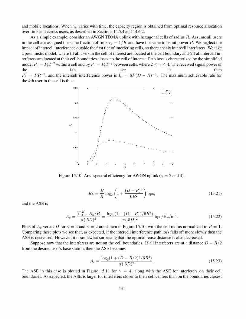
and mobile locations. When γk varies with time, the capacity region is obtained from optimal resource allocation

over time and across users, as described in Sections 14.5.4 and 14.6.2.

As a simple example, consider an AWGN TDMA uplink with hexagonal cells of radius R. Assume all users

in the cell are assigned the same fraction of time τk = 1/K and have the same transmit power P . We neglect the

impact of intercell interference outside the first tier of interfering cells, so there are six intercell interferers. We take

a pessimistic model, where (i) all users in the cell of interest are located at the cell boundary and (ii) all intercell in-

terferers are located at their cell boundaries closest to the cell of interest. Path loss is characterized by the simplified

model Pr = Ptd−2 within a cell and byPr = Ptd

−γ between cells, where 2 ≤ γ ≤ 4. The received signal power of

the kth user is then

Pk = PR−2, and the intercell interference power is Ik = 6P (D − R)−γ . The maximum achievable rate for

the kth user in the cell is thus

Figure 15.10: Area spectral efficiency for AWGN uplink (γ = 2 and 4).

Rk =B

Klog2

(

1 +(D −R)γ

6R2

)

bps, (15.21)

and the ASE is

Ae =

∑Kk=1 Rk/B

π(.5D)2=

log2(1 + (D− R)γ/6R2)

π(.5D)2bps/Hz/m2. (15.22)

Plots of Ae versus D for γ = 4 and γ = 2 are shown in Figure 15.10, with the cell radius normalized to R = 1.

Comparing these plots we see that, as expected, if the intercell interference path loss falls off more slowly then the

ASE is decreased. However, it is somewhat surprising that the optimal reuse distance is also decreased.

Suppose now that the interferers are not on the cell boundaries. If all interferers are at a distance D − R/2

from the desired user’s base station, then the ASE becomes

Ae =log2(1 + (D − R/2)γ/6R2)

π(.5D)2. (15.23)

The ASE in this case is plotted in Figure 15.11 for γ = 4, along with the ASE for interferers on their cell

boundaries. As expected, the ASE is larger for interferers closer to their cell centers than on the boundaries closest

531

to the cell they interfere with, and the optimal reuse distance is smaller.

Area spectral efficiency has been characterized in [69] for a cellular system uplink with orthogonal chan-

nelization assuming variable-rate transmission as well as best-case, worst-case, and average intercell interference

conditions. The impact of different fading models, cell sizes, and system load conditions was also investigated.

The results indicate that the optimal reuse factor is unity for both best-case and average interference conditions.

That is, channels should be reused in every cell even though there is no interference reduction from spreading.

Moreover, the ASE decreases as an exponential of a fourth-order polynomial relative to the cell radius, thus quan-

tifying the capacity gains associated with reducing cell size. A similar framework was used in [70] to characterize

the ASE of cellular downlinks.

Figure 15.11: ASE for interferers at distanceD − R/2 and at distanceD(γ = 4).

532

Chapter 12 Problems

1. Consider a city of 10 square kilometers. A macrocellular system design divides the city into square cells of

1 square kilometer, where each cell can accommodate 100 users. Find the total number of users that can be

accommodated in the system and the length of time it takes a mobile user to traverse a cell (approximate

time needed for a handoff) when moving at 30 km per hour. If the cell size is reduced to 100 square meters

and everything in the system scales so that 100 users can be accommodated in these smaller cells, find the

total number of users the system can accommodate and the length of time it takes to traverse a cell.

2. Show that the reuse distanceD =√

3R√

i2 + j2 + ij for the channel assignment algorithm associated with

hexagonal cells that is described in

Section 15.2.

3. Consider a cellular system with diamond-shaped cells of radius R = 100 m. Suppose the minimum distance

between cell centers using the same frequency must be D = 600 m to maintain the required SIR.

(a) Find the required reuse factor N and the number of cells per cluster.

(b) If the total number of channels for the system is 450, find the number of channels that can be assigned

to each cell.

(c) Sketch two adjacent cell clusters and show a channel assignment for the two clusters with the required

reuse distance.

4. Consider a cellular system with hexagonal cells of radius R = 1 km. Suppose the minimum distance

between cell centers using the same frequency must be D = 6 km to maintain the required SIR.

(a) Find the required reuse factor N and the number of cells per cluster.

(b) If the total number of channels for the system is 1200, find the number of channels that can be assigned

to each cell.

(c) Sketch two adjacent cell clusters and show a channel assignment for the two clusters with the required

reuse distance.

5. Compute the SIR for a TDMA cellular system with diamond-shaped cells, where the cell radius R = 10 mand the reuse distance D = 60 m. Assume that the path-loss exponent within the cell is γI = 2 but that the

intercell interference has path-loss exponent γ0 = 4. Compare with the SIR for γ = γI = γ0 = 4 and for

γ = γI = γ0 = 2. Explain the relative orderings of SIR in each case.

6. Find the minimum reuse distance and user capacity for a TDMA cellular system with hexagonally shaped

cells, path-loss exponent γ = 2 for all signal propagation in the system, and BPSK modulation. Assume an

AWGN channel model with required Pb = 10−6, a total system bandwidth of B = 50 MHz, and a required

signal bandwidth of 100 kHz for each user.

7. Consider a CDMA system with perfect power control, a processing gain of G = 100, spreading codes with

ξ = 1, and the ratio λ = 1.5. For BPSK modulation with a target Pb of 10−6, under an AWGN channel

model find the user capacity of this system with no sectorization and with N = 3 sectors.

8. In this problem we consider the impact of voice activity factor, which creates a random amount of interfer-

ence. Consider a CDMA system with

SIR =G

∑Nc−1i=1 χi +N

;

533

here G is the processing gain of the system, the χi represent intracell interference and follow a Bemoulli

distribution with probability α = p(χi = 1) equal to the voice activity factor, and N characterizes intercell

interference and is assumed to be Gaussian, with mean .247Nc and variance .078Nc. The probability of

outage is defined as the probability that the SIR is below some target SIR0:

Pout = p(SIR < SIR0).

(a) Show that

Pout = p

(Nc−1∑

i=1

χi +N >G

SIR0

)

.

(b) Find an analytical expression for Pout.

(c) Using the analytical expression obtained in part (b), compute the outage probability forNc = 35 users,

α = .5, and a target SIR of SIR0 = 5(7 dB). Assume G = 150.

Figure 15.12: One-dimensional cellular system with square cells (Problem 15-11).

(d) Assume now that Nc is sufficiently large that the random variable∑Nc−1

i=1 χi can be approximated as

a Gaussian random variable. Under this approximation, find the distribution of∑Nc−1

i=1 χi + N as a

function of Nc as well as an analytical expression for outage probability based on this approximation.

(e) Compute the outage probability using this approximation for Nc = 35, α = .5, G = 150, and a target

SIR of SIR0 = 5(7 dB). Compare with your results in part (c).

9. Assume a cellular system with K users, and suppose that the minimum SIR for each user on the downlink

is given as γ∗1 , . . . , γ∗K. Write down the conditions such that a power control vector exists that will satisfy

these constraints.

10. Plot the ASE versus reuse distance D(0 ≤ D ≤ 10) of a TDMA uplink with hexagonal cells of radius

R = 1, assuming that all users in the cell are assigned the same fraction of time and the same transmit power

and that all users are located on a cell boundary. Your computation should be based on a path loss of γ = 2

and interference from only the first ring of interfering cells, where the interferers have probability 1/5 of

being in one of the following five locations: the cell boundary closest to the cell of interest; halfway between

the base station and this closest cell boundary; in the cell center; the cell boundary farthest from the cell of

interest; or halfway between the base station and this farthest cell boundary. Also plot the ASE and optimal

reuse distance for the cases where, with probability 1, the interferers are on the (a) closest or (b) farthest cell

boundary. Compare the differences in these plots.

11. Consider a one-dimensional cellular system deployed along a highway. The system has square cells of length

2R = 2 km, as shown in Figure 15.12. This problem focuses on downlink transmission from base stations

to mobiles. Assume that each cell has two mobiles located as shown in the figure, so that the mobiles in

534

each cell have the exact same location relative to their respective base stations. Assume a total transmit

power at each base station of Pt = 5 W, which is evenly divided between the two users in its cell. The total

system bandwidth is 100 kHz, and the noise power spectral density at each receiver is 10−16 W/Hz. The

propagation follows the model Pr = PtK(d0/d)3, where d0 = 1 m and K = 100. All interference should

be treated as AWGN, and interference outside the first ring of interfering cells can be neglected. The system

uses a frequency-division strategy, with the bandwidth allocated to each base station evenly divided between

the two users in its cell.

(a) For a reuse distance D = 2 (frequencies reused every other cell), what bandwidth is allocated to each

user in the system?

(b) Compute the minimum reuse distanceD required to achieve a 10−3 BER for BPSK modulation in fast

Rayleigh fading.

(c) Neglecting any fading or shadowing, use the Shannon capacity formula for user rates to compute the

area spectral efficiency of each cell under frequency division, where frequencies are reused every other

cell (D = 2).

12. In this problem we investigate the per-user capacity for the uplink of a cellular system for different system

parameters. Assume a cellular system uplink where the total system bandwidth is B = 100 kHz. Assume in

each cell that the noise PSD N0/2 at each base station receiver has N0 = 10−9 W/Hz and that all mobiles

have the same transmit power P .

(a) Plot the per-user capacity for the uplink, as given by (15.18), for K = 10 users, transmit power

P = 10 mW per user, and 0 ≤ α ≤ 1. Explain the shape of the curve relative to α.

(b) For α = .5 and P = 10 mW, plot the per-user capacity for 1 ≤ K ≤ 30. Explain the shape of the

curve relative to K.

(c) For α = .5 and K = 10 users, plot the per-user capacity for 0 ≤ P ≤ 100 mW. Explain the shape of

the curve relative to P .

535

Bibliography

[1] T. S. Rappaport, Wireless Communications – Principles and Practice, 2nd ed., Prentice-Hall, Englewood

Cliffs, NJ, 2001.

[2] V. Erceg, A. J. Rustako, and R. S. Roman, “Diffiaction around corners and its effects on the microcell cover-

age area in urban and suburban environments at 900 MHz, 2 GHz, and 4 GHz,” IEEE Trans. Veh. Tech., pp.

762–6, August 1994.

[3] A. J. Goldsmith and L. J. Greenstein, “A measurement-based model for predicting coverage areas of urban

microcells,” IEEE J. Sel. Areas Commun., pp. 1013–23, September 1993.

[4] S. Dehghan and R. Steele, “Small cell city,” IEEE Commun. Mag., pp. 52–9, August 1997.

[5] H. Holma and A. Toskala, WCDMA for UMTS Radio Access for Third Generation Mobile Communications,

3rd ed., Wiley, New York, 2004.

[6] M. V. Clark, V. Erceg, and L. J. Greenstein, “Reuse efficiency in urban microcellular networks,” IEEE Trans.

Veh. Tech., pp. 279–88, May 1997.

[7] M. K. Simon, Probability Distributions Involving Gaussian Random Variables, Kluwer, Dordrecht, 2002.

[8] G. L. Stuber, Principles of Mobile Communications, 2nd ed., Kluwer, Dordrecht, 2001.

[9] R. Prasad and A. Kegel, “Effects of Rician faded and log-normal shadowed signals on spectrum efficiency in

microcellular radio,” IEEE Trans. Veh. Tech., pp. 274–81, August 1993.

[10] R. Kohno, R. Meidan, and L. B. Milstein, “Spread spectrum access methods for wireless communications,”

IEEE Commun. Mag., pp. 58–67, January 1995.

[11] K. S. Gilhousen, I. M. Jacobs, R. Padovani, A. J. Viterbi, L. A. Weaver, Jr., and C. E. Wheatley III, “On the

capacity of a cellular CDMA system,” IEEE Trans. Veh. Tech., pp. 303–12, May 1991.

[12] P. T. Brady, “A statistical analysis of on–off patterns in 16 conversations,” Bell System Tech. J., pp. 73–91,

January 1968.

[13] V. V. Veeravalli and A. Mantravadi, “The coding–spreading trade-off in CDMA systems,” IEEE J. Sel. Areas

Commun., pp. 396–408, February 2002.

[14] P. Jung, P. W. Baier, and A. Steil, “Advantages of CDMA and spread spectrum techniques over FDMA and

TDMA in cellular mobile radio applications,” IEEE Trans. Veh. Tech., pp. 357–64, August 1993.

[15] T. S. Rappaport and L. B. Milstein, “Effects of radio propagation path loss on DS-CDMA cellular frequency

reuse efficiency for the reverse channel,” IEEE Trans. Veh. Tech., pp. 231–42, August 1992.

536

[16] B. Gundmundson, J. Skold, and J. K. Ugland, “A comparison of CDMA and TDMA systems,” Proc. IEEE

Veh. Tech. Conf., pp. 732–5, May 1992.

[17] J. Winters, “Smart antennas for wireless systems,” IEEE Pers. Commun. Mag., pp. 23–7, February 1998.

[18] S. Verdu, Multiuser Detection, Cambridge University Press, 1998.

[19] B. M. Zaidel, S. Shamai, and S. Verdu, “Multicell uplink spectral efficiency of coded DS-CDMA with random

signatures,” IEEE J. Sel. Areas Commun., pp. 1556–69, August 2001.

[20] J. G. Andrews, “Interference cancellation for cellular systems: A contemporary overview,” IEEE Wireless

Commun. Mag., pp. 19–29, April 2005.

[21] S. Shamai and B. M. Zaidel, “Enhancing the cellular downlink capacity via co-processing at the transmitting

end,” Proc. IEEE Veh. Tech. Conf., pp. 1745–9, May 2001.

[22] H. Viswanathan, S. Venkatesan, and H. Huang, “Downlink capacity evaluation of cellular networks with

known-interference cancellation,” IEEE J. Sel. Areas Commun., pp. 802–11, June 2003.

[23] S. A. Jafar, G. J. Foschini, and A. J. Goldsmith, “PhantomNet: Exploring op-

timal multicellular multiple antenna systems,” J. Appl. Signal Proc. (EURASIP),

pp. 591–605, May 2004.

[24] M. Costa, “Writing on dirty paper,” IEEE Trans. Inform. Theory, pp. 439–41, May 1983.

[25] E. H. Choi, W. Choi, and J. Andrews, “Throughput of the lx EV-DO system with various scheduling algo-

rithms,” Proc. Internat. Sympos. Spread Spec. Tech. Appl., pp. 359–63, August 2004.

[26] D. Wu and R. Negi, “Downlink scheduling in a cellular network for quality-of-service assurance,” IEEE

Trans. Veh. Tech., pp. 1547–57, September 2004.

[27] L. Xu, X. Shen, and J. W. Mark, “Dynamic fair scheduling with QoS constraints in multimedia wideband

CDMA cellular networks,” IEEE Trans. Wireless Commun., pp. 60–73, January 2004.

[28] X. Qiu, L. Chang, Z. Kostic, T. M. Willis, N. Mehta, L. G. Greenstein, K. Chawla, J. F. Whitehead, and

J. Chuang, “Some performance results for the downlink shared channel in WCDMA,” Proc. IEEE Internat.

Conf. Commun., pp. 376–80, April 2002.

[29] A. C. Varsou and H. V. Poor, “HOLPRO: A new rate scheduling algorithm for the downlink of CDMA

networks,” Proc. IEEE Veh. Tech. Conf., pp. 948–54, September 2000.

[30] E. Villier, P. Legg, and S. Barrett, “Packet data transmissions in a W-CDMA network – Examples of uplink

scheduling and performance,” Proc. IEEE Veh. Tech. Conf., pp. 2449–53, May 2000.

[31] L. Qian and K. Kumaran, “Uplink scheduling in CDMA packet-data systems,” Proc. IEEE Infocom Conf.,

pp. 292–300, March 2003.

[32] L. Qian and K. Kumaran, “Scheduling on uplink of CDMA packet data network with successive interference

cancellation,” Proc. IEEE Wireless Commun. Network Conf., pp. 1645–50, March 2003.

[33] H. Boche and M. Wiczanowski, “Queueing theoretic optimal scheduling for multiple input multiple output

multiple access channel,” Proc. IEEE Internat. Sympos. Signal Proc. Inform. Tech., pp. 576–9, December

2003.

537

[34] K.-N. Lau, “Analytical framework for multiuser uplink MIMO space-time scheduling design with convex

utility functions,” IEEE Trans. Wireless Commun., pp. 1832–43, September 2004.

[35] L. F. Chang, X. Qiu, K. Chawla, and C. Jian, “Providing differentiated services in EGPRS through radio

resource management,” Proc. IEEE Internat. Conf. Commun., pp. 2296–2301, June 2001.

[36] I. Katzela and M. Naghshineh, “Channel assignment schemes for cellular mobile telecommunication systems-

A comprehensive survey,” IEEE Pers. Commun. Mag., pp. 10–31, June 1996.

[37] D. C. Cox, “Wireless network access for personal communications,” IEEE Commun. Mag., pp. 96–115,

December 1992.

[38] R. J. McEliece and K. N. Sivarajan, “Performance limits for channelized cellular telephone systems,” IEEE

Trans. Inform. Theory, pp. 21–4, January 1994.

[39] D. Everitt and D. Manfield, “Performance analysis of cellular mobile communication systems with dynamic

channel assignment,” IEEE J. Sel. Areas Commun., pp. 1172–81, October 1989.

[40] J. Zander and H. Eriksson, “Asymptotic bounds on the performance of a class of dynamic channel assignment

algorithms,” IEEE J. Sel. Areas Commun., pp. 926–33, August 1993.

[41] M. R. Garey and D. S. Johnson, Computers and Intractability: A Guide to the Theory of NP-Completeness,

Freeman, New York, 1979.

[42] D. Kunz, “Channel assignment for cellular radio using neural networks,” IEEE Trans. Veh. Tech., pp. 188–93,

February 1991.

[43] R. Mathar and J. Mattfeldt, “Channel assignment in cellular radio networks,” IEEE Trans. Veh. Tech., pp.

647–56, November 1993.

[44] A. Lozano and D. C. Cox, “Distributed dynamic channel assignment in TDMA mobile communication sys-

tems,” IEEE Trans. Veh. Tech., pp. 1397–1406, November 2002.

[45] L. Chen, U. Yoshida, H. Murata, and S. Hirose, “Dynamic timeslot allocation algorithms suitable for asym-

metric traffic in multimedia TDMA/TDD cellular radio,” Proc. IEEE Veh. Tech. Conf., pp. 1424–8, May

1998.

[46] Y. Hara, T. Nabetani, and S. Hara, “Performance evaluation of cellular SDMA/TDMA systems with variable

bit rate multimedia traffic,” Proc. IEEE Veh. Tech. Conf., pp. 1731–4, October 2001.

[47] A. C. Kam, T. Minn, and K.-Y. Siu, “Supporting rate guarantee and fair access for bursty data traffic in

W-CDMA,” IEEE J. Sel. Areas Commun., pp. 2121–30, November 2001.

[48] U. C. Kozat, I. Koutsopoulos, and L. Tassiulas, “Dynamic code assignment and spreading gain adaptation

in synchronous CDMA wireless networks,” Proc. Internat. Sympos. Spread Spec. Tech. Appl., pp. 593–7,

November 2002.

[49] D. Ayyagari and A. Ephremides, “Cellular multicode CDMA capacity for integrated (voice and data) ser-

vices,” IEEE J. Sel. Areas Commun., pp. 928–38, May 1999.

[50] E. Biglieri, G. Caire, and G. Taricco, “CDMA system design through asymptotic analysis,” IEEE Trans.

Commun., pp. 1882–96, November 2000.

538

[51] J. Zander, “Performance of optimum transmitter power control in cellular radio systems,” IEEE Trans. Veh.

Tech., pp. 57–62, February 1992.

[52] G. J. Foschini and Z. Miljanic, “A simple distributed autonomous power control algorithm and its conver-

gence,” IEEE Trans. Veh. Tech., pp. 641–6, November 1993.

[53] S. A. Grandhi, R. Vijayan, and D. J. Goodman, “Distributed power control in cellular radio systems,” IEEE

Trans. Commun., pp. 226–8, Febmary–April 1994.

[54] S. A. Grandhi, R. D. Yates, and D. J. Goodman, “Resource allocation for cellular radio systems,” IEEE Trans.

Veh. Tech., pp. 581–7, August 1997.

[55] A. Lozano and D. C. Cox, “Integrated dynamic channel assignment and power control in TDMA mobile

wireless communication systems,” IEEE J. Sel. Areas Commun., pp. 2031–40, November 1999.

[56] R. Veronesi, V. Tralli, J. Zander, and M. Zorzi, “Distributed dynamic resource allocation with power shaping

for multicell SDMA packet access networks,” Proc. IEEE Wireless Commun. Network Conf., pp. 2515–20,

March 2004.

[57] F. Berggren, S.-L. Kim, R. Jantti, and J. Zander, “Joint power control and intracell scheduling of DS-CDMA

nonreal time data,” IEEE J. Sel. Areas Commun., pp. 1860–70, October 2001.

[58] H. C. Akin and K. M. Wasserman, “Resource allocation and scheduling in uplink for multimedia CDMA

wireless systems,” IEEE/Sarnoff Sympos. Adv. Wired Wireless Commun., pp. 185–8, April 2004.

[59] T. H. Hu and M. M. K. Liu, “A new power control function for multirate DS-CDMA systems,” IEEE Trans.

Commun. pp. 896–904, June 1999.

[60] S.-J. Oh, D. Zhang, and K. M. Wasserman, “Optimal resource allocation in multiservice CDMA networks,”

IEEE Trans. Wireless Commun., pp. 811–21, July 2003.

[61] D. Ayyagari and A. Ephremides, “Optimal admission control in cellular DS-CDMA systems with multimedia

traffic,” IEEE Trans. Wireless Commun., pp. 195–202, January 2003.

[62] S. V. Hanly and P. Whiting, “Information theory and the design of multi-receiver networks,” Proc. Internat.

Sympos. Spread Spec. Tech. Appl., pp. 103–6, November 1992.

[63] A. Wyner, “Shannon-theoretic approach to a Gaussian cellular,” IEEE Trans. Inform. Theory, pp. 1713–27,

November 1994.

[64] T. Cover and J. Thomas, Elements of Information Theory, Wiley, New York, 1991.

[65] E. C. van der Meulen, “Some reflections on the interference channel,” in R. E. Blahut, D. J. Costello, and

T. Mittelholzer, Eds., Communications and Cryptography: Two Sides of One Tapestry, pp. 409–21, Kluwer,

Boston, 1994.

[66] M. H. M. Costa and A. A. El Gamal, “The capacity region of the discrete memoryless interference channel

with strong interference,” IEEE Trans. Inform. Theory, pp. 710–11, September 1987.

[67] S. Shamai and A. D. Wyner, “Information-theoretic considerations for symmetric, cellular, multiple-access

fading channels: Part I,” IEEE Trans. Inform. Theory, pp. 1877–94, November 1997.

539

[68] S. Shamai and A. D. Wyner, “Information-theoretic considerations for symmetric, cellular, multiple-access

fading channels: Part II,” IEEE Trans. Inform. Theory, pp. 1895–1911, November 1997.

[69] M.-S. Alouini and A. J. Goldsmith, “Area spectral efficiency of cellular mobile radio systems,” IEEE Trans.

Veh. Tech., pp. 1047–66, July 1999.

[70] M. F. Tariz and A. Nix, “Area spectral efficiency of a channel adaptive cellular mobile radio system in a

correlated shadowed environment,” Proc. IEEE Veh. Tech. Conf., pp. 1075–9, May 1998.

540

Chapter 16

Ad Hoc Wireless Networks

This chapter has not yet been updated for the 2nd edition

An ad hoc wireless network is a collection of wireless mobile nodes that self-configure to form a network

without the aid of any established infrastructure, as shown in Figure 16.1. Without an inherent infrastructure, the

mobiles handle the necessary control and networking tasks by themselves, generally through the use of distributed

control algorithms. Multihop routing, whereby intermediate nodes relay packets toward their final destination, can

improve the throughput and power efficiency of the network. The Merriam-Webster dictionary lists two relevant

definitions for ad hoc: “formed or used for specific or immediate problems”, and “fashioned from whatever is

immediately available” These definitions capture two of the main benefits of ad hoc wireless networks: they

can be tailored to specific applications, and they can be formed from whatever network nodes are available. Ad

hoc wireless networks have other appealing features as well. They avoid the cost, installation, and maintenance

of network infrastructure. They can be rapidly deployed and reconfigured. They also exhibit great robustness

owing to their distributed nature, node redundancy, and the lack of single points of failure. These characteristics

are especially important for military applications, and much of the groundbreaking research in ad hoc wireless

networking was supported by the (Defense) Advanced Research Projects Agency (DARPA) and the U.S. Navy

[1, 2, 3, 4, 5, 6]. Many of the fundamental design principles for ad hoc wireless networks were identified and

investigated in that early research. However, despite many advances over the last several decades in wireless

communications in general – and in ad hoc wireless networks in particular – the optimal design, performance, and

fundamental capabilities of these networks remain poorly understood, at least in comparison with other wireless

network paradigms.

This chapter begins with an overview of the primary applications for ad hoc wireless networks, as applica-

tions drive many of the design requirements. Next, the basic design principles and challenges of these networks

are described. The concept of protocol layering is then discussed, along with layer interaction and the benefits of

cross-layer design. Fundamental capacity limits and scaling laws for these networks are also outlined. The chap-

ter concludes with a discussion of the unique design challenges inherent to energy-constrained ad hoc wireless

networks.

16.1 Applications

This section describes some of the most prevalent applications for ad hoc wireless networks. The self-configuring

nature and lack of infrastructure inherent to these networks make them highly appealing for many applications,

even if it results in a significant performance penalty. The lack of infrastructure is highly desirable for low-cost

commercial systems, since it obviates the need for a large investment to get the network up and running, and

deployment costs may then scale with network success. Lack of infrastructure is also highly desirable for military

systems, where communication networks must be configured quickly as the need arises, often in remote areas.

541

Figure 16.1: Ad hoc network.

Other advantages of ad hoc wireless networks include ease of network reconfiguration and reduced maintenance

costs. However, these advantages must be balanced against any performance penalty resulting from the multihop

routing and distributed control inherent to these networks.

We will focus on the following applications: data networks, home networks, device networks, sensor net-

works, and distributed control systems. This list is by no means comprehensive; in fact, the success of ad hoc

wireless networks hinges on making them sufficiently flexible so that there can be accidental successes. Therein

lies the design dilemma for these networks. If the network is designed for maximum flexibility to support many

applications (a one-size-fits-all network) then it will be difficult to tailor the network to different application re-

quirements. This will likely result in poor performance for some applications, especially those with high rate

requirements or stringent delay constraints. On the other hand, if the network is optimized for a few specific appli-

cations then designers must predict in advance what these “killer applications” will be – a risky proposition. Ideally

an ad hoc wireless network should be sufficiently flexible to support many different applications while adapting

its performance to the applications in operation at any given time. An adaptive cross-layer design can provide this

flexibility along with the ability to tailor protocol design to different constraints in the nodes.

16.1.1 Data Networks

Ad-hoc wireless data networks primarily support data exchange between laptop computers, palmtops, personal

digital assistants (PDAs), and other information devices. These data networks generally fall into three categories

based on their coverage area: LANs, MANs, and WANs (for “local”, “metropolitan”, and “wide” area networks).

Infrastructure-based wireless LANs are already quite prevalent, and they deliver good performance at low cost.

However, ad hoc wireless data networks have some advantages over these infrastructure-based networks. First,

542

with multihop routing only one access point is needed to connect nodes that are dispersed throughout the area to

the backbone wired infrastructure: this reduces cost and installation requirements. In addition, it can sometimes

be inefficient for nodes to communicate through an access point or base station. For example, PDAs that are next

to each other can exchange information directly rather than routing through an intermediate node.

Wireless MANs typically require multihop routing, often over many hops, because they cover a larger area.

The challenge in these networks is to support high data rates in a cost-effective manner and over multiple hops,

where the link quality of each hop is different and changes with time. The lack of centralized network control and

potential for high-mobility users further complicate this objective. Military programs such as DARPA’s GLOMO

(global mobile information systems) have invested much time and money in building high-speed ad hoc wireless

MANs that support multimedia, with limited success [7, 8]. Ad hoc wireless MANs have also permeated the

commercial sector, with Metricom the best example [9]. Although Metricom did deliver fairly high data rates

throughout several major metropolitan areas, significant demand never materialized and so the company eventually

filed for bankruptcy.

Wireless WANs are needed for applications where network infrastructure to cover a wide area is too costly

or impractical to deploy. For example, sensor networks may be dropped into remote areas where network infras-

tructure cannot be developed. In addition, networks that must be built up and tom down quickly (e.g., for military

applications or disaster relief) are unfeasible without an ad hoc approach.

16.1.2 Home Networks

Home networks are envisioned to support communication between PCs, laptops, PDAs, cordless phones, smart

appliances, security and monitoring systems, consumer electronics, and entertainment systems anywhere in and

around the home. Such networks could enable smart rooms that sense people and movement and adjust light and

heating accordingly, as well as “aware homes” that feature network sensors and computers for assisted living of

seniors and those with disabilities. Home networks also encompass video or sensor monitoring systems with the

intelligence to coordinate and interpret data and alert the home owner and the appropriate police or fire department

of unusual patterns; intelligent appliances that coordinate with each other and with the Internet for remote control,

software upgrades, and to schedule maintenance; and entertainment systems that allow access to a VCR, set-top

box, or PC from any television or stereo system in the home [10, 11, 12, 13].

There are several design challenges for such networks. One of the biggest is the need to support the varied

quality-of-service (QoS) requirements for different home networking applications. Quality of service in this con-

text refers to the requirements of a particular application – typically data rates and delay constraints, which can be

quite stringent for home entertainment systems. Other major challenges include cost and the need for standard-

ization, since all of the devices being supported on this type of home network must follow the same networking

standard. Note that the different devices accessing a home network have very different power constraints: some

will have a fixed power source and be effectively unconstrained, while others will have limited battery power

and may not be rechargeable. Thus, one of the biggest challenges in home network design is to leverage power

in unconstrained devices to take on the heaviest communication and networking burden so that the networking

requirements for all nodes in the network, regardless of their power constraints, can be met.

16.1.3 Device Networks

Device networks support short-range wireless connections between devices. Such networks are primarily intended

to replace inconvenient cabled connections with wireless connections. Thus, the need for cables and the cor-

responding connectors between cell phones, modems, headsets, PDAs, computers, printers, projectors, network

access points, and other such devices is eliminated. The main technology drivers for such networks are low-cost

low-power radios with networking capabilities such as Bluetooth [14, 15], ZigBee [16], and ultrawideband or

543

UWB [17]. The radios are integrated into commercial electronic devices to provide networking capabilities be-

tween devices. Some common applications include wireless versions of USB and RS232 connectors, PCMCIA

cards, set-top boxes, and cell-phone headsets.

16.1.4 Sensor Networks

Wireless sensor networks consist of small nodes with sensing, computation, and wireless networking capabilities,

and as such these networks represent the convergence of these three important technologies. Sensor networks

have enormous potential for both consumer and military applications. Military missions require sensors and other

intelligence gathering mechanisms that can be placed close to their intended targets. The potential threat to these

mechanisms is therefore quite large, so it follows that the technology used must be highly redundant (or robust)

and require as little human intervention as possible. An apparent solution to these constraints lies in large arrays of

passive electromagnetic, optical, chemical, and biological sensors. These can be used to identify and track targets,

and they serve also as a first line of detection for various types of attacks. Such networks can also support the

movement of unmanned robotic vehicles. For example, optical sensor networks can provide networked navigation,

routing vehicles around obstacles while guiding them into position for defense or attack. The design considerations

for some industrial applications are quite similar to those for military applications. In particular, sensor arrays can

be deployed and used for remote sensing in nuclear power plants, mines, and other industrial venues.

Examples of sensor networks for the home environment include electricity, gas, and water meters that can be

read remotely through wireless connections. The broad use of simple metering devices within the home can help

monitor and regulate appliances like air conditioners and hot-water heaters that are significant consumers of power

and gas. Simple attachments to power plugs can serve as the metering and communication devices for individual

appliances. One can imagine a user tracking various types of information on home energy consumption from a

single terminal: the home computer. Television usage and content could be tracked or controlled in similar ways.

Another important home application is smoke detectors that could not only monitor different parts of the house but

also communicate to trace the spread of the fire. Such information (along with house blueprints) could be conveyed

to local firefighters before they arrived on the scene. A similar type of array could be used to detect the presence

and spread of gas leaks or other toxic fumes.

Sensor arrays also have great potential for use at the sites of large accidents. Consider, for example, the use of

remote sensing in rescue operations following the collapse of a building. Sensor arrays could be rapidly deployed

at the site of the accident and be used to track heat, natural gas, and toxic substances. Acoustic sensors and

localization techniques could be utilized to detect and locate trapped survivors. It may even be possible to prevent

such tragedies altogether through the use of sensor arrays. The collapse of bridges, walkways, and balconies, for

example, could be predicted in advance using stress and motion sensors built into the structures from the outset.

By inserting a large number of these low-cost, low-power sensors directly into the concrete before it is poured,

material fatigue could be detected and tracked over time throughout the structure. Such sensors must be robust and

self-configuring and would require a long lifetime, commensurate with the lifetime of the structure.

Most sensors will be deployed with non-rechargeable batteries. The problem of battery lifetime in such sen-

sors may be circumvented by using ultrasmall energy-harvesting radios. Research in this area promises radios

smaller than one cubic centimeter, weighing less than 100 grams, and with a power dissipation level below 100

microwatts [18]. This low level of power dissipation enables nodes to extract sufficient power from the environ-

ment – energy harvesting – to maintain operation indefinitely. Such radios open up new applications for sensor

deployment in buildings, homes, and even the human body.

544

16.1.5 Distributed Control Systems

Ad hoc wireless networks also enable distributed control applications, with remote plants, sensors and actuators

linked together via wireless communication channels. Such networks allow coordination of unmanned mobile units

and feature greatly reduced maintenance and reconfiguration costs in comparison to distributed control systems

with wired communication links. Ad hoc wireless networks could be used to support coordinated control of

multiple vehicles in an automated highway system, remote control of manufacturing and other industrial processes,

and coordination of unmanned airborne vehicles for military applications.

Current distributed control designs provide excellent performance as well as robustness to uncertainty in

model parameters. However, these designs are based on closed-loop performance that assumes a centralized archi-

tecture, synchronous clocked systems, and fixed topology. Consequently, these systems require that the sensor and

actuator signals be delivered to the controller with a small, fixed delay. Ad hoc wireless networks cannot provide

any performance guarantees in terms of data rate, delay, or loss characteristics: delays are typically random and

packets may be lost. Unfortunately, most distributed controllers are not robust to these types of communication

errors, and effects of small random delays can be catastrophic [19, 20]. Thus, distributed controllers must be re-

designed for robustness to the random delays and packet losses inherent to wireless networks [21]. Ideally, the ad

hoc wireless network can jointly designed with the controller to deliver the best possible end-to-end performance.

16.2 Design Principles and Challenges

The most fundamental aspect of an ad hoc wireless network is its lack of infrastructure, and most design principles

and challenges stem from this characteristic. The lack of infrastructure inherent to ad hoc wireless networks

is best illustrated by contrast with the most prevalent wireless networks: cellular systems and wireless LANs.

Cellular systems divide the geographic area of interest into cells, and mobiles within a cell communicate with

a base station in the cell center that is connected to a backbone wired network. Thus, there is no peer-to-peer

communication between mobiles. All communication is via the base station through single-hop routing. The

base stations and backbone network perform all networking functions, including authentication, call routing, and

handoff. Most wireless LANs have a similar, centralized, single-hop architecture: mobile nodes communicate

directly with a centralized access point that is connected to the backbone Internet, and the access point performs all

networking and control functions for the mobile nodes.1 In contrast, an ad hoc wireless network has peer-to-peer

communication, networking and control functions that are distributed among all nodes, and routing that can exploit

intermediate nodes as relays.

Ad hoc wireless networks can form an infrastructure or node hierarchy, either permanently or dynamically.

For example, many ad hoc wireless networks form a backbone infrastructure from a subset of nodes in the network

to improve network reliability, scalability, and capacity [22]. If a node in this backbone subset leaves the network,

the backbone can be reconfigured. Similarly, some nodes may be chosen to perform as base stations for neighboring

nodes [14]. Thus, ad hoc wireless networks may create structure to improve network performance, but such

structure is not a fundamental design requirement of the network.

A lack of canonical structure is quite common in wired networks. Indeed, most metropolitan area networks

(MANs) and wide area networks (WANs), including the Internet, have an ad hoc structure. However, the broadcast

nature of the radio channel introduces characteristics in ad hoc wireless networks that are not present in their

wired counterparts. In particular, with sufficient transmit power any node can transmit a signal directly to any

other node. For a fixed transmit power, the link signal-to-interference-plus-noise power ratio (SINR) between

two communicating nodes will typically decrease as the distance between the nodes increases, and it will also

depend on the signal propagation and interference environment. Moreover, this link SINR varies randomly over

1The 802.11 wireless LAN standard does include ad hoc network capabilities, but this component of the standard is rarely used.

545

time owing to fading of the signal and interference. Link SINR determines the communication performance of the

link: the data rate and associated probability of packet error or bit error rate (BER) that can be supported on the

link. Links with very low SINRs are not typically used due to their extremely poor performance, leading to partial

connectivity among all nodes in the network, as shown in Figure 16.1. However, link connectivity is not a binary

decision, as nodes can adapt to the SINR using adaptive modulation or change it using power control. The different

SINR values for different links are illustrated by the different line widths in Figure 16.1. Thus, in theory, every

node in the network can transmit data directly to any other node. However, this may not be feasible if the nodes are

separated by a large distance, and direct transmission even over a relatively short link may have poor performance

or cause much interference to other links. Network connectivity also changes as nodes enter and leave the network,

and this connectivity can be controlled by adapting the transmit power of existing network nodes to the presence

of a new node [23].

The flexibility in link connectivity that results from varying link parameters such as power and data rate has

major implications for routing. Nodes can send packets directly to their final destination via single-hop routing as

long as the link SINR is above some minimal threshold. However, the SINR can be quite poor under single-hop

routing, and this routing method also causes excessive interference to surrounding nodes. In most ad hoc wireless

networks, packets are forwarded from source to destination through intermediate relay nodes. Since path loss

causes an exponential decrease in received power as a function of distance, intermediate relays can greatly reduce

the total transmit power (the sum of transmit power at the source and all relays) needed for end-to-end packet

transmission. Multihop routing using intermediate relay nodes is a key feature of ad hoc wireless networks: it

allows for communication between geographically dispersed nodes and facilitates the scalability and decentralized

control of the network. However, it is much more challenging to support high data rates and low delays over a

multihop wireless channel than over the single-hop wireless channels inherent to cellular systems and wireless

LANs. This is one of the main difficulties in using an ad hoc wireless network to support applications (e.g. video)

that require a high data rate and low delay.

Scalability is required for ad hoc wireless networks with a large number of nodes. The key to scalability lies in

the use of distributed network control algorithms, which adjust local performance to account for local conditions.

By forgoing the use of centralized information and control resources, protocols can scale as the network grows

because they rely on local information only. Work on protocol scalability in ad hoc wireless networks has mainly

focused on self-organization [24, 25], distributed routing [26], mobility management [22], and security [27]. Note

that distributed protocols often consume a fair amount of energy in local processing and message exchange; this

is analyzed in detail for security protocols in [28]. Thus, interesting trade-offs arise concerning how much local

processing should be done versus transmitting information to a centralized location for processing. This trade-off

is particularly apparent in sensor networks, where nodes close together have correlated data and also coordinate

in routing that data through the network. Most experimental work on scalability in ad hoc wireless networks has

focused on relatively small networks, fewer than a hundred nodes. Many ad hoc network applications, especially

sensor networks, could have hundreds to thousands of nodes or even more. The ability of existing wireless network

protocols to scale to such large network sizes remains unclear.

Energy constraints are another big challenge in ad hoc wireless network design [29]. These constraints arise

in wireless (e.g. sensor) network nodes powered by batteries that cannot be recharged. Hard energy constraints

significantly affect network design considerations. First, there is no longer a notion of data rate, since only a

finite number of bits can be transmitted at each node before the battery dies. There is also a trade-off between the

duration of a bit and energy consumption: sending bits more slowly conserves transmit energy but may increase

circuit energy [30]. Standby operation can consume significant energy, so sleep modes must be employed for

energy conservation – but then having nodes go to sleep can complicate network control and routing. In fact,

energy constraints affect almost all of the network protocols in some manner, so energy consumption must be

optimized over all aspects of the network design.

546

16.3 Protocol Layers

Protocol layering is a common abstraction in network design. Layering provides design modularity for network

protocols, which facilitates standardization and implementation. Unfortunately, the layering paradigm does not

work well in ad hoc wireless networks, where many protocol design issues are intertwined. In this section we

describe protocol layering as it applies to ad hoc wireless networks as well as the interactions between protocol

layers, which motivate the need for cross-layer design.

An international standard called the open systems interconnect (OSI) model was developed as a framework

for protocol layering in data networks. The OSI model divides the required functions of the network into seven

layers: the application layer, presentation layer, session layer, transport layer, network layer, data link control layer,

and physical layer. Each layer is responsible for a separate set of tasks, with a fixed interface between layers to

exchange control information and data. The basic premise behind the OSI model is that the protocols developed

at any given layer can interoperate with protocols developed at other layers without regard to the details of the

protocol implementation. For example, the application layer need not consider how data is routed through the

network, or what modulation and coding technique is used on a given link. The set of protocols associated with all

layers is referred to as the protocol stack of the network. Details of the OSI model and the functionality associated

with each of its layers are given in [31, Chap. 1.3].

The Internet has driven the actual implementation of layering, which is built around the transmission control

protocol (TCP) for the transport layer and the Internet protocol (IP) for routing at the network layer. Thus, in most

networks the OSI layering model has been replaced by a five-layer model, also called the TCP/IP model, that is

defined by the main functionality of the TCP and IP protocols. The five layers consist of the application layer,

transport layer, network layer, access layer, and physical layer. These layers are illustrated in Figure 16.2, along

with their primary functions in ad hoc wireless networks. These functions will be described in more detail below.

Note that power control sits at two layers, the physical and access layers, and is part of resource allocation at the

network layer as well [32].

Thus, power control spans multiple layers of the protocol stack, as discussed in more detail below. Most ad

hoc wireless network designs do not use the IP protocol for routing, since routing through a wireless network is

much different than for the Internet. Moreover, the addressing and subnetting in the IP protocol is not well suited

to ad hoc wireless networks. Transport protocols do not necessarily use TCP either. However, the five-layer model

is a common abstraction for the modular design of protocol layers in wireless networks.

The layering principle for protocol design works reasonably well in wired networks like the Internet, where the

data rates associated with the physical layer can exceed gigabits per second and packets are rarely lost. However,

even in this setting, layering makes it difficult to support high–data-rate applications with hard delay constraints,

such as video or even voice. Wireless networks can have very low physical layer data rates and very high packet

and bit error probabilities. In this setting, protocol layering can give rise to tremendous inefficiencies and also

precludes exploiting interactions between protocol layers for better performance. Crosslayer design considers

multiple layers of the protocol stack together, either in terms of a joint design or in information exchange between

the layers. Cross-layer design can exhibit tremendous performance advantages over a strictly layered approach.

We now describe the layers of the five-layer model and their functionality in wireless networks. We then discuss

the basic principles of cross-layer design and the performance advantages of this approach over strict layering.

16.3.1 Physical Layer Design

The physical layer deals primarily with transmitting bits over a point-to-point wireless link, so it is also referred to

as the link layer. Chapters 5–13 comprehensively covered the design trade-offs associated with the physical layer,

including modulation, coding, diversity, adaptive techniques, MIMO, equalization, multicarrier modulation, and

spread spectrum. However, the design trade-offs for a link that is part of an ad hoc wireless network have an impact

547

Figure 16.2: Five-layer model for network protocol design.

on protocol layers above the physical layer. In fact, few aspects of the physical layer design in an ad hoc wireless

network do not affect in some way the protocols associated with the higher layers. We now give some examples of

this interaction for physical layer design choices related to packet error rate, multiple antennas, and power control.

In most wireless ad hoc networks, bits are packetized for transmission as described in Section 14.3. The

design choices at the physical layer along with the channel and interference conditions determine the link packet

error rate (PER). Many access layer protocols retransmit packets received in error, so PER based on the physical

layer design affects the retransmission requirements at the access layer. Similarly, as described in Section 10.9,

multiple antennas give rise to a multiplexing/diversity/directionality trade-off: the antennas can be used to increase

the data rate on the link, to provide diversity in fading so that average BER is reduced, or to provide directionality

to reduce fading and the interference a signal causes to other signals. Diversity gain will reduce PER, leading to

fewer retransmissions. Multiplexing will increase the link rate, which reduces congestion and delay on the link and

benefits all multihop routes using that link. Directionality reduces interference to other links, thereby improving

their performance. Thus, the best use of multiple antennas in an ad hoc wireless network clearly transcends just

the physical layer; in fact, it simultaneously affects the physical, access, network, and transport layers.

The transmit power of a node at the physical layer also has a broad impact across many layers of the protocol

stack. Increasing transmit power at the physical layer reduces PER, thereby affecting the retransmissions required

at the access layer. In fact any two nodes in the network can communicate directly with sufficiently high transmit

power, so this power drives link connectivity. However, a high transmit power from one node in the network

can cause significant interference to other nodes, thereby degrading their performance and possibly breaking their

548

connectivity on some links. In particular, link performance in an ad hoc wireless network is driven by SINR, so the

transmit power of all nodes has an impact on the performance of all links in the network. Broadly speaking, the

transmit power coupled with adaptive modulation and coding for a given node defines its “local neighborhood” –

the collection of nodes that it can reach in a single hop – and thus defines the context in which access, routing, and

other higher-layer protocols operate. Therefore, the transmit power of all nodes in the network must be optimized

with respect to all layers that it affects. As such, it is a prime motivator for a cross-layer design.

16.3.2 Access Layer Design

The access layer controls how different users share the available spectrum and ensures successful reception of

packets transmitted over this shared spectrum. Allocation of signaling dimensions to different users is accom-

plished through either multiple access or random access, and a detailed discussion of these access techniques can

be found in Sections 14.2 and 14.3. Multiple access divides the signaling dimensions into dedicated channels via

orthogonal or nonorthogonal channelization methods. The most common of these methods are TDMA, FDMA,

and CDMA. The access layer must also provide control functionality in order to assign channels to users and to

deny access to users when they cannot be accommodated by the system. In random access, channels are assigned

to active users dynamically, and in multihop networks these protocols must contend with hidden and exposed ter-

minals. The most common random access methods are different forms of ALOHA, carrier-sense multiple access

(CSMA), and scheduling (see Section 14.3). These random access methods incorporate channel assignment and

access denial into their protocols.

As discussed in the prior section, transmit power associated with a single node affects all other nodes. Thus,

power control across all nodes in the network is part of the access layer functionality. The main role of power

control is to ensure that SINR targets can be met on all links in the network. This is often unfeasible, as discussed

in more detail below. The power control algorithms described in Sections 14.4 and 15.5.3 for meeting SINR targets

in multiple access and cellular systems, respectively, can be extended to ad hoc networks as follows. Consider an

ad hoc wireless network with K nodes and N links between different transmitter–receiver pairs of these nodes.2

The SINR on link k is given by

γk =gkkPk

nk + ρ∑

j 6=k gkjPj, k, j ∈ 1, 2, . . . , N, (16.1)

where gkj > 0 is the channel power gain from the transmitter of the jth link to the receiver of the kth link, Pkis the power of the transmitter on the kth link, nk is the noise power of the receiver on the kth link, and ρ is the

interference reduction due to signal processing (i.e., ρ ≈ 1/G for CDMA with processing gain G and ρ = 1 in

TDMA). Suppose that the kth link requires an SINR of γ∗k as determined, for example, by the connectivity and

data-rate requirements for that link. Then the SINR constraints for all links can be represented in matrix form as

(I −F)P ≥ u with P > 0, where P = (P1, P2, . . . , PN)T is the vector of transmit powers associated with the

transmitters on the N links,

u =

(γ∗1n1

g11,γ∗2n2

g22, . . . ,

γ∗NnNgNN

)T

(16.2)

is the vector of noise powers scaled by the SINR constraints and channel gains, and F is a matrix with

Fkj =

0 k = j,

γ∗kgkjρ/gkk k 6= j,(16.3)

2As noted previously, all nodes can communicate with all other nodes, so there are K(K − 1) links for a network with K nodes.

However, we assume that only N ≤ K(K − 1) of these are used, so we need only consider the SINR on these N links.

549

where k, j ∈ 1, 2, . . . , N. As in the uplink and cellular power control problems described in Section 14.4 and

Section 15.5.3, if the Perron–Frobenius (maximum modulus) eigenvalue of F is less than unity then there exists

a vector P > 0 (i.e., Pk > 0 for all k) such that the SINR requirements of all links are satisfied, with P∗ =(I −F)−1u the Pareto optimal solution [33, 34, 35]. Thus P∗ meets the SINR requirements with the minimum

transmit power on all links. Moreover, a distributed iterative power control algorithm, where the transmitter on the

kth link updates its transmit power at time i+ 1 as

Pk(i+ 1) =γ∗kγk(i)

Pk(i), (16.4)

can be shown [34, 35] to converge to the optimal solution P∗. This is a simple distributed algorithm for power

control in an ad hoc wireless network, since it requires only that the SINR of the kth link be known to the transmitter

on that link. Then, if this SINR is below its target the transmitter increases its power, and if it is above this target

the transmitter decreases the power. It is quite remarkable that such a simple distributed algorithm converges to a

globally optimal power control. However, when the channel gains are not static, SINR constraints can no longer be

met with certainty, and it is much more difficult to develop distributed power control algorithms that meet a desired

performance target [36]. In particular, the algorithm described by (16.4) can exhibit large fluctuations in link SINR

when the channel gains vary over time. More importantly, it is often impossible to meet the SINR constraints of all

nodes simultaneously even when the link gains are static, owing to the large number of interferers and the range of

channel gains associated with all signals in the network. When the SINR constraints cannot be met, the distributed

power control algorithm will diverge such that all nodes transmit at their maximum power and still cannot meet

their SINR constraints. This is obviously an undesirable operational state, especially for energy-constrained nodes.

In [37], the distributed power control algorithm assuming static link gains is extended to include distributed

admission control. The admission control provides protection for existing link SINR targets when a new user

enters the system. In this scheme the active links have a slightly higher SINR target than needed. This buffer

is used so that, when a new user who attempts to access the system transmits at alow power level, he will not

cause the active links to fall below their minimum SINR targets. The new user gradually ramps up his power

and checks if he gets closer to his SINR target as a result. If the new user can be accommodated by the system

without violating the SINR constraints of existing links, then the distributed algorithm with this gradual ramp-up

will eventually converge to a new P∗ that satisfies the SINR constraints of the new and existing links. However,

if the new user cannot be accommodated, his gradual ramp-up will not approach his required SINR and he will

eventually be forced to leave the system. Note that the criteria for denial of access is difficult to optimize in time-

varying channels with distributed control [36]. These ideas are combined with transmission scheduling in [38, 39]

to improve power efficiency and reduce interference. The power control algorithm can also be modified to take

into account delay constraints [23, 40]. However, delay constraints are associated with the full multihop route of

a packet, so power control should be coordinated with network layer protocols to ensure delay constraints are met

on the end-to-end route.

The access layer is also responsible for retransmissions of packets received in error over the wireless link,

often referred to as the automatic repeat request (ARQ) protocol. Specifically, data packets typically have an error

detection code that is used by the receiver to determine if one or more bits in the packet were corrupted and cannot

be corrected. For such packets, the receiver will usually discard the corrupted packet and inform the transmitter via

a feedback channel that the packet must be retransmitted. However, rather than discarding the packet, the access

layer can save it and use a form of diversity to combine the corrupted packet with the retransmitted packet for a

higher probability of correct packet reception. Alternatively, rather than retransmitting the original packet in its

entirety, the transmitter can just send some additional coded bits to provide a stronger error correction capability for

the receiver to correct for the corrupted bits in the original packet. This technique is called incremental redundancy,

since the transmitter need only send enough redundant bits to correct for the bits corrupted in the original packet

550

transmission. Diversity and incremental redundancy methods have been shown to substantially improve throughput

in comparison with simple retransmissions [41].

16.3.3 Network Layer Design

The network layer is responsible for establishing and maintaining end-to-end connections in the network. This

typically requires a network that is fully connected, whereby every node in the network can communicate with

every other node, although these connections may entail multihop routing through intermediate nodes.3 The main

functions of the network layer in an ad hoc wireless network are neighbor discovery, routing, and dynamic resource

allocation. Neighbor discovery is the process by which a node discovers its neighbors when it first enters the

network. Routing is another key function of the network layer: the process of determining how packets are routed

through the network from their source to their destination. Routing through intermediate nodes is typically done

by relaying, although other techniques that better exploit multiuser diversity can also be used. Dynamic resource

allocation dictates how network resources such as power and bandwidth are allocated throughout the network,

although resource allocation in general occurs at multiple layers of the protocol stack and thus requires cross-layer

design.

NEIGHBOR DISCOVERY AND TOPOLOGY CONTROL

Neighbor discovery is one of the first steps in the initialization of a network with randomly distributed nodes.

From the perspective of the individual node, this is the process of determining the number and identity of network

nodes with which direct communication can be established, given some maximum power level and minimum link

performance requirements (typically in terms of data rate and associated BER). Clearly, the higher the allowed

transmit power, the greater the number of nodes in a given neighborhood. Note that different addressing schemes

at different protocol layers can complicate neighbor discovery, which must resolve these differences.

Neighbor discovery typically begins with a probe of neighboring nodes using some initial transmit power.

If this power is not sufficient to establish a connection with N ≥ 1 neighbors then transmit power is increased

and probing repeated. The process continues until N connections are established or the maximum power Pmax is

reached. The parameter N is set based on network requirements for minimal connectivity, while Pmax is based

on the power limitations of each node and the network design. If N and/or Pmax is small then the network

may form in a disconnected manner, with small clusters of nodes that communicate together but cannot reach

other clusters. This is illustrated in Figure 16.3, where the dashed circles centered around a node indicate the

neighborhood within which it can establish connections with other nodes. If N and Pmax are large then – although

the network is typically fully connected – many nodes are transmitting at higher power than necessary for full

network connectivity, which can waste power and increase interference. Once the network is fully connected, a

more sophisticated distributed power control algorithm such as (16.4) can be activated to meet target SINR levels

on all links with minimal transmit power. Alteratively, power control can be used to create a desired topology [8].

The exact number of neighbors that each node requires in order to establish a fully connected network depends

on the exact network configuration and channel characteristics, but it is generally on the order of six to eight for

randomly distributed immobile nodes with channels characterized by path loss alone [2, 31]. The number required

for full connectivity under more general assumptions is analyzed in [42, 43, 44]. As node mobility increases, links

typically experience large gain variations due to fading. These variations can make it harder for the network to stay

fully connected at all times unless the nodes can increase their transmit powers to compensate for instantaneous

fading. If the data is tolerant of delay then fading can actually improve network connectivity because it provides

network diversity [45]. As network density decreases, network connectivity typically suffers [43, 46, 47, 48].

3This definition differs from that in graph theory, where every node in a fully connected graph has an edge to every other node.

551

Figure 16.3: Disconnected network.

Connectivity is also heavily influenced by the ability to adapt at the physical layer such parameters as rate, power,

and coding, since communication is possible even on links with low SINR if these parameters are adapted.

ROUTING

The routing protocol in an ad hoc wireless network is a significant design challenge – especially under node

mobility, where routes must be dynamically reconfigured owing to rapidly changing connectivity. There is broad

and extensive work spanning several decades on routing protocols for ad hoc wireless networks, which is difficult

to classify in a simple manner. We will focus on three main categories of routing protocols: flooding, proactive

(centralized, source-driven, or distributed), and reactive routing [49, Chap. 5].

In flooding, a packet is broadcast to all nodes within receiving range. These nodes also broadcast the packet,

and the forwarding continues until the packet reaches its ultimate destination. Flooding has the advantage that

it is highly robust to changing network topologies and requires little routing overhead. In fact, in highly mobile

networks flooding may be the only feasible routing strategy. The obvious disadvantage is that multiple copies of

the same packet traverse through the network, wasting bandwidth and battery power of the transmitting nodes.

This disadvantage makes flooding impractical for all but the smallest of networks.

The opposite philosophy to flooding is centralized route computation. In this approach, information about

channel conditions and network topology is determined by each node and forwarded to a centralized location that

computes the routing tables for all nodes in the network. These tables are then communicated to the nodes. The

criterion used to compute the optimal route depends on the optimization objectives. Common objectives for route

optimization include minimum average delay, minimum number of hops, and minimum network congestion [50].

In general these objectives are mapped to the cost associated with each hop along a route. The minimum cost route

between the source and destination is then obtained using classic optimization techniques such as the Bellman–Ford

or Dijkstra’s algorithm (see [51]). Although centralized route computation provides the most efficient routing in

terms of the optimality condition, it cannot adapt to fast changes in the channel conditions or network topology, and

it also requires considerable overhead for periodically collecting local node information and then disseminating the

routing information. Centralized route computation, like flooding, is typically used only in very small networks.

A variation on centralized route computation is source-driven routing, where each node obtains connectivity

information about the entire network that is then used to calculate the best route from the node to its desired

destination. Source-driven routing must also periodically collect network connectivity information, which entails

significant overhead. Both centralized and source-driven routing can be combined with hierarchical routing, where

552

nodes are grouped into a hierarchy of clusters and then routing is performed within a cluster at each level of the

hierarchy.

Distributed route computation is the most common routing procedure used in ad hoc wireless networks. In

this protocol, nodes send their connectivity information to neighboring nodes and then routes are computed from

this local information. In particular, nodes determine the next hop in the route of a packet based on this local infor-

mation. There are several advantages to distributed route computation. First, the overhead of exchanging routing

information with local nodes is minimal. In addition, this strategy adapts quickly to link and connectivity changes.

The disadvantages of this strategy are that global routes based on local information are typically suboptimal, and

routing loops – routes where a packet cycles between the same intermediate nodes without ever reaching its final

destination – are often common in the distributed route computation. These loops can be avoided by using the des-

tination sequenced distance vector (DSDV) protocol, which incorporates sequence numbers as part of the routing

tables [52].

Both centralized and distributed routing require fixed routing tables optimized for a given criterion. Route

optimization to minimize hop count is called distance vector routing, while optimizing routes with respect to a

more general cost function associated with each hop is called link state routing. Because of network dynamics, the

routing tables obtained by either centralized or distributed route optimization must be updated at regular intervals.

An alternate approach is reactive (on-demand) routing, where routes are created only at the initiation of a source

node that has traffic to send to a given destination. This eliminates the overhead of maintaining routing tables for

routes not currently in use. In this strategy, a source node initiates a route discovery process when it has data to

send. This process will determine if one or more routes are available to the destination. The route or routes are

maintained until the source has no more data for that particular destination. The advantage of reactive routing is that

globally efficient routes can be obtained with relatively little overhead, because these routes need not be maintained

at all times. The disadvantage is that reactive routing can entail significant initial delay because the route discovery

process is initiated when there is data to send, yet transmission of this data cannot commence until the route

discovery process has concluded. The most common protocols for on-demand routing are ad hoc on-demand

distance vector routing (AODV) [53] and dynamic source routing (DSR) [54]. Reactive and proactive routing are

combined in a hybrid technique called the zone routing protocol (ZRP), which reduces the delay associated with

reactive routing as well as the overhead associated with proactive routing [55].

Mobility has a huge impact on routing protocols, since it can cause established routes to no longer exist. High

mobility especially degrades the performance of proactive routing, since routing tables quickly become outdated,

requiring an enormous amount of overhead to keep them up to date. Flooding is effective in maintaining routes

under high mobility but has a huge price in terms of network efficiency. A modification of flooding called multipath

routing can be effective without adding significant overhead. In multipath routing, a packet is duplicated on only a

few end-to-end paths between its source and destination. Since it is unlikely that the duplicate packets are lost or

significantly delayed on all paths simultaneously, the packet has a high probability of reaching its final destination

with minimal delay on at least one of the paths [56]. This technique has been shown to perform well under

dynamically changing topologies.

The routing protocol is based on an underlying network topology: packets can only be routed over links

between two nodes of reasonable quality. However, as described earlier, the definition of connectivity between

two nodes is somewhat flexible: it depends on the SINR of the link as well as the physical layer design, which

determines the required SINR for data to be reliably transmitted over the link. The access layer also plays a role

in connectivity, since it dictates the interference between links. Thus, there is significant interaction between the

physical, access, and network layers [57]. This interaction was investigated in [38], where it was found that if

CSMA with collision avoidance is coupled with a routing protocol that uses low-SINR links, network through-

put is significantly reduced. Another interesting result in [38] is that maintaining a single route between any

source–destination pair is suboptimal in terms of total network throughput. Multiplexing between multiple routes

553

associated with any given source–destination pair provides an opportunity to change the interference that pair

causes to other end-to-end routes, and this diversity can be exploited to increase network throughput.

Routing algorithms can also be optimized for requirements associated with higher-layer protocols, in partic-

ular delay and data-rate requirements of the application layer. Such algorithms are referred to as QoS routing.

The goal of QoS routing is to find routes through the network that can satisfy the end-to-end delay and data rate

requirements specified by the application. Examples of QoS routing and its performance are given in [58, 59, 60].

Most routing protocols use a decode-and-forward strategy at each relay node, where packets received by

the relay are decoded to remove errors through error correction and where retransmissions are requested when

errors are detected but cannot be corrected. An alternate strategy is amplify-and-forward, where the relay node

simply retransmits the packet it has received without attempting to remove errors or detect corrupted packets. This

simplifies the relay design, reduces processing energy at the relay, and reduces delay. However, amplify-and-

forward does not work well in a wireless setting, since each wireless link is unreliable and often introduces errors,

which are compounded on each hop of a route. An alternative to these two strategies is cooperative diversity, where

the diversity associated with spatially distributed users is exploited in forwarding packets [61, 62]. This idea was

originally proposed in [63, 64], where multiple transmitters cooperate by repeating detected symbols of the others,

thereby forming a repetition code with spatial diversity. These ideas have led to more sophisticated cooperative

coding techniques [65] along with forms of cooperative diversity other than coding [66]. Finally, network coding

fuses data received along multiple routes to increase network capacity [67, 68, 69]. Though network coding has

been primarily applied to multicasting in wired networks, it can also be used in a wireless setting [70].

RESOURCE ALLOCATION AND FLOW CONTROL

A routing protocol dictates the route a packet should follow from a source node to its destination. When the

routing optimization is based on minimum congestion or delay, routing becomes intertwined with flow control,

which typically sits at the transport layer. If the routing algorithm sends too much data over a given link, then this

link becomes congested and so the routing algorithm should find a different route to avoid this link. Moreover, the

delay associated with a given link is a function of the link data rate or capacity: the higher the capacity, the more

data that can flow over the link with minimal delay. Because link capacity depends on the resources allocated to

the link – in particular, transmit power and bandwidth – we see that routing, resource allocation, and flow control

are all interdependent.

The classic metric for delay on a link from node i to node j, neglecting processing and propagation delay, is

Dij =fij

Cij − fij(16.5)

[31, Chap. 5.4], where fij is the traffic flow assigned to the link and Cij is its capacity (the maximum flow that the

link can support). This formula has its roots in queueing theory and provides a good metric in practice, since the

closer the flow is to the maximum data rate on a given link, the more likely the link will become congested and

incur delay. Another metric on the link between nodes i and j is the link utilization, given by

Dij =fijCij

. (16.6)

As discussed in [31, Chap. 5.4], this metric has properties that are comparable to those of the delay metric (16.5)

and is also a quasi-convex function4 of both flow and capacity, which allows efficient convex optimization methods

to be applied in the routing computations. If the data flows across links in the network are fixed, then the routing

algorithm can compute the per-hop cost for each link based on the delay metric (16.5) or the utilization metric

4A function is quasi-convex if the set over which its value is below any given threshold is convex.

554

(16.6) and use these per-hop costs to find the minimum cost route through the network. The difference between

these two metrics is that delay grows asymptotically large as the flow approaches link capacity, whereas link

utilization approaches unity. Thus, the delay metric (16.5) has a much higher cost than the utilization metric (16.6)

when flow is assigned to a link that is operating at close to its capacity. Once the new route is established, it will

change the link flows along that route. In most cases this change in flow will not be large, since the contribution

of any one node to overall traffic is not large, but in small to moderately sized networks a demanding application

such as video can cause significant self-congestion.

The link metrics (16.5) and (16.6) assume a fixed link capacity Cij . However, this capacity is a function of the

SINR on the link and also of the bandwidth allocated to that link. By dynamically allocating network resources such

as power and bandwidth to congested links, their capacities can be increased and their delay reduced. However, this

may take away resources from other links, thereby decreasing their capacity. These changes in link capacity will in

turn change the link metrics used to compute optimal routes and thus ultimately affect the overall performance of

the network. Hence, the performance of the network depends simultaneously on routing, flow control, and resource

allocation.

The joint optimization of flow control, routing, and resource allocation can be formulated as a convex op-

timization problem over the flow and communications variables, assuming the cost and capacity functions are

convex (or quasi-convex). Interior-point convex optimization methods can then be applied to solve for the optimal

design. This approach has been investigated in [71, 72, 73] for both TDMA and CDMA wireless networks in order

to minimize power, maximize link utilization, or maximize flow utility through joint routing and resource alloca-

tion. Similar ideas using iterative optimization were explored in [74]. The maximum throughput in this setting

can lead to highly unfair allocation of system resources [75], although the framework can be modified to include

fairness constraints [76].

16.3.4 Transport Layer Design

The transport layer provides the end-to-end functions of error recovery, retransmission, reordering, and flow con-

trol. Although individual links provide error detection and retransmissions, these mechanisms are not foolproof.

The transport layer provides an extra measure of protection by (i) monitoring for corrupt or lost packets on the

end-to-end route and (ii) requesting a retransmission from the original source node if a packet is determined to be

lost or corrupted. In addition, packets may arrive out of order owing to multipath routing, delays and congestion,

or packet loss and retransmission. The transport layer serves to order packets transmitted over an end-to-end route

before passing them to the application layer.

The transport layer also provides flow control for the network, allocating flows associated with the application

layer to different routes. The transmission control protocol for the transport layer does not work well in wireless

networks, since it assumes all lost packets are due to congestion and invokes congestion control as a result. In

wired networks, congestion is the primary reason for packet loss and so the TCP works well; this is why it is

used for the transport layer of the Internet. However, in wireless networks packets are mostly lost as a result of

channel impairments and node mobility. Invoking congestion control in this case can lead to extreme inefficiency

[49, Chap. 11.5]. There has been some limited progress on developing mechanisms to improve TCP performance

for wireless networks by providing transport-layer feedback about link failures.

In general, flow control in wireless networks is intricately linked to resource allocation and routing, as de-

scribed in Section 16.3.3. This interdependency is much tighter in wireless networks than in their wired counter-

parts. In particular, wired networks have links with fixed capacity, whereas the capacity of a wireless link depends

on the interference between links. Traffic flows assigned to a given link will cause interference to other links,

thereby affecting their capacity and delay. This interdependency makes it difficult to separate out the functions of

flow control, resource allocation, and routing into separate network and transport layers, motivating a cross-layer

design encompassing both layers.

555

16.3.5 Application Layer Design

The application layer generates the data to be sent over the network and processes the corresponding data received

over the network. As such, this layer provides compression of the application data along with error correction

and concealment. The compression must be loss-less for data applications but can be lossy for video, voice, or

image applications, where some loss can be tolerated in the reconstruction of the original data. The higher the level

of compression, the less the data rate burden imposed on the network. However, highly compressed data is more

sensitive to errors because most of the redundancy has been removed. Data applications cannot tolerate any loss, so

packets that are corrupted or lost in the end-to-end transmission must be retransmitted, which can entail significant

delay. Voice, video, and image applications can tolerate some errors, and techniques like error concealment or

adaptive playback can mitigate the impact of these errors on the perceived quality at the receiving end [77, 78].

Thus, a trade-off at the application layer is data rate versus robustness: higher rates burden the network but enable

data transmissions that are more robust with respect to network performance.

The application layer can also provide a form of diversity through multiple description coding (MDC) [79, 80],

which is a form of compression whereby multiple descriptions of the data are generated. The original data can be

reconstructed from any of these descriptions with some loss, and the more descriptions that are available, the better

the reconstruction. If multiple descriptions of the source data are sent through the network then some of these

descriptions can be lost, delayed, or corrupted without significantly degrading overall performance. Thus, MDC

provides a form of diversity at the application layer to unreliable network performance. Moreover, MDC can be

combined with multipath routing to provide cross-layer diversity in both the application description and the routes

over which these descriptions are sent [81]. The trade-off is that, for a given data rate, an MDC entails more

distortion than a compression technique that is not geared to providing multiple descriptions. This can be viewed

as a performance–diversity trade-off: the application sacrifices some level of performance in order to provide

robustness to uncertainty in the network.

Many applications require a guaranteed end-to-end data rate and delay for good performance, collectively

referred to as QoS. The Internet today – even with high-speed, high-quality fixed communication links – is unable

to deliver guaranteed QoS to applications in terms of guaranteed end-to-end rates or delays. For ad hoc wireless

networks – with their low-capacity, error-prone time-varying links, mobile users, and dynamic topologies – the

notion of being able to guarantee these forms of QoS is simply unrealistic. Therefore, ad hoc wireless network

applications must adapt to the time-varying QoS parameters offered by the network. Although adaptivity in the

physical, access, and network layers (as described in previous sections) will provide the best possible QoS to the

application, this QoS will vary with time as channel conditions, network topology, and user demands change.

Applications should therefore adapt to the QoS that is offered. There can also be some negotiation in which users

with a higher priority can obtain a better QoS by lowering the QoS of less-important users.

As a simple example, the network may offer the application a rate–delay trade-off curve that is derived from

the capabilities of the lower-layer protocols [82]. The application layer must then decide at which point on this

curve to operate. Some applications may be able to tolerate a higher delay but not a lower overall rate. Examples

include data applications in which the overall data rate must be high yet some latency is tolerable. Other applica-

tions (e.g., a distributed control application) might be extremely sensitive to delay but might be able to tolerate a

lower rate (e.g., via a coarser quantization of sensor data). Lossy applications like voice or video might exchange

some robustness to errors for a higher data rate. Energy constraints introduce another set of trade-offs related to

network performance versus longevity. Hence trade-off curves in network design will typically be multidimen-

sional, incorporating rate, delay, robustness, and longevity. These trade-offs will also change with time as the

number of users in the network and the network environment change.

556

16.4 Cross-Layer Design

The decentralized control, lack backbone infrastructure, and unique characteristics of wireless links make it diffi-

cult to support demanding applications over ad hoc wireless networks, especially applications with high–data-rate

requirements and hard delay constraints. The layering approach to wireless (and wired) network design – where

each layer of the protocol stack is oblivious to the design and operation of other layers – has not worked well in

general, especially under stringent performance requirements. Layering precludes the benefits of joint optimiza-

tion discussed in prior sections. Moreover, good protocol designs for isolated layers often interact in negative ways

across layers, which can significantly degrade end-to-end performance and also make the network extremely frag-

ile to network dynamics and interference. Thus, stringent performance requirements for wireless ad hoc networks

can only be met through a cross-layer design. Such a design requires that the interdependencies between layers be

characterized, exploited, and jointly optimized. Cross-layer design clearly requires information exchange between

layers, adaptivity to this information at each layer, and diversity built into each layer to ensure robustness.

Although cross-layer design can be applied to both wireless and wired networks, wireless ad hoc networks

pose unique challenges and opportunities for this design framework owing to the characteristics of wireless chan-

nels. The existence of a link between nodes, which can be used to communicate between the nodes or cause

them to interfere with each other, can be controlled by adaptive protocols such as adaptive modulation and coding,

adaptive signal processing in space, time, or frequency, and adaptive power control. Since higher-layer protocols

(access and routing) depend on underlying node connectivity and interference, adaptivity at the physical layer can

be exploited by higher-layer protocols to achieve better performance. At the same time, some links exhibit extreme

congestion or fading. Higher-layer protocols can bypass such links through adaptive routing, thereby minimizing

delays and bottlenecks that arise as a result of weak links. At the highest layer, information about the throughput

and delay of end-to-end routes can be used to change the compression rate of the application or send data over

multiple routes via MDCs. Thus, higher-layer protocols can adapt to the status of lower layers.

Adaptation at each layer of the protocol stack should compensate for variations at that layer based on the

time scale of these variations. Specifically, variations in link SINR are very fast: on the order of microseconds

for fast fading. Network topology changes more slowly, on the order of seconds, while variations of user traffic

based on their applications may change over tens to hundreds of seconds. The different time scales of the network

variations suggest that each layer should attempt to compensate for variation at that layer first. If adapting locally is

unsuccessful then information should be exchanged with higher layers for a broader response to the problem. For

example, suppose the SINR on a given link in an end-to-end route is low. By the time this connectivity information

is relayed to a higher level of the protocol stack (i.e., the network layer for rerouting or the application layer

for reduced-rate compression), the link SINR will most likely have changed. Therefore, it makes sense for each

protocol layer to adapt to variations that are local to that layer. If this local adaptation is insufficient to compensate

for the local performance degradation then the performance metrics at the next layer of the protocol stack will

consequently degrade. Adaptation at this next layer may then correct or at least mitigate the problem that could not

be fixed through local adaptation. For example, consider again a low SINR link. Link SINR can be measured quite

accurately and quickly at the physical layer. The physical layer protocol can therefore respond to the low SINR by

increasing transmit power or the level of error correction coding. This will correct for variations in connectivity

due to, for example, multipath flat fading. However, if the weak link is caused by something difficult to correct

for at the physical layer – for example, the mobile unit is inside a tunnel – then it is better for a higher layer of

the network protocol stack to respond by (say) delaying packet transmissions until the mobile leaves the tunnel.

Similarly, if nodes in the network are highly mobile then link characteristics and network topology will change

rapidly. Informing the network layer of highly mobile nodes might change the routing strategy from unicast to

broadcast in the general direction of the intended user. Ultimately, if the network cannot deliver the QoS requested

by the application, then the application must adapt to whatever QoS is available or suffer the degradation associated

with requiring network performance that cannot be delivered. It is this integrated approach to adaptive networking

557

– how each layer of the protocol stack should respond to local variations given adaptation at higher layers – that

constitutes an adaptive cross-layer protocol design.

Diversity is another mechanism that can be exploited in cross-layer design. Diversity is commonly used to

provide robustness to fading at the physical layer. However, the basic premise of diversity can be extended across all

layers in the network protocol stack. Cooperative diversity provides diversity at the access layer by using multiple

spatially distributed nodes to aid in forwarding a given packet. This provides robustness to packet corruption on

any one link. Network layer diversity is inherent to multipath routing, where multiple routes through the network

are used to send a single packet. This induces a diversity–throughput trade-off at the network layer that is similar

to that described for MIMO systems at the physical layer (see Section 10.5. Specifically, a packet transmitted over

multiple routes through the network is unlikely to be dropped or significantly delayed simultaneously on all routes.

Thus, the packet dropping probability and average delay is decreased by network diversity. However, such a packet

utilizes network resources that could be used to send other packets, thereby reducing overall network throughput.

Application layer diversity follows from using MDCs to describe the application data: as long as one of the

descriptions is received, the source data can be reproduced (albeit with higher distortion than if the reproduction is

based on all descriptions). Diversity across all layers of the protocol stack, especially when coupled with adaptive

cross-layer design, can ensure reliability and good performance over wireless ad hoc networks despite their inherent

challenges.

Cross-layer design across multiple protocol layers below the application layer were discussed in the preceding

sections. Cross-layer design that includes the application layer along with lower layers is a difficult challenge

requiring interdisciplinary expertise, and there is little work addressing this challenge to date. Moreover, there are

potential pitfalls to cross-layer design, including increased complexity and reduced architectural flexibility [83].

Even so, the potential performance gains are significant, as illustrated by the cross-layer designs in [84, 85, 86] for

video and image transmission in ad hoc wireless networks.

Cross-layer design is particularly important in energy-constrained networks, where each node has a finite

amount of energy that must be optimized across all layers of the protocol stack. Energy constraints pose unique

challenges and opportunities for cross-layering. Some of these design issues will be discussed in Section 16.6.4.

16.5 Network Capacity Limits

The fundamental capacity limits of an ad hoc wireless network – the set of maximum data rates possible between

all nodes – is a challenging problem in information theory. For a network ofK nodes, each node can communicate

with K − 1 other nodes and so the capacity region has dimensionK(K − 1) for sending independent information

between nodes. The capacity region for sending both independent and common information (multicasting) is

much larger. Even for a small number of nodes, the capacity for simple channel configurations (such as the general

relay and interference channel) within an ad hoc wireless network remains unsolved [87]. Although rate sums

between any two disjoint sets of network nodes can be upper bounded by the corresponding mutual information

[87, Thm. 14.10.1], simplifying this formula into a tractable expression for the ad hoc network capacity region is

an immensely complex problem.

Given that the entire capacity region appears intractable to find, insights can be obtained by focusing on a

less ambitious goal. A landmark result by Gupta and Kumar [88] obtained scaling laws for network throughput

as the number of nodes in the network K grows asymptotically large. The authors found that the throughput in

terms of bits per second for each node in the network decreases withK at a rate between 1/√K logK and 1/

√K.

In other words, the per-node rate of the network goes to zero, although the total network throughput (which is

equal to the per-node rate multiplied by K) grows at a rate between√

K/ logK and√K. This surprising result

indicates that, even with optimal routing and scheduling, the per-node rate in a large ad hoc wireless network goes

to zero. The reason is that intermediate nodes spend much of their resources forwarding packets for other nodes,

558

Figure 16.4: Capacity region slice of five-node network along the plane Rij = 0, where ij 6= 12, 34 and

i 6= j. (a) Single-hop routing, no spatial reuse. (b) Multihop routing, no spatial reuse. (c) Multihop routing with

spatial reuse. (d) Two-level power control added to (c). (e) Successive interference cancellation added to (c).

so few resources are left to send their own data. To some extent this is a pessimistic result: it assumes that nodes

choose their destination node at random, whereas in many networks communication between nodes is mostly

local. These results were extended in [89] to show that, if mobile nodes can transmit information by physically

transporting it close to its desired destination, then node mobility actually increases the per-node rate to a constant;

that is, mobility increases network capacity. This increase follows because mobility introduces variation in the

network that can be exploited to improve per-user rates. However, in order to exploit the variations due to mobility,

significant delay can be incurred. The trade-off between through-put and delay in asymptotically large fixed and

mobile networks was characterized in [90, 91]. Similar ideas were applied to finite-size networks and networks

with relays in [43, 92].

An alternative approach to scaling laws is to compute achievable rate regions based on suboptimal transmis-

sion strategies. This approach was taken in [45] to obtain achievable rate regions based on a time-division strategy

associated with all possible rate matrices. The rate matrices describe the set of rates that can be sustained simul-

taneously by all source–destination pairs at any moment in time. By taking a convex combination of rate matrices

at different timeslots, all achievable rates between source–destination pairs under a time-division strategy can be

obtained. A rate matrix is a function of the nodes transmitting at that time and the resulting SINR on all links, as

well as the transmission strategy. The more capable the transmission strategy, the larger the data rates in a given

matrix and the more matrices that are available for use in the time-division scheme. Some of the strategies con-

sidered in [45] include variable-rate transmission, single-hop or multihop routing, power control, and successive

interference cancellation. The framework can also include the effects of mobility and fading. Figure 16.4 illus-

trates a two-dimensional slice of a rate region for a network of five nodes randomly distributed in a square area.

It is assumed that signal propagation between nodes is governed by the simplified path-loss model with path-loss

exponent γ = 4. This two-dimensional slice of the 20-dimensional rate region indicates the rates achievable be-

tween two pairs of nodes – from node 1 to 2 and from node 3 to 4 – when all other nodes in the network may

be used to help forward traffic between these nodes but do not generate any independent data of their own. The

figure assumes variable-rate transmission based on the link SINRs, and it plots the achievable rate region assuming

559

single-hop or multihop routing, spatial reuse, power control, and successive interference cancellation. We see a

substantial capacity increase by adding multihop routing, spatial reuse, and interference cancellation. Power con-

trol does not provide a significant increase, because adaptive modulation is already being exploited and so adding

power control as well does not make much difference – at least for this particular network configuration.

Network capacity regions under different forms of cooperative diversity have also been explored [93, 94, 95,

96, 97]. Since the capacity region of a general ad hoc network is unknown, capacity under cooperation has mainly

been characterized by lower bounds based on achievable rate regions or upper bounds based on the rate-sum mutual

information bound. Results show that cooperation can lead to substantial gains in capacity, but the advantages of

transmitter and/or receiver cooperation – as well as the most advantageous cooperative techniques to use – are

highly dependent on network topology and the availability of channel information.

16.6 Energy-Constrained Networks

Many ad hoc wireless network nodes are powered by batteries with a limited lifetime. Thus, it is important to

consider the impact of energy constraints in the design of ad hoc wireless networks. Devices with rechargeable

batteries must conserve energy in order to maximize time between recharging. In addition, many interesting

applications have devices that cannot be recharged–for example, sensors that are imbedded in walls or dropped into

a remote region. Such radios must operate for years solely on battery energy and/or energy that can be harvested

from the environment. The µ-AMPs and Picoradio projects are aimed at developing radios for these applications

that can operate on less than 100 microwatts and exploit energy harvesting to prolong lifetime [18, 98, 99].

Energy constraints affect the hardware operation, transmit power, and signal processing associated with node

operation. The required transmit energy per bit for a given BER target in a noisy channel is minimized by spreading

the signal energy over all available time and bandwidth dimensions [100]. However, transmit power is not the

only factor in power consumption. The signal processing associated with packet transmission and reception, and

even hardware operation in standby mode, consume nonnegligible power as well [24, 101, 102]. This entails

interesting energy trade-offs across protocol layers. At the physical layer, many communication techniques that

reduce transmit power require a significant amount of signal processing. It is widely assumed that the energy

required for this processing is small and continues to decrease with ongoing improvements in hardware technology

[24, 103]. However, the results in [101, 102] suggest that these energy costs are still significant. This would

indicate that energy-constrained systems must develop energy-efficient processing techniques that minimize power

requirements across all levels of the protocol stack and also minimize message passing for network control, since

these operations are performed at significant cost to transmitter and receiver energy. Sleep modes for nodes must

be similarly optimized, since these modes conserve standby energy but may entail energy costs at other protocol

layers due to the associated complications in access and routing. The hardware and operating system design in the

node can also be optimized to conserve energy; techniques for this optimization are described in [101, 104]. In fact,

energy constraints affect all layers of the protocol stack and hence make cross-layer design even more important

if energy-constrained networks are to meet their performance requirements [23, 105, 106, 107]. In this section we

describe some of the dominant design considerations for ad hoc wireless networks with energy-constrained nodes.

16.6.1 Modulation and Coding

Modulation and coding choices are typically made based on trade-offs between required transmit power, data rate,

BER, and complexity. However, the power consumed within the analog and digital signal processing circuitry can

be comparable to the required transmit power for short-range applications. In this case design choices should be

based on the total energy consumption, including both the transmit and circuit energy consumption. Modeling

circuit energy consumption is quite challenging and depends very much on the exact hardware used [108], which

560

makes it difficult to make broad generalizations regarding trade-offs between circuit and transmit energy. However,

the trade-offs certainly exist, especially for short-range applications where transmit energy can be quite low.

Because circuit energy consumption increases with transmission time, minimizing transmission time and

then putting nodes to sleep can yield significant energy savings. These ideas were investigated in [98], where

it was shown that M -ary modulation may enable energy savings (over binary modulation) for some short-range

applications by decreasing the transmission time and shutting down most of the circuitry after transmission. This

approach was analyzed for MQAM modulation in [109], which proposed optimal strategies for minimizing the total

energy consumption. These ideas were extended in [30] to jointly optimize modulation bandwidth, transmission

time, and constellation size for MQAM and MFSK in both AWGN and Rayleigh fading channels. These results

indicate that energy consumption is significantly reduced by optimizing transmission time relative to transmission

distance: at large distances transmit power dominates, so smaller constellations with larger transmission times are

best; but the opposite is true at small transmission distances. As a result, MQAM was slightly more energy efficient

than MFSK at short distances because it could transmit over a shorter time duration, but at larger distances MFSK

was better owing to the superior energy characteristics of nonlinear amplifiers.

Energy constraints also change the trade-offs inherent to coding. Coding typically reduces the required trans-

mit energy per bit for a given BER target. However, this savings comes at a cost of the processing energy associated

with the encoder and decoder. Moreover, some coding schemes (such as block and convolutional codes) encode bits

into a codeword that is longer than the original bit sequence; this is sometimes referred to as bandwidth expansion.

Although the total transmit energy required for the codeword to achieve a given BER may be less than that required

for the uncoded bits, it takes longer for the codeword to be sent, and a longer transmission time consumes more

circuit energy. Joint modulation and coding techniques such as trellis coding do not have bandwidth expansion

and hence incur no bandwidth expansion energy penalty. However, their encoder and decoder processing energy

must still be taken into account to determine if they yield a net energy savings. The impact of energy constraints

on coded MQAM and MFSK was studied in [30]. The results indicate that trellis-coded MQAM provides energy

savings at almost all transmission distances of interest (above 1 meter for the hardware parameters considered).

However, coding techniques for MFSK are not generally bandwidth efficient, so coding is beneficial for MFSK

only at moderate transmissions distances (above 30 meters for the hardware parameters considered).

Figure 16.5: Cooperative MIMO.

16.6.2 MIMO and Cooperative MIMO

Multiple-input multiple-output techniques can significantly enhance performance of wireless systems through mul-

tiplexing or diversity gain. For a given transmit energy per bit, multiplexing gain provides a higher data rate

whereas diversity gain provides a lower BER in fading. However, MIMO systems entail significantly more circuit

561

energy consumption than their single-antenna counterparts, because separate circuitry is required for each antenna

signal path and the signal processing associated with MIMO can be highly complex. Thus, it is not clear if MIMO

techniques result in performance gain under energy constraints. This question was investigated in [110], where it

was found that MIMO does provide energy savings over a single-antenna system for most transmission distances

of interest if the constellation size is optimized relative to the distance. The reason is that the MIMO system can

support a higher data rate for a given energy per bit, so it transmits the bits more quickly and can then be shut down

to save energy.

Many energy-constrained networks consist of very small nodes that cannot support multiple antennas. In this

case, nodes that are close together can exchange information to form a multiple-antenna transmitter, and nodes

close together on the receive end can cooperate to form a multiple-antenna receiver; see Figure 16.5. As long

as the distance between the cooperating nodes is small, the energy associated with their exchange of information

is small relative to the energy savings associated with the resulting MIMO system. The energy associated with

cooperative MIMO was quantified in [110], where it was shown that this cooperation provides energy savings when

the transmit and receive clusters are 10 to 20 times the distance separating the cooperating nodes. When there is

less of a difference between the separation of the cooperating nodes and the transmission distance between these

clusters, the energy cost required for the local exchange of information exceeds the energy benefits of cooperating.

Cooperative MIMO is one form of cooperative diversity. Others were discussed in Section 16.3.3, and these other

techniques may provide energy savings comparable to or exceeding those of cooperative MIMO, depending on the

network topology.

16.6.3 Access, Routing, and Sleeping

Random access schemes can be made more energy efficient by (i) minimizing collisions and the resulting retrans-

missions and (ii) optimizing transmit power to the minimum required for successful transmission. One way to

reduce collisions is to increase error protection as collisions become more frequent [111]. Alternatively, adaptively

minimizing power through probing as part of the random access protocol has been shown to significantly increase

energy efficiency [111, 38]. Another method for energy-efficient access is to formulate the distributed access prob-

lem using a game-theoretic approach, where energy and delay are costs associated with the game [112]. Several

different approaches to energy-efficient access were evaluated in [113]. However, no clear winner emerged because

the performance of each protocol is highly dependent on channel characteristics. Delay and fairness constraints can

also be incorporated into an energy-efficient access framework, as investigated in [114]. Many of these techniques

avoid collisions through a version of TDMA, although setting up channelized access under distributed control can

lead to large delays.

If users have long strings of packets or a continuous stream of data, then random access works poorly since

most transmissions result in collisions. Hence channels must be assigned to users in a more systematic fashion

by transmission scheduling. Energy constraints add a new wrinkle to scheduling optimization. In [100] it was

shown that the energy required to send a bit is minimized by transmitting it over all available bandwidth and time

dimensions. However, when multiple users wish to access the channel, the system time and bandwidth resources

must be shared among all users. More recent work has investigated optimal scheduling algorithms to minimize

transmit energy for multiple users sharing a channel [115]. In this work, scheduling was optimized to minimize

the transmission energy required by each user subject to a deadline or delay constraint. The energy minimization

was based on judiciously varying packet transmission time (and corresponding energy consumption) to meet the

delay constraints of the data. This scheme was shown to be significantly more energy efficient than a deterministic

schedule with the same deadline constraint.

Energy-constrained networks also require routing protocols that optimize routes relative to energy consump-

tion. If the rate of energy consumption is not evenly distributed across all nodes then some nodes may expire

sooner than others, leading to a partitioning of the network. Routing can be optimized to minimize end-to-end

562

energy consumption by applying the standard optimization procedure described in Section 16.3.3, with energy per

hop (instead of congestion or delay) as the hop cost [116]. Alternatively, the routes can be computed based on costs

associated with the batteries in each node–for example, maximizing the minimum battery lifetime across all nodes

in the network [116, 117]. Different cost functions to optimize energy-constrained routing were evaluated via sim-

ulation in [116] and were all roughly equivalent. The cost function can also be extended to include the traditional

metric of delay along with energy [118]. This method allows the route optimization to trade off between delay and

energy consumption through different weighting of their respective contribution to the overall cost function. Note

that computation and dissemination of routing tables can entail significant cost: this can be avoided by routing

traffic geographically (i.e., in the general direction of its destination), which requires little advance computation

[119].

Energy-constrained nodes consume significant power even in standby mode, when they are just passive par-

ticipants in the network with minimal exchange of data to maintain their network status. The paging industry

developed a solution to this problem several decades ago by scheduling “sleep” periods for pagers. The basic idea

is that each pager need only listen for transmissions during certain short periods of time. This is a simple solution

to implement when a central controller is available, but it is less obvious how to implement such strategies within

the framework of distributed network control. Sleep decisions must take into account network connectivity, so it

follows that these decisions are local but not autonomous. Mechanisms that support such decisions can be based

on neighbor discovery coupled with some means for ordering decisions within the neighborhood. In a given area,

the opportunity to sleep should be circulated among the nodes, ensuring that connectivity is not lost through the

coincidence of several simultaneous decisions to sleep.

16.6.4 Cross-Layer Design under Energy Constraints

The unique attributes of energy-constrained networks make them prime candidates for cross-layer design. If node

batteries cannot be recharged, then each node can transmit only a finite number of bits before it dies, after which

time it is no longer available to perform its intended function (e.g. sensing) or to participate in network activities

such as routing. Thus, energy must be used judiciously across all layers of the protocol stack in order to prolong

network lifetime and meet application requirements.

Energy efficiency at all layers of the protocol stack typically imposes trade-offs between energy consumption,

delay, and throughput [120]. However, at any given layer, the optimal operating point on this trade-off curve must

be driven by considerations at higher layers. For example, if a node transmits slowly then it conserves transmit

energy, but this complicates access for other nodes and increases end-to-end delay. A routing protocol may use a

centrally located node for energy-efficient routing, but this will increase congestion and delay on that route and also

bum up that node’s battery energy quickly, thereby removing it from the network. Ultimately the trade-offs between

energy, delay, throughput, and node/network lifetime must be optimized relative to the application requirements.

An emergency rescue operation needs on-the-scene information quickly, but typically the network supporting this

local information exchange need only last a few hours or days. In contrast, a sensor network embedded into the

concrete of a bridge to measure stress and strain must last decades, though the information need only be collected

every day or week.

16.6.5 Capacity per Unit Energy

When transmit energy is constrained, it is not possible to transmit any finite number of bits with asymptotically

small error probability. This is easy to see intuitively by considering the transmission of a single bit. The only

way to ensure that two different values in signal space (representing the two possible bit values) can be decoded

with arbitrarily small error is to make their separation arbitrarily large, which requires arbitrarily large energy.

563

Since arbitrarily small error probability is not possible under a hard energy constraint, a different notion of reliable

communication is needed for energy-constrained nodes.

A capacity definition for reliable communication under energy constraints was proposed in [121] (see also

[100]) as the maximum number of bits per unit energy that can be transmitted so that the probability of error

goes to zero with energy. This new notion of capacity per unit energy requires both energy and blocklength to

grow asymptotically large for asympotically small error probability. Thus, a finite energy system transmitting at

capacity per unit energy does not have an asymptotically small error probability. Insight into this definition for

AWGN channels is obtained by examining the minimum energy per bit required to transmit at the normalized

Shannon capacity CB = C/B bps/Hz [100]. Specifically, the received energy per bit equals the ratio of received

power to data rate: Eb = P/R = P/C for transmission at rates approaching the Shannon capacity C. Using this

expression in the Shannon capacity formula for an AWGN channel yields

C = B log2

(

1 +P

N0B

)

= B log2

(

1 +EbC

N0B

)

. (16.7)

Inverting (16.7) yields the energy per bit required to transmit at rates approaching the normalized capacity CB =

C/B as

EbN0

(CB) =2CB − 1

CB. (16.8)

As the channel bandwidth B increases, CB goes to zero, yielding the minimum energy per bit in the wideband

limit:

(EbN0

)

min

= limCB→0

2CB − 1

CB= ln2 = −1.59 dB. (16.9)

It was also shown in [100] that a form of on–off signaling such as pulse position modulation achieves this minimum

energy per bit in AWGN. Moreover, results in [122, 123] indicate that the minimum energy per bit for reliable

communication in flat fading is also given by (16.9), even when the fading is unknown to the receiver. These

results indicate that: (i) in the limit of infinite bandwidth, minimum energy per bit is not affected by fading or

receiver knowledge; and (ii) on–off signaling is near optimal for minimum energy communication.

Many energy-constrained wireless systems have large but finite bandwidth, and the results obtained for the

limiting case of infinite bandwidth can be misleading for designing such systems (see [123, 124]). In particular,

the bandwidth required to operate at an energy per bit close to the minimum (16.9) is very sensitive to the fading

distribution and what is known about the fading at the receiver. If fading is known at the receiver then coherent

QPSK is the optimal signaling scheme with on–off signaling distinctly suboptimal, but an asymptotic form of

on–off signaling is optimal without this receiver knowledge.

The capacity per unit energy for single-user channels has been extended to broadcast and multiple access

channels in [121, 126, 125]. These results indicate that, in the wideband limit, TDMA is optimal for both channels

because it achieves the minimum energy per bit required for reliable communication. However, in the large but

finite bandwidth regime, it was shown in [126] that superposition strategies – such as CDMA coupled with mul-

tiuser detection – achieve reliable communication with the same minimum energy per bit and less bandwidth than

TDMA.

564

Chapter 16 Problems

1. Consider a signal that must be transmitted 1 km. Suppose the path loss follows the simplified model Pr =

Ptd−γ .

(a) Find the required transmit power Pt such that the received power is 10 mW for γ = 2 and γ = 4.

(b) Suppose now that a relay node halfway between the transmitter and receiver is used for multihop

routing. For γ = 2 and γ = 4, if both the transmitter and relay transmit at power Pt, how big must

Pt be in order for the relay to receive a signal of 10 mW from the transmitter and the destination to

receive a signal of 10 mW from the relay? Find the total power used in the network – that is, the sum

of powers at both the transmitter and the relay – for γ = 2 and γ = 4.

(c) Derive a general formula for the total power used in the network withN relays, evenly spaced between

the transmitter and receiver, such that each relay and the receiver receive 10 mW of power.

2. Consider an ad hoc wireless network with three users. Users 1 and 2 require a received SINR of 7 dB while

user 3 requires an SINR of 10 dB. Assume that all receivers have the same noise power ni = 1 and that there

is no processing gain to reduce interference (ρ = 1). Assume a matrix of gain values (indexed by the user

numbers) of

G =

1 .06 .04

.09 .9 .126

.064 .024 .8

.

(a) Confirm that the equation (I −F)P ≥ u is equivalent to the SINR constraints of each user.

(b) Show that a feasible power vector exists for this system such that all users achieve their desired SINRs.

(c) Find the optimal power vector P∗ such that users achieve their desired SINRs with minimum power.

3. This problem uses the same setup as in the prior problem. Suppose each user starts out with power 50, so

the initial power vector P(0) = (P1(0), P2(0), P3(0)) = (50, 50, 50). Following the recursive formula

(16.4) for each user, plot Pi(k) for each of the users (i = 1, 2, 3) over the range k = 1, . . . , N , where N is

sufficiently large that the power vector P(N ) is close to its optimal value P∗. Also plot the SINRs of each

user for k = 1, . . . , N .

4. Assume an infinite grid of network nodes spaced every 10 meters along a straight line. Assume the simplified

path-loss model Pr = Ptd−γ and that Pr must be at least 10 mW to establish communication between two

nodes.

(a) For γ = 2, find Pmax such that every node has a neighborhood of N = 2 other nodes. What happens

if nodes have a peak power constraint less than this Pmax?

(b) Find Pmax for γ = 2 and N = 4.

(c) Find Pmax for γ = 4 and N = 4.

5. Consider a geographical region of 100 square meters. Suppose thatN nodes are randomly distributed in this

region according to a uniform distribution and that each node has transmit power sufficient to communicate

with any node within a distance of R meters. Compute the average number of nodes E[N ] as a function

of radius R, 1 ≤ R ≤ 20, required for the network to be fully connected. The average E[N ] should be

computed based on 100 samples of the random node placement within the region.

565

6. Consider a network with multipath routing, so that every packet is sent over N independent routes from

its source to its destination. Suppose delay d along each of the multiple end-to-end routes is exponentially

distributed with mean D : p(d) = e−d/D/D, d > 0. Find the probability that all N copies of the packet

arrive at the destination with a delay exceeding D as a function of N , and evaluate for N = 1 and N = 5.

Also determine how throughput is affected by multipath routing as a function of N . Qualitatively, describe

the throughput/delay trade-off associated with multipath routing.

7. Show that (16.6) is convex in both fij and Cij .

8. Assume a link with capacity C = 10 Mbps. Plot the delay given by (16.5) and by (16.6) for a data flow

ranging from 0 to 10 Mbps: 0 ≤ fij < 10 Mbps.

9. In this problem we consider the difference in the two delay metrics (16.5) and (16.6). Let λ be the ratio of

(16.5) to (16.6).

(a) Find λ as a function of fij/Cij .

(b) Using the fact that the flow fij must be less than Cij , find the range of values that λ can take.

(c) Find the value of fij/Cij such that λ > 10 – that is, where the delay associated with metric (16.5)

exceeds that of (16.6) by an order of magnitude.

(d) Consider a network design where route costs are computed based on either metric (16.5) or (16.6). For

which metric will the links be more congested, and why?

10. This problem shows the gains from cross-layer design between the network layer and the application layer.

For transmission of applications like video, the application layer will try to use a high-rate encoding scheme

to improve the quality. Now consider that the application is real-time. Given a capacity assignment made by

the network layer, if the rate of transmission is high then there will be congestion on the link that will delay

the packets and hence many packets will not reach the decoder in time, leading to poorer quality. Thus we

see a trade-off. A simple model of distortion capturing both these effects can be given as

Dist(R) = D0 +θ

R−R0+ κe−(C−R)T/L. (16.10)

The first two terms correspond to distortion at the application layer due to source encoding, and the last

term corresponds to distortion due to delayed packets. Let D0 = .38, R0 = 18.3 kbps, θ = 2537, scaling

factor κ = 1, effective packet length L = 3040 bits, and playout deadline T = 350 ms. Capacity C and

transmission rate R are described below.

(a) If the capacity C takes on the values 45 kbps, 24 kbps, and 60 kbps with probabilities .5, .25, and

.25 (respectively), find the optimal rate R that minimizes average distortion Dist (R). Assume full

cooperation between the application layer and the network layer: the application layer always knows

the instantaneous capacity C associated with the network layer.

(b) Now consider the case when there is no cross-layer optimization and the application layer encodes at

a fixed rate of R = 22 kbps at all times. Find the average distortion Dist(R) for the same capacity

distribution as given in part (a).

(c) Comparing parts (a) and (b), find the percentage increase in distortion when cross-layer optimization

is not used.

566

11. Show that the ratio Eb/N0 as a function of CB = C/B, as given by (16.8), increases withC forB fixed and

decreases with B for C fixed. Also show that

limCB→0

(EbN0

)

(CB) = ln 2.

567

Bibliography

[1] R. E. Kahn, S. A. Gronemeyer, J. Burchfiel, and R. C. Kunzelman, “Advances in packet radio technology,”

Proc. IEEE, pp. 1468–96, November 1978.

[2] L. Kleinrock and J. Silvester, “Optimum transmission radii for packet radio networks or why six is a magic

number,” Proc. IEEE Natl. Telecomm. Conf., pp. 4.3.1–4.3.5, December 1978.

[3] A. Ephremides, J. E. Wieselthier, and D. J. Baker, “A design concept for reliable mobile radio networks with

frequency hopping signaling,” Proc. IEEE, pp. 56–73, January 1987.

[4] J. Jubin and J. D. Tornow, “The DARPA packet radio network protocols,” Proc. IEEE, pp. 21–32, January

1987.

[5] M. B. Pursley, “The role of spread spectrum in packet radio networks,” Proc. IEEE, pp. 116–34, January

1987.

[6] F. A. Tobagi, “Modeling and performance analysis of multihop packet radio networks,” Proc. IEEE, pp.

135–55, January 1987.

[7] B. Leiner, R. Ruther, and A. Sastry, “Goals and challenges of the DARPA Glomo program (global mobile

information systems),” IEEE Pers. Commun. Mag., pp. 34–43, December 1996.

[8] R. Ramanathan and R. Rosales-Hain, “Topology control of multihop wireless networks using transmit power

adjustment,” Proc. IEEE Infocom Conf., pp. 404–13, March 2000.

[9] M. Ritter, R. Friday, and M. Cunningham, “The architecture of Metricom’s microcellular data network and

details of its implementation as the 2nd and 3rd generation ricochet wide-area mobile data service,” Proc.

IEEE Emerg. Technol. Sympos. Broadband Commun., pp. 143–52, September 2001.

[10] M. N. Huhns, “Networking embedded agents,” IEEE Internet Comput., pp. 91–3, January/February 1999.

[11] W. W. Gibbs “As we may live,” Scientific American, pp. 36, 40, November 2000.

[12] K. J. Negus, A. P. Stephens, and J. Lansford, “HomeRF: Wireless networking for the connected home,” IEEE

Pers. Commun. Mag., pp. 20–7, February 2000.

[13] A. Schmidt, “How to build smart appliances,” IEEE Pers. Commun. Mag., pp. 66–71, August 2001.

[14] J. Haartsen “The Bluetooth radio system,” IEEE Pers. Commun. Mag., pp. 28–36, February 2000.

[15] J. Haartsen and S. Mattisson, “Bluetooth: A new low-power radio interface providing short-range connectiv-

ity,” Proc. IEEE, pp. 1651–61, October 2000.

568

[16] I. Poole, “What exactly is . . . ZigBee?” IEEE Commun. Eng., pp. 44–5, August/September 2004.

[17] T. Mitchell, “Broad is the way (ultra-wideband technology),” IEE Review, pp. 35–9, January 2001.

[18] J. Rabaey, J. Ammer, J. L. da Silva, Jr., and D. Roundy, “PicoRadio supports ad hoc ultra-low power wireless

networking,” IEEE Computer, pp. 42–8, July 2000.

[19] J. Nilsson, B. Bernhardsson, and B. Wittenmark, “Stochastic analysis and control of real-time systems with

random time delays,” Automatica, pp. 57–64, January 1998.

[20] X. Liu, S. S. Mahal, A. Goldsmith, and J. K. Hedrick, “Effects of communication delay on string stability in

vehicle platoons,” Proc. IEEE Internat. Conf. Intell. Transp. Syst., pp. 625–30, August 2001.

[21] S. R. Graham, G. Baliga, and P. R. Kumar, “Issues in the convergence of control with communication and

computing: Proliferation, architecture, design, services, and middleware,” Proc. IEEE Conf. Decision Con-

trol, pp. 1466–71, December 2004.

[22] S. Basagni, D. Turgut, and S. K. Das, “Mobility-adaptive protocols for managing large ad hoc networks,”

Proc. IEEE Internat. Conf. Commun., pp. 1539–43, June 2001.

[23] N. Bambos, “Toward power-sensitive network architectures in wireless communications: Concepts, issues,

and design aspects,” IEEE Pers. Commun. Mag., pp. 50–9, June 1998.

[24] K. Sohrabi, J. Gao, V. Ailawadhi, and G. Pottie, “Protocols for self-organization of a wireless sensor network,”

IEEE Pers. Commun. Mag., pp. 16–27, October 2000.

[25] L. Subramanian and R. H. Katz, “An architecture for building self-configurable systems,” Proc. Mobile Ad

Hoc Network Comput. Workshop, pp. 63–73, August 2000.

[26] R. Jain, A. Puri, and R. Sengupta, “Geographical routing using partial information for wireless ad hoc net-

works,” IEEE Pers. Commun. Mag., pp. 48–57, February 2001.

[27] L. Zhou and Z. J. Haas, “Securing ad hoc networks,” IEEE Network, pp. 24–30, November/December 1999.

[28] R. Karri and P. Mishra, “Modeling energy efficient secure wireless networks using network simulation,” Proc.

IEEE Internat. Conf. Commun., pp. 61–5, May 2003.

[29] IEEE Wireless Commun. Mag., Special Issue on Energy Aware Ad Hoc Wireless Networks (A. J. Goldsmith

and S. B. Wicker, Eds.), August 2002.

[30] S. Cui, A. J. Goldsmith, and A. Bahai, “Energy-constrained modulation optimization,” IEEE Trans. Wireless

Commun., September 2005.

[31] D. Bertsekas and R. Gallager, Data Networks, 2nd ed., Prentice-Hall, Englewood Cliffs, NJ, 1992.

[32] V. Kawadia and P. R. Kumar, “Principles and protocols for power control in wireless ad hoc networks,” IEEE

J. Sel. Areas Commun., pp. 76–88, January 2005.

[33] J. Zander, “Performance of optimum transmitter power control in cellular radio systems,” IEEE Trans. Veh.

Tech., pp. 57–62, February 1992.

[34] S. A. Grandhi, R. Vijayan, and D. J. Goodman, “Distributed power control in cellular radio systems,” IEEE

Trans. Commun., pp. 226–8, February–April 1994.

569

[35] G. J. Foschini and Z. Miljanic, “A simple distributed autonomous power control algorithm and its conver-

gence,” IEEE Trans. Veh. Tech., pp. 641–6, November 1993.

[36] T. Holliday, N. Bambos, A. J. Goldsmith, and P. Glynn, “Distributed power control for time varying wireless

networks: Optimality and convergence,” Proc. Allerton Conf. Commun., Control, Comput., pp. 1024–33,

October 2003.

[37] N. Bambos, G. Pottie, and S. Chen, “Channel access algorithms with active link protection for wireless

communications networks with power control,” IEEE/ACM Trans. Network., pp. 583–97, October 2000.

[38] S. Toumpis and A. J. Goldsmith, “Performance, optimization, and cross-layer design of media access proto-

cols for wireless ad hoc networks,” Proc. IEEE Internat. Conf. Commun., pp. 2234–40, May 2003.

[39] T. ElBatt and A. Ephremides, “Joint scheduling and power control for wireless ad hoc networks,” IEEE Trans.

Wireless Commun., pp. 74–85, January 2004.

[40] S. Kandukuri and N. Bambos, “Power controlled multiple access (PCMA) in wireless communication net-

works,” Proc. IEEE Infocom Conf., pp. 386–95, March 2000.

[41] S. Kallel, “Analysis of memory and incremental redundancy ARQ schemes over a nonstationary channel,”

IEEE Trans. Commun., pp. 1474–80, September 1992.

[42] V. Rodoplu and T. H. Meng, “Minimum energy mobile wireless networks,” IEEE J. Sel. Areas Commun., pp.

1333–44, August 1999.

[43] P. Gupta and P. R. Kumar, “Towards an information theory of large networks: An achievable rate region,”

IEEE Trans. Inform. Theory, pp. 1877–94, August 2003.

[44] F. Xue and P. R. Kumar, “The number of neighbors needed for connectivity of wireless networks,” Wireless

Networks, pp. 169–81, March 2004.

[45] S. Toumpis and A. Goldsmith, “Capacity regions for ad hoc networks,” IEEE Trans. Wireless Commun., pp.

736–48, July 2003.

[46] O. Dousse, P. Thiran, and M. Hasler, “Connectivity in ad-hoc and hybrid networks,” Proc. IEEE Infocom

Conf., pp. 1079–88, June 2002.

[47] B. Krishnamachari, S. B. Wicker, and R. Bejar, “Phase transition phenomena in wireless ad hoc networks,”

Proc. IEEE Globecom Conf., pp. 2921–5, November 2001.

[48] M. Penrose, Random Geometric Graphs, Oxford University Press, 2004.

[49] C.-K. Toh, Ad Hoc Mobile Wireless Networks: Protocols and Systems, Prentice-Hall, Englewood Cliffs, NJ,

2002.

[50] S.-J. Lee and M. Gerla, “Dynamic load-aware routing in ad hoc networks,” Proc. IEEE Internat. Conf. Com-

mun., pp. 3206–10, June 2001.

[51] L. L. Peterson and B. S. Davie, Computer Networks – A Systems Approach, 2nd ed., Morgan-Kaufman, San

Mateo, CA, 2000.

[52] C. P. P. Bhagwat, “Highly dynamic destination-sequenced distance vector routing (DSDV) for mobile com-

puters,” Proc. ACM SIGCOMM, pp. 234–44, September 1994.

570

[53] C. E. Perkins and E. M. Royer, “Ad hoc on-demand distance vector routing,” Proc. IEEE Workshop Mobile

Comput. Syst. Appl., pp. 90–100, February 1999.

[54] D. B. Johnson and D. A. Maltz, “Dynamic source routing in ad hoc wireless networks,” in T. Imielinsky and

H. Korth, Eds., Mobile Computing, Kluwer, Dordrecht, 1996.

[55] M. R. Pearlman, Z. J. Haas, and S. I. Mir, “Using routing zones to support route maintenance in ad hoc

networks,” Proc. IEEE Wireless Commun. Network Conf., pp. 1280–4, September 2000.

[56] A. Tsirigos and Z. J. Haas, “Multipath routing in the presence of frequent topological changes,” IEEE Com-

mun. Mag., pp. 132–8, November 2001.

[57] D. Ayyagari, A. Michail, and A. Ephremides, “A unified approach to scheduling, access control and routing

for ad-hoc wireless networks,” Proc. IEEE Veh. Tech. Conf., pp. 380–4, May 2000.

[58] S. Chen and K. Nahrstedt, “Distributed quality-of-service routing in ad hoc networks,” IEEE J. Sel. Areas

Commun., pp. 1488–1505, August 1999.

[59] C. R. Lin and J.-S. Liu, “QoS routing in ad hoc wireless networks,” IEEE J. Sel. Areas Commun., pp. 1426–38,

August 1999.

[60] M. Mirhakkak, N. Schult, and D. Thomson, “Dynamic bandwidth management and adaptive applications for

a variable bandwidth wireless environment,” IEEE J. Sel. Areas Commun., pp. 1984–97, October 2001.

[61] A. Nosratinia, T. E. Hunter, and A. Hedayat, “Cooperative communication in wireless networks,” IEEE

Commun. Mag., pp. 74–80, October 2004.

[62] S. Cui and A. J. Goldsmith, “Energy efficient routing using cooperative MIMO techniques,” Proc. IEEE

Internat. Conf. Acous., Speech, Signal Proc., pp. 805–8, March 2005.

[63] A. Sendonaris, E. Erkip, and B. Aazhang, “User cooperation diversity. Part I: System description,” IEEE

Trans. Commun., pp. 1927–38, November 2003.

[64] A. Sendonaris, E. Erkip, and B. Aazhang, “User cooperation diversity. Part II: Implementation aspects and

performance analysis,” IEEE Trans. Commun., pp. 1939–48, November 2003.

[65] M. Janani, A. Hedayat, T. E. Hunter, and A. Nosratinia, “Coded cooperation in wireless communications:

Space-time transmission and iterative decoding,” IEEE Trans. Signal Proc., pp. 362–71, February 2004.

[66] J. N. Laneman, D. N. C. Tse, and G. W. Wornell, “Cooperative diversity in wireless networks: Efficient

protocols and outage behavior,” IEEE Trans. Inform. Theory, pp. 3062–80, December 2004.

[67] R. Ahlswede, N. Cai, S.-Y. R. Li, and R. W. Yeung, “Network information flow,” IEEE Trans. Inform. Theory,

pp. 1204–16, July 2000.

[68] R. Koetter and M. Medard, “An algebraic approach to network coding,” IEEE/ACM Trans. Network., pp.

782–95, October 2003.

[69] S.-Y. R. Li, R. W. Yeung, and N. Cai, “Linear network coding,” IEEE Trans. Inform. Theory, pp. 371–81,

February 2003.

[70] N. Cai and R. W. Yeung, “Network error correction,” Proc. IEEE Inform. Theory Workshop., p. 101, June

2003.

571

[71] R. L. Cruz and A. V. Santhanam, “Optimal routing, link scheduling and power control in multihop wireless

networks,” Proc. IEEE Infocom Conf., pp. 702–11, April 2003.

[72] M. Johansson, L. Xiao, and S. P. Boyd, “Simultaneous routing and power allocation in CDMA wireless data

networks,” Proc. IEEE Internat. Conf. Commun., pp. 51–5, May 2003.

[73] L. Xiao, M. Johansson, and S. P. Boyd, “Optimal routing, link scheduling and power control in multihop

wireless networks,” IEEE Trans. Commun., pp. 1136–44, July 2004.

[74] Y. Wu, P. A. Chou, Q. Zhang, K. Jain, W. Zhu, and S.-Y. Kung, “Network planning in wireless ad hoc

networks: A cross-layer approach,” IEEE J. Sel. Areas Commun., pp. 136–50, January 2005.

[75] B. Radunovic and J. Y. Boudec, “Rate performance objectives of multihop wireless networks,” IEEE Trans.

Mobile Comput., pp. 334–49, October–December 2004.

[76] D. Julian, M. Chiang, D. O’Neill, and S. Boyd, “QoS and fairness constrained convex optimization of re-

source allocation for wireless cellular and ad hoc networks,” Proc. IEEE Infocom Conf., pp. 477–86, June

2002.

[77] Y. Wang and Q.-F. Zhu, “Error control and concealment for video communication: A review,” Proc. IEEE,

pp. 974–97, May 1998.

[78] E. Steinbach, N. Farber, and B. Girod, “Adaptive playout for low latency video streaming,” Proc. IEEE

Internat. Conf. Image Proc., pp. 962–5, October 2001.

[79] D. G. Sachs, R. Anand, and K. Ramchandran, “Wireless image transmission using multiple-description based

concatenated codes,” Proc. IEEE Data Compress. Conf., p. 569, March 2000.

[80] S. D. Servetto, K. Ramchandran, V. A. Vaishampayan, and K. Nahrstedt, “Multiple description wavelet based

image coding,” IEEE Trans. Image Proc., pp. 813–26, May 2000.

[81] M. Alasti, K. Sayrafian-Pour, A. Ephremides, and N. Farvardin, “Multiple description coding in networks

with congestion problem,” IEEE Trans. Inform. Theory, pp. 891–902, March 2001.

[82] T. Holliday and A. Goldsmith, “Joint source and channel coding for MIMO systems: Is it better to be robust

or quick,” Proc. Joint Workshop Commun. Cod., p. 24, October 2004.

[83] V. Kawadia and P. R. Kumar, “A cautionary perspective on cross-layer design,” IEEE Wireless Commun.

Mag., pp. 3–11, February 2005.

[84] W. Kumwilaisak, Y. T. Hou, Q. Zhang, W. Zhu, C.-C. J. Kuo, and Y. Q. Zhang, “A cross-layer quality-

of-service mapping architecture for video delivery in wireless networks,” IEEE J. Sel. Areas Commun., pp.

1685–98, December 2003.

[85] T. Yoo, E. Setton, X. Zhu, A. Goldsmith, and B. Girod, “Cross-layer design for video streaming over wireless

ad hoc networks,” Proc. IEEE Internat. Workshop Multi. Signal Proc., pp. 99–102, September 2004.

[86] W. Yu, K. J. R. Liu, and Z. Safar, “Scalable cross-layer rate allocation for image transmission over hetero-

geneous wireless networks,” Proc. IEEE Internat. Conf. Acous., Speech, Signal Proc., pp. 4.593–4.596, May

2004.

[87] T. Cover and J. Thomas, Elements of Information Theory, Wiley, New York, 1991.

572

[88] P. Gupta and P. R. Kumar, “The capacity of wireless networks,” IEEE Trans. Inform. Theory, pp. 388–404,

March 2000.

[89] M. Grossglauser and D. N. C. Tse, “Mobility increases the capacity of ad-hoc wireless networks,”

IEEE/ACM Trans. Network., pp. 1877–94, August 2002.

[90] A. El Gamal, J. Mammen, B. Prabhakar, and D. Shah, “Throughput–delay trade-off in wireless networks,”

Proc. IEEE Infocom Conf., pp. 464–75, March 2004.

[91] S. Toumpis, “Large wireless networks under fading, mobility, and delay constraints,” Proc. IEEE Infocom

Conf., pp. 609–19, March 2004.

[92] M. Gastpar and M. Vetterli, “On the capacity of wireless networks: The relay case,” Proc. IEEE Infocom

Conf., pp. 1577–86, June 2002.

[93] A. Host-Madsen, “A new achievable rate for cooperative diversity based on generalized writing on dirty

paper,” Proc. IEEE Internat. Sympos. Inform. Theory, p. 317, June 2003.

[94] A. Host-Madsen, “On the achievable rate for receiver cooperation in ad-hoc networks,” Proc. IEEE Internat.

Sympos. Inform. Theory, p. 272, June 2004.

[95] M. A. Khojastepour, A. Sabharwal, and B. Aazhang, “Improved achievable rates for user co-operation and

relay channels,” Proc. IEEE Internat. Sympos. Inform. Theory, p. 4, June 2004.

[96] N. Jindal, U. Mitra, and A. Goldsmith, “Capacity of ad-hoc networks with node cooperation,” Proc. IEEE

Internat. Sympos. Inform. Theory, p. 271, June 2004.

[97] C. T. K. Ng and A. J. Goldsmith, “Transmitter cooperation in ad-hoc wireless networks: Does dirty-paper

coding beat relaying?” IEEE Inform. Theory Workshop, pp. 277–82, October 2004.

[98] A. Chandrakasan, R. Amirtharajah, S. Cho, J. Goodman, G. Konduri, J. Kulik, W. Rabiner, and A. Y. Wang,

“Design considerations for distributed microsensor systems,” Proc. IEEE Custom Integrated Circuits Conf.,

pp. 279–86, May 1999.

[99] J. Rabaey, J. Ammer, J. L. da Silva, Jr., and D. Patel, “PicoRadio: Ad-hoc wireless networking of ubiquitous

low-energy sensor/monitor nodes,” IEEE Comput. Soc. Workshop on VLSI, pp. 9–12, April 2000.

[100] S. Verdu, “On channel capacity per unit cost,” IEEE Trans. Inform. Theory, pp. 1019–30, September 1990.

[101] P. Agrawal, “Energy efficient protocols for wireless systems,” Proc. Internat. Sympos. Pers., Indoor, Mobile

Radio Commun., pp. 564–9, September 1998.

[102] W. R. Heinzelman, A. Sinha, and A. P. Chandrakasan, “Energy-scalable algorithms and protocols for wire-

less microsensor networks,” Proc. IEEE Internat. Conf. Acous., Speech, Signal Proc., pp. 3722–5, June 2000.

[103] J. M. Kahn, R. H. Katz, and K. S. Pister, “Emerging challenges: Mobile networking for Smart Dust,” J.

Commun. Networks, pp. 188–96, August 2000.

[104] A. Chandrakasan and R. W. Brodersen, Low Power Digital CMOS Design, Kluwer, Norwell, MA, 1995.

[105] A. Ephremides, “Energy concerns in wireless networks,” IEEE Wireless Commun. Mag., pp. 48–59, August

2002.

573

[106] A. J. Goldsmith and S. B. Wicker, “Design challenges for energy-constrained ad hoc wireless networks,”

IEEE Wireless Commun. Mag., pp. 8–27, August 2002.

[107] W. Stark, H. Wang. A. Worthen, S. Lafortune, and D. Teneketzis, “Low-energy wireless communication

network design,” IEEE Wireless Commun. Mag., pp. 60–72, August 2002.

[108] E. Shih, P. Bahl, and M. Sinclair, “Wake on wireless: An event driven energy saving strategy battery operated

devices,” Proc. Internat. Conf. Mobile Comput. Network., pp. 160–71, September 2002.

[109] C. Schurgers and M. B. Srivastava, “Energy efficient wireless scheduling: Adaptive loading in time,” Proc.

IEEE Wireless Commun. Network Conf., pp. 706–11, March 2002.

[110] S. Cui, A. J. Goldsmith, and A. Bahai, “Energy-efficiency of MIMO and cooperative MIMO in sensor

networks,” IEEE J. Sel. Areas Commun., pp. 1089–98, August 2004.

[111] M. Zorzi and R. R. Rao, “Energy-constrained error control for wireless channels,” IEEE Pers. Commun.

Mag., pp. 27–33, December 1997.

[112] A. B. MacKenzie and S. B. Wicker, “Selfish users in ALOHA: A game-theoretic approach,” Proc. IEEE

Veh. Tech. Conf., pp. 1354–7, October 2001.

[113] A. Chockalingam and M. Zorzi, “Energy efficiency of media access protocols for mobile data networks,”

IEEE Trans. Commun., pp. 1418–21, November 1998.

[114] J.-H. Youn and B. Bose, “An energy conserving medium access control protocol for multihop packet radio

networks,” IEEE Internat. Conf. Comput. Commun. Network., pp. 470–5, October 2001.

[115] E. Uysal-Biyikoglu, B. Prabhakar, and A. El Gamal, “Energy-efficient packet transmission over a wireless

link,” IEEE/ACM Trans. Network., pp. 487–99, August 2002.

[116] C.-K. Toh, “Maximum battery life routing to support ubiquitous mobile computing in wireless ad hoc net-

works,” IEEE Commun. Mag., pp. 138–47, June 2001.

[117] J. H. Chang and L. Tassiulas, “Energy conserving routing in wireless ad-hoc networks,” Proc. IEEE Infocom

Conf., pp. 609–19, August 2000.

[118] M. A. Youssef, M. F. Younis, and K. A. Arisha, “A constrained shortest-path energy-aware routing algorithm

for wireless sensor networks,” Proc. IEEE Wireless Commun. Network Conf., pp. 794–9, March 2002.

[119] M. Zorzi and R. R. Rao, “Geographic random forwarding (GeRaF) for ad hoc and sensor networks: Energy

and latency performance,” IEEE Trans. Mobile Comput., pp. 349–65, October–December 2003.

[120] S. Cui, R. Madan, A. J. Goldsmith, and S. Lall, “Joint routing, MAC, and link layer optimization in sensor

networks with energy constraints,” Proc. IEEE Internat. Conf. Commun., May 2005.

[121] R. G. Gallager, “Energy limited channels: Coding, multiaccess and spread spectrum,” Proc. Inform. Syst.

Sci. Conf., p. 372, March 1988. [See also Technical Report LIDS-P-1714, MIT, November 1987.]

[122] R. S. Kennedy, Fading Dispersive Communication Channels, Wiley, New York, 1969.

[123] S. Verdu, “Spectral efficiency in the wideband regime,” IEEE Trans. Inform. Theory, pp. 1319–43, June

2002.

574

[124] S. Verdu, “Recent results on the capacity of wideband channels in the low-power regime,” IEEE Wireless

Commun. Mag., pp. 40–5, August 2002.

[125] A. Lapidoth, I. E. Telatar, and R. Urbanke, “On wide-band broadcast channels,” IEEE Trans. Inform. Theory,

pp. 3250–8, December 2003.

[126] G. Caire, D. Tuninetti, and S. Verdu, “Suboptimality of TDMA in the low-power regime,” IEEE Trans.

Inform. Theory, pp. 608–20, April 2004.

575

Appendix A

Representation of Bandpass Signals and

Channels

Many signals in communication systems are real bandpass signals with a frequency response that occupies a narrow

bandwidth 2B centered around a carrier frequency fc with 2B fc, as shown in Figure A.1. Since bandpass

signals are real, their frequency response has conjugate symmetry: a bandpass signal s(t) has |S(f)| = |S(−f)|and ∠S(f) = −∠S(−f). However, bandpass signals are not necessarily conjugate symmetric within the signal

bandwidth about the carrier frequency fc; that is, we may have |S(fc + f)| 6= |S(fc − f)| or ∠S(fc + f) 6=−∠S(fc − f) for some f : 0 < f ≤B. This asymmetry in |S(f)| about fc (i.e., |S(fc + f)| 6= |S(fc − f)| for

some f <B) is illustrated in the figure. Bandpass signals result from modulation of a baseband signal by a carrier,

or from filtering a deterministic or random signal with a bandpass filter. The bandwidth 2B of a bandpass signal

is roughly equal to the range of frequencies around fc where the signal has nonnegligible amplitude. Bandpass

signals are commonly used to model transmitted and received signals in communication systems. These are real

signals because the transmitter circuitry can only generate real sinusoids (not complex exponentials), and the

channel simply introduces an amplitude and phase change at each frequency of the real transmitted signal.

We begin by representing a bandpass signal s(t) at carrier frequency fc in the following form:

s(t) = sI(t) cos(2πfct) − sQ(t) sin(2πfct), (A.1)

where sI(t) and sQ(t) are real lowpass (baseband) signals of bandwidth B fc. This is a common representation

for bandpass signals or noise. In fact, modulations such as MPSK and MQAM are commonly described using this

representation. We call sI(t) the in-phase component of s(t) and sQ(t) the quadrature component of s(t). Define

the complex signal u(t) = sI(t) + jsQ(t), so sI (t) = Reu(t) and sQ(t) = Imu(t). Then u(t) is a complex

lowpass signal of bandwidthB. With this definition we see that

s(t) = Reu(t) cos(2πfct) − Imu(t) sin(2πfct) = Reu(t)ej2πfct. (A.2)

The representation on the right-hand side of this equation is called the complex lowpass representation of the

bandpass signal s(t), and the baseband signal u(t) is called the equivalent lowpass signal for s(t) or its complex

envelope. Note that U(f) is conjugate symmetric about f = 0 only if u(t) is real (i.e., if sQ(t) = 0).

Using properties of the Fourier transform, we can show that

S(f) = .5[U(f − fc) + U∗(−f − fc)]. (A.3)

Since s(t) is real, it follows that S(f) is conjugate symmetric about f = 0. However, the lowpass signals U(f)

and U∗(f) are not necessarily conjugate symmetric about f = 0, which leads to an asymmetry of S(f) within the

576

Figure A.1: Bandpass signal S(f).

bandwidth 2B about the carrier frequency fc, as shown in Figure A.1. In fact, S(f) is conjugate symmetric about

the carrier frequency within this bandwidth only if u(t) = sI(t) – that is, if there is no quadrature component in

u(t). We will see shortly that this asymmetry affects the response of bandpass channels to bandpass signals.

An alternate representation of the equivalent lowpass signal is

u(t) = a(t)ejφ(t), (A.4)

with envelope

a(t) =√

s2I(t) + s2Q(t) (A.5)

and phase

φ(t) = tan−1

(sQ(t)

sI (t)

)

. (A.6)

With this representation,

s(t) = Rea(t)ejφ(t)ej2πfct = a(t) cos(2πfct+ φ(t)). (A.7)

Let us now consider a real channel impulse response h(t) with Fourier transform H(f). If h(t) is real then

H∗(−f) = H(f). In communication systems we are mainly interested in the channel frequency response H(f)for |f − fc| < B, since only these frequency components of H(f) affect the received signal within the bandwidth

of interest. A bandpass channel is similar to a bandpass signal: it has a real impulse response h(t) with frequency

response H(f) centered at a carrier frequency fc with a bandwidth of 2B fc. To capture the frequency

response of H(f) around fc, we develop an equivalent lowpass channel model similar to the equivalent lowpass

signal model, as follows. Because the impulse response h(t) corresponding to H(f) is a bandpass signal, it can be

written using an equivalent lowpass representation as

h(t) = 2 Rehl(t)ej2πfct, (A.8)

where the extra factor of 2 is to avoid constant factors in theH(f) representation given by (A.9). We call hl(t) the

equivalent lowpass channel impulse response for H(f). By (A.2) and (A.3), the representation (A.8) implies that

H(f) = Hl(f − fc) +H∗l (−f − fc), (A.9)

so H(f) consists of two components: Hl(f) shifted up by fc, and H∗l (f) shifted down by fc. Note that if H(f)

is conjugate symmetric about the carrier frequency fc within the bandwidth 2B then hl(t) will be real and its

frequency response Hl(f) will be conjugate symmetric about zero. However, in many wireless channels (e.g.,

frequency-selective fading channels) H(f) is not conjugate symmetric about fc, in which case hl(t) is complex

with in-phase component hl,I(t) = Rehl(t) and quadrature component hl,Q(t) = Imhl(t). Note that if hl(t)

is complex then Hl(f) is not conjugate symmetric about zero.

577

We now use equivalent lowpass signal and channel models to study the output of a bandpass channel with

a bandpass signal input. Let s(t) denote the input signal with equivalent lowpass signal u(t). Let h(t) denote

the bandpass channel impulse response with equivalent lowpass channel impulse response hl(t). The transmitted

signal s(t) and channel impulse response h(t) are both real, so the channel output r(t) = s(t) ∗ h(t) is also real,

with frequency responseR(f) = H(f)S(f). Since S(f) is a bandpass signal,R(f) will also be a bandpass signal.

Therefore, it has a complex lowpass representation of

r(t) = Rev(t)ej2πfct. (A.10)

We now consider the relationship between the equivalent lowpass signals corresponding to the channel input

s(t), channel impulse response h(t), and channel output r(t). We can express the frequency response of the

channel output as

R(f) = H(f)S(f)

= .5[Hl(f − fc) +H∗l (−f − fc)][U(f − fc) + U∗(−f − fc)]. (A.11)

For bandpass signals and channels where the bandwidthB of u(t) and hl(t) is much less than the carrier frequency

fc, we have

Hl(f − fc)U∗(−f − fc) = 0

and

H∗l (−f − fc)U(f − fc) = 0.

Thus,

R(f) = .5[Hl(f − fc)U(f − fc) +H∗l (−f − fc)U

∗(−f − fc)]. (A.12)

Given (A.2) and (A.3), (A.10) implies that

R(f) = .5[V (f − fc) + V ∗(−f − fc)]. (A.13)

Equating terms at positive and negative frequencies in (A.12) and (A.13), we get that

V (f − fc) = Hl(f − fc)U(f − fc) (A.14)

and

V ∗(−f − fc) = H∗l (−f − fc)U

∗(−f − fc) (A.15)

or, equivalently, that

V (f) = Hl(f)U(f). (A.16)

Taking the inverse Fourier transform then yields

v(t) = u(t) ∗ hl(t). (A.17)

Thus, we can obtain the equivalent lowpass signal v(t) for the received signal r(t) by taking the convolution of

hl(t) and u(t). The received signal is therefore given by

578

r(t) = Re(u(t) ∗ hl(t))ej2πfct. (A.18)

Note that V (f) = Hl(f)U(f) is conjugate symmetric about f = 0 only if both U(f) and Hl(f) are. In other

words, the equivalent lowpass received signal will in general be complex, with nonzero in-phase and quadrature

components, if either u(t) or hl(t) is complex. Moreover, if u(t) = sI(t) is real (no quadrature component) but

the channel impulse response hl(t) = hl,I(t)+jhl,Q(t) is complex (as with, e.g., frequency-selective fading), then

v(t) = sI(t) ∗ (hl,I(t) + jhl,Q(t)) = sI(t) ∗ hl,I(t) + jsI(t) ∗ hl,Q(t) (A.19)

is complex, so the received signal will have both an in-phase and a quadrature component. More generally, if

u(t) = sI (t) + jsQ(t) and hl(t) = hl,I(t) + jhl,Q(t) then

v(t) = [sI(t) + jsQ(t)] ∗ [hl,I(t) + jhl,Q(t)]

= [sI(t) ∗ hl,I(t) − sQ(t) ∗ hl,Q(t)] + j[sI(t) ∗ hl,Q(t) + sQ(t) ∗ hl,I(t)]. (A.20)

Hence the in-phase component of v(t) depends on both the in-phase and quadrature components of u(t), and

similarly for the quadrature component of v(t). This creates problems in signal detection, since it causes the

in-phase and quadrature parts of a modulated signal to interfere with each other in the demodulator.

The main purpose for the equivalent lowpass representation is to analyze bandpass communication systems

using the equivalent lowpass models for the transmitted signal, channel impulse response, and received signal. This

removes the carrier terms from the analysis – in particular, the dependency of the analysis on the carrier frequency

fc.

579

Appendix B

Probability Theory, Random Variables, and

Random Processes

This appendix provides a brief overview of the main concepts in probability theory, random variables, and random

processes that are used throughout the book. More detailed treatments of these broad and deep topics, along with

proofs for the properties stated in this appendix, can be found in [1, 2, 3, 4, 5, 6, 7, 8].

B.1 Probability Theory

Probability theory provides a mathematical characterization for random events. Such events are defined on an

underlying probability space (Ω, E , p(·)). The probability space consists of a sample space Ω of possible outcomes

for random events; a set of random events E , where each A ∈ E is a subset of Ω; and a probability measure p(·)defined on these subsets. Thus, E is a set of sets, and the probability measure p(A) is defined for every set A ∈ E .

A probability space requires that the set E be a σ-field. Intuitively, a set E of sets is a σ-field if it contains all

intersections, unions, and complements of its elements.1 More precisely, E is a σ-field if: the set of all possible

outcomes Ω is one of the sets in E ; a set A ∈ E implies that Ac ∈ E ; and, for any sets A1, A2, . . .with Ai ∈ E , we

have⋃∞i=1 Ai ∈ E . The set E must be a σ-field in order for the probability of intersections and unions of random

events to be defined. We also require that the probability measure associated with a probability space have the

following three fundamental properties.

1. p(Ω) = 1.

2. 0 ≤ p(A) ≤ 1 for any event A ∈ E .

3. If A and B are mutually exclusive (i.e., their intersection is zero), then p(A ∪B) = p(A) + p(B).

Throughout this section, we consider only sets in E , since the probability measure is defined only on these sets.

Several important characteristics of the probability measure p(·) can be derived from its fundamental proper-

ties. In particular, p(Ac) = 1 − p(A). Moreover, consider sets A1, . . . , An where Ai and Aj(i 6= j) are disjoint:

Ai∩Aj = ∅. Then, ifA1∪A2∪· · ·∪An = Ω, we have∑n

i=1 p(Ai) = 1. We call the set A1, . . . , An with these

properties a partition of Ω. For two setsAi and Aj that are not disjoint, p(Ai∪Aj) = p(Ai)+p(Aj)−p(Ai∩Aj).

This leads to the union bound, which states that, for any sets A1, . . . , An,

1We use the notation A ∩ B to denote the intersection of A and B – that is, all elements in both A and B. The union of A and B,

denoted A ∪ B, is the set of all elements in A or B. The complement of a set A ⊂ Ω, denoted by Ac, is defined as all elements in Ω that

are not in the set A.

580

p(A1 ∪A2 ∪ · · · ∪An) ≤n∑

i=1

p(Ai). (B.1)

The occurrence of one random event can affect the probability of another random event, since observing one

random event indicates which subsets in E could have contributed to the observed outcome. To capture this effect,

we define the probability of event B conditioned on the occurence of event A as p(B|A) = p(A ∩ B)/p(A),

assuming p(A) 6= 0. This implies that

p(A ∩B) = p(A|B)p(B) = p(B|A)p(A). (B.2)

The conditional probability p(B|A) = p(A∩B)/p(A) essentially normalizes the probability of B with respect to

the outcomes associated with A, since it is known that A has occurred. We obtain Bayes’ rule from (B.2) as

p(B|A) =p(A|B)p(B)

p(A). (B.3)

Independence of events is a function of the probability measure p(·). In particular, eventsA and B are independent

if p(A ∩B) = p(A)p(B). This implies that p(B|A) = p(B) and p(A|B) = p(A).

B.2 Random Variables

Random variables are defined on an underlying probability space (Ω, E , p(·)). In particular, a random variable

X is a function mapping from the sample space Ω to a subset of the real line. If X takes discrete values on the

real line it is called a discrete random variable, and if it takes continuous values it is called a continuous random

variable. The cumulative distribution function (cdf) of a random variable X is defined as PX(x)∆= p(X ≤ x)

for some x ∈ R. The cdf is derived from the underlying probability space as p(X ≤ x) = p(X−1(−∞, x)),

where X−1(·) is the inverse mapping from the real line to a subset of Ω:X−1(−∞, x) = ω ∈ Ω : X(ω) ≤ x.

Properties of the cdf are based on properties of the underlying probability measure. In particular, the cdf satisfies

0 ≤ PX(x) = p(X−1(−∞, x)) ≤ 1. In addition, the cdf is nondecreasing: PX(x1) ≤ PX(x2) for x1 ≤ x2. This

is because PX(x2) = p(X−1(−∞, x2)) = p(X−1(−∞, x1)) + p(X−1(x1, x2)) ≥ p(X−1(−∞, x1)) = PX(x1).

The probability density function (pdf) of a random variableX is defined as the derivative of its cdf: pX(x)∆=

ddxPX(x). For X a continuous random variable, pX(x) is a function over the entire real line; for X a discrete

random variable, pX(x) is a set of delta functions at the possible values of X . The pdf, also referred to as the

probability distribution or distribution of X , determines the probability that X lies in a given range of values:

p(x1 < X ≤ x2) = p(X ≤ x2)− p(X ≤ x1) = PX(x2) − PX(x1) =

∫ x2

x1

pX(x) dx. (B.4)

Since PX(∞) = 1 and PX(−∞) = 0, the pdf integrates to 1:

∫ ∞

−∞pX(x) dx = 1. (B.5)

Note that the subscriptX is often omitted from the pdf and cdf when it is clear from the context that these functions

characterize the distribution of X . In such cases the pdf is written as p(x) and the cdf as P (x).

The mean or expected value of a random variable X is its probabalistic average, defined as

µX = E[X ]∆=

∫ ∞

−∞xpX(x) dx. (B.6)

581

The expectation operator E[·] is linear and can also be applied to functions of random variables. In particular, the

mean of a function of X is given by

E[g(X)] =

∫ ∞

−∞g(x)pX(x) dx. (B.7)

A function of particular interest is the nth moment of X ,

E[Xn] =

∫ ∞

−∞

xnpX(x) dx. (B.8)

The variance of X is defined in terms of its mean and second moment as

Var[X ] = σ2X

∆= E[(X − µX)2] = E[X2]− µ2

X . (B.9)

The variance characterizes the average squared difference between X and its mean µX . The standard deviation

of X, σX, is the square root of its variance. From the linearity of the expectation operator it is easily shown that,

for any constant c,E[cX ] = cE[X ], Var[cX ] = c2Var[X ],E[X + c] = E[X ] + c, and Var[X + c] = Var[X ].

Thus, scaling a random variable by a constant scales its mean by the same constant and its variance by the constant

squared. Adding a constant to a random variable shifts the mean by the same constant but doesn’t affect the

variance.

The distribution of a random variable X can be determined from its characteristic function, defined as

φX(ν)∆= E[ejνX ] =

∫ ∞

−∞pX(x)ejνxdx. (B.10)

We see from (B.10) that the characteristic function φX(ν) of X is the inverse Fourier transform of the distribution

pX(x) evaluated at ν/(2π). Thus we can obtain pX(x) from φX(ν) as

pX(x) =1

2π

∫ ∞

−∞φX(ν)e−jνxdx. (B.11)

This will become significant in finding the distribution for sums of random variables. We can obtain the nth

moment of X from φX(ν) as

E[Xn] = (−j)n∂nφX(ν)

∂νn

∣∣∣∣ν=0

.

The moment generating function (MGF) of X , defined as MX(ν)∆= E[eνX ], is similar to the characteristic

function. However, it may diverge for some values of ν. If the MGF is finite for ν in the neighborhood around

zero, then the nth moment of X is obtained as

E[Xn] =∂nMX(ν)

∂νn

∣∣∣∣ν=0

.

Let X be a random variable and g(x) a function on the real line. Let Y = g(X) define another random vari-

able. Then PY (y) =∫

x:g(x)≤y pX(x) dx. For g monotonically increasing and one-to-one, this becomes PY (y) =∫ g−1(y)−∞ pX(x) dx. For g monotonically decreasing and one-to-one, this becomes PY (y) =

∫∞g−1(y) pX(x) dx.

We now consider joint random variables. Two random variables must share the same underlying probability

space for their joint distribution to be defined. Let X and Y be two random variables defined on the same probabil-

ity space (Ω, E , p(·)). Their joint cdf is defined as PXY (x, y)∆= p(X ≤ x, Y ≤ y). Their joint pdf (distribution)

is defined as the derivative of the joint cdf:

582

pXY (x, y)∆=∂2PXY (x, y)

∂x∂y. (B.12)

Thus,

PXY (x, y) =

∫ x

−∞

∫ y

−∞pXY (v, w) dvdw. (B.13)

For joint random variables X and Y , we can obtain the distribution of X by integrating the joint distribution with

respect to Y :

pX(x) =

∫ ∞

−∞pXY (x, y) dy. (B.14)

Similarly,

pY (y) =

∫ ∞

−∞pXY (x, y) dx. (B.15)

The distributions pX(x) and pY (y) obtained in this manner are sometimes referred to as the marginal distributions

relative to the joint distribution pXY (x, y). Note that the joint distribution must integrate to unity:

∫ ∞

−∞

∫ ∞

−∞pXY (x, y) dx dy = 1. (B.16)

The definitions for joint cdf joint pdf of two random variables extend in a straightforward manner to any finite

number of random variables.

As with random events, observing the value for one random variable can affect the probability of another ran-

dom variable. We define the conditional distribution of the random variable Y given a realizationX = x of random

variable X as follows: pY (y|X = x) = pXY (x, y)/pX(x). This implies that pXY (x, y) = pY (y|X = x)pX(x).

Independence between two random variables X and Y is a function of their joint distribution. Specifically, X and

Y are independent random variables if their joint distribution pXY (x, y) factors into separate distributions for Xand Y : pXY (x, y) = pX(x)pY (y). For independent random variables, it is easily shown that E[f(X)g(Y )] =

E[f(X)]E[g(Y )] for any functions f(x) and g(y).

For X and Y joint random variables with joint pdf pXY (x, y), we define their ijth joint moment as

E[X iY j ]∆=

∫ ∞

−∞

∫ ∞

−∞xiyjpXY (x, y) dx dy. (B.17)

The correlation of X and Y is defined as E[XY ]. The covariance of X and Y is defined as Cov[XY ]∆= E[(X −

µX)(Y − µY )] = E[XY ] − µXµY . Note that the covariance and correlation of X and Y are equal if either X

or Y has mean zero. The correlation coefficient of X and Y is defined in terms of their covariance and standard

deviations as ρ∆= Cov[XY ]/(σXσY ). We say that X and Y are uncorrelated if their covariance is zero or,

equivalently, if their correlation coefficient is zero. Note that uncorrelated random variables (e.g., X and Y with

Cov[XY ] = E[XY ] − µXµY = 0) will have a nonzero correlation (E[XY ] 6= 0) if their means are not zero.

For random variables X1, . . . , Xn, we define their covariance matrix Σ as an n × n matrix with ijth element

Σij = Cov[XiXj]. In particular, the ith diagonal element of Σ is the variance of Xi:Σii = Var[Xi].

Consider two independent random variables X and Y . Let Z = X + Y define a new random variable on the

probability space (Ω, E , p(·)). We can show directly (or by using characteristic functions) that the distribution of Z

is the convolution of the distributions of X and Y : pZ(z) = pX(x) ∗ pY (y). Equivalently, φZ(ν) = φX(ν)φY (ν).

With this distribution it can be shown that E[Z] = E[X ] + E[Y ] and that Var[Z] = Var[X ] + Var[Y ]. So, for

583

sums of independent random variables, the mean of the sum is the sum of the means and the variance of the sum is

the sum of the variances.

A distribution that arises frequently in the study of communication systems is the Gaussian distribution. The

Gaussian distribution for a random variable X is defined in terms of its mean µX and variance σ2X as

pX(x) =1√

2πσXe−[(x−µX)2/(2σ2

X)]. (B.18)

The Gaussian distribution, also called the normal distribution, is denoted as N (µX , σ2X). Note that the tail of the

distribution (i.e., the value of pX(x) as xmoves away from µX ) decreases exponentially. The cdf PX(x) = p(X ≤x) for this distribution does not exist in closed form. It is defined in terms of the Gaussian Q-function as

PX(x) = p(X ≤ x) = 1 −Q

(x− µXσX

)

, (B.19)

where the Gaussian Q-function, defined by

Q(x)∆=

∫ ∞

x

1√2πe−y

2/2dy, (B.20)

is the probability that a Gaussian random variable X with mean 0 and variance 1 is larger than x:Q(x) =p(X ≥ x) for X ∼ N (0, 1). The Gaussian Q-function is related to the complementary error function as

Q(x) = .5 erfc(x/√

2). These functions are typically calculated using standard computer math packages.

Let X = (X1, . . . , Xn) denote a vector jointly Gaussian random variables. Their joint distribution is given

by

pX1,...,Xn(x1, . . . , xn) =1

√

(2π)n det[Σ]exp[−.5(x− µX)TΣ−1(x − µX)], (B.21)

where µX = E[X]T = (E[X1], . . . ,E[Xn])T is the mean of X and where Σ is the n × n covariance matrix of

X (i.e., Σij = Cov[XiXj]). It can be shown from (B.21) that, for jointly Gaussian random variables X and Y , if

Cov[XY ] = 0 then pXY (x, y) = pX(x)pY (y). In other words, Gaussian random variables that are uncorrelated

are independent.

A complex random variable Z is complex Gaussian if Z = X + jY for X and Y jointly Gaussian real

random variables. The distribution of Z is then obtained from the joint distribution of X and Y , as given by (B.21)

for the vector (X, Y ). Similarly, a complex random vector Z = (Z1, . . . , ZN) = (X1 + jY1, . . . , XN + jYN)is complex Gaussian if the random variables X1, . . . , Xn, Y1, . . . , YN are jointly Gaussian real random variables.

The distribution of Z is obtained from joint distribution of these random variables, given by (B.21) for the vector

(X1, . . . , XN , Y1, . . . , YN ).

The underlying reason why the Gaussian distribution commonly occurs in communication system models

is the central limit theorem (CLT), which defines the limiting distribution for the sum of a large number of in-

dependent random variables with the same distribution. Specifically, let Xi be independent and identically dis-

tributed (i.i.d.) joint random variables. Let Yn =∑n

i=1 Xi and Zn = (Yn − µYn)/σYn . The CLT states that

the distribution of Zn as n goes to infinity converges to a Gaussian distribution with mean 0 and variance 1:

limn→∞ pZn(x) = N (0, 1). Thus, any random variable equal to the sum of a large number of i.i.d. random com-

ponents has a distribution that is approximately Gaussian. For example, noise in a radio receiver typically consists

of spurious signals generated by the various hardware components, and with a large number of i.i.d. components

this noise is accurately modeled as Gauss distributed.

Two other common distributions that arise in communication systems are the uniform distribution and the

binomial distribution. A random variable X that is uniformly distributed has pdf pX(x) = 1/(b − a) for x in

584

the interval [a, b] and zero otherwise. A random phase θ is commonly modeled as uniformly distributed on the

interval [0, 2π], which we denote as θ ∼ U [0, 2π]. The binomial distribution often arises in coding analysis. Let

Xi(i = 1, . . . , n) be discrete random variables that take one of two possible values, 0 or 1. Suppose the Xi are

i.i.d. with p(Xi = 1) = p and p(Xi = 0) = 1 − p. We call Xi a Bernoulli random variable. Let Y =∑n

i=1 Xi.

Then Y is a discrete random variable that takes integer values k = 0, 1, 2, . . . . The distribution of Y is the binomial

distribution, given by

p(Y = k) =

(

n

k

)

pk(1 − p)n−k, (B.22)

where

(

n

k

)

∆=

n!

k!(n− k)!. (B.23)

B.3 Random Processes

A random process X(t) is defined on an underlying probability space (Ω, E , p(·)). In particular, it is a function

mapping from the sample space Ω to a set of real functions x1(t), x2(t), . . ., where each xi(t) is a possible real-

ization of X(t). Samples ofX(t) at times t0, t1, . . . , tn are joint random variables defined on the underlying prob-

ability space. Thus, the joint cdf of samples at times t0, t1, . . . , tn is given by PX(t0)X(t1),...,X(tn)(x0, . . . , xn) =p(X(t0) ≤ x0, X(t1) ≤ x1, . . . , X(tn) ≤ xn). The random process X(t) is fully characterized by its joint cdf

PX(t0)X(t1),...,X(tn)(x0, . . . , xn) for all possible sets of sample times t0, t1, . . . , tn.

A random process X(t) is stationary if for all T , all n, and all sets of sample times t0, . . . , tn we have

p(X(t0) ≤ x0, X(t1) ≤x1, . . . , X(tn) ≤ xn)

= p(X(t0 + T ) ≤ x0, X(t1 + T ) ≤ x1, . . . , X(tn + T ) ≤ xn).

Intuitively, a random process is stationary if time shifts do not affect its probability. Stationarity of a process is

often difficult to prove because it requires checking the joint cdf of all possible sets of samples for all possible time

shifts. Stationarity of a random process is often inferred from the stationarity of the source generating the process.

The mean of a random process is defined as E[X(t)]. Since the mean of a stationary random process is

independent of time shifts, it must be constant: E[X(t)] = E[X(t− t)] = E[X(0)] = µX . The autocorrelation

of a random process is defined as AX(t, t+ τ)∆= E[X(t)X(t+ τ)]. The autocorrelation of X(t) is also called

its second moment. Since the autocorrelation of a stationary process is independent of time shifts, it follows that

AX(t, t + τ) = E[X(t − t)X(t + τ − t)] = E[X(0)X(τ)]∆= AX(τ). Thus, for stationary processes, the

autocorrelation depends only on the time difference τ between the samples X(t) and X(t + τ) and not on the

absolute time t. The autocorrelation of a process measures the correlation between samples of the process taken at

different times.

Two random processes X(t) and Y (t) defined on the same underlying probability space have joint cdf char-

acterized by

PX(t0),...,X(tn)Y (t′0),...,Y (t′m)(x0, . . . , xn, y0, . . . , ym)

= p(X(t0) ≤ x0, . . . , X(tn) ≤ xn, Y (t′0) ≤ y0, . . . , Y (t′m) ≤ ym) (B.24)

585

for all possible sets of sample times t0, . . . , tn and t′0, . . . , t′m. Two random processes X(t) and Y (t) are

independent if for all such sets we have

pX(t0),...,X(tn)Y (t′0),...,Y (t′m)(X(t0) ≤x0, . . . , X(tn) ≤ xn, Y (t′0) ≤ y0, . . . , Y (t′m) ≤ ym)

= pX(t0),...,X(tn)(X(t0) ≤ x0, . . . , X(tn) ≤ xn)

· pY (t′0),...,Y (t′m)(Y (t′0) ≤ y0, . . . , Y (t′m) ≤ ym). (B.25)

The cross-correlation between two random processes X(t) and Y (t) is defined as

AXY (t, t+ τ)∆= E[X(t)Y (t+ τ)].

The two processes are uncorrelated if E[X(t)Y (t + τ)] = E[X(t)]E[Y (t + τ)] for all t and τ . As with the

autocorrelation, if bothX(t) and Y (t) are stationary then the cross-correlation is a function of τ only: AXY (t, t+

τ) = E[X(t− t)Y (t+ τ − t)] = E[X(0)Y (τ)]∆= AXY (τ).

In most analyses of random processes we focus only on the first and second moments. Wide-sense stationarity

is a notion of stationarity that depends on only the first two moments of a process, and it can be easily verified.

Specifically, a process is wide-sense stationary (WSS) if its mean is constant, E[X(t)] = µX , and its autocorrela-

tion depends only on the time difference of the samples, AX(t, t+ τ) = E[X(t)X(t+ τ)] = AX(τ). Stationary

processes are WSS, but WSS processes are not necessarily stationary. For WSS processes, the autocorrelation is a

symmetric function of τ , sinceAX(τ) = E[X(t)X(t+ τ)] = E[X(t+ τ)X(t)] = AX(−τ). Moreover, it can be

shown that AX(τ) takes its maximum value at τ = 0; that is, |AX(τ)| ≤ AX(0) = E[X2(t)]. As with stationary

processes, if two processes X(t) and Y (t) are both WSS then their cross-correlation is independent of time shifts

and thus depends only on the time difference of the processes: AXY (t, t+ τ) = E[X(0)Y (τ)] = AXY (τ).

The power spectral density (PSD) of a WSS process is defined as the Fourier transform of its autocorrelation

function with respect to τ :

SX(f) =

∫ ∞

−∞AX(τ)e−j2πfτdτ. (B.26)

The autocorrelation can be obtained from the PSD through the inverse transform:

AX(τ) =

∫ ∞

−∞SX(f)ej2πfτdf. (B.27)

The PSD takes its name from the fact that the expected power of a random process X(t) is the integral of its PSD:

E[X2(t)] = AX(0) =

∫ ∞

−∞SX(f) df, (B.28)

which follows from (B.27). Similarly, from (B.26) we get that SX(0) =∫∞−∞AX(τ) dτ . Since AX(τ) is real

and symmetric, from (B.26) we have that SX(f) is also symmmetric – that is, SX(f) = SX(−f). White noise

is defined as a zero-mean WSS random process with a PSD that is constant over all frequencies. Thus, a white

noise process X(t) has E[X(t)] = 0 and SX(f) = N0/2 for some constant N0; this constant is typically referred

to as the one-sided white noise PSD. By the inverse Fourier transform, the autocorrelation of white noise is given

by AX(τ) = (N0/2)δ(τ). In some sense, white noise is the most random of all possible noise processes, since it

decorrelates instantaneously.

Random processes are often filtered or modulated, and when the process is WSS the impact of these operations

can be characterized in a simple way. In particular, if a WSS process with PSD SX(f) is passed through a linear

586

time-invariant filter with frequency responseH(f), then the filter output is also a WSS process with power spectral

density |H(f)|2SX(f). If a WSS process X(t) with PSD SX(f) is multiplied by a carrier cos(2πfct+θ) with θ ∼U [0, 2π], the multiplication results in a WSS processX(t) cos(2πfct+θ) with PSD .25[SX(f−fc)+SX(f+fc)].

A white Gaussian noise process with mean zero and PSD N0/2 can be passed through an ideal bandpass

filter centered at frequency fc with bandwidth 2B to create a narrowband noise process n(t). This narrowband

process can be represented using the complex lowpass representation as n(t) = Renl(t)ej2πfct, where nl(t) =nI(t) + jnQ(t) is a complex lowpass Gaussian process with nI(t) and nQ(t) real lowpass Gaussian processes. It

can be shown that nI (t) and nQ(t) are independent, each with mean zero and PSD N0 (i.e., their PSD is twice that

of the original noise process).

Stationarity and WSS are properties of the underlying probability space associated with a random process.

We are also often interested in time averages associated with random processes, which can be characterized by

different notions of ergodicity. A random process X(t) is ergodic in the mean if its time-averaged mean, defined

as

µtaX = lim

T→∞

1

2T

∫ T

−TX(t) dt, (B.29)

is constant for all possible realizations ofX(t). In other words,X(t) is ergodic in the mean if limT→∞1

2T

∫ T−T xi(t) dt

equals the same constant µtaX for all possible realizationsxi(t) ofX(t). Similarly, a random processX(t) is ergodic

in the nth moment if its time-averaged nth moment

µtaXn = lim

T→∞

1

2T

∫ T

−TXn(t) dt (B.30)

is constant for all possible realizations of X(t). We can also define the ergodicity of X(t) relative to its time-

averaged autocorrelation

AtaX(τ) = lim

T→∞

1

2T

∫ T

−T

X(t)X(t+ τ) dt. (B.31)

Specifically, X(t) is ergodic in autocorrelation if limT→∞1

2T

∫ T−T xi(t)xi(t+ τ) dt equals the same valueAta

X(τ)

for all possible realizations xi(t) of X(t). Ergodicity of the autocorrelation in higher-order moments requires that

the (nm)th-order time-averaged autocorrelation

AtaX(n,m, τ) = lim

T→∞

1

2T

∫ T

−T

Xn(t)Xm(t+ τ) dt (B.32)

is constant for all realizations ofX(t). A process that is ergodic in all order moments and autocorrelations is called

ergodic. Ergodicity of a process requires that its time-averaged nth moment and (ij)th autocorrelation, averaged

over all time, be constant for all n, i, and j. This implies that the probability associated with an ergodic process is

independent of time shifts and thus the process is stationary. In other words, an ergodic process must be stationary.

However, a stationary process can be either ergodic or nonergodic. Since an ergodic process is stationary, it follows

that

587

µtaX = E[µta

X ]

= E

[

limT→∞

1

2T

∫ T

−TX(t) dt

]

= limT→∞

1

2T

∫ T

−T

E[X(t)] dt

= limT→∞

1

2T

∫ T

−TµX dt = µX . (B.33)

Thus, the time-averaged mean of X(t) equals its probabilistic mean. Similarly,

AtaX(τ) = E[Ata

X(τ)]

= E

[

limT→∞

1

2T

∫ T

−T

X(t)X(t+ τ) dt

]

= limT→∞

1

2T

∫ T

−TE[X(t)(t+ τ)] dt

= limT→∞

1

2T

∫ T

−TAX(τ) dt = AX(τ), (B.34)

so the time-averaged autocorrelation of X(t) equals its probabilistic autocorrelation.

B.4 Gaussian Processes

Noise processes in communication systems are commonly modeled as a Gaussian process. A random processX(t)is a Gaussian process if, for all values of T and all functions g(t), the random variable

Xg =

∫ T

0

g(t)X(t) dt (B.35)

has a Gaussian distribution. A communication receiver typically uses an integrator in signal detection, so this

definition implies that, if the channel introduces a Gaussian noise process at the receiver input, then the distribution

of the random variable associated with the noise at the output of the integrator will have a Gaussian distribution.

The mean of Xg is

E[Xg] =

∫ T

0g(t)E[X(t)] dt (B.36)

and the variance is

Var[Xg] =

∫ T

0

∫ T

0g(t)g(s)E[X(t)X(s)] dt ds− (E[Xg])

2. (B.37)

If X(t) is WSS then these equations simplify to

E[Xg] =

∫ T

0g(t)µX dt (B.38)

588

and

Var[Xg] =

∫ T

0

∫ T

0g(t)g(s)RX(s− t) dt ds− (E[Xg])

2. (B.39)

Several important properties of Gaussian random processes can be obtained from this definition. In particular,

if a Gaussian random process is input to a linear time-invariant filter, then the filter output is also a Gaussian random

process. Moreover, we expect samples X(ti), i = 0, 1, . . ., of a Gaussian random process to be jointly Gaussian

random variables, and indeed this follows from the definition by setting g(t) = δ(t− ti) in (B.35). These samples

are Gaussian random variables, so if the samples are uncorrelated then they are also independent. In addition, for

a WSS Gaussian processes, the distribution of Xg in (B.35) depends only on the mean and autocorrelation of the

process X(t). Finally, note that a random process is completely defined by the joint probability of its samples over

all sets of sample times. For a Gaussian process, these samples are jointly Gaussian with their joint distribution

determined by the mean and autocorrelation of the process. Thus, since the underlying probability of a Gaussian

process is completely determined by its mean and autocorrelation, it follows that a WSS Gaussian process is also

stationary. Similarly, a Gaussian process that is ergodic in the mean and autocorrelation is an ergodic process.

589

Bibliography

[1] W. Feller, An Introduction to Probability Theory and Its Applications, vols. I and II, Wiley, New York, 1968

and 1971.

[2] R. M. Gray and L. D. Davisson, Random Processes: A Mathematical Approach for Engineers, Prentice-Hall,

Englewood Cliffs, NJ, 1986.

[3] W. B. Davenport, Jr., and W. L. Root, An Introduction to the Theory of Random Signals and Noise, McGraw-

Hill, New York, 1987.

[4] A. Leon-Garcia, Probability and Random Processes for Electrical Engineering, 2nd ed., Addison-Wesley,

Reading, MA, 1994.

[5] P. Billingsley, Probability and Measure, 3rd ed., Wiley, New York, 1995.

[6] R. G. Gallager, Discrete Stochastic Processes, Kluwer, Dordrecht, 1996.

[7] H. Stark and J. W. Woods, Probability and Random Processes with Applications to Signal Processing, 3rd ed.,

Prentice-Hall, Englewood Cliffs, NJ, 2001.

[8] A. Papoulis and S. U. Pillai, Probability, Random Variables and Stochastic Processes, McGraw-Hill, New

York, 2002.

590

Appendix C

Matrix Definitions, Operations, and Properties

This appendix summarizes the definitions, operations, and properties of matrices that are used in the book. More

detailed treatments of matrices, along with proofs for the properties stated in this appendix, can be found in

[1, 2, 3, 4].

C.1 Matrices and Vectors

An N ×M matrix A is a rectangular array of values with N rows and M columns, written as

A =

a11 · · · a1M

.... . .

...

aN1 · · · aNM

. (C.1)

The (ij)th element (or entry) of A (i.e., the element in the ith row and jth column) is written as Aij . In (C.1) we

have Aij = aij . The matrix elements are also called scalars to indicate that they are single numbers. An N ×Mmatrix is called a square matrix if N = M , a skinny matrix if N > M , and a fat matrix if N < M .

The diagonal elements of a matrix are the elements along the diagonal line starting from the top left of the

matrix (i.e., the elements Aij with i = j). The trace of a square N × N matrix is the sum of its diagonal

elements: Tr[A] =∑N

i=1 Aii. A square matrix is called a diagonal matrix if all elements that are not diagonal

elements, referred to as the off-diagonal elements, are zero: Aij = 0, j 6= i. We denote a diagonal matrix with

diagonal elements a1, . . . , aN as diag[a1, . . . , aN ]. The N × N identity matrix IN is a diagonal matrix with

Iii = 1, i = 1, . . . , N ; that is, IN = diag[1, . . . , 1]. The subscript N of IN is omitted when the size is clear from

the context (e.g., from the size requirements for a given operation like matrix multiplication).

A square matrix A is called upper triangular if all its elements below the diagonal are zero (i.e., Aij =

0, i > j). A lower triangular matrix is a square matrix where all elements above the diagonal are zero (i.e.,

Aij = 0, i < j). Diagonal matrices are both upper triangular and lower triangular.

Matrices can be formed from entries that are themselves matrices, as long as the dimensions are consistent.

In particular, if B is an N × M1 matrix and C is an N × M2 matrix then we can form the N × (M1 + M2)

matrix A = [B C]. The ith row of this matrix is [Ai1 . . .Ai(M1+M2)] = [Bi1 . . .BiM1Ci1 . . .CiM2]. The matrix

A formed in this way is also written as A = [B|C]. If we also have a K × L1 matrix D and a K × L2 matrix E,

then if M1 +M2 = L1 + L2 we can form the (N +K) × (M1 +M2) matrix

A =

[

B C

D E

]

. (C.2)

591

The matrices B, C, D, and E are called submatrices of A. A matrix can be composed of any number of submatrices

as long as the sizes are compatible. A submatrix A′ of A can also be obtained by deleting certain rows and/or

columns of A.

A matrix with only one column (i.e., with M = 1) is called a column vector or just a vector. The number of

rows of a vector is referred to as its dimension. For example, an N -dimensional vector x is given by

x =

x1

...

xN

. (C.3)

The ith element of vector x is written as xi. We call an N -dimensional vector with each element equal to 1 a ones

vector and denote it by 1N . An N -dimensional vector with one element equal to one and the rest equal to zero is

called a unit vector. In particular, the ith unit vector ei has eii = 1 and eij = 0 for j 6= i. A matrix with only one

row (i. e., with N = 1) is called a row vector. The number of columns in a row vector is called its dimension, so

an M -dimensional row vector x is given by x = [x1 . . .xM ] with ith element xi = xi. The Euclidean norm of an

N -dimensional row or column vector, also called its norm, is defined as

‖x‖ =

√√√√

N∑

i=1

|xi|2. (C.4)

C.2 Matrix and Vector Operations

If A is an N ×M matrix then the transpose of A, denoted AT , is the M ×N matrix defined by ATij = Aji:

AT =

a11 · · · a1M

.... . .

...

aN1 · · · aNM

T

=

a11 · · · aN1

.... . .

...

a1M · · · aNM

. (C.5)

In other words, AT is obtained by transposing the rows and columns of A, so the ith row of A becomes the ithcolumn of AT . The transpose of a row vector x = [x1 . . .xN ] yields a vector with the same elements:

xT = [x1 . . .xN ]T =

x1

...

xN

. (C.6)

We therefore often write a column vector x with elements xi as x = [x1 . . .xN ]T . Similarly, the transpose of an

N -dimensional vector x with ith element xi is the row vector [x1 . . .xN ]. Note that for x a row or column vector,

(xT )T = x.

The complex conjugate A∗ of a matrix A is obtained by taking the complex conjugate of each element of A:

A∗ =

a11 · · · a1M

.... . .

...

aN1 · · · aNM

∗

=

a∗11 · · · a∗1M...

. . ....

a∗N1 · · · a∗NM

. (C.7)

592

The Hermitian of a matrix A, denoted as AH , is defined as its conjugate transpose: AH = (A∗)T . Note that

applying the Hermitian operation twice results in the original matrix: (AH)H = A, so A is the Hermitian of AH .

A square matrix A is a Hermitian matrix if it equals its Hermitian: A = AH . A square matrix A is a normal

matrix if AHA = AAH . A Hermitian matrix is a normal matrix, since AH = A implies AHA = AAH .

The complex conjugate and Hermitian operators can also be applied to row or column vectors. In particular, the

complex conjugate of a row or column vector x, denoted as x∗, is obtained by taking the complex conjugate of

each element of x. The Hermitian of a vector x, denoted as xH , is its conjugate transpose: xH = (x∗)T .

Two N ×M matrices can be added together to form a new matrix of sizeN ×M . The addition is performed

element by element. In other words, if two N ×M matrices A and B are added, the resulting N ×M matrix

C = A + B has (ij)th element Cij = Aij+Bij . Since matrix addition is done element by element, it inherits the

commutative and associative properties of addition: A + B = B + A and (A + B) + C = A + (B + C). The

transpose of a sum of matrices is the sum of the transposes of the individual matrices: (A + B)T = AT + BT .

Matrix subtraction is similar: for two N ×M matrices A and B, C = A −B is an N ×M matrix with (ij)th

element Cij = Aij−Bij . Two row or column vectors of the same dimension can be added using this definition of

matrix addition because such vectors are special cases of matrices. In particular, an N -dimensional column vector

x can be added to another column vector y of the same dimension to form the new N -dimensional column vector

z = x + y with ith element zi = xi + yi. Similarly, if x and y are row vectors of dimension N then their sum

z = x + y is an N -dimensional row vector with ith element zi = xi + yi. However, a row vector of dimension

N > 1 cannot be added to a column vector of dimension N , since these vectors are matrices of different sizes

(1 × N for the row vector, N × 1 for the column vector). The linear combination of column vectors x and y of

dimension N yields a new N -dimensional column vector z = cx + dy with ith element zi = cxi + dyi, where cand d are arbitrary scalars. Similarly, row vectors x and y of dimension N can be linearly combined to form the

N -dimensional row vector z = cx + dy with ith element zi = cxi + dyi for arbitrary scalars c and d.

A matrix can be multiplied by a scalar, in which case every element of the matrix is multiplied by the scalar.

Specifically, multiplication of the matrix A by a scalar k results in the matrix kA given by

kA = k

a11 · · · a1M

.... . .

...

aN1 · · · aNM

=

ka11 · · · ka1M

.... . .

...

kaN1 · · · kaNM

. (C.8)

A row vector x multiplied by scalar k yields kx = [kx1 . . .kxN ], and a column vector x multiplied by scalar k

yields kx = [kx1 . . .kxN ]T .

Two matrices can be multiplied together provided they have compatible dimensions. In particular, matrices A

and B can be multiplied if the number of columns of A equals the number of rows of B. If A is an N ×M matrix

and B is aM×Lmatrix then their product C = AB is anN×Lmatrix with (ij)th element Cij =∑M

k=1 AikBkj .

Matrix multiplication is not commutative in general (i.e., usually AB 6= BA). In fact, if A is an N ×M matrix

and B is a M × L matrix then the product BA exists only if L = N . In this case BA is an M ×M matrix,

which may be a different size than the N × L matrix AB. Even if M = L = N , so that AB and BA are the

same size, they may not be equal. If A is a square matrix then we can multiply A by itself. In particular, we

define A2 = AA. Similarly Ak = A · · ·A is the product of k copies of A. This implies that AkAl = Ak+l .

Multiplication of any matrix by the identity matrix of compatible size results in the same matrix; that is, if A is

an N ×M matrix, then INA = AIM = A. The transpose of a matrix product is the product of the transpose of

the individual matrices in reverse order: (AB)T = BTAT . The product of an N ×M matrix A and its M × NHermitian AH is a square matrix. In particular, AAH is an N × N square matrix while AHA is an M ×M

square matrix. The Frobenius norm of a matrix A, denoted as ‖A‖F , is defined as ‖A‖F =√

Tr[AAH ] =√

Tr[AHA] =√∑N

i=1

∑Mj=1 |Aij|2. Matrix multiplication is associative, since (AB)C = A(BC) as long as

593

the matrix dimensions are compatible for multiplication (hence the parentheses are typically omitted). Matrix

multiplication is also distributive: A(B + C) = AB + AC and (A + B)C = AC + BC.

An M -dimensional vector can be multiplied by a matrix with M columns. Specifically, if A is an N ×Mmatrix and x is an M -dimensional vector (i.e., an M×1 matrix) then their product yields anN -dimensional vector

y = Ax with ith element yi =∑M

k=1 Aikxk. Note that a matrix must left-multiply a vector, since the dimensions

are not compatible for the product xA. However, if x is an N -dimensional row vector, then xA is a compatible

multiplication for A an N ×M matrix and results in the M -dimensional row vector y = xA with ith element

yi =∑N

k=1 xkAki. An N -dimensional row vector x can be multiplied by an N -dimensional vector y, which

results in a scalar z = xy =∑N

i=1 xiyi. Note that the transpose of an N -dimensional vector is an N -dimensional

row vector. The inner product of two N -dimensional vectors x and y is defined as 〈x, y〉 = xTy =∑N

i=1 xiyi.

Given a matrix A, a subset of rows of A form a linearly independent set if any row in the subset is not equal to a

linear combination of the other rows in the subset. Similarly, a subset of columns of A form a linearly independent

set if any column in the subset is not equal to a linear combination of the other columns in the subset. The rankRA

of a matrix A is equal to the number of rows in the largest subset of linearly independent rows of A, which can be

shown to equal the number of columns in the largest subset of linearly independent columns of A. This implies that

the rank of an N ×M matrix cannot exceed min[N,M ]. An N ×M matrix A is full rank if RA = min[N,M ].The determinant of a 2 × 2 matrix A is defined as det[A] = A11A22 − A21A12. For an N × N matrix A

with N > 2, det[A] is defined recursively as

det[A] =

N∑

i=1

Aijcij (C.9)

for any j(1 ≤ j ≤ N ). Here cij is the cofactor corresponding to the matrix element Aij , defined as

cij = (−1)i+j det[A′], (C.10)

where A′ is the submatrix of A obtained by deleting the ith row and jth column of A.

If A is an N × N square matrix and if there is another N × N matrix B such that BA = IN , then we

say that A is invertible or nonsingular. We call B the inverse of A, and we denote this inverse as A−1. Thus,

A−1A = IN . Moreover, for A−1 defined in this way, we also have that AA−1 = IN . Only square matrices

can be invertible, and the matrix inverse is the same size as the original matrix. A square invertible matrix U is

unitary if UUH = I, which implies that UH = U−1 and thus UHU = I. Not every square matrix is invertible.

If a matrix is not invertible, we say it is singular or noninvertible. The inverse of an inverse matrix is the original

matrix: (A−1)−1 = A. The inverse of the product of matrices is the product of the inverses in opposite order:

(AB)−1 = B−1A−1. The kth power of the inverse is A−k = (A−1)k.

For a diagonal matrix D = diag[d1, . . . , dN ] with di 6= 0 (i = 1, . . . , N ), the inverse exists and is given by

D−1 = diag[1/d1, . . . , 1/dN ]. For a general 2×2 matrix A with (ij)th element aij , its inverse exists if det[A] 6= 0and is given by

A−1 =

[

a11 a12

a21 a22

]−1

=1

det[A]

[

a22 −a12

−a21 a11

]

. (C.11)

There are more complicated formulas for the inverse of N ×N invertible matrices with N > 2. However, matrix

inverses are usually obtained using computer math packages.

Matrix inverses are commonly used to solve systems of linear equations. In particular, consider a set of linear

equations expressed in matrix form as

y = Ax. (C.12)

594

If the matrix A is invertible then, given y, there is a unique vector x = A−1y that satisfies this system of equations.

C.3 Matrix Decompositions

Given a square matrix A, a scalar value λ for which there exists a nonzero vector x such that Ax = λx is

called an eigenvalue of A. The vector x is called the eigenvector of A corresponding to λ. The eigenvalues

of a matrix A are all values of λ that satisfy the characteristic equation of A, defined as det[A − λI] = 0.

The polynomial in λ defined by det[A − λI] is called the characteristic polynomial of A, so the eigenvalues

of A are the roots of its characteristic polynomial. The characteristic polynomial of an N × N matrix has N

unique roots r1, . . . , rN(ri 6= rj) if it is of the form det[A − λI] = (−1)N(λ − r1) · · · (λ − rN). When the

characteristic polynomial includes a term (λ− ri)k, k > 1, we say that root ri has multiplicity k. For example, if

det[A − λI] = −(λ − r1)2(λ − r2)

3 then root r1 has multiplicity 2 and root r2 has multiplicity 3. An N × Nmatrix has N eigenvalues λ1, . . . , λN , although they will not all be unique if any of the roots of the characteristic

polynomial have multiplicity greater than 1. It can be shown that the determinant of a matrix equals the product of

all its eigenvalues (i.e., an eigenvalue ri with multiplicity k would contribute rki to the product).

The eigenvalues of a Hermitian matrix are always real, although the eigenvectors can be complex. Moreover,

if A is an N ×N normal matrix then it can be written in the following form:

A = UΛUH , (C.13)

where U is a unitary matrix whose columns are the eigenvectors of A and Λ = diag[λ1, . . . , λK, 0, . . . , 0] is an

N × N diagonal matrix whose first K diagonal elements are the nonzero eigenvalues of A. For A Hermitian, the

Λ in (C.13) has only real elements. We say that a matrix A is positive definite if, for all nonzero vectors x, we have

xHAx > 0. A Hermitian matrix is positive definite if and only if all its eigenvalues are positive. Similarly, we say

the matrix A is positive semidefinite or nonnegative definite if, for all nonzero vectors x, xHAx ≥ 0. A Hermitian

matrix is nonnegative definite if and only if all of its eigenvalues are nonnegative.

Suppose that A is an N × M matrix of rank RA. Then there exist an N ×M matrix Σ and two unitary

matrices U and V of size N ×N and M ×M (respectively) such that

A = UΣVH . (C.14)

We call the columns of V the right singular vectors of A and the columns of U the left singular vectors of A. The

matrix Σ has a special form: all elements that are not diagonal elements are zero, so

ΣN×M =

σ1 · · · 0...

. . ....

0 · · · σM

0 · · · 0...

. . ....

0 · · · 0

(C.15)

for N ≥M and

ΣN×M =

σ1 · · · 0 0 · · · 0...

. . ....

.... . .

...

0 · · · σN 0 · · · 0

(C.16)

595

for N < M , where σi =√λi for λi the ith eigenvalue of AAH . The values of σi are called the singular values of

A, and RA of these singular values are nonzero, where RA is the rank of A. The decomposition (C.14) is called

the singular value decomposition (SVD) of A. The singular values of a matrix are always nonnegative.

Let A be an N ×M matrix whose ith column we denote as Ai. Treating each column as a submatrix, we

can write A = [A1 A2 · · ·AM ]. The vectorization of the matrix A, denoted as vec(A), is defined as the (NM)-

dimensional vector that results from stacking the columns Ai (i = 1, . . . ,M) of matrix A on top of each other to

form a vector:

vec(A) =

A1

...

AM

= [A11 A21 . . .AN1 A12 . . .AN2 . . .A1M · · ·ANM ]T . (C.17)

Let A be an N ×M matrix and B an L ×K matrix. The Kronecker product of A and B, denoted A ⊗ B, is an

NL×MK matrix defined by

A ⊗ B =

A11B · · · A1MB...

. . ....

AN1B · · · ANMB

. (C.18)

596

Bibliography

[1] B. Nobel and J. W. Daniel, Applied Linear Algebra, Prentice-Hall, Englewood Cliffs, NJ, 1977.

[2] G. Strang, Linear Algebra and Its Applications, 2nd ed., Academic Press, New York, 1980.

[3] R. A. Hom and C. R. Johnson, Matrix Analysis, Cambridge University Press, 1985.

[4] R. A. Hom and C. R. Johnson, Topics in Matrix Analysis, Cambridge University Press, 1991.

597