Majorization and Matrix-Monotone Functions in Wireless Communications
30
Majorization and Matrix-Monotone Functions in Wireless Communications Eduard A. Jorswieck Signal Processing, School of Electrical Engineering Royal Institute of Technology Osquldas v¨ ag 10, 100 44 Stockholm, Sweden Fall 2007
-
Upload
tu-braunschweig -
Category
Documents
-
view
0 -
download
0
Transcript of Majorization and Matrix-Monotone Functions in Wireless Communications

Majorization and Matrix-Monotone Functions in Wireless
Communications
Eduard A. Jorswieck
Signal Processing,School of Electrical EngineeringRoyal Institute of Technology
Osquldas vag 10, 100 44 Stockholm, Sweden
Fall 2007

Majorization and Matrix-Monotone Functions Eduard A. Jorswieck
5th Lecture
Majorization - Applications II
1
Majorization and Matrix-Monotone Functions Eduard A. Jorswieck
User distributions
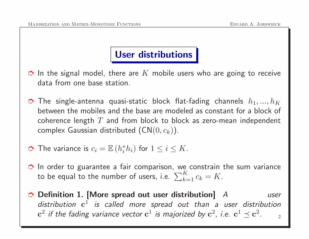
➮ In the signal model, there are K mobile users who are going to receivedata from one base station.
➮ The single-antenna quasi-static block flat-fading channels h1, ..., hK
between the mobiles and the base are modeled as constant for a block ofcoherence length T and from block to block as zero-mean independentcomplex Gaussian distributed (CN(0, ck)).
➮ The variance is ci = E (h∗i hi) for 1 ≤ i ≤ K.
➮ In order to guarantee a fair comparison, we constrain the sum varianceto be equal to the number of users, i.e.
∑Kk=1 ck = K.
➮ Definition 1. [More spread out user distribution] A userdistribution c1 is called more spread out than a user distributionc2 if the fading variance vector c1 is majorized by c2, i.e. c1 � c2. 2

Majorization and Matrix-Monotone Functions Eduard A. Jorswieck
Symmetric scenario c1 = (1, 1, ..., 1)
3

Majorization and Matrix-Monotone Functions Eduard A. Jorswieck
One mobile moves to the base and another to the cell edge. The sum oftheir fading variances stays constant. c2 = (1 + α, 1, 1, ..., 1 − α)
4

Majorization and Matrix-Monotone Functions Eduard A. Jorswieck
All but one mobile at the cell edge c3 = (8, 0, ..., 0)
5
Majorization and Matrix-Monotone Functions Eduard A. Jorswieck
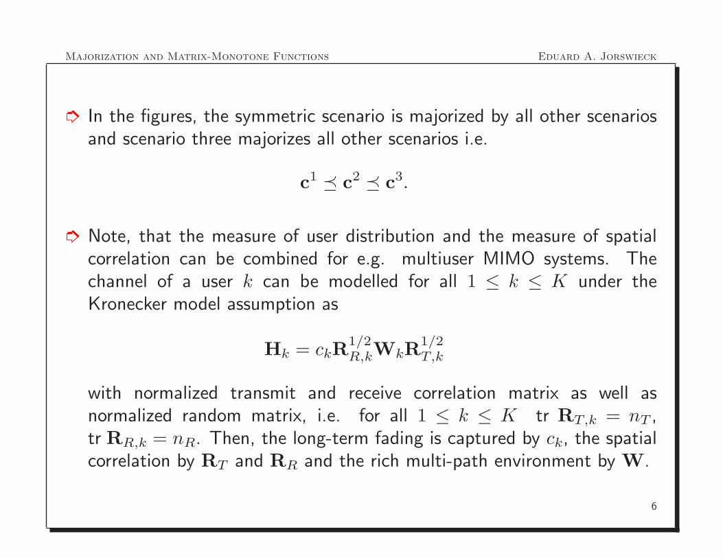
➮ In the figures, the symmetric scenario is majorized by all other scenariosand scenario three majorizes all other scenarios i.e.
c1 � c2 � c3.
➮ Note, that the measure of user distribution and the measure of spatialcorrelation can be combined for e.g. multiuser MIMO systems. Thechannel of a user k can be modelled for all 1 ≤ k ≤ K under theKronecker model assumption as
Hk = ckR1/2R,kWkR
1/2T,k
with normalized transmit and receive correlation matrix as well asnormalized random matrix, i.e. for all 1 ≤ k ≤ K tr RT,k = nT ,tr RR,k = nR. Then, the long-term fading is captured by ck, the spatialcorrelation by RT and RR and the rich multi-path environment by W.
6
Majorization and Matrix-Monotone Functions Eduard A. Jorswieck
Average sum rate in BC
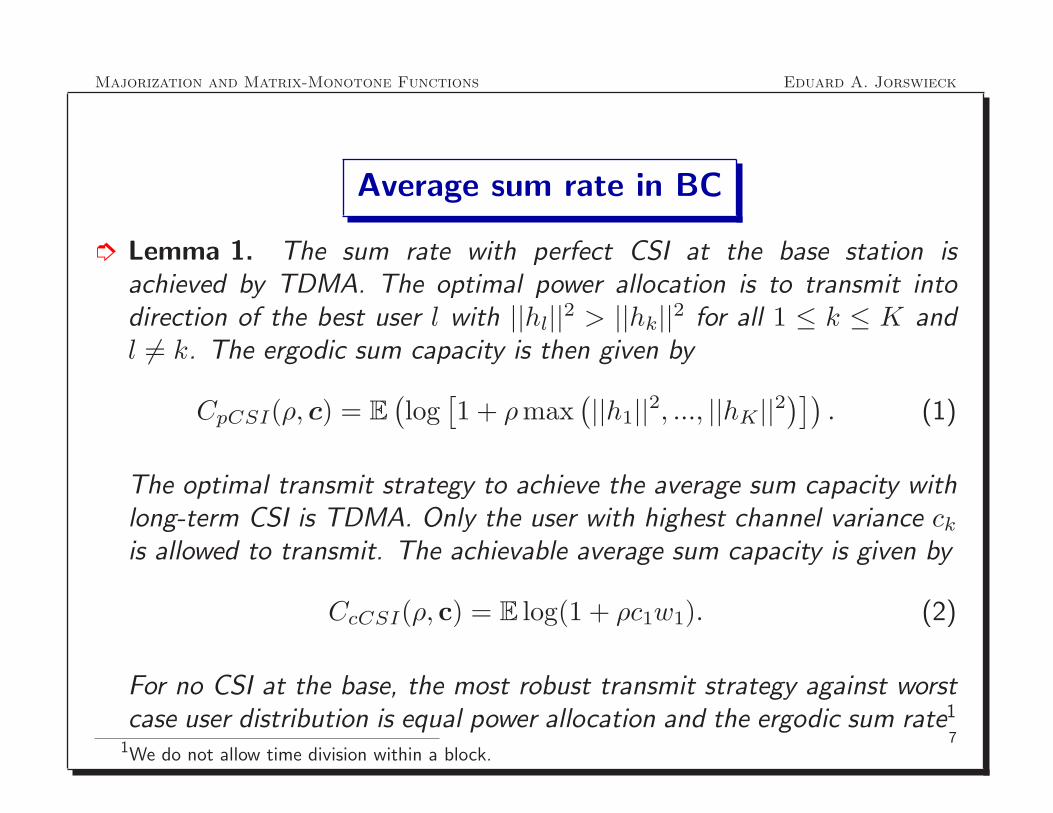
➮ Lemma 1. The sum rate with perfect CSI at the base station isachieved by TDMA. The optimal power allocation is to transmit intodirection of the best user l with ||hl||
2 > ||hk||2 for all 1 ≤ k ≤ K and
l 6= k. The ergodic sum capacity is then given by
CpCSI(ρ, c) = E(
log[
1 + ρmax(
||h1||2, ..., ||hK||2
)])
. (1)
The optimal transmit strategy to achieve the average sum capacity withlong-term CSI is TDMA. Only the user with highest channel variance ck
is allowed to transmit. The achievable average sum capacity is given by
CcCSI(ρ, c) = E log(1 + ρc1w1). (2)
For no CSI at the base, the most robust transmit strategy against worstcase user distribution is equal power allocation and the ergodic sum rate1
1We do not allow time division within a block.7

Majorization and Matrix-Monotone Functions Eduard A. Jorswieck
is given by
CnoCSI(ρ, c) = E log
(
1 + ρ
K∑
k=1
ckwk
)
. (3)
➮ Theorem 1. Assume perfect CSI at the mobiles. For perfect CSI atthe base, the ergodic sum capacity in (1) is a Schur-convex functionw.r.t. the fading variance vector c. For a base which knows the fadingvariances, the ergodic sum capacity in (2) is a Schur-convex functionw.r.t. the fading variance vector c. For an uninformed base station, theergodic sum rate in (3) is a Schur-concave function w.r.t. the fadingvariance vector c.
8
Majorization and Matrix-Monotone Functions Eduard A. Jorswieck
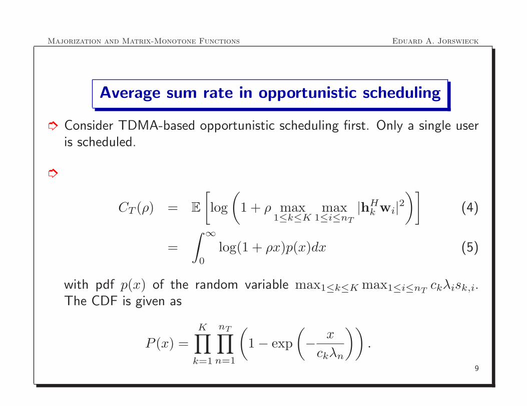
Average sum rate in opportunistic scheduling
➮ Consider TDMA-based opportunistic scheduling first. Only a single useris scheduled.
➮
CT (ρ) = E
[
log
(
1 + ρ max1≤k≤K
max1≤i≤nT
|hHk wi|
2
)]
(4)
=
∫ ∞
0
log(1 + ρx)p(x)dx (5)
with pdf p(x) of the random variable max1≤k≤K max1≤i≤nTckλisk,i.
The CDF is given as
P (x) =
K∏
k=1
nT∏
n=1
(
1 − exp
(
−x
ckλn
))
.
9
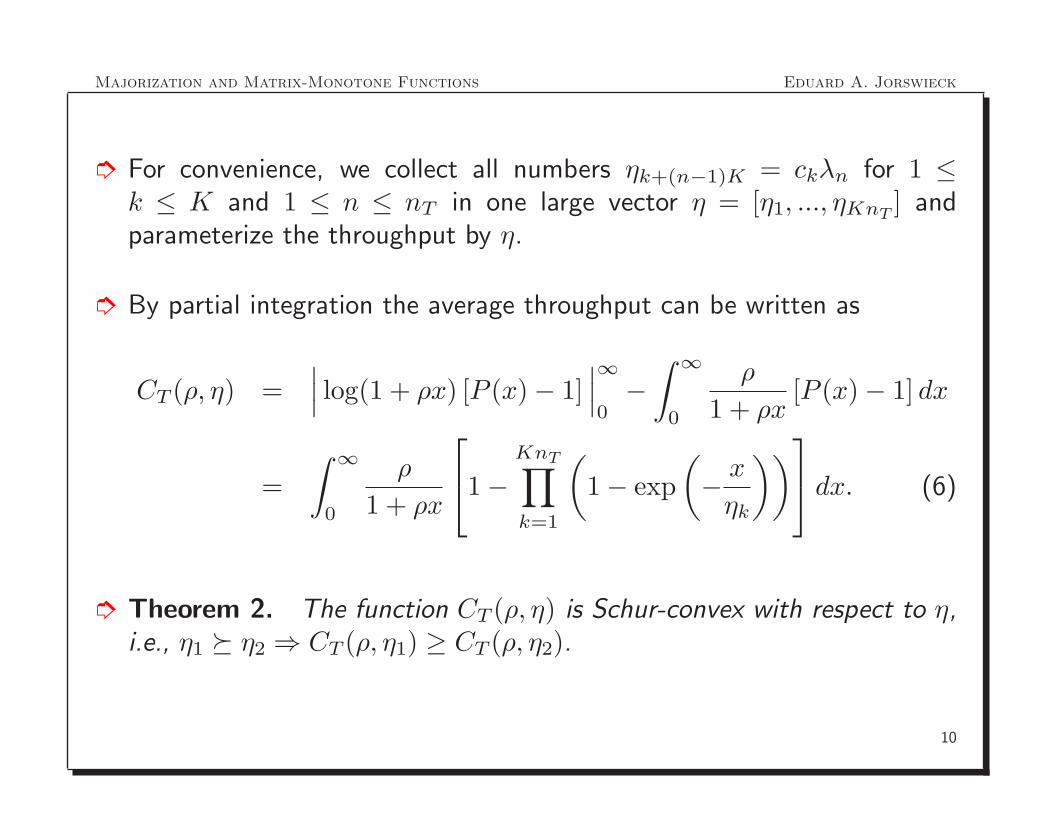
Majorization and Matrix-Monotone Functions Eduard A. Jorswieck
➮ For convenience, we collect all numbers ηk+(n−1)K = ckλn for 1 ≤k ≤ K and 1 ≤ n ≤ nT in one large vector η = [η1, ..., ηKnT
] andparameterize the throughput by η.
➮ By partial integration the average throughput can be written as
CT (ρ, η) =∣
∣
∣log(1 + ρx) [P (x) − 1]
∣
∣
∣
∞
0−
∫ ∞
0
ρ
1 + ρx[P (x) − 1] dx
=
∫ ∞
0
ρ
1 + ρx
1 −
KnT∏
k=1
(
1 − exp
(
−x
ηk
))
dx. (6)
➮ Theorem 2. The function CT (ρ, η) is Schur-convex with respect to η,i.e., η1 � η2 ⇒ CT (ρ, η1) ≥ CT (ρ, η2).
10

Majorization and Matrix-Monotone Functions Eduard A. Jorswieck
−10 −5 0 5 10 15 200
2
4
6
8
SNR [dB]
Avera
ge s
um
rate
[bit/c
u]
CT
max(ρ)
CT
min(ρ)
CT(ρ,η)
∆∞
➮ Average sum rate in bits per channel use (bit/cu) vs. SNR for TDMA-OB: Best-case, worst-case, and intermediate scenario. The high-SNRpower difference is 3.2 dB.
11

Majorization and Matrix-Monotone Functions Eduard A. Jorswieck
➮ In SDMA based opportunistic beamforming: The resulting averagethroughput can be upper bounded by [Sharif2005]
C(ρ, c,R) = nTE log
(
1 + max1≤k≤K
SINR k
)
(7)
with SINR k =||wH
i hk||2
σ2n+∑
l 6=i ||wHl
hk||2.
➮ Theorem 3. The average throughput of SDMA-OB is upper limited by
B(K, nT ,1) = limρ→∞
C(ρ,1, I) =(Ψ(K + 1) + γ)nT
(nT − 1) log(2)
=nT
(nT − 1) log(2)
K∑
k=1
1
k(8)
12

Majorization and Matrix-Monotone Functions Eduard A. Jorswieck
which is tight for asymptotically high SNR and Ψ(x) is the Psi-function.
➮ Theorem 4. The upper bound on the average sum capacity of SDMA-OB B(K, nT , c) is Schur-concave with respect to c, i.e., c1 � c2 ⇒B(K, nT , c1) ≤ B(K, nT , c2). The upper bound on the average sumrate of SDMA-OB is largest for the balanced scenario B(K, nT ,1) andsmallest for the completely unequally distributed scenario B(1, nT ) =B(K, nT , [K, 0, ..., 0]).
13
Majorization and Matrix-Monotone Functions Eduard A. Jorswieck
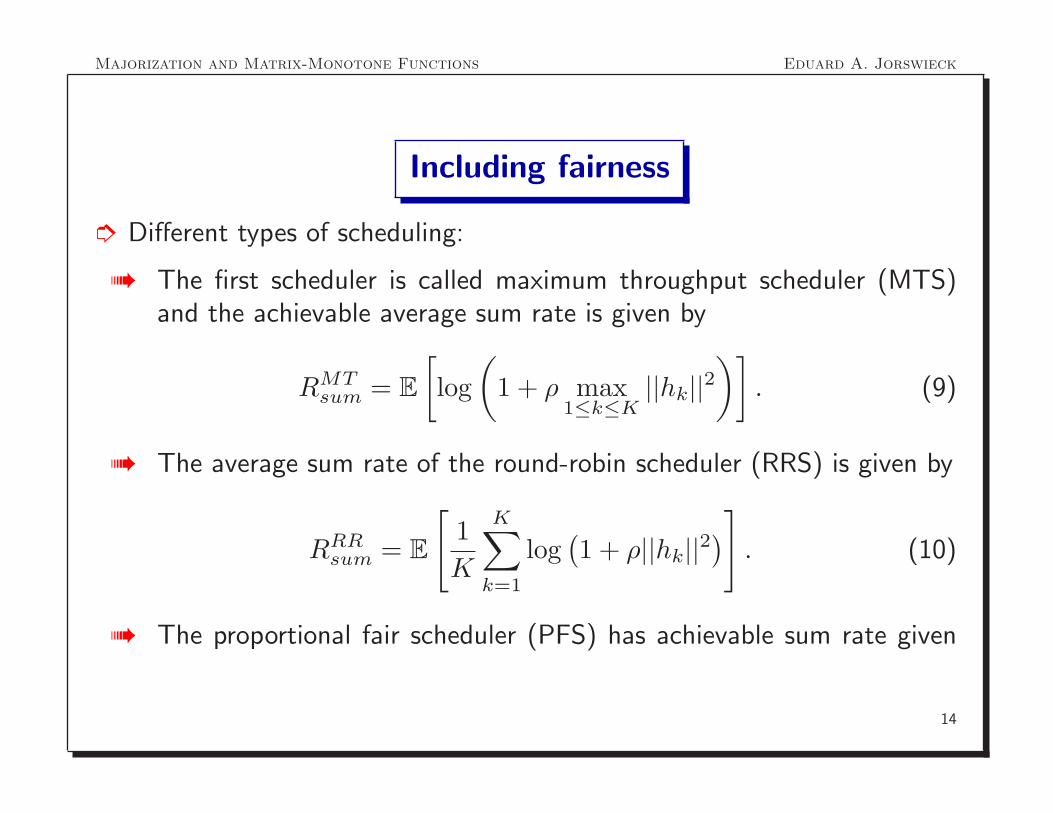
Including fairness
➮ Different types of scheduling:
➠ The first scheduler is called maximum throughput scheduler (MTS)and the achievable average sum rate is given by
RMTsum = E
[
log
(
1 + ρ max1≤k≤K
||hk||2
)]
. (9)
➠ The average sum rate of the round-robin scheduler (RRS) is given by
RRRsum = E
[
1
K
K∑
k=1
log(
1 + ρ||hk||2)
]
. (10)
➠ The proportional fair scheduler (PFS) has achievable sum rate given
14

Majorization and Matrix-Monotone Functions Eduard A. Jorswieck
by
RPFsum = E
[
log(
1 + ρ||hk∗||2)]
with (11)
k∗ = arg max1≤k≤K
||hk||2
ck.
Note that (11) can be rewritten as
RPFsum =
1
K
K∑
k=1
E
[
log
(
1 + ρck max1≤l≤K
wl
)]
(12)
=1
K
K∑
k=1
K∑
l=1
(−1)l−1
(
K
l
)
Ei
(
1,l
ρck
)
el
ρck
because the scheduling probability of all users is equal to 1K .
15

Majorization and Matrix-Monotone Functions Eduard A. Jorswieck
➠ The sum rate performance of the opportunistic round robin scheduler(ORS) is given by
RORsum =
1
K2
K∑
n=1
n
K∑
i=1
n−1∑
j=0
(
n − 1j
)
(−1)j
·e
1+jci
1 + jEi
(
1,1 + j
ci
)
. (13)
➠ Lemma 2. The average sum rate of the ORS (13) can be written as
∫ ∞
0
[
1 −1
K2
K∑
n=1
K∑
i=1
(
1 − e− t
ci
)n]
ρ
1 + ρtdt. (14)
➮ Analysis of the sum rate performance
16

Majorization and Matrix-Monotone Functions Eduard A. Jorswieck
➠ Theorem 5. The average sum rate of the MTS is Schur-convex withrespect to the vector of average user powers c, i.e.
c � d =⇒ RMTsum(c) ≥ RMT
sum(d). (15)
➠ Theorem 6. The average sum rate of the RRS is Schur-concavewith respect to the vector of average user powers c, i.e.
c � d =⇒ RRRsum(c) ≤ RRR
sum(d). (16)
➠ Theorem 7. The average sum rate of the PFS is Schur-concave withrespect to the vector of average user powers c, i.e.
c � d =⇒ RPFsum(c) ≤ RPF
sum(d). (17)
➠ Theorem 8. The average sum rate of the ORS is Schur-concave
17

Majorization and Matrix-Monotone Functions Eduard A. Jorswieck
with respect to the vector of average user power c, i.e.
c � d =⇒ RORsum(c) ≤ ROR
sum(d). (18)
➮ Fairness analysis: The average worst-case delay E[Dm,K] measures theaverage number of transmissions that are needed until all K users havebeen active at least m times. We define D1 = E[D1,K].
➮ Average worst-case delay of the deterministic schedulers
DRRS1 = DORS
1 = K. (19)
➮ Average worst-case of PFS
DPFS1 = K
∫ ∞
0
1 − (1 − exp(−x))Kdt (20)
18

Majorization and Matrix-Monotone Functions Eduard A. Jorswieck
Note that (20) can be written as
DPFS1 = K (Ψ(K + 1) + γ) (21)
with the Ψ-function and Euler’s constant γ.
➮ Average worst-case of MTS
DMTS1 = n
∫ ∞
0
(
1 −
K∏
k=1
(
1 −Γ(m, dkt)
Γ(m)
)
)
dt. (22)
➮ Theorem 9. The average worst-case delay E[D1,K] of MTS is Schur-convex with respect to d, i.e.
d1 � d2 −→ DMTS1 (d1) ≥ DMTS
1 (d2). (23)
19
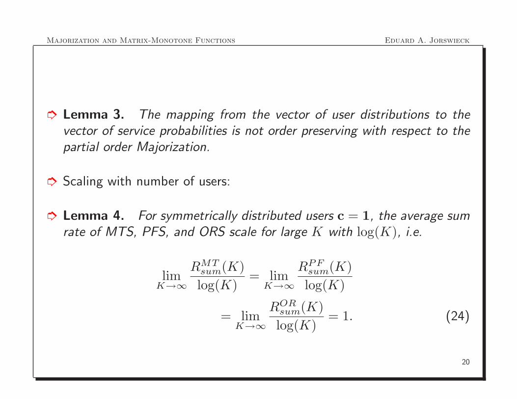
Majorization and Matrix-Monotone Functions Eduard A. Jorswieck
➮ Lemma 3. The mapping from the vector of user distributions to thevector of service probabilities is not order preserving with respect to thepartial order Majorization.
➮ Scaling with number of users:
➮ Lemma 4. For symmetrically distributed users c = 1, the average sumrate of MTS, PFS, and ORS scale for large K with log(K), i.e.
limK→∞
RMTsum(K)
log(K)= lim
K→∞
RPFsum(K)
log(K)
= limK→∞
RORsum(K)
log(K)= 1. (24)
20

Majorization and Matrix-Monotone Functions Eduard A. Jorswieck
➮ Lemma 5. For symmetrically distributed users, the average worst-casedelay scales linearly with K for RRS and ORS. For MTS and PFS, itscales as K log(K), i.e.
limK→∞
DRRS1 (K)
K= lim
K→∞
DORS1 (K)
K= 1
limK→∞
DMTS1 (K)
K log(K)= lim
K→∞
DPFS1 (K)
K log(K)= 1. (25)
➮ Illustrations:
21

Majorization and Matrix-Monotone Functions Eduard A. Jorswieck
2 4 6 8 10 12 14 16 18 202.5
3
3.5
4
4.5
5
5.5Scaling with number of users [symmetrical distribution]
Number of users
Avera
ge s
um
rate
[bpcu]
RRSMTSPFSORS
2 4 6 8 10 12 14 16 18 202
2.5
3
3.5
4
4.5
5
5.5
6
Number of users
Avera
ge s
um
rate
[bpcu]
Scaling with number of users [assymetrical with t=0.2]
RRSMTSPFSORS
➮ Observation and main conclusion: Therefore, taking the tradeoff betweenfairness and average sum rate into account, the PFS and ORS performreasonable well. PFD is advantageous in symmetric scenarios whereasORS performs better in asymmetric scenarios.
22

Majorization and Matrix-Monotone Functions Eduard A. Jorswieck
References I
i) E. Jorswieck, P. Svedman, and B. Ottersten, ”On the Performance ofTDMA and SDMA based Opportunistic Beamforming”, submitted toIEEE Transactions on Wireless Communications, 2007.
ii) E. Jorswieck, A. Sezgin, and X. Zhang, ”Framework for analysis ofopportunistic schedulers: average sum rate vs. average fairness”, to besubmitted to RAWCOM 2008.
23

Majorization and Matrix-Monotone Functions Eduard A. Jorswieck
Spectral correlation in OFDM systems
➮ Consider the standard frequency selective channel model described in timedomain by a cannel impulse response h1, ..., hL with L taps probablycorrelated with channel correlation matrix R, i.e. Rk,l = E[hkh
∗l ].
➮ Ideal cyclic prefix OFDM is applied with N > L carriers.
➮ The fading on carrier k is given by Hk =∑L−1
l=0 hl exp(
−i2π kN
)
.
➮ Therefore, the power of carrier k is distributed according to an exponentialdistribution with mean
ak(R) = E[|Hk|2] = 2
L−2∑
n=0
L−1∑
m=n+1
Rm,n cos
(
2πk
N(m − n)
)
+
L∑
k=1
Rk,k
for all 1 ≤ k ≤ N .24

Majorization and Matrix-Monotone Functions Eduard A. Jorswieck
➮ N parallel flat-fading channels are obtained by ideal CP-OFDM yk =Hkxk + nk for 1 ≤ k ≤ N , transmit signals xk and AWGN nk.
➮ In the following, we focus on the average rate of the system as a functionof the power allocation p = [p1, ..., pN ], the inverse noise power ρ = 1
σ2n,
and the fading variances a = [a1, ..., aN ]
C(a, ρ) = E [R(H, ρ,p)] (26)
with instantaneous rate which depends on the channel vector H =[H1, ...,HN ] and the power allocation
R(H, ρ,p) =1
N
N∑
k=1
log (1 + ρHkpk) . (27)
25

Majorization and Matrix-Monotone Functions Eduard A. Jorswieck
➮ We assume that the receiver has perfect CSI and consider three differenttypes of CSI at the transmitter.
➮ At first, assume the transmitter does not have CSI at all. Then theoptimal power allocation is equal power allocation and the achievableaverage rate is given by
Cno(a, ρ) = E
[
1
N
N∑
k=1
log
(
1 +P
Nρak
)
]
. (28)
➮ If the transmitter has information about R it can adapt its powerallocation to a and the average rate is given by
Cpart(a, ρ) = maxpk≥0,
∑
pk=PE
[
1
N
N∑
k=1
log (1 + ρHkpk)
]
. (29)
26

Majorization and Matrix-Monotone Functions Eduard A. Jorswieck
➮ If the transmitter has perfect CSI, spectral power allocation is optimaland the average rate is given by
Cp(a, ρ) = E
[
maxpk≥0,
∑
pk=P
1
N
N∑
k=1
log (1 + ρHkpk)
]
. (30)
➮ Definition 2. The frequency selective channel described by R has morecorrelated taps than the channel described by S if
a(R) � a(S), (31)
i.e. a(R) majorizes a(S), i.e.
n∑
k=1
ak(R) ≥
n∑
k=1
ak(S) for 1 ≤ n ≤ N − 1 and
N∑
k=1
ak(R) ≥
N∑
k=1
ak(S).
27

Majorization and Matrix-Monotone Functions Eduard A. Jorswieck
➮ Consider for example two taps L = 2 with R(c) =
(
1 c
c 1
)
and N = 4
carriers. The average channel power of the four carriers is then given by
a(R(c)) = [2 + 2c, 2, 2, 2 − 2c]. (32)
For completely uncorrelated coefficients, a(R(0)) = [2, 2, 2, 2]. Forcompletely correlated coefficients, a(R(1)) = [4, 2, 2, 0]. From (32), itfollows that all correlation matrices R(c1),R(c2) are comparable.
➮ TBD-List:
➠ Is it possible to compare all channel correlation matrices R?➠ Are C(a, ρ) Schur-convex or Schur-concave? High SNR behavior
analysis.➠ Maximum Loss/Gain due to spectral correlation?
28

Majorization and Matrix-Monotone Functions Eduard A. Jorswieck
References II
i) Kafedziski, V. Capacity of Frequency Selective Slowly Fading Channelswith Correlated Coefficients Proc. of SCC, will appear, 2008.
ii) Yao, Y. and Giannakis, G. B. Rate-Maximizing Power Allocation inOFDM Based on Partial Channel Knowledge IEEE Trans. on WirelessCommunications, 2005, 4, 1073-1083.
29