fractal and fractional

Article

Monotone Iterative Method for ψ-Caputo FractionalDifferential Equation with Nonlinear Boundary Conditions

Zidane Baitiche 1,†, Choukri Derbazi 1,† , Jehad Alzabut 2,3,*,† , Mohammad Esmael Samei 4,5,† ,Mohammed K. A. Kaabar 6,7,*,† and Zailan Siri 6,*,†

Citation: Baitiche, Z.; Derbazi, C.;

Alzabut, J.; Samei, M.E.; Kaabar,

M.K.A.; Siri, Z. Monotone Iterative

Method forψ-Caputo Fractional

Differential Equation with Nonlinear

Boundary Conditions. Fractal Fract.

2021, 5, 81. https://doi.org/10.3390/

fractalfract5030081

Academic Editors: Amar Debbouche

and Boris Baeumer

Received: 29 May 2021

Accepted: 27 July 2021

Published: 29 July 2021

Publisher’s Note: MDPI stays neutral

with regard to jurisdictional claims in

published maps and institutional affil-

iations.

Copyright: © 2021 by the authors.

Licensee MDPI, Basel, Switzerland.

This article is an open access article

distributed under the terms and

conditions of the Creative Commons

Attribution (CC BY) license (https://

creativecommons.org/licenses/by/

4.0/).

1 Laboratoire Equations Differntielles, Department of Mathematics, Faculty of Exact Sciences, University FrèresMentouri, Constantine 25000, Algeria; baitichezidane19@gmail.com (Z.B.); choukriedp@yahoo.com (C.D.)

2 Department of Mathematics and General Sciences, Prince Sultan University, Riyadh 11586, Saudi Arabia3 Department of Industrial Engineering, OSTIM Technical University, Ankara 06374, Turkey4 Department of Mathematics, Faculty of Basic Science, Bu-Ali Sina University, Hamedan 65178, Iran;

mesamei@basu.ac.ir5 Department of Medical Research, China Medical University Hospital, China Medical University,

Taichung 40402, Taiwan6 Institute of Mathematical Sciences, Faculty of Science, University of Malaya, Kuala Lumpur 50603, Malaysia7 Department of Mathematics and Statistics, Washington State University, Pullman, WA 99163, USA* Correspondence: jalzabut@psu.edu.sa (J.A.); mohammed.kaabar@wsu.edu (M.K.A.K.);

zailansiri@um.edu.my (Z.S.)† These authors contributed equally to this work.

Abstract: The main contribution of this paper is to prove the existence of extremal solutions for anovel class of ψ-Caputo fractional differential equation with nonlinear boundary conditions. For thispurpose, we utilize the well-known monotone iterative technique together with the method of upperand lower solutions. Finally, we provide an example along with graphical representations to confirmthe validity of our main results.

Keywords: ψ-Caputo operator; extremal solutions; monotone iterative style; upper (lower) solutions;boundary conditions

MSC: 26A33; 34A08; 39A12; 39A13; 39A21

1. Introduction

In the mathematical modeling of real life phenomena, the study of fractional dif-ferential equations has gained notable importance among interested researchers. It isrealized that the use of fractional calculus methods is quite prominent in modeling variousprocesses. The main reason for the widespread use (applications) of fractional operatorsis the fact that, unlike “integer” operators, these operators possess non-local behaviorwhich enables us to trace the past effects of the involved phenomena [1–5]. Based onsome classical approaches, such as Riemann-Liouville, Caputo, and Hadamard fractionaloperators, there are many new definitions which have attempted to provide a generalplatform that includes these classical operators [6–8]. For the sake of consolidating thesedifferent definitions under one single fractional operator, theψ-fractional operator has beenintroduced [9,10]. The main feature of the the ψ-fractional operator is that the functionin its integral kernel an be adapted to accommodate other definitions when replacing itby specific functions. Other significant features include non-local behavior and the semi-group property which are clearly preserved. It has been recognized that these types ofoperators have been successfully used to describe and model many real life phenomena;therefore, several related research works have been produced [11–13]. Along with therecent developments in fractional differential equations, researchers have contributed manyresearch studies that discus the solutions’ behavior in terms of different types of fractionaldifferential equations [14–27].

Fractal Fract. 2021, 5, 81. https://doi.org/10.3390/fractalfract5030081 https://www.mdpi.com/journal/fractalfract

Fractal Fract. 2021, 5, 81 2 of 16

There are different types of fractional differential equations involving different frac-tional operators, which are associated with the various types of initial and boundary condi-tions that have been investigated by many researchers in various research works [28–30]. Byexploring the literature, one can figure out that the existence of solutions has been the maintarget of investigations. In order to prove this, researchers often utilize some fixed pointhypothesis along with certain mathematical inequalities. To the best of our observations,the monotone iterative technique combined with the method of upper and lower solutionshas not been used to study the existence of solutions for ψ-Caputo fractional differentialequation with nonlinear boundary conditions. For more expository details on monotoneiterative method, the readers can consult some interesting research works [31–35].

Oriented by the above discussion, we study the following ψ-Caputo fractional differ-ential equation (CpFDE) with nonlinear boundary conditions:

cDτ;ψa+

(cDλ;ψ

a+ − σ)z(ϑ) = F

(ϑ, z(ϑ), cDλ;ψ

a+ (ϑ))

,

H(

cDλ;ψa+ z(a), cDλ;ψ

a+ z(b))= 0, G(z(a), z(b)) = 0,

(1)

for ϑ ∈ Ω := [a, b], where cDτ;ψa+ and cDλ;ψ

a+ denote the ψ-Caputo fractional derivativesof order τ and λ, respectively, such that τ, λ ∈ (0, 1], σ > 0, F ∈ C(Ω × R2,R), G,H ∈ C(R2,R). It is worth mentioning here that, unlike the above mentioned relevantworks, the CpFDE (1) is subject to nonlinear boundary conditions. The above equation isthe deterministic fractional differential equation, therefore, a fractional differential equationwith its deterministic solution is only considered in this work without the involvement ofany random processes.

The remaining part of the paper is organized as follows: In Section 2, we present somedefinitions and lemmas that will be used to prove our results. In Section 3, we prove ourmain results, which conveys the existence of extremal solutions for CpFDE (1). For thispurpose, we use the monotone iterative method together with the technique of upper andlower solutions. In Section 4, we apply our results by providing an example and illustratethe solutions of behavior graphically.

2. Relevant Preliminaries

In the current section, we state some basic concepts of fractional calculus that arerelated to our work. Let Ω = [a, b], 0 ≤ a < b < ∞ be a finite interval and ψ : Ω → R bean increasing differentiable function such that ψ′(ϑ) 6= 0, for all ϑ ∈ Ω.

Definition 1 ( [9]). The Riemann–Lebesgue (RL) fractional integral of order τ > 0 for an integrablefunction z : Ω→ R with respect to ψ is described by the following:

Iτ;ψa+ z(ϑ) =

1Γ(τ)

∫ ϑ

aψ′(η)(ψ(ϑ)−ψ(η))τ−1z(η)dη, (2)

where Γ(τ) =∫ +∞

0 ϑτ−1e−ϑ dϑ, τ > 0 is the Gamma function.

Definition 2 ( [9]). Let ψ, z ∈ Cn(Ω,R). The RL fractional derivative of a function z of ordern− 1 < τ < n with respect to ψ is given by the following:

Dτ;ψa+ z(ϑ) =

(Dϑ

ψ′(ϑ)

)nIn−τ;ψ

a+ z(ϑ)

=1

Γ(n− τ)

(Dϑ

ψ′(ϑ)

)n ∫ ϑ

aψ′(η)(ψ(ϑ)−ψ(η))n−τ−1z(η)dη,

where n = [τ] + 1, n ∈ N and Dϑ = ddϑ .

Fractal Fract. 2021, 5, 81 3 of 16

Definition 3 ( [9]). Let ψ, z ∈ Cn(Ω,R). The Caputo fractional derivative of z of order n− 1 <τ < n with respect to ψ is defined by the following

cDτ;ψa+ z(ϑ) = In−τ;ψ

a+ z[n]ψ (ϑ),

where n = [τ] + 1 for τ /∈ N, n = τ for τ ∈ N and z[n]ψ (ϑ) =

(Dϑψ′(ϑ)

)nz(ϑ). From the definition,

it is clear that the following is the case.

cDτ;ψa+ z(ϑ) =

∫ ϑ

a

ψ′(η)(ψ(ϑ)−ψ(η))n−τ−1

Γ(n− τ)z[n]ψ (η)dη, τ /∈ N,

z[n]ψ (ϑ), τ ∈ N.

(3)

Some basic properties of the ψ-fractional operators are listed in the following Lemma.

Lemma 1 ( [9]). Let τ, λ > 0, and z ∈ C(Ω,R). Then for each ϑ ∈ Ω, we have the following.

1. cDτ;ψa+ Iτ;ψ

a+ z(ϑ) = z(ϑ),

2. Iτ;ψa+

cDτ;ψa+ z(ϑ) = z(ϑ)− z(a) for 0 < τ ≤ 1,

3. Iτ;ψa+ (ψ(ϑ)−ψ(a))λ−1 = Γ(λ)

Γ(λ+τ)(ψ(ϑ)−ψ(a))λ+τ−1,

4. cDτ;ψa+ (ψ(ϑ)−ψ(a))λ−1 = Γ(λ)

Γ(λ−τ)(ψ(ϑ)−ψ(a))λ−τ−1,

5. cDτ;ψa+ (ψ(ϑ)−ψ(a))k = 0, for all k ∈ 0, . . . , n− 1, n ≥ 1.

Definition 4 ( [36]). The Mittag–Leffler functions (MLFs) of one and two parameters are givenby:

Eν(v) =∞

∑k=0

vk

Γ(νk + 1), (v ∈ R, ν > 0), (4)

and

Eν,λ(v) =∞

∑k=0

vk

Γ(νk + λ), (ν, λ > 0, v ∈ R), (5)

respectively. It is obvious that E1,1(v) = E1(v) = ev.

We denote the set X by the following.

X = Cλ(Ω) =

x : cDλ;ψa+ x(ξ) ∈ C(Ω)

.

Equipped with the norm, we have the following:

‖x‖X = ‖x‖∞ +∥∥∥cDλ;ψ

a+ x∥∥∥

∞,

where ‖x‖∞ = maxξ∈Ω |x(ξ)| and one can conclude that (X, ‖ · ‖X) is a Banach space.

Lemma 2. For a given ` ∈ C(Ω,R), λ, τ ∈ (0, 1] and σ > 0, the linear fractional initial valueproblem is as follows:

cDτ;ψa+

(cDλ;ψ

a+ − σ)z(ϑ) = `(ϑ),

cDλ;ψa+ z(a) = zλ, z(a) = za,

(6)

Fractal Fract. 2021, 5, 81 4 of 16

for ϑ ∈ Ω is equivalent to the following Volterra integral equation.

z(ϑ) = za +zλ − σza

Γ(λ + 1)(ψ(ϑ)−ψ(a))λ + σIλ;ψ

a+ z(ϑ) + Iτ+λ;ψa+ `(ϑ). (7)

Moreover, the explicit solution of the Volterra integral Equation (7) can be represented by thefollowing.

z(ϑ) =za + zλ(ψ(ϑ)−ψ(a))λEλ,λ+1

(σ(ψ(ϑ)−ψ(a))λ

)+∫ ϑ

aψ′(η)(ψ(ϑ)−ψ(η))λ+τ−1

×Eλ,λ+τ

(σ(ψ(ϑ)−ψ(η))λ

)`(η)dη.

(8)

Proof. Applying the ψ-Riemann-Liouville fractional integral of order τ to both sides of (6)and by using Lemma 1, we obtain the following.

cDλ;ψa+ z(ϑ) = zλ + σ(z(ϑ)− za) + Iτ;ψ

a+ `(ϑ). (9)

Hence, we have the following.

z(ϑ) = za +zλ − σza

Γ(λ + 1)(ψ(ϑ)−ψ(a))λ + σIλ;ψ

a+ z(ϑ) + Iτ+λ;ψa+ `(ϑ). (10)

The converse can be proven by direct computation. Now, we apply the method ofsuccessive approximations in order to prove that the integral Equation (7) can be expressedby the following.

z(ϑ) =za + zλ(ψ(ϑ)−ψ(a))λEλ,λ+1

(σ(ψ(ϑ)−ψ(a))λ

)+∫ ϑ

aψ′(η)(ψ(ϑ)−ψ(η))λ+τ−1

×Eλ,λ+τ

(σ(ψ(ϑ)−ψ(η))λ

)`(η)dη.

For this, we set the following.z0(ϑ) = za +

zλ − σza

Γ(λ + 1)(ψ(ϑ)−ψ(a))λ,

zm(ϑ) = z0(ϑ) + σIλ;ψa+ zm−1(ϑ) + Iτ+λ;ψ

a+ `(ϑ).(11)

It follows from Equation (11) and Lemma 1 that the following is the case.

z1(ϑ) = z0(ϑ) + σIλ;ψa+ z0(ϑ) + Iλ+τ;ψ

a+ `(ϑ)

= za +zλ − σza

Γ(λ + 1)(ψ(ϑ)−ψ(a))λ + σ

za

Γ(λ + 1)[ψ(ϑ)−ψ(a)]λ

+ σzλ − σza

Γ(2λ + 1)(ψ(ϑ)−ψ(a))2λ + Iλ+τ;ψ

a+ `(ϑ).

(12)

Similarly, Equations (11) and (12) and Lemma 1 yield the following.

z2(ϑ) = z0(ϑ) + σIλ;ψa+ z1(ϑ) + Iλ+τ;ψ

a+ `(ϑ)

= za +zλ − σza

Γ(λ + 1)(ψ(ϑ)−ψ(a))λ

+ σIλ;ψa+

(za +

zλ − σza

Γ(λ + 1)(ψ(ϑ)−ψ(a))λ

Fractal Fract. 2021, 5, 81 5 of 16

+ σza

Γ(λ + 1)(ψ(ϑ)−ψ(a))λ + σ

zλ − σza

Γ(2λ + 1)(ψ(ϑ)

−ψ(a))2λ + Iλ+τ;ψa+ `(ϑ)

)+ Iλ+τ;ψ

a+ `(ϑ)

= za +2

∑k=0

σk

Γ(kλ + 1)(ψ(ϑ)−ψ(a))kλ

+ (zλ − σza)2

∑k=0

σk

Γ(kλ + λ + 1)(ψ(ϑ)−ψψ(a))kλ+λ

+ σI2λ+τ;ψa+ `(ϑ) + Iλ+τ;ψ

a+ `(ϑ)

= za +2

∑k=0

σk

Γ(kλ + 1)(ψ(ϑ)−ψ(a))kλ

+ (zλ − σza)2

∑k=0

σk

Γ(kλ + λ + 1)(ψ(ϑ)−ψ(a))kλ+λ

+∫ ϑ

aψ′(η)

2

∑k=1

σk−1(ψ(ϑ)−ψ(η))kλ+τ−1

Γ(kλ + τ)`(η)dη.

In continuing this process, we derive the following relation.

zm(ϑ) = za +m

∑k=0

σk

Γ(kλ + 1)(ψ(ϑ)−ψ(a))kλ

+ (zλ − σza)m

∑k=0

σk

Γ(kλ + λ + 1)(ψ(ϑ)−ψ(a))kλ+λ

+∫ ϑ

aψ′(η)

m

∑k=1

σk−1(ψ(ϑ)−ψ(η))kλ+τ−1

Γ(kλ + τ)`(η)dη

= za +m

∑k=0

σk

Γ(kλ + 1)(ψ(ϑ)−ψ(a))kλ

+(zλ − σza)

σ

m

∑k=1

σk

Γ(kλ + 1)(ψ(ϑ)−ψ(a))kλ

+∫ ϑ

aψ′(η)(ψ(ϑ)−ψ(η))λ+τ−1

m

∑k=1

σk−1(ψ(ϑ)−ψ(η))kλ−λ

Γ(kλ + τ)`(η)dη.

Taking the limit as m → ∞, we obtain the following explicit solution z(ϑ) of theintegral Equation (7).

z(ϑ) = za +∞

∑k=0

σk

Γ(kλ + 1)(ψ(ϑ)−ψ(a))kλ

+(zλ − σza)

σ

∞

∑k=1

σk

Γ(kλ + 1)(ψ(ϑ)−ψ(a))kλ

+∫ ϑ

aψ′(η)(ψ(ϑ)−ψ(η))λ+τ−1

∞

∑k=0

σk(ψ(ϑ)−ψ(η))kλ

Γ(kλ + λ + τ)`(η)dη

= za +zλ

σ

∞

∑k=1

σk

Γ(kλ + 1)(ψ(ϑ)−ψ(a))kλ

+∫ ϑ

aψ′(η)(ψ(ϑ)−ψ(η))λ+τ−1Eλ,λ+τ

(σ(ψ(ϑ)−ψ(η))λ

)`(η)dη

= za + zλ(ψ(ϑ)−ψ(a))λEλ,λ+1

(σ(ψ(ϑ)−ψ(a))λ

)

Fractal Fract. 2021, 5, 81 6 of 16

+∫ ϑ

aψ′(η)(ψ(ϑ)−ψ(η))λ+τ−1Eλ,λ+τ

(σ(ψ(ϑ)−ψ(η))λ

)`(η)dη.

Then, the proof is completed.

Lemma 3 (Comparison Result). Let λ, τ ∈ (0, 1], and σ > 0. If ∆ ∈ C(Ω,R) fulfills thefollowing inequalities:

cDτ;ψa+

(cDλ;ψ

a+ − σ)

∆(ϑ) ≥ 0, ϑ ∈ (a, b],

∆(a) ≥ 0, cDλ;ψa+ ∆(a) ≥ 0,

then ∆(ϑ) ≥ 0 and cDλ;ψa+ ∆(ϑ) ≥ 0 for all ϑ ∈ Ω.

Proof. Since Eρ1,ρ2(x) ≥ 0 for ρ1 ∈ (0, 1], ρ2 ≥ ρ1, x ∈ R, we allow the following:

`(ϑ) = cDτ;ψa+

(cDλ;ψ

a+ − σ)

∆(ϑ) ≥ 0,

∆(a) = za ≥ 0 and cDλ;ψa+ ∆(a) = zλ ≥ 0 in Lemma 2. Then, it follows by Equations (8)

and (9) that the conclusion of Lemma 3 holds.

Let (X , T ) be a topological Hausdorff space and g1, g2 : X → R be a lower semi-continuous function and an upper semi-continuous function, respectively. This means thatfor every r ∈ R, the subsets of the following:

g1 > r

:=

x ∈ X : g1(x) > r

,

g2 < r

:=

x ∈ X : g2(x) < r

,

are open in X . Suppose that g1(x) ≤ g2(x) for all x ∈ X and we allow the interval[g1, g2] consist of those upper or lower semi-continuous functions h : X → R such thatg1(x) ≤ h(x) ≤ g2(x) for all x ∈ X . Let Ω : [g1, g2]→ [g1, g2] be a monotone mapping inthe sense that g1 ≤ h1 ≤ h2 ≤ g2 implies g1 ≤ Ω(h1) ≤ Ω(h2) ≤ g2. In addition, supposethat the sequence Ω(hn)n∈N ⊂ [g1, g2] consist of lower semi-continuous functions thatincrease pointwise to Ω(h) whenever the sequence hnn∈N ⊂ [g1, g2] consist of lowersemi-continuous functions that increase pointwise to h. A similar assumption is made whenthe sequence hnn∈N ⊂ [g1, g2] consist of upper semi-continuous functions, which de-creases pointwise to h ∈ [g1, g2]. In particular, assume that Ω(h) is lower semi-continuouswhenever h is lower semi-continuous and that Ω(h) is upper semi-continuous whenever his so. Then for every n ∈ N, we have the following.

g1 ≤ Ωn(g1) ≤ Ωn+1(g1) ≤ Ωn+1(g2) ≤ Ωn(g2) ≤ g2.

Substitute ω1 = supn∈N Ωn(g1) and ω2 = supn∈N Ωn(g2). Then, ω1 and ω2 belongto the interval [g1, g2], the function ω1 is lower semi-continuous, the function ω2 is uppersemi-continuous, and the equalities Ω(ω1) = ω1 and Ω(ω2) = ω2 are valid. If themonotone mapping Ω has at most one fixed point, then ω1 = ω2 = Ω(ω1) = Ω(ω2) isa continuous function. When the mapping Ω : [g1, g2] → [g1, g2] does not posses thissequential continuity property, then one needs a more subtle version of the Tarski–Knasterfixed point theorem. More precisely, define the functions hpre f ix and hpost f ix, respectively,by the following:

hprefix = inf

h ∈ [g1, g2]Ω(h) ≤ h, h is upper semi-contiunous

,

and the following.

hpostfix = sup

h ∈ [g1, g2]Ω(h) ≥ h, h is lower semi-contiunous

.

Fractal Fract. 2021, 5, 81 7 of 16

Then, we obtain the following.

Ω(hprefix) = hprefix ≤ infn∈N

Ωn(g2), Ω(hpostfix) = hpostfix ≥ supn∈N

Ωn(g1).

Moreover, the function hprefix is upper semi-continuous and the function hpostfix islower semi-continuous. Consequently, if Ω has at most one fixed point, then

Ω(hprefix) = hprefix = Ω(hpostfix) = hpostfix,

and, therefore, this unique fixed point is a continuous function.

3. Main Results

In this section, we prove the existence of extremal solutions for problem (1). Before pro-ceeding, we provide the definitions of lower and upper solutions of the problem (1).

Definition 5. A function z0 ∈ X is called a lower solution of (1), if it satisfies the following:cDτ;ψ

a+

(cDλ;ψ

a+ − σ)z0(ϑ) ≤ F

(ϑ, z0(ϑ), cDλ;ψ

a+ z0(ϑ))

,

H(

cDλ;ψa+ z0(a), cDλ;ψ

a+ z0(b))≤ 0, G(z0(a), z0(b)) ≤ 0,

for ϑ ∈ Ω.

Definition 6. A function z0 ∈ X is called an upper solution of (1), if it satisfies the following:cDτ;ψ

a+

(cDλ;ψ

a+ − σ)z0(ϑ) ≥ F

(ϑ, z0(ϑ), cDλ;ψ

a+ z0(ϑ))

,

H(

cDλ;ψa+ z0(a), cDλ;ψ

a+ z0(b))≥ 0, G(z0(a), z0(b)) ≥ 0,

for each ϑ ∈ Ω.

Theorem 1. Let F : Ω × R2 → R be a continuous function such that the following assump-tions hold:

(H1) There exist z0 and z0 as lower and upper solutions of (1) in X, respectively, with z0(ϑ) ≤z0(ϑ) and;

cDλ;ψa+ z0(ϑ) ≤ cDλ;ψ

a+ z0(ϑ), ϑ ∈ Ω.

(H2) F satisfies the following condition:

F(ϑ, y(ϑ), cDλ;ψa+ y(ϑ)) ≤ F(ϑ, z(ϑ), cDλ;ψ

a+ z(ϑ)),

for y0(ϑ) ≤ y(ϑ) ≤ z(ϑ) ≤ z0(ϑ) and the following:

cDλ;ψa+ y0(ϑ) ≤ cDλ;ψ

a+ y(ϑ) ≤ cDλ;ψa+ z(ϑ) ≤ cDλ;ψ

a+ z0(ϑ),

for each ϑ ∈ Ω.(H3) There exist constants c > 0 and d ≥ 0, such that for z0(a) ≤ ξ1 ≤ ξ2 ≤ z0(a) and

z0(b) ≤ ζ1 ≤ ζ2 ≤ z0(b),

G(ξ2, ζ2)−G(ξ1, ζ1) ≤ c(ξ2 − ξ1)− d(ζ2 − ζ1).

(H4) There exist constants e > 0 and f ≥ 0, such that for the following:

cDλ;ψa+ z0(a) ≤ ξ1 ≤ ξ2 ≤ cDλ;ψ

a+ z0(a),

Fractal Fract. 2021, 5, 81 8 of 16

cDλ;ψa+ z0(b) ≤ ζ1 ≤ ζ2 ≤ cDλ;ψ

a+ z0(b),

and the following obtains.

H(ξ2, ζ2)−H(ξ1, ζ1) ≤ e(ξ2 − ξ1)− f (ζ2 − ζ1).

Then, there exist monotone iterative sequences zn and zn, which converge uniformly onΩ to the extremal solutions of (1) in the sector [z0, z0], where

[z0, z0] =z ∈ X : z0(ϑ) ≤ z(ϑ) ≤ z0(ϑ), ϑ ∈ Ω

.

Proof. For any z0, z0 ∈ X, we define the following:

cDτ;ψa+

(cDλ;ψ

a+ − σ)zn+1(ϑ) = F

(ϑ, zn(ϑ), cDλ;ψ

a+ zn(ϑ))

, ϑ ∈ Ω,

cDλ;ψa+ zn+1(a) = cDλ;ψ

a+ zn(a)− 1eH(

cDλ;ψa+ zn(a), cDλ;ψ

a+ zn(b))

,

zn+1(a) = zn(a)− 1cG(zn(a), zn(b)),

(13)

and the following as well.

cDτ;ψa+

(cDλ;ψ

a+ − σ)zn+1(ϑ) = F

(ϑ, zn(ϑ), cDλ;ψ

a+ zn(ϑ))

, ϑ ∈ Ω,

cDλ;ψa+ zn+1(a) = cDλ;ψ

a+ zn(a)− 1eH(

cDλ;ψa+ zn(a), cDλ;ψ

a+ zn(b))

,

zn+1(a) = zn(a)− 1cG(zn(a), zn(b)).

(14)

By Lemma 2, we know that (13) and (14) have unique solutions in X that are thefollowing.

zn+1(ϑ) = zn(a)− 1cG(zn(a), zn(b))

+

(cDλ;ψ

a+ zn(a)− 1eH(

cDλ;ψa+ zn(a), cDλ;ψ

a+ zn(b)))

× (ψ(ϑ)−ψ(a))λEλ,λ+1

(σ(ψ(ϑ)−ψ(a))λ

)+∫ ϑ

aψ′(η)(ψ(ϑ)−ψ(η))λ+τ−1

×Eλ,λ+τ

(σ(ψ(ϑ)−ψ(η))λ

)F(

η, zn(η), cDλ;ψa+ zn(η)

)dη,

zn+1(ϑ) = zn(a)− 1cG(zn(a), zn(b))

+

(cDλ;ψ

a+ zn(a)− 1eH(cDλ;ψ

a+ zn(a), cDλ;ψa+ zn(b))

)× (ψ(ϑ)−ψ(a))λEλ,λ+1

(σ(ψ(ϑ)−ψ(a))λ

)+∫ ϑ

aψ′(η)(ψ(ϑ)−ψ(η))λ+τ−1

×Eλ,λ+τ

(σ(ψ(ϑ)−ψ(η))λ

)F(

η, zn(η), cDλ;ψa+ zn(η)

)dη.

First, we show that the sequences zn(ϑ) and zn(ϑ)(n ≥ 1) are lower and uppersolutions of (1), respectively, and zn(ϑ) and zn(ϑ)(n ≥ 1) satisfy the following relations:

z0(ϑ) ≤ z1(ϑ) ≤ · · · ≤ zn(ϑ) ≤ · · · ≤ zn(ϑ) ≤ · · · ≤ z1(ϑ) ≤ z0(ϑ), (15)

Fractal Fract. 2021, 5, 81 9 of 16

for ϑ ∈ Ω and the following is the case:

cDλ;ψa+ z0(ϑ) ≤ cDλ;ψ

a+ z1(ϑ) ≤ · · · ≤ cDλ;ψa+ zn(ϑ) ≤ · · · ≤ cDλ;ψ

a+ zn(ϑ) ≤ · · ·

≤ cDλ;ψa+ z1(ϑ) ≤ cDλ;ψ

a+ z0(ϑ), (16)

for ϑ ∈ Ω, respectively. Now, we show that z0(ϑ) ≤ z1(ϑ) ≤ z1(ϑ) ≤ z0(ϑ), for ϑ ∈ Ω and

cDλ;ψa+ z0(ϑ) ≤ cDλ;ψ

a+ z1(ϑ) ≤ cDλ;ψa+ z1(ϑ) ≤ cDλ;ψ

a+ z0(ϑ),

for each ϑ ∈ Ω. For this end, set ∆(ϑ) = z1(ϑ)− z0(ϑ). From (13) and Definition 5, weobtain the following.

cDτ;ψa+(cDλ;ψ

a+ − σ)∆(ϑ) = cDτ;ψ

a+

(cDλ;ψ

a+ − σ)z1(ϑ)− cDτ;ψ

a+

(cDλ;ψ

a+ − σ)z0(ϑ)

= F(

ϑ, z0(ϑ), cDλ;ψa+ z0(ϑ)

)− cDτ;ψ

a+

(cDλ;ψ

a+ − σ)z0(ϑ) ≥ 0.

Again, this is because the following is the case.∆(a) = − 1

cG(z0(a), z0(b)) ≥ 0,

cDλ;ψa+ ∆(a) = − 1

eH(cDλ;ψa+ z0(a), cDλ;ψ

a+ z0(b)) ≥ 0.

Invoking Lemma 3, we obtain ∆(ϑ) ≥ 0 and cDλ;ψa+ ∆(ϑ) ≥ 0 for ϑ ∈ Ω. Thus,

z0(ϑ) ≤ z1(ϑ) and the following is the case:

cDλ;ψa+ z0(ϑ) ≤ cDλ;ψ

a+ z1(ϑ),

ϑ ∈ Ω. In a similar manner, we can find that z1(ϑ) ≤ z0(ϑ) and the following:

cDλ;ψa+ z1(ϑ) ≤ cDλ;ψ

a+ z0(ϑ),

ϑ ∈ Ω. Now, let ∆(ϑ) = z1(ϑ)− z1(ϑ). Using (13) and (14) together with assumptions(H1)–(H3) we obtain the following.

cDτ;ψa+

(cDλ;ψ

a+ − σ)

∆(ϑ) = F(

ϑ, z0(ϑ), cDλ;ψa+ z0(ϑ)

)− F

(ϑ, z0(ϑ), cDλ;ψ

a+ z0(ϑ))≥ 0.

Notice the following inequalities:

∆(a) = z0(a)− z0(a)− 1c[G(z0(a), z0(b))−G(z0(a), z0(b))]

≥ dc(z0(b)− z0(b)) ≥ 0,

and the following is the case.

cDλ;ψa+ ∆(a) = cDλ;ψ

a+ z0(a)− cDλ;ψa+ z0(a)

− 1e

[H(

cDλ;ψa+ z0(a), cDλ;ψ

a+ z0(b))−H

(cDλ;ψ

a+ z0(a), cDλ;ψa+ z0(b)

)]≥ f

e

(cDλ;ψ

a+ z0(b)− cDλ;ψa+ z0(b)

)≥ 0.

According to Lemma 3, we obtainz1(ϑ) ≤ z1(ϑ) and

cDλ;ψa+ z1(ϑ) ≤ cDλ;ψ

a+ z1(ϑ),

Fractal Fract. 2021, 5, 81 10 of 16

ϑ ∈ Ω. Next, we show that the functions z1(ϑ), z1(ϑ) are a lower and an upper solutionof the equation in (1), respectively. Since z0 and z0 are lower and upper solutions of (1),by (H2) and (H3), it follows that the following is the case:

cDτ;ψa+(cDλ;ψ

a+ − σ)z1(ϑ) = F

(ϑ, z0(ϑ), cDλ;ψ

a+ z0(ϑ))≤ F

(ϑ, z1(ϑ), cDλ;ψ

a+ z1(ϑ))

G(z1(a), z1(b)) ≤ G(z0(a), z0(b)) + c(z1(a)− z0(a))− d(z1(b)− z0(b))

= −d(z1(b)− z0(b)) ≤ 0,

and the following obtains.

H(

cDλ;ψa+ z1(a), cDλ;ψ

a+ z1(b))≤ H

(cDλ;ψ

a+ z0(a), cDλ;ψa+ z0(b)

)+ e(cDλ;ψ

a+ z1(a)− cDλ;ψa+ z0(a)

)− f (cDλ;ψ

a+ z1(b)− cDλ;ψa+ z0(b))

= − f (cDλ;ψa+ z1(b)− cDλ;ψ

a+ z0(b)) ≤ 0.

Therefore, z1(ϑ) is a lower solution of (1). Analogously, it can be obtained that z1(ϑ)is an upper solution of (1). By the above arguments and mathematical induction, wecan show that the sequences zn(ϑ), zn(ϑ), (n ≥ 1) are lower and upper solutions of (1),respectively, and the relations (15) and (16) are true. On the contrary, by employing theearlier arguments, together with Ascoli–Arzela’s Theorem, we can show that the following:

‖zn − z∗‖X → 0, ‖zn − z∗‖X → 0,

when n → ∞. Finally, it remains to show that z∗ and z∗ are extremal solutions of (1) in[z0, z0]. To conduct this, let z ∈ [z0, z0] be any solution of (1). Suppose for some n ∈ N∗ thatthe following is the case:

zn(ϑ) ≤ z(ϑ) ≤ zn(ϑ), cDλ;ψa+ zn(ϑ) ≤ cDλ;ψ

a+ z(ϑ) ≤ cDλ;ψa+ zn(ϑ), (17)

for ϑ ∈ Ω. Setting ∆(ϑ) = z(ϑ)− zn+1(ϑ). It follows that the following obtains.

cDτ;ψa+(cDλ;ψ

a+ − σ)∆(ϑ) = F

(ϑ, z(ϑ), cDλ;ψ

a+ z(ϑ))− F

(ϑ, zn(ϑ), cDλ;ψ

a+ zn(ϑ))≥ 0.

Notice the inequalities in the following:

zn+1(a) = zn(a) +1c[G(z(a), z(b))−G(zn(a), zn(b))

]≤ z(a)− d

c(z(b)− zn(b)

)≤ z(a),

and the following.

cDλ;ψa+ zn+1(a) = cDλ;ψ

a+ zn(a) +1e[H(z(a), zz(b))−H(zn(a), zzn(b))]

≤ cDλ;ψa+ z(a)− f

e

(cDλ;ψ

a+ z(b)− cDλ;ψa+ zn(b)

)≤ cDλ;ψ

a+ z(a).

By Lemma 3, we obtain ∆(ϑ) ≥ 0, ϑ ∈ Ω, which implies zn+1(ϑ) ≤ z(ϑ) and thefollowing:

cDλ;ψa+ zn+1(ϑ) ≤ cDλ;ψ

a+ z(ϑ),

for almost all ϑ ∈ Ω.

Fractal Fract. 2021, 5, 81 11 of 16

By using the same method, we can show that z(ϑ) ≤ zn+1(ϑ) and

cDλ;ψa+ z(ϑ) ≤ cDλ;ψ

a+ zn+1(ϑ),

for each ϑ ∈ Ω. Hence, zn+1(ϑ) ≤ z(ϑ) ≤ zn+1(ϑ), for ϑ ∈ Ω, and the following is the case:

cDλ;ψa+ zn+1(ϑ) ≤ cDλ;ψ

a+ z(ϑ) ≤ cDλ;ψa+ zn+1(ϑ),

for ϑ ∈ Ω. Therefore, (17) holds on Ω for all n ∈ N. Taking the limit as n → ∞ on bothsides of (17), we obtain z∗(ϑ) ≤ z(ϑ) ≤ z∗(ϑ) and the following:

cDλ;ψa+ z∗(ϑ) ≤ cDλ;ψ

a+ z(ϑ) ≤ cDλ;ψa+ z∗(ϑ),

for each ϑ ∈ Ω. This means that z∗, z∗ are the extremal solutions of (1) in [z0, z0]. Thus,the proof of Theorem 1 is complete.

4. Illustration

The theoretical outcomes are verified by a particular example with specific values.All the experiments are carried out in MATLAB Ver. 8.5.0.197613 (R2015a) on a computerequipped with a CPU AMD Athlon(tm) II X2 245 at 2.90 GHz running under the operatingsystem Windows 7.

Example 1. Consider problem (1) with the following.

τ = λ = 0.5, σ =

√π

2, a = 0, b = 1,ψ(ϑ) = ϑ. (18)

In order to illustrate Theorem 1, we take the following:

F(

ϑ, z(ϑ), cDλ;ψ0+ z(ϑ)

)= (1−

√ϑ)

× exp(z(ϑ) + cDλ;ψ

0+ z(ϑ)− 2√π− 2)

, (19)

for ϑ ∈ [0, 1] and obtain.

H(

cDλ;ψ0+ z(0), cDλ;ψ

0+ z(1))= cDλ;ψ

0+ z(0),

G(z(0), z(1)) = z(0)− 1.(20)

Obviously, F, G and H are continuous. In addition, we can easily verify that z0(ϑ) = 1and z0(ϑ) = 1 + ϑ are lower and upper solutions of (1), respectively. Moreover, we can obtainz0(ϑ) ≤ z0(ϑ) and the following:

cDλ;ψ0+ z0(ϑ) ≤ cDλ;ψ

0+ z0(ϑ),

for all ϑ ∈ [0, 1]. On the other hand, one can observe that the assumptions (H2)–(H4) of Theorem 1are fulfilled. So, An application of Theorem 1 shows that the problem (1) with the data (18) and (19)has extremal solutions in [z0, z0], which can be approximated by the following iterative sequences:

zn+1(ϑ) = 1 +∫ ϑ

0E0.5

(√π(ϑ− η)

2

)(1−√η)

× exp(zn(η) +

cDλ;ψ0+ zn(η)−

2√π− 2)

dη, (21)

Fractal Fract. 2021, 5, 81 12 of 16

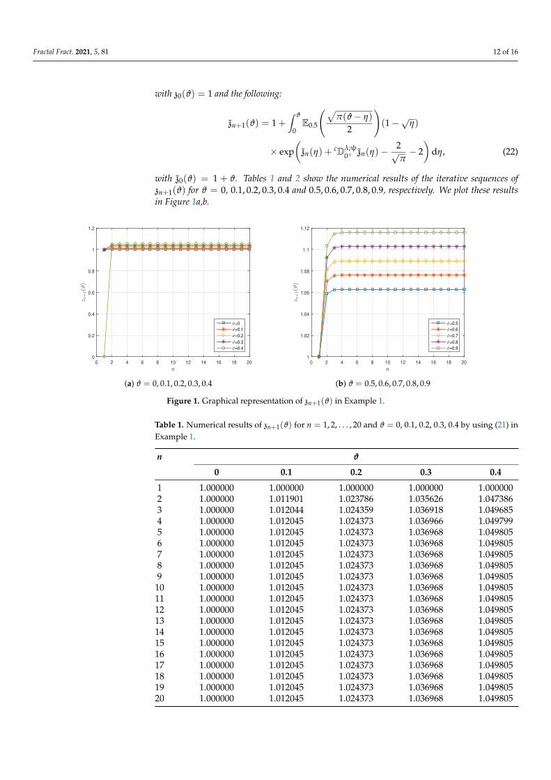
with z0(ϑ) = 1 and the following:

zn+1(ϑ) = 1 +∫ ϑ

0E0.5

(√π(ϑ− η)

2

)(1−√η)

× exp(zn(η) +

cDλ;ψ0+ zn(η)−

2√π− 2)

dη, (22)

with z0(ϑ) = 1 + ϑ. Tables 1 and 2 show the numerical results of the iterative sequences ofzn+1(ϑ) for ϑ = 0, 0.1, 0.2, 0.3, 0.4 and 0.5, 0.6, 0.7, 0.8, 0.9, respectively. We plot these resultsin Figure 1a,b.

n

0 2 4 6 8 10 12 14 16 18 20

zn+1(ϑ)

0

0.2

0.4

0.6

0.8

1

1.2

ϑ=0

ϑ=0.1

ϑ=0.2

ϑ=0.3

ϑ=0.4

(a) ϑ = 0, 0.1, 0.2, 0.3, 0.4

n

0 2 4 6 8 10 12 14 16 18 20

zn+1(ϑ)

1

1.02

1.04

1.06

1.08

1.1

1.12

ϑ=0.5

ϑ=0.6

ϑ=0.7

ϑ=0.8

ϑ=0.9

(b) ϑ = 0.5, 0.6, 0.7, 0.8, 0.9

Figure 1. Graphical representation of zn+1(ϑ) in Example 1.

Table 1. Numerical results of zn+1(ϑ) for n = 1, 2, . . . , 20 and ϑ = 0, 0.1, 0.2, 0.3, 0.4 by using (21) inExample 1.

n ϑ

0 0.1 0.2 0.3 0.4

1 1.000000 1.000000 1.000000 1.000000 1.0000002 1.000000 1.011901 1.023786 1.035626 1.0473863 1.000000 1.012044 1.024359 1.036918 1.0496854 1.000000 1.012045 1.024373 1.036966 1.0497995 1.000000 1.012045 1.024373 1.036968 1.0498056 1.000000 1.012045 1.024373 1.036968 1.0498057 1.000000 1.012045 1.024373 1.036968 1.0498058 1.000000 1.012045 1.024373 1.036968 1.0498059 1.000000 1.012045 1.024373 1.036968 1.04980510 1.000000 1.012045 1.024373 1.036968 1.04980511 1.000000 1.012045 1.024373 1.036968 1.04980512 1.000000 1.012045 1.024373 1.036968 1.04980513 1.000000 1.012045 1.024373 1.036968 1.04980514 1.000000 1.012045 1.024373 1.036968 1.04980515 1.000000 1.012045 1.024373 1.036968 1.04980516 1.000000 1.012045 1.024373 1.036968 1.04980517 1.000000 1.012045 1.024373 1.036968 1.04980518 1.000000 1.012045 1.024373 1.036968 1.04980519 1.000000 1.012045 1.024373 1.036968 1.04980520 1.000000 1.012045 1.024373 1.036968 1.049805

Fractal Fract. 2021, 5, 81 13 of 16

Table 2. Numerical results of zn+1(ϑ) for n = 1, 2, . . . , 20 and ϑ = 0.5, 0.6, 0.7, 0.8, 0.9 by using (21) inExample 1.

n ϑ

0.5 0.6 0.7 0.8 0.9

1 1.000000 1.000000 1.000000 1.000000 1.0000002 1.059021 1.070482 1.081716 1.092662 1.1032583 1.062609 1.075629 1.088674 1.101659 1.1144904 1.062834 1.076019 1.089293 1.102578 1.1157845 1.062848 1.076049 1.089348 1.102672 1.1159336 1.062849 1.076051 1.089353 1.102682 1.1159517 1.062849 1.076051 1.089353 1.102683 1.1159538 1.062849 1.076051 1.089353 1.102683 1.1159539 1.062849 1.076051 1.089353 1.102683 1.11595310 1.062849 1.076051 1.089353 1.102683 1.11595311 1.062849 1.076051 1.089353 1.102683 1.11595312 1.062849 1.076051 1.089353 1.102683 1.11595313 1.062849 1.076051 1.089353 1.102683 1.11595314 1.062849 1.076051 1.089353 1.102683 1.11595315 1.062849 1.076051 1.089353 1.102683 1.11595316 1.062849 1.076051 1.089353 1.102683 1.11595317 1.062849 1.076051 1.089353 1.102683 1.11595318 1.062849 1.076051 1.089353 1.102683 1.11595319 1.062849 1.076051 1.089353 1.102683 1.11595320 1.062849 1.076051 1.089353 1.102683 1.115953

Tables 3 and 4 show the numerical results of the iterative sequences of zn+1(ϑ) for ϑ = 0,0.1, 0.2, 0.3, 0.4 and 0.5, 0.6, 0.7, 0.8, 0.9, respectively. We plot these results in Figure 2a,b.

Table 3. Numerical results of zn+1(ϑ) for n = 1, 2, . . . , 20 and ϑ = 0, 0.1, 0.2, 0.3, 0.4 by using (22) inExample 1.

n ϑ

0 0.1 0.2 0.3 0.4

1 1.000000 1.100000 1.200000 1.300000 1.4000002 1.000000 1.018793 1.048121 1.089222 1.1443113 1.000000 1.017327 1.041341 1.072265 1.1117524 1.000000 1.017302 1.041061 1.071050 1.1081725 1.000000 1.017301 1.041050 1.070964 1.1077856 1.000000 1.017301 1.041049 1.070958 1.1077437 1.000000 1.017301 1.041049 1.070957 1.1077398 1.000000 1.017301 1.041049 1.070957 1.1077389 1.000000 1.017301 1.041049 1.070957 1.10773810 1.000000 1.017301 1.041049 1.070957 1.10773811 1.000000 1.017301 1.041049 1.070957 1.10773812 1.000000 1.017301 1.041049 1.070957 1.10773813 1.000000 1.017301 1.041049 1.070957 1.10773814 1.000000 1.017301 1.041049 1.070957 1.10773815 1.000000 1.017301 1.041049 1.070957 1.10773816 1.000000 1.017301 1.041049 1.070957 1.10773817 1.000000 1.017301 1.041049 1.070957 1.10773818 1.000000 1.017301 1.041049 1.070957 1.10773819 1.000000 1.017301 1.041049 1.070957 1.10773820 1.000000 1.017301 1.041049 1.070957 1.107738

Fractal Fract. 2021, 5, 81 14 of 16

n

0 2 4 6 8 10 12 14 16 18 20

zn+1(ϑ)

1

1.05

1.1

1.15

1.2

1.25

1.3

1.35

1.4

ϑ=0

ϑ=0.1

ϑ=0.2

ϑ=0.3

ϑ=0.4

(a) ϑ = 0, 0.1, 0.2, 0.3, 0.4

n

0 2 4 6 8 10 12 14 16 18 20

zn+1(ϑ)

1.1

1.2

1.3

1.4

1.5

1.6

1.7

1.8

1.9

2 ϑ=0.5

ϑ=0.6

ϑ=0.7

ϑ=0.8

ϑ=0.9

ϑ=1.0

(b) ϑ = 0.5, 0.6, 0.7, 0.8, 0.9, 1.0

Figure 2. Graphical representation of zn+1(ϑ) in Example 1.

Table 4. Numerical results of zn+1(ϑ) for n = 1, 2, . . . , 20 and ϑ = 0.5, 0.6, 0.7, 0.8, 0.9, 1 by using (22)in Example 1.

n ϑ

0.5 0.6 0.7 0.8 0.9 1.0

1 1.500000 1.600000 1.700000 1.800000 1.900000 2.0000002 1.216106 1.307784 1.422976 1.565785 1.740782 1.9530023 1.162695 1.229793 1.320631 1.447644 1.631747 1.9092494 1.154233 1.212553 1.289440 1.397764 1.566487 1.8703245 1.152934 1.208920 1.280551 1.378410 1.530698 1.8370986 1.152735 1.208162 1.278068 1.371156 1.512041 1.8097417 1.152705 1.208004 1.277379 1.368474 1.502577 1.7878908 1.152700 1.207972 1.277187 1.367487 1.497842 1.7708609 1.152699 1.207965 1.277134 1.367124 1.495491 1.75784310 1.152699 1.207963 1.277120 1.366991 1.494327 1.74804311 1.152699 1.207963 1.277116 1.366942 1.493752 1.74074712 1.152699 1.207963 1.277115 1.366925 1.493469 1.73536313 1.152699 1.207963 1.277114 1.366918 1.493329 1.73141414 1.152699 1.207963 1.277114 1.366916 1.493260 1.72853215 1.152699 1.207963 1.277114 1.366915 1.493225 1.72643516 1.152699 1.207963 1.277114 1.366914 1.493209 1.72491317 1.152699 1.207963 1.277114 1.366914 1.493200 1.72381118 1.152699 1.207963 1.277114 1.366914 1.493196 1.72301319 1.152699 1.207963 1.277114 1.366914 1.493194 1.72243720 1.152699 1.207963 1.277114 1.366914 1.493193 1.722021

5. Conclusions

This paper is devoted to the study of a new type of ψ-Caputo fractional differentialequation. The addressed problem is considered in the framework of nonlinear boundaryvalue conditions. Our work is different from the existing results in the literature, whichare basically based on fixed point approaches. However, we have proved our main resultswith the help of monotone iterative techniques along with the method of upper and lowersolutions. It is observed that these methods are closely related to the Tarski–Knastertheorem and that, essentially speaking, also results in fixed point results. The main resultshave been verified and demonstrated by an example with explicit numerical values.

Fractal Fract. 2021, 5, 81 15 of 16

Author Contributions: Conceptualization, Z.B., C.D., M.K.A.K., J.A., and M.E.S.; methodology, Z.B.,C.D., M.K.A.K., J.A., M.E.S. and Z.S.; software, M.E.S.; validation, C.D., M.E.S., J.A. and M.K.A.K.;formal analysis, Z.B., C.D.; investigation, M.E.S., J.A., and M.K.A.K.; resources, M.K.A.K., J.A.,Z.S.; data curation, M.E.S. and M.K.A.K.; writing—original draft preparation, Z.B., C.D., M.K.A.K.,J.A., M.E.S., and Z.S.; writing—review and editing, M.K.A.K., J.A., M.E.S.; visualization, M.E.S.;supervision, M.K.A.K., J.A., M.E.S., and Z.S.; project administration, M.K.A.K.; funding acquisition,M.K.A.K. All authors have read and agreed to the published version of the manuscript.

Funding: Not applicable.

Institutional Review Board Statement: Not applicable.

Informed Consent Statement: Not applicable.

Data Availability Statement: Data sharing not applicable.

Acknowledgments: The third author was supported by Prince Sultan University and OSTIM Techni-cal University. The fourth author was supported by Bu-Ali Sina University.

Conflicts of Interest: The authors declare that they have no competing interest.

References1. Hilfer, R. Applications of Fractional Calculus in Physics; World Scientific: Singapore, 2000.2. Podlubny, I. Fractional Differential Equations; Academic Press: San Diego, CA, USA, 1999.3. Sabatier, J.; Agrawal, O.P.; Machado, J.A.T. Advances in Fractional Calculus-Theoretical Developments and Applications in Physics and

Engineering; Springer: Dordrecht, The Netherlands, 2007.4. Tarasov, V.E. Fractional dynamics, Nonlinear Physical Science; Springer: Berlin/Heidelberg, Germany, 2010.5. Pratap, A.; Raja, R.; Alzabut, J.; Dianavinnarasi, J.; Rajchakit, G. Finite-time Mittag-Leffler stability of fractional-order quaternion-

valued memristive neural networks with impulses. Neural Process Lett. 2020, 51, 1485–1526. [CrossRef]6. Caputo, M.; Fabrizio, M. A new definition of fractional derivative without singular kernel. Progr. Fract. Differ. Appl. 2015, 1, 1–13.7. Jarad, F.; Abdeljawad, T.; Alzabut, J. Generalized fractional derivatives generated by a class of local proportional derivatives. Eur.

Phys. J. Spec. Top. 2017, 226, 3457–3471. [CrossRef]8. Khalil, R.; Horani, M.A.; Yousef, A.; Sababheh, M. A new definition of fractional derivative. J. Comput. Appl. Math. 2014, 264, 65–70.

[CrossRef]9. Almeida, R. A Caputo fractional derivative of a function with respect to another function. Commun. Nonlinear Sci. Numer. Simul.

2017, 44, 460–481. [CrossRef]10. Almeida, R.; Malinowska, A.; Monteiro, M. Fractional differential equations with a Caputo derivative with respect to a kernel

function and their applications. Math. Meth. Appl. Sci. 2018, 41, 336–352. [CrossRef]11. Abdo, M.; Panchal, S.K.; Saeed, A.M. Fractional boundary value problem with Ψ-Caputo fractional derivative. Proc. Math. Sci.

2019, 129, 65. [CrossRef]12. Jarad, F.; Abdeljawad, T.; Rashid, S. More properties of the proportional fractional integrals and derivatives of a function with

respect to another function. Adv. Diff. Equ. 2020, 2020, 303. [CrossRef]13. Promsakon, C.; Suntonsinsoungvon, E.; Ntouyas, S.K. Impulsive boundary value problems containing Caputo fractional

derivative of a function with respect to another function. Adv. Diff. Equ. 2019, 2019, 486. [CrossRef]14. da C. Sousa, J.V.; de Oliveira, E.C. On the ψ-Hilfer fractional derivative. Commun. Nonlinear Sci. Numer. Simul. 2018, 60, 72–91.15. Alzabut, J.; Viji, J.; Muthulakshmi, V.; Sudsutad, W. Oscillatory behavior of a type of generalized proportional fractional

differential equations with forcing and damping terms. Mathematics 2020, 8, 1037. [CrossRef]16. Alzabut, J.; Mohammadaliee, B.; Samei, M.E. Solutions of two fractional q–integro–differential equations under sum and integral

boundary value conditions on a time scale. Adv. Diff. Equ. 2020, 2020, 304. [CrossRef]17. Samei, M.E.; Hedayati, V.; Rezapour, S. Existence results for a fraction hybrid differential inclusion with caputo-hadamard type

fractional derivative. Adv. Diff. Equ. 2019, 2019, 163. [CrossRef]18. Abbas, S.; Benchohra, M.; Hamidi, N.; Henderson, J. Caputo–Hadamard fractional differential equations in Banach spaces. Fract.

Calc. Appl. Anal. 2018, 2139, 1027–1045. [CrossRef]19. Matar, M.M.; Lubbad, A.A.; Alzabut, J. On p-Laplacian boundary value problem involving Caputo-Katugampula fractional

derivatives. Math. Methods Appl. Sci. 2020, 51, 1485–1526. [CrossRef]20. Rezapour, S.; Imran, A.; Hussain, A.; Martínez, F.; Etemad, S.; Kaabar, M.K.A. Condensing Functions and Approximate Endpoint

Criterion for the Existence Analysis of Quantum Integro-Difference FBVPs. Symmetry 2021, 13, 469. [CrossRef]21. Matar, M.M.; Abbas, M.I.; Alzabut, J.; Kaabar, M.K.A.; Etemad, S.; Rezapour, S. Investigation of the p-Laplacian nonperiodic

nonlinear boundary value problem via generalized Caputo fractional derivatives. Adv. Differ. Equ. 2021, 2021, 1–18.22. Abbas, S.; Benchohra, M.; Samet, B.; Zhou, Y. Coupled implicit Caputo fractional q-difference systems. Adv. Diff. Equ. 2019,

2019, 527. [CrossRef]

Fractal Fract. 2021, 5, 81 16 of 16

23. Kucche, K.D.; da, C.; Sousa, J.V. On the nonlinear Ψ-Hilfer fractional differential equations. Comput. Appl. Math. 2019, 38, 25.[CrossRef]

24. Zhou, Y. Basic Theory of Fractional Differential Equations; World Scientific: Singapore, 2014.25. Zhou, Y. Fractional Evolution Equations and Inclusions: Analysis and Control; Elsevier: Amsterdam, The Netherlands, 2016.26. Samei, M.E.; Ghaffari, R.; Yao, S.W.; Kaabar, M.K.A.; Martínez, F. Existence of Solutions for a Singular Fractional q-Differential

Equations under Riemann–Liouville Integral Boundary Condition. Symmetry 2021, 13, 469. [CrossRef]27. Mohammadi, H.; Kaabar, M.K.A.; Alzabut, J.; Selvam, A.G.M.; Rezapour, S. A Complete Model of Crimean-Congo Hemorrhagic

Fever (CCHF) Transmission Cycle with Nonlocal Fractional Derivative. J. Funct. Spaces 2021, 2021, 1–12. [CrossRef]28. Kaabar, M.K.A.; Martínez, F.; Gómez-Aguilar, J.F.; Ghanbari, B.; Kaplan, M.; Günerhan, H. New approximate analytical solutions

for the nonlinear fractional Schrödinger equation with second-order spatio-temporal dispersion via double Laplace transformmethod. Math. Methods Appl. Sci. 2021, 1–19. [CrossRef]

29. Alzabut, J.; Selvam, A.; Dhineshbabu, R.; Kaabar, M.K.A. The Existence, Uniqueness, and Stability Analysis of the DiscreteFractional Three-Point Boundary Value Problem for the Elastic Beam Equation. Symmetry 2021, 13, 789. [CrossRef]

30. Etemad, S.; Souid, M.S.; Telli, B.; Kaabar, M.K.A.; Rezapour, S. Investigation of the neutral fractional differential inclusions ofKatugampola-type involving both retarded and advanced arguments via Kuratowski MNC technique. Adv. Differ. Eq. 2021,2021, 1–20.

31. Al-Refai, M.; Hajji, M.A. Monotone iterative sequences for nonlinear boundary value problems of fractional order. NonlinearAnal. 2011, 74, 3531–3539. [CrossRef]

32. Chen, C.; Bohner, M.; Jia, B. Method of upper and lower solutions for nonlinear Caputo fractional difference equations and itsapplications. Fract. Calc. Appl. Anal. 2019, 22, 1307–1320. [CrossRef]

33. Kucche, K.D.; Mali, A.D. Initial time difference quasilinearization method for fractional differential equations involvinggeneralized Hilfer fractional derivative. Comput. Appl. Math. 2020, 39, 33. [CrossRef]

34. Wang, G. Monotone iterative technique for boundary value problems of a nonlinear fractional differential equation with deviatingarguments. J. Comput. Appl. Math. 2012, 236, 2425–2430. [CrossRef]

35. Zhang, S. Monotone iterative method for initial value problem involving Riemann-Liouville fractional derivatives. NonlinearAnal. 2009, 71, 2087–2093. [CrossRef]

36. Gorenflo, R.; Kilbas, A.A.; Mainardi, F.; Rogosin, S.V. Mittag–Leffler Functions, Related Topics and Applications; Springer: New York,NY, USA, 2014.