Dynamical Systems and Non-Hermitian Iterative Eigensolvers

SIAM J. NUMER. ANAL. c© 2009 Society for Industrial and Applied MathematicsVol. 47, No. 2, pp. 1445–1473

DYNAMICAL SYSTEMS AND NON-HERMITIAN ITERATIVEEIGENSOLVERS∗

MARK EMBREE† AND RICHARD B. LEHOUCQ‡

Abstract. Simple preconditioned iterations can provide an efficient alternative to more elabo-rate eigenvalue algorithms. We observe that these simple methods can be viewed as forward Eulerdiscretizations of well-known autonomous differential equations that enjoy appealing geometric prop-erties. This connection facilitates novel results describing convergence of a class of preconditionedeigensolvers to the leftmost eigenvalue, provides insight into the role of orthogonality and biorthog-onality, and suggests the development of new methods and analyses based on more sophisticateddiscretizations. These results also highlight the effect of preconditioning on the convergence andstability of the continuous-time system and its discretization.

Key words. eigenvalues, dynamical systems, inverse iteration, preconditioned eigensolvers,geometric invariants

AMS subject classifications. 15A18, 37C10, 65F15, 65L20

DOI. 10.1137/07070187X

1. Introduction. Suppose we seek a small number of eigenvalues (and the asso-ciated eigenspace) of the non-Hermitian matrix A ∈ Cn×n, having at our disposal anonsingular matrix N ∈ Cn×n that approximates A. Given a starting vector p0 ∈ Cn,compute

(1.1) pj+1 = pj + N−1(θj − A)pj ,

where θj − A is shorthand for Iθj − A, and

θj =(Apj ,pj)(pj ,pj)

for some inner product (·, ·). Knyazev, Neymeyr, and others have studied this iterationfor Hermitian positive definite A; see [21, 22] and references therein for convergenceanalysis and numerical experiments.

Clearly the choice of N will influence the behavior of this iteration. With N = A,the method (1.1) reduces to (scaled) inverse iteration:

pj+1 = A−1pjθj .

We are interested in the case where N approximates A, yet one can apply N−1 to avector much more efficiently than A−1 itself. Such a N acts as a preconditioner forA, and, hence, (1.1) represents a preconditioned iteration.

∗Received by the editors September 4, 2007; accepted for publication (in revised form) November7, 2008; published electronically March 13, 2009.

http://www.siam.org/journals/sinum/47-2/70187.html†Department of Computational and Applied Mathematics, Rice University, 6100 Main Street –

MS 134, Houston, TX 77005-1892 ([email protected]). This author’s research supported by U.S.Department of Energy grant DE-FG03-02ER25531 and National Science Foundation grant DMS-CAREER-0449973.

‡Sandia National Laboratories, P.O. Box 5800, MS 1110, Albuquerque, NM 87185–1110 ([email protected]). Sandia is a multiprogram laboratory operated by Sandia Corporation, a LockheedMartin Company, for the U.S. Department of Energy under contract DE-AC04-94AL85000.

1445

1446 MARK EMBREE AND RICHARD B. LEHOUCQ

This method contrasts with a different class of algorithms, based on inverse itera-tion (or the shift-invert Arnoldi algorithm), that apply a preconditioner to acceleratean “inner iteration” that approximates the solution to a linear system at each step; see,e.g., [24, 13, 16] and [6, Chapter 11]. For numerous practical large-scale non-Hermitianeigenvalue problems, such as those described in [25, 41], these inner iterations can beextremely expensive and highly dependent on the quality of the preconditioner. Incontrast, as we shall see, the iteration (1.1) can converge to a leftmost eigenpair evenwhen N is a suitable multiple of the identity.

This paper provides a rigorous convergence theory that establishes sufficient con-ditions for (1.1) to converge to the leftmost eigenpair for non-Hermitian A. We obtainthese results by viewing this iteration as the forward Euler discretization of the au-tonomous nonlinear differential equation

(1.2) p = N−1

(p

(Ap,p)(p,p)

− Ap)

with a unit step size. Here A and N are fixed but p depends on a parameter,t; p denotes differentiation with respect to t. In the absence of preconditioning,the differential equation (1.2) has been studied in connection with power iteration[10, 29], as described in more detail below. The nonzero steady-states of this systemcorrespond to (right) eigenvectors of A, and, hence, one might attempt to computeeigenvalues by driving this differential equation to steady-state as swiftly as possible.Properties of the preconditioner determine which of the eigenvectors is an attractingsteady-state.

The differential equation (1.2) enjoys a distinguished property, observed, for ex-ample, in [10, 29] with N = I. Suppose that p solves (1.2), θ = (p,p)−1(Ap,p), andN is self-adjoint and invertible (A may be non-self-adjoint). Then for all t,

d

dt(p,Np) =

(N−1(pθ − Ap),Np

)+(p,NN−1(pθ − Ap)

)= (pθ,p) − (Ap,p) + (p,pθ) − (p,Ap)= 0.(1.3)

Thus, (p,Np) is an invariant (or first integral), as its value is independent of time;see [19, section 1.3] for a discussion of the unpreconditioned case (N = I), and, e.g.,[4, 18] for a general introduction to invariant theory and geometric integration.

The invariant describes a manifold in n-dimensional space, (p,Np) = (p0,Np0),on which the solution to the differential equation with p(0) = p0 must fall. Simplediscretizations, such as Euler’s method (1.1), do not typically respect such invari-ants, giving approximate solutions that drift from the manifold. Invariant-preservingalternatives (see, e.g., [18, 26]) generally require significantly more computation perstep (though a tractable method for the unpreconditioned, Hermitian case has beenproposed by Nakamura, Kajiwara, and Shiotani [28]). Our goal is to explain the rela-tionship between convergence and stability of the continuous and discrete dynamicalsystems. In particular, the quadratic invariant is a crucial property of the continuoussystem, and plays an important role in the convergence theory of the correspondingdiscretization, even when that iteration does not preserve the invariant.

For a non-Hermitian problem, one naturally wonders how (1.1) can be modifiedto incorporate estimates of both left and right eigenvectors. In this case, we obtain

DYNAMICAL SYSTEMS AND ITERATIVE EIGENSOLVERS 1447

the coupled iteration (given here without preconditioning)

(1.4){p = pθ − Ap,

q = qθ − A∗q,θ =

(Ap,q)(p,q)

,

and a simple derivation reveals that (p,q) is invariant. Our analysis demonstratesthat this two-sided dynamical system often suffers from finite-time blowup; in thediscrete scheme this is tantamount to incurable breakdown, a well-known ailment ofoblique projection methods (see [5] for a discussion and references to the literaturewithin the context of non-Hermitian Lanczos methods).

A longstanding association exists between eigenvalue iterations and differentialequations [1, 2, 3, 10, 11, 15, 19], often involving the observation that iterates of aparticular eigenvalue algorithm are exactly discrete-time samples of some underlyingcontinuous-time system. Notable examples include Rayleigh quotient gradient flow[10, 27], connections between the QR algorithm for dense eigenproblems and Todaflow [29, 39], and more general “isospectral flows” [42]. For example, Chu notes thatthe iterates of the standard power method can be obtained as integer-time samples ofthe solution to the system (1.2) with N = I and A replaced by logA [10, eq. (2.7)].

The present study draws upon this body of work, but takes a different perspec-tive: we seek a better understanding of iterations such as (1.1) that provide onlyapproximate solutions (with a truncation error due to discretization) to continuoustime systems such as (1.2). The distinction is significant: for example, a continuous-time generalization of the power method will converge, with mild caveats, to thelargest magnitude eigenvalue, whereas the related systems we study can potentiallyconverge to the leftmost eigenvalue at a shift-independent rate with little more workper iteration than the power method; see Theorems 4.4 and 6.3.

The connection between eigensolvers and continuous-time dynamical systems alsoarises in applications. For example, the Car–Parrinello method [8] determines theKohn–Sham eigenstates from a second-order ordinary differential equation, Newton’sequations of motion (see [34, p. 1086] for a formulation using (1.2) with no precon-ditioning). The heavy ball optimization method [35] also formulates the minimum ofthe Rayleigh quotient via a second order ordinary differential equation. In [7], theground state solution of Bose–Einstein condensates are determined via a normalizedgradient flow discretized by several time integration schemes. (Both the Kohn–Shameigenstates and Bose–Einstein condensates give rise to self-adjoint nonlinear eigen-value problems.)

We begin our investigation with a study of various unpreconditioned iterations(N = I). Section 2 introduces basic differential equations for computation of invariantsubspaces of matrix pencils, and then identifies parameter choices that yield invariant-preserving iterations. Near steady states, the solutions to these systems can be viewedas exact invariant subspaces for nearby matrices, as observed in section 3. From thispoint we focus on single vector iterations for standard eigenvalue problems. Section 4describes exact solution formulas for two unpreconditioned continuous-time systems,one-sided and two-sided methods. As such exact solutions for the preconditioned caseare elusive, we analyze such systems asymptotically using center manifold theory insection 5. These two sections provide the foundation for the main result of section 6,the development of sufficient conditions for convergence of (1.1) for non-Hermitianmatrices.

2. Dynamical systems and invariant manifolds. We first examine proper-ties of the dynamical system (1.2) and various generalizations suitable for computing


eigenvalues of non-Hermitian matrix pencils. Let A,B ∈ Cn×n be general matriceswith fixed (time-invariant) entries. For the generalized eigenvalue problem Ax = Bxλwith N = I, the system (1.2) expands to

p = Bpθ − Ap

for appropriate θ = θ(t). This equation suggests a generalization from a system withthe single vector p ∈ Cn to a system that evolves an entire subspace, given by therange of a matrix P ∈ Cn×k:

P = BPL − AP,

where differentiation is still with respect to the autonomous variable t; we shall addressthe choice of L(t) ∈ C

k×k momentarily. (Quantities such as L are t-dependent unlessexplicitly stated otherwise; we typically suppress the t argument to simplify notation.)

For non-Hermitian problems one might simultaneously evolve an equation for theadjoint to obtain approximations to the left eigenspace, which suggests the system

(2.1) P = BPL − APQ = B∗QM∗ − A∗Q,

with initial conditions P(0) = P0 and Q(0) = Q0, where P,Q ∈ Cn×k, and L,M ∈Ck×k. The choice we make for the time-dependent L,M ∈ Ck×k can potentiallycouple P and Q as introduced in (1.4). Here ·∗ denotes the conjugate transpose and(·, ·) the standard Euclidean inner product (though this analysis generalizes readilyto arbitrary inner products). If this system is at a steady state, i.e., P = Q = 0, then

(2.2) BPL = AP, B∗QM∗ = A∗Q,

and, hence, provided P and Q have full column rank, the eigenvalues of L and M areincluded in the spectrum of the pencil A − λB, while the columns of P and Q spanright- and left-invariant subspaces of the same pencil. We shall motivate the choice ofL and M through generalizations of the invariant discussed in the introduction. Thefollowing notation facilitates the analysis of these subspace iterations.

Definition 2.1. Given P,Q ∈ Cn×k, define (P,Q) = Q∗P ∈ C

k×k; i.e., the(i, j) entry of (P,Q) satisfies (P,Q)i,j := (Pej ,Qei), where e� denotes the �th columnof the k × k identity matrix.

In this notation, we have the homogeneity property (PL,Q) = Q∗PL = (P,Q)L.Consider the pairs of (time-dependent) functions

(2.3) (Q,P), (P,Q) and (P,P), (Q,Q)

with derivatives

d

dt(Q,P) =

(Q,P

)+(Q, P

),

d

dt(P,Q) =

(P,Q

)+(P, Q

),

and

d

dt(P,P) =

(P,P

)+(P, P

),

d

dt(Q,Q) =

(Q,Q

)+(Q, Q

).

Inspired by (1.3), we next investigate how best to choose L and M to make eitherpair in (2.3) invariant under the system (2.1).


Theorem 2.2. For the system of ordinary differential equations (2.1) with initialconditions P(0) = P0 ∈ Cn×k and Q(0) = Q0 ∈ Cn×k, the choices

(2.4) L = (BP,Q)−1(AP,Q), M∗ = (Q,BP)−1(Q,AP)

give

d

dt(P,Q) =

d

dt(Q,P) = 0,

and, hence, (P,Q) = (P0,Q0) and (Q,P) = (Q0,P0) hold for all t.Proof. Note that

d

dt(P,Q) =

(P,Q

)+(P, Q

)= (BP,Q)L − (AP,Q) + M(P,B∗Q) − (P,A∗Q)(

d

dt(Q,P)

)∗=(P, Q

)+(P,Q

)= M(P,B∗Q) − (P,A∗Q) + (BP,Q)L − (AP,Q),

where we have used (2.1) and the homogeneity property. We can force (d/dt)(P,Q)to zero by setting L and M as in (2.4).

The next result is a direct analogue of Theorem 2.2 for the second pair in (2.3).We omit the proof, a minor adaptation of the last one.

Theorem 2.3. For the system of ordinary differential equations (2.1) with initialconditions P(0) = P0 ∈ Cn×k and Q(0) = Q0 ∈ Cn×k, the choices

L = (BP,P)−1(AP,P), M∗ = (Q,BQ)−1(Q,AQ)

give

d

dt(P,P) =

d

dt(Q,Q) = 0,

and, hence, (P,P) = (P0,P0) and (Q,Q) = (Q0,Q0) for all t.The formulations for L and M given in Theorems 2.2 and 2.3 are known as

generalized Rayleigh quotients [38]. With these values of L and M, we refer to (2.1) asthe two-sided and one-sided dynamical systems. Theorem 2.2 shows that if P∗

0Q0 = I,then the two-sided solutions will preserve this property (allowing for biorthogonalbases for left and right invariant subspaces), though possibly at the expense of growing‖P‖ or ‖Q‖. Theorem 2.3, on the other hand, shows that the one-sided iterationmaintains ‖P‖ and ‖Q‖, though biorthogonality will generally be lost. From theinvariants we also see that the system preserves the rank of solutions to both one-and two-sided equations—provided they exist (see section 4). Since (P,P) is fixed forthe one-sided system, so too are all singular values (and, thus, the rank) of P. For thetwo-sided system, if (P0,Q0) is full rank, (P,Q) must always be as well, and, hence,P and Q individually have full rank.

We denote the dynamical systems (2.1) given the generalized Rayleigh quotientsof Theorems 2.2 and 2.3 as “two-sided” and “one-sided”, respectively. We refer to theensuing schemes that result from discretizing (2.1) as “two-sided” and “one-sided”iterations.


3. Invariants and backward stability. We saw in (2.2) that, at a steadystate, the eigenvalues of L and M are exact eigenvalues of the pencil A − λB. Asthe system approaches a steady state, how well do the eigenvalues of the invariant-preserving choices for L and M approximate the eigenvalues of the pencil?

First, consider the one-sided system, with L as given in Theorem 2.3 and P fullrank. The first part of (2.1) can then be written as

0 = BPL −(A + P(P,P)−1P∗

)P,

from which we see that the eigenvalues of L form a subset of the spectrum of theperturbed pencil (A + P(P,P)−1P∗) − λB. How large can such perturbations be?Note that (P,P)−1P∗ = P+ is the pseudoinverse of P, and so

∥∥∥P(P,P)−1P∗∥∥∥ ≤

∥∥∥P∥∥∥∥∥P+∥∥ =

∥∥∥P∥∥∥σk

,

where σk is the smallest singular value of P ∈ Cn×k. As discussed at the end ofsection 2, the choice of L in Theorem 2.3 that makes (P,P) invariant also makes σk

invariant. Thus, when ‖P‖ is small, i.e., near a steady state, we conclude that theeigenvalues of L are the exact eigenvalues of a nearby pencil, with σ−1

k acting as acondition number does in a backward error bound; that condition number can be setto one simply by taking (P0,P0) = I. (This is related to an error bound for Rayleigh–Ritz eigenvalue estimates for a Hermitian matrix using a nonorthogonal basis; see [32,Theorem 11.10.1].) This analysis suggests that a departure from orthogonality in anumerical integration of the differential equation is reflected in degrading accuracy ofthe approximate eigenvalues.

Now consider the two-sided system with L and M as given by Theorem 2.2 withnonsingular (BP,Q). We wish to rewrite (2.1) in the form

0 = BPL − (A + E)P0 = B∗QM∗ − (A∗ + E∗)Q

for the same E in both iterations. Lemma 1 of [20] implies that such a perturbationE exists if and only if

(BP,Q)L = M(BP,Q),

which holds for the choice of L and M given in Theorem 2.2. The perturbation E isnot unique, but EP = P and E∗Q = Q. Moreover, the “main theorem” of [20] gives

min ‖E‖2 = max{∥∥P∥∥

2,∥∥Q∥∥

2

}if (P,P) = Ik and (Q,Q) = Ik. However, as the authors of [20] explain, a small ‖E‖2

is irrelevant unless ‖(P,Q)−1‖2 is also small. In particular, when P is orthogonal toQ, min ‖E‖2 is undefined. The discussion following Theorem 4.1 in subsection 4.1explains that a large (or undefined) ‖(P,Q)−1‖2 is equivalent to near breakdown (orserious breakdown) of the two-sided dynamical system.

We caution the reader that backward stability alone does not provide informationon forward error, or accuracy, of the steady-states when A �= A∗. The relevance ofbackward stability is that the solution of our one- and two-sided systems are, at alltimes, steady-states for a related dynamical system. The distance to this relatedperturbed system depends upon the norm of the residuals.


4. Convergence analysis. At least for single-vector iterations (i.e., k = 1),the analysis of the one- and two-sided dynamical systems follows readily from theremarkable fact that, in many cases, simple formulas give the exact solutions of thesenonlinear differential equations. This observation, inspired by a lemma of Nanda [29],informs convergence analysis of the eigeniterations that result from the discretizationof these equations. Though expressed for the standard eigenvalue problem, these re-sults can naturally be adapted to the generalized case by replacing A with B−1A. Wediscuss the solution operators for two-sided systems, followed by one-sided systems.

4.1. Two-sided systems. The following result generalizes a result of Nanda[29, Lemma 1.4] for the two-sided dynamical system.

Theorem 4.1. Consider the partitioned set of ordinary differential equations

(4.1)p = pθ − Apq = qθ − A∗q,

with p(0) = p0 and q(0) = q0, where p,q ∈ Cn, (p0,q0) �= 0, and

θ =(Ap,q)(p,q)

.

Then there exists some tf > 0 such that for all t ∈ [0, tf),

p(t) = e−Atp0π(t), q(t) = e−A∗tq0π(t),

where

(4.2) π(t) =

√(p0,q0)

(e−Atp0, e−A∗tq0).

Proof. We define p(t) = e−Atp0π(t) and q(t) = e−A∗tq0π(t), and will show thatthese formulas satisfy the system (4.1). Note that

π =π

2

((Ae−Atp0, e

−A∗tq0

)+(e−Atp0,A∗e−A∗tq0

))(e−Atp0, e−A∗tq0)

= π

(Ae−Atp0, e

−A∗tq0

)(e−Atp0, e−A∗tq0)

= π

(Ae−Atp0π, e−A∗tq0π

)(e−Atp0π, e−A∗tq0π)

= π(Ap,q)(p,q)

= πθ.

Differentiating the formulas for p and q, thus, gives

p = −Ae−Atp0π + e−Atp0π = −Ap + θp

q = −A∗e−A∗tq0π + e−A∗tq0 ˙π = −A∗q + θq,

as required. The hypothesis that (p0,q0) �= 0 ensures the existence of the solution attime t = 0. The formula will hold for all t > 0, until potentially

(4.3)(e−Atp0, e

−A∗tq0

)= 0.


We define tf to be the smallest positive t for which (4.3) holds. If no such positive texists, the solution exists for all t > 0 and we can take tf = ∞ in the statement of thetheorem.

Theorem 4.1 gives (p,q) = (p0,q0), precisely as Theorem 2.2 indicates. Underthe conditions of Theorem 4.1, solutions of the two-sided single-vector equations (4.1)have the same direction as solutions of the simpler linear systems x = −Ax, x(0) = p0

and y = −A∗y, y(0) = q0, but the magnitudes of p and q vary nonlinearly with(4.2). In particular, the inner product of p and q can be zero—even with both p andq nonzero—leading to finite time blow-up of (4.1). Note that if(

e−Atp0√(p0,q0)

,e−A∗tq0√(q0,p0)

)= 0,

then π(t) is undefined. Hence, finite time blow-up is analogous to serious breakdown[43, p. 389], a problem endemic to oblique projection methods (see, e.g., [5]). Thisratio will be nonzero but small in the vicinity of blow-up (or near-breakdown), asituation that commonly occurs in discretizations of these equations. The salientissue is that p and q are nearly orthogonal and so

(4.4)(p,q)‖p‖ ‖q‖ =

(e−Atp0

‖e−Atp0‖ ,e−A∗tq0

‖e−A∗tq0‖)

is a useful quantity to measure. This number is small when the secant of the anglebetween p and q is large. In section 6 we shall see the important consequences ofthese observations for eigensolvers derived from the discretization of (4.1).

One can avoid breakdown altogether by using starting vectors p0 and q0 that aresufficiently accurate approximations to the right and left eigenvectors of A associatedwith the leftmost eigenvalue. Suppose A is diagonalizable with a simple leftmosteigenvalue λ1, and all other eigenvalues strictly to the right of λ1. Thus, there existsinvertible X and diagonal Λ such that

A = XΛX−1

with Λ1,1 = λ1. Write λj = Λj,j , so that Re λj > Re λ1 for j = 2, . . . , n. Definer = X−1p0 and s = X∗q0; i.e., r and s are the expansions of the starting vectors inbiorthogonal bases of right and left eigenvectors of A.

Theorem 4.2. Under the setting established in the last paragraph, the condition

|r1s1| >n∑

j=2

|rjsj |

is sufficient to ensure that the dynamical system (4.1) has a solution for all t ≥ 0given by Theorem 4.1; i.e., no incurable breakdown occurs.

Proof. First note that(e−Atp0, e

−A∗tq0

)=(Xe−ΛtX−1p0,X−∗e−Λ∗tX∗q0

)= (e−2Λtr, s) =

n∑j=1

rjsje−2λjt.

Since Re λ1 < Re λj for j > 2, we have |e−2λ1t| ≥ |e−2λjt| for all t ≥ 0. The hypothesisinvolving r and s, thus, implies, for t ≥ 0, that∣∣r1s1e

−2λ1t∣∣ ≥ n∑

j=2

∣∣rjsje−2λjt

∣∣ .


Given this expression, we can twice apply the triangle inequality to conclude

0 <∣∣r1s1e

−2λ1t∣∣− n∑

j=2

∣∣rjsje−2λjt

∣∣≤ ∣∣r1s1e

−2λ1t∣∣−

∣∣∣∣∣∣n∑

j=2

rjsje−2λjt

∣∣∣∣∣∣ ≤∣∣∣∣∣∣

n∑j=1

rjsje−2λjt

∣∣∣∣∣∣ =∣∣∣(e−Atp0, e

−A∗tq0

)∣∣∣ .Hence, π(t) in Theorem 4.1 is finite for all t ≥ 0, ensuring that the solution to thedynamical system (4.1) does not blow up at finite time.

Theorem 4.2 implies that finite-time blow-up (or serious breakdown) is not genericfor (4.1). However, the sufficient condition provided suggests that excellent initialapproximations to the leftmost (left and right) eigenvectors are needed.

4.2. One-sided systems. The single vector one-sided system possesses a similarexact solution, which has been studied in the context of gradient flows associated withRayleigh quotient iteration. We shall see that finite-time blow-up is never a concernfor such systems. The following is a modest restatement of a result of Nanda [29,Lemma 1.4] (who considers the differential equation acting on the unit ball in Rn).

Theorem 4.3. Consider the ordinary differential equation

(4.5) p = pθ − Ap,

with A ∈ Rn×n and initial condition p(0) = p0 ∈ Rn, where p0 �= 0 and

θ =(Ap,p)(p,p)

.

Then for all t ≥ 0, (4.5) has the exact solution

p(t) = e−Atp0ω(t),

where

ω(t) =

√(p0,p0)

(e−Atp0, e−Atp0).

We omit the proof of this result, which closely mimics that of Theorem 4.1. Ofcourse, a similar formula can be written for the one-sided equation for q(t). The re-striction to real matrices guarantees that (Ae−Atp0, e

−Atp0) = (e−Atp0,Ae−Atp0);the result also hold for complex Hermitian A.

As before, p has the same direction as the solution to the dynamical systemx = −Ax with x(0) = p0, but the magnitude is scaled by the nonlinear scalar ω.Provided p0 �= 0, the one-sided system (4.5) cannot blow up in finite time, since(p,p) �= 0, in stark contrast to the two-sided iteration. This collinearity implies thatthe p vectors produced by the one- and two-sided systems provide equally accurateapproximations to the desired eigenvector, at least until the latter breaks down.

When A has a unique simple eigenvalue of smallest real part and the hypothesesof Theorem 4.1 or 4.3 are met, the asymptotic analysis of the associated dynamicalsystem readily follows; cf. [19, section 1.3] for a generic asymptotic linear stability


analysis of the one-sided iteration. In fact, one can develop explicit bounds on thesine of the angle between p and the desired eigenvector x1, defined as

sin ∠(p,x1) := minα∈C

‖αp− x1‖‖x1‖ .

Theorem 4.4. Suppose A can be diagonalized, A = XΛX−1, and the eigenvaluesof A can be ordered as

Real(λ1) < Real(λ2) ≤ · · · ≤ Real(λn).

Let x1 and y1 denote right and left eigenvectors associated with λ1, with ‖x1‖ = 1and y∗

1x1 = 1. Then the solution p(t) to both systems (4.1) and (4.5) satisfies

sin∠(p(t),x1) ≤ ‖X‖ ‖X−1‖ ‖p0‖|y∗

1p0|eRe(λ1−λ2)t

for all t ≥ 0 in the case of (4.5), and for all t ∈ [0, tf) in the case of (4.1).Proof. Since x1 is a unit vector, we can write

sin ∠(p(t),x1) = minα∈C

‖αp(t) − x1‖.

In both (4.5) and (4.1), p(t) is collinear with e−Atp0, so we can proceed with

sin ∠(p(t),x1) = minα∈C

∥∥αXe−ΛtX−1p0 − x1

∥∥≤∥∥∥∥ eλ1t

y∗1p0

Xe−ΛtX−1p0 − x1

∥∥∥∥ ≤ ‖X‖ ∥∥X−1∥∥ ‖p0‖|y∗

1p0|eRe(λ1−λ2)t.

The first inequality follows from choosing a (suboptimal) value of α that cancels theterms in the x1 direction. (For similar analysis of the Arnoldi eigenvalue iteration,see [37, Proposition 2.1].)

An analogous bound could be developed for the convergence of q to the lefteigenvector y1. When A is far from normal, one typically observes a transient stage ofconvergence that could be better described via analysis that avoids the diagonalizationof A; see, e.g., [40, section 28], which includes similar analysis for the power method.

The two-sided iteration converges to left and right eigenvectors of A associatedwith the leftmost eigenvalue, provided the method does not breakdown on the way tothis limit. Several natural questions arise: How common is breakdown? How welldo discretizations mimic this dynamical system? Before investigating these issues insection 6, we first address how preconditioning can accelerate—and complicate—theconvergence of these continuous-time systems.

5. Preconditioned dynamical systems. What does it mean to preconditionthe eigenvalue problem? Several different strategies have been proposed in the lit-erature (see especially the discussion in [21, pp. 109–110]); here we shall investigateanalogous approaches for our continuous time dynamical systems, and the implicationssuch modifications have on the convergence behavior described in the last section.

One might first consider applying to the generalized eigenvalue problem

Ap = Bpλ,

left and right preconditioners M and N, so as to obtain the equivalent pencil

(5.1)(M−1AN

) (N−1p

)=(M−1BN

) (N−1p

)λ.


Provided B is invertible, one could then define

A :=(M−1BN

)−1 (M−1AN

)= N−1B−1AN

p := N−1p,

then apply the concepts from the preceding sections to the standard eigenvalue prob-lem Ap = pλ. For example, we could seek the leftmost eigenpair of A by evolvingthe dynamical system

˙p = pθ − Ap,

with the (preconditioned) Rayleigh quotient

θ =

(Ap, p

)(p, p)

=

(N−1B−1Ap,N−1p

)(N−1p,N−1p)

.

Note that A and B−1A share the same spectrum because they are similar, and, hence,the asymptotic rate in Theorem 4.4 is immune to the preconditioner. The applicationof N could affect the system’s transient behavior, but M exerts no influence at all.1

Several choices for N are interesting. Taking N = A−1 gives A = AB−1, analternative to the B−1A form suggested by the original problem. Similarity trans-formations can also be used to balance a matrix to improve the conditioning of theeigenvalue problem [31, 33], in which case N is constructed as a diagonal matrixthat reduces the norm of A. Such balancing tends to decrease the departure fromnormality associated with the largest magnitude eigenvalues. In fact, in the 1960 ar-ticle that introduced this idea, Osborne refers to this procedure as “pre-conditioning”[31]. A more extreme—if impractical—approach takes N to be a matrix that diago-nalizes B−1A (provided such a matrix exists), a choice that minimizes the constant‖X‖‖X−1‖ that describes the departure from normality in Theorem 4.4.

As useful as such improvements might be, these strategies fail to alter the asymp-totic convergence rate described in Theorem 4.4. To potentially improve this rate,one can apply the preconditioner N−1 directly to the residual pθ−Ap. Consider thedynamical system

(5.2) p = N−1(pθ − Ap),

where θ refers to the usual (unpreconditioned) Rayleigh quotient θ = (Ap,p)/(p,p).Discretization of this system results in the familiar preconditioned eigensolver de-scribed in (1.1). For this case, a generalization of Theorem 4.3 has proved elusive; wehave found no closed form for the exact solution. Indeed, as we shall next see, thechoice of preconditioner can even complicate the system’s local behavior.

Let x1 denote a unit eigenvector of A associated with the eigenvalue λ1. Notethat x1 is a steady-state of (5.2), linearizing about which gives the Jacobian

(5.3) J = N−1(I − x1x∗1)(λ1 − A).

As Jx1 = 0, the Jacobian J always has a zero eigenvalue, adding complexity toconventional linear stability analysis. The challenge can be magnified by a poor

1Alternatively, by substituting (M−1BN)−1p := N−1p in (5.1), we obtain a system driven by

A = M−1AB−1M that is independent of N.


choice for N. For example, suppose

A =[1 00 2

], N = N−1 =

[0 11 0

], x1 =

[10

], λ1 = 1,

so that

J =[0 11 0

] [0 00 1

] [0 00 −1

]=[0 −10 0

];

i.e., the Jacobian is a Jordan block with a double eigenvalue at zero.To obtain a rough impression of the behavior of the continuous system when θ is

in the vicinity of λ1, consider the constant-coefficient equation p = N−1(pλ1 −Ap),whose solution obeys the simple formula

p(t) = eN−1(λ1−A)tp(0).

Hence, the asymptotic behavior of p is controlled by the spectrum of N−1(λ1 − A).Assuming that N−1(λ1 − A) has a simple zero eigenvalue, the convergence of thissystem to the dominant eigenvector depends on the nonzero eigenvalues of N−1(λ1 −A): if this matrix has any other eigenvalues in the closed right half plane, the systemwill not generically converge; if all nonzero eigenvalues are in the open left half plane,then the convergence rate will be determined by the rightmost of them.

Specific choices for N−1 will naturally depend significantly on the applicationproblem at hand; in our general setting we seek to characterize basic traits of effec-tive preconditioners. From the perspective of the convergence rate of the continuousdynamical system, we seek a preconditioner N−1 such that the nonzero eigenvaluesof N−1(λ1 − A) are as far to the left as possible. While the leftmost eigenvalues ofN−1(λ1 − A) do not much affect the behavior of the continuous system, they canhave a significant effect on the stability of the discretized difference equation, i.e.,the related eigensolvers. For example, if N−1(λ1 − A) moves all nonzero eigenval-ues into the left half plane, then replacing N by 1

2N doubles the convergence rate ofthe continuous system. (We shall see on page 1461 that there is “no free lunch” forpractical computations: the improved convergence rate of the continuous system iscounter-balanced by the need to use a smaller step size in the discretized system.)

To rigorously analyze the local behavior of the fully nonlinear system when papproximates the eigenvector x1, we shall apply the center manifold theorem [9, 17],a tool for studying a dynamical system whose Jacobian has an eigenvalue on theimaginary axis. (Alternatively, we could restrict the system to the unit sphere in Rn.)We assume that A ∈ Rn×n. Without loss of generality, assume that λ1 = 0, so thatthe Jacobian at x1 (5.3) takes the form J = −N−1(I − x1x

∗1)A. Thus, for p near x1

we have

p = Jp + F(p)

for the nonlinear function F(p) = N−1(θ(p)p− (Ap,x1)x1) that, by definition of theJacobian, satisfies ‖F(p)‖ = o(‖p − x1‖).

Suppose that J has a simple zero eigenvalue, and the rest of its spectrum is inthe open left half plane. There exists some invertible (real, if J is real) matrix S withfirst column x1 and

S−1JS =[0 00 C

]for some C ∈ R(n−1)×(n−1) whose spectrum is in the open left half plane.


We now transform coordinates into a form in which the center manifold theoremcan most readily be applied. Define

r(t) = S−1(p(t) − x1),

so that

r =(S−1JS

)S−1(p − x1) + S−1F(p) =

[0 00 C

]r + G(r),

where G(r) := S−1F(Sr + x1) = S−1F(p). By design, S−1x1 = e1; hence, G(r)satisfies

(5.4) G(r) = S−1N−1S((

(ASr,Sr) + (ASr,x1)(Sr,Sr) + 2(x1,Sr) + 1

)(r + e1) − (ASr,x1)e1

).

Now we are prepared to cast this diagonalized problem into the conventional settingfor center manifold theory. We write

r =[αb

]for α ∈ R and b ∈ Rn−1. Using MATLAB index notation for convenience, the rsystem is simply [

α

b

]=[0 00 C

] [αb

]+[

G([α;b])1G([α;b])2:n

],

that is,

α = G([α;b])1, b = Cb + G([α;b])2:n.

Notice that the component α only figures in the nonlinear terms; we wish todetermine how that contribution affects the magnitude of the b component—thatis, the portion of the solution that we hope decays as t → ∞. Notice that b = 0corresponds to the case when p is collinear with x1. In this case p may differ fromthe unit eigenvector x1, but regardless it is a fixed point of the dynamical system,and provided p �= 0 we are content. In particular, if b = 0, then ASr = 0 too (recallthat λ = 0), and we can see from (5.4) that G(r) = 0. In this case

α = G([α;0])1 = 0, b = C0 + G([α;0])2:n = 0,

so any such r is a fixed point of the dynamical system. We can put this in granderlanguage: there exists some δ > 0 such that if

r0 ∈{[

α0

]: |x| < δ

}=: M,

then the dynamical system with r(0) = r0 satisfies r(t) ∈ M for all t > 0. (Inparticular, r(t) = r(0) ∈ M.) The set M is called a local invariant manifold. We candefine this manifold (locally) by the requirement that

b = g(α) := 0,


which trivially satisfies g(0) = 0 and the Jacobian of g at α = 0 is Dg(0) = 0;furthermore, g is arbitrarily smooth near α = 0. Together, these properties ensurethat M is a center manifold of the dynamical system. (We are fortunate in this caseto have an explicit, trivial expression for this manifold.)

All that remains is to apply Theorem 2 from Carr [9, p. 4]. Consider the equation

u = G([u;g(u)])1 = G([u;0])1 = 0.

The solution u(t) = 0 is clearly stable—if u(t) = ε, then |u(t) − 0| = |ε| is boundedfor all t > 0—and, thus, Theorem 2(a) from [9] implies that the solution r(t) = 0 isa stable solution of the system

r =[0 00 C

]r + G(r).

Note that the solution u(t) = 0 is not asymptotically stable, that is, we do not haveu(t) → 0 if u(0) = ε for small, nonzero ε. Were this the case, then we would beable to conclude that the r system was asymptotically stable. This would contradictour expectation that the original dynamical system will converge to something inspan{x1}, not necessarily to x1 itself. In particular, if N is self-adjoint, then (Np,p)is an invariant of the system, and so we expect that p(t) → ξx1 for ξ determined by

|ξ|2 =(Np,p)

(Nx1,x1).

We now have stability of the zero state of the r system, but that only meansthat solutions sufficiently close to r = 0 do not diverge. To say more—to say thatthe solutions actually converge to the center manifold—we can apply Theorem 2(b)of [9], which we slightly paraphrase here. Since the zero solution of the r equationis stable, for ‖[α(0);b(0)]‖ sufficiently small, there exists some solution u(t) of theequation u(t) = G([u;g(u)])1 = 0 and positive constant γ such that

α(t) = u(t) + O(e−γt

), b(t) = g(u(t)) + O

(e−γt

).

In particular, in our setting such solutions u(t) will be constant: u(t) = c, and sothere exist

α(t) = c + O(e−γt

), b(t) = O

(e−γt

),

and, in particular, ‖b(t)‖ → 0 as t → ∞. Thus, for ‖r0‖ sufficiently small,

r(t) =[c0

]+ O

(e−γt

),

so that p(t) = Sr(t) +x1 = (1 + c)x1 + O(e−γt). The preceding discussion is summa-rized in the following result.

Theorem 5.1. If ‖p(0)−x1‖ is sufficiently small and N−1(I−x1x∗1)(λ−A) has

a simple zero eigenvalue with all other eigenvalues in the open left half plane, thenthere exists γ > 0 and ξ ∈ R such that, as t → ∞,

‖p(t) − ξx1‖ = O(e−γt

).

In the case of self-adjoint, invertible N, |ξ| = |(p0,Np0)|.Note that if N is Hermitian and invertible but indefinite, then there always exists

some unit vector p0 such that (p0,Np0) = 0. If this starting vector is sufficientlyclose to the unit eigenvector x1 of A, then we have not ruled out the possibility thatthe system converges to the zero vector, rather than a desired eigenvector.


6. Discrete dynamical systems. The previous sections have addressed thequadratic invariant and convergence behavior of the continuous-time, one- and two-sided dynamical systems. For purposes of computation, one naturally wonders howclosely such properties are mimicked by the solutions to discretizations of these sys-tems. The present section considers the convergence and preservation of the quadraticinvariant by the discrete flow under a forward Euler time integration. We focus onthis canonical integrator for three reasons: (1) this discretization leads to the algo-rithm (1.1) proposed in the literature; (2) analysis for forward Euler serves as a firststep toward understanding more sophisticated algorithms; (3) more elaborate meth-ods are not always practical. For example, the implicit midpoint rule will preservethe quadratic invariant (p,Np) [18, IV.2.1] of the one-sided system (1.2), but sincethis method takes the form

pj+1 = pj + hN−1

(θj+1

(pj + pj+1

2

)− A

(pj + pj+1

2

))

θj+1 =(pj + pj+1)TA(pj + pj+1)(pj + pj+1)T (pj + pj+1)

,

its implementation requires the solution of a (nonlinear) system of equations at eachstep: a far more expensive proposition (per step) than the humble forward Eulermethod. (For a more sophisticated discretization in the unpreconditioned Hermitiancase, along with a cautionary note about use of large step-size in the forward Eulermethod, see [28].)

6.1. Departure from the manifold. Given A ∈ Rn×n, for notational conve-nience we rewrite the two-sided system in the form

(6.1)p = pθ − Ap =: f(p,q)q = qθ − ATq =: g(p,q),

with θ = (qT p)−1qT Ap = θT and initial conditions p(0) = p0 ∈ Rn and q(0) = q0 ∈R

n. Similarly, the one-sided system (now including preconditioning) is

(6.2) p = N−1(pθ − Ap) =: N−1f(p,p),

with θ = (pT p)−1pT Ap = θT and p(0) = p0 ∈ Rn.In section 2 we showed that this system preserves the quadratic invariant qT p.

To what extent do discretizations respect such conservation, and what are the impli-cations of any drift from this manifold? To understand the role of discrete quadraticinvariants, we consider the error when using a forward Euler time integrator.

We begin with the two-sided iteration. The finite-time blow-up established inTheorem 4.1 is a strike against this method. Before abandoning it altogether, we wishto investigate the consequences of the blow-up on the discrete two-sided eigensolver.The forward Euler applied to (6.1) leads to the iteration

pj+1 = pj + hfj(6.3)qj+1 = qj + hgj,(6.4)

where fj := f(pj ,qj) and gj := g(pj ,qj). With the mild caveat that qTj pj �= 0, the

form of the Rayleigh quotient gives

qTj fj = 0 = pT

j gj .


This simple observation is critical to understanding the drift of the forward Euleriterates from the invariant manifold. It implies, for example, that the first iterationof (6.3)–(6.4) produces a iterate that is quadratically close to the manifold:

qT1 p1 = qT

0 p0 + h2(gT

0 f0),

which is perhaps surprising given the forward Euler method’s O(h) accuracy. Writingthe departure from the manifold as

dj = qTj pj − qT

0 p0,

we, thus, have d1 = h2(gT0 f0). From this we can compute

d2 =(qT

2 p2 − qT1 p1

)+ d1 = h2

(gT

1 f1 + gT0 f0

)and, in general, dj+1 = h2

∑jk=0 gT

k fk. (This result is a special case of one derivedin [18] for partitioned Runge–Kutta systems.) Thus, we can bound the relative driftfrom the manifold as

(6.5)

∣∣qTj+1pj+1 − qT

0 p0

∣∣∣∣qT0 p0

∣∣ ≤ h2

j∑k=0

‖fk‖ ‖gk‖∣∣qT0 p0

∣∣ .

The definitions of f(p,q) and g(p,q) imply

‖fk‖ ≤ (|θk| + ‖A‖) ‖pk‖ ≤(

1 +‖qk‖‖pk‖|qT

k pk|)‖A‖‖pk‖

‖gk‖ ≤ (|θk| + ‖A‖) ‖qk‖ ≤(

1 +‖pk‖‖qk‖|pT

k qk|)‖A‖‖qk‖.

Substituting these formulas into (6.5), we arrive at the following result.Theorem 6.1. The forward Euler iterates (6.3)–(6.4) for the two-sided dynamical

system (6.1) satisfy

(6.6)

∣∣qTj+1pj+1 − qT

0 p0

∣∣∣∣qT0 p0

∣∣ ≤ h2 ‖A‖2∣∣qT0 p0

∣∣ j∑k=0

(1 +

‖qk‖‖pk‖|qT

k pk|)2

‖qk‖‖pk‖.

This bound implies that the departure from the manifold is proportional to thesquare of the step size, and involves the secants of the angles formed by qk and pk,k = 0, . . . , j, as well as the norms of qk and pk. Moreover, unless the cosines ofthe angles between qk and pk are bounded away from zero, there does not exist astep size h such that all iterates remain near the quadratic manifold. The proof of thetheorem demonstrates that the secant of the angle is at least as large as the normalizedresiduals. Numerical experiments indicate that these bounds are descriptive; see thefirst example in section 6.3. A conclusion is that serious breakdown (as discussed afterTheorem 4.1) leads to incurable breakdown of the two-sided iteration because forwardEuler mimics the continuous solution and cannot “step-over” the point of blow-up.

Given the shortcomings of the two-sided iteration, we shall, henceforth, focus onthe one-sided dynamical system, and also include preconditioning (6.2). The associ-ated forward Euler discretization takes the form

(6.7) pj+1 = pj + hN−1fj ,


where now fj = f(pj ,pj). (Here we see that the time-step h directly multiplies thepreconditioner N, so that the effect of scaling N to improve the convergence rate ofthe continuous-time system, as discussed on page 1456, is equivalent to choosing asmaller time-step in the discrete setting.)

The following analysis will play a useful role in our main convergence result,Theorem 6.3. For the rest of the paper we assume that N is symmetric and invertible,which, as seen in the Introduction, ensures that solutions of the continuous systemreside on an invariant manifold pTNp = constant. At each time step, the discreteiteration incurs a local departure from that manifold of

ej+1 := pTj+1Npj+1 − pT

j Npj = h2fTj N−1fj .

Hence, if N−1 is additionally positive definite (e.g., N−1 = I), the drift is monotoneincreasing—an important property for the forthcoming convergence theory.

When N is positive definite, we can define vector norms

‖z‖2N−1 := zT N−1z, ‖z‖2

N := zT Nz

(which in turn induce matrix norms), with ‖z‖N−1 ≤ ‖N−1‖‖z‖N. Thus, we write

ej+1 = h2‖fj‖2N−1 ≤ h2

∥∥N−1∥∥2 ‖fj‖2

N = h2∥∥N−1

∥∥2 ‖rj‖2N‖pj‖2

N,

where we use the normalized residual rj := fj/‖pj‖N = (θj − A)pj/‖pj‖N. Nowconsider the aggregate, global drift from the manifold:

dj+1 := pTj+1Npj+1 − pT

0 Np0

=j+1∑k=1

ek ≤ h2∥∥N−1

∥∥2j∑

k=0

‖rk‖2N

(dk + ‖p0‖2

N

).

In particular, dj+1 is determined by the step size, the residual norms, and the growthin the norm of the iterates. For further simplification, choose some M > 0 such that‖rk‖2

N ≤ M for all k = 0, . . . , j. One coarse (but j-independent) possibility is

(6.8) M := infs∈R

4‖A− s‖2N ≥ inf

s∈R

‖(A − s) − (θk − s)‖2N ≥ ‖rk‖2

N,

which is invariant to shifts in A. (In terms of the Euclidean norm, we, thus, haveM ≤ 4κ(N) infs∈R ‖A− s‖2, where κ(N) = ‖N‖‖N−1‖.) Hence,

dj+1 ≤ h2M∥∥N−1

∥∥2j∑

k=0

(dk + ‖p0‖N)2 = h2M∥∥N−1

∥∥2

((j + 1)‖p0‖2

N +j∑

k=1

dk

)

(since d0 = 0). Thus, if we define the sequence {dk} by

(6.9) dj+1 = h2M∥∥N−1

∥∥2

((j + 1) +

j∑k=1

dk

),

then the departure from the manifold obeys dj+1 ≤ dj+1‖p0‖2N. Equation (6.9) is a

binomial recurrence whose solution can be written explicitly:

dj+1 =j+1∑k=1

(j + 1

k

)(h2M‖N−1‖2

)k=(1 + h2M‖N−1‖2

)j+1 − 1.


Theorem 6.2. Let N ∈ Rn×n be symmetric and positive definite, and defineM by (6.8). Then the forward Euler iterates (6.7) for the preconditioned one-sideddynamical system (6.2) satisfy

(6.10) 0 ≤ pTj+1Npj+1 − pT

0 Np0

pT0 Np0

≤ (1 + h2M‖N−1‖2

)j+1 − 1,

the upper bound being asymptotic to (j + 1)h2‖N−1‖2M as h → 0.Note that a small eigenvalue of N results in a small time-step h. The bound also

provides an estimate of a critical time-step

h√

j + 1 � 1‖N−1‖√M

for forward Euler, limiting the departure from the quadratic manifold. Highly non-normal problems for which ‖A− s‖ maxk |λk − s| also result in tiny time-steps.

Theorem 6.2 leads to an interesting observation—despite the fact that the for-ward Euler method generally incurs an O(h) truncation error and the global errorgrows exponentially in j for fixed h (see (6.12) and, e.g., [14, section 1.3]), for aone-sided iteration the drift from the quadratic manifold is O(h2) and both linearand nondecreasing in j for all starting vectors, under mild restrictions. This mono-tone departure from the manifold is exploited in the discrete convergence analysis tofollow. So, although explicit Runge–Kutta methods (such as forward Euler) do notpreserve quadratic invariants (see [18, Chapter IV]), the forward Euler iterates forthe one-sided systems remain nearby. The reader is referred to [18, Chapter IV] forfurther information and references, including the use of projection to remain on thequadratic manifold.

6.2. Discrete convergence theory. Just as the local drift from the manifold ateach iteration contributes to the global drift, so local truncation errors committed byeach step of an ODE solver aggregate into a global error. How does this accumulatederror affect convergence of the discrete method as we compute pj with j → ∞?

In this section, we seek conditions that will ensure that the discrete preconditionedone-sided iteration (6.7) converges to the same eigenvector as the continuous system.

First, we establish the setting that will be used through this rest of this sec-tion. Suppose A ∈ Rn×n has a simple eigenvalue λ1 strictly to the left of all othereigenvalues (and, hence, real). Without loss of generality (via a unitary similaritytransformation) we can assume that A takes the form

(6.11) A =[λ1 dT

0 C

].

Let x1 and y1 denote unit-length right and left eigenvectors associated with λ1; inthese coordinates we can take x1 = [1, 0, . . . , 0]T . Theorems 4.3, 4.4, and 5.1 provideconditions under which the solution p(t) of the continuous system converges in angleto the eigenvector x1 (e.g., if N = I and yT

1 p0 �= 0).Before beginning the convergence analysis, one should appreciate that the con-

ditions established in the last paragraph are not sufficient to guarantee convergenceof the discrete iteration. Consider the following example. When N = I, the forwardEuler iterate of the one-sided system at step k can be written as

pk =k−1∏j=0

ϕj(A)p0


for linear factors ϕj(z) = 1+h(θj−z). If any of these factors has λ1 as a root, then pk

will have no component in the direction of the eigenvector x1, and so λ1 and x1 willnot influence the iteration: convergence of pk to x1 is impossible. Concrete matricesthat exhibit such behavior are simple to construct. For any fixed h > 0, set

A =[0 −1 − 2/h0 1

], p0 =

[11

].

Theorem 4.3 guarantees that the continuous one-sided system will converge for this Aand p0. At the first step of the forward Euler method θ0 = −1/h, so that ϕ0(0) = 0and p1 = [h+2,−h]T is an eigenvector for λ2 = 1, and pk will never have a componentin the x1 direction for any k ≥ 1. (Note that ϕj(λ1) = 1+h(θj −λ1) = 0 implies thatθj − λ1 = −1/h < 0, and this is impossible if A is normal. As h is reduced, completedeflation requires an increasing departure from normality.) The more sophisticatedrestarted Arnoldi algorithm exhibits a similar phenomenon; see [12].

Under what circumstances can we guarantee convergence? To answer this ques-tion, we first review the conventional global error analysis for the forward Eulermethod; for details, see, e.g., [14, section 1.3]. The first step begins with the ex-act solution at time t = 0: p0 = p(0). Each subsequent step introduces a localtruncation error, while also magnifying the global error aggregated at previous steps.Suppose we wish to integrate for t ∈ [0, τ ] with τ = kh for some integer k. With thelocal truncation error at each step bounded by

Th := max0≤t≤τ

12h‖p(t)‖,

one can show that

(6.12) ‖pk − p(τ)‖ ≤ Th

L

(eτL − 1

),

where L is a Lipschitz constant for our differential equation; in Appendix A we showthat L = 10‖N−1‖‖A‖ will suffice. This expression for the global error captures anessential feature: for fixed τ , the fact that Th = O(h) implies that we can alwaysselect h > 0 sufficiently small as to make the difference between the forward Euleriterate pτ/h and the exact solution p(τ) arbitrarily small. However, if we increase kwith h > 0 fixed, the bound indicates an exponential growth in the error. To showthat pk converges (in angle) to an eigenvector as k → ∞, further work is required. Inthis effort, the preservation of the quadratic invariant characterized in Theorem 6.2plays an essential role.

Preconditioning significantly complicates the convergence theory. For simplicity,our analysis imposes the stringent requirement that, in the coordinates in which Atakes the form (6.11), we have

(6.13) N−1 =[η 00 M

]in addition to the requirement that N−1 be symmetric and positive definite. The triv-ial off-diagonal blocks prevent the preconditioner from using the growing componentof pk in x1 to enlarge the component in the unwanted eigenspace.

A crucial ingredient in our convergence analysis is the constant

γ := ‖Π1(I + hN(λ1 − A))‖ = ‖I + hM(λ1 − C)‖,


where Π1 := I − x1xT1 is a projector onto the complement of the desired invariant

subspace. This constant γ, a function of h, measures the potency of the preconditioner:the smaller, the better. For example, in the ideal case that M = (C−λ1)−1, we haveγ = |1 − h|, giving γ = 0 for the large step size h = 1, and that γ → 1 as h → 0.

With γ in hand, we are prepared to state our convergence result. Here, κ(N) =‖N‖‖N−1‖ denotes the condition number of the preconditioner.

Theorem 6.3. Given (6.11), (6.13), and assumptions on λ1, x1, and N estab-lished in the previous paragraphs, suppose that p0 is chosen so that the continuousdynamical system converges in angle to an eigenvector associated with the distinct,simple leftmost eigenvalue λ1 (e.g., yT

1 p0 �= 0 suffices if N = I). Furthermore, sup-pose there exists h > 0 for which

(6.14) γ ∈ [0, 1/√

κ(N)).

Then after preliminary iteration with a sufficiently small time-step h0, the forwardEuler method with time-step h will converge (in angle) to the desired eigenvector:

(6.15) sin(∠(pk,x1)) = O(γk).

Asymptotically, the Rayleigh quotient converges to λ at the same rate:

(6.16) |θk − λ| = O(γk),

which in the case d = 0 improves to |θk − λ| = O(γ2k).Proof. Denote the kth iterate by

pk =[αk

bk

].

• Convergence of the forward Euler method to the continuous solution, and conver-gence of the continuous solution to the eigenvector, together ensure that preliminaryforward Euler steps will get close to the eigenvector. To show that sin(∠(pk,x1)) → 0as k → ∞, we will show that ‖bk‖ → 0 while |αk| is bounded away from zero. Theconvergence of the forward Euler method at a fixed time τ ≥ 0 (see (6.12)), with theassumption that the continuous system converges for the given p0 (as described insections 4–5), ensures that we can run the forward Euler iteration with a sufficientlysmall time-step that, after k ≥ 0 iterations, ‖bk‖ is sufficiently small that

(6.17)‖bk‖2‖λ1 − C‖

α2k + ‖bk‖2

+‖bk‖‖d‖√α2

k + ‖bk‖2≤ ε

h‖M‖

for some ε ∈ [0, 1/√

κ(N) − γ); here γ ∈ [0, 1/√

κ(N)) and h > 0 are as in thestatement of the theorem. Note that the left-hand side of (6.17) will get small when‖bk‖ is small, since |αk| is bounded away from zero. This follows from Theorem 6.2(monotonic drift of the invariant) and the fact that N is symmetric positive definite,which imply that for any j,

(6.18) ‖pj‖2 ≥ 1‖N‖p

Tj Npj ≥ 1

‖N‖pTj−1Npj−1 ≥ 1

κ(N)‖pj−1‖2.

• Condition (6.17) ensures that θk is close to λ1. Since

θk =λ1α

2k + αkdT bk + bT

k Cbk

α2k + ‖bk‖2

,


we have

|θk − λ1| =

∣∣λ1α2k + αkdTbk + bT

k Cbk − λ1

(α2

k + bTk bk

)∣∣α2

k + ‖bk‖2

≤∣∣bT

k (C − λ1)bk

∣∣α2

k + ‖bk‖2+

|αk|‖bk‖‖d‖α2

k + ‖bk‖2

≤ ‖bk‖2 ‖C− λ1‖α2

k + ‖bk‖2+

‖bk‖‖d‖√α2

k + ‖bk‖2,(6.19)

where the last inequality uses the fact that |αk| ≤ √α2

k + ‖bk‖2. Now condition(6.17) implies that the Rayleigh quotient θk is sufficiently close to the eigenvalue λ1:

(6.20) |θk − λ1| ≤ ε

h‖M‖ .

The next step of the iteration, with time-step h > 0 specified in the statement of thetheorem, produces[

αk+1

bk+1

]= pk+1 = pk + hN−1(θk − A)pk =

[αk + ηh

((θk − λ1)αk − dTbk

)(I + hM(θk − C))bk

].

Adding zero in a convenient way gives

‖bk+1‖ = ‖(I + hM(λ1 − C))bk + h(θk − λ1)Mbk‖≤ ‖I + hM(λ1 − C)‖‖bk‖ + h|λ1 − θk|‖M‖‖bk‖≤ (γ + ε)‖bk‖.(6.21)

In particular, since 0 ≤ γ + ε < 1/κ(N) ≤ 1, this guarantees a fixed reduction inthe component of the forward Euler iterate in the unwanted eigenspace. (The secondinequality follows from condition (6.14) and bound (6.20).) After checking a fewdetails, we shall see that this condition is the key to convergence.• Subsequent Rayleigh quotients must also remain close to λ1. We now show that thenew Rayleigh quotient, θk+1, automatically satisfies the requirement (6.20) with thesame ε > 0 and time-step. Repeating the calculation that culminated in (6.19), weobtain

|θk+1 − λ1| ≤ ‖bk+1‖2 ‖C− λ1‖α2

k+1 + ‖bk+1‖2+

‖d‖‖bk+1‖√α2

k+1 + ‖bk+1‖2.

Now we use (6.18), a consequence of the monotonic drift from the invariant manifold,to deduce that

|θk+1 − λ1| ≤ κ(N)(γ + ε)2‖bk‖2 ‖C− λ1‖α2

k + ‖bk‖2+

√κ(N)(γ + ε)‖d‖‖bk‖√

α2k + ‖bk‖2

≤ ‖bk‖2 ‖C− λ1‖α2

k + ‖bk‖2+

‖d‖‖bk‖√α2

k + ‖bk‖2,

since γ + ε < 1/√

κ(N). The condition (6.17) then implies that

|θk+1 − λ1| ≤ ε

h‖M‖ ,

which guarantees that the Rayleigh quotient cannot wander too far from λ1.


• Subsequent iterates and Rayleigh quotients must eventually converge. The boundon |θk+1 −λ1| just established allows us to repeat the argument resulting in (6.21) atfuture steps, giving

‖bk+m‖ ≤ (γ + ε)m‖bk‖

along with, via a slight modification of (6.18),

|θk+m − λ1| ≤ κ(N)(γ + ε)2m‖bk‖2 ‖C− λ1‖α2

k + ‖bk‖2+

√κ(N)(γ + ε)m‖d‖‖bk‖√

α2k + ‖bk‖2

(6.22)

≤ ‖bk‖2 ‖C− λ1‖α2

k + ‖bk‖2+

‖d‖‖bk‖√α2

k + ‖bk‖2.

Thus, |θk+m − λ1| ≤ ε/(h‖M‖) for all m ≥ 1. As ‖bk+m‖ → 0, the component in thedesired eigenvector does not vanish, as again a generalization of (6.18) gives

‖pk+m‖ ≥ 1√κ(N)

‖p0‖.

Thus, with x1 = e1, we have

sin ∠(pk+m,x1) = minξ

‖ξpk+m − x1‖‖x1‖ = min

ξ

∥∥∥∥ [ξαk+m − 1ξbk+m

] ∥∥∥∥≤ ‖bk+m‖

|αk+m| ≤ (γ + ε)m ‖bk‖|αk+m| ,

where we have taken ξ = α−1k+m for the first inequality. As |αk+m| is bounded away

from zero, we have sin∠(pk+m,x1) = O((γ + ε)m) as m → ∞. Since ‖bk+m‖ → 0as m → ∞, we can take the ε used in (6.19) to be arbitrarily small as the iterationsprogress, giving the asymptotic rate given in (6.15). Similarly, from (6.22) we observethat the Rayleigh quotient converges as in (6.16). The O(γm) term in that boundfalls out if d = 0.

We now make several remarks concerning Theorem 6.14 and its proof. (1) As Nbecomes increasingly ill-conditioned, the hypothesis (6.14) in the theorem becomesmore and more difficult to satisfy. We can only guarantee convergence for an ill-conditioned preconditioner if that preconditioner gives a small value of γ, i.e., if it givesa rapid convergence rate. (2) A curiosity of condition (6.17) is that the requirementis more strict when convergence is slower, i.e., when γ is near κ(N)−1/2. (3) One doesnot in general know whether θk falls to the left or right of λ1. If A is normal, then asθk must fall the convex hull of its spectrum, and so θk ≥ λ1; for nonnormal A, it ispossible that θk < λ1. (4) The proof of the theorem exploits the monotonic drift fromthe manifold described by Theorem 6.2. This drift is easily monitored, so providinga useful (and cheap) check on convergence of the iteration during computation. Ifthis drift reaches a point where it is not small, projection to the quadratic manifoldis easily undertaken; see [18, Chapter IV] for further information.

Theorem 6.3 considers the general case of nonsymmetric A and a somewhat strin-gent notion of preconditioning. For the important special case of symmetric positivedefinite A, Knyazev and Neymeyr [23] provide convergence estimates (and reviewmuch literature) for the one-sided forward Euler discretization (6.3). They provide


rates of convergence given a symmetric positive definite preconditioner N for A. How-ever, a connection with dynamical systems is not made and instead optimization isapplied to the Rayleigh quotient.

If M = I, and C is normal (which is possible even if A itself is not normal dueto d �= 0) with spectrum given by σ(C) = {λ2, . . . , λn}, we can estimate an optimaltime-step as follows. We wish to minimize

γ = maxi=2,...,n

|1 + h(λ1 − λi)|,

a simple minimax approximation problem on a discrete set; see, e.g., [36, section 8.5].In particular, if all the eigenvalues are real (i.e., C is symmetric) and λ2 ≤ λ3 ≤ · · · ≤λn, then the best h must give

1 + h(λ1 − λ2) = −1 − h(λ1 − λn).

This can be solved to obtain h = 2/(λ2 + λn − 2λ1), from which we compute

γ =λn − λ2

λn + λ2 − 2λ1.

Notice that this agrees with the convergence rate of the power method applied toA− σI for the optimal shift σ = 1

2 (λ2 + λn) to the leftmost eigenvector x1; see, e.g.,[43, p. 572]. With the optimal choice of h, the forward Euler method recovers theconvergence rate of an optimally shifted power method to x1.

Again, suppose that M = I, so that γ = γ(h) → 1 as h → 0. However, thislimit need not be approached from below; that is, for some matrices C we will haveγ(h) > 1 for all h sufficiently small.2 The behavior of γ in this limit bears a closeconnection to the logarithmic norm of λ1 − C, which is defined as

β(λ1 − C) := limh↓0

‖I + h(λ1 − C)‖ − 1h

;

see, e.g., [30], [40, Chapter 17]. In particular, γ(h) < 1 for all sufficiently smallh > 0 provided β(λ1 − C) < 0. One can show that the logarithmic norm of a matrixcoincides with the numerical abscissa, that is, the real part of the rightmost point inthe numerical range:

β(λ1 − C) = maxv∈Cn−1,‖v‖=1

Re v∗(λ1 − C)v

= max{η : η ∈ σ(1

2

((λ1 − C) +

(λ1 − CT

))};

see, e.g., [40, Theorem 17.4]. When is γ(h) > 1? That is, for what matrices can wenot apply our convergence theory by taking h arbitrarily small? We can answer thisquestion by finding requirements on C that ensure β(λ1 − C) < 0. From the aboveanalysis we see that

β(λ1 − C) = λ1 − minv∈Cn−1,‖v=1‖

Re v∗Cv.

Since C is essentially the restriction A|x⊥1

of A to the orthogonal complement of theeigenvector x1, we can summarize as follows.

Lemma 6.4. Suppose N = I. Then γ < 1 for all h sufficiently small if and onlyif λ1 is not in the numerical range of A|x⊥

1(equivalently, C).

2In this case the matrix A does not satisfy the hypotheses of the theorem; convergence is stillpossible. Experiments with a small example gave convergence after a bit of initial irregularity.


0 0.1 0.2 0.3 0.4 0.5 0.6 0.7 0.8 0.9 1

100

102

104

106

108

p(t) residualq(t) residual

(a) Residual norms (‖p‖, ‖q‖), exact flow

0 0.1 0.2 0.3 0.4 0.5 0.6 0.7 0.8 0.9 110

1

102

103

104

105

106

107

108

(b) sec ∠(p, q) =‖p‖‖q‖|qT p| , exact flow

0 0.2 0.4 0.6 0.8 1

100

102

104

106

108

pk residual

qk residual

(c) FE residual norms (‖fk‖, ‖gk‖), h = 0.025

0 0.2 0.4 0.6 0.8 1

10−2

100

102

104

106

108

(d) FE invariant drift,∣∣∣ qT

j pj

qT0 p0

− 1∣∣∣, h = 0.025

Fig. 6.1. Sampled flow and forward Euler (FE) approximations for the two-sided system withT100

ρ and ρ = 1/(20 · 101). The horizontal axis denotes time. Note the blow-up of the exact solutionnear t = 0.675, and the consequences of this behavior for the discretized method.

6.3. Numerical experiments. In this section we investigate Theorems 4.1, 6.1,and 6.3 through several computational examples. Our first experiment applies to thetridiagonal matrix

Tnρ ≡

⎡⎢⎢⎢⎢⎣2 −1 + ρ 0

−1 − ρ 2. . .

. . . . . . −1 + ρ0 −1 − ρ 2

⎤⎥⎥⎥⎥⎦ ∈ Rn×n,

where n = 100 and ρ = 1/(20(n + 1)). The eigenvalues are all real and the conditionnumber of the matrix of eigenvectors is modest. All computations in Figure 6.1 usethe same starting vectors p0 and q0, which are taken to be (different) random vectors.(Results vary with the other choices for these vectors.)

Figures 6.1(a) and 6.1(b) show the exact solution to the two-sided unprecondi-tioned system, as given by Theorem 4.1. The residuals ‖ · p‖ = ‖pθ − Ap‖ and‖ · q‖ = ‖qθ − A∗q‖ begin to decrease, but then rise as t approaches a critical point


0 100 200 300 400 50010

−8

10−6

10−4

10−2

100

102

|θk−λ

1|

||bk||

0 100 200 300 400 50010

−5

10−4

10−3

10−2

10−1

100

101

|θk−λ

1|

||bk||

γk

γ2k

γk

γ2k

iteration, k iteration, k

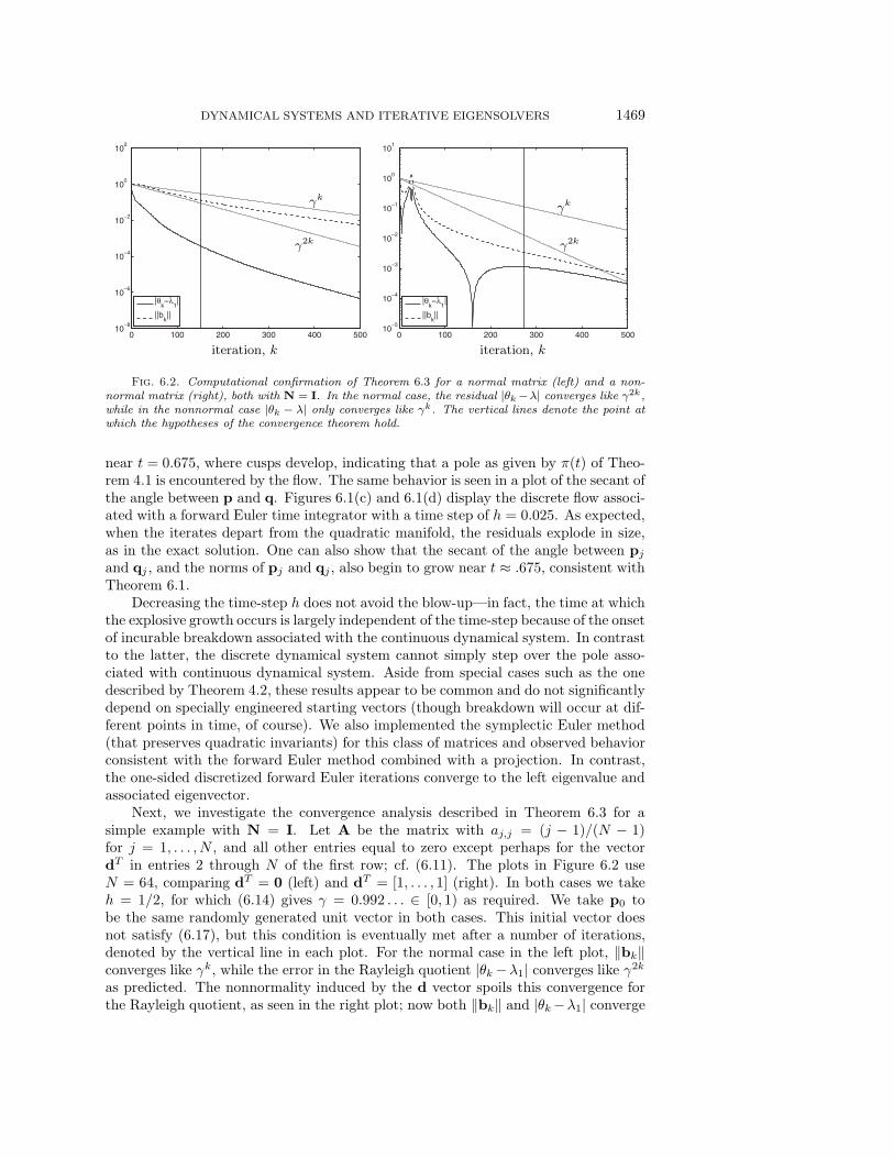
Fig. 6.2. Computational confirmation of Theorem 6.3 for a normal matrix (left) and a non-normal matrix (right), both with N = I. In the normal case, the residual |θk −λ| converges like γ2k,while in the nonnormal case |θk − λ| only converges like γk. The vertical lines denote the point atwhich the hypotheses of the convergence theorem hold.

near t = 0.675, where cusps develop, indicating that a pole as given by π(t) of Theo-rem 4.1 is encountered by the flow. The same behavior is seen in a plot of the secant ofthe angle between p and q. Figures 6.1(c) and 6.1(d) display the discrete flow associ-ated with a forward Euler time integrator with a time step of h = 0.025. As expected,when the iterates depart from the quadratic manifold, the residuals explode in size,as in the exact solution. One can also show that the secant of the angle between pj

and qj , and the norms of pj and qj , also begin to grow near t ≈ .675, consistent withTheorem 6.1.

Decreasing the time-step h does not avoid the blow-up—in fact, the time at whichthe explosive growth occurs is largely independent of the time-step because of the onsetof incurable breakdown associated with the continuous dynamical system. In contrastto the latter, the discrete dynamical system cannot simply step over the pole asso-ciated with continuous dynamical system. Aside from special cases such as the onedescribed by Theorem 4.2, these results appear to be common and do not significantlydepend on specially engineered starting vectors (though breakdown will occur at dif-ferent points in time, of course). We also implemented the symplectic Euler method(that preserves quadratic invariants) for this class of matrices and observed behaviorconsistent with the forward Euler method combined with a projection. In contrast,the one-sided discretized forward Euler iterations converge to the left eigenvalue andassociated eigenvector.

Next, we investigate the convergence analysis described in Theorem 6.3 for asimple example with N = I. Let A be the matrix with aj,j = (j − 1)/(N − 1)for j = 1, . . . , N , and all other entries equal to zero except perhaps for the vectordT in entries 2 through N of the first row; cf. (6.11). The plots in Figure 6.2 useN = 64, comparing dT = 0 (left) and dT = [1, . . . , 1] (right). In both cases we takeh = 1/2, for which (6.14) gives γ = 0.992 . . . ∈ [0, 1) as required. We take p0 tobe the same randomly generated unit vector in both cases. This initial vector doesnot satisfy (6.17), but this condition is eventually met after a number of iterations,denoted by the vertical line in each plot. For the normal case in the left plot, ‖bk‖converges like γk, while the error in the Rayleigh quotient |θk −λ1| converges like γ2k

as predicted. The nonnormality induced by the d vector spoils this convergence forthe Rayleigh quotient, as seen in the right plot; now both ‖bk‖ and |θk −λ1| converge


like γk, consistent with Theorem 6.3. The spikes in the latter plot correspond to pointswhere the Rayleigh quotient θk crossed over the desired eigenvalue λ1, something onlypossible for nonnormal iterations.

7. Summary. This paper demonstrates the fruitful relationship between severalnonlinear dynamical systems and certain simple preconditioned eigensolvers for non-symmetric eigenvalue problems. Properties of the continuous-time systems, such assystem invariants and the asymptotic behavior of the exact solution, can inform theconvergence theory for practical algorithms derived from discretizations, as we illus-trate with Theorem 6.1 for the forward Euler discretization. Generalizations to moresophisticated discretizations, along with relaxation of the stringent requirements onthe preconditioner in Theorem 6.1, are natural avenues for future research.

Appendix A. Lipschitz constant for Euler’s method. To apply the stan-dard convergence theory for the forward Euler method applied to the system

p = N−1(θ(p)p − Ap),

we seek a constant L > 0 such that∥∥N−1(θ(u)u − Au) − N−1(θ(v)v − Av)∥∥ ≤ L‖u− v‖

for all u,v ∈ Rn. First we note that

‖(θ(u)u − Au) − (θ(v)v − Av)‖ ≤ ‖θ(u)u − θ(v)v‖ + ‖A‖‖u− v‖.We focus attention on the first term on the right:

‖θ(u)u − θ(v)v‖ ≤ ‖θ(u)u − θ(v)u + θ(v)u − θ(v)v‖≤ |θ(u) − θ(v)|‖u‖ + |θ(v)|‖u − v‖≤ |θ(u) − θ(v)|‖u‖ + ‖A‖‖u− v‖.(A.1)

(In this last inequality and others that follow, we neglect the opportunity to taketighter bounds that would lead to smaller constants but greater analytical complexity.)

Next, we need to bound |θ(u) − θ(v)|‖u‖ in terms of ‖u − v‖. For convenience(assuming neither u nor v is zero), define the unit vectors u = u/‖u‖ and v = v/‖v‖,with ε = v − u, so that

|θ(u) − θ(v)| =∣∣uTAu − vTAv

∣∣=∣∣uTAu − uTAu − εTAu − uTAε + εTAε

∣∣≤ 2‖ε‖‖A‖ + ‖ε‖2‖A‖.(A.2)

Now note that

‖ε‖ = ‖v − u‖ =‖‖u‖v − ‖v‖v + ‖v‖v − ‖v‖u‖

‖u‖‖v‖ ≤ |‖u‖ − ‖v‖|‖u‖ +

‖u− v‖‖u‖ .

Apply the triangle inequality to obtain |‖u‖−‖v‖| ≤ ‖u−v‖, from which we conclude

(A.3) ‖ε‖ ≤ 2‖u‖‖u− v‖.


Since u and v are unit vectors, we alternatively have the coarse bound ‖ε‖ = ‖u−v‖ ≤2, which we can apply to (A.2) to obtain

|θ(u) − θ(v)| ≤ 2‖ε‖‖A‖ + ‖ε‖2‖A‖≤ 2‖ε‖‖A‖ + 2‖ε‖‖A‖ = 4‖A‖‖ε‖.

Now using (A.3), the bound first bound on ‖ε‖,

|θ(u) − θ(v)| ≤ 8‖A‖‖u‖ ‖u− v‖.

Substituting this bound into (A.1) gives

‖θ(u)u − θ(v)v‖ ≤ 9‖A‖‖u− v‖,

and, finally, we arrive at the Lipschitz constant∥∥N−1(θ(u)u − Au) − N−1(θ(v)v − Av)∥∥ ≤ 10

∥∥N−1∥∥ ‖A‖‖u− v‖.

Thus, we define

(A.4) L = 10∥∥N−1

∥∥ ‖A‖.

The Rayleigh quotient θ(p) is undefined in the case that p = 0. However, as‖p‖ → 0, we have that ‖θ(p)p − Ap‖ → 0, and this motivates the definition thatθ(p)p − Ap = 0 if p = 0.

The above analysis excludes the case that u = 0 and/or v = 0, but with ourdefinition of this singular case we have, e.g., if u = 0, that

‖ (θ(u)u − Au) − (θ(v)v − Av)‖ = ‖(θ(v)v − Av)‖ ≤ 2‖A‖‖v‖ ≤ 10‖A‖‖u− v‖,

and obviously if u = v = 0, we have

‖(θ(u)u − Au) − (θ(v)v − Av)‖ = 0 = 10‖A‖‖u− v‖.

Hence, the Lipschitz constant (A.4) holds for all u and v.

Acknowledgments. We thank Pierre-Antoine Absil, Moody Chu, Kyle Galli-van, Anthony Kellems, Christian Lubich, and Qiang Ye, and anonymous referees fortheir numerous helpful suggestions concerning this work and its presentation.

REFERENCES

[1] P.-A. Absil, Continuous-time systems that solve computational problems, Int. J. Uncov. Com-put., 2 (2006), pp. 291–304.

[2] P.-A. Absil, R. Mahony, and R. Sepulchre, Optimization Algorithms on Matrix Manifolds,Princeton University Press, Princeton, NJ, 2008.

[3] P.-A. Absil, R. Sepulchre, and R. Mahony, Continuous-time subspace flows related to thesymmetric eigenproblem, Pacific J. Optim., 4 (2008), pp. 179–194.

[4] V. I. Arnold, Ordinary Differential Equations, 3rd ed., Springer-Verlag, Berlin, 1992.[5] Z. Bai, D. Day, and Q. Ye, ABLE: An adaptive block Lanczos method for non-Hermitian

eigenvalue problems, SIAM J. Matrix Anal. Appl., 20 (1999), pp. 1060–1082.[6] Z. Bai, J. Demmel, J. Dongarra, A. Ruhe, and H. van der Vorst, eds., Templates for the

Solution of Algebraic Eigenvalue Problems: A Practical Guide, SIAM, Philadelphia, 2000.


[7] W. Bao and Q. Du, Computing the ground state solution of Bose–Einstein condensates by anormalized gradient flow, SIAM J. Sci. Comp., 25 (2004), pp. 1674–1697.

[8] R. Car and M. Parrinello, Unified approach for molecular dynamics and density functionaltheory, Phys. Rev. Lett., 55 (1985), pp. 2471–2474.

[9] J. Carr, Applications of Centre Manifold Theory, Springer-Verlag, New York, 1981.[10] M. T. Chu, Curves on sn−1 that lead to eigenvalues or their means of a matrix, SIAM J. Alg.

Disc. Math., 7 (1986), pp. 425–432.[11] M. T. Chu, On the continuous realization of iterative processes, SIAM Rev., 30 (1988), pp. 375–

387.[12] M. Embree, The Arnoldi eigenvalue iteration with exact shifts can fail, SIAM J. Matrix Anal.

Appl., to appear.[13] M. A. Freitag and A. Spence, Convergence theory for inexact inverse iteration applied to the

generalised nonsymmetric eigenvalue problem, Electron. Trans. Numer. Anal., 28 (2007),pp. 40–64.

[14] C. W. Gear, Numerical Initial Value Problems in Ordinary Differential Equations, Prentice-Hall, Englewood Cliffs, NJ, 1971.

[15] G. H. Golub and L.-Z. Liao, Continuous methods for extreme and interior eigenvalue prob-lems, Linear Algebra Appl., 415 (2006), pp. 31–51.

[16] G. H. Golub and Q. Ye, Inexact inverse iteration for generalized eigenvalue problems, BIT,(2000), pp. 671–684.

[17] J. Guckenheimer and P. Holmes, Nonlinear Oscillations, Dynamical Systems, and Bifurca-tions of Vector Fields, Springer-Verlag, New York, 1983.

[18] E. Hairer, C. Lubich, and G. Wanner, Geometric Numerical Integration: Structure-Preserving Algorithms for Ordinary Differential Equations, 2nd ed., Springer-Verlag,Berlin, 2006.

[19] U. Helmke and J. B. Moore, Optimization and Dynamical Systems, Springer, London, 1994.[20] W. Kahan, B. N. Parlett, and E. Jiang, Residual bounds on approximate eigensystems of

nonnormal matrices, SIAM J. Num. Anal., 19 (1982), pp. 470–484.[21] A. V. Knyazev, Preconditioned eigensolvers—an oxymoron?, Elec. Trans. Numer. Anal., 7

(1998), pp. 104–123.[22] A. V. Knyazev and K. Neymeyr, Efficient solution of symmetric eigenvalue problems using

multigrid preconditioners in the locally optimal block conjugate gradient method, Elec.Trans. Numer. Anal., 7 (2003), pp. 38–55.

[23] A. V. Knyazev and K. Neymeyr, A geometric theory for preconditioned inverse iteration.III: A short and sharp convergence estimate for generalized eigenvalue problems, LinearAlgebra Appl., 358 (2003), pp. 95–114.

[24] Y.-L. Lai, K.-Y. Lin, and W.-W. Lin, An inexact inverse iteration for large sparse eigenvalueproblems, Numer. Linear Algebra Appl., 1 (1997), pp. 1–13.

[25] R. B. Lehoucq and A. J. Salinger, Large-scale eigenvalue calculations for stability analysisof steady flows on massively parallel computers, Internat. J. Numer. Methods Fluids, 36(2001), pp. 309–327.

[26] B. Leimkuhler and S. Reich, Simulating Hamiltonian Dynamics, Cambridge University Press,Cambridge, 2005.

[27] R. Mahony and P.-A. Absil, The continuous time Rayleigh quotient flow on the sphere,Linear Algebra Appl., 368 (2003), pp. 343–357.

[28] Y. Nakamura, K. Kajiwara, and H. Shiotani, On an integrable discretization of the Rayleighquotient gradient system and the power method with a shift, J. Comput. Appl. Math., 96(1998), pp. 77–90.

[29] T. Nanda, Differential equations and the QR algorithm, SIAM J. Numer. Anal., 22 (1985),pp. 310–321.

[30] O. Nevanlinna, Convergence of Iterations for Linear Equations, Birkhauser, Basel, 1993.[31] E. E. Osborne, On pre-conditioning of matrices, J. ACM, 7 (1960), pp. 338–345.[32] B. N. Parlett, The Symmetric Eigenvalue Problem, no. 20 in Classics in Applied Mathematics,

SIAM, Philadelphia, 1998. Amended reprint of 1980 Prentice-Hall edition.[33] B. N. Parlett and C. Reinsch, Balancing a matrix for calculation of eigenvalues and eigen-

vectors, Numer. Math., 13 (1969), pp. 293–304.[34] M. C. Payne, M. P. Teeter, D. C. Allan, T. Arias, and J. Joannopoulos, Iterative

minimization techniques for ab initio total-energy calculations: Molecular dynamics andconjugate gradients, Rev. Mod. Phys, 64 (1992), pp. 1045–1097.

[35] B. T. Polyak, Introduction to Optimization, Translation Series in Mathematics and Engineer-ing, Optimization Software, Inc., New York, 1987.

[36] M. J. D. Powell, Approximation Theory and Methods, Cambridge University Press, Cam-bridge, 1981.


[37] Y. Saad, Variations on Arnoldi’s method for computing eigenelements of large unsymmetricmatrices, Linear Algebra Appl., 34 (1980), pp. 269–295.

[38] G. W. Stewart and J.-g. Sun, Matrix Perturbation Theory, Academic Press, San Diego, CA,1990.

[39] W. W. Symes, The QR algorithm and scattering for the finite nonperiodic Toda lattice, Phys-ica D, 4 (1982), pp. 275–280.

[40] L. N. Trefethen and M. Embree, Spectra and Pseudospectra: The Behavior of NonnormalMatrices and Operators, Princeton University Press, Princeton, NJ, 2005.

[41] J. S. Warsa, T. A. Wareing, J. E. Morel, J. M. McGhee, and R. B. Lehoucq, Krylov sub-space iterations for deterministic k-eigenvalue calculations, Nuc. Sci. Engrg., 147 (2004),pp. 26–42.

[42] D. S. Watkins, Isospectral flows, SIAM Rev., 26 (1984), pp. 379–391.[43] J. H. Wilkinson, The Algebraic Eigenvalue Problem, Oxford University Press, Oxford, 1965.

Dynamical Systems and Non-Hermitian Iterative Eigensolvers

Documents

Transcript of Dynamical Systems and Non-Hermitian Iterative Eigensolvers