Computational StatisticsDOI 10.1007/s00180-007-0090-8

ORIGINAL PAPER

Iterative Denoising

Kendall E. Giles · Michael W. Trosset ·David J. Marchette · Carey E. Priebe

Received: 6 July 2007 / Accepted: 4 September 2007© Springer-Verlag 2007

Abstract One problem in many fields is knowledge discovery in heterogeneous,high-dimensional data. As an example, in text mining an analyst often wishes toidentify meaningful, implicit, and previously unknown information in an unstructuredcorpus. Lack of metadata and the complexities of document space make this taskdifficult. We describe Iterative Denoising, a methodology for knowledge discovery inlarge heterogeneous datasets that allows a user to visualize and to discover potentiallymeaningful relationships and structures. In addition, we demonstrate the features ofthis methodology in the analysis of a heterogeneous Science News corpus.

Keywords Knowledge discovery · Text mining · Classification · Clustering

1 Introduction

A user who wants to understand a large, heterogeneous, and high-dimensional set ofdata and find interesting information and relationships in that data needs a sufficiently

K. E. Giles (B)Department of Statistical Sciences and Operations Research,Virginia Commonwealth University, Richmond, VA 23284, USAe-mail: kendallgiles@gmail.com

M. W. TrossetDepartment of Statistics, Indiana University, Bloomington, IN 47405, USA

D. J. MarchetteDahlgren Division, Naval Surface Warfare Center, Dahlgren, VA 22448, USA

C. E. PriebeDepartment of Applied Mathematics and Statistics, Johns Hopkins University,Baltimore, MD 21218, USA

123

K. E. Giles et al.

flexible and powerful computational framework in hand to facilitate data processingand knowledge discovery. For example, imagine that a user has been presented a largecollection of text documents and wants to examine and understand those documentsfrom an analytical perspective. The user might have an information retrieval task inmind, where it is desired to find a set of documents relevant to a specific query. Or theuser might wish to understand relationships between multiple documents. The usermight also wish to identify the topic of discussion in a collection of emails, or to clusterthem according to relevant criteria. However, increasingly, the user must analyze large,complex, unstructured datasets, meaning that the dataset may not include class labelsfor the documents, the number of documents to be analyzed is large, and there maybe local (as opposed to global) structures that characterize some of the data. So theuser’s task is to explore the data, extract meaningful, implicit, and previously unknowninformation from a large unstructured corpus.

From this scenario we can identify several relevant issues and needs. First, if weconsider a word or phrase in one document as one dimension, then the dimensionalityof the search space, from a performance perspective, would be prohibitively expensiveand difficult for operations on a corpus even on the order of tens-of-thousands of docu-ments and tens-of-thousands of words per document. The computational performanceof processing such high dimensional data can be limiting. Moreover, visualizing andcomprehending high dimensional spaces can be difficult for the user, who typicallyunderstands data best in two or three dimensions. Second, in large, complicated data-sets, an important finding for the user might be relationships found in local structures,where features of the data may have differing relationships in different parts of thedata. Third, the lack of existing class labels limits the ability of a user to analyze thecorpus without first applying some structure to the data.

This paper presents a general methodological instantiation of a general machinelearning decomposition framework, described in, e.g., Schalkoff (1991). In particular,our methodology, called Iterative Denoising, is designed for knowledge discovery inlarge heterogeneous datasets to tease out local structures and relationships of possibleinterest, display useful information to the user, and address scaleability and high-dimensionality concerns, as in Giles (2006).

2 Methodology

Based on the principle of integrated sensing and processing (Priebe et al. 2004a), thebasic philosophy of our methodology is that, starting with a heterogeneous dataset C,based on the selection of appropriate features we denoise C into {C1, . . . , CJ }, whereeach C j is meant to be more homogeneous than C (Priebe et al. 2004b). We note thatin order to highlight certain types of multivariate structure in the data, the featuresin C are transformed and/or represented in a lower-dimensional space before they arepartitioned, and so we mean “denoising” to be a bit more than just the “clustering”of typical machine learning approaches. We also note that this lower-dimensionalrepresentation is important for user visualization and interaction. The denoising ofeach C j continues recursively until the collection is homogeneous enough for inferenceto proceed. The resulting clusters are organized into a hierarchical, divisive tree.

123

Iterative Denoising

Fig. 1 Iterative Denoisingflowchart

(a) Complete Flowchart (b) Denoising Detail

We present a high-level version of our methodology in Fig. 1a. The first componentin the figure is Extract Summary Metrics. We are initially given a datasetC = {C1, . . . , Cn} consisting of n elements, where n is large. These elements, whichmay come from a database or stream, are the observations of interest—they can be textdocuments, images, web pages, computer network flows, etc. In this step we extractout useful (essential) summary metrics � for each document that we can refer tothroughout future processing:

� = {�1, . . . , �n} = essentials(C).

The exact form of the metrics is data-dependent, but one example of summary metricsis word counts for words in a document.

Next, once we have summarized the node’s data, we want toExtract Featuresfrom the data—we use these features to measure the similarity or dissimilarity of ob-jects in the node. Note that the features are dependent on the data in a particular node.For this reason, we call this function cdfe, for corpus-dependent feature extraction.

Let f� be the set of features in the current collection of metrics �, then compute:

X� = cdfe(�),

where X� is a |�| × | f�| matrix. Note that both the features and the number offeatures depend on the collection of documents in the current node represented by �.For example, for text documents the features might be a mutual information measurebased on associations of occurrences of Ngrams among documents in the corpus, asin Lin and Pantel (2002), or they may be simple word-frequency counts.

Next, we want toDenoise the current node. Using the desired features we partitionthe X� after it has been represented in a lower-dimensional space, to highlight certaintypes of multivariate structure. As mentioned above, we end up with a number of child

123

K. E. Giles et al.

partitions or cells (γ of them) that are more homogeneous than the parent node. Thisdenoising process is expanded in detail in the next section.

An important attribute of our methodology is that users may want to Interactwith the resulting visualized representations. We are not only providing to the userslower-dimensional-space representations to highlight (possibly) desired structures inthe data, but we are also allowing the user to interact with the data. For example, theuser may wish to change the displayed geometry relationships between objects, sayto reflect some metadata intelligence the user has received that is not reflected in theoriginal data (see Priebe et al. 2004b). But through interaction, the user dynamicallyaffects the growth of the tree.

For each resulting child node, which represents data from the previously discusseddenoising and user interaction steps, we recursively start over from the ExtractFeatures component. It is necessary to extract new features for each node becausethe objects in the child node are a subset of the objects that were in the parent node, andthus the feature metrics need to be recomputed to reflect the changed node membership.The flow continues, recursively denoising and growing the tree, until some stoppingcriteria has been met for a particular node (such as reaching the node’s minimumnumber of objects) or for the tree itself (such as reaching the maximum desired levelof the denoising tree). Because our methods are intended for interactive use withlarge data sets, and because our methods proceed by recursively denoising previouslyidentified subsets of data, we call our methodology Iterative Denoising.

2.1 Denoising

Given a node and its corresponding feature matrix, X�, we seek to partition theobjects in the node into two or more subsets of objects of greater homogeneity thanthe entire node. This is essentially the problem of clustering, i.e., of identifying subsetsof objects that exhibit “internal cohesion” and “external isolation” (Cormack 1971).The fundamental challenge of Denoising is to identify and/or develop clusteringmethodologies that scale well to large data sets and that facilitate user interaction, alimitation of most clustering algorithms.

Note that one cannot claim that subsets of a node are more homogeneous than thenode itself unless one has some way of measuring which pairs of objects are nearbyand which pairs of objects are far apart. Every clustering methodology necessarilyrelies on some measure of pairwise proximity; hence, the first step of Denoising isto Compute Proximities.

Assuming that our proximities are symmetric, then the introduction of proximitiesallows us to represent the objects in the current node as an edge-weighted undirectedgraph G. Each vertex in the graph corresponds to an object; the edge weights are thepairwise proximities. This representation of the data transforms the clustering probleminto a graph partitioning problem.

Given a threshold on the proximities we construct G ′ to be the unweighted graphwith edges corresponding to those of G with weight less than the threshold. Then,a natural way to partition G ′ into a specified number of subgraphs is to choose thepartition so as to balance the number of vertices in each subgraph and to minimize

123

Iterative Denoising

the number of edges between subgraphs. Unfortunately, this problem is NP-complete(Garey et al. 1974).

A number of heuristic and approximate approaches to graph partitioning have beensuggested. For example, Kernighan and Lin (1970) proposed an exchange algorithmthat swaps pairs of nodes between clusters. Similar approaches are summarized inAlpert and Kahng (1995), but none of these algorithms scale well to large datasets. Oneway of addressing scalability is through recursive partitioning, in precisely the samespirit as Iterative Denoising. In multilevel approaches to graph partitioning, the originalgraph is approximated by a sequence of increasingly smaller graphs. The smallestgraph is then partitioned and that partition is propagated back to the original graph(Hendrickson and Leland 1995), as implemented by, for example, METIS (Karypisand Kumar 1998).

A fundamental difficulty with traditional graph partitioning methods, however, isthat they do not represent the data in ways that facilitate visualization and user interac-tion. To accommodate the abilities of most users, we attempt to represent the objectsas points in a low-dimensional Euclidean space, in such a way that proximate pairshave small Euclidean distances. The construction of such representations is calledembedding, or (in psychometrics and statistics) multidimensional scaling. Thus, afterwe Compute Proximities, we Embed.

Our desire to embed the data in a low-dimensional space means that we are notsimply embedding the data, but also reducing the dimensionality of the data. In fact,the conceptually distinct steps of Compute Proximities and Embed can bediscerned in various methods for nonlinear dimension reduction, or manifold learning,such as in the popular Isomap (Tenenbaum et al. 2000) approach to manifold learning.Though we formalize and generalize these common approaches by noting distinctsteps in the process, as discussed in further detail in the next section, the steps ofDenoising are summarized in Fig. 1b.

2.2 Compute proximities

The proximity of two objects is generally measured by computing similarities ordissimilarities. Because most embedding algorithms approximate dissimilarities withEuclidean distances, similarities are often transformed to dissimilarities prior toembedding. The conventional transformation exploits a well-known connection bet-ween squared Euclidean distances and Euclidean inner products (see, e.g., Critchley1988).

Note that an appropriate measure of (dis)similarity is application-specific. Recallthat summary features, e.g., mutual information measures of association betweendocuments for specific Ngrams, have already been extracted. We compute proximitiesas follows:

1. We conceive the | f�| features of object i as a vector, yi ∈ R| f�|.

2. For each pair of objects i and j , we compute

ri j = 〈yi , y j 〉‖yi‖ ‖y j‖ .

123

K. E. Giles et al.

Notice that, were we to center the feature vectors before performing this operation,ri j would be Pearson’s product-moment correlation coefficient.

3. We construct a weighted undirected graph G with edge weights ri j . For each vertex,we desire the k nearest vertices, as measured by shortest path length, where k isspecified by the user. However, to reduce the computational complexity of findingnearest vertices, we do not insist on finding the exact set of k nearest vertices;instead, we settle for an approximation thereof.

4. We construct an unweighted undirected graph G ′ in which vertices i and j areconnected by an edge if either vertex i belongs to the set of (approximate) k nearestneighbors of vertex j , or vertex j belongs to the set of (approximate) k nearestneighbors of vertex i .

5. We construct the adjacency matrix, A = [ai j ], of the unweighted graph G ′, i.e.,ai j = 1 if an edge connects vertices i and j , otherwise ai j = 0. The adjacenciesare crude—but efficiently computed—pairwise similarities.

2.3 Embed

Roughly speaking, there are two general approaches to embedding: approaches that fitdistances and approaches that fit inner products. The distance approach encompassesboth extremely fast heuristic methods like FastMap (Faloutsos and Lin 1995) and moreprincipled methods that require numerical optimization of an error criterion, e.g., themajorization algorithm of de Leeuw (1988) for minimizing the raw stress criterion. Thelatter tend to be prohibitively expensive for large data sets, but see Trosset and Groenen(2005) for an algorithm that decreases the raw stress criterion with a computationalcomplexity of O(n).

The inner product approach encompasses classical multidimensional scaling(CMDS) (Torgerson 1952; Gower 1966), as used in Isomap, as well as various othertechniques for constructing “eigenmaps,” e.g., Belkin and Niyogi (2003), Roweis andSaul (2000), and Donoho and Grimes (2003). What these methods have in commonis the extraction of d eigenvectors from a symmetric, centered, matrix B of Eucli-dean inner products. The eigenvalues and eigenvectors of this matrix are then used toconstruct a configuration of points in R

d .To apply CMDS to our adjacency matrix, A, we must first convert similarities (adja-

cencies) to dissimilarities. As explained in Saerens et al. (2004), this is accomplishedimplicitly by constructing a Laplacian eigenmap. The (implicit) dissimilarities areaverage commute times between pairs of vertices, based on a Markov-chain model ofa random walk through the graph.

Define the diagonal matrix D = [di j ], di j = 0 for i �= j , by

dii =∑

k

aik,

the number of vertices to which vertex i is adjacent. The symmetric, positive semide-finite matrix L = D − A is the Laplacian matrix of the unweighted graph G ′. Someyears ago, Fiedler (1973) argued that the eigenvector corresponding to the smallest

123

Iterative Denoising

positive eigenvalue of L facilitates clustering the vertices of G ′. This insight is theinspiration for spectral clustering.

To construct the d-dimensional representation that we will call Fiedler space, let0 < λ1 ≤ · · · ≤ λd denote the smallest nonzero eigenvalues and let v1, . . . , vd denotethe corresponding eigenvectors. The Cartesian coordinates of the points in Fiedlerspace are then obtained as rows of the matrix

F =[

v1√λ1

∣∣∣∣ · · ·∣∣∣∣

vd√λd

].

Other scalings of the eigenvectors are also used, but dividing each eigenvector by thesquare root of its eigenvalue corresponds to embedding by CMDS after the transforma-tion to dissimilarity implicit in Saerens et al. (2004). The feature matrix, F , providesCartesian coordinates used to visualize and partition the objects in the current node ofthe Iterative Denoising tree.

2.4 Partition

Finally, we measure dissimilarity in Fiedler space by Euclidean distance, then use stan-dard clustering methods to further partition the current node of the Iterative Denoisingtree. Our approach allows us to choose any of the myriad algorithms available forclustering points in Euclidean space; see, for example, Everitt (1993), Gordon (1999),and Mirkin (2005) for surveys of various approaches.

To date, our development of Iterative Denoising has relied on k-means clustering.In this approach to clustering, the user specifies γ = k, the number of subsets in apartition of x1, . . . , xN ∈ R

d . Algorithms for k-means clustering then attempt to finda partition, {C1, . . . , Ck}, that minimizes the squared error criterion

W (C1, . . . , Ck) =k∑

i=1

∑

x j ∈Ci

∥∥x j − xi∥∥2

,

where xi = x(Ci ) is the mean of the x j ∈ Ci . There exist a number of algorithms thatmonotonically decrease W and converge to a locally optimal partition, but algorithmsthat guarantee global solutions are usually overwhelmed by several hundred xi . Forthis reason, we are content to find good (not necessarily optimal) partitions.

3 Implementation description

While the previous sections describe the Iterative Denoising methodology, we notethat there are numerous possible algorithmic implementations. For example, for theCompute Proximities step, we could choose to implement dissimilarities orapproximate nearest neighbor adjacencies; for the Embed step we could perform mul-tidimensional scaling or Laplacian eigenmapping—all such implementations wouldbe within our methodology, and analysis of these implementation differences will fuel

123

K. E. Giles et al.

Table 1 Text corpus metricsSymbol Description

m·· The total number of words in Cmo· The total number of all words in that document

mow The number of times word w appears in o

m·w The total number of times the word appears in C

future research. We describe our initial implementation of Iterative Denoising in thissection; the following section describes our use of this implementation to analyze atext corpus.

3.1 Extract summary metrics

Because the first component, Extract Summary Metrics, is only performedonce per dataset and is not part of the main Iterative Denoising recursive structure, wedesigned the Extract Summary Metrics component as a stand-alone functionthat can be run as a separate program or called from the main program. We also madethis a stand-alone function because this is the only step that is dataset-dependent—it ishere that the raw data is abstracted into a collection of summary metrics. As mentionedpreviously, in our initial implementation we focused on text documents, and so thisstep’s description of the implementation is specific to abstracting text.

In order to extract summary metrics from the raw dataset, we decomposed theproblem into three substeps. First, we clean each document using an implementation ofthe Porter stemming algorithm (Porter 1980). This algorithm removes common suffixesfrom English words and non-word text, and returns a set of word stems or tokens.For example, the stem for the words connect, connected, connecting, connection,and connections is connect. Second, we convert the word stems into Ngrams (whereNgrams can be defined as sequences of word stems) using the count script of theNgram Statistics Package (Banerjee and Pedersen 2003). This script inputs raw textfiles, creates a list of the Ngrams in those files, and outputs the Ngrams with theirfrequencies, in descending order by frequency.

Next, using a large hash structure, documents × unique Ngrams (words), we outputfor each document o: the word w, the number of times word w appears in o (mow), thetotal number of times the word appears in C (m·w), and the Ngram number. This givesus a set of metrics �. From these summary metrics we can also determine m··, thetotal number of words in corpus C, and for each document o ∈ C the total number ofall words in that document mo·. The extracted metrics for processing text documentsare summarized in Table 1.

3.2 Extract features

In this step we use the summary metrics � computed in Extract SummaryMetrics to extract the features of the documents. For our implementation, weextracted mutual information values for each document and unique word in the corpus.

123

Iterative Denoising

Using our previously noted essentials, this mutual information value is computed as:

MIow = logmow

mo·

/m·wm··

.

The number of features is the number of distinct words in the corpus; for each documentwe compute that number of mutual information values.

3.3 Compute proximities

From our summary features we wish to create a structure that reflects object simi-larities. As described in Sect. 2.2, we do so by constructing an unweighted undi-rected graph for which vertices correspond to objects and edges connect pairs ofobjects whose proximity attains a specified threshold. One natural way to implementproximity-thresholding is to use a nearest-neighbor search algorithm. In R

d , traditional(exact) nearest neighbor algorithms use either nO(d) space or O(dn) time. However,due to the curse of dimensionality, exact searches perform little better than sequen-tial searches as n gets large. Recent work on approximate nearest neighbor algorithms(Houle 2003, Houle and Sakuma 2005, Arya et al. 1998, Kushilevitz et al. 1998, Indykand Motwani 1998, Gionis et al. 1999, Clarkson 1999) has attempted to circumventthe curse of dimensionality by essentially relaxing the exact nearest neighbor searchrestriction in return for faster search performance. It is precisely this relaxation thatwe exploit to realize our proximity-thresholded graph G ′.

In our implementation we use the SASH data structure (Houle 2003; Houle andSakuma 2005) to perform nearest neighbor searches to find the K nearest neighborsto a particular object. Using SASH, we realize G = sash(X�). However, G may notbe symmetric due to the geometry of the object similarities, and so we add missingedges to G as G ′ = symmetrize(G). From G ′ we create the adjacency matrix Aas noted in Sect. 2.2. Since A is large and sparse, we actually do not store A but use asparse representation both for storage and matrix computations, which we will furtherdetail in the next section.

For n objects, the discussion in Sect. 2.2 conveys the impression that it is necessaryto pre-compute all n(n − 1)/2 proximities. In fact, it is not necessary to compute allO(n2) proximities in order to find approximate nearest neighbors. Because the SASHdata structure is organized as a multi-level hierarchy of random samples, where objectsin a given level are connected only to approximate nearest neighbors drawn from thelevel immediately above, not all pairs of proximities are necessarily computed.

3.4 Embed

In order to embed our high-dimensional objects in a low-dimensional space, as dis-cussed in Sect. 2.3, we want to convert our computed similarities to dissimilarities inpart by computing the d smallest positive eigenvalues of our Laplacian eigenmap L .One difficulty in computing these eigenvalues is that L may be quite large. But L mayalso be sparse, and so we utilize the ARPACK library (Lehoucq and Yang 1988) to

123

K. E. Giles et al.

exploit this sparsity in order to address scalability issues. ARPACK is a collection ofFortran routines that solve large eigenvalue problems by implementing a variant ofthe Arnoldi process (Arnoldi 1951) [which in the symmetric case reduces to a variantof the Lanczos process (Lanczos 1950)]. Because ARPACK does not have a modein which it calculates the d smallest positive eigenvalues, we ask for the d ′ smallesteigenvalues, then use the d < d ′ smallest positive eigenvalues and correspondingeigenvectors to construct an embedding. The discrepancy, d ′ − d, equals the numberof connected components of the graph G ′. ARPACK is an iterative method that suc-cessively computes vectors and asks for matrix–vector products. ARPACK does notactually store or factor the matrix, L , but rather queries a user-provided function thatcomputes the product of L with an ARPACK-provided vector.

3.5 Partition

As noted in Sect. 2.4, to measure dissimilarity in Fiedler space by Euclidean distance,we use k-means clustering. In our implementation we use the k-means implementationof Lloyd’s algorithm in Kanungo et al. (2004). k-means clustering supposes that,given a set of n ∈ R

d data points and a number of desired centers γ , minimize themean-squared distance from each data point to its nearest center. Lloyd’s algorithm, asimplemented in Kanungo et al. (2004), observes that the optimal placement of a centeris at the centroid of its associated cluster. For a set of k centers z ∈ Z , Lloyd’s algorithmiteratively moves every center z to the centroid of the corresponding neighborhood ofdata points V (z) until convergence.

3.6 Interact

For visualization and user interaction, we utilize SpaceTree (Grosjean et al. 2002).Among other changes, we modified the original code to allow for images to be dis-played when a user clicks on a particular denoising tree code. Our Interact com-ponent outputs an XML file containing information on node contents and tree hierarchyinformation in the format desired by SpaceTree.

4 Application: Science News corpus

As an example, we used a heterogeneous corpus D = {D1, . . . ,Dn} of n text docu-ments from the Science News (SN) website. Table 2 shows the number of documentsin D per class, where |D| = 1,047. In addition, we note the symbol scheme used toidentify class membership in the following figures. We again stress that our frameworkis an unsupervised approach, and so the class labels are just for validation; we appliedthe previously described implementation of Iterative Denoising to this database toexamine the structures and relationships contained therein.

Each document in the corpus is represented in its own text file. The result of ourExtract Summary Metrics step was a collection of 1,047 files, each contai-ning the Ngrams for that document and appropriate summary counts. For this example,

123

Iterative Denoising

Table 2 Science news corpusClass Number of documents Symbol

Anthropology 54 ◦ Open circle

Astronomy 121 � Closed diamond

Behavioral Sciences 72 � Open square

Earth Sciences 137 Open triangle

Life Sciences 205 ♦ Open diamond

Math & CS 60 � Closed square

Medicine 280 • Closed circle

Physics 118 � Closed triangle

we only used monograms. Once the summary metrics were extracted, we began theIterative Denoising recursion by choosing some initial parameter values and invokingour implementation on the dataset. We used initial parameters of K = 20 nearestneighbors, γ = 3 partition cells, and d = 4 dimensions for our Fiedler space embed-ding. Depending on the size of the nodes deeper into the Iterative Denoising tree, weadjusted K to keep the K/n ratio small.

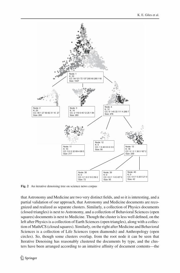
Figure 2 shows the resulting Iterative Denoising tree. Each node in the figure showsthe node index, the K used for that node, counts for each class (in the order given inTable 2), and the size of the node. Below each node label is a view of that node’s Fied-ler Space embedding of the documents in that node. There are a total of four levels tothe tree, though for space limitations the entire tree is not shown. In general, IterativeDenoising trees are not symmetric—iteration occurs if the node is sufficiently largeand non-homogeneous. For example, Node 12 is small and relatively pure—this nodecontains a large collection of Behavioral Sciences documents that have been extractedfrom among the Medicine documents, so it may be sufficient for iteration to stop there.However, Node 13 is large and mixed, so iteration can proceed to another level. Whereappropriate, some of the Fiedler Space embeddings will be shown below in a magnifiedform for exposition. However, this tree view shows an example of the overall Itera-tive Denoising framework, where a large collection of non-homogeneous documents,in Node 1, is iteratively denoised to produce relatively homogeneous collections ofdocuments in the leaves of the tree, as seen in Node 12. Finally, it should be remembe-red that iteration proceeds as a function of corpus-dependent feature extraction—newfeatures and dimension reduction processing are recomputed for subsets of a noderather than relying on simple hierarchical clustering, as described in Sect. 2 and asdetailed in the following.

In Fig. 2, and throughout, each document is shaded according to its partition, eachdocument’s location is noted by a symbol appropriate to the class of the document,and each location is plotted according to the smallest two Fiedler vectors. Note thatpartition boundaries are not linear—partitioning occurs in the entirety of the embed-ding space (in this example, d = 4, though only the first two dimensions are plotted).The resulting geometric relationships immediately reveal a large cluster of Medicinedocuments (closed circles) in the southeast portion of the figure, and a cluster of Astro-nomy documents (closed diamonds) in the southwest. It is not unreasonable to suggest

123

K. E. Giles et al.

Fig. 2 An iterative denoising tree on science news corpus

that Astronomy and Medicine are two very distinct fields, and so it is interesting, and apartial validation of our approach, that Astronomy and Medicine documents are reco-gnized and realized as separate clusters. Similarly, a collection of Physics documents(closed triangles) is next to Astronomy, and a collection of Behavioral Sciences (opensquares) documents is next to Medicine. Though the cluster is less well defined, on theleft after Physics is a collection of Earth Sciences (open triangles), along with a collec-tion of Math/CS (closed squares). Similarly, on the right after Medicine and BehavioralSciences is a collection of Life Sciences (open diamonds) and Anthropology (opencircles). So, though some clusters overlap, from the root node it can be seen thatIterative Denoising has reasonably clustered the documents by type, and the clus-ters have been arranged according to an intuitive affinity of document contents—the

123

Iterative Denoising

(a) With CDFE (b) Without CDFE

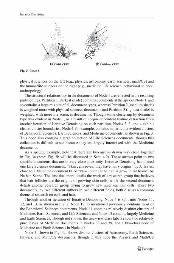
Fig. 3 Node 4

physical sciences on the left (e.g., physics, astronomy, earth sciences, math/CS) andthe human/life sciences on the right (e.g., medicine, life science, behavioral science,anthropology).

The structural relationships in the documents of Node 1 are reflected in the resultingpartitionings. Partition 1 (darkest shade) contains documents at the apex of Node 1, andso contains a large mixture of all document types, whereas Partition 2 (medium shade)is weighted more with physical sciences documents and Partition 3 (lightest shade) isweighted with more life sciences documents. Though some clustering by documenttype was evident in Node 1, as a result of corpus-dependent feature extraction fromanother iteration of Iterative Denoising on each partition, Nodes 2, 3, and 4 exhibitclearer cluster boundaries. Node 4, for example, contains in particular evident clustersof Behavioral Sciences, Earth Sciences, and Medicine documents, as shown in Fig. 3.This node also contains a large collection of Life Sciences documents, though thiscollection is difficult to see because they are largely intermixed with the Medicinedocuments.

As a specific example, note that there are two arrows drawn very close togetherin Fig. 3a (note: Fig. 3b will be discussed in Sect. 4.2). These arrows point to twospecific documents that are in very close proximity. Iterative Denoising has placedone Life Sciences document, “Skin cells reveal they have hairy origins” by J. Travis,close to a Medicine document titled “New inner ear hair cells grow in rat tissue” byNathan Seppa. The first document details the work of a research group that believesthat hair follicles are the origins of growing skin cells, while the second documentdetails another research group trying to grow new inner ear hair cells. These twodocuments, by two different authors in two different fields, both discuss a commontheme of research on cells and hair.

Through another iteration of Iterative Denoising, Node 4 is split into Nodes 11,12, and 13, as shown in Fig. 2. Node 12, as mentioned previously, contains most ofthe Behavioral Sciences documents, Node 11 contains relatively distinct clusters ofMedicine, Earth Sciences, and Life Sciences, and Node 13 contains largely Medicineand Earth Sciences. Though not shown, the tree-view class labels show two relativelypure leaves of Medicine documents in Nodes 38 and 39, and a two-class node ofMedicine and Earth Sciences in Node 40.

Node 3, shown in Fig. 4a, shows distinct clusters of Astronomy, Earth Sciences,Physics, and Math/CS documents, though in this node the Physics and Math/CS

123

K. E. Giles et al.

(a) Node 3. (b) Node 8.

(c) Node 9. (d) Node 10.

Fig. 4 Nodes 3, 8–10 of Fiedler space embedding

clusters are not that distinct. Similar to the recursion for Node 4, Fig. 4b, c, d show theLevel 3 embeddings of Node 3. Node 8 shows mainly the two classes of Earth Sciencesand Astronomy, Node 9 shows a homogeneous class of Astronomy documents, exceptfor one Life Sciences document, and Node 10 shows mainly two distinct clusters ofPhysics and Math/CS. Again, whereas Physics and Math/CS clusters were overlappedin Fig. 4, their clusters are largely distinct in Node 10.

4.1 A detailed analysis of clustered documents

While the above illustrates how, on the whole, Iterative Denoising denoises and clus-ters documents according to rough document types, it can be seen, however, that thisclustering is not perfect, as shown in Fig. 4b. The two dominant classes, Astronomy andEarth Sciences, contain 33 and 42 documents, respectively. In addition, there are alsotwo Anthropology, three Physics, one Math/CS, and five Life Sciences documents inthis cluster. If the goal of Iterative Denoising was only to create homogeneous clustersof documents in an unsupervised fashion based on assigned document types, then theaddition in particular of at least the life sciences documents would indicate a possibleshortcoming of the approach, considering that this node is dominated by the physicalsciences. However, consideration of the placement of these life sciences documentsin this physical sciences node suggests that Iterative Denoising can cluster by docu-ment subtype in addition to document type. Table 3 shows a summary of some ofthe Life Sciences and Anthropology documents placed in this node. Each document isfollowed by its nearest physical sciences neighbor, for comparison. Along with each

123

Iterative Denoising

Table 3 Similarities in Node 8 document neighbors

Class Title Representative sentence

Anthropology Primordial Water A meteorite’s saltytale

A water-rich, icy projectile, such as a co-met, could have plowed into the new-born asteroid and spilled some of itswater.

Astronomy Searching for Life in a Martian Me-teorite A seesaw of results

Jeffrey L. Bada of the Scripps Institu-tion of Oceanography in La Jolla, Ca-lif., says he’s all but convinced that cellwalls and other biological artifacts, iffound, come from meltwater that pas-sed through the meteorite during its13,000-year sojourn in the Antarctic.

Life Sciences Myriad Monsters Confirmed in WaterDroplets

Within these droplets danced a varietyof little animals, some “so exceedinglysmall that millions of millions mightbe contained in one drop of water,” hereports.

Physics Big guns, bench work: How lifecould’ve come from above

Could life’s building blocks have stowedaway on such space debris and thensurvived an impact with Earth?

Life Sciences Bacteria under ice: Some don’t like ithot

Bacteria with odd lifestyles have comeunder increasing scrutiny of late, withmost research focused on the so-called thermophilic species, which pre-fer scalding homes.

Earth Sciences Core Concerns The hidden reaches ofEarth are starting to reveal some oftheir secrets

Peering deep into the bowels of the pla-net, he saw vast currents of molten ironalloy swirling at temperatures above5,000 kelvins, nearly as hot as the sur-face of the sun.

document class label, we show the title of the document and a representative sentencefrom that document. The first document, “Primordial Water A meteorite’s salty tale”,details the analysis of water-containing meteorites found on Earth that might explainhow water originated on this planet. If these meteorites contained water that originatedfrom somewhere off Earth, then this would give weight to the theory that Earth got itswater from bombardment by water-containing meteors. This document’s neighboringAstronomy document, “Searching for Life in a Martian Meteorite A seesaw of results”,also is concerned about the contents of meteorites—especially whether or not a parti-cular meteor contains fossils of bacteria originating from Mars. The debate is whetherthe structures found are bacteria structures, and whether or not the bacteria could haveseeped into the meteor through meltwater once the meteor landed on Earth. So, bothdocuments deal with the analysis of meteors and the tales they might tell about life onEarth. Certainly it seems plausible that these two documents be placed together due tothe similarity of their contents. In fact, this Anthropology document could be conside-red well-placed here, since this document could be a welcome find for a researcher oranalyst searching documents relating to the study of meteorites on Earth, who might

123

K. E. Giles et al.

not have otherwise discovered the questionably labeled Anthropology document hadhe been looking exclusively in Astronomy or physical sciences documents.

One pair where the relationship is not as evident is the Life Sciences “Bacteriaunder ice: Some don’t like it hot”, and the Earth Sciences “Core Concerns The hiddenreaches of Earth are starting to reveal some of their secrets”. The former article des-cribes how a large portion of bacteriological research focuses on bacteria that thrivein scalding environments, though research focusing on bacteria that lives in extremecold environments is of great interest. The latter article details researchers studyingcomputer models of the Earth’s (hot) inner core. The relationship seems to be thatboth articles detail the study of extreme environments—one of ice and one of molteniron. A common author may also explain the geometric affinity of these two docu-ments. We detail one additional document pair. The Life Sciences document “MyriadMonsters Confirmed in Water Droplets”, written as if it were a Science News articlefrom the year 1677, describes experiments with viewing tiny creatures inside dropsof water using a new scientific apparatus called a microscope. Its closest physicalsciences neighbor is a Physics document, “Big guns, bench work: How life could’vecome from above”, that describes experiments with testing whether meteors could havebrought the building-blocks for life to Earth. So, both documents evoke the study of lifeon the small-scale in small containers—in drops of water and chunks of rock. Eachof the remaining life sciences documents has some similarly reasonable connection toits closest physical sciences neighbor. From this detailed analysis, Iterative Denoisingcan emphasize subtype relationships, such as documents relating to the study of me-teorites, over global document labels, such as “Astronomy” and “Anthropology”. It isalso interesting that a common theme of all the documents in this table seems to reflecta common theme of the study of and the search for life in extreme environments. Thisfeature of Iterative Denoising suggests that this document classification approach mayhave practical benefits for analysts and data miners.

4.2 Illustration by comparison of two key features

Finally, we illustrate two features of the methodology that distinguish it from conven-tional machine learning approaches. First, we present a specific example of denoi-sing (where the projection at the branch node is superior for some purpose to that atthe root) compared to hierarchical clustering. Second, we demonstrate the utility ofcorpus-dependent feature extraction specific to text mining. In Iterative Denoising, thefeatures (e.g., word-weights) are recomputed on the subset, as opposed to repartitio-ning the subset based on features computed at the root, and we give an example wherethis processing choice affects discovered relationships between documents.

We illustrate the first point by considering, for simplicity, a four-class subset ofthe original document corpus. Here, the corpus is composed of Astronomy, Physics,Medicine, and Math/CS documents, for n = 579, with class counts and symbols as inTable 2. Using initial parameters of K = 10 nearest neighbors, γ = 3 partition cells,and d = 3 dimensions for our Fiedler space embedding, Fig. 5 shows the Fiedlerembedding for the root node. Partition membership is again noted by shade. Notethat the four classes cluster cleanly, with one partition relatively homogeneous for

123

Iterative Denoising

Fig. 5 Four-class science news,root node

Astronomy, one partition relatively homogeneous for Medicine, and the final partitioncontaining a mix of Physics and Math/CS.

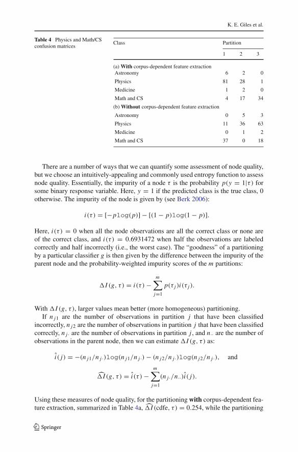
With corpus-dependent feature extraction, Iterative Denoising embeds the mixedpartition as in Fig. 6a after one iteration. Whereas, in the root node, one partition wasmixed Physics and Math/CS, after one iteration of Iterative Denoising that partitionhas been denoised into one relatively homogeneous partition containing most of thePhysics documents, one relatively homogeneous partition containing a large portionof the Math/CS documents, and one mixed partition. Table 4a shows the resultingconfusion matrix.

Contrast this performance with that of hierarchical clustering. Figure 6b shows theresults of taking the mixed partition in the root node and then performing k-meansclustering. Here the quality of the clusters is not as good compared to the quality of theleaves using corpus-dependent feature extraction. As can be seen from the resultingconfusion matrix in Table 4b, a comparatively large number of physics documents arein all three partitions, and the partition containing the most Physics documents alsocontains a large number of Math/CS documents. In addition, the partition containingthe largest number of Math/CS documents also contains a large number of Physicsdocuments. Here, Partition 1 is estimated to be Math and CS, Partition 2 is estimatedto be Physics, and Partition 3 is estimated to be Physics. So, with corpus-dependentfeature extraction, the clusters appear to be more homogeneous by class than withoutcorpus-dependent feature extraction.

(a) With CDFE. (b) Without CDFE.

Fig. 6 Iterative Denoising versus hierarchical clustering

123

K. E. Giles et al.

Table 4 Physics and Math/CSconfusion matrices

Class Partition

1 2 3

(a) With corpus-dependent feature extractionAstronomy 6 2 0

Physics 81 28 1

Medicine 1 2 0

Math and CS 4 17 34

(b) Without corpus-dependent feature extraction

Astronomy 0 5 3

Physics 11 36 63

Medicine 0 1 2

Math and CS 37 0 18

There are a number of ways that we can quantify some assessment of node quality,but we choose an intuitively-appealing and commonly used entropy function to assessnode quality. Essentially, the impurity of a node τ is the probability p(y = 1|τ) forsome binary response variable. Here, y = 1 if the predicted class is the true class, 0otherwise. The impurity of the node is given by (see Berk 2006):

i(τ ) = [−plog(p)] − [(1 − p)log(1 − p)].

Here, i(τ ) = 0 when all the node observations are all the correct class or none areof the correct class, and i(τ ) = 0.6931472 when half the observations are labeledcorrectly and half incorrectly (i.e., the worst case). The “goodness” of a partitioningby a particular classifier g is then given by the difference between the impurity of theparent node and the probability-weighted impurity scores of the m partitions:

�I (g, τ ) = i(τ ) −m∑

j=1

p(τ j )i(τ j ).

With �I (g, τ ), larger values mean better (more homogeneous) partitioning.If n j1 are the number of observations in partition j that have been classified

incorrectly, n j2 are the number of observations in partition j that have been classifiedcorrectly, n j · are the number of observations in partition j , and n·· are the number ofobservations in the parent node, then we can estimate �I (g, τ ) as:

i( j) = −(n j1/n j ·)log(n j1/n j ·) − (n j2/n j ·)log(n j2/n j ·), and

�I (g, τ ) = i(τ ) −m∑

j=1

(n j ·/n··)i( j).

Using these measures of node quality, for the partitioning with corpus-dependent fea-ture extraction, summarized in Table 4a, �I (cdfe, τ ) = 0.254, while the partitioning

123

Iterative Denoising

goodness without corpus-dependent feature extraction, summarized in Table 4b,�I (no cdfe, τ ) = 0.133. So, between the two approaches, subjectively and quan-titatively, in this example corpus-dependent feature extraction has produced leaves ofbetter quality than hierarchical clustering.

We illustrate the second point, the utility of corpus-dependent feature extractionto text mining, by returning to Node 4 of the original document corpus, shown inFig. 3a. In this node, which was produced by an iteration of Iterative Denoising onPartition 3 of the root node, a relationship was noted between two similar documentsfrom two different classes and written by two different authors that were placed inclose proximity in the Fiedler space embedding. By recomputing the features for asubset of documents, corpus-dependent feature selection has an effect of ‘tuning’ thefeatures for that subset by only considering the documents in that subset. A commonalternative is to reuse the features that were computed at the root node based on all thedocuments in the root. One benefit of having word-weights for a node be computedbased on only the documents in that node is that relationships may be found that areobscured when using global-computed word-weights.

As an example, Fig. 3b shows the resulting geometric relationships when globalword-weights are used instead of word-weights computed based on only the documentsin a subset. While much of the global document type clusters are similar to those seenin Fig. 3a, note the geometric distance between the two similar documents that werefound in close proximity when using corpus-dependent feature extraction. Here, itmight be difficult for an analyst to find these similar documents, whereas before theirclose proximity suggested they might have some relationship. In Fig. 3b, the nearestneighbor to the Life Sciences document “Skin cells reveal they have hairy origins” byJ. Travis is the Medicine document “The Y copies another chromosome’s gene”, alsoby J. Travis. The only relationship between these two documents appears to be just theauthor. So, in this case using global word-weights obscured the topic area relationshipbetween two documents that might have been of interest to an analyst, a relationshipthat was discovered by Iterative Denoising using corpus-dependent feature extraction.

5 Conclusions

Though further analysis is warranted, we have detailed our Iterative Denoising frame-work and have demonstrated its performance on a heterogeneous document corpus.In our analysis of a real-world dataset, we illustrated the usefulness of our metho-dology for allowing an analyst to discover potentially meaningful relationships inhigh-dimensional data. These results suggest that Iterative Denoising can assist theuser in the discovery of relationships of interest between documents. For example, theuser may have a known document that he/she wishes to place in context with otherunknown documents, and so visually comparing the proximity of the known docu-ment with the unknown documents may provide useful information. Also, the usermay wish to uncover common themes within a large corpus, and so the user wouldexplore the different identified clusters to find broad categories or ideas shared amongthe documents. Thus, the adjudication of these tasks can be effectively and practicallyaided by Iterative Denoising.

123

K. E. Giles et al.

References

Alpert C, Kahng A (1995) Recent directions in netlist partitioning: a summary. Integr VLSI J 19(1):1–81Arnoldi W (1951) The principle of minimized iterations in the solution of the matrix eigenvalue problem.

Q J Appl Math 9:17–29Arya S, Mount D, Netanyahu N, Silverman R, Wu A (1998) An optimal algorithm for approximate nearest

neighbor searching in fixed dimensions. J ACM 45(6):891–923Banerjee S, Pedersen T (2003) The design, implementation, and use of the ngram statistics package. In:

Proceedings of the fourth international conference on intelligent text processing and computationallinguistics. Mexico City, Mexico

Belkin M, Niyogi P (2003) Laplacian eigenmaps for dimensionality reduction and data representation.Neural Comput 15(6):1373–1396

Berk R (2006) An introduction to ensemble methods for data analysis. Sociol Methods Res 34(3):263–295Clarkson K (1999) Nearest neighbor queries in metric spaces. Discrete Comput Geom 22(1):63–69Cormack R (1971) A review of classification (with discussion). J R Stat Soc Ser A (General) 134(3):321–

367Critchley F (1988) On certain linear mappings between inner-product and squared-distance matrices. Linear

Algebra Appl 105:91–107de Leeuw J (1988) Convergence of the majorization method for multidimensional scaling. J Classif 5:163–

180Donoho D, Grimes C (2003) Hessian eigenmaps: locally linear embedding techniques for high-dimensional

data. Proc Natl Acad Sci 100(10):5591–5596Everitt B (1993) Cluster analysis, 3rd edn. Halsted Press, New YorkFaloutsos C, Lin K (1995) FastMap: a fast algorithm for indexing, data-mining, and visualization of tradi-

tional and multimedia datasets. In: Proceedings of the 1995 ACM SIGMOD international conferenceon management of data, pp 163–174

Fiedler M (1973) Algebraic connectivity of graphs. Czech Math J 23(98):298–305Garey M, Johnson D, Stockmeyer L (1974) Some simplified NP-complete problems. In: Proceedings of the

sixth annual ACM symposium on theory of computing, pp 47–63Giles K (2006) Knowledge discovery in computer network data: a security perspective. Ph.D. dissertation.

Johns Hopkins University, BaltimoreGionis A, Indyk P, Motwani R (1999) Similarity search in high dimensions via hashing. In: Proceedings of

25th VLDB conference, pp 518–529Gordon A (1999) Classification, 2nd edn. Chapman & Hall/CRC, Boca RatonGower J (1966) Some distance properties of latent root and vector methods in multivariate analysis. Bio-

metrika 53:325–338Grosjean J, Plaisant C, Bederson B (2002) Spacetree: supporting exploration in large node link tree, design

evolution and empirical evaluation. In: Proceedings of IEEE symposium on information visualization,pp 57–64

Hendrickson B, Leland R (1995) A multilevel algorithm for partitioning graphs. In: Supercomputing ’95:Proceedings of the 1995 ACM/IEEE conference on supercomputing (CDROM), ACM Press

Houle M (2003) Sash: a spatial approximation sample hierarchy for similarity search, Technical ReportRT-0517, IBM Tokyo Research Laboratory

Houle M, Sakuma J (2005) Fast approximate similarity search in extremely high-dimensional data sets. In:21st International Conference on Data Engineering, pp 619–630

Indyk P, Motwani R (1998) Approximate nearest neighbors: towards removing the curse of dimensionality.In: Proceedings of 30th ACM symposium on theory of computing, pp 604–613

Kanungo T, Mount D, Netanyahu N, Piatko C, Silverman R, Wu A (2004) A local search approximationalgorithm for k-means clustering. Comput Geom Theory Appl 28:89–112

Karypis G, Kumar V (1998) A fast and high quality multilevel scheme for partitioning irregular graphs.SIAM J Sci Comput 20(1):359–392

Kernighan B, Lin S (1970) An efficient heuristic procedure for partitioning graphs. Bell Syst Tech J49(2):291–307

Kushilevitz E, Ostrovsky R, Rabani Y (1998) An algorithm for approximate closest-point queries. In:Proceedings of the 30th ACM symposium on theory of computing, pp 614–623

Lanczos C (1950) An iteration method for the solution of the eigenvalue problem of linear differential andintegral operators. J Res Natl Bur Stand 45(4):255–282

123

Iterative Denoising

Lehoucq R, Yang C (1998) ARPACK users guide: solution of large-scale eigenvalue problems with impli-citly restarted Arnoldi methods. SIAM, Philadelphia

Lin D, Pantel P (2002) Concept discovery from text. In: Proceedings of conference on computationallinguistics, pp 577–583

Mirkin B (2005) Clustering for data mining: a data recovery approach. Chapman & Hall/CRC, Boca RatonPorter M (1980) An algorithm for suffix stripping. Program 14(3):130–137Priebe C, Marchette D, Healy D (2004a) Integrated sensing and processing decision trees. IEEE Trans

Pattern Anal Mach Intell 26(6):699–708Priebe C, Marchette D, Park Y, Wegman E, Solka J, Socolinsky A, Karakos D, Church K, Guglielmi R,

Coifman R, Lin D, Healy D, Jacobs M, Tsao A (2004b) Iterative denoising for cross-corpus discovery.In: Antoch J (ed), COMPSTAT: Proceedings in computational statistics, 16th symposium. Physica-Verlag, Springer, pp 381–392

Roweis S, Saul L (2000) Nonlinear dimensionality reduction by locally linear embedding. Science290(5500):2323–2326

Saerens M, Fouss F, Yen L, Dupont P (2004) The principal components analysis of a graph and its relation-ships to spectral clustering. In: Proceedings of the 15th European conference on machine learning.Lecture Notes in Artificial Intelligence, pp 371–383

Schalkoff R (1991) Pattern recognition: statistical structural and neural approaches. Wiley, New YorkTenenbaum J, DeSilva V, Langford J (2000) A global geometric framework for nonlinear dimensionality

reduction. Science 290(5500):2319–2322Torgerson W (1952) Multidimensional scaling: I theory and method. Psychometrika 17:401–419Trosset M, Groenen P (2005) Multidimensional scaling algorithms for large data sets. Comput Sci Stat

123