Data Adaptive Dual Domain Denoising - IPOL Journal

Published in Image Processing On Line on 2017–05–24.Submitted on 2017–02–06, accepted on 2017–05–10.ISSN 2105–1232 c© 2017 IPOL & the authors CC–BY–NC–SAThis article is available online with supplementary materials,software, datasets and online demo athttps://doi.org/10.5201/ipol.2017.203

2015/06/16

v0.5.1

IPOL

article

class

Data Adaptive Dual Domain Denoising: a Method to

Boost State of the Art Denoising Algorithms

Nicola Pierazzo and Gabriele Facciolo

CMLA, ENS Paris-Saclay, Cachan, France{Nicola.Pierazzo,facciolo}@cmla.ens-cachan.fr

Communicated by Antoni Buades Demo edited by Gabriele Facciolo

Abstract

This article presents DA3D (Data Adaptive Dual Domain Denoising), a “last step denoising”method that takes as input a noisy image and as a guide the result of any state-of-the-artdenoising algorithm. The method performs frequency domain shrinkage on shape and data-adaptive patches. DA3D doesn’t process all the image samples, which allows it to use largepatches (64× 64 pixels). The shape and data-adaptive patches are dynamically selected, effec-tively concentrating the computations on areas with more details, thus accelerating the processconsiderably. DA3D also reduces the staircasing artifacts sometimes present in smooth parts ofthe guide images. The effectiveness of DA3D is confirmed by extensive experimentation. DA3Dimproves the result of almost all state-of-the-art methods, and this improvement requires littleadditional computation time.

Source Code

The C++ source code, the code documentation, and the online demo are accessible at theIPOL web page of this article web site1 Compilation and usage instruction are included in theREADME.txt file of the archive.

Keywords: image denoising; Fourier shrinkage; shape adaptive; bilateral

1 Introduction

Image denoising is one of the fundamental image restoration challenges [25]. It consists in estimatingan unknown noiseless image y from a noisy observation x. We consider the classic image degradationmodel

y = x+ n, (1)

where the observation y of the image x is contaminated by an additive white Gaussian noise n ofvariance σ2.

1https://doi.org/10.5201/ipol.2017.203

Nicola Pierazzo and Gabriele Facciolo, Data Adaptive Dual Domain Denoising: a Method to

Boost State of the Art Denoising Algorithms, Image Processing On Line, 7 (2017), pp. 93–114. https://doi.org/10.5201/ipol.2017.203


(a) Original

20.17 dB

(b) Noisy

37.00 dB

(c) Guide: NL-Bayes

37.17 dB

(d) DDID step

37.99 dB

(e) Sparse DDID

38.07 dB

(f) DA3D

1.76%

(g) Sparse DDID samples

1.52%

(h) DA3D samples

Figure 1: Results of applying different post-processing steps on the same image (with noise σ = 25). The numbers atthe bottom of the images correspond to PSNR values, and for (g) and (h) to densities of the sparse samples. The guidewas produced with Non-Local Bayes. Figures (g) and (h) show the centers of the blocks used for denoising (e) and (f)respectively (with τ = 2). Image (d) was generated with 31 × 31 blocks, while for (e) and (f) 64 × 64 blocks were used.Notice in (e) and (f) the difference on the cheek and the forehead of the girl. Also, notice that in this case, with manysmooth areas, the amount of patches used in the process is small (1.52% in the case of DA3D).

All denoising methods assume some underlying image regularity. Depending on this assumptionthey can be divided, among others, into transform-domain and spatial-domain methods.

Transform domain methods work by shrinking (or thresholding) the coefficients of some transformdomain [34, 21, 13]. The Wiener filter [41] is one of the first such methods operating on the Fouriertransform. Donoho et al. [9] extended it to the wavelet domain.

Space-domain methods traditionally use a local notion of regularity with edge-preserving algo-rithms such as total variation [33], anisotropic diffusion [26], or the bilateral filter [38]. Nowadayshowever spatial-domain methods achieve remarkable results by exploiting the self-similarities of theimage [2]. Patch-based methods are called non-local because they denoise by averaging similarpatches in the image. Patch-based denoising has developed into attempts to model the patch spaceof an image, or of a set of images. These techniques model each patch as a sparse representation ona learned patch dictionary [11, 23, 22, 44, 8], using a Gaussian Scale Mixture model [45, 31, 32], orwith non-parametric approaches by sampling from a huge patch database [19, 20, 29, 24].

Current state-of-the-art denoising methods such as BM3D [5] and NL-Bayes [17] take advantage ofboth space- and transform-domain approaches. They group similar image patches and jointly denoisethem by collaborative filtering on a transformed domain. In addition, they proceed by applying twoslightly different denoising stages, the second stage using the output of the first one as its guide.

Some recently proposed methods use the result of a different algorithm as their guide for a newdenoising step. Combining for instance, non-local principles with spectral decomposition [37], orBM3D with neural networks [4]. This allows one to mix different denoising principles, to improvethe image quality.

DDID [15] is an iterative algorithm that uses a guide image (from a previous iteration) to de-

94

Data Adaptive Dual Domain Denoising: a Method to Boost State of the Art Denoising Algorithms

termine spatially uniform regions to which Fourier shrinkage could be applied without introducingringing artifacts. Several methods [14, 16, 27] use a single step of DDID with a guide image producedby a different algorithm. This yields much better results than the original DDID. The reason fortheir success is the use of large (31× 31) and shape-adaptive patches. Indeed, the Fourier shrinkageworks better on large stationary blocks.

Unfortunately, DDID has a prohibitive computational cost, as it paradoxically denoises a largepatch to recover a single pixel. Moreover, contrary to other methods, aggregation of these patchesdoesn’t improve the results since it introduces blur. In [30] these two problems were solved byintroducing a new patch selection, accompanied by a weighted aggregation strategy.

This paper describes the DA3D (Data Adaptive Dual Domain Denoising) algorithm, briefly in-troduced in the conference paper [30]. It is a “last step” denoising method that performs frequencydomain shrinkage on shape-adaptive and data-adaptive patches. DA3D consistently improves theresults of state-of-the-art methods such as BM3D or NL-Bayes with little additional computationtime.

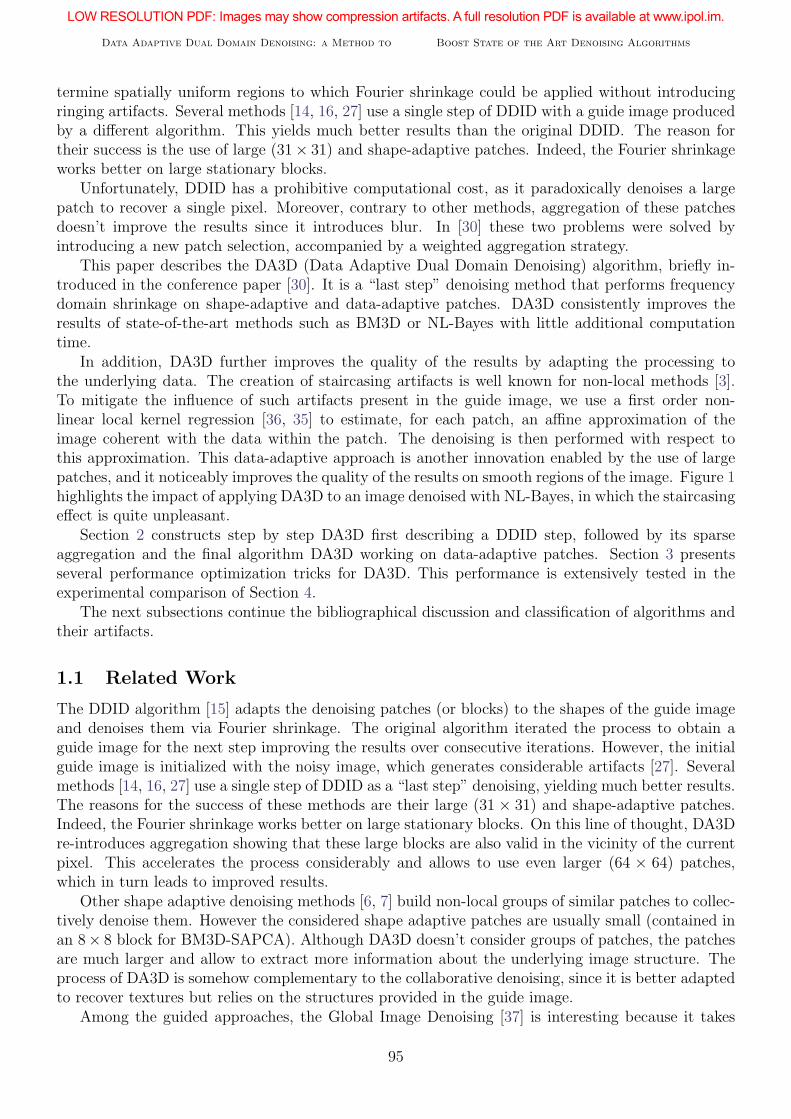
In addition, DA3D further improves the quality of the results by adapting the processing tothe underlying data. The creation of staircasing artifacts is well known for non-local methods [3].To mitigate the influence of such artifacts present in the guide image, we use a first order non-linear local kernel regression [36, 35] to estimate, for each patch, an affine approximation of theimage coherent with the data within the patch. The denoising is then performed with respect tothis approximation. This data-adaptive approach is another innovation enabled by the use of largepatches, and it noticeably improves the quality of the results on smooth regions of the image. Figure 1highlights the impact of applying DA3D to an image denoised with NL-Bayes, in which the staircasingeffect is quite unpleasant.

Section 2 constructs step by step DA3D first describing a DDID step, followed by its sparseaggregation and the final algorithm DA3D working on data-adaptive patches. Section 3 presentsseveral performance optimization tricks for DA3D. This performance is extensively tested in theexperimental comparison of Section 4.

The next subsections continue the bibliographical discussion and classification of algorithms andtheir artifacts.

1.1 Related Work

The DDID algorithm [15] adapts the denoising patches (or blocks) to the shapes of the guide imageand denoises them via Fourier shrinkage. The original algorithm iterated the process to obtain aguide image for the next step improving the results over consecutive iterations. However, the initialguide image is initialized with the noisy image, which generates considerable artifacts [27]. Severalmethods [14, 16, 27] use a single step of DDID as a “last step” denoising, yielding much better results.The reasons for the success of these methods are their large (31 × 31) and shape-adaptive patches.Indeed, the Fourier shrinkage works better on large stationary blocks. On this line of thought, DA3Dre-introduces aggregation showing that these large blocks are also valid in the vicinity of the currentpixel. This accelerates the process considerably and allows to use even larger (64 × 64) patches,which in turn leads to improved results.

Other shape adaptive denoising methods [6, 7] build non-local groups of similar patches to collec-tively denoise them. However the considered shape adaptive patches are usually small (contained inan 8× 8 block for BM3D-SAPCA). Although DA3D doesn’t consider groups of patches, the patchesare much larger and allow to extract more information about the underlying image structure. Theprocess of DA3D is somehow complementary to the collaborative denoising, since it is better adaptedto recover textures but relies on the structures provided in the guide image.

Among the guided approaches, the Global Image Denoising [37] is interesting because it takes

95


(a) Original

σ = 40

(b) Noisy

26.74 dB

(c) Non-Local Means

27.08 dB

(d) DCT denoising

27.72 dB

(e) BM3D

28.17 dB

(f) NL-Bayes

28.36 dB

(g) NL-Bayes + DA3D

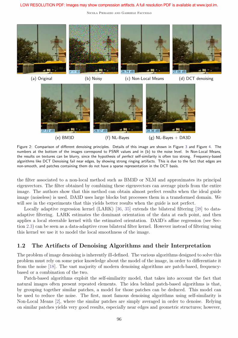
Figure 2: Comparison of different denoising principles. Details of this image are shown in Figure 3 and Figure 4. Thenumbers at the bottom of the images correspond to PSNR values and in (b) to the noise level. In Non-Local Means,the results on textures can be blurry, since the hypothesis of perfect self-similarity is often too strong. Frequency-basedalgorithms like DCT Denoising fail near edges, by showing strong ringing artifacts. This is due to the fact that edges arenon-smooth, and patches containing them do not have a sparse representation in the DCT basis.

the filter associated to a non-local method such as BM3D or NLM and approximates its principaleigenvectors. The filter obtained by combining these eigenvectors can average pixels from the entireimage. The authors show that this method can obtain almost perfect results when the ideal guideimage (noiseless) is used. DA3D uses large blocks but processes them in a transformed domain. Wewill see in the experiments that this yields better results when the guide is not perfect.

Locally adaptive regression kernel (LARK) [36, 35] extends the bilateral filtering [38] to data-adaptive filtering. LARK estimates the dominant orientation of the data at each point, and thenapplies a local steerable kernel with the estimated orientation. DA3D’s affine regression (see Sec-tion 2.3) can be seen as a data-adaptive cross bilateral filter kernel. However instead of filtering usingthis kernel we use it to model the local smoothness of the image.

1.2 The Artifacts of Denoising Algorithms and their Interpretation

The problem of image denoising is inherently ill-defined. The various algorithms designed to solve thisproblem must rely on some prior knowledge about the model of the image, in order to differentiate itfrom the noise [18]. The vast majority of modern denoising algorithms are patch-based, frequency-based or a combination of the two.

Patch-based algorithms exploit the self-similarity model, that takes into account the fact thatnatural images often present repeated elements. The idea behind patch-based algorithms is that,by grouping together similar patches, a model for those patches can be deduced. This model canbe used to reduce the noise. The first, most famous denoising algorithms using self-similarity isNon-Local Means [2], where the similar patches are simply averaged in order to denoise. Relyingon similar patches yields very good results, especially near edges and geometric structures; however,

96


(a) Original (b) Noisy (c) Non-Local Means (d) DCT denoising

(e) BM3D (f) NL-Bayes (g) NL-Bayes + DA3D

Figure 3: Comparison of different denoising principles and their best representative algorithms. Detail of borders and high-contrast textures. Notice that DA3D removes all the artifacts from Non-Local Bayes, and at the same time it improves thecontrast in textures.

(a) Original (b) Noisy (c) Non-Local Means (d) DCT denoising

(e) BM3D (f) NL-Bayes (g) NL-Bayes + DA3D

Figure 4: Comparison of different denoising principles and algorithms. Detail of smooth and textured areas.

97


(a) Smooth signal (b) Signal with discontinu-ity (edge)

(c) DCT of smooth signal (d) DCT of signal with dis-continuity

Figure 5: Behaviour of DCT coefficients. Signals containing discontinuities have their energy less concentrated in the DCTdomain. This makes the DCT basis less effective for denoising purposes in presence of edges.

the results on textures can be blurry (see Figure 2c), since the hypothesis of perfect self-similarity isoften too strong. Recently, patch-based denoising has developed into attempts to model the patchspace of an image, or of a set of images. These techniques model the patch as sparse representationson dictionaries [11, 23, 22, 44, 8], using Gaussian Scale Mixtures models [45, 31, 32], or with non-parametric approaches by sampling from a huge database of patches [19, 20, 29, 24].

Other algorithms are frequency based. These algorithms suppose a certain degree of regularity onthe image, and therefore they try to represent its patches in a basis that “sparsifies” them [34, 21,13]. Since white noise is unaffected by an orthogonal change of basis, in the transform domain thesignal regarding the image is concentrated in few frequencies, while the noise itself remains evenlydistributed, and therefore can be easily removed (for example, by a simple thresholding or with aWiener filter [41]). A simple algorithm that uses this model is DCT denoising [43], that uses theDCT basis and a Wiener filter on the coefficients. The DCT basis has the property that smoothsignals have most of the energy concentrated on the low frequencies. The problem with frequency-based denoising is that, sometimes, the patches do not follow the model that works well with thebasis. For DCT denoising, in Figure 2d, the failures of the algorithm are evident near the edges.This follows from the fact that edges are non-smooth parts of the image, and patches containingthem have their energy less concentrated in the DCT domain (as shown in Figure 5). Denoisingby DCT thresholding therefore reverberates around the edges, creating oscillations known as Gibbseffect. The class of frequency based algorithms is not limited to the DFT or DCT basis. SimilarGibbs effects are observed with algorithms that perform filtering in other wavelet domains [9].

Modern algorithms try to use both self-similarity and frequency priors, to achieve better results.Among them, the most famous is BM3D [5], that denoises blocks of similar patches in the DCTdomain. Since the patches are denoised together, this effectively allows to take into account theirsimilarity. BM3D is nowadays considered as one of the best denoising algorithms, and it has verygood results in terms of PSNR. Its main drawback is that, since it uses the DCT basis for thethresholding operation, it can still present Gibbs artefacts around the edges (as in Figure 2e).

An evolution of BM3D that uses an adaptive Bayesian model instead of the fixed DCT basisused in BM3D is Non-Local Bayes. This algorithm presents fewer artifacts than BM3D, especiallyin smooth areas, and has a similar performance in terms of PSNR. Compared to BM3D, Non-LocalBayes loses some contrast in textures.

DA3D applied to the result of a patch-based denoising algorithm such as Non-Local Bayes givesthe best result in terms of both PSNR and visual quality. Notice in particular the results near bordersand textures (Figure 3 and 4).

98


Figure 6: Illustration of DDIDs preprocessing of a patch. The kernel k is computed using the guide g. In the modified patchym all object discontinuities have been removed, leaving only the texture information corresponding to the object selectedby the kernel k. The removed pixels are replaced by the average of the relevant part of the patch.

2 Stepwise Construction of DA3D

2.1 Interpreting the Performance of a Dual Domain Image DenoisingStep

A DDID step is a single iteration of the DDID algorithm [15], but it can also be used as a lastdenoising step for other methods [27, 14]. This section, along with the pseudocode in Algorithm 1,summarizes it.

This interpretation differs from the one originally proposed by Knaus and Zwicker [15], but itleads to the same exact algorithm. The original interpretation of DDID splits the image into a low-and a high-contrast layer, which are treated respectively with a spatial and a frequency domainmethod. Here, the spatial domain filtering is seen as a pre-processing to improve the frequencydomain denoising.

To denoise a pixel p from the noisy image y the DDID step extracts a 31× 31 pixel block aroundit (denoted y) and the corresponding block g from the guide image g.

The blocks are processed to eliminate discontinuities that may cause artifacts in the subsequentfrequency-domain denoising. To that end, the weight function k is derived from g. The weightsidentify the pixels of the block belonging to the same object as the center p. This weight functionhas the form of the bilateral filter [42, 38]

k(q) = exp

(

−|g(q)− g(p)|2

γrσ2

)

exp

(

−|q − p|2

2σ2s

)

. (2)

The first term in this function is the range kernel, and it is used to identify the pixels belonging tothe same structure as p, by selecting the ones with a similar color in the guide. The parameter γr ischosen empirically in [15] and it is equal to 0.7, and σ is the standard deviation of the noise. Theway (2) is constructed means that, when there is less noise, a much more uniform, albeit smaller,area is taken into account.

The second term of (2) is the spatial kernel, and it removes the periodization discontinuitiesassociated with the Fourier transform. This term does not depend on the noise, but it is roughlyrelated to the size of the block and in [15] it is set to 7.0.

As said in Section 1.2, denoising by filtering Fourier coefficients presents problems in presence ofedges (due to the Gibbs phenomenon). To avoid that, the blocks are made as regular as possible,by removing the parts that are not selected by k (and therefore not relevant to the denoising of thecentral pixel). First, the average of the “relevant” part of both the noisy and the guide blocks iscomputed

s =

∑

k(q)y(q)∑

k(q), g =

∑

k(q)g(q)∑

k(q), (3)

99


where the sums are computed over Np, the domain of the d × d block centered at p. After that,the parts of the block not taken into account by k are set to the respective average. The resultingmodified block is

ym(q) = k(q)y(q) + (1− k(q))s. (4)

As illustrated in Figure 6 the block ym is similar to y in the parts belonging to the same object asthe central pixel (including the noise) and smooth in the rest. The same procedure is applied to theblock extracted from the guide

gm(q) = k(q)g(q) + (1− k(q))g. (5)

In this way the “relevant” part of the blocks (similar to the central pixel) is retained by ym and gm,and their average value is assigned to the rest.

At this point, ym and gm are two patches, built in the same way, in which discontinuities havebeen strongly reduced and only information “relevant” to denoise the central pixel has been kept. Itis therefore safe to apply the Fourier transform and to continue the process in the frequency domain

G(f) =∑

q∈Np

exp

(

−2iπ(q − p)f

d

)

gm(q), (6)

S(f) =∑

q∈Np

exp

(

−2iπ(q − p)f

d

)

ym(q). (7)

Assuming that y contains an additive white Gaussian noise of variance σ2, the amount of noisepresent in ym only depends on k. In particular, for a pixel q, ym(q) contains a noise equal to σ2k(q)2.An interesting property of the Fourier transform is that the noise in every pixel is evenly distributedover all frequencies. Thus every frequency of S has Gaussian noise with the same variance

σ2f = σ2

∑

q∈Np

k(q)2. (8)

The patch is then denoised by shrinking its Fourier coefficients S(f) by the shrinkage factor

K(f) =

{

1 if f = 0,

exp(

−γfσ

2f

|G(f)|2

)

otherwise,(9)

where γf is a parameter of the algorithm, and it is determined in [15] to be 0.8. Since discontinuitieshave been removed from the blocks, filtering in the Fourier domain doesn’t introduce ringing, whichis a major advance made by DDID in transform thresholding methods.

The denoised value of the central pixel is finally recovered by reversing the Fourier transform.Since the inverse Fourier transform evaluated in the center of the patch is the average of the frequen-cies, the central pixel’s value can be computed as

x(p) =1

d2

∑

f

S(f)K(f). (10)

This process is repeated for every pixel of the image.For color images, k is computed by using the Euclidean distance, while the shrinkage is done

independently on each channel of the YUV color space. For more details about DDID refer to [15, 27].An example of the result is shown in Figure 8d.

100


Algorithm 1: Pseudo-code for DDID step, Sparse DDID and DA3D. The lines used only in theDDID step are highlighted in blue. Bullets show the operations of each algorithm. Variables inbold denote whole images, while italics denote single blocks. Multiplication and division arepixel-wise.

DDID

Sparse

DA3D Input: y (noisy image), g (guide)

Output: denoised image

- • • 1 w← 0• • • 2 out← 0• - - 3 for all pixels p ∈ y do- • • 4 while min(w) < τ do- • • 5 p← argmin(w) // fast alternative to linear search explained in Section 3• • • 6 y ← ExtractPatch(y, p)• • • 7 g ← ExtractPatch(g, p)- - • 8 kreg ← ComputeKreg(g) // regression weight, Equation (12)- - • 9 P ← argminP

∑

[y(q)− P (q)]2 · kreg(q) // regression plane, Equation (11)- - • 10 y ← y − P // subtract plane from the block- - • 11 g ← g − P // and from guide• • • 12 k ← ComputeK(g) // eq. 2- • • 13 if ‖k‖1 < η then // If patch weights are too small (Section 3)- • • 14 aggw ← k · k // compute aggregation weight- • • 15 w← AddPatchAt(p,w, aggw)- • • 16 out← AddPatchAt(p,out, aggw · (g + P )) // copy guide to output- • • 17 continue // and skip to the next patch

• • • 18 ym ← k · y + (1− k) ·(∑

k(l)y(l)∑k(l)

)

• • • 19 gm ← k · g + (1− k) ·(∑

k(l)g(l)∑k(l)

)

• • • 20 Y ← DFT(ym)• • • 21 G← DFT(gm)• • • 22 σ2

f ← σ2∑

k(q)2

• • • 23 K ← ComputeShrinkageFactor(

|G(f)|2

σ2f

)

// shrinkage

• • • 24 xm ← IDFT(K · Y )

- • • 25 x←[

xm − (1− k)(∑

k(l)y(l)∑k(l)

)]

/k // revert line 18

- - • 26 x← x+ P // add plane back to the block- • • 27 aggw ← k · k // aggregation weight• - - 28 out(p)← ExtractCentralPixel(xm)

// accumulate patch in the correct position- • • 29 w← AddPatchAt(p,w, aggw)- • • 30 out← AddPatchAt(p,out, aggw · x)• - - 31 return out- • • 32 return out/w

101


0 1 2 3 4 50

0.1

0.2

0.3

0.4

0.5

% of samples

PSNR

gainindB

k

k2

Peppers

Traffic

k3

Figure 7: Comparison of aggregation weights using k, k2, and k3. The curves show the improvement of DA3D (withrespect to the PSNR of the guide NL-Bayes) as a function of the number of processed samples. Most of the images behaveas Traffic, where similar results are obtained using k or k2. However for some images (such as Peppers) k is worse andintroduces artifacts.

2.2 Sparsifying a DDID Step

The DDID step explained in Section 2.1 is slow in practice because it has to process a block forevery pixel. In fact, each pixel is denoised several times, but the result is discarded every time thatit is not in the center of the current block. Since the denoising remains valid for all pixels in the“relevant” part of the block, we propose to aggregate the processed blocks to form the final result.As a result only a small number of blocks needs to be processed, thus accelerating the algorithmconsiderably. Note that since the processing is done with the modified block, line 18 of Algorithm 1must be reverted to obtain the denoised block (line 25).

In the selection-aggregation process of Sparse DDID, the image is treated by color-coherent blocksand the results are aggregated with weights deduced from the guide image. This weighted average canalso be seen as the interpolation of the denoised image from a subset of processed blocks [10, 1, 12].We found that the best aggregation weights are obtained by squaring the weights (2). In Figure 7various choices of aggregation weights are compared, among which k and k2 give the best results.However, in practice the choice of k2 is preferable, since in some cases k introduces small artifacts.

We now describe the greedy approach used for selecting the image blocks to be processed. Ateach iteration a weight map w with the sum of the aggregation weights is updated. This weight mappermits to identify the pixel in the image with the lowest aggregation weight (Section 3 describes anefficient way to store and lookup the aggregation weights), which will be selected as the center of thenext block to process (line 5 of Algorithm 1). This process iterates until the total weight for eachpixel becomes larger than a threshold τ . The weight function k is always equal to 1 in the center, sothe algorithm always terminates. The procedure is detailed in Algorithm 1. Sparse DDID is fasterto execute than a single DDID step, since only a small number of blocks are actually processed.This allows bigger patches to be used, that in turn gives better results in terms of denoising quality.Experimentally, good results are achieved with patches as large as 64× 64, which is to be contrastedto patch based methods using mostly 8× 8 patches. An example of the result is shown in Figure 8e.The total number of processed blocks depends on the image complexity. The centers of the effectivelyprocessed blocks are shown in Figure 8g. They concentrate on edges and details.

2.3 Ending with Data Adaptive Dual Domain Denoising (DA3D)

We now address a main drawback of the weight function (2), used for the bilateral filter and formany bilateral-inspired filters, including patch based methods. This weight function selects pixelsof the block with a similar value. As a result, Sparse DDID works by processing parts of the image

102


(a) Original

20.17 dB

(b) Noisy

26.03 dB

(c) Guide: NL-Bayes

26.05 dB

(d) DDID step

26.20 dB

(e) Sparse DDID

26.21 dB

(f) DA3D

16.9%

(g) Sparse DDID samples

16.5%

(h) DA3D samples

Figure 8: Results of applying different post-processing steps on the same image (with noise σ = 25). The numbers atthe bottom of the images correspond to PSNR values, and for (g) and (h) to densities of the sparse samples. The guidewas produced with Non-Local Bayes. Figures (g) and (h) show the centers of the blocks used for denoising (e) and (f)respectively (with τ = 2). Image (d) was generated with 31 × 31 blocks, while for (e) and (f) 64 × 64 blocks were used.Unlike Figure 1, DA3D uses a bigger portion of the image patches to denoise the image. This is due to a prominence oftextured areas.

that are roughly piecewise constant, considering the image as composed by many “flat” layers. Thismodel is not well adapted for images that contain gradients or shadings, as the same smooth regionmay be split in many thin regions. The previous method can be extended to “normalize” eachpatch by subtracting an estimation of the gradient around the patch center. In practice, this meansestimating an affine model of the block, as proposed in [36], which can be computed using a weightedleast squares regression

minP

∑

[y(q)− P (q)]2 · kreg(q), (11)

where the sum is computed over the domain of y and kreg is a bilateral weight function

kreg(q) = exp

(

−|g(q)− g(p)|2

γrrσ2−|q − p|2

2σ2sr

)

, (12)

which selects the parts of the block that gets approximated by P . To ensure that the central pixelgets denoised, the constraint P (p) = g(p) is also added. Since the weights kreg should capture theoverall shape of the block, they are computed using a larger range parameter than the bilateralweight function in (2). It is worth noting that although kreg uses the guide to select the parts of theblock in which to perform the estimation, the regression is performed directly on the noisy data y,thus allowing to correct any staircasing effect already present in the guide. The parameters σsr andγrr are specific of the algorithm. The case of color images is identical, since (11) is separable andcan be computed independently on every channel.

Once estimated, the local plane P is subtracted from the patch, effectively removing shades andgradients. Then the standard DDID step is used to denoise the block and at the end the plane isadded back. The whole procedure is detailed in Algorithm 1 (lines 8-11, 26). A real example of thealgorithm run on a patch is shown in Figure 9.

103


y kreg g

y − P P g − P

ym gm

denoised ym output for ag-

gregation

k

y kreg g

y − P P g − P

ym gm

denoised ym output for ag-

gregation

k

Figure 9: Steps of the DA3D algorithm. The figure on the left shows what happens to a noisy patch taken in a naturalimage, containing an edge. The figure on the right corresponds to a patch containing only a texture. The arrows indicatethe elements needed to compute every step of the algorithm. Notice that, thanks to the weight function, the useful part ofthe patch is kept, while the discontinuities are completely removed.

An example of the result is shown in Figure 8f. Observe that the result presents fewer staircas-ing effects and has a larger PSNR. In addition, fewer blocks are treated to denoise the gradients(Figure 8h).

Shrinkage curves tests. In DA3D the shrinkage is performed via a simple exponential dampening,the same that is used in DDID. Since DA3D is conceived to be applied on top of another algorithm,we can expect to have a better result if the shrinkage function is adapted to the guide.

However we observed that optimizing the shrinkage curve is less important than expected. Ourresults indicate that the effectiveness of DA3D lies more on the bilateral weight and on the sparseaggregation than on the shrinkage step itself. We observed that even big changes in the parameterswere reflected in small improvements on the overall PSNR.

Moreover, the patches that are more affected by changes of the shrinkage curve are the ones witha large support. Yet, if a patch has a large support (or, in other terms, a large weight k), this meansthat the patch is mostly flat. A mostly flat patch will have almost all its coefficients already close tozero, so changing the shrinkage curve will not yield a big difference.

3 Reducing the Computational Complexity of DA3D

The algorithm, as it is described in the previous sections, can still be slow if implemented naively. Inparticular, keeping track of the minimum weight (Algorithm 1, lines 4–5) can require scanning the

104


MIN

MIN

MIN

MIN

MIN MIN

Figure 10: Scheme of the quad-tree used in DA3D to keep track of the minimum weight. Each node of the tree containsthe minimum value of its four children. In order to retrieve the position of the minimum value, one has simply to traversethe tree from the root to the leaf, always choosing one of the children with the minimum value.

whole image. In addition, the matter of parallel processing was not addressed. This section describesthese improvements.

3.1 Copying from the Guide if the Selected Patch is Too Small

We observed that if the patch being processed by DA3D does not contain enough information (forinstance the texture patch in Figure 9), then the frequency processing does not improve the overallresult. Therefore, when k (computed in Algorithm 1, line 12) has a total weight below a certainthreshold η, the patch is not further processed and its guide value is used for the aggregation.

We found that a value of η = 10 allows a substantial speed-up, especially on heavily texturedimages, without significant changes to the result.

3.2 Tracking the Minimum Weight

A naive implementation of the selection of the position with the lowest aggregation weight (asexplained in Section 2.2) consists in using a simple linear search. This approach shows its limitswhen the size of the image increases. Selecting a new block to process requires approximately O(n)operations, where n is the number of pixels of the image. Therefore, under the reasonable assumptionthat the number of processed blocks is a fraction of the total (from the original article, between 1%and 20%), and since the denoising of a block is performed in a bounded time, the complexity of thealgorithm is O(n2).

Therefore, in [28] we proposed to use a quad-tree to keep track of the minimum (illustrated inFigure 10). The weight map w is in the leaves of the tree, and every node contains the minimumvalue of its four children. This can also be interpreted as a multi-scale version of w, built using amin filter. The space complexity for this data structure is

logn∑

i=0

n

4i≤

4

3n = O(n) (13)

because every “layer” of the tree contains a fourth of the values of the previous one.In order to retrieve the position of the minimum value, one has simply to traverse the tree from

the root to the leaf, always choosing one of the children with the minimum value. This guaranteesthat the chosen pixel is a global minimum for w, and has time complexity O(log n).

105


Figure 11: Test images used in the experiments. No parameter learning or fitting was performed on this database. Theimage were chosen to include different features normally found in natural images, i.e. smooth areas, textures and geometricelements.

To update the tree, it suffices to update the appropriate leaves, and then recompute the minimain the upper nodes until the top. One could be tempted to update the tree by inserting the valuesof the patch one by one. Although this could be simpler to implement, it is slower, having a timecomplexity of O(k log n). Since the aggregation is done one patch at a time, it is simple to calculateat each level which nodes need to be updated, thus avoiding to recompute the values for areas inwhich w has not changed. The time complexity for this update is O(k), where k is the number ofpixels of the patch that is being aggregated. Since k is constant, the aggregation does not increasethe complexity of the algorithm.

3.3 Parallel Processing

Since DA3D selects the patches to denoise in a greedy fashion, it is impossible to know where thenext patch will be prior to the aggregation step of the current one. This makes parallelization morecomplex than in other denoising algorithms.

In order to denoise a pixel p, the algorithm uses the other pixels inside a (64×64) window, all thepixels needed to denoise p are at a distance of at most 32. This makes the algorithm local, and allowsto solve the problem of parallelism by just dividing the image in tiles. Each tile can be denoisedseparately, and then the results can be combined together.

It is clear that the patches chosen in this way will not correspond exactly to the patches chosenwithout parallelism. The main difference can be an over-sampling of the areas near the edges, sincethe weights from a neighboring tile are not taken into account. This could result in a slight overheadin the processing time. However, the experiments show that the overhead is negligible, and theresults of the simple and parallel versions of the algorithm are identical from a practical standpoint.With bigger images, the overlap area becomes smaller, therefore the factor of acceleration becomeseven closer to the number of processors.

4 Experimental Comparison of Algorithms

Our implementation of the DA3D algorithm has been tested against the set of images shown inFigure 11. For γr and γf , the parameters of DDID [15] were kept (γr = 0.7, γf = 0.8), but sinceDA3D does not need to process all patches, the size of the patches themselves was chosen as 64× 64,with σs = 14. The parameters τ = 2, σsr = 20, γrr = 7, and η = 10 were chosen experimentally on

106


(a) Original

32.764 dB

(b) SAPCA

32.724 dB

(c) PID

32.998 dB

(d) BM3D+DA3D

Figure 12: Denoising results for Montage, σ=25. Staircasing effects are present in (b) and (c), and they are significantlyreduced in (d) by DA3D.

images outside the test database.The DA3D method was applied to the results of several state-of-the-art algorithms. Each method

was tested with noises of σ = 5, 10, 25, 40, 80. The results are summarized in Table 1.DA3D improves the PSNR of every algorithm except NLDD and PID (which is to be expected,

since they are based on a similar shrinkage strategy). This improvement is more marked with highernoises, which makes sense since the parameters of DDID were optimized for medium to high noise.It is worth mentioning that DA3D is even able to improve over BM3D-SAPCA, which is consideredthe best denoising algorithm up to date for grayscale images. Similar results are obtained usingSSIM [39] as metric.

In general BM3D+DA3D (DA3D using BM3D as guide) offers one of the best performances witha reasonable computational cost. As an example the results of the best two performing methods forthe image “Montage” are shown in Figure 12, along with the result of BM3D+DA3D. The latteroutperforms the other algorithms in terms of PSNR and image quality. Despite having a high PSNRvalue, the results of the other two algorithms present artifacts close to the edges and some staircasing(BM3D-SAPCA in particular).

Table 2 shows the results obtained for color images. In this case fewer algorithms have beentested since most methods only work for grayscale images. While for small noise levels DA3D doesnot improve the PSNR of the existing methods, for higher noise levels the gain is considerable. Inthe case of BM3D and NL-Bayes, this improvement is even larger than for grayscale images. As inthe grayscale case, NLDD and PID are not improved (or just marginally improved) by DA3D.

Figure 13 shows the two best denoising results for the image “Dice”, along with the result ofBM3D+DA3D. Most of the artifacts generated by BM3D disappear with the post-processing, andat the same time the edges becomes sharper and the gradients smoother.

Comparison with other last-step denoising methods. Figure 14 compares the result of threealgorithms: DA3D, G-NLM [37] and the third iteration of DDID [15] (as done in NLDD[27]). ThePSNR gain over Non-Local Means is shown for every algorithm and for every image in the test set.Non-Local Means has been chosen as a guide to make a fairer comparison, since it is the one used inG-NLM. It can be seen that DA3D achieves better results for all noise levels.

Running time. The time needed to run the analyzed algorithms is summarized in Table 3. UsingDA3D as a post-processing method demands little additional time, while the gain is substantial (inPSNR and in visual quality). For example, BM3D + DA3D turns out to take 1.52s, while BM3Dalone requires 1.26s. Therefore, while BM3D+DA3D is comparable to BM3D-SAPCA in terms ofperformance, its computation is more than 200 times faster.

107


Method σ=5 σ=10 σ=25 σ=40 σ=80

BM3D 38.43 34.94 30.58 28.27 24.69- 38.39 34.95 30.67 28.41 25.09

SAPCA [6] -0.04 +0.01 +0.10 +0.14 +0.39

38.24 34.70 30.37 27.99 24.94

BM3D [5] 38.24 34.78 30.54 28.23 25.03

+0.00 +0.08 +0.16 +0.24 +0.09

37.95 34.55 30.34 28.05 24.68DDID [15] 37.90 34.52 30.39 28.16 24.84

-0.04 -0.03 +0.05 +0.11 +0.16

37.91 34.29 29.90 27.64 24.46EPLL [45] 37.92 34.39 30.21 28.04 24.80

+0.01 +0.10 +0.31 +0.40 +0.34

35.07 33.54 29.19 26.87 23.45G-NLM [37] 35.67 33.97 29.77 27.49 24.10

+0.60 +0.43 +0.58 +0.63 +0.65

38.29 34.75 30.35 28.07 24.78LSSC [22] 38.34 34.88 30.61 28.32 24.97

+0.05 +0.13 +0.27 +0.25 +0.19

MLP 34.63 30.44+ 34.78 30.61

BM3D [4] +0.15 +0.17

38.19 34.62 30.13 27.86 24.45NLB [17] 38.20 34.72 30.38 28.14 24.78

+0.02 +0.10 +0.25 +0.28 +0.33

38.12 34.62 30.30 28.11 24.83NLDD [27] 38.09 34.60 30.29 28.09 24.77

-0.04 -0.02 -0.01 -0.02 -0.05

37.31 33.58 28.97 26.50 22.72NLM [2] 37.49 33.98 29.66 27.45 24.17

+0.18 +0.40 +0.69 +0.95 +1.44

37.97 34.56 30.38 28.18 24.99

PID [16] 37.90 34.48 30.28 28.08 24.81-0.07 -0.08 -0.10 -0.11 -0.18

38.31 34.78 30.39 28.16 25.00

SAIST [8] 38.31 34.82 30.53 28.27 25.07

-0.01 +0.04 +0.14 +0.11 +0.07

Table 1: Average PSNR comparison between state-of-the-art methods on grayscale images. The first line of each row showsthe average PSNR. The second line shows the average PSNR of DA3D using the corresponding algorithm to generate theguide. The third line shows the average improvement due to DA3D. The best result for each noise level is shown in bold,and the ones within a range of 0.2 dB are shown in gray. MLP+BM3D only works for some specific levels of noise, theother levels are left blank.

108


Method σ=5 σ=10 σ=25 σ=40 σ=80

39.55 36.01 31.79 29.23 26.83

BM3D [5] 39.59 36.23 32.15 29.95 27.00

+0.05 +0.22 +0.36 +0.72 +0.16

39.20 35.91 31.88 29.75 26.41DDID [15] 39.11 35.87 31.99 29.98 26.85

-0.09 -0.04 +0.11 +0.23 +0.43

39.77 36.09 31.71 29.35 26.64NLB [17] 39.67 36.26 32.18 30.09 26.74

-0.10 +0.16 +0.47 +0.74 +0.11

39.26 35.90 31.98 29.90 26.60NLDD [27] 39.17 35.87 31.99 29.97 26.63

-0.09 -0.04 +0.02 +0.07 +0.03

39.03 35.81 32.05 30.10 27.00

PID [16] 38.99 35.80 32.03 30.02 26.83

-0.04 -0.02 -0.02 -0.08 -0.17

Table 2: Average PSNR comparison between state-of-the-art methods for color images. The first line of each row showsthe average PSNR obtained by denoising the test images. The second line shows the average PSNR of DA3D using thecorresponding denoising algorithm to generate the guide. The third line shows the average improvement due to DA3D. Thebest result for each noise level is shown in bold, and the ones within a range of 0.2 dB are shown in gray.

(a) Original

39.452 dB

(b) BM3D

38.999 dB

(c) NL-Bayes

40.303 dB

(d) BM3D+DA3D

Figure 13: Denoising results for Dice, σ = 25.

Size Global SAPCA NLB PID BM3D SAIST MLP EPLL DDIDBM3D+DA3D

256×256 357 s 639 s 0.48 s 188 s 1.26 s 37.8 s 16.5 s 71.7 s 5.26 s 1.52 s512×512 3359 s 2490 s 0.80 s 725 s 4.94 s 140 s 60.7 s 272 s 20.4 s 5.59 s

Table 3: Average running time depending on image size between grayscale denoising methods. The experiments wereperformed on an 8-core 2.67GHz Xeon CPU. Every algorithm was tested using its official implementation. For DA3D theC++ implementation of this article was used.

109


DA3DDDID step

Global

σ=5

DA3DDDID step

Global

σ=10

DA3DDDID step

Global

σ=25

PSNR gain in dB

DA3DDDID step

Global

σ=40

1.5 1.0 0.5 0.0 0.5 1.0 1.5 2.0

DA3DDDID step

Global

σ=80

Figure 14: PSNR gain for three different “last step” denoising methods. NLM was used to generate the guide. Each dotrepresents an image of the test set. Note that DA3D does not only improve the results on average, but it does it consistently.

5 Conclusion

In this paper we described DA3D, a fast Data Adaptive Dual Domain Denoising algorithm for “laststep” processing. It performs frequency domain shrinkage on shape and data-adaptive patches. Thekey innovations of this method are a sparse processing that allows bigger blocks to be used and aplane regression that greatly improves the results on gradients and smooth parts. The experimentsshow that DA3D improves the results of most denoising algorithms with reasonable computationalcost, achieving a performance superior to the state-of-the-art.

Acknowledgment

Work partly founded by BPI France and Region Ile de France, in the framework of the FUI 18 PleinPhare project, the European Research Council (advanced grant Twelve Labours n246961), the Officeof Naval research (ONR grant N00014-14-1-0023), Centre National d’Etudes Spatiales (CNES, MISSProject), and ANR-DGA project ANR-12-ASTR-0035. The authors would also like to thank Prof.Jean-Michel Morel for his support, suggestions, and many fruitful discussions.

Image Credits

Miguel Colom, CC-BY

The USC-SIPI Image Database [40]

Standard test images

Crop of Maggie Grace official photo2

2http://www.imdb.com/name/nm1192254/

110


References

[1] A. Adams, High-dimensional Gaussian filtering for computational photography, Stanford Uni-versity, 2011.

[2] A. Buades, B. Coll, and J-M. Morel, A Review of Image Denoising Algorithms, with aNew One, Multiscale Modeling & Simulation, 4 (2005), pp. 490–530. https://doi.org/10.

1137/040616024.

[3] , The staircasing effect in neighborhood filters and its solution, IEEE Transactions on ImageProcessing, 15 (2006), pp. 1499–1505. https://doi.org/10.1109/TIP.2006.871137.

[4] H.C. Burger, C.J. Schuler, and S. Harmeling, Learning how to combine internal andexternal denoising methods, vol. 8142 LNCS of Lecture Notes in Computer Science, SpringerBerlin Heidelberg, 2013, pp. 121–130. https://doi.org/10.1007/978-3-642-40602-7_13.

[5] K. Dabov, A. Foi, V. Katkovnik, and K. Egiazarian, Image Denoising by Sparse 3-DTransform-Domain Collaborative Filtering, IEEE Transactions on Image Processing, 16 (2007),pp. 2080–2095. https://doi.org/10.1109/TIP.2007.901238.

[6] , Image Denoising With Shape-Adaptive Principal Component Analysis, SPARS, (2008).

[7] C.A. Deledalle, V. Duval, and J. Salmon, Non-local methods with shape-adaptive patches(NLM-SAP), Journal of Mathematical Imaging and Vision, 43 (2012), pp. 103–120. https:

//doi.org/10.1007/s10851-011-0294-y.

[8] W. Dong, G. Shi, and X. Li, Nonlocal image restoration with bilateral variance estimation:A low-rank approach, IEEE Transactions on Image Processing, 22 (2013), pp. 700–711. https://doi.org/10.1109/TIP.2012.2221729.

[9] D.L. Donoho and J.M. Johnstone, Ideal spatial adaptation by wavelet shrinkage,Biometrika, 81 (1994), pp. 425–455. https://doi.org/10.1093/biomet/81.3.425.

[10] F. Durand and J. Dorsey, Fast bilateral filtering for the display of high-dynamic-rangeimages, ACM Transactions on Graphics, 21 (2002), pp. 257–266. https://doi.org/10.1145/566654.566574.

[11] M. Elad and M. Aharon, Image denoising via sparse and redundant representation overlearned dictionaries, IEEE Transations on Image Processing, 15 (2006), pp. 3736–3745. https://doi.org/10.1109/TIP.2006.881969.

[12] E.S. L. Gastal and M.M. Oliveira, Adaptive manifolds for real-time high-dimensionalfiltering, ACM Transactions on Graphics, 31 (2012), pp. 1–13. https://doi.org/10.1145/

2185520.2335384.

[13] D. Gnanadurai and V. Sadasivam, Image De-Noising Using Double Density WaveletTransform Based Adaptive Thresholding Technique, International Journal of Wavelets, Mul-tiresolution and Information Processing, 03 (2005), pp. 141–152. https://doi.org/10.1142/

S0219691305000701.

[14] C. Knaus, Dual-Domain Image Denoising, PhD thesis, University of Bern, 2013.

111


[15] C. Knaus and M. Zwicker, Dual-domain image denoising, Proceedings of IEEE InternationalConference on Image Processing, ICIP, (2013), pp. 440–444. https://doi.org/10.1109/ICIP.2013.6738091.

[16] , Progressive image denoising, IEEE Transactions on Image Processing, 23 (2014), pp. 3114–3125. https://doi.org/10.1109/TIP.2014.2326771.

[17] M. Lebrun, A. Buades, and J.-M. Morel, Implementation of the Non-Local Bayes (NL-Bayes) Image Denoising Algorithm, Image Processing On Line, 3 (2013), pp. 1–42. https:

//doi.org/10.5201/ipol.2013.16.

[18] M. Lebrun, M. Colom, A. Buades, and J-M. Morel, Secrets of image denoising cuisine,Acta Numerica, 21 (2012), pp. 475–576. https://doi.org/10.1017/S0962492912000062.

[19] A. Levin and B. Nadler, Natural image denoising: Optimality and inherent bounds, in Pro-ceedings of the IEEE Computer Society Conference on Computer Vision and Pattern Recogni-tion, 2011, pp. 2833–2840. https://doi.org/10.1109/CVPR.2011.5995309.

[20] A. Levin, B. Nadler, F. Durand, and W.T. Freeman, Patch complexity, finite pixelcorrelations and optimal denoising, Lecture Notes in Computer Science, 7576 (2012), pp. 73–86.https://doi.org/10.1007/978-3-642-33715-4_6.

[21] H-Q. Li, S-Q. Wang, and C-Z. Deng, New Image Denoising Method Based Wavelet andCurvelet Transform, WASE International Conference on Information Engineering, 1 (2009).https://doi.org/10.1109/ICIE.2009.228.

[22] J. Mairal, F. Bach, J. Ponce, G. Sapiro, and A. Zisserman, Non-local sparse modelsfor image restoration, Proceedings of the IEEE International Conference on Computer Vision,(2009), pp. 2272–2279. https://doi.org/10.1109/ICCV.2009.5459452.

[23] J. Mairal, G. Sapiro, and M. Elad, Learning Multiscale Sparse Representations for Imageand Video Restoration, Multiscale Modeling & Simulation, 7 (2008), pp. 214–241. https:

//doi.org/10.1137/070697653.

[24] I. Mosseri, M. Zontak, and M. Irani, Combining the power of Internal and Externaldenoising, IEEE International Conference on Computational Photography, ICCP, (2013), pp. 1–9. https://doi.org/10.1109/ICCPhot.2013.6528298.

[25] M.C. Motwani, M.C. Gadiya, R.C. Motwani, and F.C Harris, Survey of Image De-noising Techniques, GSPX, (2004), pp. 27–30.

[26] P. Perona and J. Malik, Scale-space and edge detection using anisotropic diffusion, IEEETransactions on Pattern Analysis and Machine Intelligence, 12 (1990), pp. 629–639. https:

//doi.org/10.1109/34.56205.

[27] N. Pierazzo, M. Lebrun, M. Rais, J-M. Morel, and G. Facciolo, Non-Local DualImage Denoising, IEEE International Conference on Image Processing (ICIP), (2014).

[28] N. Pierazzo, J-M. Morel, and G. Facciolo, Optimizing the Data Adaptive Dual DomainDenoising Algorithm, in XX Iberoamerican Congress on Pattern Recognition (CIARP), vol. 9423of Lecture Notes in Computer Science, Springer International Publishing, 2015, pp. 358–365.https://doi.org/10.1007/978-3-319-25751-8_43.

112


[29] N. Pierazzo and M. Rais, Boosting Shotgun Denoising By Patch Normalization, IEEE In-ternational Conference on Image Processing (ICIP), (2013).

[30] N. Pierazzo, M. Rais, J-M. Morel, and G. Facciolo, DA3D: Fast and Data AdaptiveDual Domain Denoising, in IEEE International Conference on Image Processing (ICIP), 2015,pp. 432–436. https://doi.org/10.1109/ICIP.2015.7350835.

[31] J. Portilla, V. Strela, M.J. Wainwright, and E.P. Simoncelli, Image denoising usingscale mixtures of Gaussians in the wavelet domain, IEEE Transactions on Image Processing, 12(2003), pp. 1338–1351. https://doi.org/10.1109/TIP.2003.818640.

[32] B. Rajaei, An Analysis and Improvement of the BLS-GSM Denoising Method, Image Process-ing On Line, 4 (2014), pp. 44–70. https://doi.org/10.5201/ipol.2014.86.

[33] L.I. Rudin, S. Osher, and E. Fatemi, Nonlinear total variation based noise removal algo-rithms, Physica D: Nonlinear Phenomena, 60 (1992), pp. 259–268. https://doi.org/10.1016/0167-2789(92)90242-F.

[34] J-L. Starck, E.J. Candes, and D. L. Donoho, The Curvelet Transform for Image De-noising, IEEE Transactions on Image Processing, 11 (2002), pp. 670–684.

[35] H. Takeda, S. Farsiu, and P. Milanfar, Higher Order Bilateral Filters and Their Proper-ties, Electronic Imaging, (2007), pp. 64980S–64980S–9. https://doi.org/10.1117/12.714507.

[36] , Kernel regression for image processing and reconstruction, IEEE Transactions on ImageProcessing, 16 (2007), pp. 349–366. https://doi.org/10.1109/TIP.2006.888330.

[37] H. Talebi and P. Milanfar, Global image denoising, IEEE Transactions on Image Process-ing, 23 (2014), pp. 755–768. https://doi.org/10.1109/TIP.2013.2293425.

[38] C. Tomasi and R. Manduchi, Bilateral filtering for gray and color images, Sixth InternationalConference on Computer Vision, (1998). https://doi.org/10.1109/ICCV.1998.710815.

[39] Z. Wang, A.C. Bovik, H.R. Sheikh, and E.P. Simoncelli, Image quality assessment:From error visibility to structural similarity, IEEE Transactions on Image Processing, 13 (2004),pp. 600–612.

[40] Allan G Weber, The USC-SIPI image database version 5, USC-SIPI Report, 315 (1997),pp. 1–24.

[41] N. Wiener, The Extrapolation, Interpolation and Smoothing of Stationary Time Series, TheMIT Press, 1949. ISBN 9780262257190.

[42] L. Yaroslavsky, Local adaptive image restoration and enhancement with the use of DFT andDCT in a running window, Proceedings of SPIE, Applications in Signal and Image ProcessingIV, (1996), pp. 1–13. https://doi.org/10.1117/12.255218.

[43] G. Yu and G. Sapiro, DCT image denoising: a simple and effective image denoising algo-rithm, Image Processing On Line, (2011). https://doi.org/10.5201/ipol.2011.ys-dct.

[44] G. Yu, G. Sapiro, and S. Mallat, Image modeling and enhancement via structured sparsemodel selection, Proceedings of International Conference on Image Processing, ICIP, (2010),pp. 1641–1644. https://doi.org/10.1109/ICIP.2010.5653853.

113


[45] D. Zoran and Y. Weiss, From learning models of natural image patches to whole imagerestoration, Proceedings of the IEEE International Conference on Computer Vision, (2011),pp. 479–486. https://doi.org/10.1109/ICCV.2011.6126278.

114

Data Adaptive Dual Domain Denoising - IPOL Journal

Documents

Transcript of Data Adaptive Dual Domain Denoising - IPOL Journal