Image/video denoising based on a mixture of Laplace distributions with local parameters in...

ARTICLE IN PRESS

0165-1684/$ - se

doi:10.1016/j.si

�Correspondfax: +9821 664

E-mail addr

hrabbani@bme

[email protected]

Signal Processing 88 (2008) 158–173

www.elsevier.com/locate/sigpro

Image/video denoising based on a mixture of Laplacedistributions with local parameters in multidimensional complex

wavelet domain

Hossein Rabbani�, Mansur Vafadust

Department of Bioelectric, Biomedical Engineering Faculty, Amirkabir University of Technology (Tehran Polytechnic),

424, Hafez Ave., Tehran, Iran

Received 25 October 2006; received in revised form 7 June 2007; accepted 11 July 2007

Available online 22 July 2007

Abstract

Noise reduction in the wavelet domain can be expressed as an estimation problem in a Bayesian framework. So, the

proposed distribution for the noise-free wavelet coefficients plays a key role in the performance of wavelet-based image/

video denoising. This paper presents a new image/video denoising algorithm based on the modeling of wavelet coefficients

in each subband with a mixture of Laplace probability density functions (pdfs) that uses local parameters for the mixture

model. The mixture model is able to capture the heavy-tailed nature of wavelet coefficients and the local parameters model

the intrascale dependency between the coefficients. Therefore, this relatively new pdf potentially can fit better the statistical

properties of the wavelet coefficients than several other existing models. Within this framework, we describe a novel

method for image/video denoising based on designing a maximum a posteriori (MAP) estimator, which relies on the

mixture distributions for each wavelet coefficient in each subband. We employ two different versions of expectation

maximization (EM) algorithm to find the parameters of mixture model and compare our new method with other image

denoising techniques that are based on (1) non mixture pdfs that are not local, (2) non mixture pdfs with local variances,

(3) mixture pdfs without local parameters and (4) methods that consider both heavy-tailed and locality properties. The

simulation results show that our proposed technique is among the best reported in the literature both visually and in terms

of peak signal-to-noise ratio (PSNR). In addition, we use the proposed algorithm for video denoising in multidimensional

complex wavelet domain. Because 3-D complex wavelet transform provides a motion-based multiscale decomposition for

video, we can see that our algorithm for video denoising, has very good performance without explicitly using motion

estimation.

r 2007 Elsevier B.V. All rights reserved.

Keywords: Multidimensional complex wavelet transforms; Image/video denoising; Parameter estimation; Statistical modeling

e front matter r 2007 Elsevier B.V. All rights reserved

gpro.2007.07.016

ing author. Tel.: +98 21 64542355;

95655.

esses: [email protected],

.aut.ac.ir (H. Rabbani),

c.ir (M. Vafadust).

1. Introduction

Usually, noise reduction is an essential part ofmany image processing systems. The main sourcesof noise are arising from the electronic hardware(shot noise) and from the channels during transmission

.

www.elsevier.com/locate/sigpro

dx.doi.org/10.1016/j.sigpro.2007.07.016

mailto:[email protected],

mailto:[email protected]

mailto:[email protected]

ARTICLE IN PRESSH. Rabbani, M. Vafadust / Signal Processing 88 (2008) 158–173 159

(thermal noise). In the recent years there has been afair amount of research on wavelet-based imagedenoising [1–7,26,27]. The motivation of denoisingin the wavelet domain is that while the wavelettransform is good in order to compact energy, thesmall coefficients are more likely caused by noiseand large coefficients are caused by important signalfeatures [1]. The small coefficients can be thre-sholded without affecting the significant features ofthe image [2]. Thresholding is a simple non-lineartechnique, which usually operates on one waveletcoefficient at a time [2]. In its most basic form, eachcoefficient is thresholded by comparing against athreshold: if the coefficient is smaller than thethreshold, is set to zero; otherwise it is kept ormodified. Replacing the small noisy coefficientsby zero and applying the inverse wavelet transformon the result may lead to reconstruction withthe essential signal characteristics and with lessnoise [2].

Many of wavelet-based image denoising algo-rithms have been developed based on the softthresholding proposed by Donoho [2]. Early meth-ods, such as VisuShrink [2] use a universal thresh-old, while more recent ones, such as SureShrink [3]and BayesShrink [4] are subband adaptive algo-rithms and have better performances. Recently, ithas been shown that algorithms using local prob-ability density functions (pdfs), which employ aseparate threshold for each pixel of each subband,are among the best [6,7,26].

The problem of wavelet-based image denoisingcan be expressed as estimation of the cleancoefficients from the noisy data observations, withBayesian estimation techniques in the waveletdomain. The type of wavelet transform andestimator play key roles in this problem.

1.1. Type of wavelet transform

In this paper, we use discrete complex wavelettransform (DCWT) [8] instead of ordinary discretewavelet transform (DWT). DCWT is an over-complete wavelet transform featuring near shiftinvariance and improved directional selectivitycompared to the DWT [8]. Because DWT uses realfilters, the spectrum of each DWT in 2-D frequencyplane covers both positive and negative frequenciesand thus the checkerboard phenomenon occurs inthe HH subband of DWT [9]. In contrast, becausethe 2-D frequency plane of DCWT is one sided(only cover positive or negative frequencies), this

visual artifact is not observed in DCWT. So, imagedenoising in the 2-D DCWT domain leads to lowervisual artifacts in comparison to denoising in theDWT domain.

Although video is a 3-D data set, 3-D datatransforms, which are separable implementations of1-D transforms (such as 3-D DWT), are usually notused for its representation. Indeed, for most videodata, the standard 3-D data transforms do notprovide useful representations with good energycompaction property. Thus, in contrast to stillimage denoising literature, relatively few publica-tions have addressed so far multiresolution videodenoising. Roosmalen et al. [10] propose videodenoising by thresholding the coefficients of aspecific 3-D multiresolution representation, whichcombines 2-D steerable pyramid decomposition(of the spatial content) and a 1-D DWT (in time).A motion adaptive filtering scheme, which uses 2-DDWT of several successive video frames, is pro-posed in [11]. But Selesnick and Li [9] investigatewavelet thresholding in a non-separable 3-D dis-crete complex wavelet representation. 3-D DCWT isa non-separable and oriented transform that gives amotion-based multiscale decomposition for videoand is able to isolate motion along differentdirections in its subbands. Using DCWT, it is morelikely that the multiresolution framework, whichhas proved to be very effective for image denoising,can also be effectively applied to video denoising.Because this oriented 3-D transform can representmotion information, it provides a tool for videodenoising that takes into account the motion ofimage elements, without explicitly using motionestimation.

1.2. Estimator

In this paper, we use the maximum a posteriori(MAP) estimator for wavelet-based image denois-ing. In this case, the solution requires a priori

knowledge about the distribution of noise-freewavelet coefficients. Based on the proposed dis-tribution, the corresponding estimator (shrinkagefunction) is obtained. Various pdfs such asGaussian, Laplace and generalized Gaussian havebeen proposed for modeling noise-free waveletcoefficients [12–19]. For example, the classical softthreshold shrinkage function can be obtained by aLaplacian pdf [19].

Clustering property of the wavelet transformstates that if a particular wavelet coefficient is

ARTICLE IN PRESSH. Rabbani, M. Vafadust / Signal Processing 88 (2008) 158–173160

large/small, then the adjacent coefficients are likelyto be large/small too. This property can be modeledusing local pdfs. For example, in [7] a Gaussian pdfwith local variance is employed to capture noise-freewavelet coefficients. Compression is another prop-erty of the wavelet transforms which states thatwavelet coefficients of real-world signals tend to besparse. In order to take this property into account,in [20–22] mixture distributions have been pro-posed. For example, because Laplacian mixturemodel has a large peak at zero and its tails fallsignificantly slower than a single Laplace pdf, amixture of Laplace pdfs can improve modeling ofwavelet coefficients distribution [22]. In [23],ProbShrink is proposed for wavelet-based imagedenoising based on the estimation of the probabilityof significant signal presence. In fact this method isbased on a mixture pdf of one, which captures thestatistics of the significant coefficients and the otherone, which captures the statistics of the insignificantcoefficients and ProbShrink is produced using anapproximation of the minimum mean squared error(MMSE) estimator. In [23] the probabilities areestimated assuming a local generalized Gaussianpdf and it has been shown that denoising using thismodel improves the result. In this paper, we employmixture pdfs with local parameters to capturesimultaneously the locality and heavy-tailed proper-ties of noise-free wavelet coefficients and use MAPestimator to find the denoised image.

The rest of this paper is organized as follows. Aftera brief review on the basic idea of Bayesian denoisingin Section 2, we employ Laplace pdf with localvariance to obtain a shrinkage function namely,SoftL, which is an extension of Mikcak’s work [7]based on a Gaussian pdf with local variance. InSection 3 the theoretical basis of mixture models withlocal parameters is introduced and we propose twoversions of expectation maximization (EM) algorithmto find local parameters. In Section 4 we obtain theshrinkage function derived from our local Laplacianmixture model namely, LapMixShrinkL. In Section 5we use our model for wavelet-based denoising ofseveral images and videos corrupted with additivewhite Gaussian noise (AWGN) in various noiselevels. The simulation results for image denoisingshow that our algorithm achieves better performancevisually and in terms of peak signal-to-noise ratio(PSNR) in comparison with the following algorithms:

(1)
Primary wavelet-based denoising methods such asVisuShrink [2], SureShrink [3], BayesShrink [4].
(2)
Methods using non mixture pdfs with localvariances such as Selesnick’s method [6] andMihcak’s work [7].
(3)
Methods employing mixture pdfs without localparameters such as Gaussian mixture model andLaplacian mixture model [20–22].
(4)
Methods that consider both heavy-tailed andlocality properties such as ProbShrink [23].
We also implement our algorithm in 2-D/3-DDWT/DCWT domain for video denoising that for2-D DWT/DCWT domain, 2-D transform isapplied to each frame individually. Despite thesimplicity of our method in implementation, itachieves better performance especially in 3-DDCWT than other methods such as Selesnick’smethod [9] quantitatively and qualitatively.

Finally, the concluding remarks are given inSection 6. To apply shrinkage functions producedfrom the mixture models, we need to implement(generalized) EM algorithm [24] to determineparameters of a mixture model. A simple descrip-tion of the EM algorithm can be found inAppendix.

2. Bayesian denoising

In this section, the denoising of a set ofcoefficients corrupted by AWGN is considered.We observe noisy coefficient g ¼ x+n where n isindependent, zero-mean Gaussian noise and wish toestimate the noise-free coefficients x as accuratelyas possible according to some criteria. In thewavelet domain, if we use an orthogonal wavelettransform, the problem can be formulated asy ¼ w+n where y is the noisy wavelet coefficients,w is the noise-free wavelet coefficient and n isnoise, which is yet independent, white, zero-meanGaussian.

If pW(w) denotes pdf of random variable W forW ¼ w and pWjY(wjy) denotes the conditional pdf ofrandom variable W for W ¼ w while given randomvariable Y for Y ¼ y, the MAP estimator is usedbelow to estimate w from the noisy observation, y.This estimator is defined as

wðyÞ ¼ argmaxw

pwjyðwjyÞ. (1)

Suppose that the pdf of each wavelet coefficient isdifferent from the other coefficients. In this case, wehave y(k) ¼ w(k)+n(k), where k ¼ 1,y,N and N isthe number of set of coefficients. Thus we can


obtain the MAP estimation of w(k) as

wðkÞ ¼ argmaxwðkÞ

pwðkÞjyðkÞðwðkÞjyðkÞÞ. (2)

Using Bayes’ rule we get

pwðkÞjyðkÞðwðkÞjyðkÞÞ

¼pyðkÞjwðkÞðyðkÞjwðkÞÞpwðkÞðwðkÞÞ

pyðkÞðyðkÞÞ. ð3Þ

Therefore, one gets


pyðkÞjwðkÞðyðkÞjwðkÞÞpwðkÞðwðkÞÞ

pyðkÞðyðkÞÞ. (4)

Because the term py(k)(y(k)) does not depend onw(k), the value of w(k) that maximizes right-handside is not influenced by the denominator. Thereforethe MAP estimate of w(k) is given by


½pyðkÞjwðkÞðyðkÞjwðkÞÞpwðkÞðwðkÞÞ�. (5)

Because y(k) is the sum of w(k) and n(k), a zero-mean Gaussian pdf, when w(k) is a known constant,y(k) is a Gaussian pdf with mean w(k). So, if the pdfof n(k) is pn(n(k)), then pyðkÞjwðkÞðyðkÞjwðkÞÞ ispnðyðkÞ � wðkÞÞ.

Thus, (2) can be written as


½pnðyðkÞ � wðkÞÞpwðkÞðwðkÞÞ�. (6)

Eq. (6) is also equivalent to


½logðpnðyðkÞ � wðkÞÞÞ

þ logðpwðkÞðwðkÞÞÞ�. ð7Þ

We have assumed the noise is AWGN withvariance sn,

pnðnðkÞÞ

¼ GaussianðnðkÞ;snÞ:¼1

sn

ffiffiffiffiffiffi2pp exp �

n2ðkÞ

2s2n

� �. ð8Þ

Replacing (8) in (7) yields


�ðyðkÞ � wðkÞÞ2

2s2nþ logðpwðkÞðwðkÞÞÞ

� �.

(9)

Therefore, we can obtain the MAP estimate ofw(k) by setting the derivative to zero with respectto wðkÞ. That gives the following equation to solve

for wðkÞ:

ðyðkÞ � wðkÞÞ=s2n þd logðpwðkÞðwðkÞÞÞ

dwðkÞ¼ 0

) wðkÞ ¼ yðkÞ þ s2nd logðpwðkÞðwðkÞÞÞ

dwðkÞ. ð10Þ

For example if the pdf of w(k), pw(k)(w(k)), isassumed to be Gaussian(w(k), s(k)) [7], then theestimator can be written as

wðkÞ ¼ yðkÞs2ðkÞ

s2ðkÞ þ s2n. (11)

2.1. Denoising based on Laplace pdf with local

variance

We now need a model pw(k)(w(k)) for thedistribution of noise-free wavelet coefficients.Mihcak et al. [7] proposed a Gaussian pdf withlocal variance to model wavelet coefficients. We useLaplace pdf instead of Gaussian pdf as

pwðkÞðwðkÞÞ ¼ LaplaceðwðkÞ;sðkÞÞ

:¼1

sðkÞffiffiffi2p e�

ffiffi2pjwðkÞj=sðkÞ. ð12Þ

In this case, wðkÞ ¼ yðkÞ � ðffiffiffi2p

s2n=sðkÞÞsignðwðkÞÞ,which is often written in the following way:

wðkÞ ¼ signðyðkÞÞðjyðkÞj �ffiffiffi2p

s2n=sðkÞÞþ, (13)

where (a)+ ¼ max(a, 0). Let us define the SoftLoperator as

SoftLðgðkÞ; tðkÞÞ:¼signðgðkÞÞðjgðkÞj � tðkÞÞþ. (14)

The shrinkage function (13) can be written as

wðkÞ ¼ SoftLðyðkÞ;ffiffiffi2p

s2n=sðkÞÞ. (15)

To apply the SoftL rule we need to know sn

and s. Experiments show that not only s is quitedifferent from scale to scale but also the variance ofeach pixel of each subband is different from theother pixels in the same subband. Thus, we mustestimate a different s for each pixel of each subbandfrom the noisy data observation.

Suppose that the noise-free wavelet coefficientsand the noise are independent, we have

VAR½yðkÞ� ¼ VAR½wðkÞ� þ VAR½nðkÞ�, (16)

where VAR[x(k)] is variance of the random vari-able x(k).


Assuming the noise variance is known, we canwrite

s2ðkÞ ¼ VAR½yðkÞ� � s2n. (17)

The pdf of y(k), which equals the convolution ofGaussian pdf (distribution of n(k)) and Laplacianpdf (distribution of w(k)), has no proper form forcomputing the Maximum Likelihood (ML) or MAPestimator. So, for each data point y(k), we use asimple estimate of VAR[y(k)] using data in localneighborhood N(k), which is a square windowcentered at y(k). This unbiased and consistentempirical estimate for s(k) is defined as

s2ðkÞ ¼X

j2NðkÞ

y2ðjÞ=M � s2n, (18)

where M is the number of coefficients in N(k).In case that we have a negative value under the

square root (it is possible because these areestimates) we can use

sðkÞ ¼

ffiffiffiffiffiffiffiffiffiffiffiffiffiffiffiffiffiffiffiffiffiffiffiffiffiffiffiffiffiffiffiffiffiffiffiffiffiffiffiffiffiffiffiffiffiffiffiffiffiffiffiffiffiffiffiffiffiffiffiffiffiffiffimax

Xj2NðkÞ

y2ðjÞ=M � s2n; eps

!vuut , (19)

where eps is a very little positive number.When sn is unknown, to estimate the noise

variance from the noisy wavelet coefficients, arobust median estimator is used from the finestscale wavelet coefficients [2]

sn ¼medianðjyijÞ

0:6745yi 2 subband HH in finest scale: ð20Þ

3. Mixture models with local parameters

A mixture model for a random variable has a pdfthat is the sum of two simpler pdfs,

pðwÞ ¼ ap1ðwÞ þ ð1� aÞp2ðwÞ. (21)

When p1(w) and p2(w) are two non negativefunctions that integrate to 1, then p(w) is a valid pdf.As the mixture model has more parameters thanp1(w) or p2(w), it is more flexible for matching thehistogram of a given dataset. Increasing the numberof parameters (e.g. using a mixture of four validpdfs) causes more flexibility. However it is difficultto estimate accurately, too many parameters fromdata. It means that there is a trade off between thenumber of parameters (performance) and the abilityto estimate them.

In [20], Crouse et al. propose a mixture of twoGaussian pdfs

pwðwÞ ¼ aGaussianðw;s1Þ þ ð1� aÞGaussianðw;s2Þ

¼ a1

s1ffiffiffiffiffiffi2pp exp �

w2

2s21

� �

þ ð1� aÞ1

s2ffiffiffiffiffiffi2pp exp �

w2

2s22

� �ð22Þ

and in [21,22] a mixture of Laplace pdfs areproposed

pwðwÞ ¼ aLaplaceðw; s1Þ þ ð1� aÞLaplaceðw;s2Þ

¼ a1

s1ffiffiffi2p exp �

ffiffiffi2p

s1jwj

!

þ ð1� aÞ1

s2ffiffiffi2p exp �

ffiffiffi2p

s2jwj

!. ð23Þ

For these models, it is necessary to estimate thethree parameters s1, s2 and a from data. While s1and s2 represent the standard deviation of theindividual components, they are not very easilyrelated to the standard deviation of the randomvariable w; for example VAR½w�aa2s21 þ ð1� a2Þs22.The estimation of the three parameters is moredifficult than it is for a single component model. Fora mixture model, an iterative numerical algorithm isrequired to estimate the parameters. The mostfrequently used algorithm to determine the para-meters of a mixture model is the EM algorithm [24].A simple description of the EM algorithm can befound in Appendix.

Note that the random variable w in (21) is not theresult of adding two random variables (because inthis case p(w) would be the convolution of p1(w) andp2(w)). Instead, w can be generated using a two-stepprocedure. First, generate a binary random variablev according to p(v ¼ 1) ¼ a, p(v ¼ 2) ¼ 1�a. Thevalue of v is either 1 or 2. For v ¼ 1, p1 is used togenerate w and for v ¼ 2, p2 is used to generate w.Because this procedure produces a random variable,w, with the pdf in (21), w can be considered as beinggenerated by either p1 or by p2.

Since Laplace pdf has a large peak at zero andtails that fall significantly slower than a Gaussianpdf of the same variance, a mixture of Laplace pdfscan improve modeling of wavelet coefficientsdistribution [22]. In [25,26] it has been shown thatlocal models are able to capture the variancedependency of the wavelet coefficients. In thispaper, we propose a new model that not only is


mixture but is also local. We use a mixture of twoknown pdfs (such as Gaussian or Laplacian) withlocal parameters to model the distribution ofwavelet coefficients of images as follows:

pwðkÞðwðkÞÞ ¼ aðkÞp1ðwðkÞÞ þ ð1� aðkÞÞp2ðwðkÞÞ.

(24)

If we use a mixture of Gaussian pdfs with localparameters we would have

pwðkÞðwðkÞÞ ¼ aðkÞp1ðwðkÞÞ þ ð1� aðkÞÞp2ðwðkÞÞ

¼aðkÞ

s1ðkÞffiffiffiffiffiffi2pp e�ðw

2ðkÞÞ=2s21ðkÞ

þ1� aðkÞ

s2ðkÞffiffiffiffiffiffi2pp e�ðw

2ðkÞÞ=2s22ðkÞ ð25Þ

and for Laplacian mixture model with local para-meters we can write

pwðkÞðwðkÞÞ ¼ aðkÞp1ðwðkÞÞ þ ð1� aðkÞÞp2ðwðkÞÞ

¼aðkÞ

s1ðkÞffiffiffi2p e�

ffiffi2pjwðkÞjÞ=s1ðkÞ

þ1� aðkÞ

s2ðkÞffiffiffi2p e�ð

ffiffi2pjwðkÞjÞ=s2ðkÞ: ð26Þ

For each of these models, it is necessary toestimate the parameters s1(k), s2(k) and a(k) fromdata. The ordinary EM algorithm gives a single s1,s2 and a for each k. Thus, we need to update thisalgorithm for its compatibility with local para-meters. For this reason, in this paper we producetwo new versions of EM algorithm, namely, EM1and EM2 that can calculate the local parameters foreach pixel in each subband.

3.1. EM1 algorithm: EM algorithm based on the

executing of ordinary EM algorithm for each pixel

In this new version of EM algorithm, for eachdata point w(k), we consider a square window N(k)centered at w(k). Then we implement the ordinaryEM algorithm for each window. Therefore, for eachw(k) we have a data set in N(k) and for each data setwe can calculate a(k), s1(k) and s2(k). It is clear thatthe size of windows N(k) is an effective factor in theperformance of EM1 algorithm. Usually, small sizesof window are suitable for crowded area and viceversa for uncrowded area; large sizes of windowshave better performance. Although this algorithmhas a good performance for computing localparameters but it suffers from an essential problem.The implementation time of EM1 algorithm

strongly depends on the sizes of image and squarewindow, N(k).

3.2. EM2 algorithm: EM algorithm based on the

local E and M steps

In contrast to the EM1 algorithm, implementa-tion of EM algorithm for each pixel and updatingparameters of each pixel separately, in EM2algorithm we update parameters of all pixelstogether in iterations of algorithm. For this reason,we update the E- and M-step as follows:

The E-step calculates the responsibility factors

r1ðkÞ aðkÞp1ðwðkÞÞ

aðkÞp1ðwðkÞÞ þ ð1� aðkÞÞp2ðwðkÞÞ, (27)

r2ðkÞ ð1� aðkÞÞp2ðwðkÞÞ

aðkÞp1ðwðkÞÞ þ ð1� aðkÞÞp2ðwðkÞÞ. (28)

The M-step updates the parameters a(k), s1(k)and s2(k). The mixture parameter a(k) is com-puted by

aðkÞ X

j2NðkÞ

r1ðjÞ=M (29)

and the parameters s1(k) and s2(k) for Laplacianmixture are computed by

siðkÞ ffiffiffi2p X

j2NðkÞ

riðjÞjwðkÞj

!, Xj2NðkÞ

riðjÞ

!,

i ¼ 1; 2, ð30Þ

where M is the number of coefficients in squarewindow N(k) centered at w(k). For many mixturemodels a closed form for computing si(k), i ¼ 1,2does not exist. According to the generalizedEM algorithm (see Appendix) [24], in thesecases the following formula, produced from amixture of Gaussian pdf, can be used to approx-imate si(k)

s2i ðkÞ X

j2NðkÞ

riðjÞjwðkÞj2

!, Xj2NðkÞ

riðjÞ

!,

i ¼ 1; 2. ð31Þ

Our experiments show that EM1 algorithm, incomparison with the other algorithm, EM2, needs along time for implementation. We employed thesealgorithms for noise reduction with the proposedalgorithm in this paper (see Section 4). Three


512� 512 grayscale images namely, Lena, Boat andBarbara corrupted with AWGN in various levelssn ¼ 10, 20, 30 were used for this purpose anddenoising algorithm was implemented using variouswindow sizes 2� 2, 3� 3, 4� 4, 5� 5, 7� 7. For 32various cases (various images, noise levels andwindow sizes) the average of PSNR of denoisedimages using EM1 algorithm and EM2 algorithmwere, respectively, 31.13, 30.77, but they took,respectively, 53.64 and 2.92min. It is clear that fordenoising applications, gaining 0.1 dB for a ten-foldincrease in computation time is not really an optionin most cases.

3.3. Modeling of wavelet coefficients as a mixture of

Laplace pdf with local parameters

Much of the literature has focused on eitherdeveloping the best uniform threshold or bestbasis selection. For example in [20] a mixture ofGaussian pdfs and in [21,22] a Laplacian mixturemodel are proposed for modeling wavelet coeffi-cients distribution. These pdfs can be producedfrom (25) and (26) when a(k) ¼ a, s1(k) ¼ s1 ands2(k) ¼ s2 for each k, and are able to modelthe heavy-tailed nature of wavelet coefficients.However, not much of the effort has been doneto make the threshold values adapted to thespatially changing statistics of the images. Sincethis adaptivity allows additional local informa-tion of the image (such as the identification ofsmooth or edge regions) to be incorporated intothe algorithm, it can improve the thresholdingperformance. The basic notion of this paper,i.e., using a mixture model rather than a singlemodel and local, rather than global, parameterestimation, leads to a better fit to the actualdistribution, as the number of degrees of freedomincreases.

4. Denoising with Laplacian mixture models and

local parameters

This section describes a non-linear shrinkagefunction for wavelet-based denoising, derived withassumption that the noise-free wavelet coefficientsfollow a mixture model with local parameters.Specifically, we assume that the noise-free waveletcoefficients are modeled as Eqs. (25) and (26) state.If w(k) follows the mixture pdf, pðwðkÞÞ ¼

aðkÞp1ðwðkÞÞ þ ð1� aðkÞÞp2ðwðkÞÞ, where p1 and p2are valid pdfs individually, then how can we

estimate w(k) from a noisy observation y(k) ¼w(k)+n(k), where n is an independent, zero-mean, Gaussian random variable with standarddeviation sn? We do that by using a binarysample space (including H0 and H1), and com-bining the estimates of w(k) under H0 and H1,as follows:

wðkÞ ¼ pa yðkÞð Þw1ðkÞ þ p1�a yðkÞð Þw2ðkÞ, (32)

where p H0jyðkÞð Þ:¼pa yðkÞð Þ and p H1jyðkÞð Þ:¼p1�a yðkÞð Þ are, respectively, the probability thatw(k) is generated by H0 and H1, when y(k) hasbeen observed. The expression w1ðkÞ and w2ðkÞ areestimate of w(k) based on the assumption that w(k)is generated under H0 and H1, respectively. If H0

and H1 state that our proposed pdfs are Laplacianwith variances s1(k) and s2(k), then the SoftLfunction can be used to get w1ðkÞ and w2ðkÞ. In thiscase, we would have

wðkÞ ¼ paðyðkÞÞSoftLðyðkÞ; ðffiffiffi2p

s2nÞ=s1ðkÞÞ

þ p1�aðyðkÞÞSoftLðyðkÞ; ðffiffiffi2p

s2nÞ=s2ðkÞÞ. ð33Þ

We use the following Bayes’ rule in order tocalculate pa(y(k)) and p1�a(y(k)):

paðyðkÞÞ ¼aðkÞg1ðyðkÞÞ

aðkÞg1ðyðkÞÞ þ ð1� aðkÞÞg2ðyðkÞÞ, (34)

p1�aðyðkÞÞ ¼ð1� aðkÞÞg2ðyðkÞÞ

aðkÞg1ðyðkÞÞ þ ð1� aðkÞÞg2ðyðkÞÞ,

(35)

where p yðkÞjH0ð Þ:¼g1ðyðkÞÞ and p yðkÞjH1ð Þ:¼g2ðyðkÞÞ denotes the pdf of y(k) according tothe assumption that w(k) was generated under H0

and H1. So we have

wðkÞ ¼aðkÞg1ðyðkÞÞ

aðkÞg1ðyðkÞÞ þ ð1� aðkÞÞg2ðyðkÞÞ

�SoftL yðkÞ;

ffiffiffi2p

s2ns1ðkÞ

!

þð1� aðkÞÞg2ðyðkÞÞ

aðkÞg1ðyðkÞÞ þ ð1� aðkÞÞg2ðyðkÞÞ

�SoftL yðkÞ;

ffiffiffi2p

s2ns2ðkÞ

!. ð36Þ

4.1. LapGauss pdf

Because y(k) is the sum of w(k) and independentGaussian noise, the pdf of y(k) is the convolution of


the pdf of w(k) and the Gaussian pdf,

pyðkÞðyðkÞÞ ¼ ðaðkÞp1ðyðkÞ

þ ð1� aðkÞÞp2ðyðkÞÞÞ � pnðyðkÞ

¼ aðkÞp1ðyðkÞÞ � pnðyðkÞÞ

þ ð1� aðkÞÞp2ðyðkÞÞÞ � pnðyðkÞÞ

¼ aðkÞg1ðyðkÞÞ þ ð1� aðkÞÞg2ðyðkÞÞ. ð37Þ

If w(k) follows the Laplacian mixture model withlocal parameters according to Eq. (25) we have

g1ðyðkÞÞ ¼ LaplaceðyðkÞ;s1ðkÞÞ �GaussianðyðkÞ;snÞ,

(38)

g2ðyðkÞÞ ¼ LaplaceðyðkÞ;s2ðkÞÞ �GaussianðyðkÞ;snÞ.

(39)

g1(y(k)) and g2(y(k)) are not one of the standardpdfs that are commonly known. A formula for pdfof y(k) that is sum of a Laplace random variablewith standard deviation si and a zero-meanGaussian random variable with variance sn is givenby [5]

giðyðkÞÞ:¼LapGaussðyðkÞ;siðkÞ; snÞ

¼ exp �yðkÞ2

2s2n

� �erfcx

sn

siðkÞ�

yðkÞffiffiffi2p

sn

� ��

þerfcxsn

siðkÞþ

yðkÞffiffiffi2p

sn

� ��, ð40Þ

where

erfðxÞ ¼2ffiffiffipp

Z x

0

e�t2 dt,

erfcðxÞ ¼ 1� erfðxÞ,

erfcxðxÞ ¼ expðx2Þerfcðx2Þ.

So y(k) is a mixture of two LapGauss pdf with thefollowing pdf:

pyðkÞðyðkÞÞ ¼ aðkÞg1ðyðkÞÞ þ ð1� aðkÞÞg2ðyðkÞÞ

¼ aðkÞLapGaussðyðkÞ; s1ðkÞ;snÞ

þ ð1� aðkÞÞLapGaussðyðkÞ;s2ðkÞ; snÞ.

ð41Þ

4.2. LapMixShrinkL function

After canceling some common terms and rearran-ging Eqs. (34) and (35) we get paðyðkÞÞ ¼ 1=ð1þ RÞ

where

R ¼

1�aðkÞs2ðkÞ

erfcx sn

s2ðkÞ�

yðkÞffiffi2p

sn

� �þ erfcx sn

s2ðkÞþ

yðkÞffiffi2p

sn

� �h iaðkÞs1ðkÞ

erfcx sn

s1ðkÞ�

yffiffi2p

sn

� �þ erfcx sn

s1ðkÞþ

yðkÞffiffi2p

sn

� �h i .

(42)

As pa(y)+p1�a(y) ¼ 1 we get p1�a(y) ¼ R/(1+R)and so

wðkÞ ¼SoftL yðkÞ;

ffiffi2p

s2ns1ðkÞ

� �þ RSoftL yðkÞ;

ffiffi2p

s2ns1ðkÞ

� �1þ R

.

(43)

Note that in order to use this type of shrinkagefunction, it is necessary to estimate the parametersof the local mixture model (a(k), s1(k) and s2(k))from noisy data. In practice, we have only noisydata y(k) ¼ w(k)+n(k) as a mixture of two Lap-Gauss components, and assuming the noise var-iance sn is known (if sn is unknown we can estimateit easily using (20)). We can estimate the modelparameters a(k), s1(k) and s2(k) using EM1 orEM2 algorithm. Like the soft threshold function,this shrinkage function that we call it LapMixSh-rinkL, reduces (or shrinks) the value of y(k) toestimate w(k).

Instead of LapMixShrikL, other nonlinearshrinkage functions can be found with othermixture models. For example, if w(k) follows theGaussian mixture model (25), p1(w(k)) and p2(w(k))are Gaussian pdfs with parameters s1 and s2,respectively. Therefore, using (11) to get w1ðkÞ andw2ðkÞ in (32), we would have

w1ðkÞ ¼s21ðkÞ

s21ðkÞ þ s2nyðkÞ, (44)

w2ðkÞ ¼s22ðkÞ

s22ðkÞ þ s2nyðkÞ. (45)

In this case, g1(y(k)) and g2(y(k)) are

g1ðyðkÞÞ ¼ GaussianðyðkÞ; s1ðkÞÞ �GaussianðyðkÞ;snÞ

¼ Gaussian yðkÞ;ffiffiffiffiffiffiffiffiffiffiffiffiffiffiffiffiffiffiffiffiffis21ðkÞ þ s2n

q� �, ð46Þ

g2ðyðkÞÞ ¼ GaussianðyðkÞ; s2ðkÞÞ �GaussianðyðkÞ;snÞ

¼ Gaussian yðkÞ;ffiffiffiffiffiffiffiffiffiffiffiffiffiffiffiffiffiffiffiffiffis22ðkÞ þ s2n

q� �. ð47Þ

ARTICLE IN PRESS

p

p

w

H. Rabbani, M. Vafadust / Signal Processing 88 (2008) 158–173166

Thus, (34) and (35) can be written as

aðyðkÞÞ ¼aðkÞGaussian yðkÞ;

ffiffiffiffiffiffiffiffiffiffiffiffiffiffiffiffiffiffiffiffiffis21ðkÞ þ s2n

q� �aðkÞGaussian yðkÞ;


q� �þ ð1� aðkÞÞGaussian yðkÞ;


q� � ,

1�aðyðkÞÞ ¼ð1� aðkÞÞGaussian yðkÞ;


q� �aðkÞGaussian yðkÞ;




q� � .Therefore, we can write (32) as

^ ðkÞ ¼aðkÞGaussian yðkÞ;


q� �s21ðkÞ

s21ðkÞþs2n

yðkÞ þ ð1� aðkÞÞGaussian yðkÞ;ffiffiffiffiffiffiffiffiffiffiffiffiffiffiffiffiffiffiffiffiffis22ðkÞ þ s2n

q� �s22ðkÞ

s22ðkÞþs2n

yðkÞ

aðkÞGaussian yðkÞ;ffiffiffiffiffiffiffiffiffiffiffiffiffiffiffiffiffiffiffiffiffis21ðkÞ þ s2n



q� � .

(48)

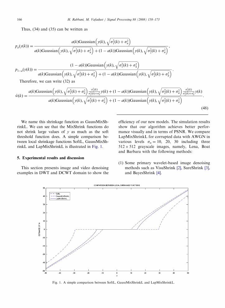
We name this shrinkage function as GaussMixSh-rinkL. We can see that the MixShrink functions donot shrink large values of y as much as the softthreshold function does. A simple comparison be-tween local shrinkage functions SoftL, GaussMixSh-rinkL and LapMixShrinkL is illustrated in Fig. 1.

5. Experimental results and discussion

This section presents image and video denoisingexamples in DWT and DCWT domain to show the

Fig. 1. A simple comparison between SoftL, G

efficiency of our new models. The simulation resultsshow that our algorithm achieves better perfor-mance visually and in terms of PSNR. We compareLapMixShrinkL for corrupted data with AWGN invarious levels sn ¼ 10, 20, 30 including three512� 512 grayscale images, namely, Lena, Boatand Barbara with the following methods:

(1)

aus

Some primary wavelet-based image denoisingmethods such as VisuShrink [2], SureShrink [3],and BayesShrink [4].

sMixShrinkL and LapMixShrinkL.

ARTICLE IN PRESS

Table 1

PSNR results in decibels for several denoising methods

Noise

variance

Noisy Visu

Shrink

[2]

Sure

Shrink

[3]

Bayes

Shrink

[4]

SoftL

(7� 7)

Mihcak’s

method in

DCWT

domain

Selesnick

[6]

GaussMix

Shrink

[20]

LMDM

[21]

LapMix

Shrik

[22]

ProbShrink

[23]

LapMix

ShrinkL3

(9� 9)

Lena

10 28.18 28.76 33.28 33.32 34.15 34.10 35.34 33.84 34.86 34.83 35.24 35.35

20 22.14 26.46 30.22 30.17 30.94 30.89 32.40 30.39 31.62 31.96 32.20 32.31

30 18.62 25.14 28.38 28.48 29.14 29.05 30.54 28.35 29.76 29.88 30.33 30.58

Boat

10 28.16 26.49 31.19 31.80 32.14 32.25 33.10 32.28 33.13 32.96 32.25 33.28

20 22.15 24.43 28.14 28.48 28.93 29.00 30.08 28.54 29.70 29.48 29.93 29.88

30 18.62 23.33 26.52 26.60 27.07 27.06 28.31 26.83 27.61 27.59 28.04 28.03

Barbara

10 28.16 24.81 30.21 30.86 31.90 31.99 33.35 31.36 32.34 33.04 33.46 33.76

20 22.14 22.81 25.91 27.13 28.06 27.94 29.80 27.80 28.06 28.85 29.53 29.90

30 18.62 22.00 24.33 25.16 25.98 25.80 27.65 25.11 25.69 26.56 27.17 27.73

Table 2

The results of choosing the various window sizes in DWT and DCWT domain

Noise

variance

DWT domain DCWT domain

LapMix

Shrik2

LapMix

Shrink3

LapMix

ShrinkL

(7� 7)

GaussMix

ShrinkL

(7� 7)

GaussMix

ShrinkL

(11� 11)

GaussMix

ShrinkL

(15� 15)

LapMix

Shrik2

LapMix

Shrink3

LapMix

ShrinkL3

(7� 7)

LapMix

ShrikL

(3� 3)

LapMix

ShrinkL

(7� 7)

LapMix

ShrinkL

(11� 11)

LapMix

ShrinkL

(15� 15)

Lena

10 33.60 33.63 34.18 35.24 35.28 35.24 34.83 34.86 35.34 35.30 35.25 35.31 35.25

20 30.41 30.42 30.88 31.88 32.07 32.04 31.96 31.72 32.31 32.28 32.26 32.13 32.15

30 28.67 28.75 28.99 29.82 30.08 30.09 29.88 29.91 30.46 30.38 30.38 30.43 30.31

Boat

10 31.94 31.99 32.34 33.34 33.35 33.32 32.96 33.02 33.28 33.28 33.23 33.24 33.21

20 28.59 28.63 28.95 29.84 29.83 29.81 29.48 29.52 29.91 29.87 29.80 29.85 29.80

30 26.74 26.84 27.01 27.83 27.95 27.96 27.59 27.63 28.03 28.00 27.92 27.99 27.93

Barbara

10 31.40 31.43 32.21 33.69 33.62 33.53 33.04 33.06 33.78 33.79 33.64 33.68 33.61

20 27.25 27.30 28.12 29.85 29.84 29.69 28.85 28.87 29.86 29.90 29.86 29.78 29.68

30 25.14 25.18 25.99 27.71 27.68 27.68 26.56 26.59 27.66 27.69 27.50 27.66 27.48

H. Rabbani, M. Vafadust / Signal Processing 88 (2008) 158–173 167

(2)
Methods using non mixture pdfs with localvariances such as Selesnick’s method [6] andMihcak’s work [7].
(3)
Methods employing mixture pdfs without localparameters such as Gaussian mixture model(Gauss MixShrink) and Laplacian mixturemodel (LapMixShrink) [20–22].
(4)
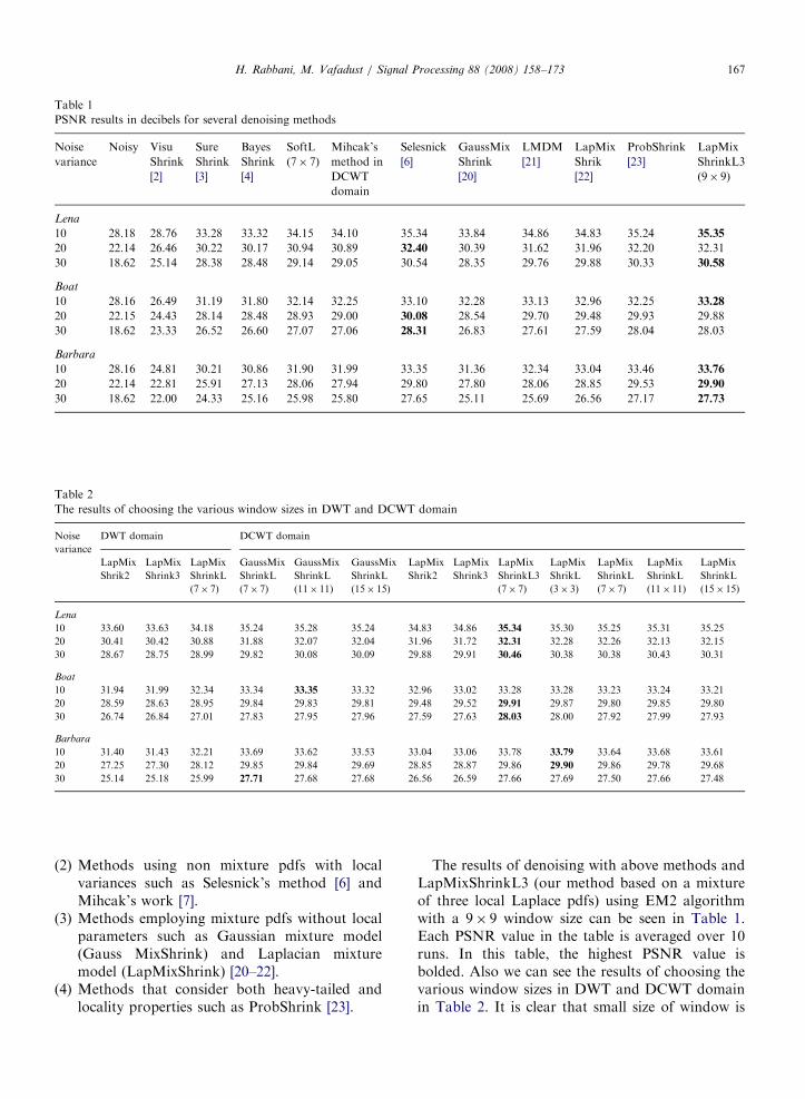
Methods that consider both heavy-tailed andlocality properties such as ProbShrink [23].
The results of denoising with above methods andLapMixShrinkL3 (our method based on a mixtureof three local Laplace pdfs) using EM2 algorithmwith a 9� 9 window size can be seen in Table 1.Each PSNR value in the table is averaged over 10runs. In this table, the highest PSNR value isbolded. Also we can see the results of choosing thevarious window sizes in DWT and DCWT domainin Table 2. It is clear that small size of window is

ARTICLE IN PRESS

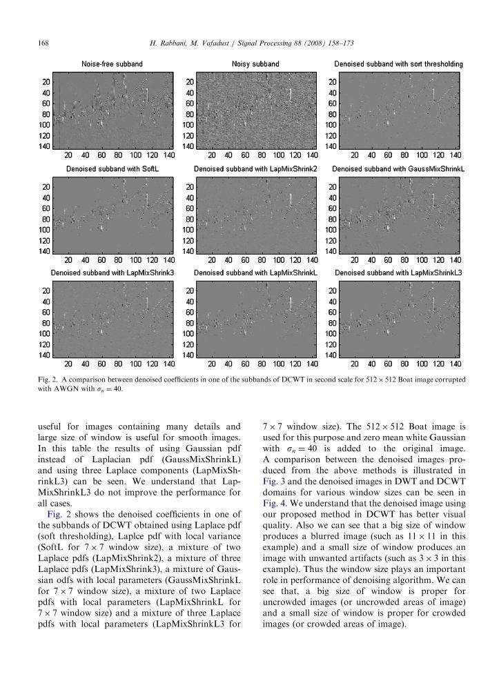
Fig. 2. A comparison between denoised coefficients in one of the subbands of DCWT in second scale for 512� 512 Boat image corrupted

with AWGN with sn ¼ 40.


useful for images containing many details andlarge size of window is useful for smooth images.In this table the results of using Gaussian pdfinstead of Laplacian pdf (GaussMixShrinkL)and using three Laplace components (LapMixSh-rinkL3) can be seen. We understand that Lap-MixShrinkL3 do not improve the performance forall cases.

Fig. 2 shows the denoised coefficients in one ofthe subbands of DCWT obtained using Laplace pdf(soft thresholding), Laplce pdf with local variance(SoftL for 7� 7 window size), a mixture of twoLaplace pdfs (LapMixShrink2), a mixture of threeLaplace pdfs (LapMixShrink3), a mixture of Gaus-sian odfs with local parameters (GaussMixShrinkLfor 7� 7 window size), a mixture of two Laplacepdfs with local parameters (LapMixShrinkL for7� 7 window size) and a mixture of three Laplacepdfs with local parameters (LapMixShrinkL3 for

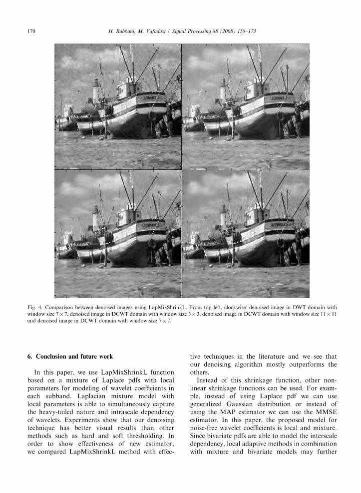
7� 7 window size). The 512� 512 Boat image isused for this purpose and zero mean white Gaussianwith sn ¼ 40 is added to the original image.A comparison between the denoised images pro-duced from the above methods is illustrated inFig. 3 and the denoised images in DWT and DCWTdomains for various window sizes can be seen inFig. 4. We understand that the denoised image usingour proposed method in DCWT has better visualquality. Also we can see that a big size of windowproduces a blurred image (such as 11� 11 in thisexample) and a small size of window produces animage with unwanted artifacts (such as 3� 3 in thisexample). Thus the window size plays an importantrole in performance of denoising algorithm. We cansee that, a big size of window is proper foruncrowded images (or uncrowded areas of image)and a small size of window is proper for crowdedimages (or crowded areas of image).

ARTICLE IN PRESS

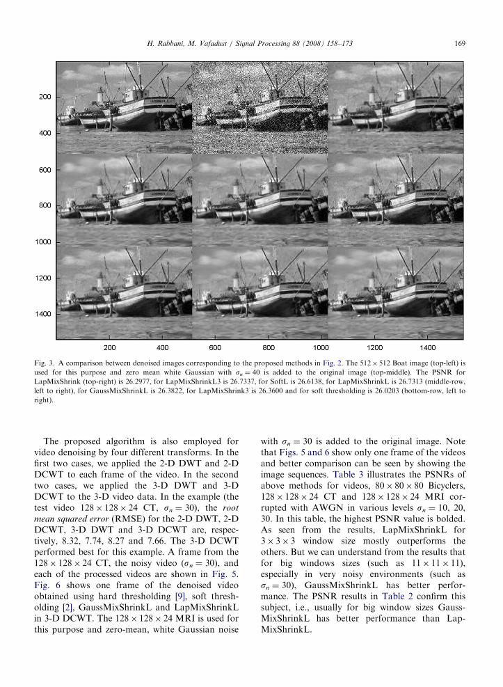
Fig. 3. A comparison between denoised images corresponding to the proposed methods in Fig. 2. The 512� 512 Boat image (top-left) is

used for this purpose and zero mean white Gaussian with sn ¼ 40 is added to the original image (top-middle). The PSNR for

LapMixShrink (top-right) is 26.2977, for LapMixShrinkL3 is 26.7337, for SoftL is 26.6138, for LapMixShrinkL is 26.7313 (middle-row,

left to right), for GaussMixShrinkL is 26.3822, for LapMixShrink3 is 26.3600 and for soft thresholding is 26.0203 (bottom-row, left to

right).


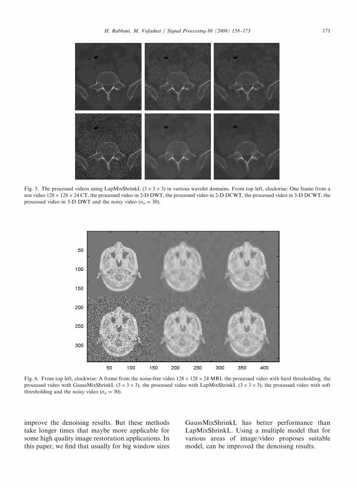
The proposed algorithm is also employed forvideo denoising by four different transforms. In thefirst two cases, we applied the 2-D DWT and 2-DDCWT to each frame of the video. In the secondtwo cases, we applied the 3-D DWT and 3-DDCWT to the 3-D video data. In the example (thetest video 128� 128� 24 CT, sn ¼ 30), the root

mean squared error (RMSE) for the 2-D DWT, 2-DDCWT, 3-D DWT and 3-D DCWT are, respec-tively, 8.32, 7.74, 8.27 and 7.66. The 3-D DCWTperformed best for this example. A frame from the128� 128� 24 CT, the noisy video (sn ¼ 30), andeach of the processed videos are shown in Fig. 5.Fig. 6 shows one frame of the denoised videoobtained using hard thresholding [9], soft thresh-olding [2], GaussMixShrinkL and LapMixShrinkLin 3-D DCWT. The 128� 128� 24 MRI is used forthis purpose and zero-mean, white Gaussian noise

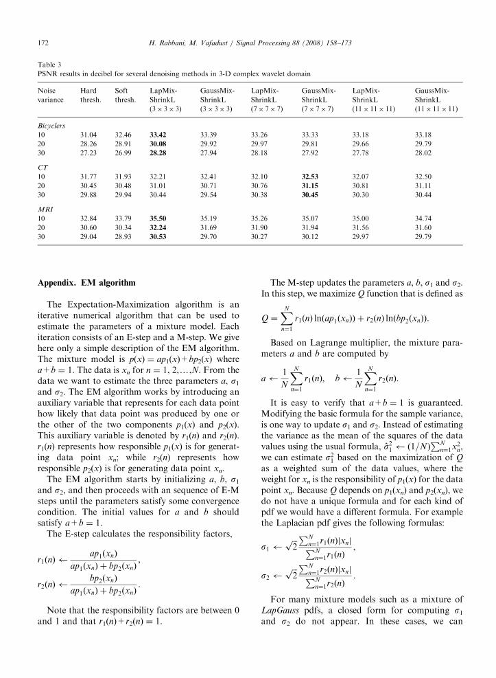
with sn ¼ 30 is added to the original image. Notethat Figs. 5 and 6 show only one frame of the videosand better comparison can be seen by showing theimage sequences. Table 3 illustrates the PSNRs ofabove methods for videos, 80� 80� 80 Bicyclers,128� 128� 24 CT and 128� 128� 24 MRI cor-rupted with AWGN in various levels sn ¼ 10, 20,30. In this table, the highest PSNR value is bolded.As seen from the results, LapMixShrinkL for3� 3� 3 window size mostly outperforms theothers. But we can understand from the results thatfor big windows sizes (such as 11� 11� 11),especially in very noisy environments (such assn ¼ 30), GaussMixShrinkL has better perfor-mance. The PSNR results in Table 2 confirm thissubject, i.e., usually for big window sizes Gauss-MixShrinkL has better performance than Lap-MixShrinkL.

ARTICLE IN PRESS

Fig. 4. Comparison between denoised images using LapMixShrinkL. From top left, clockwise: denoised image in DWT domain with

window size 7� 7, denoised image in DCWT domain with window size 3� 3, denoised image in DCWT domain with window size 11� 11

and denoised image in DCWT domain with window size 7� 7.


6. Conclusion and future work

In this paper, we use LapMixShrinkL functionbased on a mixture of Laplace pdfs with localparameters for modeling of wavelet coefficients ineach subband. Laplacian mixture model withlocal parameters is able to simultaneously capturethe heavy-tailed nature and intrascale dependencyof wavelets. Experiments show that our denoisingtechnique has better visual results than othermethods such as hard and soft thresholding. Inorder to show effectiveness of new estimator,we compared LapMixShrinkL method with effec-

tive techniques in the literature and we see thatour denoising algorithm mostly outperforms theothers.

Instead of this shrinkage function, other non-linear shrinkage functions can be used. For exam-ple, instead of using Laplace pdf we can usegeneralized Gaussian distribution or instead ofusing the MAP estimator we can use the MMSEestimator. In this paper, the proposed model fornoise-free wavelet coefficients is local and mixture.Since bivariate pdfs are able to model the interscaledependency, local adaptive methods in combinationwith mixture and bivariate models may further

ARTICLE IN PRESS

Fig. 5. The processed videos using LapMixShrinkL (3� 3� 3) in various wavelet domains. From top left, clockwise: One frame from a

test video 128� 128� 24 CT, the processed video in 2-D DWT, the processed video in 2-D DCWT, the processed video in 3-D DCWT, the

processed video in 3-D DWT and the noisy video (sn ¼ 30).

Fig. 6. From top left, clockwise: A frame from the noise-free video 128� 128� 24 MRI, the processed video with hard thresholding, the

processed video with GaussMixShrinkL (3� 3� 3), the processed video with LapMixShrinkL (3� 3� 3), the processed video with soft

thresholding and the noisy video (sn ¼ 30).


improve the denoising results. But these methodstake longer times that maybe more applicable forsome high quality image restoration applications. Inthis paper, we find that usually for big window sizes

GaussMixShrinkL has better performance thanLapMixShrinkL. Using a multiple model that forvarious areas of image/video proposes suitablemodel, can be improved the denoising results.

ARTICLE IN PRESS

Table 3

PSNR results in decibel for several denoising methods in 3-D complex wavelet domain

Noise

variance

Hard

thresh.

Soft

thresh.

LapMix-

ShrinkL

(3� 3� 3)

GaussMix-

ShrinkL

(3� 3� 3)

LapMix-

ShrinkL

(7� 7� 7)

GaussMix-

ShrinkL

(7� 7� 7)

LapMix-

ShrinkL

(11� 11� 11)

GaussMix-

ShrinkL

(11� 11� 11)

Bicyclers

10 31.04 32.46 33.42 33.39 33.26 33.33 33.18 33.18

20 28.26 28.91 30.08 29.92 29.97 29.81 29.66 29.79

30 27.23 26.99 28.28 27.94 28.18 27.92 27.78 28.02

CT

10 31.77 31.93 32.21 32.41 32.10 32.53 32.07 32.50

20 30.45 30.48 31.01 30.71 30.76 31.15 30.81 31.11

30 29.88 29.94 30.44 29.54 30.38 30.45 30.30 30.44

MRI

10 32.84 33.79 35.50 35.19 35.26 35.07 35.00 34.74

20 30.60 30.34 32.24 31.69 31.90 31.94 31.56 31.60

30 29.04 28.93 30.53 29.70 30.27 30.12 29.97 29.79


Appendix. EM algorithm

The Expectation-Maximization algorithm is aniterative numerical algorithm that can be used toestimate the parameters of a mixture model. Eachiteration consists of an E-step and a M-step. We givehere only a simple description of the EM algorithm.The mixture model is p(x) ¼ ap1(x)+bp2(x) wherea+b ¼ 1. The data is xn for n ¼ 1, 2,y,N. From thedata we want to estimate the three parameters a, s1and s2. The EM algorithm works by introducing anauxiliary variable that represents for each data pointhow likely that data point was produced by one orthe other of the two components p1(x) and p2(x).This auxiliary variable is denoted by r1(n) and r2(n).r1(n) represents how responsible p1(x) is for generat-ing data point xn; while r2(n) represents howresponsible p2(x) is for generating data point xn.

The EM algorithm starts by initializing a, b, s1and s2, and then proceeds with an sequence of E-Msteps until the parameters satisfy some convergencecondition. The initial values for a and b shouldsatisfy a+b ¼ 1.

The E-step calculates the responsibility factors,

r1ðnÞ ap1ðxnÞ

ap1ðxnÞ þ bp2ðxnÞ,

r2ðnÞ bp2ðxnÞ

ap1ðxnÞ þ bp2ðxnÞ.

Note that the responsibility factors are between 0and 1 and that r1(n)+r2(n) ¼ 1.

The M-step updates the parameters a, b, s1 and s2.In this step, we maximize Q function that is defined as

Q ¼XN

n¼1

r1ðnÞ lnðap1ðxnÞÞ þ r2ðnÞ lnðbp2ðxnÞÞ.

Based on Lagrange multiplier, the mixture para-meters a and b are computed by

a 1

N

XN

n¼1

r1ðnÞ; b 1

N

XN

n¼1

r2ðnÞ.

It is easy to verify that a+b ¼ 1 is guaranteed.Modifying the basic formula for the sample variance,is one way to update s1 and s2. Instead of estimatingthe variance as the mean of the squares of the datavalues using the usual formula, s21 ð1=NÞ

PNn¼1x2

n,we can estimate s21 based on the maximization of Q

as a weighted sum of the data values, where theweight for xn is the responsibility of p1(x) for the datapoint xn. Because Q depends on p1(xn) and p2(xn), wedo not have a unique formula and for each kind ofpdf we would have a different formula. For examplethe Laplacian pdf gives the following formulas:

s1 ffiffiffi2pPN

n¼1r1ðnÞjxnjPNn¼1r1ðnÞ

,

s2 ffiffiffi2pPN

n¼1r2ðnÞjxnjPNn¼1r2ðnÞ

.

For many mixture models such as a mixture ofLapGauss pdfs, a closed form for computing s1and s2 do not appear. In these cases, we can


use generalized EM algorithm that states we canchoose parameters in new iteration in the way thatincrease Q in comparison to previous iteration.For example the following formulas producedfrom a mixture of Gaussian pdfs can be used toapproximate s1 and s2:

s21 PN

n¼1r1ðnÞx2nPN

n¼1r1ðnÞ; s22

PNn¼1r2ðnÞx

2nPN

n¼1r2ðnÞ.

References

[1] S. Mallat, A theory for multiresalution signal decomposi-

tion: the wavelet representation, IEEE Trans. Pattern Anal.

Mach. Intell. PAMI-11 (1989) 674–693.

[2] D.L. Donoho, Denoising by soft-thresholding, IEEE Trans.

Inform. Theory 41 (May 1995) 613–627.

[3] D.L. Donoho, I.M. Johnstone, Ideal spatial adaptation by

wavelet shrinkage, Biometrika 81 (3) (1994).

[4] D.L. Donoho, I.M. Johnstone, Adapting to unknown

smoothness via wavelet shrinkage, J. Am. Stat. Assoc. 90

(432) (1995) 1200–1224.

[5] M. Hansen, B. Yu, Wavelet thresholding via MDL for

natural images, IEEE Trans. Inform. Theory 46 (5) (2000).

[6] L. Sendur, I.W. Selesnick, Bivariate shrinkage with local

variance estimation, IEEE Signal Process. Lett. 12 (11)

(Dec. 2002) 438–441.

[7] M.K. Mihcak, I. Kozintsev, K. Ramchandran, P. Moulin,

Low complexity image denoising based on statistical

modeling of wavelet coefficients, IEEE Signal Process. Lett.

6 (Dec. 1999) 300–303.

[8] I. Selesnick, R.G. Baraniuk, N. Kingsbury, The dual-tree

complex wavelet transforms—a coherent frame-work for

multiscale signal and image processing, IEEE Signal Process.

Mag. 22 (6) (November 2005) 123–151.

[9] I. Selesnick, K. Li, Video denoising using 2d and 3d dual-

tree complex wavelet transforms, in: Proceedings of the SPIE

Wavelet Applications in Signal and Image Processing,

San Diego, August 4–8, 2003, p. 5207.

[10] P. Roosmalen, S. Westen, R. Lagendijk, J. Biemond, Noise

reduction for image sequences using an oriented pyramid

thresholding technique, in: Proceedings of the IEEE Con-

ference on Image Processing, Switzerland, September 1996,

pp. 375–378.

[11] V. Zlokolica, A. Pizurica, W. Philips, Video denoising using

multiple class averaging with multi-resolution, in: Interna-

tional Workshop VLBV03, Madrid, Spain, September 2003.

[12] S. Chang, B. Yu, M. Vetterli, Adaptive wavelet thresholding

for image denoising and compression, IEEE Trans. Image

Process. 9 (September 2000) 1532–1546.

[13] M.A.T. Figueiredo, R.D. Nowak, Wavelet-based image

estimation: an empirical bayes approach using Jeffrey’s

noninformative prior, IEEE Trans. Image Process. 10

(September 2001) 1322–1331.

[14] H. Gao, Wavelet shrinkage denoising using the nonnegative

garrote, J. Comput. Graph. Stat. 7 (1998) 469–488.

[15] A. Hyvarinen, E. Oja, P. Hoyer, Image denoising by sparse

code shrinkage, in: S. Haykin, B. Kosko (Eds.), Intelligent

Signal Processing, IEEE, Piscataway, NJ, 2001.

[16] E.P. Simoncelli, Bayesian denoising of visual images in the

wavelet domain, in: P. Muller, B. Vidakovic (Eds.), Bayesian

Inference in Wavelet Based Models, Springer, New York,

1999.

[17] E.P. Simoncelli, E.H. Adelson, Noise removal via Bayesian

wavelet coring, in: Proceedings of the IEEE International

Conference on Image Processing, vol. I, January 1996,

pp. 379–382.

[18] B. Vidakovic, Statistical Modeling by Wavelets, Wiley,

New York, 1999.

[19] L. Sendur, I.W. Selesnick, Bivariate shrinkage functions

for wavelet-based denoising exploiting interscale depen-

dency, IEEE. Trans. Signal Process. 50 (11) (2002)

2744–2756.

[20] M.S. Crouse, R.D. Nowak, R.G. Baraniuk, Wavelet-based

signal processing using hidden Markov models, IEEE Trans.

Signal Process. 46 (April 1998) 886–902.

[21] B.S. Raghavendra, P. Subbanna Bhat, Shift-invariant

image denoising using mixture of Laplace distributions

in wavelet-domain, Lect. Notes Comput. Sci. 3851 (2006)

180–188.

[22] H. Rabbani, M. Vafadoost, Wavelet based image denoising

with mixed Laplace model, in: Proceedings of the 11th

International Computer Society of Iran Computer Con-

ference (CSICC 2006), Tehran, 24–26 January 2006.

[23] A. Pizurica, W. Philips, Estimating the probability of the

presence of a signal of interest in multiresolution single- and

multiband image denoising, IEEE Trans. Image Process. 15

(3) (March 2006) 654–665.

[24] A.P. Dempster, N.M. Laird, D.B. Rubin, Maximum like-

lihood from incomplete data via the EM algorithm, J. Roy.

Stat. Soc. Ser. B (Methodological) 39 (1) (1977) 1–38.

[25] H.J. Park, T.-W. Lee, Modeling nonlinear dependencies in

natural images using mixture of Laplacian distribution, in:

L.K. Saul, Y. Weiss, L. Bottou (Eds.), Advances in Neural

Information Processing Systems, vol. 17, MIT Press,

Cambridge, MA, 2005.

[26] V. Strela, J. Portilla, E. Simoncelli, Image denoising

using a local Gaussian scale mixture model in the wavelet

domain, in: Proceedings of the SPIE 45th Annual Meeting,

2000.

[27] A. Achim, E.E. Kuruoglu, Image denoising using bivariate

alpha-stable distributions in the complex wavelet domain,

IEEE Signal Process. Lett. 12 (January 2005) 17–20.

Image/video denoising based on a mixture of Laplace distributions with local parameters in...

Documents

Transcript of Image/video denoising based on a mixture of Laplace distributions with local parameters in...