2012 International Conference on Lightning Protection (ICLP), Vienna, Austria

Denoising of Lightning Electric Field Signals Using Fractional Fourier Transform

Herbert Rojas Universidad Nacional de Colombia

Electromagnetic Compatibility Group EMC-UNC

Bogotá, Colombia herojasc@unal.edu.co

Camilo Cortes Universidad Nacional de Colombia

Electromagnetic Compatibility Group EMC-UNC

Bogotá, Colombia caacortesgu@unal.edu.co

Francisco Santamaria Universidad Distrital FJC

Electromagnetic Compatibility and Interference Group GCEM

Bogotá, Colombia fsantamariap@udistrital.edu.co

Abstract— In recent years, several activities have been carried out by EMC-UNC (research group) to measure, study and classify the parameters of lightning electric fields signals in Bogotá, Colombia. However, measurements are distorted and exhibit significant noise levels caused by undesired signals from the electromagnetic environment together with other types of disturbances produced by the measuring system, which inevitably introduces noise in signal measurements.

This paper shows the results of applying the fractional Fourier transform (FRFT) as an alternative technique to reduce the presence of noise and also of undesired signal components within a set of electric field signatures. Basic conditions to carry out the filtering process in the fractional Fourier domain (FRFd) are presented. Afterwards, some lightning electric field temporal characteristics are analyzed by using the processed signatures. Important differences between processed and measured waveforms are observed.

Keywords- fractional Fourier transform, fractional Fourier domains, filtering, lightning, electric field, denoising.

I. INTRODUCTION

In recent years, several studies have been conducted to address the analysis and implementation of processing techniques applied to the electromagnetic signals (radiated and/or conducted) generated by lightning [1–4]. The aim of such studies was to analyze the parameters and characteristics of lightning in detail, gaining deeper knowledge of these phenomena, and thereby improving safety for people, equipment and systems.

Considering that regional geographical conditions, such as air density and height above sea level, affect lightning characteristics, EMC-UNC (research group) has launched a programme to study and classify lightning in Bogotá-Colombia. In the experiments, electric-field measurements captured during discharges are used. The recorded signals can be expressed as the sum of the electric field generated by lightning plus other existing signals in the electromagnetic environment, and noise (mainly caused by the measuring system itself). In such scenario, it is extremely useful for the study of the lightning, to separate the original signal from the other undesired signals, which include noise components.

Some methods and techniques to remove these undesired components from the lightning-electric-field original signal have been proposed in the past, including filtering in the conventional Fourier domain [5], [6], the use of Wavelet transform (WT) [3], [7] and other techniques to process time-varying signals based on a mix of time-frequency signal representations (TFRs) [8–11].

Recently, filtering in the conventional Fourier domain (frequency domain) has been extended to its generalized version, namely the fractional Fourier transform (FRFT) domain. It has been stated that working in the FRFT domain is more advantageous to process some kind of signals, such as chirps and non-stationary signals [12–14].

This paper provides a first approach to noise reduction in lightning-electric-field measurements using filters in the fractional Fourier domain. It is suggested that the FRFT can be implemented to separate, in a very effective way, the unwanted signal components from the electric-field measurements, preserving the essentials characteristics of the original signal. The basic signal model considered in this article assumes that the measured signal is a linear combination of the desired signal distorted by noise components and other unwanted signals .

The motivation behind this study lies in the fact that some signals can be better analyzed in certain fractional domains. In addition, the FRFT offers the user some degree of freedom in terms of transform parameters. Such parameters can be exploited in an effective way when compared to the type of filtering used in the conventional Fourier domain and in others TFRs, without increasing computational complexity.

The paper continues in section 2 with a review of the continuous FRFT and its discrete version derived from the spectral expansion of the discrete Fourier transform (DFT). In section 3, the definition of filtering in the fractional domain (FRFd) is discussed. Section 4 describes the process of noise reduction using FRFT. A brief explanation of the measuring system and of some lightning electric-field signatures is presented in section 5. Section 6 shows the results of the noise reduction process using the filtering in the fractional domain. Section 7 is intended to compare the results of the lightning temporal parameters obtained before (and after) using the

proposed technique. Finally, some conclusions are presented in section 8.

II. FRACTIONAL FOURIER TRANSFORM (FRFT)

FRFT is a generalization of the conventional Fourier transform (FT). Mathematically defined by Namias [15], McBride and Kerr [16]; FRFT has been used in several applications such as optical systems, quantum mechanics, radar, sonar, pattern recognition, data compression, space/time-frequency representations, time-varying filtering and signal processing [17].

The th-order FRFT of a signal , denoted as , can be interpreted as a rotation of the signal by an angle in the time-frequency plane (Wigner domain) [14]. The FRFT of the signal is defined as [18]:

≡ , (1)

≡ , (2)

where the transform kernel , of the FRFT is given by [15], [18]:

,exp cot csc 0 2 4…

0 4… 2 6…

(3)

For this kernel 1 cot 2⁄ and 2⁄ . The definition given in (1) is valid for any real value of , as shown in (3), the definition can be easily extended since is the identity operation. First order FRFT is the ordinary Fourier transform, whereas the zero-order FRFT is the identity transformation, i.e., the signal itself. Positive and negative integer value of corresponds to consecutive FT applications and the inverse FT, respectively.

Some essential properties of FRFT are as follows: (a) it is a linear operator; (b) first order ( 1) of FRFT corresponds to the conventional FT; (c) operation are additive in index,

; and (d) The inverse FRFT (IFRFT) operator is expressed as . The existence conditions of FRFT, its properties and its integration kernel are explained in [15], [16], [18], [19].

The direct computation of FRFT has become an important issue because FRFT is a potentially useful tool for time-varying signal analysis and signal processing [20]. In this paper, a discrete version of FRFT (DFRFT) was applied. Such discrete version is based on a spectral expansion of the discrete Fourier transform (DFT) matrix as well as on the calculation of its eigenvalues and eigenvectors from the commutation matrix

[21–23]. A brief explanation of this definition can be found in Appendix A.

III. FILTERING IN THE FRACTIONAL DOMAIN

Consider a given signal with additive distortion (e.g. noise), namely:

(4)

Consider also the case in which FT is calculated for the input signal and the spectrum of both the original signal

and the distortion term do not overlap. This distortion can be easily eliminated in the frequency domain

1 using a suitable multiplicative filter, as follows:

∙ (5)

where the FT operator is defined as , and is the multiplicative filter operator. Now, considering the especial case shown in Fig. 1 where the original signal and the distortion term are presents on the same time-frequency (TF) plane. Since these representations, using both the (time domain) and axes (frequency domain) overlap, it is not possible to eliminate the effect of noise components altogether in the 0 and 1-st fractional orders. However, it is possible to completely eliminate the noise term filtering the input signal in a coordinate plane, which is obtained applying the FRFT to the input signal.

Figure 1. WD of a signal and the undesired noise term in the fractional

Fourier domain.

From this hypothesis it is possible to deal with the process of filtering in the FRFT domain in two ways: (i) find a suitable fractional filter operator in the -th order, so:

∙ (6)

where is the output signal of the system and is a multiplicative filter function in the -th fractional order, or (ii) for a pre-set filter operator , find the most suitable fractional order to perform the filtering process in order to obtain the desired signal. Fig. 2 shows a schematic representation of the filtering process in the FRFT domain.

Figure 2. Multiplicative filter in the fractional Fourier domain.

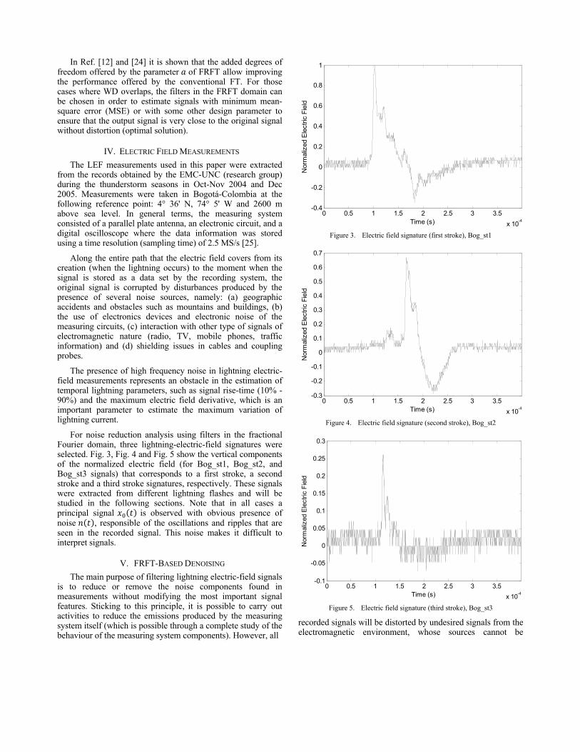
In Ref. [12] and [24] it is shown that the added degrees of freedom offered by the parameter of FRFT allow improving the performance offered by the conventional FT. For those cases where WD overlaps, the filters in the FRFT domain can be chosen in order to estimate signals with minimum mean-square error (MSE) or with some other design parameter to ensure that the output signal is very close to the original signal without distortion (optimal solution).

IV. ELECTRIC FIELD MEASUREMENTS

The LEF measurements used in this paper were extracted from the records obtained by the EMC-UNC (research group) during the thunderstorm seasons in Oct-Nov 2004 and Dec 2005. Measurements were taken in Bogotá-Colombia at the following reference point: 4° 36' N, 74° 5' W and 2600 m above sea level. In general terms, the measuring system consisted of a parallel plate antenna, an electronic circuit, and a digital oscilloscope where the data information was stored using a time resolution (sampling time) of 2.5 MS/s [25].

Along the entire path that the electric field covers from its creation (when the lightning occurs) to the moment when the signal is stored as a data set by the recording system, the original signal is corrupted by disturbances produced by the presence of several noise sources, namely: (a) geographic accidents and obstacles such as mountains and buildings, (b) the use of electronics devices and electronic noise of the measuring circuits, (c) interaction with other type of signals of electromagnetic nature (radio, TV, mobile phones, traffic information) and (d) shielding issues in cables and coupling probes.

The presence of high frequency noise in lightning electric-field measurements represents an obstacle in the estimation of temporal lightning parameters, such as signal rise-time (10% - 90%) and the maximum electric field derivative, which is an important parameter to estimate the maximum variation of lightning current.

For noise reduction analysis using filters in the fractional Fourier domain, three lightning-electric-field signatures were selected. Fig. 3, Fig. 4 and Fig. 5 show the vertical components of the normalized electric field (for Bog_st1, Bog_st2, and Bog_st3 signals) that corresponds to a first stroke, a second stroke and a third stroke signatures, respectively. These signals were extracted from different lightning flashes and will be studied in the following sections. Note that in all cases a principal signal is observed with obvious presence of noise , responsible of the oscillations and ripples that are seen in the recorded signal. This noise makes it difficult to interpret signals.

V. FRFT-BASED DENOISING

The main purpose of filtering lightning electric-field signals is to reduce or remove the noise components found in measurements without modifying the most important signal features. Sticking to this principle, it is possible to carry out activities to reduce the emissions produced by the measuring system itself (which is possible through a complete study of the behaviour of the measuring system components). However, all

Figure 3. Electric field signature (first stroke), Bog_st1

Figure 4. Electric field signature (second stroke), Bog_st2

Figure 5. Electric field signature (third stroke), Bog_st3

recorded signals will be distorted by undesired signals from the electromagnetic environment, whose sources cannot be

0 0.5 1 1.5 2 2.5 3 3.5

x 10-4

-0.4

-0.2

0

0.2

0.4

0.6

0.8

1

Time (s)

Nor

mal

ized

Ele

ctric

Fie

ld

0 0.5 1 1.5 2 2.5 3 3.5

x 10-4

-0.3

-0.2

-0.1

0

0.1

0.2

0.3

0.4

0.5

0.6

0.7

Time (s)

Nor

mal

ized

Ele

ctric

Fie

ld

0 0.5 1 1.5 2 2.5 3 3.5

x 10-4

-0.1

-0.05

0

0.05

0.1

0.15

0.2

0.25

0.3

Time (s)

Nor

mal

ized

Ele

ctric

Fie

ld

controlled or eliminated. For this reason, it is necessary to submit the recorded signatures to a filtering process using mathematical and computational techniques.

FRFT has been used as a denoising tool in several areas [17], [26]. Its advantage with respect to other conventional techniques, like FT, is that certain types of signals (irregulars, non-periodic or transient) can be better resolved in certain fractional domains taking advantage of some degrees of freedom offered by FRFT, such as the order of the transform and the filtering function.

To reduce noise components in lightning-electric-field measurements, the filtering process (in the fractional Fourier domain - FRFd) presented in this work is based on the application of the second alternative discussed in section 3, i.e., choosing a preset filter function in the fractional domain and leaving the -th fractional order as a single degree of freedom. In this case, the aim is to find the most suitable rotation angle 2⁄ so as to remove noise as effectively as possible from the input signal .

Determination of the fractional order in which the selected filter will give the best results can be based on: a visual comparison of the filtered signal and the measured signal, the minimum MSE, the maximum signal-to-noise ratio (SNR) of the output signal, or the best correlation between the input signal and the output signal .

Because the nature of lightning electric fields radiated during discharge has a random behaviour and the waveforms depend on the distance from the lightning strike point, it is not possible to have a desired signal that represents the phenomena. This disadvantage makes it difficult for the process to minimize the MSE [13]. For this work, both maximum SNR of the filtered signal and the cross-correlation operations were selected as appropriate indicators for comparing results.

The cross-correlation R between the measured signal x t and the filtered signal y t can be maximized by the cross-correlation coefficient ρ as follows:

∙ (7)

where R m ∑ x n ∙ y∗ n m is the largest cross-correlation between the signals with a shift m and the signals energy of x t and y t are defined as E y E respectively. It is worth mentioning that the cross-correlation expressed in (12) is a comparison parameter that should be interpreted with caution since the best correlation is not always the best possible solution. This can be seen in the worst case of the filtering process, where the measured signal and the filtered signal are equal and so the cross-correlation is equal to 1.

VI. SIGNAL PROCESSING RESULTS

Applying the methodology discussed in section 3, the three lightning-electric-field signatures were processed using the same filter function in three fractional orders: 0.25, 0.50 and 0.75. In order to compare the results of the filtering process in

the fractional Fourier domain, a similar filter in the conventional Fourier domain ( 1) was also implemented, i.e., using the classic FT. The filtered signals in each fractional order are shown in Fig. 6 - 14. In all cases the analyzed signals were normalized, taking the maximum value of its respective flash as the reference value.

Fig. 6 shows how the use of filters in the fractional domain have a better performance compared with the classic FT technique. Fig. 7 is an enlarged version (zoom in) of the first peak of filtered signal; it was found that the best results are obtained with the filter in the fractional order 0.25. The most relevant differences appear in the rise-time of the signal, the main peak, and the secondary peaks that are separated a few tents of microseconds. These secondary peaks are caused by fast changes in current and speed when the return stroke front reaches the step leader ramifications [27].

Figure 6. Electric field signature Bog_st1 using fractional filters with

0.25, 0.50, 0.75, 1

Figure 7. First peak zoom of the Electric field signature Bog_st1 using

fractional filters with 0.25, 0.50, 0.75, 1

Fig. 8 shows a comparison between the measured signal and the filtered signal in the fractional order 0.25 . A

0 0.5 1 1.5 2 2.5 3 3.5

x 10-4

-0.4

-0.2

0

0.2

0.4

0.6

0.8

1

Time (s)

Nor

mal

ized

Ele

ctric

Fie

ld

a=0.25a=0.50a=0.75a=1 (FT)

0.9 1 1.1 1.2 1.3 1.4 1.5 1.6 1.7

x 10-4

0.3

0.4

0.5

0.6

0.7

0.8

0.9

1

Time (s)

Nor

mal

ized

Ele

ctric

Fie

ld

a=0.25a=0.50a=0.75a=1 (FT)

visual improvement is evident in the waveform, essentially in the temporal features of the electric field signature.

Figure 8. Measured signal Bog_st1 vs. filtered signal in FRFd 0.25

The same behaviour can be observed in the processing of the Bog_st2 electric field signature, see Fig. 9 and Fig. 10. Although the waveform obtained with the FT is similar to the measured signal and it does not presents evident oscillations, this method shows divergences in the rise-time and peak values of the filtered signal. This can be stated because maximum normalized electric field using FT reach a value of 0.56 V/m while the peak value of the filtered signal using FRFT with a fractional order 0.25 is 0.64 V/m. These differences between the measured signal and the filtered signal certainly represent difficulties when interpretation in the assessment of lightning parameters.

Figure 9. Electric field signature Bog_st2 using fractional filters with

0.25, 0.50, 0.75, 1

Figure 10. First and second peak zoom of the Electric field signature Bog_st2

using fractional filters with 0.25, 0.50, 0.75, 1

Figure 11. Measured signal Bog_st2 vs. filtered signal in FRFd 0.25

In Figures 12 and 13 it can be seen that the filtered signal in the fractional domain 0.25 is also the signal that presents the best results. It is important to note here that, for Bog_st3 signature, the signal processing realized with the classic FT delivers different results than those obtained with fractional filtering regarding both the ascent speed and the waveform. Moreover, for this particular signal, the waveform of the first and second peak are substantially distorted by the filtering in the frequency domain with FT, reducing these two peaks to only one, and also reducing the maximum electric field value from 0,24 V/m to 0,16 V/m.

Fig. 14 shows a comparison between the measured signal and the filtered signal in the fractional order 0.25. In this case, compared with the FT results, the FRFT filtering removed the unwanted components found in the measured signal and maintained the essential characteristics of such signal.

0 0.5 1 1.5 2 2.5 3 3.5

x 10-4

-0.4

-0.2

0

0.2

0.4

0.6

0.8

1

Time (s)

Nor

mal

ized

Ele

ctric

Fie

ld

Measured signal

Filtering in the FRFd with a=0.25

0 0.5 1 1.5 2 2.5 3 3.5

x 10-4

-0.3

-0.2

-0.1

0

0.1

0.2

0.3

0.4

0.5

0.6

0.7

Time (s)

Nor

mal

ized

Ele

ctric

Fie

ld

a=0.25a=0.50a=0.75a=1 (FT)

1.5 1.6 1.7 1.8 1.9 2 2.1

x 10-4

0.25

0.3

0.35

0.4

0.45

0.5

0.55

0.6

0.65

Time (s)

Nor

mal

ized

Ele

ctric

Fie

ld

a=0.25a=0.50a=0.75a=1 (FT)

0 0.5 1 1.5 2 2.5 3 3.5

x 10-4

-0.2

-0.1

0

0.1

0.2

0.3

0.4

0.5

0.6

0.7

0.8

Time (s)

Nor

mal

ized

Ele

ctric

Fie

ld

Measured signal

Filtering with a=0.25

Figure 12. Electric field signature Bog_st3 using fractional filters with

0.25, 0.50, 0.75, 1

Figure 13. First peak zoom of the Electric field signature Bog_st3 using

fractional filters with 0.25, 0.50, 0.75, 1

Figure 14. Measured signal Bog_st3 vs. filtered signal in FRFd 0.25

In addition to the results obtained from visual comparison, Table I shows the cross-correlation coefficient defined in (7),

the peak value and SNR of the filtered signal for different fractional orders . The results show that for the three signatures the filtering in the fractional domain 0.25 achieves the best results without affecting the waveform of the measured signal; neither are oscillations observed nor significant ripples that could influence the analysis of the signal temporal features.

Although in signals Bog_st1 and Bog_st2 the differences of the cross-correlation coefficients are not as significant, the denoising results in the fractional domain are better, as observed in their SNR improvements. Moreover, as discussed in the next section, several differences can be established in the signal features, such as the maximum electric field value (peak value), the signal rise-time, slow front time, fast transition time, and the zero crossing time.

TABLE I: CORRELATION AND CROSS-CORRELATION COEFFICIENT IN

DIFFERENT FRACTIONAL ORDERS FOR FILTERED ELECTRIC FIELD

SIGNATURES BOG_ST1, BOG_ST2 AND BOG_ST3

Signal Fractional

order Peak value

(p.u) SNR (dB)

Bog_st1

0.25 0.992 0.990 35,7 0.50 0.981 0.860 20,4 0.75 0.971 0.795 16,1

1 0.951 0.764 12,4

Bog_st2

0.25 0.992 0.637 30.4 0.50 0.987 0.629 22.5 0.75 0.976 0.581 16.5

1 0.951 0.560 12.0

Bog_st3

0.25 0.848 0.236 21.4 0.50 0.805 0.176 14.6 0.75 0.786 0.163 17.6

1 0.763 0.160 12.5

By comparing the SNR of the measured signal against the best result obtained with filtering using FRFT, it is possible to notice that for signal Bog_st1 (shown in Fig. 8), the change in SNR ranged from 21.9 dB to 35.7 dB after filtering, for signal Bog_st2 (shown in Fig. 11), the SNR exhibits a change from 18.4 dB to 30.4 dB; while for signal Bog_st3 (shown in Fig. 14), the improvement of SNR ranged from 6.1 dB to 21.4 dB after filtering.

VII. TEMPORAL PARAMETERS COMPARISON

The estimation and assessment of lightning current features from LEF signals is one of the tasks performed in this lightning study. This section presents the results obtained from comparing the temporal parameters between the measured signal and the filtered signal resulting from the signal processing method described in section VI.

The parameters selected for analysis are as follows: maximum electric filed (Ep), maximum electric field derivative ( / ), 10 – 90 % signal rise-time (Tr), slow front time (F), fast front time (R) and zero crossing time (ZC). The maximum values of the electric field and the electric field derivative are presented in per-unit basis, taking the maximum value of the measured signal as the reference value.

0 0.5 1 1.5 2 2.5 3 3.5

x 10-4

-0.05

0

0.05

0.1

0.15

0.2

0.25

0.3

Time (s)

Nor

mal

ized

Ele

ctric

Fie

ld

a=0.25a=0.50a=0.75a=1 (FT)

1 1.1 1.2 1.3 1.4 1.5

x 10-4

0

0.05

0.1

0.15

0.2

Time (s)

Nor

mal

ized

Ele

ctric

Fie

ld

a=0.25a=0.50a=0.75a=1 (FT)

0 0.5 1 1.5 2 2.5 3 3.5

x 10-4

-0.1

-0.05

0

0.05

0.1

0.15

0.2

0.25

0.3

Time (s)

Nor

mal

ized

Ele

ctric

Fie

ld

Measured signal

Filtering with a=0.25

Based on the main results of lightning-electric-field signal processing (summarized in Table II) it can be conclude that the maximum normalized electric field shows a slight variation, between 1 and 4% in the cases where SNR is high; while for Bog_st3, corresponding to a low SNR environment, the variation in the maximum normalized electric field reached 10%. These results show that the magnitude of this parameter depends on the signal noise levels.

TABLE II: CALCULATED ELECTRIC FIELD PARAMETERS BEFORE AND

AFTER TO APPLY THE PROCESSING TECHNIQUE

Signal Ep

(p.u) Ep/dt (p.u)

Tr (s)

F (s)

R (s)

CZ (s)

Bog_st1

Measured 1 1 8.44 7.80 4.78 78.20

Processed 0.99 0.667 5.63 9.00 4.20 78.95

Bog_st2

Measured 0.667 1 7.8 3.10 2.80 39.4

Processed 0.637 0.471 5.4 3.25 2.95 42.9

Bog_st3

Measured 0.262 1 5.8 2.4 1.6 18.1

Processed 0.236 0.250 5 2.7 1.5 38.2

In the estimation of the maximum electric field derivative

notable differences were observed between the results obtained from the measured signatures and the processed ones. These differences were 33, 53 and 75% for Bog_st1, Bog_st2 and Bog_st3 signatures, respectively. Waveforms in Fig. 15 are an example of such differences. These results mean that the lightning-electric-field signatures had a considerable high frequency noise component.

Figure 15. Calculated electric field derivative of LEF signature Bog_st1

shows in Fig. 8

VIII. CONCLUSIONS

This paper shows how FRFT can be applied to the problem of time-varying filtering of non-stationary, finite energy processes, particularly how FRFT can be used as a useful signal processing technique for noise reduction and the

improvement of lightning-electric-field measurements. A simple methodology was established to apply filters in the fractional Fourier domain in order to identify some temporal features of lightning-electric-field signals.

Simulation examples show that the noise reduction achieved in certain fractional domains can produce better results than other methods for certain types of signal and noise environment. The presence of undesired signals (time-varying and non-stationary), which distort the main signal, suggests that FRFT can be used with good results in the denoising process of lightning-electric-field measurements, and also that improvements in its application depend on the selection of particular fractional orders (chosen in this work as the only degree of freedom) and their corresponding multiplicative filter functions.

The initial results provided by this study were encouraging. However, future work in this area should be oriented to perform the following tasks: (a) building a definition of noise in the fractional domain, (b) improving the procedure for selecting the most suitable fractional order and the filter function so as to perform the filtering process through the implementation of optimal or adaptive filters, (c) setup a process to estimate an adequate desired signal, and (d) conducting a detailed study of both the electromagnetic environment and the measuring system in order to characterize the noise that is introduced in measurements and so identify the spectrum of these undesired signals (in the fractional Fourier domain) as accurately as possible.

APPENDIX A: DISCRETE VERSION OF THE FRFT

Many methods for defining a discrete FRFT (DFRFT) has been developed [23], [28–31]. The definition of DFRFT that appears in this paper is subject to the spectral expansion of the DFT matrix and the commutation matrix defined in [21–23].

A. DFT eigenvalues and eigenvectors

The DFT can be expressed in a matrix form as follow:

,√

∙ (8)

where is the 1 discrete signal matrix and is the DFT matrix representation. From (8) it is possible to represent the DFT matrix as a linear operator [32]:

√∑ ⁄ ; , 0,1, … , 1 (9)

From the results presented in [21], [22], the properties of the eigenvalues and eigenvectors of the DFT matrix can be summarized as follows:

The eigenvalues of are 1, 1, , , for this reason the DFT matrix representation not is unique. See proof in [21].

The eigenvectors of can be obtained using the matrix defined in (10). Matrix satisfies the commutative property,

. See proof in [22], [23].

0 1 2 3 4

x 10-4

-1

-0.8

-0.6

-0.4

-0.2

0

0.2

0.4

0.6

0.8

1

Time (s)

Nor

mal

ized

ele

ctric

fiel

d de

rivat

ive

From measured signal

From filtered signal using FRFT

2 1 0 0 ⋯ 0 11 2 cos 4 1 0 ⋯ 0 0

0 1 2 cos 4 1 ⋯ 0 0

⋮ ⋮ ⋮ ⋮ ⋱ ⋮ ⋮1 0 0 0 ⋯ 1 2 cos 4

(10)

Since the matrix commutes with the DFT matrix, there must be a unique and orthogonal eigenvector set of both and

, but such set corresponds to different eigenvalues. Because matrix is real and symmetric, this eigenvector set is real and orthonormal.

B. DFRFT definition

The DFRFT operator can be defined using the spectral decomposition theorem as an operator in a N-dimension vector space, as shown in (11):

, ∑ , (11)

, 1,2, … ,

where is the k-th orthonormal eigenvector of the DFT matrix and it is associated with the corresponding

eigenvalue . Thus, the DFRFT operator is expressed in a similar way to the kernel of the FRFT shown in (3). Since the continuous normalized Hermite-Gaussian (H-G) functions are well known to be eigenfunctions of the Fourier transform and are also eigenfunctions of FRFT [15], it is possible to define the eigenvectors as a discrete counterparts of the H-G functions [23], [28]. Now, if is the matrix representation of a -sample discretized signal, DFRFT by spectral decomposition can be defined as:

∑ ∙⁄⁄ (12)

The definition of DFRFT, shown in (12), satisfies the following requirements [23]: (a) unitarity; (b) reduction to the DFT when 1 ; (c) additive order, ; (d) approximation of the continuous FRFT.

It is important to note that for the computational implementation of DFRFT used here, some changes were made with respect to the definition given in [23]. First, the eigenvectors of matrix are not exactly the same as H-G functions, because they differ by a scaling constant 2 ⁄ . Second, DFRFT is a direct approximation of FRFT only in the case where the sampling time of the continuous signal is 2 ⁄ . Since it is not possible to satisfy this condition with fast time-varying signals (because that would require extremely short sampling periods), it is necessary to include a compensation factor to calculate DFRFT [28].

REFERENCES [1] F. J. Miranda, “Wavelet analysis of lightning return stroke,” Journal

of Atmospheric and Solar-Terrestrial Physics, vol. 70, no. 11–12, pp. 1401-1407, 2008.

[2] O. Nedjah, A. M. Hussein, S. Krishnan, and R. Sotudeh, “Comparative study of sdaptive techniques for denoising CN tower lightning current derivative signals,” Digital Signal Process, vol. 20, pp. 607–618, 2010.

[3] C. Cortés, F. Santamaría, F. Roman, F. Rachidi, and C. Gomes, “Analysis of wavelet based denoising methods applied to measured lightning electric fields,” in 30th International conference on lightning protection - ICLP 2010, 2010, pp. 1-6.

[4] S. R. Sharma, V. Cooray, M. Fernando, and F. J. Miranda, “Temporal features of different lightning events revealed from wavelet transform,” Journal of Atmospheric and Solar-Terrestrial Physics, vol. 73, no. 4, pp. 507-515, Mar. 2011.

[5] H. M. Ozaktas, Z. Zalevsky, and M. A. Kutay, The Fractional Fourier Transform with Applications in Optics and Signal Processing. New York: John Wiley & Sons, 2001, p. 513.

[6] R. N. Bracewell, The Fourier Transform and Its Applications, 3rd ed. New York: McGraw-Hill, 2000, p. 616.

[7] F. Santamaría, C. A. Cortés, and F. Roman, “Noise reduction of measured lightning electric fields signals using the wavelet transform,” in X International Symposium on Lightning Protection, 2009.

[8] K. B. Wolf, Integral Transforms in Science and Engineering. New York: Plenum, 1979.

[9] W. Martin and P. Flandrin, “Wigner-Ville spectral analysis of nonstationary processes,” IEEE Transactions on Acoustics, Speech, and Signal Processing, vol. ASSP–33, no. 6, pp. 1461-1470, 1985.

[10] N. M. Astaf’eva, “Wavelet analysis: Basic theory and some applications,” Physics-Uspekhi, vol. 39, no. 11, pp. 1085-1108, 1996.

[11] S.-C. Pei and J.-J. Ding, “Fractional fourier transform, wigner distribution, and filter design for stationary and nonstationary random processes,” IEEE Transactions on Signal Processing, vol. 58, no. 8, pp. 4079-4092, 2010.

[12] H. M. Ozaktas, B. Barshan, D. Mendlovic, and L. Onural, “Convolution, filtering, and multiplexing in fractional Fourier domains and their relation to chirp and wavelet transforms,” Journal of the Optical Society of America A, vol. 11, no. 2, p. 547, 1994.

[13] M. A. Kutay, H. M. Ozaktas, and O. Ankan, “Optimal filtering in fractional fourier domains,” IEEE Transactions on Signal Processing, vol. 45, no. 5, pp. 1129-1143, 1997.

[14] K. Sharma and S. Joshi, “Signal separation using linear canonical and fractional Fourier transforms,” Optics Communications, vol. 265, no. 2, pp. 454-460, 2006.

[15] V. Namias, “The Fractional Order Fourier Transform and its Application to Quantum Mechanics,” IMA Journal of Applied Mathematics, vol. 25, no. 3, pp. 241-265, 1980.

[16] A. C. McBride and F. H. Kerr, “On Namias’s Fractional Fourier Transforms,” IMA Journal of Applied Mathematics, vol. 39, no. 2, pp. 159-175, 1987.

[17] E. Sejdić, I. Djurović, and L. Stanković, “Fractional Fourier transform as a signal processing tool: An overview of recent developments,” Signal Processing, vol. 91, no. 6, pp. 1351-1369, 2011.

[18] L. B. Almeida, “The fractional Fourier transform and time-frequency representations,” IEEE Transactions on Signal Processing, vol. 42, no. 11, pp. 3084-3091, 1994.

[19] H. M. Ozaktas, J. Ojeda-Castan, and W. T. Cathey, “The Fractional Fourier Transform,” New York, vol. 16, no. 2, pp. 316-322, 1999.

[20] R. Tao, F. Zhang, and Y. Wang, “Research progress on discretization of fractional Fourier transform,” Science in China, Series F: Information Sciences, vol. 51, no. 7, pp. 859-880, 2008.

[21] J. McClellan and T. Parks, “Eigenvalue and eigenvector decomposition of the discrete Fourier transform,” IEEE Transactions on Audio and Electroacoustics, vol. 20, no. 1, pp. 66-74, Mar. 1972.

[22] B. Dickinson and K. Steiglitz, “Eigenvectors and functions of the discrete Fourier transform,” IEEE Transactions on Acoustics, Speech, and Signal Processing, vol. 30, no. 1, pp. 25-31, Feb. 1982.

[23] C. Candan, M. A. Kutay, and H. M. Ozaktas, “The discrete fractional Fourier transform,” IEEE Transactions on Signal Processing, vol. 48, no. 5, pp. 1329-1337, 2000.

[24] L. Chen and D. Zhao, “Application of fractional Fourier transform on spatial filtering,” Optik International Journal for Light and Electron Optics, vol. 117, no. 3, pp. 107-110, 2006.

[25] F. Santamaria, C. Gomes, and F. Roman, “Comparison Between the

Signatures of Lightning Electric Field Measured in Colombia and that in Sri Lanka,” in Proceedings of the 28th International Conference on Lightning Protection, 2006, pp. 254-256.

[26] R. Saxena and K. Singh, “Fractional Fourier transform: A novel tool for signal processing,” Journal of the Indian Institute of Science, vol. 85, no. 1, pp. 11-26, 2005.

[27] V. Cooray, “The Lightning Flash,” in Chapter 4, pp. 127-240, London: IEE Power Engineering Series, 2003, p. 570.

[28] S. Pei, M. Yeh, and C. Tseng, “Discrete fractional Fourier transform based on orthogonal projections,” IEEE Transactions on Signal Processing, vol. 47, no. 5, pp. 1335-1348, May 1999.

[29] T. Ran, P. Xianjun, S. Yu, and Z. Xinghao, “A novel discrete

fractional Fourier transform,” in Radar, 2001 CIE International Conference on, Proceedings, 2001, vol. 129, pp. 1027–1030.

[30] M. Yeh and S. Pei, “A method for the discrete fractional Fourier transform computation,” IEEE Transactions on Signal Processing, vol. 51, no. 3, pp. 889-891, Mar. 2003.

[31] S. Pei and W. Hsue, “Random Discrete Fractional Fourier Transform,” Signal Processing, vol. 16, no. 12, pp. 1015-1018, 2009.

[32] H. Hsu, Theory and Problems of Signals and Systems. McGraw-Hill, 1995.