ECG Denoising Based on Adaptive Signal Processing ... - CORE

ECG Denoising Based on Adaptive SignalProcessing Technique

ANTÓNIO JOSÉ MATOS DE MEIRELESNovembro de 2011EC

G D

enoi

sing

Bas

ed o

n A

dapt

ive

Sign

al P

roce

ssin

g Te

chni

que

AN

TÓN

IO JO

SÉ M

ATO

S D

E M

EIRE

LES

Nov

embr

o de

201

1

ISEPInstituto Superior de Engenharia do Porto

ECG DenoisingBased on Adaptive Signal Processing Technique

Master Thesis

To obtain the degree of master at theInstituto Superior de Engenharia do Porto,

public defend on November by

Antonio Jose Matos Meireles

Degree in Electronics and Computer SciencePorto, Portugal.

Supervisor:

Prof. Dr. Lino Figueiredo

Composition of Supervisory Committee:

Prof. Dr. Jose Antonio Tenreiro MachadoProf. Dr. Ramiro de Sousa BarbosaProf. Dr. Antonio Avelino Amorim Marques

Copyright c© 2011 by Antonio Meireles

All rights reserved. No part of the material protected by this copyright notice maybe reproduced or utilized in any form or by any means, electronic or mechanical,including photocopying, recording or by any information storage and retrievalsystem, without the prior permission of the author.

isbn ++-++++-+++-+

Author email: [email protected]

To my wife.

Acknowledgments

I am heartily thankful to my supervisor, Lino Figueiredo, who patiently providedme guidance and support from the initial to the final level of my work.I would also like to offer my regards to my wife for the support provided during thecompletion of this work.

Abstract

An Electrocardiogram (ECG) monitoring system deals with several challenges re-

lated with noise sources. The main goal of this text was the study of Adaptive

Signal Processing Algorithms for ECG noise reduction when applied to real signals.

This document presents an adaptive filtering technique based on Least Mean Square

(LMS) algorithm to remove the artefacts caused by electromyography (EMG) and

power line noise into ECG signal. For this experiments it was used real noise signals,

mainly to observe the difference between real noise and simulated noise sources. It

was obtained very good results due to the ability of noise removing that can be

reached with this technique.

A recolha de sinais electrocardiograficos (ECG) sofre de diversos problemas rela-

cionados com ruıdos. O objectivo deste trabalho foi o estudo de algoritmos adapt-

ativos para processamento digital de sinal, para reducao de ruıdo em sinais ECG

reais. Este texto apresenta uma tecnica de reducao de ruıdo baseada no algoritmo

Least Mean Square (LMS) para remocao de ruıdos causados quer pela actividade

muscular (EMG) quer por ruıdos causados pela rede de energia electrica. Para as

experiencias foram utilizados ruıdos reais, principalmente para aferir a diferenca de

performance do algoritmo entre os sinais reais e os simulados. Foram conseguidos

bons resultados, essencialmente devido as excelentes caracterısticas que esta tecnica

tem para remover ruıdos.

i

Contents

1 Introduction 1

1.1 Terminology . . . . . . . . . . . . . . . . . . . . . . . . . . . . . . . . 2

1.2 Scope and Proposes . . . . . . . . . . . . . . . . . . . . . . . . . . . 3

1.3 Outline of the Thesis . . . . . . . . . . . . . . . . . . . . . . . . . . . 3

2 Anatomy and Physiology of the Heart 5

2.1 Heart Muscle . . . . . . . . . . . . . . . . . . . . . . . . . . . . . . . 5

2.1.1 The Special Heart Transmission Fibres . . . . . . . . . . . . . 7

2.1.2 Distribution of the Purkinje Fibres in the Ventricles . . . . . 7

2.2 Heart Physiology . . . . . . . . . . . . . . . . . . . . . . . . . . . . . 8

2.2.1 Regulation of Heart Pumping . . . . . . . . . . . . . . . . . . 9

2.3 Action Potentials . . . . . . . . . . . . . . . . . . . . . . . . . . . . . 10

2.3.1 Cardiac Impulse Transmission . . . . . . . . . . . . . . . . . . 13

2.4 The Normal Electrocardiogram . . . . . . . . . . . . . . . . . . . . . 13

2.4.1 Voltage and Time of Electrocardiogram . . . . . . . . . . . . 15

2.4.2 The Cardiac Cycle . . . . . . . . . . . . . . . . . . . . . . . . 16

3 Electrocardiography 19

3.1 Methods for Recording Electrocardiograms . . . . . . . . . . . . . . 19

3.1.1 Electrocardiographic Leads . . . . . . . . . . . . . . . . . . . 20

3.2 ECG Instrumentation . . . . . . . . . . . . . . . . . . . . . . . . . . 25

3.2.1 The Ambulatory ECG . . . . . . . . . . . . . . . . . . . . . . 26

3.2.2 Electrocardiograph Block diagram . . . . . . . . . . . . . . . 28

3.3 ECG Electrods . . . . . . . . . . . . . . . . . . . . . . . . . . . . . . 28

4 Noise 31

4.1 Noise Properties . . . . . . . . . . . . . . . . . . . . . . . . . . . . . 32

4.1.1 Noise Characteristics . . . . . . . . . . . . . . . . . . . . . . . 32

4.1.2 Signal-to-Noise Ratio . . . . . . . . . . . . . . . . . . . . . . . 33

4.1.3 Separability of Signal and Noise . . . . . . . . . . . . . . . . 34

4.1.4 Noise Correlation . . . . . . . . . . . . . . . . . . . . . . . . . 35

iii

CONTENTS

4.2 Noise Sources . . . . . . . . . . . . . . . . . . . . . . . . . . . . . . . 35

4.2.1 Biomedical Noises Sources . . . . . . . . . . . . . . . . . . . . 36

4.3 ECG Noises Sources . . . . . . . . . . . . . . . . . . . . . . . . . . . 37

4.4 ECG Noise Cancelation Techniques . . . . . . . . . . . . . . . . . . . 38

5 Filtering 41

5.1 Signal Processing Methods . . . . . . . . . . . . . . . . . . . . . . . . 41

5.2 Adaptive Signal Processing . . . . . . . . . . . . . . . . . . . . . . . 44

5.2.1 Adapting Filtering Scheme . . . . . . . . . . . . . . . . . . . 45

5.3 Adapting Filtering Implementation . . . . . . . . . . . . . . . . . . . 45

5.3.1 Least Mean Square vs Recursive Least Square . . . . . . . . . 48

5.3.2 The Least Mean Square Algorithm . . . . . . . . . . . . . . . 48

6 Practical Results 51

6.1 Experience Parameters . . . . . . . . . . . . . . . . . . . . . . . . . . 51

6.2 FIR Filtering . . . . . . . . . . . . . . . . . . . . . . . . . . . . . . . 52

6.2.1 EMG Denoising with FIR filter . . . . . . . . . . . . . . . . . 53

6.2.2 Hum Denoising with FIR filter . . . . . . . . . . . . . . . . . 53

6.3 Adaptive Filtering . . . . . . . . . . . . . . . . . . . . . . . . . . . . 53

6.3.1 EMG Denoising with Adaptive Filter . . . . . . . . . . . . . 54

6.3.2 Hum Denoising with Adaptive Filter . . . . . . . . . . . . . . 55

7 Conclusions and Future Work 57

7.1 Conclusions . . . . . . . . . . . . . . . . . . . . . . . . . . . . . . . . 57

7.2 Future Work . . . . . . . . . . . . . . . . . . . . . . . . . . . . . . . 58

iv Antonio Meireles

List of Figures

2.1 Structure of the heart . . . . . . . . . . . . . . . . . . . . . . . . . . 6

2.2 Transmission of the cardiac impulse through the heart . . . . . . . . 8

2.3 Distribution of blood . . . . . . . . . . . . . . . . . . . . . . . . . . . 9

2.4 Membrane potential. . . . . . . . . . . . . . . . . . . . . . . . . . . . 10

2.5 Cardiac action potentials. . . . . . . . . . . . . . . . . . . . . . . . . 11

2.6 Action potential waveforms and propagation. . . . . . . . . . . . . . 12

2.7 Monophasic action potential and Electrocardiogram recorded simul-

taneously. . . . . . . . . . . . . . . . . . . . . . . . . . . . . . . . . . 12

2.8 Transmission of the cardiac impulse through the heart . . . . . . . . 13

2.9 Normal electrocardiogram. . . . . . . . . . . . . . . . . . . . . . . . . 14

2.10 Events of the cardiac cycle . . . . . . . . . . . . . . . . . . . . . . . . 16

3.1 Flow of current in the chest around partially depolarized ventricles. . 20

3.2 Conventional arrangement for recording the standard electrocardio-

graphic. . . . . . . . . . . . . . . . . . . . . . . . . . . . . . . . . . . 21

3.3 Einthoven Triangle. . . . . . . . . . . . . . . . . . . . . . . . . . . . . 22

3.4 Normal electrocardiograms recorded from the three standard electro-

cardiographic leads. . . . . . . . . . . . . . . . . . . . . . . . . . . . 23

3.5 Connections of the body with the electrocardiograph for recording

chest leads. . . . . . . . . . . . . . . . . . . . . . . . . . . . . . . . . 24

3.6 Normal electrocardiograms recorded from the six standard chest leads. 25

3.7 The angular position of Augmented Unipolar Limb Leads. . . . . . . 25

3.8 Normal electrocardiograms recorded from the three augmented uni-

polar limb leads. . . . . . . . . . . . . . . . . . . . . . . . . . . . . . 26

3.9 Willem Einthoven. . . . . . . . . . . . . . . . . . . . . . . . . . . . . 26

3.10 Willem Einthoven. . . . . . . . . . . . . . . . . . . . . . . . . . . . . 27

3.11 Holter monitor. . . . . . . . . . . . . . . . . . . . . . . . . . . . . . . 27

3.12 ECG system block diagram. . . . . . . . . . . . . . . . . . . . . . . . 28

3.13 Liner model of an electrode. . . . . . . . . . . . . . . . . . . . . . . . 29

3.14 ECG electrodes. . . . . . . . . . . . . . . . . . . . . . . . . . . . . . 30

v

LIST OF FIGURES

4.1 SNR ECG Comparison . . . . . . . . . . . . . . . . . . . . . . . . . . 34

4.2 Illustration of signal and noise separability. . . . . . . . . . . . . . . 35

4.3 Relative power spectrum of QRS complex . . . . . . . . . . . . . . . 38

5.1 FIR Structure . . . . . . . . . . . . . . . . . . . . . . . . . . . . . . . 42

5.2 IIR Structure . . . . . . . . . . . . . . . . . . . . . . . . . . . . . . . 43

5.3 Typical signal denoising setup Adp.[1]. . . . . . . . . . . . . . . . . . 46

5.4 N-tap transversal adaptive filter. . . . . . . . . . . . . . . . . . . . . 47

5.5 MSE surface for a two-tap FIR filter . . . . . . . . . . . . . . . . . . 49

6.1 Lead I ECG signal contaminated with real EMG noise and filtered

with FIR filter. . . . . . . . . . . . . . . . . . . . . . . . . . . . . . . 53

6.2 Lead I ECG signal contaminated with real power line noise and filtered

with FIR filter. . . . . . . . . . . . . . . . . . . . . . . . . . . . . . . 54

6.3 MIT-BIH ECG signal contaminated with simulated EMG noise. . . . 54

6.4 Lead I ECG signal contaminated with real EMG noise. . . . . . . . . 55

6.5 MIT-BIH ECG signal contaminated with sine wave sweeping between

40.5Hz and 50.5Hz. . . . . . . . . . . . . . . . . . . . . . . . . . . . . 56

6.6 ECG signal contaminated with real power line noise. . . . . . . . . . 56

vi Antonio Meireles

List of Tables

2.1 Summary of ECG Waves, Intervals, and Segments [2] . . . . . . . . . 15

6.1 Parameters used for filters . . . . . . . . . . . . . . . . . . . . . . . . 52

vii

Acronyms

AV Atrioventricular

dB decibel

DSP Digital Signal Processor

ECG Electrocardiogram

EEG Electroencephalography

EMG Electromyography

FIR Finite Impulse Response

HRECG High Resolution ECG

IIR Infinite Impulse Response

LCD Liquid Crystal Display

LMS Least Mean Square

MIT-BIH Massachusetts Institute of Technology - Beth Israel Hospital database

MSE Mean Square Error

PCG Phonocardiogram

RLS Recursive Least Square

RMS Root-Mean-Squared

SA Sinoatrial

SG Stochastic Gradient

SNR Signal-to-Noise Ratio

ix

1Introduction

Biomedical signals are produced by physiological activities in the organism. All

living organisms, from gene and protein sequences to neural and cardiac rhythms

are capable to produce signals. These signals could be observed or monitored to

realize some aspects of a particular physiologic system. In medical assistance, the

cardiac signal, ECG, is the more common signal used by doctors to evaluate heart

anomalies. The ECG is a representation of heart electrical activity in time, which

is highly used to detect heart disorders. According to the most recent statistics,

reported by the World Health organization, cardiovascular diseases remaining the

main specific cause of mortality in any region of the world[3].

Several studies demonstrate the importance of reducing the time delay to treat-

ment for improving the clinical outcome of the patients in case of acute coronary

syndromes[4]. Some of the most common cardiac problems, are myocardial infarction

(heart attack), ventricular tachycardia, ventricular fibrillation or atrial fibrillation,

where the early detection of the first symptoms occurrence is crucial, which signific-

antly decreases mortality rate and admission time in a hospital or medical centres[5].

These are sufficient reasons for considering ECG signal as a relevant signal to be

monitored by portable systems.

ECG signal is a low amplitude voltage signal, and due to the amount of noise

sources that can destroy it, the ECG signal recording should take this problem into

account. ECG noises sources are many; the most common sources noises arise from

1

CHAPTER 1. INTRODUCTION

instrumentation, interference of power lines and biological systems nearby the heart.

Organic systems like heart are complex, and they are always affected by other or-

ganic systems or subsystems that surrounding him. Therefore, heart signals usually

contain signals of other parts of the human bodye.g Electromyography (EMG) sig-

nals. Removing unwanted signal components from ECG signal can underlie better

interpretation of the signal. Hence, signal processing is present in a vast of ECG

systems for noise reduction.

A fundamental method for noise cancelation analyzes the signal spectra and sup-

presses undesired frequency components. The problem is that noise can overlap the

entire signal, and in these cases the classical methods for signal denoising are not

adequate. To overtake this difficulty it should be taken into account new methods

based in advanced signal processing techniques such as Adaptive Signal Processing.

Adaptive signal processing methods can perform some tuning in their filtering para-

meters in such way that will improve their performance. These filters are defined as

a self-designing system that relies on a recursive algorithm for its operation. This

algorithm allows the filter to perform good accuracy for signals even when relevant

signals statistics are not available.

One of the first algorithms used in adaptive signal processing was Least Mean

Square (LMS) developed by Widrow and Hoff in 1959. Nowadays this algorithm

is widely used due to its robustness and simplicity.

1.1 Terminology

Some terms have to be defined before going further. These terms are resumed here,

but some of them are highlighted during the text.

Heart Apex is the lowest superficial part of the heart. Systole is the term used to

describe the heart contraction. Diastole is the period of time when the heart fills

with blood after systole. AV node is the only point of electrical contact between

atria and ventricles. AV bundle or atrioventricular bundle, it transmits the elec-

trical impulses from the AV node to apex. Cell permeability is the ability of

cells to passage of substances through membranes. Purkinje fibres are specialized

myocardial fibres that conduct an electrical stimulus or impulse through the heart.

Great vessels is a term used to refer collectively to the four large vessels that bring

2 Antonio Meireles

1.2. SCOPE AND PROPOSES

blood to and from the heart. Pericardium is a double-walled sac that contains the

heart and the roots of the great vessels. Endocardium is the innermost layer of

the heart. Myocardium is the middle layer of the walls of the heart.

1.2 Scope and Proposes

The purpose of this work is to explore the potentialities of adaptive signal processing

for ECG denoising. The main objective is to understand how adaptive filter works,

and study the performance of this technique in biological signal denoising.

The main activities to accomplish this task are the following:

• Two ECG signals from different sources will be considered in this work, intend-

ing to grasp the efficiency of denoising process for high and low quality ECG

signals. One ECG signal is a high resolution record from Massachusetts Insti-

tute of Technology - Beth Israel Hospital database (MIT-BIH), and the other

signal is from a human volunteer captured with a low cost electrocardiograph.

• The noises under consideration will be electromyography and power line noises.

These are the more common noises in ECG recordings. As for ECG signal,

will be considered simulated and real noise signals, where in denoising process

will be compared the denoising performance for simulated noises against real

noises.

• The adaptive algorithms used in denoising process should tack into account

low computational resources and considerable efficiency. For the case, it will

be studied a recursive algorithm used for adaptive filter named LMS algorithm.

This algorithm offers slow computational requirements and high efficiency.

• It is also considered FIR filtering for same signal and noises, aiming to realise

the differences between both techniques.

1.3 Outline of the Thesis

This thesis is organized as follows:

Chapter 2 introduces the basic concepts of anatomy and physiology of the heart.

The anatomy is concerned to anatomic structures, and physiology intends to explain

the physical and chemical factors that are responsible for the heart function.

Chapter 3 describes the methods used for recording electrocardiograms and the

Antonio Meireles 3

CHAPTER 1. INTRODUCTION

respective equipment and electrodes. In this chapter it is also referred the Holter

system for long term ECG recording.

Chapter 4 presents the noise properties and characteristics, as well as the most

common noise sources associated to ECG. This chapter also presents a literature

review about the methodologies used to ECG signal denoising.

Chapter 5 introduces the basic concepts of Finite Impulse Response (FIR) and

Infinite Impulse Response (IIR) digital filters, and the adaptive signal processing

schemes for signal denoising based on FIR filters. In this chapter, it is also discussed

several aspects about the LMS algorithm.

Chapter 6 exposes the implementation procedures, the tests and the respective res-

ults.

Chapter 7 summarizes the main conclusions and discusses future work.

4 Antonio Meireles

2Anatomy and Physiology of the Heart

The function of the heart is pumping the blood into the circulation system to service

the needs of the body tissues. The heart is the most important muscle in the body,

it can beat more than 100.000 times a day and pumping around 7000 litres of blood

every day.

This chapter will present a short resume of anatomic and physiologic functions of the

human heart, where the contents are based on literature resume of [6]. The chapter

will start with a description of heart muscular characteristics, and the respective

characteristics of the four major chambers. Then will be described some aspects

related with the special mechanisms for transmitting action potentials throughout

the heart muscle that cause the continuing succession of heart contractions. The re-

maining sections of this chapter describe the ECG generation, from action potentials

to normal ECG waveform.

2.1 Heart Muscle

The human heart has four major chambers pumps disposed as shown in Figure 2.1.

These four major chambers are: right atrium; right ventricle; left atrium and left

ventricle.

Each pair of chambers is divided by cardiac valves, used to block the blood flow

during the heart pumping. The tricuspid valve prevents the blood flow between left

ventricle and left atrium; the mitral valve has the same function on the right side.

5

CHAPTER 2. ANATOMY AND PHYSIOLOGY OF THE HEART

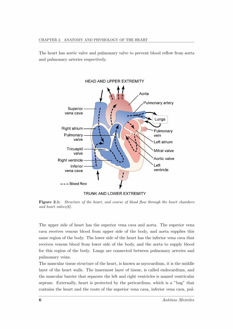
The heart has aortic valve and pulmonary valve to prevent blood reflow from aorta

and pulmonary arteries respectively.

Figure 2.1: Structure of the heart, and course of blood flow through the heart chambersand heart valves[6].

The upper side of heart has the superior vena cava and aorta. The superior vena

cava receives venous blood from upper side of the body, and aorta supplies this

same region of the body. The lower side of the heart has the inferior vena cava that

receives venous blood from lower side of the body, and the aorta to supply blood

for this region of the body. Lungs are connected between pulmonary arteries and

pulmonary veins.

The muscular tissue structure of the heart, is known as myocardium, it is the middle

layer of the heart walls. The innermost layer of tissue, is called endocardium, and

the muscular barrier that separate the left and right ventricles is named ventricular

septum. Externally, heart is protected by the pericardium, which is a ”bag” that

contains the heart and the roots of the superior vena cava, inferior vena cava, pul-

6 Antonio Meireles

2.1. HEART MUSCLE

monary artery and aorta1.

Human heart is composed by three major types of cardiac muscles: atrial muscle

fibres, ventricular muscle fibres, and specialized excitatory and conductive muscle

fibres. The characteristics of these muscular fibres, accomplish different require-

ments in the heart pumping system. Atrial and ventricular muscles fibres contract

in much the same way as skeletal muscle, except that the duration of contraction

is much longer in the heart. Conversely, the specialized excitatory and conductive

fibres have a softly contract, because they contain only a few contractile fibres. In-

stead, they exhibit either automatic rhythmical electrical discharge in the form of

action potentials or conduction of the action potentials through the heart, providing

an excitatory system that controls the rhythmical beating of the heart.

2.1.1 The Special Heart Transmission Fibres

The special heart transmission fibres are located in the inner ventricular walls of the

heart, just below the endocardium, as shown in Figure 2.2 a). These special fibres

conducing the electrical stimulus or impulses through heart tissues. The Sinoatrial

(SA) node located in the right atrium of the heart, is the impulse generator, and

thus the generator of normal sinus rhythm. In parallel, the signal travels to the

Atrioventricular (AV) node via internodal pathways.

2.1.2 Distribution of the Purkinje Fibres in the Ventricles

The fibres fom the AV node to the end of ventricles are the Purkinje fibres. They con-

sist into AV bundle2 and left and right bundle branches. Each branch spreads down-

ward toward the apex of the ventricle, progressively dividing into smaller branches.

An important aspect is that AV bundle has a special characteristic; it is the in-

ability, of action potentials to travel backward from the ventricles to the atria. This

effect is commonly called One-Way Conduction , Figure 2.2 b) shows an detailed

image of this area. This characteristic prevents re-entry of cardiac impulses, by this

route, from the ventricles to the atriums, allowing only forward conduction from the

atriums to the ventricles.

1This group of four vessels are commonly called as great vessels2Also called bundle of His due to Wilhelm His, which was the first to describe them

Antonio Meireles 7


Figure 2.2: a) Sinus node, and the Purkinje system of the heart, showing also the AVnode, atrial inter-nodal pathways, and ventricular bundle branches. b) Organization of theAV node[6].

2.2 Heart Physiology

The rate of blood that flows through human body tissues is controlled in response

to tissues needed for nutrients. Therefore, the heart and circulation are dynamically

controlled by the autonomic nervous system, which automatically control de heart

rate. The details of circulatory function are complex but, in summary, the needs of

the individual tissues are served specifically by bload circulation, where the heart is

the main pump of the system. Figure 2.3 resumes the blood circulation and division

of blood, in percentage, into the systemic circulation and the pulmonary circulation.

The systemic circulation, also called the greater circulation or peripheral circulation,

is responsible to supplies blood to all the tissues in the body except the lungs, and

pulmonary circulation with respect to lungs.

Each atrium is a weak primer pump for the ventricle, helping blood flow into the

ventricle. The right atrium receives the blood poor in oxygen from the body and

delivery it to right ventricle. Then, the right ventricle pumps the blood through the

pulmonary artery into the lungs, were will became oxygenated. The left side receives

this rich oxygenated blood from the lungs and then pumps the blood through the

aorta back to the rest of the body. In resume, the right side of the heart pumps

blood through the lungs, and left side pumps blood through the peripheral organs.

It is clear that the ventricles supply the main pumping force that propels the blood

through the pulmonary circulation and through the peripheral circulation. Due to

8 Antonio Meireles

2.2. HEART PHYSIOLOGY

Figure 2.3: Distribution of blood (in percentage of total blood) in the different parts of thecirculatory system[6].

the higher requirement of pressure to supplies the systemic circulation, left ventricle

has more muscular tissue than right ventricle.

2.2.1 Regulation of Heart Pumping

It was referred that the function of the heart is pumping the blood into the circulation

system to service the needs of the body tissues. When a person is resting the heart

pumps only 4 to 6 litres of blood each minute, but if in severe exercise, the heart

may be required to pump four to seven times this amount.

Under most conditions, the amount of blood pumped by the heart each minute is

determined almost entirely by the rate of blood flow into the heart from the veins,

which is called venous return, i.e. the blood that refill the right atrium. That is,

each peripheral tissue of the body controls its own local blood flow. The heart, in

turn, automatically pumps this incoming blood into the arteries, so that it can flow

around the circuit again.

When an extra amount of blood flows into the ventricles, the cardiac muscle itself

is stretched to greater length. Because of this increased pumping, the ventricles

Antonio Meireles 9


automatically pump the extra blood into the arteries.

2.3 Action Potentials

Cardiac cells, and all living cells in the body, have an electrical potential across the

cell membrane. Figure 2.4 shows a cell membrane, where many ions have a concen-

tration gradient across the membrane, including potassium (K+), with high concen-

tration inside the cell (intracellular) and a low concentration outside (extracellular)

the membrane. Sodium (Na+) and chloride (Cl-) ions are at high concentrations

in the extracellular region, and low concentations in the intracellular regions. This

voltage is established when the membrane has permeability to one or more ions.

In the example of Figure 2.4, if the membrane has selective permeability to po-

Figure 2.4: Membrane potential is the difference in electrical potential between the interiorand exterior of a biological cell Adp. [7].

tassium, these positive charged ions can diffuse through the membrane channel to

the outside of the cell, leaving behind uncompensated negative charges. This charges

separation is what causes the membrane potential. This potential can be measured

by inserting a microelectrode into the cell and measuring the electrical potential,

in millivolts (mV), inside the cell relative to the outside of the cell3. The voltage

across the membrane, ranges from about - 50 to - 200 millivolts, where the minus

sign indicates that inside of the cell is negative relative to outside[8]. Human heart

has three types of membrane ion channels:

1. fast sodium channels,

3By convention, the outside of the cell is considered 0 mV.

10 Antonio Meireles

2.3. ACTION POTENTIALS

2. slow sodiumcalcium channels,

3. potassium channels.

These channels will control the speed that signal travels through cardiac muscle,

due to the permeability to ions such as sodium and potassium.

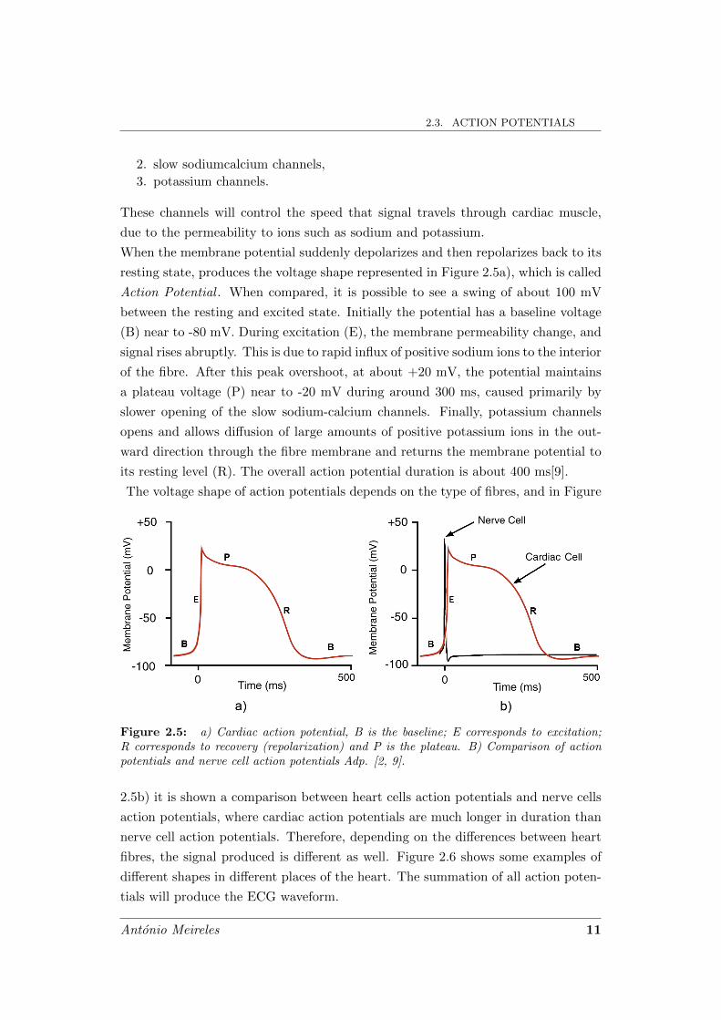
When the membrane potential suddenly depolarizes and then repolarizes back to its

resting state, produces the voltage shape represented in Figure 2.5a), which is called

Action Potential . When compared, it is possible to see a swing of about 100 mV

between the resting and excited state. Initially the potential has a baseline voltage

(B) near to -80 mV. During excitation (E), the membrane permeability change, and

signal rises abruptly. This is due to rapid influx of positive sodium ions to the interior

of the fibre. After this peak overshoot, at about +20 mV, the potential maintains

a plateau voltage (P) near to -20 mV during around 300 ms, caused primarily by

slower opening of the slow sodium-calcium channels. Finally, potassium channels

opens and allows diffusion of large amounts of positive potassium ions in the out-

ward direction through the fibre membrane and returns the membrane potential to

its resting level (R). The overall action potential duration is about 400 ms[9].

The voltage shape of action potentials depends on the type of fibres, and in Figure

Figure 2.5: a) Cardiac action potential, B is the baseline; E corresponds to excitation;R corresponds to recovery (repolarization) and P is the plateau. B) Comparison of actionpotentials and nerve cell action potentials Adp. [2, 9].

2.5b) it is shown a comparison between heart cells action potentials and nerve cells

action potentials, where cardiac action potentials are much longer in duration than

nerve cell action potentials. Therefore, depending on the differences between heart

fibres, the signal produced is different as well. Figure 2.6 shows some examples of

different shapes in different places of the heart. The summation of all action poten-

tials will produce the ECG waveform.

Antonio Meireles 11


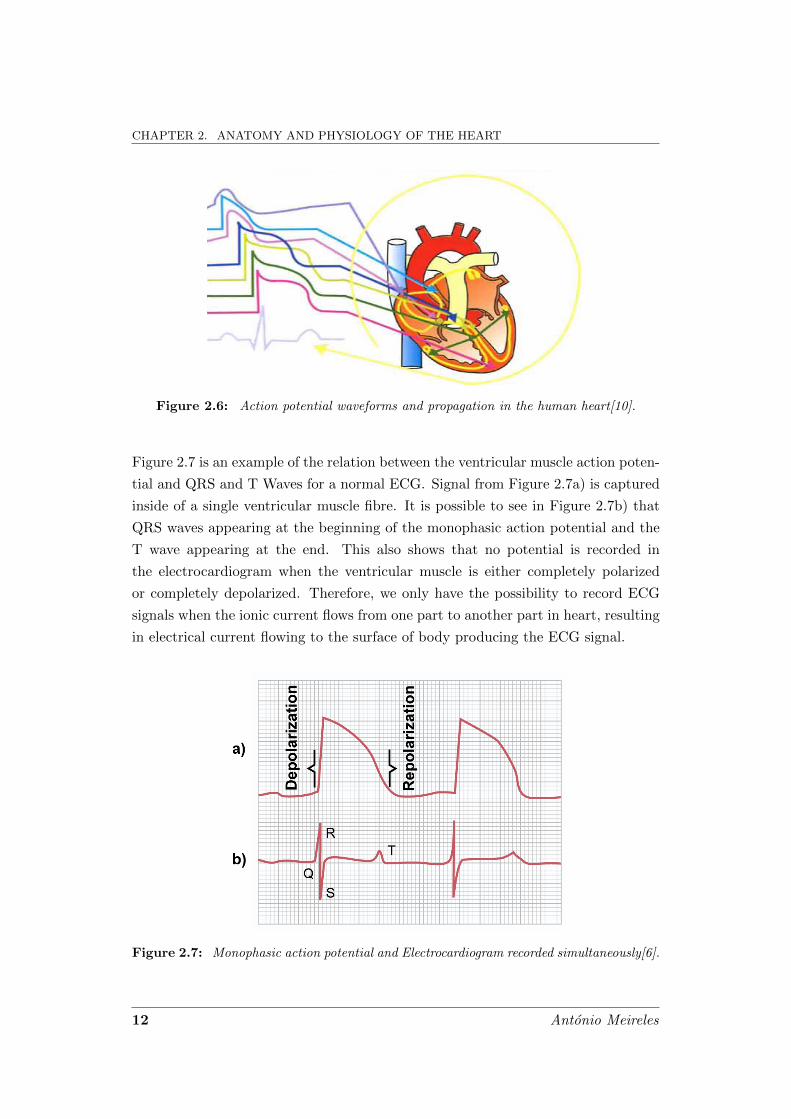
Figure 2.6: Action potential waveforms and propagation in the human heart[10].

Figure 2.7 is an example of the relation between the ventricular muscle action poten-

tial and QRS and T Waves for a normal ECG. Signal from Figure 2.7a) is captured

inside of a single ventricular muscle fibre. It is possible to see in Figure 2.7b) that

QRS waves appearing at the beginning of the monophasic action potential and the

T wave appearing at the end. This also shows that no potential is recorded in

the electrocardiogram when the ventricular muscle is either completely polarized

or completely depolarized. Therefore, we only have the possibility to record ECG

signals when the ionic current flows from one part to another part in heart, resulting

in electrical current flowing to the surface of body producing the ECG signal.

Figure 2.7: Monophasic action potential and Electrocardiogram recorded simultaneously[6].

12 Antonio Meireles

2.4. THE NORMAL ELECTROCARDIOGRAM

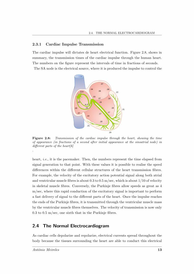
2.3.1 Cardiac Impulse Transmission

The cardiac impulse will dictates de heart electrical function. Figure 2.8, shows in

summary, the transmission times of the cardiac impulse through the human heart.

The numbers on the figure represent the intervals of time in fractions of seconds.

The SA node is the electrical source, where it is produced the impulse to control the

120 Unit III The Heart

of the Purkinje system. Thus, the total time for trans-mission of the cardiac impulse from the initial bundlebranches to the last of the ventricular muscle fibers inthe normal heart is about 0.06 second.

Summary of the Spread of the CardiacImpulse Through the Heart

Figure 10–4 shows in summary form the transmissionof the cardiac impulse through the human heart. Thenumbers on the figure represent the intervals of time,in fractions of a second, that lapse between the originof the cardiac impulse in the sinus node and its appear-ance at each respective point in the heart. Note thatthe impulse spreads at moderate velocity through theatria but is delayed more than 0.1 second in the A-Vnodal region before appearing in the ventricular septalA-V bundle. Once it has entered this bundle, it spreadsvery rapidly through the Purkinje fibers to the entireendocardial surfaces of the ventricles.Then the impulseonce again spreads slightly less rapidly through theventricular muscle to the epicardial surfaces.

It is extremely important that the student learn indetail the course of the cardiac impulse through theheart and the precise times of its appearance in eachseparate part of the heart, because a thorough quanti-tative knowledge of this process is essential to theunderstanding of electrocardiography, to be discussedin Chapters 11 through 13.

Control of Excitation andConduction in the Heart

The Sinus Node as the Pacemaker of the Heart

In the discussion thus far of the genesis and transmis-sion of the cardiac impulse through the heart, we havenoted that the impulse normally arises in the sinusnode. In some abnormal conditions, this is not the case.A few other parts of the heart can exhibit intrinsicrhythmical excitation in the same way that the sinusnodal fibers do; this is particularly true of the A-Vnodal and Purkinje fibers.

The A-V nodal fibers, when not stimulated fromsome outside source, discharge at an intrinsic rhyth-mical rate of 40 to 60 times per minute, and the Purk-inje fibers discharge at a rate somewhere between 15 and 40 times per minute. These rates are in contrastto the normal rate of the sinus node of 70 to 80 timesper minute.

The question we must ask is: Why does the sinusnode rather than the A-V node or the Purkinje fiberscontrol the heart’s rhythmicity? The answer derivesfrom the fact that the discharge rate of the sinus nodeis considerably faster than the natural self-excitatorydischarge rate of either the A-V node or the Purkinjefibers. Each time the sinus node discharges, its impulseis conducted into both the A-V node and the Purkinjefibers, also discharging their excitable membranes. Butthe sinus node discharges again before either the A-Vnode or the Purkinje fibers can reach their own thresh-olds for self-excitation. Therefore, the new impulsefrom the sinus node discharges both the A-V node andthe Purkinje fibers before self-excitation can occur ineither of these.

Thus, the sinus node controls the beat of the heartbecause its rate of rhythmical discharge is faster thanthat of any other part of the heart. Therefore, the sinusnode is virtually always the pacemaker of the normalheart.

Abnormal Pacemakers—“Ectopic” Pacemaker. Occasionallysome other part of the heart develops a rhythmical dis-charge rate that is more rapid than that of the sinusnode. For instance, this sometimes occurs in the A-Vnode or in the Purkinje fibers when one of thesebecomes abnormal. In either case, the pacemaker ofthe heart shifts from the sinus node to the A-V nodeor to the excited Purkinje fibers. Under rarer condi-tions, a place in the atrial or ventricular muscle devel-ops excessive excitability and becomes the pacemaker.

A pacemaker elsewhere than the sinus node iscalled an “ectopic” pacemaker. An ectopic pacemakercauses an abnormal sequence of contraction of the different parts of the heart and can cause significantdebility of heart pumping.

Another cause of shift of the pacemaker is blockageof transmission of the cardiac impulse from the sinusnode to the other parts of the heart. The new pace-maker then occurs most frequently at the A-V node or

.04

.03.07

.07

.07

.05 .03

.00A-V

S-A.09

.06

.16

.19

.19

.22

.21

.21

.20

.18

.18

.17.17

Figure 10–4

Transmission of the cardiac impulse through the heart, showingthe time of appearance (in fractions of a second after initialappearance at the sinoatrial node) in different parts of the heart.

Figure 2.8: Transmission of the cardiac impulse through the heart, showing the timeof appearance (in fractions of a second after initial appearance at the sinoatrial node) indifferent parts of the heart[6]

.

heart, i.e., it is the pacemaker. Then, the numbers represent the time elapsed from

signal generation to that point. With these values it is possible to realise the speed

differences within the different cellular structures of the heart transmission fibres.

For example, the velocity of the excitatory action potential signal along both atrial

and ventricular muscle fibres is about 0.3 to 0.5 m/sec, which is about 1/10 of velocity

in skeletal muscle fibres. Conversely, the Purkinje fibres allow speeds as great as 4

m/sec, where this rapid conduction of the excitatory signal is important to perform

a fast delivery of signal to the different parts of the heart. Once the impulse reaches

the ends of the Purkinje fibres, it is transmitted through the ventricular muscle mass

by the ventricular muscle fibres themselves. The velocity of transmission is now only

0.3 to 0.5 m/sec, one sixth that in the Purkinje fibres.

2.4 The Normal Electrocardiogram

As cardiac cells depolarize and repolarize, electrical currents spread throughout the

body because the tissues surrounding the heart are able to conduct this electrical

Antonio Meireles 13


currents. When these electrical currents are measured by an array of electrodes

placed at specific locations on the body surface, the recorded tracing is called an

ECG. A normal ECG trace is represented in Figure 2.9, where P wave and the

components of the QRS complex are depolarization waves and T wave is the repol-

arisation wave. P wave is caused by electrical potentials generated due to normal

depolarization in the atriums immediately before their contractions. The ventricu-

lar depolarization occurs after atrial depolarization, which is represented by QRS

complex. Finally, the heart re-establishes their potentials recovering from the state

of depolarization. This recovering is known as repolarization, producing the T wave.

This process occurs in a continuous way producing the hart-rate.

The PR interval represents the time required for the depolarization waves to trans-

Figure 2.9: Normal electrocardiogram[6].

verse the atria and the atrioventricular node; the Q-T interval represents the period

of ventricular depolarization and repolarisation; and the ST segment is the isoelec-

tric period when the entire ventricle is depolarized.

The rate of heartbeat can be easily achieved from an electrocardiogram because the

heart rate is the inverse of the time interval between two successive heartbeats. The

normal interval between two successive QRS complexes (RR interval) in the adult

person is about 0.83 second. This is a heart rate of 60/0.83 times per minute, or 72

beats per minute.

14 Antonio Meireles


2.4.1 Voltage and Time of Electrocardiogram

All recordings of electrocardiograms are made with appropriate calibration lines

on the recording paper. Either these calibration lines are already ruled on the

paper, as is the case when a pen recorder is used, or they are recorded on the

paper at the same time that the electrocardiogram is recorded, which is the case

with the photographic types of electrocardiographs. As shown in Figure 2.9, the

horizontal calibration lines are arranged so that 10 of the small line divisions upward

or downward in the standard electrocardiogram represent 1 millivolt, with positive

values in upward direction and negative values in downward direction. The vertical

lines on the electrocardiogram are time calibration lines. Each five vertical segment

lines represent 0.20 second. The 0.20 second intervals are then broken into five

smaller intervals by thin lines, therefore, each of which represents 0.04 second.

When electrocardiograms are recorded from electrodes on the two arms or on one

arm and one leg, the voltage of the QRS complex usually is 1.0 to 1.5 millivolt

from the top of the R wave to the bottom of the S wave; the voltage of the P wave

is between 0.1 and 0.3 millivolt; and the T wave is between 0.2 and 0.3 millivolt.

Moreover, the wave recorded voltages in the normal electrocardiogram depend on

the manner in which the electrodes are applied to the surface of the body and how

close the electrodes are to heart. If one electrode is placed directly over the ventricles

and a second electrode is placed far away from the heart, the voltage of QRS complex

may be as great as 3 to 4 millivolts. Even this voltage is small in comparison with

the monophasic action potentials recorded directly at the heart muscle membrane.

The summary for a normal ECG waves, intervals, and segments are shown in Table

2.1.

Table 2.1: Summary of ECG Waves, Intervals, and Segments [2]

ECG Component Represents Duration (sec)

P wave Atrial depolarization 0.08 - 0.10

QRS complex Ventricular depolarization 0.06 - 0.10

T wave Ventricular repolarization 1

P-R interval Atrial depolarization plus AV nodal delay 0.12 - 0.20

ST segment Isoelectric period of depolarized ventricles 1

Q-T interval Length of depolarization plus repolarization - 0.20 - 0.402

corresponds to action potential duration

1Duration not normally measured.

2High heart rates reduce the action potential duration and therefore the Q-T interval.

Antonio Meireles 15


2.4.2 The Cardiac Cycle

As referred in section 2.4, through RR interval it is possible to achieve the heart

rate. The successive heart contractions forced by SA node is called Cardiac Cycle .

Several events can be observed during the cardiac cycle, Figure 2.10 shows the

Chapter 9 Heart Muscle; The Heart as a Pump and Function of the Heart Valves 107

the electrocardiogram, and the sixth a phonocardio-gram, which is a recording of the sounds produced bythe heart—mainly by the heart valves—as it pumps. Itis especially important that the reader study in detailthis figure and understand the causes of all the eventsshown.

Relationship of the Electrocardiogramto the Cardiac Cycle

The electrocardiogram in Figure 9–5 shows the P, Q,R, S, and T waves, which are discussed in Chapters 11,12, and 13. They are electrical voltages generated bythe heart and recorded by the electrocardiograph fromthe surface of the body.

The P wave is caused by spread of depolarizationthrough the atria, and this is followed by atrial con-traction, which causes a slight rise in the atrial pres-sure curve immediately after the electrocardiographicP wave.

About 0.16 second after the onset of the P wave, theQRS waves appear as a result of electrical depolariza-tion of the ventricles, which initiates contraction of theventricles and causes the ventricular pressure to beginrising, as also shown in the figure. Therefore, the QRScomplex begins slightly before the onset of ventricu-lar systole.

Finally, one observes the ventricular T wave in theelectrocardiogram. This represents the stage of repo-larization of the ventricles when the ventricular musclefibers begin to relax. Therefore, the T wave occursslightly before the end of ventricular contraction.

Function of the Atria as Primer Pumps

Blood normally flows continually from the great veinsinto the atria; about 80 per cent of the blood flowsdirectly through the atria into the ventricles evenbefore the atria contract. Then, atrial contractionusually causes an additional 20 per cent filling of theventricles. Therefore, the atria simply function as

120

100

Pre

ssu

re (

mm

Hg

)

80

60

40

20

0130

90

Vo

lum

e (m

l)

50

Systole

1st 2nd 3rd

SystoleDiastole

QS

T

R

P

a c v

Phonocardiogram

Electrocardiogram

Ventricular volume

Ventricular pressure

Atrial pressure

Aortic pressure

A-V valveopens

A-V valvecloses

Aortic valvecloses

Aortic valveopens

Isovolumiccontraction

Ejection

Isovolumic relaxation

Rapid inflow

DiastasisAtrial systole

Figure 9–5

Events of the cardiac cycle for left ventricular function, showing changes in left atrial pressure, left ventricular pressure, aortic pressure,ventricular volume, the electrocardiogram, and the phonocardiogram.

Figure 2.10: Events of the cardiac cycle for left ventricular function, showing changesin left atrial pressure, left ventricular pressure, aortic pressure, ventricular volume, theelectrocardiogram, and the phonocardiogram[6].

different events during this cycle for the left side of the heart. The cardiac cycle

consists of a period of relaxation called diastole, during which the heart fills with

blood, followed by a period of contraction called systole. The top three curves of

this figure shows the pressure changes in the aorta, left ventricle, and left atrium,

respectively. The fourth curve depicts the changes in left ventricular volume, the

fifth the electrocardiogram, and the sixth a Phonocardiogram (PCG)4.

It is important to refer that a few other parts of the heart can exhibit intrinsic

rhythmical excitation in the same way that the sinus nodal fibres. This is the case

of AV nodal and Purkinje fibres! Without outside excitation, the AV nodal fibres

discharge at an intrinsic rhythmical rate of 40 to 60 times per minute, and the Purk-

inje fibres discharge at a rate somewhere between 15 and 40 times per minute. This

4A Phonocardiogram is a plot of sounds made by the heart during a cardiac cycle.

16 Antonio Meireles


time differences leads to each time the sinus node discharges, its impulse will dis-

charges both the AV node and the Purkinje fibres, before self-excitation can occur

in either of these. Thus, the sinus node controls the beat of the heart because its

rate of rhythmical discharge is faster than any other part of the heart.

The rhythmical and conductive system of the heart is susceptible to damage by

heart disease, especially by ischemia of the heart tissues resulting from poor coron-

ary blood flow. The result is often a bizarre heart rhythm or abnormal sequence of

contraction of the heart chambers, and the pumping effectiveness of the heart often

is affected severely, even to the extent of causing death.

Antonio Meireles 17

3Electrocardiography

Electrocardiography is the interpretation of electrical activity of the heart over a

period of time, which produces a representation of ECG. The ECG is a crucial

diagnostic tool in clinical practice. It is especially useful in diagnosing rhythm dis-

turbances, changes in electrical conduction, and myocardial ischemia and infarction.

In noninvasive electrocardiography, the signal is detected by electrodes attached to

the outer surface of the skin and recorded by a device external to the body. The

sections of this chapter describe the methods used for recording Electrocardiograms.

The locals of electrodes and the respective signal associated to those locals. Then

will be presented a brief exposition about the instrumentation used in ECG field.

3.1 Methods for Recording Electrocardiograms

The ECG is recorded by placing an array of electrodes at specific locations on

the body surface. This is possible because the heart is suspended in a conductive

medium. Figure 3.1 shows the ventricular muscle within the chest. When one

portion of the ventricles depolarizes and therefore becomes negative with respect

to the remainder parts of the heart, forming a potential difference. The electrical

currents flow from the depolarized area to the polarized area in large circuitous

routes.

It is this electrical field that can be collected under surface of the heart. In fact,

this is the summation of all action potentials mentioned in section 2.3.

19

CHAPTER 3. ELECTROCARDIOGRAPHY

Chapter 11 The Normal Electrocardiogram 127

remainder, electrical current flows from the depolar-ized area to the polarized area in large circuitousroutes, as noted in the figure.

It should be recalled from the discussion of thePurkinje system in Chapter 10 that the cardiac impulsefirst arrives in the ventricles in the septum and shortlythereafter spreads to the inside surfaces of the remain-der of the ventricles, as shown by the red areas and thenegative signs in Figure 11–5. This provides elec-tronegativity on the insides of the ventricles and elec-tropositivity on the outer walls of the ventricles, withelectrical current flowing through the fluids surround-ing the ventricles along elliptical paths, as demon-strated by the curving arrows in the figure. If onealgebraically averages all the lines of current flow (theelliptical lines), one finds that the average current flowoccurs with negativity toward the base of the heart andwith positivity toward the apex.

During most of the remainder of the depolarizationprocess, current also continues to flow in this samedirection, while depolarization spreads from the endo-cardial surface outward through the ventricularmuscle mass. Then, immediately before depolarizationhas completed its course through the ventricles, theaverage direction of current flow reverses for about0.01 second, flowing from the ventricular apex towardthe base, because the last part of the heart to becomedepolarized is the outer walls of the ventricles near thebase of the heart.

Thus, in normal heart ventricles, current flows fromnegative to positive primarily in the direction from the base of the heart toward the apex during almostthe entire cycle of depolarization, except at the veryend. And if a meter is connected to electrodes on the surface of the body as shown in Figure 11–5, theelectrode nearer the base will be negative, whereas the electrode nearer the apex will be positive, and the recording meter will show positive recording in theelectrocardiogram.

Electrocardiographic Leads

Three Bipolar Limb Leads

Figure 11–6 shows electrical connections between thepatient’s limbs and the electrocardiograph for record-ing electrocardiograms from the so-called standardbipolar limb leads. The term “bipolar” means that theelectrocardiogram is recorded from two electrodes

+-----

-------+++++++

+++++++

++++++++++++++

++

0

A

B

--

+

+

Figure 11–5

Flow of current in the chest around partially depolarized ventricles.

- +

- +- +

+0.3 mV

+0.7 mV

+0.5 mV

+1.0 mV

Lead III

+1.2 mV

Lead II

Lead I

-0.2 mV

0- +

- +- -

++

0- +

0- +

Figure 11–6

Conventional arrangement of electrodes for recording the stan-dard electrocardiographic leads. Einthoven’s triangle is superim-posed on the chest.

Figure 3.1: Flow of current in the chest around partially depolarized ventricles[6].

3.1.1 Electrocardiographic Leads

Conventionally, electrodes are placed on each arm and leg, and six electrodes are

placed at defined locations on the chest. Three basic types of ECG leads are recorded

by these set of electrodes: standard bipolar limb leads, chest leads and augmented

limb leads. The limb leads are referred as bipolar leads because each lead uses a

single pair of positive and negative electrodes. The augmented leads and chest leads

are unipolar leads because they have a single positive electrode with other electrodes

coupled together electrically to serve as a common negative electrode.


Figure 3.2 shows electrical connections between the patient limbs and the electrocar-

diograph for recording electrocardiograms from the so-called standard bipolar limb

leads. In these arrangements the electrocardiogram is recorded from two electrodes

located on different sides of the heart, in this case, on the limbs. Three different

connections are possible, Lead I, Lead II and Lead III.

Lead I In recording limb Lead I, the negative terminal of the electrocardiograph

is connected to the right arm and the positive terminal to the left arm. Therefore,

20 Antonio Meireles

3.1. METHODS FOR RECORDING ELECTROCARDIOGRAMS


remainder, electrical current flows from the depolar-ized area to the polarized area in large circuitousroutes, as noted in the figure.

It should be recalled from the discussion of thePurkinje system in Chapter 10 that the cardiac impulsefirst arrives in the ventricles in the septum and shortlythereafter spreads to the inside surfaces of the remain-der of the ventricles, as shown by the red areas and thenegative signs in Figure 11–5. This provides elec-tronegativity on the insides of the ventricles and elec-tropositivity on the outer walls of the ventricles, withelectrical current flowing through the fluids surround-ing the ventricles along elliptical paths, as demon-strated by the curving arrows in the figure. If onealgebraically averages all the lines of current flow (theelliptical lines), one finds that the average current flowoccurs with negativity toward the base of the heart andwith positivity toward the apex.

During most of the remainder of the depolarizationprocess, current also continues to flow in this samedirection, while depolarization spreads from the endo-cardial surface outward through the ventricularmuscle mass. Then, immediately before depolarizationhas completed its course through the ventricles, theaverage direction of current flow reverses for about0.01 second, flowing from the ventricular apex towardthe base, because the last part of the heart to becomedepolarized is the outer walls of the ventricles near thebase of the heart.

Thus, in normal heart ventricles, current flows fromnegative to positive primarily in the direction from the base of the heart toward the apex during almostthe entire cycle of depolarization, except at the veryend. And if a meter is connected to electrodes on the surface of the body as shown in Figure 11–5, theelectrode nearer the base will be negative, whereas the electrode nearer the apex will be positive, and the recording meter will show positive recording in theelectrocardiogram.

Electrocardiographic Leads


Figure 11–6 shows electrical connections between thepatient’s limbs and the electrocardiograph for record-ing electrocardiograms from the so-called standardbipolar limb leads. The term “bipolar” means that theelectrocardiogram is recorded from two electrodes

+---

---------++++

+++

+++++++

++++++++++++++

++

0

A

B

--

+

+

Figure 11–5

Flow of current in the chest around partially depolarized ventricles.

- +

- +- +

+0.3 mV

+0.7 mV

+0.5 mV

+1.0 mV

Lead III

+1.2 mV

Lead II

Lead I

-0.2 mV

0- +

- +- -

++

0- +

0- +

Figure 11–6

Conventional arrangement of electrodes for recording the stan-dard electrocardiographic leads. Einthoven’s triangle is superim-posed on the chest.

Figure 3.2: Conventional arrangement of electrodes for recording the standard electrocar-diographic leads. Einthoven’s triangle is superimposed on the chest[6].

the electrode of the right arm is electronegative with respect to the electrode of

the left arm. The electrocardiograph records a positive signal, that is, above the

zero voltage reference line in the electrocardiogram. When the opposite is true, the

electrocardiograph records below this line.

Lead II To record limb lead II, the negative terminal of the electrocardiograph

is connected to the right arm and the positive terminal to the left leg. Therefore,

when the right arm is negative with respect to the left leg, the electrocardiograph

records positively.

Antonio Meireles 21


Lead III To record limb lead III, the negative terminal of the electrocardiograph

is connected to the left arm and the positive terminal to the left leg. This means

that the electrocardiograph records a positive signal when the left arm is negative

with respect to the left leg.

These three limb leads roughly form an equilateral triangle with the heart at the

Figure 3.3: Einthoven Triangle with the placement of the standard ECG limb leads andthe location of the positive and negative recording electrodes for each of the three leads. RA,right arm; LA, left arm; RL, right leg; LL, left leg Adp. [2].

center, refer to Figure 3.3. This triangle is called Einthoven’s triangle in respect of

Willem Einthoven who developed the ECG in 1901. The two vertices at the up-

per part of the triangle represent the points at which the two arms are electrically

connected, and the lower vertex is the electrode located on the right leg used as a

ground point.

Depending on the lead used to record the ECG signal, the resultant shape is slightly

different, this differences can be observed in Figure 3.4.

In the three electrocardiograms represented in Figure 3.4, it can be seen, that at

any given instant the sum of the potentials in leads I and III equals the potential in

lead II, thus illustrating the validity of Einthoven’s law.

The signals from these leads are identical between them, it does not matter greatly

which lead is recorded when one wants to diagnose different cardiac arrhythmias,

because diagnosis of arrhythmias depends mainly on the time relations between the

different waves of the cardiac cycle.

22 Antonio Meireles

3.1. METHODS FOR RECORDING ELECTROCARDIOGRAMS

Lead I Lead II Lead III

Figure 3.4: Normal electrocardiograms recorded from the three standard electrocardio-graphic leads[6].

Chest Leads

When it is important to diagnose damages in the ventricular or atrial muscles, or

in the Purkinje conducting system, the three Bipolar Limb Leads records are not

useful. For these cases, we need leads that can show the abnormalities of cardiac

muscle contraction or cardiac impulse conduction in these areas. The preferred leads

for diagnose these cases are the chest leads, also called Precordial Leads, which are

represented in Figure 3.5. These leads are used to record ECG with one electrode

placed on the anterior surface of the chest directly over the heart at one of the

points shown in Figure 3.5. The different recordings are known as leads V1, V2,

V3, V4, V5, and V6. This electrode is connected to the positive terminal of the

electrocardiograph, and the negative electrode, called the indifferent electrode, is

connected through equal electrical resistances to the right arm, left arm, and left

leg, all at the same time. Usually these six standard chest leads are recorded, one

at a time, where the chest electrode is being placed sequentially at the six points

shown in the figure.

Figure 3.6 illustrates the electrocardiograms of the healthy heart as recorded from

these six standard chest leads. Each chest lead records mainly the electrical potential

of the cardiac musculature immediately beneath the electrode, because the heart

surfaces are close to the chest wall. Therefore, relatively minute abnormalities in

the ventricles, particularly in the anterior ventricular wall, can cause marked changes

in the electrocardiograms recorded from individual chest leads.

Antonio Meireles 23



change the patterns of the electrocardiogramsmarkedly in some leads yet may not affect other leads.Electrocardiographic interpretation of these two types of conditions—cardiac myopathies and cardiacarrhythmias—is discussed separately in Chapters 12and 13.

Chest Leads (Precordial Leads)

Often electrocardiograms are recorded with one elec-trode placed on the anterior surface of the chestdirectly over the heart at one of the points shown inFigure 11–8.This electrode is connected to the positiveterminal of the electrocardiograph, and the negativeelectrode, called the indifferent electrode, is connectedthrough equal electrical resistances to the right arm,left arm, and left leg all at the same time, as also shownin the figure. Usually six standard chest leads arerecorded, one at a time, from the anterior chest wall,the chest electrode being placed sequentially at the sixpoints shown in the diagram. The different recordingsare known as leads V1, V2, V3, V4, V5, and V6.

Figure 11–9 illustrates the electrocardiograms of thehealthy heart as recorded from these six standardchest leads. Because the heart surfaces are close to the chest wall, each chest lead records mainly the

electrical potential of the cardiac musculature imme-diately beneath the electrode. Therefore, relativelyminute abnormalities in the ventricles, particularly inthe anterior ventricular wall, can cause markedchanges in the electrocardiograms recorded from indi-vidual chest leads.

In leads V1 and V2, the QRS recordings of thenormal heart are mainly negative because, as shown inFigure 11–8, the chest electrode in these leads is nearerto the base of the heart than to the apex, and the baseof the heart is the direction of electronegativity duringmost of the ventricular depolarization process. Con-versely, the QRS complexes in leads V4, V5, and V6 aremainly positive because the chest electrode in theseleads is nearer the heart apex, which is the directionof electropositivity during most of depolarization.

Augmented Unipolar Limb Leads

Another system of leads in wide use is the augmentedunipolar limb lead. In this type of recording, two of the limbs are connected through electrical resistancesto the negative terminal of the electrocardiograph,

- +

0- +

1 23 456

LARA

5000ohms

5000ohms

5000ohms

Figure 11–8

Connections of the body with the electrocardiograph for record-ing chest leads. LA, left arm; RA, right arm.

V1 V2 V3 V4 V5 V6

Figure 11–9

Normal electrocardiograms recorded from the six standard chestleads.

aVR aVL aVF

Figure 11–10

Normal electrocardiograms recorded from the three augmentedunipolar limb leads.

Figure 3.5: Connections of the body with the electrocardiograph for recording chest leads.LA, left arm; RA, right arm[6].

Augmented Unipolar Limb Leads

Another system of leads in wide use is the augmented unipolar limb lead. In this

type of recording, two of the limbs are connected through electrical resistances to

the negative terminal of the electrocardiograph, and the third limb is connected to

the positive terminal. When the positive terminal is on the right arm, the lead is

known as the aVR lead; when on the left arm, the aVL lead; and when on the left

leg, the aVF lead. Figure 3.7 showns the angular position of these leads in respect

to bipolar limb leads. The normal recordings of this arrangement are shown in

Figure 3.8. They are all similar to the standard limb lead recordings, except that

the recording from the aVR lead is inverted due to the polarity connections to the

24 Antonio Meireles

3.2. ECG INSTRUMENTATION

Figure 3.6: Normal electrocardiograms recorded from the six standard chest leads[6].

electrocardiograph.

�60º, and so forth is arbitrary, it is the ac-cepted convention. With this axial referencesystem, a wave of depolarization oriented at�60º produces the greatest positive deflectionin lead II. A wave of depolarization oriented�90º relative to the heart produces equallypositive deflections in both leads II and III. Inthe latter case, lead I shows no net deflectionbecause the wave of depolarization is headingperpendicular to the 0º, or lead I, axis (seeECG rules).

Three augmented limb leads exist in ad-dition to the three bipolar limb leads de-scribed. Each of these leads has a single posi-tive electrode that is referenced against acombination of the other limb electrodes. Thepositive electrodes for these augmented leadsare located on the left arm (aVL), the right arm(aVR), and the left leg (aVF; the “F” stands for“foot”). In practice, these are the same posi-tive electrodes used for leads I, II, and III.(The ECG machine does the actual switchingand rearranging of the electrode designa-tions.) The axial reference system in Figure 2-20 shows that the aVL lead is at –30º relativeto the lead I axis; aVR is at –150º, and aVF is at�90º. It is critical to learn which lead is asso-ciated with each axis.

The three augmented leads, coupled withthe three standard limb leads, constitute thesix limb leads of the ECG. These leads recordelectrical activity along a single plane, thefrontal plane relative to the heart. The direc-tion of an electrical vector can be determined

at any given instant using the axial referencesystem and these six leads. If a wave of depo-larization is spreading from right to left alongthe 0º axis (heading toward 0º), lead I showsthe greatest positive amplitude. Likewise, ifthe direction of the electrical vector for depo-larization is directed downward (�90º), aVF

shows the greatest positive deflection.

Determining the Mean Electrical Axis from the Six Limb LeadsThe mean electrical axis for the ventricle canbe estimated by using the six limb leads andthe axial reference system. The mean electri-cal axis corresponds to the axis that is perpen-dicular to the lead axis with the smallest netQRS amplitude (net amplitude � positive mi-nus negative deflection voltages of the QRS

ELECTRICAL ACTIVITY OF THE HEART 35

0° Lead

+60°Lead II

+120°Lead III

I

III II

I

IIIII

LL

LARA

Axial Reference SystemEinthoven’s Triangle

I

FIGURE 2-19 Transformation of leads I, II, and III from Einthoven’s triangle into the axial reference system. Leads I, II,and III correspond to 0º, 60º, and 120º in the axial reference system. RA, right arm; LA, left arm; LL, left leg.

I

IIaV

aV aV

IIIF

LR

0°

+60°+90°

-30° -150°

+120°

FIGURE 2-20 The axial reference system showing thelocation within the axis of the positive electrode for allsix limb leads.

Ch02_009-040_Klabunde 4/21/04 10:53 AM Page 35

Figure 3.7: The angular position of Augmented Unipolar Limb Leads in respect to BipolarLimb Leads[2].

3.2 ECG Instrumentation

The electrical activity of the heart is fairly simple to measure. In the very early

1900s, Willem Einthoven won the Nobel Prize in medicine for his work identifying

and recording the parts of the electrocardiogram. Figure 3.9b) shows a photography

of Willem Einthoven and Figure 3.9a) a photography of its complete electrocardio-

graph machine with a patient. Today’s medical instruments are considerably more

complicated and diverse, mainly because they incorporate electronic systems for

sense, manipulate, store, and display data and information. Today, an electrocardi-

ograph is more compact and offers several functionalities, e.g. the model PageWriter

Antonio Meireles 25


Figure 3.8: Normal electrocardiograms recorded from the three augmented unipolar limbleads[6].

Figure 3.9: a) Photograph of a complete electrocardiograph, showing the manner in whichthe electrodes are attached to patient, in this case the hands and one foot being immersed injars of salt solution. b) Willem Einthoven in the lab.

TC70 from Philips shown in Figure 3.10a) offers the possibility to record 20 minutes

of up to 16 leads simultaneously, into a box of 40 x 33 x 16 cm. In Figure 3.10b) it

is shown the model StressVue from same supplier used for stress ECG recordings,

for example during an exercise.

Mostly of these equipments are considered High Resolution ECG (HRECG) sys-

tems, where at least three bipolar leads are used in an anatomic xyz coordinate

system.

3.2.1 The Ambulatory ECG

Due to their complexity, medical ECG equipments are used mostly in hospitals and

medical centres by trained personnel, but some also can be found in private homes

operated by patients themselves or their caregivers. Examples of these equipments

are the portable devices for personal usage and long term recorders called Holter

26 Antonio Meireles

3.2. ECG INSTRUMENTATION

Figure 3.10: a) Philips electrocardiograph model PageWriter TC70. b) Philips stresstesting system StressVue.

devices. The original large-scale clinical use of this technology was to identify pa-

tients who developed heart block transiently and could be treated by implanting a

cardiac pacemaker. The very first device was developed by Dr. Norman Jeff Holter

in the early 1940s, refer to Figure 3.11a), where the data is recorded into a tape and

the weight of this equipment surrounds 38 Kg, Figure 3.11b) shows a patient holding

the Holter monitor[11]. The evolution of Holter ECG is closely followed by technical

Figure 3.11: a) Dr. Norman Jeff Holter (1914-1983) with original Holter; b) A patientwith the original Holter device from 1947; c) Low cost modern Holter model MIC-12H-3Lfrom Beijing Jinco Medical.

and clinical progress. A modern Holter device can record tree to twelve simultaneous

leads from 24 to 48 hours into a digital memory. Figure 3.11c) shows an example

of a low cost modern Holter model MIC-12H-3L from Beijing Jinco Medical, with

Antonio Meireles 27


ability to record twelve leads during 24 hours.

3.2.2 Electrocardiograph Block diagram 1 de 1Página e

26-10-2010file://C:\Users\António Meireles\Desktop\6163.gif

Figure 3.12: ECG system block diagram[12].

Figure 3.12 shows the block diagram of an ECG system. Basic functions of an

ECG machine include: ECG waveform display, either through Liquid Crystal Dis-

play (LCD) screen or printed paper media, and heart rhythm indication as well as

simple user interface through buttons. More features, such as patient record stor-

age through convenient media, wireless/wired transfer and 2D/3D display on large

LCD screen with touch screen capabilities, are required in more and more ECG

products. Multiple levels of diagnostic capabilities are also assisting doctors and

people without specific ECG trainings to understand ECG patterns and their indic-

ation of a certain heart condition. After the ECG signal is captured and digitized,

it will be sent for display and analysis, which involves further signal processing[12].

3.3 ECG Electrods

The measurements of electrical activity in the heart, muscles, or brain are examples

of direct measurements of physiological energy. For these measurements, the energy

is already electrical and only needs to be converted from ionic to electronic current

using an electrode. To collect ECG at surface of skin, it is indispensable the use of

electrodes, and the electrodes used by non-evasive electrocardiography are so many

28 Antonio Meireles

3.3. ECG ELECTRODS

that will be only covered here their principal aspects.

The electric characteristics of bio-potential electrodes are generally nonlinear and a

function of the current density at their surface. But electrodes are usually represen-

ted by linear models due to they operation at low potentials and currents[13, 14, 15,

16]. Under these conditions, electrodes and the skin model can be represented by the

equivalent circuit shown in Figure 3.13. In this circuit RP and CP are components

Figure 3.13: Liner model of an electrical equivalent circuit for a bio-potential electrode.

that represent the impedance associated with the electrode-electrolyte interface and

polarization at this interface. Rs is the series resistance associated with interfacial

effects and the resistance of the electrode materials themselves, and Vep represents

the half-cell potential. Half-cell potential is associated to the distribution of ions

or charged molecules in a biologic structure. The half-cell potential occurs due to

the interaction between the metal of the electrode and the solution used near to the

metal surface. The use of this solution is crucial for better adapting the contact

between the electrodes and the skin. In fact, when the cations in this solution and

the metal of the electrodes are the same, the half-cell potential is reduced[17, 18].

The values of these potentials are dependent of the characteristics of materials and

can be described by the Nernst:

Vep = −GTnF

lnQ (3.1)

Where T is the absolute temperature (Kelvin), G = 8.31451Jmol−1K−1) is the

ideal gas constant, F = 96485.3Cmol−1 is Faraday’s constant, and n is the number

or electrons transferred in the balanced oxidation/reduction reaction, and Q is the

reaction quotient, i.e. the extracellular and intracellular concentrations.

Vep value is the value corresponding to materials/reactions Ag+Cl− → AgCl+e− =

+0.223V . This constant is based on the assumption that electrode distance between

metal and skin is constant. If this distance changes Vep take much higher values,

which is described as motion artefacts1. The most important aspect is that the

presence of the electrode does not affect the variable being measured.

1Motion artefacts are a typical noise associated to movements of electrodes in the skin.

Antonio Meireles 29


Depending on the type of ECG that are being measured, different electrodes

Figure 3.14: ECG electrodes: a) electrodes for diagnostic resting, b) electrodes for stresstest and Holter, c) electrodes for monitoring.

should be used. In the market it is possible to find different types of electrodes, but

they mainly occupy three different families: electrodes for diagnostic resting ECG,

Figure 3.14a); electrodes for stress test and Holter ECG, Figure 3.14b); electrodes

for monitoring ECG, Figure 3.14c).

30 Antonio Meireles

4Noise

Noise is present in almost all environments, and can be defined as an undesirable

signal that interferes with the desired signal. A noise itself is a signal that can

be generated from several sources, and takes different spectrum distributions. In

fact, biomedical electrical signals, which are the scope of this work, are always pol-

luted with some kind of noise. These interference signals includes interferences from

power supplies, motion artefacts due to patient movement, radio frequency interfer-

ence, defibrillation pulses, pace maker pulses, interferences from other monitoring

equipment, etc[12]. The big challenge of noise in biomedical signals is closely related

with amplitude of the desired signals face to the noise, i.e. the Signal-to-Noise Ra-

tio (SNR). For instance, an ECG measurement gets challenging due to the presence

of the large DC offset and various interference signals. This potential can be up to

300 mV for a typical electrode, which is several times larger than ECG signal.

Noise reduction is an important task to solve in biomedical signals and for this

reason, the understanding of noise characteristics is the focus of the contents in

this chapter. The chapter will starts with noise properties and characteristics as

SNR and separability, followed by most common noises sources associated to ECG.

Finally it is presented the literature review about the methodologies used to ECG

signal denoising.

31

CHAPTER 4. NOISE

4.1 Noise Properties

Depending on its frequency or time characteristics, a noise process can be classified

in several categories: Narrowband noise, White noise, Band-limited white noise,

Coloured noise, Impulsive noise and Transient noise pulses[19]. Narrowband noise

is a noise process with a narrow bandwidth such as a 50Hz hum from the power

lines. White noise is purely random noise that has a flat power spectrum. White

noise theoretically contains all frequencies in equal intensity. Band-limited white

noise it is a noise with flat spectrum and limited bandwidth that usually covers the

limited spectrum of the device or the signal of interest. Coloured noise it is non-

white noise or any wideband noise whose spectrum has a non-flat shape; examples

are pink noise, brown noise and autoregressive noise. Impulsive noise consists of

short-duration pulses of random amplitude and random duration. And transient

noise pulses consists of relatively long duration noise pulses.

4.1.1 Noise Characteristics

Noise is usually represented as a random variable, x(n), and describing his properties

as a function of time it is not very useful. Therefore, it is more common the evalu-

ation of its probability distribution, range of variability, or frequency characteristics[20].

While noise can take a variety of different probability distributions, the Central

Limit Theorem1 implies that noises will have a Gaussian or normal distribution.

The probability p(x) of a Gaussianly distributed variable, x, is specified by the

normal or Gaussian distribution equation:

p(x) =1

σ√

2πe

−(x−a)2

2σ2 (4.1)

Where, a it is the mean, or average value, and σ2 is the variance. The arithmetic

quantities of mean and variance are frequently used in signal processing algorithms.

The mean value of a discrete array of N samples is evaluated as:

x =1

N

N∑k=1

xk (4.2)

1The central limit theorem explains why many distributions tend to be close to the normaldistribution, i.e., when noise is generated by a large number of independent sources it will have aGaussian probability distribution.

32 Antonio Meireles

4.1. NOISE PROPERTIES

And the variance, σ2, is calculated as:

σ2 =1

N − 1

N∑k=1

(xk − x)2 (4.3)

From Equation (4.3) we grasp the standard deviation σ, which is just the square

root of the variance.

Normalizing Equation (4.3) by:1

N − 1(4.4)

will produces the best estimate of the variance if x is a sample from a Gaussian

distribution. Alternatively, normalizing the Equation (4.3) by:

1

N(4.5)

produces the second moment of the data around x, which is equivalent to RMS value

of the data if the data have zero as mean value.

If noise is captured from different sensors, such as sensor array, or multiple observa-

tions from the same source, the standard deviation of noise becomes reduced by the

square root of the number of averages.

4.1.2 Signal-to-Noise Ratio

From previous notes at beginning of this chapter, signal and noise are relative terms:

general speaking, signal is the waveform of interest while noise is everything else.

The relative amount of signal and noise present in a waveform is usually quantified

by the SNR. As the name implies, this is simply the ratio of signal to noise, both

measured in Root-Mean-Squared (RMS) amplitude. The SNR is often expressed in

decibel (dB) where:

SNR = 20logSignal

Noise(4.6)

To convert from dB scale to a linear scale:

SNRlinear = 10dB20 (4.7)

For example, a ratio of 20 dB means that the RMS value of the signal was 10 times

the RMS value of the noise, because 1020/20 = 10. A common value in this area is

+3 dB, which indicates a ratio of 103/20 = 1.414, and -3 dB means that the ratio is

1/1.414. If noise and signal has the same amount in RMS value, this means 0 dB.

Antonio Meireles 33

CHAPTER 4. NOISE

As an example, Figure 4.1 shows an ECG signal with different amounts of white

noise. Notice that it is very difficult to detect presence of ECG signal visually when

the SNR is -3 dB, and impossible when the SNR is -10 dB.

a) b)

d)c)

Figure 4.1: A ECG signal with varying amounts of added noise. The signal is barelydiscernable when the SNR is -3 dB and not visible when the SNR is -10 dB.

4.1.3 Separability of Signal and Noise

A signal is completely recoverable from noise if the spectra of the signal and the

noise do not overlap. An example of a noisy signal with separable signal and noise

spectra is shown in Figure 4.2(a). In this case, the signal and noise are placed in

different parts of the frequency spectrum, and signal can be denoised with a low-

pass filter. Although, Figure 4.2(b) illustrates a more common example of signal

and noise, with overlapping spectra. For these cases, it is not possible to completely

separate the signal from the noise; however, the effects of the noise can be more or

less reduced depending on the filter technique used.

34 Antonio Meireles

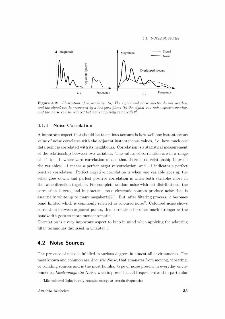
4.2. NOISE SOURCESSome Applications of Wiener Filters 195

deduced. For additive noise, the Wiener filter frequency response is a real positive number in the range 1)(0 ≤≤ fW . Now consider the two limiting cases of (a) a noise-free signal ∞=)( fSNR and (b) an extremely noisy signal SNR(f)=0. At very high SNR, 1)( ≈fW , and the filter applies little or no attenuation to the noise-free frequency component. At the other extreme, when SNR(f)=0, W(f)=0. Therefore, for additive noise, the Wiener filter attenuates each frequency component in proportion to an estimate of the signal to noise ratio. Figure 6.4 shows the variation of the Wiener filter response W(f), with the signal-to-noise ratio SNR(f). An alternative illustration of the variations of the Wiener filter frequency response with SNR(f) is shown in Figure 6.5. It illustrates the similarity between the Wiener filter frequency response and the signal spectrum for the case of an additive white noise disturbance. Note that at a spectral peak of the signal spectrum, where the SNR(f) is relatively high, the Wiener filter frequency response is also high, and the filter applies little attenuation. At a signal trough, the signal-to-noise ratio is low, and so is the Wiener filter response. Hence, for additive white noise, the Wiener filter response broadly follows the signal spectrum. 6.6.2 Wiener Filter and the Separability of Signal and Noise A signal is completely recoverable from noise if the spectra of the signal and the noise do not overlap. An example of a noisy signal with separable signal and noise spectra is shown in Figure 6.6(a). In this case, the signal

Sepa

rabl

e sp

ectr

a

Signal

Noise Magnitude Magnitude

Frequency Frequency

Overlapped spectra

(a) (b) Figure 6.6 Illustration of separability: (a) The signal and noise spectra do not overlap, and the signal can be recovered by a low-pass filter; (b) the signal and noise spectra overlap, and the noise can be reduced but not completely removed.

Figure 4.2: Illustration of separability: (a) The signal and noise spectra do not overlap,and the signal can be recovered by a low-pass filter; (b) the signal and noise spectra overlap,and the noise can be reduced but not completely removed[19].

4.1.4 Noise Correlation

A important aspect that should be taken into account is how well one instantaneous

value of noise correlates with the adjacent instantaneous values, i.e. how much one

data point is correlated with its neighbours. Correlation is a statistical measurement

of the relationship between two variables. The values of correlation are in a range

of +1 to −1, where zero correlation means that there is no relationship between

the variables; −1 means a perfect negative correlation; and +1 indicates a perfect

positive correlation. Perfect negative correlation is when one variable goes up the

other goes down, and perfect positive correlation is when both variables move in

the same direction together. For complete random noise with flat distributions, the

correlation is zero, and in practice, most electronic sources produce noise that is

essentially white up to many megahertz[20]. But, after filtering process, it becomes

band limited which is commonly referred as coloured noise2. Coloured noise shows

correlation between adjacent points, this correlation becomes much stronger as the

bandwidth goes to more monochromatic.

Correlation is a very important aspect to keep in mind when applying the adapting

filter techniques discussed in Chapter 5.

4.2 Noise Sources

The presence of noise is fulfilled in various degrees in almost all environments. The

most known and common are:Acoustic Noise, that emanates from moving, vibrating,

or colliding sources and is the most familiar type of noise present in everyday envir-

onments; Electromagnetic Noise, wich is present at all frequencies and in particular

2Like coloured light; it only contains energy at certain frequencies

Antonio Meireles 35

CHAPTER 4. NOISE

at radio frequencies; Processing Noise, that results from the signal processing, e.g.

quantisation noise in digital coding, or lost data packets in digital data communic-

ation systems.

4.2.1 Biomedical Noises Sources

Noise frequently is a limitation factor in the performance of medical instrumentation,

producing variability. In biomedical measurements, variability has four different

origins:

1. Physiological variability;2. Transducer artifact;3. Environmental noise or interference;4. Electronic noise.

Physiological Variability Physiological variability is due to the presence of other

sources of biological influences than those of interest. For example, assessment of

respiratory function based on the measurement of blood pO23 could be confounded

with other physiological mechanisms that change blood pO2[20]. Physiological vari-

ability can be a very difficult problem to solve, where to solve it, sometimes it is

required information provided by different sources to help in validation.

Transducer Artefact Transducer artefact is produced when the transducer is

the responsible to change the desired signal. For example, non-invasive recordings

of electrical potentials using electrodes placed on the skin are sensitive to motion

artefact.

Environmental Noise Environmental noise is generated from existing sources,

either external or internal to the body. For example, in a fetal ECG recording, the

fetal ECG is corrupted by the mother ECG. In these cases it is not possible to

describe the specific characteristics of environmental noise.

Electronic Noise Electronic noise falls into two broad classes: thermal or John-

son noise4, and shot noise. The former is produced primarily in resistor or resistance

materials while the latter is related to voltage barriers associated with semiconduct-

ors. Both sources produce noise with a broad range of frequencies often extending

from DC to 1012 − 1013Hz.3Partial Pressures of O2.4Statistical fluctuation of electric charge exists in all conductors, producing random variation of

potential between the ends of the conductor[21].

36 Antonio Meireles

4.3. ECG NOISES SOURCES

4.3 ECG Noises Sources

ECG signals always have background noise associated, and noise sources are so many

that noise reduction became an important frontend signal processing task for bio-

medical signals. The most common noises that usually should be considered are:

Power line interference, muscular contraction (EMG), Instrumentation noise gener-

ated by electronic devices, Baseline drift and ECG amplitude modulation[22, 23].

Power line interference is a narrow-band noise centred at 50 Hz with a bandwidth

of less than 1 Hz. This type of noise usually contains harmonics due to parasite

currents through human body. Power line interference is relatively constant during

the ECG measurement. Cables used in electrodes connections are another source of

power line noise[24].

Muscular contractions produce artefacts within millivolts level potentials. This sig-

nal is normally transient bursts of zero mean band-limited Gaussian noise[22]. The

worst case of muscular contractions interference is when the measurements are made

at same time as muscular activity, i.e., in sports or jobs with intense body activ-

ity. In these cases, the muscular amplitude signal can completely overlaps the ECG

signals. Without muscular activity the noise produced can be negligible due to its

insignificant amplitude.

Artefacts generated by electronic devices can produce several different interferences,

conducing to unpredictable noise shapes, leading to complete signal distortion or

equipment saturation. If they do not consider these situations, these artefacts could

be considered similar to Gaussian noise.

Baseline drift and ECG amplitude modulation with respiration occurs during the

breathing cycle. The amplitude of ECG signal varies mainly influenced by relative

distance between heart and electrodes. This distance is increased when lungs fill

and reduces at time of lungs become empty. The effect can be observed as a slow

modulation of the ECG amplitude with same frequency as the breathing cycle. The

amplitude of the ECG signal also varies by about 15% with respiration[25, 26, 27, 28].

In addition, physiological and environmental noise affects the ECG power spectrum.

ECG power spectrum can provide useful information about heart condition, and if

ECG signal is polluted with noise for overall spectrum, becomes difficult to aim this

information with good accuracy. Figure 4.3 summarizes the relative power spectra

of the ECG, QRS complexes, P and T waves, motion artefact, and muscle noise.

This graph reveals that the ECG signal has their energy mainly concentrated in fre-

quencies below than 25 Hz, where the QRS complex assumes the major area. Also

Antonio Meireles 37

CHAPTER 4. NOISE

ECG QRS Detection 237

prior to the power spectrum analysis. The peak of the frequency spectrum obtained corresponds to the peak energy of the QRS complex.

The ECG waveform contains, in addition to the QRS complex, P and T waves, 60-Hz noise from powerline interference, EMG from muscles, motion artifact from the electrode and skin interface, and possibly other interference from electrosurgery equipment in the operating room. Many clinical instruments such as a cardiotachometer and an arrhythmia monitor require accurate real-time QRS detectioo. It is necessary to extract the signal of interest, the QRS complex, from the other noise sources such as the P and T waves. Figure 12.1 summarizes the relative power spectra of the ECG, QRS complexes, P and T waves, motion artifact, and muscle noise based on our previous research (Thakor et aI., 1983).

1.0 ------------------------

•

0.8

~ 0.6 Q)

~ o c. ~ .~ 0.4 -Q) a:

0.2

P-T waves

Motion artifact

/

0.0 -------:: o 5 10

ECG

QRS complex

Muscle noise

15 20 25 30 35 40

Frequency (Hz)

Figure 12.1 Relative power spectra of QRS complex, P and T waves, muscle noise and motion artifacts based on an average of 150 beats .

•

12.2 BANDPASS FILTERING TECHNIQUES

From the power spectral analysis of the various signal components in the ECG signal, a filter can be designed which effectively selects the QRS complex from the ECG. Another study that we perfonned examined the spectral plots of the ECG and the QRS complex from 3875 beats (Thakor et aI., 1984). Figure 12.2 shows a plot of the signal-to-noise ratio (SNR) as a function of frequency. The study of the

Figure 4.3: Relative power spectrum of QRS complex, P and T waves, muscle noise andmotion artefacts based on an average of 150 beats[29].

shows that motion artefact overlapping a small part of ECG signal, and the EMG

noise overlaps the entire ECG signal. It is clear that EMG noise can completely

destroy ECG in a presence of low SNR.

4.4 ECG Noise Cancelation Techniques

Noise cancellation requires different strategies for different noise sources or types.

Since the focus of this paper is a non classical method, the approaches covered in

this section are all included in the non-classical methods used by several authors.

An useful method for removing power line and baseline disturbances is the applica-

tion of a digital linear phase filtering[30]. This method can be used to reduce signal

magnitude spectrum while preserving the signal time domain as much as possible.

The disadvantage of this method is the computational requirements. This is mainly

caused by linear phase narrow-band filtering, that requires a long impulse response,

and the corresponding number of filter coefficients caused by a large number of mul-

tiplications involved in the time domain[31].

Random and stationary noise can be removed using a temporal averaging method.

Noise reduction by temporal averaging method is proportional to the square root

of the number of frames or beats taken into the average[32]. This method only

offers effective performance if a large number of samples is used. Moreover, due to

heartbeats variability, it can cause considerable errors, producing distorted results,

or extremely smooth waves.

38 Antonio Meireles

4.4. ECG NOISE CANCELATION TECHNIQUES

To increase signal quality, some authors refer the performance of spatial averaging[33,

34, 35]. But spatial averaging requires a large number of electrodes in the same re-

gion, which cause the main drawback of the method for portable equipment. This

not only causes a discomfort to the users, as well as an amount of signals to be re-

corded and treated. Meanwhile, solutions like wearable sensors might be the answer

to discomfort, but at time these solutions produces high noise levels due to a bad

contact of electrodes at skin surface producing high levels of noise.

To remove muscle noise artifacts in exercise ECG’s, Joseph Suresh et al.[36] proposed

the SVD (Singular Value Decomposition) method. For a satisfactory performance,

SVD filtering do not requires prior information about the onset or offset points of

ECG signal, nor knowledge of heartbeat intervals. This is very important since in

the presence of a noisy ECG signal it wouldn’t be possible to grasp the right pos-

ition of the wave. SVD method is based on matrix factorization, and the problem

of this technique is the matrix dimension and computational calculations before a

possible reduction of the matrix. However, the authors of [36] mentioned that with

a minimum value of matrix size, the results performance of the MSE (mean square

error) are identical to the results of the Wiener filter MSE using a discrete cosine

transform.

One promising solution for noise reduction is the use of adaptive filters. There are

several advantages for adaptive filtering approaches: adapting filtering do not needs

a priori knowledge of the statistical or spectral properties of the signal and noise;

constantly adapt the weights of filter for better performance; when applied to a

set of samples does not require higher power computation requirements. For some

applications, the drawback of adaptive filtering approach is that requires the correl-

ation of noise with signal. For the case of ECG, this is not a problem due to the

possibility to obtain this correlation from the electro in the leg. Several authors,

e.g.[37, 38, 39], have done their works in this field of signal processing, but mainly

with ECG signals from databases as MIT-BIH.

Antonio Meireles 39

5Filtering

Filtering is closely related with signal processing discipline, and can be classified

into two main categories, analogue signal processing and digital signal processing.

Analogue signal processing is for signals that have not been digitized, which involves

linear or nonlinear electronic circuits, such as passive or active filters. Digital signal

processing is the processing of digitized discrete time sampled signals, where signal

treatment is performed by computers or digital circuits, e.g. Digital Signal Processor

(DSP) devices, running mathematical algorithms such as FIR or IIR. Additionally,

filtering can be classified into linear or nonlinear process. If the filtered output is a

linear function of the input observations, the filters is said to be linear, otherwise

the filter is considered nonlinear. Moreover, filtering is directly related with spectral

analysis, because the goal of filtering is to reshape the signal spectrum. For that

reason, filtering techniques and filter types differing in the way that they reshape

the signal spectrum.

This chapter will start with a brief presentation of signal processing methods and

then the main focus will be the Adaptive Signal processing technique, based on LMS

algorithm.

5.1 Signal Processing Methods

Depending on the statistical distribution of signal, digital signal processing al-

gorithms can assume different realisations. If the signal statistical distribution is

41

CHAPTER 5. FILTERING

unknown, it is used Non-parametric Signal Processing methods. These methods

lead with signals in a ”blind” way, i.e., they do not care about the signal itself,

because they are not specialised to any particular class of signals. The drawback

is that they can lose performance due to their generality. Some examples of non-

parametric methods include digital filtering and transform-based signal processing

methods such as the Fourier analysis and discrete cosine transform. By other hand, if

the statistical distribution of signal is known, it is commonly used Model-Based Sig-

nal Processing methods. Model-based methods normally outperform non-parametric

methods, since they make use of more information in the form of a model of the

signal process. These signal processing methods use a description of the expected

patterns in the signal process, for these cases the methods are more dedicated and

less generalist. However, they can be sensitive to signal deviations due to their

restrictions[19, 40]. They are commonly used in low-bit-rate speech coding, digital

video codification and speech recognition.

Filtering has a close relationship with signal spectrum, and for that reason, they

can be classified in two big groups: FIR filters and IIR filters.

FIR filters are non-recursive filters, because only the input is used in the filter

Figure 5.1: FIR Structure

algorithm, Figure 5.1 shows a block diagram of an FIR filter, whit an input x(k)

and an output y(k). The output y(k) is defined as:

y(k) = a0x(k) + a1x(k − 1) + a2x(k − 2) + . . . ; k = 0, 1, . . . , N − 1. (5.1)

Leading to:

y(k) =

N−1∑i=0

aix(k − i) (5.2)

42 Antonio Meireles

5.1. SIGNAL PROCESSING METHODS

Where ai is the filter feed forward coefficients needed to generate the necessary fil-

tering response, such as low-pass or high-pass, and N is the number of filter taps

contained in the function, Z−1 is the signal delay and k is the discrete-time index.

The ai coefficients are the zeros of the filter.

This filters have the advantage of always being stable and having linear phase shifts.

The downside of FIR filters is that they are less efficient in terms of computer time

and memory than IIR filters[20].

FIR filters uses feed-forward calculations only, and in if we allowed feed-back, then

the filter impulse response is non-zero over an infinite length of time. This is called

IIR filters, which is represented in Figure 5.2.

Figure 5.2 shows a block diagram of an IIR filter, whit an input x(k) and an output

Figure 5.2: IIR Structure

y(k). The output y(k) is defined as:

y(k) = a0x(k)+a1x(k−1)+a2x(k−2)+· · ·−b1y(k−1)−b2y(k−2); k = 0, 1, . . . , N−1.

(5.3)

Leading to:

y(k) =

N−1∑i=0

aix(k − i)−N−1∑i=1

biy(k − i) (5.4)

Where bi is the filter feedback coefficients, which is the poles of the filter, and the

remaining variables are equal to the FIR filter.

Due to the existence of poles, IIR filters can be unstable, which can be a disad-

vantage. However, IIR filters are sometimes preferred over FIR filters, because it is

possible to achieve the same transition region as FIR filters with less order.

Antonio Meireles 43


FIR and IIR filters are considered fixed1; their characteristics are projected to a

specific signal, and independently of their dynamics or statistical properties their

parameters remains static. To lead with signals whose statistical properties are

unknown, fixed algorithms do not process these signals efficiently. Due to this in-

efficiency, new methods have been studded. This new methods are self-designing

systems defined as adaptive filters. Adaptive filters may be classified into supervised

adaptive filters, that are based on training sequence that provides different realiz-

ations of a desired response for a specified input signal, or unsupervised adaptive

filters, which performs the adjustments of their free parameters without requiring

a desired response. These filters are commonly used where there is no access to a

desired response, e.g. system identification.

5.2 Adaptive Signal Processing

Aiming to achieve best filtering performance, signal processing methods have pro-

gressed considerably in algorithm complexity. In general, the computational re-

quirement for signal processing methods have being increased exponentially face to

algorithmic complexity. Therefore, finding an algorithm with ability to filtering sig-

nals efficiently, with automatic performance adaptation, and at same time offering a

good balance between performance and computation requirements, becomes an in-

teresting motivation to work with non-classical filtering2 schemes as adaptive signal

processing techniques. Conversely to classical FIR and IIR filters, adaptive filters

automatically changes theirs characteristics, by optimizing the internal parameters.

It is important to refer the close relationship of the adaptive signal processing tech-

nique with Wiener filter. Wiener filter is based on the minimization of the Mean

Square Error (MSE) value of signal that is defined as the difference between some

desired response and the actual filter output. But, it is only possible to design a

Wiener filter with optimal performance if a priori information about the statistics of

the data to be processed is known[41]. Adaptive filters are quite similar to Wiener

filters, they are based on the same concept, the minimization of the MSE. But

unlike Wiener filters, the parameters of adaptive filters are constantly adapted to

reach the MSE.

Adaptive filters are widely used in several applications including the treatment of

1a and b are fixed values.2An example of classical filters are FIR and IIR

44 Antonio Meireles

5.3. ADAPTING FILTERING IMPLEMENTATION

biomedical signals. Biomedical signals such as ECG, EMG, and Electroencephalo-

graphy (EEG) are important in diagnosis and patient monitoring. But these signals

have very small amplitude, therefore they are commonly affected by noise. It is

difficult to filter noise from these signals, and errors resulting from filtering may

distort them.

5.2.1 Adapting Filtering Scheme

The complete specification of an adaptive system consists in three main points:

application, structure and algorithm[42].

Application What is the application where the filter will be used? The type of

application is defined by the signals applied to the input and the desired output sig-

nals. The number of different applications in which adaptive techniques are being

successfully used increases every day. Some examples are echo cancellation, equal-

ization of dispersive channels, system identification, signal enhancement, adaptive

beam forming, noise cancelling, and control.

Structure Which filtering structure better satisfy the characteristics of applic-

ation? Adaptive filters can be implemented in a number of different structures or

realizations. The choice of the structure can influence the computational complexity

and also the necessary number of iterations to achieve a desired performance level.

Basically, the two major classes of adaptive digital filter realizations are the FIR

and IIR filters.

Algorithm What kind of algorithm should I use to update the filter parameters?

The algorithm is the procedure used to adjust the adaptive filter coefficients in order

to achieve the best filtering performance. In such way, adaptation algorithms are

based on the mean square error minimization criterion. This error is the difference

between the output of the signal processing module and the reference signal. To

achieve optimum parameters for the filter, three methods are commonly used: the

Recursive Least Square (RLS) method, the LMS and the Stochastic Gradient (SG)

method.

5.3 Adapting Filtering Implementation

Adaptive filters are considered nonlinear systems, in the sense that it does not

obey the superposition principle. This is a direct consequence of application of

Antonio Meireles 45


a recursive algorithm whereby the parameters of an adaptive filter are updated

between iterations, which turns it data dependent. Their behaviour analysis is more

complicated than for fixed filters, because the adaptive filters are self designing

filters, from the practical point of view their design can be considered more proactive

solution than for the cases of digital filters with fixed coefficients. Adaptive filters

are used for non-stationary signals and environments or in applications where a

sample-by-sample process adaptation or a low processing delay is required.

Figure 5.3 shows a typical signal denoising setup based on Adaptive Filtering. The

primary input is the x(k) with noise n1(k), and the noise correlated reference input

corresponds to noise input signal n2(k). The n2(k) needs to be correlated with signal

from primary input.

Figure 5.4 shows a N-tap transversal adaptive FIR filter, where the relation between

Figure 5.3: Typical signal denoising setup Adp.[1].

filter input x(k) and filter output y(k) is given by:

y(k) =N−1∑i=0

Wi(k)X(k − i) (5.5)

where k is the discrete-time index, N is the number of filter taps contained in the

function, Z−1 is the signal delay and the parameter vector Wi is the Wiener filter

coefficient vector. This equation is identical to Equation (5.2), where the filter coef-

ficients ai were replaced by the Wiener coefficients.

In Equation (5.5) the filtering operation is expressed in two alternative and equival-

ent forms of a convolutional sum and an inner vector product.

The Wiener filter error signal, e(k) in Figure 5.4 is defined as the difference between

the desired signal d(k) and the filter output signal y(k):

e(k) = d(k)−W T (k)X(k) = d(k)− y(k) (5.6)

46 Antonio Meireles


Figure 5.4: N-tap transversal adaptive filter.

Where d(k) is considered the desired signal, it is the primary input in the Figure

5.3, e(k) is the system output and x(k) is the noise correlated reference.

In Equation 5.6, for a given input signal x(k) and a desired signal d(k), the filter

error e(k) depends on the filter coefficient vector W . The Equation (5.6) can be

expanded for N samples of the signals d(k) and x(k) with P as the filter length:

e(0)

e(1)

e(2)...

e(N − 1)

=

d(0)

d(1)

d(2)...

d(N − 1)

−

−

x(0) x(−1) x(−2) · · · x(1− P )

x(1) x(0) x(−1) · · · x(2− P )

x(2) x(1) x(0) · · · x(3− P )...

......

. . ....

x(N−1) x(N − 2) x(N − 3) · · · x(N − P )

·

w0

w1

w2

...

wP−1

(5.7)

In a compact vector notation this matrix equation may be written as:

E = D −XW (5.8)

where E is the error vector, D is the desired signal vector, X is the input signal

matrix and XW = Y is the Wiener filter output signal vector. In Equation (5.7),

if the number of signal samples is equal to the number of filter coefficients N = P ,

then we have a square matrix equation, and there is a unique filter solution W , with

Antonio Meireles 47


a zero estimation error e = 0, such that y = XW . If N < P then the number of

signal samples N is insufficient to obtain a unique solution for the filter coefficients,

in this case there are an infinite number of solutions with zero estimation error,

and the matrix equation is said to be underdetermined. In practice, the number of

signal samples is much larger than the filter length N > P ; in this case, the matrix

equation is said to be over-determined and has a unique solution, usually with a

non-zero error.

5.3.1 Least Mean Square vs Recursive Least Square

LMS and RLS can be considered a simplest form of the steepest-descent search3.

LMS was the first algorithm used to design a linear adaptive filter algorithm by

Widrow and Hoff in 1959. The LMS algorithm has established itself as the workhorse

of adaptive signal processing for two primary reasons: computational efficiency and

robust performance[43]. However, for signals with a large spectral dynamic range,

the LMS has a no-smooth and slow rate of convergence. In addition if the signal

is also non-stationary. e.g. speech and audio signals, then the LMS can be an

unsuitable adaptation method. LMS algorithms are known as slowly converging

algorithm. The speed of convergence define the number of signal intervals that are

necessary to obtaining reliable filter coefficients[42][19].

RLS type algorithms have much better starting convergence properties but are much

more complex and for that reason, not so suitable for low computational devices.

RLS method, has better convergence rate and less sensitivity to the eigenvalue spread

than LMS.

5.3.2 The Least Mean Square Algorithm

To achieve the optimum parameters for the filter, were used the LMS method, due to

their simplicity and robustness. The LMS algorithm requires only 2N + 1 multiplic-

ations and 2N additions per iteration for a N tap weight vector. Therefore it has a

relatively simple structure and the hardware requirements are directly proportional

to the number of weights.

The aim of LMS algorithm is to find the optimum weights W in Equation (5.9) in

such way that starting from some arbitrary initial point in the weights, progress-

ively moves towards the optimum point. This is grasped trough the evaluation of the

gradient of error in the Equation (5.9). The LMS algorithm uses a computationally

simpler version of steepest-descent method to calculate the optimum weights, which

3Steepest-descent search is a gradient-based method for searching the least square error.

48 Antonio Meireles


Figure 5.5: MSE surface for a two-tap FIR filter[19].

is the instantaneous squared error defined as:

e2(k) = [d(k)−W T (k)X(k)]2 (5.9)

For example, for a filter with only two coefficients (w0, w1), the mean square error

function is a bowl-shaped surface, with a single minimum point, as illustrated in

Figure 5.5. The LMS error point corresponds to the minimum error power. At this

optimal operating point the MSE surface has zero gradient.

The LMS adaptation method is defined as:

W (k + 1) = W (k) + µ

(− ∂e

2(k)

∂W (k)

)(5.10)

The instantaneous gradient of the squared error can be re-expressed as:

∂e2(k)

∂W (k)=

∂

∂W (k)[d(k)−W T (k)X(k)]2 =

= −2X(k)[d(k)−W T (k)X(k)] = (5.11)

= −2X(k)e(k).

Substituting Equation (5.11) into the recursion update equation of the filter para-

meters, Equation (5.10) yields the LMS adaptation equation:

W (k + 1) = W (k) + 2µe(k)X(k) (5.12)

Antonio Meireles 49


where µ is the step-size. This parameter is important, and dictates the speed of

error convergence to a minimum.

LMS equation shows that for applications in which the minimum error is non-zero,

such as noise reduction, the incremental update term µ would remain non-zero even

when the optimal point is reached. Thus at the convergence, the LMS filter will

randomly vary about the minimum error point, with the result that minimum error

for LMS algorithm will be in excess of this minimum error for Wiener methods[41].

Some of the classical applications of adaptive filtering are system identification,

channel equalization, signal denoising, and prediction. Due to the main goal of this

work is ECG noise removal, it will only be focusing the signal denoising. The ef-

fectiveness of the signal denoising scheme depends on the high correlation between

n1(k) and n2(k) signals in Figure 5.3. In some applications, it is useful to include a

delay of L samples in the reference signal or in the input signal, such that their relat-

ive delay yields a maximum cross-correlation between y(k) and n1(k), reducing the

MSE[19]. This delay provides a kind of synchronization between the signals involved.

50 Antonio Meireles

6Practical Results

The aims of this chapter is the application of adaptive filtering technique, based on

LMS algoritm, to realise its efficiency when leading with low resolution ECG signals,

which is very common in ECG portable devices.

The experiments took place with simulated data against real data, mainly to observe

the algorithm efficiency between real noise and simulated noise sources, as well as

their performance with a simple ECG signal captured with low cost equipment.

This chapter will start with an exposition of the experience parameters, followed by

the tests: EMG denoising with FIR Filter; EMG Denoising with Adaptive Filter

and Hum Denoising with Adaptive Filter.

6.1 Experience Parameters

The filtering process was applied to two different ECG signals, one from MIT-BIH

data base, and other from a human volunteer through Lead I. Lead I corresponds

to one electrode connected to right arm, one to left arm, and a reference electrode

connected to right leg. The ECG waveform from MIT-BIH Database has 15 seconds

with a sample-rate of 100 Hz. Lead I ECG, was recorded with Biopac System 35 at

same sample-rate as MIT-BIH signal, 100 Hz. Both signals were contaminated with

noise. MIT-BIH was contaminated with:

• White noise to simulate the muscular electrical activity EMG;

51

CHAPTER 6. PRACTICAL RESULTS

• Sine-wave sweeping between 40.5 Hz and 50.5 Hz to simulate power line noise

with a possible frequency oscillation.

White noise was created in Matlab as well as the sine wave sweep. Lead I signal it

was contaminated with:

• Real EMG signal;

• Real Power line noise.

EMG signal and power line noise was collected with same equipment as ECG. The

EMG was collected with on electrode on right forearm muscle. With an identical

process was recorded hum noise, using the body as an ”antenna” near to an electro-

magnetic noise source. It was chosen a source with power line noise and a certain

amount of unpredictable noise, for the case, a switch mode power supply.

The parameters for filters are resumed in Table 6.1. The parameters are identical

Table 6.1: Parameters used for filters

Noise Stepsize Filter initial Conditions

Order Cut-off frequency

EMG Noise – Low-pass FIR 15 0.7

Hum Noise – Low-pass FIR 15 0.7

White Noise 0.08 LMS FIR 15 0.4

EMG Noise 0.08 LMS FIR 15 0.4

Sweep Noise 0.2 LMS FIR 11 0.3

Hum Noise 0.001 LMS FIR 11 0.3

for all the cases from same family (classical FIR and LMS FIR), with an exception

for step-size used with real hum noise. For this case, if a bigger step-size is used,

the filter never reaches the minimum error. The implementation of the algorithms

was done in Matlab.

6.2 FIR Filtering

FIR filtering is used to compare the results of adaptive filtering with a classical filter

technique. It was done two experiments, one with EMG noise and other with power

line noise.

52 Antonio Meireles

6.3. ADAPTIVE FILTERING

6.2.1 EMG Denoising with FIR filter

The first experiment carried out was with a FIR filter to remove the real EMG noise

from Lead I ECG signal. The parameters for this experience are presented in Table

6.1, and the results of filtering process are shown in Figure 6.1. Figure 6.1a) is

the recorded ECG trough Lead I; Figure 6.1b) shows the ECG signal contaminated

with real EMG noise; and Figure 6.1c) is the filtered signal. The classical FIR

filter cannot remove this EMG noise due to the fact of EMG noise is low frequency

random noise which overlaps the ECG signal, and the imposition of fixed weights in

the filter.

Figure 6.1: Lead I ECG signal contaminated with real EMG noise and filtered with FIRfilter. a) Recorded ECG trough Lead I; b) representation of ECG signal contaminated withreal EMG noise; c) FIR filtered signal.

6.2.2 Hum Denoising with FIR filter

For the case of real power line noise, the filtering results are shown in Figure 6.2.

Figure 6.2a) is the recorded ECG trough Lead I; Figure 6.2b) is the representation

of ECG signal contaminated with real hum noise; and Figure 6.2c) shows the result

of filtered signal. As expected, a simple low-pass FIR filter can effectively remove

this noise, because ECG signal has a frequency spectrum with almost the energy

concentrated below 35 Hz, and the hum noise is centred at 50 Hz.

6.3 Adaptive Filtering

Recurring to LMS algorithm to actualise the filter parameters, it was filtered the

MIT-BIH and real ECG signal contaminated with EMG and power line noise.

Antonio Meireles 53


Figure 6.2: Lead I ECG signal contaminated with real power line noise and filtered withFIR filter. a) Recorded ECG trough Lead I; b) representation of ECG signal contaminatedwith real hum noise; c) FIR filtered signal.

6.3.1 EMG Denoising with Adaptive Filter

The results of MIT-BIH ECG signal contaminated with simulated white noise is

shown in Figure 6.3. Figure 6.3a) shows the ECG signal from MIT-BIH database;

Figure 6.3b) is a representation of ECG signal contaminated with simulated EMG

noise; Figure 6.3c) shows the progress of denoising process; and finally Figure 6.3d)

is a representation of the amount of average error during denoising progress.

Figure 6.3: MIT-BIH ECG signal contaminated with simulated EMG noise. a) originalECG signal; b) ECG signal contaminated with simulated white noise; c) progress of denoisingprocess; d) average error during denoise progress.

It is possible to see that the process took almost 10 seconds to reach to an accept-

able result. Meanwhile, after filtering it is clear the good results of adapting filtering

technique, since noise it was practically removed and EGC signal was kept almost

unchanged.

54 Antonio Meireles

6.3. ADAPTIVE FILTERING

It was used the same sequence to filtering the ECG from Lead I. The results of this

experiment are shown in Figure 6.4. Figure 6.4a) shows the recorded ECG through

Lead I; Figure 6.4b) is a representation of ECG signal contaminated with real EMG

noise; Figure 6.4c) shows the denoising process; and Figure 6.4d) is the amount of

average error during the denoise progress.

Figure 6.4: Lead I ECG signal contaminated with real EMG noise. a) Recorded ECG troughLead I; b) representation of ECG signal contaminated with real EMG noise; c) progress ofdenoising process; d) average error during denoise progress.

Based in same conditions as the ones used in previews case, the filtered signal took

slightly more time to rise up identical signal results. This shows that real noise is

more difficult to remove, mainly because real EMG has not a so flat distribution as

white noise; producing more disturbances into ECG signal.

6.3.2 Hum Denoising with Adaptive Filter

The results of the implementation for remove noise from MIT-BIH ECG signal con-

taminated with simulated hum noise (a sine wave sweeping between 40.5 Hz and

50.5 Hz) is shown in Figure 6.5. Figure 6.5a) is the original ECG signal; Figure

6.5b) is the ECG signal contaminated with simulated power line noise; Figure 6.5c)

it is the progress of denoising process, and Figure 6.5d) it is the average error during

denoise progress.

The results of denoising process for this case show that it is possible to reach to a

reasonable ECG signal after two seconds. After six seconds, the noise is practically

undetectable and the EGC signal still almost unchanged when compared with ori-

ginal.

Antonio Meireles 55


Figure 6.5: MIT-BIH ECG signal contaminated with sine wave sweeping between 40.5Hzand 50.5Hz. a) original ECG signal; b) ECG signal contaminated with simulated hum noise;c) progress of denoising process; d) average error during denoise progress.

Figure 6.6 shows the result of denoising implementation for Lead I ECG signal con-

taminated with real power line noise. Figure 6.6a) is the original ECG signal; Figure

6.6b) is the ECG signal contaminated with real power line noise; Figure 6.6c) rep-

resents the progress of denoising process, and Figure 6.6d) shows the average error

during denoise progress.

These results, when compared with results provided before, are slightly worst. It is

because real hum noise has more harmonics than simulated noise, mainly due to the

exposition to switch mode power supply.

Figure 6.6: ECG signal contaminated with real power line noise. a) original ECG signal;b) ECG signal contaminated with hum noise; c) progress of denoising process; d) averageerror during denoise progress.

56 Antonio Meireles

7Conclusions and Future Work

This chapter will discuss a set of conclusions related to the evaluation and analysis

of ECG denoising based on adaptive signal Processing technique. Also, some future

work is presented that may enhance and increase the work developed.

7.1 Conclusions

The main purpose of this work was to explore the potentialities of adaptive signal

processing in ECG denoising, aiming to prove if adaptive denoising filters are a suit-

able method for biological signal denoising.

It was used the LMS method to achieve the optimum parameters for the adaptive

filter. The LMS adaptive filter showed to be a good choice for ECG noise removal.

To verify LMS algorithm performance, it was used two kinds of ECG signals from

different sources: One ECG signal is a high resolution record from MIT-BIH, and

other is captured from a human volunteer with a low cost electrocardiograph. The

noises under consideration were electromyography and power line noises, and it was

used simulated and real noise signals. It was evaluated the performance of the al-

gorithm using these signals, where in both cases, it was obtained very good results,

proving the high efficiency of LMS adaptive filter compared with FIR filter. The

ability of LMS adaptive filter to ECG denoising is very promising even for extreme

noisy signals.

It was also shown that Adapting Filter needs a couple of samples, or time, to reach

57

CHAPTER 7. CONCLUSIONS AND FUTURE WORK

good results. This could be undesired for some applications, but for EGC monit-

oring is not crucial since ECG signals are collected during a large period of time

giving the possibility to reject the first samples.

It was proven that an adaptive structure is more reliable than fixed algorithms such

as classical FIR filter. The denoising results reached from FIR filtering with complex

noisy signals,e.g., EMG noise, are very poor proving the inability of this technique

to lead with this noise source. For less complex noise signals, e.g., power line noise,

where a simple notch filter is suitable, the adaptive filtering does not offer an added

value when compared with classical FIR.

7.2 Future Work

The LMS algorithm is not complex and needs low computation requirements, there-

fore, this method could be useful to run into a portable device based on low cost

processors such as microcontrollers for signal processing.

As future work, it will be interesting to implement the LMS adaptive filter in hard-

ware, using a low cost and low power microcontroller with signal processing capab-

ilities.

It will be also important to develop an algorithm to adjust the step-size dynamically,

which could be useful to adapt the algorithm to different noise sources.

In this work it was evaluated the performance of LMS adaptive filter to remove

electromyography and power line noises from ECG signal. The process was imple-

mented in a sequential mode, i.e., first it was removed electromyography noise and

then, with different parameters, it was removed the power line noise. This process

could be improved by using a concurrent structure of LMS adaptive filters that is

capable of removing the two types of noise in parallel.

Finally, it could be reduced the computational requirements if the process for Wiener

tap-weights actualization is done in blocks instead of every sample. The performance

will be affected, but depending on the purpose, this could be a profitable solution

for very low computational hardware systems.

58 Antonio Meireles

Bibliography

[1] E. Cliffs, The Biomedical Engineering HandBook - Biomedical Sensors (PrenticeHall, New Jersey, 1993).

[2] R. E. Klabunde, in Cardiovascular Physiology Concepts, W. K. group, ed.,(Lippincott Williams and Wilkins, Philadelphia, United States, 2007).

[3] W. H. Organization, “World Health Statistics,” (2009).

[4] G. D. Luca, H. Suryapranata, J. P. Ottervanger, and E. M. Antman, “Timedelay to treatment and mortality in primary angioplasty for acute myocardialinfarction: Every minute of delay counts,” In , 109, 1223–1225 (2004).

[5] J. Fayn, “A Classification Tree Approach for Cardiac Ischemia Detection UsingSpatiotemporal Information From Three Standard ECG Leads,” In , 58, 95–102(2011).

[6] A. C. Guyton and J. E. Hall, Textbook of Medical Physiology, 11th ed. (Elsevier,1600 John F. Kennedy Blvd., Suite 1800, Philadelphia, Pennsylvania 19103-2899, 2006).

[7] t. f. e. Wikipedia, “Membrane potential@ONLINE, at: http: //en.wikipedia.org/wiki /Membrane potential,”, 2011.

[8] J. B. Reece, L. A. Urry, M. L. Cain, S. A. Wasserman, P. V. Minorsky, andR. B. Jackson, Biology (Benjamin Cummings; 9 edition, San Francisco BostonNew York, 2010).

[9] R. C. Barr, in The Biomedical Engineering HandBook - Basic Electrophysiology,2nd ed., E. J. D. Bronzino, ed., (CRC and IEEE Press, N.W., Boca Raton,Florida 33431., 2000).

[10] J. C. M. Rodrigues, Electrocardiografia Clinica, Princıpios Fundamentais, 1sted. (Lidel, Lidel-Edicoes Tecnicas,Lda , 1049-057 Lisboa, Portugal, 2008),Vol. 1.

[11] J. Gawtowska and J. K. Wranicz, “History of Cardiology,” Cardiology Journal16, 1–2 (2009).

[12] T. Instruments, “Electrocardiogram Solution from Texas Instru-ments@ONLINE, at: http: //focus.ti.com /docs /solution /folders /print/464.html,”, 2010.

59

BIBLIOGRAPHY

[13] M. R. Neuman, The Biomedical Engineering Handbook: Biopotential Electrodes(Ed. Joseph D. Bronzino, Boca Raton: CRC Press LLC, 2000).

[14] T. Yamamoto and Y. Yamamoto, “Non-linear electrical properties of the skinin the low frequency range,” Medical Biological Engineering and Computing14, 151–158 (1981).

[15] S. J. Dorgan and R. B. Reilly, “A Model for Human Skin Impedance DuringSurface Functional Neuromuscular Stimulation,” IEEE Transactions on Rehab-ilitation Engineering 7, 1063–6528 (1999).

[16] T. Yamamoto and Y. Yamamoto, “Electrical properties of the epidermalstratum corneum,” Med. Biol. Eng. Computing 19, 302–310 (1981).

[17] C. Boccaletti, F.Castrica, G. Fabbri, and M. Santello, “A Non-Invasive Biopo-tential Electrode for the Correct Detection of Bioelectrical Currents,” Biomed-ical Engineering, IASTED international Conference on pp. 353 –358 (2008).

[18] A. Lackermeier, A. Pirke, E. McAdams, and J. Jossinet, “Non-linearity of theskin’s AC impedance,” Engineering in Medicine and Biology Society, 1996.Bridging Disciplines for Biomedicine. Proceedings of the 18th Annual Inter-national Conference of the IEEE 5, 1945–1946 (1996).

[19] S. V. Vaseghi, Advanced Digital Signal Processing and Noise Reduction, 2nd ed.(John Wiley & Sons Ltd, New York, NY 10158-0012, USA, 2000).

[20] J. L. Semmlo, Biosignal and Biomedical Image Processing, 2nd ed. (MarcelDekker, 270 Madison Avenue, New York, NY 10016, U.S.A., 2004).

[21] J. B. Johnson, “Thermal Agitation of Electricity in Conductors,” Phys. Rev.,American Physical Society 32 (1928).

[22] G. Friesen, T. Jannett, M. Jadallah, S. Yates, S. Quint, and H. Nagle, “A com-parison of the noise sensitivity of nine QRS detection algorithms,” BiomedicalEngineering, IEEE Transactions on 37, 85 –98 (1990).

[23] A. Travaglini, C. Lamberti, J. DeBie, and M. Ferri, “Respiratory signal derivedfrom eight-lead ECG,” In Computers in Cardiology 1998, pp. 65–68 (1998).

[24] B.-U. Kohler, C. Hennig, and R. Orglmeister, “The principles of software QRSdetection,” Engineering in Medicine and Biology Magazine, IEEE 21, 42 –57(2002).

[25] G. Friesen, T. Jannett, M. Jadallah, S. Yates, S. Quint, and H. Nagle, “A com-parison of the noise sensitivity of nine QRS detection algorithms,” BiomedicalEngineering, IEEE Transactions on 37, 85 –98 (1990).

[26] G. B. Moody, R. G. Mark, A. Zoccola, and S. Mantero, “Derivation of Respirat-ory Signals from Multi-lead ECG’s,” Computers in Cardiology, IEEE ComputerSociety Press 12, 113–116 (1985).

60 Antonio Meireles

BIBLIOGRAPHY

[27] G. B. Moody, R. G. Mark, M. A. Bump, J. S. Weinstein, A. D. Berman, J. E.Mietus, and A. L. Goldberger, “Clinical Validation of the ECG-Derived Res-piration (EDR) Technique,” Computers in Cardiology, IEEE Computer SocietyPress 13, 507–510 (1986).

[28] A. Travaglini, C. Lamberti, J. DeBie, and M. Ferri, “Respiratory signal derivedfrom eight-lead ECG,” In Computers in Cardiology 1998, pp. 65 –68 (1998).

[29] V. X. Afonso, in The Biomedical Engineering HandBook - Biomedical Sensors,W. J. Tompkins, ed., (Prentice Hall, Englewood Cliffs, New Jersey 07632, 1993).

[30] H. Kim, R. Yazicioglu, P. Merken, C. Van Hoof, and H.-J. Yoo, “ECG SignalCompression and Classification Algorithm With Quad Level Vector for ECGHolter System,” Information Technology in Biomedicine, IEEE Transactions on14, 93–100 (2010).

[31] J. A. Van Alste and T. S. Schilder, “Removal of Base-Line Wander and Power-Line Interference from the ECG by an Efficient FIR Filter with a ReducedNumber of Taps,” Biomedical Engineering, IEEE Transactions on BME-32,1052 –1060 (1985).

[32] A. Cohen and D. Landsberg, “Adaptive Real-Time Wavelet Detection,” Bio-medical Engineering, IEEE Transactions on BME-30, 332 –340 (1983).

[33] B. Khaddoumi, H. Rix, O. Meste, M. Fereniec, and R. Maniewski, “Body Sur-face ECG Signal Shape Dispersion,” Biomedical Engineering, IEEE Transac-tions on 53, 2491 –2500 (2006).

[34] M. Shen, L. Wang, K. Zhu, and J. Zhu, “Multi-lead ECG classification based onIndependent Component Analysis and Support Vector Machine,” In BiomedicalEngineering and Informatics (BMEI), 2010 3rd International Conference on,3, 960 –964 (2010).

[35] F. Rincon, N. Boichat, V. Barbero, N. Khaled, and D. Atienza, “Multi-leadwavelet-based ECG delineation on a wearable embedded sensor platform,” InComputers in Cardiology, 2009, pp. 289–292 (2009).

[36] J. Paul, M. Reddy, and V. Kumar, “A transform domain SVD filter for sup-pression of muscle noise artefacts in exercise ECG’s,” Biomedical Engineering,IEEE Transactions on 47, 654 –663 (2000).

[37] M. Rahman, R. Shaik, and D. Reddy, “Adaptive noise removal in the ECG usingthe Block LMS algorithm,” In Adaptive Science Technology, 2009. ICAST 2009.2nd International Conference on, pp. 380–383 (2009).

[38] Y. Weiting and Z. Runjing, “An Improved Self-Adaptive Filter Based on LMSAlgorithm for Filtering 50Hz Interference in ECG Signals,” In Electronic Meas-urement and Instruments, 2007. ICEMI ’07. 8th International Conference on,pp. 3–874 –3–878 (2007).

Antonio Meireles 61

BIBLIOGRAPHY

[39] M. Rahman, R. Shaik, and D. Reddy, “Noise cancellation in ECG signals usingnormalized Sign-Sign LMS algorithm,” In Signal Processing and InformationTechnology (ISSPIT), 2009 IEEE International Symposium on, pp. 288–292(2009).

[40] E. Hines, E. Llobet, and J. Gardner, “Electronic noses: a review of signalprocessing techniques,” Circuits, Devices and Systems, IEE Proceedings - 146,297 –310 (1999).

[41] P. S. Diniz, Adaptive Filtering Algorithms and Practical Implementation, 3thed. (Springer, Springer Science+Business Media, LLC, 233 Spring Street, NewYork, NY 10013, USA, 2008).

[42] Rozic, N., Rajilic, S., and D. Begusic, “Adaptive algorithms for digital signalprocessing,” Electrotechnics, 1988. Conference Proceedings on Area Commu-nication, EUROCON 88., 8th European Conference on pp. 98 –101 (1988).

[43] L. Atlas and P. Duhamel, “Recent developments in the core of digital signalprocessing,” Signal Processing Magazine, IEEE 16, 16 – 31 (1999).

62 Antonio Meireles

Index

Action Potential, 11Action Potentials, 10Adapting Filtering

Algorithm, 45Application, 45Implementation, 45Least Mean Square, 48Recursive Least Square, 48Scheme, 45Structure, 45

AVbundle, 7node, 7, 8, 17

Cardiaccells, 13Cycle, 16diastole, 16Impulse Transmission, 13self-excitation, 17systole, 16

Cardiac cells, 10Cell membrane, 10Cell permeability, 11

ECG Noises Sources, 37Einthoven’s triangle, 22Electrocardiogram

horizontal calibration, 15vertical lines, 15Voltage and Time, 15

ElectrocardiographBlock diagram, 28Holter, 27

Electrocardiography, 19Ambulatory, 26Chest Leads, 23Electrods , 28Instrumentation, 25Lead I, 20Lead II, 21

Lead III, 21Leads, 20noninvasive, 19Recording, 19Unipolar Limb Leads, 24

Filtering, 41

HeartMuscle, 5Physiology, 8Pumping, 9Transmission Fibres , 7

NoiseBiomedical Sources, 36Characteristics, 32Correlation, 35Electronic, 36Environmental, 36Properties, 32Separability, 34Sources, 35

NoisesCancelation Techniques, 38

One-Way Conduction, 7

P wave, 13pacemaker, 13Physiological Variability, 36PR interval, 14Purkinje fibres, 7, 13

QRS complex, 13

Signal ProcessingAdaptive, 44FIR, 41IIR, 41Methods, 41Model-Based, 42

63

INDEX

Non-parametric, 42Signal-to-Noise Ratio, 33

T wave, 13Transducer Artefact, 36

ventricular septum, 6

64 Antonio Meireles

ECG Denoising Based on Adaptive Signal Processing ... - CORE

Documents

Transcript of ECG Denoising Based on Adaptive Signal Processing ... - CORE