Comparison of extrasystolic ECG signal classifiers using discrete wavelet transforms

www.elsevier.com/locate/patrec

Pattern Recognition Letters 27 (2006) 393–407

Comparison of extrasystolic ECG signal classifiers usingdiscrete wavelet transforms

Tom Froese a, Sillas Hadjiloucas b,*, Roberto K.H. Galvao c,Victor M. Becerra b, Clarimar Jose Coelho d

a Department of Informatics, The University of Sussex, Brighton BN1 9QH, UKb Department of Cybernetics, The University of Reading, P.O. Box 225, Whiteknights Campus, Reading, Berkshire RG6 6AY, UK

c Divisao de Engenharia Eletronica, Instituto Tecnologico de Aeronautica, Sao Jose dos Campos, SP 12228-900, Brazild Departamento de Ciencia da Computacao, Universidade Catolica de Goias, Goiania, GO 74605-010, Brazil

Received 22 October 2004; received in revised form 4 August 2005Available online 27 October 2005

Communicated by Prof. H.H.S. Ip

Abstract

This work compares and contrasts results of classifying time-domain ECG signals with pathological conditions taken from the MIT–BIH arrhythmia database. Linear discriminant analysis and a multi-layer perceptron were used as classifiers. The neural network wastrained by two different methods, namely back-propagation and a genetic algorithm. Converting the time-domain signal into the waveletdomain reduced the dimensionality of the problem at least 10-fold. This was achieved using wavelets from the db6 family as well as usingadaptive wavelets generated using two different strategies. The wavelet transforms used in this study were limited to two decompositionlevels. A neural network with evolved weights proved to be the best classifier with a maximum of 99.6% accuracy when optimised wave-let-transform ECG data was presented to its input and 95.9% accuracy when the signals presented to its input were decomposed usingdb6 wavelets. The linear discriminant analysis achieved a maximum classification accuracy of 95.7% when presented with optimised and95.5% with db6 wavelet coefficients. It is shown that the much simpler signal representation of a few wavelet coefficients obtainedthrough an optimised discrete wavelet transform facilitates the classification of non-stationary time-variant signals task considerably.In addition, the results indicate that wavelet optimisation may improve the classification ability of a neural network.� 2005 Elsevier B.V. All rights reserved.

Keywords: ECG; Discrete wavelet transform; Neural networks; Genetic algorithms; Linear discriminant analysis

1. Introduction

We discuss the classification of extrasystolic heart beats,which are beats that have occurred prematurely within thecardiac cycle. When the source of the arrhythmias is local-ized in the upper part (atria) of the heart it is referred to asatrial, whereas when it is localized in the lower part (ventri-cles) of the heart they are referred to as of the ventriculartype (Rangayyan, 2001). The classification is carried out

0167-8655/$ - see front matter � 2005 Elsevier B.V. All rights reserved.

doi:10.1016/j.patrec.2005.09.002

* Corresponding author. Tel.: +44 1189316787; fax: +44 1189318220.E-mail address: [email protected] (S. Hadjiloucas).

on the basis of the QRS complex, the electrical signatureof ventricular contraction, which is the most prominentfeature of the electrocardiographic (ECG) signal. Atrialbeats usually have a normal QRS morphology and aber-rated atrial beats are rare because the propagation of theelectrical impulse proceeds normally after it reaches theventricles. However, some alterations in the QRS morphol-ogy may be observed along an ECG record as a result ofoccasional abnormalities in the electrical conduction sys-tem of the heart. The ventricular beats, on the other hand,show a large morphological variability. Their shapedepends upon the region in the ventricle where the beatwas actually triggered (Galvao and Yoneyama, 2004).

mailto:[email protected]

394 T. Froese et al. / Pattern Recognition Letters 27 (2006) 393–407

Examples of both types of extrasystolic beats are shown inFig. 1. Atrial extrasystoles may occur frequently, even innormal persons, without serious health consequences. Incontrast, ventricular extrasystoles have severe implicationsin heart patients, because they may trigger life-threateningarrhythmias and ultimately ventricular fibrillation withconsequent cardiac arrest. In intensive care units, alarmsmay be set to ring if the number of ventricular extrasystolesper minute exceeds a certain threshold (Jacobson andWebster, 1977).

This work compares and contrasts three different classi-fiers, (a) an artificial neural network (ANN) trained withback-propagation, (b) an ANN where a genetic algorithm(GA) was used to evolve the weights and (c) a lineardiscriminant analysis (LDA) classifier. These methods arerepresentative of parametric (LDA) and non-parametric(ANN) approaches to the design of classification laws. Itis worth noting that the use of GAs in this context is moti-vated by one of the main difficulties involved in ANNtraining, namely the existence of several local minima inthe cost function.

Although it is possible to assign one ANN input forevery point in the ECG time-domain sequence and performclassification using a standard multi-layer perceptron(MLP), the resulting architecture would be exceedinglylarge. Alternatively, one could consider using a recurrentMLP with only one input and present to it the entiretime-domain sequence sequentially. The resulting feedbackbetween the layers, however, would complicate the trainingprocess. Alternative training methods e.g., Angeline et al.(1994) should therefore, be used instead of the standardback-propagation procedure. Of further concern is the factthat the application of feedback to the neural network cancause a system that is originally stable to become unstable(Haykin, 1999).

Furthermore, a reduction of the input feature space tofewer dimensions is clearly desirable in order to simplifyand improve the classification procedure (Duda et al.,2001; Kudo and Sklansky, 2000). The relevance of reducingthe input dimensionality can be more easily illustrated in

Fig. 1. Mean-centered ECG segments showing the QRS complex; the dataventricular type. The amplitude of the signals was divided by 200.

the context of parametric classification strategies, in whichthe training of the classifier consists of estimating a para-meter vector h from a given set of M objects D = {xm,m = 1,2, . . . ,M} of known categories. For instance, in lin-ear discriminant analysis, h comprises the elements of themean vectors of each class (l1,l2, . . . ,lC), as well as the ele-ments of the common covariance matrix R. If the numberM of training samples is not sufficiently large, as comparedto the number of parameters to be estimated, the estima-tion may become ill-conditioned and overfitting problemsin the determination of the decision surfaces are likely tooccur (Tabachnick and Fidell, 2001).

If the object to be classified is described by a discrete-time signal, a reduction in dimensionality can usually beachieved by exploiting the autocorrelation properties ofthe signal. Such a reduction can be achieved by using thepower spectral density (PSD) of the signal, for instance,because the autocorrelation between adjoining time sam-ples causes the PSD to be concentrated in low frequencies.However, the PSD may not be the best dimensionalityreduction technique when the signal has distinctive featureslocalized in time (such as sharp transitions and peaks),because these features are associated to harmonic com-ponents with a broad frequency range. In such cases, jointtime–frequency analysis tools may be more appropriate(Qian and Chen, 1996). In this context, the use of multi-resolution signal processing, such as the filter bank imple-mentation of the discrete wavelet transform (Daubechies,1992; Strang andNguyen, 1996) shown in Fig. 2 has becomewidespread. In particular, electrocardiogram (ECG) sig-nals, which are non-stationary in the time-domain, can berepresented well in compressed form without significant lossof information using the wavelet transform (WT) (Addison,2002).

This paper is organized as follows. In Section 2 we dis-cuss different ways of transforming the time-domain ECGsignals into the wavelet domain using the discrete WT. Twodifferent wavelet optimisation strategies are considered.The differences between these adaptive wavelets and dis-crete wavelets from the db6 family are highlighted. All

has been extracted from MIT–BIH DB record 223: (a) atrial type; (b)

d(1)G

H 2

2

G

H 2

2

c(1)

c(2)

d(2)x

...

J

J / 2

J / 2

J / 4

J / 4Number of

points

Increase in Scale

J / 2

Fig. 2. Two-channel filter bank implementation of the wavelet transformapplied to a data vector x. Blocks H and G represent a low-pass and ahigh-pass filter respectively and #2 denotes the operation of dyadicdownsampling. The decomposition can be carried out in more resolutionlevels by successively splitting the low-pass channel.

T. Froese et al. / Pattern Recognition Letters 27 (2006) 393–407 395

wavelet transforms used in this study have two decomposi-tion levels. Section 3 provides information on the threeclassifiers used, namely an LDA classifier, and an ANNtrained using either back-propagation or weight evolutionusing a GA. In Section 4, we firstly provide some detailson the MIT–BIH arrhythmia database where the ECGsignals were taken from. Then we examine the normalisedvariance of the wavelet transformed coefficients that resultfrom the decomposition of the time-domain signals usingdb6 wavelets and optimal wavelets generated using thetwo different optimisation strategies. The optimal numberof wavelet coefficients that had to be presented to the inputof each classifier is determined and a comparison betweenthe classification accuracy for testing and validation datasets is provided. Our results are discussed taking intoaccount previous classification attempts using differentmethods. Finally, the main conclusions of this study aresummarised in Section 5.

2. Optimisation of the discrete wavelet transform

The time-domain ECG signatures were firstly de-trended by subtracting the mean and a transformationwas performed using the discrete wavelet transform (Strangand Nguyen, 1996). Each time-domain signature was repre-sented by a data vector x of length J, where the nth elementof x, denoted by xn, represents the measured signal at thenth sampling instant.

As described in the wavelet literature (Vaidyanathan,1993; Sherlock and Monro, 1998; Tuqun and Vaidyana-than, 2000), the discrete wavelet transform can be calcu-lated in a fast manner by using a finite-impulse-response(FIR) filter bank structure of the form depicted in Fig. 2.

Table 1Convolution procedure for low-pass filtering showing results before and after

x0 x1 � � � x2N�1 x2N � � � xJ�1

h2N�1 h2N�2 � � � h0h2N�1 � � � h1 h0

� � � ...

h2N�1

It is worth noting that general multi-channel FIR filterbank decompositions could also be employed in this con-text (Vetterli and Kovacevic, 1995), but the scope of thepresent work will be restricted to two-channel filter banks.In this filter bank, the low-pass filtering result undergoessuccessive filtering iterations with the number of iterationsNit chosen by the analyst. The final result of the decom-position of data vector x is a vector resulting from the con-catenation of row vectors c(Nit) (termed approximationcoefficient at the largest scale level) and d(s) (termed detailcoefficients at the sth scale level, s = 1, . . . ,Nit) in the fol-lowing manner:

t ¼ ½cðN itÞjdðN itÞjdðN it � 1Þj � � � jdð1Þ� ð1Þwith coefficients in larger scales (e.g. d(Nit), d(Nit � 1),d(Nit � 2), . . .) associated with broad features in the datavector, and coefficients in smaller scales (e.g. d(1),d(2),d(3), . . .) associated with narrower features such as sharppeaks.

The filter bank transform can be regarded as a change invariables from RJ to RJ performed according to the fol-lowing operation,

tj ¼XJ�1

n¼0

xnmjðnÞ; j ¼ 0; 1; . . . ; J � 1 ð2Þ

where tj is a transformed variable and mjðnÞ 2 R is a trans-form weight. It proves convenient to write the transform inmatrix form as

t1�J ¼ x1�JVJ�J ð3Þwhere x ¼ ½x0 x1 � � � xJ�1� is the row vector of originalvariables, t is the row vector of new (transformed) variablesand V is the matrix of weights. Choosing V to be unitary(that is, VTV = I), the transform is said to be orthogonaland it, therefore, consists of a simple rotation in the coor-dinate axes (with the new axes directions determined by thecolumns of V).

Let {h0,h1, . . . ,h2N�1} and {g0,g1, . . . ,g2N�1} be theimpulse responses of the low-pass and high-pass filtersrespectively. Assuming that filtering is carried out by circu-lar convolution, the procedure for generating the approxi-mation coefficients from the data vector x is illustrated inTable 1. The convolution consists of flipping the filteringsequence and moving it alongside the data vector. For eachposition of the filtering sequence with respect to the datavector, the scalar product of the two is calculated (withmissing points in the filtering sequence replaced withzeros). For instance, if N = 2, the third row in Table 1

dyadic down-sampling

x0 x1 � � � x2N�2 Before After

� � � c00� � � c01 c0

� � � ... ..

.

h2N�2 h2N�3 � � � c0J�2

h2N�1 h2N�2 � � � h0 c0J�1 cJ/2�1


shows that c01 ¼ x1h3 þ x2h2 þ x3h1 þ x4h0. Dyadic down-sampling is then performed to c02iþ1 to generate coefficientsci. The detail coefficients di are obtained in a similar man-ner by using the high-pass filtering sequence.

If the approximation c and detail d coefficients arestacked in vector t = [cjd], the wavelet transform can beexpressed in the matrix form with the transformationmatrix given by

ð4ÞA requirement for the transform to be orthogonal (i.e.,

VTV = I) is that the sum of the squares of each columnmust be equal to one and the scalar product of differentcolumns must be equal to zero. Therefore, for a filter bankthat utilizes low-pass and high-pass filters, the followingconditions ensure orthogonality of the transform so thatno information is lost in the decomposition process (Strangand Nguyen, 1996):X2N�1�2l

n¼0

hnhnþ2l ¼1; l ¼ 0

0; 0 < l < N

�ð5aÞ

gn ¼ ð�1Þnþ1h2N�1�n; n ¼ 0; 1; . . . ; 2N � 1 ð5bÞUnder these conditions, the filter bank is said to enjoy

a perfect reconstruction (PR) property, because x can bereconstructed from t which means that there is no loss ofinformation in the decomposition process. Although othernon-orthogonal filter bank transforms can also enjoy a PRproperty, provided that they are associated to a non-singu-lar matrix V, the analysis in the present work is restricted toorthogonal transforms. In fact, the orthogonality of thetransform (with the consequent PR property) ensures thatno information that may be potentially useful for classifica-tion purposes is lost in the decomposition process. More-over, convenient parameterisation schemes may then beemployed to cast the transform filters into forms amenableto optimisation, as discussed below.

One limitation of the procedure described for the trans-formation of the time-domain ECG signatures in the wave-let domain is that the low-pass and high-pass filters must bechosen a priori and are not adapted to optimally describethe experimental data set. Optimising the transform tomaximize its compression ability and therefore its efficiencyis normally achieved by optimising the orthonormal filterbank.

Condition (5b) shows that the high-pass filter is entirelydefined once the low-pass filter is chosen. Condition Eq.(5a) states that the 2N weights {hn} of the low-pass filterare subject to N restrictions. Thus, there are N degrees offreedom that can be used to optimise the filter bank accord-ing to some performance criterion. However, since therestrictions are non-linear and may define a non-convexsearch space, the optimisation task is not trivial. To cir-cumvent this problem, a convenient parameterisation canbe employed to describe the orthonormal filter bank by aset of free parameters that can be adjusted to maximizethe compression ability of the transform.

The parameterisation of PR FIR filter banks proposedby Vaidyanathan (1993) as adapted by Sherlock andMonro (1998) to parameterise orthonormal wavelets ofarbitrary compact support may be used for this purpose.For a filter bank of the form shown in Fig. 2 where the con-ditions in Eqs. (5a) and (5b) are satisfied, the transfer func-tion of the low-pass filter in the z-domain can be written as

H ðNÞðzÞ ¼X2N�1

n¼0

hðNÞn z�n ¼ H ðNÞ

0 ðz2Þ þ z�1H ðNÞ1 ðz2Þ ð6Þ

where superscript (N) denotes that the filtering sequenceshave length 2N. The terms H ðNÞ

0 ðzÞ and H ðNÞ1 ðzÞ, which

denote polyphasic components of H(N)(z), are given by

H ðNÞ0 ðzÞ ¼

XN�1

i¼0

hðNÞ2i z�i ð7aÞ

H ðNÞ1 ðzÞ ¼

XN�1

i¼0

hðNÞ2iþ1z

�i ð7bÞ

Defining the polyphasic components GðNÞ0 ðzÞ and GðNÞ

1 ðzÞof the high-pass filter G(N)(z) in a similar manner, a matrixF(N)(z) may be defined:

F ðNÞðzÞ ¼H ðNÞ

0 ðzÞ H ðNÞ1 ðzÞ

GðNÞ0 ðzÞ GðNÞ

1 ðzÞ

" #ð8Þ

It can be shown (Sherlock and Monro, 1998; Tuqun andVaidyanathan, 2000) that F(N)(z) can be factorised as

F ðNÞðzÞ ¼C0 S0

�S0 C0

� �YN�1

k¼1

1 0

0 z�1

� �Ck Sk

�Sk Ck

� �ð9Þ

where each pair of parameters (Ck,Sk) are related to acommon angular parameter hk as Ck = cos(hk) andSk = sin(hk), k = 0,1, . . . ,N � 1. It follows that the filterscan be completely parameterised by N angles h0, h1, . . . ,hN�1, which can assume any value in the set of real num-bers, as shown in Fig. 3a.

The weights of the low-pass filter can be easily recoveredfrom a set of angles {hk} by using the following recursiveformula (Vaidyanathan, 1993):

F ðkþ1ÞðzÞ ¼ F ðkÞðzÞ1 0

0 z�1

� �Ck Sk

�Sk Ck

� �ð10Þ

for k = 1,2, . . . ,N � 1 with

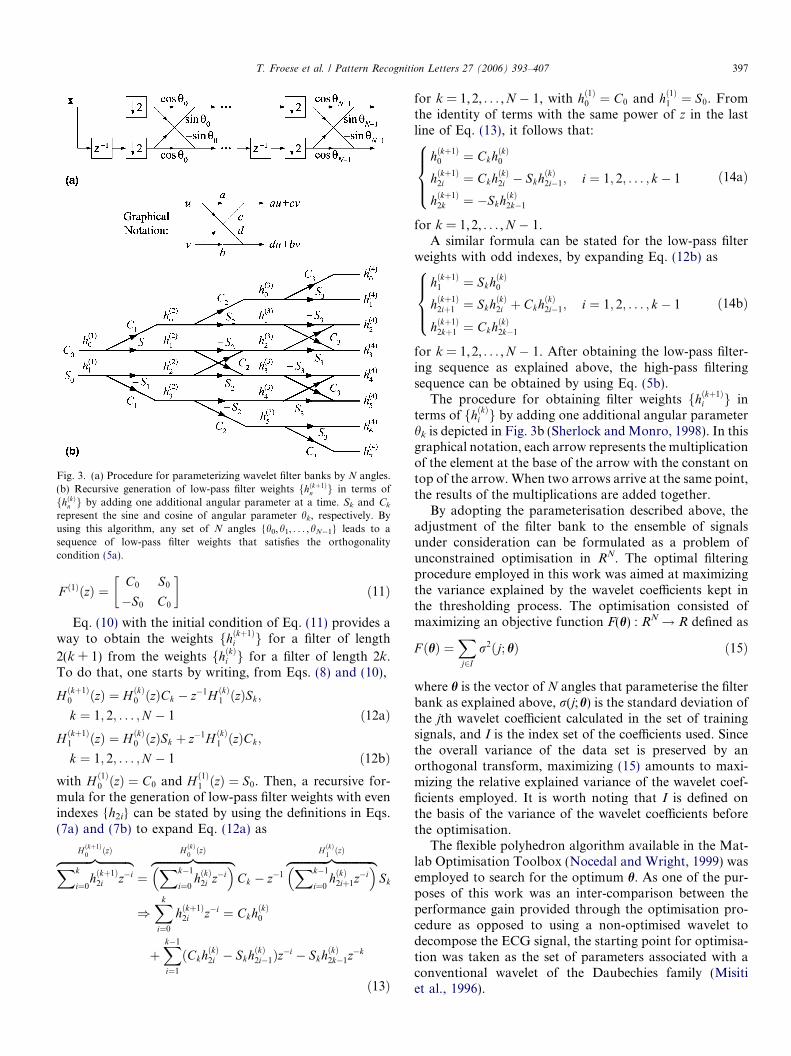
Fig. 3. (a) Procedure for parameterizing wavelet filter banks by N angles.(b) Recursive generation of low-pass filter weights fhðkþ1Þ

n g in terms offhðkÞn g by adding one additional angular parameter at a time. Sk and Ck

represent the sine and cosine of angular parameter hk, respectively. Byusing this algorithm, any set of N angles {h0,h1, . . . ,hN�1} leads to asequence of low-pass filter weights that satisfies the orthogonalitycondition (5a).


F ð1ÞðzÞ ¼C0 S0

�S0 C0

� �ð11Þ

Eq. (10) with the initial condition of Eq. (11) provides away to obtain the weights fhðkþ1Þ

i g for a filter of length

2(k + 1) from the weights fhðkÞi g for a filter of length 2k.To do that, one starts by writing, from Eqs. (8) and (10),

H ðkþ1Þ0 ðzÞ ¼ H ðkÞ

0 ðzÞCk � z�1H ðkÞ1 ðzÞSk;

k ¼ 1; 2; . . . ;N � 1 ð12aÞH ðkþ1Þ

1 ðzÞ ¼ H ðkÞ0 ðzÞSk þ z�1H ðkÞ

1 ðzÞCk;

k ¼ 1; 2; . . . ;N � 1 ð12bÞwith H ð1Þ

0 ðzÞ ¼ C0 and H ð1Þ1 ðzÞ ¼ S0. Then, a recursive for-

mula for the generation of low-pass filter weights with evenindexes {h2i} can be stated by using the definitions in Eqs.(7a) and (7b) to expand Eq. (12a) as

Xk

i¼0hðkþ1Þ2i z�i

zfflfflfflfflfflfflfflfflfflffl}|fflfflfflfflfflfflfflfflfflffl{H ðkþ1Þ0

ðzÞ

¼Xk�1

i¼0hðkÞ2i z

�i� �zfflfflfflfflfflfflfflfflfflfflffl}|fflfflfflfflfflfflfflfflfflfflffl{H ðkÞ

0ðzÞ

Ck � z�1Xk�1

i¼0hðkÞ2iþ1z

�i� �zfflfflfflfflfflfflfflfflfflfflfflfflffl}|fflfflfflfflfflfflfflfflfflfflfflfflffl{H ðkÞ

1ðzÞ

Sk

)Xk

i¼0

hðkþ1Þ2i z�i ¼ Ckh

ðkÞ0

þXk�1

i¼1

ðCkhðkÞ2i � Skh

ðkÞ2i�1Þz�i � Skh

ðkÞ2k�1z

�k

ð13Þ

for k = 1,2, . . . ,N � 1, with hð1Þ0 ¼ C0 and hð1Þ1 ¼ S0. Fromthe identity of terms with the same power of z in the lastline of Eq. (13), it follows that:

hðkþ1Þ0 ¼ Ckh

ðkÞ0

hðkþ1Þ2i ¼ Ckh

ðkÞ2i � Skh

ðkÞ2i�1; i ¼ 1; 2; . . . ; k � 1

hðkþ1Þ2k ¼ �Skh

ðkÞ2k�1

8>><>>: ð14aÞ

for k = 1,2, . . . ,N � 1.A similar formula can be stated for the low-pass filter

weights with odd indexes, by expanding Eq. (12b) as

hðkþ1Þ1 ¼ Skh

ðkÞ0

hðkþ1Þ2iþ1 ¼ Skh

ðkÞ2i þ Ckh

ðkÞ2i�1; i ¼ 1; 2; . . . ; k � 1

hðkþ1Þ2kþ1 ¼ Ckh

ðkÞ2k�1

8>><>>: ð14bÞ

for k = 1,2, . . . ,N � 1. After obtaining the low-pass filter-ing sequence as explained above, the high-pass filteringsequence can be obtained by using Eq. (5b).

The procedure for obtaining filter weights fhðkþ1Þi g in

terms of fhðkÞi g by adding one additional angular parameterhk is depicted in Fig. 3b (Sherlock andMonro, 1998). In thisgraphical notation, each arrow represents the multiplicationof the element at the base of the arrow with the constant ontop of the arrow. When two arrows arrive at the same point,the results of the multiplications are added together.

By adopting the parameterisation described above, theadjustment of the filter bank to the ensemble of signalsunder consideration can be formulated as a problem ofunconstrained optimisation in RN. The optimal filteringprocedure employed in this work was aimed at maximizingthe variance explained by the wavelet coefficients kept inthe thresholding process. The optimisation consisted ofmaximizing an objective function F(h) : RN ! R defined as

F ðhÞ ¼Xj2I

r2ðj; hÞ ð15Þ

where h is the vector of N angles that parameterise the filterbank as explained above, r(j;h) is the standard deviation ofthe jth wavelet coefficient calculated in the set of trainingsignals, and I is the index set of the coefficients used. Sincethe overall variance of the data set is preserved by anorthogonal transform, maximizing (15) amounts to maxi-mizing the relative explained variance of the wavelet coef-ficients employed. It is worth noting that I is defined onthe basis of the variance of the wavelet coefficients beforethe optimisation.

The flexible polyhedron algorithm available in the Mat-lab Optimisation Toolbox (Nocedal and Wright, 1999) wasemployed to search for the optimum h. As one of the pur-poses of this work was an inter-comparison between theperformance gain provided through the optimisation pro-cedure as opposed to using a non-optimised wavelet todecompose the ECG signal, the starting point for optimisa-tion was taken as the set of parameters associated with aconventional wavelet of the Daubechies family (Misitiet al., 1996).

Fig. 4. Graphical representation of the cost function �F(h).


For illustration, Fig. 4 depicts a graph of the cost func-tion (objective function with minus sign) obtained by usinga wavelet transform with two degrees of freedom as wouldbe the case if a db2 wavelet was used. It is worth notingthat the graph is repeated at modulo 2p, because of theperiodicity of the sine and cosine functions involved inthe parameterisation. As shown in Fig. 4, it is possible thatthe objective function (15) may have local maxima differentfrom the global maximum. In that case, the flexible polyhe-dron algorithm will tend to converge to the closest localmaximum. However, even if the global maximum is notattained, an improvement over the original wavelet trans-form may still be obtained.

An approach to circumvent the local maxima problemof the formulation described above consists of exploitingthe product filter parameterisation proposed by Moulinet al. (1997). In order to describe the optimisation process,we use again a circular convolution process for the datavectors under the downsampling operation c 0 = hX andd 0 = gX where h = [h2N�1,h2N�2, . . . ,h0] and g = [g2N�1,g2N�2, . . . ,g0] are the corresponding impulse responsesequences of the low-and high-pass filters respectively andX is a circulant matrix formed from the data vector x as

�X ¼

x0 x1 � � � xJ�2 xJ�1

x1 x2 � � � xJ�1 x0x2 x3 � � � x0 x1

..

. ... ..

. ...

x2N�1 x2N � � � x2N�3 x2N�2

266666664

377777775

2N�J

ð16Þ

and we consider the power (energy divided by the numberof coefficients) of the low-pass and high-pass filter outputs.Since the number of coefficients is J/2, due to the down-sampling operation, the power values of the approximation(cm) and of the detail (dm) coefficients for the mth trainingsignal are given by

Pmc ¼ cmcm

T

J=2ð17aÞ

Pmd ¼ dmdmT

J=2ð17bÞ

If M training signals are employed, the overall power ofthe approximations and details are

Pc ¼XMi¼1

Pmc ð18aÞ

Pd ¼XMi¼1

Pmd ð18bÞ

The relation between Pc and Pd can be expressed in anobjective function F : R2N �R2N ! R given by

F ðh; gÞ ¼ 0:5ðPc þ PdÞffiffiffiffiffiffiffiffiffiffiPcP d

p ð19Þ

which is similar to the coding gain used to assess the com-pression performance of two-channel filter bank structures(Tuqun and Vaidyanathan, 2000).

If the conditions in Eq. (5) are satisfied, the WT isorthogonal, and thus it preserves power (Strang and Ngu-yen, 1996). As a result, the power of the input signal xm

equals the sum of the power in both output channels,Pmc þ Pm

d . Hence, for a given training set, the sum A =Pc + Pd is constant and thus maximizing F is equivalentto maximizing Pc. Writing:

F 2 ¼ 0:25A2

APc � P 2c

ð20Þ

it follows that F reaches a minimum of 1 when Pc = A/2,that is, when the power is equally divided between theapproximation and detail coefficients. As Pc increases fromA/2 to A, F increases and tends to +1 when Pc tends to A,i.e., when all the power is contained in the approximationcoefficients. The advantage of aiming at maximizing Pc liesin the fact that the signal-to-noise ratio is usually larger inthe low-pass filter output. Thus, maximizing Pc further im-proves the filtering performance. It is worth noting that, ifthe data set is mean-centered (variable-wise) prior to thewavelet decomposition, the power is equal to the variance.In this manner, the optimisation amounts to maximizingthe variance explained by the approximation coefficients.

Since Pc only depends on the low-pass filter weights h,the problem can be restated as the maximization of anobjective function e : R2N ! R given by

eðhÞ ¼ Pc ¼1

J=2

XMm¼1

cmcmT ffi 1

J

XMi¼1

c0mc0mT ð21Þ

where c0m ¼ h�Xmis the vector of detail coefficients for the

mth training signal, before the downsampling operationas shown in Table 1 and Xm is the circulant matrix formedfrom xm. This holds because we may assume that the powerof the detail coefficients before and after downsampling isapproximately the same. Using (21) one may write:

eðhÞ ¼ 1

J

XMm¼1

h�Xm �X

mT

hT ¼ hXM

m¼1

1

J�X

m �XmT

� |fflfflfflfflfflfflfflfflfflfflfflfflfflfflffl{zfflfflfflfflfflfflfflfflfflfflfflfflfflfflffl}

R

hT ð22Þ

-3 -2 -1 0 1 2 3-3

-2

-1

0

1

2

3

θ0

θ 1

-2 -1.5 -1 -0.5 0

1

1.5

2

2.5

Fig. 5. Contour plot depicting the locus of the points associated with thedb2 (circle), Sherlock and Monro�s optimisation (cross) and Moulin�soptimisation (triangle) in relation to the cost function landscape �F(h).The inset shows further detail.


Since �Xm �X

mT

is Toeplitz for any xm, then R2N·2N is alsoa Toeplitz matrix. Thus, the constraints in Eq. (5) allow theobjective function to be rewritten, with a slight abuse ofnotation, in the following linear form (Moulin et al., 1997)

eðaÞ ¼ r02þXN�1

n¼0

anr2nþ1 ð23Þ

where {r0, r1, . . . , r2N�1} are the elements of the first row ofR and vector a = [a0 a1 � � � aN�1] contains the coefficientsof the product filter P(z) defined as

P ðzÞ ¼ HðzÞHðz�1Þ ¼ 1þXN�1

n¼0

anðz�2n�1 þ z2nþ1Þ ð24Þ

Given a, the transfer function H(z) of the desired filtercan be recovered from P(z) by a spectral factorisation pro-cedure (Strang and Nguyen, 1996). This factorisation ispossible provided that the frequency response of the prod-uct filter given by Q(f) = P(ej2pf) (where j is the imaginaryunity), is non-negative at all frequencies f, that is,Qðf Þ P 0; 8f 2 R. It follows that the following restrictionmust be enforced:

Qðf Þ ¼ 1þ 2XN�1

n¼0

an cos½2pf ð2nþ 1Þ� P 0 ð25Þ

Since Q(f) is periodic with period 1 and Qðf Þ þ Qðf þ0:5Þ ¼ 2; 8f 2 R, it is sufficient to consider the restrictionQ(f) P 0 in the interval 0 6 f 6 0.5, that is

1þ 2XN�1

n¼0

an cos½2pf ð2nþ 1Þ� P 0; 0 6 f 6 0:5 ð26Þ

Maximizing e(a) defined in Eq. (23) with respect to asubject to the inequality restrictions in Eq. (26) is a linearsemi-infinite programming (LSIP) problem (Hettich andKortanek, 1993), because there is a finite number of vari-ables (a0,a1, . . . ,aN�1) and infinitely many restrictions. Thisproblem can be solved by discretising the frequency inter-val [0, 0.5] to generate a finite number of restrictions, andthen applying standard linear programming techniques(Chvatal, 1983). The solution ~a to this approximatedproblem can then be used to generate a feasible solutionaf to the original problem as discussed by Moulin et al.(1997):

af ¼~a

1� dð27Þ

where d 6 0 is the minimum of Q(f) in the interval0 6 f 6 0.5 when ~a is used instead of a in Eq. (25).

From the above description, it may be concluded that byadopting the coding gain as a measure of the compressionperformance of the low-pass/high-pass filter pair (Unser,1993), the optimisation of coefficients {a0,a1, . . . ,aN�1}can be cast into a LSIP problem. By using a convenient dis-cretisation procedure (Moulin et al., 1997) such a problemcan then be converted into a linear programming one,for which efficient solution algorithms exist (Chvatal,1983).

In the present work, the filter bank was optimised byapplying the above-mentioned approach to each low-pass/high-pass filter pair separately. For this purpose, thefirst-level pair was initially optimised. The low-pass filteroutput was then employed as the input signal for the sec-ond-level optimisation. Moreover, an overall coding gainwas employed to measure the compression ability of the fil-ter bank for the ensemble of signals in the training data set.In contrast to Sherlock and Monro�s (1998) optimisation,in this case the resulting optimisation problem is convexand the solution found is guaranteed to be the global max-imum of the objective function. However, it is worth not-ing that the objective function cannot target a specific setof wavelet coefficients, unlike the previous formulation.Instead, the optimisation is focused on maximizing the var-iance explained by the approximation coefficients. Thatmay be a shortcoming if the model is to include detail coef-ficients in addition to the approximation ones.

In order to illustrate the effect of using different objectivefunctions for the optimisation of the wavelet decomposi-tion algorithms, in Fig. 5 we depict a contour plot of thecost surface shown in Fig. 4. The circle, the cross and thetriangle indicate the points associated with three differentwavelets (db2, Sherlock and Monro�s and Moulin�s), whenthe optimisations were performed using only two angles. Adetail of the region around these three points is presentedas an inset graph to Fig. 5 (note the different scaling used).

It can be seen that the db2 locus lies on a flat surfacebetween two local minima. In this case, the flexible poly-hedron algorithm employed in Sherlock and Monro�s opti-misation was not able to move away from that plateautowards neighbouring minima. The inset graph shows thatMoulin�s solution lies in approximately the same cost level


as Sherlock and Monro�s, on the other side of a local min-imum basin.

As described earlier, in Moulin�s approach we optimisedboth decomposition levels (the first level solution is shownin Fig. 5). However, the optimisation is performed in asequential manner rather than a batch manner as is inthe Sherlock and Monro�s case (we first optimise the firstlevel and then we optimise the second level). Moreover, itis worth noting that, although both techniques are designedto optimise the compression performance of the filter bank,each technique employs a different criterion (either (15) or(19)) to evaluate the compression performance. In Fig. 5,the results are compared with regard to Sherlock andMonro�s criterion (Eq. (15)). Furthermore, it is worth not-ing that neither of the techniques is designed to optimisethe classification performance in a direct manner. However,we anticipated that an improvement in compression abilityshould be reflected in an improvement in the classificationperformance.

In contrast to the simplified example presented above,for the ECG classification study we used the db6 waveletwhere six angles would have to be used to fully describethe low-pass filter. The calculations performed for Sherlockand Monro�s optimisation as well as for Moulin�s optimisa-tion were also carried out by using six angles. The illustra-tion in Fig. 5 using two angles avoids the problem ofdepicting possible differences occurring in a six-dimen-

1 2 3 4 5 6 7 8 9 10 11 12-1

-0.5

0

0.5

1

1 2 3 4 5 6 7 8 9 10 11 12-1

-0.5

0

0.5

1

(a)

(b)

1 2 3 4 5 6 7 8 9 10 11 12-1

-0.5

0

0.5

1

1 2 3 4 5 6 7 8 9 10 11 12-1

-0.5

0

0.5

1

Filter tap

(c)

(d)

Fig. 6. (a) Low-pass and (b) high-pass filters: db6 (solid line), Moulin�soptimisation (dashed line), Sherlock and Monro�s optimisation (dottedline) at the first decomposition level. (c) and (d) depict the same filters atthe second decomposition level.

sional space. A comparison between the filters resultingfrom the two optimisation procedures described and thedb6 filters is presented in Fig. 6.

Using Moulin�s approach, it can be seen, that eventhough the filter configurations have been optimised byLSIP so that each decomposition level can have its own fil-ter coefficients, the resulting filters are still relatively similarto each other. Such similarity between the filter coefficientsof the first and second decomposition level has also beenobserved elsewhere (Coelho et al., 2003), where the LSIPstrategy was also used to optimise the wavelet transform.For other approaches to the optimisation of the wavelettransform the reader is referred to other relevant literature(Vetterli and Kovacevic, 1995; Ramchandran et al., 1996).

3. ECG classifiers

3.1. Linear discriminant analysis

The most widely used discriminant analysis method is theone developed by Fisher in 1936, which attempts to maxi-mize the ratio of between-groups to within-groups variance(Lachenbruch, 1975). For the classification of the ECG sig-nals, the row vectors t of the transformed variables accord-ing to Eq. (2) were used. Using vector-matrix notation, thefollowing discriminant function can be derived for the caseof binary classification in the wavelet domain:

ZðtÞ ¼ ðl1 � l2ÞR�1t ð28Þwhere Z : RJ ! R is a discriminant function, t ¼½t0 t1 � � � tJ�1�T is a vector of J classification variables,l1 2 RJ and l2 2 RJ are the sample mean vectors of eachgroup, and R is the common sample covariance matrixwith dimensions J · J. Eq. (28) is commonly written inexpanded form as: Z = w0t0 + w1t1 + � � � + wJ�1tJ�1 = wTt,where w ¼ ½w0 w1 � � � wJ�1�T is a vector of coefficients:w ¼ R�1ðl1 � l2Þ. The cut-off value for classification is cal-culated as the midpoint of the mean scores of the two sam-ples given by zc ¼ 0:5ðl1 � l2ÞR�1ðl1 þ l2Þ. A given vectort is assigned to class 1 if Z(t) > Zc, and to class 2 otherwise.

3.2. The artificial neural network

The artificial neural network type used for this researchwas the standard feed-forward multi-layer perceptron. As astarting point, we define the net input to a processing ele-ment q for the mth ECG input pattern as

mqðmÞ ¼XJ�1

j¼0

wqjtjðmÞ þ bq ð29Þ

where tj(m), j = 0,1, . . . ,J � 1 are the values of the waveletcoefficients for the mth input pattern, wqj is the neural net-work weight of the connection between coefficient j andprocessing element q and bq is an ANN bias element. Theoutput of the processing element is the result of passingthe scalar value mq(m) through its activation function


uq(Æ) : yq(m) = uq(mq(m)). In this work we have used thelogistic sigmoid function, which has a range of valuesbetween zero and one:

uqðmqðmÞÞ ¼1

1þ e�mqðmÞð30Þ

The output of the feed-forward MLP is of the formy = u2(W2u1(W1x + b1) + b2), where u1 is the activationfunction of the hidden layer, which is assumed to apply ele-ment-wise to its vector argument, b2 is the scalar bias in theoutput layer, W1 and W2 are weight matrices and b1 is abias vector. We have used a back-propagation trainingalgorithm that employs a gradient search to minimise themean-square-error (MSE) cost function:

MSE ¼ 1

M

XMm¼1

½yðmÞ � dðmÞ�2 ð31Þ

where d(m) is the desired output for the mth training pat-tern, y(m) is the actual MLP output and M is the totalnumber of training samples. The MLP weights wereadjusted through a learning process with each trainingpattern being presented to it in a sequential manner. AnANN topology consisting of 2 hidden layers with 10 nodeseach, was found sufficient to learn the training data. Theoutput layer consisted of just 1 node and the number ofnodes in the input layer was set equal to the number ofwavelet coefficients used as inputs. All nodes except forthe ones contained in the input layer had a bias associatedwith them.

Very often, the ANN architectures used are based on theprinciple that the neural network should be larger thanrequired rather than not sufficiently complex. As a conse-quence of this design choice, there existed the possibilityof data over-fitting, which is undesirable since such practicecan potentially compromise the generalisation ability of thenetwork. To minimise the risk of data over-fitting a cross-validation method (Stone, 1978) can be used, where theavailable data is divided into three distinct data sets: thetraining set, the validation set and the testing set. TheANN was then trained as usual with the training data setbut every so often its generalisation ability was cross-vali-dated with the validation set. As soon as the classificationaccuracy of the validation set deteriorated, the trainingstopped. This is commonly referred to in the NN literatureas the ‘‘early stopping method of training’’ (Haykin, 1999).

Since the data set used in this work was limited to makethe classification task more challenging, it was not feasibleto divide the data into three different but equally represen-tative sets. It was decided that the training of the neuralnetwork would be continued until the training set was fullyrecognised (accuracy of 100%) by the ANN within a max-imum of 1000 epochs or 1500 generations depending on theapproach used. The neural network performance was thenassessed using the testing data set. This approach has theadvantage that no independent cross-validation test isrequired and that the data can be used for determiningthe ideal number of wavelet coefficients instead. A draw-

back of the method is that it assumes that the data was100% correctly classified by the experts. It was hoped thatthis measure would preserve the generalisation ability ofthe ANN by preventing over-fitting. The results presentedlater in this paper support this view.

3.3. The genetic algorithm

The third classifier was a feed-forward MLP where asteady-state genetic algorithm was used during the trainingprocess. Half of the fittest population was set to survive tothe next generation. This provided an appropriate trade-offbetween speeding up the evolution by producing moresolutions (offsprings) at every generation and preventingpremature convergence by having a larger parental vari-ability. The genetic representation of a neural networkwas implemented as a fixed two-dimensional array offloats. Each floating-point number directly correspondsto one weight of the ANN, which allows the crossoverand mutation operators to have a one to one mapping.This is also known in the GA literature as direct encoding(Fogel, 1995). It is believed that this approach is superiorto randomly flipping bits of a binary representation sincein that case, an additional mapping function would alsobe required (Yao, 1999). The crossover operator usedmaintained the gene pool sufficiently diverse. Since a recentstudy found no significant difference between the effects ofseveral popular crossover operators when used to evolveANN�s (Pendharkar and Rodger, 2004), it was decided thata standard one-point crossover was sufficient for thepurpose of this study. In addition, the representationalredundancy usually associated with direct encodingschemes gives the GA more possibilities of hitting on fitsolutions (Hancock, 1992). Improved genotypes were fine-tuned by mutation. Whenever an individual was mutated,a �coin flip� biased by the mutation rate was executed foreach connection weight. For every successful mutation, arandom number picked from a standard Gaussian distribu-tion was then added to that weight.

The selection operator that was used is known as theroulette wheel selector, which picks an individual basedon the magnitude of its fitness score compared to the restof the population. The advantage of this selection operatoris that it does not always guarantee that the best solution ispassed on. This also helped reduce the chance of prematureconvergence. The GA terminated when either the trainingdata was fully recognised or the given number of genera-tions had run out.

The simplest implementation of a fitness or objectivefunction for the classification task was to reward individu-als proportionally to the percentage accuracy achieved onthe entire training data set. A record was considered cor-rectly classified when its absolute error was below a speci-fied threshold, where the absolute error refers to theabsolute difference between the target (binary: 0 or 1)and actual output (continuous: 0 to 1). The thresholdwas first set to 0.5, however, this turned out to be too high

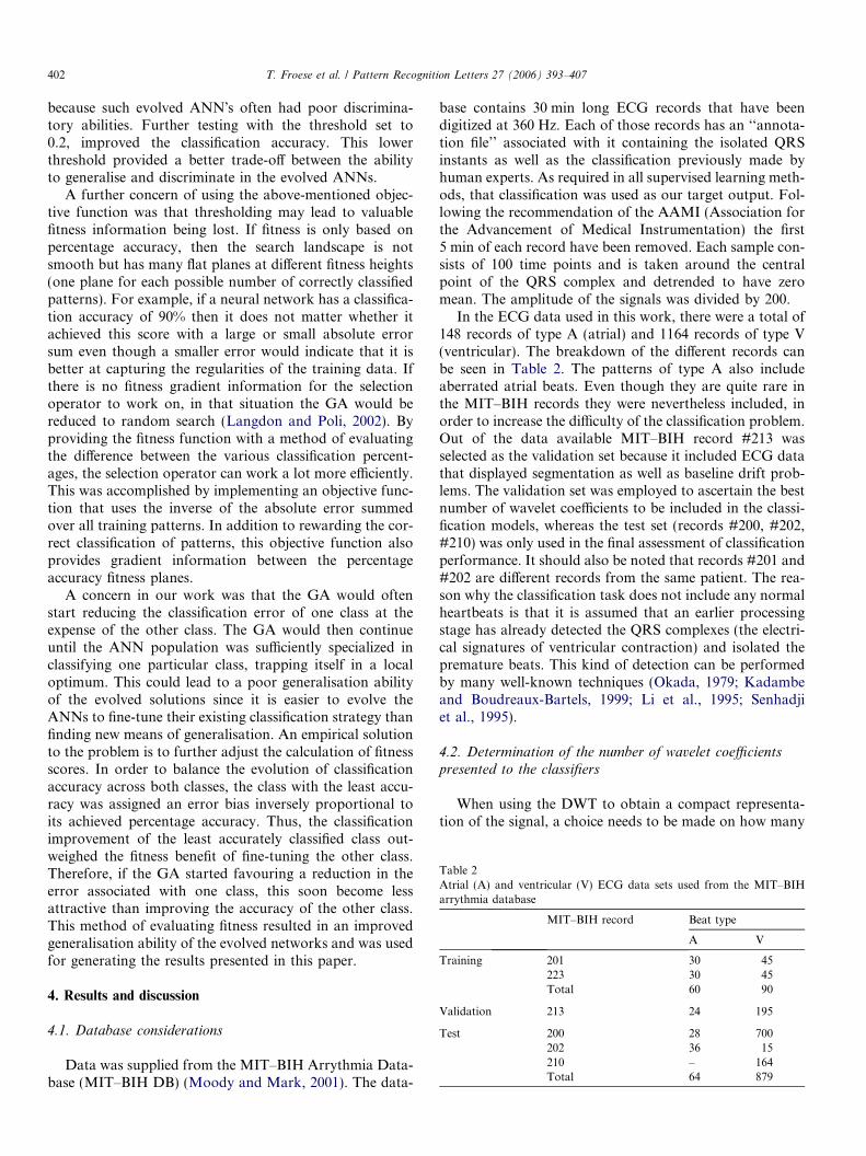
Table 2Atrial (A) and ventricular (V) ECG data sets used from the MIT–BIHarrythmia database

MIT–BIH record Beat type

A V

Training 201 30 45223 30 45Total 60 90

Validation 213 24 195

Test 200 28 700202 36 15210 – 164Total 64 879


because such evolved ANN�s often had poor discrimina-tory abilities. Further testing with the threshold set to0.2, improved the classification accuracy. This lowerthreshold provided a better trade-off between the abilityto generalise and discriminate in the evolved ANNs.

A further concern of using the above-mentioned objec-tive function was that thresholding may lead to valuablefitness information being lost. If fitness is only based onpercentage accuracy, then the search landscape is notsmooth but has many flat planes at different fitness heights(one plane for each possible number of correctly classifiedpatterns). For example, if a neural network has a classifica-tion accuracy of 90% then it does not matter whether itachieved this score with a large or small absolute errorsum even though a smaller error would indicate that it isbetter at capturing the regularities of the training data. Ifthere is no fitness gradient information for the selectionoperator to work on, in that situation the GA would bereduced to random search (Langdon and Poli, 2002). Byproviding the fitness function with a method of evaluatingthe difference between the various classification percent-ages, the selection operator can work a lot more efficiently.This was accomplished by implementing an objective func-tion that uses the inverse of the absolute error summedover all training patterns. In addition to rewarding the cor-rect classification of patterns, this objective function alsoprovides gradient information between the percentageaccuracy fitness planes.

A concern in our work was that the GA would oftenstart reducing the classification error of one class at theexpense of the other class. The GA would then continueuntil the ANN population was sufficiently specialized inclassifying one particular class, trapping itself in a localoptimum. This could lead to a poor generalisation abilityof the evolved solutions since it is easier to evolve theANNs to fine-tune their existing classification strategy thanfinding new means of generalisation. An empirical solutionto the problem is to further adjust the calculation of fitnessscores. In order to balance the evolution of classificationaccuracy across both classes, the class with the least accu-racy was assigned an error bias inversely proportional toits achieved percentage accuracy. Thus, the classificationimprovement of the least accurately classified class out-weighed the fitness benefit of fine-tuning the other class.Therefore, if the GA started favouring a reduction in theerror associated with one class, this soon become lessattractive than improving the accuracy of the other class.This method of evaluating fitness resulted in an improvedgeneralisation ability of the evolved networks and was usedfor generating the results presented in this paper.

4. Results and discussion

4.1. Database considerations

Data was supplied from the MIT–BIH Arrythmia Data-base (MIT–BIH DB) (Moody and Mark, 2001). The data-

base contains 30 min long ECG records that have beendigitized at 360 Hz. Each of those records has an ‘‘annota-tion file’’ associated with it containing the isolated QRSinstants as well as the classification previously made byhuman experts. As required in all supervised learning meth-ods, that classification was used as our target output. Fol-lowing the recommendation of the AAMI (Association forthe Advancement of Medical Instrumentation) the first5 min of each record have been removed. Each sample con-sists of 100 time points and is taken around the centralpoint of the QRS complex and detrended to have zeromean. The amplitude of the signals was divided by 200.

In the ECG data used in this work, there were a total of148 records of type A (atrial) and 1164 records of type V(ventricular). The breakdown of the different records canbe seen in Table 2. The patterns of type A also includeaberrated atrial beats. Even though they are quite rare inthe MIT–BIH records they were nevertheless included, inorder to increase the difficulty of the classification problem.Out of the data available MIT–BIH record #213 wasselected as the validation set because it included ECG datathat displayed segmentation as well as baseline drift prob-lems. The validation set was employed to ascertain the bestnumber of wavelet coefficients to be included in the classi-fication models, whereas the test set (records #200, #202,#210) was only used in the final assessment of classificationperformance. It should also be noted that records #201 and#202 are different records from the same patient. The rea-son why the classification task does not include any normalheartbeats is that it is assumed that an earlier processingstage has already detected the QRS complexes (the electri-cal signatures of ventricular contraction) and isolated thepremature beats. This kind of detection can be performedby many well-known techniques (Okada, 1979; Kadambeand Boudreaux-Bartels, 1999; Li et al., 1995; Senhadjiet al., 1995).

4.2. Determination of the number of wavelet coefficientspresented to the classifiers

When using the DWT to obtain a compact representa-tion of the signal, a choice needs to be made on how many


wavelet coefficients to retain. One way to determine the sig-nificance of a particular coefficient is to look at its variance.When ordering the coefficients from highest to lowest var-iance there comes a point when adding components oflower variance does not make a difference to the informa-tion content of the wavelet representation anymore. Therelationship between variance and number of wavelet coef-ficients for the three wavelet networks is depicted in Fig. 7.It can be seen from the graph that after the 25th coefficient,the variance becomes negligible. Therefore, a preliminaryreduction was performed by only preserving the first 25wavelet coefficients. It is worth noting that these coeffi-cients were all of the approximation type (output of thelow-pass filter at the second resolution level). Such findingis in line with the assumption of Moulin�s optimisationstrategy, as mentioned above.

After this preliminary reduction there was still the pos-sibility that even fewer wavelet coefficients were sufficientfor the classification task. It was suspected that the infor-mation required to distinguish between the atrial and ven-tricular classes might be contained within a handful ofcoefficients.

4.2.1. Number of wavelet coefficients presented

to the LDA classifier

The LDA approach does not have a problem of dataoverfitting so severe as the ANN does and, therefore, servesas a benchmark to the performance achieved using ANNclassifiers. The reason why it is desirable to reduce thenumber of coefficients used for LDA is that the moreinputs are used the more uncertain become the estimatesof the covariance matrices. The number of training pointsincreases linearly with J, the number of inputs, but thenumber of unknowns to be estimated increases with thesquare of J. This is because by presenting J inputs to theclassifier, the covariance matrix has [J(J + 1)]/2 differententries that need to be estimated. The best number of wave-let coefficients presented to the linear discriminant modelwas determined on the basis of the resulting error rate

5 10 15 20 25 30 35 40 45 500

0.1

0.2

0.3

0.4

0.5

0.6

0.7

0.8

0.9

1

Coefficient

Nor

mal

ized

var

ianc

e

Fig. 7. Normalised variance of the first 50 wavelet coefficients (two-leveldecomposition): db6 (solid line); Moulin�s optimisation (dashed line);Sherlock and Monro�s optimisation (dotted line).

(average of the two-atrial and ventricular- classes of data)on the validation data set. The average was taken so asnot to bias the results in favour of the class with morerecords. The coefficients were added in decreasing orderof variance. The percentage error to the classification taskfor each of the possible number of wavelet coefficientsranging from 1 to 25 was then calculated.

As shown in Fig. 8, the smallest validation error in LDAwas achieved using three wavelet coefficients irrespective ofthe method used to generate the wavelet coefficients.

4.2.2. Number of wavelet coefficients presented to the

ANN trained by back-propagation

The best number of wavelet coefficients to be used asinputs for training the neural network with back-propaga-tion was determined in an empirical manner. The learningrate was set to 0.4 throughout the experiment, which isclose enough to the 0.35 suggested by Rich and Knight(1991) but should allow the weight configuration to con-verge slightly faster. Each training session was scheduledto run over a maximum of 1000 epochs unless the trainingdata set was 100% correctly classified.

The ANN started off with 25 wavelet coefficient inputsand after five training sessions with random initial weightsthe coefficient with the lowest variance was removedand the procedure was repeated. After each training sessionthe classification performance was tested on the validationdata set and the resulting accuracy was recorded. From thefive training sessions the best result was selected to repre-sent the corresponding number of coefficients. The resultsfor all three data sets were quite similar. For the db6 data,11 wavelet coefficients were chosen as inputs because thatconfiguration achieved a 97.6% classification accuracy onthe validation data set. For the Moulin optimised datathe best number of coefficients was 12 and a 97.4% accu-racy was achieved. Finally, a classification accuracy of97.6% was achieved when the network was presentedwith 11 wavelet coefficients generated using Sherlock andMonro�s wavelet optimisation strategy. The percentage

3 5 10 15 20 250

10

20

30

40

50

60

70

Number of coefficients included in the model

% E

rror

Fig. 8. Average validation error in LDA as a function of the number ofwavelet coefficients included in the model (two-level transform): db6 (solidline), Moulin�s optimisation (dashed line), Sherlock and Monro�s optimi-sation (dotted line).

0

25

50

75

100

0 5 10 15 20 25Number of Wavelet Coefficients

Per

cen

tag

e A

ccu

racy

(%

)

Maximum

Average0

25

50

75

100


Per

cen

tag

e A

ccu

racy

(%

)

Maximum

Average0

25

50

75

100

0 5 10 15 20 25

Number of Wavelet Coefficients

Per

cen

tag

e A

ccu

racy

(%

)

Maximum

Average

(a) (b) (c)

Fig. 9. Validation back-propagation classification results on (a) db6 two-level transform input data and optimised data; (b) using Moulin�s optimisation;and (c) using Sherlock and Monro�s optimisation method.


accuracy in the classification of the validation data set for thestandard db6 and optimised wavelets are shown in Fig. 9.

It can be observed that further addition of wavelet coef-ficients result in a steep increase in the classification accu-racy. Performing, however, a classification by presentingto the ANN more than 13 coefficients decreased theachieved accuracy since very little additional informationwas encoded in subsequent coefficients. We concluded thatwithin the first 13 coefficients, the neural network had allthe information and complexity needed to almost classify100% of the validation data correctly. Any further additionof dimension in the ANN feature space would not provideany useful information that could be used to improve theclassification accuracy but would only make it harder forthe ANN to converge to the best solution. It is worth not-ing that although the variance of each additional coefficientgets smaller the neural network treats each of its inputswith the same importance.

4.2.3. Number of wavelet coefficients presented to the

ANN trained by a GA

In order to evolve the connection weights the followingprocedure was adopted. Firstly, a steady-state GA wasused where 50% of the population was replaced after everygeneration. Through a trial and error process, it was foundthat the evolved solutions were not very sensitive to theparameter variations and the achieved classification accu-

0

25

50

75

100


Per

cen

tag

e A

ccu

racy

(%

)

Maximum

Average0

25

50

75

100

0 5 10Number of Wav

Per

cen

tag

e A

ccu

racy

(%

)

(a) (b)

Fig. 10. Validation GA classification results on (a) db6 two-level transform inpSherlock and Monro�s optimisation method.

racies were difficult to improve upon by further changingthe ANN. The population was kept to a constant of 100individuals. Each new offspring had a 5% chance of beingselected for genetic crossover. The mutation rate was setto 5% as well. Therefore, at least one in every twentynetwork weights of the offspring would be mutated bystandard Gaussian mutation. The maximum number ofgenerations was set to 1500. The GA was also terminatedif an individual achieved 100% classification accuracy onthe training data set.

Whenever an evolutionary run was finished, the bestindividual of the population was taken and its performancewas tested on the validation data set. The rest of the proce-dure was the same as for the back-propagation approach.Five evolutionary runs were performed after presentingthe same number of wavelet coefficients to the input ofthe network and the best classification result among the fiveruns was recorded as the �score� for that amount of coeffi-cients. The process was then repeated after increasing thenumber of coefficients presented to the input of the net-work. The percentage accuracy in the classification of thevalidation data set for the standard db6 and optimisedwavelets are shown in Fig. 10.

One of the ANNs that was evolved with the db6 trainingdata was actually able to classify the validation data 100%correctly with only 8 wavelet coefficients as inputs. TheANN architecture with 9 inputs also did very well with

15 20 25elet Coefficients

Maximum

Average0

25

50

75

100


Per

cen

tag

e A

ccu

racy

(%

)

Maximum

Average

(c)

ut data and optimised data (b); using Moulin�s optimisation; and (c) using


99.5% classification accuracy. The choice for the number ofcoefficients to be used with the optimally compressed datagenerated using Moulin�s algorithm was slightly more diffi-cult because there were quite a few configurations achiev-ing around 97% classification accuracy on the validationdata set. Included in this selection was the configurationwith 12 inputs and since it had already proven to be thebest choice for the back-propagation method it was chosenfor the evolutionary weight approach as well. This ANNconfiguration achieved a 99.6% classification accuracy.Finally, a classification accuracy of 97.6% was achievedwhen the network was presented with 10 wavelet coeffi-cients generated using Sherlock and Monro�s wavelet opti-misation strategy.

4.3. Comparison of classification accuracy for testing

data sets

The classification results for the test set are summarisedin Table 3 below. A metric based on the average classifica-tion accuracy makes sure that equal weighting is given toboth atrial and ventricular data sets. All methods per-formed reasonably well. Overall the neural networks wereslightly more successful than LDA at correctly classifyingthe ECG signals. In addition, the wavelet optimisation pro-cesses facilitated the classification task. The best classifierresulted from a combination of a neural network architec-ture with 12 inputs, training through weight evolution andthe use of the optimised wavelet coefficients using Moulin�sapproach. It is worth noting that the wavelet transformreduced the dimensionality of the problem by a factor ofabout 10.

It was to be expected that the neural network classifierswould generally outperform an LDA classifier because thelatter is best suited for linearly separable problems. Thereason why the GA produced better weight configurationsthan the standard back-propagation algorithm can beattributed to the fact that the GA is better at avoiding localoptima. It is worth noting that the neural network trainedby GA also provided the best classification results for ven-tricular beats, which is an important aspect from a medicalpoint of view, in light of the potential hazards associated to

0

25

50

75

100

0 5 10 15 20 25

Number of Wavelet Coefficients

Per

cen

tag

e A

ccu

racy

(%

)

Testing

Validation

0

25

50

75

100

0 5 10Number of Wa

Per

cen

tag

e A

ccu

racy

(%

)

(a) (b)

Fig. 11. Comparison between testing and validation classification accuracy ooptimised data; and (c) Sherlock and Monro optimised data.

such type of extrasystole. The best classification accuracyon both the testing and validation data sets was achievedwhen the ECG signals were transformed in the waveletdomain using a db6 decomposition as shown in Fig. 11a.

By choosing a difficult data set that included a lot ofabnormal records the neural networks were forced to bevery good at generalisation in order to succeed in their clas-sification task. This generalisation ability then translated togood classification results on the relatively easier testingdata set. Fig. 11a–c support this view.

It is worth noting that one of the usual requirements forstandard wavelets is that they have zero mean to assure theinversibility of the wavelet transform. For such tasks, theoptimisation procedures described is well suited to tacklethe problem. If, however, the goal of the transformationis not to reconstruct the original signal-as is the case inour current application- but to reduce the number of inputsto the classifier so as to concentrate the discrimina-tory information as much as possible, a biased waveletapproach may also be suitable. The advantages using suchapproach are that (a) usually a large number of wavelets isrequired to make up for any zero-mean characteristics ofa signal, (b) the non-biased wavelets lose time resolutionwhen they are analyzing low-frequency features and (c)whereas conventional wavelets act as moving difference fil-ters, bias allows the wavelet transform to calculate eitherdifferences or averages depending on which is more suitedto extract a particular feature. Results presented elsewhere(Galvao and Yoneyama, 1999), which adopted such abiased wavelet approach, indicate that the introductionof a bias improves the discriminatory capabilities of theneural network classifier considerably. In that work, theECG data to be classified into either 0 (atrial) or 1 (ventric-ular) came from the same MIT database as the data for thiswork. An important difference between the two studies isthat in the previous work, the output included a range(0.25–0.75), where the classification was deferred to anexpert cardiologist in order to reduce the risk of misdiagno-sis. This contrasts with our GA approach where any pre-diction with an absolute error larger than 0.2 was alreadyrejected. It was concluded that the biased wavelet neuralnetwork classified 89% of the records correctly while the

15 20 25velet Coefficients

Testing

Validation

0

25

50

75

100


Per

cen

tag

e A

ccu

racy

(%

)

Testing

Validation

(c)

f an ANN trained using back-propagation on (a) db6 data; (b) Moulin

Table 3Best classification results for the test set from the three classifiers using the output of the three wavelet transforms as the input to each classifier

Classifier type Wavelet procedure Atrial (%) Ventricular (%) Average (%) Number of waveletcoefficients

LDA Db6 95.3 95.6 95.5 3Moulin et al. 95.3 96.0 95.7 3Sherlock and Monro 89.1 94.7 91.9 3

Back-prop. ANN Db6 93.8 99.1 96.5 11Moulin et al. 98.4 99.3 98.9 12Sherlock and Monro 98.4 99.0 98.7 11

GA trained ANN Db6 96.9 94.8 95.9 8Moulin et al. 100 99.1 99.6 12Sherlock and Monro 98.4 97.7 98.1 10


unbiased counterpart only classified 41% correctly. Gener-ally, the biased wavelet approach in the previously pub-lished work showed to be inferior to the results presentedin Table 3.

Since the computing time required to train the neuralnetworks was not significant on a standard PC for bothback-propagation and artificial evolution, the methodol-ogy presented is also applicable to other databases whichare likely to evolve as a by-product of the proliferationof wirelessly networkable wearable sensing schemes forECG monitoring. Currently, in Europe there are significantincentives for the proliferation of web-based services,which have the potential of reducing the enormous work-load of the public health services.

5. Conclusions

Very good classification results can be obtained bytransforming time-variant ECG into the wavelet domain.All three methods resulted in very promising classifiersbut in the end a neural network classifier trained by agenetic algorithm was shown to be best suited for the prob-lem at hand. Although the filter banks resulting from thetwo wavelet optimisation strategies differed from eachother at each decomposition level, both approaches couldbe efficiently used to generate a data vector that wouldbe presented at the input of the classifier. It was alsorevealed that wavelet optimisation actually improved theresults by allowing the neural networks to generalise better.This was particularly important because in this study wehave chosen to work with a limited amount of ECG data.Although it can be argued that a GA could evolve a feed-back structure as well as the connection weights (Schafferet al., 1992), the results presented here suggest that sucha complex feedback system may not be actually neededfor this particular application.

References

Addison, P.S., 2002. The Illustrated Wavelet Transform Handbook:Introductory Theory and Applications in Science, Engineering, Med-icine and Finance. The Institute of Physics Publishing, London.

Angeline, P.J., Saunders, G.M., Pollack, J.B., 1994. An evolutionaryalgorithm that constructs recurrent neural networks. IEEE Trans.Neural Networks 5, 54–65.

Chvatal, V., 1983. Linear Programming. Freeman, New York.Coelho, C.J., Galvao, R.K.H., Araujo, M.C.U., Pimentel, M.F., Silva,

E.C., 2003. A linear semi-infinite programming strategy for construct-ing optimal wavelet transforms in multivariate calibration problems.J. Chem. Inf. Comput. Sci. 43 (3), 928–933.

Daubechies, I., 1992. Ten lectures on waveletsCBMS-NSF Series inApplied Maths, vol. 61. SIAM, Philadelphia.

Duda, R.O., Hart, P.E., Stork, D.G., 2001. Pattern Classification, seconded. John Wiley, New York.

Fogel, D.B., 1995. Phenotypes, genotypes, and operators in evolutionarycomputation. In: Proc. IEEE Conf. on Evolutionary Computation, pp.193–198.

Galvao, R.K.H., Yoneyama, T., 1999. Improving the discriminatorycapabilities of a neural classifier by using a biased-wavelet layer.Internat. J. Neural Syst. 9 (3), 167–174.

Galvao, R.K.H., Yoneyama, T., 2004. A competitive wavelet network forsignal clustering. IEEE Trans. Systems Man Cybernet. Part B—Cybernetics 34 (2), 1282–1288.

Hancock, P.J.B., 1992. Genetic algorithms and permutation problems: Acomparison of recombination operators for neural net structurespecification. In: Proc. Internat. Workshop on Combinations of GAsand ANNs, pp. 108–122.

Haykin, S., 1999. Neural Networks: A Comprehensive Foundation,second ed. Prentice Hall, New Jersey.

Hettich, R., Kortanek, K.O., 1993. Semi-infinite programming—theory,methods, and applications. SIAM Rev. 35, 380–429.

Jacobson, B., Webster, J.G., 1977. Medicine and Clinical Engineering.Prentice Hall, New Jersey.

Kadambe, S., Boudreaux-Bartels, G.F., 1999. Wavelet transform-basedQRS complex detector. IEEE Trans. Biomed. Eng. 46 (7), 838–848.

Kudo, M., Sklansky, J., 2000. Comparison of algorithms that selectfeatures for pattern classifiers. Pattern Recognition 33, 25–41.

Lachenbruch, P.A., 1975. Discriminant Analysis. Hafner Press, NewYork.

Langdon, W.B., Poli, R., 2002. Foundations of Genetic Programming.Springer-Verlag, London.

Li, C., Zheng, C., Tai, C., 1995. Detection of ECG characteristic pointsusing wavelet transforms. IEEE Trans. Biomed. Eng. 42 (1), 21–28.

Misiti, M., Misiti, Y., Oppenheim, G., Poggi, J.M., 1996. WaveletToolbox User�s Guide. Mathworks, Natick.

MIT/BIH arrhythmia database directory, 1992. Technical Report BMECTR010, MIT, Cambridge.

Moody, G.B., Mark, R.G., 2001. The impact of the MIT/BIH arrhythmiadatabase, history, lessons learned and its influence on current andfuture databases. IEEE Eng. Med. Biol. 20 (3), 45–50.


Moulin, P., Anitescu, M., Kortanek, K.O., Potra, F.A., 1997. The role oflinear semi-infinite programming in signal-adapted QMF bank design.IEEE Trans. Signal Process. 45, 2160–2174.

Nocedal, J., Wright, S.J., 1999. Numerical Optimization. Springer Seriesin Operations Research. Springer Verlag, New York.

Okada, M., 1979. A digital filter for the QRS complex detection. IEEETrans. Biomed. Eng. 26 (12), 700–703.

Pendharkar, P.C., Rodger, J.A., 2004. An empirical study of impact ofcrossover operators on the performance of non-binary genetic algo-rithm based neural approaches for classification. Comput. Operat.Res. 31, 481–498.

Qian, S., Chen, D., 1996. Joint Time–Frequency Analysis—Methods andApplications. Prentice Hall PTR, New Jersey.

Ramchandran, K., Vetterli, M., Herley, C., 1996. Wavelets, subbandcoding, and best bases. Proc. IEEE 84 (4), 541–560.

Rangayyan, R.M., 2001. Biomedical Signal Analysis—A Case-StudyApproach. IEEE-Wiley.

Rich, E., Knight, K., 1991. Artificial Intelligence, second ed. McGraw-Hill, New York.

Schaffer, J.D., Whitley, D., Eshelman, L.J., 1992. Combinations of geneticalgorithms and neural networks: A survey of the state of the art.In: Proc. Internat. Workshop on Combinations of GAs and ANNs,pp. 1–37.

Senhadji, L., Carrault, G., Bellanger, J.J., Passariello, G., 1995. Compar-ing wavelet transforms for recognizing cardiac patterns. IEEE Trans.Med. Biol. 13 (2), 167–173.

Sherlock, B.G., Monro, D.M., 1998. On the space of orthonormalwavelets. IEEE Trans. Signal Process. 46, 1716–1720.

Stone, M., 1978. Cross-validation: A review. Math. Operation. Statist.,Serie Statistics 9, 127–138.

Strang, G., Nguyen, T., 1996. Wavelets and Filter Banks. Wellesley-Cambridge, Massachusetts.

Tabachnick, B.G., Fidell, L.S., 2001. Using Multivariate Statistics, fourthed. Allyn and Bacon, Boston.

Tuqun, J., Vaidyanathan, P.P., 2000. A state-space approach to the designof globally optimal FIR energy compaction filters. IEEE Trans. SignalProcess. 48 (10), 2822–2838.

Unser, M., 1993. On the optimality of ideal filters for pyramid and waveletsignal approximation. IEEE Trans. Signal Process. 41, 3591–3596.

Vaidyanathan, P.P., 1993. Multirate Systems and Filter Banks. PrenticeHall, New Jersey.

Vetterli, M., Kovacevic, J., 1995. Wavelets and Subband Coding. Prentice-Hall PTR, New Jersey.

Yao, X., 1999. Evolving artificial neural networks. Proc. IEEE 87 (9),1423–1447.

Comparison of extrasystolic ECG signal classifiers using discrete wavelet transforms

Documents

Transcript of Comparison of extrasystolic ECG signal classifiers using discrete wavelet transforms