HAL Id: hal-01083716https://hal.inria.fr/hal-01083716

Submitted on 17 Nov 2014

HAL is a multi-disciplinary open accessarchive for the deposit and dissemination of sci-entific research documents, whether they are pub-lished or not. The documents may come fromteaching and research institutions in France orabroad, or from public or private research centers.

L’archive ouverte pluridisciplinaire HAL, estdestinée au dépôt et à la diffusion de documentsscientifiques de niveau recherche, publiés ou non,émanant des établissements d’enseignement et derecherche français ou étrangers, des laboratoirespublics ou privés.

Fast generic polar harmonic transformsThai Hoang, Salvatore Tabbone

To cite this version:Thai Hoang, Salvatore Tabbone. Fast generic polar harmonic transforms. IEEE Transactions onImage Processing, Institute of Electrical and Electronics Engineers, 2014, 23 (7), pp.2961 - 2971.�10.1109/TIP.2014.2322933�. �hal-01083716�

1

Fast Generic Polar Harmonic TransformsThai V. Hoang and Salvatore Tabbone

Abstract—Generic polar harmonic transforms have recentlybeen proposed to extract rotation-invariant features from imagesand their usefulness has been demonstrated in a number ofpattern recognition problems. However, direct computation ofthese transforms from their definition is inefficient and is usuallyslower than some efficient computation strategies that have beenproposed for other competing methods. This paper presents anumber of novel strategies to compute these transforms rapidly.The proposed methods are based on the inherent recurrencerelations among complex exponential and trigonometric functionsused in the definition of the radial and angular kernels ofthese transforms. The employment of these relations leads torecursive and addition chain-based strategies for fast computa-tion of harmonic function-based kernels. Experimental resultsshow that the proposed method is about 10× faster than directcomputation and 5× faster than fast computation of Zernikemoments using the q-recursive strategy. Thus, among all existingrotation-invariant feature extraction methods, polar harmonictransforms are the fastest.

Index Terms—Polar harmonic transforms; orthogonal mo-ments; recurrence relation; shortest addition chain; Chebyshevpolynomials; fast computation

I. INTRODUCTION

Image moments extracted from a unit disk region are usuallyused in invariant pattern recognition problems as rotation-invariant features [1]. Let f be the image function, its momentHnm of order n and repetition m (n,m ∈ Z) over the unitdisk region is computed as

Hnm =

¨

x2+y2≤1

f(x, y)V ∗nm(x, y) dxdy, (1)

where Vnm is the decomposing kernel and the asterisk denotesthe complex conjugate. It was shown in [2] that in order tohave the “invariance in form” property on Hnm, the polar formof the kernel, Vnm(r, θ), should take the form Rn(r)Am(θ)with Am(θ) = eimθ. In addition, orthogonality is oftenpreferred in many practical situations to reduce informationredundancy in compression, to avoid difficulties in imagereconstruction, and to increase accuracy in pattern recogni-tion. Orthogonality between kernels means 〈Vnm, Vn′m′〉 =´ 1

0Rn(r)R∗n′(r)r dr

´ 2π

0Am(θ)A∗m′(θ) dθ = δnn′δmm′ . From

the orthogonality between angular kernels:ˆ 2π

0

Am(θ)A∗m′(θ) dθ = 2πδmm′ , (2)

the remaining condition for radial kernels isˆ 1

0

Rn(r)R∗n′(r)r dr =1

2πδnn′ . (3)

T. V. Hoang is with Inria Nancy - Grand Est, 615 rue du Jardin Botanique,54600 Villers-lès-Nancy, France

S. Tabbone is with Université de Lorraine, LORIA, Campus scientifique,54506 Vandœuvre-lès-Nancy, France

The above equation represents the condition for the definitionof a set of radial kernels in order to have orthogonalitybetween kernels. There exists a number of methods thatsatisfies this condition. One direction is to employ polynomialsof the variable r for Rn, which turn out to be specialcases of the Jacobi polynomials [3], [4]. Popular methodsare Zernike moments (ZM) [5], pseudo-Zernike moments(PZM) [6], orthogonal Fourier–Mellin moments (OFMM) [7],Chebyshev–Fourier moments [8], and pseudo Jacobi–Fouriermoments (PJFM) [9] (see [10, Section 6.3] or [11, Section3.1] for a comprehensive survey). Despite its popularity, thisclass of orthogonal moments involves factorial computation,which results in high computational complexity and numericalinstability, which often limit its practical usefulness.

The second direction defines Vnm as the eigenfunctions ofthe Laplacian ∇2 on the unit disk, similar to the interpretationof Fourier basis as the set of eigenfunctions of the Laplacianon a rectangular domain. These eigenfunctions are obtainedby solving the Helmholtz equation, ∇2V + λ2V = 0, in polarcoordinates to have the radial kernels defined based on Besselfunctions of the first and second kinds [12]. By imposingthe condition in Equation (3), a class of orthogonal momentsare obtained [13] and different boundary conditions havebeen used for the proposal of different methods with distinctdefinition of λ: Fourier–Bessel modes (FBM) [14], Bessel–Fourier moments (BFM) [15], and disk-harmonic coefficients(DHC) [16]. However, the main disadvantage of these methodsis the lack of an explicit definition of their radial kernels otherthan Bessel functions. And this leads to inefficiency in termsof computation complexity.

The third direction uses harmonic functions to defineRn by taking advantage of their orthogonality. Harmonicfunctions are known to possess elegant orthogonality relationswhich are “similar in form” to the condition in Equation(3). For example, the orthogonality relation between complexexponential functions in Equation (2) “differs in form” from thatin Equation (3) by a single multiplicative term r. Adaptationto overcome r was attempted and led to a number of proposals.Complex exponential functions are used in polar complexexponential transform (PCET) [17] and trigonometric functionsare used in radial harmonic Fourier moments (RFHM) [18],polar cosine transform (PCT), and polar sine transform (PST)[17]. A recent study [19] gives a generic view on the use ofharmonic functions to define the radial kernels, leading to theproposal of generic polar harmonic transforms (GPHT). Thestudy also demonstrates some beneficial properties of GPHTon representation and recognition capabilities. Since harmonicfunctions are so much simpler than Jacobi polynomials andBessel functions, computing GPHT thus promises to be fasterthan computing unit disk-based moments with radial kernelsdefined based on Jacobi polynomials or Bessel functions. It

2

should be noted that the generalization of polar harmonictransforms by introducing a parameter is similar to thegeneralization of the R-transform published recently [20].

Direct computation of GPHT from their definition is in-efficient and may be slower than some efficient computationstrategies that have been proposed for methods based on Jacobipolynomials [21], [22], [23]. This paper presents a numberof novel strategies for fast computation of GPHT in order tofurther support them in terms of computational complexity. Theproposed methods are based on the inherent recurrence relationsamong harmonic functions that are used in the definitions of theradial and angular kernels of GPHT. The employment of theserelations leads to recursive and addition chain-based strategiesfor fast computation of GPHT kernels. The proposed strategieshave been compared with direct computation and, in terms ofkernel computation time, the best strategy is about 10× faster.When compared with recursive computation of Zernike kernelsusing the q-recursive strategy [21], the proposed strategy isalso 5× faster.

The content of this paper is a comprehensive extension ofa previous research work [24], which only presents recursivecomputation of complex exponential functions. A similarwork on fast computation of polar harmonic transforms hasrecently presented in [25]. This work, however, focuses onlyon recursive computation of trigonometric functions and doesnot cover complex exponential functions, efficient computationflows, and addition chain-based strategy as in this paper. Thenext section will give some background on GPHT, their discreteapproximation, and revisit a fast computation strategy basedon geometrical symmetry. Sections III and IV present therecurrence relations among harmonic functions and proposesome strategies for their fast computation using recursion orthe shortest addition chain. Experimental results to validate theproposed strategies are then given in Section V and conclusionsare finally drawn in Section VI.

II. THE GENERIC POLAR HARMONIC TRANSFORMS

A generic view on the use of harmonic functions for thedefinition of radial kernels has recently led to the proposalof four generic classes of polar harmonic transforms (GPHT)[19]: generic polar complex exponential transform (GPCET),generic radial harmonic Fourier moment (GRHFM), genericpolar cosine transform (GPCT), and generic polar sine trans-form (GPST). While still owning “invariance in form” andorthogonality properties, these transforms have been shown tohave some other beneficial properties in terms of representationand recognition capabilities. The radial kernels of GPCET,GRHFM, GPCT, and GPST are respectively defined as

Rns(r) =

√srs−2

2πei2πnr

s

RHns(r) =

√srs−2

2π

1, n = 0√

2 sin(π(n+ 1)rs), n odd > 0√2 cos(πnrs), n even > 0

RCns(r) =

√srs−2

2π

{1, n = 0√

2 cos(πnrs), n > 0

m = 0 m = 1 m = 2

n=

0n

=1

n=

2

(a) s = 0.5

m = 0 m = 1 m = 2

n=

0n

=1

n=

2

(b) s = 1

m = 0 m = 1 m = 2

n=

0n

=1

n=

2(c) s = 2

m = 0 m = 1 m = 2

n=

0n

=1

n=

2

(d) s = 4

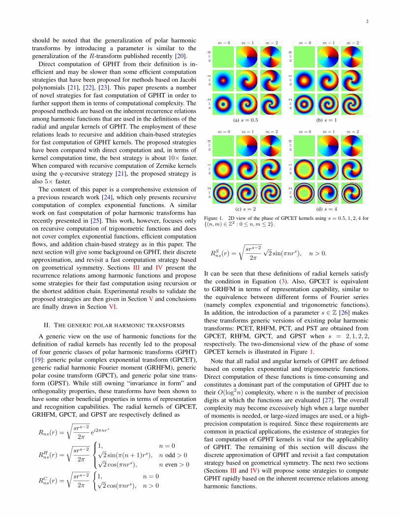
Figure 1. 2D view of the phase of GPCET kernels using s = 0.5, 1, 2, 4 for{(n,m) ∈ Z2 : 0 ≤ n,m ≤ 2}.

RSns(r) =

√srs−2

2π

√2 sin(πnrs), n > 0.

It can be seen that these definitions of radial kernels satisfythe condition in Equation (3). Also, GPCET is equivalentto GRHFM in terms of representation capability, similar tothe equivalence between different forms of Fourier series(namely complex exponential and trigonometric functions).In addition, the introduction of a parameter s ∈ Z [26] makesthese transforms generic versions of existing polar harmonictransforms: PCET, RHFM, PCT, and PST are obtained fromGPCET, RHFM, GPCT, and GPST when s = 2, 1, 2, 2,respectively. The two-dimensional view of the phase of someGPCET kernels is illustrated in Figure 1.

Note that all radial and angular kernels of GPHT are definedbased on complex exponential and trigonometric functions.Direct computation of these functions is time-consuming andconstitutes a dominant part of the computation of GPHT due totheir O(log2n) complexity, where n is the number of precisiondigits at which the functions are evaluated [27]. The overallcomplexity may become excessively high when a large numberof moments is needed, or large-sized images are used, or a high-precision computation is required. Since these requirements arecommon in practical applications, the existence of strategies forfast computation of GPHT kernels is vital for the applicabilityof GPHT. The remaining of this section will discuss thediscrete approximation of GPHT and revisit a fast computationstrategy based on geometrical symmetry. The next two sections(Sections III and IV) will propose some strategies to computeGPHT rapidly based on the inherent recurrence relations amongharmonic functions.

3

Discrete approximation

The image processed in digital systems is not defined in acontinuous domain, but a grid of pixels. Over each pixel region,a constant value is used to represent the intensity of the imagefunction at that pixel location. Accordingly, the continuousintegration in Equation (1) needs to be approximated in twoseparate ways: in the domain of integration (geometrically)and in the kernel values (numerically). To be precise, a latticeof pixels is selected to cover the unit disk for geometricapproximation, and some values are assigned to each kernel ateach pixel location for numerical approximation.

Geometric approximation is required to linearly map arectangular grid of pixels onto a continuous and circular domainof the unit disk since an exact mapping is impossible dueto their different geometric nature. In this work, the incirclemapping strategy [28] which puts a disk inside the image’srectangular domain as illustrated in Figure 2 is used. In thisway, most of the circular region is involved in the computation.However, some image pixels that lie outside the circular region(the white pixels) will not be used in the computation. Usingincircle also leads to the consideration of image pixels that lieat the disk boundary since using these pixels causes an inherenterror, called geometric error in the literature. In the figure, theblue and cyan pixels at the disk boundary have their centerslying outside and inside the circular region, respectively. Whilethe error caused by the cyan pixels can be fixed, that by theblue pixels cannot be fixed and remains the main source ofgeometric error [29]. The impact of this error type dependsheavily on the behavior of the radial kernels around the pointr = 1. Let f be the digital image of size M ×N , the domain[0,M ]× [0, N ] of f is mapped onto [−1, 1]× [−1, 1] by

i −→ 2i−MM

= i∆x− 1, 0 ≤ i ≤M

j −→ 2j −NN

= j∆y − 1, 0 ≤ j ≤ N

where ∆x = 2M and ∆y = 2

N . In order to avoid geometricerror in this work, only the image pixels that lie entirely insidethe unit disk (the yellow pixels) are used in the computation.The values of the image function over the intersection regionsbetween the unit disk and the blue/cyan pixels are then assumedto take value 0. Note that an algorithm to compute ZM thateliminates the geometric error by performing interpolation andthen doing computation in polar coordinates was proposed in[30]. However, for simplicity and to avoid interpolation error,this algorithm is not used in this study.

Numerical approximation arises naturally when GPHT arecomputed from the approximated lattice of pixels over the unitdisk. Let [i, j] denote one pixel region in the domain of fhaving a constant intensity value f [i, j], its mapped regionin the unit disk is

[xi − ∆x

2 , xi + ∆x2

]×[yj − ∆y

2 , yj + ∆y2

],

where (xi, yj) are the coordinates of the center of the mappedregion. The condition for this mapped region to be labeledyellow color is that its four corners lie inside the unit disk.Mathematically, the set C of pixels that satisfies this condition

is defined as C =

{[i, j] :

(xi ± ∆x

2

)2+(yj ± ∆y

2

)2≤ 1

}.

The integration in Equation (1) can then be approximated as a

Figure 2. Lattice-point approximations of a circular region of an image of32× 32 pixels using incircle.

(a) (b)

Figure 3. (a) Illustration of the value of Vnm over the mapped region of size∆x×∆y. (b) Some approximation schemes for numerical integration of 2Dfunctions over a square region. The red dots represent the sampling locations.

discrete sum indexed by pixels in C:

Hnm =∑

[i,j]∈C

f [i, j]hnm[i, j],

where Hnm is an estimate of Hnm and

hnm[i, j] =

ˆ xi+∆x2

xi−∆x2

ˆ yj+ ∆y2

yj−∆y2

V ∗nm(x, y) dxdy (4)

represents the accumulation of V ∗nm over a region of size ∆x×∆y in the unit disk that represents the pixel [i, j] (see Figure3a). Since Vnm is originally defined in polar coordinates whilehnm[i, j] is evaluated in Cartesian ones, computing hnm[i, j]in practice usually relies on numerical integration techniques.

There exist many such techniques that can be employedto approximately evaluate hnm[i, j] [28]. The simplest is therectangle formula (scheme M1 in Figure 3b) written as

hnm[i, j] ' V ∗nm(xi, yj)∆x∆y. (5)

This approximation assumes that the value of Vnm over themapped region of the pixel [i, j] is constant and equals itsvalue at the central point (xi, yj). The order of approximationerror in this case is O

((∆x∆y)2

), thus depends on the area of

the mapped region. Therefore, a more accurate approximationcould be obtained by “pseudo” up-sampling the pixel [i, j]and then using Equation (5) on each up-sampled pixel (theL = 3× 3 up-sampling is shown in scheme M2 in Figure 3b).Other approaches use the L-dimensional cubature formulas[31] defined as

hnm[i, j] 'L∑k=1

wkV∗nm(uk, vk)∆x∆y,

4

where {(uk, vk) : 1 ≤ k ≤ L} is a set of design pointsbelonging to the mapped region that represents the pixel [i, j]and {wk : 1 ≤ k ≤ L} is a set of the corresponding weights. Asan example, a five-dimensional cubature formula (scheme M3in Figure 3b) has the definition hnm[i, j] ' 1

3

[−V ∗nm(xi, yj)+

V ∗nm(xi + ∆x

4 , yj)+V ∗nm

(xi − ∆x

4 , yj)+V ∗nm

(xi, yj + ∆x

4

)+

V ∗nm(xi, yj − ∆x

4

) ]∆x∆y. The order of approximation error

now reduces to O((∆x∆y)L+1

). Thus, a higher accuracy is

obtained when a larger value of L is used. Note that the gainin accuracy has to be paid by an increase in computationalcomplexity, which is not always preferred in real applications.In this work, for simplicity and for the purpose of comparison,the scheme M1 in Figure 3b is used to compute hnm[i, j] inGPHT and comparison methods.

In the literature, the aforementioned approximation error incomputing hnm[i, j] is often called numerical error [28]. Theimpact of this type of error depends heavily on the behaviorof Vnm over the mapped region that represents the pixel [i, j]and thus varies according to the actual moment and the ordersn,m. In the case of GPHT, the radial and angular kernels thatconstitute Vnm are defined based on harmonic functions andoscillate within their respective intervals, i.e., [0, 1] and [0, 2π).This means that Vnm will oscillate at a higher frequency when nand m take higher values. In addition, since the aforementionedapproximation schemes are based on the sampled values ofVnm, the value of Hnm is susceptible to information loss ifVnm has been under-sampled. This is because the number ofsampling points is fixed and determined by the size of theinput image. Thus, when a moment of a too-high order n or mis considered, a fixed sampling of Vnm becomes insufficient.

There exist some approaches that try to eliminate numericalerror by avoiding direct approximation of hnm[i, j] over eachmapped region of the pixel [i, j]. Some stick to the Cartesianspace and perform the integration in Equation (4) analyticallyafter converting Vnm from being defined by polar coordinatesto being defined by Cartesian ones [32], [33]. This is possibledue to the relationship between Zernike and geometric moments[6] or by piecewise polynomial interpolation of Vnm. Anotherapproach [30] computes the moments directly in polar space byusing bicubic interpolation to convert the digital image f frombeing defined as a piecewise constant function in the Cartesianspace to being defined as a piecewise constant function inthe polar space. Optimization techniques were recently usedto improve the orthogonality of the approximated discretekernels for more accurate image reconstruction [34]. However,these approaches to eliminate numerical error are much morecomputationally expensive than the aforementioned approxi-mation schemes because interpolation makes any recurrencerelation between radial and/or angular kernels invalid and alsooptimization requires iterative evaluations. In addition, theseapproaches also introduce new error into the value of Hnm dueto the interpolation or optimization process. For these reasons,in this work, these approaches are not used to compute GPHTand comparison methods.

Geometrical symmetry-based fast computationIt can be seen from Figure 4 that the seven symmetrical

points of a point P1 across the y-axis, the origin, the x-axis,

Figure 4. Symmetrical points of a point P1 inside the unit disk across they-axis, the origin, and the x-axis.

Table ICARTESIAN AND POLAR COORDINATES OF THE SYMMETRICAL POINTS OF A

POINT P1 EXPRESSED VIA THOSE OF P1 .

Symmetricalpoint

Symmetricalaxis

Cartesiancoordinates

Radialcoordinate

Angularcoordinate

P1 (x, y) r θ

P2 y-axis (−x, y) r π − θP3 origin (−x,−y) r π + θ

P4 x-axis (x,−y) r −θQ1 y = x (y, x) r π

2− θ

Q2 y = x, y-axis (−y, x) r π2

+ θ

Q3 y = x, origin (−y,−x) r −π2− θ

Q4 y = x, x-axis (y,−x) r −π2

+ θ

and the line y = x in the Cartesian coordinate system have thesame radial and related angular coordinates as those of P1 (seeTable I). From the properties of complex exponential functions,the radial kernel takes the same value and the angular kernelhas related values at these points. Thus, geometrical symmetryin the distribution of pixels inside the unit disk can be exploitedto reduce the need of computing the radial and angular kernelsfor all pixels inside the unit disk to only pixels in one of theeight equal pies in Figure 4. This idea was initially proposedin [35] for Zernike moments and is applicable to all unit disk-based moments. In addition, due to its geometrical nature,this strategy is independent of the aforementioned pixel-baseddiscrete approximation and thus can be used in combinationwith strategies for fast computation of radial/angular kernelsproposed in the following two sections to further reducethe computational complexity. This observation will haveexperimental evidence in Section V.

III. FAST COMPUTATION OF EXPONENTIAL FUNCTIONS

Complex exponential functions are used in the definition ofGPCET radial kernels and GPHT angular kernels. This sectionpresents two different strategies to compute these functionsefficiently using recursion and the shortest addition chain.

Recursive exponentiation

From the following recursive definition of exponentiation:

base case: e0α = 1,

5

Figure 5. Computation of Rns and Am based on recursive computation ofcomplex exponential functions.

inductive clause: ekα = e(k−1)α eα, k ∈ Z,

the complex exponential functions in the definition of GPCETradial kernels, Rns, and GPHT angular kernels, Am, can becomputed recursively as

ei2πnrs

= ei2π(n−1)rsei2πrs

, (6)

eimθ = ei(m−1)θ eiθ,

using the base cases ei2π0rs = 1 and ei0θ = 1, respectively.

Assuming that{√

srs−2

2π , ei2πrs

, eiθ}

have been pre-computed

and stored in memory for the polar coordinates (r, θ) of all pixelcenters mapped inside the unit disk, the following recurrencerelations of Rns and Am:

Rns(r) =

√srs−2

2πei2πnr

s

= R(n−1)s(r) ei2πrs

, (7)

Am(θ) = eimθ = Am−1(θ) eiθ, (8)

lead to their recursive computation with the base casesR0s(r) =

√srs−2

2π and A0(θ) = 1, respectively. Thus,computing Rns from R(n−1)s and Am from Am−1 eachrequires only one multiplication for each pixel location, whichis very fast when compared to direct exponentiation. It shouldbe noted that these forms of recurrence relations are simplerthan those that were previously proposed for the radial kernelsdefined based on Jacobi polynomials (see [21], [22] andreferences therein). By using Equations (7) and (8), only tworecursive computational threads are needed to reach everyGPCET radial kernel and GPHT angular kernel, whereas manythreads would be required to cover all radial kernels definedbased on Jacobi polynomials. The corresponding computationflows for Rns and Am are illustrated in Figure 5. Note also thatthe method proposed here is much faster than the one mentionedin [17] where direct exponentiation is used to compute PCETradial and angular kernels.

The aforementioned recursive computation of Rns and Amcould be employed for extremely fast computation of GPCETkernels when the order set S composes a square region in Z2

and takes the origin as its center as

S = {(n,m) : n,m ∈ Z2, |n|, |m| ≤ K},

where K is a certain positive integer. By using the compu-tational flow depicted in Figure 6a, computing Vnms(r, θ)requires only two multiplications: one for updating Rns(r)or Am(θ) and one for computing Vnms(r, θ) = Rns(r)Am(θ).As a result, computing a GPCET moment requires only threevector multiplications (two for computing Vnms and one formultiplying Vnms by f ), followed by a discrete sum over allthe pixel locations.

(a) Four quadrants (b) One quadrant

Figure 6. Computation flows for GPCET kernels starting from the order(0, 0). At each step, one of the orders n and m changes its value by adding 1or −1, depending on the current direction of the flow. Computing each kernelVnms thus requires two multiplications, one for computing Rns or Am usingEquations (7) or (8), depending on whether the value of n or m has just beenchanged, and the other for multiplying Rns by Am to get Vnms.

To further boost the computation speed, instead of lettingthe computational flow to visit all (n,m) ∈ S in the fourquadrants in the Cartesian space, it is sufficient to visit only(n,m) ∈ S in one quadrant (n,m ≥ 0) as illustrated in Figure6b. This is possible due to the following relations:

R−ns(r) = R∗ns(r),

A−m(θ) = A∗m(θ).

Thus, whenever Rns and Am are available, computing the fourrelated GPCET kernels requires only two multiplications andthree conjugations:

Vnms(r, θ) = Rns(r)Am(θ),

V−nms(r, θ) = R∗ns(r)Am(θ),

V−n−ms(r, θ) = V ∗nms(r, θ),

Vn−ms(r, θ) = V ∗−nms(r, θ).

Since eight multiplications are needed to compute these fourkernels if the computational flow in Figure 6a is used, thesimple trick of staying in one quadrant leads to a 8

3 -timereduction in the number of multiplications.

When there is enough memory space to store all the radialkernels Rns (|n| ≤ K) and angular kernels Am (|m| ≤ K),then pre-computing and keeping their values in memory maylead to a further reduction in computational complexity by usingthe computational flow in Figure 7. It can be seen that, foreach pixel location, the total number of multiplications requiredto update the values of Rns or Am using the computationalflow in Figure 6a is (K + 1)2 − 1 whereas pre-computationusing the computational flow in Figure 7 needs only 2Kmultiplications. However, besides the memory requirementto store pre-computed values, this strategy has a disadvantageconcerning the data accessing time. The pre-computed valuesof all Rns (or Am) are often stored in a matrix Rs (or A)indexed by r and n (or θ and m). When the kernel Vnms needsto be computed, the values in the nth column of Rs and in themth column of A are retrieved from memory. Since fetchingdata from memory is less efficient than directly using data inCPU cache as in the case of recursive computation, the pre-

6

Figure 7. Computation of GPCET kernels Vnms from the pre-computedand stored values of the radial kernels Rns and angular kernels Am (0 ≤n,m ≤ K).

computing strategy may not provide any computational speed-up as expected. This concern will be supported by experimentalevidence in Section V.

In real situations, the speed-up in computing GPCETkernels leads to the possibility of increasing the number ofGPCET moments without changing the system throughput. Thisincrease is equivalent to an increase in the number of featuresor, more importantly, an increase in the number of patternclasses the system can discriminate. Another by-product of fastcomputation is the reduction in storage space requirement. Inmethods based on orthogonal polynomials the common practiceis to pre-compute and store kernels in memory in order toavoid their repetitive expensive computation. For example, if Lmoments are needed then the L corresponding kernels need tobe pre-computed and stored. In the case of GPCET, since thekernel of any order can be computed rapidly, there is merely

a need to store the set{√

srs−2

2π , ei2πrs

, eiθ}

for the polar

coordinates (r, θ) of all the pixel centers mapped into the unitdisk, regardless the required number of moments. This practicealso leads to a reduction in storage space by 2K

3 .

Addition-chain-based exponentiation

In some situations where only some kernels Vnms of certainorders n and m are needed, the recursive strategies proposedpreviously in this section are not optimal since all Rps andAq with 0 ≤ p ≤ n and 0 ≤ q ≤ m need to be computed(Figure 5), leading to n + m + 1 multiplications for eachpixel location. There exists in the literature methods that allowcomputing Rns from R0s and Am from A0 quickly usingaddition-chain exponentiation [36]. The basic idea is based onthe minimal number of multiplications necessary to computegn from g (n ∈ Z), given that the only permitted operation ismultiplication of two already-computed powers of g. In fact,this minimal number is the length of the shortest addition chainfor n, which is a list of positive integers a1, a2, . . . , a` witha1 = 1 and a` = n such that for each 1 < i ≤ n, there aresome j and k satisfying 1 ≤ j ≤ k < i and ai = aj + ak. Itthus can be seen that a shorter addition chain for n results infaster computation of gn by computing ga2 , ga3 , . . . , ga`−1 , gn

Algorithm 1 Computation of gn by the “square-and-multiply”exponentiation method.

1: a← 12: for i = `→ 0 do3: a← a ∗ a4: if ci = 1 then5: a = a ∗ g6: end if7: end for

in sequence. While the shortest addition chain for a relativelysmall number can be obtained from lookup table [37], findingthis chain for a large number is known as an NP-completeproblem [38]. For this reason, a near-optimal solution is oftenused as a substitution in practical situation.

A number of methods has been proposed to find near-optimal addition chains for a number. One of the simplestand most frequently used is the binary method, also knownas the “square-and-multiply” method, which is based on thefollowing formula to compute gn (n > 0) recursively usingsquaring and multiplication as

gn =

1, if n = 0,

g ×(g

n−12

)2

, if n is odd(g

n2

)2, if n is even

Let n =∑`i=0 ci 2i be the binary expansion of a positive

integer n, the pseudo-code for the computation of gn (n > 0)using the “square-and-multiply” method is given in Algorithm1. At the beginning of each iteration i of the “for loop”, ais equal to gt, where t has its binary expansion equal to thefirst ` − i prefix of the binary expansion of n. Squaring ahas the effect of doubling t, and multiplying by g puts a 1 inthe last digit if the corresponding bit ci is 1. It can be seenthat this algorithm uses log n squaring operations and at mostlog n multiplications. In other words, the “square-and-multiply”method takes 2 log n multiplications in the worst case and32 log n on average. Since the lower bound for the number ofmultiplications required to do a single exponentiation is log n,this method is usually considered as “good enough” and iscomputationally much more efficient than the recursive methodof multiplying the base g with itself repeatedly to get gn,requiring n multiplications. The application of this “square-and-multiply” method for the computation of GPCET radial kernelsand GPHT angular kernels when only some moments of certainorders need to be computed will speedup the computation.This observation will be supported by experimental evidencein Section V.

Comparison with the existing recursion-based method

In order to evaluate the improvement in computationalcomplexity obtained by the proposed method over the methodrecently presented in [25], a theoretical comparison on thecomputational complexity of PCET (or GPCET at s = 2) hasbeen carried out and the results are summarized in Table II.

7

Table IICOMPUTATIONAL COMPLEXITY COMPARISON ON RECURSIVE

COMPUTATION OF THE ANGULAR AND RADIAL KERNELS OF PCET.

Addition Multiplication Table lookup

[25] 3 4 2Proposed method 0 1 1

Note that [25] only presents recursive computation of complexexponential functions for the angular and radial kernels ofPCET by employing the recurrence relations of trigonometricfunctions. It does not have efficient computation flows as inFigure 6 and the addition chain-based exponentiation presentedin this paper. So a direct comparison with the method in[25] should only involve Equations (7), (8) and Figure 5.Nevertheless, the comparison results demonstrate clearly thesuperiority of the proposed method over the method in [25].

IV. FAST COMPUTATION OF TRIGONOMETRIC FUNCTIONS

The trigonometric functions used in the definition of theradial kernels of GRHFM, GPCT, and GPST can also becomputed rapidly. This is because cosine and sine functionsare equivalent to complex exponential functions in terms ofcomputational complexity due to

cos(πnrs) = Re{eiπnrs

} =eiπnr

s

+ e−iπnrs

2,

sin(πnrs) = Im{eiπnrs

} =eiπnr

s − e−iπnrs

2i.

By using these identities, the recursive strategies to computeGPCET radial kernels and GPHT angular kernels presentedin Section III can also be employed to compute the radialkernels of GRHFM, GPCT, and GPST. In other words, theimplementation of GRHFM, GPCT, and GPST can rely on thatof GPCET for low computational complexity. In this way, allthe computational gains claimed for GPCET in the previoussection by using recursion and addition chain are still validfor GRHFM, GPCT, and GPST.

Recursive computation

Apart from relying on complex exponential functions, cosineand sine functions could also be fast computed by using thefollowing recurrence relations:

T0(x) = 1

T1(x) = x

Tn+1(x) = 2xTn(x)− Tn−1(x), for n ≥ 1, (9)

and

U0(x) = 1

U1(x) = 2x

Un+1(x) = 2xUn(x)− Un−1(x), for n ≥ 1 (10)

with

Tn(cos(πrs)) = cos(πnrs),

Un(cos(πrs)) =sin(π(n+ 1)rs)

sin(πrs)

sin(πnrs) = Un−1(cos(πrs)) sin(πrs),

where Tn and Un are the Chebyshev polynomials of the first andsecond kinds, respectively [39]. Accordingly, the computationof cos(πnrs) and sin(πnrs) can also be carried out recursivelywith the base cases {1, cos(πrs)} for Equation (9) and{1, 2 cos(πrs)} for Equation (10), provided that 2 cos(πrs) andsin(πrs) have been pre-computed and are available throughoutthe computation process. The computation flow for GRHFM,GPCT, and GPST radial kernels are illustrated in Figure 8.It can be seen that computing cos(πnrs) and sin(πnrs) eachrequires only one multiplication and one subtraction, which isalmost equivalent to one multiplication required to computeei2πnr

s

as in Equation (6).

Addition-chain-based computation

Fast computation of cosine and sine functions for certainn-multiple angles using the “square-and-multiply” method isalso possible by using the recurrence relations of Chebyshevpolynomials of the first and second kinds [40, page 782]

Tn1+n2(x) + Tn1−n2

(x) = 2Tn1(x)Tn2

(x),

U2n−1(x) = 2Tn(x)Un−1(x),

Un1+n2−1(x)− Un1−n2−1(x) = 2Tn1(x)Un2−1(x).

By letting n2 = n1 = n and n2 = n1 − 1 = n− 1:

T2n(x) = 2T 2n(x)− 1,

T2n−1(x) = 2Tn(x)Tn−1(x)− x,U2n−1(x) = 2Tn(x)Un−1(x),

U2n−2(x) = 2Tn(x)Un−2(x) + 1.

These identities are “similar in form” to g2n = (gn)2 andg2n−1 = g (gn−1)2, which are the bases for the “square-and-multiply” exponentiation. It can also be seen here thatusing addition chain to compute cos(πnrs) and sin(πnrs) iscomputationally more efficient than using recursion.

V. EXPERIMENTAL RESULTS

The computational complexity of existing unit disk-basedorthogonal moments is evaluated in terms of the elapsed timerequired to compute their kernels/moments from an image ofsize 128 × 128. For this image size, the incircle illustratedin Figure 2 contains 12596 pixels that lie entirely inside theunit disk (the yellow pixels). Experiments are performed ona single core of a PC equipped with a 2.33 GHz CPU, 4 GBRAM, and running Linux kernel 2.6.38. MATLAB version7.7 (R2008b) is used as the programming environment. LetK be a certain integer constant, all the kernels/moments oforders (n,m) of each method that satisfy the conditions listedin Table III are computed and the average elapsed time overall feasible orders is used as the kernel/moment computationtime at that value of K. In order to study the trends inthe dependence of kernel/moment computation time on themaximal kernel/moment order K, the value of K is variedin the range 0 ≤ K ≤ 20 in all experiments. In addition,

8

Figure 8. Computation of GRHFM, GPCT, and GPST radial kernels based on recursive computation of cosine and sine functions.

Table IIITHE CONSTRAINTS ON THE MOMENT ORDERS (n,m) OF COMPARISON

METHODS FOR A FIXED VALUE OF K IN THE EXPERIMENTS ONCOMPUTATIONAL COMPLEXITY.

Method Order range

ZM |m| ≤ n ≤ K, n− |m| = evenPZM |m| ≤ n ≤ K

OFMM/CHFM/PJFM 0 ≤ |m|, n ≤ KFBM/BFM/DHC 0 ≤ |m|, n ≤ K

GPCET |m|, |n| ≤ KGRHFM |m| ≤ K, 0 ≤ n ≤ 2K

GPCT 0 ≤ |m|, n ≤ KGPST |m| ≤ K, 1 ≤ n ≤ K

for more reliable results, all the computation times reportedin this section are the average values over 100 trials. Thissection reports the computation time of kernel/moment byusing definitions (Section V-A), recurrence relations (SectionV-B), and the shortest addition chains (Section V-C). For fastcomputation of GPHT, the experiments focus on complexexponential functions (i.e., GPCET) since harmonic functionsare equivalent in terms of computational complexity. This isbecause the recurrence relations of complex exponential andtrigonometric functions developed in Sections III and IV aresimilar. Thus, all conclusions drawn in this section for GPCETare also valid for GRHFM, GPCT, and GPST.

A. Direct computation

In this experiment, the kernels of all unit disk-basedorthogonal moments are computed using their correspondingdefinitions, no recursive strategy is used. The computationtimes per kernel in milliseconds of comparison methods atdifferent values of K are given in Figure 9. It can be seen fromthe figure that Jacobi polynomial-based methods (ZM, PZM,OFMM, CHFM, PJFM) have their kernel computation timesincrease almost linearly with the increase in K, meaning thata longer time is needed to compute a kernel of a higher order.This is because when K increases, factorials of larger integersneed to be evaluated and more additive terms in the finalsummation need to be computed. Among Jacobi polynomial-based methods, OFMM and PJFM have the highest and similarcomplexity while ZM has the lowest. This complexity rankingof these methods is consistent with the ranking according tothe number of multiplications required to compute their radialkernels by using definition.

Eigenfunction-based methods (FBM, BFM, DHC) requirethe longest times to compute their kernels over all comparisonmoments. Among these methods, FBM and DHC have almostthe same complexity whereas that of BFM is slightly less. Thehigh complexity of eigenfunction-based methods can be partly

0 2 4 6 8 10 12 14 16 18 200

5

10

15

20

25

30

35

40

45

50

K

Tim

e / k

ern

el (m

s)

ZM

PZM

OFMM

CHFM

PJFM

FBM

BFM

DHC

GPCET

GPCT

GPST

GRHFM

Figure 9. Kernel computation times of comparison methods by directcomputation at different values of K. For each method and at a specificvalue of K, the kernel orders used in the computation should satisfy theconditions described in Table III and the average elapsed time over all feasibleorders is used as the kernel computation time.

explained by the need of finding the zeros of (the derivativeof) Bessel functions in order to define their radial kernels.And, there exists no formulation that allows fast computationof Bessel functions in the literature. In addition, the lowercomplexity of BFM is due to its use of a fixed-order Besselfunction while FBM and DHC use Bessel functions of differentorders. In this experiment, the evaluation of Bessel functionsis facilitated by the MATLAB built-in function besselj.

Harmonic function-based methods (GPCET, GRHFM, GPCT,GPST) each requires an almost-constant time to compute itskernels of different orders. The constant kernel computationtime is the direct result of the similarity in the form of theirradial kernels at different orders. A change in the kernel orderonly leads to a change in the input to the complex exponentialfunction (GPCET) or cosine/sine functions (GRHFM, GPCT,GPST) and, as a result, does not affect the kernel computationtime. It can also be seen from Figure 9 that the kernelcomputation times of harmonic function-based methods arealmost the same. This is because complex exponential, cosine,and sine functions are equivalent in terms of computationalcomplexity [27].

From the above observations on the direct kernel computationtime of all unit disk-based orthogonal moments, it can be con-cluded here that the simple, resembling, and relating definitionsof harmonic function-based kernels have resulted in an almost-constant kernel computation time, regardless of the maximalkernel order K. This makes a strong contrast with Jacobipolynomial-based and eigenfunction-based methods where ahigher kernel order K means a longer kernel computation time.

9

0 5 10 15 200

0.2

0.4

0.6

0.8

1

K

Tim

e /

ke

rne

l (m

s)

ZM: q−recursive

GPCET: recursiveFour

GPCET: recursiveOne

GPCET: recursivePre

Figure 10. ZM and GPCET kernel computation times at different values ofK using the q-recursive and three recursive strategies proposed in this paper.

B. Recursive computation

The proposed recursive strategies for fast computation ofGPCET kernels are evaluated and compared with its directcomputation and fast computation strategies for ZM kernels.The reason for comparing only to ZM lies in the lack ofbenchmarks on fast computation strategies for other methodsand the popularity of recursive strategies for ZM computationin the literature. In this comparison, ZM kernels are computedusing the q-recursive strategy [21]. The comparison resultsare given in Figure 10 where the legends recursiveFour,recursiveOne, and recursivePre denote recursive computationof GPCET kernels using the computational flows in Figures6a, 6b, and 7, respectively. It can be seen from Figure 10that ZM kernel computation time by using q-recursive is notconstant. It increases in the range K = 0→ 5 and graduallydecreases when K > 5. This is because the q-recursive strategy,which requires pre-computing two ZM radial kernels Rnn andRn(n−2) for each order n, is applicable only when K ≥ 4and is profitable when K ≥ 6. In addition, as K increases,more ZM radial kernels are computed by recursion and thusthe proportion of pre-computed radial kernels decreases. Thisfinally leads to a decrease in the average computation time ofZM radial kernels as K increases.

Using recursiveFour and recursiveOne to compute GPCETkernels leads to an almost-constant computation time, regardlessof the maximal kernel order K. recursiveOne can be seen to bealmost two-time faster than recursiveFour. The only exceptionis at K = 1 where the computation time suddenly dropsbelow the average value. This might be because MATLABsimply copies the pre-computed value of eiθ into A1(θ)since A0(θ) = 1, instead of performing the more complexmultiplication in order to optimize the calculation. A constantcomputation time of GPCET kernel is due to the fact that therecurrence relations in Equations (7) and (8) do not dependon the kernel orders and that there is no need to pre-computeGPCET radial kernels of any order as in the ZM q-recursivestrategy. The “purely” recursive computation of radial andangular kernels is a distinct characteristic of harmonic function-based methods. It can also be seen from the figure that theperformance of recursivePre is not as good as expected; it isnot faster than recursiveOne. The kernel computation time ofrecursivePre, unlike that of recursiveOne and recursiveFour,increases with the increase in K. The only possible explication

0 5 10 15 200

0.2

0.4

0.6

0.8

1

K

Tim

e /

mo

me

nt

(ms)

GPCET: recursiveOne

GPCET: recursiveOne + symGeo

Figure 11. GPCET moment computation times at different values of Kwithout and with geometrical symmetry.

for this phenomenon is the added burden of accessing column-wise data from the pre-computed matrices Rs and A asdescribed in Section III, instead of benefiting from CPU caching.On average, recursive computation of GPCET kernels usingrecursiveOne is approximately 10× faster than their directcomputation and 5× faster than recursive computation of ZMkernels by using the q-recursive strategy.

In computing GPCET moments, that is a combination ofcomputing GPCET kernels and performing the inner productbetween these kernels and image, recursiveOne could be com-bined with the strategy based on geometrical symmetry (SectionII) to further reduce the moment computation time. Figure 11provides the average elapsed times to compute one GPCETmoment using recursiveOne without and with geometricalsymmetry (symGeo). It can be seen from the figure that thecombination of recursiveOne with symGeo is on average 7×faster than using recursiveOne alone, leading to an effectivereduction in the computation time per moment from 0.4406 msto 0.0634 ms at K = 20. These results clearly demonstrate thatthe strategies for fast computation of GPCET moments basedon recursive computation of complex exponential functions andon geometrical symmetry are independent. Combining themdefinitely leads to a multiplication of the computational gainsobtained individually by each of these two strategies.

C. Addition chain-based computation

Performance of fast computation of GPCET kernels usingaddition chain has also been evaluated at some selected valuesof order n. In this experiment, assuming that at each valueof n, only the kernel Vnns is computed, not all Vn′m′s with|n′|, |m′| ≤ n as in the previous experiments. In the caseof recursion, all the radial kernels Rn′s and angular kernelsAm′ with n′,m′ ≤ n need to be computed and the number ofmultiplications required to compute Vnns at each pixel locationis 2n + 1. On the contrary, the number of multiplicationsrequired to compute Vnns at each pixel location in the case ofaddition chain is only 2 log n+ 1.

The comparison results between recursive and addition chain-based computation for n = 1, 2, 4, 8, 16, 32, 64 are given inFigure 12. It can be seen from the figure that as n increases,the GPCET kernel computation time using recursion increasesalmost linearly with the increase in n. This linear relationshipagrees with the recursion scheme illustrated in Figure 5 where

10

0 16 32 48 640

1

2

3

4

5

6

n

Tim

e /

ke

rne

l (m

s)

GPCET recursion

GPCET addition chain

Figure 12. GPCET kernel computation times at different values of n byusing recursive and addition chain-based computation.

a kernel of a higher order requires more recursion steps tocompute. On the contrary, the GPCET kernel computation timeusing addition chain only increases logarithmically with theincrease in n, agreeing with the theoretical estimation on thecomplexity of addition chain-based method. The benefit ofusing addition chain becomes more evident at a higher valueof n. Thus, in situations where only harmonic kernels of certainorders need to be computed, the addition chain-based strategyshould be used instead of the recursive strategy.

VI. CONCLUSIONS

Fast computation strategies for GPHT have been proposedin this paper by exploiting the recurrence relations betweenharmonic functions, leading to a method that is approximately10× faster than direct computation. When compared with theq-recursive strategy for fast computation of ZM kernels, theproposed method is also approximately 5× faster. In addition,combination of the proposed method with the method basedon geometrical symmetry leads to a multiplication of thecomputational gains obtained individually by the two methods.GPHT thus provide the fastest way to extract rotation-invariantfeatures from images. Although other important issues suchas robustness to discretization, noise, blurring, and symmetrypreservation [41], [42] need further studies, GPHT are thepromising replacements of ZM in image analysis applicationswhere low computational complexity is an important method-selection criterion.

It is worth noting here that the value of the parameter sonly slightly affects the direct computation of GPHT and doesnot affect at all the proposed computation strategies. This isbecause s has no role in the recurrence relations in Equations(7) and (8), even though it appears in the definition of GPHTradial kernels. As a result, all the conclusions drawn in thispaper hold for every s. In addition, the methods proposed inthis paper can also be employed to compute the angular kernelsof all existing unit disk-based moments and the radial kernelsof ART [43] and GFD [44] since they are defined based onharmonic functions albeit the radial kernels of ART and GFDdo not satisfy the condition in Equation (3).

REFERENCES

[1] M. R. Teague, “Image analysis via the general theory of moments,”Journal of the Optical Society of America, vol. 70, no. 8, pp. 920–930,1980.

[2] A. B. Bhatia and E. Wolf, “On the circle polynomials of Zernike andrelated orthogonal sets,” Mathematical Proceedings of the CambridgePhilosophical Society, vol. 50, pp. 40–48, 1954.

[3] Z. Ping, H. Ren, J. Zou, Y. Sheng, and W. Bo, “Generic orthogonalmoments: Jacobi–Fourier moments for invariant image description,”Pattern Recognition, vol. 40, no. 4, pp. 1245–1254, 2007.

[4] T. V. Hoang and S. Tabbone, “Errata and comments on “Genericorthogonal moments: Jacobi–Fourier moments for invariant imagedescription”,” Pattern Recognition, vol. 46, no. 11, pp. 3148–3155, 2013.

[5] A. Khotanzad and Y. H. Hong, “Invariant image recognition byZernike moments,” IEEE Transactions on Pattern Analysis and MachineIntelligence, vol. 12, no. 5, pp. 489–497, 1990.

[6] C.-H. Teh and R. T. Chin, “On image analysis by the methodsof moments,” IEEE Transactions on Pattern Analysis and MachineIntelligence, vol. 10, no. 4, pp. 496–513, 1988.

[7] Y. Sheng and L. Shen, “Orthogonal Fourier–Mellin moments for invariantpattern recognition,” Journal of the Optical Society of America A, vol. 11,no. 6, pp. 1748–1757, 1994.

[8] Z. Ping, R. Wu, and Y. Sheng, “Image description with Chebyshev–Fourier moments,” Journal of the Optical Society of America A, vol. 19,no. 9, pp. 1748–1754, 2002.

[9] G. Amu, S. Hasi, X. Yang, and Z. Ping, “Image analysis by pseudo-Jacobi (p = 4, q = 3)–Fourier moments,” Applied Optics, vol. 43, no. 10,pp. 2093–2101, 2004.

[10] J. Flusser, T. Suk, and B. Zitová, Moments and Moment Invariants inPattern Recognition. John Wiley & Sons, 2009.

[11] T. V. Hoang, “Image representations for pattern recognition,” Ph.D.dissertation, University of Nancy, 2011.

[12] F. Bowman, Introduction to Bessel Functions. Dover Publications, 1958.[13] Q. Wang, O. Ronneberger, and H. Burkhardt, “Rotational invariance

based on Fourier analysis in polar and spherical coordinates,” IEEETransactions on Pattern Analysis and Machine Intelligence, vol. 31,no. 9, pp. 1715–1722, 2009.

[14] S. Guan, C.-H. Lai, and G. W. Wei, “Fourier–Bessel analysis of patternsin a circular domain,” Physica D: Nonlinear Phenomena, vol. 151, no.2-4, pp. 83–98, 2001.

[15] B. Xiao, J.-F. Ma, and X. Wang, “Image analysis by Bessel–Fouriermoments,” Pattern Recognition, vol. 43, no. 8, pp. 2620–2629, 2010.

[16] S. C. Verrall and R. Kakarala, “Disk-harmonic coefficients for invariantpattern recognition,” Journal of the Optical Society of America A, vol. 15,no. 2, pp. 389–401, 1998.

[17] P.-T. Yap, X. Jiang, and A. C. Kot, “Two-dimensional polar harmonictransforms for invariant image representation,” IEEE Transactions onPattern Analysis and Machine Intelligence, vol. 32, no. 6, pp. 1259–1270,2010.

[18] H. Ren, Z. Ping, W. Bo, W. Wu, and Y. Sheng, “Multidistortion-invariantimage recognition with radial harmonic Fourier moments,” Journal ofthe Optical Society of America A, vol. 20, no. 4, pp. 631–637, 2003.

[19] T. V. Hoang and S. Tabbone, “Generic polar harmonic transforms forinvariant image representation,” Image and Vision Computing, 2014.

[20] ——, “The generalization of the R-transform for invariant patternrepresentation,” Pattern Recognition, vol. 45, no. 6, pp. 2145–2163,2012.

[21] C.-W. Chong, P. Raveendran, and R. Mukundan, “A comparativeanalysis of algorithms for fast computation of Zernike moments,” PatternRecognition, vol. 36, no. 3, pp. 731–742, 2003.

[22] C. Singh and E. Walia, “Fast and numerically stable methods for thecomputation of Zernike moments,” Pattern Recognition, vol. 43, no. 7,pp. 2497–2506, 2010.

[23] W. Gautschi, Orthogonal Polynomials: Computation and Approximation.Oxford University Press, 2004.

[24] T. V. Hoang and S. Tabbone, “Fast computation of orthogonal polar har-monic transforms,” in Proceedings of the 21th International Conferenceon Pattern Recognition, 2012, pp. 3160–3163.

[25] C. Singh and A. Kaur, “Fast computation of polar harmonic transforms,”Journal of Real-Time Image Processing, pp. 1–8, 2012.

[26] T. V. Hoang and S. Tabbone, “Generic polar harmonic transformsfor invariant image description,” in Proceedings of the 18th IEEEInternational Conference on Image Processing, 2011, pp. 845–848.

[27] J. M. Borwein and P. B. Borwein, “On the complexity of familiarfunctions and numbers,” SIAM Review, vol. 30, no. 4, pp. 589–601,1988.

[28] S. X. Liao and M. Pawlak, “On the accuracy of Zernike moments forimage analysis,” IEEE Transactions on Pattern Analysis and MachineIntelligence, vol. 20, no. 12, pp. 1358–1364, 1998.

11

[29] M. Pawlak and S. X. Liao, “On the recovery of a function on a circulardomain,” IEEE Transactions on Information Theory, vol. 48, no. 10, pp.2736–2753, 2002.

[30] Y. Xin, M. Pawlak, and S. X. Liao, “Accurate computation of Zernikemoments in polar coordinates,” IEEE Transactions on Image Processing,vol. 16, no. 2, pp. 581–587, 2007.

[31] H. Engels, Numerical Quadrature and Cubature. Academic Press, 1980.[32] L. G. Kotoulas and I. Andreadis, “Accurate calculation of image moments,”

IEEE Transactions on Image Processing, vol. 16, no. 8, pp. 2028–2037,2007.

[33] C.-Y. Wee and P. Raveendran, “On the computational aspects of Zernikemoments,” Image and Vision Computing, vol. 25, no. 6, pp. 967–980,2007.

[34] H. Lin, J. Si, and G. P. Abousleman, “Orthogonal rotation-invariantmoments for digital image processing,” IEEE Transactions on ImageProcessing, vol. 17, no. 3, pp. 272–282, 2008.

[35] S.-K. Hwang and W.-Y. Kim, “A novel approach to the fast computationof Zernike moments,” Pattern Recognition, vol. 39, no. 11, pp. 2065–2076,2006.

[36] D. M. Gordon, “A survey of fast exponentiation methods,” Journal ofAlgorithms, vol. 27, no. 1, pp. 129–146, 1998.

[37] D. E. Knuth, The Art of Computer Programming, 3rd ed. Addison-Wesley, 1997, vol. 2: “Seminumerical Algorithms”.

[38] P. J. Downey, B. L. Leong, and R. Sethi, “Computing sequences withaddition chains,” SIAM Journal on Computing, vol. 10, no. 3, pp. 638–646, 1981.

[39] T. H. Koornwinder, R. Wong, R. Koekoek, and R. F. Swarttouw,“Orthogonal polynomials,” in NIST Handbook of Mathematical Functions,F. W. J. Olver, D. W. Lozier, R. F. Boisvert, and C. W. Clark, Eds.Cambridge University Press, 2010, ch. 15, pp. 435–484.

[40] M. Abramowitz and I. A. Stegun, Eds., Handbook of MathematicalFunctions with Formulas, Graphs, and Mathematical Tables. DoverPublications, 1964.

[41] M. Pawlak, Image Analysis by Moments: Reconstruction and Computa-tional Aspects. Oficyna Wydawnicza Politechniki Wrocławskiej, 2006.

[42] N. Bissantz, H. Holzmann, and M. Pawlak, “Testing for image symmetries- with application to confocal microscopy,” IEEE Transactions onInformation Theory, vol. 55, no. 4, pp. 1841–1855, 2009.

[43] M. Bober, F. Preteux, and W.-Y. Y. Kim, “Shape descriptors,” inIntroduction to MPEG 7: Multimedia Content Description Language,B. S. Manjunat, P. Salembier, and T. Sikora, Eds. John Wiley & Sons,2002, pp. 231–260.

[44] D. Zhang and G. Lu, “Shape-based image retrieval using generic Fourierdescriptor,” Signal Processing: Image Communication, vol. 17, no. 10,pp. 825–848, 2002.

Thai V. Hoang received the Diploma degree inelectrical engineering from the Hanoi Universityof Science and Technology, Hanoi, Vietnam, in2003, and the M.Sc. degree in robotics from theKorea Advanced Institute of Science and Technology,Daejeon, Korea, in 2007. Since 2008, he has beena Research Assistant at LORIA, Nancy, France, andreceived the Ph.D. degree in computer science fromUniversité Nancy 2, Nancy, in 2011. From 2012to 2013, he held a post-doctoral position at InriaNancy–Grand Est, Nancy, where he was involved

in developing high-performance algorithms and software for cryoelectronmicroscopy. Since 2014, he has been a Post-Doctoral Researcher with theInstitute of Genetics and Molecular and Cellular Biology, Illkirch, France,where he is involved in computational algorithms for whole-cell modelingusing FIB/SEM data. His research interests include image processing, patternrecognition, structural bioinformatics, and high-performance computing.

Salvatore Tabbone is a Professor of ComputerScience at Université de Lorraine, Nancy, France.He received the Ph.D. degree in computer sciencefrom the Institut Polytechnique de Lorraine, Nancy,in 1994. Since 2007, he has been the Head of theQGAR team at the LORIA Laboratory, Universitéde Lorraine, Nancy, France. His research is relatedto image and graphics document processing andindexing, pattern recognition, image filtering andsegmentation, and content-based image retrieval.He has been the leader of several national and

international projects funded by the French and European institutes. He hasauthored and co-authored more than 100 articles in refereed journal andconferences. He serves as a PC Member for several international and nationalconferences.