Learning near-optimal policies with Bellman ... - Hal-Inria

HAL Id: inria-00117130https://hal.inria.fr/inria-00117130

Submitted on 30 Nov 2006

HAL is a multi-disciplinary open accessarchive for the deposit and dissemination of sci-entific research documents, whether they are pub-lished or not. The documents may come fromteaching and research institutions in France orabroad, or from public or private research centers.

L’archive ouverte pluridisciplinaire HAL, estdestinée au dépôt et à la diffusion de documentsscientifiques de niveau recherche, publiés ou non,émanant des établissements d’enseignement et derecherche français ou étrangers, des laboratoirespublics ou privés.

Learning near-optimal policies with Bellman-residualminimization based fitted policy iteration and a single

sample pathAndras Antos, Csaba Szepesvari, Rémi Munos

To cite this version:Andras Antos, Csaba Szepesvari, Rémi Munos. Learning near-optimal policies with Bellman-residualminimization based fitted policy iteration and a single sample path. Conference On Learning Theory,Jun 2006, Pittsburgh, USA. �inria-00117130�

https://hal.inria.fr/inria-00117130

https://hal.archives-ouvertes.fr

Learning Near-Optimal Policies withBellman-Residual Minimization Based FittedPolicy Iteration and a Single Sample Path

Andras Antos1, Csaba Szepesvari1, and Remi Munos2

1 Computer and Automation Research Inst.of the Hungarian Academy of Sciences

Kende u. 13-17, Budapest 1111, Hungary{antos, szcsaba}@sztaki.hu

2 Centre de Mathematiques AppliqueesEcole Polytechnique

91128 Palaiseau Cedex, [email protected]

Abstract. We consider batch reinforcement learning problems in contin-uous space, expected total discounted-reward Markovian Decision Prob-lems. As opposed to previous theoretical work, we consider the case whenthe training data consists of a single sample path (trajectory) of somebehaviour policy. In particular, we do not assume access to a generativemodel of the environment. The algorithm studied is policy iteration wherein successive iterations the Q-functions of the intermediate policies are ob-tained by means of minimizing a novel Bellman-residual type error. PAC-style polynomial bounds are derived on the number of samples neededto guarantee near-optimal performance where the bound depends on themixing rate of the trajectory, the smoothness properties of the underlyingMarkovian Decision Problem, the approximation power and capacity ofthe function set used.

1 Introduction

Consider the problem of optimizing a controller for an industrial environment. Inmany cases the data is collected on the field by running a fixed controller and thentaken to the laboratory for optimization. The goal is to derive an optimized con-troller that improves upon the performance of the controller generating the data.

In this paper we are interested in the performance improvement that canbe guaranteed given a finite amount of data. In particular, we are interestedin how performance scales as a function of the amount of data available. Westudy Bellman-residual minimization based policy iteration assuming that theenvironment is stochastic and the state is observable and continuous valued.The algorithm considered is an iterative procedure where each iteration involvessolving a least-squares problem, similar to the Least-Squares Policy Iterationalgorithm of Lagoudakis and Parr [1]. However, whilst Lagoudakis and Parrconsidered the so-called least-squares fixed-point approximation to avoid prob-lems with Bellman-residual minimization in the case of correlated samples, we

G. Lugosi and H.U. Simon (Eds.): COLT 2006, LNAI 4005, pp. 574–588, 2006.c© Springer-Verlag Berlin Heidelberg 2006

Learning Near-Optimal Policies with Bellman-Residual Minimization 575

modify the original Bellman-residual objective. In a forthcoming paper we studypolicy iteration with approximate iterative policy evaluation [2].

The main conditions of our results can be grouped into three parts: Condi-tions on the system, conditions on the trajectory (and the behaviour policy usedto generate the trajectory) and conditions on the algorithm. The most impor-tant conditions on the system are that the state space should be compact, theaction space should be finite and the dynamics should be smooth in a sense to bedefined later. The major condition on the trajectory is that it should be rapidlymixing. This mixing property plays a crucial role in deriving a PAC-bound on theprobability of obtaining suboptimal solutions in the proposed Bellman-residualminimization subroutine. The major conditions on the algorithm are that anappropriate number of iterations should be used and the function space usedshould have a finite capacity and be sufficiently rich at the same time. It followsthat these conditions, as usual, require a good balance between the power ofthe approximation architecture (we want large power to get good approximationof the action-value functions of the policies encountered during the algorithm)and the number of samples: If the power of the approximation architecture is in-creased the algorithm will suffer from overfitting, as it also happens in supervisedlearning. Although the presence of the tradeoff between generalization error andmodel complexity should be of no surprise, this tradeoff is somewhat underrep-resented in the reinforcement literature, presumably because most results wherefunction approximators are involved are asymptotic.

The organization of the paper is as follows: In the next section (Section 2)we introduce the necessary symbols and notation. The algorithm is given inSection 3. The main results are presented in Section 4. This section, just like theproof, is broken into three parts: In Section 4.1 we prove our basic PAC-stylelemma that relates the complexity of the function space, the mixing rate of thetrajectory and the number of samples. In Section 4.2 we prove a bound on thepropagation of errors during the course of the procedure. Here the smoothnessproperties of the MDP are used to bound the ‘final’ approximation error asa function of the individual errors. The proof of the main result is finishedSection 4.3. In Section 5 some related work is discussed. Our conclusions aredrawn in Section 6.

2 Notation

For a measurable space with domain S we let M(S) denote the set of all prob-ability measures over S. For ν ∈ M(S) and f : S → R measurable we let‖f‖ν denote the L2(ν)-norm of f : ‖f‖2

ν =∫

f2(s)ν(ds). We denote the space ofbounded measurable functions with domain X by B(X ), the space of measurablefunctions bounded by 0 < K < ∞ by B(X ; K). We let ‖f‖∞ denote the supre-mum norm: ‖f‖∞ = supx∈X |f(x)|. IE denotes the indicator function of eventE, whilst 1 denotes the function that takes on the constant value 1 everywhereover the domain of interest.

576 A. Antos, C. Szepesvari, and R. Munos

A discounted Markovian Decision Problem (MDP) is defined by a quintuple(X , A, P, S, γ), where X is the (possible infinite) state space, A = {a1, a2, . . . , aL}is the set of actions, P : X × A → M(X ) is the transition probability kernel,P (·|x, a) defining the next-state distribution upon taking action a from statex, S(·|x, a) gives the corresponding distribution of immediate rewards, and γ ∈(0, 1) is the discount factor.

We make the following assumptions on the MDP:

Assumption 1 (MDP Regularity). X is a compact subspace of the s-dimen-sional Euclidean space. We assume that the random immediate rewards arebounded by Rmax, the conditional expectations r(x, a) =

∫rS(dr|x, a) and con-

ditional variances v(x, a) =∫

(r − r(x, a))2S(dr|x, a) of the immediate rewardsare both uniformly bounded as functions of (x, a) ∈ X × A. We let Rmax denotethe bound on the expected immediate rewards: ‖r‖∞ ≤ Rmax.

A policy is defined as a mapping from past observations to a distribution overthe set of actions. A policy is deterministic if the probability distribution con-centrates on a single action for all histories. A policy is called stationary if thedistribution depends only on the last state of the observation sequence.

The value of a policy π when it is started from a state x is defined as the totalexpected discounted reward that is encountered while the policy is executed:V π(x) = Eπ [

∑∞t=0 γtRt|X0 = x] . Here Rt is the reward received at time step t,

Rt ∼ S(·|Xt, At), Xt evolves according to Xt+1 ∼ P (·|Xt, At) where At is sam-pled from the distribution assigned to the past observations by π. We introduceQπ : X × A → R, the action-value function, or simply the Q-function of policyπ: Qπ(x, a) = Eπ [

∑∞t=0 γtRt|X0 = x, A0 = a].

The goal is to find a policy that attains the best possible values, V ∗(x) =supπ V π(x) for all states x ∈ X . V ∗ is called the optimal value function. A policyis called optimal if it attains the optimal values V ∗(x) for any state x ∈ X , i.e.,if Vπ(x) = V ∗(x) for all x ∈ X . The function Q∗(x, a) is defined analogously:Q∗(x, a) = supπ Qπ(x, a). It is known that for any policy π, V π, Qπ are boundedby Rmax/(1 − γ), just like Q∗ and V ∗. We say that a (deterministic stationary)policy π is greedy w.r.t. an action-value function Q ∈ B(X × A) if, for all x ∈X ,a ∈ A, π(x) ∈ argmaxa∈A Q(x, a). Since A is finite, such a greedy policyalways exist. It is known that under mild conditions the greedy policy w.r.t.Q∗ is optimal [3]. For a deterministic stationary policy π define the operatorT π : B(X ×A) → B(X ×A) by (T πQ)(x, a) = r(x, a)+γ

∫Q(y, π(y))P (dy|x, a).

For any deterministic stationary policy π : X → A let the operator Eπ :B(X × A) → B(X ) be defined by (EπQ)(x) = Q(x, π(x)); Q ∈ B(X × A).We define two operators corresponding to the transition probability kernel Pas follows: A right-linear operator is defined by P · : B(X ) → B(X × A) and(PV )(x, a) =

∫V (y)P (dy|x, a), whilst a left-linear operator is defined by ·P :

M(X ×A) → M(X ) with (ρP )(dy) =∫

P (dy|x, a)ρ(dx, da). This operator is alsoextended to act on measures over X via (ρP )(dy) = 1

L

∑a∈A

∫P (dy|x, a)ρ(dx).


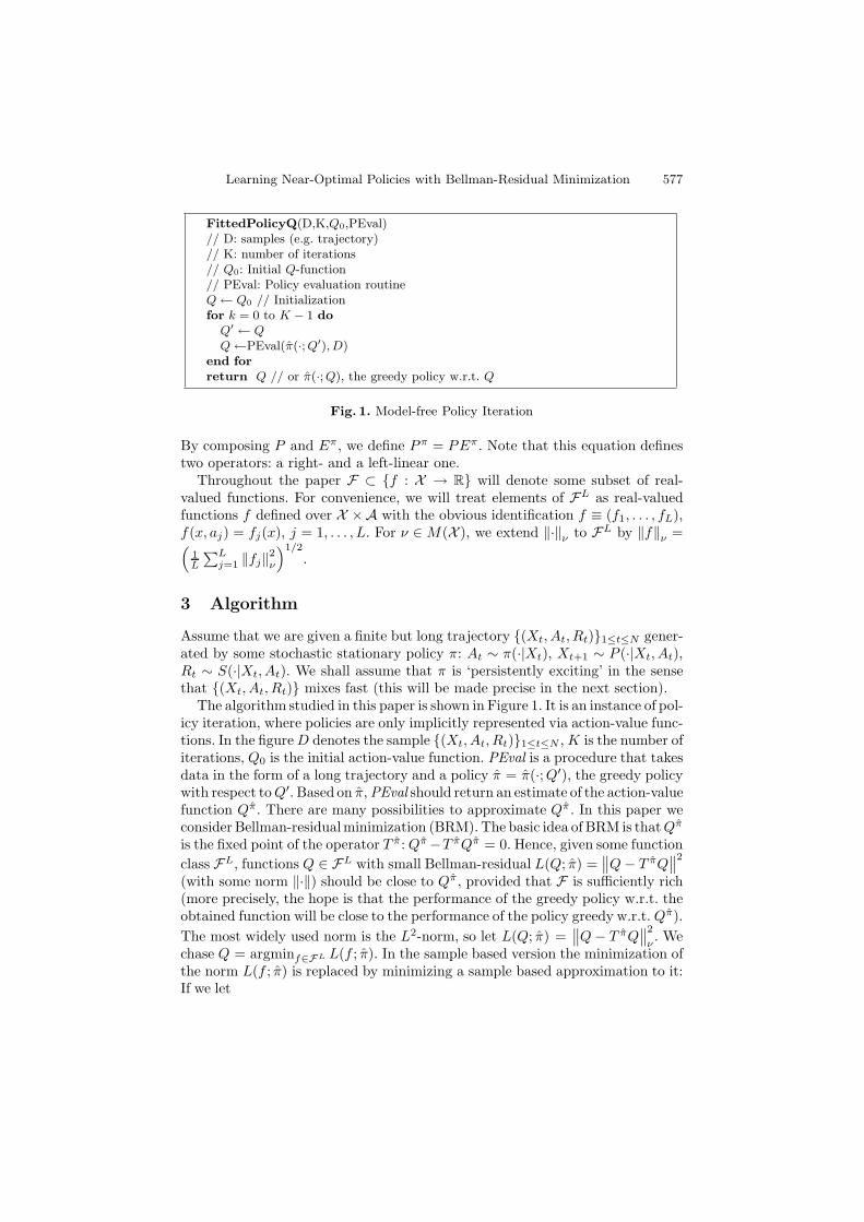
FittedPolicyQ(D,K,Q0,PEval)// D: samples (e.g. trajectory)// K: number of iterations// Q0: Initial Q-function// PEval: Policy evaluation routineQ ← Q0 // Initializationfor k = 0 to K − 1 do

Q′ ← QQ ←PEval(π(·; Q′), D)

end forreturn Q // or π(·; Q), the greedy policy w.r.t. Q

Fig. 1. Model-free Policy Iteration

By composing P and Eπ, we define P π = PEπ. Note that this equation definestwo operators: a right- and a left-linear one.

Throughout the paper F ⊂ {f : X → R} will denote some subset of real-valued functions. For convenience, we will treat elements of FL as real-valuedfunctions f defined over X × A with the obvious identification f ≡ (f1, . . . , fL),f(x, aj) = fj(x), j = 1, . . . , L. For ν ∈ M(X ), we extend ‖·‖ν to FL by ‖f‖ν =(

1L

∑Lj=1 ‖fj‖2

ν

)1/2.

3 Algorithm

Assume that we are given a finite but long trajectory {(Xt, At, Rt)}1≤t≤N gener-ated by some stochastic stationary policy π: At ∼ π(·|Xt), Xt+1 ∼ P (·|Xt, At),Rt ∼ S(·|Xt, At). We shall assume that π is ‘persistently exciting’ in the sensethat {(Xt, At, Rt)} mixes fast (this will be made precise in the next section).

The algorithm studied in this paper is shown in Figure 1. It is an instance of pol-icy iteration, where policies are only implicitly represented via action-value func-tions. In the figure D denotes the sample {(Xt, At, Rt)}1≤t≤N , K is the number ofiterations, Q0 is the initial action-value function. PEval is a procedure that takesdata in the form of a long trajectory and a policy π = π(·; Q′), the greedy policywith respect to Q′. Based on π, PEval should return an estimate of the action-valuefunction Qπ. There are many possibilities to approximate Qπ. In this paper weconsider Bellman-residualminimization (BRM). The basic idea of BRM is that Qπ

is the fixed point of the operator T π: Qπ −T πQπ = 0. Hence, given some functionclass FL, functions Q ∈ FL with small Bellman-residual L(Q; π) =

∥∥Q − T πQ

∥∥2

(with some norm ‖·‖) should be close to Qπ, provided that F is sufficiently rich(more precisely, the hope is that the performance of the greedy policy w.r.t. theobtained function will be close to the performance of the policy greedy w.r.t. Qπ).The most widely used norm is the L2-norm, so let L(Q; π) =

∥∥Q − T πQ

∥∥2

ν. We

chase Q = argminf∈FL L(f ; π). In the sample based version the minimization ofthe norm L(f ; π) is replaced by minimizing a sample based approximation to it:If we let


LN(f ; π) =1

NL

N∑

t=1

L∑

j=1

I{At=aj}π(aj |Xt)

(f(Xt, aj) − Rt − γf(Xt+1, π(Xt+1)))2

then the most straightforward way to compute an approximation to Qπ seems touse Q = argminf∈FL LN(f ; π). At a first sight, the choice of LN seems to be logi-cal as for any given Xt, At and f , Rt+γf(Xt+1, π(Xt+1) is an unbiased estimate of(T πf)(Xt, At). However, as it is well known (see e.g. [4][pp. 220], [5, 1]), LN is nota “proper” approximation to the corresponding L2 Bellman-error:E

[LN (f ; π)

]=

L(f ; π). In fact, an elementary calculus shows that for Y ∼ P (·|x, a), R ∼ S(·|x, a),

E[(f(x, a) − R − γf(Y, π(Y )))2

]= (f(x, a) − (T πf)(x, a))2

+Var [R + γf(Y, π(Y ))] .

It follows that minimizing LN(f ; π) involves minimizing the term Var [f(Y, π(Y ))]in addition to minimizing the ‘desired term’ L(f ; π). The unwanted term acts like apenalty factor, favouring smooth solutions (if f is constant then Var [f(Y, π(Y ))] =0). Although in some cases smooth functions are preferable, in general it is betterto control smoothness penalties in a direct way.

The common suggestion to overcome this problem is to use “double” (uncor-related) samples. In our setup, however, this is not an option. Another possibil-ity is to reuse samples that are close in space (e.g., use nearest neighbours). Thedifficulty with that approach is that it requires a definition of what it means forsamples being close. Here, we pursue an alternative approach based on the intro-duction of an auxiliary function that is used to cancel the variance penalty. Theidea is to select h to ‘match’ (T πf)(x, a) = E [R + γf(Y, π(Y ))] and use it to can-cel the unwanted term. Define L(f, h; π) = L(f ; π) −

∥∥h − T πf

∥∥2

νand

LN(f, h; π) =1

NL

N∑

t=1

L∑

j=1

I{At=aj}π(aj |Xt)

((f(Xt, aj) − Rt − γf(Xt+1, π(Xt+1)))2

−(h(Xt, aj) − Rt − γf(Xt+1, π(Xt+1)))2). (1)

Then, E

[LN (f, h; π)

]= L(f, h; π) and L(f, T πf ; π) = L(f ; π). Hence we let PE-

val solve for Q = argminf∈FL suph∈FL LN (f, h; π). Note that for linearly parame-terized function classes the solution can be obtained in a closed form. In general,one may expect that the number of parameters doubles as a result of the intro-duction of the auxiliary function. Although this may represent a considerable ad-ditional computational burden on the algorithm, given the merits of the Bellman-residual minimization approach over the least-squares fixed point approach [5] wethink that the potential gain in the performance of the final policy might wellworth the extra effort. However, the verification of this claim is left for future work.

Our main result can be formulated as follows: Let ε, δ > 0 be given and choosesome target distribution ρ that will be used to measure performance. Regardingthe function setF weneed the following essential assumptions:F has finite pseudo-dimension (similarly to the VC-dimension, the pseudo-dimension of a function


class also describes the ‘complexity’ of the class) and the set of 0 level-sets of the dif-ferences of pairs of functions from F should be a VC-class.Further, we assume thatthe set FL is ε/2-invariant under operators from T = {T π(·;Q) : Q ∈ FL} withrespect to the ‖·‖ν norm (cf. Definition 3) and that FL approximates the fixed-points of the operators of T well (cf. Definition 4). The MDP has to be regular(satisfying Assumption 1), the dynamics has to satisfy some smoothness proper-ties and the sample path has to be fast mixing. Then for large enough values of N ,K the value-function V πK of the policy πK returned by fitted policy iteration withthe modified BRM criterion will satisfy

‖V πK − V ∗‖ρ ≤ ε

with probability larger than 1 − δ. In particular, if the rate of mixing of the tra-jectory is exponential with parameters (b, κ), then N, K ∼ poly(L, Rmax/(1 −γ), 1/b, V, 1/ε, log(1/δ)), where V is a VC-dimension like quantity characterizingthe complexity of the function class F and the degree of the polynomial is 1+1/κ.

The main steps of the proof are the followings:

1. PAC-Bounds for BRM: Starting from a (random) policy that is derived froma random action-value function, we show that BRM is “PAC-consistent”, i.e.,one can guarantee small Bellman-error with high confidence provided that thenumber of samples N is large enough.

2. Error propagation: If for approximate policy iteration the Bellman-error issmall for K steps, then the final error will be small, too (this requires thesmoothness conditions).

3. Final steps: The error of the whole procedure is small with high probabilityprovided that the Bellman-error is small throughout all the steps with highprobability.

4 Main Result

Before describing the main result we need some definitions.We start with a mixing-property of stochastic processes. Informally, a process

is mixing if future depends only weakly on the past, in a sense that we now makeprecise:

Definition 1. Let {Zt}t=1,2,... be a stochastic process. Denote by Z1:n the collec-tion (Z1, . . . , Zn), where we allow n = ∞. Let σ(Zi:j) denote the sigma-algebragenerated by Zi:j (i ≤ j). The m-th β-mixing coefficient of {Zt}, βm, is defined by

βm = supt≥1

E

[

supB∈σ(Zt+m:∞)

|P (B|Z1:t) − P (B)|]

.

A stochastic process is said to be β-mixing if βm → 0 as m → ∞.

Note that there exist many other definitions of mixing. The weakest among thosemost commonly used is called α-mixing. Another commonly used one is φ-mixingwhich is stronger than β-mixing (see [6]). A β-mixing process is said to mix at anexponential rate with parameters b, κ > 0 if βm = O(exp(−bmκ)).


Assumption 2 (SamplePath Properties).Assume that {(Xt, At, Rt)}t=1,...,N

is the sample path of π, Xt is strictly stationary, and Xt ∼ ν ∈ M(X ). Further, weassume that {(Xt, At, Rt, Xt+1)} is β-mixing with exponential-rate (b, κ). We fur-ther assume that the sampling policy π satisfies π0

def= mina∈A infx∈X π(a|x) > 0.

The β-mixing property will be used to establish tail inequalities for certain em-pirical processes.

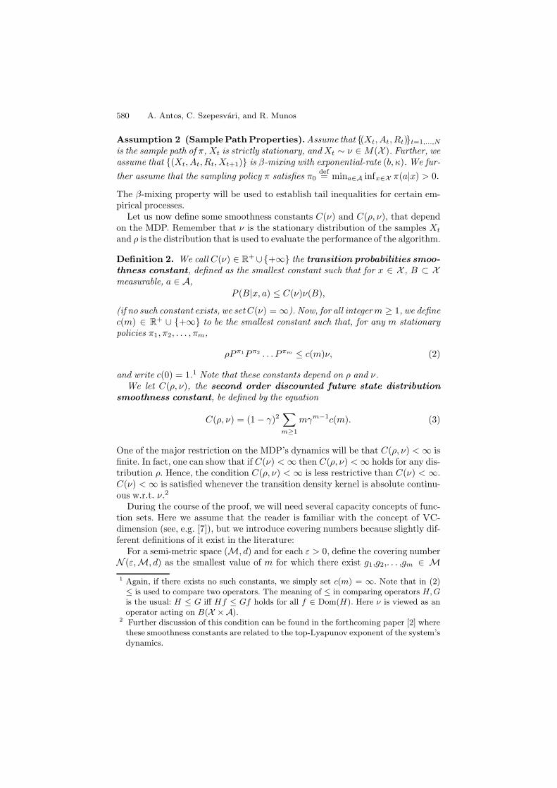
Let us now define some smoothness constants C(ν) and C(ρ, ν), that dependon the MDP. Remember that ν is the stationary distribution of the samples Xt

and ρ is the distribution that is used to evaluate the performance of the algorithm.

Definition 2. We call C(ν) ∈ R+ ∪{+∞} the transition probabilities smoo-

thness constant, defined as the smallest constant such that for x ∈ X , B ⊂ Xmeasurable, a ∈ A,

P (B|x, a) ≤ C(ν)ν(B),

(if no such constant exists, we set C(ν) = ∞). Now, for all integer m ≥ 1, we definec(m) ∈ R

+ ∪ {+∞} to be the smallest constant such that, for any m stationarypolicies π1, π2, . . . , πm,

ρP π1P π2 . . . Pπm ≤ c(m)ν, (2)

and write c(0) = 1.1 Note that these constants depend on ρ and ν.We let C(ρ, ν), the second order discounted future state distribution

smoothness constant, be defined by the equation

C(ρ, ν) = (1 − γ)2∑

m≥1

mγm−1c(m). (3)

One of the major restriction on the MDP’s dynamics will be that C(ρ, ν) < ∞ isfinite. In fact, one can show that if C(ν) < ∞ then C(ρ, ν) < ∞ holds for any dis-tribution ρ. Hence, the condition C(ρ, ν) < ∞ is less restrictive than C(ν) < ∞.C(ν) < ∞ is satisfied whenever the transition density kernel is absolute continu-ous w.r.t. ν.2

During the course of the proof, we will need several capacity concepts of func-tion sets. Here we assume that the reader is familiar with the concept of VC-dimension (see, e.g. [7]), but we introduce covering numbers because slightly dif-ferent definitions of it exist in the literature:

For a semi-metric space (M, d) and for each ε > 0, define the covering numberN (ε, M, d) as the smallest value of m for which there exist g1,g2,. . . ,gm ∈ M1 Again, if there exists no such constants, we simply set c(m) = ∞. Note that in (2)

≤ is used to compare two operators. The meaning of ≤ in comparing operators H, Gis the usual: H ≤ G iff Hf ≤ Gf holds for all f ∈ Dom(H). Here ν is viewed as anoperator acting on B(X × A).

2 Further discussion of this condition can be found in the forthcoming paper [2] wherethese smoothness constants are related to the top-Lyapunov exponent of the system’sdynamics.


such that for every f ∈ M, minj d(f, gj) < ε. If no such finite m exists thenN (ε, M, d) = ∞. In particular, for a class F of X → R functions and pointsx1:N = (x1, x2, . . . , xN ) in X , we use the empirical covering numbers, i.e., thecovering number of F with respect to the empirical L1 distance

lx1:N (f, g) =1N

N∑

t=1

|f(xt) − g(xt)|.

In this case N (ε, F , lx1:N ) shall be denoted by N1(ε, F , x1:N ).

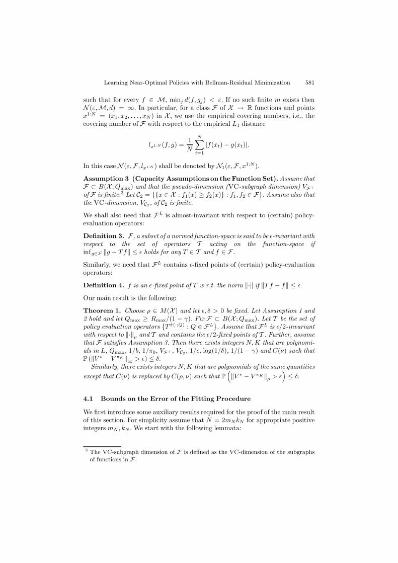
Assumption 3 (Capacity Assumptions on the Function Set). Assume thatF ⊂ B(X ; Qmax) and that the pseudo-dimension (VC-subgraph dimension) VF+

of F is finite.3 Let C2 = {{x ∈ X : f1(x) ≥ f2(x)} : f1, f2 ∈ F}. Assume also thatthe VC-dimension, VC2 , of C2 is finite.

We shall also need that FL is almost-invariant with respect to (certain) policy-evaluation operators:

Definition 3. F , a subset of a normed function-space is said to be ε-invariant withrespect to the set of operators T acting on the function-space ifinfg∈F ‖g − Tf‖ ≤ ε holds for any T ∈ T and f ∈ F .

Similarly, we need that FL contains ε-fixed points of (certain) policy-evaluationoperators:

Definition 4. f is an ε-fixed point of T w.r.t. the norm ‖·‖ if ‖Tf − f‖ ≤ ε.

Our main result is the following:

Theorem 1. Choose ρ ∈ M(X ) and let ε, δ > 0 be fixed. Let Assumption 1 and2 hold and let Qmax ≥ Rmax/(1 − γ). Fix F ⊂ B(X ; Qmax). Let T be the set ofpolicy evaluation operators {T π(·;Q) : Q ∈ FL}. Assume that FL is ε/2-invariantwith respect to ‖·‖ν and T and contains the ε/2-fixed points of T . Further, assumethat F satisfies Assumption 3. Then there exists integers N, K that are polynomi-als in L, Qmax, 1/b, 1/π0, VF+ , VC2 , 1/ε, log(1/δ), 1/(1 − γ) and C(ν) such thatP (‖V ∗ − V πK ‖∞ > ε) ≤ δ.

Similarly, there exists integers N, K that are polynomials of the same quantitiesexcept that C(ν) is replaced by C(ρ, ν) such that P

(‖V ∗ − V πK ‖ρ > ε

)≤ δ.

4.1 Bounds on the Error of the Fitting Procedure

We first introduce some auxiliary results required for the proof of the main resultof this section. For simplicity assume that N = 2mNkN for appropriate positiveintegers mN , kN . We start with the following lemmata:

3 The VC-subgraph dimension of F is defined as the VC-dimension of the subgraphsof functions in F .


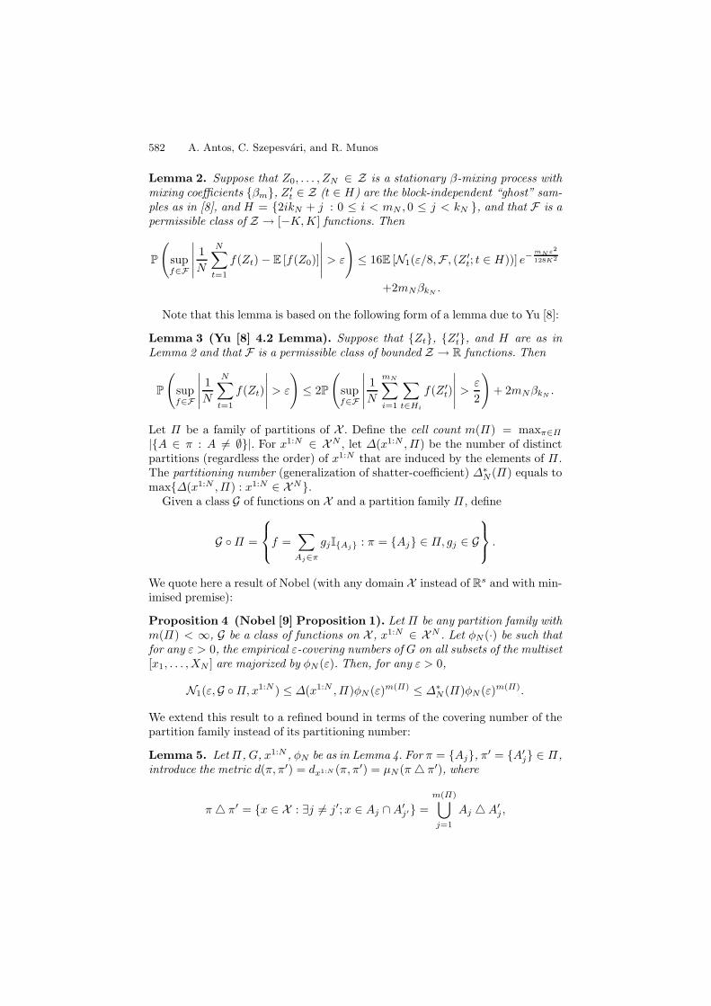
Lemma 2. Suppose that Z0, . . . , ZN ∈ Z is a stationary β-mixing process withmixing coefficients {βm}, Z ′

t ∈ Z (t ∈ H) are the block-independent “ghost” sam-ples as in [8], and H = {2ikN + j : 0 ≤ i < mN , 0 ≤ j < kN }, and that F is apermissible class of Z → [−K, K] functions. Then

P

(

supf∈F

∣∣∣∣∣1N

N∑

t=1

f(Zt) − E [f(Z0)]

∣∣∣∣∣> ε

)

≤ 16E [N1(ε/8, F , (Z ′t; t ∈ H))] e−

mN ε2

128K2

+2mNβkN .

Note that this lemma is based on the following form of a lemma due to Yu [8]:

Lemma 3 (Yu [8] 4.2 Lemma). Suppose that {Zt}, {Z ′t}, and H are as in

Lemma 2 and that F is a permissible class of bounded Z → R functions. Then

P

(

supf∈F

∣∣∣∣∣1N

N∑

t=1

f(Zt)

∣∣∣∣∣> ε

)

≤ 2P

(

supf∈F

∣∣∣∣∣1N

mN∑

i=1

∑

t∈Hi

f(Z ′t)

∣∣∣∣∣>

ε

2

)

+ 2mNβkN .

Let Π be a family of partitions of X . Define the cell count m(Π) = maxπ∈Π

|{A ∈ π : A = ∅}|. For x1:N ∈ X N , let Δ(x1:N , Π) be the number of distinctpartitions (regardless the order) of x1:N that are induced by the elements of Π .The partitioning number (generalization of shatter-coefficient) Δ∗

N (Π) equals tomax{Δ(x1:N , Π) : x1:N ∈ X N}.

Given a class G of functions on X and a partition family Π , define

G ◦ Π =

⎧⎨

⎩f =

∑

Aj∈π

gjI{Aj} : π = {Aj} ∈ Π, gj ∈ G

⎫⎬

⎭.

We quote here a result of Nobel (with any domain X instead of Rs and with min-

imised premise):

Proposition 4 (Nobel [9] Proposition 1). Let Π be any partition family withm(Π) < ∞, G be a class of functions on X , x1:N ∈ X N . Let φN (·) be such thatfor any ε > 0, the empirical ε-covering numbers of G on all subsets of the multiset[x1, . . . , XN ] are majorized by φN (ε). Then, for any ε > 0,

N1(ε, G ◦ Π, x1:N ) ≤ Δ(x1:N , Π)φN (ε)m(Π) ≤ Δ∗N (Π)φN (ε)m(Π).

We extend this result to a refined bound in terms of the covering number of thepartition family instead of its partitioning number:

Lemma 5. Let Π, G, x1:N , φN be as in Lemma 4. For π = {Aj}, π′ = {A′j} ∈ Π,

introduce the metric d(π, π′) = dx1:N (π, π′) = μN (π � π′), where

π � π′ = {x ∈ X : ∃j = j′; x ∈ Aj ∩ A′j′} =

m(Π)⋃

j=1

Aj � A′j ,


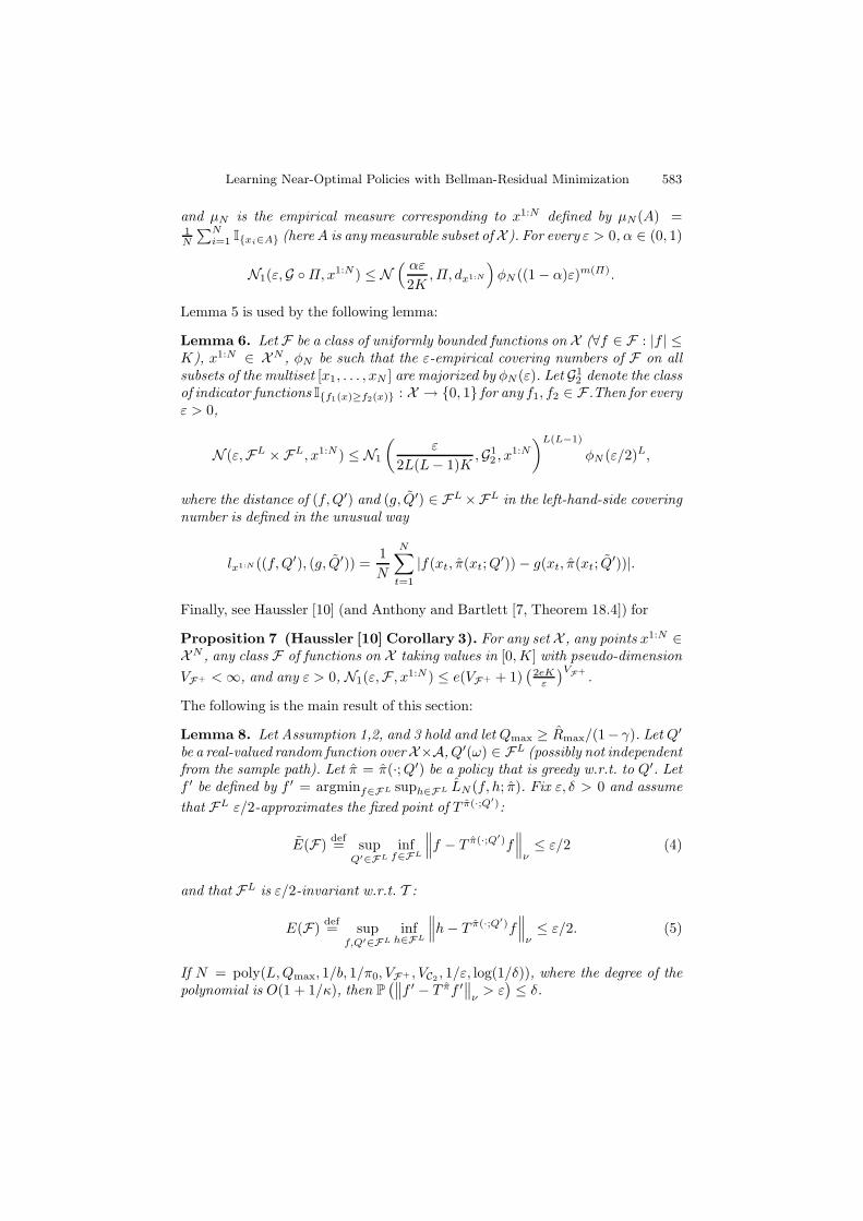
and μN is the empirical measure corresponding to x1:N defined by μN(A) =1N

∑Ni=1 I{xi∈A} (here A is any measurable subset of X ). For every ε > 0, α ∈ (0, 1)

N1(ε, G ◦ Π, x1:N ) ≤ N( αε

2K, Π, dx1:N

)φN ((1 − α)ε)m(Π).

Lemma 5 is used by the following lemma:

Lemma 6. Let F be a class of uniformly bounded functions on X (∀f ∈ F : |f | ≤K), x1:N ∈ X N , φN be such that the ε-empirical covering numbers of F on allsubsets of the multiset [x1, . . . , xN ] are majorized by φN (ε). Let G1

2 denote the classof indicator functions I{f1(x)≥f2(x)} : X → {0, 1} for any f1, f2 ∈ F .Then for everyε > 0,

N (ε, FL × FL, x1:N ) ≤ N1

(ε

2L(L − 1)K, G1

2 , x1:N)L(L−1)

φN (ε/2)L,

where the distance of (f, Q′) and (g, Q′) ∈ FL × FL in the left-hand-side coveringnumber is defined in the unusual way

lx1:N ((f, Q′), (g, Q′)) =1N

N∑

t=1

|f(xt, π(xt; Q′)) − g(xt, π(xt; Q′))|.

Finally, see Haussler [10] (and Anthony and Bartlett [7, Theorem 18.4]) for

Proposition 7 (Haussler [10] Corollary 3). For any set X , any points x1:N ∈X N , any class F of functions on X taking values in [0, K] with pseudo-dimensionVF+ < ∞, and any ε > 0, N1(ε, F , x1:N ) ≤ e(VF+ + 1)

(2eKε

)VF+ .

The following is the main result of this section:

Lemma 8. Let Assumption 1,2, and 3 hold and let Qmax ≥ Rmax/(1 − γ). Let Q′

be a real-valued random function over X×A, Q′(ω) ∈ FL (possibly not independentfrom the sample path). Let π = π(·; Q′) be a policy that is greedy w.r.t. to Q′. Letf ′ be defined by f ′ = argminf∈FL suph∈FL LN (f, h; π). Fix ε, δ > 0 and assumethat FL ε/2-approximates the fixed point of T π(·;Q′):

E(F) def= supQ′∈FL

inff∈FL

∥∥∥f − T π(·;Q′)f

∥∥∥

ν≤ ε/2 (4)

and that FL is ε/2-invariant w.r.t. T :

E(F) def= supf,Q′∈FL

infh∈FL

∥∥∥h − T π(·;Q′)f

∥∥∥

ν≤ ε/2. (5)

If N = poly(L, Qmax, 1/b, 1/π0, VF+ , VC2 , 1/ε, log(1/δ)), where the degree of thepolynomial is O(1 + 1/κ), then P

(∥∥f ′ − T πf ′∥∥

ν> ε

)≤ δ.


Proof. (Sketch) We have to show that f ′ is close to the corresponding T π(·;Q′)f ′

with high probability, noting that Q′ may not be independent from the sample

path. By (4), it suffices to show that L(f ′; Q′) def=∥∥∥f ′ − T π(·;Q′)f ′

∥∥∥

2

νis close to

inff∈FL L(f ; Q′). Denote the difference of these two quantities by Δ(f ′, Q′). Notethat Δ(f ′, Q′) is increased by taking its supremum over Q′. By (5), L(f ; Q′) andL(f ; Q′) def= suph∈FL L(f, h; π(·; Q′)), as functions of f and Q′, are uniformly closeto each other. This reduces the problem to bounding supQ′(L(f ′; Q′) −inff∈FL L(f ; Q′)). Since E

[LN(f, h; π)

]= L(f, h; π) holds for any f, h ∈ FL

and policy π, by defining a suitable error criterion lf,h,Q′(x, a, r, y) in accordancewith (1), the problem can be reduced to a usual uniform deviation problem overLF = {lf,h,Q′ : f, h, Q′ ∈ FL}. Since the samples are correlated, Pollard’s tailinequality cannot be used directly. Instead, we use the method of Yu [8]: We splitthe samples into mN pairs of blocks {(Hi, Ti)|i = 1, . . . , mN}, each block com-promised of kN samples (for simplicity we assume N = 2mNkN ) and then useLemma 2 with Z = X ×A×R×X , F = LF . The covering numbers of LF can bebounded by those of FL and FL × FL, where in the latter the distance is definedas in Lemma 6. Next we apply Lemma 6 and then Proposition 7 to bound theresulting three covering numbers in terms of VF+ and VC2 (note that the pseudo-dimension of FL cannot exceed LVF+). Defining kN = N

11+κ +1, mN = N/(2kN)

and substituting βm ≤ e−bmκ

, we get the desired polynomial bound on the num-ber of samples after some tedious calculations. ��

4.2 Propagation of Errors

Let Qk denote the kth iterate of (some) approximate policy iteration algorithmwhere the next iterates are computed by means of some Bellman-residual mini-mization procedure. Let πk be the kth policy. Our aim here is to relate the per-formance of the policy πK to the magnitude of the Bellman-residuals εk

def= Qk −T πkQk, 0 ≤ k < K.

Lemma 9. Let p ≥ 1. For any η > 0, there exists K that is linear in log(1/η) andlog Rmax such that, if the Lp,ν norm of the Bellman-residuals are bounded by someconstant ε, i.e. ‖εk‖p,ν ≤ ε for all 0 ≤ k < K, then

‖Q∗ − QπK ‖∞ ≤ 2γ

(1 − γ)2[C(ν)]1/pε + η (6)

and‖Q∗ − QπK ‖p,ρ ≤ 2γ

(1 − γ)2[C(ρ, ν)]1/pε + η. (7)

Proof. We have C(ν) ≥ C(ρ, ν) for any ρ. Thus, if the bound (7) holds for any ρ,choosing ρ to be a Dirac at each state implies that (6) also holds. Therefore, weonly need to prove (7).

Let Ek = P πk+1(I − γP πk+1)−1 − P π∗(I − γP πk)−1. Closely following the

proof of [5][Lemma 4], we get Q∗ − Qπk+1 ≤ γP π∗(Q∗ − Qπk) + γEkεk. Thus, by


induction, Q∗−QπK ≤ γ∑K−1

k=0 (γP π∗)K−k−1Ekεk+ηKwith ηK = (γP π∗

)K(Q∗−Qπ0). Hence, ‖ηK‖∞ ≤ 2Qmaxγ

K .Now, let Fk = P πk+1(I − γP πk+1)−1 + P π∗

(I − γP πk)−1. By taking the ab-solute value pointwise in the above bound on Q∗ − QπK we get Q∗ − QπK ≤γ∑K−1

k=0 (γP π∗)K−k−1Fk|εk|+(γP π∗

)K |Q∗ −Qπ0 |. From this, using the fact thatQ∗ − Qπ0 ≤ 2

1−γ Rmax1, we arrive at

|Q∗ − QπK | ≤ 2γ(1 − γK+1)(1 − γ)2

[K−1∑

k=0

αkAk|εk| + αKAKRmax1

]

.

Here we introduced the positive coefficients αk = (1−γ)γK−k−1

1−γK+1 , for 0 ≤ k <

K, and αK = (1−γ)γK

1−γK+1 , and the operators Ak = 1−γ2 (P π∗

)K−k−1Fk, for 0 ≤ k <

K, AK = (P π∗)K . Note that

∑Kk=0 αk = 1 and the operators Ak are stochastic

when considered as a right-linear operators: for any (x, a) ∈ X × A, λ(k)(x,a)(B) =

(AkχB)(x, a) is a probability measure and (AkQ)(x, a) =∫

λ(k)(x,a)(dy)Q(y, π(y)).

Here χB : B(X × A) → [0, 1] is defined by χB(x, a) = I{x∈B}.

Let λK =[

2γ(1−γK+1)(1−γ)2

]p

. Now, by using two times Jensen’s inequality we get

‖Q∗ − QπK ‖pp,ρ =

1L

∑

a∈A

∫ρ(dx)|Q∗(x, a) − QπK (x, a)|p

≤ λKρ

[K−1∑

k=0

αkAk|εk|p + αKAK(Rmax)p1

]

.

From the definition of the coefficients c(m), ρAk ≤ (1−γ)∑

m≥0 γmc(m+K−k)νand we deduce

‖Q∗−QπK‖pp,ρ ≤λK

⎡

⎣(1−γ)K−1∑

k=0

αk

∑

m≥0

γmc(m + K − k) ‖εk‖pp,ν + αK(Rmax)p

⎤

⎦.

Replace αk by their values, and from the definition of C(ρ, ν), and since ‖εk‖p,ν

≤ ε, we have

‖Q∗ − QπK ‖pp,ρ ≤ λK

[1

1 − γK+1 C(ρ, ν)εp +(1 − γ)γK

1 − γK+1 (Rmax)p

]

.

Thus there is K linear in log(1/η) and log Rmax, e.g. such that γK <[

(1−γ)2

2γRmaxη]p

so that the second term is bounded by ηp. Thus, ‖Q∗ − QπK ‖pp,ρ ≤

[2γ

(1−γ)2

]p

C(ρ, ν)εp + ηp and hence ‖Q∗ − QπK ‖p,ρ ≤ 2γ(1−γ)2 [C(ρ, ν)]1/pε+ η, fin-

ishing the proof. ��


4.3 Proof of the Main Result

Proof. Consider the kth iteration of the algorithm. Let εk = Qk − T πkQk. Bythe reasoning used in the proof of Lemma 9, we only need to prove the secondpart of the result. Since 0 < γ < 1, there exists K that is linear in log(1/ε) and

log Rmax such that γK <[

(1−γ)2

2γRmax

ε2

]p

. Now, from Lemma 8, there exists N that ispoly(L, Qmax, 1/b, 1/π0, VF+ , VC2 , 1/ε, log(1/δ)), such that, for each 0 ≤ k < K,P

(‖εk‖p,ν > (1−γ)2

2C1/pε2

)< δ/K. Thus, P

(‖εk‖p,ν > (1−γ)2

2C1/pε2 , for all 0 ≤ k < K

)

< δ. Applying Lemma 9 with η = ε/2 ends the proof. ��

5 Discussion and Related Work

The idea of using value function approximation goes back to the early days ofdynamic programming [11, 12]. With the recent growth of interest in reinforce-ment learning, work on value function approximation methods flourished [13, 14].Recent theoretical results mostly concern supremum-norm approximation errors[15, 16], where the main condition on the way intermediate iterates are mapped(projected) to the function space is that the corresponding operator, Π , must be anon-expansion. Practical examples when Π satisfies the said property include cer-tain kernel-based methods, see e.g. [15, 16, 17, 18]. However, the growth-restrictionimposed on Π rules out many popular algorithms, such as regression-based ap-proaches that were found, however, to behave well in practice (e.g. [19, 20, 1]). Theneed for analysing the behaviour of such algorithms provided the basic motivationfor this work.

One of the main novelties of our paper is that we introduced a modified Bellman-residual that guarantees asymptotic consistency even with a single sample path.

The closest to the present work is the paper of Szepesvari and Munos [21]. How-ever, as opposed to paper [21], here we dealt with a fitted policy iteration algorithmand unlike previously, we worked with dependent samples. The technique used todeal with dependent samples was to introduce (strong) mixing conditions on thetrajectory and extending Pollard’s inequality along the lines of Meir [22].

Also, the bounds developed in Section 4.2 are closely related to those developedin [5]. However, there only the case C(ν) < ∞ was considered, whilst in this paperthe analysis was extended to the significantly weaker condition C(ν, ρ) < ∞. Al-though in [21] the authors considered a similar condition, there the propagationof the approximation errors was considered only in a value iteration context. Notethat approximate value iteration per se is not suitable for learning from a singletrajectory since approximate value iteration requires at least one successor statesample per action per sampled state.

That we had to work with fitted policy iteration significantly added to the com-plexity of the analysis, as the policy to be evaluated at stage k became dependenton the whole set of samples, introducing non-trivial correlations between succes-sive approximants. In order to show that these correlations do not spoil conver-gence, we had to introduce problem-specific capacity conditions on the functionclass involved. Although these constraints are satisfied by many popular function


classes (e.g., regression trees, neural networks, etc.), when violated unstable be-haviour may arise (i.e., increasing the sample size does not improves the perfor-mance).

Note that the conditions that dictate that F should be rich (namely, that Fshould be “almost invariant” under the family of operators T = {T π(·;Q) : Q ∈ F}and that F should be close to the set of fixed points of T ) are non-trivial to guar-antee. One possibility is to put smoothness constraints on the transition dynamicsand the immediate rewards. It is important to note, however, that both conditionsare defined with respect to weighted L2-norm. This is much less restrictive than ifsupremum-norm were used here. This observation suggests that one should prob-ably look at frequency domain representations of systems in order to guaranteethese properties. However, this is well out of the scope of the present work.

6 Conclusions

We have considered fitted policy iteration with Bellman-residual minimization.We modified the objective function to allow the procedure to work with asingle (but long) trajectory. Our results show that the number of samples neededto achieve a small approximation error depend polynomially on the pseudo-dimension of the function class used in the empirical loss minimization step andthe smoothness of the dynamics of the system. Future work should concern theevaluation of the proposed procedure in practice. The theoretical results can beextended in many directions: Continuous actions spaces will require substantialadditional work as the present analysis relies crucially on the finiteness of the ac-tion set. The exploration of interplay between the MDPs dynamics and the ap-proximability of the fixed points and the invariance of function sets with respectto policy evaluation operators also requires substantial further work.

Acknowledgements

We would like to acknowledge support for this project from the Hungarian Na-tional Science Foundation (OTKA), GrantNo. T047193 (Cs. Szepesvari) and fromthe Hungarian Academy of Sciences (Cs. Szepesvari, Bolyai Fellowship).

References

1. M. Lagoudakis and R. Parr. Least-squares policy iteration. Journal of MachineLearning Research, 4:1107–1149, 2003.

2. A. Antos, Cs. Szepesvari, and R. Munos. Learning near-optimal policies with fittedpolicy iteration and a single sample path: approximate iterative policy evaluation.(submitted to ICML’2006, 2006.

3. D. P. Bertsekas and S.E. Shreve. Stochastic Optimal Control (The Discrete TimeCase). Academic Press, New York, 1978.

4. R.S. Sutton and A.G. Barto. Toward a modern theory of adaptive networks: Expec-tation and prediction. In Proc. of the Ninth Annual Conference of Cognitive ScienceSociety. Erlbaum, Hillsdale, NJ, USA, 1987.


5. R. Munos. Error bounds for approximate policy iteration. 19th International Con-ference on Machine Learning, pages 560–567, 2003.

6. S.P. Meyn and R. Tweedie. Markov Chains and Stochastic Stability. Springer-Verlag,New York, 1993.

7. M. Anthony and P. L. Bartlett. Neural Network Learning: Theoretical Foundations.Cambridge University Press, 1999.

8. B. Yu. Rates of convergence for empirical processes of stationary mixing sequences.The Annals of Probability, 22(1):94–116, January 1994.

9. A. Nobel. Histogram regression estimation using data-dependent partitions. Annalsof Statistics, 24(3):1084–1105, 1996.

10. D. Haussler. Sphere packing numbers for subsets of the boolean n-cube withbounded Vapnik-Chervonenkis dimension. Journal of Combinatorial Theory SeriesA, 69:217–232, 1995.

11. A.L. Samuel. Some studies in machine learning using the game of checkers. IBMJournal on Research and Development, pages 210–229, 1959. Reprinted in Com-puters and Thought, E.A. Feigenbaum and J. Feldman, editors, McGraw-Hill, NewYork, 1963.

12. R.E. Bellman and S.E. Dreyfus. Functional approximation and dynamic program-ming. Math. Tables and other Aids Comp., 13:247–251, 1959.

13. Dimitri P. Bertsekas and J. Tsitsiklis. Neuro-Dynamic Programming. Athena Sci-entific, 1996.

14. Richard S. Sutton and Andrew G. Barto. Reinforcement learning: An introduction.Bradford Book, 1998.

15. Geoffrey J. Gordon. Stable function approximation in dynamic programming. InArmand Prieditis and Stuart Russell, editors, Proceedings of the Twelfth Interna-tional Conference on Machine Learning, pages 261–268, San Francisco, CA, 1995.Morgan Kaufmann.

16. J. N. Tsitsiklis and B. Van Roy. Feature-based methods for large scale dynamicprogramming. Machine Learning, 22:59–94, 1996.

17. Carlos Guestrin, Daphne Koller, and Ronald Parr. Max-norm projections for fac-tored mdps. Proceedings of the International Joint Conference on Artificial Intelli-gence, 2001.

18. D. Ernst, P. Geurts, and L. Wehenkel. Tree-based batch mode reinforcement learn-ing. Journal of Machine Learning Research, 6:503–556, 2005.

19. X. Wang and T.G. Dietterich. Efficient value function approximation using regres-sion trees. In Proceedings of the IJCAI Workshop on Statistical Machine Learningfor Large-Scale Optimization, Stockholm, Sweden, 1999.

20. T. G. Dietterich and X. Wang. Batch value function approximation via supportvectors. In T. G. Dietterich, S. Becker, and Z. Ghahramani, editors, Advances inNeural Information Processing Systems 14, Cambridge, MA, 2002. MIT Press.

21. Cs. Szepesvari and R. Munos. Finite time bounds for sampling based fitted valueiteration. In ICML’2005, 2005.

22. R. Meir. Nonparametric time series prediction through adaptive model selection.Machine Learning, 39(1):5–34, April 2000.

Learning near-optimal policies with Bellman ... - Hal-Inria

Documents

Transcript of Learning near-optimal policies with Bellman ... - Hal-Inria