bellman function method and sharp inequalities for martingales
65
ROCKY MOUNTAIN JOURNAL OF MATHEMATICS Volume 43, Number 6, 2013 SURVEY ARTICLE: BELLMAN FUNCTION METHOD AND SHARP INEQUALITIES FOR MARTINGALES ADAM OSE ¸ KOWSKI ABSTRACT. The Bellman function method is an efficient device which enables relating certain types of estimates arising in probability and harmonic analysis to the existence of the as- sociated special function satisfying appropriate majorization and concavity. This technique has gained considerable inter- est in recent years and led to many interesting results con- cerning the boundedness of wide classes of singular integrals, Fourier multipliers, maximal functions and other related ob- jects. The objective of this survey is to describe the Bellman function approach to certain classical results for martingale transforms. We present the detailed study of the weak-type and moment estimates, and develop some arguments which al- low us to simplify and extend the statements, originally proven by Burkholder and others. 1. Introduction. The Bellman function method is a powerful tool in proving various types of inequalities arising in probability and har- monic analysis. The technique has its origins in the theory of stochastic optimal control, and its fruitful connection with other areas of math- ematics was firstly observed by Burkholder in [6], during the study of certain sharp inequalities for martingale transforms. Since then, the approach has been extended and applied essentially in two directions. The first path is probabilistic: Burkholder’s arguments from [8] were modified and exploited extensively to investigate numerous estimates for semimartingales. The literature here is quite large; we mention only the subsequent works of Burkholder [10 13], Choi [14, 15], Suh [44], Wang [52, 53] and the monograph [33] by the author, which con- tains the more complete bibliography on the subject. The second path, which pushed the method towards applications in harmonic analysis, started with the seminal paper [29] by Nazarov and Treil (inspired by 2010 AMS Mathematics subject classification. Primary 60G42, Secondary 42A05, 60G46, 49K20. Keywords and phrases. Martingale, Bellman function, best constants. This research was partially supported by the NCN grant DEC-2012/05/B/ST1/ 00412. Received by the editors on July 7, 2013, and in revised form on November 19, 2013. DOI:10.1216/RMJ-2013-43-6-1759 Copyright c 2013 Rocky Mountain Mathematics Consortium 1759
-
Upload
khangminh22 -
Category
Documents
-
view
1 -
download
0
Transcript of bellman function method and sharp inequalities for martingales

ROCKY MOUNTAINJOURNAL OF MATHEMATICSVolume 43, Number 6, 2013
SURVEY ARTICLE: BELLMAN FUNCTION METHODAND SHARP INEQUALITIES FOR MARTINGALES
ADAM OSEKOWSKI
ABSTRACT. The Bellman function method is an efficientdevice which enables relating certain types of estimates arisingin probability and harmonic analysis to the existence of the as-sociated special function satisfying appropriate majorizationand concavity. This technique has gained considerable inter-est in recent years and led to many interesting results con-cerning the boundedness of wide classes of singular integrals,Fourier multipliers, maximal functions and other related ob-jects. The objective of this survey is to describe the Bellmanfunction approach to certain classical results for martingaletransforms. We present the detailed study of the weak-typeand moment estimates, and develop some arguments which al-low us to simplify and extend the statements, originally provenby Burkholder and others.
1. Introduction. The Bellman function method is a powerful toolin proving various types of inequalities arising in probability and har-monic analysis. The technique has its origins in the theory of stochasticoptimal control, and its fruitful connection with other areas of math-ematics was firstly observed by Burkholder in [6], during the study ofcertain sharp inequalities for martingale transforms. Since then, theapproach has been extended and applied essentially in two directions.The first path is probabilistic: Burkholder’s arguments from [8] weremodified and exploited extensively to investigate numerous estimatesfor semimartingales. The literature here is quite large; we mentiononly the subsequent works of Burkholder [10 13], Choi [14, 15], Suh[44], Wang [52, 53] and the monograph [33] by the author, which con-tains the more complete bibliography on the subject. The second path,which pushed the method towards applications in harmonic analysis,started with the seminal paper [29] by Nazarov and Treil (inspired by
2010 AMS Mathematics subject classification. Primary 60G42, Secondary42A05, 60G46, 49K20.
Keywords and phrases. Martingale, Bellman function, best constants.This research was partially supported by the NCN grant DEC-2012/05/B/ST1/
00412.Received by the editors on July 7, 2013, and in revised form on November 19,
2013.
DOI:10.1216/RMJ-2013-43-6-1759 Copyright c©2013 RockyMountainMathematics Consortium
1759

1760 ADAM OSEKOWSKI
the preprint version of [30]). This analytic approach has been con-tinued in many papers, including the works of Dragicevic and Volberg[20 22], Ivanishvili et al. [23], Melas [26], Melas and Nikolidakis [27],Nazarov, Treil and Volberg [31], Slavin, Stokolos and Vasyunin [41],Slavin and Vasyunin [42, 43], Vasyunin [45, 46], Vasyunin and Vol-berg [47 49] and the author [35]. The results in the aforementionedpapers have found many important applications, including tight boundsfor wide classes of Fourier multipliers and stochastic integrals: see thepapers cited above, consult also Banuelos, Bielaszewski and Bogdan[1], Banuelos and Wang [2], Borichev, Janakiraman and Volberg [3,4], Nazarov and Volberg [32], the author [34], and the works of manyother mathematicians.
The purpose of the current work is to present the refined studyof some fundamental results for martingale transforms, with the useof both probabilistic and analytic aspects of the Bellman functionmethod. The contents of this survey extend and complement thematerial contained in the monograph [33]. Our contribution will be ofa twofold nature. First, this mixed approach will allow us to strengthensome of the classical results: we will obtain more exact information onthe control of a martingale over its ±1-transforms. Second, we willpresent a certain simplification argument which, in a sense, splits theproblem of identifying a given Bellman function into two easier steps. Insome cases, this argument significantly reduces the technical difficultiesinvolved in the search of the corresponding Bellman function and, aswe hope, can be applied and further extended in many other problemsof this type.
We start with some motivation and introduce some basic notation.Let (hn)n≥0 be the Haar system on [0, 1]. Recall that this family offunctions is given by:
h0 = [0, 1), h1 = [0, 1/2) − [1/2, 1),
h2 = [0, 1/4) − [1/4, 1/2), h3 = [1/2, 3/4)− [3/4, 1),
h4 = [0, 1/8) − [1/8, 1/4), h5 = [1/4, 3/8)− [3/8, 1/2),
h6 = [1/2, 5/8)− [5/8, 3/4), h7 = [3/4, 7/8)− [7/8, 1)
and so on (here we have identified a set with its indicator function).As shown by Schauder [40], this collection forms a basis in Lp(0, 1)(endowed with Lebesgue measure) for 1 ≤ p < ∞. A classical result of

SURVEY ARTICLE: BELLMAN FUNCTION METHOD 1761
Marcinkiewicz [25] (exploiting the earlier work of Paley [37]) assertsthat this basis is unconditional if and only if 1 < p < ∞. That is,for any such p, there is a finite constant βp (depending only on p),such that the following holds: for any sequence a0, a1, a2, . . . of realnumbers and any sequence ε0, ε1, ε2, . . . of signs, we have
(1.1)
∥∥∥∥n∑
k=0
εkakhk
∥∥∥∥Lp(0,1)
≤ βp
∥∥∥∥n∑
k=0
akhk
∥∥∥∥Lp(0,1)
, n = 0, 1, 2, . . . .
This beautiful property of (hn)n≥0 is a starting point for various exten-sions, which greatly influenced the shape of contemporary mathemat-ics and stimulated the development of many areas, including harmonicanalysis, complex analysis, interpolation theory and the geometry ofBanach spaces.
We will be interested in the probabilistic version of (1.1), obtained in1966 by Burkholder [5]. Suppose that (Ω,F ,P) is a probability space,filtered by (Fn)n≥0, a non-decreasing family of sub-σ-algebras of F .Let f = (f0, f1, f2, . . . ) be a real, adapted martingale with differencesequence df = (df0, df1, df2, . . . ). That is,
fn =n∑
k=0
dfk, n = 0, 1, 2, . . . ,
where for each k the variable dfk : Ω → R is integrable and Fk-measurable with E(dfk+1 | Fk) = 0 (the latter condition is equivalentto saying that for any bounded function ϕ : Rk+1 → R we haveE[dfk+1ϕ(f0, f1, . . . , fk)] = 0). We say that g = (g0, g1, g2, . . . ) is a±1-transform of f , if there is a deterministic sequence ε0, ε1, ε2, . . . ofsigns such that
gn =
n∑k=0
εkdfk, n = 0, 1, 2, . . . .
That is, for any n ≥ 0, we have dgn ≡ dfn or dgn ≡ −dfn. Note that thesequence g is also an adapted martingale. The aforementioned resultof Burkholder can be stated as follows.
Theorem 1.1. For any 1 < p < ∞ there is a constant βp dependingonly on p, such that if f is a martingale and g is its ±1-transform,

1762 ADAM OSEKOWSKI
then
(1.2) ||gn||p ≤ βp||fn||p, n = 0, 1, 2, . . . .
Here we have used the notation ||fn||p = ||fn||Lp(Ω). Actually,Burkholder proved this strong-type estimate in the more general casewhen ε0, ε1, ε2, . . . is an arbitrary predictable sequence bounded inabsolute value by 1. Here by predictability we mean that each εk isF(k−1)∨0-measurable (and in particular, it may be random). However,in our considerations below, we will be mainly concerned with the casewhen ε is a deterministic sequence of signs: in most situations, havingproved an estimate in this extremal setting, one deduces the moregeneral predictable version with the use of appropriate decompositiontheorems (cf. [10, Lemma A.1]).
The Haar system forms a martingale difference sequence on theprobability space ([0, 1],B(0, 1), | · |) (equipped with its natural, dyadicfiltration), and hence so does (anhn)n≥0, for an arbitrary sequencea0, a1, a2, . . . of real numbers. Consequently, the above statement doesgeneralize (1.1). As a further illustration, let us provide another, closelyrelated example.
Definition 1.2. A system {An,i : i = 1, 2, . . . , 2n, n = 0, 1, 2, . . .}of subsets of [0, 1] is called a dyadic tree if, for all n and 1 ≤ i ≤ 2n, wehave
An+1,2i−1 ∩An+1,2i = ∅
and
An+1,2i−1 ∪An+1,2i = An,i.
Definition 1.3. Given a dyadic tree of sets satisfying μ(An,i) > 0for all n and i, we define the associated generalized Haar sequenceh = (hk)k≥0 by h0 = h0,1 = χA0,1/||χA0,1 ||1 and
h2n−1+i−1 = hn,i = Hn,i/||Hn,i||1,

SURVEY ARTICLE: BELLMAN FUNCTION METHOD 1763
where
Hn,i =χAn,2i−1
μ(An,2i−1)− χAn,2i
μ(An,2i), i ≤ 2n, n = 1, 2, . . . .
As in the classical case, one easily verifies that the generalized Haarsystem (hn)n≥0 is a martingale difference sequence with respect tothe filtration it generates. Thus, if (hn)n≥0 forms a basis of Lp(0, 1)(for some 1 < p < ∞), then (1.2) implies that it is automaticallyunconditional. This statement is a particular case of a more generalfact, which also follows from (1.2), that every monotone basis of Lp(0, 1)is unconditional; see Dor and Odell [18] and Pe�lczynski and Rosenthal[38]. Consult also the first of these papers and the work of Doust [19]for closely related results concerning contractive projections in Lp.
Let us say a few words about the proof of (1.2). In his originalapproach, Burkholder established first the related weak-type bound
(1.3) P(|gn| ≥ 1) ≤ c||fn||1, n = 0, 1, 2, . . . ,
for some absolute constant c. Since ‖gn‖2 = ‖fn‖2 (which isa consequence of the orthogonality of martingale differences), theMarcinkiewicz interpolation theorem gives the Lp bound for 1 < p < 2,and the case 2 < p < ∞ follows from duality arguments. This reason-ing, though simple and very natural, does not produce the best (i.e.,the least possible) value of the constant βp. From the viewpoint ofapplications (as well as for aesthetic reasons), it is desirable to identifythis optimal number for each p. To accomplish this, Burkholder refinedhis proof and constructed in [5] a certain special object: the Bellmanfunction associated with the inequality (1.2). The careful exploitationof the properties of this function yields that the best βp in (1.2) equalsp∗ − 1, where p∗ = max{p, p/(p− 1)}. In fact, the paper [5] contains anumber of other estimates, proved by the Bellman function approach,including the sharp version of (1.3) as well as the more general sharpweak-type (p, p) estimate for 1 ≤ p ≤ 2:
(1.4) P(|gn| ≥ 1) ≤ 2
Γ(p + 1)||fn||pp, n = 0, 1, 2, . . . .
For a review of further results in this direction, we refer the interestedreader to the monograph [33] and the references therein.

1764 ADAM OSEKOWSKI
In what follows, we will mainly focus on the estimates (1.2), (1.3),(1.4) and their various improvements. The remainder of this paper isorganized as follows. The next section contains the description of theBellman function method in the probabilistic setting. In Section 3, weapply the technique to study various versions of weak-type inequalitiesfor martingale transforms. The final part of the paper addresses thestrong-type bound and its certain aspects.
Before we proceed, we would like to point out that, in general, theidentification of the Bellman function is a difficult task, and in fact, inmost cases it is the heart of the matter. Having constructed this specialobject, the verification that it enjoys all the necessary properties (andhence yields the desired bound) is just a question of some more or lesscomplicated calculations. For the readers’ convenience, in most of theestimates studied below, we have decided to present the detailed stepswhich lead to the discovery of the associated Bellman function. Wehope this can be helpful during the study of other related problemswhich naturally arise in the area. On the other hand, to control thesize of this survey, we have decided to skip some technicalities, referringinstead to the papers where they were originally proved.
2. Bellman function method. The underlying concept of theBellman function method, both in the probabilistic and analytic ver-sion, relates the validity of a certain given inequality to the existenceof a certain special function, which possesses appropriate majorizationand concavity-type properties. Actually, this special object often car-ries much more information concerning the problem; see below. Thepurpose of this section is to present the probabilistic version of the tech-nique. The contents of this part of the survey is a refined version of[33, Chapter 2], combined with some arguments taken from the works[8, 10, 29, 49].
2.1. A basic version. Assume that (Ω,F ,P) is a probability spaceequipped with the filtration (Fn)n≥0, a nondecreasing sequence of sub-σ-algebras of F . In what follows, f = (fn)n≥0, g = (gn)n≥0 will betwo adapted martingales taking values in R, with the correspondingdifference sequences (dfn)n≥0 and (dgn)n≥0, respectively. We may andwill assume that (Fn)n≥0 is the natural filtration of f and g, i.e.,Fn = σ(f0, g0, f1, g1, . . . , fn, gn) for each n ≥ 0.
SURVEY ARTICLE: BELLMAN FUNCTION METHOD 1765
In the previous section, we assumed that dgn = εndfn for each n,but it will be convenient to work with a wider class of sequences. Forany x, y ∈ R, let M(x, y) denote the class of all pairs (f, g) of adaptedmartingales satisfying (f0, g0) ≡ (x, y) (that is, f starts from x andg starts from y), such that dgn ≡ dfn or dgn ≡ −dfn for any n ≥ 1.Thus, we see that g need not be the ±1-transform of f , but this canbe violated only on the first difference (which happens if and only ifx �= ±y). We stress here that the filtration can vary, as well as theunderlying probability space (unless it is nonatomic). For technicalreasons, we will assume throughout that f is a simple martingale;that is, for any nonnegative integer n the random variable fn takesa finite number of values and there is a deterministic integer N suchthat fN = fN+1 = fN+2 = · · · . Of course, then g is also simple, and ina typical situation it suffices to deal with a given martingale inequalityunder a more restrictive assumption (the passage to the general casefollows by standard approximation).
Next, let V : R×R → R be a function, not necessarily Borel or evenmeasurable. Suppose that we are interested in the numerical value ofthe associated Bellman function(2.1)
B0(x, y) = sup{EV (fn, gn) : (f, g) ∈ M(x, y), n = 0, 1, 2, . . .
}.
Of course, there is no problem with measurability or integrability ofV (fn, gn), since the sequences f and g are simple.
The relation between the function B0 and the bounds mentioned inthe previous section is evident. For instance, the inequality (1.2) isequivalent to saying that B0(x,±x) ≤ 0 for all x ∈ R, where theunderlying function V is given by V (x, y) = |y|p − βp
p |x|p. The sameapplies to (1.3), (1.4), and it is clear that a large class of martingaleinequalities (encoded with appropriate V ) can be deduced from thecorresponding upper bounds for B0. At first glance, it seems thatonly the values of B0 at the diagonals y = ±x are relevant, but thisis not the case: the use of a certain inductive argument (see below)requires the knowledge of the values of B0 on the whole domain R×R.As a by-product, if we successfully estimate B0 on the plane, we getmore information about the underlying inequality: we obtain a relatedresult for martingales starting from arbitrary points (but then evolvingaccording to the transforming sequence ε1, ε2, . . . ).

1766 ADAM OSEKOWSKI
The key idea during the search of an upper bound for B0 is tointroduce a class of special functions. The class consists of all B :R×R → R which satisfy the following conditions:
1◦ (Majorization property). For all x, y ∈ R,
(2.2) B(x, y) ≥ V (x, y).
2◦ (Concavity-type property). For all x, y ∈ R, ε ∈ {−1, 1} and anyα ∈ (0, 1), t1, t2 ∈ R such that αt1 + (1 − α)t2 = 0, we have
(2.3) αB(x + t1, y + εt1) + (1 − α)B(x + t2, y + εt2) ≤ B(x, y).
By a straightforward induction argument, the condition 2◦ is equiv-alent to the following: for any (x, y) ∈ R2, any ε ∈ {−1, 1} and anysimple mean-zero variable ξ, we have
(2.4) EB(x + ξ, y + εξ) ≤ B(x, y),
that is to say, (2.3) means that the function B is diagonally concave,i.e., concave along the lines of slope ±1.
What is the connection between the above class and the Bellmanfunction B0? The answer is contained in the two statements below,Theorems 2.1 and 2.2.
Theorem 2.1. Suppose that B satisfies 1◦ and 2◦, and let f , g betwo simple martingales such that dgn ≡ dfn or dgn ≡ −dfn for alln ≥ 1. Then we have
(2.5) EV (fn, gn) ≤ EB(f0, g0), n = 0, 1, 2, . . . .
In particular, this implies
(2.6) B0(x, y) ≤ B(x, y) for all x, y ∈ R.
Proof. The general fact, which is valid in essentially all versions of theBellman method, is that the composition of the special function withthe underlying processes forms a supermartingale. In our situation,

SURVEY ARTICLE: BELLMAN FUNCTION METHOD 1767
the sequence (B(fn, gn))n≥0 has this property. Indeed, all the variablesinvolved are integrable (by simplicity of f and g); furthermore, for anyn ≥ 1, we have
E[B(fn, gn) | Fn−1
]= E
[B(fn−1 + dfn, gn−1 + dgn) | Fn−1
].
Applying (2.4) conditionally on Fn−1, with x = fn−1, y = gn−1, ε = εnand ξ = dfn, we get the supermartingale property. Combining this withthe majorization 1◦, we obtain
(2.7) EV (fn, gn) ≤ EB(fn, gn) ≤ EB(f0, g0),
and the proof is complete.
As a corollary, we see that B0(x, y) ≤ infB(x, y), where the infimumis taken over all B satisfying 1◦ and 2◦. The remarkable feature of themethod is that the reverse estimate is also valid. Namely, we have thefollowing statement.
Theorem 2.2. If B0 is finite, then it is the least function satisfying1◦ and 2◦.
Proof. The fact that B0 satisfies 1◦ is immediate: the deterministicconstant pair (x, y) belongs to M(x, y). To prove 2◦, we make use ofthe so called “splicing argument.” Take x, y, ε, α, t1, t2 as in thestatement of the condition. Pick two arbitrary pairs (f j, gj) from theclass M(x + tj , y + εtj), j = 1, 2. We may assume that these pairs aregiven on Lebesgue’s probability space ([0, 1],B([0, 1]), | · |), equippedwith some filtration. By the simplicity, there is a deterministic integerT such that these pairs terminate before time T . Now we will “glue”these pairs into one using the number α. To be precise, let (f, g) be apair on ([0, 1],B([0, 1]), | · |), given by (f0, g0) ≡ (x, y),
(f2n−1, g2n−1)(ω) =
{(f1
n−1, g1n−1)(ω/α) if ω ∈ [0, α),
(f2n−2, g2n−2)(ω) if ω ∈ [α, 1)
and
(f2n, g2n)(ω) =
⎧⎨⎩
(f2n−1, g2n−1)(ω) if ω ∈ [0, α),
(f2n−1, g
2n−1)
(ω−α1−α
)if ω ∈ [α, 1),

1768 ADAM OSEKOWSKI
when n = 1, 2, . . . , T . Finally, we let dfn = dgn ≡ 0 for n > 2T . Thenit is straightforward to check that f , g are martingales with respect tonatural filtration and (f, g) ∈ M(x, y). Therefore, by the very definitionof B0,
B0(x, y) ≥ EV (f2T , g2T )
=
∫ α
0
V (f1T−1, g
1T−1)
(ω
α
)dω
+
∫ 1
α
V (f2T−1, g
2T−1)
(ω − α
1 − α
)dω
= αEV (f1T−1, g
1T−1) + (1 − α)EV (f2
T−1, g2T−1).
Taking the supremum over the pairs (f1, g1) and (f2, g2) gives
B0(x, y) ≥ αB0(x + t1, y + εt1) + (1 − α)B0(x + t2, y + εt2),
which is 2◦. To see that B0 is the least special function, simply apply(2.6).
The above two facts give the following general method of provinginequalities for ±1-transforms. Let V : R×R → R be a given function,and suppose we are interested in showing that
(2.8) EV (fn, gn) ≤ 0, n = 0, 1, 2, . . . ,
for all simple f , g, such that dgn ≡ dfn or dgn ≡ −dfn for all n (inparticular, also for n = 0).
Theorem 2.3. Inequality (2.8) is valid if and only if there existsB : R×R → R satisfying 1◦, 2◦ and the initial condition
3◦ B(x,±x) ≤ 0 for all x ∈ R.
Proof. If there is a function B satisfying 1◦, 2◦ and 3◦, then (2.8)follows immediately from (2.5), since 3◦ guarantees that the termEB(f0, g0) is nonpositive. To get the reverse implication, we useTheorem 2.2; as we know from its proof, the function B0 satisfies 1◦
and 2◦. It also enjoys 3◦, directly from the definition of B0 combined

SURVEY ARTICLE: BELLMAN FUNCTION METHOD 1769
with the inequality (2.8). The only thing which needs to be checkedis the finiteness of B0, which is assumed in Theorem 2.2. SinceB0 ≥ V > −∞, we only need to show the upper bound B0(x, y) < ∞for every (x, y). The condition 3◦, which we have already established,guarantees the inequality on the diagonals y = ±x. Suppose that|x| �= |y|, and let (f, g) be any pair from M(x, y). Consider anothermartingale pair (f ′, g′), which starts from ((x + y)/2, (x + y)/2) and,in the first step, moves to (x, y) or to (y, x). If it jumped to (y, x),it stops; otherwise, we determine (f ′, g′) by the assumption that theconditional distribution of (f ′
n, g′n)n≥1 with respect to F1 coincides with
the (unconditional) distribution of (fn, gn)n≥0. We easily check that g′
is a ±1-transform of f ′, and hence, for any n ≥ 1,
0 ≥ EV (f ′n, g
′n) =
1
2V (y, x) +
1
2EV (fn−1, gn−1).
Consequently, taking the supremum over f , g and n gives B0(x, y) ≤−V (y, x), and we are done.
Let us say a few words about the notation we plan to use throughout;we hope that the reader will find it helpful. Typically, the superscript“0” will be reserved for “theoretical” Bellman functions as in (2.1): thatis, for such objects, we will use the symbols B0, b0, b0c , and so on. Onthe other hand, the lack of this superscript (e.g., B, b, bc) will indicatethat we work with the corresponding candidates. We conclude thissubsection by providing several important comments and observations.
(a) Suppose we want to show the inequality (2.8) for some givenV . As we have already proved, if this estimate holds true, it can beestablished with the use of Theorem 2.3. A very natural question arises:is the special function B unique (i.e., does it necessarily equal B0)? Theanswer in general is no, and in some situations the choice of the rightfunction does simplify the calculations involved. On the other hand,we would like to repeat (and stress) here that the knowledge of B0 isdesirable; the discovery of this function brings much more informationabout estimate (2.8).
(b) As previously, suppose we are given a function V and we want toprove (2.8). A natural idea in the search of the corresponding specialfunction is to take a look at definition (2.1). This formula shows thatB0 inherits some types of properties from V . For instance, if V enjoys

1770 ADAM OSEKOWSKI
the symmetry property
(2.9) V (x, y) = V (−x, y) for all x, y ∈ R,
then so does B0. Indeed, we have (f, g) ∈ M(x, y) if and only if(−f, g) ∈ M(−x, y), so
B0(−x, y) = sup{EV (fn, gn) : (f, g) ∈ M(−x, y), n = 0, 1, 2, . . .
}= sup
{EV (−fn, gn) : (−f, g) ∈ M(x, y), n = 0, 1, 2, . . .
}= B0(x, y).
Analogously, if V is homogeneous of order p, then the same is truefor B0. This can be shown as above, with the use of the fact that(f, g) ∈ M(x, y) if and only if (λf, λg) = M(λx, λy) for all λ �= 0. Inother words, if V has a property of the above type, then we may searchfor the Bellman function in the class of all functions which share thisproperty.
(c) The above method concerns real-valued martingales f and g. Thiscan be easily modified to the case when the sequences take values insome other domains. For instance, suppose we are interested in show-ing (2.8) for nonnegative f (but g may take negative values). Then allof the above arguments remain valid (only some minor straightforwardmodifications are required). Namely, one needs to construct appropri-ate special functions on [0,∞)×R and the parameters x, ti appearingin 2◦ must be assumed to satisfy x + ti ≥ 0. We leave the necessarychanges to the reader. Analogously, one extends the method so that itworks for Hilbert or Banach-space valued sequences; see subsection 2.2below, and [10, 33] for a more detailed exposition.
(d) There is an iterative procedure which may be helpful in somesituations, as it provides some approximation for Bellman function.This type of reasoning has its roots in the theory of moments. Forthe description of this theory, see e.g., Kemperman [24] and Cox [16,17]. Suppose that V : R ×R → R is given and fixed, and we aim atsolving (2.1). Consider the sequence (Vn)n≥0 of real-valued functionson R×R, given by V0 = V and, for n ≥ 0 and (x, y) ∈ R2,
(2.10) Vn+1(x, y) = supEVn(x + ξ, y + εξ),
where the supremum is taken over all ε ∈ {−1, 1} and all two-point centered random variables ξ. This recurrence has a very nice

SURVEY ARTICLE: BELLMAN FUNCTION METHOD 1771
geometrical interpretation. Given Vn, let us consider all the intervalsof slope ±1, with endpoints lying on the graph of this function (hereby slope ±1 we mean that the endpoints are of the form (x, y, V (x, y)),(x + t, y ± t, V (x + t, y ± t)) for some x, y, t ∈ R; in particular,we allow t = 0). Then the graph of Vn+1 is the upper boundaryof the union of all such intervals. Clearly, the sequence (Vn)n≥0 isnondecreasing; furthermore, if B0 is finite, then it coincides with thepointwise limit of (Vn)n≥0. To prove the latter statement, observe thatby straightforward induction, the equality (2.10) holds for arbitrarysimple centered random variable ξ. Therefore, we have the followingalternative definition of Vn:
Vn(x, y) = sup{EV (fn, gn) : (f, g) ∈ M(x, y)
},
or, to put it yet another way, Vn is a version of B0 in which onlythe martingales of length n + 1 are considered. This clearly gives thepointwise convergence of (Vn)n≥0 to B0. In particular, if the iteration(2.10) stabilizes after a finite number of steps, then the “fixed function”must coincide with B0.
2.2. An extension. Sometimes it is of interest to study the function(2.1) under more restrictive assumptions on the martingales f andg. We will consider this problem given some additional integral-normbounds on f and/or g. To formulate the statement rigorously, assumethat Φ, Ψ : R → R are two fixed functions, and let x, y, t, s be four realnumbers. We define M(x, y, s, t) as the class of all pairs (f, g) ∈ M(x, y)such that
(2.11) EΦ(f∞) = s and EΨ(g∞) = t.
Here, and below, f∞, g∞ denote the pointwise limits of f and g, whichexist because of the simplicity of the martingales. Suppose that theclass M(x, y, s, t) is nonempty for all (x, y, s, t). In analogy with thepreceding setting, assume that we are interested in the numerical valueof
(2.12) B0(x, y, s, t) = sup{EV (fn, gn) :
(f, g) ∈ M(x, y, s, t), n = 0, 1, 2, . . .}.

1772 ADAM OSEKOWSKI
Of course, this problem is more difficult that (2.1), and the solutionto it gives much more information about the behavior of the pairs(f, g) (indeed, having successfully identified B0, we recover the Bellmanfunction from the previous section by taking the supremum over all sand t). As previously, in order to study (2.12), we introduce a classof special functions. The modification of the method requires somechanges in conditions 1◦ and 2◦, which become
1◦ (Majorization). For all (x, y, s, t) ∈ R4,
(2.13) B(x, y, s, t) ≥ V (x, y).
2◦ (Concavity). For all (x, y, s, t) ∈ R4, ε ∈ {−1, 1} and anyα ∈ (0, 1), d1, d2, s1, s2, t1, t2 ∈ R such that
αd1 + (1 − α)d2 = 0, αs1 + (1 − α)s2 = s, αt1 + (1 − α)t2 = t,
we have
(2.14) αB(x + d1, y + εd1, s1, t1) + (1 − α)B(x + d2, y + εd2, s2, t2)
≤ B(x, y, s, t).
Sometimes we will also refer to (2.14) as to diagonal concavity of B.Observe that, by a simple induction argument, this property implies thefollowing: for any x, y, s, t ∈ R, ε ∈ {−1, 1} and any simple randomvariables ξ, S, T satisfying Eξ = 0, ES = s and ET = t,
(2.15) EB(x + ξ, y + εξ, S, T ) ≤ B(x, y, s, t).
We have the following version of Theorems 2.1 and 2.2.
Theorem 2.4. (i) Suppose that B : R4 → R is a function satisfying1◦ and 2◦. Then B0 ≤ B.
(ii) If B0 is finite on R4, then it is the least function satisfying 1◦
and 2◦.
Proof. (i) Pick (f, g) ∈ M(x, y, s, t), and consider the auxiliary mar-tingales Sn = E(Φ(f∞) | Fn), Tn = E(Ψ(g∞) | Fn), n = 0, 1, 2, . . . .

SURVEY ARTICLE: BELLMAN FUNCTION METHOD 1773
Then, arguing as in the proof of Theorem 2.1 (i.e., using the conditionalversion of (2.15)), we show that the sequence (B(fn, gn, Sn, Tn))n≥0 isa supermartingale. Therefore, by (2.13),
EV (fn, gn) ≤ EB(fn, gn, Sn, Tn) ≤ EB(f0, g0, S0, T0).
But F0 is a trivial σ-field, so S0 = EΦ(f∞) = s, T0 = EΨ(g∞) = t,and hence
EV (fn, gn) ≤ B(x, y, s, t).
Taking the supremum over all n ≥ 0 and all (f, g) from M(x, y, s, t)yields the claim.
(ii) We proceed exactly in the same manner as in the proof ofTheorem 2.2. The function B0 clearly satisfies (2.13): we may alwaystake n = 0 in its definition. To prove (2.14), pick two pairs (f j , gj) ∈M(x + dj , y + εdj , sj, tj) and splice them into one pair (f, g) as above.Then f , g are simple martingales starting from x and y, respectively,which satisfy dfn ≡ dgn or dfn ≡ dgn for all n ≥ 1. Furthermore,the distribution of (f∞, g∞) is an appropriate mixture of (f1∞, g1∞) and(f2
∞, g2∞), so the inclusion (f, g) ∈ M(x, y, s, t) is valid. Thus,
B0(x, y, s, t) ≥ EV (f∞, g∞) = αEV (f1∞, g1∞) + (1 − α)EV (f2
∞, g2∞),
and taking the supremum over all (f1, g1), (f2, g2) as above completesthe proof.
The above theorem covers only an exemplary situation. The modifi-cations mentioned at the end of the previous subsection are valid (withsome obvious alterations). Let us describe here some further changeswhich will be often used later.
(e) In practice, the class M(x, y, s, t) may be empty for some choicesof the parameters (x, y, s, t), and one has to restrict to appropriatesubsets of R4. For instance, if one assumes that Φ, Ψ are nonnegative,then the requirement (x, y, s, t) ∈ R4 should be replaced by (x, y, s, t) ∈R2 × R2
+. Another important example concerns the case when Φ, Ψare convex. Then one has to consider the set {(x, y, s, t) : s ≥ Φ(x), t ≥Ψ(y)}.
(f) If we want to impose the restriction (2.11) on one martingaleonly, the corresponding boundary value problem simplifies to three-dimensional. This is evident if we study (2.12) for all (f, g) ∈ M(x, y)

1774 ADAM OSEKOWSKI
such that, say,EΦ(f∞) = t,
then the function B0 depends only on three variables, x, y and t.
(g) Sometimes it is convenient to work with the modification of (2.11)in which equalities are replaced by inequalities
(2.16) EΦ(f∞) ≤ s, and EΨ(g∞) ≤ t.
Then the whole methodology can be applied, since the class M(x, y, s, t)(which this time consists of all (f, g) ∈ M(x, y) which satisfy (2.16)) ismonotone in the sense that it grows when s, t increase. The necessarychange in the approach is as follows. In Theorem 2.4, instead of workingwith B which satisfies 1◦ and 2◦, one considers the class of all functionswhich enjoys 1◦, 2◦ and the additional property
2◦′ For any s′ ≤ s, t′ ≤ t we have B(x, y, s′, t′) ≤ B(x, y, s, t).
Indeed, then the technique works. In the proof of (i), we write
EV (fn, gn) ≤ EB(f0, g0, S0, T0)
= B(x, y,EΦ(f∞),EΨ(g∞)
)≤ B(x, y, s, t)
so the assertion holds true; in the proof of the second half, we observethat B0 satisfies 2◦′ directly from its definition and the monotonicityof class M .
There is a very natural question which we want to address now.Namely, given V , how can we proceed in the search of the correspondingfunction B0? Remark (b) mentioned above shows that we can restrictourselves to symmetric or homogeneous functions only if V enjoys theseproperties. We will present some further, intuitive observations whichmay be helpful. In many aspects, the search is similar to that arisingin the optimal stopping problems. In that setting, one looks for theleast superharmonic majorant (in the sense of an underlying Markovprocess) of the gain function, which in turn leads to the correspondingfree-boundary problem (a convenient reference is [39]). To give someideas, assume that we are in the setting of Theorem 2.4. The “statespace” R4 can be split into two sets:
S = {(x, y, s, t) : B0(x, y, s, t) = V (x, y)},C = {(x, y, s, t) : B0(x, y, s, t) > V (x, y)},

SURVEY ARTICLE: BELLMAN FUNCTION METHOD 1775
which, in the theory of optimal stopping, are called the stopping andthe continuation region, respectively. This is due to the followinginterpretation. During the computation of B0(x, y, s, t), on the set Sthe best choice is just to take any pair (f, g) ∈ M(x, y, s, t) and evaluateit at its starting point; so, from the viewpoint of B0, the pair could juststop at the point (x, y) (its further evolution occurs only due to theassumptions on M(x, y, s, t)). On the contrary, when (x, y, s, t) ∈ C,then there is a nontrivial choice of (f, g) and n, that is, there are non-constant sequences which matter in the computation of B0(x, y, s, t).
Thus, the problem reduces to finding C and the restriction of B0 toC. Since B0 is the least diagonally concave majorant of V , it seemsplausible to assume the following. For each (x, y, s, t) ∈ C, there is adirection along which B0 is locally linear; otherwise, it would be possibleto make B0 a little smaller. More precisely, for such (x, y, s, t), thereare ε ∈ {−1, 1} and m, n ∈ R such that
d �−→ B0(x + d, y + εd, s + md, t + nd)
is linear for d lying in some neighborhood of 0. In other words, thewhole set C can be “foliated” into line segments of appropriate slopealong which the function B0 is linear. If B0 were twice differentiable onC (this is quite a reasonable expectation; this function is extremal, so itshould possess some additional regularity), the latter condition yieldsthe second-order differential equation for B0. It is more convenient tostate it in terms of the“rotated” function
M(x, y, s, t) = B0(x + y, x− y, s, t).
After this change of variables, we see that the condition on B0 becomes
i) the functions (x, s, t) �→ M(x, y, s, t), (y, s, t) �→ M(x, y, s, t) areconcave, and, for each point (x, y, s, t), one of them is linear in somedirection.
In particular, this enforces the following “system” of Monge-Ampereequations: for each (x, y, s, t) we have
det
⎡⎣Mxx Mxs Mxt
Msx Mss Mst
Mtx Mts Mtt
⎤⎦ (x, y, s, t) = 0

1776 ADAM OSEKOWSKI
or
det
⎡⎣Myy Mys Myt
Msy Mss Mst
Mty Mts Mtt
⎤⎦ (x, y, s, t) = 0.
Sometimes this system can be explicitly solved, see e.g., [8, 49, 50], andthis brings the candidate for the Bellman function. It may not satisfythe assumed regularity (i.e., it need not be of class C2 on C), but this isnot important. Having obtained the candidate, one proves rigorouslythat the function has all the desired properties, and the problem issolved.
There is an alternative approach, which will also be of interest for usbelow. Namely, from more or less formal arguments, one can guess the(approximate) shape of C and then try to get the formula for B0 byindicating the appropriate foliation of this set. Though this approachseems difficult and sometimes the reasoning does depend on luck, it hasturned out to be very efficient. Actually, having seen several Bellmanfunctions, in some cases the discovery of the new special function is nothard at all. The foliations often share some common features.
2.3. Further extensions. This subsection is irrelevant for ourfurther considerations, but we decided to include it here to indicatesome further refinements and extensions of the methodology. Ourprimary goal is to show here how to modify the technique so that itworks for a wider class of processes.
Our first comment concerns the values of the transforming sequence.In our previous setting, we assumed that (εn)n≥0 is deterministicand its terms are ±1. However, it is easy to adjust the methodto the less restrictive case. Namely, suppose that the sequence ε issimple, predictable and takes values in [−1, 1]; furthermore, allow themartingales to be vector-valued. Then we have the following statement.The proof is the same as in the real-valued setting and hence is omitted.
Theorem 2.5. Let X be a Banach space, and let V : X ×X → Rbe a given function. Consider the estimate
EV (fn, gn) ≤ 0, n = 0, 1, 2, . . . ,

SURVEY ARTICLE: BELLMAN FUNCTION METHOD 1777
where (f, g) runs over the class of all simple pairs of X-valued martin-gales such that g is a transform of f by a predictable sequence boundedin absolute value by 1. This inequality holds true if and only if thereexists B : X ×X → R satisfying the following three conditions.
1◦ B ≥ V on X ×X.
2◦ For all (x, y) ∈ X × X, any deterministic a ∈ [−1, 1] and anyα ∈ (0, 1), t1, t2 ∈ B such that αt1 + (1 − α)t2 = 0, we have
αB(x + t1, y + at1) + (1 − α)B(x + t2, y + at2) ≤ B(x, y).
3◦ B(x, y) ≤ 0 for all x, y ∈ X such that y = ax for some a ∈ [−1, 1].
Straightforward modifications lead to the similar vector-valued ver-sion of Theorem 2.4. The details are left to the reader.
The next extension concerns another very important class of martin-gale pairs. It is much wider than that considered in the previous twosubsections and has many interesting applications. Assume that X isa Banach space with the norm | · |.
Definition 2.6. Suppose that f , g are martingales taking values inX . Then g is differentially subordinate to f , if for any n = 0, 1, 2, . . . ,we have
|dgn| ≤ |dfn|with probability 1.
If g is a transform of f by a predictable sequence bounded inabsolute value by 1, then, obviously, g is differentially subordinateto f . Another very important example is related to the martingalesquare function. Namely, suppose that f takes values in X , and letg be �2(X)-valued martingale, whose difference sequence is defined bydgn = (0, 0, . . . , 0, dfn, 0, . . . ), n = 0, 1, 2, . . . (the term dfn appearson the nth place). If we treat f as an �2(X)-valued process, via theembedding fn ∼ (fn, 0, 0, . . . ), then g is differentially subordinate to fand f is differentially subordinate to g. However,
‖gn‖�2(X) =
( n∑k=0
| dfk|2)1/2
, n = 0, 1, 2, . . . ,

1778 ADAM OSEKOWSKI
is the square function of f . Thus, any inequality valid for differentiallysubordinated martingales with values in �2(X) leads to a correspondingestimate for the square function of a X-valued martingale. Thisobservation has turned out to be particularly efficient when X is aseparable Hilbert space (cf. [10]).
Let us formulate the version of the Bellman function method when theconsidered martingales satisfy the differential subordination. Assumethat V : X ×X → R is a given Borel function, and consider the classof all B : X ×X → R such that
1◦ B(x, y) ≥ V (x, y) for all x, y ∈ X ,
2◦ there are Borel a, b : X×X → X∗ such that for any x, y ∈ X andany h, k ∈ X with |k| ≤ |h|. We have
B(x + h, y + k) ≤ B(x, y) + 〈a(x, y), h〉 + 〈b(x, y), k〉.
3◦ B(x, y) ≤ 0 for all x, y ∈ X with |y| ≤ |x|.
Theorem 2.7. Suppose that B satisfies 1◦, 2◦ and 3◦. Let f , g beB-valued martingales such that g is differentially subordinate to f and
(2.17)E|V (fn, gn)| < ∞, E|B(fn, gn)| < ∞,
E(|a(fn, gn)|| dfn+1| + |b(fn, gn)|| dgn+1|
)< ∞,
for all n = 0, 1, 2, . . . . Then
(2.18) EV (fn, gn) ≤ 0, n = 0, 1, 2, . . . .
The proof is similar to that above. Using 2◦, we show that thecomposition (B(fn, gn))n≥0 is a supermartingale and then apply 1◦
and 3◦ to get
EV (fn, gn) ≤ EB(fn, gn) ≤ EB(f0, g0) ≤ 0.
The details are left to the reader. Analogously, one can extendTheorem 2.4 to this new setting.
Finally, let us mention that it is possible to extend the Bellman func-tion method to other, less restrictive, classes of semimartingales. For

SURVEY ARTICLE: BELLMAN FUNCTION METHOD 1779
instance, one can handle the case in which the transformed sequence(fn)n≥0 is a submartingale, i.e., an adapted sequence of integrable vari-ables satisfying E(dfk+1 | Fk) ≥ 0 for each k ≥ 0. This setting is maybenot that important for analytic applications but plays a distinguishedrole in stochastic analysis. Again, we focus on appropriate version ofTheorems 2.1 and 2.2; the modification which leads to the analogue ofTheorem 2.4 is left to the reader. For a given V : R×R → R, let
B0(x, y) = sup{EV (fn, gn) : (f, g) ∈ S(x, y), n = 0, 1, 2, . . . }.
Here S(x, y) denotes the class of all simple pairs (f, g) starting from(x, y) such that f is a submartingale and, for each n ≥ 1, we havedgn ≡ dfn or dgn ≡ −dfn. To study this object, consider the classwhich consists of all B : R×R → R satisfying:
1◦ we have B ≥ V on R2,
2◦ for any x, y ∈ R, any ε ∈ {−1, 1} and any α ∈ (0, 1), t1, t2 ∈ Rsuch that αt1 + (1 − α)t2 ≥ 0, we have
αB(x + t1, y + εt1) + (1 − α)B(x + t2, y + εt2) ≤ B(x, y).
By induction, 2◦ implies that
EB(x + ξ, y + εξ) ≤ B(x, y)
for all x, y ∈ R, ε ∈ {−1, 1} and all simple random variables with non-negative expectation. In other words, B is concave and nondecreasing(when going “from left to the right”) on each line of slope ±1.
Repeating the proofs of Theorems 2.1 and 2.2, we get the followingstatement.
Theorem 2.8. (i) Suppose that B : R2 → R is a function satisfying1◦ and 2◦. Then B0 ≤ B.
(ii) If B0 is finite on R2, then it is the least function satisfying 1◦
and 2◦.
For further discussion and many examples, we refer the reader to [11]and to the monograph [33].

1780 ADAM OSEKOWSKI
3. Weak type (1, 1) inequalities for martingale transforms.The purpose of this section is to apply the above methodology in thestudy of sharp weak-type (1, 1) inequalities for martingale transforms.
3.1. A toy example. Suppose we are interested in the sharpestimate
P(|gn| ≥ 1) ≤ C1‖fn‖1, n = 0, 1, 2, . . . ,
where f is a martingale and g is its ±1-transform. By standardapproximation, we may assume that f is simple and thus the problemcan be rewritten in the form (2.8), with V (x, y) = 1{|y|≥1} − C1|x|.There are two objects to be determined: the a priori unknown optimalvalue of the constant C1 and an appropriate special function (whichmay be equal to B0, but need not, see Remark (a) in subsection 2.1).To gain some intuition about the special function to be found, let uswrite down the definition (2.1) of B0:
B0(x, y) = sup{P(|gn| ≥ 1) − C1E|fn| :
(f, g) ∈ M(x, y), n = 0, 1, 2, . . .}.
It is not difficult to determine the formula for B0, based on theconditions 1◦, 2◦ and 3◦. We will present two different approachesto this problem. The first will be probabilistic, while the second willhave analytic flavor.
Probabilistic approach. We will construct B0 by the very definition.For each (x, y), we will provide the corresponding extremal example.We split the reasoning into three steps.
Step 1. The case |y| ≥ 1. Under this assumption, we have
(3.1) B0(x, y) = 1 − C1|x|.Indeed, if (f, g) ∈ M(x, y), then P(|gn| ≥ 1) ≤ 1 and E|fn| ≥ |x| forany n. This gives the inequality in one direction; letting f ≡ x andg ≡ y (or using 1◦) yields the reverse estimate.
Step 2. The case |x| + |y| ≥ 1. Next, we show that, for such (x, y),
(3.2) B0(x, y) = 1 − C1|x|.We have already done this for |y| ≥ 1, so let us assume that |x|+ |y| ≥1 > |y|. Furthermore, we may restrict ourselves to nonnegative x

SURVEY ARTICLE: BELLMAN FUNCTION METHOD 1781
and y, since B0(x, y) = B0(−x, y) = B0(x,−y) for all x, y, seeRemark (b) in subsection 2.1. Reasoning as in the previous step, weobtain B0(x, y) ≤ 1 − C1|x|. To get the reverse bound, we need anexample. It is not difficult to find it. We must have P(|gn| ≥ 1) = 1and E|fn| = |x| for some n; thus, we want to send g outside (−1, 1),and, on the other hand, f cannot change sign (otherwise, E|fn| wouldincrease). A little experimentation leads to the following element ofM(x, y). We set (f0, g0) ≡ (x, y), assume that df1 = −dg1 is a centeredrandom variable taking values in {−x, y+1} (we do not need to specifythe probabilities: they are uniquely determined by the requirement thatthe variable has mean zero) and put dfn = dgn ≡ 0 for n ≥ 2. Thenf ≥ 0, so E|fn| = x for all n; furthermore, g1 takes values in theset {−1, x + y}, so |g1| ≥ 1 almost surely. This implies the reverseinequality B0(x, y) ≥ 1 − C1|x| and yields (3.2).
Step 3. The case |x| + |y| < 1. How should one construct anappropriate example in this case? A little thought and experimentationleads to the following idea. Start the pair (f, g) at (x, y), then, at thefirst step, send it to the set {(x, y) : x + y ∈ {−1, 1}}, and then moveaccording to the pattern described in Step 2. Precisely, consider thefollowing Markov martingale (f, g):
(i) It starts from (x, y): (f0, g0) ≡ (x, y).
(ii) The random variable df1 = dg1 is centered and takes values in{(1 − x− y)/2, (−1 − x− y)/2}.
(iii) Conditionally on {df1 > 0} and conditionally on {df1 < 0},the random variable df2 = −dg2 is centered and takes values in{−f1, g1 + 1}.
(iv) Put dfn = dgn ≡ 0 for n ≥ 3.
Then we have P(|g2| ≥ 1) = 1. Furthermore, we easily derive thatdf1 takes values (1 − x − y)/2 and (−1 − x − y)/2 with probabilitiesp− = (1+x+y)/2 and p+ = (1−x−y)/2, respectively. In consequence,since f2 has the same sign as f1, we may write
E|f2| = E|f1| =
∣∣∣∣x +1 − x− y
2
∣∣∣∣ · 1 + x + y
2
+
∣∣∣∣x +−1 − x− y
2
∣∣∣∣ · 1 − x− y
2

1782 ADAM OSEKOWSKI
=1 + |x|2 − |y|2
2,
and hence
(3.3) B0(x, y) ≥ 1 − C1(1 + |x|2 − |y|2)/2.
If we apply the initial condition 3◦, we get 1 −C1/2 ≤ B0(0, 0) ≤ 0, orC1 ≥ 2. Assuming equality here and in (3.3), we obtain that B0(x, y)should be equal to |y|2−|x|2. Summarizing, the above three steps haveled us to the candidate
(3.4) B(x, y) =
{ |y|2 − |x|2 if |x| + |y| ≤ 1,
1 − 2|x| if |x| + |y| > 1.
Now, one can easily check that this candidate satisfies 1◦, 2◦ and 3◦.Consequently, we get B0 ≤ B and C1 ≤ 2. However, we have alreadyproved that C1 ≥ 2; hence, we actually have C1 = 2. Now the equalityB0 = B follows directly from Step 2 and (3.3). For a related reasoning,consult [6, 8].
Analytic approach. Here we will use the iterative procedure de-scribed in Remark (d) from subsection 2.1. We start with the functionV0(x, y) = 1{|y|≥1} − C1|x|, where C1 is a constant to be found. Thensome lengthy, but straightforward, calculations show that for C1 ≤ 2we have
V2(x, y)=V3(x, y)= · · ·={
1 − C1|x| if |x| + |y| ≥ 1,
1 − C1(1 + |x|2 − |y|2)/2 if |x| + |y| < 1.
For C1 > 2, the situation is more complicated. We will study thiscase in our later considerations. Therefore, we get that B0 = V2 whenC1 ≤ 2. In the limit case C1 = 2, the function B0 satisfies 3◦, andhence 2 is the best constant in the weak-type (1, 1) inequality.
Remark 3.1. There is a very natural question about the vector-valuedversion of the above weak-type estimate. Though we will not go furtherin this direction, let us say a few words about this more general setting,as they may shed some light on the differences between the scalar andvector cases. It turns out that if the transformed martingale f takesvalues in a Hilbert space X , then the best constant is still 2. This can

SURVEY ARTICLE: BELLMAN FUNCTION METHOD 1783
FIGURE 1. Examples arising in the study of B0. When |y| ≥ 1, the examples areconstant; when |y| < 1, they evolve as indicated.
be shown with the use of the Bellman function (3.4), with | · | being thenorm of X . However, this function does not coincide with B0 (unlessthe Hilbert space is one-dimensional)! It can be shown (consult [9])that
B0(x, y)
=
{1−(1+2(x+y, x−y)+|x+y|2|x−y|2)1/2 if |x+y| ∨ |x−y| < 1,
1−2|x| if |x+y| ∨ |x−y| ≥ 1,
where (·, ·) denotes the scalar product of X . In the case when X is aBanach space which is not isomorphic to a Hilbert space, the situationis even more interesting (and much more difficult). Namely, it can beproved that the best constant for such X is strictly larger than 2, andit is finite if and only if X is the so-called UMD space (where UMDis the abbreviation for Unconditional for Martingale Differences). Inthis setting, the problem of identification of the weak-type constantbecomes very difficult. See [7, 9, 33] for more information on thesubject.
3.2. Related one-sided bound. The estimate P(|gn| ≥ 1) ≤2E|fn| we have just proved has its weaker, one-sided version, which is
1784 ADAM OSEKOWSKI
also of interest. Namely, we have
(3.5) P(gn ≥ 1) ≤ 2E|fn|, n = 0, 1, 2, . . . ,
and it turns out that 2 is also the best here (modify slightly the aboveexamples; see also [28, 33, 36]). The purpose of this section is to givean explicit formula for the related Bellman function:
B0(x, y, t)
= sup{P(gn ≥ 1) : (f, g) ∈ M(x, y), E|f∞| ≤ t, n = 0, 1, 2, . . .
},
defined on the set {(x, y, t) : t ≥ |x|} (it is obvious that, for each(x, y, t) from this set, there is at least one pair (f, g) which satisfiesthe requirements under the supremum). By the facts presented above,we have B0(x,±x, t) ≤ 2t, but for some points the inequality is strict.Thus, the identification of B0 can be regarded as a stronger, more exactversion of (3.5). Furthermore, the formula for B0 will be useful for uslater, when we study analogous Bellman function corresponding to thetwo-sided bound for g. Due to the appearance of control condition onE|f∞|, we are forced to take the more difficult approach described insubsection 2.2.
We present two solutions to this problem. In the first of them we willfollow the path described at the end of subsection 2.2. We will exploita certain homogeneity property of B0 and point out the appropriatefoliation. The second approach is different and is of independentinterest, as it can be applied successfully in other Bellman functionproblems. Namely, we will show that the search for B0 can be splitinto two parts: first, one searches for the whole family of simpler (lessdimensional) Bellman functions, and then comes back to the originalproblem by appropriate optimization argument.
Approach 1. A direct use of Theorem 2.4. It is more convenientto work with
B(x, y, t)
= sup{P(gn ≥ 0) : (f, g) ∈ M(x, y), E|f∞| ≤ t, n = 0, 1, 2, . . .
},
which is related to B0 by the identity B0(x, y, t) = B(x, y − 1, t) for all(x, y, t) ∈ R3 such that t ≥ |x|. By Theorem 2.4, the function B isdiagonally concave and satisfies the majorization
(3.6) B(x, y, t) ≥ 1{y≥0}.

SURVEY ARTICLE: BELLMAN FUNCTION METHOD 1785
The reason why we have turned to B is that this function enjoys thehomogeneity-type property
(3.7) B(±αx, αy, αt) = B(x, y, t), for all α > 0.
Indeed, we have P(gn ≥ 0) = P(αgn ≥ 0) and the equivalence(f, g) ∈ M(x, y), E|f∞| ≤ t if and only if (±αf, αg) ∈ M(αx, αy),E|αf∞| ≤ αt.
In particular, (3.7) implies that the function x �→ B(x,−x, x) isconstant on (0,∞). On the other hand, this function is concave onR, in view of the diagonal concavity of B. Hence,
(3.8) B(1/2,−1/2, 1/2) ≥ B(0, 0, 0) = 1,
where the latter equality follows from (3.6) and the obvious boundB ≤ 1. Next, let us introduce the function
b(x, y) = B
(x + 1
2,x− 1
2, y
),
defined on the set D = {(x, y) ∈ R2 : y ≥ |x + 1/2|}. Using (3.7), wesee that for x �= ±y,
b
(x + y
x− y,
t
x− y
)= B(x, y, t) = B(−x, y, t) = b
(x− y
x + y,− t
x + y
),
and hence b satisfies
(3.9) b (x, y) = b
(1
x,− y
x
).
Furthermore, since B is diagonally concave, we see that b is a concavefunction, and the majorization (3.6) implies that b(x, y) ≥ 1{x≥1} ≥ 0.The condition (3.8) implies that b(0, 1/2) ≥ 1; hence, using theconcavity of b along the halflines starting from (0, 1/2) and containedin D, we infer that b(x, y) ≥ 1 (and hence b(x, y) = 1) providedy ≥ −x/2 + 1/2. Therefore, all that remains is to identify the explicitformula for b on
Ω = {(x, y) ∈ D : y ≤ −x/2 + 1/2}.

1786 ADAM OSEKOWSKI
It is easy to show that b(−1, 0) = B(0,−1, 0) = 0; indeed, theconditions (f, g) ∈ M(0,−1), E|f∞| ≤ 0 are satisfied by only one,constant pair (0,−1). The line segment which joins (−1, 0) and (0, 1/2)is a part of the boundary of Ω, so it seems plausible to guess that b islinear along this segment, b(2y − 1, y) = 2y for y ∈ [0, 1/2].
Next, we impose some regularity on b. Assume that b is of class C1
in the interior of Ω. By (3.9), we may restrict our search to the triangleΩ∩{(x, y) : x ≥ −1}. Let us try to identify the foliation F of b restrictedto this set (i.e., split the triangle into the union of maximal segmentsalong which b is linear). We already know that the segment with theendpoints (0, 1/2) and (−1, 1), as well as the boundary segment withendpoints (−1, 0) and (0, 1/2), belong to the foliation. Now pick asegment I ∈ F which contains the point (−1, y) for a given y ∈ (0, 1).If I intersects one of the two boundary segments (call it J), at a pointdifferent from (0, 1/2), then b must be linear in the triangle spanned byI and J (i.e., the convex hull of I ∪ J). In particular, this implies thatb must be linear along the segment which joins (−1, y) with (0, 1/2).Consequently, we see that there is only one reasonable foliation: thefan of segments from the vertex (0, 1/2). This implies
b(−1, y) − 1 = −bx(−1, y) + by(−1, y)
(y − 1
2
).
On the other hand, differentiating (3.9) with respect to x at the point(−1, y), y ∈ (0, 1), yields
2bx(−1, y) = yby(−1, y).
If we combine the two latter identities, we obtain the following differ-ential equation. For ϕ(y) = b(−1, y), y ∈ [0, 1], we have
ϕ(y) − 1 = ϕ′(y) · y − 1
2.
The solution is ϕ(y) = K(y − 1)2 + 1 for some parameter K. Todetermine this number, note that ϕ(0) = B(0,−1, 0) = 0; this givesK = −1 and therefore
b(x, y) = (1+x)b
(0,
1
2
)−xb
(−1,
1 + x− 2y
2x
)= 1− ((x − 1/2) + y)2
x

SURVEY ARTICLE: BELLMAN FUNCTION METHOD 1787
for (x, y) ∈ Ω, x ∈ [−1, 0]. By (3.9), the same formula is valid on thewhole Ω. This yields the candidate
B(x, y, t) = B(x, y − 1, t) = b
(x + y − 1
x− y + 1,
t
x− y + 1
),
which is given explicitly by
(3.10) B(x, y, t) =
{1 if y + t ≥ 1,
1 − (1 − y − t)2/((1 − y)2 − x2) if y + t < 1.
We easily check that this function indeed satisfies the conditions 1◦ and2◦, which implies B0 ≤ B. Actually, it can be shown that it coincideswith the desired function B0 (cf., [28]; one can also consult [33, 36]).An alternative reasoning will be presented below.
Approach 2. Two-step procedure. Now we will present avery simple, yet powerful argument, which in some cases considerablysimplifies the whole approach. Let us first note that the reasoningpresented above rests on a direct search of a special function of threevariables. The key is to reduce the problem to the simpler two-dimensional case described in subsection 2.1. To accomplish this, wetake the restriction E|f∞| ≤ t and, in a sense, we move it into theoptimized expression. More precisely, we consider a slightly differentproblem: let
(3.11) b0(x, y)
= sup
{P(gn ≥ 0) −E|fn| : (f, g) ∈ M(x, y), n = 0, 1, 2, . . .
}.
We already know that b0 is the least diagonally concave function whichmajorizes V : R×R → R given by V (x, y) = 1{y≥0} − |x|. To find b0,we split the reasoning into a few parts.
Step 1. If |x| + y ≥ 0, then b0(x, y) = 1 − |x|. Indeed, the estimate“≤” follows from the inequalities P(gn ≥ 0) ≤ 1 and E|fn| ≥ |x| (validfor all (f, g) ∈ M(x, y)), while “≥” can be shown with the use of thefollowing example. Take a large number M > |x| and consider a pair(f, g) satisfying
(i) (f0, g0) ≡ (x, y),

1788 ADAM OSEKOWSKI
(ii) df1 = −sgnx · dg1 is a centered random variable taking values(M − |x|)sgnx and −x only,
(iii) df2 = df3 = · · · = dg2 = dg3 = · · · ≡ 0.
Then f does not change its sign, so E|f∞| = |x|. Furthermore, on theset where df1 = −x we have g1 = y + |x| ≥ 0, so
P(|g∞| ≥ 0) ≥ M − |x|M
,
which can be made arbitrarily close to 1. Hence, b0(x, y) ≥ 1 − |x|.Step 2. Consider the sets
S = {(x, y) : b0(x, y) = V (x, y)}, C = {(x, y) : b0(x, y) > V (x, y)},
which we have called the stopping region and the continuation region.We will study the “shape” of S and C. Assume that |x| + y < 0 andobserve that, if x �= 0, then (x, y) ∈ C. This can easily be shownby the construction of an appropriate martingale pair. Clearly, there is(f, g) ∈ M(x, y) such that f does not change its sign and P(gn ≥ 0) > 0for some n ≥ 1; thus, b0(x, y) ≥ P(gn ≥ 0) − E|fn| > −|x| = V (x, y).Next, note that, for any fixed x, the function b0(x, ·) is nondecreasing.This follows directly from the fact that V has this property. Indeed,fix a pair (f, g) ∈ M(x, y). Then for any d ≥ 0 we have (f, g + d) ∈M(x, y + d) and
P(gn ≥ 0) −E|fn| ≤ P(gn + d ≥ 0) −E|fn| ≤ b0(x, y + d).
Taking the supremum over all (f, g) ∈ M(x, y) gives the desiredmonotonicity of b0. Thus, if (0, y) ∈ S, then automatically the wholehalfline {0}× (−∞, y] is contained within S. These considerations leadus to the following conjecture. We have
S = (R × [0,∞)) ∪ ({0} × (−∞, y0])
and C = R2 \ S,
for some y0 < 0 to be found.
Step 3. Now we guess the right foliation and the formula forb0. Let us first look at the set {|x| + y ≤ y0}. If we decomposedthe set into halflines of slope −1, this would lead to the function(x, y) �→ −|x| which, as we have already observed above, does not work

SURVEY ARTICLE: BELLMAN FUNCTION METHOD 1789
(indeed, then we would get (x, y) ∈ S). Thus, it is natural to foliatethe angle into line segments of slope −1. Actually, a little thoughtsuggests extending this foliation (i.e., all the segments) to the whole set{(x, y) : |x|+y ≤ 0, y ≤ |x|+y0}. We already know b0 on {0}×(−∞, y0]and {(x,−|x|) : x ∈ R}, so we obtain
b0(x, y) ≥ 2|x||x| − y
(1 − |x| − y
2
)=
2|x||x| − y
− |x|.
Let us denote the right-hand side by b(x, y). Before we proceed, letus specify the examples which lead to the value of b(x, y). We willdescribe them for x > 0; in the case when x is negative we proceedsymmetrically. Let M be a large positive number, and consider (f, g)such that
(i) (f0, g0) ≡ (x, y),
(ii) df1 = dg1 is a centered random variable taking values −x and(−x− y)/2 (so, (f1, g1) moves along the line of slope 1, and ends at theline x = 0 or at the line y = −x).
(iii) On the set where df1 = −x, put df2 = dg2 ≡ 0; on the set wheredf1 = (−x − y)/2, we have (f1, g1) = ((x − y)/2, (−x + y)/2), and wecopy the example from Step 1. That is, conditionally on this set, weassume that df2 = −dg2 is a centered random variable taking values(−x + y)/2 and M only.
(iv) df3 = df4 = · · · = dg3 = dg4 = · · · ≡ 0.
Step 4. Finally, we turn our attention to the value of y0 and thelower bound for b0 on the remaining part of the domain. In manysituations, it is natural to conjecture that the Bellman function hassome additional regularity. For instance, in our case, it is plausible toassume that the derivative b0x(0, y), y ∈ [y0, 0), exists (and thus is equalto zero, by the symmetry of b0). On the other hand, by the previousstep, b0x(0, y0) = −1−2/y0. This suggests y0 = −2, and thus all we needis to construct a candidate on the square {(x, y) : |x|+ y < 0, y− |x| ≥−2}. This is done with the use of similar examples as in the two-sidedcase above, which we will describe in a Markovian language. Namely,for (x, y) from the square, consider a pair (f, g) satisfying
(i) (f0, g0) ≡ (x, y),
(ii) (f1, g1) moves along the line of slope −1 and ends at the linex + y = 0 or x + y = −2.

1790 ADAM OSEKOWSKI
(iii) Depending on whether f1 + g1 = 0 or f1 + g1 = −2, the process(fn, gn)n≥2 evolves according to the rules listed in Step 1 or Step 3,respectively.
Computing EV (f∞, g∞), we get the candidate b(x, y) = [(y + 2)2 −x2]/4. Summarizing, we have constructed the following special func-tion:(3.12)
b(x, y) =
⎧⎨⎩
1 − |x| if |x| + y ≥ 0,
[(y + 2)2 − x2]/4 if |x| + y < 0, y − |x| ≥ −2,
(2|x|)/(|x| − y) − |x| if |x| + y < 0, y − |x| < −2.
So far, we can only say that b0 ≥ b, since the construction of b wasbased on examples. To prove the reverse, we check that b satisfies theconditions 1◦ and 2◦ (cf., [33]). Hence, b = b0, and the first part of ouranalysis is complete.
Remark 3.2. Alternatively, it is also quite easy to identify b0 with theuse of “iteration procedure” described in Remark (d) of subsection 2.2.Namely, it can be shown that the sequence (Vn)n≥0 stabilizes afterthree steps, and V4 = V5 = · · · is the function given by (3.12).
Now, we come back to the problem of identifying B0. We have justshown that, for any (f, g) ∈ M(x, y), we have
P(gn ≥ 0) −E|fn| ≤ b0(x, y), n = 0, 1, 2, . . . .
Now we apply a simple homogenization and translation argument. Forany (f, g) as above and any α > 0, the pair (αf, αg − α) belongs toM(αx, αy − α), and hence
P(αgn − α ≥ 0) − αE|fn| ≤ b0(αx, αy − α), n = 0, 1, 2, . . . ,
or, in other words,
P(gn ≥ 1) ≤ b0(αx, αy − α) + αE|fn|, n = 0, 1, 2, . . . .
Therefore, if we additionally assume that E|f∞| ≤ t (and hence alsoE|fn| ≤ t), we obtain that
B0(x, y, t) ≤ b0(αx, αy − α) + αt

SURVEY ARTICLE: BELLMAN FUNCTION METHOD 1791
FIGURE 2. The parallelogram P.
for all α > 0. All that is left is to optimize over α. Actually, one easilychecks that
B(x, y, t) = infα>0
{b0(αx, αy − α) + αt
}gives precisely the function (3.10). This proves B0 ≤ B. The reversebound can be verified with the use of the examples from Steps 1, 3 and 4above. More precisely, if y+ t ≥ 1, then the equality B0(x, y, t) = 1 canbe proved with the use of a similar pair as in Step 1 (we only need to add1 to y to ensure that P(|g1| ≥ 1) is arbitrarily close to 1). If y + t < 1,we consider all the examples of Steps 3 and 4, starting from the pointsof the form (αx, αy−α), where α runs over all positive numbers. Fromall these pairs (f, g), we pick one which satisfies E|f∞| = αt (there aremany such pairs; we pick the one corresponding to a large parameterM). Then (f, g) = (f/α, g/α + 1) belongs to M(x, y), E|f∞| = tand, after some calculations, we check that P(g∞ ≥ 1) can be madearbitrarily close to B(x, y, t) (by taking M sufficiently large). Thisyields the desired lower bound B0 ≥ B.
3.3. More exact information on the two-sided bound. Nowwe will provide the explicit formula for the function
(3.13) B0(x, y, t)
= sup{P(|gn| ≥ 1) : (f, g) ∈ M(x, y), E|f∞| ≤ t, n = 0, 1, 2, . . .
}.

1792 ADAM OSEKOWSKI
This will be accomplished by the technique described in Section 2, withV (x, y) = 1{|y|≥1}.
Approach 1. In comparison to the one-sided case, this situationis more difficult since the function B0 does not seem to have anyhomogeneity-type property. Nevertheless, it majorizes the Bellmanfunction corresponding to the one-sided estimate, which gives(3.14)
B0(x, y, t) ≥{
1 if |y| + t ≥ 1,
1 − (1 − |y| − t)2/[(1 − |y|)2 − x2] if |y| + t < 1.
This, in particular, yields
(3.15) B0(x, y, t) = 1 provided |y| + t ≥ 1.
Next, we proceed as follows. Fix a ∈ (0, 1), and consider the function
b(x, y) = B0
(x + a
2,x− a
2, y
),
given on the set {(x, y) ∈ R2 : y ≥ |(x + a)/2|}. This function isconcave and, by (3.15), we have b(x, y) = 1 for y ≥ 1 − |(x − a)/2|.Thus, all we need is to determine the formula for b on the parallelogramP = {(x, y) : |(x + a)/2| ≤ y < 1 − |(x− a)/2|} (see Figure 2).
Directly from the concavity of b, we obtain that b(x, y) = 1 if (x, y)lies on or above the dotted diagonal of P precisely, the line segmentwith endpoints (−1, (1 − a/2)) and (1, (1 + a/2)) due to the fact thatb equals 1 when evaluated at the sides of P lying above this segment.For (x, y) lying below the diagonal we have, by (3.14),
b(x, y) ≥ ζ(x, y) = 1 − (1 − |(x − a)/2| − y)2
(1 − a)(1 + x).
Let us search for the least concave majorant of ζ. Some experi-ments lead to the following idea. Take an interval I with endpoints(1, (1 + a/2)) and (t,−(t + a/2)), where t ∈ (−1,−a] (see Figure 2). Itis easy to check that ζ is not concave along this interval and that theleast concave majorant of ζ|I is given by
b0(x, y) =
{ζ(x, y) if (x, y) ∈ I, y < (a/2) − ((1/2) − a)x,
2y − ax if (x, y) ∈ I, y ≥ (a/2) − ((1/2) − a)x.

SURVEY ARTICLE: BELLMAN FUNCTION METHOD 1793
Assuming b = b0 for all (x, y) below the diagonal, we obtain thecandidate for the Bellman function, given as follows. Consider thesets
D1 = {(x, y, t) : |x| + |y| ≥ 1}∪{
(x, y, t) : |x| + |y| < 1, t ≥ 1
2(x2 − y2 + 1)
},
D2 = {(x, y, t) : |x| + |y| < 1, t < x2 − y2 + |y|},D3 =
{(x, y, t) : |x| + |y| < 1, x2 − y2 + |y| ≤ t <
1
2(x2 − y2 + 1)
}.
Note that, if |x| + |y| < 1, then x2 − y2 + |y| < (x2 − y2 + 1)/2; thus,the subsets are pairwise disjoint. The candidate B we obtain is givenby
(3.16) B(x, y, t) =
⎧⎨⎩
1 on D1,
1 − (1 − |y| − t)2/[(1 − |y|)2 − x2] on D2,
2t− x2 + y2 on D3.
It can be shown that this function satisfies 1◦ and 2◦ and hence B0 ≤ B;on the other hand, the bound B0 ≥ B follows directly from the aboveconstruction. Thus, B0 = B, as originally proved in [36].
Approach 2. As in the one-sided case, there is a questionwhether the function (3.16) can be discovered with the use of the two-dimensional boundary value problem. The answer is positive, however,due to the fact that since we have no additional homogeneity, we willactually need to study a whole family of auxiliary estimates. Namely,for c ≥ 0, let Vc : R × R → R be given by Vc(x, y) = 1{|y|≥1} − c|x|,and let
b0c(x, y) = sup{EVc(fn, gn) : (f, g) ∈ M(x, y), n = 0, 1, 2, . . .
}.
We will find the formula for b0c in several steps below.
Step 1. For c ≤ 2, we proceed exactly in the same manner as in thesearch for (3.4) (or follow the analytic approach presented there). Oneway or another, we obtain that
b0c(x, y) =
{c(y2 − x2)/2 + 1 − (c/2) if |x| + |y| ≤ 1,
1 − c|x| if |x| + |y| > 1.

1794 ADAM OSEKOWSKI
Step 2. The situation gets more interesting when c > 2. The aboveformula does not work any more, since the majorization b0c(0, 0) ≥Vc(0, 0) is no longer valid. How can we proceed? Again, some intuitioncan be gained from the one sided version of the problem. In a sense, weexpect that b0c will be a “symmetrized” modification of that Bellmanfunction. A little thought leads to the following splitting of R2:
D1 = {(x, y) : |x| + |y| ≥ 1},D2 = {(x, y) : |x| + |y| < 1, |y| ≤ |x|},D3 = {(x, y) : |x| + |y| < 1, |x| < |y| < |x| + α},D4 = R2 \ (D1 ∪D2 ∪D3).
Here the parameter α, to be determined later, has the property thatb0c(0, y) = V (0, y) = 0 for |y| ≤ α, and b0c(0, y) > 0 for |y| > α. Whatabout the formula for b0c? The same arguments as previously give thatb0c(x, y) = 1− c|x| on D1. Furthermore, both D2 and D4 consist of twosquares; on each square, in analogy with the preceding considerations,we expect b0c to be linear along line segments of slope ±1 (in otherwords, it is quadratic there, see the computations below). Finally, onD3 ∩ [0,∞)2, b0c should be linear along the segments of slope 1 (theremaining part of D3 is dealt with using symmetry).
Step 3. Now let us present some computations. For any 0 ≤ y ≤ α,the candidate bc satisfies bc(0, y) = 0, bc((1 − y)/2, (1 + y)/2) =1 − c|1 − y|/2 (because ((1 − y)/2, (1 + y)/2) ∈ D1) and is linear alongthe line segment joining the two evaluated points. Thus,
bc(x, y) =2|x|
1 + |x| − |y| − c|x| on D3.
As in the one-sided case, we expect the equality bcx(0, α) = 0. Thisgives α = 1−2/c. Now the discovery of the candidate bc on D2 and D4
is just a mere repetition of the calculations from the one-sided setting.As the reader may easily verify, at the very end we obtain
bc(x, y) =
⎧⎪⎪⎨⎪⎪⎩
1 − c|x| if (x, y) ∈ D1,
y2 − x2 + 2|x| − c|x| if (x, y) ∈ D2,
2|x|/(1 + |x| − |y|) − c|x| if (x, y) ∈ D3,
1 − c(1 − |y|) + (c2/4)((|y| − 1)2 − x2
)if (x, y) ∈ D4.
SURVEY ARTICLE: BELLMAN FUNCTION METHOD 1795
As we have already seen a few times, all that we can claim so far isthe bound bc ≤ b0c (the construction of bc rests on examples). Nowwe will verify that bc satisfies 1◦ and 2◦. We start with 2◦. Fixy ∈ R, and consider the function G(t) = bc(t, y − t), t ∈ R. It sufficesto prove that this function is concave (then, by the symmetry of bc,we will obtain that the sections of the form t �→ bc(t, y + t) are alsoconcave, and the property will follow). Note that, if (t, y − t) lies inthe interior of one of the sets D2 or D4, we have G′′(t) = 0. Thesame is true if (t, y − t) belongs to the interior of D1 or D3 (for thelatter set, simply compute the second derivative), unless t = 0. Inthis particular case, the second derivative of G does not exist, butwe easily check that G′(0−) ≥ G′(0+), so the concavity is preserved.Thus, by the continuity of G, all we need is to verify that there areappropriate inequalities between one sided derivatives when (t, y − t)lies at the common boundary of some Di’s. By the symmetry, wemay and do assume that t ≤ 0. If (t, y − t) ∈ ∂D1 ∩ ∂D4, thenG′(t−) = c ≥ c − 2y − 2 = G′(t+); if (t, y − t) ∈ ∂D1 ∩ ∂D2, thenG′(t−) = c ≥ c− 2(1 − y)−1 = G′(t+). Next, if (t, y − t) ∈ ∂D1 ∩D4,then G′(t−) = c and
G′(t+) =c2
2(1 − y) − c ≤ c− c = 0,
since y ≥ 1−2/c (which follows from the assumption on (t, y− t)). Theremaining cases (i.e., (t, y− t) ∈ ∂D2∩∂D3 and (t, y− t) ∈ ∂D3∩∂D4)are studied in a similar manner; we leave the details to the reader.
Finally, we turn our attention to 1◦. We have equality for |x|+ |y| ≥ 1and bc(0, |y|) ≥ 0 for y ∈ (−1, 1). All we need is to combine this withthe fact that, on the left and on the right halfplane, the function Vc islinear, while bc is diagonally concave. This gives the majorization, andhence bc = b0c .
Remark 3.3. As in the preceding settings, the function bc can beidentified with the use of the iterative approach described in Remark (d)in subsection 2.1 (the recurrence stabilizes after three steps). Thecalculations are not very difficult, but there are several cases to beconsidered, and one may find this path a little tedious.
Now we come back to the problem of identifying B0 defined in (3.13).For any (f, g) ∈ M(x, y) satisfying E|f∞| ≤ t, we have
P(|gn| ≥ 1) ≤ b0c(x, y) + cE|fn| ≤ b0c(x, y) + ct,

1796 ADAM OSEKOWSKI
and hence B0(x, y, t) ≤ minc≥0{b0c(x, y) + ct}. Let us denote the righthand side by B, and let us derive its explicit formula. Assume first that|x|+ |y| ≥ 1. Then bc(x, y) = 1− c|x| and bc(x, y) + ct = 1 + c(t− |x|).Thus, we must take c = 0, and we get B(x, y, t) = 1. Next, supposethat |x| + |y| < 1, but |x| ≥ |y|. Then
b0c(x, y) + ct =
{c(y2 − x2)/2 + 1 − (c/2) + ct if c ≤ 2,
y2 − x2 + 2|x| − c|x| + ct if c > 2.
If we compute the derivative with respect to c, we get
d
dc
[b0c(x, y) + ct
]=
{t− (1 + x2 − y2)/2 if c < 2,
t− |x| if c > 2.
So, we have two possibilities. If t ≥ (1 +x2− y2)/2, then the derivativeis nonnegative on (0, 2)∪ (2,∞), so the minimum is attained for c = 0.This gives B(x, y, t) = 1. On the other hand, if t < (1 + x2 − y2)/2,then the derivative is negative on (0, 2) and positive on (2,∞), so
B(x, y) = b02(x, y) + 2t = y2 − x2 + 2t.
Next, assume that |x| + |y| < 1 and |y| > |x|. Put α = 1 − 2/c. Then
b0c(x, y) + ct =
⎧⎪⎪⎪⎪⎨⎪⎪⎪⎪⎩
c(y2 − x2)/2 + 1 − (c/2) + ct if c ≤ 2,
1 − c(1 − |y|)+c2
((|y| − 1)2 − x2
)/4 + ct if c>2, |y|−|x|>α,
2|x|/(1 + |x| − |y|) − c|x| + ct if c>2, |y|−|x|≤α
=
⎧⎪⎪⎪⎪⎪⎪⎨⎪⎪⎪⎪⎪⎪⎩
c(y2 − x2)/2 + 1 − (c/2) + ct if c ≤ 2,
1 − c(1 − |y|)+c2 (|y|−1)2−x2
4 +ct if c∈(2, 21−|y|+|x|),
2|x|1+|x|−|y|−c|x|+ct if c ≥ 2/(1−|y|+|x|).
Therefore,
d
dc
[b0c(x, y) + ct
]
=
⎧⎪⎨⎪⎩
t− (1 + x2 − y2)/2 if c < 2,
t + |y| − 1 + c((|y| − 1)2 − x2
)/2 if c ∈ (2, (2/1 − |y| + |x|)),
t− |x| if c > (2/1 − |y| + |x|).

SURVEY ARTICLE: BELLMAN FUNCTION METHOD 1797
This time we have three possibilities. If t ≥ (x2 − y2 + 1)/2, then forc > 2,
t + |y| − 1 +c
2
((|y| − 1)2 − x2
) ≥ t + |y| − 1 + (|y| − 1)2 − x2
≥ −x2 + (|y| − 1)2
2> 0,
so the minimum defining B is attained for c = 0. Therefore, B(x, y, t) =1 in this case. Suppose then that t < (x2 − y2 + 1)/2, but
t + |y| − 1 + (|y| − 1)2 − x2 = t− x2 + y2 − |y| ≥ 0.
Then the choice c = 2 is optimal: B(x, y, t) = b02(x, y)+2t = y2−x2+2t.Finally, if t < (x2 − y2 + 1)/2 and t− x2 + y2 − |y| < 0, then the abovederivative vanishes for c = 2(1 − |y| − t)/((|y| − 1)2 − x2), and then
B(x, y, t) = b0c(x, y) + ct = 1 − (1 − |y| − t)2
(y − 1)2 − x2.
Thus, we end up with the function (3.16). So, we have shown thatB0 ≤ B, and the proof of the reverse bound rests on the constructionof appropriate examples. For an alternative argument, see Approach 1or consult [36].
4. Weak type (p, p) estimates for martingale transforms,p > 1. Now we will study the versions of the above weak-type boundsin the case p > 1. Precisely, we will determine the best constants Cp
such that
(4.1) P(|gn| ≥ 1) ≤ CppE|fn|p, n = 0, 1, 2, . . . .
These best constants were originally identified by Burkholder in [8]for 1 < p ≤ 2, and by Suh [44] for remaining values of p. Ourconsiderations below will strengthen the results from those papers.Quite unexpectedly, the arguments presented in the cases 1 < p ≤ 2and p > 2 are entirely different. The two situations will be consideredseparately.
4.1. The case 1 < p ≤ 2. We proceed according to the methodologydescribed in subsection 2.1 and write down the formula (2.1):
B0(x, y) = sup{EVβ(fn, gn) : (f, g) ∈ M(x, y), n = 0, 1, 2, . . .
}.
1798 ADAM OSEKOWSKI
Here β ≥ 0 and Vβ(x, y) = 1{|y|≥1} − β|x|p. The function B0 satisfiesthe symmetry condition
(4.2) B0(x, y) = B0(−x, y) = B0(x,−y) for all x, y ∈ R,
so it suffices to determine it in the first quadrant [0,∞) × [0,∞).
Step 1. The case y ≥ 1. For these y we have
(4.3) B0(x, y) = 1 − βxp.
Indeed, for all f, g as above we may write P(|gn| ≥ 1) ≤ 1 andE|fn|p ≥ xp, where the latter follows from Jensen’s inequality. Thisgives the estimate in one direction, and the choice of constant f and gyields the reverse.
Step 2. Two key assumptions. Now we will impose twoconditions on the candidate B for the Bellman function. The firstof them concerns regularity on the set R × [−1, 1], while the secondindicates the foliation on [0,∞)× [0, 1]. Precisely, the first assumptionreads
(A1) B is continuous on {(x, y) : |y| ≤ 1} and of class C1 in theinterior of this set,
while the second is
(A2) on [0,∞)× [0, 1], the function B is linear along the line segmentsof slope −1.
The latter condition comes out when one considers appropriate exem-plary martingale pairs. Suppose, for instance, that x > 0, y ∈ (0, 1)with x + y > 1, and assume we are interested in identifying (f, g) ∈M(x, y) for which B0(x, y) is (almost) attained. Intuitively speaking,we want to make P(|gn| ≥ 1) large, keeping E|fn|p relatively small.Since the second derivative of t �→ tp goes to 0 as t → ∞, the differenceE|fn+1|p − E|fn|p is insignificant, at least when fn is large. Thus, itis reasonable to consider the pair (f, g) ∈ M(x, y) which satisfies thefollowing. Fix a small positive δ, and assume that (f0, g0) ≡ (x, y),
(i) df1 = −dg1 is a centered random variable with values in {y−1, y}.
(ii) if (f, g) = (x + y + 2kδ, 0) for some nonnegative integer k,then at the next step (f, g) moves to (x + y + 2kδ − 1,−1) or to(x + y + (2k + 1)δ, δ).

SURVEY ARTICLE: BELLMAN FUNCTION METHOD 1799
(iii) if (f, g) = (x + y + (2k + 1)δ, δ) for some nonnegative integer k,then at the next step (f, g) moves to (x + y + (2k + 2)δ − 1, 1) or to(x + y + (2k + 2)δ, 0).
Note that P(|gn| ≥ 1) → 1 as n → ∞; furthermore, we “push” theevolution of fn towards infinity, thus making the increase of the p-th moment smaller and smaller. Properties (i) (iii) mean that on[0,∞) × [0, 1], (f, g) moves along the lines of slope −1, while on[0,∞)× [−1, 0], along the lines of slope 1. This is where (A2) originatesfrom. For convenience, denote a(t) = B(t, 1) = 1 − βtp, b(t) = B(t, 0)and c(t) = B(0, t). Then (A2) means that(4.4)
B(x, y) = ya(x + y − 1) + (1 − y)b(x + y) if x + y ≥ 1 ≥ y ≥ 0,
B(x, y) =y
x + yc(x + y) +
x
x + yb(x + y) if x, y ≥ 0, x + y < 1.
Step 3. Derivation of a candidate. Now we will see that theabove conditions (A1) and (A2) uniquely determine the candidate B.The symmetry condition (4.2) implies
(4.5) Bx(0, y) = By(x, 0) = 0 for x ∈ R and y ∈ (−1, 1).
Using this and (4.4), we obtain the differential equations
c′(y) =c(y) − b(y)
yfor y ∈ [0, 1),(4.6)
b′(x) =b(x) − c(x)
xfor x ∈ [0, 1),(4.7)
and
b′(x) = b(x) − a(x− 1) for x ≥ 1.(4.8)
By (4.6), (4.7) and the condition b(0) = c(0) = B(0, 0), we havethat b(x) + c(x) = 2c(0) on [0, 1]. Plugging this into (4.6) yieldsc(y) = c(0) + αy2 for all y ∈ [0, 1] and some fixed α ∈ R. Sincec(1) = a(0) = 1, we see that α = 1− c(0), so b(x) = c(0)− (1− c(0))x2
and c(y) = c(0) + (1 − c(0))y2 for x, y ∈ [0, 1]. Applying the secondequality in (4.4), we get that
B(x, y) = c(0) + (1 − c(0))(y2 − x2) if |x| + |y| ≤ 1.

1800 ADAM OSEKOWSKI
Similarly, solving (4.8) (recall that a(t) = 1 − βtp) gives
b(x) = 1 − βex∫ ∞
x
e−t(t− 1)p dt + γex
for x > 1 and some γ ∈ R. Note that −βxp ≤ b(x) ≤ 1 − βxp, directlyfrom the definition of b and B0; this implies γ = 0, simply by lettingx → ∞ above. By continuity of b at 1, we derive that
1 − βe
∫ ∞
1
e−t(t− 1)p dt = 2c(0) − 1,
or
β =2 − 2c(0)
Γ(p + 1).
By the first equation in (4.4), for |x| + |y| > 1, we have
B(x, y) = 1 − |y|β(|x| + |y| − 1)p − β(1 − |y|)e|x|+|y|−1
×∫ ∞
|x|+|y|−1
e−ssp ds.
Now it can be checked that, if c(0) ∈ [0, 1], then the above function Bsatisfies 1◦ and 2◦, so B0 = B. Thus, we have successfully identifiedthe Bellman function for β ≤ 2/Γ(p + 1). How is it related to (4.1)?To answer this, we need to look at the condition 3◦: one easily provesthat B(x,±x) ≤ c(0), and hence the above reasoning yields the sharpbound
P(|gn| ≥ 1) ≤ 2 − 2c(0)
Γ(p + 1)E|fn|p + c(0), n = 0, 1, 2, . . . ,
for an arbitrary c(0) ∈ [0, 1]. In particular, taking c(0) = 0, we obtainthat the best choice for Cp is (2/Γ(p + 1))1/p.
Question 1. What is the formula for B when β > 2/Γ(p + 1)?
4.2. The case p > 2. As previously, we will study the more generalsetting in which the constant Cp
p in (4.1) is replaced by an arbitraryβ ≥ 0. That is, introduce the Bellman function(4.9)
B0(x, y) = sup{EVβ(fn, gn) : (f, g) ∈ M(x, y), n = 0, 1, 2, . . .
},

SURVEY ARTICLE: BELLMAN FUNCTION METHOD 1801
where, as above, Vβ(x, y) = 1{|y|≥1} − β|x|p. In analogy with thepreceding case, we will denote by B the candidate for B0, which willbe obtained after a number of assumptions. Actually, we will manageto find the Bellman function only for β ≥ 2p−1/p. The analysis in thecase 0 < β < 2p−1/p has eluded us.
Step 1. The case |y| ≥ 1. The same argument as previously yieldsB0(x, y) = 1 − β|x|p.
Step 2. A special curve. The following intuitive observation isa key part of the construction. Let x be a large real number and lety ∈ (−1, 1). Suppose that we are interested in determining B0(x, y).To do this, loosely speaking, we need to find such f , g and n, for whichP(|gn| ≥ 1) is large and E|fn|p is relatively small. However, the “gain”we can get from the first term is at most 1. This may not be enoughto compensate the “loss” coming from the growth of the p-th momentof f (at least if |x| is sufficiently large). This is a consequence of thefact that the second derivative of x �→ xp grows to infinity as x → ∞.This is where the condition p > 2 plays a role. In other words, ify ∈ (−1, 1) and |x| is large, it is natural to conjecture that the bestpair (f, g) ∈ M(x, y) is the constant one; hence, B0(x, y) = −β|x|p.This suggests the following assumption:
(A1) there are c ≥ 0 and a nondecreasing function γ : [c,∞) → [0, 1]of class C1 such that, if |y| ≤ γ(|x|), then B(x, y) = −β|x|p.
As we shall see, the condition β ≥ 2p−1/p enforces c to not be toolarge: c ≤ 1/2. Thus, we will restrict ourselves to these values of thisparameter. Now, what can be said about the value of γ(c)? Extendingthe function γ “as far as possible” leads to the following assumption:
(A2) We have c = 0 or γ(c) = 0.
See Figures 3, 4 and 5 below, which illustrate the possibilities that canoccur.
Step 3. Further assumptions. So, it remains to determine Bon the set J = {(x, y) : x > 0, γ(x) < y < 1}. Let a(y) = B(0, y)and b(x) = B(x, 0) for x, y ∈ R. It seems reasonable to impose thefollowing regularity condition on B.
(A3) The function B is continuous on R× [−1, 1] and of class C1 inthe interior of this set.

1802 ADAM OSEKOWSKI
By symmetry of Vβ , we may restrict ourselves to the functions satisfying
(4.10) B(x, y) = B(−x, y) = B(x,−y) for all x, y ∈ R.
By (A3), this gives
(4.11) Bx(0, y) = 0 and By(x, 0) = 0 for x, y ≥ 0.
Now we will introduce an important structural condition on B. Insteadof examples, we will just indicate the foliation along which they evolve(compare the assumption (A2) in the previous case, and the discussionfollowing it). Suppose first that c = 0. Then the condition reads
(A4) There is y∗ ∈ [0, 1] such that for (x, y) ∈ J ,
(4.12) B(x, y) =x
x + tB(x + t, y − t) +
t
x + ta(x + y) if x + y ≤ y∗,
where t = t(x, y) is the unique positive number satisfying y − t =γ(x + t), and(4.13)
B(x, y) =x
x + 1 − yB(x+1−y, 1)+
1 − y
x + 1 − ya(y−x) if −x+y ≥ y∗.
The condition (A4) enforces B to be linear along line segments of slope−1 contained in D4 and line segments of slope 1 contained in D5 (theregions D4 and D5 are as in Figure 3 and will be formally definedbelow).
In the case c ∈ (0, 1/2], the assumption is slightly different:
(A4) There is y∗ ∈ [0, 1] such that for (x, y) ∈ J ,
(4.14) B(x, y) =x
x + tB(x+t, y−t)+
t
x + ta(x+y) if c ≤ x+y ≤ y∗,
where t = t(x, y) is the unique positive number satisfying y − t =γ(x + t). If (x, y) ∈ J and x + y < c, then
(4.15) B(x, y) =x
x + yb(x + y) +
y
x + ya(x + y).

SURVEY ARTICLE: BELLMAN FUNCTION METHOD 1803
FIGURE 3. Bellman function for the weak-type (p, p) estimate in the case c =γ(c) = 0.
Finally,
(4.16) B(x, y) =x
x + 1 − yB(x + 1 − y, 1) +
1 − y
x + 1 − ya(y − x)
if − x + y ≥ y∗.
Take a look at Figures 3 5 and compare the cases c = 0, c > 0.
Step 4. A special case. From now on, until we say otherwise, weassume that c = γ(c) = 0; the function corresponding to this choice ofparameters will play a distinguished role in the considerations below(and will lead to the special functions of remaining cases via somesimple transformations). Pick a nonnegative x satisfying x+γ(x) ≤ y∗,and let t ∈ [0, x]. By (A3) and (A4), we have
B(x− t, γ(x) + t) = B(x, γ(x)) + (−Bx(x, γ(x)) + By(x, γ(x)))t,
so, by (A1),
(4.17) B(x − t, γ(x) + t) = −βxp + pβxp−1t.
Take t = x and differentiate both sides over x. We get
By(0, γ(x) + x)(γ′(x) + 1) = p(p− 1)βxp−1.

1804 ADAM OSEKOWSKI
FIGURE 4. Bellman function for the weak-type (p, p) estimate in the case c = 0 <γ(c).
FIGURE 5. Bellman function for the weak-type (p, p) estimate in the case γ(c) =0 < c.

SURVEY ARTICLE: BELLMAN FUNCTION METHOD 1805
On the other hand, differentiate in (4.17) over t, then let t = x anduse (4.11) to obtain
By(0, γ(x) + x) = pβxp−1.
The two equations above give γ′(x) = p− 2, and hence γ(x) = (p− 2)xprovided x + γ(x) ≤ y∗.
By (4.12) and (4.13), the function B is linear on the line segmentsI± of slope ±1 such that (0, y∗) ∈ I± ⊂ J . Combining this with thesymmetry condition B(x, y) = B(−x, y), we get that the function
F (t) := B
(y∗
p− 1− t,
(p− 2)y∗p− 1
+ t
)
is linear on [0, 1− (p− 2)y∗/(p− 1)]. Indeed, for t lying in this interval,the points (
y∗p− 1
− t,(p− 2)y∗p− 1
+ t
)
fill out the line segment of slope −1, passing through (0, y∗), with oneendpoint lying on the line y = 1, and the other being the endpoint ofthe found linear piece of γ. Thus, we see that
B(y∗ − 1, 1) = F
(1 − (p− 2)y∗
p− 1
)
= F (0) + F ′(0)
(1 − (p− 2)y∗
p− 1
).
However, by assumptions (A1), (A3) and the fact that (y∗/(p− 1),(p− 2)y∗/(p−1)) lies on the linear piece of γ, we know what F (0) andF ′(0) are. Namely, F (0) = −β(y∗/(p− 1))p and
F ′(0) = −Bx
(y∗
p− 1,
(p− 2)y∗p− 1
)+ By
(y∗
p− 1,
(p− 2)y∗p− 1
)
= pβ
(y∗
p− 1
)p−1
.
Therefore, the preceding equality can be rewritten in the form
β =[(1 − y∗)p − yp∗(p− 1)2−p + pyp−1
∗ (p− 1)1−p]−1
.

1806 ADAM OSEKOWSKI
Now, if we replace y∗ by a certain number y (close to y∗), a similarargument yields
(4.18) β ≥ [(1 − y)p − yp(p− 1)2−p + pyp−1(p− 1)1−p
]−1.
Indeed, this inequality is equivalent to saying that the line, tangentto the curve t �→ Vβ((y/p− 1) − t, [(p− 2)y]/(p− 1) + t) at the pointt = 0, must majorize t �→ Bβ((y/p− 1) − t, [(p− 2)y]/(p− 1) + t) fort = 1 − (p − 2)y/(p − 1). Thus, we see that the derivative of theexpression in the square brackets of (4.18) must vanish for y = y∗.This equality is equivalent to
(1 − y∗)
((1 − y∗y∗
)p−2
− (p− 1)2−p
)= 0,
and hence y∗ = 1 − p−1. This, in turn, implies β = pp−1/2.
Step 5. A final assumption. We still work under the conditionc = γ(c) = 0. Observe that the segments I+ and I−, introduced in theprevious step (see also Figure 3), have the same length. This suggeststhe final assumption (A5), below, which to formulate we need somenotation. Introduce the curve
κ =
{(x− 1 − γ(x)
2, γ(x) +
1 − γ(x)
2
): x ≥ p−1
}
(for a better understanding of κ, see the geometric properties of I+(z)and I−(z) below). Let D1 ⊂ J be the closed set bounded by the linesy = 1, −x + y = y∗ and the curve κ; let D2 ⊂ J be the closed setbounded by the line x + y = y∗, the curve κ and the graph of γ (seeFigure 3). Note that D1 and D2 have the following property. Takeany z ∈ κ, and let I+(z) ⊂ D1 (respectively, I−(z) ⊂ D2) denote themaximal line segment of slope 1 (respectively, −1), which contains z asone of its endpoints. Then I+(z) and I−(z) have the same length; so,in a sense, κ divides the set
{(x, y) : y∗ − x ≤ y ≤ y∗ + x, γ(x) ≤ y ≤ 1}into two halves. The assumption can be stated as follows.
(A5) We assume that
B is linear on each I+(z), z ∈ κ,(4.19)
SURVEY ARTICLE: BELLMAN FUNCTION METHOD 1807
and
B is linear on each I−(z), z ∈ κ.(4.20)
Step 6. A formula for γ in the case c = γ(c) = 0. So far, wehave derived that
γ(x) = (p− 2)x for x ∈ [0, p−1],
and we need to determine this function on the remaining part of thepositive halfline. By (A3) and (4.20), equation (4.17) is valid forall x ≥ p−1 and t ∈ [0, (1 − γ(x))/2]. This enables us to deriveBx(z)+By(z) for any z ∈ κ. If z = (x−(1−γ(x))/2, γ(x)+(1−γ(x))/2),then
Bx(z) + By(z) = −pβxp−1 +p(p− 1)βxp−2(1 − γ(x))
1 + γ′(x).
On the other hand, by (A3) and (4.19), this must be equal to
B(x, 1) −B(z)
(1 − γ(x))/2.
After some easy manipulations, this yields
(4.21) γ′(x) + 1 =pp(p− 1)
4xp−2(1 − γ(x))2.
Standard argumentation (cf. [44]) gives the existence of a unique γ :(p−1,∞) → [0, 1] satisfying γ(p−1+) = 1− 2/p; then γ′(p−1+) = p− 2.Thus, we have obtained the desired function γ.
Step 7. The formula for B, the case c = γ(c) = 0. Puttingeverything together, equations (4.12), (4.13), (4.19) and (4.20) yieldthe candidate B, the one invented by Suh. Let D0 = {(x, y) : x >0, y ≥ 1}, and recall D1 and D2 introduced in Step 5. Moreover, let
D3 = {(x, y) : x ≥ 0, 0 ≤ y ≤ γ(x)},D4 = {(x, y) : x ≥ 0, γ(x) ≤ y ≤ −x + y∗},D5 = {(x, y) : R+ ×R+ \ (D0 ∪D1 ∪D2 ∪D3 ∪D4)}

1808 ADAM OSEKOWSKI
(see Figure 3). Suppose that G is the inverse to the function x �→x + γ(x). Then(4.22)
B(x, y) =
⎧⎪⎪⎪⎪⎪⎪⎪⎪⎪⎪⎪⎪⎨⎪⎪⎪⎪⎪⎪⎪⎪⎪⎪⎪⎪⎩
1 − (pp−1/2)xp on D0,
1 − [2(1 − y)]/[1 − γ(x− y + 1)]
−(1/2)pp−1(x− y + 1)p−1(x− (p− 1)(1 − y)
)on D1,
(pp−12)(G(x + y))p−1 ((p− 1)G(x + y) − px) on D2,
−(pp−1/2)xp on D3,
(1/2)(p/p− 1)p−1(x + y)p−1(y − (p− 1)x) on D4,
(pp−1/2)(1 + x− y)p−1((1 − y)/(p− 1) − x)
−(p2(1 − y))/(2(p− 1)) + 1 on D5.
The description of B is completed by the condition (4.10). One cannow check that the function satisfies the conditions 1◦, 2◦ as well as3◦: B(x,±x) ≤ 0 for x ∈ R. However, this requires a large amount ofwork and patience; for details, see [44].
This gives us the Bellman function (4.9) for β = pp−1/2. Further-more, we have obtained that the best Cp in (4.1) equals (pp−1/2)1/p.
Step 8. The formula for B0 for β > pp−1/2. There is a verynatural modification of Suh’s function (4.22), which can be obtainedby appropriate scaling. This object will correspond to β > pp−1/2 andthe case c = 0, γ(c) > 0. Namely, for any α ∈ (0, 1), consider thefunction
Bα(x, y) =
{B (|x|/α, (|y| − 1 + α)/α) if |y| ≥ 1 − α,
− pp−1|x|p2αp if |y| < 1 − α.
Obviously, this function is of class C1 and diagonally concave (therescaling factor α−1 occurs on both coordinates in the definition ofBα). Furthermore, we easily check that Bα majorizes Vβ correspondingto β = pp−1/(2αp), and hence B0 ≤ Bα. However, it is also evidentthat the reverse holds true. If the function B0 were strictly smaller atsome point (x, y), then the appropriate improvement of B would alsobe possible.
Step 9. The formula for B0 for β < pp−1/2. In this case, theBellman function is also closely related to Suh’s function (4.22), butthere is a little more to do. Again, the candidate comes into one’s mind

SURVEY ARTICLE: BELLMAN FUNCTION METHOD 1809
after taking a closer look at the picture, see Figure 5. Namely, considerthe following scaling of B. Let α ∈ (2/p, 1) be a fixed parameter and,for any x, y ∈ R put
Bα(x, y) = B (α|x|, α|y| + 1 − α) .
It follows at once from the majorization property of B that Bα(x, y) ≥1{|y|≥1}−αppp−1|x|p/2. Unfortunately, this function does not work, asthe diagonal concavity fails to hold: for |x| < (1 − α)/((p− 2)α), thefunction ξ(t) = Bα(x+ t, t) satisfies ξ′(0−) < ξ′(0+). To overcome thisproblem, we modify Bα on the square
{(x, y) ∈ R2 : |x| + |y| ≤ 1 − α
(p− 2)α
},
putting Bα(x, y) = κ1(y2 − x2) + κ2 there. The parameters κ1, κ2
depend only on p and α, and we determine them by requiring that Bα
be continuous. We obtain
κ1 =pp(1 − α)p−2α2
4(p− 2)p−2and κ2 =
pp−1(1 − α)p
4(p− 2)p−1.
It turns out that, if α ≥ 2/p, then the modified Bα has the requiredconcavity (one easily verifies that the partial derivatives match ap-propriately at the boundary of the square). Thus, Bα majorizes theBellman function (4.9) corresponding to β = αppp−1/2. However, it isclear that we actually have equality (for instance, by considering ap-propriate examples). Let us also mention that, as a by-product, we getthe sharp inequality
P(|gn| ≥ 1) ≤ 1
2αppp−1E|fn|p +
pp−1(1 − α)p
4(p− 2)p−1,
valid for α ∈ [2p−1, 1]. Now it is also clear that c must not exceed1/2; otherwise, the line segments I± would not fit into the picture, seeFigure 5.
Question 2. What is the formula for B0 for β < 2p−1/p?

1810 ADAM OSEKOWSKI
4.3. One sided bound, p > 2. We turn our attention to theone-sided version of (4.9). Consider the function
B0(x, y) = sup{EV (fn, gn) : (f, g) ∈ M(x, y), n = 0, 1, 2, . . .
},
where V (x, y) = 1{y≥0} − |x|p. It is more convenient to study firstthe situation when p is large; then, the special function can be easilydeduced from Suh’s function, with the use of appropriate scaling.Namely, put(4.23)
b(x, y) =
{B((2/pp−1)1/px, (2/pp−1)1/py + 1) if y ≥ −(pp−1/2)1/p,
−|x|p if y < −(pp−1/2)1/p,
where B is given by (4.22). We easily check that b is of class C1 onR×(−∞, 0) and hence, by the properties of B, it is diagonally concave.Furthermore, b(x, y) ≥ V (x, y) for all (x, y) ∈ R2. This is obvious fory < −(pp−1/2)1/p and for remaining points it follows immediately fromthe corresponding majorization for B. Thus, we have B0 ≤ b. On theother hand, if we had a strict inequality at some point (x, y), thennecessarily we would have y > −(pp−1/2)1/p, and then the function Bwould not be the Bellman function for (4.9).
Clearly, the above arguments, combined with appropriate translationand homogenization, give the formula for the “shifted” function
(x, y) �−→ sup{P(|gn| ≥ 1) − cE|fn|p :
(f, g) ∈ M(x, y), n = 0, 1, 2, . . .},
for any fixed c. Now it is easy to see that this new function satisfies3◦ if and only if c ≥ pp−1/2, and thus we obtain the sharp one-sidedbound
P(gn ≥ 1) ≤ pp−1
2E|fn|p, n = 0, 1, 2, . . . ,
valid for all martingales f and their ±1-transforms g.
4.4. One sided bound, 1 < p ≤ 2. Now we deal with themore interesting case of small p. The discovery of the correspondingBellman function is not difficult, especially in the light of the aboveconsiderations. Namely, a closer inspection of the arguments from the

SURVEY ARTICLE: BELLMAN FUNCTION METHOD 1811
case p = 1 and p > 2 suggests the appropriate candidate. We willrequire the following auxiliary result, see [33] for the proof.
Theorem 4.1. Let 1 < p < 2. There is a continuous functionH = Hp : [0,∞) → [0,∞) satisfying the differential equation
(4.24) H ′(x) =p(p− 1)
2xp−2(H(x) − x)2
for x > 0 and such that
(4.25) H(0) =(2p/(p− 1))1/pΓ(p + 1/p)
Γ(p− 1/p).
We proceed as in the previous subsection. The desired Bellmanfunction B0 is defined by the same formula. To define the candidate b,let us first distinguish certain subsets of R ×R. Here H = Hp is thefunction studied in the preceding theorem, and h = hp stands for itsinverse.
D0 = {(x, y) : y ≥ 0},D1 = {(x, y) : h(|x| − y) − y < |x|, −|x| ≤ y < 0},D2 = {(x, y) : h(|x| − y) < |x| ≤ h(|x| − y) − y, y − |x| ≤ −H(0)},D3 = {(x, y) : |x| −H(0) < y < −|x|},D4 = {(x, y) : |x| ≤ h(|x| − y)}.
See Figure 6. What is the reason for such regions and what can be saidabout B? Arguing as above, we immediately get that b(x, y) = 1−|x|pfor y ≥ 0 (this gives the justification for D0). Let us describe the ideabehind the shape of D4. To compute B0(x, y), we need pairs (f, g)for which P(gn ≥ 0) is large, while E|fn|p is small. For a given x, ify is sufficiently small, then the best pair is the constant one; for anyother pair, the increase of the p-th moment of f is not compensatedby the gain coming from pushing g on or above the x-axis. Thus, weexpect B0(x, y) = −|x|p for small y. On the other hand, fix such a yand start increasing x. Since p is smaller than 2, the second derivative
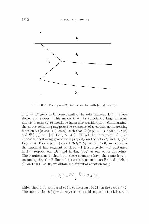
1812 ADAM OSEKOWSKI
FIGURE 6. The regions D0 D4, intersected with {(x, y) : x ≥ 0}.
of x �→ xp goes to 0; consequently, the p-th moment E|fn|p growsslower and slower. This means that, for sufficiently large x, somenontrivial pairs (f, g) should be taken into consideration. Summarizing,the above reasoning suggests the existence of a certain nonincreasingfunction γ : [0,∞) → (−∞, 0), such that B0(x, y) = −|x|p for y ≤ γ(x)and B0(x, y) > −|x|p for y > γ(x). To get the description of γ, weimpose the following geometrical property on the sets D1 and D2 (seeFigure 6). Pick a point (x, y) ∈ ∂D1 ∩ D2, with x > 0, and considerthe maximal line segment of slope −1 (respectively, +1) containedin D1 (respectively, D2) and having (x, y) as one of its endpoints.The requirement is that both these segments have the same length.Assuming that the Bellman function is continuous on R2 and of classC1 on R× (−∞, 0), we obtain a differential equation for γ:
1 − γ′(x) =p(p− 1)
2xp−2γ(x)2,
which should be compared to its counterpart (4.21) in the case p ≥ 2.The substitution H(x) = x−γ(x) transfers this equation to (4.24), and

SURVEY ARTICLE: BELLMAN FUNCTION METHOD 1813
hence the function γ does exist. Furthermore, the solution satisfies:
γ(0) =(2p/(p− 1))1/pΓ(p + 1/p)
Γ(p− 1/p),
see (4.25). Where does this equality come from? It is a consequence ofthe fact that we want γ to be defined on the whole halfline [0,∞) andto satisfy γ′(t) → 0 as t → ∞ (all the other solutions γ, correspondingto different initial conditions, violate one of these two properties).
We come back to the search for the candidate b. It is clear whatfoliation we should use. On D1 ∩ {(x, y) : x > 0}, the function shouldbe concave along the lines of slope −1. The set D2 ∩ {(x, y) : x > 0}should be split into segments of slope 1. Finally, on D3, we expectlinearity along the line of both slopes ±1 (i.e., the Bellman functionshould be quadratic there). A little calculation reveals the followingcandidate. Put H(x) = x − γ(x) for x > 0, and let h be the inversefunction to H . Then(4.26)
b(x, y) =
⎧⎪⎪⎪⎪⎪⎪⎪⎨⎪⎪⎪⎪⎪⎪⎪⎩
1 − xp if (x, y) ∈ D0,
1 + (x + y)p−1((p− 1)y − x)
+(2y)/(H(x + y) − x− y) if (x, y) ∈ D1,
[h(x− y)]p−1[(p− 1)h(x− y) − px] if (x, y) ∈ D2,
[(y + H(0))2 − x2](H(0))−2 if (x, y) ∈ D3,
−xp if (x, y) ∈ D4.
Some lengthy calculations (cf. [33]) show that this function enjoys theconditions 1◦ and 2◦, so it coincides with B0. As in the case p > 2,by appropriate translation and homogenization, we obtain the sharpone-sided bound
P(gn ≥ 1) ≤ (2p/(p− 1))1/pΓ(p + 1/p)
Γ(p− 1/p)E|fn|p, n = 0, 1, 2, . . . ,
valid for all 1 < p < 2 and all martingale pairs (f, g) such that g is a±1-transform of f .
4.5. More exact information on weak-type bounds. The finalpart of this section concerns the Bellman functions
B0(x, y, t)
= sup{P(gn ≥ 1) : (f, g) ∈ M(x, y), E|f∞|p ≤ t, n = 0, 1, 2, . . .
}

1814 ADAM OSEKOWSKI
and the two-sided version,
(4.27) B0(x, y, t)
= sup{P(|gn| ≥ 1) : (f, g) ∈ M(x, y), E|f∞|p ≤ t, n = 0, 1, 2, . . .
}.
We will be brief. The first of these functions can be easily extractedfrom the analysis of the above one-sided bounds. We simply repeatthe translation/homogenization arguments from the case p = 1. Un-fortunately, the formula we obtain is complicated and non-explicit, sowe have decided not to include it here. The function (4.27) could behandled similarly, but, unfortunately, in both cases 1 < p < 2, p > 2the analysis of (4.9) is incomplete (there are some values of β for whichthe function has not been found) and this disables the identification of(4.27).
We omit the further details in this direction, and leave them to thereader.
5. Strong-type inequalities for martingale transforms. Weturn to Burkholder’s celebrated Lp-estimates for martingale transforms:
(5.1) ‖gn‖p ≤ (p∗ − 1)‖fn‖p, 1 < p < ∞, n = 0, 1, 2, . . . ,
where p∗ = max{p, p/(p− 1)}. Thus,
p∗ − 1 =
{(p− 1)−1 if 1 < p ≤ 2,
p− 1 if p ≥ 2.
The primary goal of this section is to determine the explicit formulafor the associated Bellman function
(5.2) B0(x, y, t)
= sup{E|gn|p : (f, g) ∈ M(x, y), E|f∞|p ≤ t, n = 0, 1, 2, . . .
},
originally invented by Burkholder in [8]. The reasoning we will presentis a combination of probabilistic and analytic arguments. For an alter-native, analytic approach which exploits the Monge-Ampere equationand the method of characteristics, see the recent work of Vasyunin andVolberg [50].

SURVEY ARTICLE: BELLMAN FUNCTION METHOD 1815
5.1. On the search of extremal examples. We start our analysisfrom some natural examples, which will be helpful later. Let 1 < p < ∞be fixed, and suppose that βp ≥ 1 is the best constant in the inequality
(5.3) ‖gn‖p ≤ βp‖fn‖p, n = 0, 1, 2, . . . ,
where f is a martingale and g is its ±1-transform. The case p = 2 istrivial; we have ‖gn‖2 = ‖fn‖2 for each n and hence the best constantis equal to 1. Thus, suppose that p �= 2. Since βp cannot be improved,there must be martingales f , g for which both sides are equal, orasymptotically equal. A natural idea during the search for f and gis to let n → ∞ and look for sequences which satisfy the pointwiseequality |g∞| ≡ βp|f∞|. The construction of such a pair is not difficult.Actually, from the viewpoint of our further reasoning, it will be moreconvenient to introduce the whole family of Markov martingales. Fixa small δ > 0 (eventually, we will let it go to 0), and consider thefollowing transition function:
(i) The states lying in the set {(x, y) : |y| ≥ βp|x|} are absorbing.
(ii) The state (x, y) with 0 < y < βpx, leads to (x + y, 0) orto ((x + y)/(βp + 1), (βp(x + y))/(βp + 1)) (the move along the line ofslope −1).
(iii) The state (x, 0) with x > 0 leads to (x + δx, δx) or to(x/(βp + 1),−(βpx)/(βp + 1)) (the move along the line of slope 1).
(iv) The remaining states (x, y) behave in a symmetrical way whencompared to (ii) and (iii).
Now if we assume that the pair (f, g) starts from (1, 1) and movesaccording to (i) (iv), then indeed |g∞| = βp|f∞|. At first glance, thisseems to show that the Lp bound does not hold with any βp, since theratio |g∞|/|f∞| can be arbitrarily large. However, this is not the case.The above martingales are bounded in Lp if and only if βp < (p−1)−1,and we have
limβp↑(p−1)−1
‖f∞‖p = ∞
(cf., [33, pages 55, 56], or modify slightly the reasoning in [8, pages669, 670]). That is, if the constant is at least (p−1)−1, then both sidesof (5.3) are infinite and hence the estimate holds true. On the otherhand, the above example shows the lower bound βp ≥ (p− 1)−1. This

1816 ADAM OSEKOWSKI
is of value only for 1 < p < 2; for p > 2, the stronger bound βp ≥ 1 isgiven for free. How to modify the example when p > 2? A good ideais to reflect the above transition function with respect to the diagonaly = x, that is, let (i) (iv) describe the evolution of (g, f), not (f, g).Actually, a small modification is required: without it, the points ofthe diagonal are absorbing, so the above recipe would give us constantpairs (g, f) (for which we only have ‖g‖p/‖f‖p = 1). We modify theexample as follows. We assume that (f, g) starts from (x, x) for somex > 0, then make it move to (2x, 0) or to (0, 2x), and then require that(g, f) moves according to (i) (iv). Then, as previously, f ∈ Lp if andonly if βp ≥ (p− 1)−1, and hence
limβp↓(p−1)−1
‖g‖p/‖f‖p = p− 1.
Thus, the best constant is at least p− 1. Actually, we can consider theabove Markov family for various choices of βp ∈ ((p− 1)−1,∞). As weshall see, they will also play a role.
5.2. Basic inequality. In order to study the (difficult) Bellmanfunction B0, we implement our “splitting procedure.” As previously, wemove the p-th moment E|f∞|p from the assumption to the optimizedexpression and work with an appropriate family of estimates. Moreprecisely, we will determine the explicit formula for the two-dimensionalBellman function(5.4)
b0(x, y) = sup{EVβ(fn, gn) : (f, g) ∈ M(x, y), n = 0, 1, 2, . . .
},
where Vβ(x, y) = |y|p − βp|x|p and β is a given constant. Then,optimizing over β, we will obtain the desired function (5.2). Actually,as we shall see in a moment in subsection 5.3, only the case p �= 2 isof interest; when p = 2, the Bellman function B0 can be derived withpractically no effort.
We will present the detailed reasoning in the case 1 < p < 2 only.As we have proved above, only the case β ≥ (p − 1)−1 is of interest;for smaller β, the Bellman function b0 is infinite. So, assume thatβ ≥ (p− 1)−1, and suppose that b0 is finite. This function satisfies 1◦
and 2◦; moreover, directly from (5.4), we have that it is homogeneousof order p (since V has this property)
b0(λx,±λy) = |λ|pb0(x, y), x, y ∈ R, λ �= 0.

SURVEY ARTICLE: BELLMAN FUNCTION METHOD 1817
Consider the function w : R → R, given by
(5.5) w(x) = b0(x, 1 − x).
It is enough to determine w on [0, 1]. Then, by homogeneity, we willobtain b0 on its whole domain. Note that w is concave and satisfies(5.6)
w(x) = b0(x, 1 − x) = b0(x, x − 1) = (2x− 1)pw
(x
2x− 1
)for x > 1.
Furthermore, it majorizes u : R → R given by u(x) = Vβ(x, 1− x). Bythe direct differentiation, we see that
u′′(x) = p(p− 1)[(1 − x)p−2 − βpxp−2
], x ∈ (0, 1),
and hence u is concave on (0, x0) and convex on (x0, 1) for somex0 ∈ (0, 1). This suggests considering the following candidate for w:
w(x) =
{u(x) if x ∈ (0, x1),
u′(x1)(x − x1) + u(x1) if x ∈ [x1, 1),
where x1 < x0 is a parameter which needs to be specified. To find x1,we compare the behavior of the left- and the right-hand derivative ofw at 1. Namely, note that (5.6) implies
w(x)−w(1)
x−1+ (2x−1)p−1w(1)−w(x/(2x−1))
1−x/(2x−1)= 2w(1)
(2x−1)p−1
(2x−1)−1
for x > 1, so letting x ↓ 1, we get w′(1+) +w′(1−) = 2pw(1), and thus
u′(x1) = w′(1−)≥ w′(1+)+w′(1−)
2= pw(1) = pu′(x1)(1−x1)+pu(x1).
Now, it will be convenient to switch to the parameter γ, given byx1 = (1 + γ)−1. Then the above inequality is equivalent to (p− 1)βp ≥(2−p)γp−1 +γp−2. We assume that we actually have equality here, so,
(5.7) βp =(2 − p)γp−1 + γp−2
p− 1.
Note that the expression on the right of (5.7), considered as a functionof γ, is decreasing on (0, (p − 1)−1) and increasing on ((p − 1)−1,∞).

1818 ADAM OSEKOWSKI
Furthermore, its minimal value equals (p− 1)−p. Thus, if β is strictlylarger than (p− 1)−1, we have two choices for γ, and in such a case wepick the smaller one, i.e., γ < (p− 1)−1.
Coming back to b0, we obtain the following candidate for the Bellmanfunction:
b(x, y) =
{(γ
γ+1
)p−2
(|x| + |y|)p−1(|y| − |x|
p−1
)if |y| ≤ γ|x|,
|y|p − βp|x|p if |y| > γ|x|.
Now, it is straightforward to check that b satisfies 1◦ (this followsdirectly from the homogeneity and the inequality w ≥ u). Furthermore,some tedious calculations show that the condition 2◦ is also satisfied,see e.g., [10, page 17]. Therefore, b0 ≤ b. Actually, we have equalityb0(x, y) = b(x, y) for all (x, y), which can be verified with the use ofexamples from the previous section, with βp := γ (or just follows fromthe above construction). This is the place where we use the fact that wehave chosen smaller γ in (5.7); for the larger choice, the computation ofsupn≥0 EV (fn, gn) would not lead to b(x, y), but to a strictly smallerconstant. We have yet another analytic explanation for the smallerγ’s: the function b corresponding to larger choice would lead to a strictmajorant of b0.
In the case p > 2, we proceed similarly. Let us briefly describe themain steps of the analysis. Exploitation of the examples of subsec-tion 5.1 leads us to the inequality β ≥ p − 1. The function u (givenby the same formula as above), restricted to [0, 1], has dual convex-ity/concavity regions; that is, it is convex for small arguments andconcave for large ones (i.e., close to 1). Thus, it is natural to conjec-ture that the restriction w|[0,1] (where w is given by (5.5)) is of theform
w(x) =
{u′(x1)(x − x1) + u(x1) if x ∈ (0, x1],
u(x) if x ∈ (x1, 1),
for some x1. Passing to γ = 1−x−11 as above and analyzing the behavior
of w′ in the neighborhood of 0, we obtain βp ≥ (p− 1)γp−1/(γ+ 2−p).We assume that both sides are equal. Again, for a given β > p − 1,there are two γ’s which satisfy the equation, and this time we pick thelarger one. Putting all these facts together, we obtain the candidate :
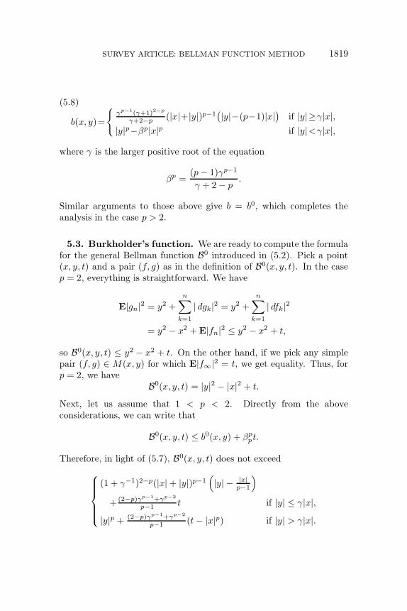
SURVEY ARTICLE: BELLMAN FUNCTION METHOD 1819
(5.8)
b(x, y)=
{γp−1(γ+1)2−p
γ+2−p (|x|+|y|)p−1(|y|−(p−1)|x|) if |y|≥γ|x|,
|y|p−βp|x|p if |y|<γ|x|,
where γ is the larger positive root of the equation
βp =(p− 1)γp−1
γ + 2 − p.
Similar arguments to those above give b = b0, which completes theanalysis in the case p > 2.
5.3. Burkholder’s function. We are ready to compute the formulafor the general Bellman function B0 introduced in (5.2). Pick a point(x, y, t) and a pair (f, g) as in the definition of B0(x, y, t). In the casep = 2, everything is straightforward. We have
E|gn|2 = y2 +
n∑k=1
| dgk|2 = y2 +
n∑k=1
| dfk|2
= y2 − x2 + E|fn|2 ≤ y2 − x2 + t,
so B0(x, y, t) ≤ y2 − x2 + t. On the other hand, if we pick any simplepair (f, g) ∈ M(x, y) for which E|f∞|2 = t, we get equality. Thus, forp = 2, we have
B0(x, y, t) = |y|2 − |x|2 + t.
Next, let us assume that 1 < p < 2. Directly from the aboveconsiderations, we can write that
B0(x, y, t) ≤ b0(x, y) + βppt.
Therefore, in light of (5.7), B0(x, y, t) does not exceed
⎧⎪⎪⎪⎨⎪⎪⎪⎩
(1 + γ−1)2−p(|x| + |y|)p−1(|y| − |x|
p−1
)+ (2−p)γp−1+γp−2
p−1 t if |y| ≤ γ|x|,|y|p + (2−p)γp−1+γp−2
p−1 (t− |x|p) if |y| > γ|x|.

1820 ADAM OSEKOWSKI
Denote this expression by B(x, y, t, γ), and let us minimize it over allγ ≤ (p− 1)−1. If |y| ≥ (p− 1)−1|x|, then
B(x, y, t, γ) = |y|p + (2−p)γp−1+γp−2
p−1 (t− |x|p)
for all γ. We easily see that
∂B∂γ (x, y, t, γ) = (2 − p)(p− 1)−1γp−3(−1 + (p− 1)γ) ≤ 0,
and thus the choice γ = (p − 1)−1 is optimal. This calculation alsoshows that if |y| < (p− 1)−1|x|, then γ �→ B(x, y, t, γ) is nonincreasingon (0, |y|/|x|), and hence the minimum is attained on [|y|/|x|, (p−1)−1].A direct differentiation gives that γ0 which minimizes B is the uniquenumber γ from that interval, satisfying the equation
(|x|+|y|)p−1
t
(|y| − |x|
p−1
)− (1 + γ)p + p
p−1 (1 + γ)p−1 = 0.
Plugging the above optimal choices of γ into the definition of B, wefinally get that
B0(x, y, t) ≤{ |y|p + (p− 1)−p(t− |x|p) if |y| ≥ (p− 1)−1|x|,γp0 t if |y| < (p− 1)−1|x|.
We actually have equality here, which can be verified with the examplesconsidered in the previous subsection (see also [8]). This gives us thedesired formula for B0, which was originally discovered by Burkholder.
Case p > 2 remains to be dealt with. We proceed analogouslyand exploit the function defined by (5.8). In comparison to the case1 < p < 2, there are no additional arguments, so we leave the detailsto the reader. Let us only write down the result: having carried out allthe computations, we end up with
B0(x, y, t) =
{ |y|p + (p− 1)p(t− |x|p) if |y| ≤ (p− 1)|x|,γp0 t if |y| > (p− 1)|x|,
where γ0 is the unique γ ∈ [p− 1,∞) satisfying the equation
(|x|+|y|)p−1
t
(|y| − (p− 1)|x|) + p(γ + 1)p−1 − (γ + 1)p = 0.
This completes the analysis.

SURVEY ARTICLE: BELLMAN FUNCTION METHOD 1821
Acknowledgments. The author would like to thank anonymousReferees for the careful reading of the first version of the paper andmany helpful comments and suggestions. This survey is an extendedversion of the mini-course given at Chebyshev Laboratory in St. Peters-burg, Russia. The author would like to express his sincerest gratitudeto A. Logunov, L. Slavin, D. Stolyarov, V. Vasyunin and P. Zatitskiyfor their warm hospitality and enjoyable meeting.
REFERENCES
1. R. Banuelos, A. Bielaszewski and K. Bogdan, Fourier multipliers for non-symmetric Levy processes, Banach Center Publ. 95 (2011), 9 25.
2. R. Banuelos and G. Wang, Sharp inequalities for martingales with applicationsto the Beurling-Ahlfors and Riesz transformations, Duke Math. J. 80 (1995),575 600.
3. A. Borichev, P. Janakiraman and A. Volberg, Subordination by conformalmartingales in Lp and zeros of Laguerre polynomials, Duke Math. J. 162 (2013),889 924.
4. , On Burkholder function for orthogonal martingales and zeros ofLegendre polynomials, Amer. J. Math. 135 (2012), 207 236.
5. D.L. Burkholder, Martingale transforms, Ann. Math. Stat. 37 (1966), 1494 1504.
6. , A sharp inequality for martingale transforms, Ann. Prob. 7 (1979),858 863.
7. , A geometrical characterization of Banach spaces in which martingaledifference sequences are unconditional, Ann. Prob. 9 (1981), 997 1011.
8. , Boundary value problems and sharp inequalities for martingale trans-forms, Ann. Prob. 12 (1984), 647 702.
9. , Martingales and Fourier analysis in Banach spaces, Prob. Anal., Lect.Notes Math. 1206, Springer, Berlin, 1986.
10. D.L. Burkholder, Explorations in martingale theory and its applications, Lect.Notes Math. 1464, Springer, Berlin, 1991.
11. , Strong differential subordination and stochastic integration, Ann.Prob. 22 (1994), 995 1025.
12. , Sharp norm comparison of martingale maximal functions andstochastic integrals, Proc. Symp. Appl. Math. 52, American Mathematical Soci-ety, Providence, 1997.
13. , The best constant in the Davis’ inequality for the expectation of themartingale square function, Trans. Amer. Math. Soc. 354 (2002), 91 105.
14. K.P. Choi, Some sharp inequalities for martingale transforms, Trans. Amer.Math. Soc. 307 (1988), 279 300.
15. , A sharp inequality for martingale transforms and the unconditionalbasis constant of a monotone basis in Lp(0, 1), Trans. Amer. Math. Soc. 330 (1993),509 529.

1822 ADAM OSEKOWSKI
16. D.C. Cox, The best constant in Burkholder’s weak-L1 inequality for themartingale square function, Proc. Amer. Math. Soc. 85 (1982), 427 433.
17. , Some sharp martingale inequalities related to Doob’s inequality, inInequalities in statistics and probability, IMS Lect. Notes Monograph Ser. 5 (1984),78 83.
18. L.E. Dor and E. Odell, Monotone bases in Lp, Pac. J. Math. 60 (1975),51 61.
19. I. Doust, Contractive projections on Banach spaces, Proc. Centre for Math.Anal., Austr. Natl. Univ. 20 (1988), 50 58.
20. O. Dragicevic and A. Volberg, Bellman function, Littlewood-Paley estimates,and asymptotics of the Ahlfors-Beurling operator in Lp(), p > 1, Indiana Math. J.54 (2005), 971 995.
21. , Bellman function and dimensionless estimates of classical andOrnstein-Uhlenbeck Riesz transforms, J. Oper. Theor. 56 (2006), 167 198.
22. , Linear dimension-free estimates in the embedding theorem forSchrodinger operators, J. Lond. Math. Soc. 85 (2012), 191 222.
23. P. Ivanishvili, N.N. Osipov, D.M. Stolyarov, V. Vasyunin and P. Zatitskiy,On Bellman function for extremal problems in BMO, C.R. Math. Acad. Sci. 350(2012), 561 564.
24. J.H.B. Kemperman, The general moment problem, a geometric approach,Ann. Math. Stat. 39 (1968), 93 122.
25. J. Marcinkiewicz, Quelques theoremes sur les series orthogonales, Ann. Soc.Polon. Math. 16 (1937), 84 96.
26. A.D. Melas, Sharp general local estimates for dyadic-like maximal operatorsand related Bellman functions, Adv. Math. 220 (2009), 367 426.
27. A.D. Melas and E.N. Nikolidakis, Dyadic-like maximal operators on integrablefunctions and Bellman functions related to Kolmogorov’s inequality, Trans. Amer.Math. Soc. 362 (2010), 1571 1597.
28. F. Nazarov, A. Reznikov, V. Vasyunin and A. Volberg, A1 conjecture:Weak norm estimates of weighted singular operators and Bellman function, http://sashavolberg.files.wordpress.com/2010/11/a11 7loghilb11 21 2010.pdf.
29. F.L. Nazarov and S.R. Treil, The hunt for a Bellman function: Applications toestimates for singular integral operators and to other classical problems of harmonicanalysis, St. Petersburg Math. J. 8 (1997), 721 824.
30. F.L. Nazarov, S.R. Treil and A. Volberg, The Bellman functions and two-weight inequalities for Haar multipliers, J. Amer. Math. Soc. 12 (1999), 909 928.
31. , Bellman function in stochastic optimal control and harmonic analysis(how our Bellman function got its name), Oper. Theory: Adv. Appl. 129 (2001),393 424.
32. F. Nazarov and A. Volberg, Heating of the Ahlfors-Beurling operator andestimates of its norm, St. Petersburg Math. J. 15 (2004), 563 573.
33. A. Osekowski, Sharp martingale and semimartingale inequalities, Mono.Matem. 72 (2012), Birkhauser. Basel.
34. , Sharp logarithmic inequalities for Riesz transforms, J. Funct. Anal.263 (2012), 89 108.

SURVEY ARTICLE: BELLMAN FUNCTION METHOD 1823
35. A. Osekowski, Sharp inequalities for the dyadic square function in the BMOsetting, Acta Math. Hungar. 139 (2013), 85 105.
36. , Some sharp estimates for the Haar system and other bases inL1(0, 1), Math. Scand., to appear.
37. R.E.A.C. Paley, A remarkable series of orthogonal functions, Proc. Lond.Math. Soc. 34 (1932), 241 264.
38. A. Pe�lczynski and H.P. Rosenthal, Localization techniques in Lp spaces, Stud.Math. 52 (1975), 263 289.
39. G. Peskir and A. Shiryaev, Optimal stopping and free-boundary problem,Lect. Math., ETH Zurich.
40. J. Schauder, Eine Eigenschaft des Haarschen Orthogonalsystems, Math. Z.28 (1928), 317 320.
41. L. Slavin, A. Stokolos and V. Vasyunin, Monge-Ampere equations and Bell-man functions: The dyadic maximal operator, C.R. Acad. Sci. 346 (2008), 585 588.
41. L. Slavin and V. Vasyunin, Sharp results in the integral-form John-Nirenberginequality, Trans. Amer. Math. Soc. 363 (2011), 4135 4169.
42. , Sharp Lp estimates on BMO, Indiana Math. J. 61 (2012), 1051 1110.
43. Y. Suh, A sharp weak type (p, p) inequality (p > 2) for martingale transformsand other subordinate martingales, Trans. Amer. Math. Soc. 357 (2005), 1545 1564.
44. V. Vasyunin, The exact constant in the inverse Holder inequality for Muck-enhoupt weights, Alg. Anal. 15 (2003), 73 117 (in Russian); St. Petersburg Math.J. 15 (2004), 49 79 (in English).
45. , Mutual estimates for Lp-norms and the Bellman function, Zap.Nauchn. Sem. S.-Petersburg. Otdel. Mat. Inst. Steklov. (POMI) 355 (2008), Issl.Lineinym Oper. Teor. Funkt. 36, 81 138, 237 238 (in Russian); J. Math. Sci. (N.Y.)156 (2009), 766 798 (in English).
46. V. Vasyunin and A. Volberg, Bellman functions technique in harmonicanalysis, sashavolberg.wordpress.com.
47. , The Bellman function for certain two weight inequality: The casestudy, St. Petersburg Math. J. 18 (2007), 201 222.
48. , Monge-Ampere equation and Bellman optimization of Carlesonembedding theorems, Amer. Math. Soc. Transl. 226 (2009), 195 238.
49. , Burkholder’s function via Monge-Ampere equation, Illinois J. Math.54 (2010), 1393 1428.
50. G. Wang, Sharp square-function inequalities for conditionally symmeticMartingales, Trans. Amer. Math. Soc. 328 (1991), 393 419.
51. , Sharp inequalities for the conditional square function of a martingale,Ann. Probab. 19 (1991), 1679 1688.
52. , Differential subordination and strong differential subordination forcontinuous time martingales and related sharp inequalities, Ann. Probab. 23 (1995),522 551.
Faculty of Mathematics, Informatics and Mechanics, University of War-saw, Banacha 2, 02-097 Warsaw, PolandEmail address: [email protected]